10,000 Matching Annotations
  1. Oct 2025
    1. Author Response

      The following is the authors’ response to the original reviews.

      We thank the editors and reviewers for their tremendously helpful comments. We outline below changes we have made to the manuscript in response to each point. These include new analyses and a substantial rewrite to address the concerns about lack of clarity.

      We believe the revisions strengthen the evidence for our conclusion that grid fields can be either anchored to or independent from a task reference frame, and that anchoring is selectively associated with successful path integration-dependent behaviour. Our additional analyses of non-grid cells indicate that while some are coherent with the grid population, many are not, suggesting cell populations within the MEC may implement grid-dependent and grid-independent computations in parallel.

      We hope the reviewers will agree that our novel experimental strategy complements and avoids limitations of perturbation-based approaches, and by providing evidence to dissociate the two major hypotheses for whether and when grid cells contribute to behaviour our results are likely to have a substantial impact on the field.

      Public Reviews:

      Reviewer #1 (Public Review):

      In this study, Clark et. al. uncovered an association between the positional encoding of grid cell activity with good performance in spatial navigation tasks that requires path integration, highlighting the contribution of grid firing to behaviour… The conclusions of this paper are mostly well supported by data, the finding about the association between grid cell encoding and behaviour in spatial memory tasks is important. However, some aspects of the analysis need to be clarified or extended.

      Thankyou for the overview and constructive comments.

      (1) While the current dataset aims to demonstrate a "correlation" between grid cell encoding and task performance, the other variables that could confound this correlation should be carefully examined.

      (1.1) The exact breakdown of the fraction of beaconed/non-beaconed/probe trials is never shown. if the session makeup has a significant effect on the coding scheme or other results, this variable should be accounted for.

      The lack of information about the trial organisation was a substantial oversight in our preparation of the first version of the manuscript. Session make up can not account for effects on grid stability and its relationship to behavioural outcome but this was not made at all clear.

      In all sessions trial types were varied in a fixed repeating sequence. Therefore, continuous blocks of trials on which grid firing is anchored (or independent from) the track can not be explained by the mouse experiencing a particular trial type. We have revised the manuscript to make this clearer, e.g. p 5, ‘These switches could not be explained by variation between trials in the availability of cues or rewards, as these were interleaved in blocks that repeated throughout a session (see Methods), whereas periods in which grid cell activity was in a given mode extended across the repeating blocks (e.g. Figures 3D,E, 4A, 5E,F).’ and methods p 12, ‘Trials were delivered in repeating blocks throughout a recording session…’

      (1.2) The manuscript did not provide information about whether individual mice experienced sessions with different combinations of the three trial types, and whether they show different preferences in position or distance encoding even in comparable sessions. This leads to the question of whether different behaviour and activity encoding were dominated by experimental or natural differences between individual mice. Presenting the data per mouse will be helpful.

      As we note above, because trial types were interleaved in a fixed sequence, experience of a particular trial type can not account for switching between task-anchored and taskindependent firing modes. This was insufficiently clear in the first version of the manuscript.

      We varied the proportions of trials of a particular type between sessions with the aim of maximising the number of non-beaconed and probe trials. This was necessary because we find that if we introduce too high a proportion of these trials early in training then mice appear to ‘lose interest’ in the task and their performance drops off. We therefore used an approach in which we increased the proportions of non-beaconed and probe trials over training days as mice became familiar with the task. This is now described in the methods (p 12).

      Because the decision for when to vary the proportion of trial types was based on the previous day’s performance, the experimental design was not optimised for addressing the reviewer’s question about dissociating experimental from natural differences in mice. To provide some initial insight we have analysed the relationship between task anchored coding and proportion of beaconed trials in a session (Figure 3, Figure Supplement 7). While on average there is a higher proportion of trials in which grid fields are task-anchored in sessions with more beaconed trials, this effect is small and most of the variance is independent from the proportion of beaconed trials.

      (1.3) Related to the above point, in Figure 5, the mice appeared to behave worse in probe trials than non-beaconed trials. If the mouse did not know if a trial is a probe or a non-beacon trial, they should behave equivalently until the reward location and thus should stop an equal amount. If this difference is because multiple probe trials are placed consecutively, did the mouse learn that it will not get a reward and then stop trying to get rewards? Did this affect switching between position and distance coding?

      Thankyou for flagging this. This reflected an inconsistency arising from the way we detected stops that we have now corrected. Briefly, the temporal resolution of the processed location data against which the stop detection threshold was applied was insufficiently high. As a result, stops in the non-beaconed group were picked up, as they tended to be longer because mice remained still to consume rewards, whereas some stops in the probe group were missed because they were relatively short. We have corrected this by repeating the analyses on raw position data at the highest temporal resolution available. This analysis is now clearly described in the Methods (see p13 “A stop was registered in Blender3D if the speed of the mouse dropped below 4.7 cm/s. Speed was calculated on a rolling basis from the previous 100 ms at a rate of 60 Hz.”).

      (1.4) It is not shown how the behaviours (e.g., running speed away from the reward zone, licking for reward) in beaconed/non-beaconed/probe trials were different and whether the difference in behaviours led to the different encoding schemes.

      Because trial types were interleaved and repeated with a period less than the length of typical trial sequences during which grid cell activity remained either task-anchored or taskindependent, differences between trial types are unlikely to explain use of the different coding schemes. Hopefully, this is clarified by the comments above.

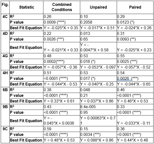
      To further describe the relationship between behavioural outcomes, trial types and grid anchoring, we now also show running speed as a function of location for each combination of trial types and trial outcomes (Figure 6, Figure Supplement 1). This illustrates and replicates our previous findings (Tennant et al. 2018) that running speed profiles are similar for a given trial outcome regardless of trial type (Figure 6, Figure Supplement 1A), and further further shows that the behavioural profile for a given trial outcome and trial-type does not differ when grid cells are in task-anchored and task-independent modes (Figure 6, Figure Supplement 1B). This further argues against the possibility that difference in behaviours leads to the different encoding schemes.

      (2) Regarding the behaviour and activity encoding on a trial-by-trial basis, did the behavioural change occur first, or did the encoding switch occur first, or did they happen within the same trial? This analysis will potentially determine whether the encoding is causal for the behaviour, or the other way around.

      This is a good question but our experimental design lacks sufficient statistical power to address the timing of mode switches within a trial. This is because mode switching is relatively infrequent (so the n for switching is low) and only a subset of trials are uncued (making the relevant n even lower), while at a trial level the behavioural outcome is variable (increasing the required n for adequate power).

      (3) The author determined that the grid cell coding schemes were limited to distance encoding and position encoding. However, there could be other schemes, such as switching between different position encodings (with clear spatial fields but at different locations), as indicated by Low et. al., 2021, and switching between different distant encodings (with different distance periods). If these other schemes indeed existed in the data, they might contribute to the variation of the behaviours.

      Switching between position encoding schemes appears to be rare within our dataset and unlikely to contribute to variation in behaviour. In most sessions we did not observe switching between grid phases / position encodings (e.g. Figures 2A-B, 3B-E, 4A, 5C-D, F). In one session we found switching between different phases when grid cells were taskanchored. Because the grid period was unchanged, the spatial periodograms remained similar. We report this example in the revised manuscript (Figure 5E).

      (4) The percentage of neurons categorised in each coding scheme was similar between nongrid and grid cells. This implies that non-grid cells might switch coding schemes in sync with grid cells, which would mean the whole MEC network was switching between distance and position coding. This raises the question of whether the grid cell coding scheme was important per se, or just the MEC network coding scheme.

      We very much appreciate this suggestion. We note first that while the proportion of taskanchored grid and non-grid cells is similar, task-independent periodic firing of non-grid cells is much rarer than for grid cells (Figure 2E), suggesting a dissociation between the populations. To further address the question we have included additional analyses of nongrid cells (Figure 3, Figure Supplement 5). This shows that while some non-grid cells have anchoring that switches coherently with simultaneously recorded grid cells, others do not. Figures 4 and 5 now show examples of non-grid cell activity recorded simultaneously with grid cells.

      Together, our data suggest that the MEC implements multiple coding schemes: one that is associated with the grid network and includes some non-grid cells; and one (or more) that can be independent from the grid network. This dissociation adds to the insights into MEC function that are provided by our study and is now highlighted in the abstract and discussion.

      (5) In Figure 2 there are several cell examples that are categorised as distance or position coding but have a high fraction of the other coding scheme on a per-trial basis. Given this variation, the full session data in F should be interpreted carefully, since this included all cells and not just "stable" coding cells. It will be cleaner to show the activity comparison only between the stable cells.

      We have now included examples in Figure 2A-C where the grid mode is stable throughout a session. As the view of activity at a session level is important, we have not updated Figure 2F, but have clarified the terminology to now clearly refer to classification at either season or trial levels. In addition, we have repeated the analyses shown in Figure 2F but after grouping cells according to whether their firing has a single mode on >85% of the trials (Figure 3 Figure Supplement 4). This analysis supports similar conclusions to those of Figure 2F.

      (6) The manuscript is not well written. Throughout the manuscript, there are many unexplained concepts (especially in the introduction) and methods, mis-referenced figures, and unclear labels.

      We very much appreciate the feedback and have substantially rewritten the manuscript. We have paid particular attention to explaining key concepts in the introduction and have carefully checked the figures. We welcome further feedback on whether this is now clearer.

      Reviewer #2 (Public Review):

      Clark and Nolan's study aims to test whether the stability of grid cell firing fields is associated with better spatial behaviour performance on a virtual task… This study is very timely as there is a pressing need to identify/delimitate the contribution of grid cells to spatial behaviours. More studies in which grid cell activity can be associated with navigational abilities are needed.

      Thank you for the supportive comments and highlighting the importance of the question.

      The link proposed by Clark and Nolan between "virtual position" coding by grid cells and navigational performance is a significant step toward better understanding how grid cell activity might support behaviour. It should be noted that the study by Clark and Nolan is correlative. Therefore, the effect of selective manipulations of grid cell activity on the virtual task will be needed to evaluate whether the activity of grid cells is causally linked to the behavioural performance on this task. In a previous study by the same research group, it was shown that inactivating the synaptic output of stellate cells of the medial entorhinal cortex affected mice's performance of the same virtual task (Tennant et al., 2018). Although this manipulation likely affects non-grid cells, it is still one of the most selective manipulations of grid cells that are currently available.

      Again, thank you for the supportive comments. We recognise the previous version of the manuscript did not sufficiently clarify the motivation for our approach, or the benefits of capitalising on behavioural variable variability as a complementary strategy to perturbation approaches. We now make this clearer in the revised introduction (p 2, paragraphs 2 and 3).

      When interpreting the "position" and "distance" firing mode of grid cells, it is important to appreciate that the "position" code likely involves estimating distance. The visual cues on the virtual track appear to provide mainly optic flow to the animal. Thus, the animal has to estimate its position on the virtual track by estimating the distance run from the beginning of the track (or any other point in the virtual world).

      We appreciate the ambiguity here was confusing. We have re-named the groups to ‘taskanchored’, corresponding to when grid cells encode position on the track (as well as distance as the reviewer correctly points out), and ‘task-independent’, corresponding to the group we previously referred to as distance encoding.

      It is also interesting to consider how grid cells could remain anchored to virtual cues. Recent work shows that grid cell activity spans the surface of a torus (Gardner et al., 2022). A run on the track can be mapped to a trajectory on the torus. Assuming that grid cell activity is updated primarily from self-motion cues on the track and that the grid cell period is unlikely to be an integer of the virtual track length, having stable firing fields on the virtual track likely requires a resetting mechanism taking place on each trial. The resetting means that a specific virtual track position is mapped to a constant position on the torus. Thus, the "virtual position" mode of grid cells may involve 1) a trial-by-trial resetting process anchoring the grid pattern to the virtual cues and 2) a path integration mechanism. Just like the "virtual position" mode of grid cell activity, successful behavioural performance on non-beaconed trials requires the animal to anchor its spatial behaviour to VR cues.

      Reviewer #3 (Public Review):

      This study addresses the major question of 'whether and when grid cells contribute to behaviour'. There is no doubt that this is a very important question. My major concern is that I'm not convinced that this study gives a significant contribution to this question, although this study is well-performed and potentially interesting. This is mainly due to the fact that the relation between grid cell properties and behaviour is exclusively correlative and entirely based on single cell activity, although the introduction mentions quite often the grid cell network properties and dynamics. In general, this study gives the impression that grid cells exclusively support the cognitive processes involved in this task. This problem is in part related to the text.

      Thank you for the comments. We recognise now that the previous text was insufficiently clear. We have modified the introduction to clarify the value of an approach that takes advantage of behavioural variability. Importantly, this approach is complementary to perturbation strategies we and others have used previously. In particular it addresses critical limitations of perturbation strategies which can be confounded by off-target effects and possible adaptation, both of which are extremely difficult to fully rule out. We hope that with this additional clarification it is now clear that as for any important question multiple and complementary testing strategies are required to make progres, and second, that our study makes a new and important contribution by introducing a novel experimental approach and by following this up with careful analyses that clearly distinguish competing hypotheses.

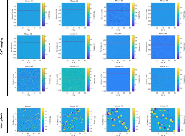
      However, it would be interesting to look at the population level (even beyond grid cells) to test whether at the network level, the link between behavioural performance and neural activity is more straightforward compared to the single-cell level. This approach could reconcile the present results with those obtained in their previous study following MEC inactivation.

      We’re unclear here about what the reviewer means by ‘more straightforward’ as clear relationships between activity of single grid cells and populations of grid cells are well established (Gardner et al., 2021; Waaga et al., 2021; Yoon et al., 2013).

      To give a clearer indication of the corresponding population level representations, as mentioned in response to Reviewer #1, we now include additional data showing many simultaneously recorded neurons, and analyses of non-grid as well as grid cells (Figures 4, 5, Figure 5 Figure Supplement 2).

      To reconcile results with our previous study of MEC inactivation we have paid additional attention to the roles of non-grid cells (following suggestions by Reviewer #1). We show that while some non-grid cells show transitions between task-anchored and task-independent firing that are coherent with the grid population, many others have more stable firing that is independent of grid representations. This is consistent with the idea that the MEC supports localised behaviour in the cued and uncued versions of the task (Tennant et al., 2018), and suggests that while grid cells preferentially contribute when cues are absent, non-grid cells could also support the cued version. We make this additional implication clear in the revised abstract and discussion.

      The authors used a statistical method based on the computation of the frequency spectrum of the spatial periodicity of the neural firing to classify grid cells as 'position-coding' (with fields anchored to the virtual track) and 'distance-coding' (with fields repeating at regular intervals across trials). This is an interesting approach that has nonetheless the default to be based exclusively on autocorrelograms. It would be interesting to compare with a different method based on the similarities between raw maps.

      While our main analyses use a periodogram-based method to identify when grid cells are / are not anchored to the task environment, we validate these analyses by examination of the rate maps in each condition (Figures 2-4). For example, when grid cells are task-anchored, according to the periodogram analysis, the rate maps clearly show spatially aligned peaks, whereas when grid cells are not anchored the peaks in their rate maps are not aligned (Figure 2A vs 2B; Figure 3B-E; Figure 4C). We provide further validation by showing that spatial information (in the track reference frame) is substantially higher when grid cell activity is task-anchored vs task-independent (Figures 2F, 3G, 4F and Figure 3 Figure Supplement 4).

      To further address this point we have carried out additional complementary analyses in which we identify task anchored vs task independent modes using a template matching method applied to the raw rate maps (Figure 6, Figure Supplement 2). These analyses support similar conclusions to our periodogram-based analyses.

      Beyond this minor point, cell categorization is performed using all trial types.

      Each trial type (i.e. beacon or non-beacon) is supposed to force mice to use different strategies and should induce different spatial representations within the entorhinal-hippocampal circuit (and not only in the grid cell system). In that context, since all trials are mixed, it is difficult to extrapolate general information.

      We recognise that the description of the task design was insufficiently clear but are unsure why ‘it is difficult to extrapolate general information’. Before addressing this point, we should first be clear that mice are not ‘forced’ to adopt any particular strategy. Rather, on uncued trials a path integration strategy is the most efficient way to solve the task. However, mice could instead use a less efficient strategy, for example by stopping at short intervals they still obtain rewards. Detailed behavioural analyses indicate that such random stopping strategies are used by naive mice, while with training mice learn to use spatial stopping strategies (Tennant et al. 2018).

      In terms of ‘extracting general information’ from the task, the following findings lead to general predictions: 1) Grid cells can exist in either task-anchored or task-independent periodic firing modes; 2) These modes can be stable across a session, but often modeswitching occurs within a session; 3) While some non-grid cells show task-independent periodic firing, this is much less common than for grid cells, which suggests a model in which many non-grid MEC neurons operate independently from the grid network; 4) When a marker cue is available mice locate a reward equally well when grid cells are in taskanchored versus task-independent modes, which argues against theories in which grid cells are a key part of a general system for localisation; 5) When markers cues are absent taskanchored grid firing is associated with successful reward localisation, which corroborates a key prediction of theories in which grid cells contribute to path integration.

      In revising the manuscript we have attempted to improve the writing to make these advances clearer, and have clarified methodological details that made interpretation more challenging than it should have been. For example, as noted in our response to Reviewer #1, we have included additional details to clarify the organisation of trials and relationships between trials, behavioural outcomes and neural codes observed.

      On page 5 the authors state that 'Since only position representations should reliably predict the reward location, ..., we reasoned that the presence of positional coding could be used to assess whether grid firing contributes to the ongoing behaviour'. I do not agree with this statement. First of all, position coding should be more informative only in a cue-guided trial. Second, distance coding could be as informative as position coding since at the network level may provide information relevant to the task (such as distance from the reward).

      Again, this point perhaps reflects a lack of clarity on our part in writing the manuscript. When grid cells are anchored to the track reference frame (now called ‘tasked anchored’, previously ‘position encoding’), then the location of the rate peaks in grid firing is reliable from trial to trial. This is the case whether or not the trial is cued. When grid cells are independent of the track reference frame (now called ‘task independent’, previously ‘distance encoding’), then the location of the firing rate peaks vary from trial to trial. In the latter case, position can not be read out directly from trial to trial.

      In principle, in the task-independent mode track position could be calculated by storing the grid network configuration at the start of the track, which would differ on each trial, and then implementing a mechanism to readout relative distance as mice move along the track. However, if mice do use this computation we would expect them to do so equally well on cued and uncued trials. By contrast, our results clearly show a dissociation between trial types in the relationship between grid firing and behavioural outcome. We highlight and discuss this possibility in the revised manuscript (p 10, ‘Alternatively, mice could in principle estimate track location with a system that utilises information about distance travelled obtained from task-independent grid representations’).

      Third, position-coding is interpreted as more relevant because it predominates in correct trials. However, this does not imply that this coding scheme is indeed used to perform correct trials.

      We have revised the manuscript to clarify our goal of distinguishing major hypotheses for the roles of grid cells in behaviour (Introduction, ‘On the one hand, theoretical arguments that grid cell populations can generate high capacity codes imply that they could in principle contribute to all spatial behaviours (Fiete et al., 2008; Mathis et al., 2012; Sreenivasan and Fiete, 2011). On the other hand, if the behavioural importance of grid cells follows from their hypothesised ability to generate position representations by integrating self-motion signals (McNaughton et al., 2006), then their behavioural roles may be restricted to tasks that involve path integration strategies.’

      By showing that performance on cued trials is similar regardless of whether grid cells are task-anchored or not, we provide strong evidence against the idea that grid firing is in general necessary for location-based behaviours. By showing that task anchoring is associated with successful localisation when cues are absent we corroborate a key prediction of hypothesised roles for grid cells in path integration-dependent behaviour. Therefore, we substantially reduce the space of behaviours to which grid cells might contribute. Importantly, this space is much larger for the MEC, which is required for cued and uncued versions of the task. We have revised the introduction and discussion to make these points clearer.

      While we believe our results add a key piece of evidence to the puzzle of when and where grid cells contribute to behaviour, we agree that further work will be required to develop and test more refined hypotheses. Alternative models also remain plausible, for example perhaps the behaviourally relevant computations are implemented elsewhere in the brain with grid anchoring to the track as an indirect consequence. Nevertheless, explanations of this kind are more difficult to reconcile with evidence that inactivation of stellate cells in the MEC impairs learning of the task, and other manipulations that modify grid firing impair performance on similar tasks. We now discuss these possibilities (discussion p 10, ‘mice could in principle estimate track location with a system that utilises information about distance travelled obtained from task-independent grid representations’).

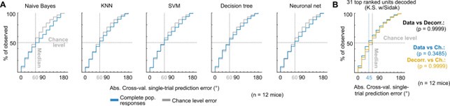
      It could be more informative to push forward the correlative analysis by looking at whether behavioural performance can be predicted by the coding scheme on a trial-by-trial basis.

      The previous version of the manuscript showed these analyses (now in Figure 6). Thus, task anchored grid firing predicts more successful performance on uncued trials at the session level (Figure 6A-B) and at the trial level (Figure 6C-D).

      Reviewer #1 (Recommendations For The Authors):

      (1) The author particularly mentioned that the 1D tracks are different from the "cue-rich environments that are typically used to study grid cells". It is not clear what conclusions would hold for a cue-rich environment or a track, which may require relatively less path integration compared to the cue-sparse environment. This point should be discussed.

      This is an important point that we did not pay sufficient attention to in the previous version of the manuscript. Our finding of successful localisation in the cued environment when grid cells are not task anchored implies that grid anchoring is not required to solve cued tasks. The implication here is that cue rich environments may then not be the most suitable for investigation of grid roles in behaviour as non-grid mechanisms may suffice, although this does not rule out the possibility that anchored grid codes may play important roles in learning about cue rich environments. We now address this point in the discussion (p 10, ‘An implication of this result is that cue rich tracks often used to investigate grid activity patterns may not engage behaviours that require anchored grid firing.’).

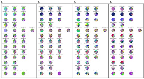
      (2) It would be good to see the statistics for the number of different cells (stable position or distance encoding, and unstable cells) identified per mouse/session and the number of grid cells per session.

      These are now added to Supplemental Data 2 and will also be accessible through code and datasets that we will make available alongside the version of record.

      (3) Figure 2F: any explanation about why AG cells had high spatial information?

      Previously the calculation used bits per spike and as aperiodic cells have low firing rates the spatial information was high. We have replaced this with bits per second, which provides a more intuitive measure and no longer implies high spatial information. We have amended this in the methods (p 15, ‘Spatial information was calculated in bits per second…’).

      (4) The following methods sections should provide additional details:

      (4.1) Details of the training protocol are largely left to reference papers. The reference papers give a general outline of the training protocol, but the details are not completely comparable given the single experiment performed on these mice. More details should be given on training stages and experience at the time of the experiment.

      The task is more clearly described in the introduction (p 3), and additional details of the training protocol are now provided in the methods (p 12-13).

      (4.2) The methods reference mean speed across sessions, but it is not clear where this was used.

      This was very poor wording. We have now changed this to ‘For each session the mean speed was calculated for each trial outcome’.

      (4.3) The calculation of the spatial autocorrelogram on a per-trial basis should be more explicitly stated. Is it the average of each 10 cm increment with the centre trial?

      We have added additional information to the methods (p 16-18).

      (4.4) 1D field detection is not sufficiently explained in Figure 1/S2. This information should also appear in the methods section.

      This is now clarified on page 16 in section ‘Analysis of neural activity and behaviour during the location memory task’.

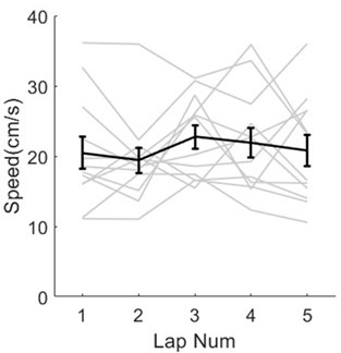
      (5) The data in Figure 4A and B only shows speed vs. location for one example mouse. The combined per mouse or per session data should also be shown.

      This is now shown in Figure 5A and Figure 5, Figure Supplemental 2

      (6) Figure 5 is somewhat confusing. Why are A/B by session and C/D by trial? The methods imply that A/B are originally averaged by cell, but that duplicate cells in the same session are excluded because behaviour versus session type is identical. This method should be valid if all grid cells within a session are all "stable". This is likely given the synchrony of code-switching between grid cells, but not all co-active grid cells behaved identically.

      It is understandable that C/D are performed by trial, but it should be made clear that it is not a comparable analysis to A/B. It is unclear what N refers to in C. The figure says by trial, but the legend says the error bar is by cell. If data is calculated by trial and then averaged by cell, this should be more clearly stated.

      In Figure 6A/B (previously Figure 5A/B) we focus our analysis on sessions in which the mode of grid firing, either task-anchored or task-independent, was relatively stable on a trialto-trial basis (see Figure 3F for definitions). This enables us to then compare behaviour averaged across each session, with sessions categorised as task-anchored and task independent. This analysis has the advantage that it focuses on large blocks of time (whole sessions) in which the mode of grid firing is unambiguous, but the disadvantage is that it excludes many sessions in which grid firing switches between task-anchored and taskindependent modes.

      Figure 6C/D (previously Figure 5C/D) addresses this limitation by carrying out similar analyses with behaviour sorted into task-anchored versus task-independent groups at the level of trials. A potential limitation for this analysis is that grid firing is somewhat variable on a trial-by-trial basis and so some trials may be mis-classified. We don’t expect this to lead to systematic bias, but it may make the data more noisy. Nevertheless, these analyses are important to include as they allow assessment of whether conclusions from 6A/B hold when all sessions are considered.

      We have added additional clarification of the rationale for these analyses to the main text (p7-8, ‘’We addressed this by using additional trial-level comparisons’). We have also added clarification in the methods section for categorisation of task-anchored versus taskindependent trials when multiple grid cells were recorded simultaneously (p 17, ‘When assigning a common classification across a group of cells recorded simultaneously...’) and an explanation for the N in the figure legend. We also clarify that the analyses use a nested random effects design to account for dependencies at the levels of sessions and mice (methods, p 20, ‘Random effects had a nested structure to account for animals and sessions…’) .

      (7) Panels E and F of Figure 5 are not explained in the main text.

      This is now corrected (see p8, ‘Additional analyses…’).

      (8) Figure 5: Since stable grid cells and all grid cells are shown, it will be better to show unstable cells, which can be compared with grid cells.

      Given that the rationale for differences between Figure 6A/B and C/D (previously Figure 5AD) were not previously clear, the reason for focussing on stable grid cells here was likely also not clear (see point 6 above). We don’t show unstable grid cells in Figure 6A-B as the behaviour averaged at the level of a session would be a mix of trials when they are taskanchored and when they are task-independent. Therefore, the analysis would not test predictions about the relationship between task-anchored vs task-independent modes and behaviour. We hope this is now clear in the manuscript given the revisions introduced to address point 6 above.

      (9) The methods describing the statistics for these experiments are also confusing. The methods section should be written more clearly, and it should be made clear in the text or figure legend whether this data is the "original" data or is processed in relation to the model, such as excluding duplicate grid cells within a session. The figure legend should also state that a GLMM was used to calculate the statistics.

      We have revised the methods section with the goal of improving clarity, adding detail and removing ambiguity. This includes updates of the methods for the GLMM analysis, which are referred to within the Figure 6 legend. A clear definition of a stable session is now also added to the Figure 6 legend.

      Reviewer #2 (Recommendations For The Authors):

      When grid fields are anchored to the virtual world (position mode), there is probably small trialto-trial variability in the firing location of the firing fields. Is this trial-to-trial variability related to the variability in the stop location? This would provide a more direct link between path integration in grid cell networks and behaviour that depends on path integration.

      When attempting to address this we find that the firing of individual grid cells is too variable to allow sufficiently precise decoding of their fields at a single trial level. This is expected given the Poisson statistics of spike generation and previous evaluations of grid coding (e.g. (Stemmler et al., 2015)).

      The conclusion of the abstract is: "Our results suggest that positional anchoring of grid firing enhances the performance of tasks that require path integration." This statement is slightly confusing. The task requires 1) anchoring the behaviour to the visual cues presented at the start of the trial and 2) path integration from thereon to identify the rewarded location. The performance is higher when grid cells anchor to the visual cues presented at the start of the trial. What the results show is that the anchoring of grid firing fields to visual landmarks enhances the performance of tasks that require path integration from visual landmarks (i.e. grid cells being anchored to the reference frame that is behaviorally relevant).

      To try to more clearly explain the logic and conclusion we have rewritten the abstract, including the final sentence.

      Similar comment for the title of Figure 5: "Positional grid coding is not required for cued spatial localisation but promotes path integration-dependent localisation." Positional coding means that grid cells are anchored to the behaviorally relevant reference frame.

      To address the lack of clarity we have modified the little of Figure 6 (previously Figure 5) to read ‘Anchoring of grid firing to the task reference frame promotes localisation by path integration but is not required for cued localisation’.

      In Figure 1, there is a wide range of beaconed (40-80%) and non-beaconed (10-60%) trials given. It is not 100% clear whether these refer to the percentage of trials of a given type within the recording sessions. Was the proportion of non-beaconed trials manipulated? If so, was the likelihood of position and distance coding changing according to the percentage of nonbeaconed trials?

      The ranges given refer to proportions across different behavioural sessions. Within any given behavioural session the proportion was constant. We now make this clear in the figure legend and in the results and methods sections.

      We did not manipulate proportions of trial types during a session. Manipulations betweens sessions were carried out with the goal of maximising the numbers of uncued trials that the mice would carry out (see response to public comments above). While the effect of trial-type at the session level is not relevant to the hypotheses we aim to test here, we have included an additional analysis of the relationship between task anchoring and the proportions of trial types in a session (Figure 3, Figure Supplement 7)(also discussed above). As disentangling the effects of learning and motivation will be complex and likely require new experimental designs we have not drawn strong conclusions or pursued the analysis further..

      I was not convinced that the labels "position" and "distance" were appropriate for the two grid cell firing modes. My understanding is that the "position" code also requires the grid cell network to estimate distance. It seems that the main difference between the "position" and "distance" modes is that when in the "position" mode, the activity on the torus is reset to a constant toroidal location when the animal reaches a clearly identifiable location on the virtual track. In the "distance" mode, this resetting does not take place.

      As previously mentioned, we agree these terms weren’t the best and have since relabelled these as “task-anchored” and “task-independent”.

      There are a few sections in the manuscript that implicitly suggest that a causal link between grid cell activity and behaviour was demonstrated. For instance: "It has been challenging to directly test whether and when grid cells contribute to behaviour.": The assumption here is that the manuscript overcomes this challenge, but the study is correlative.

      We have modified the wording to be clear that we are introducing new tests of predictions made by hypotheses about causal relationships between grid coding and behaviour (introduction, p 1-2). We also clarify that our results argue against the hypothesis that grid cells provide a general coded for behaviour, but corroborate predictions of hypotheses in which they are specifically important for path integration (discussion, p 10).

      We have modified the title abstract and main text to try to treat claims about causality with care. We now more thoroughly introduce and contrast the approach we report here with previous experiments that use perturbations (introduction, p2). While it is tempting to make stronger claims for causality with these approaches, there are also logical limitations with perturbation-based approaches, for example the challenges of fully excluding off target effects and adaptation. We now explain how these strategies are complementary. Our view is that both strategies will be required to develop strong arguments for whether and when grid cells contribute to behaviour. From this perspective, it is encouraging that our conclusions are in agreement with what are probably the most specific perturbations of grid cells reported to date (Gil et al. 2017), while perturbations that more generally affect MEC function appear to impair cued and path integration-dependent behaviours (Tennant et al. 2018). We now discuss these points more clearly (introduction, p 2).

      I am slightly confused by the references to the panels in Figure 4.

      "In some sessions, localization of the reward occurred almost exclusively when grid cells were anchored to position and not when they encoded distance (Figure 4C). Figure 4C only shows position coding.

      "In other sessions, animals localised the reward when grid firing was anchored to position or distance, but overall performance was improved on positional trials (Figure 4D-E)." The reference should probably point to Figure 4E-F or just to 4E.

      "In a few sessions, we observed spatial stopping behaviour comparable to cued trials, even when grid firing almost exclusively encoded distance rather than position (Figure 4F)." From Figure 4F, it seems that the performance on non-beaconed trials is better during "position" coding.

      We have now updated Figure 5 (Figure 4 in the original manuscript) and references to the Figure in the text. Now Figure 5 shows the activity of cells recorded in stable and unstable task-anchored and task-independent sessions (see Figure 5C-F).

      Minor issues:

      Is this correct: (Figure 4A and Figure 4, Figure Supplement 1).

      This has been corrected.

      Figure 4B: There could be an additional label for position and distance.

      Figure 4B from the original manuscript has now been removed.

      Figure 4C-F. The panels on the right side should be explained in the Figure Legend.

      Legends for Figure 5C-F (previously Figure 4C-F) have now been updated.

      Reviewer #3 (Recommendations For The Authors):

      Specific questions :

      (1) Position coding reflects a coding scheme in which fields are spaced by a fixed distance; previous studies have shown that a virtual track grid map is a slice of the 2D classic grid. In that case, the fields are still anchored to the track but would produce a completely different map. Did the authors check whether it is the case at least for some cells? If not, what could explain such a major difference?

      Το avoid confusion we now use the term ‘task-anchored’ rather than ‘position coding’ (see comments above). We should further clarify that our conclusions rest on whether or not the grid fields are anchored to the track. Task anchored firing does not require that grid fields maintain their spacing from 2D environments, only that fields are at the same track position on each trial. Thus, whether the spacing of the fields corresponds to a slice through a 2D grid makes no difference to the hypotheses we test here.

      We agree that the relationship between 1D and 2D field organisation could be an interesting future direction, for example anchoring could involve resetting the grid phase while maintaining a stable period, or it could be achieved through local distortions in the grid period. However, since these outcomes would not help distinguish the hypotheses we test here we have not included analyses to address them.

      (2) Previous studies have highlighted the role of grid cells in goal coding. Here there is an explicit reward in a particular area. Are there any grid modifications around this area? This question is not addressed in this study.

      Again, we note that the hypotheses we test here relate to the firing mode of grid cells - taskanchored or task-independent - and interpretation of our results is independent from the specific pattern of grid fields on the track. This question nevertheless leads to an interesting prediction that if grid fields cluster in the goal area then this clustering should be apparent in the task-anchored but not the task-independent firing mode.

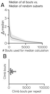
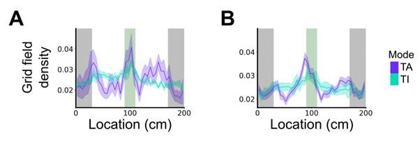
      We test this by considering the average distribution of firing fields across all grid cells in each firing mode (Reviewer Figure 1). We find that when grid firing is task-anchored there is a clear peak around the reward zone, which is consistent with previous work by Butler et al. and Boccara et al. Consistent with our other prediction, this peak is reduced when grid cells are in the task-independent mode.

      Author response image 1.

      Plot shows the grid field distribution during stable grid cell session (> 85 % task-anchored or task-independent) (A) or during task-anchored and task-independent trials (B). Shaded regions in A and B represent standard error of the mean measured across sessions and epochs respectively.

      (3) The behavioural procedure during recording is not fully explained. Do trial types alternate within the same session by blocks? How many trials are within a block? Is there any relation between trial alternation and the switch in the coding scheme observed in a large subset of the grid cells?

      We agree this wasn’t sufficiently clear in the previous version of the manuscript. Trial types were interleaved in a fixed order within each session. We have updated the results and methods sections to provide details (see responses above).

      (4) From the examples in Figure 2 it seems that firing fields tend to shift toward the start position. Is it the case in all cells? Could this reflect some reorganisation at the network level with cells signalling the starting as time progresses?

      This is inconsistent between cells. To make this variability clear we have included additional examples of spiking profiles from different grid cells (Figure 2 - 5). Because quantification of the phenomena would not, so far as we can tell, help distinguish our core hypotheses we have not included further analyses here.

      (5) Are grid cells with different coding properties recorded in different parts of the MEC? Are there any differences between these cell categories in the 2D map?

      The recordings we made are from the dorsal region of the MEC (stated at the start of the results section). We don’t have data to speak to other parts of the MEC.

      Minor:

      There are very few grid cell examples that repeat in the different figures. I would suggest showing more examples both in the main text and supplementary material.

      We have now provided multiple additional examples in Figures 2, 4 and 5. Grid cell examples repeat in the main figures twice, in both cases only when showing additional examples are shown from the same recording session (Figure 2A example #1 with Figure 5C, Figure 3E with Figure 4A). Further similar repeats are found in the supplemental figures (Figure 3D with Figure 5, Figure Supplement 2A, Figure 3C with Figure 5, Figure Supplement 2F).

      Fig1 A-B shows the predictions in a 1D track based on distance or position coding. The A inset represents the modification of field distribution from a 2D arena to a 1D track, as performed in this study. The inset B is misleading since it represents the modifications expected from a circular track to a 1D track as in Jacob et al 2019, that is not what the authors studied. It would be better to present either the predictions based on the present study or the prediction based on previous studies. In that case, they should mention the possibility that the 1D map is a slice of the 2D map.

      The goal of Figure 1A-B is to illustrate predictions (right) based on conclusions from previous studies (left). Figure 1A shows predicted 1D track firing given anchoring to the environment typically observed in grid cell studies in 2D arenas. Figure 1B shows predicted 1D track firing given the firing shifting firing patterns observed by Jacob et al. in a circular 2D track. To improve clarity, we have modified the legend to make clear that the schematics to the right are predictions given the previous evidence summarised to the left. As we outline above, the critical prediction relates to whether the representations anchor to the track. Whether the 1D representation is a perfect slice isn’t relevant to the hypotheses tested and so isn’t included in the schematic (see comments above).

    1. Author Response

      The following is the authors’ response to the original reviews.

      Public Reviews:

      Reviewer #1 (Public Review):

      The authors of this study seek to visualize NS1 purified from dengue virus infected cells. They infect vero cells with DV2-WT and DV2 NS1-T164S (a mutant virus previously characterized by the authors). The authors utilize an anti-NS1 antibody to immunoprecipitate NS1 from cell supernatants and then elute the antibody/NS1 complex with acid. The authors evaluate the eluted NS1 by SDS-PAGE, Native Page, mass spec, negative-stain EM, and eventually Cryo-EM. SDS-PAGE, mas spec, and native page reveal a >250 Kd species containing both NS1 and the proteinaceous component of HDL (ApoA1). The authors produce evidence to suggest that this population is predominantly NS1 in complex with ApoA1. This contrasts with recombinantly produced NS1 (obtained from a collaborator) which did not appear to be in complex with or contain ApoA1 (Figure 1C). The authors then visualize their NS1 stock in complex with their monoclonal antibody by CryoEM. For NS1-WT, the major species visualized by the authors was a ternary complex of an HDL particle in complex with an NS1 dimer bound to their mAB. For their mutant NS1-T164S, they find similar structures, but in contrast to NS1-WT, they visualize free NS1 dimers in complex with 2 Fabs (similar to what's been reported previously) as one of the major species. This highlights that different NS1 species have markedly divergent structural dynamics. It's important to note that the electron density maps for their structures do appear to be a bit overfitted since there are many regions with electron density that do not have a predicted fit and their HDL structure does not appear to have any predicted secondary structure for ApoA1. The authors then map the interaction between NS1 and ApoA1 using cross-linking mass spectrometry revealing numerous NS1-ApoA1 contact sites in the beta-roll and wing domain. The authors find that NS1 isolated from DENV infected mice is also present as a >250 kD species containing ApoA1. They further determine that immunoprecipitation of ApoA1 out of the sera from a single dengue patient correlates with levels of NS1 (presumably COIPed by ApoA1) in a dose-dependent manner.

      In the end, the authors make some useful observations for the NS1 field (mostly confirmatory) providing additional insight into the propensity of NS1 to interact with HDL and ApoA1. The study does not provide any functional assays to demonstrate activity of their proteins or conduct mutagenesis (or any other assays) to support their interaction predications. The authors assertion that higher-order NS1 exists primarily as a NS1 dimer in complex with HDL is not well supported as their purification methodology of NS1 likely introduces bias as to what NS1 complexes are isolated. While their results clearly reveal NS1 in complex with ApoA1, the lack of other NS1 homo-oligomers may be explained by how they purify NS1 from virally infected supernatant. Because NS1 produced during viral infection is not tagged, the authors use an anti-NS1 monoclonal antibody to purify NS1. This introduces a source of bias since only NS1 oligomers with their mAb epitope exposed will be purified. Further, the use of acid to elute NS1 may denature or alter NS1 structure and the authors do not include controls to test functionality of their NS1 stocks (capacity to trigger endothelial dysfunction or immune cell activation). The acid elution may force NS1 homo-oligomers into dimers which then reassociate with ApoA1 in a manner that is not reflective of native conditions. Conducting CryoEM of NS1 stocks only in the presence of full-length mAbs or Fabs also severely biases what species of NS1 is visualized since any NS1 oligomers without the B-ladder domain exposed will not be visualized. If the residues obscured by their mAb are involved in formation of higher-order oligomers then this antibody would functionally inhibit these species from forming. The absence of critical controls, use of one mAb, and acid elution for protein purification severely limits the interpretation of these data and do not paint a clear picture of if NS1 produced during infection is structurally distinct from recombinant NS1. Certainly there is novelty in purifying NS1 from virally infected cells, but without using a few different NS1 antibodies to purify NS1 stocks (or better yet a polyclonal population of antibodies) it's unclear if the results of the authors are simply a consequence of the mAb they selected.

      Data produced from numerous labs studying structure and function of flavivirus NS1 proteins provide diverse lines of evidence that the oligomeric state of NS1 is dynamic and can shift depending on context and environment. This means that the methodology used for NS1 production and purification will strongly impact the results of a study. The data in this manuscript certainly capture one of these dynamic states and overall support the general model of a dynamic NS1 oligomer that can associate with both host proteins as well as itself but the assertions of this manuscript are overall too strong given their data, as there is little evidence in this manuscript, and none available in the large body of existing literature, to support that NS1 exists only as a dimer associated with ApoA1. More likely the results of this paper are a result of their NS1 purification methodology.

      Suggestions for the Authors:

      Major:

      (1) Because of the methodology used for NS1 purification, it is not clear from the data provided if NS1 from viral infection differs from recombinant NS1. Isolating NS1 from viral infection using a polyclonal antibody population would be better to answer their questions. On this point, Vero cells are also not the best candidate for their NS1 production given these cells do not come from a human. A more relevant cell line like U937-DC-SIGN would be preferable.

      We performed an optimization of sNS1 secretion from DENV infection in different cell lines (Author response image 1 below) to identify the best cell line candidate to obtain relatively high yield of sNS1 for the study. As shown in Author response image 1, the levels of sNS1 in the tested human cell lines Huh7 and HEK 293T were at least 3-5 fold lower than in Vero cells. Although using a monocytic cell line expressing DC-SIGN as suggested by the reviewer would be ideal, in our experience the low infectivity of DENV in monocytic cell lines will not yield sufficient amount of sNS1 needed for structural analysis. For these practical reasons we decided to use the closely related non-human primate cell line Vero for sNS1 production supported by our optimization data.

      Author response image 1.

      sNS1 secretion in different mammalian and mosquito cell lines after DENV2 infection. The NS1 secretion level is measured using PlateliaTM Dengue NS1 Ag ELISA kit (Bio-Rad) on day 3 (left) and day 5 (right) post infection respectively.

      (2) The authors need to support their interaction predictions and models via orthogonal assays like mutagenesis followed by HDL/ApoA1 complexing and even NS1 functional assays. The authors should be able to mutate NS1 at regions predicted to be critical for ApoA1/HDL interaction. This is critical to support the central conclusions of this manuscript.

      In our previous publication (Chan et al., 2019 Sci Transl Med), we used similarly purified sNS1 (immunoaffinity purification followed by acid elution) from infected culture supernatants from both DENV2 wild-type and T164S mutant (both also studied in the present work) to carry out stimulation assay on human PBMCs as described by other leading laboratories investigating NS1 (Modhiran et al., 2015 Sci Transl Med). For reader convenience we have extracted the data from our published paper and present it as Author response image 2 below.

      Author response image 2.

      (A) IL6 and (B) TNFa concentrations measured in the supernatants of human PBMCs incubated with either 1µg/ml or 10µg/ml of the BHK-21 immunoaffinity-purified WT and TS mutant sNS1 for 24 hours. Data is adapted from Chan et al., 2019.

      Incubation of immunoaffinity-purified sNS1 (WT and TS) with human PBMCs from 3 independent human donors triggered the production of proinflammatory cytokines IL6 and TNF in a concentration dependent manner (Author response image 2), consistent with the published data by Modhiran et al., 2015 Sci Transl Med. Interestingly the TS mutant derived sNS1 induced a higher proinflammatory cytokines production than WT virus derived sNS1 that appears to correlate with the more lethal and severe disease phenotype in mice as also reported in our previous work (Chan et al., 2019). Additionally, the functionality of our immune-affinity purified infection derived sNS1 (isNA1) is now further supported by our preliminary results on the NS1 induced endothelial cell permeability assay using the purified WT and mutant isNS1 (Author response image 3). As shown in Author response image 3, both the isNS1wt and isNS1ts mutant reduced the relative transendothelial resistance from 0 to 9 h post-treatment, with the peak resistance reduction observed at 6 h post-treatment, suggesting that the purified isNS1 induced endothelial dysfunction as reported in Puerta-Guardo et al., 2019, Cell Rep.) It is noteworthy that the isNS1 in our study behaves similarly as the commercial recombinant sNS1 (rsNS1 purchased from the same source used in study by Puerta-Guardo et al., 2019) in inducing endothelial hyperpermeability. Collectively our previous published and current data suggest that the purified isNS1 (as a complex with ApoA1) has a pathogenic role in disease pathogenesis that is also supported in a recent publication by Benfrid et al., EMBO 2022). The acid elution has not affected the functionality of NS1.

      Author response image 3.

      Functional assessment of isNS1wt and isNS1ts on vascular permeability in vitro. A trans-endothelial permeabilty assay via measurement of the transendothelial electrical resistance (TEER) on human umbilical vascular endothelial cells (hUVEC) was performed, as described previously (Puerta-Guardo et al., 2019, Cell Rep). Ovalbumin serves as the negative control, while TNF-α and rsNS1 serves as the positive controls.

      We agree with reviewer about the suggested mutagnesis study. We will perform site-directed mutagenesis at selected residues and further structural and functional analyses and report the results in a follow-up study.

      (3) The authors need to show that the NS1 stocks produced using acid elution are functional compared to standard recombinantly produced NS1. Do acidic conditions impact structure/function of NS1?

      We are providing the same response to comments 1 & 2 above. We would like to reiterate that we have previously used sNS1 from immunoaffinity purification followed by acid elution to test its function in stimulating PBMCs to produce pro-inflammatory cytokines (Chan et al., 2019; Author response image 2). Similar to Modhiran et al. (2015) and Benfrid et al. (2022), the sNS1 that we extracted using acid elution are capable of activating PBMCs to produce pro-inflammatory cytokines. We have now further demonstrated the ability of both WT and TS isNS1 in inducing endothelial permeability in vitro in hUVECs, using the TEER assay (Author response image 3). Based on the data presented in the rebuttal figures as well as our previous publication we do not think that the acid elution has a significant impact on function of isNS1.

      We performed affinity purification to enrich the complex for better imaging and analysis (Supp Fig. 1b) since the crude supernatant contains serum proteins and serum-free infections also do not provide sufficient isNS1. The major complex observed in negative stain is 1:1 (also under acidic conditions which implies that the complex are stable and intact). We agree that it is possible that other oligomers can form but we have observed only a small population (74 out of 3433 particles, 2.15%; 24 micrographs) of HDL:sNS1 complex at 1:2 ratio as shown in the Author response image 4 below and in the manuscript (p. 4 lines 114-117, Supp Fig. 1c). Other NS1 dimer:HDL ratios including 2:1 and 3:1 have been reported by Benfrid et al., 2022 by spiking healthy sera with recombinant sNS1 and subsequent re-affinity purification. However, this method used an approximately 8-fold higher sNS1 concentration (400 ug/mL) than the maximum clinically reported concentration (50 ug/mL) (Young et al., 2000; Alcon et al., 2002; Libraty et al., 2002). In our hands, the sNS1 concentration in the concentrated media from in vitro infection was quantified as 30 ug/mL which is more physiologically relevant.

      We conclude that the integrity of the HDL of the complex is not lost during sample preparation, as we are able to observe the complex under the negative staining EM as well as infer from XL-MS. Our rebuttal data and our previous studies with our acid-eluted isNS1 from immunoaffinity purification clearly show that our protein is functional and biologically relevant.

      Author response image 4.

      (A) Representative negative stain micrograph of sNS1wt (B) Representative 2D averages of negative stained isNS1wt. Red arrows indicating the characteristic wing-like protrusions of NS1 inserted in HDL. (C) Data adapted from Figure 2 in Benfrid et al. (2022).

      (4) Overall, the data obtained from the mutant NS1 (contrasted to WT NS1) reveals how dynamic the oligomeric state of NS1 proteins are but the authors do not provide any insight into how/why this is, some additional lines of evidence using either structural studies or mutagenesis to compare WT and their mutant and even NS1 from a different serotype of DENV would help the field to understand the dynamic nature of NS1.

      The T164S mutation in DENV2 NS1 was proposed as the residue associated with disease severity in 1997 Cuban dengue epidemic (Halsted SB. “Intraepidemic increases in dengue disease severity: applying lessons on surveillance and transmission”. Whitehorn, J., Farrar. J., Eds., Clinical Insights in Dengue: Transmission, Diagnosis & Surveillance. The Future Medicine (2014), pp. 83-101). Our previous manuscript examined this mutation by engineering it into a less virulent clade 2 DENV isolated in Singapore and showed that sNS1 production was higher without any change in viral RNA replication. Transcript profiling of mutant compared to WT virus showed that genes that are usually induced during vascular leakage were upregulated for the mutant. We also showed that infection of interferon deficient AG129 mice with the mutant virus resulted in disease severity, increased complement protein expression in the liver, tissue inflammation and greater mortality compared to WT virus infected mice. The lipid profiling in our study (Chan et al., 2019) suggested small differences with WT but was overall similar to HDL as described by Gutsche et al. (2011). We were intrigued by our functional results and wanted to explore more deeply the impact of the mutation on sNS1 structure which at that stage was widely believed to be a trimer of NS1 dimers with a central channel (~ X Å) stuffed with lipid as established in several seminal publications (Flamand et al., 1999; Gutsche et al., 2011; Muller et al., 2012). In fact “This Week in Virology” netcast (https://www.microbe.tv/twiv/twiv-725/) discussed two back-to-back publications in Science (Modhiran et al., 371(6625)190-194; Biering et al., Science 371(6625):194-200)) which showed that therapeutic antibodies can ameliorate the NS1 induced pathogenesis and expert discussants posed questions that also pointed to the need for more accurate definition of the molecular composition and architecture of the circulating NS1 complex during virus infection to get a clearer handle on its pathogenic mechanism. Our current studies and also the recent high resolution cryoEM structures (Shu et al., 2022) do not support the notion of a central channel “stuffed with lipid”. Even in the rare instances where trimer of dimers are shown, the narrow channel in the center could only accommodate one molecule of lipoid molecule no bigger than a typical triglyceride molecule. This hexamer model cannot explain the lipid proeotmics data in the literature.

      In our study we observed predominantly 1:1 NS1 dimer to HDL (~30 μg/mL) mirroring maximum clinically reported concentration of sNS1 in the sera of DENV patients (40-50 μg/mL) as we highlighted in our main text (P. 18, lines 461-471). What is often quoted (also see later) is the recent study of Flamand & co-workers which show 1-3 NS1 dimers per HDL (Benfrid et al, 2022) by spiking rsNS1 (400 μg/mL) with HDL. This should not be confused with the previous models which suggested a lipid filled central channel holding together the hexamer. The use of physiologically relevant concentrations is important for these studies as we have highlighted in our main text (P. 18, lines 461-471).

      Our interpretation for the mutant (isNS1ts) is that it is possible that the hydrophilic serine at residue 164 located in the greasy finger loop may weaken the isNS1ts binding to HDL hence the observation of free sNS1 dimers in our immunoaffinity purified (acid eluted sample). The disease severity and increased complement protein expression in AG129 mice liver can be ascribed to weakly bound mutant NS1 with fast on/off rate with HDL being transported to the liver where specific receptors bind to free sNS1 and interact with effector proteins such as complement to drive inflammation and associated pathology. Our indirect support for this is that the XL-MS analysis of purified isNS1ts identified only 7 isNS1ts:ApoA1 crosslinks while 25 isNS1wt:ApoA1 crosslinks were identified from purified isNS1wt (refer to Fig. 4 and Supp. Fig. 8).

      Taken together, the cryoEM and XL-MS analysis of purified isNS1ts suggest that isNS1ts has weaker affinity for HDL compared to isNS1wt. We welcome constructive discussion on our interpretation that we and others will hopefully obtain more data to support or deny our proposed explanation. Our focus has been to compare WT with mutant sNS1 from DENV2 and we agree that it will be useful to study other serotypes.

      Reviewer #2:

      CryoEM:

      Some of the neg-stain 2D class averages for sNS1 in Fig S1 clearly show 1 or 2 NS1 dimers on the surface of a spherical object, presumably HDL, and indicate the possibility of high-quality cryoEM results. However, the cryoEM results are disappointing. The cryo 2D class averages and refined EM map in Fig S4 are of poor quality, indicating sub-optimal grid preparation or some other sample problem. Some of the FSC curves (2 in Fig S7 and 1 in Fig S6) have extremely peculiar shapes, suggesting something amiss in the map refinement. The sharp drop in the "corrected" FSC curves in Figs S5c and S6c (upper) indicate severe problems. The stated resolutions (3.42 & 3.82 Å) for the sNS1ts-Fab56.2 are wildly incompatible with the images of the refined maps in Figs 3 & S7. At those resolutions, clear secondary structural elements should be visible throughout the map. From the 2D averages and 3D maps shown in the figures this does not seem to be the case. Local resolution maps should be shown for each structure.

      The same sample is used for negative staining and the cryoEM results presented. The cryoEM 2D class averages are similar to the negative stain ones, with many spherical-like densities with no discernible features, presumably HDL only or the NS1 features are averaged out. The key difference lies in the 2D class averages where the NS1 could be seen. The side views of NS1 (wing-like protrusion) are more obvious in the negative stain while the top views of NS1 (cross shaped-like protrusion) are more obvious under cryoEM. HDL particles are inherently heterogeneous and known to range from 70-120 Å, this has been highlighted in the main text (p. 8, lines 203 and 228). This helps to explain why the reviewer may find the cryoEM result disappointing. The sample is inherently challenging to resolve structurally as it is (not that the sample is of poor quality). In terms of grid preparation, Supp Fig 4b shows a representative motion-corrected micrograph of the isNS1ts sample whereby individual particles can be discerned and evenly distributed across the grid at high density.

      We acknowledge that most of the dips in the FSC curves (Fig S5-7) are irregular and affect the accuracy of the stated resolutions, particularly for the HDL-isNS1ts-Fab56.2 and isNS1ts-Fab56.2 maps for which the local resolution maps are shown (Fig S7d-e). Probable reasons affecting the FSC curves include (1) the heterogeneous nature of HDL, (2) preferred orientation issue (p 7, lines 198 -200), and (3) the data quality is intrinsically less ideal for high resolution single particle analysis. Optimizing of the dynamic masking such that the mask is not sharper than the resolution of the map for the near (default = 3 angstroms) and far (12 angstroms) parameters during data processing, ranging from 6 - 12 and 14 - 20 respectively, did not help to improve the FSC curves. To report a more accurate global resolution, we have revised the figures S5-7 with new FSC curve plots generated using the remote 3DFSC processing server.

      Regardless, the overall architecture and the relative arrangement of NS1 dimer, Fab, and HDL are clearly visible and identifiable in the map. These results agree well with our biochemical data and mass-spec data.

      The samples were clearly challenging for cryoEM, leading to poor quality maps that were difficult to interpret. None of the figures are convincing that NS1, Ab56.2 or Fab56.2 are correctly fit into EM maps. There is no indication of ApoA1 helices. Details of the fit of models to density for key regions of the higher-resolution EM maps should be shown and the models should be deposited in the PDB. An example of modeling difficulty is clear in the sNS1ts dimer with bound Fab56.2 (figs 3c & S7e). For this complex, the orientation of the Fab56.2 relative to the sNS1ts dimer in this submission (Fig 3c) is substantially different than in the bioRxiv preprint (Fig 3c). Regions of empty density in Fig 3c also illustrate the challenge of building a model into this map.

      We acknowledge the modelling challenge posed by low resolution maps in general, such as the handedness of the Fab molecule as pointed out by the reviewer (which is why others have developed the use of anti-fab nanobody to aid in structure determination among other methods). The change in orientation of the Fab56.2 relative to the sNS1ts dimer was informed by the HDX-MS results which was not done at the point of bioRxiv preprint mentioned. With regards to indication of ApoA1 helices, this is expected given the heterogeneous nature of HDL. To the best of our knowledge, engineered apoA1 helices were also not reported in many cryoEM structures of membrane proteins solved in membrane scaffold protein (MSP) nanodiscs. This is despite nanodiscs, comprised of engineered apoA1 helices, having well-defined size classifications.

      Regions of weak density in Fig 3c is expected due to the preferred orientation issue acknowledged in the results section of the main text (p. 9, line 245). The cryoEM density maps have been deposited in the Electron Microscopy Data Bank (EMDB) under accession codes EMD-36483 (isNS1ts:Fab56.2) and EMD-36480 (Fab56.2:isNS1ts:HDL). The protein model files for isNS1ts:Fab56.2 and Fab56.2:isNS1ts:HDL model are available upon request. Crosslinking MS raw files and the search results can be downloaded from https://repository.jpostdb.org/preview/14869768463bf85b347ac2 with the access code: 3827. The HDX-MS data is deposited to the ProteomeXchange consortium via PRIDE partner repository51 with the dataset identifier PXD042235.

      Mass spec:

      Crosslinking-mass spec was used to detect contacts between NS1 and ApoA1, providing strong validation of the sNS1-HDL association. As the crosslinks were detected in a bulk sample, they show that NS1 is near ApoA1 in many/most HDL particles, but they do not indicate a specific protein-protein complex. Thus, the data do not support the model of an NS1-ApoA1 complex in Fig 4d. Further, a specific NS1-ApoA1 interaction should have evidence in the EM maps (helical density for ApoA1), but none is shown or mentioned. If such exists, it could perhaps be visualized after focused refinement of the map for sNS1ts-HDL with Fab56.2 (Fig S7d). The finding that sNS1-ApoA1 crosslinks involved residues on the hydrophobic surface of the NS1 dimer confirms previous data that this NS1 surface engages with membranes and lipids.

      We thank the reviewer for the comment. The XL-MS is a method to identify the protein-protein interactions by proximity within the spacer arm length of the crosslinker. The crosslinking MS data do support the NS1-ApoA1 complex model obtained by cryo-EM because the identified crosslinks that are superimposed on the EM map are within the cut-off distance of 30 Å. We agree that the XL-MS data do not dictate the specific interactions between specific residues of NS1-ApoA1 in the EM model. We also do not claim that specific residue of NS1 in beta roll or wing domain is interacting with specific residue of ApoA1 in H4 and H5 domain. We claim that beta roll and wing domain regions of NS1 are interacting with ApoA1 in HDL indicating the proximity nature of NS1-ApoA1 interactions as warranted by the XL-MS data.

      As explained in the previous response on the lack of indication of ApoA1 helical density, this is expected given the heterogeneous nature of HDL. It is typical to see lipid membranes as unstructured and of lower density than the structured protein. In our study, local refinement was performed on either the global map (presented in Fig S7d) or focused on the NS1-Fab region only. Both yielded similar maps as illustrated in the real space slices shown in Author response image 5. The mask and map overlay is depicted in similar orientations to the real space slices, and at different contour thresholds at 0.05 (Author response image 5e) and 0.135 (Author response image 5f). While the overall map is of poor resolution and directional anisotropy evident, there is clear signal differences in the low density region (i.e. the HDL sphere) indicative of NS1 interaction with ApoA1 in HDL, extending from the NS1 wing to the base of the HDL sphere.

      Author response image 5.

      Real Space Slices of map and mask used during Local Refinement for overall structure (a-b) and focused mask on NS1 region (c-d). The corresponding map (grey) contoured at 0.05 (e) and 0.135 (f) in similar orientations as shown for the real space slices of map and masks. The focused mask of NS1 used is colored in semi-transparent yellow. Real Space Slices of map and mask are generated during data processing in Cryosparc 4.0 and the map figures were prepared using ChimeraX.

      Sample quality:

      The paper lacks any validation that the purified sNS1 retains established functions, for example the ability to enhance virus infectivity or to promote endothelial dysfunction.

      Please see detailed response for question 2 in Reviewer #1’s comments. In essence, we have showed that both isNS1wt and isNS1ts are capable of inducing endothelial permeability in an in vitro TEER assay (Rebuttal Fig 3) and also in our previous study that quantified inflammation in human PBMC’s (Rebuttal Fig 2).

      Peculiarities include the gel filtration profiles (Fig 2a), which indicate identical elution volumes (apparent MWs) for sNS1wt-HDL bound to Ab562 (~150 kDa) and to the ~3X smaller Fab56.2 (~50 kDa). There should also be some indication of sNS1wt-HDL pairs crosslinked by the full-length Ab, as can be seen in the raw cryoEM micrograph (Fig S5b).

      Obtaining high quality structures is often more demanding of sample integrity than are activity assays. Given the low quality of the cryoEM maps, it's possible that the acidification step in immunoaffinity purification damaged the HDL complex. No validation of HDL integrity, for example with acid-treated HDL, is reported.

      Please see detailed response for question 3 in Reviewer #1’s comments.

      Acid treatment is perhaps discounted by a statement (line 464) that another group also used immunoaffinity purification in a recent study (ref 20) reporting sNS1 bound to HDL. However the statement is incorrect; the cited study used affinity purification via a strep-tag on recombinant sNS1.

      We thank the Reviewer for pointing this out and have rewritten this paragraph instead (p 18, line 445-455). We also expanded our discussion to highlight our prior functional studies showing that acid-eluted isNS1 proteins do induce endothelial hyperpermeability (p 18-19, line 470-476).

      Discussion:

      The Discussion reflects a view that the NS1 secreted from virus-infected cells is a 1:1 sNS1dimer:HDL complex with the specific NS1-ApoA1 contacts detected by crosslinking mass spec. This is inconsistent with both the neg-stain 2D class average with 2 sNS1 dimers on an HDL (Fig S1c) and with the recent study of Flamand & co-workers showing 1-3 NS1 dimers per HDL (ref 20). It is also ignores the propensity of NS1 to associate with membranes and lipids. It is far more likely that NS1 association with HDL is driven by these hydrophobic interactions than by specific protein-protein contacts. A lengthy Discussion section (lines 461-522) includes several chemically dubious or inconsistent statements, all based on the assumption that specific ApoA1 contacts are essential to NS1 association with HDL and that sNS1 oligomers higher than the dimer necessarily involve ApoA1 interaction, conclusions that are not established by the data in this paper.

      We thank the Reviewer and have revised our discussion to cover available structural and functional data to draw conclusions that invariably also need further validation by others. One point that is repeatedly brought up by Reviewer 1 & 2 is the quality and functionality of our sample. Our conclusion now reiterates this point based on our own published data (Chan et al., 2019) and also the TEER assay data provided as Author response image 3.

      Reviewer #1 (Recommendations For The Authors):

      Minor:

      (1) Fig. S3B, should the label for lane 4 be isNS1? In figure 1C you do not see ApoA1 for rsNS1 but for S3B you do? Which is correct?

      This has been corrected in the Fig. S3B, the label for lane 4 has been corrected to isNS1 and lane 1 to rsNS1, where no ApoA1 band (25 kDa) is found.

      (2) Line 436, is this the correct reference? Reference 43?

      This has been corrected in the main text. (p 20, Line 507; Lee et al., 2020, J Exp Med).

      Reviewer #2 (Recommendations For The Authors):

      The cryoEM data analysis is incompletely described. The process (software, etc) leading to each refined EM map should be stated, including the use of reference structures in any step. These details are not in the Methods or in Figs S4-7, as claimed in the Methods. The use of DeepEMhancer (which refinements?) with the lack of defined secondary structural features in the maps and without any validation (or discussion of what was used as "ground truth") is concerning. At the least, the authors should show pre- and post-DeepEMhancer maps in the supplemental figures.

      The data processing steps in the Methods section have been described with improved clarity. DeepEMhancer is a deep learning solution for cryo-EM volume post-processing to reduce noise levels and obtain more detailed versions of the experimental maps (Sanchez-Garcia, et al., 2021). DeepEMhancer was only used to sharpen the maps and reduce the noise for classes 1 and 2 of isNS1wt in complex with Ab56.2 for visualization purpose only and not for any refinements. To avoid any confusion, the use of DeepEMhancer has been removed from the supp text and figures.

      Line 83 - "cryoEM structures...recently reported" isn't ref 17

      This reference has been corrected in to Shu et al. (2022) in p 3, line 83.

      Fig. S3 - mis-labeled gel lanes

      This has been corrected in the Fig. S3B, the label for lane 4 has been corrected to isNS1 and lane 1 to rsNS1.

      Fig S6c caption - "Representative 2D classes of each 3D classes, white bar 100 Å. Refined 3D map for classes 1 and 2 coloured by local resolution". The first sentence is unclear, and there is no white scale bar and no heat map.

      Fig S6c caption has been corrected to “Representative 3D classes contoured at 0.06 and its particle distribution as labelled and coloured in cyan. Scale bar of 100 Å as shown. Refined 3D maps and their respective FSC resolution charts and posterior precision directional distribution as generated in crysosparc4.0”.

    1. Author response:

      The following is the authors’ response to the original reviews.

      Reviewer #1 (Public Review):

      Summary:

      This study explores the sequence characteristics and features of high-occupancy target (HOT) loci across the human genome. The computational analyses presented in this paper provide information into the correlation of TF binding and regulatory networks at HOT loci that were regarded as lacking sequence specificity.

      By leveraging hundreds of ChIP-seq datasets from the ENCODE Project to delineate HOT loci in HepG2, K562, and H1-hESC cells, the investigators identified the regulatory significance and participation in 3D chromatin interactions of HOT loci. Subsequent exploration focused on the interaction of DNA-associated proteins (DAPs) with HOT loci using computational models. The models established that the potential formation of HOT loci is likely embedded in their DNA sequences and is significantly influenced by GC contents. Further inquiry exposed contrasting roles of HOT loci in housekeeping and tissue-specific functions spanning various cell types, with distinctions between embryonic and differentiated states, including instances of polymorphic variability. The authors conclude with a speculative model that HOT loci serve as anchors where phase-separated transcriptional condensates form. The findings presented here open avenues for future research, encouraging more exploration of the functional implications of HOT loci.

      Strengths:

      The concept of using computational models to define characteristics of HOT loci is refreshing and allows researchers to take a different approach to identifying potential targets. The major strengths of the study lies in the very large number of datasets analyzed, with hundreds of ChIP-seq data sets for both HepG2 and K562 cells as part of the ENCODE project. Such quantitative power allowed the authors to delve deeply into HOT loci, which were previously thought to be artifacts.

      Weaknesses:

      While this study contributes to our knowledge of HOT loci, there are critical weaknesses that need to be addressed. There are questions on the validity of the assumptions made for certain analyses. The speculative nature of the proposed model involving transcriptional condensates needs either further validation or be toned down. Furthermore, some apparent contradictions exist among the main conclusions, and these either need to be better explained or corrected. Lastly, several figure panels could be better explained or described in the figure legends.

      We thank the reviewer for their valuable comments.

      - We have extended the study and included a new chapter focusing on the condensate hypothesis, added more supporting evidence (including the ones suggested by the reviewer), and made explicit statements on the speculative nature of this model.

      - We have restructured the text to remove the sentences which might be construed as contradictory.

      Reviewer #2 (Public Review):

      Summary:

      The paper 'Sequence characteristic and an accurate model of abundant hyperactive loci in human genome' by Hydaiberdiev and Ovcharenko offers comprehensive analyses and insights about the 'high-occupancy target' (HOT) loci in the human genome. These are considered genomic regions that overlap with transcription factor binding sites. The authors provided very comprehensive analyses of the TF composition characteristics of these HOT loci. They showed that these HOT loci tend to overlap with annotated promoters and enhancers, GC-rich regions, open chromatin signals, and highly conserved regions, and that these loci are also enriched with potentially causal variants with different traits.

      Strengths:

      Overall, the HOT loci' definition is clear and the data of HOT regions across the genome can be a useful dataset for studies that use HepG2 or K562 as a model. I appreciate the authors' efforts in presenting many analyses and plots backing up each statement.

      Weaknesses:

      It is noteworthy that the HOT concept and their signature characteristics as being highly functional regions of the genome are not presented for the first time here. Additionally, I find the main manuscript, though very comprehensive, long-winded and can be put in a shorter, more digestible format without sacrificing scientific content.

      The introduction's mention of the blacklisted region can be rather misleading because when I read it, I was anticipating that we are uncovering new regulatory regions within the blacklisted region. However, the paper does not seem to address the question of whether the HOT regions overlap, if any, with the ENCODE blacklisted regions afterward. This plays into the central assessment that this manuscript is long-winded.

      The introduction also mentioned that HOT regions correspond to 'genomic regions that seemingly get bound by a large number of TFs with no apparent DNA sequence specificity' (this point of 'no sequence specificity' is reiterated in the discussion lines 485-486). However, later on in the paper, the authors also presented models such as convolutional neural networks that take in one-hot-encoded DNA sequence to predict HOT performed really well. It means that the sequence contexts with potential motifs can still play a role in forming the HOT loci. At the same time, lines 59-60 also cited studies that "detected putative drive motifs at the core segments of the HOT loci". The authors should edit the manuscript to clarify (or eradicate) contradictory statements.

      We thank the reviewer for their valuable comments. Below are our responses to each paragraph in the given order:

      We added a statement in the commenting and summarizing other publications that studied the functional aspects of HOT loci with the following sentence in the introduction part:

      “Other studies have concluded that these regions are highly functionally consequential regions enriched in epigenetic signals of active regulatory elements such as histone modification regions and high chromatin accessibility”.

      We significantly shortened the manuscript by a) moving the detailed analyses of the computational model to the supplemental materials, and b) shortening the discussions by around half, focusing on core analyses that would be most beneficial to the field.

      Given that the ENCODE blacklisted regions are the regions that are recommended by the ENCODE guidelines to be avoided in mapping the ChIP-seq (and other NGS), we excluded them from our analyzed regions before mapping to the genome. Instead, we relied on the conclusions of other publications on HOT loci that the initial assessments of a fraction of HOT loci were the result of factoring in these loci which later were included in blacklisted regions.

      We addressed the potential confusion by using the expression of “no sequence specificity” by a) changing the sentence in the introduction by adding a clarification as “... with no apparent DNA sequence specificity in terms of detectible binding motifs of corresponding motifs” and b) removing that part from the sentence in the discussions.

      Reviewer #3 (Public Review):

      Summary:

      Hudaiberdiev and Ovcharenko investigate regions within the genome where a high abundance of DNA-associated proteins are located and identify DNA sequence features enriched in these regions, their conservation in evolution, and variation in disease. Using ChIP-seq binding profiles of over 1,000 proteins in three human cell lines (HepG2, K562, and H1) as a data source they're able to identify nearly 44,000 high-occupancy target loci (HOT) that form at promoter and enhancer regions, thus suggesting these HOT loci regulate housekeeping and cell identity genes. Their primary investigative tool is HepG2 cells, but they employ K562 and H1 cells as tools to validate these assertions in other human cell types. Their analyses use RNA pol II signal, super-enhancer, regular-enhancer, and epigenetic marks to support the identification of these regions. The work is notable, in that it identifies a set of proteins that are invariantly associated with high-occupancy enhancers and promoters and argues for the integration of these molecules at different genomic loci. These observations are leveraged by the authors to argue HOT loci as potential sites of transcriptional condensates, a claim that they are well poised to provide information in support of. This work would benefit from refinement and some additional work to support the claims.

      Comments:

      (1) Condensates are thought to be scaffolded by one or more proteins or RNA molecules that are associated together to induce phase separation. The authors can readily provide from their analysis a check of whether HOT loci exist within different condensate compartments (or a marker for them). Generally, ChIPSeq signal from MED1 and Ronin (THAP11) would be anticipated to correspond with transcriptional condensates of different flavors, other coactivator proteins (e.g., BRD4), would be useful to include as well. Similarly, condensate scaffolding proteins of facultative and constitutive heterochromatin (HP1a and EZH2/1) would augment the authors' model by providing further evidence that HOT Loci occur at transcriptional condensates and not heterochromatin condensates. Sites of splicing might be informative as well, splicing condensates (or nuclear speckles) are scaffolded by SRRM/SON, which is probably not in their data set, but members of the serine arginine-rich splicing factor family of proteins can serve as a proxy-SRSF2 is the best studied of this set. This would provide a significant improvement to their proposed model and be expected since the authors note that these proteins occur at the enhancers and promoter regions of highly expressed genes.

      (2) It is curious that MAX is found to be highly enriched without its binding partner Myc, is Myc's signal simply lower in abundance, or is it absent from HOT loci? How could it be possible that a pair of proteins, which bind DNA as a heterodimer are found in HOT loci without invoking a condensate model to interpret the results?

      (3) Numerous studies have linked the physical properties of transcription factor proteins to their role in the genome. The authors here provide a limited analysis of the proteins found at different HOT-loci by employing go terms. Is there evidence for specific types of structural motifs, disordered motifs, or related properties of these proteins present in specific loci?

      (4) Condensates themselves possess different emergent properties, but it is a product of the proteins and RNAs that concentrate in them and not a result of any one specific function (condensates can have multiple functions!)

      (5) Transcriptional condensates serve as functional bodies. The notion the authors present in their discussion is not held by practitioners of condensate science, in that condensates exist to perform biochemical functions and are dissolved in response to satisfying that need, not that they serve simply as reservoirs of active molecules. For example, transcriptional condensates form at enhancers or promoters that concentrate factors involved in the activation and expression of that gene and are subsequently dissolved in response to a regulatory signal (in transcription this can be the nascently synthesized RNA itself or other factors). The association reactions driving the formation of active biochemical machinery within condensates are materially changed, as are the kinetics of assembly. It is unnecessary and inaccurate to qualify transcriptional condensates as depots for transcriptional machinery.

      6) This work has the potential to advance the field forward by providing a detailed perspective on what proteins are located in what regions of the genome. Publication of this information alongside the manuscript would advance the field materially.

      We thank the reviewer for constructive comments and suggestions. Below are our point-by-point responses:

      (1) We added a new short section “Transcriptional condensates as a model for explaining the HOT regions” with additional support for the condensate hypothesis, wherein some of the points raised here were addressed. Specifically, we used a curated LLPS proteins (CD-CODE) database and provided statistics of those annotation condensate-related DAPs.

      Regarding the DAPs mentioned in this question, we observed that the distributions corresponding ChIP-seq peaks confirm the patterns expected by the reviewer (Author response image 1). Namely:

      - MED1 and Ronin (THAP11) are abundant in the HOT loci, being present 67% and 64% of HOT loci respectively.

      - While the BRD4 is present in 28% of the HOT loci, we observed that the DAPs with annotated LLPS activity ranged from 3% to 73%, providing further support for the condensate hypothesis.

      - ENCODE database does not contain ChIP-seq dataset for HP1A. EZH2 peaks were absent in the HOT loci (0.4% overlap), suggesting the lack of heterochromatin condensate involvement.

      - Serine-rich splicing factor family proteins were present only in 7.7% of the HOT loci, suggesting the absence or limited overlap with splicing condensates or nuclear speckles.

      Author response image 1.

      (2) In this study we selected the TF ChIP-seq datasets with stringent quality metrics, excluding those which had attached audit warning and errors. As a result, the set of DAPs analyzed in HepG2 did not include MYC, since the corresponding ChIP-seq dataset had the audit warning tags of "borderline replicate concordance, insufficient read length, insufficient read depth, extremely low read depth". Analyses in K562 and H1 did include MYC (alongside MAX) ChIP-seq dataset.

      To address this question, we added the mentioned ChIP-seq dataset (ENCODE ID: ENCFF800JFG) and analyzed the colocalization patterns of MYC and MAX. We observed that the MYC ChIP-seq peaks in HepG2 display spurious results, overlapping with only 5% of HOT loci. Meanwhile in K562 and H1, MYC and MAX are jointly present in 54% and 44% of the HOT loci, respectively (Author response image 2).

      Author response image 2.

      These observations were also supported by Jaccard indices between the MYC and MAX ChIP-seq peaks. To do this analysis, we calculated the pairwise Jaccard indices between MYC and MAX and divided them by the average Jaccard indices of 2000 randomly selected DAP pairs. In K562 and H1, the Jaccard indices between MYC and MAX are 5.72x and 2.53x greater than the random background, respectively. For HepG2, the ratio was 0.21x, clearly indicating that HepG2 MYC ChIP-seq dataset is likely erroneous.

      Author response image 3.

      (3) Despite numerous publications focusing on different structural domains in transcription factors, we could not find an extensive database or a survey study focusing on annotations of structural motifs in human TFs. Therefore, surveying such a scale would be outside of this study’s scope. We added only the analysis of intrinsically disordered regions, as it pertains to the condensate hypothesis. To emphasize this shortcoming, we added the following sentence to the end of the discussions section.

      “Further, one of the hallmarks of LLPS proteins that have been associated with their abilities to phase-separate is the overrepresentation of certain structural motifs, which we did not pursue due to size limitations.”

      (4, 5) We agree with these statements and thank the reviewer for pointing out this faulty statement. We modified the sections in the discussions related to the condensates and removed the part where we implied that the condensate model could be because of mostly a single function of TF reservoir.

      (6) We added a table to the supplemental materials (Zenodo repository) with detailed annotation of HOT and non-HOT DAP-bound loci in the genome.

      Recommendations for the authors:

      Reviewing Editor (Recommendations For The Authors):

      The clause with "inadequate" would be dropped if the authors sufficiently address reviewer concerns about clarity of writing, including:

      (1) Editing the title to better reflect the findings of the paper.

      (2) Making clear that the condensate model is speculative and not explicitly tested in this study (and may be better described as a hypothesis).

      (3) Resolving apparent contradictions regarding DNA sequence specificity and the interpretation of ChIP-seq signal intensity.

      (4) Better specifying and justifying model parameters, thresholds, and assumptions.

      (5) Shortening the manuscript to emphasize the main, well-supported claims and to enhance readability (especially the discussion section).

      We thank the Editor for their work. We followed their advice and implemented changes and additions to address all 5 points.

      Reviewer #1 (Recommendations For The Authors):

      (1) The title "Sequence characteristics and an accurate model of abundant hyperactive loci in the human genome" does not accurately reflect the findings of the paper. We are unclear as to what the 'accurate model' refers to. Is it the proposed model 'based on the existence of large transcriptional condensates' (abstract)? If so, there are concerns below regarding this statement (see comment 2). If the authors are referring to the computational modeling presented in Figure 5, it is unclear that any one of them performed that much better than the others and the best single model was not identified. Furthermore, the models being developed in the study constitute only a portion of the paper and lacked validation through additional datasets. Additionally, sequence characteristics were not a primary focus of the study. Only figure 5 talks about the model and sequence characteristics, the rest of the figures are left out of the equation.

      We agree with and thank the reviewer for this idea of clarifying the intended meaning.

      (1) We changed the title and clarified that the computational model is meant:

      “Functional characteristics and a computational model of abundant hyperactive loci in the human genome”.

      (2) Shortened the part of the manuscript discussing the computational models and pointed out the CNNs as “the best single model”.

      (2) The abstract and discussion (and perhaps the title) propose a model of transcriptional condensates in relation to HOT loci. However, there is no data provided in the manuscript that relates to condensates. Therefore, anything relating to condensates is primarily speculative. This distinction needs to be properly made, especially in the abstract (and cannot be included in the title). Otherwise, these statements are misleading. Although the field of transcriptional condensates is relatively new, there have been several factors studied. The authors could include in Figure 2d which factors have been shown to form transcriptional condensates. This might provide some support for the model, though it would still largely remain speculative unless further testing is done.

      We added a new short chapter “Transcriptional condensates as a model for explaining the HOT regions”,  with additional analyses testing the condensates hypothesis. We provided supportive evidence by analyzing the metrics used as hallmarks of condensates including the distributions of annotated condensate-related proteins, nascent transcription, and protein-RNA interaction levels in HOT loci. Still, we acknowledge that this is a speculative hypothesis and we clarified that with the following statement in the discussions:

      “It is important to note here that our proposed condensate model is a speculative hypothesis. Further experimental studies in the field are needed to confirm or reject it.”

      (3) Several apparent contradictions exist throughout the manuscript. For example, "HOT locus formation are likely encoded in their DNA sequences" (lines 329-330) vs the proposed model of formation through condensates (abstract). These two statements do not seem compatible, or at the very least, the authors can explain how they are consistent with each other. Another example: "ChIP-seq signal intensity as a proxy for... binding affinity" (line 229) vs. "ChIP-seq signal intensities do not seem to be a function of the DNA-binding properties of the DAPs" (lines 259-260). The first statement is the assumption for subsequent analyses, which has its own concerns (see comment 4). But the conclusion from that analysis seems to contradict the assumption, at least as it is stated.

      In this study, we argue that the two statements may not necessarily contradict each other. We aimed to a) demonstrate that the observed intensity of DAP-DNA interactions as measured by ChIP-seq experiments at HOT loci cannot be explained with direct DNA-binding events of the DAPs alone and b) propose a hypothesis that this observation can be at least partially explained if the HOT loci have the propensity to either facilitate or take part in the formation of transcriptional condensates.

      One of the conditions for condensates to form at enhancers was shown to be the presence of strong binding sites of key TFs (Shrinivas et al. 2019 “Enhancer features that drive the formation of transcriptional condensates”), where the study was conducted using only one TF (OCT4) and one coactivator (MED1). To the best of our knowledge, no such study has been conducted involving many TFs and cofactors simultaneously. We also know that the factors that lead to liquid-to-liquid phase separation include weak multivalent IDR-IDR, IDR-DNA, and IDR-RNA interactions. As a result, the observed total sum of ChIP-seq peaks in HOT loci is the direct DNA-binding events combined with the indirect DAP-DNA interactions, some of which may be facilitated by condensates. And, the fact that CNNs can recognize the HOT loci with high accuracy suggests that there must be an underlying motif grammar specific to HOT loci.

      We emphasized this conclusion in the discussions.

      The comment on using the ChIP-seq signal as a proxy for DNA-binding affinity is addressed under comment 4.

      (4) In lines 229-230, the authors used "the ChIP-seq signal intensity as a proxy for the DAP binding affinity." What is the basis for this assumption? If there is a study that can be referenced, it should be added. However, ChIP-seq signal intensity is generally regarded as a combination of abundance, frequency, or percentage of cells with binding. RNA Pol2 is a good example of this as it has no specific binding affinity but the peak heights indicate level of expression. Therefore, the analyses and conclusions in Figure 4, particularly panel A, are problematic. In addition, clarification from lines 258-260 is needed as it contradicts the earlier premise of the section (see comment 3).

      We thank the reviewer for pointing out this error. The main conclusion of the paragraph is that the average ChIP-seq signal values at HOT loci do not correlate well with the sequence-specificity of TFs. We reworded the paragraph stating that we are analyzing the patterns of ChIP-seq signals across the HOT loci, removing the part that we use them as a proxy for sequence-specific binding affinity.

      (5) In Figure 1A, the authors show that "the distribution of the number of loci is not multimodal, but rather follows a uniform spectrum, and thus, this definition of HOT loci is ad-hoc" (lines 92-95). The threshold to determine how a locus is considered to be HOT is unclear. How did the authors decide to use the current threshold given the uniform spectrum observed? How does this method of calling HOT loci compare to previous studies? How much overlap is there in the HOT loci in this study versus previous ones?

      We moved the corresponding explanation from the supplemental methods to the main methods section of the manuscript.

      Briefly, our reasoning was as follows: assuming that an average TFBS is 8bp long and given that we analyze the loci of length 400bp, we can set the theoretical maximum number of simultaneous binding events to be 50. Hence, if there are >50 TF ChIP-seq peaks in a given 400bp locus, it is highly unlikely that the majority of ChIP-seq peaks can be explained by direct TF-DNA interactions. The condition of >50 TFs corresponded to the last four bins of our binning scale, which was used as an operational definition for HOT loci.

      We have compared our definition of HOT loci to those reported in previous studies by Remaker et al. and Boyle et al. The results of our analyses are in lines 147-154.

      (6) In Figure 3B, the authors state that of "the loop anchor regions with >3 overlapping loops, 51% contained at least one HOT locus, suggesting an interplay between chromatin loops and HOT loci." However, it is unclear how "51%" is calculated from the figure. Similarly, in the following sentence, "94% of HOT loci are located in regions with at least one chromatin interaction". It is unclear as to how the number was obtained based on the referenced figure.

      Initially, the x-axis on the Figure 3B was missing, making it hard to understand what we meant. We added the x-axis numbers and changed the “51%” to “more than half”. We intend to say that, of the loci with 4 and 5 overlapping loops, exactly 50% contain at least one HOT locus. However, since for x=6 the percentage is 100% (since there’s only one such locus), the percentage is technically “more than half”.

      The percentage of HOT loci engaging in chromatin interaction regions (91%) was calculated by simply overlapping the HOT regions with Hi-C long-range contact anchors. The details of extracting these regions using FitHiChip are described in Supplemental Methods 1.3.

      (7) While we have a limited basis to evaluate computational models, we would like to see a clearer explanation of the model set-up in terms of the number of trained vs. test datasets. In addition, it would be interesting to see if the models can be applied to data from different cell lines.

      We added the table with the sizes of the datasets used for classification in Supplemental Methods 1.6.1.

      Evaluating the models trained on the HOT loci of HepG2 and K562 on other cell lines would pose challenges since the number of available ENCODE TF ChIP-seq datasets is significantly less compared to the mentioned cell lines. Therefore, we conducted the proposed analysis between the studied cell lines. Specifically, we used the CNN models trained on HOT and regular enhancers of HepG2 and K562. Then, we evaluated each model on the test sets of each classification experiment (Author response image 4). We observed that the classification results of the HOT loci demonstrated a higher level of tissue-specificity compared to the same classification results of the regular enhancers.

      Author response image 4.

      (8) Lines 349-351. The significance of highly expressed genes being more prone to having multiple HOT loci, and vice versa, appears conventional and remains unclear. Intuitively, it makes sense for higher expressed genes to have more of the transcriptional machinery bound, and would bias the analysis. One way to circumvent this is to only analyze sequence-specific TFs and remove ones that are directly related to transcription machinery.

      We thank the reviewer for this suggestion. Our attempt to re-annotate the HOT loci with only sequence-specific TFs led to a significantly different set of loci, which would not be strictly comparable to the HOT loci defined by this study. Analyzing these new sets of loci would create a noticeable departure from the flow of the manuscript and further extend the already long scope of the study.

      Moreover, numerous studies have shown that super-enhancers recruit large numbers of TFs via transcriptional condensates (Boija et al., 2018; Cho et al., 2018; Sabari et al., 2018). We hope that our results can serve as data-driven supportive evidence for those studies.

      (9) Lines 393-396. We would like to see a reference to the models shown in the figures, if these models have been published previously.

      We could not understand the question. The lines 393-396 contains the following sentence:

      “However, many of the features of the loci that we’ve analyzed so far demonstrated similar patterns (GC contents, target gene expressions, ChIP-seq signal values etc.) when compared to the DAP-bound loci in HepG2 and K562, suggesting that albeit limited, the distribution of the DAPs in H1 likely reflects the true distribution of HOT loci.”

      In case the question was about the models that we trained to classify the HOT loci, we included the models and codebase to Zenodo and GitHub repository.

      (10) Values in Figure 7D are not reflected in the text. Specifically, the text states "Average ... phastCons of the developmental HOT loci are 1.3x higher than K562 and HepG2 HOT loci (Figure 7D)" (lines 408-409). Figure 7D shows conservation scores between HOT enhancers vs promoters for each cell line, and does not seem to reflect the text.

      We modified the figure to reflect the statement appropriately.

      (11) Methodology should include a justification for the use of the Mann-Whitney U-test (non-parametric) over other statistical tests.

      We added the following description to the methods section:

      “For calculating the statistical significance, we used the non-parametric Mann-Whitney U-test when the compared data points are non-linearly correlated and multi-modal. When the data distributions are bell-curve shaped, the Student’s t-test was used.“

      Minor:

      (1) Figure 2b was never mentioned in the paper. This can be added alongside Figure S6C, line 148.

      Indeed, Figure 2B was supposed to be listed together with Figure S6C, which was omitted by mistake. It was corrected.

      (2) Supplementary Figure 8 has two Cs. Needs to be corrected to D.

      Fixed.

      (3) Figure 3B is missing labels on the x-axis.

      Fixed.

      (4) The horizontal bar graph on the bottom left of Figure 1E needs to be described in the figure legend.

      Description added to the figure caption.

      (5) Line 345, Fig 15A should be Fig S15A.

      Corrected.

      Reviewer #2 (Recommendations For The Authors):

      I listed all my concerns about the paper in the public comments. I think the manuscript is very comprehensive and it is valuable, but it should be cut short and presented in a more digestible way.

      We thank the reviewer for their valuable comments and suggestions. We addressed all the concerns listed in the public comments. We shortened the manuscript by reducing the paragraph that focuses on computational classification models and reduced the discussions by about half in length.

      Line 55: What are chromatin-associated proteins, i.e. are they histone modifications?

      To clarify the definition used from the citation we changed the sentence to the following:

      “For instance, Partridge et al. studied the HOT loci in the context of 208 proteins including TFs, cofactors, and chromatin regulators which they called chromatin-associated proteins.”

      Though most of the paper can be cut short to avoid analysis paralysis for readers, there are details that still need filling in. For example, how did the authors perform PCA analysis, i.e. what are the features of each data point in the PCA analysis? Lines 214-215: How do we calculate the number of multi-way contacts in Hi-C data?

      We added clarifying descriptions and changed the mentioned sentences to the following:

      PCA:

      “To analyze the signatures of unique DAPs in HOT loci, we performed a PCA analysis where each HOT locus is represented by a binary (presence/absence) vector of length equal to the total number of DAPs analyzed.”

      Multi-way contacts on loop anchors:

      “To investigate further, we analyzed the loop anchor regions harboring HOT loci and observed that the number of multi-way contacts on loop anchors (i.e. loci which serve as anchors to multiple loops) correlates with the number of bound DAPs (rho=0.84 p-value<10E-4; Pearson correlation). “

      - Lines 251-252: How did the referenced study categorize DAPs? It is important for any manuscript to be self-contained.

      We added the explanation and changed the sentence to the following:

      “To test this hypothesis, we classified the DAPs into those two categories using the definitions provided in the study (Lambert et al. 2018) 28, where the TFs are classified by manual curation through extensive literature review and supported by annotations such as the presence of DNA-binding domains and validated binding motifs. Based on this classification, we categorized the ChIP-seq signal values into these two groups.“

      - Lines 181-185, sentences starting with 'To test' can be moved to the methods, leaving only brief mentions of the statistic tests if needed.

      We removed the mentioned sentence and moved to the supplemental methods (1.4).

      - Lines 217-220: I find this sentence extremely redundant unless it can offer more specific insights about a particular set of DAPs or if the DAPs are closer/or a proven distal enhancer to a confirmed causal gene.

      We removed the mentioned sentence from the text.

      - Lines 243-246: How did the authors determine the set DAPs that have stabilizing effects, and how exactly are the 'stabilizing effects' observed/measured?

      We added explanations to Supplemental Methods 3.1 and Fig S18, S19.

      While addressing this comment we realized that the reported value of the ratio is 1.91x, not 1.7x. We corrected that value in the main text and added the p-value.

      - When discussing the phastCons scores analyses, such as in lines 268-271, how did the authors calculate the relationship between phastCons scores and HOT loci, i.e. was the score averaged across the 400-bp locus to obtain a locus-specific conservation score?

      Yes, per-locus conservation scores were averaged over the bps of loci. We added this clarification to the methods.

      - Line 311: What is the role of the 'control sets' in the analyses of the sequence's relationship with HOT?

      In this specific case, the control sets are used as background or negative sets to set up the classification tasks. In other words, we are asking, whether the HOT loci can be distinguished when compared to random chromatin-accessible regions, promoters, or regular enhancers. We clarified this in the text.

      - I also find the discussion about different machine learning methods that classify HOT loci based on sequence contexts quite redundant UNLESS the authors decide to go further into the features' importance (such as motifs) in the models that predict/ are associated with HOT loci, which in itself can constitute another study.

      We agree with the reviewer, and shortened the part with the discussions of models by limiting it to only 3 main models and moved the rest to the supplemental materials.

      - Can the authors clarify where they obtain data on super-enhancers?

      We obtained the super-enhancer definitions from the original study (Hnisz et al. 2013, PMID: 24119843) where the super-enhancers were defined for multiple cell lines. We clarified this in the methods.

      - Figure 1B, the x and y axis should be clarified.

      We clarified it by using MAX as an example case in the figure caption as follows:

      “Prevalence of DAPs in HOT loci. Each dot represents a DAP. X-axis: percentage of HOT loci in which DAP is present (e.g. MAX is present in 80% of HOT loci). Y-axis: percentage of total peaks of DAPs that are located in HOT loci (e.g. 45% of all the ChIP-seq peaks of MAX is located in the HOT loci). Dot color and size are proportional to the total number of ChIP-seq peaks of DAP.”

      Reviewer #3 (Recommendations For The Authors):

      The list of proteins associated with different types of genomic loci at a meta level (enhancers, promoters, and gene body etc.), and an annotation of the genome at the specific loci level.

      The authors use a wide range of acronyms throughout the text and figure legends, they do a reasonably good job, but the main text section "HOT-loci are enriched in causal variants" and Figure 8 would be materially improved if they held it to the same standard.

      Size is a physical property and not a physicochemical property.

      We thank the reviewer for their comments and suggestions. We added a table to supplemental files with detailed annotations of analyzed loci.

      We reviewed the section “HOT loci are enriched in causal variants” and corrected a few mismatches in the acronyms.

    1. Author response:

      The following is the authors’ response to the original reviews.

      Public Reviews:

      Reviewer #1 (Public Review):

      Summary: 

      In this paper, Kalidindi and Crevecoeur ask why sequential movements are sometimes coarticulated. To answer this question, first, they modified a standard optimal controller to perform consecutive reaches to two targets (T1 and T2). They investigated the optimal solution with and without a constraint on the endpoint's velocity in the via target (T1). They observed that the controller coarticulates the movements only when there is no constraint on the speed at the via-point. They characterized coarticulation in two ways: First, T2 affected the curvature of the first reach in unperturbed reaches. Second, T2 affected corrective movements in response to a mechanical perturbation of the first reach. 

      Parallel to the modeling work, they ran the same experiment on human participants. The participants were instructed to either consider T1 as via point (go task) or to slow down in T1 and then continue to T2 (stop task). Mirroring the simulation results, they observed coarticulation only in the go task. Interestingly, in the go task, when the initial reach was occasionally perturbed, the long-latency feedback responses differed for different T2 targets, suggesting that the information about the final target was already present in the motor circuits that mediate the long-latency response. In summary, they conclude that coarticulation in sequential tasks depends on instruction, and when coarticulation happens, the corrections in earlier segments of movement reflect the entirety of the coarticulated sequence.

      Evaluation 

      Among many strengths of this paper, most notably, the results and the experiment design are grounded in, and guided by the optimal control simulation. The methods and procedures are appropriate and standard. The results and methods are explained sufficiently and the paper is written clearly. The results on modulation of long-latency response based on future goals are interesting and of broad interest for future experiments on motor control in sequential movement. However, I find the authors' framing of these results, mostly in the introduction section, somewhat complicated.

      The current version of the introduction motivates the study by suggesting that "coarticulation and separation of sub-movement [in sequential movements] have been formulated as distinct hypotheses" and this apparent distinction, which led to contradictory results, can be resolved by Optimal Feedback Control (OFC) framework in which task-optimized control gains control coarticulation. This framing seems complicated for two main reasons. First, the authors use chunking and coarticulation interchangeably. However, as originally proposed by (Miller 1956), the chunking of the sequence items may fully occur at an abstract level like working memory, with no motoric coarticulation of sequence elements at the level of motor execution. In this scenario, sequence production will be faster due to the proactive preparation of sequence elements. This simple dissociation between chunking and coarticulation may already explain the apparent contradiction between the previous works mentioned in the introduction section. Second, the authors propose the OFC as a novel approach for studying neural correlates of sequence production. While I agree that OFC simulations can be highly insightful as a normative model for understanding the importance of sequence elements, it is unclear to me how OFCs can generate new hypotheses regarding the neural implementation of sequential movements. For instance, if the control gains are summarizing the instruction of the task and the relevance of future targets, it is unclear in which brain areas, or how these control gains are implemented. I believe the manuscript will benefit from making points more clear in the introduction and the discussion sections. 

      We agree that chunking may occur at different levels that do not necessarily involve motor coarticulation. We clarified that our contribution is towards answering why sequence movements sometimes coarticulate, and how the way sequences are executed influences the representation of future goals in the sensorimotor system.

      To address this point, we made the following modifications in the introduction:

      Line 44:

      “It remains unclear how future goals are integrated in the sensorimotor system. For rapid execution of a sequence, one possible solution is to represent multiple goals within low-level control circuits (3, 16), enabling the execution of several elements as a single entity, called “motor chunk”. Note that chunking can also occur at a higher level such as in working memory-guided sequences, which in this case may or may not involve the production of a movement (17, 18).”

      Lines 50:

      “Recent neural recordings in the primary motor cortex (M1) have shown no specific influence of future goals on the population responses governing ongoing action (19, 20). Specifically, Zimnik and Churchland (20) observed in a two-reach sequence task that, there was no coarticulation in sub-movement kinematics although the execution got faster with practice. Notably, M1 displayed separate phases of execution related activity for each sub-movement. Using a neural network model, they interpreted that sequence goals could be separated and serially specified to the controller from regions upstream of M1 (Figure 1A). These findings contrast with earlier studies showing coarticulation of sub-movements and whole sequence representations in M1 (21–23). As a result, it has been suggested that coarticulation and separation in rapid sequences may involve distinct computations: coarticulation possibly involves replacing sub-movements with a motor chunk, while separation possibly indicates independent control of each sub-movement with chunking at a higher-level (4, 20).  Thus, there are unresolved questions regarding why sequential movements sometimes coarticulate, and how the representation of future goals in the sensorimotor system influences the way sequences are executed.”

      With respect to the second part of your concern about OFC, we agree that this framework does not make direct prediction about the neural implementation and our statements required clarifications. The first link between the model and prediction about neural data follows from the observation that long-latency circuits participate in task-dependent sequence production, thus indicating that transcortical pathways must express this task dependency. The second link between our work and neural activities is by providing a counter argument to previous interpretation: indeed, Zimnik and Churchland argued that independent or “holistic” sequence production should be associated with different representations in monkey’s brain. In contrast we suggest that the same controller can flexibly generate both kinds of sequences, without implying a different structure in the controller, only a different cost-function. We thus refine the expectation about neural correlates of sequence representations by showing that it potentially relates to the encoding of task constraints.

      To address this point, we added the following changes in the introduction and discussion:

      Line 69 in Introduction: 

      “The theory of optimal feedback control (OFC) has been particularly useful in predicting the influence of numerous task parameters on the controller (27–34), thus reproducing goal-directed motor commands during both unperturbed movements and feedback responses to disturbances (30). OFC has been used in numerous studies to interpret flexible feedback responses occurring in the long-latency response period (30, 35).” 

      Line 454 in Discussion:

      “Although OFC has been predominantly used as a behavioral level framework agnostic to neural activity patterns, it can shed light on the planning, state estimation and execution related computations in the transcortical feedback pathway (Takei et al.,). Using OFC, our study proposes a novel and precise definition of the difference to expect in neural activities in order to identify coarticulated versus independent sequence representations from a computational point of view. Because each condition (i.e., overlapping versus non-overlapping controllers as in Figure 2) was associated with different cost-functions and time-varying control gains, it is the process of deriving these control gains, using the internal representation of the task structure, that may differ across coarticulated and separated sequence conditions. To our knowledge, how and where this operation is performed is unknown. A corollary of this definition is that the preparatory activity (20, 50) may not discern independently planned or coarticulated sequences because these situations imply different control policies (and cost functions), as opposed to different initial states. Moreover, the nature of the sequence representation is potentially not dissociable from its execution for the same reason.”

      Reviewer #2 (Public Review):

      Summary: 

      In this manuscript, the authors examine the question of whether discrete action sequences and coarticulated continuous sequential actions can be produced from the same controller, without having to derive separate control policies for each sequential movement. Using modeling and behavioral experiments, the authors demonstrate that this is indeed possible if the constraints of the policy are appropriately specified. These results are of interest to those interested in motor sequences, but it is unclear whether these findings can be interpreted to apply to the control of sequences more broadly (see weaknesses below). 

      Strengths: 

      The authors provide an interesting and novel extension of the stochastic optimal control model to demonstrate how different temporal constraints can lead to either individual or coarticulated movements. The authors use this model to make predictions about patterns of behavior (e.g., in response to perturbations), which they then demonstrate in human participants both by measuring movement kinematics as well as EMG. Together this work supports the authors' primary claims regarding how changes in task instructions (i.e., task constraints) can result in coarticulated or separated movement sequences and the extent to which the subsequent movement goal affects the planning and control of the previous movement. 

      Weaknesses: 

      I reviewed a prior version of this manuscript, and appreciate the authors addressing many of my previous comments. However, there are some concerns, particularly with regard to how the authors interpret their findings. 

      We thank the reviewer for their continued assessment of our work and for helping us to improve the paper. We are convinced that this and the previous review helped us clarifying our work considerably.

      (1) It would be helpful for the authors to discuss whether they think there is a fundamental distinction between a coarticulated sequence and a single movement passing through a via point (or equivalently, avoiding an obstacle). The notion of a coarticulated sequence brings with it the notion of sequential (sub)movements and temporal structure, whereas the latter can be treated as more of a constraint on the production of a single continuous movement. If I am interpreting the authors' findings correctly it seems they are suggesting that these are not truly different kinds of movements at the level of a control policy, but it would be helpful for the authors to clarify this claim. 

      Indeed, this is our interpretation of the results/simulations. This suggestion can also be observed in Ramkumar et al., article on chunking. To clarify this, we added a statement in the discussion as follows: 

      Line 449: 

      “Notably, in the framework of optimal feedback control, an intermediate goal is equivalent to a via-point that constrains the execution of the sequence (similar to (13)). It is thus possible that coarticulation in motor systems be processed similarly as other kinds of movement constraints, such as via-points, avoiding obstacles, or changes in control policies.”

      (2) The authors' model clearly shows that each subsequent target only influences the movement of one target back, but not earlier ones (page 7 lines 199-204). This stands in contrast to the paper they cite from Kashefi 2023, in which those authors clearly show that people account for at least 2 targets in the future when planning/executing the current movement. It would be useful to know whether this distinction arises because of a difference in experimental methodology, or because the model is not capturing something about human behavior.  

      Thank you for raising this point. There are some differences between the study of Kashefi and colleagues (2023), and ours. Both studies looked into planning of more than one reach. In the study of Kashefi et al., the results of Figure 6 showed that in H2 condition, there was no significant curvature, and the curvature increases in H3 and H4 conditions (only in the 75ms dwell-time scenario). Note that H2 condition in their work meant the presentation of +2 target after the initiation of +1 reach. Hence, we think the GO task in our case should be compared to the H3 condition, resulting in similar curvature as in our study. These authors also showed that curvature increased even in the H4 condition (75 ms dwell). OFC also accommodates this observation, if we consider the relationship between the cost of intermediate goals and spatial location of the targets (see figure below, also added to Supplementary Figure 4). To see this, we performed additional 3 target simulations where the constraint on intermediate goal velocity (at T1 and T2) was varied to achieve similar dwell velocity at the intermediate targets (Supplementary Figure 4C). In this case, the hand curvature of the first reach differed while the dwell velocity was similar across T3 up and T3 down conditions, as may be instructed experimentally. Again, the task instructions and the spatial location of the future goals together determine how much the first reach components are influenced by the next ones, and this may impact several reaches ahead. 

      We added the following clarification in the result to describe this. 

      Line 199:

      “It is worth noting that the OFC model can be generalized to longer sequences (10) through the incorporation of additional cost terms (in Equation 10 of Methods) and targets, enabling simultaneous planning for more than two targets. Simulations of a sample three-reach sequence (Supplementary Figure S4) revealed that, varying the cost of dwell velocity at intermediate targets (w2 and w3 parameters in Methods) caused a variation in control gains. Different amount of change in control gains can be expected for intermediate versus late targets (Supplementary Figure 4A). Notably, even when we used the same dwell velocity cost (w2 = w3 = 0), the observed velocity profiles were different between the two sequences towards different final targets (T3 up and T3 down) (Supplementary Figure 4B). We tested a condition in which both sequence reaches were forced to have similar dwell velocity profiles by increasing the dwell velocity costs in the sequence towards one of the targets (T3 down), while leaving this parameter unchanged for the other target (T3 up). In this scenario, T3 up sequence had the parameters (w2, w3) = (0, 0), while T3 down sequence had the parameters (0.8, 0.8). In this case, the curvature of the first reach was different, and predominantly occurred due to differences in K2 between the two sequence reaches (Supplementary Figure S4C). These simulations highlight that, planning for a longer horizon sequence can indirectly influence the curvature of early reaches, due to the interaction between intermediate dwell constraints, spatial arrangement of targets, and sequence horizon in a task dependent manner.”

      (3) In my prior review I raised a concern that the authors seem to be claiming that because they can use a single control policy for both coarticulated and separated movement sequences, there need not be any higher-level or explicit specification of whether the movements are sequential. While much of that language has been removed, it still appears in a few places (e.g., p. 13, lines 403-404). As previously noted, the authors' control policy can generate both types of movements as long as the proper constraints are provided to the model. However, these constraints must be specified somewhere (potentially explicitly, as the authors do by providing them as task instructions). Moreover, in typical sequence tasks, although some movements become coarticulated, people also tend to form chunks with distinct chunk boundaries, which presumably means that there is at least some specification of the sequential ordering of these chunks that must exist (otherwise the authors' model might suggest that people can coarticulate forever without needing to exhibit any chunk boundaries). Hence the authors should limit themselves to the narrow claim that a single control policy can lead to separated or coarticulated movements given an appropriate set of constraints, but acknowledge that their work cannot speak to where or how those constraints are specified in humans (i.e., that there could still be an explicit sequence representation guiding coarticulation). 

      We thank the reviewer for raising this point. We do not dispute the statement that the controller needs to be set dependent on the constraints of the task that must be specified somewhere. In our view, this problem is similar to the question of how a cost-function (or a task representation) is transformed into a control policy in the brain, which is unknown in general. In the earlier version, our intention was to stress that separation can occur without necessarily implying that the goals be processed independently (as in Figure 1A and Zimnik 2021). To avoid confusion on this point, we modified this statement in the new version as follows:

      Line 405: 

      “A straightforward interpretation could be that the stopping at the first target invoked a completely different strategy in which the control of the two reaches was performed independently (Figure 1A), effectively separating the two movements, whereas executing them rapidly could produce the merging of the two sub-movements into a coarticulated sequence. While this is conceptually valid, it is not necessary and the model provides a more nuanced view: both apparent separation or coarticulation of the two motor patterns can be explained within the same framework of flexible feedback control. These different modes of sequence execution still require proper specification of the task constraints in the model, such as number of intermediate steps, dwell-time, or velocity limit. Such specifications must be considered as input to the controller.”

      Recommendations for the authors:

      Reviewer #1 (Recommendations For The Authors): 

      Line 57: Distinct hypotheses. 

      Line 209, The term "planned holistically" is confusing here. Seems like the authors suggest that the sequence is "planned holistically" as long as all sequence elements are given during the optimization process. 

      We changed the sentence as follows.

      Line 218: 

      “Overall, the model predicted that even if a feedback control policy was computed by optimizing the whole sequence over a long time-horizon, the requirements associated with intermediate goals determine how early in the sequence the second (future) target can influence the feedback controller”

      Line 336, It was not clear to me why the authors explained "the weak significant" results of PEC shortening in R0 given the nonsignificant values in R1. 

      We wanted to be transparent about whether changing the statistical analysis will lead to different interpretations, such as the sequence encoding even before long latency epochs. But we realized that it could lead to confusion and we deleted this sentence in the updated manuscript.

      Reviewer #2 (Recommendations For The Authors): 

      About Weakness #2, to clarify this point the authors should either model and discuss what it would take for their model to account for multiple targets ahead, or else run a study to show that in this task people indeed only ever plan 1 target ahead.  

      Please see our response above (in Weakness #2).

      I am still puzzled by why people would resist the perturbation more when they eventually have to move in the direction of the perturbation (e.g., p 10 lines 313-314). Perhaps this is simply due to the geometry of the task, but it could also depend on what participants were trying to accomplish in the experiment. To help clarify this, the authors should report exactly what instructions were given to participants in each task condition.  

      The simulations suggest that the observed perturbation movements are an optimal way to perform the task given the task constraints on accuracy, control effort and constraints at intermediate goals. The intuition is that modulating the acceleration at the intermediate goal is preferred rather than missing it. This however depends on the cost parameter. 

      Below, in Author response figure 1, we show the simulations by varying the accuracy requirements at intermediate goal and the total motor cost parameters. Clearly, as expected, increasing the cost on accuracy of the intermediate reach, or decreasing the cost on motor output modulated the hand deviation (simulations not included in the article).

      Author response image 1.

      Impact of movement costs (motor effort and intermediate goal reach errors) on the hand path following a mechanical perturbation   

      Our observation suggests that participants’ behaviour agreed with the interpretation that can result from the model. We clarified the exact instructions in the methods section. Note that the instructions were given at the beginning of the task and did not differ across the different conditions involving changes in the location of T2 or perturbation direction:

      Line 594:

      Participants were given the following instructions verbally: “Wait in the starting circle until you receive a GO signal, where the target circles turn red and you will simultaneously hear a beep sound. When the circles turn red, react quickly, move as soon, and as straight as possible to target 1 and then move to target 2. You will get two points at the end of the trial if you reach T1 in the prescribed time window and then move to T2, and in all other cases you will not receive any points. Importantly, once you reach T1 you should try to come out of it quickly. If you stay in T1 for more than 150 ms then T2 will disappear and you will receive only one point. Additionally, in some trials, a force will perturb your hand towards the right or left direction randomly while moving towards T1. The instructions remain the same in the presence of perturbations. Try to score as many points as you can.”

      Additionally, we added the following lines in the results description:

      Line 284:

      “The influence of second target on the lateral hand deviation was qualitatively similar to that observed in model simulations, and counterintuitive to what we might expect without the help of the model simulations. As observed in the model simulations (see also Supplementary Figure S2), lateral hand deviation was smaller when the perturbation was in the direction of the second target (T2) and vice-versa. This was consistent for both rightward and leftward perturbation conditions. Both the model and humans expressed this strategy that can be seen as an emergent feature of efficient feedback control during production of movement sequences. Additionally, even though behavior was reproduced in simulations, changing the cost on control effort and/or accuracy of intermediate reaches could modulate the sequencedependent changes in curvature.”

      I am not sure if "the data and code for simulations can be provided by the corresponding author" satisfies the eLife/PLoS software guidelines (i.e., that it be deposited in a public repository).

      Thank you for pointing this out. This sentence was added by mistake.

      We modified this statement in the updated manuscript. 

      “The data and code from simulations and experiments is available in the public repository ‘figshare’ in the following link (https://figshare.com/s/865a8b77c264ef17a181).”

    1. Author response:

      The following is the authors’ response to the original reviews.

      Public Reviews:

      Reviewer #1 (Public Review):

      Summary:

      In this study, Millard and colleagues investigated if the analgesic effect of nicotine on pain sensitivity, assessed with two pain models, is mediated by Peak Alpha Frequency (PAF) recorded with resting state EEG. The authors found indeed that nicotine (4 mg, gum) reduced pain ratings during phasic heat pain but not cuff pressor algometry compared to placebo conditions. Nicotine also increased PAF (globally). However, mediation analysis revealed that the reduction in pain ratings elicited by the phasic heat pain after taking nicotine was not mediated by the changes in PAF. Also, the authors only partially replicated the correlation between PAF and pain sensitivity at baseline (before nicotine treatment). At the group-level no correlation was found, but an exploratory analysis showed that the negative correlation (lower PAF, higher pain sensitivity) was present in males but not in females. The authors discuss the lack of correlation.

      In general, the study is rigorous, methodology is sound and the paper is well-written. Results are compelling and sufficiently discussed.

      Strengths:

      Strengths of this study are the pre-registration, proper sample size calculation, and data analysis. But also the presence of the analgesic effect of nicotine and the change in PAF.

      Weaknesses:

      It would even be more convincing if they had manipulated PAF directly.

      We thank Reviewer #1 for their positive and constructive comments regarding our study. We appreciate the view that the study was rigorous and methodologically sound, that the paper was well-written, and that the strengths included our pre-registration, sample size calculation, and data analysis.

      In response to the reviewer's comment about more directly manipulating Peak Alpha Frequency (PAF), we agree that such an approach could provide a more direct investigation of the role of PAF in pain processing. We chose nicotine to modulate PAF as the literature suggested it was associated with a reliable increase in PAF speed. As mentioned in our Discussion, there are several alternative methods to manipulate PAF, such as non-invasive brain stimulation techniques (NIBS) like transcranial alternating current stimulation (tACS) or neurofeedback training. These approaches could help clarify whether a causal relationship exists between PAF and pain sensitivity. Although methods such as NIBS still require further investigation as there is little evidence for these approaches changing PAF (Millard et al., 2024).

      Reviewer #2 (Public Review):

      Summary:

      The study by Millard et al. investigates the effect of nicotine on alpha peak frequency and pain in a very elaborate experimental design. According to the statistical analysis, the authors found a factor-corrected significant effect for prolonged heat pain but not for alpha peak frequency in response to the nicotine treatment.

      Strengths:

      I very much like the study design and that the authors followed their research line by aiming to provide a complete picture of the pain-related cortical impact of alpha peak frequency. This is very important work, even in the absence of any statistical significance. I also appreciate the preregistration of the study and the well-written and balanced introduction. However, it is important to give access to the preregistration beforehand.

      Weaknesses:

      The weakness of the study revolves around three aspects:

      (1) I am not entirely convinced that the authors' analysis strategy provides a sufficient signal-tonoise ratio to estimate the peak alpha frequency in each participant reliably. A source separation (ICA or similar) would have been better suited than electrode ROIs to extract the alpha signal. By using a source separation approach, different sources of alpha (mu, occipital alpha, laterality) could be disentangled.

      (2) Also, there's a hint in the literature (reference 49 in the manuscript) that the nicotine treatment may not work as intended. Instead, the authors' decision to use nicotine to modulate the peak alpha frequency and pain relied on other, not suitable work on chronic pain and permanent smokers. In the present study, the authors use nicotine treatment and transient painful stimulation on nonsmokers.

      (3) In my view, the discussion could be more critical for some aspects and the authors speculate towards directions their findings can not provide any evidence. Speculations are indeed very important to generate new ideas but should be restricted to the context of the study (experimental pain, acute interventions). The unfortunate decision to use nicotine severely hampered the authors' aim of the study.

      Impact:

      The impact of the study could be to show what has not worked to answer the research questions of the authors. The authors claim that their approach could be used to define a biomarker of pain. This is highly desirable but requires refined methods and, in order to make the tool really applicable, more accurate approaches at subject level.

      We thank reviewer #2 for their recognition of the study’s design, the importance of this research area, and the pre-registration of our study. In response to the weaknesses highlighted:

      (1) We appreciate the reviewer’s suggestion to improve the signal-to-noise ratio by applying source separation techniques, such as ICA, which have now been performed and incorporated into the manuscript. Our original decision to use sensor-level ROIs followed the precedent set in previous studies, our rationale being to improve reproducibility and avoid  biases from picking individual electrodes or manually picking sources. We have  added analyses using an automated pipeline that selects components based on the presence of a peak in the alpha range and alignment with a predefined template topography representing sensorimotor sites. Here again we found no significant differences in the mediation results that used a sensor space sensorimotor ROI, further supporting the robustness of the chosen approach. ICA could still potentially disentangle different sources of alpha, such as occipital alpha and mu rhythm, and provide new insights into the PAF-pain relationship. We have now added a discussion in the manuscript about the potential advantages of source separation techniques and suggest that the possible contributions of separate alpha sources be investigated and compared to sensor space PAF as a direction for future research.

      (2) We recognise the reviewer's concern regarding our choice of nicotine as a modulator of pain and alpha peak frequency (PAF). The meta-analysis by Ditre et al. (2016) indeed points to small effect sizes for nicotine's impact on experimental pain and highlights the potential for publication bias. However, our decision to use nicotine in this study was not primarily based on its direct analgesic effects, but rather on its well-documented ability to modulate PAF, in smoking and non-smoker populations, as outlined in our study aims.

      In this regard, the intentional use of nicotine was to assess whether changes in PAF could mediate alterations in pain. This approach aligns with the broader concept that a direct effect of an intervention is not necessary to observe indirect effects (Fairchild & McDaniel, 2017). We have, however, revised our introduction to further clarify this rationale, highlighting that nicotine was used as a tool for PAF modulation, not solely for its potential analgesic properties.

      (3) We agree with the reviewer’s observation that certain aspects of the Discussion could be more cautious, particularly regarding speculations about nicotine’s effects and PAF as a biomarker of pain. We have revised the Discussion to ensure that our interpretations are better grounded in the data from this study, clearly stating the limitations and avoiding overgeneralization. This revision focuses on a more critical evaluation of the potential relationships between PAF, nicotine, and pain sensitivity based solely on our experimental context.

      Finally, We also apologize for not providing access to the preregistration earlier. This was an oversight on our end, and we will ensure that future preregistrations are made available upfront.

      Reviewer #3 (Public Review):

      In this manuscript, Millard et al. investigate the effects of nicotine on pain sensitivity and peak alpha frequency (PAF) in resting state EEG. To this end, they ran a pre-registered, randomized, double-blind, placebo-controlled experiment involving 62 healthy adults who received either 4 mg nicotine gum (n=29) or placebo (n=33). Prolonged heat and pressure were used as pain models. Resting state EEG and pain intensity (assessed with a visual analog scale) were measured before and after the intervention. Additionally, several covariates (sex at birth, depression and anxiety symptoms, stress, sleep quality, among others) were recorded. Data was analyzed using ANCOVAequivalent two-wave latent change score models, as well as repeated measures analysis of variance. Results do not show *experimentally relevant* changes of PAF or pain intensity scores for either of the prolonged pain models due to nicotine intake.

      The main strengths of the manuscript are its solid conceptual framework and the thorough experimental design. The researchers make a good case in the introduction and discussion for the need to further investigate the association of PAF and pain sensitivity. Furthermore, they proceed to carefully describe every aspect of the experiment in great detail, which is excellent for reproducibility purposes. Finally, they analyse the data from almost every possible angle and provide an extensive report of their results.

      The main weakness of the manuscript is the interpretation of these results. Even though some of the differences are statistically significant (e.g., global PAF, pain intensity ratings during heat pain), these differences are far from being experimentally or clinically relevant. The effect sizes observed are not sufficiently large to consider that pain sensitivity was modulated by the nicotine intake, which puts into question all the answers to the research questions posed in the study.

      We would like to express our gratitude to Reviewer #3 for their thoughtful and constructive review, including the positive feedback on the strengths of our study's conceptual framework, experimental design, and thorough methodological descriptions.

      We acknowledge the concern regarding the experimental and clinical relevance of some statistically significant results (e.g., global PAF and pain intensity during heat pain) and agree that small effect sizes may limit their practical implications. However, our primary goal was to assess whether nicotine-induced changes in PAF mediate pain changes, rather than to demonstrate large direct effects on pain sensitivity. Nicotine was chosen for its known ability to modulate PAF, and our focus was on the mechanistic role of PAF in pain perception. To clarify this, we have revised the discussion to better differentiate between statistical significance, experimental relevance, and clinical applicability. We emphasize that this study represents a preliminary step towards understanding PAF’s mechanistic role in pain, rather than a direct clinical application.

      We appreciate the suggestion to refine our interpretation. We have adjusted our language to ensure it aligns with the effect sizes observed and made recommendations for future research, such as testing different nicotine doses, to potentially uncover stronger or more clinically relevant effects.

      Although modest, we believe these findings offer valuable insights into the potential mechanisms by which nicotine affects alpha oscillations and pain. We have also discussed how these small effects could become more pronounced in different populations (e.g., chronic pain patients) and over time, offering guidance for future research on PAF modulation and pain sensitivity.

      Recommendations for the authors:

      Reviewer #2 (Recommendations For The Authors):

      I have a number of points that the authors may want to consider for this or future work.

      (1) By reviewing the literature provided by the authors in the introduction I think that using nicotine as a means to modulate pain and alpha peak frequency was a mistake. The only work that may give a hint on whether nicotine can modulate experimental pain is the meta-analysis by Ditre and colleagues (2016). They suggest that their small effect may contain a publication bias. I think the other "large body of evidence" is testing something else than analgesia.

      Thank you for your consideration of our choice of nicotine in the study. The meta-analysis by Ditre and colleagues (2016) suggests small effect sizes for nicotine's impact on experimental pain, compared to the moderate effects claimed in some papers, especially when accounting for the potential publication bias you mentioned. However, our selection of nicotine was primarily driven by its documented ability to modulate PAF rather than its direct analgesic effects, as clearly stated in our aims. Therefore, we do not view our decision to use nicotine as a mistake; instead, it was aligned with our goal of assessing whether changes in PAF mediate alterations in pain and thus served as a valuable tool. This perspective aligns with the broader concept that a direct effect is not a prerequisite for observing indirect effects of an intervention on an outcome (Fairchild &

      McDaniel, 2017). To further enhance clarity, we've revised the introduction to emphasize the role of nicotine in manipulating PAF in relation to our study's aims.

      Previously we wrote: “A large body of evidence suggests that nicotine is an ideal choice for manipulating PAF, as both nicotine and smoking increase PAF speed [37,40–47] as well as pain thresholds and tolerance [48–52].” This has been changed to read: “Because evidence suggests that nicotine can modulate PAF, where both nicotine and smoking increase PAF speed [37,40–47], we chose nicotine to assess our aim of whether changes in PAF mediate changes in pain in a ‘mediation by design’ approach [48]. In addition, given evidence that nicotine may increase experimental pain thresholds and tolerance [49–53], nicotine could also influence pain ratings during tonic pain.”

      (2) As mentioned above, the OSF page is not accessible.

      We apologise for this. We had not realised that the pre-registration was under embargo, but we have now made it available.

      (3) I generally struggle with the authors' approach to investigating alpha. With the approach the authors used to detect peak alpha frequency it might be that the alpha signal may just show such a low amplitude that it is impossible to reliably detect it at electrode level. In my view, the approach is not accurate enough, which can be seen by the "jagged" shape of the individual alpha peak frequency. In my view, a source separation technique would have been more useful. I wonder which of the known cortical alphas contributes to the effects the authors have reported previously: occipital, mu rhythms projections or something else? A source separation approach disentangles the different alphas and will increase the SNR. My suggestion would be to work on ICA components or similar approaches. The advantage is that the components are almost completely free of any artefacts. ICAs could be run on the entire data or separately for each individual. In the latter case, it might be that some participants do not exhibit any alpha component.

      We appreciate your thoughtful consideration of our approach to investigating alpha. The calculation of PAF involves various methods and analysis steps across the literature (Corcoran et al., 2018; Gil Avila et al., 2023; McLain et al., 2022). Your query about which known cortical alphas contribute to reported effects is important. Initially focusing on a sensorimotor component from an ICA in Furman et al., 2018, subsequent work from our labs suggested a broader relationship between PAF and pain across the scalp (Furman et al., 2019; Furman et al., 2020; Millard et al., 2022), and a desire to conduct analyses at the sensor level in order to improve the reproducibility of the methods (Furman et al., 2020). However, based on your comment we have made several additions to the manuscript, including: explaining why we did not use manual ICA methods, suggest this for future research, and added an exploratory analysis using a recently developed automated pipeline that selects components based on the presence of a peak in the alpha range and alignment with a predefined template topography representing activity from occipital or motor sites.

      While we acknowledge that ICA components can offer a better signal-to-noise ratio (SNR) and possibly smoother spectral plots, we opted for our chosen method to avoid potential bias inherent in deciding on a component following source separation. The desire for a quick, automated, replicable, and unbiased pipeline, crucial for potential clinical applications of PAF as a biomarker, influenced this decision. At the time of analysis registration, automated methods for deciding which alpha components to extract following ICA were not apparent. We have now added this reasoning to Methods.

      “Contrary to some previous studies that used ICA to isolate sensory region alpha sources (Furman et al., 2018; De Martino et al., 2021; Valentini et al., 2022), we used pre-determined sensor level ROIs to improve reproducibility and reduce the potential for bias when individually selecting ICA components. Using sensor level ROIs may decrease the signal-to-noise ratio of the data; however, this approach has still been effective for observing the relationship between PAF and experimental pain (Furman et al., 2019; Furman et al., 2020).”

      We have also added use of ICA and development of methods as a suggestion for future research in the discussion:

      “Additionally, the use of global PAF may have introduced mediation measurement error into our mediation analysis. The spatial precision used in the current study was based on previous literature on PAF as a biomarker of pain sensitivity, which have used global and/or sensorimotor ROIs (Furman et al., 2018; Furman et al., 2020). Identification and use of the exploratory electrode clusters found in this study could build upon the current work (e.g., Furman et al., 2021). However, exploratory analysis of the clusters found in the present analysis demonstrated no influence on mediation analysis results (Supplementary Materials 3.8-3.10). Alternatively, independent component analysis (ICA) could be used to identify separate sources of alpha oscillations (Choi et al., 2005), as used in other experimental PAF-pain studies (Furman et al., 2018; Valentini et al., 2022), which could aid to disentangle the potential relevance of different alpha sources in the PAFpain relationship. Although this comes with the need to develop more reproducible and automated methods for identifying such components.”

      The specific location or source of PAF that relates to pain remains unclear. Because of this, we did employ an exploratory cluster-based permutation analysis to assess the potential for variations in the presence of PAF changes across the scalp at sensor level, and emphasise that location of PAF change could be explored in future. However, we have now conducted the mediation analysis (difference score 2W-LCS model) using averages from the data-driven parietal cluster, frontal cluster, and both clusters together. For these we see a stronger effect of gum on PAF change, which was expected given the data driven approach of picking electrodes. There was still a total and direct effect of nicotine on pain during the PHP model, but still no indirect effect via change in PAF. For the CPA models, there were still no significant total, direct, or indirect effects of nicotine on CPA ratings. Therefore, using these data-driven clusters did not alter results compared to the model using the global PAF variable.

      The reader has been directed to this supplementary material so:

      “The potential mediating effect of this change in PAF on change in PHP and CPA was explored (not pre-registered) by averaging within each cluster (central-parietal: CP1, CP2, Cpz, P1, P2, P3, P4, Pz, POz; right-frontal: F8, FT8, FT10) and across both clusters. This averaging across electrodes produced three new variables, each assessed in relation to mediating effects on PHP and CPA ratings. The resulting in six exploratory mediation analysis (difference score 2W-LCS) models demonstrated minimal differences from the main analysis of global PAF (8-12 Hz), except for the

      expected stronger effect of nicotine on change in PAF (bs = 0.11-0.14, ps < .003; Supplementary

      Materials 3.8-3.10).”

      Moreover, our team has been working on an automated method for selecting ICA components, so in response to your comment we assessed whether using this method altered the results of the current analysis. The in-depth methodology behind this new automatic pipeline will be published with a validation from some co-authors in the current collaboration in due course. At present, in summary, this automatic pipeline conducts independent component analysis (ICA) 10 times for each resting state, and selects the component with the highest topographical correlation to a template created of a sensorimotor alpha component from Furman et al., (2018). 

      The results of the PHP or CPA mediation models were not substantially different using the PAF calculated from independent components than that using the global PAF. For the PHP model, the total effect (b = -0.648, p \= .033) and direct effects (b = -0.666, p \= .035) were still significant, and there was still no significant indirect effect (b = 0.018, p \= .726). The general fit was reduced, as although the CFI was above 0.90, akin to the original model, the RMSEA and SRMR were not below 0.08, unlike the original models (Little, 2013). For the CPA model, there were still no significant total (b = -0.371, p \= .357), direct (b = -0.364, p \= .386), or indirect effects (b = -0.007, p \= .906), and the model fit also decreased, with CFI below 0.90 and RMSEA and SRMR above 0.08. See supplementary material (3.11). Note that still no correlations were seen between this IC sensorimotor PAF and pain (PHP: r = 0.11, p = .4; CPA: r \= -0.064, p = .63).

      Interestingly, in both models, there was now no longer a significant a-path (PHP: b = 0.08, p =

      0.292; CPA: b = 0.039, p = 0.575), unlike previously observed (PHP: b = 0.085, p = 0.018; CPA: b = 0.089, p = 0.011). We interpret this as supporting the previously highlighted difference between finding an effect on PAF globally but not in a sensorimotor ROI (and now a sensorimotor IC), justifying the exploratory CBPA and the suggestion in the discussion to explore methodology.

      We understand that this analysis does not fully uncover the reviewer’s question in which they wondered which of the known cortical alphas contributes to the effects reported in our previous work. However, we consider this exploration to be beyond the scope of the current paper, as it would be more appropriately addressed with larger datasets or combinations of datasets, potentially incorporating MEG to better disentangle oscillatory sources. The highlighted differences seen between global PAF, sensorimotor ROI PAF, sensorimotor IC PAF, as well as the CBPA of PAF changes provide ample directions for future research to build upon: 1) which alpha (sensor or source space) are related to pain, 2) how are these alpha signals represented robustly in a replicable way, and 3) which alpha (sensor or source space) are manipulable through interventions. These are all excellent questions for future studies to investigate.

      The below text has been added to the Discussion:

      In-house code was developed to compare a sensorimotor component to the results presented in this manuscript (Supplementary Material 3.11), showing similar results to the sensorimotor ROI mediation analysis presented here. However, examination of which alpha - be it sensor or source space - are related to pain, how they can be robustly represented, and how they can be manipulated are ripe avenues for future study.

      (4) I have my doubts that you can get a reliable close to bell-shaped amplitude distribution for every participant. The argument that the peak detection procedure is hampered by the high-amplitude lower frequency can be easily solved by subtracting the "slope" before determining the peak. My issue is that the entire analysis is resting on the assumption that each participant has a reliable alpha effect at electrode level. This is not the case. Non-alpha participants can severely distort the statistics. ICA-based analyses would be more sensitive but not every participant will show alpha. You may want to argue with robust group effects but In my view, every single participant counts, particularly for this type of data analysis, where in the case of a low SNR the "peak" can easily shift to the extremes. In case there is an alpha effect for a specific subject, we should see a smooth bump in the frequency spectrum between 8 and 12 12Hz. Anything beyond that is hard to believe. The long stimulation period allows a broad FFT analysis window with a good frequency resolution in order to detect the alpha frequency bump.

      The reviewer is correct that non-alpha participants can distort the statistics. We did visually assess the EEG of each individual’s spectra at baseline to establish the presence of global peaks, as we believe this is good practice to aid understanding of the data. Please see Author response image 1 for individual spectra seen at baseline. Although not all participants had a ‘smooth bump in the frequency spectrum between 8 and 12 Hz’, we prefer to not apply/necessitate this assumption to our data. Chiang et al., (2011) suggest that ~3% of individuals do not have a discernible alpha peak, and in our data we observed only one participant without a very obvious spectral peak (px-39). But, this participant does have enough activity within the alpha range to identify PAF by the CoG method (i.e. not just flat spectra and activity on top of 1/f characteristics). Without a pre-registered and standardised decision process to remove such a participant in place, we opted to not remove any participants to avoid curation of our data.

      Author response image 1.

      (5) I find reports on frequent channel rejections reflect badly on the data quality. Bad channels can be avoided with proper EEG preparation. EEG should be continuously monitored during recording in order to obtain best data quality. Have any of the ROI channels been rejected?

      We appreciate your attention to the channel rejection. We believe that the average channels removed (0.94, 0.98, 0.74, and 0.87 [range: 0-4] for each of the four resting states out of 64 channels) does not suggest overly frequent rejection, as it was less than one electrode on average and the numbers are below the accepted number of bad channels to remove/interpolate (i.e. 10%) in EEG pipelines (Debnath et al., 2020; Kayhan et al., 2022). To maintain data quality, consistently poor channels were identified and replaced over time. We hope you will accept our transparency on this issue and note that by stating how channel removal decisions were made (i.e. 8 or more deviations) and reporting the number of channels removed, we adhere to the COBIDAS guidelines (Pernet et al., 2018; 2020).

      During analysis, cases of sensorimotor ROI channels being rejected were noted and are now specified in our manuscript. “Out of 248 resting states recorded, 14 resting states had 4 ROI channels instead of 5. Importantly, no resting state had fewer than 4 channels for the sensorimotor ROI.”

      Note, we also realised that we had not specified that we did interpolate channels for the cluster based permutation analysis. This has been corrected with the following sentence:

      “Removed channels were not interpolated for the pre-registered global and sensorimotor ROI averaged analyses, but were interpolated for an exploratory cluster based permutation analysis using the nearest neighbour average method in `Fieldtrip`.”

      (6) I have some issues buying the authors' claims that there is an effect of nicotine on prolonged pain. By looking at the mean results for the nicotine and placebo condition, this can not be right. What was the point in including the variables in the equation? In my view, in this within-subject design the effect of nicotine should be universal, no matter what gender, age, or depression. The unconditional effect of nicotine is close to zero. I can not get my head around how any of the variables can turn the effects into significance. There must be higher or lower variable scores that might be related to a higher or lower effect on nicotine. The question is not to consider these variables as a nuisance but to show how they modulate the pain-related effect of nicotine treatment. Still, the overall nicotine effect of the entire group is basically zero.

      Another point is that for within-subject analyses even tiny effects can become statistically significant if they are systematically in one direction. This might be the case here. There might be a significant effect of nicotine on pain but the actual effect size (5.73 vs. 5.78) is actually not interpretable. I think it would be interesting for the reader how (in terms of pain rating difference) each of the variables can change the effect of nicotine.

      Thank you for your comments. We recognize the concern about interpreting the effect of nicotine on prolonged pain solely based on mean results, and in fact wish to discourage this approach. It's crucial to note that both PAF and pain are highly individual measures (i.e. high inter-individual variance), necessitating the use of random intercepts for participants in our analyses to acknowledge the inherent variability at baseline across participants. Including random intercepts rather than only considering the means helps address the heterogeneity in baseline levels among participants. We also recognise that displaying the mean PHP ratings for all participants in Table 2 could be misleading, firstly because these means do not have weight in an analysis that takes into account a random-effects intercept for participants, and secondly because two participants (one from each group) did not have post-gum PHP assessments and were not included in the mediation analysis due to list-wise deletion of missing data. Therefore, to reduce the potential for misinterpretation, we have added extra detail to display both the full sample and CPA mediation analysis (i.e. N=62) and the data used for PHP mediation analysis (i.e. n=60) in Table 2. We hope that the extra details added to this table will help the readers interpretation of results.

      In light of this, we have also altered the PAF Table 3 to reflect both the pre-post values used for the CPA mediation and baseline correlations with CPA and PHP pain (i.e. N=62), and the pre-post values used for the PHP mediation (i.e. n=60).

      It is inherently difficult to visualise the findings of a mediation analysis with confounding variables that also used latent change scores (LCS) and random-effect intercepts for participants. LCS was specifically used because of issues of regression to the mean that occur if you calculate a straightforward ‘difference-score’, therefore calculating the difference in order to demonstrate the results of the statistical model in a figure, for example, does not provide a full description of the data assessed (Valente & McKinnon, 2017). Nevertheless, if we look at the data descriptively with this in mind, then calculating the change in PHP ratings does indicate that, for the nicotine group, the mean change in PHP ratings was -0.047 (SD = 1.05, range: -4.13, 1.45). Meanwhile, for the placebo group the mean change in PHP ratings was 0.33 (SD = 0.75, range: -1.37, 1.66). Therefore suggesting a slight decrease in pain ratings on average for the nicotine group compared to a slight increase on average for the placebo group. With control for pre-determined confounders, we found that the latent change score was -0.63 lower for the nicotine group compared to the control group (i.e. the direct effect of nicotine on change in pain).

      If the reviewer is only discussing the effect of nicotine on pain, we do not believe that this effect ‘should be universal’. There is clear evidence that effects of nicotine on other measures can vary greatly across individuals (Ettinger et al., 2009; Falco & Bevins, 2015; Pomerleau et al., 1995). Our intention would not be to propose a universal effect but to understand how these variables may influence nicotine's impact on pain for individuals. Here we focus on the effects of nicotine on PAF and pain sensitivity, but attempted to control for the potential influence of these other confounding factors. Therefore, our statistical approach goes beyond mean values, incorporating variables like sex at birth, age, and depression to control for and explore potential modulating factors. Control for confounding factors is an important aspect of mediation analysis (Lederer et al., 2019; VanderWeele, 2019).

      Regarding the seemingly small effect size, we understand your concern. Indeed ‘tiny effects can become statistically significant if they are systematically in one direction’, which may be what we see in this analysis. We do not agree that the effect is ‘not interpretable’, rather that it should be interpreted in light of its small effect size (effect size being the beta coefficient in our analysis, rather than the mean group difference). We agree on the importance of considering practical significance alongside statistical significance and hope to conduct additional experiments and analyses in future to elucidate the contribution of each variable to the subtle and therefore not entirely conclusive overall effect you mention.

      Your feedback on this is valuable, and we have ensured a more detailed discussion in the revised manuscript on how these factors should be interpreted alongside some additional post-hoc analyses of confounding factors that were significant in our mediation, with the note that investigation of these interactions is exploratory. We had already discussed the potential contribution of sex on the effect of nicotine on PAF, with exploratory post-hoc analysis on this included in supplementary materials. In addition, we have now added an exploratory post-hoc analysis on the potential contribution of stress on the effect of nicotine on pain. This then shows the stratified effects by the covariates that our model suggest are influencing change in PAF and pain.

      Results edits:

      “There was also a significant effect of perceived stress at baseline on change in PHP ratings when controlling for group allocation and other confounding variables (b = -0.096, p = .048, bootstrapped 95% CI: [-0.19, -0.000047]), where higher perceived stress resulted in larger decreases in PHP ratings (see Supplementary Material 3.3 for post-hoc analysis of stress).”

      Supplementary material addition:

      “3.3 Exploratory analysis of the influence of perceived stress on the effects of nicotine on change in PHP ratings “

      “Due to the significant estimated effects of perceived stress on change in PHP ratings in the 2WLCS mediation model, we also explored post-hoc effects of stress on change in PHP ratings. We found that there is strong evidence for a negative correlation between stress and change in PHP rating within the nicotine group (n = 28, r = −0.39, BF10 = 13.65; Figure 3) that is not present in the placebo group, with equivocal evidence (n = 32, r = −0.14, BF10 = 0.46). This suggests that those with higher baseline stress who had nicotine gum experienced greater decreases in PHP ratings. Note that there was less, but still sufficient evidence for this relationship within the nicotine group when the participant who was a potential outlier for change in PHP rating was removed (n = 27, r = −0.32, BF10 = 1.45). “

      Author response image 2.

      Spearman correlations od baseline perceived stress with the change in phasic heat pain (PHP) ratings, suggest strong evidence for a negative relationship for the nicotine gum groupin orange (n=28; BF<sub>10</sub>=13.65) but not for the placebo group in grey (n=32; BF<sub>10</sub>=0.46). Regression lines and 95% confidence intervals.

      Discussion edits:

      “For example, in addition to the effect of nicotine on prolonged heat pain ratings, our results suggest an effect of stress on changes in heat pain ratings, with those self-reporting higher stress at baseline having greater reductions in pain. Our post-hoc analysis suggested that this relationship between higher stress and larger decrease in PHP ratings was only present for the nicotine group (Supplementary Material 3.3). As stress is linked to nicotine use [69,70] and pain [71–73], these interactions should be explored in future.”

      (7) Is the differential effect of nicotine vs. placebo based on the pre vs. post treatment effect of the placebo condition or on the pre vs. post effect of the nicotine treatment? Can the mediation model be adapted and run for each condition separately? The placebo condition seems to have a stronger effect and may have driven the result.

      Thank you for your comments. In our mediation analysis, the differential effect of nicotine vs. placebo is assessed as a comparison between the pre-post difference within each condition. A latent change score (i.e. pre-post) is calculated for each condition (nicotine and placebo), and then the effect of being in the nicotine group (dummy coded as 1) is compared to being in the placebo group (dummy coded as 0). The comparison between conditions is needed for this model (Valente & MacKinnon, 2017), as we are assessing the change in PAF and pain in the nicotine group compared to the change in the placebo group.

      However, to address your response, it is possible to simplify and assess the relationship between the change in peak alpha frequency (PAF) and change in pain within each gum group (nicotine and placebo) independently, without including the intervention as a factor. To do this, the mediation model can be simplified to regression analysis with latent change scores that focus purely on these relationships. The results of this can help to understand whether change in PAF influences change in pain within each group separately. As with the main analysis, we see no significant influence of change in PAF on change in pain while controlling for the same confounding variables within the nicotine group (Beta = -0.146 +/- 1.105, p = 0.895, 95% CI: -2.243, 2.429) or the placebo group (Beta = 0.730 +/- 2.061, p = 0.723, 95% CI: -4.177, 3.625).

      When suggesting that the “the placebo condition seems to have a stronger effect and may have driven the result”, we believe you are referring to the increase in mean PHP ratings within the placebo group from pre (5.51 +/- 2.53) to post-placebo gum (5.84 +/- 2.67). Indeed there was a significant increase in pain ratings pre to post chewing placebo gum (t(31) = -2.53, p = 0.0165, 95% CI: -0.603, -0.0653), that was not seen after chewing nicotine gum (t(27) = 0.237, p = 0.81, 95% CI: -0.358, 0.452). In lieu of a control where no gum was chewed (i.e. simply a second pain assessment ~30 minutes after the first), we assume the gum without nicotine is a good reference that controls for the effect of time plus expectation of chewing nicotine gum. With this in mind, as we describe in our results, the change in PHP ratings is reduced in the nicotine group compared to the placebo group. Note that this phrasing keeps the effect of placebo on pain as our reference from which to view the effect of nicotine on pain. However, you are correct that we need to ensure we emphasise that the change in pain in the PHP group is reduced in comparison to the change seen after placebo.

      We have not included these extra statistics in our revised manuscript, but hope that they aid the your understanding and interpretation of the included analyses and have highlighted these nuances in the discussion.

      “However, we note that the observed effect of nicotine on pain was small in magnitude, and most prominent in comparison to the effect of placebo, where pain ratings increased after chewing, which brings into question whether this reduction in pain is meaningful in practice.”

      (8) I would not dare to state that nicotine can function as an acute analgesic. Acute analgesics need to work for everyone. The average effect here is close to zero.

      In light of your feedback, we have refined our language to avoid a sweeping assertion of universal analgesic effects and emphasize individual variability. Nicotine's role as a coping strategy for pain is acknowledged in the literature (Robinson et al., 2022), with the meta-analysis by Ditre et al. (2016) discussing its potential as an acute analgesic in humans, along with some evidence from animal research (Zhang et al., 2020). Our revised discussion underscores the need for further exploration into factors influencing nicotine's potential impact on pain. We have also specified the short-term nature of nicotine use in this context to distinguish acute effects from potential opposing effects after long-term use (Zhang et al., 2020).

      “Short-term nicotine use is thought to have acute analgesic properties in experimental settings, with a review reporting that nicotine increased pain thresholds and pain tolerance [49]. In addition, research in a rat model suggests analgesic effects on mechanical thresholds after short-term nicotine use (Zhang et al., 2020). However, previous research has not assessed the acute effects of nicotine on prolonged experimental pain models. The present study found that 4 mg of nicotine reduced heat pain ratings during prolonged heat pain compared to placebo for our human participants, but that prolonged pressure pain decreased irrespective of which gum was chewed. Our findings are thus partly consistent with the idea that nicotine may have acute analgesic properties [49], although further research is required to explore factors that may influence nicotine’s potential impact on a variety of prolonged pain models. We further advance the literature by reporting this effect in a

      model of prolonged heat pain, which better approximates the experience of clinical pain than short lasting models used to assess thresholds and tolerance [50]. However, we note that the observed effect of nicotine on pain was small in magnitude, and most prominent in comparison to the effect of placebo, where pain ratings increased after chewing, which brings into question whether this reduction in pain is meaningful in practice. Future research should examine whether effects on pain increase in magnitude with different nicotine administration regimens (i.e. dose and frequency).”

      (9) Figures 2E and 2F are not particularly intuitive. Usually, the colour green in "jet" colour coding is being used for "zero" values. I would suggest to cut off the blue and use only the range between red green and red.

      We have chosen to retain the current colour scale for several reasons. In our analysis, green represents the middle of the frequency range (approx 10 Hz in this case), and if we were to use green as zero, it would effectively remove both blue and green from the plot, resulting in only red shades. Additionally, we have provided a clear colour scale for reference next to the plot, which allows readers to interpret the data accurately. Our intention is to maintain clarity and precision in representing the data, rather than conforming strictly to conventional practices in color coding.

      We believe that the current representation effectively conveys the results of our study while allowing readers to interpret the data within the context provided. Thank you again for your suggestion, and we hope you understand our reasoning in this matter.

      (10) Did the authors do their analysis on the parietal ROI or on the pre-registerred ROI?

      The analysis was conducted on the pre-registered sensorimotor ROI and on the global values. We have now also conducted the analysis with the regions suggested with the cluster based permutation analysis as requested by reviewer 2, comment 3.

      (11) Point 3.2 in the discussion. I would be very cautious to discuss smoking and chronic pain in the context of the manuscript. The authors can not provide any additional knowledge with their design targeting non-smokers, acute nicotine and experimental pain. The information might be interesting in the introduction in order to provide the reader with some context but is probably misleading in the discussion.

      We appreciate your perspective and agree with your caution regarding the discussion of smoking and chronic pain. While our study specifically targets non-smokers and focuses on acute nicotine effects in experimental pain, we understand the importance of contextual clarity. We have removed these points from the discussion to not mislead the reader.

      Previously we wrote, and have removed: “For those with chronic pain, smoking and nicotine use is reported as a coping strategy for pain [52]; abstinence can increase pain sensitivity [48,50], and pain is thus seen as a barrier to smoking cessation due to fear of worsening pain [51,52]. Therefore, continued understanding of the acute effects of nicotine on models of prolonged pain could improve understanding of the role of nicotine and smoking use in chronic pain [49,51,52].”

      (12) I very much appreciate section 3.3 of the discussion. I would not give up on PAF as a target to modulate pain. A modulation might not be possible in such a short period of experimental intervention. PAF might need longer and different interventions to gradually shift in order to attenuate the intensity of pain. As discussed by the authors themselves, I would also consider other targets for alpha analysis (as mentioned above not other electrodes or ROIs but separated sources.)

      Thank you for your comments on section 3.3. We appreciate your recognition of the potential significance of PAF as a target for pain modulation. Your insights align with our considerations that the experimental intervention duration or type might be a limiting factor in observing substantial shifts in PAF to attenuate pain intensity. We had mentioned the use of the exploratory electrode clusters in future work, but have now also mentioned that the use of ICA to identify separate ICA sources may provide an alternative approach. See responses to your previous ICA comment regarding separate sources.

      REFERENCES for responses to reviewer 2

      Chiang, A. K. I., Rennie, C. J., Robinson, P. A., Van Albada, S. J., & Kerr, C. C. (2011). Age trends and sex differences of alpha rhythms including split alpha peaks. Clinical Neurophysiology, 122(8), 1505-1517.

      Debnath, R., Buzzell, G. A., Morales, S., Bowers, M. E., Leach, S. C., & Fox, N. A. (2020). The Maryland analysis of developmental EEG (MADE) pipeline. Psychophysiology, 57(6), e13580.

      Ettinger, U., Williams, S. C., Patel, D., Michel, T. M., Nwaigwe, A., Caceres, A., ... & Kumari, V. (2009). Effects of acute nicotine on brain function in healthy smokers and non-smokers: estimation of inter-individual response heterogeneity. Neuroimage, 45(2), 549-561.

      Falco, A. M., & Bevins, R. A. (2015). Individual differences in the behavioral effects of nicotine: a review of the preclinical animal literature. Pharmacology Biochemistry and Behavior, 138, 80-90.

      Kayhan, E., Matthes, D., Haresign, I. M., Bánki, A., Michel, C., Langeloh, M., ... & Hoehl, S. (2022). DEEP: A dual EEG pipeline for developmental hyperscanning studies. Developmental cognitive neuroscience, 54, 101104.

      Lederer, D. J., Bell, S. C., Branson, R. D., Chalmers, J. D., Marshall, R., Maslove, D. M., ... & Vincent, J. L. (2019). Control of confounding and reporting of results in causal inference studies. Guidance for authors from editors of respiratory, sleep, and critical care journals. Annals of the American Thoracic Society, 16(1), 22-28.

      Little TD. Longitudinal structural equation modeling. Guilford press; 2013.

      Pernet, C., Garrido, M., Gramfort, A., Maurits, N., Michel, C. M., Pang, E., ... & Puce, A. (2018). Best practices in data analysis and sharing in neuroimaging using MEEG.

      Pernet, C., Garrido, M. I., Gramfort, A., Maurits, N., Michel, C. M., Pang, E., ... & Puce, A. (2020). Issues and recommendations from the OHBM COBIDAS MEEG committee for reproducible EEG and MEG research. Nature neuroscience, 23(12), 1473-1483.

      Pomerleau, O. F. (1995). Individual differences in sensitivity to nicotine: implications for genetic research on nicotine dependence. Behavior genetics, 25(2), 161-177.

      Robinson, C. L., Kim, R. S., Li, M., Ruan, Q. Z., Surapaneni, S., Jones, M., ... & Southerland, W. (2022). The Impact of Smoking on the Development and Severity of Chronic Pain. Current Pain and Headache Reports, 26(8), 575-581.

      Xia, J., Mazaheri, A., Segaert, K., Salmon, D. P., Harvey, D., Shapiro, K., ... & Olichney, J. M. (2020). Event-related potential and EEG oscillatory predictors of verbal memory in mild cognitive impairment. Brain communications, 2(2), fcaa213.

      VanderWeele, T. J. (2019). Principles of confounder selection. European journal of epidemiology, 34, 211-219.

      Valente, M. J., & MacKinnon, D. P. (2017). Comparing models of change to estimate the mediated effect in the pretest–posttest control group design. Structural Equation Modeling: A Multidisciplinary Journal, 24(3), 428-450.

      Vimolratana, O., Aneksan, B., Siripornpanich, V., Hiengkaew, V., Prathum, T., Jeungprasopsuk, W., ... & Klomjai, W. (2024). Effects of anodal tDCS on resting state eeg power and motor function in acute stroke: a randomized controlled trial. Journal of NeuroEngineering and Rehabilitation, 21(1), 1-15.

      Zhang, Y., Yang, J., Sevilla, A., Weller, R., Wu, J., Su, C., ... & Candiotti, K. A. (2020). The mechanism of chronic nicotine exposure and nicotine withdrawal on pain perception in an animal model. Neuroscience letters, 715, 134627.

      Reviewer #3 (Recommendations For The Authors):

      Introduction

      (1) Rationale and link to chronic pain. I am not sure I agree with the statement "The ability to identify those at greater risk of developing chronic pain is limited". I believe there is an abundance of literature associating risk factors with the different instances of chronic pain (e.g., Mills et al., 2019). The fact that the authors cite studies involving potential neuroimaging biomarkers leads me to believe that they perhaps did not intend to make such a broad statement, or that they wanted to focus on individual prediction instead of population risk.

      We thank the reviewer for the thought put into this comment. We did indeed wish to refer to individual prediction, but also realise that the focus on predicting pain might not be the most appropriate opening for this manuscript. Therefore, we have adjusted the below sentence to refer to the need to identify modifiable factors rather than the need to predict pain.

      “Identifying modifiable factors that influence pain sensitivity could be a key step in reducing the presence and burden of chronic pain (van der Miesen et al., 2019; Davis et al., 2020; Tracey et al., 2021).”

      (2) The statement "Individual peak alpha frequency (PAF) is an electro-physiological brain measure that shows promise as a biomarker of pain sensitivity, and thus may prove useful for predicting chronic pain development" is a non sequitur. PAF may very well be a biomarker of pain sensitivity, but the best measures of pain sensitivity we have (selfreported pain intensity ratings) in general are not in themselves predictive of the development of chronic pain. Conversely, features that are not related to pain sensitivity could be useful for predicting chronic pain (e.g., Tanguay-Sabourin et al., 2023).

      We agree that it is essential to acknowledge that self-reported pain intensity ratings alone are not definitive predictors of chronic pain development. To align with this, we have revised the sentence, removing the second clause to avoid overstatement. The adjusted sentence now reads, "Individual peak alpha frequency (PAF) is an electrophysiological brain measure that shows promise as a biomarker of pain sensitivity."

      (3) Finally, some of the statements in the discussion comparing a tonic heat pain model with chronic neuropathic pain might be an overstatement. Whereas it is true that some of the descriptors are similar, the time courses and mechanisms are vastly different.

      We appreciate this comment, and agree that it is difficult to compare the heat pain model used to clinical neuropathic pain. This was an oversight and with further understanding we have removed this comment from the introduction and the discussion:

      “In parallel, we saw no indication of a relationship between PAF and pain ratings during CPA. The introduction of the CPA model, specifically calibrated to a moderate pain threshold, provides further support for the notion that the relationship between PAF and pain is specific to certain pain types [17,28]. Prolonged heat pain was pre-dominantly described as moderate/severe shooting, sharp, and hot pain, whereas prolonged pressure pain was predominantly described as mild/moderate throbbing, cramping, and aching in the present study. It is possible that the PAF–pain relationship is specific to particular pain models and protocols [12,17].”

      Methodology

      (4) or the benefit of good science. However, I am compelled to highlight that I could not access the preregistered files, even though I waited for almost two weeks after requesting permission to do so. This was a problem on two levels: the main one is that I could not check the hypothesized effect sizes of the sample size estimation, which are not only central to my review, and in general negate all the benefits that should go with preregistration (i.e., avoiding phacking, publication bias, data dredging, HARKing, etc.). The second one is that I had to provide an email address to request access. This allows the authors to potentially identify the reviewers. Whereas I have no issues with this and I support transparent peer review practices (https://elifesciences.org/inside-elife/e3e90410/increasingtransparency-in-elife-s-review-process), I also note that this might condition other reviewers.

      We apologise for this. We had not realised that the pre-registration was under embargo, but we have now made it available.

      Interpretation of results

      (5)To be perfectly clear, I trust the results of this study more than some of the cited studies regarding nicotine and pain because it was preregistered, the sample size is considerably larger, and it seems carefully controlled. I just do not agree with the interpretation of the results, stated in the first paragraph of the Discussion. Quoting J. Cohen, "The primary product of a research inquiry is one or more measures of effect size, not P values" (Cohen, 1990). As I am sure the authors are aware of, even tiny differences between conditions, treatments or groups will eventually be statistically significant given arbitrarily large sample sizes. What really matters then is the magnitude of these differences. In general, the authors hypothesize on why there were no differences on the pressure pain model, and why decreases in heat pain were not mediated by PAF, but do not seem to consider the possibility that the intervention just did not cause the intended effect on the nociceptive system, which would be a much more straightforward explanations for all observations.

      While acknowledging and agreeing with the concern that 'even tiny differences between conditions, treatments, or groups will eventually be statistically significant given arbitrarily large sample sizes,' it's crucial to clarify that our sample size of N=62 does not fall into the category of arbitrarily large. We carefully considered the observed outcomes in the pressure pain model and the lack of PAF mediation in heat pain, as dictated by our statistical approach and the obtained results.

      The suggestion of a straightforward explanation aligning with the intervention not causing the intended effect on the nociceptive system is a valid consideration. We did contemplate the possibility of a false positive, emphasising this in the limitations of our findings and the need for replication to draw stronger conclusions to follow up this initial study.

      (6) In this regard, I do not believe that an average *increase* of 0.05 / 10 (Nicotine post - pre) can be considered a "reduction of pain ratings", regardless of the contrast with placebo (average increase of 0.24 / 10). This tiny effect size is more relevant in the context of the considerable inter-individual variation, in which subjects scored the same heat pain model anywhere from 1 to 10, and the same pressure pain model anywhere from 1 to 8.5. In this regard, the minimum clinically or experimentally important differences (MID) in pain ratings varies from study to study and across painful conditions but is rarely below 1 / 10 in a VAS or NRS scale, see f. ex. (Olsen et al., 2017). It is not my intention to question whether nicotine can function as an acute analgesic in general (as stated in the Discussion), but instead, if it worked as such under these very specific experimental conditions. I also acknowledge that the authors note this issue in two lines in the Discussion, but I believe that this is not weighed properly.

      We appreciate your perspective on the interpretation of the effect size, and we understand the importance of considering it in the context of individual variation.

      As also discussed in response to comment 6 From reviewer 2, we recognize the concern about interpreting the effect of nicotine on prolonged pain solely based on mean results, and in fact wish to discourage this approach. It's crucial to note that both PAF and pain are highly individual measures (i.e. high inter-individual variance), necessitating the use of random intercepts for participants in our analyses to acknowledge the inherent variability at baseline across participants. Including random intercepts rather than only considering the means helps address the heterogeneity in baseline levels among participants. We also recognise that displaying the mean PHP ratings for all participants in Table 2 could be misleading, firstly because these means do not have weight in an analysis that takes into account a random-effects intercept for participants, and secondly because two participants (one from each group) did not have post-gum PHP assessments and were not included in the mediation analysis due to list-wise deletion of missing data. Therefore, to reduce the potential for misinterpretation, we have added extra detail to display both the full sample and CPA mediation analysis (i.e. N=62) and the data used for PHP mediation analysis (i.e. n=60) in Table 2. We hope that the extra details added to this table will help the readers interpretation of results.

      Moreover, we have made sure refer to the comparison with the placebo group when discussing the reduction or decrease in pain seen in the nicotine group, for example:

      “2) nicotine reduced prolonged heat pain intensity but not prolonged pressure pain intensity compared to placebo gum;”

      “The nicotine group had a decrease in heat pain ratings compared to the placebo group and increased PAF speed across the scalp from pre to post-gum, driven by changes at central-parietal and right-frontal regions.”

      We have kept our original comment of whether this effect on pain is meaningful in practice to refer to the minimum clinically or experimentally important differences in pain ratings as highlighted by Olsen et al., 2017.

      “While acknowledging the modest effect size, it’s essential to consider the broader context of our study’s focus. Assessing the clinical relevance of pain reduction is pertinent in applications involving the use of any intervention for pain management [69]. However, from a mechanistic standpoint, particularly in understanding the implications of and relation to PAF, the specific magnitude of the pain effect becomes less pivotal. Nevertheless, future research should examine whether effects on pain increase in magnitude with different nicotine administration regimens (i.e. dose and frequency).”

      (7) In line with the topic of effect sizes, average effect sizes for PAF in the study cited in the manuscript range from around 1 Hz (Boord et al., 2008; Wydenkeller et al., 2009; Lim et al., 2016), to 2 Hz (Foulds et al., 1994), compared with changes of 0.06 Hz (Nicotine post - pre) or -0.01 Hz (Placebo post - pre). MIDs are not so clearly established for peak frequencies in EEG bands, but they should be certainly larger than some fractions of a Hertz (which is considerably below the reliability of the measurement).

      We appreciate your care of these nuances. We acknowledge the differences in effect sizes between our study and those referenced in the manuscript. Given the current state of the literature, it's noteworthy that ‘MIDs’ for peak frequencies in EEG bands, particularly PAF changes, are not clearly established, other than a recent publication suggesting that even small changes in PAF are reliable and meaningful (Furman et al., 2021). In light of this, we have addressed the uncertainty around the existence and determination of MIDs in our revision, highlighting the need for further research in this area.

      In addition, our study employed a greater frequency resolution (0.2 Hz) compared to some of the referenced studies, with approximately 0.5 Hz resolution (Boord et al., 2008; Wydenkeller et al., 2009; Foulds et al., 1994). This improved resolution allows for a more precise measurement of changes in PAF. Considering this, it is plausible that studies with lower resolution might have conflated increases in PAF, and our higher resolution contributes to a more accurate representation of the observed changes.

      We have also incorporated this insight into the manuscript, emphasising the methodological advancements in our study and their potential impact on the interpretation of PAF changes. Thank you for your thoughtful feedback.

      “The ability to detect changes in PAF can be considerably impacted by the frequency resolution used during Fourier Transformations, an element that is overlooked in recent methodological studies on PAF calculation [16,95]. Changes in PAF within individuals might be obscured or conflated by lower frequency resolutions, which should be considered further in future research.”

      (8) The authors also ran alternative statistical models to analyze the data and did not find consistent results in terms of PHP ratings (PAF modulation was still statistically significantly different). The authors attribute this to the necessity of controlling for covariates. Now, considering the effects sizes, aren't these statistically significant differences just artifacts stemming from the inclusion of too many covariates (Simmons et al., 2011)? How much influence should be attributable to depression and anxiety symptoms, stress, sleep quality and past pain, considering that these are healthy volunteers? Should these contrasting differences call the authors to question the robustness of the findings (i.e., whether the same data subjected to different analysis provides the same results), particularly when the results do not align with the preregistered hypothesis (PAF modulation should occur on sensorimotor ROIs)?

      Thank you for your comments on our alternative statistical models. By including these covariates, we aim to provide a more nuanced understanding of the complexities within our data by considering their potential impact on the effects of interest. The decision to include covariates was preregistered (apologies again that this was not available) and made with consideration of balancing model complexity and avoiding potential confounding. Moreover, we hope that the insights gained from these analyses will offer valuable information about the behaviour of our data and aid future research in terms of power calculations, expected variance, and study design.

      (9) Beyond that, I believe in some cases that the authors overreach in an attempt to provide explanations for their results. While I agree that sex might be a relevant covariate, I cannot say whether the authors are confirming a pre-registered hypothesis regarding the gender-specific correlation of PAF and pain, or if this is just a post hoc subgroup analysis. Given the large number of analyses performed (considering the main document and the supplementary files), caution should be exercised on the selective interpretation of those that align with the researchers' hypotheses.

      We chose to explore the influence of sex on the correlation between PAF and pain, because this has also been investigated in previous publications of the relationship (Furman et al., 2020).  We state that the assessment by sex is exploratory in our results on p.17: “in an exploratory analysis of separate correlations in males and females (Figure 5, plot C)”. For clarity regarding whether this was a pre-registered exploration or not, we have adjusted this to be: “in an exploratory analysis (not pre-registered) of separate correlations in males and females (Figure 5, plot C), akin to those conducted in previous research on this topic (Furman et al., 2020),

      We have made sure to state this in the discussion also. Therefore, when we previously said on p.22:

      “Regarding the relationship between PAF and pain at baseline, the negative correlation between PAF and pain seen in previous work [7–11,15] was only observed here for male participants during the PHP model for global PAF.” We have now changed this to: “Regarding the relationship between PAF and pain at baseline, the negative correlation between PAF and pain seen in previous work [7– 11,15] was only observed here for male participants during the PHP model for global PAF in an exploratory analysis.”

      Please also note that we altered the colour and shape of points on the correlation plot (Figure 5 in initial submission), the male brown was changed to a dark brown as we realised that the light brown colour was difficult to read. The shape was then changed for male points so that the two groups can be distinguished in grey-scale.

      Overall, your thoughtful feedback is instrumental in refining the interpretation of our findings, and we look forward to presenting a more comprehensive and nuanced discussion. Thank you for your comments.

      REFERENCES for responses to reviewer 3

      Arendt-Nielsen, L., & Yarnitsky, D. (2009). Experimental and clinical applications of quantitative sensory testing applied to skin, muscles and viscera. The Journal of Pain, 10(6), 556-572.

      Chowdhury, N. S., Skippen, P., Si, E., Chiang, A. K., Millard, S. K., Furman, A. J., ... & Seminowicz, D. A. (2023). The reliability of two prospective cortical biomarkers for pain: EEG peak alpha frequency and TMS corticomotor excitability. Journal of Neuroscience Methods, 385, 109766.

      Fishbain, D. A., Lewis, J. E., & Gao, J. (2013). Is There Significant Correlation between SelfReported Low Back Pain Visual Analogue Scores and Low Back Pain Scores Determined by Pressure Pain Induction Matching?. Pain practice, 13(5), 358-363.

      Furman, A. J., Prokhorenko, M., Keaser, M. L., Zhang, J., Chen, S., Mazaheri, A., & Seminowicz, D. A. (2021). Prolonged pain reliably slows peak alpha frequency by reducing fast alpha power.

      bioRxiv, 2021-07.

      Heitmann, H., Ávila, C. G., Nickel, M. M., Dinh, S. T., May, E. S., Tiemann, L., ... & Ploner, M. (2022). Longitudinal resting-state electroencephalography in patients with chronic pain undergoing interdisciplinary multimodal pain therapy. Pain, 163(9), e997.

      McLain, N. J., Yani, M. S., & Kutch, J. J. (2022). Analytic consistency and neural correlates of peak alpha frequency in the study of pain. Journal of neuroscience methods, 368, 109460.

      Ngernyam, N., Jensen, M. P., Arayawichanon, P., Auvichayapat, N., Tiamkao, S., Janjarasjitt, S., ... & Auvichayapat, P. (2015). The effects of transcranial direct current stimulation in patients with neuropathic pain from spinal cord injury. Clinical Neurophysiology, 126(2), 382-390.

      Parker, T., Huang, Y., Raghu, A. L., FitzGerald, J., Aziz, T. Z., & Green, A. L. (2021). Supraspinal effects of dorsal root ganglion stimulation in chronic pain patients. Neuromodulation: Technology at the Neural Interface, 24(4), 646-654.

      Petersen-Felix, S., & Arendt-Nielsen, L. (2002). From pain research to pain treatment: the role of human experimental pain models. Best Practice & Research Clinical Anaesthesiology, 16(4), 667680.

      Sarnthein, J., Stern, J., Aufenberg, C., Rousson, V., & Jeanmonod, D. (2006). Increased EEG power and slowed dominant frequency in patients with neurogenic pain. Brain, 129(1), 55-64.

      Sato, G., Osumi, M., & Morioka, S. (2017). Effects of wheelchair propulsion on neuropathic pain and resting electroencephalography after spinal cord injury. Journal of Rehabilitation Medicine, 49(2), 136-143.

      Sufianov, A. A., Shapkin, A. G., Sufianova, G. Z., Elishev, V. G., Barashin, D. A., Berdichevskii, V. B., & Churkin, S. V. (2014). Functional and metabolic changes in the brain in neuropathic pain syndrome against the background of chronic epidural electrostimulation of the spinal cord. Bulletin of experimental biology and medicine, 157(4), 462-465.

    1. Author response:

      The following is the authors’ response to the original reviews.

      eLife Assessment

      In an important fMRI study with an elegant experimental design and rigorous cross-decoding analyses, this work shows a solid dissociation between two parietal regions in visually processing actions. Specifically, aIPL is found to be sensitive to the causal effects of observed actions, while SPL is sensitive to the patterns of body motion involved in those actions. Additional analysis and explanation would help to determine the strength of evidence and the mechanistic underpinnings would benefit from closer consideration. Nevertheless, the work will be of broad interest to cognitive neuroscientists, particularly vision and action researchers.

      We thank the editor and the reviewers for their assessment and their excellent comments and suggestions. We really believe they helped us to provide a stronger and more nuanced paper. In our revision, we addressed all points raised by the reviewers. Most importantly, we added a new section on a series of analyses to characterize in more detail the representations isolated by the action-animation and action-PLD cross-decoding. Together, these analyses strengthen the conclusion that aIPL and LOTC represent action effect structures at a categorical rather than specific level, that is, the type of change (e.g., of location or configuration) rather than the specific effect type (e.g. division, compression). SPL is sensitive to body-specific representations, specifically manuality (unimanual vs. bimanual) and movement kinematics. We also added several other analyses and addressed each point of the reviewers. Please find our responses below.

      Public Reviews:

      Reviewer #1 (Public Review):

      Summary:

      The authors report a study aimed at understanding the brain's representations of viewed actions, with a particular aim to distinguish regions that encode observed body movements, from those that encode the effects of actions on objects. They adopt a cross-decoding multivariate fMRI approach, scanning adult observers who viewed full-cue actions, pantomimes of those actions, minimal skeletal depictions of those actions, and abstract animations that captured analogous effects to those actions. Decoding across different pairs of these actions allowed the authors to pull out the contributions of different action features in a given region's representation. The main hypothesis, which was largely confirmed, was that the superior parietal lobe (SPL) more strongly encodes movements of the body, whereas the anterior inferior parietal lobe (aIPL) codes for action effects of outcomes. Specifically, region of interest analyses showed dissociations in the successful cross-decoding of action category across full-cue and skeletal or abstract depictions. Their analyses also highlight the importance of the lateral occipito-temporal cortex (LOTC) in coding action effects. They also find some preliminary evidence about the organisation of action kinds in the regions examined.

      Strengths:

      The paper is well-written, and it addresses a topic of emerging interest where social vision and intuitive physics intersect. The use of cross-decoding to examine actions and their effects across four different stimulus formats is a strength of the study. Likewise, the a priori identification of regions of interest (supplemented by additional full-brain analyses) is a strength.

      Weaknesses:

      I found that the main limitation of the article was in the underpinning theoretical reasoning. The authors appeal to the idea of "action effect structures (AES)", as an abstract representation of the consequences of an action that does not specify (as I understand it) the exact means by which that effect is caused, nor the specific objects involved. This concept has some face validity, but it is not developed very fully in the paper, rather simply asserted. The authors make the claim that "The identification of action effect structure representations in aIPL has implications for theories of action understanding" but it would have been nice to hear more about what those theoretical implications are. More generally, I was not very clear on the direction of the claim here. Is there independent evidence for AES (if so, what is it?) and this study tests the following prediction, that AES should be associated with a specific brain region that does not also code other action properties such as body movements? Or, is the idea that this finding -- that there is a brain region that is sensitive to outcomes more than movements -- is the key new evidence for AES?

      Thank you for raising this important issue. We reasoned that AES should exist to support the recognition of perceptually variable actions, including those that we have never experienced before. To the best of our knowledge, there is only indirect evidence for the existence of AES, namely that humans effortlessly and automatically recognize actions (and underlying intentions and feelings) in movements of abstract shapes, as in the famous Heider and Simmel (1949) animations. As these animations do not contain any body posture or movement information at all, the only available cues are the spatiotemporal relations between entities and entity parts in the perceived scene. We think that the effortless and automatic attribution of actions to these stimuli points toward an evolutionary optimized mechanism to capture action effect structures from highly variable action instantiations (so general that it even works for abstract animations). Our study thus aimed to test for the existence of such a level of representation in the brain. We clarified this point in the introduction.

      In our revised manuscript, we also revised our discussion of the implications of the finding of AES representations in the brain:

      "The identification of action effect structure representations in aIPL and LOTC has implications for theories of action understanding: Current theories (see for review e.g. Zentgraf et al., 2011; Kemmerer, 2021; Lingnau and Downing, 2024) largely ignore the fact that the recognition of many goal-directed actions requires a physical analysis of the action-induced effect, that is, a state change of the action target. Moreover, premotor and inferior parietal cortex are usually associated with motor- or body-related processing during action observation. Our results, together with the finding that premotor and inferior parietal cortex are similarly sensitive to actions and inanimate object events (Karakose-Akbiyik et al., 2023), suggest that large parts of the 'action observation network' are less specific for body-related processing in action perception than usually thought. Rather, this network might provide a substrate for the physical analysis and predictive simulation of dynamic events in general (Schubotz, 2007; Fischer, 2024). In addition, our finding that the (body-independent) representation of action effects substantially draws on right LOTC contradicts strong formulations of a 'social perception' pathway in LOTC that is selectively tuned to the processing of moving faces and bodies (Pitcher and Ungerleider, 2021). The finding of action effect representation in right LOTC/pSTS might also offer a novel interpretation of a right pSTS subregion thought to specialized for social interaction recognition: Right pSTS shows increased activation for the observation of contingent action-reaction pairs (e.g. agent A points toward object; agent B picks up object) as compared to two independent actions (i.e., the action of agent A has no effect on the action of agent B) (Isik et al., 2017). Perhaps the activation reflects the representation of a social action effect - the change of an agent's state induced by someone else's action. Thus, the representation of action effects might not be limited to physical object changes but might also comprise social effects not induced by a physical interaction between entities. Finally, not all actions induce an observable change in the world. It remains to be tested whether the recognition of, e.g., communication (e.g. speaking, gesturing) and perception actions (e.g. observing, smelling) similarly relies on structural action representations in aIPL and LOTC"

      On a more specific but still important point, I was not always clear that the significant, but numerically rather small, decoding effects are sufficient to support strong claims about what is encoded or represented in a region. This concern of course applies to many multivariate decoding neuroimaging studies. In this instance, I wondered specifically whether the decoding effects necessarily reflected fully five-way distinction amongst the action kinds, or instead (for example) a significantly different pattern evoked by one action compared to all of the other four (which in turn might be similar). This concern is partly increased by the confusion matrices that are presented in the supplementary materials, which don't necessarily convey a strong classification amongst action kinds. The cluster analyses are interesting and appear to be somewhat regular over the different regions, which helps. However: it is hard to assess these findings statistically, and it may be that similar clusters would be found in early visual areas too.

      We agree that in our original manuscript, we did not statistically test what precisely drives the decoding, e.g., specific actions or rather broader categories. In our revised manuscript, we included a representational similarity analysis (RSA) that addressed this point. In short, we found that the action-animation decoding was driven by categorical distinctions between groups of actions (e.g. hit/place vs. the remaining actions) rather than a fully five-way distinction amongst all action kinds. The action-PLD decoding was mostly driven by , specifically manuality (unimanual vs. bimanual)) and movement kinematics; in left and right LOTC we found additional evidence for action-specific representations.

      Please find below the new paragraph on the RSA:

      "To explore in more detail what types of information were isolated by the action-animation and action-PLD cross-decoding, we performed a representational similarity analysis.

      We first focus on the representations identified by the action-animation decoding. To inspect and compare the representational organization in the ROIs, we extracted the confusion matrices of the action-animation decoding from the ROIs (Fig. 5A) and compared them with different similarity models (Fig. 5B) using multiple regression. Specifically, we aimed at testing at which level of granularity action effect structures are represented in aIPL and LOTC: Do these regions encode the broad type of action effects (change of shape, change of location, ingestion) or do they encode specific action effects (compression, division, etc.)? In addition, we aimed at testing whether the effects observed in EVC can be explained by a motion energy model that captures the similarities between actions and animations that we observed in the stimulus-based action-animation decoding using motion energy features. We therefore included V1 in the ROI analysis. We found clear evidence that the representational content in right aIPL and bilateral LOTC can be explained by the effect type model but not by the action-specific model (all p < 0.005; two-sided paired t-tests between models; Fig. 5C). In left V1, we found that the motion energy model could indeed explain some representational variance; however, in both left and right V1 we also found effects for the effect type model. We assume that there were additional visual similarities between the broad types of actions and animations that were not captured by the motion energy model (or other visual models; see Supplementary Information). A searchlight RSA revealed converging results, and additionally found effects for the effect type model in the ventral part of left aIPL and for the action-specific model in the left anterior temporal lobe, left dorsal central gyrus, and right EVC (Fig. 5D). The latter findings were unexpected and should be interpreted with caution, as these regions (except right EVC) were not found in the action-animation cross-decoding and therefore should not be considered reliable (Ritchie et al., 2017). The motion energy model did not reveal effects that survived the correction for multiple comparison, but a more lenient uncorrected threshold of p = 0.005 revealed clusters in left EVC and bilateral posterior SPL.

      To characterize the representations identified by the action-PLD cross-decoding, we used a manuality model that captures whether the actions were performed with both hands vs. one hand, an action-specific model as used in the action-animation RSA above, and a kinematics model that was based on the 3D kinematic marker positions of the PLDs (Fig. 6B). Since pSTS is a key region for biological motion perception, we included this region in the ROI analysis. The manuality model explained the representational variance in the parietal ROIs, pSTS, and LOTC, but not in V1 (all p < 0.002; two-sided paired t-tests between V1 and other ROIs; Fig. 6C). By contrast, the action-specific model revealed significant effects in V1 and LOTC, but not in pSTS and parietal ROIs (but note that effects in V1 and pSTS did not differ significantly from each other; all other two-sided paired t-tests between mentioned ROIs were significant at p < 0.0005). The kinematics model explained the representational variance in all ROIs. A searchlight RSA revealed converging results, and additionally found effects for the manuality model in bilateral dorsal/medial prefrontal cortex and in right ventral prefrontal cortex and insula (Fig. 6D).”

      We also included an ROI covering early visual cortex (V1) in our analysis. While there was significant decoding for action-animation in V1, the representational organization did not substantially match the organization found in aIPL and LOTC: A cluster analysis revealed much higher similarity between LOTC and aIPL than between these regions and V1:

      (please note that in this analysis we included the action-PLD RDMs as reference, and to test whether aIPL shows a similar representational organization in action-anim and action-PLD; see below)

      Given these results, we think that V1 captured different aspects in the action-animation cross-decoding than aIPL and LOTC. We address this point in more detail in our response to the "Recommendations for The Authors".

      Reviewer #2 (Public Review):

      Summary:

      This study uses an elegant design, using cross-decoding of multivariate fMRI patterns across different types of stimuli, to convincingly show a functional dissociation between two sub-regions of the parietal cortex, the anterior inferior parietal lobe (aIPL) and superior parietal lobe (SPL) in visually processing actions. Specifically, aIPL is found to be sensitive to the causal effects of observed actions (e.g. whether an action causes an object to compress or to break into two parts), and SPL to the motion patterns of the body in executing those actions.

      To show this, the authors assess how well linear classifiers trained to distinguish fMRI patterns of response to actions in one stimulus type can generalize to another stimulus type. They choose stimulus types that abstract away specific dimensions of interest. To reveal sensitivity to the causal effects of actions, regardless of low-level details or motion patterns, they use abstract animations that depict a particular kind of object manipulation: e.g. breaking, hitting, or squashing an object. To reveal sensitivity to motion patterns, independently of causal effects on objects, they use point-light displays (PLDs) of figures performing the same actions. Finally, full videos of actors performing actions are used as the stimuli providing the most complete, and naturalistic information. Pantomime videos, with actors mimicking the execution of an action without visible objects, are used as an intermediate condition providing more cues than PLDs but less than real action videos (e.g. the hands are visible, unlike in PLDs, but the object is absent and has to be inferred). By training classifiers on animations, and testing their generalization to full-action videos, the classifiers' sensitivity to the causal effect of actions, independently of visual appearance, can be assessed. By training them on PLDs and testing them on videos, their sensitivity to motion patterns, independent of the causal effect of actions, can be assessed, as PLDs contain no information about an action's effect on objects.

      These analyses reveal that aIPL can generalize between animations and videos, indicating that it is sensitive to action effects. Conversely, SPL is found to generalize between PLDs and videos, showing that it is more sensitive to motion patterns. A searchlight analysis confirms this pattern of results, particularly showing that action-animation decoding is specific to right aIPL, and revealing an additional cluster in LOTC, which is included in subsequent analyses. Action-PLD decoding is more widespread across the whole action observation network.

      This study provides a valuable contribution to the understanding of functional specialization in the action observation network. It uses an original and robust experimental design to provide convincing evidence that understanding the causal effects of actions is a meaningful component of visual action processing and that it is specifically localized in aIPL and LOTC.

      Strengths:

      The authors cleverly managed to isolate specific aspects of real-world actions (causal effects, motion patterns) in an elegant experimental design, and by testing generalization across different stimulus types rather than within-category decoding performance, they show results that are convincing and readily interpretable. Moreover, they clearly took great care to eliminate potential confounds in their experimental design (for example, by carefully ordering scanning sessions by increasing realism, such that the participants could not associate animation with the corresponding real-world action), and to increase stimulus diversity for different stimulus types. They also carefully examine their own analysis pipeline, and transparently expose it to the reader (for example, by showing asymmetries across decoding directions in Figure S3). Overall, this is an extremely careful and robust paper.

      Weaknesses:

      I list several ways in which the paper could be improved below. More than 'weaknesses', these are either ambiguities in the exact claims made, or points that could be strengthened by additional analyses. I don't believe any of the claims or analyses presented in the paper show any strong weaknesses, problematic confounds, or anything that requires revising the claims substantially.

      (1) Functional specialization claims: throughout the paper, it is not clear what the exact claims of functional specialization are. While, as can be seen in Figure 3A, the difference between action-animation cross-decoding is significantly higher in aIPL, decoding performance is also above chance in right SPL, although this is not a strong effect. More importantly, action-PLD cross-decoding is robustly above chance in both right and left aIPL, implying that this region is sensitive to motion patterns as well as causal effects. I am not questioning that the difference between the two ROIs exists - that is very convincingly shown. But sentences such as "distinct neural systems for the processing of observed body movements in SPL and the effect they induce in aIPL" (lines 111-112, Introduction) and "aIPL encodes abstract representations of action effect structures independently of motion and object identity" (lines 127-128, Introduction) do not seem fully justified when action-PLD cross-decoding is overall stronger than action-animation cross-decoding in aIPL. Is the claim, then, that in addition to being sensitive to motion patterns, aIPL contains a neural code for abstracted causal effects, e.g. involving a separate neural subpopulation or a different coding scheme. Moreover, if sensitivity to motion patterns is not specific to SPL, but can be found in a broad network of areas (including aIPL itself), can it really be claimed that this area plays a specific role, similar to the specific role of aIPL in encoding causal effects? There is indeed, as can be seen in Figure 3A, a difference between action-PLD decoding in SPL and aIPL, but based on the searchlight map shown in Figure 3B I would guess that a similar difference would be found by comparing aIPL to several other regions. The authors should clarify these ambiguities.

      We thank the reviewer for this careful assessment. The observation of action-PLD cross-decoding in aIPL is indeed not straightforward to interpret: It could mean that aIPL encodes both body movements and action effect structures by different neural subpopulations. Or it could mean that representations of action effect structures were also activated by the PLDs, which lead to successful decoding in the action-PLD cross-decoding. Our revision allows a more nuanced view on this issue:

      First, we included the results of a behavioral test show that PLDs at least weakly allow for recognition of the specific actions (see our response to the second comment), which in turn might activate action effect structure representations. Second, the finding that also the cross-decoding between animations and PLDs revealed effects in left and right aIPL (as pointed out by the reviewer in the second comment) supports the interpretation that PLDs have activated, to some extent, action effect structure representations.

      On the other hand, if aIPL encodes only action-effect-structures, that were also captured in the action-PLD cross-decoding, we would expect that the RDMs in aIPL are similar for the action-PLD and action-animation cross-decoding. However, the cluster analysis (see our response to Reviewer 1 above) does not show this; rather, all action-PLD RDMs are representationally more similar with each other than with action-animation RDMs, specifically with regard to aIPL. In addition, the RSA revealed sensitivity to manuality and kinematics also in aIPL. This suggests that the action-PLD decoding in aIPL was at least partially driven by representations related to body movements.

      Taken together, these findings suggest that aIPL encodes also body movements. In fact, we didn't want to make the strong claim that aIPL is selectively representing action effect structures. Rather, we think that our results show that aIPL and SPL are disproportionally sensitive to action effects and body movements, respectively. We added this in our revised discussion:

      "The action-PLD cross-decoding revealed widespread effects in LOTC and parietal cortex, including aIPL. What type of representation drove the decoding in aIPL? One possible interpretation is that aIPL encodes both body movements (isolated by the action-PLD cross-decoding) and action effect structures (isolated by the action-animation cross-decoding). Alternatively, aIPL selectively encodes action effect structures, which have been activated by the PLDs. A behavioral test showed that PLDs at least weakly allow for recognition of the specific actions (Tab. S2), which might have activated corresponding action effect structure representations. In addition, the finding that aIPL revealed effects for the cross-decoding between animations and PLDs further supports the interpretation that PLDs have activated, at least to some extent, action effect structure representations.  On the other hand, if aIPL encodes only action effect structures, we would expect that the representational similarity patterns in aIPL are similar for the action-PLD and action-animation cross-decoding. However, this was not the case; rather, the representational similarity pattern in aIPL was more similar to SPL for the action-PLD decoding, which argues against distinct representational content in aIPL vs. SPL isolated by the action-PLD decoding. In addition, the RSA revealed sensitivity to manuality and kinematics also in aIPL, which suggests that the action-PLD decoding in aIPL was at least partially driven by representations related to body movements. Taken together, these findings suggest that aIPL encodes not only action effect structures, but also representations related to body movements. Likewise, also SPL shows some sensitivity to action effect structures, as demonstrated by effects in SPL for the action-animation and pantomime-animation cross-decoding. Thus, our results suggest that aIPL and SPL are not selectively but disproportionally sensitive to action effects and body movements, respectively."

      A clarification to the sentence "aIPL encodes abstract representations of action effect structures independently of motion and object identity": Here we are referring to the action-animation cross decoding only; specifically, the fact that because the animations did not show body motion and concrete objects, the representations isolated in the action-animation cross decoding must be independent of body motion and concrete objects. This does not rule out that the same region encodes other kinds of representations in addition.

      And another side note to the RSA: It might be tempting to test the "effects" model (distinguishing change of shape, change of location and ingest) also in the action-PLD multiple regression RSA in order to test whether this model explains additional variance in aIPL, which would point towards action effect structure representations. However, the "effect type" model is relatively strongly correlated with the "manuality" model (VIF=4.2), indicating that multicollinearity might exist. We therefore decided to not include this model in the RSA. However, we nonetheless tested the inclusion of this model and did not find clear effects for the "effects" model in aIPL (but in LOTC). The other models revealed largely similar effects as the RSA without the "effects" model, but the effects appeared overall noisier. In general, we would like to emphasize that an RSA with just 5 actions is not ideal because of the small number of pairwise comparisons, which increases the chance for coincidental similarities between model and neural RDMs. We therefore marked this analysis as "exploratory" in the article.

      (2) Causal effect information in PLDs: the reasoning behind the use of PLD stimuli is to have a condition that isolates motion patterns from the causal effects of actions. However, it is not clear whether PLDs really contain as little information about action effects as claimed. Cross-decoding between animations and PLDs is significant in both aIPL and LOTC, as shown in Figure 4. This indicates that PLDs do contain some information about action effects. This could also be tested behaviorally by asking participants to assign PLDs to the correct action category. In general, disentangling the roles of motion patterns and implied causal effects in driving action-PLD cross-decoding (which is the main dependent variable in the paper) would strengthen the paper's message. For example, it is possible that the strong action-PLD cross-decoding observed in aIPL relies on a substantially different encoding from, say, SPL, an encoding that perhaps reflects causal effects more than motion patterns. One way to exploratively assess this would be to integrate the clustering analysis shown in Figure S1 with a more complete picture, including animation-PLD and action-PLD decoding in aIPL.

      With regard to the suggestion to behaviorally test how well participants can grasp the underlying action effect structures: We indeed did a behavioral experiment to assess the recognizability of actions in the PLD stick figures (as well as in the pantomimes). In short, this experiment revealed that participants could not well recognize the actions in the PLD stick figures and often confused them with kinematically similar but conceptually different actions (e.g. breaking --> shaking, hitting --> swiping, squashing --> knitting). However, the results also show that it was not possible to completely eliminate that PLDs contain some information about action effects.

      Because we considered this behavioral experiment as a standard assessment of the quality of the stimuli, we did not report them in the original manuscript. We now added an additional section to the methods that describes the behavioral experiments in detail:

      "To assess how much the animations, PLD stick figures, and pantomimes were associated with the specific action meanings of the naturalistic actions, we performed a behavioral experiment. 14 participants observed videos of the animations, PLDs (without stick figures), and pantomimes in three separate sessions (in that order) and were asked to describe what kind of actions the animations depict and give confidence ratings on a Likert scale from 1 (not confident at all) to 10 (very confident). Because the results for PLDs were unsatisfying (several participants did not recognize human motion in the PLDs), we added stick figures to the PLDs as described above and repeated the rating for PLD stick figures with 7 new participants, as reported below.

      A general observation was that almost no participant used verb-noun phrases (e.g. "breaking a stick") in their descriptions for all stimulus types. For the animations, the participants used more abstract verbs or nouns to describe the actions (e.g. dividing, splitting, division; Tab. S1). These abstract descriptions matched the intended action structures quite well, and participants were relatively confident about their responses (mean confidences between 6 and 7.8). These results suggest that the animations were not substantially associated with specific action meanings (e.g. "breaking a stick") but captured the coarse action structures. For the PLD stick figures (Tab. S2), responses were more variable and actions were often confused with kinematically similar but conceptually different actions (e.g. breaking --> shaking, hitting --> turning page, squashing --> knitting). Confidence ratings were relatively low (mean confidences between 3 and 5.1). These results suggest that PLD stick figures, too, were not substantially associated with specific action meanings and additionally did not clearly reveal the underlying action effect structures. Finally, pantomimes were recognized much better, which was also reflected in high confidence ratings (mean confidences between 8 and 9.2; Tab. S3). This suggests that, unlike PLD stick figures, pantomimes allowed much better to access the underlying action effect structures."

      We also agree with the second suggestion to investigate in more detail the representational profiles in aIPL and SPL. We think that the best way to do so is the RSA that we reported above. However, to provide a complete picture of the results, we also added the whole brain maps and RDMs for the animation-pantomime, animation-PLD, pantomime-PLD, and action-pantomime to the supplementary information.

      (3) Nature of the motion representations: it is not clear what the nature of the putatively motion-driven representation driving action-PLD cross-decoding is. While, as you note in the Introduction, other regions such as the superior temporal sulcus have been extensively studied, with the understanding that they are part of a feedforward network of areas analyzing increasingly complex motion patterns (e.g. Riese & Poggio, Nature Reviews Neuroscience 2003), it doesn't seem like the way in which SPL represents these stimuli are similarly well-understood. While the action-PLD cross-decoding shown here is a convincing additional piece of evidence for a motion-based representation in SPL, an interesting additional analysis would be to compare, for example, RDMs of different actions in this region with explicit computational models. These could be, for example, classic motion energy models inspired by the response characteristics of regions such as V5/MT, which have been shown to predict cortical responses and psychophysical performance both for natural videos (e.g. Nishimoto et al., Current Biology 2011) and PLDs (Casile & Giese Journal of Vision 2005). A similar cross-decoding analysis between videos and PLDs as that conducted on the fMRI patterns could be done on these models' features, obtaining RDMs that could directly be compared with those from SPL. This would be a very informative analysis that could enrich our knowledge of a relatively unexplored region in action recognition. Please note, however, that action recognition is not my field of expertise, so it is possible that there are practical difficulties in conducting such an analysis that I am not aware of. In this case, I kindly ask the authors to explain what these difficulties could be.

      Thank you for this very interesting suggestion. We conducted a cross-decoding analysis that was based on the features of motion energy models as described in Nishimoto et al. (2011). Control analyses within each stimulus type revealed high decoding accuracies (animations: 100%, PLDs: 100%, pantomimes: 65%, actions: 55%), which suggests that the motion energy data generally contains information that can be detected by a classifier. However, the cross-decoding between actions and PLDs was at chance (20%), and the classification matrix did not resemble the neural RDMs. We also tested optical flow vectors as input to the decoding, which revealed similarly high decoding for the within-stimulus-type decoding (animations: 75%, PLDs: 100%, pantomimes: 65%, actions: 40%), but again at-chance decoding for action-PLD (20%), notably with a very different classification pattern:

      Author response image 1.

      Given these mixed results, we decided not to use these models for a statistical comparison with the neural action-PLD RDMs.

      It is notable that the cross-decoding worked generally less well for decoding schemes that involve PLDs, which is likely due to highly different feature complexity of actions and PLDs: Naturalistic actions have much richer visual details, texture, and more complex motion cues. Therefore, motion energy features extracted from these videos likely capture a mixture of both fine-grained and broad motion information across different spatial frequencies. By contrast, motion energy features of PLDs are sparse and might not match the features of naturalistic actions. In a way, this was intended, as we were interested in higher-level body kinematics rather than lower-level motion features. We therefore decided to use a different approach to investigate the representational structure found in the action-PLD cross-decoding: As the PLDs were based on kinematic recordings of actions that were carried out in exactly the same manner as the naturalistic actions, we computed the dissimilarity of the 5 actions based on the kinematic marker positions. Specifically, we averaged the kinematic data across the 2 exemplars per PLD, vectorized the 3D marker positions of all time points of the PLDs (3 dimensions x 13 markers x 200 time points), computed the pairwise correlations between the 5 vectors, and converted the correlations into dissimilarity values by subtracting 1 - r. This RDM was then compared with the neural RDMs extracted from the action-PLD cross-decoding. This was done using a multiple regression RSA (see also our response to Reviewer 1's public comment 2), which allowed us to statistically test the kinematic model against other dissimilarity models: a categorical model of manuality (uni- vs. bimanual) and an action-specific model that discriminates each specific action from each other with equal distance.

      This analysis revealed interesting results: the kinematic model explained the representational variance in bilateral SPL and (particularly right) pSTS as well as in right fusiform cortex and early visual cortex. The action-specific model revealed effects restricted to bilateral LOTC. The manuality model revealed widespread effects throughout the action observation network but not in EVC.

      (4) Clustering analysis: I found the clustering analysis shown in Figure S1 very clever and informative. However, there are two things that I think the authors should clarify. First, it's not clear whether the three categories of object change were inferred post-hoc from the data or determined beforehand. It is completely fine if these were just inferred post-hoc, I just believe this ambiguity should be clarified explicitly. Second, while action-anim decoding in aIPL and LOTC looks like it is consistently clustered, the clustering of action-PLD decoding in SPL and LOTC looks less reliable. The authors interpret this clustering as corresponding to the manual vs. bimanual distinction, but for example "drink" (a unimanual action) is grouped with "break" and "squash" (bimanual actions) in left SPL and grouped entirely separately from the unimanual and bimanual clusters in left LOTC. Statistically testing the robustness of these clusters would help clarify whether it is the case that action-PLD in SPL and LOTC has no semantically interpretable organizing principle, as might be the case for a representation based entirely on motion pattern, or rather that it is a different organizing principle from action-anim, such as the manual vs. bimanual distinction proposed by the authors. I don't have much experience with statistical testing of clustering analyses, but I think a permutation-based approach, wherein a measure of cluster robustness, such as the Silhouette score, is computed for the clusters found in the data and compared to a null distribution of such measures obtained by permuting the data labels, should be feasible. In a quick literature search, I have found several papers describing similar approaches: e.g. Hennig (2007), "Cluster-wise assessment of cluster stability"; Tibshirani et al. (2001) "Estimating the Number of Clusters in a Data Set Via the Gap Statistic". These are just pointers to potentially useful approaches, the authors are much better qualified to pick the most appropriate and convenient method. However, I do think such a statistical test would strengthen the clustering analysis shown here. With this statistical test, and the more exhaustive exposition of results I suggested in point 2 above (e.g. including animation-PLD and action-PLD decoding in aIPL), I believe the clustering analysis could even be moved to the main text and occupy a more prominent position in the paper.

      With regard to the first point, we clarified in the methods that we inferred the 3 broad action effect categories after the stimulus selection: "This categorization was not planned before designing the study but resulted from the stimulus selection."

      Thank you for your suggestion to test more specifically the representational organization in the action-PLD and action-animation RDMs. However, after a careful assessment, we decided to replace the cluster analysis with an RSA. We did this for two reasons:

      First, we think that RSA is a better (and more conventional) approach to statistically investigate the representational structure in the ROIs (and in the whole brain). The RSA allowed us, for example, to specifically test the mentioned distinction between unimanual and bimanual actions, and to test it against other models, i.e., a kinematic model and an action-specific model. This indeed revealed interesting distinct representational profiles of SPL and LOTC.

      Second, we learned that the small number of items (5) is generally not ideal for cluster analyses (absolute minimum for meaningful interpretability is 4, but to form at least 2-3 clusters a minimum of 10-15 items is usually recommended). A similar rule of thumb applies to methods to statistically assess the reliability of cluster solutions (e.g., Silhouette Scores, Cophenetic Correlation Coefficient, Jaccard Coefficient). Finally, the small number of items is not ideal to run a permutation test because the number of unique permutations (for shuffling the data labels: 5! = 30) is insufficient to generate a meaningful null distribution. We therefore think it is best to discard the cluster analysis altogether. We hope you agree with this decision.

      (5) ROI selection: this is a minor point, related to the method used for assigning voxels to a specific ROI. In the description in the Methods (page 16, lines 514-24), the authors mention using the MNI coordinates of the center locations of Brodmann areas. Does this mean that then they extracted a sphere around this location, or did they use a mask based on the entire Brodmann area? The latter approach is what I'm most familiar with, so if the authors chose to use a sphere instead, could they clarify why? Or, if they did use the entire Brodmann area as a mask, and not just its center coordinates, this should be made clearer in the text.

      We indeed used a sphere around the center coordinate of the Brodmann areas. This was done to keep the ROI sizes / number of voxels constant across ROIs. Since we aimed at comparing the decoding accuracies between aIPL and SPL, we thereby minimized the possibility that differences in decoding accuracy between ROIs are due to ROI size differences. The approach of using spherical ROIs is a quite well established practice that we are using in our lab by default (e.g. Wurm & Caramazza, NatComm, 2019; Wurm & Caramazza, NeuroImage, 2019; Karakose, Caramazza, & Wurm, NatComm, 2023). We clarified that we used spherical ROIs to keep the ROI sizes constant in the revised manuscript.

      Reviewer #3 (Public Review):

      This study tests for dissociable neural representations of an observed action's kinematics vs. its physical effect in the world. Overall, it is a thoughtfully conducted study that convincingly shows that representations of action effects are more prominent in the anterior inferior parietal lobe (aIPL) than the superior parietal lobe (SPL), and vice versa for the representation of the observed body movement itself. The findings make a fundamental contribution to our understanding of the neural mechanisms of goal-directed action recognition, but there are a couple of caveats to the interpretation of the results that are worth noting:

      (1) Both a strength of this study and ultimately a challenge for its interpretation is the fact that the animations are so different in their visual content than the other three categories of stimuli. On one hand, as highlighted in the paper, it allows for a test of action effects that is independent of specific motion patterns and object identities. On the other hand, the consequence is also that Action-PLD cross-decoding is generally better than Action-Anim cross-decoding across the board (Figure 3A) - not surprising because the spatiotemporal structure is quite different between the actions and the animations. This pattern of results makes it difficult to interpret a direct comparison of the two conditions within a given ROI. For example, it would have strengthened the argument of the paper to show that Action-Anim decoding was better than Action-PLD decoding in aIPL; this result was not obtained, but that could simply be because the Action and PLD conditions are more visually similar to each other in a number of ways that influence decoding. Still, looking WITHIN each of the Action-Anim and Action-PLD conditions yields clear evidence for the main conclusion of the study.

      The reviewer is absolutely right: Because the PLDs are more similar to the actions than the animations, a comparison of the effects of the two decoding schemes is not informative. As we also clarified in our response to Reviewer 2, we cannot rule out that the action-PLD decoding picked up information related to action effect structures. Thus, the only firm conclusion that we can draw from our study is that aIPL and SPL are disproportionally sensitive to action effects and body movements, respectively. We clarified this point in our revised discussion.

      (2) The second set of analyses in the paper, shown in Figure 4, follows from the notion that inferring action effects from body movements alone (i.e., when the object is unseen) is easier via pantomimes than with PLD stick figures. That makes sense, but it doesn't necessarily imply that the richness of the inferred action effect is the only or main difference between these conditions. There is more visual information overall in the pantomime case. So, although it's likely true that observers can more vividly infer action effects from pantomimes vs stick figures, it's not a given that contrasting these two conditions is an effective way to isolate inferred action effects. The results in Figure 4 are therefore intriguing but do not unequivocally establish that aIPL is representing inferred rather than observed action effects.

      We agree that higher decoding accuracies for Action-Pant vs. Action-PLD and Pant-PLD could also be due to visual details (in particular of hands and body) that are more similar in actions and pantomimes relative to PLDs. However, please note that for this reason we included also the comparison of Anim-Pant vs. Anim-PLD. For this comparison, visual details should not influence the decoding. We clarified this point in our revision.

      Recommendations for the authors:

      Reviewer #1 (Recommendations For The Authors):

      It struck me that there are structural distinctions amongst the 5 action kinds that were not highlighted and may have been unintentional. Specifically, three of the actions are "unary" in a sense: break(object), squash(object), hit(object). One is "binary": place(object, surface), and the fifth (drink) is perhaps ternary - transfer(liquid, cup, mouth)? Might these distinctions be important for the organization of action effects (or actions generally)?

      This is an interesting aspect that we did not think of yet. We agree that for the organization of actions (and perhaps action effects) this distinction might be relevant. One issue we noticed, however, is that for the animations the suggested organization might be less clear, in particular for "drink" as ternary, and perhaps also for "place" as binary. Thus, in the action-animation cross-decoding, this distinction - if it exists in the brain - might be harder to capture. We nonetheless tested this distinction. Specifically, we constructed a dissimilarity model (using the proposed organization, valency model hereafter) and tested it in a multiple regression RSA against an effect type model and two other models for specific actions (discriminating each action from each other with the same distance) and motion energy (as a visual control model). This analysis revealed no effects for the "valency" model in the ROI-based RSA. Also a searchlight analysis revealed no effects for this model. Since we think that the valency model is not ideally suited to test representations of action effects (using data from the action-animation cross-decoding) and to make the description of the RSA not unnecessarily complicated, we decided to not include this model in the final RSA reported in the manuscript.

      In general, I found it surprising that the authors treated their LOTC findings as surprising or unexpected. Given the long literature associating this region with several high-level visual functions related to body perception, action perception, and action execution, I thought there were plenty of a priori reasons to investigate the LOTC's behaviour in this study. Looking at the supplementary materials, indeed some of the strongest effects seem to be in that region.

      (Likewise, classically, the posterior superior temporal sulcus is strongly associated with the perception of others' body movements; why not also examine this region of interest?)

      One control analysis that would considerably add to the strength of the authors' conclusions would be to examine how actions could be cross-decoded (or not) in the early visual cortex. Especially in comparisons of, for example, pantomime to full-cue video, we might expect a high degree of decoding accuracy, which might influence the way we interpret similar decoding in other "higher level" regions.

      We agree that it makes sense to also look into LOTC and pSTS, and also EVC. We therefore added ROIs for these regions: For EVC and LOTC we used the same approach based on Brodmann areas as for aIPL and SPL, i.e., we used BA 17 for V1 and BA 19 for LOTC. For pSTS, we defined the ROI based on a meta analysis contrast for human vs. non-human body movements (Grobras et al., HBM 2012). Indeed we find that the strongest effects (for both action effect structures and body movements) can be found in LOTC. We also found effects in EVC that, at least for the action-animation cross-decoding, are more difficult to interpret. To test for a coincidental visual confound between actions and animations, we included a control model for motion energy in the multiple regression RSA, which could indeed explain some of the representational content in V1. However, also the effect type model revealed effects in V1, suggesting that there were additional visual features that caused the action-animation cross-decoding in V1. Notably, as pointed out in our response to the Public comments, the representational organization in V1 was relatively distinct from the representational organization in aIPL and LOTC, which argues against the interpretation that effects in aIPL and LOTC were driven by the same (visual) features as in V1.

      Regarding the analyses reported in Figure 4: wouldn't it be important to also report similar tests for SPL?

      In the analysis of implied action effect structures, we focused on the brain regions that revealed robust effects for action-animation decoding in the ROI and the searchlight analysis, that is, aIPL and SPL. However, we performed a whole brain conjunction analysis to search for other brain regions that show a profile for implied action effect representation. This analysis (that we forgot to mention in our original manuscript; now corrected) did not find evidence for implied action effect representations in SPL.

      However, for completeness, we also added a ROI analysis for SPL. This analysis revealed a surprisingly complex pattern of results: We observed stronger decoding for Anim-Pant vs. Anim-PLD, whereas there were no differences for the comparisons of Action-Pant with Action-PLD and Pant-PLD:

      This pattern of results is not straightforward to explain: First, the equally strong decoding for Action-Pant, Action-PLD, and Pant-PLD suggests that SPL is not substantially sensitive to body part details. Rather, the decoding relied on the coarse body part movements, independently of the specific stimulus type (action, pantomime, PLD). However, the stronger difference between Anim-Pant and Anim-PLD suggests that SPL is also sensitive to implied AES. This appears unlikely, because no effects (in left aIPL) or only weak effects (in right SPL) were found for the more canonical Action-Anim cross-decoding. The Anim-Pant cross-decoding was even stronger than the Action-Anim cross-decoding, which is counterintuitive because naturalistic actions contain more information than pantomimes, specifically with regard to action effect structures. How can this pattern of results be interpreted? Perhaps, for pantomimes and animations, not only aIPL and LOTC but also SPL is involved in inferring (implied) action effect structures. However, for this conclusion, also differences for the comparison of Action-Pant with Action-PLD and for Action-Pant with Pant-PLD should be found. Another non-mutually exclusive interpretation is that both animations and pantomimes are more ambiguous in terms of the specific action, as opposed to naturalistic actions. For example, the squashing animation and pantomime are both ambiguous in terms of what is squashed/compressed, which might require additional load to infer both the action and the induced effect. The increased activation of action-related information might in turn increase the chance for a match between neural activation patterns of animations and pantomimes.

      In any case, these additional results in SPL do not question the effects reported in the main text, that is, disproportionate sensitivity for action effect structures in right aIPL and LOTC and for body movements in SPL and other AON regions. The evidence for implied action effect structures representation in SPL is mixed and should be interpreted with caution.

      We added this analysis and discussion as supplementary information.

      Statistical arguments that rely on "but not" are not very strong, e.g. "We found higher cross-decoding for animation-pantomime vs. animation-PLD in right aIPL and bilateral LOTC (all t(23) > 3.09, all p < 0.0025; one-tailed), but not in left aIPL (t(23) = 0.73, p = 0.23, one-tailed)." Without a direct statistical test between regions, it's not really possible to support a claim that they have different response profiles.

      Absolutely correct. Notably, we did not make claims about different profiles of the tested ROIs with regard to implied action effect representations. But of course it make sense to test for differential profiles of left vs. right aIPL, so we have added a repeated measures ANOVA to test for an interaction between TEST (animation-pantomime, animation-PLD) and ROI (left aIPL, right aIPL), which, however, was not significant (F(1,23)=3.66, p = 0.068). We included this analysis in the revised manuscript.

      Reviewer #2 (Recommendations for The Authors):

      (1) I haven't found any information about data and code availability in the paper: is the plan to release them upon publication? This should be made clear.

      Stimuli, MRI data, and code are deposited at the Open Science Framework (https://osf.io/am346/). We included this information in the revised manuscript.

      (2) Samples of videos of the stimuli (or even the full set) would be very informative for the reader to know exactly what participants were looking at.

      We have uploaded the full set of stimuli on OSF (https://osf.io/am346/).

      (3) Throughout the paper, decoding accuracies are averaged across decoding directions (A->B and B->A). To my knowledge, this approach was proposed in van den Hurk & Op de Beeck (2019), "Generalization asymmetry in multivariate cross-classification: When representation A generalizes better to representation B than B to A". I believe it would be fair to cite this paper.

      Absolutely, thank you very much for the hint. We included this reference in our revised manuscript.

      (4) Page 3, line 70: this is a very nitpicky point, but "This suggests that body movements and the effects they induce are at least partially processed independently from each other." is a bit of an inferential leap from "these are distinct aspects of real-world actions" to "then they should be processed independently in the brain". The fact that a distinction exists in the world is a prerequisite for this distinction existing in the brain in terms of functional specialization, but it's not in itself a reason to believe that functional specialization exists. It is a reason to hypothesize that the specialization might exist and to test that hypothesis. So I think this sentence should be rephrased as "This suggests that body movements and the effects they induce might be at least partially processed independently from each other.", or something to that effect.

      Your reasoning is absolutely correct. We revised the sentence following your suggestion.

      (5) Page 7, line 182: the text says "stronger decoding for action-animation vs. action-PLD" (main effect of TEST), which is the opposite of what can be seen in the figure. I assume this is a typo?

      Thanks for spotting this, it was indeed a typo. We corrected it: “…stronger decoding for action-PLD vs. action-animation cross-decoding..”

      (6) Page 7, Figure 3B: since the searchlight analysis is used to corroborate the distinction between aIPL and SPL, it would be useful to overlay the contours of these ROIs (and perhaps LOTC as well) on the brain maps.

      We found that overlaying the contours of the ROIs onto the decoding searchlight maps would make the figure too busy, and the contours would partially hide effects. However, we added a brain map with all ROIs in the supplementary information.

      (7) Page 9, Figure 4A: since the distinction between the significant difference between anim-pant and anim-PLD is quite relevant in the text, I believe highlighting the lack of difference between the two decoding schemes in left aIPL (for example, by writing "ns") in the figure would help guide the reader to see the relevant information. It is generally quite hard to notice the absence of something.

      We added “n.s.” to the left aIPL in Fig. 4A.

      (8) Page 11, line 300: "Left aIPL appears to be more sensitive to the type of interaction between entities, e.g. how a body part or an object exerts a force onto a target object" since the distinction between this and the effect induced by that interaction" is quite nuanced, I believe a concrete example would clarify this for the reader: e.g. I guess the former would involve a representation of the contact between hand and object when an object is pushed, while the latter would represent only the object's displacement following the push?

      Thank you for the suggestion. We added a concrete example: “Left aIPL appears to be more sensitive to the type of interaction between entities, that is, how a body part or an object exerts a force onto a target object (e.g. how a hand makes contact with an object to push it), whereas right aIPL appears to be more sensitive to the effect induced by that interaction (the displacement of the object following the push).”

      (9) Page 12, line 376: "Informed consent, and consent to publish, was obtained from the participant in Figure 2." What does this refer to? Was the person shown in the figure both a participant in the study and an actor in the stimulus videos? Since this is in the section about participants in the experiment, it sounds like all participants also appeared in the videos, which I guess is not the case. This ambiguity should be clarified.

      Right, the statement sounds misleading in the “Participants” section. We rephrased it and moved it to the “Stimuli” section: “actions…were shown in 4 different formats: naturalistic actions, pantomimes, point light display (PLD) stick figures, and abstract animations (Fig. 2; informed consent, and consent to publish, was obtained from the actor shown in the figure).”

      (10) Page 15, line 492: Here, "within-session analyses" are mentioned. However, these analyses are not mentioned in the text (only shown in Figure S2) and their purpose is not clarified. I imagine they were a sanity check to ensure that the stimuli within each stimulus type could be reliably distinguished. This should be explained somewhere.

      We clarified the purpose of the within session decoding analyses in the methods section: "Within-session decoding analyses were performed as sanity checks to ensure that for all stimulus types, the 5 actions could be reliably decoded (Fig. S2)."

      (11) Page 20, Figure S1: I recommend using the same color ranges for the two decoding schemes (action-anim and action-PLD) in A and C, to make them more directly comparable.

      Ok, done.

      Reviewer #3 (Recommendations For The Authors):

      (1) When first looking at Figure 1B, I had a hard time discerning what action effect was being shown (I thought maybe it was "passing through") Figure 2 later clarified it for me, but it would be helpful to note in the caption that it depicts breaking.

      Thank you for the suggestion. Done.

      (2) It would be helpful to show an image of the aIPL and SPL ROIs on a brain to help orient readers - both to help them examine the whole brain cross-decoding accuracy and to aid in comparisons with other studies.

      We added a brain map with all ROIs in the supplementary information.

      (3) Line 181: I'm wondering if there's an error, or if I'm reading it incorrectly. The line states "Moreover, we found ANOVA main effects of TEST (F(1,24)=33.08, p=7.4E-06), indicating stronger decoding for action-animation vs. action-PLD cross-decoding..." But generally, in Figure 3A, it looks like accuracy is lower for Action-Anim than Action-PLD in both hemispheres.

      You are absolutely right, thank you very much for spotting this error. We corrected the sentence: “…stronger decoding for action-PLD vs. action-animation cross-decoding..”

      (4) It might be useful to devote some more space in the Introduction to clarifying the idea of action-effect structures. E.g., as I read the manuscript I found myself wondering whether there is a difference between action effect structures and physical outcomes in general... would the same result be obtained if the physical outcomes occurred without a human actor involved? This question is raised in the discussion, but it may be helpful to set the stage up front.

      We clarified this point in the introduction:

      In our study, we define action effects as induced by intentional agents. However, the notion of action effect structures might be generalizable to physical outcomes or object changes as such (e.g. an object's change of location or configuration, independently of whether the change is induced by an agent or not).

      (5) Regarding my public comment #2, it would perhaps strengthen the argument to run the same analysis in the SPL ROIs. At least for the comparison of Anim-Pant with Anim-PLD, the prediction would be no difference, correct?

      The prediction would indeed be that there is no difference for the comparison of Anim-Pant with Anim-PLD, but also for the comparison of Action-Pant with Action-PLD and for Action-Pant with Pant-PLD, there should be no difference. As explained in our response to the public comment #2, we ran a whole brain conjunction (Fig. 4B) to test for the combination of these effects and did not find SPL in this analysis. However, we did found differences for Anim-Pant vs. Anim-PLD, which is not straightforward to interpret (see our response to your public comment #2 for a discussion of this finding).

    1. Author response:

      The following is the authors’ response to the original reviews

      Public Reviews:

      Reviewer #1 (Public review):

      Summary:

      Amaral et al. presents a study investigating the mesoscale modelling and dynamics of bolalipids.

      Strengths:

      The figures in this paper are exceptional. Both those to outline and introduce the lipid types, but also the quality and resolution of the plots. The data held within also appears to be outstanding and of significant (hopefully) general interest.

      We thank the reviewer for their kind words and the appreciation of our work.

      Weaknesses:

      In the introduction, I would like to have read more specifics on the biological role of bolalipids. Archaea are mentioned, but this kingdom is huge - there must be specific species that can be discussed where bolalipids are integral to archaeal life. The authors should go beyond ’extremophiles’. In short, they should unpack why the general audience should be interested in these lipids, within a subset of organisms that are often forgotten about.

      Following the reviewer’s advice we have revised the introduction of the manuscript, in which we now discuss specific species (Sulfolobus acidocaldarius and Thermococcus kodakarensis) and how in these species bolalipids are integral to archaeal life. We explain that the ratio between bilayer and bolalipids, and the number of cyclopentane rings contained within bolalipids can change to adapt to the environment. The revised parts of the introduction read (p.1 ):

      “Like for bacteria and eukaryotes, archaea must keep their lipid membranes in a fluid state (homeoviscous adaptation). This is important even under extreme environmental conditions, such as hot and cold temperatures, or high and low pH values [7]. Because of this, many archaea adapt to changes in their environment by tuning the lipid composition of their membranes: altering the ratio between bola- and bilayer lipids in their membranes [8, 9] and/or by changing the number of cyclopentane rings in their lipid tails, which are believed to make lipid molecules more rigid [5]. For example, Thermococcus kodakarensis increases its tetraether bolalipid ratio from around 50% to over 80% when the temperature of the environment increases from 60 to 85 C [10]. Along the same lines, the cell membrane of Sulfolobus acidocaldarius, can contain over 90 % of bolalipids with up to 8 cyclopentane rings at 70 C and pH 2.5 [5, 11]. It is worth mentioning that in exceptional cases bacteria also synthesise bolalipids in response to high temperatures [12], highlighting that the study of bolalipid membranes is relevant not only for archaeal biology but also from a general membrane biophysics perspective.”

      Reviewer #2 (Public review):

      Summary:

      The authors aimed to understand the biophysical properties of archeal membranes made of bolalipids. Bacterial and eukaryotic membranes are made of lipids that self-assemble into bilayers. Archea, instead, use bolalipids, lipids that have two headgroups and can span the entire bilayer. The authors wanted to determine if the unique characteristics of archaea, which are often extremophiles, are in part due to the fact that their membranes contain bolalipids.

      The authors develop a minimal computational model to compare the biophysics of bilayers made of lipids, bolalipids, and mixtures of the two. Their model enables them to determine essential parameters such as bilayer phase diagrams, mechanical moduli, and the bilayer behaviour upon cargo inclusion and remodelling.

      The author demonstrates that bolalipid bilayers behave as binary mixtures, containing bolalipids organized either in a straight conformation, spanning the entire bilayer, or in a u-shaped one, confined to a single leaflet. This dynamic mixture allows bolalipid bilayers to be very sturdy but also provides remodelling. However, remodelling is energetically more expensive than with standard lipids. The authors speculate that this might be why lipids were more abundant in the evolutionary process. Strengths:

      This is a wonderful paper, a very fine piece of scholarship. It is interesting from the point of view of biology, biophysics, and material science. The authors mastered the modelling and analysis of these complex systems. The evidence for their findings is really strong and complete. The paper is written superbly, the language is precise and the reading experience is very pleasant. The plots are very well-thought-out.

      Weaknesses:

      I would not talk about weaknesses, because this is really a nice paper. If I really had to find one, I would have liked to see some clear predictions of the model expressed in such a way that experimentalists could design validation experiments.

      We thank the reviewer for their very kind assessment. We incorporated their recommendations regarding experimental validation in the discussion section, as follows (p.14):

      “Our model makes a number of predictions that could be tested by experiment either in cells or in vitro. First, it predicts that a small increase in the fraction of archaeal bilayer lipids should be sufficient to soften a bolalipid-rich membrane. While this could be tested in the future, so far only very few studies have yet reported experimental analysis of archaeal membrane mixtures [18, 50]. Second, we observed that membranes with moderate bolalipid molecular rigidity k<sub>bola</sub> exhibit curvature-dependent bending rigidity. To experimentally verify this, one could extrude membrane tethers from cells while controlling for membrane tension. Finally, to get to the core mechanism underlying our findings, it will be important to develop experimental methods that will allow the fraction of U-shaped bolalipid conformers per leaflet to be imaged and measured.”

      Reviewer #3 (Public review):

      Summary:

      The authors have studied the mechanics of bolalipid and archaeal mixed-lipid membranes via comprehensive molecular dynamics simulations. The Cooke-Deserno 3-bead-per-lipid model is extended to bolalipids with 6 beads. Phase diagrams, bending rigidity, mechanical stability of curved membranes, and cargo uptake are studied. Effects such as the formation of U-shaped bolalipids, pore formation in highly curved regions, and changes in membrane rigidity are studied and discussed. The main aim has been to show how the mixture of bolalipids and regular bilayer lipids in archaeal membrane models enhances the fluidity and stability of these membranes.

      Strengths:

      The authors have presented a wide range of simulation results for different membrane conditions and conformations. For the most part, the analyses and their results are presented clearly and concisely. Figures, supplementary information, and movies very well present what has been studied. The manuscript is well-written and is easy to follow.

      We thank the reviewer for the detailed assessment of our work and their constructive feedback.

      Major issues

      R3.Q1: The Cooke-Deserno model, while very powerful for biophysical analysis of membranes at the mesoscale, is very much void of chemical information. It is parametrized such that it is good in producing fluid membranes and predicting values for bending rigidity, compressibility, and even thermalexpansioncoefficientfallingintheacceptedrangeofvaluesforbilayermembranes. But it still represents a generic membrane. Now, the authors have suggested a similar model for the archaeal bolalipids, which have chemically different lipids (the presence of cyclopentane rings for one), and there is no good justification for using the same pairwise interactions between their representative beads in the coarse-grained model. This does not necessarily diminish the worth of all the authors’ analyses. What is at risk here is the confusion between ”what we observe this model of bolalipidor mixed-membranes do” and ”how real bolalipid-containing archaeal membranes behave at these mechanical and thermal conditions.”.

      As the reviewer correctly notes, Cooke and Deserno used a minimal model, devoid of chemical detail, to represent fluid lipid membranes composed of bilayer lipids. Indeed archaeal lipids are chemically different compared to non-archaeal lipids, but just like non-archaeal lipids, they can be very different from one another. Given the chemical diversity of bolalipids between each other, instead of representing their complexity in a complicated model with many experimentally unconstrained parameters, we here defined a minimal model for bolalipids. The power of this minimal model is to represent the key physical/geometrical characteristics of archaeal membranes, namely the fact that lipid heads on two sides of the membrane are often connected, that bolalipids can exhibit a conformational change, and that bolalipids mix with some percentage of bilayer molecules. We then ask a general question: how do these unique geometrical characteristics of archaeal membranes influence their mechanics and reshaping? The reviewer is however right in pointing out that a model, regardless of its level of details (atomistic, coarse-grained, minimal), is still a model.

      Our approach of extending an established coarse-grained model for bilayer lipids to bolalipids is further supported by experimental observations, which report that archaeal bilayer lipids can form membranes of comparable bending rigidity to those of non-archaeal bilayer membranes [53]. Hence, different lipid linkages (archaeal vs. non-archaeal) give rise to fluid, deformable membranes of not too dissimilar rigidities, suggesting that both archaeal and non-archaeal bilayer lipids can be represented by a similar minimal coarse-grained model for the purpose of mesoscopic biophysical investigations. Since archaeal bolalipids have the same core chemical structure as two archaeal bilayer lipids joined by their tail ends, similarly we model a bolalipid by joining two bilayer lipids. Such an approach also efficiently enables us to compare bolalipid with bilayer membranes, and connect to the large body of knowledge on the physics of bilayer membranes.

      To conclude, our coarse-grained model is indeed intended to capture the main physical properties of bolalipid membranes, and not their chemical diversity.

      R3.Q2: Another more specific, major issue has to do with using the Hamm-Kozlov model for fitting the power spectrum of thermal undulations. The 1/q<sup>2</sup> term can very well be attributed to membrane tension. While a barostat is indeed used, have the authors made absolutely sure that the deviation from 1/q<sup>4</sup> behaviour does not correspond to lateral tension?

      To the casual observer, any 1/q<sup>2</sup> trend might point at membrane tension. However, the precise functional form is relevant as it determines whether the 1/q<sup>2</sup> dominates the 1/q<sup>4</sup> trend for small or large values of the wave number q in the fitted power spectrum.

      The first model (including lipid tilt) exhibits the functional form 1/(kq<sup>4</sup>) + 1/(kq<sup>2</sup>). In contrast, the second model (including membrane tension) exhibits the functional form 1/(kq<sup>4</sup> + ∑q<sup>2</sup>). Importantly, the two models obey a different functional form. Here k and k<sub>θ</sub>, are the bending and tilt moduli, which are assumed positive, and ∑ is the membrane tension, which can be either positive or negative. For the first model (with tilt), while for small q the amplitude is proportional to q<sup>-4</sup>, for large q the amplitude is proportional to q<sup>-2</sup>. In contrast, for the second model (with positive tension) while for small q the amplitude is proportional to q<sup>-2</sup>, for large q the amplitude is proportional to q<sup>-4</sup>. If membrane tension were to be negative in the second model, the slope would cross from negative infinity for small q to -4 for large q. The functional dependencies are summarized in Author response image 1A.

      For rigid bolalipid membranes, it is clearly visible that the slope of the power spectrum plotted against the wave number q decreases with increasing q (Author response image 1B). While the slope initially assumes a value close to 4, it gradually approaches 2 for larger values of q. We conclude that only the model including lipid tilt can fit the power spectrum of membrane fluctuations appropriately (solid-dashed line), whereas the model with tension fails to fit the data (dashed line). We note that the combined model containing both lipid tilt and membrane tension does not give a better fit (dotted line).

      To demonstrate that the tension model cannot fit the data, we included the best fits for both models for rigid bolalipid membranes in the new SI section 16 (p. S22) and show that only the tilt model leads to acceptable fits. We also measured the projected membrane tension - , where P<sub>x</sub>,P<sub>y</sub> are respectively the pressure in x and y direction and  L<sub>z</sub> is the dimension of the simulation box in z axis. We found the projected membrane tension to give a negligible value similarly to the one that we indirectly measured by fitting a combined model with both tension and tilt, further confirming our conjecture.

      Author response image 1.

      (A) Schematic showing the decay of the power spectrum as a function of the wave number q in the tilt model (top), in the tension model with positive membrane tension (middle), and in the tension model with negative membrane tension (bottom). (B) Fitted power spectrum as a function of q for rigid bolalipid membranes (k<sub>bola</sub>=5k<sub>B</sub>T). The fit shows that while the model with tension (dashed line) cannot fit the data, the model with tilt nicely fits the spectrum (solid-dashed line). The combined model including both tension and tilt does not fit the spectrum any better (dotted line).

      R3.Q3: I got more worried when I noticed in the SI that the simulations had been done with combined ”fix langevin” and ”fix nph” LAMMPS commands. This combination does not result in a proper isothermal-isobaric ensemble. The importance of tilt terms for bolalipids is indeed very interesting, but I believe more care is needed to establish that.

      In what follows, we show that there is no reason to worry. First of all we want to clarify that the physical setup we simulate is that of a membrane contained in a heat bath under negligible tension with correct diffusional dynamics. To achieve this physical setup, for which we use a Langevin thermostat combined with pressure control via an overdamped barostat, which we implement in LAMMPS by combining ”fix langevin” and ”fix nph”.

      In more detail: we simulated particles in an implicit solvent, for which we use a Langevin thermostat to get the right diffusional dynamics. To apply the theory of fitting fluctuation spectrums the simulation box length needs to be (near) constant. However, simulating membranes at a fixed box size results in an average non-zero membrane tension, making it hard to measure bending rigidity. The reason is that the effect of membrane tension is most influential on the largest wavelength modes, which are also most decisive when determining mechanical membrane properties like membrane rigidity. To minimize the effect of tension, we perform our simulation with an overdamped barostat (𝜏<sub>baro</sub> = 10 𝜏 <sub>langevin</sub>), which keeps the membrane near tensionless, as also done before [32]. In the revised manuscript, we have clarified the statement on the physical ensemble used (p.S2):

      “For simulating flat membrane patches of bolalipids, we combined the previously used Langevin thermostat with relaxation time of 1𝜏 with a Nosé–Hoover barostat with relaxation time of 10𝜏. In LAMMPS this amounts to combining the commands ’fix langevin’ with ’fix nph’. We configured the barostat to set lateral pressure P<sub>xy</sub> to zero by re-scaling the simulation box in the x-y plane. We compare this setup to a fixed box length setup, and an NPT ensemble setup, in SI section 17.”

      To connect our results with statistical mechanics ensemble theory we tested alternative setups. Similar setups, including the formal isothermal-isobaric ensemble, where N,P,T are kept constant using Nose-Hoover style equations for thermostating and barostating with modern corrections [34], which the reviewer refers to, result in very similar fluctuation spectrums. Consequently, our measurements of bending and tilt modulus hold true regardless of the integration scheme. However, such a setup does not correctly capture implicit solvent and diffusional dynamics.

      In even more detail: we tested our setup (implemented via ”fix langevin”+”fix nph”) versus a isothermal-isobaric ensemble (implemented via ”fix npt”). We measured volume mean and standard deviation, and found them matching for a reference LJ gas.

      To be completely sure, and to please the reviewer, we have performed additional verifications in the new SI section 17, which we summarize in the following. We simulated three representative membranes with different integration schemes: ”fix npt”, ”fix langevin”+”fix nph”, and ”fix langevin” (Langevin dynamics with projected area fixed at the average value obtained from a ”langevin+nph”). We checked that the ”fix nph” barostat is merely equilibrating the membrane to a tensionless configuration, after which the projected membrane area (A<sub>p</sub> = L<sub>x</sub>L<sub<y</sub>) is practically constant. Consequently, the different schemes resulted in minor changes in the longest wavelength modes that we tracked down to small changes in the negligible tension. The resulting measurements of bending modulus change by less than 10%, and our main text conclusions do not change. Author response image 2 compares the fluctuation spectrums for the different integration schemes.

      Author response image 2.

      Height fluctuation spectrum, for a bilayer membrane at T<sub>eff</sub> =1.1, simulated with Langevin dynamics (pink, ‘langevin‘), our setup (purple, ‘nph+langevin‘), and under an isothermal-isobaric ensemble (blue, ‘npt‘); fits are shown as dotted lines.

      R3.Q4: This issue is reinforced when considering Figure 3B. These results suggest that increasing the fraction of regular lipids increases the tilt modulus, with the maximum value achieved for a normal Cooke-Deserno bilayer void of bolalipids. But this is contradictory. For these bilayers, we don’t need the tilt modulus in the first place.

      We understand the concern why this might be counter-intuitive, and we thank the reviewer for pointing it out. We first want to stress that the tilt modulus can also be measured for bilayer membranes even if it is not needed to fit the fluctuation spectrum. If we measure the tilt modulus for a bilayer membrane, we obtain a value similar to the previously measured one [36]. Importantly, here we also report measurements for the tilt modulus for bolalipid membranes.

      To understand the seemingly contradictory behaviour of the tilt modulus, it is insightful to rewrite the expression for the fluctuation spectrum as done in Eq. (1):

      where is a characteristic length scale related to tilt, which we call the tilt persistence length. From the last equation it is easy to see that the tilt modulus 𝜅<sub>𝜃</sub> becomes relevant for the fluctuation spectrum if the tilt persistence length l<sub>𝜃</sub>  is not negligible. In other words, this means that we have to consider the tilt modulus 𝜅<sub>𝜃</sub> as relevant, if it is sufficiently small compared to the bending rigidity 𝜅.

      However, this is not only counter-intuitive, but also difficult to communicate graphically. Per the excellent reviewer’s suggestion, to make the interpretation more accessible, we converted in the main text and its figures the tilt modulus to the more directly interpretable tilt persistence length l<sub>𝜃</sub>, as this is small when tilt is irrelevant (for bilayer lipids and flexible bolalipids) and large otherwise (for rigid bolalipids). This includes changes to the main text on p.6 and p.8 , and to the insets in Figs. 2C and 3B. We note that for completeness we also report the tilt modulus 𝜅<sub>𝜃</sub>  in the SI.

      R3.Q5: Also, from the SI, I gathered that the authors have neglected the longest wavelength mode because it is not equilibrated. If this is indeed the case, it is a dangerous thing to do, because with a small membrane patch, this mode can very well change the general trend of the power spectrum. As a lot of other analyses in the manuscript rely on these measurements, I believe more elaboration is in order.

      We thank the reviewer for the careful examination of our supplementary material. For each fluctuation spectrum measurement, we ran multiple replicas. We observed that the largest wavelength modes were not fully equilibrated. In the simulations the first mode of the fluctuation spectrum is probed at different amplitudes and phases. We thus expected the potential systematic error would show up clearly when comparing spectrums of the different replicas. As we saw no correlation in these systematic offsets between replicas, we concluded that the simulations are sufficiently equilibrated and we could safely exclude the first mode of the fluctuation spectrum from our analysis.

      To show without doubt that this procedure does not randomly bias our results, we also ran simulations for three representative membranes until all modes were equilibrated. On the modes previously equilibrated, the resulting spectrums agree with our previous shorter simulations. On the largest wavelength modes that were previously not fully equilibrated, we noticed a small deviation from theory, specifically for flexible membranes (small bending modulus). These small deviations can be explained by including a negligible negative tension. Importantly, however, the resulting bending modulus σ stays nearly the same. We note that the small negative tension disappears when we halve the timestep (see Author response image 3). This verification is shown in SI section 17.

      R3.Q6: The authors have found that ”there is a strong dependency of the bending rigidity on the membrane mean curvature of stiffer bolalipids.” The effect is negative, with the membrane becoming less stiff at higher mean curvatures. Why is that? I would assume that with more flexible bolalipids, the possibility of reorganization into U-shaped chains should affect the bending rigidity more (as Figure 2E suggests). While for a stiff bolalipid, not much would change if you increase the mean curvature. This should be either a tilt effect, or have to do with asymmetry between the leaflets. But on the other hand, the tilt modulus is shown to decrease with increasing bolalipid rigidity. The authors get back to this issue only on page 10, when they consider U-shaped lipids in the inner and outer leaflets and write, ”this suggested that an additional membrane-curving mechanism must be involved.” But then again, in the Discussion, the authors write, ”It is striking that membranes made from stiffer bolalipids showed a curvature-dependent bending modulus, which is a clear signature that bolalipid membranes exhibit plastic behaviour during membrane reshaping,” adding to the confusion.

      Author response image 3.

      Height fluctuation spectrum, for a bilayer membrane at T<sub>eff</sub> =1.1, as simulated in the main text (grey, for 60⇥10<sup>3</sup>τ), for longer duration (1_.44⇥10<sup>6</sup>τ) (pink), and with the longer duration and halved timestep =0.005_τ(purple); fits are shown as dotted lines (tension and tilt) or dash-dot lines (tilt only).

      We thank the reviewer for asking this important question. Membrane bending rigidity in bolalipid membranes decreases dramatically once a small fraction of U-shapes is allowed to form, but then plateaus once this U-shape fraction reaches 20%. In a curved bolalipid membrane, U-shapes must accumulate in the outer leaflet to accommodate for area difference. Together, the bending rigidity non-linear dependence on U-shape fraction, and the promotion of U-shapes by curvature, explain why in a membrane made of moderately stiff bolalipids (k<sub>bola</sub> = 1k<sub>B</sub>T), which contain very few U-shapes in the flatstate, the bending rigidity of the membrane decreases as curvature increases. While in a membrane made of flexible bolalipid molecules (k<sub>bola</sub> = 0), where many U-shapes are present in the flat membrane, the bending rigidity does not change with curvature.

      Bending rigidity 𝜅 in flat membranes composed of bolalipids decreases dramatically once a small fraction of U-shapes is allowed to form, but plateaus once more than 20% of U-shaped bolalipids are present. In details, our data shows that with an increasing bolalipid molecular rigidity k<sub>bola</sub>, both the number of U-shaped bolalipids decreases (Fig. 2B) and the membrane rigidity 𝜅 increases (Fig. 2C). Thus, the correlation suggests that U-shaped bolalipids soften the membrane, in a non-linear way where most of the change in membrane bending rigidity happens for U-shaped bolalipid fraction < 20% (Figure S11).

      Separately, membrane curvature affects the area difference between curved membrane leaflets and thus drives U-shape accumulation. To be specific, a cylindrical membrane with area A, mean curvature H and thickness h has the outer leaflet with area A(1 + Hh) and the inner leaflet with smaller area A(1 Hh). This can be large, in our simulations up to an area change of Hh \= 25%. For pure bolalipid membranes, straight bolalipids occupy the same space in each leaflet. Area difference can then be achieved only by having a different amount of U-shaped bolalipids in each leaflet, which can result in a different U-shape fraction between leaflets and thus ’asymmetry between leaflets’. Figure S10 confirms U-shape head fraction asymmetry that increases with curvature, for both flexible (k<sub>bola</sub> = 0) and moderately stiff bolalipids (k<sub>bola</sub> = 1k<sub>B</sub>T).

      Together, these two effects result in membrane softening under curvature for the moderately stiff bolalipids, but constant rigidity for flexible bolalipids (Fig. 2F). In details: for membranes composed of moderately stiff bolalipid molecules (k<sub>bola</sub> = 1k<sub>B</sub>T), the U-shape bolalipid head fraction only increases in the outer leaflet, goingfrom10to20%(Figure S10). This is in the high sensitivity region where the bending rigidity is expected to change the most (Figure S11). We hypothesize that the molecular rigidity of a U-shaped bolalipid creates compression on the outer leaflet that stabilizes the membrane curvature and thus causes membrane softening. We suspect that for membranes composed of rigid bolalipids (k<sub></sub> > 1k<sub>B</sub>T), the effect is likely not present due to the absence of U-shape formation even under strong bending.

      By contrast, for membranes composed of flexible bolalipids (k<sub></sub> = 0), the U-shaped bolalipid head fraction changes relatively little from its value for flat membranes (from 50% to respectively 60 and 40% for the outer and inner leaflet, Figure S10). This is in the region where the membrane bending rigidity is expected to respond weakly to U-shape fraction (Figure S11). Additionally, the change is symmetric, so presumably the outer leaflet becomes softer as the inner leaflet becomes stiffer, thus creating opposing effects and only weakly affecting the membrane bending rigidity as a whole. We note that the distinction between the U-shape head fraction that we plot (Figure S10) and U-shape fraction (Figure S11) matters little for this analysis.

      We have added this deduction and its plots to SI section 8, and revised the corresponding statement in the main text accordingly (p.7 ).

      “Changing membrane curvature alters the area differently in the two membrane leaflets. To adapt to the area difference, we thus expect the fraction of U-shaped bolalipids to change as the membrane curvature changes. Moreover, the results of Fig. 2B and Fig. 2C showed that the U-shaped bolalipid fraction and the membrane bending rigidity are correlated. As a result, we predict that the fraction of straight versus U-shaped bolalipids in a membrane will change in response to membrane bending, in a way that makes the bending rigidity of a bolalipid membrane curvature dependent.”

      R3.Q7: This issue is repeated when the authors study nanoparticle uptake. They write: ”to reconcile these seemingly conflicting observations we reason that the bending rigidity, similar to Figure 2F, is not constant but softens upon increasing membrane curvature, due to dynamic change in the ratio between bolalipids in straight and U-shaped conformation. Hence, bolalipid membranes show stroking plastic behaviour as they soften during reshaping.” But the softening effect that they refer to, as shown in Figure 4B, occurs for very stiff bolalipids, for which not much switching to U-shaped conformation should occur.

      We thank the reviewer for locating a particularly dense sentence. We changed the text to explicitly refer to the range k<sub></sub> 2 [0,2] k<sub>B</sub>T for which there is significant change in U-shape fraction (p.8 ):

      “To reconcile these seemingly conflicting observations we reason that the bending rigidity κ, similar to Fig. 2F, is not constant but softens in the range k<sub></sub> 2 [0,2] k<sub>B</sub>T, upon increasing membrane curvature. This is due to the dynamic change in the ratio between bolalipids in straight and U-shaped conformation.”

      As for Fig. 4B, for k<sub></sub> > 2k<sub>B</sub>T, pores form thus explaining the plateau in adsorption energy.

      R3.Q8: Another major issue is with what the authors refer to as the ”effective temperature”. While plotting phase diagrams for kT/eps value is absolutely valid, I’m not a fan of calling this effective temperature. It is a dimensionless quantity that scales linearly with temperature, but is not a temperature. It is usually called a ”reduced temperature”. Then the authors refer to their findings as studying the stability of archaeal membranes at high temperatures. I have to disagree because eps is not the only potential parameter in the simulations (there are at least space exclusion and angle-bending stiffnesses) so one cannot identify changing eps with changing the global simulation temperature. This only works when you have one potential parameter, like an LJ gas.

      We indeed thought about this before and found that it makes little difference in our set-up. To thoroughly show that the distinction matters very little, per reviewer’s question, we computed our phase diagrams by scaling temperature T explicitly (and not lipid tail interactions T<sub>eff</sub> = k<sub>B</sub>T /ϵ<sub>p</sub>). We added these results to the SI section 14 and found no significant difference when comparing scaling tail interactions (Figure S15A) with scaling temperature explicitly (Figure S15B).

      We also computed Fig. 2A-C for scaling interactions (Figure S17A) and scaling temperature explicitly (Figure S17B). We found a slightly increased U-shaped bolalipid fraction for low k<sub></sub> when comparing scaling interactions (Figure S17A) with temperature scaling (Figure S17B). The reason is that the U-shaped fraction depends on temperature, as with higher temperature bolalipids can easier transition into the U-shape. Most importantly, however, we found no qualitative changes on the liquid region or the mechanical membrane properties when we compared the different scaling variants.

      The reason why both scaling variants match so well can be understood easily. All pair potentials, including volume exclusion interactions between head beads and other membrane beads, were also scaled in the same manner as tail-to-tail interactions, as described in the SI. In contrast, the energy scales for maintaining the lipid bonds, the bilayer lipid angles and the bolalipid angles are relatively large compared to the energy scales involved in tail-to-tail interactions. This separation of energy scales guarantees that there will be little effect when increasing global temperature. Regarding nomenclature, we take the reviewer’s advice and have added ’reduced temperature’ as an alias for T<sub>eff</sub> in the main text.

      In the revised version of the manuscript, we mention these observations in the SI section 14 and point towards these results in the main text (p.4 ):

      “This interaction strength governs the membrane phase behaviour and can be interpreted as the effective temperature or reduced temperature T<sub>eff</sub> = k<sub>B</sub>T /ϵ<sub>p</sub>. As the distinction between scaling interactions (T<sub>eff</sub>) or temperature (T) is not important for our analysis (see Supplemental Information (SI) section 14), for simplicity we refer to T<sub>eff</sub> as temperature in the following.”

      Minor issues

      R3.Q9: As the authors have noted, the fact that the membrane curvature can change the ratio of U-shaped to straight bolalipids would render the curvature elasticity non-linear (though the term ”plastic” should not be used, as this is still structurally reversible when the stress is removed. Technically, it is hypoelastic behaviour, possibly with hysteresis.) With this in mind, when the authors use essentially linear elastic models for fluctuation analysis, they should make a comparison of maximum curvatures occurring in simulations with a range that causes significant changes in bolalipid conformational ratios.

      We thank the reviewer for their suggestion on calling the non-linear behaviour of the curvature elasticity hypoelastic. We have edited the main text accordingly (p.8 ):

      “In an elastic material, the strain modulus holds constant and deformation is reversible. For bolalipid membranes at k<sub></sub> = 1k<sub>B</sub>T, however, the bending modulus decreases when deformation increases, rendering bolalipid membranes hypoelastic.”

      Moreover, regarding the maximum curvatures occurring in the fluctuation simulations: We first note that the ensemble average of the mean curvature H from the fluctuation measurements is indicated as a vertical line in Fig. 2F. As the average value is nearly zero, the membrane can be considered as flat in good approximation. To investigate the question in more detail, we extended the SI with a careful analysis of the validity of the maximum membrane curvature and the validity of the Monge gauge approximation (SI section 15).

      In short, we found that the involved membrane curvatures are small and therefore are unlikely to trigger any significant changes of the bending modulus. Moreover, since we are dealing with two bolalipid conformations, we also tested the homogeneity of the membrane. In our simulations of flat membrane patches we did not observe clustering or phase separation between the two bolalipid conformations beyond the [2,3]σ range. Furthermore, we get good agreement between our fluctuation measurement and the cylinder simulations in Fig. 2F. We now mention this verification in the revised version of the manuscript (p.8 ):

      “Fortunately, this dependency on curvature does not invalidate our fluctuation results, where the curvature is small enough that its effect on the bending modulus is negligible (SI section 15).”

      Last but least, simulating bending/unbending cycles of an arc-shaped membrane (frozen endpoints) shows agreement with cylinder membrane simulations, and no hysteresis at the rates of deformation employed (cf. M. Amaral’s thesis [54], soon to be out of the embargo period).

      R3.Q10: The Introduction section of the manuscript is written with a biochemical approach, with very minor attention to the simulation works on this system. Some molecular dynamics works are only cited as existing previous work, without mentioning what has already been studied in archaeal membranes. While some information, like the binding of ESCRT proteins to archaeal membranes, though interesting, helps little to place the study within the discipline. The Introduction should be revised to show what has already been studied with simulations (as the authors mention in the Discussion) and how the presented research complements it.

      The present research for the first time covers archaeal membranes with a single coarse-grained model capable of assuming both bolalipid in-membrane conformations and sweeps through temperature, membrane composition, and molecular rigidity. The work shows the first curvature dependent bending modulus for pure bolalipid membranes. It also investigates systematically bending modulus and Gaussian modulus, and tests the model in an all-encompassing budding simulation that incorporates topology changes. Existing atomistic or coarse-grained MD simulations (MARTINI or similar force fields) are limited to small patches of membrane, with no study of large-scale deformations or topology changes; plus, they rely on force fields that were parametrized for bilayer membranes.

      To give a comprehensive overview of the field, we revised the introduction section of the manuscript, in which we now discuss previous computational work investigating membrane diffusivity, U-shaped lipid fraction, and bending rigidity (p.3 ):

      “By contrast, only a few studies have investigated bolalipid membranes applying computational or theoretical tools [24, 25]. Specifically, the pore closure time in bolalipid membranes, and the role of cyclopentane rings for membrane properties has been investigated using all-atom simulations, showing decreased lateral mobility, reduced permeability to water, and increased lipid packing [26–28]. Moreover, using coarse-grained simulations, it was suggested that bolalipid membranes are thicker [29], exhibit a gel-to-liquid phase transition at higher temperature [30], and exhibit a reduced diffusivity [31]. However, little research has been devoted to investigating mechanics and reshaping of bolalipid membranes at the mesoscale despite the obvious importance of this question from evolutionary, biophysics, and biotechnological perspectives and although different membrane physics is expected to manifest.”

      Following the reviewer’s advice and to keep the introduction concise and focused on bolalipid membranes, we have removed the paragraph on ESCRT-III proteins in the revised manuscript.

      R3.Q11: The authors have been a bit loose with using the term ”stability”. I’d like to see the distinction in each case, as in ”chemical/thermal/mechanical/conformational stability”.

      We have clarified when applicable the type of stability throughout the manuscript. In all other instances, if not clear from context, we mean simply that the membrane persists being a membrane. At our coarse-grained level, this means the membrane does not disassemble into a gas phase.

      R3.Q12: In the original Cooke-Deserno model, a so-called ”poorman’s angle-bending term” is used, which is essentially a bond-stretching term between the first and third particle. However, I notice the authors using the full harmonic angle-bending potential. This should be mentioned.

      This is made clear in the SI (Eq. (S3)). Cooke and Deserno mention the harmonic angle potential as a valid alternative in their original publication. We now also added this detail to the main text (p.3 ):

      “The angle formed by the chain of three beads is kept near 180° via an angular potential with strength k<sub>0</sub>, instead of the approximation by a bond between end beads of the original model [32].”

      R3.Q13: The analysis of energy of U-shaped lipids with the linear model E \= c<sub>0</sub> + c<sub>1</sub>k<sub></sub> is indeed very interesting. I am curious, can this also be corroborated with mean energy measurements? The minor issue is calling the source of the favorability of U-shaped lipids ”entropic”, while clearly an energetic contribution is found. The two conformations, for example, might differ in the interactions with the neighbouring lipids.

      We were also curious and thank the reviewer for the suggestion of mean energy measurements. We concluded that there must be either an entropic contribution to the free energy or an intermolecular interaction energy favouring U-shaped bolalipids. We have now included these measurements in SI section 6 (p.S5 ):

      “By splitting the average potential energy between an internal contribution (bonds, angles and pair interactions between particles in the same molecule) and an external contribution (pair interactions between a molecule and its neighbours), we determined the transition energy from straight to U-shaped bolalipids in detail. We found that this transition lowers the internal potential energy of the bolalipid while increasing its interaction energy. In total, we obtained an energy barrier for the transition of ΔE<sub>s→u</sub> = 0.79±0.01k<sub>B</sub>T. Since the fit indicates, however, that the U-shaped bolalipid conformation is preferred over the straight conformation, we conclude that there must be either an entropic contribution to the free energy or an intermolecular interaction energy favouring U-shaped bolalipids.”

      We refer to these measurements in the main text (p.6 ):

      “For the fit it appears that c<sub>0</sub> < 0, which implies that bolalipids in U-shape conformation are slightly favoured over straight bolalipids at k<sub></sub> = 0 (explored in SI section 6).”

      R3.Q14: The authors write in the Discussion, ”In any case, our results indicate that membrane remodelling, such as membrane fission during membrane traffic, is much more difficult in bolalipid membranes [34].” Firstly, I’m not sure if studying the dependence of budding behaviour on adhesion energy with nanoparticles is enough to make claims about membrane fission. Secondly, why is the 2015 paper by Markus Deserno cited here?

      We thank the reviewer for giving us the opportunity to clarify. We make an energetic argument on membrane fission based on the observed difference in the ratio of .

      Splitting a spherical membrane vesicle into two spherical vesicles (fission) increases the bending energy by 8𝜋𝜅 and decreases the energy related to the Gaussian bending modulus by . The second part of the argument is given for example in the review by Markus Deserno (p.23, right column), that’s why we cite the paper here. Together, this gives an energy barrier, required for membrane fission in the considered geometry of ∆E<sub>fission</sub> = . We found that is around 0.5 for bolalipid membranes and around 1 for bilayer membranes. Since 𝜅 was typically larger in bolalipid membranes we thus expect the energy barrier for fission ∆E<sub>fission</sub> to be larger for bolalipid membranes. We therefore predict that membrane remodelling, such as membrane fission during membrane trafficking, is harder in bolalipid membranes. We explain our reasoning in the discussion of the revised manuscript (p.13 ):

      “Membrane remodelling, such as the fission of one spherical vesicle into two, increases the bending energy by 8πκ but decreases the energy related to the Gaussian modulus by – [39], giving rise to a fission energy barrier of ∆E<sub>fission</sub> = . Our results indicated that while in bolalipid membranes 𝜅 is larger, is smaller compared to bilayer membranes. Our results thus predict a larger energy barrier for membrane fission ∆E<sub>fission</sub> in bolalipid membranes compared to bilayer membranes.”

      R3.Q15: In the SI, where the measurement of the diffusion coefficient is discussed, the expression for D is missing the power 2 of displacement.

      We thank the reviewer for spotting this oversight. We corrected it in the revised version of the SI (p.S5 ).

      R3.Q16: Where cargo uptake is discussed, the term ”adsorption energy” is used. I think the more appropriate term would be ”adhesion energy”.

      For the sake of simplicity, we changed the term to adhesion energy (caption of Fig. 4, and p.10). We do not have a strong opinion on this, but we believe that adsorption energy would be equally correct as we describe the adsorption of many lipid head beads to a nanoparticle.

      R3.Q17: Typos:

      Page 1, paragraph 2: Adaption → Adaptation. Page 10, paragraph 1: Stroking → Striking.

      We thank the reviewer for spotting these typos which we have corrected in the revised version of the manuscript.

      Recommendations for the authors

      Reviewer #1 (Recommendations for the authors):

      A few thoughts (likely out of the scope of this paper but possibly to consider upon revision):

      R1.Q1: Do bolalipids always have the same headgroup? I don’t recall reading this in the introduction/discussion. R1 and R2 are in Figure 1, but I don’t know whether there are standard types. Could this be expanded upon? Is the model able to take these differences into account?

      We thank the reviewer for raising this important question. Similar to bacteria and eukaryotes, in archaea there is a huge variety in terms of the different head groups that lipids can contain and thus also lipid variety. Most archaeal lipids have head groups that contain either phosphate groups or sugar residues. Typically, archaeal bolalipids are asymmetric and contain a phosphatidyl and a sugar moiety at the two ends of the lipid molecule. Within the membrane the lipid is oriented such that the phosphatidyl moiety points towards the interior of the cell whereas the sugar moiety points towards the outside of the cell as it occupies more space [5].

      In our computational model, however, we consider symmetric bolalipids for the sake of simplicity and to decouple the role of ”connected geometry” from other effects. In principle, we could investigate the effect of lipid asymmetry by increasing the size of one of the lipid head beads. However, this investigation exceeds the scope of the present study and therefore requires future work.

      In the revised version of the manuscript, we now clarify that bolalipids can have different headgroups (p.1 and the caption of Fig. 1):

      “The hydrophilic heads can be composed of different functional groups with phosphatidyl and sugar being the most relevant moieties. For bolalipids the two head groups at either end of the molecule are typically distinct (Fig. 1A right) [5].”

      “The hydrophilic head of a bolalipid can be composed of different functional groups represented by R1 and R2 (right).”

      We also explicitly state that we neglect lipid head group asymmetry for the sake of simplicity (p.4 ):

      “To decouple the effect of the connected geometry of the bolalipids from that of lipid asymmetry, we assume both head beads of a bolalipid to share the same properties.”

      R1.Q2: Is it possible to compare the mesoscale models to either Coarse-grained or even all-atom lipid models? Have simulations previously been performed for bolalipids at those levels of description?

      A few studies have investigated bolalipids membranes in simulations previously. These studies either used all-atom or coarse-grained simulations. However, none of these studies investigated how bolalipids respond to membrane deformations. Therefore, it is currently not possible to directly compare our results to studies in the literature. However, to recapitulate our predictions experimentally is certainly something that could and should be done in the future. As a reply to this reviewer and reviewer 3, we discuss the current state of modelling bolalipid membranes in simulations in the revised version of the manuscript (p.3 ):

      “By contrast, only a few studies have investigated bolalipid membranes applying computational or theoretical tools [24, 25]. Specifically, the pore closure time in bolalipid membranes, and the role of cyclopentane rings for membrane properties has been investigated using all-atom simulations, showing decreased lateral mobility, reduced permeability to water, and increased lipid packing [26–28]. Moreover, using coarse-grained simulations, it was suggested that bolalipid membranes are thicker [29], exhibit a gel-to-liquid phase transition at higher temperature [30], and exhibit a reduced diffusivity [31]. However, little research has been devoted to investigating mechanics and reshaping of bolalipid membranes at the mesoscale despite the obvious importance of this question from evolutionary, biophysics, and biotechnological perspectives and although different membrane physics is expected to manifest.”

      We want to mention, however, that we do compare membrane diffusivity, U-shaped lipid fraction, and bending rigidity to the behaviour and values that have been previously measured in simulations in the discussion section. In general, we find good agreement between our results and previously reported behaviour/values (p.13 ):

      “While flexible bolalipid membranes are liquid under the same conditions as bilayer membranes, we found that stiff bolalipids form membranes that operate in the liquid regime at higher temperatures. These results agree well with previous molecular dynamics simulations that suggested that bolalipid membranes are more ordered and have a reduced diffusivity compared to bilayer membranes [24, 29]. In our simulations, this is due to the fact that completely flexible bolalipids molecules adopt both straight (transmembrane) as well as the U-shaped (loop) conformation with approximately the same frequency. In contrast, stiff bolalipids typically only take on the straight conformation when assembled in a membrane. These results agree with the previous coarse-grained molecular dynamics simulations using the MARTINI force field which showed that the ratio of straight to U-shaped bolalipids increased upon stiffening the linker between the lipid tails [29].

      [...]

      When we determined the bending rigidity of bolalipid membranes by measuring their response to thermal fluctuations, we found that membranes made from flexible bolalipids are only slightly more rigid than bilayer membranes. This result is consistent with previous atomistic simulations, which showed that the membrane rigidity was similar for membranes composed of bilayer lipids and flexible synthetic bolalipids [45].”

      R1.Q3: How would membrane proteins alter the behaviour of bolalipids? Either those integral to the membrane or those binding peripherally?

      The reviewer asks an important question. However, the question is difficult to answer due to its scope and the gaps in the current literature. Important examples of integral or peripheral membrane proteins that alter the behaviour of bolalipids and archaeal bolalipid membranes are involved in cell homeostasis, cell division, membrane trafficking, and lipid synthesis.

      The cells of many archaeal species are enclosed in a paracrystalline protein layer called the Slayer, which is attached to the lipid membrane [4, 55]. The main function of the S-layer is to keep the cell’s shape and to protect it against osmotic stress. Due to the embedding of the S-layer in the membrane at specific locations, it is to be expected that the membrane properties are influenced by the S-layer. Furthermore, archaea execute cell division by locally reshaping the membrane using FtsZ and ESCRT-III proteins [56]. While Asgard archaeal genomes encode proteins with homology to those regulating aspects of eukaryotic membrane remodelling and trafficking [57], they have yet to be observed undergoing a process like endocytosis [58]. In addition, it has been speculated that the proteins that drive the synthesis of two diether lipids into a tetraether lipid are either membrane associated or integral membrane proteins [59].

      However, to the best of our knowledge it is not known how membrane proteins specifically alter the behaviour of bolalipids. Future work will need to be executed to answer this question. Following the advice of reviewer 3 and to keep the introduction concise and focused on bolalipid membranes, we do not mention these observations in the revised manuscript.

      R1.Q4: Is there a mechanism in cells to convert or switch bolalipids from a straight to a u-shaped description? Does this happen spontaneously or are there enzymes responsible for this?

      We thank the reviewer for bringing up this important point. Despite the relevance of the question, little is currently known about the mechanism that make bolalipids transition between a straight and a U-shaped configuration mainly because there is to date no established experimental method.

      Besides our own results, most of what we know comes from coarse-grained molecular dynamics simulations, which showed that bolalipids can spontaneously transition between the straight and U-shaped configuration [29]. In addition, by using comparative genomic analysis, it has been predicted that many archaeal species contain flippases, i.e., membrane proteins that are able, upon the consumption of energy, to transfer (flipflop) bilayer lipids between the two membrane leaflets [43]. Moreover, it has been shown that Halobacterium salinarum (an archaeon with a bilayer lipid membrane) [44] contains scramblases, which are membrane proteins that passively transfer bilayer lipids from one membrane leaflet to the other. It is therefore tempting to speculate that similar proteins might exist for bolalipids which could facilitate the straight to U-shaped transition.

      In addition, it has been reported that vesicles composed of bolalipid membranes can undergo fusion with enveloped influenza viruses [17]. In this context, it has been suggested that the influenza fusion protein hemagglutinin may locally induce U-shaped bolalipids to facilitate membrane fusion. However, all these hints are by far no proof of a mechanism that can drive the straight to U-shaped bolalipid transition, and further work needs to be done to investigate this question in detail.

      In the revised version of the manuscript, we now discuss what is known about potential mechanisms to facilitate the straight to U-shaped transition in the discussion section (p.13 ):

      “While previous coarse-grained simulations predicted that bolalipids spontaneously transition between the straight and U-shaped conformations [29], how this happens in archaeal membranes and whether membrane proteins are involved in this conformational transition needs to be clarified in the future. Experimental studies suggest that archaeal membranes contain flippases and scramblases for the transitioning of bilayer lipids between membrane leaflets [43, 44], raising the possibility that similar proteins could also facilitate conformational transitions in bolalipids. In addition, it has been suggested that the viral fusion protein hemagglutinin could cause a transition from straight to U-shaped bolalipid conformation during the fusion of bolalipid vesicles with influenza viruses [17]. However, future investigation is required.”

      R1.Q5: Ideally, coordinates and any parameter files required to run the molecular simulations should be included for reproducibility.

      We absolutely share the reviewer’s concern with reproducibility and as such have included in the original submission as part of our data availability section a link to a code repository (available at: https://doi.org/10.5281/zenodo.13934991 [51]) that allows initializing and simulating flat membrane patches, with user control of the parameters explored in this paper (𝜔,T<sub>eff</sub>,k<sub>bola</sub>,f<sup>bi</sup>).

      Reviewer #2 (Recommendations for the authors):

      This is a great paper and I congratulate the authors for writing such a fine piece of scholarship. The only nitty-gritty feedback that I have is summarized in the following three points:

      R2.Q1: In the introduction the authors talk about archaea adapting their membrane to retain membrane fluidity. However, homeoviscous adaptation is also fundamental in bacteria and eukaryotes.

      The reviewer is correct, like archaea the membranes of bacteria and eukaryotes must balance between flexibility and stability. Moreover, the cell membranes in all 3 domains of life need to maintain membrane fluidity and provide mobility to the embedded lipids and membrane proteins (homeoviscous adaptation). The general idea is that these organisms change the ratio of different lipids to change membrane properties and thereby optimally adapt to their environments [10]. Importantly, however, there are differences of how homeoviscous adaptation is maintained across the different domains of life. As a reply to this reviewer and reviewer 3, we now discuss the underlying mechanisms in the revised parts of the introduction (p.1 ):

      “Like for bacteria and eukaryotes, archaea must keep their lipid membranes in a fluid state (homeoviscous adaptation). This is important even under extreme environmental conditions, such as hot and cold temperatures, or high and low pH values [7]. Because of this, many archaea adapt to changes in their environment by tuning the lipid composition of their membranes: altering the ratio between bola- and bilayer lipids in their membranes [8, 9] and/or by changing the number of cyclopentane rings in their lipid tails, which are believed to make lipid molecules more rigid [5]. For example, Thermococcus kodakarensis increases its tetraether bolalipid ratio from around 50% to over 80% when the temperature of the environment increases from 60 to 85 C [10]. Along the same lines, the cell membrane of Sulfolobus acidocaldarius, can contain over 90 % of bolalipids with up to 8 cyclopentane rings at 70 C and pH 2.5 [5, 11]. It is worth mentioning that in exceptional cases bacteria also synthesise bolalipids in response to high temperatures [12], highlighting that the study of bolalipid membranes is relevant not only for archaeal biology but also from a general membrane biophysics perspective.”

      R2.Q2: Uncertainties in Gaussian rigidity modulus estimates are not properly reported.

      The large uncertainties in the Gaussian rigidity modulus were due to the fact how they were calculated. In short, is determined in cap folding simulations [41] (SI section 9), by using the measured values of the dimensionless parameter 𝜉, related to the folding probability, the bending modulus 𝜅, the membrane line tension , and the cap radius R. In our case, the main source of uncertainty for determining comes from the uncertainty in the measurement of the bending rigidity 𝜅. To obtain 𝜅, previously, we fitted fluctuation spectra for different seeds and only then averaged the obtained values. In the revised version of the manuscript, we now first pool the fluctuation spectra of the different simulation seeds before we fit all spectra at the same time. This new approach results in smaller uncertainties for the bending rigidity 𝜅 and also the Gaussian rigidity modulus .

      As a consistency check, in addition to the simulations that we previously performed at T<sub>eff</sub> = 1.3, we have repeated the cap folding and line tension simulations at T<sub>eff</sub> = 1.2, resulting in similar values for . In the revised version of the manuscript, we report the newly calculated values and uncertainties for at T<sub>eff</sub>  = 1.2 in the main text (p.8 ):

      “At T<sub>eff</sub>  = 1.2, we obtained = 4.30±0.22kBT and thus a ratio of = 0.89±0.04 for bilayer membranes, similar to what has been reported previously [41]. For flexible bolalipid membranes, we got a slightly smaller value for = 5.04 ± 0.37kBT. Due to the larger bending modulus, however, flexible bolalipid membranes show a significantly smaller ratio = 0.64± 0.04 (k<sub></sub> = 0). At larger temperature (Teff = 1.3), the ratio can be even smaller = 0.45 ± 0.07 (see SI section 9).”

      In addition, we report the values at T<sub>eff</sub> = 1.3 and T<sub>eff</sub> = 1.2 in the SI (p.S15 , Tabl. S4):

      We have also adapted the discussion of the Gaussian bending modulus accordingly (p.13 ):

      “Another marked difference between bilayer and flexible bolalipid membranes is the ratio of the Gaussian rigidity to the bending modulus. Instead of being around 1 as for bilayer membranes [41], it is around 1/2 and therefore only half of that of bilayer lipids.”

      Reviewer #3 (Recommendations for the authors):

      While I think the bulk of the work presented is useful, some of the issues that I raised in my review are indeed major. Without properly addressing them, it is hard to accept the conclusions of the manuscript. I hope the authors can address them by revising their analysis.

      We thank the reviewer for their constructive feedback, which helped us to improve the manuscript. We have addressed all points raised by the reviewer in our detailed point-by-point response to the reviewer (see above). We hope the reviewer will now find it easier to accept our conclusions.

      (1) R. Phillips, J. Kondev, J. Theriot, and H. Garcia, Physical biology of the cell (Garland Science, New York, 2012).

      (2) H. T. McMahon and J. L. Gallop, Membrane curvature and mechanisms of dynamic cell membrane remodelling, Nature 438, 590 (2005).

      (3) S. B. Gould, Membranes and evolution, Curr. Biol. 28, R381 (2018).

      (4) S.-V. Albers and B. H. Meyer, The archaeal cell envelope, Nat. Rev. Microbiol. 9, 414 (2011).

      (5) P. M. Oger and A. Cario, Adaptation of the membrane in Archaea, Biophys. Chem. 183, 42 (2013).

      (6) K. Rastädter, D. J. Wurm, O. Spadiut, and J. Quehenberger, The Cell Membrane of Sulfolobus spp.—Homeoviscous Adaption and Biotechnological Applications, International Journal of Molecular Sciences 21, 3935 (2020).

      (7) P. L.-G. Chong, Archaebacterial bipolar tetraether lipids: Physico-chemical and membrane properties, Chem. Phys. Lipids 163, 253 (2010).

      (8) M. Tourte, P. Schaeffer, V. Grossi, and P. M. Oger, Functionalized Membrane Domains: An Ancestral Feature of Archaea?, Front. Microbiol. 11, 526 (2020).

      (9) Y. H. Kim, G. Leriche, K. Diraviyam, T. Koyanagi, K. Gao, D. Onofrei, J. Patterson, A. Guha, N. Gianneschi, G. P. Holland, M. K. Gilson, M. Mayer, D. Sept, and J. Yang, Entropic effects enable life at extreme temperatures, Sci. Adv. 5, eaaw4783 (2019).

      (10) M. F. Siliakus, J. van der Oost, and S. W. M. Kengen, Adaptations of archaeal and bacterial membranes to variations in temperature, pH and pressure, Extremophiles 21, 651 (2017).

      (11) D. W. Grogan, Phenotypic characterization of the archaebacterial genus sulfolobus: comparison of five wild-type strains, J. Bacteriol. 171, 6710 (1989).

      (12) D. X. Sahonero-Canavesi, M. F. Siliakus, A. Abdala Asbun, M. Koenen, F. von Meijenfeldt, S. Boeren, N. J. Bale, J. C. Engelman, K. Fiege, L. Strack van Schijndel, J. S. Sinninghe Damsté, and L. Villanueva, Disentangling the lipid divide: Identification of key enzymes for the biosynthesis of membrane-spanning and ether lipids in Bacteria, Sci. Adv. 8, eabq8652 (2022).

      (13) M. van Wolferen, A. A. Pulschen, B. Baum, S. Gribaldo, and S.-V. Albers, The cell biology of archaea, Nat. Microbiol. 10.1038/s41564-022-01215-8 (2022).

      (14) U. Bakowsky, U. Rothe, E. Antonopoulos, T. Martini, L. Henkel, and H.-J. Freisleben, Monomolecular organization of the main tetraether lipid from Thermoplasma acidophilum at the water–air interface, Chem. Phys. Lipids 105, 31 (2000).

      (15) C. Jeworrek, F. Evers, M. Erlkamp, S. Grobelny, M. Tolan, P. L.-G. Chong, and R. Winter, Structure and Phase Behavior of Archaeal Lipid Monolayers, Langmuir 27, 13113 (2011).

      (16) D. P. Brownholland, G. S. Longo, A. V. Struts, M. J. Justice, I. Szleifer, H. I. Petrache, M. F. Brown, and D. H. Thompson, Phase Separation in Binary Mixtures of Bipolar and Monopolar Lipid Dispersions Revealed by 2H NMR Spectroscopy, Small Angle X-Ray Scattering, and Molecular Theory, Biophysical Journal 97, 2700 (2009).

      (17) A. Bhattacharya, I. D. Falk, F. R. Moss, T. M. Weiss, K. N. Tran, N. Z. Burns, and S. G. Boxer, Structure–function relationships in pure archaeal bipolar tetraether lipids, Chem. Sci. 15, 14273 (2024).

      (18) V. Vitkova, D. Mitkova, V. Yordanova, P. Pohl, U. Bakowsky, G. Staneva, and O. Batishchev, Elasticity and phase behaviour of biomimetic membrane systems containing tetraether archaeal lipids, Colloids Surf. A Physicochem. Eng. Asp. 601, 124974 (2020).

      (19) E. Chang, Unusual thermal stability of liposomes made from bipolar tetraether lipids, Biochem. Biophys. Res. Commun. 202, 673 (1994).

      (20) O. V. Batishchev, A. S. Alekseeva, D. S. Tretiakova, T. R. Galimzyanov, A. Y. Chernyadyev, N. R. Onishchenko, P. E. Volynsky, and I. A. Boldyrev, Cyclopentane rings in hydrophobic chains of a phospholipid enhance the bilayer stability to electric breakdown, Soft Matter 16, 3216 (2020).

      (21) U. Seifert, Configurations of fluid membranes and vesicles, Adv. Phys. 46, 13 (1997).

      (22) H. Noguchi, Membrane Simulation Models from Nanometer to Micrometer Scale, J. Phys. Soc. Jpn. 78, 041007 (2009).

      (23) F. Frey and T. Idema, More than just a barrier: using physical models to couple membrane shape to cell function, Soft Matter 17, 3533 (2021).

      (24) C. Huguet, S. Fietz, A. Rosell-Melé, X. Daura, and L. Costenaro, Molecular dynamics simulation study of the effect of glycerol dialkyl glycerol tetraether hydroxylation on membrane thermostability, Biochimica et Biophysica Acta (BBA) - Biomembranes 1859, 966 (2017).

      (25) T. R. Galimzyanov, P. I. Kuzmin, P. Pohl, and S. A. Akimov, Elastic deformations of bolalipid membranes, Soft Matter 12, 2357 (2016).

      (26) T. R. Galimzyanov, P. E. Volynsky, and O. V. Batishchev, Continuum elasticity and molecular dynamics of a pore in archaeal bolalipid membranes, Soft Matter 21, 687 (2025).

      (27) A. O. Chugunov, P. E. Volynsky, N. A. Krylov, I. A. Boldyrev, and R. G. Efremov, Liquid but Durable: Molecular Dynamics Simulations Explain the Unique Properties of Archaeal-Like Membranes, Sci. Rep. 4, 7462 (2015).

      (28) L. F. Pineda De Castro, M. Dopson, and R. Friedman, Biological Membranes in Extreme Conditions: Simulations of Anionic Archaeal, PLoS One 11, e0155287 (2016).

      (29) M. Bulacu, X. Périole, and S. J. Marrink, In Silico Design of Robust Bolalipid Membranes, Biomacromolecules 13, 196 (2012).

      (30) C. H. Davis, H. Nie, and N. V. Dokholyan, Insights into thermophilic archaebacterial membrane stability from simplified models of lipid membranes, Phys. Rev. E 75, 051921 (2007).

      (31) S. Dey and J. Saha, Minimal Coarse-Grained Modeling toward Implicit Solvent Simulation of Generic Bolaamphiphiles, J. Phys. Chem. B 124, 2938 (2020).

      (32) I. R. Cooke and M. Deserno, Solvent-free model for self-assembling fluid bilayer membranes: Stabilization of the fluid phase based on broad attractive tail potentials, J. Chem. Phys. 123, 224710 (2005).

      (33) P. L.-G. Chong, U. Ayesa, V. Prakash Daswani, and E. C. Hur, On Physical Properties of Tetraether Lipid Membranes: Effects of Cyclopentane Rings, Archaea 2012, 1 (2012).

      (34) A. P. Thompson, H. M. Aktulga, R. Berger, D. S. Bolintineanu, W. M. Brown, P. S. Crozier, P. J. in ’t Veld, A. Kohlmeyer, S. G. Moore, T. D. Nguyen, R. Shan, M. J. Stevens, J. Tranchida, C. Trott, and S. J. Plimpton, LAMMPS - a flexible simulation tool for particle-based materials modeling at the atomic, meso, and continuum scales, Comput. Phys. Commun. 271, 108171 (2022).

      (35) A. Stukowski, Visualization and analysis of atomistic simulation data with ovito–the open visualization tool, Modelling and Simulation in Materials Science and Engineering 18, 015012 (2009).

      (36) E. R. May, A. Narang, and D. I. Kopelevich, Role of molecular tilt in thermal fluctuations of lipid membranes, Physical Review E 76, 021913 (2007).

      (37) W. Helfrich, Elastic Properties of Lipid Bilayers: Theory and Possible Experiments, Z. Naturforsch. C 28, 693 (1973).

      (38) M. Hamm and M. Kozlov, Elastic energy of tilt and bending of fluid membranes, Eur. Phys. J. E 3, 323 (2000).

      (39) M. Deserno, Fluid lipid membranes: From differential geometry to curvature stresses, Chemistry and Physics of Lipids 185, 11 (2015).

      (40) V. A. Harmandaris and M. Deserno, A novel method for measuring the bending rigidity of model lipid membranes by simulating tethers, The Journal of Chemical Physics 125, 204905 (2006).

      (41) M. Hu, J. J. Briguglio, and M. Deserno, Determining the Gaussian Curvature Modulus of Lipid Membranes in Simulations, Biophys. J. 102, 1403 (2012).

      (42) M. Deserno, Elastic deformation of a fluid membrane upon colloid binding, Phys. Rev. E 69, 031903 (2004), arXiv: cond-mat/0303656.

      (43) K. S. Makarova, M. Y. Galperin, and E. V. Koonin, Comparative genomic analysis of evolutionarily conserved but functionally uncharacterized membrane proteins in archaea: Prediction of novel components of secretion, membrane remodeling and glycosylation systems, Biochimie 118, 302 (2015).

      (44) A. Verchère, W.-L. Ou, B. Ploier, T. Morizumi, M. A. Goren, P. Bütikofer, O. P. Ernst, G. Khelashvili, and A. K. Menon, Light-independent phospholipid scramblase activity of bacteriorhodopsin from Halobacterium salinarum, Sci. Rep. 7, 9522 (2017).

      (45) T. B. H. Schroeder, G. Leriche, T. Koyanagi, M. A. Johnson, K. N. Haengel, O. M. Eggenberger, C. L. Wang, Y. H. Kim, K. Diraviyam, D. Sept, J. Yang, and M. Mayer, Effects of lipid tethering in extremophile-inspired membranes on H(+)/OH(-) flux at room temperature, Biophys. J. 110, 2430 (2016).

      (46) R. Xu, A. Dehghan, A.-C. Shi, and J. Zhou, Elastic property of membranes self-assembled from diblock and triblock copolymers, Chem. Phys. Lipids 221, 83 (2019).

      (47) Z. Dogic and S. Fraden, Ordered phases of filamentous viruses, Curr. Opin. Colloid Interface Sci. 11, 47 (2006).

      (48) E. Barry and Z. Dogic, Entropy driven self-assembly of nonamphiphilic colloidal membranes, Proc. Natl. Acad. Sci. U.S.A. 107, 10348 (2010).

      (49) A. J. Balchunas, R. A. Cabanas, M. J. Zakhary, T. Gibaud, S. Fraden, P. Sharma, M. F. Hagan, and Z. Dogic, Equation of state of colloidal membranes, Soft Matter 15, 6791 (2019).

      (50) M. Saracco, P. Schaeffer, M. Tourte, S.-V. Albers, Y. Louis, J. Peters, B. Demé, S. Fontanay, and P. M. Oger, Bilayer-Forming Lipids Enhance Archaeal Monolayer Membrane Stability, Int. J. Mol. Sci. 26, 3045 (2025).

      (51) M. Amaral, archaeal_membranes : code and examples (2024), available at https://doi.org/10.5281/zenodo. 13934991.

      (52) M. F. Ergüder and M. Deserno, Identifying systematic errors in a power spectral analysis of simulated lipid membranes, The Journal of Chemical Physics 154, 214103 (2021).

      (53) J. Genova, N. Ulrih, V. Kralj-Iglič, A. Iglič, and I. Bivas, Bending Elasticity Modulus of Giant Vesicles Composed of Aeropyrum Pernix K1 Archaeal Lipid, Life 5, 1101 (2015).

      (54) M. Amaral, Archaeal Membranes: In Silico Modelling and Design, Ph.D. thesis, Institute of Science and Technology Austria (2024).

      (55) M. Pohlschroder, F. Pfeiffer, S. Schulze, and M. F. A. Halim, Archaeal cell surface biogenesis, FEMS Microbiol. Rev. 42, 694 (2018).

      (56) K. S. Makarova, N. Yutin, S. D. Bell, and E. V. Koonin, Evolution of diverse cell division and vesicle formation systems in Archaea, Nat. Rev. Microbiol. 8, 731 (2010).

      (57) C. W. Stairs and T. J. Ettema, The Archaeal Roots of the Eukaryotic Dynamic Actin Cytoskeleton, Curr. Biol. 30, R521 (2020).

      (58) B. Baum and D. A. Baum, The merger that made us, BMC Biol. 18, 72 (2020).

      (59) Z. Zeng, H. Chen, H. Yang, Y. Chen, W. Yang, X. Feng, H. Pei, and P. V. Welander, Identification of a protein responsible for the synthesis of archaeal membrane-spanning GDGT lipids, Nat. Commun. 13, 1545 (2022).

    1. Author Response

      The following is the authors’ response to the original reviews.

      We sincerely thank the reviewers for their constructive feedback. We have revised our manuscript to address some important concerns. The main changes are summarized as follows:

      (1) A major concern as reflected in the eLife assessment and reviewer comments, was that the “evidence supporting the conclusion that striatal neurons encode single-limb gait is incomplete.” We have now provided an expanded analysis of gait phase-locking to different limbs in Figure 2 – figure supplement 1. The analysis reveals three key new insights: 1) most striatal neurons are significantly entrained to only one or two limbs; 2) for neurons entrained to two limbs, most limb pairs are diagonal pairs, whose phases are closely aligned; 3) the strength of phase-locking, as measured by the mean vector length, is biased toward a single limb. From these results we conclude that striatal neurons are indeed better correlated with single-limb (as opposed to multiple limbs’) gait. However, we speculate that because of the inherently correlated motion across limbs, some neurons also display significant phaselocking to multiple limbs, particularly to diagonal pairs.

      (2) Reviewer 2 noted the lack of a manipulation experiment which would help establish the striatum’s relationship to gait control. We have therefore included the results of new experimental data in Figure 6 – figure supplement 2, in which we show that optogenetically activating D2 MSNs alters both some measures of whole-body motion and single-limb gait. We recognize that these experiments are not ideal, for example, the optical stimulation was not entrained to limb phase. Nevertheless, they hopefully allay any concern that the striatum is incapable of influencing gait performance.

      (3) We have further characterized the relationship between vector length and firing rate, and firing rate between D1 and D2 MSNs. We now show that: 1) vector length is negatively correlated with session-wide firing rate (Figure 2 – figure supplement 1E); 2) session-wide firing rates are similar between D1 and D2 MSNs in both healthy and dopamine lesioned animals (Figure 4D and Figure 6H). Thus, the imbalance in the vector length between D1 and D2 MSNs following dopamine lesions is unlikely to be explained by changes in the overall firing rates of these cells.

      (4) We have added new data similar to Figure 1 with distributions of stride frequency, duration, and length to illustrate the difference between sham and 6OHDA mice (Figure 5 – figure supplement 1B,C).

      (5) We have expanded the Discussion section to discuss a number of important points raised by the reviewers. These include: 1) speculating on the origins of gait coding in the striatum; 2) discussion of some literature which reported similar levels of D1/D2 MSN start coding in contrast to our results in healthy mice; 3) discussion of the finding that almost all phase-locked cells also have a firing rate related to speed or start/stop signals; 4) discussion of one of the limitations of the unilateral 6OHDA model, namely, the strong turning bias, and its potential implications for our results.

      Public Reviews:

      Reviewer #1 (Public Review):

      Summary:

      Yang et al combine high-speed video tracking of the limbs of freely moving mice with in vivo electrophysiology to demonstrate how striatal neurons encode single-limb gait. They also examine encoding other well-known aspects of locomotion, such as movement velocity and the initiation/termination of movement. The authors show that striatal neurons exhibit rhythmic firing phase-locked with mouse gait, while mice engage in spontaneous locomotion in an open field arena. Moreover, they describe gait deficits induced by severe unilateral dopamine neuron degeneration and associate these deficits with a relative strengthening of gait-modulation in the firing of D2-expressing MSNs. Although the source and function of this gait-modulation remain unclear, this manuscript uncovers an important physiological correlate of striatal activity with gait, which may have implications for gait deficits in Parkinson's Disease.

      Strengths:

      While some previous work has looked at the encoding of gait variables in the striatum and other basal ganglia nuclei, this paper uses more careful quantification of gait with video tracking. In addition, few if any papers do this in combination with optically-labeled recordings as were performed here.

      Weaknesses:

      The data collected has a great richness at the physiological and behavioral levels, and this is not fully described or explored in the manuscript. Additional analysis and display of data would greatly expand the interest and interpretability of the findings.

      There are also some caveats to the interpretation of the analyses presented here, including how to compare encoding of gait variables when animals have markedly different behaviors (eg comparing sham and unilaterally 6-OHDA treated mice), or how to interpret the loss of gait modulation when single unit activity is overall very low.

      (1) The authors use circular analysis to quantify the degree to which striatal neurons are phaselocked to individual limbs during gait. The result of this analysis is shown as the proportion of units phase-locked to each limb, vector length, and vector angle (Fig 2H-K; Fig 4E-F; Fig 6E-F). Given that gait is a cyclic oscillation of the trajectories of all four limbs, one could expect that if one unit is phase-locked to one limb, it will also be phase-locked to the other three limbs but at a different phase. Therefore, it is not clear in the manuscript how the authors determine to which limb each unit is locked, and how some units are locked to more than one limb (Fig 2H). More methodological/analytical detail would be especially helpful.

      We thank the reviewer for raising this important issue, which was not sufficiently explored in our original manuscript. This relates to a major concern that “evidence supporting the conclusion that striatal neurons encode single-limb gait is incomplete.” We have now prepared a new figure supplement to address whether neurons are preferentially entrained to only one or multiple limbs (Figure 2 – figure supplement 1, panels A-C).

      Author response image 1.

      Panels A-C. Phase-locking to different limbs.

      Panel A shows the percentage of striatal neurons (all neurons including untagged cells) with significant phase-locking to only 1, 2, 3, or all 4 limbs. The results indicate that most phaselocked cells are entrained to either only 1, or only 2 limbs, as opposed to 3 or all 4 limbs. We next looked more closely at the cells which were entrained to only 2 limbs: Panel B shows that a significant majority of those cells were coupled to diagonal limb pairs. This finding is insightful because diagonal limb pairs move at nearly the same phase during walking, thus some overlap in phase-locking to these limbs is to be expected. Finally, Panel C shows the mean vector length per neuron ranked from the highest to lowest value. The results reveal that the vector length is significantly biased toward the highest ranked limb. This bias would be absent if neurons were entrained to all 4 limbs with similar strength. Together, these results support the conclusion that striatal neuron spiking is preferentially coupled to single limbs as opposed to multiple limbs. However, we speculate that because of the inherently correlated motion across limbs, some neurons also display significant phase-locking to multiple limbs, particularly to diagonal pairs.

      (2) In Figures 2 and 3, the authors describe the modulation of striatal neurons by gait, velocity, and movement transitions (start/end), with most of their examples showing firing rates compatible with rates typical of striatal interneurons, not MSNs. In order to have a complete picture of the relationship between striatal activity and gait, a cell type-specific analysis should be performed. This could be achieved by classifying units into putative MSN, FS interneurons, and TANs using a spike waveform-based unit classification, as has been done in other papers using striatal single-unit electrophysiology. An example of each cell type's modulation with gait, as well as summary data on the % modulation, would be especially helpful.

      We appreciate the reviewer’s suggestion to analyze our data after classifying units into different putative cell types (MSN, FSI, TAN). Indeed, we have frequently adopted this practice in our other publications (e.g., Bakhurin & Masmanidis 2016, 2017; Lee & Masmanidis 2019). However, this study already relies on a more rigorous method – optogenetic tagging – to identify D1 and D2 MSNs. We felt that adding a second, more subjective and therefore less rigorous identification method based on spike waveforms would add unnecessary confusion in how the results are presented and interpreted. For example, we were unsure how to address the situation where an opto-tagged D1 or D2 MSN may be classified as a putative FSI or TAN according to spike waveform criteria. For this reason, we decided not to perform an analysis by putative MSN, FSI, and TAN. Finally, we have made all our electrophysiological data available should someone want to perform this analysis themselves.

      (3) By normalizing limb trajectories to the nose-tail axis, the analysis ignores whether the mouse is walking straight, or making left/right turns. Is the gait-modulation of striatal activity shaped by ipsi- and contralateral turning? This would be especially important to understand changes in the unilateral disease model, given the imbalance in turning of 6-OHDA mice.

      This is an important question, which our data are unfortunately underpowered to address. Lesioned mice turn sharply for nearly the entire duration of walking, while healthy mice walk in a nearly straight line, with occasional brief turning bouts. Thus, we do not have sufficient stride numbers during healthy turning to enable a rigorous analysis of gait phase locking during left/right turns. This raises some questions about the interpretation of the higher D2 MSN vector length in dopamine lesioned mice – does the higher vector length relate to the impaired gait, or the higher incidence of turning in this PD model? We have acknowledged this issue in the Discussion section as a limitation of the unilateral 6OHDA model. And, in future work we hope to investigate turning effects in more detail using behavioral arenas which force animals to turn left or right at specific locations.

      (4) It looks like the data presented in Figure 4 D-F comes from all opto-identified D1- and D2MSNs. How many of these are gait-modulated? This information is missing (line 110). Pooling all units may dilute differences specific to gait-modulated units, therefore a similar analysis only on gait-modulated units should be performed.

      The reviewer is correct that the data presented in Figure 4 comes from all optogenetically tagged cells. We have now included a new panel, Figure 4H, which shows the proportion of D1 and D2 MSNs which encode limb phase, body speed, or start/stop. The reviewer suggested that a similar analysis only gait-modulated units should be performed. We prefer to stick to our current approach (of using all cells, regardless of whether they show significant gait modulation) because it is less biased. For example, even cells which do not pass our threshold for statistical significance may display weak but visible gait modulation.

      (5) Since 6-OHDA lesions are on the right hemisphere, we would expect left limbs to be more affected than right limbs (although right limbs may also compensate). It is therefore surprising that RF and RR strides seem slightly shorter than LF and LR (Fig 5G), and no differences in other stride parameters (Fig 5H-J). Could the authors comment on that? It may be that this is due to rotational behavior. One interesting analysis would be to compare activity during similar movements in healthy and 6-OHDA mice, eg epochs in which mice are turning right (which should be present in both groups) or walking a few steps straight ahead (which are probably also present in both groups).

      Unilateral 6OHDA lesions are associated with ipsiversive turning (in this case, toward the right). The reviewer noted that the stride length is shorter for the two right compared to the two left limbs (Figure 5G), which is consistent with a right turning bias. In line with this observation, the stride speed for the right limbs also seemed slower than for the left limbs (Figure 5I), though we agree this is a bit difficult to see in the plot due to the choice of y-axis range. We appreciate the reviewer’s suggestion to analyze activity during similar movements in healthy and lesioned mice. As discussed in reply to their third comment above, our data did not contain sufficient bouts of straight walking in lesioned mice, or turning in healthy mice, to make such analysis possible. We have acknowledged this issue in the Discussion section as a limitation of the unilateral 6OHDA model. And, in future work we hope to investigate turning effects in more detail using behavioral arenas which force animals to turn left or right at specific locations.

      (6) Multiple publications have shown that firing rates of D1-MSN and D2-MSN are dramatically changed after dopamine neuron loss. Is it possible that changes observed in gait-modulation might be biased by changes in firing rates? For example, dMSNs have exceptionally low overall activity levels after dopamine depletion (eg Parker...Schnitzer, 2018; Ryan...Nelson, 2018; Maltese...Tritsch, 2021); this might reduce the ability to detect modulation in the firing of dMSNs as compared to iMSNs, which have similar or increased levels of activity in dopamine depleted mice. Does vector length correlate with firing rate? In addition, the normalization method used (dividing firing rate by minimum) may amplify very small changes in absolute rates, given that the firing rates for MSN are very low. The authors could show absolute values or Z-score firing rates (Figure 6 A, D).

      The reviewer asked a number of important questions here. First, is it possible that changes in gait modulation are biased by changes in firing rates? We have included a new analysis comparing the average session-wide firing rate of D1 and D2 MSNs (Figure 6D & 6H). This showed that firing rates were statistically similar between D1 and D2 MSNs for both sham and dopamine lesioned mice. Thus, it seems unlikely that the imbalance in vector length is purely due to changes in firing rate. The reviewer referenced some literature (e.g. Parker & Schnitzer; Ryan & Nelson; Maltese & Tritsch) which does appear to show significant changes in the relative firing levels of D1/D2 MSNs after dopamine lesions. While we can only speculate about the reason for the discrepancy (e.g., differences in measurement method, behavioral task, or analysis method), we note that not all prior literature has reported such changes (e.g., Ketzef & Silberberg 2017).

      Author response image 2.

      Panels D & H. No difference in firing between D1 and D2 MSNs.

      Second, does vector length correlate with firing rate? Interestingly, we found that indeed it does. We now show that vector length is negatively correlated with firing rate (Figure 2 – figure supplement 1E), implying that cells with higher overall firing rates tend to have weaker phaselocking to the gait cycle. Though not shown in the manuscript, we found a similar negative correlation for D1 and D2 MSNs in both healthy and dopamine lesioned mice.

      Author response image 3,

      Panel E. Vector length is negatively correlated to firing rate.

      Third, the reviewer asked about our normalization method in Figure 6A etc, in which we divide by the minimum rate. We would like to clarify that this normalization method was only used for visualizing our data, but not for calculating the vector length. Therefore, we chose to leave the plots as they are.

      (7) The analysis shown in Fig 3C should also be done for opto-identified D1- and D2-MSNs (and for waveform-based classified units as noted above).

      We have now performed the same analysis for optogenetically tagged D1 and D2 MSNs from healthy mice (Figure 4H). As with our original analysis, both populations showed a similar proportion of neurons which encoded limb phase, start of movement, body speed, and the combination of these. We did not perform this analysis for waveform-based classified units as per our reason outlined in reply to the reviewer’s second comment above.

      Author response image 4.

      Panel H. Venn diagrams showing the percentage of D1 and D2 MSNs with significant responses to limb phase of at least one limb, body speed, and start and/or stop of motion.

      (8) Discussion: the origin of the gait-modulation as well as the possible mechanisms driving the alterations observed in 6-OHDA mice should be discussed in more detail.

      Our Discussion section includes the following paragraph speculating on the origin of gait modulation: “Movement-related neural activity is widespread in many brain areas, and it is plausible that the striatum receives both motor and sensory signals involved in gait generation. For example, the primary motor cortex, which projects to dorsal striatum, has been shown to exhibit rhythmic spiking activity consistent with gait phase coding (Armstrong & Drew 1984), suggesting a shared mechanism underlying the production of this code.” We appreciate the request to also discuss the possible mechanisms driving the alterations in 6OHDA mice. But this is a very complex topic which our study is not aimed at addressing. The range of possible mechanisms uncovered in the literature is vast – from synaptic changes in striatal microcircuits, to altered intrinsic excitability of D1/D2 MSNs, and network-level alterations. Therefore, we preferred to keep the discussion focused on gait and movement coding.

      Reviewer #2 (Public Review):

      Summary:

      Yang et al. recorded the activity of D1- and D2-MSNs in the dorsal striatum and analyzed their firing activity in relation to single-limb gait in normal and 6-OHDA lesioned mice. Although some of the observations of striatal encoding are interesting, the novelty and implications of this firing activity in relation to gait behavior remain unclear. More specifically, the authors made two major claims. First, the striatal D1- and D2-MSNs were phase-locked to the walking gait cycles of individual limbs. Second, dopamine lesions led to enhanced phase-locking between D2-MSN activity and walking gait cycles. The second claim was supported by the increase of vector length in D2-MSNs after unilateral 6-OHDA administration to the medial forebrain bundle. However, for the first claim, the authors failed to convincingly demonstrate that striatal MSNs were more phase-locked to gait with single-limb and step resolution than to the global gait cycles.

      We thank the reviewer for their feedback and for their comment that “the authors failed to convincingly demonstrate that striatal MSNs were more phase-locked to gait with single-limb and step resolution than to the global gait cycles.” We now present new analysis demonstrating that neurons are more phase-locked to single-limb gait rather than multiple limbs (Figure 2 – figure supplement 1, panels A-C). These results are discussed in detail in response to Reviewer #1’s first comment. For conciseness we will not repeat the same response here but instead refer the reviewer to Reviewer #1, comment #1.

      Strengths:

      It is a technically advanced study.

      Weaknesses:

      (1) The authors focused on striatal encoding of gait information in current studies. However, it remains unclear whether the part of the striatum for which the authors performed neuronal recording is really responsible for or contributing to gait control. A lesion or manipulation experiment disrupting the part of the striatum recorded seems a necessary step to test or establish its relationship to gait control.

      We agree that our study – like many others which employ recordings – is largely correlative, and that a direct causal relationship was lacking. We have therefore decided to present some data which, despite some caveats, shows that the striatum is in principle capable of altering gait performance (Figure 6 – figure supplement 2).

      Author response image 5.

      Optogenetic activation of D2 MSNs alters whole-body movement and single-limb gait.

      These new results are from healthy mice (n=4) receiving optogenetic stimulation of D2 MSNs over a 5 minute period. Panels A-E show changes in a variety of whole-body measures of motion, mostly replicating the results of Kravitz & Kreitzer 2010. Panels F-I show changes (statistically significant or trending) in a variety of gait parameters, with the greatest effects found on the single-limb stride duration and stride speed. Interestingly, Kravitz & Kreitzer 2010 actually examined effects of this stimulation on gait; quoting from their paper: “we examined gait parameters in D1-ChR2 and D2-ChR2 mice in response to illumination, using a treadmill equipped with a high-speed camera. We quantified multiple gait parameters with the laser on and off, and found no significant differences in the average or variance of stride length, stance width, stride frequency, stance duration, swing duration, paw angle and paw area on belt for either line….This indicates that activation of direct and indirect pathways in the dorsomedial striatum regulates the pattern of motor activity, without changing the coordination of ambulation itself.” We wonder therefore if the reviewer’s comment about causality may have stemmed from the negative result in Kravitz & Kreitzer 2010. In any event, we now present results which firmly show a link between striatal D2 MSNs and gait. To be clear, we are not claiming that Kravitz & Kreitzer’s study was fundamentally flawed, but that perhaps their ability to resolve gait changes using a commercial treadmill system, or their choice of dorsomedial as opposed to more lateral regions of the striatum may have contributed to the negative result.

      It is also important to acknowledge a limitation of our optogenetic stimulation experiment. Our optical stimulation was not phase-locked to the gait cycle; thus, technically, we did not address whether the phase code per se is involved in producing gait. We mention this caveat in the manuscript. Despite this, we believe the new data address the reviewer’s concern about lack of causality.

      (2) The authors attributed one of the major novelties to phase-locking of striatal neural activities with single-limb gait cycles. The claim was not clearly supported, as the authors did not demonstrate that phase-locking to single-limb gaits was more significant than phase-locking to global walking gait cycles. In rhythmic walking, the LR and RF limbs were roughly anti-phase with the LF and RR limbs (Fig. 1D, E). In line with this relationship, striatal neurons were mainly in-phase with LR and RF limbs and anti-phase with LF and RR limbs (Fig. 2J, K). One could instead interpret this as the striatal neurons spanned all the phases of the global walking gait cycles (Fig. 3D). To demonstrate phase-locking with individual limb movements, the authors need to show that neural activities were better correlated with a specific limb than to the global gait cycles.

      We sincerely appreciate the reviewer’s comment. As described above we now present new analysis demonstrating that neurons are more phase-locked to single-limb gait rather than multiple limbs (Figure 2 – figure supplement 1, panels A-C). These results are discussed in detail in response to Reviewer #1’s first comment. For conciseness we will not repeat the same response here but instead refer the reviewer to Reviewer #1, comment #1.

      (3) The observation of the enhancement of coupling between D2 MSN firing and the gait cycles was interesting, but the physiological interpretation was not clear (as the authors also noted in the Discussion), which hampers the significance of the observation.

      In the Discussion we comment on the potential behavioral significance of our findings, keeping in mind the reviewer’s earlier concern about the correlative nature of recordings. For example, we speculate that the increase in D2 MSN limb phase-locking strength contributes to bradykinetic symptoms, specifically the production and maintenance of a normal gait cycle and rhythm. We respectfully disagree with the reviewer about the limited significance of the observations, as this is the first study to describe striatal gait phase coding in detail, noting that gait impairments are a major motor symptom in PD. We believe that progress in better understanding and eventually treating PD will be made through a combination of correlative observations (i.e., neural recordings) and causal manipulations. There are both advantages and disadvantages to correlative as well as causal experiments.

      (4) Due to the lack of causality experiments as mentioned in the first comment above, the observations of coupling between striatal neuronal activity and gait control might well result from a third brain region/factor serving as the common source to both, whether in normal or dopamine lesioned brain. If this is the case, the significance and implications of current findings will be greatly limited.

      As mentioned above we have included new data to address this concern (Figure 6 – figure supplement 2). Please refer to Reviewer #2, comment #4 for a detailed discussion of these results and their caveats.

      Reviewer #3 (Public Review):

      In this study, Yang et al. address a fundamental question of the role of dorsal striatum in neural coding of gait. The authors study the respective roles of D1 and D2 MSNs by linking their balanced activity to detailed gait parameters. In addition, they put in parallel the striatal activity related to whole-body measures such as initiation/cessation of movement or body speed. They are using an elegant combination of high-resolution single-limb motion tracking, identification of bouts of movements, and electrophysiological recordings of striatal neurons to correlate those different parameters. Subpopulations of striatal output neurons (D1 and D2 expressing neurons) are identified in neural recordings with optogenetic tagging. Those complementary approaches show that a subset of striatal neurons have phase-locked activity to individual limbs. In addition, more than a third of MSNs appear to encode all three aspects of motor behavior addressed here, initiation/cessation of movement, body speed, and gait. This activity is balanced between D1 and D2 neurons, with a higher activity of D1 neurons only for movement initiation. Finally, alterations of gait, and the associated striatal activity, are studied in a mouse model of Parkinson's Disease, using 6-OHDA lesions in the medial forebrain bundle (MFB). In the 6OHDA mice, there is an imbalance toward D2 activity.

      Strengths:

      There is a long-standing debate on the respective role of D1 and D2 MSNs on the control of movement. This study goes beyond prior work by providing detailed quantification of individual limb kinematics, in parallel with whole-body motion, and showing a high proportion of MSNs to be phase-locked to precise gait cycle and also encoding whole-body motion. The temporal resolution used here highlights the preferential activity of D1 MSN at the movement starts, whereas previous studies described a more balanced involvement. Finally, they reveal neural mechanisms of dopamine depletion-induced gait alterations, with a preponderant phase-locked activity of D2 neurons. The results are convincing, and the methodology supports the conclusions presented here.

      Weaknesses:

      Some more detailed explanations would improve the clarity of the results in the corresponding section. Analysis of the 6OHDA experiments could be expanded to extract more relevant information.

      Recommendations for the authors:

      Reviewer #1 (Recommendations For The Authors):

      (1) Panels I and J from Figure 6 are referred to in the text (line 158) but they don't exist.

      Thank you, we have corrected this in the text.

      (2) For the classification of striatal units into putative MSN, FS interneurons, and TANs, see Gage et al. DOI: 10.1016/j.neuron.2010.06.034 or Thorn et al. DOI: 10.1523/JNEUROSCI.178213.2014.

      As explained in the Public Reviews, Reviewer #1 comment #2 we opted not to perform an analysis by putative MSN, FSI, and TAN. We have performed analysis of different putative cell types in several of our other publications (e.g., Bakhurin & Masmanidis 2016, 2017; Lee & Masmanidis 2019). However, this study already relies on a more rigorous method – optogenetic tagging – to identify D1 and D2 MSNs. We felt that adding a second, more subjective and therefore less rigorous identification method based on spike waveforms would add unnecessary confusion in how the results are presented and interpreted. For example, we were unsure how to address the situation where an opto-tagged D1 or D2 MSN may be classified as a putative FSI or TAN according to spike waveform criteria. For this reason, we decided not to perform an analysis by putative MSN, FSI, and TAN. Finally, we have made all our electrophysiological data available should someone want to perform this analysis themselves.

      (3) The discussion section could be improved by elaborating on the origin and function of these gait signals in the striatum, as well as the mechanisms underlying changes in the 6-OHDA model. In addition, it would be important to discuss the limitations of this model, since unilateral 6-OHDA lesions may not accurately recapitulate parkinsonian gait deficits, as it results in a very asymmetric gait.

      Our Discussion section includes a paragraph speculating on the origin of gait modulation in the striatum, and another paragraph addressing the limitation that unilateral 6OHDA lesions induce gait asymmetry. We appreciate the request to also discuss the possible mechanisms driving the alterations in 6OHDA mice. But this is a very complex topic which our study is not aimed at addressing. The range of possible mechanisms uncovered in the literature is vast – from synaptic changes in striatal microcircuits, to altered intrinsic excitability of D1/D2 MSNs, and network-level alterations. Therefore, we preferred to keep the discussion focused on gait and movement coding.

      Reviewer #2 (Recommendations For The Authors):

      (1) The authors denoted the limb movement sequences as LR-LF-RR-RF, with limbs on the same left/right side moving first. However, considering multiple gait cycles, the sequence could also be described as RF-LR-LF-RR, with movements of the diagonal limbs temporally closer to each other, which was more intuitive from the visual inspection of Fig. 1D. The LR-LF-RR-RF denotation would make more sense if the authors could demonstrate that a walking bout almost always started from LR, as seen in the two examples in Fig. 1D.

      We designated the sequence as LR-LF-RR-RF to illustrate the lateral sequence pattern. But the reviewer is correct that a shifted version of this sequence, such as RF-LR-LF-RR, is also valid. We are not making any claim that the LR limb is always the first to move in a walking bout, but rather, that limbs on the same side of the body move one after the other, followed by the limbs on the opposite side. We have edited the text to hopefully clarify this point: “Mice walked with a lateral sequence gait pattern (e.g., LRLFRRRF), with the limbs on the same side of the body moving one after the other, followed by movement of limbs on the opposite side (Figure 1E).”

      (2) The study identified a biased D1-MSN activation at movement initiation, which was not reported in previous studies that relied on measuring calcium dynamics. The authors attributed the difference to the temporal resolution of electrophysiological versus optic methods. The authors would probably notice that in some previous studies that relied also on optic-tagging and electrophysiological recordings, start/stop activity was not found to be different between direct and indirect pathway MSNs. The authors should discuss these studies and offer some possible explanations.

      This is an oversight on our part, and we thank the reviewer for noting this. We are aware of one such study (Jin & Costa 2014); we apologize if other studies were missed. The Discussion has been updated as follows to discuss this paper: “We also note that another study employing optogenetic tagging did not find significant D1/D2 MSN differences is start/stop activity (Jin & Costa 2014). However, the movement being measured was an instrumental action (rewardguided lever pressing), as opposed to self-initiated motion examined in our work. This suggests either that imbalances between D1 and D2 MSN start activity may be more pronounced under specific behavioral conditions, or that results vary depending on how movement initiation and cessation events are identified.”

      (3) The authors could add some denotations to the peak firing rates in Fig. 3D to aid visualization, so that readers could get a sense of the distribution of neurons preferring each phase of the movements.

      We appreciate this suggestion. We tried adding various colored lines to denote the peak firing rates, but ultimately, we felt the lines were not helpful and potential deleterious for some readers. We thus decided not to add any lines to the plot.

      (4) Although the relative strength of D1/D2-MSN coding of body speed and movement cessation was found after dopamine lesion, it seemed that D1-MSNs cessation coding, as well as D1- and D2-MSN speed coding, were all altered after dopamine lesion (Fig. S3). The authors could mention these to avoid misunderstandings.

      We thank the reviewer for their observation. In the Results, we now mention that “while speed coding remained balanced between D1 and D2 MSNs, there was a substantial reduction in the speed coding score of both cell types after dopamine lesions.” The stop modulation index did not change appreciably.

      Reviewer #3 (Recommendations For The Authors):

      (1) A suggestion would be to put more emphasis in the title on the first parts of the study, i.e. detailed correlation between striatal activity and quantified motion, and not only focus on the dopamine depletion model.

      We considered other titles, but felt that our current choice is appropriate given that the study’s climax is with the dopamine lesion results in Figures 5 & 6.

      (2) The calculation and the significance of the vector length should be more detailed in the results as it is used all along as a measure of "the strength of neural entrainment to the gait cycle".

      We have added the following statement in the Results section to clarify the significance of vector length: “The vector length is a unitless parameter which can theoretically vary from 0 to 1, with 0 representing a neuron whose spikes occur at random limb phases, and 1 representing a neuron which always spikes at the same phase. Thus, higher vector length indicates a stronger entrainment of spiking activity to a specific limb phase.” For details on how vector length is calculated we refer readers to our Methods, specifically the section entitled “Gait phase coding analysis.”

      (3) There is no difference in the ipsi- or contralateral limbs while recordings are made only in the right hemisphere. Given that MSNs receive inputs from IT and PT neurons from the motor cortex, would it not be expected to have differences in the phase-locked activity to right versus left limbs? This is a question also with the dopamine depletion model which is performed with unilateral 6OHDA injections.

      This is something we also wondered and were somewhat surprised by the lack of a contralateral bias in the phase locking vector length, as shown in Figure 2 – figure supplement 1D. We have two hypotheses as to why there is no ipsi/contra-lateral bias. First, it is possible that striatal neurons receive similar levels of synaptic input signaling ipsi/contra-lateral limb movements. Second, the strongly correlated motion of diagonally opposed limbs may give the appearance that neurons that are phase-locked to one limb (e.g., LF) are also locked to the diagonally opposite limb (i.e., RR). We see evidence of this diagonal limb coupling in Figure 2 – figure supplement 1B.

      (4) Among the 45% of striatal neurons that display significant phase-locking to at least one limb, it would be interesting to describe the % of neurons being phase-locked to several limbs and whether they are specific subtypes. Are there animals with more phase-locked cells in several limbs?

      This is indeed a very interesting and important point which relates to the major concern that “evidence supporting the conclusion that striatal neurons encode single-limb gait is incomplete.” As described above we now present new analysis demonstrating that neurons are more phaselocked to single-limb gait rather than multiple limbs (Figure 2 – figure supplement 1, panels AC). These results are discussed in detail in response to Reviewer #1’s first comment. For conciseness we will not repeat the same response here but instead refer the reviewer to Reviewer #1, comment #1. With regard to whether there are specific subtypes, we performed the same analysis on optogenetically identified D1/D2 MSNs and found similar trends, but did not show these results in the manuscript to avoid redundancy.

      (5) The Venn diagram in Fig. 3C shows ~40% of striatal cells encoding body speed, single-limb and start/stop information. Nevertheless, this percentage is limited by the number of single-limb phase-locked cells as almost all have a firing rate related to body speed and start/stop signals. This could be discussed.

      This is a very interesting observation. Basically, the reviewer is noting that almost all the phaselocked cells also encode start/stop and/or speed. We have now updated the Discussion to specifically discuss this observation: “We found a different percentage of striatal neurons which encoded limb phase, movement initiation or cessation, and speed (Figure 3). Among these three categories, limb phase coding cells represented the smallest population with ~45% of neurons, as opposed to ~90% for start/stop or speed. In addition, nearly all phase coding cells were also significantly responsive to start/stop or speed, whereas a sizable proportion of start/stop or speed coding cells were not entrained to limb phase. It is unclear, however, whether these population size differences reflect a proportionally smaller role for the striatum in regulating single-limb gait as opposed to whole-body movement initiation, cessation or speed.”

      (6) D1/D2 analysis:

      For optogenetic identification of D1 and D2 neurons, 39 D1 neurons and 40 D2 neurons were extracted from the total of 274 recorded neurons while 222 neurons were optogenetically tagged according to the mat and meth. Were there any technical difficulties that made it difficult to identify more neurons?

      The low yield of optogenetic tagging is quite common in the literature due to the rigorous criteria which must be satisfied in order to qualify as a tagged neuron (e.g., Kvitsiani & Kepecs 2013). The number 222 neurons quoted in the methods reflects the entirety of optogenetically tagged neurons in this study. Our study contained 33 mice, thus the average number of tagged units per animal was 222/33 ~ 6.7 units/animal. This is actually comparable to or slightly better than the yield reported in some other striatal literature (see for example, Figure 1 of Ryan & Nelson 2018).

      It is mentioned that "a subset" of these were phase-locked to a single limb. It would be interesting to specify the exact percentage of those neurons for D1 and D2 populations.

      Phase-locking of D2 neurons seems less sharp than D1 neurons, with a lower firing rate (Fig. 4D), please comment. Also difference in vector length for LR while none for other limbs, why? There is a balanced activity of D1 and D2 MSNs during walking (speed) and single-limb movements, but more D1 MSNs active at movement initiation. Is it also true for stop signals? Are they separated based on the speed threshold of 20 mm/s?

      As mentioned above, our new analysis specifically examines the percentage of all neurons which are phase locked to a single limb (Figure 2 – figure supplement 1, panels A-C). We have performed the same analysis on optogenetically tagged D1/D2 MSNs and found similar trends, but not show these results in the manuscript to avoid redundancy. With regard to whether phase-locking of D2 is less sharp than D1 MSNs, the “sharpness” of phase-locking is characterized by the mean vector length. And we show that on average, the vector length is statistically the same for D1 and D2 MSNs in healthy mice (Figure 4F). The reviewer noted that the D2 vector length in Figure 4F appears visibly higher for LR while not for other limbs, however, this difference is not statistically significant. With regard to whether more D1 MSNs are active during movement cessation, we show that both sham and dopamine lesioned mice have similar levels of D1/D2 MSN activity during stop (Figure 6 – figure supplement 1, panels A & B). Details of how start, stop, and speed are calculated are provided in the Methods.

      The relationship between firing and body speed (Fig. 4H) displays differences between D1 and D2. If a speed inferior to 20 mm/s, corresponds to "start or stop signal" as mentioned in the mat and meth, then early difference would correspond to start, but still there is a difference between 20 and 100 mm/s and after 150 mm/s. These results should be commented on.

      The reviewer is correct that in the plot of firing rate vs body speed (Figure 4J), there visibly appears to be a difference between D1 and D2 MSNs at low speeds. However, according to our pre-determined measure of speed coding which relies on the correlation coefficient between firing rate and speed, D1 and D2 MSNs have similar speed coding indices. Since there is a precedent for using the correlation coefficient to quantify speed coding (Fobbs & Kravitz 2020; Kropff & Moser 2015), we prefer to stick with this measure despite some caveats. Furthermore, the apparent difference between D1 and D2 MSNs in Figure 4J is not seen in either sham or dopamine lesioned mice (Figure 6 – figure supplement 1, panels D & E). Taken together, we do not believe the apparent speed coding difference in Figure 4J rises to the level of a consistent result.

      (7) The timing of normalized firing rate in relation to start/stop signals might be also quite interesting to comment on. D1 neurons have stronger activation for start signals and it seems that it is also earlier, with D2 activated after the onset of the movement (Fig. 4G).

      We appreciate the observation that D1 neurons appear to fire a little earlier than D2 neurons in Figure 4I. However, this did not rise to the level of a statistically significant result by our attempted quantitative analysis (not shown). Furthermore, the earlier timing of D1 is not apparent in sham lesioned animals in Figure 6I, thus overall we cannot make any confident statements about earlier timing of D1 start signals.

      In dopamine lesion experiments, in sham mice, it seems that both D1 and D2 have higher activity after the onset of the movement and that the peak of D2 activity is earlier (Fig. 6G). In 6OHDA mice, both peaks are after the onset of the movement although they are much less clearly defined.

      Both peaks become less sharp after 6OHDA lesions, but in terms of amplitude the main effect is a reduction in the D1 start signal. This is reflected in the reduced D1 start modulation index whereas the D2 index remains relatively constant.

      (8) 6OHDA model displays much fewer walking bouts with lower speed and initiation rate. It would be important to include in the figure a similar representation to Fig.1 with distributions of stride frequency, duration, and length to illustrate the difference between control and 6OHDA mice. On average, how many walking bouts were analyzed in control and 6OHDA animals?

      We have added new data similar to Figure 1 with distributions of stride frequency, duration, and length to illustrate the difference between sham and 6OHDA mice (Figure 5 – figure supplement 1, panels B & C). We also added the following information on the number of walking bouts: “The mean number of walking bouts per session was reduced from 124 ± 42 in sham to 47 ± 19 in dopamine lesioned mice (mean ± SD).”

      The initiation rate is particularly low in 6OHDA animals, 3-4 per minute, did the authors make longer behavioral recordings to extract enough initiation/stop signals for neural correlation analysis?

      All of our recordings were of the same duration (30 minutes). This duration was pre-determined at the beginning of the study to ensure consistency.

      The stride length seems smaller on the right limbs in 6OHDA mice and vector length in D2 neurons as well, while there is no change in D1 neurons. Is it a significant effect? If yes, it would be important to comment on this.

      The ANOVA test in those figures was not designed to perform post-hoc multiple comparisons between different limbs. However, if one changes the ANOVA design then the effect for stride length is significant. This is probably related to the ipsiversive turning bias in the unilateral 6OHDA lesion model. Though we have not changed the ANOVA design, in the Discussion we do comment on the shorter stride length on the right limbs in 6OHDA mice in Figure 5G. There is no significant difference in D2 vector length between different limbs.

    1. Author response:

      The following is the authors’ response to the original reviews.

      In summary, the changes made in the revision process include:

      An addition of a paragraph in the result section that discusses the absolute values of measured Young’s moduli in the light of probing frequencies, accompanied by a new supplementary figure and a supplementary table that support that discussion

      - Fig. S10. Absolute Young’s modulus values across the frequencies characteristic for the three measurement methods.

      - Table S9. Operation parameters of the three methods used for characterizing the mechanical properties of cells.

      Three new supplementary figures that display the expression matrices for the genes from the identified modules in carcinoma datasets used for validation:

      - Fig. S4. Expression of identified target genes in the CCLE microarray dataset used for validation.

      - Fig. S5. Expression of identified target genes in the CCLE RNA-Seq dataset used for validation.

      - Fig. S6. Expression of identified target genes in the Genentech dataset used for validation.

      An addition of a paragraph in the discussion section that discusses the intracellular origins of resistance to deformation and the dominance of actin cortex at low deformations.

      - Refinement of the manuscript text and figures based on the specific feedback from the Reviewers.

      Please see below for detailed responses to the Reviewers’ comments.

      Reviewer #1 (Public Review)

      In this work, Urbanska and colleagues use a machine-learning based crossing of mechanical characterisations of various cells in different states and their transcriptional profiles. Using this approach, they identify a core set of five genes that systematically vary together with the mechanical state of the cells, although not always in the same direction depending on the conditions. They show that the combined transcriptional changes in this gene set is strongly predictive of a change in the cell mechanical properties, in systems that were not used to identify the genes (a validation set). Finally, they experimentally after the expression level of one of these genes, CAV1, that codes for the caveolin 1 protein, and show that, in a variety of cellular systems and contexts, perturbations in the expression level of CAV1 also induce changes in cell mechanics, cells with lower CAV1 expression being generally softer. 

      Overall the approach seems accessible, sound and is well described. My personal expertise is not suited to judge its validity, novelty or relevance, so I do not make comments on that. The results it provides seem to have been thoroughly tested by the authors (using different types of mechanical characterisations of the cells) and to be robust in their predictive value. The authors also show convincingly that one of the genes they identified, CAV1, is not only correlated with the mechanical properties of cells, but also that changing its expression level affects cell mechanics. At this stage, the study appears mostly focused on the description and validation of the methodological approach, and it is hard to really understand what the results obtain really mean, the importance of the biological finding - what is this set of 5 genes doing in the context of cell mechanics? Is it really central, or is it just one of the set of knobs on which the cell plays - and it is identified by this method because it is systematically modulated but maybe, for any given context, it is not the dominant player - all these fundamental questions remain unanswered at this stage. On one hand, it means that the study might have identified an important novel module of genes in cell mechanics, but on the other hand, it also reveals that it is not yet easy to interpret the results provided by this type of novel approach. 

      We thank the Reviewer #1 for the thoughtful evaluation of our manuscript. The primary goal of the manuscript was to present a demonstration of an unbiased approach for the identification of genes involved in the regulations of cell mechanics. The manuscript further provides a comprehensive computational validation of all genes from the identified network, and experimental validation of a selected gene, CAV1. 

      We agree that at the current stage, far-reaching conclusions about the biological meaning of the identified network cannot be made. We are, however, convinced that the identification of an apparently central player such as CAV1 across various cellular systems is per se meaningful, in particular since CAV1 modulation shows clear effects on the cell mechanical state in several cell types. 

      We anticipate that our findings will encourage more mechanistic studies in the future, investigating how these identified genes regulate mechanical properties and interact with each other. Notwithstanding, the identified genes (after testing in specific system of interest) can be readily used as genetic targets for modulating mechanical properties of cells. Access to such modifications is of huge relevance not only for performing further research on the functional consequence of cell mechanics changes (in particular in in-vivo systems where using chemical perturbations is not always possible), but also for the potential future implementation in modulating mechanical properties of the cells to prevent disease (for example to inhibit cancer metastasis or increase efficacy of cancer cell killing by cytotoxic T cells).

      We have now added a following sentence in the first paragraph of discussion to acknowledge the open ends of our study:

      “(...). Here we leveraged this opportunity by performing discriminative network analysis on transcriptomes associated with mechanical phenotype changes to elucidate a conserved module of five genes potentially involved in cell mechanical phenotype regulation. We provided evidence that the inferred conserved functional network module contains an ensemble of five genes that, in particular when combined in a unique combinatorial marker, are universal, specific and trustworthy markers of mechanical phenotype across the studied mouse and human systems. We further demonstrated on the example of a selected marker gene, CAV1, that its experimental up- and downregulation impacts the stiffness of the measured cells. This demonstrates that the level of CAV1 not only correlates with, but also is causative of mechanical phenotype change. The mechanistic insights into how precisely the identified genes are involved in regulating mechanical properties, how they interact with each other, and whether they are universal and dominant in various contexts all remain to be established in

      future studies.”

      Reviewer #2 (Public Review)

      A key strength is the quantitative approaches all add rigor to what is being attempted. The approach with very different cell culture lines will in principle help identify constitutive genes that vary in a particular and predictable way. To my knowledge, one other study that should be cited posed a similar pan-tissue question using mass spectrometry proteomics instead of gene expression, and also identified a caveolae component (cavin-1, PTRF) that exhibited a trend with stiffness across all sampled tissues. The study focused instead on a nuclear lamina protein that was also perturbed in vitro and shown to follow the expected mechanical trend (Swift et al 2013). 

      We thank the Reviewer #2 for the positive evaluation of the breadth of the results and for pointing us to the relevant reference for the proteomic analysis related to tissue stiffness (Swift et al., 2013). This study, which focused primarily on the tissue-level mechanical properties, identifying PTRF, a caveolar component, which links to our observation of another caveolar component, CAV1, at the single-cell level. 

      We have now included the citation in the following paragraph of the discussion:

      “To our knowledge, there are no prior studies that aim at identifying gene signatures associated with single-cell mechanical phenotype changes, in particular across different cell types. There are, however, several studies that investigated changes in expression upon exposure of specific cell types to mechanical stimuli such as compression (87, 88) or mechanical stretch (22, 80, 89), and one study that investigated difference in expression profiles between stiffer and softer cells sorted from the same population (90). Even though the studies concerned with response to mechanical stimuli answer a fundamentally different question (how gene expression changes upon exposure to external forces vs which genes are expressed in cells of different mechanical phenotype), we did observe some similarities in the identified genes. For example, in the differentially expressed genes identified in the lung epithelia exposed to compression (87), three genes from our module overlapped with the immediate response (CAV1, FHL2, TGLN) and four with the long-term one (CAV1, FHL2, TGLN, THBS1). We speculate that this substantial overlap is caused by the cells undergoing change in their stiffness during the response to compression (and concomitant unjamming transition). Another previous study explored the association between the stiffness of various tissues and their proteomes. Despite the focus on the tissue-scale rather than single-cell elasticity, the authors identified polymerase I and transcript release factor (PTRF, also known as cavin 1 and encoding for a structural component of the caveolae) as one of the proteins that scaled with tissue stiffness across samples (91).”

      Reviewer #3 (Public Review)

      In this work, Urbanska et al. link the mechanical phenotypes of human glioblastoma cell lines and murine iPSCs to their transcriptome, and using machine learning-based network analysis identify genes with putative roles in cell mechanics regulation. The authors identify 5 target genes whose transcription creates a combinatorial marker which can predict cell stiffness in human carcinoma and breast epithelium cell lines as well as in developing mouse neurons. For one of the target genes, caveolin1 (CAV1), the authors perform knockout, knockdown, overexpression and rescue experiments in human carcinoma and breast epithelium cell lines. They determine the cell stiffness via RT-DC, AFM indentation and AFM rheology and confirm that high CAV1 expression levels correlate with increased stiffness in those model systems. This work brings forward an interesting approach to identify novel genes in an unbiased manner, but surprisingly the authors validate caveolin 1, a target gene with known roles in cell mechanics regulation. 

      I have two main concerns with the current version of this work: 

      (1) The authors identify a network of 5 genes that can predict mechanics. What is the relationship between the 5 genes? If the authors aim to highlight the power of their approach by knockdown, knockout or over-expression of a single gene why choose CAV1 (which has an individual p-value of 0.16 in Fig S4)? To justify their choice, the authors claim that there is limited data supporting the direct impact of CAV1 on mechanical properties of cells but several studies have previously shown its role in for example zebrafish heart stiffness, where a knockout leads to higher stiffness (Grivas et al., Scientific Reports 2020), in cancer cells, where a knockdown leads to cell softening (Lin et al., Oncotarget 2015), or in endothelial cell, where a knockout leads to cell softening (Le Master et al., Scientific Reports 2022). 

      We thank the reviewer for their comments. First, we do acknowledge that studying the relationship between the five identified genes is an intriguing question and would be a natural extension of the currently presented work. It is, however, beyond the scope of presented manuscript, in which our primarily goal was to introduce a general pipeline for de novo identification of genes related to cell mechanics. We did add a following statement in the discussion (yellow highlight) to acknowledge the open ends of our study:

      “The mechanical phenotype of cells is recognized as a hallmark of many physiological and pathological processes. Understanding how to control it is a necessary next step that will facilitate exploring the impact of cell mechanics perturbations on cell and tissue function (76).

      The increasing availability of transcriptional profiles accompanying cell state changes has recently been complemented by the ease of screening for mechanical phenotypes of cells thanks to the advent of high-throughput microfluidic methods (77). This provides an opportunity for data-driven identification of genes associated with the mechanical cell phenotype change in a hypothesis-free manner. Here we leveraged this opportunity by performing discriminative network analysis on transcriptomes associated with mechanical phenotype changes to elucidate a conserved module of five genes potentially involved in cell mechanical phenotype regulation. We provided evidence that the inferred conserved functional network module contains an ensemble of five genes that, in particular when combined in a unique combinatorial marker, are universal, specific and trustworthy markers of mechanical phenotype across the studied mouse and human systems. We further demonstrated on the example of a selected marker gene, CAV1, that its experimental up- and downregulation impacts the stiffness of the measured cells. This demonstrates that the level of CAV1 not only correlates with, but also is causative of mechanical phenotype change. The mechanistic insights into how precisely the identified genes are involved in regulating mechanical properties, how they interact with each other, and whether they are universal and dominant in various contexts all remain to be established in future studies.”

      Regarding the selection of CAV1 as the gene that we used for validation experiment; as mentioned in the introductory paragraph of the result section “Perturbing expression levels of CAV1 changes cells stiffness” (copied below), we were encouraged by the previous data already linking CAV1 with cell mechanics when selecting it as our first target. The relationship between CAV1 and cell mechanics regulation, however, is not very well established (of note, two of the latest manuscripts came out after the initial findings of our study). 

      Regarding the citations suggested by the reviewer: two are already included in the original manuscript (Lin et al., Oncotarget 2015 – Ref (63), Le Master –2022 Ref (67)), along with an additional one (Hsu et al 2018 (66)), and the third one (Grivas et al, 2020 (68)) is now also added to the manuscript. Though, we would like to highlight that even though Grivas et al state that the CAV1 KO cells are stiffer, the AFM indentation measurements were performed on the cardiac tissue, with a spherical tip of 30 μm radius and likely reflect primarily supracelluar, tissue-scale properties, as opposed to cell-scale measurements performed in our study (we used cultured cells which mostly lack the extracellular tissue structures, deformability cytometry was performed on dissociated cells and picks up on cell properties exclusively, and in case of AFM measurements a spherical tip with 5 μm radius was used).

      “We decided to focus our attention on CAV1 as a potential target for modulating mechanical properties of cells, as it has previously been linked to processes intertwined with cell mechanics. In the context of mechanosensing, CAV1 is known to facilitate buffering of the membrane tension (45), play a role in β1-inegrin-dependent mechanotransduction (58) and modulate the mechanotransduction in response to substrate stiffness (59). CAV1 is also intimately linked with actin cytoskeleton — it was shown to be involved in cross-talk with Rho-signaling and actin cytoskeleton regulation (46, 60–62), filamin A-mediated interactions with actin filaments (63), and co-localization with peripheral actin (64). The evidence directly relating CAV1 levels with the mechanical properties of cells (47, 62, 65, 66) and tissues (66, 67) , is only beginning to emerge.”

      Regarding the cited p-value of 0.16, we would like to clarify that it is the p-value associated with the coefficient of the crude linear regression model fitted to the data for illustrative purposes in Fig S4. This value only says that from the linear fit we cannot conclude much about the correlation of the level of Cav1 with the Young’s modulus change. Much more relevant parameters to look at are the AUC-ROC values and associated p-values reported in the Table 4 in the main text (see below), which show good performance of CAV1 in separating soft and stiff cell states. 

      The positive hypothesis I assumes that markers are discriminative of samples with stiff/soft mechanical phenotype regardless of the studied biological system, and CAV1 has a clear trend with the minimum AUC-ROC on 3 datasets of 0.78, even though the p-value is below the significance level. The positive hypothesis II assumes that markers are discriminative of samples with stiff/soft mechanical phenotype in carcinoma regardless of data source, and CAV1 has a clear significance because the minimum AUC-ROC on 3 datasets is 0.89 and the p-value is 0.02.

      (2) The authors do not show how much does PC-Corr outperforms classical co-expression network analysis or an alternative gold standard. It is worth noting that PC-Corr was previously published by the same authors to infer phenotype-associated functional network modules from omics datasets (Ciucci et al., Scientific Reports 2017). 

      As pointed out by the Reviewer, PC-corr has been introduced and characterized in detail in a previous publication (Ciucci et al, 2017, Sci. Rep.), where it was compared against standard co-expression analysis (below reported as: p-value network) on molecules selected using univariate statistical analysis. 

      See the following fragment of Discussion in Ciucci et al, 2017:

      “The PC-corr networks were always compared to P-value networks. The first strategical difference lies in the way features are selected: while the PC-corr adopts a multivariate approach, i.e. it uses a combination of features that are responsible for the sample discrimination, in the P-value network the discriminating features are singly selected (one by one) with each Mann-Whitney test (followed by Benjamini-Hochberg procedure). The second strategical difference lies in the generation of the correlation weights in the network. PC-corr combines in parallel and at the same time in a unique formula the discrimination power of the PC-loadings and the association power of the Pearson correlation, directly providing in output discriminative omic associations. These are generated using a robust (because we use as merging factor the minimum operator, which is a very penalizing operator) mathematical trade-off between two important factors: multivariate discriminative significance and correlation association. In addition, as mentioned above, the minimum operator works as an AND logical gate in a digital circuit, therefore in order to have a high link weight in the PCcorr network, both the discrimination (the PC-loadings) and the association (the Pearson correlations) of the nodes adjacent to the link should be simultaneously high. Instead, the Pvalue procedure begins with the pre-selection of the significant omic features and, only in a second separated step, computes the associations between these features. Therefore, in P-value networks, the interaction weights are the result neither of multivariate discriminative significance, nor of a discrimination/association interplay.”

      Here we implement PC-corr for a particular application and do not see it as central to the message of the present manuscript to compare it with other available methods. We considered it much more relevant to focus on an in-silico validation on dataset not used during the PCcorr analysis (see Table 3 and 4 for details).

      Altogether, the authors provide an interesting approach to identify novel genes associated with cell mechanics changes, but the current version does not fulfill such potential by focusing on a single gene with known roles in cell mechanics. 

      Our manuscript presents a demonstration of an overall approach for the identification of genes involved in the regulation of cell mechanics, and the perturbations performed on CAV1 have a demonstrative role (please also refer to the explanations of why we decided to perform the verification focused on CAV1 above). The fact that we identify CAV1, which has been implicated in regulating cell mechanics in a handful of studies, de novo and in an unbiased way speaks to the power of our approach. We do agree that investigation into the effect of manipulating the expression of the remaining genes from the identified network module, as well as into the mutual relationships between those genes and their covariance in perturbation experiments, constitutes a desirable follow-up on the presented results. It is, however, beyond the scope of the current manuscript. Regardless, the other genes identified can be readily tested in systems of interest and used as potential knobs for tuning mechanical properties on demand.

      Reviewer #1 (Recommendations For Authors)

      I am not a specialist of the bio-informatics methods used in this study, so I will not make any specific technical comments on them. 

      In terms of mechanical characterisation of cells, the authors use well established methods and the fact that they systematically validate their findings with at least two independent methods (RT-DC and AFM for example) makes them very robust. So I have no concerns with this part.  The experiments of perturbations of CAV 1 are also performed to the best standards and the results are clear, no concern on that. 

      My main concerns are rather questions I was asking myself and could not answer when reading the article. Maybe the authors could find ways to clarify them - the discussion of their article is already very long and maybe it should not be lengthened to much. In my opinion, some of the points discussed are not really essential and rather redundant with other parts of the paper. This could be improved to give some space to clarify some of the points below:  

      We thank the Reviewer #1 for an overall positive evaluation of the manuscript as well as the points of criticism which we addressed in a point-by-point manner below.

      (1) This might be a misunderstanding of the method on my side, but I was wondering whether it is possible to proceed through the same steps but choose other pairs of training datasets amongst the 5 systems available (there are 10 such pairs if I am not mistaken) and ask whether they always give the same set of 5 genes. And if not, are the other sets also then predictive, robust, etc. Or is it that there are 'better' pairs than others in this respect. Or the set of 5 genes is the only one that could be found amongst these 5 datasets - and then could it imply that it is the only group 'universal' group of predictive genes for cell mechanics (when applied to any other dataset comprising similar mechanical measures and expression profiles, for other cells, other conditions)? 

      I apologize in case this question is just the result of a basic misunderstanding of the method on my side. But I could not answer the question myself based on what is in the article and it seems to be important to understand the significance of the finding and the robustness of the method. 

      We thank the Reviewer for this question. To clarify: while in general it is possible to proceed through the same analysis steps choosing a different pair of datasets (see below for examples), we have purposefully chosen those two and not any other datasets because they encompassed the highest number of samples per condition in the RNAseq data (see Fig 4 and Table R1 below), originated from two different species and concerned least related tissues (the other option for mouse would be neural progenitors which in combination with the glioblastoma would likely result in focusing on genes expressed in neural tissues). This is briefly explained in the following fragment of the manuscript on Page 10:

      “For the network construction, we chose two datasets that originate from different species, concern unrelated biological processes, and have a high number of samples included in the transcriptional analysis: human glioblastoma and murine iPSCs (Table 1).”

      To further address the comment of the reviewer: there is indeed a total of 10 possible two-set combinations of datasets, 6 of those pairs are human-mouse combinations (highlighted in orange in Author response Table 1), 3 are human-human combinations (highlighted in blue), and 1 is mousemouse (marked in green).

      Author response table 1.

      Possible two-set combinations of datasets. For each combination, the number of common genes is indicated. The number on the diagonal represents total number of transcripts in the individual datasets, n corresponds to the number of samples in the respective datasets.  * include non-coding genes.

      To reiterate, we have chosen the combination of set A (glioblastoma) and set D (iPSCs) to choose datasets from different species and with highest sample number. 

      As for the other combinations of human-mouse datasets:

      • set A & E lead to derivation of a conserved module, however as expected this module includes genes specific for neuronal tissues (such as brain & testis specific immunoglobulin IGSF11, or genes involved in neuronal development such as RFX4, SOX8)

      Author response image 1.

      • the remaining combinations (set B&D, B&E, C&D and C&E) do not lead to a derivation of a highly interconnected module

      Author response image 2.

      Author response image 3.

      Author response image 4.

      Author response image 5.

      Finally, it would have also been possible to perform the combined PC-corr procedure on all 5 datasets. However, this would prevent us from doing validation using unknown datasets.

      Hence, we decided to proceed with the 2 discovery and 4 validation datasets.

      For the sake of completeness, we present below some of the networks obtained from the analysis performed on all 5 datasets (which intersect at 8059 genes).

      Author response image 6.

      The above network was created by calculating mean/minimum PC-corr among all five datasets and applying the threshold. The thresholding can be additionally restricted in that we:

      a. constrain the directionality of the correlation between the genes (𝑠𝑔𝑛(𝑐) ) to be the same among all or at least n datasets

      b. constrain the directionality of the correlation between the cell stiffness and gene expression level (𝑠𝑔𝑛(𝑉)) for individual genes.

      Some of the resulting networks for such restrictions are presented below.

      Author response image 7.

      Author response image 8.

      Of note, some of the nodes from the original network presented in the paper (CAV1, FHL2, and IGFBP7) are preserved in the 5-set network (and highlighted with blue rims),

      (2) The authors already use several types of mechanical characterisation of the cells, but there are even more of them, in particular, some that might not directly correspond to global cell stiffness but to other aspects, like traction forces, or cell cortex rheology, or cell volume or passage time trough constrictions (active or passive) - they might all be in a way or another related, but they are a priori independent measures. Would the authors anticipate finding very different 'universal modules' for these other mechanical properties, or again the same one? Is there a way to get at least a hint based on some published characterisations for the cells used in the study? Basically, the question is whether the gene set identified is specific for a precise type of mechanical property of the cell, or is more generally related to cell mechanics modulation - maybe, as suggested by the authors because it is a set of molecular knobs acting upstream of general mechanics effectors like YAP/TAZ or acto-myosin? 

      We thank the Reviewer for this comment. We would like to first note that in our study, we focused on single-cell mechanical phenotype understood as a response of the cells to deformation at a global (RT-DC) or semi-local (AFM indentation with 5-μm bead) level and comparatively low deformations (1-3 μm, see Table S9). There is of course a variety of other methods for measuring cell mechanics and mechanics-related features, such as traction force microscopy mentioned by the reviewer. Though, traction force microscopy probes how the cells apply forces and interact with their environment rather than the inherent mechanical properties of the cells themselves which were the main interest of our study. 

      Nevertheless, as mentioned in the discussion, we found some overlap with the genes identified in other mechanical contexts, for example in the context of mechanical stretching of cells:

      “Furthermore, CAV1 is known to modulate the activation of transcriptional cofactor yesassociated protein, YAP, in response to changes in stiffness of cell substrate (60) and in the mechanical stretch-induced mesothelial to mesenchymal transition (74).”

      Which suggests that the genes identified here may be more broadly related to mechanical aspects of cells. 

      Of note, we do have some insights connected to the changes of cell volume — one of the biophysical properties mentioned by the reviewer — from our experiments.  For all measurements performed with RT-DC, we can also calculate cell volumes from 2D cell contours (see Author response images 9, 10, and 11). For most of the cases (all apart from MEF CAV1KO), the stiffer phenotype of the cells, associated with higher levels of CAV1, shows a higher volume.

      Author response image 9.

      Cell volumes for the divergent cell states in the five characterized biological systems. (A) Glioblastoma. (B) Carcinoma, (C) MCF10A, (D) iPSCs, (E) Developing neurons. Data corresponds to Figure 2. Cell volumes were estimated using Shape-Out 1.0.10 by rotation of the cell contours.

      Author response image 10.

      Cell volumes for CAV1 perturbation experiments. (A) CAV1 knock down performed in TGBC cells. (B) CAV1 overexpression in ECC4 and TGBC cells. Data corresponds to Figure 5. Cell volumes were estimated using Shape-Out 1.0.10 by rotation of the cell contours.  

      Author response image 11.

      Cell volumes for WT and CAV1KO MEFs. Data corresponds to Figure S9. Cell volumes were estimated using Shape-Out 1.0.10 by rotation of the cell contours.  

      (3) The authors have already tested a large number of conditions in which perturbations of the level of expression of CAV1 correlates with changes in cell mechanics, but I was wondering whether it also has some direct explanatory value for the initial datasets used - for example for the glioblastoma cells from Figure 2, in the different media, would a knock-down of CAV1 prevent the increase in stiffness observed upon addition of serum, or for the carcinoma cells from different tissues treated with different compounds - if I understand well, the authors have tested a subset of these (ECC4 versus TGBC in figure 5) - how did they choose these and how general is it that the mechanical phenotype changes reported in Figure 2 are all mostly dependant on CAV1 expression level? I must say that the way the text is written and the results shown, it is hard to tell whether CAV1 is really having a dominant effect on cell mechanics in most of these contexts or only a partial effect. I hope I am being clear in my question - I am not questioning the conclusions of Figures 5 and 6, but asking whether the level of expression of CAV1, in the datasets reported in Figure 2, is the dominant explanatory feature for the differences in cell mechanics. 

      We thank reviewer for this comment and appreciate the value of the question about the generality and dominance of CAV1 in influencing cell mechanics.

      On the computational side, we have addressed these issues by looking at the performance of CAV1 (among other identified genes) in classifying soft and stiff phenotypes across biological systems (positive hypothesis I), as well as across data of different type (sequencing vs microarray data) and origin (different research institutions) (positive hypothesis II). CAV1 showed strong classification performance (Table 4), suggesting it is a general marker of stiffness changes.  

      On the experimental side, we conducted the perturbation experiments in two systems of choice: two intestinal carcinoma cell lines (ECC4 and TGBC) and the MCF10A breast epithelial cell line. These choices were driven by ease of handling, accessibility, as well as (for MCF10A) connection with a former study (Taveres et al, 2017). While we observed correlations between CAV1 expression and cell mechanics in wide range of datasets, the precise role of CAV1 in each system may vary, and further perturbation experiments in specific systems could be performed to solidify the direct/dominant role of CAV1 in cell mechanics. We hypothesize that the suggested knockdown of CAV1 upon serum addition in glioblastoma cells could reduce or prevent the increase in stiffness observed, though this experiment has not been performed. 

      In conclusion, while the computational analysis gives us confidence that CAV1 is a good indicator of cell stiffness, we predict that it acts in concert with other genes and in specific context could be replaced by other changes. We suggest that the suitability of CAV1 for manipulation of the mechanical properties should be tested in each system of interested before use. 

      To highlight the fact that the relevance of CAV1 for modulating cell mechanics in specific systems of interest should be tested and the mechanistic insights into how CAV1 regulates cell mechanics are still missing, we have added the following sentence in the discussion:

      “The mechanical phenotype of cells is recognized as a hallmark of many physiological and pathological processes. Understanding how to control it is a necessary next step that will facilitate exploring the impact of cell mechanics perturbations on cell and tissue function (76). The increasing availability of transcriptional profiles accompanying cell state changes has recently been complemented by the ease of screening for mechanical phenotypes of cells thanks to the advent of high-throughput microfluidic methods (77). This provides an opportunity for data-driven identification of genes associated with the mechanical cell phenotype change in a hypothesis-free manner. Here we leveraged this opportunity by performing discriminative network analysis on transcriptomes associated with mechanical phenotype changes to elucidate a conserved module of five genes potentially involved in cell mechanical phenotype regulation. We provided evidence that the inferred conserved functional network module contains an ensemble of five genes that, in particular when combined in a unique combinatorial marker, are universal, specific and trustworthy markers of mechanical phenotype across the studied mouse and human systems. We further demonstrated on the example of a selected marker gene, CAV1, that its experimental up- and downregulation impacts the stiffness of the measured cells. This demonstrates that the level of CAV1 not only correlates with, but also is causative of mechanical phenotype change. The mechanistic insights into how precisely the identified genes are involved in regulating mechanical properties, how they interact with each other, and whether they are universal and dominant in various contexts all remain to be established in future studies.”

      (4) It would be nice that the authors try to more directly address, in their discussion, what is the biological meaning of the set of 5 genes that they found - is it really mostly a product of the methodology used, useful but with little specific relevance to any biology, or does it have a deeper meaning? Either at a system level, or at an evolutionary level. 

      We would like to highlight that our manuscript is focused on the method that we introduce to identify sets of genes involved in the regulation of cell mechanics. The first implementation included here is only the beginning of this line of work which, in the future, will include looking in detail at the biological meaning and the interconnectivity of the genes identified. Most likely, there is a deeper meaning of the identified module which could be revealed with a lot of dedicated future work. As it is a mere speculation at this point, we would like to refrain from going into more detail about it in the current manuscript. We provide below a few words of extended explanation and additional analysis that can shed light on the current limited knowledge of the connections between the genes and evolutionary preservation of the genes. 

      While it is difficult to prove at present, we do believe that the identified node of genes may have an actual biological meaning and is not a mere product of the used methodology. The PC-corr score used for applying the threshold and obtaining the gene network is high only if the Pearson’s correlation between the two genes is high, meaning that the high connected module of genes identified show corelated expression and is likely co-regulated. Additionally, we performed the GO Term analysis using DAVID to assess the connections between the genes (Figure S3). We have now performed an additional analysis using two orthogonal tools the functional protein association tool STRING and KEGG Mapper. 

      With STRING, we found a moderate connectivity using the five network nodes identified in our study, and many of the obtained connections were based on text mining and co-expression, rather than direct experimental evidence (Author response image 12A). A more connected network can be obtained by allowing STRING to introduce further nodes (Author response image 12B). Interestingly, some of the nodes included by STRING in the extended network are nodes identified with milder PCcorr thresholds in our study (such as CNN2 or IGFBP3, see Table S3). 

      With KEGG Mapper, we did not find an obvious pathway-based clustering of the genes from the module either. A maximum of two genes were assigned to one pathway and those included: 

      • focal adhesions (pathway hsa04510): CAV1 and THBS1

      • cytoskeleton in muscle cells (pathway hsa04820): FHL2 and THBS1

      • proteoglycans in cancer (pathway hsa05205): CAV1 and THBS1.

      As for the BRITE hierarchy, following classification was found:

      • membrane trafficking(hsa04131): CAV1, IGFBP7, TAGLN, THBS, with following subcategories:

      - endocytosis / lipid raft mediated endocytosis/caveolin-mediated endocytosis:

      CAV1

      - endocytosis / phagocytosis / opsonins: THBS1

      - endocytosis / others/ insulin-like growth factor-binding proteins: IGFBP7 o others / actin-binding proteins/others: TAGLN.

      Taken together, all that analyses (DAVID, STRING, KEGG) show that at present no direct relationship/single pathway can be found that integrates all the genes from the identified modules. Future experiments, including investigations of how other module nodes are affected when one of the genes is manipulated, will help to establish actual physical or regulatory interactions between the genes from our module. 

      To touch upon the evolutionary perspective, we provide an overview of occurrence of the genes from the identified module across the evolutionary tree. This overview shows that the five identified genes are preserved in phylum Chordata with quite high sequence similarity, and even more so within mammals (Author response image 13).

      Author response image 12.

      Visualisation of interactions between the nodes in the identified module using functional protein association networks tool STRING. (A) Connections obtained using multiple proteins search and entering the five network nodes. (B) Extended network that includes further genes to increase indirect connectivity. The genes are added automatically by STRING. Online version of STRING v12.0 was used with Homo sapiens as species of interest.   

      Author response image 13.

      Co-occurrence of genes from the network module across the evolutionary tree. Mammals are indicated with the green frame, glires (include mouse), as well as primates (include human) are indicated with yellow frames. The view was generated using online version of STRING 12.0.

      Reviewer #2 (Recommendations For Authors) 

      (1) The authors need to discuss the level of sensitivity of their mechanical measurements with RT-DC for changes to the membrane compared to changes in microtubules, nucleus, etc. The limited AFM measurements also seem membrane/cortex focused. For these and further reasons below, "universal" doesn't seem appropriate in the title or abstract, and should be deleted. 

      We thank the reviewer for this comment. Indeed, RT-DC is a technique that deforms the entire cell to a relatively low degree (inducing ca 17% mean strain, i.e. a deformation of approximately 2.5 µm on a cell with a 15 µm diameter, see Table S9 and Urbanska et al., Nat Methods 2020). Similarly, the AFM indentation experiments performed in this study (using a 5-µm diameter colloidal probe and 1 µm indentation) induce low strains, at which, according to current knowledge, the actin cortex dominates the measured deformations. However, other cellular components, including the membrane, microtubules, intermediate filaments, nucleus, other organelles, and cytoplasmic packing, can also contribute. We have reviewed these contributions in detail in a recent publication (Urbanska and Guck, 2024, Ann Rev Biophys., PMID 38382116). For a particular system, it is hard to speculate without further investigation which parts of the cell have a dominant effect on the measured deformability. We have added now a following paragraph in the discussion to include this information:

      “The mechanical phenotype of single cells is a global readout of cell’s resistance to deformation that integrates contributions from all cellular components. The two techniques implemented for measuring cell mechanical in this study — RT-DC and AFM indentation using a spherical indenter with 5 µm radius — exert comparatively low strain on cells (< 3 µm, see Table S9), at which the actin cortex is believed to dominate the measured response. However, other cellular components, including the membrane, microtubules, intermediate filaments, nucleus, other organelles, and cytoplasmic packing, also contribute to the measured deformations (reviewed in detail in (79)) and, for a particular system, it is hard to speculate without further investigation which parts of the cell have a dominant effect on the measured deformability.”

      The key strength of measuring the global mechanics is that such measurements are agnostic of the specific origin of the resistance to shape change. As such, the term “universal” could be seen as rather appropriate, as we are not testing specific contributions to cell mechanics, and we see the two methods used (RT-DC and AFM indentation) as representative when it comes to measuring global cell mechanics. And we highlighted many times throughout the text that we are measuring global single-cell mechanical phenotype. 

      Most importantly, however, we have used the term “universal” to capture that the genes are preserved across different systems and species, not in relation to the type of mechanical measurements performed and as such we would like to retain the term in the title.

      (2) Fig.2 cartoons of tissues is a good idea to quickly illustrate the range of cell culture lines studied. However, it obligates the authors to examine the relevant primary cell types in singlecell RNAseq of human and/or mouse tissues (e.g. Tabula Muris). They need to show CAV1 is expressed in glioblastoma, iPSCs, etc and not a cell culture artifact. CAV1 and the other genes also need to be plotted with literature values of tissue stiffness.  

      We thank the reviewer for this the comment; however, we do believe that the cartoons in Figure 2 should assist the reader to readily understand whether cultured cells derived from the respective tissues were used (see cartoons representing dishes), or the cells directly isolated from the tissue were measured (this is the case for the developing neurons dataset). 

      We did, however, follow the suggestion of the reviewer to use available resources and checked the expression of genes from the identified network module across various tissues in mouse and human. We first used the Mouse Genome Informatics (MGI; https://www.informatics.jax.org/) to visualize the expression of the genes across organs and organ systems (Author response image 14) as well as across more specific tissue structures (Author response image 15). These two figures show that the five identified genes are expressed quite broadly in mouse. We next looked at the expression of the five genes in the scRNASeq dataset from Tabula Muris (Author response image 16). Here, the expression of respective genes seemed more restricted to specific cell clusters. Finally, we also collected the cross-tissue expression of the genes from our module in human tissues from Human Protein Atlas v23 at both mRNA (Author response image 17) and protein (Author response image 18) levels. CAV1, IGFBP7, and THBS1 showed low tissue specificity at mRNA level, FHL2 was enriched in heart muscle and ovary (the heart enrichment is also visible in Author response image 15 for mouse) and TAGLN in endometrium and intestine. Interestingly, the expression at the protein level (Author response image 18) did not seem to follow faithfully the mRNA levels (Author response image 17). Overall, we conclude that the identified genes are expressed quite broadly across mouse and human tissues. 

      Author response image 14.

      Expression of genes from the identified module across various organ and organ systems in mouse. The expression matrices for organs (A) and organ systems (B) were generated using Tissue x Gene Matrix tool of Gene eXpression Database (https://www.informatics.jax.org/gxd/, accessed on 22nd September 2024). No pre-selection of stage (age) and assay type (includes RNA and protein-based assays) was applied. The colors in the grid (blues for expression detected and reds for expression not detected) get progressively darker when there are more supporting annotations. The darker colors do not denote higher or lower levels of expression, just more evidence.

      Author response image 15.

      Expression of genes from the identified module across various mouse tissue structures. The expression matrices for age-selected mouse marked as adult (A) or young individuals (collected ages labelled P42-84 / P w6-w12 / P m1.5-3.0) (B) are presented and were generated using RNASeq Heatmap tool of Gene eXpression Database (https://www.informatics.jax.org/gxd/, accessed on 2nd October 2024).

      Author response image 16.

      Expression of genes from the identified module across various cell types and organs in t-SNE embedding of Tabula Muris dataset. (A) t-SNE clustering color-coded by organ. (B-F) t-SNE clustering colorcoded for expression of CAV1 (B), IGFBP7 (C), FHL2 (D), TAGLN (E), and THBS1 (F). The plots were generated using FACS-collected cells data through the visualisation tool available at https://tabulamuris.sf.czbiohub.org/ (accessed on 22nd September 2024).

      Author response image 17.

      Expression of genes from the identified module at the mRNA level across various human tissues. (A-E) Expression levels of CAV1 (A), IGFBP7 (B), FHL2 (C), TAGLN (D), and THBS1 (E). The plots were generated using consensus dataset from Human Protein Atlas v23 https://www.proteinatlas.org/ (accessed on 22nd September 2024).

      Author response image 18.

      Protein levels of genes from the identified module across various human tissues. (A-E) Protein levels of CAV1 (A), IGFBP7 (B), FHL2 (C), TAGLN (D), and THBS1 (E). The plots were generated using Human Protein Atlas v23 https://www.proteinatlas.org/ (accessed on 22nd September 2024).

      Regarding literature values and tissue stiffness, we would like to argue that cell stiffness is not equivalent to tissue stiffness, and we are interested in the former. Tissue stiffness is governed by a combination of cell mechanical properties, cell adhesions, packing and the extracellular matrix. There can be, in fact, mechanically distinct cell types (for example characterized by different metabolic state, malignancy level etc) within one tissue of given stiffness. Hence, we consider that testing for the correlation between tissue stiffness and expression of identified genes is not immediately relevant.

      (3) Fig.5D,H show important time-dependent mechanics that need to be used to provide explanations of the differences in RT-DC (5B,F) and in standard AFM indentation expts (5C,G). In particular, it looks to me that RT-DC is a high-f/short-time measurement compared to the AFM indentation, and an additional Main or Supp Fig needs to somehow combine all of this data to clarify this issue. 

      We thank the reviewer for this comment. It is indeed the case, that cells typically display higher stiffness when probed at higher rates. We have now expanded on this aspect of the results and added a supplementary figure (Fig. S10) that illustrates the frequencies used in different methods and summarizes the apparent Young’s moduli values into one plot in a frequencyordered manner. Of note, we typically acquire RT-DC measurements at up to three flowrates, and the increase in measurement flow rates accompanying increase in flow rate also results in higher extracted apparent Young’s moduli (see Fig. S10 B,D). We have further added Table S9 that summarizes operating parameters of all three methods used for probing cell mechanics in this manuscript:

      “The three techniques for characterizing mechanical properties of cells — RT-DC, AFM indentation and AFM microrheology — differ in several aspects (summarized in Table S9), most notably in the frequency at which the force is applied to cells during the measurements, with RT-DC operating at the highest frequency (~600 Hz), AFM microrheology at a range of frequencies in-between (3–200 Hz), and AFM indentation operating at lowest frequency (5 Hz) (see Table S9 and Figure S10A). Even though the apparent Young’s moduli obtained for TGBCS cells were consistently higher than those for ECC4 cells across all three methods, the absolute values measured for a given cell line varied depending on the methods: RT-DC measurements yielded higher apparent Young’s moduli compared to AFM indentation, while the apparent Young’s moduli derived from AFM microrheology measurements were frequency-dependent and fell between the other two methods (Fig. 5B–D, Fig. S10B). The observed increase in apparent Young’s modulus with probing frequency aligns with previous findings on cell stiffening with increased probing rates observed for both AFM indentation (68, 69) and microrheology assays (70–72).”

      (4) The plots in Fig.S4 are important as main Figs, particularly given the cartoons of different tissues in Fig.1,2. However, positive correlations for a few genes (CAV1, IGFBP7, TAGLN) are most clear for the multiple lineages that are the same (stomach) or similar (gli, neural & pluri). The authors need to add green lines and pink lines in all plots to indicate the 'lineagespecific' correlations, and provide measures where possible. Some genes clearly don't show the same trends and should be discussed. 

      We thank reviewer for this comment. It is indeed an interesting observation (and worth highlighting by adding the fits to lineage-restricted data) that the relationship between relative change in Young’s modulus and the selected gene expression becomes steeper for samples from similar tissue contexts. 

      For the sake of keeping the main manuscript compact, we decided to keep Fig. S7 (formerly Fig. S4) in the supplement, however, we did add the linear fit to the glioblastoma dataset (pink line) and a fit to the related neural/embryonic datasets (gli, neural & pluri – purple line) as advised — see below.

      We did not pool the stomach data since it is represented by a single point in the figure, aligning with how the data is presented in the main text—stomach adenocarcinoma cell lines (MKN1 and MKN45) are pooled in Fig. 1B (see below).

      We have also amended the respective results section to emphasize that, in certain instances, the correlation between changes in mechanical phenotype and alterations in the expression of analysed genes may be less pronounced:

      “The relation between normalized apparent Young’s modulus change and fold-change in the expression of the target genes is presented in Fig. S7. The direction of changes in the expression levels between the soft and stiff cell states in the validation datasets was not always following the same direction (Fig. 4, C to F, Fig. S7). This suggests that the genes associated with cell mechanics may not have a monotonic relationship with cell stiffness, but rather are characterized by different expression regimes in which the expression change in opposite directions can have the same effect on cell stiffness. Additionally, in specific cases a relatively high change in Young’s modulus did not correspond to marked expression changes of a given gene — see for example low CAV1 changes observed in MCF10A PIK3CA mutant (Fig. S7A), or low IGFBP7 changes in intestine and lung carcinoma samples (Fig. S7C). This indicates that the importance of specific targets for the mechanical phenotype change may vary depending on the origin of the sample.”

      (5) Table-1 neuro: Perhaps I missed the use of the AFM measurements, but these need to be included more clearly in the Results somewhere. 

      To clarify: there were no AFM measurements performed for the developing neurons (neuro) dataset, and it is not marked as such in Table 1. There are previously published AFM measurements for the iPSCs dataset (maybe that caused the confusion?), and we referred to them as such in the table by citing the source (Urbanska et al (30)) as opposed to the statement “this paper” (see the last column of Table 1). We did not consider it necessary to include these previously published data. We have added additional horizontal lines to the table that will hopefully help in the table readability.

      Reviewer #3 (For Authors) 

      Major 

      -  I strongly encourage the authors to validate their approach with a gene for which mechanical data does not exist yet, or explore how the combination of the 5 identified genes is the novel regulator of cell mechanics. 

      We appreciate the reviewer’s insightful comment and agree that it would be highly interesting to validate further targets and perform combinatorial perturbations. However, it is not feasible at this point to expand the experimental data beyond the one already provided. We hope that in the future, the collective effort of the cell mechanics community will establish more genes that can be used for tuning of mechanical properties of cells.

      - If this paper aims at highlighting the power of PC-Corr as a novel inference approach, the authors should compare its predictive power to that of classical co-expression network analysis or an alternative gold standard. 

      We thank the reviewer for the suggestion to compare the predictive power of PC-Corr with classical co-expression network analysis or an alternative gold standard. PC-corr has been introduced and characterized in detail in a previous publication (Ciucci et al, 2017, Sci. Rep.), where it was compared against standard co-expression analysis methods. Here we implement PC-corr for a particular application. Thus, we do not see it as central to the message of the present manuscript to compare it with other available methods again.

      - The authors call their 5 identified genes "universal, trustworthy and specific". While they provide a great amount of data all is derived from human and mouse cell lines. I suggest toning this down. 

      We thank the reviewers for this comment. To clarify, the terms universal, trustworthy and specific are based on the specific hypotheses tested in the validation part of the manuscript, but we understand that it may cause confusion. We have now toned that the statement by adding “universal, trustworthy and specific across the studied mouse and human systems” in the following text fragments:

      (1) Abstract

      “(…) We validate in silico that the identified gene markers are universal, trustworthy and specific to the mechanical phenotype across the studied mouse and human systems, and demonstrate experimentally that a selected target, CAV1, changes the mechanical phenotype of cells accordingly when silenced or overexpressed. (...)”

      (2) Last paragraph of the introduction

      “(…) We then test the ability of each gene to classify cell states according to cell stiffness in silico on six further transcriptomic datasets and show that the individual genes, as well as their compression into a combinatorial marker, are universally, specifically and trustworthily associated with the mechanical phenotype across the studied mouse and human systems. (…)”

      (3) First paragraph of the discussion

      “We provided strong evidence that the inferred conserved functional network module contains an ensemble of five genes that, in particular when combined in a unique combinatorial marker, are universal, specific and trustworthy markers of mechanical phenotype across the studied mouse and human systems.”

      Minor suggestions 

      -  The authors point out how genes that regulate mechanics often display non-monotonic relations with their mechanical outcome. Indeed, in Fig.4 developing neurons have lower CAV1 in the stiff group. Perturbing CAV1 expression in that model could show the nonmonotonic relation and strengthen their claim. 

      We thank reviewer for highlighting this important point. It would indeed be interesting to explore the changes in cell stiffness upon perturbation of CAV1 in a system that has a potential to show an opposing behavior. Unfortunately, we are unable to expand the experimental part of the manuscript at this time. We do hope that this point can be addressed in future research, either by our team or other researchers in the field. 

      -  In their gene ontology enrichment assay, the authors claim that their results point towards reduced transcriptional activity and reduced growth/proliferation in stiff compared to soft cells. Proving this with a simple proliferation assay would be a nice addition to the paper. 

      This is a valuable suggestion that should be followed up on in detail in the future. To give a preliminary insight into this line of investigation, we have had a look at the cell count data for the CAV1 knock down experiments in TGBC cells. Since CAV1 is associated with the GO Term “negative regulation of proliferation/transcription” (high CAV1 – low proliferation), we would expect that lowering the levels of CAV1 results in increased proliferation and higher cell counts at the end of experiment (3 days post transfection). As illustrated in Author response image 19 below, the cell counts were higher for the samples treated with CAV1 siRNAs, though, not in a statistically significant way. Interestingly, the magnitude of the effect partially mirrored the trends observed for the cell stiffness (Figure 5F).

      Author response image 19.

      The impact of CAV1 knock down on cell counts in TGBC cells. (A) Absolute cell counts per condition in a 6-well format. Cell counts were performed when harvesting for RT-DC measurements using an automated cell counter (Countess II, Thermo Fisher Scientific). (B) The event rates observed during the RT-DC measurements. The harvested cells are resuspended in a specific volume of measuring buffer standardized per experiment (50-100 μl); thus, the event rates reflect the absolute cell numbers in the respective samples. Horizontal lines delineate medians with mean absolute deviation (MAD) as error, datapoints represent individual measurement replicates, with symbols corresponding to matching measurement days. Statistical analysis was performed using two sample two-sided Wilcoxon rank sum test.

      Methods

      - The AFM indentation experiments are performed with a very soft cantilever at very high speeds. Why? Also, please mention whether the complete AFM curve was fitted with the Hertz/Sneddon model or only a certain area around the contact point. 

      We thank the reviewer for this comment. However, we believe that the spring constants and indentation speeds used in our study are typical for measurements of cells and not a cause of concern. 

      For the indentation experiments, we used Arrow-TL1 cantilevers (nominal spring constant k = 0.035-0.045 N m<sup>−1</sup>, Nanoworld, Switzerland) which are used routinely for cell indentation (with over 200 search results on Google Scholar using the term: "Arrow-TL1"+"cell", and several former publications from our group, including Munder et al 2016, Tavares et al 2017, Urbanska et al 2017, Taubenberger et al 2019, Abuhattum et al 2022, among others). Additionally, cantilevers with the spring constants as low as 0.01 N m−1 can be used for cell measurements (Radmacher 2002, Thomas et al, 2013). 

      The indentation speed of 5 µm s<sup>−1</sup> is not unusually high and does not result in significant hydrodynamic drag. 

      For the microrheology experiments, we used slightly stiffer and shorter (100/200 µm compared to 500 µm for Arrow-TL1) cantilevers: PNP-TR-TL (nominal spring constant k = 0.08 N m<sup>−1</sup>, Nanoworld, Switzerland). The measurement frequencies of 3-200 Hz correspond to movements slightly faster than 5 µm s<sup>−1</sup>, but cells were indented only to 100 nm, and the data were corrected for the hydrodynamic drag (see equation (8) in Methods section).

      Author response image 20.

      Exemplary indentation curve obtained using arrow-TL1 decorated with a 5-µm sphere on a ECC4 cell. The shown plot is exported directly from JPK Data Processing software. The area shaded in grey is the area used for fitting the Sneddon model.  

      In the indentation experiments, the curves were fitted to a maximal indentation of 1.5 μm (rarely exceeded, see Author response image 20). We have now added this information to the methods section:

      - Could the authors include the dataset wt #1 in Fig 4D? Does it display the same trend? 

      We thank the reviewer for this comment. To clarify: in the MCF10A dataset (GEO: GSE69822) there are exactly three replicates of each wt (wild type) and ki (knock-in, referring to the H1047R mutation in the PIK3CA) samples. The numbering wt#2, wt#3, wt#4 originated from the short names that were used in the working files containing non-averaged RPKM (possibly to three different measurement replicates that may have not been exactly paired with the ki samples). We have now renamed the samples as wt#1, wt#2 and wt#3 to avoid the confusion. This naming also reflects better the sample description as deposited in the GSE69822 dataset (see Author response table 2).

      Author response table 2.

      - Reference (3) is an opinion article with the last author as the sole author. It is used twice as a self-standing reference, which is confusing, as it suggests there is previous experimental evidence. 

      We thank the reviewer for pointing this out and agree that it may not be appropriate to cite the article (Guck 2019 Biophysical Reviews, formerly Reference (3), currently Reference (76)) in all instances. The references to this opinion article have now been removed from the introduction:

      “The extent to which cells can be deformed by external loads is determined by their mechanical properties, such as cell stiffness. Since the mechanical phenotype of cells has been shown to reflect functional cell changes, it is now well established as a sensitive label-free biophysical marker of cell state in health and disease (1-2).”

      “Alternatively, the problem can be reverse-engineered, in that omics datasets for systems with known mechanical phenotype changes are used for prediction of genes involved in the regulation of mechanical phenotype in a mechanomics approach.”

      But has been kept in the discussion:

      “The mechanical phenotype of cells is recognized as a hallmark of many physiological and pathological processes. Understanding how to control it is a necessary next step that will facilitate exploring the impact of cell mechanics perturbations on cell and tissue function

      (76).”.

      This reference seems appropriate to us as it expands on the point that our ability to control cell mechanics will enable the exploration of its impact on cell and tissue function, which is central to the discussion of the current manuscript. 

      -The authors should mention what PC-corr means. Principle component correlation? Pearson's coefficient correlation? 

      PC-corr is a combination of loadings from the principal component (PC) analysis and Pearson’s correlation for each gene pair. We have aimed at conveying this in the “Discriminative network analysis on prediction datasets” result section. We have now added and extra sentence at the first appearance of PC-corr to clarify that for the readers from the start:

      “After characterizing the mechanical phenotype of the cell states, we set out to use the accompanying transcriptomic data to elucidate genes associated with the mechanical phenotype changes across the different model systems. To this end, we utilized a method for inferring phenotype-associated functional network modules from omics datasets termed PCCorr (28), that relies on combining loadings obtained from the principal component (PC) analysis and Pearson’s correlation (Corr) for every pair of genes. PC-Corr was performed individually on two prediction datasets, and the obtained results were overlayed to derive a conserved network module. Owing to the combination of the Pearson’s correlation coefficient and the discriminative information included in the PC loadings, the PC-corr analysis does not only consider gene co-expression — as is the case for classical co-expression network analysis — but also incorporates the relative relevance of each feature for discriminating between two or more conditions; in our case, the conditions representing soft and stiff phenotypes. The overlaying of the results from two different datasets allows for a multi-view analysis (utilizing multiple sets of features) and effectively merges the information from two different biological systems.”

      - The formatting of Table 1 is confusing. Horizontal lines should be added to make it clear to the reader which datasets are human and which mouse as well as which accession numbers belong to the carcinomas. 

      Horizontal lines have now been added to improve the readability of Table 1. We hope that makes the table easier to follow and satisfies the request. We assume that further modifications to the table appearance may occur during publishing process in accordance with the publisher’s guidelines. 

      - In many figures, data points are shown in different shapes without an explanation of what the shapes represent. 

      We thank the reviewer for this comment and apologize for not adding this information earlier. We have added explanations of the symbols to captions of Figures 2, 3, 5, and 6 in the main text:

      “Fig. 2. Mechanical properties of divergent cell states in five biological systems. Schematic overviews of the systems used in our study, alongside with the cell stiffness of individual cell states parametrized by Young’s moduli E. (…) Statistical analysis was performed using generalized linear mixed effects model. The symbol shapes represent measurements of cell lines derived from three different patients (A), matched experimental replicates (C), two different reprogramming series (D), and four different cell isolations (E). Data presented in (A) and (D) were previously published in ref (29) and (30), respectively.”

      “Fig. 3. Identification of putative targets involved in cell mechanics regulation. (A) Glioblastoma and iPSC transcriptomes used for the target prediction intersect at 9,452 genes. (B, C) PCA separation along two first principal components of the mechanically distinct cell states in the glioblastoma (B) and iPSC (C) datasets. The analysis was performed using the gene expression data from the intersection presented in (A). The symbol shapes in (B) represent cell lines derived from three different patients. (…)”

      “Fig. 5. Perturbing levels of CAV1 affects the mechanical phenotype of intestine carcinoma cells. (…) In (E), (F), (I), and (J), the symbol shapes represent experiment replicates.”

      “Fig. 6. Perturbations of CAV1 levels in MCF10A-ER-Src cells result in cell stiffness changes. (…)  Statistical analysis was performed using a two-sided Wilcoxon rank sum test. In (B), (D), and (E), the symbol shapes represent experiment replicates.”

      As well as to Figures S2, S9, and S11 in the supplementary material (in Figure S2, the symbol explanation was added to the legends in the figure panels as well): 

      “Fig. S2. Plots of area vs deformation for different cell states in the characterized systems. Panels correspond to the following systems: (A) glioblastoma, (B) carcinoma, (C) non-tumorigenic breast epithelia MCF10A, (D) induced pluripotent stem cells (iPSCs), and (E) developing neurons. 95%- and 50% density contours of data pooled from all measurements of given cell state are indicated by shaded areas and continuous lines, respectively. Datapoints indicate medians of individual measurements. The symbol shapes represent cell lines derived from three different patients (A), two different reprogramming series (D), and four different cell isolations (E), as indicated in the respective panels. (…).”

      “Fig. S9. CAV1 knock-out mouse embryonic fibroblasts (CAV1KO) have lower stiffness compared to the wild type cells (WT). (…) (C) Apparent Young’s modulus values estimated for WT and CAV1KO cells using areadeformation data in (B). The symbol shapes represent experimental replicates. (…)”

      “Fig. S11. Plots of area vs deformation from RT-DC measurements of cells with perturbed CAV1 levels. Panels correspond to the following experiments: (A and B) CAV1 knock-down in TGBC cells using esiRNA (A) and ONTarget siRNA (B), (C and D) transient CAV1 overexpression in ECC4 cells (C) and TGBC cells (D). Datapoints indicate medians of individual measurement replicates. The isoelasticity lines in the background (gray) indicate regions of of same apparent Young’s moduli. The symbol shapes represent experimental replicates.”

      - In Figure 2, the difference in stiffness appears bigger than it actually is because the y-axes are not starting at 0. 

      While we acknowledge that starting the y-axes at a value other than 0 is generally not ideal, we chose this approach to better display data variability and minimize empty space in the plots.

      A similar effect can be achieved with logarithmic scaling, which is a common practice (see  Author response image 21 for visualization). We believe our choice of axes cut-off enhances the interpretability of the data without misleading the viewer.

      Author response image 21.

      Visualization of different axis scaling strategies applied to the five datasets presented in Figure 2 of the manuscript. 

      Of note, apparent Young’s moduli obtained from RT-DC measurements typically span 0.5-3.0 kPa (see Figure 2.3 from Urbanska et al 2021, PhD thesis). Differences between treatments rarely exceed a few hundred pascals. For example, in an siRNA screen of mitotic cell mechanics regulators in Drosophila cells (Kc167), the strongest hits (e.g., Rho1, Rok, dia) showed changes in stiffness of 100-150 Pa (see Supplementary Figure 11 from Rosendahl, Plak et al 2018, Nature Methods 15(5): 355-358).

      - In Figure 3, I don't personally see the benefit of showing different cut-offs for PC-corr. In the end, the paper focuses on the 5 genes in the pentagram. I think only showing one of the cutoffs and better explaining why those target genes were picked would be sufficient and make it clearer for the reader. 

      We believe it is beneficial to show the extended networks for a few reasons. First, it demonstrates how the selected targets connect to the broader panel of the genes, and that the selected module is indeed much more interconnected than other nodes. Secondly, the chosen PC-corr cut-off is somewhat arbitrary and it may be interesting to look through the genes from the extended network as well, as they are likely also important for regulating cell mechanics. This broader view may help readers identify familiar genes and recognizing the connections to relevant signaling networks and processes of interest.

      - In Figure 4C, I suggest explaining why the FANTOM5 and not another dataset was used for the visualization here and mentioning whether the other datasets were similar. 

      In Figure 4C, we have chosen to present data corresponding to FANTOM5, because that was the only carcinoma dataset in which all the cell lines tested mechanically are presented. We have now added this information to the caption of Figure 4. Additionally, the clustergrams corresponding to the remaining carcinoma datasets (CCLE RNASeq, Genetech ) are presented in supplementary figures S4-S6. 

      “The target genes show clear differences in expression levels between the soft and stiff cell states and provide for clustering of the samples corresponding to different cell stiffnesses in both prediction and validation datasets (Fig. 4, Figs. S4-S6).”

      Typos 

      We would like to thank the Reviewer#3 for their detailed comments on the typos and details listed below. This is much appreciated as it improved the quality of our manuscript.

      -  In the first paragraph of the results section the 'and' should be removed from this sentence: Each dataset encompasses two or more cell states characterized by a distinct mechanical phenotype, and for which transcriptomic data is available. 

      The sentence has been corrected and now reads:

      “Each dataset encompasses two or more cell states characterized by a distinct mechanical phenotype, and for which transcriptomic data is available.”

      -  In the methods in the MCF10A PIK3CA cell lines part, it says cell liens instead of cell lines. 

      The sentence has been corrected and now reads:

      “The wt cells were additionally supplemented with 10 ng ml<sup>−1</sup> EGF (E9644, Sigma-Aldrich), while mutant cell lienes were maintained without EGF.”

      -  In the legend of Figure 6 "accession number: GSE17941, data previously published in ())" the reference is missing. 

      The reference has been added.

      -  In the legend of Figure 5 "(E) Verification of CAV1 knock-down in TGBC cells using two knock-down system" 'a' between using and two is missing. 

      The legend has been corrected (no ‘a’ is missing, but it should say systems (plural)):

      -  In Figure 5B one horizontal line is missing. 

      The Figure 5B has been corrected accordingly. 

      -  Terms such as de novo or in silico should be written in cursive. 

      We thank the Reviewer for this comment; however, we believe that in the style used by eLife, common Latin expressions such as de novo or in vitro are used in regular font.

      -  In the heading of Table 4 "The results presented in this table can be reproducible using the code and data available under the GitHub link reported in the methods section." It should say reproduced instead of reproducible. 

      Yes, indeed. It has been corrected.

      -  The citation of reference 20 contains several author names multiple times. 

      Indeed, it has been fixed now:

      -  In Figure S2 there is a vertical line in the zeros of the y axis labels. 

      I am not sure if there was some rendering issue, but we did not see a vertical line in the zeros of the y axis label in Figure S2.

      - The Text in Figure S4 is too small.                   

      We thank the reviewer for pointing this out. We have now revised Figure S7 (formerly Figure S4) to increase the text size, ensuring better readability. (It has also been updated to include additional fits as requested by Reviewer #2).

      - In Table 3 "positive hypothesis II markers are discriminative of samples with stiff/soft independent of data source" the words 'mechanical phenotype' are missing. 

      The column headings in Table 3 have now been updated accordingly.

      - In Table S3 explain in the table headline what vi1, vi2 and v are. I assume the loading for PC1, the loading for PC2 and the average of the previous two values. But it should be mentioned somewhere.

      The caption of table S3 has been updated to explain the meaning of vi1, vi2 and v.

    1. Author Response

      The following is the authors’ response to the original reviews.

      Reviewer #1 (Recommendations for the Authors):

      The authors provide their data and code via Github, and that shiny apps allow easy access to their data. However, spending a few minutes with the snRNAseq app I could not figure out how to search for individual genes (e.g. DBH) on their web interface. Some changes could help to make this app more user-friendly.

      While it was not possible to easily modify the user interface of the snRNA-seq app itself, we have instead added two additional supplementary figures displaying screenshots and schematics with sequential instructions that provide a short tutorial showing how to search for individual genes and display either spatial gene expression (for the Visium SRT data) or gene expression by cluster or population (for the snRNA-seq data) in each interactive web app (Figure 3-figure supplement 20-21). We hope this makes the apps more accessible and assists users to more easily query specific genes that they are interested in.

      The first sentence of the abstract and line 70 on page 2 need to be revised for language / grammar / clarity.

      We have revised these two sentences. Line 70 on page 2 contained a typo / copy-paste error. Thank you for pointing this out.

      Reviewer #2 (Recommendations For The Authors):

      While the efforts of the authors to identify NE neurons in the LC is appreciated, the data fall a little short of conclusively calling these neurons solely noradrenergic as there is an apparent lack of overlap between TH and SLC6A2 in the spots. Undoubtedly, some spots contain both which is consistent with the RNA scope results, but there is clearly a pattern that shows spots that don't contain both. It would be worth testing the presence of other catecholamines in some of these certain spots particularly dopamine (Kempadoo et al. 2016, Takeuchi et al., 2016, Devoto et al. 2005).

      We agree this is an important point. To more rigorously investigate whether TH is co-expressed within cells that produce other catecholamines, particularly dopamine (DA) in addition to norepinephrine (NE), we have included additional analyses of the snRNA-seq and Visium data, as well as generated additional RNAscope data in the revised manuscript, as follows.

      (i) We investigated the spatial expression of DA neuron marker genes besides TH, including SLC6A3 (encoding the dopamine transporter), ALDH1A1, and SLC26A7 in the Visium samples (Figure 3-figure supplement 15), which shows that these genes are not strongly expressed within the manually annotated LC regions in the Visium samples (see Figure 2-figure supplement 1).

      (ii) We investigated expression of DA neuron marker genes SLC6A3, ALDH1A1, and SLC26A7 in the snRNA-seq clustering (updated heatmap in Figure 3-figure supplement 8), which shows minimal expression of these genes within the NE neuron cluster (cluster 6).

      (iii) Despite the data above suggesting little expression of markers for DA neurons within the human LC, we wanted to investigate this question more thoroughly with an orthogonal method given that relatively lower coverage in the sequencing approaches may miss expression, particularly for more lowly expressed transcripts. We generated new high-resolution RNAscope smFISH images at 40x magnification for samples from 3 additional donors (Br8689, Br5529, and Br5426) showing expression of NE neuron marker genes (DBH and TH), a 5-HT neuron marker gene (TPH2), and a DA neuron marker gene (SLC6A3) within individual cells within the LC regions in these samples. Expression of SLC6A3 within individual NE neurons (identified by co-expression of DBH and TH) was not apparent in these RNAscope images (Figure 3-figure supplement 16).

      Together with the previous high-magnification RNAscope images showing co-expression of NE neuron marker genes (DBH, TH, and SLC6A2) within individual NE neurons (Figure 3-figure supplement 4), these new results further strengthen the conclusion that the observed TH+ cells we profiled in the LC are NE-producing neurons. In our view, the lack of observed co-expression of TH and SLC6A2 within some individual Visium spots is likely due to sampling variability and relatively lower sequencing coverage in the Visium data, rather than a true lack of co-expression. We have included additional text in the Results and Discussion further discussing this issue.

      Likewise, given the low throughput of RNA scope, and the fact that it was not done in a systematic manner, it does not conclusively identify the cell types in the region. It might be worth a systematic survey of the cells in the region with both NE and DA markers. Otherwise, it is suggested that the authors be more conservative with their annotations.

      As discussed above, we have now generated additional high-magnification RNAscope images for 3 independent donors (Br8689, Br5529, and Br5426), visualizing expression of two NE neuron marker genes (DBH and TH), one 5-HT neuron marker gene (TPH2), and one DA neuron marker gene (SLC6A3, encoding the dopamine transporter) within individual cells within the LC region in each sample (Figure 3-figure supplement 16). Expression of the DA neuron marker gene (SLC6A3) within individual NE neuron cell bodies (identified by co-expression of DBH and TH) was not apparent in these RNAscope images. Together with our previous RNAscope images showing co-expression of DBH, TH, and SLC6A2 within individual cells (Figure 3-figure supplement 4), in our view, these results provide strong evidence that the observed TH+ cells in the LC are NE-producing neurons, and the data do not provide supporting evidence for the existence of DA-synthesizing neurons in the human LC.

      For the manual annotation, it would be useful to include HE tissue images to better understand how the annotations were derived especially because the annotations are not well corroborated by the clustering.

      We have now included the H&E stained histology images for the Visium samples in Figure 2-figure supplement 2A, which can be compared with the previous figures showing the manual annotations for the LC regions (Figure 2-figure supplement 1). The histology images can also be viewed at higher resolution through the Shiny web app (https://libd.shinyapps.io/locus-c_Visium/).

      The unsupervised clustering is certainly contingent on the number of genes detected, which is in turn dependent on the quality of the material and the success of the experiment. It is unclear from the methods whether the samples were pooled for clustering. If they were pooled, the author might consider using only the samples with UMIs > 500. The low UMI may represent free-floating RNA, suggesting issues with tissue permeabilization in turn influencing the ability to confidently associate genes with spots. Sticking with the higher quality sample may improve the ability to perform unsupervised clustering.

      For the spot-level unsupervised clustering using BayesSpace, our aim was to demonstrate whether it is feasible to segment the LC and non-LC regions in the Visium samples in a data-driven manner using a spatial clustering algorithm, instead of relying on manual annotations. We performed clustering across samples (i.e. pooled) -- we have included additional wording in the text and figure caption to clarify this. We agree with the reviewer there may be further optimizations possible, such as filtering out spots or samples with low UMI counts. However, filtering out low-UMI spots may also confound the clustering if low-UMI spots are associated with biological signal (e.g. preferentially located in white matter regions).

      Overall, we found that applying data-driven methods such as BayesSpace to segment the LC and non-LC regions did not perform sufficiently to rely on for our downstream analyses (Figure 2-figure supplement 6), and, in our view, further incremental optimizations were unlikely to reach sufficient performance and robustness, so we chose to rely on the manual annotations instead. In addition, as noted in the Results, this avoids potentially inflated false discoveries due to issues of circularity when performing differential gene expression testing between regions defined by unsupervised clustering on the same sets of genes (Gao et al. 2022). We included the BayesSpace results (Figure 2-figure supplement 6) to provide information and ideas to method developers interested in using this dataset as a test case for further development of spatial clustering algorithms. However, further adapting or optimizing these spatial clustering algorithms ourselves was not within the scope of our current work.

      It is not entirely clear why the authors used FANS, especially with the scored tissue. Do the authors think this could have negatively influenced the capture of the desired cell type since FANS can compromise the integrity of the nuclei? In other words, have the authors considered that this may have resulted in a loss rather than enrichment? The proportion of "NE" neurons in the snRNA-Seq data is less than 2% in all cases and at its lowest in sample 6522 which does not correspond well with the proportion of tissue that was manually annotated as containing NE cells, even when taken into consideration the potential size difference of cells. In the same vein, in some samples, there are more "5-HT" neurons in the region than "NE" according to the numbers.

      As noted in our initial response to reviewers (“Response to Public Review Comments”), we used FANS to enrich for neurons based on our previous success with this approach to identify relatively rare neuronal populations in other brain regions (e.g. nucleus accumbens and amygdala; Tran and Maynard et al. 2021). Based on this previous work, our rationale was that without neuronal enrichment, we could potentially miss the LC-NE population, given the relative scarcity and low absolute number of this neuronal population (e.g. estimates of ~50K total in the entire human LC).

      We do not have a definitive answer to the question of whether our use of FANS to enrich for neurons may have led to damage and contributed to the low recovery rate of LC-NE neurons (as well as the relatively increased levels of mitochondrial contamination compared to other brain regions / preparations in the human brain in our hands). Due to our limited tissue resources for this study, we did not have sufficient tissue to perform a direct comparison with non-sorted data. However, we agree with the reviewer that this is plausible, and warrants further investigation in future work. In particular, the relatively large size and fragility of LC-NE neurons, as well as our use of a standard cell straining approach (70 µm, which may not be ideal for this population), may also be contributing factors.

      Systematically optimizing the preparation to attempt to increase recovery rate (and decrease mitochondrial contamination) are important avenues for future work, and we have decided to share our data and experiences now to assist other groups performing related work. We have included additional wording in the Discussion to further highlight these issues.

      The majority of the snRNA-seq remained unannotated "ambiguous" neurons. It would be highly advantageous to include an annotation for these numerous cells.

      These nuclei were unidentifiable due to ambiguous marker gene expression profiles, i.e. expression of pan-neuronal marker genes without clear expression of either excitatory or inhibitory neuronal marker genes (see Figure 3A and Figure 3-figure supplement 8). Since we were not able to clearly identify these clusters, and due to our additional concerns regarding the data quality (e.g. low recovery rate of the NE neuron population of interest, potential cell damage, and mitochondrial contamination), we decided to label these neuronal clusters as “ambiguous” instead of assigning low-confidence cluster labels. We have included additional wording in the Results section to explain this issue.

      The most likely explanation for identifying serotonergic neurons in these samples is the inclusion of the Raphe Nucleus within the dissection, especially since these cells do not map to the LC per se. As such, is there a way to neuroanatomically define the potential inclusion of this region from these tissue blocks used? Or to the contrary, definitively demonstrate the exclusion of the Raphe?

      As noted in our initial response to reviewers (“Response to Public Review Comments”), our dissection strategy in this initial study precluded the ability to keep track of the exact orientation of the tissue sections on the Visium arrays with respect to their location within the brainstem. Therefore, it is not possible to definitively answer the question of whether the dissections included the raphe nucleus, and if so, which portion of it, based on neuroanatomy from the tissue blocks.

      However, during the course of this study and in parallel, ongoing work for other small, challenging brain regions, we developed a number of specialized technical and logistical strategies for keeping track of orientation and mounting serial sections from the same tissue block onto a single spatial array, which is extremely technically challenging. We are now well-prepared for addressing these issues in future studies, e.g. keeping track of the orientation of the dissections and potential inclusion of adjacent neuroanatomical structures. We have included additional details on this issue in the Discussion.

      Given that one sample (Visium capture area) was excluded as it did not seem to contain a representation of the LC for the profiling of "NE" cells, does it make sense to include this sample in the analysis of 5HT cells given the authors are trying to make claims about the cell composition in and around the LC? Since there appears to be little 5HT contribution from this sample and its inclusion results in inconsistency across experiments and not any notable advantages, the authors might want to reconsider its inclusion in the results.

      We identified a cluster of 5-HT neurons in the snRNA-seq data (Figure 3) and used the Visium samples to further investigate the spatial distribution of this population (Figure 3-figure supplement 9). For the enrichment analyses in the Visium data (Figure 3-figure supplement 9C), we used only the 8 Visium samples that passed quality control (QC). We included the 9th sample (which did not pass QC) in the spot plot visualizations (Figure 3-figure supplement 9A-B) for completeness, but did not base our main conclusions on this sample (in this sample, the tissue resource was likely depleted during earlier sections, so the section for the Visium sample was taken slightly past the extent of the LC within this tissue block). We have included additional wording in the Results section and figure captions to clarify this issue.

      For the RNAscope images, it would be useful to include (draw) the manual annotation of the LC to facilitate interpretation. This is especially useful for demonstrating the separate populations of 5HT and "NE" cells. In general, it would be useful to keep a hashed line perimeter for all sections processed by Visium.

      We have now added a dashed outline indicating the manually annotated LC region in the RNAscope image showing the full tissue section (Figure 3-figure supplement 11). The high-magnification RNAscope images (Figure 3-figure supplement 4, 16, and 17) show regions entirely within the LC regions -- we have included additional wording to note this in the figure captions. For the Visium spot

      plots, we either labeled spots within the annotated regions within the figures or included additional wording in the figure captions to refer to the figures showing the annotations (Figure 2-figure supplement 1).

      The authors state that they successfully mapped the NE neuron population from snRNA-seq to the manually annotated regions on the Visium slides. Based on the color-coded map, these results are not very convincing since the abundance of the given transcript profile is extremely low. Here again, it would help to draw a hashed line perimeter on the slide to denote the manually annotated region. Perhaps the authors could try a different strategy for mapping snRNA signal to the slide? However, it appears that the mapping worked better for the capture areas with higher UMI/genes counts. Perhaps the authors should consider using only the slides with high gene/UMI counts.

      We agree that the performance of these analyses (Figure 3-figure supplement 14) was not clearly described in the previous version of the manuscript. We have rewritten the corresponding paragraph in the Results section to make it more clear that the mapping (spot-level deconvolution) performance was relatively poor overall, and that we did not use these results for further downstream analyses. We did however want to include these results from the cell2location algorithm to provide information and data for method developers on the challenges of these types of analyses in our dataset (e.g. due to the presence of rare populations, relatively subtle differences in expression profiles between neuronal subpopulations, and potential issues due to large nuclei size and high transcriptional activity for NE neurons). While further approaches for these types of analyses exist, and additional optimizations such as subsetting samples or spots with high UMI counts could also be investigated, in our view, these further optimizations lie outside the scope of our current work. We have also added wording in the figure caption to refer to Figure 2-figure supplement 1, which displays the corresponding annotated LC regions per sample.

      It is hard to see if the RNA scope image Supplementary Figure 11 shows co-localization of SLC6A2, TH, and DBH. Having the individual image from each microscope filter along with the merged image is required to properly assess the colocalization of the signals.

      We updated the multi-channel RNAscope images to show both the merged channels and individual channels in separate panels (Figure 3-figure supplement 4, 16, and 17), which makes the visualization more clear. Thank you for this suggestion. (Note that the previous Supplementary Figure 11 has been re-numbered to Figure 3-figure supplement 4.)

      The heatmap showing the level of marker transcripts shows a much lower expression of specific markers, TH, DBH, SLC6A2 in NE vs other clusters looks surprisingly low (particularly TH), while the much broader marker SLC18A2 (monoamine transporter) is considerably more differential. What do the authors make of this finding?

      This is correct. In the snRNA-seq data, we observed that SLC18A2 is one of the most highly differentially expressed (DE) genes in the NE neuron cluster vs. other neuronal clusters, with a high level of expression in the NE neuron cluster (Figure 3C). Note that this heatmap shows the top 70 DE genes (excluding mitochondrial genes) out of the full list of 327 statistically significant DE genes with elevated expression in the NE neuron cluster (the full list of 327 genes is provided in Supplementary File 2C). While all four of these genes (DBH, TH, SLC6A2, and SLC18A2) are identified as statistically significant DE genes, SLC18A2 is the most highly DE out of these and has an especially high level of expression in the NE neuron cluster, as noted by the reviewer (Figure 3C). This could be due to the fact that SLC18A2 transcripts are expressed at higher absolute levels in these neurons than the transcripts that are more specific to LC-NE neurons. While it is true that SLC18A2 is a “broader” marker in the sense that it is found in more cell types -- e.g. cell types within brain nuclei that contain monoaminergic as well as brain nuclei that contain catecholaminergic cells -- expression of SLC18A2 within the LC is highly specific to the catecholaminergic LC-NE neurons given its specialized functional role within monoamine and catecholamine neurons in packaging amine neurotransmitters into synaptic vesicles. We note that SLC18A2 plays a specialized role that is critical to the core function of LC-NE neurons, and hence we are not particularly surprised with this finding and think that one possibility is that this differential expression appears more robustly due to higher absolute levels of the marker.

      While it is understandable that the authors decided to include cells/nuclei with high mitochondrial reads, further work is needed to ensure these cells are of sufficient quality to use in an unbiased way knowing that a high percentage of mitochondrial reads in nuclei sequencing is usually indicative of low-quality nuclei. This can be assessed by evaluating the quality of the nuclei with GWA, which stains an intact nuclear membrane acting as a measure of the integrity of the nuclei.

      To further investigate these results, we added additional analyses evaluating quality control (QC) metrics for the NE neuron cluster in the snRNA-seq data, which had an unusually high proportion of mitochondrial reads (Figure 3-figure supplement 2, shown also below in comments for Reviewer 3) (see also related Figure 3-figure supplement 1, 3, which were included in the manuscript previously). These additional QC analyses do not show any other problematic values for this cluster, other than the high mitochondrial proportion, so we do not believe this is purely a data quality issue. We are aware that this is an unexpected result -- in most cell populations, a high proportion of mitochondrial reads would be indicative of cell damage and poor data quality. However, we have recently also observed high mitochondrial proportions in other relatively rare neuronal populations characterized by large size and high metabolic demand. As discussed below for Reviewer 3, we believe that this is mitochondrial “contamination”, as there should be no mitochondrial reads per se within the nuclear compartment.

      However, it may be possible that in cell populations that have abundant levels of mitochondria and high transcript expression of mitochondrial transcripts in the cell body, that the likelihood of ambient RNA capture of mitochondrial transcripts during nuclear preparation may be higher than for other cell types that have lower expression of mitochondrial transcripts. Hence, we believe that our interpretation is likely correct, i.e. that a combination of technical and biological factors contributes to the inclusion of a relatively high amount of mitochondrial RNA within the droplets for these nuclei. We agree with the reviewer that this finding warrants further investigation in future work. However, in our current study, the tissue resource is depleted for any further experimental validation of this question, so we preferred to provide our data to the community in its current form, while transparently noting this unexpected finding in our results. We have included additional text in the Results section describing the new QC analyses shown in Figure 3-figure supplement 2.

      Minor comments:

      Line 319-321 could be written more clearly to indicate that due to the lack of resolution in a given spot, there are "contaminating reads" that reduce the precision of the cell profile. This reduced precision is likely what results in the "lack of conservation" across species.

      We have added additional wording to this sentence to clarify this point.

      In the discussion, the authors write that the analyses "unbiasedly identified a number of genes enriched in human LC", however, given the manual annotation of the region for each capture area, this resulted in a biased assessment of the spots.

      We have replaced this wording to refer to “untargeted, transcriptome-wide” analyses (i.e. analyses that are not based on a targeted panel of genes) instead of “unbiased”. We agree that the meaning of “unbiased” is ambiguous in this context.

      Reviewer #3 (Recommendations For The Authors):

      Major points:

      Overall, the discovery of some cells in the LC region that express serotonergic markers is intriguing. However, no evidence is presented that these neurons actually produce 5-HT. Perhaps more conservative language would be appropriate (i.e. "cells that possess mRNA signatures of serotonergic neurons" or something like that). Did these cells co-express other markers one would expect in 5-HT neurons like 5-HT autoreceptors and SLC6A18? Also would be useful to compare expression profiles of these putative 5-HT neurons with any published material on bona fide dorsal raphe 5-HT neurons. For the RNAscope confirmation in the supplementary material, it would be helpful to show each marker separately as well as the overlay, and to include representative higher magnification images like were provided for the ACH markers.

      Thank you for this comment. In order to further investigate the identity of these cells, we have investigated the expression of several additional genes including SLC6A18, 5-HT autoreceptor genes (HTR1A, HTR1B), marker genes for 5-HT neurons (SLC18A2, FEV), and marker genes for 5-HT neuronal subpopulations within the dorsal and median raphe nuclei from the literature (Ren et al. 2019), in both the Visium and the snRNA-seq data.

      We observed some expression of SLC18A2 and FEV within the same areas as SLC6A4 and TPH2 in the Visium samples (Figure 3-figure supplement 10A-B, reproduced below; note that SLC18A2 is also a marker gene for NE neurons located within the LC regions), consistent with Ren et al. (2019). However, we did not observe a strong or consistent expression signal for the 5-HT autoreceptors (HTR1A, HTR1B) (Figure 3-figure supplement 10C-D, reproduced below), and we observed zero expression of SLC6A18 in the Visium samples. In the snRNA-seq data, within the cluster identified as 5-HT neurons, we observed some expression of SLC18A2, low expression of FEV, and almost zero expression of SLC6A18 (Figure 3-figure supplement 8, reproduced below; note that SLC6A18 is not shown since it was removed during filtering for low-expressed genes). Similarly, we observed very low expression of the 5-HT autoreceptors (HTR1A, HTR1B) and the additional marker genes for 5-HT neuronal subpopulations from Ren et al. (2019) -- with the possible exception of the neuropeptide receptor gene HCRTR2, which was identified by Ren et al. (2019) within several clusters in both the dorsal and median raphe in mice (Figure 3-figure supplement 8, reproduced below).

      Overall, these additional results give us some further confidence that these are likely 5-HT neurons (due to expression of SLC18A2 and FEV), while also raising further questions (due to the absence of 5-HT autoreceptor genes HTR1A, HTR1B and 5-HT neuronal subpopulation marker genes). While we believe that the most likely explanation is the inclusion of 5-HT neurons from the edges of the adjacent dorsal raphe nuclei in our samples, we acknowledge that the evidence presented is not fully conclusive and does not identify specific subpopulations of 5-HT neurons. In addition, the limited size of our dataset (number of samples and cells) and the lack of information on sample orientation precludes any definitive identification of subpopulations based on their association with specific anatomical regions within the dorsal raphe nuclei. We have updated the manuscript by (i) adjusting our language in the Results and Discussion, (ii) including the additional analyses, supplementary figures, and reference to the literature (Ren et al. 2019) discussed above, and (iii) including additional wording in the Discussion on improvements to the dissection strategy that would allow these questions to be addressed in future studies via a focused molecular profiling of the dorsal raphe nuclei across the rostral-caudal axis.

      Regarding the RNAscope images, we have included additional images showing channels side-by-side and higher magnification, as suggested (and also discussed above for Reviewers 1 and 2). In addition, we have added an outline highlighting the LC region in Figure 3-figure supplement 11 (as suggested above by Reviewer 2), and included an additional high-magnification RNAscope image demonstrating co-expression of 5-HT neuron marker genes (TPH2 and SLC6A4) within individual cells (Figure 3-figure supplement 12).

      Concerning the snRNA-seq experiments, why were only 3 of the 5 donors used, particularly given the low number of LC-NE nuclear transcriptomes obtained? How were the 3 donors chosen from the 5 total donors and how many 100 um sections were used from each donor? Are the 295 nuclei obtained truly representative of the LC population or are they just the most resilient LC nuclei? How many LC nuclei would be estimated to be captured from staining the 100 um tissue sections?

      As discussed in our previous response to reviewers (“Response to Public Review Comments”), the reason we included only 3 of the 5 donors for the snRNA-seq assays was due to tissue availability on the tissue blocks. In this study, we were working with a finite tissue resource. Due to the logistics and thickness of the required tissue sections for Visium (10 μm) and snRNA-seq (100 μm), running Visium first allowed us to ensure that we could collect data from both assays -- if we ran snRNA-seq first and captured no neurons, the tissue block would be depleted. Due to resource depletion, we did not have sufficient available tissue remaining on all tissue blocks to run the snRNA-seq assay for all donors. We have conducted extensive piloting in other brain regions on the amount (mg) of tissue that is needed from various sized cryosections, and the LC is particularly difficult since these are small tissue blocks and the extent of the structure is small. Hence, in some of the subjects, we did not have sufficient tissue available for the snRNA-seq assay.

      We have included details on the number of 100 μm sections used for each donor in Methods -- this varied between 10-15 sections per donor, approximating 50-80 mg of tissue per donor.

      Regarding the question about the representativeness / resilience of the LC nuclei -- as discussed in our previous response to reviewers (“Response to Public Review Comments”) and above for Reviewer 2, we agree that this is a concern. As discussed above for Reviewer 2, it is plausible that our use of FANS may have contributed to cell damage and the low recovery rate of LC-NE neurons. The relatively large size and fragility of LC-NE neurons, as well as our use of a standard cell straining approach (70 µm, which may not be ideal for this population), may also be contributing factors. Due to our limited tissue resource, we did not have sufficient tissue to perform a direct comparison with non-sorted data.

      Systematically optimizing the preparation to attempt to increase recovery rate is an important avenue for future work. We have included additional discussion of this issue in the Discussion.

      Regarding the question about the number of expected nuclei, we have now included estimates of the number of cells per spot within the LC regions in the Visium data (see also related point below, and Figure 2-figure supplement 2B reproduced below), based on the H&E stained histology images and use of cell segmentation software (VistoSeg; Tippani et al. 2022). While we do not have any confident estimates of the number of expected nuclei in the snRNA-seq data, these estimates of cell density from the Visium data could, together with information on additional factors such as the accuracy of the tissue scoring and the effectiveness of FANS, be used to help derive an an expected number of nuclei in future studies. We have included additional wording in the Discussion to note that these estimates could be used in this manner during future studies.

      The LC displays rostral/caudal and dorsal/ventral differences, including where they project, which functions they regulate, and which parts are vulnerable in neurodegenerative disease (e.g. Loughlin et al., Neuroscience 18:291-306, 1986; Dahl et al., Nat Hum Behav 3:1203-14, 2019; Beardmore et al., J Alzheimer's Dis 83:5-22, 2021; Gilvesy et al., Acta Neuropathol 144:651-76, 2022; Madelung et al., Mov Disord 37:479-89, 2022). Which part(s) of the LC was captured for the SRT and snRNAseq experiments?

      As discussed in our previous response to reviewers (“Response to Public Review Comments”), a limitation of this study was that we did not record the orientation of the anatomy of the tissue sections, precluding our ability to annotate the tissue sections with the rostral/caudal and dorsal/ventral axis labels. We agree with the reviewer that additional spatial studies, in future work, could offer needed and important information about expression profiles across the spatial axes (rostral/caudal, ventral/dorsal) of the LC. Our study provides us with insight about optimizing the dissections for spatial assays, as well as bringing to light a number of technical and logistical issues that we had not initially foreseen. For example, during the course of this study and parallel, ongoing work in other, small, challenging regions, we have now developed a number of specialized technical and logistical strategies for keeping track of orientation and mounting serial sections from the same tissue block onto a single spatial array, which is extremely technically challenging. We are now well-prepared for addressing these issues in future studies with larger numbers of donors and samples in order to make these types of insights. We have included additional details in the Discussion to further discuss this point.

      The authors mention that in other human SRT studies, there are typically between 1-10 cells per expression spot. I imagine that this depends heavily on the part of the brain being studied and neuronal density. In this specific case, can the authors estimate how many LC cells were contained in each expression spot?

      We have now performed additional analyses to provide an estimate of the number of cells per spot in the Visium data (Figure 2-figure supplement 2B), based on the application of cell segmentation software (VistoSeg; Tippani et al. 2022) to identify cell bodies in the H&E stained histology images. We applied this methodology and calculated summary statistics within the annotated LC regions for 6 samples (see Methods), and found that the median number of cells per spot within the LC regions ranged from 2 to 5 per sample. We note that these estimates include both NE neurons and other cell types within the LC regions, and that applying cell segmentation software in this brain region is particularly challenging due to the wide range in cell body sizes, with NE neurons being especially large. We have included these updated estimates in the Results and Discussion, and additional details in Methods.

      Regarding comparison of human LC-associated genes with rat or mouse LC-associated genes (Fig. 2D-F), the authors speculate that the modest degree of overlap may be due to species differences between rodent and human and/or methodological differences (SRT vs microarray vs TRAP). Was there greater overlap between mouse and rat than between mouse/rat and human? If so, that is evidence for the former. If not, that is evidence for the latter. Also would be useful for more in-depth comparison with snRNA-seq data from mouse LC. https://www.biorxiv.org/content/10.1101/2022.06.30.498327v1

      Our comparisons with the mouse (Mulvey et al. 2018) and rat (Grimm et al. 2004) data showed that we observed a relatively higher overlap between the human vs. mouse data than the human vs. rat data (Figures 2F-G and 3D-E). However, we note that the substantially different technologies used (TRAP-seq in mouse vs. laser capture microdissection and microarrays in rat) make it difficult to confidently interpret the degree of overlap between the two studies, and a direct comparison of these alternative platforms (TRAP-seq vs. LCM / microarray) or species (mouse vs. rat) lies outside the scope of our study. We have included updated wording in the Results and Discussion to explain this issue and help interpret these results.

      Regarding the newer mouse study using snRNA-seq (Luskin and Li et al. 2022), we have extended our analyses to perform a more in-depth comparison with this study. Specifically, we have evaluated the expression of an additional set of GABAergic neuron marker genes from this study within our secondary clustering of inhibitory neurons in the snRNA-seq data (Figure 3-figure supplement 13B). We observe some evidence of cluster-specific expression of several genes, including CCK, PCSK1, PCSK2, PCSK1N, PENK, PNOC, SST, and TAC1. We have also included additional text describing these results in the Results section.

      The finding of ACHE expression in LC neurons is intriguing. Susan Greenfield has published a series of papers suggesting that ACHE has functions independent of ACH metabolism that contributes to cellular vulnerability in neurodegenerative disease. This might be worth mentioning.

      We thank the reviewer for pointing this out. We were very surprised too by the observed expression of SLC5A7 and ACHE in the LC regions (Visium data) and within the LC-NE neuron cluster (snRNA-seq data), coupled with absence of other typical cholinergic marker genes (e.g. CHAT, SLC18A3), and we do not have a compelling explanation or theory for this. Hence, the work of Susan Greenfield and colleagues suggesting non-cholinergic actions of ACHE, particularly in other catecholaminergic neuron populations (e.g. dopaminergic neurons in the substantia nigra) is very interesting. We have included references to this work and how it could inform interpretation of this expression (Greenfield 1991; Halliday and Greenfield 2012) in the Discussion.

      High mitochondrial reads from snRNA-seq can indicate lower quality. Can the authors comment on this and explain why they are confident in the snRNA-seq data from presumptive LC-NE neurons?

      As mentioned above for Reviewer 2, we have included additional analyses to further compare quality control (QC) metrics for the NE neuron cluster (which had an unusually high proportion of mitochondrial reads) against other neuronal and non-neuronal clusters and nuclei in the snRNA-seq data (Figure 3-figure supplement 2). These additional QC analyses do not show any other problematic values for this cluster. Specifically, we show that the QC metric values for sum UMIs and detected genes per droplet for the NE neuron cluster fall within the range for (A) other neurons and (B) all other nuclei (excluding droplets with ambiguous / unidentifiable neuronal signatures). In addition, we observe that the droplets with the highest mitochondrial percentages (>75%) (C-D), which also have unusually low number of detected genes (D), tend to be from the ambiguous category (droplets with ambiguous / unidentifiable neuronal signatures), suggesting that true low-quality droplets are correctly identified and included within the ambiguous category (e.g. consisting of a mixture of debris from partial damaged nuclei) instead of as NE neurons. Since our QC analyses for the NE neuron cluster do not show any problems other than the high mitochondrial percentage, we do not believe these are simply mis-classified low-quality droplets. We also note that we have recently observed high mitochondrial proportions in other relatively rare neuronal populations characterized by large size and high metabolic demand in human data. We believe that our interpretation is correct -- i.e. that a combination of technical and biological factors has led to the inclusion of a relatively high amount of mitochondrial RNA within the droplets for these nuclei. We have included these additional QC analyses (Figure 3-figure supplement 2) and further discussion of this issue in the Results section.

      The Discussion could be expanded. Because there is a lot known and/or assumed about the LC, discussing all of it is certainly beyond the scope of this manuscript. However, perhaps the authors could pick a few more for confirmation and hypothesis generation. For example, one of the most well studied and important aspects of the LC is its regulation by neuromodulatory inputs. It would be interesting for the authors to discuss the expression of receptors for CRF, cannabinoids, orexin, galanin, 5-HT, etc, particularly when compared with the available rodent TRAP and snRNA-seq data (https://www.biorxiv.org/content/10.1101/2022.06.30.498327v1) contained some surprises, such as very low expression of CRF1 in LC-NE neurons, suggesting that the powerful activation of LC cells by CRF is indirect. Does this hold up in humans?

      We have expanded the Discussion to include additional discussion and references on several points, as discussed also above. Indeed these are interesting questions and these neuromodulatory systems are all of interest in the context of signaling within the LC in terms of function of the LC-NE system. We note that the manuscript serves primarily as a data resource and will be useful in many different ways depending on the different goals and interests of the readers. This is precisely why we wanted to take the time to make accessible and easy to use tools to interrogate and visualize the data. We have provided screenshots in Author response image 1-4 from the Shiny visualization app for the Visium data (https://libd.shinyapps.io/locus-c_Visium/) querying several main receptors of the neuromodulatory systems that this reviewer is particularly interested in to illustrate how the visualization apps can readily be used to query specific genes and systems of interest.

      Author response image 1.

      CRHR1:

      Author response image 2.

      CNR1:

      Author response image 3.

      OXR1:

      Author response image 4.

      GALR1:

      Minor points:

      Line 46 add stress responses to the key functions of LC neurons

      We have added this point and included additional references to support the findings.

      Line 47 add that the LC was so named "blue spot" because of its signature production of neuromelanin pigment

      We have added this point.

      Line 49 LC's capacity to synthesize NE is not "unique" - several other brainstem/medullary nuclei also synthesize NE (e.g. A1-A7; LC is A6)

      We have updated this wording.

      Line 54 Although prior evidence indicated age-related LC cell loss in people without frank neurodegenerative disease, recent studies that are better powered and used unbiased stereological methods have refuted the idea that LC neurons die during normal aging (reviewed in Matchett et al., Acta Neuropathologica 141:631-50, 2021)

      We have updated this part of the Introduction to focus on cell loss in the LC in neurodegenerative disease and removed the older references describing studies that suggested LC neurons die in normal aging.

      Line 62 Would also be worth mentioning the role of the LC in other mood disorders where adrenergic drugs are often prescribed, such as PTSD (e.g. prazosin), opioid withdrawal (e.g. lofexidine), anxiety and depression (e.g. NE reuptake inhibitors).

      We have added additional references to these disorders and their treatment with noradrenergic drugs in the Introduction.

      Additional updates from Public Review Comments:

      We have also included the following updates, in response to additional reviewer comments received during the initial round of “Public Review Comments” and which are not already described in the responses to the “Recommendations for the Authors” above.

      ● We included updated wording in the Results section and Figure 1C caption to more clearly describe the number of donors included in the final SRT and snRNA-seq data used for analyses after all quality control (QC) steps (4 donors for SRT data, 3 donors for snRNA-seq data).

      ● Figure 3-figure supplement 1D (number of nuclei per cluster in unsupervised clustering of snRNA-seq data) has been updated to show percentages of nuclei per cluster.

      ● We have added comparisons between the lists of differentially expressed (DE) genes identified in the Visium and snRNA-seq data. To make these sets comparable, we have added (i) snRNA-seq DE testing results between the NE neuron cluster and all other clusters (instead of other neuronal clusters only, as shown in the main results in Figure 3) (excluding ambiguous neuronal) (Figure 3-figure supplement 6 and Supplementary File 2D), and (ii) calculated overlaps and comparisons between the sets of DE genes between the Visium data (pseudobulked LC vs. non-LC regions) and the snRNA-seq data (NE neuron cluster vs. all other clusters excluding ambiguous neuronal). This comparison generated a list of 51 genes that were identified as statistically significant DE genes (FDR < 0.05 and FC > 2) in both the Visium and the snRNA-seq data (Figure 3-figure supplement 7 and Supplementary File 2E).

      Other additional updates:

      We have added an additional data repository (Globus). Raw data files (FASTQ sequencing data files and high-resolution TIF image files) are now available via Globus from the WeberDivecha2023_locus_coeruleus data collection from the jhpce#globus01 Globus endpoint, which is also listed at http://research.libd.org/globus/. The Globus repository is not publicly accessible due to individually identifiable donor genetic variants in the FASTQ files. Approved users may request access from the corresponding authors. This data repository is listed in the Data Availability section.

    1. Author response:

      The following is the authors’ response to the previous reviews.

      Public Reviews:

      Reviewer #1 (Public review):

      This paper presents a model of the whole somatosensory non-barrel cortex of the rat, with 4.2 million morphologically and electrically detailed neurons, with many aspects of the model constrained by a variety of data. The paper focuses on simulation experiments, testing a range of observations. These experiments are aimed at understanding how the multiscale organization of the cortical network shapes neural activity.

      Strengths:

      (1) The model is very large and detailed. With 4.2 million neurons and 13.2 billion synapses, as well as the level of biophysical realism employed, it is a highly comprehensive computational representation of the cortical network.

      (2) Large scope of work - the authors cover a variety of properties of the network structure and activity in this paper, from dendritic and synaptic physiology to multi-area neural activity.

      (3) Direct comparisons with experiments, shown throughout the paper, are laudable.

      (4) The authors make a number of observations, like describing how high-dimensional connectivity motifs shape patterns of neural activity, which can be useful for thinking about the relations between the structure and the function of the cortical network.

      (5) Sharing the simulation tools and a "large subvolume of the model" is appreciated.

      We thank the reviewer for these comments and are pleased they appreciated these aspects of the work.

      Weaknesses:

      (1) A substantial part of this paper - the first few figures - focuses on single-cell and single-synapse properties, with high similarity to what was shown in Markram et al., 2015. Details may differ, but overall it is quite similar.

      We thank the reviewer for this useful comment and agree that it is important to better highlight the incremental improvements to the model’s low-level physiology. The validity of any model can continuously be improved at all spatial scales and the validity of emergent network activity increases with improved validity at lower levels. For this reason, we felt it was valuable to improve the low-level physiology of the model.

      Regarding neuron physiology, we have added the following in Section 2.1 on page 5:

      “2.1 Improved modeling and validation of neuron physiology

      Similarly to Markram et al. (2015), electrical properties of single neurons were modelled by optimizing ion channel densities in specific compartment-types (soma, axon initial segment (AIS), basal dendrite, and apical dendrite) (Figure 2B) using an evolutionary algorithm (IBEA; Van Geit et al., 2016) so that each neuron recreates electrical features of its corresponding electrical type (e-type) under multiple standardized protocols. Compared to Markram et al. (2015), electrical models were optimized and validated using 1) additional in vitro data, features and protocols, 2) ion channel and electrophysiological data corrected for the liquid junction potential, and 3) stochastic channels (StochKv3) now including inactivation profiles. The methodology and resulting electrical models are described in Reva et al. (2023) (see Methods), and generated quantitatively more accurate electrical activity, including improved attenuation of excitatory postsynaptic potentials (EPSPs) and back-propagating action potentials.”

      And page 8:

      “The new neuron models saw a 5-fold improvement in generalizability compared to Markram et al. (2015) (Reva et al., 2023).”

      We have also made the descriptions of the improvements to synaptic physiology more explicit in Section 2.2 on page 9:

      “2.2 Improved modeling and validation of synaptic physiology

      The biological realism of synaptic physiology was improved relative to Markram et al. (2015) using additional data sources and by extending the stochastic version of the Tsodyks-Markram model (Tsodyks and Markram, 1997; Markram et al., 1998; Fuhrmann et al., 2002; Loebel et al., 2009) to feature multi-vesicular release, which in turn improved the accuracy of the coefficient of variations (CV; std/mean) of postsynaptic potentials (PSPs) as described in Barros-Zulaica et al. (2019) and Ecker et al. (2020). The model assumes a pool of available vesicles that is utilized by a presynaptic action potential, with a release probability dependent on the extracellular calcium concentration ([Ca2+]o; Ohana and Sakmann, 1998; Rozov et al., 2001; Borst, 2010). Additionally, single vesicles spontaneously release as an additional source of variability with a low frequency (with improved calibration relative to Markram et al. (2015)). The utilization of vesicles leads to a postsynaptic conductance with bi-exponential kinetics. Short-term plasticity (STP) dynamics in response to sustained presynaptic activation are either facilitating (E1/I1), depressing (E2/I2), or pseudo-linear (I3). E synaptic currents consist of both AMPA and NMDA components, whilst I currents consist of a single GABAA component, except for neurogliaform cells, whose synapses also feature a slow GABAB component. The NMDA component of E synaptic currents depends on the state of the Mg2+ block (Jahr and Stevens, 1990), with the improved fitting of parameters to cortical recordings from Vargas-Caballero and Robinson (2003) by Chindemi et al. (2022).”

      (2) Although the paper is about the model of the whole non-barrel somatosensory cortex, out of all figures, only one deals with simulations of the whole non-barrel somatosensory cortex. Most figures focus on simulations that involve one or a few "microcolumns". Again, it is rather similar to what was done by Markram et al., 2015 and constitutes relatively incremental progress.

      We thank the reviewer for this comment and have added the following text to the Discussion on page 33 to explain our rationale:

      “In keeping with the philosophy of compartmentalization of parameters and continuous model refinement (see Introduction), it was essential to improve validity at the columnar scale (relative to Markram et al. (2015)) as part of demonstrating validity of the full nbS1. Indeed, improved parametrization and validation at smaller scales was essential to parameterizing background input which generated robust nbS1 activity within realistic [Ca<sup>2+</sup>]<sub>o</sub> and firing rate ranges. We view this as a major achievement, as it was unknown whether the model would achieve a stable and meaningful regime at the start of our investigation. Whilst we would have liked to go further, our primary goal was to publish a well characterized model as an open resource that others could use to undertake further in-depth studies. In this regard, we are pleased that the parametrization of the nbS1 model has already been used to study EEG signals (Tharayil et al., 2024), as well as propagation of activity between two subregions (Bolaños-Puchet and Reimann, 2024).”

      We also make it clearer in the Introduction on page 4 that the improved validation of the emergent columnar regime was essential to stable activity at the larger scale:

      “These initial validations demonstrated that the model was in a more accurate regime compared to Markram et al. (2015) – an essential step before testing more complex or larger-scale validations. For example, under the same parameterization we then observed selective propagation of stimulus-evoked activity to downstream areas, and…”

      (3) With a model like this, one has an opportunity to investigate computations and interactions across an extensive cortical network in an in vivo-like context. However, the simulations presented are not addressing realistic specific situations corresponding to animals performing a task or perceiving a relevant somatosensory stimulus. This makes the insights into the roles of cell types or connectivity architecture less interesting, as they are presented for relatively abstract situations. It is hard to see their relationship to important questions that the community would be excited about - theoretical concepts like predictive coding, biophysical mechanisms like dendritic nonlinearities, or circuit properties like feedforward, lateral, and feedback processing across interacting cortical areas. In other words, what do we learn from this work conceptually, especially, about the whole non-barrel somatosensory cortex?

      We thank the reviewer for this comment and agree that it would be very interesting to explore such topics. In the Introduction on page 4, we have updated the list of papers which have so far used the model for more in depth studies:

      “…propagation of activity between cortical areas (Bolaños-Puchet and Reimann, 2024) the role of non-random connectivity motifs on network activity (Pokorny et al., 2024) and reliability (Egas Santander et al., 2024), the composition of high-level electrical signals such as the EEG (Tharayil et al., 2024), and how spike sorting biases population codes (Laquitaine et al., 2024).”

      In the Discussion on page 33 we also add our additional thoughts on this topic:

      “Whilst we would have liked to go further, our primary goal was to publish a well characterized model as an open resource that others could use to undertake further in-depth studies. In this regard, we are pleased that the parametrization of the nbS1 model has already been used to study EEG signals (Tharayil et al., 2024), as well as propagation of activity between two subregions (Bolaños-Puchet and Reimann, 2024). Investigation, improvement and validation must be continued at all spatial scales in follow up papers with detailed description, figures and analysis, which cannot be covered in this manuscript. Each new study increases the scope and validity of future investigations. In this way, this model and paper act as a stepping stone towards more complex questions of interest to the community such as perception, task performance, predictive coding and dendritic processing. This was similar for Markram et al. (2015) where the initial paper was followed by more detailed studies. Unlike the Markram et al. (2015) model, the new model can also be exploited by the community and has already been used in a number of follow up papers studying (Ecker et al., 2024a,b; Bolaños-Puchet and Reimann, 2024; Pokorny et al., 2024; Egas Santander et al., 2024; Tharayil et al., 2024; Laquitaine et al., 2024). We believe that the number of use cases for such a general model is vast, and is made larger by the increased size of the model.”

      (4) Most comparisons with in vivo-like activity are done using experimental data for whisker deflection (plus some from the visual stimulation in V1). But this model is for the non-barrel somatosensory cortex, so exactly the part of the cortex that has less to do with whiskers (or vision). Is it not possible to find any in vivo neural activity data from the non-barrel cortex?

      We agree with the reviewer that this is a weakness. We have expanded our discussion of the need to mix data sources to also consider our view for network level activity:

      “This paper and its companion paper serve to present a methodology for modeling micro- and mesoscale anatomy and physiology, which can be applied for other cortical regions and species. With the rapid increase in openly available data, efforts are already in progress to build models of mouse brain regions with reduced reliance on data mixing thanks to much larger quantities of available atlas-based data. This also includes data for the validation of emergent network level activity. Here we chose to compare network-level activity to data mostly from the barrel cortex, as well as a single study from primary visual cortex. Whilst a lot of the data used to build the model was from the barrel cortex, the barrel cortex also represents a very well characterized model of cortical processing for simple and controlled sensory stimuli. The initial comparison of population-wise responses in response to accurate thalamic input for single whisker deflections was essential to demonstrating that the model was closer to in vivo, and we were unaware of similar data for nonbarrel somatosensory regions. Moreover, our optogenetic & lesion study demonstrated the capacity to compare and extend studies of canonical cortical processing in the whisker system.”

      (5) The authors almost do not show raw spike rasters or firing rates. I am sure most readers would want to decide for themselves whether the model makes sense, and for that, the first thing to do is to look at raster plots and distributions of firing rates. Instead, the authors show comparisons with in vivo data using highly processed, normalized metrics.

      We thank the reviewer for this comment and agree that better visualizations of the network activity under different conditions is essential for helping the reader assess the work. In addition to raster plots in Video 1, Video 3, Fig 6, Fig 5C, Fig S9a, S16a, we have additionally:

      a) Changed the histograms of spontaneous activity in Fig 4G on page 13 to raster plots for the seven column subvolume for two contrasting meta-parameter regimes.

      b) Added 4 new videos (Video 6a,b and 8a,b) showing all spontaneous and evoked meta-parameter combinations in hex0 and hex39 of the nbS1:

      We have added improved plots showing the distributions of firing rates in the seven column subvolume on page 74:

      With more detailed consideration in the Results on page 15:

      “Long-tailed population firing rate distributions with means ∼ 1Hz

      To study the firing rate distributions of different subpopulations and m-types, we ran 50s simulations for the meta-parameter combinations: [Ca<sup>2+</sup>]<sub>o</sub>: 1.05mM, R<sub>OU</sub>: 0.4,P<sub>FR</sub>: 0.3, 0.7 (Figure S4). Different subpopulations showed different sparsity levels (proportion of neurons spiking at least once) ranging from 6.6 to 42.5%. Wohrer et al. (2013) considered in detail the biases and challenges in obtaining ground truth firing rate distributions in vivo, and discuss the wide heterogeneity of reports in different modalities using different recording techniques. They conclude that most evidence points towards longtailed distributions with peaks just below 1Hz. We confirmed that spontaneous firing rate distributions were long-tailed (approximately lognormally distributed) with means on the order of 1Hz for most subpopulations. Importantly the layer-wise means were just below 1Hz in all layers for the P<sub>FR</sub> = 0.3 meta-parameter combination. Moreover, our recent work applying spike sorting to extracellular activity using this meta-parameter combination found spike sorted firing rate distributions to be lognormally distributed and very similar to in vivo distributions obtained using the same probe geometry and spike sorter (Laquitaine et al., 2024).

      (6) While the authors claim that their model with one set of parameters reproduces many experimentally established metrics, that is not entirely what one finds. Instead, they provide different levels of overall stimulation to their model (adjusting the target "P_FR" parameter, with values from 0 to 1, and other parameters), and that influences results. If I get this right (the figures could really be improved with better organization and labeling), simulations withP<sub>FR</sub> closer to 1 provide more realistic firing rate levels for a few different cases, however, P<sub>FR</sub> of 0.3 and possibly above tends to cause highly synchronized activity - what the authors call bursting, but which also could be called epileptic-like activity in the network.

      We thank the reviewer for this comment. We can now see that the motivation for P<sub>FR</sub> parameter was introduced very briefly in the results and that the results of the calibration and analysis of the spontaneous activity regime are not interpreted in relation to this parameter.

      To address this, we have given more detail where it is first introduced in the Results on page 12:

      “to account for uncertainty in the firing rate bias during spontaneous activity from extracellular spike sorted recordings…”

      We then reconsider that it represents an unknown bias when interpreting the calibration and spontaneous activity results on page 15:

      “We reemphasize that the [Ca<sup>2+</sup>]<sub>o</sub>, R<sub>OU</sub> and P<sub>FR</sub> meta-parameters account for uncertainty of in vivo extracellular calcium concentration, the nature of inputs from other brain regions and the bias of extracellularly recorded firing rates. Whilst estimates for [Ca<sup>2+</sup>]<sub>o</sub> are between 1.0 - 1.1mM (Jones and Keep, 1988; Massimini and Amzica, 2001; Amzica et al., 2002; Gonzalez et al., 2022) and estimates for PFR are in the range of 0.1 - 0.3 (Olshausen and Field, 2006), combinations of these parameters supporting in vivo-like stimulus responses in later sections will offer a prediction for the true values of these parameters. Both these later results and our recent analysis of spike sorting bias using this model (Laquitaine et al., 2024) predict a spike sorting bias corresponding to P<sub>FR</sub> ∼ 0.3, confirming the prediction of Olshausen and Field (2006).”

      And in relation to the stimulus evoked responses on page 17:

      “Specifically, simulations with PFR from 0.1 to 0.5 robustly support realistic stimulus responses, with the middle of this range (0.3) corresponding with estimates of in vivo recording bias; both the previous estimates of Olshausen and Field (2006) and from a spike sorting study using this model (Laquitaine et al., 2024).”

      Following these considerations, the remainder of the experiments using the seven column subvolume only use a single meta-parameter on page 19.

      For the full nbS1 we further discuss the importance of a P_FR value between 0.1 and 0.3 in the Results on page 26:

      “Stable spontaneous activity only emerges in nbS1 at predicted in vivo firing rates

      After calibrating the model of extrinsic synaptic input for the seven column subvolume, we tested to what degree the calibration generalizes to the entire nbS1. Notably, this included the addition of mid-range connectivity (Reimann et al., 2024). The total number of local and mid-range synapses in the model was 9138 billion and 4075 billion, i.e., on average full model simulations increased the number of intrinsic synapses onto a neuron by 45%. Particularly, we ran simulations for P<sub>FR</sub></i ∈ [0.1, 0.15, ..., 0.3] using the OU parameters calibrated for the seven column subvolume for [Ca<sup>2+</sup>]<sub>o</sub> = 1.05mM and R<sub>OU</sub> = 0.4. Each of these full nbS1 simulations produced stable non-bursting activity (Figure 8A), except for the simulation for P<sub>FR</sub></i = 0.3, which produced network-wide bursting activity (Video 6). Activity levels in the simulations of spontaneous activity were heterogeneous (Figure 8B, Video 7). In some areas, firing rates were equal to the target P<sub>FR</sub>, whilst in others they increased above the target (Figure 8C). In the more active regions, mean firing rates (averaged over layers) were on the order of 30-35% of the in vivo references for the maximum non-bursting P<sub>FR</sub> simulation (target P<sub>FR</sub> : 0.25). This range of firing rates again fits with the estimate of firing rate bias from our paper studying spike sorting bias (Laquitaine et al., 2024) and the meta-parameter range supporting realistic stimulus responses in the seven column subvolume. This also predicts that the nbS1 cannot sustain higher firing rates without entering a bursting regime.

      Finally, we also added to our discussion of biases in extracellular firing rates in the Discussion on page 32:

      “This is also inline with our recent work using the model, which estimated a spike sorting bias corresponding to PFR = 0.3 using virtual extracellular electrodes (Laquitaine et al., 2024).”

      We also thank the reviewer for pointing out that we did not define the term “bursting” in the main text. We have added the following definition and discussion in the Results on page 15:

      “Note that the most correlated meta-parameter combination [Ca<sup>2+</sup>]<sub>o</sub>: 1.1mM, R<sub>OU</sub>: 0.2, P<sub>FR</sub>: 1.0 produced network-wide “bursting” activity, which we define as highly synchronous all or nothing events (Video 1). Such activity, which may be characteristic of epileptic activity, can be studied with the model but is not the focus of this study.”

      (7) The authors mention that the model is available online, but the "Resource availability" section does not describe that in substantial detail. As they mention in the Abstract, it is only a subvolume that is available. That might be fine, but more detail in appropriate parts of the paper would be useful.

      Firstly, we are pleased to say that the full nbS1 model is now available to download, in addition to the seven hexagon subvolume. In the manuscript, we have:

      a) Added to the Introduction at the bottom of page 4:

      “To provide a framework for further studies and integration of experimental data, the full model is made available with simulation tools, as well as a smaller subvolume with the optional new connectome capturing inhibitory targeting rules from electron microscopy”.

      b) Updated the open source panel of Figure 1:

      Secondly, we thank the reviewer for noticing that the description of the available model is not well described in the “Resource availability” statement and have addressed this by:

      a) Adding the following to the “Resource availability” statement on page 36:

      “Both the full nbS1 model and smaller seven hexagon subvolume are available on Harvard Dataverse and Zenodo respectively in SONATA format (Dai et al., 2020) with simulation code. DOIs are listed under the heading ``Final simulatable models'' in the Key resources table. An additional link is provided to the SM-Connectome with instructions on how to use it with the seven hexagon subvolume model.”

      b) Creating a new subheading in the “Key resources table” titled: “Final simulatable models” to make it clearer which links refer to the final models.

      Reviewer #2 (Public review):

      Summary:

      This paper is a companion to Reimann et al. (2022), presenting a large-scale, data-driven, biophysically detailed model of the non-barrel primary somatosensory cortex (nbS1). To achieve this unprecedented scale of a bottom-up model, approximately 140 times larger than the previous model (Markram et al., 2015), they developed new methods to account for inputs from missing brain areas, among other improvements. Isbister et al. focus on detailing these methodological advancements and describing the model's ability to reproduce in vivo-like spontaneous, stimulus-evoked, and optogenetically modified activity.

      Strengths:

      The model generated a series of predictions that are currently impossible in vivo, as summarized in Table S1. Additionally, the tools used in this study are made available online, fostering community-based exploration. Together with the companion paper, this study makes significant contributions by detailing the model's constraints, validations, and potential caveats, which are likely to serve as a basis for advancing further research in this area.

      We thank the reviewer for these comments, and are pleased they appreciate these aspects of the work.

      Weaknesses:

      That said, I have several suggestions to improve clarity and strengthen the validation of the model's in vivo relevance.

      Major:

      (1) For the stimulus-response simulations, the authors should also reference, analyze, and compare data from O'Connor et al. (2010; https://pubmed.ncbi.nlm.nih.gov/20869600/) and Yu et al .(2016; https://pubmed.ncbi.nlm.nih.gov/27749825/) in addition to Yu et al. 2019, which is the only data source the authors consider for an awake response. The authors mentioned bias in spike rate measurements, but O'Connor et al. used cell-attached recordings, which do not suffer from activity-based selection bias (in addition, they also performed Ca2+ imaging of L2/3). This was done in the exact same task as Yu et al., 2019, and they recorded from over 100 neurons across layers. Combining this data with Yu et al., 2019 would provide a comprehensive view of activity across layers and inhibitory cell types. Additionally, Yu et al. (2016) recorded VPM neurons in the same task, alongside whole-cell recordings in L4, showing that L4 PV neurons filter movement-related signals encoded in thalamocortical inputs during active touch. This dataset is more suitable for extracting VPM activity, as it was collected under the same behavior and from the same species (Unlike Diamond et al., 1992, which used anesthetized rats). Furthermore, this filtering is an interesting computation performed by the network the authors modeled. The validation would be significantly strengthened and more biologically interesting if the authors could also reproduce the filtering properties, membrane potential dynamics, and variability in the encoding of touch across neurons, not just the latency (which is likely largely determined by the distance and number of synapses).

      We thank the reviewer for pointing out these very useful studies. We have taken on board this suggestion for a future model of the mouse barrel cortex.

      (2) The authors mention that in the model, the response of the main activated downstream area was confined to L6. Is this consistent with in vivo observations? Additionally, is there any in vivo characterization of the distance dependence of spiking correlation to validate Figure 8I?

      We are not aware of data confirming the propagation of activity to downstream areas being confined to layer 6 but have considered the connectivity further between these two regions on page 27, as well as studying this further in follow up work:

      “Stable propagation of evoked activity through mid-range connectivity only emerges in nbS1 at predicted in vivo firing rates

      We repeated the previous single whisker deflection evoked activity experiment in the full model, providing a synchronous thalamic input into the forelimb sub-region (S1FL; Figure 8E; Video 8 & 9). Responses in S1FL were remarkably similar to the ones in the seven column subvolume, including the delays and decays of activity (Figure 8F). However, in addition to a localized primary response in S1FL within 350μm of the stimulus, we found several secondary responses at distal locations (Figure 8E; Video 9), which was suggestive of selective propagation of the stimulus-evoked signal to downstream areas efferently connected by mid-range connectivity. The response of the main activated downstream area (visible in Figure 8E) was confined to L6 (Figure 8G). In a follow up study using the model to explore the propagation of activity between cortical regions (Bolaños-Puchet and Reimann, 2024), it is described how the model contains both a feedforward projection pattern, which projects to principally to synapses in L1 & L23, and a feedback type pattern, which principally projects to synapses in L1 & L6. On visualizing the innervation profile from the stimulated hexagon to the downstream hexagon we can see that we have stimulated a feedback pathway (Figure S16)”

      With referenced Figure S16 on page 85:

      We did find in vivo evidence of similar layer-wise and distance dependence of correlations in the somatosensory cortex discussed on page 27 of the Results:

      “The distance dependence of correlations followed a similar profile to that observed in a dataset characterizing spontaneous activity in the somatosensory cortex (Reyes-Puerta et al., 2015a) (compare red line in Figure 8I with Figure S16). In the in vivo dataset spiking correlation was also low but highest in lower layers, with short “up-states” in spiking activity constrained to L5 & 6 (see Figure 1E,F in (Reyes-Puerta et al., 2015a)). In the model, they are constrained to L6.”

      With Figure S16a on page 85 showing the distance dependence of correlations in the anaesthetized barrel cortex during spontaneous activity (digitization from the reference paper):

      (3) Across the figures, activity is averaged across neurons within layers and E or I cell types, with a limited description of single-cell type and single-cell responses. Were there any predictions regarding the responses of particular cell types that significantly differ from others in the same layer? Such predictions could be valuable for future investigations and could showcase the advantages of a data-driven, biophysically detailed model.

      We thank the review for this comment. In addition to new analyses at higher granularity addressed in other comments, we have added the following comparison of stimulus-evoked membrane potential dynamics in different subpopulations for the original connectome and SM-connectome in Figure 7 on page 24.

      This gave interesting results discussed in a new subsection on page 26:

      “EM targeting trends hyperpolarize Sst+ and HT3aR+ late response, and disinhibit L5/6 E

      Studying somatic membrane potentials for different subpopulations in response to whisker deflections shows that PV+, L23E and L4E subpopulations are largely unaffected in the SM-connectome (Figure 7E). Interestingly, Sst+ and 5HT3aR+ subpopulations show a strong hyperpolarization in the late response that isn’t present in the original connectome. Interestingly, this corresponds with a stronger late response in L5/6 E populations, which could be caused by disinhibition due to the Sst+ and 5HT3aR+ hyperpolarization. This could be explored further in follow up studies using our connectome manipulator tool (Pokorny et al., 2024).”

      (4) 2.4: Are there caveats to assuming the OU process as a model for missing inputs? Inputs to the cortex are usually correlated and low-dimensional (i.e., communication subspace between cortical regions), but the OU process assumes independent conductance injection. Can (weakly) correlated inputs give rise to different activity regimes in the model? Can you add a discussion on this?

      We agree with the reviewer that there are caveats to assuming an OU process for the model of missing inputs and have added the following to the Discussion on page 31:

      “The calibration framework could optimize per population parameters for other compensation methods, whilst still offering an interpretable spectrum of firing rate regimes at different levels of P<sub>FR</sub>. For example, more realistic compensation schemes could be explored which introduce a) correlations between the inputs received by different neurons and b) compensation distributed across dendrites, as well as at the soma. We predict that such changes would make spontaneous activity more correlated at the lower spontaneous firing rates which supported in vivo like responses (P<sub>FR</sub> : 0.1 − 0.5), which would in turn make stimulus-responses more noise correlated.”

      (5) 2.6: The network structure is well characterized in the companion paper, where the authors report that correlations in higher dimensions were driven by a small number of neurons with high participation ratios. It would be interesting to identify which cell types exhibit high node participation in high-dimensional simplices and examine the spiking activity of cells within these motifs. This could generate testable predictions and inform theoretical cell-type-specific point neuron models for excitatory/inhibitory balanced networks and cortical processing.

      We thank the reviewer for this suggestion. We have added two supplementary figures to address this suggestion, which are discussed in the Results on Page 16:

      “Additionally, we studied the structural effect on the firing rate (here measured as the inverse of the inter-spike interval, ISI, which can be thought of as a proxy of non-zero firing rate). We found that for the connected circuit, the firing rate increases with simplex dimension; in contrast with the disconnected circuit, where this relationship remains flat (see Figure S6 red vs. blue curves and Methods).

      This also demonstrates high variability between neurons, in line with biology, both structurally (Towlson et al., 2013; Nigam et al., 2016) and functionally (Wohrer et al., 2013; Buzs´aki and Mizuseki, 2014). We next identified the cell types that are overexpressed in the group of neurons that have the 5% highest values of node participation across dimensions (Figure S7). This could inform theoretical point neuron models with cell-type specificity, for example. We found that while in dimension one (i.e., node degree) this consists mostly of inhibitory cells, in higher dimensions the cell types concentrate in layers 4, 5 and 6, especially for TPC neurons. This is in line with our structural layer-wise findings in Figure 8B in Reimann et al. (2024).”

      Which reference new Figures S6 and S7:

      With the methodology for S6 described on page 49 of the Methods:

      “For any numeric property of neurons, e.g., firing rate, we evaluate the effect of dimension on it by taking weighted averages across dimensions. That is for each dimension k, we take the weighted average of the property across neurons where the weights are given by node participation on dimension k. More precisely, let N be the number of neurons and −→V ∈ RN, be a vector of a property on all the neurons e.g., the vector of firing rates. Then in each dimension k we compute

      Where is the vector of node participation on dimension k for all neurons and ・ is the dot product.

      To measure the over and underexpression of the different m-types among those with the highest 5% of values of node participation, we used the hypergeometric distribution to determine the expected distribution of m-types in a random sample of the same size. More precisely, for each dimension k and m-type m, let N<sub>total</sub> be the total number of neurons in the circuit, Nm be the number of neurons of m-type m in the circuit, Ctop be the number of neurons with the highest 5% values of node participation in dimension k, Cm the number of neurons of mtype m among these, and let P = hypergeom(N<sub>total</sub<,N<sub>m</sub>,C<sub>top</sub>) be the hypergeometric distribution.

      By definition, P(x) describes the probability of sampling x neurons of m-type m in a random sample of size C<sub>top</sub>. Therefore, using the cumulative distribution F(x) = P(Counts ≤ x), we can compute the p-values as follows:

      Small values indicate under and over representation respectively….”

      Minor:

      (1) Since the previous model was published in 2015, the neuroscience field has seen significant advancements in single-cell and single-nucleus sequencing, leading to the clustering of transcriptomic cell types in the entire mouse brain. For instance, the Allen Institute has identified ~10 distinct glutamatergic cell types in layer 5, which exceeds the number incorporated into the current model. Could you discuss 1) the relationship between the modeled me-types and these transcriptomic cell types, and 2) how future models will evolve to integrate this new information? If there are gaps in knowledge in order to incorporate some transcriptome cell types into your model, it would be helpful to highlight them so that efforts can be directed toward addressing these areas.

      We thank the reviewer for this suggestion, particularly the idea to describe what types of data would be valuable towards improving the model in future. We have added the following to the Discussion on page 33:

      “In our previous work (Roussel et al., 2023) we linked mouse inhibitory me-models to transcriptomic types (t-types) in a whole mouse cortex transcriptomic dataset (Gouwens et al., 2019). This can provide a direct correspondence in future large-scale mouse models. As we model only a single electrical type for pyramidal cells there is no one-to-one correspondence between our me-models and the 10 different pyramidal cell types identified there. We are not currently aware of any method which can recreate the electrical features of different types of pyramidal cells using only generic ion channel models. To achieve the firing pattern behavior of more specific electrical types, usually ion channel kinetics are tweaked, and this would violate the compartmentalization of parameters. In future we hope to build morpho-electric-transcriptomic type (met-type) models by selecting gene-specific ion channel models (Ranjan et al., 2019, 2024) based on the met-type’s gene expression. Data specific to different neuron sections (i.e. soma, AIS, apical/basel dendrites) of different met-types, such as gene expression, distribution of ion channels, and voltage recordings under standard single cell protocols would be particularly useful.”

      (2) For the optogenetic manipulation, it would be interesting if the model could reproduce the paradoxical effects (for example, Mahrach et al. reported paradoxical effects caused by PV manipulation in S1; https://pubmed.ncbi.nlm.nih.gov/31951197/). This seems a more relevant and non-trivial network phenomenon than the V1 manipulation the authors attempted to replicate.

      We thank the reviewer for this valuable idea. Indeed, our model is able to reproduce paradoxical effects under certain conditions. We added the following new supplementary Figure S12 demonstrating this finding (black arrows).

      Which we discuss in the Results on page 22:

      “However, at high contrasts, we observed a paradoxical effect of the optogenetic stimulation on L6 PV+ neurons, reducing their activity with increasing stimulation strength (Figure S12B; cf. Mahrach et al. (2020)). This effect did not occur under grey screen conditions (i.e., at contrast 0.0) with a constant background firing rate of 0.2 Hz or 5 Hz respectively (not shown). The individual…”

      and added to the Discussion on page 32:

      “Also, we predicted a paradoxical effect of optogenetic stimulation on L6 PV+ interneurons, namely a decrease in firing with increased stimulus strength. This is reminiscent of the paradoxical responses found by Mahrach et al. (2020) in the mouse anterior lateral motor cortex (in L5, but not in L2/3) and barrel cortex (no layer distinction) respectively. While Mahrach et al. (2020) conducted their recordings in awake mice not engaged in any behavior, we observed this effect only when drifting grating patterns with high contrast were presented. Nevertheless, consistent with their findings, we found the effect only in deep but not in superficial layers, and only for PV+ interneurons but not for PCs. Our model could therefore be used to improve the understanding of this paradoxical effect in follow up studies. These examples demonstrate that the approach of modeling entire brain regions can be used to further probe the topics of the original articles and cortical processing.”

      Recommendations for the authors:

      Reviewer #1 (Recommendations for the authors):

      My specific comments are in the Public Review. The summarizing point is that this is a sprawling paper, and it is easy for readers to get confused. Focusing on specific connections between known functional properties and findings in this model, especially for the full-scale model, will be helpful.

      We thank the reviewer for this comment and for their related recommendation (4) below, and have added subheadings through-out the results.

      Reviewer #2 (Recommendations for the authors):

      (1) P4. What are the 10 free parameters?

      We thank the reviewer for pointing out that it would be useful to summarize the 10 parameters at this stage of the text, and have adjusted the sentence to:

      “As a result, the emerging in-vivo like activity is the consequence of only 10 free parameters representing the strength of extrinsic input from other brain regions into 9 layer-specific excitatory and inhibitory populations, and a parameter controlling the noise structure of this extrinsic input.”

      (2) Table 1 and S1 are extremely useful. Could you provide a table summarizing the major assumptions or gaps in the model, their potential influence on the results, and possible ways to collect data that could support or challenge these assumptions? Currently, this information is scattered throughout the manuscript.

      We thank the reviewer for this very useful suggestion and have added a Table S8 on page 68:

      (3) Figure 4F is important, but the legend is unclear. What is the unit on the x-axis? The values seem too large to represent per-neuron measurements.

      Thank you to the reviewer for raising this. Indeed the values are estimated mean numbers of missing number synapses per neuron by population. Such numbers are difficult to estimate but we have further discussed our rationale, justification and consideration of whether these numbers are accurate in the Results, as follows:

      “Heterogeneity in synaptic density within and across neuron classes and sections makes estimating the number of missing synapses challenging (DeFelipe and Fariñas, 1992). Changing the assumed synaptic density value of 1.1 synapses/μm would only change the slope of the relationship, however. Estimates of mean number of existing and missing synapses per population were within reasonable ranges; even the larger estimate for L5 E (due to higher dendritic length; Figure S3) was within biological estimates of 13,000 ± 3,500 total afferent synapses (DeFelipe and Fariñas, 1992).”

      This text references the new supplementary Figure S3:

      Moreover, these numbers represent the number of synapses, rather than the number of connections. The number of connections is usually used for quantifications such as indegree, and are usually much lower.

      We have also updated the caption and axis labels of the original figure:

      (4) Including additional subsections or improving the indexing in the Results section could be beneficial. In its current format, it's difficult to distinguish where the model description ends and where the validation begins. Some readers may want to focus more on the validation than other parts, so clearer segmentation would improve readability.

      We have addressed this comment with the opening comment in the authors “Recommendations for authors”.

      (5) P4. 2nd paragraph. Original vs rewired connectome. The term "rewired connectome" may give the impression that it refers to an artificial manipulation rather than a modification based on the latest data. It might be helpful to use a different term (e.g., SM-connectome as described later in the paper?).

      We have adjusted the text in the introduction:

      “Additionally, we generated a new connectome which captured recently characterized spatially-specific targeting rules for different inhibitory neuron types (Schneider-Mizell et al., 2023) in the MICrONS electron microscopy dataset (MICrONS-Consortium et al., 2021), such as increased perisomatic targeting by PV+ neurons, and increased targeting of inhibitory populations by VIP+ neurons. Comparing activity to the original connectome gave predictions about the role of these additional targeting rules.”

      (6) Figures 7 B, C, D: what is v1/v2? Original vs SM-Connectome?

      We thank the reviewer for noticing this and have corrected the figure to use “Orig” and “SM” consistent with the rest of the figure.

      (7) Page 23, 2.10: what is phi?

      We thank the reviewer for noticing this inconsistency with the earlier text, and have updated the text to read: “Particularly, we ran simulations for PF R ∈ [0.1, 0.15, ..., 0.3] using the OU para-maters calibrated for the seven column subvolume for [Ca<sup>2+</sup>] = 1.05 mM and R<sub>OU</sub> = 0.4.”

    1. Author response:

      The following is the authors’ response to the original reviews

      Public Reviews:

      Reviewer #1 (Public review):

      Summary:

      The study addresses how faces and bodies are integrated in two STS face areas revealed by fMRI in the primate brain. It builds upon recordings and analysis of the responses of large populations of neurons to three sets of images, that vary face and body positions. These sets allowed the authors to thoroughly investigate invariance to position on the screen (MC HC), to pose (P1 P2), to rotation (0 45 90 135 180 225 270 315), to inversion, to possible and impossible postures (all vs straight), to the presentation of head and body together or in isolation. By analyzing neuronal responses, they found that different neurons showed preferences for body orientation, head orientation, or the interaction between the two. By using a linear support vector machine classifier, they show that the neuronal population can decode head-body angle presented across orientations, in the anterior aSTS patch (but not middle mSTS patch), except for mirror orientation.

      Strengths:

      These results extend prior work on the role of Anterior STS fundus face area in face-body integration and its invariance to mirror symmetry, with a rigorous set of stimuli revealing the workings of these neuronal populations in processing individuals as a whole, in an important series of carefully designed conditions.

      Minor issues and questions that could be addressed by the authors:

      (1) Methods. While monkeys certainly infer/recognize that individual pictures refer to the same pose with varying orientations based on prior studies (Wang et al.), I am wondering whether in this study monkeys saw a full rotation of each of the monkey poses as a video before seeing the individual pictures of the different orientations, during recordings.

      The monkeys had not been exposed to videos of a rotating monkey pose before the recordings. However, they were reared and housed with other monkeys, providing them with ample experience of monkey poses from different viewpoints.

      (2) Experiment 1. The authors mention that neurons are preselected as face-selective, body-selective, or both-selective. Do the Monkey Sum Index and ANOVA main effects change per Neuron type?

      We have performed a new analysis to assess whether the Monkey Sum Index is related to the response strength for the face versus the body as measured in the Selectivity Test of Experiment 1. To do this we selected face- and body-category selective neurons, as well as neurons responding selectively to both faces and bodies. First, we selected those neurons that responded significantly to either faces, bodies, or the two control object categories, using a split-plot ANOVA for these 40 stimuli. From those neurons, we selected face-selective ones having at least a twofold larger mean net response to faces compared to bodies (faces > 2 * bodies) and the control objects for faces (faces  > 2* objects). Similarly, a body-selective neuron was defined by a twofold larger mean net response to bodies compared to faces and the control objects for bodies. A body-and-face selective neuron was defined as having a twofold larger net response to the faces compared to their control objects, and to bodies compared to their control objects, with the ratio between mean response to bodies and faces being less than twofold. Then, we compared the distribution of the Monkey Sum Index (MSI) for each region (aSTS; mSTS), pose (P1, P2), and centering (head- (HC) or monkey-centered (MC)) condition. Too few body-and-face selective neurons were present in each combination of region, pose, and centering (a maximum of 7) to allow a comparison of their MSI distribution with the other neuron types. The Figure below shows the distribution of the MSI for the different orientation-neuron combinations for the body- and face-selective neurons (same format as in Figure 3a, main text). The number of body-selective neurons, according to the employed criteria, varied from 21 to 29, whereas the number of face-selective neurons ranged from 14 to 24 (pooled across monkeys). The data of the two subjects are shown in a different color and the number of cases for each subject is indicated (n1: number of cases for M1; n2: number of cases for M2). The arrows indicate the medians for the data pooled across the monkey subjects. For the MC condition, the MSI tended to be more negative (i.e. relatively less response to the monkey compared to the sum of the body and face responses) for the face compared to the body cells, but this was significant only for mSTS and P1 (p = 0.043; Wilcoxon rank sum test; tested after averaging the indices per neuron to avoid dependence of indices within a neuron). No consistent, nor significant tendencies were observed for the HC stimuli. This absence of a consistent relationship between MSI and face- versus body-selectivity is in line with the absence of a correlation between the MSI and face- versus body-selectivity using natural images of monkeys in a previous study (Zafirova Y, Bognár A, Vogels R. Configuration-sensitive face-body interactions in primate visual cortex. Prog Neurobiol. 2024 Jan;232:102545).

      We did not perform a similar analysis for the main effects of the two-way ANOVA because the very large majority of neurons showed a significant effect of body orientation and thus no meaningful difference between the two neuron types can be expected.

      Author response image 1.

      (3) I might have missed this information, but the correlation between P1 and P2 seems to not be tested although they carry similar behavioral relevance in terms of where attention is allocated and where the body is facing for each given head-body orientation.

      Indeed, we did not compute this correlation between the responses to the sitting (P1) and standing (P2) pose avatar images. However, as pointed out by the reviewer, one might expect such correlations because of the same head orientations and body-facing directions. Thus, we computed the correlation between the 64 head-body orientation conditions of P1 and P2 for those neurons that were tested with both poses and showed a response for both poses (Split-plot ANOVA). This was performed for the Head-Centered and Monkey-Centered tests of Experiment 1 for each monkey and region. Note that not all neurons were tested with both poses (because of failure to maintain isolation of the single unit in both tests or the monkey stopped working) and not all neurons that were recorded in both tests showed a significant response for both poses, which is not unexpected since these neurons can be pose selective. The distribution of the Pearson correlation coefficients of the neurons with a significant response in both tests is shown in Figure S1. The median correlation coefficient was significantly larger than zero for each region, monkey, and centering condition (outcome of Wilcoxon tests, testing whether the median was different from zero (p1 = p-value for M1; p2: p-value for M2) in Figure), indicating that the effect of head and/or body orientation generalizes across pose. We have noted this now in the Results (page 12) and added the Figure (New Figure S1) in the Suppl. Material.

      (4) Is the invariance for position HC-MC larger in aSTS neurons compared to mSTS neurons, as could be expected from their larger receptive fields?

      Yes, the position tolerance of the interaction of body and head orientation was significantly larger for aSTS compared to mSTS neurons, as we described on pages 11 and 12 of the Results. This is in line with larger receptive fields in aSTS than in mSTS. However, we did not plot receptive fields in the present study.

      (5) L492 "The body-inversion effect likely results from greater exposure to upright than inverted bodies during development". Monkeys display more hanging upside-down behavior than humans, however, does the head appear more tilted in these natural configurations?

      Indeed, infant monkeys do spend some time hanging upside down from their mother's belly. While we lack quantitative data on this behavior, casual observations suggest that even young monkeys spend more time upright. The tilt of the head while hanging upside down can vary, just as it does in standing or sitting monkeys (as when they search for food or orient to other individuals). To our knowledge, no quantitative data exist on the frequency of head tilts in upright versus upside-down monkeys. Therefore, we refrain from further speculation on this interesting point, which warrants more attention.

      (6) Methods in Experiment 1. SVM. How many neurons are sufficient to decode the orientation?

      The number of neurons that are needed to decode the head-body orientation angle depends on which neurons are included, as we show in a novel analysis of the data of Experiment 1. We employed a neuron-dropping analysis, similar to Chiang et al. (Chiang FK, Wallis JD, Rich EL. Cognitive strategies shift information from single neurons to populations in prefrontal cortex. Neuron. 2022 Feb 16;110(4):709-721) to assess the positive (or negative) contribution of each neuron to the decoding performance. We performed cross-validated linear SVM decoding N times, each time leaving out a different neuron (using N-1 neurons; 2000 resamplings of pseudo-population vectors). We then ranked decoding accuracies from highest to lowest, identifying the ‘worst’ (rank 1) to ‘best’ (rank N) neurons. Next, we conducted N decodings, incrementally increasing the number of included neurons from 1 to N, starting with the worst-ranked neuron (rank 1) and sequentially adding the next (rank 2, rank 3, etc.). This analysis focused on zero versus straight angle decoding in the aSTS, as it yielded the highest accuracy. We applied it when training on MC and testing on HC for each pose. Plotting accuracy as a function of the number of included neurons suggested that less than half contributed positively to decoding. We show also the ten “best” neurons for each centering condition and pose. These have a variety of tuning patterns for head and body orientation suggesting that the decoding of head-body orientation angle depends on a population code. Notably, the best-ranked (rank N) neuron alone achieved above-chance accuracy. We have added this interesting and novel result to the Results (page 16) and Suppl. Material (new Figure S3).

      (7) Figure 3D 3E. Could the authors please indicate for each of these neurons whether they show a main effect of face, body, or interaction, as well as their median corrected correlation to get a flavor of these numbers for these examples?

      We have indicated these now in Figure 3.

      (8) Methods and Figure 1A. It could be informative to precise whether the recordings are carried in the lateral part of the STS or in the fundus of the STS both for aSTS and mSTS for comparison to other studies that are using these distinctions (AF, AL, MF, ML).

      In experiment 1, the recording locations were not as medial as the fundus. For experiments 2 and 3, the ventral part of the fundus was included, as described in the Methods. We have added this to the Methods now (page 31).

      Wang, G., Obama, S., Yamashita, W. et al. Prior experience of rotation is not required for recognizing objects seen from different angles. Nat Neurosci 8, 1768-1775 (2005). https://doi-org.insb.bib.cnrs.fr/10.1038/nn1600

      Reviewer #2 (Public review):

      Summary:

      This paper investigates the neuronal encoding of the relationship between head and body orientations in the brain. Specifically, the authors focus on the angular relationship between the head and body by employing virtual avatars. Neuronal responses were recorded electrophysiologically from two fMRI-defined areas in the superior temporal sulcus and analyzed using decoding methods. They found that: (1) anterior STS neurons encode head-body angle configurations; (2) these neurons distinguish aligned and opposite head-body configurations effectively, whereas mirror-symmetric configurations are more difficult to differentiate; and (3) an upside-down inversion diminishes the encoding of head-body angles. These findings advance our understanding of how visual perception of individuals is mediated, providing a fundamental clue as to how the primate brain processes the relationship between head and body - a process that is crucial for social communication.

      Strengths:

      The paper is clearly written, and the experimental design is thoughtfully constructed and detailed. The use of electrophysiological recordings from fMRI-defined areas elucidated the mechanism of head-body angle encoding at the level of local neuronal populations. Multiple experiments, control conditions, and detailed analyses thoroughly examined various factors that could affect the decoding results. The decoding methods effectively and consistently revealed the encoding of head-body angles in the anterior STS neurons. Consequently, this study offers valuable insights into the neuronal mechanisms underlying our capacity to integrate head and body cues for social cognition-a topic that is likely to captivate readers in this field.

      Weaknesses:

      I did not identify any major weaknesses in this paper; I only have a few minor comments and suggestions to enhance clarity and further strengthen the manuscript, as detailed in the Private Recommendations section.

      Reviewer #3 (Public review):

      Summary:

      Zafirova et al. investigated the interaction of head and body orientation in the macaque superior temporal sulcus (STS). Combining fMRI and electrophysiology, they recorded responses of visual neurons to a monkey avatar with varying head and body orientations. They found that STS neurons integrate head and body information in a nonlinear way, showing selectivity for specific combinations of head-body orientations. Head-body configuration angles can be reliably decoded, particularly for neurons in the anterior STS. Furthermore, body inversion resulted in reduced decoding of head-body configuration angles. Compared to previous work that examined face or body alone, this study demonstrates how head and body information are integrated to compute a socially meaningful signal.

      Strengths:

      This work presents an elegant design of visual stimuli, with a monkey avatar of varying head and body orientations, making the analysis and interpretation straightforward. Together with several control experiments, the authors systematically investigated different aspects of head-body integration in the macaque STS. The results and analyses of the paper are mostly convincing.

      Weaknesses:

      (1) Using ANOVA, the authors demonstrate the existence of nonlinear interactions between head and body orientations. While this is a conventional way of identifying nonlinear interactions, it does not specify the exact type of the interaction. Although the computation of the head-body configuration angle requires some nonlinearity, it's unclear whether these interactions actually contribute. Figure 3 shows some example neurons, but a more detailed analysis is needed to reveal the diversity of the interactions. One suggestion would be to examine the relationship between the presence of an interaction and the neural encoding of the configuration angle.

      This is an excellent suggestion. To do this, one needs to identify the neurons that contribute to the decoding of head-body orientation angles. For that, we employed a neuron-dropping analysis, similar to Chiang et al. (Chiang FK, Wallis JD, Rich EL. Cognitive strategies shift information from single neurons to populations in prefrontal cortex. Neuron. 2022 Feb 16;110(4):709-721.) to assess the positive (or negative) contribution of each neuron to the decoding performance. We performed cross-validated linear SVM decoding N times, each time leaving out a different neuron (using N-1 neurons; 2000 resamplings of pseudo-population vectors). We then ranked decoding accuracies from highest to lowest, identifying the ‘worst’ (rank 1) to ‘best’ (rank N) neurons. Next, we conducted N decodings, incrementally increasing the number of included neurons from 1 to N, starting with the worst-ranked neuron (rank 1) and sequentially adding the next (rank 2, rank 3, etc.). This analysis focused on zero versus straight angle decoding in the aSTS, as it yielded the highest accuracy. We applied it when training on MC and testing on HC for each pose. Plotting accuracy as a function of the number of included neurons suggested that less than half contributed positively to decoding (see Figure S3). We examined the tuning for head and body orientation of the 10 “best” neurons (Figure S3). For half or more of those the two-way ANOVA showed a significant interaction. These are indicated by the red color in the Figure. They showed a variety of tuning patterns for head and body orientation, suggesting that the decoding of the head-body orientation angle results from a combination of neurons with different tuning profiles. Based on a suggestion from reviewer 2, we performed for each neuron of experiment 1 a one-way ANOVA with as factor head-body orientation angle. To do that, we combined all 64 trials that had the same head-body orientation angle. The percentage of neurons (required to be responsive in the tested condition) for which this one-way ANOVA was significant was low but larger than the expected 5% (Type 1 error), with a median of 16.5% (range: 3 to 23%) in aSTS and 8% for mSTS (range: 0-19%). However, a higher percentage of the 10 best neurons for each pose (indicated by the star) showed a significant one-way ANOVA for angle (for P1, MC: 50% (95% confidence interval (CI): 19% – 81%); P1, HC: 70% (CI: 35% - 93%); P2, MC: 70% (CI: 35% – 93%); P2: HC: 50% (CI: 19%-81%)). These percentages were significantly higher than expected for a random sample from the population of neurons for each pose-centering combination (expected percentages listed in the same order as above: 16%, 13%, 16%, and 10%; all outside CI). Thus, for at least half of the “best” neurons, the response differed significantly among the head-orientation angles at the single neuron level. Nonetheless, the tuning profiles were diverse, suggesting a populationl code for head-body orientation angle. We have added this interesting and novel result to the Results (page 16) and Suppl. Material (Figure S3).

      (2) Figure 4 of the paper shows a better decoding of the configuration angle in the anterior STS than in the middle STS. This is an interesting result, suggesting a transformation in the neural representation between these two areas. However, some control analyses are needed to further elucidate the nature of this transformation. For example, what about the decoding of head and body orientations - dose absolute orientation information decrease along the hierarchy, accompanying the increase in configuration information?

      We have performed now two additional analyses, one in which we decoded the orientation of the head and another one in which we decoded the orientation of the body. We employed the responses to the avatar of experiment 1, using the same sample of neurons of which we decoded the head-body orientation angle. To decode the head orientation, the trials with identical head orientation, irrespective of their body orientation, were given the same label. For this, we employed only responses in the head-centered condition. To decode the body orientation, the trials with identical body orientation, irrespective of their head orientation, had the same label, and we employed only responses in the body-centered condition. The decoding was performed separately for each pose (P1 and P2) and region. We decoded either the responses of 20 neurons (10 randomly sampled from each monkey for each of the 1000 resamplings), 40 neurons (20 randomly sampled per monkey), or 60 neurons (30 neurons per monkey) since the sample of 60 neurons yielded close to ceiling performance for the body orientation decoding. For each pose, the body orientation decoding was worse for aSTS than for mSTS, although this difference reached significance only for P1 and for the 40 neurons sample of P2 (p < 0.025; two-tailed test; same procedure as employed for testing the significance of the decoding of whole-body orientation for upright versus inverted avatars (Experiment 3))). Face orientation decoding was significantly worse for aSTS compared to mSTS. These results are in line with the previously reported decreased decoding of face orientation in the anterior compared to mid-STS face patches (Meyers EM, Borzello M, Freiwald WA, Tsao D. Intelligent information loss: the coding of facial identity, head pose, and non-face information in the macaque face patch system. J Neurosci. 2015 May 6;35(18):7069-81), and decreased decoding of body orientation in anterior compared to mid-STS body patches (Kumar S, Popivanov ID, Vogels R. Transformation of Visual Representations Across Ventral Stream Body-selective Patches. Cereb Cortex. 2019 Jan 1;29(1):215-229). As mentioned by the reviewer, this contrasts with the decoding of the head-body orientation angle, which increases when moving more anteriorly. We mention this finding now in the Discussion (page 27) and present the new Figure S10 in the Suppl. Material.    

      (3) While this work has characterized the neural integration of head and body information in detail, it's unclear how the neural representation relates to the animal's perception. Behavioural experiments using the same set of stimuli could help address this question, but I agree that these additional experiments may be beyond the scope of the current paper. I think the authors should at least discuss the potential outcomes of such experiments, which can be tested in future studies.

      Unfortunately, we do not have behavioral data. One prediction would be that the discrimination of head-body orientation angle, irrespective of the viewpoint of the avatar, would be more accurate for zero versus straight angles compared to the right versus left angles. We have added this to the Discussion (page 28).

      Recommendations for the authors:

      Reviewer #1 (Recommendations for the authors):

      (1) P22 L373. It should read Figure S5C instead of S4C.

      Thanks; corrected.

      (2) Figure 7B. All inverted decoding accuracies, although significantly lower than upright decoding accuracies, appear significantly above baseline. Should the title be amended accordingly?

      Thanks for pointing this out. To avoid future misunderstanding we have changed the title to:

      “Integration of head and body orientations in the macaque superior temporal sulcus is stronger for upright bodies”

      (3) Discussion L432-33. "with some neurons being tuned to a particular orientation of both the head and the body". Wouldn't that be visible as a diagonal profile on the normalized net responses in Fig 3D? Or can the Anova evidence such a tuning?

      We meant to say that some neurons were tuned to a particular combination of head and body orientation, like the third aSTS example neuron shown in Figure 3D. We have corrected the sentence.

      Reviewer #2 (Recommendations for the authors):

      Major comment:

      This paper effectively demonstrates that the angular relationship between the head and body can be decoded from population responses in the anterior STS. In other words, these neurons encode information about the head-body angle. However, how exactly do these neurons encode this information? Given that the study employed electrophysiological recordings from a local population of neurons, it might be possible to provide additional data on the response patterns of individual neurons to shed light on the underlying encoding mechanisms.

      Although the paper already presents example response patterns (Figures 3D, E) and shows that STS neurons encode interactions between head and body orientations (Figure 3B), it remains unclear whether the angle difference between the head and body has a systematic effect on neuronal responses. For instance, a description of whether some neurons preferentially encode specific head-body angle differences (e.g., a "45-degree angle neuron"), or additional population analyses such as a one-way ANOVA with angle difference as the main effect (or two-way ANOVA with angle difference as one of the main effect), would be very informative. Such data could offer valuable insights into how individual neurons contribute to the encoding of head-body angle differences-a detail that may also be reflected in the decoding results. Alternatively, it is possible that the encoding of head-body angle is inherently complex and only discernible via decoding methods applied to population activity. Either scenario would provide interesting and useful information to the field.

      We have performed two additional analyses which are relevant to this comment. First, we attempted to relate the tuning for body and head orientation with the decoding of the head-body orientation angle. To do this, one needs to identify the neurons that contribute to the decoding of head-body orientation angles. For that, we employed a neuron-dropping analysis, similar to Chiang et al. (Chiang FK, Wallis JD, Rich EL. Cognitive strategies shift information from single neurons to populations in prefrontal cortex. Neuron. 2022 Feb 16;110(4):709-721.) to assess the positive (or negative) contribution of each neuron to the decoding performance. We performed cross-validated linear SVM decoding N times, each time leaving out a different neuron (using N-1 neurons; 2000 resamplings of pseudo-population vectors). We then ranked decoding accuracies from highest to lowest, identifying the ‘worst’ (rank 1) to ‘best’ (rank N) neurons. Next, we conducted N decodings, incrementally increasing the number of included neurons from 1 to N, starting with the worst-ranked neuron (rank 1) and sequentially adding the next (rank 2, rank 3, etc.). This analysis focused on zero versus straight angle decoding in the aSTS, as it yielded the highest accuracy. We applied it when training on MC and testing on HC for each pose. Plotting accuracy as a function of the number of included neurons suggested that less than half contributed positively to decoding (see Figure S3). We examined the tuning for head and body orientation of the 10 “best” neurons (Figure S3). For half or more of those the two-way ANOVA showed a significant interaction. These are indicated by the red color in the Figure. They showed a variety of tuning patterns for head and body orientation, suggesting that the decoding of the head-body orientation angle results from a combination of neurons with different tuning profiles.

      Second, we have followed the suggestion of the reviewer to perform for each neuron of experiment 1 a one-way ANOVA with as factor head-body orientation angle. To do that, we combined all 64 trials that had the same head-body orientation angle. The percentage of neurons (required to be responsive in the tested condition) for which this one-way ANOVA was significant is shown in the Tables below for each region, separately for each pose (P1, P2), centering condition (MC = monkey-centered; HC = head-centered) and monkey subject (M1, M2). The percentages were low but larger than the expected 5% (Type 1 error), with a median of 16.5% (range: 3 to 23%) in aSTS and 8% for mSTS (range: 0-19%).

      Author response table 1.

      Interestingly, a higher percentage of the 10 best neurons for each pose (indicated by the star in the Figure above) showed a significant one-way ANOVA for angle (for P1, MC: 50% (95% confidence interval (CI): 19% – 81%); P1, HC: 70% (CI: 35% - 93%); P2, MC: 70% (CI: 35% – 93%); P2: HC: 50% (CI: 19%-81%)). These percentages were significantly higher than expected for a random sample from the population of neurons for each pose-centering combination (expected percentages listed in the same order as above: 16%, 13%, 16%, and 10%; all outside CI). Thus, for at least half of the “best” neurons, the response differed significantly among the head-orientation angles at the single neuron level. Nonetheless, the tuning profiles were quite diverse, suggesting population coding of head-body orientation angle. We have added this interesting and novel result to the Results (page 16) and Suppl. Material (Figure S3).    

      Minor comments:

      (1) Figure 4A, Fourth Row Example (Zero Angle vs. Straight Angle, Bottom of the P2 Examples): The order of the example stimuli might be incorrect- the 0{degree sign} head with 180{degree sign} body stimulus (leftmost) might be swapped with the 180{degree sign} head with 0{degree sign} body stimulus (5th from the left). While this ordering may be acceptable, please double-check whether it reflects the authors' intended arrangement.

      We have changed the order of the two stimuli in Figure 4A, following the suggestion of the reviewer.

      (2) Page 12, Lines 192-194: The text states, "Interestingly, some neurons (e.g. Figure 3D) were tuned to a particular combination of a head and body irrespective of centering." However, Figure 3D displays data for a total of 10 neurons. Could you please specify which of these neurons are being referred to in this context?

      The wording was not optimal. We meant to say that some neurons were tuned to a particular combination of head and body orientation, like the third aSTS example neuron of Figure 3D. We have rephrased the sentence and clarified which example neuron we referred to.

      (3) Page 28, Lines 470-471: The text states, "We observed no difference in response strength between anatomically possible and impossible configurations." Please clarify which data were compared for response strength, as I could not locate the corresponding analyses.

      The anatomically possible and impossible configurations differ in the head-body orientation angle. However, as we reported before in the Results, there was no effect of head-body orientation angle on mean response strength across poses (Friedman ANOVA; all p-values for both poses and centerings > 0.1). We have clarified this now in the Discussion (page 28).

      (4) Pages 40-43, Decoding Analyses: In experiments 2 and 3, were the decoding analyses performed on simultaneously recorded neurons? If so, such analyses might leverage trial-by-trial correlations and thus avoid confounds from trial-to-trial variability. In contrast, experiment 1, which used single-shank electrodes, would lack this temporal information. Please clarify how trial numbers were assigned to neurons in each experiment and how this assignment may have influenced the decoding performance.

      For the decoding analyses of experiments 2 and 3, we combined data from different daily penetrations, with only units from the same penetration being recorded simultaneously. In the decoding analyses of each experiment, the trials were assigned randomly to the pseudo-population vectors, shuffling on each resampling the trial order per neuron. This shuffling abolishes noise correlations in the analysis of each experiment.

      (5) Page 41, Lines 792-802: The authors state that "To assess the significance of the differences in classification scores between pairs of angles ... we computed the difference in classification score between the two pairs for each resampling and the percentile of 0 difference corresponded to the p-value." In a two-sided test under the null hypothesis of no difference between the distributions, the conventional approach would be to compute the p-value as the proportion of resampled differences that are as extreme or more extreme than the observed difference. Since a zero difference might be relatively rare, relying solely on its percentile could potentially misrepresent the tail probabilities relevant to a two-sided test. Could you clarify how their method addresses this issue?

      This test is based on the computation of the distribution of the difference between classification accuracies across resamplings. This is similar to the computation of the confidence interval of a  difference. Thus, we assess whether the theoretical zero value (= no difference; = null hypothesis) is outside the 2.5 and 97.5 percentile interval of the computed distribution of the empirically observed differences. We clarified now in the Methods (page 41) that for a two-tailed test the computed p-value (the percentile of the zero value) should be smaller than 0.025.

      (6) Page 43, Lines 829-834: The manuscript explains: "The mean of 10 classification accuracies (i.e., of 10 resamplings) was employed to obtain a distribution (n=100) of the differences in classification accuracy ... The reported standard deviations of the classification accuracies are computed using also the means of 10 resamplings." I am unfamiliar with this type of analysis and am unclear about the rationale for calculating distributions and standard deviations based on the means of 10 resamplings rather than using the original distribution of classification accuracies. This resampling procedure appears to yield a narrower distribution and smaller standard deviations than the original data. Could you please justify this approach?

      The logic of the analysis is to reduce the noise in the data, by averaging across 10 randomly selected resamplings, but still keeping a sufficient number of data (100 values) for a test.

      Reviewer #3 (Recommendations for the authors):

      (1) Some sentences are too long and difficult to parse. For example, in line 177: "the correlations between the responses to the 64 head-body orientation conditions of the two centerings for the neuron and pose combinations showing significant head-body interactions for the two centerings were similar to those observed for the whole population."

      We have modified this sentence: For neuron and pose combinations with significant head-body interactions in both centerings, the correlations between responses to the 64 head-body orientation conditions were similar to those observed in the whole population.

      (2) The authors argue in line 485: "in our study, a search bias cannot explain the body-inversion effect since we selected responsive units using both upright and inverted images." However, the body-selective patches were localized using upright images, correct?

      The monkey-selective patches were localized using upright images indeed. However, we recorded in experiment 3 (and 2) also outside the localized patches (as we noted before in the Methods:  “In experiments 2 and 3 we recorded from a wider region, which overlapped with the two monkey patches and the recording locations of experiment 1”). Furthermore, the preference for upright monkey images is not an all-or-nothing phenomenon: most units still responded to inverted monkeys. Also, we believe it is likely that the mean responses to the inverted bodies in the monkey patches, defined by upright bodies versus objects, would be larger than those to objects and we would be surprised to learn that there is a patch selective for inverted bodies that we would have missed with our localizer.

      (3) Typo: line 447, "this independent"->"is independent"?

      Corrected.

    1. Author Response

      The following is the authors’ response to the original reviews.

      Reviewer #1

      Public Review

      Summary:

      (1) This work describes a simple mechanical model of worm locomotion, using a series of rigid segments connected by damped torsional springs and immersed in a viscous fluid.

      (2) It uses this model to simulate forward crawling movement, as well as omega turns.

      Strengths:

      (3) The primary strength is in applying a biomechanical model to omega-turn behaviors.

      (4) The biomechanics of nematode turning behaviors are relatively less well described and understood than forward crawling.

      (5) The model itself may be a useful implementation to other researchers, particularly owing to its simplicity.

      Weaknesses:

      (6) The strength of the model presented in this work relative to prior approaches is not well supported, and in general, the paper would be improved with a better description of the broader context of existing modeling literature related to undulatory locomotion.

      (7) This paper claims to improve on previous approaches to taking body shapes as inputs.

      (8) However, the sole nematode model cited aims to do something different, and arguably more significant, which is to use experimentally derived parameters to model both the neural circuits that induce locomotion as well as the biomechanics and to subsequently compare the model to experimental data.

      (9) Other modeling approaches do take experimental body kinematics as inputs and use them to produce force fields, however, they are not cited or discussed.

      (10) Finally, the overall novelty of the approach is questionable.

      (11) A functionally similar approach was developed in 2012 to describe worm locomotion in lattices (Majmudar, 2012, Roy. Soc. Int.), which is not discussed and would provide an interesting comparison and needed context.

      9-11: The paper you recommended and our manuscript have some similarities and differences.

      Similarities

      Firstly, the components constituting the worm are similar in both models. ElegansBot models the worm as a chain of n rods, while the study by Majmudar et al. (2012) models it as a chain of n beads. Each bead in the Majmudar et al. model has a directional vector, making it very similar to ElegansBot's rod. However, there's a notable difference: in the Majmudar et al. model, each bead has an area for detecting contact between the obstacle and the bead, while in ElegansBot, the rod does not feature such an area.

      Secondly, the types of forces and torques acting on the components constituting the worm are similar. Each rod in ElegansBot receives frictional force, muscle force, and joint force. Each bead in the Majmudar et al. model receives a constraint force, viscous force, and a repulsive force from obstacles. Each rod in ElegansBot receives frictional torque, muscle torque, and joint torque. Each bead in the Majmudar et al. model receives elastic torque, constraint torque, drive torque, and viscous torque. The Majmudar et al. model's constraint force and torque are similar to ElegansBot's joint force and torque in that they prevent two connected components of the worm from separating. The Majmudar et al. model's viscous force and torque are similar to ElegansBot's frictional force and torque in that they are forces exchanged between the worm and its surrounding environment (ground surface). The Majmudar et al. model's drive torque is similar to ElegansBot's muscle force and muscle torque as a cause of the worm's motion. However, unlike ElegansBot, the Majmudar et al. model did not consider the force generating the drive torque, and there are differences in how each force and torque is calculated. This will be discussed in more detail below.

      Differences

      Firstly, the medium in which the worm locomotes is different. ElegansBot is a model describing motion in a homogeneous medium like agar or water without obstacles, while the Majmudar et al. model describes motion in water with circular obstacles fixed at each lattice point. This is because the purposes of the models are different. ElegansBot analyzes locomotion patterns based on the friction coefficient, while the Majmudar et al. model analyzes locomotion patterns based on the characteristics of the obstacle lattice, such as the distance between obstacles. Also, for this reason, the Majmudar et al. model's bead, unlike ElegansBot's rod, receives a repulsive force from obstacles.

      Secondly, the specific methods of calculating similar types of forces differ. ElegansBot calculates joint forces by substituting frictional forces, muscle forces, frictional torques, and muscle torques into an equation derived from differentiating a boundary condition equation twice over time, where two neighboring rods always meet at one point. This involves determining the process through which various forces and torques are transmitted across the worm. Specifically, it entails calculating how the frictional forces and torques, as well as the muscle forces and torques acting on each rod, are distributed throughout the entire length of the worm. In contrast, The Majmudar et al. model uses Lagrange multipliers method based on a boundary condition that the curve length determined by each bead's tangential angle does not change, to calculate the constraint force and torque before calculating the drive torque and viscous force. This implies that the Majmudar et al. model did not consider the mechanism by which the drive torque and viscous force received by one bead are distributed throughout the worm. ElegansBot's rod receives an anisotropic Stokes frictional force from the ground surface, while the Majmudar et al. model considered the frictional force according to the Navier-Stokes equation for incompressible fluid, assuming the fluid velocity at the bead's location as the bead's velocity.

      Thirdly, unlike the Majmudar et al. model, ElegansBot considers the inertia of the worm components. Therefore, ElegansBot can simulate regardless of how low or high the ground surface's friction coefficient is. the Majmudar et al. model is not like this.

      (12) The idea of applying biomechanical models to describe omega turns in C. elegans is a good one, however, the kinematic basis of the model as used in this paper (the authors do note that the control angle could be connected to a neural model, but don't do so in this work) limits the generation of neuromechanical control hypotheses.

      8, 12: We do not agree with the claim that ElegansBot could limit other researchers in generating neuromechanical control hypotheses. The term θ_("ctrl" ,i)^((t) ) used in our model is designed to be replaceable with neuromechanical control in the future.

      (13) The model may provide insights into the biomechanics of such behaviors, however, the results described are very minimal and are purely qualitative.

      (14-1) Overall, direct comparisons to the experiments are lacking or unclear.

      14-1: If you look at the text explaining Fig. 2 and 5 (Fig. 2 and 4 in old version), it directly compares the velocity, wave-number, and period as numerical indicators representing the behavior of the worm, between the experiment and ElegansBot.

      (14-2) Furthermore, the paper claims the value of the model is to produce the force fields from a given body shape, but the force fields from omega turns are only pictured qualitatively.

      13, 14-2: We gratefully accept the point that our analysis of the omega-turn is qualitative. Therefore, we have conducted additional quantitative analysis on the omega-turn and inserted the results into the new Fig. 4. We have considered the term 'Force field' as referring to the force vector received by each rod. We have created numerical indicators representing various behaviors of the worm and included them in the revised manuscript.

      (15) No comparison is made to other behaviors (the force experienced during crawling relative to turning for example might be interesting to consider) and the dependence of the behavior on the model parameters is not explored (for example, how does the omega turn change as the drag coefficients are changed).

      Thank you for the great idea. To compare behaviors, first, a clear criterion for distinguishing behaviors is needed. Therefore, we have created a new mathematical definition for behavior classification in the revised manuscript (“Defining Behavioral Categories” in Method). After that, we compared the force and power (energy consuming rate) between each forward locomotion, backward locomotion, and omega-turn (Fig. 4). And in the revised manuscript, we newly analyzed how the turning behavior changes with variations in the friction coefficients in Figs. S4-S7.

      (16) If the purpose of this paper is to recapitulate the swim-to-crawl transition with a simple model, and then apply the model to new behaviors, a more detailed analysis of the behavior of the model variables and their dependence on the variables would make for a stronger result.

      In our revised manuscript, we have quantitatively analyzed the changes occurring in turning behavior from water to agar, and the results are presented in Figs. S9 and S10.

      (17) In some sense, because the model takes kinematics as an input and uses previously established techniques to model mechanics, it is unsurprising that it can reproduce experimentally observed kinematics, however, the forces calculated and the variation of parameters could be of interest.

      (18) Relatedly, a justification of why the drag coefficients had to be changed by a factor of 100 should be explored.

      (19) Plate conditions are difficult to replicate and the rheology of plates likely depends on a number of factors, but is for example, changes in hydration level likely to produce a 100-fold change in drag? or something more interesting/subtle within the model producing the discrepancy?

      18, 19: As mentioned in the paper, we do not know if the friction coefficients in the study of Boyle et al. (2012) and the friction coefficients in the experiment of Stephens et al. (2016) are the same. In our revised manuscript, we have explored more in detail the effects of the friction coefficient's scale factor, and explained why we chose a scale factor of 1/100 (“Proper Selection of Friction Coefficients” in Supplementary Information). In summary, we analyzed the changes in trajectory due to scaling of the friction coefficient, and chose the scale factor 1/100 as it allowed ElegansBot to accurately reproduce the worm's trajectory while also being close to the friction coefficients in the Boyle et al. paper.

      (20) Finally, the language used to distinguish different modeling approaches was often unclear.

      (21) For example, it was unclear in what sense the model presented in Boyle, 2012 was a "kinetic model" and in many situations, it appeared that the term kinematic might have been more appropriate. Thank you for the feedback. As you pointed it out, we have corrected that part to 'kinematic' in the revised manuscript.

      (22) Other phrases like "frictional forces caused by the tension of its muscles" were unclear at first glance, and might benefit from revision and more canonical usage of terms.

      We agree that the expression may not be immediately clear. This is due to the word limit for the abstract (the abstract of eLife VOR should be under 200 words, and our paper's abstract is 198 words), which forced us to convey the causality in a limited number of words. Therefore, although we will not change the abstract, the expression in question means that the muscle tension, which is the cause of the worm's locomotion, ultimately generates the frictional force between the worm and the ground surface.

      Recommendations For The Authors

      (23) As I stated in my public review, I think the paper could be made much stronger if a more detailed exploration of turning mechanics was presented.

      (24) Relatedly, rather than restricting the analysis to individual videos of turning behaviors, I wonder if a parameterized model of the turning kinematics would be fruitful to study, to try to understand how different turning gaits might be more or less energetically favorable.

      We thank the reviewer once again for their suggestion. Thanks to their proposal, we were able to conduct additional quantitative analysis on turning behavior.

      Reviewer #2

      Public Review

      Summary:

      (1) Developing a mechanical model of C. elegans is difficult to do from basic principles because it moves at a low (but not very small) Reynolds number, is itself visco-elastic, and often is measured moving at a solid/liquid interface.

      (2) The ElegansBot is a good first step at a kinetic model that reproduces a wide range of C. elegans motiliy behavior.

      Strengths: (3) The model is general due to its simplicity and likely useful for various undulatory movements.

      (4) The model reproduces experimental movement data using realistic physical parameters (e.g. drags, forces, etc).

      (5) The model is predictive (semi?) as shown in the liquid-to-solid gait transition.

      (6) The model is straightforward in implementation and so likely is adaptable to modification and addition of control circuits.

      Weaknesses:

      (7) Since the inputs to the model are the actual shape changes in time, parameterized as angles (or curvature), the ability of the model to reproduce a realistic facsimile of C. elegans motion is not really a huge surprise. (8) The authors do not include some important physical parameters in the model and should explain in the text these assumptions.

      (9. 1) The cuticle stiffness is significant and has been measured [1].

      (10. 2) The body of C. elegans is under high hydrostatic pressure which adds an additional stiffness [2].

      (11. 3) The visco-elasticity of C. elegans body has been measured. [3]

      Thank you for asking. The stiffness of C. elegans is an important consideration. We took this into account when creating ElegansBot, but did not explain it in the paper. The detailed explanation is as follows. C. elegans indeed has stiffness due to its cuticle and internal pressure. This stiffness is treated as a passive elastic force (elastic force term of lateral passive body force) in the paper of Boyle et al. (2012). However, the maximum spring constant of the passive elastic force is 1/20 of the maximum spring constant of the active elastic force. If we consider this fact in our model, the elastic term of the muscle torque is as follows: ( is the active torque elasticity coefficient, is the passive torque elasticity coefficient)

      where

      Therefore, there is no need to describe the active and passive terms separately in

      Furthermore, since , assuming , then and .

      (12) There is only a very brief mention of proprioception.

      (13) The lack of inclusion of proprioception in the model should be mentioned and referenced in more detail in my opinion.

      As you emphasized, proprioception is an important aspect in the study of C. elegans' locomotion. In our paper, its importance is briefly introduced with a sentence each in the introduction and discussion. However, our research is a model about the process of the creation of body motion originated from muscle forces, and it does not model the sensory system that senses body posture. Therefore, there is no mention of using proprioception in our paper's results section. What is mentioned in the discussion is that ElegansBot can be applied as the kinetic body model part in a combination model of a kinetic body model and a neuronal circuit model that receives proprioception as a sensory signal.

      (14) These are just suggested references.

      (15) There may be more relevant ones available.

      The papers you provided contain specific information about the Young's modulus of the C. elegans body. The first paper (Rahimi et al., 2022) measured the Young's modulus of the cuticle after chemically isolating it from C. elegans, while the second paper (Park et al., 2007) and third paper (Backholm et al., 2013) measured the elasticity and Young's modulus of C. elegans without separating the cuticle. Based on the Young's modulus provided in each paper (although the second and third papers did not measure stiffness in the longitudinal direction), we derived the elastic coefficient (assuming a worm radius of 25 μm, cuticle thickness of 0.5 μm, and 1/25 of longitudinal length of the cuticle of 40 μm). The range was quite broad, from 9.82ⅹ1011 μg/sec2 (from the first paper) to 2.16 ⅹ 108 μg / sec2 (from the third paper). Although the elastic coefficient value in our paper falls within this range, since the range of the elastic coefficient is wide, we think we can modify the elastic coefficient in our paper and will be able to reapply our model if more accurate values become known in the future.

      Reviewer #3

      Public Review

      Summary:

      (1) A mechanical model is used with input force patterns to generate output curvature patterns, corresponding to a number of different locomotion behaviors in C. elegans

      Strengths:

      (2) The use of a mechanical model to study a variety of locomotor sequences and the grounding in empirical data are strengths.

      (3) The matching of speeds (though qualitative and shown only on agar) is a strength.

      Weaknesses:

      (4) What is the relation between input and output data?

      ElegansBot takes the worm's body control angle as the input, and produces trajectory and force of each segment of the worm as the output.

      (5) How does the input-output relation depend on the parameters of the model?

      If 'parameter' is understood as vertical and horizontal friction coefficients, then the explanation for this can be found in Fig. 5 (Fig. 4 in the old version).

      (6) What biological questions are addressed and can significant model predictions be made?

      Equation of motion deciphering locomotion of C. elegans including turning behaviors which were relatively less well understood.

      Recommendations For The Authors

      (7) The novelty and significance of the paper should be clarified.

      We have added quantitative analyses of turning behavior in the revised manuscript, and we hope this will be helpful to you.

      (8) Previously much more detailed models have been published, as compared to this one.

      We hope the reviewer can point out any previous model that we may have missed.

      (9) The mechanics here are simplified (e.g. no information about dorsal/ventral innervation but only a bending angle) setting limitations on the capacity for model predictiveness.

      (10) Such limitations should be discussed.

      We view the difference between dorsal/ventral innervation and bending angle not as a matter of simplification, but rather as a reflection of the hierarchy that our model implements. Our model does not consider dorsal/ventral innervation, but it uses the bending angle to reproduce behavior in various input and frictional environments, which signifies the strong predictiveness of ElegansBot (Figure 2, 3, 5 (2, 3, 4 in the old version)). Moreover, if the midline of C. elegans is incompressible, then modeling by dividing into dorsal/ventral, as opposed to modeling solely with the bending angle, does not increase the degree of freedom of the worm model, and therefore does not increase its predictiveness.

      (11) The aims of the paper and results need to be supported quantitatively and analyzed through parameter sweeps and intervention.

      We have conducted additional quantitative analyses on turning behavior as suggested by Reviewer #1 (Fig. 4, S4-S7, S9, and S10).

      (12) The methods are given only in broad brushstrokes, and need to be much more clear (and ideally sharing all code).

      We have thoroughly detailed every aspect of this research, from deriving the physical constants of C. elegans, agar, and water to developing the formulas and proofs necessary for operating ElegansBot and its applications. This comprehensive information is all presented in the Results, Methods, and Supplementary Information sections, as well as in the source code. Moreover, we have already ensured that our research can be easily reproduced by providing detailed explanations and by making ElegansBot accessible through public software databases (PyPI, GitHub). To further aid in its application and understanding, especially for those less familiar with the subject, we have also included minimal code as examples in the database. This code is designed to simplify the process of reproducing the results of the paper, thereby making our research more accessible and understandable. Therefore, we believe that readers will easily gain significant assistance from the extensive information we have provided. Should readers require further help, they can always contact us, and we will be readily available to offer support.

      (13) The supporting figures and movies need to include a detailed analysis to evidence the claims.

      We have conducted and provided additional quantitative analyses on turning behavior as suggested by Reviewer #1 (Fig. 4, S4-S7, S9, and S10).

    1. Author Response

      The following is the authors’ response to the original reviews.

      We thank the reviewers for truly valuable advice and comments. We have made multiple corrections and revisions to the original pre-print accordingly per the following comments:

      1. Pro1153Leu is extremely common in the general population (allele frequency in gnomAD is 0.5). Further discussion is warranted to justify the possibility that this variant contributes to a phenotype documented in 1.5-3% of the population. Is it possible that this variant is tagging other rare SNPs in the COL11A1 locus, and could any of the existing exome sequencing data be mined for rare nonsynonymous variants?

      One possible avenue for future work is to return to any existing exome sequencing data to query for rare variants at the COL11A1 locus. This should be possible for the USA MO case-control cohort. Any rare nonsynonymous variants identified should then be subjected to mutational burden testing, ideally after functional testing to diminish any noise introduced by rare benign variants in both cases and controls. If there is a significant association of rare variation in AIS cases, then they should consider returning to the other cohorts for targeted COL11A1 gene sequencing or whole exome sequencing (whichever approach is easier/less expensive) to demonstrate replication of the association.

      Response: Regarding the genetic association of the common COL11A1 variant rs3753841 (p.(Pro1335Leu)), we do not propose that it is the sole risk variant contributing to the association signal we detected and have clarified this in the manuscript. We concluded that it was worthy of functional testing for reasons described here. Although there were several common variants in the discovery GWAS within and around COL11A1, none were significantly associated with AIS and none were in linkage disequilibrium (R2>0.6) with the top SNP rs3753841. We next reviewed rare (MAF<=0.01) coding variants within the COL11A1 LD region of the associated SNP (rs3753841) in 625 available exomes representing 46% of the 1,358 cases from the discovery cohort. The LD block was defined using Haploview based on the 1KG_CEU population. Within the ~41 KB LD region (chr1:103365089- 103406616, GRCh37) we found three rare missense mutations in 6 unrelated individuals, Table below. Two of them (NM_080629.2:c.G4093A:p.A1365T; NM_080629.2:c.G3394A:p.G1132S), from two individuals, are predicted to be deleterious based on CADD and GERP scores and are plausible AIS risk candidates. At this rate we could expect to find only 4-5 individuals with linked rare coding variants in the total cohort of 1,358 which collectively are unlikely to explain the overall association signal we detected. Of course, there also could be deep intronic variants contributing to the association that we would not detect by our methods. However, given this scenario, the relatively high predicted deleteriousness of rs3753841 (CADD= 25.7; GERP=5.75), and its occurrence in a GlyX-Y triplet repeat, we hypothesized that this variant itself could be a risk allele worthy of further investigation.

      Author response table 1.

      We also appreciate the reviewer’s suggestion to perform a rare variant burden analysis of COL11A1. We did conduct pilot gene-based analysis in 4534 European ancestry exomes including 797 of our own AIS cases and 3737 controls and tested the burden of rare variants in COL11A1. SKATO P value was not significant (COL11A1_P=0.18), but this could due to lack of power and/or background from rare benign variants that could be screened out using the functional testing we have developed.

      1. COL11A1 p.Pro1335Leu is pursued as a direct candidate susceptibility locus, but the functional validation involves both: (a) a complementation assay in mouse GPCs, Figure 5; and (b) cultured rib cartilage cells from Col11a1-Ad5 Cre mice (Figure 4). Please address the following:

      2A. Is Pro1335Leu a loss of function, gain of function, or dominant negative variant? Further rationale for modeling this change in a Col11a1 loss of function cell line would be helpful.

      Response: Regarding functional testing, by knockdown/knockout cell culture experiments, we showed for the first time that Col11a1 negatively regulates Mmp3 expression in cartilage chondrocytes, an AIS-relevant tissue. We then tested the effect of overexpressing the human wt or variant COL11A1 by lentiviral transduction in SV40-transformed chondrocyte cultures. We deleted endogenous mouse Col11a1 by Cre recombination to remove the background of its strong suppressive effects on Mmp3 expression. We acknowledge that Col11a1 missense mutations could confer gain of function or dominant negative effects that would not be revealed in this assay. However as indicated in our original manuscript we have noted that spinal deformity is described in the cho/cho mouse, a Col11a1 loss of function mutant. We also note the recent publication by Rebello et al. showing that missense mutations in Col11a2 associated with congenital scoliosis fail to rescue a vertebral malformation phenotype in a zebrafish col11a2 KO line. Although the connection between AIS and vertebral malformations is not altogether clear, we surmise that loss of the components of collagen type XI disrupt spinal development. in vivo experiments in vertebrate model systems are needed to fully establish the consequences and genetic mechanisms by which COL11A1 variants contribute to an AIS phenotype.

      2B. Expression appears to be augmented compared WT in Fig 5B, but there is no direct comparison of WT with variant.

      Response: Expression of the mutant (from the lentiviral expression vector) is increased compared to mutant. We observed this effect in repeated experiments. Sequencing confirmed that the mutant and wildtype constructs differed only at the position of the rs3753841 SNP. At this time, we cannot explain the difference in expression levels. Nonetheless, even when the variant COL11A1 is relatively overexpressed it fails to suppress MMP3 expression as observed for the wildtype form.

      2C. How do the authors know that their complementation data in Figure 5 are specific? Repetition of this experiment with an alternative common nonsynonymous variant in COL11A1 (such as rs1676486) would be helpful as a comparison with the expectation that it would be similar to WT.

      Response: We agree that testing an allelic series throughout COL11A1 could be informative, but we have shifted our resources toward in vivo experiments that we believe will ultimately be more informative for deciphering the mechanistic role of COL11A1 in MMP3 regulation and spine deformity.

      2D. The y-axes of histograms in panel A need attention and clarification. What is meant by power? Do you mean fold change?

      Response: Power is directly comparable to fold change but allows comparison of absolute expression levels between different genes.

      2E. Figure 5: how many technical and biological replicates? Confirm that these are stated throughout the figures.

      Response: Thank you for pointing out this oversight. This information has been added throughout.

      1. Figure 2: What does the gross anatomy of the IVD look like? Could the authors address this by showing an H&E of an adjacent section of the Fig. 2 A panels?

      Response: Panel 2 shows H&E staining. Perhaps the reviewer is referring to the WT and Pax1 KO images in Figure 3? We have now added H&E staining of WT and Pax1 KO IVD as supplemental Figure 3E to clarify the IVD anatomy.

      1. Page 9: "Cells within the IVD were negative for Pax1 staining ..." There seems to be specific PAX1 expression in many cells within the IVD, which is concerning if this is indeed a supposed null allele of Pax1. This data seems to support that the allele is not null.

      Response: We have now added updated images for the COL11A1 and PAX1 staining to include negative controls in which we omitted primary antibodies. As can be seen, there is faint autofluorescence in the PAX1 negative control that appears to explain the “specific staining” referred to by the reviewer. These images confirm that the allele is truly a null.

      1. There is currently a lack of evidence supporting the claim that "Col11a1 is positively regulated by Pax1 in mouse spine and tail". Therefore, it is necessary to conduct further research to determine the direct regulatory role of Pax1 on Col11a1.

      Response: We agree with the reviewer and have clarified that Pax1 may have either a direct or indirect role in Col11a1 regulation.

      1. There is no data linking loss of COL11A1 function and spine defects in the mouse model. Furthermore, due to the absence of P1335L point mutant mice, it cannot be confirmed whether P1335L can actually cause AIS, and the pathogenicity of this mutation cannot be directly verified. These limitations need to be clearly stated and discussed. A Col11a1 mouse mutant called chondroysplasia (cho), was shown to be perinatal lethal with severe endochondral defects (https://pubmed.ncbi.nlm.nih.gov/4100752/). This information may help contextualize this study.

      Response: We partially agree with the reviewer. Spine defects are reported in the cho mouse (for example, please see reference 36 Hafez et al). We appreciate the suggestion to cite the original Seegmiller et al 1971 reference and have added it to the manuscript.

      1. A recent article (PMID37462524) reported mutations in COL11A2 associated with AIS and functionally tested in zebrafish. That study should be cited and discussed as it is directly relevant for this manuscript.

      Response: We agree with the reviewer that this study provides important information supporting loss of function I type XI collagen in spinal deformity. Language to this effect has been added to the manuscript and this study is now cited in the paper.

      1. Please reconcile the following result on page 10 of the results: "Interestingly, the AISassociated gene Adgrg6 was amongst the most significantly dysregulated genes in the RNA-seq analysis (Figure 3c). By qRT-PCR analysis, expression of Col11a1, Adgrg6, and Sox6 were significantly reduced in female and male Pax1-/- mice compared to wild-type mice (Figure 3d-g)." In Figure 3f, the downregulation of Adgrg6 appears to be modest so how can it possibly be highlighted as one of the most significantly downregulated transcripts in the RNAseq data?

      Response: By “significant” we were referring to the P-value significance in RNAseq analysis, not in absolute change in expression. This language was clearly confusing, and we have removed it from the manuscript.

      1. It is incorrect to refer to the primary cell culture work as growth plate chondrocytes (GPCs), instead, these are primary costal chondrocyte cultures. These primary cultures have a mixture of chondrocytes at differing levels of differentiation, which may change differentiation status during the culturing on plastic. In sum, these cells are at best chondrocytes, and not specifically growth plate chondrocytes. This needs to be corrected in the abstract and throughout the manuscript. Moreover, on page 11 these cells are referred to as costal cartilage, which is confusing to the reader.

      Response: Thank you for pointing out these inconsistencies. We have changed the manuscript to say “costal chondrocytes” throughout.

      Minor points

      • On 10 of the Results: "These data support a mechanistic link between Pax1 and Col11a1, and the AIS-associated genes Gpr126 and Sox6, in affected tissue of the developing tail." qRT-PCR validation of Sox6, although significant, appears to be very modestly downregulated in KO. Please soften this statement in the text.

      Response: We have softened this statement.

      • Have you got any information about how the immortalized (SV40) costal cartilage affected chondrogenic differentiation? The expression of SV40 seemed to stimulate Mmp13 expression. Do these cells still make cartilage nodules? Some feedback on this process and how it affects the nature of the culture what be appreciated.

      Response: The “+ or –“ in Figure 5 refers to Ad5-cre. Each experiment was performed in SV40-immortalized costal chondrocytes. We have removed SV40 from the figure and have clarified the legend to say “qRT-PCR of human COL11A1 and endogenous mouse Mmp3 in SV40 immortalized mouse costal chondrocytes transduced with the lentiviral vector only (lanes 1,2), human WT COL11A1 (lane 3), or COL11A1P1335L. Otherwise we absolutely agree that understanding Mmp13 regulation during chondrocyte differentiation is important. We plan to study this using in vivo systems.

      • Figure 1: is the average Odds ratio, can this be stated in the figure legend?

      Response: We are not sure what is being asked here. The “combined odds ratio” is calculated as a weighted average of the log of the odds.

      • A more consistent use of established nomenclature for mouse versus human genes and proteins is needed.

      Human:GENE/PROTEIN

      Mouse: Gene/PROTEIN

      Response: Thank you for pointing this out. The nomenclature has been corrected throughtout the manuscript.

      • There is no Figure 5c, but a reference to results in the main text. Please reconcile. -There is no Figure 5-figure supplement 5a, but there is a reference to it in the main text. Please reconcile.

      Response: Figure references have been corrected.

      • Please indicate dilutions of all antibodies used when listed in the methods.

      Response: Antibody dilutions have been added where missing.

      • On page 25, there is a partial sentence missing information in the Histologic methods; "#S36964 Invitrogen, CA, USA)). All images were taken..."

      Response: We apologize for the error. It has been removed.

      • Table 1: please define all acronyms, including cohort names.

      Response: We apologize for the oversight. The legend to the Table has been updated with definitions of all acronyms.

      • Figure 2: Indicate that blue staining is DAPI in panel B. Clarify that "-ab" as an abbreviation is primary antibody negative.

      Response: A color code for DAPI and COL11A! staining has been added and “-ab” is now defined.

      • Page 4: ADGRG6 (also known as GPR126)...the authors set this up for ADGRG6 but then use GPR126 in the manuscript, which is confusing. For clarity, please use the gene name Adgrg6 consistently, rather than alternating with Gpr126.

      Response: Thank you for pointing this out. GPR126 has now been changed to ADGRG6 thoughout the manuscript.

      • REF 4: Richards, B.S., Sucato, D.J., Johnston C.E. Scoliosis, (Elsevier, 2020). Is this a book, can you provide more clarity in the Reference listing?

      Response: Thank you for pointing this out. This reference has been corrected.

      • While isolation was addressed, the methods for culturing Rat cartilage endplate and costal chondrocytes are poorly described and should be given more text.

      Response: Details about the cartilage endplate and costal chondrocyte isolation and culture have been added to the Methods.

      • Page 11: 1st paragraph, last sentence "These results suggest that Mmp3 expression"... this sentence needs attention. As written, I am not clear what the authors are trying to say.

      Response: This sentence has been clarified and now reads “These results suggest that Mmp3 expression is negatively regulated by Col11a1 in mouse costal chondrocytes.”

      • Page 13: line 4 from the bottom, "ECM-clearing"? This is confusing do you mean ECM degrading?

      Response: Yes and thank you. We have changed to “ECM-degrading”.

      • Please use version numbers for RefSeq IDs: e.g. NM_080629.3 instead of NM_080629 Response: This change has been made in the revised manuscript.

      • It would be helpful for readers if the ethnicity of the discovery case cohort was clearly stated as European ancestry in the Results main text.

      Response: “European ancestry” has been added at first description of the discovery cohort in the manuscript.

      • Avoid using the term "mutation" and use "variant" instead.

      Response: Thank you for pointing this out. “Variant” is now used throughout the manuscript.

      • Define error bars for all bar charts throughout and include individual data points overlaid onto bars.

      Response: Thank you. Error bars are now clarified in the Figure legends.

    1. Author response:

      The following is the authors’ response to the original reviews.

      Public Reviews:

      Reviewer #1 (Public Review):

      The aim of this paper is to describe a novel method for genetic labelling of animals or cell populations, using a system of DNA/RNA barcodes.

      Strengths:

      • The author's attempt at providing a straightforward method for multiplexing Drosophila samples prior to scRNA-seq is commendable. The perspective of being able to load multiple samples on a 10X Chromium without antibody labelling is appealing.

      • The authors are generally honest about potential issues in their method, and areas that would benefit from future improvement.

      • The article reads well. Graphs and figures are clear and easy to understand.

      We thank the reviewer for these positive comments.

      Weaknesses:

      • The usefulness of TaG-EM for phototaxis, egg laying or fecundity experiments is questionable. The behaviours presented here are all easily quantifiable, either manually or using automated image-based quantification, even when they include a relatively large number of groups and replicates. Despite their claims (e.g., L311-313), the authors do not present any real evidence about the cost- or time-effectiveness of their method in comparison to existing quantification methods.

      While the behaviors that were quantified in the original manuscript were indeed relatively easy to quantify through other methods, they nonetheless demonstrated that sequencing-based TaG-EM measurements faithfully recapitulated manual behavioral measurements. In response to the reviewer’s comment, we have added additional experiments that demonstrate the utility of TaG-EM-based behavioral quantification in the context of a more labor-intensive phenotypic assay (measuring gut motility via food transit times in Drosophila larvae, Figure 4, Supplemental Figure 7). We found that food transit times in the presence and absence of caffeine are subtly different and that, as with larger effect size behaviors, TaG-EM data recapitulates the results of the manual assay. This experiment demonstrates both that TaG-EM can be used to streamline labor-intensive behavioral assays (we have included an estimate of the savings in hands-on labor for this assay by using a multiplexed sequencing approach, Supplemental Figure 8) and that TaG-EM can quantify small differences between experimental groups. We also note in the discussion that an additional benefit of TaGEM-based behavioral assays is that the observed is blinded as to the experimental conditions as they are intermingled in a single multiplexed assay. We have added the following text to the paper describing these experiments.

      Results:

      “Quantifying food transit time in the larval gut using TaG-EM

      Gut motility defects underlie a number of functional gastrointestinal disorders in humans (Keller et al., 2018). To study gut motility in Drosophila, we have developed an assay based on the time it takes a food bolus to transit the larval gut (Figure 4A), similar to approaches that have been employed for studying the role of the microbiome in human gut motility (Asnicar et al., 2021). Third instar larvae were starved for 90 minutes and then fed food containing a blue dye. After 60 minutes, larvae in which a blue bolus of food was visible were transferred to plates containing non-dyed food, and food transit (indicated by loss of the blue food bolus) was scored every 30 minutes for five hours (Supplemental Figure 7). 

      Because this assay is highly labor-intensive and requires hands-on effort for the entire five-hour observation period, there is a limit on how many conditions or replicates can be scored in one session (~8 plates maximum). Thus, we decided to test whether food transit could be quantified in a more streamlined and scalable fashion by using TaG-EM (Figure 4B). Using the manual assay, we observed that while caffeinecontaining food is aversive to larvae, the presence of caffeine reduces transit time through the gut (Figure 4C, Supplemental Figure 7). This is consistent with previous observations in adult flies that bitter compounds (including caffeine) activate enteric neurons via serotonin-mediated signaling and promote gut motility (Yao and Scott, 2022). We tested whether TaG-EM could be used to measure the effect of caffeine on food transit time in larvae. As with prior behavioral tests, the TaG-EM data recapitulated the results seen in the manual assay (Figure 4D). Conducting the transit assay via TaGEM enables several labor-saving steps. First, rather than counting the number of larvae with and without a food bolus at each time point, one simply needs to transfer nonbolus-containing larvae to a collection tube. Second, because the TaG-EM lines are genetically barcoded, all the conditions can be tested at once on a single plate, removing the need to separately count each replicate of each experimental condition. This reduces the hands-on time for the assay to just a few minutes per hour.  A summary of the anticipated cost and labor savings for the TaG-EM-based food transit assay is shown in Supplemental Figure 8.”

      Discussion:

      “While the utility of TaG-EM barcode-based quantification will vary based on the number of conditions being analyzed and the ease of quantifying the behavior or phenotype by other means, we demonstrate that TaG-EM can be employed to cost-effectively streamline labor-intensive assays and to quantify phenotypes with small effect sizes (Figure 4, Supplemental Figure 8). An additional benefit of multiplexed TaG-EM behavioral measurements is that the experimental conditions are effectively blinded as the multiplexed conditions are intermingled in a single assay.”

      Methods:

      “Larval gut motility experiments

      Preparing Yeast Food Plates

      Yeast agar plates were prepared by making a solution containing 20% Red Star Active Dry Yeast 32oz (Red Star Yeast) and 2.4% Agar Powder/Flakes (Fisher) and a separate solution containing 20% Glucose (Sigma-Aldrich). Both mixtures were autoclaved with a 45-minute liquid cycle and then transferred to a water bath at 55ºC. After cooling to 55ºC, the solutions were combined and mixed, and approximately 5 mL of the combined solution was transferred into 100 x 15 mm petri dishes (VWR) in a PCR hood or contamination-free area. For blue-dyed yeast food plates, 0.4% Blue Food Color (McCormick) was added to the yeast solution. For the caffeine assays, 300 µL of a solution of 100 mM 99% pure caffeine (Sigma-Aldrich) was pipetted onto the blue-dyed yeast plate and allowed to absorb into the food during the 90-minute starvation period.

      Manual Gut Motility Assay

      Third instar Drosophila larvae were transferred to empty conical tubes that had been misted with water to prevent the larvae from drying out. After a 90-minute starvation period the larvae were moved from the conical to a blue-dyed yeast plate with or without caffeine and allowed to feed for 60 minutes. Following the feeding period, the larvae were transferred to an undyed yeast plate. Larvae were scored for the presence or absence of a food bolus every 30 minutes over a 5-hour period. Up to 8 experimental replicates/conditions were scored simultaneously. 

      TaG-EM Gut Motility Assay

      Third instar larvae were starved and fed blue dye-containing food with or without caffeine as described above. An equal number of larvae from each experimental condition/replicate were transferred to an undyed yeast plate. During the 5-hour observation period, larvae were examined every 30 minutes and larvae lacking a food bolus were transferred to a microcentrifuge tube labeled for the timepoint. Any larvae that died during the experiment were placed in a separate microcentrifuge tube and any larvae that failed to pass the food bolus were transferred to a microcentrifuge tube at the end of the experiment. DNA was extracted from the larvae in each tube and TaG-EM barcode libraries were prepared and sequenced as described above.”

      • Behavioural assays presented in this article have clear outcomes, with large effect sizes, and therefore do not really challenge the efficiency of TaG-EM. By showing a Tmaze in Fig 1B, the authors suggest that their method could be used to quantify more complex behaviours. Not exploring this possibility in this manuscript seems like a missed opportunity.

      See the response to the previous point.

      • Experiments in Figs S3 and S6 suggest that some tags have a detrimental effect on certain behaviours or on GFP expression. Whereas the authors rightly acknowledge these issues, they do not investigate their causes. Unfortunately, this question the overall suitability of TaG-EM, as other barcodes may also affect certain aspects of the animal's physiology or behaviour. Revising barcode design will be crucial to make sure that sequences with potential regulatory function are excluded.

      We have determined that the barcode (BC#8) that had no detectable Gal4induced gene expression in Figure S6 (now Supplemental Figure 9) has a deletion in the GFP coding region that ablates GFP function. Interestingly, the expressed TaG-EM barcode transcript is still detectable in single cell sequencing experiments, but obviously this line cannot be used for cell enrichment (at least based solely on GFP expression from the TaG-EM construct). While it is unclear how this line came to have a lesion in the GFP gene, we have subsequently generated >150 additional TaG-EM stocks and we have tested the GFP expression of these newly established stocks by crossing them to Mhc-Gal4. All of the additional stocks had GFP expression in the expected pattern, indicating that the BC#8 construct is an outlier with respect to inducibility of GFP. We have added the following text to the results section to address this point:

      “No GFP expression was visible for TaG-EM barcode number 8, which upon molecular characterization had an 853 bp deletion within the GFP coding region (data not shown). We generated and tested GFP expression of an additional 156 TaG-EM barcode lines (Alegria et al., 2024), by crossing them to Mhc-Gal4 and observing expression in the adult thorax. All 156 additional TaG-EM lines had robust GFP expression (data not shown).”

      It is certainly the case that future improvements to the construct design may be necessary or desirable and that back-crossing could likely be used to alleviate line-toline differences for specific phenotypes, we also address this point in the discussion with the following text:

      “We excluded this poor performing barcode line from the fecundity tests, however, backcrossing is often used to bring reagents into a consistent genetic background for behavioral experiments and could also potentially be used to address behavior-specific issues with specific TaG-EM lines. In addition, other strategies such as averaging across multiple barcode lines or permutation of barcode assignment across replicates could also mitigate such deficiencies.”

      • For their single-cell experiments, the authors have used the 10X Genomics method, which relies on sequencing just a short segment of each transcript (usually 50-250bp - unknown for this study as read length information was not provided) to enable its identification, with the matching paired-end read providing cell barcode and UMI information (Macosko et al., 2015). With average fragment length after tagmentation usually ranging from 300-700bp, a large number of GFP reads will likely not include the 14bp TaG-EM barcode. 

      The 10x Genomics 3’ workflows that were used for sequencing TaG-EM samples reads the cell barcode and UMI in read one and the expressed RNA sequence in read two. We sequenced the samples shown in Figure 5 in the initial manuscript using a run configuration that generated 150 bp for read two. The TaG-EM barcodes are located just upstream of the poly-adenylation sites (based on the sequencing data, we observe two different poly-A sites and the TaG-EM barcode is located 35 and 60 bp upstream of these sites). Based on the location of the TaG-EM barcodes,150 bp reads is sufficient to see the barcode in any GFP-associated read (when using the 3’ gene expression workflow). In addition to detecting the expression of the TaG-EM barcodes in the 10x Genomics gene expression library, it is possible to make a separate library that enriches the barcode sequence (similar to hashtag or CITE-Seq feature barcode libraries). We have added experimental data where we successfully performed an enrichment of the TaG-EM barcodes and sequenced this as a separate hashtag library (Supplemental Figure 18). We have added text to the results describing this work and also included a detailed information in the methods for performing TaG-EM barcode enrichment during 10x library prep. 

      Results:

      “In antibody-conjugated oligo cell hashing approaches, sparsity of barcode representation is overcome by spiking in an additional primer at the cDNA amplification step and amplifying the hashtag oligo by PCR. We employed a similar approach to attempt to enrich for TaG-EM barcodes in an additional library sequenced separately from the 10x Genomics gene expression library. Our initial attempts at barcode enrichment using spike-in and enrichment primers corresponding to the TaG-EM PCR handle were unsuccessful (Supplemental Figure 18). However, we subsequently optimized the TaG-EM barcode enrichment by 1) using a longer spike-in primer that more closely matches the annealing temperature used during the 10x Genomics cDNA creation step, and 2) using a nested PCR approach to amplify the cell-barcode and unique molecular identifier (UMI)-labeled TaG-EM barcodes (Supplemental Figure 18). Using the enriched library, TaG-EM barcodes were detected in nearly 100% of the cells at high sequencing depths (Supplemental Figure 19). However, although we used a polymerase that has been engineered to have high processivity and that has been shown to reduce the formation of chimeric reads in other contexts (Gohl et al., 2016), it is possible that PCR chimeras could lead to unreliable detection events for some cells. Indeed, many cells had a mixture of barcodes detected with low counts and single or low numbers of associated UMIS. To assess the reliability of detection, we analyzed the correlation between barcodes detected in the gene expression library and the enriched TaG-EM barcode library as a function of the purity of TaG-EM barcode detection for each cell (the percentage of the most abundant detected TaG-EM barcode, Supplemental Figure 19). For TaG-EM barcode detections where the most abundance barcode was a high percentage of the total barcode reads detected (~75%-99.99%), there was a high correlation between the barcode detected in the gene expression library and the enriched TaG-EM barcode library. Below this threshold, the correlation was substantially reduced. 

      In the enriched library, we identified 26.8% of cells with a TaG-EM barcode reliably detected, a very modest improvement over the gene expression library alone (23.96%), indicating that at least for this experiment, the main constraint is sufficient expression of the TaG-EM barcode and not detection. To identify TaG-EM barcodes in the combined data set, we counted a positive detection as any barcode either identified in the gene expression library or any barcode identified in the enriched library with a purity of >75%. In the case of conflicting barcode calls, we assigned the barcode that was detected directly in the gene expression library. This increased the total fraction of cells where a barcode was identified to approximately 37% (Figure 6B).”

      Methods:

      “The resulting pool was prepared for sequencing following the 10x Genomics Single Cell 3’ protocol (version CG000315 Rev C), At step 2.2 of the protocol, cDNA amplification, 1 µl of TaG-EM spike-in primer (10 µM) was added to the reaction to amplify cDNA with the TaG-EM barcode. Gene expression cDNA and TaG-EM cDNA were separated using a double-sided SPRIselect (Beckman Coulter) bead clean up following 10x Genomics Single Cell 3’ Feature Barcode protocol, step 2.3 (version CG000317 Rev E). The gene expression cDNA was created into a library following the CG000315 Rev C protocol starting at section 3. Custom nested primers were used for enrichment of TaG-EM barcodes after cDNA creation using PCR.  The following primers were tested (see Supplemental Figure 18):

      UMGC_IL_TaGEM_SpikeIn_v1:

      GTGACTGGAGTTCAGACGTGTGCTCTTCCGATCTCTTCCAACAACCGGAAGT*G*A UMGC_IL_TaGEM_SpikeIn_v2:

      GTGACTGGAGTTCAGACGTGTGCTCTTCCGATCTGCAGCTTATAACTTCCAACAACCGGAAGT*G*A

      UMGC_IL_TaGEM_SpikeIn_v3:

      TGTGCTCTTCCGATCTGCAGCTTATAACTTCCAACAACCGGAAGT*G*A D701_TaGEM:

      CAAGCAGAAGACGGCATACGAGATCGAGTAATGTGACTGGAGTTCAGACGTGTGCTCTTCCGATCTGCAGC*T*T

      SI PCR Primer:

      AATGATACGGCGACCACCGAGATCTACACTCTTTCCCTACACGACGC*T*C

      UMGC_IL_DoubleNest:

      GTGACTGGAGTTCAGACGTGTGCTCTTCCGATCTGCAGCTTATAACTTCCAACAACCGG*A*A

      P5: AATGATACGGCGACCACCGA

      D701:

      GATCGGAAGAGCACACGTCTGAACTCCAGTCACATTACTCGATCTCGTATGCCGTCTTCTGCTTG

      D702:

      GATCGGAAGAGCACACGTCTGAACTCCAGTCACTCCGGAGAATCTCGTATGCCGTCTTCTGCTTG

      After multiple optimization trials, the following steps yielded ~96% on-target reads for the TaG-EM library (Supplemental Figure 18, note that for the enriched barcode data shown in Figure 6 and Supplemental Figure 19, a similar amplification protocol was used TaG-EM barcodes were amplified from the gene expression library cDNA and not the SPRI-selected barcode pool). TaG-EM cDNA was amplified with the following PCR reaction: 5 µl purified TaG-EM cDNA, 50 µl 2x KAPA HiFi ReadyMix (Roche), 2.5 µl UMGC_IL_DoubleNest primer (10 µM), 2.5 µl SI_PCR primer (10 µM), and 40 µl nuclease-free water. The reaction was amplified using the following cycling conditions: 98ºC for 2 minutes, followed by 15 cycles of 98ºC for 20 seconds, 63ºC for 30 seconds, 72ºC for 20 seconds, followed by 72ºC for 5 minutes. After the first PCR, the amplified cDNA was purified with a 1.2x SPRIselect (Beckman Coulter) bead cleanup with 80% ethanol washes and eluted into 40 µL of nuclease-water. A second round of PCR was run with following reaction: 5 µl purified TaG-EM cDNA, 50 µl 2x KAPA HiFi ReadyMix (Roche), 2.5 µl D702 primer (10 µM), 2.5 µl p5 Primer (10 µM), and 40 µl nuclease-free water. The reaction was amplified using the following cycling conditions: 98ºC for 2 minutes, followed by 10 cycles of 98ºC for 20 seconds, 63ºC for 30 seconds, 72ºC for 20 seconds, followed by 72ºC for 5 minutes. After the second PCR, the amplified cDNA was purified with a 1.2x SPRIselect (Beckman Coulter) bead cleanup with 80% ethanol washes and eluted into 40uL of nuclease-water. The resulting 3’ gene expression library and TaG-EM enrichment library were sequenced together following Scenario 1 of the BioLegend “Total-Seq-A Antibodies and Cell Hashing with 10x Single Cell 3’ Reagents Kit v3 or v3.1” protocol. Additional sequencing of the enriched TaG-EM library also done following Scenario 2 from the same protocol.” 

      When a given cell barcode is not associated with any TaG-EM barcode, then demultiplexing is impossible. This is a major problem, which is particularly visible in Figs 5 and S13. In 5F, BC4 is only detected in a couple of dozen cells, even though the Jon99Ciii marker of enterocytes is present in a much larger population (Fig 5C). Therefore, in this particular case, TaG-EM fails to detect most of the GFP-expressing cells. 

      Figure 5 in the original manuscript represented data from an experiment in which there were eight different TaG-EM barcoded samples present, including four replicates of the pan-midgut driver (each of which included enterocyte populations). One would not expect the BC4 enterocyte driver expression to be observed in all of the Jon99Ciii cells, since the majority of the GFP+ cells shown in the UMAP plot were likely derived from and are labeled by the pan-midgut driver-associated barcodes. Thus, the design and presentation of this particular experiment (in particular, the presence of eight distinct samples in the data set) is making the detection of the TaG-EM barcodes look sparser than it actually is. We have added a panel in both Figure 6B and Supplemental Figure 17B that shows the overall detection of barcodes in the enriched barcode library and gene expression library or the gene expression library only, respectively, for this experiment.

      However, the reviewer’s overall point regarding barcode detection is still valid in that if we consider all eight barcodes, we only see TaG-EM barcode labeling associated with about a quarter of all the cells in this gene expression library, or about 37% of cells when we include the enriched TaG-EM barcode library. While improving barcode detection will improve the yield and is necessary for some applications (such as robust detection of multiplets), we would argue that even at the current level of success this approach has significant utility. First, if one’s goal is to unambiguously label a cell cluster and trace it to a defined cell population in vivo, sparse labeling may be sufficient. Second, demultiplexing is still possible (as we demonstrate) but involves a trade off in yield (not every cell is recovered and there is some extra sequencing cost as some sequenced cells cannot be assigned to a barcode). 

      Similarly, in S13, most cells should express one of the four barcodes, however many of them (maybe up to half - this should be quantified) do not. Therefore, the claim (L277278) that "the pan-midgut driver were broadly distributed across the cell clusters" is misleading. Moreover, the hypothesis that "low expressing driver lines may result in particularly sparse labelling" (L331-333) is at least partially wrong, as Fig S13 shows that the same Gal4 driver can lead to very different levels of barcode coverage.

      As described above, since this experiment included eight different TaG-EM barcodes expressed by five different drivers, the expectation is that only about half of the cells in Figure S13 (now Figure S20) should express a TaG-EM barcode. It is not clear why BC2 is underrepresented in terms of the number of cells labeled and BC7 is overrepresented. We agree with the reviewer that this should be described more accurately in the paper and that it does impact our interpretation related to driver strength and barcode detection. We have revised this sentence in the discussion and also added additional text in the results describing the within driver variability seen in this experiment.

      Results text:

      “As expected, the barcodes expressed by the pan-midgut driver were broadly distributed across the cell clusters (Supplemental Figure 20). However, the number of cells recovered varied significantly among the four pan-midgut driver associated barcodes.”

      Discussion text:

      “It is likely that the strength of the Gal4 driver contributes to the labeling density. However, we also observed variable recovery of TaG-EM barcodes that were all driven by the same pan-midgut Gal4 driver (Supplemental Figure 20).”

      • Comparisons between TaG-EM and other, simpler methods for labelling individual cell populations are missing. For example, how would TaG-EM compare with expression of different fluorescent reporters, or a strategy based on the brainbow/flybow principle?

      The advantage of TaG-EM is that an arbitrarily large number of DNA barcodes can be used (contingent upon the availability of transgenic lines – we described 20 barcoded lines in our initial manuscript and we have now extended this collection to over 170 lines), while the number of distinguishable FPs is much lower. Brainbow/Flybow uses combinatorial expression of different FPs, but because this combinatorial expression is stochastic, tracing a single cell transcriptome to a defined cell population in vivo based on the FP signature of a Brainbow animal would likely not be possible (and would almost certainly be impossible at scale).

      • FACS data is missing throughout the paper. The authors should include data from their comparative flow cytometry experiment of TaG-EM cells with or without additional hexameric GFP, as well as FSC/SSC and fluorescence scatter plots for the FACS steps that they performed prior to scRNA-seq, at least in supplementary figures.

      We have added Supplemental Figures with the FACS data for all of the single cell sequencing data presented in the manuscript (Supplemental Figures 12 and 14).

      • The authors should show the whole data described in L229, including the cluster that they chose to delete. At least, they should provide more information about how many cells were removed. In any case, the fact that their data still contains a large number of debris and dead cells despite sorting out PI negative cells with FACS and filtering low abundance barcodes with Cellranger is concerning.

      This description was referring to the unprocessed Cellranger output (not filtered for low abundance barcodes). Prior to filtering for cell barcodes with high mitochondria or rRNA (or other processing in Seurat/Scanpy), we saw two clusters, one with low UMI counts and enrichment of mitochondrial genes (see Cellranger report below). 

      Author response image 1.

      These cell barcodes were removed by downstream quality filtering and the remaining cells showed expression of expected intestinal stem cell and enteroblast marker genes.

      Overall, although a method for genetic tagging cell populations prior to multiplexing in single-cell experiments would be extremely useful, the method presented here is inadequate. However, despite all the weaknesses listed above, the idea of barcodes expressed specifically in cells of interest deserves more consideration. If the authors manage to improve their design to resolve the major issues and demonstrate the benefits of their method more clearly, then TaG-EM could become an interesting option for certain applications.

      We thank the reviewer for this comment and hope that the above responses and additional experiments and data that we have added have helped to alleviate the noted weaknesses.

      Reviewer #2 (Public Review):

      In this manuscript, Mendana et al developed a multiplexing method - Targeted Genetically-Encoded Multiplexing or TaG-EM - by inserting a DNA barcode upstream of the polyadenylation site in a Gal4-inducible UAS-GFP construct. This Multiplexing method can be used for population-scale behavioral measurements or can potentially be used in single-cell sequencing experiments to pool flies from different populations. The authors created 20 distinctly barcoded fly lines. First, TaG-EM was used to measure phototaxis and oviposition behaviors. Then, TaG-EM was applied to the fly gut cell types to demonstrate its applications in single-cell RNA-seq for cell type annotation and cell origin retrieving.

      This TaG-EM system can be useful for multiplexed behavioral studies from nextgeneration sequencing (NGS) of pooled samples and for Transcriptomic Studies. I don't have major concerns for the first application, but I think the scRNA-seq part has several major issues and needs to be further optimized.

      Major concerns:

      (1) It seems the barcode detection rate is low according to Fig S9 and Fig 5F, J and N. Could the authors evaluate the detection rate? If the detection rate is too low, it can cause problems when it is used to decode cell types.

      See responses to Reviewer #1 on this topic above.  

      (2) Unsuccessful amplification of TaG-EM barcodes: The authors attempted to amplify the TaG-EM barcodes in parallel to the gene expression library preparation but encountered difficulties, as the resulting sequencing reads were predominantly offtarget. This unsuccessful amplification raises concerns about the reliability and feasibility of this amplification approach, which could affect the detection and analysis of the TaG-EM barcodes in future experiments.

      As noted above, we have now established a successful amplification protocol for the TaG-EM barcodes. This data is shown in Figure 6, and Supplemental Figures 18-19 and we have included a detailed information in the methods for performing TaG-EM barcode enrichment during 10x library prep. We have also included code in the paper’s Github repository for assigning TaG-EM barcodes from the enriched library to the associated 10x Genomics cell barcodes.

      (3) For Fig 5, the singe-cell clusters are not annotated. It is not clear what cell types are corresponding to which clusters. So, it is difficult to evaluate the accuracy of the assignment of barcodes.

      We have added annotation information for the cell clusters based on expression of cell-type-specific marker genes (Figure 6A, Supplemental Figures 16-17).

      (4) The scRNA-seq UMAP in Fig 5 is a bit strange to me. The fly gut epithelium contains only a few major cell types, including ISC, EB, EC, and EE. However, the authors showed 38 clusters in fig 5B. It is true that some cell types, like EE (Guo et al., 2019, Cell Reports), have sub-populations, but I don't expect they will form these many subtypes. There are many peripheral small clusters that are not shown in other gut scRNAseq studies (Hung et al., 2020; Li et al., 2022 Fly Cell Atlas; Lu et al., 2023 Aging Fly Cell Atlas). I suggest the authors try different data-processing methods to validate their clustering result.

      For all of the single cell experiments, after doublet and ambient RNA removal (as suggested below), we have reclustered the datasets and evaluated different resolutions using Clustree. As the Reviewer points out, there are different EE subtypes, as well as regionalized expression differences in EC and other cell populations, so more than four clusters are expected (an analysis of the adult midgut identified 22 distinct cell types). With this revised analysis our results more closely match the cell populations observed in other studies (though it should be noted that the referenced studies largely focus on the adult and not the larval stage).  

      (5) Different gut drivers, PMC-, PC-, EB-, EC-, and EE-GAL4, were used. The authors should carefully characterize these GAL4 expression in larval guts and validate sequencing data. For example, does the ratio of each cell type in Fig 5B reflect the in vivo cell type ratio? The authors used cell-type markers mostly based on the knowledge from adult guts, but there are significant morphological and cell ratio differences between larval and adult guts (e.g., Mathur...Ohlstein, 2010 Science).

      We have characterized the PC driver which is highlighted in Supplemental Figure 13, and the EC and EE drivers which are highlighted in Figure 6G-N in detail in larval guts and have added this data to the paper (Supplemental Figure 21). The EB driver was not characterized histologically as EB-specific antibodies are not currently available. The PMG-Gal4 line exhibits strong expression throughout the larval gut (Figure 5B and barcodes are recovered from essentially all of the larval gut cell clusters using this driver (Supplemental Figure 20). We don’t necessarily expect the ratios of cells observed in the scRNA-Seq data to reflect the ratios typically observed in the gut as we performed pooled flow sorting on a multiplexed set of eight genotypes and driver expression levels, flow sorting, and possibly other processing steps could all influence the relative abundance of different cell types. However, detailed characterization of these driver lines did reveal spatial expression patterns that help explain aspects of the scRNA-Seq data. We have also added the following text to the paper to further describe the characterization of the drivers:

      Results:

      “Detailed characterization of the EC-Gal4 line indicated that although this line labeled a high percentage of enterocytes, expression was restricted to an area at the anterior and middle of the midgut, with gaps between these regions and at the posterior (Supplemental Figure 21). This could explain the absence of subsets of enterocytes, such as those labeled by betaTry, which exhibits regional expression in R2 of the adult midgut (Buchon et al., 2013).”

      “Detailed characterization of the EE-Gal4 driver line indicated that ~80-85% of Prospero-positive enteroendocrine cells are labeled in the anterior and middle of the larval midgut, with a lower percentage (~65%) of Prospero-positive cells labeled in the posterior midgut (Supplemental Figure 21). As with the enterocyte labeling, and consistent with the Gal4 driver expression pattern, the EE-Gal4 expressed TaG-EM barcode 9 did not label all classes of enteroendocrine cells and other clusters of presumptive enteroendocrine cells expressing other neuropeptides such as Orcokinin, AstA, and AstC, or neuropeptide receptors such as CCHa2 (not shown) were also observed.”

      Methods:

      “Dissection and immunostaining

      Midguts from third instar larvae of driver lines crossed to UAS-GFP.nls or UAS-mCherry were dissected in 1xPBS and fixed with 4% paraformaldehyde (PFA) overnight at 4ºC. Fixed samples were washed with 0.1% PBTx (1xPBS + 0.1% Triton X-100) three times for 10 minutes each and blocked in PBTxGS (0.1% PBTx + 3% Normal Goat Serum) for 2–4 hours at RT. After blocking, midguts were incubated in primary antibody solution overnight at 4ºC. The next day samples were washed with 0.1% PBTx three times for 20 minutes each and were incubated in secondary antibody solution for 2–3 hours at RT (protected from light) followed by three washes with 0.1% PBTx for 20 minutes each. One µg/ml DAPI solution prepared in 0.1% PBTx was added to the sample and incubated for 10 minutes followed by washing with 0.1% PBTx three times for 10 minutes each. Finally, samples were mounted on a slide glass with 70% glycerol and imaged using a Nikon AX R confocal microscope. Confocal images were processed using Fiji software. 

      The primary antibodies used were rabbit anti-GFP (A6455,1:1000 Invitrogen), mouse anti-mCherry (3A11, 1:20 DSHB), mouse anti-Prospero (MR1A, 1:50 DSHB) and mouse anti-Pdm1 (Nub 2D4, 1:30 DSHB). The secondary antibodies used were goat antimouse and goat anti-rabbit IgG conjugated to Alexa 647 and Alexa 488 (1:200) (Invitrogen), respectively. Five larval gut specimens per Gal4 line were dissected and examined.”

      (6) Doublets are removed based on the co-expression of two barcodes in Fig 5A. However, there are also other possible doublets, for example, from the same barcode cells or when one cell doesn't have detectable barcode. Did the authors try other computational approaches to remove doublets, like DoubleFinder (McGinnis et al., 2019) and Scrublet (Wolock et al., 2019)?

      We have included DoubleFinder-based doublet removal in our data analysis pipeline. This is now described in the methods (see below).

      (7) Did the authors remove ambient RNA which is a common issue for scRNA-seq experiments?

      We have also used DecontX to remove ambient RNA. This is now described in the methods:

      “Datasets were first mapped and analyzed using the Cell Ranger analysis pipeline (10x Genomics). A custom Drosophila genome reference was made by combining the BDGP.28 reference genome assembly and Ensembl gene annotations. Custom gene definitions for each of the TaG-EM barcodes were added to the fasta genome file and .gtf gene annotation file. A Cell Ranger reference package was generated with the Cell Ranger mkref command. Subsequent single-cell data analysis was performed using the R package Seurat (Satija et al., 2015). Cells expressing less than 200 genes and genes expressed in fewer than three cells were filtered from the expression matrix. Next, percent mitochondrial reads, percent ribosomal reads cells counts, and cell features were graphed to determine optimal filtering parameters. DecontX (Yang et al., 2020) was used to identify empty droplets, to evaluate ambient RNA contamination, and to remove empty cells and cells with high ambient RNA expression. DoubletFinder (McGinnis et al., 2019) to identify droplet multiplets and remove cells classified as multiplets. Clustree (Zappia and Oshlack, 2018) was used to visualize different clustering resolutions and to determine the optimal clustering resolution for downstream analysis. Finally, SingleR (Aran et al., 2019) was used for automated cell annotation with a gut single-cell reference from the Fly Cell Atlas (Li et al., 2022). The dataset was manually annotated using the expression patterns of marker genes known to be associated with cell types of interest. To correlate TaG-EM barcodes with cell IDs in the enriched TaG-EM barcode library, a custom Python script was used (TaGEM_barcode_Cell_barcode_correlation.py), which is available via Github: https://github.com/darylgohl/TaG-EM.”

      (8) Why does TaG-EM barcode #4, driven by EC-GAL4, not label other classes of enterocyte cells such as betaTry+ positive ECs (Figures 5D-E)? similarly, why does TaG-EM barcode #9, driven by EE-GAL4, not label all EEs? Again, it is difficult to evaluate this part without proper data processing and accurate cell type annotation.

      As noted in the response to a comment by Reviewer #1 above, part of this apparent sparsity of labeling is due to the way that this experiment was designed and visualized. We have added a new Figure panel in both Figure 6B and Supplemental Figure 17B that shows the overall detection of barcodes in the enriched barcode library and gene expression library or the gene expression library only, respectively, to better illustrate the efficacy of barcode detection. See also the response to point 5 above. Both the lack of labelling of betaTry+ ECs and subsets of EEs is consistent with the expression patterns of the EC-Gal4 and EE-Gal4 drivers.

      (9) For Figure 2, when the authors tested different combinations of groups with various numbers of barcodes. They found remarkable consistency for the even groups. Once the numbers start to increase to 64, barcode abundance becomes highly variable (range of 12-18% for both male and female). I think this would be problematic because the differences seen in two groups for example may be due to the barcode selection rather than an actual biologically meaningful difference.

      While there is some barcode-to-barcode variability for different amplification conditions, the magnitude of this variation is relatively consistent across the conditions tested. We looked at the coefficient of variation for the evenly pooled barcodes or for the staggered barcodes pooled at different relative levels. While the absolute magnitude of the variation is higher for the highly abundant barcodes in the staggered conditions, the CVs for these conditions (0.186 for female flies and for 0.163 male flies) were only slightly above the mean CV (0.125) for all conditions (see Supplemental Figure 3):

      We have added this analysis as Supplemental Figure 3 and added the following text to the paper:(

      “The coefficients of variation were largely consistent for groups of TaG-EM barcodes pooled evenly or at different levels within the staggered pools (Supplemental Figure 3).”

      (10) Barcode #14 cannot be reliably detected in oviposition experiment. This suggests that the BC 14 fly line might have additional mutations in the attp2 chromosome arm that affects this behavior. Perhaps other barcode lines also have unknown mutations and would cause issues for other untested behaviors. One possible solution is to backcross all 20 lines with the same genetic background wild-type flies for >7 generations to make all these lines to have the same (or very similar) genetic background. This strategy is common for aging and behavior assays.

      See response to Reviewer #1 above on this topic.

      Reviewer #3 (Public Review):

      The work addresses challenges in linking anatomical information to transcriptomic data in single-cell sequencing. It proposes a method called Targeted Genetically-Encoded Multiplexing (TaG-EM), which uses genetic barcoding in Drosophila to label specific cell populations in vivo. By inserting a DNA barcode near the polyadenylation site in a UASGFP construct, cells of interest can be identified during single-cell sequencing. TaG-EM enables various applications, including cell type identification, multiplet droplet detection, and barcoding experimental parameters. The study demonstrates that TaGEM barcodes can be decoded using next-generation sequencing for large-scale behavioral measurements. Overall, the results are solid in supporting the claims and will be useful for a broader fly community. I have only a few comments below:

      We thank the reviewer for these positive comments.

      Specific comments:

      (1) The authors mentioned that the results of structure pool tests in Fig. 2 showed a high level of quantitative accuracy in detecting the TaG-EM barcode abundance. Although the data were generally consistent with the input values in most cases, there were some obvious exceptions such as barcode 1 (under-represented) and barcodes 15, 20 (overrepresented). It would be great if the authors could comment on these and provide a guideline for choosing the appropriate barcode lines when implementing this TaG-EM method.

      See the response to point 9 from Reviewer 2. Although there seem to be some systematic differences in barcode amplification, the coefficient of variation was relatively consistent across all of the barcode combinations and relative input levels that we examined. Our recommendation (described in the text) is to average across 3-4 independent barcodes (which yielded a R2 values of >0.99 with expected abundance in the structured pooled tests).  

      (2) In Supplemental Figure 6, the authors showed GFP antibody staining data with 20 different TaG-EM barcode lines. The variability in GFP antibody staining results among these different TaG-EM barcode lines concerns the use of these TaG-EM barcode lines for sequencing followed by FACS sorting of native GFP. I expected the native GFP expression would be weaker and much more variable than the GFP antibody staining results shown in Supplemental Figure 6. If this is the case, variation of tissue-specific expression of TaG-EM barcode lines will likely be a confounding factor.

      Aside from barcode 8, which had a mutation in the GFP coding sequence, we did not see significant variability in expression levels either in the wing disc. Subtle differences seen in this figure most likely result from differences in larval staging. Similar consistent native (unstained) GFP expression of the TaG-EM constructs was seen in crosses with Mhc-Gal4 (described above). 

      (3) As the authors mentioned in the manuscript, multiple barcodes for one experimental condition would be a better experimental design. Could the authors suggest a recommended number of barcodes for each experiential condition? 3? 4? Or more? 

      See response to Reviewer #3, point number 1 above.

      (3b) Also, it would be great if the authors could provide a short discussion on the cost of such TaG-EM method. For example, for the phototaxis assay, if it is much more expensive to perform TaG-EM as compared to manually scoring the preference index by videotaping, what would be the practical considerations or benefits of doing TaG-EM over manual scoring?

      While this will vary depending on the assay and the scale at which one is conducting experiments, we have added an analysis of labor savings for the larval gut motility assay (Supplemental Figure 8). We have also added the following text to the Discussion describing some of the trade-offs to consider in assessing the potential benefit of incorporating TaG-EM into behavioral measurements:

      “While the utility of TaG-EM barcode-based quantification will vary based on the number of conditions being analyzed and the ease of quantifying the behavior or phenotype by other means, we demonstrate that TaG-EM can be employed to cost-effectively streamline labor-intensive assays and to quantify phenotypes with small effect sizes (Figure 4, Supplemental Figure 8).”

      Recommendations for the authors:  

      While recognising the potential of the TaG-EM methodology, we had a few major concerns that the authors might want to consider addressing:

      As stated above, we are grateful to the reviewers and editor for their thoughtful comments. We have addressed many of the points below in our responses above, so we will briefly respond to these points and where relevant direct the reader to comments above.

      (1) We were concerned about the efficacy of TaG-EM in assessing more complex behaviours than oviposition and phototaxis. We note that Barcode #14 cannot be reliably detected in oviposition experiment. This suggests that the BC 14 fly line might have additional mutations in the attp2 chromosome arm that affects this behavior. Perhaps other barcode lines also have unknown mutations and would cause issues for other untested behaviors. One possible solution is to back-cross all 20 lines with the same genetic background wild-type flies for >7 generations to make all these lines to have the same (or very similar) genetic background. This strategy is common for aging and behavior assays.

      See response to Reviewer #1 and Reviewer #2, item 10, above.

      (2) We were unable to assess the drop-out rates of the TaG-EM barcode from the sequencing. The barcode detection rate is low (Fig S9 and Fig 5F, J and N). This would be a considerable drawback (relating to both experimental design and cost), if a large proportion of the cells could not be assigned an identity.

      See comments above addressing this point.

      (3) The effectiveness of TaG-EM scRNA-seq on the larvae gut is not very effective - the cells are not well annotated, the barcodes seem not to have labelled expected cell types (ECs and EEs), and there is no validation of the Gal4 drivers in vivo.

      See previous comments. We have addressed specific comments above on data processing and annotation, included a visualization of the overall effectiveness of labeling, added a protocol and data on enriched TaG-EM barcode libraries, and have added detailed characterization of the Gal4 drivers in the larval gut (Figure 6, Supplemental Figures 17-21).

      (4) A formal assessment of the cost-effectiveness would be an important consideration in broad uptake of the methodology.

      While this is difficult to do in a comprehensive manner given the breadth of potential applications, we have included estimates of labor savings for one of the behavioral assays that we tested (Supplemental Figure 8). We have also included a discussion of some of the factors that would make TaG-EM useful or cost-effective to apply for behavioral assays (see response to Reviewer #3, comment 3b, above). We have also added the following text to the discussion to address the cost considerations in applying TaG-EM for scRNA-Seq:

      “For single cell RNA-Seq experiments, the cost savings of multiplexing is roughly the cost of a run divided by the number of independent lines multiplexed, plus labor savings by also being able to multiplex upstream flow cytometry, minus loss of unbarcoded cells. Our experiments indicated that for the specific drivers we tested TaG-EM barcodes are detected in around one quarter of the cells if relying on endogenous expression in the gene expression library, though this fraction was higher (~37%) if sequencing an enriched TaG-EM barcode library in parallel (Figure 6, Supplemental Figures 18-19).”

      (5) Similarly, a formal assessment of the effect of the insertion on the variability in GFP expression and the behaviour needs to be documented.

      See responses to Reviewer #1, Reviewer #2, item 9, and Reviewer #3, item 2 above.

      Reviewer #1 (Recommendations For The Authors):

      (in no particular order of importance)

      • L84-85: the authors should either expand, or remove this statement. Indeed, lack of replicates is only true if one ignores that each cell in an atlas is indeed a replicate. Therefore, depending on the approach or question, this statement is inaccurate.

      This sentence was meant to refer to experiments where different experimental conditions are being compared and not to more descriptive studies such as cell atlases. We have revised this sentence to clarify.

      “Outside of descriptive studies, these costs are also a barrier to including replicates to assess biological variability; consequently, a lack of biological replicates derived from independent samples is a common shortcoming of single-cell sequencing experiments.”

      • L103-104: this sentence is unclear.

      We have revised this sentence as follows:

      “Genetically barcoded fly lines can also be used to enable highly multiplexed behavioral assays which can be read out using high throughput sequencing.”

      • In Fig S1 it is unclear why there are more than 20 different sequences in panel B where the text and panel A only mention the generation of 20 distinct constructs. This should be better explained.

      The following text was added to the Figure legend to explain this discrepancy:

      “Because the TaG-EM barcode constructs were injected as a pool of 29 purified plasmids, some of the transgenic lines had inserts of the same construct. In total 20 unique lines were recovered from this round of injection.”

      • It would be interesting to compare the efficiency of TaG-EM driven doublet removal (Fig 5A) with standard doublet-removing software (e.g., DoubletFinder, McGinnis et al., 2019).

      We have done this comparison, which is now shown in Supplemental Figure 15.

      • I would encourage the authors to check whether barcode representation in Fig S13  can be correlated to average library size, as one would expect libraries with shorter reads to be more likely to include the 14-bp barcode and therefore more accurately recapitulate TaG-EM barcode expression.

      These are not independent sequencing libraries, but rather data from barcodes that were multiplexed in a single flow sort, 10x droplet capture, and sequencing library. Thus, there must be some other variable that explains the differential recovery of these barcodes.

      • Fig 4A should appear earlier in the paper.

      We have moved Figure 4A from the previous manuscript (a schematic showing the detailed design of the TaG-EM construct) to Figure 1A in the revised version.

      Reviewer #2 (Recommendations For The Authors):

      Minor:

      (1) There is a typo for Fig S13 figure legends: BC1, BC1, BC3... should be BC1, BC2, BC3.

      Fixed.

      Reviewer #3 (Recommendations For The Authors):

      Comments to authors:

      (1) It would be great if the authors could provide an additional explanation on how these 29 barcode sequences were determined.

      Response: This information is in the Methods section. For the original cloned plasmids:

      “Expected construct size was verified by diagnostic digest with _Eco_RI and _Apa_LI. DNA concentration was determined using a Quant-iT PicoGreen dsDNA assay (Thermo Fisher Scientific) and the randomer barcode for each of the constructs was determined by Sanger sequencing using the following primers:

      SV40_post_R: GCCAGATCGATCCAGACATGA

      SV40_5F: CTCCCCCTGAACCTGAAACA”

      For transgenic flies, after DNA extraction and PCR enrichment (details also in the Methods section):

      “The barcode sequence for each of the independent transgenic lines was determined by Sanger sequencing using the SV40_5F and SV40_PostR primers.”

      (2) Why did the authors choose myr-GFP as the backbone instead of nls-GFP if the downstream application is to perform sequencing?

      We initially chose myr::GFP as we planned to conduct single cell and not single nucleus sequencing and myr::GFP has the advantage of labeling cell membranes which could facilitate the characterization or confirmation of cell type-specific expression, particularly in the nervous system. However, we have considered making a version of the TaG-EM construct with a nuclear targeted GFP (thereby enabling “NucEM”). In the Discussion, we mention this possibility as well as the possibility of using a second nuclear-GFP construct in conjunction with TaG-EM lines is nuclear enrichment is desired:

      “In addition, while the original TaG-EM lines were made using a membrane-localized myr::GFP construct, variants that express GFP in other cell compartments such as the cytoplasm or nucleus could be constructed to enable increased expression levels or purification of nuclei. Nuclear labeling could also be achieved by co-expressing a nuclear GFP construct with existing TaG-EM lines in analogy to the use of hexameric GFP described above.”

      Minor comments:

      (1) Line 193, Supplemental Figure 4 should be Supplemental Figure 5

      Fixed.

      (2) Scale bars should be added in Figure 4, Supplemental Figures 6, 7, and 8A.

      We have added scale bars to these figures and also included scale bars in additional Supplemental Figures detailing characterization of the gut driver lines.

      (3) Were Figure 4C and Supplemental Figure 7 data stained with a GFP antibody?

      No, this is endogenous GFP signal. This is now noted in the Figure legends.

      (4) Line 220, specify the three barcode lines (lines #7, 8, 9) in the text. 

      Added this information.

      Same for Lines 251-254. Line 258, which 8 barcode Gal4 line combinations?

      (5) Line 994, typo: (BC1, BC1, BC3, and BC7)-> (BC1, BC2, BC3, and BC7)

      Fixed.

      (6) Figure 5 F, J and N, add EC-Gal4, EB-Gal4, and EE-Gal4 above each panel to improve readability.

      We have added labels of the cell type being targeted (leftmost panels), the barcode, and the marker gene name to Figure 6 C-N.

    1. Author Response

      The following is the authors’ response to the original reviews.

      Thank you for the detailed and constructive reviews. We revised the paper accordingly, and a point-by-point reply appears below. The main changes are:

      • An extended discussion section that places our work in context with other related developments in theory and modeling.

      • A new results section that demonstrates a substantial improvement in performance from a non-linear activation function. This led to addition of a co-author.

      • The mathematical proof that the resolvent of the adjacency matrix leads to the shortest path distances has been moved to a separate article, available as a preprint and attached to this resubmission. This allows us to present that work in the context of graph theory, and focus the present paper on neural modeling.

      Reviewer #1 (Public Review):

      This paper presents a highly compelling and novel hypothesis for how the brain could generate signals to guide navigation towards remembered goals. Under this hypothesis, which the authors call "Endotaxis", the brain co-opts its ancient ability to navigate up odor gradients (chemotaxis) by generating a "virtual odor" that grows stronger the closer the animal is to a goal location. This idea is compelling from an evolutionary perspective and a mechanistic perspective. The paper is well-written and delightful to read.

      The authors develop a detailed model of how the brain may perform "Endotaxis", using a variety of interconnected cell types (point, map, and goal cells) to inform the chemotaxis system. They tested the ability of this model to navigate in several state spaces, representing both physical mazes and abstract cognitive tasks. The Endotaxis model performed reasonably well across different environments and different types of goals.

      The authors further tested the model using parameter sweeps and discovered a critical level of network gain, beyond which task performance drops. This critical level approximately matched analytical derivations.

      My main concern with this paper is that the analysis of the critical gain value (gamma_c) is incomplete, making the implications of these analyses unclear. There are several different reasonable ways in which the Endotaxis map cell representations might be normalized, which I suspect may lead to different results. Specifically, the recurrent connections between map cells may either be an adjacency matrix, or a normalized transition matrix. In the current submission, the recurrent connections are an unnormalized adjacency matrix. In a previous preprint version of the Endotaxis manuscript, the recurrent connections between the map cells were learned using Oja's rule, which results in a normalized state-transition matrix (see "Appendix 5: Endotaxis model and the successor representation" in "Neural learning rules for generating flexible predictions and computing the successor representation", your reference 17). The authors state "In summary, this sensitivity analysis shows that the optimal parameter set for endotaxis does depend on the environment". Is this statement, and the other conclusions of the sensitivity analysis, still true if the learned recurrent connections are a properly normalized state-transition matrix?

      Yes, this is an interesting topic. In v.1 of our bioRxiv preprint we used Oja’s rule for learning, which will converge on a map connectivity that reflects the transition probabilities. The matrix M becomes a left-normalized or right-normalized stochastic matrix, depending on whether one uses the pre-synaptic or the post-synaptic version of Oja’s rule. This is explained well in Appendix 5 of Fang 2023.

      In the present version of the model we use a rule that learns the adjacency matrix A, not the transition matrix T. The motivation is that we want to explain instances of oneshot learning, where an agent acquires a route after traversing it just once. For example, we had found experimentally that mice can execute a complex homing route on the first attempt.

      An agent can establish whether two nodes are connected (adjacency) the very first time it travels from one node to the other. Whereas it can evaluate the transition probability for that link only after trying this and all the other available links on multiple occasions. Hence the normalization terms in Oja’s rule, or in the rule used by Fang 2023, all involve some time-averaging over multiple visits to the same node. This implements a gradual learning process over many experiences, rather than a one-shot acquisition on the first experience.

      Still one may ask whether there are advantages to learning the transition matrix rather than the adjacency matrix. We looked into this with the following results:

      • The result that (1/γ − A)−1 is monotonically related to the graph distances D in the limit of small γ (a proof now moved to the Meister 2023 preprint) , holds also for the transition matrix T. The proof follows the same steps. So in the small gain limit, the navigation model would work with T as well.

      • If one uses the transition matrix to compute the network output (1/γ − T)-1 then the critical gain value is γc = 1. It is well known that the largest eigenvalue of any Markov transition matrix is 1, and the critical gain γc is the inverse of that. This result is independent of the graph. So this offers the promise that the network could use the same gain parameter γ regardless of the environment.

      • In practice, however, the goal signal turned out to be less robust when based on T than when based on A. We illustrate this with the attached Author response image 1. This replicates the analysis in Figure 3 of the manuscript, using the transition matrix instead of the adjacency matrix. Some observations:

      • Panel B: The goal signal follows an exponential dependence on graph distance much more robustly for the model with A than with T. This holds even for small gain values where the exponential decay is steep.

      • Panel C: As one raises the gain closer to the critical value, the goal signal based on T scatters much more than when based on A.

      • Panels D, E: Navigation based on A works better than based on T. For example, using the highest practical gain value, and a readout noise of ϵ = 0.01, navigation based on T has a range of only 8 steps on this graph, whereas navigation based on A ranges over 12 steps, the full size of this graph.

      We have added a section “Choice of learning rule” to explain this. The Author response image 1 is part of the code notebook on Github.

      Author response image 1.

      Overall, this paper provides a very compelling model for how neural circuits may have evolved the ability to navigate towards remembered goals, using ancient chemotaxis circuits.

      This framework will likely be very important for understanding how the hippocampus (and other memory/navigation-related circuits) interfaces with other processes in the brain, giving rise to memory-guided behavior.

      Reviewer #2 (Public Review):

      The manuscript presents a computational model of how an organism might learn a map of the structure of its environment and the location of valuable resources through synaptic plasticity, and how this map could subsequently be used for goal-directed navigation.

      The model is composed of 'map cells', which learn the structure of the environment in their recurrent connections, and 'goal-cell' which stores the location of valued resources with respect to the map cell population. Each map cell corresponds to a particular location in the environment due to receiving external excitatory input at this location. The synaptic plasticity rule between map cells potentiates synapses when activity above a specified threshold at the pre-synaptic neuron is followed by above-threshold activity at the post-synaptic neuron. The threshold is set such that map neurons are only driven above this plasticity threshold by the external excitatory input, causing synapses to only be potentiated between a pair of map neurons when the organism moves directly between the locations they represent. This causes the weight matrix between the map neurons to learn the adjacency for the graph of locations in the environment, i.e. after learning the synaptic weight matrix matches the environment's adjacency matrix. Recurrent activity in the map neuron population then causes a bump of activity centred on the current location, which drops off exponentially with the diffusion distance on the graph. Each goal cell receives input from the map cells, and also from a 'resource cell' whose activity indicates the presence or absence of a given values resource at the current location. Synaptic plasticity potentiates map-cell to goal-cell synapses in proportion to the activity of the map cells at time points when the resource cell is active. This causes goal cell activity to increase when the activity of the map cell population is similar to the activity where the resource was obtained. The upshot of all this is that after learning the activity of goal cells decreases exponentially with the diffusion distance from the corresponding goal location. The organism can therefore navigate to a given goal by doing gradient ascent on the activity of the corresponding goal cell. The process of evaluating these gradients and using them to select actions is not modelled explicitly, but the authors point to the similarity of this mechanism to chemotaxis (ascending a gradient of odour concentration to reach the odour source), and the widespread capacity for chemotaxis in the animal kingdom, to argue for its biological plausibility.

      The ideas are interesting and the presentation in the manuscript is generally clear. The two principle limitations of the manuscript are: i) Many of the ideas that the model implements have been explored in previous work. ii) The mapping of the circuit model onto real biological systems is pretty speculative, particularly with respect to the cerebellum.

      Regarding the novelty of the work, the idea of flexibly navigating to goals by descending distance gradients dates back to at least Kaelbling (Learning to achieve goals, IJCAI, 1993), and is closely related to both the successor representation (cited in manuscript) and Linear Markov Decision Processes (LMDPs) (Piray and Daw, 2021, https://doi.org/ 10.1038/s41467-021-25123-3, Todorov, 2009 https://doi.org/10.1073/pnas.0710743106). The specific proposal of navigating to goals by doing gradient descent on diffusion distances, computed as powers of the adjacency matrix, is explored in Baram et al. 2018 (https://doi.org/10.1101/421461), and the idea that recurrent neural networks whose weights are the adjacency matrix can compute diffusion distances are explored in Fang et al. 2022 (https://doi.org/10.1101/2022.05.18.492543). Similar ideas about route planning using the spread of recurrent activity are also explored in Corneil and Gerstner (2015, cited in manuscript). Further exploration of this space of ideas is no bad thing, but it is important to be clear where prior literature has proposed closely related ideas.

      We have added a discussion section on “Theories and models of spatial learning” with a survey of ideas in this domain and how they come together in the Endotaxis model.

      Regarding whether the proposed circuit model might plausibly map onto a real biological system, I will focus on the mammalian brain as I don't know the relevant insect literature. It was not completely clear to me how the authors think their model corresponds to mammalian brain circuits. When they initially discuss brain circuits they point to the cerebellum as a plausible candidate structure (lines 520-546). Though the correspondence between cerebellar and model cell types is not very clearly outlined, my understanding is they propose that cerebellar granule cells are the 'map-cells' and Purkinje cells are the 'goal-cells'. I'm no cerebellum expert, but my understanding is that the granule cells do not have recurrent excitatory connections needed by the map cells. I am also not aware of reports of place-field-like firing in these cell populations that would be predicted by this correspondence. If the authors think the cerebellum is the substrate for the proposed mechanism they should clearly outline the proposed correspondence between cerebellar and model cell types and support the argument with reference to the circuit architecture, firing properties, lesion studies, etc.

      On further thought we agree that the cerebellum-like circuits are not a plausible substrate for the endotaxis algorithm. The anatomy looks compelling, but plasticity at the synapse is anti-hebbian, and - as the reviewer points out - there is little evidence for recurrence among the inputs. We changed the discussion text accordingly.

      The authors also discuss the possibility that the hippocampal formation might implement the proposed model, though confusingly they state 'we do not presume that endotaxis is localized to that structure' (line 564).

      We have removed that confusing bit of text.

      A correspondence with the hippocampus appears more plausible than the cerebellum, given the spatial tuning properties of hippocampal cells, and the profound effect of lesions on navigation behaviours. When discussing the possible relationship of the model to hippocampal circuits it would be useful to address internally generated sequential activity in the hippocampus. During active navigation, and when animals exhibit vicarious trial and error at decision points, internally generated sequential activity of hippocampal place cells appears to explore different possible routes ahead of the animal (Kay et al. 2020, https://doi.org/10.1016/j.cell.2020.01.014, Reddish 2016, https:// doi.org/10.1038/nrn.2015.30). Given the emphasis the model places on sampling possible future locations to evaluate goal-distance gradients, this seems highly relevant.

      In our model, the possible future locations are sampled in real life, with the agent moving there or at least in that direction, e.g. via VTE movements. In this simple form the model has no provision for internal planning, and the animal never learns any specific route sequence. One can envision extending such a model with some form of sequence learning that would then support an internal planning mechanism. We mention this in the revised discussion section, along with citation of these relevant articles.

      Also, given the strong emphasis the authors place on the relationship of their model to chemotaxis/odour-guided navigation, it would be useful to discuss brain circuits involved in chemotaxis, and whether/how these circuits relate to those involved in goal-directed navigation, and the proposed model.

      The neural basis of goal-directed navigation is probably best understood in the insect brain. There the locomotor decisions seem to be initiated in the central complex, whose circuitry is getting revealed by the fly connectome projects. This area receives input from diverse sensory areas that deliver the signal on which the decisions are based. That includes the mushroom body, which we argue has the anatomical structure to implement the endotaxis algorithm. It remains a mystery how the insect chooses a particular goal for pursuit via its decisions. It could be revealing to force a change in goals (the mode switch in the endotaxis circuit) while recording from brain areas like the central complex. Our discussion now elaborates on this.

      Finally, it would be useful to clarify two aspects of the behaviour of the proposed algorithm:

      1) When discussing the relationship of the model to the successor representation (lines 620-627), the authors emphasise that learning in the model is independent of the policy followed by the agent during learning, while the successor representation is policy dependent. The policy independence of the model is achieved by making the synapses between map cells binary (0 or 1 weight) and setting them to 1 following a single transition between two locations. This makes the model unsuitable for learning the structure of graphs with probabilistic transitions, e.g. it would not behave adaptively in the widely used two-step task (Daw et al. 2011, https://doi.org/10.1016/ j.neuron.2011.02.027) as it would fail to differentiate between common and rare transitions. This limitation should be made clear and is particularly relevant to claims that the model can handle cognitive tasks in general. It is also worth noting that there are algorithms that are closely related to the successor representation, but which learn about the structure of the environment independent of the subjects policy, e.g. the work of Kaelbling which learns shortest path distances, and the default representation in the work of Piray and Daw (both referenced above). Both these approaches handle probabilistic transition structures.

      Yes. Our problem statement assumes that the environment is a graph with fixed edge weights. The revised text mentions this and other assumptions in a new section “Choice of learning rule”.

      2) As the model evaluates distances using powers of adjacency matrix, the resulting distances are diffusion distances not shortest path distances. Though diffusion and shortest path distances are usually closely correlated, they can differ systematically for some graphs (see Baram et al. ci:ted above).

      The recurrent network of map cells implements a specific function of the adjacency matrix, namely the resolvent (Eqn 7). We have a mathematical proof that this function delivers the shortest graph distances exactly, in the limit of small gain (γ in Eqn 7), and that this holds true for all graphs. For practical navigation in the presence of noise, one needs to raise the gain to something finite. Figure 3 analyzes how this affects deviations from the shortest graph distance, and how nonetheless the model still supports effective navigation over a surprising range. The mathematical details of the proof and further exploration of the resolvent distance at finite gain have been moved to a separate article, which is cited from here, and attached to the submission. The preprint by Baram et al. is cited in that article.

      Reviewer #3 (Public Review):

      This paper argues that it has developed an algorithm conceptually related to chemotaxis that provides a general mechanism for goal-directed behaviour in a biologically plausible neural form.

      The method depends on substantial simplifying assumptions. The simulated animal effectively moves through an environment consisting of discrete locations and can reliably detect when it is in each location. Whenever it moves from one location to an adjacent location, it perfectly learns the connectivity between these two locations (changes the value in an adjacency matrix to 1). This creates a graph of connections that reflects the explored environment. In this graph, the current location gets input activation and this spreads to all connected nodes multiplied by a constant decay (adjusted to the branching number of the graph) so that as the number of connection steps increases the activation decreases. Some locations will be marked as goals through experiencing a resource of a specific identity there, and subsequently will be activated by an amount proportional to their distance in the graph from the current location, i.e., their activation will increase if the agent moves a step closer and decrease if it moves a step further away. Hence by making such exploratory movements, the animal can decide which way to move to obtain a specified goal.

      I note here that it was not clear what purpose, other than increasing the effective range of activation, is served by having the goal input weights set based on the activation levels when the goal is obtained. As demonstrated in the homing behaviour, it is sufficient to just have a goal connected to a single location for the mechanism to work (i.e., the activation at that location increases if the animal takes a step closer to it); and as demonstrated by adding a new graph connection, goal activation is immediately altered in an appropriate way to exploit a new shortcut, without the goal weights corresponding to this graph change needing to be relearnt.

      As the reviewer states, allowing a graded strengthening of multiple synapses from the map cells increases the effective range of the goal signal. We have now confirmed this in simulations. For example, in the analysis of Fig 3E, a single goal synapse enables perfect navigation only over a range of 7 steps, whereas the distributed goal synapses allow perfect navigation over the full 12 steps. This analysis is included in the code notebook on Github.

      Given the abstractions introduced, it is clear that the biological task here has been reduced to the general problem of calculating the shortest path in a graph. That is, no real-world complications such as how to reliably recognise the same location when deciding that a new node should be introduced for a new location, or how to reliably execute movements between locations are addressed. Noise is only introduced as a 1% variability in the goal signal. It is therefore surprising that the main text provides almost no discussion of the conceptual relationship of this work to decades of previous work in calculating the shortest path in graphs, including a wide range of neural- and hardwarebased algorithms, many of which have been presented in the context of brain circuits.

      The connection to this work is briefly made in appendix A.1, where it is argued that the shortest path distance between two nodes in a directed graph can be calculated from equation 15, which depends only on the adjacency matrix and the decay parameter (provided the latter falls below a given value). It is not clear from the presentation whether this is a novel result. No direct reference is given for the derivation so I assume it is novel. But if this is a previously unknown solution to the general problem it deserves to be much more strongly featured and either way it needs to be appropriately set in the context of previous work.

      As far as we know this proposal for computing all-pairs-shortest-path is novel. We could not find it in textbooks or an extended literature search. We have discussed it with two graph theorist colleagues, who could not recall seeing it before, although the proof of the relationship is elementary. Inspired by the present reviewer comment, we chose to publish the result in a separate article that can focus on the mathematics and place it in the appropriate context of prior work in graph theory. For related work in the area of neural modeling please see our revised discussion section.

      Once this principle is grasped, the added value of the simulated results is somewhat limited. These show: 1) in practical terms, the spreading signal travels further for a smaller decay but becomes erratic as the decay parameter (map neuron gain) approaches its theoretical upper bound and decreases below noise levels beyond a certain distance. Both follow the theory. 2) that different graph structures can be acquired and used to approach goal locations (not surprising) .3) that simultaneous learning and exploitation of the graph only minimally affects the performance over starting with perfect knowledge of the graph. 4) that the parameters interact in expected ways. It might have been more impactful to explore whether the parameters could be dynamically tuned, based on the overall graph activity.

      This is a good summary of our simulation results, but we differ in the assessment of their value. In our experience, simulations can easily demolish an idea that seemed wonderful before exposure to numerical reality. For example, it is well known that one can build a neural integrator from a recurrent network that has feedback gain of exactly 1. In practical simulations, though, these networks tend to be fickle and unstable, and require unrealistically accurate tuning of the feedback gain. In our case, the theory predicts that there is a limited range of gains that should work, below the critical value, but large enough to avoid excessive decay of the signal. Simulation was needed to test what this practical range was, and we were pleasantly surprised that it is not ridiculously small, with robust navigation over a 10-20% range. Similarly, we did not predict that the same parameters would allow for effective acquisition of a new graph, learning of targets within the graph, and shortest-route navigation to those targets, without requiring any change in the operation of the network.

      Perhaps the most biologically interesting aspect of the work is to demonstrate the effectiveness, for flexible behaviour, of keeping separate the latent learning of environmental structure and the association of specific environmental states to goals or values. This contrasts (as the authors discuss) with the standard reinforcement learning approach, for example, that tries to learn the value of states that lead to reward. Examples of flexibility include the homing behaviour (a goal state is learned before any of the map is learned) and the patrolling behaviour (a goal cell that monitors all states for how recently they were visited). It is also interesting to link the mechanism of exploration of neighbouring states to observed scanning behaviours in navigating animals.

      The mapping to brain circuits is less convincing. Specifically, for the analogy to the mushroom body, it is not clear what connectivity (in the MB) is supposed to underlie the graph structure which is crucial to the whole concept. Is it assumed that Kenyon cell connections perform the activation spreading function and that these connections are sufficiently adaptable to rapidly learn the adjacency matrix? Is there any evidence for this?

      Yes, there is good evidence for recurrent synapses among Kenyon cells (map cells in the model), and for reward-gated synaptic plasticity at the synapses onto mushroom body output cells (goal cells in our model). We have expanded this material in the discussion section. Whether those functions are sufficient to learn the structure of a spatial environment has not been explored; we hope our paper might give an impetus, and are exploring behavioral experiments on flies with colleagues.

      As discussed above, the possibility that an algorithm like 'endotaxis' could explain how the rodent place cell system could support trajectory planning has already been explored in previous work so it is not clear what additional insight is gained from the current model.

      Please see our revised discussion section on “theories and models of spatial learning”. In short, some ingredients of the model have appeared in prior work, but we believe that the present formulation offers an unexpectedly simple end-to-end solution for all components of navigation: exploration, target learning, and goal seeking.

      Reviewer #1 (Recommendations For The Authors):

      Major concern:

      See the public review. How do the results change depending on whether the recurrent connections between map cells are an adjacency matrix vs. a properly normalized statetransition matrix? I'm especially asking about results related to critical gain (gamma_c), and the dependence of the optimal parameter values on the environment.

      Please see our response above including the attached reviewer figure.

      Minor concerns:

      It is not always clear when the learning rule is symmetric vs asymmetric (undirected vs directed graph), and it seems to switch back and forth. For example, line 127 refers to a directed graph; Fig 2B and the intro describe symmetric Hebbian learning. Most (all?) of the simulations use the symmetric rule. Please make sure it's clear.

      For simplicity we now use a symmetric rule throughout, as is appropriate for undirected graphs. We mention that a directed learning rule could be used to learn directed graphs. See the section on “choice of learning rule”. M_ij is not defined when it's first introduced (eq 4). Consider labeling the M's and the G's in Fig 2.

      Done.

      The network gain factor (gamma, eq 4) is distributed over both external and recurrent inputs (v = gamma(u + Mv)), instead of local to the recurrent weights like in the Successor Representation. This notational choice is obviously up to the authors. I raise slight concern for two reasons -- first, distributing gamma may affect some of the parameter sweep results (see major concern), and second, it may be confusing in light of how gamma is used in the SR literature (see reviewer's paper for the derivation of how SR is computed by an RNN with gain gamma).

      In our model, gamma represents the (linear) activation function of the map neuron, from synaptic input to firing output. Because the synaptic input comes from point cells and also from other map cells, the gain factor is applied to both. See for example the Dayan & Abbott book Eqn 7.11, which at steady state becomes our Eqn 4. In the formalism of Fang 2023 (Eqn 2), the factor γ is only applied to the recurrent synaptic input J ⋅ f, but somehow not to the place cell input ϕ. Biophysically, one could imagine applying the variable gain only to the recurrent synapses and not the feed-forward ones. Instead we prefer to think of it as modulating the gain of the neurons, rather than the synapses. The SR literature follows conventions from the early reinforcement learning papers, which were unconstrained by thinking about neurons and synapses. We have added a footnote pointing the reader to the uses of γ in different papers.

      In eq 13, and simulations, noise is added to the output only, not to the activity of recurrently connected neurons. It is possible this underestimates the impact of noise since the same magnitude of noise in the recurrent network (map cells) could have a compounded effect on the output.

      Certainly. The equivalent output noise represents the cumulative effect of noise everywhere in the network. We argue that a cumulative effect of 1% is reasonable given the overall ability of animals at stimulus discrimination, which is also limited by noise everywhere in the network. This has been clarified in the text.

      Fig 3 E, F, it looks like the navigated distance may be capped. I ask because the error bars for graph distance = 12 are so small/nonexistent. If it's capped, this should be in the legend.

      Correct. 12 is the largest distance on this graph. This has been added to the caption.

      Fig 3D legend, what does "navigation failed" mean? These results are not shown.

      On those occasions the agent gets trapped at a local maximum of the goal signal other than the intended goal. We have removed that line as it is not needed to interpret the data.

      Line 446, typo (Lateron).

      Fixed.

      Line 475, I'm a bit confused by the discussion of birds and bats. Bird behavior in the real world does involve discrete paths between points. Even if they theoretically could fly between any points, there are costs to doing so, and in practice, they often choose discrete favorite paths. It is definitely plausible that animals that can fly could also employ Endotaxis, so it is confusing to suggest they don't have the right behavior for Endotaxis, especially given the focus on fruit flies later in the discussion.

      Good points, we removed that remark. Regarding fruit flies, they handle much important business while walking, such as tracking a mate, fighting rivals over food, finding a good oviposition site.

      Section 9.3, I'm a bit confused by the discussion of cerebellum-like structures, because I don't think they have as dense recurrent connections as needed for the map cells in Endotaxis. Are you suggesting they are analogous to the output part of Endotaxis only, not the whole thing?

      Please see our reply in the public review. We have removed this discussion of cerebellar circuits.

      Line 541, "After sufficient exploration...", clarify that this is describing learning of just the output synapses, not the recurrent connections between map cells?

      We have revised this entire section on the arthropod mushroom body.

      In lines 551-556, the discussion is confusing and possibly not consistent with current literature. How can a simulation prove that synapses in the hippocampus are only strengthened among immediately adjacent place fields? I'd suggest either removing this discussion or adding further clarification. More broadly, the connection between Endotaxis and the hippocampus is very compelling. This might also be a good point to bring up BTSP (though you do already bring it up later).

      As suggested, we removed this section.

      Line 621 "The successor representation (at least as currently discussed) is designed to improve learning under a particular policy" That's not actually accurate. Ref 17 (reviewer's manuscript, cited here) is not policy-specific, and instead just learns the transition statistics experienced by the animal, using a biologically plausible learning rule that is very similar to the Endotaxis map cell learning rule (see our Appendix 5, comparing to Endotaxis, though that was referencing the previous version of the Endotaxis preprint where Oja's rule was used).

      We have edited this section in the discussion and removed the reference to policyspecific successor representations.

      Line 636 "Endotaxis is always on" ... this was not clear earlier in the paper (e.g. line 268, and the separation of different algorithms, and "while learning do" in Algorithm 2).

      The learning rules are suspended during some simulations so we can better measure the effects of different parts of endotaxis, in particular learning vs navigating. There is no interference between these two functions, and an agent benefits from having the learning rules on all the time. The text now clarifies this in the relevant sections.

      Section 9.6, I like the idea of tracing different connected functions. But when you say "that could lead to the mode switch"... I'm a bit confused about what is meant here. A mode switch doesn't need to happen in a different brain area/network, because winnertake-all could be implemented by mutual inhibition between the different goal units.

      This is an interesting suggestion for the high-level control algorithm. A Lorenzian view is that the animal’s choice of mode depends on internal states or drives, such as thirst vs hunger, that compete with each other. In that picture the goal cells represent options to be pursued, whereas the choice among the options occurs separately. But one could imagine that the arbitrage between drives happens through a competition at the level of goal cells: For example the consumption of water could lead to adaptation of the water cell, such that it loses out in the winner-take-all competition, the food cell takes over, and the mouse now navigates towards food. In this closed-loop picture, the animal doesn’t have to “know” what it wants at any given time, it just wants the right thing. This could eliminate the homunculus entirely! Of course this is all a bit speculative. We have edited the closing comments in a way that leaves open this possibility.

      Line 697-704, I need more step-by-step explanation/derivation.

      We now derive the properties of E step by step starting from Eqn (14). The proof that leads to Eqn 14 is now in a separate article (available as a preprint and attached to this submission).

      Reviewer #3 (Recommendations For The Authors):

      • Please include discussion and comparison to previous work of graph-based trajectory planning using spreading activation from the current node and/or the goal node. Here is a (far from comprehensive) list of papers that present similar algorithms:

      Glasius, R., Komoda, A., & Gielen, S. C. (1996). A biologically inspired neural net for trajectory formation and obstacle avoidance. Biological Cybernetics, 74(6), 511-520.

      Gaussier, P., Revel, A., Banquet, J. P., & Babeau, V. (2002). From view cells and place cells to cognitive map learning: processing stages of the hippocampal system. Biological cybernetics, 86(1), 15-28.

      Gorchetchnikov A, Hasselmo ME. A biophysical implementation of a bidirectional graph search algorithm to solve multiple goal navigation tasks. Connection Science. 2005;17(1-2):145-166

      Martinet, L. E., Sheynikhovich, D., Benchenane, K., & Arleo, A. (2011). Spatial learning and action planning in a prefrontal cortical network model. PLoS computational biology, 7(5), e1002045.

      Ponulak, F., & Hopfield, J. J. (2013). Rapid, parallel path planning by propagating wavefronts of spiking neural activity. Frontiers in computational neuroscience, 7, 98.

      Khajeh-Alijani, A., Urbanczik, R., & Senn, W. (2015). Scale-free navigational planning by neuronal traveling waves. PloS one, 10(7), e0127269.

      Adamatzky, A. (2017). Physical maze solvers. All twelve prototypes implement 1961 Lee algorithm. In Emergent computation (pp. 489-504). Springer, Cham.

      Please see our reply to the public review above, and the new discussion section on “Theories and models of spatial learning”, which cites most of these papers among others.

      • Please explain, if it is the case, why the goal cell learning (other than a direct link between the goal and the corresponding map location) and calculation of the overlapping 'goal signal' is necessary, or at least advantageous.

      Please see our reply in the public review above.

      • Map cells are initially introduced (line 84) as getting input from "only one or a few point cells". The rest of the paper seems to assume only one. Does it work when this is 'a few'? Does it matter that 'a few' is an option?

      We simplified the text here to “only one point cell”. A map cell with input from two distant locations creates problems. After learning the map synapses from adjacencies in the environment, the model now “believes” that those two locations are connected. This distorts the graph on which the graph distances are computed and introduces errors in the resulting goal signals. One can elaborate the present toy model with a much larger population of map cells that might convey more robustness, but that is beyond our current scope.

      • (line 539 on) Please explain what feature in the mushroom body (or other cerebellumlike) circuits is proposed to correspond to the learning of connections in the adjacency matrix in the model.

      Please see our response to this critique in the public review above. In the mushroom body, the Kenyon cells exhibit sparse responses and are recurrently connected. These would correspond to map cells in Endotaxis. For vertebrate cerebellum-like circuits, the correspondence is less compelling, and we have removed this topic from the discussion.

    1. Author response:

      The following is the authors’ response to the original reviews

      Reviewer #1 (Public review):

      Weaknesses:  

      (1) The heatmaps (for example, Figure 3A, B) are challenging to read and interpret due to their size. Is there a way to alter the visualization to improve interpretability? Perhaps coloring the heatmap by general anatomical region could help? We feel that these heatmaps are critical to the utility of the registration strategy, and hence, clear visualization is necessary. 

      We thank the reviewers for this point on aesthetic improvement, and we agree that clearer visualization of our correlation heatmaps is important. To address this point, we have incorporated the capability of grouping “child” subregions in anatomical order by their more general “parent” region into the package function, plot_correlation_heatmaps(). Parent regions will be can now be plotted as smaller sub-facets in the heatmaps. We have also rearranged our figures to fit enlarged heatmaps in Figures 3-5, and Supplementary Figure 10 for easier visualization. 

      (2) Additional context in the Introduction on the use of immediate early genes to label ensembles of neurons that are specifically activated during the various behavioral manipulations would enable the manuscript and methodology to be better appreciated by a broad audience. 

      We thank the reviewers for this suggestion and have revised the first part of our Introduction to reflect the broader use and appeal of immediate early genes (IEGs) for studying neural changes underlying behavior.

      (3) The authors mention that their segmentation strategies are optimized for the particular staining pattern exhibited by each reporter and demonstrate that the manually annotated cell counts match the automated analysis. They mention that alternative strategies are compatible, but don't show this data. 

      We thank the reviewers for this comment. We also appreciate that integration with alternative strategies is a major point of interest to readers, given that others may be interested in compatibility with our analysis and software package, rather than completely revising their own pre-existing pipelines. 

      Generally, we have validated the ability to import datasets generated from completely different workflows for segmentation and registration. We have since released documentation on our package website with step-by-step instructions on how to do so (https://mjin1812.github.io/SMARTTR/articles/Part5.ImportingExternalDatasets). We believe this tutorial is a major entry point to taking advantage of our analysis package, without adopting our entire workflow.

      This specific point on segmentation refers to the import_segmentation_custom()function in the package. As there is currently not a standard cell segmentation export format adopted by the field, this function still requires some data wrangling into an import format saved as a .txt file. However, we chose not to visually demonstrate this capability in the paper for a few reasons.  

      i) A figure showing the broad testing of many different segmentation algorithms, (e.g., Cellpose, Vaa3d, Trainable Weka Segmentation) would better demonstrate the efficacy of segmentation of these alternative approaches, which have already been well-documented. However, demonstrating importation compatibility is more of a demonstration of API interface, which is better shown in website documentation and tutorial notebooks.

      ii) Additionally, showing importation with one well-established segmentation approach is still a demonstration of a single use case. There would be a major burden-of-proof in establishing importation compatibility with all potential alternative platforms, their specific export formats, which may be slightly different depending on post-processing choices, and the needs of the experimenters (e.g., exporting one versus many channels, having different naming conventions, having different export formats). For example, output from Cellpose can take the form of a NumPy file (_seg.npy file), a .png, or Native ImageJ ROI archive output, and users can have chosen up to four channels. Until the field adopts a standardized file format, one flexible enough to account for all the variables of experimental interest, we currently believe it is more efficient to advise external groups on how to transform their specific data to be compatible with our generic import function.  

      (4) The authors provided highly detailed information for their segmentation strategy, but the same level of detail was not provided for the registration algorithms. Additional details would help users achieve optimal alignment.

      We apologize for this lack of detail. The registration strategy depends upon the WholeBrain (Fürth et al., 2018) package for registration to the Allen Mouse Common Coordinate Framework. While this strategy has been published and documented elsewhere, we have substantially revised our methods section on the registration process to better incorporate details of this approach.

      (5) The authors illustrate registration to the Allen atlas. Can they comment on whether the algorithm is compatible with other atlases or with alternative sectioning planes (horizontal/sagittal)? 

      Since the current registration workflow integrates WholeBrain (Fürth et al., 2018), any limitations of WholeBrain apply to our approach, which means limited support for registering non-coronal sectioning planes and reliance on the Allen Mouse Atlas (Dong, 2008). However, network analysis and plotting functions are currently compatible with the Allen Mouse Brain Atlas and the Kim Unified Mouse Brain Atlas version (2019) (Chon et al., 2019). Therefore, current limitations in registration do not preclude the usefulness of the SMARTTR software in generating valuable insights from network analysis of externally imported datasets. 

      There are a number of alternative workflows, such as the QUINT workflow (Yates et al., 2019), that support multiple different mouse atlases, and registration of arbitrarily sectioned angles. We have plans to support and a facilitate an entry point for this workflow in a future iteration of SMARTTR, but believe it is of benefit to the wider community to release and support SMARTTR in its current state.

      (6) Supplemental Figures S10-13 do not have a legend panel to define the bar graphs. 

      We apologize for this omission and have fixed our legends in our resubmission. Our supplement figure orders have changed and the corresponding figures are now Supplemental Figures S11-14.

      (7) When images in a z-stack were collapsed, was this a max intensity projection or average? Assuming this question is in regards to our manual cell counting validation approach, the zstacks were collapsed as a maximum intensity projection.  

      Reviewer #2 (Public review): 

      Weaknesses: 

      (1) While I was able to install the SMARTR package, after trying for the better part of one hour, I could not install the "mjin1812/wholebrain" R package as instructed in OSF. I also could not find a function to load an example dataset to easily test SMARTR. So, unfortunately, I was unable to test out any of the packages for myself. Along with the currently broken "tractatus/wholebrain" package, this is a good example of why I would strongly encourage the authors to publish SMARTR on either Bioconductor or CRAN in the future. The high standards set by Bioc/CRAN will ensure that SMARTR is able to be easily installed and used across major operating systems for the long term. 

      We greatly thank the reviewer for pointing out this weakness; long-term maintenance of this package is certainly a mutual goal. Loading an .RDATA file is accomplished by either doubleclicking directly on the file in a directory window, after specifying this file type should be opened in RStudio or by using the load() function, (e.g., load("directory/example.RData")). We have now explicitly outlined these directions in the online documentation. 

      Moreover, we have recently submitted our package to CRAN and are currently working on revisions following comments. This has required a package rebranding to “SMARTTR”, as there were naming conflicts with a previously archived repository on CRAN. Currently, SMARTTR is not dependent on the WholeBrain package, which remains optional for the registration portion of our workflow. Ultimately, this independence will allow us to maintain the analysis and visualization portion of the package independently.

      In the meantime, we have fully revised our installation instructions (https://mjin1812.github.io/SMARTTR/articles/SMARTTR). SMARTTR is now downloadable from a CRAN-like repository as a bundled .tar.gz file, which should ease the burden of installation significantly. Installation has been verified on a number of different versions of R on different platforms. Again, we hope these changes are sufficient and improve the process of installation. 

      (2) The package is quite large (several thousand lines include comments and space). While impressive, this does inherently make the package more difficult to maintain - and the authors currently have not included any unit tests. The authors should add unit tests to cover a large percentage of the package to ensure code stability. 

      We have added unit testing to improve the reliability of our package. Unit tests now cover over 71% of our source code base and are available for evaluation on our github website (https://github.com/mjin1812/SMARTTR). We focused on coverage of the most front-facing functions. We appreciate this feedback, which has ultimately enhanced the longevity of our software.

      (3) Why do the authors choose to perform image segmentation outside of the SMARTTR package using ImageJ macros? Leading segmentation algorithms such as CellPose and StarMap have well-documented APIs that would be easy to wrap in R. They would likely be faster as well. As noted in the discussion, making SMARTTR a one-stop shop for multi-ensemble analyses would be more appealing to a user. 

      We appreciate this feedback. We believe parts of our response to Reviewer 1, Comment 3, are relevant to this point. Interfaces for CellPose and ClusterMap (which processes in situ transcriptomic approaches, like STARmap) are both in python, and currently there are ways to call python from within R (https://rstudio.github.io/reticulate/index.html). We will certainly explore incorporating these APIs from R. However, we would anticipate this capability is more similar to “translation” between programming languages, but would not currently preclude users from the issue of needing some familiarity with the capabilities of these python packages, and thus with python syntax.

      (4) Given the small number of observations for correlation analyses (n=6 per group), Pearson correlations would be highly susceptible to outliers. The authors chose to deal with potential outliers by dropping any subject per region that was> 2 SDs from the group mean. Another way to get at this would be using Spearman correlation. How do these analyses change if you use Spearman correlation instead of Pearson? It would be a valuable addition for the author to include Spearman correlations as an option in SMARTTR. 

      We thank reviewers for this suggestion and we have updated our code base to include the possibility for using Spearman’s correlation coefficient as opposed to Pearson’s correlation coefficient for heatmaps in the get_correlations() function. Users can now use the `method` parameter, set to either “pearson” or “spearman” and results will propagate throughout the rest of the analysis using these results.

      Below, in Author response image 1 we show a visual comparison of the correlation heat maps for active eYFP<sup>+</sup> ensembles in the CT and IS groups using both Pearson and Spearman correlations. We see a strongly qualitative similarity between the heat maps. Of course, since the statistical assumptions underlying the relationship between variables using Pearson correlation (linear) vs Spearman correlation (monotonic) are different, users should take this into account when interpreting results using different approaches.

      Author response image 1.

      Pearson and Spearmen regional correlations of eYFP+ ensembles activity in the CT and IS groups.

      (5) I see the authors have incorporated the ability to adjust p-values in many of the analysis functions (and recommend the BH procedure) but did not use adjusted p-values for any of the analyses in the manuscript. Why is this? This is particularly relevant for the differential correlation analyses between groups (Figures 3P and 4P). Based on the un-adjusted pvalues, I assume few if any data points will still be significant after adjusting. While it's logical to highlight the regional correlations that strongly change between groups, the authors should caution which correlations are "significant" without adjusting for multiple comparisons. As this package now makes this analysis easily usable for all researchers, the authors should also provide better explanations for when and why to use adjusted p-values in the online documentation for new users. 

      We appreciate the feedback note that our dataset is presented as a more demonstrative and exploratory resource for readers and, as such, we accept a high tolerance for false positives, while decreasing risk of missing possible interesting findings. As noted by Reviewer #2, it is still “logical to highlight the regional correlations that strongly change between groups.” We have clarified in our methods that we chose to present uncorrected p-values when speaking of significance. 

      We have also removed any previous recommendations for preferred methods for multiple comparisons adjustment in our function documentations, as some previous documentation was outdated. Moreover, the standard multiple comparisons adjustment approaches assume complete independence between tests, whereas this assumption is violated in our differential correlational analysis (i.e., a region with one significantly altered connection is more likely than another to have another significantly altered connection).

      Ultimately, the decision to correct for multiple comparisons with standard FDR, and choice of significance threshold, should still be informed by standard statistical theory and user-defined tolerance for inclusion of false-positives and missing of false-negatives. This will be influenced by factors, such as the nature and purpose of the study, and quality of the dataset.  

      (6) The package was developed in R3.6.3. This is several years and one major version behind the current R version (4.4.3). Have the authors tested if this package runs on modern R versions? If not, this could be a significant hurdle for potential users. 

      We thank reviewers for pointing out concerns regarding versioning. We have since updated our installation approach for SMARTTR, which is compatible with versions of R >= 3.6 and has been tested on Mac ARM-based (Apple silicon) architecture (R v4.4.2), and Windows 10 (R v3.6.3, v4.5.0 [devel]). 

      The recommendation for users to install R 3.6.3 is primarily for those interested in using our full workflow, which requires installation of the WholeBrain package, which is currently a suggested package. We anticipate updating and supporting the visualization and network analysis capabilities, whilst maintaining previous versioning for the full workflow presented in this paper.  

      (7) In the methods section: "Networks were constructed using igraph and tidygraph packages." - As this is a core functionality of the package, it would be informative to specify the exact package versions, functions, and parameters for network construction. 

      We thank reviewers for pointing out the necessity for these details for code reproducibility. We have since clarified our language in the manuscript on the exact functions we use in our analysis and package versions, which we also fully document in our online tutorial. Additionally. We have printed our package development and analysis environment online at https://mjin1812.github.io/SMARTTR/articles/Part7.Development.

      (8) On page 11, "Next, we examined the cross-correlations in IEG expression across brain regions, as strong co-activation or opposing activation can signify functional connectivity between two regions" - cross-correlation is a specific analysis in signal processing. To avoid confusion, the authors should simply change this to "correlations". 

      We thank the reviewer for pointing out this potentially confusing phrasing. We have changed all instances of “cross-correlation” to “correlation”.

      (9) Panels Q-V are missing in Figure 5 caption. 

      We thank the reviewer for pointing out this oversight. We have now fixed this in our revision.

      References

      Chon, U., Vanselow, D. J., Cheng, K. C., & Kim, Y. (2019). Enhanced and unified anatomical labeling for a common mouse brain atlas. Nature Communications, 10(1), 5067. https://doi.org/10.1038/s41467-019-13057-w

      Dong, H. W. (2008). The Allen reference atlas: A digital color brain atlas of the C57Bl/6J male mouse (pp. ix, 366). John Wiley & Sons Inc.

      Fürth, D., Vaissière, T., Tzortzi, O., Xuan, Y., Märtin, A., Lazaridis, I., Spigolon, G., Fisone, G., Tomer, R., Deisseroth, K., Carlén, M., Miller, C. A., Rumbaugh, G., & Meletis, K. (2018). An interactive framework for whole-brain maps at cellular resolution. Nature Neuroscience, 21(1), 139–149. https://doi.org/10.1038/s41593-017-0027-7

      Yates, S. C., Groeneboom, N. E., Coello, C., Lichtenthaler, S. F., Kuhn, P.-H., Demuth, H.-U., Hartlage-Rübsamen, M., Roßner, S., Leergaard, T., Kreshuk, A., Puchades, M. A., & Bjaalie, J. G. (2019). QUINT: Workflow for Quantification and Spatial Analysis of Features in Histological Images From Rodent Brain. Frontiers in Neuroinformatics, 13. https://www.frontiersin.org/articles/10.3389/fninf.2019.00075

    1. Author response:

      The following is the authors’ response to the original reviews.

      eLife Assessment

      This is a useful report of a spatially-extended model to study the complex interactions between immune cells, fibroblasts, and cancer cells, providing insights into how fibroblast activation can influence tumor progression. The model opens up new possibilities for studying fibroblast-driven effects in diverse settings, which is crucial for understanding potential tumor microenvironment manipulations that could enhance immunotherapy efficacy. While the results presented are solid and follow logically from the model’s assumptions, some of these assumptions may require further validation, as they appear to oversimplify certain aspects in light of complex experimental findings, system geometry, and general principles of active matter research.

      We thank the editor for recognizing the usefulness of our work. This work does not aim to precisely describe the complexity of the tumor microenvironment in lung cancer, but rather to classify and rigorously calibrate a minimum number of parameters to the clinical data we collect and generate, and reproduce the global structures of the microenvironment. We identify different scenarios, and show how they depend on the local interactions within this framework. Although we started in the first version with coalescence in the main text and anisotropic geometry in the supporting information, we realized that we needed to provide more directions to better show how our model can be extended. Thus, in Section III-4 we added an analysis of a microenvironment with blood vessels, and showed how to introduce anisotropic friction as a function of fiber orientation, as well as active stress, paving the way for further studies, that would make our model more complex. However, in a first step, it is crucial to start with a limited number of parameters that can be rigorously determined, and this is how this first work was conceived.

      Public Reviews:

      Reviewer #1 (Public review):

      The authors present an important work where they model some of the complex interactions between immune cells, fibroblasts and cancer cells. The model takes into account the increased ECM production of cancer-associated fibroblasts. These fibres trap the cancer but also protect it from immune system cells. In this way, these fibroblasts’ actions both promote and hinder cancer growth. By exploring different scenarios, the authors can model different cancer fates depending on the parameters regulating cancer cells, immune system cells and fibroblasts. In this way, the model explores non-trivial scenarios. An important weakness of this study is that, though it is inspired by NSCLC tumors, it is restricted to modelling circular tumor lesions and does not explore the formation of ramified tumors, as in NSCLC. In this way, is only a general model and it is not clear how it can be adapted to simulate more realistic tumor morphologies.

      We thank the reviewer for highligting the importance of our work. We acknowledge that although we provided anisotropic geometries and the study of the coalescence in the first version, more effort was needed to provide tools to extend our formalism to non-ideal cases. This is now added as Section III-4, where we analyze the impact of blood vessels, and the anisotropic friction due to the nematic order for the fibers; this nematic order can also be used to introduce active nematic stress.

      Reviewer #2 (Public review):

      Summary:

      The authors develop a computational model (and a simplified version thereof) to treat an extremely important issue regarding tumor growth. Specifically, it has been argued that fibroblasts have the ability to support tumor growth by creating physical conditions in the tumor microenvironment that prevent the relevant immune cells from entering into contact with, and ultimately killing, the cancer cells. This inhibition is referred to as immune exclusion. The computational approach follows standard procedures in the formulation of models for mixtures of different material species, adapted to the problem at hand by making a variety of assumptions as to the activity of different types of fibroblasts, namely ”normal” versus ”cancer-associated”. The model itself is relatively complex, but the authors do a convincing job of analyzing possible behaviors and attempting to relate these to experimental observations.

      Strengths:

      As mentioned, the authors do an excellent job of analyzing the behavior of their model both in its full form (which includes spatial variation of the concentrations of the different cellular species) and in its simplified mean field form. The model itself is formulated based on established physical principles, although the extent to which some of these principles apply to active biological systems is not clear (see Weaknesses). The results of the model do offer some significant insights into the critical factors which determine how fibroblasts might affect tumor growth; these insights could lead to new experimental ways of unraveling these complex sets of issues and enhancing immunotherapy.

      We thank the referee for this summary and for recognizing the strengths of our paper.

      Weaknesses:

      Models of the form being studied here rely on a large number of assumptions regarding cellular behavior. Some of these seemed questionable, based on what we have learned about active systems. The problem of T cell infiltration as well as the patterning of the extracellular matrix (ECM) by fibroblasts necessarily involve understanding cell motion and cell interactions due e.g. to cell signaling. Adopting an approach based purely on physical systems driven by free energies alone does not consider the special role that active processes can play, both in motility itself and in the type of self-organization that can occur due to these cell-cell interactions. This to me is the primary weakness of this paper.

      We thank the referee for this important comment, that allows us to clarify this important point. Although biological materials are out of equilibrium, their behavior often resembles that dictated by thermodynamics. Hence the usefulness of constructing a free energy, in terms of these variables. In a first approach to decipher the complex interactions and describe the different and sometimes non-trivial outcomes in this system that involves many components, we must start by minimizing the number of parameters, and identifying those complex processes, that control the evolution of the system. The free energy that we build on this biological system contains therefore out-of-equilibrium processes that can be approximated by a ”close to equilibrium” description. Our approach is a classical one in statistical physics of active systems, namely in the effort to construct an equivalent free-energy for out-of-equilibrium systems. This allows to gain a clearer insight into those complex processes.

      We have added a sentence in the main text, section III.1, to clarify this point:

      “Building a free-energy density for a biological material is justified, because, although biological materials are out of equilibrium, their behavior often resembles that dictated by thermodynamics. It is therefore useful to write a free energy in terms of state variables.”

      Nevertheless, we recognize that we should have provided more tools for using our formalism by making it active. This is why we introduced the nematic order in the fibers in Section III-4. This nematic order can be used to introduce active stress, and we have cited previous works by some of us see [?, ?, ?] as references for building active processes out of it.

      We must also note that cell signaling has been introduced a minima in our system for providing the cue for the arrival of T-cells and NAFs from the boundaries. However, we found that although we had evoked the other role of the chemicals in the transformation from NAFs to CAFs in the text, details were not well explained. We have therefore corrected and added some explanations in the introduction of section III, and III.1, III.2.

      A separate weakness concerns the assumption that fibroblasts affect T cell behavior primarily by just making a more dense ECM. There are a number of papers in the cancer literature (see, for some examples, Carstens, J., Correa de Sampaio, P., Yang, D. et al. Spatial computation of intratumoral T cells correlates with survival of patients with pancreatic cancer. Nat Commun 8, 15095 (2017);Sun, Xiujie, Bogang Wu, Huai-Chin Chiang, Hui Deng, Xiaowen Zhang, Wei Xiong, Junquan Liu et al. ” Tumour DDR1 promotes collagen fibre alignment to instigate immune exclusion.” Nature 599, no. 7886 (2021): 673-678) that seem to indicate that density alone is not a sufficient indicator of T cell behavior. Instead, the organization of the ECM (for example, its anisotropy) could be playing a much more essential role than is given credit for here. This possibility is hinted at in the Discussion section but deserves much more emphasis.

      The referee is right in his comment, and we thank him for raising this issue. We have therefore introduced the anisotropic orientation of the fibers, which induces an anisotropic friction in a new section III-4. In addition, the references pointed out were included in this section. However, although the anisotropy strongly influences the fate of the tumor when the fibers are oriented perpendicular to the surface of the cancer nest, it is less effective when the fibroblasts are oriented in the direction of surface of the cancer nest. In the latter case, which is often the case before cancer cells reshape the tumor microenvironment, the matrix density should correlate with the friction.

      Finally, the mixed version of the model is, from a general perspective, not very different from many other published models treating the ecology of the tumor microenvironment (for a survey, see Arabameri A, Asemani D, Hadjati J (2018), A structural methodology for modeling immune-tumor interactions including pro-and anti-tumor factors for clinical applications. Math Biosci 304:48-61). There are even papers in this literature that specifically investigate effects due to allowing cancer cells to instigate changes in other cells from being tumor-inhibiting to tumor-promoting. This feature occurs not only for fibroblasts but also for example for macrophages which can change their polarization from M1 to M2. There needed to be some more detailed comparison with this existing literature.

      The referee is right that the first part of our approach, namely the dynamical system may be common in this kind of system, and it needs to be mentioned. So we added the following sentence in the discussion: ”This is in line with several similar mathematical models, that study through this lens the inhibition/activation of the immune system by cancer cells either by means of compartmental nonlinear models similar to our dynamical system, for instance regarding macrophage recruitment and cytokine signaling {arabameri2018structural} {li2019computational}, or mixture models {fotso2024mixture}. We combine the two approaches in order to rigorosly derive the parameters of the model and gain insights from both.”

      Recommendations for the authors:

      Reviewer #1 (Recommendations for the authors):

      The authors should address the following points:

      Major issues

      (1) The shape of tumors simulated differs immensely from the observed tumors in Fig. 2. Here, the tumor is constituted by irregular domains, not dissimilar from domains in phase separating mixtures. The domains simulated are circular. Since the authors are using the space dependent model to model the increase in tumor cells with time in the different scenarios (immune-desert, immune-excluded, immune inflamed), it should explain how non-spherical tumor structures can be observed in these scenarios. The authors introduce tumor coalescence in page 28, however, it is not expected that the structures observed in Fig 2 are the result from different tumors merging and coalescing, because that would result from an unlikely large number of initial mutation events in the same region of the tissue. The authors should explain what mechanisms present in the model can lead to non-spherical forms.

      We agree with the reviewer that real tumors are rarely round contrary to what our numerics suggests. In fact, only the last figure of our paper in the supporting information was more appropriate for such a discussion. We are now adding discussions and new figures to better illustrate our spatial model, see Figure 6 and section III-4. The in situ geometry of tumors depends on the shape of the host organ, the diffusive (chemical) or advected species such as T cells and fibroblasts, and on the nutrients. Thus, in our case, only cancer cells are produced locally, but during growth the tumor is strongly constrained by the microenvironment, and thus the geometry of the domain we model in the numerics and its boundary conditions. This is also true for the chemicals responsible for growth, cellular advection and phenotypic transformation. Their concentration depends on a convection-diffusion equation and boundary conditions. For a tumor in situ, such as in the lung, the available space is a constraint that will dominate the final geometry of the tumor nests. We do not think that coalescence is controlled by mutational events, but most likely by the search for space necessary for growth. Compared to the first version, we add new figures (Figure 6) that show that the geometry of the organ, as well as the localization of blood vessels, are a cause of the irregularity of the tumor shapes. We also introduce orientational order, which as suggested in section III-4, can induce anisotropic friction and stresses, as well as anisotropic growth. We cite (Ackermann, Joseph, and Martine Ben Amar. ”Onsager’s variational principle in proliferating biological tissues, in the presence of activity and anisotropy.” The European Physical Journal Plus 138.12 (2023): 1103.) where we described active stresses and coupling related to anisotropic growth.

      (2) According to the authors, the model presented in equations (1) and onwards simulates the evolution of the fraction of tumor cells in the tissue. However the fraction of tumor cells, for example, depends itself on the variation of other cell types. For example, if fibroblasts were to proliferate with rate alpha, even without tumor cells proliferating, the fraction of tumor cells in the mixture should decrease as alpha times the tumor cells fraction. These terms are missing. The equations do not describe the evolution of the cells’ fractions but of the amount of cells of each type, normalised by the total carrying capacity of non-normal cells in the tissue. The text should be rewritten accordingly.

      We agree with the referee: our definition of cell density was not precise enough and may appear misleading. In the paragraph II1, we more explictly introduce the word mass fraction which is the correct physical quantity to introduce into the spatial model.

      ”All these cells have the same mass density and the sum of their mass fraction satisfies the relationship S = C + T + F<sub>NA</sub> + F<sub>A</sub> = 1-N, where N is a healthy non active component as healthy cells, for example.”

      It is less intuitive than ”number of cells per unit volume” but necessary for the following (III)

      (3) The authors start by calculating fixed points of different versions of the dynamical system without spatial dependence. They should explain what is the relevance of these fixed points: in a real situation, where the concentration of tumor fibroblasts and T-cells depend on position, in which conditions are these fixed points relevant?

      The referee is right and we will clarify this point: the dynamic analysis is a help for understanding and predicting the scenario occurring in the system. After all the steps of paragraph 2.2, we are faced with 11 independent parameters only for the dynamical system and without the parameters generated by the space modeling itself. Our estimation concerns only lung cancer. These parameters do not appear in the literature. The parameters introduced in Sec. III which are more related to physical interactions such as friction, cell-cell adhesion, etc. can be found in the literature or can be estimated and thus measured in in vitro experiments (see Ackermann and Ben Amar, EPJP 2023, P. Benaroch, J. Nikolic et al. 2024, biorxiv). So what are the fixed points for: they help to get the right numbers for spatial analysis. To recover special features of cancer evolution, we need a model, but also correct estimates of the data in a code that is quite technical and heavy, with each simulation taking a certain amount of time. For users who only need rough predictions, the analysis in section 2 is sufficient.

      It is also important to note that the global result depends only on the source terms, and on the boundary conditions. This can be illustrated with a simple example: Consider the governing equation for the density of a component with velocity v and source term:

      Integrating the equation over a fixed volume V of surface S gives:

      . This integrated equation can then be approximated by the dynamical system that we write. Thus, while the dynamical system does not give any information about the local structure of the system, it may be indicative of its global outcome.

      (4)   In page 15, the authors identify that α<sub>NA</sub> is proportional to δ𝝐<sup>4</sup>. However, in equation (7), they replace α<sub>NA</sub> by δ𝝐<sup>4</sup> without the proportionality constant. This should be corrected.

      Thank you for your remark. This typo is now corrected.

      (5) The tumor cell movement should be much slower than the T-cells. Here, the authors assign a similar friction coefficient for the cancer cells and T-cells, for example. However, in lung cancer tumor cells are epithelial, and adhere to each other in the tissue. Their movement is very restricted by the basement membranes and by cell-cell adhesion. Immune cells and T-cells on the other hand move rapidly throughout the stroma. It is a gross simplification to not consider the low epitelial tissue mobility in the context of lung cancer.

      It is possible to assume different friction coe cients for each phase pair. This has been done in a previous publication, Ackermann et al., Physics report 2021. It is also possible to play with the cell-cell adhesion in the energy density and on the diffusion coe cient introduced in the Flory-Higgins free energy. Cell-cell adhesion is taken into account in the energy, and this makes the tumor a more dense phase, while T-cells can move towards cancer cells to which they are attracted. In the last part of the paper, we show the role of an anisotropic friction due to a nematic order for activated fibroblasts and all the other cells

      (6) What is the biological mechanism by which the T-cells form a colony with a surface tension? In the phase-field model, the authors have a surface tension assigned to the cancer cells, T-cells and fibroblasts. Can the authors justify biologically why do they consider these surface tensions?

      The fact that T-cells form a colony is due to the accumulation of T-cells at the outer boundary of the tumor, as they are attracted to it but cannot penetrate due to the strong cell-cell adhesion of the tumor cells in the nest. Adding a gradient square is standard in continuous models to limit the sharp variations. In a continuous approach, the gradient square contribution limits the sharp variations in cell density which are not physical.

      Minor issues

      (a) Page 6 (end), characterisation of the fibre barrier produced by CAFs missing: what is the fibre density, how it can hinder the spread of cancer and T-cell motility? Is it so dense that it prevents ameboid movement? Can cells move through it using matrix degradation proteins?

      The fiber density corresponds to the fibrous organic extracellular matrix secreted by cancer-associated fibroblasts. In desmotic (highly fibrous tumors such as PDAC or NSCLC), this extracellular matrix deposited around the tumor forms a physical barrier around the tumor nest, preventing both cell migration and capillary and immune cells penetration. In these cases, the fibrous belt actually prevents ameboid movement and cells must deform significantly to migrate. The role of this barrier was particularly demonstrated in the reference (Grout, John A., et al. ”Spatial positioning and matrix programs of cancer-associated fibroblasts promote T-cell exclusion in human lung tumors.” Cancer Discovery 12.11 (2022): 2606-2625.). In later stages of cancer, the tumor may adapt and develop strategies to metastasize, such as matrix degradation. This matrix can be oriented, organized or disordered. To build a minimal model, we first considered an isotropic friction and also an anisotropic friction of the nematic belt, due to the activated fibroblasts. In the case of T-cells, as mentioned in section I.1, it is true that the biological literature also considers a phenotypic transformation of the T cells by the activated fibroblasts: this concerns both their proliferative capacities, antigen recognition and also their cytotoxic function. To better document the different mechanisms, we add the following publication: Cancer associated fibroblasts-an impediment to effective anti-cancer T cell immunity, by Koppensteiner, Lilian and Mathieson, Layla and O’Connor, Richard A and Akram, Ahsan R, Frontiers in immunology (2022).

      However, our goal is to build a minimal model and to characterize and quantify the physical process in which CAFs are involved, namely the role of a physical barrier, that has been documented, as documented above.

      (b) Page 19 (Fig 3), in the figure legend it is written ”resting fibroblasts”, should be ”non-activated fibroblasts”.

      The referee is right: it will be better to write non-activated fibroblasts. This is now changed in the main text.

      (c) Page 21 (equation), what is dΩ? It is dr?

      We thank the referee for raising this point. The text was indeed ambiguous as sometimes dΩ was replaced by dr. To be clearer, all the elements of volume are now noted dV , and the element of surface of the system are noted dS.

      In the article the units are in italic and should be in roman.

      Thank you for raising this point. It has been corrected.

      (d) Page 25 (beginning section III.3), the authors mention that the simulation is 2D, however, the simulation has radial symmetry. A 1D simulation in radial coordinates could simulate a 3D spherical system. Is the simulation of this section equivalent to a 1D radial simulation (in 2D)?

      The referee is right that in radial symmetry, a 1d equation may be written. We therefore present numerics with irregular shapes of the tumor nest in order to make the system fully 2d.

      (e) Page 26 (Fig 4). Legends inside the plots of plates A, B, C and D are not clear. Colorbar range of plates A and D is different. Would facilitate if the ranges were the same.

      The referee is right: the surface plots presented in figure 4 would be easier to compare with the same colorbar range for the legends. In fact, as the referee noted, figures in A, B and C have the same legends, while figure in D has a different one. This is due to the fact that D represents the case of the immune-inflamed tumor where the cancer mass fraction is quite vanishing, resulting in values that are of 3 orders of magnitude lower than those present in A, B and C. Therefore, they would disappear if the colorbar range were equal to the others.We insist more on the change of scale in the legend of Figure 4, in the new version.

      (f) Page 29 (Fig 5), would facilitate if the order of immune-desert, immune-excluded, immune-inflamed was maintained throughout the document. In this figure the immune-inflamed case appears first.

      We agree with the reviewer that following the same order in which the different cases are presented throughout the manuscript would be helpful in comparing the different figures. Therefore, we have modified Figure 5.

      (g) Page 31, the authors indicate that pharmacodynamics and pharmacokinetics are highly dependent on tumour spatial structure. Can they provide examples and citations?

      In the discussion, we have added references concerning pharmacodynamics.

      (h) Page 33 (Fig Sup2), would facilitate if the order of immune-desert, immune-excluded, immune-inflamed was maintained throughout the document. ±±

      We thank the reviewer for pointing this out, the order of the different scenarios in Fig Sup 2 has now been changed.

      Reviewer #2 (Recommendations for the authors):

      Major points

      (1) Following on from the discussion in the public review, I feel that there are a number of critical issues that need to be addressed regarding modeling assumptions. I would like to understand why the authors believe it is possible to use a free energy-driven model of the microenvironment when many of the processes relevant for their study have an undeniably ”active media” flavor.

      The referee is right that processes in biology are active processes. However, it is a classical approach to model physical interactions between biological components with a free-energy, especially cell adhesion, as they often lead to quasi-stationary equilibrium-like patterns. The free-energy approach has also the advantage to derive straight-forwardly complex phenomena involving many components. Activity can indeed be introduced in such a framework, if we know that the fibroblasts transform into myo-fibroblasts, see for example our previous publication Ackermann and Ben Amar, EPJP 2023. However, in the interest of simplification and reduction of the number of free parameters, we have not not considered further complication of the model here, as a minimal model allows to distinguish the main processes that occur. Nevertheless, introducing more precisely activity, in the nematic approach already achieved for the friction, is a natural continuation of our work: See the new Section III-4, where we introduce the nematic order, and we indicate that active nematic stresses can be written from it.

      Next, I don’t understand the assumption that T cells do not proliferate once they detect neoantigens on the cancer cells; activation of T cells usually causes them to become more proliferative.

      We thank the referee for this question. The T-cell fraction has two origins: proliferation of T-cells in situ in the stroma or inside tumor nest or external arrival from the sources that we privilege. We recognize that a full analysis of the tumor-microenvironment would require to consider proliferation near the tumor, as many more other processes which is do able but requires the knowledge of more biological date. In addition, besides, the proliferation of T-cells will be equivalent to increase the killing abilities of T-cells and these two effect overlapp in our approach.

      In order to clarify this point, we modify the following sentence in Section II.2:

      “Although proliferation of cytotoxic T-cells has been observed, we do not consider explicitly proliferation in our study as we focus on their ability to infiltrate the tumor.”

      Rather, we consider that T-cells proliferate outside the domain boundaries, so that this proliferation is included in the boundary source contributions.

      Finally, the issue of whether the density of fibers is sufficient to understand the role of fibroblasts is not at all settled. There should be a full discussion of this issue including mentioning of the Nature paper (cited in the public review) that argues that orientation (and not density) is the key to the role of fibers, as well as the earlier cited work of Kalluri and collaborators on the role of ECM density in pancreatic cancer.

      We thank the referee for this remark. As we wrote above in the response to the public review, we introduced significant additions that aim to tackle this question in the article.

      (2) The authors present a picture of a tumor cell with fibroblasts apparently arrayed circumferentially around the tumor boundary and therefore blocking infiltration. This type of tumor structure has been seen before, for example in ”On the mechanism of long-range orientational order of fibroblasts.” Proceedings of the National Academy of Sciences 114, no. 34 (2017): 8974-8979, which should be cited. More importantly, in that paper the argument is made that positive feedback between fibroblasts and ECM geometry can cause structures like this to form. If this is indeed what is occurring, this would indicate the crucial importance of a mechanism beyond what is contained in the current model. This issue should therefore be discussed within this paper. This issue is of course connected to the previous point regarding the role of ECM structure beyond density.

      We completely agree that the interplay between the fibroblast layer and the tumor shapes the tumor boundary. One of the authors has worked recently on this precise topic (Aging and freezing of active nematic dynamics of cancer-associated fibroblasts by fibronectin matrix remodeling, C Jacques, J Ackermann, S Bell, C Hallopeau, CP Gonzalez, ... bioRxiv, 2023.11. 22.568216, Ordering, spontaneous flows and aging in active fluids depositing tracks S Bell, J Ackermann, A Maitra, R Voituriez arXiv preprint arXiv:2409.05195). Since the fibroblast layer is an active material, it contributes to an anisotropic stress that can be introduced into the model. Our first strategy was to present the simplest modeling in order to focus on the most important interactions as cell-cell adhesion and cell-tissue adhesion. However, we recognize that those questions should be discussed in the text, and we discuss it in the new section III-4

      Minor points

      There are also a number of more minor points to consider:

      (1) Since the parameter is taken to be O(1), why exactly does it matter how the other parameters scale with it?

      It is very important to compare the order of magnitude of the other parameters once the selected parameter of order O(1) is really the driving parameter of the coupling. It gives a first picture of the main interactions that has to consider.

      (2) I didn’t understand the relevance of referring specifically to IL 6 among many other possibly relevant signals, as is currently done on page 7.

      This corresponds to studies aiming to correlate lung cancer risks and the concentration of interleukin, mostly IL6 and IL8 (McKeown, D. J., et al. ”The relationship between circulating concentrations of C-reactive protein, inflammatory cytokines and cytokine receptors in patients with non-small-cell lung cancer.” British journal of cancer 91.12 (2004): 1993-1995.,Brenner, Darren R., et al. ”Inflammatory cytokines and lung cancer risk in 3 prospective studies.” American journal of epidemiology 185.2 (2017): 86-95. ) but in the absence of very detailed biological information, the modeling and its results are not modified if other chemicals intervene..We slightly modeified the following phrase in section I.1:

      “In particular, in the family of inflammatory proteins, also called cytokines, Interlukin-6 (IL6) and (IL8) seem, among others to stimulate the infiltration of CD8<sup>+</sup>.

      (3) The authors need to mention the possibility of T-cell chemotaxis to the tumor being ”self-amplified” in the T cell system, as put forth in Galeano Nin˜o, Jorge Luis, Sophie V. Pageon, Szun S. Tay, Feyza Colakoglu, Daryan Kempe, Jack Hywood, Jessica K. Mazalo et al. ”Cytotoxic T cells swarm by homotypic chemokine signalling.” eLife 9 (2020): e56554. This might again reveal a needed extension of the current modelling strategy.

      We thank the referee for his/her comment on the self-amplification of T-cell population in the stroma and we mention the indicated reference in our paper. This auto-chemoatactic process which induces a dynamic of more e cient recruitment towards the tumor, may be important for immunotherapy. To have more e cient T-cell arriving at the site of the tumor, will lead a better issue for the patient, if the swarming organization is maintained in a desmoplastic nematic stroma.

      (4) It is not obvious to me that in sub figures 3F and 3H the tumor is enroute to being totally eradicated, as is stated in the text. The blue lines seemed to asymptote at non-zero population values.

      Looking at sub-figures 3F and 3H, we stated in the main text that the tumor is eradicated as the representative population approaches a 0 value fraction, or at least decays around the 0 (0.01/0.05 to be more precise). This is even more evident when compared with the other cases where the tumor mass fraction reaches values of a higher order (up to 0.6), thus leading us to dinstinguish between these different scenarios.

      (5) The description of the interaction of cells with fibers as being increased friction might be misleading, as the real effect could be actual trapping in the network (as opposed to just slowing down the motion).

      We thank the referee for this question as it allow us to make an important distinction. Indeed, what the referee describes seems to correspond to a discrete event, namely a cell trapped in a network. However, coarse-graining the dynamics to the continuous modeling seems to us as leading to an effective friction between the two phases. Moreover, we also now introduced an anisotropic friction which can represent a trapping. The velocities are not only directed around the tumor but can also be oriented towards the tumor, so that eventually the friction along the radius mimics a trapping (see Fig.4 on top). We have introduced this anisotropic friction via a nematic model, see the appendix.

    1. Author response:

      The following is the authors’ response to the original reviews

      Reviewer #1:

      (1) Figure 2 and related text: it would be useful to explain more explicitly what is meant by "neurogenic" and "non-neurogenic" models. I presume that the total number of neurons in non-neurogenic models is lower than in neurogenic models because no new neurons are added. It would be useful to plot the number of GCs as a function of timesteps.

      We have clarified the distinction between neurogenic and non-neurogenic models in the text (Lines 142-145), explicitly noting that in non-neurogenic models, no new GCs are added, resulting in a lower total neuron count over time. In response to the reviewer’s suggestion, we generated a plot showing the number of GCs over time (see below). Because the neurogenic model exhibits a simple linear increase, we found this plot not especially informative for inclusion in the manuscript. However, we agree with the reviewer’s later comments that similar plots are useful for interpreting specific results, and we have included those where appropriate.

      Author response image 1.

      Number of GCs over time for neurogenic (solid line) and non-neurogenic (dotted line) networks

      (2) Figure 2F, G: memory declines dramatically when the number of GCs at enrichment onset increases beyond an optimum. Why?

      We have explained the reasoning more thoroughly in the text (Lines 174-177) and added a new supplemental figure to support this reasoning (Figure S2). As the number of GCs increases, the network becomes overly inhibited and the response of abGCs to the stimuli decreases (Fig S2A). This leads to a smaller population of GCs being able to integrate with the stimulus (Fig S2B) which is expected given the activity-dependent plasticity rule. Moreover, it can be seen in Fig S2C that for networks with increasing size, the GCs that do learn only connect to MCs that are driven strongest by the stimuli until they struggle to connect to any MCs at all.

      In principle, a homeostatic mechanism like synaptic scaling could reduce activity to restore balance, but such a mechanism would also likely disrupt existing memories. Alternatively, we suggest activity-dependent apoptosis as a superior homeostatic mechanism because it leads to a stable level of activity without substantially erasing existing memories.

      (3) The paragraph describing synaptic connectivity of abGCs (related to Figure 2H) is confusing. What is the directionality of synapses considered here: mitral-to-granule, or granule-to-mitral? The text is opaque here. Connectivity matrix in Figure 2H: who is presynaptic, who is postsynaptic? If I understand correctly, these questions are actually irrelevant because all mitralgranule synapses in the network are reciprocal. This should be pointed out explicitly in the figure legend. Generally: the fact that the network is fully reciprocal (if I understand correctly) is very important but not stated with sufficient emphasis. It should be stated very explicitly in the text that connectivity matrices are fully reciprocal, and an equation clarifying this point should be included in Methods.

      (6) Connectivity matrix: to what degree was connectivity between mitral and granule cells reciprocal (fraction of connections in either direction that were paired with a connection in the opposite direction between the same cell pair)? Was connectivity shaped by experience (enrichment) reciprocal?

      (7) Directly related to the above: it would be useful to show the disynaptic connectivity matrix between mitral cells and analyze its symmetry. For the symmetric component, it should then be analyzed what fraction of this can be attributed to the reciprocal synapses, and what fraction is contributed by connectivity via different granule cells. This should then be compared to models with biologically realistic fractions of reciprocal connections. Is the model proposed here consistent with a biologically realistic fraction of reciprocal synapses between mitral-granule cell pairs?

      We appreciate these insightful and detailed comments. We agree that the assumption that MC-GC synapses were fully reciprocal was not clearly stated. We now explicitly state this in the main text (lines 90-94, 369-370, Figure 2 caption) and methods (line 561), emphasize its importance. As the reviewer points out, this is a simplifying assumption and does not fully reflect the biology because not all synapses are reciprocal in the true system. We also note that our synaptic plasticity model does not break the reciprocity assumption: all connections added or pruned during learning remain reciprocal. As a result, the disynaptic connectivity matrix (Bottom panel below, MCs sorted by stimulus as shown in the top panel) is always symmetric.

      We have now made these statements explicit in the main text and in the methods. Regarding functional consequences of this assumption, earlier work by our group has examined the impact of the degree of reciprocity of MC-GC synapses in a similar OB model (Chow, Wick & Riecke, Plos Comp Bio 2012). The study examined three different changes in reciprocity by (1) redirecting a fraction of the inhibitory connections of each GC to randomly chosen MCs instead of the MCs that drive that GC, (2) allowing heterogeneity in reciprocal weights so that there is no relationship between the strength of the MC -> GC synapse and the GC -> MC synapse, (3) reducing the level of self-inhibition a MC receives from the GCs that it excites. The model was found to be quite robust to each of these manipulations, suggesting that our present model likely remains functionally relevant even if biological reciprocity is partial. We reference this work now in the discussion, lines 490-492.

      Author response image 2.

      Disynaptic connectivity. Top: MC activity in response to the two stimuli, sorted by MC selectivity. Bottom: Disynaptic connectivity matrix (diagonal subtracted).

      (4) How were mitral cells sorted in Figure 2H? This needs to be explained.

      (5) Directly related to the point above: the text mentions that synaptic connectivity between GCs of the "learning cluster" and mitral cells (which direction?) is increased for mitral cells responding by enrichment odors, but this is not shown in the figure. This statement suggests that mitral cells sorted to the bottom of the y-axis respond more strongly to enrichment odors, but the information is not given directly. Please provide more information to back up your statements.

      Indeed as the reviewer inferred, MCs in Figure 2H were sorted so that those that receive the strongest stimulation from the odor were at the bottom of the y-axis. We have clarified this in the Figure 2 caption and added a subplot to Figure 2H showing the average MC input to make this more explicit.

      (8) Apoptosis (Figure 4 and related text): paragraph 231ff is somewhat difficult to comprehend because the "number" of enrichments should really be the "frequency" of enrichments. In Figure 4, it is not mentioned explicitly that each enrichment is with different random new odors.

      We agree that the term “number” of enrichments was imprecise and have revised the text to refer instead to the frequency of enrichment events (Lines 255-267). We also clarified that in Figure 4, each enrichment corresponds to a different set of randomly sampled odors, and we now state this explicitly in both the Figure 4 legend and main text (Lines 260-261).

      (9) Apoptosis: apoptosis improves memory but the underlying reason remains opaque. A simple prediction of the data in Figure 4D and 4E is that the number of GCs in 4E. It would be helpful to show this. Furthermore, an obvious question that arises is whether a higher frequency of enrichments improves memories because the total number of granule cells is kept low, or because granule cells are removed specifically based on their activity (or both). This could be addressed easily by artificially removing a random subset of granule cells in a simulation such as 4E to match granule cell numbers to the case in 4D.

      Apoptosis improves learning is because it reduces the total inhibition in the network by removing GCs and thus prevents deficits in learning that occur in Fig. 2G as GCs accumulate in the network. As the reviewer inferred, the number of GCs in Figure 4D is lower than in 4E and this is now clarified in the text. This difference was shown implicitly in Supplementary Figure S4D (previously S3D), but we now explicitly reference this plot to support this point as well (Line 266).

      As the reviewer notes, there is a question in whether increased enrichment frequency improves memory because it limits the total number of GCs, or because apoptosis selectively removes GCs based on their activity, or both. Our model supports both mechanisms. Importantly, simply reducing GC numbers through random deletion will degrade existing memories: random removal erodes memory representations encoded by those GCs. In contrast, our age and activity dependent apoptosis rule targets a specific cohort of adult-born GCs. This selective removal minimizes damage to existing memories encoded by GCs outside of this cohort while keeping GC numbers within a regime that supports robust learning (as shown in Figure 2G).

      However, we note that if enrichment frequency becomes too high, even recent memories can be lost due to premature pruning of GCs that have not yet stabilized their synaptic connections. This tradeoff has been shown experimentally (Forest et al., Nat Comm 2019) which we reproduce in our model (Figure S4).

      (10) Text related to Figure 5: "Learning flexibility...approached a steady state when the growth of the network started to saturate". Please show the growth (better: size) of the network (total number of GCs) for these simulations (and other panels in Figure 5). It would also be useful to show the total number of GCs in other figures (e.g. Figure 4; see above).

      We have now added a supplementary figure (Figure S6) that shows the total number of GCs over time for the simulations presented. This confirms that the network size approaches a steady state around the same time that learning flexibility begins to plateau, as noted in the original text (now line 275), and highlights the large number of GCs without apoptosis as well as the slightly reduced number of GCs in the permanent encoding model (line 312).

      (11) As much as I appreciate the comprehensive discussion of the results in a broader context, I feel that the discussion can be somewhat shortened. The section on lateral inhibition is not fully valid given that synaptic connectivity is reciprocal. I also feel that much of the final section (Model assumptions and outlook) can be dropped (except for the last paragraph), not because anything is irrelevant, but because these points have been made, onen repeatedly, in the text above.

      We agree that the discussion could be streamlined and have revised the manuscript accordingly. Specifically, we have shortened the section on lateral inhibition and clarified that the OB relies predominantly on reciprocal connectivity (Line 370). We also agree that parts of the final section were repetitive and have removed these. However, to address comments by Reviewer 3, we also expanded on some of the model assumptions. We thank the reviewer for helping us improve the clarity and focus of the manuscript.

      (12) Figure 5: bolding every 5th curve is confusing.

      We have adjusted our figure accordingly.

      (13) "...we biased the dendritic field...": it would be helpful to explain the idea of a "dendritic field" in a bit more detail prior to this sentence.

      We have now noted that GC’s "dendritic field" refers to the subset of MCs with which it is capable of forming synaptic connections when we initially describe the model (Line 97).

      Reviewer #3:

      (1) The authors find that a network with age-dependent synaptic plasticity outperforms one with constant age-independent plasticity and that having more GC per se is not sufficient to explain this effect. In addition, having an initial higher excitability of GCs leads to increased performance. To what degree the increased excitability of abGCs is conceptually necessarily independent of them having higher synaptic plasticity rates / fast synapses?

      We thank the reviewer for this question, as the difference between excitability and plasticity rate in memory formation is something we intended to highlight in this study. We have updated the (Lines 157-198) to clarify this.

      At the cellular level, a neuron's excitability and its rate of synaptic plasticity are mechanistically distinct: excitability is governed by factors such as ion channel expression or membrane resistance, whereas plasticity rates are influenced by molecular pathways involved in synapse and dendritic spine formation and remodeling. While these are independent properties, they are functionally coupled: most synaptic plasticity rules are activity-dependent, so greater excitability can increase the likelihood of plasticity being induced but does not itself guarantee learning.

      Our model reflects this distinction. Increased excitability biases which neurons become activated and thus eligible to undergo plasticity, but actual learning still depends on the plasticity rate itself. This can be seen by comparing the model constant plasticity and excitability (solid blue and green curves in Figure 2C) to the model with only transient excitability (solid blue and green lines in Figure 2E). In both cases, the strength and duration of the memory remain limited by the plasticity rate. We note additionally that, in this network, neurons compete to learn new stimuli: as GCs start to learn, they suppress MC activity through recurrent inhibition which suppresses learning in other GCs who otherwise would have been in position to learn the odor. As a result there is not a significant increase in the overall number of neurons recruited to learn (Figure 2J). In a different network architecture, such as a feedforward network, we would not expect this to be the case; greater excitability in a population of neurons would likely increase the memory by increasing the number of neurons recruited to learn. Transiently enhanced excitability biases which neurons join the memory engram (Figure 2J), but the extent and rate of learning still depend on the plasticity rates themselves. We did note in the original text (now lines 284-286) that this bias in recruitment subtly increases memory stability, but the extent is not great. In principle, a model can be engineered to rely on transiently increased excitability to encode memories in orthogonal subpopulations of neurons and that this could resolve the flexibility-stability dilemma. However, in that case, the number of memories that can be stored within a short time would be bounded by the size of this subpopulation such that even if a large number of odors are presented, mature GCs cannot become part of the engram and the network would likely fail to learn the stimuli. However, when this was tested experimentally (Forest et al. Cereb Cor. 2020), it was found that mature GCs participated in the engram when the number of odors was sufficiently high. Our results are consistent with these experiments: for complex odor environments, neonatal GCs, which are mature during odor exposure, and abGCs both participate in the engrams.

      Author response image 3.

      Simulating learning in more complex odor environments. Top: enrichment consisted of three odor pairs presented sequentially in a random order. Bottom: enrichment consisted of five odor pairs. Left: discriminability of the odor pairs over time. Middle: connectivity between MCs (sorted by odor selectivity) and GCs (sorted by age). In both cases AbGCs develop a clear connectivity structure. In more complex environments neonatal GCs also start to develop a clear connectivity structure. Right: combined engram membership across all stimuli by GC age.

      In sum, transiently increased excitability alone will not make learning any faster, so a fast learning system must have a high plasticity rate. If this plasticity rate stays high, then memories stored in these neurons, even if no longer highly excitable, will be vulnerable as the neurons can still be driven above their plasticity threshold by moderately interfering stimuli and will thus be quickly forgotten. Conversely, if the reviewer is wondering if a greater increase in the plasticity rate of new neurons can compensate for a lack of excitability, this is not the case: if a newborn neuron is not sufficiently driven by the stimulus it will not learn regardless of how high its plasticity rate is.

      (2) The authors do not mention previous theoretical work on the specificity of mitral to granule cell interactions from several groups (Koulakov & Rinberg - Neuron, 2011; Gilra & Bhalla, PLoSOne, 2015; Grabska-Bawinska...Mainen, Pouget, Latham, Nat. Neurosci. 2017; Tootoonian, Schaefer, Latham, PLoS Comput. Biol., 2022), nor work on the relevance of top-down feedback from the olfactory cortex on the abGC during odor discrimination tasks (Wu & Komiyama, Sci. Adv. 2020), or of top-down regulation from the olfactory cortex on regulating the activity of the mitral/tuned cells in task engaged mice (Lindeman et al., PLoS Comput. Biol., 2024), or in naïve mice that encounter odorants (in the absence of specific context; Boyd, et al., Cell Rep, 2015; Otazu et al., Neuron 2015, Chae et al., Neuron, 2022). In particular, the presence of rich topdown control of granule cell activity (including of abGCs) puts into question the plausibility of one of the opening statements of the authors with respect to relying solely on local circuit mechanisms to solve the flexibility-stability dilemma. I think the discussion of this work is important in order to put into context the idea of specific interactions between the abGCs and the mitral cells.

      We thank the reviewer for these detailed and thorough comments, and whole-heartedly agree that it is important to discuss the listed studies in order to contextualize our work through the broader lens of how information is processed in the OB. We have expanded our discussion to further acknowledge and integrate insight from previous theoretical and experimental work cited by the reviewer. (Lines 361-366, 493-550)

      Regarding the importance of top-down feedback, we of course recognize that in practice cortical inputs play a critical role in abGC survival and synaptic integration. However, its nature is not quite clear and is likely variable across behavioral seungs. In the paradigm that we study in the manuscript, there is likely no key reward value or contextual signal that is relayed to the OB. One plausible interpretation is that in this task, cortical feedback provides a random, variable baseline excitatory drive to GCs. This would likely be consistent with many of the listed studies, e.g.

      (1) Glomerular layer targeting of feedback would be explicitly unrelated to glomerular odor specificity, as in Boyd et al.

      (2) GC activity would decrease if these cortical inputs were silenced, resulting in stronger MC responses as in Otazu et al., Chae et al.

      (3) Silencing PCx during learning would prevent GCs from reaching activity-dependent plasticity thresholds, resulting in decreased spine density as in Wu & Komiyama.

      Likewise activating PCx would lead to increased spine density.

      In this interpretation, the effect of top-down input could be captured implicitly by adjusting model parameters such as activity or plasticity thresholds. For the purposes of our study, we opted to neglect these inputs in favor of model simplicity.

      Critically, even if top-down inputs play a substantially larger role, by perhaps even going as far as providing signals to abGCs to modulate their development, the core solution to the flexibility-stability dilemma that we describe stays local: we predict that the memory persists in the same network in which it was formed.

      (3) To what the degree of specific connectivity reflects a specific stimulus configuration, and is a good proxy for determining the stimulus discriminability and memory capacity in terms of temporal activity patterns (difference in latency/phase with respect to the respiration cycle, etc.) which may account to a substantial fraction of ability to discriminate between stimuli? The authors mention in the discussion that this is, indeed, an upper bound and specific connectivity is necessary for different temporal activity patterns, but a further expansion on this topic would help in understanding the limitations of the model.

      We thank the reviewer for raising this important point. Indeed, there have been several recent experimental studies indicating that much of the information needed for olfactory discrimination is encoded in the temporal activity patterns of mitral and tuned cells. Our model does not explicitly simulate these dynamics. It was for this reason that we defined memory in terms of the learned structure of the network rather than by firing rate activity. This is motivated by the idea that learned patterns of connectivity constrain the space of neural activity the network can support, and thus shape stimulus responses. We now make this limitation more explicit in the discussion and clarify that the specific MC–GC connectivity we analyze should be seen as a structural substrate that constrains the possible temporal transformations the network could support (Lines 492-506).

      (4) Reward or reward prediction error signals are not considered in the model. They however are ubiquitous in nature and likely to be encountered and shape the connectivity and activity patterns of the abGC-mitral cell network. Including a discussion of how the model may be adjusted to incorporate reward/error signals would strengthen the manuscript.

      We appreciate the reviewer’s suggestion and agree that reward and reward prediction error signals are critical components of many learning paradigms. We deliberately chose not to model associative learning, reward signals or top-down neuromodulation in this work. Our goal is to investigate the role of adult neurogenesis in a regime where its contribution has been shown to be experimentally necessary. Specifically, we focused on an unsupervised perceptual learning paradigm where adult neurogenesis is required for successful odor discrimination (Moreno et al. PNAS, 2008). In contrast, when the same odors are used in a rewarded learning paradigm, performance remains intact even when adult neurogenesis is ablated (Imayoshi et al., Nat. Neuro., 2008). This dissociation suggests that neurogenesis is dispensable in contexts where reward can guide learning. As such, we argue that isolating the contribution of local circuit dynamics in an unsupervised setting is critical to understanding what neurogenesis is uniquely enabling, especially given the evolutionary cost of maintaining it.

      We agree that extending this work to incorporate reward-driven plasticity or neuromodulatory influences would be a valuable direction for future research. In particular, it could help clarify how different learning paradigms engage distinct abGC cohorts (e.g., Mandairon et al., eLife 2018; Wu & Komiyama, Sci. Adv. 2020), and how task structure shapes memory allocation and engram composition. We have incorporated this into the discussion regarding extending our model to include top down feedback (lines 539-553).

      Specific comments

      (1) Lines 84-86; 507-509; Eq(3): Sensory input is defined by a basal parameter of MCs spontaneous activity (Sspontaneus) and the odor stimuli input (Siodor) but is not clear from the main text or methods how sensory inputs (glomerular patterns) were modeled

      We now clarify in the Methods section "Stimulus model" how the sensory inputs were modeled. Specifically, odor-evoked inputs to mitral cells (Siodor) were generated either as Gaussian profiles across the mitral cell population (Figs. 2,3) or as sparser random patterns (Figs. 4,5). In Figures 2 and 3, the denser Gaussian stimuli require more GCs to learn the odors, aiding in visualization of the connectivity matrix (Figure 2H) and abGC recruitment plots (Figure 2I,J; Figure 3C,E). However, real olfactory stimuli activate a sparse set of MCs, so in Figures 4 and 5 where we address learning of many stimuli, we utilize sparser, binary, stimuli delivered to only 10% of MCs, in range of experimental data (Wachowiak and Cohen, Neuron, 2001). The fact that the stimuli are binary, however, is not realistic and leads to denser representations. This leads to a worst-case scenario for the model as denser memory representations are easier to overwrite. These points has been added explicitly to the Methods section "Stimulus model" to improve clarity.

      (2) Lines 118-122: The used perceptual learning task explanation is done only in the context of the discriminability of similar artificial stimuli using the Fisher discriminant and "Memory" metric. A detailed description of the logic of the perceptual learning task methods and objective, taking into account Comment 1, would help to better understand the model.

      We thank the reviewer for pointing out had not adequately described the task and have updated the main text (lines 125-132) and included a new methods section "Perceptual learning task" to describe it more explicitly. The experiments that inspired the simulation followed an ecological model of discrimination learning (Moreno et al. PNAS 2009): For one hour a day over a ten day "enrichment period", two tea balls containing similar but distinct odors were suspended from the lid of each mouse's home cage. The mice engaged with the stimuli under self-directed conditions, therefore learning through natural experience. As a result the mice use olfactory information to discriminate between the similar stimuli, a skill potentially relevant for navigation or social behaviors.

      In our simulations, we model these experiments as follows. During the enrichment period, the model is stimulated with a randomly selected stimulus chosen from a set of two similar stimuli, corresponding to a mouse choosing to sniff one of the tea balls. During enrichment, in between these bouts of "sniffing", the model only receives spontaneous activity, reflecting the temporal sparsity of sensory input even over the enrichment period. Outside of enrichment, the model again receives only spontaneous input.

      (3) Rapid re-learning of forgotten odor pair is enabled by sensory-dependent dendritic elaboration of neurons that initially encoded the odors and the observed re-learning would occur even if neurogenesis was blocked following the first enrichment and even though the initial learning did require neurogenesis. When this would ever occur in nature? The re-learning of an odor period? Why is this highlighted in the study?

      We believe that this sort of learning is certainly relevant in nature. To clarify: by “learning,” we do not refer to the memory of an entire “odor period”, but simply an altered mapping of specific stimuli. Therefore, forgeung could occur if these specific stimuli are absent from the environment for a period of time, and re-learning would occur when these stimuli are re-encountered. Natural odor environments are highly dynamic, as environmental conditions and social contexts change over time. The odors an animal encounters also depend strongly on its own behavior; as it explores different environments, it may be exposed to particular odors intermittently: it could encounter them in one location, then not return to that location for some time before returning again.

      Such natural variability in odor exposure makes the ability to forget and re-learn especially valuable, allowing the animal to prioritize relevant information while maintaining flexibility. To this end, we show in Figure 5G that the synaptic forgetting of odors is beneficial to the performance of the model because it reduces interference in the network. Therefore we highlight that re-learning enabled by adult neurogenesis is a highly efficient strategy for memory storage and retrieval, which is why he emphasize it in this study.

      (4) Figure 2A: I understand that the ages shown at the bottom of the colored boxes represent the GC age. If so, find a better way to express that to avoid confusing 'GC ages' from the days shown in the perceptual learning task description (Figure 2B).

      We have updated the text in the figure to disambiguate the two and refer to the “days” shown in the perceptual learning task description now as “time relative to enrichment”

      (5) Figure 2B: Clarify how the two-dimensional arrays are arranged to represent the patterns shown. Does each point of the array represent one neuron? If so, are these neurons re-arranged to help the readers visually differentiate patterns A and B? Are the patterns of activity of MCs in the model spatially and temporally sparse as observed in experimental work?

      In Figure 2B, each point in the two-dimensional array represents the activity of a single mitral cell. The layout is purely for visualization—neurons are re-arranged to make the differences between odor patterns A and B visually apparent. This ordering does not reflect anatomical position or model architecture. We revised the Figure 2 caption to say this explicitly.

      Regarding spatial sparseness, as we mentioned in the response to the reviewer’s comment (1), the activity of mitral cells in response to odors is spatially sparse in the model. Regarding temporal sparseness, while the model is not spiking and does not include temporal dynamics within the timescale of the breath, however, odor input is delivered in discrete, odorspecific epochs interleaved with periods of no input, which leads to temporally structured activity patterns. This information has been made explicit in the new methods sections "Stimulus model" and "Perceptual learning task"

      (6) Figure 3C and Line 189: potential confusion between the color code mentioned in the legend for the enrichment and developing periods.

      It appeared to be a confusion in the text and has been corrected (Lines 212-213).

      (7) Figure 5F: For clarity, this would benefit from replacing the bold line with areas in the plot to depict the enrichment periods.

      We agree that replacing the bolded line segments with shaded areas is more clear and have updated the figure accordingly, and appreciate the reviewer's suggestion to clarify the figure.

      (8) Lines 380, 416: Potential role of cortical feedback and or neuromodulation depending on behavioral relevance or permanent exposure? Later mentioned in Lines 467 - 474.

      We have updated the text to acknowledge the role of potential cortical feedback and neuromodulation, now in lines 403-407.

    1. Author Response

      The following is the authors’ response to the original reviews.

      Reviewer #1 (Public Review):

      In this manuscript, Butkovic et al. perform a genome-wide association (GWA) study on Arabidopsis thaliana inoculated with the natural pathogen turnip mosaic virus (TuMV) in laboratory conditions, with the aim to identify genetic associations with virus infection-related parameters. For this purpose, they use a large panel of A. thaliana inbred lines and two strains of TuMV, one naïve and one pre-adapted through experimental evolution. A strong association is found between a region in chromosome 2 (1.5 Mb) and the risk of systemic necrosis upon viral infection, although the causative gene remains to be pinpointed.

      This project is a remarkable tour de force, but the conclusions that can be reached from the results obtained are unfortunately underwhelming. Some aspects of the work could be clarified, and presentation modified, to help the reader.

      (Recommendations For The Authors):

      • It is important to note that viral accumulation and symptom development do not necessarily correlate, and that only the former is a proxy for "virus performance". These concepts need to be clear throughout the text, so as not to mislead the reader.

      This has been explained better in line 118-120, “Virus performance has been removed.

      • Sadly, only indirect measures of the viral infection (symptoms) are used, and not viral accumulation. It is important to note that viral accumulation and symptom development do not necessarily correlate and that only the former is a proxy for "virus performance". These concepts need to be clear throughout the text, so as not to mislead the reader. The mention of "virus performance" in line 143 is therefore not appropriate, nor is the reference to viral replication and movement in the Discussion section.

      "Virus performance" was removed. Also, the reference to viral replication and movement in the Discussion section has been removed.

      Now we mention: “We did not measure viral accumulation, but note this is significantly correlated with intensity of symptoms within the Col-0 line (Corrêa et al. 2020), although it is not clear if this correlation occurs in all lines.”

      • Since symptoms are at the center of the screen, images representing the different scores in the arbitrary scales should ideally be shown.

      Different Arabidopsis lines would look different and this could mislead a reader not familiar with the lines. In order to make a representation of our criteria to stablish the symptoms, we believe that a schematic representation is clearer to interpret. Here are some pictures of different lines showing variating symptoms:

      Author response image 1.

      • Statistical analyses could be added to the figures, to ease interpretation of the data presented.

      Statistical analysis can be found in methods. We prefer to keep the figure legend as short as possible.

      • The authors could include a table with the summary of the phenotypes measured in the panel of screened lines (mean values, range across the panel, heritability, etc.).

      These data are plotted in Fig. 1. We believe that repeating this information in tabular form would not contribute to the main message of the work. Phenotype data and the code to reproduce figure 1 are available at GitHub (as stated in Data Availability), anyone interested can freely explore the phenotypes of the screened lines.

      • The definition of the association peak found in chromosome 2 could be explained further: is the whole region (1.5 Mb) in linkage disequilibrium? How many genes are found within this interval, and how were the five strong candidates the authors mention in line 161 selected? It is also not clear which are these 5 candidates, apart from AT2G14080 and DRP3B - and among those in Table 1 (which, by the way, is cited only in the Discussion and not in the Results section)? Why were AT2G14080 and DRP3B in particular chosen?

      We have replaced Table 1 with an updated Table S1 listing all genes found within the range of significant SNPs for each peak. We now highlight a subset of these genes as candidate genes if they have functions related to disease resistance or defence, and mentioned them explicitly in the text (lines 173-179. We have explicitly described how this table was constructed in the methods (lines 525-538).

      • Concerning the validation of the association found in chromosome 2 (line 169 and onward): the two approaches followed cannot be considered independent validations; wouldn't using independent accessions, or an independent population (generated by the cross between two parental lines, showing contrasting phenotypes, for example) have been more convincing?

      We aim to compare the hypothesis that the association is due to a causal locus to the null hypothesis that the observed association is a fluke due to, for example, the small number of lines showing necrosis. If this null hypothesis is true then we would not expect to see the association if we run the experiment again using the same lines. An alternative hypothesis is that the genotype at the QTL and disease phenotypes are not directly causally linked, but are both correlated with some other factor, such as another QTL, or maternal effects. We agree that an independent sample would be required to exclude the latter hypothesis, but argue that the former is the more pertinent. We have edited the text to be explicit about the hypothesis we are testing, and altered the language to shift the focus from ‘validation’ to ‘confirming the robustness’ of the association (line 182).

      • Regarding the identification of the transposon element in the genomic region of AT2G14080: is the complementation of the knock-out mutant with the two alleles (presence/absence of the transposon) possible to confirm its potential role in the observed phenotype?

      This could be feasible but we cannot do it as none of the researchers can continue this project.

      • On the comparison between naïve and evolved viral strains: is the evolved TuMV more virulent in those accessions closer to Col-0?

      This is not something we have looked at but would certainly be an interesting follow-up investigation.

      • The Copia-element polymorphism is identified in an intron; the potential functional consequences of this insertion could be discussed. In the example the authors provide, the transposable element is inserted into the protein-coding sequence instead.

      We now state explicitly that such insertions are expected to influence expression; beyond that we can only speculate. We have removed the reference to the insertion in the coding sequence.

      • The authors state in line 398 that "susceptibility is unquestionably deleterious" - is this really the case? Are the authors considering susceptibility as the capacity to be infected, or to develop symptoms? Viral infections in nature are frequently asymptomatic, and plant viruses can confer tolerance to other stresses.

      We have tone down the expression and clarify our wording: “Given that potyvirus outbreaks are common in nature (Pagán et al., 2010) and susceptibility to symptomatic infection can be deleterious”

      Additional minor comments:

      • In Table 1, Wu et al., 2018 should refer to DRP2A and 2B, not 3B.

      We have removed Table 1 altogether.

      • Line 126: a 23% increase in symptom severity is mentioned, but how is this calculated, considering that severity is measured in four different categories?

      This is the change in mean severity of symptoms between the two categories.

      • Figure 1F: "...symptoms"

      Fixed.

      • Line 179: "...suggesting an antiviral role..."

      Changed.

      • Lines 288-300: This paragraph does not fit into the narrative and could be omitted.

      It has been removed and some of the info moved to the last paragraph of the Intro, when the two TuMV variants were presented.

      • Lines 335-337: The rationale here is unclear since DRP2B will also be in the background - wouldn't DRPB2B and 3B be functionally redundant in the viral infection?

      Our results suggest that DRPB3B is redundant with DRPB2B for the ancestral virus but not for the evolved viral strain. We speculate that the evolved viral isolate may have acquired the capacity to recruit DRPB3B for its replication and hence it produces less symptoms when the plant protein is missing.

      We have spotted a mistake that may have add to the confusion. Originally the text said “In contrast, loss of function of DRP3B decreased symptoms relative to those in Col-0 in response to the ancestral, but not the evolved virus”. The correct statement is “In contrast, loss of function of DRP3B decreased symptoms relative to those in Col-0 in response to the evolved, but not the ancestral virus.”  

      Reviewer #2 (Public Review):

      The manuscript presents a valuable investigation of genetic associations related to plant resistance against the turnip mosaic virus (TuMV) using Arabidopsis thaliana as a model. The study infects over 1,000 A. thaliana inbred lines with both ancestral and evolved TuMV and assesses four disease-related traits: infectivity, disease progress, symptom severity, and necrosis. The findings reveal that plants infected with the evolved TuMV strain generally exhibited more severe disease symptoms than those infected with the ancestral strain. However, there was considerable variation among plant lines, highlighting the complexity of plant-virus interactions.

      A major genetic locus on chromosome 2 was identified, strongly associated with symptom severity and necrosis. This region contained several candidate genes involved in plant defense against viruses. The study also identified additional genetic loci associated with necrosis, some common to both viral isolates and others specific to individual isolates. Structural variations, including transposable element insertions, were observed in the genomic region linked to disease traits.

      Surprisingly, the minor allele associated with increased disease symptoms was geographically widespread among the studied plant lines, contrary to typical expectations of natural selection limiting the spread of deleterious alleles. Overall, this research provides valuable insights into the genetic basis of plant responses to TuMV, highlighting the complexity of these interactions and suggesting potential avenues for improving crop resilience against viral infections.

      Overall, the manuscript is well-written, and the data are generally high-quality. The study is generally well-executed and contributes to our understanding of plant-virus interactions. I suggest that the authors consider the following points in future versions of this manuscript:

      1. Major allele and minor allele definition: When these two concepts are mentioned in the figure, there is no clear definition of the two words in the text. Especially for major alleles, there is no clear definition in the whole text. It is recommended that the author further elaborate on these two concepts so that readers can more easily understand the text and figures.

      We agree that the distinction between major/minor alleles and major/minor associations in our previous manuscript may have been confusing. In the current manuscript we now define the minor allele at a locus as the less-common allele in the population (line 167). We have removed references to major/minor associations, and instead refer to strong/weak associations.

      1. Possible confusion caused by three words (Major focus / Major association and major allele): Because there is no explanation of the major allele in the text, it may cause readers to be confused with these two places in the text when trying to interpret the meaning of major allele: major locus (line 149)/ the major association with disease phenotypes (line 183).

      See our response to the previous comment.

      1. Discussion: The authors could provide a more detailed discussion of how the research findings might inform crop protection strategies or breeding programs.

      We would prefer to restrain speculating about future applications in breeding programs.

      (Recommendations For The Authors):

      1. Stacked bar chart for the Fig 1F. It is recommended that the author use the form of a stacked bar chart to display the results of Fig 1F. On the one hand, it can fit in with the format of Fig 1D/E/G, on the other hand, it can also display the content more clearly.

      We think the results are easier to interpret without the stacked bar chart.

      1. Language Clarity: While there are no apparent spelling errors, some sentences could be rewritten for greater clarity, especially when explaining the results in Figure 1 and Figure 2.

      We have reviewed these sections and attempted to improve clarity where that seemed appropriate.

      There are some possibilities to explore in the future. For example: clarity of mechanisms for the future. While the study identifies genetic associations, it lacks an in-depth exploration of the underlying molecular mechanisms. Elaborating on the mechanistic aspects would enhance the scientific rigor and practical applicability of the findings.

      Yes, digging into the molecular mechanisms is an ongoing task and will be published elsewhere. It was out of the scope of this already dense manuscript.  

      Reviewer #3 (Public Review):

      Summary of Work

      This paper conducts the largest GWAS study of A. thaliana in response to a viral infection. The paper identifies a 1.5 MB region in the chromosome associated with disease, including SNPs, structural variation, and transposon insertions. Studies further validate the association experimentally with a separate experimental infection procedure with several lines and specific T-DNA mutants. Finally, the paper presents a geographic analysis of the minor disease allele and the major association. The major take-home message of the paper is that structural variants and not only SNPs are important changes associated with disease susceptibility. The manuscript also makes a strong case for negative frequency-dependent selection maintaining a disease susceptibility locus at low frequency.

      Strengths and Weaknesses

      A major strength of this manuscript is the large sample sizes, careful experimental design, and rigor in the follow-up experiments. For instance, mentioning non-infected controls and using methods to determine if geographic locus associations were due to chance. The strong result of a GWAS-detected locus is impressive given the complex interaction between plant genotypes and strains noted in the results. In addition to the follow-up experiments, the geographic analysis added important context and broadened the scope of the study beyond typical lab-based GWAS studies. I find very few weaknesses in this manuscript.

      Support of Conclusions

      The support for the conclusions is exceptional. This is due to the massive amount of evidence for each statement and also due to the careful consideration of alternative explanations for the data.

      Significance of Work

      This manuscript will be of great significance in plant disease research, both for its findings and its experimental approach. The study has very important implications for genetic associations with disease beyond plants.

      (Recommendations For The Authors):

      Line 41 - Rephrase, not clear "being the magnitude and sign of the difference dependent on the degree of adaptation of the viral isolate to A. thaliana."

      Now it reads: “When inoculated with TuMV, loss-of-function mutant plants of this gene exhibited different symptoms than wild-type plants, where the scale of the difference and the direction of change between the symptomatology of mutant and wild-type plants depends on the degree of adaptation of the viral isolate to A. thaliana.”

      Line 236 - typo should read: "and 21-fold"

      Changed.

    1. Author response:

      The following is the authors’ response to the original reviews

      Reviewer 1:

      I would suggest that the authors focus on what I think is the main goal of the work, namely, to consider the whole cell contour when characterizing cell shape instead of only some points on the contour. A reference to the connection with Minkowski tensors and the biologically relevant mathematical consequences of this connection would suffice; a detailed definition of the Minkowski tensors does not seem to be necessary. Especially because you do not really use them. You could use the analysis of the simulation data to explain what the γ<sub>p</sub> miss and for which statements they would be sufficient.

      We argue that the explanation of Minkowski tensors is helpful and should remain in the Methods and materials section. There are two reasons: First, our argumentation relays on the robustness and stability properties of Minkowski tensors. Introducing q<sub>p</sub> without the connection to Minkowski tensors would not allow us to make these statements. Second, Minkowski tensors seem not well known in the community, otherwise measures like γ<sub>p</sub> would not have been introduced. Furthermore, readers not interested in the technical details could skip this part of the manuscript and directly go to the Results section. Concerning the questions, what the γ<sub>p</sub> miss and for which statements they would be sufficient, the answer from a purly mathematical point of view is rather simple: As γ<sub>p</sub> does not share robustness and stability it should not be used in any case! The provided results on computational and experimental data demonstrate the consequences of using such measures. In case of the proposed nematic-hexatic transition in Armengol-Collade et al. (2023) the consequence is severe, as this transition is specific only to the used method but not to the underlying physics. A second aspect which we now further highlight is the influence of approximating a cell by a polygon. We demonstrate that this approximation is responsible for a strong hexatic order on the cellular scale in the considered MDCK data from Armengol-Collade et al. (2023).

      It is not clear to me what we should learn about the two tissue models by using q<sub>2</sub> and q<sub>6</sub> to quantify cell shape. Can you clearly formulate one or more conclusions?

      What we can learn from the research is a dependence of q<sub>p</sub> on model parameters in the two tissue models is

      increases with higher activity or deformability

      decreases with higher activity or deformability.

      Furthermore, q<sub>2</sub> and q<sub>6</sub> are independent and describe distinct properties. Using these models as a basis to coarse-grain and derive continuous models on the tissue scale, these results indicate that more general p-atic liquid crystal theories should be used and the simplest nematic liquid crystal theories might not be sufficient.

      The experimental data and their analysis does not seem to add anything to the work. Do you report only data from independent measurements, or did you consider all images of a monolayer?

      As we now also analyze experimental data from Armengol-Collado et al. (2023) which confirm our findings on independency of q<sub>2</sub> and q<sub>6</sub> and also confirm that the proposed nematic-hexatic transition is only specific to the use of γ<sub>p</sub> for characterizing the shape, additional experimental data are indeed no longer needed. We, therefore, skip the detailed analysis of this data and only keep the results in Fig 1 and Fig 2 and the corresponding figures in the appendix as illustrating examples.

      L13: ”P-atic liquid crystal theories offer new perspectives on how cells self-organize (...)” This is a difficult entry, because the average reader of eLife might not be familiar with p-atic liquid crystals.

      We agree that p-atic liquid crystals might not be familiar to the average reader. For this reason we introduce orientational order in the introduction with examples demonstrating that not only nematic, but also tetratic and hexatic order have been identified in tissue and introduce the different symmetries. Furthermore, we provide examples for p-atic liquid crystals from other fields and various references. In the conclusion, we also cite models for p-atic liquid crystal theories. Even if the average reader is not familiar with these theories, it should become evident that nematic order might not be sufficient to describe tissue as other symmetries are present as well.

      L32: ”nematic” needs to be introduced.

      Nematic order is already explained as rotational order with 180° degrees. The references cited discuss nematic liquid crystals in the context of morphological changes in tissue. We therefore only added a standard text book as reference for liquid crystal theories and refrain introducing it in more detail in the manuscript.

      Figure 1: Why do you show the data for q<sub>3</sub>, q<sub>4</sub>, and q<sub>5</sub>, which you do not really consider in this manuscript? Same for Figure 2. Why not combine the two figures? Furthermore, you show q<sub>p</sub> without having defined them yet.

      We consider all p \= 2,3,4,5,6, but focus on p = 2,6 in the main text and p = 3,4,5 in the appendix. Figures 1 and 2 essentially only introduce the subject and help to relate p-atic order to cell shapes and introduce the methodology to analyze the data. Our conclusion is that all p can be important and should be considered in continuous descriptions of tissue.

      Equation 1: The notation is confusing: the domain of integration (C or ∂C) also appears as the variable you integrate.

      The equation is correct. The variable of integration is 1 or H and the domain of integration is C (cell) or ∂C (cell contour).

      L68: ”a snapshot of the considered monolayer of wild-type MDCK cells”. Did you analyse only one monolayer? Please, provide information about the number of monolayers that were imaged and how many cell shapes were analyzed.

      We have analyzed one monolayer and have added the missing information.

      L86: ”field-specific prefactors” I do not understand what is meant by these.

      Different communities, e.g. physics, mathematics, cosmology, .... use different prefactors in the definition. We have removed this statement.

      L89: ”Hadwiger’s characterization theorem”. What is this?

      This mathematical result is important to claim robustness and stability, it can be found in the cited reference.

      L104: ”the essential property is the continuity”. Essential for what?

      Essential ”for our purpose” to characterize the shape of cells by a robust method.

      L120: ”the theory also guarantees robust description of p-atic orientation for p = 3,4,5,6,...” I do not understand what you mean.

      The previous examples only consider p \= 2. However, the cited theoretical results also hold for p = 3,4,5,6,..

      Equations (5) and (6): You define ψ<sub>p</sub>(C) twice. Are the definitions equivalent? Why do you need both?

      This is not a different definition, equation (6) is a reformulation which is more useful for our purpose. But we indeed define ϑ<sub>p</sub> twice. We now use a new symbol to distinguish ϑ<sub>p</sub> in Equation 7 and 9.

      Figure 4: ”The visualization uses rotationally-symmetric direction fields (known as p-RoSy fields in computer graphics (Vaxman et al., 2016)).” I guess that you have used these fields already in Figure 1, so why introduce them only now?

      We have moved this comment to Figure 1.

      Figure 6: Using a few discrete values cannot illustrate continuity. Also, the ”jump” in γ<sub>p</sub> results from deleting a vertex, so I doubt that this is a fair comparison. Still, I think that it is important to point out to the reader that the value γ<sub>p</sub> depends on the number of vertices (here, I allow that two edges connected by a vertex are aligned).

      We adjusted the caption to make our point more clear. The last image is a triangle and according to the definition of γ<sub>p</sub> is, therefore, described by only three vertices. So, it is indeed a fair comparison. The reviewer is right that the value of γ<sub>p</sub> has a strong dependency of the number of used vertices, this is exactly the point that we are trying to make with this figure. Also, adding vertices artificially to make γ<sub>p</sub> continuous leads to more problems, as the values for γ<sub>p</sub> change if we change the number of vertices. But an equilateral triangle should be recognized as an equilateral triangle, no matter if there is an artificial fourth vertex or not. The triangle in our picture and the triangle that the reviewer mentioned (so our triangle with an artificial fourth vertex) both have the shape of an equilateral triangle, yet for one it is |γ<sub>3</sub>| = 1.0 and for the other one it is |γ<sub>3</sub>| = 0.935.

      While we agree on the reviewers statement about continuity, we did not modify the sentence, as the meaning should be clear.

      L160: The definition of the center of mass is incorrect as it is not that of an extended object whose contour is defined by a polygon, but only of the set of vertices. In Figure 6 you write ”the choice of the center of mass highly influences the value of γ<sub>p</sub>” - is there really a choice of the center of mass? I thought that it was uniquely defined.

      We here only repeat the definition from Armengol-Collado et al. (2023) in order to be able to directly compare our analyses with the results presented therein. We adjusted the caption to be more clear.

      L166: What is the weighting you refer to in Equation 9?

      We apologize, the reference is to Equation 8. We have modified this.

      L312: ”Quantifying orientational order in biological tissues can be realized by Minkowsky tensors”. As mentioned above, you do not really use them, but use Equation (7), which can be defined without reference to Minkowski tensors.

      Eq. (7) is part of the irreducible representations of the Minkowsky tensor. Therefore the sentence is correct.

      L318: I do not quite understand the link between being able (or not) to compare q<sub>p</sub>’s for different values of p and the interpretability of q<sub>2</sub> and q<sub>6</sub>. Also, since you introduce q<sub>p</sub>, how can the question about their comparability be a recurrent challenge? Finally, would you agree that even though a comparison between the absolute values of q<sub>2</sub> and q<sub>6</sub> is inappropriate, one can still meaningfully compare relative changes as a parameter is changed or when comparing cells in different conditions?

      We have modified the sentence. Furthermore we agree that one can still meaningfully compare relative changes as a parameter is changed, as we do. However, our claim that q<sub>2</sub> and q<sub>6</sub> are independent, does not allow to conclude any kind of nematic-hexatic phase transition. We have now provided further evidence using the published data of Armengol-Collado et al. (2023), which unequivocally supports this statement. We would also like to remark that the detection of a phase-transition requires a single order parameter, which cannot exist as q<sub>2</sub> and q<sub>6</sub> are independent.

      We have further explained this in the main text.

      Figure 7: The axes are not labeled.

      We added the labels.

      L359: ”q<sub>2</sub> and q<sub>6</sub> values cluster tightly”, L362 ”q<sub>2</sub> and q<sub>6</sub> values become highly scattered” Please, quantify.

      We kept these formulations but have added statistical measures to these qualitative descriptions, see Supplementary Figures to Fig 7 for the distance correlation and the P-values of the distance correlation. These data support our claim of independence.

      L362: ”each q<sub>2</sub> value spans a broad range of q<sub>6</sub> values and vice versa, demonstrating their independence”. Please, use a quantitative test of statistical independence.

      We have added statistical information by using the distance correlation and statistical tests, see Supplementary Figures to Fig 7. Similar results are obtained for the Pearson correlation and corresponding tests. However, they are not included as the distance correlation is more general.

      L371: Please, define Q<sub>2</sub> and Q<sub>6</sub> in the main text.

      We have now added the definition to the Materials and methods section.

      L420: A reference seems to be missing.

      Thanks for pointing this out. This was a formatting error, we only wanted to cite Balasubramaniam et al. (2021).

      L425: ”strong dependence of cell shape on cell density”. But q<sub>6</sub> seems to be rather independent of density, see Figure 11. Also, what do you mean by ”strong”? Can you quantify?

      The dependency of the cell shape on the cell density is shown in detail in (Eckert et al., 2023). Furthermore, to describe the cell shape the values for all p are needed. So the change in q<sub>2</sub> already indicates a change in the overall cell shape even as q<sub>6</sub> is barely changing. As we excluded these experimental results now in favor of the experimental data also used in Armengol-Collado et al. (2023), we did not add further evaluations regarding cell density.

      L453 ”These divergences [nonmonotonic dependence of γ<sub>p</sub> on activity or deformability] highlight the limitations of γ<sub>p</sub> in capturing consistent patterns”. I am not sure to follow your argument here.

      Besides the quantitative differences seen in comparing Fig. 1 and Fig 2 with the corresponding figures in the appendix, these results show qualitative differences. Using a method which is not robust and not continuous leads to qualitative different results. The nonmonotonic dependence of γ<sub>p</sub> is specific to the method but not to the underlying physics.

      Appendix 3 - Figure 20: It is not clear how to compare this figure to Figure 3e of Armengol-Collado et al 2023. Please, provide more details.

      Appendix 3 - Figure 20 (Appendix 3 - Figure 25 in the revised version) and Figure 3e in Armengol-Collado et al. (2023) cannot be directly compared. Fig 3e shows results of experiments and multiphase field simulations for one parameter stetting and Fig 20 results of the active vertex model for various parameter settings. But both are considered using γ<sub>p</sub> and Γ<sub>p</sub>. We have added these computation, see Fig. 13, which indeed reproduces the results from Fig 3e. We refrain from considering corresponding plots to Fig 20 for the multiphase field model, as this first requires computing the vertices and no additional information can be expected.

      Reviewer 2:

      The manuscript lacks statistical information. The following should be addressed: How often have the experiments been performed? How many monolayers have been analyzed? How many time steps have been considered and in what duration? How many cells have been included in the analysis? What are the p-values to determine if q<sub>p</sub>’s (Figure 2, panel a) and γ<sub>p</sub>’s (Appendix 3-Figure 17, panel a) are significantly different? Same figures: How many cells and experiments have been considered here? Figure 11: What is the density of cells for each condition? Please provide the corresponding values. How significant are the differences? How many times has the experiment been repeated? Figure 12: Due to cell proliferation, the cell density changes over time. Does this need to be taken into account?

      We agree, our information have only been qualitative. We have added the missing information. Especially we added statistical information by using the distance correlation and statistical tests, see Supplementary Figures to Fig. 7. Similar results are obtained for the Pearson correlation and corresponding tests (not included). As we excluded the experimental results previously shown in Figure 11 and Figure 12, in the revised version in favor of the experimental data that is already published in Armengol-Collado et al. (2023), we did not add further statistics regarding this. We added the number of frames and cells in the text.

      The image analysis part of the Method section states that time-series were xy-drift corrected, and cells were tracked. However, the manuscript does not contain results of dynamical data, timedependent analyses, or discussions of how q<sub>p</sub> changes over time. The authors mention that the fluidity of the tissue was confirmed by the MSD, neighbor number variance, and the self-intermediate scattering function, but none of the results are shown in the manuscript. I would like to ask the authors to provide the results and related content in the Method section.

      We have modified the description and removed all parts related to dynamical data. Due to the heavy overload of images in the manuscript we refrain from providing all the results for the phase diagram to distinguish solid and fluid phase. These measures have been provided previously for the considered modeling approaches and provide here only a side remark. Our results do not depend on an exact localization of a solid-fluid phase boundary.

      Additional information is missing in the Image analysis part of the Method section. Could the authors provide the information on the image analysis steps between obtaining the segmented image and inputting the parameters for the Minkowski tensor? This should include how the normal vectors have been determined and whether this has been done for all pixels along the contour.

      We added further details in the section Extraction of the contour in Experimental setup in Methods and Materials and also provide the code to compute q<sub>p</sub> for segmented images.

      The authors have analyzed low-resolution phase contrast images acquired with a 10x objective to experimentally support their introduced Minkowski tensors. This may have decreased the resolution of the cell boundary detection and its curvature. I strongly suggest imaging the tissue with higher magnification (40x or 63x) and/or fluorescent markers to visualize the cell boundaries in high quality. This would allow the authors to distinguish between circles and circle-like shapes (lines 432-434) and to further investigate differences between MDCK wild-type and MDCK E-cad KO cells.

      We agree that higher resolution of the images would be beneficial. However, we are convinced that this will not influence our findings. Instead of performing the experiments with higher magnification or using fluorescent markers, we have considered the experimental data from Armengol-Collado et al. (2023) to support our results.

      The authors have coarse-grained the shape function, Γ<sub>p</sub>, and have chosen the active vertex model (Appendix 3-Figure 20) for comparison with the Minkowski tensors, Q<sub>p</sub> (Appendix 2 Figure 13). In both figures, the hexatic-nematic crossover does not occur. Armengol-Collado et al. have previously reported that the Voronoi model failed to achieve the hexatic-nematic crossover and argued that this is due to the artificial enhancement of the polygon’s hexagonality, leading to high hexatic order at the tissue scale. Since the authors have used the Voronoi-tailing method (line 196), I would like to ask the authors to compare the multiphase field models for Γ<sub>p</sub> andQ<sub>p</sub> instead.

      We would like to mention that we do not consider a Voronoi model but an active vertex model. A Voronoi model is only used for initialization. Both models are certainly related but not identical and claims for a Voronoi model do not need to hold for an active vertex model. The suggested comparison for the multi phasefield model is not an easy task as it requires to compute the vertices from the phase field variables. There are gaps between cells and a reliable algorithm to identify the vertices is a task on its own. We, therefore, refrain from doing these calculations. Instead, we have used the experimental data from Armengol-Collado et al. (2023) for which the polygonal information are provided, see Figure 11. Especially for p \= 6, strong differences can be seen by comparing the PDF obtained by the full shape and the polygonal shape. Indeed, the strong hexatic order at the cellular scale is only a consequence of the approximation by polygons. With this result analysing the multi phasefield data by γ<sub>p</sub> does not add any new information as this first requires an approximation by polygons.

      The authors show the q<sub>p</sub> distributions for the experimental systems (Figure 2, Figure 11). For completeness, I would like to ask the authors to also coarse-grain q<sub>p</sub> and γ<sub>p</sub> of the experimental data as shown for the computational models in Appendix 2 - Figure 13 and Appendix 2 - Figure 14. It would be interesting to see if the hexatic-nematic crossover appears. I would recommend that the authors avoid using the Voronoi tailing of the experimental system, as this may fail to obtain the crossover as explained in (5) above. Instead, I suggest using the real vertex positions for γ<sub>p</sub>, which can be obtained from the segmented images.

      It remains open what is meant by ”the real vertex positions for γ<sub>p</sub>, which can be obtained from the segmented images”. Segmenting the images leads to smooth contours, partly even with gaps between cells. As the magnitude of γ<sub>p</sub> depends on the number of points used in the calculation it is not meaningful to use all points of the contour for calculating γ<sub>p</sub>, as this would lead to artificially low values for |γ<sub>p</sub>|. Identifying the vertex positions for an approximating polygon is an issue of its own and the consequence of this approximation is already mentioned above. For a comparison we therefore added the experimental data from Armengol-Collado et al (2023) and used the provided vertex positions to compute q<sub>p</sub> and γ<sub>p</sub> as well as the raw data and performed the segmentation and used these data to compute q<sub>p</sub>. See Figure 11. These results confirm our findings and show that the proposed nematic-hexatic phase transition is specific to γ<sub>p</sub> to characterize shape.

      In order to show that shape descriptors like the shape function, γ<sub>p</sub>, introduced by Armengol-Collado et al., ’fail to capture the nuance of irregular shapes’ (line 445), the authors have compared γ<sub>p</sub> with the Minkowski tensors, q<sub>p</sub>, using the same dataset (Figure 1 with Appendix 3 - Figure 16, Figure 2 with Appendix 3 - Figure 17, and Figure 4 with Appendix 3 - Figure 15 Appendix 3). I agree that γ<sub>p</sub> and q<sub>p</sub> are different, not showing identical values. However, I see no evidence in these figures that q<sub>p</sub> describes the symmetry of a cell better than γ<sub>p</sub>, since the values are similar and vary quite similarly between different p-atic orders. What is the quantitative difference that shows the failure of the shape function to capture the nuance of irregular shapes?

      The statement already follows from the mathematical properties of robustness and stability, which is illustrated in Fig. 6. The mentioned comparisons for simulation and experimental data only demonstrate that the lack of robustness and stability of γ<sub>p</sub> also leads to different results if applied to averages of cell measures. The differences are twofold, first the approximation of cells by polygons leads to different results, and second even for polygons different results follow, as only one approach is continuous and the other not. This has strong consequences for the proposed nematic-hexatic phase transition if coarse-grained. Our added results for the experimental data from Armengo-Collado et al. (2023) show that this behavior is not a physical feature but only specific to the use of γ<sub>p</sub>.

      The authors claim that the Minkowski tensors provide a ’reliable framework’ and that this framework ’opens new pathways for understanding the role of orientational symmetries in tissue mechanics and development’ (line 78-79). However, the p-atic orders in the experimental systems peak at very low orders of q<sub>p</sub> < 0.3, which may not allow conclusions about (non-)dominant orientational symmetry(ies) of cells. Can this framework be applied to experimental systems? Since the Minkowski tensors display the independence of the hexatic and nematic symmetry, the variations of cell shapes in experimental systems are too strong to provide any additional results (line 437), as stated by the authors, and no crossover was found, while the crossover was reported by Armengol-Collado et al., what new pathways can be opened to study tissues?

      We have added a comparison with experimental data from Armengol-Collado et al. (2023) and demonstrate that the proposed nematic-hexatic transition is only specific to the use of γ<sub>p</sub> for characterizing the shape. So our results first of all essentially close the ”pathway for understanding the role of orientational symmetries in tissue mechanics and development”, which was proposed on this nematic-hexatic transition. On the other side, even if q<sub>p</sub> peaks at relatively low values, the results demonstrate independence of the measures for different p’s, for two different modeling approaches and two different sets of experimental data. This motivates to consider p-atic order for different p simultaneously. Such theories of ”multi”-p-atic liquid crystals, as proposed in the conclusions, are the mentioned new pathways.

      In principle, the introduced Minkowski tensors integrate the orientation of the normal vectors (Equation 6) and consider the perimeter of the contour (Equation 1). Do the tensors distinguish between convex and concave curvature since both are present in tissues? Does a square with 4 concave and a square with 4 convex edges (same curvature) have the same q<sub>p</sub> values?

      For the specific situation of a square with 4 concave or 4 convex edges even p would lead to the same orientation and the same value for q<sub>p</sub>, as even p have a 180 degree symmetry. Odd p would result in the same value for q<sub>p</sub> but in a different orientation ϑ<sub>p</sub>. In more general cases, e.g. shapes with concave and convex edges, no general statements can be made. In general the theoretical results on stability of q<sub>p</sub> only hold for convex shapes. However, as discussed in Methods and materials the known counterexamples for concave shapes are not relevant for cell shapes.

      In lines 169-172 and Figure 6, the authors report a jump in γ<sub>p</sub>. Why has the fourth vertex in the last image been removed? The vertices are essential for the calculation of γ<sub>p</sub>. If the fourth vertex is not removed, the following values result: γ<sub>3</sub> = 0.935 and γ<sub>4</sub> = 0.474, which leads to changes of the same order of magnitude as those of q<sub>p</sub>. I think it is therefore not the choice of the center of mass that ’heavily influences the value of γ<sub>p</sub>’, but the removal of the fourth vertex.

      We adjusted the caption to make our point more clear. The last image is a triangle and according to the definition of γ<sub>p</sub> is therefore described by only three vertices. The reviewer is right that the value of γ<sub>p</sub> has a strong dependency of the number of used vertices, this is exactly the point that we are trying to make with this figure. An equilateral triangle should be recognized as an equilateral triangle, no matter if there is an artificial fourth vertex or not. The triangle in our picture and the triangle that the reviewer described (so our triangle with an artificial fourth vertex) both have the shape of an equilateral triangle, yet for one |γ<sub>3</sub>| = 1.0 and for the other one it is |γ<sub>3</sub>| = 0.935. This can be seen even more clearly if even more artificial vertices on the outline of the equilateral triangle are added, which will decrease |γ<sub>3</sub>| even more. Furthermore, we think there was a misunderstanding regarding our statement about the center of mass. The general problem of γ<sub>p</sub> - so the dependence of the values on the number of vertices - is independent of the calculation of the center of mass. The exact values of γ<sub>p</sub> on the other hand depend on the choice of this. We follow Armengol-Collado et al. (2023) and use the mean of all vertex coordinates as center of mass. If the reviewer would use the center of mass of the equilateral triangle and do the same calculations the resulting values for γ<sub>p</sub> would be different. This is what we meant with ’heavily influences the value of γ<sub>p</sub>’.

      In Appendix 3 - Figure 18, the authors show that the shape function, γ<sub>6</sub>, exhibits a non-monotonic trend as a function of activity and deformability. I have no objection to this statement. However, I would like to ask the authors to check the values for γ<sub>6</sub>. In the bottom-left corner, for example, γ<sub>6</sub> = 0.55. This value seems very low to me. In Appendix 3-Figure 20, |Q<sub>6</sub>| for R/Rcell = 2 is already in this range, while |Q<sub>6</sub>| for R/Rcell = 1 (not shown), corresponding to γ<sub>6</sub>, must be even higher. Also, the parameters p<sub>6</sub> = 3.5 and v<sub>0</sub> = 0.1 should result in a nearly hexagonal lattice, which should be captured with high γ<sub>6</sub> values. I would expect γ<sub>6</sub> to be in the same range as q<sub>6</sub>.

      Many thanks for pointing this out. There are two different points addressed in this question: The first is if |Γ<sub>p</sub>| is too high. We checked the values, |Γ<sub>p</sub>| = 0.5075 for R/R<sub>cell</sub> = 2, so it is lower than = 0.58. The second question is why γ<sub>p</sub> and q<sub>p</sub> are not in the same value range. You are right that for a perfectly hexagonal lattice both should give the same value, namely = = 1.0. However, even at p<sub>6</sub> = 3.5 and v<sub>0</sub> = 0.1 this is not a perfectly hexagonal lattice anymore and how fast the values of q<sub>6</sub> and |γ<sub>6</sub>| drop if we move away from a perfect hexagon scales differently. As q<sub>p</sub> is stable and only changes slightly for slight changes in the shape it makes sense, that q<sub>p</sub> is still close to 1.0 . We included an image, see below, of one time step in said parameter to showcase that cells do not form a perfect hexagonal lattice anymore.

      Reviewer 3:

      Could the authors show why and how this method could bring new information which were missing so far in the understanding of morphogenesis in vitro and in vivo with the current quantification?

      The introduction provides examples of how orientational order and its topological defects can be linked to morphological changes in tissues. The orientational order emerges from the shape of the cells. Most commonly nematic order has been considered, but more recently also hexatic order and even a nematic-hexactic crossover on larger scales. This suggests a mechanical mechanism for morphogenesis, like a phase transition from hexatic to nematic, which would have consequences on the evolution of shape. We demonstrate that the measures q<sub>2</sub> and q<sub>6</sub> are independent. Furthermore the proposed nematic-hexatic transition is only specific to the use of γ<sub>p</sub> for characterizing the shape and coarse-graining of the associated order. These measures are not robust and therefore should not be used. Results for the robust measures q<sub>p</sub> suggest to consider all p for a coarse-grained theory to model morphological changes in tissues.

      Could authors show quantitative comparisons between available methods with the same sets of data and highlight pros and cons?

      Author response image 1.

      Screenshot from p<sub>6</sub> = 3.5 and v<sub>0</sub> = 0.1

      In addition to what was already done for the simulation data we have added data from Armengol-Collado et al. (2023) and compared the results for q<sub>p</sub> and Q<sub>p<sub> and γ<sub>p</sub> and Γ<sub>p</sub>. The theoretical results and the illustrating example in Fig. 6 already show that there are no pros for γ<sub>p</sub>. Other methods belong to the class of bond-order methods and measure neighbor relations instead of shape. We already comment that these methods are inappropriate to classify shape, see Methods and materials, last sentence and Mickel et al. (2013) for a detailed discussion why these methods are not robust.

      Instead of using phase contrast images, which exhibit curved cell-cell contours, could authors use data with E-cadherin staining instead - as used in many epithelial studies in vitro and in vivo? Could they show both images for wild type and for the E-cadherin KO cell lines with fluorescent readout?

      We are convinced that our results do not depend on the way to visualize the cell contours. Furthermore the images do not provide additional information. To further strengthen the experimental part of the manuscript, we instead analyzed data from Armengol-Collado et al. (2023).

      They confirm our findings.

      The authors acknowledge differences in density between cell lines p. 13 so this calls for new experiments with solid readouts and analysis using comparable experimental conditions.

      Additionally, we analyzed data from Armengol-Collado et al. (2023) which confirm our findings. Our results are now supported by two different modeling approaches and two different experimental settings. Because of redundancy we removed the original experimental data from the revised manuscript.

    1. Author response:

      The following is the authors’ response to the original reviews.

      eLife assessment

      This valuable work analyzes how specialized cells in the auditory cells, known as the octopus cells, can detect coincidences in their inputs at the submillisecond time scale. While previous work indicated that these cells receive no inhibitory inputs, the present study unambiguously demonstrates that these cells receive inhibitory glycinergic inputs. The physiologic impact of these inputs needs to be studied further. It remains incomplete at present but could be made solid by addressing caveats related to similar sizes of excitatory postsynaptic potentials and spikes in the octopus neurons.

      We apologize for not explicitly describing our experimental methods and analyses procedures that ensure the discrimination between action potentials and EPSPs. This has been addressed in responses to reviewer comments and amended in the manuscript.

      Reviewer #1 (Public Review):

      Kreeger and colleagues have explored the balance of excitation and inhibition in the cochlear nucleus octopus cells of mice using morphological, electrophysiological, and computational methods. On the surface, the conclusion, that synaptic inhibition is present, does not seem like a leap. However, the octopus cells have been in the past portrayed as devoid of inhibition. This view was supported by the seeming lack of glycinergic fibers in the octopus cell area and the lack of apparent IPSPs. Here, Kreeger et al. used beautiful immunohistochemical and mouse genetic methods to quantify the inhibitory and excitatory boutons over the complete surface of individual octopus cells and further analyzed the proportions of the different subtypes of spiral ganglion cell inputs. I think the analysis stands as one of the most complete descriptions of any neuron, leaving little doubt about the presence of glycinergic boutons.

      Kreeger et al then examined inhibition physiologically, but here I felt that the study was incomplete. Specifically, no attempt was made to assess the actual, biological values of synaptic conductance for AMPAR and GlyR. Thus, we don't really know how potent the GlyR could be in mediating inhibition. Here are some numbered comments:

      (1) "EPSPs" were evoked either optogenetically or with electrical stimulation. The resulting depolarizations are interpreted to be EPSPs. However previous studies from Oertel show that octopus cells have tiny spikes, and distinguishing them from EPSPs is tricky. No mention is made here about how or whether that was done. Thus, the analysis of EPSP amplitude is ambiguous.

      We agree that large EPSPs can be difficult to distinguish from an octopus cell’s short spikes during experiments. During analysis, we distinguished spikes from EPSPs by generating phase plots, which allow us to visualize the first derivative of the voltage trace on the y-axis and the value of the voltage on the x-axis at each moment in time. In the example shown below, four depolarizing events were electrically evoked in an octopus cell (panel A). The largest of these events (shown in orange in panels B-D) has an amplitude of ~9mV and could be a small spike. The first derivative of the voltage (panel C) reveals a bi-phasic response in the larger orange trace, where during the rising phase (mV/ms > 0) of the EPSP there is a second, sharper rising phase for the spike. Like more traditionally sized action potentials, phase plots for octopus cell spikes also reveal a sharp change in the rate of voltage change over time (Author response image 1 panel D, ✱) after the rising action of the EPSP begins to slow. EPSPs (shown in blue in panels B-D) lack the deflection in the phase plot. Not all cases were as unambiguous as this example. Therefore, our analysis only included subthreshold stimulation that unambiguously evoked EPSPs, not spikes. A brief description of this analysis has been added to the methods text (lines 625-627) and we have noted in the results section that both ChR2-evoked and electrically-evoked stimulation can produce small action potentials, which were excluded from analysis (lines 156-158).

      Author response image 1.

      (2) For this and later analysis, a voltage clamp of synaptic inputs would have been a simple alternative to avoid contaminating spikes or shunts by background or voltage-gated conductances. Yet only the current clamp was employed. I can understand that the authors might feel that the voltage clamp is 'flawed' because of the failure to clamp dendrites. But that may have been a good price to pay in this case. The authors should have at least justified their choice of method and detailed its caveats.

      We agree that data collected using voltage-clamp would have eliminated the confound of short action potentials and avoided the influence of voltage-gated conductances. The large-diameter, and comparatively simple dendritic trees of octopus cells make them good morphological candidates for reliable voltage clamp. However, as suggested, we were concerned that the abundance of channels open at the neuron’s resting potential would make it difficult to sufficiently clamp dendrites. Ultimately, given the low input resistances of octopus cells and the fast kinetics of excitatory inputs, we determined that bad voltage clamp conditions were likely to result in unclamped synaptic events with unpredicted distortions in kinetics and attenuation (To et al. 2022; PMID: 34480986; DOI: 10.1016/j.neuroscience.2021.08.024). We therefore chose to focus our efforts on current-clamp.

      Beyond the limits of both current-clamp and voltage-clamp, we chose to leave all conductances that influence EPSP dendritic propagation intact because our model demonstrates that active Kv and leak conductances shape and attenuate synaptic inputs as they travel through the dendritic tree (Supp. Fig. 4F-G). The addition of voltage-clamp recordings would not impact the conclusions we make about EPSP summation at the soma. Future studies will need to focus on a dendrite-centric view of local excitatory and inhibitory summation. For dendrite-centric experiments, dendritic voltage-clamp recordings are well suited to answer that set of questions.

      (3) The modeling raised several concerns. First, there is little presentation of assumptions, and of course, a model is entirely about its assumptions. For example, what excitatory conductance amplitudes were used? The same for inhibitory conductance? How were these values arrived at? The authors note that EPSGs and IPSGs had peaks at 0.3 and 3 ms. On what basis were these numbers obtained? The model's conclusions entirely depend on these values, and no measurements were made here that could have provided them. Parenthetical reference is made to Figure S5 where a range of values are tested, but with little explanation or justification.

      We apologize for not providing this information. We used our octopus neuron model to fit both EPSP and IPSP parameters to match experimental data. We have expanded the methods to include final values for the conductances (lines 649-651), which were adjusted to match experimental values seen in current-clamp recordings. We have also expanded the results section to describe each of the parameters we tuned (lines 203-222). An example of these adjustments is illustrated in Fig. 4F where the magnitude of inhibitory potentials at different conductances (100nS and 1nS) was compared to experimental data over a range of octopus cell input resistance conditions. Kinetic parameters were determined by aligning modeled PSPs to the rise times and full width at half maximum (FWHM) measurements from experiments under control and Kv block conditions. The experimental data for EPSPs and IPSPs that was used to fit the model is shown in Author response image 2 below.

      Author response image 2.

      (4) In experiments that combined E and I stimulation, what exactly were time courses of the conductance changes, and how 'synchronous' were they, given the different methods to evoke them? (had the authors done voltage clamp they would know the answers).

      We chose to focus data collection on voltage changes at the soma under physiological conditions to better understand how excitation and inhibition integrate at the somatic compartment. Our conclusions in the combined E and I stimulation experiments require the resting membrane properties of octopus cells to be intact to make physiologically-relevant conclusions. Our current-clamp data includes the critical impact of leak, Kv, and HCN conductances on this computation. Reliable voltage-clamp would necessitate the removal of the Kv and HCN conductances that shape PSP magnitude, shape, and speed. Because it was not necessary to measure the conductances and kinetics of specific channels, we chose to use current-clamp.

      Evoked IPSPs and EPSPs had cell-to-cell variability in their latencies to onset. Somatically-recorded optically-evoked inhibition under pharmacological conditions that changed cable properties had onset latencies between 2.5 and 4.3ms; electrically-evoked excitation under control conditions had latencies between 0.8 and 1.4ms. To overcome cell-to-cell timing variabilities, we presented a shuffled set of stimulation pairings that had a 3ms range of timings with 200µs intervals. As the evoked excitation and inhibition become more ‘synchronous’, the impact on EPSP magnitude and timing is greatest. Data presented in this paper was for the stimulation pairings that evokes a maximal shift in EPSP timing. On average, this occurred when the optical stimulation began ~1.2ms before electrical stimulation. Stimulation pairing times ranged between a 0ms offset and a 1.8ms offset at the extremes. An example of the shuffled stimulation pairings is shown in Author response image 3 below, and we have included information about the shuffled stimulus in the methods (lines 627-630)

      Author response image 3.

      (5) Figure 4G is confusing to me. Its point, according to the text, is to show that changes in membrane properties induced by a block of Kv and HCN channels would not be expected to alter the amplitudes of EPSCs and IPSCs across the dendritic expanse. Now we are talking about currents (not shunting effects), and the presumption is that the blockers would alter the resting potential and thus the driving force for the currents. But what was the measured membrane potential change in the blockers? Surely that was documented. To me, the bigger concern (stated in the text) is whether the blockers altered exocytosis, and thus the increase in IPSP amplitude in blockers is due BOTH to loss of shunting and increase in presynaptic spike width. Added to this is that 4AP will reduce the spike threshold, thus allowing more ChR2-expressing axons to reach the threshold. Figure 4G does not address this point.

      These are valuable points that motivated us to improve the clarity of this figure and the corresponding text. We discussed two separate points in this paragraph and were not clear. Our intention with Figure 4G was to address concerns that using pharmacological blockers changes driving forces and may confound the measured change in magnitude of postsynaptic potentials. Membrane potentials hyperpolarized by approximately 8-10 mV after application of blockers. We corrected for this effect by adding a holding current to depolarize the neuron to its baseline resting potential. Text in the results (lines 187-190) and figure legends have been changed to clarify these points.

      We also removed any discussion of presynaptic effects from this portion of the text because our description was incomplete and we did not directly collect data related to these claims. We originally wrote, “While blocking Kv and HCN allowed us to reveal IPSPs at the soma, 4-AP increases the duration of the already unphysiological ChR2-evoked presynaptic action potential (Jackman et al., 2014; DOI: 10.1523/jneurosci.4694-13.2014), resulting in altered release probabilities and synaptic properties, amongst other caveats (Mathie et al., 1998; DOI: 10.1016/S0306-3623(97)00034-7)”. Ultimately, effects on exocytosis, presynaptic excitability, or release probability are only relevant for the experiments presented in Figure 4. Figure 4 serves as evidence that synaptic release of glycine elicits strychnine-sensitive inhibitory postsynaptic potentials in octopus cells. Concerns of presynaptic effects do not carry over to the data presented in Figure 5, as Kv and HCN were not blocked in these experiments. Therefore, we have removed this portion of the text.

      (6) Figure 5F is striking as the key piece of biological data that shows that inhibition does reduce the amplitude of "EPSPs" in octopus cells. Given the other uncertainties mentioned, I wondered if it makes sense as an example of shunting inhibition. Specifically, what are the relative synaptic conductances, and would you predict a 25% reduction given the actual (not modeled) values?

      We agree that both shunting and hyperpolarizing inhibition could play a role in the measured EPSP changes. Because we focused data collection on voltage changes at the soma under physiological conditions, we cannot calculate the relative synaptic conductances. Together, our experimental current-clamp results paired with estimates from the model provide compelling evidence for the change we observe in EPSPs. Regardless, the relative weights of the synaptic conductances is a very interesting question, but this information is not necessary to answer the questions posed in this study, namely the impact of dendritic inhibition on the arrival of EPSPs in the soma.

      (7) Some of the supplemental figures, like 4 and 5, are hardly mentioned. Few will glean anything from them unless the authors direct attention to them and explain them better. In general, the readers would benefit from more complete explanations of what was done.

      We apologize for not fully discussing these figures in the results text. We have fully expanded the results section to detail the experiments and results presented in the supplement (lines 203-238).

      Reviewer #2 (Public Review):

      Summary:

      Kreeger et.al provided mechanistic evidence for flexible coincidence detection of auditory nerve synaptic inputs by octopus cells in the mouse cochlear nucleus. The octopus cells are specialized neurons that can fire repetitively at very high rates (> 800 Hz in vivo), yield responses dominated by the onset of sound for simple stimuli, and integrate auditory nerve inputs over a wide frequency span. Previously, it was thought that octopus cells received little inhibitory input, and their integration of auditory input depended principally on temporally precise coincidence detection of excitatory auditory nerve inputs, coupled with a low input resistance established by high levels of expression of certain potassium channels and hyperpolarization-activated channels.

      In this study, the authors used a combination of numerous genetic mouse models to characterize synaptic inputs and enable optogenetic stimulation of subsets of afferents, fluorescent microscopy, detailed reconstructions of the location of inhibitory synapses on the soma and dendrites of octopus cells, and computational modeling, to explore the importance of inhibitory inputs to the cells. They determined through assessment of excitatory and inhibitory synaptic densities that spiral ganglion neuron synapses are densest on the soma and proximal dendrite, while glycinergic inhibitory synaptic density is greater on the dendrites compared to the soma of octopus cells. Using different genetic lines, the authors further elucidated that the majority of excitatory synapses on the octopus cells are from type 1a spiral ganglion neurons, which have low response thresholds and high rates of spontaneous activity. In the second half of the paper, the authors employed electrophysiology to uncover the physiological response of octopus cells to excitatory and inhibitory inputs. Using a combination of pharmacological blockers in vitro cellular and computational modeling, the authors conclude that glycine in fact evokes IPSPs in octopus cells; these IPSPs are largely shunted by the high membrane conductance of the cells under normal conditions and thus were not clearly evident in prior studies. Pharmacological experiments point towards a specific glycine receptor subunit composition. Lastly, Kreeger et. al demonstrated with in vitro recordings and computational modeling that octopus cell inhibition modulates the amplitude and timing of dendritic spiral ganglion inputs to octopus cells, allowing for flexible coincidence detection.

      Strengths:

      The work combines a number of approaches and complementary observations to characterize the spatial patterns of excitatory and inhibitory synaptic input, and the type of auditory nerve input to the octopus cells. The combination of multiple mouse lines enables a better understanding of and helps to define, the pattern of synaptic convergence onto these cells. The electrophysiology provides excellent functional evidence for the presence of the inhibitory inputs, and the modeling helps to interpret the likely functional role of inhibition. The work is technically well done and adds an interesting dimension related to the processing of sound by these neurons. The paper is overall well written, the experimental tests are well-motivated and easy to follow. The discussion is reasonable and touches on both the potential implications of the work as well as some caveats.

      Weaknesses:

      While the conclusions presented by the authors are solid, a prominent question remains regarding the source of the glycinergic input onto octopus cells. In the discussion, the authors claim that there is no evidence for D-stellate, L-stellate, and tuberculoventral cell (all local inhibitory neurons of the ventral and dorsal cochlear nucleus) connections to octopus cells, and cite the relevant literature. An experimental approach will be necessary to properly rule out (or rule in) these cell types and others that may arise from other auditory brainstem nuclei. Understanding which cells provide the inhibitory input will be an essential step in clarifying its roles in the processing of sound by octopus cells.

      We are glad that the reviewer agrees with the conclusions we have made and is interested in learning more about how these findings impact sound processing. We agree that defining the source of inhibition will dramatically shape our understanding of the computation octopus cells are making. However, this is not an easy task, given the small size of the octopus cell area, and will involve considerable additional work. Since the overall findings do not depend on knowing the source of inhibition, we have instead re-written the discussion to clarify the lack of evidence for intrinsic inhibitory inputs to octopus cells, in addition to presenting likely candidates. As genetic profiles of cochlear nucleus and other auditory brainstem neurons become available, we intend to make and utilize genetic mouse models to answer questions like this.

      The authors showed that type 1a SGNs are the most abundant inputs to octopus cells via microscopy. However, in Figure 3 they compare optical stimulation of all classes of ANFs, then compare this against stimulation of type 1b/c ANFs. While a difference in the paired-pulse ratio (and therefore, likely release probability) can be inferred by the difference between Foxg1-ChR2 and Ntng1-ChR2, it would have been preferable to have specific data with selective stimulation of type 1a neurons.

      We agree that complete genetic access to only the Ia population would have been the preferable approach, but we did not have an appropriate line when beginning these experiments. Because our results did not suggest a meaningful difference between the populations, we did not pursue further investigation once a line was available.

      Recommendations for the authors:

      Reviewer #1 (Recommendations For The Authors):

      Besides the points mentioned in the main review:

      Minor

      (1) I really like the graphics and the immunohistological presentation.

      (2) Lines 316-319 say that octopus cells lack things like back-propagating spikes and dendritic Ca spikes. How do you know this?

      This statement was intended to be a summary of suggestions from the literature and lacked references and context as written. We have rewritten this section and clarified that our hypothesis was formed from data found in the literature (lines 334-337).

      (3) Spectrograms of Figure 6A...where were these data obtained?

      We recorded and visualized human-generated rhythmic tapping and high-frequency squeaking sounds using Audacity. The visualizations of rhythmic tapping and imitated vocalizations are meant to show two different types of multi-frequency stimuli we hypothesize would result in somatic summation within an octopus cell’s spike integration window, despite differences in timing. We rewrote the figure legend to explain more clearly what is shown and how it relates to the model in Figure 6.

      (4) 'on-path' and 'off-path' seem like jargon that may not be clear to the average reader.

      Thank you for pointing out our use of unapproachable jargon. We have replaced the term from the figure with “proximal” and “distal” inhibition. In the main text, we now describe on-path and off-path together as the effect of location of dendritic inhibition on somatically recorded EPSPs.

      (5) The paper could benefit from a table of modeled values.

      We have added specific details about the modelling in the text and clarified which modeled values were referenced from previous computational models and which were tuned to fit experimental data. Since most values were taken from a referenced publication, we did not add a table and instead point readers towards that source.

      (6) Figure S4A-C what currents were delivered to the modeled cells?

      The model cells were injected with a -0.8 nA DC current for 300 ms in current clamp mode. This information has been added to the figure legend.

      (7) In that figure "scaling factors" scale exactly which channels?

      Scaling factor is used to scale low-voltage activated K<sup>+</sup> (ḡ<sub>KLT</sub>), high threshold K<sup>+</sup> (ḡ<sub>KHT</sub>), fast transient K<sup>+</sup> (ḡ<sub>KA</sub>), hyperpolarization-activated cyclic nucleotide-gated HCN (ḡ<sub>h</sub>) but not fast Na<sup>+</sup> (ḡ<sub>Na</sub>) and leak K<sup>+</sup> (ḡ<sub>leak</sub>). This information has been added to the text (lines 205-208 and 646-653).

      (8) In performing and modeling Kv/HCN block, do you know how complete the level of the block is?

      Since we cannot assess how complete the level of block is, we have changed the language in the text to clarify that we are reducing Kv and HCN channel conductance to the degree needed to increase resistance of the neuron (line 185).

      (9) More on this Figure S4. It is hardly referred to in the text except to say that it supports that blocking the Kv/HCN channels will enhance the IPSP. Given how large the figure is, can you offer more of a conclusion than that? Also, in the synaptic model in that figure, the IPSCs are presumably happening in current-clamp conditions, and the reduction in amplitude of the IPSC (as opposed to the increase in IPSP) is due to hyperpolarization. Can you simply state that so readers can track what this figure is showing? Other similar things: what is a transfer impedance? How is it measured? What do we take from the analysis?

      We have elaborated on our description of both Supp. Fig. 4 and Supp. Fig. 5 in the results section of the text (lines 203-238).

      (10) Figure S5 also needs a better explanation. E.g., in C-D, what does 'average' mean? The gray is an SD of this average? You modeled a range of values...but which ones are physiological? To me, this is a key point.

      We have elaborated on our description of both Supp. Fig. 4 and Supp. Fig. 5 in the results section of the text (lines 203-238).

      Reviewer #2 (Recommendations For The Authors):

      General:

      The images and 3-D reconstructions are visually stunning, but they are not colorblind-friendly and in some cases, hard to distinguish. This shows up particularly in the green and blue colors used in Figure 1. Also, better representative images could be used for Figure 1B.

      Thank you for pointing out that blue and green were difficult to distinguish in Figure 1H. We have outlined the green inhibitory puncta in this image to make them more distinguishable. We have also increased the resolution of the image in Figure 1B for better clarity. All other colors are selected from Wong, 2011 (PMID: 21850730; DOI: https://doi.org/10.1038/nmeth.1618).

      Supplemental Figure 1D: The low-power view is good to have, but the CN is too small and the image appears a bit noisy. An inset showing the CN on a larger scale (higher resolution image?) would be more convincing. In this image, I see what appear to be cells in the DCN labeled, which calls into question the purity of the source of optogenetic synaptic activation. It is also difficult to tell whether there are other cells labeled in the VCN. Such inputs would still be minor, but it would be good to be very clear about the expression pattern.

      To offer more information about the activity of the Ntng1<sup>Cre</sup> line in other regions of the auditory system, we increased the resolution of the image included in Supp. Fig. 1D and have also included an additional image (Supp. Fig. 1E) of a coronal section of the cochlear nucleus complex with Ntng1-tdT labelling. This image provides additional context for the cells labeled in the DCN. The text in the figure legend has been changed to clarify that some cells in the DCN were labeled (lines 118-120).

      We agree that in the Ntng1<sup>Cre</sup> experiments, there is the possibility of minor contamination from excitatory cells that express ChR2 outside of the spiral ganglion. This is also true for our Foxg1<sup>Cre</sup> and Foxg1<sup>Flp</sup> experiments, because these lines label cortical cells in addition to cochlear cells. However, we do not observe direct descending inputs from the cortex into the PVCN, making contamination from other Foxg1<sup>Cre</sup>-positive neurons unlikely. While non-cochlear inputs from the Ntng1<sup>Cre</sup> line are possible, evidence from both lines gives us confidence that we are not capturing inputs to octopus cells outside the cochlea. Central axons from Type I spiral ganglion neurons have VGLUT1+ synaptic terminals. When comparing the overlap between VGLUT1+ terminals and Foxg1-tdT labelling, we see full coverage. That is, all VGLUT+ terminals on octopus cells are co-labelled by Foxg1<sup>Cre</sup>-mediated expression of tdTomato. An example image is shown below. Here, an octopus cell soma is labeled with blue fluorescent Nissl stain and inputs to the cochlear nucleus complex are labeled with Foxg1<sup>Cre</sup>-dependent tdTomato (Foxg1-tdT; magenta). We have also immunolabeled for VGLUT1 puncta in green. This eliminates the possibility that VGLUT+ cells from outside the cochlea and cortex are sources of excitation to octopus cells.

      Author response image 4.

      Further, we have looked at expression of Ntng1-tdT and Foxg1-EYFP together in the octopus cell area.  An example image is shown below. All Ntng1-tdT+ fibers (magenta) are also Foxg1-EYFP+ (green), suggesting that all Ntng1<sup>Cre</sup>-targeted inputs to octopus cells are a part of the Foxg1<sup>Cre</sup>-targeted input population, which are very likely to only be from the cochlea. We have expanded the results section to include information about the overlap in expression driven by the Ntng1<sup>Cre</sup> and Foxg1<sup>Flp</sup> lines.

      Author response image 5.

      Supplemental Figure 2 G: These are a bit hard to read. Perhaps use a different image, or provide a reference outline drawing telling us what is what.

      We have used a different image with a Thy1-YFP labeled octopus cell for clarity.

      In some places, the term "SGN" is used when referencing the axons and terminals within the CN, and without some context, this was occasionally confusing (SGN would seem to refer to the cell bodies). In some places in the text, it may be preferable to separate SGN, auditory nerve fibers (ANFs), and terminals, as entities for clarity.

      In order to make the study accessible to a broad neuroscience audience, we refer to the neurons of the spiral ganglion and their central axon projections using one name. We understand why, for those well acquainted with the auditory periphery, condensing terminology may feel awkward. However, for those readers unfamiliar with the anatomy of the cochlea and auditory nerve, we feel that the use of “SGN central axon” makes it clear that the “auditory nerve fibers” come from neurons in the spiral ganglion. This is clarified in the first paragraph of the introduction (lines 29-31) and in the methods (line 533).

      Specific: Numbers refer to the line numbers on the manuscript.

      L29-31: Cochlear nucleus neurons are more general in their responses than this sentence indicates. While we can all agree that they are specialized to carry (or improve upon) the representation of these specific features of sound, they also respond more generally to sounds that might not have specific information in any of these domains. They are not silos of neural computation, and their outputs become mixed and "re-represented" well before they reach the auditory cortex. Octopus cells are no exception to this. I suggest striking most of the first paragraph, and instead using the first sentence to lead into the second paragraph, and putting the last sentence (of the current first paragraph) at the end of the second (now first) paragraph.

      We agree with this assessment and have made major changes to the introduction in line with these suggestions.

      L33-46: A number of points in this paragraph need references (exp. line 41).

      We agree and have added references accordingly.

      L43: Not sure what is meant by "fire at the onset of the sound, breaking it up into its frequency components"?

      We changed this text as part of a major reworking of the introduction.

      L47-66: Again more citations are needed (at the end of sentence at line 55, probably moving some of the citations from the next sentence up).

      We agree and have added references accordingly.

      L51: The consistent orientation of octopus cell dendrites across the ANFs has been claimed in the literature (as mentioned here), but there are some (perhaps problematic - plane of sectioning?) counterexamples from the older Golgi-stained images, and even amongst intracellularly stained cells (for example see Reccio-Spinoza and Rhode, 2020). This is important with regards to the broader hypothesis regarding traveling-wave compensation (e.g., McGinley et al; but also many others); if the cells are not all in the appropriate orientation then such compensation may be problematic. Likewise, the data from Lu et al., 2022, points towards a range of sensitivity to frequency-swept stimuli, some of which work in opposition to the traveling wave compensation hypothesis. It would seem that with the Thy1 mice, you have an opportunity to clarify the orientation. Figures 1A and 2A show a consistent dendritic orientation, assuming that these drawings are reconstructions of the cells as they were actually oriented in the tissue. Can you either comment on this or provide clearer evidence?

      We are happy to offer more information about the appearances of octopus cells in our preparations. In our hands, sparsely labeled octopus cells in Thy1-YFP-H mice show consistent dendritic orientation when visualized in a 15 degree parasaggital plane, with the most diversity apparent in cells with somas located more dorsally in the octopus cell area. We hypothesize that this is due to the limited area through which the central projections of spiral ganglion neurons (i.e. ANFs) must pass through before they enter the dorsal cochlear nucleus and continue their tonotopic organization in that area.

      A caveat to studies without physiological or genetic identification of octopus cells is the assumption that all neurons in the octopus cell area are octopus cells. We find, especially along the borders of the octopus cell area, that stellate cells can be seen amongst octopus cells. Because stellate cell dendrites are not oriented like octopus cell dendrites, any stellate cells misidentified as octopus cells would appear to have poorly-oriented dendrites. This may explain why some studies report this finding. In addition, it can be difficult to assess tonotopic organization because of the 3D trajectory of tightly bundled axons, which is not capturable by a single section plane. Although a parasaggital plane of sectioning captures the tonotopic axis in one part of the octopus cell area, that same plane may be perpendicular at the opposing end.

      L67: canonical -> exceptional.

      Thank you for the suggestion. We have made this change in the introduction.

      L127: This paragraph was confusing on first reading. I don't think Supplemental Figure 1D shows the restricted pattern of expression very clearly. The "restricted to SGNs" might be better as "restricted to auditory nerve fibers" (except in the DCN, where there seem to be some scattered small cells?). A higher magnification image of the CN, but lower magnification than in panel E, would be helpful here.

      To avoid confusion, we have re-written this paragraph (lines 117-127) and included a higher magnification image of the CN in a revised Supp. Fig. 1.

      L168: Here, perhaps say ANFs instead of SGNs.

      As above, we have decided to describe ANFs as SGN central axons to make the anatomy more accessible to people unfamiliar with cochlear anatomy.

      L201-204: The IPSPs are surprisingly slow (Figures 5B, C), especially given the speed of the EPSPs/EPSCs in these cells. This is reminiscent of the asymmetry between EPSC and IPSC kinetics in bushy cells (Xie and Manis, 2014). The kinetics used in the model (3 ms; mentioned on line 624) however seem a bit arbitrary and no data is provided for the selection of that value. Were there any direct measurements of the IPSC kinetics (all of the traces in the paper are in the current clamp) that were used to justify this value?

      The kinetics of the somatically-recorded IPSPs are subject to the effects of our pharmacological manipulations. EPSPs measured at the soma under control conditions are small amplitude and rapid. With pharmacological reduction of HCN and Kv channels, EPSPs are larger and slower (please see figure in response to a similar question posed by Reviewer #1). We expect that this change also occurs with the IPSP kinetics under pharmacological conditions. Our justification of kinetics has been expanded and justified in the methods section (lines 641-661).

      L594: Technically, this is a -11 mV junction potential, but thanks for including the information.

      We have corrected this in the text (line 618). Thank you for the close reading of all experimental and methodological details.

      L595: The estimated power of the LED illumination at the focal plane should be measured and indicated here.

      We measured the power of the LED illumination at the focal plane using a PM100D Compact Power and Energy Meter Console (Thorlabs), a S120C Photodiode Power Sensor (Thorlabs), and a 1000µm diameter Circular Precision Pinhole (Thorlabs). Light intensity at the focal plane ranged between 1.9 and 4.1mW/mm<sup>2</sup>, corresponding to 6% and 10% intensity on the Colibri5 system. We have reported these measurements in the results section (Lines 621-622).

      L609: One concern about the model is that the integration time of 25 microseconds is rather close to the relative shifts in latency. While I doubt it will make a difference (except in the number), it may be worth verifying (spot checks, at least) that running the model with a 5 or 10-microsecond step yields a similar pattern of latency shifts (e.g., Supplementary Figure 5, Figure 5).

      Also, it is not clear what temperature the model was executed at (I would presume 35C); this needs to be given, and channel Q10's listed.

      We realize that additional information is needed to fully understand the model and have added this to the results and the methods. The synaptic mechanism (.mod) files were obtained from Manis and Campagnola (2018) (PMID: 29331233; DOI: https://doi.org/10.1016/j.heares.2017.12.017). Q10 (3) and temperature (22°C) were also matched to parameters from Manis and Campagnola (2018). Because temperature is a critical factor for channel kinetics, we verified that our primary results remain consistent under conditions using a temperature of 35°C and a time step of 5µs, depicted below. Panel A illustrates the increase in IPSP as a function of glycine conductance under Kv+HCN block conditions at 35°C. As at 22°C, an increase in IPSP magnitude is absent in the control condition at 35°C. Panels B and C provide a direct comparison between the initial (i.e. 22°C) and suggested (i.e. 35°C) simulation conditions. Again we found that temperature does not have a major impact on the amplitude of IPSPs. Thus, results at 35°C do not change the conclusions we make from the model.

      Author response image 6.

      The nominal conductance densities should at least be provided in a table (supplemental, in addition to including them in the deposited code). The method for "optimization" of the conductance densities to match the experimental recordings needs to be described; the parameter space can be quite large in a model such as this. The McGinley reference needs a number.

      We added a more thorough description of modeling parameters and justification of choices in the methods section of the text (lines 641-661). We have also added a reference number to the McGinley 2012 reference in the text.

      I think this is required by the journal:

      The model code, test results, and simulation results should be deposited in a public resource (Github would be preferable, but dryad, Zenodo, or Figshare could work), and the URL/doi for the resource provided in the manuscript. This includes the morphology swc/hoc file. The code should be in a form, and with a description, that readily allows an interested party with appropriate skills to download it and run it to generate the figures.

      We will upload the code and all associated simulation files to the ModelDB repository upon publication.

    1. Author response:

      The following is the authors’ response to the original reviews.

      eLife assessment

      This valuable study uses a novel experimental design to elegantly demonstrate how we exploit stimulus structure to overcome working memory capacity limits. While the behavioural evidence is convincing, the neural evidence is incomplete, as it only provides partial support for the proposed information compression mechanism. This study will be of interest to cognitive neuroscientists studying structure learning and memory.

      Public Reviews:

      Reviewer #1 (Public Review):

      Summary:

      Huang and Luo investigated whether regularities between stimulus features can be exploited to facilitate the encoding of each set of stimuli in visual working memory, improving performance. They recorded both behavioural and neural (EEG) data from human participants during a sequential delayed response task involving three items with two properties: location and colour. In the key condition ('aligned trajectory'), the distance between locations of successively presented stimuli was identical to their 'distance' in colour space, permitting a compression strategy of encoding only the location and colour of the first stimulus and the relative distance of the second and third stimulus (as opposed to remembering 3 locations and 3 colours, this would only require remembering 1 location, 1 colour, and 2 distances). Participants recalled the location and colour of each item after a delay.

      Consistent with the compression account, participants' location and colour recall errors were correlated and were overall lower compared to a non-compressible condition ('misaligned trajectory'). Multivariate analysis of the neural data permitted decoding of the locations and colours during encoding. Crucially, the relative distance could also be decoded - a necessary ingredient for the compression strategy.

      Strengths:

      The main strength of this study is a novel experimental design that elegantly demonstrates how we exploit stimulus structure to overcome working memory capacity limits. The behavioural results are robust and support the main hypothesis of compressed encoding across a number of analyses. The simple and well-controlled design is suited to neuroimaging studies and paves the way for investigating the neural basis of how environmental structure is detected and represented in memory. Prior studies on this topic have primarily studied behaviour only (e.g., Brady & Tenenbaum, 2013).

      Thanks for the positive comments and excellent summary.

      Weaknesses:

      The main weakness of the study is that the EEG results do not make a clear case for compression or demonstrate its neural basis. If the main aim of this strategy is to improve memory maintenance, it seems that it should be employed during the encoding phase. From then on, the neural representation in memory should be in the compressed format. The only positive evidence for this occurs in the late encoding phase (the re-activation of decoding of the distance between items 1 and 2, Fig. 5A), but the link to behaviour seems fairly weak (p=0.068).

      Thanks for raising this important concern. The reviewer is correct that in principle subjects should employ the compression strategy during the encoding phase when sequence stimuli are presented, yet our results show that the 1-2 trajectory could only be decoded during the late encoding phase.

      Meanwhile, subjects could not get enough information to form the compressed strategy for the location and color sequences until the appearance of the 3rd item. Specifically, based on the first two items, the 1st and 2nd item, they only learn whether the 1st-2nd trajectories are congruent between location and color features. However, they could not predict whether it would also apply to the incoming 2nd-3rd trajectory. This is exactly what we found in neural decoding results. The 1st-2nd trajectory could be decoded after the 2nd item presentation, and the 2nd-3rd trajectory appears after the 3rd item onset. Most critically, the 1st-2nd trajectory is reactivated after the 3rd item but only for alignment condition, implicating formation of the full-sequence compression strategy wherein the previously formed 1st-2nd trajectory is reactivated to be connected to the 2nd-3rd trajectory.

      Regarding the difference between higher- and lower-correlation groups, previously we used the time window based on the overall 2nd-3rd neural reactivations, which might not be sensitive to reactivation strength. We now re-chose the time window based on the higher-correlation group (bootstrap test, p = 0.037, two sides).

      Results have been updated (Figure 5; Results, Page 16). Interpretations about the formation of compression strategy during encoding phase have been added to Results (Page 15-16) and Discussion (Page 18).

      Stronger evidence would be showing decoding of the compressed code during memory maintenance or recall, but this is not presented. On the contrary, during location recall (after the majority of memory maintenance is already over), colour decoding re-emerges, but in the un-compressed item-by-item code (Fig. 4B). The authors suggest that compression is consolidated at this point, but its utility at this late stage is not obvious.

      Thank you for the important question we apologize for omitting previously - neural evidence for the compressive account.

      The reason we did not perform neural decoding during maintenance is that previous EEG/MEG studies including our own failed to reveal robust and sustained time-resolved memory decoding during this period. This is posited to arise from “activity-silent” WM states, wherein memories are not necessarily retained in sustained firing but silently stored within connection weights of WM networks (Stokes, Trends Cogn. Sci., 2015; Rose, Curr Dir Psychol Sci, 2020). Our previous work showed that by transiently perturbing the 'activity-silent' WM using a retrocue or neutral impulse, memories could be reactivated and robustly decoded from neural activities (Huang et al., eLife, 2021). However, due to the lack of transient events during retention in the current design, we do not expect robust decoding results during maintenance. As shown below (AB), this is indeed what we have observed, i.e., no robust neural decoding of trajectories during retention.

      We further used alpha-band (8-11 Hz) neural activities, which have been shown to carry WM information (de Vries et al., Trends Cogn. Sci, 2020; Foster et al., Curr. Biol, 2016; Fukuda et al., J. Neurophysiol, 2016; Sutterer et al., PLOS Biol., 2019) to perform decoding analysis of compression trajectories during maintenance. As shown below, the alpha-band decoding results are indeed stronger than raw activities. Importantly, as shown below (CD), the aligned condition indeed showed significant and long-lasting decoding of compression trajectories (1st-2nd, 2nd-3rd) during retention, while the misaligned condition only showed decoding at the beginning (GH), which might be due to the non-specific offset response of the 3rd item. The results, although not as clear as those during encoding and recalling periods, support the reviewer’s hypothesis that the compressive strategy, if exploited, would be demonstrated during both encoding and maintenance periods. New results and related discussion have been added (Page 16, Supplementary Figure 4).

      With regards to the observed item-by-item color replay during location recall, the reviewer was concerned that this was not consistent with the compressive account, given the lack of trajectory decoding.

      First, item sequences stored in compressive formats need to be converted to sequences during serial recall. In other words, even though color and location sequences are retained in a compressive format (i.e., common 1st-2nd, 2nd-3rd trajectories) throughout the encoding and retention phases, they should be transferred to two sequences as outputs. This is exactly why we performed decoding analysis on individual color and location items rather than trajectories.

      Second and most importantly, we observed serial replay of color sequences when recalling locations. In our view, these results constitute strong evidence for common structure, since the spontaneous color replay during location recall for aligned condition highlights the close bound between color and location sequences stored in WM. In fact, item-by-item serial replay has been well acknowledged as a critical neural index of cognitive maps, not only for spatial navigation but also for higher-order tasks (e.g., Liu et al., Cell, 2019; Liu et al., Science, 2021). Therefore, spontaneous color sequence replay during location sequence recall supports their shared underlying cognitive map.

      Finally, spontaneous serial replay is also correlated with the reactivation of compressive trajectories during encoding (Supplementary Figure 3). This further indicates that serial replay during recalling is associated with memory reorganization formed during encoding.

      Taken together, we posit that memories need to be converted to sequences as outputs, which leads to serial reactivations during recalling. Importantly, the observed spontaneous replay of color sequences for the aligned condition provides strong evidence supporting the associations between color and location sequences in WM.

      We have now added relevant interpretations and discussions (Page 11&13).

      Reviewer #2 (Public Review):

      Summary:

      In this study, the authors wanted to test if using a shared relational structure by a sequence of colors in locations can be leveraged to reorganize and compress information.

      Strength:

      They applied machine learning to EEG data to decode the neural mechanism of reinstatement of visual stimuli at recall. They were able to show that when the location of colors is congruent with the semantically expected location (for example, green is closer to blue-green than purple) the related color information is reinstated at the probed location. This reinstatement was not present when the location and color were not semantically congruent (meaning that x displacement in color ring location did not displace colors in the color space to the same extent) and semantic knowledge of color relationship could not be used for reducing the working memory load or to benefit encoding and retrieval in short term memory.

      Weakness:

      The experiment and results did not address any reorganization of information or neural mechanism of working memory (that would be during the gap between encoding and retrieval).

      We apologize for not presenting clear neural evidence for memory reorganization, particularly neural decoding during WM maintenance and retrieval, in the previous version. As below, we explain why the findings provide converging neural evidence for WM reorganization based on a shared cognitive map.

      First, during the encoding phase when location and color sequences are serially presented, our results reveal reactivation of the 1st-2nd trajectories upon the onset of the 3rd item when location and color sequences are aligned with each other. The reactivation of 1st-2nd trajectory right after the emergence of 2nd-3rd trajectory for aligned but not for misaligned sequences strongly supports WM reorganization, since only stimulus sequences that could be compressed based on shared trajectories (aligned condition) show the co-occurrence of 1st-2nd and 2nd-3rd trajectories. Moreover, the relevance of 1st-2nd reactivation to behavioral measurements of color-location reorganization (i.e., behavioral trajectory correlation, Figure 5D) further indicates its link to WM reorganization.

      Second, the reason we originally did not perform neural decoding during maintenance is that previous EEG/MEG studies including our own failed to reveal robust and sustained time-resolved memory decoding during this period. This is posited to arise from “activity-silent” WM states, wherein memories are not necessarily retained in sustained firing but silently stored within connection weights of WM networks (Stokes, Trends Cogn. Sci., 2015; Wolff et al., Nat. Neurosci, 2017; Rose et al., Curr Dir Psychol Sci, 2020). Our previous work showed that by transiently perturbing the 'activity-silent' WM using a retrocue or neutral impulse, memories could be reactivated and robustly decoded from neural activities (Huang et al., eLife, 2021). However, due to the lack of transient events during retention in the current design, we do not expect robust decoding results during maintenance. As shown in Supplementary Figure 4(AB), this is indeed what we have observed, i.e., no robust neural decoding of trajectories during retention.

      We then used alpha-band (8-11 Hz) neural activities, which have been found to carry WM information (de Vries et al., Trends Cogn. Sci, 2020; Foster et al., Curr. Biol, 2016; Fukuda et al., J. Neurophysiol, 2016; Sutterer et al., PLOS Biol., 2019) to perform decoding analysis of compression trajectories during maintenance. As shown below, the alpha-band decoding results are indeed stronger than raw activities. Importantly, as shown in Supplementary Figure 4(CD), the aligned condition indeed showed significant and long-lasting decoding of compression trajectories (1st-2nd, 2nd-3rd) during retention, while the misaligned condition only showed decoding at the beginning (GH), which might be due to the non-specific offset response of the 3rd item. The results, although not as clear as those during encoding and recalling periods, thus also support WM reorganization.

      Finally, during the recalling period, we observed automatic serial replay of color sequences when recalling locations. In our view, these results constitute strong evidence for common structure, since the spontaneous color replay during location recall for aligned condition highlights the close bound between color and location sequences stored in WM. In fact, item-by-item serial replay has been well acknowledged as a critical neural index of cognitive maps, not only for spatial navigation but also for higher-order tasks (e.g., Liu et al., Cell, 2019; Liu et al., Science, 2021). Therefore, spontaneous replay of color sequence during location recall supports their shared underlying cognitive map. Moreover, the spontaneous serial replay is correlated with the reactivation of compressive trajectories during encoding (Supplementary Figure 3). This further indicates that serial replay during recalling is associated with memory reorganization formed during encoding.

      Taken together, we have added updated results about the maintenance period (Page 16, Supplementary Figure 4) and included clarifications and interpretations about why the findings during the encoding and retrieval periods support the WM reorganization view (Page 15-16).

      There was also a lack of evidence to rule out that the current observation can be addressed by schematic abstraction instead of the utilization of a cognitive map.

      The likely impact of the initial submission of the study would be in the utility of the methods that would be helpful for studying a sequence of stimuli at recall. The paper was discussed in a narrow and focused context, referring to limited studies on cognitive maps and replay. The bigger picture and long history of studying encoding and retrieval of schema-congruent and schema-incongruent events is not discussed.

      We agree with the reviewer that cognitive map referred here could be understood as schematic abstraction. Cognitive map refers to the internal representation of spatial relations in a specific environment (Tolman 1948). Schematic abstraction denotes a more broad range of circumstances, whereby the gist or structure of multiple environments or episodes can be integrated (Bartlett, 1932; Farzanfar et al., Nat. Rev. Neurosci, 2023).

      In other words, schema refers to highly abstract framework of prior knowledge that captures common patterns across related experiences, which does not necessarily occur in a spatial framework as cognitive maps do. Meanwhile, in the current design, we specifically manipulate the consistency of spatial trajectory distance between color and location sequences. Therefore, we would argue that cognitive map is a more conservative and appropriate term to frame our findings.

      Relevant discussions have been added (Page 3&19).

      We apologize for the lack of more generalized discussion and have added schema-related literatures. Thanks for the suggestion.

      Recommendations for the authors:

      Reviewer #1 (Recommendations For The Authors):

      (1) Do time-frequency-domain data (e.g., alpha-band power) in the delay provide evidence for delay-period decoding of trajectory lengths? This might strengthen the case for compression.

      Thanks for the suggestion. We now performed decoding analysis of the delay period based on alpha-band power. As shown in supplementary figure 4, both the 1st-2nd and 2nd-3rd trajectories could be decoded for the aligned condition.

      Added in supplementary figure 4 and Page 16.  

      (2) Do participants erroneously apply the compression strategy in the misaligned condition? This would not show up in the trajectory error correlation analysis, but might be visible when examining correlations between raw trajectory lengths.

      Thanks for raising this interesting suggestion. To test the hypothesis, we chose a typical misaligned condition where 1st-2nd trajectory distances are same between location and color sequences, while the 2nd-3rd trajectory distances are different between the two features.

      In this case, participants might exploit the compression strategy for the first two items and erroneously apply the strategy to the 3rd item. If so, we would expect better memory performance for the first two items but worse memory for the 3rd item, compared to the rest of misaligned trials. As shown below, the 1st-2nd aligned trials showed marginally significant higher performance than misaligned trials for the first two items (t(32) = 1.907, p = 0.066, Cohen’s d = 0.332) . Unfortunately, we did not find significant worse performance for the 3rd item between the two conditions (t(32) = -0.4847, p = 0.631, Cohen’s d = -0.084). We observed significant interactions between the last two items and the alignment effect (t(32) = 2.082, p = 0.045, Cohen’s d = 0.362), indicating a trend of applying wrong compression strategy to the 3nd item.

      Author response image 1.

      (3a) Some more detail on some of the methods might help readers. For instance, did trajectories always move in a clockwise direction? Could the direction reverse on the third item? If not, did this induce a response bias? Could such a bias possibly account for the trajectory error correlations

      Sorry for the unclear statement. For individual trial, both the color and location features of the three items are randomly selected from nine possible values without any constraint about the directions. That is to say, the trajectories can move in a clockwise or anticlockwise direction, and the direction can also reverse on the third item in some trials. Thus, we think the current design can actually help us to reduce the influence of response bias. Taking a step back, if trajectory error correlations are due to response bias, we should expect consistent significant correlation for all conditions, instead of only observing significant correlation for 1st-2nd and 2nd-3rd trajectories but not for 1st-3rd trajectory and only in aligned trajectory condition but not in misaligned condition. Therefore, we think the trajectory error correlations cannot be simply explained by response bias.

      Details have been added (Page 23).

      (3b) Is the colour wheel always oriented the same way for a participant? If so, given there are only nine colors, it seems possible that colors are mapped to locations and remembered in a location code instead. This does not seem to be a problem in principle for the behavioural findings, but might change the interpretation of what is being decoded from the EEG. If this is a possibility then this might be acknowledged.

      The color wheel is always oriented the same way for each participant. We agree with the reviewer that it is possible that participants tend to map colors to locations and remembered in a location code. We don’t have sufficient evidence to rule out this possibility. One possible way could be running another experiment with varied color wheel during response period. Meanwhile, we would like to point out that the underlying logic of the current design is based on the facts that thinking spatially is intuitive and spatial metaphors like “location” and “distance” is commonly used to describe world, e.g., the well-known mental number line (Dehaene et al., JEP: General, 1993). Therefore, we expected participants to associate or integrate location and color maps based on trajectory distance.

      The reviewer is correct that the color decoding would reflect spatial location rather than the genuine color feature. This is actually the point of the experimental design, whereby two irrelevant features could be possibly combined within a common cognitive map. Without the realignment of the two feature maps defined in space, subjects could not at all form the strategy to compress the two sequences. In other words, decoding of color sequences could be understood as neural representation of a series of corresponding locations along the ring that are independent of the physical locations of the items.

      Interpretations and clarifications have been added (Page 23&26).

      (4) Does the discretisation of the stimulus distribution (to only 9 possible locations) make the compression strategy easier to use? If the features had been continuously distributed across the location/colour circle, would participants still pick up on and use the shared trajectory structure?

      Thanks for the question. Without further data, it’s hard to say whether the discretization of the stimulus distribution would make the compression strategy easier to use or not, compared to continuous distribution. Both outcomes seem possible. On the one hand, discrete stimulus distribution would result in discrete trajectory distribution, which helps participants to realize the common trajectory strategy. On the other hand, discrete stimulus distribution would result in category or label representation, which may weaken the effectiveness of structure compression strategy. We postulate that our findings could be generalized to continuous trajectories in a cognitive map within certain resolution.

      (5a) Minor point: I disagree that avoiding the same points for location and colour for a given item allows them to be independently decoded. I would argue the contrary - this kind of constraint should create a small anti-correlation that in principle could lead to spurious decoding of one variable (although this seems unlikely here).

      We appreciate the concern. As mentioned above, with discrete stimulus distribution (9 possible values for both color and location domains), it is quite possible that a fraction of trials would share same values in location and color. Therefore, the neural decoding for one domain might be confounded by another domain. To dissociate their neural representations, we imposed constraints that color and location could not occupy the same value for a given item.

      We agree that this kind of constraint might create a small anti-correlation, even though it is not observed here. Future studies using continuous stimulus distribution would reduce the correlation or anti-correlation between stimuli.

      (5b) Very minor point: 1,000 permutations for significance testing seems on the low side. Since some of the p-values are close to 0.05 it may be worth running more permutations.

      Thanks for this suggestion. We got similar results using 1000 or 10000 permutations.

      (6) Missing reference: H. H. Li et al., 2021 (line 213) seems not to be on the list of references.

      Sorry for the mistake. Added.

      Reviewer #2 (Recommendations For The Authors):

      The study aimed to discuss the working memory mechanism, instead, it seems to be focused on the encoding and recall strategies after a short while, I recommend updating the manuscript to refer to the relevant cognitive mechanism.

      There was a strong voice on the effect of using the cognitive map in working memory, without any tests on if indeed a cognitive map was used (for example the novel link between stimuli and how a cognitive map can be used to infer shortcuts). Was the participant required to have any mental map beyond the schema of the shown color ring?

      In the current experiment, to discuss if the effect is driven by utilizing a cognitive map or schematic abstraction of color-relatedness, further analysis is required to possibly assess the effects of schema on neural activity and behavior. Namely,<br /> (1) Was there any reinstatement of schematically congruent (expected) colors that were probed by location 1, at locations 2 and 3 in the MAT condition?

      Thanks for pointing out this possibility. However, we don’t think there will be stable color expectations given location information under the MAT condition. First, as the trajectory distance varied on a trial-by-trial basis, no prior common trajectory knowledge could be used to make inference about the current stimuli in individual trial. Second, the starting points for color and location (1st item) were randomly and independently selected, such that color sequence could not be predicted based on the location sequence for both aligned and misaligned conditions.

      (2) Given that response time can be a behavioral marker of schematic conflict, was the response time faster for congruent than incongruent conditions?

      Thanks for this question. Unfortunately, due to the experimental design, the response time could not be used as a behavioral marker to infer mental conflicts, since participants were not required to respond as fast as possible. Instead, they took their own pace to reproduce sequences without time limit. They could even take a short break before submitting their response to initiate the next trial.

      (3) In case you cannot rule out that utilizing schema is the cognitive mechanism that supports working memory performance (the behavior), please add the classical literature (on the memory of schematically congruent and incongruent events) to the discussion.

      Thanks for this suggestion and we have added relevant literatures now (Page 3&19).

      (4) On page 6, 'common structure in the cognitive map' is the schema, isn't it?

      Correct. Based on our understanding, ‘common structure in the cognitive map’ is a spatial schema.

      (5) In Figure 2 EFG, would you please use a mixed effect model or show evidence that all participants demonstrated a correlation between the location trajectory error and color trajectory error?

      Thanks for the suggestion. We have added the mixed effect model results, which are consistent with Figure 2EFG (AT: 1st-2nd trajectory, β = 0.071, t = 4.215, p < 0.001; 2nd-3rd trajectory, β = 0.077, t = 3.570, p < 0.001; 1st-3rd trajectory, β = 0.019, t = 1.118, p = 0.264; MAT: 1st-2nd trajectory, β = 0.031, t = 1.572, p = 0.116; 2nd-3rd trajectory, β = 0.002, t = 0.128 , p = 0.898; 1st-3rd trajectory, β = -0.017, t = -1.024, p = 0.306).

      In general, doesn't such correlation just show that good participants/trials were good (some did well in the study and some did poorly throughout?)

      We don’t think the trajectory error correlation results just reveal that some participants did well and some participants did poorly. If that is the case, we shouldn’t observe significant correlation in Figure 2D, where we first run correlation for each participant and then test correlation significance at group level. Indeed, trajectory error correlation between color and location domains characterizes the consistent changes between the two domains.

      It is worth to note that the correlation was estimated with signed trajectory errors in color and location domains, which meant that we indeed cared about whether the errors in the two domains were consistently varied in the same direction, i.e., whether longer trajectory memory compared to the actual trajectory in location domain would predict longer trajectory memory in color domain.

      Moreover, as shown in Figure 2EFG, by dividing trials into 4 bins according to the location trajectory error for each participant and pooling the data across participants, we observed 4 clusters along x-axis (location trajectory error). This suggests that participants’ memory performance is rather consistent instead of being extremely good or bad. Besides, if trajectory error correlation is due to different overall memory performance between participants, we should observe significant trajectory error correlations both in AT and MAT conditions, instead of only under AT condition and for 1st-2nd and 2nd-3rd trajectories but not for 1st-3rd trajectory.

      In Figure 2 G, is the marginal error just too big to be sensitive? I am not sure what we are learning here, please clarify.

      Sorry for the confusion. To examine this possibility, we excluded errors which are beyond 2.5 * σ, and still observed non-significant 1st-3rd trajectory error correlation between color and location domains (r = 0.119, p = 0.167).

      The 1st-3rd trajectory showed nonsignificant behavioral correlation and neural representation, which suggests that the current sequential memory task would encourage participants to organize all information by relying more on the adjacent items and their distance. Thus, we think the 1st-3rd trajectory would serve as a control trajectory, which helps us not only exclude other possible explanation (e.g., systematic response bias), but also validate current findings both in behavioral and neural level.

      Results and statements (Page 10-11) added now.

      Author response image 2.

      (6) Regarding the first lines on page 11, did you do qualitative research to know if less information was encoded in congruent conditions?

      The current experimental design is inspired by the mental compression of spatial sequence studies from Dehaene’s lab (Amalric er al., 2017; Roumi et al., 2021), in which they propose that human brain compresses spatial sequence using an abstract language and formalize minimal description length of a sequence as the “language-of-thought complexity.” Based on this evidence, we think less information is required to describe congruent condition compared to incongruent condition. This idea is supported by better memory performance for congruent condition. Unfortunately, we couldn’t manage to quantify how less information was encoded in congruent condition.

    1. Author response:

      The following is the authors’ response to the original reviews

      Public Reviews:

      Reviewer #1 (Public review):

      Summary:

      This work by Ding et al uses agent-based simulations to explore the role of the structure of molecular motor myosin filaments in force generation in cytoskeletal structures. The focus of the study is on disordered actin bundles which can occur in the cell cytoskeleton and have also been investigated with in vitro purified protein experiments.

      Strengths:

      The key finding is that cooperative effects between multiple myosin filaments can enhance both total force and the efficiency of force generation (force per myosin). These trends were possible to obtain only because the detailed structure of the motor filaments with multiple heads is represented in the model.

      We appreciate your comments about the strength of our study. 

      Weaknesses:

      It is not clearly described what scientific/biological questions about cellular force production the work answers. There should be more discussion of how their simulation results compare with existing experiments or can be tested in future experiments.

      Please see our response to the comment (1) below.

      The model assumptions and scientific context need to be described better.

      We apologize for the insufficient descriptions about the model and the scientific context. We revised the manuscript to better explain model assumptions and scientific context as described in our responses below.

      The network contractility seems to be a mere appendix to the bundle contractility which is presented in much more detail.

      Please see our response to the comment (6) below.

      Reviewer #1 (Recommendations for the authors):

      (1) It is not clearly described what scientific/biological questions about cellular force production the work answers. There should be more discussion of how their simulation results compare with existing experiments, or can be tested in future experiments. The authors do briefly mention Reference 4 where different myosin isoforms were used, but it is not clear that these experiments support the scalings predicted in this work in Figures 3-6. Also, the experiments in Ref. 4 apparently did not involve passive crosslinkers (ACPs) which are key in this study.

      Thank you for the comment. In the 5th paragraph of the discussion section of the original manuscript, we applied our findings to understand how structural differences between ventral stress fibers and actin arcs could affect force generation. In addition, at the end of the discussion section, we mentioned that experiments with artificially-made myosin thick filaments could be used for verifying our results. 

      The experiments in Ref. 4 were only ones that we could directly compare our results with. In previous study, actomyosin bundles were experimentally created with ACPs (K.L. Weirich et al., Biophys J, 2021, 120: 1957-1970), but the motions of myosin thick filaments were only quantities measured in the experiments. In general, measuring forces generated by in vitro actomyosin bundles is very challenging. This is why the predictions from our model are particularly valuable for understanding the force generation of actomyosin structures. 

      (2) The architecture of the bundles seems to be prescribed by hand in these simulations. Several well-known stochastic aspects of the dynamics of actin and actin-binding proteins are not included in the model. For example, there is no remodeling of the actin structures through actin polymerization and depolymerization, or crosslink (ACP) binding and unbinding. Can the authors comment on why these effects could be neglected for the questions they want to address?

      Thank you for the comment. We previously showed that the force generation process in actomyosin networks and bundles is affected by actin dynamics (Q. Yu et al., Biophys J, 2018, 115: 2003-2013) and the unbinding of ACPs (T. Kim, Biomech Model Mechanobiol, 2015, 14(2): 345-355 and W. Jung et al., Comput Part Mech, 2015, 2(4): 317-327). 

      However, we did not include the actin dynamics and the ACP unbinding in the current study to clearly understand the effects of the structural properties of thick filaments on the force generation process. We have learned that the stochastic behaviors of cytoskeletal components lead to noisier results, which requires us to run a much larger number of simulations to obtain statistically convincing data. We added the following paragraph in the discussion section of the revised manuscript:

      “Although this study focused mainly on parameters related to motor structures, we expect that other parameters would affect the force generation process. For example, as we showed before, a decrease in ACP density would reduce forces by deteriorating connectivity between filaments. With very low ACP density, some of neighboring motors may not have ACPs between them, thus adding up their forces as shown in Fig. 2. However, such low ACP density may not maintain the structure of bundles or cross-linked networks well. In addition, the force-dependent unbinding of ACPs could change the spatial distribution of ACPs during force generation. If they behave as a slip bond which unbinds more frequently with higher forces, ACPs may not stay between two motors for long time due to high tension. Then, forces generated by two motors may have a higher chance to add up. By contrast, if they behave as a catch bond which unbinds less frequently with larger forces, more ACPs will be recruited between two motors, reducing a chance to add up

      forces. The length of actin filaments is unlikely to affect the force generation process significantly unless filaments are very short. Additionally, as we showed before, actin turnover would reduce forces by competing with motor activities, change connectivity between filaments over time, and prevent motors from being stalled for long time, all of which could affect force generation.”

      (3) The present study is confined to the fixed density of motors and ACPs. However, these can be easily varied in in vitro experiments. Works such as Reference 4 show an optimum in contractility vs myosin concentration. Myosins act not only to slide actin filaments but also crosslink them.

      Can the authors vary myosin concentration to demonstrate such effects in their model?

      As the reviewer pointed out, there is a belief that myosin thick filaments can serve as crosslinkers as well. However, unless there are a fraction of dead myosins (which remain bound on filaments without walking) or myosins dwell at the barbed ends filaments for very long time, it looks very hard for bundles or networks to generate large forces. A former experiment showed that active myosins increases the viscosity of actin networks, not elasticity (D. Humphrey et al., Nature, 2002, 416: 413-416) Computer simulations with reasonable assumptions did not show significant force generation without cross-linkers. We have tested systems with a large number of motors and a few cross-linkers in previous studies (T. Kim, Biomech Model Mechanobiol, 2015, 14(2): 345-355 and W. Jung et al., Comput Part Mech, 2015, 2(4): 317-327). We observed that large force/stress was generated momentarily, but it was relaxed very fast. It is expected that there will be similar outcomes if we try such conditions in the current study.

      (4) Why is there a (factor of 1.5-2) discrepancy in the measured (Ftot) and estimated (Fest) force values in Figure 4-6? How can the authors improve their scaling arguments to capture this? What about the estimated efficiency?

      Thank you for the comment. Indeed, there was a discrepancy between the actual and estimated forces. When the estimated force was calculated, we used the z positions of motors without consideration of the actual bundle geometry with multiple filaments. For example, if two motors are located on the opposite sides of the bundle (i.e., if they are located far from each other in x or y direction), forces generated by them may not counterbalance each other. Then, the estimated force can be smaller than the actual force because counterbalance between motors can be overcounted. The original manuscript had the following sentences to clarify this point: “F</sub>est</sub> was generally smaller than F<sub>tot</sub> because this analysis does not account for actual bundle geometry consisting of multiple F-actins; if two motors are located far from each other in x or y direction, they may not counterbalance or add up forces. Nevertheless, we found that F<sub>est</sub> captures the overall dependence of F<sub>tot</sub> on parameters well.”

      (5) Several choices of parameter values used in the simulations are not clear:

      a) Why consider F actin of 140 nm specifically? Actin can come in a range of lengths. How do their results depend upon the length scale of actin?

      It seems that there is a misunderstanding. 140 nm is the equilibrium length of one actin segment in our model. The actual F-actin consists of multiple actin segments. The length of Factin was 9 μm in bundle simulations and 10 μm (average) in network simulations. We expect that the general tendency of our results would not change with different filament length. However, if filament length becomes too short, the force generation process would be impaired due to lack of connectivity between filaments. 

      b) Similarly, very specific values of myosin backbone length (42 nm), number of myosin heads (8), number of arms (24), and Actin Cross-linking Proteins (ACPs). What informs these values and how will the results change if they are different? It is not especially clear how an "Arm" differs from "heads" and what kind of coarse-graining is involved.

      In the “model overview” section of the original manuscript, we mentioned the following to clarify the definitions of motor arms and motor heads: 

      “To mimic the structure of bipolar filaments, each motor has a backbone, consisting of serially linked segments, and two arms on each endpoint of the backbone segments that represent 8 myosin heads (N<sub>h</sub> = 8).”

      We devised this coarse-graining scheme of myosin thick filaments in our previous work (T. Kim, Biomech Model Mechanobiol, 2015, 14(5): 1143-1155). Through extensive tests, we showed that force generation and motor behaviors are largely independent of coarse-graining level. In other words, a motor with the same value of N<sub>h</sub>N<sub>a</sub> leads to similar outcomes regardless of the value of N<sub>a</sub>. However, in a bundle with multiple filaments, each motor has a sufficient number of arms to ensure simultaneous interactions with those filaments. This is why we decided to useN<sub>h</sub> = 8 and N<sub>a</sub> = 24. 

      To match the length of thick filaments and the total number of heads (N<sub>h</sub>N<sub>a</sub>) in the model with real myosin thick filaments, we have used 42 nm for each backbone length. Varying this length is equivalent to a variation in L<sub>sp</sub> that we did for Fig. 6.

      We used high ACP density to ensure connections between all neighboring pairs of actin filaments. We already showed how the presence of ACPs affects the force generation process in Fig. 2 using two actin filaments. It is expected that a variation of ACP density would affect our results to some extent. Since the main focus of the current study is the structural properties of motors, we did not explore the effects of ACP density. I hope that the reviewer would understand our intention. 

      (6) The manuscript focuses on disordered bundles with only one figure on networks. However, actin fibers also ubiquitously exist as disordered networks, and it is important to explore in more detail the contractile forces in such network arrangements.

      We appreciate the comment. Because we plan to delve into the effects of motor structures on the force generation in networks as a follow-up study, we showed the minimal results in the current study to prove the generality of our findings. I hope that the reviewer would understand our intention and plan.

      It is not described very clearly how these networks were generated.

      We apologize for lack of explanation about how the networks were generated. We added the following section in Supplementary Text of the revised manuscript:

      “Network assembly

      Unlike F-actin in bundle simulations, F-actin in network simulations is formed by stochastic processes as in our previous studies. The formation of F-actin is initiated from a nucleation event with a constant rate constant, k<sub>n,A</sub>, with the appearance of one cylindrical segment in a random position with a random orientation perpendicular to the z direction. The polymerization of F-actin is simulated by adding cylindrical segments at the barbed end of existing filaments with a rate constant, k<sub>p,A</sub>. The ratio of k<sub>n,A</sub>to k<sub>p,A</sub> is adjusted to result in the average filament length of ~10 μm. The rest of the assembly process is identical to that described in the main text.”

      Crosslinked biopolymers like actin typically form disordered elastic networks with their coordination number below rigidity percolation threshold (z=4 in 2D), see for example review by Broedersz and Mackintosh Rev. Mod, Phys. 2013. Such networks should exist in the bendingdominated regime, where bending forces play a vital role in force propagation. Was that observed in the simulations? Why or why not?

      We appreciate the comment. We are aware of the bending-dominated regime and indeed showed the importance of the bending stiffness of actin filaments at low shear strain level in our previous work (T. Kim et al., PLOS Comput Biol, 2009, 5(7): e1000439). In case of active networks with motors, such a bending-dominated regime has not been observed without external shear strain. Instead, buckling of actin filaments was found to be essential for breaking symmetry between tensile and compressive forces developed by motor activities. We have shown that the free contraction of networks is inhibited if filament bending stiffness is increased substantially (J. Li et al., Soft Matter, 2017, 13: 3213-3220 and T. Bidone et al., PLOS Comput Biol, 2017, 13(1): e1005277). We expect that contractile forces generated by bundles or networks will be reduced significantly if we highly increase bending stiffness. However, considering the focus of the current study is on the structural properties of motors, we did not perform such simulations. 

      (7) It would be interesting to see the simulated predictions of the bundle or network contraction dynamics. This can be done by changing to free boundary conditions so that the bundle can contract.

      Thank you for the suggestion. We have previously investigated the free contraction of actomyosin networks with different motor density and ACP density (J Li et al., Soft Matter, 2017, 13: 3213). We observed that the rate of network contraction was higher with more motors and ACPs. However, we did not test the effects of the structural properties of thick filaments in the previous study. We plan to investigate the effects in future studies because the focus of the current study is the force generation process. Please note that in the discussion section of the original manuscript, we mentioned the following:

      “Although we focused on force generation, the contractile behaviors of actomyosin structures (i.e., a decrease in length) have also been of great interest. Our model can be used to study such contractile behaviors by deactivating the periodic boundary condition and removing connection between one end of bundle/network and a domain boundary as done previously [20]. To achieve higher contractile speed with the same total number of myosin heads, the existence of multiple contractile units would be better as suggested in a previous work [4]. This means that there is a trade-off between force generation and contractile speed. Previous studies also showed that the contractile speed of networks is proportional to motor density [18, 43, 51]. We may be able to use our model to systematically investigate how the contractile speed is regulated by parameters that we tested in this study, including the number, distribution, length, and structure of motors.”

      Minor suggestions for improvement:

      (1) What are the vertical markers in Figures 1E and F? They should be labelled. if they are crosslinkers, it is not clear why the color is different from Figure 1A and B.

      We believe that the reviewer meant Figs. 2E, F. Those vertical lines are indeed ACPs (crosslinkers). We changed the color of ACPs in Fig. 1A and Fig. 2B-D to purple to be consistent. In addition, we changed the colors of two filaments in Figs. 2B-D slightly to be consistent with Fig. 2E.

      (2) To help understanding, please include a figure showing how forces are measured.

      We added Fig. S1 in the revised manuscript to explain how the bundle force is calculated.

      (3) It should be possible to extend the scaling arguments to predict what is the crossover myosin density (N_M) in Figure 4a at which the efficiency changes from going as 1/N_M to saturating. 

      As the reviewer might have observed, the slope of the efficiency in Fig. 4A gradually changes, rather than showing a sharp transition. Thus, it is hard to define one crossover myosin density. 

      Similarly, what are the slopes in Figure 6a-b?

      We drew the reference lines in those two plots. Unfortunately, we do not have explanations about the origin of these slopes.

      (4) Some more explanation for the observed values should be added. Figure 4: Why does efficiency plateau at a value close to 0.8 in (A)? 

      We assume that the reviewer meant the plateau of η close to 0.08, not 0.8. Our speculation for the origin of this plateau value is related to L<sub>M</sub> (= 462 nm under the reference condition). Ideally, ~43 motors are required to cover the entire length of the bundle (= 20 μm). Under this condition, η is ~0.023. Although this is not 0.08, we believe that these two values are related to each other. For example, if we increase L<sub>M</sub>, this plateau level would increase. We added the following sentences in the result section of the revised manuscript:

      “The plateau level of η at ~0.08 is related to the minimum number of motors required for saturating an entire bundle, implying that the plateau level would be higher if each motor is longer.”

      Figure 5: Overlapping between motors seems to increase the total force applied by them because of cooperative effects. However, it is not abundantly clear why that should peak at a value of f = 0.06.

      As shown in Fig. 5B, smaller f always results in higher F<sub>tot</sub> due to higher level of cooperative overlap. The minimum value of f we tested in this study was 0.06, so F<sub>tot</sub> was maximal at f = 0.06.

      (5) Why is the network force expected to scale approximately as sqrt(N_M)? Is it because of the 2D geometry where the number of motors along the x or y-direction scale as sqrt(N_M)?

      We initially thought that the weaker dependence of the total force on N<sub>M</sub> was related to the random orientations of motors. However, if the network is fully saturated with motors, the inclusion of more motors will increase forces in both x and y directions almost linearly, resulting in the direct proportionality of F<sub>tot</sub> to N<sub>M</sub>. Our new hypothesis for weaker dependence is consistent with the reviewer’s speculation; the network is not fully saturated even with 1000 motors, so the entire regime shown in Fig. 7B corresponds to that with N<sub>M</sub> < 100 in Fig. 4A where similar weaker dependence on N<sub>M</sub> was observed. We added the following sentence in the result section of the revised manuscript to clarify this point:

      “the average number of motors in each direction which can experience the cooperative overlap would be ~. Maximal N<sub>M</sub> tested with the network was ~2,500, so the dependence of F<sub>tot</sub> on N<sub>M</sub> with the network is similar to that with N<sub>M</sub> < ~50 with the bundle (Fig. 4A).”

      (6) Figures 6 D and A: Figure 6D suggests that there is a more full overlap in the cases where there was a longer bare zone or larger spacing between motor arms. However, the quantification of the total force in A shows that the force is highest for the case where LM was increased by increasing the number of arms. Why do the authors think that is? I would expect from the explanation in Fig 6D that the Lsp and Lbz would be higher than Na in Fig 6A.

      Fig. 6D shows a difference in the level of the cooperative overlap () between two motors. As the reviewer pointed out, the case with more arms shows the lowest , resulting in the lowest as we showed in Fig. S2B. However, as show in in Eq. 7, the total force is a function of both N<sub>a</sub> and . Thus, due to higher N<sub>a</sub> and lower , the force in the case with different N<sub>a</sub> can be similar to that in the case with different L<sub>bz</sub>. In the original manuscript, we had the following sentence to explain how the force can be similar between the two cases: 

      “Thus, was higher (Fig. S2B, blue), resulting in higher F<sub>tot</sub> and η despite smaller N<sub>a</sub>.”

      Reviewer #2 (Public review):

      Summary:

      In this study, the authors use a mechanical model to investigate how the geometry and deformations of myosin II filaments influence their force generation. They introduce a force generation efficiency that is defined as the ratio of the total generated force and the maximal force that the motors can generate. By changing the architecture of the myosin II filaments, they study the force generation efficiency in different systems: two filaments, a disorganized bundle, and a 2D network. In the simple two-filament systems, they found that in the presence of actin crosslinking proteins motors cannot add up their force because of steric hindrances. In the disorganized bundle, the authors identified a critical overlap of motors for cooperative force generation. This overlap is also influenced by the arrangement of the motor on the filaments and influenced by the length of the bare zone between the motor heads.

      Strengths:

      The strength of the study is the identification of organizational principles in myosin II filaments that influence force generation. It provides a complementary mechanistic perspective on the operation of these motor filaments. The force generation efficiency and the cooperative overlap number are quantitative ways to characterize the force generation of molecular motors in clusters and between filaments. These quantities and their conceptual implications are most likely also applicable in other systems.

      Thank you for the comments about the strength of our study. 

      Weaknesses:

      The detailed model that the authors present relies on over 20 numerical parameters that are listed in the supplement. Because of this vast amount of parameters, it is not clear how general the findings are. On the other hand, it was not obvious how specific the model is to myosin II, meaning how well it can describe experimental findings or make measurable predictions. The model seems to be quantitative, but the interpretation and connection to real experiments are rather qualitative in my point of view.

      As the reviewer mentioned, all agent-based computational models for simulating the actin cytoskeleton are inevitably involved with such a large number of parameters. Some of the parameter values are not known well, so we have tuned our parameter values carefully by comparing our results with experimental observations in our previous studies since 2009.We were aware of the importance of rigorous representation of unbinding and walking rates of myosin motors, so we implemented the parallel cluster model, which can predict those rates with consideration of the mechanochemical rates of myosin II, into our model. Thus, we are convincing that our motors represent myosin II.

      In our manuscript, our results were compared with prior observations in Ref. 4 (Thoresen et al., Biophys J, 2013) several times. In particular, larger force generation with more myosin heads per thick filament was consistent between the experiment and our simulations. 

      Our study can make various predictions. First, our study explains why non-muscle myosin II in stress fibers shows focal distributions rather than uniform distributions; if they stay closely, they can generate much larger forces in the stress fibers via the cooperative overlap. Our study also predicts a difference between bipolar structures (found in skeletal muscle myosins and nonmuscle myosins) and side polar structures (found in smooth muscle myosins) in terms of the likelihood of the cooperative overlap. As shown below, myosin filaments with the bipolar structure can add up their forces better than those with the side polar structure when their overlap level is the same.

      Author response image 1.


      It was often difficult for me to follow what parameters were changed and what parameters were set to what numerical values when inspecting the curve shown in the figures. The manuscript could be more specific by explicitly giving numbers. For example, in the caption for Figure 6, instead of saying "is varied by changing the number of motor arms, the bare zone length, the spacing between motor arms", the authors could be more specific and give the ranges: "is varied by changing the number of motor arms form ... to .., the bare zone length from .. to..., and the spacing between motor arms from .. to ..".

      This unspecificity is also reflected in the text: "We ran simulations with a variation in either L<sub>sp</sub> or L<sub>bz</sub>" What is the range of this variation? "WhenL<sub>M</sub> was similar" similar to what? "despite different N<sub>M</sub>." What are the different values for N<sub>M</sub>? These are only a few examples that show that the text could be way more specific and quantitative instead of qualitative descriptions.

      We appreciate the comment. In the revised manuscript, we specified the range of the variation in each parameter.

      In the text, after equation (2) the authors discuss assumptions about the binding of the motor to the actin filament. I think these model-related assumptions and explanations should be discussed not in the results section but rather in the "model overview" section.

      Thank you for pointing this out. In the original manuscript, we described all the details of the model in Supplementary Material. We feel that the assumptions about interactions between motors and actin filaments are too detailed information to be included in the model overview section.

      The lines with different colors in Figure 2A are not explained. What systems and parameters do they represent?

      The different colors used in Fig. 2A were used for distinguishing 20 cases. We added the explanation about the colors in the figure caption in the revised manuscript.

      Reviewer #2 (Recommendations for the authors):

      To guarantee the reproducibility of the results, I recommend that the authors publish their simulation code on GitHub.

      We appreciate the reviewer’s suggestion. Following the suggestion, we prepared and posted the code on GitHub as mentioned in the Data Availability of the revised manuscript: The source code of our model is available on GitHub: https://github.com/ktyman2/ThickFilament”

    1. Author response:

      The following is the authors’ response to the original reviews.

      Public Reviews:

      Reviewer #1 (Public Review):

      Summary:

      This study by Wang et al. identifies a new type of deacetylase, CobQ, in Aeromonas hydrophila. Notably, the identification of this deacetylase reveals a lack of homology with eukaryotic counterparts, thus underscoring its unique evolutionary trajectory within the bacterial domain.

      Strengths:

      The manuscript convincingly illustrates CobQ's deacetylase activity through robust in vitro experiments, establishing its distinctiveness from known prokaryotic deacetylases. Additionally, the authors elucidate CobQ's potential cooperation with other deacetylases in vivo to regulate bacterial cellular processes. Furthermore, the study highlights CobQ's significance in the regulation of acetylation within prokaryotic cells.

      Weaknesses:

      While the manuscript is generally well-structured, some clarification and some minor corrections are needed.

      Reviewer #2 (Public Review):

      In recent years, lots of researchers have tried to explore the existence of new acetyltransferase and deacetylase by using specific antibody enrichment technologies and high-resolution mass spectrometry. This study adds to this effort. The authors studied a novel Zn2+- and NAD+-independent KDAC protein, AhCobQ, in Aeromonas hydrophila. They studied the biological function of AhCobQ by using a biochemistry method and used MS identification technology to confirm it. The results extend our understanding of the regulatory mechanism of bacterial lysine acetylation modifications. However, I find their conclusion to be a little speculative, and unfortunately, it also doesn't totally support the conclusion that the authors provided. In addition, regarding the figure arrangement, lots of the supplementary figures are not mentioned, and tables are not all placed in context.

      Major concerns:

      - In the opinion of this reviewer, is a little arbitrary to come to the title "Aeromonas hydrophila CobQ is a new type of NAD+- and Zn2+-independent protein lysine deacetylase in prokaryotes." This should be modified to delete the "in the prokaryotes", unless the authors get new or more evidence in the other prokaryotes for the existence of the AhCobQ.

      Thanks for your suggestions. " in the prokaryotes " has been deleted in the revised manuscript.

      - I was confused about the arrangement of the supplementary results. There are no citations for Figures S9-S19.

      Thank you very much for your suggestion. We have made revisions and highlighted in the undated manuscript.

      - No data are included for Tables S1-S6.;

      Dear reviewer, sorry to confuse you. We have included the Supplementary Tables in the undated manuscript.

      - The load control is not all integrated. All of the load controls with whole PAGE gel or whole membrane western blot results should be provided. Without these whole results, it is not convincing to come to the conclusion that the authors have.

      Dear reviewer, thanks for your suggestion. We have meticulously incorporated the complete PVDF membranes from our Western blot experiments into Supplementary Material 1. Furthermore, we have included the Coomassie Blue R-350 staining outcomes of these PVDF membranes, post-Western blot detection, as a loading control in accordance with the protocol outlined in the reference by Charlotte et al. (Journal of Proteome Research, 2011, 10:1416–1419).

      - The materials & methods section should be thoroughly reviewed. It is unclear to me what exactly the authors are describing in the method. All the experimental designs and protocols should be described in detail, including growth conditions, assay conditions, purification conditions, etc.

      Dear reviewer, thanks for your valuable comments. We have carefully reviewed the entire manuscript and made revisions, highlighted in red.

      - Relevant information should be included about the experiments performed in the figure legends, such as experimental conditions, replicates, etc. Often it is not clear what was done based on the figure legend description.

      Thank you very much for your suggestion. We have made revisions and highlighted in red.

      Reviewer #3 (Public Review):

      Summary:

      This study reports on a novel NAD+ and Zn2+-independent protein lysine deacetylase (KDAC) in Aeromonas hydrophila, termed AhCobQ (AHA_1389). This protein is annotated as a CobQ/CobB/MinD/ParA family protein and does not show similarity with known NAD+-dependent or Zn2+-dependent KDACs. The authors show that AhCobQ has NAD+ and Zn2+-independent deacetylase activity with acetylated BSA by western blot and MS analyses. They also provide evidence that the 195-245 aa region of AhCobQ is responsible for the deacetylase activity, which is conserved in some marine prokaryotes and has no similarity with eukaryotic proteins. They identified target proteins of AhCobQ deacetylase by proteomic analysis and verified the deacetylase activity using site-specific acetyllysine-incorporated target proteins. Finally, they show that AhCobQ activates isocitrate dehydrogenase by deacetylation at K388.

      Strengths:

      The finding of a new type of KDAC has a valuable impact on the field of protein acetylation. The characters (NAD+ and Zn2+-independent deacetylase activity in an unknown domain) shown in this study are very unexpected.

      Weaknesses:

      (1) As the characters of AhCobQ are very unexpected, to convince readers, MSMS data would be needed to exactly detect deacetylation at the target site in deacetylase activity assays. The authors show the MSMS data in assays with acetylated BSA, but other assays only rely on western blot.

      (2) They prepared site-specific Kac proteins and used them in deacetylase activity assays. The incorporation of acetyllysine at the target site needs to be confirmed by MSMS and shown as supplementary data.

      (3) The authors imply that the 195-245 aa region of AhCobQ may represent a new domain responsible for deacetylase activity. The feature of the region would be of interest but is not sufficiently described in Figure 5. The amino acid sequence alignments with representative proteins with conserved residues would be informative. It would be also informative if the modeled structure predicted by AlphaFold is shown and the structural similarity with known deacetylases is discussed.

      Recommendations for the authors:

      Reviewer #1 (Recommendations For The Authors):

      (1) The protein molecules of AhCobB and AhCobQ are greater than 45 kDa. But the gene sequences don't seem to match. Please explain.

      We are sorry to confuse you. The vector used for the purification of CobB and CobQ in the manuscript is pET-32a, which carries the TrxA fusion protein and is approximately 20kDa in size. Therefore, the final molecular weight of recombinant AhCobB and AhCobQ is 48.3(28.3+ ~20kDa) and 49.8 (29.8+ ~20kDa), respectively.

      (2) Figure 7: The gels look very smeary. Please explain.

      Dear esteemed reviewer, in our study, we have meticulously crafted recombinant site-specific Kac proteins utilizing an innovative two-plasmid system, grounded on the seminal work published in Nature Chemical Biology (2017, 13(12): 1253-1260), which introduced the genetic encoding of Nᵋ-acetyllysine into recombinant proteins. However, we have encountered a prevalent challenge—the occurrence of protein truncation due to premature translation termination at the reassigned codon. This phenomenon not only diminishes protein yields, as highlighted in ChemBioChem (2017, 18(20): 1973-1983), but also plagues many recombinant proteins with a troublesome backdrop in Western Blot (WB) outcomes.

      Despite our rigorous approach, involving at least two independent repetitions for WB analysis of site-specific Kac proteins, yielding consistent results, we acknowledge that the overall quality of these WB assays remains suboptimal. This variability is inherently tied to the intrinsic properties of the target proteins themselves. Illustratively, the WB outcomes for proteins such as ENO and ICD exhibit notable differences in quality across biological replicates, emphasizing the complexity and nuances involved in this process.

      Thus, while our methodology remains robust and reproducible, we are mindful of the limitations imposed by the nature of the proteins under investigation and strive to continually refine our approaches to mitigate these challenges.

      (3) To ensure that the phenotype shown in Figure 1 is not due to polar effects, results of supplementing complementary strains should be provided.

      Thank you for your suggestion. We have constructed a complement strain and tested the bacterial migration ability. As shown in the Figure S1, the complement strain does not affect the physiological phenotype mentioned above.

      (4) The caption to Figure 8 includes * and *** to indicate significance levels, but only *** appears in the picture.

      Thank you for your suggestion. It has been modified and highlighted in red.

      (5) Has the mechanistic role of lysine 388 in ICD been characterized?

      Thank you for your invaluable professional insights. Indeed, the acetylation sites of ICD have been established to exert a significant influence on its enzymatic activity. Sumana Venkat et al., in their seminal work published in the Journal of Molecular Biology (2018, 430(13): 1901-1911), convincingly demonstrated that the acetylation of specific lysine residues—K100, K230, K55, and K350—in ICD proteins from E. coli serves as a negative regulatory mechanism for enzyme activity. Intriguingly, the functional implications of the Kac modification on K387 (corresponding to the K388 site in ICD from A. hydrophila ATCC 7966, as featured in this manuscript) remain an uncharted territory.

      Our experimental endeavors have illuminated that the K388 site of ICD in A. hydrophila holds the potential to modulate enzymatic activity and is under the regulatory influence of AhCobQ.

      (6) The format of the references is not uniform enough, for example, some journal names are abbreviated, and some are not, please check and correct.

      Thank you for your suggestion. It has been modified and highlighted in red.

      (7) Page 23, line 13, gene not expressed in italics, please correct.

      Thank you for your suggestion. It has been modified and highlighted in red.

      (8) Figure S8 does not appear to match the gene size.

      We are sorry to confuse you. The vector used for the purification of recombinant protein in the manuscript is pET-32a, which carries the TrxA fusion protein and is approximately 20kDa in size. Therefore, the final molecular weight of recombinant protein is 25.5(5.5+ ~20kDa).

      (9) The format of the two figures in Figure S10 is not uniform.

      Thank you for your suggestion. It has been modified and highlighted in red.

      Reviewer #2 (Recommendations For The Authors):

      Minor concerns:

      L147, L177 - Please arrange the results as they are shown in the content sequentially. For example, rename Figure S2 with Figure S1.

      Thank you for your suggestion. It has been modified and highlighted in red.

      L174 Figure 2D - There is no big change in the acetylation between the wild type and ahcobQ mutant from Figure 2D, but the ahcobB mutant is.

      I am extremely grateful for your insightful comment. As clearly depicted in the right panel of Figure 2D, the overall Kac protein levels in both the ahcobQ and ahcobB knockout strains exhibit a marked elevation compared to the wild-type strain, despite equivalent loading of total cellular proteins (the left panel of Figure 2D). Notably, this increase is particularly pronounced among proteins with a molecular weight below 35 kDa. We wholeheartedly concur with your perspective that the deletion of ahcobB leads to a more substantial enhancement in Kac protein levels, suggesting CobB may play a pivotal role in regulating a broader spectrum of acetylated proteins or Kac sites. This hypothesis is further strengthened by subsequent mass spectrometry analyses, which lend additional credence to our shared understanding.

      L174-187, L795 - Please show the whole membrane (or PAGE gel) of the loading control of CobB, and CobQ, except for the Kac-BSA.

      Dear esteemed reviewer, we have thoroughly revised our submission to include the full western blot (WB) membrane for all figures and supplementary figures within the updated Supplementary Material 1. Additionally, we would like to clarify a few crucial points to ensure transparency and accuracy.

      Firstly, in Figure 2D, we present WB results solely pertaining to whole-cell samples from cobB or cobQ mutant strains. Consequently, these findings do not directly correlate with recombinant CobB or CobQ proteins.

      Secondly, the objective of Figure 2 is to validate the lysine deacetylase activity of AhCobQ protein through a qualitative, rather than quantitative, experimental approach. Hence, the crucial loading control lies in the amount of Kac-BSA, rather than CobB or CobQ. Prior to conducting the in vitro deacetylase assay, we ensured equal protein concentrations of purified CobB or CobQ using BCA assay, adhering to the protocol's specified deacetylase-to-Kac-BSA loading ratio of 1:5. However, this ratio renders the deacetylase (CobB or CobQ) undetectable on Coomassie Blue R-350-stained blots or WB membranes (as detailed in the whole WB membrane in Supplementary Material 1).

      To reinforce our observations, we reiterated the analysis of protein samples by subjecting them once again to SDS-PAGE, maintaining the same loading quantity as utilized in the preceding western blotting experiment shown in Figure 2E. As Author response image 1 clearly illustrates, the CobB/CobQ bands are indeed discernible, albeit they exhibit significantly fainter intensities when compared to the Kac-BSA bands. Notably, upon reviewing the full strained PVDF membrane presented in Supplementary Material 1, we find that the CobB/CobQ bands are not readily visible. This observation can be attributed to the potential loss of proteins during the transfer process from SDS-PAGE to the PVDF membrane.

      Author response image 1.

      The SDS-PAGE gel displayed the loading amounts of Kac-BSA and CobB/CobQ.

      Furthermore, recognizing the potential for confusion given the similar molecular weights of CobB (257aa) and CobQ (264aa, excluding fusion tags), we conducted a comparative analysis of deacetylase activity between His-tagged and GST-fused recombinant CobQ proteins. Encouragingly, both variants exhibited deacetylase activity (as presented in Figure S5 of the revised manuscript), thereby excluding any influence from nonspecific proteins that might have contaminated the purification process.

      We hope these clarifications and additions to our submission address your concerns and enhance the overall quality of our work. Thank you for your valuable time and consideration.

      - Could you provide the raw data of these anti-acetylation western blot results?

      Thank you very much for your suggestion. The raw results have been uploaded in the supplementary materials.

      - According to the loading control, the protein quantity of BSA is very big, however, why is the acetylation of Kac-BSA relatively low? Is it consistent between the western blot and loading control?

      Thank you very much for your suggestion, first of all, all the western blot and loading control in the manuscript are the same membrane, and the specific method is described in "Western blot". Therefore, there is no possibility that the western blot and loading control do not correspond. Secondly, not every site of BSA has acetylation modifications, and the amount of modifications at each site is also different, so there will be a large amount of protein but a small amount of acetylation.

      Figure 2C - Could the Dot blot experiment be described in detail in the Methods part?

      Thank you for your suggestion. It has been added and highlighted in red.

      Figure 2C&2D - Please provide the anti-acetylation antibody information.

      Thank you for your suggestion. It has been added and highlighted in red.

      Figure 2E - It is confusing why the acetylation of Kac-BSA is higher than adding NAD+ with CobB? But only CobB can deacetylate the Kac-BSA without NAD+?

      We are sorry to confuse you. The information in the figure is incorrect. For somehow, we provided the uncorrected version, and we have revised it in the undated manuscript.

      Figure 2F - The control of this experiment should include the NAM, CobB, and NAM+CobB. Similar to 2E, it also should include NAD, CobB, and NAD+CobB, respectively. Same with 2H.

      We are sorry to confuse you. The intent of Figure 2F is to further confirm that AhCobQ is different from AhCobQ and can remove the acetylation modification of BSA without relying on NAD+, so NAD+ was added to this group of experiments. We have revised the manuscript to add details about the experiments.

      L178 Figure S1C - One question about the protein AhAcuC. From the PCR results, it is larger than ahcobB and ahcobQ, however, why is the protein AhAcuC smaller than them?

      We are sorry to confuse you. The images in the original manuscript may have had some errors in protein size due to different PAGE gels. We have re-run the gels and replaced them in the manuscript in the Supplementary Figure S3 in revised manuscript.

      - All the proteins are expressed and purified from E.coli BL21(DE3). How did you avoid the pollution of the deacetylase from the E.coli? There is no control over it in your experiment. Without this control, it is not easy to come to the conclusion that the deacetylation is from the AhCobQ but not from the pollution from the protein purification.

      In response to your inquiry, we have conducted a meticulous comparative analysis of the deacetylase activity exhibited by both His-tagged and GST-fused recombinant AhCobQ proteins. Reassuringly, our findings reveal that both variants possess robust deacetylase activity, as clearly demonstrated in Figure S5 of the revised manuscript. Furthermore, to ensure the rigor of our experiments, we employed GST protein purified from E.coli strains as a negative control in Figure S8. The Western blot (WB) results conclusively demonstrate that GST protein alone lacks deacetylase activity, thereby reinforcing the authenticity of our findings and effectively mitigating any concerns regarding potential interference from nonspecific proteins during the purification process.

      L190 - Could you provide the raw data for Table S1?

      Thank you very much for your suggestion. The raw MS data were deposited in the public ProteomeXchange Consortium via the PRIDE partner repository with the dataset identifier PXD038735 or IPX0005366000(iProx database). We also uploaded the analysis results in Table S1 and Supplementary material 2.

      - I am not an expert on MS. I have one question about the MS results. Why there is no peak for the CobB or CobQ as they add to the reaction system?

      Thank you for your insightful question. To clarify, the Kac peptides identified from Kac-BSA, as presented in Table S1, were meticulously selected for the purpose of enhancing their display and facilitating interpretation. The comprehensive raw mass spectrometry (MS) data, along with detailed analytical outcomes, have been diligently deposited within the ProteomeXchange Consortium, specifically through the PRIDE partner repository, under the dataset identifier PXD038735 or alternatively accessible via the iProx database under IPX0005366000. The analysis results also included in the Table S1 and Supplementary material 2.

      Furthermore, it is crucial to note that in this study, we utilized Bovine serum albumin (BSA) as the foundational database for our MS searches. Consequently, the absence of CobB or CobQ proteins in our MS results stems from the inherent focus on BSA and the specific experimental design, which did not encompass the detection of these particular proteins.

      We appreciate your attention to these details and hope this clarification addresses your query.

      L189-L206 - Based on the results here, the function of CobB and CobQ overlaps on the same STDKac peptides.

      Dear esteemed reviewer, our mass spectrometry (MS) analysis has revealed an intriguing finding: CobB and CobQ indeed function on the same STDKac peptide, suggesting a potential collaboration among distinct deacetylases in regulating protein function. This observation is further corroborated by our subsequent quantitative Kac proteomics results, which were obtained from three deacetylase mutants. These results underscore the possibility that CobB, CobQ, and AcuC possess both unique and overlapping protein substrates, reinforcing our hypothesis that multiple deacetylases work in concert to modulate protein activity.

      - Do you assay the Km and Kcat about the CobQ by using Kac-BAS as the substrate by comparing with AhCobB?

      Dear reviewer, thanks for your professional suggestion. In accordance with your guidance, we diligently attempted to analyze the Km or Kcat values of CobQ during its incubation with the substrate Kac-BSA using LC-MS/MS, repeating the process twice. However, to our disappointment, our current experimental platform has been unable to detect any discernible metabolites. We suspect that this may stem from operational proficiency challenges, as even our positive control experiment involving CobB incubation has failed to yield satisfactory results.

      Given our uncertainty regarding the root cause of these issues, coupled with the suggestion from experts that the LC column might be a contributing factor except for skill, we have decided against repeating the experiments at this juncture. Nonetheless, we would like to assure you that we have rigorously validated the deacetylase activity of CobQ proteins through mass spectrometry, as detailed in our manuscript.

      Furthermore, I am delighted to share that our preliminary findings have sparked interest among other research teams. In fact, one such group, upon reading our preprint, has independently tested the activity of CobQ and uncovered an additional intriguing function. We are actively exploring the possibility of collaborating with this team to delve deeper into the research and, hopefully, in the future, conduct a more refined analysis of the Km and Kcat of CobQ.

      L214- Same question with Figures 2E-2H. Could you provide the whole page gel about the loading control? I want to know the quantity of the AhCobQ in this experiment except for the Kac-BSA. To tell the truth, the quantity of BSA is too much in the deacetylation reaction system to be able to tell its deacetylation activity in vitro.

      Thank you very much for your suggestion. The raw data has been uploaded in the supplementary materials and the clarification is similar with above mentioned.

      L217 - There might be a wrong citation of Figure S2 here.

      Thank you for your suggestion. It has been corrected.

      L244-250, Figure 6A - Are there 47, not 46 Kac proteins?

      Thank you for your suggestion. It has been corrected.

      - Are there nineteen, not nine increased Kac peptides common between the ΔahcobQ and ΔahacuC strains?

      Thank you for your suggestion. It has been corrected.

      - Are there ten, not six increased Kac peptides common between the ΔahcobQ and ΔahcobB strains?

      Thank you for your suggestion. It has been corrected.

      - Are there 69, not 65 increased Kac peptides common between the ΔahcobB and ΔahacuC strains?

      Thank you for your suggestion. It has been corrected.

      - Where is the raw data for Table S2?

      Thank you very much for your suggestion. The raw data has been uploaded in the supplementary materials.

      Figure 6B - Are there 52, not 51 Kac peptides?

      Thank you for your suggestion. It has been corrected.

      L272 - Why do you choose these 11 target proteins? There is no description of this background in the context.

      We have opted to prioritize these proteins for subsequent validation, as their Kac levels exhibit a notable upregulation in the ΔahcobQ strain, potentially indicating their role as protein substrates for AhCobQ. We will incorporate this clarification into the revised manuscript to ensure clarity and comprehensiveness.

      L277 - Figure S6 - Please show the whole PAGE gel about the loading control.

      Dear esteemed reviewer, we sincerely apologize for any confusion our previous presentation may have caused. We would like to clarify that the bottom panel of Figure S6 depicts a Coomassie Blue R-350 stained whole PVDF membrane, rather than a PAGE gel, as may have been mistakenly inferred. To facilitate a comprehensive understanding, we have included the entire stained PVDF membranes in Supplementary Material 1.

      As we have previously elaborated, the recombinant His-tagged or GST-fused AhCobQ proteins were not as discernible on the PVDF membrane due to a relatively lower loading amount compared to that of Kac-BSA.

      -There might be a wrong citation in Figure S6. As you mentioned in the context, you expressed and purified 11 proteins and then tested their acetylation background.

      Thank you for your suggestion. It has been corrected.

      L280 - Figure S7 -The label of the Figure should be modified for the ATP.

      Thank you for your suggestion. It has been modified.

      - How did you do the experiment for 0h of ATP? There is no description of it in the Methods.

      Thank you for your suggestion. It has been added.

      - Please show the whole PAGE gel about the loading control.

      Thank you very much for your suggestion. The whole PAGE gel has been uploaded in the supplementary materials.

      L282 - Figure 7 - Please show the whole PAGE gel about the loading control.

      Dear esteemed reviewer, we sincerely apologize for any confusion our previous presentation may have caused. We would like to clarify that the bottom panel of Figure S6 depicts a Coomassie Blue R-350 stained whole PVDF membrane, rather than a PAGE gel, as may have been mistakenly inferred. To facilitate a comprehensive understanding, we have included the entire stained PVDF membranes in Supplementary Material 1.

      - Please adjust the font size of "A" and "B".

      Thank you for your suggestion. It has been adjusted.

      Figure 7A - The anti-acetylation Western blot here does not look good. All the western blots here should be re-done.

      Dear reviewer, the recombinant site-specific Kac proteins were constructed by two-plasmid system based on genetically encoding Nᵋ-acetyllysine in recombinant proteins in this study (Nature chemical biology, 2017, 13(12): 1253-1260). However, a common problem experienced is protein truncation arising from translation termination at the reassigned codon, lowering protein yields (ChemBioChem, 2017, 18(20): 1973-1983), and leading to a dirty background of WB results in many recombinant proteins. Although we did perform at least two times independent repeats for site-specific Kac protein WB and got similar results, the WB quality of site-specific Kac proteins are general poor and that depend on the properties of target proteins. For example, the WB results of ENO and ICD can display considerable qualities in different biological repeats.

      - Why did you choose the PAGE gel but not the anti-His Western blot as the loading control?

      Thank you very much for your suggestion. Labeling antibodies is a very effective loading control. However, in order to ensure the accuracy of the data, both the experimental data and loading control in this manuscript are required to be reflected on the same membrane. If His tags are used, the membrane will be washed repeatedly for secondary color development. Based on the fact that acetylation modification is already difficult for color development, this will greatly affect the quality of the results presented. Meanwhile, while ensuring consistent protein levels, we believe that changes in acetylation modifications can also explain the issue. Therefore, you choose the PAGE gel but not the anti-His Western blot as the loading control.

      L278 - Where are the results of the site-specific lysine acetylation of the target protein by using two-plasmid-based system of genetically encoded Nε-acetyllysine. Usually, there will be a shift when it is full acetylated by compared with the wild-type protein.

      Sorry for the confusion caused. As the size of the acetyl group is only about 40.6Da, which is thousands of times smaller than the size of the protein, the changes in size of the protein before and after modification cannot be seen with the naked eye.

      L287 - Where is Figure 7C?

      We are sorry to confuse you. It has been corrected.

      - Here the citation might be Figure 7A but not Figure 7B.

      Thank you for your suggestion. It has been corrected.

      L290 - It is difficult to read here, please rearrange this Figure S8. There is no useful label.

      Thank you for your suggestion. It has been corrected.

      - The citation of Figure S8 is wrong.

      Thank you for your suggestion. It has been corrected.

      - For Figure S8, please add the label on the figure. And add anti-GST western blot as well. Because the GST is about 26KD, why are the purified recombinant truncated proteins (GST-fusion) so small?

      Sorry for the inconvenience caused. The truncated fragment used for recombinant purification in Figure S8 is very small, and when converted to protein, it is approximately between 1-5kDa. Therefore, the resulting protein is also very small.

      - Why there are two Figure S8 in the supplemental materials?

      We are sorry to confuse you. It has been corrected.

      L293 - Where is Figure 7D?

      We are sorry to confuse you. It has been corrected.

      L297-313 - Please provide the MS result of the ICDK388?

      Author response image 2.

      The mass spectrum of Kac modification on ICD protein at K388 site.

      Dear reviewer, we are pleased to present the mass spectrum data pertaining to the Kac modification at the K388 site of the ICD protein in Δ_ahcobQ_ strain in Figure2 in this responding letter. It is important to clarify that, while we have not directly validated the Kac status of site-specific lysine acetylation at the recombinant ICD K388 site through mass spectrometry (MS) in this particular study, we have strong reasons to believe in its specificity.

      Firstly, our confidence stems from the well-established and rigorously validated two-plasmid system methodology for site-directed acetylation modification. This approach has been successfully employed in modifying diverse and specific sites across various proteins, as evidenced by the pioneering work of David et al. in Nature Chemical Biology (2017, 13(12), 1253-1260).

      Secondly, we have taken meticulous measures to ensure the accuracy and reliability of our findings. This includes double-checking our PCR primers and DNA sequencing for the genetic code expansion technology employed. Furthermore, we have included control experiments utilizing proteins that were not subjected to site-directed acetylation (ICD), as detailed in Figure 8A in revised manuscript, thereby providing an additional layer of validation and reinforcing the robustness of our results.

      We believe that these two lines of evidence, combined with our rigorous experimental design and execution, provide a solid foundation for our conclusion regarding the specific acetylation of the K388 site in ICD.

      - Please provide the whole PAGE gel of loading control. Or other anti-His results?

      Dear esteemed reviewer, we sincerely apologize for any confusion our previous presentation may have caused. We would like to clarify that the bottom panel of Figure S6 depicts a Coomassie Blue R-350 stained whole PVDF membrane, rather than a PAGE gel, as may have been mistakenly inferred. To facilitate a comprehensive understanding, we have included the entire stained PVDF membranes in Supplementary Material 1.

      - Do you have site-specific antibody of ICDK388? It should be better to identify the ICDK388 with site-specific anti-acetylation antibody.

      Thank you for your insightful suggestion. We fully concur that a site-specific antibody targeting ICDK388 would be an optimal tool to elucidate the impact of CobQ on the acetylation status (Kac) of this protein. Unfortunately, we are currently without such an antibody due to the intricate and time-consuming process of its production, which also requires rigorous validation to ensure specificity. Furthermore, the cost associated with its development is considerable.

      To address this limitation, in the present manuscript, we have innovatively employed a two-plasmid system for site-directed acetylation modification of ICDK388. This method, which has been extensively validated and utilized in modifying diverse specific sites (David et al., Nature Chemical Biology, 2017, 13(12), 1253-1260), allowed us to precisely manipulate the acetylation status of our target protein. Additionally, we incorporated control experiments using proteins that were not subjected to site-directed acetylation, as depicted in Figure 8A in revised manuscript, thereby reinforcing the robustness and reliability of our findings.

      - Please give some background information about K388 site of ICD in the context.

      Thank you for your suggestion. It has been added.

      L484 - Could you provide the reference for this assay method "Protein deacetylation assay in vitro"?

      Thank you for your suggestion. The work published in science 327, 1004 (2010) and Nat. Protoc.5, 1583-1595.

      L490 - There is no detailed information about the growh condition for the quantitative acetylome analysis. Without these information, the proportion of the Kac peptides doesn't make any sense.

      Thank you for your suggestion. It has been added.

      L531 - Insert one line before the paragraph of Western blot.

      Thank you for your suggestion. It has been inserted.

      Reviewer #3 (Recommendations For The Authors):

      Tables S1 and S2 are missing. I could not fully understand the manuscript without them.

      We are sorry to confuse you.The data has been uploaded in the supplementary materials.

      Line 130. The gene IDs of AhCobB and AhAcuC should be presented.

      Thank you for your suggestion. It has been presented.

      Line 285. What is different between ArcA and ArcA-2? Please clarify.

      Thank you for your suggestion. ArcA is aerobic respiration control protein ArcA, gene name AHA_3026 (https://www.uniprot.org/uniprotkb/A0KMM9/entry). ArcA-2 is arginine deiminase, which gene name is AHA_4093  (https://www.uniprot.org/uniprotkb/A0KQG6/entry). Therefore, they are different proteins according to Uniport annotation.

      Line 303. 8further, a bug?

      We are sorry to confuse you. It has been corrected.

      Line 412-416. The related papers on ICD acetylation in E. coli should be cited.

      We are sorry to confuse you. It has been added.

      Line 478. Not in vivo but in vitro?

      Sorry to confuse you. It should be in vitro. We have revised in the updated manuscript.

      Figure 3C and 3D. The image resolution is bad. The figures should be improved so that readers to know easily that Kac is exactly incorporated at the target site.

      Thank you for your suggestion. It has been corrected.

      Figure 4B. The amino acid residues of the whole AhCobB should be 1-264 aa.

      Thank you for your suggestion. It has been corrected.

      Figure 8. It would be better to use the same colors between panels C and D. It should be shown the significance between ICD-Kac388 and ICD-Kac388+AhCobB to support the authors' conclusion that AhCobQ activates ICD by deacetylation at K388.

      Thank you for your suggestion. It has been adjusted.

    1. Author response:

      The following is the authors’ response to the original reviews.

      We thank the reviewers and editors for their careful read of our paper, and appreciate the thoughtful comments.

      Both reviewers agreed that our work had several major strengths: the large dataset collected in collaboration across ten labs, the streamlined processing pipelines, the release of code repositories, the multi-task neural network, and that we definitively determined that electrode placement is an important source of variability between datasets.

      However, a number of key potential improvements were noted: the reviewers felt that a more standard model-based characterization of single neuron responses would benefit our reproducibility analysis, that more detail was needed about the number of cells, sessions, and animals, and that more information was needed to allow users to deploy the RIGOR standards and to understand their relationship to other metrics in the field.

      We agree with these suggestions and have implemented many major updates in our revised manuscript. Some highlights include:

      (1)  A new regression analysis that specifies the response profile of each neuron, allowing a comparison of how similar these are across labs and areas (See Figure 7 in the new section, “Single neuron coefficients from a regression-based analysis are rep oducible across labs”);

      (2) A new decoding analysis (See Figure 9 in the section, “Decodability of task variables is consistent across labs, but varies by brain region”);

      (3) A new RIGOR notebook to ease useability;

      (4) A wealth of additional information about the cells, animals and sessions in each figure;

      (5) Many new additional figure panels in the main text and supplementary material to clarify the specific points raised by the reviewers.

      Again, we are grateful to the reviewers and editors for their helpful comments, which have significantly improved the work. We are hopeful that the many revisions we have implemented will be sufficient to change the “incomplete” designation that was originally assigned to the manuscript.

      Reviewer #1 (Public review):

      Summary:

      The authors explore a large-scale electrophysiological dataset collected in 10 labs while mice performed the same behavioral task, and aim to establish guidelines to aid reproducibility of results collected across labs. They introduce a series of metrics for quality control of electrophysiological data and show that histological verification of recording sites is important for interpreting findings across labs and should be reported in addition to planned coordinates. Furthermore, the authors suggest that although basic electrophysiology features were comparable across labs, task modulation of single neurons can be variable, particularly for some brain regions. The authors then use a multi-task neural network model to examine how neural dynamics relate to multiple interacting task- and experimenter-related variables, and find that lab-specific differences contribute little to the variance observed. Therefore, analysis approaches that account for correlated behavioral variables are important for establishing reproducible results when working with electrophysiological data from animals performing decision-making tasks. This paper is very well-motivated and needed. However, what is missing is a direct comparison of task modulation of neurons across labs using standard analysis practice in the fields, such as generalized linear model (GLM). This can potentially clarify how much behavioral variance contributes to the neural variance across labs; and more accurately estimate the scale of the issues of reproducibility in behavioral systems neuroscience, where conclusions often depend on these standard analysis methods.

      We fully agree that a comparison of task-modulation across labs is essential. To address this, we have performed two new analyses and added new corresponding figures to the main text (Figures 7 and 9). As the reviewer hoped, this analysis did indeed clarify how much behavioral variance contributes to the variance across labs. Critically, these analyses suggested that our results were more robust to reproducibility than the more traditional analyses would indicate.

      Additional details are provided below (See detailed response to R1P1b).

      Strengths:

      (1) This is a well-motivated paper that addresses the critical question of reproducibility in behavioural systems neuroscience. The authors should be commended for their efforts.

      (2) A key strength of this study comes from the large dataset collected in collaboration across ten labs. This allows the authors to assess lab-to-lab reproducibility of electrophysiological data in mice performing the same decision-making task.

      (3) The authors' attempt to streamline preprocessing pipelines and quality metrics is highly relevant in a field that is collecting increasingly large-scale datasets where automation of these steps is increasingly needed.

      (4) Another major strength is the release of code repositories to streamline preprocessing pipelines across labs collecting electrophysiological data.

      (5) Finally, the application of MTNN for characterizing functional modulation of neurons, although not yet widely used in systems neuroscience, seems to have several advantages over traditional methods.

      Thanks very much for noting these strengths of our work.

      Weaknesses:

      (1) In several places the assumptions about standard practices in the field, including preprocessing and analyses of electrophysiology data, seem to be inaccurately presented:

      a) The estimation of how much the histologically verified recording location differs from the intended recording location is valuable information. Importantly, this paper provides citable evidence for why that is important. However, histological verification of recording sites is standard practice in the field, even if not all studies report them. Although we appreciate the authors' effort to further motivate this practice, the current description in the paper may give readers outside the field a false impression of the level of rigor in the field.

      We agree that labs typically do perform histological verification. Still, our methods offer a substantial improvement over standard practice, and this was critical in allowing us to identify errors in targeting. For instance, we used new software, LASAGNA, which is an innovation over the traditional, more informal approach to localizing recording sites. Second, the requirement that two independent reviewers concur on each proposed location for a recording site is also an improvement over standard practice. Importantly, these reviewers use electrophysiological features to more precisely localize electrodes, when needed, which is an improvement over many labs. Finally, most labs use standard 2D atlases to identify recording location (a traditional approach); our use of a 3D atlas and a modern image registration pipeline has improved the accuracy of identifying the true placement of probes in 3D space.

      Importantly, we don’t necessarily advocate that all labs adopt our pipeline; indeed, this would be infeasible for many labs. Instead, our hope is that the variability in probe trajectory that we uncovered will be taken into account in future studies. Here are 3 example ways in which that could happen. First, groups hoping to target a small area for an experiment might elect to use a larger cohort than previously planned, knowing that some insertions will miss their target. Second, our observation that some targeting error arose because experimenters had to move probes due to blood vessels will impact future surgeries: when an experimenter realizes that a blood vessel is in the way, they might still re-position the probe, but they can also adjust its trajectory (e.g., changing the angle) knowing that even little nudges to avoid blood vessels can have a large impact on the resulting insertion trajectory. Third, our observation of a 7 degree deviation between stereotaxic coordinates and Allen Institute coordinates can be used for future trajectory planning steps to improve accuracy of placement. Uncovering this deviation required many insertions and our standardized pipeline, but now that it is known, it can be easily corrected without needing such a pipeline.

      We thank the reviewer for bringing up this issue and have added new text (and modified existing text) in the Discussion to highlight the innovations we introduced that allowed us to carefully quantify probe trajectory across labs (lines 500 - 515):

      “Our ability to detect targeting error benefited from an automated histological pipeline combined with alignment and tracing that required agreement between multiple users, an approach that greatly exceeds the histological analyses done by most individual labs. Our approach, which enables scalability and standardization across labs while minimizing subjective variability, revealed that much of the variance in targeting was due to the probe entry positions at the brain surface, which were randomly displaced across the dataset. … Detecting this offset relied on a large cohort size and an automated histological pipeline, but now that we have identified the offset, it can be easily accounted for by any lab. Specifically, probe angles must be carefully computed from the CCF, as the CCF and stereotaxic coordinate systems do not define the same coronal plane angle. Minimizing variance in probe targeting is another important element in increasing reproducibility, as slight deviations in probe entry position and angle can lead to samples from different populations of neurons. Collecting structural MRI data in advance of implantation could reduce targeting error, although this is infeasible for most labs. A more feasible solution is to rely on stereotaxic coordinates but account for the inevitable off-target measurements by increasing cohort sizes and adjusting probe angles when blood vessels obscure the desired location.”

      b) When identifying which and how neurons encode particular aspects of stimuli or behaviour in behaving animals (when variables are correlated by the nature of the animals behaviour), it has become the standard in behavioral systems neuroscience to use GLMs - indeed many labs participating in the IBL also has a long history of doing this (e.g., Steinmetz et al., 2019; Musall et al., 2023; Orsolic et al., 2021; Park et al., 2014). The reproducibility of results when using GLMs is never explicitly shown, but the supplementary figures to Figure 7 indicate that results may be reproducible across labs when using GLMs (as it has similar prediction performance to the MTNN). This should be introduced as the first analysis method used in a new dedicated figure (i.e., following Figure 3 and showing results of analyses similar to what was shown for the MTNN in Figure 7). This will help put into perspective the degree of reproducibility issues the field is facing when analyzing with appropriate and common methods. The authors can then go on to show how simpler approaches (currently in Figures 4 and 5) - not accounting for a lot of uncontrolled variabilities when working with behaving animals - may cause reproducibility issues.

      We fully agree with the reviewer's suggestion. We have addressed their concern by implementing a Reduced-Rank Regression (RRR) model, which builds upon and extends the principles of Generalized Linear Models (GLMs). The RRR model retains the core regression framework of GLMs while introducing shared, trainable temporal bases across neurons, enhancing the model’s capacity to capture the structure in neural activity (Posani, Wang, et al., bioRxiv, 2024). Importantly, Posani, Wang et al compared the predictive performance of GLMs vs the RRR model, and found that the RRR model provided (slightly) improved performance, so we chose the RRR approach here.

      We highlight this analysis in a new section (lines 350-377) titled, “Single neuron coefficients from a regression-based analysis are reproducible across labs”. This section includes an entirely new Figure (Fig. 7), where this new analysis felt most appropriate, since it is closer in spirit to the MTNN analysis that follows (rather than as a new Figure 3, as the reviewer suggested). As the reviewer hoped, this analysis provides some reassurance that including many variables when characterizing neural activity furnishes results with improved reproducibility. We now state this in the Results and the Discussion (line 456-457), highlighting that these analyses complement the more traditional selectivity analyses, and that using both methods together can be informative.

      When the authors introduce a neural network approach (i.e. MTNN) as an alternative to the analyses in Figures 4 and 5, they suggest: 'generalized linear models (GLMs) are likely too inflexible to capture the nonlinear contributions that many of these variables, including lab identity and spatial positions of neurons, might make to neural activity'). This is despite the comparison between MTNN and GLM prediction performance (Supplement 1 to Figure 7) showing that the MTNN is only slightly better at predicting neural activity compared to standard GLMs. The introduction of new models to capture neural variability is always welcome, but the conclusion that standard analyses in the field are not reproducible can be unfair unless directly compared to GLMs.

      In essence, it is really useful to demonstrate how different analysis methods and preprocessing approaches affect reproducibility. But the authors should highlight what is actually standard in the field, and then provide suggestions to improve from there.

      Thanks again for these comments. We have also edited the MTNN section slightly to accommodate the addition of the previous new RRR section (line 401-402).

      (2) The authors attempt to establish a series of new quality control metrics for the inclusion of recordings and single units. This is much needed, with the goal to standardize unit inclusion across labs that bypasses the manual process while keeping the nuances from manual curation. However, the authors should benchmark these metrics to other automated metrics and to manual curation, which is still a gold standard in the field. The authors did this for whole-session assessment but not for individual clusters. If the authors can find metrics that capture agreed-upon manual cluster labels, without the need for manual intervention, that would be extremely helpful for the field.

      We thank the reviewer for their insightful suggestions regarding benchmarking our quality control metrics against manual curation and other automated methods at the level of individual clusters. We are indeed, as the reviewer notes, publishing results from spike sorting outputs that have been automatically but not manually verified on a neuron-by-neuron basis. To get to the point where we trust these results to be of publishable quality, we manually reviewed hundreds of recordings and thousands of neurons, refining both the preprocessing pipeline and the single-unit quality metrics along the way. All clusters, both those passing QCs and those not passing QCs, are available to review with detailed plots and quantifications at https://viz.internationalbrainlab.org/app (turn on “show advanced metrics” in the upper right, and navigate to the plots furthest down the page, which are at the individual unit level). We would emphasize that these metrics are definitely imperfect (and fully-automated spike sorting remains a work in progress), but so is manual clustering. Our fully automated approach has the advantage of being fully reproducible, which is absolutely critical for the analyses in the present paper. Indeed, if we had actually done manual clustering or curation, one would wonder whether our results were actually reproducible independently. Nevertheless, it is not part of the present manuscript’s objectives to validate or defend these specific choices for automated metrics, which have been described in detail elsewhere (see our Spike Sorting whitepaper, https://figshare.com/articles/online_resource/Spike_sorting_pipeline_for_the_International_Brain_La boratory/19705522?file=49783080). It would be a valuable exercise to thoroughly compare these metrics against a careful, large, manually-curated set, but doing this properly would be a paper in itself and is beyond the scope of the current paper. We also acknowledge that our analyses studying reproducibility across labs could, in principle, result in more or less reproducibility under a different choice of metrics, which we now describe in the Discussion (line 469-470)”:

      “Another significant limitation of the analysis presented here is that we have not been able to assess the extent to which other choices of quality metrics and inclusion criteria might have led to greater or lesser reproducibility.”

      (3) With the goal of improving reproducibility and providing new guidelines for standard practice for data analysis, the authors should report of n of cells, sessions, and animals used in plots and analyses throughout the paper to aid both understanding of the variability in the plots - but also to set a good example.

      We wholeheartedly agree and have added the number of cells, mice and sessions for each figure. This information is included as new tabs in our quality control spreadsheet (https://docs.google.com/spreadsheets/d/1_bJLDG0HNLFx3SOb4GxLxL52H4R2uPRcpUlIw6n4 n-E/). This is referred to in line 158-159 (as well as its original location on line 554 in the section, “Quality control and data inclusion”).

      Other general comments:

      (1) In the discussion (line 383) the authors conclude: 'This is reassuring, but points to the need for large sample sizes of neurons to overcome the inherent variability of single neuron recording'. - Based on what is presented in this paper we would rather say that their results suggest that appropriate analytical choices are needed to ensure reproducibility, rather than large datasets - and they need to show whether using standard GLMs actually allows for reproducible results.

      Thanks. The new GLM-style RRR analysis in Figure 7, following the reviewer’s suggestion, does indeed indicate improved reproducibility across labs. As described above, we see this new analysis as complementary to more traditional analyses of neural selectivity and argue that the two can be used together. The new text (line 461) states:

      “This is reassuring, and points to the need for appropriate analytical choices to ensure reproducibility.”

      (2) A general assumption in the across-lab reproducibility questions in the paper relies on intralab variability vs across-lab variability. An alternative measure that may better reflect experimental noise is across-researcher variability, as well as the amount of experimenter experience (if the latter is a factor, it could suggest researchers may need more training before collecting data for publication). The authors state in the discussion that this is not possible. But maybe certain measures can be used to assess this (e.g. years of conducting surgeries/ephys recordings etc)?

      We agree that understanding experimenter-to-experimenter variability would be very interesting and indeed we had hoped to do this analysis for some time. The problem is that typically, each lab employed one trainee to conduct all the data collection. This prevents us from comparing outcomes from two different experimenters in the same lab. There are exceptions to this, such as the Churchland lab in which 3 personnel (two postdocs and a technician) collected the data. However, even this fortuitous situation did not lend itself well to assessing experimenter-to-experimenter variation: the Churchland lab moved from Cold Spring Harbor to UCLA during the data collection period, which might have caused variability that is totally independent of experimenter (e.g., different animal facilities). Further, once at UCLA, the postdoc and technician worked closely together- alternating roles in animal training, surgery and electrophysiology. We believe that the text in our current Discussion (line 465-468) accurately characterizes the situation:

      “Our experimental design precludes an analysis of whether the reproducibility we observed was driven by person-to-person standardization or lab-to-lab standardization. Most likely, both factors contributed: all lab personnel received standardized instructions for how to implant head bars and train animals, which likely reduced personnel-driven differences.”

      Quantifying the level of experience of each experimenter is an appealing idea and we share the reviewer’s curiosity about its impact on data quality. Unfortunately, quantifying experience is tricky. For instance, years of conducting surgeries is not an unambiguously determinable number. Would we count an experimenter who did surgery every day for a year as having the same experience as an experimenter who did surgery once/month for a year? Would we count a surgeon with expertise in other areas (e.g., windows for imaging) in the same way as surgeons with expertise in ephys-specific surgeries? Because of the ambiguities, we leave this analysis to be the subject of future work; this is now stated in the Discussion (line 476).

      (3) Figure 3b and c: Are these plots before or after the probe depth has been adjusted based on physiological features such as the LFP power? In other words, is the IBL electrophysiological alignment toolbox used here and is the reliability of location before using physiological criteria or after? Beyond clarification, showing both before and after would help the readers to understand how much the additional alignment based on electrophysiological features adjusts probe location. It would also be informative if they sorted these penetrations by which penetrations were closest to the planned trajectory after histological verification.

      The plots in Figure 3b and 3c reflect data after the probe depth has been adjusted based on electrophysiological features. This adjustment incorporates criteria such as LFP power and spiking activity to refine the trajectory and ensure precise alignment with anatomical landmarks. The trajectories have also been reviewed and confirmed by two independent reviewers. We have clarified this in line 180 and in the caption of Figure 3.

      To address this concern, we have added a new panel c in Figure 3 supplementary 1 (also shown below) that shows the LFP features along the probes prior to using the IBL alignment toolbox. We hope the reviewer agrees that a comparison of panels (a) and (c) below make clear the improvement afforded by our alignment tools.

      In Figure 3 and Figure 3 supplementary 1, as suggested, we have also now sorted the probes by those that were closest to the planned trajectory. This way of visualizing the data makes it clear that as the distance from the planned trajectory increases, the power spectral density in the hippocampal regions becomes less pronounced and the number of probes that have a large portion of the channels localized to VISa/am, LP and PO decreases. We have added text to the caption to describe this. We thank the reviewer for this suggestion and agree that it will help readers to understand how much the additional alignment (based on electrophysiological features) adjusts probe location.

      (4) In Figures 4 and 6: If the authors use a 0.05 threshold (alpha) and a cell simply has to be significant on 1/6 tests to be considered task modulated, that means that they have a false positive rate of ~30% (0.05*6=0.3). We ran a simple simulation looking for significant units (from random null distribution) from these criteria which shows that out of 100.000 units, 26500 units would come out significant (false error rate: 26.5%). That is very high (and unlikely to be accepted in most papers), and therefore not surprising that the fraction of task-modulated units across labs is highly variable. This high false error rate may also have implications for the investigation of the spatial position of task-modulated units (as effects of the spatial position may drown in falsely labelled 'task-modulated' cells).

      Thank you for this concern. The different tests were kept separate, so we did not consider a neuron modulated if it was significant in only one out of six tests, but instead we asked whether a neuron was modulated according to test one, whether it was modulated according to test two, etc., and performed further analyses separately for each test. Thus, we are only vulnerable to the ‘typical’ false positive rate of 0.05 for any given test. We made this clearer in the text (lines 232-236) and hope that the 5% false positive rate seems more acceptable.

      (5) The authors state from Figure 5b that the majority of cells could be well described by 2 PCs. The distribution of R2 across neurons is almost uniform, so depending on what R2 value one considers a 'good' description, that is the fraction of 'good' cells. Furthermore, movement onset has now been well-established to be affecting cells widely and in large fractions, so while this analysis may work for something with global influence - like movement - more sparsely encoded variables (as many are in the brain) may not be well approximated with this suggestion. The authors could expand this analysis into other epochs like activity around stimulus presentation, to better understand how this type of analysis reproduces across labs for features that have a less global influence.

      We thank the reviewer for the suggestion and fully agree that the window used in our original analysis would tend to favor movement-driven neurons. To address this, we repeated the analysis, this time using a window centered around stimulus onset (from -0.5 s prior to stimulus onset until 0.1 s after stimulus onset). As the reviewer suspected, far fewer neurons were active in this window and consequently far fewer were modelled well by the first two PCs, as shown in Author response image 1b (below). Similar to our original analysis using the post-movement window, we found mixed results for the stimulus-centered window across labs. Interestingly, regional differences were weaker in this new analysis compared to the original analysis of the post-movement window. We have added a sentence to the results describing this. Because the results are similar to the post-movement window main figure, we would prefer to restrict the new analysis only to this point-by-point response, in the hopes of streamlining the paper.

      Author response image 1.

      PCA analysis applied to a stimulus-aligned window ([-0.5, 0.1] sec relative to stim onset). Figure conventions as in main text Fig 5. Results are comparable to the post-movement window analysis, however regional differences are weaker here, possibly because fewer cells were active in the pre-movement window. We added panel j here and in the main figure, showing cell-number-controlled results. I.e. for each test, the minimum neuron number of the compared classes was sampled from all classes (say labs in a region), this sampling was repeated 1000 times and p-values combined via Fisher’s method, overall resulting in much fewer significant differences across laboratories and, independently, regions.

      (6) Additionally, in Figure 5i: could the finding that one can only distinguish labs when taking cells from all regions, simply be a result of a different number of cells recorded in each region for each lab? It makes more sense to focus on the lab/area pairing as the authors also do, but not to make their main conclusion from it. If the authors wish to do the comparison across regions, they will need to correct for the number of cells recorded in each region for each lab. In general, it was a struggle to fully understand the purpose of Figure 5. While population analysis and dimensionality reduction are commonplace, this seems to be a very unusual use of it.

      We agree that controlling for varying cell numbers is a valuable addition to this analysis. We added panel j in Fig. 5 showing cell-number-controlled test results of panel i. I.e. for a given statistical comparison, we sample the lowest number of cells of compared classes from the others, do the test, and repeat this sampling 1000 times, before combining the p-values using Fisher’s method. This cell-number controlled version of the tests resulted in clearly fewer significant differences across distributions - seen similarly for the pre-movement window shown in j in Author response image 1. We hope this clarified our aim to illustrate that low-dimensional embedding of cells’ trial-averaged activity can show how regional differences compare with laboratory differences.

      As a complementary statistical analysis to the shown KS tests, we fitted a linear-mixed-effects model (statsmodels.formula.api mixedlm), to the first and second PC for both activity windows (“Move”: [-0.5,1] first movement aligned; “Stim”: [-0.5,0.1] stimulus onset aligned), independently. Author response image 2 (in this rebuttal only) is broadly in line with the KS results, showing more regional than lab influences on the distributions of first PCs for the post-movement window.

      Author response image 2:

      Linear mixed effects model results for two PCs and two activity windows. For the post-movement window (“Move”), regional influences are significant (red color in plots) for all but one region while only one lab has a significant model coefficient for PC1. For PC2 more labs and three regions have significant coefficients. For the pre-movement window (“Stim”) one region for PC1 or PC2 has significant coefficients. The variance due to session id was smaller than all other effects (“eids Var”). “Intercept” shows the expected value of the response variable (PC1, PC2) before accounting for any fixed or random effects. All p-values were grouped as one hypothesis family and corrected for multiple comparisons via Benjamini-Hochberg.

      (7) In the discussion the authors state: " Indeed this approach is a more effective and streamlined way of doing it, but it is questionable whether it 'exceeds' what is done in many labs.

      Classically, scientists trace each probe manually with light microscopy and designate each area based on anatomical landmarks identified with nissl or dapi stains together with gross landmarks. When not automated with 2-PI serial tomography and anatomically aligned to a standard atlas, this is a less effective process, but it is not clear that it is less precise, especially in studies before neuropixels where active electrodes were located in a much smaller area. While more effective, transforming into a common atlas does make additional assumptions about warping the brain into the standard atlas - especially in cases where the brain has been damaged/lesioned. Readers can appreciate the effectiveness and streamlining provided by these new tools without the need to invalidate previous approaches.

      We thank the reviewer for highlighting the effectiveness of manual tracing methods used traditionally. Our intention in the statement was not to invalidate the precision or value of these classical methods but rather to emphasize the scalability and streamlining offered by our pipeline. We have revised the language to more accurately reflect this (line 500-504):

      “Our ability to detect targeting error benefited from an automated histological pipeline combined with alignment and tracing that required agreement between multiple users, an approach that greatly exceeds the histological analyses done by most individual labs. Our approach, which enables scalability and standardization across labs while minimizing subjective variability, revealed that much of the variance in targeting was due to the probe entry positions at the brain surface, which were randomly displaced across the dataset.”

      (8) What about across-lab population-level representation of task variables, such as in the coding direction for stimulus or choice? Is the general decodability of task variables from the population comparable across labs?

      Excellent question, thanks! We have added the new section “Decodability of task variables is consistent across labs, but varies by brain region” (line 423-448) and Figure 9 in the revised manuscript to address this question. In short, yes, the general decodability of task variables from the population is comparable across labs, providing additional reassurance of reproducibility.

      Reviewer #2 (Public review):

      Summary:

      The authors sought to evaluate whether observations made in separate individual laboratories are reproducible when they use standardized procedures and quality control measures. This is a key question for the field. If ten systems neuroscience labs try very hard to do the exact same experiment and analyses, do they get the same core results? If the answer is no, this is very bad news for everyone else! Fortunately, they were able to reproduce most of their experimental findings across all labs. Despite attempting to target the same brain areas in each recording, variability in electrode targeting was a source of some differences between datasets.

      Major Comments:

      The paper had two principal goals:

      (1) to assess reproducibility between labs on a carefully coordinated experiment

      (2) distill the knowledge learned into a set of standards that can be applied across the field.

      The manuscript made progress towards both of these goals but leaves room for improvement.

      (1) The first goal of the study was to perform exactly the same experiment and analyses across 10 different labs and see if you got the same results. The rationale for doing this was to test how reproducible large-scale rodent systems neuroscience experiments really are. In this, the study did a great job showing that when a consortium of labs went to great lengths to do everything the same, even decoding algorithms could not discern laboratory identity was not clearly from looking at the raw data. However, the amount of coordination between the labs was so great that these findings are hard to generalize to the situation where similar (or conflicting!) results are generated by two labs working independently.

      Importantly, the study found that electrode placement (and thus likely also errors inherent to the electrode placement reconstruction pipeline) was a key source of variability between datasets. To remedy this, they implemented a very sophisticated electrode reconstruction pipeline (involving two-photon tomography and multiple blinded data validators) in just one lab-and all brains were sliced and reconstructed in this one location. This is a fantastic approach for ensuring similar results within the IBL collaboration, but makes it unclear how much variance would have been observed if each lab had attempted to reconstruct their probe trajectories themselves using a mix of histology techniques from conventional brain slicing, to light sheet microscopy, to MRI imaging.

      This approach also raises a few questions. The use of standard procedures, pipelines, etc. is a great goal, but most labs are trying to do something unique with their setup. Bigger picture, shouldn't highly "significant" biological findings akin to the discovery of place cells or grid cells, be so clear and robust that they can be identified with different recording modalities and analysis pipelines?

      We agree, and hope that this work may help readers understand what effect sizes may be considered “clear and robust” from datasets like these. We certainly support the reviewer’s point that multiple approaches and modalities can help to confirm any biological findings, but we would contend that a clear understanding of the capabilities and limitations of each approach is valuable, and we hope that our paper helps to achieve this.

      Related to this, how many labs outside of the IBL collaboration have implemented the IBL pipeline for their own purposes? In what aspects do these other labs find it challenging to reproduce the approaches presented in the paper? If labs were supposed to perform this same experiment, but without coordinating directly, how much more variance between labs would have been seen? Obviously investigating these topics is beyond the scope of this paper. The current manuscript is well-written and clear as is, and I think it is a valuable contribution to the field. However, some additional discussion of these issues would be helpful.

      We thank the reviewer for raising this important issue. We know of at least 13 labs that have implemented the behavioral task software and hardware that we published in eLife in 2021, and we expect that over the next several years labs will also implement these analysis pipelines (note that it is considerably cheaper and faster to implement software pipelines than hardware). In particular, a major goal of the staff in the coming years is to continue and improve the support for pipeline deployment and use. However, our goal in this work, which we have aimed to state more clearly in the revised manuscript, was not so much to advocate that others adopt our pipeline, but instead to use our standardized approach as a means of assessing reproducibility under the best of circumstances (see lines 48-52): “A high level of reproducibility of results across laboratories when procedures are carefully matched is a prerequisite to reproducibility in the more common scenario in which two investigators approach the same high-level question with slightly different experimental protocols.”

      Further, a number of our findings are relevant to other labs regardless of whether they implement our exact pipeline, a modified version of our pipeline, or something else entirely. For example, we found probe targeting to be a large source of variability. Our ability to detect targeting error benefited from an automated histological pipeline combined with alignment and tracing that required agreement between multiple users, but now that we have identified the offset, it can be easily accounted for by any lab. Specifically, probe angles must be carefully computed from the CCF, as the CCF and stereotaxic coordinate systems do not define the same coronal plane angle. Relatedly, we found that slight deviations in probe entry position can lead to samples from different populations of neurons. Although this took large cohort sizes to discover, knowledge of this discovery means that future experiments can plan for larger cohort sizes to allow for off-target trajectories, and can re-compute probe angle when the presence of blood vessels necessitates moving probes slightly. These points are now highlighted in the Discussion (lines 500-515).

      Second, the proportion of responsive neurons (a quantity often used to determine that a particular area subserves a particular function), sometimes failed to reproduce across labs. For example, for movement-driven activity in PO, UCLA reported an average change of 0 spikes/s, while CCU reported a large and consistent change (Figure 4d, right most panel, compare orange vs. yellow traces). This argues that neuron-to-neuron variability means that comparisons across labs require large cohort sizes. A small number of outlier neurons in a session can heavily bias responses. We anticipate that this problem will be remedied as tools for large scale neural recordings become more widely used. Indeed, the use of 4-shank instead of single-shank Neuropixels (as we used here) would have greatly enhanced the number of PO neurons we measured in each session. We have added new text to Results explaining this (lines 264-268):

      “We anticipate that the feasibility of even larger scale recordings will make lab-to-lab comparisons easier in future experiments; multi-shank probes could be especially beneficial for cortical recordings, which tend to be the most vulnerable to low cell counts since the cortex is thin and is the most superficial structure in the brain and thus the most vulnerable to damage. Analyses that characterize responses to multiple parameters are another possible solution (See Figure 7).”

      (2) The second goal of the study was to present a set of data curation standards (RIGOR) that could be applied widely across the field. This is a great idea, but its implementation needs to be improved if adoption outside of the IBL is to be expected. Here are three issues:

      (a) The GitHub repo for this project (https://github.com/int-brain-lab/paper-reproducible-ephys/) is nicely documented if the reader's goal is to reproduce the figures in the manuscript. Consequently, the code for producing the RIGOR statistics seems mostly designed for re-computing statistics on the existing IBL-formatted datasets. There doesn't appear to be any clear documentation about how to run it on arbitrary outputs from a spike sorter (i.e. the inputs to Phy).

      We agree that clear documentation is key for others to adopt our standards. To address this, we have added a section at the end of the README of the repository that links to a jupyter notebook (https://github.com/int-brain-lab/paper-reproducible-ephys/blob/master/RIGOR_script.ipynb) that runs the RIGOR metrics on a user’s own spike sorted dataset. The notebook also contains a tutorial that walks through how to visually assess the quality of the raw and spike sorted data, and computes the noise level metrics on the raw data as well as the single cell metrics on the spike sorted data.

      (b) Other sets of spike sorting metrics that are more easily computed for labs that are not using the IBL pipeline already exist (e.g. "quality_metrics" from the Allen Institute ecephys pipeline [https://github.com/AllenInstitute/ecephys_spike_sorting/blob/main/ecephys_spike_sorting/m odules/quality_metrics/README.md] and the similar module in the Spike Interface package [https://spikeinterface.readthedocs.io/en/latest/modules/qualitymetrics.html]). The manuscript does not compare these approaches to those proposed here, but some of the same statistics already exist (amplitude cutoff, median spike amplitude, refractory period violation).

      There is a long history of researchers providing analysis algorithms and code for spike sorting quality metrics, and we agree that the Allen Institute’s ecephys code and the Spike Interface package are the current options most widely used (but see also, for example, Fabre et al. https://github.com/Julie-Fabre/bombcell). Our primary goal in the present work is not to advocate for a particular implementation of any quality metrics (or any spike sorting algorithm, for that matter), but instead to assess reproducibility of results, given one specific choice of spike sorting algorithm and quality metrics. That is why, in our comparison of yield across datasets (Fig 1F), we downloaded the raw data from those comparison datasets and re-ran them under our single fixed pipeline, to establish a fair standard of comparison. A full comparison of the analyses presented here under different choices of quality metrics and spike sorting algorithms would undoubtedly be interesting and useful for the field - however, we consider it to be beyond the scope of the present work. It is therefore an important assumption of our work that the result would not differ materially under a different choice of sorting algorithm and quality metrics. We have added text to the Discussion to clarify this limitation:

      “Another significant limitation of the analysis presented here is that we have not been able to assess the extent to which other choices of quality metrics and inclusion criteria might have led to greater or lesser reproducibility.”

      That said, we still intend for external users to be able to easily run our pipelines and quality metrics.

      (c) Some of the RIGOR criteria are qualitative and must be visually assessed manually. Conceptually, these features make sense to include as metrics to examine, but would ideally be applied in a standardized way across the field. The manuscript doesn't appear to contain a detailed protocol for how to assess these features. A procedure for how to apply these criteria for curating non-IBL data (or for implementing an automated classifier) would be helpful.

      We agree. To address this, we have provided a notebook that runs the RIGOR metrics on a user’s own dataset, and contains a tutorial on how to interpret the resulting plots and metrics (https://github.com/int-brain-lab/paper-reproducible-ephys/blob/master/RIGOR_script.ipynb).

      Within this notebook there is a section focused on visually assessing the quality of both the raw data and the spike sorted data. The code in this section can be used to generate plots, such as raw data snippets or the raster map of the spiking activity, which are typically used to visually assess the quality of the data. In Figure 1 Supplement 2 we have provided examples of such plots that show different types of artifactual activity that should be inspected.

      Other Comments:

      (1) How did the authors select the metrics they would use to evaluate reproducibility? Was this selection made before doing the study?

      Our metrics were selected on the basis of our experience and expertise with extracellular electrophysiology. For example: some of us previously published on epileptiform activity and its characteristics in some mice (Steinmetz et al. 2017), so we included detection of that type of artifact here; and, some of us previously published detailed investigations of instability in extracellular electrophysiological recordings and methods for correcting them (Steinmetz et al. 2021, Windolf et al. 2024), so we included assessment of that property here. These metrics therefore represent our best expert knowledge about the kinds of quality issues that can affect this type of dataset, but it is certainly possible that future investigators will discover and characterize other quality issues.

      The selection of metrics was primarily performed before the study (we used these assessments internally before embarking on the extensive quantifications reported here), and in cases where we refined them further during the course of preparing this work, it was done without reference to statistical results on reproducibility but instead on the basis of manual inspection of data quality and metric performance.

      (2) Was reproducibility within-lab dependent on experimenter identity?

      We thank the reviewer for this question. We have addressed it in our response to R1 General comment 2, as follows:

      We agree that understanding experimenter-to-experimenter variability would be very interesting and indeed we had hoped to do this analysis for some time. The problem is that typically, each lab employed one trainee to conduct all the data collection. This prevents us from comparing outcomes from two different experimenters in the same lab. There are exceptions to this, such as the Churchland lab in which 3 personnel (two postdocs and a technician) collected the data. However, even this fortuitous situation did not lend itself well to assessing experimenter-to-experimenter variation: the Churchland lab moved from Cold Spring Harbor to UCLA during the data collection period, which might have caused variability that is totally independent of experimenter (e.g., different animal facilities). Further, once at UCLA, the postdoc and technician worked closely together- alternating roles in animal training, surgery and electrophysiology. We believe that the text in our current Discussion (line 465-468) accurately characterizes the situation:

      “Our experimental design precludes an analysis of whether the reproducibility we observed was driven by person-to-person standardization or lab-to-lab standardization. Most likely, both factors contributed: all lab personnel received standardized instructions for how to implant head bars and train animals, which likely reduced personnel-driven differences.”

      Quantifying the level of experience of each experimenter is an appealing idea and we share the reviewer’s curiosity about its impact on data quality. Unfortunately, quantifying experience is tricky. For instance, years of conducting surgeries is not an unambiguously determinable number. Would we count an experimenter who did surgery every day for a year as having the same experience as an experimenter who did surgery once/month for a year? Would we count a surgeon with expertise in other areas (e.g., windows for imaging) in the same way as surgeons with expertise in ephys-specific surgeries? Because of the ambiguities, we leave this analysis to be the subject of future work; this is now stated in the Discussion (line 476).

      (3) They note that UCLA and UW datasets tended to miss deeper brain region targets (lines 185-188) - they do not speculate why these labs show systematic differences. Were they not following standardized procedures?

      Thank you for raising this point. All researchers across labs were indeed following standardised procedures. We note that our statistical analysis of probe targeting coordinates and angles did not reveal a significant effect of lab identity on targeting error, even though we noted the large number of mis-targeted recordings in UCLA and UW to help draw attention to the appropriate feature in the figure. Given that these differences were not statistically significant, we can see how it was misleading to call out these two labs specifically. While the overall probe placement surface error and angle error both show no such systematic difference, the magnitude of surface error showed a non-significant tendency to be higher for samples in UCLA & UW, which, compounded with the direction of probe angle error, caused these probe insertions to land in a final location outside LP & PO.

      This shows how subtle differences in probe placement & angle accuracy can lead to compounded inaccuracies at the probe tip, especially when targeting deep brain regions, even when following standard procedures. We believe this is driven partly by the accuracy limit or resolution of the stereotaxic system, along with slight deviations in probe angle, occurring during the setup of the stereotaxic coordinate system during these recordings.

      We have updated the relevant text in lines 187-190 as follows, to clarify:

      “Several trajectories missed their targets in deeper brain regions (LP, PO), as indicated by gray blocks, despite the lack of significant lab-dependent effects in targeting as reported above. These off-target trajectories tended to have both a large displacement from the target insertion coordinates and a probe angle that unfavorably drew the insertions away from thalamic nuclei (Figure 2f).”

      (4) The authors suggest that geometrical variance (difference between planned and final identified probe position acquired from reconstructed histology) in probe placement at the brain surface is driven by inaccuracies in defining the stereotaxic coordinate system, including discrepancies between skull landmarks and the underlying brain structures. In this case, the use of skull landmarks (e.g. bregma) to determine locations of brain structures might be unreliable and provide an error of ~360 microns. While it is known that there is indeed variance in the position between skull landmarks and brain areas in different animals, the quantification of this error is a useful value for the field.

      We thank the reviewer for their thoughtful comment and are glad that they found the quantification of variance useful for the field.

      (5) Why are the thalamic recording results particularly hard to reproduce? Does the anatomy of the thalamus simply make it more sensitive to small errors in probe positioning relative to the other recorded areas?

      We thank the reviewer for raising this interesting question. We believe that they are referring to Figure 4: indeed when we analyzed the distribution of firing rate modulations, we saw some failures of reproducibility in area PO (bottom panel, Figure 4h). However, the thalamic nuclei were not, in other analyses, more vulnerable to failures in reproducibility. For example, in the top panel of Figure 4h, VisAM shows failures of reproducibility for modulation by the visual stimulus. In Fig. 5i, area CA1 showed a failure of reproducibility. We fear that the figure legend title in the previous version (which referred to the thalamus specifically) was misleading, and we have revised this. The new title is, “Neural activity is modulated during decision-making in five neural structures and is variable between laboratories.” This new text more accurately reflects that there were a number of small, idiosyncratic failures of reproducibility, but that these were not restricted to a specific structure. The new analysis requested by R1 (now in Figure 7) provides further reassurance of overall reproducibility, including in the thalamus (see Fig. 7a, right panels; lab identity could not be decoded from single neuron metrics, even in the thalamus).

      Reviewer #1 (Recommendations for the authors):

      (1) Figure font sizes and formatting are variable across panels and figures. Please streamline the presentation of results.

      Thank you for your feedback. We have remade all figures with the same standardized font sizes and formatting.

      (2) Please correct the noncontinuous color scales in Figures 3b and 3d.

      Thank you for pointing this out, we fixed the color bar.

      (3) In Figures 5d and g, the error bars are described as: 'Error bands are standard deviation across cells normalised by the square root of the number of sessions in the region'. How does one interpret this error? It seems to be related to the standard error of the mean (std/sqrt(n)) but instead of using the n from which the standard deviation is calculated (in this case across cells), the authors use the number of sessions as n. If they took the standard deviation across sessions this would be the sem across sessions, and interpretable (as sem*1.96 is the 95% parametric confidence interval of the mean). Please justify why these error bands are used here and how they can be interpreted - it also seems like it is the only time these types of error bands are used.

      We agree and for clarity use standard error across cells now, as the error bars do not change dramatically either way.

      (4) It is difficult to understand what is plotted in Figures 5e,h, please unpack this further and clarify.

      Thank you for pointing this out. We have added additional explanation in the figure caption (See caption for Figure 5c) to explain the KS test.

      (5) In lines 198-201 the authors state that they were worried that Bonferroni correction with 5 criteria would be too lenient, and therefore used 0.01 as alpha. I am unsure whether the authors mean that they are correcting for multiple comparisons across features or areas. Either way, 0.01 alpha is exactly what a Bonferroni corrected alpha would be when correcting for either 5 features or 5 areas: 0.05/5=0.01. Or do they mean they apply the Bonferroni correction to the new 0.01 alpha: i.e., 0.01/5=0.002? Please clarify.

      Thank you, that was indeed written confusingly. We considered all tests and regions as whole, so 7 tests * 5 regions = 35 tests, which would result in a very strong Bonferroni correction. Indeed, if one considers the different tests individually, the correction we apply from 0.05 to 0.01 can be considered as correcting for the number of regions, which we now highlight better. We apply no further corrections of any kind to our alpha=0.01. We clarified this in the manuscript in all relevant places (lines 205-208, 246, 297-298, and 726-727).

      (6) Did the authors take into account how many times a probe was used/how clean the probe was before each recording. Was this streamlined between labs? This can have an effect on yield and quality of recording.

      We appreciate the reviewer highlighting the potential impact of probe use and cleanliness on recording quality and yield. While we did not track the number of times each probe was used, we ensured that all probes were cleaned thoroughly after each use using a standardized cleaning protocol (Section 16: Cleaning the electrode after data acquisition in Appendix 2: IBL protocol for electrophysiology recording using Neuropixels probe). We acknowledge that tracking the specific usage history of each probe could provide additional insights, but unfortunately we did not track this information for this project. In prior work the re-usability of probes has been quantified, showing insignificant degradation with use (e.g. Extended Data Fig 7d from Jun et al. 2017).

      (7) Figure 3, Supplement1: DY_013 missed DG entirely? Was this included in the analysis?

      Thank you for this question. We believe the reviewer is referring to the lack of a prominent high-amplitude LFP band in this mouse, and lack of high-quality sorted units in that region. Despite this, our histology did localize the recording trajectory to DG. This recording did pass our quality control criteria overall, as indicated by the green label, and was used in relevant analyses.

      The lack of normal LFP features and neuron yield might reflect the range of biological variability (several other sessions also have relatively weak DG LFP and yield, though DY_013 is the weakest), or could reflect some damage to the tissue, for example as caused by local bleeding. Because we could not conclusively identify the source of this observation, we did not exclude it.

      (8) Given that the authors argue for using the MTNN over GLMs, it would be useful to know exactly how much better the MTNN is at predicting activity in the held-out dataset (shown in Figure 7, Supplement 1). It looks like a very small increase in prediction performance between MTNN and GLMs, is it significantly different?

      The average variance explained on the held-out dataset, as shown in Figure 8–Figure Supplement 1 Panel B, is 0.065 for the GLMs and 0.071 for the MTNN. As the reviewer correctly noted, this difference is not significant. However, one of the key advantages of the MTNN over GLMs lies in its flexibility to easily incorporate covariates, such as electrophysiological characteristics or session/lab IDs, directly into the analysis. This feature is particularly valuable for assessing effect sizes and understanding the contributions of various factors.

      (9) In line 723: why is the threshold for mean firing rate for a unit to be included in the MTNN results so high (>5Hz), and how does it perform on units with lower firing rates?      

      We thank the reviewer for pointing this out. The threshold for including units with a mean firing rate above 5 Hz was set because most units with firing rates below this threshold were silent in many trials, and reducing the number of units helped keep the MTNN training time reasonable. Based on this comment, we ran the MTNN experiments including all units with firing rates above 1 Hz, and the results remained consistent with our previous conclusions (Figure 8). Crucially, the leave-one-out analysis consistently showed that lab and session IDs had effect sizes close to zero, indicating that both within-lab and between-lab random effects are small and comparable.

      Reviewer #2 (Recommendations for the authors):

      (1) Most of the more major issues were already listed in the above comments. The strongest recommendation for additional work would be to improve the description and implementation of the RIGOR statistics such that non-IBL labs that might use Neuropixels probes but not use the entire IBL pipeline might be able to apply the RIGOR framework to their own data.

      We thank the reviewer for highlighting the importance of making the RIGOR statistics more accessible to a broader audience. We agree that improving the description and implementation of the RIGOR framework is essential for facilitation of non-IBL labs using Neuropixels probes. To address this we created a jupyter notebook with step-by-step guidance that is not dependent on the IBL pipeline. This tool (https://github.com/int-brain-lab/paper-reproducible-ephys/blob/develop/RIGOR_script.ipynb) is publicly available through the repository, accompanied by example datasets and usage tutorials.

      (2) Table 1: How are qualitative features like "drift" defined? Some quantitative statistics like "presence ratio" (the fraction of the dataset where spikes are present) already exist in packages like ecephys_spike_sorting. Who measured these qualitative features? What are the best practices for doing these qualitative analyses?

      At the probe level, we compute the estimate of the relative motion of the electrodes to the brain tissue at multiple depths along the electrode. We overlay the drift estimation over a raster plot to detect sharp displacements as a function of time. Quantitatively, the drift is the cumulative absolute electrode motion estimated during spike sorting (µm). We clarified the corresponding text in Table 1.

      The qualitative assessments were carried out by IBL staff and experimentalists. We have now provided code to run the RIGOR metrics along with an embedded tutorial, to complement the supplemental figures we have shown about qualitative metric interpretation.

      (3) Table 1: What are the units for the LFP derivative?

      We thank the reviewer for noting that the unit was missing. The unit (decibel per unit of space) is now in the table.

      (4) Table 1: For "amplitude cutoff", the table says that "each neuron must pass a metric". What is the metric?

      We have revised the table to include this information. This metric was designed to detect potential issues in amplitude distributions caused by thresholding during deconvolution, which could result in missed spikes. There are quantitative thresholds on the distribution of the low tail of the amplitude histogram relative to the high tail, and on the relative magnitude of the bins in the low tail. We now reference the methods text from the table, which includes a more extended description and gives the specific threshold numbers. Also, the metric and thresholds are more easily understood with graphical assistance; see the IBL Spike Sorting Whitepaper for this (Fig. 17 in that document and nearby text; https://doi.org/10.6084/m9.figshare.19705522.v4). This reference is now also cited in the text.

      (5) Figure 2: In panel A, the brain images look corrupted.

      Thanks; in the revised version we have changed the filetype to improve the quality of the panel image.

      (6) Figure 7: In panel D, make R2 into R^2 (with a superscript)

      Panel D y-axis label has been revised to include superscript (note that this figure is now Figure 8).

      Works Cited

      Julie M.J. Fabre, Enny H. van Beest, Andrew J. Peters, Matteo Carandini, and Kenneth D. Harris. Bombcell: automated curation and cell classification of spike-sorted electrophysiology data, July 2023. URL https://doi.org/10.5281/zenodo.8172822.

      James J. Jun, Nicholas A. Steinmetz, Joshua H. Siegle, Daniel J. Denman, Marius Bauza, Brian Barbarits, Albert K. Lee, Costas A. Anastassiou, Alexandru Andrei, C¸ a˘gatayAydın, Mladen Barbic, Timothy J. Blanche, Vincent Bonin, Jo˜ao Couto, Barundeb Dutta, Sergey L. Gratiy, Diego A. Gutnisky, Michael H¨ausser, Bill Karsh, Peter Ledochowitsch, Carolina Mora Lopez, Catalin Mitelut, Silke Musa, Michael Okun, Marius Pachitariu, Jan Putzeys, P. Dylan Rich, Cyrille Rossant, Wei-lung Sun, Karel Svoboda, Matteo Carandini, Kenneth D. Harris, Christof Koch, John O’Keefe, and Timothy D.Harris. Fully integrated silicon probes for high-density recording of neural activity.Nature, 551(7679):232–236, Nov 2017. ISSN 1476-4687. doi: 10.1038/nature24636. URL https://doi.org/10.1038/nature24636.

      Simon Musall, Xiaonan R. Sun, Hemanth Mohan, Xu An, Steven Gluf, Shu-Jing Li, Rhonda Drewes, Emma Cravo, Irene Lenzi, Chaoqun Yin, Bj¨orn M. Kampa, and Anne K. Churchland. Pyramidal cell types drive functionally distinct cortical activity patterns during decision-making. Nature Neuroscience, 26(3):495– 505, Mar 2023. ISSN 1546-1726. doi: 10.1038/s41593-022-01245-9. URL https://doi.org/10.1038/s41593-022-01245-9.

      Ivana Orsolic, Maxime Rio, Thomas D Mrsic-Flogel, and Petr Znamenskiy. Mesoscale cortical dynamics reflect the interaction of sensory evidence and temporal expectation during perceptual decision-making. Neuron, 109(11):1861–1875.e10, April 2021. Hyeong-Dong Park, St´ephanie Correia, Antoine Ducorps, and Catherine Tallon-Baudry.Spontaneous fluctuations in neural responses to heartbeats predict visual detection.Nature Neuroscience, 17(4):612–618, Apr 2014. ISSN 1546-1726. doi: 10.1038/nn.3671. URL https://doi.org/10.1038/nn.3671.

      Lorenzo Posani, Shuqi Wang, Samuel Muscinelli, Liam Paninski, and Stefano Fusi. Rarely categorical, always high-dimensional: how the neural code changes along the cortical hierarchy. bioRxiv, 2024. doi: 10.1101/2024.11.15.623878. URL https://www.biorxiv.org/content/early/2024/12/09/2024.11.15.623878.

      Nicholas A. Steinmetz, Christina Buetfering, Jerome Lecoq, Christian R. Lee, Andrew J. Peters, Elina A. K. Jacobs, Philip Coen, Douglas R. Ollerenshaw, Matthew T. Valley, Saskia E. J. de Vries, Marina Garrett, Jun Zhuang, Peter A. Groblewski, Sahar Manavi, Jesse Miles, Casey White, Eric Lee, Fiona Griffin, Joshua D. Larkin, Kate Roll, Sissy Cross, Thuyanh V. Nguyen, Rachael Larsen, Julie Pendergraft, Tanya Daigle, Bosiljka Tasic, Carol L. Thompson, Jack Waters, Shawn Olsen, David J. Margolis, Hongkui Zeng, Michael Hausser, Matteo Carandini, and Kenneth D. Harris. Aberrant cortical activity in multiple gcamp6-expressing transgenic mouse lines. eNeuro, 4(5), 2017. doi: 10.1523/ENEURO.0207-17.2017. URL https://www.eneuro.org/content/4/5/ENEURO.0207-17.2017.

      Nicholas A. Steinmetz, Peter Zatka-Haas, Matteo Carandini, and Kenneth D. Harris. Distributed coding of choice, action and engagement across the mouse brain. Nature, 576(7786):266–273, Dec 2019. ISSN 1476-4687. doi: 10.1038/s41586-019-1787-x. URL https://doi.org/10.1038/s41586-019-1787-x.

      Nicholas A. Steinmetz, Cagatay Aydin, Anna Lebedeva, Michael Okun, Marius Pachitariu, Marius Bauza, Maxime Beau, Jai Bhagat, Claudia B¨ohm, Martijn Broux, Susu Chen, Jennifer Colonell, Richard J. Gardner, Bill Karsh, Fabian Kloosterman, Dimitar Kostadinov, Carolina Mora-Lopez, John O’Callaghan, Junchol Park, Jan Putzeys, Britton Sauerbrei, Rik J. J. van Daal, Abraham Z. Vollan, Shiwei Wang, Marleen Welkenhuysen, Zhiwen Ye, Joshua T. Dudman, Barundeb Dutta, Adam W. Hantman,Kenneth D. Harris, Albert K. Lee, Edvard I. Moser, John O’Keefe, Alfonso Renart, Karel Svoboda, Michael H¨ausser, Sebastian Haesler, Matteo Carandini, and Timothy D. Harris. Neuropixels 2.0: A miniaturized high-density probe for stable, long-term brain recordings. Science, 372(6539):eabf4588, 2021. doi: 10.1126/science.abf4588.URL https://www.science.org/doi/abs/10.1126/science.abf4588.

      Charlie Windolf, Han Yu, Angelique C. Paulk, Domokos Mesz´ena, William Mu˜noz, Julien Boussard, Richard Hardstone, Irene Caprara, Mohsen Jamali, Yoav Kfir, Duo Xu, Jason E. Chung, Kristin K. Sellers, Zhiwen Ye, Jordan Shaker, Anna Lebedeva, Manu Raghavan, Eric Trautmann, Max Melin, Jo˜ao Couto, Samuel Garcia, Brian Coughlin, Csaba Horv´ath, Rich´ard Fi´ath, Istv´an Ulbert, J. Anthony Movshon, Michael N. Shadlen, Mark M. Churchland, Anne K. Churchland, Nicholas A. Steinmetz, Edward F. Chang, Jeffrey S. Schweitzer, Ziv M. Williams, Sydney S. Cash, Liam Paninski, and Erdem Varol. Dredge: robust motion correction for high-density extracellular recordings across species. bioRxiv, 2023. doi: 10.1101/2023.10.24.563768. URL https://www.biorxiv.org/content/early/2023/10/29/2023.10.24.563768.

    1. Author response:

      The following is the authors’ response to the original reviews.

      Public Reviews:

      Reviewer #1 (Public Review):

      This study extends the previous interesting work of this group to address the potentially differential control of movement and posture. Their earlier work explored a broad range of data to make the case for a downstream neural integrator hypothesized to convert descending velocity movement commands into postural holding commands. Included in that data were observations from people with hemiparesis due to stroke. The current study uses similar data but pushes into a different, but closely related direction, suggesting that these data may address the independence of these two fundamental components of motor control. I find the logic laid out in the second sentence of the abstract ("The paretic arm after stroke is notable for abnormalities both at rest and during movement, thus it provides an opportunity to address the relationships between control of reaching, stopping, and stabilizing") less than compelling, but the study does make some interesting observations. Foremost among them, is the relation between the resting force postural bias and the effect of force perturbations during the target hold periods, but not during movement. While this interesting observation is consistent with the central mechanism the authors suggest, it seems hard to me to rule out other mechanisms, including peripheral ones. 

      Response 1.1. Thank you for your comments, which we address in detail below and in our response to Recommendations to the authors (see pp. 15-19 of this letter). We would first like to clarify the motivation behind our use of a stroke population to understand the interactions between the control of reaching in and holding. We agree that this idea can be laid out in a more compelling way.

      The fact that stroke patients usually display issues with their control of both reaching and holding, allows for within-individual comparisons of those two modes of control. Further, the magnitude of abnormalities is relatively large, making it easier to measure, compare and investigate effects. And, importantly, these two modes of control can be differentially affected after stroke (also pointed out by Reviewer 2, point 4 in Comments to the Authors). Finally, this kind of work – examining interactions between positive signs of stroke (such as abnormal posture or synergy) vs. negative signs (such as loss of motor control) – needs to be done in humans, as positive signs are relatively absent even in primates (Tower, 1940).

      We have changed our abstract (changes shown below in red), and our intro (expanding the second paragraph, lines 75-76), to lay out our motivation more clearly.

      From the abstract:

      “The paretic arm after stroke exhibits different abnormalities during rest vs. movement, providing an opportunity to ask whether control of these behaviors is independently affected in stroke. “

      On the other hand, the relation between force bias and the well-recognized flexor synergy seems rather self-evident, and I don't see that these results add much to that story.

      Response 1.2. While it seems natural that these biases would be the resting expression of abnormal flexor synergies (given their directionality towards the body, as shown in Figures 2-3, and the other similarities we demonstrate in Figure 8), we do not believe it is self-evident. These biases are measured at rest, with the patient passively moved and held still, whereas abnormal synergies emerge when the patient actively tries to move. The lack of relationship we find between these resting force biases and active movement underlines that the relation between force bias and flexor synergy should not be taken as self-evident, making it worthwhile to examine it (as we motivate in lines 589-596 and show in Figure 8).

      The paradox here is that, in spite of a relationship between force bias and flexor synergy (itself manifesting during attempted movement), there seems to be no relationship between force bias and direct measures of active movement (Figures 5,6). This is the paradox that inspired our conceptual model (Figure 9) and inspires to further investigate the factors under which these two systems are intermingled or kept separate. We thus find it to be a helpful element in the story.

      I am also struck by what seems to be a contradiction between the conclusions of the current and former studies: "These findings in stroke suggest that moving and holding still are functionally separable modes of control" and "the commands that hold the arm and finger at a target location depend on the mathematical integration of the commands that moved the limb to that location." The former study is mentioned here only in passing, in a single phrase in the discussion, with no consideration of the relation between the two studies. This is odd and should be addressed. 

      Response 1.3. While these two sets of findings are not contradictory, we understand how they can appear as such without providing context. We now discuss the relationship between our present study and the previous one more directly (lines 66-70 and 663-669 of the revised manuscript).

      The previous study examined how the control of movement informs the control of holding after the movement was over; the current study examines whether abnormalities in holding measured at rest with the movement leading to the rest position being passive. There are thus two important distinctions:

      First, directionality of potential effects: here we examine the effect of (abnormalities in) holding control upon movement, but the 2020 study (Albert et al., 2020) examines the effects of movement upon holding control. Stroke patient data in the 2020 study showed that, under CST damage, while the reach controller is disrupted, the hold controller can continue to integrate the malformed reach commands faithfully. In line with this, we proposed a model where the postural controller system sits downstream of the moving controller (Figure 7G in the 2020 paper). We thus did not claim, in 2020, that integration of movement commands is the only way to do determine posture control, as we stated explicitly back then, e.g. (emphasis ours):

      “Equations (1) and (2) describe how the integration of move activity may relate to changes in hold commands, but does not specify the hold command at the target.”

      In short, finding no effect of holding abnormalities upon movement (present finding) does not mean there is no potential effect of movement upon holding (2020 finding). This is something we had alluded to in the Discussion but not clarified, which we do now (see edits at the end of our response to this point).

      Second, active vs. passive movement: here, we measure holding control at rest (Experiment 1). The 2020 study shows that endpoint forces reflect the integration of learned dynamics exerted during active movement that led to the endpoint position. However, in Experiment 1, there is no active reaching to integrate, as the robot passively moves the arm to the held position. Thus, resting postural forces measured in Experiment 1 could not reflect the integration of reach commands that led to each rest position.  

      Thus, the two sets of findings are not contradictory. Taking our current and 2020 findings together suggests that active holding control would comprise would reflect both the integration of movement control that led to assuming the held position, plus the force biases measured at rest.

      Hence our decision to describe these two systems as functionally separable: while these systems can interact, the effects of post-stroke malfunctions in each can be independent depending on the function and conditions at hand. This does not make this a limited finding: being able to dissociate post-stroke impairment based on each of these two modes of control may inform rehabilitation, and also importantly, understanding the conditions in which these two modes of control become separable can substantially advance our understanding of both how different stroke signs interact with each other and how motor control is assembled in the healthy motor system. Figure 9 illustrates our conceptual model behind this and may serve as a blueprint to further dissect these circuits in the future.

      We discuss these issues briefly in lines 663-669 in our Discussion section, reproduced below for convenience:

      “It should be noted, however, that having distinct neural circuits for reaching and holding does not rule out interactions between them. For example, we recently demonstrated how arm holding control reflects the integration of motor commands driving the preceding active movement that led to the hold position, in both healthy participants and patients with hemiparesis (Albert et al., 2020). However, in that paper, we did not claim that this integration is the only source of holding control. Indeed, in Experiment 1 of the current study, we used passive movement to bring the arm to each probed position, which means that the postural biases could not be the result of integration of motor commands.” 

      And, we have adjusted our Introduction to provide pertinent context regarding our 2020 work (first paragraph, lines 66-70 of the updated manuscript).

      A minor wording concern I had is that the term "holding still" is frequently hard to parse. A couple of examples: "These findings in stroke suggest that moving and holding still are functionally separable modes of control." This example is easily read, "moving and holding [continue to be] functionally separable". Another: "...active reaching and holding still in the same workspace, " could be "...active reaching and holding [are] still in the same workspace." Simply "holding", "posture" or "posture maintenance" would all be better options.

      Response 1.4. Thank you for your suggestion. Following your comment, we have abbreviated this term to simply “holding”, both on the title and throughout the text.

      Reviewer #2 (Public Review):

      Summary: 

      Here the authors address the idea that postural and movement control are differentially impacted with stroke. Specifically, they examined whether resting postural forces influenced several metrics of sensorimotor control (e.g., initial reach angle, maximum lateral hand deviation following a perturbation, etc.) during movement or posture. The authors found that resting postural forces influenced control only following the posture perturbation for the paretic arm of stroke patients, but not during movement. They also found that resting postural forces were greater when the arm was unsupported, which correlated with abnormal synergies (as assessed by the Fugl-Meyer). The authors suggest that these findings can be explained by the idea that the neural circuitry associated with posture is relatively more impacted by stroke than the neural circuitry associated with movement. They also propose a conceptual model that differentially weights the reticulospinal tract (RST) and corticospinal tract (CST) to explain greater relative impairments with posture control relative to movement control, due to abnormal synergies, in those with stroke.

      Strengths: 

      The strength of the paper is that they clearly demonstrate with the posture task (i.e., active holding against a load) that the resting postural forces influence subsequent control (i.e., the path to stabilize, time to stabilize, max. deviation) following a sudden perturbation (i.e., suddenly removal of the load). Further, they can explain their findings with a conceptual model, which is depicted in Figure 9. 

      Weaknesses: 

      Current weaknesses and potential concerns relate to i) not displaying or reporting the results of healthy controls and non-paretic arm in Experiment 2 and ii) large differences in force perturbation waveforms between movement (sudden onset) and posture (sudden release), which could potentially influence the results and or interpretation. 

      Response 2.0. Thank you for your assessment, and for pointing out ways to improve our paper. We address the weakness and potential concerns in detail below.

      Larger concerns

      (1) Additional analyses to further support the interpretation. In Experiment 1 the authors present the results for the paretic arm, non-paretic arm, and controls. However, in Experiment 2 for several key analyses, they only report summary statistics for the paretic arm (Figure 5D-I; Figure 6D-E; Figure 7F). It is understood that the controls have much smaller resting postural force biases, but they are still present (Figure 3B). It would strengthen the position of the paper to show that controls and the non-paretic arm are not influenced by resting postural force biases during movement and particularly during posture, while acknowledging the caveat that the resting positional forces are smaller in these groups. It is recommended that the authors report and display the results shown in Figure 5D-I; Figure 6D-E; Figure 7F for the controls and non-paretic arm. If these results are all null, the authors could alternatively place these results in an additional supplementary. 

      Response 2.1a. Thank you for your recommendations. We agree both on the value of these analyses and the caveat associated with them: these resting postural force biases are substantially smaller for the non-paretic and control data (for example, the magnitude of resting biases in the supported condition is 2.8±0.4N for the paretic data, but only 1.8±0.4N and 1.3±0.2N for the non-paretic and control data, respectively; the difference is even greater in the unsupported condition, though this is not the one being compared to Experiment 2).

      We now conduct a comprehensive series of supplementary analyses, including the examination of non-paretic and control data for all three components of Experiment 2 (unperturbed reaches; pulse perturbations; and active holding control). These are mentioned in the Results (lines 422-424, 512513, and 574-574 of the revised manuscript) and illustrated in the supplementary materials: Supplementary Figures S5-1, S6-1, and S7-1 contain the main analyses (comparisons of instances with the most extreme resting biases for each individual) for the unperturbed reach analysis, pulse perturbation analysis, and active holding control analysis, respectively.

      We find that non-paretic and control data do not display effects of resting biases upon unperturbed reaching control (Figure S5-1) or control against a pulse perturbation early during movement (Figure S6-1) – as is the case with the paretic data. Non-paretic and control data do not display evidence of influence of their resting force biases upon active holding control either (Figure S7-1), unlike the paretic data. For the non-paretic data, however, these influences are nominally towards the same direction as in the paretic data. Given that resting biases are substantially weaker for the non-paretic case, it is possible a similar relationship exists but requires increased statistical power to discern. Moreover, it is possible that the effect of resting biases is non-linear, with small biases effectively kept under check so that their impact upon active holding control is even less than a linearly scaled version of the impact of the stronger, paretic-side biases. This can be the subject of future work.

      Please also note that, following your recommendation (Recommendations to the Authors, point 2.1), we have conducted secondary analyses which estimate sensitivity to resting bias using all datapoints, validating our main analyses; these analyses were also performed for control and non-paretic data, with similar results (Response 2.A.1).

      Further, the results could be further boosted by reporting/displaying additional analyses. In Figure 6D the authors performed a correlation analysis. Can they also display the same analysis for initial deviation and endpoint deviation for the data shown in Figure 5D-F & 5G-I, as well for 7F for the path to stabilization, time to stabilization, and max deviation? This will also create consistency in the analyses performed for each dependent variable across the paper.

      Response 2.1b. Here, we set to test whether resting biases affect movement. It is best to do this using a within-individual comparison design, rather than using across-individual correlations: while correlation analyses can in general be informative, they obscure within-individual effects which are the main comparisons of interest in our study. Consider a participant with strong resting bias towards one direction, tested on opposing perturbations; averaging these responses for each individual would mostly cancel out any effects of resting biases. Even if we were to align responses to the direction of the perturbation before averaging, the power of correlation analyses may be diluted by inter-individual differences in other factors, such as overall stiffness.

      Thus, our analysis design was instead focused on examining the differential effects of resting posture biases within each individual’s data. We compared the most extreme opposing/aligned or clockwise/counter-clockwise instances within each individual, specifically to assess these differential effects. In our revised version, we have further reinforced these analyses to include all data rather than the most extreme instances (see response 2.A.1.a to the Reviewer’s recommendation to the authors) where we performed correlations of within-individual resting posture vs. the corresponding dependent variables and compared the resulting slopes. 

      The across-individual correlation analyses add little to that for the reasons we outlined above. At the same time, it is possible they can be helpful in e.g. illustrating across-individual variability. We thus now include across-individual correlation analyses for all dependent variables, but, given their limited value, only in the supplementary material. This also means that, for consistency, we moved the correlation analysis in Figure 6 to the corresponding supplementary figure as well (Figure S6-3).

      In addition, following the Reviewer’s comment about consistency in the analyses performed for each dependent variable across the paper, we added within-individual comparisons for settling time following the pulse perturbations (Figure 6D, right).

      (2) Inconsistency in perturbations that would differentially impact muscle and limb states during movement and posture. It is well known that differences in muscle state (activation / preloaded, muscle fiber length and velocity) and limb state (position and velocity) impact sensorimotor control (Pruszynski, J. A., & Scott, S. H. (2012). Experimental brain research, 218, 341-359.). Of course, it is appreciated that it is not possible to completely control all states when comparing movement and posture (i.e., muscle and limb velocity). However, using different perturbations differentially impacts muscle and limb states. Within this paper, the authors used very different force waveforms for movement perturbations (i.e., 12 N peak, bell-shaped, 0.7ms duration -> sudden force onset to push the limb; Figure 6A) and posture perturbations (i.e., 6N, 2s ramp up -> 3s hold -> sudden force release that resulted in limb movement; Figure 4) that would differentially impact muscle (and limb) states. Preloaded muscle (as in the posture perturbation) has a very different response compared to muscle that has little preload (as in the movement perturbations, where muscles that would resist a sudden lateral perturbation would likely be less activated since they are not contributing to the forward movement). Would the results hold if the same perturbation had been used for both posture and movement (e.g., 12 N pulse for both experiments)? It is recommended that the authors comment and discuss in the paper why they chose different perturbations and how that might impact the results. 

      Response 2.2a. We agree that it can be impossible to completely control all states when comparing movement and posture. We would also like to stress that these perturbations were not designed so that responses are directly compared to each other (though of course there is an indirect comparison in the sense that we show influence of biases in one type of perturbation but not the other). Instead, Experiment 2 tried to implement a probe optimized for each motor control modality (moving vs. holding). However, the Reviewer has a point that the potential impact of differences between the perturbations is important to discuss in the paper.

      The Reviewer points out two potentially interesting differences between the two perturbations. First, the magnitude (6N for the posture perturbation vs. 12N for the pulse perturbation); second, the presence of background load in the posture perturbation, in contrast to the pulse perturbation.

      For the movement perturbation, we used a 12-N, 70ms pulse. This perturbation and scaled versions have been tested before in both control and patient populations (Smith et al., 2000; Fine and Thoroughman, 2006). For the holding perturbation, we used a background load to ensure that active holding control is engaged, and the duration of the probe (holding for about 5s) made using a stronger perturbation impractical –maintaining a background load at, say, 12N for that long could lead to increased fatigue.

      The question raised by the Reviewer, whether the findings would be the same if the same, 12-N pulse were used to probe both moving and holding control, is interesting to investigate. We would expect the same qualitative findings (i.e. there would still be a connection between resting posture and active holding control when the latter were probed with a 12N pulse). Recent work provides more specific insight into what to expect. Our posture perturbation task is similar to the Unload Task in (Lowrey et al., 2019), whereby a background torque is released, whereas our pulse perturbation is more similar to their Load Task, whereby a torque is imposed against no background load (though it is a step perturbation rather than a pulse). Lowrey et al., 2019 find that their Unload task is harder than the Load task, with 2x the fraction of patient trials classified as failed (with failure defined as task performance being outside of the 95% confidence interval for controls), though there are still clear effects for the Load task. 

      This suggests that the potential effects of using a pulse-like perturbation to probe posture control would likely be weaker in magnitude, all other things being equal. At the same time, however, the Load and Unload tasks in Lowrey et al., 2019 were perturbations of the same magnitude; it is thus also likely that the reduction in effect would be mitigated, or reversed, by the fact that we would be using a 12N instead of a 6N perturbation.

      A relevant consequence of the Lowrey et al., 2019 findings is that the Unload paradigm is superior in its ability to detect impairment in static, posture perturbations, and thus provides a better signal to detect potential relationships with resting posture biases. This is not surprising, as a background load further engages the control of active holding, which what we were trying to probe in the first place.

      But then why not use the same paradigm (preloading and release) for movement? There are two main reasons. First, requiring a background load throughout the experiment is unfeasible due to fatigue. Second, for the holding perturbation, we wanted to ensure that the postural control system is meaningfully engaged when the perturbation hits, hence we picked the background load. Were we to impose the same during moving – i.e. impose a lateral background load on the movement - we could be engaging posture control on top of movement control. This preloading would reduce the degree to which the pulse probe isolates movement control, and lead to intrusion of the posture control system in the movement task by design. This relates to what the Reviewer proposes in the comment below: preloading may result in postural biases i.e. engage posture control; see below where we argue this interpretation is within the scope of our conceptual model rather a counter to it.

      We now explain the rationale behind our perturbation design in the Methods section (lines 211-220).

      Relatedly, an alternative interpretation of the results is that preloading muscle for stroke patients, whether by supporting the weight of one's arm (experiment 1) or statically resisting a load prior to force release (experiment 2), leads to a greater postural force bias that can subsequently influence control. It is recommended that the authors comment on this. 

      Response 2.2b. We find this interpretation valid, but we do not see how it meaningfully differs from the framework we propose. We already state that the RST may be tailored for both posture/holding control and the production of large forces (which would include muscle preloading):

      “Thus, the accumulated evidence suggests that the RST could control posture and large force production in the upper limb.“ (lines 698-699 in the current version)

      “the RST, in contrast, is weighted more towards slower postural control and generation of large isometric forces” (lines 724-726 in the current version)

      And, we discuss other conditions where the RST is involved in large force production, such as power grip, and how these interact with the role of the RST in posture/holding control (lines 758-768 in the current version).

      To better explain our model, we now provide the two examples mentioned by the reviewer along with our description of the proposed role for the RST (lines 726-727):

      “…the RST, in contrast, is weighted more towards slower postural control and generation of large isometric forces (such as vertical forces for arm support, or horizontal forces for holding the arm still against a background load like in our posture/release perturbation trials).”

      We note, however, that we find resting posture abnormalities even in the presence of arm support, suggesting the involvement of the RST in holding control even when the forces involved (and the need to preload the muscle) are small.

      Reviewer #3 (Public Review): 

      The authors attempt to dissociate differences in resting vs active vs perturbed movement biases in people with motor deficits resulting from stroke. The analysis of movement utilizes techniques that are similar to previous motor control in both humans and non-human primates, to assess impairments related to sensorimotor injuries. In this regard, the authors provide additional support to the extensive literature describing movement abnormalities in patients with hemiparesis both at rest and during active movement. The authors describe their intention to separate out the contribution of holding still at a position vs active movement as a demonstration that these two aspects of motor control are controlled by two separate control regimes.

      Strengths: 

      (1) The authors utilize a device that is the same or similar to devices previously used to investigate motor control of movement in normal and impaired conditions in humans and non-human primates. This allows comparisons to existing motor control studies. 

      (2) Experiment 1 demonstrates resting flexion biases both in supported and unsupported forelimb conditions. These biases show a correlated relationship with FM-UE scores, suggesting that the degree of motor impairment and the degree of resting bias are related.

      (3) The stroke patient participant population had a wide range of both levels of impairment and time since stroke, including both sub-acute and chronic cases allowing the results to be compared across impairment levels.

      The authors describe several results from their study: 1. Postural biases were systematically toward the body (flexion) and increased with distance from the body (when the arm was more extended) and were stronger when the arm was unsupported. 2. These postural biases were correlated with FM-UE score. 3. They found no evidence of postural biases impacting movement, even when that movement was perturbed. 4. When holding a position at the end of a movement, if the position was perturbed opposite of the direction of bias, movement back to the target was improved compared to the perturbation in the direction of bias. Taken together, the authors suggest that there are at least two separate motor controls for tasks at rest versus with motion. Further, the authors propose that these results indicate that there is an imbalance between cortical control of movement (through the corticospinal tracts) and postural control (through the reticulospinal tract).

      Response 3.1. Thank you for pointing out some of the strengths of our work and summarizing our findings. A minor clarification we would like to make, related to (3), is that, while our study did enroll two patients towards the end of the subacute stage (2-3 months), the rest of the population were at the chronic stage, at one year and beyond. We thus find it very unlikely that time after stroke was the primary driver of differences in impairment in the population we studied.

      There are several weaknesses related to the interpretation of the results:

      In Experiment 1, the participants are instructed to keep their limbs in a passive position after being moved. The authors show that, in the impaired limb, these resting biases are significantly higher when the limb is unsupported and increase when the arm is moved to a more extended position.

      When supported by the air sled, the arm is in a purely passive position, not requiring the same antigravity response so will have less RST but also less CST involvement. While the unsupported task invokes more involvement of the reticulospinal tract (RST), it likely also has significantly higher CST involvement due to the increased difficulty and novelty of the task.

      If there were an imbalance in CST regulating RST as proposed by the authors, the bias should be higher in the supported condition as there should be relatively less CST activation/involvement/ modulation leading to less moderating input onto the RST and introducing postural biases. In the unsupported condition, there is likely more CST involvement, potentially leading to an increased modulatory effect on RST. If the proportion of CST involvement significantly outweighs the RST activation in the unsupported task, then it isn't obvious that there is a clear differentiation of motor control. As the degree of resting force bias and FM-UE score are correlated, an argument could be made that they are both measuring the impairment of the CST unrelated to any RST output. If it is purely the balance of CST integrity compared to RST, then the degree of bias should have been the same in both conditions. In this idea of controller vs modulator, it is unclear when this switch occurs or how to weigh individual contributions of CST vs. extrapyramidal tracts. Further, it isn't clear why less modulation on the RST would lead only to abnormal flexion.

      Response 3.2. Our model posits two mechanisms by which CST impairment would lead to increased RST involvement. The first – which is the one discussed by the Reviewer here - is a direct one, whereby weaker modulation of the RST by the CST leads to increased RST involvement. The second is an indirect one, whereby the incapacity of CST to drive sufficient motor output to deal with tasks eventually leads to increased RST drive.

      The reviewer suggests it is likely that the unsupported task demands increased activation through both the CST and the RST. If that were the case, however, it would exaggerate the effects of CST/RST imbalance after stroke compared to healthy motor control: if task conditions (lack of support) required higher CST involvement, then CST damage would have an even larger effect. In turn, this would lead to even higher RST involvement and further diminishing the ability of CST to moderate RST. Thus, RST-driven biases would be higher in the unsupported condition.

      And, given that the CST itself is damaged and has to deal with an even-increased RST activation, we would not expect that the proportion of CST involvement would outweigh RST activation, but the opposite. In fact, a series of relatively recent findings suggest just this. For example,

      • Zaaimi et al., 2012  showed that unilateral CST lesions in monkeys lead to significant increases in the excitability of the contralesional RST (Zaaimi et al., 2012). Interestingly, this effect was present in flexors but not extensors, potentially explaining why less modulation and/or overactivation of the RST would primarily lead to abnormal flexion. 

      • McPherson et al. (further discussed in point 2.A.23, by Reviewer 2 – Recommendations to the Authors) showed that, after stroke, contralesional activity (which would include the ipsilateral RST) increases relative to ipsilesional activity (which would include the contralateral CST)

      (McPherson et al., 2018). The same study also provides evidence that FM-UE may primarily reflect RST-driven impairment. The ipsilateral(RST)/contralateral(CST) balance, expressed as a laterality index, correlated with FM-UE, with lower FM-UE for indices indicating higher RST involvement. (Interestingly, the slope of this relationship was steeper when the laterality of brain activation patterns was examined under tasks with less arm support, mirroring the steeper FM-UE vs resting bias slope when arm support is absent, as shown in our Figure 8).

      • Wilkins et al., 2020 (Wilkins et al., 2020) found that providing less support (i.e. requiring increased shoulder abduction) increases ipsilateral activation (representing RST) relative to contralateral activation (representing CST).

      This resting bias could be explained by an imbalance in the activation of flexors vs extensors which follows the results that this bias is larger as the arm is extended further, and/or in a disconnect in sensory integration that is overcome during active movement. Neither would necessitate separate motor control for holding vs active movement. 

      Response 3.3. We do not think that either of these points necessarily argue against our model. First, the resting biases we observe are clearly pointed towards increased flexion, and can thus be seen as the outcome of an imbalance in the activation of flexors vs. extensors at rest. This imbalance between flexors/extensors can also be explained by the CST/RST imbalance posited by our conceptual model: in their study of CST lesions in the monkey, Zaaimi et al., 2012 found increased RST activation for flexors but not extensors, suggesting that RST over-involvement may specifically lead to flexor abnormalities (Zaaimi et al., 2012). Second, overcoming a disconnect in sensory integration may be one way the motor system switches between separate controllers; how this switch happens is not examined by our conceptual model.

      In Experiment 2, the participants are actively moving to and holding at targets for all trials while being supported by the air sled. Even with the support, the paretic participants all showed start- and endpoint force biases around the movement despite not showing systematic deviations in force direction during active movement start or stop. There could be several factors that limit systematic deviations in force direction. The most obvious is that the measured biases are significantly higher when the limb is unsupported and by testing with a supported limb the authors are artificially limiting any effect of the bias.

      Response 3.4. We do expect, in line with what the reviewer suggests, that any potential effects would be stronger in the unsupported condition. The decision to test active motor control with arm support was done as running the same Experiment 2 would pose challenges, particularly with our most impaired patients, given the duration of Experiment 2 (~2 hours, about 1 hour with each arm) and the expected fatigue that would ensue.

      However, a key characteristic of our comparisons is that we are comparing Experiment 2 active control data under arm support, against Experiment 1 resting bias data also under arm support. While Experiment 1 measured biases without arm support as well, these are not used for this comparison. And, while resting biases are weaker with arm support, they are still clear and significant; yet they do not lead to detectable changes in active movement.

      At the same time, we do not rule out that, if we were to repeat Experiment 2 without arm support, we could find some systematic deviation in the direction of resting bias in movement control. Our conceptual model, in fact, suggests that this may be the case, as we described in lines 618-620 of our original manuscript. The idea here is that, when arm support is not provided, the increased strength requirements lead to increased drive through the RST, to the point that posture control (and its abnormalities) spills into movement control (Figure 9). We now better clarify this position in our Discussion (lines 744-750):

      “The interesting implication of this conceptual model is that synergies are in fact postural abnormalities that spill over into active movement when the CST can no longer modulate the increased RST activation that occurs when weight support is removed (i.e. resting biases may influence active reaching in absence of weight support). Supporting this idea, a study found increased ipsilateral activity (which primarily represents activation via the descending ipsilateral RST (Zaaimi et al., 2012)) when the paretic arm had reduced support compared to full support (McPherson et al., 2018).”

      It is also possible that significant adaptation or plasticity with the CST or rubrospinal tracts could give rise to motor output that already accounts for any intrinsic resting bias.  

      Response 3.5. This kind of adaptation – regardless of the tracts potentially involved – is an issue we examined in our experiment. As we talk about in our Results (lines 458-460 in the updated manuscript), with most of our patient population in the chronic stage, it could be likely that their motor system adapted to those biases to the point that movement planning took them into account, thereby limiting their effect. This motivated us to examine responses to unpredictable perturbations during movement (Figure 6) where we still find lack of an obvious effect of resting biases upon reaching control. We thus believe that our findings are not explained by this kind of adaptation, though we agree it would be of great interest for future work to compare resting biases and reaching control in acute vs. chronic stroke populations to examine the degree to which stroke patients adapt to these biases as they recover.

      In any case, the results from the reaching phase of Experiment 2 do not definitively show that directional biases are not present during active reaching, just that the authors were unable to detect them with their design. The authors do acknowledge the limitations in this design (a 2D constrained task) in explaining motor impairment in 3D unconstrained tasks. 

      Response 3.6. It is, of course, an inherent limitation of a negative finding is that it cannot be proven. What we show here is that, there is no hint of intrusion of resting posture abnormalities upon active movement in spite of these resting posture abnormalities being substantial and clearly demonstrated even under arm support. To allow for the maximum bandwidth to detect any such effects, we specifically chose to compare the most extreme instances (resting bias-wise) for each individual, and yet we did not find any relationship between biases and active reaching.

      This suggests that, even if these biases could be in some form present during active movement, their effect would be minimal and thus limited in meaningfully explaining post-stroke impairment in active movement under arm support.

      Note that, as we already discuss, our conceptual model (Figure 9) suggests that the degree to which directional biases would be present in active reaching may be influenced by arm support (or the specific movements examined – hence our limitation in not examining 3D movement). Thus we do not claim that this independence is absolute. Examples include the last line of the passage quoted right above, and the summary statement of our Discussion quoted below (lines 639-641):

      “…which raises the possibility that the observed dissociation of movement and posture control for planar weight-supported movements may break down for unsupported 3D arm movements.”

      Finally, we now more explicitly acknowledge that abnormal resting biases may influence active movement in the absence of arm support (see Response 3.4).

      It would have been useful, in Experiment 2, to use FM-UE scores (and time from injury) as a factor to determine the relationship between movement and rest biases. Using a GLMM would have allowed a similar comparison to Experiment 1 of how impairment level is related to static perturbation responses. While not a surrogate for imaging tractography data showing a degree of CST involvement in stroke, FM-UE may serve as an appropriate proxy so that this perturbation at hold responses may be put into context relative to impairment.

      Response 3.7. Here the Reviewer suggests we use FM-UE scores as a proxy for CST integrity. We do not think this analysis would be particularly helpful in our case for a number of reasons:

      First, while FM-UE is a general measure of post-stroke impairment, it was designed to track - among other things - the emergence and resolution of abnormal synergies, a sign assumed to result from abnormally high RST outflow (McPherson et al., 2018; McPherson and Dewald, 2022). In line with this, the FM-UE scales with EMG-based measures of synergy abnormality (Bourbonnais et al., 1989). Impairments in dexterity, a sign associated with damage to the CST (Lawrence and Kuypers, 1968; Porter and Lemon, 1995; Duque et al., 2003), dissociate with synergy abnormalities when compared under arm support as we do here (Levin, 1996; Hadjiosif et al., 2022). This means that FM-UE would be a stronger proxy for RST activity and thus not a direct proxy for CST integrity particularly when one wants to dissociate RST-specific vs. CST-specific abnormalities. In fact, as we discuss in Response 3.2 above, there is a number of studies supporting this idea: for example, Zaaimi et al., 2012 show that relative RST activation – the balance between ipsilateral excitability, primarily reflecting RST, and contralateral excitability, primarily reflecting the CST, scales with FM-UE (Zaaimi et al., 2012).

      Second, this kind of analysis would obscure within-individual effects, since FM-UE scores are, of course, assigned to each individual. This is the same issue as doing across-individual correlation analyses in general (see response 2.1b).Strong resting force bias would have opposite effects on opposing perturbations, averaging across subjects would occlude these effects.

      Third, while FM-UE is a good measure of synergy abnormality, weakness alone could also give an abnormal FM-UE (Avni et al., 2024).

      The Reviewer also suggests we use time from injury for this analysis. Time from injury can indeed potentially be an important factor. However, this analysis would not be appropriate for our dataset, since the effective variation in recovery stage within our population is limited: our sample is essentially chronic (only two patients were examined within the subacute stage – at 2 and 3 months after stroke - with everybody else examined more than a year after stroke) with the “positive” elements of their phenotype (and FM-UE itself) essentially plateaued (Twitchell, 1951; Cortes et al., 2017). We thus would not expect to see any meaningful effects of time from injury within our population. It would be an excellent question for future work to investigate both resting biases and their relationship to reaching in acute/subacute patients, and examine whether the trajectory of resting biases (both emergence and abatement due to recovery) follows the one for abnormal synergies.

      It is not clear that even in the static perturbation trials that the hold (and subsequent move from perturbation) is being driven by reticulospinal projections. Given a task where ~20% of the trials are going to be perturbed, there is likely a significant amount of anticipatory or preparatory signaling from the CST. How does this balance with any proposed contribution that the RST may have with increased grip?

      Response 3.8. We included our response to this as part of Response 3.2. In brief, while we cannot rule out that these tasks may recruit increased CST signaling, this would tend to increase, rather than reduce, the effects of post-stroke impairment: the requirement for increased signaling from a CST that is damaged would magnify the effects of this damage, in turn leading to increased recruitment of other tracts, such as the RST.

      In general, the weakness of the interpretation of the results with respect to the CST/RST framework is that it is necessary to ascribe relative contributions of different tracts to different phases of movement and hold using limited or indirect measures. Barring any quantification of this data during these tasks, different investigators are likely to assess these contributions in different ways and proportions limiting the framework's utility.

      Response 3.9. We believe that our Reponses 3.2-3.6 put our findings in fair perspective, and the edits undertaken based on the Reviewer’s comments have clarified our position as to how the dissociation between holding and moving control may break down. We do agree, however, that our framework would be strengthened by the use of direct measures of CST/RST connectivity in future research. We present our conceptual model as a comprehensive explanation of our findings and how they blend with current hypotheses regarding the role of these two tracts in motor control after stroke.  As such, it provides a blueprint towards future research that more directly measures or modulates CST and RST involvement, using tools such as tractography or non-invasive brain stimulation.

      Recommendations for the authors:   

      Reviewer #1 (Recommendations For The Authors):

      L226 “…of this issue, we repeated the analysis of Figure 7F (a) by excluding these four patients…”.  Should this be three, based on the previous sentence? 

      Response 1.A.1. Thank you for pointing this typo, which is now corrected. The analysis in question (Figure S1 in the original submission, now re-numbered as Figure S7-4), excluded the three patients mentioned in the previous sentence.

      L254 “…the hand was held in a more distal position. The postural force biases were strongest when…”  Could this be "extended" rather than distal? See my later comment about the inadequate description of targets.

      Response 1.A.2. The reviewer is correct that, the arm will tend to be more extended in the distal targets. However, since these positions were defined in extrinsic coordinates, we think the terms distal/proximal are also appropriate. In either case, we now clarify these definitions in the text (see Response 1.A.3 below).

      L263 “…contained both distal and proximal targets, and, importantly, they were also the movement…”.  Distal/proximal targets were never described as part of the task. 

      Response 1.A.3. We improved our description by (i) changing the wording above to “represented positions both distal and proximal to the body,”, (ii) doing the same in our Methods (line 175) and (iii) indicating distal/proximal targets in Figure 3A (bottom right of panel A).

      L378 “…the pulse perturbation. We hypothesized that, should resting postural forces play a role, they…”  L379 “…would tend to reduce the effect of the pulse if they were in the opposite direction, and…”  Not really obvious why. A reduction in the displacement caused by a force pulse might be caused by different stiffness or viscosity, but not by a linear, time-invariant force bias. This situation is different from that of "moving the arm through a high-postural bias area vs. a low-postural bias area" where it would encounter time- (actually spatially) varying forces and varying amounts of displacement. Clarify the logic if this is a critical point.

      Response 1.A.4. We thank the Reviewer for highlighting this point of potential confusion. We now clarify that these postural bias forces are neuromuscular in origin (Kanade-Mehta et al., 2023), and likely result from an expression of abnormal synergy, at least under static conditions. In this case, we hypothesized that force pulses acting against the gradient of the postural bias field would act to stretch the already active muscles, which would lead to a further increase in postural resistance due to inherent length-tension properties of active muscle. By contrast, force pulses acting along the gradient of the postural bias field would act to shorten the same active muscles, which would lead to a reduction in postural resistance. The data did not support this in the case of force pulses imposed during movement. We note, however, that similar effects would affect responses to static perturbations as well, wherein we do find an effect of resting biases. We now better explain this reasoning (lines 479482).

      L466 “resting postural force). In short, our perturbations revealed that resting flexor biases switched  467 on after movement was over, providing evidence for separate control between moving” and 

      L468 “holding still.”

      I do not think the authors have presented clear evidence that forces, "switch on", implying the switch to a different controller which they posit. This could as easily be a nonlinear or time-varying property of a single controller (admittedly, the latter possibility overlaps broadly with their idea of distinct, interacting controllers). An example that the authors are certainly aware of is that of muscle "thixotropy" a purely peripheral mechanism due to the dynamics of crossbridge cycling that causes resting muscle to be stiffer than moving muscle, changing with a time constant of ~1-2 seconds. Neither this particular example nor changing levels of contraction (more likely during the unpredictable force perturbations) would be in the direction to explain the main observation here -- a point perhaps worth making, together with the stretch reflex comments. 

      Response 1.A.5. Thank you for this perspective. Indeed, it might be that “switching on” represents a shift along a nonlinear property of the same controller: in the extreme, if this nonlinearity is a step (on/off) function, this single controller would be functionally identical to two separate controllers. We thus cannot tell if these controllers are distinct in the strict sense. What we argue here is that, no matter the underlying controller architecture - two distinct controllers or two distinct modes of the same controller - is that the control of reaching vs. holding can be functionally separable even after stroke. In line with this idea, we used a more nuanced phrasing (e.g. “separable functional modes for moving vs. holding”) throughout our manuscript, and we have now edited out a mention of “separate controllers” to be consistent with this.

      Moreover, thank you for pointing out the example of thixotropy, showing how peripheral mechanisms could interact with central control. As you point out, this effect would not explain the main observation here: in fact, if stiffness were substantially higher during rest or holding (instead of moving) that would reduce the impact of the static perturbation, making it harder to detect any effects of resting biases compared to the moving perturbation case.

      L480 “…during movement (Sukal et al., 2007). Yet, Experiment 2 found no relationship between resting…” L481”… postural force biases and active movement control. To further investigate this apparent…”  The methods of the two studies seem fairly similar, but this question warrants a more careful comparison. How did the size of the two workspaces compare? What about the magnitude of the exerted forces? The movement condition in this study was done with the limb entirely supported. Under that condition, the Sukal study also found fairly small effects of the range of motion.

      Response 1.A.6. Sukal et al., 2007 did not directly measure exerted forces, but instead compared the active range of motion under different loading conditions. They used the extent of reach area to quantify the effect of abnormal synergies, with a more extended active range of motion signifying reduced effect of abnormal synergies. As the Reviewer points out, Sukal et al. found fairly small effects of synergies upon the range of motion when arm support was provided (the reach area for the paretic side was found to be about 85% of the nonparetic side under full arm support, though they were statistically significantly different, Figure 5 of their paper). They found increasing effect of synergies as arm support was reduced: on average, the reach area when participants had to fully support the arm was less than 50% the reach area when full arm support was given (comparing the 0% vs. 100% active support conditions [i.e. 100% vs. 0% external support] in their Figure 5). As we discuss in our paper, this effect of arm support upon synergy mirrors the one we found for resting postures.

      To compare our workspace with the one in Sukal et al., we overlaid our workspace (the array of positions for which the posture biases were measured, for a typical participant from Experiment 1) on the one they used as shown in their Figure 4. Note that their figure only shows an example participant, and thus our ability to compare is limited by the fact that each participant can vary widely in terms of their impairment, and assumptions had to be made to prepare this overlay (e.g. that (0,0) represents the position of the right acromion point). 

      For this example, and our assumptions, our workspace was smaller, with the main points of interest (red dots, the movement start/end points used for Experiment 2) within the Sukal et al. workspace. That our workspace is smaller is not surprising, given that the area in Sukal et al. represents the limit of what can be reached, and thus motor control *has* to be examined in a subset of that area.

      Author response image 1.

      Comparing the two study methodologies, however, suggests an advantage of measuring resting biases in terms of sensitivity and granularity: first, resting biases can be clearly detected even under arm support (something we point out in our Discussion, lines 715-717); second, they can measure abnormalities at any point in the workspace, rather than a binary within/without the reach area. The resting bias approach may thus be a more potent tool to probe the shared bias/synergy mechanisms we propose here.

      Figure 2 

      Needs color code. 

      The red dots could be bigger.

      Response 1.A.7. We have increased the size of the red dots and added a color code to explain the levels illustrated by the contours. We also expanded our caption to better explain this illustration.

      Figure 3

      Labeling is confusing. Drop the colored words (from both A and B), and stick to the color legend. Consider using open and filled symbols (and bars) to represent arm support or lack thereof. The different colored ovals are very hard to distinguish.

      Response 1.A.8. We find these recommendations improve the readability of Figure 3 and we have thus adopted them - see updated Figure 3.

      Figure 4

      Not terribly necessary.  

      Response 1.A.9. While this figure is indeed redundant based our descriptions in the text, we kept it as we believe it can be useful in clarifying the different stages of movement we examine.

      Figure 5 

      Tiny blue and green arrows are impossible to distinguish. 

      Although the general idea is clear, E and H are not terribly intuitive.  Add distance scale bars for D-I. 

      Response 1.A.10. For improved contrast, we now use red and blue (also in line with comment below regarding Figure 7), and switched to brighter colors in general. To make E and H more intuitive and easier to follow, we expanded the on-panel legend. Thank you for pointing out that distance scale bars are missing; we have now added them (panels EFHI).

      Figure 6 

      Panel E inset is too small. 

      Response 1.A.11. We have now moved the inset to the right and enlarged it.

      Figure 7 

      Green and blue colors are not good. 

      Response 1.A.12. For improved contrast, we now use red and blue.

      Figure 8 

      Delete or move to supplement? 

      Response 1.A.13. We respectfully disagree. While the relationships on these data are also captured by the ANOVA, we believe these scatter plots offer a better overview of the relationships between force biases and FM-UE across different conditions.

      Really minor

      L113 “…participants' lower arm was supported using a custom-made air-sled (Figure 1C). Above the  participant's…” 

      Response 1.A.14. We put the apostrophe after the s so to refer to participants in general (plural).

      L117 ”…subject-produced forces on the handle were recorder using a 6-axis force transducer.”  recorded 

      Response 1.A.14. Thank you for pointing out this error which we have now corrected.

      L136 “…2013), Experiment 1 assessed resting postural forces by passively moving participants to>…”  The experiment did not move the participant. 

      Response 1.A.15. We now fix this issue: “by having the robot passively move…”

      L248 “…experiment blocks: two with each arm, with or without arm weight support (provided by an air experimental…”

      Response 1.A.16. We have now corrected this.

      L364 “…responses to mid-movement perturbations. In 1/3 of randomly selected reaching movements…”  Obviously, you mean 1/3 of all movements: "One-third of the reaching movements were chosen randomly"  

      Response 1.A.17. We now clarify: “In 1/3 of reaching movements in Experiment 2, chosen randomly”. Also please note our response to Reviewer 2, point 10: we now report the exact number of trials for which each kind of perturbation was present.

      L609 “Damage to the CST after stroke reduces its moderating influence upon the RST (Figure 9,…”  "its" refers to the subject, "Damage", not "CST".

      Response 1.A.18. We have changed this to “Post-stroke damage to the CST reduces the moderating influence the CST has upon the RST”.

      Reviewer #2 (Recommendations For The Authors):

      (1) Throughout, the authors cleverly selected the most opposed and most aligned resting postural force biases to perform a within-subject analysis. However, this approach excludes a lot of data. The authors could perform an additional within-subject analysis. For each participant they could correlate lateral resting posture force bias to each dependent variable, utilizing all the trials of a participant. 

      Response 2.A.1a. Thank you for your appreciating our analysis design, and suggesting additional analyses. We focused our within-subject analysis design on the most extreme instances, as we believe that this approach would offer the best opportunity to detect any potential effects of resting biases. We reasoned that, since resting biases tend to be relatively small for most locations in the workspace, taking all biases into account would inject a disproportionate amount of noise in our analysis, which would in turn diminish our ability to detect any potential relationships. This could be because small biases lead to small effects but also small biases may themselves be more likely to reflect measurement noise in the first place. Note that our study talks about separability of active reaching from resting abnormalities based on lack of relationships between the two. While one cannot definitely prove a negative, it is also important to take the approach that maximizes the ability to detect any such relationship if there were one. We believe taking the most extreme instances fulfills that role.

      However, as the Reviewer points out, this approach also excludes a substantial amount of data. We agree that our findings could be further strengthened by exploring additional within-subject analyses that utilize all trials. Thus, following the reviewer’s suggestion, we estimated the sensitivity of each dependent variable to lateral resting posture force bias. Specifically, we estimated the slope of this relationship for each individual (separately for paretic and non-paretic data) using linear regression, and assessed whether the average slope is significant for each group (paretic data, non-paretic data, and control data).

      This secondary analysis replicated our main findings: lack of relationship between posture biases and active reaching control (both for unperturbed and perturbed movement), and a significant relationship between posture biases and active holding control. In addition, in line with main point 2.1 by the reviewer, we performed the same analyses for non-paretic and control data. While there are no definitive conclusions to be made for these cases (as was likely, given that the resting force biases are smaller, as also pointed out by the Reviewer in 2.1) these data are worthy of discussion, with potentially interesting insights (for example, there are hints that the connection between resting biases and active holding control is present in the non-paretic arm as well, and may be explored in future research).

      We have included these analyses in the supplementary materials, and we point to them in the main text. Specifically:

      First, in line with our main analyses in Figure 5, we find no effect (the average slope is insignificant) for start and endpoint biases upon the corresponding reaching angles. This is now mentioned in lines 425-434 of the Results, and illustrated in Figure S5-2. There was a lack of effect for the non-paretic and control data as well.

      Second, in line with our main analyses in Figure 6, we find no effect of start biases upon responses to the pulse (Figure S6-2, mentioned in lines 513-517 of the Results). As above, there was no effect of non-paretic or control data either.

      And, finally, in line with our main analysis in Figure 7, we find an effect of resting biases upon performance for the static perturbation (Figure S7-2, mentioned in lines 578-586 of the Results). Interestingly, there is a suggestion that resting biases may affect static perturbation responses in the non-paretic data as well based on the relationship between posture bias and maximum deviation, but not the other two metrics. Given the lack of consistency of resting bias effects for all three different dependent variables examined, however, our current data are thus unable to give a definite answer as to whether there is the connection between resting biases and active holding control is also present in the non-paretic side. Our hypothesis is that, since resting abnormalities and their effects are the pathological over-manifestations of mechanisms inherent in the motor system in general, then such a relationship would exist. Answering this question, however, would require an experiment design better tailored to detect relationships in the non-paretic arm, where resting biases are weaker.

      We thank the Reviewer for their suggestions and believe that these additional analyses provide a more complete picture of the data, and their consistency with our main results reinforces the message of the paper.

      Then, they can report the percentage of participants that display significant correlations separately for the paretic, nonparetic, and control arms. 

      Response 2.A.1b. We note that, even in cases where the average slope (across individuals) is significant, the individual slopes themselves are usually not significant, likely due to the large amount of noise for datapoints corresponding to weak resting biases. To further examine this, we performed additional analyses whereby we examined slopes by (a) pooling all participant data together (centered separately for each individual), and then (b) took a further step to normalize each participant’s data not only by centering but by also adjusting by each individual’s variability along each axis (i.e. assess the slope between z-scores of resting bias vs. z-scores of each dependent variable). These two analyses confirmed our finding that resting biases interacted with active motor control, with significant slopes between resting biases and outcome variables. (a) Pooling all data together: path to stabilization: p = 0.032; time to stabilization: p = 1.4x10⁻⁵; maximum deviation: p = 0.021. (b) Pooling and normalizing: path to stabilization: p = 0.0013; time to stabilization: p = 8.6x10⁻⁶; maximum deviation: p = 0.00056. The latter analysis showed even stronger connection between resting bias and active holding control, probably due to better accounting for differences in the range of resting biases across participants). For simplicity, however, we only provide the across-individual slope comparisons in the paper.

      (2) An important aspect of all the analyses is that they rely heavily on estimates of the resting postural force bias. How stable are these resting postural force biases at the individual level? The authors could assess this by reporting within-subject variance for both the magnitude and direction of the resting postural force bias.

      Response 2.A.2. Thank you for your suggestion. We now assess the individual-level variance in error across measurements for patients’ paretic data using an ANOVA: the variance that remains after all other factors (same probe location; same arm support condition; same participant) are taken into account. We found that individual level measurement variance explained a mere 9.0% of total variance for resting bias magnitude. (We note that the same figure was 20.2% for the non-paretic data, in line with the weaker average biases which would be more susceptible to noise). We now note this in the Methods, as part of the new subsection “Stability of resting posture bias measurements in Experiment 1” (lines 266-273).

      (3) Does resting postural force bias influence hand movement immediately following force release from the postural perturbation? This could be assessed before any volitional responses by examining the velocity of the hand during the first 50 ms following the postural perturbation.

      Response 2.A.3. The influence seems fairly rapid, within the first 100ms as shown to the right. Here we plot hand deviation in the direction of the perturbation for the most-opposed (red) vs. most-aligned (blue) instances to examine when these curves become different. The bottom plots show the difference between these two, whereas shading indicates SEM (note that these curves are referenced to the average deviation in the last 0.5 s before force release). The rightmost plots zoom in to make it easier to see how responses to the most opposed vs. most aligned instances diverge.

      To detect the earliest post-perturbation timepoint for which this effect was significant, we performed paired t-tests at each timestep, and found that the two responses were systematically statistically different 95ms after perturbation onset onwards. For reference, the same method detected a response at 25ms for the most aligned instances and 40ms for the most opposed instances.

      We have now added Supplementary Figure S7-4 with short commentary in the Supplementary Materials.

      (4) Abstract. lines 7-9. At a glance (and when reading the manuscript linearly) this sentence is unclear. If the paretic arm is compromised across rest and movement, how does that afford the opportunity to address the relationship between reaching, stopping, and stabilizing when all could be impacted? It might be useful to specify that these factors may impacted differently relative to one another with stroke, providing an opportunity to better understand the differences between movement and postural control. 

      Response 2.A.4. Thank you for pointing out this issue (also related to Reviewer 1’s point – Response 1.1). We have changed this to more clearly reflect our reasoning and highlight that the issue is that stroke can differentially impact reaching vs. holding, copied below:

      “The paretic arm after stroke exhibits different abnormalities during rest vs. movement, providing an opportunity to ask whether control of these behaviors is independently affected in stroke.”

      (5) Line 27. It is perhaps more appropriate to say conceptual model than simply 'model'.  

      Response 2.A.5. Thank you for your suggestion, which we have adopted throughout the manuscript.

      (6) Line 122-125. Figure 1A caption. The authors should specify that resting posture force biases occur when the limb or hand is physically constrained in a specific position. 

      Response 2.A.6. Thank you for pointing this out – we have clarified the caption:

      “If one were to physically constrain the hand in a position away from the resting posture, the torques involved in each component of the abnormal resting posture translate to a force on the hand (blue arrow);”

      (7) Line 147. Why was the order not randomized or counterbalanced? 

      Response 2.A.7. We prioritized paretic data, as the primary analyses and comparisons in our paper involved resting posture biases and active movement with the paretic arm. We note that our primary analyses, which rely on paretic-paretic comparisons, would not be affected by paretic vs. non-paretic ordering effects. However, ordering effects could potentially affect comparisons between paretic and non-paretic data. We now note the reasoning behind the absence of counterbalancing, and mention the potential limitation in interpreting paretic to non-paretic comparisons in lines 124-129 of the Methods.

      (8) Line 172. 12N is the peak force of the pulse?

      Response 2.A.8. The reviewer is correct; we have clarified our description (line 463 in the updated manuscript):

      “a 70 ms bell-shaped force pulse which was 12N at its peak”

      (9) Line 175. What is a clockwise pulse? Was the force vector rotating in direction over time so that it was always acting orthogonally to the movement, or did it always act leftwards or rightwards?

      Response 2.A.9. The force vector was not rotating in direction over time. Here, we used clockwise/counterclockwise to indicate rightwards/leftwards with respect to the ideal movement direction – the line from start position to target (which is what we understand the Reviewer means by “always act rightwards or leftwards”). We have clarified the text to indicate this (lines 193-195):

      …was applied by the robot lateral to the ideal movement direction (i.e. the direction formed between the center of the start position and the center of the target) after participants reached 2cm away from the starting position (Smith and Shadmehr, 2005; Fine and Thoroughman, 2006).

      (10) Lines 177-182. It might be useful to explicitly mention the frequency of each of the perturbations, just for ease of the reader. 

      Response 2.A.10. We have added this information to our Methods (lines 206-210):

      Thus, in summary, each 96-movement block consisted of 64 unperturbed movements and 32 movements perturbed with a force pulse (16 clockwise, and 16 counter-clockwise). For 20 out of the 96 movements in each block, the hold period was extended to test the hold perturbation (4 trials for each of the 5 target locations, each one of the 4 trials testing one perturbation direction as shown in Figure 7C).

      (11) Line 191. Lines 188-190. It would be useful to see a sample of several of these force traces over time (0-5s) that were used to make the average for a position. That would give insight into the stability of the forces of a participant for one of the postures. These traces could be shown in Figure 2.

      Response 2.A.11. Thank you for your suggestion. We have added these panels to Figure 1, (as Figure 2 was already large). Each panel illustrates the three measurements taken at similar positions (closest to midline, distal from the body) and the same condition (paretic arm, with arm support given) for one participant (same participants as in Figure 2). Solid lines indicate the force on the x-axis (positive values indicate forces towards the left), whereas dashed lines indicate the force on the y-axis (positive values indicate forces towards the body). The shaded area indicates the part averaged in order to estimate the resting bias, illustrating how resting biases were relatively stable by the 2s mark. Note that these examples include one trial (blue traces in the third panel) which was rejected following visual inspection as described in Materials and Methods – Data Exclusion Criteria (“trials where forces appeared unstable and/or there was movement during the robot hold period”). We find this helpful as this illustrates (and motivates) one component of our methodology. 

      (12) Line 196. Figure 1D (not 1E).  

      Response 2.A.12. Thank you for catching this error, which we have now corrected.

      (13) Line 215: The authors mentioned similar results. Were there any different results that impacted interpretation? Some evidence of this, similar to and in addition to Supplementary 1, would be helpful. 

      Response 2.A.13. We repeated our analyses without these exclusion criteria, with no impact to the interpretation. We now include versions of the main outcome panels from Figures 5, 6, and 7 in the supplementary materials calculated without this outlier exclusion (Figures S5-E, S6-E, and S7-E, respectively). 

      (14) Line 231: Perhaps better to explicitly state the furthest three positions are being across as the distal targets for the ANOVA. 

      Response 2.A.14. Thank you for your suggestion. We now explicitly clarify this in line 276:

      “distal targets [furthest three positions] vs. proximal targets [closest two positions]”

      (15) Figure 3B, lines 265. Clearly, these are different, but the authors should report statistics. 

      Response 2.A.15. We now report these numbers (lines 339-346 of the revised manuscript, which also include statistics related to bias direction as described in 2.A.17 below).

      (16) Figure 2 should have a heat map scale.  

      Response 2.A.16. We have now added this (also Response 1.A.7), including an explanation of what the heat map represents in the caption.

      (17) Figure 3C: It would be useful to quantify and plot the direction of the resting force bias vector. 

      Response 2.A.17. Thank you for your suggestion. We have expanded Figure 3 to include the average direction of the resting force bias vector (note the readjustment of colors following Reviewer 1’s comment: striped bars indicate No Support data, and full bars indicate Support data, with the colors being the same). The direction of the force bias vector, however, may not be very informative in cases where the magnitude is small (and the signal-to-noise ratio is small), whereas averaging the direction of the force bias vector across different positions for one participant may average out systematic variations in this direction across different locations. Nevertheless, the average direction appears generally towards the body (around -90°, or 6 o’clock) even in the non-paretic and control data (though the noise – as suggested by the size of the errorbars – is much higher in the latter cases, especially when the arm is supported). This is a (weak) suggestion that these resting biases may be present, though much subdued, in the nonparetic limb and healthy individuals; further work will be needed to elucidate this.

      (18) Line 428. It is not significantly longer compared to controls. Can the authors slightly revise this sentence?

      Response 2.A.18. We have revised this sentence (lines 529-532):

      Patients showed impaired capacity to resist and recover from this perturbation (the abrupt release of the imposed force). The time to stabilization for the paretic side (0.94±0.05s) was longer compared to the non-paretic side (0.79±0.03s, p = 0.024) and controls (0.78±0.06s, though this was statistically marginal, p = 0.061) as shown in Figure 7E, left.

      (19) Line 541. It is unclear how these data support the idea of three distinct controllers. Can the authors please clarify? 

      Response 2.A.19. Here, we compared our findings to previous ideas about distinct controllers, and discuss a potential fusion of these ideas with ours. Specifically, we find that holding is distinct from both initial reaching and coming to a stop. Previous work argues that initial reaching and coming to a stop are themselves distinct (Ghez et al., 2007; Jayasinghe et al., 2022). Combining these two sets of arguments, we arrive at the possibility of three distinct controllers. 

      (20) It would be useful if the authors provided a definition of synergy, as well as distinguishing between muscle and movement synergies. 

      Response 2.A.20. We now provide this in lines 591-594:

      Here, “synergies” refer to abnormal co-activation patterns across joints that manifest as the patient tries to move – for example, the elbow involuntarily flexing as the patient tries to abduct their shoulder (Twitchell, 1951; Brunnstrom, 1966). 

      (21) Line 592-593. The wording of this sentence could be improved. 

      Response 2.A.21. We have switched this sentence to active voice for more clarity:

      Thus, while full weight support reduces both resting flexor biases and movement-related flexor synergies, this reduction seems more complete for synergies rather than resting biases.

      (22) Figure 9. In the left column, it should read normal synergies and normal resting posture.  

      Response 2.A.22. We intentionally used the same terminology, as the idea behind our conceptual model is that these patterns, which manifest as well-recognized abnormal synergies and abnormal resting postures in stroke, may be present in the healthy motor system as well, but kept in check by CST moderating the RST. At the same time, we recognize that, by definition, synergies and posture in controls are the “normal” reference point against which “abnormal” synergies and posture are defined after stroke. To clarify this issue, we thus decided to forgo the use of the terms “abnormal” in the figure, and instead refer to “synergistic movement ” and “synergistic resting posture”.

      (23) Figure 9. With stroke, is RST upregulated, a decreased influence of CST, or both? All seem plausible.

      Response 2.A.23a. We believe both can be happening. From previous work (e.g. McPherson et al., 2018) it seems safe to say that RST upregulation is the case, whereas one would also expect a decreased CST influence due to its damage due to the stroke. The relative weight of these influences would be interesting to elucidate in future work.

      I have not read the paper, but did McPherson et al., 2018 test these different hypotheses?  

      Response 2.A.23b. The main point of McPherson et al., 2018 is that increased synergy expression is due to increased RST involvement, rather than reduced CST influence. However, McPherson et al. do not show separate increases/reductions in RST/CST activity; they show that contralesional activity relative to ipsilesional activity is increased (using a laterality index). While it does seem that RST is upregulated in this case, this does not exclude the possibility that CST influence is reduced as well.

      We also noticed that the citation itself, while mentioned in the text, was missing from the bibliography. This is now fixed.

      For Figure 9, McPherson is cited as they provide evidence for the idea that RST involvement increases when arm support is decreased. This evidence is both direct (e.g. in their Figure 3 where they show that “Stroke participants exhibited increased activity in the contralesional (R) hemisphere as SABD loading increased” [i.e. arm support was reduced]) and indirect: they connect synergies to RST involvement, and also show increased synergies with reduced arm support (also shown multiple times previously). Both these arguments suggest that arm support reduces RST involvement. We have clarified the relevant sentence:

      The interesting implication of this conceptual model is that synergies are in fact postural abnormalities that spill over into active movement when the CST can no longer modulate the increased RST activation that occurs when weight support is removed. Supporting this idea, McPherson et al. found increased ipsilateral activity (which primarily represents activation via the descending RST (Zaaimi et al., 2012)) when the paretic arm had reduced support compared to full support (McPherson et al., 2018).

      Reviewer #3 (Recommendations For The Authors):

      For Experiment 2, it is not immediately clear how the within-subject values are being pooled and compared across the different conditions. For instance, in the static perturbation trials, there are four blocks with 20 perturbation trials per block per arm (80 total per arm) with each location and direction once per block. For each participant, the comparison is between the location/direction that was most opposed (although this doesn't look accurately represented in Fig 7F). Therefore, the within-subject comparison is 4 trials per participant? Were these values averaged or pooled? It is a little odd that the SD for all the within-subjects trials are identical or nearly identical across conditions especially when looking at the example patient data in 7B and 7F.  

      Response 3.A.1. For static perturbation trials, the within-subject comparison involves 8 trials per participant: 4 trials corresponding to the perturbation direction/position combination with resting bias most opposed to the perturbation, and 4 trials corresponding to the perturbation direction/position combination with resting bias most aligned with the perturbation. These values were averaged for each individual. We have expanded our methods to make this part of our data analysis clear (lines 284-296) for all types of comparisons (unperturbed movement, pulse perturbation, static perturbations – now referred to as “release perturbation”).

      The across-subject SDs for the average resting forces for each one of these two conditions, shown in Figure 7F are indeed identical. This is due to how these two instances (most aligned vs. most resistive) were selected: because the perturbation directions come in pairs that exactly oppose each other (Figure 7B), if one were to select the position with the most opposing resting bias, that would mean that the combination with same position and the oppositely-directed perturbation would be the one with the most assistive resting bias. Hence the resting biases selected for the most opposing/assistive instances would be equal in magnitude and opposite to each other for each participant, as illustrated in Figure 7F, whereby the most-opposed bias for each individual is exactly opposite to the corresponding most-aligned bias for the same individual. We have added a brief commentary about this on the caption (lines 551-554), reproduced below:

      Note how the most-opposed resting bias for each patient is equal and opposite to the their mostaligned resting bias. This is because the same resting bias, when projected along the direction of two oppositely-directed perturbations (illustrated in C), it would oppose one with the same magnitude it would align with the other.

      Importantly, following suggestions by Reviewer 2 (see point 2.A.1), we now provide supplementary analyses that use the entirety of the relevant data, rather than the most extreme instances, which provide evidence supporting our main findings (Figures S5-2, S6-2, and S7-2).

      The printed colors in Figure 3 are very muddled and hard to read/interpret, especially in panel A. 

      Response 3.A.2. Thank you for pointing out this issue, also raised by Reviewer 1. We have adjusted the colors to be more distinct from each other and look clear both in print and on-screen, making use of dashed lines and stripes rather than different shades.

      I think it would improve readability and interpretation if Figure 8 and the results related to FM-UE were contained within the description of results for Experiment 1.

      Response 3.A.3. Thank you for this suggestion. This is actually a debate we had among ourselves earlier, and we can see merits to either ordering. It is very arguable that moving Figure 8 and the FMUE results within the rest of Experiment 1 may improve readability somewhat. However, we believe that presenting these results at the end better serves to illustrate the apparent paradox between the lack of direct connection between resting biases and active movement on one hand, and the relationship between resting biases and abnormal synergies on the other. We believe that this better sets the stage to present our conceptual model, which explains this paradox based on the role arm support plays in modulating the expression of both resting biases and abnormal synergies.

      Additional changes/corrections not outlined above

      Figure 1D displayed a right arm, but showed a target array (red dots) for a left arm paradigm. We now flip the target array shown for consistency.

      We corrected Figure 6C, which accidentally used an earlier definition of settling time which was based on lateral stabilization throughout the entire movement, rather focus on the period immediately following the pulse. The intended definition of settling time (as we had described in the Methods, lines 204-206 of original submission) focuses on lateral corrections specific to the pulse (rather than corrections when the participant approaches the endpoint) and better matches the one for settling time for the release (static) perturbation trials. Note that this change did not affect the (lack of) relationship between settling time and resting force bias, both across individuals (correlation plots now in Figure S6-1) and within individuals (now shown in the right part of panel 6D). Also in panel C, an error in the scaling for the maximum lateral deviation in the pulse direction (right side of the panel) is also now corrected.

      In addition, we made minor edits throughout the text to improve readability.

      References

      Albert ST, Hadjiosif AM, Jang J, Zimnik AJ, Soteropoulos DS, Baker SN, Churchland MM, Krakauer JW, Shadmehr R (2020) Postural control of arm and fingers through integration of movement commands. Elife 9:e52507.

      Avni I, Arac A, Binyamin-Netser R, Kramer S, Krakauer JW, Shmuelof L (2024) The Kinematics of 3D Arm Movements in Sub-Acute Stroke: Impaired Inter-Joint Coordination is Attributable to Both Weakness and Flexor Synergy Intrusion. Neurorehabil Neural Repair 38:646–658.

      Bourbonnais D, VANDEN NOVEN S, Carey KM, Rymer WZ (1989) Abnormal spatial patterns of elbow muscle activation in hemiparetic human subjects. Brain 112:85–102.

      Brunnstrom S (1966) Motor testing procedures in hemiplegia: based on sequential recovery stages. Phys Ther 46:357–375.

      Cortes JC, Goldsmith J, Harran MD, Xu J, Kim N, Schambra HM, Luft AR, Celnik P, Krakauer JW,

      Kitago T (2017) A Short and Distinct Time Window for Recovery of Arm Motor Control Early After Stroke Revealed With a Global Measure of Trajectory Kinematics. Neurorehabil Neural Repair 31:552–560.

      Duque J, Thonnard J, Vandermeeren Y, Sébire G, Cosnard G, Olivier E (2003) Correlation between impaired dexterity and corticospinal tract dysgenesis in congenital hemiplegia. Brain 126:732–747.

      Fine MS, Thoroughman KA (2006) Motor Adaptation to Single Force Pulses: Sensitive to Direction but Insensitive to Within-Movement Pulse Placement and Magnitude. J Neurophysiol 96:710–720.

      Ghez C, Scheidt R, Heijink H (2007) Different Learned Coordinate Frames for Planning Trajectories and Final Positions in Reaching. J Neurophysiol 98:3614–3626.

      Hadjiosif AM, Branscheidt M, Anaya MA, Runnalls KD, Keller J, Bastian AJ, Celnik PA, Krakauer JW (2022) Dissociation between abnormal motor synergies and impaired reaching dexterity after stroke. J Neurophysiol 127:856–868.

      Jayasinghe SA, Scheidt RA, Sainburg RL (2022) Neural Control of Stopping and Stabilizing the Arm. Front Integr Neurosci 16.

      Kanade-Mehta P, Bengtson M, Stoeckmann T, McGuire J, Ghez C, Scheidt RA (2023) Spatial mapping of posture-dependent resistance to passive displacement of the hypertonic arm post-stroke. J NeuroEngineering Rehabil 20:163.

      Lawrence DG, Kuypers HG (1968) The functional organization of the motor system in the monkey: II. The effects of lesions of the descending brain-stem pathways. Brain 91:15–36.

      Levin MF (1996) Interjoint coordination during pointing movements is disrupted in spastic hemiparesis. Brain 119:281–293.

      Lowrey CR, Bourke TC, Bagg SD, Dukelow SP, Scott SH (2019) A postural unloading task to assess fast corrective responses in the upper limb following stroke. J NeuroEngineering Rehabil 16:1–17.

      McPherson JG, Chen A, Ellis MD, Yao J, Heckman C, Dewald JP (2018) Progressive recruitment of contralesional cortico-reticulospinal pathways drives motor impairment post stroke. J Physiol 596:1211–1225.

      McPherson LM, Dewald JP (2022) Abnormal synergies and associated reactions post-hemiparetic stroke reflect muscle activation patterns of brainstem motor pathways. Front Neurol 13:934670.

      Porter R, Lemon R (1995) Corticospinal function and voluntary movement. Oxford University Press.

      Smith MA, Brandt J, Shadmehr R (2000) Motor disorder in Huntington’s disease begins as a dysfunction in error feedback control. Nature 403:544.

      Smith MA, Shadmehr R (2005) Intact ability to learn internal models of arm dynamics in Huntington’s disease but not cerebellar degeneration. J Neurophysiol 93:2809–2821.

      Tower SS (1940) Pyramidal lesion in the monkey. Brain 63:36–90.

      Twitchell TE (1951) The restoration of motor function following hemiplegia in man. Brain 74:443–480.

      Wilkins KB, Yao J, Owen M, Karbasforoushan H, Carmona C, Dewald JP (2020) Limited capacity for ipsilateral secondary motor areas to support hand function post-stroke. J Physiol 598:2153– 2167.

      Zaaimi B, Edgley SA, Soteropoulos DS, Baker SN (2012) Changes in descending motor pathway connectivity after corticospinal tract lesion in macaque monkey. Brain 135:2277–2289.

    1. Author response:

      The following is the authors’ response to the original reviews.

      eLife assessment

      This study provides an important cell atlas of the gill of the mussel Gigantidas platifrons using a single nucleus RNA-seq dataset, a resource for the community of scientists studying deep sea physiology and metabolism and intracellular host-symbiont relationships. The work, which offers solid insights into cellular responses to starvation stress and molecular mechanisms behind deep-sea chemosymbiosis, is of relevance to scientists interested in host-symbiont relationships across ecosystems.

      Public Reviews:

      Reviewer #1 (Public Review):

      Wang et al have constructed a comprehensive single nucleus atlas for the gills of the deep sea Bathymodioline mussels, which possess intracellular symbionts that provide a key source of carbon and allow them to live in these extreme environments. They provide annotations of the different cell states within the gills, shedding light on how multiple cell types cooperate to give rise to the emergent functions of the composite tissues and the gills as a whole. They pay special attention to characterizing the bacteriocyte cell populations and identifying sets of genes that may play a role in their interaction with the symbiotes.

      Wang et al sample mussels from 3 different environments: animals from their native methane-rich environment, animals transplanted to a methane-poor environment to induce starvation, and animals that have been starved in the methane-poor environment and then moved back to the methane-rich environment. They demonstrated that starvation had the biggest impact on bacteriocyte transcriptomes. They hypothesize that the upregulation of genes associated with lysosomal digestion leads to the digestion of the intracellular symbiont during starvation, while the non-starved and reacclimated groups more readily harvest the nutrients from symbiotes without destroying them.

      Strengths:

      This paper makes available a high-quality dataset that is of interest to many disciplines of biology. The unique qualities of this non-model organism and the collection of conditions sampled make it of special interest to those studying deep sea adaptation, the impact of environmental perturbation on Bathymodioline mussels populations, and intracellular symbiotes. The authors do an excellent job of making all their data and analysis available, making this not only an important dataset but a readily accessible and understandable one.

      The authors also use a diverse array of tools to explore their data. For example, the quality of the data is augmented by the use of in situ hybridizations to validate cluster identity and KEGG analysis provides key insights into how the transcriptomes of bacteriocytes change.

      The authors also do a great job of providing diagrams and schematics to help orient non-mussel experts, thereby widening the audience of the paper.

      Thank the reviewer for the valuable feedback on our study. We are grateful that the reviewers found our work to be interesting and we appreciate their thorough evaluation of our research. Their constructive comments will be considered as we continue to develop and improve our study.

      Weaknesses:

      One of the main weaknesses of this paper is the lack of coherence between the images and the text, with some parts of the figures never being referenced in the body of the text. This makes it difficult for the reader to interpret how they fit in with the author's discussion and assess confidence in their analysis and interpretation of data. This is especially apparent in the cluster annotation section of the paper.

      We appreciate the feedback and suggestions provided by the reviewer, and we have revised our manuscript to make it more accessible to general audiences.

      Another concern is the linking of the transcriptomic shifts associated with starvation with changes in interactions with the symbiotes. Without examining and comparing the symbiote population between the different samples, it cannot be concluded that the transcriptomic shifts correlate with a shift to the 'milking' pathway and not other environmental factors. Without comparing the symbiote abundance between samples, it is difficult to disentangle changes in cell state that are due to their changing interactions with the symbiotes from other environmental factors.

      We are grateful for the valuable feedback and suggestions provided by the reviewer. Our keen interest lies in understanding symbiont responses, particularly at the single-cell level. However, it's worth noting that existing commercial single-cell RNA-seq technologies rely on oligo dT priming for reverse transcription and barcoding, thus omitting bacterial gene expression information from our dataset. We hope that advancements in technology will soon enable us to perform an integrated analysis encompassing both host and symbiont gene expression.

      Additionally, conclusions in this area are further complicated by using only snRNA-seq to study intracellular processes. This is limiting since cytoplasmic mRNA is excluded and only nuclear reads are sequenced after the organisms have had several days to acclimate to their environment and major transcriptomic shifts have occurred.

      We appreciate the comments shared by the reviewer and agree that scRNA-seq provides more comprehensive transcriptional information by targeting the entire mRNA of the cell. However, we would like to highlight that snRNA-seq has some unique advantages over scRNA-seq. Notably, snRNA-seq allows for simple snap-freezing of collected samples, facilitating easier storage, particularly for samples obtained during field trips involving deep-sea animals and other ecologically significant non-model animal samples. Additionally, unlike scRNA-seq, snRNA-seq eliminates the need for tissue dissociation, which often involves prolonged enzymatic treatment of deep-sea animal tissue/cells under atmospheric pressure. This process can potentially lead to the loss of sensitive cells or alterations in gene expression. Moreover, snRNA-seq procedures disregard the size and shape of animal cells, rendering it a superior technology for constructing the cell atlas of animal tissues. Consequently, we assert that snRNA-seq offers flexibility and represents a suitable choice for the research objects of our current research.

      Reviewer #2 (Public Review):

      Wang, He et al. shed insight into the molecular mechanisms of deep-sea chemosymbiosis at the single-cell level. They do so by producing a comprehensive cell atlas of the gill of Gigantidas platifrons, a chemosymbiotic mussel that dominates the deep-sea ecosystem. They uncover novel cell types and find that the gene expression of bacteriocytes, the symbiont-hosting cells, supports two hypotheses of host-symbiont interactions: the "farming" pathway, where symbionts are directly digested, and the "milking" pathway, where nutrients released by the symbionts are used by the host. They perform an in situ transplantation experiment in the deep sea and reveal transitional changes in gene expression that support a model where starvation stress induces bacteriocytes to "farm" their symbionts, while recovery leads to the restoration of the "farming" and "milking" pathways.

      A major strength of this study includes the successful application of advanced single-nucleus techniques to a non-model, deep-sea organism that remains challenging to sample. I also applaud the authors for performing an in situ transplantation experiment in a deep-sea environment. From gene expression profiles, the authors deftly provide a rich functional description of G. platifrons cell types that is well-contextualized within the unique biology of chemosymbiosis. These findings offer significant insight into the molecular mechanisms of deep-sea host-symbiont ecology, and will serve as a valuable resource for future studies into the striking biology of G. platifrons.

      The authors' conclusions are generally well-supported by their results. However, I recognize that the difficulty of obtaining deep-sea specimens may have impacted experimental design. In this area, I would appreciate more in-depth discussion of these impacts when interpreting the data.

      Thank the reviewer for their valuable feedback on our study. We're grateful that the reviewers found our work interesting, and we appreciate their thorough evaluation of our research. We'll consider their constructive comments as we continue to develop and improve our study.

      Because cells from multiple individuals were combined before sequencing, the in situ transplantation experiment lacks clear biological replicates. This may potentially result in technical variation (ie. batch effects) confounding biological variation, directly impacting the interpretation of observed changes between the Fanmao, Reconstitution, and Starvation conditions. It is notable that Fanmao cells were much more sparsely sampled. It appears that fewer cells were sequenced, resulting in the Starvation and Reconstitution conditions having 2-3x more cells after doublet filtering. It is not clear whether this is due to a technical factor impacting sequencing or whether these numbers are the result of the unique biology of Fanmao cells. Furthermore, from Table S19 it appears that while 98% of Fanmao cells survived doublet filtering, only ~40% and ~70% survived for the Starvation and Reconstitution conditions respectively, suggesting some kind of distinction in quality or approach.

      There is a pronounced divergence in the relative proportions of cells per cell type cluster in Fanmao compared to Reconstitution and Starvation (Fig. S11). This is potentially a very interesting finding, but it is difficult to know if these differences are the expected biological outcome of the experiment or the fact that Fanmao cells are much more sparsely sampled. The study also finds notable differences in gene expression between Fanmao and the other two conditions- a key finding is that bacteriocytes had the largest Fanmao-vs-starvation distance (Fig. 6B). But it is also notable that for every cell type, one or both comparisons against Fanmao produced greater distances than comparisons between Starvation and Reconstitution (Fig. 6B). Again, it is difficult to interpret whether Fanmao's distinctiveness from the other two conditions is underlain by fascinating biology or technical batch effects. Without biological replicates, it remains challenging to disentangle the two.

      As highlighted by the reviewer, our experimental design involves pooling multiple biological samples within a single treatment state before sequencing. We acknowledge the concern regarding the absence of distinct biological replicates and the potential impact of batch effects on result interpretation. While we recognize the merit of conducting multiple sequencing runs for a single treatment to provide genuine biological replicates, we contend that batch effects may not exert a strong influence on the observed patterns.

      In addition, we applied a bootstrap sampling algorithm to assess whether the gene expression patterns within a cluster are more similar than those between clusters. This algorithm involves selecting a portion of cells per cluster and examining whether this subset remains distinguishable from other clusters. Our assumption was that if different samples exhibited distinct expression patterns due to batch effect, the co-assignment probabilities of a cluster would be very low. This expectation was not met in our data, as illustrated in Fig. S2. The lack of significantly low co-assignment probabilities within clusters suggests that batch effects may not exert a strong influence on our results.

      Indeed, we acknowledge a noticeable shift in the expression patterns of certain cell types, such as the bacteriocyte. However, this is not universally applicable across all cell types. For instance, the UMAP figure in Fig. 6A illustrates a substantial overlap among basal membrane cell 2 from Fanmao, Starvation, and Reconstitution treatments, and the centroid distances between the three treatments are subtle, as depicted in Fig. 6B. This consistent pattern is also observed in DEPC, smooth muscle cells, and the food groove ciliary cells.

      The reviewer also noted variations in the number of cells per treatment. Specifically, Fanmao sequencing yielded fewer than 10 thousand cells, whereas the other two treatments produced 2-3 times more cells after quality control (QC). It is highly probable that the technician loaded different quantities of cells into the machine for single-nucleus sequencing—a not uncommon occurrence in this methodology. While loading more cells may increase the likelihood of doublets, it is crucial to emphasize that this should not significantly impact the expression patterns post-QC. It's worth noting that overloading samples has been employed as a strategic approach to capture rare cell types, as discussed in a previous study (reference: 10.1126/science.aay0267).

      The reviewer highlighted the discrepancy in cell survival rates during the 'doublet filtering' process, with 98% of Fanmao cells surviving compared to approximately 40% and 70% for the Starvation and Reconstitution conditions, respectively. It's important to clarify that the reported percentages reflect the survival of cells through a multi-step QC process employing various filtering strategies.

      Post-doublet removal, we filtered out cells with <100 or >2500 genes and <100 or >6000 unique molecular identifiers (UMIs). Additionally, genes with <10 UMIs in each data matrix were excluded. The observed differences in survival rates for Starvation and Reconstitution cells can be attributed to the total volume of data generated in Illumina sequencing. Specifically, we sequenced approximately 91 GB of data for Fanmao, ~196 GB for Starvation, and ~249 GB for Reconstitution. As a result, the qualified data obtained for Starvation and Reconstitution conditions was only about twice that of Fanmao due to the limited data volume.

      The reviewer also observed a divergence in the relative proportions of cells per cell type cluster in Fanmao compared to Reconstitution and Starvation, as depicted in Fig. S1. This discrepancy may hold true biological significance, presenting a potentially intriguing finding. However, our discussion on this pattern was rather brief, as we acknowledge that the observed differences could be influenced by the sample preparation process for dissection and digestion. It is crucial to consider that cutting a slightly different area during dissection may result in variations in the proportion of cells obtained. While we recognize the potential impact of this factor, we do not think that the sparsity of sampling alone could significantly affect the relative proportions of cells per cell type.

      In conclusion, we acknowledge the reviewer's suggestion that sequencing multiple individual samples per treatment condition would have been ideal, rather than pooling them together. However, the homogenous distribution observed in UMAP and the consistent results obtained from bootstrap sampling suggest that the impact of batch effects on our analyses is likely not substantial. Additionally, based on our understanding, the smaller number of cells in the Fanmao sample should not have any significant effect on the resulting different proportion of cells or the expression patterns per each cluster.

      Reviewer #3 (Public Review):

      Wang et al. explored the unique biology of the deep-sea mussel Gigantidas platifrons to understand the fundamental principles of animal-symbiont relationships. They used single-nucleus RNA sequencing and validation and visualization of many of the important cellular and molecular players that allow these organisms to survive in the deep sea. They demonstrate that a diversity of cell types that support the structure and function of the gill including bacteriocytes, specialized epithelial cells that host sulfur-oxidizing or methane-oxidizing symbionts as well as a suite of other cell types including supportive cells, ciliary, and smooth muscle cells. By performing experiments of transplanting mussels from one habitat which is rich in methane to methane-limited environments, the authors showed that starved mussels may consume endosymbionts versus in methane-rich environments upregulated genes involved in glutamate synthesis. These data add to the growing body of literature that organisms control their endosymbionts in response to environmental change.

      The conclusions of the data are well supported. The authors adapted a technique that would have been technically impossible in their field environment by preserving the tissue and then performing nuclear isolation after the fact. The use of single-nucleus sequencing opens the possibility of new cellular and molecular biology that is not possible to study in the field. Additionally, the in-situ data (both WISH and FISH) are high-quality and easy to interpret. The use of cell-type-specific markers along with a symbiont-specific probe was effective. Finally, the SEM and TEM were used convincingly for specific purposes in the case of showing the cilia that may support water movement.

      We appreciate the valuable feedback provided by the reviewer on our study. It is encouraging to know that our work was found to be interesting and that they conducted a thorough evaluation of our research. We will take their constructive comments into account as we strive to develop and enhance our study. Thank the reviewer for all the input.

      The one particular area for clarification and improvement surrounds the concept of a proliferative progenitor population within the gill. The authors imply that three types of proliferative cells within gills have long been known, but their study may be the first to recover molecular markers for these putative populations. The markers the authors present for gill posterior end budding zone cells (PEBZCs) and dorsal end proliferation cells (DEPCs) are not intuitively associated with cell proliferation and some additional exploration of the data could be performed to strengthen the argument that these are indeed proliferative cells. The authors do utilize a trajectory analysis tool called Slingshot which they claim may suggest that PEBZCs could be the origin of all gill epithelial cells, however, one of the assumptions of this analysis is that differentiated cells are developed from the same precursor PEBZC population.

      However, these conclusions do not detract from the overall significance of the work of identifying the relationship between symbionts and bacteriocytes and how these host bacteriocytes modulate their gene expression in response to environmental change. It will be interesting to see how similar or different these data are across animal phyla. For instance, the work of symbiosis in cnidarians may converge on similar principles or there may be independent ways in which organisms have been able to solve these problems.

      We are grateful for the valuable comments and suggestions provided by the reviewer. All suggestions have been carefully considered, and the manuscript has been revised accordingly. We particularly value the reviewer's insights regarding the characterization of the G. platifrons gill proliferative cell populations. In a separate research endeavor, we have conducted experiments utilizing both cell division and cell proliferation markers on these proliferative cell populations. While these results are not incorporated into the current manuscript, we would be delighted to share our preliminary findings with the reviewer. Our preliminary results indicate that the proliferative cell populations exhibit positivity for cell proliferation markers and contain a significant number of mitotic cells..

      Recommendations for the authors:

      Reviewer #1 (Recommendations For The Authors):

      Further experiments are needed to link the changes in transcriptomes of Bathymodioline mussels in the different environmental conditions to changes in their interactions with symbiotes. For example, quantifying the abundance and comparing the morphology of symbiotes between the environmental conditions would lend much support for shifting between milking and farming strategies. Without analyzing the symbiotes and comparing them across populations, it is difficult to comment on the mechanisms of interactions between symbiotes and the hosts. Without this analysis, this data is better suited towards comments about the general effect of environmental perturbation and stress on gene expression in these mussels.

      We appreciate the reviewer’s comments. We are also very curious about the symbiont responses, especially at the single-cell level. However, all the current commercial single-cell RNA-seq technologies are based on oligo dT priming for reverse transcription and barcoding. Therefore, the bacterial gene expression information is omitted from our dataset. Hopefully, with the development of technology, we could conduct an integrated analysis of both host and symbiont gene expression soon.

      Additionally, clarification is needed on which types of symbiotes are being looked at. Are they MOX or SOX populations? Are they homogenous? What are the concentrations of sulfur at the sampled sites?

      We thank you for your valuable comments and suggestions. Gigantidas platifrons harbors a MOX endosymbiont population characterized by a single 16S rRNA phylotype. We apologize for any confusion resulting from our previous wording. To clarify, we have revised lines 57-59 of our introduction

      In the text and images, consider using standardized gene names and leaving out the genome coordinates. This would greatly help with readability. Also, be careful to properly follow gene naming and formatting conventions (ie italicizing gene names and symbols).

      We appreciate the reviewer’s insightful comments. In model animals, gene nomenclature often stems from forward genetic approaches, such as the identification of loss-of-function mutants. These gene names, along with their protein products, typically correspond to unique genome coordinates. Conversely, in non-model invertebrates (e.g., Gigantidas platifrons of present study), gene prediction relies on a combination of bioinformatics methods, including de novo prediction, homolog-based prediction, and transcriptomics mapping. Subsequently, the genes are annotated by identifying their best homologs in well-characterized databases. Given that different genes may encode proteins with similar annotated functions, we chose to include both the gene ID (genome coordinates) and the gene name in our manuscript. This dual labeling approach ensures that our audience receives accurate and comprehensive information regarding gene identification and annotation.

      Additionally, extending KEGG analysis to the atlas annotation section could help strengthen the confidence of annotations. For example, when identifying bacteriocyte populations, the functional categories of individual marker genes (lysosomal proteases, lysosomal traffic regulators, etc) are used to justify the annotation. Presenting KEGG support that these functional categories are upregulated in this population relative to others would help further support how you characterize this cluster by showing it's not just a few specific genes that are enriched in this cell group, but rather an overall functionality.

      We appreciate the valuable suggestion provided by the reviewer. Indeed, incorporating KEGG analysis into the atlas annotation section could further enhance the confidence in our annotations. However, in our study, we encountered some limitations that impeded us from conducting a comprehensive KEGG enrichment analysis.

      Firstly, the number of differentially expressed genes (DEGs) that we identified for certain cell populations was relatively small, making it challenging to meet the threshold required for meaningful KEGG enrichment analysis. For instance, among the 97 marker genes identified for the Bacteriocyte cluster, only two genes, Bpl_scaf_59648-4.5 (lysosomal alpha-glucosidase-like) and Bpl_scaf_52809-1.6 (lysosomal-trafficking regulator-like isoform X1), were identified as lysosomal genes. To generate reliable KEGG enrichments, a larger number of genes is typically required.

      Secondly, single-nucleus sequencing, as employed in our study, tends to yield a relatively smaller number of genes per cell compared to bulk RNA sequencing. This limited gene yield can make it challenging to achieve sufficient gene representation for rigorous KEGG enrichment analysis.

      Furthermore, many genes in the genome still lack comprehensive annotation, both in terms of KEGG and GO annotations. In our dataset, out of the 33,584 genes obtained through single-nuclei sequencing, 26,514 genes have NO KEGG annotation, and 25,087 genes have NO GO annotation. This lack of annotations further restricts the comprehensive application of KEGG analysis in our study.

      The claim that VEPCs are symbiote free is not demonstrated. Additional double in situs are needed to show that markers of this cell type localize in regions free of symbiotes.

      We appreciate your comments and suggestions. In Figure 5B, our results demonstrate that the bacteriocytes (green fluorescent signal) are distant from the VEPCs, which are located around the tip of the gill filaments (close to the food groove). We have revised our Figure 5B to make it clear.

      Additionally, it does not seem like trajectory analysis is appropriate for these sampling conditions. Generally, to create trajectories confidently, more closely sampled time points are needed to sufficiently parse out the changes in expression. More justification is needed for the use of this type of analysis here and a discussion of the limitations should be mentioned, especially when discussing the hypotheses relating to PEBZCs, VEPCs, and DEPCs.

      We greatly appreciate your thoughtful commentary. It is important to acknowledge that in the context of a developmental study, incorporating more closely spaced time points indeed holds great value. In our ongoing project investigating mouse development, for instance, we have implemented time points at 24-hour intervals. However, in the case of deep-sea adult animals, we hypothesized a slower transcriptional shift in such extreme environment, which led us to opt for a time interval of 3-7 days. Examining the differential expression profiles among the three treatments, we observed that most cell types exhibited minimal changes in their expression profiles. For the cell types strongly impacted by in situ transplantation, their expression profiles per cell type still exhibited highly overlap in the UMAP analysis (Figure 6a), thus enabling meaningful comparisons. Nevertheless, we recognize that our sampling strategy may not be flawless. Additionally, the challenging nature of conducting in situ transplantation in 1000-meter depths limited the number of sampling occasions available to us. We sincerely appreciate your input and understanding.

      Finally, more detail should be added on the computational methods used in this paper. For example, the single-cell genomics analysis protocol should be expanded on so that readers unfamiliar with BD single-cell genomics handbooks could replicate the analysis. More detail is also needed on what criteria and cutoffs were used to calculate marker genes. Also, please be careful to cite the algorithms and software packages mentioned in the text.

      Acknowledged, thank you for highlighting this. In essence, the workflow closely resembles that of the 10x Genomics workflow (despite the use of a different software, i.e., Cell Ranger). We better explain the workflow below, and also noting that this information may no longer be relevant for newer users of BD or individuals who are not acquainted with BD, given that the workflow underwent a complete overhaul in the summer of 2023.

      References to lines

      Line 32: typo "..uncovered unknown tissue heterogeny" should read "uncovering" or "and uncovered")

      Overall abstract could include more detail of findings (ex: what are the "shifts in cell state" in line 36 that were observed)

      We apologize for the mistakes, and have revised the manuscript accordingly.

      Line 60: missing comma "...gill filament structure, but also"

      We apologize for the mistakes, and have revised the manuscript accordingly.

      Line 62-63: further discussion here, or in the relevant sections of the specific genes identified in the referenced bulk RNA-seq project could help strengthen confidence in annotation

      We appreciate the comment, and have revised the manuscript accordingly.

      Line 112: what bootstrapping strategy? Applied to what?

      This is a bootstrap sampling algorithm to assess the robustness of each cell cluster developed in a recent biorxiv paper. (Singh, P. & Zhai, Y. Deciphering Hematopoiesis at single cell level through the lens of reduced dimensions. bioRxiv, 2022.2006.2007.495099 (2022). https://doi.org:10.1101/2022.06.07.495099)

      Lines 127-129: What figures demonstrate the location of the inter lamina cells? Are there in situs that show this?

      We apologize for any errors; the referencing of figures in the manuscript has been revised for clarity

      Lines 185-190: does literature support these as markers of SMCs? Are they known smooth muscle markers in other systems?

      We characterized the SMCs by the expression of LDL-associated protein, angiotensin-converting enzyme-like protein, and the "molecular spring" titin-like protein, all of which are commonly found in human vascular smooth muscle cells. Based on this analysis, we hypothesize that these cells belong to the smooth muscle cell category.

      Line 201: What is meant by "regulatory roles"?

      In this context, we are discussing the expression of genes encoding regulatory proteins, such as SOX transcription factors and secreted-frizzled proteins.

      Line 211: which markers disappeared? What in situs show this?

      We apologize for the mistakes, and have revised the manuscript accordingly.

      Line 211: typo, "role" → "roll"

      We apologize for the mistakes, and have revised the manuscript accordingly.

      Line 214: what are these "hallmark genes"

      We apologize for the mistakes, here we are referring to the genes listed in figure 4B. We have revised the manuscript accordingly.

      Line 220: are there meristem-like cells in metazoans? If so, this would be preferable to a comparison with plants.

      In this context, we are discussing the morphological characteristics of gill proliferative cell populations found in filibranch bivalves. These populations, namely PEPC, VEPC, and DEPC, consist of cells exhibiting morphological traits akin to those of plant cambial-zone meristem cells. These cells typically display small, round shapes with a high nucleus-to-plasma ratio. We acknowledge that while these terms are utilized in bivalve studies (citations below), they lack the robust support seen in model systems backed by molecular biology evidences. The present snRNA-seq data, however, may offer valuable cell markers for future comprehensive investigations.

      Leibson, N. L. & Movchan, O. T. Cambial zones in gills of Bivalvia. Mar. Biol. 31, 175-180 (1975). https://doi.org:10.1007/BF00391629

      Wentrup, C., Wendeberg, A., Schimak, M., Borowski, C. & Dubilier, N. Forever competent: deep-sea bivalves are colonized by their chemosynthetic symbionts throughout their lifetime. Environ. Microbiol. 16, 3699-3713 (2014). https://doi.org:10.1111/1462-2920.12597

      Cannuel, R., Beninger, P. G., McCombie, H. & Boudry, P. Gill Development and its functional and evolutionary implications in the blue mussel Mytilus edulis (Bivalvia: Mytilidae). Biol. Bull. 217, 173-188 (2009). https://doi.org:10.1086/BBLv217n2p173

      Line 335: what is slingshot trajectory analysis? Does this differ from the pseudotime analysis?

      Slingshot is an algorithm that uses the principal graph of the cells to infer trajectories. It models trajectories as curves on the principal graph, capturing the progression and transitions between different cellular states.

      Both Slingshot and pseudotime aim to infer cellular trajectories. Slingshot focuses on capturing branching patterns which is fully compatible with the graph generated using dimensionality reduction such as UMAP and PHATE, while pseudotime analysis aims to order cells along a continuous trajectory. It does not rely on dimensionality reduction graphs. We used both in the MS for different purposes.

      Line 241: introduce FISH methodology earlier in the paper, when in situ images are first referenced

      We appreciate the comment, and have revised the manuscript accordingly.

      Line 246-249: can you quantify the decrease in signal or calculate the concentration of symbiotes in the cells? Was 5C imaged whole? This can impact the fluorescent intensity in tissues of different thicknesses.

      We appreciate your comment. In Figure 5C, most of the typical gill filament region is visible (the ventral tip of the gill filament, and the mid part of the gill filament) except for the dorsal end. The gill filament of bathymodioline mussels exhibits a simple structure: a single layer of bacteriocytes grow on the basal membrane. Consequently, the gill slices have a fairly uniform thickness (with two layers of bacteriocytes and one layer of interlamina cells in between), minimizing any potential impact on fluorescent intensity. As of now, detailed quantification of intracellular symbionts may necessitate continuous TEM or ultra-resolution confocal sections to 3D reconstruct the bacteriocytes, which may exceed the scope of the current study. Therefore, fluorescent intensity remains the only method available to us for estimating bacterial density/distribution across the gill filament.

      Line 249: What is meant by 'environmental gradient?'

      Here we are refereeing the gases need for symbiont’s chemosynthesis. We have revised the manuscript to make it clear.

      Lines 255-256: Were the results shown in the TEM images previously known? Not clear what novel information is conveyed in images Fig 5 C and D

      In the Fig 5 C and D, we’ve delivered a high-quality SEM TEM image of a typical bacteriocyte, showcasing its morphology and subcellular machinery with clarity. These electron microscopy images offer the audience a comprehensive introduction to the cellular function of bacteriocytes. Additionally, they serve as supportive evidence for the bacteriocytes' snRNA-seq data.

      Line 295-296: Can you elaborate on what types of solute carrier genes have been shown to be involved with symbioses?

      We appreciate the comment, and have revised the manuscript accordingly. The putative functions of the solute carriers could be found in Figure 5I.

      Line 297-301: Which genes from the bulk RNA-seq study? Adding more detail and references in cluster annotation would help readers better understand the justifications.

      We appreciate the comment, and have revised the manuscript accordingly.

      Line 316 -322: Can you provide the values of the distances?

      We also provide values in the main text, in addition to the Fig6b. We also provide a supplementary Table (Supplementary Table S19).

      Line 328: What are the gene expression patterns?

      We observed genes that are up- and down-regulated in Starvation and reconstitution.

      LIne 334-337: A visualization of the different expression levels of the specific genes in clusters between sites might be helpful to demonstrate the degree of difference between sites.

      We have prepared a new supplementary file showing the different expression levels.

      Line 337: Citation needed

      We appreciate the comment. Here, we hypothesize the cellular responds based on the gene’s function and their expression patterns.

      Line 402-403: Cannot determine lineages from data presented. Need lineage tracing over time to determine this

      We acknowledge the necessity of conducting lineage tracing over time to validate this hypothesis. Nonetheless, in practical terms, it is difficult to obtain samples for testing this. Perhaps, it is easier to use their shallow sea relatives to test this hypothesis. However, in practice, it is very difficult.

      413-414: What are the "cell-type specific responses to environmental change"? It could be interesting to present these results in the "results and discussion" section

      These results are shown in Supplementary Figure S8.

      Line 419-424: Sampling details might go better earlier on in the paper, when the sampling scheme is introduced.

      We appreciate the comments. Here, we are discussing the limitations of our current study, not sampling details.

      Line 552: What type of sequencing? Paired end? How long?

      We conducted 150bp paired-end sequencing.

      556-563: More detail here would be useful to readers not familiar with the BD guide. Also be careful to cite the software used in analysis!

      The provided guide and handbook elucidate the intricacies of gene name preparation, data alignment to the genome, and the generation of an expression matrix. It is worth mentioning that we relied upon outdated versions of the aforementioned resources during our data analysis phase, as they were the only ones accessible to us at the time. However, we have since become aware of a newer pipeline available this year, rendering the information presented here of limited significance to other researchers utilizing BD.

      Many thanks for your kind reminding. We have now included a reference for STAR. All other software was cited accordingly. There are no scholarly papers or publications to refer to for the BD pipeline that we can cite.

      Line 577-578: How was the number of clusters determined? What is meant by "manually combine the clusters?" If cells were clustered by hand, more detail on the method is needed, as well as direct discussion and justification in the body of the paper.

      It would be more appropriate to emphasize the determination of cell types rather than clusters. The clusters were identified using a clustering function, as mentioned in the manuscript. It's important to note that the clustering function (in our case, the FindClusters function of Seurat) provides a general overview based on diffuse gene expression. Technically speaking, there is no guarantee that one cluster corresponds to a single cell type. Therefore, it is crucial to manually inspect the clustering results to assign clusters to the appropriate cell types. In some cases, multiple clusters may be assigned to the same cell type, while in other cases, a single cluster may need to be further subdivided into two or more cell types or sub-cell types, depending on the specific circumstances.

      For studies conducted on model species such as humans or mice, highly and specifically expressed genes within each cluster can be compared to known marker genes of cell types mentioned in previous publications, which generally suffices for annotation purposes. However, in the case of non-model species like Bathymodioline mussels, there is often limited information available about marker genes, making it challenging to confidently assign clusters to specific cell types. In such situations, in situ hybridisation proves to be incredibly valuable. In our study, WISH was employed to visualise the expression and morphology of marker genes within clusters. When WISH revealed the expression of marker genes from a cluster in a specific type of cell, we classified that cluster as a genuine cell type. Moreover, if WISH demonstrated uniform expression of marker genes from different clusters in the same cell, we assigned both clusters to the same cell type.

      We expanded the description of the strategy in the Method section.

      LIne 690-692: When slices were used, what part of the gill were they taken from?

      We sectioned the gill around the mid part which could represent the mature bacteriocytes.

      References to figures:

      General

      Please split the fluorescent images into different channels with an additional composite. It is difficult to see some of the expression patterns. It would also make it accessible to colorblind readers.

      We appreciate the comments and suggestions from the reviewer. We have converted our figures to CMYK colour which will help the colorblind audiences to read our paper.

      Please provide the number of replicates for each in situ and what proportion of those displayed the presented pattern.

      We appreciate the reviewer’s comments. We have explained in the material and methods part of the manuscript.

      Figure 2.C' is a fantastic summary and really helps the non-mussel audience understand the results. Adding schematics like this to Figures 3-5 would be helpful as well.

      We value the reviewer's comments. We propose that Figures 3K, 4C, and 5A-D could offer similar schematic explanations to assist the audience.

      Figure 2:

      Figures 2.C-F, 2.C', 2.H-J are not referenced in the text. Adding in discussions of them would help strengthen your discussions on the cluster annotation

      We appreciate the reviewer's comments. We have revise the manuscript accordingly.

      In 2.B. 6 genes are highlighted in red and said to be shown in in situs, but only 5 are shown.

      We apology for the mistake. We didn’t include the result 20639-0.0 WISH in present study. We have changed the label to black.

      Figure 3:

      FIg 2C-E not mentioned.

      We appreciate the reviewer's comments. We have revise the manuscript accordingly.

      In 3.B 8 genes are highlighted in red and said to be shown in in situs. Only 6 are.

      The result of the WISH were provided in Supplementary Figures S4 and S5.

      FIgure 3.K is not referenced in the legend.

      We appreciate the comment, and have revised the manuscript accordingly.

      Figure 4:

      In Figure D, it might be helpful to indicate the growth direction.

      We appreciate the comment, and have revised the manuscript accordingly by adding an arrow in panel D to indicate growth direction.

      4F: A double in situ with the symbiote marker is needed to demonstrate the nucleolin-like positive cells are symbiote free.

      We appreciate the comment. The symbiont free region could be found in Figure 5A.

      Figure 5:

      In 5.A, quantification of symbiote concentration would help support your conclusion that they are denser around the edges.

      We appreciate the comment, as we mentioned above, detailed quantification of intracellular symbionts may necessitate continuous TEM or ultra-resolution confocal sections to 3D reconstruct the bacteriocytes, which may exceed the scope of the current study. Therefore, fluorescent intensity remains the only method available to us for estimating bacterial density/distribution across the gill filament.

      In 5.D, the annotation is not clear. Adding arrows like in 5.C would be helpful.

      We appreciate the comment, and have revised the manuscript accordingly.

      A few genes in 5.F are not mentioned in the paper body when listing other genes. Mentioning them would help provide more support for your clustering.

      We appreciate the comment, and have revised the manuscript accordingly.

      Is 5.I meant to be color coded with the gene groups from 5.F? Color Coding the gene names, rather than organelles or cellular structures might portray this better and help visually strengthen the link between the diagram and your dot plot.

      We appreciate the suggestions. We've experimented with color-coding the gene names, but some colors are less discernible against a white background.

      Figure 6:

      6.B Is there a better way to visualize this data? The color coding is confusing given the pairwise distances. Maybe heatmaps?

      We attempted a heatmap, as shown in the figure below. However, all co-authors agree that a bar plot provides clearer visualization compared to the heatmap. We agree that the color scheme maya be confusing because they use the same color as for individual treatment. So we change the colors.

      Author response image 1.

      Figure 6.D: Why is the fanmao sample divided in the middle?

      Fig6C show that single-cell trajectories include branches. The branches occur because cells execute alternative gene expression programs. Thus, in Fig 6D, we show changes for genes that are significantly branch dependent in both lineages at the same time. Specifically, in cluster 2, the genes are upregulated during starvation but downregulated during reconstitution. Conversely, genes in cluster 1 are downregulated during starvation but upregulated during reconstitution. It's of note that Fig 6D displays only a small subset of significantly branch-dependent genes.

      FIgure 6.D: Can you visualize the expression in the same format as in figures 2-5?

      We appreciate the comments from the reviewer. As far as we know, this heatmap are the best format to demonstrate this type of gene expression profile.

      Supplementary Figure S2:

      Please provide a key for the cell type abbreviations

      We appreciate the comment, and have added the abbreviations of cell types accordingly.

      Supplementary Figures S4 and S5:

      What part of the larger images are the subsetted image taken from?

      We appreciate the comment, these images were taken from the ventral tip and mid of the gill slices, respectively. We have revised the figure legends to make it clear.

      Supplemental Figure S7:

      If clusters 1 and 2 show genes up and downregulated during starvation, what do clusters 4 and 3 represent?

      Cluster 1: Genes that are obviously upregulated during Starvation, and downregulated during reconstitution; luster4: genes are downregulated during reconstitution but not obviously upregulated during Starvation.

      Cluster 2 show genes upregulated during reconstitution, and cluster 3 obviously downregulated during Starvation.

      Author response table 1.

      Supplemental Figure S8:

      This is a really interesting figure that I think shows some of the results really well! Maybe consider moving it to the main figures of the paper?

      We appreciate the comments and suggestions. We concur with the reviewer on the significance of the results presented. However, consider the length of this manuscript, we have prioritized the inclusion of the most pertinent information in the main figures. Supplementary materials containing additional figures and details on the genes involved in these pathways are provided for interested readers.

      Supplemental Figure S11:

      Switching the axes might make this image easier for the reader to interpret. Additionally, calculating the normalized contribution of each sample to each cluster could help quantify the extent to which bacteriocytes are reduced when starving.

      Thank you for the insightful suggestion, which we have implemented as detailed below. We acknowledge the importance of understanding the changes in bacteriocyte proportions across different treatments. However, it's crucial to note that the percentage of cells per treatment is highly influenced by factors such as the location of digestion and sequencing, as previously mentioned.

      Author response image 2.

      Reviewer #2 (Recommendations For The Authors):

      The following are minor recommendations for the text and figures that may help with clarity:

      Fig. 3K: This figure describes water flow induced by different ciliary cells. It is not clear what the color of the arrows corresponds to, as they do not match the UMAP (i.e. the red arrow) and this is not indicated in the legend. Are these colours meant to indicate the different ciliary cell types? If so it would be helpful to include this in the legend.

      We appreciate the reviewer's comments and suggestions. The arrows indicate the water flow that might be agitated by the certain types of cilium. We have revised our figure and figure legends to make it clear.

      Line 369: The incorrect gene identifier is given for the mitochondrial trifunctional enzyme. This gene identifier is identical to the one given in line 366, which describes long-chain-fatty-acid-ligase ACSBG2-like (Bpl_scaf_28862-1.5).

      We appreciate the reviewer's comments and suggestions. We have revised our manuscript accordingly.

      Line 554: The Bioproject accession number (PRJNA779258) does not appear to lead to an existing page in any database.

      We appreciate the reviewer's comments and suggestions. We have released this Bioproject to the public.

      Line 597-598: it would be helpful to know the specific number of cells that the three sample types were downsampled to, and the number of cells remaining in each cluster, as this can affect the statistical interpretation of differential expression analyses.

      The number of cells per cluster in our analysis ranged from 766 to 14633. To mitigate potential bias introduced by varying cell numbers, we implemented downsampling, restricting the number of cells per cluster to no more than 3500. This was done to ensure that the differences between clusters remained less than 5 times. We experimented with several downsampling strategies, exploring cell limits of 4500 and 2500, and consistently observed similar patterns across these variations.

      Data and code availability:

      The supplementary tables and supplementary data S1 appear to be the final output of the differential expression analyses. Including the raw data (e.g. reads) and/or intermediate data objects (e.g. count matrices, R objects), in addition to the code used to perform the analyses, may be very helpful for replication and downstream use of this dataset. As mentioned above, the Bioproject accession number appears to be incorrect.

      We appreciate the reviewer's comments and suggestions. Regarding our sequencing data, we have deposited all relevant information with the National Center for Biotechnology Information (NCBI) under Bioproject PRJNA779258. Additionally, we have requested the release of the Bioproject. Furthermore, as part of this round of revision, we have included the count matrices for reference.

      Reviewer #3 (Recommendations For The Authors):

      As noted in the public review, my only major concerns are around the treatment of progenitor cell populations. I am sympathetic to the challenges of these experiments but suggest a few possible avenues to the authors.

      First, there could be some demonstration that these cells in G. platifrons are indeed proliferative, using EdU incorporation labeling or a conserved epitope such as the phosphorylation of serine 10 in histone 3. It appears in Mytilus galloprovincialis that proliferating cell nuclear antigen (PCNA) and phospho-histone H3 have previously been used as good markers for proliferative cells (Maiorova and Odintsova 2016). The use of any of these markers along with the cell type markers the authors recover for PEBZCs for example would greatly strengthen the argument that these are proliferative cells.

      If performing these experiments would not be currently possible, the authors could use some computation approaches to strengthen their arguments. Based on conserved cell cycle markers and the use of Cell-Cycle feature analysis in Seurat could the authors provide evidence that these progenitors occupy the G2/M phase at a greater percentage than other cells? Other than the physical position of the cells is there much that suggests that these are proliferative? While I am more convinced by markers in VEPCs the markers for PEBZCs and DEPCs are not particularly compelling.

      While I do not think the major findings of the paper hinge on this, comments such as "the PBEZCs gave rise to new bacteriocytes that allowed symbiont colonization" should be taken with care. It is not clear that the PBEZCs are proliferative and there does not seem to be any direct evidence that PBEZCs (or DEPCs or VEPCS for that manner) are the progenitor cells through any sort of labeling or co-expression studies.

      We appreciate the comments and suggestions from the reviewer. We have considered all the suggestions and have revised the manuscript accordingly. We especially appreciate the reviewer’s suggestions about the characterisations of the G. platifrons gill proliferative cell populations. In a separate research project, we have tested both cell division and cell proliferation markers on the proliferation cell populations. Though we are not able to include these results in the current manuscript, we are happy to share our preliminary results with the reviewer. Our results demonstrate the proliferative cell populations, particularly the VEPCs, are cell proliferation marker positive, and contains high amount of mitotic cells.

      Author response image 3.

      Finally, there is a body of literature that has examined cell proliferation and zones of proliferation in mussels (such as Piquet, B., Lallier, F.H., André, C. et al. Regionalized cell proliferation in the symbiont-bearing gill of the hydrothermal vent mussel Bathymodiolus azoricus. Symbiosis 2020) or other organisms (such as Bird, A. M., von Dassow, G., & Maslakova, S. A. How the pilidium larva grows. EvoDevo. 2014) that could be discussed.

      We appreciate the comments and suggestions from the reviewer. We have considered all the suggestions and have revised the manuscript accordingly (line 226-229).

      Minor comments also include:

      Consider changing the orientation of diagrams in Figure 2C' in relationship to Figure 2C and 2D-K.

      We appreciate the comments and suggestions from the reviewer. The Figure 2 has been reorganized.

      For the diagram in Figure 3K, please clarify if the arrows drawn for the direction of inter lamina water flow is based on gene expression, SEM, or some previous study.

      We are grateful for the reviewer's valuable feedback and suggestions. The arrows in the figure indicate the direction of water flow that could be affected by specific types of cilium. Our prediction is based on both gene expression and SEM results. To further clarify this point, we have revised the figure legend of Fig. 3.

      Please include a label for the clusters in Figure 5E for consistency.

      We have revised our Figure 5E to keep our figures consistent.

      Please include a note in the Materials and Methods for Monocle analysis in Figure 6.

      We conducted Monocle analyses using Monocle2 and Monocle 3 in R environment. We have revised our material and methods with further information of Figure 6.

      In Supplement 2, the first column is labeled PEBC while the first row is labeled PEBZ versus all other rows and columns have corresponding names. I am guessing this is a typo and not different clusters?

      We appreciate the great effort of the reviewer in reviewing our manuscript. We have corrected the typo in the revised version.

    1. Author response:

      The following is the authors’ response to the original reviews.

      eLife assessment

      This important study presents a novel pipeline for the large-scale genomic prediction of members of the non-ribosomal peptide group of pyoverdines based on a dataset from nearly 2000 Pseudomonas genomes. The advance presented in this study is largely based on solid evidence, although some main claims are only incompletely supported. This study on bacterial siderophores has broad theoretical and practical implications beyond a singular subfield.

      Thank you for the supportive and encouraging words. We appreciate the editor’s and reviewers’ careful and professional assessment of this manuscript. The reviewers’ scrutiny has helped us to improve the presentation and discussion of our work. We have now carefully revised the manuscript following their instructive suggestions and comments. Please find below our detailed responses (marked in blue) to each of the comments.

      Public Reviews:

      Reviewer #1 (Public Review):

      The manuscript introduces a bioinformatic pipeline designed to enhance the structure prediction of pyoverdines, revealing an extensive and previously overlooked diversity in siderophores and receptors. Utilizing a combination of feature sequence and phylogenetic approaches, the method aims to address the challenging task of predicting structures based on dispersed gene clusters, particularly relevant for pyoverdines.

      Predicting structures based on gene clusters is still challenging, especially pyoverdines as the gene clusters are often spread to different locations in the genome. An improved method would indeed be highly useful, and the diversity of pyoverdine gene clusters and receptors identified is impressive.

      However, so far the method basically aligns the structural genes and domains involved in pyoverdine biosynthesis and then predicts A domain specificity to predict the encoded compounds. Both methods are not particularly new as they are included in other tools such as PRISM (10.1093/nar/gkx320) or Sandpuma (https://doi.org/10.1093/bioinformatics/btx400) among others. The study claims superiority in A domain prediction compared to existing tools, yet the support is currently limited, relying on a comparison solely with AntiSMASH. A more extensive and systematic comparison with other tools is needed.  

      Thanks for pointing this out. In the revised manuscript, we have included a comprehensive comparative analysis, in which we compared our pipeline to six different commonly used methods, including NP.searcher, PRISM4, AdenPredictor, SeMPI2, SANDPUMA, antiSMASH5 (see Supplementary_table 6 for details, and lines 281-286). These approaches either consist of a single specific algorithm or integrate several methods. Our approach performs best (see table below), demonstrating a clear improvement over previous tool. The improvements are due to several methodological differences inherent to our approach. Additionally, while exploring existing prediction tools, we found that some had not been maintained for years. For instance, we were unable to access NRPSsp (www.nrpssp.com) and NRPSpredictor2 (http://nrps.informatik.uni-tuebingen.de/). Below, we briefly explain these differences, particularly in relation to PRISM and SANDPUMA, as highlighted by the reviewer. 

      Author response table 1.

      PRISM annotates biosynthetic gene clusters (BGC) and reconstructs the linear structures of NRPS synthetases, with this function depending on proper annotations of open reading frames. This pipeline can have difficulties in assembling the linear structure into a final product. In our approach, we found that the annotations of NRPS gene are frequently truncated because of sequencing errors and annotation issues. Our method fixes this problem through rescanning all possible reading frames of the BGC to rebuild complete pyoverdine synthetase genes. 

      Sandpum and our approach are based on similar ideas (using the prediCAT algorithm) to predict A domain substrates, namely by using the closest reference A domain annotated. However, our method uses a self-adaptive feature extraction step to reduce the co-founding influence of phylogeny. This small adjustment significantly improves the performance of our approach and even works well for small training sets (101 experimentally validated A domains with our approach as opposed to 494 A domains used by Sandpuma from MIBiG).

      Additionally, in contradiction to the authors' claims, the method's applicability seems constrained to well-known and widely distributed gene clusters. The absence of predictions for new amino acids raises concerns about its generalizability to NRPS beyond the studied cases.

      We thank the reviewers for this comment. We acknowledge that our method cannot directly predict new amino acids. Nevertheless, for several reasons we believe that our approach is not constrained and can be widely applied in the future.

      First, our method can identify A domains that select new unknown amino acid substrates. In fact, three of the four unresolved cases in our experimental verification analysis (Fig. 3d) represent new amino acids. Obviously, experimental verification is required to characterize the unknown substrate. Once verified, the new A domains and their substrates can expand the reference dataset, allowing targeted improvement of our phylogeny-focused prediction technique. We now discuss this aspect in lines 634-645.

      Second, despite that the overall substrate diversity in NRPS is high across the microbial kingdom, our analysis suggests that the number of amino acids used for a specific group of secondary metabolites quickly reaches a saturation point. The discovery rate of new amino acids was 1.7% for our experimental Pseudomonas data set (Fig. 3d). The discovery rate of new amino acids was even 0.0 % for the Burkholderiales data set. This suggests that as the database expands, the discovery rate of novel amino acid substrates is expected to drop rapidly.

      Third, we acknowledge that the inability to predict the substrates of unknown domains is a common limitation among all knowledge-guided learning algorithms, including ours. However, we have made significant improvements in prediction accuracy. As the database grows, we expect the rate of unknown substrates to decrease, and the prediction accuracy to increase.

      The manuscript lacks clarity on how the alignment of structural genes operates when dealing with multiple NRPS gene clusters on different genome contigs. How would the alignment of each BGC work?

      We thank the reviewers for this comment. The pyoverdine molecules consist of a conserved fluorescent chromophore (Flu) and a peptide chain (Pep), both synthesized by NRPS enzymes. In most instances (over 90%), Flu and Pep are produced by two separate biosynthetic gene clusters (BGCs). In these cases, we merge the two BGCs by positioning Flu at the head and Pep at the tail. For the remaining less than 10%, there are two scenarios: 1. Flu and Pep are located on the same BGC, which eliminates any issues with BGC alignment. 2. In very rare cases, Flu and Pep are synthesized by three BGCs. Here, Flu is still synthesized by one BGC at the head, while Pep is produced by two BGCs. We put the BGC containing the Thioesterase (TE) domain as the tail and the BGC not containing the TE domain in the middle.

      (see lines 165-169).

      Another critical concern is that a main challenge in NRPS structure prediction is not the backbone prediction but rather the prediction of tailoring reactions, which is not addressed in the manuscript at all, and this limitation extensively restricts the applicability of the method.

      While we thank the reviewer for this comment, we only partly agree with it. Peptide backbone predictions are still a significant challenge. This challenge is clearly visible in our new analysis comparing prediction accuracies of different pipelines, such as antiSMASH5, PRISM4, AdenPredictor, SeMPI2, NP.searcher, Sandpuma. Unresolved and wrong substrate predictions are still common, highlighting the importance of our contribution in developing a new approach with improved high accuracy. 

      However, we agree with the reviewer that our current algorithm does not predict tailoring reactions (now discussed on lines 680-685). Although tailoring reactions are important for predicting the final NRPS product structure, none of the other existing pipelines address this issue either, and it remains a challenge for future work. For our study, it is important to note that the specificity of pyoverdines is primarily determined by the backbone composition, whereas tailoring reactions seem to play a minor role.

      The manuscript presents a potentially highly useful bioinformatic pipeline for pyoverdine structure prediction, showcasing a commendable exploration of siderophore diversity. However, some of the claims made remain unsubstantiated. Overall, while the study holds promise, further validation and refinement are required to fulfill its potential impact on the field of bioinformatic structure prediction.

      Thank you for the supportive and encouraging words. We deeply appreciate your constructive comments and suggestions. 

      Reviewer #2 (Public Review):

      Pyoverdines, siderophores produced by many Pseudomonads, are one of the most diverse groups of specialized metabolites and are frequently used as model systems. Thousands of Pseudomonas genomes are available, but large-scale analyses of pyoverdines are hampered by the biosynthetic gene clusters (BGCs) being spread across multiple genomic loci and existing tools' inability to accurately predict amino acid substrates of the biosynthetic adenylation (A) domains. The authors present a bioinformatics pipeline that identifies pyoverdine BGCs and predicts the A domain substrates with high accuracy. They tackled a second challenging problem by developing an algorithm to differentiate between outer membrane receptor selectivity for pyoverdines versus other siderophores and substrates. The authors applied their dataset to thousands of Pseudomonas strains, producing the first comprehensive overview of pyoverdines and their receptors and predicting many new structural variants.

      The A domain substrate prediction is impressive, including the correction of entries in the MIBiG database. Their high accuracy came from a relatively small training dataset of A domains from 13 pyoverdine BGCs. The authors acknowledge that this small dataset does not include all substrates, and correctly point out that new sequence/structure pairs can be added to the training set to refine the prediction algorithm. 

      The authors could have been more comprehensive in finding their training set data. For instance, the authors claim that histidine "had not been previously documented in pyoverdines", but the sequenced strain P. entomophila L48, incorporates His (10.1007/s10534-009-9247-y). 

      Thank you for highlighting this issue. We agree that stating histidine has not been reported before in pyoverdine was incorrect. We have reviewed the full text and made the necessary corrections.

      The primary reason for excluding the sequenced strains P. syringae 1448a (10.1186/14712180-11-218) and P. entomophila L48 (10.1007/s10534-009-9247-y) from the training set is that the pyoverdine structures of these strains were not determined solely through experimental methods. In these works, the pyoverdine structures were predicted based on the synthetic gene sequence using bioinformatical analysis, followed by structural analysis experiments based on this predicted structure. We found that pre-prediction probably has introduced biases into downstream analyses. Specifically, in the case of Pseudomonas entomophila L48, we discovered inaccuracies in the annotation of certain domains (see figures below). For example, the third A domain of the peptide chain in P. entomophila L48 pyoverdine was initially annotated with Dab specificity. However, upon closer examination, it appears to differ significantly from other Dab references (top) or Dab from our experimentally validated (right) domains (left panel in the figure below). By analyzing the interface (I) domain (10.1073/pnas.1903161116) in its predicted site, we suggested that it should actually recognize OHHis. The OHAsp domain of P. entomophila L48 reported in the paper is actually close in sequence similarity to the OHAsp domain (left panel in the figure below), while the Ala domain reported is more similar to the Ser domain (right panel in the figure below). For these reasons, we did not include this supervised pyoverdine structure analysis strain in the training set data.

      Author response image 1.

      The workflow cannot differentiate between different variants of Asp and OHOrn, and it's not clear if this is a limitation of the workflow, the training data, or both. 

      Thanks for pointing this out. It is generally challenging to differentiate between variants of the same amino acid (for all the algorithms existing to date). In this sense, it is a limitation of our but also of all other workflows. Nonetheless, we wish to stress that we observed feature sequence divergence (using the A motif4-5 region), which helped us to separate some (but not all) of the Asp and Orn variants. For example, separations between Asp-variants are distinct (left panel in the figure below). To be on the conservative side, we only differentiated between OHAsp and Asp for our predictions, but also differentiation between DOHAsp and OHAsp would be possible. In the case of Orn-variants, there was a clear separation between Orn and the OHOrn variants (right panel). In contrast, it was difficult to differentiate between the subgroups of OHOrn variants. We believe that no A domain prediction tool will be able to solve this issue. Instead, it would be important to include information on substrate-modifying enzymes in future approaches.

      Author response image 2.

      The prediction workflow holds up well in Burkholderiales A domains, however, they fail to mention in the main text that they achieved these numbers by adding more A domains to their training set.

      We thank the reviewers for this comment. We apologize for not having mentioned the training data set in the main text, while we described it in detail in the methods section (lines 714-732). We now provided more details on the analysis procedure in the main text (lines 307313). Important to note is that we did not add more A domains to the training data set but built up a new independent data set for Burkholderiales. The aim was to mirror the analysis we performed for pyoverdines with a completely new data set, featuring 124 A domains for training and 178 A domains as test set.

      To validate their predictions, they elucidated structures of several new pyoverdines, and their predictions performed well. However, the authors did not include their MS/MS data, making it impossible to validate their structures. In general, the biggest limitation of the submitted manuscript is the near-empty methods section, which does not include any experimental details for the 20 strains or details of the annotation pipeline (such as "Phydist" and "Syndist"). The source code also does not contain the requisite information to replicate the results or re-use the pipeline, such as the antiSMASH version and required flags. That said, skimming through the source code and data (kindly provided upon request) suggests that the workflow itself is sound and a clear improvement over existing tools for pyoverdine BGC annotation.

      Thank you for highlighting these issues. We agree that the methods section is short. This is because the entire paper is a step-by-step methodological introduction to our pipeline. We have now carefully revised the main text to add the information requested by the reviewer. Moreover, we have included a supplementary file with the MS/MS data of the experimentally analyzed pyoverdine structures. Finally, we further include a link to a one-click online notebook that can be used to replicate the annotation and substrate prediction results See: https://drive.google.com/drive/folders/1JsfyPUGDTFo8BDDZk8JLSvKry8emzMhr?usp=drive_ link , following a more detail explanation on code.

      Predicting outer membrane receptor specificity is likewise a challenging problem and the authors have made a promising achievement by finding specific gene regions that differentiate the pyoverdine receptor FpvA from FpvB and other receptor families. Their predictions were not tested experimentally, but the finding that only predicted FpvA receptors were proximate to the biosynthesis genes lends credence to the predictive power of the workflow. The authors find predicted pyoverdine receptors across an impressive 468 genera, an exciting finding for expanding the role of pyoverdines as public goods beyond Pseudomonas. However, whether or not these receptors can recognize pyoverdines (and if so, which structures!) remains to be investigated.

      Thank you for the supportive and encouraging words. The bioinformatic analysis and experimental testing of pyoverdine-receptor matching is complicated and it is not part of this paper. We treated it in a separate manuscript in which we developed an experimentally verified co-evolution algorithm that matches pyoverdines to receptors. With this algorithm, we can identify self-receptors (i.e. receptors used to take up the self-produced pyoverdine), and therefore establish pyoverdine sharing and interaction networks across strains in communities.

      Please see DOI:10.1101/2023.11.05.565711 for details.

      In all, the authors have assembled a rich dataset that will enable large-scale comparative genomic analyses. This dataset could be used by a variety of researchers, including those studying natural product evolution, public good eco/evo dynamics, and NRPS engineering.

      Thank you for the supportive and encouraging words. We are grateful for the reviewers’ instructive suggestions and comments.

      Reviewer #3 (Public Review):

      Summary:

      Secondary metabolites are produced by numerous microorganisms and have important ecological functions. A major problem is that neither the function of a secondary metabolite enzyme nor the resulting metabolite can be precisely predicted from gene sequence data.

      In the current paper, the authors addressed this highly relevant question.

      The authors developed a bioinformatic pipeline to reconstruct the complete secondary metabolism pathway of pyoverdines, a class of iron-scavenging siderophores produced by Pseudomonas spp. These secondary metabolites are biosynthesized by a series of nonribosomal peptide synthetases and require a specific receptor (FpvA) for uptake. The authors combined knowledge-guided learning with phylogeny-based methods to predict with high accuracy encoding NRPSs, substrate specificity of A domains, pyoverdine derivatives, and receptors. After validation, the authors tested their pipeline with sequence data from 1664 phylogenetically distinct Pseudomonas strains and were able to determine 18,292 enzymatic A domains involved in pyoverdine synthesis, reliably predicted 97.8% of their substrates, identified 188 different pyoverdine molecule structures and 4547 FpvA receptor variants belonging to 94 distinct groups. All the results and predictions were clearly superior to predictions that are based on antiSMASH. Novel pyoverdine structures were elucidated experimentally by UHPLC-HR-MS/MS.

      To assess the extendibility of the pipeline, the authors chose Burkholderiales as a test case which led to the results that the pipeline consistently maintains high prediction accuracy within Burkholderiales of 83% which was higher than for antiSMASH (67%).

      Together, the authors concluded that supervised learning based on a few known compounds produced by species from the same genus probably outperforms generalized prediction algorithms trained on many products from a diverse set of microbes for NRPS substrate predictions. As a result, they also show that both pyoverdine and receptor diversity have been vastly underestimated.

      Strengths:

      The authors developed a very useful bioinformatic pipeline with high accuracy for secondary metabolites, at least for pyoverdines. The pipelines have several advantages compared to existing pipelines like the extensively used antiSMASH program, e.g. it can be applied to draft genomes, shows reduced erroneous gene predictions, etc. The accuracy was impressively demonstrated by the discovery of novel pyoverdines whose structures were experimentally substantiated by UHPLC-HR-MS/MS.

      The manuscript is very well written, and the data and the description of the generation of pipelines are easy to follow.

      Weaknesses:

      The only major comment I have is the uncertainty of whether the pipeline can be applied to more complex non-ribosomal peptides. In the current study, the authors only applied their pipeline to a very narrow field, i.e., pyoverdines of Pseudomonas and Burkholderia strains.

      Thanks for your positive and encouraging comment. Regarding your only major comment, we think that the design concept of our pipeline has the potential to be applied to more complex non-ribosomal peptides. Currently, our method is tailored to accurately predict the structural composition of the Pseudomonas siderophore pyoverdine (see also response 3). A key point emphasized in our article is the importance of considering phylogeny in developing substrate prediction algorithms for A domains. Currently, the main challenge in advancing these algorithms is the limited availability of data on A domains and their corresponding substrates. However, with the future accumulation of more reference data, we are confident that the design principles of our method will enable precise predictions of the structural compositions of all products synthesized by non-ribosomal peptide synthetases (see our discussions in lines 634-

      645). 

      Recommendations for the authors:

      Reviewer #1 (Recommendations For The Authors):

      I believe that the manuscript would benefit from focusing solely on the task of improving pyoverdine predictions. This aspect alone is significant, and robustly supporting this claim would strengthen the manuscript. The diversity analysis provided is valuable and would undoubtedly benefit the scientific community. However, additional systematic comparisons with other methods are necessary. Furthermore, clarification of certain terms, such as 'featurebased' (e.g., whether it refers to NRPS domains or CDS), would enhance clarity.

      Thank you for the supportive and encouraging words. We followed the reviewer’s suggestion and now provide the requested method comparison, see also response 2 for details. Furthermore, we have carefully checked the main text to clarify terms whenever needed. Specifically, we now define the terms “feature sequence” and “feature sequence distance” in lines 227-229.  

      Additionally, several minor points could be improved upon:

      In line 85, clarification is needed on how pyoverdine genes were identified.

      Thank you for your thorough review. In the introduction section, we provided a brief overview of our work, while the detailed methodology is outlined in the results section on lines 160-174.

      In line 382, it would be helpful to know the source of the sequences.

      We agree and have now carefully revised the manuscript following your suggestions (lines 403-405).

      Line 392 could be explained more clearly. Does it mean that the authors used an hmm search to search pHMMs against each reference sequence?

      Thanks for your comment. Yes, we used an hmm search to search pHMMs against each reference sequence. We have now revised the manuscript to improve explanations (lines 413-418).

      Reviewer #2 (Recommendations For The Authors):

      The authors state they "elucidated the chemical structure of the 20 pyoverdines using culturebased methods combined with UHPLC-HR-MS/MS", so I was alarmed to see that KR and LB already published several of those structures in the cited paper. I hope that this "double dipping" will be fixed in a revision process.

      Thank you for pointing this out. We agree that we have not explained clearly enough what steps were conducted in this study and which data were used from a previous paper (https://doi.org/10.1007/s00216-022-03907-w). The genomes of the 20 strains used for the verification analysis (Fig. 3d) were sequenced as part of this study (access code now provided). 14 out of the 20 pyoverdine structures were elucidated with UHPLC-HR-MS/MS in this study. For 6 out of the 20 pyoverdines, we had structural information already at hand from the previous paper. We have now clarified these details in our manuscript (lines 276-280). 

      Thank you for providing the source code and data, and I hope that the final non-redundant dataset will be uploaded to Zenodo or another repository. Please deposit the 20 newlysequenced genomes to GenBank or another public repository. Please also show the UHPLC-

      HR-MS/MS data, preferably in the form of raw data uploaded to GNPS.

      We have followed the reviewer’s advice and deposited our data:

      - The sequences of the 20 newly sequenced strains are available on ENA accession PRJEB76792.

      - The MS/MS plots of the 14 newly analyzed pyoverdines are shown in the Supplementary Materials.

      - We provide a one-click online notebook to allow readers to replicate the pyoverdine cluster annotation and substrate prediction of the 20 experimentally analyzed strains.

      I suggest adding "at least" or a similar qualifier when the 73 variants are mentioned unless the literature search was truly exhaustive. What were the criteria for inclusion of the 13 strains in Table S2? For instance, sequenced strains P. syringae 1448a (10.1186/1471-2180-11-218) and P. entomophila L48 (10.1007/s10534-009-9247-y) were not included.

      Thank you for your comment. We have now carefully revised the manuscript following your suggestions (lines 291-295). Regarding the criteria for including the 13 strains in Table S2, we aimed to select strains with the high credibility for inclusion in the training set data. The primary reason for excluding the two strains from the training set is that their siderophore structures were analyzed through supervised experiments. We wanted to avoid any form of biases that bioinformatic pre-predictions could introduce to downstream analyses (see Response 13 for details).

      OHAsp in pyoverdines has been reported to arise from hydroxylation of Asp after it's already been activated by the A domain (10.1073/pnas.1903161116). Was there a clear difference between A domains that lead to Asp and OHAsp? Conversely, acetylation and formylation of OHOrn occur before adenylation. Can your workflow be used to differentiate cOHOrn, fOHOrn, and AcOHOrn, which are currently difficult to predict through genome mining?

      Thank you for these considerations. We treated these aspects in our response 8.  

      Throughout, define non-proteinogenic AA substrate abbreviations (ex: Rsc, Dab).

      Revised as per suggestion (lines 329-333).

      Additional line comments:

      189: Mention PhyloPhlAn in the main text.

      Revised as per suggestion (lines 189).

      191: Define these filtering/selection criteria.

      Thanks for your comment, we have added the criteria in the main text (line 196 and line 198). 

      309, 620: An A domain presumably loading histidine is present in sequenced strain P. entomophila L48 (10.1007/s10534-009-9247-y). Please also clarify that Val has previously been seen in a pyoverdine (it is in Table S1) albeit not sequenced.

      We have clarified these aspects as per suggestion (lines 314-315 and line 630).

      310: The pipeline can "highlight" new substrates, but not identify them.

      Revised as per suggestion (line 295).

      354: Please clarify "13 amino acid substrates form the core of all the 188 pyoverdine structures", considering that 279 A domain substrates couldn't be predicted.

      Thanks for your comments. We have now clarified “our analysis found that 13 amino acids form the main structural substrates of all the 188 pyoverdine structures.” (lines

      360-363)

      630: "discovered" implies that there is experimental evidence. I suggest something like "here we predicted 151 putatively new variants".

      Revised as per suggestion (line 648).

      Reviewer #3 (Recommendations For The Authors):

      Weakness:

      The only major comment I have is the uncertainty of whether the pipeline can be applied to more complex non-ribosomal peptides. In the current study, the authors only applied their pipeline to a very narrow field, i.e., pyoverdines of Pseudomonas and Burkholderia strains

      Thanks for your comment. Please see our Responses 3+13 above, where we treat this concern in detail. Moreover, we discussed the possibility of extension to other groups of secondary metabolites in our discussion. We believe that we deliver a balanced view on the applicability of our approach and the next steps to be taken.  

      Please comment on this aspect.

      Minor:

      (1)  When you speak about "synthesis" it is rather biosynthesis. Synthesis is chemical synthesis.

      Please replace all instances of the word synthesis with biosynthesis.

      Revised as per suggestion.

      (2)  Line 188: synthetase is rather synthetases

      Revised as per suggestion (line 191).

    1. Author response:

      The following is the authors’ response to the original reviews.

      Reviewer #1:

      Point 1: While the manuscript is methodologically sound, the following aspects of image acquisition and data analysis need to be clarified to ensure replicability and reproducibility. The authors state that the sample is a "population-derived adult lifespan sample", the lack of demographic information makes it impossible to know if the sample is truly representative. Though this may seem inconsequential, education may impact both cognitive performance and functional activation patterns. Moreover, the authors do not report race/ethnicity in the manuscript. This information is essential to ensure representativeness in the sample. It is imperative that barriers to study participation within minoritized groups are addressed to ensure rigor and reproducibility of findings.

      First, the section Methods-Participants has been updated to refer readers to a prior article where the sample’s demographics are broken down into nine decile age groups (see Wu et al. 2023 Table 1), including information about their education levels. Secondly, we have updated the Data Availability section text to indicate that all Cam-CAN IDs are included in the available OSF datasets, allowing anyone to verify additional participant demographics described in the Cam-CAN protocol article (Shafto et al., 2014). Third, we have updated the Participants section text to refer to another prior study that reported on the representativeness of the Cam-CAN sample indicating that at least some elements of the sample have been independently deemed as representative (e.g., Sex).

      Page-24

      “A healthy population-derived adult lifespan human sample (N = 223; ages approximately uniformly distributed from 19 - 87 years; females = 112; 50.2%) was collected as part of the Cam-CAN study (Stage 3 cohort; Shafto et al., 2014). Participants were fluent English speakers in good physical and mental health, based on the Cam-CAN cohort’s exclusion criteria which includes poor mini mental state examination, ineligibility for MRI and medical, psychiatric, hearing or visual problems. Throughout analyses, age is defined at the Home Interview (Stage 1; Shafto et al., 2014). The study was approved by the Cambridgeshire 2 (now East of England–Cambridge Central) Research Ethics Committee and participants provided informed written consent. Further demographic information of the sample is reported in Wu et al. (2023) and is openly available (see section Data Availability) with a recent report indicating the representativeness of the sample across sexes (Green et al., 2018).”

      Page-30

      “Raw and minimally pre-processed MRI (i.e., from automatic analysis; Taylor et al., 2017) and behavioural data are available by submitting a data request to Cam-CAN (https://camcan-archive.mrc-cbu.cam.ac.uk/dataaccess/). The univariate and multivariate ROI data, and behavioural data, can be downloaded from the Open Science Framework, which includes Cam-CAN participant identifiers allowing the retrieval of any additional demographic data (https://osf.io/v7kmh), while the analysis code is available on GitHub.”

      Point 2: For the whole-brain analysis in which the ROIs were derived, the authors used a threshold-free cluster enhancement (TFCE; Smith & Nichols 2009). The methodological paper cited suggests that individuals' TCFE image should still be corrected for multiple comparisons using the following: "to correct for multiple comparisons, one [...] has to build up the null distribution (across permutations of the input data) of the maximum (across voxels) TFCE score, and then test the actual TFCE image against that. Once the 95th percentile in the null distribution is found then the TFCE image is simply thresholded at this level to give inference at the p < 0.05 (corrected) level." (Smith & Nichols, 2009). Although the authors mention that clusters were estimated using 2000 permutations, there is no mention of the TFCE image itself being thresholded. While this would impact the overall size of the ROIs used in the study, the remaining analyses are methodologically sound.

      We have updated the text to detail the t=1.97 (i.e., p = .05) threshold we applied before interpretation of the resultant TFCE images to the section: Experimental Design & Statistical Analysis. This threshold value can also be verified in the analytics code that is referenced on GitHub from the section Data Availability within the requisite toolbox functions: https://github.com/kamentsvetanov/CommonalityAnalysis/blob/main/code/ca_vba_tfce_threshold.m#L24 and https://github.com/kamentsvetanov/CommonalityAnalysis/blob/main/code/external/ca_matlab_tfce_transform.m

      Page-30

      “For whole-brain voxelwise analyses, clusters were estimated using threshold-free cluster enhancement (TFCE; Smith & Nichols 2009) with 2000 permutations and the resulting images were thresholded at a t-statistic of 1.97 before interpretation.”

      Point 3: The authors should consider moving the ROI section to results. The way the manuscript currently reads, the ROIs seem to be derived a priori as opposed to being derived from activation maps in the current study.

      After consideration of this point, we have decided to leave the methodological details regarding the definition of ROIs in the methods, to maintain the focus of the Results section. However, we have improved signposting in the results section to highlight that the ROIs were derived from the overlapped activation maps.

      Page-8

      “Crucially, two areas of the brain showed spatially-overlapping positive effects of age and performance, which is suggestive of an age-related compensatory response (Figure 2A yellow intersection). These were in bilateral cuneal cortex (Figure 2B magenta) and bilateral frontal cortex (Figure 2B brown), the latter incorporating parts of the middle frontal gyri and anterior cingulate. Therefore, based on traditional univariate analyses, these are two candidate regions for age-related functional compensation (Cabeza et al. 2013; 2018). Accordingly, we defined regions of interest within these two regions using the overlap activation maps (see section: ROIs) to be used for subsequent univariate and multivariate analysis.”

      Point 4: The manuscript can be strengthened by explaining why the authors chose a greedy search algorithm over a dynamic Bayesian model.

      The text is updated to refer to appropriateness of the computationally efficient greedy search implementation, due to the size of the fMRI cohort dataset.

      Page-28

      “The pattern weights specifying the mapping of data features to the target variable are optimized with a greedy search algorithm using a standard variational scheme (Friston et al., 2007) which was particularly appropriate given the large dataset.”

      Reviewer #2:

      Point 1: However, it might have been nice to see an analysis of a more crystallised intelligence task included too, as a contrast since this is an area that does not demonstrate such a decline (and perhaps continues to improve over aging).

      We (Samu et al., 2017) have previously investigated, but failed to find, univariate evidence for functional compensation in this cohort’s performance on a sentence comprehension task that is more closely aligned to a measure of crystallised intelligence. Based on the additional previous studies where we have applied these types of univariate and multivariate criteria of functional compensation (Morcom & Henson, 2018; Knights et al., 2021), we have consistently observed that the uni-/multivariate effects are in the same direction. Therefore, we would not initially expect a different conclusion here, where the univariate and multivariate effects suggest different outcomes. Notably, the univariate analysis approach in Samu et al. (2017) did differ from focusing on the age x behaviour interaction term here, so it could still be worth future investigation, but it does seem less likely that evidence of compensation would be observed than for fluid intelligence. However, as the Reviewer suggests, such a task may make another good contrast to show evidence against the existence of functional compensation (as in Morcom & Henson, 2018; Knights et al., 2021).

      Point 2: Figure 1B: Consider adding coefficients describing relationships to plots.

      Annotations of the coefficients have been added to Figure 1B:

      Point 3: Figure 2C. The scale of the axis for RSFA-Scales cuneal cortex ROI activations should be the same as the other 3 plots.

      Figure axes are updated such that ROIs are on matching scales, according to whether data were RSFA-scaled or not.

      Point 4: Figure 2C. Adding in the age ranges for each of the three groups following the tertile split may be informative to the reader.

      The age group tertile definition used for Figure 2C visualisations is now added to the Figure description.

      Page-10

      “Figure 2. Univariate analysis. (A) Whole-brain effects of age and performance. Age (green) and performance (red) positively predicted unique aspects of increased task activation, with their spatial overlap (yellow) being overlaid on a template MNI brain, using p < 0.05 TFCE. (B) Intersection ROIs. A bilateral cuneal (magenta) and frontal cortex (brown) ROI were defined from voxels that showed a positive and unique effect of both age and performance (yellow map in Figure 2A). (C) ROI Activation. Activation (raw = left; RSFA-scaled = right) is plotted against behavioural performance based on a tertile split between three age groups (19-44, 45-63 & 64-87 years).”

      Reviewer #3:

      Point 1: [Public Review] 1) I don't quite follow the argumentation that compensatory recruitment would need to show via non-redundant information carried by any given non-MDN region (cf. p14). Wouldn't the fact that a non-MDN region carries task-related information be sufficient to infer that it is involved in the task and, if activated increasingly with increasing age, that its stronger recruitment reflects compensation, rather than inefficiency or dedifferentiation? Put differently, wouldn't "more of the same" in an additional region suffice to qualify as compensation, as compared to the "additional information in an additional region" requirement set by the authors? As a consequence, in my honest opinion, showing that decoding task difficulty from non-MDN ROIs works better with higher age would already count as evidence for compensation, rather than asking for age-related increases in decoding boosts obtained from adding such ROIs. It would be interesting to see whether the arguably redundant frontal ROI would satisfy this less demanding criterion. At any rate, it seems useful to show whether the difference in log evidence for the real vs. shuffled models is also related to age.

      We agree with the logic for conducting a weaker assessment of functional compensation whereby a brain region does not necessarily have to provide a unique contribution beyond that of the ordinarily activated task-relevant network. However, although non-unique recruitment is predicted by a compensation theory, it can also be explained by a nonspecific mechanism that recruits multiple regions in tandem. In contrast, unique additional recruitment is compatible with compensation but not with nonspecific recruitment. In this article, and those prior (Morcom & Henson, 2018; Knights et al. 2021), we have also deliberately avoided using the specific kind of analysis proposed (i.e., testing for an effect of age on differential log evidence) because these would involve applying statistical tests directly to the log evidence, a variable that is already a statistical test output.

      Nevertheless, temporarily putting these caveats aside, we did run the suggested test. Results from multiple regression showed that using log evidence from frontal cortex models still did not meet this less demanding criterion for functional compensation as there was an effect of age in the opposite direction to that expected by functional compensation: there was a significant negative effect of age (t(218) = -7.95, p = < .001) indicating that as age increased, the difference in log evidence decreased. This effect is visualised below for transparency, but we preferred not to add this information to the article because we do not wish to encourage using this kind of analysis for the reason mentioned above. Thus, although our main multivariate test of interest is stringent, the additional step of mapping log evidence back to the boost-likelihood categories (e.g., boost vs. no difference to model performance) lends itself to the more appropriate logistic regression statistical approach.

      Author response image 1.

      Negative effect of age on MVB log evidence model outcomes for frontal cortex.

      A different approach that could be taken to assess a more lenient definition of functional compensation would be to analyse the effects of age on the spread of multivariate responses predicting task difficulty (i.e., standard deviation of fitted MVB voxel weights; also see Morcom & Henson, 2018; Knights et al., 2021) specifically from models that only include the candidate ‘compensation’ ROIs.

      Accordingly, these analyses and their discussion have been added to the article. To summarise, these analyses showed that (1) the frontal cortex still did not show evidence of functional compensation (i.e., a negative effect of age like in Morcom & Henson, 2018) and (2) no effect of age on the cuneal ROI, implying that the original model comparison approach (i.e., Figure 2C in the manuscript now) can provide more sensitivity for detecting evidence of functional compensation (perhaps because of the importance of including task-relevant network responses when building decoding models).

      Page-15

      “As a final analysis, we also tested a more lenient definition of functional compensation, whereby the multivariate contribution from the “compensation ROI” does not necessarily need to be above and beyond that of the task-relevant network (Morcom & Henson, 2018; Knights et al., 2021). To do this, we again assessed whether age was associated with an increase in the spread (standard deviation) of the weights over voxels, for smaller models containing only the cuneal or frontal ROI. This tested whether increased age led to more voxels carrying substantial information about task difficulty, a pattern predicted by functional compensation (but also consistent with non-specific additional recruitment). In this case, the results of this test did not support functional compensation, as there was no effect detected for the cuneal cortex and even a negative effect of age for the frontal cortex where the spread of the information across voxels was lower for older age (Figure 3C; Table 2).”

      Page-21

      “The age- and performance-related activation in our frontal region satisfied the traditional univariate criteria for functional compensation, but our multivariate (MVB) model comparison analysis showed that additional multivariate information beyond that in the MDN was absent in this region, which is inconsistent with the strongest definition of compensation. In fact, the results from the spread analysis showed that as age increased, this frontal area processed less, rather than more, multivariate information about the cognitive outcome (Figure 3C) as previously observed in two (memory) tasks for a comparable ROI within the same Cam-CAN cohort (Morcom & Henson, 2018).”

      Page-24

      “This said, univariate criteria for functional compensation will continue to play a role in hypothesis testing. For instance, the over-additive interaction observed in the cuneal cortex - where the increase in activity with better performance is more pronounced in older adults - offers stronger evidence of compensation compared to the simple additive effect of age and performance observed in the frontal cortex (Figure 2C). So far, the two studies that have combined these rigorous univariate, behavioral and multivariate approaches to assess functional compensation (i.e., Knights et al., 2021; the present study) have generally found converging evidence regardless of the method used. However, it is important to note that the MVB approach uniquely shifts the focus from individual differences to the specific task-related information that compensatory neural activations are assumed to carry and provides a specific test of region- (or network-) unique information. With further studies, it may also be that multivariate approaches prove more sensitive for detecting compensation effects than when using mean responses over voxels (e.g., Friston et al., 1995) particularly since over-additive effects are challenging to observe because compensatory effects are typically ‘partial’ and do not fully restore function (for review see Scheller et al., 2014; Morcom & Johnson, 2015). Within the multivariate analysis options themselves, it is also interesting to highlight that the stringent MVB boost likelihood analysis could detect functional compensation unlike the more lenient analysis focusing on the spread of MVB voxel weights. This suggests the importance of including task-relevant network responses when building decoding models to assess compensation.”

      Page-32

      “Alongside the MVB boost analysis, we also included an additional measure using the spread (standard deviation) of voxel classification weights (Morcom & Henson, 2018). This measure indexes the absolute amplitude of voxel contributions to the task, reflecting the degree to which multiple voxels carry substantial task-related information. When related to age this can serve as a multivariate index of information distribution, unlike univariate analyses. However, it is worth highlighting that even if an ROI shows an effect of age on this spread measure, such an effect could instead be explained by a non-specific mechanism that represents the same information in tandem across multiple regions (rather than reflecting compensation) as seen previously (Knights et al., 2021; also see Morcom & Johnson, 2015). Thus, it is the MVB boost analysis that is the most compelling assessment of functional compensation because it can directly detect novel information representation.”

      Point 2: [Public Review] 2) Relatedly, does the observed boost in decoding by adding the cuneal ROI (in older adults) really reflect "additional, non-redundant" information carried by this ROI? Or could it be that this boost is just a statistical phenomenon that is obtained because the cuneus just happens to show a more clear-cut, less noisy difference in hard vs. easy task activation patterns than does the MDN (which itself may suffer from increased neural inefficiency in older age), and thus the cuneaus improves decoding performance without containing additional (novel) pieces of information (but just more reliable ones)? If so, the compensation account could still be maintained by reference to the less demanding rationale for what constitutes compensation laid out above.

      We agree that this is a possibility and have added this as an additional explanation to the Discussion. We have also discussed why we think it is a less likely possibility, but do concede that it cannot be ruled out currently.

      Page-20

      “Another possibility is that the age-related increases in fMRI activations (for hard versus easy) in one or both of our ROIs do not reflect greater fMRI signal for hard problems in older than younger people, but rather lower fMRI signal for easy problems in the older. Without a third baseline condition, we cannot distinguish these two possibilities in our data. However, a reduced “baseline” level of fMRI signal (e.g., for easy problems) in older people is consistent with other studies showing an age-related decline in baseline perfusion levels, coupled with preserved capacity of cerebrovascular reactivity to meet metabolic demands of neuronal activity at higher cognitive load  (Calautti et al., 2001; Jennings et al., 2005). Though age-related decline in baseline perfusion occurs in the cuneal cortex (Tsvetanov et al., 2021), the brain regions showing modulation of behaviourally-relevant Cattell fMRI activity by perfusion levels did not include the cuneal cortex (Wu et al., 2023). This suggests that the compensatory effects in the cuneus are unlikely to be explained by age-related hypo-perfusion, consistent with the minimal effect here of adjusting for RSFA (Figure 2C).

      One final possibility is whether the observed boost in decoding from adding the cuneal ROI simply reflects less noisy task-related information (i.e., a better signal-to-noise ratio (SNR)) than the MDN and, consequently, the boosted decoding is the result of more resilient patterns of information (rather than the representation of additional information) based on a steeper age-related decline of SNR in the MDN. Overall then, as none of the explanations above agree with all aspects of the results, to functionally explain the role of the cuneal cortex in this task would require further investigation.”

      Point 3: [Public Review] 3) On page 21, the authors state that "...traditional univariate criteria alone are not sufficient for identifying functional compensation." To me, this conclusion is quite bold as I'd think that this depends on the unvariate criterion used. For instance, it could be argued that compensation should be more clearly indicated by an over additive interaction as observed for the relationship of cuneal activity with age and performance (i.e., the activity increase with better performance becomes stronger with age), rather than by an additive effect of age and performance as observed for the prefrontal ROI (see Fig. 2C). In any case, I'd appreciate it if the authors discussed this issue and the relationship between univariate and multivariate results in more detail (e.g. how many differences in sensitivity between the two approaches have contributed), in particular since the sophisticated multivariate approach used here is not widely established in the field yet.

      We have now considered this point further in a section of the Discussion (which is merged with points 1 & 2 above) about the relevance and distinction of univariate / multivariate criteria for functional compensation. As described in text below, whilst we agree that univariate / behavioural approaches have a role in testing functional compensation, we still view the MVB boost analysis to be a particularly compelling approach for assessing this theory.

      Page-22

      “This said, univariate criteria for functional compensation will continue to play a role in hypothesis testing. For instance, the over-additive interaction observed in the cuneal cortex - where the increase in activity with better performance is more pronounced in older adults - offers evidence of compensation compared to the simple additive effect of age and performance observed in the frontal cortex (Figure 2C). However, the conclusions that can be drawn from age-related differences in cross-sectional associations of brain and behaviour are limited, mainly because individual performance differences are largely lifespan-stable (see Lindenberger et al., 2011; Morcom & Johnson, 2015). So far, the two studies that have combined these univariate-behavioral and multivariate approaches to assess functional compensation (i.e., Knights et al., 2021; the present study) have generally found converging evidence regardless of the method used. However, it is important to note that the MVB approach uniquely shifts the focus from individual differences to the specific task-related information that compensatory neural activations are assumed to carry. With further studies, it may also be that multivariate approaches prove more sensitive for detecting compensation effects than when using mean responses over voxels (e.g., Friston et al., 1995) particularly since over-additive effects are challenging to observe because compensatory effects are typically ‘partial’ and do not fully restore function. Within the multivariate analysis options themselves, it is also interesting to highlight that the stringent MVB boost likelihood analysis could detect functional compensation unlike the more lenient analysis focusing on the spread of MVB voxel weights. This suggests the importance of including task-relevant network responses when building decoding models to asses compensation.”

      Point 4: [Public Review] 4) As to the exclusion of poorly performing participants (see p24): If only based on the absolute number of errors, wouldn't you miss those who worked (overly) slowly but made few errors (possibly because of adjusting their speed-accuracy tradeoff)? Wouldn't it be reasonable to define a criterion based on the same performance measure (correct - incorrect) as used in the main behavioural analyses?

      This is a good point, though if we were to exclude participants using a chance level exclusion rate based on the formulae used for measuring behavioural performance, this removes identical subjects to those originally excluded. Based on this, the text has been updated to reflect this more parsimonious approach for defining exclusion criteria.

      Page-25

      “In a block design, participants completed eight 30-second blocks which contained a series of puzzles from one of two difficulty levels (i.e., four hard and four easy blocks completed in an alternating block order; Figure 1A). The fixed block time allowed participants to attempt as many trials as possible. Therefore, to balance speed and accuracy, behavioural performance was measured by subtracting the number of incorrect from correct trials and averaging over the hard and easy blocks independently (i.e., ((hard correct - hard incorrect) + (easy correct - easy incorrect))/2; Samu et al., 2017). For assessing reliability and validity, behavioural performance (total number of puzzles correct) was also collected from the same participants during a full version of the Cattell task (Scale 2 Form A) administered outside the scanner at Stage 2 of the Cam-CAN study (Shafto et al., 2014). Both the in- and out-of-scanner measures were z-scored. We excluded participants (N = 28; 17 females) who performed at chance level ((correct + incorrect) / incorrect < 0.5) on the fMRI task, leading to the same subset as reported in Samu et al. (2017).”

      Point 5: [Public Review] 5) Did the authors consider testing for negative relationships between performance and brain activity, given that there is some literature arguing that neural efficiency (i.e. less activation) is the hallmark of high intelligence (i.e. high performance levels in the Cattell task)? If that were true, at least for some regions, the set of ROIs putatively carrying task-related information could be expanded beyond that examined here. If no such regions were found, it would provide some evidence bearing on the neural efficiency hypothesis.

      No, we did not test for negative relationships between performance and brain activity in this study. However, In Wu et al. (2023) we did specifically test for this and neither of the relevant results reported in section 3.3.1 (i.e., unique relationship between activity and performance) nor section 3.3.2 (i.e., age-related relationship between activity and performance) showed the queried direction of effects. Note that the negative effect in section 3.3.2 (Age U Performance) is a more unique suppression effect representing a positive relationship between performance and activity where this becomes stronger as age is added to the model.

      Point 6: [Recommendations for the authors] 1) Page 26: It is not quite clear how the authors made sure their age and performance covariates functioned as independent regressors in the univariate group-level GLM, given the correlation between age and performance (i.e. shared variance).

      We included age and performance as covariates (of the age x performance effect of interest) by simply including these as independent regressors in the group-level GLM design matrix in addition to the interaction term (i.e., activity ~ age*performance + covariates equivalent to activity ~ age:performance + age + performance + covariates; Wilkinson & Roger 1973 notation), allowing us to examine the unique variance explained by each predictor (Table 1 and Table 2) and to control for their shared variance.

      We should note that while the GLM approach we used accounts for unique and shared effects, it does not explicitly report shared effects in its standard output. To directly examine shared variance, one would need to employ commonality analysis. For reference, results from a commonality analysis on this task have been previously reported in Wu et al. (2023).

      Prompted by this point, we have made some further minor improvements to help ensure our methodological steps are reproducible, as highlighted below.

      Page-30

      “Continuous age and behavioural performance variables were standardised and treated as linear predictors in multiple regression throughout the behavioural (Figure 1B), wholebrain voxelwise (Figure 1C/2A), univariate (Table 1; Figure 1B/2B) and MVB (Table 2; Figure 3) analyses. Throughout, sex was included as a covariate. The models, including interaction terms, can be described, according to Wilkinson & Roger’s (1973) notation, as activity ~ age * performance + covariates (which is equivalent to activity ~ age:performance + age + performance + covariates), allowing us to examine the unique variance explained by each predictor (Table 1) and to control for their shared variance. For whole-brain voxelwise analyses, clusters were estimated using threshold-free cluster enhancement (TFCE; Smith & Nichols 2009) with 2000 permutations and the resulting images were thresholded at a t-statistic of 1.97 before interpretation. Bonferroni correction was applied to a standard alpha = 0.05 based on the two ROIs (cuneal and frontal) that were examined. For Bayes Factors, interpretation criteria norms were drawn from Jarosz & Wiley (2014).”

      Point 7: [Recommendations for the authors] 2) Figure 3: I suggest changing the subheading in panel B to "Joint vs. MDN-only Model," in line with the wording in the main text.

      The subheading of Figure 3B is updated as suggested to `Joint vs. MDN-only Model`.

      Point 8: [Recommendations for the authors] 3) In Figures 1C and 2A, MNI z coordinates should be added to the section views. The appreciation of Figure 2B could be enhanced by adding some rendering with a saggital (medial and/or lateral) view.

      The slice mosaics in Figure 1C and 2A are now updated with each slice’s MNI Z coordinates and mentioned in the figure descriptions.

      Point 9: [Recommendations for the authors] 4) Page 7 (l. 135): What exactly is meant by "lateral occipital temporal cortex"?

      The text is updated to specify the anatomical landmarks that were used for guidance when referring to activation within the lateral occipital temporal cortex, based on ROI criteria definitions used in Knights, Mansfield et al. (2021):

      Page-7 Line-135:

      “Additional activation was observed bilaterally in the inferior/ventral and lateral occipital temporal cortex (i.e., a cluster around the lateral occipital sulcus that extended anteriorly beyond the anterior occipital sulcus), likely due to the visual nature of the task.”

      Point 10: [Recommendations for the authors] 5) On p18ff. (ll. 259-318) the authors discuss in quite some detail how the age-related decoding boost seen with the cuneus ROI can be functionally explained, but it seems like none of the explanations agrees with all aspects of the results. While this is not a major problem for the paper, it may be advisable if this part of the discussion ends with a clearer statement that this issue is not fully solved yet and provides material for future research.

      A more direct sentence has been added to make it clear that future investigation will be needed to explain the role of the cuneal cortex here.

      Page-20 Line-322:

      “Another possibility is that the age-related increases in fMRI activations (for hard versus easy) in one or both of our ROIs do not reflect greater fMRI signal for hard problems in older than younger people, but rather lower fMRI signal for easy problems in the older. Without a third baseline condition, we cannot distinguish these two possibilities in our data. However, a reduced “baseline” level of fMRI signal (e.g., for easy problems) in older people is consistent with other studies showing an age-related decline in baseline perfusion levels, coupled with preserved capacity of cerebrovascular reactivity to meet metabolic demands of neuronal activity at higher cognitive load  (Calautti et al., 2001; Jennings et al., 2005). Though age-related decline in baseline perfusion occurs in the cuneal cortex (Tsvetanov et al., 2021), the brain regions showing modulation of behaviourally-relevant Cattell fMRI activity by perfusion levels did not include the cuneal cortex (Wu et al., 2021). This suggests that the compensatory effects in the cuneus are unlikely to be explained by age-related hypo-perfusion, consistent with the minimal effect here of adjusting for RSFA (Figure 2C). Overall then, as none of the explanations above agree with all aspects of the results, to functionally explain the role of the cuneal cortex in this task will require further investigation.”

      Point 11: [Recommendations for the authors] 6) The threshold choice for Bayesian log evidence (> 3) should be motivated in some more detail, rather than just pointing to a book reference, as there is no established convention in the field, the choice may depend on the type of data and/or analysis, and a sizeable part of the readership may not be deeply familiar with the particular Bayesian approach used here.

      Text is updated to further clarify our motivation for using the log evidence BF>3 criterion:

      Page-29

      “The outcome measure was the log evidence for each model (Morcom & Henson, 2018; Knights et al., 2021). To test whether activity from an ROI is compensatory, we used an ordinal boost measure (Morcom & Henson, 2018; Knights et al., 2021) to assess the contribution of that ROI for the decoding of task-relevant information (Figure 3B). Specifically, Bayesian model comparison assessed whether a model that contains activity patterns from a compensatory ROI and the MDN (i.e., a joint model) boosted the prediction of task-relevant information relative to a model containing the MDN only. The compensatory hypothesis predicts that the likelihood of a boost to model decoding will increase with older age. The dependent measure, for each participant, was a categorical recoding of the relative model evidence to indicate the outcome of the model comparison. The three possible outcomes were: a boost to model evidence for the joint vs. MDN-only model (difference in log evidence > 3), ambiguous evidence for the two models (difference in log evidence between -3 to 3), or a reduction in evidence for the joint vs. MDN-only model (difference in log evidence < -3).These values were selected because a log difference of three corresponds to a Bayes Factor of 20, which is generally considered strong evidence (Lee & Wagenmakers, 2014). Further, with uniform priors, this chosen criterion (Bayes Factor > 3) corresponds to a p-value of p<~.05 (since the natural logarithm of 20 equals three, as evidence for the alternative hypothesis).”

      Point 12: [Recommendations for the authors] 7) Adding page numbers would be helpful.

      Page numbers have been added to the manuscript file – apologies for this oversight.

      References

      Green, E., Bennett, H., Brayne, C., & Matthews, F. E. (2018). Exploring patterns of response across the lifespan: The Cambridge Centre for Ageing and Neuroscience (Cam-CAN) study. BMC Public Health18, 1-7.

      Knights, E., Mansfield, C., Tonin, D., Saada, J., Smith, F. W., & Rossit, S. (2021). Hand-selective visual regions represent how to grasp 3D tools: brain decoding during real actions. Journal of Neuroscience41(24), 5263-5273.

      Samu, D., Campbell, K. L., Tsvetanov, K. A., Shafto, M. A., & Tyler, L. K. (2017). Preserved cognitive functions with age are determined by domain-dependent shifts in network responsivity. Nature communications, 8(1), 14743.

      Shafto, M. A., Tyler, L. K., Dixon, M., Taylor, J. R., Rowe, J. B., Cusack, R., ... & Cam-CAN. (2014). The Cambridge Centre for Ageing and Neuroscience (Cam-CAN) study protocol: a cross-sectional, lifespan, multidisciplinary examination of healthy cognitive ageing. BMC neurology14, 1-25.

      Wu, S., Tyler, L. K., Henson, R. N., Rowe, J. B., & Tsvetanov, K. A. (2023). Cerebral blood flow predicts multiple demand network activity and fluid intelligence across the adult lifespan. Neurobiology of aging121, 1-14.

    1. Author response:

      The following is the authors’ response to the original reviews.

      Reviewer #1 (Public Reviewer):

      It is not clear from the analysis presented in the paper how persistent those environmentally induced changes, do they remain with the bats till the end of their lives.

      Currently, the long-term effects of enrichment on the bats remain uncertain. Preliminary results suggest that these differences may persist throughout the bats’ lifetimes; however, further data analysis is ongoing to determine the extent of these effects. We also addressed now at the manuscript discussion

      Reviewer #2 (Public Reviewer):

      (1) Assessing personality metrics and the indoor paradigm: While I applaud this effort and think the metrics used are justified, I see a few issues in the results as they are currently presented:

      (a) [Major] I am somewhat concerned that here, the foraging box paradigm is being used for two somewhat conflicting purposes: (1) assessing innate personality and (2) measuring changes in personality as a result of experience. If the indoor foraging task is indeed meant to measure and reflect both at the same time, then perhaps this can be made more explicit throughout the manuscript. In this circumstance, I think the authors could place more emphasis on the fact that the task, at later trials/measurements, begins to take on the character of a "composite" measure of personality and experience.

      Personality traits should generally be stable over time, but personality can also somewhat change with experience. We used the foraging box to assess individual personality, but we also examined the assumption that what we are measuring is a proxy of personality and hence is stable over time. We now clarify this in the manuscript. 

      (b) [Major] Although you only refer to results obtained in trials 1 and 2 when trying to estimate "innate personality" effects, I am a little worried that the paradigm used to measure personality, i.e. the stable components of behavior, is itself affected by other factors such as age (in the case of activity, Fig. 1C3, S1C1-2), the environment (see data re trial 3), and experience outdoors (see data re trials 4/5).

      We found that boldness was the most consistent trait, showing persistence between trials 1 to 5, i.e., 144 days apart on average. We thus also used Boldness as the primary parameter for assessing the effects of personality on the outdoors behavior. While we evaluated other traits for completeness, boldness was the only one that consistently met the criteria for personality, which is why we focused on it in our analyses. The other traits which were not stable over time could be used to assess the effects of experience on behavior

      Ideally, a study that aims to disentangle the role of predisposition from early-life experience would have a metric for predisposition that is relatively unchanging for individuals, which can stand as a baseline against a separate metric that reflects behavioral differences accumulated as a result of experience.

      I would find it more convincing that the foraging box paradigm can be used to measure personality if it could be shown that young bats' behavior was consistent across retests in the box paradigm prior to any environmental exposure across many baseline trials (i.e. more than 2), and that these "initial settings" were constant for individuals. I think it would be important to show that personality is consistent across baseline trials 1 and 2. This could be done, for example, by reproducing the plots in Fig. 1C1-3 while plotting trial 1 against trial 2. (I would note here that if a significant, positive correlation were to be found (as I would expect) between the measures across trial 1 and 2, it is likely that we would see the "habituation effect" the authors refer to expressed as a steep positive slope on the correlation line (indicating that bold individuals on trial 1 are much bolder on trial 2).)

      We agree and thus used boldness which was found to be stable over five trials (three of which were without external experience). We note that if Boldness as we measured it increased over time, the differences between individuals remained similar and this is what is expected from personality traits measured in the same paradigm several times (after the animal acquires experience).  

      (c) Related to the previous point, it was not clear to me why the data from trial 2 (the second baseline trial) was not presented in the main body of the paper, and only data from trial 1 was used as a baseline.

      We added a main figure, showing the correlation between the two baseline trials

      In the supplementary figure and table, you show that the bats tended to exhibit more boldness and exploratory behavior, but fewer actions, in trial 2 as compared with trial 1. You explain that this may be due to habituation to the experimental setup, however, the precise motivation for excluding data from trial 2 from the primary analyses is not stated. I would strongly encourage the authors to include a comparison of the data between the baseline trials in their primary analysis (see above), combine the information from these trials to form a composite baseline against which further analyses are performed, or further justify the exclusion of data as a baseline.

      We had no intention of excluding data from baseline 2. As we have shown several times before (e.g., Harten, 2021) bats’ boldness as we measure it in the box experiment increases over sessions performed nearby in time. This means that trial 2’s boldness was higher than that of trial 1 and trial 3 which made the data less suitable for a Linear model. Moreover, our measurement of boldness is capped (with a maximum of 1) again making it less suitable for a Linear model. However, following the reviewer’s question we now ran all analyses with trial 2’s data included and not only that the results remained the same, some of the models fit better (based on the AIC criterion). We added this information to the revised manuscript.  

      (2) Comparison of indoor behavioral measures and outdoor behavioral measures Regarding the final point in the results, correlation between indoor personality on Trial 4 and outdoor foraging behavior: It is not entirely clear to me what is being tested (neither the details of the tests nor the data or a figure are plotted). Given some of the strong trends in the data - namely, (1) how strongly early environment seems to affect outdoor behavior, (2) how strongly outdoor experience affects boldness, measured on indoor behavior (Fig. 1D) - I am not convinced that there is no relationship, as is stated here, between indoor and outdoor behavior. If this conclusion is made purely on the basis of a p-value, I would suggest revisiting this analysis.

      We agree that the relationship between indoor personality measures and outdoor foraging behavior is of great interest and had expected to find some correspondence between the two. To test this, we conducted multiple GLM analyses using the different indoor behavioral traits as predictors of outdoor behaviors. These analyses did not reveal any significant correlations. We also performed a separate analysis using PC1 (derived from the indoor behavioral variables) as a predictor, and again found no significant associations with outdoor behavior.

      We were indeed surprised by this outcome. It is possible that the behavioral traits we assessed indoors (boldness, exploration, and activity) do not fully capture the dimensions of behavior that are most relevant to foraging in the wild. For example, traits such as neophobia or decisionmaking under risk, which we did not assess directly, may have had stronger predictive value for outdoor behavior. We now highlight this point more clearly in the Discussion and acknowledge the possibility that alternative or additional personality traits might have revealed meaningful relationships.

      (3) Use of statistics/points regarding the generalized linear models While I think the implementation of the GLMM models is correct, I am not certain that the interpretation of the GLMM results is entirely correct for cases where multivariate regression has been performed (Tables 4s and S1, and possibly Table 3). (You do not present the exact equation they used for each model (this would be a helpful addition to the methods), therefore it is somewhat difficult to evaluate if the following critique properly applies, however...)

      The "estimate" for a fixed effect in a regression table gives the difference in the outcome variable for a 1 unit increase in the predictor variable (in the case of numeric predictors) or for each successive "level" or treatment (in the case of categorical variables), compared to the baseline, the intercept, which reflects the value of the outcome variable given by the combination of the first value/level of all predictors. Therefore, for example, in Table 4a - Time spend outside: the estimate for Bat sex: male indicates (I believe) the difference in time spent outside for an enriched male vs. an enriched female, not, as the authors seem to aim to explain, the effect of sex overall. Note that the interpretation of the first entry, Environmental condition: impoverished, is correct. I refer the authors to the section "Multiple treatments and interactions" on p. 11 of this guide to evaluating contrasts in G/LMMS: https://bbolker.github.io/mixedmodelsmisc/notes/contrasts.pdf

      We are not certain we fully understand the comment; however, if our understanding is correct, we respectfully disagree. A GLM analysis without interaction terms—as conducted in our study—functions as a multiple linear regression, wherein each factor's estimate reflects its individual effect on the dependent variable. For example in the case of sex, it examines he effect of sex on the tie spent out independently of enrichment. An interaction term would be needed to test sex*enrichment. We have added the models’ formula, and we hope this clarifies our approach

      Reviewer #1 (Recommendations for the authors):

      I would recommend the following:

      (1) As video tracking and behavioral analysis softwares are wide spread, it would be great to see this applied to the bat behavior indoor to answer questions like how does the bat velocity or heading or acceleration correlate with the behavioral measures boldness , activity or exploration? In the same gist, can one infer boldness, activity or exploration from measured bat velocity or other parameters? I think this will further make the indoor behavior more quantitative.

      In a tent of the size used in our study, bats’ flight behavior tends to be highly stereotypical: they typically perch on the wall, take off, circle the tent—sometimes multiple times—and then either land or not, and enter or not. Flight velocity is largely determined by individual maneuverability and the physical constraints of the space; thus, precise tracking is unlikely to provide further insight into boldness. In contrast, decision-making behaviors—such as whether to land or enter—more accurately reflect personality traits, as we have shown previously (Harten et al., 2018). Moreover, accurate 3D tracking in such an environment is possible but definitely not easy due to the many blind-spots resulting from the cameras being inside the 3D volume.  Nonetheless, we quantified flight activity and assessed its correlation with the other behavioral axes. As it was highly correlated with general activity, we did not include it as an independent parameter in the main analysis. However, in response to the reviewer’s suggestion, we now present this analysis in the Supplementary Materials.

      (2) It is not clear whether the bats come from the same genetic background. they might be but it is not mentioned in the methods under the experimental subjects.

      We have shown in the past that there is no familial relations in a randomly caught sample of bats in the colony where we usually work (Harten et al., 2018). The bats were caught in three, not related wild colonies. The text referring to the table was clarified in the revised manuscript

      (3) It will be great to include the author's thoughts about mechanisms underlying those environmentally induced changes in behavior in the discussion section along with how this will affect the bats' social foraging abilities. Another question that comes to mind is whether growing up with a large number of bats constitute an enriched environment in itself.

      We agree that this could count as an enrichment, and we thus ensured similar group sizes in both groups for this reason. We clarify this in the revised manuscript. 

      We have elaborated on the underlying mechanisms in the discussion, focusing on how they contribute to behavioral changes.

      Reviewer #2 (Recommendations for the authors):

      (1) Outdoor foraging behavior

      If I understand correctly, the data you display in Fig. 3A is only from the 2nd to 3rd weeks of exploration, i.e. just before the first post-exploration trial.

      What does the data look like for the second outdoor exploration data, i.e. before the final trial?

      Is there a specific reason why these measures were only computed on the GPS data from the 3rd week outside? If so, can this sampling of the data be motivated or briefly addressed (in the methods and wherever else necessary)?

      In order to allow a comparison between individuals, we had to restrict ourself to a period we had data from many individuals (some dissapeared later on).

      Following the reviewer suggestion – we added a supplemenry figure including days 21-26

      I would find it important and of great interest to see movement maps for more animals, as these give very rich information that is not entirely captured by the three proxies of outdoor activity.

      Are these four exemplary animals sampled from both seasons?

      Did you check to see if there were any overall differences in outdoor foraging behavior as a function of the season in which the bats were captured?

      Yes, the samples represent individuals from both tested years. This was clarified, and additional examples were included in a supplementary figure.

      Variable of time spent outdoors: You mention that you did not include the nights that the bat spent in the colony in these calculations. Did you also look to see if 'the number of nights when the bats left the colony' predicted the bat's earlier enrichment treatment? This could also be interesting to consider.

      In response to the reviewer’s comment, we conducted an additional analysis to test whether the proportion of nights each bat spent foraging outside the roost was predicted by its earlier environmental condition (enriched vs. impoverished). We also examined whether sex or age influenced this variable. This analysis showed no significant effect of environmental condition, sex, or age on the proportion of nights spent foraging outside the roost

      [Following on point 3 in public review...]

      When wishing to discuss the effect/significance of predictors overall, it is common to present the modelling results as an analysis of variance table. See, for example, the two-way anova section (p. 182) in the book Practical Regression and ANOVA using R: https://cran.r-project.org/doc/contrib/Faraway-PRA.pdf

      I think the output of passing the model object to an "anova" yields the table that you may be looking for, where the variance accounted for by a predictor is given overall, and not just relative to the first level of all predictors. Naturally, this information can be used in combination with the information provided by the raw model output presented in the paper.

      I assume you have done this analysis in R, but am not sure, as the statistical software used is not mentioned. There are several packages in R that allow users to quickly plot the graphical interaction of the parameters they use in models, which aids in interpreting results. It would be good to check results of model fitting in this manner.

      Relatedly, I was unable to locate the data and code for this paper using the DOI provided. Neither searching the internet using the doi nor entering the doi on the Mendeley Data website returned the right results. I tried searching Mendeley Data using the senior author's last name, but the most recent entry does not appear to be from this paper. https://data.mendeley.com/datasets/fr48bmnhxj/1

      We thank the reviewer for the helpful comment. The analysis was indeed conducted in MATLAB, and this has now been clarified in the manuscript. We have also revised the result tables to improve clarity and included the exact formulas used for each model. Regarding the data availability, the reviewer is correct — the dataset had not yet been published at the time of submission. It is now available at the provided DOI link.

      ### Suggestions and questions for the present paper, grouped thematically:

      [Major] Expansion and development of results: I thought there were many interesting and suggestive points in this data that could be expanded upon. I mention some of these here. While the authors of course do not need to implement all of these suggestions, I think the paper would benefit from a more substantial presentation of this rich data set:

      (a) Individual differences as such are not emphasized in the paper so much, as the analyses, particularly those expressed as boxplots, are grouped. The scatter plots in Figure 1 give the richest insight into how individual behavior changes throughout the course of the experiment. I would advocate for the authors to show additional comparisons using such scatter plots (perhaps in the supplementary, if needed).

      We thank the reviewer and added scatter plots to figure 2

      (b) In the second paragraph of the results, the authors introduce the concept of a pareto front and that of personality archetypes (lines 101-107). I found this very interesting, but these concepts were never reiterated upon later in the results or in the discussion. In fact, at many points, I found myself curious as to how the three indoor measures of personality might be combined to form a composite measure of personality (and likewise for outdoor measures). Have you tried to combine measures into a composite and tried to measure whether this composite metric provides any additional insight into these phenomena? For example, what if you mapped the starting position of each bat as a point in a three-dimensional space, given by the three personality measures, and then evaluated their trajectory through this space with measurements taken at later trials. Could innate personality be interpreted as the starting vector in this space (measured across the two baseline trials)? 

      Following the reviewer’s (justified) curiosity we ran a PCA analysis on the behavioral data from trials 1 and 5 and found that there is a significant correlation between the individual scores on PC1. This can be thought of as a measurement that takes both boldness and exploration into account (the weight of activity was very low). We added this information to the revised manuscript and also use this new behavioral parameter as a predisposition in the models (instead of exploration and activity). 

      Could environmental exposure be quantified as a warping of the trajectory through this space? Finally, could outdoor experience also be incorporated to evaluate how an individual arrives at its final measurement of personality combined with experience (trial 5)?

      The paper currently tries to explain outdoors behavior given personality and not vice versa. While this is a very interesting suggestion, we feel that adding this analysis would make the premise of the paper less clear and since the paper is already somewhat complex, we prefer to leave this analysis for a future study. 

      Examining the 3D trajectories of the individuals through the personality space did not reveal any immediate clear pattern (triangles mark the first trial and colours depict the environmental treatment) – 

      Author response image 1.

      Related to this point: I think the strongest part of the paper is the result showing that bats exposed to enriched environments explore farther, more often, and over larger distances than bats that were raised in an impoverished environment.

      We completely agree and tried to further emphasize this  

      (c) While these results of the outdoor GPS tracking are very clear, I wish that more information were extracted from the tracking data, which is incredibly rich and certainly can be used to derive many interest parameters beyond those that the authors have shown here. Examples might include: distance travelled (as opposed to estimated km2 or farthest point), a metric of navigational ability (how much "dead reckoning" the animal engages in). I even wonder if the areas or landmarks visited by the enriched bats might be found to be more complex, challenging, or richer by some measure.

      This study was a first step, aiming to establish a connection between early exposure and outdoors foraging

      We agree that there are many more analyses that can be done and indeed that ones related to navigation capabilities are missing. We are still collecting data on these bats and hope to present a more advanced analysis with a time span of years. 

      (d) Related to the above point: I find it very interesting that in 3 of the 4 bats for which you show exemplary movement data (Fig. 3, panels B and C), they appear to travel to the farthest distances and cover the most ground early on, and become more "conservative" in their flight paths on later evenings. This point is not explored in the discussion, nor related to earlier measurements.

      During the first months of exploration, bats will occasionally perform long exploratory flights in between bouts of shorter flights where they return to nearby familiar trees. This behavior can be seen in more detail in Harten et al Science 2020. We are currently quantifying this more carefully for another study. 

      (e) Finally, my points about the possible strength of a composite measure of the three personality metrics is related to my concern about one of the conclusions, which is that innate personality does not have an effect on outdoor foraging behavior. I think the manner in which this was tested statistically is likely to bias the results against finding such a result given that personality metrics are used to predict outdoor behaviors in an individual manner (6 models in total, each examining a single comparison of predisposition to outdoor behavior), while both indoor personality metrics (Fig 1B) and outdoor behaviors appear to be correlated with each other (Table 5).

      Are there other analyses you have performed that are not presented in the paper and that have led you to conclude that there is no relationship here?

      We agree with the reviewer, that our findings do not exclude an effect of innate personality on foraging but only suggest no such affect for the parameter we measured. That said, we did expect to find an effect of boldness because this parameter has been shown to differentiate much between groups (Harten et al., 2018), and to correlate with other parameters of behavior. We were therefore surprised to find no significant effects, as we had anticipated observing some differences.

      Following the reviewer’s previous comment we now also tested another predisposition parameter – the PC1 score and also found that it did not explain foraging. 

      (f) Personality measured before and after early environmental exposure (related to point (a) above): I find it interesting that the positive correlation in boldness between baseline and post-enrichment or baseline and post-release suggests that the individuals that were the most bold remained bold (and likewise for less adventurous individuals). The correlation for activity, too, still suggests that more active individuals early in life are likely to remain very active after enrichment, even accounting for the fact that activity is confounded with age.

      Perhaps you could place some emphasis on the fact that the initial variation between individuals also appears to be relatively stable over repeated trials. You might also consider measuring this directly (population variance over successive trials; relationship of population variance on indoor measures vs. outdoor measures...)

      Yes – this is a main point of interest. We further emphasize that in the revised manuscript 

      (g) Effect of indoor behavior following early experience on outdoor behavior: You evaluate the effect of predisposition (measured on baseline trial 1) and environmental condition on measures of outdoor activity (Table 4). I wonder if you also tried using indoor behavioral measures measured on the post-enrichment trial 3 to predict outdoor foraging behavior.

      Assuming that these measures are in fact reflecting a combination of predisposition and accumulated experience, then measurements at this closer time point may tell you how the combination of innate traits and early acquired experience affect behavior in the wild.

      We appreciate the reviewer’s insightful suggestion to test whether indoor behavior from post-enrichment Trial 3, reflecting both innate traits and experience, predicts outdoor foraging behavior. We conducted this analysis, but found that the boldness in Trial 3 did not significantly predict any of the outdoor activity measures.

      (2) [Minor] Age/development: While the authors discuss the effect of their manipulations on behavioral measures, they do not much discuss the effect of age.

      I think it would be important to include at some point a mention of the developmental stages of Rousettus, giving labels to certain age ranges, e.g. pup, juvenile, adult, and to provide more context about the stages at which bats were tested in the discussion. Presently, age is only really mentioned as an explanation for declining activity levels, but I wonder if it might also have an influence on boldness.

      It would also be very elegant for figures where age is given in days, to additional label then with these stages.

      All bats were juveniles during the trials (approximately 4 to 8 months old), so they could not be divided into distinct age groups. To assess the effect of age, it was included as a predictor (in days) in the GLM analysis.

      (3) [Major] Effect of early experience and outdoor experience on the indoor task: In the paragraph on lines 278-285, you argue that the effect of seeing earlyenriched bats exhibit more boldness in trial 5 was likely due to post-sampling bias...

      I tend to disagree with this conclusion. I actually find this result both interesting and intuitive - that bats that were exposed to an enriched environment and have had experience in the wild, show much bolder activity on a familiar indoor foraging test (i.e. outside experience has made the animals bolder than before) (Fig 1, lines 159-161, Fig. S1). I did not notice this possibility mentioned in the discussion of the results.

      I also do not fully understand this argument. Could you please explain further?

      We accept the reviewer's comment and updated the manuscript (lines 336346) explaining the two hypotheses more clearly and arguing that it is difficult to tell them apart with the current data.

      [Minor] You also say that "this difference... can be seen in Figure 2 when examining only the bats that had remained until the last trial (Figure 2A2)." Do you mean supplementary Figure S1 A2? In fact, I am entirely unclear on what data is plotted in the supplementary Figure S1 and what differentiates the two columns of figures and the two models presented in the supplementary table. Did you plot data similar to that in Figure 2, with only bats that were present for all trials, but not show this data?

      There was a mistake: what was previously referred to as 2A2 is actually S2 A2.

      On the right side—only among the individuals with GPS data—the change is already evident at Baseline 2, where only the bolder individuals remain. If you have suggestions for a better analysis approach, we would be happy to hear them.

      ### Minor points

      General points regarding figures:

      For Figures 2 and 3A1-3 (as well as Fig. S1): Authors must show the raw data points over the box plots. It is very difficult to interpret the data and conclusions without being able to see the true distribution.

      Done

      For all figures showing grouped individual data, please annotate all panels or sets of boxplots with the number of bats whose data entered into each, as it is a little difficult to keep track of the changing sample sizes across experimental stages.

      To enhance transparency, we have added individual data points to all boxplots, allowing visual estimation of sample sizes across experimental stages. While numerical annotations are not included on the figures, the exact number of bats contributing to each group is provided in the Methods section (Table 8), ensuring this information is readily accessible to readers.In response to the reviewer’s request, we have updated all relevant figures to display individual data points within each boxplot. This addition makes it easier to track changes in sample size across different experimental stages.

      Unless I've missed the reason behind differences in axis labelling across the figures, it seems that trials are not always referred to consistently. E.g. Fig. 1 labels say "Trial 1 (baseline)" and fig. 2 labels say "Baseline 1 0 days." I'm not entirely sure if these correspond to exactly the same data. If so, perhaps the labels can be made uniform. I think the descriptive ones (Baseline 1, Postenrichment...) may be more helpful to the reader than providing the trial number (Trial 1, etc....).

      Done

      Figure 1:

      Very good Fig. 1A and 1B.

      For panels C1-3 & D, I think it would make it easier for the reader if the personality measure labels were placed at the top of each panel, e.g. "Boldness (entrance proportion)". The double axis labels are not only harder to read, they are also redundant, as the personality measure label repeats on both axes.

      Done

      Panel C1: For the first panel in this sequence, I think it would be elegant to include an annotation in the figure that indicates what the datapoints lying on either side of the dashed line means, i.e. "bolder after enrichment treatment" in the upper left corner, and "bolder before enrichment treatment" in the bottom right corner.

      Panel C2: It appears as though many of the data points in this panel overlap, and it appears to me that the blue data points in particular are overlaid by the orange ones. I am guessing this happens because proportion values based on entrances to only 6 boxes end up giving a more "discrete" looking distribution. I wonder if you can find a way to allow all the data to be visible by, e.g., jittering the data slightly; if there is rounding being done to the proportions, perhaps don't round them so that minute differences will allow them to escape the overlap; or possibly split the panel by enrichment treatment.

      Caption for C1-3: it may be helpful to mention the correlation line color scheme: "enriched (blue lines), the impoverished (orange lines)". The caption also says positive correlations were found for "both environments together," but this correlation line is not shown. Perhaps mention "(not shown)" or show line. Please rephrase the sentence "Dashed line represents the Y=X line." for more transparency and clarity. I understand you mean an "equality" or "unity" line, but perhaps you can explicitly state the information that this line provides, something like e.g. "Dashed line indicates equal values measured on both trials."

      We added the line for a reference, the caption was corrected

      Figure 3:

      Panels B1-C2: I would suggest giving these panels supertitles that indicate that B panels are enriched, C panels are impoverished, and that each panel is data from a different individual.

      The legend was corrected to be more clear about the figure

      General points regarding tables:

      Please revisit tables for formatting and typos, particularly in Table 4. Please also revise table captions for clarity. E.g. "first exploration as predisposition" to "Exploration (Baseline 1)" or similar

      Done

      Supplementary Tables and Figure: these are missing captions and explanations.

      The missing parts were adddad and corrected

      Points of clarification/style:

      It would seem to me more logical to present the results shown in Table 3 before those in Table 2, given that the primary in-lab manipulation is discussed with relation to Table 3, and the analysis in Table 2 is discussed rather as a limitation (though I believe this result can be expanded upon further, see above).

      For the activity metric, I would suggest showing this data as actions/hour instead of actions/minute. I think it is much more intuitive to consider, for example, that a bat makes 2 actions every hour, than that it makes 0.002 actions per minute.

      Done

    1. Author response:

      The following is the authors’ response to the original reviews.

      Public Reviews:

      Reviewer #1 (Public Review):

      Summary:

      The authors report an fMRI investigation of the neural mechanisms by which selective attention allows capacity-limited perceptual systems to preferentially represent task-relevant visual stimuli. Specifically, they examine competitive interactions between two simultaneously-presented items from different categories, to reveal how task-directed attention to one of them modulates the activity of brain regions that respond to both. The specific hypothesis is that attention will bias responses to be more like those elicited by the relevant object presented on its own, and further that this modulation will be stronger for more dissimilar stimulus pairs. This pattern was confirmed in univariate analyses that measured the mass response of a priori regions of interest, as well as multivariate analyses that considered the patterns of evoked activity within the same regions. The authors follow these neuroimaging results with a simulation study that favours a "tuning" mechanism of attention (enhanced responses to highly effective stimuli, and suppression for ineffective stimuli) to explain this pattern.

      Strengths:

      The manuscript clearly articulates a core issue in the cognitive neuroscience of attention, namely the need to understand how limited perceptual systems cope with complex environments in the service of the observer's goals. The use of a priori regions of interest, and the inclusion of both univariate and multivariate analyses as well as a simple model, are further strengths. The authors carefully derive clear indices of attentional effects (for both univariate and multivariate analyses) which makes explication of their findings easy to follow.

      Weaknesses:

      There are some relatively minor weaknesses in presentation, where the motivation behind some of the procedural decisions could be clearer. There are some apparently paradoxical findings reported -- namely, cases in which the univariate response to pairs of stimuli is greater than to the preferred stimulus alone -- that are not addressed. It is possible that some of the main findings may be attributable to range effects: notwithstanding the paradox just noted, it seems that a floor effect should minimise the range of possible attentional modulation of the responses to two highly similar stimuli. One possible limitation of the modelled results is that they do not reveal any attentional modulation at all under the assumptions of the gain model, for any pair of conditions, implying that as implemented the model may not be correctly capturing the assumptions of that hypothesis.

      We thank the reviewer for the constructive comments. In response, in the current version of the manuscript we have improved the presentation. We further discuss how the response in paired conditions is in some cases higher than the response to the preferred stimulus in this letter. For this, we provide a vector illustration, and a supplementary figure of the sum of weights to show that the weights of isolated-stimulus responses for each category pair are not bound to the similarity of the two isolated responses.

      Regarding the simulation results, we have clarified that the univariate effect of attention is not the attentional modulation itself, but the change in the amount of attentional modulation in the two paired conditions. We provide an explanation for this in this letter below, and have changed the term “attentional modulation” to “univariate shift” in the manuscript to avoid the confusion.

      Reviewer #2 (Public Review):

      Summary:

      In an fMRI study requiring participants to attend to one or another object category, either when the object was presented in isolation or with another object superimposed, the authors compared measured univariate and multivariate activation from object-selective and early visual cortex to predictions derived from response gain and tuning sharpening models. They observed a consistent result across higher-level visual cortex that more-divergent responses to isolated stimuli from category pairs predicted a greater modulation by attention when attending to a single stimulus from the category pair presented simultaneously, and argue via simulations that this must be explained by tuning sharpening for object categories.

      Strengths:

      - Interesting experiment design & approach - testing how category similarity impacts neural modulations induced by attention is an important question, and the experimental approach is principled and clever.

      - Examination of both univariate and multivariate signals is an important analysis strategy.

      - The acquired dataset will be useful for future modeling studies.

      Weaknesses:

      - The experimental design does not allow for a neutral 'baseline' estimate of neural responses to stimulus categories absent attention (e.g., attend fixation), nor of the combination of the stimulus categories. This seems critical for interpreting results (e.g., how should readers understand univariate results like that plotted in Fig. 4C-D, where the univariate response is greater for 2 stimuli than one, but the analyses are based on a shift between each extreme activation level?).

      We are happy to clarify our research rationale. We aimed to compare responses in paired conditions when the stimuli were kept constant while varying the attentional target. After we showed that the change in the attentional target resulted in a response change , we compared the amount of this response change to different stimulus category pairs to investigate the effect of representation similarity between the target and the distractor on the response modulation caused by attentional shift. While an estimate of the neural responses in the absence of attention might be useful for other modeling studies, it would not provide us with more information than the current data to answer the question of this study.

      Regarding the univariate results in Fig. 4C-D (and other equivalent ROI results in the revised version) and our analyses, we did not impose any limit on the estimated weights of the two isolated responses in the paired response and thus the sum of the two weights could be any number. We however see that the naming of “weighted average”, which implies a sum of weights being capped at one, has been misleading . We have now changed the name of this model to “linear combination” to avoid confusion

      Previous studies (Reddy et al., 2009, Doostani et al., 2023) using a similar approach have shown a related results pattern: the response to multiple stimuli is higher than the average, but lower than the sum of the isolated responses, which is exactly what our results suggest. We have added discussion on this topic in the Results section in lines 409-413 for clarification:

      “Note that the response in paired conditions can be higher or lower than the response to the isolated more preferred stimulus (condition Mat), depending on the voxel response to the two presented stimuli, as previously reported (Doostani et al. 2023). This is consistent with previous studies reporting the response to multiple stimuli to be higher than the average, but lower than the sum of the response to isolated stimuli (Reddy et al. 2009).”

      We are not sure what the reviewer means by “each extreme activation level”. Our analyses are based on all four conditions. The two isolated conditions are used to calculate the distance measures and the two paired conditions are used for calculating the shift index. Please note that either the isolated or the paired conditions could show the highest response and we seeboth cases in our data. For example, as shown in Figure 4A in EBA, the isolated Body condition and the paired BodyatCar condition show the highest activation levels for the Body-Car pair, whereas in Figure 4C, the two paired conditions (BodyatCat and BodyCatat) elicit the highest response.

      - Related, simulations assume there exists some non-attended baseline state of each individual object representation, yet this isn't measured, and the way it's inferred to drive the simulations isn't clearly described.

      We agree that the simulations assume a non-attended baseline state, and that we did not measure that state empirically. We needed this non-attended response in the simulations to test which attention mechanism led to the observed results. Thus, we generated the non-attended response using the data reported in previous neural studies of object recognition and attention in the visual cortex (Ni et al., 2012, Bao and Tsao, 2018). Note that the simulations are checking for the profile of the modulations based on category distance. Thus, they do not need to exactly match the real isolated responses in order to show the effect of gain and tuning shift on the results. We include the clarification and the range of neural responses and attention parameters used in the simulations in the revised manuscript in lines 327-333:

      “To examine which attentional mechanism leads to the effects observed in the empirical data, we generated the neural response to unattended object stimuli as a baseline response in the absence of attention, using the data reported by neural studies of object recognition in the visual cortex (Ni et al., 2012, Bao and Tsao, 2018). Then, using an attention parameter for each neuron and different attentional mechanisms, we simulated the response of each neuron to the different task conditions in our experiment. Finally, we assessed the population response by averaging neural responses.”

      - Some of the simulation results seem to be algebraic (univariate; Fig. 7; multivariate, gain model; Fig. 8)

      This is correct. We have used algebraic equations for the effect of attention on neural responses in the simulations. In fact, thinking about the two models of gain and tuning shift leads to the algebraic equations, which in turn logically leads to the observed results, if no noise is added to the data. The simulations are helpful for visualizing these logical conclusions. Also, after assigning different noise levels to each condition for each neuron, the results are not algebraic anymore which is shown in updated Figure 7 and Figure 8.

      - Cross-validation does not seem to be employed - strong/weak categories seem to be assigned based on the same data used for computing DVs of interest - to minimize the potential for circularity in analyses, it would be better to define preferred categories using separate data from that used to quantify - perhaps using a cross-validation scheme? This appears to be implemented in Reddy et al. (2009), a paper implementing a similar multivariate method and cited by the authors (their ref 6).

      Thank you for pointing out the missing details about how we used cross-validation. In the univariate analysis, we did use cross validation, defining preferred categories and calculating category distance on one half of the data and calculating the univariate shift on the other half of the data. Similarly, we employed cross-validation for the multivariate analysis by using one half of the data to calculate the multivariate distance between category pairs, and the other half of the data to calculate the weight shift for each category pair. We have now added this methodological information in the revised manuscript.

      - Multivariate distance metric - why is correlation/cosine similarity used instead of something like Euclidean or Mahalanobis distance? Correlation/cosine similarity is scale-invariant, so changes in the magnitude of the vector would not change distance, despite this likely being an important data attribute to consider.

      Since we are considering response patterns as vectors in each ROI, there is no major difference between the two measures for similarity. Using euclidean distance as a measure of distance (i.e. inverse of similarity) we observed the same relationship between weight shift and category euclidean distance. There was a positive correlation between weight shift and the euclidean category distance in all ROIs ( ps < 0.01, ts > 2.9) except for V1 (p = 0.5, t = 0.66). We include this information in the revised manuscript in the Results section lines 513-515:

      “We also calculated category distance based on the euclidean distance between response patterns of category pairs and observed a similarly positive correlation between the weight shift and the euclidean category distance in all ROIs (ps < 0.01, ts >2.9) except V1 ( p = 0.5, t = 0.66).”

      - Details about simulations implemented (and their algebraic results in some cases) make it challenging to interpret or understand these results. E.g., the noise properties of the simulated data aren't disclosed, nor are precise (or approximate) values used for simulating attentional modulations.

      We clarify that the average response to each category was based on previous neurophysiology studies (Ni et al., 2012, Bao and Tsao, 2018). The attentional parameter was also chosen based on previous neurophysiology (Ni et al., 2012) and human fMRI (Doostani et al., 2023) studies of visual attention by randomly assigning a value in the range from 1 to 10. We have included the details in the Methods section in lines 357-366:

      “We simulated the action of the response gain model and the tuning sharpening model using numerical simulations. We composed a neural population of 4⨯105 neurons in equal proportions body-, car-, cat- or house-selective. Each neuron also responded to object categories other than its preferred category, but to a lesser degree and with variation. We chose neural responses to each stimulus from a normal distribution with the mean of 30 spikes/s and standard deviation of 10 and each neuron was randomly assigned an attention factor in the range between 1 and 10 using a uniform distribution. These values are comparable with the values reported in neural studies of attention and object recognition in the ventral visual cortex (Ni et al. 2012, Bao and Tsao 2018). We also added poisson noise to the response of each neuron (Britten et al. 1993), assigned randomly for each condition of each neuron.”

      - Eye movements do not seem to be controlled nor measured. Could it be possible that some stimulus pairs result in more discriminable patterns of eye movements? Could this be ruled out by some aspect of the results?

      Subjects were instructed to direct their gaze towards the fixation point. Given the variation in the pose and orientation of the stimuli, it is unlikely that eye movements would help with the task. Eye movements have been controlled in previous experiments with individual stimulus presentation (Xu and Vaziri-Pashkam, 2019) and across attentional tasks in which colored dots were superimposed on the stimuli (Vaziri-Pashkam and Xu, 2017) and no significant difference for eye movement across categories or conditions was observed. As such, we do not think that eye movements would play a role in the results we are observing here.

      - A central, and untested/verified, assumption is that the multivariate activation pattern associated with 2 overlapping stimuli (with one attended) can be modeled as a weighted combination of the activation pattern associated with the individual stimuli. There are hints in the univariate data (e.g., Fig. 4C; 4D) that this might not be justified, which somewhat calls into question the interpretability of the multivariate results.

      If the reviewer is referring to the higher response in the paired compared to the isolated conditions, as explained above, we have not forced any limit on the sum of the estimated weights to equal 1 or 2. Therefore, our model is an estimation of a linear combination of the two multivariate patterns in the isolated conditions. In fact, Leila Reddy et al. (reference 6) reported that while the combination is closer to a weighted average than to a weighted sum, the sum of the weights are on average larger than 1. In Figure 4C and 4D the responses in the paired conditions are higher than either of the isolated-condition responses. This suggests that the weights for the linear combination of isolated responses in the multivariate analysis should add up to larger than one. This is what we find in our results. We have added a supplementary figure to Figure 6, depicting the sum of weights for different category pairs in all ROIs. The figure illustrates that in each ROI, the sum of weights are greater than 1 for some category pairs. It is however noteworthy that we normalized the weights in each condition by the sum of weights to calculate the weight shift in our analysis. The amount of the weight shift was therefore not affected by the absolute value of the weights.

      - Throughout the manuscript, the authors consistently refer to "tuning sharpening", an idea that's almost always used to reference changes in the width of tuning curves for specific feature dimensions (e.g., motion direction; hue; orientation; spatial position). Here, the authors are assaying tuning to the category (across exemplars of the category). The link between these concepts could be strengthened to improve the clarity of the manuscript.

      The reviewer brings up an excellent point. Whereas tuning curves have been extensively used for feature dimensions such as stimulus orientation or motion direction, here, we used the term to describe the variation in a neuron’s response to different object stimuli.

      With a finite set of object categories, as is the case in the current study, the neural response in object space is discrete, rather than a continuous curve illustrated for features such as stimulus orientation. However, since more preferred and less preferred features (objects in this case) can still be defined, we illustrated the neural response using a hypothetical curve in object space in Figure 3 to show how it relates with other stimulus features. Therefore, here, tuning sharpening refers to the fact that the response to the more preferred object categories has been enhanced while the response to the less preferred stimulus categories is suppressed.

      We clarify this point in the revised manuscript in the Discussion section lines 649-659:

      “While tuning curves are commonly used for feature dimensions such as stimulus orientation or motion direction, here, we used the term to describe the variation in a neuron’s response to different object stimuli. With a finite set of object categories, as is the case in the current study, the neural response in object space is discrete, rather than a continuous curve illustrated for features such as stimulus orientation. The neuron might have tuning for a particular feature such as curvature or spikiness (Bao et al., 2020) that is present to different degrees in our object stimuli in a continuous way, but we are not measuring this directly. Nevertheless, since more preferred and less preferred features (objects in this case) can still be defined, we illustrate the neural response using a hypothetical curve in object space. As such, here, tuning sharpening refers to the fact that the response to the more preferred object categories has been enhanced while the response to the less preferred stimulus categories is suppressed.”

      Recommendations for the authors:

      Reviewer #1 (Recommendations For The Authors):

      a. The authors should address the apparent paradox noted above (and report whether it is seen in other regions of interest as well). On what model would the response to any pair of stimuli exceed that of the response to the preferred stimulus alone? This implies some kind of Gestalt interaction whereby the combined pair generates a percept that is even more effective for the voxels in question than the "most preferred" one?

      The response to a pair of stimuli can exceed the response to each of the stimuli presented in isolation if the voxel is responsive to both stimuli and as long as the voxel has not reached its saturation level. This phenomenon has been reported in many previous studies (Zoccolan et al., 2005, Reddy et al., 2009, Ni et al., 2012, Doostani et al., 2023) and can be modeled using a linear combination model which does not limit the weights of the isolated responses to equal 1 (Doostani et al., 2023). Note that the “most preferred” stimulus does not necessarily saturate the voxel response, thus the response to two stimuli could be more effective based on voxel responsiveness to the second stimulus.

      As for the current study, the labels “more preferred” and “less preferred” are only relatively defined (as explained in the Methods section), meaning that the more preferred stimulus is not necessarily the most preferred stimulus for the voxels. Furthermore, the presented stimuli are semi-transparent and presented with low-contrast, which moves the responses further away from the saturation level. Based on reported evidence for multiple-stimulus responses, responses to single stimuli are in many cases sublinearly added to yield the multiple-stimulus response (Zoccolan et al., 2005, Reddy et al., 2009, Doostani et al., 2023). This means that the multiple-stimulus response is lower than the sum of the isolated responses and not lower than each of the isolated responses. Therefore, it is not paradoxical to observe higher responses in paired conditions compared to the isolated conditions. We observe similar results in other ROIs, which we provide as supplementary figures to Figure 4 in the revised manuscript.

      We address this observation and similar reports in previous studies in the Results section of the revised manuscript in lines 409-413:

      “Note that the response in paired conditions can be higher or lower than the response to the isolated more preferred stimulus (condition Mat), depending on the voxel preference for the two presented stimuli, as previously reported (Doostani et al., 2023). This is consistent with previous studies reporting the response to multiple stimuli to be higher than the average, but lower than the sum of the response to isolated stimuli (Reddy et al., 2009).”

      b. Paradox aside, I wondered to what extent the results are in part explained by range limits. Take two categories that evoke a highly similar response (either mean over a full ROI, or in the multivariate sense). That imposes a range limit such that attentional modulation, if it works the way we think it does, could only move responses within that narrow range. In contrast, the starting point for two highly dissimilar categories leaves room in principle for more modulation.

      We do not believe that the results can be explained by range limits because responses in paired conditions are not limited by the isolated responses, as can be observed in Figure 4. However, to rule out the possibility of the similarity between responses in isolated conditions affecting the range within which responses in paired conditions can change, we turned to the multivariate analysis. We used the weight shift measure as the change in the weight of each stimulus with the change in the attentional target. In this method, no matter how close the two isolated vectors are, the response to the pair could still have a whole range of different weights of the isolated responses. We have plotted an example illustration of two-dimensional vectors for better clarification. Here, the vectors Vxat and Vyat denote the responses to the isolated x and y stimuli, respectively, and the vector Pxaty denotes the response to the paired condition in which stimulus x is attended. The weights a1 and a2 are illustrated in the figure, which are equal to regression coefficients if we solve the equation Pxaty \= [a1 a2] [x y]’. While the weight values depend on the amplitude of and the angle between the three vectors, they are not limited by a lower angle between Vxat and Vyat.

      We have updated Figure 2 in the manuscript to avoid the confusion. We have also added a figure including the sum of weights for different category pairs in different regions, showing that the sum of weights are not dependent on the similarity between the two stimuli. The conclusions based on the weight shift are therefore not confounded by the similarity between the two stimuli.

      c. Finally, related to the previous point, while including V1 is a good control, I wonder if it is getting a "fair" test here, because the range of responses to the four categories in this region, in terms of (dis)similarity, seems compressed relative to the other categories.

      We believe that V1 is getting a fair test because the single-subject range of category distance in V1 is similar to LO, as can be observed Author response image 1_:_

      Author response image 1.

      Range of category distance in each ROI averaged across participants

      The reason that V1 is showing a more compressed distance range on the average plot is that the category distance in V1 is not consistent among participants. Although the average plots are shown in Figure 5 and Figure 6, we tested statistical significance in each ROI based on single-subject correlation coefficients.

      Please also note that a more compressed range of dissimilarity does not necessarily lead to a less strong effect of category distance on the effect of attention. For instance, while LO shows a more compressed dissimilarity range for the presented categories compared to the other object selective regions, it shows the highest correlation between weight shift and category distance. Furthermore, as illustrated in Figure 5, no significant correlation is observed between univariate shift and category distance in V1, even though the range of the univariate distance in V1 is similar to LO and pFs, where we observed a significant correlation between category distance and univariate shift.

      d. In general, the manuscript does a very good job explaining the methods of the study in a way that would allow replication. In some places, the authors could be clearer about the reasoning behind those methodological choices. For example: - How was the sample size determined?

      Estimating conservatively based on the smallest amount of attentional modulation we observed in a previous study (Doostani et al., 2023), we chose a medium effect size (0.3). For a power of 0.8, the minimum number of participants should be 16. We have added the explanation to the Methods section in lines 78-81:

      “We estimated the number of participants conservatively based on the smallest amount of attentional modulation observed in our previous study (Doostani et al., 2023). For a medium effect size of 0.3 and a power of 0.8, we needed a minimum number of 16 participants.”

      - Why did the authors choose those four categories? What was the evidence that would suggest these would span the range of similarities needed here?

      We chose these four categories based on a previous behavioral study reporting the average reaction time of participants when detecting a target from one category among distractors from another category (Xu and Vaziri-Pashkam, 2019). Ideally the experiment should include as many object categories as possible. However, since we were limited by the duration of the experiment, the number of conditions had to be controlled, leading to a maximum of 4 object categories. We chose two animate and two inanimate object categories to include categories that are more similar and more different based on previous behavioral results (Xu and Vaziri-Pashkam, 2019). We included body and house categories because they are both among the categories to which highly responsive regions exist in the cortex. We chose the two remaining categories based on their similarity to body and house stimuli. In this way, for each category there was another category that elicited similar cortical responses, and two categories that elicited different responses. While we acknowledge that the chosen categories do not fully span the range of similarities, they provide an observable variety of similarities in different ROIs which we find acceptable for the purposes of our study.

      We include this information in the Methods section of the revised manuscript in lines 89-94:

      “We included body and house categories because there are regions in the brain that are highly responsive and unresponsive to each of these categories, which provided us with a range of responsiveness in the visual cortex. We chose the two remaining categories based on previous behavioral results to include categories that provided us with a range of similarities (Xu and Vaziri-Pashkam, 2019). Thus, for each category there was a range of responsiveness in the brain and a range of similarity with the other categories.”

      - Why did the authors present the stimuli at the same location? This procedure has been adopted in previous studies, but of course, it does also move the stimulus situation away from the real-world examples of cluttered scenes that motivate the Introduction.

      We presented the stimuli at the same location because we aimed to study the mechanism of object-based attention and this experimental design helped us isolate it from spatial attention. We do not think that our design moves the stimulus situation away from real-world examples in such a way that our results are not generalizable. We include real-world instances, as well as a discussion on this point, in the Discussion section of the revised manuscript, in lines 611-620:

      “Although examples of superimposed cluttered stimuli are not very common in everyday life, they still do occur in certain situations, for example reading text on the cellphone screen in the presence of reflection and glare on the screen or looking at the street through a patterned window. Such instances recruit object-based attention which was the aim of this study, whereas in more common cases in which attended and unattended objects occupy different locations in space, both space-based and object-based attention may work together to resolve the competition between different stimuli. Here we chose to move away from usual everyday scenarios to study the effect of object-based attention in isolation. Future studies can reveal the effect of target-distractor similarity, i.e. proximity in space, on space-based attention and how the effects caused by object-based and space-based attention interact.”

      - While I'm not concerned about this (all relevant comparisons were within-participants) was there an initial attempt to compare data quality from the two different scanners?

      We compared the SNR values of the two groups of participants and observed no significant difference between these values (ps > 0.34, ts < 0.97). We have added this information to the Methods section.

      Regarding the observed effect, we performed a t-test between the results of the participants from the two scanners. For the univariate results, the observed correlation between univariate attentional modulation and category distance was not significantly different for participants of the two scanners in any ROIs (ps > 0.07 , ts < 1.9). For the multivariate results, the observed correlation between the weight shift and multivariate category distance was not significantly different in any ROIs (ps > 0.48 , ts < 0.71) except for V1 (p-value = 0.015 , t-value = 2.75).

      We include a sentence about the comparison of the SNR values in the preprocessing section in the revised manuscript.

      e. There are a couple of analysis steps that could be applied to the existing data that might strengthen the findings. For one, the authors have adopted a liberal criterion of p < 0.001 uncorrected to include voxels within each ROI. Why, and to what extent is the general pattern of findings robust over more selective thresholds? Also, there are additional regions that are selective for bodies (fusiform body area) and scenes (occipital place area and retrosplenial cortex). Including these areas might provide more diversity of selectivity patterns (e.g. different responses to non-preferred categories) that would provide further tests of the hypothesis.

      We selected this threshold to allow for selection of a reasonable number of voxels in each hemisphere across all participants. To check whether the effect is robust over more selective thresholds, we exemplarily redefined the left EBA region using p < 0.0001 and p < 0.00001 and observed that the weight shift effect remained equivalent. We have made a note of this analysis in the Results section. As for the additional regions suggested by the reviewer, we chose not to include them because they could not be consistently defined in both hemispheres of all participants. Please note that the current ROIs also show different responses to non-preferred categories (e.g. in LO and pFs). We include this information in the Methods section in lines 206-207:

      “We selected this threshold to allow for selection of a reasonable number of voxels in each hemisphere across all participants.”

      And in the Results section in lines 509-512:

      “We performed the analysis including only voxels that had a significantly positive GLM coefficient across the runs and observed the same results. Moreover, to check whether the effect is robust over more selective thresholds for ROI definition, we redefined the left EBA region with p < 0.0001 and p < 0.00001 criteria. We observed a similar weight shift effect for both criteria.”

      f. One point the authors might address is the potential effect of blocking the paired conditions. If I understood right, the irrelevant item in each paired display was from the same category throughout a block. To what extent might this knowledge shape the way participants attend to the task-relevant item (e.g. by highlighting to them certain spatial frequencies or contours that might be useful in making that particular pairwise distinction)? In other words, are there theoretical reasons to expect different effects if the irrelevant category is not predictable?

      We believe that the participants’ knowledge about the distractor does not significantly affect our results because our results are in agreement with previous behavioral data (Cohen et al., 2014, Xu and Vaziri-Pashkam, 2019), in which the distractor could not be predicted. These reports suggest there is a theoretical reason to expect similar effects if the participants could not predict the distractor. To directly test this, one would need to perform an fMRI experiment using an event-related design, an interesting venue for future research.

      We have made a note of this point in the Discussion section of the revised manuscript in lines 621-626:

      “Please note that we used a blocked design in which the target and distractor categories could be predicted across each block. While it is possible that the current design has led to an enhancement of the observed effect, previous behavioral data (Cohen et al., 2014, Xu and Vaziri-Pashkam, 2019) have reported the same effect in experiments in which the distractor was not predictable. To study the effect of predictability on fMRI responses, however, an event-related design is more appropriate, an interesting venue for future fMRI studies.”

      g. The authors could provide behavioural data as a function of the specific category pairs. There is a clear prediction here about which pairs should be more or less difficult.

      We provide the behavioral data as a supplementary figure to Figure 1 in the revised manuscript. We however do not see differences in behavior for the different category paris. This is so because our fMRI task was designed in a way to make sure the participants could properly attend to the target for all conditions. The task was rather easy across all conditions and due to the ceiling effect, there was no significant difference between behavioral performance for different category pairs. However, the effect of category pair on behavior has been previously tested and reported in a visual search paradigm with the same categories (Xu and Vaziri-Pashkam, 2019), which was in fact the basis for our choice of categories in this study (as explained in response to point “d” above).

      h. Figure 4 shows data for EBA in detail; it would be helpful to have a similar presentation of the data for the other ROIs as well.

      We provide data for all ROIs as figure supplements 1-4 to Figure 4 in the revised manuscript.

      i. For the pFs and LOC ROIs, it would be helpful to have an indication of what proportion of voxels was most/least responsive to each of the four categories. Was this a relatively even balance, or generally favouring one of the categories?

      In LO, the proportion of voxels most responsive to each of the four categories was relatively even for Body (31%) and House (32%) stimuli, which was higher than the proportion of Car- and Cat-preferring voxels (18% and 19%, respectively). In pFs, 40% of the voxels were house-selective, while the proportion was relatively even for voxels most responsive to bodies, cars, and houses with 21%, 17%, and 22% of the voxels, respectively. We include the percentage of voxels most responsive to each of the four categories in each ROI as Appendix 1-table 1.

      j. Were the stimuli in the localisers the same as in the main experiment?

      No, we used different sets of stimuli for the localizers and the main experiment. We have added the information in line 146 of the Methods section.

      Reviewer #2 (Recommendations For The Authors):

      (1) Why are specific ROIs chosen? Perhaps some discussion motivating these choices, and addressing the possible overlap between these and retinotopic regions (based on other studies, or atlases - Wang et al, 2015) would be useful.

      Considering that we used object categories, we decided to look at general object-selective regions (LO, pFS) as well as regions that are highly selective for specific categories (EBA, PPA). We also looked at the primary visual cortex as a control region. We have added this clarification in the Methods section lines 128-133:

      “Considering that we used object categories, we investigated five different regions of interest (ROIs): the object-selective areas lateral occipital cortex (LO) and posterior fusiform (pFs) as general object-selective regions, the body-selective extrastriate body area (EBA) and the scene-selective parahippocampal place area (PPA) as regions that are highly selective for specific categories, and the primary visual cortex (V1) as a control region. We chose these regions because they could all be consistently defined in both hemispheres of all participants and included a large number of voxels.”

      (2) The authors should consider including data on the relative prevalence of voxels preferring each category for each ROI (and/or the mean activation level across voxels for each category for each ROI). If some ROIs have very few voxels preferring some categories, there's a chance the observed results are a bit noisy when sorting based on those categories (e.g., if a ROI has essentially no response to a given pair of categories, then there's not likely to be much attentional modulation detectable, because the ROI isn't driven by those categories to begin with).

      We thank the reviewer for the insightful comment.

      We include the percentage of voxels most responsive to each of the four categories in each ROI in the Appendix ( Appendix 1-table 1, please see the answer to point “i” of the first reviewer).

      We also provide a table of average activity across voxels for each category in all ROIs as Appendix 1-table 2.

      As shown in the table, voxels show positive activity for all categories in all ROIs except for PPA, where voxels show no response to body and cat stimuli. This might explain why we observed a marginally significant correlation between weight shift and category distance in PPA only. As the reviewer mentions, since this region does not respond to body and cat stimuli, we do not observe a significant change in response due to the shift in attention for some pairs. We include the table in the Appendix and add the explanation to the Results section of the revised manuscript in lines 506-508:

      _“_Less significant results in PPA might arise from the fact that PPA shows no response to body and cat stimuli and little response to car stimuli (Appendix 1-table 2). Therefore, it is not possible to observe the effect of attention for all category pairs.”

      a. Related - would it make sense to screen voxels for inclusion in analysis based on above-basely activation for one or both of the categories? [could, for example, imagine you're accidentally measuring from the motor cortex - you'd be able to perform this analysis, but it would be largely nonsensical because there's no established response to the stimuli in either isolated or combined states].

      We performed all the analyses including only voxels that had a significantly positive GLM coefficient across the runs and the results remained the same. We have added the explanation in the Results section in line 509-510.

      (3) Behavioral performance is compared against chance level, but it doesn't seem that 50% is chance for the detection task. The authors write on page 4 that the 1-back repetition occurred between 2-3 times per block, so it doesn't seem to be the case that each stimulus had a 50% chance of being a repetition of the previous one.

      We apologize for the mistake in our report. We have reported the detection rate for the target-present trials (2-3 per block), not the behavioral performance across all trials. We have modified the sentence in the Results section.

      (4) Authors mention that the stimuli are identical for 2-stimulus trials where each category is attended (for a given pair) - but the cue is different, and the cue appears as a centrally-fixated word for 1 s. Is this incorporated into the GLM? I can't imagine this would have much impact, but the strict statement that the goals of the participant are the only thing differentiating trials with otherwise-identical stimuli isn't quite true.

      The word cue was not incorporated as a separate predictor into the GLM. As the reviewer notes, the signals related to the cue and stimuli are mixed. But given that the cues are brief and in the form of words rather than images, they are unlikely to have an effect on the response in the regions of interest.

      To be more accurate, we have included the clarification in the Methods section in lines 181-182:

      “We did not enter the cue to the GLM as a predictor. The obtained voxel-wise coefficients for each condition are thus related to the cue and the stimuli presented in that condition.”

      And in the Results section in lines 425-428 :

      “It is important to note that since the cue was not separately modeled in the GLM, the signals related to the cue and the stimuli were mixed. However, given that the cues were brief and presented in the form of words, they are unlikely to have an effect on the responses observed in the higher-level ROIs.”

      (5) Eq 5: I expected there to be some comparison of a and b directly as ratios (e.g., a_1 > b_1, as shown in Fig. 2). The equations used here should be walked through more carefully - it's very hard to understand what this analysis is actually accomplishing. I'm not sure I follow the explanation of relative weights given by the authors, nor how that maps onto the delta_W quantity in Equation 5.

      We provide a direct comparison of a and b, as well as a more thorough clarification of the analysis, in the Methods section in lines 274-276:

      “We first projected the paired vector on the plane defined by the isolated vectors (Figure 2A) and then determined the weight of each isolated vector in the projected vector (Figure 2B).”

      And in lines 286-297:

      “A higher a1 compared to a2 indicates that the paired response pattern is more similar to Vxat compared to Vyat, and vice versa. For instance, if we calculate the weights of the Body and Car stimuli in the paired response related to the simultaneous presentation of both stimuli, we can write in the LO region: VBodyatCar \= 0.81 VBody + 0.31 VCar, VBodyCarat \= 0.43 VBody + 0.68 VCar. Note that these weights are averaged across participants. As can be observed, in the presence of both body and car stimuli, the weight of each stimulus is higher when attended compared to the case when it is unattended. In other words, when attention shifts from body to car stimuli, the weight of the isolated body response (VBody) decreases in the paired response. We can therefore observe that the response in the paired condition is more similar to the isolated body response pattern when body stimuli are attended and more similar to the isolated car response pattern when car stimuli are attended.”

      And lines 303-306:

      “As shown here, even when body stimuli are attended, the effect of the unattended car stimuli is still present in the response, shown in the weight of the isolated car response (0.31). However, this weight increases when attention shifts towards car stimuli (0.68 in the attended case).”

      We also provide more detailed clarification for the 𝛥w and the relative weights in lines 309-324:

      “To examine whether this increase in the weight of the attended stimulus was constant or depended on the similarity of the two stimuli in cortical representation, we defined the weight shift as the multivariate effect of attention:

      𝛥w = a1/(a1+a2) – b1/(b1+b2)                                                                                          (5)

      Here, a1, a2, b1,and b2 are the weights of the isolated responses, estimated using Equation 4. We calculate the weight of the isolated x response once when attention is directed towards x (a1), and a second time when attention is directed towards y (b1). In each case, we calculate the relative weight of the isolated x in the paired response by dividing the weight of the isolated x by the sum of weights of x and y (a1+a2 when attention is directed towards x, and b1+b2 when attention is directed towards y). We then define the weight shift, Δw, as the change in the relative weight of the isolated x response in the paired response when attention shifts from x to y. A higher Δw for a category pair indicates that attention is more efficient in removing the effect of the unattended stimulus in the pair. We used relative weights as a normalized measure to compensate for the difference in the sum of weights for different category pairs. Thus, using the normalized measure, we calculated the share of each stimulus in the paired response. For instance, considering the Body-Car pair, the share of the body stimulus in the paired response was equal to 0.72 and 0.38, when body stimuli were attended and unattended, respectively. We then calculated the change in the share of each stimulus caused by the shift in attention using a simple subtraction ( Equation 5: Δw=0.34 for the above example of the Body-Car pair in LO) and used this measure to compare between different pairs.”

      We hope that this clarification makes it easier to understand the multivariate analysis and the weight shift calculation in Equation 5.

      We additionally provide the values of the weights (a1, b1, a2, and b2 ) for each category pair averaged across participants as Appendix 1 -table 4.

      (6) For multivariate analyses (Fig. 6A-E), x axis is normalized (pattern distance based on Pearson correlation), while the delta_W does not seem to be similarly normalized.

      We calculated ΔW by dividing the weights in each condition by the sum of weights in that condition. Thus, we use relative weights which are always in the range of 0 to 1, and ΔW is thus always in the range of -1 to 1. This means that both axes are normalized. Note that even if one axis were not normalized, the relationship between the independent and the dependent variables would remain the same despite the change in the range of the axis.

      (7) Simulating additional scenarios like attention to both categories just increasing the mean response would be helpful - is this how one would capture results like those shown in some panels of Fig. 4?

      We did not have a condition in which participants were asked to attend to both categories. Therefore it was not useful for our simulations to include such a scenario. Please also note that the goal of our simulations is not to capture the exact amount of attentional modulation, but to investigate the effect of target-distractor similarity on the change in attentional modulation (univariate shift and weight shift).

      As for the results in some panels of Figure 4, we have explained the reason underlying higher responses in paired conditions compared to isolated conditions) in response to the “weaknesses” section of the second reviewer. We hope that these points satisfy the reviewer’s concern regarding the results in Figure 4 and our simulations.

      (8) Lines 271-276 - the "latter" and "former" are backwards here I think.

      We believe that the sentence was correct, but confusing.. We have rephrased the sentence to avoid the confusion in lines 371-376 of the revised manuscript:

      “We modeled two neural populations: a general object-selective population in which each voxel shows preference to a particular category and voxels with different preferences are mixed in with each other (similar to LO and pFS), and a category-selective population in which all voxels have a similar preference for a particular category (similar to EBA and PPA).”

      (9) Line 314 - "body-car" pair is mentioned twice in describing the non-significant result in PPA ROI.

      Thank you for catching the typo. We have changed the second Body-Car to Body-Cat.

      (10) Fig. 5 and Fig. 6 - I was expecting to see a plot that demonstrated variability across subjects rather than across category pairs. Would it be possible to show the distribution of each pair's datapoints across subjects, perhaps by coloring all (e.g.) body-car datapoints one color, all body-cat datapoints another, etc? This would also help readers better understand how category preferences (which differ across ROIs) impact the results.

      We demonstrated variability across category pairs rather than subjects because we aimed to investigate how the variation in the similarity between categories (i.e. category distance) affected the univariate and multivariate effects of attention. The variability across subjects is reflected in the error bars in the bar plots of Figure 5 and Figure 6.

      Here we show the distribution of each category pair’s data points across subjects by using a different color for each pair:

      Author response image 2.

      Univariate shift versus category distance including single-subject data points in all ROIs.

      Author response image 3.

      Weight shift versus category distance including single-subject data points in all ROIs.

      As can be observed in the figures, category preference has little impact on the results. Rather, the similarity in the preference (in the univariate case) or the response pattern (in the multivariate case) to the two presented categories is what impacts the amount of the univariate shift and the weight shift, respectively. For instance, in EBA we observe a low amount of attentional shift both for the Body-Cat pair, with two stimuli for which the ROI is highly selective, and the Car-House pair, including stimuli to which the region shows little response. A similar pattern is observed in the object-selective regions LO and pFs which show high responses to all stimulus categories.

      We believe that the figures including the data points related to all subjects are not strongly informative. However, we agree that using different colors for each category pair helps the readers better understand that category preference has little impact on the results in different ROIs. We therefore present the colored version of Figure 5 and Figure 6 in the revised manuscript, with a different color for each category pair.

      (11) Fig. 5 and Fig. 6 use R^2 as a dependent variable across participants to conclude a positive relationship. While the positive relationship is clear in the scatterplots, which depict averages across participants for each category pair, it could still be the case that there are a substantial number of participants with negative (but predictive, thus high positive R^2) slopes. For completeness and transparency, the authors should illustrate the average slope or regression coefficient for each of these analyses.

      We concluded the positive relationship and calculated the significance in Figure 5 and Figure 6 using the correlation r rather than r.^2 This is why the result was not significantly positive in V1. We acknowledge that the use of r-squared in the bar plot leads to confusion. We have therefore changed the bar plots to show the correlation coefficient instead of the r-squared. Furthermore, we have added a table of the correlation coefficient for all participants in all ROIs for the univariate and weight shift analyses supplemental to Figure 5 and Figure 6, respectively.

      (12) No statement about data or analysis code availability is provided

      Thanks for pointing this out. The fMRI data is available on OSF. We have added a statement about it in the Data Availability section of the revised manuscript in line 669.

    1. Author response:

      The following is the authors’ response to the original reviews.

      Public Reviews:

      Reviewer #1 (Public Review):

      In this manuscript, the authors investigated the dynamics of a neural network model characterized by sparsely connected clusters of neuronal ensembles. They found that such a network could intrinsically generate sequence preplay and place maps, with properties like those observed in the real-world data. Strengths of the study include the computational model and data analysis supporting the hippocampal network mechanisms underlying sequence preplay of future experiences and place maps.

      Previous models of replay or theta sequences focused on circuit plasticity and usually required a pre-existing place map input from the external environment via upstream structures. However, those models failed to explain how networks support rapid sequential coding of novel environments or simply transferred the question to the upstream structure. On the contrary, the current proposed model required minimal spatial inputs and was aimed at elucidating how a preconfigured structure gave rise to preplay, thereby facilitating the sequential encoding of future novel environments.

      In this model, the fundamental units for spatial representation were clusters within the network. Sequential representation was achieved through the balance of cluster isolation and their partial overlap. Isolation resulted in a self-reinforced assembly representation, ensuring stable spatial coding. On the other hand, overlap-induced activation transitions across clusters, enabling sequential coding.

      This study is important when considering that previous models mainly focused on plasticity and experience-related learning, while this model provided us with insights into how network architecture could support rapid sequential coding with large capacity, upon which learning could occur efficiently with modest modification via plasticity.

      I found this research very inspiring and, below, I provide some comments aimed at improving the manuscript. Some of these comments may extend beyond the scope of the current study, but I believe they raise important questions that should be addressed in this line of research.

      (1) The expression 'randomly clustered networks' needs to be explained in more detail given that in its current form risks to indicate that the network might be randomly organized (i.e., not organized). In particular, a clustered network with future functionality based on its current clustering is not random but rather pre-configured into those clusters. What the authors likely meant to say, while using the said expression in the title and text, is that clustering is not induced by an experience in the environment, which will only be later mapped using those clusters. While this organization might indeed appear as randomly clustered when referenced to a future novel experience, it might be non-random when referenced to the prior (unaccounted) activity of the network. Related to this, network organization based on similar yet distinct experiences (e.g., on parallel linear tracks as in Liu, Sibille, Dragoi, Neuron 2021) could explain/configure, in part, the hippocampal CA1 network organization that would appear otherwise 'randomly clustered' when referenced to a future novel experience.

      As suggested by the reviewer, we have revised the text to clarify that the random clustering is random with respect to any future, novel environment (lines 111-114 and 710-712).

      Lines 111-114: “To reconcile these experimental results, we propose a model of intrinsic sequence generation based on randomly clustered recurrent connectivity, wherein place cells are connected within multiple overlapping clusters that are random with respect to any future, novel environment.”

      Lines 710-712: “Our results suggest that the preexisting hippocampal dynamics supporting preplay may reflect general properties arising from randomly clustered connectivity, where the randomness is with respect to any future, novel experience.”

      The cause of clustering could be prior experiences (e.g. Bourjaily and Miller, 2011) or developmental programming (e.g. Perin et al., 2011; Druckmann et al., 2014; Huszar et al., 2022), and we have modified lines 116 and 714-718 to state this.

      Lines 116: Added citation of “Perin et al., 2011”

      Lines 714-718: “Synaptic plasticity in the recurrent connections of CA3 may primarily serve to reinforce and stabilize intrinsic dynamics, which could be established through a combination of developmental programming (Perin et al., 2011; Druckmann et al., 2014; Huszar et al., 2022) and past experiences (Bourjaily and Miller, 2011), rather than creating spatial maps de novo.”

      We thank the reviewer for suggesting that the results of Liu et al., 2021 strengthen the support for our modeling motivations. We agree, and we now cite their finding that the hippocampal representations of novel environments emerged rapidly but were initially generic and showed greater discriminability from other environments with repeated experience in the environment (lines 130-134).

      Lines 130-134: “Further, such preexisting clusters may help explain the correlations that have been found in otherwise seemingly random remapping (Kinsky et al., 2018; Whittington et al., 2020) and support the rapid hippocampal representations of novel environments that are initially generic and become refined with experience (Liu et al., 2021).”

      (2) The authors should elaborate more on how the said 'randomly clustered networks' generate beyond chance-level preplay. Specifically, why was there preplay stronger than the time-bin shuffle? There are at least two potential explanations:

      (1) When the activation of clusters lasts for several decoding time bins, temporal shuffle breaks the continuity of one cluster's activation, thus leading to less sequential decoding results. In that case, the preplay might mainly outperform the shuffle when there are fewer clusters activating in a PBE. For example, activation of two clusters must be sequential (either A to B or B to A), while time bin shuffle could lead to non-sequential activations such as a-b-a-b-a-b where a and b are components of A and B;

      (2) There is a preferred connection between clusters based on the size of overlap across clusters. For example, if pair A-B and B-C have stronger overlap than A-C, then cluster sequences A-B-C and C-B-A are more likely to occur than others (such as A-C-B) across brain states. In that case, authors should present the distribution of overlap across clusters, and whether the sequences during run and sleep match the magnitude of overlap. During run simulation in the model, as clusters randomly receive a weak location cue bias, the activation sequence might not exactly match the overlap of clusters due to the external drive. In that case, the strength of location cue bias (4% in the current setup) could change the balance between the internal drive and external drive of the representation. How does that parameter influence the preplay incidence or quality?

      Explanation 1 is correct: Our cluster-activation analyses (Figure 5) showed that the parameter values that generate preplay correspond to the parameter regions that support sustained cluster activity over multiple decoding time bins, which led us to the conclusion of the reviewer’s first proposed explanation.

      We have now added additional analyses supporting the conclusion that cluster-wise activity is the main driver of preplay rather than individual cell-identity (Figures 6 and 7). In Figure 6 we show that cluster-identity alone is sufficient to produce significant preplay by performing decoding after shuffling cell identity within clusters, and in Figure 7 we show that this result holds true when considering the sequence of spiking activity within population bursts rather than the spatial decoding.

      Lines 495-515: The pattern of preplay significance across the parameter grid in Figure 4f shows that preplay only occurs with modest cluster overlap, and the results of Figure 5 show that this corresponds to the parameter region that supports transient, isolated cluster-activation. This raises the question of whether cluster-identity is sufficient to explain preplay. To test this, we took the sleep simulation population burst events from the fiducial parameter set and performed decoding after shuffling cell identity in three different ways. We found that when the identity of all cells within a network are randomly permuted the resulting median preplay correlation shift is centered about zero (t-test 95% confidence interval, -0.2018 to 0.0012) and preplay is not significant (distribution of p-values is consistent with a uniform distribution over 0 to 1, chi-square goodness-of-fit test p=0.4436, chi-square statistic=2.68; Figure 6a). However, performing decoding after randomly shuffling cell identity between cells that share membership in a cluster does result in statistically significant preplay for all shuffle replicates, although the magnitude of the median correlation shift is reduced for all shuffle replicates (Figure 6b). The shuffle in Figure 6b does not fully preserve cell’s cluster identity because a cell that is in multiple clusters may be shuffled with a cell in either a single cluster or with a cell in multiple clusters that are not identical. Performing decoding after doing within-cluster shuffling of only cells that are in a single cluster results in preplay statistics that are not statistically different from the unshuffled statistics (t-test relative to median shift of un-shuffled decoding, p=0.1724, 95% confidence interval of -0.0028 to 0.0150 relative to the reference value; Figure 6c). Together these results demonstrate that cluster-identity is sufficient to produce preplay.

      Lines 531-551: While cluster-identity is sufficient to produce preplay (Figure 6b), the shuffle of Figure 6c is incomplete in that cells belonging to more than one cluster are not shuffled. Together, these two shuffles leave room for the possibility that individual cell-identity may contribute to the production of preplay. It might be the case that some cells fire earlier than others, both on the track and within events. To test the contribution of individual cells to preplay, we calculated for all cells in all networks of the fiducial parameter point their mean relative spike rank and tested if this is correlated with the location of their mean place field density on the track (Figure 7). We find that there is no relationship between a cell’s mean relative within-event spike rank and its mean place field density on the track (Figure 7a). This is the case when the relative rank is calculated over the entire network (Figure 7, “Within-network”) and when the relative rank is calculated only with respect to cells with the same cluster membership (Figure 7, “Within-cluster”). However, because preplay events can proceed in either track direction, averaging over all events would average out the sequence order of these two opposite directions. We performed the same correlation but after reversing the spike order for events with a negative slope in the decoded trajectory (Figure 7b). To test the significance of this correlation, we performed a bootstrap significance test by comparing the slope of the linear regression to the slope that results when performing the same analysis after shuffling cell identities in the same manner as in Figure 6. We found that the linear regression slope is greater than expected relative to all three shuffling methods for both the within-network mean relative rank correlation (Figure 6c) and the within-cluster mean relative rank correlation (Figure 6d).

      Lines 980-1000:

      “Cell identity shuffled decoding

      We performed Bayesian decoding on the fiducial parameter set after shuffling cell identities in three different manners (Figures 6 and 7). To shuffle cells in a cluster-independent manner (“Across-network shuffle”), we randomly shuffled the identity of cells during the sleep simulations. To shuffle cells within clusters (“Within-cluster shuffle”), we randomly shuffled cell identity only between cells that shared membership in at least one cluster. To shuffle cells within only single clusters (“Within-single-cluster shuffle”), we shuffled cells in the same manner as the within-cluster shuffle but excluded any cells from the shuffle that were in multiple clusters.

      To test for a correlation between spike rank during sleep PBEs and the order of place fields on the track (Figure 7), we calculated for each excitatory cell in each network of the fiducial parameter set its mean relative spike rank and correlated that with the location of its mean place field density on the track (Figure 7a). To account for event directionality, we calculated the mean relative rank after inverting the rank within events that had a negatively sloped decoded trajectory (Figure 7b). We calculated mean relative rank for each cell relative to all cells in the network (“Within-network mean relative rank”) and relative to only cells that shared cluster membership with the cell (“Within-cluster mean relative rank”). We then compared the slope of the linear regression between mean relative rank and place field location against the slope that results when applying the same analysis to each of the three methods of cell identify shuffles for both the within-network regression (Figure 7c) and the within-cluster regression (Figure 7d).”

      We also now show that the sequence of cluster-activation in events with 3 active clusters does not match the sequence of cluster biases on the track above chance levels and that events with fewer active clusters have the largest increase in median weighted decode correlation (Figure 5—figure supplement 1), showing that the reviewer’s second explanation is not the case.

      Lines 466-477: “The results of Figure 5 suggest that cluster-wise activation may be crucial to preplay. One possibility is that the random overlap of clusters in the network spontaneously produces biases in sequences of cluster activation which can be mapped onto any given environment. To test this, we looked at the pattern of cluster activations within events. We found that sequences of three active clusters were not more likely to match the track sequence than chance (Figure 5—figure supplement 1a). This suggests that preplay is not dependent on a particular biased pattern in the sequence of cluster activation. We then we asked if the number of clusters that were active influenced preplay quality. We split the preplay events by the number of clusters that were active during each event and found that the median preplay shift relative to shuffled events with the same number of active clusters decreased with the number of active clusters (Spearman’s rank correlation, p=0.0019, =-0.13; Figure 5—figure supplement 1b).”

      Lines 1025-1044:

      “Active cluster analysis

      To quantify cluster activation (figure 5), we calculated the population rate for each cluster individually as the mean firing rate of all excitatory cells belonging to the cluster smoothed with a Gaussian kernel (15 ms standard deviation). A cluster was defined as ‘active’ if at any point its population rate exceeded twice that of any other cluster during a PBE. The active clusters’ duration of activation was defined as the duration for which it was the most active cluster.

      To test whether the sequence of activation in events with three active clusters matched the sequence of place fields on the track, we performed a bootstrap significance test (Figure 5—figure supplement 1). For all events from the fiducial parameter set that had three active clusters, we calculated the fraction in which the sequence of the active clusters matched the sequence of the clusters’ left vs right bias on the track in either direction. We then compared this fraction to the distribution expected from randomly sampling sequences of three clusters without replacement.

      To determine if there was a relationship between the number of active clusters within an event and it’s preplay quality we performed a Spearman’s rank correlation between the number of active clusters and the normalized absolute weighted correlation across all events at the fiducial parameter set. The absolute weighted correlations were z-scored based on the absolute weighted correlations of the time-bin shuffled events that had the same number of active clusters.”

      We also now add control simulations showing that without the cluster-dependent bias the population burst events no longer significantly decode as preplay (Figure 4—figure supplement 4e).

      (3) The manuscript is focused on presenting that a randomly clustered network can generate preplay and place maps with properties similar to experimental observations. An equally interesting question is how preplay supports spatial coding. If preplay is an intrinsic dynamic feature of this network, then it would be good to study whether this network outperforms other networks (randomly connected or ring lattice) in terms of spatial coding (encoding speed, encoding capacity, tuning stability, tuning quality, etc.)

      We agree that this is an interesting future direction, but we see it as outside the scope of the current work. There are two interesting avenues of future work: 1) Our current model does not include any plasticity mechanisms, but a future model could study the effects of synaptic plasticity during preplay on long-term network dynamics, and 2) Our current model does not include alternative approaches to constructing the recurrent network, but future studies could systematically compare the spatial coding properties of alternative types of recurrent networks.

      (4) The manuscript mentions the small-world connectivity several times, but the concept still appears too abstract and how the small-world index (SWI) contributes to place fields or preplay is not sufficiently discussed.

      For a more general audience in the field of neuroscience, it would be helpful to include example graphs with high and low SWI. For example, you can show a ring lattice graph and indicate that there are long paths between points at opposite sides of the ring; show randomly connected graphs indicating there are no local clustered structures, and show clustered graphs with several hubs establishing long-range connections to reduce pair-wise distance.

      How this SWI contributes to preplay is also not clear. Figure 6 showed preplay is correlated with SWI, but maybe the correlation is caused by both of them being correlated with cluster participation. The balance between cluster overlap and cluster isolation is well discussed. In the Discussion, the authors mention "...Such a balance in cluster overlap produces networks with small-world characteristics (Watts and Strogatz, 1998) as quantified by a small-world index..." (Lines 560-561). I believe the statement is not entirely appropriate, a network similar to ring lattice can still have the balance of cluster isolation and cluster overlap, while it will have small SWI due to a long path across some node pairs. Both cluster structure and long-range connection could contribute to SWI. The authors only discuss the necessity of cluster structure, but why is the long-range connection important should also be discussed. I guess long-range connection could make the network more flexible (clusters are closer to each other) and thus increase the potential repertoire.

      We agree that the manuscript would benefit from a more concrete explanation of the small-world index. We have added a figure illustrating different types of networks and their corresponding SWI (Figure 1—figure supplement 1) and a corresponding description in the main text (lines 228-234).

      Lines 228-234: “A ring lattice network (Figure 1—figure supplement 1a) exhibits high clustering but long path lengths between nodes on opposite sides of the ring. In contrast, a randomly connected network (Figure 1—figure supplement 1c) has short path lengths but lacks local clustered structure. A network with small world structure, such as a Watts-Strogatz network (Watts and Strogatz, 1998) or our randomly clustered model (Figure 1—figure supplement 1b), combines both clustered connectivity and short path lengths. In our clustered networks, for a fixed connection probability the SWI increases with more clusters and lower cluster participation…”

      We note that while our most successful clustered networks are indeed those with small-world characteristics, there are other ways of producing small-world networks which may not show good place fields or preplay. We have modified lines 690-692 to clarify that that statement is specific to our model.

      Lines 690-692: “In our clustered network structure, such a balance in cluster overlap produces networks with small-world characteristics (Watts and Strogatz, 1998) as quantified by a small-world index (SWI, Figure 1g; Neal, 2015; Neal, 2017).”

      (5) What drives PBE during sleep? Seems like the main difference between sleep and run states is the magnitude of excitatory and inhibitory inputs controlled by scaling factors. If there are bursts (PBE) in sleep, do you also observe those during run? Does the network automatically generate PBE in a regime of strong excitation and weak inhibition (neural bifurcation)?

      During sleep simulations, the PBEs are spontaneously generated by the recurrent connections in the network. The constant-rate Poisson inputs drive low-rate stochastic spiking in the recurrent network, which then randomly generates population events when there is sufficient internal activity to transiently drive additional spiking within the network.

      During run simulations, the spatially-tuned inputs drive greater activity in a subset of the cells at a given point on the track, which in turn suppress the other excitatory cells through the feedback inhibition.

      We have added a brief explanation of this in the text in lines 281-284.

      Lines 281-284: “During simulated sleep, sparse, stochastic spiking spontaneously generates sufficient excitement within the recurrent network to produce population burst events resembling preplay (Figure 2d-f)”

      (6) Is the concept of 'cluster' similar to 'assemblies', as in Peyrache et al, 2010; Farooq et al, 2019? Does a classic assembly analysis during run reveal cluster structures?

      Our clusters correspond to functional assemblies in that cells that share a cluster membership have more-similar place fields and are more likely to reactivate together during population burst events. In the figure to the right, we show for an example network at the fiducial parameter set the Pearson correlation between all pairs of place fields split by whether the cells share membership in a cluster (blue) or do not (red).

      Author response image 1.

      We expect an assembly analysis would identify assemblies similarly to the experimental data, but we see this additional analysis as a future direction. We have added a description of this correspondence in the text at lines 134-137.

      Lines 134-137: “Such clustered connectivity likely underlies the functional assemblies that have been observed in hippocampus, wherein groups of recorded cells have correlated activity that can be identified through independent component analysis (Peyrache et al., 2010; Farooq et al., 2019).”

      (7) Can the capacity of the clustered network to express preplay for multiple distinct future experiences be estimated in relation to current network activity, as in Dragoi and Tonegawa, PNAS 2013?

      We agree this is an interesting opportunity to compare the results of our model to what has been previously found experimentally. We report here preliminary results supporting this as an interesting future direction.

      Author response image 2.

      We performed a similar analysis to that reported in Figure 3C of Dragoi and Tonegawa, 2013. We determined the statistical significance of each event individually for each of the two environments by testing whether the decoded event’s absolute weighted correlation exceeded that 99th percentile of the corresponding shuffle events. We then fit a linear regression to the fraction of events that were significant for each of the two tracks and that were significant to either of the two tracks (left panel of above figure). We then estimated the track capacity as the number of tracks at the point where the linear regression reached 100% of the network capacity. We find that applying this analysis to our fiducial parameter set returns an estimate of ~8.6 tracks (Dragoi and Tonegawa, 2013, found ~15 tracks).

      We performed this same analysis for each parameter point in our main parameter grid (right panel of above figure). The parameter region that produces significant preplay (Figure 4f) corresponds to the region that has a track capacity of approximately 8-25 tracks. In the parameter grid region that does not produce preplay, the estimated track capacity approaches the high values that this analysis would produce when applied to events that are significant only at the false-positive rate. This analysis is based on the assumption that each preplay event would significantly correspond to at least one future event. Interesting interpretation issues arise when applying this analysis to parameter regions that do not produce statistically significant preplay, which we leave to future directions to address.

      We note two differences between our analysis here and that in Dragoi and Tonegawa, 2013. First, their track capacity analysis was performed on spike sequences rather than decoded spatial sequences, which is the focus of our manuscript. Second, they recorded rats exploring three novel tracks, while in our manuscript we only simulated two novel tracks, which reduces the accuracy of our linear extrapolation of track capacity.

      Reviewer #2 (Public Review):

      Summary:

      The authors show that a spiking network model with clustered neurons produces intrinsic spike sequences when driven with a ramping input, which are recapitulated in the absence of input. This behavior is only seen for some network parameters (neuron cluster participation and number of clusters in the network), which correspond to those that produce a small world network. By changing the strength of ramping input to each network cluster, the network can show different sequences.

      Strengths:

      A strength of the paper is the direct comparison between the properties of the model and neural data.

      Weaknesses:

      My main critiques of the paper relate to the form of the input to the network.

      First, because the input is the same across trials (i.e. all traversals are the same duration/velocity), there is no ability to distinguish a representation of space from a representation of time elapsed since the beginning of the trial. The authors should test what happens e.g. with traversals in which the animal travels at different speeds, and in which the animal's speed is not constant across the entire track, and then confirm that the resulting tuning curves are a better representation of position or duration.

      We thank the reviewer for pointing out this important limitation. We see extensive testing of the time vs space coding properties of this network as a future direction, but we have performed simulations that demonstrate the robustness of place field coding to variations in traversal speeds and added the results as a supplemental figure (Figure 3—figure supplement 1).

      Lines 332-336: “To verify that our simulated place cells were more strongly coding for spatial location than for elapsed time, we performed simulations with additional track traversals at different speeds and compared the resulting place fields and time fields in the same cells. We find that there is significantly greater place information than time information (Figure 3—figure supplement 1).

      Lines 835-841: “To compare coding for place vs time, we performed repeated simulations for the same networks at the fiducial parameter point with 1.0x and 2.0x of the original track traversal speed. We then combined all trials for both speed conditions to calculate both place fields and time fields for each cell from the same linear track traversal simulations. The place fields were calculated as described below (average firing rate within each of the fifty 2-cm long spatial bins across the track) and the time fields were similarly calculated but for fifty 40-ms time bins across the initial two seconds of all track traversals.”

      Second, it's unclear how much the results depend on the choice of a one-dimensional environment with ramping input. While this is an elegant idealization that allows the authors to explore the representation and replay properties of their model, it is a strong and highly non-physiological constraint. The authors should verify that their results do not depend on this idealization. Specifically, I would suggest the authors also test the spatial coding properties of their network in 2-dimensional environments, and with different kinds of input that have a range of degrees of spatial tuning and physiological plausibility. A method for systematically producing input with varying degrees of spatial tuning in both 1D and 2D environments has been previously used in (Fang et al 2023, eLife, see Figures 4 and 5), which could be readily adapted for the current study; and behaviorally plausible trajectories in 2D can be produced using the RatInABox package (George et al 2022, bioRxiv), which can also generate e.g. grid cell-like activity that could be used as physiologically plausible input to the network.

      We agree that testing the robustness of our results to variations in feedforward input is important. We have added new simulation results (Figure 4—figure supplement 4) showing that the existence of preplay in our model is robust to variations in the form of input.

      Testing the model in a 2D environment is an interesting future direction, but we see it as outside the scope of the current work. To our knowledge there are no experimental findings of preplay in 2D environments, but this presents an interesting opportunity for future modeling studies.

      Lines 413-420: To test the robustness of our results to variations in input types, we simulated alternative forms of spatially modulated feedforward inputs. We found that with no parameter tuning or further modifications to the network, the model generates robust preplay with variations on the spatial inputs, including inputs of three linearly varying cues (Figure 4—figure supplement 4a) and two stepped cues (Figure 4—figure supplement 4b-c). The network is impaired in its ability to produce preplay with binary step location cues (Figure 4—figure supplement 4d), when there is no cluster bias (Figure 4—figure supplement 4e), and at greater values of cluster participation (Figure 4—figure supplement 4f).

      Finally, I was left wondering how the cells' spatial tuning relates to their cluster membership, and how the capacity of the network (number of different environments/locations that can be represented) relates to the number of clusters. It seems that if clusters of cells tend to code for nearby locations in the environment (as predicted by the results of Figure 5), then the number of encodable locations would be limited (by the number of clusters). Further, there should be a strong tendency for cells in the same cluster to encode overlapping locations in different environments, which is not seen in experimental data.

      Thank you for making this important point and giving us the opportunity to clarify. We do find that subsets of cells with identical cluster membership have correlated place fields, but as we show in Figure 9b (original Figure 7b) the network place map as a whole shows low remapping correlations across environments, which is consistent with experimental data (Hampson et al., 1996; Pavlides, et al., 2019).

      Our model includes a relatively small number of cells and clusters compared to CA3, and with a more realistic number of clusters, the level of correlation across network place maps should reduce even further in our model network. The reason for a low level of correlation in the model is because cluster membership is combinatorial, whereby cells that share membership in one cluster can also belong to separate/distinct other clusters, rendering their activity less correlated than might be anticipated.

      We have added text at lines 627-630 clarifying these points.

      Lines 628-631: “Cells that share membership in a cluster will have some amount of correlation in their remapping due to the cluster-dependent cue bias, which is consistent with experimental results (Hampson et al., 1996; Pavlides et al., 2019), but the combinatorial nature of cluster membership renders the overall place field map correlations low (Figure 9b).”

      Reviewer #3 (Public Review):

      Summary:

      This work offers a novel perspective on the question of how hippocampal networks can adaptively generate different spatial maps and replays/preplays of the corresponding place cells, without any such maps pre-existing in the network architecture or its inputs. Unlike previous modeling attempts, the authors do not pre-tune their model neurons to any particular place fields. Instead, they build a random, moderately-clustered network of excitatory (and some inhibitory) cells, similar to CA3 architecture. By simulating spatial exploration through border-cell-like synaptic inputs, the model generates place cells for different "environments" without the need to reconfigure its synaptic connectivity or introduce plasticity. By simulating sleep-like random synaptic inputs, the model generates sequential activations of cells, mimicking preplays. These "preplays" require small-world connectivity, so that weakly connected cell clusters are activated in sequence. Using a set of electrophysiological recordings from CA1, the authors confirm that the modeled place cells and replays share many features with real ones. In summary, the model demonstrates that spontaneous activity within a small-world structured network can generate place cells and replays without the need for pre-configured maps.

      Strengths:

      This work addresses an important question in hippocampal dynamics. Namely, how can hippocampal networks quickly generate new place cells when a novel environment is introduced? And how can these place cells preplay their sequences even before the environment is experienced? Previous models required pre-existing spatial representations to be artificially introduced, limiting their adaptability to new environments. Other models depended on synaptic plasticity rules which made remapping slower than what is seen in recordings. This modeling work proposes that quickly-adaptive intrinsic spiking sequences (preplays) and spatially tuned spiking (place cells) can be generated in a network through randomly clustered recurrent connectivity and border-cell inputs, avoiding the need for pre-set spatial maps or plasticity rules. The proposal that small-world architecture is key for place cells and preplays to adapt to new spatial environments is novel and of potential interest to the computational and experimental community.

      The authors do a good job of thoroughly examining some of the features of their model, with a strong focus on excitatory cell connectivity. Perhaps the most valuable conclusion is that replays require the successive activation of different cell clusters. Small-world architecture is the optimal regime for such a controlled succession of activated clusters.

      The use of pre-existing electrophysiological data adds particular value to the model. The authors convincingly show that the simulated place cells and preplay events share many important features with those recorded in CA1 (though CA3 ones are similar).

      Weaknesses:

      To generate place cell-like activity during a simulated traversal of a linear environment, the authors drive the network with a combination of linearly increasing/decreasing synaptic inputs, mimicking border cell-like inputs. These inputs presumably stem from the entorhinal cortex (though this is not discussed). The authors do not explore how the model would behave when these inputs are replaced by or combined with grid cell inputs which would be more physiologically realistic.

      We chose the linearly varying spatial inputs as the minimal model of providing spatial input to the network so that we could focus on the dynamics of the recurrent connections. We agree our results will be strengthened by testing alternative types of border-like input. We show in Figure 4—figure supplement 4that our preplay results are robust to several variations in the location-cue inputs. However, given that a sub-goal of our model was to show that place fields could arise in locations at which no neurons receive a peak in external input, whereas combining input from multiple grid cells produces peaked place-field like input, adding grid cell input (and the many other types of potential hippocampal input) is beyond the scope of the paper.

      Even though the authors claim that no spatially-tuned information is needed for the model to generate place cells, there is a small location-cue bias added to the cells, depending on the cluster(s) they belong to. Even though this input is relatively weak, it could potentially be driving the sequential activation of clusters and therefore the preplays and place cells. In that case, the claim for non-spatially tuned inputs seems weak. This detail is hidden in the Methods section and not discussed further. How does the model behave without this added bias input?

      We apologize for a lack of clarity if we have caused confusion about the type of inputs and if we implied an absence of spatially-tuned information in the network. In order for place fields to appear the network must receive spatial information, which we model as linearly-varying cues and illustrate in Figure 1b and describe in the caption (original lines 156-157), Results (original lines 189-190 & 497-499), and Methods (original lines 671-683). Such input is not place-field like, as the small bias to any cell linearly decreases from one boundary of the track or the other.

      The cluster-dependent bias, which is also described in the same lines (Figure 1 caption (original lines 156-157), Results (original lines 189-190 & 497-499), and Methods (original lines 671-683)), only affects the strength of the spatial cues that are present during simulated run periods. Crucially, this cluster-dependent bias is absent during sleep simulations when preplay occurs, which is why preplay can equally correlate with place field sequences in any context.

      We have modified the text (lines 207-210, 218, and 824-827) to clarify these points. We have also added results from a control simulation (Figure 4—figure supplement 4e) showing that preplay is not generated in the absence of the cluster-dependent bias.

      Lines 207-210: “This bias causes cells that share cluster memberships to have more similar place fields during the simulated run period, but, crucially, this bias is not present during sleep simulations so that there is no environment-specific information present when the network generates preplay.”

      Lines 218: “Second, to incorporate cluster-dependent correlations in place fields, a small…”

      Lines 824-827: “The addition of this bias produced correlations in cells’ spatial tunings based on cluster membership, but, importantly, this bias was not present during the sleep simulations, and it did not lead to high correlations of place-field maps between environments (Figure 9b).”

      Unlike excitation, inhibition is modeled in a very uniform way (uniform connection probability with all E cells, no I-I connections, no border-cell inputs). This goes against a long literature on the precise coordination of multiple inhibitory subnetworks, with different interneuron subtypes playing different roles (e.g. output-suppressing perisomatic inhibition vs input-gating dendritic inhibition). Even though no model is meant to capture every detail of a real neuronal circuit, expanding on the role of inhibition in this clustered architecture would greatly strengthen this work.

      This is an interesting future direction, but we see it as outside the scope of our current work. While inhibitory microcircuits are certainly important physiologically, we focus here on a minimal model that produces the desired place cell activity and preplay, as measured in excitatory cells. We have added a brief discussion of this to the manuscript.

      Lines 733-739: “Additionally, the in vivo microcircuitry of CA3 is complex and includes aspects such as nonlinear dendritic computations and a variety of inhibitory cell types (Rebola et al., 2017). This microcircuitry is crucial for explaining certain aspects of hippocampal function, such as ripple and gamma oscillogenesis (Ramirez-Villegas et al., 2017), but here we have focused on a minimal model that is sufficient to produce place cell spiking activity that is consistent with experimentally measured place field and preplay statistics.”

      For the modeling insights to be physiologically plausible, it is important to show that CA3 connectivity (which the model mimics) shares the proposed small-world architecture. The authors discuss the existence of this architecture in various brain regions but not in CA3, which is traditionally thought of and modeled as a random or fully connected recurrent excitatory network. A thorough discussion of CA3 connectivity would strengthen this work.

      We agree this is an important point that is missing, and we have modified lines 114-116 to address the clustered connectivity reported in CA3.

      Lines 114-116: “Such clustering is a common motif across the brain, including the CA3 region of the hippocampus (Guzman et al., 2016) as well as cortex (Song et al., 2005), …”

      Recommendations for the authors:

      Reviewer #1 (Recommendations For The Authors):

      (1) Based on Figure 3, the place fields are not uniformly distributed in the maze. Meanwhile, based on Figure 1b and Methods, the total input seems to be uniform across the maze. Why does the uniform total external input lead to nonuniform network activities?

      While the total input to the network is constant across the maze, the input to any individual cell can peak only at either end of the track. All excitatory cells receive input from both the left-cue and the right-cue with different input strengths. By chance and due to the cluster-dependent bias some cells will have stronger input from one cue than the other and will therefore be more likely to have a place field toward that side of the track. However, no cell receives a peak of input in the center of the track. We have modified lines 141-143 to clarify this.

      Lines 141-143: “While the total input to the network is constant as a function of position, each cell only receives a peak in its spatially linearly varying feedforward input at one end of the track.”

      (2) I find these sentences confusing: "...we expected that the set of spiking events that significantly decode to linear trajectories in one environment (Figure 4) should decode with a similar fidelity in another environment..." (Lines 513-515) and "As expected... but not with the place fields of trajectories from different environments (Figure 7c)" (Line 517-520). What is the expectation for cross-environment decoding? Should they be similar or different? Also, in Figure 7c, the example is not fully convincing. In the figure caption, it states that decoding is significant in the top row but not in the bottom row, but they look similar across rows.

      Original lines 513-515 refer to the entire set of events, while original lines 517-520 refer to one example event. The sleep events are simulated without any track-specific information present, so the degree to which preplay occurs when decoding based on the place fields of a specific future track should be independent of any particular track when considering the entire set of decoded PBEs, as shown in Figure 9d (original Figure 7). However, because there is strong remapping across tracks (Figure 9b), an individual event that shows a strong decoded trajectory based on the place fields of one track (Figure 9c, top row) should show chance levels of a decoded trajectory when decoded with the place fields of an alternative track (Figure 9c, bottom row).

      We have revised lines 643-650 for clarity, and we have added statistics for the events shown in Figure 9c.

      Lines 644-651: “Since the place field map correlations are high for trajectories on the same track and near zero for trajectories on different tracks, any individual event would be expected to have similar decoded trajectories when decoding based on the place fields from different trajectories in the same environment and dissimilar decoded trajectories when decoding based on place fields from different environments. A given event with a strong decoded trajectory based on the place fields of one environment would then be expected to have a weaker decoded trajectory when decoded with place fields from an alternative environment (Figure 9c).

      Lines 604-608: “(c) An example event with a statistically significant trajectory when decoded with place fields from Env. 1 left (absolute correlation at the 99th percentile of time-bin shuffles) but not when decoded with place fields of the other trajectories (78th, 45th, and 63rd percentiles, for Env. 1 right, Env. 2 left, and Env. 2 right, respectively). shows a significant trajectory when it is decoded with place fields from one environment (top row), but not when it is decoded with place fields from another environment (bottom row). “

      (3) In Methods, the equation at line 610, E in the last term should be E_ext.

      We modeled the feedforward inputs as excitatory connections with the same reversal potential as the recurrent excitatory connections, so  is the proper value.

      (4) Equation line 617 states that conductances follow exponential decay, but the initial conductances of g_I.g_E and g_SRA are not specified.

      We have added a description of the initial values in lines 760-764.

      Lines 760-764: “Initial feed-forward input conductances were set to values approximating their steady-state values by randomly selecting values from a Gaussian with a mean of   and a standard deviation of . Initial values of the recurrent conductances and the SRA conductance were set to zero.”

      (5) In the parameter table below line 647, W_E-E, W_E-I, and W_I-E are not described in the text.

      We have clarified in lines 757-760 that the step increase in conductance corresponds to these parameter values.

      Lines 757-760: “A step increase in conductance occurs at the time of each spike by an amount corresponding to the connection strength for each synapse ( for E-to-E connections, for E-to-I connections, and  for I-to-E connections), or by  for .”

      (6) On line 660, "...Each environment and the sleep session had unique context cue input weights...". Does that mean that within a sleep session, the network received the same context input? How strongly are the sleep dynamics driven by that context input rather than by intrinsic dynamics? Usually, sleep activity is high dimensional, what would happen if the input during sleep is more stochastic?

      Yes, within a sleep session each network receives a single set of context inputs, which are implemented as independent Poisson spike trains (so being independent, in small time-windows the dimensionality is equal to the number of neurons). The effects of any particular set of sleep context cue inputs should be minor, since the standard deviation of the input weights, , is small. Further, because the preplay analysis is performed across many networks at each parameter point, the observation of preplay is independent of any particular realization of either the recurrent network or the sleep context inputs.

      Further exploring the effects of more biophysically realistic neural dynamics during simulated sleep is an interesting future direction.

      (7) One bracket is missing in the denominator in line 831.

      We have fixed this error.

      Line 1005: “)” -> “()”

      Reviewer #2 (Recommendations For The Authors):

      - I would suggest the authors cite Chenkov et al 2017, PLOS Comp Bio, in which "replay" sequences were produced in clustered networks, and discuss how their work differs.

      We have included a contrast of our model to that of Chenkov et al., 2017 in lines 73-78.

      Lines 73-78: “Related to replay models based on place-field distance-dependent connectivity is the broader class of synfire-chain-like models. In these models, neurons (or clusters of neurons) are connected in a 1-dimensional feed-forward manner (Diesmann et al., 1999; Chenkov et al., 2017). The classic idea of a synfire-chain has been extended to included recurrent connections, such as by Chenkov et al., 2017, however such models still rely on an underlying 1-dimensional sequence of activity propagation.”

      - Figure legend 2e says "replay", should be "preplay".

      We have fixed this error.

      Line 255: “(e) Example preplay event…”

      - How much does the context cue affect the result? e.g. Is sleep notably different with different sleep context cues?

      As discussed above in our response to Reviewer 1, the context cue weights have a small standard deviation, , which means that differences in the effects of different realizations of the context inputs are small. Different sets of context cues will cause cells to have slightly higher or lower spiking rates during sleep simulations, but because there is no correlation between the sleep context cue and the place field simulations there should be no effect on preplay quality.

      - Figure 4 should include a control with a single cluster.

      We thank the reviewer for this suggestion and have added additional control simulations.

      In our model, the recurrent structure of a network with a single cluster is equivalent to a cluster-less random network. Additionally, any network where cluster participation equals the number of clusters is equivalent to a cluster-less random network, since all neurons belong to all clusters and can therefore potentially connect to any other neuron. Such a condition corresponds to a diagonal boundary where the number of clusters equals the cluster participation, which occurs at higher values of cluster participation than we had shown in our primary parameter grid.

      We now include simulation results that extend to this boundary, corresponding to cluster-less networks (Figure 4—figure supplement 4f). Networks at these parameter points do not show preplay. See our earlier response for the new text associated with Figure 4—figure supplement 4.

      - The results of Figure 4 are very noisy. I would recommend increasing the sampling, both in terms of the number of population events in each condition and the number of conditions.

      We have run simulations for longer durations (300 seconds) and with more networks (20) to produce more accurate empirical values for the statistics calculated across the parameter grids in Figures 3 and 4. Our additional simulations (Figure 4—figure supplement 4) provide support that the parameter region of preplay significance is reliable.

      Lines 831-833: “For the parameter grids in Figures 3 and 4 we simulated 20 networks with 300 s long sleep sessions in order to get more precise empirical estimates of the simulation statistics.”

      - It's not entirely clear what's different between the analysis described in lines 334-353, and the preplay analysis in Figure 2. In general, the description of this result was difficult to follow, as it included a lot of text that would be better served in the methods.

      In Figure 2 we first introduce the Bayesian decoding method, but it is not until Figure 4 that the shuffle-based significance testing is first introduced. We have simplified the description of the shuffle comparison in lines 371-375 and now refer the reader to the methods for details.

      Lines 371-375: “We find significant preplay in both our reference experimental data set (Shin et al., 2019; Figure 4a, b; see Figure 4—figure supplement 1 for example events) and our model (Figure 4c, d) when analyzed by the same methods as Farooq et al., 2019, wherein the significance of preplay is determined relative to time-bin shuffled events (see Methods). For each detected event we calculated its absolute weighted correlation. We then generated 100 time-bin shuffles of each event, and for each shuffle recalculated the absolute weighted correlation to generate a null distribution of absolute weighted correlations.”

      - Many of the figures have low text resolution (e.g. Figure 6).

      We have now fixed this.

      - How does the clustered small world network compare to e.g. a small world ring network as used in Watts and Strogatz 1998?

      As described in our above response to Reviewer 1's fourth point, we have added a supplementary figure (Figure 1—figure supplement 1, with corresponding text) comparing our model with the Watts-Strogatz model.

      Reviewer #3 (Recommendations For The Authors):

      Figure 5 would benefit from a plot of the overlap of activated clusters per event.

      In our cluster activation analysis in Figure 5, we defined a cluster as “active” if at any point in the event its population rate was twice that of any other clusters’. We used this definition—which permits no overlap of activated clusters—rather than a definition based on a z-scoring of the rate, because we determined that preplay required periods of spiking dominated by individual clusters.

      Author response image 3.

      The choice of such a definition is supported by our observation that most spiking activity within an event is dominated by whichever cluster is most active at each point in time. In the left panel of the above figure we show the distribution of the average fraction of spikes within each event that came from the most active cluster at each point in time. The right panel shows the distribution of the average across time within each event of the ratio of the population activity rate of the most active cluster to the second most active cluster. The data for both panels comes from all events at the fiducial parameter set.

      Author response image 4.

      Rather than overlapping at a given moment in time, clusters might have overlap in their probability of being active at some point within an event. We do find that there is a small but significant correlation in cluster co-activation. For each network we calculated the activation correlation across events for each pair of clusters (example network show in the left panel). We compared the distribution of resulting absolute correlations against the values that results after shuffling the correlations between cluster activations (right panel, all correlations for all networks from the fiducial parameter point).

      Figures 4e/f are referred to as 4c/d in the text (pg 14).

      We have fixed this error.

      Lines 400-412: “4c” -> “4e” and “4d” -> “4f”

    1. Author response:

      The following is the authors’ response to the original reviews.

      Reviewer #1 (Public Review):

      Summary:

      The Notch signaling pathway plays an important role in many developmental and disease processes. Although well-studied there remain many puzzling aspects. One is the fact that as well as activating the receptor through trans-activation, the transmembrane ligands can interact with receptors present in the same cell. These cis-interactions are usually inhibitory, but in some cases, as in the assays used here, they may also be activating. With a total of 6 ligands and 4 receptors, there is potentially a wide array of possible outcomes when different combinations are co-expressed in vivo. Here the authors set out to make a systematic analysis of the qualitative and quantitative differences in the signaling output from different receptor-ligand combinations, generating sets of "signaling" (ligand expressing) and "receiving" (receptor +/- ligand expressing cells).

      The readout of pathway activity is transcriptional, relying on the fusion of GAL4 in the intracellular part of the receptor. Positive ligand interactions result in the proteolytic release of Gal4 that turns on the expression of H2B-citrine. As an indicator of ligand and receptor expression levels, they are linked via TA to H2B mCherry and H2B mTurq expression respectively. The authors also manipulate the expression of the glycosyltransferase Lunatic-Fringe (LFng) that modifies the EGF repeats in the extracellular domains impacting their interactions. The testing of multiple ligand-receptor combinations at varying expression levels is a tour de force, with over 50 stable cell lines generated, and yields valuable insights although as a whole, the results are quite complex.

      Strengths:

      Taking a reductionist approach to testing systematically differences in the signaling strength, binding strength, and cis-interactions from the different ligands in the context of the Notch1 and Notch 2 receptors (they justify well the choice of players to test via this approach) produces a baseline understanding of the different properties and leads to some unexpected and interesting findings. Notably:

      -                Jag1 ligand expressing cells failed to activate Notch1 receptor although were capable of activating Notch2. Conversely, Jag2 cells elicited the strongest activation of both receptors. The results with

      Jag1 are surprising also because it exhibits some of the strongest binding to plate-bound ligands. The failure to activate Notch1 has major functional significance and it will be important in the future to understand the mechanistic basis.

      -                Jagged ligands have the strongest cis-inhibitory effects and the receptors differ in their sensitivity to cis-inhibition by Dll ligands. These observations are in keeping with earlier in vivo and cell culture studies. More referencing of those would better place the work in context but it nicely supports and extends previous studies that were conducted in different ways.

      -                Responses to most trans-activating ligands showed a degree of ultrasensitivity but this was not the case for cis-interactions where effects were more linear. This has implications for the way the two mechanisms operate and for how the signaling levels will be impacted by ligand expression levels.

      -                Qualitatively similar results are obtained in a second cell line, suggesting they reflect fundamental properties of the ligands/receptors.

      We appreciate the positive and constructive feedback.

      Weaknesses:

      One weakness is that the methods used to quantify the expression of ligands and receptors rely on the co-translation of tagged nuclear H2B proteins. These may not accurately capture surface levels/correctly modified transmembrane proteins. In general, the multiple conditions tested partly compensate for the concerns - for example, as Jag1 cells do activate Notch2 even if they do not activate Notch1 some Jag1 must be getting to the surface. But even with Notch2, Jag1 activities are on the lower side, making it important to clarify, especially given the different outcomes with the plated ligands. Similarly, is the fact that all ligands "signalled strongest to Notch2" an inherent property or due to differences in surface levels of Notch 2 compared to Notch1? The results would be considerably strengthened by calibration of the ligand/receptor levels (and ideally their sub-cellular localizations). Assessing the membrane protein levels would be relatively straightforward to perform on some of the basic conditions because their ligand constructs contain Flag tags, making it plausible to relate surface protein to H2B, and there are antibodies available for Notch1 and Notch2.

      We agree that mCherry fluorescence does not provide a direct readout of active surface ligand levels. As the reviewer points out, the ability of Jag1 to activate Notch2 demonstrates that expressed Jag1 is competent for signaling. Further, in some cases, Jag1-Notch2 activation can be comparable to Dll1-Notch2 activation (Figure 2A). Following the reviewer’s suggestion, we performed a Western blot for multiple expression levels for each of three surface ligands (Dll1, Dll4, Jag1) (Figure 2—figure supplement 2). This blot revealed a signal for surface expression of Jag1. Interpretation is complicated by the expected dependence of the efficiency of surface protein purification on the number of primary amines in the protein, which varies among these ligands, and qualitatively correlates with the staining intensity. While this makes quantitative interpretation difficult, this result further supports the notion that Jag1 is present on the cell surface. Finally, we note that high signaling activity need not, in general, directly correlate with surface expression levels. In fact, one study showed an example in which increased ligand activity occurred with decreased basal ligand surface levels (Antfolk et al., 2017). While one would ideally like to know all parameters of the system, including surface protein levels, rates of recycling, etc. the perspective taken here is that the net effect of these many post-translational processing steps can be subsumed into the overall relationship between the expression of the protein (which, in our case, is read out by the co-translational reporter) and its activity, which is relevant for the behavior of developmental circuits, among other systems. To address this comment, we now explicitly mention the limitation of mCherry as a proxy for surface protein, and add a reference to previous work highlighting the relationship between surface levels and ligand activity.

      In terms of the dependence of signaling on Notch levels, the metric of signaling activity used here is explicitly normalized by the mTurquoise co-translational reporter of Notch expression to account for differences in receptor expression across receiver clones. We have added a new figure to show the variation in expression (Figure 1—figure supplement 1A) and to demonstrate this normalization (Figure 1—figure supplement 5). Having said that, as the reviewer correctly points out, we cannot directly address the dependence on surface receptor levels with mTurquoise alone. To address this comment, we have added a figure that shows cotranslational and surface receptor expression for a subset of our receiver clones (Figure 1—figure supplement 1B). Although antibody binding strengths may vary, it appears unlikely that higher surface levels could explain most ligands’ preferential activation of Notch2 over Notch1, since Notch2 levels were lower than Notch1 levels in both surface expression and cotranslational expression.

      Cis-activation as a mode of signaling has only emerged from these synthetic cell culture assays raising questions about its physiological relevance. Cis-activation is only seen at the higher ligand (Dll1, Dll4) levels, how physiological are the expression levels of the ligands/receptors in these assays? Is it likely that this would make a major contribution in vivo? Is it possible that the cells convert themselves into "signaling" and "receiving" sub-populations within the culture by post-translational mechanism? Again some analysis of the ligand/receptors in the cultures would be a valuable addition to show whether or not there are major heterogeneities.

      The cis-activation results in this paper are, as the reviewer points out, conducted in synthetic cell culture assays. Cis-activation is observed across a large dynamic range of ligand expression, possibly including non-physiologically high levels. However, our previous work (Nandagopal et al, eLife 2019) showed that cis-activation does not require over-expression, as it occurred in unmodified Caco-2 and NMuMG cells with their endogenous ligand and receptor expression levels. As shown here in Figure 4B, cis-activation for Notch2 increases monotonically and is substantial even at intermediate ligand concentrations. In other cases, cis-activation is maximal at intermediate concentrations. We agree that the in vivo role remains unclear, and is difficult to determine due to the typical close contacts among cells in tissues. Therefore, these assays do not speak to in vivo relevance. Note that we can, however, rule out the possibility of trans signaling between well-mixed cell populations at these densities (Figure 4A).

      It is hard to appreciate how much cell-to-cell variability in the "output" there is. For example, low "outputs" could arise from fewer cells becoming activated or from all cells being activated less. As presented, only the latter is considered. That may be already evident in their data, but not easy for the reader to distinguish from the way they are presented. For example, in many of the graphs, data have been processed through multiple steps of normalization. Some discussion/consideration of this point is needed.

      We agree that in different experiments changes in a mean response can reflect changes in fraction of activated cells, or level of activation or some combination of both. In this work, most assays were conducted by flow cytometry, which provides a full distribution of cellular responses. We provided distributions for some experiments in the supplementary figures (i.e., Figure 4—figure supplement 1, and Figure 5—figure supplement 4). The sheer number of experiments and samples prevents us from displaying all underlying histograms. Therefore, we have provided all flow data sets in an extensive archive that is publicly available on data.caltech.edu (https://doi.org/10.22002/gjjkn-wrj28).

      Impact:

      Overall, cataloging the outcomes from the different ligand-receptor combinations, both in cis and trans, yields a valuable baseline for those investigating their functional roles in different contexts. There is still a long way to go before it will be possible to make a predictive model for outcomes based on expression levels, but this work gives an idea about the landscape and the complexities. This is especially important now that signaling relationships are frequently hypothesized based on single-cell transcriptomic data. The results presented here demonstrate that the relationships are not straightforward when multiple players are involved.

      We appreciate this concise impact summary, and agree with its conclusions.

      Reviewer #2 (Public Review):

      Summary:

      In this manuscript, the authors extend their previous studies on trans-activation, cis-inhibition (PMID: 25255098), and cis-activation (PMID: 30628888) of the Notch pathway. Here they create a large number of cell lines using CHO-K1 and C2C12 cells expressing either Notch1-Gal4 or Notch2-Gal4 receptors which express a fluorescent protein upon receptor activation (receiver cells). For cis-inhibition and cis-activation assays, these cells were engineered to express one of the four canonical Notch ligands (Dll1, Dll4, Jag1, Jag2) under tetracycline control. Some of the receiver cells were also transfected with a Lunatic fringe (Lfng) plasmid to produce cells with a range of Lfng expression levels. Sender cells expressing all of the canonical ligands were also produced. Cells were mixed in a variety of co-culture assays to highlight trans-activation, cis-activation, and cis-inhibition. All four ligands were able to trans-activate Notch1 and Notch 2, except Jag1 did not transactivate Notch1. Lfng enhanced trans-activation of both Notch receptors by Dll1 and Dll2, and inhibited Notch1 activation by Jag2 and Notch2 activation by both Jag 1 and Jag2. Cis-expression of all four ligands was predominantly inhibitory, but Dll1 and Dll4 showed strong cis-activation of Notch2. Interestingly, cis-ligands preferentially inhibited trans-activation by the same ligand, with varying effects on other trans-ligands.

      Strengths:

      This represents the most comprehensive and rigorous analysis of the effects of canonical ligands on cis- and trans-activation, and cis-inhibition, of Notch1 and Notch2 in the presence or absence of Lfng so far. Studying cis-inhibition and cis-activation is difficult in vivo due to the presence of multiple Notch ligands and receptors (and Fringes) that often occur in single cells. The methods described here are a step towards generating cells expressing more complex arrays of ligands, receptors, and Fringes to better mimic in vivo effects on Notch function.

      In addition, the fact that their transactivation results with most ligands on Notch1 and 2 in the presence or absence of Lfng were largely consistent with previous publications provides confidence that the author's assays are working properly.

      We appreciate the thoughtful comments and feedback.

      Weaknesses:

      It was unusual that the engineered CHO cells expressing Notch1-Gal4 were not activated at all by co-culture with Jag1-expressing CHO cells. Many previous reports have shown that Jag1 can activate Notch1 in co-culture assays, including when Notch1 was expressed in CHO cells. Interestingly, when the authors used Jag1-Fc in a plate coating assay, it did activate Notch1 and could be inhibited by the expression of Lfng.

      In our assays, we do in fact also see some signaling of Jag1 to Notch1, especially when dLfng is coexpressed (Figure 2—figure supplement 4, formerly Figure 2—figure supplement 3). While these levels are lower than those observed for other ligand-receptor combinations, they are significantly elevated compared to baseline. In specific natural contexts, it will be important to determine whether the weak but non-zero Jag1-Notch1 signaling acts negatively to suppress signaling from other ligands, or provides weak but potentially functionally important levels of signaling. Evidence for both modes exists in the literature. To address this, we have expanded the discussion of Jag1-Notch1 signaling and added references to other work on Jag1-Notch1 signaling to the Discussion section.

      The cell surface level of the ligands was determined by flow cytometry of a co-translated fluorescent protein. Some calibration of the actual cell surface levels with the fluorescent protein would strengthen the results.

      This issue was also raised by Reviewers #1 and #3. Please see responses to Reviewer #1, above.

      Reviewer #3 (Public Review):

      Summary:

      This manuscript reports a comprehensive analysis of Notch-Delta/Jagged signaling inclusive of the human Notch1 and Notch2 receptors and DLL1, DLL4, JAG1, and JAG2 ligands. Measurements

      encompassed signaling activity for ligand trans-activation, cis-activation, cis-inhibition, and activity modulation by Lfng. The most striking observations of the study are that JAG1 has no detectable activity as a Notch1 ligand when presented on a cell (though it does have activity when immobilized on a surface), even though it is an effective cis-inhibitor of Notch1 signaling by other ligands, and that DLL1 and DLL4 exhibit cis-activating activity for Notch1 and especially for Notch2. Notwithstanding the artificiality of the system and some of its shortcomings, the results should nevertheless be a valuable resource for the Notch signaling community.

      Strengths:

      (1)  The work is systematic and comprehensive, addressing questions that are of importance to the community of researchers investigating mammalian Notch proteins, their activation by ligands, and the modulation of ligand activity by LFng.

      (2)  A quantitative and thorough analysis of the data is presented.

      Weaknesses:

      (1) The manuscript is primarily descriptive and does not delve into the underlying, mechanistic origin or source of the different ligand activities.

      We agree that the goals of this paper were largely to discover the range of signaling modes that occur. A mechanistic analysis would be beyond the scope of this work, but we agree it is an important next step.

      (2) The amount of ligand or receptor expressed is inferred from the flow cytometry signal of a co-translated fluorescent protein-histone fusion, and is not directly measured. The work would be more compelling if the amount of ligand present on the cell surface were directly measured with anti-ligand antibodies, rather than inferred from measurements of the fluorescent protein-histone fusion.

      This issue was also raised by Reviewers #1 and #2. Please see responses to Reviewer #1, above.

      (3) It would be helpful to see plots of the raw activity data before transformation and normalization, because the plots present data after several processing steps, and it is not clear how the processed data relate to the original values determined in each measurement.

      We included examples showing how raw data is processed in Figure 4—figure supplement 1 and Figure 5—figure supplement 4. The sheer number of experiments precludes including similar figures for all data sets. However, all raw and processed data and data analysis code is publicly available at (https://doi.org/10.22002/gjjkn-wrj28).

      (4) The authors use sparse plating of engineered cells with parental (no ligand or receptor-expressing cell to measure cis activation). However, the cells divide within the cultured period of 22-24 h and can potentially trans-activate each other.

      If measured cis-activation signal arises solely from trans-activation, then the measured cis-activation signal per cell should increase with cell density, since trans-activation per cell does depend on cell density (Figure 4A). However, for the strongest cis-activators (Dll1- and Dll4-Notch2), signaling magnitude is similar when these cells are cultured sparsely or at confluence, which would otherwise allow efficient trans signaling (Figure 5A). Thus, for Dll1- and Dll4-Notch2 receivers, total signaling strength per cell depends little or not at all on the opportunity to signal intercellularly. Moreover, cis-activation signal for the Dll1- and Dll4-Notch2 combinations exceeded the maximum trans-signaling levels we could achieve for the same receivers when cis-ligand was suppressed (Figure 4B). These results argue that cis interactions dominate signaling in this context. However, we have not ruled out the possibility that trans-signaling between sister cells after division contributes to the comparatively weak cis-activation observed for Notch1 receivers.

      Reviewer #1 (Recommendations For The Authors):

      As outlined in the public review, there is a question of whether the nuclear H2B accurately reflects the surface levels of the transmembrane proteins (ligand and receptor). Clearly, it would not be feasible to check levels in all of the experimental conditions, but some baseline conditions should be analyzed.

      We addressed this above.

      Reviewer #2 (Recommendations For The Authors):

      (1)  As mentioned above, it was unusual that Jag1 did not activate Notch1 in co-culture assays, but did activate Notch1 in plate-coating assays. The authors should add some text to the Discussion to explain why they think this is happening in their engineered cells. One possibility is that the CHO cells express Manic fringe (Mfng) which is known to reduce Jag1-Notch1 activation. Data for Mfng levels in CHO cells were not included in Supplemental Table 2. Knocking down all three Fringes in CHO cells might increase Jag1-Notch1 activation.

      This is already addressed in a sentence in the results: “Strikingly, while Jag1 sender cells failed to activate Notch1 receivers above background (Figure 2D), plate-bound Jag1-ext-Fc activated Notch1 only ~3-fold less efficiently than it activated Notch2 (Figure 3B-D). This suggests that the natural endocytic activation mechanism, or potential differences in tertiary structure between the expressed and recombinant Jag1 extracellular domains, could play roles in preventing Jag1-Notch1 signaling in coculture.” Regarding the point about Mfng, we added a note to Supplementary Table about other CHO-K1 expression data.

      (2) Figure 1-supplemental figure 1: Both the Notch1-Jag1 and Notch1-Jag2 cells show high expression of Jag1 in low 4epi, but any higher concentration reduces to control levels. How much of a problem is this for interpreting your data?

      This was not the ideal behavior, but by binning cells by co-translational reporters for ligand expression, we were able to obtain enough cells in intermediate bins. (Note: Figure 1—figure supplement 1 is now Figure 1—figure supplement 2.)

      (3)  Figure 1C legend: Are these stably-expressing cells or Tet-off cells? Please state in legend.

      The figure legend has been updated.

      (4)  Figure 1E: How long is the knockdown of Rfng and Lfng effective? Does it affect the expression of Lfng later?

      siRNA effects generally last for at least 72-96 hours, so we do not anticipate this being an issue.

      (5) Page 9: "Lfng significantly decreased trans-activation of both receptors by Jag1 (>2.5-fold)". If there is no Jag1-Notch1 activation, how can Lfng decrease trans-activation?

      We added a note in the main text to clarify that while Jag1-Notch1 signaling is relatively low, it can still be detectably decreased.

      (6) Figure 4A legend: Please define what "2.5k ea senders and Rec" means. In the text, it says "To focus on cis-interactions alone, we then cultured receiver cells at low density, amid an excess of wildtype CHO-K1 cells" (page 14).

      This was clarified in the text.

      (7)  Page 14: "By contrast, Notch2 was cis-activated by both Dll1 and Dll4, to levels exceeding those produced by trans-activation by high-Dll1 senders (Figure 4B, lower left)." Where is the trans-activation data? 4B, lower right?

      We updated this reference in the main text.

      (8)  Page 16: "For Notch2-Dll1 and Notch2-Dll4, single cell reporter activities correlated with cis-ligand expression, regardless of whether cells were pre-induced at a high or low culture density (Figure 4D)." It appears that Notch2-Dll1 has lower Notch activation at sparse culture than confluent.

      We agree that the level signaling is lower in sparse compared to confluent on average. This is explained by the sensitivity of the Tet-OFF promoter to culture density (Figure 4—figure supplement 2). However, the key point of this experiment is the positive correlation, which is consistent with cis-activation, and inconsistent with the pre-generation of NEXT hypothesis diagrammed in Figure 4C, which would not be expected to produce such a correlation.

      (9a) For the creation of the C2C12-Nkd cells: Has genomic sequencing been done to confirm editing of Notch2 and Jag1 loci?

      We confirmed the knockdown but did not do genomic sequencing.

      (9b) The gel in Figure 7-Supplement 1C is not adequate for showing loss of Jag1. It should be repeated.

      In this case, we have only the single gel. We added a note in figure legend that no duplicate was performed.

      (10) Figure 7A: Which Fringes are expressed in C2C12 cells? You should provide a rationale for knocking down just Rfng.

      Figure 7—figure supplement 1A shows the levels of expression in C2C12. Note that Mfng is not highlighted because its levels were undetectable.

      (11) Figure 7-Supplement 1D: This is confusing. Notch2 levels are not reduced in the left panel, and Notch1 and Notch2 levels are not reduced in the right panel?

      C2C12-Nkd cells exhibit reduced levels of Notch1 and Notch3. This can be seen in Figure 7—figure supplement 1A. Panel D presents the results of additional siRNA knockdown, performed to prevent subsequent up-regulation of Notch1 and Notch3 during the assay. These knockdown results were variable, as shown. The Notch2 siRNA knockdown was not essential for these experiments, but performed despite very low levels of Notch2 to begin with. In the revision, we have added this note to the Methods.

      Reviewer #3 (Recommendations For The Authors):

      (1) The results section of the manuscript is very dense and difficult to follow, as are the figure legends.

      We appreciate the criticism, and regret that it is not easier to read in its current form.

      (2) The authors could emphasize areas of concordance with published results (where available) to place their artificial, engineered system into a better biological context. Are there any examples of studies in whole organisms where cis-activation plays a role?

      We are not aware of examples of cis-activation in whole organisms at this point.

      (3) How do the authors rationalize the different responses of Notch1 to cell-presented Jag1 as opposed to immobilized Jag1, where its signal strength is second in rank order on a molar basis?

      This comment was addressed above in response to the first recommendation from Reviewer #2.

      It is also difficult to understand Figure 2_—_figure Supplement 3B, in which it appears that Jag1 induces a Notch1 reporter response when LFng is knocked down (dLfng), and how those data relate to the inactive response to Jag1 shown in the main figures.

      The issue here is a difference of normalization. Figure 2A in the main text is normalized to the sender expression level, i.e. relative signaling strength. By contrast, Figure 2—figure supplement 4B (previously Figure 2—figure supplement 3B) shows absolute signaling activity, which can appear higher because it does not normalize for ligand expression. For Jag1-Notch1 signaling in particular, substantial signaling required very high levels of Jag1. We have added a new figure to demonstrate these two types of normalization (Figure 2—figure supplement 1A).

      See the Authr response image 1 below for a direct comparison of these two normalization modes using data from both Figure 2A and Figure 2—figure supplement 4B. Note how the Jag1-Notch1 signaling activities that are nonzero in the top plot go to zero in the bottom plot as a result of normalizing the values to ligand expression.

      Author response image 1. Comparison of normalization modes in Figure 2A and Figure 2—figure supplement 4B (formerly 3B). Normalized trans-activation signaling activities for different ligand-receptor combinations (with dLfng only), either with further normalization to ligand expression (bottom row) or without further normalization (top row). Normalized signaling activity is defined as reporter activity (mCitrine, A.U.) divided by cotranslational receptor expression (mTurq2, A.U.), normalized to the strongest biological replicate-averaged signaling activity across all ligand-receptor-Lfng combinations in this experiment. Saturated data points, defined here as those with normalized signaling activity over 0.75 in both dLfng and Lfng conditions, were excluded. Colors indicate the identity of the trans-ligand expressed by cocultured sender cells. Error bars denote bootstrapped 95% confidence intervals (Methods), in this case sampled from the number of biological replicates given in the legend—n1 (for Notch1) or n2 (for Notch2). See Methods and Figure 2A caption for more details. Note that the only difference between this figure and the new Figure 2—figure supplement 1A is that this figure additionally includes the Jag1-high data from Figure 2—figure supplement 4B.

    1. Author response:

      The following is the authors’ response to the original reviews.

      Reviewer #1

      (1) In the "Introduction" section, an important aspect that requires attention pertains to the discussion surrounding the heterodimerization of CXCR4 and CCR5. Notably, the manuscript overlooks a recent study (https://doi.org/10.1038/s41467-023-42082-z) elucidating the mechanism underlying the formation of functional dimers within these G protein-coupled receptors (GPCRs)…The inclusion of this study within the manuscript would significantly enrich the contextual framework of the work, offering readers a comprehensive understanding of the current knowledge surrounding the structural dynamics and functional implications of CXCR4 and CCR5 heterodimerization.

      We thank the reviewer for his/her recommendation to enrich the contextual framework of our study. The Nature Communications paper by Di Marino et al. was published after we sent the first version of our manuscript to eLife, and therefore was not included in the discussion. As the reviewer rightly indicates, this paper elucidates the mechanism underlying the formation of functional dimers within CCR5 and CXCR4. Using metadynamics approaches, the authors emphasize the importance of distinct transmembrane regions for dimerization of the two receptors. In particular, CXCR4 shows two low energy dimer structures and the TMVI-TMVII helices are the preferred interfaces involved in the protomer interactions in both cases. Although the study uses in silico techniques, it also includes the molecular binding mechanism of CCR5 and CXCR4 in the membrane environment, as the authors generate a model in which the receptors are immersed in a 1-palmitoyl-2-oleoyl-sn-glycero-3-phosphocholine (POPC) phospholipid bilayer with 10% cholesterol. This is an important point in this study, as membrane lipids also interact with membrane proteins, and the lipid composition affects CXCR4 oligomerization (Gardeta S.R. et al. Front. Immunol. 2023). In particular, Di Marino et al. find a cholesterol molecule placed in-between the two CXCR4 protomers where it engages a series of hydrophobic interactions with residues including Leu132, Val214, Leu216 and Phe249. Then, the polar head of cholesterol forms an H-bond with Tyr135 that further stabilizes protomer binding. In our hands, the F249L mutation in CXCR4 reverted the antagonism of AGR1.137, suggesting that the compound binds, among others, this residue. We should, nonetheless, indicate that we analyzed receptor oligomerization and not CXCR4 dimerization, which was the main object of the Di Marino et al. study. It is therefore also plausible that other residues than those described as essential for CXCR4 dimerization might participate in receptor oligomerization. We can speculate that AGR1.137 might affect cholesterol binding to CXCR4 and, therefore, alter dimerization/oligomerization. Additionally, the CXCR4 x-ray structure with PDB code 3ODU (Wu B. et al. Science, 2010) experimentally shows the presence of two fatty acid molecules in contact with both TMV and TMVI. These molecules closely interact with hydrophobic residues in the protein, thereby stabilizing it in a hydrophobic environment. Although more experiments will be needed to clarify the mechanism involved, our results suggest that cholesterol and/or other lipids also play an important role in CXCR4 oligomerization and function, as seen for other GPCRs (Jakubik J. & ElFakahani E.E. Int J Mol Sci. 2021). However, we should also consider that other factors not included in the analysis by Di Marino et al. can also affect CXCR4 oligomerization; for instance, the co-expression of other chemokine receptors and/or other GPCRs that heterodimerize with CXCR4 might affect CXCR4 dynamics at the cell membrane, similar to other membrane proteins such as CD4, which also forms complexes with CXCR4 (Martinez-Muñoz L. et al. Mol. Cell 2018).

      The revised discussion contains references to the study by Di Marino et al. to enrich the contextual framework of our data.

      (2) In "various sections" of the manuscript, there appears to be confusion surrounding the terminology used to refer to antagonists. It is recommended to provide a clearer distinction between allosteric and orthosteric antagonists to enhance reader comprehension. An orthosteric antagonist typically binds to the same site as the endogenous ligand, directly blocking its interaction with the receptor. On the other hand, an allosteric antagonist binds to a site distinct from the orthosteric site, inducing a conformational change in the receptor that inhibits the binding of the endogenous ligand. By explicitly defining the terms "allosteric antagonist" and "orthosteric antagonist" within the manuscript, readers will be better equipped to discern the specific mechanisms discussed in the context of the study.

      The behavior of the compounds described in our manuscript (AGR1.35 and AGR1.137) fits with the definition of allosteric antagonists, as they bind on a site distinct from the orthosteric site, although they only block some ligand-mediated functions and not others. This would mean that they are not formally antagonists and should be not considered as allosteric compounds, as their binding on CXCR4 does not alter CXCL12 binding, although they might affect its affinity. In this sense, our compounds respond much better to the concept of negative allosteric modulators (Gao Z.-G. & Jacobson K.A. Drug Discov. Today Technol. 2013). They act by binding on a site distinct from the orthosteric site and selectively block some downstream signaling pathways but not others induced by the same endogenous agonist.

      To avoid confusion and to clarify the role of the compounds described in this study, we now refer to them as negative allosteric modulators along the manuscript.

      (3) In the Results section, the computational approach employed for "screening small compounds targeting CXCR4, particularly focusing on the inhibition of CXCL12-induced CXCR4 nanoclustering", requires clarification due to several points of incomprehension. The following recommendations aim to address these concerns and enhance the overall clarity of the section:

      (1) Computational Approach and Binding Mode Description: 

      -Explicitly describe the methodology for identifying the pocket/clef area in angstroms (Å) on the CXCR4 protein structure. Include details on how the volume of the cleft enclosed by TMV and TMVI was determined, as this information is not readily apparent in the provided reference (https://doi.org/10.1073/pnas.1601278113).

      The identification of the cleft was based on the observations by Wu et al. (Wu B. et al. Science 2010) who described the presence of bound lipids in the area formed by TMV and VI, and those of Wescott et al. (Wescott M.P. et al. Proc. Natl. Acad. Sci. 2016) on the importance of TMVI in the transmission of conformational changes promoted by CXCL12 on CXCR4 towards the cytoplasmic surface of the receptor to link the binding site with signaling activation. Collectively, these results, and our previous data on the critical role of the N-terminus region of TMVI for CXCR4 oligomerization (Martinez-Muñoz L. et al. Mol. Cell 2018), focused our in silico screening to this region. Once we detected that several compounds bound CXCR4 in this region, the cleavage properties were calculated by subtracting the compound structure. The resulting PDB was analyzed using the PDBsum server (Laskowski R.A. et. al. Protein Sci. 2018). Volume calculations were obtained using the server analyzing surface clefts by SURFNET (Laskowski R. A. J. Mol. Graph. 1995). The theoretical interaction surface between the selected compounds and CXCR4 and the atomic distances between the protein residues and the compounds was calculated using the PISA server (Krissinel E. & Henrick K. J. Mol. Biol. 2007) (Fig. I, only for review purposes). The analysis of the cleft occupied by AGR1.135 showed two independent cavities of 434 Å3 and 1,381 Å3 that were not connected to the orthosteric site. In the case of AGR1.137, the data revealed two distinct clefts of 790 Å3 and 580 Å3 (Fig. I, only for review purposes). These details have been included in the revised manuscript (New Fig. 1A, Supplementary Fig 8A, B).

      (4) Clarify the statement regarding the cleft being "surface exposed for interactions with the plasma membrane," particularly in the context of its embedding within the membrane.

      For GPCRs, transmembrane domains represent binding sites for bioactive lipids that play important functional and physiological roles (Huwiler A. & Zangemeister-Wittke U. Pharmacol. Ther. 2018). The channel between TMV and TMVI connects the orthosteric chemokine binding pocket to the lipid bilayer and is occupied by an oleic acid molecule, according to the CXCR4 structure published in 2010 (Wu B. et al. Science 2010). In addition, the target region contains residues involved in cholesterol (and perhaps other lipids) engagement (Di Marino et al. Nat. Commun. 2023). Taken together, these data support our statement that the cleft supports interactions between CXCR4 molecules and the plasma membrane. 

      Moreover, the data of Di Marino et al. also support that CCR5 and CXCR4 have a symmetric and an asymmetric binding mode. Therefore, either dimeric structure has the possibility to form trimers, tetramers, and even oligomers by using the free binding interface to complex with another protomer. This hypothesis suggests that the interaction of dimers to form oligomers should involve residues distinct from those included in the dimeric conformation.

      The sentence has been modified in the revised manuscript to clarify comprehension.

      (5) Discuss the rationale behind targeting the allosteric binding pocket instead of the orthosteric pocket, outlining potential advantages and disadvantages.

      The advantages and disadvantages of using negative allosteric modulators vs orthosteric antagonists have been now included in the revised discussion. 

      The majority of GPCR-targeted drugs function by binding to the orthosteric site of the receptor, and are agonists, partial agonists, antagonists or inverse agonists. These orthosteric compounds can have off-target effects and poor selectivity due to highly homologous receptor orthosteric sites and to abrogation of spatial and/or temporal endogenous signaling patterns. 

      The alternative is to use allosteric modulators, which can tune the functions associated with the receptors without affecting the orthosteric site. They can be positive, negative or neutral modulators, depending on their effect on the functionality of the receptor (Foster D.J. & Conn P.J. Neuron 2017). For example, the use of a negative allosteric modulator of a chemokine receptor to dampen pathological signaling events, while retaining full signaling for non-pathological activities might limit adverse effects (Kohout T.A.et al. J. Biol. Chem. 2004). In this case, the negative allosteric modulator 873140 blocks CCL3 binding on CCR5 but does not alter CCL5 binding (Watson C. et al. Mol. Pharmacol. 2005). In other cases, allosteric modulators can stabilize a particular receptor conformation and block others. The mechanism of action of the anti-HIV-1, FDAapproved, CCR5 allosteric modulator, maraviroc (Jin J. et al. Sci. Signal. 2018) is attributed to its ability to modulate CCR5 dimer populations and their subsequent subcellular trafficking and localization to the cell membrane (Jin J .et al. Sci. Signal. 2018). Two CCR5 dimeric conformations that are imperative for membrane localization were present in the absence of maraviroc; however, an additional CCR5 dimer conformation was discovered after the addition of maraviroc, and all homodimeric conformations were further stabilized. This finding is consistent with the observation that CCR5 dimers and oligomers inhibit HIV host-cell entry, likely by preventing the HIV-1 co-receptor formation.

      It is well known that GPCRs activate G proteins, but they also recruit additional proteins (e.g., β-arrestins) that induce signaling cascades which, in turn, can direct specific subsets of cellular responses independent of G protein activation (Eichel K. et al. Nature 2018) and are responsible for either therapeutic or adverse effects. Allosteric modulators can thus be used to block these adverse effects without influencing the therapeutic benefits. This was the case in the design of G protein-biased agonists for the kappa opioid receptor, which maintain the desirable antinociceptive and antipruritic effects and eliminate the sedative and dissociative effects in rodent models (Brust T.F. et al. Sci. Signal 2016).

      (6) Provide the PDB ID of the CXCR4 structure used as a template for modeling with SwissModel. Explain the decision to model the structure from the amino acid sequence and suggest an alternative approach, such as utilizing AlphaFold structures and performing classical molecular dynamics with subsequent clustering for the best representative structure.

      The PDB used as a template for modeling CXCR4 was 3ODU. This information was already included in the material and methods section. At the time we performed these analyses, there were several crystallographic structures of CXCR4 in complex with different molecules and peptides deposited at the PDB. None of them included a full construct containing the complete receptor sequence to provide a suitable sample for Xray structure resolution, as the N- and C-terminal ends of CXCR4 are very flexible loops. In addition, the CXCR4 constructs contained T4 lysozyme inserted between helices TMV and TMVI to increase the stability of the protein––a common strategy used to facilitate crystallogenesis of GPCRs (Zou Y. et al. PLoS One 2012). Therefore, we generated a CXCR4 homology model using the SWISS-MODEL server (Waterhouse A. et al. Nucleic Acids Res. 2018). This program reconstructed the loop between TMV and TMVI, a domain particularly important in this study that was not present in any of the crystal structure available in PDB. The model structure was, nonetheless, still incomplete, as it began at P27 and ended at S319 because the terminal ends were not resolved in the crystal structure used as a template. Nevertheless, we considered that these terminal ends were not involved in CXCR4 oligomerization. 

      As Alphafold was not available at the time we initiated this project, we didn’t use it. However, we have now updated our workflow to current methods and predicted the structure of the target using AlphaFold (Jumper J. et al. Nature 2021) and the sequence available under UniProt entry P61073. We prepared the ligands using OpenBabel (O’Boyle N.M. et al., J. Cheminformatics 2011), with a gasteiger charge assignment, and generated 10 conformers for each input ligand using the OpenBabel genetic algorithm. We then prepared the target structure with Openmm, removing all waters and possible heteroatoms, and adding all missing atoms. We next predicted the target binding pockets with fPocket (Le Guilloux V. et al. BMC Bioinformatics 2009), p2rank (Krivak R. & Hoksza, J. Cheminformatics 2018), and AutoDock autosite (Ravindranath P.A. & Sanner M.F. Bioinformatics 2016). We chose only those pockets between TMV and TMVI (see answer to point 3). We merged the results of the three programs into so-called consensus pockets, as two pockets are said to be sufficiently similar if at least 75% of their surfaces are shared (del Hoyo D. et al. J. Chem. Inform. Model. 2023). From the consensus pockets, there was one pocket that was significantly larger than the others and was therefore selected. We then docked the ligand conformers in this pocket using AutoDock GPU (Santos-Martins D. et al. J. Chem. Theory Comput. 2021), LeDock (Liu N & Xu Z., IOP Conf. Ser. Earth Environ. Sci. 2019), and Vina (Eberhardt J. et al. J. Chem. Inf. Model. 2021). The number of dockings varied from 210 to 287 poses. We scored each pose with the Vina score using ODDT (Wójcikowski M. et al. J. Cheminform. 2015). Then, we clustered the different solutions into groups whose maximum RMSD was 1Å. This resulted in 40 clusters, the representative of each cluster was the one with maximum Vina score and confirmed that the selected compounds bound this pocket (Author response image 1). When required, we calculated the binding affinity using Schrodinger’s MM-GBSA procedure (Greenidge P.A. et al. J. Chem. Inf. Model. 2013), in two ways: first, assuming that the ligand and target are fixed; second, with an energy minimization of all the atoms within a distance of 3Å from the ligand. This information has now been included in the revised version of the manuscript.

      Author response image 1.

      AGR1.135 docking in CXCR4 using the updated protocol for ligand docking. Cartoon representation colored in gray with TMV and TMVI shown in blue and pink, respectively. AGR1.135 is shown in stick representation with carbons in yellow, oxygens in red and nitrogens in blue.

      (7) Specify the meaning of "minimal interaction energy" and where (if present) the interaction scores are reported in the text.

      We refer to minimal interaction energy, the best docking score, that is, the best score obtained in our docking studies. These data were not included in the previous manuscript due to space restrictions but are now included in the reviewed manuscript.

      (8) You performed docking studies using GLIDE to identify potential binding sites for the small compounds on the CXCR4 protein. The top-scoring binders were then subjected to further refinement using PELE simulations. However, I realize that a detailed description of the specific binding modes of these compounds was not provided in the text. Please make the description of binding poses more detailed

      Firstly, to assess the reliability of this method, a PELE study was carried out for the control molecule IT1t, which is a small drug-like isothiourea derivative that has been crystallized in complex with CXCR4 (PDB code: 3ODU). IT1t is a CXCR4 antagonist that binds to the CXCL12 binding cavity and inhibits HIV-1 infection (Das D. Antimicrob. Agents Chemother. 2015; Dekkers S. et al. J. Med. Chem. 2023). From the best five trajectories, two of them had clearly better binding energies, and corresponded to almost the same predicted pose of the molecule. Although the predicted binding mode was not exactly the same as the one in the crystal structure, the approximation was very good, giving validation to the approach. Although PELE is a suitable technique to find potential binding sites, the predicted poses must be subsequently refined using docking programs.

      Analyzing the best trajectories for the remaining ligands, at least one of the best-scored poses was always located at the orthosteric binding site of CXCR4. Even though these poses showed good binding energies, they were discarded as the in vitro biological experiments indicated that the compounds were unable to block CXCL12 binding or CXCL12-mediated inhibition of cAMP release or CXCR4 internalization. Collectively, these data indicated that the selected compounds did not behave as orthosteric inhibitors of CXCR4. The CXCL12 binding pocket is the biggest cavity in CXCR4, and so PELE may tend to place the molecules near it. However, all the compounds presented other feasible binding sites with a comparable binding energy.

      AGR1.135 and AGR1.137 showed interesting poses between TMV and TMVI with very good binding energy (-51.4 and -37.2 kcal/mol, respectively). This was precisely the region we had previously selected for the in silico screening, as previously described (see response to point 3).

      AGR1.131 showed two poses with low binding energy that were placed between helices TMI and TMVII (-43.6 kcal/mol) and between helices TMV and TMVI (-39.8 kcal/mol). This compound was unable to affect CXCL12-mediated chemotaxis and was therefore used as an internal negative control as it was selected in the in silico screening with the same criteria as the other compounds but failed to alter any CXCL12-mediated functions. PELE studies nonetheless provided different binding sites for each molecule, which had to be further studied using docking to obtain a more accurate binding mode. In agreement with the previous commentary, we repeated the analysis using AlphaFold and the rest of the procedure described (see our response to point 6) and calculated the binding energies for all the compounds using Schrodinger’s MM-GBSA procedure (Greenidge P.A. et al. J. Chem. Inf. Model. 2013). Calculations were performed in two ways: first, assuming that the ligand and target are fixed; second, with an energy minimization of all the atoms within a distance of 3Å from the ligand. The results using the first method indicated that AGR1.135 and AGR1.137 showed poses between TMV and TMVI with - 56.4 and -62.4 kcal/mol, respectively and AGR1.131 had a pose between TMI and TMVII with -61.6kcal/mol.  In the second method AGR1.135 and AGR1.137 showed poses between TMV and TMVI with -57.9, and -67.6 kcal/mol, respectively, and AGR1.131 of -62.2 kcal/mol between TMI and TMVII.

      This information is now included in the text.

      (9) (2) Experimental Design:-Justify the choice of treating Jurkat cells with a concentration of 50 μM of the selected compound. Consider exploring different concentrations and provide a rationale for the selected dosage. Additionally, clearly identify the type of small compound used in the initial experiment.

      The revised version contains a new panel in Fig. 1B to show a more detailed kinetic analysis with different concentrations (1-100 µM) of the compounds in the Jurkat migration experiments. In all cases, 100 µM nearly completely abrogated cell migration, but in order to reduce the amount of DMSO added to the cells we selected 50 µM for further experiments, as it was the concentration that inhibits 50-75% of ligand-induced cell migration. Regarding the type of small compounds used in the initial experiments, they were compounds included in the library described in reference #24 (Sebastian-Pérez V. et al Med. Biol. Chem. 2017), which contains heterocyclic compounds. We would note that we do not consider AGR1.137 a final compound. We think that there is scope to develop AGR1.137-based second-generation compounds with greater solubility in water, greater specificity or affinity for CXCR4, and to evaluate delivery methods to hopefully increase activity.  

      (10) Avoid reporting details in rounded parentheses within the text; consider relocating such information to the Materials and Methods section or figure captions for improved readability.

      Most of the rounded parentheses within the text have been eliminated in the revised version of the manuscript to improve readability.

      (11) Elaborate on the virtual screening approach using GLIDE software, specifying the targeted site and methodology employed.

      For the virtual screening, we used the Glide module (SP and XP function scoring) included in the Schrödinger software package, utilizing the corresponding 3D target structure and our MBC library (Sebastián-Pérez V et al. J. Chem. Inf. Model. 2017).  The center of the catalytic pocket was selected as the centroid of the grid. In the grid generation, a scaling factor of 1.0 in van der Waals radius scaling and a partial charge cutoff of 0.25 were used. A rescoring of the SP poses of each compound was then performed with the XP scoring function of the Glide. The XP mode in Glide was used in the virtual screening, the ligand sampling was flexible, epik state penalties were added and an energy window of 2.5 kcal/mol was used for ring sampling. In the energy minimization step, the distance-dependent dielectric constant was 4.0 with a maximum number of minimization steps of 100,000. In the clustering, poses were considered as duplicates and discarded if both RMS deviation is less than 0.5 Å and maximum atomic displacement is less than 1.3 Å.

      (12) Provide clarity on the statement that AGR1.131 "theoretically" binds the same motif, explaining the docking procedure used for this determination.

      In the in silico screening, AGR1.131 was one of the 40 selected compounds that showed, according to the PELE analysis (see answer to point 8), a pose with low binding energy (-39.8 kcal/mol) between TMV and TMVI helices, which is the selected area for the screening. It, nonetheless, also showed a best pose placed between helices TM1 and TM7 (-43.7 kcal/mol) using the initial workflow. In conclusion, although AGR1.131 also faced to the TMV-TMVI, the most favorable pose was in the area between TMI and TMVII. In addition, the compound was included in the biological screening, where it did not affect CXCL12-mediated chemotaxis. We thus decided to use it as an internal negative control, as it has a skeleton very similar to AGR1.135 and AGR1.137 and can interact with the TM domains of CXCR4 without promoting biological effects. This statement has been clarified in the revised text.

      (13) Toxicity Testing:

      -Enhance the explanation of the approach to testing the toxicity of the compound in Jurkat cells. Consider incorporating positive controls to strengthen the assessment and clarify the experimental design.

      All the selected compounds in the in silico screening were initially tested for propidium iodide incorporation in treated cells in a toxicity assay, and some of them were discarded for further experiments (e.g., AGR1.103 and VSP3.1).

      Further evaluation of Jurkat cell viability was determined by cell cycle analysis using propidium iodide.  Supplementary Fig. 1B included the percentage of each cell cycle phase, and data indicated no significant differences between the treatments tested. Nevertheless, at the suggestion of the reviewer, and to clarify this issue, positive controls inducing Jurkat cell death (staurosporine and hydrogen peroxide) have also been included in the new Supplementary Fig. 2. The new figure also includes a table showing the percentage of cells in each cell-cycle phase.  

      (14) In the Results section concerning "AGR1.135 and AGR1.137 blocking CXCL12-mediated CXCR4 nanoclustering and dynamics", several points can be improved to enhance clarity and coherence: 1. Specificity of Low Molecular Weight Compounds:  

      -Clearly articulate how AGR1.135 and AGR1.137 specifically target homodimeric CXCR4 and provide an explanation for their lack of impact on heterodimeric CXCR4-CCR5 in that region.

      First of all, we should clarify that when we talk about receptor nanoclustering, oligomers refer to complexes including 3 or more receptors and, therefore, the residues involved in these interactions can differ from those involved in receptor dimerization. Moreover, our FRET experiments did not indicate that the compounds alter receptor dimerization (see new Supplementary Fig. 7). Of note, mutant receptors unable to oligomerize can still form dimers (Martínez-Muñoz L. et al. Mol. Cell 2018; García-Cuesta E.M .et al. Proc. Natl. Acad. Sci. USA 2022). Additionally, we believe that these oligomers can also include other chemokine receptors/proteins expressed at the cell membrane, which we are currently studying using different models and techniques.

      We have results supporting the existence of CCR5/CXCR4 heterodimers (Martínez-Muñoz L et al. Proc. Natl. Acad. Sci. USA 2014), in line with the data published by Di Marino et al. However, in the current study we have not evaluated the impact of the selected compounds on other CXCR4 complexes distinct from CXCR4 oligomers. Our Jurkat cells do not express CCR5 and, therefore, we cannot discuss whether AGR1.137 affects CCR5/CXCR4 heterodimers. The chemokine field is very complex and most receptors can form dimers (homo- and heterodimers) as well as oligomers (Martinez-Muñoz L., et al Pharmacol & Therap. 2011) when co-expressed. To evaluate different receptor combinations in the same experiment is a complex task, as the number of potential combinations between distinct expressed receptors makes the analysis very difficult. We started with CXCR4 as a model, to continue later with other possible CXCR4 complexes. In addition, for the analysis of CCR5/CXCR4 dynamics, it is much better to use dual-TIRF techniques, which allow the simultaneous detection of two distinct molecules coupled to different fluorochromes.

      Regarding the data of Di Marino et al., it is possible that the compounds might also affect heterodimeric conformations of CXCR4. This aspect has also been broached in the revised discussion. We would again note that we evaluated CXCR4 oligomers and not monomers or dimers; this is especially relevant when we compare the residues involved in these processes as they might differ depending on the receptor conformation considered. This issue was also hypothesized by Di Marino et al. (see our response to point 4).

      (15) When referring to "unstimulated" cells, provide a more detailed explanation to elucidate the experimental conditions and cellular state under consideration.

      Unstimulated cells refer to the cells in basal conditions, that is, cells in the absence of CXCL12. For TIRF-M experiments, transiently-transfected Jurkat cells were plated on glass-bottomed microwell dishes coated with fibronectin; these are the unstimulated cells. To observe the effect of the ligand, dishes were coated as above plus CXCL12 (stimulated cells). We have clarified this point in the material and methods section of the revised version.

      (16) 2. Paragraph Organization

      -Reorganize the second paragraph to eliminate redundancy and improve overall flow. A more concise and fluid presentation will facilitate reader comprehension and engagement.

      The second paragraph has been reorganized to improve overall flow.

      (17) Ensure that each paragraph contributes distinct information, avoiding repetition and redundancy.

      We have carefully revised each paragraph of the manuscript to avoid redundancy.

      (18) 3. Claim of Allosteric Antagonism:

      -Exercise caution when asserting that "AGR1.135 and AGR1.137 behave as allosteric antagonists of CXCR4" based on the presented results. Consider rephrasing to reflect that the observed effects suggest the potential allosteric nature of these compounds, acknowledging the need for further investigations and evidence.

      To avoid misinterpretations on the effect of the compounds on CXCR4, as we have commented in our response to point 2, we have substituted the term allosteric inhibitors with negative allosteric modulators, which refer to molecules that act by binding a site distinct from the orthosteric site, and selectively block some downstream signaling pathways, whereas others induced by the same endogenous or orthosteric agonist are unaffected (Gao Z.-G. & Jacobson K.A. Drug Discov. Today Technol. 2013). Our data indicate that the selected small compounds do not block ligand binding or G protein activation or receptor internalization, but inhibit receptor oligomerization and ligand-mediated directed cell migration.

      (19) In the Results section discussing the "incomplete abolition of CXCR4-mediated responses in Jurkat cells by AGR1.135 and AGR1.137", several points can be refined for better clarity and completeness:  1. Inclusion of Positive Controls: 

      -Consider incorporating positive controls in relevant experiments to provide a comparative benchmark for assessing the impact of AGR1.135 and AGR1.137. This addition will strengthen the interpretation of results and enhance the experimental rigor. 

      The in vivo experiments (Fig. 7E,F) used AMD3100, an orthosteric antagonist of CXCR4, as a positive control. We also included AMD3100, as a positive control of inhibition when evaluating the effect of the compounds on CXCL12 binding (Fig. 3, new Supplementary Fig. 3). The revised version of the manuscript also includes the effect of this inhibitor on other relevant CXCL12-mediated responses such as cell migration (Fig. 1B), receptor internalization (Fig. 3A), cAMP production (Fig. 3C), ERK1/2 and AKT phosphorylation (Supplementary Fig. 4), actin polymerization (Fig. 4A), cell polarization (Fig. 4B, C) and cell adhesion (Fig. 4D), to facilitate the interpretation of the results and improve the experimental rigor.

      (20) 2. Clarification of Terminology: 

      -Clarify the term "CXCR4 internalizes" by providing context, perhaps explaining the process of receptor internalization and its relevance to the study.

      We refer to CXCR4 internalization as a CXCL12-mediated endocytosis process that results in reduction of CXCR4 levels on the cell surface. We use CXCR4 internalization in this study with two purposes: First, for CXCR4 and other chemokine receptors, internalization processes are mediated by ligand-induced clathrin vesicles (Venkatesan et al 2003) a process that triggers CXCR4 aggregation in these vesicles. We have previously determined that the oligomers of receptors detected by TIRF-M remain unaltered in cells treated with inhibitors of clathrin vesicle formation and of internalization processes (Martinez-Muñoz L. et al. Mol. Cell 2018). Moreover, we have described a mutant CXCR4 that cannot form oligomers but internalizes normally in response to CXCL12 (Martinez-Muñoz L. et al. Mol. Cell 2018). The observation in this manuscript of normal CXCL12-mediated endocytosis in the presence of the negative allosteric inhibitors of CXCR4 that abrogate receptor oligomerization reinforces the idea that the oligomers detected by TIRF are not related to receptor aggregates involved in endocytosis; Second, receptor internalization is not affected by the allosteric compounds, indicating that they downregulate some CXCL12-mediated signaling events but not others (new Fig. 3).

      All these data have been included in the revised discussion of the manuscript.

      (21) Elaborate on the meaning of "CXCL12 triggers normal CXCR4mut internalization" to enhance reader understanding.

      We have previously described a triple-mutant CXCR4 (K239L/V242A/L246A; CXCR4mut). The mutant residues are located in the N-terminal region of TMVI, close to the cytoplasmic region, thus limiting the CXCR4 pocket described in this study (see our response to point 3). This mutant receptor dimerizes but neither oligomerizes in response to CXCL12 nor supports CXCL12-induced directed cell migration, although it can still trigger some Ca2+ flux and is internalized after ligand activation (Martinez-Muñoz L. et al. Mol. Cell 2018).  We use the behavior of this mutant (CXCR4mut) to show that the CXCR4 oligomers and the complexes involved in internalization processes are not the same and to explain why we evaluated CXCR4 endocytosis in the presence of the negative allosteric modulators.

      As we indicated in a previous answer to the reviewer, these issues have been re-elaborated in the revised version.

      (22) 3. Discrepancy in CXCL12 Concentration:

      -Address the apparent discrepancy between the text stating, "...were stimulated with CXCL12 (50 nM, 37{degree sign}C)," and the figure caption (Fig. 3A) reporting a concentration of 12.5 nM. Rectify this inconsistency and provide an accurate and clear explanation.

      We apologize for this error, which is now corrected in the revised manuscript. With the exception of the cell migration assays in Transwells, where the optimal concentration was established at 12.5 nM, in the remaining experiments the optimal concentration of CXCL12 employed was 50 nM. These concentrations were optimized in previous works of our laboratory using the same type of experiment. We should also remark that in the experiments using lipid bilayers or TIRF-M experiments, CXCL12 is used to coat the plates and therefore it is difficult to determine the real concentration of the ligand that is retained in the surface of the plates after the washing steps performed prior to adding the cells. In addition, we use 100 nM CXCL12 to create the gradient in the chambers used to perform the directed-cell migration experiments.

      (23) 4. Speculation on CXCL12 Binding:

      -Refrain from making speculative statements, such as "These data suggest that none of the antagonists alters CXCL12 binding to CXCR4," unless there is concrete evidence presented up to that point. Clearly outline the results that support this conclusion.

      Figure 3B and Supplementary Figure 3 show CXCL12-ATTO700 binding by flow cytometry in cells pretreated with the negative allosteric modulators. We have also included AMD3100, the orthosteric antagonist, as a control for inhibition. While these experiments showed no major effect of the compounds on CXCL12 binding, we cannot discard small changes in the affinity of the interaction between CXCL12 and CXCR4. In consequence we have re-written these statements.

      (24) 5. Corroboration of Data:

      -Specify where the corroborating data from immunostaining and confocal analysis are reported, ensuring readers can access the relevant information to support the conclusions drawn in this section.

      In agreement with the suggestion of the reviewer, the revised manuscript includes data from immunostaining and confocal analysis to complement Fig. 4B (new Fig. 4C). The revised version also includes some representative videos for the TIRF experiments showed in Figure 2 to clarify readability.

      (25) In the Results section concerning "AGR1.135 and AGR1.137 antagonists and their direct binding to CXCR4", several aspects need clarification and refinement for a more comprehensive and understandable presentation: 1. Workflow Clarification:

      -Clearly articulate the workflow used for assessing the binding of AGR1.135 and AGR1.137 to CXCR4. Address the apparent contradiction between the inability to detect a direct interaction and the utilization of Glide for docking in the TMV-TMVI cleft.

      To address the direct interaction of the compounds with CXCR4, we intentionally avoided the modification of the small compounds with different labels, which could affect their properties. We therefore attempted a fluorescence a spectroscopy strategy to formally prove the ability of the small compounds to bind CXCR4, but this failed because the AGR1.135 is yellow in color, which interfered with the determinations. We also tried a FRET strategy (see new Supplementary Fig. 7) and detected a significant increase in FRET efficiency of CXCR4 homodimers when AGR1.135 was evaluated, but again the yellow color interfered with FRET determinations. Moreover, AGR1.137 did not modify FRET efficiency of CXCR4 dimers. Therefore, we were unable to detect the interaction of the compounds with CXCR4.

      We elected to develop an indirect strategy; in silico, we evaluated the binding-site using docking and molecular dynamics to predict the most promising CXCR4 binding residues involved in the interaction with the selected compounds. Next, we generated point mutant receptors of the predicted residues and re-evaluated the behavior of the allosteric antagonists in a CXCL12-induced cell migration experiment. Obviously, we first discarded those CXCR4 mutants that were not expressed on the cell membrane as well as those that were not functional when activated with CXCL12. Using this strategy, we eliminated the interference due to the physical properties of the compounds and demonstrated that if the antagonism of a compound is reversed in a particular CXCR4 mutant it is because the mutated residue participates or interferes with the interaction between CXCR4 and the compound, thus assuming (albeit indirectly) that the compound binds CXCR4. 

      To select the specific mutations included in the analysis, our strategy was to generate point mutations in residues present in the TMV-TMVI pocket of CXCR4 that were not directly proposed as critical residues involved in chemokine engagement, signal initiation, signal propagation, or G protein-binding, based on the extensive mutational study published by Wescott MP et. al. (Wescott M.P. et. al. Proc. Natl. Acad. Sci. U S A. 2016).

      (26) Provide a cohesive explanation of the transition from docking evaluation to MD analysis, ensuring a transparent representation of the methodology.

      Based on the aim of this work, the workflow shown in Author response image 2, was proposed to predict the binding mode of the selected molecules. Firstly, a CXCR4 model was generated to reconstruct some unresolved parts of the protein structure; then a binding site search using PELE software was performed to identify the most promising binding sites; subsequently, docking studies were performed to refine the binding mode of the molecules; and finally, molecular dynamics simulations were run to determine the most stable poses and predict the residues that we should mutate to test that the compounds interact with CXCR4. 

      Author response image 2.

      Workflow followed to determine the binding mode of the  studied compounds.

      (27) 2. Choice of Software and Techniques:

      -Justify the use of "AMBER14" and the PELE approach, considering  their potential obsolescence.

      These experiments were performed five years ago when the project was initiated. As the reviewer indicates, AMBER14 and PELE approaches might perhaps be considered obsolescent. Thus, we have predicted the structure of the target using AlphaFold (Jumper J. et al, Nature 2021) and the sequence available under UniProt entry P61073. The complete analysis performed (see our response to point 4) confirmed that the compounds bound the selected pocket, as we had originally determined using PELE. These new analyses have been incorporated into the revised manuscript.

      (28)-Discuss the role of the membrane in the receptor-ligand interac7on. Elaborate on how the lipidic double layer may influence the binding of small compounds to GPCRs embedded in the membrane.

      Biological membranes are vital components of living organisms, providing a diffusion barrier that separates cells from the extracellular environment, and compartmentalizing specialized organelles within the cell. In order to maintain the diffusion barrier and to keep it electrochemically sealed, a close interaction of membrane proteins with the lipid bilayer is necessary. It is well known that this is important, as many membrane proteins undergo conformational changes that affect their transmembrane regions and that may regulate their activity, as seen with GPCRs (Daemen F.J. & Bonting S.L., Biophys. Struct. Mech. 1977; Gether U. et al. EMBO J. 1997). The lateral and rotational mobility of membrane lipids supports the sealing function while allowing for the structural rearrangement of membrane proteins, as they can adhere to the surface of integral membrane proteins and flexibly adjust to a changing microenvironment. In the case of the first atomistic structure of CXCR4 (Wu B. et al. Science 2010), it was indicated that for dimers, monomers interact only at the extracellular side of helices V and VI, leaving at least a 4-Å gap between the intracellular regions, which is presumably filled by lipids. In particular, they indicated that the channel between TMV and TMVI that connects the orthosteric chemokine binding pocket to the lipid bilayer is occupied by an oleic acid molecule. Recently, Di Marino et al., analyzing the dimeric structure of CXCR4, found a cholesterol molecule placed in between the two protomers, where it engages a series of hydrophobic interactions with residues located in the area between TMI and TMVI (Leu132, Val214, Leu216, Leu246, and Phe249). The polar head of cholesterol forms an H-bond with Tyr135 that further stabilizes its binding mode. This finding confirms that cholesterol might play an important role in mediating and stabilizing receptor dimerization, as seen in other GPCRs (Pluhackova, K., et al. PLoS Comput. Biol. 2016). In addition, we have previously observed that, independently of the structural changes on CXCR4 triggered by lipids, the local lipid environment also regulates CXCR4 organization, dynamics and function at the cell membrane and modulates chemokine-triggered directed cell migration. Prolonged treatment of T cells with bacterial sphingomyelinase promoted the complete and sustained breakdown of sphingomyelins and the accumulation of the corresponding ceramides, which altered both membrane fluidity and CXCR4 nanoclustering and dynamics. Under these conditions, CXCR4 retained some CXCL12-mediated signaling activity but failed to promote efficient directed cell migration (Gardeta S.R. et al. Front. Immunol. 2022). Collectively, these data demonstrate the key role that lipids play in the stabilization of CXCR4 conformations and in regulating its lateral mobility, influencing their associated functions. These considerations have been included in the revised version of the manuscript. 

      (29) 3. Stable Trajectories and Binding Mode Superimposi7on -Specify the criteria for defining "stable trajectories" to enhance reader understanding

      There could be several ways to describe the stability of a MD simulation, based on the convergence of energies, distances or ligand-target interactions, among others. In this work, we use the expression “stable trajectories” to refer to simulations in which the ligand trajectory converges and the ligand RMSD does not fluctuate more than 0.25Å. This definition is now included in the revised text.

      (30)  Clarify the meaning behind superimposing the two small compounds and ensure that the statement in the figure caption aligns with the information presented in the main text.

      We apologize for the error in the previous Fig. 5A and in its legend. The figure was created by superimposing the protein component of the poses for the two compounds, AGR1.135 and AGR1.137, rather than the compounds themselves. As panel 5A was confusing, we have modified all Fig. 5 in the revised manuscript to improve clarity.

      (31) 4. Volume Analysis and Distances:

      -Provide details on how the volume analysis was computed and how distances were accounted for. Consider adding a figure to illustrate these analyses, aiding reader comprehension.

      The cleft search and analysis were performed using the default settings of SURFNET (Laskowski R.A. J. Mol. Graph. 1995) included in the PDBsum server (Laskowski R.A. et. al. Trends Biochem. Sci. 1997). The first run of the input model for CXCR4 3ODU identified a promising cleft of 870 Å3 in the lower half of the region flanked by TMV and TMVI, highlighting this area as a possible small molecule binding site (Fig. I, only for review purposes). Analysis of the cleft occupied by AGR1.135 showed two independent cavities of 434 Å3 and 1381 Å3 that were not connected to the orthosteric site. The same procedure for AGR1.137 revealed two distinct clefts of 790 Å3 and 580 Å3, respectively (Fig. I, only for review purposes). Analysis of the atomic distances between the protein residues and the compounds was performed using the PISA server. Krissinel E. & Henrick K. J. Mol. Biol. 2007). (Please see our response to point 3 and the corresponding figure).

      (32) 5. Mutant Selection and Relevance:

      -Clarify the rationale behind selecting the CXCR4 mutants used in the study. Consider justifying the choice and exploring the possibility of performing an alanine (ALA) scan for a more comprehensive mutational analysis.  

      The selection of the residues to be mutated along the cleft was first based on their presence in the proposed cleft and the direct interaction of the compounds with them, either by hydrogen bonding or by hydrophobic interactions. Secondly, all mutated residues did not belong to any of the critical residues involved in transmitting the signal generated by the interaction of CXCL12 with the receptor. In any case, mutants producing a non-functional CXCR4 at the cell membrane were discarded after FACS analysis and chemotaxis experiments. Finally, the length and nature of the resulting mutations were designed mainly to occlude the cleft in case of the introduction of long residues such as lysines (I204K, L208K) or to alter hydrophobic interactions by changing the carbon side chain composition of the residues in the cleft. Indeed, we agree that the alanine scan mutation analysis would have been an alternative strategy to evaluate the residues involved in the interactions of the compounds. 

      (33) Reevaluate the statement regarding the relevance of the Y256F muta7on for the binding of AGR1.137. If there is a significant impact on migra7on in the mutant (Fig. 6B), elaborate on the significance in the context of AGR1.137 binding.

      In the revised discussion we provide more detail on the relevance of Y256F mutation for the binding of AGR1.137 as well as for the partial effect of G207I and R235L mutations. The predicted interactions for each compound are depicted in new Fig. 6 C, D after LigPlot+ analysis (Laskowski R.A. & Swindells M.B. J. Chem. Inf. Model. 2011), showing that AGR1.135 interacted directly with the receptor through a hydrogen bond with Y256. When this residue was mutated to F, one of the anchor points for the compound was lost, weakening the potential interaction in the region of the upper anchor point.

      It is not clear how the Y256F mutation will affect the binding of AGR1.137, but other potential contacts cannot be ruled out since that portion of the compound is identical in both AGR1.135 and AGR1.137. This is especially true for its neighboring residues in the alpha helix, F249, L208, as shown in 3ODU structure (Fig. 6D), which are shown to be directly implicated in the interaction of both compounds. Alternatively, we cannot discard that Y256 interacts with other TMs or lipids stabilizing the overall structure, which could reverse the effect of the mutant at a later stage (Author response image 3).

      Author response image 3.

      Cartoon representation of Y256 and its intramolecular interactions in the CXCR4 Xray solved structure 3ODU. TMV helix is colored in blue and TMVI in pink.

      (34) Address the apparent discrepancy in residue involvement between AGR1.135 and AGR1.137, particularly if they share the same binding mode in the same clef.

      AGR1.135 and AGR1.137 exhibit comparable yet distinct binding modes, engaging with CXCR4 within a molecular cavity formed by TMV and TMVI. AGR1.135 binds to CXCR4 through three hydrogen bonds, two on the apical side of the compound that interact with residues TMV-G207 and TMVI-Y256 and one on the basal side that interacts with TMVI-R235 (Fig. 5A). This results in a more extended and rigid conformation when sharing hydrogen bonds, with both TMs occupying a surface area of 400 Å2 and a length of 20 Å in the cleft between TMV and TMVI (Supplementary Fig. 8A). AGR1.137 exhibits a distinct binding profile, interacting with a more internal region of the receptor. This interaction involves the formation of a hydrogen bond with TMIIIV124, which induces a conformational shift in the TMVI helix towards an active conformation (Fig. 5B; Supplementary Fig. 13). Moreover, AGR1.137 may utilize the carboxyl group of V124 in TMIII and overlap with AGR1.135 binding in the cavity, interacting with the other 19 residues dispersed between TMV and VI to create an interaction surface of 370 Å2 along 20 Å (Supplementary Fig. 8B). This is illustrated in the new Fig. 5B. AGR1.137 lacks the phenyl ring present in AGR1.135, resulting in a shorter compound with greater difficulty in reaching the lower part of TMVI where R235 sits. 

      Author response image 4.

      AGR1.135 and AGR1.137 interaction with TMV and TMVI.  The model shows the location of the compounds within the TMV-VI cleft, illustrated by a ribbon and stick representation. The CXCR4 segments of TMV and TMVI are represented in blue and pink ribbons respectively, and side chains for some of the residues defining the cavity are shown in sticks. AGR1.135 and AGR1.137 are shown in stick representation with carbon in yellow, nitrogen in blue, oxygen in red, and fluorine in green. Hydrogen bonds are indicated by dashed black lines, while hydrophobic interactions are shown in green. The figure reproduces the panels A, B of Fig. 5 in the revised manuscript.

      (35) In the Results sec7on regarding "AGR1.137 treatment in a zebrafish xenograf model", the following points can be refined for clarity and completeness: 1. Cell Line Choice for Zebrafish Xenograft Model:

      -Explain the rationale behind the choice of HeLa cells for the zebrafish xenograft model when the previous experiments primarily focused on Jurkat cells. Address any specific biological or experimental considerations that influenced this decision.

      As far as we know, there are no available models of tumors in zebrafish using Jurkat cells. We looked for a tumoral cell system that expresses CXCR4 and could be transplanted into zebrafish. HeLa cells are derived from a human cervical tumor, express a functional CXCR4, and have been previously used for tumorigenesis analyses in zebrafish (Brown H.K. et al. Expert Opin. Drug Discover. 2017; You Y. et al Front. Pharmacol. 2020). These cells grow in the fish and disseminate through the ventral area and can be used to determine primary tumor growth and metastasis. Nonetheless, we first analyzed in vitro the expression of a functional CXCR4 in these cells (Supplementary Fig. 10A), whether AGR1.137 treatment specifically abrogated CXCL12-mediated direct cell migration (Fig. 7A, B), as whether it affected cell proliferation (Supplementary Fig. 10B). As HeLa cells reproduce the in vitro effects detected for the compounds in Jurkat cells, we used this model in zebrafish. These issues were already discussed in the first version of our manuscript. 

      (36) 2. Toxicity Assessment in Zebrafish Embryos: 

      -Clarify the basis for stating that AGR1.137 is not toxic to zebrafish embryos. Consider referencing the Zebrafish Embryo Acute Toxicity Test (ZFET) and provide relevant data on lethal concentration (LC50) and non-lethal toxic phenotypes such as pericardial edema, head and tail necrosis, malformation, brain hemorrhage, or yolk sac edema.

      Tumor growth and metastasis kinetics within the zebrafish model have been extensively evaluated in many publications (White R. et al. Nat. Rev. Cancer. 2013; Astell K.R. and Sieger D. Cold Spring Harb. Perspect. Med. 2020; Chen X. et al. Front. Cell Dev. Biol. 2021; Weiss JM. Et al. eLife 2022; Lindhal G. et al NPJ Precis. Oncol. 2024). Our previous experience using this model shows that tumors start having a more pronounced proliferation and lower degree of apoptosis from day 4 onwards, but we cannot keep the tumor-baring larvae for that long due to ethical reasons and also because we don’t see much scientific benefit of unnecessarily extending the experiments. Anti-proliferative or pro-apoptotic effects of drugs can still be observed within the three days, even if this is then commonly seen as larger reduction (instead of a smaller growth as it is commonly seen in for example mouse tumor models) compared to controls. Initially we characterized the evolution of implanted tumors in our system and how much they metastasize over time in the absence of treatment before to test the compounds (Author response image 5).

      The in vivo experiments were planned to validate efficacious concentrations of the investigated drugs rather than to derive in vivo IC50 or other values, which require testing of multiple doses. We have, however, included an additional concentration to show concentration-dependence and therefore on-target specificity of the drugs in the revised version of the manuscript (data also being elaborated in ongoing experiments). At this stage, we believe that adding the LC50 does not provide interesting new knowledge, and it is standard to only show results from the experimental endpoint (in our case 3 days post implantation). We agree that showing these new data points strengthens the manuscript and facilitates independent evaluation and conclusions to be drawn from the presented data. We have created new graphs where datapoints for each compound dose are shown.  

      Author response image 5.

      Evolution of the tumors and metastasis along the time in the absence of any treatment. HeLa cells were labeled with 8 µg/mL Fast-DiI™ oil and then implanted in the dorsal perivitelline space of 2-days old zebrafish embryos. Tumors were imaged within 2 hours of implantation and re-imaged each 24 h for three days. Changes in tumor size was evaluated as tumor area at day 1, 2 and 3 divided by tumor area at day 0, and metastasis was evaluated as the number of cells disseminated to the caudal hematopoietic plexus at day 1, 2 and 3 divided by the number of cells at day  3.

      Regarding the statement that AGR1.137 was not toxic, this was based on visual inspection of the zebrafish larvae at the end of the experiment, which also revealed a lack of drug-related mortality in these experiments. There are a number of differences in how our experiment was run compared with the standardized ZFET. ZFET evaluates toxicity from 0 hours post-fertilization to 1 or 2 days post-fertilization, whereas here we exposed zebrafish from 2 days post-fertilization to 5 days post-fertilization. The ZFET furthermore requires that the embryos are raised at 26ºC whereas kept the temperature as close as possible to a physiologically relevant temperature for the tumor cells (36ºC). In the ZFET, embryos are incubated in 96-well plates whereas for our studies we required larger wells to be able to manipulate the larvae and avoid well edge-related imaging artefacts, and we therefore used 24-well plates. As such, the ZFET was for various reasons not applicable to our experimental settings. As we were not interested in rigorously determining the LD50 or other toxicity-related measurements, as our focus was instead on efficacy and we found that the targeted dose was tolerated, we did not evaluate multiple doses, including lethal doses of the drug, and are therefore not able to determine an LD50/LC50. We also did not find drug-induced non-lethal toxic phenotypes in this study, and so we cannot elaborate further on such phenotypes other than to simply state that the drug is well tolerated at the given doses. Therefore, the reference to ZFET in the manuscript was eliminated.

      (37) If supplementary information is available, consider providing it for a comprehensive understanding of toxicity assessments. 

      The effective concentration used in the zebrafish study was derived from the in vitro experiments. That being said, and as elaborated in our response to comment 36, we have added data for one additional dose to show the dose-dependent regulation of tumor growth and metastasis. 

      (38) 3. Optimization and Development of AGR1.137: 

      -Justify the need for further optimization and development of AGR1.137 if it has a comparable effect to AMD3100. Explain the specific advantages or improvements that AGR1.137 may offer over AMD3100. 

      AGR1.137 is highly hydrophobic and is very difficult to handle, particularly in in vivo assays; thus, for the negative allosteric modulators to be used clinically, it would be very important to increase their solubility in water. Contrastingly, AMD3100 is a water-soluble compound. Before using the zebrafish model, we performed several experiments in mice using AGR1.137, but the inhibitory results were highly variable, probably due to its hydrophobicity. We also believe that it would be important to increase the affinity of AGR1.137 for CXCR4, as the use of lower concentrations of the negative allosteric modulator would limit potential in vivo side effects of the drug. On the other hand, we are also evaluating distinct administration alternatives, including encapsulation of the compounds in different vehicles. These alternatives may also require modifications of the compounds. 

      AMD3100 is an orthosteric inhibitor and therefore blocks all the signaling cascades triggered by CXCL12. For instance, we observed that AMD3100 treatment blocked CXCL12 binding, cAMP inhibition, calcium flux, cell adhesion and cell migration (Fig. 3, Fig. 4), whereas the effects of AGR1.137 were restricted to CXCL12-mediated directed cell migration. Although AMD3100 was well tolerated by healthy volunteers in a singledose study, it also promoted some mild and reversible events, including white blood cells count elevations and variations of urine calcium just beyond the reported normal range (Hendrix C.W. et al. Antimicrob. Agents Chemother. 2000). To treat viral infections, continuous daily dosing requirements of AMD3100 were impractical due to severe side effects including cardiac arrhythmias (De Clercq E. Front Immunol. 2015). For AMD3100 to be used clinically, it would be critical to control the timing of administration. In addition, side effects after long-term administration have potential problems. Shorter-term usage and lower doses would be fundamental keys to its success in clinical use (Liu T.Y. et al. Exp. Hematol. Oncol. 2016). The use of a negative allosteric modulator that block cell migration but do not affect other signaling pathways triggered by CXCL12 would be, at least in theory, more specific and produce less side effects. These ideas have been incorporated into the revised discussion to reflect potential advantages or improvements that AGR1.137 may offer over AMD3100.

      (39) 4. Discrepancy in AGR1.137 and AMD3100 Effects:

      -Discuss the observed discrepancy where AGR1.137 exhibits similar effects to AMD3100 but only after 48 hours. Provide insights into the temporal dynamics of their actions and potential implications for the experimental design.

      Images and data shown in Fig. 7E, F correspond to days 0 and 3 after HeLa cell implantation (tumorigenesis) and only to day 3 in the case of metastasis data. The revised version contains the effect of two distinct doses of the compounds (10 and 50 µM, for AGR1.135 and AGR1.137 and 1 and 10 µM for AMD3100). 

      (40) In the "Discussion" section, there are several points that require clarifica7on and refinement to enhance the overall coherence and depth of the analysis:  1. Reduction of Side-Effects: 

      -Provide a more detailed explanation of how the identified compounds, specifically AGR1.135 and AGR1.137, contribute to the reduction of side effects. Consider discussing specific mechanisms or characteristics that differentiate these compounds from existing antagonists.

      The sentence indicating that AGR1.135 and AGR1.137 contribute to reduce side effects is entirely speculative, as we have no experimental evidence to support it. We have therefore corrected this in the revised version. The origin of the sentence was that orthosteric antagonists typically bind to the same site as the endogenous ligand, thus blocking its interaction with the receptor. Therefore, orthosteric inhibitors (i.e. AMD3100) block all signaling cascades triggered by the ligand and therefore their functional consequences. However, the compounds described in this project are essentially negative allosteric modulators, that is, they bind to a site distinct from the orthosteric site, inducing a conformational change in the receptor that does not alter the binding of the endogenous ligand, and therefore block some specific receptor-associated functions without altering others. We observed that AGR1.137 blocked receptor oligomerization and directed cell migration whereas CXCL12 still bound CXCR4, triggered calcium mobilization, did not inhibit cAMP release or promoted receptor internalization. This is why we speculated on the limitation of side effects. The statements have been nonetheless revised in the new version of the manuscript.

      (41) 2. Binding Site Clarification:

      -Address the apparent discrepancy between docking the small compounds in a narrow cleft formed by TMV and TMVI helices and the statement that AGR1.131 binds elsewhere. Clarify the rationale behind this assertion

      After the in silico screening, a total of 40 compounds were selected.  These compounds showed distinct degrees of interaction with the cleft formed by TMV and TMVI and even with other potential interaction sites on CXCR4, with the exception of the ligand binding site according to the data described by Wescott et al. (PNAS 2016 113:9928-9933), as this possibility was discarded in the initial approach of the in silico screening. According to PELE analysis, AGR1.131 was one of the 40 selected compounds that showed a pose with low binding energy, -39.8 kcal/mol, between TMV and TMVI helices, that is, it might interact with CXCR4 through the selected area for the screening. It nonetheless also showed a best pose placed between helices TMI and TMVII, -43.7 kcal/mol. In any case, the compound was included in the biological screening, where it was unable to impact CXCL12-mediated chemotaxis (Fig. 1B). We then focused on AGR1.135 and AGR1.137, as showed a higher inhibitory effect on CXCL12-mediated migration, and on AGR1.131 as an internal negative control. AGR1.131 has a skeleton very similar to the other compounds (Fig. 1C) and can interact with the TM domains of CXCR4 without promoting effects. None of the three compounds affected CXCL12 binding, or CXCL12mediated inhibition of cAMP release, or receptor internalization. However, whereas AGR1.135 and AGR1.137, blocked CXCL12-mediated CXCR4 oligomerization and directed cell migration towards CXCL12 gradients, AGR1.131 had no effect in these experiments (Fig. 3, Fig.  4). 

      Next, we performed additional theoretical calculations (PELE, docking, MD) to inspect in detail the potential binding modes of active and inactive molecules. Based on these additional calculations, we identified that whereas AGR1.135 and AGR1.137 showed preferent binding on the molecular pocket between TMV and TMVI, the best pose for AGR1.131 was located between TMI and TMVII, as the initial experiments indicated.  These observations and data have been clarified in the revised discussion. 

      (42) 3. Impact of Chemical Modifications:

      -Discuss the consequences of the distinct chemical groups in AGR1.135, AGR1.137, and AGR1.131, specifically addressing how variations in amine length and chemical nature may influence binding affinity and biological activity. Provide insights into the potential effects of these modifications on cellular responses and the observed outcomes in zebrafish. 

      The main difference between AGR1.131 and the other two compounds is the higher flexibility of AGR1.131 due to the additional CH2 linker, together with the lack of a piperazine ring. The additional CH2 linking the phenyl ring increases the flexibility of AGR1.131 when compared with AGR1.135 and AGR1.137, and the absence of the piperazine ring might be responsible for its lack of activity, as it makes this compound able to bind to CXCR4 (Fig. 1C).

      AGR1.137 was chosen in a second round. The additional presence of the tertiary amine (in the piperazine ring) allows the formation of quaternary ammonium salts in the aqueous medium and its substituents to increase its solubility (Fig 1C). This characteristic might be related to the absence of toxic effects of the compound in the zebrafish model.

      (43) 4. Existence of Distinct CXCR4 Conformational States: 

      -Provide more detailed support for the statement suggesting the "existence of distinct CXCR4 conformational states" responsible for activating different signaling pathways. Consider referencing relevant studies or experiments that support this claim.

      Classical models of GPCR allostery and activation, which describe an equilibrium between a single inactive and a single signaling-competent active conformation, cannot account for the complex pharmacology of these receptors. The emerging view is that GPCRs are highly dynamic proteins, and ligands with varying pharmacological properties differentially modulate the balance between multiple conformations.

      Just as a single photograph from one angle cannot capture all aspects of an object in movement, no one biophysical method can visualize all aspects of GPCR activation. In general, there is a tradeoff between high-resolution information on the entire protein versus dynamic information on limited regions. In the former category, crystal and cryo-electron microscopy (cryoEM) structures have provided comprehensive, atomic-resolution snapshots of scores of GPCRs both in inactive and active conformations, revealing conserved conformational changes associated with activation. However, different GPCRs vary considerably in the magnitude and nature of the conformational changes in the orthosteric ligand-binding site following agonist binding (Venkatakrishnan A.J.V. et al. Nature 2016). Spectroscopic and computational approaches provide complementary information, highlighting the role of conformational dynamics in GPCR activation (Latorraca N.R.V. et al. Chem. Rev 2017). In the absence of agonists, the receptor population is typically dominated by conformations closely related to those observed in inactive-state crystal structures (Manglik A. et al. Cell 2015). While agonist binding drives the receptor population towards conformations similar to those in activestate structures, a mixture of inactive and active conformations remains, reflecting “loose” or incomplete allosteric coupling between the orthosteric and transducer pockets (Dror R.O. et al. Proc. Natl. Acad. Sci. USA 2011). Surprisingly, for some GPCRs, and under some experimental conditions, a substantial fraction of unliganded receptors already reside in an active-like conformation, which may be related to their level of basal or constitutive signaling (Staus D.P. et al. J. Biol. Chem. 2019);  Ye L. et al. Nature 2016).  In our case, the negative allosteric modulators, (Staus DP, et al. J. Biol. Chem 2019); Ye L. et al. Nature 2016) did not alter ligand binding and had only minor effects on specific CXCL12-mediated functions such as inhibition of cAMP release or receptor internalization, among others, but failed to regulate CXCL12-mediated actin dynamics and receptor oligomerization. Collectively, these data suggest that the described compounds alter the active conformation of CXCR4 and therefore support the presence of distinct receptor conformations that explain a partial activation of the signaling cascade.

      All these observations are now included in the revised discussion of the manuscript.

      (44) 5. Equilibrium Shift and Allosteric Ligands: 

      -Clarify the statement about "allosteric ligands shifting the equilibrium to favor a particular receptor conformation". Support this suggestion with references or experimental evidence

      In a previous answer (see our response to point 2), we explain why we define the compounds as negative allosteric modulators. These compounds do not bind the orthosteric binding site or a site distinct from the orthosteric site that alters the ligand-binding site. Their effect should be due to changes in the active conformation of CXCR4, which allow some signaling events whereas others are blocked. Our functional data thus support that through the same receptor the compounds separate distinct receptor-mediated signaling cascades, that is, our data suggest that CXCR4 has a conformational heterogeneity. It is known that GPCRs exhibit more than one “inactive” and “active” conformation, and the endogenous agonists stabilize a mixture of multiple conformations. Biased ligands or allosteric modulators can achieve their distinctive signaling profiles by modulating this distribution of receptor conformations. (Wingler L.M. & Lefkowitz R.J. Trends Cell Biol. 2020). For instance, some analogs of angiotensin II do not appreciably activate Gq signaling (e.g., increases in IP3 and Ca2+) but still induce receptor phosphorylation, internalization, and mitogen-activated protein kinase (MAPK) signaling (Wei H, et al. Proc. Natl. Acad. Sci. USA 2003). Some of these ligands activate Gi and G12 in bioluminescence resonance energy transfer (BRET) experiments (Namkung Y. et al. Sci. Signal. 2018). A similar observation was described in the case of CCR5, where some chemokine analogs promoted G protein subtype-specific signaling bias (Lorenzen E. et al. Sci. Signal 2018). Structural analysis of distinct GPCRs in the presence of different ligands vary considerably in the magnitude and nature of the conformational changes in the orthosteric ligand-binding site following agonist binding (Venkatakrishnan A.J.V. et al. Nature 2016). Yet, these changes modify conserved motifs in the interior of the receptor core and induce common conformational changes in the intracellular site involved in signal transduction. That is, these modifications might be considered distinct receptor conformations. 

      The revised discussion contains some of these interpretations to support our statement about the stabilization of a particular receptor conformation triggered by the negative allosteric modulators. 

      (45) 6. Refinement of Binding Mode: 

      -Clarify the workflow for obtaining the binding mode, particularly the role of GLIDE and PELE. Clearly explain how these software tools were used in tandem to refine the binding mode. 

      The computational sequential workflow applied in this project included, i) Protein model construction, ii) Virtual screening (Glide), iii) PELE, iv) Docking (AutoDock and Glide) and v) Molecular Dynamics (AMBER).

      Glide was applied for the structure-based virtual screening to explore which compounds could fit and interact with the previously selected binding site.

      After the identification of theoretically active compounds (modulators of CXCR4), additional calculations were done to identify a potential binding site. PELE was used in this sense, to study how the compounds could bind in the whole surface of the target (TMV-TMVI). By applying PELE, we avoided biasing the calculation, and we found that the trajectories with better interaction energies identified the cleft between TMV and TMVI as the binding site for AGR1.135 and AGR1.137, and not for AGR1.131. AGR1.131 showed a pose with low binding energy, -39.8 kcal/mol, between TMV and TMVI helices, that is, it might interact with CXCR4 in the selected area for the screening. But it also showed a better pose placed between helices TMI and TMVII, - 43.7 kcal/mol (see our response to point 41). These data have been now confirmed using Schrodinger’s MM-GBSA procedure (see our response to points 6 and 8). In any case, the compound was included in the biological screening, where it was unable to affect CXCL12-mediated chemotaxis (Fig. 1B). Docking and MD simulations were then performed to study and refine the specific binding mode in this cavity. These data were important to choose the mutations on CXCR4 required, to test whether the compounds reversed its behavior. In these experiments we also confirmed that AGR1.131 had a better pose on the TMI-TMVII region. 

      (46) 7. Impact of Compound Differences on CXCR4-F249L mutant: 

      -Provide visual aids, such as figures, and additional experiments to support the statement about differences in the behavior of AGR1.135 and AGR1.137 on cells expressing CXCR4-F249L mutant. Elaborate on the closer interaction suggested between the triazole group of AGR1.137 and the F249 residue

      At the reviewer’s suggestion, Fig. 5 has been modified to incorporate a closer view of the interactions identified and new panels in new Fig. 6 have been added to show in detail the effect of the mutations selected on the structure of the cleft between TMV and TMVI. The main difference between AGR1.135 and AGR1.137 is how the triazole group interacts with F249 and L216 (Author response image 6). In AGR1.137, the three groups are aligned in a parallel organization, which appears to be more effective: This might be due to a better adaptation of this compound to the cleft since there is only one hydrogen bond with V124. In AGR1.135, the compound interacts with the phenyl ring of F249 and has a stronger interaction at the apical edge to stabilize its position in the cleft. However, there is still an additional interaction present. When changing F249

      Author response image 6.

      Cartoon representation of the interaction of CXCR4 F249L mutant with AGR1.135 (A) and AGR1.137 (B). The two most probable conformations of Leucine rotamers are represented in cyan A and B conformations. Van der Waals interactions are depicted in blue cyan dashed lines, hydrogen bonds in black dashed lines. CXCR4 segments of TMV and TMVI are colored in blue and pink, respectively

      to L (Fig. VIIA, B, only for review purposes) and showing the two most likely rotamers resulting from the mutation, it is observed that rotamer B is in close proximity to the compound, which may cause the binding to either displace or adopt an alternative conformation that is easier to bind into the cleft. As previously mentioned, it is likely that AGR1.135 can displace the mutant rotamer and bind into the cleft more easily due to its higher affinity.

      (47) In the "Materials and Methods" section, the computational approach for the "discovery of CXCR4 modulators" requires significant revision and clarification. The following suggestions aim to address the identified issues: 1. Structural Modeling: 

      -Reconsider the use of SWISS-MODEL if there is an available PDB code for the entire CXCR4 structure. Clearly articulate the rationale for choosing one method over the other and explain any limitations associated with the selected approach. 

      The SWISS-model server allows for automated comparative modeling of 3D protein structures that was pioneered in the fields of automated modeling. At the time we started this project. it was the most accurate method to generate reliable 3D protein structure models.

      As explained above, we have now predicted the structure of the target using AlphaFold (Jumper J. et al, Nature 2021) and performed several additional experiments that confirm that the small compounds bind the selected pocket as the original strategy indicated (see our response to point 6). (Fig. II, only for review purposes).

      (48) 2. Parametriza7on of Small Compounds: 

      -Provide a detailed description of the parametrization process for the small compounds used in the study. Specify the force field and parameters employed, considering the obsolescence of AMBER14 and ff14SB. Consider adopting more contemporary force fields and parameterization strategies. 

      When we performed these experiments, some years ago, the force fields applied (ff14SB, AMBER14 used in MD or OPLS2004 in docking with Glide) were well accepted and were gold standards. It is, however, true that the force fields have evolved in the past few years, Moreover, in the case of the MD simulations, to consider the parameters of the ligands that are not contained within the force field, we performed an additional parameterization as a standard methodology. We then generated an Ab initio optimization of the ligand geometry, defining as basis sets B3LYP 6-311+g(d), using Gaussian 09, Revision A.02, and then a single point energy calculation of ESP charges, with HF 6311+g(d) on the optimized structure. As the last step of the parametrization, the antechamber module was used to adapt these charges and additional parameters for MD simulations.

      (49) 3. Treatment of Lipids and Membrane: 

      -Elaborate on how lipids were treated in the system. Clearly describe whether a membrane was included in the simulations and provide details on its composition and structure. Address the role of the membrane in the study and its relevance to the interactions between CXCR4 and small compounds 

      To stabilize CXCR4 and more accurately reproduce the real environment in the MD simulation, the system was embedded in a lipid bilayer using the Membrane Builder tool (Sunhwan J. et al. Biophys. J. 2009) from the CHARMM-GUI server. The membrane was composed of 175 molecules of the fatty acid 1-palmitoyl-2-oleoyl-sn-glycero-3phosphocholine (POPC) in each leaflet. The protein-membrane complex was solvated with TIP3 water molecules. Chloride ions were added up to a concentration of 0.15 M in water, and sodium ions were added to neutralize the system. This information was previously described in detail.

      (50) 4. Molecular Dynamics Protocol: 

      -Provide a more detailed and coherent explanation of the molecular dynamics protocol. Clarify the specific steps, parameters, and conditions used in the simulations. Ensure that the protocol aligns with established best practices in the field.

      Simulations were calculated on an Asus 1151 h170 LVX-GTX-980Ti workstation, with an Intel Core i7-6500 K Processor (12 M Cache, 3.40 GHz) and 16 GB DDR4 2133 MHz RAM, equipped with a Nvidia GeForce GTX 980Ti available for GPU (Graphics Processing Unit) computations. MD simulations were performed using AMBER14 (Case D.A. et al. AMBERT 14, Univ. of California, San Francisco, USA, 2014) with ff14SB (Maier J.A. et al. J. Chem. Theory Comput. 2015) and lipid14 (Dickson C. J. et al. J. Chem. Theory Comput. 2014) force fields in the NPT thermodynamic ensemble (constant pressure and temperature). Minimization was performed using 3500 Steepest Descent steps and 4500 Conjugate Gradient steps three times, firstly considering only hydrogens, next considering only water molecules and ions, and finally minimizing all atoms. Equilibration raises system temperature from 0 to 300 K at a constant volume fixing everything but ions and water molecules. After thermalization, several density equilibration phases were performed. In the production phase, 50 ns MD simulations without position restraints were calculated using a time step of 2 fs. Trajectories of the most interesting poses were extended to 150 ns. All bonds involving hydrogen atoms were constrained with the SHAKE algorithm (Lippert R.A. et al. J. Chem. Phys. 2007). A cutoff of 8 Å was used for the Lennard-Jones interaction and the short-range electrostatic interactions. Berendsen barostat (Berendsen H.J. et al. J. Chem. Phys.  1984) and Langevin thermostat were used to regulate the system pression and temperature, respectively. All trajectories were processed using CPPTRAJ (Roe D.R. & Cheatham III T.E. J. Chem. Theory Comput. 2013) and visualized with VMD (Visual Molecular Dynamics) (Humphrey W. et al. J. Mol. Graphics. 1996). To reduce the complexity of the data, Principal Component Analysis (PCA) was performed on the trajectories using CPPTRAJ.

      (51) Consider updating the molecular dynamics protocol to incorporate more contemporary methodologies, considering advancements in simulation techniques and software.

      In our answer to points 6 and 47, we describe why we use the technology based on Swiss-model and PELE analysis and how we have now used Alphafold and other more contemporary methodologies to confirm that the small compounds bind the selected pocket.

      (52) Figure 1A: 

      •  Consider switching to a cavity representation for CXCL12 to enhance clarity and emphasize the cleft.

      Fig. 1A has been modified to emphasize the cleft.

      (53) Explicitly show the TMV-TMVI cleft in the figure for a more comprehensive visualization. 

      In Fig. 1A we have added an insert to facilitate TMV-TMVI visualization.

      (54) Figure 1B: 

      •  Clearly explain the meaning of the second DMSO barplot to avoid confusion. 

      To clarify this panel, we have modified the figure and the figure legend. Panel B now includes a complete titration of the three compounds analyzed in the manuscript.  The first bar shows cell migration in the absence of both treatment with AMD3100 and stimulation with CXCL12.  The second bar shows migration in response to CXCL12 in the absence of AMD3100. The third bar shows the effect of AMD3100 on CXCL12-induced migration, as a known control of inhibition of migration.  We hope that this new representation of the data results is clearer.

      (55) Figure 1C: 

      •  Provide a clear legend explaining the significance of the green shading on the small compounds. 

      The legend for Fig. 1C has been modified accordingly to the reviewer’s suggestion.

      (56) Figure 2: 

      •  Elaborate on the role of fibronectin in the experiment and explain the specific contribution of CD86-AcGFP.

      The ideal situation for TIRF-M determinations is to employ cells on a physiological substrate complemented with or without chemokines. Fibronectin is a substrate widely used in different studies that allows cell adhesion, mimicking a physiological situation. Jurkat cells express alpha4beta1 and alpha5beta1 integrins that mediate adhesion to fibronectin (Seminario M.C. et al. J. Leuk. Biol. 1999).

      Regarding the use of CD86-AcGFP in TIRF-M experiments. We currently determine the number of receptors in individual trajectories of CXCR4 using, as a reference, the MSI value of CD86-AcGFP that strictly showed a single photobleaching step (Dorsch S. et al. Nat Methods 2009).

      We preferred to use CD86-AcGFP in cells instead of AcGFP on glass, to exclude any potential effect on the different photodynamics exhibited by AcGFP when bound directly to glass. In any case, this issue has been clarified in the revised version.

      (57) Figure 3D: 

      •  Include a plot for the respective band intensity to enhance data presentation 

      The plot showing the band intensity analysis of the experiments shown in Fig. 3D was already included in the original version (see old Supplementary Fig. 3). However, in the revised version, we include these plots in the same figure as panels 3E and 3F.  As a control of inhibition of CXCL12 stimulation, we have also included a new figure (Supplementary Fig. 4) showing the effect of AMD3100 on CXCL12-induced activation of Akt and ERK as analyzed by western blot.

      (58) Consider adding AMD3100 as a control for comparison. 

      In agreement with the reviewer’s suggestion, we have added the effect of AMD3100 in most of the functional experiments performed.

      (59) Figure 4: 

      •  Address the lack of positive controls in Figure 4 and consider their inclusion for a more comprehensive analysis. 

      DMSO bars correspond to the control of the experiment, as they represent the effect of CXCL12 in the absence of any allosteric modulator. As previously described in this point-by-point reply, DMSO bars correspond to the control performed with the solvent with which the small compounds, at maximum concentration, are diluted.  Therefore, they show the effect of the solvent on CXCL12 responses. In any case, and in order to facilitate the comprehension of the figure we have also added the controls in the absence of DMSO to demonstrate that the solvent does not affect CXCL12-mediated functions, together with the effect of the orthosteric inhibitor AMD3100. In addition, we have also included representative images of the effect of the different compounds on CXCL12-induced polarization (Fig. 4C).

      (60) In Figure 4A, carefully assess overlapping error bars and ensure accurate interpreta7on. If necessary, consider alternative representation. 

      We have tried alternative representations of data in Fig. 4A, but in all cases the figure was unclear. We believe that the way we represent the data in the original manuscript is the most clear and appropriate.  Nevertheless, we have now included significance values as a table annexed to the figure, as well as the effect of AMD3100, as a control of inhibition

      (61) Supplementary Figure 1A: 

      •  Improve the clarity of bar plots for better understanding. Consider reordering them from the most significant to the least. 

      This was a good idea, and therefore Supplementary Fig. 1A has been reorganized to improve clarity.

      (62) Supplementary Figure 1C: 

      •  Clarify the rationale behind choosing the 12.5 nM concentration and explain if different concentrations of CXCL12 were tested. 

      In old Supplementary Fig. 1C, we used untreated cells, that is, CXCL12 was not present in the assay.  These experiments were performed to test the potential toxicity of DMSO (solvent) or the negative allosteric modulators on Jurkat cells. The 12.5 nM concentration of CXCL12 mentioned in the figure legend applied only to panels A and B, as indicated in the figure legend. We previously optimized this concentration for Jurkat cells using different concentrations of CXCL12 between 5 and 100 nM.  Nevertheless, we have reorganized old supplementary fig. 1 and clarified the figure legend to avoid misinterpretations (see Supplementary Fig 1A, B and Supplementary Fig. 2A, B).

      (63) Explain the observed reduction in fluorescence intensity for AGR1.135. 

      The cell cycle analysis has been moved from Supplementary Fig. 1C to a new Supplementary Fig. 2.  It now includes the flow cytometry panels to show fluorescence intensity as a function of the number of cells analyzed (Panel 1A) as well as a table (panel B) with the percentage of cells in each phase of the cell cycle. We believe that the apparent reduction in fluorescence that the reviewer observes is mainly due to the number of events analyzed. However, we have changed the flow cytometry panels for others that are more representative and included a table with the mean of the different results. When we determined the percentage of cells in each cell cycle phase, we observed that it looks very similar in all the experimental conditions. That is, none of the compounds affected any of the cell cycle phases. We have also included the effect of H2O2 and staurosporine as control compounds inducing cell death and cell cycle alteration of Jurkat cells.

      (64) Supplementary Table 1: 

      •  Include a column specifying the scoring for each compound to provide a clear reference for readers. 

      To facilitate references to readers, we have now included the inhibitory effect of each compound on Jurkat cell migration in the revised version of this table. 

      (65) Minor Points 

      Page 2 - Abstract: Rephrase the first sentence of the abstract to enhance fluidity. 

      Although the entire manuscript was revised by a professional English editor, we appreciate the valuable comments of this reviewer and we have corrected these issues accordingly.

      (66) Page 2 - Abstract: Explicitly define "CXCR4" as "C-X-C chemokine receptor type 4" the first time it appears.

      We have not used C-X-C chemokine receptor type 4 the first time it appears in the abstract. CXCR4 is an acronym normally accepted to identify this chemokine receptor, and it is used as CXCR4 in many articles published in eLife. However, we introduce the complete name the first time it appears in the introduction.

      (67) Page 2 - Abstract: Explicitly define "CXCL12" as "C-X-C motif chemokine 12" the first time it is mentioned. 

      As we have discussed in the previous response, we have not used C-X-C motif chemokine 12 the first time CXCL12 appears in the abstract, as it is a general acronym normally accepted to identify this specific chemokine, even in eLife papers. However, we introduce the complete name the first time it appears in the introduction section.

      (68) Page 2 - Abstract: Explicitly define "TMV and TMVI" upon its first mention.

      The acronym TM has been defined as “Transmembrane” in the revised version

      (69) Page 2 - Abstract: Review the use of "in silico" in the sentence for accuracy and consider revising if necessary.

      With the term “in silico” we want to refer to those experiments performed on a computer or via computer simulation software. We have carefully reviewed its use in the new version of the manuscript.

      (70) Page 2 - Abstract: Add a comma after "compound" in the sentence, "We identified AGR1.137, a small compound that abolishes...".

      A comma after “compound” has been added in the revised sentence.

      (71) Page 2 - Significance Statement: Rephrase the first sentence of the "Significance Statement" to avoid duplication with the abstract.

      The first sentence of the Significance Statement has been revised to avoid duplication with the abstract. 

      (72) Page 2 - Significance Statement: Break down the lengthy sentence, "Here, we performed in silico analyses..." for better readability. 

      The sentence starting by “Here, we performed in silico analyses…” has been broken down in the revised manuscript.

      (73) Page 2 - Introduction: Replace "Murine studies" with a more specific term for clarity.

      The term “murine studies” is normally used to refer to experimental studies developed in mice. We have nonetheless rephrased the sentence.

      (74) Page 3 - Introduction: Rephrase the sentence for clarity: "Finally, using a zebrafish model, ..."

      The sentence has been now rephrased for clarity.

      (75) Results-AGR1.135 and AGR1.137 block CXCL12-mediated CXCR4 nanoclustering and dynamics: 

      Rephrase the sentence for clarity: "Retreatment with AGR1.135 and AGR1.137, but not with AGR1.131, substantially impaired CXCL12-mediated receptor nanoclustering.”

      The sentence has been rephrased for clarity.

      (76) Results - AGR1.135 and AGR1.137 incompletely abolish CXCR4-mediated responses in Jurkat cells: Clarify the sentence: "In contrast to the effect promoted by AMD3100, a binding-site antagonist of CXCR4..."

      The sentence has been modified for clarity.

      (77) Consider using "orthosteric" instead of "binding-site" antagonist.

      The term orthosteric is now used throughout to refer to a binding site antagonist.

      (78) Discussion: Use the term "in silico" only when necessary.

      We have carefully reviewed the use of “in silico” in the manuscript.

      (79) Discussion: Clarify the sentence: "...not affect neither CXCR2-mediated cell migration...". Confirm if "CXCL12" is intended.

      The sentence refers to the chemokine receptor CXCR2, which binds the chemokine CXCL2. To test the specificity of the compounds for the CXCL12/CXCR4 axis, we evaluated CXCL2-mediated cell migration.  The results indicated that CXCL2/CXCR2 axis was not affected by the negative allosteric modulators, whereas CXCL12-mediated cell migration was blocked.  The sentence has been clarified in the new version of the manuscript.

      (80) Figure 4B: Bold the "B" in the figure label for consistency.

      The “B” in Fig. 4B has been bolded.

      Reviewer #2

      (1) Fig 2. The SPT data is sub-optimal in its presentation as well as analysis. Example images should be shown. The analysis and visualization of the data should be reconsidered for improvements. Graphs with several hundreds, in some conditions over 1000 tracks, per condition are very hard to compare. The same (randomly selected representative set) number of data points should be shown for better visualization. Also, more thorough analyses like MSD or autocorrelation functions are lacking - they would allow enhanced overall representation of the data.

      In agreement with the reviewer’s commentary, we have modified the representation of Fig. 2. We have carefully read the paper published by Lord S.J. and col. (Lord S. J. et al., J. Cell Biol. 2020) and we apply their recommendations for these type of data. We have also included as supplementary material representative videos for the TIRF-M experiments performed to allow readers to visualize the original images. Regarding the MSD analyses, they were developed to determine all D1-4 values. According to the data published by Manzo & García-Parajo (Manzo C. & García-Parajo M.F. Rep.Prog. Phys. 2015) due to the finite trajectory length the MSD curve at large tlag has poor statistics and deviates from linearity. However, the estimation of the Diffusion Coefficient (D1-4) can be obtained by fitting of the short tlag region of the MSD plot giving a more accurate idea of the behavior of particles. In agreement we show D1-4 values and not MSD data. 

      Due to the space restrictions, it is very difficult to include all the figures generated, but, only for review purposes, we included in this point-by-point reply some representative plots of the MSD values as a function of the time from individual trajectories showing different types of motion obtained in our experiments (Author response image 7).

      Author response image 7.

      Representative MSD plots from individual trajectories of CXCR4-AcGFP showing different types of motion: A) confined, B) Brownian/Free, C) direct transport of CXCR4-AcGFP particles diffusing at the cell membrane detected by SPT-TIRF in resting JKCD4 cells.

      Further analysis, such as the classification based on particle motion, has not been included in this article. This classification uses the moment scaling spectrum (MSS), described by Ewers H. et al. 2005 PNAS, and requires particles with longer trajectories (>50 frames). Only for review purposes, we include a figure showing the percentage of the MSS-based particle motion classification for each condition. As expected, most of long particles are confined, with a slight increase in the percentage upon CXCL12 stimulation in all conditions, except in cell treated with AGR1.137 (Author response image 8).

      Author response image 8.

      Effects of the negative allosteric modulators on the Types of Motion of CXCR4. Percentage of single trajectories with different types of motion, classified by MSS (DMSO: 58 particles in 59 cells on FN; 314 in 63 cells on FN+CXCL12; AGR1.131: 102 particles in 71 cells on FN; 258in 69 cells on FN+CXCL12; AGR1.135: 86 particles in 70 cells on FN; 120 in 77 cells on FN+CXCL12; AGR1.137: 47 particles in 66 cells on FN; 74 in 64 cells on FN+CXCL12) n = 3.

      (2) Fig 3. The figure legends have inadequate information on concentrations and incubation times used, both for the compounds and other treatments like CXCL12 and forskolin. For the Western blot data, also the quantification should be added to the main figure. The compounds, particularly AGR1.137 seem to lead to augmented stimulation of pAKT and pERK. This should be discussed

      The Fig. 3 legend has been corrected in the revised manuscript. Fig. 3D now contains representative western blots and the densitometry evaluation of these experiments. As the reviewer indicates, we also detected in the western blot included, augmented stimulation of pAKT and pERK in cells treated with AGR1.137. However, as shown in the densitometry analysis, no significant differences were noted between the data obtained with each compound. As a control of inhibition of CXCL12 stimulation we have included a new Supplementary Fig. 4 showing the effect of AMD3100 on CXCL12-induced activation of Akt and ERK as analyzed by western blot.

      (3) Fig. 4 immunofluorescence data on polarization as well as the flow chamber data lack the representative images of the data. The information on the source of the T cells is missing. Not clear if this experiment was done on bilayers or on static surfaces.

      Representative images for the data shown in Figure 4B have been added in the revised figure (Fig. 4C). The experiments in Fig. 4B were performed on static surfaces. As indicated in the material and methods section, primary T cell blasts were added to fibronectin-coated glass slides and then were stimulated or not with CXCL12 (5 min at 37ºC) prior to fix permeabilize and stain them with Phalloidin. Primary T cell blasts were generated from PBMCs isolated from buffy coats that were activated in vitro with IL-2 and PHA as indicated in the material and methods section.

      (4) The data largely lacks titration of different concentrations of the compounds. How were the effective concentration and treatment times determined? What happens at higher concentrations? It is important to show, for instance, if the CXCR12 binding gets inhibited at higher concentrations. most experiments were performed with 50 uM, but HeLa cell data with 100 uM. Why and how was this determined? 

      The revised version contains a new panel in Fig. 1B to show a more detailed kinetic analysis with different concentrations (1-100 µM) of the compounds in the migration experiments using Jurkat cells. We choose 50 µM for further studies as it was the concentration that inhibits 50-75% of the ligand induced cell migration. 

      We have also included the effect of two doses of the compounds (10 and 50 µM) in the zebrafish model as well as AMD3100 (1 and 10 µM) as control (new Fig. 7D, E).  Tumors were imaged within 2 hours of implantation and tumor-baring embryos were treated with either vehicle (DMSO) alone, AGR1.131 or AGR1.137 at 10 and 50 µM or AMD3100 at 1 and 10 µM for three days, followed by re-imaging.

      Regarding the amount of CXCL12 used in these experiments, with the exception of cell migration assays in Transwells, where the optimal concentration was established at 12.5 nM, in all the other experiments the optimal concentration of CXCL12 employed was 50 nM. In the case of the directional cell migration assays, we use 100 nM to create the chemokine gradient in the device. These concentrations have been optimized in previous works of our laboratory using these types of experiments. It should also be noted that in the experiments using lipid bilayers or TIRF-M experiments, CXCL12 is used to coat the plates and therefore it is difficult to determine the real concentration that is retained in the surface after the washing steps performed prior adding the cells.

      (5) The authors state that they could not detect direct binding of the compounds and the CXCR14. It should be reported what approaches were tried and discussed why this was not possible. 

      We attempted a fluorescence spectroscopy strategy to formally prove the ability of AGR1.135 to bind CXCR4, but this strategy failed because the compound has a yellow color that interfered with the determinations. We also tried a FRET strategy (see supplementary Fig. 7) and detected a significant increase in FRET efficiency of CXCR4 homodimers in cells treated with AGR1.135; this effect was due to the yellow color of this compound that interferes with FRET determinations. In the same assays, AGR1.137 did not modify FRET efficiency for CXCR4 homodimers and therefore we cannot assume that AGR1.137 binds on CXCR4. All these data have been considered in the revised discussion.

      (6) The proliferation data in Supplementary Figure 1 lacks controls that affect proliferation and indication of different cell cycle stages. What is the conclusion of this data? More information on the effects of the drug to cell viability would be important.

      Toxicity in Jurkat cells was first determined by propidium iodide incorporation. Some compounds (i.e., AGR1.103 and VSP3.1) were discarded from further analysis as they were toxic for cells. In a deeper analysis of cell toxicity, even if these compounds did not kill the cells, we checked whether they could alter the cell cycle of the cells. New Supplementary Fig. 2 includes a table (panel B) with the percentage of cells in each cell cycle phase, and no differences between any of the treatments tested were detected. 

      Nevertheless, to clarify this issue the revised version of the figure also includes H2O2 and staurosporine stimuli to induce cell death and cell cycle alterations as controls of these assays.

      (7) The flow data in Supplementary Figure 2 should be statistically analysed. 

      Bar graphs corresponding to the old Supplementary Fig. 2 (new Supplementary Fig. 3) are shown in Fig. 3B. We have also incorporated the corresponding statistical analysis to this figure. 

      (8) In general, the authors should revise the figure legends to ensure that critical details are added. 

      We have carefully revised all the figure legends in the new version of the manuscript.

      (9) Bar plots are very poor in showing the heterogeneity of the data. Individual data points should be shown whenever feasible. Superplot-type of representation is strongly advised (https://doi.org/10.1083/jcb.202001064).

      We have carefully read the paper published by Lord S.J. and col. (Lord S. J. et al., J. Cell Biol. 2020) and we apply their recommendations for our TIRF-M data (see revised Fig.  2).

    1. Author response:

      The following is the authors’ response to the original reviews.

      Reviewer #1 (Public Review): 

      Summary: 

      In this work, the authors examine the activity and function of D1 and D2 MSNs in dorsomedial striatum (DMS) during an interval timing task. In this task, animals must first nose poke into a cued port on the left or right; if not rewarded after 6 seconds, they must switch to the other port. Critically, this task thus requires animals to estimate if at least 6 seconds have passed after the first nose poke - this is the key aspect of the task focused on here. After verifying that animals reliably estimate the passage of 6 seconds by leaving on average after 9 seconds, the authors examine striatal activity during this interval. They report that D1-MSNs tend to decrease activity, while D2-MSNs increase activity, throughout this interval. They suggest that this activity follows a drift-diffusion model, in which activity increases (or decreases) to a threshold after which a decision (to leave) is made. The authors next report that optogenetically inhibiting D1 or D2 MSNs, or pharmacologically blocking D1 and D2 receptors, increased the average wait time of the animals to 10 seconds on average. This suggests that both D1 and D2 neurons contribute to the estimate of time, with a decrease in their activity corresponding to a decrease in the rate of

      'drift' in their drift-diffusion model. Lastly, the authors examine MSN activity while pharmacologically inhibiting D1 or D2 receptors. The authors observe most recorded MSNs neurons decrease their activity over the interval, with the rate decreasing with D1/D2 receptor inhibition. 

      Major strengths: 

      The study employs a wide range of techniques - including animal behavioral training, electrophysiology, optogenetic manipulation, pharmacological manipulations, and computational modeling. The behavioral task used by the authors is quite interesting and a nice way to probe interval timing in rodents. The question posed by the authors - how striatal activity contributes to interval timing - is of importance to the field and has been the focus of many studies and labs; thus, this paper can meaningfully contribute to that conversation. The data within the paper is presented very clearly, and the authors have done a nice job presenting the data in a transparent manner (e.g., showing individual cells and animals). Overall, the manuscript is relatively easy to read and clear, with sufficient detail given in most places regarding the experimental paradigm or analyses used. 

      We are glad our main points came through to the reviewer.  

      Major weaknesses: 

      I perceive two major weaknesses. The first is the impact or contextualization of their results in terms of the results of the field more broadly. More specifically, it was not clear to me how the authors are interpreting the striatal activity in the context of what others have observed during interval timing tasks. In other words - what was the hypothesis going into this experiment? Does observing increasing/decreasing activity in D2 versus D1 support one model of interval timing over another, or does it further support a more specific idea of how DMS contributes to interval timing? Or was the main question that we didn't know if D2 or D1 neurons had differential activity during interval timing? 

      This is a helpful comment. Our hypothesis is that D1 and D2 MSNs had similar patterns of activity.  Our rationale is prior behavioral work from our group describing that blocking striatal D1 and D2 dopamine receptors had similar behavioral effects on interval timing (De Corte et al., 2019; Stutt et al., 2023), We rewrote our introduction with this idea in mind (Line 89)

      “We and others have found that striatal MSNs encode time across multiple intervals by time-dependent ramping activity or monotonic changes in firing rate across a temporal interval (Emmons et al., 2017; Gouvea et al., 2015; Mello et al., 2015; Wang et al., 2018). However, the respective roles of D2-MSNs and D1-MSNs are unknown. Past work has shown that disrupting either D2-dopamine receptors (D2) or D1-dopamine receptors (D1) powerfully impairs interval timing by increasing estimates of elapsed time (Drew et al., 2007; Meck, 2006). Similar behavioral effects were found with systemic (Stutt et al., 2024) or local dorsomedial striatal D2 or D1 disruption (De Corte et al., 2019a). These data lead to the hypothesis that D2 MSNs and D1 MSNs have similar patterns of ramping activity across a temporal interval. 

      We tested this hypothesis with a combination of optogenetics, neuronal ensemble recording, computational modeling, and behavioral pharmacology. We use a well-described mouse-optimized interval timing task (Balci et al., 2008; Bruce et al., 2021; Larson et al., 2022; Stutt et al., 2024; Tosun et al., 2016; Weber et al., 2023). Strikingly, optogenetic tagging of D2-MSNs and D1-MSNs revealed distinct neuronal dynamics, with D2-MSNs tending to increase firing over an interval and D1-MSNs tending to decrease firing over the same interval, similar to opposing movement dynamics (Cruz et al., 2022; Kravitz et al., 2010; Tecuapetla et al., 2016). MSN dynamics helped construct and constrain a four-parameter drift-diffusion computational model of interval timing, which predicted that disrupting either D2MSNs or D1-MSNs would increase interval timing response times. Accordingly, we found that optogenetic inhibition of either D2-MSNs or D1-MSNs increased interval timing response times. Furthermore, pharmacological blockade of either D2- or D1receptors also increased response times and degraded trial-by-trial temporal decoding from MSN ensembles. Thus, D2-MSNs and D1-MSNs have opposing temporal dynamics yet disrupting either MSN type produced similar effects on behavior. These data demonstrate how striatal pathways play complementary roles in elementary cognitive operations and are highly relevant for understanding the pathophysiology of human diseases and therapies targeting the striatum.”

      In the second, I felt that some of the conclusions suggested by the authors don't seem entirely supported by the data they present, or the data presented suggests a slightly more complicated story. Below I provide additional detail on some of these instances. 

      Regarding the results presented in Figures 2 and 3: 

      I am not sure the PC analysis adds much to the interpretation, and potentially unnecessarily complicates things. In particular, running PCA on a matrix of noisy data that is smoothed with a Gaussian will often return PCs similar to what is observed by the authors, with the first PC being a line up/down, the 2nd PC being a parabola that is up/down, etc. Thus, I'm not sure that there is much to be interpreted by the specific shape of the PCs here. 

      We are glad the reviewer raised this point. First, regarding the components in noisy data, what the reviewer says is correct, but usually, the variance explained by PC1 is small. This is the reason we include scree plots in our PC analysis (Fig 3B and Fig 6G). When we compare our PC1s to variance explained in random data, our PC1 variance is always stronger. We have now included this in our manuscript:

      First, we generated random data and examined how much variance PC1 might generate. 

      We added this to the methods (Line 634)

      “The variance of PC1 was empirically compared against data generated from 1000 iterations of data from random timestamps with identical bins and kernel density estimates. Average plots were shown with Gaussian smoothing for plotting purposes only.”

      These data suggested that our PC1 was stronger than that observed in random data (Line 183):

      “PCA identified time-dependent ramping activity as PC1 (Fig 3A), a key temporal signal that explained 54% of variance among tagged MSNs (Fig 3B; variance for PC1 p = 0.009 vs 46 (44-49)% variance for PC1 derived from random data; Narayanan, 2016).”

      And in the pharmacology data (Line 367):

      “The first component (PC1), which explained 54% of neuronal variance, exhibited “time-dependent ramping”, or monotonic changes over the 6 second interval immediately after trial start (Fig 6F-G; variance for PC1 p = 0.001 vs 46 (45-47)% variance in random data; Narayanan, 2016).”

      Second, we note that we have used this analysis extensively in the past, and PC1 has always been identified as a linear ramping in our work and in work by others (Line 179):

      “Work by our group and others has uniformly identified PC1 as a linear component among corticostriatal neuronal ensembles during interval timing (Bruce et al., 2021; Emmons et al., 2020, 2019, 2017; Kim et al., 2017a; Narayanan et al., 2013; Narayanan and Laubach, 2009; Parker et al., 2014; Wang et al., 2018).”

      Third, we find that PC1 is highly correlated to the GLM slope (Line 205):

      “Trial-by-trial GLM slope was correlated with PC1 scores in Fig 3A-C (PC1 scores vs. GLM slope r = -0.60, p = 10-8).”

      Fourth, our goal was not to heavily interpret PC1 – but to compare D1 vs. D2 MSNs, or compare population responses to D2/D1 pharmacology. We have now made this clear in introducing PCA analyses in the results (Line 177):

      “To quantify differences in D2-MSNs vs D1-MSNs, we turned to principal component analysis (PCA), a data-driven tool to capture the diversity of neuronal activity (Kim et al., 2017a).”

      Finally, despite these arguments the reviewer’s point is well taken. Accordingly, we have removed all analyses of PC2 from the manuscript which may have been overly interpretative. 

      We have now removed language that interpreted the components, and we now find the discussion of PC1 much more data-driven. We have also removed much of the advanced PC analysis in Figure S9. Given our extensive past work using this exact analysis of PC1, we think PCA adds a considerable amount to our manuscript justified as the reviewer suggested. 

      I think an alternative analysis that might be both easier and more informative is to compute the slope of the activity of each neuron across the 6 seconds. This would allow the authors to quantify how many neurons increase or decrease their activity much like what is shown in Figure 2.  

      We agree – we now do exactly this analysis in Figure 3D. We now clarify this in detail, using the reviewer’s language to the methods (Line 648):

      “To measure time-related ramping over the first 6 seconds of the interval, we used trial-by-trial generalized linear models (GLMs) at the individual neuron level in which the response variable was firing rate and the predictor variable was time in the interval or nosepoke rate (Shimazaki and Shinomoto, 2007). For each neuron, it’s time-related “ramping” slope was derived from the GLM fit of firing rate vs time in the interval, for all trials per neuron. All GLMs were run at a trial-by-trial level to avoid effects of trial averaging (Latimer et al., 2015) as in our past work (Bruce et al., 2021; Emmons et al., 2017; Kim et al., 2017b).”

      And to the results (Line 194):

      “To interrogate these dynamics at a trial-by-trial level, we calculated the linear slope of D2-MSN and D1-MSN activity over the first 6 seconds of each trial using generalized linear modeling (GLM) of effects of time in the interval vs trial-by-trial firing rate (Latimer et al., 2015).”

      Relatedly, it seems that the data shown in Figure 2D *doesn't* support the authors' main claim regarding D2/D1 MSNs increasing/decreasing their activity, as the trial-by-trial slope is near 0 for both cell types. 

      This likely refers to Figure 3D. The reviewer is correct that the changes in slope are small and near 0. Our goal was to show that D2-MSN and D1-MSN slopes were distinct – rather than increasing and decreasing. We have added this to the abstract (Line 46)

      “We found that D2-MSNs and D1-MSNs exhibited distinct dynamics over temporal intervals as quantified by principal component analyses and trial-by-trial generalized linear models.”

      We have clarified this idea in our hypothesis (Line 96):

      “These data led to the hypothesis that D2 MSNs and D1 MSNs have similar patterns of ramping activity across a temporal interval.”

      We have added this idea to the results (Line 194)

      “To interrogate these dynamics at a trial-by-trial level, we calculated the linear slope of D2-MSN and D1-MSN activity over the first 6 seconds of each trial using generalized linear modeling (GLM) of effects of time in the interval vs trial-by-trial firing rate (Latimer et al., 2015). Nosepokes were included as a regressor for movement. GLM analysis also demonstrated that D2-MSNs had significantly different slopes (-0.01 spikes/second (-0.10 – 0.10)), which were distinct from D1MSNs (-0.20 (-0.47– -0.06; Fig 3D; F = 8.9, p = 0.004 accounting for variance between mice (Fig S3B); Cohen’s d = 0.8; power = 0.98; no reliable effect of sex (F = 0.02, p = 0.88) or switching direction (F = 1.72, p = 0.19)). We found that D2-MSNs and D1-MSNs had significantly different slopes even when excluding outliers (4 outliers excluded outside of 95% confidence intervals; F = 7.51, p = 0.008 accounting for variance between mice) and when the interval was defined as the time between trial start and the switch response on a trial-by-trial basis for each neuron (F = 4.3, p = 0.04 accounting for variance between mice). Trial-by-trial GLM slope was correlated with PC1 scores in Fig 3A-C (PC1 scores vs. GLM slope r = -0.60, p = 108). These data demonstrate that D2-MSNs and D1-MSNs had distinct slopes of firing rate across the interval and were consistent with analyses of average activity and PC1, which exhibited time-related ramping.”

      And Line 215:

      “In summary, we used optogenetic tagging to record from D2-MSNs and D1-MSNs during interval timing. Analyses of average activity, PC1, and trial-by-trial firingrate slopes over the interval provide convergent evidence that D2-MSNs and D1MSNs had distinct and opposing dynamics during interval timing. These data provide insight into temporal processing by striatal MSNs.”

      And in the discussion (Line 415):

      “We describe how striatal MSNs work together in complementary ways to encode an elementary cognitive process, interval timing. Strikingly, optogenetic tagging showed that D2-MSNs and D1-MSNs had distinct dynamics during interval timing. “

      We have now included a new plot with box plots to make the differences in Figure 3D clear

      Other reviewers requested additional qualitative descriptions of our data, and we have referred to increases / decreases in this context. 

      Regarding the results in Figure 4: 

      The authors suggest that their data is consistent with a drift-diffusion model. However, it is unclear how well the output from the model fits the activity from neurons the authors recorded. Relatedly, it is unclear how the parameters were chosen for the D1/D2 versions of this model. I think that an alternate approach that would answer these questions is to fit the model to each cell, and then examine the best-fit parameters, as well as the ability of the model to predict activity on trials held out from the fitting process. This would provide a more rigorous method to identify the best parameters and would directly quantify how well the model captures the data. 

      We are glad the reviewer raised these points. Our goal was to use neuronal activity to fit behavioral activity, not the reverse. While we understand the reviewer’s point, we note that one behavioral output (switch time) can be encoded by many patterns of neuronal activity; thus, we are not sure we can use the model developed for behavior to fit diverse neuronal activity, or an ensemble of neurons. We have made this clear in the manuscript (Line 251):

      “Our model aimed to fit statistical properties of mouse behavioral responses while incorporating MSN network dynamics. However, the model does not attempt to fit individual neurons’ activity, because our model predicts a single behavioral parameter – switch time – that can be caused by the aggregation of diverse neuronal activity.”

      To attempt to do something close to what the reviewer suggested, we attempted to predict behavior directly from neuronal ensembles.  We have now made this clear in the methods on Line 682):

      “Analysis and modeling of mouse MSN-ensemble recordings. Our preliminary analysis found that, for sufficiently large number of neurons (𝑵 > 𝟏𝟏), each recorded ensemble of MSNs on a trial-by-trial basis could predict when mice would respond. We took the following approach: First, for each MSN, we convolved its trial-by-trial spike train 𝑺𝒑𝒌(𝒕) with a 1-second exponential kernel 𝑲(𝒕) = 𝒘 𝒆-𝒕/𝒘 if 𝒕 > 𝟎 and 𝑲(𝒕) = 𝟎 if 𝒕 ≤ 𝟎 (Zhou et al., 2018; here 𝒘 = 𝟏 𝒔). Therefore, the smoothed, convolved spiking activity of neuron 𝒋 (𝒋 = 𝟏, 𝟐, … 𝑵),

      tracks and accumulates the most recent (one second, in average) firing-rate history of the 𝒋-th MSN, up to moment 𝒕. We hypothesized that the ensemble activity

      (𝒙𝟏(𝒕), 𝒙𝟐(𝒕), … , 𝒙𝑵(𝒕)), weighted with some weights 𝜷𝒋 , could predict the trial switch time 𝒕∗ by considering the sum

      and the sigmoid 

      that approximates the firing rate of an output unit. Here parameter 𝒌   indicates how fast 𝒙(𝒕) crosses the threshold 0.5 coming from below (if 𝒌 > 𝟎) or coming from above (if 𝒌 < 𝟎) and relates the weights 𝜷𝒋 to the unknowns 𝜷H𝒋 \= 𝜷𝒋/𝒌 and 𝜷H𝟎 \= −𝟎. 𝟓/𝒌. Next, we ran a logistic fit for every trial for a given mouse over the spike count predictor matrix 7𝒙𝟏(𝒕), 𝒙𝟐(𝒕), … , 𝒙𝑵(𝒕)9 from the mouse MSN recorded ensemble, and observed value 𝒕∗, estimating the coefficients 𝜷H𝟎 and 𝜷H𝒋, and so, implicitly, the weights 𝜷𝒋. From there, we compute the predicted switch time 𝒕∗𝒑𝒓𝒆𝒅 by condition 𝒙(𝒕) = 𝟎. 𝟓. Accuracy was quantified comparing the predicted accuracy within a 1 second window to switch time on a trial-by-trial basis (Fig S4).

      And in the results (Line 254): 

      We first analyzed trial-based aggregated activity of MSN recordings from each mouse (𝒙𝒋(𝒕)) where 𝒋 = 𝟏, … , 𝑵 neurons. For D2-MSN or D1-MSN ensembles of 𝑵 > 𝟏𝟏, we found linear combinations of their neuronal activities, with some 𝜷𝒋 coefficients,

      that could predict the trial-by-trial switch response times (accuracy > 90%, Fig S4; compared with < 20% accuracy for Poisson-generated spikes of same trial-average firing rate). The predicted switch time 𝒕∗𝒑𝒓𝒆𝒅 was defined by the time when the weighted ensemble activity 𝒙(𝒕) first reached the value 𝒙) = 0.5. Finally, we built DDMs to account for this opposing trend (increasing vs decreasing) of MSN dynamics and for ensemble threshold behavior defining 𝒕∗𝒑𝒓𝒆𝒅; see the resulting model (Equations 1-3) and its simulations (Figure 4A-B).”

      And we have added a new figure, Figure S4, that demonstrates these trial-by-trial predictions of switch response times.  

      Note that we have included predictions from shuffled data similar to what the reviewer suggested based on shuffled data. Predictions are derived from neuronal ensembles on that trial; thus we could not apply a leave-one-out approach to trial-by-trial predictions.

      These models are highly predictive for larger ensembles and poorly predictive for smaller ensembles.  We think this model adds to the manuscript and we are glad the reviewer suggested it. 

      Relatedly, looking at the raw data in Figure 2, it seems that many neurons either fire at the beginning or end of the interval, with more neurons firing at the end, and more firing at the beginning, for D2/D1 neurons respectively. Thus, it's not clear to me whether the drift-diffusion model is a good model of activity. Or, perhaps the model is supposed to be related to the aggregate activity of all D1/D2 neurons? (If so, this should be made more explicit. The comment about fitting the model directly to the data also still stands).  

      Our model was inspired by the aggregate activity.  We have now made this clear in the results (Line 227): 

      “Our data demonstrate that D2-MSNs and D1-MSNs have opposite activity patterns. However, past computational models of interval timing have relied on drift-diffusion dynamics with a positive slope that accumulates evidence over time (Nguyen et al., 2020; Simen et al., 2011). To reconcile how these MSNs might complement to effect temporal control of action, we constructed a four-parameter drift-diffusion model (DDM). Our goal was to construct a DDM inspired by average differences in D2MSNs and D1-MSNs that predicted switch-response time behavior.”

      Further, it's unclear to me how, or why, the authors changed the specific parameters they used to model the optogenetic manipulation. Were these parameters chosen because they fit the manipulation data? This I don't think is in itself an issue, but perhaps should be clearly stated, because otherwise it sounds a bit odd given the parameter changes are so specific. It is also not clear to me why the noise in the diffusion process would be expected to change with increased inhibition. 

      We have clarified that our parameters were chosen to best fit behavior (Line 266):

      “The model’s parameters were chosen to fit the distribution of switch-response times:

      𝑭 = 𝟏, 𝒃 = 𝟎. 𝟓𝟐 (so 𝑻 = 𝟎. 𝟖𝟕), 𝑫 = 𝟎. 𝟏𝟑𝟓, 𝝈 = 𝟎. 𝟎𝟓𝟐 for intact D2-MSNs (Fig 4A, in black); and  𝑭 = 𝟎, 𝒃 = 𝟎. 𝟒𝟖 (so 𝑻 = 𝟎. 𝟏𝟑), 𝑫 = 𝟎. 𝟏𝟒𝟏, 𝝈 = 𝟎. 𝟎𝟓𝟐 for intact D1-MSNs (Fig 4B, in black).”

      Furthermore, we have clarified the approach to noise in the results (Line 247):  

      “The drift, together with noise 𝝃(𝒕) (of zero mean and strength 𝝈), leads to fluctuating accumulation which eventually crosses a threshold 𝑻 (see Equation 3; Fig 4A-B).”

      And Line 279: 

      “The results were obtained by simultaneously decreasing the drift rate D  (equivalent to lengthening the neurons’ integration time constant) and lowering the level of network noise 𝝈: D = 𝟎. 𝟏𝟐𝟗, 𝝈 = 𝟎. 𝟎𝟒𝟑 for D2-MSNs in Fig 4A (in red; changes in noise had to accompany changes in drift rate to preserve switch response time variance); and 𝑫 = 𝟎. 𝟏𝟐𝟐, 𝝈 = 𝟎. 𝟎𝟒𝟑  for D1-MSNs in Fig 4B (in blue). The model predicted that disrupting either D2-MSNs or D1-MSNs would increase switch response times (Fig 4C and Fig 4D) and would shift MSN dynamics.”

      Regarding the results in Figure 6: 

      My comments regarding the interpretation of PCs in Figure 2 apply here as well. In addition, I am not sure that examining PC2 adds much here, given that the authors didn't examine such nonlinear changes earlier in the paper. 

      We agree – we removed PC2 for these reasons. We have also noted that the primary reason for PC1 was to compare results of D2/D1 blockade (Line 362):

      “We noticed differences in MSN activity across the interval with D2 blockade and D1 blockade at the individual MSN level (Fig 6B-D) as well as at the population level (Fig 6E). We used PCA to quantify effects of D2 blockade or D1 blockade (Bruce et al., 2021; Emmons et al., 2017; Kim et al., 2017a). We constructed principal components (PC) from z-scored peri-event time histograms of firing rate from saline, D2 blockade, and D1 blockade sessions for all mice together. The first component (PC1), which explained 54% of neuronal variance, exhibited “timedependent ramping”, or monotonic changes over the 6 second interval immediately after trial start (Fig 6F-G; variance for PC1 p = 0.001 vs 46 (45-47)% variance in random data; Narayanan, 2016).”

      As noted above, PC1 does not explain this level of variance in noisy data.

      We also reworked Figure 6 to make the effects of D2 and D1 blockade more apparent by moving the matched sorting to the main figure: 

      A larger concern though that seems potentially at odds with the authors' interpretation is that there seems to be very little change in the firing pattern after D1 or D2 blockade. I see that in Figure 6F the authors suggest that many cells slope down (and thus, presumably, they are recoding more D1 cells), and that this change in slope is decreased, but this effect is not apparent in Figure 6C, and Figure 6B shows an example of a cell that seems to fire in the opposite direction (increase activity). I think it would help to show some (more) individual examples that demonstrate the summary effect shown by the authors, and perhaps the authors can comment on the robustness (or the variability) of this result. 

      These are important suggestions, we changed our analysis to better capture the variability and main effects in the data, exactly as the reviewer suggested. First, we now included 3 individual raster examples, exactly as the reviewer suggested

      As the reviewer suggested, we wanted to compare variability for *all* MSNs. We sorted the same MSNs across saline, D2 blockade, and D1 blockade sessions. We detailed these sorting details in the methods (Line 618):

      “Single-unit recordings were made using a multi-electrode recording system (Open

      Ephys, Atlanta, GA). After the experiments, Plexon Offline Sorter (Plexon, Dallas, TX), was used to remove artifacts. Principal component analysis (PCA) and waveform shape were used for spike sorting. Single units were defined as those 1) having a consistent waveform shape, 2) being a separable cluster in PCA space, and 3) having a consistent refractory period of at least 2 milliseconds in interspike interval histograms. The same MSNs were sorted across saline, D2 blockade, and D1 blockade sessions by loading all sessions simultaneously in Offline Sorter and sorted using the preceding criteria. MSNs had to have consistent firing in all sessions to be included. Sorting integrity across sessions was quantified by comparing waveform similarity via correlation coefficients between sessions.”

      To confirm that we were able to track neurons across sessions, we quantified waveform similarity (Line 353):

      “We analyzed 99 MSNs in sessions with saline, D2 blockade, and D1 blockade. We matched MSNs across sessions based on waveform and interspike intervals; waveforms were highly similar across sessions (correlation coefficient between matched MSN waveforms: saline vs D2 blockade r = 1.00 (0.99 – 1.00 rank sum vs correlations in unmatched waveforms p = 3x10-44; waveforms; saline vs D1 blockade r = 1.00 (1.00 – 1.00), rank sum vs correlations in unmatched waveforms p = 4x10-50). There were no consistent changes in MSN average firing rate with D2 blockade or D1 blockade (F = 1.1, p = 0.30 accounting for variance between MSNs; saline: 5.2 (3.3 – 8.6) Hz; D2 blockade 5.1 (2.7 – 8.0) Hz; F = 2.2, p = 0.14; D1 blockade 4.9 (2.4 – 7.8) Hz).”

      As noted above, this enabled us to compare activity for the same MSNs across sessions in a new Figure 6 (previously, this analysis had been in Figure S9), and used PCA to quantify this variability.

      By tracking neurons across saline, D2 blockade, and D1 blockade, readers can see all the variability in MSNs. We added these data to the results (Line 362):  

      “We noticed differences in MSN activity across the interval with D2 blockade and D1 blockade at the individual MSN level (Fig 6B-D) as well as at the population level (Fig 6E). We used PCA to quantify effects of D2 blockade or D1 blockade (Bruce et al., 2021; Emmons et al., 2017; Kim et al., 2017a). We constructed principal components (PC) from z-scored peri-event time histograms of firing rate from saline, D2 blockade, and D1 blockade sessions for all mice together. The first component (PC1), which explained 54% of neuronal variance, exhibited “timedependent ramping”, or monotonic changes over the 6 second interval immediately after trial start (Fig 6F-G; variance for PC1 p = 0.001 vs 46 (45-47)% variance in random data; Narayanan, 2016). Interestingly, PC1 scores shifted with D2 blockade (Fig 6F; PC1 scores for D2 blockade: -0.6 (-3.8 – 4.7) vs saline: -2.3 (-4.2 – 3.2), F = 5.1, p = 0.03 accounting for variance between MSNs; no reliable effect of sex (F = 0.2, p = 0.63) or switching direction (F = 2.8, p = 0.10)). PC1 scores also shifted with D1 blockade (Fig 6F; PC1 scores for D1 blockade: -0.0 (-3.9 – 4.5), F = 5.8, p = 0.02 accounting for variance between MSNs; no reliable effect of sex (F = 0.0, p = 0.93) or switching direction (F = 0.9, p = 0.34)). There were no reliable differences in PC1 scores between D2 and D1 blockade. Furthermore, PC1 was distinct even when sessions were sorted independently and assumed to be fully statistically independent (Figure S10; D2 blockade vs saline: F = 5.8, p = 0.02; D1 blockade vs saline: F = 4.9, p = 0.03; all analyses accounting for variance between mice). Higher components explained less variance and were not reliably different between saline and D2 blockade or D1 blockade. Taken together, this data-driven analysis shows that D2 and D1 blockade produced similar shifts in MSN population dynamics represented by PC1. When combined with the major contributions of D1/D2 MSNs to PC1 (Fig 3C) these findings indicate that pharmacological D2 blockade and D1 blockade disrupt ramping-related activity in the striatum.”

      Finally, we included the data in which sessions were sorted independently and assumed to be fully statistically independent in a new Figure S10.

      And in the results (Line 376): 

      “Furthermore, PC1 was distinct even when sessions were sorted independently and assumed to be fully statistically independent (Figure S10; D2 blockade vs saline: F = 5.8, p = 0.02; D1 blockade vs saline: F = 4.9, p = 0.03; all analyses accounting for variance between mice). Higher components explained less variance and were not reliably different between saline and D2 blockade or D1 blockade.”

      These changes strengthen the manuscript and better show the main effects and variability of the data. 

      Regarding the results in Figure 7: 

      I am overall a bit confused about what the authors are trying to claim here. In Figure 7, they present data suggesting that D1 or D2 blockade disrupts their ability to decode time in the interval of interest (0-6 seconds). However, in the final paragraph of the results, the authors seem to say that by using another technique, they didn't see any significant change in decoding accuracy after D1 or D2 blockade. What do the authors make of this? 

      This was very unclear. The second classifier was predicting response time, but it was confusing, and we removed it. 

      Impact: 

      The task and data presented by the authors are very intriguing, and there are many groups interested in how striatal activity contributes to the neural perception of time. The authors perform a wide variety of experiments and analysis to examine how DMS activity influences time perception during an interval-timing task, allowing for insight into this process. However, the significance of the key finding - that D2/D1 activity increases/ decreases with time - remains somewhat ambiguous to me. This arises from a lack of clarity regarding the initial hypothesis and the implications of this finding for advancing our understanding of striatal functions. 

      As noted above, we clarified our hypothesis and implications, and strengthened several aspects of the data as suggested by this reviewer.  

      Reviewer #2 (Public Review): 

      Summary: 

      In the present study, the authors investigated the neural coding mechanisms for D1- and D2expressing striatal direct and indirect pathway MSNs in interval timing by using multiple strategies. They concluded that D2-MSNs and D1-MSNs have opposing temporal dynamics yet disrupting either type produced similar effects on behavior, indicating the complementary roles of D1- and D2- MSNs in cognitive processing. However, the data was incomplete to fully support this major finding. One major reason is the heterogenetic responses within the D1-or D2MSN populations. In addition, there are additional concerns about the statistical methods used. For example, the majority of the statistical tests are based on the number of neurons, but not the number of mice. It appears that the statistical difference was due to the large sample size they used (n=32 D2-MSNs and n=41 D1-MSNs), but different neurons recorded in the same mouse cannot be treated as independent samples; they should use independent mouse-based statistical analysis. 

      Strengths: 

      The authors used multiple approaches including awake mice behavior training, optogeneticassistant cell-type specific recording, optogenetic or pharmacological manipulation, neural computation, and modeling to study neuronal coding for interval timing. 

      We appreciate the reviewer’s careful read recognizing the breadth of our approach.  

      Weaknesses: 

      (1) More detailed behavior results should be shown, including the rate of the success switches, and how long it takes to wait in the second nose poke to get a reward. For line 512 and the Figure 1 legend, the reviewer is not clear about the reward delivery. The methods appear to state that the mouse had to wait for 18s, then make nose pokes at the second port to get the reward. What happens if the mouse made the second nose poke before 18 seconds, but then exited? Would the mouse still get the reward at 18 seconds? Similarly, what happens if the mice made the third or more nosepokes within 18 seconds? It is important to clarify because, according to the method described, if the mice made a second nose poke before 18 seconds, this already counted as the mouse making the "switch." Lastly, what if the mice exited before 6s in the first nosepoke? 

      We completely agree. We have now completely revised Figure 1 to include many of these task details.

      We have clarified remaining details in the methods (Line 548):

      “Interval timing switch task. We used a mouse-optimized operant interval timing task described in detail previously (Balci et al., 2008; Bruce et al., 2021; Tosun et al., 2016; Weber et al., 2023). Briefly, mice were trained in sound-attenuating operant chambers, with two front nosepokes flanking either side of a food hopper on the front wall, and a third nosepoke located at the center of the back wall. The chamber was positioned below an 8-kHz, 72-dB speaker (Fig 1A; MedAssociates, St. Albans, VT). Mice were 85% food restricted and motivated with 20 mg sucrose pellets (BioServ, Flemington, NJ). Mice were initially trained to receive rewards during fixed ratio nosepoke response trials. Nosepoke entry and exit were captured by infrared beams. After shaping, mice were trained in the “switch” interval timing task. Mice self-initiated trials at the back nosepoke, after which tone and nosepoke lights were illuminated simultaneously. Cues were identical on all trial types and lasted the entire duration of the trial (6 or 18 seconds). On 50% of trials, mice were rewarded for a nosepoke after 6 seconds at the designated first ‘front’ nosepoke; these trials were not analyzed. On the remaining 50% of trials, mice were rewarded for nosepoking first at the ‘first’ nosepoke location and then switching to the ‘second’ nosepoke location; the reward was delivered for initial nosepokes at the second nosepoke location after 18 seconds when preceded by a nosepoke at the first nosepoke location.  Multiple nosepokes at each nosepokes were allowed. Early responses at the first or second nosepoke were not reinforced. Initial responses at the second nosepoke rather than the first nosepoke, alternating between nosepokes, going back to the first nosepoke after the second nosepoke were rare after initial training. Error trials included trials where animals responded only at the first or second nosepoke and were also not reinforced. We did not analyze error trials as they were often too few to analyze; these were analyzed at length in our prior work (Bruce et al., 2021).

      Switch response time was defined as the moment animals departed the first nosepoke before arriving at the second nosepoke. Critically, switch responses are a time-based decision guided by temporal control of action because mice switch nosepokes only if nosepokes at the first location did not receive a reward after 6 seconds. That is, mice estimate if more than 6 seconds have elapsed without receiving a reward to decide to switch responses. Mice learn this task quickly (3-4 weeks), and error trials in which an animal nosepokes in the wrong order or does not nosepoke are relatively rare and discarded. Consequently, we focused on these switch response times as the key metric for temporal control of action. Traversal time was defined as the duration between first nosepoke exit and second nosepoke entry and is distinct from switch response time when animals departed the first nosepoke. Nosepoke duration was defined as the time between first nosepoke entry and exit for the switch response times only. Trials were self-initiated, but there was an intertrial interval with a geometric mean of 30 seconds between trials.”

      And in the results on Line 131: 

      “We investigated cognitive processing in the striatum using a well-described mouseoptimized interval timing task which requires mice to respond by switching between two nosepokes after a 6-second interval (Fig 1A; see Methods; (Balci et al., 2008; Bruce et al., 2021; Larson et al., 2022; Tosun et al., 2016; Weber et al., 2023)). In this task, mice initiate trials by responding at a back nosepoke, which triggers auditory and visual cues for the duration of the trial. On 50% of trials, mice were rewarded for nosepoking after 6 seconds at the designated ‘first’ front nosepoke; these trials were not analyzed. On the remaining 50% of trials, mice were rewarded for nosepoking at the ‘first’ nosepoke and then switching to the ‘second’ nosepoke; initial nosepokes at the second nosepoke after 18 seconds triggered reward when preceded by a first nosepoke. The first nosepokes occurred before switching responses and the second nosepokes occurred much later in the interval in anticipation of reward delivery at 18 seconds (Fig 1B-D). During the task, movement velocity peaked before 6 seconds as mice traveled to the front nosepoke (Fig 1E).

      We focused on the switch response time, defined as the moment mice exited the first nosepoke before entering the second nosepoke. Switch responses are a timebased decision guided by temporal control of action because mice switch nosepokes only if nosepoking at the first nosepokes does not lead to a reward after 6 seconds (Fig 1B-E). Switch responses are guided by internal estimates of time because no external cue indicates when to switch from the first to the second nosepoke (Balci et al., 2008; Bruce et al., 2021; Tosun et al., 2016; Weber et al., 2023). We defined the first 6 seconds after trial start as the ‘interval’, because during this epoch mice are estimating whether 6 seconds have elapsed and if they need to switch responses. In 30 mice, switch response times were 9.3 seconds (8.4 – 9.7; median (IQR)); see Table 1 for a summary of mice, experiments, trials, and sessions). We studied dorsomedial striatal D2-MSNs and D1-MSNs using a combination of optogenetics and neuronal ensemble recordings in 9 transgenic mice (4 D2-Cre mice switch response time 9.7 (7.0 – 10.3) seconds; 5 D1-Cre mice switch response time 8.2 (7.7 – 8.7) seconds; rank sum p = 0.73; Table 1).”

      (2) There are a lot of time parameters in this behavior task, the description of those time parameters is mentioned in several parts, in the figure legend, supplementary figure legend, and methods, but was not defined clearly in the main text. It is inconvenient, sometimes, confusing for the readers. The authors should make a schematic diagram to illustrate the major parameters and describe them clearly in the main text. 

      We agree. We have clarified this in a new schematic, shading the interval in gray:   

      And in the results on line 131:

      “We focused on the switch response time, defined as the moment mice exited the first nosepoke before entering the second nosepoke. Switch responses are a time-based decision guided by temporal control of action because mice switch nosepokes only if nosepoking at the first nosepokes does not lead to a reward after 6 seconds (Fig 1BE). Switch responses are guided by internal estimates of time because no external cue indicates when to switch from the first to the second nosepoke (Balci et al., 2008; Bruce et al., 2021; Tosun et al., 2016; Weber et al., 2023). We defined the first 6 seconds after trial start as the ‘interval’, because during this epoch mice are estimating whether 6 seconds have elapsed and if they need to switch responses. In 30 mice, switch response times were 9.3 seconds (8.4 – 9.7; median (IQR)); see Table 1 for a summary of mice, experiments, trials, and sessions). We studied dorsomedial striatal D2-MSNs and D1-MSNs using a combination of optogenetics and neuronal ensemble recordings in 9 transgenic mice (4 D2-Cre mice switch response time 9.7

      (7.0 – 10.3) seconds; 5 D1-Cre mice switch response time 8.2 (7.7 – 8.7) seconds; rank sum p = 0.73; Table 1).”

      (3) In Line 508, the reviewer suggests the authors pay attention to those trials without "switch". It would be valuable to compare the MSN activity between those trials with or without a "switch". 

      This is a great suggestion. We analyzed such error trials and MSN activity in Figure 6 of Bruce et al., 2021. However, this manuscript was not designed to analyze errors, as they are rare beyond initial training (Bruce et al., 2021 focused on early training), and too inconsistent to permit robust analysis. This was added to the methods on Line 567:

      “Early responses at the first or second nosepoke were not reinforced. Initial responses at the second nosepoke rather than the first nosepoke, alternating between nosepokes, going back to the first nosepoke after the second nosepoke were rare after initial training. Error trials included trials where animals responded only at the first or second nosepoke and were also not reinforced. We did not analyze error trials as they were often too few to analyze; these were analyzed at length in our prior work (Bruce et al., 2021).”

      (4) The definition of interval is not very clear. It appears that the authors used a 6-second interval in analyzing the data in Figure 2 and Figure 3. But from my understanding, the interval should be the time from time "0" to the "switch", when the mice start to exit from the first nose poke. 

      We have now defined it explicitly in the schematic: 

      Incidentally, this reviewer asked us to analyze a longer epoch – this analysis beautifully justifies our focus on the first 6 seconds (now in Figure S2).

      We focus on the first six seconds as there are few nosepokes and switch responses during this epoch; however, we consider the reviewer’s definition and analyze the epoch the reviewer suggests from 0 to the switch in analyses below. 

      (5) For Figure 2 C-F, the authors only recorded 32 D2-MSNs in 4 mice, and 41 D1-MSNs in 5 mice. The sample size is too small compared to the sample size usually used in the field. In addition to the small sample size, the single-cell activity exhibited heterogeneity, which created potential issues. 

      We are glad the reviewer raised these points. First, our tagging dataset is relatively standard for optogenetic tagging. Second, we now include Cohen’s d for both PC and slope results for all optogenetic tagging analysis, which demonstrate that we have adequate statistical power and medium-to-large effect sizes (Line 186): 

      “In line with population averages from Fig 2G&H, D2-MSNs and D1-MSNs had opposite patterns of activity with negative PC1 scores for D2-MSNs and positive PC1 scores for D1-MSNs (Fig 3C; PC1 for D2-MSNs: -3.4 (-4.6 – 2.5); PC1 for D1MSNs: 2.8 (-2.8 – 4.9); F = 8.8, p = 0.004 accounting for variance between mice (Fig S3A); Cohen’s d = 0.7; power = 0.80; no reliable effect of sex (F = 0.44, p = 0.51) or switching direction (F = 1.73, p = 0.19)).”

      And Line 197:

      “GLM analysis also demonstrated that D2-MSNs had significantly different slopes (0.01 spikes/second (-0.10 – 0.10)), which were distinct from D1-MSNs (-0.20 (-0.47– 0.06; Fig 3D; F = 8.9, p = 0.004 accounting for variance between mice (Fig S3B); Cohen’s d = 0.8; power = 0.98; no reliable effect of sex (F = 0.02, p = 0.88) or switching direction (F = 1.72, p = 0.19)).”

      We added boxplots to Figure 3, which better highlight differences in these distributions.

      However, the reviewer’s point is well-taken, and we have added a caveat to the discussion exactly as the reviewer suggested (Line 496):

      “Second, although we had adequate statistical power and medium-to-large effect sizes, optogenetic tagging is low-yield, and it is possible that recording more of these neurons would afford greater opportunity to identify more robust results and alternative coding schemes, such as neuronal synchrony.”

      For both D1 and D2 MSNs, the authors tried to make conclusions on the "trend" of increasing in D2-MSNs and decreasing in D1-MSNs populations, respectively, during the interval. However, such a conclusion is not sufficiently supported by the data presented. It looks like the single-cell activity patterns can be separated into groups: one is a decreasing activity group, one is an increasing activity group and a small group for on and off response. Because of the small sample size, the author should pay attention to the variance across different mice (which needs to be clearly presented in the manuscript), instead of pooling data together and analyzing the mean activity. 

      We were not clear – we now do exactly as the reviewer suggested. We are not pooling any data – instead – as we state on line 620 - we are using linear-mixed effects models to account for mouse-specific and neuron-specific variance. This approach was developed with our statistics core for exactly the reasons the reviewer suggested (see letter). We state this explicitly in the methods (Line 704):

      “Statistics. All data and statistical approaches were reviewed by the Biostatistics,

      Epidemiology, and Research Design Core (BERD) at the Institute for Clinical and Translational Sciences (ICTS) at the University of Iowa. All code and data are made available at http://narayanan.lab.uiowa.edu/article/datasets. We used the median to measure central tendency and the interquartile range to measure spread. We used Wilcoxon nonparametric tests to compare behavior between experimental conditions and Cohen’s d to calculate effect size. Analyses of putative single-unit activity and basic physiological properties were carried out using custom routines for MATLAB.

      For all neuronal analyses, variability between animals was accounted for using generalized linear-mixed effects models and incorporating a random effect for each mouse into the model, which allows us to account for inherent between-mouse variability. We used fitglme in MATLAB and verified main effects using lmer in R. We accounted for variability between MSNs in pharmacological datasets in which we could match MSNs between saline, D2 blockade, and D1 blockade. P values < 0.05 were interpreted as significant.”

      We have now stated in the results that we are explicitly accounting for variance between mice (Line 186): 

      “In line with population averages from Fig 2G&H, D2-MSNs and D1-MSNs had opposite patterns of activity with negative PC1 scores for D2-MSNs and positive PC1 scores for D1-MSNs (Fig 3C; PC1 for D2-MSNs: -3.4 (-4.6 – 2.5); PC1 for D1MSNs: 2.8 (-2.8 – 4.9); F = 8.8, p = 0.004 accounting for variance between mice (Fig S3A); Cohen’s d = 0.7; power = 0.80; no reliable effect of sex (F = 0.44, p = 0.51) or switching direction (F = 1.73, p = 0.19)).”

      And on Line 197:

      “GLM analysis also demonstrated that D2-MSNs had significantly different slopes (0.01 spikes/second (-0.10 – 0.10)), which were distinct from D1-MSNs (-0.20 (-0.47– 0.06; Fig 3D; F = 8.9, p = 0.004 accounting for variance between mice (Fig S3B); Cohen’s d = 0.8; power = 0.98; no reliable effect of sex (F = 0.02, p = 0.88) or switching direction (F = 1.72, p = 0.19)).”

      All statistics in the manuscript now explicitly account for variance between mice. 

      This is the approach that was recommended by our the Biostatistics, Epidemiology, and

      Research Design Core (BERD) at the Institute for Clinical and Translational Sciences (ICTS) at the University of Iowa, who reviews all of our work.

      We note that these Cohen d values usually interpret as medium or large. 

      We performed statistical power calculations and include these to aid readers’ interpretation. These are all >0.8. 

      Finally, the reviewer uses the word ‘trend’. We define p values <0.05 as significant in the methods, and do not interpret trends (on line 717): 

      “P values < 0.05 were interpreted as significant.”

      And, we have now plotted values for each mouse in a new Figure S3.

      As noted in the figure legend, mouse-specific effects were analyzed using linear models that account for between-mouse variability, as discussed with our statisticians. However, the reviewer’s point is well taken, and we have added this idea to the discussion as suggested (Line 496):

      “Second, although we had adequate statistical power and medium-to-large effect sizes, optogenetic tagging is low-yield, and it is possible that recording more of these neurons would afford greater opportunity to identify more robust results and alternative coding schemes, such as neuronal synchrony.”

      (6) For Figure 2, from the activity in E and F, it seems that the activity already rose before the trial started, the authors should add some longer baseline data before time zero for clarification and comparison and show the timing of the actual start of the activity with the corresponding behavior. What behavior states are the mice in when initiating the activity? 

      This is a key point. First, we are not certain what state the animal is in until they initiate trials at the back nosepoke (“Start”). Therefore, we cannot analyze this epoch.  

      However, we can show neuronal activity during a longer epoch exactly as the reviewer suggested. Although there are modulations, the biggest difference between D2 and D1 MSNs is during the 0-6 second interval. This analysis supports our focus on the 0-6 second interval. We have included this as a new Figure S2.

      (7) The authors were focused on the "switch " behavior in the task, but they used an arbitrary 6s time window to analyze the activity, and tried to correlate the decreasing or increasing activities of MSNs to the neural coding for time. A better way to analyze is to sort the activity according to the "switch" time, from short to long intervals. This way, the authors could see and analyze whether the activity of D1 or D2 MSNs really codes for the different length of interval, instead of finding a correlation between average activity trends and the arbitrary 6s time window. 

      This is a great suggestion. We did exactly this and adjusted our linear models on a trialby-trial basis to account for time between the start of the interval and the switch. This is now added to the methods (line 656): 

      “We performed additional sensitivity analysis excluding outliers and measuring firing rate from the start of the interval to the time of the switch response on a trialby-trial level for each neuron.”

      And to the results (Line 201):

      “We found that D2-MSNs and D1-MSNs had a significantly different slope even when excluding outliers (4 outliers excluded outside of 95% confidence intervals; F=7.51, p=0.008 accounting for variance between mice) and when the interval was defined as the time between trial start and the switch response on a trial-by-trial basis for each neuron (F=4.3, p=0.04 accounting for variance between mice).”

      We now state our justification for focusing on the first 6 seconds of the interval (Line 134)

      “Switch responses are guided by internal estimates of time and temporal control of action because no external cue indicates when to switch from the first to the second nosepoke (Balci et al., 2008; Bruce et al., 2021; Tosun et al., 2016; Weber et al., 2023). We defined the first 6 seconds after trial start as the ‘interval’, because during this epoch mice are estimating whether 6 seconds have elapsed and if they need to switch responses.”

      As noted previously, epoch is now justified by Figure S2E.

      And we note that this focus minimizes motor confounds (Line 511):

      “Four lines of evidence argue that our findings cannot be directly explained by motor confounds: 1) D2-MSNs and D1-MSNs diverge between 0-6 seconds after trial start well before the first nosepoke (Fig S2), 2) our GLM accounted for nosepokes and nosepoke-related βs were similar between D2-MSNs and D1-MSNs, 3) optogenetic disruption of dorsomedial D2-MSNs and D1-MSNs did not change task-specific movements despite reliable changes in switch response time, and 4) ramping dynamics were quite distinct from movement dynamics. Furthermore, disrupting D2-MSNs and D1-MSNs did not change the number of rewards animals received, implying that these disruptions did not grossly affect motivation. Still, future work combining motion tracking with neuronal ensemble recording and optogenetics and including bisection tasks may further unravel timing vs. movement in MSN dynamics (Robbe, 2023).”

      We are glad the reviewer suggested this analysis as it strengthens our manuscript.  

      Reviewer #3 (Public Review): 

      Summary: 

      The cognitive striatum, also known as the dorsomedial striatum, receives input from brain regions involved in high-level cognition and plays a crucial role in processing cognitive information. However, despite its importance, the extent to which different projection pathways of the striatum contribute to this information processing remains unclear. In this paper, Bruce et al. conducted a study using a range of causal and correlational techniques to investigate how these pathways collectively contribute to interval timing in mice. Their results were consistent with previous research, showing that the direct and indirect striatal pathways perform opposing roles in processing elapsed time. Based on their findings, the authors proposed a revised computational model in which two separate accumulators track evidence for elapsed time in opposing directions. These results have significant implications for understanding the neural mechanisms underlying cognitive impairment in neurological and psychiatric disorders, as disruptions in the balance between direct and indirect pathway activity are commonly observed in such conditions. 

      Strengths: 

      The authors employed a well-established approach to study interval timing and employed optogenetic tagging to observe the behavior of specific cell types in the striatum. Additionally, the authors utilized two complementary techniques to assess the impact of manipulating the activity of these pathways on behavior. Finally, the authors utilized their experimental findings to enhance the theoretical comprehension of interval timing using a computational model. 

      We are grateful for the reviewer’s consideration of our work and for recognizing the strengths of our approach.  

      Weaknesses: 

      The behavioral task used in this study is best suited for investigating elapsed time perception, rather than interval timing. Timing bisection tasks are often employed to study interval timing in humans and animals.

      This is a key point, and the reviewer is correct. We use our task because of its’ translational validity; as far as we know, temporal bisection tasks have been used less often in human disease and in rodent models. We have included a new paragraph describing this in the discussion (Line 472):

      “Because interval timing is reliably disrupted in human diseases of the striatum such as Huntington’s disease, Parkinson’s disease, and schizophrenia (Hinton et al., 2007; Singh et al., 2021; Ward et al., 2011), these results have relevance to human disease. Our task version has been used extensively to study interval timing in mice and humans (Balci et al., 2008; Bruce et al., 2021; Stutt et al., 2024; Tosun et al., 2016; Weber et al., 2023). However, temporal bisection tasks, in which animals hold during a temporal cue and respond at different locations depending on cue length, have advantages in studying how animals time an interval because animals are not moving while estimating cue duration (Paton and Buonomano, 2018; Robbe, 2023; Soares et al., 2016). Our interval timing task version – in which mice switch between two response nosepokes to indicate their interval estimate has elapsed – has been used extensively in rodent models of neurodegenerative disease (Larson et al., 2022; Weber et al., 2024, 2023; Zhang et al., 2021), as well as in humans (Stutt et al., 2024). Furthermore, because many therapeutics targeting dopamine receptors are used clinically, these findings help describe how dopaminergic drugs might affect cognitive function and dysfunction. Future studies of D2-MSNs and D1-MSNs in temporal bisection and other timing tasks may further clarify the relative roles of D2- and D1-MSNs in interval timing and time estimation.”

      Furthermore, we have modified the use of the definition of interval timing in the abstract, introduction, and results to reflect the reviewers comment. For instance, in the abstract (Line 43):

      “We studied dorsomedial striatal cognitive processing during interval timing, an elementary cognitive task that requires mice to estimate intervals of several seconds and involves working memory for temporal rules as well as attention to the passage of time.”

      However, we think it is important to use the term ‘interval timing’ as it links to past work by our group and others.   

      The main results from unit recording (opposing slopes of D1/D2 cell firing rate, as shown in Figure 3D) appear to be very sensitive to a couple of outlier cells, and the predictive power of ensemble recording seems to be only slightly above chance levels. 

      This is a key point raised by other reviewers as well. We have now included measures of statistical power (as we interpret the reviewer’s comment of predictive power), effect size, and perform additional sensitivity analyses (Line 187): 

      “PC1 scores for D1-MSNs (Fig 3C; PC1 for D2-MSNs: -3.4 (-4.6 – 2.5); PC1 for D1MSNs: 2.8 (-4.9 – -2.8); F=8.8, p = 0.004 accounting for variance between mice (Fig S3A);  Cohen’s d = 0.7; power = 0.80; no reliable effect of sex (F=1.9, p=0.17) or switching direction (F=0.1, p=0.75)).”

      And on Line 197:

      “GLM analysis also demonstrated that D2-MSNs had significantly different slopes (0.01 spikes/second (-0.10 – 0.10)), which were distinct from D1-MSNs (-0.20 (-0.45– 0.06; Fig 3D; F=8.9, p = 0.004 accounting for variance between mice (Fig S3B); Cohen’s d = 0.8; power = 0.98).  We found that D2-MSNs and D1-MSNs had a significantly different slope even when excluding outliers (4 outliers excluded outside of 95% confidence intervals; F=7.51, p=0.008 accounting for variance between mice) and when the interval was defined as the time between trial start and the switch response on a trial-by-trial basis for each neuron (F=4.3, p=0.04 accounting for variance between mice).”

      These are medium-to-large Cohen’s d results, and we have adequate statistical power. These results are not easily explained by chance. 

      We also added boxplots, which highlight the differences in distribution.

      Finally, we note that our conclusions are drawn from many convergent analyses (on Line 216): 

      “Analyses of average activity, PC1, and trial-by-trial firing-rate slopes over the interval provide convergent evidence that D2-MSNs and D1-MSNs had distinct and opposing dynamics during interval timing.”

      In the optogenetic experiment, the laser was kept on for too long (18 seconds) at high power (12 mW). This has been shown to cause adverse effects on population activity (for example, through heating the tissue) that are not necessarily related to their function during the task epochs. 

      This is an important point. We are well aware of heating effects with optogenetics and other potential confounds. For the exact reasons noted by the reviewer, we had opsinnegative controls – where the laser was on for the exact same amount of time (18 seconds) and at the same power (12 mW)– in Figure S5. We have now better highlighted these controls in the methods (Line 598):

      “In animals injected with optogenetic viruses, optical inhibition was delivered via bilateral patch cables for the entire trial duration of 18 seconds via 589-nm laser light at 12 mW power on 50% of randomly assigned trials. We performed control experiments in mice without opsins using identical laser parameters in D2-cre or D1-cre mice (Fig S6).”

      And in results (Line 298):

      “Importantly, we found no reliable effects for D2-MSNs with opsin-negative controls (Fig S6).”

      And Line 306): 

      “As with D2-MSNs, we found no reliable effects with opsin-negative controls in D1MSNs (Fig S6).”

      We have highlighted these data in Figure S6: 

      Furthermore, the effect of optogenetic inhibition is similar to pharmacological effects in this manuscript and in our prior work (De Corte et al., 2019; Stutt et al., 2024) on line 459): 

      “Past pharmacological work from our group and others has shown that disrupting D2- or D1-MSNs slows timing (De Corte et al., 2019b; Drew et al., 2007, 2003; Stutt et al., 2024), in line with pharmacological and optogenetic results in this manuscript.”

      And in the discussion section on Line 488: 

      “Our approach has several limitations. First, systemic drug injections block D2- and D1-receptors in many different brain regions, including the frontal cortex, which is involved in interval timing (Kim et al., 2017a). D2 blockade or D1 blockade may have complex effects, including corticostriatal or network effects that contribute to changes in D2-MSN or D1-MSN ensemble activity. We note that optogenetic inhibition of D2-MSNs and D1-MSNs produces similar effects to pharmacology in Figure 5.”

      Given the systemic delivery of pharmacological interventions, it is difficult to conclude that the effects are specific to the dorsomedial striatum. Future studies should use the local infusion of drugs into the dorsomedial striatum. 

      This is a great point - we did this experiment in De Corte et al, 2019 with local drug infusions. This earlier study was the departure point for this experiment. We now point this out in the introduction (Line 92): 

      “Past work has shown that disrupting either D2-dopamine receptors (D2) or D1dopamine receptors (D1) powerfully impairs interval timing by increasing estimates of elapsed time (Drew et al., 2007; Meck, 2006). Similar behavioral effects were found with systemic (Stutt et al., 2024) or local dorsomedial striatal D2 or D1 disruption (De Corte et al., 2019a). These data lead to the hypothesis that D2 MSNs and D1 MSNs have similar patterns of ramping activity across a temporal interval.”

      However, the reviewer makes a great point - and we will develop this in our future work (Line 485): 

      “Future studies might extend our work combining local pharmacology with neuronal ensemble recording.”

      Recommendations for the authors:

      Reviewer #1 (Recommendations For The Authors): 

      Just a few minor notes: 

      (1) Figures 2C and D should have error bars. 

      We agree.  We added error bars to these figures and other rasters as recommended.  

      (2) Figures 2G and H seem to be smoothed - how was this done? 

      We added these details.

      (3) It is unclear what the 'neural network machine learning classifier' mentioned in lines 193-199 adds if the data relevant to this analysis isn't presented. I would potentially include this. 

      We agree. This analysis was confusing and not relevant to our main points; consequently, we removed it.  

      Reviewer #2 (Recommendations For The Authors): 

      Major: 

      (1)  For Figure 2, the description of the main results in (C-F) in the main text is too brief and is not clear. 

      We have added to and clarified this text (Line 147)

      “Striatal neuronal populations are largely composed of MSNs expressing D2dopamine or D1-dopamine receptors. We optogenetically tagged D2-MSNs and D1MSNs by implanting optrodes in the dorsomedial striatum and conditionally expressing channelrhodopsin (ChR2; Fig S1) in 4 D2-Cre (2 female) and 5 D1-Cre transgenic mice (2 female). This approach expressed ChR2 in D2-MSNs or D1MSNs, respectively (Fig 2A-B; Kim et al., 2017a). We identified D2-MSNs or D1MSNs by their response to brief pulses of 473 nm light; neurons that fired within 5 milliseconds were considered optically tagged putative D2-MSNs (Fig S1B-C). We tagged 32 putative D2-MSNs and 41 putative D1-MSNs in a single recording session during interval timing. There were no consistent differences in overall firing rate between D2-MSNs and D1-MSNs (D2-MSNs: 3.4 (1.4 – 7.2) Hz; D1-MSNs 5.2 (3.1 – 8.6) Hz; F = 2.7, p = 0.11 accounting for variance between mice). Peri-event rasters and histograms from a tagged putative D2-MSN (Fig 2C) and from a tagged putative D1-MSN (Fig 2D) demonstrate prominent modulations for the first 6 seconds of the interval after trial start. Z-scores of average peri-event time histograms (PETHs) from 0 to 6 seconds after trial start for each putative D2-MSN are shown in Fig 2E and for each putative D1-MSN in Fig 2F. These PETHs revealed that for the 6-second interval immediately after trial start, many putative D2-MSN neurons appeared to ramp up while many putative D1-MSNs appeared to ramp down. For 32 putative D2-MSNs average PETH activity increased over the 6second interval immediately after trial start, whereas for 41 putative D1-MSNs, average PETH activity decreased. These differences resulted in distinct activity early in the interval (0-1 seconds; F = 6.0, p = 0.02 accounting for variance between mice), but not late in the interval (5-6 seconds; F = 1.9, p = 0.17 accounting for variance between mice) between D2-MSNs and D1-MSNs. Examination of a longer interval of 10 seconds before to 18 seconds after trial start revealed the greatest separation in D2-MSN and D1-MSN dynamics during the 6-second interval after trial start (Fig S2). Strikingly, these data suggest that D2-MSNs and D1-MSNs might display opposite dynamics during interval timing.”

      (2)  For Figure3 

      (A)  Is the PC1 calculated from all MSNs of all mice (4 D2, 5 D1 mice)? 

      We clarified this (Line 182):

      “We analyzed PCA calculated from all D2-MSNs and D1-MSNs PETHs over the 6second interval immediately after trial start.”

      And for pharmacology (Line 362): 

      “We noticed differences in MSN activity across the interval with D2 blockade and D1 blockade at the individual MSN level (Fig 6B-D) as well as at the population level (Fig 6E). We used PCA to quantify effects of D2 blockade or D1 blockade (Bruce et al., 2021; Emmons et al., 2017; Kim et al., 2017a). We constructed principal components (PC) from z-scored peri-event time histograms of firing rate from saline, D2 blockade, and D1 blockade sessions for all mice together.”

      (B)  The authors should perform PCA on single mouse data, and add the plot and error bar. 

      This is a great idea. We have now included this as a new Figure S3:   

      (C)  As mentioned before, both D2-or D1- MSNs can be divided into three groups, it is not appropriate to put them together as each MSN is not an independent variable, the authors should do the statistics based on the individual mouse, and do the parametric or non-parametric comparison, and plot N (number of mice) based error bars. 

      We have done exactly this using a linear mixed effects model, as recommend by our statistics core. They have explicitly suggested that this is the best approach to these data (see letter). We have also included measures of statistical power and effect size (Line 704):  

      “All data and statistical approaches were reviewed by the Biostatistics, Epidemiology, and Research Design Core (BERD) at the Institute for Clinical and Translational Sciences (ICTS) at the University of Iowa. All code and data are made available at http://narayanan.lab.uiowa.edu/article/datasets. We used the median to measure central tendency and the interquartile range to measure spread. We used Wilcoxon nonparametric tests to compare behavior between experimental conditions and Cohen’s d to calculate effect size. Analyses of putative single-unit activity and basic physiological properties were carried out using custom routines for MATLAB.

      For all neuronal analyses, variability between animals was accounted for using generalized linear-mixed effects models and incorporating a random effect for each mouse into the model, which allows to account for inherent between-mouse variability. We used fitglme in MATLAB and verified main effects using lmer in R. We accounted for variability between MSNs in pharmacological datasets in which we could match MSNs between saline, D2 blockade, and D1 blockade. P values < 0.05 were interpreted as significant.”

      We have now included measures of ‘power’ (which we interpret to be statistical), effect size, and perform additional sensitivity analyses (Line 187): 

      “PC1 scores for D1-MSNs (Fig 3C; PC1 for D2-MSNs: -3.4 (-4.6 – 2.5); PC1 for D1MSNs: 2.8 (-4.9 – -2.8); F=8.8, p = 0.004 accounting for variance between mice (Fig S3A); Cohen’s d = 0.7; power = 0.80; no reliable effect of sex (F=1.9, p=0.17) or switching direction (F=0.1, p=0.75)).”

      And Line 197:

      “GLM analysis also demonstrated that D2-MSNs had significantly different slopes (0.01 spikes/second (-0.10 – 0.10)), which were distinct from D1-MSNs (-0.20 (-0.45– 0.06; Fig 3D; F=8.9, p = 0.004 accounting for variance between mice (Fig S3B); Cohen’s d = 0.8; power = 0.98).  We found that D2-MSNs and D1-MSNs had a significantly different slope even when excluding outliers (4 outliers excluded outside of 95% confidence intervals; F=7.51, p=0.008 accounting for variance between mice) and when the interval was defined as the time between trial start and the switch response on a trial-by-trial bases for each neuron (F=4.3, p=0.04 accounting for variance between mice).”

      These are medium-to-large Cohen’s d results, and we have adequate statistical power. These results are not easily explained by chance. 

      We also added boxplots, which highlight the differences in distributions.

      (3) For results in Figure 5 and Figure S7, according to Figure 1 legend, lines 4 to 5, the response times were defined as the moment mice exit the first nose poke (on the left) to respond at the second nose poke; and according to method session (line 522), "switch" traversal time was defined as the duration between first nose poke exit and second nose poke entry. It seems that response time is the switch traversal time, they should be the same, but in Figures B and D, the response time showed a clear difference between the laser off and on groups, while in Figures S7 C, and G, there were no differences between laser off and on group for switch traversal time. Please reconcile these inconsistencies. 

      We were not clear. We now clarify – switch responses are the moment when mice depart the first nosepoke, whereas traversal time is the time between departing the first nosepoke and arriving at the second nosepoke. We have reworked our figures to make this clear.

      And in the methods (Line 570):

      “Switch response time was defined as the moment animals departed the first nosepoke before arriving at the second nosepoke. Critically, switch responses are a time-based decision guided by temporal control of action because mice switch nosepokes only if nosepokes at the first location did not receive a reward after 6 seconds. That is, mice estimate if more than 6 seconds have elapsed without receiving a reward to decide to switch responses. Mice learn this task quickly (3-4 weeks), and error trials in which an animal nosepokes in the wrong order or does not nosepoke are relatively rare and discarded. Consequently, we focused on these switch response times as the key metric for temporal control of action. Traversal time was defined as the duration between first nosepoke exit and second nosepoke entry and is distinct from switch response time when animals departed the first nosepoke. Nosepoke duration was defined as the time between first nosepoke entry and exit for the switch response times only. Trials were self-initiated, but there was an intertrial interval with a geometric mean of 30 seconds between trials.”

      And in Figure S8, we have added graphics and clarified the legend.

      (4) The first nose poke and second nose poke are very close, why did it take so long to move from the first nose poke to the second nose poke, even though the mouse already made the decision to switch? Please see Figure S1A, it took less than 6s from the back nose poke to the first nose poke, but it took more than 6s (up to 12s) from the first nose poke to the second nose poke, what were the mice's behavior during this period? 

      This is a key detail. There is no temporal urgency as only the initial nosepoke after 18 seconds leads to reward. In other words, making a second nosepoke prior to 18 seconds is not rewarded and, in well-trained animals, is wasted effort. We have added these details to the methods (Line 124):

      “On the remaining 50% of trials, mice were rewarded for nosepoking at the ‘first’ nosepoke and then switching to the ‘second’ nosepoke; initial nosepokes at the second nosepoke after 18 seconds triggered reward when preceded by a first nosepoke. The first nosepokes occurred before switching responses and the second nosepokes occurred much later in the interval in anticipation of reward delivery at 18 seconds (Fig 1B-D). During the task, movement velocity peaked before 6 seconds as mice traveled to the front nosepoke (Fig 1E).”

      And in Figure 1, as described in detail above. 

      (5) How many trials did mice perform in one day? How many recordings/day for how many days were performed? 

      These are key details that we have now added to Table 1.

      We have added the number of recording sessions to the methods (Line 603): 

      “For optogenetic tagging, putative D1- and D2-MSNs were optically identified via 473-nm photostimulation. Units with mean post-stimulation spike latencies of ≤5 milliseconds and a stimulated-to-unstimulated waveform correlation ratio of >0.9 were classified as putative D2-MSNs or D1-MSNs (Ryan et al., 2018; Shin et al., 2018). Only one recording session was performed for each animal per day, and one recording session was included from each animal.”

      And Line 606: 

      “Only one recording session was performed for each animal per day, and one recording session was included from saline, D2 blockade, and D1 blockade sessions.”

      (6) For results in Figure 5, the authors should analyze the speed for the laser on and off group, since the dorsomedial striatum was reported to be related to control of speed (Yttri, Eric A., and Joshua T. Dudman. "Opponent and bidirectional control of movement velocity in the basal ganglia." Nature 533.7603 (2016): 402-406.). 

      We have some initial DeepLabCut data and have included it in a new Figure 1E.

      B) DeepLabCut tracking of position during the interval timing revealed that mice moved quickly after trial start and then velocity was relatively constant throughout the trial

      We measure movement speed using nosepoke duration and traversal time, which can give some measure of movement velocity.

      In Yttri and Dudman, the mice are head-fixed and moving a joystick, whereas our mice are freely moving. However, we have now included the lack of motor control as a major limitation (Line 510): 

      “Finally, movement and motivation contribute to MSN dynamics (Robbe, 2023). Four lines of evidence argue that our findings cannot be directly explained by motor confounds: 1) D2-MSNs and D1-MSNs diverge between 0-6 seconds after trial start well before the first nosepoke (Fig S2), 2) our GLM accounted for nosepokes and nosepoke-related βs were similar between D2-MSNs and D1-MSNs, 3) optogenetic disruption of dorsomedial D2-MSNs and D1-MSNs did not change task-specific movements despite reliable changes in switch response time, and 4) ramping dynamics were quite distinct from movement dynamics. Furthermore, disrupting D2-MSNs and D1-MSNs did not change the number of rewards animals received, implying that these disruptions did not grossly affect motivation. Still, future work combining motion tracking with neuronal ensemble recording and optogenetics and including bisection tasks may further unravel timing vs. movement in MSN dynamics (Robbe, 2023).”

      (7)  Figure S3 (C, E, and F), statistics should be done based on N (number of mice), not on the number of recorded neurons.  

      We have removed this section, and all other statistics in the paper properly account for mouse-specific variance, as noted above.

      (8)  Figure S1 

      (A) Are these the results from all mice superposed together, or from one mouse on one given day? How many of the trials' data were superposed?

      We included these details in a new Figure 1.

      (B, C) How many trials were included? 

      (D) How many days did these data cover? 

      We have included a new Table 1 with these important details.

      We have noted that only 1 recording session / mouse was included in analysis (Line 606):

      “Only one recording session was performed for each animal per day, and one recording session was included from each animal.”

      And Line 614: 

      “Only one recording session was performed for each animal per day, and one recording session was included from saline, D2 blockade, and D1 blockade sessions.”

      (9) Figure S2 

      (A) Can the authors add coordinates of the brain according to the mouse brain atlas or, alternatively, show it using a coronal section? 

      Great idea – added to Figure S2 legend: 

      “Figure S1: A) Recording locations in the dorsomedial striatum (targeting AP +0.4, ML -1.4, DV -2.7). Electrode reconstructions for D2-Cre (red), D1-Cre (blue), and wild-type mice (green). Only the left striatum was implanted with electrodes in all animals.”

      We have also added it to Figure S5 legend: 

      “Figure S5: Fiber optic locations from A) an opsin-expressing mouse with mCherrytagged halorhodopsin and bilateral fiber optics, and B) across 10 D2-Cre mice (red) and 6 D1-cre mice (blue) with fiber optics (targeting AP +0.9, ML +/-1.3, DV –2.5).”

      (C) Why did the waveform of laser and no laser seem the same? 

      The optogenetically tagged spike waveforms are highly similar, indicating that optogenetically-triggered spikes are like other spikes. That is the main point – optogenetically stimulating the neuron does not change the waveform. We have added this detail to the legend of S1: 

      “Inset on bottom right – waveforms from laser trials (red) and trials without laser (blue).  Across 73 tagged neurons, waveform correlation coefficients for laser trials vs. trials without laser was r = 0.97 (0.92-0.99). These data demonstrate that optogenetically triggered spikes are similar to non-optogenetically triggered spikes.”

      (10)  Figure S7, what was the laser power used in this experiment? Have the authors tried different laser powers? 

      We have now clarified the laser power on line 598: 

      “In animals injected with optogenetic viruses, optical inhibition was delivered via bilateral patch cables for the entire trial duration of 18 seconds via 589-nm laser light at 12 mW power on 50% of randomly assigned trials.”

      And for Figure S6 (was S7 previously): 

      We did not try other laser powers; our parameters were chosen a priori based on our past work.  

      (11)  In Figure S9, what method was used to sort the neurons? 

      We now clarify in the methods (Line 617): 

      “Electrophysiology. Single-unit recordings were made using a multi-electrode recording system (Open Ephys, Atlanta, GA). After the experiments, Plexon Offline Sorter (Plexon, Dallas, TX), was used to remove artifacts. Principal component analysis (PCA) and waveform shape were used for spike sorting. Single units were defined as those 1) having a consistent waveform shape, 2) being a separable cluster in PCA space, and 3) having a consistent refractory period of at least 2 milliseconds in interspike interval histograms.  The same MSNs were sorted across saline, D2 blockade, and D1 blockade sessions by loading all sessions simultaneously in Offline Sorter and sorted using the preceding criteria. MSNs had to have consistent firing in all sessions to be included. Sorting integrity across sessions was quantified by comparing waveform similarity via R2 between sessions.”

      And in the results (Line 353):

      “We analyzed 99 MSNs in sessions with saline, D2 blockade, and D1 blockade. We matched MSNs across sessions based on waveform and interspike intervals; waveforms were highly similar across sessions (correlation coefficient between matched MSN waveforms: saline vs D2 blockade r = 1.00 (0.99 – 1.00 rank sum vs correlations in unmatched waveforms p = 3x10-44; waveforms; saline vs D1 blockade r = 1.00 (1.00 – 1.00), rank sum vs correlations in unmatched waveforms p = 4x10-50). There were no consistent changes in MSN average firing rate with D2 blockade or D1 blockade (F = 1.1, p = 0.30 accounting for variance between MSNs; saline: 5.2 (3.3 – 8.6) Hz; D2 blockade 5.1 (2.7 – 8.0) Hz; F = 2.2, p = 0.14; D1 blockade 4.9 (2.4 – 7.8) Hz).”

      (C-F) statistics should be done based on the number of mice, not on the number of recorded neurons. 

      We agree, all experiments are now quantified using linear mixed effects models which formally accounts for variance contributed across animals, as discussed at length earlier in the review and with statistical experts at the University of Iowa.

      (12) For results in Figure 6, did the authors do cell-type specific recording on D1 or D2 MSNs using optogenetic tagging? As the D1- or D2- MSNs account for ~50% of all MSNs, the inhibition of a considerable amount of neurons was not observed. The authors should discuss the relation between the results from optogenetic inhibition of D1- or D2- MSNs and pharmacological disruption of D1 or D2 dopamine receptors. 

      This is a great point. First, we did not combine cell-type specific recordings with tagging as it was difficult to get enough trials for analysis in a single session in the tagging experiments, and pharmacological interventions can further decrease performance.  However, we have made our results in Figure 6 much more focused.

      We have discussed the relationship between these data in the results (Line 380): 

      “This data-driven analysis shows that D2 and D1 blockade produced similar shifts in MSN population dynamics represented by PC1.  When combined with major contributions of D1/D2 MSNs to PC1 (Fig 3C) these findings show that pharmacologically disrupting D2 or D1 MSNs can disrupt ramping-related activity in the striatum.”

      And in the discussion (Line 417): 

      “Strikingly, optogenetic tagging showed that D2-MSNs and D1-MSNs had distinct dynamics during interval timing. MSN dynamics helped construct and constrain a four-parameter drift-diffusion model in which D2- and D1-MSN spiking accumulated temporal evidence. This model predicted that disrupting either D2MSNs or D1-MSNs would increase response times. Accordingly, we found that optogenetically or pharmacologically disrupting striatal D2-MSNs or D1-MSNs increased response times without affecting task-specific movements. Disrupting D2MSNs or D1-MSNs shifted MSN temporal dynamics and degraded MSN temporal encoding. These data, when combined with our model predictions, demonstrate that D2-MSNs and D1-MSNs contribute temporal evidence to controlling actions in time.”

      And: 

      “D2-MSNs and D1-MSNs play complementary roles in movement. For instance, stimulating D1-MSNs facilitates movement, whereas stimulating D2-MSNs impairs movement (Kravitz et al., 2010). Both populations have been shown to have complementary patterns of activity during movements (Tecuapetla et al., 2016), with MSNs firing at different phases of action initiation and selection. Further dissection of action selection programs reveals that opposing patterns of activation among D2MSNs and D1-MSNs suppress and guide actions, respectively, in the dorsolateral striatum (Cruz et al., 2022). A particular advantage of interval timing is that it captures a cognitive behavior within a single dimension — time. When projected along the temporal dimension, it was surprising that D2-MSNs and D1-MSNs had opposing patterns of activity. Past pharmacological work from our group and others have shown that disrupting D2 or D1 MSNs slows timing (De Corte et al., 2019; Drew et al., 2007, 2003; Stutt et al., 2023), in line with pharmacological and optogenetic results in this manuscript. Computational modeling predicted that disrupting either D2-MSNs or D1-MSNs increased self-reported estimates of time, which was supported by both optogenetic and pharmacological experiments. Notably, these disruptions are distinct from increased timing variability reported with administrations of amphetamine, ventral tegmental area dopamine neuron lesions, and rodent models of neurodegenerative disease (Balci et al., 2008; Gür et al., 2020, 2019; Larson et al., 2022; Weber et al., 2023). Furthermore, our current data demonstrate that disrupting either D2-MSN or D1-MSN activity shifted MSN dynamics and degraded temporal encoding, supporting prior work (De Corte et al., 2019; Drew et al., 2007, 2003; Stutt et al., 2023). Our recording experiments do not identify where a possible response threshold T is instantiated, but downstream basal ganglia structures may have a key role in setting response thresholds (Toda et al., 2017).”

      (13) For Figure 2, what is the error region for G and H? Is there a statistically significant difference between the start (e.g., 0-1 s) and the end (e.g., 5-6 s) time? 

      G and H are standard error, which we have now clarified.

      And on Line 166: 

      “These differences resulted in distinct activity early in the interval (0-1 seconds; F = 6.0, p = 0.02 accounting for variance between mice), but not late in the interval (5-6 seconds; F = 1.9, p = 0.17 accounting for variance between mice) between D2-MSNs and D1-MSNs.”

      Minor: 

      (1)  Figure 2 legend showed the wrong label "Peri-event raster C) from a D2-MSN (red) and E) from a D1-MSN (blue). It should be (D). 

      Fixed, thank you.  

      (2)  Figure 2. Missing legend for (E) and (F).  

      Fixed, thank you.  

      (3)  Line 423: mistyped "\" 

      Fixed, thank you.  

      Reviewer #3 (Recommendations For The Authors): 

      -  To clarify that complementary means opposing in this context, I suggest changing the title. 

      This is a helpful suggestion. We have changed it exactly as the reviewer suggested: 

      “Complementary opposing D2-MSNs and D1-MSNs dynamics during interval timing”

      -  I recommend adding a supplementary figure to demonstrate all the nose pokes in all trials in a given session. The current figures make it hard to assess the specifics of the behavior. For example, what happens if, in a long-interval trial, the mouse pokes in the second nose poke before 6 seconds? Is that behavior punished? Do they keep alternating between the nose poke or do they stick to one nose poke? 

      We agree. We think this is a main point, and we have now redesigned Figure 1 to describe these details: 

      And added these details to the methods (Line 548): 

      “Interval timing switch task. We used a mouse-optimized operant interval timing task described in detail previously (Balci et al., 2008; Bruce et al., 2021; Tosun et al., 2016; Weber et al., 2023). Briefly, mice were trained in sound-attenuating operant chambers, with two front nosepokes flanking either side of a food hopper on the front wall, and a third nosepoke located at the center of the back wall. The chamber was positioned below an 8-kHz, 72-dB speaker (Fig 1A; MedAssociates, St. Albans, VT). Mice were 85% food restricted and motivated with 20 mg sucrose pellets (BioServ, Flemington, NJ). Mice were initially trained to receive rewards during fixed ratio nosepoke response trials. Nosepoke entry and exit were captured by infrared beams. After shaping, mice were trained in the “switch” interval timing task. Mice self-initiated trials at the back nosepoke, after which tone and nosepoke lights were illuminated simultaneously. Cues were identical on all trial types and lasted the entire duration of the trial (6 or 18 seconds). On 50% of trials, mice were rewarded for a nosepoke after 6 seconds at the designated first ‘front’ nosepoke; these trials were not analyzed. On the remaining 50% of trials, mice were rewarded for nosepoking first at the ‘first’ nosepoke location and then switching to the ‘second’ nosepoke location; the reward was delivered for initial nosepokes at the second nosepoke location after 18 seconds when preceded by a nosepoke at the first nosepoke location.  Multiple nosepokes at each nosepokes were allowed. Early responses at the first or second nosepoke were not reinforced. Initial responses at the second nosepoke rather than the first nosepoke, alternating between nosepokes, going back to the first nosepoke after the second nosepoke were rare after initial training. Error trials included trials where animals responded only at the first or second nosepoke and were also not reinforced. We did not analyze error trials as they were often too few to analyze; these were analyzed at length in our prior work (Bruce et al., 2021).”

      -  Figures 2E and 2F suggest that some D1 cells ramp up during the first 6 seconds, while others ramp down. The same is more or less true for D2s. I wonder if the analysis will lose its significance if the two outlier D1s are excluded from Figure 3D. 

      This is a great idea suggested by multiple reviewers. We repeated this analysis with outliers removed. We used a data-driven approach to remove outliers (Line 656): 

      “We performed additional sensitivity analysis excluding outliers outside of 95% confidence intervals and measuring firing rate from the start of the interval to the time of the switch response on a trial-by-trial level for each neuron.”

      And described these data in the results (Line 201): 

      “We found that D2-MSNs and D1-MSNs had a significantly different slope even when excluding outliers (4 outliers excluded outside of 95% confidence intervals; F=7.51, p=0.008 accounting for variance between mice) and when the interval was defined as the time between trial start and the switch response on a trial-by-trial basis for each neuron (F=4.3, p=0.04 accounting for variance between mice).”

      Finally, we removed the outliers the reviewers alluded to – two D1 MSNs – and found similar results (F=6.59, p=0.01 for main effect of D2 vs. D1 MSNs controlling for between-mouse variability). We elected to include the more data driven approach based on 95% confidence intervals.

    1. Author response:

      The following is the authors’ response to the original reviews

      Public Reviews: 

      Reviewer #1 (Public review):

      Summary: 

      Authors benchmarked 5 IBD detection methods (hmmIBD, isoRelate, hap-IBD, phasedIBD, and Refined IBD) in Plasmodium falciparum using simulated and empirical data. Plasmodium falciparum has a mutation rate similar to humans but a much higher recombination rate and lower SNP density. Thus, the authors evaluated how recombination rate and marker density affect IBD segment detection. Next, they performed parameter optimization for Plasmodium falciparum and benchmarked the robustness of downstream analyses (selection detection and Ne inference) using IBD detected by each of the methods. They also tracked the computational efficiency of these methods. The authors work is valuable for the tested species and the analyses presented appear to support their claim that users should be cautious calling IBD when SNP density is low and recombination rate is high. 

      Strengths: 

      The study design was solid. The authors set up their reasoning for using P. falciparum very well. The high recombination rate and similar mutation rate to humans is indeed an interesting case. Further, they chose methods that were developed explicitly for each species. This was a strength of the work, as well as incorporating both simulated and empirical data to support their goal that IBD detection should be benchmarked in P. falciparum

      Weaknesses: 

      The scope of the optimization and application of results from the work are narrow, in that everything is finetuned for Plasmodium. Some of the results were not entirely unexpected for users of any of the tested software that was developed for humans. For example, it is known that Refined IBD is not going to do well with the combination of short IBD segments and low SNP density. Lastly, it appears the authors only did one largescale simulation (there are no reported SDs). 

      We thank the reviewer for highlighting the strengths and weaknesses of the study. 

      First, we would like to highlight that: (1) while we use Plasmodium as a model to investigate the impact of high recombination and low marker density on IBD detection and downstream analyses, our IBD benchmarking framework and strategies are widely applicable to IBD methods development for many sexually recombining species including both Plasmodium and non-Plasmodium species. (2) Although some results are not completely unexpected, such as the impact of low marker density on IBD detection, IBD-based methods have been increasingly used in malaria genomic surveillance research without comprehensive benchmarking for malaria parasites despite the high recombination rate. Due to the lack of benchmarking, researchers use a variety of different IBD callers for malaria research including those that are only benchmarked in human genomes, such as refined-ibd. Our work not only confirmed that low marker density (related to high recombination rate) can affect the accuracy of IBD detection, but also demonstrated the importance of proper parameter optimization and tool prioritization for specific downstream analyses in malaria research. We believe our work significantly contributes to the robustness of IBD segment detection and the enhancement of IBDbased malaria genomic surveillance.

      Second, we agree that there is a lack of clarity regarding simulation replicates and the uncertainty of reported estimates. We have made the following improvements, including (1) running n = 3 full sets of simulations for each analysis purpose, which is in addition to the large sample sizes and chromosomal-level replications already presented in our initial submission, and (2) updating data and figures to reflect the uncertainty at relevant levels (segment level, genome-pair level or simulation set level).   

      Reviewer #2 (Public review):

      Summary: 

      Guo et al. benchmarked and optimized methods for detecting Identity-By-Descent (IBD) segments in Plasmodium falciparum (Pf) genomes, which are characterized by high recombination rates and low marker density. Their goal was to address the limitations of existing IBD detection tools, which were primarily developed for human genomes and do not perform well in the genomic context of highly recombinant genomes. They first analysed various existing IBD callers, such as hmmIBD, isoRelate, hap-IBD, phased-IBD, refinedIBD. They focused on the impact of recombination on the accuracy, which was calculated based on two metrics, the false negative rate and the false positive rate. The results suggest that high recombination rates significantly reduce marker density, leading to higher false negative rates for short IBD segments. This effect compromises the reliability of IBD-based downstream analyses, such as effective population size (Ne) estimation. They showed that the best tool for IBD detection in Pf is hmmIBD, because it has relatively low FN/FP error rates and is less biased for relatedness estimates. However, this method is less computationally efficient. Their suggestion is to optimize human-oriented IBD methods and use hmmIBD only for the estimation of Ne. 

      Strengths: 

      Although I am not an expert on Plasmodium falciparum genetics, I believe the authors have developed a valuable benchmarking framework tailored to the unique genomic characteristics of this species. Their framework enables a thorough evaluation of various IBD detection tools for non-human data, such as high recombination rates and low marker density, addressing a key gap in the field. This study provides a

      comparison of multiple IBD detection methods, including probabilistic approaches (hmmIBD, isoRelate) and IBS-based methods (hap-IBD, Refined IBD, phased IBD). This comprehensive analysis offers researchers valuable guidance on the strengths and limitations of each tool, allowing them to make informed choices based on specific use cases. I think this is important beyond the study of Pf. The authors highlight how optimized IBD detection can help identify signals of positive selection, infer effective population size (Ne), and uncover population structure. They demonstrate the critical importance of tailoring analytical tools to suit the unique characteristics of a species. Moreover, the authors provide practical recommendations, such as employing hmmIBD for quality-sensitive analyses and fine-tuning parameters for tools originally designed for non-P. falciparum datasets before applying them to malaria research. 

      Overall, this study represents a meaningful contribution to both computational biology and malaria genomics, with its findings and recommendations likely to have an impact on the field. 

      Weaknesses: 

      One weakness of the study is the lack of emphasis on the broader importance of studying Plasmodium falciparum as a critical malaria-causing organism. Malaria remains a significant global health challenge, causing hundreds of thousands of deaths annually. The authors could have introduced better the topic, even though I understand this is a methodological paper. While the study provides a thorough technical evaluation of IBD detection methods and their application to Pf, it does not adequately connect these findings to the broader implications for malaria research and control efforts. Additionally, the discussion on malaria and its global impact could have framed the study in a more accessible and compelling way, making the importance of these technical advances clearer to a broader audience, including researchers and policymakers in the fight against malaria. 

      We thank the reviewer for highlighting the need to better contextualize the work and emphasize its relevance to malaria control and elimination efforts. We have edited the introduction and discussion sections to highlight the importance of studying Plasmodium as malaria-causing organisms and why IBD-based analysis is important to malaria researchers and policymakers. We believe the changes will better emphasize the public health relevance of the work and improve clarity for a general audience.  

      We would like to clarify that we are not recommending that researchers “optimize human-oriented IBD methods and use hmmIBD only for the estimation of Ne.” We recommended hmmIBD for Ne analysis; however, hmmIBD can be utilized for other applications, including population structure and selection detection. Thus, we generally recommend using hmmIBD for Plasmodium when phased genotypes are available. To avoid potential misunderstandings, we have revised relevant sentences in the abstract, introduction, and discussion. One reason to consider human-oriented IBD detection methods in Plasmodium research is that hmmIBD currently has limitations in handling large genomic datasets. Our ongoing research focuses on improving hmmIBD to reduce its computational runtime, making it scalable for large Plasmodium wholegenome sequence datasets.

      Recommendations for the authors

      Reviewer #1:

      (1) Additional experiments 

      (i) More simulation replicates would be valuable here. The way that results are presented, it appears as though there are no replicates. Apologies if I am incorrect, but when looking through the authors code the --num_reps defaults to one simulation and there are no SDs reported for any figure. Perhaps the authors are bypass replicates by taking a random sample of lineages? Some clarification here would be great. 

      We agree with the reviewer’s constructive suggestions. We have increased the number of simulation sets to (n = 3) in addition to the existing replicates at the chromosomal level. We did not use a larger n for full sets of simulation replicates for two reasons: (1) full replication is quite computationally intensive (n=3 simulation sets already require a week to run on our computer cluster with hundreds of CPU cores). (2), the results from different simulation sets are highly consistent with each other, likely due to our large sample size (n= 1000 haploid genomes for each parameter combination).  The consistency across simulation sets can be exemplified by the following figures (Author response image 1 and 2) based on simulation sets different from Figures and Supplementary Figures included in the manuscript. 

      Author response image 1.

      Additional simulation sets repeating experiments shown in Fig 2.

      Author response image 2.

      Post-optimization Ne estimates based on three independent simulation sets (Fig 5 shows data simulation set 1).

      In our updated figures, we address the uncertainty of measurements as follows:

      (1) For IBD accuracy based on overlapping IBD segments, we present the mean ± standard deviation (SD) at the segment level (IBD segment false positives and false negatives for each length bin) or genome-pair level (IBD error rates at the genome-wide level). Figures in the revised manuscript show results from one of the three simulation set replicates. The SD of IBD segment accuracy is included in all relevant figures. In the S2 Data file, we chose not to show SDs to avoid text overcrowding in the heatmaps; however, a detailed version, including SD plotting on the heatmap and across three simulation set replicates, is available on our GitHub repository at https://github.com/bguo068/bmibdcaller_simulations/tree/main/simulations/ext_data

      (2) For IBD-based genetic relatedness, the uncertainty is depicted in scatterplots.

      (3) For IBD-based selection signal scans, we provide the mean ± SD of the number of true selection signals and false selection signals. The SD is calculated at the simulation set level (n=3). 

      (4) For IBD network community detection, the mean ± SD of the adjusted Rand index is reported at the simulation set level (n=3). A representative simulation set is randomly chosen for visualization purposes.

      (5) For IBD-based Ne estimates, each simulation set provides confidence intervals via bootstrapping. We found Ne estimates across n=3 simulation sets to be highly consistent and decided to display Ne from one of the simulation sets.

      (6) For the measurement of computational efficiency and memory usage, the mean ± SD was calculated across chromosomes from the same simulation sets.

      We have included a paragraph titled "Replications and Uncertainty of Measures" in the methods section to clarify simulation replications. Additionally, a table of simulation replicates is provided in the new S1 Data file under the sheet named “02_simulation_replicates.”

      (ii) I might also recommend a table or illustrative figure with all the simulation parameters for the readers rather than them having to go to and through a previous paper to get a sense of the tested parameters. 

      We have now generated tables containing full lists of simulation/IBD calling parameters. We have organized the tables into two sections: simulation parameters and IBD calling parameters. For the simulations, we are using three demographic models: the single-population (SP) model, the multiple-population (MP) model, and the human population demography in the UK (UK) model, each with different sets of parameters. Parameters and their values are listed separately for each demographic model (SP, MP and UK). For the IBD calling, we have five different IBD callers, each with different parameters. We have provided lists of the parameters and their values separately for each caller. In total, there are 15 different combinations of 3 demographic models in simulation and five callers in IBD detection (Author response image 3). We provide a table for each of the 15 combinations. We also provide a single large table by concatenating all 15 tables. In the combined table, demographic model-specific or IBD caller-specific parameters are displayed in their own columns, with NA values (empty cells) appearing in rows where these parameters are not applied (see S2 Data file).

      Author response image 3.

      Schematic of combined parameters from simulations and IBD detection (also included in the S2 Data file)

      (2) Recommendations for improving the writing and presentation 

      Overall, the writing was great, especially the introduction. 

      Three thoughts: 

      (i) It would be great if the authors included a few sentences with guidance on the approach one would take if their organism was not human or P. falciparum

      We have updated our discussion with the following statement: “Beyond Plasmodium parasites, there are many other high-recombining organisms such as Apicomplexan species like Theileria, insects like Apis mellifera (honeybee), and fungi like Saccharomyces cerevisiae (Baker's yeast). For these species, our optimized parameters may not be directly applicable, but the benchmarking framework established in this study can be utilized to prioritize and optimize IBD detection methods in a context-specific manner.”

      (ii) I think there was a lot of confusion about the simulations as they were presented between the co-reviewer and I. Clarification on whether there were replicates and how sampling of lineages occurred would be helpful for a reader. 

      We have added a paragraph with heading “Replications and uncertainty of measures” under the method section to clarify simulation replicates.  Please also refer to our response above for more details (Reviewer #1 (1) Additional experiments).

      (iii) Maybe we missed it, but could the authors add a sentence or two about why isoRelate performed so poorly (e.g. lines 206-207) considering it was developed for Plasmodium? This result seems important. 

      IsoRelate assumes non-phased genotypes as input; therefore, even if phased genotypes are provided, the HMM model used in isoRelate (distinct from the hmmIBD model) may not utilize them. Below, we present examples of IBD segments between true sets and inferred sets from both isoRelate and hmmIBD, where many small IBD segments identified by tskibd (ground truth) and hmmIBD (inferred) are not detected by isoRelate (inferred), although isoRelate still captures very long IBD segments. These patterns are also illustrated in Fig. 3 and S3 Fig. We acknowledge that isoRelate may outperform other methods in the context of unphased genotypes. However, we chose not to benchmark IBD calling methods using unphased genotypes in simulations, as the results may be significantly influenced by the quality of genotype phasing for all other IBD detection methods. The characterization of deconvolution methods is beyond the scope of this paper. We have added a paragraph in the discussion to reflect the above explanation.

      Author response image 4.

      Example IBD segments inferred by isoRelate and hmmIBD compared to true IBD segments calculated by tskibd.

      (3) Minor corrections to the text and figures 

      Lines 105-110 feel like introduction because the authors are defining IBD and goals of work 

      We have shortened these sentences and retained only relevant information for transition purposes. 

      Line 121-122 The definition of false positive is incorrect, it appears to be the exact text from false negative 

      We apologize for the typo and have corrected the definition, so that  it is consistent with that in the methods section. 

      Lines 177-180 feels more like discussion than results 

      We have removed this sentence for brevity. 

      Figure 1: 

      Remove plot titles from the figure 

      Write out number in a 

      The legend in b overlaps the data so moving that inset to the right would be helpful 

      We have removed the titles from Figure 1. In Figure 1a, we have changed the format of  the y-axis tick labels from scientific notation to integers.  In Figure 1b, we have adjusted the size and location of the legend so that it does not overlap with the data points.

      Figure 2-3 & S4-5: 

      It was hard to tell the difference between [3-4) and [10-18) because the colors and shapes are similar. It might be worth using a different color or shape for one of them? 

      We have changed the color for the [10-18) group so that the two groups are easier to distinguish.

      Figure 3 & S3-5: 

      Biggest suggestion is that when an axis is logged it should not only be mentioned in the caption but also should be shown in the figure as well. 

      We have updated all relevant figures so that the log scale is noted in the figure captions (legends) as well as in the figures (in the x and/or y axis labels).

      Supplementary Figure S2 

      (i) It would be nice to either combine it with the main text Figure 1 (I don't believe it would be overwhelming) or add in the other two methods for comparison 

      We have now plotted data for all five IBD callers in S1 Fig for better comparison. 

      (ii) the legend overlaps the data so relocating it to the top or bottom would be helpful 

      We have moved the legend to the bottom of the figure to avoid overlap with the data.

      Reviewer #2:

      I don't have any major comments on the paper. It is well-written, although perhaps a bit long and repetitive in some sections. Make sure not to repeat the same concepts too many times. 

      We have consolidated and removed several paragraphs to reduce repetition of the same concepts.

      I am not a methodological developer, but it seems you have addressed several challenges regarding IBD detection in P. falciparum. You have also acknowledged the study's caveats, which I agree with. 

      Thank you for the positive comments.

      Minor comments: 

      -In my opinion, the paper would benefit from including the workflow figure in the main text rather than keeping it in the supplementary materials. This would make it more accessible and useful for readers. 

      We have moved the original S1 Fig to be Fig 1 in the main text.

      -Some of the figures (e.g. Fig. 2, 4) should be larger for better clarity and interpretation. 

      We have updated Fig 2 and Fig 4 (now labeled as Figure 3 and 5) to make them larger for improved clarity and interpretation.

      -While the focus on P. falciparum is understandable, it would have been valuable to include examples of other species and discuss the broader implications of the findings for a broader field. 

      We have updated the third-to-last paragraph to discuss implications for other species, such as Apicomplexan species like Theileria, insects like Apis mellifera (honeybee), and fungi like Saccharomyces cerevisiae (Baker's Yeast). We acknowledge that optimal parameters and tool choices may vary among species due to differences in demographic history and evolutionary parameters. However, we emphasize that the methods outlined are adaptable for prioritizing and optimizing IBD detection methods in a context-specific manner across different species.

      -Figure 6 is somewhat confusing and could use clearer labeling or additional explanation to improve comprehension. 

      We have updated the labels and titles in the figure to improve clarity. We also edited the figure caption for better clarity.

      -Although hmmIBD outperformed other tools in accuracy, its computational inefficiency due to single-threaded execution poses a significant challenge for scaling to large datasets. The trade-off between accuracy and computational cost could be discussed in more detail. 

      We have added a paragraph in the discussion section to highlight the trade-off between accuracy and computation cost. We noted that we are developing an adapted tool to enhance the hmmIBD model and significantly reduce the runtime via parallelizing the IBD inference process.

    1. Author Response

      The following is the authors’ response to the original reviews.

      We are pleased to send you a revised version of our manuscript entitled “voyAGEr: free web interface for the analysis of age-related gene expression alterations in human tissues” and the associated shiny web app, in which we incorporate the referees’ feedback. We would like to express our gratitude for their time and valuable insights, which have contributed to the improvement of our work. We appreciate the rigorous evaluation process that eLife maintains.

      In this letter, we address each of the reviewers' comments and concerns, point-by-point, offering detailed responses and clarifications. We have made several revisions to our manuscript following their recommendations.

      We must note that the revised version of the manuscript has two novel joint first authors, Rita Martins-Silva and Alexandre Kaizeler, who performed all the requested reanalyses, given that the initial first author, Arthur Schneider, already left our lab. We must also point to the following minor unsolicited improvements we took the opportunity to make:

      • Added a comprehensive tutorial to the GitHub repository on how to navigate through voyAGEr’s features.

      • Implemented sample randomisation in the scatter plots depicting gene expression across the age axis to ensure data privacy.

      • Implemented minor adjustments within the web app to enhance user comprehension and clarity when visualizing the data.

      • Improved clarity of the methodological sections.

      Reviewer 1

      (1.1) While this may be obvious to others for some reason that escaped me, I was unsure what was the basis for the authors' choice of 16 years as the very specific sliding window size. If I'm not alone in this, it might add clarity for other readers and users if this parameter choice were explained and justified more explicitly.

      We apologise for our omission in providing the rationale behind our choice in the previous version. We chose 16 years as our sliding window size because this was the minimum needed to guarantee the presence of more than one sample per window, across all the tissues considered in the study (Figure R1 below).

      We added the following sentence to the manuscript (v. Methods, ShARP-LM):

      “This was the minimum age span needed to guarantee the presence of more than one sample per window, across all considered tissues.”

      (1.2) "In particular, tissue-specific periods of major transcriptional changes in the fifth and eighth decades of human lifespan have been revealed, reflecting the so-called digital aging and consistently with what is observed in mice" here I think that "consistently" should be "consistent".

      We thank the reviewer for the comment and following the suggestion, we have revised 'Consistently' to 'consistent' as it is the correct usage in our sentence.

      (1.3) "On a different note, sex biases have been reported in for the expression of SALL1 and KAL1 in adipose tissue and lung, respectively." Here I think that "in for" should be "in".

      As recommended by the reviewer, we have replaced ‘in for’ for ‘in’. As we substituted KAL1, the current sentence now stands as “On a different note, sex biases have been reported in the expression of SALL1 and DDX43 in adipose tissue and lung, respectively”.

      (1.4) "We downloaded the matrix with the RNA-seq read counts for each gene in each GTEx v7 sample from the project's data portal (https://www.gtexportal.org/)." In my pdf manuscript this hyperlink appears to be broken.

      We appreciate the reviewer's attention to the broken link, and we have rectified the issue. The link should now be fully operational, effectively directing users to the GTEx Portal.

      (1.5) Under methods, I might suggest "Development platform" or "Development platforms" over "Development's platform" as a heading.

      We have modified the heading of this section in the methods to 'Development Platforms', as we believe it better reflects the information conveyed.

      Reviewer 2

      (2.1) In this tool/resource paper, it is crucial that the data used is up-to-date to provide the most comprehensive and relevant information to users. However, the authors utilized GTEx v7, which is an outdated (2016) version of the dataset. It is worth noting that GTEx v8 includes over 940 individuals, representing a 35% increase in individuals, and a 50% increase in the total number of samples. The authors should check the newer versions of GTEx and update the data.

      When the development of the voyAGEr web application began, GTEx version 7 was the most up to date. Nevertheless, we agree that the version 8 offers a notably more extensive dataset, encompassing a larger number of individuals, samples, and introducing new tissues. Consequently, we have updated our application to incorporate the data from GTEx version 8.

      (2.2) The authors did not address any correction for batch effects or RNA integrity numbers, which are known to affect transcriptome profiles. For instance, our analysis of GTEx v8 Cortex tissue revealed that after filtering out lowly expressed genes, in the same way authors did, PC1 (which accounts for 24% of the variation) had a Spearman's correlation value of 0.48 (p<6.1e-16) with RNA integrity number.

      We acknowledge the validity of the reviewer’s comment and appreciate the importance of such corrections to enhancing data interpretation. In response, we conducted a thorough unbiased investigation into potential batch effects, with the COHORT variable emerging as the primary driver of those observed across most tissues. Furthermore, SMRIN (as the reviewer pointed), DTHHRDY, MHSMKYRS and the number of detected genes in each sample were consistently associated with the primary sources of variation. As a result, we implemented batch effect correction for those five conditions, in a tissue-specific manner.

      We provide a detailed explanation of the batch effect correction methodology and its importance in the biological interpretation of results in the Methods section, specifically under "Read count data pre-processing". Additionally, we have included two new supplementary figures, Sup. Figures 7 and 8, to illustrate a batch effect example in lung tissue and emphasise the critical role of this correction in data interpretation.

      (2.3) The data analyzed in the GTEx dataset is not filtered or corrected for the cause of death, which can range from violent and sudden deaths to slow deaths or cases requiring a ventilator. As a result, the data may not accurately represent healthy aging profiles but rather reflect changes in the transcriptome specific to certain diseases due to the age-related increase in disease risk. While the authors do acknowledge this limitation in the discussion, stating that it is not a healthy cohort and disease-specific analysis is not feasible due to the limited number of samples, it would be useful for users to have the option to analyze only cases of fast death, excluding ventilator cases and deaths due to disease. This is typically how GTEx data is utilized in aging studies. Alternatively, the authors should consider including the "cause of death" variable in the model.

      This comment is closely related to the prior discussion (point 2.2). Notably, two of the covariates selected for batch effect correction, namely, DTHHRDY (Death classification based on the 4-point Hardy Scale1) and COHORT (indicating whether the participant was a postmortem, organ, or surgical donor1), have a direct relevance to this issue, i.e., both relate to the cause of death of the individual.

      1 According to the nomenclature of variables described in https://www.ncbi.nlm.nih.gov/projects/gap/cgibin/ GetListOfAllObjects.cgi?study_id=phs000424.v9.p2&object_type=variable

      We therefore effectively account for their influence on gene expression, mitigating these factors' impact.

      This approach represents a compromise, as it is practically infeasible to ascertain the absence of underlying health conditions in the remaining samples, even if only considering cases of “fast death”. Hence, we opted to keep all samples, independently of the cause of death of its donor, to dilute potential effects associated with individual causes of death.

      (2.4) The age distribution varies across tissues which may impact the results of the study. The authors' claim that age distribution does not affect the outcomes is inconclusive. Since the study aims to provide cross-tissue analysis, it is important to note that differing age distributions across tissues can influence the overall results. To address this, the authors should conduct downsampling to different age distributions across tissues and evaluate the level of tissue-specific or common changes that remain after the distributions are made similar.

      We acknowledge that variations in age distributions are evident across different tissues, with brain tissues displaying a notably pronounced disparity (green density lines in Figure R2 below).

      To address this issue comprehensively, we conducted tissue-specific downsampling, by reducing the number of samples in a given age window to the minimum available sample size within all age windows for a given tissue. The histograms (density plots) of the number of samples per age window of 16 years considered in the ShARP-LM model, as well as the minimum number of samples in each age window, per tissue are illustrated in Figure R1. After performing downsampling, we computed the logFC and p-value of differential expression for each gene, per age window, and compared them (for all genes in a given age window) with those involving all samples.

      Despite changes in logFC with downsampling, a considerable positive correlation is maintained (Figure R3, top panel). This suggests that the overall trends in gene expression changes persist. However, the downsampling process expectedly results in a decrease of statistical power within each age window concomitant with the decreased sample size, evident from the shift of genes from the third to the first quadrant in Figure R3, bottom panel. Consequently, we have opted for maintaining results encompassing all samples and removing the paragraph in the Discussion that asserted the absence of age distribution impact on the overall outcomes (“Indeed, we found no confounding between the distribution of samples’ ages and the trend of gene expression progression over age in any tissue.”), as we deem it inaccurate, potentially leading to misinterpretation. We have added a supplementary figure (Supplementary Figure 8, identical to Figure R3) illustrating the effect of downsampling, and the following paragraph to the manuscript’s Discussion section:

      “When downsampling to ensure a balanced age distribution, a loss of statistical power is apparent but a considerable positive correlation with the original results is maintained and a substantial number of significant alterations remain so (Supplementary Figure 8).”

      We acknowledge that this limitation can be addressed with the growing accumulation of human tissue transcriptomes in publicly available databases, a trend we anticipate in the near future. We are committed to promptly updating voyAGEr with any new data releases that may offer a solution to this concern.

      Nonetheless, we want to underscore, as the reviewer has astutely pointed out, that while voyAGEr can facilitate cross-tissue comparisons, it must be done with caution. In this regard, we inserted the following paragraph into the Discussion:

      “Due to the tissue-specific nature of the pre-processing steps (v. Read count data preprocessing in the Methods section), and given that most of the plotted gene expression distributions are centred and scaled by tissue, it is important to note that voyAGEr may not be always suited for direct comparisons between different tissues. For instance, it does not allow to directly ascertain if a gene exhibits different expression levels in different tissues or if the expression of a particular gene in one tissue changes more drastically with age than in another tissue.”

      (2.5) The GTEx resource is extremely valuable, however, it comes with challenges. GTEx contains tissue samples from the same individuals across different tissues, resulting in varying degrees of overlap in sample origin across tissues as not all tissues are collected for all individuals. This could affect the similar/different patterns observed across tissues. As this tool is meant for broader use by the community, it is crucial for the authors to either rule out this possibility by conducting a cross-tissue comparison using a non-parametric model that accounts for the dependency between samples from the same individual, or to provide information on the degree of similarity between samples so that the users can keep this possibility in mind when using the tool for hypothesis generation.

      We agree that the variable degrees of overlap between tissues (Figure R4) could lead to a confounding between trends in a population of common individuals and those associated with age. We therefore examined the contributions of variables 'donor,' 'tissue,' and 'age' to the overall variance in the data (Figure R5, panel A), having normalised the data collectively across all tissues. Tissue and donor contribute approximately 90% and 10% of the variance, respectively. Age exhibits minimal impact (around 1%), which may be attributed to the relative subtlety of its effects on gene expression and to the tissue specificity of ageing-associated changes. Notably, removing the 'donor' variable does not transfer this variance to 'age', suggesting a limited confounding between these variables (see Figure R5, panel B).

      We also specifically examined the pairs of tissues exhibiting the lowest (Brain Amygdala / Small Intestine), median (Pancreas / Heart Left Ventricle), and highest (Kidney Cortex / Muscle Skeletal) percentages of shared donors. We identified and selectively removed samples from shared donors while maintaining the original sample size imbalance between tissues. Subsequently, we calculated each gene’s mean expression within each age window from the ShARP-LM pipeline, followed by each gene’s Pearson’s correlation of expression between tissue pairs. The resulting coefficients, both with and without the removal of common donors, were compared in scatter plots (Figure R6, left plots). As this process inherently involves downsampling, which may impact results (v. comment 2.4), we performed additional downsampling by randomly removing samples from both tissues according to the proportions defined for the removal of common donors (Figure R6, right plots).

      In the chosen scenarios, we note a similar impact between the targeted removal of common donors and random downsampling. Nevertheless, the effects of removing samples may vary according to the absolute number of remaining samples. Consequently, singling out individual cases may not provide conclusive insights. To systematically address this, we represented all tissue pairs in a heatmap, colour-coded based on whether the removal of common donors is more impactful (red) or less impactful (blue) than random downsampling (Figure R7). The values depicted in the heatmap, denoted as the Impact of Common Donors (ICD), are computed for each tissue pair. This calculation involves several steps: first, we determined the absolute difference in Pearson’s correlation for each gene’s mean expression within each age window from the ShARP-LM pipeline, between the original data and the subset of data without common donors (DiffWoCD) or with random downsampling (DiffRD). Subsequently, the medians of DiffWoCD and DiffRD are computed, and the difference between these median values provides the ICD for each tissue pair. Due to the unidirectional nature of correlation (i.e., the results for tissue 1 vs tissue 2 mirror those for tissue 2 vs tissue 1), the resulting matrix is triangular in form.

      We have added a supplementary figure (Supplementary Figure 4, a composition of Figures R4-R7, together with a scatterplot relating the values of heatmaps R4 and R7) that aims to provide guidance to users when interpreting specific tissue pairs, acknowledging inherent limitations (refer to comment 2.4). We have also inserted the following paragraph into the manuscript’s Discussion section:

      “Furthermore, we must emphasise that the majority of GTEx donors contributed samples to multiple tissues (Supplementary Figure 4A), potentially introducing biases and confounders when comparing gene expression patterns between tissues. Our analyses of variance (Supplementary Figure 4B) and downsampling to control for common donors (Supplementary Figures 4C-E) suggest very limited global confounding between the impacts of donor and age on gene expression and that any potential cross-tissue bias not to depend much on the proportion of common donors (Supplementary Figure 4E). However, this effect must be taken into account when comparing specific pairs of tissues (e.g., Colon – Transverse and Whole Blood, Supplementary Figure 4D).”

      (2.6) The authors aimed to create an open-source and ever-evolving resource that could be adapted and improved with new functionality. However, this goal was only partially achieved. Although the code for the web app is open source, crucial components such as the statistical tests or the linear model are not included in the repository, limiting the tool's customizability and adaptability.

      We greatly appreciate the reviewer’s concern and share their commitment to maintaining the principles of openness, reproducibility, and adaptability for voyAGEr. voyAGEr was primarily designed as a visualisation tool, displaying pre-processed results, and indeed only the code for the Shiny app itself was accessible through the project's GitHub repository.

      To address this shortcoming, we have made the entire data preprocessing script publicly available in the GitHub repository of voyAGEr. This script encompasses, among others, filtration, normalisation, batch effect correction, the ShARP-LM pipeline and statistical tests employed, and module definition. Moreover, the web app itself offers functionality to export relevant plots and tables.

      (2.7) Furthermore, the authors' choice of visualization platform (R shiny) may not be the best fit for extensibility and open-source collaboration, as it lacks modularity. A more suitable alternative could be production-oriented platforms such as Flask or FastAPI.

      We appreciate this thoughtful concern. The decision to use Shiny was primarily driven by our data having already been prepared in the R environment during pre-processing steps. Consequently, and as the web app serves the purpose of visualisation only (and not data processing), Shiny is as a natural and convenient extension of our scripts, enabling data visualisation seamlessly.

      We acknowledge that Shiny may lack the modularity required for optimal open-source collaboration. While we recognise the merits of alternative platforms like Flask or FastAPI, we decided to keep Shiny because the current iteration of voyAGEr offers significant value to the community. Transitioning to a different platform would be a time-consuming endeavour, that would postpone the release of such resource.

      However, the reviewer’s feedback regarding modularity and open-source collaboration is duly noted and highly valuable. We will certainly take it into account when developing new web applications within our laboratory.

      (2.8) To facilitate collaboration and improve the tool's adaptability, data resulting from the preprocessing pipeline should be made publicly available. This would make it easier for others to contribute and extend the tool's functionality, ultimately enhancing its value for the scientific community.

      As outlined in point 2.6 of this rebuttal letter, certain metadata used in our analysis are subject to restricted access. To address this, we have taken several measures to foster transparency and reproducibility of our analyses. First, we have made the scripts for data pre-processing publicly available, along with a comprehensive explanation of our methodology within the main manuscript. This empowers users to replicate our analyses and provides a foundation for those interested in contributing to the tool's development. Furthermore, we have created new issues on voyAGEr’s GitHub repository, outlining novel features and improvements we envision for the application in the future. We actively encourage users to engage with this section.

      (2.9) It is unfortunate that the manuscript has no line numbers, which makes pointing out language issues or typos cumbersome. Below are some minor typos present in the current version mostly due to inconsistent usage of British vs US English, and the authors would be advised to do a thorough proofreading for the final submission.

      • Page 12: Inconsistent spelling of "analyzed" and "analysed". Should be "analyzed", since US English is used throughout the rest of the paper.

      • Page 14: "randomised"

      • Page 15: "emphasise"

      We apologise for it and include line numbers in the revised version. We have opted for British English and corrected the manuscript accordingly.

      (2.10) Some figures in the supplemental material have a low resolution (e.g. S. Fig 5). Especially figures that are not based on screenshots would ideally be of a higher resolution.

      As voyAGEr is designed as a web application for visualisation, it is inherent that some screenshots of the final resource may have lower resolutions. In response to this concern, we re-generated the figures in this manuscript with a resolution that maintains clarity and readability. We also recreated figures not derived from screenshots, further improving their resolution.

      We saved all figures in PDF format and are sending them together with this letter and the revised manuscript, to address any potential issues related to low-resolution figures that may occur during the export of the Word document.

      <(2.11) In Fig. 1 in the bottom row the sex labels are hard to see.

      We have adapted the figure to address this concern.

      (2.12) Math symbols and equations are not well formatted. For example, the GE equation on p. 13, or Oiij equation should be properly typeset. Also, the Oiij notation might be confusing, I believe the authors meant to use a capital "I", i.e. OI_ij.

      We have incorporated these recommendations into the revised manuscript.

      (2.13) The Readme file in the git repo is very short. It would be helpful to have build and run instructions.

      We have updated the README file in the GitHub repository, which now contains, among other features, instructions for launching the Shiny app and building the associated Docker image. Additionally, a simple tutorial has also been included to assist users in navigating through voyAGEr's functionalities.

      (2.14> "Module" tab's UI inconsistent to other tabs (i.e. "Gene" and "Tissue"), since it contains an "About" page. Adding the "About" page in the actual "Module" page might make the UI clearer.

      We believed that the Modules section, due to its distinct methodology, would benefit from an additional tab explaining its underlying rationale. We relate to the reviewer’s concern regarding the use of tabs throughout the application and made changes to the app in order to ensure consistency.

      (2.15) I would suggest changing the type of the article to "Tools and Resources".

      We agree and followed the reviewer’s suggestion.

      Reviewer 3

      (3.1) In the gene-centric analyses section of the result, to improve this manuscript and database, linear regression tests accounting for the entire range of age should be added. The authors' algorithm, ShARP-LM, tests locally within a 16-year window which makes it has lower power than the linear regression test with the whole ages. I suspect that the power reduction is strongly affected in the younger age range since a larger number of GTEx donors are enriched in old age. By adding the results from the lm tests, readers would gain more insight and evidence into how significantly their interest genes change with age.

      We are grateful for the reviewer's thoughtful and pertinent recommendation and have thus conducted linear regression tests covering the entire age range. The outcomes of these tests have been integrated into the web application, denoted by a dotted orange line on the 'Gene Expression Alterations Over Age' plots. Additionally, a summary of statistics of overall changes, encompassing pvalues, t-statistics, and logFC per year, has been included below the plot title. We have also updated the manuscript to include such changes (v. Methods, Gene-centric visualisation of tissue-specific expression changes across age):

      “We also applied a linear model across the entire age range, thereby providing users with more insight and supporting evidence into how a specific gene changes with age. For visualisation purposes, we incorporated a dashed orange line, with the logFC per year for the Age effect as slope, in the respective scatter plots (Figure 3B c). We depict the Sex effect therein by prominent dots on the average samples, with pink and blue denoting females and males, respectively.”

      Concerning the observation about the potential reduction in statistical power due to the limited number of samples in younger ages, we acknowledge its validity. Indeed, we have addressed this issue in the manuscript's Discussion (v. Supplementary Figure 6).

      (3.1) In line with the ShARP-LM test results, it is not clear which criterion was used to define the significant genes and the following enrichment analyses. I assume that the criterion is P < 0.05, but it should be clearly noted. Additionally, the authors should apply adjusted p-values for multiple-test correction. The ideal criterion is an adjusted P < 0.05. However, if none or only a handful of genes were found to be significant, the authors could relax the criteria, such as using a regular P < 0.01 or 0.05.

      We apologise for any confusion regarding the terminology "significant genes." Our choice to use nonadjusted p-values for determining the significance of gene expression changes with Age, Sex, and their interaction was deliberate, and we would like to clarify our reasoning:

      (1) In the "Gene" tab of the application, individual genes are examined. When users inquire about a specific gene, multiple-testing correction of the p-value does not apply.

      (2) In the "Tissue" tab, using adjusted p-values and a threshold of 0.05 yielded very few differentially expressed genes, limiting the utility of Peaks. Our objective therein is not to assess the significance of alterations in individual genes but to provide a metric for global alterations within a tissue. We then determine significance based on the False Discovery Rate (FDR), using the p-values as a nominal metric of gene expression alterations.

      To avoid using the concept of “differential expression”, commonly linked to significance, we now refer to 'altered genes' in both the manuscript and the app. For clarity and to align with voyAGEr's role as a hypothesis-generation tool, we define 'altered genes' as those with non-adjusted p-values < 0.01 or < 0.05, as discriminated in the Methods section.

      (3.3) In the gene-centric analyses section, authors should provide a full list of donor conditions and a summary table of conditions as supplementary.

      We appreciate the suggestion and we have now included a reference that directs readers to those data, alternatively to including this information as an additional supplementary table. We would like to emphasise that the web app includes information on donor conditions we hypothesise to affect gene expression.

      3.4) The tissue-specific assessment section has poor sub-titles. Every title has to contain information.

      We agree and revised the sub-titles to more accurately reflect the information conveyed in each corresponding section.

      (3.5) I have an issue understanding the meaning of NES from GSEA in the tissue-specific assessment section. The authors performed GSEA for the DEGs against the background genes ordered by tstatistics (from positive to negative) calculated from the linear model. I understand the p-value was two-tailed, which means that both positive and negative NES are meaningful as they represent up-regulated expression direction (positive coefficient) and down-regulated expression direction (negative coefficient) with age, respectively, within a window. However, in the GSEA section of Methods, authors were not fully elaborate on this directionality but stated, "The NES for each pathway was used in subsequent analyses as a metric of its over- or downrepresentation in the Peak". The authors should clearly elaborate on how to interpret the NES from their results.

      We added the following paragraph to the manuscript’s Methods section, in order to clarify the NES’ directionality:

      “We extracted the GSEA normalised enrichment score (NES), which represents the degree to which a certain gene set is overrepresented at the extreme ends of the ranked list of genes. A positive NES corresponds to the gene set’s overrepresentation amongst up-regulated genes within the age window, whereas a negative NES signifies its overrepresentation amongst down-regulated genes. The NES for each pathway was used in subsequent analyses as a metric of its up- or down-regulation in the Peak.”

      (3.6) In the Modules of co-expressed genes section, the authors did not explain how or why they selected the four tissues: brain, skeletal muscle, heart (left ventricle), and whole blood. This should be elaborated on.

      We apologise for not providing a detailed explanation for this selection. As the ‘Modules of coexpressed genes’ section was primarily intended as a proof of concept, we opted to include tissues for which we had a substantial number of samples available and availability of comprehensive cell type signatures, those being the tissues that met such criteria. Nonetheless, as the diversity of cell type signatures increases (e.g., through the increasing availability of scRNA-seq datasets), we plan to encompass a wider range of tissues in the near future. However, as this task is time-demanding and in order to avoid a substantial delay in the release of voyAGEr, we opted to approach this issue in the next version of the App and included a dedicated issue in the projects’ GitHub repository so that users can share their preferences of the next tissues to include.

      We also added a brief sentence in this regard to the Methods section of the manuscript:

      “The four tissues (Brain - Cortex, Muscle - Skeletal, Heart - Left Ventricle, and Whole Blood) covered by the Module section of voyAGEr were selected due to their relatively high sample sizes and availability of comprehensive cell type signatures. The increasing availability of human tissue scRNA-seq datasets (e.g., through the Human Cell Atlas) will allow future updates of voyAGEr to encompass a wider range of tissues.”

      (3.7) In the modules of the co-expressed genes section, the authors did not provide an explanation of the "diseases-manual" sub-tab of the "Pathway" tab of the voyAGEr tool. It would be helpful for readers to understand how the candidate disease list was prepared and what the results represent.

      We greatly appreciate the reviewer's feedback, and in response, we have restructured the 'Modules of co-expressed genes' method section to provide a more comprehensive explanation of the 'diseases' sub-section. To clarify, we obtained a curated set of diseases and their associated genes from DisGeNET v.7.0. We assessed the enrichment of modules in relation to these diseases through two methods: a manual approach utilising Fisher’s tests (i.e. comparing the genes of a given module with the genes associated with a given disease) and another through use of the disgenet2r package, employing the function disease_enrichment. Significance of these enrichments were determined by adjusting p-values using the Benjamini-Hochberg correction.

      (3.8) Most figures have low resolutions, and their fonts are too small to read.

      As already mentioned in issue 2.10, we have recreated all of the images with better resolution to enhance legibility. We also exported such figures in PDF, which we attach to this revision.

      (3.9) Authors used GTEx V7, which is not latest version. Although researchers have developed a huge amount of pipelines and tools for their research, most of them were neglected without a single update. I am sure many users, including myself, would appreciate it if the authors kept updating the database with GTEx V8 for the future version of the database.

      We express our gratitude to the reviewer for their valuable suggestion, and, as already explained in issue 2.1, we have incorporated GTEx V8 into voyAGEr.

      (3.10) I would like to have an option for downloading the results as a whole for gene, tissue, and coexpressed genes. This would be a great option for secondary analysis by users.

      The implementation of such feature would be a time-demanding endeavour that would delay the release of voyAGEr, and we therefore chose not to perform it for this version. However, we agree that it would be a good resource for secondary analyses and acknowledge the possibility of adding this feature in the future. For now, voyAGEr allows the user to download all plots and corresponding data.

      (3.11) How the orders of tissues in the heatmaps (both gene and tissue section) were determined? Did the authors apply hierarchical clustering? If not, I would recommend the authors perform the hierarchical clustering and add it to display the heatmap display.

      We apologise for the oversight in explaining the process behind determining the order of tissues. To clarify, we employed hierarchical clustering to establish the tissue order for visualisation within the app. Although the reviewer suggested adding a dendrogram to illustrate this clustering, we decided against it. The reason for such is that including a dendrogram, while informative, is not essential for the app's primary purpose.

      (3.12) I understand that this is a vast amount of work, but I hope that the authors can expand the coexpressed module analysis to include other tissues in the future version of the database.

      Knowing what co-expressed genes in line with aging are and their pathway and disease enrichments across tissues would be highly informative, and I'm sure many users, including myself, would greatly appreciate it. <br /> We express our gratitude to the reviewer for the valuable suggestion and for acknowledging the extensive effort required to incorporate new tissues into the module section. We completely agree that understanding co-expressed genes across the aging process is of significant value, and we are committed to the ongoing inclusion of additional tissues. As already stated in issue 3.6, comprehensive list of tissues slated for integration in future voyAGEr versions is readily available on voyAGEr’s GitHub repository.

      Author response image 1.

      Density plots (“smoothed” histograms) of the distribution of numbers of samples per moving age window for the ShARP-LM pipeline, categorised by tissue. The numerical value within each rectangle represents the minimum number of samples observed across all age windows for that particular tissue.

      Author response image 2.

      Density lines (“smoothed” histograms) of the distribution of the age of donors per tissue. As depicted in the chart, there are more samples for older ages, particularly of brain tissues.

      Author response image 3.

      Effect of downsampling in ShARP-LM results. A – Per tissue violin plots of gene-wide distributions of Pearson’s correlation coefficients between original and downsampled logFC values for the Age variable across age windows, with tissues coloured by and ordered by increasing percentage of downsampling-associated reduction in the number of samples. B – Density scatter plots of comparison of associated original and downsampled p-values for each tissue, coloured by the downsampling percentage in each age window, highlighting the low range of p-values (from 0 to 0.1). Despite changes in logFC with downsampling, a considerable correlation in significance is maintained, although downsampling naturally results in a loss of statistical power, evident by the shift of points towards the first quadrant (dashed lines: p-value = 0.05).

      Author response image 4.

      Heatmap depicting the percentage of common donors between pairs of tissues. A given square illustrates the percentage of all samples of tissue in the x axis (Tissue 1) that is in common with the tissue in the y axis (Tissue 2)

      Author response image 5.

      Assessment of the relative contributions of different sources to the dataset’s variance. A - tissue accounts for approximately 90% of the total variance, while donor contributes around 10%; age has a minimal impact (1%), likely due to the relative subtlety of its effects on gene expression and to the tissue specificity of ageing dynamics. B - Removal of the donor variable does not transfer variance to age, suggesting limited confounding between the two variables.

      Author response image 6.

      Impact of the relative proportion of common donors on gene expression correlation between tissue pairs. Panels A, B, and C showcase the tissue pairs with the highest (Muscle Skeletal / Kidney Cortex), median (Pancreas / Heart Left Ventricle), and lowest (Small Intestine / Brain Amygdala) percentages of common donors, respectively. The left panels illustrate gene-bygene Pearson’s correlations of gene expression between the two tissues, comparing the scenarios with (x-axis) and without (yaxis) the removal of common donors. The ri ght panels depict the same comparisons, but with random downsampling (y-axis) in both tissues based on the proportions defined for common donor removal. The depicted examples show that the outcomes are comparable when removing common donors or employing random downsampling.

      Author response image 7.

      Comparison of the impacts of removing common donor samples and random downsampling across tissue pairs. The heatmap is coloured based on whether the removal of common donors has a greater (red) or lesser impact (blue) than random downsampling. The values depicted in the heatmap, denoted as the Impact of Common Donors (ICD), are computed for each tissue pair. This calculation involves several steps: first, by determining the absolute difference in Pearson’s correlation for each gene’s mean expression within each age window from the ShARP-LM pipeline, between the original data and the subset of data without common donors (DiffWoCD) or with random downsampling (DiffRD). Subsequently, the medians of DiffWoCD and DiffRD are computed, and the difference between these median values provides the ICD for each tissue pair. Due to the unidirectional nature of correlation (i.e., the results for tissue 1 vs tissue 2 mirror those for tissue 2 vs tissue 1), the resulting matrix is triangular in form. Grey tiles denote NA values, i.e., where the tissue-tissue comparison does not have a meaning, namely self-self and between sex-specific tissues. Top right insert: density line (“smoothed” histogram) of all ICD values.

    1. Author Response

      The following is the authors’ response to the original reviews.

      Reviewer #1 (Public Review):

      Summary

      The authors investigated the antigenic diversity of recent (2009- 2017) A/H3N2 influenza neuraminidases (NAs), the second major antigenic protein after haemagglutinin. They used 27 viruses and 43 ferret sera and performed NA inhibition. This work was supported by a subset of mouse sera. Clustering analysis determined 4 antigenic clusters, mostly in concordance with the genetic groupings. Association analysis was used to estimate important amino acid positions, which were shown to be more likely close to the catalytic site. Antigenic distances were calculated and a random forest model was used to determine potential important sites.

      This has the potential to be a very interesting piece of work. At present, there are inconsistencies in the methods, results and presentation that limit its impact. In particular, there are weaknesses in some of the computational work.

      Strengths

      (1) The data cover recent NA evolution and a substantial number (43) of ferret (and mouse) sera were generated and titrated against 27 viruses. This is laborious experimental work and is the largest publicly available neuraminidase inhibition dataset that I am aware of. As such, it will prove a useful resource for the influenza community.

      (2) A variety of computational methods were used to analyse the data, which give a rounded picture of the antigenic and genetic relationships and link between sequence, structure and phenotype.

      Weaknesses

      (1) Inconsistency in experimental methods

      Two ferret sera were boosted with H1N2, while recombinant NA protein for the others. This, and the underlying reason, are clearly explained in the manuscript. The authors note that boosting with live virus did not increase titres. Nevertheless, these results are included in the analysis when it would be better to exclude them (Figure 2 shows much lower titres to their own group than other sera).

      As an exercise, we have excluded the H1N2 boosted ferrets sera and no major impact was observed in the antigenic grouping (see Author response image 1a). Another way to control for differences in immunogenicity is to normalize the NAI values with the homologous ELISA titers for each antigen. Clustering based on these ELISA normalized NAI titers reveals the same 4 distinct antigenic groups but with one change: Kan17 is shifted from group 1 to group 2 (Author response image 1b). Note that a homologous ELISA titer is not available for A/West-Virginia/17/2012 and thus this serum sample is not included in Author response image 1b.

      Author response image 1.

      Antigenic and phylogenetic relatedness of N2 NAs. Phylogenetic tree based on the N2 NA head domain amino acid sequences and heat-map representing the average of normalized neuraminidase inhibition titer per H6N2 [log2 (max NAI/NAI)] determined in ferret sera after the boost (listed vertically). The red-to-blue scale indicates high-to-low NAI observed in ELLA against the H6N2 reassortants (listed at the bottom). UPGMA clustering of H6N2s inhibition profiles are shown on top of the heat map and colored according to the phylogenetic groups.(a) Based on the ferret sera with exclusion of the sera that were obtained following prime-boost by infection with H1N2 (A/Estonia/91625/2015 and A/Stockholm/15/2014). (b) Based on serum NAI titers that were normalized by the homologous ELISA titer.

      (2) Inconsistency in experimental results

      Clustering of the NA inhibition results identifies three viruses which do not cluster with their phylogenetic group. Again, this is clearly pointed out in the paper. Further investigation of this inconsistency is required to determine whether this has a genetic basis or is an experimental issue. It is difficult to trust the remaining data while this issue is unresolved.

      We understand the concern of the reviewer. It is important to keep in mind that discrete grouping of antigens allows to visualize major antigenic drifts. However, within closely related groups the cross reactivity of antisera is more likely distributed in a spectrum. When we constructed an antigenic map based on the antigenic cartography algorithm (as described by Smith D. et al, 2004), Kansas17, Wis15, and Ala15 are positioned more closely to antigenic group 1 than the majority of other antigens that were classified as group 2 (Author response image 2a). Similar results were obtained when individual ferret sera from the biological duplicates were used (Author response image 2b). This antigenic cartography map is now added as Figure 2. Figure supplement 3 to the revised manuscript.

      Author response image 2.

      The antigenic cartography was constructed using averaged data from pairs of ferrets (a). Similar analysis was performed on individual ferrets sera (b).

      (3) Inconsistency in group labelling

      A/Hatay/4990/2016 & A/New Caledonia/23/2016 are in phylogenetic group 1 in Figure 2 and phylogenetic group 1 in Figure 5 - figure supplement 1 panel a.

      Our apologies: there was indeed a mistake in labeling of Figure 5. A new antigenic cartography was constructed and included in the revised manuscript. As a result Figure 5 - figure supplement has now become redundant and was removed from the manuscript.

      A/Kansas/14/2017 is selected as a representative of antigenic group 2, when in Figure 2 it is labelled as AC1 (although Figure 2 - supplement 4 which the text is referring to shows data for A/Singapore/Infimh-16-0019/2016 as the representative of AC2). A/Kansas/14/2017 is coloured and labelled as AC2 in Figure 2 - supplement 5.

      Thank you for pointing out this inconsistency. Kan17 clustered antigenically in group 1 based on the NAI values that were normalized relative to the serum with the maximal NAI value against the H6N2 virus that was tested. When using NAI titers that are normalization with the homologous ELISA titer, Kan17 is positioned in group 2. Likewise, antigenic cartography mapping positions Kan17 in group 2. Therefore, we conclude that A/Kansas/14/2017 NA is a representative of group 2.

      The colouring is changed for Figure 3a at the bottom. A/Heilongjiang-Xiangyang/1134/2011 is coloured the same as AC4 viruses when it is AC1 in Figure 2. This lack of consistency makes the figures misleading.

      We apologize for this mistake. The coloring in Figure 3a has been corrected.

      (4) Data not presented, without explanation

      The paper states that 44 sera and 27 H6N2 viruses were used (line 158). However, the results for the Kansas/14/2017 sera do not appear to be presented in any of the figures (e.g. Figure 2 phylogenetic tree, Figure 5 - figure supplement 1). It is not obvious why these data were not presented. The exclusion of this serum could affect the results as often the homologous titre is the highest and several heatmaps show the fold down from the highest titre.

      Serum against A/Kansas/14/2017 was not prepared. For that reason, it is not included in the analysis. We agree that such homologous serum ideally should have been included and in the NAI assay would have resulted in a high if not the highest titer. However, we noticed that homologous sera did not always have the highest titers, especially in panels like ours were some antigens are closely related. The highest titer obtained against Kan17 H6N2 was from A/Bris/16 sera: 1/104, a titer that is in the range of other, homologous titers observed in the panel (Table S3). The Bris16 and Kan17 NAs have five amino acid differences. In summary, inclusion of Kan17 homologous sera would likely not impact the analysis and interpretation of the results because there are multiple highly cross-inhibiting heterologous serum samples against Kan17.

      (5) The cMDS plot does not have sufficient quality assurance A cMDS plot is shown in Figure 5 - figure supplement 1, generated using classical MDS. The following support for the appropriateness of this visualisation is not given. a. Goodness of fit of the cMDS projection, including per point and per titre. b. Testing of the appropriate number of dimensions (the two sera from phylogenetic group 3 are clustered with phylogenetic group 2; additional dimensions might separate these groups). c. A measure of uncertainty in positioning, e.g. bootstrapping. d. A sensitivity analysis of the assumption about titres below the level of detection (i.e. that <20 = 10). Without this information, it is difficult to judge if the projection is reliable.

      We agree with these comments. We have removed Figure 5 – figure supplement 1, and added new figure 2 – figure supplement 3 (antigenic cartography) instead.

      (6) Choice of antigenic distance measure

      The measure of antigenic distance used here is the average difference between titres for two sera. This is dependent on which viruses have been included in the analysis and will be biased by the unbalanced number of viruses in the different clusters (12, 8, 2, 5).

      To verify the impact of the number of antigens on our analysis, the matrix of differences was generated with only 4 H6N2s representing at least one phylogenetic group (Per09, Sin16, Hel823 and Ind11) (Author response image 3a). This matrix is very similar to the one calculated based on all 27 antigens (Author response image 3b). The obtained matrix (Author response image 3a) was used in random forest to model antigenic distances and the result of prediction was plotted against real differences calculated based on the full data. The correlation coefficient (R2) of predicted vs observed values dropped from 0.81 to 0.71, suggesting that the number of antigens tested does not drastically affect the antigenic differences calculated based on serum values (Author response image 3e). Importantly, amino acid substitutions potentially associated with increased antigenic distances are similarly identified (Author response image 3c, d and f).

      Author response image 3.

      Matrix of differences was calculated using only 4 H6N2 antigens (a) or the full panel (b). The matrixes from (c) 4 or (d) 27 antigens were used in random forest modeling to estimate the impact of amino acid changes, respectively. The rf modeling data generated from 4 H6N2 only was plotted and correlated with values calculated from the full panel of 27 H6N2s (e). The multi-way importance plot indicates in red that 7 out of the 10 most important substitutions were identified by the analysis using only 4 H6N2s (f).

      Interestingly, when matrix of differences is calculated using only 4 H6N2s data but not including at least one representative of antigenic group 1 and 2, the correlation coefficient between the predicted values and values obtained from the full panel is dramatically impacted (R2 values drops from 0.81 to 0.5 and 0.57. It is important to note that most of the sera also belong to phylogenetic antigens from groups 1 and 2. As a consequence, poorer prediction of those antigens would more drastically impact the correlation. No drastic drop was observed when representative H6N2s from group 3 or 4 were excluded from the data (from 0.81 to 0.75 and 0.73, Author response image 4 c and d).

      Author response image 4.

      Random forest analysis was repeated using only 4 antigens, but excluding representatives of one of the phylogenetic groups (a) no group 1, (b) no group 2, (c) no group 3, and (d) no group 4.

      We also used Euclidean distances as a measure of differences (Author response image 5). The predictive values obtained in rf have a slightly reduced R2 compared to the values obtained using average of differences.

      In conclusion the unbalanced number of antigens used per group and metric of distance does not seem to impact per se our analysis.

      Author response image 5.

      Antigenic distances were calculated using Euclidian distances of sera to sera. Those antigenic distances were used in rf for estimation of antigenic distance and importance of each amino acid substitution.

      (7) Association analysis does not account for correlations

      For each H6N2 virus and position, significance was calculated by comparing the titres between sera that did or did not have a change at that position. This does not take into account the correlations between positions. For haemagglutinin, it can be impossible to determine the true antigenic effects of such correlated substitutions with mutagenesis studies.

      Most of the potential correlated effects cannot be addressed with the panel of N2s, except for combinations of substitution that are included in the panel, such as 245/247 with or without 468. Only mutagenesis studies would shed light on the epistatic effects. However, it is important to keep in mind that those individual substitutions in such kind of study likely do not reflect natural evolution of N2 (cfr. the importance of the NA charge balance (Wang et al., 2021: 10.7554/eLife.72516).

      (8) Random forest method

      25 features are used to classify 43 sera, which seems high (p/3 is typical for classification). By only considering mismatches, rather than the specific amino acid changes, some signals may be lost (for example, at a given position, one amino acid change might be neutral while another has a large antigenic effect). Features may be highly, or perfectly correlated, which will give them a lower reported importance and skew the results.

      The number of features were optimized in the range from 5 to 80, with 25 being optimal (best R-value in predicted vs observed antigenic distances). Those features refer to the number of amino acid substitutions used in each tree. The number of trees was also optimized in the range of 100 to 2000.

      In random forest the matrix of differences is made considering only position based and not the type of substitution in pairs of NA. Indeed, substitutions with distinct effects may skew results by indicating lower reported importance.

      We have highlighted such potential bias in our discussion:

      “Also, our modelling does not consider that substitution by other amino acids can have a distinct impact on the antigenic distance. As a consequence, predictions based on the model could underestimate or overestimate the importance of a particular amino acid residue substitution in some cases.”

      Reviewer #2 (Public Review):

      Summary:

      The authors characterized the antigenicity of N2 protein of 44 selected A(H3N2) influenza A viruses isolated from 2009-2017 using ferret and mice immune sera. Four antigenic groups were identified, which correlated with their respective phylogenic/ genetic groups. Among 102 amino acids differed by the 44 selected N2 proteins, the authors identified residues that differentiate the antigenicity of the four groups and constructed a machine-learning model that provides antigenic distance estimation. Three recent A(H3N2) vaccine strains were tested in the model but there was no experimental data to confirm the model prediction results.

      Strengths:

      This study used N2 protein of 44 selected A(H3N2) influenza A viruses isolated from 2009-2017 and generated corresponding panels of ferret and mouse sera to react with the selected strains. The amount of experimental data for N2 antigenicity characterization is large enough for model building.

      Weaknesses:

      The main weakness is that the strategy of selecting 44 A(H3N2) viruses from 2009-2017 was not explained. It is not clear if they represent the overall genetic diversity of human A(H3N2) viruses circulating during this time. A comprehensive N2 phylogenetic tree of human A(H3N2) viruses from 2009-2017, with the selected 44 strains labeled in the tree, would be helpful to assess the representativeness of the strains included in the study.

      The selection of antigens was performed using the method described by Bien and Tibshirani 2011 (doi: 10.1198/jasa.2011.tm10183). This method calculates MinMax distances to identify a central representative among distinct clusters.

      To facilitate visualization of in a phylogenetic tree, only 180 representative N2 proteins from 2009-2017 were randomly selected (20 strains per year, unlabelled). Those 180 representatives and 44 readout panel strains (labelled) are shown in the phylogenetic tree below. Readout strains cover the major branches of the tree. The tree has been built using PhyML 3.0 using JTT substitution model and default parameters (Guindon S. et al, Systematic Biology 59(3):307-21, 2010) and visualized using ETE3 (Huerta-Cepas J. et al, Mol. Biol. Evol 33(6):1635-38, 2016).

      Author response image 6.

      The second weakness is the use of double-immune ferret sera (post-infection plus immunization with recombinant NA protein) or mouse sera (immunized twice with recombinant NA protein) to characterize the antigenicity of the selected A(H3N2) viruses. Conventionally, NA antigenicity is characterized using ferret sera after a single infection. Repeated influenza exposure in ferrets has been shown to enhance antibody binding affinity and may affect the cross-reactivity to heterologous strains (PMID: 29672713). The increased cross-reactivity is supported by the NAI titers shown in Table S3, as many of the double immune ferret sera showed the highest reactivity not against its own homologous virus but to heterologous strains. Although the authors used the post-infection ferret sera to characterize 5 viruses (Figure 2, Figure Supplement 4), the patterns did not correlate well. If the authors repeat the NA antigenic analysis using the post-infection ferret sera with lower cross-reactivity, will the authors be able to identify more antigenic groups instead of 4 groups?

      This is a very valuable remark. In their paper, Kosikova et al. (CID 2018) report that repeated infection of ferrets with antigenically slightly different H3N2 viruses results in a broader anti-HA response, compared to a prime infection of an influenza naïve ferret, which results in a narrower anti-HA response. In our ferret immunizations the boost was performed with recombinant, enzymatically active NA that was homologous to the NA of the H1N2 virus that was used for the priming by infection. We determined the NAI responses in sera from ferrets after H1N2 infection against 5 different H6N2 viruses (Figure 2 – figure supplement 5). Compared to NAI responses in sera from H1N2 infected and subsequently NA protein boosted ferrets, the NAI titers obtained after a single infection were considerably lower. Although the normalized NAI titers of day 14 and day 42 sera correlated well, we cannot exclude a degree of broadening of the NAI response in the NA protein boost sera (Author response image 7). On the other hand, repeated influenza antigen exposure is the reality for the majority of people.

      Author response image 7.

      Correlation obtained on NAI data from ferrets at day 14 after infection vs data from day 42 after boost.

      Another weakness is that the authors used the newly constructed model to predict the antigenic distance of three recent A(H3N2) viruses but there is no experimental data to validate their prediction (eg. if these viruses are indeed antigenically deviating from group 2 strains as concluded by the authors).

      Indeed, there is no experimental data from A/Hong_Kong/45/2018, A/Tasmania/503/2020, or A/Darwin/9/2021. The generation of data to determine experimental values for A/Hong_Kong/45/2018, A/Tasmania/503/2020, or A/Darwin/9/2021 would require the generation of new reassortant viruses (H1N2s), recombinant protein and immunization of new ferrets. The ferrets sera would have to be analyzed against all 27 H6N2s, including duplicated control sera for normalization. The major point of the modeling was to evaluate if it is possible to predict the antigenic behavior based on amino acid substitutions.

      As an exercise we have run the model again but this time excluding the Swe17 and HK17 antigens from the data set. Sequences of Sw17 or HK17 were then used to predict antigenic distances. The modeled versus experimental data are plotted in Author response image 8 and show a robust predictive outcome with R2 values of 0.94 and 0.91 for Sw17 and HK17, respectively.

      Author response image 8.

      Antigenic distances from Swe17 and HK17 calculated using the random forest algorithm that was constructed without experimental data from Swe17 and HK17. The predicted distances were plotted side by side to the experimental distances in (a) and correlations are shown in (b).

      Reviewer #3 (Public Review):

      Summary:

      This paper by Portela Catani et al examines the antigenic relationships (measured using monotypic ferret and mouse sera) across a panel of N2 genes from the past 14 years, along with the underlying sequence differences and phylogenetic relationships. This is a highly significant topic given the recent increased appreciation of the importance of NA as a vaccine target, and the relative lack of information about NA antigenic evolution compared with what is known about HA. Thus, these data will be of interest to those studying the antigenic evolution of influenza viruses. The methods used are generally quite sound, though there are a few addressable concerns that limit the confidence with which conclusions can be drawn from the data/analyses.

      Strengths:

      • The significance of the work, and the (general) soundness of the methods.

      • Explicit comparison of results obtained with mouse and ferret sera.

      Weaknesses:

      • Approach for assessing the influence of individual polymorphisms on antigenicity does not account for the potential effects of epistasis.

      Indeed, possible epistatic effects or individual polymorphisms were not assessed, which is limited by the nature of the panel of N2s selected in the study. We now emphasize this in the discussion as follows:

      “Also, our modelling does not consider that substitution by different amino acids can have distinct impact on antigenic distance. As a consequence, predictions based on the model could underestimate the importance of a particular amino acid residue substitution in some cases.”

      • Machine learning analyses were neither experimentally validated nor shown to be better than simple, phylogenetic-based inference.

      This is a valid remark and indeed we have found a clear correlation between NAI cross reactivity and phylogenetic relatedness. However, besides achieving good prediction of the experimental data (as shown in Figure 5 and in FigureR7), machine Learning analysis has the potential to rank or indicate major antigenic divergences based on available sequences before it has consolidated as new clade. ML can also support the selection and design of broader reactive antigens.

      Recommendations for the authors:

      Reviewer #1 (Recommendations For The Authors):

      Major corrections

      No major corrections, beyond the issues I touched on in the public review, for which I give a little more detail below:

      Point 2. If there's not a putative genetic basis for the unexpected clustering seen in the NAI, then reiterating a small subset of the data would show the reliability of the experimental methods and substantiate this unexpected finding.

      We thank the reviewer for this pertinent point and suggestion. We have modified our analysis by reiterating individual ferret data normalized with the homologous ELISA titers. This reiteration is shown in figure R1b. In this case both Kan17 and Wis15 are switched to antigenic group 2. The profile of sera inhibition against those 2 strains that shift from antigenic cluster 1 to 2, is clearly an intermediate between profiles observed in those 2 groups. Considering that antigenic evolution occurs gradually, it is not unexpected that those intermediate profiles would swing from one side to another when pushed to forced discrimination. Antigenic cartography mapping, as in Smith et al. (2004), also indicated that those H6N2s are located closer to G1 than overall antigens from G2. Raw data distribution (max and min EC50) also do not indicate potential bias in analysis.

      Point 5. If you want to use antigenic cartography (Smith et al 2004), there is the R CRAN package (https://CRAN.R-project.org/package=Racmacs) which can handle threshold titres (like <20) and has functions for the diagnostic tools I describe, in order to quality assure the resulting plot. It does use a different antigenic distance metric than the paper currently uses, so you might not want to take that route.

      Thank you for this suggestion. We have performed antigenic cartography using the methodology described by Smith et al made accessible by Sam Wilks. The outcome of this analysis has been added to the manuscript as Figure 2 – Figure supplement 3.

      Point 6. More robust measures of antigenic distance take into account the homologous titre, homologous and heterologous titres (Archetti & Horsfall, 1950) or use the highest observed titre for a serum (Smith et al 2004). A limitation of the first two is that the antigenic distance can only be calculated when you have the homologous titre, which will limit you as you only have this for 26/43 sera. They may give similar results to your average antigenic distance, in which case your analysis still stands. Calculating antigenic distance using the homologous or maximum titre only gives the antigenic distance between the antigen and the serum. If you want the distance between all the sera, then further analysis is required (making an antigenic map and outputting the serum-serum distances, see the point above).

      We thank the reviewer for these suggestions. A complete set of 43 H6N2 viruses that matches all 43 sera would have been ideal. This would require the generation of 17 additional H6N2 viruses and their testing in ELLA, a significant amount of work in terms of time and resources. Instead, we have generated an antigenic map of the 27 antigens and homologous sera (cfr. our response to point 5 above). Despite different methods the outcome showing 4 major antigenic groups is consistent.

      Minor corrections

      Table S1

      A/New_Castle/67/2016 should be A/Newcastle/67/2016

      A/Gambia/2012 is not the full virus name

      Corrected.

      Table S3 has multiple values of exactly 10.0. I think these should be <20 as they are below the threshold of detection for the assay.

      All the values lower than 20 in Table S3 were replaced by “< 20”.

      Line 376: A/Sidney/5/1997 should be A/Sydney/5/1997

      Corrected.

      Line 338: "25 randomly sampled data" is a bit vague, "25 randomly sampled features" would be better

      Corrected.

      Include RMSE of the random forest model.

      RMSE=19.6 RMSE/mean = 0.207 is now mentioned in the manuscript.

      Figure 5 - supplement 1: These plots are difficult to interpret as the aspect ratio is not 1:1, and panels a & b are difficult to compare as they have not been aligned (using a Procrustes analysis). It would be neater if they were labelled with short names.

      We have generated an antigenic cartography map instead. As a consequence, the MDS has become redundant and Figure 5 – supplement 1 was removed.

      Line 562: 98 variable residues, where it is 102 elsewhere in the text.

      There are 4 mutations near the end of the NA stalk domain, which are not resolved in the N2 structure. Therefore, amino acid distances to these residues cannot be calculated.

      No data availability statement. Some of the raw data is available in Table S3 and there is no link to the code.

      The data and code used for generation of rf modelling was uploaded to Github and made available. The following statement has been added to the manuscript: “The data and code used for the generation of the rf model is available at https://github.com/SaelensLAB/RF..”

      Reviewer #2 (Recommendations For The Authors):

      (1) More than 42,000 NA sequences are available for the mentioned period on GISAID, it is therefore important to understand the selection criteria for the 44 strains and if these strains represent the overall genetic diversity of N2 of human A(H3N2) viruses. To demonstrate the representativeness of the 44 selected strains, please construct a representative N2 phylogenetic tree for human A(H3N2) viruses circulated in 2009-2017 and label the 44 selected strains on the tree.

      The selection of antigens was performed using the method described by Bien and Tibshirani 2011 (doi: 10.1198/jasa.2011.tm10183). This method uses MinMax distances to identify a central representative among distinct clusters.

      To facilitate visualization tree only of 180 representative N2 proteins from 2009-2017 were randomly selected (20 strains per year, unlabelled). Those 180 representatives and 44 readout panel strains (labelled) are shown in the phylogenetic tree below. Readout strains cover the major branches of the tree. The tree has been built using PhyML 3.0 using JTT substitution model and default parameters (Guindon S. et al, Systematic Biology 59(3):307-21, 2010) and visualized using ETE3 (Huerta-Cepas J. et al, Mol. Biol. Evol 33(6):1635-38, 2016).

      Author response image 9.

      (2) Double immune ferret sera may increase antibody binding affinity and cross-reactivity against heterologous strains. Using single-infection ferret sera may yield different antigenic grouping results (eg. may identify more antigenic groups). Can the authors repeat the NA antigenic grouping using single-infection ferret sera? Although data from a subset of 5 strains was presented (Figure 2, Figure Supplement 4), the information was not sufficient to support if the use of single-infection or double immune ferret sera will yield similar antigenic grouping results.

      In our ferret immunizations the boost was performed with recombinant, enzymatically active NA that was homologous to the NA of the H1N2 virus that was used for the priming by infection. We determined the NAI responses in sera from ferrets after H1N2 infection against 5 different H6N2 viruses (Figure 2 – figure supplement 5). Compared to NAI responses in sera from H1N2 infected and subsequently NA protein boosted ferrets, the NAI titers obtained after a single infection were considerably lower. Although the normalized NAI titers of day 14 and day 42 sera correlated well, we cannot exclude a degree of broadening of the NAI response in the NA protein boost sera (Figure R6). On the other hand, repeated influenza antigen exposure is the reality for the majority of people.

      (3) NA antigenicity data is presented in heat maps and the authors would often describe the heat map patterns matches without further explanations. Line 234-235, the heat map of mouse sera (Figure 2. Figure supplement 5) was described to match the results of ferret sera (Figure 2), but this tends to be subjective. A correlation analysis of 7 selected antigens showed a positive correlation, what about the other 37 antigens?

      The interpretation of heatmaps is indeed very subjective, for this reason the correlation of the 7 selected antigens was also provided. The other 37 antigens were not tested. Considering the results using post boost sera, a simulation of using random forest modeling indicate that the data from one antigen of each antigenic group is sufficient to achieve a reliable predictive output (R2=0.71) (Figure R3 of this rebuttal).

      (4) Can the authors explain in more detail how data in Figure 4a was generated? According to the authors, residues close to the catalytic pocket are more likely to impact NAI. Can the authors explain how they define if a residue is close to the catalytic pocket?

      The correlation of distances of amino acid residues with significance values is explained as follows. Consider 7 distinct elements that are distributed horizontally as shown by the squares in the figure below (Author response image 10a). The elements highlighted in yellow have a numerical propriety (in case of N2 neuraminidase this was the significance values obtained in the association study). Taking P1 as reference we can calculate the distance (red arrows) between P1 and P2, P4 and P7, those distances can them be correlated to intrinsic values of P2, P4 and P7, which enables the calculation of the correlation coefficient Tau. This same process is repeated for each position (or each amino acid), as a consequence every position will have a correlation coefficient calculated (Author response image 8b). This correlation coefficient can be represented as a heat map at the surface of N2.

      Author response image 10.

      The 2D scheme represents the strategy used to calculate the correlation (i.e. the Tau values) between distances and p-values. Tau values can then be presented in a heat map.

      (5) Can the authors provide experimental data using the three recent A(H3N2) viruses as antigens and perform NAI assay to confirm if they are antigenic all deviating from group 2 viruses?

      The generation of data to determine experimental values for A/Hong_Kong/45/2018, A/Tasmania/503/2020, or A/Darwin/9/2021 would require the generation of new reassortant viruses (H1N2s), recombinant protein and immunization of new ferrets. The ferrets sera would have to be analyzed against all 27 H6N2s, including duplicated control sera for normalization. The major point of the modeling was to evaluate if it is possible to predict the antigenic behavior based on amino acid substitutions.

      As an exercise we have run the model again but this time excluding the Swe17 and HK17 antigens from the data set. Sequences of Sw17 or HK17 were then used to predict antigenic distances. The modeled versus experimental data are plotted in Author response image 7 and show a robust predictive outcome with R2 values of 0.94 and 0.91 for Sw17 and HK17, respectively.

      (6) According to Ge et al. 2022 (PMID: 35387078), N2 NA's before 2014 (2007-2013) showed a 329-N-glycosylation and E344, and they were subsequently replaced by H3N2 viruses with E344K and 329 non-glycosylation changing the NI reactivity in ferret antisera towards later strains. Were these residues also predicted to be important to N2 antigenicity from your machine-learning method?

      Three of the N2 NAs used in our panel, A/Victoria/361/2011, A/Hong_Kong/3089/2017, and A/Tennessee/18/2017, lack this N-glycosylation motif. The E344K substitution is present in another 3 NAs, derived from A/Nagano/2153/2017, A/Minnesota/11/2010, and A/Indiana/08/2011. The importance of those mutations is among the lowest ones predicted in our modeling. However, the differences in NAI reported by Ge et al. are low (not even twofold). The experimental variability in our study potentially limits the identification of substitutions with a subtle impact NAI. We have added the following to the discussion in our revised manuscript:

      “It has been reported that an N-glycosylation site at position 329 combined with E344 in NA from human H3N2 viruses from 2007 to 2013 was gradually lost in later H3N2 viruses (Ge et al., 2022). This loss of an N-glycosylation site at position 329 combined with an E344K substitution was associated with a change in NAI reactivity in ferret sera. Three N2 NAs in our panel, derived from A/Victoria/361/2011, A/Hong_Kong/3089/2017, and A/Tennessee/18/2017, lack this N-glycosylation motif. The E344K substitution is present in three other NAs, derived from A/Nagano/2153/2017, A/Minnesota/11/2010, and A/Indiana/08/2011. The importance of those mutations is among the lowest ones predicted by our modeling. However, the differences in NAI reported by Ge et al. are very modest (lower than twofold). The experimental variability in our study potentially limits the identification of substitutions with a subtle impact NAI.”

      Reviewer #3 (Recommendations For The Authors):

      Specific suggestions:

      Line 132: Did the authors confirm the absence of compensatory mutations due to a heterologous H6 background that could potentially confound downstream NAI results?

      All NAs genes of the rescued H6N2 viruses were fully sequenced and were found to be identical to the expected NA sequences, with the only exception being the A/Tasmania/1018/2015 were a mixed population of wt and M467I was found. This substitution is located at the surface and at the top of the NA head domain, and thus could potentially impact NA antigenicity. However, A/Tasmania/1018/2015 H6N2s had a similar inhibition profile as other H6N2s in phylogenetic and antigenic group 1. This indicates that, at least in this mixed population, antigenicity was not drastically affected by the M467I substitution.

      Line 96: how do these data rule out variation in the fraction of properly folded protein across NAs? They certainly show that properly folded NA protein is present, but not whether amounts vary between the different NAs.

      SEC-MALS (size exclusion chromatography-Multiangle light scattering) data and enzymatic activity were considered as a proxy for correctly folded NA. Although the specific activity of the recombinant N2 NAs is expressed per mass unit (microgram), we cannot exclude that the fraction of properly folded protein across the different recombinant NAs may vary.

      Lines 262-269: this analysis approach (based on my reading) seems to consider each polymorphism in isolation and thus does not seem well suited for accounting for epistatic interactions within the NA. For example, the effect of a substitution on NAI may be contingent upon other alleles within NA that are not cleanly segregated between the two serum comparator groups. Can the authors address the potential of epistasis within NA to confound the results shown in Figure 3?

      Unfortunately, epistatic interactions cannot be solved using the panel of N2 selected for the study. This limitation is mentioned in our discussion:

      “It is important to highlight that co-occurring substitutions in our panel (the ones present in the main branches of the phylogenetic tree) cannot be individually assessed by association analysis or the random forest model. The individual weight of those mutation on NA drift thus remains to be experimentally demonstrated.”

      Line 331: is there a way to visualize and/or quantify how these two plots (F5 supplement 1a/b) reflect each other or not? Without this, it is hard to ascertain how they relate to each other.

      We have generated an antigenic cartography map instead. As a consequence, the MDS has become redundant and Figure 5 – supplement 1 was removed.

      Figure 4B structural images are not well labelled.

      The active site in 1 of the protomers is now indicated with an arrow in the top and side views of the NA tetramer.

      Lines 339-359: the ML predictions are just predictions and kind of meaningless without experimental validation of the predicted antigenic differences between recent NAs. This section would also be strengthened by an assessment of whether the ML approach obtains more accurate results than simply using phylogeny to predict antigenic relationships.

      Indeed, there is no experimental data from A/Hong_Kong/45/2018, A/Tasmania/503/2020, or A/Darwin/9/2021. The generation of data to determine experimental values for A/Hong_Kong/45/2018, A/Tasmania/503/2020, or A/Darwin/9/2021 would require the generation of new reassortant viruses (H1N2s), recombinant protein and immunization of new ferrets. The ferrets sera would have to be analyzed against all 27 H6N2s, including duplicated control sera for normalization. The major point of the modeling was to evaluate if it is possible to predict the antigenic behavior based on amino acid substitutions.

      As an exercise we have run the model again but this time excluding the Swe17 and HK17 antigens from the data set. Sequences of Sw17 or HK17 were then used to predict antigenic distances. The modeled versus experimental data are plotted in figure R7 and show a robust predictive outcome with R2 values of 0.94 and 0.91 for Sw17 and HK17, respectively. A major advantage of antigenic modeling is the potential to rank or indicate major antigenic divergences based on available sequences before it has consolidated as new clade. The support in selecting or designing broader reactive antigens is another advantage of machine learning analysis.

      Lines 416-421: appreciate the direct comparison of results obtained from ferrets versus mice.

      We thank the reviewer for expressing this appreciation.

    1. Author Response

      The following is the authors’ response to the original reviews.

      eLife assessment

      This study provides potentially important, new information about the combination of information from the two eyes in humans. The data included frequency tagging of each eye's inputs and measures reflecting both cortical (EEG) and sub-cortical processes (pupillometry). Binocular combination is of potentially general interest because it provides -in essence- a case study of how the brain combines information from different sources and through different circuits. The strength of supporting evidence appears to be solid, showing that temporal modulations are combined differently than spatial modulations, with additional differences between subcortical and cortical pathways. However, the manuscript's clarity could be improved, including by adding more convincing motivations for the approaches used.

      We thank the editor and reviewers for their detailed comments and suggestions regarding our paper. We have implemented most of the suggested changes. In doing so we noticed a minor error in our analysis code that affected the functions shown in Figure 2e (previously Figure 1e), and have fixed this and rerun the modelling. Our main results and conclusions are unaffected by this change. We have also added a replication data set to the Appendix, as this bears on one of the points raised by a reviewer, and included a co-author who helped run this experiment.

      Reviewer #1 (Public Review):

      In this paper, the interocular/binocular combination of temporal luminance modulations is studied. Binocular combination is of broad interest because it provides a remarkable case study of how the brain combines information from different sources. In addition, the mechanisms of binocular combination are of interest to vision scientists because they provide insight into when/where/how information from two eyes is combined.

      This study focuses on how luminance flicker is combined across two eyes, extending previous work that focused mainly on spatial modulations. The results appear to show that temporal modulations are combined in different ways, with additional differences between subcortical and cortical pathways.

      1. Main concern: subcortical and cortical pathways are assessed in quite different ways. On the one hand, this is a strength of the study (as it relies on unique ways of interrogating each pathway). However, this is also a problem when the results from two approaches are combined - leading to a sort of attribution problem: Are the differences due to actual differences between the cortical and subcortical binocular combinations, or are they perhaps differences due to different methods. For example, the results suggest that the subcortical binocular combination is nonlinear, but it is not clear where this nonlinearity occurs. If this occurs in the final phase that controls pupillary responses, it has quite different implications.

      At the very least, this work should clearly discuss the limitations of using different methods to assess subcortical and cortical pathways.

      The modelling asserts that the nonlinearity is primarily interocular suppression, and that this is stronger in the subcortical pathway. Moreover the suppression impacts before binocular combination. So this is quite a specific location. We now say more about this in the Discussion, and also suggest that fMRI might avoid the limits on the conclusions we can draw from different methods.

      1. Adding to the previous point, the paper needs to be a better job of justifying not only the specific methods but also other details of the study (e.g., why certain parameters were chosen). To illustrate, a semi-positive example: Only page 7 explains why 2Hz modulation was used, while the methods for 2Hz modulation are described in detail on page 3. No justifications are provided for most of the other experimental choices. The paper should be expanded to better explain this area of research to non-experts. A notable strength of this paper is that it should be of interest to those not working in this particular field, but this goal is not achieved if the paper is written for a specialist audience. In particular, the introduction should be expanded to better explain this area of research, the methods should include justifications for important empirical decisions, and the discussion should make the work more accessible again (in addition to addressing the issues raised in point 1 above). The results also need more context. For example, why EEG data have overtones but pupillometry does not?

      We now explain the choice of frequency in the final paragraph of the introduction as follows:

      ‘We chose a primary flicker frequency of 2Hz as a compromise between the low-pass pupil response (see Barrionuevo et al., 2014; Spitschan et al., 2014), and the relatively higher-pass EEG response (Regan, 1966).’

      We also mention why the pupil response is low-pass:

      ‘The pupil response can be modulated by periodic changes in luminance, and is temporally low-pass (Barrionuevo et al., 2014; Spitschan et al. 2014), most likely due to the mechanical limitations of the iris sphincter and dilator muscles’.

      Reviewer #2 (Public Review):

      Previous studies have extensively explored the rules by which patterned inputs from the two eyes are combined in the visual cortex. Here the authors explore these rules for un-patterned inputs (luminance flicker) at both the level of the cortex, using Steady-State Visual Evoked Potentials (SSVEPs) and at the sub-cortical level using pupillary responses. They find that the pattern of binocular combination differs between cortical and sub-cortical levels with the cortex showing less dichoptic masking and somewhat more binocular facilitation.

      Importantly, the present results with flicker differ markedly from those with gratings (Hou et al., 2020, J Neurosci, Baker and Wade 2017 cerebral cortex, Norcia et al, 2000 Nuroreport, Brown et al., 1999, IOVS). When SSVEP responses are measured under dichoptic conditions where each eye is driven with a unique temporal frequency, in the case of grating stimuli, the magnitude of the response in the fixed contrast eye decreases as a function of contrast in the variable contrast eye. Here the response increases by varying (small) magnitudes. The authors favor a view that cortex and perception pool binocular flicker inputs approximately linearly using cells that are largely monocular. The lack of a decrease below the monocular level when modulation strength increase is taken to indicate that previously observed normalization mechanism in pattern vision does not play a substantial role in the processing of flicker. The authors present a computational model of binocular combination that captures features of the data when fit separately to each data set. Because the model has no frequency dependence and is based on scalar quantities, it cannot make joint predictions for the multiple experimental conditions which is one of its limitations.

      A strength of the current work is the use of frequency-tagging of both pupil and EEG responses to measure responses for flicker stimuli at two anatomical levels of processing. Flicker responses are interesting but have been relatively neglected. The tagging approach allows one to access responses driven by each eye, even when the other eye is stimulated which is a great strength. The tagging approach can be applied at both levels of processing at the same time when stimulus frequencies are low, which is an advantage as they can be directly compared. The authors demonstrate the versatility of frequency tagging in a novel experimental design which may inspire other uses, both within the present context and others. A disadvantage of the tagging approach for studying sub-cortical dynamics via pupil responses is that it is restricted to low temporal frequencies given the temporal bandwidth of the pupil. The inclusion of a behavioral measure and a model is also a strength, but there are some limitations in the modeling (see below).

      The authors suggest in the discussion that luminance flicker may preferentially drive cortical mechanisms that are largely monocular and in the results that they are approximately linear in the dichoptic cross condition (no effect of the fixed contrast stimulus in the other eye). By contrast, prior research using dichoptic dual frequency flickering stimuli has found robust intermodulation (IM) components in the VEP response spectrum (Baitch and Levi, 1988, Vision Res; Stevens et al., 1994 J Ped Ophthal Strab; France and Ver Hoeve, 1994, J Ped Ophthal Strab; Suter et al., 1996 Vis Neurosci). The presence of IM is a direct signature of binocular interaction and suggests that at least under some measurement conditions, binocular luminance combination is "essentially" non-linear, where essential implies a point-like non-linearity such as squaring of excitatory inputs. The two views are in striking contrast. It would thus be useful for the authors could show spectra for the dichoptic, two-frequency conditions to see if non-linear binocular IM components are present.

      This is an excellent point, and one that we had not previously appreciated the importance of. We have generated a figure (Fig 8) showing the IM response in the cross frequency conditions. There is a clear response at 0.4Hz in the pupillometry data (2-1.6Hz), and at 3.6Hz in the EEG data (2+1.6Hz). We therefore agree that this shows the system is essentially nonlinear, despite the binocular combination appearing approximately linear. We now say in the Discussion:

      ‘In the steady-state literature, one hallmark of a nonlinear system is the presence of intermodulation responses at the sums and differences of fundamental flicker frequencies (Baitch & Levi, 1988; Tsai et al., 2012). In Figure 8 we plot the amplitude spectra of conditions from Experiment 1 in which the two eyes were stimulated at different frequencies (2Hz and 1.6Hz) but at the same contrast (48%; these correspond to the binocular cross and dichoptic cross conditions in Figures 2d,e and 3d,e). Consistent with the temporal properties of pupil responses and EEG, Figure 8a reveals a strong intermodulation difference response at 0.4Hz (red dashed line), and Figure 8b reveals an intermodulation sum response at 3.6Hz (red dashed line). The presence of these intermodulation terms is predicted by nonlinear gain control models of the type considered here (Baker and Wade, 2017; Tsai et al., 2012), and indicates that the processing of monocular flicker signals is not fully linear prior to the point at which they are combined across the eyes.’

      If the IM components are indeed absent, then there is a question of the generality of the conclusions, given that several previous studies have found them with dichoptic flicker. The previous studies differ from the authors' in terms of larger stimuli and in their use of higher temporal frequencies (e.g. 18/20 Hz, 17/21 Hz, 6/8 Hz). Either retinal area stimulated (periphery vs central field) or stimulus frequency (high vs low) could affect the results and thus the conclusions about the nature of dichoptic flicker processing in cortex. It would be interesting to sort this out as it may point the research in new directions.

      This is a great suggestion about retinal area. As chance would have it, we had already collected a replication data set where we stimulated the periphery, and we now include a summary of this data set as an Appendix. In general the results are similar, though we obtain a measurable (though still small) second harmonic response in the pupillometry data with this configuration, which is a further indication of nonlinear processing.

      Whether these components are present or absent is of interest in terms of the authors' computational model of binocular combination. It appears that the present model is based on scalar magnitudes, rather than vectors as in Baker and Wade (2017), so it would be silent on this point. The final summation of the separate eye inputs is linear in the model. In the first stage of the model, each eye's input is divided by a weighted input from the other eye. If we take this input as inhibitory, then IM would not emerge from this stage either.

      We have performed the modelling using scalar values here for simplicity and transparency, and to make the fitting process computationally feasible (it took several days even done this way). This type of model is quite capable of processing sine waves as inputs, and producing a complex output waveform which is Fourier transformed and then analysed in the same way as the experimental data (see e.g. Tsai, Wade & Norcia, 2012, J Neurosci; Baker & Wade, 2017, Cereb Cortex). However our primary aim here was to fit the model, and make inferences about the parameter values, rather than to use a specific set of parameter values to make predictions. We now say more about this family of models and how they can be applied in the methods section:

      “Models from this family can handle both scalar contrast values and continuous waveforms (Tsai et al., 2012) or images (Meese and Summers, 2007) as inputs. For time-varying inputs, the calculations are performed at each time point, and the output waveform can then be analysed using Fourier analysis in the same way as for empirical data.This means that the model can make predictions for the entire Fourier spectrum, including harmonic and intermodulation responses that arise as a consequence of nonlinearities in the model (Baker and Wade, 2017). However for computational tractability, we performed fitting here using scalar contrast values.”

      As a side point, there are quite a lot of ways to produce intermodulation terms, meaning they are not as diagnostic as one might suppose. We demonstrate this in Author response image 1, which shows the Fourier spectra produced by a toy model that multiplies its two inputs together (for an interactive python notebook that allows various nonlinearities to be explored, see here). Intermodulation terms also arise when two inputs of different frequencies are summed, followed by exponentiation. So it would be possible to have an entirely linear binocular summation process, followed by squaring, and have this generate IM terms (not that we think this is necessarily what is happening in our experiments).

      Author response image 1

      Related to the model: One of the more striking results is the substantial difference between the dichoptic and dichoptic-cross conditions. They differ in that the latter has two different frequencies in the two eyes while the former has the same frequency in each eye. As it stands, if fit jointly on the two conditions, the model would make the same prediction for the dichoptic and dichoptic-cross conditions. It would also make the same prediction whether the two eyes were in-phase temporally or in anti-phase temporally. There is no frequency/phase-dependence in the model to explain differences in these cases or to potentially explain different patterns at the different VEP response harmonics. The model also fits independently to each data set which weakens its generality. An interpretation outside of the model framework would thus be helpful for the specific case of differences between the dichoptic and dichoptic-cross conditions.

      As mentioned above, the limitations the reviewer highlights are features of the specific implementation, rather than the model architecture in general. Furthermore, although this particular implementation of the model does not have separate channels for different phases, these can be added (see e.g. Georgeson et al., 2016, Vis Res, for an example in the spatial domain). In future work we intend to explore the phase relationship of flicker, but do not have space to do this here.

      Prior work has defined several regimes of binocular summation in the VEP (Apkarian et al.,1981 EEG Journal). It would be useful for the authors to relate the use of their terms "facilitation" and "suppression" to these regimes and to justify/clarify differences in usage, when present. Experiment 1, Fig. 3 shows cases where the binocular response is more than twice the monocular response. Here the interpretation is clear: the responses are super-additive and would be classed as involving facilitation in the Apkarian et al framework. In the Apkarian et al framework, a ratio of 2 indicates independence/linearity. Ratios between 1 and 2 indicate sub-additivity and are diagnostic of the presence of binocular interaction but are noted by them to be difficult to interpret mechanistically. This should be discussed. A ratio of <1 indicates frank suppression which is not observed here with flicker.

      Operationally, we use facilitation to mean an increase in response relative to a monocular baseline, and suppression to mean a decrease in response. We now state this explicitly in the Introduction. Facilitation greater than a factor of 2 indicates some form of super-additive summation. In the context of the model, we also use the term suppression to indicate divisive suppression between channels, however this feature does not always result in empirical suppression (it depends on the condition, and the inhibitory weight). We think that interpretation of results such as these is greatly aided by the use of a computational modelling framework, which is why we take this approach here. The broad applicability of the model we use in the domain of spatial contrast lends it credibility for our stimuli here.

      Can the model explore the full range of binocular/monocular ratios in the Apkarian et al framework? I believe much of the data lies in the "partial summation" regime of Apkarian et al and that the model is mainly exploring this regime and is a way of quantifying varying degrees of partial summation.

      Yes, in principle the model can produce the full range of behaviours. When the weight of suppression is 1, binocular and monocular responses are equal. When the weight is zero, the model produces linear summation. When the weight is greater than 1, suppression occurs. It is also possible to produce super-additive summation effects, most straightforwardly by changing the model exponents. However this was not required for our data here, and so we kept these parameters fixed. We agree that the model is a good way to unify the results across disparate experimental paradigms, and that is our main intention with Figure 7i.

      Reviewer #3 (Public Review):

      This manuscript describes interesting experiments on how information from the two eyes is combined in cortical areas, sub-cortical areas, and perception. The experimental techniques are strong and the results are potentially quite interesting. But the manuscript is poorly written and tries to do too much in too little space. I had a lot of difficulty understanding the various experimental conditions, the complicated results, and the interpretations of those results. I think this is an interesting and useful project so I hope the authors will put in the time to revise the manuscript so that regular readers like myself can better understand what it all means.

      Now for my concerns and suggestions:

      The experimental conditions are novel and complicated, so readers will not readily grasp what the various conditions are and why they were chosen. For example, in one condition different flicker frequencies were presented to the two eyes (2Hz to one and 1.6Hz to the other) with the flicker amplitude fixed in the eye presented to the lower frequency and the flicker amplitude varied in the eye presented to the higher frequency. This is just one of several conditions that the reader has to understand in order to follow the experimental design. I have a few suggestions to make it easier to follow. First, create a figure showing graphically the various conditions. Second, come up with better names for the various conditions and use those names in clear labels in the data figures and in the appropriate captions. Third, combine the specific methods and results sections for each experiment so that one will have just gone through the relevant methods before moving forward into the results. The authors can keep a general methods section separate, but only for the methods that are general to the whole set of experiments.

      We have created a new figure (now Fig 1) that illustrates the conditions from Experiment 1, and is referenced throughout the paper. We have kept the names constant, as they are rooted in a substantial existing literature, and it will be confusing to readers familiar with that work if we diverge from these conventions. We did consider separating out the methods section, but feel it helps the flow of the results section to keep it as a single section.

      I wondered why the authors chose the temporal frequencies they did. Barrionuevo et al (2014) showed that the human pupil response is greatest at 1Hz and is nearly a log unit lower at 2Hz (i.e., the change in diameter is nearly a log unit lower; the change in area is nearly 2 log units lower). So why did the authors choose 2Hz for their primary frequency? And why did the authors choose 1.6Hz which is quite close to 2Hz for their off frequency? The rationale behind these important decisions should be made explicit.

      We now explain this in the Introduction as follows:

      ‘We chose a primary flicker frequency of 2Hz as a compromise between the low-pass pupil response (see Barrionuevo et al., 2014; Spitschan et al., 2014), and the relatively higher-pass EEG response (Regan, 1966).’

      It is a compromise frequency that is not optimal for either modality, but generates a measurable signal for both. The choice of 1.6 Hz was for similar reasons - for a 10-second trial it is four frequency bins away from the primary frequency, so can be unambiguously isolated in the spectrum.

      By the way, I wondered if we know what happens when you present the same flicker frequencies to the two eyes but in counter-phase. The average luminance seen binocularly would always be the same, so if the pupil system is linear, there should be no pupil response to this stimulus. An experiment like this has been done by Flitcroft et al (1992) on accommodation where the two eyes are presented stimuli moving oppositely in optical distance and indeed there was no accommodative response, which strongly suggests linearity.

      We have not tried this yet, but it’s on our to-do list for future work. The accommodation work is very interesting, and we now cite it in the manuscript as follows:

      ‘Work on the accommodative response indicates that binocular combination there is approximately linear (Flitcroft et al. 1992), and can even cancel when signals are in antiphase (we did not try this configuration here).’

      Figures 1 and 2 are important figures because they show the pupil and EEG results, respectively. But it's really hard to get your head around what's being shown in the lower row of each figure. The labeling for the conditions is one problem. You have to remember how "binocular" in panel c differs from "binocular cross" in panel d. And how "monocular" in panel d is different than "monocular 1.6Hz" in panel e. Additionally, the colors of the data symbols are not very distinct so it makes it hard to determine which one is which condition. These results are interesting. But they are difficult to digest.

      We hope that the new Figure 1 outlining the conditions has helped with interpretation here.

      The authors make a strong claim that they have found substantial differences in binocular interaction between cortical and sub-cortical circuits. But when I look at Figures 1 and 2, which are meant to convey this conclusion, I'm struck by how similar the results are. If the authors want to continue to make their claim, they need to spend more time making the case.

      Indeed, it is hard to make direct comparisons across figures - this is why Figure 4 plots the ratio of binocular to monocular conditions, and shows a clear divergence between the EEG and pupillometry results at high contrasts.

      Figure 5 is thankfully easy to understand and shows a very clear result. These perceptual results deviate dramatically from the essentially winner-take-all results for spatial sinewaves shown by Legge & Rubin (1981); whom they should cite by the way. Thus, very interestingly the binocular combination of temporal variation is quite different than the binocular combination of spatial variation. Can the pupil and EEG results also be plotted in the fashion of Figure 5? You'd pick a criterion pupil (or EEG) change and use it to make such plots.

      We now cite Legge & Rubin. We see what you mean about plotting the EEG and pupillometry results in the same coordinates as the matching data, but we don’t think this is especially informative as we would end up only with data points along the axes and diagonal of the plot, without the points at other angles. This is a consequence of how the experiments were conducted.

      My main suggestion is that the authors need to devote more space to explaining what they've done, what they've found, and how they interpret the data. I suggest therefore that they drop the computational model altogether so that they can concentrate on the experiments. The model could be presented in a future paper.

      We feel that the model is central to the understanding and interpretation of our results, and have retained it in the revised version of the paper.

      Reviewer #2 (Recommendations For The Authors):

      I found the terms for the stimulus conditions confusing. I think a simple schematic diagram of the conditions would help the reader.

      Now added (the new Fig 1).

      In reporting the binocular to monocular ratio, please clarify whether the monocular data was from one eye alone (and how that eye was chosen) or from both eyes and then averaged, or something else. It would be useful to plot the results from the dichoptic condition in this form, as well.

      These were averaged across both eyes. We now say in the Methods section:

      ‘We confirmed in additional analyses that the monocular consensual pupil response was complete, justifying our pooling of data across the eyes.’

      Also, clarify whether the term facilitation is used as above throughout (facilitation being > 2 times monocular response under binocular condition) or if a different criterion is being used. If we take facilitation to mean a ratio > 2, then facilitation depends on temporal frequency in Figure 4.

      We now explain our use of these terms in the final paragraph of the Introduction:

      ‘Relative to the response to a monocular signal, adding a signal in the other eye can either increase the response (facilitation) or reduce it (suppression).’

      The magnitude of explicit facilitation attained is interesting, but not without precedent. Ratios of binocular to mean monocular > 2, have been reported previously and values of summation depend strongly on the stimulus used (see for example Apkarian et al., EEG Journal, 1981, Nicol et al., Doc Ophthal, 2011).

      We now mention this in the Discussion as follows:

      ‘(however we note that facilitation as substantial as ours has been reported in previous EEG work by Apkarian et al. (1981))’

      In Experiment 3, the authors say that the psychophysical matching results are consistent with the approximately linear summation effects observed in the EEG data of Experiment 1. In describing Fig. 3, the claim is that the EEG is non-linear, e.g. super-additive - at least at high contrasts. Please reconcile these statements.

      We think that the ‘superadditive’ effects are close enough to linear that we don’t want to make too much of a big deal about them - this could be measurement error, for example. So we use terms such as near-linear, or approximately linear, when referring to them throughout.

      Reviewer #3 (Recommendations For The Authors):

      Let me make some more specific comments using a page/paragraph/line format to indicate where in the text they're relevant.

      1/2 (middle)/3 from end. "In addition" seems out of place here.

      Removed.

      1/3/4. By "intensities" do you mean "contrasts"?

      Fixed.

      1/3/last. "... eyes'...".

      Fixed.

      2/5/3. By "one binocular disc", you mean into "one perceptually fused disc".

      Rewritten as: ‘to help with their perceptual fusion, giving the appearance of a single binocular disc’

      3/1/1. "calibrated" seems like the wrong word here. I think you're just changing the vergence angle to enable fusion, right?

      Now rewritten as: ‘Before each experiment, participants adjusted the angle of the stereoscope mirrors to achieve binocular fusion’

      3/1/1. "adjusting the angles...". And didn't changing the mirror angles affect the shapes of the discs in the retinal images?

      Perhaps very slightly, but this is well within the tolerance of the visual system to compensate for in the fused image, especially for such high contrast edges.

      3/3/5. "fixed contrast" is confusing here because it's still a flickering stimulus if I follow the text here. Reword.

      Now ‘fixed temporal contrast’

      3/4/1. It would be clearer to say "pupil tracker" rather than "eye tracker" because you're not really doing eye tracking.

      True, but the device is a commercial eye tracker, so this is the appropriate term regardless of what we are using it for.

      3/5/6. I'm getting lost here. "varying contrast levels" applies to the dichoptic stimulus, right?

      Yes, now reworded as ‘In the other interval, a target disc was displayed, flickering at different contrast levels on each trial, but with a fixed interocular contrast ratio across the block.’

      3/5/7. Understanding the "ratio of flicker amplitudes" is key to understanding what's going on here. More explanation would be helpful.

      Addressed in the above point.

      4/3/near end. Provide some explanation about why the Fourier approach is more robust to noise.

      Added ‘(which can make the phase and amplitude of a fitted sine wave unstable)’

      Figure 1. In panel a, explain what the numbers on the ordinate mean. What's zero, for example? Which direction is dilation? Same question for panel b. It's interesting in panel c that the response in one eye to 2Hz increases when the other eye sees 1.6Hz. Would be good to point that out in the text.

      Good idea about panel (a) - we have changed the y-axis to ‘Relative amplitude’ for clarity, and now note in the figure caption that ‘Negative values indicate constriction relative to baseline, and positive values indicate dilation.’ Panel (b) is absolute amplitude, so is unsigned. Panel (c) only contains 2Hz conditions, but there is some dichoptic suppression across the two frequencies in panels (d,e) - we now cover this in the text and include statistics.

      6/2/1. Make clear in the text that Figure 1c shows contrast response functions for the pupil.

      Now noted in the caption.

      Figure 3. I'm lost here. I feel like I should be able to construct this figure from Figures 1 and 2, but don't know how. More explanation is needed at least in the caption.

      Done. The caption now reads:

      ‘Ratio of binocular to monocular response for three data types. These were calculated by dividing the binocular response by the monocular response at each contrast level, using the data underlying Figures 2c, 3c and 3f. Each value is the average ratio across N=30 participants, and error bars indicate bootstrapped standard errors.’

      9/1/1-2. I didn't find the evidence supporting this statement compelling.

      We now point the reader to Figure 4 as a reminder of the evidence for this difference.

      9/1/6-9. You said this. But this kind of problem can be fixed by moving the methods sections as I suggested above.

      As mentioned, we feel that the results section flows better with the current structure.

      Figure 4. Make clear that this is EEG data.

      Now added to caption.

      Figure 5 caption. Infinite exponent in what equation?

      Now clarified as: ‘models involving linear combination (dotted) or a winner-take-all rule (dashed)’

      Figure 6. I hope this gets dropped. No one will understand how the model predictions were derived. And those who look at the data and model predictions will surely note (as the authors do) that they are rather different from one another.

      As noted above, we feel that the model is central to the paper and have retained this figure. We have also worked out how to correct the noise parameter in the model for the number of participants included in the coherent averaging, which fixes the discrepancy at low contrasts. The correspondence between the data and model in is now very good, and we have plotted the data points and curves in the same panels, which makes the figure less busy.

      12/1. Make clear in this paragraph that "visual cortex" is referring to EEG and perception results and that "subcortical" is referring to pupil. Explain clearly what "linear" would be and what the evidence for "non-linear" is.

      Good suggestion, we have added qualifiers linking to both methods. Also tidied up the language to make it clearer that we are talking about binocular combination specifically in terms of linearity, and spelled out the evidence for each point.

      12/2/6-9. Explain the Quaia et al results enough for the reader to know what reflexive eye movements were studied and how.

      We now specify that these eye movements are also known as the ‘ocular following response’ and were measured using scleral search coils.

      12/2/9-10. Same for Spitchan and Cajochen: more explanation.

      Added:

      “(melatonin is a hormone released by the pineal gland that regulates sleep; its production is suppressed by light exposure and can be measured from saliva assays)”

      12/3/2-3. Intriguing statements about optimally combining noisy signals, but explain this more. It won't be obvious to most readers.

      We have added some more explanation to this section.

      13/1. This is an interesting paragraph where the authors have a chance to discuss what would be most advantageous to the organism. They make the standard argument for perception, but basically punt on having an argument for the pupil.

      Indeed, we agree that this point is necessarily speculative, however we think it is interesting for the reader to consider.

      13/2/1. "Pupil size affects the ..." is more accurate.

      Fixed.

      13/2/2 from end. Which "two pathways"? Be clear.

      Changed to ‘the pupil and perceptual pathways’

    1. Author response:

      The following is the authors’ response to the original reviews.

      Public Reviews:

      Reviewer #1 (Public Review):

      Summary:

      In this study, the authors address whether the dorsal nucleus of the inferior colliculus (DCIC) in mice encodes sound source location within the front horizontal plane (i.e., azimuth). They do this using volumetric two-photon Ca2+ imaging and high-density silicon probes (Neuropixels) to collect single-unit data. Such recordings are beneficial because they allow large populations of simultaneous neural data to be collected. Their main results and the claims about those results are the following:

      (1) DCIC single-unit responses have high trial-to-trial variability (i.e., neural noise);

      (2) approximately 32% to 40% of DCIC single units have responses that are sensitive tosound source azimuth;

      (3) single-trial population responses (i.e., the joint response across all sampled single unitsin an animal) encode sound source azimuth "effectively" (as stated in title) in that localization decoding error matches average mouse discrimination thresholds;

      (4) DCIC can encode sound source azimuth in a similar format to that in the central nucleusof the inferior colliculus (as stated in Abstract);

      (5) evidence of noise correlation between pairs of neurons exists;

      and 6) noise correlations between responses of neurons help reduce population decoding error.

      While simultaneous recordings are not necessary to demonstrate results #1, #2, and #4, they are necessary to demonstrate results #3, #5, and #6.

      Strengths:

      - Important research question to all researchers interested in sensory coding in the nervous system.

      - State-of-the-art data collection: volumetric two-photon Ca2+ imaging and extracellularrecording using high-density probes. Large neuronal data sets.

      - Confirmation of imaging results (lower temporal resolution) with more traditionalmicroelectrode results (higher temporal resolution).

      - Clear and appropriate explanation of surgical and electrophysiological methods. I cannot comment on the appropriateness of the imaging methods.

      Strength of evidence for claims of the study:

      (1) DCIC single-unit responses have high trial-to-trial variability - The authors' data clearlyshows this.

      (2) Approximately 32% to 40% of DCIC single units have responses that are sensitive tosound source azimuth - The sensitivity of each neuron's response to sound source azimuth was tested with a Kruskal-Wallis test, which is appropriate since response distributions were not normal. Using this statistical test, only 8% of neurons (median for imaging data) were found to be sensitive to azimuth, and the authors noted this was not significantly different than the false positive rate. The Kruskal-Wallis test was not performed on electrophysiological data. The authors suggested that low numbers of azimuth-sensitive units resulting from the statistical analysis may be due to the combination of high neural noise and relatively low number of trials, which would reduce statistical power of the test. This may be true, but if single-unit responses were moderately or strongly sensitive to azimuth, one would expect them to pass the test even with relatively low statistical power. At best, if their statistical test missed some azimuthsensitive units, they were likely only weakly sensitive to azimuth. The authors went on to perform a second test of azimuth sensitivity-a chi-squared test-and found 32% (imaging) and 40% (e-phys) of single units to have statistically significant sensitivity. This feels a bit like fishing for a lower p-value. The Kruskal-Wallis test should have been left as the only analysis. Moreover, the use of a chi-squared test is questionable because it is meant to be used between two categorical variables, and neural response had to be binned before applying the test.

      The determination of what is a physiologically relevant “moderate or strong azimuth sensitivity” is not trivial, particularly when comparing tuning across different relays of the auditory pathway like the CNIC, auditory cortex, or in our case DCIC, where physiologically relevant azimuth sensitivities might be different. This is likely the reason why azimuth sensitivity has been defined in diverse ways across the bibliography (see Groh, Kelly & Underhill, 2003 for an early discussion of this issue). These diverse approaches include reaching a certain percentage of maximal response modulation, like used by Day et al. (2012, 2015, 2016) in CNIC, and ANOVA tests, like used by Panniello et al. (2018) and Groh, Kelly & Underhill (2003) in auditory cortex and IC respectively. Moreover, the influence of response variability and biases in response distribution estimation due to limited sampling has not been usually accounted for in the determination of azimuth sensitivity.

      As Reviewer #1 points out, in our study we used an appropriate ANOVA test (KruskalWallis) as a starting point to study response sensitivity to stimulus azimuth at DCIC. Please note that the alpha = 0.05 used for this test is not based on experimental evidence about physiologically relevant azimuth sensitivity but instead is an arbitrary p-value threshold. Using this test on the electrophysiological data, we found that ~ 21% of the simultaneously recorded single units reached significance (n = 4 mice). Nevertheless these percentages, in our small sample size (n = 4) were not significantly different from our false positive detection rate (p = 0.0625, Mann-Whitney, See Author response image 1 below).  In consequence, for both our imaging (Fig. 3C) and electrophysiological data, we could not ascertain if the percentage of neurons reaching significance in these ANOVA tests were indeed meaningfully sensitive to azimuth or this was due to chance. 

      Author response image 1.

      Percentage of the neuropixels recorded DCIC single units across mice that showed significant median response tuning, compared to false positive detection rate (α = 0.05, chance level).

      We reasoned that the observed markedly variable responses from DCIC units, which frequently failed to respond in many trials (Fig. 3D, 4A), in combination with the limited number of trial repetitions we could collect, results in under-sampled response distribution estimations. This under-sampling can bias the determination of stochastic dominance across azimuth response samples in Kruskal-Wallis tests. We would like to highlight that we decided not to implement resampling strategies to artificially increase the azimuth response sample sizes with “virtual trials”, in order to avoid “fishing for a smaller p-value”, when our collected samples might not accurately reflect the actual response population variability.

      As an alternative to hypothesis testing based on ranking and determining stochastic dominance of one or more azimuth response samples (Kruskal-Wallis test), we evaluated the overall statistical dependency to stimulus azimuth of the collected responses.  To do this we implement the Chi-square test by binning neuronal responses into categories. Binning responses into categories can reduce the influence of response variability to some extent, which constitutes an advantage of the Chi-square approach, but we note the important consideration that these response categories are arbitrary.

      Altogether, we acknowledge that our Chi-square approach to define azimuth sensitivity is not free of limitations and despite enabling the interrogation of azimuth sensitivity at DCIC, its interpretability might not extend to other brain regions like CNIC or auditory cortex. Nevertheless we hope the aforementioned arguments justify why the Kruskal-Wallis test simply could not “have been left as the only analysis”.

      (3) Single-trial population responses encode sound source azimuth "effectively" in that localization decoding error matches average mouse discrimination thresholds - If only one neuron in a population had responses that were sensitive to azimuth, we would expect that decoding azimuth from observation of that one neuron's response would perform better than chance. By observing the responses of more than one neuron (if more than one were sensitive to azimuth), we would expect performance to increase. The authors found that decoding from the whole population response was no better than chance. They argue (reasonably) that this is because of overfitting of the decoder modeltoo few trials used to fit too many parameters-and provide evidence from decoding combined with principal components analysis which suggests that overfitting is occurring. What is troubling is the performance of the decoder when using only a handful of "topranked" neurons (in terms of azimuth sensitivity) (Fig. 4F and G). Decoder performance seems to increase when going from one to two neurons, then decreases when going from two to three neurons, and doesn't get much better for more neurons than for one neuron alone. It seems likely there is more information about azimuth in the population response, but decoder performance is not able to capture it because spike count distributions in the decoder model are not being accurately estimated due to too few stimulus trials (14, on average). In other words, it seems likely that decoder performance is underestimating the ability of the DCIC population to encode sound source azimuth.

      To get a sense of how effective a neural population is at coding a particular stimulus parameter, it is useful to compare population decoder performance to psychophysical performance. Unfortunately, mouse behavioral localization data do not exist. Therefore, the authors compare decoder error to mouse left-right discrimination thresholds published previously by a different lab. However, this comparison is inappropriate because the decoder and the mice were performing different perceptual tasks. The decoder is classifying sound sources to 1 of 13 locations from left to right, whereas the mice were discriminating between left or right sources centered around zero degrees. The errors in these two tasks represent different things. The two data sets may potentially be more accurately compared by extracting information from the confusion matrices of population decoder performance. For example, when the stimulus was at -30 deg, how often did the decoder classify the stimulus to a lefthand azimuth? Likewise, when the stimulus was +30 deg, how often did the decoder classify the stimulus to a righthand azimuth?

      The azimuth discrimination error reported by Lauer et al. (2011) comes from engaged and highly trained mice, which is a very different context to our experimental setting with untrained mice passively listening to stimuli from 13 random azimuths. Therefore we did not perform analyses or interpretations of our results based on the behavioral task from Lauer et al. (2011) and only made the qualitative observation that the errors match for discussion.

      We believe it is further important to clarify that Lauer et al. (2011) tested the ability of mice to discriminate between a positively conditioned stimulus (reference speaker at 0º center azimuth associated to a liquid reward) and a negatively conditioned stimulus (coming from one of five comparison speakers positioned at 20º, 30º, 50º, 70 and 90º azimuth, associated to an electrified lickport) in a conditioned avoidance task. In this task, mice are not precisely “discriminating between left or right sources centered around zero degrees”, making further analyses to compare the experimental design of Lauer et al (2011) and ours even more challenging for valid interpretation.

      (4) DCIC can encode sound source azimuth in a similar format to that in the central nucleusof the inferior colliculus - It is unclear what exactly the authors mean by this statement in the Abstract. There are major differences in the encoding of azimuth between the two neighboring brain areas: a large majority of neurons in the CNIC are sensitive to azimuth (and strongly so), whereas the present study shows a minority of azimuth-sensitive neurons in the DCIC. Furthermore, CNIC neurons fire reliably to sound stimuli (low neural noise), whereas the present study shows that DCIC neurons fire more erratically (high neural noise).

      Since sound source azimuth is reported to be encoded by population activity patterns at CNIC (Day and Delgutte, 2013), we refer to a population activity pattern code as the “similar format” in which this information is encoded at DCIC. Please note that this is a qualitative comparison and we do not claim this is the “same format”, due to the differences the reviewer precisely describes in the encoding of azimuth at CNIC where a much larger majority of neurons show stronger azimuth sensitivity and response reliability with respect to our observations at DCIC. By this qualitative similarity of encoding format we specifically mean the similar occurrence of activity patterns from azimuth sensitive subpopulations of neurons in both CNIC and DCIC, which carry sufficient information about the stimulus azimuth for a sufficiently accurate prediction with regard to the behavioral discrimination ability.

      (5) Evidence of noise correlation between pairs of neurons exists - The authors' data andanalyses seem appropriate and sufficient to justify this claim.

      (6) Noise correlations between responses of neurons help reduce population decodingerror - The authors show convincing analysis that performance of their decoder increased when simultaneously measured responses were tested (which include noise correlation) than when scrambled-trial responses were tested (eliminating noise correlation). This makes it seem likely that noise correlation in the responses improved decoder performance. The authors mention that the naïve Bayesian classifier was used as their decoder for computational efficiency, presumably because it assumes no noise correlation and, therefore, assumes responses of individual neurons are independent of each other across trials to the same stimulus. The use of decoder that assumes independence seems key here in testing the hypothesis that noise correlation contains information about sound source azimuth. The logic of using this decoder could be more clearly spelled out to the reader. For example, if the null hypothesis is that noise correlations do not carry azimuth information, then a decoder that assumes independence should perform the same whether population responses are simultaneous or scrambled. The authors' analysis showing a difference in performance between these two cases provides evidence against this null hypothesis.

      We sincerely thank the reviewer for this careful and detailed consideration of our analysis approach. Following the reviewer’s constructive suggestion, we justified the decoder choice in the results section at the last paragraph of page 18:

      “To characterize how the observed positive noise correlations could affect the representation of stimulus azimuth by DCIC top ranked unit population responses, we compared the decoding performance obtained by classifying the single-trial response patterns from top ranked units in the modeled decorrelated datasets versus the acquired data (with noise correlations). With the intention to characterize this with a conservative approach that would be less likely to find a contribution of noise correlations as it assumes response independence, we relied on the naive Bayes classifier for decoding throughout the study. Using this classifier, we observed that the modeled decorrelated datasets produced stimulus azimuth prediction error distributions that were significantly shifted towards higher decoding errors (Fig. 5B, C) and, in our imaging datasets, were not significantly different from chance level (Fig. 5B). Altogether, these results suggest that the detected noise correlations in our simultaneously acquired datasets can help reduce the error of the IC population code for sound azimuth.”

      Minor weakness:

      - Most studies of neural encoding of sound source azimuth are done in a noise-free environment, but the experimental setup in the present study had substantial background noise. This complicates comparison of the azimuth tuning results in this study to those of other studies. One is left wondering if azimuth sensitivity would have been greater in the absence of background noise, particularly for the imaging data where the signal was only about 12 dB above the noise. The description of the noise level and signal + noise level in the Methods should be made clearer. Mice hear from about 2.5 - 80 kHz, so it is important to know the noise level within this band as well as specifically within the band overlapping with the signal.

      We agree with the reviewer that this information is useful. In our study, the background R.M.S. SPL during imaging across the mouse hearing range (2.5-80kHz) was 44.53 dB and for neuropixels recordings 34.68 dB. We have added this information to the methods section of the revised manuscript.

      Reviewer #2 (Public Review):

      In the present study, Boffi et al. investigate the manner in which the dorsal cortex of the of the inferior colliculus (DCIC), an auditory midbrain area, encodes sound location azimuth in awake, passively listening mice. By employing volumetric calcium imaging (scanned temporal focusing or s-TeFo), complemented with high-density electrode electrophysiological recordings (neuropixels probes), they show that sound-evoked responses are exquisitely noisy, with only a small portion of neurons (units) exhibiting spatial sensitivity. Nevertheless, a naïve Bayesian classifier was able to predict the presented azimuth based on the responses from small populations of these spatially sensitive units. A portion of the spatial information was provided by correlated trial-to-trial response variability between individual units (noise correlations). The study presents a novel characterization of spatial auditory coding in a non-canonical structure, representing a noteworthy contribution specifically to the auditory field and generally to systems neuroscience, due to its implementation of state-of-the-art techniques in an experimentally challenging brain region. However, nuances in the calcium imaging dataset and the naïve Bayesian classifier warrant caution when interpreting some of the results.

      Strengths:

      The primary strength of the study lies in its methodological achievements, which allowed the authors to collect a comprehensive and novel dataset. While the DCIC is a dorsal structure, it extends up to a millimetre in depth, making it optically challenging to access in its entirety. It is also more highly myelinated and vascularised compared to e.g., the cerebral cortex, compounding the problem. The authors successfully overcame these challenges and present an impressive volumetric calcium imaging dataset. Furthermore, they corroborated this dataset with electrophysiological recordings, which produced overlapping results. This methodological combination ameliorates the natural concerns that arise from inferring neuronal activity from calcium signals alone, which are in essence an indirect measurement thereof.

      Another strength of the study is its interdisciplinary relevance. For the auditory field, it represents a significant contribution to the question of how auditory space is represented in the mammalian brain. "Space" per se is not mapped onto the basilar membrane of the cochlea and must be computed entirely within the brain. For azimuth, this requires the comparison between miniscule differences between the timing and intensity of sounds arriving at each ear. It is now generally thought that azimuth is initially encoded in two, opposing hemispheric channels, but the extent to which this initial arrangement is maintained throughout the auditory system remains an open question. The authors observe only a slight contralateral bias in their data, suggesting that sound source azimuth in the DCIC is encoded in a more nuanced manner compared to earlier processing stages of the auditory hindbrain. This is interesting, because it is also known to be an auditory structure to receive more descending inputs from the cortex.

      Systems neuroscience continues to strive for the perfection of imaging novel, less accessible brain regions. Volumetric calcium imaging is a promising emerging technique, allowing the simultaneous measurement of large populations of neurons in three dimensions. But this necessitates corroboration with other methods, such as electrophysiological recordings, which the authors achieve. The dataset moreover highlights the distinctive characteristics of neuronal auditory representations in the brain. Its signals can be exceptionally sparse and noisy, which provide an additional layer of complexity in the processing and analysis of such datasets. This will be undoubtedly useful for future studies of other less accessible structures with sparse responsiveness.

      Weaknesses:

      Although the primary finding that small populations of neurons carry enough spatial information for a naïve Bayesian classifier to reasonably decode the presented stimulus is not called into question, certain idiosyncrasies, in particular the calcium imaging dataset and model, complicate specific interpretations of the model output, and the readership is urged to interpret these aspects of the study's conclusions with caution.

      I remain in favour of volumetric calcium imaging as a suitable technique for the study, but the presently constrained spatial resolution is insufficient to unequivocally identify regions of interest as cell bodies (and are instead referred to as "units" akin to those of electrophysiological recordings). It remains possible that the imaging set is inadvertently influenced by non-somatic structures (including neuropil), which could report neuronal activity differently than cell bodies. Due to the lack of a comprehensive ground-truth comparison in this regard (which to my knowledge is impossible to achieve with current technology), it is difficult to imagine how many informative such units might have been missed because their signals were influenced by spurious, non-somatic signals, which could have subsequently misled the models. The authors reference the original Nature Methods article (Prevedel et al., 2016) throughout the manuscript, presumably in order to avoid having to repeat previously published experimental metrics. But the DCIC is neither the cortex nor hippocampus (for which the method was originally developed) and may not have the same light scattering properties (not to mention neuronal noise levels). Although the corroborative electrophysiology data largely eleviates these concerns for this particular study, the readership should be cognisant of such caveats, in particular those who are interested in implementing the technique for their own research.

      A related technical limitation of the calcium imaging dataset is the relatively low number of trials (14) given the inherently high level of noise (both neuronal and imaging). Volumetric calcium imaging, while offering a uniquely expansive field of view, requires relatively high average excitation laser power (in this case nearly 200 mW), a level of exposure the authors may have wanted to minimise by maintaining a low the number of repetitions, but I yield to them to explain.

      We assumed that the levels of heating by excitation light measured at the neocortex in Prevedel et al. (2016), were representative for DCIC also. Nevertheless, we recognize this approximation might not be very accurate, due to the differences in tissue architecture and vascularization from these two brain areas, just to name a few factors. The limiting factor preventing us from collecting more trials in our imaging sessions was that we observed signs of discomfort or slight distress in some mice after ~30 min of imaging in our custom setup, which we established as a humane end point to prevent distress. In consequence imaging sessions were kept to 25 min in duration, limiting the number of trials collected. However we cannot rule out that with more extensive habituation prior to experiments the imaging sessions could be prolonged without these signs of discomfort or if indeed influence from our custom setup like potential heating of the brain by illumination light might be the causing factor of the observed distress. Nevertheless, we note that previous work has shown that ~200mW average power is a safe regime for imaging in the cortex by keeping brain heating minimal (Prevedel et al., 2016), without producing the lasting damages observed by immunohistochemisty against apoptosis markers above 250mW (Podgorski and Ranganathan 2016, https://doi.org/10.1152/jn.00275.2016).

      Calcium imaging is also inherently slow, requiring relatively long inter-stimulus intervals (in this case 5 s). This unfortunately renders any model designed to predict a stimulus (in this case sound azimuth) from particularly noisy population neuronal data like these as highly prone to overfitting, to which the authors correctly admit after a model trained on the entire raw dataset failed to perform significantly above chance level. This prompted them to feed the model only with data from neurons with the highest spatial sensitivity. This ultimately produced reasonable performance (and was implemented throughout the rest of the study), but it remains possible that if the model was fed with more repetitions of imaging data, its performance would have been more stable across the number of units used to train it. (All models trained with imaging data eventually failed to converge.) However, I also see these limitations as an opportunity to improve the technology further, which I reiterate will be generally important for volume imaging of other sparse or noisy calcium signals in the brain.

      Transitioning to the naïve Bayesian classifier itself, I first openly ask the authors to justify their choice of this specific model. There are countless types of classifiers for these data, each with their own pros and cons. Did they actually try other models (such as support vector machines), which ultimately failed? If so, these negative results (even if mentioned en passant) would be extremely valuable to the community, in my view. I ask this specifically because different methods assume correspondingly different statistical properties of the input data, and to my knowledge naïve Bayesian classifiers assume that predictors (neuronal responses) are assumed to be independent within a class (azimuth). As the authors show that noise correlations are informative in predicting azimuth, I wonder why they chose a model that doesn't take advantage of these statistical regularities. It could be because of technical considerations (they mention computing efficiency), but I am left generally uncertain about the specific logic that was used to guide the authors through their analytical journey.

      One of the main reasons we chose the naïve Bayesian classifier is indeed because it assumes that the responses of the simultaneously recorded neurons are independent and therefore it does not assume a contribution of noise correlations to the estimation of the posterior probability of each azimuth. This model would represent the null hypothesis that noise correlations do not contribute to the encoding of stimulus azimuth, which would be verified by an equal decoding outcome from correlated or decorrelated datasets. Since we observed that this is not the case, the model supports the alternative hypothesis that noise correlations do indeed influence stimulus azimuth encoding. We wanted to test these hypotheses with the most conservative approach possible that would be least likely to find a contribution of noise correlations. Other relevant reasons that justify our choice of the naive Bayesian classifier are its robustness against the limited numbers of trials we could collect in comparison to other more “data hungry” classifiers like SVM, KNN, or artificial neuronal nets. We did perform preliminary tests with alternative classifiers but the obtained decoding errors were similar when decoding the whole population activity (Author response image 2A). Dimensionality reduction following the approach described in the manuscript showed a tendency towards smaller decoding errors observed with an alternative classifier like KNN, but these errors were still larger than the ones observed with the naive Bayesian classifier (median error 45º). Nevertheless, we also observe a similar tendency for slightly larger decoding errors in the absence of noise correlations (decorrelated, Author response image 2B). Sentences detailing the logic of classifier choice are now included in the results section at page 10 and at the last paragraph of page 18 (see responses to Reviewer 1).

      Author response image 2.

      A) Cumulative distribution plots of the absolute cross-validated single-trial prediction errors obtained using different classifiers (blue; KNN: K-nearest neighbors; SVM: support vector machine ensemble) and chance level distribution (gray) on the complete populations of imaged units. Cumulative distribution plots of the absolute cross-validated singletrial prediction errors obtained using a Bayes classifier (naive approximation for computation efficiency) to decode the single-trial response patterns from the 31 top ranked units in the simultaneously imaged datasets across mice (cyan), modeled decorrelated datasets (orange) and the chance level distribution associated with our stimulation paradigm (gray). Vertical dashed lines show the medians of cumulative distributions. K.S. w/Sidak: Kolmogorov-Smirnov with Sidak.

      That aside, there remain other peculiarities in model performance that warrant further investigation. For example, what spurious features (or lack of informative features) in these additional units prevented the models of imaging data from converging?

      Considering the amount of variability observed throughout the neuronal responses both in imaging and neuropixels datasets, it is easy to suspect that the information about stimulus azimuth carried in different amounts by individual DCIC neurons can be mixed up with information about other factors (Stringer et al., 2019). In an attempt to study the origin of these features that could confound stimulus azimuth decoding we explored their relation to face movement (Supplemental Figure 2), finding a correlation to snout movements, in line with previous work by Stringer et al. (2019).

      In an orthogonal question, did the most spatially sensitive units share any detectable tuning features? A different model trained with electrophysiology data in contrast did not collapse in the range of top-ranked units plotted. Did this model collapse at some point after adding enough units, and how well did that correlate with the model for the imaging data?

      Our electrophysiology datasets were much smaller in size (number of simultaneously recorded neurons) compared to our volumetric calcium imaging datasets, resulting in a much smaller total number of top ranked units detected per dataset. This precluded the determination of a collapse of decoder performance due to overfitting beyond the range plotted in Fig 4G.

      How well did the form (and diversity) of the spatial tuning functions as recorded with electrophysiology resemble their calcium imaging counterparts? These fundamental questions could be addressed with more basic, but transparent analyses of the data (e.g., the diversity of spatial tuning functions of their recorded units across the population). Even if the model extracts features that are not obvious to the human eye in traditional visualisations, I would still find this interesting.

      The diversity of the azimuth tuning curves recorded with calcium imaging (Fig. 3B) was qualitatively larger than the ones recorded with electrophysiology (Fig. 4B), potentially due to the larger sampling obtained with volumetric imaging. We did not perform a detailed comparison of the form and a more quantitative comparison of the diversity of these functions because the signals compared are quite different, as calcium indicator signal is subject to non linearities due to Ca2+ binding cooperativity and low pass filtering due to binding kinetics. We feared this could lead to misleading interpretations about the similarities or differences between the azimuth tuning functions in imaged and electrophysiology datasets. Our model uses statistical response dependency to stimulus azimuth, which does not rely on features from a descriptive statistic like mean response tuning. In this context, visualizing the trial-to-trial responses as a function of azimuth shows “features that are not obvious to the human eye in traditional visualizations” (Fig. 3D, left inset).

      Finally, the readership is encouraged to interpret certain statements by the authors in the current version conservatively. How the brain ultimately extracts spatial neuronal data for perception is anyone's guess, but it is important to remember that this study only shows that a naïve Bayesian classifier could decode this information, and it remains entirely unclear whether the brain does this as well. For example, the model is able to achieve a prediction error that corresponds to the psychophysical threshold in mice performing a discrimination task (~30 {degree sign}). Although this is an interesting coincidental observation, it does not mean that the two metrics are necessarily related. The authors correctly do not explicitly claim this, but the manner in which the prose flows may lead a non-expert into drawing that conclusion.

      To avoid misleading the non-expert readers, we have clarified in the manuscript that the observed correspondence between decoding error and psychophysical threshold is explicitly coincidental.

      Page 13, end of middle paragraph:

      “If we consider the median of the prediction error distribution as an overall measure of decoding performance, the single-trial response patterns from subsamples of at least the 7 top ranked units produced median decoding errors that coincidentally matched the reported azimuth discrimination ability of mice (Fig 4G, minimum audible angle = 31º) (Lauer et al., 2011).”

      Page 14, bottom paragraph:

      “Decoding analysis (Fig. 4F) of the population response patterns from azimuth dependent top ranked units simultaneously recorded with neuropixels probes showed that the 4 top ranked units are the smallest subsample necessary to produce a significant decoding performance that coincidentally matches the discrimination ability of mice (31° (Lauer et al., 2011)) (Fig. 5F, G).”

      We also added to the Discussion sentences clarifying that a relationship between these two variables remains to be determined and it also remains to be determined if the DCIC indeed performs a bayesian decoding computation for sound localization.

      Page 20, bottom:

      “… Concretely, we show that sound location coding does indeed occur at DCIC on the single trial basis, and that this follows a comparable mechanism to the characterized population code at CNIC (Day and Delgutte, 2013). However, it remains to be determined if indeed the DCIC network is physiologically capable of Bayesian decoding computations. Interestingly, the small number of DCIC top ranked units necessary to effectively decode stimulus azimuth suggests that sound azimuth information is redundantly distributed across DCIC top ranked units, which points out that mechanisms beyond coding efficiency could be relevant for this population code.

      While the decoding error observed from our DCIC datasets obtained in passively listening, untrained mice coincidentally matches the discrimination ability of highly trained, motivated mice (Lauer et al., 2011), a relationship between decoding error and psychophysical performance remains to be determined. Interestingly, a primary sensory representations should theoretically be even more precise than the behavioral performance as reported in the visual system (Stringer et al., 2021).”

      Moreover, the concept of redundancy (of spatial information carried by units throughout the DCIC) is difficult for me to disentangle. One interpretation of this formulation could be that there are non-overlapping populations of neurons distributed across the DCIC that each could predict azimuth independently of each other, which is unlikely what the authors meant. If the authors meant generally that multiple neurons in the DCIC carry sufficient spatial information, then a single neuron would have been able to predict sound source azimuth, which was not the case. I have the feeling that they actually mean "complimentary", but I leave it to the authors to clarify my confusion, should they wish.

      We observed that the response patterns from relatively small fractions of the azimuth sensitive DCIC units (4-7 top ranked units) are sufficient to generate an effective code for sound azimuth, while 32-40% of all simultaneously recorded DCIC units are azimuth sensitive. In light of this observation, we interpreted that the azimuth information carried by the population should be redundantly distributed across the complete subpopulation of azimuth sensitive DCIC units.

      In summary, the present study represents a significant body of work that contributes substantially to the field of spatial auditory coding and systems neuroscience. However, limitations of the imaging dataset and model as applied in the study muddles concrete conclusions about how the DCIC precisely encodes sound source azimuth and even more so to sound localisation in a behaving animal. Nevertheless, it presents a novel and unique dataset, which, regardless of secondary interpretation, corroborates the general notion that auditory space is encoded in an extraordinarily complex manner in the mammalian brain.

      Reviewer #3 (Public Review):

      Summary:

      Boffi and colleagues sought to quantify the single-trial, azimuthal information in the dorsal cortex of the inferior colliculus (DCIC), a relatively understudied subnucleus of the auditory midbrain. They used two complementary recording methods while mice passively listened to sounds at different locations: a large volume but slow sampling calcium-imaging method, and a smaller volume but temporally precise electrophysiology method. They found that neurons in the DCIC were variable in their activity, unreliably responding to sound presentation and responding during inter-sound intervals. Boffi and colleagues used a naïve Bayesian decoder to determine if the DCIC population encoded sound location on a single trial. The decoder failed to classify sound location better than chance when using the raw single-trial population response but performed significantly better than chance when using intermediate principal components of the population response. In line with this, when the most azimuth dependent neurons were used to decode azimuthal position, the decoder performed equivalently to the azimuthal localization abilities of mice. The top azimuthal units were not clustered in the DCIC, possessed a contralateral bias in response, and were correlated in their variability (e.g., positive noise correlations). Interestingly, when these noise correlations were perturbed by inter-trial shuffling decoding performance decreased. Although Boffi and colleagues display that azimuthal information can be extracted from DCIC responses, it remains unclear to what degree this information is used and what role noise correlations play in azimuthal encoding.

      Strengths:

      The authors should be commended for collection of this dataset. When done in isolation (which is typical), calcium imaging and linear array recordings have intrinsic weaknesses. However, those weaknesses are alleviated when done in conjunction with one another - especially when the data largely recapitulates the findings of the other recording methodology. In addition to the video of the head during the calcium imaging, this data set is extremely rich and will be of use to those interested in the information available in the DCIC, an understudied but likely important subnucleus in the auditory midbrain.

      The DCIC neural responses are complex; the units unreliably respond to sound onset, and at the very least respond to some unknown input or internal state (e.g., large inter-sound interval responses). The authors do a decent job in wrangling these complex responses: using interpretable decoders to extract information available from population responses.

      Weaknesses:

      The authors observe that neurons with the most azimuthal sensitivity within the DCIC are positively correlated, but they use a Naïve Bayesian decoder which assume independence between units. Although this is a bit strange given their observation that some of the recorded units are correlated, it is unlikely to be a critical flaw. At one point the authors reduce the dimensionality of their data through PCA and use the loadings onto these components in their decoder. PCA incorporates the correlational structure when finding the principal components and constrains these components to be orthogonal and uncorrelated. This should alleviate some of the concern regarding the use of the naïve Bayesian decoder because the projections onto the different components are independent. Nevertheless, the decoding results are a bit strange, likely because there is not much linearly decodable azimuth information in the DCIC responses. Raw population responses failed to provide sufficient information concerning azimuth for the decoder to perform better than chance. Additionally, it only performed better than chance when certain principal components or top ranked units contributed to the decoder but not as more components or units were added. So, although there does appear to be some azimuthal information in the recoded DCIC populations - it is somewhat difficult to extract and likely not an 'effective' encoding of sound localization as their title suggests.

      As described in the responses to reviewers 1 and 2, we chose the naïve Bayes classifier as a decoder to determine the influence of noise correlations through the most conservative approach possible, as this classifier would be least likely to find a contribution of correlated noise. Also, we chose this decoder due to its robustness against limited numbers of trials collected, in comparison to “data hungry” non linear classifiers like KNN or artificial neuronal nets. Lastly, we observed that small populations of noisy, unreliable (do not respond in every trial) DCIC neurons can encode stimulus azimuth in passively listening mice matching the discrimination error of trained mice. Therefore, while this encoding is definitely not efficient, it can still be considered effective.

      Although this is quite a worthwhile dataset, the authors present relatively little about the characteristics of the units they've recorded. This may be due to the high variance in responses seen in their population. Nevertheless, the authors note that units do not respond on every trial but do not report what percent of trials that fail to evoke a response. Is it that neurons are noisy because they do not respond on every trial or is it also that when they do respond they have variable response distributions? It would be nice to gain some insight into the heterogeneity of the responses.

      The limited number of azimuth trial repetitions that we could collect precluded us from making any quantification of the unreliability (failures to respond) and variability in the response distributions from the units we recorded, as we feared they could be misleading. In qualitative terms, “due to the high variance in responses seen” in the recordings and the limited trial sampling, it is hard to make any generalization. In consequence we referred to the observed response variance altogether as neuronal noise. Considering these points, our datasets are publicly available for exploration of the response characteristics.

      Additionally, is there any clustering at all in response profiles or is each neuron they recorded in the DCIC unique?

      We attempted to qualitatively visualize response clustering using dimensionality reduction, observing different degrees of clustering or lack thereof across the azimuth classes in the datasets collected from different mice. It is likely that the limited number of azimuth trials we could collect and the high response variance contribute to an inconsistent response clustering across datasets.

      They also only report the noise correlations for their top ranked units, but it is possible that the noise correlations in the rest of the population are different.

      For this study, since our aim was to interrogate the influence of noise correlations on stimulus azimuth encoding by DCIC populations, we focused on the noise correlations from the top ranked unit subpopulation, which likely carry the bulk of the sound location information.  Noise correlations can be defined as correlation in the trial to trial response variation of neurons. In this respect, it is hard to ascertain if the rest of the population, that is not in the top rank unit percentage, are really responding and showing response variation to evaluate this correlation, or are simply not responding at all and show unrelated activity altogether. This makes observations about noise correlations from “the rest of the population” potentially hard to interpret.

      It would also be worth digging into the noise correlations more - are units positively correlated because they respond together (e.g., if unit x responds on trial 1 so does unit y) or are they also modulated around their mean rates on similar trials (e.g., unit x and y respond and both are responding more than their mean response rate). A large portion of trial with no response can occlude noise correlations. More transparency around the response properties of these populations would be welcome.

      Due to the limited number of azimuth trial repetitions collected, to evaluate noise correlations we used the non parametric Kendall tau correlation coefficient which is a measure of pairwise rank correlation or ordinal association in the responses to each azimuth. Positive rank correlation would represent neurons more likely responding together. Evaluating response modulation “around their mean rates on similar trials” would require assumptions about the response distributions, which we avoided due to the potential biases associated with limited sample sizes.

      It is largely unclear what the DCIC is encoding. Although the authors are interested in azimuth, sound location seems to be only a small part of DCIC responses. The authors report responses during inter-sound interval and unreliable sound-evoked responses. Although they have video of the head during recording, we only see a correlation to snout and ear movements (which are peculiar since in the example shown it seems the head movements predict the sound presentation). Additional correlates could be eye movements or pupil size. Eye movement are of particular interest due to their known interaction with IC responses - especially if the DCIC encodes sound location in relation to eye position instead of head position (though much of eye-position-IC work was done in primates and not rodent). Alternatively, much of the population may only encode sound location if an animal is engaged in a localization task. Ideally, the authors could perform more substantive analyses to determine if this population is truly noisy or if the DCIC is integrating un-analyzed signals.

      We unsuccessfully attempted eye tracking and pupillometry in our videos. We suspect that the reason behind this is a generally overly dilated pupil due to the low visible light illumination conditions we used which were necessary to protect the PMT of our custom scope.

      It is likely that DCIC population activity is integrating un-analyzed signals, like the signal associated with spontaneous behaviors including face movements (Stringer et al., 2019), which we observed at the level of spontaneous snout movements. However investigating if and how these signals are integrated to stimulus azimuth coding requires extensive behavioral testing and experimentation which is out of the scope of this study. For the purpose of our study, we referred to trial-to-trial response variation as neuronal noise. We note that this definition of neuronal noise can, and likely does, include an influence from un-analyzed signals like the ones from spontaneous behaviors.

      Although this critique is ubiquitous among decoding papers in the absence of behavioral or causal perturbations, it is unclear what - if any - role the decoded information may play in neuronal computations. The interpretation of the decoder means that there is some extractable information concerning sound azimuth - but not if it is functional. This information may just be epiphenomenal, leaking in from inputs, and not used in computation or relayed to downstream structures. This should be kept in mind when the authors suggest their findings implicate the DCIC functionally in sound localization.

      Our study builds upon previous reports by other independent groups relying on “causal and behavioral perturbations” and implicating DCIC in sound location learning induced experience dependent plasticity (Bajo et al., 2019, 2010; Bajo and King, 2012), which altogether argues in favor of DCIC functionality in sound localization.

      Nevertheless, we clarified in the discussion of the revised manuscript that a relationship between the observed decoding error and the psychophysical performance, or the ability of the DCIC network to perform Bayesian decoding computations, both remain to be determined (please see responses to Reviewer #2).

      It is unclear why positive noise correlations amongst similarly tuned neurons would improve decoding. A toy model exploring how positive noise correlations in conjunction with unreliable units that inconsistently respond may anchor these findings in an interpretable way. It seems plausible that inconsistent responses would benefit from strong noise correlations, simply by units responding together. This would predict that shuffling would impair performance because you would then be sampling from trials in which some units respond, and trials in which some units do not respond - and may predict a bimodal performance distribution in which some trials decode well (when the units respond) and poor performance (when the units do not respond).

      In samples with more that 2 dimensions, the relationship between signal and noise correlations is more complex than in two dimensional samples (Montijn et al., 2016) which makes constructing interpretable and simple toy models of this challenging. Montijn et al. (2016) provide a detailed characterization and model describing how the accuracy of a multidimensional population code can improve when including “positive noise correlations amongst similarly tuned neurons”. Unfortunately we could not successfully test their model based on Mahalanobis distances as we could not verify that the recorded DCIC population responses followed a multivariate gaussian distribution, due to the limited azimuth trial repetitions we could sample.

      Significance:

      Boffi and colleagues set out to parse the azimuthal information available in the DCIC on a single trial. They largely accomplish this goal and are able to extract this information when allowing the units that contain more information about sound location to contribute to their decoding (e.g., through PCA or decoding on top unit activity specifically). The dataset will be of value to those interested in the DCIC and also to anyone interested in the role of noise correlations in population coding. Although this work is first step into parsing the information available in the DCIC, it remains difficult to interpret if/how this azimuthal information is used in localization behaviors of engaged mice.

      Recommendations for the authors:

      Reviewer #2 (Recommendations For The Authors):

      General:

      The manuscript is generally well written, but could benefit from a quick proof by a native English speaker (e.g., "the" inferior colliculus is conventionally used with its article). The flow of arguments is also generally easy to follow, but I would kindly ask the authors to consider elaborating or clarifying the following points (including those already mentioned in my public review).

      (1) Choice of model:

      There are countless ways one can construct a decoder or classifier that can predict a presented sensory stimulus based on a population neuronal response. Given the assumptions of independence as mentioned in my public review, I would ask the authors to explicitly justify their choice of a naïve Bayesian classifier.

      A section detailing the logic of classifier choice is now included in the results section at page 10 and the last paragraph of page 18 from the revised version of the manuscript.

      (2) Number of imaging repetitions:

      For particularly noisy datasets, 14 repetitions is indeed quite few. I reckon this was not the choice of the authors, but rather limited by the inherent experimental conditions. Despite minimisation of required average laser power during the development of s-TeFo imaging, the authors still required almost 200 mW (which is still quite a lot of exposure). Although 14 repetitions for 13 azimuthal locations every 5 s is at face value a relatively short imaging session (~15 min.), at 191 mW, with the desire to image mice multiple times, I could imagine that this is a practical limitation the authors faced (to avoid excessive tissue heating or photodamage, which was assessed in the original Nature Methods article, but not here). Nevertheless, this logic (or whatever logic they had) should be explained for non-imaging experts in the readership.

      This is now addressed in the answers to the public reviews.

      (3) Redundancy:

      It is honestly unclear to me what the authors mean by this. I don't speculate that they mean there are "redundant" (small) populations of neurons that sufficiently encode azimuth, but I'm actually not certain. If that were the case, I believe this would need further clarification, since redundant representations would be both inconsistent with the general (perhaps surprising) finding that large populations are not required in the DCIC, which is thought to be the case at earlier processing stages.

      In the text we are referring to the azimuth information being redundantly distributed across DCIC top ranked units. We do not mention redundant “populations of neurons”.

      (4) Correspondence of decoding accuracy with psychometric functions in mice: While this is an interesting coincidental observation, it should not be interpreted that the neuronal detection threshold in the DCIC somehow is somehow responsible its psychometric counterpart (which is an interesting yet exceedingly complex question). Although I do not believe the authors intended to suggest this, I would personally be cautious in the way I describe this correspondence. I mention this because the authors point it out multiple times in the manuscript (whereas I would have just mentioned it once in passing).

      This is now clarified in the revised manuscript.

      (5) Noisy vs. sparse:

      I'm confident that the authors understand the differences between these terms, both in concept (stochastic vs. scattered) and in context (neuronal vs. experimental), but I personally would be cautious in the way I use them in the description of the study. Indeed, auditory neuronal signals are to my knowledge generally thought to be both sparse and noisy, which is in itself interesting, but the study also deals with substantial experimental (recording) noise, and I think it's important for the readership to understand when "noise" refers to the recordings (in particular the imaging data) and to neuronal activity. I mention this specifically because "noisy" appears in the title.

      We have clarified this issue at the bottom of page 5 by adding the following sentences to the revised manuscript:

      “In this section we used the word “noise” to refer to the sound stimuli used and recording setup background sound levels or recording noise in the acquired signals. To avoid confusion, from now on in the manuscript the word “noise” will be used in the context of neuronal noise, which is the trial-to-trial variation in neuronal responses unrelated to stimuli, unless otherwise noted.”

      (6)  More details in the Methods:

      The Methods section is perhaps the least-well structured part of the present manuscript in my view, and I encourage the authors to carefully go through it and add the following information (in case I somehow missed it).

      a. Please also indicate the number of animals used here.

      Added.

      b. How many sessions were performed on each mouse?

      This is already specified in the methods section in page 25:

      “mice were imaged a total of 2-11 times (sessions), one to three times a week.”

      We added for clarification:

      “Datasets here analyzed and reported come from the imaging session in which we observed maximal calcium sensor signal (peak AAV expression) and maximum number of detected units.”

      c. For the imaging experiments, was it possible to image the same units from session tosession?

      This is not possible for sTeFo 2P data due to low spatial resolution which makes precisely matching neuron ROIs across sessions challenging.

      d. Could the authors please add more detail to the analyses of the videos (to track facialmovements) or provide a reference?

      Added citation.

      e. The same goes for the selection of subcellular regions of interest that were used as"units."

      Added to page 25:

      “We used the CaImAn package (Giovannucci et al., 2019) for automatic ROI segmentation through constrained non negative matrix factorization and selected ROIs (Units) showing clear Ca transients consistent with neuronal activity, and IC neuron somatic shape and size (Schofield and Beebe, 2019).”

      Specific: In order to maximise the efficiency of my comments and suggestions (as there are no line numbers), my numerated points are organised in sequential order.

      (1) Abstract: I wouldn't personally motivate the study with the central nucleus of the IC (i.e. Idon't think this is necessary). I think the authors can motivate it simply with the knowledge gaps in spatial coding throughout the auditory system, in which such large data sets such as the ones presented here are of general value.

      (2) Page 4: 15-50 kHz "white" noise is incorrect. It should be "band-passed" noise.

      Changed.

      (3) Supplemental figure 1, panel A: Since the authors could not identify cell bodiesunequivocally from their averaged volume timeseries data, it would be clearer to the readership if larger images are shown, so that they can evaluate (speculate) for themselves what subcellular structures were identified as units. Even better would be to include a planar image through a cross-section. As mentioned above, not everything determined for the cortex or hippocampus can be assumed to be true for the DCIC.

      The raw images and segmentations are publicly available for detailed inspections.

      (4) Supplemental figure 2, panel A: This panel requires further explanation, in particular thepanel on the right. I assume that to be a simple subtraction of sequential frames, but I'm thrown off by the "d(Grey)" colour bar. Also, if "grey" refers to the neutral colour, it is conventionally spelled "gray" in US-American English.

      Changed.

      (5) Supplemental figure 2, panel B: I'm personally curious why the animals exhibitedmovement just prior to a stimulus. Did they learn to anticipate the presentation of a sound after some habituation? Is that somehow a pre-emptive startle response? We observe that in our own experiments (but as we stochastically vary the inter-trial-intervals, the movement typically occurs directly after the stimulus). I don't suggest the authors dwell on this, but I find it an interesting observation.

      It is indeed interesting, but we can’t conclude much about it without comparing it to random inter-trial-intervals.

      (6) Supplemental figure 3: I personally find these data (decoding of all electrophysiologicaldata) of central relevance to the study, since it mirrors the analyses presented for its imaging data counterpart and encourage the authors to move it to the main text.

      Changed.

      (7) Page 12: Do the authors have any further analyses of spatial tuning functions? We allknow they can parametrically obscure (i.e., bi-lobed, non-monotonic, etc.), but having these parameters (even if just in a supplemental figure) would be informative for the spatial auditory community.

      We dedicated significant effort to attempt to parametrize and classify the azimuth response dependency functions from the recorded DCIC cells in an unbiased way. Nevertheless, given the observed response noise and the “obscure” properties of spatial tuning functions mentioned by the reviewer, we could only reach the general qualitative observation of having a more frequent contralateral selectivity.

      (8) Page 14 (end): Here, psychometric correspondence is referenced. Please add theLauer et al., (2011) reference, or, as I would, remove the statement entirely and save it for the discussion (where it is also mentioned and referenced).

      Changed.

      (9) Figure 5, Panels B and C: Why don't the authors report the Kruskal-Wallis tests (forincreasing number of units training the model), akin to e.g., Panel G of Figure 4? I think that would be interesting to see (e.g., if the number of required units to achieve statistical significance is the same).

      Within class randomization produced a moderate effect on decoder performance, achieving statistical significance at similar numbers of units, as seen in figure 5 panels B and C. We did not include these plots for the sake of not cluttering the figure with dense distributions and fuzzing the visualization of the differences between the distributions shown.

      (10) Figure 5, Panels B and C (histograms): I see a bit of skewedness in the distributions(even after randomisation). Where does this come from? This is just a small talking point.

      We believe this is potentially due to more than one distribution of pairwise correlations combined into one histogram (like in a Gaussian mixture model).

      (11) Page 21: Could the authors please specify that the Day and Delgutte (2013) study wasperformed on rabbits? Since rabbits have an entirely different spectral hearing range compared to mice, spatial coding principles could very well be different in those animals (and I'm fairly certain such a study has not yet been published for mice).

      Specified.

      (12) Page 22: I'd encourage the authors to remove the reference to Rayleigh's duplextheory, since mice hardly (if at all) use interaural time differences for azimuthal sound localisation, given their generally high-frequency hearing range.

      That sentence is meant to discuss beyond the mouse model an exciting outlook of our findings in light of previous reports, which is a hypothetical functional relationship between the tonotopy in DCIC and the spatial distribution of azimuth sensitive DCIC neurons. We have clarified this now in the text.

      (13) Page 23: I believe the conventional verb for gene delivery with viruses is still"transduce" (or "infect", but not "induce"). What was the specific "syringe" used for stereotactic injections? Also, why were mice housed separately after surgery? This question pertains to animal welfare.

      Changed. The syringe was a 10ml syringe to generate positive or negative pressure, coupled to the glass needle through a silicon tubing via a luer 3-way T valve. Single housing was chosen to avoid mice compromising each other’s implantations. Therefore this can be seen as a refinement of our method to maximize the chances of successful imaging per implanted mouse.

      (14) Page 25: Could the authors please indicate the refractory period violation time windowhere? I had to find it buried in the figure caption of Supplementary figure 1.

      Added.

      (15) Page 27: What version of MATLAB was used? This could be important for reproductionof the analyses, since The Mathworks is infamously known to add (or even more deplorably, modify) functions in particular versions (and not update older ones accordingly).

      Added.

      Reviewer #3 (Recommendations For The Authors):

      Overall I thought this was a nice manuscript and a very interesting dataset. Here are some suggestions and minor corrections:

      You may find this work of interest - 'A monotonic code for sound azimuth in primate inferior colliculus' 2003, Groh, Kelly & Underhill.

      We thank the reviewer for pointing out this extremely relevant reference, which we regrettably failed to cite. It is now included in the revised version of the manuscript.

      In your introduction, you state "our findings point to a functional role of DCIC in sound location coding". Though your results show that there is azimuthal information contained in a subset of DCIC units there's no evidence in the manuscript that shows a functional link between this representation and sound localization.

      This is now addressed in the answers to the public reviews.

      I found the variability in your DCIC population quite striking - especially during the intersound intervals. The entrainment of the population in the imaging datatset suggests some type of input activating the populations - maybe these are avenues for further probing the variability here:

      (1) I'm curious if you can extract eye movements from your video. Work from Jennifer Grohshows that some cells in the primate inferior colliculus are sensitive to different eye positions (Groh et. al., 2001). With recent work showing eye movements in rodents, it may explain some of the variance in the DCIC responses.

      This is now addressed in the answers to the public reviews.

      (2) I was also curious if the motor that moves the speaker made noise It could be possiblesome of the 'on going' activity could be some sound-evoked response.

      We were careful to set the stepper motor speed so that it produced low frequency noise, within a band mostly outside of the hearing range of mice (<4kHz). Nevertheless, we cannot fully rule out that a very quiet but perhaps very salient component of the motor noise could influence the activity during the inter trial periods. The motor was stationary and quiet for a period of at least one stimulus duration before and during stimulus presentation.  

      (3) Was the sound you present frozen or randomly generated on each trial? Could therebe some type of structure in the noise you presented that sometimes led cells to respond to a particular azimuth location but not others?

      The sound presented was frozen noise. This is now clarified in the methods section.

      It may be useful to quantify the number of your units that had refractory period violations.

      Our manual curation of sorted units was very stringent to avoid mixing differently tuned neurons. The single units analyzed had very infrequent refractory period violations, in less than ~5% of the spikes, considering a 2 ms refractory period.

      Was the video recording contralateral or ipsilateral to the recording?

      The side of the face ipsilateral to the imaged IC was recorded. Added to methods.

      I was struck by the snout and ear movements - in the example shown in Supplementary Figure 2B it appears as they are almost predicting sound onset. Was there any difference in ear movements in the habituated and non-habituated animals? Also, does the placement of the cranial window disturb any of the muscles used in ear movement?

      Mouse snout movements appear to be quite active perhaps reflecting arousal (Stringer et al., 2019). We cannot rule out that the cranial window implantation disturbed ear movement but while moving the mouse headfixed we observed what could be considered normal ear movements.

      Did you correlate time-point by time-point in the average population activity and movement or did you try different temporal labs/leads in case the effect of the movements was delayed in some way?

      Point by point due to 250ms time resolution of imaging.

      Are the video recordings only available during the imaging? It would be nice to see the same type of correlations in the neuropixel-acquired data as well.

      Only imaging. For neuropixels recordings, we were skeptical about face videography as we suspected that face movements were likely influenced by the acute nature of the preparation procedure. Our cranial window preparation in the other hand involved a recovery period of at least 4 weeks. Therefore we were inclined to perform videographical interrogation of face movements on these mice instead.

      If you left out more than 1 trial do you think this would help your overfitting issue (e.g. leaving out 20% of the data).

      Due to the relatively small number of trial repetitions collected, fitting the model with an even smaller training dataset is unlikely to help overfitting and will likely decrease decoder performance.

      It would be nice to see a confusion matrix - even though azimuthal error and cumulative distribution of error are a fine way to present the data - a confusion matrix would tell us which actual sounds the decoder is confusing. Just looking at errors could result in some funky things where you reduce the error generally but never actually estimate the correct location.

      We considered confusion matrices early on in our study but they were not easily interpretable or insightful, likely due to the relatively low discrimination ability of the mouse model with +/- 30º error after extensive training. Therefore, we reasoned that in passively listening mice (and likely trained mice too) with limited trial repetitions, an undersampled and diffuse confusion matrix is expected which is not an ideal means of visualizing and comparing decoding errors. Hence we relied on cumulative error distributions.

      Do your top-ranked units have stronger projections onto your 10-40 principal components?

      It would be interesting to know if the components are mostly taking into account those 30ish percent of the population that is dependent upon azimuth.

      Inspection of PC loadings across units ranked based on response dependency to stimulus azimuth does not show a consistent stronger projection of top ranked units onto the first 10-40 principal components (Author response image 3).

      Author response image 3.

      PC loading matrices for each recorded mouse. The units recorded in each mouse are ranked in descending order of response dependency to stimulus azimuth based on  the p value of the chi square test. Units above the red dotted line display a chi square p value < 0.05, units below this line have p values >= 0.05.

      How much overlap is there in the tuning of the top-ranked units?

      This is quite varying from mouse to mouse and imaging vs electrophysiology, which makes it hard to make a generalization since this might depend on the unique DCIC population sampled in each mouse.

      I'm not really sure I follow what the nS/N adds - it doesn't really measure tuning but it seems to be introduced to discuss/extract some measure of tuning.

      nS/N is used to quantify how noisy neurons are, independent of how sensitive their responses are to the stimulus azimuth.

      Is the noise correlation - observed to become more positive - for more contralateral stimuli a product of higher firing rates due to a more preferred stimulus presentation or a real effect in the data? Was there any relationship between distance and strength of observed noise correlation in the DCIC?

      We observed a consistent and homogeneous trend of pairwise noise correlation distributions either shifted or tailed towards more positive values across stimulus azimuths, for imaging and electrophysiology datasets (Author response image 3). The lower firing frequency observed in neuropixels recordings in response to ipsilateral azimuths could have affected the statistical power of the comparison between the pairwise noise correlation coefficient distribution to its randomized chance level, but the overall histogram shapes qualitatively support this consistent trend across azimuths (Author response image 4).

      Author response image 4.

      Distribution histograms for the pairwise correlation coefficients (Kendall tau) from pairs of simultaneously recorded top ranked units across mice (blue) compared to the chance level distribution obtained through randomization of the temporal structure of each unit’s activity to break correlations (purple). Vertical lines show the medians of these distributions. Imaging data comes from n = 12 mice and neuropixels data comes from n = 4 mice.

      Typos:

      'a population code consisting on the simultaneous" > should on be of?

      'half of the trails' > trails should be trials?

      'referncing the demuxed channels' > should it be demixed?

      Corrected.

    1. Author response:

      The following is the authors’ response to the original reviews.

      Public Reviews:

      Reviewer #1 (Public Review):

      The paper proposes an interesting perspective on the spatio-temporal relationship between FC in fMRI and electrophysiology. The study found that while similar network configurations are found in both modalities, there is a tendency for the networks to spatially converge more commonly at synchronous than asynchronous time points. However, my confidence in the findings and their interpretation is undermined by an apparent lack of justification for the expected outcomes for each of the proposed scenarios, and in the analysis pipeline itself.

      Main Concerns

      (1) Figure 1 makes sense to me conceptually, including the schematics of the trajectories, i.e.

      Scenario 1: Temporally convergent, same trajectories through connectome state space

      Scenario 2: Temporally divergent, different trajectories through connectome state space

      However, based on my understanding I am concerned that these scenarios do not necessarily translate into the schematic CRP plots shown in Figure 2C, or the statements in the main text:

      For Scenario 1: "epochs of cross-modal spatial similarity should occur more frequently at on-diagonal (synchronous) than off-diagonal (asynchronous) entries, resulting in an on-/off-diagonal ratio larger than unity"

      For Scenario 2: "epochs of spatial similarity could occur equally likely at on-diagonal and off-diagonal entries (ratio≈1)"

      Where do the authors get these statements and the schematics in Figure 2C from? Are they based on previous literature, theory, or simulations?

      I am not convinced based on the evidence currently in the paper, that the ratio of off- to on-diagonal entries (and under what assumptions) is a definitive way to discriminate between scenarios 1 and 2.

      For example, what about the case where the same network configuration reoccurs in both modalities at multiple time points? It seems to me that one would get a CRP with entries occurring equally on the on-diagonal as on the off-diagonal, regardless of whether the dynamics are matched between the two modalities or not (i.e. regardless of scenario 1 or 2 being true).

      This thought experiment example might have a flaw in it, and the authors might ultimately be correct, but nonetheless, a systematic justification needs to be provided for using the ratio of off- to on-diagonal entries to discriminate between scenarios 1 and 2 (and under what assumptions it is valid).

      In the absence of theory, a couple of ways I can think of to gain insight into this key aspect are:

      (1) Use surrogate data for scenarios 1 and 2:

      a. For scenario 1: Run the CRP using a single modality. E.g. feed in the EEG into the analysis as both modality 1 AND modality 2. This should provide at least one example of CRP under scenario 1 (although it does not ensure that all CRPs under this scenario will look like this, it is at least a useful sanity check)

      b. For scenario 2: Run the CRP using a single modality plus a shuffled version. E.g. feed in the EEG into the analysis as both modality 1 AND a temporally shuffled version of the EEG as modality 2. The temporal shuffling of the EEG could be done by simply splitting the data into blocks of say ~10s and then shuffling them into a new order. This should provide a version of the CRP under scenario 2 (although it does not ensure that all CRPs under this scenario will look like this, it is at least a useful sanity check).

      (2) Do simulations, with clearly specified assumptions, for scenarios 1 and 2. One way of doing this is to use a simplified (state-space) setup and randomly simulate N spatially fixed networks that are independently switching on and off over time (i.e. "activation" is 0 or 1). Note that this would result in a N-dimensional connectome state space.

      The authors would only need to worry about simulating the network activation time courses, i.e. they would not need to bother with specifying the spatial configuration of each network, instead, they would make the implied assumption that each of these networks has the same spatial configuration in modality 1 and modality 2.

      With that assumption, the CRP calculation should simply correspond to calculating, at each time i in modality 1 and time j in modality 2, the number of networks that are activating in both modality 1 and modality 2, by using their activation time courses. Using this, one can simulate and compute the CRPs for the two scenarios:

      a. Scenario 1: where the simulated activation timecourses are set to be the same between both modalities

      b. Scenario 2: where the simulated activation timecourses are simulated separately for each of the modalities

      We thank the reviewer for raising this important matter as it directly relates to our study hypothesis. To address this point, we chose to focus on the first of the two alternative suggestions of the reviewer, as it provides evidence based on empirical data. In line with the reviewer’s suggestion 1, recurrence plots have indeed been previously applied to connectome dynamics data from the same modality [Hansen et al., NeuroImage 2015; Fig. 2B]. As shown in the referenced study, where the recurrence plot has been estimated within fMRI connectome dynamics, the on-diagonal entries have noticeably larger correlation values in comparison to off-diagonal entries. As the authors state, this contrast emphasizes the autocorrelation of connectome dynamics in their single modality recurrence plot. Extending these findings to our cross-modal recurrence plots, more synchronicity of connectome dynamics across fMRI and EEG will -by theory- translate into stronger correlation values along the diagonal axis as it represents neighboring timepoints in the data. On the other hand, less cross-modal synchronicity translates to a lack of such correlation prevalence along the diagonal axis.

      Complementing these statements with empirical data, Author response image 1 shows the fMRI-to-iEEG and fMRI-to-fMRI CRPs side by side as suggested by the reviewer. For simplicity, we thresholded each CRP at the top 5% of entries and calculated their corresponding on-/off-diagonal ratios. The on/off-diagonal ratio for fMRI-to-fMRI CRP was 4.32 ± 6.26 across -5 to +5 TR lags (with a maximum of 16.56 at a lag of one TR), while this value was 1.00 ± 0.31 for fMRI-to-iEEG CRP. Thus, it becomes apparent that synchronicity of connectome dynamics directly translates to the on-/off-diagonal ratio in CRP.

      Author response image 1.

      Sample CRP shown for a subject for comparing two cases: fMRI-to-iEEG (left) and fMRI-to-fMRI (right). The comparison shows that in the presence of genuine synchronous connectome dynamics, as expected for the within-molality case (right panel), the on-/off-diagonal ratio is expected to show noticeably higher values. This figure establishes a strong link between our proposed metric of on-/off-diagonal ratio and the extent of synchronicity of connectome dynamics.

      Author response image 2.

      On-/off-diagonal ratio in the fMRI-to-fMRI recurrence plot is considerably higher than the cross-modal fMRI-to-iEEG case. Horizontal axis shows the lag where the metric was calculated in the CRP. The bars reflect the group average metric while the whickers show standard deviation. Note that for the within-modality case, ratio is not defined at lag zero because of identical connectome frames.

      (2) Choices in the analysis pipeline leading up to the computation of FC in fMRI or EEG will affect the quality of information available in the FC. For example, but not only, the choice of parcellation (in the study, the number of parcels is very high given the number of EEG sensors). I think it is important that we see the impact of the chosen pipeline on the time-averaged connectomes, an output that the field has some idea about what is sensible. This would give confidence that the information being used in the main analyses in the paper is based on a sensible footing and relates to what the field is used to thinking about in terms of FC. This should be trivial to compute, as it is just a case of averaging the time-varying FCs being used for the CRP over all time points. Admittedly, this approach is less useful for the intracranial EEG.

      We agree with the reviewer on ensuring that the time-averaged FC aligns with expectations of the field and prior work. For this reason, our supplementary analysis already included an analysis that replicates the well-established (albeit modest) spatial similarity between fMRI static connectome and EEG/iEEG static connectomes:

      “In scalp EEG-fMRI data, cross-modal spatial (2D) Pearson correlation of group-level time-averaged connectomes between fMRI and EEG-FCAmp or fMRI and EEG-FCPhase were calculated across all frequency bands. The average spatial correlation value across frequency bands r = 0.28 and r = 0.28 for EEG-FCAmp and EEG-FCPhase, respectively. The spatial correlation values across all frequency bands and connectivity measures were significantly higher than the corresponding null distributions generated by phase-permuted group-level fMRI-FC spatial organization (p<0.005; 200 repetitions; FDR-corrected at q<0.05 for the number of frequency bands). …. Of note, the small effect sizes are strongly in line with prior literature (Hipp and Siegel, 2015; Wirsich et al., 2017; Betzel et al., 2019) and may point to possible divergence in the dynamic domain as investigated in the main manuscript.”

      This replication directly confirms the validity of our selected atlas for further investigations into the connectome dynamics. We acknowledge that with 64 EEG channels, one can only estimate a relatively coarse connectome. Among the well-known coarse atlases, we chose the Desikan-Killiany atlas as it is based on anatomical features, eliminating possible biases towards a particular functional data modality. Moreover, this atlas has been commonly used for multimodal functional connectivity studies, facilitating the confirmation of prior findings in the time-averaged domain [Deligianni et al. Front. Neurosci 2104, Wirsich et al. NeuroImage, 2020, Wirsich et al., NeuroImage 2021].

      (3) Leakage correction. The paper states: "To mitigate this issue, we provide results from source-localized data both with and without leakage correction (supplementary and main text, respectively)." Given that FC in EEG is dominated by spatial leakage (see Hipp paper), then I cannot see how it can be justified to look at non-spatial leakage correction results at all, let alone put them up front as the main results. All main results/figures for the scalp EEG should be done using spatial leakage-corrected EEG data.

      We agree that relying on leakage-uncorrected scalp EEG alone would be problematic. It is for this reason that the intracranial data constructs the core of our results, emphasizing that the observed multiplex architecture of connectomes is indeed present in the absence of source leakage. Only when this finding is established in the intracranial EEG, do we provide the scalp EEG data as a generalization to whole-cortex coverage connectomes of healthy subjects. Moreover, it is known that existing source-leakage correction algorithms may inadvertently remove some of the genuine zero-lag connectivity. For instance, Finger and colleagues have shown that the similarity of functional connectivity to structural connectivity diminishes after correction for source-leakage (Finger et. al, PLOS Comp. Biol. 2016). Therefore, we have deliberately chosen to include our generalization findings before source-leakage correction (main text) as well as after source-leakage correction reflecting a more stringent approach (supplementary analysis). Importantly, our conclusions hold true for both before and after source-leakage correction.

      Reviewer #2 (Public Review):

      Summary:

      The study investigates the brain's functional connectivity (FC) dynamics across different timescales using simultaneous recordings of intracranial EEG/source-localized EEG and fMRI. The primary research goal was to determine which of three convergence/divergence scenarios is the most likely to occur.

      The results indicate that despite similar FC patterns found in different data modalities, the time points were not aligned, indicating spatial convergence but temporal divergence.

      The researchers also found that FC patterns in different frequencies do not overlap significantly, emphasizing the multi-frequency nature of brain connectivity. Such asynchronous activity across frequency bands supports the idea of multiple connectivity states that operate independently and are organized into a multiplex system.

      Strengths:

      The data supporting the authors' claims are convincing and come from simultaneous recordings of fMRI and iEEG/EEG, which has been recently developed and adapted.

      The analysis methods are solid and involve a novel approach to analyzing the co-occurrence of FC patterns across modalities (cross-modal recurrence plot, CRP) and robust statistics, including replication of the main results using multiple operationalizations of the functional connectome (e.g., amplitude, orthogonalized, and phase-based coupling).

      In addition, the authors provided a detailed interpretation of the results, placing them in the context of recent advances and understanding of the relationships between functional connectivity and cognitive states.

      Weaknesses:

      Despite the impressive work, the paper still lacks some analyses to make it complete.

      Firstly, the effect of the window size is unclear, especially in the case of different frequencies where the number of cycles that fall in a window will vary drastically. A typical oscillation lasts just a few cycles (see Myrov et al., 2024), and brain states are usually short-lived because of meta-stability (see Roberts et al., 2019).

      We now replicate our results with an additional window size. Please see section “Recommendations for the authors”.

      Secondly, the authors didn't examine frequencies lower than 1Hz despite similarities between fMRI and infra-slow oscillations found in prior literature (see Palva et al., 2014; Zhang et al., 2023).

      We address this issue below. Please see section “Recommendations for the authors”.

      On a minor note, the phase-locking value (PLV) is positively biased for EEG data (see Palva et al., 2018) and a different metric for phase coupling could be a more appropriate choice (e.g., iPLV/wPLI, see Vinck et al., 2011).

      While iPLV and wPLI are not positively biased, they may reduce genuine zero-phase connectivity as they were initially designed to address spurious zero-phase connectivity from source leakage in scalp EEG. Indeed, PLV connectivity is shown to be more strongly correlated with structural connectivity than wPLI and other phase coupling methods [Finger et al., PLOS Comp. Biol. 2016], emphasizing that it contains genuine connectivity that may be lacking when zero-phase connectivity is removed. We chose PLV because it is a widely used functional connectivity metric, particularly in intracranial data where source leakage is not a critical concern. Thus, using PLV facilitates cross-study comparisons including to our prior work [e.g. Mostame et al. NeuroImage 2020, Mostame et al. J Neurosci 2021].

      The repository with the code is also unavailable.

      Thank you for bringing this to our attention. We have now made our repository publicly accessible at: https://github.com/connectlab/Mostame2024_Multiplex_iEEG_fMRI.

      Recommendations for the authors:

      Reviewer #1 (Recommendations For The Authors):

      The window widths used to compute FC as a function of time are an important aspect, so I feel that this should be briefly described up-front in the main Results text.

      Methods. "Finally, to compensate for the time lag between hemodynamic and neural responses of the brain (Logothetis et al., 2001), we shifted the fMRI-FC time course 6 seconds backwards in time." What about the effects of temporal blurring from the HRF? Do we need to care about that?

      We agree with the importance to investigate the effect if temporal blurring of the HRF. The main text already included a replication of findings from CRPs generated using fMRI data and EEG amplitude signals convolved with the canonical HRF. This method serves as an alternative to the 6-second shifting. Both approaches produced similar results.

      Methods. In fMRI connectome computation it is common to look at partial correlation rather than full correlation. Partial correlation focuses more on direct connections. It would be good if the paper acknowledged and justified why it is OK to use full correlation.

      We have now added a brief explanation in this regard in the main text (Methods section) as follows:

      “In fMRI connectome computation, some prior work has used partial correlation instead of full correlation. Partial correlation emphasizes direct connections by calculating correlation between any pair of bran regions after regressing out the timeseries of all other regions. However, we have opted to use full correlation because this permits interpretation of our outcomes in the context of the vast existing literature that uses full correlations in fMRI including the majority of bimodal (EEG-fMRI) connectome studies (e.g. Tagliazucchi et al., 2012; Deligianni et al., 2014; Wirsich et al., 2017b, 2020, 2021; Allen et al., 2018).”

      The paper should relate the results to findings showing clear links between simultaneously recorded EEG and fMRI beyond FC. E.g. Mantini (PNAS) 2007 and Van De Ville (PNAS) 2010 to name two.

      In line with this important point, we have extended the existing discussion section that compares our outcomes to EEG-fMRI beyond functional connectivity:

      “Prior multi-modal studies of neural dynamics have predominantly aimed at methodologically cross-validating hemodynamic and electrophysiological observations, thus focusing on their convergence. These important foundational studies include e.g., the cross-modal comparison of region-wise (Mukamel et al., 2005; Nir et al., 2007) or ICN-wise (Mantini et al., 2007) activity fluctuations, instantaneous activity maps (Hunyadi et al., 2019; Zhang et al., 2020) or EEG microstates (Van de Ville 2010), infraslow connectome states (Abreu et al., 2020), or connection-wise FC including studies in the iEEG-fMRI and scalp EEG-fMRI data used in the current study (Ridley et al., 2017; and Wirsich et al., 2020, respectively). In contrast to this prior work, the current study investigated the highly time-resolved cross-modal temporal relationship at the level of FC patterns distributed over all available pairwise connections, and found a connectome-level temporal divergence. The discrepancy between temporal divergence in our study and convergence in prior studies implies that infraslow fluctuations of activity in individual regions or of FC in individual region-pairs observable in both modalities (prior studies) are neurally distinct from connectome-wide FC dynamics observable separately in each modality (current study). Indeed, we confirmed the existence of infraslow electrophysiological FC dynamics driving cross-modal temporal associations at the level of individual connections (Fig. S3) …”

      Reviewer #2 (Recommendations For The Authors):

      (1) Check different window sizes and stability of the FC patterns as a function of it.

      We thank the reviewer for the helpful feedback. We agree that the window size could possibly affect the estimation of individual connectome frames, particularly given that neural processes unfold at hundreds of milliseconds rather than seconds. However, we expect that the asynchronous nature of cross-modal convergence observed in our data would remain intact regardless of the specific window length used for FC calculations. To confirm this, we replicated some of our main analyses in the iEEG-fMRI data with a window length of 500ms (as opposed to 3s, equivalent to one TR) as follows:

      First, we showed that changing the window length does not substantially impact the overall architecture of the connectomes (Author response image 3). Particularly, the time-averaged connectome patterns across different frequency bands were all strongly correlated between the two analyses (500ms and 3s window lengths).

      Author response image 3.

      Time-averaged connectome patterns are highly replicable when calculated using 3s or 500ms window lengths. Horizontal axis represents frequency bands, while each dot represents a subject. Vertical axis shows 2D Pearson correlation of the two connectomes. The group average within each frequency band is marked by a horizontal line.

      Second, we replicated our major findings of CRP and its on-/off-diagonal ratio in the iEEG-fMRI dataset using a window length of 500ms for FC calculations. Indeed, the data does not show a substantial difference in the on-/off-diagonal ratios of the CRP entries between the 3s and 500ms window lengths. Specifically, the ratio was equal to 1.02 ± 0.07 for 500ms window length, emphasizing absence of significant temporal convergence of the connectome dynamics (see Author response image 4). A paired t-test between group-averaged ratios across different lags confirms a lack of significant difference between the two analyses (p= 0.50). This finding further emphasizes the genuine asynchronous nature of connectome dynamics across the neural timescales measured in fMRI and electrophysiology. We have added this analysis to the supplementary data.

      Author response image 4.

      On-/off-diagonal ratio is shown across lags for both analyses: 3s window length (blue) and 500ms window length (red). Each bar shows the mean across subjects, while the whiskers show the corresponding standard deviations.

      (2) Try to decrease the lowest frequency of the analysis below 1Hz or just compute it for multiple log-spaced frequencies from infra-slow delta to high-gamma band.

      Thank you for pointing out this matter. We do not expect considerable signal in the frequency range below the current lower bound of delta (1Hz) because as in most other EEG recordings, EEG was not recorded in DC setting and has a hardware high-pass filter of 0.1Hz. Nonetheless, we investigated the power spectral density of our iEEG-fMRI data and found that there is indeed little signal power left in the available infraslow range [0.5 – 1 Hz] after the preprocessing steps (Author response image 5).

      Author response image 5.

      Power spectral density of all subjects in the fMRI-iEEG dataset shows lack of sufficient power in the infraslow range. Infraslow range signals are almost always filtered out during recording unless the recording setup includes a DC amplifier. The infraslow signal of EEG that is often considered correlated with the fMRI signals in the literature most commonly are extracted from the slow-changing envelope of the bandlimited signals, like envelope of gamma oscillations.

      Accordingly, when the iEEG signals are filtered within the range of [0.5, 1], there is little signal variation observed in the signal timeseries, contrasting the adjacent delta band signal (Author response image 6). Importantly, the power envelope of the delta band (and all other canonical bands not shown here) comprise major fluctuations in the infraslow range, as expected. We would like to emphasize that the existing studies addressing infraslow EEG signal dynamics typically consider the infraslow envelope fluctuations of band-limited signals in traditional frequency bands [e.g. Nir et. al, Nat Neurosci 2008] rather than direct recordings in the infraslow frequency range. Investigating HRF-convolved EEG signals similarly captures the infraslow characteristics of the timeseries [e.g. Mantini et al. PNAS 2007, Sadaghiani et al., J Neurosci 2010] (and note that HRF-convolved analyses are included as supplementary investigation in the current study). To the best of our knowledge, very few studies have investigated direct infraslow EEG signals using DC EEG, and we are aware of only two DC-EEG studies with concurrent fMRI [Hiltunen et al., J Neurosci 2014, Grooms et al., Brain Connectivity 2017]. The infraslow correlates of fMRI in electrophysiological signals reported in prior work therefore reflect the slow changes in faster activity or connectivity of traditional frequency bands, which is indeed already included in the current study.

      Author response image 6.

      Sample timeseries of the iEEG signal of the nine subjects (nine rows) for a 400 second interval. Blue signals show the bandlimited delta with its envelope shown as darker blue. The red signal represents the infraslow signal component left in the data, which is much lower in power.

    1. Author response:

      The following is the authors’ response to the original reviews.

      Public Reviews:

      Reviewer #1 (Public Review):

      Ritvo and colleagues present an impressive suite of simulations that can account for three findings of differentiation in the literature. This is important because differentiation-in which items that have some features in common, or share a common associate are less similar to one another than are unrelated items-is difficult to explain with classic supervised learning models, as these predict the opposite (i.e., an increase in similarity). A few of their key findings are that differentiation requires a high learning rate and low inhibitory oscillations, and is virtually always asymmetric in nature.

      This paper was very clear and thoughtful-an absolute joy to read. The model is simple and elegant, and powerful enough to re-create many aspects of existing differentiation findings. The interrogation of the model and presentation of the findings were both extremely thorough. The potential for this model to be used to drive future work is huge. I have only a few comments for the authors, all of which are relatively minor.

      (1) I was struck by the fact that the "zone" of repulsion is quite narrow, compared with the zone of attraction. This was most notable in the modeling of Chanales et al. (i.e., just one of the six similarity levels yielded differentiation). Do the authors think this is a generalizable property of the model or phenomenon, or something idiosyncratic to do with the current investigation? It seems curious that differentiation findings (e.g., in hippocampus) are so robustly observed in the literature despite the mechanism seemingly requiring a very particular set of circumstances. I wonder if the authors could speculate on this point a bit-for example, might the differentiation zone be wider when competitor "pop up" is low (i.e., low inhibitory oscillations), which could help explain why it's often observed in hippocampus? This seems related a bit to the question about what makes something "moderately" active, or how could one ensure "moderate" activation if they were, say, designing an experiment looking at differentiation.

      We thank the reviewer for this comment. In the previous version of the manuscript, in the section entitled “Differentiation Requires a High Learning Rate and Is Sensitive to Activation Dynamics”, we discussed some reasons why differentiation may be more likely to be found in the hippocampus – namely, the high learning rate of the hippocampus and the sparsity of hippocampal activation patterns (pp. 27-28):

      “These results have implications for where to look for differentiation in the brain. Our finding that differentiation requires a high learning rate suggests that differentiation will be more evident in the hippocampus than in neocortex, insofar as hippocampus is thought to have a higher learning rate than neocortex (McClelland et al., 1995). In keeping with this prediction, numerous studies have found differentiation effects in hippocampus but not in neocortical regions involved in sensory processing (e.g., Chanales et al., 2017; Favila et al., 2016; Zeithamova et al., 2018). At the same time, some studies have found differentiation effects in neocortex (e.g., Schlichting et al., 2015; Wammes et al., 2022). One possible explanation of these neocortical differentiation effects is that they are being ``propped up’’ by top-down feedback from differentiated representations in the hippocampus. This explanation implies that disruptions of hippocampal processing (e.g., lesions, stimulation) will eliminate these neocortical differentiation effects; we plan to test this prediction in future work.

      Additionally, the simulations where we adjusted the oscillation amount (using our model of Schlichting et al., 2015) imply that differentiation will be most evident in brain regions where it is relatively hard to activate competitors. Given the U shape of the NMPH learning rule, limiting competitor activity makes it less likely that plasticity will ``cross over'' from weakening (and differentiation) to strengthening (and integration). Thus, within the hippocampus, subregions with sparser activity (e.g., dentate gyrus, and to a lesser extent, CA3; Barnes et al., 1990, GoodSmith et al., 2017; West et al., 1991) will be more prone to differentiation. There is strong empirical support for this prediction. For example, Wammes et al. (2022) manipulated the similarity of stimuli in a statistical learning experiment and found that moderate levels of visual similarity were associated with significant differentiation in the dentate gyrus but not other subregions. Also, numerous studies have found greater differentiation in dentate gyrus / CA3 than in CA1 (e.g., Dimsdale-Zucker et al., 2018; Wanjia et al., 2021; Molitor et al., 2021; Kim et al., 2017; but see Zheng et al., 2021).”

      In the revised draft we have supplemented this discussion with a new section entitled “Reconciling the Prevalence of Differentiation in the Model and in the Data” (pp. 30-31):

      “A key lesson from our model is that, from a computational perspective, it is challenging to obtain differentiation effects: The region of parameter space that gives rise to differentiation is much smaller than the one that gives rise to integration (for further discussion of this issue, see the section in Methods on Practical Advice for Getting the Model to Show Differentiation). However, the fact that integration is more prevalent in our simulations across parameter configurations does not mean that integration will be more prevalent than differentiation in real-life circumstances. What really matters in predicting the prevalence of differentiation in real life is how the parameters of the brain map on to parameters of the model: If the parameters of the brain align with regions of model parameter space that give rise to differentiation (even if these regions are small), this would explain why differentiation has been so robustly observed in extant studies. Indeed, this is exactly the case that we sought to make above about the hippocampus – i.e., that its use of especially sparse coding and a high learning rate will give rise to the kinds of neural dynamics that cause differentiation (as opposed to integration). As another example, while it is true that half of the overlap conditions in our simulation of Chanales et al. (2021) give rise to integration, this does not imply that integration will occur half of the time in the Chanales et al. (2021) study; it may be that the levels of overlap that are actually observed in the brain in Chanales et al. (2021) are more in line with the levels of overlap that give rise to differentiation in our model.”

      (2) With real fMRI data we know that the actual correlation value doesn't matter all that much, and anti-correlations can be induced by things like preprocessing decisions. I am wondering if the important criterion in the model is that the correlations (e.g., as shown in Figure 6) go down from pre to post, versus that they are negative in sign during the post learning period. I would think that here, similar to in neural data, a decrease in correlation would be sufficient to conclude differentiation, but would love the authors' thoughts on that.

      We thank the reviewer for bringing this up. In the paper, we define differentiation as the moving apart of representations – so we agree with the reviewer that it would be appropriate to conclude that differentiation is taking place when correlations go down from pre to post.

      In addition to the definitional question (“what counts as differentiation”), one can also ask the mechanistic question of what is happening in the model at the (simulated) neuronal level in conditions where differentiation (i.e., an average decrease in similarity from pre to post) occurs. Here, the model’s answer is clear: When the similarity of two pairmates decreases, it is because the pairmates have acquired anticorrelated representations at the (simulated) neuronal level. When similarity decreases on average from pre to post, but the average “post” similarity value is not negative, this is because there is a mix of outcomes across runs of the model (due to variance in the initial, random model weights and also variance in the order in which items are presented across training epochs) – some runs lead to differentiation (manifested as anticorrelated pairmate representations) whereas others lead to no change or integration. The average pre-to-post change depends on the relative frequencies with which these different outcomes occur.

      We have made several edits to the paper to clarify this point.

      We added a new section under “Results” in our simulation of Chanales et al. (2021) entitled, “Pairs of Items that Differentiate Show Anticorrelated Representations” (p. 15):

      “Figure 6B also highlights that, for learning rates where robust differentiation effects occur in aggregate (i.e., there is a reduction in mean pattern similarity, averaging across model runs), these aggregate effects involve a bimodal distribution across model runs: For some model runs, learning processes give rise to anticorrelated representations, and for other model runs the model shows integration; this variance across model runs is attributable to random differences in the initial weight configuration of the model. The aggregate differentiation effect is therefore a function of the proportion of model runs showing differentiation (here, anticorrelation) and the proportion of model runs showing integration. The fact that differentiation shows up as anticorrelation in the model's hidden layer relates to the learning effects discussed earlier:

      Unique competitor units are sheared away from (formerly) shared units, so the competitor ends up not having any overlap with the target representation (i.e., the level of overlap is less than you would expect due to chance, which mathematically translates into anticorrelation). We return to this point and discuss how to test for anticorrelation in the Discussion section.”

      We added new text to the “Take-Home Lessons” section in the Chanales et al. (2021) simulation (p. 17):

      “In particular, the simulations expose some important boundary conditions for when representational change can occur according to the NMPH (e.g., that differentiation depends on a large learning rate, but integration does not), and the simulations provide a more nuanced account of exactly how representations change (e.g., that differentiation driven by the NMPH is always asymmetric, whereas integration is sometimes asymmetric and sometimes symmetric; and that, when differentiation occurs on a particular model run, it tends to give rise to anticorrelated representations in the model's hidden layer).”

      We added new text to the “Nature of Representational Change” section in the Favila et al. (2016) simulation (p. 21):

      “Figure 8 - Supplement 1 also indicates that, as in our simulation of Chanales et al. (2021), individual model runs where differentiation occurs show anticorrelation between the pairmate representations, and gradations in the aggregate level of differentiation that is observed across conditions reflect differences in the proportion of trials showing this anticorrelation effect.”

      We added new text to the “Take-Home Lessons” section in the Favila et al. (2016) simulation (p.21):

      “As in our simulation of \cite{chanales2021adaptive}, we found that the NMPH-mediated differentiation was asymmetric, manifested as anticorrelation between pairmate representations on individual model runs, and required a high learning rate, leading to abrupt representational change.”

      We added new text to the “Nature of Representational Change” section in the Schlichting et al. (2015) simulation (p. 26):

      “Also, as in our other simulations, when differentiation occurs on a particular model run it tends to give rise to anticorrelated representations (results not shown).”

      We added new text to the “Take-Home Lessons” section in the Schlichting et al. (2015) simulation (pp. 26-27):

      “As in the other versions of our model, differentiation requires a high learning rate, and – on model runs when it occurs – it is asymmetric and gives rise to anticorrelated representations.”

      We added new text at the start of the Discussion (p. 27):

      “In addition to qualitatively replicating the results from the studies we simulated, our model gives rise to several novel predictions – most notably, that differentiation driven by the NMPH requires a rapid learning rate and, when it occurs for a particular pair of items, it is asymmetric and gives rise to anticorrelated representations.”

      We also added a new section in the Discussion entitled “Testing the Model's Prediction about Anticorrelation”, which (among other things) highlights the reviewer’s point that fMRI pattern similarity values can be affected by preprocessing choices (p. 30):

      “Even though we operationally define differentiation as a reduction in similarity with learning, the way that it actually shows up on individual model runs is as anticorrelation between pairmates; in the model, the size of the aggregate differentiation effect is determined by the proportion of model runs that show this anticorrelation effect (vs. no change or integration). This implies that, if we could get a clean measurement of the similarity of pairmates in an experiment, we might see a multimodal distribution, with some pairmates showing anticorrelation, and others showing increased correlation (integration) or no change in similarity. This kind of clean readout of the similarity of individual pairs might be difficult to obtain with fMRI; it is more feasible that this could be obtained with electrophysiology. Another challenge with using fMRI to test this prediction is that anticorrelation at the individual-neuron level might not scale up to yield anticorrelation at the level of the BOLD response; also, fMRI pattern similarity values can be strongly affected by preprocessing choices – so a negative pattern similarity value does not necessarily reflect anticorrelation at the individual-neuron level. A final caveat is that, while we predict that differentiation will show up as anticorrelation in the brain region that gives rise to the differentiation effect, this might not translate into anticorrelation in areas that are downstream of this region (e.g., if the hippocampus is the source of the differentiation effect, we would expect anticorrelation there, but not necessarily in neocortical regions that receive input from the hippocampus; we revisit this point later in the discussion, when we address limitations and open questions).”

      We added new text in the Discussion, under “Limitations and Open Questions” (p. 31):

      “Importantly, while hippocampus can boost the representation of unique features in neocortex, we expect that neocortex will continue to represent shared perceptual features (e.g., in Favila et al., 2016, the fact that both pairmates are photos of barns). For this reason, in paradigms like the one used by Favila et al. (2016), the predicted effect of hippocampal differentiation on neocortical representations will be a reduction in pattern similarity (due to upregulation in the representation of unique pairmate features) but neocortex should not cross over into anticorrelation in these paradigms (due to its continued representation of shared perceptual features). Indeed, this is exactly the pattern that Wanjia et al. (2021) observed in their study, which used similar stimuli to those used in Favila et al. (2016).”

      Lastly, we updated the Abstract (p. 1)

      “What determines when neural representations of memories move together (integrate) or apart (differentiate)? Classic supervised learning models posit that, when two stimuli predict similar outcomes, their representations should integrate. However, these models have recently been challenged by studies showing that pairing two stimuli with a shared associate can sometimes cause differentiation, depending on the parameters of the study and the brain region being examined. Here, we provide a purely unsupervised neural network model that can explain these and other related findings. The model can exhibit integration or differentiation depending on the amount of activity allowed to spread to competitors – inactive memories are not modified, connections to moderately active competitors are weakened (leading to differentiation), and connections to highly active competitors are strengthened (leading to integration). The model also makes several novel predictions – most importantly, that when differentiation occurs as a result of this unsupervised learning mechanism, it will be rapid and asymmetric, and it will give rise to anticorrelated representations in the region of the brain that is the source of the differentiation. Overall, these modeling results provide a computational explanation for a diverse set of seemingly contradictory empirical findings in the memory literature, as well as new insights into the dynamics at play during learning.”

      (3) For the modeling of the Favila et al. study, the authors state that a high learning rate is required for differentiation of the same-face pairs. This made me wonder what happens in the low learning rate simulations. Does integration occur?

      For the same-face condition of the Favila simulation, lowering learning rate does not result in an overall integration effect:

      Author response image 1.

      In other cases, we do see integration emerge at lower learning rates – e.g., in the Schlichting interleaved condition we see a small integration effect emerge for a learning rate value of 0.3:

      Author response image 2.

      Our view is that, while integration can emerge at low learning rates, it is not a reliable property of the model – in some cases, there is a “window” of learning rates where there is enough learning to drive integration but not enough to drive differentiation, and in other cases there is not. Given this lack of reliability across simulations, we would prefer not to discuss this in the paper.

      This paradigm has a lot of overlap with acquired equivalence, and so I am thinking about whether these are the sorts of small differences (e.g., same-category scenes and perhaps a high learning rate) that bias the system to differentiate instead of integrate.

      We agree that it would be very interesting to use the model to explore acquired equivalence and related phenomena, but we think it is out of scope of the current paper. We have added some text to the Discussion under “Limitations and Open Questions” (p. 32):

      “Another important future direction is to apply the model to a wider range of learning phenomena involving representational change – for example, acquired equivalence, which (like some of the studies modeled here) involves linking distinct stimuli to a shared associate (see, e.g., Honey and Hall, 1989; Shohamy and Wagner, 2008; Myers et al., 2003; Meeter et al., 2009; de Araujo Sanchez and Zeithamova, 2023). It is possible that some of these phenomena might be better explained by supervised learning, or a mixture of unsupervised and supervised learning, than by unsupervised learning alone.”

      (4) For the simulations of the Schlichting et al. study, the A and B appear to have overlap in the hidden layer based on Figure 9, despite there being no similarity between the A and B items in the study (in contrast to Favila et al., in which they were similar kinds of scenes, and Chanales et al., in which they were similar colors). Why was this decision made? Do the effects depend on some overlap within the hidden layer? (This doesn't seem to be explained in the paper that I saw though, so maybe just it's a visualization error?)

      Overlap in the pretrained hidden representations of A and B is not strictly necessary for these effects – it would be possible to reconfigure other parameters to get high levels of competition even if there were no overlap (e.g., by upregulating the strengths of connections from shared input features). Having said that, it is definitely true that overlap between the pretrained hidden representations boosts competition, and we think it is justified to posit this in the Schlichting simulation. We have now added an explanation for this in the paper (p. 23):

      “New text in Schlichting, “Knowledge Built into the Network”

      Matching the previous two simulations, we pretrained the weights so the hidden representations of the stimuli initially had 2/6 units in common. Even though the A and B stimuli used in the actual experiment did not have obvious feature overlap (they were randomly selected novel objects), it is important to note that the hidden layer is not simply a representation of the sensory features of the A and B stimuli; the hidden layer also receives input from the output layer, which represents the shared associate of A and B (X). We think that the presence of this shared associate justifies our use of initially-overlapping hidden representations.”

      (5) It seems as though there were no conditions under which the simulations produced differentiation in both the blocked and intermixed conditions, which Schlichting et al. observed in many regions (as the present authors note). Is there any way to reconcile this difference?

      We thank the reviewer for bringing this up. If we set the connection strength between X (in the output layer) and A (in the hidden layer) in the blocked condition to .9 instead of .999 (keeping this connection strength at .8 for the interleaved condition) and we set Osc to .0615, we observe differentiation in both conditions.

      Rather than replacing the original results in the paper, which would entail re-making the associated videos, etc., we have added a supplementary figure (Figure 10 - Supplement 1), which is included on p. 46.

      We also added the following to the Results section of the Schlichting simulation in the main text (p. 26):

      “Figure 10 - Supplement 1 shows results from an alternative parameterization where, in the low-oscillation-amplitude condition, differentiation is observed in both the blocked and interleaved conditions (mirroring results from Schlichting et al., 2015, who found differentiation in both conditions in several regions of interest, including parts of the hippocampus and medial prefrontal cortex).”

      (6) A general question about differentiation/repulsion and how it affects the hidden layer representation in the model: Is it the case that the representation is actually "shifted" or repelled over so it is no longer overlapping? Or do the shared connections just get pruned, such that the item that has more "movement" in representational space is represented by fewer units on the hidden layer (i.e., is reduced in size)? I think, if I understand correctly, that whether it gets shifted vs. reduce would depend on the strength of connections along the hidden layer, which would in turn depend on whether it represents some meaningful continuous dimension (like color) or not. But, if the connections within the hidden layer are relatively weak and it is the case that representations become reduced in size, would there be any anticipated consequences of this (e.g., cognitively/behaviorally)?

      The representations are shifted – this is discussed in the Chanales results section:

      “Because the activity ``set point'' for the hidden layer (determined by the kWTA algorithm) involves having 6 units active, and the unique parts of the competitor only take up 4 of these 6 units, this leaves room for activity to spread to additional units. Given the topographic projections in the output layer, the model is biased to ``pick up'' units that are adjacent in color space to the currently active units; because activity cannot flow easily from the competitor back to the target (as a result of the aforementioned severing of connections), it flows instead {\em away} from the target, activating two additional units, which are then incorporated into the competitor representation. This sequence of events (first a severing of the shared units, then a shift away from the target) completes the process of neural differentiation, and is what leads to the behavioral repulsion effect in color recall (because the center-of-mass of the color representation has now shifted away from the target).”

      Reviewer #2 (Public Review):

      This paper addresses an important computational problem in learning and memory. Why do related memory representations sometimes become more similar to each other (integration) and sometimes more distinct (differentiation)? Classic supervised learning models predict that shared associations should cause memories to integrate, but these models have recently been challenged by empirical data showing that shared associations can sometimes cause differentiation. The authors have previously proposed that unsupervised learning may account for these unintuitive data. Here, they follow up on this idea by actually implementing an unsupervised neural network model that updates the connections between memories based on the amount of coactivity between them. The goal of the authors' paper is to assess whether such a model can account for recent empirical data at odds with supervised learning accounts. For each empirical finding they wish to explain, the authors built a neural network model with a very simple architecture (two inputs layers, one hidden layer, and one output layer) and with prewired stimulus representations and associations. On each trial, a stimulus is presented to the model, and inhibitory oscillations allow competing memories to pop up. Pre-specified u-shaped learning rules are used to update the weights in the model, such that low coactivity leaves model connections unchanged, moderate coactivity weakens connections, and high coactivity strengthens connections. In each of the three models, the authors manipulate stimulus similarity (following Chanales et al), shared vs distinct associations (following Favila et al), or learning strength (a stand in for blocked versus interleaved learning schedule; following Schlichting et al) and evaluate how the model representations evolve over trials.

      As a proof of principle, the authors succeed in demonstrating that unsupervised learning with a

      simple u-shaped rule can produce qualitative results in line with the empirical reports. For instance, they show that pairing two stimuli with a common associate (as in Favila et al) can lead to *differentiation* of the model representations. Demonstrating these effects isn't trivial and a formal modeling framework for doing so is a valuable contribution. Overall, the authors do a good job of both formally describing their model and giving readers a high level sense of how their critical model components work, though there are some places where the robustness of the model to different parameter choices is unclear. In some cases, the authors are very clear about this (e.g. the fast learning rate required to observe differentiation). However, in other instances, the paper would be strengthened by a clearer reporting of the critical parameter ranges.

      We thank the reviewer for raising this point. The interdependence of parameters in our model makes it infeasible to identify critical parameter ranges. We have added a paragraph to the “Approach to Parameterization and Data Fitting” section in the Methods to address this point (p. 33):

      “The overall goal of this modeling work is to account for key empirical regularities regarding differentiation and integration and to establish boundary conditions on these regularities. As such, the modeling work described below focuses more on qualitative fits to general properties of the data space than on quantitative fits to results from specific studies. Automatic parameter optimization is not feasible for this kind of model, given the large number of model parameters and the highly interactive, nonlinear nature of competitive dynamics in the model; consequently, model fitting was done by hand.

      These complex interactions between parameters also make it infeasible to list “critical parameter ranges” for generating particular model outcomes. Our experience in working with the model has been that activation dynamics are what matter most for learning, and that disparate parameter sets can give rise to the same activation dynamics and -- through this -- the same learning effects; likewise, similar parameter sets can give rise to different activation dynamics and different learning outcomes. Consequently, in this paper we have focused on characterizing the dynamics that give rise to different learning effects (and how they can be affected by local parameter perturbations, e.g., relating to learning rate and oscillation size), rather than the – impossible, we believe – task of enumerating the full set of parameter configurations that give rise to a particular result.”

      For instance, it's clear from the manipulation of oscillation strength in the model of Schlichting et al that this parameter can dramatically change the direction of the results. The authors do report the oscillation strength parameter values that they used in the other two models, but it is not clear how sensitive these models are to small changes in this value.

      In some cases, the effects of oscillation strength are relatively smooth. For example, in the Favila simulation, increasing the oscillation amplitude Osc effectively recapitulates the U-shaped curve (i.e., higher levels of Osc lead to more competitor activation, which initially leads to weakening / differentiation but then gives way to strengthening / integration), as is shown for the Favila Different Face condition in this plot:

      Author response image 3.

      In the Chanales 2/6 overlap condition, the effects of varying Osc are more nonlinear:

      Author response image 4.

      We think this is attributable to the increased “all-or-none” recurrent dynamics in this simulation (due to the recurrent projections within the output layer), which make it more difficult to evoke moderate (vs. high) levels of activation. This difficulty in reliably obtaining graded activation dynamics is likely a consequence of the small-scale (“toy”) nature of the model and the simple inhibitory mechanisms employed here, as opposed to being a generalizable property of the brain – presumably, the actual brain employs more nuanced and effective means of controlling activation. Furthermore, we don’t think that the high prevalence of integration in the model’s parameter space necessarily translates into a prediction that integration should be more prevalent overall – see the new “Reconciling the Prevalence of Differentiation in the Model and in the Data” section described in response to one of the reviewer’s other points below. Due to the paper already being quite long, we have opted not to include the above plots / discussion in the paper.

      Similarly, it's not clear whether the 2/6 hidden layer overlap (only explicitly manipulated in the model of Chanales et al) is required for the other two models to work.

      When we were parameterizing the model, we opted to keep the 2/6 level of overlap for all of the simulations and we adjusted other parameters to fit the data; in part, this was because overlap can only be adjusted in discrete jumps, whereas other influential parameters in the model can be adjusted in a more graded, real-valued way. Our use of 2/6 overlap (as opposed to, say, 1/6 or 3/6 overlap) for the Favila and Schlichting models was done out of convenience, and should not be interpreted as a strong statement that this particular level of overlap is necessary for obtaining differentiation; we could easily get the model to show differentiation given other overlap levels by adjusting other parameters.

      Finally, though the u-shaped learning rule is essential to this framework, the paper does little formal investigation of this learning rule. It seems obvious that allowing the u-shape to collapse too much toward a horizontal line would reduce the model's ability to account for empirical results, but there may be other more interesting features of the learning rule parameterization that are essential for the model to function properly.

      Given that the paper is already quite long, we have opted not to include further exploration of the parameters of the U-shaped learning rule in the paper. However, for the reviewer’s information, we report the effects of a few illustrative manipulations of these parameters below. As a general principle, the effects of these manipulations make sense in light of the theoretical framework described in the paper.

      For example, the parameter “DRevMag” controls the size of the negative “dip” in the U-shaped curve (more negative values = a larger dip). Given that this negative dip is essential for severing weights to competitors and causing differentiation, shifting DRevMag upwards towards zero should shift the balance of the model away from differentiation and towards integration. This is indeed what we observe, as shown in this parameter sweep from the Chanales simulation:

      Author response image 5.

      As another example: The “DRev” parameter controls where the U-shaped curve transitions from negative weight change to positive weight change. Lower values of DRev mean that the region of coactivity values leading to negative weight change will be smaller, and the region of coactivity values leading to positive weight change will be larger. As such, we would expect that lower values of DRev would bias the model toward integration. That is indeed the case, as shown in this parameter sweep from the Schlichting Blocked simulation:

      Author response image 6.

      There are a few other points that may limit the model's ability to clearly map onto or make predictions about empirical data. The model(s) seems very keen to integrate and do so more completely than the available empirical data suggest. For instance, there is a complete collapse of representations in half of the simulations in the Chanales et al model and the blocked simulation in the Schlichting et al model also seems to produce nearly complete integration Even if the Chanales et al paper had observed some modest behavioral attraction effects, this model would seem to over-predict integration. The author's somewhat implicitly acknowledge this when they discuss the difficulty of producing differentiation ("Practical Advice for Getting the Model to Show Differentiation") and not of producing integration, but don't address it head on.

      We thank the reviewer for this comment – R1 had a similar comment. We have added a new section to the Discussion to address this point (p. 30):

      “Reconciling the Prevalence of Differentiation in the Model and in the Data.

      A key lesson from our model is that, from a computational perspective, it is challenging to obtain differentiation effects: The region of parameter space that gives rise to differentiation is much smaller than the one that gives rise to integration (for further discussion of this issue, see the section in Methods on Practical Advice for Getting the Model to Show Differentiation). However, the fact that integration is more prevalent in our simulations across parameter configurations does not mean that integration will be more prevalent than differentiation in real-life circumstances. What really matters in predicting the prevalence of differentiation in real life is how the parameters of the brain map on to parameters of the model: If the parameters of the brain align with regions of model parameter space that give rise to differentiation (even if these regions are small), this would explain why differentiation has been so robustly observed in extant studies. Indeed, this is exactly the case that we sought to make above about the hippocampus – i.e., that its use of especially sparse coding and a high learning rate will give rise to the kinds of neural dynamics that cause differentiation (as opposed to integration). As another example, while it is true that half of the overlap conditions in our simulation of Chanales et al. (2021) give rise to integration, this does not imply that integration will occur half of the time in the Chanales et al. (2021) study; it may be that the levels of overlap that are actually observed in the brain in Chanales et al. (2021) are more in line with the levels of overlap that give rise to differentiation in our model.”

      Second, the authors choice of strongly prewiring associations in the Chanales and Favila models makes it difficult to think about how their model maps onto experimental contexts where competition is presumably occurring while associations are only weakly learned. In the Chanales et al paper, for example, the object-face associations are not well learned in initial rounds of the color memory test. While the authors do justify their modeling choice and their reasons have merit, the manipulation of AX association strength in the Schlichting et al model also makes it clear that the association strength has a substantial effect on the model output. Given the effect of this manipulation, more clarity around this assumption for the other two models is needed.

      We thank the reviewer for bringing this up. We have edited the section entitled “A Note on Prewiring Representations” in the Methods to further justify our choice to prewire associations in the Chanales and Favila models (p. 37):

      “In our model, our practice of ``prewiring'' memory representations for the A and B pairmates serves two functions. In some cases, it is meant to stand in for actual training (as in the blocked / interleaved manipulation; the connections supporting the AX association are prewired to be stronger in the blocked condition than in the interleaved condition). However, the other, more fundamental role of prewiring is to ensure that the A and B input patterns evoke sparse distributed representations in the hidden layer (i.e., where some units are strongly active but most other units are inactive). In the real brain, this happens automatically because the weight landscape has been extensively sculpted by both experience and evolution. For example, in the real hippocampus, when the second pairmate is presented for the first time, it will evoke a sparse distributed representation in the CA3 subfield (potentially overlapping with the first pairmate’s CA3 representation) even before any learning of the second pairmate has occurred, due to the strong, sparse mossy fiber projections that connect the dentate gyrus to CA3 (McNaughton & Morris, 1987). As discussed above, we hypothesize that this initial, partial overlap between the second pairmate’s representation and the first pairmate’s representation can lead to pop-up of the unique features of the first pairmate’s representation, triggering learning that leads to differentiation or integration. In our small-scale model, we are effectively starting with a ``blank brain''; in the absence of prewiring, the A and B inputs would activate overly diffuse representations that do not support these kinds of competitive dynamics. As such, prewiring in our model is necessary for proper functioning. The presence of prewired A and B representations should therefore not be interpreted as reflecting a particular training history (except in the blocked / interleaved case above); rather, these prewired representations constitute the minimum step we would take to ensure well-defined competitive dynamics in our small-scale model.

      The fact that connection strengths serve this dual function – sometimes reflecting effects of training (as in our simulation of Schlichting et al., 2015) and in other cases reflecting necessary prewiring – complicates the interpretation of these strength values in the model. Our view is that this is a necessary limitation of our simplified modeling approach – one that can eventually be surmounted through the use of more biologically-detailed architectures (see Limitations and Open Questions in the Discussion).”

      Overall, this is strong and clearly described work that is likely to have a positive impact on computational and empirical work in learning and memory. While the authors have written about some of the ideas discussed in this paper previously, a fully implemented and openly available model is a clear advance that will benefit the field. It is not easy to translate a high-level description of a learning rule into a model that actually runs and behaves as expected. The fact that the authors have made all their code available makes it likely that other researchers will extend the model in numerous interesting ways, many of which the authors have discussed and highlighted in their paper.

      Reviewer #3 (Public Review):

      This paper proposes a computational account for the phenomenon of pattern differentiation (i.e., items having distinct neural representations when they are similar). The computational model relies on a learning mechanism of the nonmonotonic plasticity hypothesis, fast learning rate and inhibitory oscillations. The relatively simple architecture of the model makes its dynamics accessible to the human mind. Furthermore, using similar model parameters, this model produces simulated data consistent with empirical data of pattern differentiation. The authors also provide insightful discussion on the factors contributing to differentiation as opposed to integration. The authors may consider the following to further strengthen this paper:

      The model compares different levels of overlap at the hidden layer and reveals that partial overlap seems necessary to lead to differentiation. While I understand this approach from the perspective of modeling, I have concerns about whether this is how the human brain achieves differentiation. Specifically, if we view the hidden layer activation as a conjunctive representation of a pair that is the outcome of encoding, differentiation should precede the formation of the hidden layer activation pattern of the second pairmate. Instead, the model assumes such pattern already exists before differentiation. Maybe the authors indeed argue that mechanistically differentiation follows initial encoding that does not consider similarity with other memory traces?

      Related to the point above, because the simulation setup is different from how differentiation actually occurs, I wonder how valid the prediction of asymmetric reconfiguration of hidden layer connectivity pattern is.

      We thank the reviewer for this comment. In the revised manuscript, we have edited the “Note on Prewiring Representations” in the Methods to clarify how our assumptions about prewiring relate to what we really think is happening in the brain (p. 37):

      “In our model, our practice of ``prewiring'' memory representations for the A and B pairmates serves two functions. In some cases, it is meant to stand in for actual training (as in the blocked / interleaved manipulation; the connections supporting the AX association are prewired to be stronger in the blocked condition than in the interleaved condition). However, the other, more fundamental role of prewiring is to ensure that the A and B input patterns evoke sparse distributed representations in the hidden layer (i.e., where some units are strongly active but most other units are inactive). In the real brain, this happens automatically because the weight landscape has been extensively sculpted by both experience and evolution. For example, in the real hippocampus, when the second pairmate is presented for the first time, it will evoke a sparse distributed representation in the CA3 subfield (potentially overlapping with the first pairmate’s CA3 representation) even before any learning of the second pairmate has occurred, due to the strong, sparse mossy fiber projections that connect the dentate gyrus to CA3 (McNaughton & Morris, 1987). As discussed above, we hypothesize that this initial, partial overlap between the second pairmate’s representation and the first pairmate’s representation can lead to pop-up of the unique features of the first pairmate’s representation, triggering learning that leads to differentiation or integration. In our small-scale model, we are effectively starting with a ``blank brain''; in the absence of prewiring, the A and B inputs would activate overly diffuse representations that do not support these kinds of competitive dynamics. As such, prewiring in our model is necessary for proper functioning. The presence of prewired A and B representations should therefore not be interpreted as reflecting a particular training history (except in the blocked / interleaved case above); rather, these prewired representations constitute the minimum step we would take to ensure well-defined competitive dynamics in our small-scale model.

      The fact that connection strengths serve this dual function – sometimes reflecting effects of training (as in our simulation of Schlichting et al., 2015) and in other cases reflecting necessary prewiring – complicates the interpretation of these strength values in the model. Our view is that this is a necessary limitation of our simplified modeling approach – one that can eventually be surmounted through the use of more biologically-detailed architectures (see Limitations and Open Questions in the Discussion).”

      Although as the authors mentioned, there haven't been formal empirical tests of the relationship between learning speed and differentiation/integration, I am also wondering to what degree the prediction of fast learning being necessary for differentiation is consistent with current data. According to Figure 6, the learning rates lead to differentiation in the 2/6 condition achieved differentiation after just one-shot most of the time. On the other hand, For example, Guo et al (2021) showed that humans may need a few blocks of training and test to start showing differentiation.

      We thank the reviewer for mentioning this. We have added a paragraph to the “Differentiation Requires a High Learning Rate and Is Sensitive to Activity Dynamics” section of the Discussion that addresses this point (pp. 28-29):

      “Although the results from Wanjia et al. (2021) provide strong support for the model's prediction that differentiation will be abrupt, they raise another question: What explains variance across items in when this abrupt change takes place? The answer to this question remains to be seen, but one possibility is encoding variability: If we assume that participants stochastically sample (i.e., attend to) the features of the scene pairmates, it is possible that participants might initially fail to sample the features that distinguish the scene pairmates, which can be quite subtle – and if the distinguishing features of the pairmates are not represented in high-level visual regions (i.e., the pairmates are represented in these regions as having the same features), this could delay the onset of differentiation until the point at which the distinguishing features happen (by chance) to be sampled.”

      Related to the point above, the high learning rate prediction also seems to be at odds with the finding that the cortex, which has slow learning (according to the theory of complementary learning systems), also shows differentiation in Wammes et al (2022).

      We now address this point in the section of the Discussion entitled “Differentiation Requires a High Learning Rate and Is Sensitive to Activity Dynamics” (p. 27):

      “Our finding that differentiation requires a high learning rate suggests that differentiation will be more evident in the hippocampus than in neocortex, insofar as hippocampus is thought to have a higher learning rate than neocortex (McClelland et al., 1995). In keeping with this prediction, numerous studies have found differentiation effects in hippocampus but not in neocortical regions involved in sensory processing (e.g., Chanales et al., 2017; Favila et al., 2016; Zeithamova et al., 2018). At the same time, some studies have found differentiation effects in neocortex (e.g., Schlichting et al., 2015; Wammes et al., 2022). One possible explanation of these neocortical differentiation effects is that they are being ``propped up’’ by top-down feedback from differentiated representations in the hippocampus.”

      More details about the learning dynamics would be helpful. For example, equation(s) showing how activation, learning rate and the NMPH function work together to change the weight of connections may be added. Without the information, it is unclear how each connection changes its value after each time point.

      We thank the reviewer for this comment. We have made two major changes to address this concern. First, we have edited the “Learning” section within “Basic Network Properties” in the main text (pp. 6-7):

      “Connection strengths in the model between pairs of connected units x and y were adjusted at the end of each trial (i.e., after each stimulus presentation) as a U-shaped function of the coactivity of x and y, defined as the product of their activations on that trial. The parameters of the U-shaped learning function relating coactivity to change in connection strength (i.e., weakening / strengthening) were specified differently for each projection where learning occurs (bidirectionally between the input and hidden layers, the hidden layer to itself, and the hidden to output layer). Once the U-shaped learning function for each projection in each version of the model was specified, we did not change it for any of the various conditions. Details of how we computed coactivity and how we specified the U-shaped function can be found in the Methods section.”

      Second, we have added the requested equations to the “Learning” part of the Methods (pp. 37-38):

      The right side of the function, strong activation leads to strengthening of the connectivity, which I assume will lead to stronger activation on the next time point. The model has an upper limit of connection strength to prevent connection from strengthening too much. The same idea can be applied to the left side of the function: instead of having two turning points, it can be a linear function such that low activation keeps weakening connection until the lower limit is reached. This way the NMPH function can take a simpler form (e.g., two line-segments if you think the weakening and strengthening take different rates) and may still simulate the data.

      We thank the reviewer for mentioning this. We have added a new paragraph in the “Learning” section of the Methods to justify the particular shape of the learning curve (pp. 38-39):

      “Evidence for the U-shaped plasticity function used here (where low activation leads to no change, moderate activation leads to weakening, and higher levels of activation lead to strengthening) was previously reviewed in Ritvo et al. (2019). In brief, there are three lines of work that support the U shape: First, multiple neurophysiological studies have found that moderate postsynaptic depolarization leads to synaptic weakening and higher levels of depolarization lead to synaptic strengthening (e.g., Artola et al., 1990; Hansel et al., 1996). Second, human neuroscience studies have used pattern classifiers, applied to fMRI and EEG data, to measure memory activation, and have related this measure to subsequent memory accessibility; several studies using this approach have found that low levels of activation lead to no change in memory strength, moderate levels of activation lead to impaired subsequent memory, and higher levels of activation lead to increased subsequent memory (e.g., Newman and Norman, 2010; Detre et al., 2013; Kim et al., 2014; for related findings, see Lewis-Peacock and Norman, 2014; Wang et al., 2019). Third, a recent human fMRI study by Wammes et al. (2022) manipulated memory activation by varying the visual similarity of pairmates and observed a U-shaped function relating visual similarity to representational change in the hippocampus, whereby low levels of pairmate similarity were associated with no change, moderate levels of similarity were associated with differentiation, and the differentiation effect went away at higher levels of similarity.

      We have also included a pointer to this new paragraph in the “Nonmonotonic Plasticity Hypothesis” section of Introduction (p. 2):

      (for further discussion of the empirical justification for the NMPH, see the Learning subsection in the Methods)”

      Recommendations for the authors:

      Reviewer #1 (Recommendations For The Authors):

      A few additional minor things about data presentation and the like:

      (1) Figure 1 legend - a more general description of how to interpret the figure might be helpful for more naive readers (e.g., explaining how one can visualize in the schematic that there is overlap in the hidden layer between A and B). Also, from the Figure 1 depiction, it's not clear what is different about the setup from the initial left hand side panels in A, B, C, to make it such that activity spreads strongly to A in panel A, weakly in panel B, and not at all in panel C since the weights are the same. Is there a way to incorporate this into the graphic, or describe it in words?

      To address this point, we have added the following text to the Figure 1 caption (p. 3):

      “Note that the figure illustrates the consequences of differences in competitor activation for learning, without explaining why these differences would arise. For discussion of circumstances that could lead to varying levels of competitor activation, see the simulations described in the text.”

      (2) I believe not all of the papers cited on lines 193-195 actually have similarity manipulations in them. I'd recommend double checking this list and removing those less relevant to the statement.

      Thank you for pointing this out; we have removed the Ballard reference and we have clarified what we mean by similarity reversal (p. 7):

      “The study was inspired by recent neuroimaging studies showing ``similarity reversals'', wherein stimuli that have more features in common (or share a common associate) show less hippocampal pattern similarity (Favila et al., 2016; Schlichting et al., 2015; Molitor et al., 2021; Chanales et al., 2017; Dimsdale-Zucker et al., 2018; Wanjia et al., 2021; Zeithamova et al., 2018; Jiang et al., 2020; Wammes et al., 2022).”

      (3) I wanted a bit more detail about how the parameters were set in the main paper, not just in the methods. Even something as brief as noting that model fitting was done by hand by tweaking parameters to re-create the empirical patterns (if I'm understanding correctly) would have been helpful for me.

      To address this point, we have added the following text under “Basic Network Properties” (p. 4):

      “Our goal was to qualitatively fit key patterns of results from each of the aforementioned studies. We fit the parameters of the model by hand as they are highly interdependent (see the Methods section for more details).”

      (4) In Figure 4E, it would be helpful to describe the x and y axes of the MDS plots in the legend.

      To address this point, we have added the following new text to the Figure 4 caption that clarifies how the MDS plots were generated (p. 11):

      “MDS plots were rotated, shifted, and scaled such that pairmate 1before is located at (0,0), pairmate 2before is located directly to the right of pairmate 1before, and the distance between pairmate 1before and pairmate 2before is proportional to the baseline distance between the pairmates.”

      (5) Figure 6 - at first I thought the thicker line was some sort of baseline, but I think it is just many traces on top of one another. If other readers may be similarly confused, perhaps this could be stated.

      Thanks for this comment. We have updated Figure 6 (p. 16).

      We have also updated the caption.

      I am having a lot of difficulty understanding the terms "competitor-to-competitor,"

      "competitor-to-target/shared," and "target/shared-to-target/shared," and therefore I don't fully get Figure 5. I think it might be helpful to expand the description of these terms where they are first introduced in the paper (p. 13?). I think I am missing something crucial here, and I am not quite sure what that is-which I know is not very helpful! But, to narrate my confusion a bit, I thought that these terms would somehow relate to connections between different connections of the network. For example is competitor-to-competitor within the hidden layer? Or is this somehow combining across relevant connections that might span different pairs of layers in the model? And, I really have no idea why it is "target/shared."

      Thank you for these comments. We have updated Figure 5 and we have also made several changes to the main text and the figure caption to address these points.

      Changes to the main text (p. 13):

      “Whether symmetric or asymmetric integration occurs depends on the relative strengths of connections between pairs of unique competitor units (competitor-competitor connections) compared to connections between unique competitor units and shared units (competitor-shared connections) after the first trial (Figure 5; note that the figure focuses on connections between hidden units, but the principle also applies to connections that span across layers). Generally, coactivity between unique competitor units (competitor-competitor coactivity) is less than coactivity between unique competitor units and shared units (competitor-shared coactivity), which is less than coactivity between unique target units and shared units (target-shared coactivity).”

      (7) Relatedly in Figure 13, I understand how some competitor-to-target/shared connections could be spared in the bottom instance given panel B. However, I'm struggling to understand how that relates to the values in the corresponding chart in panel A. What about panel A, bottom (vs. the top) means lower coactivities between some competitor-to-target/shared? Is it because if the noise level is higher, the "true" activation of competitor-to-target/shared connections is weaker? I think again, I'm missing something critical here! and wonder if other readers may be in the same situation. (I know the authors described this also on p. 36, but I'm still confused!)

      We have updated Figure 13 to clarify these points.

      (8)  In Figure 9, I believe there is no caption for panel D. Also, it looks as though the item unit active for A and B is the same. I wonder if this is an error?

      Thank you for catching these errors! They have both been fixed.

      Reviewer #2 (Recommendations For The Authors):

      -Perhaps I missed it, but I think defining coactivity (how it is computed) in the main text would be useful for readers, as this is critical for understanding the model. I did find it in the methods.

      We thank the reviewer for this suggestion. We have updated the “Learning” section within “Basic Network Properties” in the main text to address this point (pp. 6-7):

      “Connection strengths in the model between pairs of connected units x and y were adjusted at the end of each trial (i.e., after each stimulus presentation) as a U-shaped function of the coactivity of x and y, defined as the product of their activations on that trial. The parameters of the U-shaped learning function relating coactivity to change in connection strength (i.e., weakening / strengthening) were specified differently for each projection where learning occurs (bidirectionally between the input and hidden layers, the hidden layer to itself, and the hidden to output layer). Once the U-shaped learning function for each projection in each version of the model was specified, we did not change it for any of the various conditions. Details of how we computed coactivity and how we specified the U-shaped function can be found in the Methods section.”

      -The modeling results in the different face condition are at odds with the data for the Favila et al model (they observe some differentiation in the paper and the model predicts no change). This could be due to a number of unmodeled factors, but it is perhaps worth noting.

      Thank you for pointing this out. It is possible to better capture the pattern of results observed by Favila et al. in their paper (with some differentiation in the different-face condition and even more differentiation in the same-face condition) by slightly adjusting the model parameters (specifically, by setting the oscillation amplitude Osc for the hidden layer to .1 instead of .067).

      Rather than replacing the old (Osc \= .067) results in the paper, which would entail re-making the associated videos, etc., we have added a supplementary figure (Figure 8 - Supplement 1; see p.45):

      We also added new text to the Favila Results, under “Differentiation and Integration” (p. 20):

      “Note also that the exact levels of differentiation that are observed in the different-face and same-face conditions are parameter dependent; for an alternative set of results showing some differentiation in the different-face condition (but still less than is observed in the same-face condition), see Figure 8 - Supplement 1.”

      -Related to my comment in the public review about pre-wiring associations, in the caption for Figure 9 (Schlichting model), the authors report "In both conditions, the pre-wired connection linking the "item B" hidden units to the "item X" output unit is set to .7. In the interleaved condition, the connection linking the "item A" hidden units to the "item X" output unit is set to .8, to reflect some amount of initial AX learning. In the blocked condition, the connection linking the "item A" hidden units to the "item X" output unit is set a higher value (.999), to reflect extra AX learning." What are the equivalent values for the other models, especially the Favila model since the structure is the same as Schlichting? I understood all the "strong" connections to be .99 unless otherwise stated. If that's the case, I don't understand why the blocked Schlichting model and the Favila model produce opposite effects. More clarity would be useful here.

      We have added a new paragraph to the results section for the Schlicting model (under “Differentiation and Integration”) to clarify why the blocked Schlichting model and the Favila model show different results (p. 24):

      “Note that the key feature driving integration in the blocked condition of this simulation is not the high strength of the connection from X to A on its own – rather, it is the asymmetry in the pretrained connection strengths from X to A (.999) and from X to B (.7). This asymmetry, which is meant to reflect the extensive training on A-X that occurred before the initial presentation of B-X, results in the A-X hidden representation decisively winning the competition during B-X presentation, which then leads to the B input also being linked to this representation (i.e., integration). It is instructive to compare this to the same-face condition from our simulation of Favila et al. (2016): In that simulation, the two pairmates are also linked strongly (.99 initial connection strength) to a shared associate, but in that case the connections are equally strong, so there is more balanced competition -- in this case, the competitor representation only comes to mind moderately (instead of displacing the target representation), so the result is differentiation instead of integration.”

      -The meaning of the different colored dots in Figure 5 is bit hard to keep track of, even given the legend labels. The figure might benefit from a model sketch highlighting each of the different coactivity types. The left side of Fig 13 was useful but again somehow mapping on the colors would help further. Another note on these figures: what does having two dots of each color mean? Is it just an illustration of the variance? There would be more dots if there was one dot per coactivity value.

      We have updated Figure 5 and Figure 13 to clarify these points (including a clarification that the dots only represent a subset of the possible pairings between units).

      -While I appreciate the goal of the paper is to account for these three studies, readers who aren't familiar with or specifically interested in these studies may appreciate a small amount of intuition on why formalizing unsupervised learning models may be broadly important for computational investigations of learning/memory/cognition.

      We have added the following text under “Basic Network Properties” in the Introduction to address this point (p. 4):

      “Achieving a better understanding of unsupervised learning is an important goal for computational neuroscience, given that learning agents have vastly more opportunities to learn in an unsupervised fashion than from direct supervision (for additional discussion of this point, see, e.g., Zhuang et al., 2021).”

    1. Author response:

      The following is the authors’ response to the original reviews

      Public Reviews:

      Reviewer #1 (Public review):

      This work provides a new Python toolkit for combining generative modeling of neural dynamics and inversion methods to infer likely model parameters that explain empirical neuroimaging data. The authors provided tests to show the toolkit's broad applicability and accuracy; hence, it will be very useful for people interested in using computational approaches to better understand the brain.

      Strengths:

      The work's primary strength is the tool's integrative nature, which seamlessly combines forward modelling with backward inference. This is important as available tools in the literature can only do one and not the other, which limits their accessibility to neuroscientists with limited computational expertise. Another strength of the paper is the demonstration of how the tool can be applied to a broad range of computational models popularly used in the field to interrogate diverse neuroimaging data, ensuring that the methodology is not optimal to only one model. Moreover, through extensive in-silico testing, the work provided evidence that the tool can accurately infer ground-truth parameters, which is important to ensure results from future hypothesis testing are meaningful.

      We are happy to hear the positive feedback on our effort to provide an open-source and widely accessible tool for both fast forward simulations and flexible model inversion, applicable across popular models of large-scale brain dynamics.

      Weaknesses:

      Although the tool itself is the main strength of the work, the paper lacked a thorough analysis of issues concerning robustness and benchmarking relative to existing tools.

      The first issue is the robustness to the choice of features to be included in the objective function. This choice significantly affects the training and changes the results, as the authors even acknowledged themselves multiple times (e.g., Page 17 last sentence of first paragraph or Page 19 first sentence of second paragraph). This brings the question of whether the accurate results found in the various demonstrations are due to the biased selection of features (possibly from priors on what worked in previous works). The robustness of the neural estimator and the inference method to noise was also not demonstrated. This is important as most neuroimaging measurements are inherently noisy to various degrees.

      The second issue is on benchmarking. Because the tool developed is, in principle, only a combination of existing tools specific to modeling or Bayesian inference, the work failed to provide a more compelling demonstration of its added value. This could have been demonstrated through appropriate benchmarking relative to existing methodologies, specifically in terms of accuracy and computational efficiency.

      We fully agree with the reviewer that the VBI estimation heavily depends on the choice of data features, and this is the core of the inference procedure, not its weakness. We have demonstrated different scenarios showing how the informativeness of features (commonly used in the literature) results in varying uncertainty quantification. For instance, using summary statistics of functional connectivity (FC) and functional connectivity dynamics (FCD) matrices to estimate global coupling parameter leads to fast convergence; however, it is not sufficient to accurately estimate the whole-brain heterogeneous excitability parameter, which requires features such as statistical moments of time series. VBI provides a taxonomy of data features that users can employ to test their hypotheses. It is important to note that one major advantage of VBI is its ability to make estimation using a battery of data features, rather than relying on a limited set (such as only FC or FCD) as is often the case in the literature. In the revised version, we will elaborate further by presenting additional scenarios to demonstrate the robustness of the estimation. We will also evaluate the robustness of the neural density estimators to (dynamical/additive) noise.

      More importantly, relative to benchmarking, we would like to draw attention to a key point regarding existing tools and methods. The literature often uses optimization for fitting whole-brain network models, and its limitations for reliable causal hypothesis testing have been pointed out in the Introduction/Discussion. As also noted by the reviewer under strengths, and to the best of our knowledge, there are no existing tools other than VBI that can scale and generalize to operate across whole-brain models for Bayesian model inversion. Previously, we developed Hamiltonian Monte Carlo (HMC) sampling for Epileptor model in epilepsy (Hashemi et al., 2020, Jha et al., 2022). This phenomenological model is very well-behaved in terms of numerical integration, gradient calculation, and dynamical system properties (Jirsa et al., 2014). However, this does not directly generalize to other models, particularly the Montbrió model for resting-state, which exhibits bistability with noise driving transitions between states. As shown in Baldy et al., 2024, even at the level of a single neural mass model (i.e., one brain region), gradient-based HMC failed to capture such switching behaviour, particularly when only one state variable (membrane potential) was observed while the other (firing rate) was missing. Our attempts to use other methods (e.g., the second-derivative-based Laplace approximation used in Dynamic Causal Modeling) also failed, due to divergence in gradient calculation. Nevertheless, reparameterization techniques (Baldy et al., 2024) and hybrid algorithms (Gabrié et al., 2022) could offer improvements, although this remains an open problem for these classes of computational models.

      In sum, for oscillatory systems, it has been shown previously that SBI approach used in VBI substantially outperforms both gradient-based and gradient-free alternative methods (Gonçalves et al., 2020, Hashemi et al., 2023, Baldy et al., 2024). Importantly, for bistable systems with switching dynamics, gradient-based methods fail to converge, while gradient-free methods do not scale to the whole-brain level (Hashemi et al., 2020). Hence, the generalizability of VBI relies on the fact that neither the model nor the data features need to be differentiable. We will clarify this point in the revised version. Moreover, we will provide better explanations for some terms mentioned by the reviewer in Recommendations.

      Hashemi, M., Vattikonda, A. N., Sip, V., Guye, M., Bartolomei, F., Woodman, M. M., & Jirsa, V. K. (2020). The Bayesian Virtual Epileptic Patient: A probabilistic framework designed to infer the spatial map of epileptogenicity in a personalized large-scale brain model of epilepsy spread. NeuroImage, 217, 116839.

      Jha, J., Hashemi, M., Vattikonda, A. N., Wang, H., & Jirsa, V. (2022). Fully Bayesian estimation of virtual brain parameters with self-tuning Hamiltonian Monte Carlo. Machine Learning: Science and Technology, 3(3), 035016.

      Jirsa, V. K., Stacey, W. C., Quilichini, P. P., Ivanov, A. I., & Bernard, C. (2014). On the nature of seizure dynamics. Brain, 137(8), 2210-2230.

      Baldy, N., Breyton, M., Woodman, M. M., Jirsa, V. K., & Hashemi, M. (2024). Inference on the macroscopic dynamics of spiking neurons. Neural Computation, 36(10), 2030-2072.

      Baldy, N., Woodman, M., Jirsa, V., & Hashemi, M. (2024). Dynamic Causal Modeling in Probabilistic Programming Languages. bioRxiv, 2024-11.

      Gabrié, M., Rotskoff, G. M., & Vanden-Eijnden, E. (2022). Adaptive Monte Carlo augmented with normalizing flows. Proceedings of the National Academy of Sciences, 119(10), e2109420119.

      Gonçalves, P. J., Lueckmann, J. M., Deistler, M., Nonnenmacher, M., Öcal, K., Bassetto, G., ... & Macke, J. H. (2020). Training deep neural density estimators to identify mechanistic models of neural dynamics. elife, 9, e56261.

      Hashemi, M., Vattikonda, A. N., Jha, J., Sip, V., Woodman, M. M., Bartolomei, F., & Jirsa, V. K. (2023). Amortized Bayesian inference on generative dynamical network models of epilepsy using deep neural density estimators. Neural Networks, 163, 178-194.

      Reviewer #2 (Public review):

      Summary:

      Whole-brain network modeling is a common type of dynamical systems-based method to create individualized models of brain activity incorporating subject-specific structural connectome inferred from diffusion imaging data. This type of model has often been used to infer biophysical parameters of the individual brain that cannot be directly measured using neuroimaging but may be relevant to specific cognitive functions or diseases. Here, Ziaeemehr et al introduce a new toolkit, named "Virtual Brain Inference" (VBI), offering a new computational approach for estimating these parameters using Bayesian inference powered by artificial neural networks. The basic idea is to use simulated data, given known parameters, to train artificial neural networks to solve the inverse problem, namely, to infer the posterior distribution over the parameter space given data-derived features. The authors have demonstrated the utility of the toolkit using simulated data from several commonly used whole-brain network models in case studies.

      Strengths:

      (1) Model inversion is an important problem in whole-brain network modeling. The toolkit presents a significant methodological step up from common practices, with the potential to broadly impact how the community infers model parameters.

      (2) Notably, the method allows the estimation of the posterior distribution of parameters instead of a point estimation, which provides information about the uncertainty of the estimation, which is generally lacking in existing methods.

      (3) The case studies were able to demonstrate the detection of degeneracy in the parameters, which is important. Degeneracy is quite common in this type of model. If not handled mindfully, they may lead to spurious or stable parameter estimation. Thus, the toolkit can potentially be used to improve feature selection or to simply indicate the uncertainty.

      (4) In principle, the posterior distribution can be directly computed given new data without doing any additional simulation, which could improve the efficiency of parameter inference on the artificial neural network if well-trained.

      We thank the reviewer for the careful consideration of important aspects of the VBI tool, such as uncertainty quantification, degeneracy detection, parallelization, and amortization strategy.

      Weaknesses:

      (1) While the posterior estimator was trained with a large quantity of simulated data, the testing/validation is only demonstrated with a single case study (one point in parameter space) per model. This is not sufficient to demonstrate the method's accuracy and reliability, but only its feasibility. Demonstrating the accuracy and reliability of the posterior estimation in large test sets would inspire more confidence.

      (2) The authors have only demonstrated validation of the method using simulated data, but not features derived from actual EEG/MEG or fMRI data. So, it is unclear if the posterior estimator, when applied to real data, would produce results as sensible as using simulated data. Human data can often look quite different from the simulated data, which may be considered out of distribution. Thus, the authors should consider using simulated test data with out-of-distribution parameters to validate the method and using real human data to demonstrate, e.g., the reliability of the method across sessions.

      (3) The z-scores used to measure prediction error are generally between 1-3, which seems quite large to me. It would give readers a better sense of the utility of the method if comparisons to simpler methods, such as k-nearest neighbor methods, are provided in terms of accuracy.

      (4) A lot of simulations are required to train the posterior estimator, which seems much more than existing approaches. Inferring from Figure S1, at the required order of magnitudes of the number of simulations, the simulation time could range from days to years, depending on the hardware. Although once the estimator is well-trained, the parameter inverse given new data will be very fast, it is not clear to me how often such use cases would be encountered. Because the estimator is trained based on an individual connectome, it can only be used to do parameter inversion for the same subject. Typically, we only have one session of resting state data from each participant, while longitudinal resting state data where we can assume the structural connectome remains constant, is rare. Thus, the cost-efficiency and practical utility of training such a posterior estimator remains unclear.

      We agree with the reviewer that it is necessary to show results on larger synthetic test sets, and we will elaborate further by presenting additional scenarios to demonstrate the robustness of the estimation. However, there are some points raised by the reviewer that we need to clarify.

      The validation on empirical data was beyond the scope of this study, as it relates to model validation rather than the inversion algorithms. This is also because we aimed to avoid repetition, given that we have previously demonstrated model validation on empirical data using theses techniques, for invasive sEEG (Hashemi et al., 2023), MEG (Sorrentino et al., 2024), EEG (Angiolelli et al., 2025) and fMRI (Lavanga et al., 2024, Rabuffo et al., 2025). Note that if the features of the observed data are not included during training, VBI ignores them, as it requires an invertible mapping function between parameters and data features.

      We have used z-scores and posterior shrinkage to measure prediction performance, as these are Bayesian metrics that take into account the variance of both prior and posterior rather than only the mean value or thresholding for ranking of the prediction used in k-NN or confusion matrix methods. This helps avoid biased accuracy estimation, for instance, if the mean posterior is close to the true value but there is no posterior shrinkage. Although shrinkage is bounded between 0 and 1, we agree that z-scores have no upper bound for such diagnostics.

      Finally, the number of required simulations depends on the dimensionality of the parameter space and the informativeness of the data features. For instance, estimating a single global scaling parameter requires around 100 simulations, whereas estimating whole-brain heterogeneous parameters requires substantially more simulations. Nevertheless, we have provided fast simulations, and one key advantage of VBI is that simulations can be run in parallel (unlike MCMC sampling, which is more limited in this regard). Hence, with commonly accessible CPUs/GPUs, the fast simulations and parallelization capabilities of the VBI tool allow us to run on the order of 1 million simulations within 2–3 days on desktops, or in less than half a day on supercomputers at cohort level, rather than over several years! It has been previously shown that the SBI method used in VBI provides an order-of-magnitude faster inversion than HMC for whole-brain epilepsy spread (Hashemi et al., 2023). Moreover, after training, the amortized strategy is critical for enabling hypothesis testing within seconds to minutes. We agree that longitudinal resting-state data under the assumption of a constant structural connectome is rare; however, this strategy is essential in brain diseases such as epilepsy, where experimental hypothesis testing is prohibitive.

      We will clarify these points and better explain some terms mentioned by the reviewer in the revised manuscript.

      Hashemi, M., Vattikonda, A. N., Jha, J., Sip, V., Woodman, M. M., Bartolomei, F., & Jirsa, V. K. (2023). Amortized Bayesian inference on generative dynamical network models of epilepsy using deep neural density estimators. Neural Networks, 163, 178-194.

      Sorrentino, P., Pathak, A., Ziaeemehr, A., Lopez, E. T., Cipriano, L., Romano, A., ... & Hashemi, M. (2024). The virtual multiple sclerosis patient. IScience, 27(7).

      Angiolelli, M., Depannemaecker, D., Agouram, H., Regis, J., Carron, R., Woodman, M., ... & Sorrentino, P. (2025). The virtual parkinsonian patient. npj Systems Biology and Applications, 11(1), 40.

      Lavanga, M., Stumme, J., Yalcinkaya, B. H., Fousek, J., Jockwitz, C., Sheheitli, H., ... & Jirsa, V. (2023). The virtual aging brain: Causal inference supports interhemispheric dedifferentiation in healthy aging. NeuroImage, 283, 120403.

      Rabuffo, G., Lokossou, H. A., Li, Z., Ziaee-Mehr, A., Hashemi, M., Quilichini, P. P., ... & Bernard, C. (2025). Mapping global brain reconfigurations following local targeted manipulations. Proceedings of the National Academy of Sciences, 122(16), e2405706122.

      Recommendations for the authors:

      We appreciate the time and effort of the reviewers, and their insightful and constructive comments to improve the paper. We have now addressed the reviewers’ comments in our revised manuscript and provide here below detailed explanations of the changes.

      We have adapted the Wilson-Cowan model to follow the same brain network modeling notation as the other models (Fig. 3 in the main text and Figs. S2–S4 in the supplementary materials). Additionally, we have included multiple figures in the supplementary material presenting extensive in-silico testing to demonstrate the accuracy and reliability of the estimations across different configurations, as well as the sensitivity to both additive and dynamical noise.

      Reviewer #1 (Recommendations for the authors):

      (1) There were some inaccurate statements throughout the text that need to be corrected.

      a) In section 2.1, paragraph 1, the authors mentioned that they would describe network models corresponding to different types of neuroimaging recordings. This is inaccurate. The models were developed to approximate various aspects of the architecture of neural circuits. They were not developed per se to solely describe a specific neuroimaging modality.

      Thank you for pointing this out. We agree that our phrasing in Section 2.1, paragraph 1, was not clear that the network models were developed to generate neural activity at the source level, and that a projection needs to be established to transform the simulated neural activity into empirically measurable quantities, such as BOLD fMRI, EEG, or MEG. We have revised the wording in the revised manuscript to clarify this point accordingly.

      b) The use of the term "spatio-temporal data features" is misleading as there are no true spatial features extracted.

      We have clarified that:Following Hashemi et al., 2024, we use the term spatio-temporal data features to refer to both statistical and temporal features derived from time series. In contrast, we refer to the connectivity features extracted from FC/FCD matrices as functional data features. We would like to retain this term, as it is used consistently in the code.

      (2) The authors need to improve the model descriptions in Equations (1)-(10). Several variables/parameters were not explained, limiting the accessibility of the work to those without prior experience in computational modeling.

      Thank you for pointing this out. In the revised manuscript, we have improved the model descriptions, all variables and parameters used in these equations.

      (3) Various things need further clarification and/or explanation:

      a) There is a need to highlight that the models section only provides examples of one of the many possible variants of the models. For example, the Wilson-Cowan model described is not your typical and more popular cortico-cortical-based Wilson-Cowan model. This is important to ensure that the work reflects an accurate account of the literature, avoiding future references that the models presented are THE models.

      This is a very important point. We have now highlighted that each model represents one of many possible variants. Moreover, we adapted the Wilson-Cowan model as a whole-brain network modeling approach to harmonize with all other models.

      b) In Figure 1, it is unclear where the empirical data come into play. The neural density estimator also sounds like a black box and needs further explanation (e.g., its architecture).

      Thank you for the careful reading. This is correct. We have now clarified where the empirical data enters as input to the neural density estimator and have added further explanation in section 2.2.

      c) There is also a need to better explain what shrinkage means and what the z-score vs shrinkage implies.

      We have elaborated on the definition of posterior z-score and shrinkage.

      d) It is unclear how the authors decided on the number of training samples to use.

      There is no specific rule for determining the optimal number of simulations required for training. In general, the larger number of simulations, within the available computational budget, the better the posterior estimation is likely to be. In the case of synthetic data, we have monitored the z-score and posterior shrinkage to assess the quality and reliability of the inferred parameters.  This also critically depends on the parameter dimensionality. For instance, in estimating only global coupling parameter, a maximum of 300 simulations was used, demonstrating accurate estimation across models and different realizations (Fig S20), except for the Jansen-Rit model, where coupling did not induce a significant change in the intrinsic frequency of regional activity. We have now pointed this out in the discussion.

      e) In the Results section, paragraph 1, there is a need to clarify that "ground truth" is available because you simulate data using predefined parameters. In fact, these predefined parameters and how they were chosen to generate the observed data were never described in the text.

      The "ground truth" is often chosen randomly within biologically plausible ranges, typically with some level of heterogeneity, and this has now been highlighted.

      f) Can the authors comment on why the median of the posterior distributions (e.g., in Figure 4E) is actually far off from the ground truth parameters? This is probably understandable in the Jansen-Ritt model due to complexity, but not obvious in the very low-dimensional Stuart-Landau oscillator model.

      This can happen due to non-identifiability in high-dimensional settings. Figure 4E represents the posterior estimation using Jansen-Rit model with high-dimensional parameters. An accurate estimation close to the true values can be observed in the low-dimensional Stuart-Landau model, as shown in Figure 5.

      g) In Figure 7, the FC and FCD matrices look weird relative to those typically seen in other works.

      We have updated Figure 7. To do the our best, we have followed the code and the parameters from the following paper Kong et al., Nat Commun 12, 6373 (2021), and the following repo https://github.com/ThomasYeoLab/CBIG/blob/master/stable_projects/fMRI_dynamics/Kong2021_pMFM/examples/scripts/CBIG_pMFM_parameter_estimation_example.py

      We considered 300 iterations for optimizing the parameters, using CMA-ES method, and with window length of 60 sec, and TR=0.72 sec, yielding a 1118 × 1118 FCD matrix for each run. Nevertheless, some discrepancy can happen with the shown FC/FCD, due to convergence of the optimization process and other model parameters.

      h) In Figure 8, results for the J parameter are missing. Also, the BOLD signal time series of some regions in Figure 8B looks very weird, with some having very large deflections.

      We have updated Figure 8. In this figure, the parameter J is not inferred; it is instead presented in the appendix (S18). Please note that the system is in a bistable regime. We have implemented the full Wong-Wang model (Deco, 2014, Journal of Neuroscience), by optimized external current and global coupling (using CMA-ES optimization) to maximize the fluidity of FCD, as those typically seen in other works:

      Author response image 1.

      i) On page 14, the authors mentioned that they perform a PCA on the FC/FCD matrices. Can the authors explain this step further and what it specifically gives out, as this is something unusual in the generative model fitting literature?

      Indeed, PCA is a widely used dimension reduction method in machine learning. Please note that in SBI, any dimensionality reduction technique, such as PCA, can be used, as long as it preserves information relevant to the target parameters.

      j) On page 3, what does ABC in ABC methods stand for?

      ABC stands for Approximate Bayesian Computation, which is now spelled out in the text.

      Reviewer #2 (Recommendations for the authors):

      Overall, I found the paper well-written. These are basically just minor comments:

      We appreciate your positive feedback.

      (1) P3:

      - Amortization requires more explanation for the neuroscience audience.

      - What does ABC stand for?

      We have elaborated on Amortization. ABC stands for Approximate Bayesian Computation, which is now spelled out in the text.

      (2) Section 2.1:

      Should clarify the parcellation used

      In section 2.1, we now mentioned that: “The structural connectome was built with TVB-specific reconstruction pipeline using generally available neuroimaging software (Schirner et al., Neuroimage 2015)”.

      (3) P20: The method for sensitivity analysis (Figure 5F) is not clearly described.

      We have now added a subsection in the Methods section to explain the sensitivity analysis.

      (4) P21: statement that 10k simulations took less than 1 min doesn't match info shown in Figure S1. Please clarify.

      This is correct, as for the Epileptor model, the total integration time is less than 100 ms. Due to the model’s stable behavior with a large time step and the use of 10 CPU cores, all simulations were completed in less than a minute. Previously (Hashemi et al., 2023) it has been reported that each VEP run to simulate 100sec of whole-brain epileptic patterns takes only 0.003 s using a JIT compiler. The other models require more computational cost due to longer integration durations and smaller time steps. We have clarified this point.

      (5) P23-24: the distribution of FCDs also doesn't match well even if we don't consider element-wise correspondence. Please clarify.

      This is correct, as we used summary statistics of the FCD, such as fluidity, and due to noise, each realization of the FCD matrix exhibits different element-wise correspondence. We have already mentioned this point.

    1. Author Response

      The following is the authors’ response to the original reviews.

      Reviewer #1 (Public Review):

      This manuscript by Neininger-Castro and colleagues presents a novel automatic image analysis method for assessing sarcomeres, the basic units of myofibrils and validates this tool in a couple of experimental approaches that interfere with sarcomere assembly in iPSCcardiomyocytes (iPSC-CM).

      Automatic quantification of sarcomeres is definitely something that is useful to the field. I am surprised that there is no reference in the manuscript to SarcTrack, published by Toepfer and colleagues in 2019 (PMID 30700234), which has exactly the same purpose. The advantage of the image analysis software presented in the current manuscript appears to me to be that it can cover both mature sarcomeres and nascent sarcomeres in premyofibrils effectively.

      We whole-heartedly disagree that SarcTrack has the exact same purpose as sarcApp. sarcApp measures more than the frequency of actinin2 images, and can measure real-space quantifications of actinin, myomesin, and titin, which has not been done before in this way. However, SarcTrack is an interesting method that we hope many researchers find helpful in their research. SarcTrack is a particle tracker that outputs the dimensions of the objects found, but does not distinguish between Z-Lines and other actinin2-positive structures (Z-Bodies, adhesions). It also does not group these structures into higher order structures such as myofibrils and muscle stress fibers.

      When going through the manuscript there were a few issues that should be addressed in a revised version of the manuscript:

      1) I am a bit puzzled that they took 1.4 um length as a cutoff length for a mature A-band in their quantifications, since the consensus in the field for thick filament length seems to be 1.6 um?

      We use 1.4 µm as a cutoff length for the length of a Z-Line rather than the A-Band. We believe the reviewer is referring to the width of the A-Band perpendicular to the Z-lines, which is indeed 1.6 µm. However, we are referring to the length of the Z-Lines, which can span anywhere from 1.4 µm to up to 10 or more µm. Thank you for allowing us to make the clarification.

      2) When doing the knockdown for alpha and beta-myosin heavy chain, respectively, why did they not also do a Western blot for the "other" isoform as well (Figure 7)? We know that iPSCCM express a mixture, so the relatively mild phenotype that they observe in single knockdown experiments may well be due to concomitant upregulation of the expression of the other isoform. In my point of view this should be checked.

      It is likely that in the single knockdown experiments the other isoform is upregulated, which is why we were careful in stating that neither muscle myosin alone is required for sarcomere formation. We do agree this would be an interesting experiment to check beyond the scope of this manuscript.

      3) There seems to be a disconnect between the images for myomesin knockdown shown in Figure 8H and the quantification shown in Figure 8I, which makes me wonder whether the image shown in H middle (MYOM1 (1) KD), where the beta-myosin doublets do not seem to be much affected is really representative?

      The image shown in the middle of H is representative of the mean length of beta-myosin doublets in MYOM1 (1) KD hiCMs. While the beta-myosin doublets are still present and organized, they are significantly shorter. In the zoomed out image, you can appreciate much shorter arrays of beta-myosin doublets that, while extending across the entire cell, are thinner than control cells.

      Reviewer #2 (Public Review):

      Neininger-Castro et al report on their original study entitled "Independent regulation of Z-lines and M-lines during sarcomere assembly in cardiac myocytes revealed by the automatic image analysis software sarcApp", In this study, the research team developed two software, yoU-Net and sarcApp, that provide new binarization and sarcomere quantification methods. The authors further utilized human induced pluripotent stem cell-derived cardiomyocytes (hiCMs) as their model to verify their software by staining multiple sarcomeric components with and without the treatment of Blebbistatin, a known myosin II activity inhibitor. With the treatment of different Blebbistatin concentrations, the morphology of sarcomeric proteins was disturbed. These disrupted sarcomeric structures were further quantified using sarcApp and the quantification data supported the phenotype. The authors further investigated the roles of muscle myosins in sarcomere assembly by knocking down MYH6, MYH7, or MYOM in hiCMs. The knockdown of these genes did not affect Z-line assembly yet the knockdown of MYOM affected M-line assembly. The authors demonstrated that different muscle myosins participate in sarcomere assembly in different manners.

      Reviewer #3 (Public Review):

      Neininger-Castro and colleagues developed software tools for the quantification of sarcomeres and sarcomere-precursor features in immunostained human induced pluripotent stem cellderived cardiac myocytes (hiCMs). In the first part they used a deep-learning- based model called a U-Net to construct and train a network for binarization of immunostained cardiomyocyte images. They also wrote graphical user interface (GUI) software that will assist other labs in using this approach and made it publicly available. They did not compare their approach to existing ones, but an example from one image suggests their binarization tool outperforms Otsu thresholding binarization.

      In the second part they developed a software tool called sarcApp that classifies sarcomere structures in the binarized image as a Z-Line or Z-Body and assigns each to either a myofibril or to stress fibers. The tools can then automatically count and measure multiple features (33 per cell and 24 per myofibril) and report them on a per-cell, per-myofibril, and per- stress fiber basis.

      To test the tools they used Blebbistatin to inhibit sarcomere assembly and showed that the sarcApp tool could capture changes in multiple features such as fewer myofibrils, fewer Z-Lines, decreased myofibril persistence, decreased Z-Line length and altered myofibril orientation in the Blebbistatin treated cells. With some changes the tool was also shown to quantify sarcomeres in titin and myomesin stained cardiomyocytes.

      Finally they used sarcApp to quantify the changes in sarcomere assembly after siRNA mediated knockout of MYH7, MYH7, or MYOM. The analysis indicates that neither MYH6 nor MYH7 knockdown perturbed the assembly of Z- or M-lines, and that knockdown of MYOM perturbed the A-band/M-Line but not the Z-Line assembly according to features captured by the sarcApp tool.

      Overall the authors developed and made publicly available an excellent software tool that will be very useful for labs that are interested in studying sarcomere assembly. Multiple features that are difficult to measure or count manually can be automatically measured by the software quickly and accurately.

      There are however some remaining questions about these tools:

      1) The binarization tool which is tailored to sarcomere image binarization appears promising but was not systematically compared with existing approaches.

      We compared it with the existing approach we used previously in the lab, which was Otsu’s method for binarization. We are not aware of several other binarization approaches to compare to, other than using other machine learning techniques that are less advanced than a U-Net, the current standard in image-to-image translation.

      2) How robust is the tool? The tool was tested on images from one type of cardiomyocytes (hiCMs) taken from one lab using Nikon Spinning Disk confocal microscope equipped with Apo TIRF Oil 100X 1.49 NA objective or instant Structured Illumination Microscopy (iSIM), using deconvolution (Microvolution software) and in a specific magnification. It remains to be seen whether the tool would be equally effective with images taken with other microscopy systems, with other cardiomyocytes (chick or neonatal rat), with different magnifications, live imaging, etc.

      We tested the software with several magnifications, with live imaging, and with other tissues. We did not include the information in the manuscript because the data we tested the software with is for future manuscripts studying different aspects of sarcomere formation and maintenance. sarcApp reliably identifies Z-Lines and sarcomeres with deconvolved widefield fluorescence images of hiCMs and frozen human tissue, and are currently using it to measure zebrafish data for another study. Further, it works for live imaging with an actinin2-GFP (or similar) label. For the titin quantification, we would recommend using only 60-100X magnification, as the titin structures (doublets and rings) are not resolvable at lower magnifications.

      3) The tool was developed for evaluation of sarcomere assembly. The authors show that for this application it can detect the perturbation by Blebbistatin, or knockdown of sarcomeric genes. It remains to be seen if this tool is also useful for assessment of sarcomere structure for other questions beside sarcomere assembly and in other sarcomere pathologies.

      While this is beyond the scope of this specific methods paper, we welcome other researchers to use our software for other questions in other pathologies. We are currently doing the same for other manuscripts from our lab.

      Reviewer #1 (Recommendations For The Authors):

      1)"alpha-actinin..., which border the sarcomeric contractile machinery (thin and thick filaments); Z-lines do NOT border thick filaments in a relaxed sarcomere

      We have removed “(thin and thick filaments)” from the text.

      2) myomesin targeting siRNAs (gene name MYOM): there are actually three genes encoding for myomesin family members, specify, which one was targeted (I am assuming MYOM1).

      Thank you for the clarification: we do target MYOM1

      3) I am not surprised that they found not many mature Z-lines in the absence of both sarcomeric myosins; a similar codependence of assembly of mature Z-discs and the presence of functional thick filaments was previously shown by Geach and colleagues in 2015 (PMID 25845369)

      Thank you for sharing this manuscript: we have added a reference to it in our study.

      Reviewer #2 (Recommendations For The Authors):

      This work offers the possibility to gain more insights into the process of sarcomere assembly through the advancement in sarcomeric or myofibril structure analyses. However, some clarifications are needed from the authors, please see below for the comments.

      1) It is recommended that the authors include the time points for replating and harvesting hiCMs. After replating, the cardiomyocytes require at least three to four days for sarcomeric structures to reform. If the hiCMs were fixed before sarcomere assembly had completed, the staining of sarcomeric proteins including ACTN2 and titin could be compromised and it is difficult to tell if the phenotypes observed were consequences of drug treatments or knockdown of sarcomeric genes or simply because the replating hiCMs were fixed before their sarcomeric structures had fully regrown. It is also recommended that the authors replate hiCMs at a fixed time point to avoid discrepancies in the data.

      Cardiomyocytes do not require three to four days for sarcomeric structures to re-form, and indeed only require 24 hours, with the first sarcomeres typically appearing at ~6 hours. We and others have published several studies demonstrating this (Fenix et al., eLIfe 2018, Taneja, Neininger and Burnette MBoC 2020, Chen et al. Nature Methods, 2022). While sarcomeres continue to develop and turn over after this time, our lab is interested in the beginning steps of sarcomerogenesis rather than the turnover of mature structures.

      2) The sarcApp automatically identifies Z-lines and Z-bodies; however, is there an option for the users to set their own thresholds? Some users may select different criterions when quantifying sarcomeres. Moreover, the Z-lines and Z-bodies identified by the software are not always accurate. Can the users modify the list manually in an unbiased way. If this function is not available, the authors may consider adding this function to their software. sarcApp measures Zline and Z-bodies length but does not measure Z-line and Z-bodies width, but sometimes it is also necessary to measure the width.

      Absolutely, users can modify the thresholds to identify Z-Lines and Z-Bodies. There is not a way for users to modify the list in an unbiased way per se, as editing the list of Z-Lines and Z-Bodies based on non-mathematical measurements is inherently biased, but the user is free to add in other Z-Lines and Z-Bodies as they wish. In this context, “manually” and “unbiased” is mutually exclusive.

      3) It is recommended that the authors include the original images beside the sarcomeric structures identified by sarcApp (Figure 2A, 2C, 4C-F and more). It would be easier to compare the original Z-lines and Z-bodies with those identified by the software.

      We have added these in Author response image 1.

      Author response image 1.

      Uncropped images and merges from Figures 2, 4 and 6, respectively.

      4) The M-line length quantification data in Figure 3G, 5F, and 6H showed different colored-dots labeling n1 to n3, but the authors did not discuss the significance of these symbols.

      We are not sure what the reviewer means by this statement: there is no significance of the different colored dots other than to mark the biological replicate shown. These graphs were created using SuperPlots, which was not stated in the original methods. It has now been added to the Statistical Analysis section.

      5) Can the authors elaborate more on the reasons why they treated Blebbistatin at concentrations of 50µM and 100µM. Previous studies showed that 25µM of Blebbistatin was sufficient to delay the transformation of cardiomyocytes (PMID 27072942). Can the authors also comment on why they selected 6 hours, 12 hours, and 24 hours post replating for drug treatment. Moreover, the drug treatment at different time points was only done on ACTN2 but not titin or myomesin.

      We selected 6, 12, and 24 hours for actinin2 to show the time course of sarcomere formation and to show that sarcomeres are developed by 24 hours, as also mentioned above. We are interested in future studies of the time course of titin and myomesin over time, and are working on it in the lab.

      We chose 50 and 100 µM Blebbistatin as these completely blocked sarcomere assembly whereas treatment with 25 µM did not. This manuscript is a methods paper that aims to validate sarcApp and show how it could be used. We did not intend for it to be a comprehensive study of how different concentrations of blebbistatin affects sarcomere assembly.

      We are also unsure what the reviewer means by “transformation of cardiomyocytes”. The manuscript with the PMID of 27072942 does not address this issue. The paper is a “review and analyze readmission data for patients who received a continuous flow left ventricular assist device (LVAD)”. We assume the reviewer is referring to differentiation. The model system we developed and published in eLife in 2018 does not use differentiating iPSC cardiac myocytes. The hiCMs we use are terminally differentiated but still immature, as they are more transcriptionally similar to primary fetal myocytes. As such, they do not maintain their sarcomeres when they removed from the 96 well and plated onto a glass coverslip for highresolution microscopy. These assemble sarcomeres within 24 hours with the sarcomeres forming close to the dorsal membrane and then rearrange overtime (e.g., moving from the top of the cell to the bottom) (Fenix et al., eLife 2018). With that said, we do agree with the reviewer that a study of sarcomere assembly in the context of cardiac myocyte differentiation would be a fascinating direction for future studies, and we think sarcApp could facilitate such studies.

      6) The authors mentioned that the myofibrils of Z-line, titin, and M-line were randomly oriented after Blebbistatin treatments. The myofibrils were randomly oriented for titin and M-line. However, the orientation of Z-line after 50µM Blebbistatin treatment was not necessarily random, only the orientation after 100µM Blebbistatin treatment was randomized. The authors might consider changing bar graph to other types of charts if the orientation was really randomized after quantification.

      We find that the bar chart is the most informative to us, but users can consider other types of charts in their analyses.

      7) It is recommended that the authors include images staining ACTN2 at lower magnifications (Figure 1A, 1C). With current images, it is true that yoU-Net can separate Z-lines from Z-bodies yet it is difficult to tell if yoU-Net can still distinguish Z-lines from Z-bodies with larger images or it only applies to a small portion of the image.

      The yoU-Net can distinguish Z-Lines from Z-Bodies with images of any size, as image size (height vs. width in pixels) does not affect how binarization occurs. During binarization, the only pixel requirement is that the width and height are divisible by 8 (for downsampling purposes). Usually this is not the case with raw images, so the image borders are slightly cropped to make them usable. In terms of resolution, we recommend using 60X-100X objectives on confocal or superresolution data for the clearest results. We have, however, successfully binarized deconvolved widefield images at 100X as well.

      8) The authors mentioned that the knockdown of MYH7 did not affect Z-lines and M-lines; however, the structures of ACTN2, myomesin, and titin appeared more organized as compared to those in control.

      We agree that the sarcomeres and myofibrils look slightly more organized, and did mean to state that the knockdown did not negatively affect Z-Lines and M-Lines and have updated the manuscript to be more accurate.

      9) Please provide the merge images for Fig. 4D, 4E, 6B

      The merge images for Fig. 4D, 4E, and 6B are included with the original images requested above (point 3)

      10) In the text, they described" "antibodies to the titin I-band localize to both MSFs and sarcomeres in hiCMs (Figure 4A). Titin forms ring-like structures around the Z-Bodies of MSFs that are closer to the apparent sarcomere transition point (Figure 4A)" However, based on the antibody information they provided, it is not explicitly recognized for N-or C-terminus TITIN. Please provide TTN N-terminus or TTN-C terminus co-stainings with ACTN2 antibody to understand which part of TTN together with ACTN2 forms a Z-Body.

      The TTN antibody is an N-terminal antibody localizing to the I-Band region of sarcomeres. We agree with the reviewer that a more thorough study of titin will be of interest and we are currently undertaking such a study. However, this is a methods paper presenting a tool. While some of the data we present does point to mechanistic hypotheses, it is beyond the scope of this study to fully characterize titin during sarcomere assembly.

      11) TITIN doublet was used to indicate a sarcomere in Fig. 4C-D. Moreover, they also used another combination (myomesin and F-ACTIN) to label a sarcomere in Fig. 6D. Can they compare the difference between these two methods or by using these two methods (TITIN doublet) and (myomesin and F-ACTIN), how is the average length of sarcomere? Will the sarcomere length be the same?

      We noted in the manuscript that due to the organization of titin doublets (wrapping around the ends of Z-Lines) that the average titin doublet will be approximately 0.3 um longer than the ZLine. We did not expect to see a difference in lengths of myomesin M-Lines and mature actinin2 Z-Lines and indeed do not see major differences in the average lengths (between 2.0 and 2.5 um in 24 hour control cells)

      12) They used siRNA method to knockdown MYH6, MYH7 and MYOM and concluded that the knockdown of these genes did not affect the Z-line assembly. Even though they showed very nice knockdown efficiency of these proteins, they should (1) co-stain MYH6/TITIN/actinin2 and MYH6/ myomesin /actinin2 for Fig. 7C. (2) MYH7/TITIN/actinin2 and MYH7/ myomesin /actinin2 for Fig. 7I. (3) MYOM1/TITIN/actinin2 and MYOM2/TITIN/actinin2 for Fig. 8A. (4) MYH7/MYOM1 and MYH7/MYOM2 for Fig. 8H to make sure the cells they measured were truly knockdownpositive cells,

      The antibodies for alpha and beta myosin are not very efficient for immunofluorescence, and work best for western blots. We decided also to choose a random subset of the cells on the dish to be sure to eliminate any risk of cherry-picking. While imaging cells on the dish, we looked only at the DAPI nuclear channel and selected 50 cells minimum per dish with only this channel, then imaged the other channels.

      Minor comments:

      1) Well-organized sarcomere structure on DMSO treated cells in Fig.5A and Fig. 6A, but it was disarray in Fig. S3M. Why?

      Figure S3 shows hiCMs that have only been allowed to spread for 6 hours, which have not formed mature sarcomeres yet, hence the disarray.

      2) Fig 1A, Fig2B: please label the name of the antibody, not the actin filament

      We used phalloidin labelling here, which marks actin filaments. We have updated the figure legends to be more clear. Thank you!

      3) Fig. 7I: actinin2 instead of actinin

      Thank you for catching this! We have fixed it.

      Reviewer #3 (Recommendations For The Authors):

      Testing the app using images shot by other microscopy systems, magnifications, and cardiomyocytes from other species, as noted in the public review above, should make the app even more wildly useful.

      A more formal head-to-head comparison with other approaches will be more convincing in showing the new tool is superior

      I also think that a more detailed protocol for using the app will help other investigators.

      The app counts and measures many features, but it is not always clear how and using what algorithm these are measured. Including these details in a protocol or even as comments in the code will be very helpful for others.

      The protocol found on the public GitHub for the app will help other investigators to download, use, and understand the application. We have received contact from researchers who have been able to use the application without assistance from us, which is a good sign that the application is user-friendly and that the online protocol is sufficient.

    1. Author Response

      The following is the authors’ response to the original reviews.

      eLife assessment:

      This important study represents a comprehensive computational analysis of Plasmodium falciparum gene expression, with a focus on var gene expression, in parasites isolated from patients; it assesses changes that occur as the parasites adapt to short-term in vitro culture conditions. The work provides technical advances to update a previously developed computational pipeline. Although the findings of the shifts in the expression of particular var genes have theoretical or practical implications beyond a single subfield, the results are incomplete and the main claims are only partially supported.

      The authors would like to thank the reviewers and editors for their insightful and constructive assessment. We particularly appreciate the statement that our work provides a technical advance of our computational pipeline given that this was one of our main aims. To address the editorial criticisms, we have rephrased and restructured the manuscript to ensure clarity of results and to support our main claims. For the same reason, we removed the var transcript differential expression analysis, as this led to confusion.

      Public Reviews:

      Reviewer #1:

      The authors took advantage of a large dataset of transcriptomic information obtained from parasites recovered from 35 patients. In addition, parasites from 13 of these patients were reared for 1 generation in vivo, 10 for 2 generations, and 1 for a third generation. This provided the authors with a remarkable resource for monitoring how parasites initially adapt to the environmental change of being grown in culture. They focused initially on var gene expression due to the importance of this gene family for parasite virulence, then subsequently assessed changes in the entire transcriptome. Their goal was to develop a more accurate and informative computational pipeline for assessing var gene expression and secondly, to document the adaptation process at the whole transcriptome level.

      Overall, the authors were largely successful in their aims. They provide convincing evidence that their new computational pipeline is better able to assemble var transcripts and assess the structure of the encoded PfEMP1s. They can also assess var gene switching as a tool for examining antigenic variation. They also documented potentially important changes in the overall transcriptome that will be important for researchers who employ ex vivo samples for assessing things like drug sensitivity profiles or metabolic states. These are likely to be important tools and insights for researchers working on field samples.

      One concern is that the abstract highlights "Unpredictable var gene switching..." and states that "Our results cast doubt on the validity of the common practice of using short-term cultured parasites...". This seems somewhat overly pessimistic with regard to var gene expression profiling and does not reflect the data described in the paper. In contrast, the main text of the paper repeatedly refers to "modest changes in var gene expression repertoire upon culture" or "relatively small changes in var expression from ex vivo to culture", and many additional similar assessments. On balance, it seems that transition to culture conditions causes relatively minor changes in var gene expression, at least in the initial generations. The authors do highlight that a few individuals in their analysis showed more pronounced and unpredictable changes, which certainly warrants caution for future studies but should not obscure the interesting observation that var gene expression remained relatively stable during transition to culture.

      Thank you for this comment. We were happy to modify the wording in the abstract to have consistency with the results presented by highlighting that modest but unpredictable var gene switching was observed while substantial changes were found in the core transcriptome. Moreover, any differences observed in core transcriptome between ex vivo samples from naïve and pre-exposed patients are diminished after one cycle of cultivation making inferences about parasite biology in vivo impossible.

      Therefore, – to our opinion – the statement in the last sentence is well supported by the data presented.

      Line 43–47: “Modest but unpredictable var gene switching and convergence towards var2csa were observed in culture, along with differential expression of 19% of the core transcriptome between paired ex vivo and generation 1 samples. Our results cast doubt on the validity of the common practice of using short-term cultured parasites to make inferences about in vivo phenotype and behaviour.” Nevertheless, we would like to note that this study was in a unique position to assess changes at the individual patient level as we had successive parasite generations. This comparison is not done in most cross-sectional studies and therefore these small, unpredictable changes in the var transcriptome are missed.

      Reviewer #2:

      In this study, the authors describe a pipeline to sequence expressed var genes from RNA sequencing that improves on a previous one that they had developed. Importantly, they use this approach to determine how var gene expression changes with short-term culture. Their finding of shifts in the expression of particular var genes is compelling and casts some doubt on the comparability of gene expression in short-term culture versus var expression at the time of participant sampling. The authors appear to overstate the novelty of their pipeline, which should be better situated within the context of existing pipelines described in the literature.

      Other studies have relied on short-term culture to understand var gene expression in clinical malaria studies. This study indicates the need for caution in over-interpreting findings from these studies.

      The novel method of var gene assembly described by the authors needs to be appropriately situated within the context of previous studies. They neglect to mention several recent studies that present transcript-level novel assembly of var genes from clinical samples. It is important for them to situate their work within this context and compare and contrast it accordingly. A table comparing all existing methods in terms of pros and cons would be helpful to evaluate their method.

      We are grateful for this suggestion and agree that a table comparing the pros and cons of all existing methods would be helpful for the general reader and also highlight the key advantages of our new approach. A table comparing previous methods for var gene and transcript characterisation has been added to the manuscript and is referenced in the introduction (line 107).

      Author response table 1.

      Comparison of previous var assembly approaches based on DNA- and RNA-sequencing.

      Reviewer #3:

      This work focuses on the important problem of how to access the highly polymorphic var gene family using short-read sequence data. The approach that was most successful, and utilized for all subsequent analyses, employed a different assembler from their prior pipeline, and impressively, more than doubles the N50 metric.

      The authors then endeavor to utilize these improved assemblies to assess differential RNA expression of ex vivo and short-term cultured samples, and conclude that their results "cast doubt on the validity" of using short-term cultured parasites to infer in vivo characteristics. Readers should be aware that the various approaches to assess differential expression lack statistical clarity and appear to be contradictory. Unfortunately, there is no attempt to describe the rationale for the different approaches and how they might inform one another.

      It is unclear whether adjusting for life-cycle stage as reported is appropriate for the var-only expression models. The methods do not appear to describe what type of correction variable (continuous/categorical) was used in each model, and there is no discussion of the impact on var vs. core transcriptome results.

      We agree with the reviewer that the different methods and results of the var transcriptome analysis can be difficult to reconcile. To address this, we have included a summary table with a brief description of the rationale and results of each approach in our analysis pipeline.

      Author response table 2.

      Summary of the different levels of analysis performed to assess the effect of short-term parasite culturing on var and core gene expression, their rational, method, results, and interpretation.

      Additionally, the var transcript differential expression analysis was removed from the manuscript, because this study was in a unique position to perform a more focused analysis of var transcriptional changes across paired samples, meaning the per-patient approach was more suitable. This allowed for changes in the var transcriptome to be identified that would have gone unnoticed in the traditional differential expression analysis.

      We thank the reviewer for his highly important comment about adjusting for life cycle stage. Var gene expression is highly stage-dependent, so any quantitative comparison between samples does need adjustment for developmental stage. All life cycle stage adjustments were done using the mixture model proportions to be consistent with the original paper, described in the results and methods sections:

      • Line 219–221: “Due to the potential confounding effect of differences in stage distribution on gene expression, we adjusted for developmental stage determined by the mixture model in all subsequent analyses.”

      • Line 722–725: “Var gene expression is highly stage dependent, so any quantitative comparison between samples needs adjustment for developmental stage. The life cycle stage proportions determined from the mixture model approach were used for adjustment.“

      The rank-expression analysis did not have adjustment for life cycle stage as the values were determined as a percentage contribution to the total var transcriptome. The var group level and the global var gene expression analyses were adjusted for life cycle stages, by including them as an independent variable, as described in the results and methods sections.

      Var group expression:

      • Line 321–326: “Due to these results, the expression of group A var genes vs. group B and C var genes was investigated using a paired analysis on all the DBLα (DBLα1 vs DBLα0 and DBLα2) and NTS (NTSA vs NTSB) sequences assembled from ex vivo samples and across multiple generations in culture. A linear model was created with group A expression as the response variable, the generation and life cycle stage as independent variables and the patient information included as a random effect. The same was performed using group B and C expression levels.“

      • Line 784–787: “DESeq2 normalisation was performed, with patient identity and life cycle stage proportions included as covariates and differences in the amounts of var transcripts of group A compared with groups B and C assessed (Love et al., 2014). A similar approach was repeated for NTS domains.”

      Gobal var gene expression:

      • Line 342–347: “A linear model was created (using only paired samples from ex vivo and generation 1) (Supplementary file 1) with proportion of total gene expression dedicated to var gene expression as the response variable, the generation and life cycle stage as independent variables and the patient information included as a random effect. This model showed no significant differences between generations, suggesting that differences observed in the raw data may be a consequence of small changes in developmental stage distribution in culture.”

      • Line 804–806: “Significant differences in total var gene expression were tested by constructing a linear model with the proportion of gene expression dedicated to var gene expression as the response variable, the generation and life cycle stage as an independent variables and the patient identity included as a random effect.“

      The analysis of the conserved var gene expression was adjusted for life cycle stage:

      • Line 766–768: “For each conserved gene, Salmon normalised read counts (adjusted for life cycle stage) were summed and expression compared across the generations using a pairwise Wilcoxon rank test.”

      And life cycle stage estimates were included as covariates in the design matrix for the domain differential expression analysis:

      • Line 771–773: “DESeq2 was used to test for differential domain expression, with five expected read counts in at least three patient isolates required, with life cycle stage and patient identity used as covariates.”

      Reviewer #1:

      1. In the legend to Figure 1, the authors cite "Deitsch and Hviid, 2004" for the classification of different var gene types. This is not the best reference for this work. Better citations would be Kraemer and Smith, Mol Micro, 2003 and Lavstsen et al, Malaria J, 2003.

      We agree and have updated the legend in Figure 1 with these references, consistent with the references cited in the introduction.

      1. In Figures 2 and 3, each of the boxes in the flow charts are largely filled with empty space while the text is nearly too small to read. Adjusting the size of the text would improve legibility.

      We have increased the size of the text in these figures.

      1. My understanding of the computational method for assessing global var gene expression indicates an initial step of identifying reads containing the amino acid sequence LARSFADIG. It is worth noting that VAR2CSA does not contain this motif. Will the pipeline therefore miss expression of this gene, and if so, how does this affect the assessment of global var gene assessment? This seems relevant given that the authors detect increased expression of var2csa during adaptation to culture.

      To address this question, we have added an explanation in the methods section to better explain our analysis. Var2csa was not captured in the global var gene expression analysis, but was analyzed separately because of its unique properties (conservation, proposed role in regulating var gene switching, slightly divergent timing of expression, translational repression).

      • Line 802/3: “Var2csa does not contain the LARSFADIG motif, hence this quantitative analysis of global var gene expression excluded var2csa (which was analysed separately).”
      1. In Figures 4 and 7, panels a and b display virtually identical PCA plots, with the exception that panel A displays more generations. Why are both panels included? There doesn't appear to be any additional information provided by panel B.

      We agree and have removed Figure 7b for the core transcriptome PCA as it did not provide any new information. The var transcript differential analysis (displayed in Figure 4) has been removed from the manuscript.

      1. On line 560-567, the authors state "However, the impact of short-term culture was the most apparent at the var transcript level and became less clear at higher levels." What are the high levels being referred to here?

      We have replaced this sentence to make it clearer what the different levels are (global var gene expression, var domain and var type).

      • Line 526/7: “However, the impact of short-term culture was the most apparent at the var transcript level and became less clear at the var domain, var type and global var gene expression level.”

      Reviewer #2:

      The authors make no mention or assessment of previously published var gene assembly methods from clinical samples that focus on genomic or transcriptomic approaches. These include:

      https://pubmed.ncbi.nlm.nih.gov/28351419/

      https://pubmed.ncbi.nlm.nih.gov/34846163/

      These methods should be compared to the method for var gene assembly outlined by the co-authors, especially as the authors say that their method "overcomes previous limitations and outperforms current methods" (128-129). The second reference above appears to be a method to measure var expression in clinical samples and so should be particularly compared to the approach outlined by the authors.

      Thank you for pointing this out. We have included the second reference in the introduction of our revised manuscript, where we refer to var assembly and quantification from RNA-sequencing data. We abstained from including the first paper in this paragraph (Dara et al., 2017) as it describes a var gene assembly pipeline and not a var transcript assembly pipeline.

      • Line 101–105: “While approaches for var assembly and quantification based on RNA-sequencing have recently been proposed (Wichers et al., 2021; Stucke et al., 2021; Andrade et al., 2020; TonkinHill et al., 2018, Duffy et al., 2016), these still produce inadequate assembly of the biologically important N-terminal domain region, have a relatively high number of misassemblies and do not provide an adequate solution for handling the conserved var variants (Table S1).”

      Additionally, we have updated the manuscript with a table (Table S1) comparing these two methods plus other previously used var transcript/gene assembly approaches (see comment to the public reviews).

      But to address this particular comment in more detail, the first paper (Dara et al., 2017) is a var gene assembly pipeline and not a var transcript assembly pipeline. It is based on assembling var exon 1 from unfished whole genome assemblies of clinical samples and requires a prior step for filtering out human DNA. The authors used two different assemblers, Celera for short reads (which is no longer maintained) and Sprai for long reads (>2000bp), but found that Celera performed worse than Sprai, and subsequently used Sprai assemblies. Therefore, this method does not appear to be suitable for assembling short reads from RNA-seq.

      The second paper (Stucke et al. 2021) focusses more on enriching for parasite RNA, which precedes assembly. The capture method they describe would complement downstream analysis of var transcript assembly with our pipeline. Their assembly pipeline is similar to our pipeline as they also performed de novo assembly on all P. falciparum mapping and non-human mapping reads and used the same assembler (but with different parameters). They clustered sequences using the same approach but at 90% sequence identity as opposed to 99% sequence identity using our approach. Then, Stucke et al. use 500nt as a cut-off as opposed to the more stringent filtering approach used in our approach. They annotated their de novo assembled transcripts with the known amino acid sequences used in their design of the capture array; our approach does not assume prior information on the var transcripts. Finally, their approach was validated only for its ability to recover the most highly expressed var transcript in 6 uncomplicated malaria samples, and they did not assess mis-assemblies in their approach.

      For the methods (619–621), were erythrocytes isolated by Ficoll gradient centrifugation at the time of collection or later?

      We have updated the methods section to clarify this.

      • Line 586–588: “Blood was drawn and either immediately processed (#1, #2, #3, #4, #11, #12, #14, #17, #21, #23, #28, #29, #30, #31, #32) or stored overnight at 4oC until processing (#5, #6, #7, #9, #10, #13, #15, #16, #18, #19, #20, #22, #24, #25, #26, #27, #33).”

      Was the current pipeline and assembly method assessed for var chimeras? This should be described.

      Yes, this was quantified in the Pf 3D7 dataset and also assessed in the German traveler dataset. For the 3D7 dataset it is described in the result section and Figure S1.

      • Line 168–174: “However, we found high accuracies (> 0.95) across all approaches, meaning the sequences we assembled were correct (Figure 2 – Figure supplement 1b). The whole transcript approach also performed the best when assembling the lower expressed var genes (Figure 2 – Figure supplement 1e) and produced the fewest var chimeras compared to the original approach on P. falciparum 3D7. Fourteen misassemblies were observed with the whole transcript approach compared to 19 with the original approach (Table S2). This reduction in misassemblies was particularly apparent in the ring-stage samples.” - Figure S1:

      Author response image 1.

      Performance of novel computational pipelines for var assembly on Plasmodium falciparum 3D7: The three approaches (whole transcript: blue, domain approach: orange, original approach: green) were applied to a public RNA-seq dataset (ENA: PRJEB31535) of the intra-erythrocytic life cycle stages of 3 biological replicates of cultured P. falciparum 3D7, sampled at 8-hour intervals up until 40hrs post infection (bpi) and then at 4-hour intervals up until 48 (Wichers al., 2019). Boxplots show the data from the 3 biological replicates for each time point in the intra-erythrocytic life cycle: a) alignment scores for the dominantly expressed var gene (PF3D7_07126m), b) accuracy scores for the dominantly var gene (PF3D7_0712600), c) number of contigs to assemble the dominant var gene (PF3D7_0712600), d) alignment scores for a middle ranking expressed vargene (PF3D7_0937800), e) alignment scores for the lowest expressed var gene (PF3D7_0200100). The first best blast hit (significance threshold = le-10) was chosen for each contig. The alignment score was used to evaluate the each method. The alignment score represents √accuracy* recovery. The accuracy is the proportion of bases that are correct in the assembled transcript and the recovery reflects what proportion of the true transcript was assembled. Assembly completeness of the dominant vargene (PF3D7 071200, length = 6648nt) for the three approaches was assessed for each biological f) biological replicate 1, g) biological replicate 2, h) biological replicate 3. Dotted lines represent the start and end of the contigs required to assemble the vargene. Red bars represent assembled sequences relative to the dominantly whole vargene sequence, where we know the true sequence (termed “reference transcript”).

      For the ex vivo samples, this has been discussed in the result section and now we also added this information to Table 1.

      • Line 182/3: “Remarkably, with the new whole transcript method, we observed a significant decrease (2 vs 336) in clearly misassembled transcripts with, for example, an N-terminal domain at an internal position.”

      • Table 1:

      Author response table 3.

      Statistics for the different approaches used to assemble the var transcripts. Var assembly approaches were applied to malaria patient ex vivo samples (n=32) from (Wichers et al., 2021) and statistics determined. Given are the total number of assembled var transcripts longer than 500 nt containing at least one significantly annotated var domain, the maximum length of the longest assembled var transcript in nucleotides and the N50 value, respectively. The N50 is defined as the sequence length of the shortest var contig, with all var contigs greater than or equal to this length together accounting for 50% of the total length of concatenated var transcript assemblies. Misassemblies represents the number of misassemblies for each approach. **Number of misassemblies were not determined for the domain approach due to its poor performance in other metrics.

      Line 432: "the core gene transcriptome underwent a greater change relative to the var transcriptome upon transition to culture." Can this be shown statistically? It's unclear whether the difference in the sizes of the respective pools of the core genome and the var genes may account for this observation.

      We found 19% of the core transcriptome to be differentially expressed. The per patient var transcript analysis revealed individually highly variable but generally rather subtle changes in the var transcriptome. The different methods for assessing this make it difficult to statistically compare these two different results.

      The feasibility of this approach for field samples should be discussed in the Discussion.

      In the original manuscript we reflected on this already several times in the discussion (e.g., line 465/6; line 471–475; line 555–568). We now have added another two sentences at the end of the paragraph starting in line 449 to address this point. It reads now:

      • Line 442–451: “Our new approach used the most geographically diverse reference of var gene sequences to date, which improved the identification of reads derived from var transcripts. This is crucial when analysing patient samples with low parasitaemia where var transcripts are hard to assemble due to their low abundancy (Guillochon et al., 2022). Our approach has wide utility due to stable performance on both laboratory-adapted and clinical samples. Concordance in the different var expression profiling approaches (RNA-sequencing and DBLα-tag) on ex vivo samples increased using the new approach by 13%, when compared to the original approach (96% in the whole transcript approach compared to 83% in Wichers et al., 2021. This suggests the new approach provides a more accurate method for characterising var genes, especially in samples collected directly from patients. Ultimately, this will allow a deeper understanding of relationships between var gene expression and clinical manifestations of malaria.”

      MINOR

      The plural form of PfEMP1 (PfEMP1s) is inconsistently used throughout the text.

      Corrected.

      404-405: statistical test for significance?

      Thank you for this suggestion. We have done two comparisons between the original analysis from Wichers et al., 2021 and our new whole transcript approach to test concordance of the RNAseq approaches with the DBLα-tag approach using paired Wilcoxon tests. These comparisons suggest that our new approach has significantly increased concordance with DBLα-tag data and might be better at capturing all expressed DBLα domains than the original analysis (and the DBLα-approach), although not statistically significant. We describe this now in the result section.

      • Line 352–361: “Overall, we found a high agreement between the detected DBLα-tag sequences and the de novo assembled var transcripts. A median of 96% (IQR: 93–100%) of all unique DBLα-tag sequences detected with >10 reads were found in the RNA-sequencing approach. This is a significant improvement on the original approach (p= 0.0077, paired Wilcoxon test), in which a median of 83% (IQR: 79–96%) was found (Wichers et al., 2021). To allow for a fair comparison of the >10 reads threshold used in the DBLα-tag approach, the upper 75th percentile of the RNA-sequencingassembled DBLα domains were analysed. A median of 77.4% (IQR: 61–88%) of the upper 75th percentile of the assembled DBLα domains were found in the DBLα-tag approach. This is a lower median percentage than the median of 81.3% (IQR: 73–98%) found in the original analysis (p= 0.28, paired Wilcoxon test) and suggests the new assembly approach is better at capturing all expressed DBLα domains.”

      Figure 4: The letters for the figure panels need to be added.

      The figure has been removed from the manuscript.

      Reviewer #3:

      It is difficult from Table S2 to determine how many unique var transcripts would have enough coverage to be potentially assembled from each sample. It seems unlikely that 455 distinct vars (~14 per sample) would be expressed at a detectable level for assembly. Why not DNA-sequence these samples to get the full repertoire for comparison to RNA? Why would so many distinct transcripts be yielded from fairly synchronous samples?

      We know from controlled human malaria infections of malaria-naive volunteers, that most var genes present in the genomic repertoire of the parasite strain are expressed at the onset of the human blood phase (heterogenous var gene expression) (Wang et al., 2009; Bachmann et al, 2016; Wichers-Misterek et al., 2023). This pattern shifts to a more restricted, homogeneous var expression pattern in semi-immune individuals (expression of few variants) depending on the degree of immunity (Bachmann et al., 2019).

      Author response image 2.

      In this cohort, 15 first-time infections are included, which should also possess a more heterogenous var gene expression in comparison to the pre-exposed individuals, and indeed such a trend is already seen in the number of different DBLa-tag clusters found in both patient groups (see figure panel from Wichers et al. 2021: blue-first-time infections; grey–pre-exposed). Moreover, Warimwe et al. 2013 have shown that asymptomatic infections have a more homogeneous var expression in comparison to symptomatic infections. Therefore, we expect that parasites from symptomatic infections have a heterogenous var expression pattern with multiple var gene variants expressed, which we could assemble due to our high read depth and our improved var assembly pipeline for even low expressed variants.

      Moreover, the distinct transcripts found in the RNA-seq approach were confirmed with the DBLα tag data. To our opinion, previous approaches may have underestimated the complexity of the var transcriptome in less immune individuals.

      Mapping reads to these 455 putative transcripts and using this count matrix for differential expression analysis seems very unlikely to produce reliable results. As acknowledged on line 327, many reads will be mis-mapped, and perhaps most challenging is that most vars will not be represented in most samples. In other words, even if mapping were somehow perfect, one would expect a sparse matrix that would not be suitable for statistical comparisons between groups. This is likely why the per-patient transcript analysis doesn't appear to be consistent. I would recommend the authors remove the DE sections utilizing this approach, or add convincing evidence that the count matrix is useable.

      We agree that this is a general issue of var differential expression analysis. Therefore, we have removed the var differential expression analysis from this manuscript as the per patient approach was more appropriate for the paired samples. We validated different mapping strategies (new Figure S6) and included a paragraph discussing the problem in the result section:

      • Line 237–255: “In the original approach of Wichers et al., 2021, the non-core reads of each sample used for var assembly were mapped against a pooled reference of assembled var transcripts from all samples, as a preliminary step towards differential var transcript expression analysis. This approach returned a small number of var transcripts which were expressed across multiple patient samples (Figure 3 – Figure supplement 2a). As genome sequencing was not available, it was not possible to know whether there was truly overlap in var genomic repertoires of the different patient samples, but substantial overlap was not expected. Stricter mapping approaches (for example, excluding transcripts shorter than 1500nt) changed the resulting var expression profiles and produced more realistic scenarios where similar var expression profiles were generated across paired samples, whilst there was decreasing overlap across different patient samples (Figure 3 – Figure supplement 2b,c). Given this limitation, we used the paired samples to analyse var gene expression at an individual subject level, where we confirmed the MSP1 genotypes and alleles were still present after short-term in vitro cultivation. The per patient approach showed consistent expression of var transcripts within samples from each patient but no overlap of var expression profiles across different patients (Figure 3 – Figure supplement 2d). Taken together, the per patient approach was better suited for assessing var transcriptional changes in longitudinal samples. It has been hypothesised that more conserved var genes in field isolates increase parasite fitness during chronic infections, necessitating the need to correctly identify them (Dimonte et al., 2020, Otto et al., 2019). Accordingly, further work is needed to optimise the pooled sample approach to identify truly conserved var transcripts across different parasite isolates in cross-sectional studies.” - Figure S6:

      Author response image 3.

      Var expression profiles across different mapping. Different mapping approaches Were used to quantify the Var expression profiles of each sample (ex Vivo (n=13), generation I (n=13), generation 2 (n=10) and generation 3 (n=l). The pooled sample approach in Which all significantly assembled van transcripts (1500nt and containing3 significantly annotated var domains) across samples were combined into a reference and redundancy was removed using cd-hit (at sequence identity = 99%) (a—c). The non-core reads of each sample were mapped to this pooled reference using a) Salmon, b) bowtie2 filtering for uniquely mapping paired reads with MAPQ and c) bowtie2 filtering for uniquely mapping paired reads with a MAPQ > 20. d) The per patient approach was applied. For each patient, the paired ex vivo and in vitro samples were analysed. The assembled var transcripts (at least 1500nt and containing3 significantly annotated var domains) across all the generations for a patient were combined into a reference, redundancy was removed using cd-hit (at sequence identity: 99%), and expression was quantified using Salmon. Pie charts show the var expression profile With the relative size of each slice representing the relative percentage of total var gene expression of each var transcript. Different colours represent different assembled var transcripts with the same colour code used across a-d.

      For future cross-sectional studies a per patient analysis that attempts to group per patient assemblies on some unifying structure (e.g., domain, homology blocks, domain cassettes etc) should be performed.

      Line 304. I don't understand the rationale for comparing naïve vs. prior-exposed individuals at ex-vivo and gen 1 timepoints to provide insights into how reliable cultured parasites are as a surrogate for var expression in vivo. Further, the next section (per patient) appears to confirm the significant limitation of the 'all sample analysis' approach. The conclusion on line 319 is not supported by the results reported in figures S9a and S9b, nor is the bold conclusion in the abstract about "casting doubt" on experiments utilizing culture adapted

      We have removed this comparison from the manuscript due to the inconsistencies with the var per patient approach. However, the conclusion in the abstract has been rephrased to reflect the fact we observed 19% of the core transcript differentially expressed within one cycle of cultivation.

      Line 372/391 (and for the other LMM descriptions). I believe you mean to say response variable, rather than explanatory variable. Explanatory variables are on the right hand side of the equation.

      Thank you for spotting this inaccuracy, we changed it to “response variable” (line 324, line 343, line 805).

      Line 467. Similar to line 304, why would comparisons of naïve vs. prior-exposed be informative about surrogates for in vivo studies? Without a gold-standard for what should be differentially expressed between naïve and prior-exposed in vivo, it doesn't seem prudent to interpret a drop in the number of DE genes for this comparison in generation 1 as evidence that biological signal for this comparison is lost. What if the generation 1 result is actually more reflective of the true difference in vivo, but the ex vivo samples are just noisy? How do we know? Why not just compare ex vivo vs generation 1/2 directly (as done in the first DE analysis), and then you can comment on the large number of changes as samples are less and less proximal to in vivo?

      In the original paper (Wichers et al., 2021), there were differences between the core transcriptome of naïve vs previously exposed patients. However, these differences appeared to diminish in vitro, suggesting the in vivo core transcriptome is not fully maintained in vitro.

      We have added a sentence explaining the reasoning behind this analysis in the results section:

      • Lines 414–423: “In the original analysis of ex vivo samples, hundreds of core genes were identified as significantly differentially expressed between pre-exposed and naïve malaria patients. We investigated whether these differences persisted after in vitro cultivation. We performed differential expression analysis comparing parasite isolates from naïve (n=6) vs pre-exposed (n=7) patients, first between their ex vivo samples, and then between the corresponding generation 1 samples. Interestingly, when using the ex vivo samples, we observed 206 core genes significantly upregulated in naïve patients compared to pre-exposed patients (Figure 7 – Figure supplement 3a). Conversely, we observed no differentially expressed genes in the naïve vs pre-exposed analysis of the paired generation 1 samples (Figure 7 – Figure supplement 3b). Taken together with the preceding findings, this suggests one cycle of cultivation shifts the core transcriptomes of parasites to be more alike each other, diminishing inferences about parasite biology in vivo.”

      Overall, I found the many DE approaches very frustrating to interpret coherently. If not dropped in revision, the reader would benefit from a substantial effort to clarify the rationale for each approach, and how each result fits together with the other approaches and builds to a concise conclusion.

      We agree that the manuscript contains many different complex layers of analysis and that it is therefore important to explain the rationale for each approach. Therefore, we now included the summary Table 3 (see comment to public review). Additionally, we have removed the var transcript differential expression due to its limitations, which we hope has already streamlined our manuscript.

    1. Author response:

      The following is the authors’ response to the original reviews.

      Reviewer #1 (Public Review):

      The authors in this paper investigate the nature of the activity in the rodent EPN during a simple freely moving cue-reward association task. Given that primate literature suggests movement coding whereas other primate and rodent studies suggest mainly reward outcome coding in the EPNs, it is important to try to tease apart the two views. Through careful analysis of behavior kinematics, position, and neural activity in the EPNs, the authors reveal an interesting and complex relationship between the EPN and mouse behavior.

      Strengths:

      (1) The authors use a novel freely moving task to study EPN activity, which displays rich movement trajectories and kinematics. Given that previous studies have mostly looked at reward coding during head-fixed behavior, this study adds a valuable dataset to the literature. (2) The neural analysis is rich and thorough. Both single neuron level and population level (i.e. PCA) analysis are employed to reveal what EPN encodes.

      Thank you very much for this appreciation.

      Weaknesses:

      (1) One major weakness in this paper is the way the authors define the EPN neurons. Without a clear method of delineating EPN vs other surrounding regions, it is not convincing enough to call these neurons EPNs solely from looking at the electrode cannula track from Figure 2B. Indeed, EPN is a very small nucleus and previous studies like Stephenson-Jones et al (2016) have used opto-tagging of Vglut2 neurons to precisely label EPN single neurons. Wallace et al (2017) have also shown the existence of SOM and PV-positive neurons in the EPN. By not using transgenic lines and cell-type specific approaches to label these EPN neurons, the authors miss the opportunity to claim that the neurons recorded in this study do indeed come from EPN. The authors should at least consider showing an analysis of neurons slightly above or below EPN and show that these neurons display different waveforms or firing patterns.

      We thank the reviewer for their comment, and we thank the opportunity to expand on the inclusion criteria of studied units after providing an explanation. 

      As part of another study, we performed experiments recording in EPN with optrodes and photoidentification in PV-Cre animals. We found optoidentified units in both: animals with correct placement (within the EPN) and on those with off-target placement (within the thalamus or medial to the EPN). Thus, despite the use of Cre animals, we relied on histology to ensure correct EPN recording. We believe that the optotagging based purely on neural makers such as PV, SOM, VGLUT, VGAT would not provide a better anatomical delineation of the EPN since adjacent structures are rich in those same markers. The thalamic reticular nucleus is just dorsal to the EPN and it has been shown to express both SOM and PV (Martinez-Garcia et al., 2020). 

      On the other hand, the lateral hypothalamus (just medial to the EPN) also expresses vGlut2 and SOM. Stephenson-Jones (2016), Extended Data Figure 1, panel g, shows vGluT2 and somatostatin labeling of neurons, with important expression of neurons dorsal, ventral and medial to the EPN. Thus, we believe that viral strategies relying on single neuronal markers still depend on careful histological analysis of recording sites.

      A combination of neural markers or more complex viral strategies might be more suitable to delineate the EPN. As an example, for anatomical tracing Stephenson-Jones et al. 2016 performed a rabies-virus based approach involving retrogradely transported virus making use of projection sites through two injections. Two step viral approaches were also performed in Wallace, M. et al. 2017. We attempted to perform a two-step viral approach, using an anterogradely transported Cre-expressing virus (AAV1.hSyn.Cre.WPRE.hGH) injected into the striatum and a second Cre dependent ChR2 into the EPN. However, our preliminary experiments showed that this double viral approach had a stark effect decreasing the performance of animals during the task (we attempted re-training 2-3 weeks after viral infections and animals failed to turn to the contralateral side of the injections). We believe that this approach might have had a toxic effect (Zingg et al., 2017). 

      To this point, a recent paper (Lazaridis et al., 2019) repeated an optogenetic experiment performed in the Stephenson-Jones et al. study, using a set of different viral approaches and concluded that increasing the activity of GPi-LHb is not aversive, as it had been previously reported. Thus, future studies attempting to increase anatomical specificity are a must, but they will require using viral approaches amenable to the behavioral paradigm.

      We attempted to find properties regarding waveforms, firing rate, and firing patterns from units above or below, however, we did not find a marker that could generate a clear demarcation. We show here a figure that includes the included units in this study as well as excluded ones to show that there is a clear overlap.

      Author response image 1.

      Finally, we completely agree with the reviewer in that there is still room for improvement. We have further expanded the Methods section to explain better our efforts to include units recorded within the EPN. Further, we have added a paragraph within the Discussion section to point out this limitation (lines 871-876).

      Methods (lines 116-131):

      “Recordings. Movable microwire bundles (16 microwires, 32 micrometers in diameter, held inside a cannula, Innovative Neurophysiology, Durham, NC)] were stereotaxtically implanted just above the entopeduncular nucleus (-0.8 AP, 1.7 ML, 3.9 DV). Post surgical care included antibiotic, analgesic and antiinflammatory pharmacological treatment. After 5 days of recovery, animals were retrained for 1-2 weeks. Unitary activity was recorded for 2-6 days at each dorsoventral electrode position and the session with the best electrophysiological (signal to noise ratio (>2), stability across time) and behavioral [performance, number of trials (>220)] quality was selected. Microwire electrodes were advanced in 50 micrometer dorsoventral steps for 500 micrometers in total. After experiment completion, animals were perfused with a 4% paraformaldehyde solution. Brains were extracted, dehydrated with a 30% sucrose solution and sectioned in a cryostat into 30micron thick slices. Slices were mounted and photographed using a light microscope. Microwire tracks of the 16-microwire bundle were analyzed (Fig. 2A-B) and only animals with tracks traversing the EPN were selected (6 out of 10). Finally, we located the final position of microwire tips and inferred the dorsoventral recording position of each of the recording sessions. Only units recorded within the EPN were included.” 

      Discussion (lines 871-876):

      “A weakness of the current study is the lack of characterization of neuronal subtypes. An area of opportunity for future research could be to perform photo-identification of neuronal subtypes within the EPN which could contribute to the overall description of the information representation. Further, detailed anatomical viral vector strategies could aid to improve anatomical localization of recordings, reduce reliance on histological examination, and solve some current controversies (Lazaridis et al., 2019).” 

      (2) The authors fail to replicate the main finding about EPN neurons which is that they encode outcome in a negative manner. Both Stephenson-Jones et al (2016) and Hong and Hikosaka (2008) show a reward response during the outcome period where firing goes down during reward and up during neutral or aversive outcome. However, Figure 2 G top panel shows that the mean population is higher during correct trials and lower during incorrect trials. This could be interesting given that the authors might try recording from another part of EPN that has not been studied before. However, without convincing evidence that the neurons recorded are from EPN in the first place (point 1), it is hard to interpret these results and reconcile them with previous studies.

      We really thank the reviewer for pointing out that we need to better explain how EPN units encode outcome. We now provide an additional panel in Figure 4, its corresponding text in the results section (lines 544-562) and a new paragraph in the discussion related to this comment.

      We believe that we do indeed recapitulate findings of both of Stephenson-Jones et al (2016) and Hong and Hikosaka (2008). Both studies focus on a specific subpopulation of GPi/EPN neurons that project to the lateral habenula (LHb). Stephenson-Jones et al (2016) posit that GPi-LHb neurons (which they opto-tag as vGluT2) exhibit a decreased firing rate during rewarding outcomes. Hong and Hikosaka (2008) antidromically identified LHb projecting neurons through within the GPi and found reward positive and reward negative neurons, which were respectively modulated either by increasing or decreasing their firing rate with a rewarding outcome (red and green dots on the x-axis of Figure 5A in their paper).

      As the reviewer pointed out the zScore may be misleading. Therefore, in our study we also decomposed population activity on reward axis through dPCA. When marginalizing for reward in Figure 3F, we find that the weights of individual units on this axis are centered around zero, with positive and negative values (Figure 3F, right panel). Thus, units can code a rewarding outcome as either an increase or a decrease of activity. We show example units of such modulation in Figure 3-1g and h.

      We had segregated our analysis of spatio-temporal and kinematic coding upon the reward coding of units in Figure 4L-M. Yet, following this comment and in an effort of further clarifying this segregation, we introduced panels with the mean zScore of units during outcome evaluation in Figure 4L.

      We amended the main text to better explain these findings (lines 544-562).

      “Previous reports suggest that EPN units that project to the lateral habenula encode reward as a decrease in firing rate. Thus, we wished to ask whether reward encoding units can code kinematic and spatio-temporal variables as well.

      To this end, we first segregated units upon their reward coding properties: reward positive (which increased activity with reward) and reward negative units (which decreased activity with reward). We performed auROC on the 250ms after head entry comparing rewarded trials and incorrect trails (p<0.001, permutation test). Mean activity of reward insensitive, positive and negative units is shown in Fig. 4L. Next, we performed a dimensionality reduction on the coefficients of the model that best explained both contexts (kinematic + spatio-temporal model on pooled data) using UMAP (McInnes et al., 2018). We observe a continuum rather than discrete clusters (Fig. 4L). Note that individual units are color coded according to their responsivity to reward. We did not find a clear clustering either.”  

      Paragraph added in the discussion (lines 749-755):

      “In this study, we found that rewarding outcomes can be represented by EPN units through either an increase or a decrease in firing rate (Fig. 3F, 3-1g-h, 4L). While Stephenson-Jones et al., 2016 found that lateral habenula (LHb)-projecting neurons within the EPN of mice primarily encoded rewarding outcomes by a decrease in firing rate, Hong and Hikosaka, 2008 observed that in primates, LHb-projecting units could encode reward through either a decrease or an increase in firing rate. Thus, our results align more closely with the latter study, which also employed an operant conditioning task.”

      (3) The authors say that: 'reward and kinematic doing are not mutually exclusive, challenging the notion of distinct pathways and movement processing'. However, it is not clear whether the data presented in this work supports this statement. First, the authors have not attempted to record from the entire EPN. Thus it is possible that the coding might be more segregated in other parts of EPN. Second, EPNs have previously been shown to display positive firing for negative outcomes and vice versa, something which the authors do not find here. It is possible that those neurons might not encode kinematic and movement variables. Thus, the authors should point out in the main text the possibility that the EPN activity recorded might be missing some parts of the whole EPN.

      We thank the reviewer for the opportunity to expand on this topic. We believe it is certainly possible that other not-recorded regions of the EPN might exhibit greater segregation of reward and kinematics. However, we considered it worthwhile pointing out that from the dataset collected in this study reward-sensitive units encode kinematics in a similar fashion to reward-insensitive ones (Fig. 4L,M). Moreover, we asked specifically whether reward-negative units (that decrease firing rate with rewarding outcomes, as previously reported) could encode kinematics and spatio-temporal variables with different strength than reward-insensitive ones and could not find significant differences (Fig. 4M).

      We did indeed find units that displayed decreased firing rate upon rewarding outcomes, as has been previously reported. We have addressed this fact more thoroughly in point (2). 

      Finally, we agree with the reviewer that the dataset collected in this study is by no means exhaustive of the entire EPN and have thus included a sentence pointing this out in the Discussion section (lines 805-806):

      “Given that we did not record from the entire EPN, it is still possible that another region of the nucleus might exhibit more segregation.”

      (4) The authors use an IR beam system to record licks and make a strong claim about the nature of lick encoding in the EPN. However, the authors should note that IR beam system is not the most accurate way of detecting licks given that any object blocking the path (paw or jaw-dropping) will be detected as lick events. Capacitance based, closed-loop detection, or video capturing is better suited to detect individual licks. Given that the authors are interested in kinematics of licking, this is important. The authors should either point this out in the main text or verify in the system if the IR beam is correctly detecting licks using a combination of those methods.

      We thank the reviewer for the opportunity of clarifying the lick event acquisition. We have experience using electrical alternatives to lickometers; however, we believe they were not best suited to this application. Closed-loop lickometers generally use a metallic grid upon which animals stand so that the loop can be closed; however, we wanted to have a transparent floor. We have found capacitance based lickometers to be useful in head-fixed conditions but have noticed that they are very dependent on animal position and proximity of other bodyparts such as limbs. Given the freely moving aspect of the task this was difficult to control. Finally, both electric alternatives for lickometers are more prone to noise and may introduce electrical artifacts that might contaminate the spiking signal. This is why we opted to use a slit in combination with an IR beam that would only fit the tongue and that forced enough protrusion such that individual licks could be monitored. Further, the slit could not fit other body-parts like the paw or jaw. We have now included a video (Supp. Video 2) showing a closeup of this behavior that better conveys how the jaw and paw do not fit inside the slit. The following text has been added in the corresponding methods section (lines 97-98):

      “The lickometer slit was just wide enough to fit the tongue and deep enough to evoke a clear tongue protrusion.”

      Reviewer #1 (Recommendations For The Authors):

      (1)The authors should verify using opto-tagging of either Vglut2, SOM, or PV neurons whether they can see the same firing pattern. If not, the authors should address this weakness in the paper.

      We thank the reviewer for this important point, we have provided a more detailed reply above.

      (2)The way dPCA or PCA is applied to the data is not stated at all in the main text. Are all units from different mice combined? Or applied separately for each mouse? How does that affect the interpretation of the data? At least a brief text should be included in the main text to guide the readers.

      We thank the reviewer for pointing out this important omission. We have included an explanation in the Methods section and in the Main text.

      Methods (lines 182-184):

      “For all population level analyses individual units recorded from all sessions and all animals were pooled to construct pseudo-simultaneous population response of combined data mostly recorded separately.”

      Main text (lines 397-399):

      “For population level analyses throughout the study, we pooled recorded units from all animals to construct a pseudo-simultaneous population.”

      Discussion (lines 729-730):

      “…(from pooled units from all animals to construct a pseudo-simultaneous population, which assumes homogeneity across subjects)”

      (3) The authors argue that they do not find 'value coding' in this study. However, the authors never manipulate reward size or probability, but only the uncertainty or difficulty of the task. This might be better termed 'difficulty', and it is difficult to say whether this correlates with value in this task. For instance, mice might be very confident about the choice, even for an intermediate frequency sweep, if the mouse had waited long enough to hear the full sweep. In that case, the difficulty would not correlate with value, given that the mouse will think the value of the port it is going to is high. Thus, authors should avoid using the term value.

      We agree with the reviewer. We have modified the text to specify that difficulty was the variable being studied and added the following sentence in the Discussion (lines 747-748):

      “It is still possible that by modifying reward contingencies such as droplet size value coding could be evidenced.”

      (4) How have the authors obtained Figure 7D bottom panel? It is unclear at all what this correlation represents. Are the authors looking at a correlation between instantaneous firing rate and lick rate during a lick bout?

      We thank the reviewer for pointing out that omission. It is indeed correlation coefficient between the instantaneous firing rate and the instantaneous lick rate for a lick bout. We have included labeling in Figure 7D and pointed this out in the main text [lines 680-681]:

      “Fig.7D, lower panel shows the correlation coefficient between the instantaneous firing rate and the instantaneous lick rate within a lick bout for all units.”

      Reviewer #2 (Public Review):

      This paper examined how the activity of neurons in the entopeduncular nucleus (EPN) of mice relates to kinematics, value, and reward. The authors recorded neural activity during an auditory-cued two-alternative choice task, allowing them to examine how neuronal firing relates to specific movements like licking or paw movements, as well as how contextual factors like task stage or proximity to a goal influence the coding of kinematic and spatiotemporal features. The data shows that the firing of individual neurons is linked to kinematic features such as lick or step cycles. However, the majority of neurons exhibited activity related to both movement types, suggesting that EPN neuronal activity does not merely reflect muscle-level representations. This contradicts what would be expected from traditional action selection or action specification models of the basal ganglia.

      The authors also show that spatiotemporal variables account for more variability compared to kinematic features alone. Using demixed Principal Component Analysis, they reveal that at the population level, the three principal components explaining the most variance were related to specific temporal or spatial features of the task, such as ramping activity as mice approached reward ports, rather than trial outcome or specific actions. Notably, this activity was present in neurons whose firing was also modulated by kinematic features, demonstrating that individual EPN neurons integrate multiple features. A weakness is that what the spatiotemporal activity reflects is not well specified. The authors suggest some may relate to action value due to greater modulation when approaching a reward port, but acknowledge action value is not well parametrized or separated from variables like reward expectation.

      We thank the reviewer for the comment. We indeed believe that further exploring these spatiotemporal signals is important and will be the subject of future studies.

      A key goal was to determine whether activity related to expected value and reward delivery arose from a distinct population of EPN neurons or was also present in neurons modulated by kinematic and spatiotemporal features. In contrast to previous studies (Hong & Hikosaka 2008 and Stephenson-Jones et al., 2016), the current data reveals that individual neurons can exhibit modulation by both reward and kinematic parameters. Two potential differences may explain this discrepancy: First, the previous studies used head-fixed recordings, where it may have been easier to isolate movement versus reward-related responses. Second, those studies observed prominent phasic responses to the delivery or omission of expected rewards - responses largely absent in the current paper. This absence suggests a possibility that neurons exhibiting such phasic "reward" responses were not sampled, which is plausible since in both primates and rodents, these neurons tend to be located in restricted topographic regions. Alternatively, in the head-fixed recordings, kinematic/spatial coding may have gone undetected due to the forced immobility.

      Thank you for raising this point. Nevertheless, there is some phasic activity associated with reward responses, which can be seen in the new panel in Figure 4L.

      Overall, this paper offers needed insight into how the basal ganglia output encodes behavior. The EPN recordings from freely moving mice clearly demonstrate that individual neurons integrate reward, kinematic, and spatiotemporal features, challenging traditional models. However, the specific relationship between spatiotemporal activity and factors like action value remains unclear.

      We really appreciate this reviewer for their valuable comments.

      Reviewer #2 (Recommendations For The Authors):

      One small suggestion is to make sure that all the panels in the figures are well annotated. I struggled in places to know what certain alignments or groupings meant because they were not labelled. An example would be what do the lines correspond to in the lower panels of Figure 2D and E. I could figure it out from other panels but it would have helped if each panel had better labelling.

      Thanks for pointing this out, we have improved labelling across the figures and corrected the specific example you have pointed out.

      The paper is very nice though. Congratulations!

      Thank you very much.

      Editor's note:

      Should you choose to revise your manuscript, please include full statistical reporting including exact p-values wherever possible alongside the summary statistics (test statistic and df) and 95% confidence intervals. These should be reported for all key questions and not only when the p-value is less than 0.05 in the main manuscript.

      We thank the editor for the comment. A statistics table has been added.

      References:

      Lazaridis, I., Tzortzi, O., Weglage, M., Märtin, A., Xuan, Y., Parent, M., Johansson, Y., Fuzik, J., Fürth, D., Fenno, L. E., Ramakrishnan, C., Silberberg, G., Deisseroth, K., Carlén, M., & Meletis, K. (2019). A hypothalamus-habenula circuit controls aversion. Molecular Psychiatry, 24(9), 1351–1368. https://doi.org/10.1038/s41380-019-0369-5

      Martinez-Garcia, R. I., Voelcker, B., Zaltsman, J. B., Patrick, S. L., Stevens, T. R., Connors, B. W., & Cruikshank, S. J. (2020). Two dynamically distinct circuits drive inhibition in the sensory thalamus. Nature, 583(7818), 813–818. https://doi.org/10.1038/s41586-0202512-5

      McInnes, L., Healy, J., Saul, N., & Großberger, L. (2018). UMAP: Uniform Manifold Approximation and Projection. Journal of Open Source Software, 3(29), 861. https://doi.org/10.21105/joss.00861

      Zingg, B., Chou, X. lin, Zhang, Z. gang, Mesik, L., Liang, F., Tao, H. W., & Zhang, L. I. (2017). AAV-Mediated Anterograde Transsynaptic Tagging: Mapping Corticocollicular Input-Defined Neural Pathways for Defense Behaviors. Neuron, 93(1), 33–47. https://doi.org/10.1016/j.neuron.2016.11.045

    1. Author response:

      The following is the authors’ response to the original reviews

      Public Reviews:

      Reviewer #1 (Public review):

      Weakness#1: The authors claim to have identified drivers that label single DANs in Figure 1, but their confocal images in Figure S1 suggest that many of those drivers label additional neurons in the larval brain. It is also not clear why only some of the 57 drivers are displayed in Figure S1.

      As described in the Results section, we screened 57 GAL4 driver lines based on previous reports. These included drivers that had been shown to label a single dopaminergic neuron (DAN) or a small subset of DANs in the larval or adult brain hemisphere, suggesting potential for specific DAN labeling in larvae.

      In Figure 1, TH-GAL4 was used to cover all neurons in the DL1 cluster, while R58E02 and R30G08 were well known drivers for pPAM. Fly strains in Figure 1h, k, l, and m were reported as single DAN strains in larvae[1], while strains in Figure 1e, f, g were reported identifying only several DANs in adult brains[2,3]. We examined these strains and only some of them labeled single DANs in 3rd instar larval brain hemisphere (Figure 1f, g, h, l and m). Among them, only strains in Figure 1f and h labeled single DAN in the brain hemisphere, without labeling other non-DANs. Other strains labeled non-DANs in addition to single DANs (Figure 1g, l and m). Taking ventral nerve cord (VNC) into consideration, strain in Figure 1h also labeled neurons in VNC (Figure S1e), while strain in Figure 1f did not (Figure S1c).

      In summary, the driver shown in Figure 1f (R76F02AD;R55C10DBD, labeling DAN-c1) is the only line we identified that labels a single DAN in the 3rd instar larval brain hemisphere without additional labeling. The other lines shown in Figure 1 (g, h, l, m) label a single DAN but also include some non-DANs. Figure 1 focuses on strains that label a single or a pair of DANs.

      Labeling patterns for all 57 driver lines are summarized in Table 1. Figure S1 includes representative examples; full confocal images for all screened strains are available upon request, as stated in the figure legend.

      Weakness #2: Critically, R76F02-AD; R55C10-DBD labels more than one neuron per hemisphere in Figure S1c, and the authors cite Xie et al. (2018) to note that this driver labels two DANs in adult brains. Therefore, the authors cannot argue that the experiments throughout their paper using this driver exclusively target DAN-c1.

      Figure S1c shows a single dopaminergic (DA) neuron in each brain hemisphere. While additional GFP-positive signals were occasionally observed, they did not originate from the cell bodies of DA neurons, as these were not labeled by the tyrosine hydroxylase (TH) antibody. These additional GFP signals primarily appeared to be neurites, including axonal terminals, although we cannot rule out the possibility that some represent false-positive signals or weakly stained non-neuronal cell bodies. This interpretation is based on the analysis of 22 third-instar larval brains.

      To clarify this point in the manuscript, we added the following sentence to the Results section: “Based on the analysis of 22 brain samples, we observed this driver strain labels one neuron per hemisphere in the third-instar larval brain (Figure 2a–d, Figure S1c, Table S3).” Additionally, Table S3 was included to summarize the DAN-c1 labeling pattern across all 22 samples. An enlarged inset highlighting GFP-positive signals was also added to Figure S1c.

      Weakness #3: Missing from the screen of 57 drivers is the driver MB320C, which typically labels only PPL1-γ1pedc in the adult and should label DAN-c1 in the larva. If MB320C labels DAN-c1 exclusively in the larva, then the authors should repeat their key experiments with MB320C to provide more evidence for DAN-c1 involvement specifically.

      We thank the reviewer for this insightful suggestion. The MB320C driver primarily labels the PPL1-γ1pedc neuron in the adult brain, along with one or two additional weakly labeled cells. It would indeed be interesting to examine the expression pattern of this driver in third-instar larval brains. If it is found to label only DAN-c1 at this stage, we could consider using it to knock down D2R and assess whether this recapitulates our current findings.

      While we agree that this is a promising direction for future studies, we believe it is not essential for the current manuscript, given the specificity of the DAN-c1 driver (please see our response to Reviewer #3 for details). Nonetheless, we appreciate the reviewer’s suggestion, and we recognize that MB320C could be a valuable tool for future experiments.

      Weakness #4: The authors claim that the SS02160 driver used by Eschbach et al. (2020) labels other neurons in addition to DAN-c1. Could the authors use confocal imaging to show how many other neurons SS02160 labels? Given that both Eschbach et al. and Weber et al. (2023) found no evidence that DAN-c1 plays a role in larval aversive learning, it would be informative to see how SS02160 expression compares with the driver the authors use to label DAN-c1.

      We did not have our own images showing DANs in brains of SS02160 driver cross line. However, Extended Data Figure 1 in the paper of Eschbach et al. shows strongly labeled four neurons on each brain hemisphere[4], indicating that this driver is not a strain only labeling one neuron, DAN-c1.

      Weakness #5: The claim that DAN-c1 is both necessary and sufficient in larval aversive learning should be reworded. Such a claim would logically exclude any other neuron or even the training stimuli from being involved in aversive learning (see Yoshihara and Yoshihara (2018) for a detailed discussion of the logic), which is presumably not what the authors intended because they describe the possible roles of other DANs during aversive learning in the discussion.

      We agree with the reviewer that the terms “necessary” and “sufficient” may be too exclusive and could unintentionally exclude contributions from other neurons. As noted in the Discussion section, we acknowledge that additional dopaminergic neurons may also play roles in larval aversive learning. To reflect this, we have revised our wording to use “important” and “mediates” instead of the more definitive terms “necessary” and “sufficient,” making our conclusions more accurate and appropriately measured.

      Weakness #6: Moreover, if DAN-c1 artificial activation conveyed an aversive teaching signal irrespective of the gustatory stimulus, then it should not impair aversive learning after quinine training (Figure 2k). While the authors interpret Figure 2k (and Figure 5) to indicate that artificial activation causes excessive DAN-c1 dopamine release, an alternative explanation is that artificial activation compromises aversive learning by overriding DAN-c1 activity that could be evoked by quinine.

      This is an excellent point, and we agree that we cannot rule out the possibility that artificial activation interferes with aversive learning by overriding the natural activity of DAN-c1 that would normally be evoked by quinine. The observed results with TRPA1 could potentially be attributed to dopamine depletion, inactivation due to prolonged depolarization, or neural adaptation. However, we believe that our hypothesis - that over-excitation of DAN-c1 impairs learning - is more consistent with our experimental findings and with previously published data. Our rationale is as follows: (1) Associative learning in larvae occurs only when the conditioned stimulus (CS, e.g., an odor such as pentyl acetate) and unconditioned stimulus (US, e.g., quinine) are paired. In wild-type larvae, the CS depolarizes a subset of Kenyon cells in the mushroom body (MB), while the US induces dopamine (DA) release from DAN-c1 into the lower peduncle (LP) compartment (Figure 7a). When both stimuli coincide, calcium influx from CS activation and Gαs signaling via D1-type dopamine receptors activate the MB-specific adenylyl cyclase, rutabaga, which functions as a coincidence detector (Figure 7d). (2) Rutabaga converts ATP to cAMP, activating the PKA signaling pathway and modifying synaptic strength between Kenyon cells and mushroom body output neurons (MBONs) (Figure 7d). These changes in synaptic strength underlie learned behavioral responses to future presentations of the same odor. (3) Our results show that D2R is expressed in DAN-c1, and that D2R knockdown impairs aversive learning. Since D2Rs typically inhibit neuronal excitability and reduce cAMP levels[5], we hypothesize that D2R acts as an autoreceptor in DAN-c1 to restrict DA release. When D2R is knocked down, this inhibition is lifted, leading to increased DA release in response to the US (quinine). The resulting excess DA, in combination with CS-induced calcium influx, would elevate cAMP levels in Kenyon cells excessively - disrupting normal learning processes (Figure 7b). This is supported by studies showing that dunce mutants, which have elevated cAMP levels, also exhibit aversive learning deficits[6]. (4) The TRPA1 activation results are consistent with our over-excitation model. When DAN-c1 was artificially activated at 34°C in the distilled water group, this mimicked the natural activation by quinine, producing an aversive learning response toward the odor (Figure 2k or new Figure 2i, DW group). Similarly, in the sucrose group, artificial activation mimicked quinine, producing a learning response that reflected both appetitive and aversive conditioning (Figure 2k, SUC group). (5) Over-excitation impairs learning in the quinine group. When DAN-c1 was activated during quinine exposure, both artificial and natural activation combined to produce excessive DA release. This over-excitation likely disrupted the cAMP balance in Kenyon cells, impairing learning and resulting in failure of aversive memory formation (Figure 2k, QUI group). This phenotype closely mirrors the effect of D2R knockdown in DAN-c1. (6) Optogenetic activation of DAN-c1 during aversive training similarly produced elevated DA levels due to both natural and artificial stimulation. This again would result in MBN over-excitation and a corresponding learning deficit. When optogenetic activation occurred during non-training phases (resting or testing), no additional DA was released during training, and aversive learning remained intact (Figure 5b). (7) Notably, when optogenetic activation was applied during training, we observed no aversive learning in the distilled water group and no reduction in the sucrose group (Figure 5c, 5d). We interpret this as evidence that the optogenetic stimulation was strong enough to cause elevated DA release in both groups, impairing learning in a manner similar to D2R knockdown or TRPA1 overactivation. (8) We extended this over-excitation framework to directly activate Kenyon cells (MBNs). Since MBNs are involved in both appetitive and aversive learning, their over-excitation disrupted both types of learning (Figure 6), further supporting our hypothesis. In summary, we propose that DAN-c1 activity is tightly regulated by D2R autoreceptors to ensure appropriate levels of dopamine release during aversive learning. Disruption of this regulation - either through D2R knockdown or artificial overactivation of DAN-c1 - results in excessive DA release, over-excitation of Kenyon cells, and impaired learning. This over-excitation model is consistent with both our experimental results and prior literature.

      Weakness #7: The authors should not necessarily expect that D2R enhancer driver strains would reflect D2R endogenous expression, since it is known that TH-GAL4 does not label p(PAM) dopaminergic neurons.

      Just like the example of TH-GAL4, it is possible that the D2R driver strains may partially reflect the expression pattern of endogenous D2R in larval brains. When we crossed the D2R driver strains with the GFP-tagged D2R strain, however, we observed co-localization in DM1 and DL2b dopaminergic neurons, as well as in mushroom body neurons (Figure S3c to h). In addition, D2R knockdown with D2R-miR directly supported that the GFP-tagged D2R strain reflected the expression pattern of endogenous D2R (Figure 4b to d, signals were reduced in DM1). In summary, we think the D2R driver strains supported the expression pattern we observed from the GFP-tagged D2R strain, especially in DM1 DANs.

      Weakness #8: Their observations of GFP-tagged D2R expression could be strengthened with an anti-D2R antibody such as that used by Lam et al., (1999) or Love et al., (2023).

      Love et al. (2023) used the antibody originally described by Draper et al.[6]. We attempted to use the same antibody in our experiments; however, we were unable to detect clear signals following staining. This may be due to a lack of specificity for neurons in the Drosophila larval brain or incompatibility with our staining protocol. Unfortunately, we were unable to locate a copy of the Lam (1999) paper for further reference.

      Weakness #9: Finally, the authors could consider the possibility other DANs may also mediate aversive learning via D2R. Knockdown of D2R in DAN-g1 appears to cause a defect in aversive quinine learning compared with its genetic control (Figure S4e). It is unclear why the same genetic control has unexpectedly poor aversive quinine learning after training with propionic acid (Figure S5a). The authors could comment on why RNAi knockdown of D2R in DAN-g1 does not similarly impair aversive quinine learning (Figure S5b).

      We re-analyzed the data related to DAN-g1. Interestingly, knockdown of D2R in DAN-g1 larvae trained with quinine (QUI) showed a significant difference in response index (R.I.) compared to the distilled water (DW) control group. However, it also differed significantly from the DAN-g1 genetic control group trained with QUI (two-way ANOVA with Tukey’s multiple comparisons, p = 0.0002), while it was not significantly different from the UAS-D2R-miR genetic control group (p = 0.2724). Furthermore, knockdown of D2R in DAN-g1 did not lead to aversive learning deficits when larvae were trained with a different odorant, propionic acid (ProA; Figure S5a). Similarly, using an RNAi line to knock down D2R in DAN-g1 did not result in learning impairment when larvae were trained with pentyl acetate (PA; Figure S5b). These inconsistencies may stem from differences in stimulus intensity across odorants, as well as the variable efficiency of the knockdown strategies (microRNA vs. RNAi). Based on these results, we propose that D2Rs in DAN-g1 may modulate larval aversive learning in a quantitative manner but do not play as critical a role as those in DAN-c1, where knockdown produces a clear qualitative effect. We have added this paragraph to the Discussion section of the manuscript.

      Reviewer #2 (Public review):

      Weakness#1: Is not completely clear how the system DAN-c1, MB neurons and Behavioral performance work. We can be quite sure that DAN-c1;Shits1 were reducing dopamine release and impairing aversive memory (Figure 2h). Similarly, DAN-c1;ChR2 were increasing dopamine release and also impaired aversive memory (Figure 5b). However, is not clear what is happening with DAN-c1;TrpA1 (Figure 2K). In this case the thermos-induction appears to impair the behavioral performance of all three conditions (QUI, DW and SUC) and the behavior is quite distinct from the increase and decrease of dopamine tone (Figure 2h and 5b).

      The study successfully examined the role of D2R in DAN-c1 and MB neurons in olfactory conditioning. The conclusions are well supported by the data, with the exception of the claim that dopamine release from DAN-c1 is sufficient for aversive learning in the absence of unconditional stimulus (Figure 2K). Alternatively, the authors need to provide a better explanation of this point.

      Please refer to our response to Weakness #6 of Reviewer #1 above.

      Reviewer #3 (Public review):

      Weakness #1: It is a strength of the paper that it analyses the function of dopamine neurons (DANs) at the level of single, identified neurons, and uses tools to address specific dopamine receptors (DopRs), exploiting the unique experimental possibilities available in larval Drosophila as a model system. Indeed, the result of their screening for transgenic drivers covering single or small groups of DANs and their histological characterization provides the community with a very valuable resource. In particular the transgenic driver to cover the DANc1 neuron might turn out useful. However, I wonder in which fraction of the preparations an expression pattern as in Figure 1f/ S1c is observed, and how many preparations the authors have analyzed. Also, given the function of DANs throughout the body, in addition to the expression pattern in the mushroom body region (Figure 1f) and in the central nervous system (Figure S1c) maybe attempts can be made to assess expression from this driver throughout the larval body (same for Dop2R distribution).

      We thank the reviewer for the positive comments and thoughtful suggestions.

      Regarding the R76F02AD; R55C10DBD strain, we examined 22 third instar larval brains expressing GFP, Syt-GFP, or Den-mCherry. All brains clearly labeled DAN-c1. In approximately half of the samples, only DAN-c1 was labeled. In the remaining samples, 1 to 5 additional weakly labeled soma were observed, typically without associated neurites. Only 1 or 2 strongly labeled non-DAN-c1 cells were occasionally detected. These additional labeled neurons were rarely dopaminergic. In the ventral nerve cord (VNC), 8 out of 12 samples showed no labeled cells. The remaining 4 samples had 2–4 strongly labeled cells. These results support our conclusion that the R76F02AD; R55C10DBD combination predominantly and specifically labels DAN-c1 in the third instar larval brain. As for the reviewer’s question about the expression pattern of R76F02AD; R55C10DBD and D2R in the larval body, we agree that this is a very interesting avenue for further investigation. However, our current study is focused on the central nervous system and larval learning behaviors. We hope to explore this question more fully in future work.

      We added the following sentence to the Results section: “Based on analysis of 22 brain samples, we believe this driver strain consistently labels one neuron per hemisphere in the third-instar larval brain (Figure 2a - d, Figure S1c, Table S3).” In addition, we included Table S3 to summarize the DAN-c1 labeling patterns observed across these samples.

      Weakness #2: A first major weakness is that the main conclusion of the paper, which pertains to associative memory (last sentence of the abstract, and throughout the manuscript), is not justified by their evidence. Why so? Consider the paradigm in Figure 2g, and the data in Figure 2h (22 degrees, the control condition), where the assay and the experimental rationale used throughout the manuscript are introduced. Different groups of larvae are exposed, for 30min, to an odour paired with either i) quinine solution (red bar), ii) distilled water (yellow bar), or iii) sucrose solution (blue bar); in all cases this is followed by a choice test for the odour on one side and a distilled-water blank on the other side of a testing Petri dish. The authors observe that odour preference is low after odour-quinine pairing, intermediate after odour-water pairing and high after odour-sucrose pairing. The differences in odour preference relative to the odour-water case are interpreted as reflecting odour-quinine aversive associations and odour-sucrose appetitive associations, respectively. However, these differences could just as well reflect non-associative effects of the 30-min quinine or sucrose exposure per se (for a classical discussion of such types of issues see Rescorla 1988, Annu Rev Neurosci, or regarding Drosophila Tully 1988, Behav Genetics, or with some reference to the original paper by Honjo & Furukubo-Tokunaga 2005, J Neurosci that the authors reference, also Gerber & Stocker 2007, Chem Sens).

      As it stands, therefore, the current 3-group type of comparison does not allow conclusions about associative learning.

      We adopted the single-odor larval learning paradigm from Honjo et al., who first developed and validated this method for studying larval olfactory associative learning7,8. To address the reviewer’s concern regarding potential non-associative effects from 30-minute exposure to quinine or sucrose, we refer to multiple lines of evidence provided in Honjo’s studies: (1) Honjo et al. demonstrated that only larvae receiving paired presentations of odor and unconditioned stimulus (quinine or sucrose) exhibited learned responses. Exposure to either stimulus alone, or temporally dissociated presentations, failed to induce any learning response. (2) When tested with a second, non-trained odorant, larvae only responded to the odorant previously paired with the unconditioned stimulus. This rules out generalized olfactory suppression and confirms odor-specific associative learning. (3) Well-characterized learning mutants (e.g., rutabaga, dunce) that show deficits in adult reciprocal odor learning also failed to exhibit learned responses in this single-odor paradigm, further supporting its validity. (4) In our study, we used two distinct odorants (pentyl acetate and propionic acid) and two independent D2R knockdown approaches (UAS-miR and UAS-RNAi). We consistently observed that D2R knockdown in DAN-c1 impaired aversive learning. Importantly, naïve olfactory, gustatory, and locomotor assays ruled out general sensory or motor defects. Comparisons with control groups (odor paired with distilled water) also ruled out non-associative effects such as habituation. Taken together, these results strongly support that the single-odor paradigm is a robust and reliable assay for assessing larval olfactory associative learning in Drosophila. We have added a section in the Discussion to clarify and defend the use of this paradigm in our study.

      Weakness #3: A second major weakness is apparent when considering the sketch in Figure 2g and the equation defining the response index (R.I.) (line 480). The point is that the larvae that are located in the middle zone are not included in the denominator. This can inflate scores and is not appropriate. That is, suppose from a group of 30 animals (line 471) only 1 chooses the odor side and 29, bedazzled after 30-min quinine or sucrose exposure or otherwise confused by a given opto- or thermogenetic treatment, stay in the middle zone... a P.I. of 1.0 would result.

      We gave 5 min during the testing stage to allow the larvae to wander on the testing plate. Under most conditions, more than half of larvae (>50%) will explore around, and the rest may stay in the middle zone (will not be calculated). We used 25-50 larvae in each learning assay, so finally around 10-30 larvae will locate in two semicircular areas. Indeed, based on our raw data, a R.I. of 1 seldom appears. Most of the R.I.s fall into a region from -0.2 to 0.8. We should admit that the calculation equation of R. I. is not linear, so it would be sharper (change steeply) when it approaches -1 and 1. However, as most of the values fall into the region from -0.2 to 0.8, we think ‘border effects’ can be neglected if we have enough numbers of larvae in the calculation (10-30).

      Weakness #4: Unless experimentally demonstrated, claims that the thermogenetic effector shibire/ts reduces dopamine release from DANs are questionable. This is because firstly, there might be shibire/ts-insensitive ways of dopamine release, and secondly because shibire/ts may affect co-transmitter release from DANs.

      Shibire<sup>ts1</sup> gene encodes a thermosensitive mutant of dynamin, expressing this mutant version in target neurons will block neurotransmitter release at the ambient temperature higher than 30C, as it represses vesicle recycling[7]. It is a widely used tool to examine whether the target neuron is involved in a specific physiological function. We cannot rule out that there might be Shibire<sup>ts1</sup> insensitive ways of dopamine release exist. However, blocking dopamine release from DAN-c1 with Shibire<sup>ts1</sup> has already led to learning responses changing (Figure 2h). This result indicated that the dopamine release from DAN-c1 during training is important for larval aversive learning, which has already supported our hypothesis.

      For the second question about the potential co-transmitter release, we think it is a great question. Recently Yamazaki et al. reported co-neurotransmitters in dopaminergic system modulate adult olfactory memories in Drosophila[9], and we cannot rule out the roles of co-released neurotransmitters/neuropeptides in larval learning. Ideally, if we could observe the real time changes of dopamine release from DAN-c1 in wild type and TH knockdown larvae would answer this question. However, live imaging of dopamine release from one dopaminergic neuron is not practical for us at this time. On the other hand, the roles of dopamine receptors in olfactory associative learning support that dopamine is important for Drosophila learning. D1 receptor, dDA1, has been proven to be involved in both adult and larval appetitive and aversive learning[10,11]. In our work, D2R in the mushroom body showed important roles in both larval appetitive and aversive learning (Figure 6a). All this evidence reveals the importance of dopamine in Drosophila olfactory associative learning. In addition, there is too much unknow information about the co-release neurotransmitter/neuropeptides, as well as their potential complex ‘interaction/crosstalk’ relations. We believe that investigation of co-released neurotransmitter/neuropeptides is beyond the scope of this study at this time.

      Weakness #5: It is not clear whether the genetic controls when using the Gal4/ UAS system are the homozygous, parental strains (XY-Gal4/ XY-Gal4 and UAS-effector/ UAS-effector), or as is standard in the field the heterozygous driver (XY-Gal4/ wildtype) and effector controls (UAS-effector/ wildtype) (in some cases effector controls appear to be missing, e.g. Figure 4d, Figure S4e, Figure S5c).

      Almost all controls we used were homozygous parental strains. They did not show abnormal behaviors in either learnings or naïve sensory or locomotion assays. The only exception is the control for DAN-c1, the larvae from homozygous R76F02AD; R55C10DBD strain showed much reduced locomotion speed (Figure S6). To prevent this reduced locomotion speed affecting the learning ability, we used heterozygous R76F02AD; R55C10DBD/wildtype as control, which showed normal learning, naïve sensory and locomotion abilities (Figure 4e to i).

      For Figure 4d, it is a column graph to quantify the efficiency of D2R knockdown with miR. Because we need to induce and quantify the knockdown effect in specific DANs (DM1), only TH-GAL4 can be used as the control group, rather than UAS-D2R-miR. For the missing control groups in Figure S4e and S5c, we have shown them in other Figures (Figure 4e).

      We described this in the Materials and Methods part, “All control strains used in learning assays were homozygous (except DAN-c1×WT), while all experimental groups (D2R knockdown and thermogenetics) used were heterozygous by crossing the corresponding control strains”.

      We also re-organized the Figure S4e and S5c along with the control groups to make it easier to understand.

      Weakness #6: As recently suggested by Yamada et al 2024, bioRxiv, high cAMP can lead to synaptic depression (sic). That would call into question the interpretation of low-Dop2R leading to high-cAMP, leading to high-dopamine release, and thus the authors interpretation of the matching effects of low-Dop2R and driving DANs.

      We appreciate the reviewer’s suggestion. We read through this literature, which also addresses the question we mentioned in the Discussion section, about the discrepancy between the cAMP elevation in the mushroom body neurons and the reduced MBN-MBON synaptic plasticity after olfactory associative learning in Drosophila. The author gave an explanation to the existing D1R-cAMP elevation-MBN-MBON LTD axis, which is really helpful to our understanding about the learning mechanism. However, unfortunately, we do not think this offers a possible explanation for our D2R-related mechanisms. We added this literature into our citation.

      Recommendations for the authors:

      Reviewer #1 (Recommendations for the authors):

      (1) Throughout the behavioral experiments, a defect in aversive learning is defined as a relative increase in the response index (RI) after olfactory training with quinine (red) and a defect in appetitive learning as a relative decrease in RI after training with sucrose (blue). Training with distilled water (yellow) is intended to be a control for comparisons within genotypes/treatment groups but causes interpretation issues if it is also affected by experimental manipulations.

      The authors typically make comparisons between quinine, water, and sucrose within each group, but this often forces readers to infer the key comparisons of interest. For example, the key comparison in Figure 2h is the statistically significant difference between the red groups, which differ only in the temperature used during training. Many other figure panels in the paper would also benefit from more direct statistical comparisons, particularly Figure 2k.

      While I recognize the value of the water control, I strongly recommend that the authors make statistical comparisons directly between genotypes/treatment groups where possible and to interpret results with more caution when the water RI score differs substantially between groups. Also, since the authors are conducting two-way ANOVAs before Dunnett's multiple comparisons tests, they ideally should report the p-value for the main effect of each factor, plus the interaction p-value between the two factors before making multiple comparisons.

      We appreciate the reviewer’s suggestion. In response, we re-analyzed all learning assay data in Figures 2 and 4 using two-way ANOVA followed by Tukey’s multiple comparisons test. Unlike our previous analysis, which only compared each experimental group to its corresponding DW control, we now compared all groups against one another. First, we found that most R.I. values from different temperature conditions (Figure 2) or genotypes (Figure 4) trained with DW were not significantly different, with the exception of the data in Figure 2i (formerly Figure 2k; discussed further below). The R.I. from DAN-c1 × D2R-miR larvae trained with QUI was significantly different from both genotype control groups (DAN-c1 × WT and UAS-D2R-miR), while no significant difference was observed between the two controls trained with QUI. Thus, this more comprehensive statistical approach supports the conclusions we previously reported. Second, as the reviewer noted, the new analysis allows for a more direct interpretation of our findings. For example, in the thermogenetic experiments using the Shibire<sup>ts1</sup> strain, the R.I. of DAN-c1 × UAS-Shibire<sup>ts1</sup> larvae trained with QUI at 34°C was not significantly different from the DW group at 34°C, but was significantly different from the QUI group at 22°C. Both findings support our conclusion that blocking dopamine release from DAN-c1 impairs larval aversive learning (Figure 2f).

      In the dTRPA1 activation experiments, the R.I. of DAN-c1 × UAS-dTRPA1 larvae trained with DW at 34°C was significantly lower than that of the DW group at 22°C and the QUI group at 34°C, but not significantly different from the QUI group at 22°C (Figure 2i). These results indicate that activating DAN-c1 during training is sufficient to drive aversive learning even in the absence of QUI. Interestingly, when DAN-c1 × UAS-dTRPA1 larvae were trained with QUI at 34°C, their R.I. was significantly higher than that of the DW group at 34°C and significantly different from the QUI group at 22°C, but not significantly different from the DW group at 22°C (Figure 2i). We interpret this as evidence that simultaneous activation of DAN-c1 by both QUI and dTRPA1 leads to over-excitation, which in turn impairs aversive learning.

      We have revised the figures (Figures 2, 4, 5, and 6) and updated the corresponding Results sections to reflect this new statistical analysis. Additionally, we now report the p-values for interaction, row factor, and column factor - either in Table S4 (for Figure 2) or in the figure captions for Figures 4, 5, 6, S4, S5, and S7.

      (2) The authors' motivation to find tools that label DANs other than DAN-c1 was unclear until much later in the paper when I saw the screening experiments in Figures S4 and S5. The authors could provide a clearer justification for why they focus on DAN-c1 in Figure 2 rather than another DAN for which they found a specific driver in Figure 1. The motivation for looking at individual pPAM neurons was also unclear.

      We sincerely appreciate the reviewer’s thoughtful suggestion. Our study was initially motivated by the goal of characterizing the expression pattern of D2R in the larval brain. From there, we aimed to identify DAN drivers that label specific pairs of dopaminergic neurons, enabling us to assess the functional role of D2R in distinct DAN subtypes through targeted knockdown experiments. This approach ultimately led us to focus on DAN-c1, as it was the only neuronal population for which D2R knockdown resulted in a learning deficit. We then returned to examine the functional significance of DAN-c1 in aversive learning. While we recognize that a more comprehensive narrative might be desirable, the current structure of our manuscript reflects the most logical progression of our work based on our research priorities and experimental outcomes. We did explore alternative manuscript structures - such as beginning with the D2R expression pattern - but found that the current format best conveys our findings and rtionale.

      Regarding our motivation to study individual PAM neurons: we aimed to identify whether D2R plays a role in a specific pair of pPAM neurons involved in larval appetitive learning. However, we were unable to find a driver that exclusively labels DAN-j1, which we believe to be the key neuron in this context (see Figure 1). As a result, our investigation into appetitive learning did not progress beyond the observation of D2R expression in pPAM neurons (Figure 3d), and we did not proceed with learning assays in this context. While we acknowledge the limitations of our study, we believe that our focus on DAN-c1 is well-justified based on both our findings and the tools currently available. We respectfully note that a major restructuring of the manuscript would not necessarily clarify the rationale for focusing on DAN-c1, and therefore we have maintained the current organization.

      (3) The authors should also double-check and update the expression patterns of the drivers in Table 1 using references such as the FlyLight online resource. For example, MB438B labels PPL1-α'2α2, PPL1-α3, PPL1-γ1pedc according to FlyLight, not just PPL1-γ1pedc as initially reported by Aso and Hattori et al. (2014).

      We appreciate the reviewer’s suggestion. We have double-checked and updated the driver expression patterns in Table 1, using FlyLight data as a reference.

      (4) Interpreting overlaid green-and-red fluorescence confocal images would be difficult for any colorblind readers; I suggest that the authors consider using a more friendly color set.

      We thank the reviewer for the suggestion. In our study, we need three distinct colors to represent different channels. We also tested an alternative color scheme using and cyan , magenta, and yellow (CMY) instead of the standard red, green, and blue (RGB). As a comparison (see below), we used a R76F02AD;R55C10DBD (DAN-c1) GFP-labeled brain as an example. In our evaluation, the RGB combination provided clearer visualization and appeared more natural, while the CMY scheme looked somewhat artificial. Therefore, we decided to retain the original RGB color scheme and did not modify the colors in the figures.

      Author response image 1.

      (5) For Figure 4d, counting each DAN as an individual N would violate the assumption of independence made by the unpaired t test, since multiple DANs are found in each brain and therefore are not independent. Instead, it would be better to count each individual N as the average intensity of the four DANs measured in each brain.

      We revised the analysis of microRNA efficiency by averaging the fluorescence intensity of DANs within each brain, treating each brain as a single sample. Based on this approach, we re-plotted Figure 4d.

      (6) Finally, the authors ought to make it clearer throughout the paper that they have implicated a pair of DAN-c1 neurons in aversive learning, not just a single DAN as currently stated in the title.

      We thank the reviewer for the suggestion about the phrase we are using under this scenario. We have changed all “single neuron” to “a pair of neurons”.

      Reviewer #2 (Recommendations for the authors):

      (1) The results section presents: "Activation of DAN-c1 with dTRPA1 at 34°C during training induced repulsion to PA in the distilled water group (Figure 2k). These data suggested that DAN-c1 excitation and presumably increased dopamine release is sufficient for larval aversive learning in the absence of gustatory pairing."<br /> An alternative interpretation is that 30 min of TrpA activation depletes synaptic vesicle pool, or inactivates neurons because of prolonged depolarization, or DAN shows firing rate adaptation (e.g. see Pulver et al. 2009; doi:10.1152/jn.00071.2009). In such a case DA release would be reduced and not increased. Therefore, the interpretation that DAN-c1 activation is both necessary and sufficient in larval aversive learning is difficult to be sustained.

      In this regard it is important to know how the sensory motor abilities are during a thermos-induction at 34°C during 30 min.

      We thank the reviewer for the thoughtful suggestion. Regarding the concern about potential dopamine depletion or neuronal inactivation, we believe a comparison with the Shibire<sup>ts1</sup> experiments helps clarify the interpretation. Activation of Shibire<sup>ts1</sup> during training with distilled water did not result in aversive learning (Figure 2f), which is a distinct phenotype from that observed with dTRPA1 activation (Figure 2i). This suggests that the phenotypes seen with dTRPA1 activation are not due to reduced dopamine release. Additionally, as the reviewer suggested, we have revised our conclusion to state that “DAN-c1 is important for larval aversive learning,” rather than claiming it is both necessary and sufficient.

      (2) The GRASP system can label the contact of a cell in close proximity like synaptic contacts, but also other situations like no synaptic contact. It would be useful to use a more specific synaptic labelling tool, like the trans-synaptic tracing system (Talay et al., 2017 https://doi.org/10.1016/j.neuron.2017.10.011), which provides a better label of synaptic contact.

      We really appreciate the reviewer’s suggestion. First, we acknowledge that there are four general methods to reveal synaptic connections between neurons: immunohistochemistry (IHC), neuron labeling, viral tracing, GRASP, and electron microscopy (EM). Among these, IHC is not sufficiently convincing, viral tracing is challenging and rarely used in Drosophila, and EM, while the most accurate, is prohibitively expensive for our current goals. For these reasons, we chose the GRASP system to demonstrate the synaptic connections from dopaminergic neurons to the mushroom body. Second, we utilized an activity-dependent version of the GRASP system, linking split-GFP1-10 with synaptic proteins (e.g., synaptobrevin)[12] rather than with cell surface proteins like CD4 or CD8. This version significantly reduces false positive signals compared to the previous version, which was tagged with cell surface proteins. While we admit that this method does not provide as solid evidence of synaptic connections as EM, it is the most efficient method available to us for showing the synaptic connections from dopaminergic neurons to the mushroom body. Finally, we thank the reviewer for suggesting the literature on trans-synaptic tracing methods. Unfortunately, this method is not suitable for our goal, as it labels the entire postsynaptic neuron. In our study, we use GRASP to identify the specific dopaminergic neurons based on the synaptic locations and compartments within the mushroom body lobe. We require a labeling system at the subcellular level because, as noted, DAN-c1 forms synapses specifically in the lower peduncle (LP) of the mushroom body lobe, which is part of the axonal bundles from mushroom body neurons. Using the trans-synaptic tracing method would label the entire mushroom body, making it impossible to distinguish DAN-c1 from other DL1 dopaminergic neurons.

      (3) Previously, Honjo et al (2009) used a petri dish of 8.5 cm and a filter paper for reinforcement of 5.5 cm. In this study the petri dish was 10 cm and the size of the filter paper was not informed. That is important information because it will determine the probability of conditioning.

      A piece of filter paper (0.25cm<sup>2</sup> square) was used to hold odorants in this study. We have added this information to the Materials and Methods.

      (4) Statistic analysis of Behavioral performance of Fig 2H-I was made by ANOVA followed by Dunnett multiple comparisons test. Which was the control group? In each graph 2 independent Dunnett tests were performed against the DW control group?

      We have re-analyzed the data using a two-way ANOVA followed by Tukey’s multiple comparison test, as suggested by Reviewer #1. In Figure 2f-j (previously Figure 2h-l), the DW groups serve as the control groups. In our new analysis, we compared data across all groups using Tukey’s multiple comparison test, with particular focus on comparisons to the corresponding DW control groups.

      (5) The sample size in staining experiments of figures 1-4 were not informed.

      We have added Table S2 in the supplementary materials to provide the N numbers for brain samples used in the figures.

      (6) Color code in Fig 5 is missing, I assumed that is the same as in figure 4e

      We added color code in the figure legend of Figure 5.

      (7) Line 506 "0.1% QH solutions" should be 0.1% QUI solutions

      Changed.

      (8) There is no information on the availability of data

      We added Data Availability Statement: Data will be made available on request.

      Reviewer #3 (Recommendations for the authors):

      (1) Axes of behavioural experiments should better show the full span of possible values (-1;1) to allow a fair assessment.

      We have adjusted the axes in all learning assay graphs to a range from -1 to 1 for consistency and clarity.

      (2) Ns should better be given within the figures.

      We have added Table S2 in the supplementary materials to provide the N numbers for brain samples used in the figures. Additionally, Tables S4 to S6 include the N numbers for the learning assays. While we initially considered including the N numbers within the figure captions, we found it challenging to present this information clearly and efficiently. Therefore, we decided to summarize the N numbers in the tables instead.

      (3) Dot- or box-plots would be better for visualizing the data than means and SEMs.

      We agree with the reviewer’s suggestion. In the behavioral assay graphs, both dot plots and mean ± SEM have been included for better visualization of the data.

      (4) The paper reads as if Dop2R would reduce neuronal activity, rather than "just" cAMP levels. Such a misunderstanding should be avoided.

      We appreciate the reviewer’s comment. Under most conditions, dopamine binding to D2Rs activates the Gαi/o pathway, which inhibits adenylyl cyclase (AC) and reduces cAMP levels. This reduction in cAMP ultimately leads to decreased neuronal activity. In other words, D2R activation typically has an inhibitory effect on neurons. Additionally, D2R can exert inhibitory effects through other signaling pathways, such as the inhibition of voltage-gated associative learning, we continue to emphasize the importance of the D2R-mediated AC-cAMP-PKA signaling pathway. However, we do not rule out the potential involvement of additional signaling pathways, such as inhibition of voltage-gated calcium channels via Gβγ subunits[5]. As noted in the Introduction, dopamine receptors are also involved in other signaling cascades, including PKC, MAPK, and CaMKII pathways. In the context of our study, based on current understanding of molecular signaling in Drosophila olfactory, we still think D2R mediated AC-cAMP-PKA signaling pathway would be the most important one. However, we cannot rule out the involvement of other signaling pathways.

      (5) It would be better if citations were more clearly separated into ones that refer to adult flies versus work on larvae.

      We separated the citations related to adult flies from those working on larvae.

      (6) Line 81-83. DopECR is not found in mammals, is it?

      You are correct. DopECR is not found in mammals. This non-canonical receptor shares structural homology with vertebrate β-adrenergic-like receptors. It can be activated rapidly by dopamine as well as insect ecdysteroids[13,14].

      (7) Line 99: Better "a" learning center (some forms of learning work without mushroom bodies).

      We have revised the text from "the learning center" to "a learning center," as suggested by the reviewer.

      (8) Supplemental figures should be numbered according to the sequence in which they are mentioned in the text.

      We have rearranged the sequence of supplemental figures to match the order in which they are referenced in the text.

      (9) It is striking that dTRPA1-driving DANc1 is punishing in the water condition but that this effect does not summate with quinine punishment (but rather seems to impair it). Maybe you can back this up by ChR- or Chrimson-driving DANc1? Or by silencing DANc1 by GtACR1?

      We appreciate the reviewer’s suggestion. Indeed, we observed similar but not identical results when we used ChR2 to activate DAN-c1 during the training stage (Figure 5b and c). We found that activating DAN-c1 with quinine (QUI) impaired aversive learning (Figure 5b), consistent with our findings using dTRPA1 activation of DAN-c1 when trained in QUI at 34°C (Figure 2i). We propose that the over-excitation of DAN-c1, whether induced by QUI or artificial manipulation (optogenetics and thermogenetics), impairs aversive learning, which aligns with our findings for D2R knockdown (Figure 4e). However, there are some differences between dTRPA1 and ChR2 activation. While dTRPA1 activation induced aversive learning when trained with distilled water (DW) at 34°C (Figure 2i), ChR2 did not induce aversive learning under the same conditions (Figure 5c). We believe this difference is due to the varying activation levels between the two manipulations. Our optogenetic stimulus may have been stronger than the thermogenetic one, potentially leading to over-excitation in the DW group, preventing aversive learning. In the QUI group, the more severe over-excitation impaired aversive learning, producing a phenotype similar to that observed with other over-excitation methods (e.g., thermogenetics or D2R knockdown), where the phenotype reached a maximum level. We have also addressed these points in the Discussion section.

      (10) Unless I got the experimental procedure wrong, isn't it surprising that Figure S7b does not uncover a punishing effect of driving TH-Gals neurons?

      This optogenetic experiment with ChR2 expression in TH-GAL4 neurons was a pioneering attempt to activate DAN-c1 using ChR2. As explained in response to question (9), the failure to observe a punishing effect in the DW group when TH-GAL4 neurons were activated during training may be due to our optogenetic stimulus being too strong. This likely resulted in over-excitation of DAN-c1 (among the neurons labeled by TH-GAL4), impairing aversive learning and preventing the appearance of typical aversive behaviors.

      (11) It seems that Figure1f´ is repeated, in a mirrored manner, in Figure 2e.

      We have removed Figure 2e, as it was deemed redundant and not necessary for this section.

      Reference

      (1) Saumweber, T. et al. Functional architecture of reward learning in mushroom body extrinsic neurons of larval Drosophila. Nat Commun 9, 1104 (2018). https://doi.org/10.1038/s41467-018-03130-1

      (2) Aso, Y. & Rubin, G. M. Dopaminergic neurons write and update memories with cell-type-specific rules. Elife 5 (2016). https://doi.org/10.7554/eLife.16135

      (3) Xie, T. et al. A Genetic Toolkit for Dissecting Dopamine Circuit Function in Drosophila. Cell Rep 23, 652-665 (2018). https://doi.org/10.1016/j.celrep.2018.03.068

      (4) Eschbach, C. et al. Recurrent architecture for adaptive regulation of learning in the insect brain. Nat Neurosci 23, 544-555 (2020). https://doi.org/10.1038/s41593-020-0607-9

      (5) Neve, K. A., Seamans, J. K. & Trantham-Davidson, H. Dopamine receptor signaling. J Recept Signal Transduct Res 24, 165-205 (2004). https://doi.org/10.1081/rrs-200029981

      (6) Draper, I., Kurshan, P. T., McBride, E., Jackson, F. R. & Kopin, A. S. Locomotor activity is regulated by D2-like receptors in Drosophila: an anatomic and functional analysis. Dev Neurobiol 67, 378-393 (2007). https://doi.org/10.1002/dneu.20355

      (7) Honjo, K. & Furukubo-Tokunaga, K. Induction of cAMP response element-binding protein-dependent medium-term memory by appetitive gustatory reinforcement in Drosophila larvae. J Neurosci 25, 7905-7913 (2005). https://doi.org/10.1523/JNEUROSCI.2135-05.2005

      (8) Honjo, K. & Furukubo-Tokunaga, K. Distinctive neuronal networks and biochemical pathways for appetitive and aversive memory in Drosophila larvae. J Neurosci 29, 852-862 (2009). https://doi.org/10.1523/JNEUROSCI.1315-08.2009

      (9) Yamazaki, D., Maeyama, Y. & Tabata, T. Combinatory Actions of Co-transmitters in Dopaminergic Systems Modulate Drosophila Olfactory Memories. J Neurosci 43, 8294-8305 (2023). https://doi.org/10.1523/jneurosci.2152-22.2023

      (10) Selcho, M., Pauls, D., Han, K. A., Stocker, R. F. & Thum, A. S. The role of dopamine in Drosophila larval classical olfactory conditioning. PLoS One 4, e5897 (2009). https://doi.org/10.1371/journal.pone.0005897

      (11) Kim, Y. C., Lee, H. G. & Han, K. A. D1 dopamine receptor dDA1 is required in the mushroom body neurons for aversive and appetitive learning in Drosophila. J Neurosci 27, 7640-7647 (2007). https://doi.org/10.1523/JNEUROSCI.1167-07.2007

      (12) Macpherson, L. J. et al. Dynamic labelling of neural connections in multiple colours by trans-synaptic fluorescence complementation. Nat Commun 6, 10024 (2015). https://doi.org/10.1038/ncomms10024

      (13) Abrieux, A., Duportets, L., Debernard, S., Gadenne, C. & Anton, S. The GPCR membrane receptor, DopEcR, mediates the actions of both dopamine and ecdysone to control sex pheromone perception in an insect. Front Behav Neurosci 8, 312 (2014). https://doi.org/10.3389/fnbeh.2014.00312

      (14) Lark, A., Kitamoto, T. & Martin, J. R. Modulation of neuronal activity in the Drosophila mushroom body by DopEcR, a unique dual receptor for ecdysone and dopamine. Biochim Biophys Acta Mol Cell Res 1864, 1578-1588 (2017). https://doi.org/10.1016/j.bbamcr.2017.05.015

    1. Author Response

      The following is the authors’ response to the original reviews.

      We would like to first thank the Editor as well as the two reviewers for their enthusiasm and careful evaluation of our manuscript. We also appreciate their thoughtful and constructive comments and suggestions. They did, however, have concerns regarding experimental design, data analysis, and over-interpretation of our findings. We endeavored to address these concerns through refinement of our framing, inclusion of additional new analyses, and rewriting some parts of our discussion section. We hope our response can better explain the rationale of our experimental design and data interpretation. In addition, we also acknowledge the limitations of our present study, so that it will benefit future investigations into this topic. Our detail responses are provided below.

      Reviewer #1 (Public Review)

      This study examines whether the human brain uses a hexagonal grid-like representation to navigate in a non-spatial space constructed by competence and trustworthiness. To test this, the authors asked human participants to learn the levels of competence and trustworthiness for six faces by associating them with specific lengths of bar graphs that indicate their levels in each trait. After learning, participants were asked to extrapolate the location from the partially observed morphing bar graphs. Using fMRI, the authors identified brain areas where activity is modulated by the angles of morphing trajectories in six-fold symmetry. The strength of this paper lies in the question it attempts to address. Specifically, the question of whether and how the human brain uses grid-like representations not only for spatial navigation but also for navigating abstract concepts, such as social space, and guiding everyday decision-making. This question is of emerging importance.

      Thanks very much again for the evaluation and comments. Please find our revision plans to each comment below.

      The weak points of this paper are that its findings are not sufficiently supporting their arguments, and there are several reasons for this:

      (1) Does the grid-like activity reflect 'navigation over the social space' or 'navigation in sensory feature space'? The grid-like representation in this study could simply reflect the transition between stimuli (the length of bar graphs). Participants in this study associated each face with a specific length of two bars, and the 'navigation' was only guided by the morphing of a bar graph image. Moreover, any social cognition was not required to perform the task where they estimate the gridlike activity. To make social decision-making that was conducted separately, we do not know if participants needed to navigate between faces in a social space. Instead, they can recall bar graphs associated with faces and compute the decision values by comparing the length of bars. Notably, in the trust game in this study, competence and trustworthiness are not equally important to make a decision (Equation 1). The expected value is more sensitive to one over the other. This also suggests that the space might not reflect social values but perceptual differences.

      The Reviewer raises an interesting point. We apologize for not being clear enough to address this possibility in our original manuscript and we will improve the clarity in our revision. To address this issue, we would like to break it into two sub-questions and answer them separately: 1) Are participants merely memorizing the values associated with each avatar or do they place the avatars on a two-dimensional map in their internal representation. 2) If so, are the two dimensions of this internal representation social dimensions relating to competence and trust or sensory dimensions relating to bar height (i.e., social space or sensory space).

      For the first question, we hope our analysis of the distance effect on the reaction time in the comparison task can address this issue. Specifically, it came from the idea that distance is a measure of similarity between two avatars in the 2D social space. The closer two avatars are, the more similar they are, hence distinguishing them will be harder and result in longer reaction time. If participants are merely memorizing the avatars as six isolated instances without integrating them into a low-dimensional map, then avatars should be equidistant (as if they were lying on the vertices of a 5-simplex), and would not show a distance effect. Therefore, we interpreted the stronger distance effect as a behavioural index of having a better internal map-like representation. This approach is adopted from the work by Park et al. (2020), where they used the distance effect to demonstrate human brains map abstract relationships among entities from piecemeal learning.

      For the second question of ‘social space’ vs. ‘sensory space’, our study adopted the paradigm developed by, in which they used a similar way to construct a conceptual space and found that such space can be represented with grid-like code in the entorhinal and prefrontal cortex. We stayed close to the original design by Constantinescu et al. (2016) and hoped that our work could provide, to some extent, a close replication of their result but using non-spatial social concepts instead. Indeed, this led to the limitation of our study that participants are passively traversing the artificial space rather than actively navigating in the space to make decisions/inferences. And we did not find sufficient evidence as reported in previous grid-like coding fMRI studies. This may have to do with low signal quality in the medial temporal region, we are not entirely sure. Nevertheless, we don’t think our findings contradict or disprove previous findings in any way. Here we would also like to point to the work by Park et al. (2021). Their task involves making novel inferences in a 2D social hierarchy space and found that grid-like code in the entorhinal cortex and medial prefrontal cortex support such novel inferences. Hence, we argue that results from these studies and partial evidence from our study collectively support the idea that the entorhinal is important for representing abstract knowledge (spatial and non-spatial).

      (2) Does the brain have a common representation of faces in a social space? In this study, participants don't need to have a map-like representation of six faces according to their levels of social traits. Instead, they can remember the values of each trait. The evidence of neural representations of the faces in a 2-dimensional social space is lacking. The authors argued that the relationship between the reaction times and the distances between faces provides evidence of the formation of internal representations. However, this can be found without the internal representation of the relationships between faces. If the authors seek internal representations of the faces in the brain, it would be important to show that this representation is not simply driven by perceptual differences between bar graphs that participants may recall in association with each face.

      Considering these caveats, it is hard for me to agree if the authors provide evidence to support their claims.

      With regard to the common representation of faces, this is a potential limitation of our paradigm because our current task design didn’t include a stage of face presentation to properly test this question. With regard to the asymmetry between the two dimensions in determining expected value. We think that the prerequisite for identifying six-fold grid-like coding is to have an abstract space formed by orthogonal dimensions, i.e., competence and trustworthiness in our task are not correlated. In addition, the scanner task does not require computation of expected value. However, we do think that it is worth investigating whether the extent to which each dimension contributes to decision-making and inference will distort the grid-like representation of the map. Our prediction is that the entorhinal cortex will maintain a representation of the map invariant to this aspect so that it can support inferences in different contexts where different weights may be assigned to different dimensions. But this will be an interesting hypothesis for future studies to test. We hope that our revision plans with above considerations could address the Reviewer’s comments.

      Reviewer #2 (Public Review)

      Summary:

      In this work, Liang et al. investigate whether an abstract social space is neurally represented by a grid-like code. They trained participants to 'navigate' around a two-dimensional space of social agents characterized by the traits of warmth and competence, then measured neural activity as participants imagined navigating through this space. The primary neural analysis consisted of three procedures: 1) identifying brain regions exhibiting the hexagonal modulation characteristic of a grid-like code, 2) estimating the orientation of each region's grid, and 3) testing whether the strength of the univariate neural signal increases when a participant is navigating in a direction aligned with the grid, compared to a direction that is misaligned with the grid.

      From these analyses, the authors find the clearest evidence of a grid-like code in the prefrontal cortex and weaker evidence in the entorhinal cortex.

      Strengths:

      The work demonstrates the existence of a grid-like neural code for a socially-relevant task, providing evidence that such coding schemes may be relevant for a variety of two-dimensional task spaces.

      Thank you very much again for your careful evaluation and thoughtful comments. Please find our response to the comments below.

      Weaknesses:

      In various parts of this manuscript, the authors appear to use a variety of terms to refer to the (ostensibly) same neural regions: prefrontal cortex, frontal pole, ventromedial prefrontal cortex (vmPFC), and orbitofrontal cortex (OFC). It would be useful for the authors to use more consistent terminology to avoid confusing readers.

      Thanks for pointing out the use of terms, we will try to improve that in the revision of our manuscript.

      Claims about a grid code in the entorhinal cortex are not well-supported by the analyses presented. The whole-brain analysis does not suggest that the entorhinal cortex exhibits hexagonal modulation; the strength of the entorhinal BOLD signal does not track the putative alignment of the grid code there; multivariate analyses do not reveal any evidence of a grid-like representational geometry.

      On a conceptual level, it is not entirely clear how this work advances our understanding of gridlike encoding of two-dimensional abstract spaces, or of social cognition. The study design borrows heavily from Constantinescu et al. 2016, which is itself not an inherent weakness, but the Constantinescu et al. study already suggests that grid codes are likely to underlie two-dimensional spaces, no matter how abstract or arbitrary. If there were a hypothesis that there is something unique about how grid codes operate in the social domain, that would help motivate the search for social grid codes specifically, but no such theory is provided. The authors do note that warmth and competence likely have ecological importance as social traits, but other past studies have used slightly different social dimensions without any apparent loss of generality (e.g., Park et al. 2021). There are some (seemingly) exploratory analyses examining how individual difference measures like social anxiety and avoidance might affect the brain and behavior in this study, but a strong theoretical basis for examining these particular measures is lacking.

      We acknowledge that we used very similar dimensions to the work by Park et al. (2021). While Park and colleagues (2021) took a more innovative and rigorous approach, we tried to stay close to the original design by Constantinescu et al. (2016) with the hope that our work could provide, to some extent, a close replication of their result. Our data was collected before the 2021 paper came out and as the comment points out, we did not find as complete and convincing evidence as in these previous grid-like coding fMRI papers. This may be due to low signal quality in the medial temporal region, we are not entirely sure. But we don’t think our current findings can contradict or disprove previous findings in any way.

      I found it difficult to understand the analyses examining whether behavior (i.e., reaction times) and individual difference measures (i.e., social anxiety and avoidance) can be predicted by the hexagonal modulation strength in some region X, conditional on region X having a similar estimated grid alignment with some other region Y. It is possible that I have misunderstood the authors' logic and/or methodology, but I do not feel comfortable commenting on the correctness or implications of this approach given the information provided in the current version of this manuscript.

      We apologize for not being clear enough in the manuscript and we will improve the clarity in our revision. This exploratory analysis aims to examine if there is any correlation between the strength of grid-like representation of social value map and behavioral indicators of map-like representation; and test if there are any correlation between the strength of grid-like representation of this social value map and participants’ social trait. For the behavioral indicator, we used the distance effect in the reaction time of the comparison task outside the scanner. The closer a pair of avatars are, the more similar they are, hence distinguishing them will be harder and results in longer reaction time when making comparison judgement. If participants are merely memorizing the avatars as six isolated instances without integrating them into a map, all avatars should be equidistant and there wouldn’t be a distance effect. We interpreted stronger grid-like activity as a neural index of better representation of the 2D social space, and we interpreted stronger distance effect as a behavioral index of having better internal map-like representation.

      It was puzzling to see passing references to multivariate analyses using representational similarity analysis (RSA) in the main text, given that RSA is only used in analyses presented in the supplementary material.

      We speculate if RSA in entorhinal ROI would be more sensitive than the wholebrain univariate analysis to identify grid-like code because a previous paper on grid-like code in olfactory space (Bao et al., 2019) didn’t identify grid-like representation with univariate analysis but identified it with RSA analysis. However, we failed to find evidence of grid-like code in the entorhinal ROI aligned to its own putative grid orientation with the RSA approach. We reported this result in the main text to show that we carried out a relatively thorough investigation to test the hypothesis using various approaches and decided to add references to the RSA approach in the main text as well.

      Reviewer #3 (Public Review)

      Liang and colleagues set out to test whether the human brain uses distance and grid-like codes in social knowledge using a design where participants had to navigate in a two-dimensional social space based on competence and warmth during an fMRI scan. They showed that participants were able to navigate the social space and found distance-based codes as well as grid-like codes in various brain regions, and the grid-like code correlated with behavior (reaction times).

      On the whole, the experiment is designed appropriately for testing for distant-based and grid-like codes and is relatively well-powered for this type of study, with a large amount of behavioral training per participant. They revealed that a number of brain regions correlated positively or negatively with distance in the social space, and found grid-like codes in the frontal polar cortex and posterior medial entorhinal cortex, the latter in line with prior findings on grid-like activity in the entorhinal cortex. The current paper seems quite similar conceptually and in design to previous work, most notably by Park et al., 2021, Nature Neuroscience.

      Thanks very much again for your careful evaluation and comments. Please find our response to the comments below.

      Below, I raise a few issues and questions on the evidence presented here for a grid-like code as the basis of navigating abstract social space or social knowledge.

      (1) The authors claim that this study provides evidence that humans use a spatial / grid code for abstract knowledge like social knowledge.

      This data does specifically not add anything new to this argument. As with almost all studies that test for a grid code in a similar "conceptual" space (not only the current study), the problem is that when the space is not a uniform, square/circular space, and 2-dimensional then there is no reason the code will be perfectly grid-like, i.e., show six-fold symmetry. In real-world scenarios of social space (as well as navigation, semantic concepts), it must be higher dimensional - or at least more than two-dimensional. It is unclear if this generalizes to larger spaces where not all part of the space is relevant. Modelling work from Tim Behrens' lab (e.g., Whittington et al., 2020) and Bradley Love's lab (e.g., Mok & Love, 2019) have shown/argued this to be the case. In experimental work, like in mazes from the Mosers' labs (e.g., Derdikman et al., 2009), or trapezoid environments from the O'Keefe lab (Krupic et al., 2015), there are distortions in mEC cells, and would not pass as grid cells in terms of the six-fold symmetry criterion.

      The authors briefly discuss the limitations of this at the very end but do not really say how this speaks to the goal of their study and the claim that social space or knowledge is organized as a grid code and if it is in fact used in the brain in their study and beyond. This issue deserves to be discussed in more depth, possibly referring to prior work that addressed this, and raising the issue for future work to address the problem - or if the authors think it is a problem at all.

      Thanks very much for the references to the papers that we haven’t considered enough in our discussion. We will endeavour to discuss the topic in more depth in our revision. In summary, we raise this discussion point because various research groups have found gridlike representations in 2D artificial conceptual space. We think that the next step for a stronger claim would be to find the representation of more spontaneous non-spatial maps.

      Data and analysis

      (2) Concerning the negative correlation of distance with activation in the fusiform gyrus and visual cortex: this is a slightly puzzling but potentially interesting finding. However, could this be related to reaction times? The larger the distance, the longer the reaction times, so the original finding might reflect larger activations with smaller distances.

      Thanks very much for the suggestion. However, we didn’t find a correlation between response time in the choice stage in the scanner task and the negative distance activation in the fusiform gyrus (Figures below). Meanwhile, the morph period in each trial remains the same, the negative correlation of distance with activation in the fusiform gyrus could also be interpreted as a positive correlation of morphing speed with activation in the fusiform gyrus. Indeed, stronger negative activation indicates larger activation for smaller distances, but we are uncertain what it indicates concerning the functional role of Fusiform in our current task.

      Author response image 1.

      (3) Concerning the correlation of grid-like activity with behavior: is the correlation with reaction time just about how long people took (rather than a task-related neural signal)? The authors have only reported correlations with reaction time. The issue here is that the duration of reaction times also relates to the starting positions of each trial and where participants will navigate to. Considering the speed-accuracy tradeoff, could performance accuracy be negatively correlated with these grid consistency metrics? Or it could be positively correlated, which would suggest the grid signal reflects a good representation of the task.

      We apologize for not being clear enough in the manuscript and we will improve the clarity in our revision. The reaction time used to calculate the distance effect is from a task outside the scanner. The closer a pair of avatars are, the more similar they are, hence distinguishing them will be harder and results in longer reaction time when making comparison judgement. If participants are merely memorizing the avatars as six isolated instances without integrating them into a map, all avatars should be equidistant and there wouldn’t be a distance effect. We interpreted stronger grid-like activity as a neural index of better representation of the 2D social space, and we interpreted stronger distance effect as a behavioural index of having better internal map-like representation. This was the motivation behind this analysis.

      References

      Bao, X., Gjorgieva, E., Shanahan, L. K., Howard, J. D., Kahnt, T., & Gottfried, J. A. (2019). Grid-like Neural Representations Support Olfactory Navigation of a Two-Dimensional Odor Space. Neuron, 102(5), 1066-1075 e1065. https://doi.org/10.1016/j.neuron.2019.03.034

      Constantinescu, A. O., O'Reilly, J. X., & Behrens, T. E. J. (2016). Organizing conceptual knowledge in humans with a gridlike code. Science,352(6292), 1464-1468. https://doi.org/10.1126/science.aaf0941

      Park, S. A., Miller, D. S., & Boorman, E. D. (2021). Inferences on a multidimensional social hierarchy use a grid-like code. Nat Neurosci, 24(9), 1292-1301. https://doi.org/10.1038/s41593-02100916-3

      Park, S. A., Miller, D. S., Nili, H., Ranganath, C., & Boorman, E. D. (2020). Map Making: Constructing, Combining, and Inferring on Abstract Cognitive Maps. Neuron, 107(6), 1226-1238 e1228. https://doi.org/10.1016/j.neuron.2020.06.030

    1. Author response:

      The following is the authors’ response to the original reviews.

      Public Reviews:

      Reviewer #1 (Public Review):

      Summary:

      In this study, Maestri et al. use an integrative framework to study the evolutionary history of coronaviruses. They find that coronaviruses arose recently rather than having undergone ancient codivergences with their mammalian hosts. Furthermore, recent host switching has occurred extensively, but typically between closely related species. Humans have acted as an intermediate host, especially between bats and other mammal species.

      Strengths:

      The study draws on a range of data sources to reconstruct the history of virus-host codivergence and host switching. The analyses include various tests of robustness and evaluations through simulation.

      Weaknesses:

      The analyses are limited to a single genetic marker (RdRp) from coronaviruses, but using other sections of the genome might lead to different conclusions. The genetic marker also lacks resolution for recent divergences, which precludes the detailed examination of recent host switches. Careful and detailed reconstruction of the timescale would be helpful for clarifying the evolutionary history of coronaviruses alongside their hosts.

      The use of a single short genetic marker (the RdRp palmprint region) from coronaviruses is indeed a limitation. However, this marker is the one that is currently used for routinely delimiting operational taxonomic units in RNA viruses and reconstructing their evolutionary history (Edgar et al. 2022, see also the Serratus project; https://serratus.io/); therefore, we took the conscious decision early on to rely on this expertise. Unfortunately, this marker cannot provide robust timescale reconstructions for coronavirus evolution (previous estimates of coronavirus origin range from around 10 thousand years ago to 293 million years ago depending on modeling assumptions). Only future genomic work across Coronaviridae that will characterize multiple genetic regions with different evolutionary rates will allow us to precisely elucidate the timescale of the evolutionary history of coronaviruses alongside their hosts. In the meantime, we show here that, while the RdRp palmprint region cannot by itself resolve the precise timescale of coronavirus evolution, it strongly suggests, when used along with cophylogenetic approaches, a recent evolutionary origin in bats.

      We now further discuss these issues and the perspectives offered by future genomic work on lines 462-485.  

      Reviewer #2 (Public Review):

      Summary:

      In their study titled "Recent evolutionary origin and localized diversity hotspots of mammalian coronaviruses," authors Benoît Perez-Lamarque, Renan Maestri, Anna Zhukova, and Hélène Morlon investigate the complex evolutionary history of coronaviruses, particularly those affecting mammals, including humans. The study focuses on unraveling the evolutionary trajectory of these viruses, which have shown a high propensity for causing pandemics, as evidenced by the SARS-CoV2 outbreak.

      The research addresses a significant gap in our understanding of the evolutionary dynamics of coronaviruses, particularly their history, patterns of host-to-host transmission, and geographical spread. These aspects are important for predicting and managing future pandemic scenarios.

      Historically, studies have employed cophylogenetic tests to explore virus-host relationships within the Coronaviridae family, often suggesting a long history of virus-host codiversification spanning millions of years. However, the team led by Perez-Lamarque proposes a novel phylogenetic framework that contrasts this traditional view. Their approach, which involves adapting gene tree-species tree reconciliation, is designed to robustly test the validity of two competing scenarios: an ancient origination and codiversification versus a more recent emergence and diversification through host switching.

      Upon applying this innovative framework to the study of coronaviruses and their mammalian hosts, the authors' findings challenge the prevailing notion of a deep evolutionary history. Instead, their results strongly support a scenario where coronaviruses have a more recent origin, likely in bat populations, followed by diversification predominantly through hostswitching events. This diversification, interestingly, seems to occur preferentially within mammalian orders.

      A critical aspect of their findings is the identification of hotspots of coronavirus diversity, particularly in East Asia and Europe. These regions align with the proposed scenario of a relatively recent origin and subsequent localized host-switching events. The study also highlights the rarity of spillovers from bats to other species, yet underscores the relatively higher likelihood of such spillovers occurring towards humans, suggesting a significant role for humans as an intermediate host in the evolutionary journey of these viruses.

      The research also points out the high rates of host-switching within mammalian orders, including between humans, domesticated animals, and non-flying wild mammals.

      In conclusion, the study by Perez-Lamarque and colleagues presents an important quantitative advance in our understanding of the evolutionary history of mammalian coronaviruses. It suggests that the long-held belief in extensive virus-host codiversification may have been substantially overestimated, paving the way for a reevaluation of how we understand, predict, and potentially control the spread of these viruses.

      Strengths:

      The study is conceptually robust, and its conclusions are convincing.

      Weaknesses:

      Despite the availability of a dated host tree the authors were only able to use the "undated" model in ALE, with the dated method (which only allows time-consistent transfers) failing on their dataset (possibly due to dataset size?). Further exploration of the question would be potentially valuable.

      Our intuition is that ALE in its “dated” version does not necessarily fail on our dataset due to its size: ALE runs, but it provides unrealistic parameter estimates and is not able to output possible reconciliations, as mentioned in our Material and Methods section. We think this issue is mostly due to the fact that there is no pattern of codiversification: the coronavirus and mammal trees are so distinct that finding a reconciliation scenario between these trees with time-consistent switches is very difficult and ALE fails at estimating an amalgamated likelihood for such an unlikely scenario. We now ran the dated version of ALE independently on the smaller alpha and betacoronaviruses datasets. It still fails on the betacoronaviruses dataset.  On the alphacoronaviruses dataset, it does output significant reconciliations, however these reconciliations have a majority of events of transfers and losses, confirming that codiversification is unlikely in this clade.

      Reviewer #3 (Public Review):

      Summary:

      This work uses tools and concepts from co-phylogenetic analyses to reconstruct the evolutionary and diversification history of coronaviruses in mammals. It concludes that crossspecies transmissions from bats to humans are a relatively common event (compared to bats to other species). Across all mammals, the diversification history of coronaviruses suggests that there is potential for further evolutionary diversification.

      Strengths:

      The article uses an interesting approach based on jointly looking at the extant network of coronaviruses-mammals interactions, and the phylogenetic history of both these organisms. The authors do an impressive job of explaining the challenges of reconstructing evolutionary dynamics for RNA viruses, and this helps readers appraise the relevance of their approach.

      Weaknesses:

      I remain unconvinced by the argument that sampling does not introduce substantial biases in the analyses. As the authors highlight, incomplete knowledge of the extant interactions would lead to a biased reconstruction of the diversification history. In a recent paper (Poisot et al. 2023, Patterns), we look at sampling biases in the virome of mammals and suggest that is a fairly prominent issue, that is furthermore structured by taxonomy, space, and phylogenetic position. Case in point, even for betacoronaviruses, there have been many newly confirmed hosts in recent years. For organisms that have received less intense scrutiny, I think a thorough discussion of potential gaps in data would be required (see for example Cohen et al. 2022, Nat. Comms).

      I was also surprised to see little discussion of the differences between alpha and beta coronaviruses - there is evidence that they may differ in their cross-species transmission (see Caraballo et al. 2022 Micr. Spectr.), which could call into question the relevance of treating all coronaviruses as a single, homogeneous group.

      Some of the discussions in this paper also echo previous work by e.g. Geoghegan et al. (see 2017, PLOS Pathogens), which I was surprised to not see discussed, as it is a much earlier investigation of the relative frequencies of co-divergence and host switches for different viral families, with a deep discussion of how this may structure future evolutionary dynamics.

      We totally agree that sampling biases in the virome of mammals is a prominent issue, which is why we conducted a series of sensitivity analyses to test their effect on our main conclusions. We thoroughly tested the effect of (i) the unequal sampling effort across mammalian species that have been screened and (ii) the unequal screening of mammalian species across the mammalian tree of life by subsampling the data to correct for the unequal sampling effort (see Supporting Information Text). In both cases, we still reported low support for a scenario of codiversification, the origin in bats in East Asia, the preferential host switches within mammalian orders, and the rare spillovers from bats to humans. The robustness of our findings to sampling biases may be explained by the fact that the cophylogenetic approach we used (ALE) explicitly accounts for undersampling by assuming that all host switches involve unsampled intermediate hosts. To address the reviewer's comment, we now better underline the importance of sampling biases in our main text (see Discussion, lines 487-494) with supporting references (note that we did not find the Cohen et al. Nature Comm reference). We also better highlight our sensitivity analyses by moving them from the Supporting Information Text to the main text. 

      We agree that distinguishing between alpha and beta coronaviruses provides useful additional insights. We have run separate cophylogenetic analyses for these two sub-clades and now report the results of these additional analyses in the revised manuscript, and put them in context with the existing literature about the two sub-clades.

      We were not aware of the work of Geoghegan et al. (see 2017, PLOS Pathogens), thank you for providing this reference that is now cited. 

      Reviewer #1 (Recommendations For The Authors):

      (1) Overall I found this paper to be quite difficult to follow. The text needs clearer structure, which can be helped by writing in shorter paragraphs and adding section headings. For example, there are some very long paragraphs starting on L83, L176, L215, L511, and L598.

      We have now added section headings and divided these paragraphs into smaller ones.

      (2) It would be helpful to define some of the key terminology relating to the evolutionary interactions between the viruses and their hosts. Some of the terms that are typically used in the context include "coevolution", "cospeciation", "codivergence", and "codiversification". These have different meanings and need to be used carefully. The paper mostly deals with "codivergence" between coronaviruses and their host species.

      We now provide a list of definitions in Box S1. These definitions are as in our recent article clarifying the differences between these patterns/processes (Perez-Lamarque & Morlon 2024).

      Specific comments

      L83-L105: This paragraph can be written more concisely.

      We prefer to keep this paragraph like this as it contains key explanations that are necessary for understanding our approach and results.  

      Figure 1: The timescales of the trees are rather confusing. The different scales are indicated by the gray shading but this is easy to overlook. Maybe stretching or compressing the trees horizontally would help to emphasise the different timescales.

      Done.

      Figure 2: Note that the maximum clade credibility tree is a specific tree sampled from the posterior distribution - it is not a consensus tree. In the figure caption, the meaning of "location" is unclear.

      We have removed the word “consensus”, thank you for noting this. We have replaced “location” by “branching order”. 

      L461: How was the model chosen, and why were different models used in the BEAST and PhyloBayes analyses?

      We did our PhyloBayes analyses first and used the LG model following methodology outlined in previous studies using ALE (e.g. Groussin et al. 2017; Dorrell et al. 2021). Unfortunately, the LG model is not available in the default version of BEAST2 so we had to use a different model (the WAG model). We have now run BEAST2 with the LG model (thanks to the BEAST_CLASSIC package) and we obtained very similar results (see Figure below showing the BEAST consensus trees obtained with the WAG or LG models – they only slightly differ by the branching of the u7351 OTU). We have now added this information in the Methods section. 

      Author response image 1.

      L477: It is not clear to me how the PhyloBayes and BEAST analyses differ. Please expand the explanation of why PhyloBayes was used here.

      We have now clarified this (lines 594-597). 

      L568: Why not test explicitly for recombination?

      We did test for the occurrence of recombination using several approaches, including

      OpenRDP (https://github.com/PoonLab/OpenRDP), our own custom code, and Gubbins (Croucher et al. 2015). These tests were however inconclusive, indicating either the absence or presence of recombination, thus suggesting that the palmprint region is too short to infer anything about recombination. We thus do not exclude the possibility that recombination occurred, and test the robustness of our results to recombination by running our analyses on different sub-parts of the palmprint region. We have clarified this in our Material & Methods.

      L618: "DNA sequences" -> "RNA sequences"

      Done.

      The paper contains numerous minor grammatical errors and would benefit from careful proofreading and editing. Please check the use of plurals and apostrophes. Some of the errors are listed below:

      L49: "As several" -> "As with several"

      Done.

      L178: "reconciliates" -> "reconciles"?

      Done.

      L199: "extent" -> "extant"

      Done.

      L289: This sentence needs rephrasing to avoid a triple negative ("cannot ... reject ... not present")

      Done.

      L469: "temporary" -> "temporal"

      Done.

      L470: "neglectable" -> "negligible"

      Done.

      L577: "not only relying" -> "not relying only"

      Done.

      Reviewer #2 (Recommendations For The Authors):

      The study is generally well-constructed and its results are convincing. However, considering the availability of a dated host tree, conducting a dated reconciliation analysis could be beneficial. Creating a smaller sub-dataset and performing a dated reconciliation analysis would likely be a valuable addition to the research.

      We have now run the dated version of ALE on both the alpha and betacoronaviruses subclades. ALE dated still does not output reconciliations on the betacoronaviruses dataset, but it does on the smaller alphacoronaviruses dataset. We found significant reconciliations, indicating that mammal-alphacoronavirus associations are not random with respect to phylogeny, but the reconciliations involved more host switch and loss events (38 switches + 29 losses) than cospeciation events (65), indicating cophylogenetic signal in the absence of phylogenetic congruence (Perez-Lamarque & Morlon 2024). We now present the results on lines 264-282.  

      Reviewer #3 (Recommendations For The Authors):

      I think the results are written in a very speculative way, with many sentence fragments that should really be part of the discussion.

      We have carefully checked our Results section and rephrased or removed formulation that may have been perceived as speculative.  

      There are a lot of considerations in this manuscript about spread and future pandemics, but I think this is very far from the topic of this paper. When we quantified the coevolutionary risk of bats-betacovs in a recent paper (Forero et al. 2024, Virus Evol.), we only briefly touched upon this discussion because we compared our outputs with a measure of human population density. I don't think the manuscript needs to talk about epidemiology at all, and it would probably be more useful as a purely evo-bio piece.

      We think that it is useful to discuss the potential implications of our results for future pandemics, even though we agree that this discussion is rather speculative. We have removed the mention of predictions in the Abstract and have softened our wording in the Discussion.  

      References:

      Croucher, N.J., Page, A.J., Connor, T.R., Delaney, A.J., Keane, J.A., Bentley, S.D., et al. (2015). Rapid phylogenetic analysis of large samples of recombinant bacterial whole genome sequences using Gubbins. Nucleic Acids Res., 43, e15.

      Dorrell, R.G., Villain, A., Perez-Lamarque, B., Audren de Kerdrel, G., McCallum, G., Watson, A.K., et al. (2021). Phylogenomic fingerprinting of tempo and functions of horizontal gene transfer within ochrophytes. Proc. Natl. Acad. Sci., 118, e2009974118.

      Edgar, R.C. et al. (2022). Petabase-scale sequence alignment catalyses viral discovery. Nature 602, 142–147.

      Groussin, M., Mazel, F., Sanders, J.G., Smillie, C.S., Lavergne, S., Thuiller, W., et al. (2017).

      Unraveling the processes shaping mammalian gut microbiomes over evolutionary time. Nat. Commun., 8, 14319.

      Perez-Lamarque, B. & Morlon, H. (2024). Distinguishing cophylogenetic signal from phylogenetic congruence clarifies the interplay between evolutionary history and species interactions. Syst. Biol.

    1. Author response:

      The following is the authors’ response to the original reviews

      We thank the Reviewers for their thorough reading and thoughtful feedback. Below, we address each of the concerns raised in the public reviews, and outline our revisions that aim to further clarify and strengthen the manuscript.

      In our response, we clarify our conceptualization of elasticity as a dimension of controllability, formalizing it within an information-theoretic framework, and demonstrating that controllability and its elasticity are partially dissociable. Furthermore, we provide clarifications and additional modeling results showing that our experimental design and modeling approach are well-suited to dissociating elasticity inference from more general learning processes, and are not inherently biased to find overestimates of elasticity. Finally, we clarify the advantages and disadvantages of our canonical correlation analysis (CCA) approach for identifying latent relationships between multidimensional data sets, and provide additional analyses that strengthen the link between elasticity estimation biases and a specific psychopathology profile. 

      Public Reviews:

      Reviewer 1 (Public review): 

      This research takes a novel theoretical and methodological approach to understanding how people estimate the level of control they have over their environment, and how they adjust their actions accordingly. The task is innovative and both it and the findings are well-described (with excellent visuals). They also offer thorough validation for the particular model they develop. The research has the potential to theoretically inform the understanding of control across domains, which is a topic of great importance.

      We thank the Reviewer for their favorable appraisal and valuable suggestions, which have helped clarify and strengthen the study’s conclusion. 

      An overarching concern is that this paper is framed as addressing resource investments across domains that include time, money, and effort, and the introductory examples focus heavily on effort-based resources (e.g., exercising, studying, practicing). The experiments, though, focus entirely on the equivalent of monetary resources - participants make discrete actions based on the number of points they want to use on a given turn. While the same ideas might generalize to decisions about other kinds of resources (e.g., if participants were having to invest the effort to reach a goal), this seems like the kind of speculation that would be better reserved for the Discussion section rather than using effort investment as a means of introducing a new concept (elasticity of control) that the paper will go on to test.

      We thank the Reviewer for pointing out a lack of clarity regarding the kinds of resources tested in the present experiment. Investing additional resources in the form of extra tickets did not only require participants to pay more money. It also required them to invest additional time – since each additional ticket meant making another attempt to board the vehicle, extending the duration of the trial, and attentional effort – since every attempt required precisely timing a spacebar press as the vehicle crossed the screen. Given this involvement of money, time, and effort resources, we believe it would be imprecise to present the study as concerning monetary resources in particular. That said, we agree with the Reviewer that results might differ depending on the resource type that the experiment or the participant considers most. Thus, we now clarify the kinds of resources the experiment involved (lines 87-97): 

      “To investigate how people learn the elasticity of control, we allowed participants to invest different amounts of resources in attempting to board their preferred vehicle. Participants could purchase one (40 coins), two (60 coins), or three tickets (80 coins) or otherwise walk for free to the nearest location. Participants were informed that a single ticket allowed them to board only if the vehicle stopped at the station, while additional tickets provided extra chances to board even after the vehicle had left the platform. For each additional ticket, the chosen vehicle appeared moving from left to right across the screen, and participants could attempt to board it by pressing the spacebar when it reached the center of the screen. Thus, each additional ticket could increase the chance of boarding but also required a greater investment of resources—decreasing earnings, extending the trial duration, and demanding attentional effort to precisely time a button press when attempting to board.”

      In addition, in the revised discussion, we now highlight the open question of whether inferences concerning the elasticity of control generalize across different resource domains (lines 341-348):

      “Another interesting possibility is that individual elasticity biases vary across different resource types (e.g., money, time, effort). For instance, a given individual may assume that controllability tends to be highly elastic to money but inelastic to effort. Although the task incorporated multiple resource types (money, time, and attentional effort), the results may differ depending on the type of resources on which the participant focuses. Future studies could explore this possibility by developing tasks that separately manipulate elasticity with respect to different resource types. This would clarify whether elasticity biases are domain-specific or domaingeneral, and thus elucidate their impact on everyday decision-making.”

      Setting aside the framing of the core concepts, my understanding of the task is that it effectively captures people's estimates of the likelihood of achieving their goal (Pr(success)) conditional on a given investment of resources. The ground truth across the different environments varies such that this function is sometimes flat (low controllability), sometimes increases linearly (elastic controllability), and sometimes increases as a step function (inelastic controllability). If this is accurate, then it raises two questions.

      First, on the modeling front, I wonder if a suitable alternative to the current model would be to assume that the participants are simply considering different continuous functions like these and, within a Bayesian framework, evaluating the probabilistic evidence for each function based on each trial's outcome. This would give participants an estimate of the marginal increase in Pr(success) for each ticket, and they could then weigh the expected value of that ticket choice (Pr(success)*150 points) against the marginal increase in point cost for each ticket. This should yield similar predictions for optimal performance (e.g., opt-out for lower controllability environments, i.e., flatter functions), and the continuous nature of this form of function approximation also has the benefit of enabling tests of generalization to predict changes in behavior if there was, for instance, changes in available tickets for purchase (e.g., up to 4 or 5) or changes in ticket prices. Such a model would of course also maintain a critical role for priors based on one's experience within the task as well as over longer timescales, and could be meaningfully interpreted as such (e.g., priors related to the likelihood of success/failure and whether one's actions influence these). It could also potentially reduce the complexity of the model by replacing controllability-specific parameters with multiple candidate functions (presumably learned through past experience, and/or tuned by experience in this task environment), each of which is being updated simultaneously.

      We thank the Reviewer for suggesting this interesting alternative modeling approach. We agree that a Bayesian framework evaluating different continuous functions could offer advantages, particularly in its ability to generalize to other ticket quantities and prices. To test the Reviewer's suggestion, we implemented a Bayesian model where participants continuously estimate both controllability and its elasticity as a mixture of three archetypal functions mapping ticket quantities to success probabilities. The flat function provides no control regardless of how many tickets are purchased (corresponding to low controllability). The step function provides the same level of control as long as at least one ticket is purchased (inelastic controllability). The linear function increases control proportionally with each additional ticket (elastic controllability). The model computes the likelihood that each of the functions produced each new observation, and accordingly updates its beliefs. Using these beliefs, the model estimates the probability of success for purchasing each number of tickets, allowing participants to weigh expected control against increasing ticket costs. Despite its theoretical advantages for generalization to different ticket quantities, this continuous function approximation model performed significantly worse than our elastic controllability model (log Bayes Factor > 4100 on combined datasets). We surmise that the main advantage offered by the elastic controllability model is that it does not assume a linear increase in control as a function of resource investment – even though this linear relationship was actually true in our experiment and is required for generalizing to other ticket quantities, it likely does not match what participants were doing. We present these findings in a new section ‘Testing alternative methods’ (lines 686-701):

      “We next examined whether participant behavior would be better characterized as a continuous function approximation rather than the discrete inferences in our model. To test this, we implemented a Bayesian model where participants continuously estimate both controllability and its elasticity as a mixture of three archetypal functions mapping ticket quantities to success probabilities. The flat function provides no control regardless of how many tickets are purchased (corresponding to low controllability). The step function provides full control as long as at least one ticket is purchased (inelastic controllability). The linear function linearly increases control with the number of extra tickets (i.e., 0%, 50%, and 100% control for 1, 2, and 3 tickets, respectively; elastic controllability). The model computes the likelihood that each of the functions produced each new observation, and accordingly updates its beliefs. Using these beliefs, the model estimates the probability of success for purchasing each number of tickets, allowing participants to weigh expected control against increasing ticket costs. Despite its theoretical advantages for generalization to different ticket quantities, this continuous function approximation model performed significantly worse than the elastic controllability model (log Bayes Factor > 4100 on combined datasets), suggesting that participants did not assume that control increases linearly with resource investment.”

      We also refer to this analysis in our updated discussion (326-339): 

      “Second, future models could enable generalization to levels of resource investment not previously experienced. For example, controllability and its elasticity could be jointly estimated via function approximation that considers control as a function of invested resources. Although our implementation of this model did not fit participants’ choices well (see Methods), other modeling assumptions or experimental designs may offer a better test of this idea.”

      Second, if the reframing above is apt (regardless of the best model for implementing it), it seems like the taxonomy being offered by the authors risks a form of "jangle fallacy," in particular by positing distinct constructs (controllability and elasticity) for processes that ultimately comprise aspects of the same process (estimation of the relationship between investment and outcome likelihood). Which of these two frames is used doesn't bear on the rigor of the approach or the strength of the findings, but it does bear on how readers will digest and draw inferences from this work. It is ultimately up to the authors which of these they choose to favor, but I think the paper would benefit from some discussion of a common-process alternative, at least to prevent too strong of inferences about separate processes/modes that may not exist. I personally think the approach and findings in this paper would also be easier to digest under a common-construct approach rather than forcing new terminology but, again, I defer to the authors on this.

      We acknowledge the Reviewer's important point about avoiding a potential "jangle fallacy." We entirely agree with the Reviewer that elasticity and controllability inferences are not distinct processes. Specifically, we view resource elasticity as a dimension of controllability, hence the name of our ‘elastic controllability’ model. In response to this and other Reviewers’ comments, in the revised manuscript, we now offer a formal definition of elasticity as the reduction in uncertainty about controllability due to knowing the amount of resources available to the agent (lines 16-20; see further details in response to Reviewer 3 below).  

      With respect to how this conceptualization is expressed in the modeling, we note that the representation in our model of maximum controllability and its elasticity via different variables is analogous to how a distribution may be represented by separate mean and variance parameters. Even the model suggested by the Reviewer required a dedicated variable representing elastic controllability, namely the probability of the linear controllability function. More generally, a single-process account allows that different aspects of the said process would be differently biased (e.g., one can have an accurate estimate of the mean of a distribution but overestimate its variance). Therefore, our characterization of distinct elasticity and controllability biases (or to put it more accurately, 'elasticity of controllability bias' and 'maximum controllability bias') is consistent with a common construct account.

      To avoid misunderstandings, we have now modified the text to clarify that we view elasticity as a dimension of controllability that can only be estimated in conjunction with controllability. Here are a few examples:

      Lines 21-28: “While only controllable environments can be elastic, the inverse is not necessarily true – controllability can be high, yet inelastic to invested resources – for example, choosing between bus routes affords equal control over commute time to anyone who can afford the basic fare (Figure 1; Supplementary Note 1). That said, since all actions require some resource investment, no controllable environment is completely inelastic when considering the full spectrum of possible agents, including those with insufficient resources to act (e.g., those unable to purchase a bus fare or pay for a fixed-price meal).”

      Lines 45-47: “Experimental paradigms to date have conflated overall controllability and its elasticity, such that controllability was either low or elastic[16-20]. The elasticity of control, however, must be dissociated from overall controllability to accurately diagnose mismanagement of resources.”

      Lines 70-72: “These findings establish elasticity as a crucial dimension of controllability that guides adaptive behavior, and a computational marker of control-related psychopathology.”

      Lines 87-88: “To investigate how people learn the elasticity of control, we allowed participants to invest different amounts of resources in attempting to board their preferred vehicle.”

      Reviewer 2 (Public review):

      This research investigates how people might value different factors that contribute to controllability in a creative and thorough way. The authors use computational modeling to try to dissociate "elasticity" from "overall controllability," and find some differential associations with psychopathology. This was a convincing justification for using modeling above and beyond behavioral output and yielded interesting results. Interestingly, the authors conclude that these findings suggest that biased elasticity could distort agency beliefs via maladaptive resource allocation. Overall, this paper reveals some important findings about how people consider components of controllability.

      We appreciate the Reviewer's positive assessment of our findings and computational approach to dissociating elasticity and overall controllability.

      The primary weakness of this research is that it is not entirely clear what is meant by "elastic" and "inelastic" and how these constructs differ from existing considerations of various factors/calculations that contribute to perceptions of and decisions about controllability. I think this weakness is primarily an issue of framing, where it's not clear whether elasticity is, in fact, theoretically dissociable from controllability. Instead, it seems that the elements that make up "elasticity" are simply some of the many calculations that contribute to controllability. In other words, an "elastic" environment is inherently more controllable than an "inelastic" one, since both environments might have the same level of predictability, but in an "elastic" environment, one can also partake in additional actions to have additional control overachieving the goal (i.e., expend effort, money, time).

      We thank the Reviewer for highlighting the lack of clarity about the concept of elasticity. We first clarify that elasticity cannot be entirely dissociated from controllability because it is a dimension of controllability. If no controllability is afforded, then there cannot be elasticity or inelasticity. This is why in describing the experimental environments, we only label high-controllability, but not low-controllability, environments as ‘elastic’ or ‘inelastic’. For further details on this conceptualization of elasticity, and associated revisions of the text, see our response above to Reviewer 1. 

      Second, we now clarify that controllability can also be computed without knowing the amount of resources the agent is able and willing to invest, for instance by assuming infinite resources available or a particular distribution of resource availabilities. However, knowing the agent’s available resources often reduces uncertainty concerning controllability. This reduction in uncertainty is what we define as elasticity. Since any action requires some resources, this means that no controllable environment is entirely inelastic if we also consider agents that do not have enough resources to commit any action. However, even in this case, environments can differ in the degree to which they are elastic. For further details on this formal definition, and associated revisions of the text, see our response to Reviewer 3.

      Importantly, whether an environment is more or less elastic does not fully determine whether it is more or less controllable. In particular, environments can be more controllable yet less elastic. This is true even if we allow that investing different levels of resources (i.e., purchasing 0, 1, 2, or 3 tickets) constitute different actions, in conjunction with participants’ vehicle choices. Below, we show this using two existing definitions of controllability. 

      Definition 1, reward-based controllability[1]: If control is defined as the fraction of available reward that is controllably achievable, and we assume all participants are in principle willing and able to invest 3 tickets, controllability can be computed in the present task as:

      where P( S'= goal ∣ 𝑆, 𝐴, 𝐶 ) is the probability of reaching the treasure from present state 𝑆 when taking action A and investing C resources in executing the action. In any of the task environments, the probability of reaching the goal is maximized by purchasing 3 tickets (𝐶 = 3) and choosing the vehicle that leads to the goal (𝐴 = correct vehicle). Conversely, the probability of reaching the goal is minimized by purchasing 3 tickets (𝐶 = 3) and choosing the vehicle that does not lead to the goal (𝐴 = wrong vehicle). This calculation is thus entirely independent of elasticity, since it only considers what would be achieved by maximal resource investment, whereas elasticity consists of the reduction in controllability that would arise if the maximal available 𝐶 is reduced. Consequently, any environment where the maximum available control is higher yet varies less with resource investment would be more controllable and less elastic. 

      Note that if we also account for ticket costs in calculating reward, this will only reduce the fraction of achievable reward and thus the calculated control in elastic environments.   

      Definition 2, information-theoretic controllability[2]: Here controllability is defined as the reduction in outcome entropy due to knowing which action is taken:

      where H(S'|S) is the conditional entropy of the distribution of outcomes S' given the present state S, and H(S'|S, A, C) is the conditional entropy of the outcome given the present state, action, and resource investment. 

      To compare controllability, we consider two environments with the same maximum control:

      • Inelastic environment: If the correct vehicle is chosen, there is a 100% chance of reaching the goal state with 1, 2, or 3 tickets. Thus, out of 7 possible action-resource investment combinations, three deterministically lead to the goal state (≥1 tickets and correct vehicle choice), three never lead to it (≥1 tickets and wrong vehicle choice), and one (0 tickets) leads to it 20% of the time (since walking leads to the treasure on 20% of trials).

      • Elastic Environment: If the correct vehicle is chosen, the probability of boarding it is 0% with 1 ticket, 50% with 2 tickets, and 100% with 3 tickets. Thus, out of 7 possible actionresource investment combinations, one deterministically leads to the goal state (3 tickets and correct vehicle choice), one never leads to it (3 tickets and wrong vehicle choice), one leads to it 60% of the time (2 tickets and correct vehicle choice: 50% boarding + 50% × 20% when failing to board), one leads to it 10% of time (2 ticket and wrong vehicle choice), and three lead to it 20% of time (0-1 tickets).

      Here we assume a uniform prior over actions, which renders the information-theoretic definition of controllability equal to another definition termed ‘instrumental divergence’[3,4]. We note that changing the uniform prior assumption would change the results for the two environments, but that would not change the general conclusion that there can be environments that are more controllable yet less elastic. 

      Step 1: Calculating H(S'|S)

      For the inelastic environment:

      P(goal) = (3 × 100% + 3 × 0% + 1 × 20%)/7 = .46, P(non-goal) = .54  H(S'|S) = – [.46 × log<sub>2</sub>(.46) + .54 × log<sub>2</sub>(.54)] = 1 bit

      For the elastic environment:

      P(goal) = (1 × 100% + 1 × 0% + 1 × 60% + 1 × 10% + 3 × 20%)/7 = .33, P(non-goal) = .67 H(S'|S) = – [.33 × log<sub>2</sub>(.33) + .67 × log<sub>2</sub>(.67)] = .91 bits

      Step 2: Calculating H(S'|S, A, C)

      Inelastic environment: Six action-resource investment combinations have deterministic outcomes entailing zero entropy, whereas investing 0 tickets has a probabilistic outcome (20%). The entropy for 0 tickets is: H(S'|C = 0) = -[.2 × log<sub>2</sub> (.2) + 0.8 × log<sub>2</sub> (.8)] = .72 bits. Since this actionresource investment combination is chosen with probability 1/7, the total conditional entropy is approximately .10 bits

      Elastic environment: 2 actions have deterministic outcomes (3 tickets with correct/wrong vehicle), whereas the other 5 actions have probabilistic outcomes:

      2 tickets and correct vehicle (60% success): 

      H(S'|A = correct, C = 2) = – [.6 × log<sub>2</sub> (.6) + .4 × log<sub>2</sub> (.4)] = .97 bits 2 tickets and wrong vehicle (10% success): 

      H(S'|A = wrong, C = 2) = – [.1 × log<sub>2</sub> (.1) + .9 × log<sub>2</sub> (.9)] = .47 bits 0-1 tickets (20% success):

      H(S'|C = 0-1) = – [.2 × log<sub>2</sub> (.2) + .8 × log<sub>2</sub> (.8)] = .72 bits

      Thus the total conditional entropy of the elastic environment is: H(S'|S, A, C) = (1/7) × .97 + (1/7) × .47 + (3/7) × .72 = .52 bits

      Step 3: Calculating I(S'|A, S)  

      Inelastic environment: I(S'; A, C | S) = H(S'|S) – H(S'|S, A, C) = 1 – 0.1 = .9 bits 

      Elastic environment: I(S'; A, C | S) = H(S'|S) – H(S'|S, A, C) = .91 – .52 = .39 bits

      Thus, the inelastic environment offers higher information-theoretic controllability (.9 bits) compared to the elastic environment (.39 bits). 

      Of note, even if each combination of cost and success/failure to reach the goal is defined as a distinct outcome, then information-theoretic controllability is higher for the inelastic (2.81 bits) than for the elastic (2.30 bits) environment. These calculations are now included in the Supplementary materials (Supplementary Note 1). 

      In sum, for both definitions of controllability, we see that environments can be more elastic yet less controllable. We have also revised the manuscript to clarify this distinction (lines 21-28):

      “While only controllable environments can be elastic, the inverse is not necessarily true – controllability can be high, yet inelastic to invested resources – for example, choosing between bus routes affords equal control over commute time to anyone who can afford the basic fare (Figure 1; Supplementary Note 1). That said, since all actions require some resource investment, no controllable environment is completely inelastic when considering the full spectrum of possible agents, including those with insufficient resources to act (e.g., those unable to purchase a bus fare or pay for a fixed-price meal).”

      Reviewer 3 (Public review):

      A bias in how people infer the amount of control they have over their environment is widely believed to be a key component of several mental illnesses including depression, anxiety, and addiction. Accordingly, this bias has been a major focus in computational models of those disorders. However, all of these models treat control as a unidimensional property, roughly, how strongly outcomes depend on action. This paper proposes---correctly, I think---that the intuitive notion of "control" captures multiple dimensions in the relationship between action and outcome is multi-dimensional. In particular, the authors propose that the degree to which outcome depends on how much *effort* we exert, calling this dimension the "elasticity of control". They additionally propose that this dimension (rather than the more holistic notion of controllability) may be specifically impaired in certain types of psychopathology. This idea thus has the potential to change how we think about mental disorders in a substantial way, and could even help us better understand how healthy people navigate challenging decision-making problems.

      Unfortunately, my view is that neither the theoretical nor empirical aspects of the paper really deliver on that promise. In particular, most (perhaps all) of the interesting claims in the paper have weak empirical support.

      We appreciate the Reviewer's thoughtful engagement with our research and recognition of the potential significance of distinguishing between different dimensions of control in understanding psychopathology. We believe that all the Reviewer’s comments can be addressed with clarifications or additional analyses, as detailed below.  

      Starting with theory, the elasticity idea does not truly "extend" the standard control model in the way the authors suggest. The reason is that effort is simply one dimension of action. Thus, the proposed model ultimately grounds out in how strongly our outcomes depend on our actions (as in the standard model). Contrary to the authors' claims, the elasticity of control is still a fixed property of the environment. Consistent with this, the computational model proposed here is a learning model of this fixed environmental property. The idea is still valuable, however, because it identifies a key dimension of action (namely, effort) that is particularly relevant to the notion of perceived control. Expressing the elasticity idea in this way might support a more general theoretical formulation of the idea that could be applied in other contexts. See Huys & Dayan (2009), Zorowitz, Momennejad, & Daw (2018), and Gagne & Dayan (2022) for examples of generalizable formulations of perceived control.

      We thank the Reviewer for the suggestion that we formalize our concept of elasticity to resource investment, which we agree is a dimension of action. We first note that we have not argued against the claim that elasticity is a fixed property of the environment. We surmise the Reviewer might have misread our statement that “controllability is not a fixed property of the environment”. The latter statement is motivated by the observation that controllability is often higher for agents that can invest more resources (e.g., a richer person can buy more things). We clarify this in our revision of the manuscript in lines 8-15 (changes in bold): 

      “The degree of control we possess over our environment, however, may itself depend on the resources we are willing and able to invest. For example, the control a biker has over their commute time depends on the power they are willing and able to invest in pedaling. In this respect, a highly trained biker would typically have more control than a novice. Likewise, the control a diner in a restaurant has over their meal may depend on how much money they have to spend. In such situations, controllability is not fixed but rather elastic to available resources (i.e., in the same sense that supply and demand may be elastic to changing prices[14]).”

      To formalize elasticity, we build on Huys & Dayan’s definition of controllability1 as the fraction of reward that is controllably achievable, 𝜒 (though using information-theoretic definitions[2,3] would work as well). To the extent that this fraction depends on the amount of resources the agent is able and willing to invest (max 𝐶), this formulation can be probabilistically computed without information about the particular agent involved, specifically, by assuming a certain distribution of agents with different amounts of available resources. This would result in a probability distribution over 𝜒. Elasticity can thus be defined as the amount of information obtained about controllability due to knowing the amount of resources available to the agent: I(𝜒; max 𝐶). We have added this formal definition to the manuscript (lines 15-20): 

      “To formalize how elasticity relates to control, we build on an established definition of controllability as the fraction of reward that is controllably achievable[15], 𝜒. Uncertainty about this fraction could result from uncertainty about the amount of resources that the agent is able and willing to invest, 𝑚𝑎𝑥 𝐶. Elasticity can thus be defined as the amount of information obtained about controllability by knowing the amount of available resources: 𝐼(𝜒; 𝑚𝑎𝑥 𝐶).”

      Turning to experiment, the authors make two key claims: (1) people infer the elasticity of control, and (2) individual differences in how people make this inference are importantly related to psychopathology. Starting with claim 1, there are three sub-claims here; implicitly, the authors make all three. (1A) People's behavior is sensitive to differences in elasticity, (1B) people actually represent/track something like elasticity, and (1C) people do so naturally as they go about their daily lives. The results clearly support 1A. However, 1B and 1C are not supported. Starting with 1B, the experiment cannot support the claim that people represent or track elasticity because the effort is the only dimension over which participants can engage in any meaningful decision-making (the other dimension, selecting which destination to visit, simply amounts to selecting the location where you were just told the treasure lies). Thus, any adaptive behavior will necessarily come out in a sensitivity to how outcomes depend on effort. More concretely, any model that captures the fact that you are more likely to succeed in two attempts than one will produce the observed behavior. The null models do not make this basic assumption and thus do not provide a useful comparison.

      We appreciate the Reviewer's critical analysis of our claims regarding elasticity inference, which as detailed below, has led to an important new analysis that strengthens the study’s conclusions. However, we respectfully disagree with two of the Reviewer’s arguments. First, resource investment was not the only meaningful decision dimension in our task, since participant also needed to choose the correct vehicle to get to the right destination. That this was not trivial is evidenced by our exclusion of over 8% of participants who made incorrect vehicle choices more than 10% of the time. Included participants also occasionally erred in this choice (mean error rate = 3%, range [0-10%] now specified in lines 363-366). 

      Second, the experimental task cannot be solved well by a model that simply tracks how outcomes depend on effort because 20% of the time participants reached the treasure despite failing to board their vehicle of choice. In such cases, reward outcomes and control were decoupled. Participants could identify when this was the case by observing the starting location (since depending on the starting location, the treasure location could have been automatically reached by walking), which was revealed together with the outcome. To determine whether participants distinguished between control-related and non-control-related reward, we have now fitted a variant of our model to the data that allows learning from each of these kinds of outcomes by means of a different free parameter. The results show that participants learned considerably more from control-related outcomes. They were thus not merely tracking outcomes, but specifically inferred when outcomes can be attributed to control. We now include this new analysis in the revised manuscript (Methods lines 648-661):

      “To ascertain that participants were truly learning latent estimates of controllability rather than simpler associations, we conducted two complementary analyses.

      First, we implemented a simple Q-learning model that directly maps ticket quantities to expected values based on reward prediction errors, without representing latent controllability. This associative model performed substantially worse than even our simple controllability model (log Bayes Factor ≥ 1854 on the combined datasets). Second, we fitted a variant of the elastic controllability model that compared learning from control-related versus chance outcomes via separate parameters (instead of assuming no learning from chance outcomes). Chance outcomes were observed by participants in the 20% of trials where reward and control were decoupled, in the sense that participants reached the treasure regardless of whether they boarded their vehicle of choice. Results showed that participants learned considerably more from control-related, as compared to chance, outcomes (mean learning ratio=1.90, CI= [1.83, 1.97]). Together, these analyses show that participants were forming latent controllability estimates rather than direct action-outcome associations.”

      Controllability inference by itself, however, still does not suffice to explain the observed behavior. This is shown by our ‘controllability’ model, which learns to invest more resources to improve control, yet still fails to capture key features of participants’ behavior, as detailed in the manuscript. This means that explaining participants’ behavior requires a model that not only infers controllability—beyond merely outcome probability—but also assumes a priori that increased effort could enhance control. Building these a priori assumption into the model amounts to embedding within it an understanding of elasticity – the idea that control over the environment may be increased by greater resource investment. 

      That being said, we acknowledge the value in considering alternative computational formulations of adaptation to elasticity, as now expressed in the revised discussion (lines 326-333; reproduced below in response to the Reviewer’s comment on updating controllability beliefs when losing with less than 3 tickets).

      For 1C, the claim that people infer elasticity outside of the experimental task cannot be supported because the authors explicitly tell people about the two notions of control as part of the training phase: "To reinforce participants' understanding of how elasticity and controllability were manifested in each planet, [participants] were informed of the planet type they had visited after every 15 trips." (line 384).

      We thank the Reviewer for highlighting this point. We agree that our experimental design does not test whether people infer elasticity spontaneously. However, our research question was whether people can distinguish between elastic and inelastic controllability. The results strongly support that they can, and this does have potential implications for behavior outside of the experimental task. Specifically, to the extent that people are aware that in some contexts additional resource investment improves control, whereas in other contexts it does not, then our results indicate that they would be able to distinguish between these two kinds of contexts through trial-and-error learning. That said, we agree that investigating whether and how people spontaneously infer elasticity is an interesting direction for future work. We have now added this to the discussion of future directions (lines 287-295):

      “Additionally, real life typically doesn’t offer the streamlined recurrence of homogenized experiences that makes learning easier in experimental tasks, nor are people systematically instructed and trained about elastic and inelastic control in each environment. These complexities introduce substantial additional uncertainty into inferences of elasticity in naturalistic settings, thus allowing more room for prior biases to exert their influences. The elasticity biases observed in the present studies are therefore likely to be amplified in real-life behavior. Future research should examine how these complexities affect judgments about the elasticity of control to better understand how people allocate resources in real-life.”

      Finally, I turn to claim 2, that individual differences in how people infer elasticity are importantly related to psychopathology. There is much to say about the decision to treat psychopathology as a unidimensional construct. However, I will keep it concrete and simply note that CCA (by design) obscures the relationship between any two variables. Thus, as suggestive as Figure 6B is, we cannot conclude that there is a strong relationship between Sense of Agency and the elasticity bias---this result is consistent with any possible relationship (even a negative one). The fact that the direct relationship between these two variables is not shown or reported leads me to infer that they do not have a significant or strong relationship in the data.

      We agree that CCA is not designed to reveal the relationship between any two variables. However, the advantage of this analysis is that it pulls together information from multiple variables. Doing so does not treat psychopathology as unidimensional. Rather, it seeks a particular dimension that most strongly correlates with different aspects of task performance.

      This is especially useful for multidimensional psychopathology data because such data are often dominated by strong correlations between dimensions, whereas the research seeks to explain the distinctions between the dimensions. Similar considerations apply to the multidimensional task parameters, which although less correlated, may still jointly predict the relevant psychopathological profile better than each parameter does in isolation. Thus, the CCA enabled us to identify a general relationship between task performance and psychopathology that accounts for different symptom measures and aspects of controllability inference. 

      Using CCA can thus reveal relationships that do not readily show up in two-variable analyses. Indeed, the direct correlation between Sense of Agency (SOA) and elasticity bias was not significant – a result that, for completeness, we now report in Supplementary Figure 3 along with all other direct correlations. We note, however, that the CCA analysis was preregistered and its results were replicated. Additionally, participants scoring higher on the psychopathology profile also overinvested resources in inelastic environments but did not futilely invest in uncontrollable environments (Figure 6A), providing external validation to the conclusion that the CCA captured meaningful variance specific to elasticity inference. Most importantly, an auxiliary analysis specifically confirmed the contributions of both elasticity bias (Figure 6D, middle plot) and, although not reported in the original paper, of the Sense of Agency score (SOA; p=.03 permutation test; see updated Figure 6D, bottom plot) to the observed canonical correlation. The results thus enable us to safely conclude that differences in elasticity inferences are significantly associated with a profile of control-related psychopathology to which SOA contributed significantly. We now report this when presenting the CCA results (lines 255-257): 

      “Loadings on the side of psychopathology were dominated by an impaired sense of agency (SOA; contribution to canonical correlation: p=.03, Figure 6D, bottom plot), along with obsessive compulsive symptoms (OCD), and social anxiety (LSAS) – all symptoms that have been linked to an impaired sense of control[22-25].”

      Finally, whereas interpretation of individual CCA loadings that were not specifically tested remains speculative, we note that the pattern of loadings largely replicated across the initial and replication studies (see Figure 6B), and aligns with prior findings. For instance, the positive loadings of SOA and OCD match prior suggestions that a lower sense of control leads to greater compensatory effort7, whereas the negative loading for depression scores matches prior work showing reduced resource investment in depression[5-6].

      We have now revised the manuscript to clarify the justification for our analytical approach (lines 236-248):

      “To examine whether the individual biases in controllability and elasticity inference have psychopathological ramifications, we assayed participants on a range of self-report measures of psychopathologies previously linked to a distorted sense of control (see Methods, pg. 24). Examining the direct correlations between model parameters and psychopathology measures (reported in Supplementary Figure 3) does not account for the substantial variance that is typically shared among different forms of psychopathology. For this reason, we instead used a canonical correlation analysis (CCA) to identify particular dimensions within the parameter and psychopathology spaces that most strongly correlate with one another.”

      We also now include a cautionary note in the discussion (lines 309-315):

      “Whereas our pre-registered CCA effectively identified associations between task parameters and a psychopathological profile, this analysis method does not directly reveal relationships between individual variables. Auxiliary analyses confirmed significant contributions of both elasticity bias and sense of agency to the observed canonical correlation, but the contribution of other measures remains to be determined by future work. Such work could employ other established measures of agency, including both behavioral indices and subjective self-reports, to better understand how these constructs relate across different contexts and populations.”

      There is also a feature of the task that limits our ability to draw strong conclusions about individual differences in elasticity inference. As the authors clearly acknowledge, the task was designed "to be especially sensitive to overestimation of elasticity" (line 287). A straightforward consequence of this is that the resulting *empirical* estimate of estimation bias (i.e., the gamma_elasticity parameter) is itself biased. This immediately undermines any claim that references the directionality of the elasticity bias (e.g. in the abstract). Concretely, an undirected deficit such as slower learning of elasticity would appear as a directed overestimation bias. When we further consider that elasticity inference is the only meaningful learning/decisionmaking problem in the task (argued above), the situation becomes much worse. Many general deficits in learning or decision-making would be captured by the elasticity bias parameter. Thus, a conservative interpretation of the results is simply that psychopathology is associated with impaired learning and decision-making.

      We apologize for our imprecise statement that the task was ‘especially sensitive to overestimation of elasticity’, which justifiably led to Reviewer’s concern that slower elasticity learning can be mistaken for elasticity bias. To make sure this was not the case, we made use of the fact that our computational model explicitly separates bias direction (𝜆) from the rate of learning through two distinct parameters, which initialize the prior concentration and mean of the model’s initial beliefs concerning elasticity (see Methods pg. 23). The higher the concentration of the initial beliefs (𝜖), the slower the learning. Parameter recovery tests confirmed that our task enables acceptable recovery of both the bias λ<sub>elasticity</sub> (r=.81) and the concentration 𝜖<sub>elasticity</sub> (r=.59) parameters. And importantly, the level of confusion between the parameters was low (confusion of 0.15 for 𝜖<sub>elasticity</sub> → λ<sub>elasticity</sub> and 0.04 for λ<sub>elasticity</sub>→ 𝜖<sub>elasticity</sub> This result confirms that our task enables dissociating elasticity biases from the rate of elasticity learning. 

      Moreover, to validate that the minimal level of confusion existing between bias and the rate of learning did not drive our psychopathology results, we re-ran the CCA while separating concentration from bias parameters. The results (figure below) demonstrate that differences in learning rate (𝜖) had virtually no contribution to our CCA results, whereas the contribution of the pure bias (𝜆) was preserved. 

      We now report on this additional analysis in the text (lines 617-627):

      “To capture prior biases that planets are controllable and elastic, we introduced parameters λ<sub>controllability</sub> and λ<sub>elasticity</sub>, each computed by multiplying the direction (λ – 0.5) and strength (ϵ) of individuals’ prior belief. 𝜖<sub>controllability</sub> and 𝜖<sub>elasticity</sub> range between 0 and 1, with values above 0.5 indicating a bias towards high controllability or elasticity, and values below 0.5 indicating a bias towards low controllability or elasticity. 𝜖<sub>controllability</sub> and 𝜖<sub>elasticity</sub> are positively valued parameters capturing confidence in the bias. Parameter recovery analyses confirmed both good recoverability (see S2 Table) and low confusion between bias direction and strength (𝜖<sub>controllability</sub> → λ<sub>controllability</sub> = −. 07, λ<sub>controllability</sub> → 𝜖<sub>controllability</sub> =. 16, 𝜖<sub>elasticity</sub> → λ<sub>elasticity</sub> =. 15, λ<sub>elasticity</sub> → 𝜖<sub>elasticity</sub> =. 04), ensuring that observed biases and their relation to psychopathology do not merely reflect slower learning (Supplementary Figure 4), which can result from changes in bias strength but not direction.”

      We also more precisely articulate the impact of providing participants with three free tickets at their initial visits to each planet.

      Showing that a model parameter correlates with the data it was fit to does not provide any new information, and cannot support claims like "a prior assumption that control is likely available was reflected in a futile investment of resources in uncontrollable environments." To make that claim, one must collect independent measures of the assumption and the investment.

      We apologize if this and related statements seemed to be describing independent findings. They were meant to describe the relationship between model parameters and model-independent measures of task performance. It is inaccurate, though, to say that they provide no new information, since results could have been otherwise. For instance, whether a higher controllability bias maps onto resource misallocation in uncontrollable environments (as we observed) depends on the range of this parameter in our population sample. Had the range been more negative, a higher controllability bias could have instead manifested as optimal allocation in controllable environments. Additionally, these analyses serve two other purposes: as a validity check, confirming that our computational model effectively captured observed individual differences, and as a help for readers to understand what each parameter in our model represents in terms of observable behavior. We now better clarify the descriptive purposes of these regressions (lines 214-220, 231-235): 

      “To clarify how fitted model parameters related to observable behavior, we regressed participants’ opt-in rates and extra ticket purchases on the parameters (Figure 6A) ...”

      “... In sum, the model parameters captured meaningful individual differences in how participants allocated their resources across environments, with the controllability parameter primarily explaining variance in resource allocation in uncontrollable environments, and the elasticity parameter primarily explaining variance in resource allocation in environments where control was inelastic.”

      Did participants always make two attempts when purchasing tickets? This seems to violate the intuitive model, in which you would sometimes succeed on the first jump. If so, why was this choice made? Relatedly, it is not clear to me after a close reading how the outcome of each trial was actually determined.

      We thank the Reviewer for highlighting the need to clarify these aspects of the task in the revised manuscript. 

      When participants purchased two extra tickets, they attempted both jumps, and were never informed about whether either of them succeeded. Instead, after choosing a vehicle and attempting both jumps, participants were notified where they arrived at. This outcome was determined based on the cumulative probability of either of the two jumps succeeding. Success meant that participants arrived at where their chosen vehicle goes, whereas failure meant they walked to the nearest location (as determined by where they started from). 

      Though it is unintuitive to attempt a second jump before seeing whether the first succeed, this design choice ensured two key objectives. First, that participants would consistently need to invest not only more money but also more effort and time in planets with high elastic controllability. Second, that the task could potentially generalize to the many real-world situations where the amount of invested effort has to be determined prior to seeing any outcome, for instance, preparing for an exam or a job interview. We now explicitly state these details when describing the experimental task (lines 393-395):

      “When participants purchased multiple tickets, they made all boarding attempts in sequence without intermediate feedback, only learning whether they successfully boarded upon reaching their final destination. This served two purposes. First, to ensure that participants would consistently need to invest not only more money but also more effort and time in planets with high elastic controllability. Second, to ensure that results could potentially generalize to the many real-world situations where the amount of invested effort has to be determined prior to seeing any outcome (e.g., preparing for an exam or a job interview).”

      It should be noted that the model is heuristically defined and does not reflect Bayesian updating. In particular, it overestimates control by not using losses with less than 3 tickets (intuitively, the inference here depends on your beliefs about elasticity). I wonder if the forced three-ticket trials in the task might be historically related to this modeling choice.

      We apologize for not making this clear, but in fact losing with less than 3 tickets does reduce the model’s estimate of available control. It does so by increasing the elasticity estimates (a<sub>elastic≥1</sub>,a<sub>elastic2</sub> parameters), signifying that more tickets are needed to obtain the maximum available level of control, thereby reducing the average controllability estimate across ticket investment options. We note this now in the presentation of the computational model (caption Figure 4):

      “A failure to board does not change estimated maximum controllability, but rather suggests that 1 ticket might not suffice to obtain control (a<sub>elastic≥1</sub> + 1; 𝑙𝑖𝑔ℎ𝑡 𝑔𝑟𝑒𝑒𝑛 𝑑𝑖𝑚𝑖𝑛𝑖𝑠ℎ𝑒𝑑). As a result, the model’s estimate of average controllability across ticket options is reduced.”

      It would be interesting to further develop the model such that losing with less than 3 tickets would also impact inferences concerning the maximum available control, depending on present beliefs concerning elasticity, but the forced three-ticket purchases already expose participants to the maximum available control, and thus, the present data may not be best suited to test such a model. These trials were implemented to minimize individual differences concerning inferences of maximum available control, thereby focusing differences on elasticity inferences. We now explicitly address these considerations in the revised discussion (lines 326-333) with the following: 

      “Future research could explore alternative models for implementing elasticity inference that extend beyond our current paradigm. First, further investigation is warranted concerning how uncertainty about controllability and its elasticity interact. In the present study, we minimized individual differences in the estimation of maximum available control by providing participants with three free tickets at their initial visits to each planet. We made this design choice to isolate differences in the estimation of elasticity, as opposed to maximum controllability. To study how these two types of estimations interact, future work could benefit from modifying this aspect of our experimental design.”

      Furthermore, we have now tested a Bayesian model suggested by Reviewer 1, but we found that this model fitted participants’ choices worse (see details in the response to Reviewer 1’s comments). 

      Recommendations for the authors:

      Reviewer 1 (Recommendations for the authors):

      In the introduction, the definition of controllability and elasticity, and the scope of "resources" investigated in the current study were unclear. If I understand correctly, controllability is defined as "the degree to which actions influence the probability of obtaining a reward", and elasticity is defined as the change in controllability based on invested resources. This would define the controllability of the environment and the elasticity of controllability of the environment. However, phrases such as "elastic environment" seem to imply that elasticity can directly attach to an environment, instead of attaching to the controllability of the environment.

      We thank the Reviewer for highlighting the need to clarify our conceptualization of elasticity and controllability. We now provide formal definitions of both, with controllability defined as the fraction of controllably achievable reward[1], and elasticity as the reduction in uncertainty about controllability due to knowing the amount of resources the agent is willing and able to invest (see further details in the response to Reviewer 3’s public comments). In the revised manuscript, we now use more precise language to clarify that elasticity is a property of controllability, not of environments themselves. In addition, we now clarify that the current study manipulated monetary, attentional effort, and time costs together (see further details in the response to Reviewer 1’s public comments).   

      (2) Some of the real-world examples were confusing. For example, the authors mention that investing additional effort due to the belief that this leads to better outcomes in OCD patients is overestimated elasticity, but exercising due to the belief that this can make one taller is overestimated controllability. What's the distinction between the examples? The example of the chess expert practicing to win against a novice, because the amount of effort they invest would not change their level of control over the outcome is also unclear. If the control over the outcome depends on their skill set, wouldn't practicing influence the control over the outcome? In the case of the meeting time example, wouldn't the bus routes differ in their time investments even though they are the same price? In addition to focusing the introductory examples around monetary resources, I would also generally recommend tightening the link between those examples and the experimental task.

      We thank the Reviewer for highlighting the need to clarify the examples used to illustrate elasticity and controllability. We have now revised these examples to more clearly distinguish between the concepts and to strengthen their connection to the experimental task.

      Regarding the OCD example, the possibility that OCD patients overestimate elasticity comes from research suggesting they experience low perceived control but nevertheless engage in excessive resource investment2, reflecting a belief that only through repeated and intense effort can they achieve sufficient control over outcomes. As an example, consider an OCD patient investing unnecessary effort in repeatedly locking their door. This behavior cannot result from an overestimation of controllability because controllability truly is close to maximal. It also cannot result from an underestimation of the maximum attainable control, since in that case investing more effort is futile. Such behavior, however, can result from an overestimation of the degree to which controllability requires effort (i.e., overestimation of elasticity). 

      Similarly, with regards to the chess expert, we intended to illustrate a situation where given their current level, the chess expert is already virtually guaranteed to win, such that additional practice time does not improve their chances. Conversely, the height example illustrates overestimated controllability because the outcome (becoming taller through exercise) is in fact not amenable to control through any amount of resource investment.

      Finally, the meeting time example was meant to illustrate that if the desired outcome is reaching a meeting in time, then different bus routes that cost the same provide equal control over this outcome to anyone who can afford the basic fare. This demonstrates inelastic controllability with respect to money, as spending more on transportation doesn't increase the probability of reaching the meeting on time. The Reviewer correctly notes that time investment may differ between routes. However, investing more time does not improve the expected outcome. This illustrates that inelastic controllability does not preclude agents from investing more resources, but such investment does not increase the fraction of controllably achievable reward (i.e., the probability of reaching the meeting in time).

      In the revised manuscript, we’ve refined each of the above examples to better clarify the specific resources being considered, the outcomes they influence, and their precise relationship to both elasticity and controllability: 

      OCD (lines 40-43): Conversely, the repetitive and unusual amount of effort invested by people with obsessive-compulsive disorder in attempts to exert control[23,24] could indicate an overestimation of elasticity, that is, a belief that adequate control can only be achieved through excessive and repeated resource investment[25].  

      Chess expert (54-57): Alternatively, they may do so because they overestimate the elasticity of control – for example, a chess expert practicing unnecessarily hard to win against a novice, when their existing skill level already ensures control over the match's outcome.

      Height (lines 53-54): A given individual, for instance, may tend to overinvest resources because they overestimate controllability – for example, exercising due to a misguided belief that that this can make one taller, when in fact height cannot be controlled. 

      Meeting time (lines 26-28): Choosing between bus routes affords equal control over commute time to anyone who can afford the basic fare (Figure 1).

      Methods

      (1) In the elastic controllability model definition, controllability is defined as "the belief that boarding is possible" (with any number of tickets). The definition again is different from in the task description where controllability is defined as "the probability of the chosen vehicle stopping at the platform if purchasing a single ticket."

      We clarify that "the probability of the chosen vehicle stopping at the platform if purchasing a single ticket" is our definition for inelastic controllability, as opposed to overall/maximum controllability, as stated here (lines 101-103):

      "We defined inelastic controllability as the probability that even one ticket would lead to successfully boarding the vehicle, and elastic controllability as the degree to which two extra tickets would increase that probability."

      Overall controllability is the summation of the two. This summation is referred to in the elastic controllability model definition as the "the belief that boarding is possible". We now clarify this in the caption to figure 4:

      Elastic Controllability model: Represents beliefs about maximum controllability (black outline) and the degree to which one or two extra tickets are necessary to obtain it. These beliefs are used to calculate the expected control when purchasing 1 ticket (inelastic controllability) and the additional control afforded by 2 and 3 tickets (elastic controllability).    

      We also clarify this in the methods when describing the parameterization of the model (lines 529-531): 

      The expected value of one beta distribution (defined by a,sub>control</sub>, b,sub>control</sub>) represents the belief that boarding is possible (controllability) with any number of tickets. 

      (2) The free parameter K is confusing. What is the psychological meaning of this parameter? Is it there just to account for the fact that failure with 3 tickets made participants favor 3 tickets or is there meaning attached to including this parameter?

      This parameter captures how participants update their beliefs about resource requirements after failing to board with maximum resource investment. Our psychological interpretation is that participants who experience failure despite maximum investment (3 tickets) prioritize resolving uncertainty about whether control is fundamentally possible (before exploring whether control is elastic), which can only be determined by continuing to invest maximum resources. 

      We now clarify this in the methods (lines 555-559):

      To account for our finding that failure with 3 tickets made participants favor 3, over 1 and 2, tickets, we introduced a modified elastic controllability* model, wherein purchasing extra tickets is also favored upon receiving evidence of low controllability (loss with 3 tickets). This effect was modulated by a free parameter 𝜅 which reflects a tendency to prioritize resolving uncertainty about whether control is at all possible by investing maximum resources.

      This interpretation is supported by our analysis of 3-ticket choice trajectories (Supplementary Figure 2 presented in response to Reviewer 2). As shown in the figure, participants who win less than 50% of their 3-ticket attempts persistently purchase 3 tickets over the first 10 trials, despite frequent failures. This persistence gradually declines as participants accumulate evidence about their limited control, corresponding with an increase in opt-out rates.

      (3) Some additional details about the task design would be helpful. It seems that participants first completed 90 practice trials and were informed of the planet type every 15 trials (6 times during practice). What message is given to the participants about the planets? Did the authors analyze the last 15 trials of each condition in the regression analysis, and all 30 trials in the modeling analysis? How does the computational model (especially the prior beliefs parameters) reset when the planet changes? How do points accumulate over the session and/or are participants motivated to budget the points? Is it possible for participants to accumulate many points and then switch to a heuristic of purchasing 3 tickets on each trial?

      We apologize for not previously clarifying these details of the experimental design.

      During practice blocks, participants received explicit feedback about each planet's controllability characteristics, to help them understand when additional resources would or would not improve their boarding success. For high inelastic controllability planets, the message read: "Your ride actually would stop for you with 1 ticket! So purchasing extra tickets, since they do cost money, is a WASTE." For low controllability planets: "Doesn't seem like the vehicle stops for you nor does purchasing extra tickets help." Lastly, for high elastic controllability planets: "Hopefully by now it's clear that only by purchasing 3 tickets (LOADING AREA) are you consistently successful in catching your ride." We now include these messages in the methods section describing the task (lines 453-458).

      We indeed analyzed the last 15 trials of each condition in the regression analysis, and all 30 trials in the modeling analysis. Whereas the modeling attempted to explain participants’ learning process, the regression focused on explaining the resultant behavior, which in our pilot data (N=19), manifested fairly stably in the last 15 trials (ticket choices SD = 0.33 compared to .63 in the first 15 trials). The former is already stated in the text (lines 409-415), and we now also clarify the latter when discussing the model fitting procedure (line 695): 

      Reinforcement-learning models were fitted to all choices made by participants via an expectation maximization approach used in previous work.

      The computational model was initialized with the same prior parameters for all planets. When a participant moved to a new planet, the model's beliefs were reset to these prior values, capturing how participants would approach each new environment with their characteristic expectations about controllability and elasticity. We now clarify this in the methods (line 628): 

      For each new planet participants encountered, these parameters were used to initialize the beta distributions representing participants’ beliefs

      Points accumulated across all planets throughout the session, with participants explicitly motivated to maximize their total points as this directly determined their monetary bonus payment. To address the Reviewer's question about changes in ticket purchasing behavior, we conducted a mixed probit regression examining whether accumulated points influenced participants’ decisions to purchase extra tickets. We did not find such an effect (𝛽<sub>coins accumulated</sub> \= .01 𝑝 = .87), indicating that participants did not switch to simple heuristic strategies after accumulating enough coins. We now report this analysis in the methods (lines 421-427):

      Points accumulated across all planets throughout the session, with participants explicitly motivated to maximize their total points as this directly determined their monetary bonus payment. To ensure that accumulated gains did not lead participants to adopt a simple heuristic strategy of always purchasing 3 tickets, we conducted a mixed probit regression examining whether the number of accumulated coins influenced participants' decisions to purchase extra tickets. We did not find such an effect (𝛽<sub>coins accumulated</sub> = .01 𝑝 = .87), ruling out the potential strategy shift.

      Following the modeling section, it may be helpful to have a table of the fitted models, the parameters of each model, and the meaning/interpretation of each parameter.

      We thank the Reviewer for this suggestion. We have now added a table (Supplementary Table 3) that summarizes all fitted models, their parameters, and the meaning/interpretation of each parameter.

      (1) The conclusions from regressing the task choices (opt-in rates and ticket purchases) on the fitted parameters seem confusing given that the model parameters were fitted on the task behavior, and the relationship between these variables seems circular. For example, the authors found that preferences for purchasing 2 or 3 tickets (a2 and a3; computational parameters) were associated with purchasing more tickets (task behavior). But wouldn't this type of task behavior be what the parameters are explaining? It's not clear whether these correlation analyses are about how individuals allocate their resources or about the validity check of the parameters. Perhaps analyses on individual deviation from the optimal strategy and parameter associations with such deviation are better suited for the questions about whether individual biases lead to resource misallocation.

      We thank the Reviewer for highlighting this seeming confusion. These regressions were meant to describe the relationship between model parameters and model-independent measures of task performance. This serves three purposes. First, a validity check, confirming that our computational model effectively captured observed individual differences. Second, to help readers understand what each parameter in our model represents in terms of observable behavior. Third, to examine in greater detail how parameter values specifically mapped onto observable behavior. For instance, whether a higher controllability bias maps onto resource misallocation in uncontrollable environments (as we observed) depends on the range of this parameter in our population sample. Had the range been more negative, a higher controllability bias could have instead manifested as optimal allocation in controllable environments. We now better clarify the descriptive purposes of these regressions (lines 214-220, 231-235): 

      To clarify how fitted model parameters related to observable behavior, we regressed participants’ opt-in rates and extra ticket purchases on the parameters (Figure 6A) ... 

      ... In sum, the model parameters captured meaningful individual differences in how participants allocated their resources across environments, with the controllability parameter primarily explaining variance in resource allocation in uncontrollable environments, and the elasticity parameter primarily explaining variance in resource allocation in environments where control was inelastic.  

      Regarding the suggestion to analyze deviation from optimal strategy, this corresponds with our present approach in that opting in is always optimal in high controllability environments and always non-optimal in low controllability environments, and similarly, purchasing extra tickets is always optimal in elastic controllability environments and always non-optimal elsewhere. Thus, positive or negative coefficients can be directly translated into closer or farther from optimal, depending on the planet type, as indicated in the figure by color. We now clarify this mapping in the figure legend:

      (2) Minor: The legend of Figure 6A is difficult to read. It might be helpful to label the colors as their planet types (low controllability, high elastic controllability, high inelastic controllability).

      We thank the Reviewer for this helpful suggestion. We have revised the figure accordingly.

      Reviewer 2 (Recommendations for the authors):

      As noted above, I'm not sure I agree with (or perhaps don't fully understand) the claims the authors make about the distinctions between their "elastic" and "inelastic" experimental conditions. Let's take the travel example from Figure 1 - is this not just an example of “hierarchical” controllability calculations? In other words, in the elastic example, my choice is between going one speed or another (i.e., exerting more or less effort), and in the inelastic example, my choice is first, which route to take (also a consideration of speed, but with lower effort costs than the elastic scenario), and second, an estimate of the time cost (not within my direct control, but could be estimated). In the elastic scenarios, additional value considerations vary between options, and in others (inelastic), they don't, with control over the first choice point (which bus route to choose, or which lunch option to take), but not over the price. I wonder if the paper would be better framed (or emphasized) as exploring the influences of effort and related "costs" of control. There isn't really such a thing as controllability that does not have any costs associated with it (whether that be action costs, effort, money, or simply scenario complexity).

      We thank the Reviewer for highlighting the need to clarify our distinction between elastic and inelastic controllability as it manifests in our examples. We first clarify that elasticity concerns how controllability varies with resources, not costs. Though resource investment and costs are often tightly linked, that is not always the case, especially not when comparing between agents. For example, it may be equally difficult (i.e., costly) for a professional biker to pedal at a high speed as it is for a novice to pedal at a medium speed, simply because the biker’s muscles are better trained. This resource advantage increases the biker’s control over his commute time without incurring additional costs as compared to the novice. We now clarify this distinction in the text by revising our example to (lines 9-11): 

      “For example, the control a biker has over their commute time depends on the power they are willing and able to invest in pedaling. In this respect, a highly trained biker would typically have more control than a novice.”

      Second, whereas in our examples additional value considerations indeed vary in elastic environments, that does not have to be the case, and indeed, that is not the case in our experiment. In our experimental task, participants are given the option to purchase as many tickets as they wish regardless of whether they are in an elastic or an inelastic environment.  

      We agree that elastic environments often raise considerations regarding the cost of control (for instance, whether it is worth it to pedal harder to get to the destination in time). To consider this cost against potential payoffs, however, the agent must first determine what are the potential payoffs – that is, it must determine the degree to which controllability is elastic to invested resources. It is this antecedent inference that our experiment studies. We uniquely study this inference using environments where control may not only be low or high, but also, where high control may or may not require additional resource investments. We now clarify this point in Figure 1’s caption:

      “In all situations, agents must infer the degree to which controllability is elastic to be able to determine whether the potential gains in control outweigh the costs of investing additional resources (e.g., physical exertion, money spent, time invested).”

      For a formal definition of the elasticity of control, see our response to Reviewer 3’s public comments. 

      Relatedly, another issue I have with the distinctions between inelastic/elastic is that a high/elastic condition has inherently ‘more’ controllability than a high/inelastic condition, no matter what. For example, in the lunch option scenario, I always have more control in the elastic situation because I have two opportunities to exert choice (food option ‘and’ cost). Is there really a significant difference, then, between calling these distinctions "elastic/inelastic" vs. "higher/lower controllability?" Not that it's uninteresting to test behavioral differences between these two types of scenarios, just that it seems unnecessary to refer to these as conceptually distinct.

      As noted in the response above, control over costs may be higher in elastic environments, but it does not have to be so, as exemplified by the elastic environments in our experimental task. For a fuller explanation of why higher elasticity does not imply higher controllability, see our response to Reviewer 2’s public comments. 

      I also wonder whether it's actually the case that people purchased more tickets in the high control elastic condition simply because this is the optimal solution to achieve the desired outcome, not due to a preference for elastic control. To test this, you would need to include a condition in which people opted to spend more money/effort to have high elastic control in an instance where it was not beneficial to do so.

      We appreciate the Reviewer's question about potential preferences for elastic control. We first clarify that participants did not choose which environment type they encountered, so if control was low or inelastic, investing extra resources did not give them more control. Furthermore, our results show that the average participant did not prefer a priori to purchase more tickets. This is evidenced by participants’ successful adaptation to inelastic environments wherein they purchased significantly fewer tickets (see Figure 2B and 2C), and by participants’ parameter fits, which reveal an a priori bias to assume that controllability is inelastic (𝜆<sub>elasticity</sub> \= .16 ± .19), as well as a fixed preference against purchasing the full number of tickets (𝛼<sub>3</sub> \= −.74 ± .37). 

      We now clarify these findings by including a table of all parameter fits in the revised manuscript (see response to Reviewer 1). 

      It was interesting that the authors found that failure with 3 tickets made people more likely to continue to try 3 tickets, however, there is another possible interpretation. Could it be that this is simply evidence of a general controllability bias, where people just think that it is expected that you should be able to exert more money/effort/time to gain control, and if this initially fails, it is an unusual outcome, and they should try again? Did you look at this trajectory over time? i.e., whether repeated tries with 3 tickets immediately followed a failure with 3 tickets? Relatedly, does the perseveration parameter from the model also correlate with psychopathology?

      We thank the Reviewer for this suggestion. Our model accounts for a general controllability bias through the 𝜆<sub>controllability</sub> parameter, which represents a prior belief that planets are controllable. It also accounts, through the 𝜆<sub>elasticity</sub> parameter, for the prior belief that you should be able to exert more money/effort/time to gain control. Now, our addition of 𝜅 to the model captures the observation that failures with 3 tickets made participants more likely to purchase 3 tickets when they opted in. If this observation was due to participants not accepting that the planet is not controllable, then we would expect the increase in 3-ticket purchases when opting in to be coupled with a diminished reduction in opting in. To determine whether this was the case, we tested a variant of our model where 𝜅 not only increases the elasticity estimate but also reduces the controllability update (using 𝛽<sub>control</sub>+(1- 𝜅) instead of 𝛽<sub>control</sub>+1) after failures with 3 tickets. However, implementing this coupling diminished the model's fit to the data, as compared to allowing both effects to occur independently, indicating that the increase in 3 ticket purchases upon failing with 3 tickets did not result from participants not accepting that controllability is in fact low. Thus, we maintain our original interpretation that failure with 3 tickets increases uncertainty about whether control is possible at all, leading participants who continue to opt in to invest maximum resources to resolve this uncertainty. We now report these results in the revised text (lines 662-674). 

      The trajectory over time is consistent this interpretation (new Supplementary Figure 2 shown below). Specifically, we see that under low controllability (0-50%, orange line), over the first 10 trials participants show higher persistence with 3 tickets after failing, despite experiencing frequent failures, but also a higher opt-out probability. As these participants accumulate evidence about their limited control, we observe a gradual decrease in 3-ticket selections that corresponds directly with a further increase in opting out (right panel, orange line). This pattern qualitatively corresponds with the behavior of our computational model (empty circles). We present the results of the new analysis in lines 180-190: 

      “In fact, failure with 3 tickets even made participants favor 3, over 1 and 2, tickets. This favoring  of 3 tickets continued until participants accumulated sufficient evidence about their limited control to opt out (Supplementary Figure 2). Presumably, the initial failures with 3 tickets resulted in an increased uncertainty about whether it is at all possible to control one’s destination. Consequently, participants who nevertheless opted in invested maximum resources to resolve this uncertainty before exploring whether control is elastic.”

      Regarding correlations between the perseveration parameter and psychopathology, we have now conducted a comprehensive exploratory analysis of all two-way relationships between parameters and psychopathology scores (new Supplementary Figure 3). Whereas we observed modest negative correlations with social anxiety (LSAS, r=-0.13), cyclothymic temperament (r=0.13), and alcohol use (AUDIT, r=-0.13), none reached statistical significance after FDR correction for multiple comparisons. 

      Regarding the modeling, I also wondered whether a better alternative model than the controllability model would be a simple associative learning model, where a number of tickets are mapped to outcomes, regardless of elasticity.

      We thank the Reviewer for suggesting this alternative model. Following this suggestion, we implemented a simple associative learning model that directly maps each option to its expected value, without a latent representation of elasticity or controllability. Unlike our controllability model which learns the probability of reaching the goal state for each ticket quantity, this associative learning model simply updates option values based on reward prediction errors.

      We found that this simple Q-learning model performed worse than even the controllability model at explaining participant data (log Bayes Factor  ≥1854 on the combined datasets), further supporting our hypothesis that participants are learning latent estimates of control rather than simply associating options with outcomes. We present the results of this analysis in lines 662664:

      We implemented a simple Q-learning model that directly maps ticket quantities to expected values based on reward prediction errors, without representing latent controllability. This associative model performed substantially worse than even our simple controllability model (log Bayes Factor ≥ 1854 on the combined datasets).

      Reviewer 3 (Recommendations for the authors):

      Please make all materials available, including code (analysis and experiment) and data. Please also provide a link to the task or a video of a few trials of the main task.

      We thank the reviewer for this important suggestion. All requested materials are now available at https://github.com/lsolomyak/human_inference_of_elastic_control. This includes all experiment code, analysis code, processed data, and a video showing multiple sample trials of the main task.

      References

      (1)  Huys, Q. J. M., & Dayan, P. (2009). A Bayesian formulation of behavioral control. Cognition, 113(3), 314– 328.

      (2)  Ligneul, R. (2021). Prediction or causation? Towards a redefinition of task controllability. Trends in Cognitive Sciences, 25(6), 431–433.

      (3)  Mistry, P., & Liljeholm, M. (2016). Instrumental divergence and the value of control. Scientific Reports, 6, 36295.

      (4)  Lin, J. (1991). Divergence measures based on the Shannon entropy. IEEE Transactions on Information Theory, 37(1), 145–151

      (5)  Cohen RM, Weingartner H, Smallberg SA, Pickar D, Murphy DL. Effort and cognition in depression. Arch Gen Psychiatry. 1982 May;39(5):593-7. doi: 10.1001/archpsyc.1982.04290050061012. PMID: 7092490.

      (6)  Bi R, Dong W, Zheng Z, Li S, Zhang D. Altered motivation of effortful decision-making for self and others in subthreshold depression. Depress Anxiety. 2022 Aug;39(8-9):633-645. doi: 10.1002/da.23267. Epub 2022 Jun 3. PMID: 35657301; PMCID: PMC9543190.

      (7)  Tapal, A., Oren, E., Dar, R., & Eitam, B. (2017). The Sense of Agency Scale: A measure of consciously perceived control over one's mind, body, and the immediate environment. Frontiers in Psychology, 8, 1552

    1. Author response:

      The following is the authors’ response to the current reviews.

      Reviewer #1 (Public review): 

      Devakinandan et al. present a revised version of their manuscript. Their scRNA-seq data is a valuable resource to the community, and they further validate their findings via in situ hybridizations and electron microscopy. Overall, they have addressed my major concerns. I only have two minor comments. 

      (1) The authors note in Figure 4I, and K that because the number of C2 V2Rs or H2-Mv receptors increased while the normalized expression of Gnao1 remained constant (and likewise for V1Rs and Gnai2 in Figure 4-S4C) that their results are unlikely to be capturing doublets. I'm not sure that this is the case. If the authors added together two V2R cells the total count of every gene might double, but the normalized expression of Gnao1 would remain the same. To address this concern, the authors should also show the raw counts for Gnao1 as well as the total number of UMIs for these cells. 

      In Figure 4I, 4K and Figure 4-Figure supplement 4C, on Y-axis, we plotted the sum of normalized counts of all V1R/V2R/H2-Mv genes expressed in each cell along with the normalized expression value of Gnao1/Gnai2. Both VR/H2-Mv and Gnao1/Gnai2 are normalized values, with normalization based on LogNormalize (mentioned in methods). We show here plots of total expression calculated from raw counts corresponding to the same Figure. Raw counts of VRs/H2-Mv, Gnao1/Gnai2 are plotted separately due to difference in scale. The overall trend matches normalized counts, with minor fluctuations in Gnao1/Gnai2.     

      Author response image 1.

      As mentioned in our response to version-1 reviews and in our manuscript, doublets generally are a random combination of two cells and the probability that a combinatorial pattern is due to doublet is proportional to the abundance of cells expressing those genes. It is possible that some of the family-C V2R combinations represented by 2 cells are doublets because of their widespread expression. The frequency of combinatorial expression patterns, greater than a set threshold of 2 cells, that we observed for family ABD V2Rs or V1Rs (supplementary tables 7, 8) is an indication of co-expression and unlikely from random doublets. For instance, 134 cells express two V1Rs, of which 44 cells express Vmn1r85+Vmn1r86, 21 cells express Vmn1r184+Vmn1r185, 13 express Vmn1r56+Vmn1r57, 6 express Vmn1r168+Vmn1r177. Some of the co-expression combinations we reported were also identified and verified experimentally in Lee et al., 2019 and Hills et. al., 2024.

      The co-expression of multiple family-C2 V2Rs (Vmn2r2-Vmn2r7) along with ABD V2Rs per cell as shown in our data, has been shown experimentally in earlier studies.      

      (2) As requested, the authors have now added a colorbar to the pseudocolored images in Figures 7. However, this colorbar still doesn't have any units. Can the authors add some units, or clarify in the methods how the raw data relates to the colors (e.g. is it mapped linearly, at a logscale, with gamma or other adjustments, etc.)? Moreover, it's also unclear what the dots in the backgrounds of plots like Figure 7E mean. Are they pixels? Showing the individual lines, the average for each animal, or omitting them entirely, might make more sense. 

      We used the Fire LUT with linear scale within Fiji / Image-J software to assign scale to the pseudo-colored images in Figure 7. We will include this description in our methods and thank the reviewer for pointing it out. The dots in the background are mentioned in Figure 7 legend as fluorescence intensity values normalized to a 0-1 scale and color coded for each antibody. The trendline was fitted on these values.  

      Reviewer #2 (Public review): 

      Summary: 

      The study focuses on the vomeronasal organ, the peripheral chemosensory organ of the accessory olfactory system, by employing single-cell transcriptomics. The author analyzed the mouse vomeronasal organ, identifying diverse cell types through their unique gene expression patterns. Developmental gene expression analysis revealed that two classes of sensory neurons diverge in their maturation from common progenitors, marked by specific transient and persistent transcription factors. A comparative study between major neuronal subtypes, which differ in their G-protein sensory receptor families and G-protein subunits (Gnai2 and Gnao1, respectively), highlighted a higher expression of endoplasmic reticulum (ER) associated genes in Gnao1 neurons. Moreover, distinct differences in ER content and ultrastructure suggest some intriguing roles of ER in Gnao1-positive vomeronasal neurons. This work is likely to provide useful data for the community and is conceptually novel with the unique role of ER in a subset of vomeronasal neurons. This reviewer has some minor concerns and some suggestions to improve the manuscript. 

      Strengths: 

      (1) The study identified diverse cell types based on unique gene expression patterns, using single-cell transcriptomic. 

      (2) The analysis suggest that two classes of sensory neurons diverge during maturation from common progenitors, characterized by specific transient and persistent transcription factors. 

      (3) A comparative study highlighted differences in Gnai2- and Gnao1-positive sensory neurons. 

      (4) Higher expression of endoplasmic reticulum (ER) associated genes in Gnao1 neurons. 

      (5) Distinct differences in ER content and ultrastructure suggest unique roles of ER in Gnao1-positive vomeronasal neurons. 

      (6) The research provides conceptually novel on the unique role of ER in a subset of vomeronasal neurons, offering valuable insights to the community. 

      Reviewer #3 (Public review): 

      Summary: 

      In this manuscript, Devakinandan and colleagues have undertaken a thorough characterization of the cell types of the mouse vomeronasal organ, focusing on the vomeronasal sensory neurons (VSNs). VSNs are known to arise from a common pool of progenitors that differentiate into two distinct populations characterized by the expression of either the G protein subunit Gnao1 or Gnai2. Using single-cell RNA sequencing followed by unsupervised clustering of the transcriptome data, the authors identified three Gnai2+ VSN subtypes and a single Gnao1+ VSN type. To study VSN developmental trajectories, Devakinandan and colleagues took advantage of the constant renewal of the neuronal VSN pool, which allowed them to harvest all maturation states. All neurons were re-clustered and a pseudotime analysis was performed. The analysis revealed the emergence of two pools of Gap43+ clusters from a common lineage, which differentiate into many subclusters of mature Gnao1+ and Gnai2+ VSNs. By comparing the transcriptomes of these two pools of immature VSNs, the authors identified a number of differentially expressed transcription factors in addition to known markers. Next, by comparing the transcriptomes of mature Gnao1+ and Gnai2+ VSNs, the authors report an enrichment of ER-related genes in Gnao1+ VSNs. Using electron microscopy, they found that this enrichment was associated with specific ER morphology in Gnao1+ neurons. Finally, the authors characterized chemosensory receptor expression and co-expression (as well as H2-Mv proteins) in mature VSNs, which recapitulated known patterns. 

      Strengths: 

      The data presented here provide new and interesting perspectives on the distinguishing features between Gnao1+ and Gnai2+ VSNs. These features include newly identified markers, such as transcription factors, as well as an unsuspected ER-related peculiarity in Gnao1+ neurons, consisting in a hypertrophic ER and an enrichment in ER-related genes. In addition, the authors provide a comprehensive picture of specific co-expression patterns of V2R chemoreceptors and H2-Mv genes. 

      Importantly, the authors provide a browser (scVNOexplorer) for anyone to explore the data, including gene expression and co-expression, number and proportion of cells, with a variety of graphical tools (violin plots, feature plots, dot plots, ...). 


      The following is the authors’ response to the original reviews.

      Public Reviews: 

      Reviewer #1 (Public Review): 

      Devakinandan and colleagues present a manuscript analyzing single-cell RNAsequencing data from the mouse vomeronasal organ. The main advances in this manuscript are to identify and verify the differential expression of genes that distinguish apical and basal vomeronasal neurons. The authors also identify the enriched expression of ER-related genes in Gnao1 neurons, which they verify with in situ hybridizations and immunostaining, and also explore via electron microscopy. Finally, the results of this manuscript are presented in an online R shiny app. Overall, these data are a useful resource to the community. I have a few concerns about the manuscript, which I've listed below. 

      General Concerns: 

      (1) The authors mention that they were unable to identify the cells in cluster 13. This cluster looks similar to the "secretory VSN" subtype described in a recent preprint from C. Ron Yu's lab (10.1101/2024.02.22.581574). The authors could try comparing or integrating their data with this dataset (or that in Katreddi et al. 2022) to see if this is a common cell type across datasets (or arises from a specific type of cell doublets). In situ hybridizations for some of the marker genes for this cluster could also highlight where in the VNO these cells reside. 

      Cluster13 (Obp2a+) cells identified in our study have similar gene expression markers to “putative secretory” cells mentioned in Hills et al.. At the time this manuscript was available publicly, our publication was already communicated. We have now performed RNA-ISH to Obp2a, the topmost marker identified with this cluster, and found it to be expressed in cells from glandular tissue on the non-sensory side. Some of the other markers associated with this cluster such as Obp2b, Lcn3, belong to the lipocalin family of proteins. Hence in our estimate these markers collectively represent non-sensory glandular tissue. We have added Obp2a RNA-ISH to Figure 2-figure supplement-1A and results section in our revised manuscript. Cluster-13 also has cells expressing Vmn1r37, which typically is expressed in neuronal cells. However, we do not see Obp2a mRNA in the sensory epithelium. It is possible that cluster-13 comprises a heterogenous mixture of cells, some of which are clearly non-sensory cells from glandular tissue, co-clustered with other cell types as well as a  possibility that Obp2a is expressed below the detection level of our assay in neurons, which will require further experiments. We do not have any possible reason to confidently assign this cluster as a neuronal cell type, hence, we excluded it in downstream analysis of neurons. 

      We used the data from Hills et al., to compare co-expression characteristic of V2Rs, which is added as Figure 3-figure supplement 3. 

      (2) I found the UMAPs for the neurons somewhat difficult to interpret. Unlike Katreddi et al. 2022 or Hills et al. 2024, it's tricky to follow the developmental trajectories of the cells in the UMAP space. Perhaps the authors could try re-embedding the data using gene sets that don't include the receptors? It would also be interesting to see if the neuron clusters still cluster by receptor-type even when the receptors are excluded from the gene sets used for clustering. Plots relating the original clusters to the neuronal clusters, or dot plots showing marker gene expression for the neuronal clusters might both be useful. For example, right now it's difficult to interpret clusters like n8-13. 

      a) We have revised the UMAP in Figure 3A, and labeled mature, immature, progenitor neurons so that it is easier to follow the developmental trajectory. 

      b) In our revised text we have explicitly drawn equivalence between neuronal clusters from Figure 1 to re-clustered neurons in subsequent figures (Figure 3 and 4 in revised submission). For developmental analysis, we merged mature Gnao1, Gnai2 neuronal subclusters to two major clusters that are equivalent to original neuronal clusters in Figure 1. As UMAP is an arbitrary representation of cells, we also show expression of markers for major neuronal cell types in Figure 1C and Figure 3-figure supplement 1B, helpful in making the connection.  

      c) The purpose of re-clustering with higher resolution was to identify sub-populations within Gnao1 and Gnai1 neurons. It was useful to make sense of mature Gnao1 neurons, where family-C Vmn2r and H2-Mv expression maps onto distinct subclusters. Along with neuronal subclusters in revised Figure 3-figure supplement-1 we include a dot plot of gene expression markers. 

      d) In Figure 3-figure supplement-2, we show a comparison of neuronal clusters with and without VRs. Exclusion of VRs did not substantially alter mature neuron dichotomy into Gnao1/Gnai2. Only Gnao1 subclusters n1/n3 whose organization is dependent on family-C Vmn2r expression were affected, as well as redistribution of subcluster n8 from Gnai2 neurons. VR expression does not seem to be the primary determinant of VSN cluster identity.

      Reviewer #2 (Public Review): 

      Summary: 

      The study focuses on the vomeronasal organ, the peripheral chemosensory organ of the accessory olfactory system, by employing single-cell transcriptomics. The author analyzed the mouse vomeronasal organ, identifying diverse cell types through their unique gene expression patterns. Developmental gene expression analysis revealed that two classes of sensory neurons diverge in their maturation from common progenitors, marked by specific transient and persistent transcription factors. A comparative study between major neuronal subtypes, which differ in their G-protein sensory receptor families and G-protein subunits (Gnai2 and Gnao1, respectively), highlighted a higher expression of endoplasmic reticulum (ER) associated genes in Gnao1 neurons. Moreover, distinct differences in ER content and ultrastructure suggest some intriguing roles of ER in Gnao1-positive vomeronasal neurons. This work is likely to provide useful data for the community and is conceptually novel with the unique role of ER in a subset of vomeronasal neurons. This reviewer has some minor concerns and some suggestions to improve the manuscript. 

      Strengths: 

      (1) The study identified diverse cell types based on unique gene expression patterns, using single-cell transcriptomic. 

      (2) The analysis suggests that two classes of sensory neurons diverge during maturation from common progenitors, characterized by specific transient and persistent transcription factors. 

      (3) A comparative study highlighted differences in Gnai2- and Gnao1-positive sensory neurons. 

      (4) Higher expression of endoplasmic reticulum (ER) associated genes in Gnao1 neurons. 

      (5) Distinct differences in ER content and ultrastructure suggest unique roles of ER in Gnao1-positive vomeronasal neurons. 

      (6) The research provides conceptually novel on the unique role of ER in a subset of vomeronasal neurons, offering valuable insights to the community. 

      Weaknesses: 

      (1) The connection between observations from sc RNA-seq and EM is unclear.

      (2) The lack of quantification for the ER phenotype is a concern. 

      We have extensively quantified the ER phenotype as shown in Figure 7, Figure 7-figure supplement-1 in our revised version. We would like to point out that the connection between scRNA-seq and EM was made due to our observations in the same figures, that levels of a number of ER luminal and ER membrane proteins were higher in Gnao1 compared to Gnai2 neurons. This led us to hypothesize a differential ER content or ultrastructure, which was verified by EM.

      Reviewer #3 (Public Review): 

      Summary: 

      In this manuscript, Devakinandan and colleagues have undertaken a thorough characterization of the cell types of the mouse vomeronasal organ, focusing on the vomeronasal sensory neurons (VSNs). VSNs are known to arise from a common pool of progenitors that differentiate into two distinct populations characterized by the expression of either the G protein subunit Gnao1 or Gnai2. Using single-cell RNA sequencing followed by unsupervised clustering of the transcriptome data, the authors identified three Gnai2+ VSN subtypes and a single Gnao1+ VSN type. To study VSN developmental trajectories, Devakinandan and colleagues took advantage of the constant renewal of the neuronal VSN pool, which allowed them to harvest all maturation states. All neurons were re-clustered and a pseudotime analysis was performed. The analysis revealed the emergence of two pools of Gap43+ clusters from a common lineage, which differentiate into many subclusters of mature Gnao1+ and Gnai2+ VSNs. By comparing the transcriptomes of these two pools of immature VSNs, the authors identified a number of differentially expressed transcription factors in addition to known markers. Next, by comparing the transcriptomes of mature Gnao1+ and Gnai2+ VSNs, the authors report the enrichment of ER-related genes in Gnao1+ VSNs. Using electron microscopy, they found that this enrichment was associated with specific ER morphology in Gnao1+ neurons. Finally, the authors characterized chemosensory receptor expression and coexpression (as well as H2-Mv proteins) in mature VSNs, which recapitulated known patterns. 

      Strengths: 

      The data presented here provide new and interesting perspectives on the distinguishing features between Gnao1+ and Gnai2+ VSNs. These features include newly identified markers, such as transcription factors, as well as an unsuspected ER-related peculiarity in Gnao1+ neurons, consisting of a hypertrophic ER and an enrichment in ER-related genes. In addition, the authors provide a comprehensive picture of specific co-expression patterns of V2R chemoreceptors and H2-Mv genes. 

      Importantly, the authors provide a browser (scVNOexplorer) for anyone to explore the data, including gene expression and co-expression, number and proportion of cells, with a variety of graphical tools (violin plots, feature plots, dot plots, ...). 

      Weaknesses: 

      The study still requires refined analyses of the data and rigorous quantification to support the main claims. 

      The method description for filtering and clustering single-cell RNA-sequencing data is incomplete. The Seurat package has many available pipelines for single-cell RNA-seq analysis, with a significant impact on the output data. How did the authors pre-process and normalize the data? Was the pipeline used with default settings? What batch correction method was applied to the data to mitigate possible sampling or technical effects? Moreover, the authors do not describe how cell and gene filtering was performed. The data in Figure 7-Supplement 3 show that one-sixth of the V1Rs do not express any chemoreceptor, while over a hundred cells express more than one chemoreceptor. Do these cells have unusually high or low numbers of genes or counts? To exclude the possibility of a technical artifact in these observations, the authors should describe how they dealt with putative doublet cells or debris. Surprisingly, some clusters are characterized by the expression of specific chemoreceptors (VRs). Have these been used for clustering? If so, clustering should be repeated after excluding these receptors. 

      The identification of the VSN types should be consistent across the different analyses and validated. The data presented in Figure 1 lists four mature VSN types, whereas the re-clustering of neurons presented in Figure 3 leads to a different subdivision. At present, it remains unclear whether these clusters reflect the biology of the system or are due to over-clustering of the data, and therefore correspond to either noise or arbitrary splitting of continua. Clusters should be merged if they do not correspond to discrete categories of cells, and correspondence should be established between the different clustering analyses. To validate the detected clusters as cell types, markers characteristic of each of these populations can be evaluated by ISH or IHC. 

      There is a lack of quantification of imaging data, which provides little support for the ERrelated main claim. Quantification of co-expression and statistics on labeling intensity or coverage would greatly strengthen the conclusions and the title of the paper. 

      a) scRNA-seq data analysis methods: Our revised submission has expanded on the methods section with details of parameters, filtering criterion and software used.

      b) Inclusion/exclusion of VRs: Figure 3-Figure supplement-2 of our revised submission shows a comparison of neuronal sub-clusters with and without VRs. Overall sub-cluster identities were not affected by VR exclusion, except for Gnao1 sub-clusters n1/n3 -governed by family C Vmn2r1/Vmn2r2 and redistribution of Gnai2 cluster n8. The minimal effect of VRs on Gnai2 sub-clustering can also be confirmed by lack of V1R in the dot plot showing markers of neuronal clusters. 

      c) Neuronal clusters and potential over-clustering: we pooled neuronal cells from Figure-1 and re-clustered to identify sub-populations within Gnao1 and Gnai1 neurons. Several neuronal sub-clusters identified by us including progenitors, immature neurons and mature neurons are validated by previous studies with wellknown markers. Amongst the mature neurons, the biological basis of four Gnao1 neuron sub-clusters (n1-n4) is discussed in our co-expression section (Figure 4AE) and these are also validated by previous experimental studies. These Gnao1 clusters are organized according to the expression of family-C V2Rs (Vmn2r1 or Vmn2r2) as well as H2M_v_ genes. Within Gnai2 sub-clusters, n12 and n13 exclusively express markers that distinguish them from n8-n11 which we have described in our revised version. However, n8-n11 do not have definitive markers and whether these sub-clusters are part of a continuum or over-clustered, will require further extensive experiments and analysis. We prefer to show all subclusters, including Gnai2 sub-clusters, in Figure 3-Figure supplement-1, along with a dot plot of sub-cluster gene expression, so that this data is available for future experiments and analysis.  We share the concern that some Gnai2 sub-clusters may not have an obvious biological basis at this time. Hence in our revised submission, we have merged mature Gnao1 and mature Gnai2 sub-clusters for the developmental analysis shown in Figure 3A. 

      d) Quantification of the ER phenotype: In our revised submission, we provide extensive quantification of the ER phenotype in Figure 7, Figure7-figure supplement-1.   

      e) We think that the cells expressing zero as well as two V1Rs are real and cannot be attributed to debris or doublets for the following reasons:

      i) Cells expressing no V1Rs are not necessarily debris because they express other neuronal markers at the same level as cells that express one or two V1Rs. For instance, Gnai2 expression level across cells expressing 0, 1, 2 V1Rs is the same, which we have included in Figure 4-figure supplement 4-C of our revised submission. Higher expression threshold value used in our analysis may have somewhat increased the proportion of cells with zero V1Rs. Similarly, Gnao1 levels across cells expressing multiple V2Rs and H2-M_v_ per cell stay the same, indicating that these are unlikely to be doublets (Figure 4 I-K). The frequency of each co-expression combination (Supplementary Table 7 and 8) itself is an indication of whether it is represented by a single cell or an artifact.

      ii) Cells co-expressing V1R genes: We listed the frequency of cells co-expressing V1R gene combinations in Supplementary table - 8. Among 134 cells that express two V1Rs, 44 cells express Vmn1r85+Vmn1r86, 21 express Vmn1r184+Vmn1r185, 13 express Vmn1r56+Vmn1r57, 6 express Vmn1r168+Vmn1r177, and so on. Doublets generally are a random combination of two cells. Here, each specific co-expression combination represents multiple cells and is highly unlikely by random chance. Some of the co-expression combinations we reported were also identified and verified experimentally in Lee et al., 2019 and Hills et. al., 2024.  

      Recommendations for the authors:

      Reviewing Editor (Recommendations for the Authors): 

      The editor had a query about the analysis of FPRs, which are a third family of sensory receptors in the rodent VNO. 

      FPRs were found in our study as expressed in subsets of Gnai2 and Gnao1 neurons as well as non-neuronal cells. These can be easily searched in www.scvnoexplorer.com. For instance, Fpr1 and Fpr2 are expressed in immune cell clusters - 2,6,8,10; whereas Fpr-3 is expressed in Gnao1 subcluster n1. Consistent with earlier reports (10.1073/pnas.0904464106, 10.1038/nature08029) expression of Fpr-rs3, Fpr-rs4, Fprrs6, Fpr-rs7 is restricted to Gnai2 neurons, of which Fpr-rs3 and Fpr-rs4 are limited to Tmbim1+ Gnai2 neurons.  

      Reviewer #1 (Recommendations For The Authors):

      (1) The reference to "genders" on page 3 should be changed to "sexes". 

      We have modified the text.   

      (2) Did the authors identify any Ascl1+ GBCs in their data? 

      Ascl1+ GBCs were identified and are now marked in our revised version Figure3-figure supplement 1B.    

      (3) The plots in Figures 1B and 2B say they're depicting gene "Expression", but it looks like the gene expression was z-scored. If so, the authors should describe how the expression was scaled. 

      We have modified the legend title to ‘scaled expression’ and described the basis of scaling in the methods section of our revised version. 

      (4) The main text mentions Figure 2C, but maybe this refers to the right part of Figure 2B?

      Panel 2C was mistakenly not marked in the figure. We have now marked it in revised Figure 2.    

      (5) The authors should attempt to describe the other branch points in the trajectory shown in Figure 3A. If they don't seem biologically plausible, then the authors might want to reconsider using Slingshot for their analyses.

      We do not seek to claim additional branch points within mature Gnao1 or Gnai2 neurons from our analysis. Whether there exist additional branch points leading to subcategories within mature neurons, requires extensive experimental investigation. Hence, in our revised submission, we have merged mature Gnai2 / Gnao1 subclusters for pseudotime developmental analysis and to keep our analysis focused on the single branch point at immature neurons.    

      (6) The most significantly enriched gene in Figure 3B in immature Gnao1+ neurons is Cnpy1, which is also an ER protein. It could also be interesting to look at its expression or speculate on its function in immature neurons. 

      Multiple ER genes were found to be enriched in Gnao1 neurons. We would not be comfortable speculating on the function of individual genes, without a proper study, which is beyond the scope of this manuscript.      

      (7) For figures with pseudo-colored expressions, it would be useful to have color bars. I'm also not sure the pseudocolors are necessary; presenting the data in grayscale or a single color like green might also be sufficient. 

      We used pseudocolor in the IHC images of ER proteins, because there is a wide variation in the fluorescence signal intensity across apical to basal axis for various proteins. In some cases, gray scale images could lead to the false impression that there is no signal in apical Gnai2 neurons, whereas pseudocolor shows low fluorescence level in these neurons. We have added intensity scale bar to the figures in our revision version.  

      (8) For in situ images with two colors it would be more colorblind-friendly to use green and magenta rather than green and red.

      Since no single color palette can help readers with different types of colorblindness, we decided to rely on user’s operating systems that offer rendering of the images to a color palette based on their type of colorblindness. We believe this  would be a better option as described here: https://markusmeister.com/2021/07/26/figure-design-for-colorblindreaders-is-outdated/

      (9) The heatmap in Figure 7E would likely look more accurate without interpolation/aliasing/smoothing. 

      We have not performed smoothening on any of the heatmaps. We have noticed that sometimes heatmaps take time to load in software (such as Adobe Acrobat) leading to the impression of smoothing. Changing the zoom level or reopening the file may fix this.     

      (10) Rather than just citing the literature on the unfolded protein response in the MOE, it could be useful to cite work on the ATF5 expression and the UPR in the VNO (e.g.

      10.1101/239830v1 or 10.12688/f1000research.13659.1).

      We have cited and commented on the ATF5 VNO expression in our discussion. 

      (11) I might try to condense the discussion. Additionally, in the discussion, the section on receptor co-expression comes before that on the VNO ER, so I might consider reorganizing the figures and results to present all of the scRNA-seq analyses (including the receptor co-expression figure) first before the figures on the ER. 

      We welcome this suggestion and have reorganized figures and results such that the scRNA-seq analysis flow is maintained before ER results.   

      Reviewer #2 (Recommendations For The Authors): 

      (1) Upregulation of ER-related mRNAs and expanded ER lumen in Gnao1-positive neurons is interesting, but the connection between these observations is unclear. The authors can strengthen the link by adding immunohistochemistry of representative ER proteins to test if the upregulation of mRNAs related to ER results in increased levels of these proteins in the ER of these neurons.

      Connection between scRNA-seq and EM was made due to our observations that levels of a number of ER luminal and membrane proteins were higher in Gnao1 compared to Gnai2 neurons (Figure 7, Figure 7-figure supplement-1 in our revised submission). This led us to hypothesize a differential ER content or ultrastructure, which was verified by EM. We have also addressed the question of whether upregulation of mRNAs related to ER proteins results in their increased levels (Figure 7-figure supplement-2). In some cases, for example Hspa5 (Bip), mRNA as well as protein levels are upregulated in Gnao1 neurons (see Figure 3A volcano plot, Figure 5-figure supplement-1 RNA-ISH, Figure 7-figure supplement-1 comparison of mRNA levels, Figure 7F immunofluorescence). However, there are other genes in the same figures, for which mRNA levels are not upregulated, yet protein levels are higher in Gnao1 neurons. As mentioned in our text and discussion, upregulated mRNA levels as well as post-transcriptional mechanisms are both likely to play a role in upregulating ER protein levels in Gnao1 neurons.       

      (2) In Figure 3, the authors seemed to exclude cluster 13 from Figure1 in the pseudotime analysis without justification. 

      Cluster13 has markers such as Obp2a, Obp2b, Lcn3. We confirmed via RNA-ISH (Figure 2-figure supplement-1A in our revised submission) that Obp2a maps to cells from glandular tissue on the non-sensory side. Cluster-13 also has cells expressing Vmn1r37, which typically is expressed in neuronal cells. However, we do not see Obp2a mRNA in the sensory epithelium. It is possible that cluster-13 comprises a heterogenous mixture of cells, some of which are non-sensory glandular cells, co-clustered with other cell types as well as the possibility that Obp2a is expressed in neurons, below the detection level of our assay. Further experiments will be required to distinguish between these possibilities. We do not have any possible reason to confidently assign this cluster as a neuronal cell type, hence, it was excluded in the downstream analysis of neurons.

      (3) In Figure 3, the line appears to suggest that Gnao1-positive cells can be progenitors of Gnai2-positive cells. Please clarify. 

      We thank the reviewer for pointing this out. We did not seek to give the impression that Gnao1 cells can be progenitors of Gnai2 cells. This may be due to the placement of dots in the trajectory leading to misinterpretation and the UMAP itself. We have modified the pseudotime trajectory in our revised version to make it more intuitive. 

      (4) Figure 3: Please label pseudotime lineage cluster identities. 

      Cluster identities are now labeled in Figure 3A pseudotime lineage as well as in Figure 3-figure supplement-1 dot plot.     

      (5) Figure 4: Please label the genes used for in situ hybridization in the volcano plot. 

      Genes used for RNA-ISH are labeled (bold font) in the volcano plot in Figure 5A.  

      (6) Figure 4: Please clarify which genes shown in the in situ hybridization figures correspond to which GO terms. 

      We have added supplementary table-10 containing gene ontology terms associated with genes for which RNA-ISH was performed. 

      (7) The EM shown in Figure 5 makes this work unique and intriguing. However, the lack of quantification for the ER phenotype is a concern. For example, does the ER area of a given cell correlate with the relative position of the cells along the apical-basal axis of the vomeronasal organ? What about the ER morphology in the progenitor cells? 

      We show here a quantification of the ER area from the low magnification EM image shown in Figure 8A. The ER area shows an increase going towards the basal side of the cross-section. However, this quantification is complicated by the following factors: a) Processing for EM, results in some shrinkage of the tissue, b) Gnao1 neurons follow an invaginating pattern in cross-sections. Due to these reasons, some Gnao1 neurons could come very close to, and at times lie adjacent to Gnai2 neurons in EM cross-section. Due to a lack of contrast, it is harder to identify the ER within the cell at low mag, especially in the apical zone. The plot shown here does indicate that roughly, the ER area of a cell correlates with its position along the apical-basal axis. In our revised submission, we have quantified the fluorescence intensities of various ER proteins along the apical basal axis from confocal images (Figure 7, Figure 7-figure supplement-1).    

      Author response image 2.

      ROIs (yellow) are manually drawn in the sensory epithelium, wherever possible to identify ER without ambiguity. Area and centroid of ROI are calculated and x coordinates of centroid of each ROI are used to position ER area along the apical-basal axis as shown in the plot below.

      Establishing ER ultrastructure in progenitor or immature cells, as well as unambiguous quantification of ER area in mature neurons, requires identification of these cells in crosssections using fluorescent molecular markers, followed by performing correlative light and electron microscopy (CLEM). This procedure being technically challenging is beyond the scope of our manuscript.      

      Reviewer #3 (Recommendations For The Authors): 

      (1) The main claim is about ER differences between Gnao1+ and Gnai2+ VSN. The ISH, IHC, and EM microscopy images are not quantified and, therefore, poorly support this main claim.

      In our revised submission, we provide extensive quantification of the ER phenotype in Figure 7, Figure7-Figure supplement-1.  Quantification of ER area from EM images is challenging and described above it in our response to reviewer #2 recommendation 7.

      (2) The annotation of VSN subclusters should be more rigorous, consistent throughout the paper (VSN clusters are inconsistent between Figure 1 and Figure 3, and the multiplication of subclusters in Figure 3 is not discussed), and verified (using ISH or IHC) that they reflect discrete, actual cell types. The authors should provide a list of differentiating marker genes for the clusters in Figure 3. At present, it remains unclear whether these clusters are the result of over-clustering of cells (and therefore represent either noise or arbitrary splits of continua) or whether they reflect the biology of the system. Subsequent characterization of these curated VSN subtypes (as done in Figure 4) would add value to the study.

      We pooled neuronal cells from Figure-1 and re-clustered at higher resolution to identify subtypes. Several neuronal sub-clusters identified by us including progenitors, immature neurons and mature neurons are validated by previous studies with well-known markers. Amongst the mature neurons, the biological basis of four Gnao1 neuron sub-clusters (n1n4) is discussed in our analysis and these are also validated by previous experimental studies. These Gnao1 clusters are organized according to the expression of family-C V2Rs (Vmn2r1 or Vmn2r2) as well as H2Mv genes. Within Gnai2 sub-clusters, n12 and n13 exclusively express markers that distinguish them from n8-n11 which we have described in our revised version. However, Gnai2 n8-n11 do not have definitive markers and whether these sub-clusters are part of a continuum or over-clustered, will require further extensive experiments and analysis. We prefer to show all sub-clusters, including Gnai2 sub-clusters, in Figure 3-Figure supplement-1, along with a dot plot of sub-cluster gene expression, so that this data is available for future experiments and analysis. We share the concern that some Gnai2 sub-clusters may not have an obvious biological basis at this time. Hence in our revised submission, we have merged mature Gnao1 and mature Gnai2 sub-clusters for the developmental analysis shown in Figure 3A.

      (3) Some clusters are characterized by the expression of specific chemoreceptors (VRs). Have these been used for clustering? If so, clustering should be repeated after excluding these receptors.

      Figure 3-Figure supplement-2 of our revised submission shows a comparison of neuron clusters with and without VRs. We also describe in the results, specific clusters that are affected by exclusion of VRs.  

      (4) Given the title and the data, the paper should be structured around its main claim (i.e. differential ER environment between VSN types). For example, Figure 7, which deals with the characterization of receptor expression and co-expression in VSNs, is sandwiched between the validation of ER substructure (Figure 6) and the timing of coexpression of ER chaperone genes (Figure 8). The data presented in Figure 7 would fit better if used as a validation of the dataset prior to the investigation presented in the current Figure 4. In addition, we suggest that expression and co-expression diagnostics should be used to filter cells for subsequent analyses.

      We appreciate this suggestion and have reorganized the figures in our revised version.  Our subsequent analysis showing enrichment of ER related genes at RNA, protein level covers all Gnao1 neurons and is not restricted to a specific subset. This is reflected in the ISH and IHC of ER genes. 

      (5) Figure 7-Supplement 3 suggests the presence of co-expressed V1Rs in VSNs. It is unclear from the data presented whether these co-expressing cells are artifactual cell doublets and should be removed from the analysis or whether the expression of the coexpressed receptors reflects a reality. To better address this observation, one may want to see the expression levels of the individual co-expressed V1rs in Figure 7-Supplemet 3 rather than the sum of V1r expression. I am also concerned about the unusually high frequency of "empty" neurons (i.e. without expressed VRs). Could these be debris? 

      We think that the cells expressing zero as well as two V1Rs are real and cannot be attributed to debris or doublets for the following reasons:

      i) Cells expressing no V1Rs are not necessarily debris because they express other neuronal markers at the same level as cells that express one or two V1Rs. For instance Gnai2 expression level across cells expressing 0, 1, 2 V1Rs is the same, which we have included in Figure 4-figure supplement 4-C of our revised submission. Higher expression threshold values used in our analysis may have somewhat increased the proportion of cells with zero V1Rs. Similarly, Gnao1 levels across cells expressing multiple V2Rs and H2-M_v_ per cell stay the same, indicating that these are unlikely to be doublets (Figure 4 I-K). As doublets are formed randomly, the frequency of each co-expression combination (Supplementary Table 7 and 8) itself is an indication of whether it is represented by a single cell or an artifact.

      ii) Cells co-expressing V1R genes: All cells used for co-expression analysis were filtered via an expression threshold (Figure 4-figure supplement 1D), which eliminates cells with low counts of V1R expression. We listed the frequency of cells co-expressing V1R gene combinations in Supplementary table - 8. Among 134 cells that express two V1Rs, 44 cells express Vmn1r85+Vmn1r86, 21 express Vmn1r184+Vmn1r185, 13 express Vmn1r56+Vmn1r57, 6 express Vmn1r168+Vmn1r177, and so on. Doublets generally are a random combination of two cells. Here, each specific co-expression combination represents multiple cells and is highly unlikely by random chance.  iii) Some of the co-expression combinations we reported were identified earlier and verified experimentally in Lee et al., 2019 using FACS based single collection in 96-well plates following the cellseq-2 protocol with very low chance of doublets, and Hills et. al., 2024.  

      (6) The authors use either dot plots or scatter plots to show gene expression in cell clusters. It looks nice, but it is very difficult to deduce population levels of expression from these plots. Could we see the distribution of gene expression across clusters using more quantitative visualizations such as violin or box plots?

      Dot plots are majorly used in our manuscript to show markers of cell clusters in Figure 1, Figure 2 and Figure 3-figure supplement 1. We would like to show at least 5 gene markers for each cluster that are important to identify the cell type. Using violin plot or bar plot for this will make the panel extremely big and overwhelming, especially with 16 clusters in Figure 1 and 13 clusters in Figure 3-figure supplement 1 or make the bars/violin too small to interpret.  Hence, for the sake of simplicity, we used dot plots to give our reader a birds-eye of gene expression differences across clusters. Scatter plots were used when we want to compare the expression levels of genes between male and female samples and show the expression of two genes (VRs) simultaneously in a single cell. This cannot be achieved by Violin/box plot. However, we have made our dataset available at scvnoexplorer.com to explore the expression patterns across cell clusters with different visualization options, including violin or box plots.  

      (7) To investigate whether sex might bias clustering, the authors calculated the Pearson coefficient of gene expression between sexes for each cluster. Given the high coefficient observed across all clusters (although no threshold is used), the authors conclude that there was no bias. While the overall effect may show a strong similarity in gene expression in each cluster between the sexes, this overlooks all the genes that are significantly differentially expressed. It would be worth investigating and discussing these differences. Relatedly, what batch correction method was applied to the data (to mitigate any possible sampling or technical effect)?

      We chose the Pearson coefficient as a representative parameter to show that there is no bias. In addition, we have performed differential expression analysis for each cluster and the results are in supplementary table-1. Except known sexually dimorphic genes, other genes are not differentially expressed significantly with adjusted p-values greater than 0.05. This was also shown by earlier studies using bulk RNAseq (doi.org/10.1371/journal.pgen.1004593, doi.org/10.1186/s12864-017-4364-4). We used depth normalization to integrate samples and described this in the methods section of our revised version.

      (8) We found the method description to be incomplete for the single-cell RNA sequencing analyses. The method section should include a detailed explanation of the code used by the authors to analyze the data. The Seurat package has many available pipelines for single-cell RNA-seq analysis, which have a major impact on the output data. It is therefore imperative to describe which of these pipelines were used and whether the pipeline was run with default settings. 

      Our revised submission has expanded on the methods section with details of parameters, filtering criterion and software used.

    1. Author response:

      The following is the authors’ response to the original reviews.

      Public Reviews:

      Reviewer #1 (Public Review):

      This study uses a variety of approaches to explore the role of the cerebellum, and in particular Purkinje cells (PCs), in the development of postural control in larval zebrafish. A chemogenetic approach is used to either ablate PCs or disrupt their normal activity and a powerful, high-throughput behavioural tracking system then enables quantitative assessment of swim kinematics. Using this strategy, convincing evidence is presented that PCs are required for normal postural control in the pitch axis. Calcium imaging further shows that PCs encode tilt direction. Evidence is also presented that suggests the role of the cerebellum changes over the course of early development, although this claim is rather less robust in the current version of the paper. Finally, the authors build on their prior work showing that both axial muscles and pectoral fins contribute to "climbs" and show evidence that suggests PCs are required for correct engagement of the fins during this behaviour. Overall, establishing a role for the cerebellum in postural control is not very surprising. However, a clear motivation of this study was to establish a robust experimental platform to investigate the changing role of cerebellar circuits in the development of postural control in the highly experimentally accessible zebrafish larvae, and in this regard, the authors have certainly succeeded.

      Overall, I consider this an excellent paper, with some room for improvement in aspects of presentation, discussion, and some aspects of the data analysis..

      We thank the reviewer for their kind comments and support. In the revision we have addressed their concerns regarding data presentation and analysis. Additionally, we have expanded our introduction and discussion to address questions of presentation.  

      Reviewer #2 (Public Review):

      Summary:

      Franziska Auer et al. investigate the role of cerebellar Purkinje cells in controlling posture in larval zebrafish using the chemogenetic tool TRPV1/capsaicin to bidirectionally manipulate (i.e., activate or ablate) these cells. This tool has been developed for zebrafish previously but has not been applied to Purkinje cells.

      High-throughput behavioral experiments are presented to monitor how body posture is affected by these perturbations. The analysis of postural control focuses on a specific subaspect of posture: the body tilt-angle relative to horizontal just before a swim bout is executed, quantified separately for pre-ascent and pre-dive bouts. They report a broad bimodal distribution of pre-ascent bout posture ranging from -20 to +40 degrees, while the pre-dive bout posture was more Gaussian, ranging between -40 and 0 degrees. The treatment effect is quantified as the change in the median of these distributions.

      Purkinje cell activation and ablation in 7 days post-fertilization (dpf) fish shifted the median of the ascending bout posture distributions to positive values. The authors hypothesize that the stochastic nature of the activation process might desynchronize Purkinje cell activity, thus abolishing Purkinje cells' role in postural control, similar to ablation. However, this does not explain why dive bout posture decreased upon activation but was unaffected by ablation. 

      To test whether the role of Purkinje cells in postural control matures over development, the authors repeated the ablation experiments at 14 dpf. They state that "at 14 dpf, the effects of Purkinje cell lesions on posture were more widespread than at 7 dpf." However, this effect size is comparable to that observed at 7 dpf, suggesting no further maturation of the role of Purkinje cells in pre-ascending bout postural control. The median pre-dive bout posture decreased at 14 dpf, contrasting with no effect at 7 dpf, yet this change was comparable in effect size to the activation effect on Purkinje cells at 7 dpf. The current data breadth may not be sufficient to conclude that signatures of emerging cerebellar control of posture across early development were uncovered.

      The study's exploration of activating Purkinje cells in freely swimming fish using TRPV1/ capsaicin is of special interest, but the practicability of this method is unclear from the current presentation. It would be beneficial to present the distribution of the percentage of activatable Purkinje cells across animals and time points to provide insight into the method's efficiency. Discussing this limitation and potential improvements would aid in evaluating the method, especially since the authors report that the activation experiments were labor-intensive, limiting repeat experiments. This may explain why the activation experiment at 7 dpf is the only data presented with cell activation, with other analyses performed using the cell ablation capabilities of the TRPV1/capsaicin method.

      Another data point at 14dpf would significantly strengthen the conclusions.

      The authors analyze Purkinje cell-controlled fin-trunk coordination by examining ascending bout posture across different swim bout speeds. They make the important finding that pectoral fin movements contribute significant lift for median and fast swim bouts but not for slow ones, and that Purkinje cell ablation disrupts lift generation at all speeds.

      Finally, the authors examined whether Purkinje cell activity encodes postural tilt-angle by performing calcium imaging on 31 cells from 8 fish using their Tilt In Place Microscope (TIPM). They report that they could decode the tilt-angle from individual neurons with a highly tuned response, and also from neurons that were not obviously tuned when pooling them and analyzing the population response. However, due to the non-simultaneous recordings across animals, definitive conclusions about populationlevel encoding should be made cautiously, it might be better to suggest potential population encoding that needs confirmation with more targeted experiments involving simultaneous recordings.

      Strengths:

      - The study introduces a novel application of the chemogenetic tool TRPV1/capsaicin to study cerebellar function in zebrafish.

      - High-throughput behavioral experiments provide detailed analysis of postural control.

      - The further investigation of Purkinje cell-controlled fin-trunk coordination offers new insights into motor control mechanisms.

      - The use of calcium imaging to decode postural tilt-angle from Purkinje cell activity presents interesting preliminary results on neuronal population encoding.

      Weaknesses:

      - The term "disruption" for postural control effects may lead to misleading expectations.

      - The supporting data show only subtle median shifts in postural angle, raising questions about the significance of observed effects. Statistical methods that account for the hierarchical structure of the data might be required to support the conclusions.

      - The study's data breadth may not be sufficient to conclude emerging cerebellar postural control across early development.

      - The current presentation does not adequately detail the practicability and efficiency of the TRPV1/capsaicin method for activating Purkinje cells, and the labor-intensive nature of these experiments constrains the ability to replicate and validate the findings.

      - Non-simultaneous recordings in calcium imaging necessitate cautious interpretation of population-level encoding results.

      We appreciate the reviewer's thoughtful and detailed feedback. In response, we have made several changes to highlight key points in our manuscript. We have adjusted our wording to more accurately reflect the scope of our findings. Finally, we have clarified and expanded the methods used.

      Reviewer #3 (Public Review):

      Summary:

      This paper uses a new chemogenetic tool to investigate the role of cerebellar Purkinje cells in postural control. Using a high-throughput behavioral assay, they show that activation or ablation of Purkinje cells affects various aspects of postural control in zebrafish larvae during spontaneous swimming and that the effects are more pronounced at later developmental time points, where the Purkinje cell number is much greater. Using a sophisticated imaging assay, they record Purkinje cell activity in response to the tilt of the fish and show that some Purkinje cells are tuned to tilt direction and that the direction can even be decoded from untuned neurons.

      Strengths:

      Overall the study is nice, using a range of tools to address a fundamental question about the role of the cerebellum in postural control in fish.

      Weaknesses:

      (1) The data in Figure 1 that establishes the method seems to be based on a very small number of experiments and lacks some statistical analysis.

      (2) The choice and presentation of the statistical and analysis methods used in Figures 2-5 could be improved.

      We thank the reviewer for their comments.  We have added additional statistical analyses for the activation experiments, and improved data presentation .

      Recommendations for the authors:

      Reviewer #1 (Recommendations For The Authors):

      Overall I think this is a great paper.

      * Introduction and Discussion.

      The Introduction (and Discussion) do little to explain what is understood about cerebellar control of posture and what major outstanding questions remain. The first paragraph of the Introduction seems to argue that the role of the cerebellum in control of posture is well established and line 24 attempts to motivate the present study by virtue of the fact that terrestrial locomotion is "complex". This might be true but is not necessarily a major obstacle given the suite of powerful approaches available in rodent neuroscience. What are the major challenges that are hard to tackle in rodents and what specific questions can the larval zebrafish help to answer? What about development (which gets no mention at all)? I'm not suggesting a comprehensive review of every aspect of cerebellar physiology, but I think the Introduction should attempt to outline the current hypotheses in a little more detail and highlight what we still need to understand.

      We take the Reviewer’s point that there is more to say in the Introduction. We feel that multi-dimensional limb biomechanics and proprioception are two aspects of terrestrial locomotion that support our use of the word “complexity.” However, we don’t dwell on this point because, as the reviewer correctly states, the suite of tools for rodent neuroscience & behavior is expansive and, in our opinion, not a limiting factor. Instead, we said what we felt we could regarding the potential contribution of the larval zebrafish in the last paragraph of the Discussion. In the revision, we have added details about the development of cerebellum to the introduction (though this, of course, is an expansive topic and well-beyond the scope of the Introduction), highlighted some of the historical limitations in rodent posture analysis, and set up the .

      * Figure 2: 'Arrows denote the shift towards more nose-up postures'. I think the distribution is quite easy to interpret without these arrows; I suggest removing them.

      We have removed the arrows.  

      * IQR is sometimes stated as a single number and sometimes as a range. It should be consistent and unless eLife has guidance to the contrary, I suggest that it be the latter.

      Thank you for pointing that out. We now report it as the value at the 25&75th %ile for all IQRs.  

      * Figure S2: For 14 dpf fish the axes are labelled PC2/3 - is this an error?

      We have changed it to a 3-dimensional plot for both 7 and 14 dpf data to show comparable plots for both ages (now Figure S5 F and G). For the analysis in the 14dpf fish the clearest separation was in the space defined by the 2nd and 3rd principal component.  

      * In the methods, there is insufficient detail given about fluorescent imaging.

      We added additional information to how the fluorescent imaging was performed to the ‘Confocal imaging’ section as well as to the ‘Functional imaging section’

      * Abstract

      In my opinion, the statement "Here, we used a powerful chemogenetic tool (TRPV1/ capsaicin) to *define the role of Purkinje cells*..." is too strong. Whilst the evidence that PCs are required for postural control is certainly strong, what exactly these cells do in the service of postural control is far from clear (as the authors indeed acknowledge in the Discussion). As such, I wouldn't say their role has been "defined".

      We change the word to “describe” to better reflect our findings

      * aldoca transgenic.

      This appears to be a beautiful transgenic line but the data showing the extent of its expression and evidence that in the cerebellum it exclusively labels PCs isn't clear enough.

      (i) Ideally Figure 1A would show an image of a whole animal to provide an overview of transgene expression but instead it seems to be (the legend is unclear) a cartoon with a confocal projection of part of the brain overlaid.

      We have updated the figure legend to be clearer that we show a cartoon of a larval zebrafish with the confocal image overlaid. The aldoca promotor has been previously described and exclusively labels Purkinje cells (10.1523/JNEUROSCI.3352-10.2010)

      (ii) Figure 1B shows expression in the cerebellum, but how are we to understand that all the labelled cells are PCs? Are all PCs labelled, or only a subset? Perhaps a double labelling with a PC in situ marker could be done to demonstrate colocalisation?

      As above, the aldoca promotor has been previously described; to the best of our knowledge in the Hibi lab’s hands (and ours) it labels Purkinje cells exclusively, and it labels all of them (10.1523/JNEUROSCI.3352-10.2010)  

      * Chemogenetic validation.

      Overall, the chemogenetic approach to abrogate PC function looks to be very powerful. The authors state in several places that a contribution of this paper is in its "establishing the validity of TRPV1/capsaicin-mediated perturbations". However, the data in Figure 1, along with various comments in other parts of the paper raise some questions:

      (i) For experiments depolarising PCs with 1µM CSn, the same size is tiny: Two transgenic animals and one control. Moreover, it is stated 'in one fish ... we observed a small number of neurons at the 9h timepoint with bright, speckled fluorescence suggestive of cell death". Was this one out of two transgenics?! In the discussion, I didn't understand the statement "ensure adequate brightness levels *to achieve sufficient depolarization without excitotoxicity*". Does this "excitotoxicity" relate to the specked fluorescence observation?

      Overall, the very small sample size and comments about excitotoxicity and cell death raise concerns about the approach that I think warrant clearer treatment in the results (including information about the assessment of transgene expression, % embryos judged to have suitable expression), especially as this paper is seeking to establish the validity of the method.

      We note first that the method has been previously validated (https://doi.org/10.1038/ nmeth.3691) and that we build on this work. For the experiment described, the point was to identify an acceptable duration for exposure. To that end, we analyzed 6 animals for up to 6h (including the washout experiments in Figure S1B) where we never observed any speckled fluorescence; we limited our behavioral experiments to 6h accordingly. We thought it would be worth including the observation of speckled fluorescence at 9h timepoint for future reference. To directly address the comment we have increased the number of analyzed cells and fish for the 1uM capsaicin experiments and added statistical analysis (lines 65-67).

      When screening for transgene expression we selected for fish that had clearly visible expression, but that did not look overly bright, and used the same criteria when screening fish for the GCaMP imaging and for behavior. Around a quarter of the fish that had aldoca:TRPV1-tagRFP expression had a usable expression level for the activation experiment. We have added this information to the Results (line 62) and Methods (line 369-372)

      (ii) The authors note "capsaicin could sporadically activate subsets of Purkinje cells" and further speculate about PC activity and synchrony in the discussion. Figure 1 seems to rely on single images at widely spaced time points but given that they are set up to do 2-photon calcium imaging, why didn't they collect continuous time series data and analyse the temporal patterns of activity across the transgenic PC population?

      We have added time series data for calcium imaging after 1uM of Capsaicin in TRPV1-  and TRPV1+ cells to Supplementary Figure S1A. Here too we see sporadic increases in calcium levels at similar rates: 0% for TRPV1- and 15-19% for TRPV1+ (see also Figure S1 legend)

      (iii) The axonopathy and cell death resulting from 10 µM Csn is quite dramatic.

      However, here the authors do not appear to have included a TRPV1 negative control (although oddly they did for 1 µM treatment) so it is currently unclear whether or not a high conc of Csn alone might be cytotoxic.

      Chen et al (https://doi.org/10.1038/nmeth.3691) have established the TRPV1/capsaicin method in zebrafish with broad neuronal label and did not see any effect with high doses of capsaicin in TRPV1 negative fish.  

      * Behavioural assessment - stats

      Overall, the disruption of postural stability after PC manipulations is convincing.

      However, I have a few queries about the statistics:

      (i) In this section, the statistical unit was not clear. The tables, which are otherwise very useful, give no indication of N. The legend text does report "8 repeats/149 control fish" and "across experimental repeats" suggesting the statistical unit might be the repeats rather than animals, but this should be clarified. In Figure 2G, individual data points should be plotted if N=8, or a representation of the distribution (eg violin or box and whisker plots) if N = 149.

      We apologize for the confusion. Given the variable numbers of bouts, a single experimental repeat does not allow for an accurate estimate of expected value. Below we simulated how accurately the median can be estimated based on increasing sample sizes (Author response image 1). Given that large numbers of bouts are necessary to accurately estimate the median we pool the data for all experiments and use resampling statistics to estimate bias in our estimate.

      Author response image 1.

      Median estimation based on increasing sample size

      (ii) Related to the above, I hope it might be easier to interpret the unexpected change in climb posture in ablation controls once the data for individual repeats is shown.

      When we analyze the data as single repeats we see considerable variability between different repeats due to undersampling. We tested the medians for the single repeats for outliers to ensure that the shift is not due to a single repeat skewing the distribution. We did not detect any outliers in the pre-lesion control or in the post-lesion control group. (Outliers were determined as deviating more than 3 times the scaled median absolute deviation (MAD) from the median. A scaling factor of 1.4826 was used to ensure that MAD-based outlier detection is consistent with other methods like Z-scores.) We added this information to line 133-134 and the method section under Statistics. 

      (iii) In some parts of this section, including the Tables, the authors report the 95% CI of the median, rather than IQR. In this case, they should report the z-value used for 95% CI estimation.

      As we are using resampling to estimate the 95% confidence interval of the median there is no z-value as in a traditional normal distribution based confidence interval; Instead, we explicitly define the 2.5th and 97.5th percentiles from the bootstrapped sample distribution, which captures the middle 95% of the data, representing the 95% confidence interval.

      * It is stated that "fish adopted more nose-up postures before *and throughout* climb bouts". Figure 2F seems to show posture before the climb, but where is the "throughout" data? It would be useful if Figure 2E, J could be extended to make a bit clearer these two phases of postural assessment.

      We removed the phrase ‘throughout climb bouts’ as we are not showing the posture throughout the bout and to avoid over complicating the interpretation.  

      * Why were PCs not activated at 14 dpf (eg using 1 µM Csn)?

      Due to shifts in priorities the first author will not be continuing this series of experiments, and so this additional experiment will have to wait for someone to pick up this line of inquiry

      * The authors appear to claim that the difference in phenotype in 7 versus 14 dpf animals following high conc Csn treatment is indicative of a changing role for cerebellar PCs over this developmental period. For instance, in reference to the 14 dpf ablation phenotype, the authors write "reveals the functional emergence of Purkinje cell control of dives" and in the abstract they talk about "emerging control of posture across early development". However, can they rule out that the phenotypic differences might instead reflect differential sensitivity of the relevant PC (sub)populations to CSn at the two ages? If this caveat cannot be discounted then I suggest it is acknowledged e.g. in the discussion.

      As previously established, all Purkinje cells are labeled in the aldoca line (10.1523/ JNEUROSCI.3352-10.2010). Fluorescence is brighter at 14dpf compared to 7dpf, suggesting higher levels of TRPV1. We therefore assume that at 14 dpf, the high concentration of Csn is sufficient to ablate Purkinje cells. At 14 dpf, cerebellar damage is visible under a standard dissecting microscope.The preponderance of evidence therefore speaks against a previously undiscovered subpopulation of TRPV1expressing Purkinje cells that are, by mechanisms yet unknown, resistant to high doses of capsaicin. 

      * Fin-body "coordination"

      The ideas and data around fin-body coordination are very intriguing.

      (i) The statement "fin engagement is speed-dependent" would benefit from a stats test to show this is indeed significant. The data in Figure 4B suggest a rather high degree of variance.

      This is an important point; we appreciate the Reviewer’s attention. We have added statistics to show this is speed dependent to line 167-169 and show the corresponding plot in the supplement in Figure S4.  "Here, we observed that fin engagement is speeddependent, with faster bouts producing greater lift for a given axial rotation (Spearman correlation coefficient: control 0.2193; 10uM capsaicin: 0.0397; Z-test after ztransformation: p < 0.001)  

      (ii) The statement "After capsaicin exposure, the slopes of the medium fast speed bins were significantly lower (Figure 4C), reflecting *a loss of speed-dependent modulation*" is not convincing. The slope is likely a function of both speed and Csn treatment, and the comparisons in Figure 4C appear to be testing the latter, not the former.

      We understand the reviewer’s point. However, the slope for the slow bouts remains unchanged. We therefore conclude that the reduction in fin-body slope is speed dependent and not a speed independent reduction of slope overall. 

      We have made this more clear by adding Supplementary Figure S4 and changing the text in line 177-179. 

      (iii) I'd like to understand more about the phenotype of the fin-amputated animals. Were any "bout" parameters changed? Did the animals still attempt climbs and was the distribution of the upward rotation parameter similar to controls? The text states "the slope of the relationship between upward rotation and lift was indistinguishable from zero" but the stats reported in the text are comparisons between groups while Table 5 shows 95% CIs that don't span zero. Some clarification would be useful here.

      We appreciate the Reviewer’s interest. We’ve studied climbing in fin-amputated animals at length here: https://doi.org/10.7554/eLife.45839 and here: https://doi.org/10.1016/ j.celrep.2023.112573 and have added these references in line 183.

      (iv) The authors repeatedly refer to fin-body *coordination* but it is not clear whether the loss of lift after PC ablation is a result of an explicit coordination defect (i.e. changes in the relative timing and/or kinematics between fins and axial motion components), versus a simple reduction in pectoral fin engagement. Either result could be interesting, but this should be clarified.

      Thank you for pointing that out. In the fastest speed bin, we observed an increase in upward rotation and a decrease in average fin lift. In contrast, the medium speed bin showed no significant changes in average fin lift or upward rotation (see Author response image 2 and Tables 4 and 5), yet already displayed coordination deficits. Based on these observations, we argue that Purkinje cell lesions primarily affect coordination, rather than simply reducing one specific parameter such as lift or rotation (line 293-298).

      We have added fin lift and rotation values from Author response image 2 for all speed bins to tables 4 and 5.  

      Author response image 2.

      Fin lift and rotation for slow, medium and fast bouts

      * PC activity and decoding of pitch direction.

      The clever TIPM method is used to collect calcium data that convincingly shows that individual PCs can encode pitch-tilt direction. However, a population of "not tuned" cells are also identified, and here I found the analysis of their responses and the argument that they encode pitch direction at a population level difficult to follow.

      (i) First, although the naming of the cells implies that individual neurons do not encode pitch direction, I did not find this convincing. Figures 5F/G suggest that several "not tuned" cells in fact show quite consistent differences in activity across trial types and indeed in terms of their average responses sit as far from the unity line as do several "tuned" cells.

      The Reviewer’s comment helped us clarify some key points. First, tuned and untuned cells were categorized based on a Directionality Index threshold of 0.35; some cells might look similar in 5F/G but the highly variable responses of Purkinje cells have highly variable response so overall there was no consistent tuning. We have clarified this in the text in line 203-207 Below we have plotted the Up versus Down responses for the 10 least tuned cells (sorted by directionality index). While some cells have higher responses on average to one direction we think that the variability makes it difficult to support a claim for “tuning.” We have also tested the support vector machine on the least tuned cells to confirm that the chosen cutoff for tuned/untuned is not affecting our claim that untuned cells can encode position.(see also Author response image 4)

      Author response image 3.

      Trial-by-trial variability

      (ii) It is therefore not very surprising that PCA (and the SVM decoder) distinguishes trial type. I would guess that PCA assigns the largest weights to these most tuned of the "not tuned" cells, and the 3-5 cell decoders do well when these cells happen to be sampled.

      Author response image 4.

      Decoding accuracy of the 3/5/7 least tuned cells

      This was an interesting idea. To rule out that it is only the most tuned cells that contain the information, we tested the decoder on the 3/5/7 least tuned cells; here too, 5 and more cells are better able to accurately decode the direction. We have add the decoding accuracy to the text in line 221-224

      (iii) As I understand the analysis, Figure 5G shows responses for "not tuned" cells over 21 trials (of each type) but these are not the same trials for the different cells? How then is population coding being assessed?

      We have updated the text and refer to this data as a “pseudo-population” in lines 216 and 218 for all experiments where we combined cells from different fish. For technical reasons, when we perform TIPM at eccentric angles we must use sparsely labelled fish to ensure that we can find the same cells over a 60 degree range. We have repeated our analyses for TIPM centered at the horizon, where we can record from entire populations from a single fish.  

      (iv) Furthermore, Figure S2 shows a somewhat different analysis with decoding accuracy measured on a fish-by-fish basis. In this case, are these decoders for simultaneously imaged neurons? Is this a cross-validated measure of decoding accuracy?

      Yes, as above, Figure S4 (former S2) looks at fish-by-fish basis of simultaneous recorded neurons. Yes, it was 5-fold cross validated. We have updated the text in line 490-494.

      Reviewer #2 (Recommendations For The Authors):

      - Postural control involves various aspects such as balance, coordination, relative body part orientations, and stability. Discussing these and presenting in this context the specific subaspect characterized in this study would help clarify which aspect of postural control the work focuses on.

      The Reviewer makes an interesting point, but we think their description of what constitutes postural control is overly broad. Specifically, control of “relative body part orientations in space” by definition requires coordination, and subserves balance and stability. We acknowledge, of course, that different aspects can be and often are treated independently. While interesting, a full treatment of what comprises “postural control” is beyond the scope of the paper, as it would require reconciling the terms across taxa, effectors, environments and well over a century of experiments.

      We contend that posture — particularly underwater — is best defined as the relative orientation of body parts in space. For fish, those parts consist of predominantly axial muscles and secondarily fins. We present these definitions in the Introduction and thank the Reviewer for encouraging us to more clearly shape our findings.

      - Disruption of posture or postural control: The use of the word "disruption" could lead to misleading expectations. While it may not be incorrect, it suggests a significant loss of equilibrium, an obvious increase in postural variability, or at least a noticeable effect when observing an individual animal's behavior. However, the supporting data show only a subtle median shift in postural angle within a very broad distribution averaged over many individuals. This effect was only significant when comparing fish with a control group, not when comparing fish posture before and after the treatment.

      Replacing "disruption" with "modification" would be more cautious.

      We take the Reviewer’s point and have adjusted our wording to "modifies postural control.” In lines 137, 266, and 283

      - Statistical significance: Consider aligning the asterisk notation with conventional standards (e.g., * for p < 0.05, ** for p < 0.01, *** for p < 0.001) to enhance clarity for readers. On the other hand, the individual measurements might not be independent (e.g., measurements from the same fish, or the same tank are likely to be correlated), so using the Wilcoxon rank-sum test (Mann-Whitney U test) on pooled data might lead to incorrect conclusions. Methods that account for the hierarchical structure of the data might be required to support the conclusions.

      We take the Reviewer’s point about the importance of conventions, however we have never found “more stars = more significant” to be all that helpful in evaluating claims. Instead, we’ve opted to have both a significance and effect size criteria; a “star” here reflects our considered confidence in the difference we observe. 

      We agree that the hierarchical nature of pooled data is worth considering/presenting.

      We performed a two-way analysis of variance (ANOVA) on the interquartile ranges (IQRs) of the single experimental repeats for the 7 days post-fertilization (dpf) activation, 7dpf lesion, and 14dpf lesion experiments. The ANOVA revealed no significant main effects, supporting the strategy of pooling experimental repeats to estimate distributions.

      The results of the ANOVA, along with the IQRs for all experimental repeats, are presented in Tables 6-11. We have also clarified this in the methods section in lines 505-509.

      - Data representation: All data of postural angles should be represented in the form of violin plots to show the underlying distributions of the postural angles, especially given that the effect size is small relative to the dispersion of the distribution of the postural angle and that this distribution is also not Gaussian but bimodal, and different before and after the treatments.

      We take the Reviewer’s point that seeing the full distribution can be useful. We have added plots of the raw distributions for the data in Figure 3 as supplemental Figure S3.

      - Showing the distributions will provide the necessary information for the reader to evaluate the importance of the effect. For all data shown in Table 1, the distributions should be presented in the supplementary information.

      As requested, we have added the distributions of the data in Table 1 to the supplement (Figure S2)

      - Roll posture: A statement about whether roll posture is perturbed by Purkinje cell manipulation would be a piece of important additional information helping to understand how strong the 'disruption' of posture is.

      We haven’t assessed roll posture, as this is not practical in the current version of the SAMPL apparatus. We have added this limitation to the results (line 116) but also note that as our manipulations are bilateral, we don’t anticipate any systematic changes to roll.   

      - Comparison with other methods: Add a discussion on how the TRPV1/capsaicin method compares with other methods, such as using nitroreductase (Ntr) for targeted pharmaco-genetic ablation of cells by treatment with metronidazole or the the possibility to to ablate Purkinje cells by KillerRed as the author lab has done previously. Both methods have been applied to ablate Purkinje cells in larval zebrafish. What are the advantages of the TRPV1 method compared to these when neglecting the activation possibility?

      Thank you for that suggestion, we have added a section to the discussion where we compare the TRPV1/capsaicin lesion to other lesion methods (lines 334-336)

      - Describe the decoding algorithm: The decoding algorithm used could be described more in detail in the methods section.

      We have described the decoding algorithm in more detail in the methods under ‘Functional GCaMP imaging in Purkinje cells.’ Line 488+ 

      We used a support vector machine (SVM) with a linear kernel. The SVM model was trained using k-fold cross-validation, which splits the data into k subsets (folds). At each iteration, the model was trained on k-1 folds and tested on the remaining fold, ensuring that the model performance was evaluated on unseen data in each fold. Permutations were performed on randomized trial identity as a null hypothesis (5-fold cross-validation; 100 shuffles for randomization). Accuracy was calculated as 1 minus the classification loss.  

      - Availability of code: The link to the data and code repository is not working.

      Thank you for pointing that out, we have fixed it now. In the lower right of the page you can see the history of all changes to the repository, including the entry on 2023-09-08 where the corresponding author set it to “public.” When we checked thanks to your comment, it had been set to “private,” without any record of when/why. We have reset it 2024-10-17. We will continue to check it periodically in the future and apologize in advance if it is unavailable; this is the first time we’ve seen that happen.

      - Electrophysiological Control: Including an electrophysiological characterization of the activation of Purkinje cells by the TRPV1/capsaicin would significantly strengthen the validity of the method.

      We take the Reviewer’s point that electrophysiological characterization is a way to strengthen the validity of the method. However, Chen et al (h"ps://doi.org/10.1038/ nmeth.3691) have performed electrophysiology during neuronal activation and concluded that TRPV1 activation with capsaicin indeed increases neuronal activity and firing rates increased. Our calcium imaging and lesion experiments amply demonstrate that Purkinje cells are sensitive to TRPV1-mediated currents. We therefore do not believe that the additional information gained by arduous electrophysiological evaluation is merited here.

      - Describe more in detail how climb and dive bouts are defined. The height difference between consecutive bouts measured 250ms before the bout of executions.

      Climb and Dive bouts are split by the angle of their trajectory. If the fish moves up (i.e. trajectory larger 0) it is considered a climb bout and vice versa for dive bouts. 250ms prior to the maximum speed is roughly the time the fish initiate a bout, so the pre-bout posture is measured when at this point. The time-courses of bouts are dissected extensively in Zhu et. al. 2023. We have added a definition for climb and dive bouts to the method section under ‘Behavior analysis’ line 453 and 454.  

      - Figure 1H: Why can't you ablate all Purkinje cells but only about 80%?

      This is an excellent question. We opted for an extremely conservative count, and included everything that was still resembling a cell, even if it might not be functional/ already dying. Our counts are therefore likely an underestimate of the percentage of cells that were lost. We have added this point to the text in lines 393 395

      - Figure 2C: The method is not fully clear. At 8dpf 0.1uM capsaicin is added to the chamber. At what time after the application of capsaicin did the behavioral recording start?

      We recorded after about 10-15min after adding the 1uM Csn to the chambers. The fish were fed after the 6h in capsaicin. We have added this information to the method section line 404 - 408.

      - Figure 2F: What indicates the shown confidence interval? Also median with a 95% confidence interval calculated over the experiments in parallel?

      The distributions shown in Figure 2F take data from all experiments pooled. We use resampling methods to determine the variability in our estimates. The distribution plots are showing the median and the 25th and 75th percentile of the resampled distribution. We have added this information to the figure legends.

      - Figure 3: Subtitles on panel D and E indicating <climb bout posture> and would facilitate reading.

      We have added the subtitles to those panels.

      - Figure 4: Describe in the methods how recordings from individual fish were mapped onto each other to superimpose the Purkinje cell locations recorded from the 8 fish.

      We have added the respective section to the methods: Line 481 - 483

      “To map the anatomical locations of the recorded cells, we imaged overview stacks for each fish. These stacks were manually aligned in Illustrator, and the cells included in the analysis were reidentified and color-coded according to their tuning properties.”

      Reviewer #3 (Recommendations For The Authors):

      Major points:

      (1) Lines 74-81. The data presented here and in later experiments to argue for an effect of capsaicin on neural activity lacks statistical rigor because of the apparently very small numbers of animals/cells assessed. For example, the control appears to involve 4 cells assessed from 1 animal, and the experimental group is just 2 animals. Given that the interpretation of the paper depends upon this result, it is worthwhile to show the result more clearly, and with some statistical analysis. They argue in the discussion that "Our imaging assay established that 1 µM of capsaicin would stochastically activate subsets of Purkinje cells" which seems a stretch from the data as presented.

      We appreciate this point, which was shared by Reviewer 1. We have added more data and performed statistical analysis (line 63 - 67 as well as Figure S1A)

      (2) I found the practice of sorting effects by a mixture of effect size and p-value to be a little arbitrary, although in this case, it seems likely that it identified the most relevant effects. I would have preferred to see some attempt to correct for multiple comparisons (e.g. by resampling with the identities of fish shuffled to estimate the distribution of each measurement for this population size), followed by filtering for effect size after establishing a corrected threshold for significance.

      We take the Reviewer’s point, though we note that critical values for effect size and pvalue are inevitably “a little arbitrary.” We can’t do the exact analysis the Reviewer suggests as we do not measure data from individual fish for these experiments. However, we did calculate new critical p-values (added to the Tables) that account for multiple comparisons using Šidák’s method.

      (3) Figure 4. The data here is a little strange in that the slope in the control condition for medium speed is given as much larger than for slow, but the data in the two cases appears largely overlapping for most of the range of behavior, only diverging for the most extreme rotations. It seems perhaps that the measurement of slope is strongly dependent on these most extreme values. The authors might want to consider the use of robust regression methods which might mitigate these effects.

      This is an interesting observation and we appreciate the Reviewer’s thoughtful suggestion. We now use a robust regression method (bisquare weighting of residuals).

      We have adjusted all values in lines 175 - 177  and added the regression method to the Methods section line 520.

      (4) Figure 5. The 'principal component analysis' description is extremely unclear. The text says that PCA 'showed near-complete segregation of trial types' but it is not explained how this was achieved with PCA or how this was quantified. Figure panels show the data plotted using different pairs of PCs showing visual evidence of segregation. In the methods, it is stated that "We performed principal component analysis" and that "cells were used for principal component analysis and subsequent support vector machine decoding analysis". What is meant exactly by 'performed PCA'? Was PCA used in a dimensionality reduction step? And if so, how many and which PCs were chosen and why? For visualization of the separation, the authors show arbitrary pairs of PCs. Could it be better to use a method more suited to that purpose such as linear discriminant analysis?

      PCA was used to define a subspace to qualitatively evaluate if different trials could be separated. Once it became clear that it could, we next trained a binary decoder on the complete dataset (i.e. no dimensionality reduction). We did not perform linear discriminant analysis as the unsupervised PCA already showed separation of trial types.  We have made this clearer in lines 212 - 214.

      (5) Why does the decoding analysis use only untuned cells? Isn't it equally, or more, interesting to know how well tilt can be encoded using all cells? It is unclear to me what we learn by selecting only untuned cells for this analysis (although I agree it is interesting that this does work).

      We focused exclusively on untuned cells because including even a single highly tuned cell for the population coding will lead to excellent results. By using untuned cells we test if there is some directionality information that is not visible just by looking at the up/ down responses of single cells. We have made this clear in lines 217 - 218

      Minor points and corrections:

      (1) Maybe consider losing the words 'powerful' (I think it is overused and not well defined) and 'reagent'. Reagent is normally used for something that participates in a reaction. It is a bit odd to use it to refer to a transgenic animal. Later it is called a 'tool' which seems better.

      We have changed the wording and refer to it as tool for the whole paper.  

      (2) Figure 1D. Please use a color bar to indicate the scale.

      We have added a color scale to the panel

      (3) Saying that 'posture' increases is confusing, although the meaning can be inferred from the overall context and the definitions in the Methods - could Posture be capitalized to indicate a specific definition is being used rather than the general meaning?

      This suggestion agrees with those made by Reviewer 2. We have changed the wording to “postural angle.” 

      (4) The arrowheads in Figure 2FHK are unnecessary and confusing (why are some horizontal and some vertical?).

      Thank you for that suggestion, we have removed the arrowheads.

      (5) Figure 3 The legend should indicate that the image is shown with an inverted lookup table.

      We have updated the legend

      (6) Figure 3 D and E Titles would be helpful, so it is not necessary to refer to the legend to understand the difference.

      We have added titles to the figure panels

      (7) The dwell time for the 2-photon experiments is given in the manuscript, but I think the authors meant microseconds?

      Thank you for pointing that out. We have corrected it to microseconds.

    1. Author response:

      The following is the authors’ response to the original reviews.

      We performed multiple new experiments and analyses in response to the reviewers concerns, and incorporated the results of these analyses in the main text, and in multiple substantially revised or new figures. Before embarking on a point-by-point reply to the reviewers’ concerns, we here briefly summarize our most important revisions.

      First, we addressed a concern shared by Reviewers #1-3 about a lack of information about our DNA sequences. To this end, we redesigned multiple figures (Figures 3, 4, 5, S8, S9, S10, S11, and S12) to include the DNA sequences of each tested promoter, the specific mutations that occurred in it, the resulting changes in position-weight-matrix (PWM) scores, and the spacing between promoter motifs. Second, Reviewers #1 and #2 raised concerns about a lack of validation of our computational predictions and the resulting incompleteness of the manuscript. To address this issue, we engineered 27 reporter constructs harboring specific mutations, and experimentally validated our computational predictions with them. Third, we expanded our analysis to study how a more complete repertoire of other sigma 70 promoter motifs such as the UP-element and the extended -10 / TGn motif affects gene expression driven by the promoters we study. Fourth, we addressed concerns by Reviewer #3 about the role of the Histone-like nucleoid-structuring protein (H-NS) in promoter emergence and evolution. We did this by performing both experiments and computational analyses, which are now shown in the newly added Figure 5. Fifth, to satisfy Reviewer #3’s concerns about missing details in the Discussion, we have rewritten this section, adding additional details and references. 

      We next describe these and many other changes in a point-by-point reply to each reviewer’s comments. In addition, we append a detailed list of changes to each section and figure to the end of this document.

      Reviewer #1 (Public Review):

      Summary:

      This study by Fuqua et al. studies the emergence of sigma70 promoters in bacterial genomes. While there have been several studies to explore how mutations lead to promoter activity, this is the first to explore this phenomenon in a wide variety of backgrounds, which notably contain a diverse assortment of local sigma70 motifs in variable configurations. By exploring how mutations affect promoter activity in such diverse backgrounds, they are able to identify a variety of anecdotal examples of gain/loss of promoter activity and propose several mechanisms for how these mutations interact within the local motif landscape. Ultimately, they show how different sequences have different probabilities of gaining/losing promoter activity and may do so through a variety of mechanisms.

      We thank Reviewer #1 for taking the time to read and provide critical feedback on our manuscript. Their summary is fundamentally correct.

      Major strengths and weaknesses of the methods and results:

      This study uses Sort-Seq to characterize promoter activity, which has been adopted by multiple groups and shown to be robust. Furthermore, they use a slightly altered protocol that allows measurements of bi-directional promoter activity. This combined with their pooling strategy allows them to characterize expressions of many different backgrounds in both directions in extremely high throughput which is impressive! A second key approach this study relies on is the identification of promoter motifs using position weight matrices (PWMs). While these methods are prone to false positives, the authors implement a systematic approach which is standard in the field. However, drawing these types of binary definitions (is this a motif? yes/no) should always come with the caveat that gene expression is a quantitative trait that we oversimplify when drawing boundaries.

      The point is well-taken. To clarify this and other issues, we have added a section on the limitations of our work to the Discussion. Within this section we include the following sentences (lines 675-680):

      “Additionally, future studies will be necessary to address the limitations of our own work. First, we use binary thresholding to determine i) the presence or absence of a motif, ii) whether a sequence has promoter activity or not, and iii) whether a part of a sequence is a hotspot or not. While chosen systematically, the thresholds we use for these decisions may cause us to miss subtle but important aspects of promoter evolution and emergence.”

      Their approach to randomly mutagenizing promoters allowed them to find many anecdotal examples of different types of evolutions that may occur to increase or decrease promoter activity. However, the lack of validation of these phenomena in more controlled backgrounds may require us to further scrutinize their results. That is, their explanations for why certain mutations lead or obviate promoter activity may be due to interactions with other elements in the 'messy' backgrounds, rather than what is proposed.

      Thank you for raising this important point. To address it, we have conducted extensive new validation experiments for the newest version of this manuscript. For the “anecdotal” examples you described, we created 27 reporter constructs harboring the precise mutation that leads to the loss or gain of gene expression, and validated its ability to drive gene expression. The results from these experiments are in Figures 3, 4, 5, and Supplemental Figures S8-S11, and are labeled with a ′ (prime) symbol.

      These experiments not only confirm the increases and decreases in fluorescence that our analysis had predicted. They also demonstrate, with the exception of two (out of 27) falsepositive discoveries, that background mutations do not confound our analysis. We mention these two exceptions (lines 364-367):

      “In two of these hotspots, our validation experiments revealed no substantial difference in gene expression as a result of the hotspot mutation (Fig S8F′ and Fig S8J′). In both of these false positives, new -10 boxes emerge in locations without an upstream -35 box.”

      An appraisal of whether the authors achieved their aims, and whether the results support their conclusions:

      The authors express a key finding that the specific landscape of promoter motifs in a sequence affects the likelihood that local mutations create or destroy regulatory elements. The authors have described many examples, including several that are non-obvious, and show convincingly that different sequence backgrounds have different probabilities for gaining or losing promoter activity. While this overarching conclusion is supported by the manuscript, the proposed mechanisms for explaining changes in promoter activity are not sufficiently validated to be taken for absolute truth. There is not sufficient description of the strength of emergent promoter motifs or their specific spacings from existing motifs within the sequence. Furthermore, they do not define a systematic process by which mutations are assigned to different categories (e.g. box shifting, tandem motifs, etc.) which may imply that the specific examples are assigned based on which is most convenient for the narrative.

      To summarize, Reviewer #1 criticizes the following three aspects of our work in this comment. 1) The mechanisms we proposed are not sufficiently validated. 2) The description of motifs, spacing, and PWM scores are not shown. 3) How mutations are classified into different categories (i.e. box-shifting, tandem motifs, etc.) is not systematically defined. 

      These are all valid criticisms. In response, we performed an extensive set of follow-up experiments and analyses, and redesigned the majority of the figures. Here is a more detailed response to each criticism:

      (1) Proposed mechanisms for explaining changes in promoter activity are not sufficiently validated. We engineered 27 reporter constructs harboring the specific mutations in the parents that we had predicted to change promoter activity. For each, we compared their fluorescence levels with their wild-type counterpart. The results from these experiments are in Figures 3 and 4, 5, and Supplemental Figures S8, S9, S10, S11, and S12, and are labeled with a ′ (prime) symbol.

      (2) No sufficient description of the strength of emergent promoter motifs or their specific spacings. We redesigned the figures to include the DNA sequences of the parent sequences, as well as the degenerate consensus sequences for each mutation. We additionally now highlight the specific motif sequences, their respective PWM scores, and by how much the score changes upon mutation. Finally, we annotated the spacing of motifs. These changes are in Figures 3, 4, 5, and Supplemental Figures S8, S9, S10, S11, and S12.

      We note that in many cases, high-scoring PWM hits for the same motif can overlap (i.e. two -10 motifs or two -35 motifs overlap). Additionally, the proximity of a -35 and -10 box does not guarantee that the two boxes are interacting. Together, these two facts can result in an ambiguity of the spacer size between two boxes. To avoid any reporting bias, we thus often report spacer sizes as a range (see Figure panels 4F, S8D, S8F-L, S9A, S9H, S10A, and S10E). The smallest spacer we annotate is in Figure 4F with 10 bp, and the largest is in Figure S8D with 26 bp. Any more “extreme” distances are not annotated and for the reader to decide if an interaction is present or not.

      (3) No systematic process by which mutations are assigned to different categories such as box shifting, tandem motifs, etc. We opted to reformulate these categories completely, because the phenotypic effects of a previously mentioned “tandem motif” was actually a byproduct of H-NS repression (see the newly added Figure S12). 

      We also agree that the categories were ambiguous. We now introduce two terms: homo-gain and hetero-gain of -10 and -35 boxes. The manuscript now clearly defines these terms, and the relevant passage now reads as follows (lines 430-435): 

      “We found that these mutations frequently create new boxes overlapping those we had identified as part of a promoter

      (Fig S9). This occurs when mutations create a -10 box overlapping a -10 box, a -35 box overlapping a -35 box, a -10 box overlapping a -35 box, or a -35 box overlapping a -10 box. We call the resulting event a “homo-gain” when the new box is of the same type as the one it overlaps, and otherwise a “hetero-gain”. In either case, the creation of the new box does not always destroy the original box.”

      Impact of the work on the field, and the utility of the methods and data to the community: From this study, we are more aware of different types of ways promoters can evolve and devolve, but do not have a better ability to predict when mutations will lead to these effects. Recent work in the field of bacterial gene regulation has raised interest in bidirectional promoter regions. While the authors do not discuss how mutations that raise expression in one direction may affect another, they have created an expansive dataset that may enable other groups to study this interesting phenomenon. Also, their variation of the Sort-Seq protocol will be a valuable example for other groups who may be interested in studying bidirectional expression. Lastly, this study may be of interest to groups studying eukaryotic regulation as it can inform how the evolution of transcription factor binding sites influences short-range interactions with local regulator elements. Any additional context to understand the significance of the work:

      The task of computationally predicting whether a sequence drives promoter activity is difficult. By learning what types of mutations create or destroy promoters from this study, we are better equipped for this task.

      We thank Reviewer #1 again for their time and their thoughtful comments.

      Reviewer #2 (Public Review):

      Summary:

      Fuqua et al investigated the relationship between prokaryotic box motifs and the activation of promoter activity using a mutagenesis sequencing approach. From generating thousands of mutant daughter sequences from both active and non-active promoter sequences they were able to produce a fantastic dataset to investigate potential mechanisms for promoter activation. From these large numbers of mutated sequences, they were able to generate mutual information with gene expression to identify key mutations relating to the activation of promoter island sequences.

      We thank Reviewer #2 for reading and providing a thorough review of our manuscript. 

      Strengths:

      The data generated from this paper is an important resource to address this question of promoter activation. Being able to link the activation of gene expression to mutational changes in previously nonactive promoter regions is exciting and allows the potential to investigate evolutionary processes relating to gene regulation in a statistically robust manner. Alongside this, the method of identifying key mutations using mutual information in this paper is well done and should be standard in future studies for identifying regions of interest.

      Thank you for your kind words.

      Weaknesses:

      While the generation of the data is superb the focus only on these mutational hotspots removes a lot of the information available to the authors to generate robust conclusions. For instance.

      (1) The linear regression in S5 used to demonstrate that the number of mutational hotspots correlates with the likelihood of a mutation causing promoter activation is driven by three extreme points.

      A fair criticism. In response, we have chosen to remove the analysis of this trend from the manuscript entirely. (Additionally, Pnew and mutual information calculations both relied on the fluorescence scores of daughter sequences, so the finding was circular in its logic.)

      (2) Many of the arguments also rely on the number of mutational hotspots being located near box motifs. The context-dependent likelihood of this occurring is not taken into account given that these sequences are inherently box motif rich. So, something like an enrichment test to identify how likely these hot spots are to form in or next to motifs.

      Another good point. To address it, we carried out a computational analysis where we randomly scrambled the nucleotides of each parent sequence while maintaining the coordinates for each mutual information “hotspot.” This scrambling results in significantly less overlap with hotspots and boxes. This analysis is now depicted in Figure 2C and described in lines 272-296.

      (3) The link between changes in expression and mutations in surrounding motifs is assessed with two-sided Mann Whitney U tests. This method assumes that the sequence motifs are independent of one another, but the hotspots of interest occur either in 0, 3, 4, or 5s in sequences. There is therefore no sequence where these hotspots can be independent and the correlation causation argument for motif change on expression is weakened.

      This is a fair criticism and a limitation of the MWU test. To better support our reasoning, we engineered 27 reporter constructs harboring the specific mutations in the parents that we had predicted to change promoter activity. For each, we compared their fluorescence levels with their wild-type counterpart. The results from these experiments are in Figures 3, 4, 5, and Supplemental Figures S8, S9, S10, S11, and S12 and are labeled with a ′ (prime) symbol.

      These experiments not only confirm the increases and decreases in fluorescence that our analysis had predicted. They also demonstrate, with the exception of two (out of 27) falsepositive discoveries, that background mutations do not confound our analysis. We mention these two exceptions (lines 364-367):

      “In two of these hotspots, our validation experiments revealed no substantial difference in gene expression as a result of the hotspot mutation (Fig S8F′ and Fig S8J′). In both of these false positives, new -10 boxes emerge in locations without an upstream -35 box.”

      (4) The distance between -10 and -35 was mentioned briefly but not taken into account in the analysis.

      We have now included these spacer distances where appropriate. These changes are in Figures 3, 4, 5, and Supplemental Figures S8, S9, S10, S11, and S12.

      We note that in many cases, high-scoring PWM hits for the same motif can overlap (i.e. two -10 motifs or two -35 motifs overlap). Additionally, the proximity of a -35 and -10 box does not guarantee that the two boxes are interacting. Together, these two facts can result in an ambiguity of the spacer size between two boxes. To avoid any reporting bias, we thus often report spacer sizes as a range (see Figure panels 4F, S8D, S8F-L, S9A, S9H, S10A, and S10E). The smallest spacer we annotate is in Figure 4F with 10 bp, and the largest is in Figure S8D with 26 bp. More “extreme” distances are not annotated, and for the reader to decide if an interaction is present or not.

      The authors propose mechanisms of promoter activation based on a few observations that are treated independently but occur concurrently. To address this using complementary approaches such as analysis focusing on identifying important motifs, using something like a glm lasso regression to identify significant motifs, and then combining with mutational hotspot information would be more robust.

      This is a great idea, and we pursued it as part of the revision. For each parent sequence, we mapped the locations of all -10 and -35 box motifs in the daughters, then reduced each sequence to a binary representation, either encoding or not encoding these motifs, also referred to as a “hot-encoded matrix.” We subsequently performed a Lasso regression between the hot-encoded matrices and the fluorescence scores of each daughter sequence. The regression then outputs “weights” to each of the motifs in the daughters. The larger a motif’s weight is, the more the motif influences promoter activity. The Author response image 1 describes our workflow.

      Author response image 1.

      We really wanted this analysis to work, but unfortunately, the computational model does not act robustly, even when testing multiple values for the hyperparameter lambda (λ), which accounts for differences in model biases vs variance.

      The regression assigns strong weights almost exclusively to -10 boxes, and assigns weak to even negative weights to -35 boxes. While initially exciting, these weights do not consistently align with the results from the 27 constructs with individual mutations that we tested experimentally. This ultimately suggests that the regression is overfitting the data.

      We do think a LASSO-regression approach can be applied to explore how individual motifs contribute to promoter activity. However, effectively implementing such a method would require a substantially more complex analysis. We respectfully believe that such an approach would distract from the current narrative, and would be more appropriate for a computational journal in a future study. 

      Because this analysis was inconclusive, we have not made it part of the revised manuscript. However, we hope that our 27 experimentally validated new constructs with individual mutations are sufficient to address the reviewer’s concerns regarding independent verification of our computational predictions.

      Other elements known to be involved in promoter activation including TGn or UP elements were not investigated or discussed.

      Thank you for highlighting this potentially important oversight. In response, we have performed two independent analyses to explore the role of TGn in promoter emergence in evolution. First, we computationally searched for -10 boxes with the bases TGn immediately upstream of them in the parent sequences, and found 18 of these “extended -10 boxes” in the parents (lines 143145):

      “On average, each parent sequence contains ~5.32 -10 boxes and ~7.04 -35 boxes (Fig S1). 18 of these -10 boxes also include the TGn motif upstream of the hexamer.”

      However, only 20% of these boxes were found in parents with promoter activity (lines 182-185):

      “We also note that 30% (15/50) of parents have the TGn motif upstream of a -10 box, but only 20% (3/15) of these parents have promoter activity (underlined with promoter activity: P4-RFP, P6-RFP, P8-RFP, P9-RFP, P10-RFP, P11GFP, P12-GFP, P17-GFP, P18-GFP, P18-RFP, P19-RFP, P22-RFP, P24-GFP, P25-GFP, P25-RFP). “

      Second, we computationally searched through all of the daughter sequences to identify new -10 boxes with TGn immediately upstream. We found 114 -10 boxes with the bases TGn upstream. However, only 5 new -10 boxes (2 with TGn) were associated with increasing fluorescence (lines 338-345):

      “On average, 39.5 and 39.4 new -10 and -35 boxes emerged at unique positions within the daughter sequences of each mutagenized parent (Fig 3A,B), with 1’562 and 1’576 new locations for -10 boxes and -35 boxes, respectively. ~22% (684/3’138) of these new boxes are spaced 15-20 bp away from their cognate box, and ~7.3% (114/1’562) of the new -10 boxes have the TGn motif upstream of them. However, only a mere five of the new -10 boxes and four of the new 35 boxes are significantly associated with increasing fluorescence by more than +0.5 a.u. (Fig 3C,D).”

      In addition, we now study the role of UP elements. This analysis showed that the UP element plays a negligible role in promoter emergence within our dataset.  It is discussed in a new subsection of the results (lines 591-608).

      Collectively, these additional analyses suggest that the presence of TGn plus a -10 box is insufficient to create promoter activity, and that the UP element does not play a significant role in promoter emergence or evolution.

      Reviewer #3 (Public Review):

      Summary:

      Like many papers in the last 5-10 years, this work brings a computational approach to the study of promoters and transcription, but unfortunately disregards or misrepresents much of the existing literature and makes unwarranted claims of novelty. My main concerns with the current paper are outlined below although the problems are deeply embedded.

      We thank Reviewer #3 for taking the time to review this manuscript. We have made extensive changes to address their concerns about our work.

      Strengths:

      The data could be useful if interpreted properly, taking into account i) the role of translation ii) other promoter elements, and iii) the relevant literature.

      Weaknesses:

      (1) Incorrect assumptions and oversimplification of promoters.

      - There is a critical error on line 68 and Figure 1A. It is well established that the -35 element consensus is TTGACA but the authors state TTGAAA, which is also the sequence represented by the sequence logo shown and so presumably the PWM used. It is essential that the authors use the correct -35 motif/PWM/consensus. Likely, the authors have made this mistake because they have looked at DNA sequence logos generated from promoter alignments anchored by either the position of the -10 element or transcription start site (TSS), most likely the latter. The distance between the TSS and -10 varies. Fewer than half of E. coli promoters have the optimal 7 bp separation with distances of 8, 6, and 5 bp not being uncommon (PMID: 35241653). Furthermore, the distance between the -10 and -35 elements is also variable (16,17, and 18 bp spacings are all frequently found, PMID: 6310517). This means that alignments, used to generate sequence logos, have misaligned -35 hexamers. Consequently, the true consensus is not represented. If the alignment discrepancies are corrected, the true consensus emerges. This problem seems to permeate the whole study since this obviously incorrect consensus/motif has been used throughout to identify sequences that resemble -35 hexamers.

      We respectfully but strongly disagree that our analysis has misrepresented the true nature of -35 boxes. First, accounting for more A’s at position 5 in the PWM is not going to lead to a “critical error.” This is because positions 4-6 of the motif barely have any information content (bits) compared to positions 1-3 (see Fig 1A). This assertion is not just based on our own PWM, but based on ample precedent in the literature. In PMID 14529615, TTG is present in 38% of all -35 boxes, but ACA only in 8%. In PMID 29388765, with the -10 instance TATAAT, the -35 instance TTGCAA yields stronger promoters compared to the -35 instance TTGACA (See their Figure 3B).

      In PMID 29745856 (Figure 2), the most information content lies in positions 1-3, with the A and C at position 5 both nearly equally represented, as in our PWM. In PMID 33958766 (Figure 1) an experimentally-derived -35 box is even reduced to a “partial” -35 box which only includes positions 1 and 2, with consensus: TTnnnn.

      In addition, we did not derive the PWMs as the reviewer describes. The PWMs we use are based on computational predictions that are in excellent agreement with experimental results. Specifically, the PWMs we use are from PMID 29728462, which acquired 145 -10 and -35 box sequences from the top 3.3% of computationally predicted boxes from Regulon DB. See PMID 14529615 for the computational pipeline that was used to derive the PWMs, which independently aligns the -10 and -35 boxes to create the consensus sequences. The -35 PWMs significantly and strongly correlates with an experimentally derived -35 box (see Supporting Information from Figure S4 of Belliveau et al., PNAS 2017. Pearson correlation coefficient = 0.89). Within the 145 -35 boxes, the exact consensus sequence (TTGACA) that Reviewer #3 is concerned about is present 6 times in our matrix, and has a PWM score above the significance threshold. In other words, TTGACA, is classified to be a -35 box in our dataset.

      We now provide DNA sequences for each of the figures to improve accessibility and reproducibility. A reader can now use any PWM or method they wish to interpret the data.

      - An uninformed person reading this paper would be led to believe that prokaryotic promoters have only two sequence elements: the -10 and -35 hexamers. This is because the authors completely ignore the role of the TG motif, UP element, and spacer region sequence. All of these can compensate for the lack of a strong -35 hexamer and it's known that appending such elements to a lone -10 sequence can create an active promoter (e.g. PMIDs 15118087, 21398630, 12907708, 16626282, 32297955). Very likely, some of the mutations, classified as not corresponding to a -10 or -35 element in Figure 2, target some of these other promoter motifs.

      Thank you for bringing this oversight to our attention. We have performed two independent analyses to explore the role of TGn in promoter emergence in evolution. First, we computationally searched for -10 boxes with the bases TGn immediately upstream of them in the parent sequences, and found 18 of these “extended -10 boxes” in the parents (lines 143145):

      “On average, each parent sequence contains ~5.32 -10 boxes and ~7.04 -35 boxes (Fig S1). 18 of these -10 boxes also include the TGn motif upstream of the hexamer.”

      However, only 20% of these boxes were found in parents with promoter activity (lines 182-185):

      “We also note that 30% (15/50) of parents have the TGn motif upstream of a -10 box, but only 20% (3/15) of these parents have promoter activity (underlined with promoter activity: P4-RFP, P6-RFP, P8-RFP, P9-RFP, P10-RFP, P11GFP, P12-GFP, P17-GFP, P18-GFP, P18-RFP, P19-RFP, P22-RFP, P24-GFP, P25-GFP, P25-RFP).”

      Second, we computationally searched through all of the daughter sequences to identify new -10 boxes with TGn immediately upstream. We found 114 -10 boxes with the bases TGn upstream. However, only 5 new -10 boxes (2 with TGn) were associated with increasing fluorescence (lines 338-345):

      “On average, 39.5 and 39.4 new -10 and -35 boxes emerged at unique positions within the daughter sequences of each mutagenized parent (Fig 3A,B), with 1’562 and 1’576 new locations for -10 boxes and -35 boxes, respectively. ~22% (684/3’138) of these new boxes are spaced 15-20 bp away from their cognate box, and ~7.3% (114/1’562) of the new -10 boxes have the TGn motif upstream of them. However, only a mere five of the new -10 boxes and four of the new 35 boxes are significantly associated with increasing fluorescence by more than +0.5 a.u. (Fig 3C,D).”

      In addition, we now study the role of UP elements. This analysis showed that the UP element plays a negligible role in promoter emergence within our dataset.  It is discussed in a new subsection of the results (lines 591-608) and in the newly added Figure S13.

      Collectively, these additional analyses suggest that the presence of TGn plus a -10 box is insufficient to create promoter activity, and that the UP element does not play a significant role in promoter emergence or evolution.

      - The model in Figure 4C is highly unlikely. There is no evidence in the literature that RNAP can hang on with one "arm" in this way. In particular, structural work has shown that sequencespecific interactions with the -10 element can only occur after the DNA has been unwound (PMID: 22136875). Further, -10 elements alone, even if a perfect match to the consensus, are non-functional for transcription. This is because RNAP needs to be directed to the -10 by other promoter elements, or transcription factors. Only once correctly positioned, can RNAP stabilise DNA opening and make sequence-specific contacts with the -10 hexamer. This makes the notion that RNAP may interact with the -10 alone, using only domain 2 of sigma, extremely unlikely.

      This is a valid criticism, and we thank the reviewer for catching this problem. In response, we have removed the model and pertinent figures throughout the entire manuscript.

      (2) Reinventing the language used to describe promoters and binding sites for regulators.

      - The authors needlessly complicate the narrative by using non-standard language. For example, On page 1 they define a motif as "a DNA sequence computationally predicted to be compatible with TF binding". They distinguish this from a binding site "because binding sites refer to a location where a TF binds the genome, rather than a DNA sequence". First, these definitions are needlessly complicated, why not just say "putative binding sites" and "known binding sites" respectively? Second, there is an obvious problem with the definitions; many "motifs" with also be "bindings sites". In fact, by the time the authors state their definitions, they have already fallen foul of this conflation; in the prior paragraph they stated: "controlled by DNA sequences that encode motifs for TFs to bind". The same issue reappears throughout the paper.

      We agree that this was needlessly complicated. We now just refer to every sequence we study as a motif. A -10 box is a motif, a -35 box is a motif, a putative H-NS binding site is an H-NS motif, etc. The word “binding site” no longer occurs in the manuscript.

      - The authors also use the terms "regulatory" and non-regulatory" DNA. These terms are not defined by the authors and make little sense. For instance, I assume the authors would describe promoter islands lacking transcriptional activity (itself an incorrect assumption, see below)as non-regulatory. However, as horizontally acquired sections of AT-rich DNA these will all be bound by H-NS and subject to gene silencing, both promoters for mRNA synthesis and spurious promoters inside genes that create untranslated RNAs. Hence, regulation is occurring.

      Another fair point. We have thus changed the terminology throughout to “promoter” and “nonpromoter.”

      - Line 63: "In prokaryotes, the primary regulatory sequences are called promoters". Promoters are not generally considered regulatory. Rather, it is adjacent or overlapping sites for TFs that are regulatory. There is a good discussion of the topic here (PMID: 32665585). 

      We have rewritten this. The sentence now reads (lines 67-69):

      “A canonical prokaryotic promoter recruits the RNA polymerase subunit σ70 to transcribe downstream sequences (Burgess et al., 1969; Huerta and Collado-Vides, 2003; Paget and Helmann, 2003; van Hijum et al., 2009).”

      (3) The authors ignore the role of translation.

      - The authors' assay does not measure promoter activity alone, this can only be tested by measuring the amount of RNA produced. Rather, the assay used measures the combined outputs of transcription and translation. If the DNA fragments they have cloned contain promoters with no appropriately positioned Shine-Dalgarno sequence then the authors will not detect GFP or RFP production, even though the promoter could be making an RNA (likely to be prematurely terminated by Rho, due to a lack of translation). This is known for promoters in promoter islands (e.g. Figure 1 in PMID: 33958766).

      We agree that this is definitely a limitation of our study, which we had not discussed sufficiently. In response, we now discuss this limitation in a new section of the discussion (lines 680-686):

      “Second, we measure protein expression through fluorescence as a readout for promoter activity. This readout combines transcription and translation. This means that we cannot differentiate between transcriptional and post-transcriptional regulation, including phenomena such as premature RNA termination (Song et al., 2022; Uptain and Chamberlin, 1997), post-transcriptional modifications (Mohanty and Kushner, 2006), and RNA-folding from riboswitch-like sequences (Mandal and Breaker, 2004).”

      - In Figure S6 it appears that the is a strong bias for mutations resulting in RFP expression to be close to the 3' end of the fragment. Very likely, this occurs because this places the promoter closer to RFP and there are fewer opportunities for premature termination by Rho.

      The reviewer raises a very interesting possibility. To validate it, we have performed the following analysis. We took the RFP expression values from the 9’934 daughters with single mutations in all 25 parent sequences (P1-RFP, P2-RFP, … P25-RFP), and plotted the location of the single mutation (horizontal axis) against RFP expression (vertical axis) in Author response image 2. 

      Author response image 2.

      The distribution is uniform across the sequences, showing that distance from the RBS is not likely the reason for this observation. Since this analysis was uninformative with respect to distance from the RBS, we chose not to include it in the manuscript.

      (4) Ignoring or misrepresenting the literature.

      - As eluded to above, promoter islands are large sections of horizontally acquired, high ATcontent, DNA. It is well known that such sequences are i) packed with promoters driving the expression on RNAs that aren't translated ii) silenced, albeit incompletely, by H-NS and iii) targeted by Rho which terminates untranslated RNA synthesis (PMIDs: 24449106, 28067866, 18487194). None of this is taken into account anywhere in the paper and it is highly likely that most, if not all, of the DNA sequences the authors have used contain promoters generating untranslated RNAs.

      Thank you for pointing out that our original submission was incomplete in this regard. We address these concerns by new analyses, including some new experiments. First, Rhodependent termination is associated with the RUT motif, which is very rich in Cytosines (PMID: 30845912). Given that our sequences confer between 65%-78% of AT-content, canonical rhodependent termination is unlikely. However, we computationally searched for rho-dependent terminators using the available code from PMID: 30845912, but the algorithm did not identify any putative RUTs. Because this analysis was not informative, we did not include it in the paper.

      We analyzed the role of H-NS on promoter emergence and evolution within our dataset using both experimental and computational approaches. These additional analyses are now shown in the newly-added Figure 5 and the newly-added Figure S12. We found that H-NS represses P22-GFP and P12-RFP and affects the bidirectionality of P20. More specifically, to analyze the effects of H-NS, we first compared the fluorescence levels of parent sequences in a Δhns background vs the wild-type (dh5α) background in Figure 5A. We found 6 candidate H-NS targets, with P22-GFP and P12-RFP exhibiting the largest changes in fluorescence (lines 496506):

      “We plot the fluorescence changes in Fig 5A as distributions for the 50 parents, where positive and negative values correspond to an increase or decrease in fluorescence in the Δhns background, respectively. Based on the null hypothesis that the parents are not regulated by H-NS, we classified outliers in these distributions (1.5 × the interquartile range) as H-NS-target candidates. We refer to these outliers as “candidates” because the fluorescence changes could also result from indirect trans-effects from the knockout (Mattioli et al., 2020; Metzger et al., 2016). This approach identified 6 candidates for H-NS targets (P2-GFP, P19-GFP, P20-GFP, P22-GFP, P12-RFP, and P20-RFP). For GFP, the largest change occurs in P22-GFP, increasing fluorescence ~1.6-fold in the mutant background (two-tailed t-test, p=1.16×10⁻⁸) (Fig 5B). For RFP, the largest change occurs in P12-RFP, increasing fluorescence ~0.5-fold in the mutant background (two-tailed t-test, p=4.33×10⁻¹⁰) (Fig 5B).” 

      We also observed that the Δhns background affected the bidirectionality of P20 (lines 507-511):

      “We note that for template P20, which is a bidirectional promoter, GFP expression increases ~2.6-fold in the Δhns background (two-tailed t-test, p=1.59×10⁻⁶). Simultaneously, RFP expression decreases ~0.42-fold in the Δhns background (two-tailed t-test, p=4.77×10⁻⁴) (Fig S12A). These findings suggest that H-NS also modulates the directionality of P20’s bidirectional promoter through either cis- or trans-effects.”

      We then searched for regions where losing H-NS motifs in hotspots significantly changed fluorescence. We identified 3 motifs in P12-RFP and P22-GFP (lines 522-528):

      “For P22-GFP, a H-NS motif lies 77 bp upstream of the mapped promoter. Mutations which destroy this motif significantly increase fluorescence by +0.52 a.u. (two-tailed MWU test, q=1.07×10⁻³) (Fig 5E). For P12-RFP, one H-NS motif lies upstream of the mapped promoter’s -35 box, and the other upstream of the mapped promoter’s -10 box. Mutations that destroy these H-NS motifs significantly increase fluorescence by +0.53 and +0.51 a.u., respectively (two-tailed MWU test, q=3.28×10-40 and q=4.42 ×10-50) (Fig 5F,G). Based on these findings, we conclude that these motifs are bound by H-NS.”

      We are grateful for the suggestion to look at the role of H-NS in our dataset. Our analysis revealed a more plausible explanation to what we formerly referred to as a “Tandem Motif” in the original submission. Previously, we had shown that in P12-RFP, when a -35 box is created next to the promoter’s -35 box, or a -10 box next to the promoter’s -10 box, that expression decreases. These new -10 and -35 boxes, however, also overlap with the two H-NS motifs in P12-RFP. We tested these exact point mutations in reporter plasmids and in the Δhns background, and found that the Δhns background rescues this loss in expression (see Figure S12). This analysis is in the newly added subsection: “The binding of H-NS changes when new 10 and -35 boxes are gained” and can be found at lines 529-563. We summarize the findings in a final paragraph of the section (lines 556-563):

      “To summarize, we present evidence that H-NS represses both P22-GFP and P12-RFP in cis. H-NS also modulates the bidirectionality of P20-GFP/RFP in cis or trans. In P22-GFP, the strongest H-NS motif lies upstream of the promoter. In P12-RFP, the strongest H-NS motifs lie  upstream of the -10 and -35 boxes of the promoter. We note that there are 16 additional H-NS motifs surrounding the promoter in P12-RFP that may also regulate P12-RFP (Fig S12G). Mutations in two of these two H-NS motifs can create additional -10 and -35 boxes that appear to lower expression. However, the effects of these mutations are insignificant in the absence of H-NS, suggesting that these mutations actually modulate H-NS binding.”

      We also agree that the majority of these sequences are likely driving the expression of many untranslated RNAs (see Purtov et al., 2014). We thus now define a promoter more carefully as follows (lines 113-119):

      “In this study, we define a promoter as a DNA sequence that drives the expression of a (fluorescent) protein whose expression level, measured by its fluorescence, is greater than a defined threshold. We use a threshold of 1.5 arbitrary units (a.u.) of fluorescence. This definition does not distinguish between transcription and translation. We chose it because protein expression is usually more important than RNA expression whenever natural selection acts on gene expression, because it is the primary phenotype visible to natural selection (Jiang et al., 2023).” 

      We also state this as a limitation of our study in the Discussion (lines 680-686):

      “Second, we measure protein expression through fluorescence as a readout for promoter activity. This readout combines transcription and translation. This means that we cannot differentiate between transcriptional and post-transcriptional regulation, including phenomena such as premature RNA termination (Song et al., 2022; Uptain and Chamberlin, 1997), post-transcriptional modifications (Mohanty and Kushner, 2006), and RNA-folding from riboswitch-like sequences (Mandal and Breaker, 2004).”

      - The authors state that GC content does not correlate with the emergence of new promoters. It is known that GC content does correlate to the emergence of new promoters because promoters are themselves AT-rich DNA sequences (e.g. see Figure 1 of PMID: 32297955). There are two reasons the authors see no correlation in this work. First, the DNA sequences they have used are already very AT-rich (between 65 % and 78 % AT-content). Second, they have only examined a small range of different AT-content DNA (i.e. between 65 % and 78 %). The effect of AT-content on promoter emerge is most clearly seen between AT-content of between around 40 % and 60 %. Above that level, the strong positive correlation plateaus.

      We respectfully disagree that the reviewer’s point is pertinent because what the reviewer is referring to is the likelihood that the sequence is a promoter, which indeed increases with AT content, but we are focused on the likelihood that a sequence becomes a promoter through DNA mutation. We note that if a DNA sequence is more AT-rich, then it is more likely to have -10 and -35 boxes, because their consensus sequences are also AT-rich. However, H-NS and other transcriptional repressors also bind to AT-rich sequences. This could also explain the saturation observed above 60% AT-content in PMID 32297955. Perhaps we can address this trend in future works.

      - Once these authors better include and connect their results to the previous literature, they can also add some discussion of how previous papers in recent years may have also missed some of this important context.

      We apologize for this oversight. We have rewritten the Discussion section to include the following points below. Many of the newly added references come from the group of David Grainger, who works on H-NS repression, bidirectional promoters, promoter emergence, promoter motifs, and spurious transcription in E. coli. More specifically:

      (1) The role of pervasive transcription and the likelihood of promoter emergence (lines 614-621):

      “Instead, we present evidence that promoter emergence is best predicted by the level of background transcription each non-promoter parent produces, a phenomenon also referred to as “pervasive transcription” (Kapranov et al., 2007).

      From an evolutionary perspective, this would suggest that sequences that produce such pervasive transcripts – including the promoter islands (Panyukov and Ozoline, 2013) and the antisense strand of existing promoters (Dornenburg et al., 2010; Warman et al., 2021), may have a proclivity for evolving de-novo promoters compared to other sequences (Kapranov et al., 2007; Wade and Grainger, 2014).”

      (2) How our results contradict the findings from Bykov et al., 2020 (lines 622-640):

      “A previous study randomly mutagenized the appY promoter island upstream of a GFP reporter, and isolated variants with increased and decreased GFP expression. The authors found that variants with higher GFP expression acquired mutations that 1) improve a -10 box to better match its consensus, and simultaneously 2) destroy other -10 and -35 boxes (Bykov et al., 2020). The authors concluded that additional -10 and -35 boxes repress expression driven by promoter islands. Our data challenge this conclusion in several ways. 

      First, we find that only ~13% of -10 and -35 boxes in promoter islands actually contribute to promoter activity. Extrapolating this percentage to the appY promoter island, ~87% (100% - 13%) of the motifs would not be contributing to its activity. Assuming the appY promoter island is not an outlier, this would insinuate that during random mutagenesis, these inert motifs might have accumulated mutations that do not change fluorescence. Indeed, Bykov et al. (Bykov et al., 2020) also found that a similar frequency of -10 and -35 boxes were destroyed in variants selected for lower GFP expression, which supports this argument. Second, we find no evidence that creating a -10 or -35 box lowers promoter activity in any of our 50 parent sequences. Third, we also find no evidence that destruction of a -10 or -35 box increases promoter activity without plausible alternative explanations, i.e. overlap of the destroyed box with a H-NS site, destruction of the promoter, or simultaneous creation of another motif as a result of the destruction. In sum, -10 and 35 boxes are not likely to repress promoter activity.”

      (3) How other sequence features besides the -10 and -35 boxes may influence promoter emergence and activity (lines 661-671):

      “These findings suggest that we are still underestimating the complexity of promoters. For instance, the -10 and -35 boxes, extended -10, and the UP-element may be one of many components underlying promoter architecture. Other components may include flanking sequences (Mitchell et al., 2003), which have been observed to play an important role in eukaryotic transcriptional regulation (Afek et al., 2014; Chiu et al., 2022; Farley et al., 2015; Gordân et al., 2013). Recent studies on E. coli promoters even characterize an AT-rich motif within the spacer sequence (Warman et al., 2020), and other studies use longer -10 and -35 box consensus sequences (Lagator et al., 2022). Another possibility is that there is much more transcriptional repression in the genome than anticipated (Singh et al., 2014). This would also coincide with the observed repression of H-NS in P22-GFP and P12-RFP, and accounts of H-NSrepression in the full promoter island sequences (Purtov et al., 2014).”

      (4) The limits of our experimental methodology (lines 675-686):

      “Additionally, future studies will be necessary to address the limitations of our own work. First, we use binary thresholding to determine i) the presence or absence of a motif, ii) whether a sequence has promoter activity or not, and iii) whether a part of a sequence is a hotspot or not. While chosen systematically, the thresholds we use for these decisions may cause us to miss subtle but important aspects of promoter evolution and emergence. Second, we measure protein expression through fluorescence as a readout for promoter activity. This readout combines transcription and translation. This means that we cannot differentiate between transcriptional and post-transcriptional regulation, including phenomena such as premature RNA termination (Song et al., 2022; Uptain and Chamberlin, 1997), posttranscriptional modifications (Mohanty and Kushner, 2006), and RNA-folding from riboswitch-like sequences (Mandal and Breaker, 2004) “

      (5) An updated take-home message (lines 687-694):

      “Overall, our study demonstrates that -10 and -35 boxes neither prevent existing promoters from driving expression, nor do they prevent new promoters from emerging by mutation. It shows how mutations can create new -10 and -35 boxes near or on top of preexisting ones to modulate expression. However, randomly creating a new -10 or -35 box will rarely create a new promoter, even if the new box is appropriately spaced upstream or downstream of a cognate box. Ultimately our study demonstrates that promoter models need to be further scrutinized, and that using mutagenesis to create de-novo promoters can provide new insights into promoter regulatory logic.”

      (5) Lack of information about sequences used and mutations.

      - To properly assess the work any reader will need access to the sequences cloned at the start of the work, where known TSSs are within these sequences (ideally +/- H-NS, which will silence transcription in the chromosomal context but may not when the sequences are removed from their natural context and placed in a plasmid). Without this information, it is impossible to assess the validity of the authors' work.

      Thank you for raising this point. Please see Data S1 for the 25 template sequences (P1-P25) used in this study, and Data S2 for all of the daughter sequences.

      For brevity, we have addressed the reviewer’s request to look at the role of H-NS in their comment (4) “Ignoring or misrepresenting the literature.”

      We do not have information about the predicted transcription start sites (TSS) for the parent sequences because the program which identified them (Platprom) is no longer available. Regardless, having TSS coordinates would not validate or invalidate our findings, since we already know that the promoter islands produce short transcripts throughout their sequences, and we are primarily interested in promoters which can produce complete transcripts.

      - The authors do not account for the possibility that DNA sequences in the plasmid, on either side of the cloned DNA fragment, could resemble promoter elements. If this is the case, then mutations in the cloned DNA will create promoters by "pairing up" with the plasmid sequences. There is insufficient information about the DNA sequences cloned, the mutations identified, or the plasmid, to determine if this is the case. It is possible that this also accounts for mutational hotspots described in the paper.

      We agree that these are important points. To address the criticism that we provided insufficient information, we now redesigned all our figures to provide this information. Specifically, the figures now include the DNA sequences, their PWM predictions, and the exact mutations that lead to promoter activity. The figures with these changes are Figures 3, 4, 5, and Supplemental Figures S8, S9, S10, S11, and S12. We now also provide more details about pMR1 in a new section of the methods (lines 740-748):

      “Plasmid MR1 (pMR1)

      The plasmid MR1 (pMR1) is a variant of the plasmid RV2 (pRV2) in which the kan resistance gene has been swapped with the cm resistance gene (Guazzaroni and Silva-Rocha, 2014). Plasmid pMR1 encodes the BBa_J34801 ribosomal binding site (RBS, AAAGAGGAGAAA) 6 bp upstream of the start codon for GFP(LVA). The plasmid also encodes a putative RBS (AAGGGAGG) (Cazemier et al., 1999) 5 bp upstream of the start codon for mCherry on the opposite strand.

      The plasmid additionally contains the low-to-medium copy number origin of replication p15A (Westmann et al., 2018).

      A map of the plasmid is available on the Github repository: https://github.com/tfuqua95/promoter_islands

      The reviewer also makes a valid point about promoter elements of the plasmid itself. We addressed it with the following new analyses. First we re-examined each of the examples where new -10 and -35 boxes are gained or lost, to see if any of these hotspots occur on the flanking ends of the parent sequences. We looked specifically at the ends because they could potentially interact with -10 and -35 box-like sequences on the plasmid to form a promoter. 

      Only one of these hotspots (out of 27) occurred at the end of the cloned sequences, and is thus a candidate for the phenomenon the reviewer hypothesized. This hotspot occurs in P9-GFP, where gaining a -10 box at the left flank increases expression (see Figure S8E-F’). There is indeed a -35 box 22-23 bp upstream of this -10 box on the plasmid, which could potentially affect promoter activity. 

      We tested the GFP expression of a construct harboring the point mutation which creates this -10 box on the left flank of P9-GFP. However, there was no significant difference in fluorescence between this construct and the wile-type P9-GFP (see Figure S8E-F’). Thus, this -35 box on pMR1 is not likely creating a new promoter.

      (6) Overselling the conclusions.

      Line 420: The paper claims to have generated important new insights into promoters. At the same time, the main conclusion is that "Our study demonstrates that mutations to -10 and -35 boxes motifs are the primary paths to create new promoters and to modulate the activity of existing promoters". This isn't new or unexpected. People have been doing experiments showing this for decades. Of course, mutations that make or destroy promoter elements create and destroy promoters. How could it be any other way?

      In hindsight, we agree that the original conclusion was not very novel. Our new conclusion is that -10 and -35 boxes do not repress transcription, and that our current promoter models, even with the additional motifs like the UP-element and the extended -10, are insufficient to understand promoters (lines 687-694):

      “Overall, our study demonstrates that -10 and -35 boxes neither prevent existing promoters from driving expression, nor do they prevent new promoters from emerging by mutation. It shows how mutations can create new -10 and -35 boxes near or on top of preexisting ones to modulate expression. However, randomly creating a new -10 or -35 box will rarely create a new promoter, even if the new box is appropriately spaced upstream or downstream of a cognate box. Ultimately our study demonstrates that promoter models need to be further scrutinized, and that using mutagenesis to create de-novo promoters can provide new insights into promoter regulatory logic.”

      Recommendations for the authors:

      Reviewer #1 (Recommendations For The Authors):

      I would like to start by thanking the authors for presenting an interesting and well-written article for review. This paper is a welcome addition to the field, addressing modern questions in the longstanding area of bacterial gene regulation. It is both enlightening and inspiring. While I do have suggestions, I hope these are not perceived as a lack of optimism for the work.

      Thank you for your kind words and suggestions, and for providing an astute and constructive review. We feel that manuscript has greatly improved with your suggested changes.

      ABSTRACT:

      Line 11: The sentence, "It is possible that these motifs influence..." Could be rewritten to be clearer as it is the most important point of the manuscript. It is not obvious that you're talking about how the local landscape of motifs affects the probability of promoters evolving/devolving in this location.

      We have changed the sentence to read, “Here, we ask whether the presence of such motifs in different genetic sequences influences promoter evolution and emergence.”

      INTRODUCTION:

      Line 68: Is the -35 consensus motif not TTGACA? Here it is listed as TTGAAA.

      Corrected from TTGAAA to TTGACA

      RESULTS:

      Line 92-94. In finding that the. The main takeaway from this work is that different sequences have different likelihoods of mutations creating promoters and so I believe this claim could be explored deeper with more quantitative information. Could the authors supplement this claim by including? Could you look at whether there is a correlation between the baseline expression of a parent sequence and Pnew? I expect even the inactive sequences to have some variability in measured expression.

      Thank you for this great idea. We followed up on it by plotting the baseline parent sequence fluorescence scores against Pnew. You are indeed correct, i.e., Pnew increases with baseline expression following a sigmoid function, and is now shown in Figure 1D. To report our new observations, we have added the following section to the Results (lines 219-232):

      “Although mutating each of the 40 non-promoter parent sequences could create promoter activity, the likelihood Pnew that a mutant has promoter activity, varies dramatically among parents. For each non-promoter parent, Fig 1D shows the percentage of active daughter sequences. The median Pnew is 0.046 (std. ± 0.078), meaning that ~4.6% of all mutants have promoter activity. The lowest Pnew is 0.002 (P25-GFP) and the highest 0.41 (P8-RFP), a 205-fold difference.

      We hypothesized that these large differences in Pnew could be explained by minute differences in the fluorescence scores of each parent, particularly if its score was below 1.5 a.u. Plotting the fluorescence scores of each parent (N=50) and their respective Pnew values as a scatterplot (Fig 1E), we can fit these values to a sigmoid curve (see methods). This finding helps to explain why P8-RFP has a high Pnew (0.41) and P25-GFP a low Pnew (0.002), as their fluorescence scores are 1.380 and 1.009 a.u., respectively. The fact that the inflection point of the fitted curve is at 1.51 a.u. further justifies our use of 1.5 a.u. as a cutoff for promoter and non-promoter activity.”

      Another potentially interesting analysis would be to see if k-mer content is correlated with Pnew. That is, determine the abundance of all hexamers in the sequence and see if Pnew is correlated with the number of hexamers present that is one nucleotide distance away from the consensus motifs (such as TcGACA or TAcAAT).

      We performed the suggested analysis by searching for k-mers that correlate with Pnew and found that no k-mer significantly correlates with Pnew (lines 240-248):

      “We then asked whether any k-mers ranging from 1-6 bp correlated with the non-promoter Pnew values (5,460 possible k-mers). 718 of these 1-6 bp k-mers are present 3 or more times in at least one non-promoter parent. We calculated a linear regression between the frequency of these 718 k-mers and each Pnew value, and adjusted the p-values to respective q-values (Benjamini-Hochberg correction, FDR=0.05). This analysis revealed six k-mers: CTTC, GTTG,

      ACTTC, GTTGA, AACTTC, TAACTT which correlate with Pnew. However, these correlations are heavily influenced by an outlying Pnew value of 0.41 (P8-RFP) (Fig S5C-H), and upon removing P8-RFP from the analysis, no k-mer significantly correlates with Pnew (data not shown)”

      Line 152-157: How did you define the thresholds for 'active' or 'inactive'? It is not clear in the methods how this distinction was made.

      We have more clearly defined these thresholds in the text. A sequence with promoter activity has a fluorescence score greater than 1.5 a.u. (lines 168-172):

      “We declared a daughter sequence to have promoter activity or to be a promoter if its score was greater than or equal to 1.5 a.u., as this score lies at the boundary between no fluorescence and weak fluorescence based on the sort-seq bins (methods). Otherwise, we refer to a daughter sequence as having no promoter activity or being a non-promoter.”

      Lines: 152-157: In trying to find the parent expression levels, no figure was available showing the distribution of parent expression levels. Furthermore, In looking at Data S2 & filtering out for sequences with distance 0 from the parent, I found the most active sequences did not match up with the sequences described as active in this section (e.g. p19 and p20 have a higher topstrand mean over P22, yet are not listed as active top strand sequences).

      We really appreciate you taking the time to examine the supplemental data. We previously listed the parents that had only GFP activity but no RFP activity (P22), and only RFP activity but no GFP activity (P6, P12, P13, P18, P21). We then said that P19 and P20 were bidirectional promoters, because they showed both GFP and RFP activity. In hindsight, we realize that our wording was confusing. We thus rewrote the affected paragraph, such that the bidirectional promoters are now in both lists of GFP/RFP active parents. We also now make the distinction between “templates” which comprise our 25 promoter island fragments, and “parents”, where we treat both strands separately (50 parents total). The paragraph in question now reads (lines 173-187):

      “Because some sequences in our library are unmutated parent sequences, we determined that 10/50 of the parent sequences already encode promoter activity before mutagenesis. Specifically, three parents drove expression on the top strand (P19-GFP, P20-GFP, P22-GFP), and five did on the bottom strand (P6-RFP, P12-RFP, P13-RFP, P18-RFP, P19-RFP, P20-RFP, P21-RFP). Two parents harbor bidirectional promoters (P19 and P20). The remaining 40 parent sequences are non-promoters, with an average fluorescence score of 1.39 a.u. We note that some of these parents have a fluorescence score higher than 1.39 a.u., but less than 1.50 a.u. such as P8-RFP (1.38 a.u.), P16-RFP (1.39 a.u.), P9-GFP (1.49 a.u.), and P1-GFP (1.47 a.u.). Whether these are truly “promoters” or not, is based solely on our threshold value of 1.5 a.u. We also note that 30% (15/50) of parents have the TGn motif upstream of a -10 box, but only 20% (3/15) of these parents have promoter activity (underlined with promoter activity: P4-RFP, P6-RFP, P8-RFP, P9RFP, P10-RFP, P11-GFP, P12-GFP, P17-GFP, P18-GFP, P18-RFP, P19-RFP, P22-RFP, P24-GFP, P25-GFP, P25RFP). See Fig S4 for fluorescence score distributions for each parent and its daughters, and Data S2 for all daughter sequence fluorescence scores.”

      Please include a supplementary figure showing the different parent expression levels (GFP mean +/- sd). Also, please explain the discrepancy in the 'active sequences' compared to Data S2 or correct my misunderstanding.

      We have added this plot to Figure S4B. The discrepancy arose because we listed the parents that had only GFP activity but no RFP activity (P22), and only RFP activity but no GFP activity (P6, P12, P13, P18, P21). We then said that P19 and P20 were bidirectional promoters, because they showed both GFP and RFP activity. previous response regarding the ambiguity.

      Line 182: I do not see 'Fuqua and Wagner 2023' in the references (though I am familiar with the preprint).

      We have added Fuqua and Wagner, BiorXiv 2023 to the references.

      Lines 197 - 200: The distribution of hotspot locations should be compared to the distribution of mutations in the library. e.g. It is not notable that 17% of mutations are in -10 motifs if 17% of all mutations are in -10 motifs.

      Thank you for raising this point. To address it, we carried out a computational analysis where we randomly scrambled the nucleotides of each parent sequence while maintaining the coordinates for each mutual information “hotspot.” This scrambling results in significantly less overlap with hotspots and boxes. This analysis is now depicted in Figure 2C and written in lines 272-296.

      Lines 253-264: Examples 3B, 3D, and 3F should indicate the spacing between the new and existing motifs. Are these close to the 15-19 bp spacer lengths preferred by sigma70?

      Point well taken. We now annotate the spacing of motifs in Figures 3, 4, 5, and Supplemental Figures S8, S9, S10, and S11. We note that in many cases, high-scoring PWM hits for the same motif can overlap (i.e. two -10 motifs or two -35 motifs overlap). Additionally, the proximity of a 35 and -10 box does not guarantee that the two boxes are interacting. Together, these two facts can result in an ambiguity of the spacer size between two boxes. To avoid any reporting bias, we thus often report spacer sizes as a range (see Figure panels 4F, S8D, S8F-L, S9A, S9H, S10A, and S10E). The smallest spacer we annotate is in Figure 4F with 10 bp, and the largest is in Figure S8D with 26 bp. Any more “extreme” distances are not annotated, and for the reader to decide if an interaction is present or not.

      Line 255: While fun, I am concerned about the 'Shiko' analogy. My understanding is the prevailing theory is that -35 recognition occurs before -10 recognition (https://doi.org/10.1073/pnas.94.17.9022, 10.1101/sqb.1998.63.141). Given this, the 'Shiko -35' concept in 3H is a bit awkward as it suggests that sigma70 stops at -10 motifs before planting down on the -35. Considering the cited paper is still in the preprint stages (and did not observe these Shiko -35 emergences), I am concerned about how this particular example will be received by the community. Perhaps more care could be done to verify that this example is consistent with generally accepted mechanisms of promoter recognition or a short clarification could be added to clarify the extent of the analogy.

      Thank you for raising this point. We decided to remove the Shiko analogy, because several readers assumed that it relates to the physical binding of RNA polymerase, rather than being an evolutionary mechanism of mutations forming complementary motifs in a stepwise manner.

      Lines 323-326: It would be helpful to describe a more systematic approach to defining emergence events into different categories. A clear definition of each category in the methods or main text would help others consistently refer to these concepts in the future. This could be helped by showing the actual parent vs daughter sequences as a supplementary figure to figures 4B, 4D, & 4G.

      We agree this could have been more clearly communicated. We have addressed this by 1) simplifying the nomenclatures of these categories and  2) clearly defining these categories, and 3) showing the actual parent vs daughter sequences in Figure 4, and Supplemental Figures S9, S10, S11, and S12. More specifically:

      (1) Simplifying the nomenclature. We highlight events where gaining new -10 and -35 boxes can modify the promoter activity of parent sequences with promoter activity. This occurs when a new -10 or -35 box appears that partially overlaps with the -10 or -35 box of the actual promoter. Thus, we rename two terms: hetero-gain and homo-gain, shown in Figure 4B:

      (2) We clearly define these categories (lines 430-435):

      “We found that these mutations frequently create new boxes overlapping those we had identified as part of a promoter (Fig S9). This occurs when mutations create a -10 box overlapping a -10 box, a -35 box overlapping a 35 box, a -10 box overlapping a -35 box, or a -35 box overlapping a -10 box. We call the resulting event a “homogain” when the new box is of the same type as the one it overlaps, and otherwise a “hetero-gain”. In either case, the creation of the new box does not always destroy the original box.”

      In the original manuscript, there was an additional third category, where gaining a -35 box upstream of the promoter’s -35 box, and gaining a -10 box upstream of the promoter’s -10 box decreased expression. We referred to this as a “tandem motif” and it can be found in Figure S12C,D. However, in response to comment “(4) Ignoring or misrepresenting the literature” from Reviewer #3, we carried out an analysis of the binding of H-NS (see Figure 5 and Figure S12). This analysis revealed that this “tandem motif” phenomenon was actually the result of changing the affinity of H-NS to these regions. Thus, the “tandem motif” is probably spurious.

      DISCUSSION:

      Line 378-379: Since hotspots are essentially areas where promoters appear, wouldn't it be obvious that having more hotspots (i.e. areas where more promoters appear) would equate to a higher probability of new promoters? It would be helpful to clarify why this isn't obvious. This could be resolved by adding more complexity to the statement, such as showing that the level of mutual information found in a hotspot or across all hotspots in a sequence is correlated with Pnew.

      A fair criticism. In response, we have chosen to remove the analysis of this trend from the manuscript entirely. (Additionally, Pnew and mutual information calculations both relied on the fluorescence scores of daughter sequences, so the finding was circular in its logic.)

      Line 394-396: This comparison of findings to Bykov et al should include a bit more justification for the proposed mechanism and how it specifically was observed in this paper. What did they observe and how do these findings relate?

      We gladly followed this suggestion, and added the following two paragraphs to the discussion (lines 622-640).

      “A previous study randomly mutagenized the appY promoter island upstream of a GFP reporter, and isolated variants with increased and decreased GFP expression. The authors found that variants with higher GFP expression acquired mutations that 1) improve a -10 box to better match its consensus, and simultaneously 2) destroy other -10 and -35 boxes (Bykov et al., 2020). The authors concluded that additional -10 and -35 boxes repress expression driven by promoter islands. Our data challenge this conclusion in several ways. 

      First, we find that only ~13% of -10 and -35 boxes in promoter islands actually contribute to promoter activity. Extrapolating this percentage to the appY promoter island, ~87% (100% - 13%) of the motifs would not be contributing to its activity. Assuming the appY promoter island is not an outlier, this would insinuate that during random mutagenesis, these inert motifs might have accumulated mutations that do not change fluorescence. Indeed, Bykov et al. (Bykov et al., 2020) also found that a similar frequency of -10 and -35 boxes were destroyed in variants selected for lower GFP expression, which supports this argument. Second, we find no evidence that creating a -10 or -35 box lowers promoter activity in any of our 50 parent sequences. Third, we also find no evidence that destruction of a -10 or -35 box increases promoter activity without plausible alternative explanations, i.e. overlap of the destroyed box with a H-NS site, destruction of the promoter, or simultaneous creation of another motif as a result of the destruction. In sum, -10 and 35 boxes are not likely to repress promoter activity. “

      METHODS:

      Line 500: Could you provide more details on PMR1 (e.g. size, copy number, RBS strength) or a reference? I could not find this easily.

      Thank you for pointing out this oversight. In response, we have added the following subsection to the methods (lines 740-748):

      “Plasmid MR1 (pMR1)

      The plasmid MR1 (pMR1) is a variant of the plasmid RV2 (pRV2) in which the kan resistance gene has been swapped with the cm resistance gene (Guazzaroni and Silva-Rocha, 2014). Plasmid pMR1 encodes the BBa_J34801 ribosomal binding site (RBS, AAAGAGGAGAAA) 6 bp upstream of the start codon for GFP(LVA). The plasmid also encodes a putative RBS (AAGGGAGG) (Cazemier et al., 1999) 5 bp upstream of the start codon for mCherry on the opposite strand.

      The plasmid additionally contains the low-to-medium copy number origin of replication p15A (Westmann et al., 2018).

      A map of the plasmid is available on the Github repository: https://github.com/tfuqua95/promoter_islands.”

      Line 581: What was the sequencing instrument &/or depth?

      We now report this information as follows (Methods, lines 918-922):

      “Illumina sequencing

      The amplicon pool was sequenced by Eurofins Genomics (Eurofins GmbH, Germany) using a NovaSeq 6000 (Illumina, USA) sequencer, with an S4 flow cell, and a PE150 (Paired-end 150 bp) run. In total, 282’843’000 reads and 84’852’900’000 bases were sequenced. Raw sequencing reads can be found here: https://www.ncbi.nlm.nih.gov/bioproject/1071572.”

      SUPPLEMENT:

      Supplementary Figure 2: Why does the GFP control produce a bimodal distribution?

      The GFP+ culture was inoculated directly from a glycerol stock. The bimodal distribution probably results from a subset of the bacteria having lost the GFP-coding insert, because the left-most peak coincides with the negative control.

      Reviewer #2 (Recommendations For The Authors):

      This paper would benefit from a clear definition of what constitutes an active promoter as this is only mentioned as justification for the use of arbitrary values for fluorescence.

      Good point. To clarify, we now include this new paragraph in the introduction (lines 112-119):

      “In this study, we define a promoter as a DNA sequence that drives the expression of a (fluorescent) protein whose expression level, measured by its fluorescence, is greater than a defined threshold. We use a threshold of 1.5 arbitrary units (a.u.) of fluorescence. This definition does not distinguish between transcription and translation. We chose it because protein expression is usually more important than RNA expression whenever natural selection acts on gene expression, because it is the primary phenotype visible to natural selection (Jiang et al., 2023).”

      There needs to be a clear distinction in the use of the word sequences as often interchange sequences when meaning the 25 parent sequences and then the 50 possible sequences directions the promoter can act. It is confusing going from one to the other.

      We agree that this distinction is important. To make it clearer, we now introduce an additional term (lines 119-130). Our experiments start from 25 promoter island fragments (P1-P25), which we now call template sequences. Each template sequence comprises both DNA strands. The parent sequences are the top and bottom strands of each template sequence. Therefore, there are now 50 parent sequences (P1-GFP, P1-RFP, P2-GFP…, P25-RFP). By treating each strand as its own sequence, we no longer have to refer to the strand, avoiding the earlier confusion.

      The description of the hotspots is often unclear and trying to determine if 3 out of 9 hotspots come from one parent sequence or multiple is not possible. A table denoting this information would be most helpful.

      We agree, and now provide this information in Data S3.

      Finally, the description of the proposed mechanism of promoter activation via mutation of motifs should not be in the results but in the discussion, as it has insufficient evidence and would require further experimental validation.

      We remedied this problem by providing experimental validation of the proposed mechanisms. Specifically, we created the precise mutations that caused a loss or gain of a -10 or a -35 box, and measured the level of gene expression they drive with a plate reader. Because we chose to provide this experimental validation, we opted to leave the mechanisms of promoter activation in the results section.

      The (Fuqua and Wagner 20023) paper is not in the references.

      We have added Fuqua and Wagner, BiorXiv 2023 to the references.

      I enjoyed the paper and wish the authors the best for their future work.

      Thank you for taking the time to review our manuscript!

      Reviewer #3 (Recommendations For The Authors):

      The paper has major flaws. For example:

      The data need to be analysed with correct promoter sequence element sequences (TTGACA for the -35 element).

      The discrepancy lies in the frequency of A’s vs C’s at position #5 of the PWM. Our PWM was built with more A’s than C’s at this position, but also includes C’s in this position. However, we respectfully disagree that using a different -35 box PWM is going to change the outcomes of our study. First, positions 4-6 of the PWM barely have any information content (bits) compared to positions 1-3 (see Fig 1A). This assertion is not just based on our own PWM, but based on ample precedent in the literature. In PMID 14529615, TTG is present in 38% of all -35 boxes, but ACA only 8%. In PMID 29388765, with the -10 instance TATAAT, the -35 instance TTGCAA yields stronger promoters compared to the -35 instance TTGACA (See their Figure 3B). In PMID 29745856 (Figure 2), the most information content lies in positions 1-3, with the A and C at position 5 both nearly equally represented, as in our PWM. In PMID 33958766 (Figure 1) an experimentally-derived -35 box is even reduced to a “partial” -35 box which only includes positions 1 and 2, with consensus: TTnnnn. Additionally, the -35 box PWM that we used significantly and strongly correlates with an experimentally derived -35 box (see Supporting Information from Figure S4 of Belliveau et al., PNAS 2017. Pearson correlation coefficient = 0.89). We now provide DNA sequences for each of the figures to improve accessibility and reproducibility. A reader can now use any PWM or method they wish to interpret the data.

      The data need to be analysed taking into account the role of other promoter elements and sequences for translation.

      Point well taken. 

      Thank you for bringing this oversight to our attention. We have performed two independent analyses to explore the role of TGn in promoter emergence in evolution. First, we computationally searched for -10 boxes with the bases TGn immediately upstream of them in the parent sequences, and found 18 of these “extended -10 boxes” in the parents (lines 143145):

      “On average, each parent sequence contains ~5.32 -10 boxes and ~7.04 -35 boxes (Fig S1). 18 of these -10 boxes also include the TGn motif upstream of the hexamer.”

      However, only 20% of these boxes were found in parents with promoter activity (lines 182-185):

      “We also note that 30% (15/50) of parents have the TGn motif upstream of a -10 box, but only 20% (3/15) of these parents have promoter activity (underlined with promoter activity: P4-RFP, P6-RFP, P8-RFP, P9-RFP, P10-RFP, P11GFP, P12-GFP, P17-GFP, P18-GFP, P18-RFP, P19-RFP, P22-RFP, P24-GFP, P25-GFP, P25-RFP).” 

      Second, we computationally searched through all of the daughter sequences to identify new -10 boxes with TGn immediately upstream. We found 114 -10 boxes with the bases TGn upstream. However, only 5 new -10 boxes (2 with TGn) were associated with increasing fluorescence (lines 338-345):

      “Mutations indeed created many new -10 and -35 boxes in our daughter sequences. On average, 39.5 and 39.4 new 10 and -35 boxes emerged at unique positions within the daughter sequences of each mutagenized parent (Fig 3A,B), with 1’562 and 1’576 new locations for -10 boxes and -35 boxes, respectively. ~22% (684/3’138) of these new boxes are spaced 15-20 bp away from their cognate box, and ~7.3% (114/1’562) of the new -10 boxes have the TGn motif upstream of them. However, only a mere five of the new -10 boxes and four of the new -35 boxes are significantly associated with increasing fluorescence by more than +0.5 a.u. (Fig 3C,D).”

      In addition, we now study the role of UP elements. This analysis showed that the UP element plays a negligible role in promoter emergence within our dataset.  It is discussed in a new subsection of the results (lines 591-608).

      “The UP-element does not strongly influence promoter activity in our dataset.

      The UP element is an additional AT-rich promoter motif that can lie stream of a -35 box in a promoter sequence (Estrem et al., 1998; Ross et al., 1993). We asked whether the creation of UP-elements also creates or modulates promoter activity in our dataset. To this end, we first identified a previously characterized position-weight matrix for the UP element (NNAAAWWTWTTTTNNWAAASYM, PWM threshold score = 19.2 bits) (Estrem et al., 1998) (Fig S13A). We then computationally searched for UP-element-specific hotspots within the parent sequences, i.e., locations in which mutations that gain or lose UP-elements lead to significant fluorescence increases (Mann-Whitney U-test, Fig S7 and methods. See Data S8 for the coordinates, fluorescence changes, and significance). The analysis did not identify any UP elements whose mutation significantly changes fluorescence. 

      We then repeated the analysis with a less stringent PWM threshold of 4.8 bits (1/4th of the PWM threshold score). This time, we identified 74 “UP-like” elements that are created or destroyed at unique positions within the parents. 23 of these motifs significantly change fluorescence when created or destroyed. However, even with this liberal threshold, none of these UP-like elements increase fluorescence by more than 0.5 a.u. when gained, or decrease fluorescence by more than 0.5 a.u. when lost (Fig S13B). This finding ultimately suggests that the UP element plays a negligible role in promoter emergence within our dataset.”

      Collectively, these additional analyses suggest that the presence of TGn plus a -10 box is insufficient to create promoter activity, and that the UP element does not play a significant role in promoter emergence or evolution.

      The full sequences used need to be provided and mutations resulting in new promoters need to be shown.

      To Figures 3, 4, 5, and Supplemental Figures S8, S9, S10, S11, and S12, we have added the sequences which created or the destroyed the promoters, and their PWM scores.

      The paper needs to be rewritten to take into account the relevant literature on i) promoter islands (i.e. sections of horizontally acquired AT-rich DNA) ii) generation and loss of promoters by mutation.

      We have rewritten the introduction. The majority of these points are now addressed in the following two new paragraphs (lines 92-112):

      “Recent work shows that mutations can help new promoters to emerge from promoter motifs or from sequences adjacent to such motifs (Bykov et al., 2020; Fuqua and Wagner, 2023; Yona et al., 2018). However, encoding -10 and -35 boxes is insufficient to drive complete transcription of a gene coding sequence. For instance, the E. coli genome contains clusters of -10 and -35 boxes that are bound by RNA polymerase and produce short oligonucleotide fragments, but rarely create complete transcripts. Such clusters are called promoter islands, and are strongly associated with horizontally-transferred DNA (Bykov et al., 2020; Panyukov and Ozoline, 2013; Purtov et al., 2014; Shavkunov et al., 2009). 

      There are two proposed explanations for why promoter islands do not create full transcripts. First, the TF H-NS may repress promoter activity in promoter islands. This is because in a Δhns background, transcript levels from the promoter islands increases (Purtov et al., 2014). However, mutagenizing a specific promoter island (appY) until it transcribes a GFP reporter, reveals that in-vitro H-NS binding does not significantly change when GFP levels increase (Bykov et al., 2020). Thus, it is not clear whether H-NS actually represses the complete transcription of these sequences. The second proposed explanation is that excessive promoter motifs silence transcription. The aforementioned study found that promoter activity increases when mutations improve a -10 box to better match its consensus (TAAAAAT→TATACT), while simultaneously destroying surrounding -10 and -35 boxes (Bykov et al., 2020). However, we note that if these surrounding motifs never contributed to GFP fluorescence to begin with, then mutations could also simply have accumulated in them during random mutagenesis without affecting promoter activity.”

      In closing, we would like to thank all three reviewers again for your time to engage with this manuscript.

      Summary of specific changes that we have made to each section of the manuscript 

      • Abstract

      - We updated the abstract to include the finding that more than 1’500 new -10s and 35s are created in our dataset, but only ~0.3% of them actually create de-novo promoter activity.

      - We no longer highlight the conclusion that the majority of promoters emerge and evolve from -10 and -35 boxes.

      • Introduction

      - We have added more background information about the UP-element and the TGn motif.

      - We better describe the promoter islands and the results identified by Bykov et al., 2020.

      • Results: Promoter island sequences are enriched with motifs for -10 and -35 boxes.

      - We clarify how the -10 and -35 PWMs we use were derived.

      - We refer to the 25 promoter island fragments as “Template sequences” (P1-P25). The “parent sequences” now correspond to the top and bottom strands of each template (N=50, P1-GFP, P1-RFP, P2-GFP, …, P25-RFP).

      - We elaborate that ~7% of the -10 boxes in the template sequences have the TGn motif.

      - In the previous version of the manuscript, if there were overlapping -10 boxes or overlapping -35 box, we counted these to be a single -10 box or a single -35 box, respectively. In the new version of the manuscript, we now treat each motif as an independent box. Because of this, the number of -10 and -35 boxes per parent have slightly increased.  

      •Results: Non-promoters vary widely in their potential to become promoters.

      - We make a clear distinction between promoters and non-promoters, and define the parent sequences.

      - We note that only 20% of parents with an “extended -10 box” have promoter activity.

      • Results: Promoter emergence correlates with minute differences in background promoter levels.

      - We added an analysis where we compare Pnew to the parent fluorescence levels, even if they are below 1.5 a.u. We find that the distribution of Pnew matches a sigmoid function.

      • Results: Promoter emergence does not correlate with simple sequence features

      - We added an analysis comparing k-mer counts to Pnew.

      - We updated the way we count -10 and -35 boxes, and recalculated the correlation with Pnew. The P and R2 values have changed, but Pnew still does not significantly correlate with -10 or -35 box counts.

      • Results: Promoters emerge and evolve only from specific subsets of -10 and -35 boxes

      - We have added an analysis where we computationally scramble the wild-type parent sequences while maintaining the coordinates of the mutual information hotspots. This reveals that the overlap with -10 and -35 motifs is not a coincidence of dense promoter motif encoding.

      We found a computational error in our analysis and updated the percent overlap between -10 boxes and -35 boxes with mutual information hotspots. The results are similar. o 14% of -10 boxes overlap with hotspots with our new way of defining -10 and -35 boxes.

      • Results: New -10 and -35 boxes readily emerge, but rarely lead to de-novo promoter activity

      - We quantify how often a new -10 and -35 box is created at a unique position within our collection of promoter fragments, and how often this results in a -10 and -35 box being appropriately spaced, and how often this actually leads to de-novo promoter activity. o We quantify how often a TGn sequence lies upstream of a new -10 box.

      • Results: Promoters can emerge when mutations create motifs but not by destroying them.

      - For each example, we added the DNA sequences of the wild-type region of interest and the mutant region of interest that results in the gain of promoter activity, and their respective PWM scores. 

      - We created constructs to validate each example by testing their fluorescence on a plate reader.

      - We removed the P1-GFP example from the main figure, as it was a false-positive in the dataset. It is now in Fig S8.

      - We removed the Shiko Emergence metaphor because it could be confused with a binding mechanism for RNA polymerase.

      • Results – Gaining new motifs over existing motifs increases and decreases promoter activity.

      - We removed the “Tandem motif” because it is more likely caused by H-NS binding.

      - We renamed the mechanisms to be “hetero-gain” and “homo-gain” for simplicity, and clearly define how we classified each sequence into each category.

      - We now include the DNA sequences, the PWM scores, the spacer lengths, and the fluorescence values from constructs harboring the predicted point mutations.

      • Results – Histone-like nucleoid-structuring protein (H-NS) represses P12-RFP and P22-GFP.

      - This is a new analysis, which explores the role of the TF H-NS in repressing the parent sequences. 

      - We identified putative H-NS motifs in P12-RFP and P22-GFP.

      - We show experimentally that in a H-NS null background, a bidirectional promoter (P20) becomes unidirectional, even though P20 does not contain an obvious H-NS motif.

      - In the original version of the manuscript, we describe a phenomenon where gaining a -35 box upstream of a promoter’s -35 box, or a -10 box upstream of a promoter’s -10 box significantly decreases expression. We called this phenomenon a “tandem motif.” However, in the newest version of the manuscript, we find that these fluorescence decreases are rescued in a H-NS null background, suggesting the finding was actually due to H-NS binding modulation and not -10 and -35 boxes.

      • Results – The UP-element does not strongly influence promoter activity in our dataset.

      We used a PWM for the UP element to see if gaining or losing UP motifs was significantly correlated with increasing or decreasing expression. Even with a liberal PWM threshold, the analysis did not find any UP elements.

      • Discussion

      - We rewrote the discussion to account for the new analyses and the results on H-NS, the UP-element, and the extended -10.

      - We better explain how our results clash with the results from the Bykov paper.

      - We fit our results into the context of David Grainger’s papers.

      • Methods

      - Added an explanation about pMR1.

      - Added methods describing how we created the point mutation constructs.

      - Added the methods for the plate reader.

      - Added the methods for Illumina sequencing.

      - Added the methods for the sigmoid curve-fitting.

      • Figure 1

      - Panel E compares how Pnew (the probability of a daughter sequence having a fluorescence score greater than 1.5 a.u.) associates with the fluorescence scores of each parent sequence.

      - Panel F was originally in Figure S5. In the originally submitted version of the manuscript, if there were overlapping -10s or overlapping -35s, we counted these to be a single -10 or a single -35, respectively. In the new version of the manuscript, we now treat each motif as an independent box. Because of this, the r2 and p values have changed, but the conclusions have not (Pnew still does not significantly correlate with -10 or -35 box counts).

      • Figure 2

      - Panel C now includes a stacked barplot showing the percentage of -10 and -35 boxes that overlap with mutual information hotspots when the parent sequences are randomly scrambled computationally.

      • Figure 3

      - Panels A-C were added to explain how we define a new -10/-35 box, how many such new boxes each parent has. These panels also illustrate how we associate the presence or absence of a motif with significant changes in fluorescence scores of the daughter sequences.

      - We moved the example of P1-GFP to Figure S8 because when we tested the specific mutation which leads to gaining the -10 box, fluorescence did not change.

      - We now include the DNA sequences, the PWM scores, the spacer lengths, and the fluorescence values from reporter constructs harboring the point mutations predicted by our computational analyses.

      - Cartoons of RNA polymerase have been removed.

      • Figure 4

      - The tandem-motif has been removed from the figure.

      - Cartoons of RNA polymerase have been removed.

      - We now include the DNA sequences, the PWM scores, the spacer lengths, and the fluorescence values from constructs harboring the point mutations predicted by our computational analyses.

      • Figure 5

      - This is a new figure analyzing the role of H-NS in promoter evolution and emergence.

      • Figure S4

      - Panel B now shows the wild-type parent scores and their standard deviations from the sort-seq experiment.

      • Figure S5

      - Panels with -10 and -35 box counts moved to Figure 1.

      - The panel comparing Pnew to hotspot counts was removed.

      - Correlations between different k-mers and Pnew are added to panels C-H.

      • Figure S8

      - We now include the DNA sequences, the PWM scores, the spacer lengths, and the fluorescence values from constructs harboring the point mutations predicted by our computational analyses.

      • Figure S9

      - We now include the DNA sequences, the PWM scores, the spacer lengths, and the fluorescence values from constructs harboring the point mutations predicted by our computational analyses.

      • Figure S10

      - We now include the DNA sequences, the PWM scores, the spacer lengths, and the fluorescence values from constructs harboring the point mutations predicted by our computational analyses.

      • Figure S11

      - Added DNA sequences and PWM scores.

      • Figure S12

      - A new figure with further insights about H-NS.

      • Figure S13

      - A new figure regarding the UP-element analysis.

      • Figure S14

      - Added Panel D to show how we created mutant reporter constructs for validation.

    1. Author Response

      The following is the authors’ response to the original reviews.

      eLife assessment

      This valuable study reports on the potential of neural networks to emulate simulations of human ventricular cardiomyocyte action potentials for various ion channel parameters with the advantage of saving simulation time in certain conditions. The evidence supporting the claims of the authors is solid, although the inclusion of open analysis of drop-off accuracy and validation of the neural network emulators against experimental data would have strengthened the study. The work will be of interest to scientists working in cardiac simulation and quantitative pharmacology.

      Thank you for the kind assessment. It is important for us to point out that, while limited, experimental validation was performed in this study and is thoroughly described in the work.

      Reviewer 1 - Comments

      This manuscript describes a method to solve the inverse problem of finding the initial cardiac activations to produce a desired ECG. This is an important question. The techniques presented are novel and clearly demonstrate that they work in the given situation. The paper is well-organized and logical.

      Strengths:

      This is a well-designed study, which explores an area that many in the cardiac simulation community will be interested in. The article is well written and I particularly commend the authors on transparency of methods description, code sharing, etc. - it feels rather exemplary in this regard and I only wish more authors of cardiac simulation studies took such an approach. The training speed of the network is encouraging and the technique is accessible to anyone with a reasonably strong GPU, not needing specialized equipment.

      Weaknesses:

      Below are several points that I consider to be weaknesses and/or uncertainties of the work:

      C I-(a) I am not convinced by the authors’ premise that there is a great need for further acceleration of cellular cardiac simulations - it is easy to simulate tens of thousands of cells per day on a workstation computer, using simulation conditions similar to those of the authors. I do not really see an unsolved task in the field that would require further speedup of single-cell simulations. At the same time, simulations offer multiple advantages, such as the possibility to dissect mechanisms of the model behaviour, and the capability to test its behaviour in a wide array of protocols - whereas a NN is trained for a single purpose/protocol, and does not enable a deep investigation of mechanisms. Therefore, I am not sure the cost/benefit ratio is that strong for single-cell emulation currently.

      An area that is definitely in need of acceleration is simulations of whole ventricles or hearts, but it is not clear how much potential for speedup the presented technology would bring there. I can imagine interesting applications of rapid emulation in such a setting, some of which could be hybrid in nature (e.g. using simulation for the region around the wavefront of propagating electrical waves, while emulating the rest of the tissue, which is behaving more regularly/predictable, and is likely to be emulated well), but this is definitely beyond of the scope of this article.

      Thank you for this point of view. Simulating a population of few thousand cells is completely feasible on single desktop machines and for fixed, known parameters, emulation may not fill ones need. Yet we still foresee a great untapped potential for rapid evaluations of ionic models, such as for the gradient-based inverse problem, presented in the paper. Such inverse optimization requires several thousand evaluations per cell and thus finding maximum conductances for the presented experimental data set (13 cell pairs control/drug → 26 APs) purely through simulations would require roughly a day of simulation time even in a very conservative estimation (3.5 seconds per simulation, 1000 simulations per optimization). Additionally, the emulator provides local sensitivity information between the AP and maximum conductances in the form of the gradient, which enables a whole new array of efficient optimization algorithms [Beck, 2017]. To further emphasize these points, we added the number of emulations and runtime of each conducted experiment in the specific section and a paragraph in the discussion that addresses this point:

      "Cardiomyocyte EP models are already very quick to evaluate in the scale of seconds (see Section 2.3.1), but the achieved runtime of emulations allows to solve time consuming simulation protocols markedly more efficient. One such scenario is the presented inverse maximum conductance estimation problem (see Section 3.1.2 and Section 3.1.3), where for estimating maximum conductances of a single AP, we need to emulate the steady state AP at least several hundred times as part of an optimization procedure. Further applications include the probabilistic use of cardiomyocyte EP models with uncertainty quantification [Chang et al., 2017, Johnstone et al., 2016] where thousands of samples of parameters are potentially necessary to compute a distribution of the steady-state properties of subsequent APs, and the creation of cell populations [Muszkiewicz et al., 2016, Gemmell et al., 2016, Britton et al., 2013]." (Section 4.2)

      We believe that rapid emulations are valuable for several use-cases, where thousands of evaluations are necessary. These include the shown inverse problem, but similarly arise in uncertainty quantification, or cardiomyocyte population creation. Similarly, new use-cases may arise as such efficient tools become available. Additionally, we provided the number of evaluations along with the runtimes for each of the conducted experiments, showing how essential these speedups are to realize these experiments in reasonable timeframes. Utilizing these emulations in organ-level electrophysiological models is a possibility, but the potential problems in such scenarios are much more varied and depend on a number of factors, making it hard to pin-point the achievable speed-up using ionic emulations.

      C I-(b) The authors run a cell simulation for 1000 beats, training the NN emulator to mimic the last beat. It is reported that the simulation of a single cell takes 293 seconds, while emulation takes only milliseconds, implying a massive speedup. However, I consider the claimed speedup achieved by emulation to be highly context-dependent, and somewhat too flattering to the presented method of emulation. Two specific points below:

      First, it appears that a not overly efficient (fixed-step) numerical solver scheme is used for the simulation. On my (comparable, also a Threadripper) CPU, using the same model (”ToR-ORd-dyncl”), but a variable step solver ode15s in Matlab, a simulation of a cell for 1000 beats takes ca. 50 seconds, rather than 293 of the authors. This can be further sped up by parallelization when more cells than available cores are simulated: on 32 cores, this translates into ca. 2 seconds amortized time per cell simulation (I suspect that the NN-based approach cannot be parallelized in a similar way?). By amortization, I mean that if 32 models can be simulated at once, a simulation of X cells will not take X50 seconds, but (X/32)50. (with only minor overhead, as this task scales well across cores).

      Second, and this is perhaps more important - the reported speed-up critically depends on the number of beats in the simulation - if I am reading the article correctly, the runtime compares a simulation of 1000 beats versus the emulation of a single beat. If I run a simulation of a single beat across multiple simulated cells (on a 32-core machine), the amortized runtime is around 20 ms per cell, which is only marginally slower than the NN emulation. On the other hand, if the model was simulated for aeons, comparing this to a fixed runtime of the NN, one can get an arbitrarily high speedup.

      Therefore, I’d probably emphasize the concrete speedup less in an abstract and I’d provide some background on the speedup calculation such as above, so that the readers understand the context-dependence. That said, I do think that a simulation for anywhere between 250 and 1000 beats is among the most reasonable points of comparison (long enough for reasonable stability, but not too long to beat an already stable horse; pun with stables was actually completely unintended, but here it is...). I.e., the speedup observed is still valuable and valid, albeit in (I believe) a somewhat limited sense.

      We agree that the speedup comparison only focused on a very specific case and needs to be more thoroughly discussed and benchmarked. One of the main strengths of the emulator is to cut the time of prepacing to steady state, which is known to be a potential bottleneck for the speed of the single-cell simulations. The time it takes to reach the steady state in the simulator is heavily dependant on the actual maximum conductance configuration and the speed-up is thus heavily reliant on a per-case basis. The differences in architecture of the simulator and emulator further makes direct comparisons very difficult. In the revised version we now go into more detail regarding the runtime calculations and also compare it to an adaptive time stepping simulation (Myokit [Clerx et al., 2016]) in a new subsection:

      "The simulation of a single AP (see Section 2.1) sampled at a resolution of 20kHz took 293s on one core of a AMD Ryzen Threadripper 2990WX (clock rate: 3.0GHz) in CARPentry. Adaptive timestep solver of variable order, such as implemented in Myokit [Clerx et al., 2016], can significantly lower the simulation time (30s for our setup) by using small step sizes close to the depolarization (phase 0) and increasing the time step in all other phases. The emulation of a steady state AP sampled at a resolution of 20kHz for t ∈ [−10, 1000]ms took 18.7ms on a AMD Ryzen 7 3800X (clock rate: 3.9GHz) and 1.2ms on a Nvidia A100 (Nvidia Corporation, USA), including synchronization and data copy overhead between CPU and GPU.

      "The amount of required beats to reach the steady state of the cell in the simulator has a major impact on the runtime and is not known a-priori. On the other hand, both simulator and emulator runtime linearly depends on the time resolution, but since the output of the emulator is learned, the time resolution can be chosen at arbitrarily without affecting the AP at the sampled times. This makes direct performance comparisons between the two methodologies difficult. To still be able to quantify the speed-up, we ran Myokit using 100 beats to reach steady state, taking 3.2s of simulation time. In this scenario, we witnessed a speed-up of 171 and 2 · 103 of our emulator on CPU and GPU respectively (again including synchronization and data copy overhead between CPU and GPU in the latter case). Note that both methods are similarly expected to have a linear parallelization speedup across multiple cells.

      For the inverse problem, we parallelized the problem for multiple cells and keep the problem on the GPU to minimize the overhead, achieving emulations (including backpropagation) that run in 120µs per AP at an average temporal resolution of 2kHz. We consider this the peak performance which will be necessary for the inverse problem in Section 3.1.2." (Section 2.3.1)

      Note that the mentioned parallelization across multiple machines/hardware applies equally to the emulator and simulator (linear speed-up), though the utilization for single cells is most likely different (single vs. multi-cell parallelization).

      C I-(c) It appears that the accuracy of emulation drops off relatively sharply with increasing real-world applicability/relevance of the tasks it is applied to. That said, the authors are to be commended on declaring this transparently, rather than withholding such analyses. I particularly enjoyed the discussion of the not-always amazing results of the inverse problem on the experimental data. The point on low parameter identifiability is an important one and serves as a warning against overconfidence in our ability to infer cellular parameters from action potentials alone. On the other hand, I’m not that sure the difference between small tissue preps and single cells which authors propose as another source of the discrepancy will be that vast beyond the AP peak potential (probably much of the tissue prep is affected by the pacing electrode?), but that is a subjective view only. The influence of coupling could be checked if the simulated data were generated from 2D tissue samples/fibres, e.g. using the Myokit software.

      Given the points above (particularly the uncertain need for further speedup compared to running single-cell simulations), I am not sure that the technology generated will be that broadly adopted in the near future.

      However, this does not make the study uninteresting in the slightest - on the contrary, it explores something that many of us are thinking about, and it is likely to stimulate further development in the direction of computationally efficient emulation of relatively complex simulations.

      We agree that the parameter identifiability is an important point of discussion. While the provided experimental data gave us great insights already, we still believe that given the differences in the setup, we can not draw conclusions about the source of inaccuracies with absolute certainty. The suggested experiment to test the influence of coupling is of interest for future works and has been integrated into the discussion. Further details are given in the response to the recommendation R III- (t)

      Reviewer 2 - Comments

      Summary:

      This study provided a neural network emulator of the human ventricular cardiomyocyte action potential. The inputs are the corresponding maximum conductances and the output is the action potential (AP). It used the forward and inverse problems to evaluate the model. The forward problem was solved for synthetic data, while the inverse problem was solved for both synthetic and experimental data. The NN emulator tool enables the acceleration of simulations, maintains high accuracy in modeling APs, effectively handles experimental data, and enhances the overall efficiency of pharmacological studies. This, in turn, has the potential to advance drug development and safety assessment in the field of cardiac electrophysiology.

      Strengths:

      1) Low computational cost: The NN emulator demonstrated a massive speed-up of more than 10,000 times compared to the simulator. This substantial increase in computational speed has the potential to expedite research and drug development processes

      2) High accuracy in the forward problem: The NN emulator exhibited high accuracy in solving the forward problem when tested with synthetic data. It accurately predicted normal APs and, to a large extent, abnormal APs with early afterdepolarizations (EADs). High accuracy is a notable advantage over existing emulation methods, as it ensures reliable modeling and prediction of AP behavior

      C II-(a) Input space constraints: The emulator relies on maximum conductances as inputs, which explain a significant portion of the AP variability between cardiomyocytes. Expanding the input space to include channel kinetics parameters might be challenging when solving the inverse problem with only AP data available.

      Thank you for this comment. We consider this limitation a major drawback, as discussed in Section 4.3. Identifiability is already an issue when only considering the most important maximum conductances. Further extending the problem to include kinetics will most likely only increase the difficulty of the inverse problem. For the forward problem though, it might be of interest to people studying ionic models to further analyze the effects of channel kinetics.

      C II-(b) Simplified drug-target interaction: In reality, drug interactions can be time-, voltage-, and channel statedependent, requiring more complex models with multiple parameters compared to the oversimplified model that represents the drug-target interactions by scaling the maximum conductance at control. The complex model could also pose challenges when solving the inverse problem using only AP data.

      Thank you pointing out this limitation. We slightly adapted Section 4.3 to further highlight some of these limitations. Note however that the experimental drugs used have been shown to be influenced by this drug interaction in varying degrees [Li et al., 2017] (e.g. dofetilide vs. cisapride). However, the discrepancy in identifiability was mostly channel-based (0%-100%), whereas the variation in identifiability between drugs was much lower (39%-66%).

      C II-(c) Limited data variety: The inverse problem was solved using AP data obtained from a single stimulation protocol, potentially limiting the accuracy of parameter estimates. Including AP data from various stimulation protocols and incorporating pacing cycle length as an additional input could improve parameter identifiability and the accuracy of predictions.

      The proposed emulator architecture currently only considers the discussed maximum conductances as input and thus can only compensate when using different stimulation protocols. However, the architecture itself does not prohibit including any of these as parameters for future variants of the emulator. We potentially foresee future works extending on the architecture with modified datasets to include other parameters of importance, such as channel kinetics, stimulation protocols and pacing cycle lengths. These will however vary between the actual use-cases one is interested in.

      C II-(d) Larger inaccuracies in the inverse problem using experimental data: The reasons for this result are not quite clear. Hypotheses suggest that it may be attributed to the low parameter identifiability or the training data set were collected in small tissue preparation.

      The low parameter identifiability on some channels (e.g. GK1) poses a problem, for which we state multiple potential reasons. As of yet, no final conclusion can be drawn, warranting further research in this area.

      Reviewer 3 - Comments

      Summary:

      Grandits and colleagues were trying to develop a new tool to accelerate pharmacological studies by using neural networks to emulate the human ventricular cardiomyocyte action potential (AP). The AP is a complex electrical signal that governs the heartbeat, and it is important to accurately model the effects of drugs on the AP to assess their safety and efficacy. Traditional biophysical simulations of the AP are computationally expensive and time-consuming. The authors hypothesized that neural network emulators could be trained to predict the AP with high accuracy and that these emulators could also be used to quickly and accurately predict the effects of drugs on the AP.

      Strengths:

      One of the study’s major strengths is that the authors use a large and high-quality dataset to train their neural network emulator. The dataset includes a wide range of APs, including normal and abnormal APs exhibiting EADs. This ensures that the emulator is robust and can be used to predict the AP for a variety of different conditions.

      Another major strength of the study is that the authors demonstrate that their neural network emulator can be used to accelerate pharmacological studies. For example, they use the emulator to predict the effects of a set of known arrhythmogenic drugs on the AP. The emulator is able to predict the effects of these drugs, even though it had not been trained on these drugs specifically.

      C III-(a) One weakness of the study is that it is important to validate neural network emulators against experimental data to ensure that they are accurate and reliable. The authors do this to some extent, but further validation would be beneficial. In particular for the inverse problem, where the estimation of pharmacological parameters was very challenging and led to particularly large inaccuracies.

      Thank you for this recommendation. Further experimental validation of the emulator in the context of the inverse problem would be definitely beneficial. Still, an important observation is that the identifiability varies greatly between channels. While the inverse problem is an essential reason for utilizing the emulator, it is also empirically validated for the pure forward problem and synthetic inverse problem, together with the (limited) experimental validation. The sources of problems arising in estimating the maximum conductances of the experimental tissue preparations are important to discuss in future works, as we now further emphasize in the discussion. See also the response to the recommendations R III-(t).

      Reviewer 1 - Recommendations

      R I-(a) Could further detail on the software used for the emulation be provided? E.g. based on section 2.2.2, it sounds like a CPU, as well as GPU-based emulation, is possible, which is neat.

      Indeed as suspected, the emulator can run on both CPUs and GPUs and features automatic parallelization (per-cell, but also multi-cell), which is enabled by the engineering feats of PyTorch [Paszke et al., 2019]. This is now outlined in a bit more detail in Sec. 2 and 5.

      "The trained emulator is provided as a Python package, heavily utilizing PyTorch [Paszke et al., 2019] for the neural network execution, allowing it to be executed on both CPUs and NVidia GPUs." (Section 5)

      R I-(b) I believe that a potential use of NN emulation could be also in helping save time on prepacing models to stability - using the NN for ”rough” prepacing (e.g. 1000 beats), and then running a simulation from that point for a smaller amount of time (e.g. 50 beats). One could monitor the stability of states, so if the prepacing was inaccurate, one could quickly tell that these models develop their state vector substantially, and they should be simulated for longer for full accuracy - but if the model was stable within the 50 simulated beats, it could be kept as it is. In this way, the speedup of the NN and accuracy and insightfulness of the simulation could be combined. However, as I mentioned in the public review, I’m not sure there is a great need for further speedup of single-cell simulations. Such a hybrid scheme as described above might be perhaps used to accelerate genetic algorithms used to develop new models, where it’s true that hundreds of thousands to millions of cells are eventually simulated, and a speedup there could be practical. However one would have to have a separate NN trained for each protocol in the fitness function that is to be accelerated, and this would have to be retrained for each explored model architecture. I’m not sure if the extra effort would be worth it - but maybe yes to some people.

      Thank you for this valuable suggestion. As pointed out in C I-(a), one goal of this study was to reduce the timeconsuming task of prepacing. Still, in its current form the emulator could not be utilized for prepacing simulators, as only the AP is computed by the emulator. For initializing a simulation at the N-th beat, one would additionally need all computed channel state variables. However, a simple adaptation of the emulator architecture would allow to also output the mentioned state variables.

      R I-(c) Re: ”Several emulator architectures were tried on the training and validation data sets and the final choice was hand-picked as a good trade-off between high accuracy and low computational cost” - is it that the emulator architecture was chosen early in the development, and the analyses presented in the paper were all done with one previously selected architecture? Or is it that the analyses were attempted with all considered architectures, and the well-performing one was chosen? In the latter case, this could flatter the performance artificially and a test set evaluation would be worth carrying out.

      We apologize for the unclear description of the architectural validation. The validation was in fact carried out with 20% of the training data (data set #1), which is however completely disjoint with the test set (#2, #3, #4, formerly data set #1 and #2) on which the evaluation was presented. To further clarify the four different data sets used in the study, we now dedicated an additional section to describing each set and where it was used (see also our response below R I-(d)), and summarize them in Table 1, which we also added at R II-(a). The cited statement was slightly reworked.

      "Several emulator architectures were tried on the training and validation data sets and the final choice was hand-picked as a good trade-off between high accuracy on the validation set (#1) and low computational runtime cost." (Section 2.2.2)

      R I-(d) When using synthetic data for the forward and inverse problem, with the various simulated drugs, is it that split of the data into training/validation test set was done by the drug simulated (i.e., putting 80 drugs and the underlying models in the training set, and 20 into test set)? Or were the data all mixed together, and 20% (including drugs in the test set) were used for validation? I’m slightly concerned by the potential of ”soft” data leaks between training/validation sets if the latter holds. Presumably, the real-world use case, especially for the inverse problem, will be to test drugs that were not seen in any form in the training process. I’m also not sure whether it’s okay to reuse cell models (sets of max conductances) between training and validation tests - wouldn’t it be better if these were also entirely distinct? Could you please comment on this?

      We completely agree with the main points of apprehension that training, validation and test sets all serve a distinct purpose and should not be arbitrarily mixed. However, this is only a result of the sub-optimal description of our datasets, which we heavily revised in Section 2.2.1 (Data, formerly 2.3.1). We now present the data using four distinct numbers: The initial training/validation data, now called data set #1 (formerly no number), is split 80%/20% into training and validation sets (for architectural choices) respectively. The presented evaluations in Section 2.3 (Evaluation) are purely performed on data set #2 (normal APs, formerly #1), #3 (EADs, formerly #2) and #4 (experimental).

      R I-(e) For the forward problem on EADs, I’m not sure if the 72% accuracy is that great (although I do agree that the traces in Fig 12-left also typically show substantial ICaL reactivation, but this definitely should be present, given the IKr and ICaL changes). I would suggest that you also consider the following design for the EAD investigation: include models with less severe upregulation of ICaL and downregulation of IKr, getting a population of models where a part manifests EADs and a part does not. Then you could run the emulator on the input data of this population and be able to quantify true, falsexpositive, negative detections. I think this is closer to a real-world use case where we have drug parameters and a cell population, and we want to quickly assess the arrhythmic risk, with some drugs being likely entirely nonrisky, some entirely risky, and some between (although I still am not convinced it’s that much of an issue to just simulate this in a couple of thousands of cells).

      Thank you for pointing out this alternative to address the EAD identification task. Even though the values chosen in Table 2 seem excessively large, we still only witnessed EADs in 171 of the 950 samples. Especially border cases, which are close to exhibiting EADs are hardest to estimate for the NN emulator. As suggested, we now include the study with the full 950 samples (non-EAD & EAD) and classify the emulator AP into one of the labels for each sample. The mentioned 72.5% now represent the sensitivity, whereas our accuracy in such a scenario becomes 90.8% (total ratio of correct classifications):

      "The data set #3 was used second and Appendix C shows all emulated APs, both containing the EAD and non-EAD cases. The emulation of all 950 APs took 0.76s on the GPU specified in Section 2.2.3 We show the emulation of all maximum conductances and the classification of the emulation. The comparison with the actual EAD classification (based on the criterion outlined in Appendix A) results in true-positive (EAD both in the simulation and emulation), false-negative (EAD in the simulation, but not in the emulation), false-positive (EAD in the emulation, but not in the simulation) and true-negative (no EAD both in the emulation and simulation). The emulations achieved 72.5% sensitivity (EAD cases correctly classified) and 94.9% specificity (non-EAD cases correctly classified), with an overall accuracy of 90.8% (total samples correctly classified). A substantial amount of wrongly classified APs showcase a notable proximity to the threshold of manifesting EADs. Figure 7 illustrates the distribution of RMSEs in the EAD APs between emulated and ground truth drugged APs. The average RMSE over all EAD APs was 14.5mV with 37.1mV being the maximum. Largest mismatches were located in phase 3 of the AP, in particular in emulated APs that did not fully repolarize." (Section 3.1.1)

      R I-(f) Figure 1 - I think a large number of readers will understand the mathematical notation describing inputs/outputs; that said, there may be a substantial number of readers who may find that hard to read (e.g. lab-based researchers, or simulation-based researchers not familiar with machine learning). At the same time, this is a very important part of the paper to explain what is done where, so I wonder whether using words to describe the inputs/outputs would not be more practical and easier to understand (e.g. ”drug-based conductance scaling factor” instead of ”s” ?). It’s just an idea - it needs to be tried to see if it wouldn’t make the figure too cluttered.

      We agree that the mathematical notation may be confusing to some readers. As a compromise between using verbose wording and mathematical notation, we introduced a legend in the lower right corner of the figure that shortly describes the notation in order to help with interpreting the figure.

      R I-(g) ”APs with a transmembrane potential difference of more than 10% of the amplitude between t = 0 and 1000 ms were excluded” - I’m not sure I understand what exactly you mean here - could you clarify?

      With this criterion, we try to discard data that is far away from fully repolarizing within the given time frame, which applies to 116 APs in data set #1 and 50 APs in data set #3. We added a small side note into the text:

      "APs with a transmembrane potential difference of more than 10% of the amplitude between t = 0 and 1000ms (indicative of an AP that is far away from full repolarization) were excluded." (Section 2.2.1)

      R I-(h) Speculation (for the future) - it looks like a tool like this could be equally well used to predict current traces, as well as action potentials. I wonder, would there be a likely benefit in feeding back the currents-traces predictions on the input of the AP predictor to provide additional information? Then again, this might be already encoded within the network - not sure.

      Although not possible with the chosen architecture (see also R I-(b)), it is worth thinking about an implementation in future works and to study differences to the current emulator.

      Entirely minor points:

      R I-(i) ”principle component analysis” → principal component analysis

      Fixed

      R I-(j) The paper will be probably typeset by elife anyway, but the figures are often quite far from their sections, with Results figures even overflowing into Discussion. This can be often fixed by using the !htb parameters (\begin{figure}[!htb]), or potentially by using ”\usepackage[section]{placeins}” and then ”\FloatBarrier” at the start and end of each section (or subsection) - this prevents floating objects from passing such barriers.

      Thank you for these helpful suggestions. We tried reducing the spacing between the figures and their references in the text, hopefully improving the reader’s experience.

      R I-(k) Alternans seems to be defined in Appendix A (as well as repo-/depolarization abnormalities), but is not really investigated. Or are you defining these just for the purpose of explaining what sorts of data were also included in the data?

      We defined alternans since this was an exclusion criterion for generating simulation data.

      Reviewer 2 - Recommendations

      R II-(a) Justification for methods selection: Explain the rationale behind important choices, such as the selection of specific parameters and algorithms.

      Thank you for this recommendation, we tried to increase transparency of our choices by introducing a separate data section that summarizes all data sets and their use cases in Section 2.2.1 and also collect many of the explanations there. Additionally we added an overview table (Table 1) of the utilized data.

      Author response table 1.

      Table 1: Summary of the data used in this study, along with their usage and the number of valid samples. Note that each AP is counted individually, also in cases of control/drug pairs.

      R II-(b) Interpretation of the evaluation results: After presenting the evaluation results, consider interpretations or insights into what the results mean for the performance of the emulator. Explain whether the emulator achieved the desired accuracy or compare it with other existing methods. In the revised version, we tried to further expand the discussion on possible applications of our emulator (Section 4.2). See also our response to C I-(a). To the best of our knowledge, there are currently no out-of-the-box methods available for directly comparing all experiments we considered in our work.

      Reviewer 3 - Recommendations

      R III-(a) In the introduction (Page 3) and then also in the 2.1 paragraph authors speak about the ”limit cycle”: Do you mean steady state conditions? In that case, it is more common to use steady state.

      When speaking about the limit cycle, we refer to what is also sometimes called the steady state, depending on the field of research and/or personal preference. We now mention both terms at the first occurence, but stick with the limit cycle terminology which can also be found in other works, see e.g. [Endresen and Skarland, 2000].

      R III-(b) On page 3, while comparing NN with GP emulators, I still don’t understand the key reason why NN can solve the discontinuous functions with more precision than GP.

      The potential problems in modeling sharp continuities using GPs is further explained in the referenced work [Ghosh et al., 2018] and further references therein:

      "Statistical emulators such as Gaussian processes are frequently used to reduce the computational cost of uncertainty quantification, but discontinuities render a standard Gaussian process emulation approach unsuitable as these emulators assume a smooth and continuous response to changes in parameter values [...] Applying GPs to model discontinuous functions is largely an open problem. Although many advances (see the discussion about non-stationarity in [Shahriari et al., 2016] and the references in there) have been made towards solving this problem, a common solution has not yet emerged. In the recent GP literature there are two specific streams of work that have been proposed for modelling non-stationary response surfaces including those with discontinuities. The first approach is based on designing nonstationary processes [Snoek et al., 2014] whereas the other approach attempts to divide the input space into separate regions and build separate GP models for each of the segmented regions. [...]"([Ghosh et al., 2018])

      We integrated a short segment of this explanation into Section 1.

      R III-(c) Why do authors prefer to use CARPentry and not directly openCARP? The use of CARPentry is purely a practical choice since the simulation pipeline was already set up. As we now point out however in Sec. 2.1 (Simulator), simulations can also be performed using any openly available ionic simulation tool, such as Myokit [Clerx et al., 2016], OpenCOR [Garny and Hunter, 2015] and openCARP [Plank et al., 2021]. We emphasized this in the text.

      "Note, that the simulations can also be performed using open-source software such as Myokit [Clerx et al., 2016], OpenCOR [Garny and Hunter, 2015] and openCARP [Plank et al., 2021]." (Section 2.1)

      R III-(d) In paragraph 2.1:

      (a) In this sentence: ”Various solver and sampling time steps were applied to generate APs and the biomarkers used in this study (see Appendix A)” this reviewer suggests putting the Appendix reference near “biomarkers”. In addition, a figure that shows the test of various solver vs. sampling time steps could be interesting and can be added to the Appendix as well.

      (b) Why did the authors set the relative difference below 5% for all biomarkers? Please give a reference to that choice. Instead, why choose 2% for the time step?

      1) We adjusted the reference to be closer to “biomarkers”. While we agree that further details on the influence of the sampling step would be of interest to some of the readers, we feel that it is far beyond the scope of this paper.

      2) There is no specific reference we can provide for the choice. Our goal was to reach 5% relative difference, which we surpassed by the chosen time steps of 0.01 ms (solver) and 0.05 ms (sampling), leading to only 2% difference. We rephrased the sentence in question to make this clear.

      "We considered the time steps with only 2% relative difference for all AP biomarkers (solver: 0.01ms; sampling: 0.05ms) to offer a sufficiently good approximation." (Section 2.1)

      R III-(e) In the caption of Figure 1 authors should include the reference for AP experimental data (are they from Orvos et al. 2019 as reported in the Experimental Data section?)

      We added the missing reference as requested. As correctly assumed, they are from [Orvos et al., 2019].

      R III-(f) Why do authors not use experimental data in the emulator development/training?

      For the supervised training of our NN emulator, we need to provide the maximum conductances of our chosen channels for each AP. While it would be beneficial to also include experimental data in the training to diversify the training data, the exact maximum conductances in our the considered retrospective experiments are not known. In the case such data would be available with low measurement uncertainty, it would be possible to include.

      R III-(g) What is TP used in the Appendix B? I could not find the acronymous explanation.

      We are sorry for the oversight, TP refers to the time-to-peak and is now described in Appendix A.

      R III-(h) Are there any reasons for only using ST and no S1? Maybe are the same?

      The global sensitivity analysis is further outlined in Appendix B, also showing S1 (first-order effects) and ST (variance of all interactions) together (Figure 11) [Herman and Usher, 2017] and their differences (e.g. in TP) Since S1 only captures first-order effects, it may fail to capture higher-order interactions between the maximum conductances, thus we favored ST.

      R III-(i) In Training Section Page 8. It is not clear why it is necessary to resample data. Can you motivate?

      The resampling part is motivated by exactly capturing the swift depolarization dynamics, whereas the output from CARPentry is uniformly sampled. This is now further highlighted in the text.

      "Then, the data were non-uniformly resampled from the original uniformly simulated APs, to emphasize the depolarization slope with a high accuracy while lowering the number of repolarization samples. For this purpose, we resamled the APs [...]" (Section 2.2.1)

      R III-(j) For the training of the neuronal network, the authors used the ADAM algorithm: have you tested any other algorithm?

      For training neural networks, ADAM has become the current de-facto standard and is certainly a robust choice for training our emulator. While there may exist slightly faster, or better-suited training algorithms, we witnessed (qualitative) convergence in the training (Equation (2)). We thus strongly believe that the training algorithm is not a limiting factor in our study.

      R III-(k) What is the amount of the drugs tested? Is the same dose reported in the description of the second data set or the values are only referring to experimental data? Moreover, it is not clear if in the description of experimental data, the authors are referring to newly acquired data (since they described in detail the protocol) or if they are obtained from Orvos et al. 2019 work.

      In all scenarios, we tested 5 different drugs (cisapride, dofetilide, sotalol, terfenadine, verapamil). We revised our previous presentation of the data available, and now try to give a concise overview over the utilized data (Section 2.2.1 and table 1) and drug comparison with the CiPA distributions (Table 5, former 4). Note that in the latter case, the available expected channel scaling factors by the CiPA distributions vary, but are now clearly shown in Table 5.

      R III-(l) In Figure 4, I will avoid the use of “control” in the legend since it is commonly associated with basal conditions and not with the drug administration.

      The terminology “control” in this context is in line with works from the CiPA initiative, e.g. [Li et al., 2017] and refers to the state of cell conditions before the drug wash-in. We added a minor note the first time we use the term control in the introduction to emphasize that we refer to the state of the cell before administering any drugs

      "To compute the drugged AP for given pharmacological parameters is a forward problem, while the corresponding inverse problem is to find pharmacological parameters for given control (before drug administration) and drugged AP." (Section 1)

      R III-(m) In Table 1 when you referred to Britton et al. 2017 work, I suggest adding also 10.1371/journal.pcbi.1002061.

      We added the suggested article as a reference.

      R III-(n) For the minimization problem, only data set #1 has been used. Have you tested data set #2?

      In the current scenario, we only tested the inverse problem for data set #2 (former #1). The main purpose for data set #3 (former #2), was to test the possibility to emulate EAD APs. Given the overall lower performance in comparison to data set #2 (former #1), we also expect deteriorated results in comparison to the existing inverse synthetic problem.

      R III-(o) In Figure 6 you should have the same x-axis (we could not see any points in the large time scale for many biomarkers). Why dVmMax is not uniformed distributed compared to the others? Can you comment on that?

      As suggested, we re-adjusted the x-range to show the center of distributions. Additionally, we denoted in each subplot the number of outliers which lie outside of the shown range. The error distribution on dVmMax exhibits a slightly off-center, left-tailed normal distribution, which we now describe a bit more in the revised text:

      "While the mismatches in phase 3 were simply a result of imperfect emulation, the mismatches in phase 0 were a result of the difficulty in matching the depolarization time exactly. [...] Likewise, the difficulty in exactly matching the depolarization time leads to elevated errors and more outliers in the biomarkers influenced by the depolarization phase (TP and dVmMax)," (Section 3.1.1)

      R III-(p) Page 14. Can the authors better clarify ”the average RMSE over all APs 13.6mV”: is it the mean for all histograms in Figure 7? (In Figure 5 is more evident the average RMSE).

      The average RMSE uses the same definition for Figures 5 and 7: It is the average over all the RMSEs for each pair of traces (simulated/emulated), though the amount of samples is much lower for the EAD data set and not normal distributed.

      R III-(q) In Table 4, the information on which drugs are considered should be added. For each channel, we added the names of the drugs for which respective data from the CiPA initiative were available.

      R III-(r) Pag. 18, second paragraph, there is a repetition of ”and”.

      Fixed

      R III-(s) The pair’s combination of scaling factors for simulating synthetic drugs reported in Table 2, can be associated with some effects of real drugs? In this case, I suggest including the information or justifying the choice.

      The scaling factors in Table 2 are used to create data set #3 (former #2), and is meant to provide several APs which expose EADs. This is described in more detail in the new data section, Section 2.2.1:

      "Data set #3: The motivation for creating data set #3 was to test the emulator on data of abnormal APs showing the repolarization abnormality EAD. This is considered a particularly relevant AP abnormality in pharmacological studies because of their role in the genesis of drug-induced ventricular arrhythmia’s [Weiss et al., 2010]. Drug data were created using ten synthetic drugs with the hERG channel and the Cav1.2 channel as targets. To this end, ten samples with pharmacological parameters for GKr and PCa (Table 2) were generated and the synthetic drugs were applied to the entire synthetic cardiomyocyte population by scaling GKr and PCa with the corresponding pharmacological parameter. Of the 1000 APs simulated, we discarded APs with a transmembrane potential difference of more than 10% of the amplitude between t = 0 and 1000ms (checked for the last AP), indicative of an AP that does not repolarize within 1000ms. This left us with 950 APs, 171 of which exhibit EAD (see Appendix C)." (Section 2.2.1)

      R III-(t) A general comment on the work is that the authors claim that their study highlights the potential of NN emulators as a powerful tool for increased efficiency in future quantitative systems pharmacology studies, but they wrote ”Larger inaccuracies were found in the inverse problem solutions on experimental data highlight inaccuracies in estimating the pharmacological parameters”: so, I was wondering how they can claim the robustness of NN use as a tool for more efficient computation in pharmacological studies.

      The discussed robustness directly refers to efficiently emulating steady-state/limit cycle APs from a set of maximum conductances (forward problem, Section 3.1.1). We extensively evaluated the algorithm and feel that given the low emulation RMSE of APs (< 1 mV), the statement is warranted. The inverse estimation, enabled through this rapid evaluation, performs well on synthetic data, but shows difficulties for experimental data. Note however that at this point there are multiple potential sources for these problems as highlighted in the Evaluation section (Section 4.1) and Table 5 (former 4) highlights the difference in accuracy of estimating per-channel maximum conductances, revealing a potentially large discrepancy. The emulator also offers future possibilities to incorporate additional informations in the forms of either priors, or more detailed measurements (e.g. calcium transients) and can be potentially improved to a point where also the inverse problem can be satisfactorily solved in experimental preparations, though further analysis will be required.

      References [Beck, 2017] Beck, A. (2017). First-order methods in optimization. SIAM.

      [Britton et al., 2013] Britton, O. J., Bueno-Orovio, A., Ammel, K. V., Lu, H. R., Towart, R., Gallacher, D. J., and Rodriguez, B. (2013). Experimentally calibrated population of models predicts and explains intersubject variability in cardiac cellular electrophysiology. Proceedings of the National Academy of Sciences, 110(23).

      [Chang et al., 2017] Chang, K. C., Dutta, S., Mirams, G. R., Beattie, K. A., Sheng, J., Tran, P. N., Wu, M., Wu, W. W., Colatsky, T., Strauss, D. G., and Li, Z. (2017). Uncertainty quantification reveals the importance of data variability and experimental design considerations for in silico proarrhythmia risk assessment. Frontiers in Physiology, 8.

      [Clerx et al., 2016] Clerx, M., Collins, P., de Lange, E., and Volders, P. G. A. (2016). Myokit: A simple interface to cardiac cellular electrophysiology. Progress in Biophysics and Molecular Biology, 120(1):100–114.

      [Endresen and Skarland, 2000] Endresen, L. and Skarland, N. (2000). Limit cycle oscillations in pacemaker cells. IEEE Transactions on Biomedical Engineering, 47(8):1134–1137.

      [Garny and Hunter, 2015] Garny, A. and Hunter, P. J. (2015). OpenCOR: a modular and interoperable approach to computational biology. Frontiers in Physiology, 6.

      [Gemmell et al., 2016] Gemmell, P., Burrage, K., Rodr´ıguez, B., and Quinn, T. A. (2016). Rabbit-specific computational modelling of ventricular cell electrophysiology: Using populations of models to explore variability in the response to ischemia. Progress in Biophysics and Molecular Biology, 121(2):169–184.

      [Ghosh et al., 2018] Ghosh, S., Gavaghan, D. J., and Mirams, G. R. (2018). Gaussian process emulation for discontinuous response surfaces with applications for cardiac electrophysiology models.

      [Herman and Usher, 2017] Herman, J. and Usher, W. (2017). SALib: An open-source python library for sensitivity analysis. J. Open Source Softw., 2(9):97.

      [Johnstone et al., 2016] Johnstone, R. H., Chang, E. T., Bardenet, R., de Boer, T. P., Gavaghan, D. J., Pathmanathan, P., Clayton, R. H., and Mirams, G. R. (2016). Uncertainty and variability in models of the cardiac action potential: Can we build trustworthy models? Journal of Molecular and Cellular Cardiology, 96:49–62.

      [Li et al., 2017] Li, Z., Dutta, S., Sheng, J., Tran, P. N., Wu, W., Chang, K., Mdluli, T., Strauss, D. G., and Colatsky, T. (2017). Improving the in silico assessment of proarrhythmia risk by combining hERG (human ether`a-go-go-related gene) channel–drug binding kinetics and multichannel pharmacology. Circulation: Arrhythmia and Electrophysiology, 10(2).

      [Muszkiewicz et al., 2016] Muszkiewicz, A., Britton, O. J., Gemmell, P., Passini, E., S´anchez, C., Zhou, X., Carusi, A., Quinn, T. A., Burrage, K., Bueno-Orovio, A., and Rodriguez, B. (2016). Variability in cardiac electrophysiology: Using experimentally-calibrated populations of models to move beyond the single virtual physiological human paradigm. Progress in Biophysics and Molecular Biology, 120(1):115–127.

      [Orvos et al., 2019] Orvos, P., Kohajda, Z., Szlov´ak, J., Gazdag, P., Arp´adffy-Lovas, T., T´oth, D., Geramipour, A.,´ T´alosi, L., Jost, N., Varr´o, A., and Vir´ag, L. (2019). Evaluation of possible proarrhythmic potency: Comparison of the effect of dofetilide, cisapride, sotalol, terfenadine, and verapamil on hERG and native iKr currents and on cardiac action potential. Toxicological Sciences, 168(2):365–380.

      [Paszke et al., 2019] Paszke, A., Gross, S., Massa, F., Lerer, A., Bradbury, J., Chanan, G., Killeen, T., Lin, Z., Gimelshein, N., Antiga, L., Desmaison, A., Kopf, A., Yang, E., DeVito, Z., Raison, M., Tejani, A., Chilamkurthy, S., Steiner, B., Fang, L., Bai, J., and Chintala, S. (2019). PyTorch: An Imperative Style, High-Performance Deep Learning Library. In Advances in Neural Information Processing Systems, volume 32. Curran Associates, Inc.

      [Plank et al., 2021] Plank, G., Loewe, A., Neic, A., Augustin, C., Huang, Y.-L., Gsell, M. A., Karabelas, E., Nothstein, M., Prassl, A. J., S´anchez, J., Seemann, G., and Vigmond, E. J. (2021). The openCARP simulation environment for cardiac electrophysiology. Computer Methods and Programs in Biomedicine, 208:106223.

      [Shahriari et al., 2016] Shahriari, B., Swersky, K., Wang, Z., Adams, R. P., and de Freitas, N. (2016). Taking the Human Out of the Loop: A Review of Bayesian Optimization. Proceedings of the IEEE, 104(1):148–175. Conference Name: Proceedings of the IEEE.

      [Snoek et al., 2014] Snoek, J., Swersky, K., Zemel, R., and Adams, R. (2014). Input Warping for Bayesian Optimization of Non-Stationary Functions. In Proceedings of the 31st International Conference on Machine Learning, pages 1674–1682. PMLR. ISSN: 1938-7228.

      [Weiss et al., 2010] Weiss, J. N., Garfinkel, A., Karagueuzian, H. S., Chen, P.-S., and Qu, Z. (2010). Early afterdepolarizations and cardiac arrhythmias. Heart Rhythm, 7(12):1891–1899.

    1. Author Response

      The following is the authors’ response to the original reviews.

      This important study shows that two methods of sleep induction in the fly, optogenetically activation of the dorsal fan-shaped body (which is rapidly reversible and maintains a neuronal activity signature similar to wakefulness), and Gaboxadol-induced sleep (which shuts down neuronal activity), produce distinct forms of sleep and have different effects on brain-wide neural activity. The majority of the conclusions of the paper are supported by compelling data, but the evidence supporting the claim that the two interventions trigger distinct transcriptional responses is incomplete.

      Thank you for the helpful and detailed reviews. We feel that these have improved the manuscript considerably, and hopefully the additional figures in this Reply letter will help further convince our readers.

      Public Review

      In this study, Anthoney and coworkers continue an important, unique, and technologically innovative line of inquiry from the van Swinderen lab aimed at furthering our understanding of the different sleep stages that may exist in Drosophila. Here, they compare the physiological and transcriptional hallmarks of sleep that have been induced by two distinct means, a pharmacological block of GABA signaling and optogenetic activation of dorsal fan-shaped-body neurons. They first employ an incredibly impressive fly-on-the-ball 2-photon functional imaging setup to monitor neural activity during these interventions, and then perform bulk RNA sequencing of fly brains at different stages. These transcriptomic analyses leads them to (a) knocking out nicotinic acetyl-choline receptor subunits and (b) knocking down AkhR throughout the fly brain testing the impact of these genetic interventions on sleep behaviors in flies. Based on this work, the authors present evidence that optogenetically and pharmacologically induced sleep produces highly distinct brain-wide effects on physiology and transcription. The study is of significant interest, is easy to read, and the figures are mostly informative. However there are features of the experimental design and the interpretation of results that diminish enthusiasm.

      a- Conditions under which sleep is induced for behavioral vs neural and transcriptional studies

      1- There is a major conceptual concern regarding the relationships between the physiological and transcriptomic effects of optogenetic and pharmacological sleep promotion, and the effects that these manipulations have on sleep behavior. The authors show that these two means of sleep-induction produce remarkably distinct physiological and transcriptional responses, however, they also show that they produce highly similar effects on sleep behavior, causing an increase in sleep through increases in the duration of sleep bouts. If dFB neurons were promoting active sleep, the sleep it produces should be more fragmented than the sleep induced by the drug, because the latter is supposed to produce quiet sleep. Yet both manipulations seem to be biasing behavior toward quiet sleep.

      This is a correct observation, which is already evident in our sleep architecture data (Figure 2E-H): chronic optogenetic sleep induction promotes longer sleep bouts that are similar in structure (bout number vs bout duration) to those produced by THIP feeding. Since our plots in Figure 2E-H follow the 5min sleep criterion cutoff, upon the Reviewer’s advice we re-analyzed our optogenetic experiments for short (1-5min) sleep. These are graphed below in Author response image 1. As can be seen, and as suspected by the Reviewer, the optogenetic manipulation does not increase the total amount of short sleep; indeed, it decreases it compared to baseline (these are for the exact same data as in Figure 2). Optogenetic sleep induction does not create a bunch of short sleep bouts.

      Author response image 1.

      Short sleep in optogenetic experiments. A. Average baseline (±SEM) 1-5min sleep across a day and night. B. Average (±SEM) 1-5min sleep in optogenenetically-activated flies, across a day and night.

      We agree with the reviewer that this observation might seem inconsistent with the idea that optogenetic activation promotes active sleep, and that short sleep is active sleep. However, it does not necessarily follow that optogenetic activation has to produce short sleep. Indeed, we know from our brain imaging data (and the associated behavioral analysis) that active sleep will persist for as long as we induce it with red light. While we have not induced it for longer than 15 minutes (Tainton-Heap et al, Current Biology, 2021; Troup et al, J. of Neuroscience, 2023), this is already clearly longer than a <5min sleep bout. So our interpretation is that the longer sleep bouts induced by optogenetic activation are prolonged active sleep, rather than quiet sleep. In other words, this artificial sleep manipulation induces prolonged active sleep, rather than many short sleep bouts. This is of course different than what happens during spontaneous sleep. We have tried to be clearer about sleep bout durations in the revised manuscript (e.g., the new Figure 3), and we now admit early in the results (lines 376-380) that that we don’t know what optogenetic activation looks like in the fly brain beyond 15 minutes.

      2- The authors show that the pharmacological block of GABA signaling and the optogenetic activation of dorsal fan-shaped-body neurons cause different responses on brain activity. Based on these recordings and the behavioral and brain transcriptomic data they then claim that these responses correspond to different sleep states and are associated with the expression and repression of a different constellation of genes. Nevertheless, neural activity in animals was recorded following short stimulations whereas behavioral and transcriptomic data were obtained following chronic stimulation. In this regard, it would be interesting to determine how the 12-hour pharmacological intervention they employed for their transcriptomic analysis changes neural activity throughout the brain - 12 hours will likely be too long for the open-cuticle preps, but an in-between time-point (e.g. 1h) would probably be equally informative.

      The longest we’ve imaged brain activity for optogenetic sleep induction is 15 minutes, as discussed above. We see no changes in activity across this time, which would normally have led to a quiet sleep stage in spontaneous sleep recordings. Whole-brain imaging after 10 hours of optogenetic sleep induction (our RNA collection timepoint) is not realistic, and even 1 hour is difficult. We have however conducted overnight electrophysiological recordings (with multichannel silicon probes), where we activated the same R23E10 neurons for successive 20-minute bouts (alternating with 20min of no red light). We are preparing this work for publication (Van De Poll, et al). We see no evidence of optogenetic activation of this circuit ever producing anything resembling quiet sleep. Since we are not in a position to provide this new electrophysiological data in the current study, we are careful to clarify that we have not investigated what brain imaging looks like after chronic optogenetic activation (lines 376-380). We are showing through diverse lines of evidence that what is called sleep can look different in flies.

      b- Efficiency of THIP treatment under different conditions

      1- There are no data to quantify how THIP alters food consumption. It is evident that flies consume it otherwise they would not show increased sleep. However, they may consume different amounts of food overall than the minus THIP controls. This might have an influence on the animal's metabolism, which could at least explain the fact that metabolism-related genes are regulated (Figure 5). Therefore, in the current state, it is not possible to be certain that gene regulation events measured in this experiment are solely due to THIP effects on sleep.

      We have two arguments against this reasonable criticism. First, as discussed above, the optogenetic flies are sleeping at least as much as the THIP-fed flies, so in principle they also might be feeding less. But we see no metabolic gene downregulation in the optogenetic dataset. We include this counterargument in the discussion (lines 752-756). Then, together with our co-author Paul Shaw we have shown that THIP-fed flies are not eating less compared to controls (Dissel et al, Current Biology, 2015), by tracking dye consumption. We show those results again below in Author response image 2 to support our reasoning that feeding is not an issue.

      Author response image 2.

      Flies were fed blue dye in their food while being sleep deprived (SD), or while being induced to sleep with 0.1mg/ml THIP in their food, or both. Dye consumption was measured in triplicate for pooled groups of 16 flies. Average absorbance at 625nm (±stan dev) is shown. Experiments were not significantly different (ANOVA of means).

      2- A similar problem exists in the sleep deprivation experiments. If flies are snapped every 20 seconds, they may not have the freedom to consume appropriate amounts of food, and therefore their consumption of THIP or ATR may be smaller than in non-sleep deprived controls. Thus, it would be crucial to know whether the flies that are sleep-deprived (i.e. shaken every 20 seconds for 12 hours) actually consume comparable amounts of food (and therefore THIP) as those that are undisturbed. If not, then perhaps the transcriptional differences between the two groups are not sleep-specific, but instead reflect varying degrees of exposure to THIP.

      Please see our response to the similar critique above, and how Figure R2 addresses this concern.

      3- The authors should further discuss the slow action of THIP perfusion vs dFB activation, especially as flies only seem to fall asleep several minutes after THIP is being washed away. Is it a technical artifact? If not, it may not be unreasonable to hypothesize that THIP, at the concentration used, could prevent flies from falling asleep, and that its removal may lower the concentration to a point that allows its sleep-promoting action. The authors could easily test this by extending THIP treatment for another 4-5 minutes.

      The reviewer is partially correct in suggesting a technical artifact: THIP does not get washed away immediately after 5min of perfusion. The drip system we employ means that THIP concentration will slowly increase to the maximum concentration of 0.2mg/ml, and then slowly get diluted away at a rate of 1.25ml/minute (this is all in the Methods). In a previous study (Yap et al, Nature Communications, 2017) we used this exact same perfusion procedure to test a range of THIP concentrations, and settled on 0.2mg/ml as the lowest that reliably induced quiet sleep within 5 minutes. Higher concentrations induced quiet sleep faster, so the alternate explanation proposed by the Reviewer is not supported. We feel that our previous electrophysiological study provided the necessary groundwork for using the same approach and dosage here for our whole-brain imaging readout.

      c- Comments regarding the behavioral assays

      1- L319-322: the authors conclude that dFB stimulation and THIP consumption have similar behavioral effects on sleep. However, this is inaccurate as in Figure S1 they explain that one increases bout number in both day and night and the other one only during the day.

      We have now added a caveat about night bout architecture being different (lines 353-356). Figure S1 is now Figure 3.

      2- The behavioral definitions used for active and quiet sleep do not fit well with strong evidence that deep sleep (defined by lowered metabolic rates) is probably most closely associated with bouts of inactivity that are much longer than the >5min duration used here, i.e., probably 30min and longer (Stahl et al. 2017 Sleep 40: zsx084). Given that the authors are providing evidence that quiet sleep is correlated with changes in the expression of metabolism related genes, they should at least discuss the fact that reductions in metabolism have been shown to occur after relatively long bouts of inactivity and might reconsider their behavioral sleep analysis (i.e., their criteria for sleep state) with this in mind.

      Interestingly, induced sleep bout durations are on average longer for the optogenetic manipulation (40min vs 25min); this was evident in Figure S1C vs S1F (now Figure 3). So as discussed above, this provides a counterargument for sleep bout duration alone being indicative of metabolic processes associated with quiet sleep: the optogenetic dataset did not uncover metabolic-related pathways as relevant to that sleep manipulation. We refer to Stahl et al, Sleep, 2017, in our discussion (lines 748-750), making exactly this point about metabolic rates being decreased in longer sleep bouts, and flowing up with our observation that optogenetic flies sleep just as much, and their bouts are actually longer. So clearly different processes must be involved.

      d- Comments regarding the recordings of neuronal activity

      1- There is an additional concern regarding the proposed active and quiet sleep states that rest at the heart of this study. Here these two states in the fly are compared to the REM and NREM sleep states observed in mammals and the parallels between active fly sleep and REM and quiet fly sleep and NREM provide the framework for the study. The establishment of such parallel sleep states in the fly is highly significant and identifying the physiological and molecular correlates of distinct sleep stages in the fly is of critical importance to the field. However, the proposal that the dorsal fan shaped body (dFB) neurons promote active sleep runs counter to the prevailing model that these neurons act as a major site of sleep homeostasis. If quiet sleep were akin to NREM, wouldn't we expect the major site of sleep homeostasis in the brain to promote it? Furthermore, the authors state that the effects of dFB neuron excitation on transcription have "almost no overlap" (line 500) with the transcriptomic effects of sleep deprivation (Supplementary Table 3), which is not what would be expected if dFB neurons are tracking sleep pressure and promoting sleep, as suggested by a growing body of convergent work summarized on page four of the manuscript. Wouldn't the 10h excitation of the dFB neurons be predicted to mimic the effects of sleep deprivation if these neurons "...serve as the discharge circuit for the insect's sleep homeostat..." (line 60)? Shouldn't their prolonged excitation produce an artificial increase in sleep drive (even during sleep) that would favor deep, restorative sleep? How do the authors interpret their results with regard to the current prevailing model that dFB neurons act as a major site of sleep homeostasis? This study could be seen as evidence against it, but the authors do not discuss this in their Discussion.

      These are all excellent and thoughtful points, which have made us re-think parts of our discussion. First off, the potential comparison with REM and NREM is entirely speculative, and we have tried to make that more obvious in introduction) and the discussion (e.g, see lines 43, 708, 818). The evidence that the FB neurons (and maybe others) are involved in the homeostatic regulation of sleep is well-supported in the literature, so that part of the discussion holds. However, we concede that the timing of our sleep manipulations could benefit from more explanation. We conducted these during the flies’ subjective day, after the animals had presumably had a good night’s sleep. This means that we induced either kind of sleep for 10 daytime hours, which presumably replaced whatever behavioural states would ‘naturally’ be happening during the day. Female flies sleep less during the day than at night, and we have shown in previous work that daytime sleep quality is different than night-time sleep (van Alphen et al, Journal of Neuroscience, 2013), leading us to suggest that most ‘deep’ or quiet sleep happens at night, for flies. Following this reasoning, daytime optogenetic activation might not be depriving flies of much quiet sleep, or accumulating a deep sleep drive as the Reviewer proposes. Rather, both induced sleep manipulations could be providing 10 hours of either kind of sleep that the flies don’t really ‘need’. Why did we design it this way? Firstly, we were interested in simply asking what these chronic sleep manipulations do to gene expression in rested flies, and how they might be similar or different. We focussed on daytime manipulations to avoid precisely the confound of sleep pressure, and also because we observed red-light artifacts at night for our optogenetic experiments (which we reported). Our sleep deprivation strategy was designed specifically as a control for the THIP (Gaboxadol) experiments, to control for non-sleep related effects of the drug (see below our rationale for why this was less crucial for the optogenetic experiments). In conclusion, we had a logical rationale for how the experiments were done, centred on the straightforward question of whether these two different approaches to sleep induction were having similar effects in well-rested flies. In retrospect, we were not anticipating the Reviewer’s thoughtful logic regarding the dFB’s potential role in also regulating deep sleep homeostasis. We now provide some discussion along these lines to make readers aware of this line of reasoning, as well as our rationale for why prolonged optogenetic sleep induction was not sleep-depriving (lines 768-777).

      2- Regarding the physiological effects of Gaboxadol, to what extent is the quieting induced by this drug reminiscent of physiology of the brains of flies spontaneously meeting the behavioral criterion for quiet sleep? Given the relatively high dose of the drug being delivered to the de-sheathed brain in the imaging experiments (at least when compared to the dose used in the fly food), one worries that the authors may be inducing a highly abnormal brain state that might bear very little resemblance to the deeply sleeping brain under normal conditions. As the authors acknowledge, it is difficult to compare these two situations. Comparing the physiological state of brains put to sleep by Gaboxadol and brains that have spontaneously entered a deep sleep state therefore seems critical.

      As discussed above, our Gaboxadol (THIP) perfusion concentration (0.2mg/ml) was the minimal dosage that effectively induced sleep within 5 minutes, based upon previously published work (Yap et al, Nature Communications, 2017). Lower concentrations were unreliable, with some never inducing sleep at all. Comparisons with feeding THIP are tenuous, and we make that clear in our discussion (lines 731-735). Nevertheless, the Reviewer makes an excellent point about comparisons with spontaneous ‘quiet’ sleep. Here, we feel well supported (please see Author response image 3 below, comparing THIP-induced sleep (this work, B) and spontaneous sleep (A) from previous study). In our previous study (Tainton-Heap et al, 2021) we showed that neural activity and connectivity decreases during spontaneous quiet sleep. This is what we also see with THIP perfusion. In contrast, in Troup et al, J. of Neuroscience (2023) we confirm that neither neural activity nor connectivity changes during optogenetic R23E10 activation, and general anesthesia – unlike THIP – does NOT produce a quiet brain state. Our finding that THIP effects are nothing like general anesthesia (at the level of brain activity levels) suggests a physiological sleep state closer to spontaneous quiet sleep. We elaborate on this important observation in our results, also pointing to crucial differences with general anesthesia (lines 411-415).

      Author response image 3.

      THIP-induced sleep resembles quiet spontaneous sleep. A. Calcium imaging data from spontaneously sleeping flies, taken from Tainton-Heap et al, 2021. Left, percent neurons active; right, mean degree, a measure connectivity among active neurons. Both measures decrease during later stages of sleep. B. Calcium imaging data from flies induced to sleep with 5min of 0.2mg/ml THIP perfusion (this study). Left, percent neurons active; right, mean degree. Both measures are significantly decreased, resembling the later stages of spontaneous sleep, which we have termed ‘quiet sleep. Hence THIP-induced sleep resembles quiet sleep. Note that the genetic background is different in A and B, hence the different baseline activity levels.

      3- There are some issues with Figure 3, in particular 3C-D. It is not clear whether these panels show representative traces or an average, however both the baseline activity and fluorescence are different between C and D, in particular in their amplitude. Therefore, it is difficult to attribute the differences between C and D to the stimulation itself or to the previously different baseline. In addition, the fact that flies with dFB activation seem to keep a basal level of locomotor activity whereas THIP-treated ones don't is quite striking, however it is not being discussed. Finally, the authors claim that the flies eventually wake up from THIP-induced sleep (L360-361), however there are no data to support this statement.

      These are representative traces, which is a way of showing the raw calcium data (Cell ID) so readers can see for themselves that one manipulation silences whereas the other does not – even though flies become inactive for both. The Y-axis scale is standard deviation of the experiment mean. Since THIP decreases neural activity, then the baseline is comparatively higher. Since optogenetic activation does not change average neural activity levels, the baseline is centered on zero. This is an outcome of our analysis method and does not reflect any ‘true’ baseline. We have now clarified this in our figure legend. We now also confess that flies rendered asleep optogenetically can be ‘twitchy’ (line 374). Finally, we show data for 3 flies that were recorded until they woke up. The rest were verified behaviorally, after the experiment. This is now explained in the Methods.

      4- In Figure 4C, it is strange that the SEM is always exactly the same across the whole experiment. Readers should be aware that there might have been an issue when plotting the figure.

      This is not a mistake, the standard errors are just all quite close (between 0.17 and 0.22). This is because of the way we did the analysis, asking how many flies responded to each stimulus event, with incremental levels of responsiveness. This is explained in the Methods. The figure makes the important point of sleep and recovery.

      e- Comments regarding the transcript analyses

      1- General comment: the title of this manuscript is inaccurate - the "transcriptome" commonly refers to the entirety of all transcripts in a cell/tissue/organ/animal (including genes that are not differentially expressed following their interventions), and it is therefore impossible to "engage two non-overlapping transcriptomes" in the same tissue. Perhaps the word "transcriptional programs" or transcriptional profiles" would be more accurate here?

      We thank the Reviewer for this advice and have changed the title as proposed.

      2- Given the sensitivity of transcriptomic methods, there is a significant concern that the optogenetic experiments are not as well controlled as they could be. Given the need for supplemental all-trans retinal (ATR) for functional light gating of channelrhodopsins in the fly, it is convenient to use flies with Gal4-driven opsin that have not been given supplemental ATR as a negative control, particularly as a control for the effects of light. However, there is another critical control to do here. Flies bearing the UAS-opsin responder element but lacking the GAL4 driver and that have been fed ATR are critical for confirming that the observed effects of optogenetic stimulation are indeed caused by the specific excitation of the targeted neurons and not due to leaky opsin expression, or the effect of ATR feeding under light stimulation or some combination of these factors. Given the sensitivity of transcriptomic methods, it would be good to see that the candidate transcripts identified by comparing ATR+ and ATR- R23E10GAL4/UAS-Chrimson flies are also apparent when comparing R23E10GAL4/UAS-Chrimson (ATR+) with UAS-Chrimson (ATR+) alone.

      We have not done these experiments on UAS-Chrimson/+ controls. Like many others in our field, we viewed non-ATR flies as the best controls, because this involves identical genotypes. Since we were however aware that ATR feeding itself could be affect gene expression, we specifically checked for this with our early (1hour) collection timepoint. We only found 26 gene expression differences between ATR and -ATR flies at this early timepoint, compared with 277 for the 10-hour timepoint. We detail this rationale in our results, explaining why this is a convincing control for ATR feeding. If there was leaky opsin expression / activity, this would have been evident in our design. Regarding the cumulative effect of light, this would also have been accounted in our design, as only 1 hour would have elapsed in our first timepoint compared to 10 hours in our second. While the Reviewer is correct in saying that parental controls are called for in many Drosophila experiments, this becomes quickly unmanageable in transcriptomic studies, which is exactly why well-designed +ATR vs -ATR comparisons in the exact same strain are most appropriate. We feel that our 1-hr timepoint mostly addresses this concern.

      3- Figures about qPCR experiments (5G and 6G) are problematic. First, whereas the authors seem satisfied with the 'good correspondence' between their RNA-seq and qPCR results, this is true for only ~9/19 genes in 5G and 2/6 genes in 6G. Whereas discrepancies are not rare between RNA-seq and qPCR, the text in L460-461 and 540-541 is misleading. In addition, it is unclear whether the n=19 in L458 refers to the number of genes tested or the number of replicates. If the qPCR includes replicates, this should be more clearly mentioned, and error bars should be added to the corresponding figures.

      We consider that our qPCR validations were convincing, as they were all mostly changed in the ‘right’ direction. We agree that are some discrepancies, so have modified our language to reflect this. We have also clarified that 19 refers to the number of genes validated by qPCR in that THIP dataset. All qPCRs involved three technical replicates. We prefer to keep these histograms the way they are to convey these simple trends. For complete transparency, we now provide a supplemental Excel worksheet with all of the qPCR data, alongside corresponding RNAseq data and stats for the selected genes (Supplementary Table 9).

      4- There is a lack of error bars for all their RNAseq and qPCR comparisons, which is particularly surprising because the authors went to great lengths and analyzed an applaudably large amount of independent biological replicates, yet the variability observed in the corresponding molecular data is not reported.

      The genes reported in each of our datasets and associated supplemental figures and tables were all significant, as determined by criteria outlined in the Methods. However, we appreciate that readers might want to get a sense of the values and variances involved, as well as access to the entire gene datasets. We now provide all of these as additional ‘sheets’ in our existing supplemental tables (S2-S7), so this should be very easy to navigate and evaluate. In addition to the previously provided lists for significant genes, in the second Excel sheet (‘All genes’) readers will be able to see the data for all 5 replicates, for the significant genes as well as all other ~15,000 genes (listed in alphabetical order). We feel that this will be a helpful resource, because admittedly significance thresholds can still be a little arbitrary and some readers might want to look up ‘their’ genes of interest.

      Comments to authors

      Other comments

      1- Text in L441 & 606 is misleading. According to ref 52, AkhR is involved specifically in starvation-induced sleep loss, and not in general sleep regulation.

      Corrected.

      2- The language used in L568-570 and 573-574 is confusing. The authors should specify that the knock down of cholinergic subunits, rather than the subunits themselves is what causes sleep to increase or decrease.

      Corrected.

      3- The authors' investigation of cholinergic receptor subunits function is very preliminary, and it is difficult to draw any conclusion from what is presented here. In particular, their behavioral data is difficult to reconcile with the RNA-seq data showing overexpression of both short sleep increasing and short sleep decreasing subunits. Without knowing where in the brain these subunits are required for controlling sleep, the data in Figure 7 is difficult to appreciate.

      We have now conducted additional experiments where we specifically knocked down these alpha receptor subunits (all 7 of them) in the R23E10 neurons. This seemed an obvious knockdown location, to determine if any of these subunits regulated activity in the same sleep promoting neurons that were the focus of this study. We found that alpha1 knockdown in these neurons had similar sleep phenotypes, which we believe is an important result. Since this functional localisation is a logical ending for the paper, we have now made it the final figure.

      Suggestions & comments

      1- It would be interesting if the authors could discuss their findings that metabolism genes are downregulated in THIP flies in the context of recent work that showed upregulation of mitochondrial ROS after sleep deprivation (Kempf et al, 2019).

      We now add the Kempf 2019 reference and allude to how those findings could be consistent with ours.

      2- The fact that THIP-induced sleep persists long after THIP removal (Fig 3D) is very intriguing and interesting. This suggests that the drug might trigger a sleep-inducing pathway that can continue on its own without the drug, once activated.

      This is correct, and in stark contrast to the optogenetic manipulation we employ, which does not appear to show such sleep inertia. We have now added a sentence highlighting this interesting difference (lines 394-396).

      3- The authors identify many new genes regulated in response to specific methods for sleep induction. These are all potentially interesting candidates for further studies investigating the molecular basis of sleep. It would be interesting to know which of these genes are already known to display circadian expression patterns.

      By providing all of the gene lists, these are now available to ask questions such as these. We hesitate however to delve into this domain for this work, as our main goal was to compare these two kinds of sleep in flies.

      4- The brain-wide monitoring of neural activity invites a number of very exciting follow-up experiments - most importantly, it would be fascinating to establish, which neurons are active in the different phases the authors describe! Are these neurons that are involved in transmitting external visual stimuli to the central brain? Do they also project into the central complex? They could make use of the large collection of existing driver lines in the fly and they could also exploit the extraordinary knowledge of the connectome and transcriptome of the fly brain.

      Thank you for sharing our enthusiasm for these likely future directions.

      5- The Dalpha2,3,4,6 and 7 Knock-out strains they generate will be a useful reagent for the Drosophila neuroscience community once the efficiency/success of the knock-out has been confirmed by qPCR.

      These knockout strains have all been confirmed by our co-authors Hang Luong, Trent Perry, and Philip Batterham. These knockout confirmations are outlined in publications that we reference (Perry et al, 2021).

      Materials and methods:

      1- This study has employed custom-built apparatus and custom-written code/scripts, but these do not appear to be available to the reader. For the sake of replicability, the authors should make these available.

      The code/scripts are available via the University of Queensland research data management system as described in the Methods, and can be sent by the Lead Contact. The imaging hardware and analysis code are identical to what was described in a previous publication, and available as directed therein (Tainton-Heap et al, 2021).

      2- Also, the authors should give details on the food used to rear their flies. Fly media comes in several common forms and sleep is sensitive to diet.

      This has now been elaborated in the beginning of the Methods.

      3- The light regime used for optogenetic excitation of dFB neurons consists of 12h of uninterrupted bright red LED light. Most optogenetic stimulations consist of pulsed high frequency flashes interlaced with pauses in illumination. Can dFB neurons be driven constitutively with 12 hours of bright light?

      We showed in Tainton-Heap (2021) that 7Hz pulsed red light had exactly the same effect on R23E10/Chrimson readouts as continuous red light, which is why we opted here to provide continuous red light. That optogenetic sleep induction can be driven continuously for 12 hours is evident by our 24-hour sleep profiles. However, we agree that one could question whether sleep quality is similar after 12 hours. To address this, we did an additional experiment where we stimulated the flies hourly, to determine if their behavioural responsiveness to mechanical stimuli changed over the course of continued sleep induction, for both optogenetic and THIP-induced sleep. We present the data below in Author response image 4. As can be seen in these new analyses, while optogenetic sleep induction persists across 12 daytime hours (speed is close to zero throughout), flies do indeed become more responsive later in the day. This could have two different interpretations: either some sleep functions are being satisfied over time, or the activation regime is becoming less effective over time. Either way, these data show that at our 10-hour daytime timepoint, unstimulated flies are still largely inactive, even though their arousal thresholds might have gradually changed; so the uninterrupted red-light regime is still effective. The comparison with THIP is interesting: here there does not seem to be a change in responsiveness over time; the drug just decreases behavioral responsiveness throughout. Together, these experiments support our view that both approaches are sleep-promoting throughout the 12-hour day, although we appreciate that sleep quality is not identical.

      Author response image 4.

      A) The average speed of baseline (grey) and optogenetically-activated flies (green) across 24 hours. Red dots indicate vibration stimulus times. B) The average speed of control (grey) and THIP-fed flies (blue) across 24 hours. Flies are all R23E10/Chrimson. N= 87 for optogenetic, n=88 for -THIP, n=85 for +THIP.

      4- The authors use the SNAP apparatus to prevent THIP-treated flies from sleeping to tease out possible sleep-independent effects. This is an excellent control. Why have the authors not done the same with the optogenetic treatment? It's surprising not to see this control given the concern the authors express (lines 501 - 502) that the dFB manipulation might be paralyzing awake flies, which certainly seems possible given the light regimes used. Why not test this directly with SNAP?

      We appreciate that this may have been a valuable additional control. However, we designed this control for the THIP experiments specifically because of concerns about THIP’s (yet unknown) mechanism of action in flies. THIP is a gabaergic drug with most likely many off-target effects that have little to do with sleep, hence the need for a control where we compare to flies that ingested THIP but have been prevented from sleeping. In contrast, R23E10-driven sleep induction is exactly that, a circuit when activated that induces sleep. Whatever specific neurons might really be involved, the Gal4 circuit is sleep-inducing. This is well supported by multiple publications. The most appropriate control for assessing transcriptomic effects during optogenetic sleep here is not preventing sleep, but rather no increased sleep in flies that have not ingested ATR, and comparing that to effects of ATR alone, which is what we have done. Adding a sleep-deprivation layer onto both of these analyses may have been interesting, but a lot more analyses and not strictly required to identify relevant sleep-related genes. We have rephrased the misleading sentence about paralyzing flies, to instead clarify that lack of overlap with the SD dataset suggests that optogenetic activation is not preventing sleep functions from being engaged.

      5- A pairwise comparison of ZT01 and ZT10 does not address circadian expression cycles in a meaningful way. There will be strong effects of the LD cycle here. I suggest toning this down. (Though it is gratifying to see the expected changes in the core clock genes.)

      We have changed the language from ‘circadian’ to ‘light-dark’ to address this, although have kept the word ‘circadian’ when referring specifically to genes such as per, clock, timeless, etc.

      6- Line 109: There is a reference missing.

      We now provide the relevant reference.

      Results

      1- General comment regarding the figures: a general effort could be made to improve the design and quality of the figures and make them more readable. There are a lot of issues such as stretched or misaligned text, badly drawn frames, etc.

      We think we know which figures this might relate to (e.g., Figures 3,4B), so we have adjusted where appropriate.

      2- Instead of 'dFB-induced' (e.g., L77) it would be more accurate to use 'optogenetically-induced'

      Thank you for this helpful advice. We have changed our language throughout to say ‘optognetically-induced’

      3- Figure S1 should be integrated in the main figure to make the quantification more easily 4accessible.

      We have integrated Figure S1 into the main figures. It is now Figure 3.

      5- It would be good to include red light controls in Figure 2C, E, G.

      Making Figure S1 a main figure has better highlighted the fact that we have done red light controls (‘baseline’).

      6- line 313: Fig2E-H - these graphs would benefit if the authors made it more obvious where the maximum sleep amount would fall - i.e. the combination of bouts and minutes that add up to 12 hours (and therefore the entire day/night)

      If a fly were to sleep uninterrupted for all 12 hours of a day or night, that would amount to a sleep bout 720 minutes long. We do not feel that identifying this maximum on these graphs would be helpful. It should be clear from the data that a floor is reached with very few sleep bouts exceeding 60 minutes in our paradigm. To help orient the reader though, we now clarify in the figure legend that the maximum is 720 minutes or 12 hours.

      7- Fig. 2B, D: It was not clear why the authors took the 3-day average here. Doesn't that lead to a whole range of very different behaviors? I could, perhaps naively, imagine that a fly's behavior changes after 2 days of almost-permanent sleep?

      We took the 3-day average because the effect of THIP on each successive day was not significantly different (see Author response image 5, below). Flies wake up enough to have a good feed (see Author response image 2) and then go back to sleep. Since this is however an important point raised by the reviewer, we now mention in the Methods that sleep duration was not different among the 3 averaged days and nights (lines 193-195).

      Author response image 5.

      Data from THIP feeding experiment (Figure 2B) in manuscript, separated into 3 successive days and nights, with THIP-fed flies (blue) compared to controls (white). Averages  SD are shown, samples sizes are the same as in Figure 2D. No THIP data was significantly different across days and nights (ANOVA of means).

      8- In Figure 2C the authors compare optogenetically induced to "spontaneous sleep," which I think refers to baseline sleep before stimulation, according to the figure. I think the proper comparison would be to the red light control (ATR-); though see the comment above regarding optogenetic controls).

      This information was provided in Figure S1. We now provide it as a main Figure 3, as requested above.

      We also made a point about red light having an effect at night, which is why we focussed on daytime effects for our transcriptomic comparisons. We feel that the ATR-fed flies (minus red light) are an appropriate control here for optogenetically-induced sleep: same exact genotype and ATR feeding, just no optogenetic activation. We therefor would prefer to keep these graphs as they are, especially since we show -ATR data subsequently.

      9- Figures 3A and 4A are redundant; Figure 3B has some active ROIs that are outside of the brain. I am not sure how this is possible?

      We have removed the redundant 4A and replaced it with the THIP molecule to clearly signal what this figure is focussed on. In Figure 3B (now 4B), the brain mask is a visual estimate made from the middle of the image stack. Some neurons in other layers are outside this single-layer estimate. All neurons were all accounted for.

      10- Figure 4B is confusing. It took me a while to understand and so it can do with re-drawing in a more accessible way.

      We agree that this was confusing, e.g. there were too many arrows. We have redrawn and simplified (Now 5A).

      11- The authors state that flies wake up from THIP-induced sleep on the ball, but in Figure 4D there appears to be fewer samples for flies who have woken up from THIP (3) compared to those observed before THIP administration. Are flies dying?

      None of the flies died. Most flies were removed from imaging to confirm recovery, while 3 were left in our imaging setup to measure brain activity upon recovery. These results are in Figure 5C and now clarified in the Methods.

      12- Fig5C,D: I'm surprised that by far the most significant changes (in terms of log2-FC and p-val) occur in the sleep-deprived flies? It is not clear to me what the authors mean by effects that "relate waking process"? Perhaps they could elaborate on this?

      We have removed the phrase ‘relates to waking processes’. We now also remark on the high level of fold-change in many of these genes but refrain from discussing this further in the results. It is interesting though.

      13- The sentence in L425-428 is unclear - it would be good to rephrase this.

      We have rephrased this sentence, hopefully it’s clearer now.

      14- Text in L544-545 is confusing. What do you mean by 'less clear'?

      We have replaced ‘less clear’ with ‘not dominated by a single category’.

      15- It is unclear what is the control in Fig 7A. It would be good to mention what strain was used.

      Different knockout strains had different controls. These are identified in the figure legend and Methods.

      16- L579-581: it would be helpful to include this data in a supplementary figure.

      We now provide this as a supplementary figure as requested (Supplementary Figure 6).

      17- There is no information about R57C10 in the methods - it would be good to explain which neurons this line labels, and why you chose it.

      We now clarify in the methods that R57C10-Gal4 is a pan-neural driver, and provide a reference.

      18- Table S5 - If I'm not mistaken then the first line should say 1h, not 10h.

      Corrected

    1. Author response:

      The following is the authors’ response to the original reviews.

      We would like to thank the reviewers for helping us improve our article and software. The feedback that we received was very helpful and constructive, and we hope that the changes that we have made are indeed effective at making the software more accessible, the manuscript clearer, and the online documentation more insightful as well. A number of comments related to shared concerns, such as:

      • the need to describe various processing steps more clearly (e.g. particle picking, or the nature of ‘dust’ in segmentations)

      • describing the features of Ais more clearly, and explaining how it can interface with existing tools that are commonly used in cryoET

      • a degree of subjectivity in the discussion of results (e.g. about Pix2pix performing better than other networks in some cases.)

      We have now addressed these important points, with a focus on streamlining not only the workflow within Ais but also making interfacing between Ais and other tools easier. For instance, we explain more clearly which file types Ais uses and we have added the option to export .star files for use in, e.g., Relion, or meshes instead of coordinate lists. We also include information in the manuscript about how the particle picking process is implemented, and how false positives (‘dust’) can be avoided. Finally, all reviewers commented on our notion that Pix2pix can work ‘better’ despite reaching a higher loss after training. As suggested, we included a brief discussion about this idea in the supplementary information (Fig. S6) and used it to illustrate how Ais enables iteratively improving segmentation results. 

      Since receiving the reviews we have also made a number of other changes to the software that are not discussed below but that we nonetheless hope have made the software more reliable and easier to use. These include expanding the available settings, slight changes to the image processing that can help speed it up or avoid artefacts in some cases, improving the GUI-free usability of Ais, and incorporating various tools that should help make it easier to use Ais with remote data (e.g. doing annotation on an office PC, but model training on a more powerful remote PC). We have also been in contact with a number of users of the software, who reported issues or suggested various other miscellaneous improvements, and many of whom had found the software via the reviewed preprint.

      Reviewer 1 (Public Review):

      This paper describes "Ais", a new software tool for machine-learning-based segmentation and particle picking of electron tomograms. The software can visualise tomograms as slices and allows manual annotation for the training of a provided set of various types of neural networks. New networks can be added, provided they adhere to a Python file with an (undescribed) format. Once networks have been trained on manually annotated tomograms, they can be used to segment new tomograms within the same software. The authors also set up an online repository to which users can upload their models, so they might be re-used by others with similar needs. By logically combining the results from different types of segmentations, they further improve the detection of distinct features. The authors demonstrate the usefulness of their software on various data sets. Thus, the software appears to be a valuable tool for the cryo-ET community that will lower the boundaries of using a variety of machine-learning methods to help interpret tomograms. 

      We thank the reviewer for their kind feedback and for taking the time to review our article. On the basis of their  comments, we have made a number of changes to the software, article, and documentation, that we think have helped improve the project and render it more accessible (especially for interfacing with different tools, e.g. the suggestions to describe the file formats in more detail). We respond to all individual comments one-by-one below.

      Recommendations:

      I would consider raising the level of evidence that this program is useful to *convincing* if the authors would adequately address the suggestions for improvement below.

      (1) It would be helpful to describe the format of the Python files that are used to import networks, possibly in a supplement to the paper. 

      We have now included this information in both the online documentation and as a supplementary note (Supplementary Note 1). 

      (2) Likewise, it would be helpful to describe the format in which particle coordinates are produced. How can they be used in subsequent sub-tomogram averaging pipelines? Are segmentations saved as MRC volumes? Or could they be saved as triangulations as well? More implementation details like this would be good to have in the paper, so readers don't have to go into the code to investigate. 

      Coordinates: previously, we only exported arrays of coordinates as tab-separated .txt files, compatible with e.g. EMAN2. We now added a selection menu where users can specify whether to export either .star files or tsv .txt files, which together we think should cover most software suites for subtomogram averaging. 

      Triangulations: We have now improved the functionality for exporting triangulations. In the particle picking menu, there is now the option to output either coordinates or meshes (as .obj files). This was previously possible in the Rendering tab, but with the inclusion in the picking menu exporting triangulations can now be done for all tomograms at once rather than manually one by one.

      Edits in the text: the output formats were previously not clear in the text. We have now included this information in the introduction:

      “[…] To ensure compatibility with other popular cryoET data processing suites, Ais employs file formats that are common in the field, using .mrc files for volumes, tab-separated .txt or .star files for particle datasets, and the .obj file format for exporting 3D meshes.”

      (3) In Table 2, pix2pix has much higher losses than alternatives, yet the text states it achieves fewer false negatives and fewer false positives. An explanation is needed as to why that is. Also, it is mentioned that a higher number of epochs may have improved the results. Then why wasn't this attempted? 

      The architecture of Pix2pix is quite different from that of the other networks included in the test. Whereas all others are trained to minimize a binary cross entropy (BCE) loss, Pix2pix uses a composite loss function that is a weighted combination of the generator loss and a discriminator penalty, neither of which employ BCE. However, to be able to compare loss values, we do compute a BCE loss value for the Pix2pix generator after every training epoch. This is the value reported in the manuscript and in the software. Although Pix2pix’ BCE loss does indeed diminish during training, the model is not actually optimized to minimize this particular value and a comparison by BCE loss is therefore not entirely fair to Pix2pix. This is pointed out (in brief) in the legend to the able: 

      “Unlike the other architectures, Pix2pix is not trained to minimize the bce loss but uses a different loss function instead. The bce loss values shown here were computed after training and may not be entirely comparable.”

      Regarding the extra number of epochs for Pix2pix: here, we initially ran in to the problem that the number of samples in the training data was low for the number of parameters in Pix2pix, leading to divergence later during training. This problem did not occur for most other models, so we decided to keep the data for the discussion around Table 1 and Figure 2 limited to that initial training dataset. After that, we increased the sample size (from 58 to 170 positive samples) and trained the model for longer. The resulting model was used in the subsequent analyses. This was previously implicit in the text but is now mentioned explicitly and in a new supplementary figure. 

      “For the antibody platform, the model that would be expected to be one of the worst based on the loss values, Pix2pix, actually generates segmentations that are seem well-suited for the downstream processing tasks. It also output fewer false positive segmentations for sections of membranes than many other models, including the lowest-loss model UNet. Moreover, since Pix2pix is a relatively large network, it might also be improved further by increasing the number of training epochs. We thus decided to use Pix2pix for the segmentation of antibody platforms, and increased the size of the antibody platform training dataset (from 58 to 170 positive samples) to train a much improved second iteration of the network for use in the following analyses (Fig. S6).”

      (4) It is not so clear what absorb and emit mean in the text about model interactions. A few explanatory sentences would be useful here. 

      We have expanded this paragraph to include some more detail.

      “Besides these specific interactions between two models, the software also enables pitching multiple models against one another in what we call ‘model competition’. Models can be set to ‘emit’ and/or ‘absorb’ competition from other models. Here, to emit competition means that a model’s prediction value is included in a list of competing models. To absorb competition means that a model’s prediction value will be compared to all values in that list, and that this model’s prediction value for any pixel will be set to zero if any of the competing models’ prediction value is higher. On a pixel-by-pixel basis, all models that absorb competition are thus suppressed whenever their prediction value for a pixel is lower than that of any of the emitting models.”

      (5) Under Figure 4, the main text states "the model interactions described above", but because multiple interactions were described it is not clear which ones they were. Better to just specify again. 

      Changed as follows:

      “The antibody platform and antibody-C1 complex models were then applied to the respective datasets, in combination with the membrane and carbon models and the model interactions described above (Fig. 4b): the membrane avoiding carbon, and the antibody platforms colocalizing with the resulting membranes”.

      (6) The next paragraph mentions a "batch particle picking process to determine lists of particle coordinates", but the algorithm for how coordinates are obtained from segmented volumes is not described. 

      We have added a paragraph to the main text to describe the picking process:

      “This picking step comprises a number of processing steps (Fig. S7). First, the segmented (.mrc) volumes are thresholded at a user-specified level. Second, a distance transform of the resulting binary volume is computed, in which every nonzero pixel in the binary volume is assigned a new value, equal to the distance of that pixel to the nearest zero-valued pixel in the mask. Third, a watershed transform is applied to the resulting volume, so that the sets of pixels closest to any local maximum in the distance transformed volume are assigned to one group. Fourth, groups that are smaller than a user-specified minimum volume are discarded. Fifth, groups are assigned a weight value, equal to the sum of the prediction value (i.e. the corresponding pixel value in the input .mrc volume) of the pixels in the group. For every group found within close proximity to another group (using a user-specified value for the minimum particle spacing), the group with the lower weight value is discarded. Finally, the centroid coordinate of the grouped pixels is considered the final particle coordinate, and the list of all

      coordinates is saved in a tab-separated text file.

      “As an alternative output format, segmentations can also be converted to and saved as triangulated meshes, which can then be used for, e.g., membrane-guided particle picking. After picking particles, the resulting coordinates are immediately available for inspection in the Ais 3D renderer (Fig. S8).“

      The two supplementary figures are pasted below for convenience. Fig. S7 is new, while Fig. S8 was previously Fig. S10 -the reference to this figure was originally missing in the main text, but is now included.

      (7) In the Methods section, it is stated that no validation splits are used "in order to make full use of an input set". This sounds like an odd decision, given the importance of validation sets in the training of many neural networks. Then how is overfitting monitored or prevented? This sounds like a major limitation of the method. 

      In our experience, the best way of preparing a suitable model is to (iteratively) annotate a set of training images and visually inspect the result. Since the manual annotation step is the bottleneck in this process, we decided not to use validation split in order to make full use of an annotated training dataset (i.e. a validation split of 20% would mean that 20% of the manually annotated training data is not used for training)

      We do recognize the importance of using separate data for validation, or at least offering the possibility of doing so. We have now added a parameter to the settings (and made a Settings menu item available in the top menu bar) where users can specify what fraction (0, 10, 20, or 50%) of training datasets should be set aside for validation. If the chosen value is not 0%, the software reports the validation loss as well as the size of the split during training, rather than (as was done previously) the training loss. We have, however, set the default value for the validation split to 0%, for the same reason as before. We also added a section to the online documentation about using validation splits, and edited the corresponding paragraph in the methods section:

      “The reported loss is that calculated on the training dataset itself, i.e., no validation split was applied. During regular use of the software, users can specify whether to use a validation split or not. By default, a validation split is not applied, in order to make full use of an input set of ground truth annotations. Depending on the chosen split size, the software reports either the overall training loss or the validation loss during training.”

      (8) Related to this point: how is the training of the models in the software modelled? It might be helpful to add a paragraph to the paper in which this process is described, together with indicators of what to look out for when training a model, e.g. when should one stop training? 

      We have expanded the paragraph where we write about the utility of comparing different networks architectures to also include a note on how Ais facilitates monitoring the output of a model during training:

      “When taking the training and processing speeds in to account as well as the segmentation results, there is no overall best architecture. We therefore included multiple well-performing model architectures in the final library, in order to allow users to select from these models to find one that works well for their specific datasets. Although it is not necessary to screen different network architectures and users may simply opt to use the default (VGGNet), these results thus show that it can be useful to test different networks in order to identify one that is best. Moreover, these results also highlight the utility of preparing well-performing models by iteratively improving training datasets and re-training models in a streamlined interface. To aid in this process, the software displays the loss value of a network during training and allows for the application of models to datasets during training. Thus, users can inspect how a model’s output changes during training and decide whether to interrupt training and improve the training data or choose a different architecture.”

      (9) Figure 1 legend: define the colours of the different segmentations. 

      Done

      (10) It may be better to colour Figure 2B with the same colours as Figure 2A. 

      We tried this, but the effect is that the underlying density is much harder to see. We think the current grayscale image paired with the various segmentations underneath is better for visually identifying which density corresponds to membranes, carbon film, or antibody platforms.

      Reviewer 2 (Public Review):

      Summary: 

      Last et al. present Ais, a new deep learning-based software package for the segmentation of cryo-electron tomography data sets. The distinguishing factor of this package is its orientation to the joint use of different models, rather than the implementation of a given approach. Notably, the software is supported by an online repository of segmentation models, open to contributions from the community. 

      The usefulness of handling different models in one single environment is showcased with a comparative study on how different models perform on a given data set; then with an explanation of how the results of several models can be manually merged by the interactive tools inside Ais. 

      The manuscripts present two applications of Ais on real data sets; one is oriented to showcase its particlepicking capacities on a study previously completed by the authors; the second one refers to a complex segmentation problem on two different data sets (representing different geometries as bacterial cilia and mitochondria in a mouse neuron), both from public databases. 

      The software described in the paper is compactly documented on its website, additionally providing links to some YouTube videos (less than an hour in total) where the authors videocapture and comment on major workflows. 

      In short, the manuscript describes a valuable resource for the community of tomography practitioners. 

      Strengths: 

      A public repository of segmentation models; easiness of working with several models and comparing/merging the results. 

      Weaknesses: 

      A certain lack of concretion when describing the overall features of the software that differentiate it from others. 

      We thank the reviewer for their kind and constructive feedback. Following the suggestion to use the Pix2pix results to illustrate the utility of Ais for analyzing results, we have added a new supplementary figure (Fig. S6) and brief discussion, showing the use of Ais in iteratively improving segmentation results. We have also expanded the online documentation and included a note in the supplementary information about how models are saved/loaded (Supplemetary note 1) 

      Recommendations:

      I would like to ask the authors about some concerns about the Ais project as a whole: 

      (1) The website that accompanies the paper (aiscryoet.org), albeit functional, seems to be in its first steps. Is it planned to extend it? In particular, one of the major contributions of the paper (the maintenance of an open repository of models) could use better documentation describing the expected formats to submit models. This could even be discussed in the supplementary material of the manuscript, as this feature is possibly the most distinctive one of the paper. Engaging third-party users would require giving them an easier entry point, and the superficial mention of this aspect in the online documentation could be much more generous.

      We have added a new page to the online documentation, titled ‘Sharing models’ where we include an explanation of the structure of model files and demonstrate the upload page. We also added a note to the Supplementary Information that explains the file format for models, and how they are loaded/saved (i.e., that these standard keras model obects). 

      To make it easier to interface Ais with other tools, we have now also made some of the core functionality available (e.g. training models, batch segmentation) via the command line interface. Information on how to use this is included in the online documentation. All file formats are common formats used in cryoET, so that using Ais in a workflow with, e.g. AreTomo -> Ais -> Relion should now be more straightforward.

      (2) A different major line advanced by the authors to underpin the novelty of the software, is its claimed flexibility and modularity. In particular, the restrictions of other packages in terms of visualization and user interaction are mentioned. Although in the manuscript it is also mentioned that most of the functionalities in Ais are already available in major established packages, as a reader I am left confused about what exactly makes the offer of Ais different from others in terms of operation and interaction: is it just the two aspects developed in the manuscript (possibility of using different models and tools to operate model interaction)? If so, it should probably be stated; but if the authors want to pinpoint other aspects of the capacity of Ais to drive smoothly the interactions, they should be listed and described, instead of leaving it as an unspecific comment. As a potential user of Ais, I would suggest the authors add (maybe in the supplementary material) a listing of such features. Figure 1 does indeed carry the name "overview of (...) functionalities", but it is not clear to me which functionalities I can expect to be absent or differently solved on the other tools they mention.

      We have rewritten the part of the introduction where we previously listed the features as below. We think it should now be clearer for the reader to know what features to expect, as well as how Ais can interface with other software (i.e. what the inputs and outputs are). We have also edited the caption for Figure 1 to make it explicit that panels A to C represent the annotation, model preparation, and rendering steps of the Ais workflow and that the images are screenshots from the software.

      “In this report we present Ais, an open-source tool that is designed to enable any cryoET user – whether experienced with software and segmentation or a novice – to quickly and accurately segment their cryoET data in a streamlined and largely automated fashion. Ais comprises a comprehensive and accessible user interface within which all steps of segmentation can be performed, including: the annotation of tomograms and compiling datasets for the training of convolutional neural networks (CNNs), training and monitoring performance of CNNs for automated segmentation, 3D visualization of segmentations, and exporting particle coordinates or meshes for use in downstream processes. To help generate accurate segmentations, the software contains a library of various neural network architectures and implements a system of configurable interactions between different models. Overall, the software thus aims to enable a streamlined workflow where users can interactively test, improve, and employ CNNs for automated segmentation. To ensure compatibility with other popular cryoET data processing suites, Ais employs file formats that are common in the field, using .mrc files for volumes, tab-separated .txt or .star files for particle datasets, and the .obj file format for exporting 3D meshes.”

      “Figure 1 – an overview of the user interface and functionalities. The various panels represent sequential stages in the Ais processing workflow, including annotation (a), testing CNNs (b), visualizing segmentation (c). These images (a-c) are unedited screenshots of the software. a) […]”

      (3) Table 1 could have the names of the three last columns. The table has enough empty space in the other columns to accommodate this. 

      Done.

      (4) The comment about Pix2pix needing a larger number of training epochs (being a larger model than the other ones considered) is interesting. It also lends itself for the authors to illustrate the ability of their software to precisely do this: allow the users to flexibly analyze results and test hypothesis

      Please see the response to Reviewer 1 comment #3. We agree that this is a useful example of the ability to iterate between annotation and training, and have added an explicit mention of this in the text:

      “Moreover, since Pix2pix is a relatively large network, it might also be improved further by increasing the number of training epochs. In a second iteration of annotation and training, we thus increased the size of the antibody platform training dataset (from 58 to 170 positive samples) and generated an improved Pix2pix model for use in the following analyses.”

      Reviewer 3 (Public Review):

      We appreciate the reviewer’s extensive and very helpful feedback and are glad to read that they consider Ais potentially quite useful for the users. To address the reviewer’s comments, we have made various edits to the text, figures, and documentation, that we think have helped improve the clarity of our work. We list all edits below. 

      Summary

      In this manuscript, Last and colleagues describe Ais, an open-source software package for the semi-automated segmentation of cryo-electron tomography (cryo-ET) maps. Specifically, Ais provides a graphical user interface (GUI) for the manual segmentation and annotation of specific features of interest. These manual annotations are then used as input ground-truth data for training a convolutional neural network (CNN) model, which can then be used for automatic segmentation. Ais provides the option of several CNNs so that users can compare their performance on their structures of interest in order to determine the CNN that best suits their needs. Additionally, pre-trained models can be uploaded and shared to an online database. 

      Algorithms are also provided to characterize "model interactions" which allows users to define heuristic rules on how the different segmentations interact. For instance, a membrane-adjacent protein can have rules where it must colocalize a certain distance away from a membrane segmentation. Such rules can help reduce false positives; as in the case above, false negatives predicted away from membranes are eliminated. 

      The authors then show how Ais can be used for particle picking and subsequent subtomogram averaging and for the segmentation of cellular tomograms for visual analysis. For subtomogram averaging, they used a previously published dataset and compared the averages of their automated picking with the published manual picking. Analysis of cellular tomogram segmentation was primarily visual. 

      Strengths:

      CNN-based segmentation of cryo-ET data is a rapidly developing area of research, as it promises substantially faster results than manual segmentation as well as the possibility for higher accuracy. However, this field is still very much in the development and the overall performance of these approaches, even across different algorithms, still leaves much to be desired. In this context, I think Ais is an interesting package, as it aims to provide both new and experienced users with streamlined approaches for manual annotation, access to a number of CNNs, and methods to refine the outputs of CNN models against each other. I think this can be quite useful for users, particularly as these methods develop. 

      Weaknesses: 

      Whilst overall I am enthusiastic about this manuscript, I still have a number of comments: 

      (1) On page 5, paragraph 1, there is a discussion on human judgement of these results. I think a more detailed discussion is required here, as from looking at the figures, I don't know that I agree with the authors' statement that Pix2pix is better. I acknowledge that this is extremely subjective, which is the problem. I think that a manual segmentation should also be shown in a figure so that the reader has a better way to gauge the performance of the automated segmentation.

      Please see the answer to Reviewer 1’s comment #3.

      (2) On page 7, the authors mention terms such as "emit" and "absorb" but never properly define them, such that I feel like I'm guessing at their meaning. Precise definitions of these terms should be provided. 

      We have expanded this paragraph to include some more detail:

      “Besides these specific interactions between two models, the software also enables pitching multiple models against one another in what we call ‘model competition’. Models can be set to ‘emit’ and/or ‘absorb’ competition from other models. Here, to emit competition means that a model’s prediction value is included in a list of competing models. To absorb competition means that a model’s prediction value will be compared to all values in that list, and that this model’s prediction value for any pixel will be set to zero if any of the competing models’ prediction value is higher. On a pixel-by-pixel basis, all models that absorb competition are thus suppressed whenever their prediction value for a pixel is lower than that of any of the emitting models.” 

      (3) For Figure 3, it's unclear if the parent models shown (particularly the carbon model) are binary or not.

      The figure looks to be grey values, which would imply that it's the visualization of some prediction score. If so, how is this thresholded? This can also be made clearer in the text. 

      The figures show the grayscale output of the parent model, but this grayscale output is thresholded to produce a binary mask that is used in an interaction. We have edited the text to include a mention of thresholding at a user-specified threshold value:

      “These interactions are implemented as follows: first, a binary mask is generated by thresholding the parent model’s predictions using a user-specified threshold value. Next, the mask is then dilated using a circular kernel with a radius 𝑅, a parameter that we call the interaction radius. Finally, the child model’s prediction values are multiplied with this mask.”

      To avoid confusion, we have also edited the figure to show the binary masks rather than the grayscale segmentations. 

      (4) Figure 3D was produced in ChimeraX using the hide dust function. I think some discussion on the nature of this "dust" is in order, e.g. how much is there and how large does it need to be to be considered dust? Given that these segmentations can be used for particle picking, this seems like it may be a major contributor to false positives. 

      ‘Dust’ in segmentations is essentially unavoidable; it would require a perfect model that does not produce any false positives. However, when models are sufficiently accurate, the volume of false positives is typically smaller than that of the structures that were intended to be segmented. In these cases, discarding particles based on size is a practical way of filtering the segmentation results. Since it is difficult to generalize when to consider something ‘dust’ we decided to include this additional text in the Method’s section rather than in the main text:

      “… with the use of the ‘hide dust’ function (the same settings were used for each panel, different settings used for each feature).

      This ‘dust’ corresponds to small (in comparison to the segmented structures of interest) volumes of false positive segmentations, which are present in the data due to imperfections in the used models. The rate and volume of false positives can be reduced either by improving the models (typically by including more examples of the images of what would be false negatives or positives in the training data) or, if the dust particles are indeed smaller than the structures of interest, they can simply be discarded by filtering particles based on their volume, as applied here. In particle picking a ‘minimum particle volume’ is specified – particles with a smaller volume are considered ‘dust’.

      In combination with the newly included text about the method of converting volumes into lists of coordinates (see Reviewer 1’s comment #6).

      “Third, a watershed transform is applied to the resulting volume, so that the sets of pixels closest to any local maximum in the distance transformed volume are assigned to one group. Fourth, groups that are smaller than a user-specified minimum volume are discarded…”

      We think it should now be clearer that (some form of) discarding ‘dust’ is a step that is typically included in the particle picking process.

      (5) Page 9 contains the following sentence: "After selecting these values, we then launched a batch particle picking process to determine lists of particle coordinates based on the segmented volumes." Given how important this is, I feel like this requires significant description, e.g. how are densities thresholded, how are centers determined, and what if there are overlapping segmentations? 

      Please see the response to Reviewer 1’s comment #6.

      (6) The FSC shown in Figure S6 for the auto-picked maps is concerning. First, a horizontal line at FSC = 0 should be added. It seems that starting at a frequency of ~0.045, the FSC of the autopicked map increases above zero and stays there. Since this is not present in the FSC of the manually picked averages, this suggests the automatic approach is also finding some sort of consistent features. This needs to be discussed. 

      Thank you for pointing this out. Awkwardly, this was due to a mistake made while formatting the figure. In the two separate original plots, the Y axes had slightly different ranges, but this was missed when they were combined to prepare the joint supplementary figure. As a result, the FSC values for the autopicked half maps are displayed incorrectly. The original separate plots are shown below to illustrate the discrepancy:

      Author response image 1.

      The corrected figure is Figure S9 in the manuscript. The values of 44 Å and 46 Å were not determined from the graph and remain unchanged.

      (7) Page 11 contains the statement "the segmented volumes found no immediately apparent false positive predictions of these pores". This is quite subjective and I don't know that I agree with this assessment. Unless the authors decide to quantify this through subtomogram classification, I don't think this statement is appropriate. 

      We originally included this statement and the supplementary figure because we wanted to show another example of automated picking, this time in the more crowded environment of the cell. We do agree that it requires better substantiation, but also think that the demonstration of automated picking of the antibody platforms and IgG3-C1 complexes for subtomogram averaging suffices to demonstrate Ais’ picking capabilities. Since the supplementary information includes an example of picked coordinates rendered in the Ais 3D viewer (Figure S7) that also used the pore dataset, we still include the supplementary figure (S10) but have edited the statement to read:

      “Moreover, we could identify the molecular pores within the DMV, and pick sets of particles that might be suitable for use in subtomogram averaging (see Fig. S11).”

      We have also expanded the text that accompanies the supplementary figure to emphasize that results from automated picking are likely to require further curation, e.g. by classification in subtomogram averaging, and that the selection of particles is highly dependent on the thresholds used in the conversion from volumes to lists of coordinates.

      (8) In the methods, the authors note that particle picking is explained in detail in the online documentation. Given that this is a key feature of this software, such an explanation should be in the manuscript. 

      Please see the response to Reviewer 1’s comment #6. 

      Recommendations:

      (9) The word "model" seems to be used quite ambiguously. Sometimes it seems to refer to the manual segmentations, the CNN architectures, the trained models, or the output predictions. More precision in this language would greatly improve the readability of the manuscript.

      This was indeed quite ambiguous, especially in the introduction. We have edited the text to be clearer on these differences. The word ‘model’ is now only used to refer to trained CNNs that segment a particular feature (as in ‘membrane model’ or ‘model interactions’). Where we used terms such as ‘3D models’ to describe scenes rendered in 3D, we now use ‘3D visualizations’ or similar terms. Where we previously used the term ‘models’ to refer to CNN architectures, we now use terms such as ‘neural network architectures’ or ‘architecture’. Some examples:

      … with which one can automatically segment the same or any other dataset …

      Moreover, since Pix2pix is a relatively large network, …       

      … to generate a 3D visualization of ten distinct cellular …

      … with the use of the same training datasets for all network architectures …

      In Figure 1, the text in panels D and E is illegible. 

      We have edited the figure to show the text more clearly (the previous images were unedited screenshots of the website).

      (10) Prior to the section on model interactions, I was under the impression that all annotations were performed simultaneously. I think it could be clarified that models are generated per annotation type. 

      Multiple different features can be annotated (i.e. drawn by hand by the user) at the same time, but each trained CNN only segments one feature. CNNs that output segmentations for multiple features can be implemented straightforwardly, but this introduces the need to provide training data where for every grayscale image, every feature is annotated. This can make preparing the training data much more cumbersome. Reusability of the models is also hampered. We now mention the separateness of the networks explicitly in the introduction:

      “Multiple features, such as membranes, microtubules, ribosomes, and phosphate crystals, can be segmented and edited at the same time across multiple datasets (even hundreds). These annotations are then extracted and used as ground truth labels upon which to condition multiple separate neural networks, …”

      (11) On page 6, there is the text "some features are assigned a high segmentation value by multiple of the networks, leading to ambiguity in the results". Do they mean some false features? 

      To avoid ambiguity of the word ‘features’, we have edited the sentence to read:

      “… some parts of the image are assigned a high segmentation value by multiple of the networks, leading to false classifications and ambiguity in the results.”

      (12) Figures 2 and 3 would be easier to follow if they had consistent coloring. 

      We have changed the colouring in Figure 2 to match that of Figure 3 better:

      (13) For Figure 3D, I'm confused as to why the authors showed results from the tomogram in Figure 2B. It seems like the tomogram in Figure 3C would be a more obvious choice, as we would be able to see how the 2D slices look in 3D. This would also make it easier to see the effect of interactions on false negatives. Also, since the orientation of the tomogram in 2B is quite different than that shown in 3D, it's a bit difficult to relate the two.

      We chose to show this dataset because it exemplifies the effects of both model competition and model interactions better than the tomogram in Figure 3C. See Figure 3D and Author response image 2 for a comparison:

      Author response image 2.

      (14) I'm confused as to why the tomographic data shown in Figures 4D, E, and F are black on white while all other cryo-ET data is shown as white on black. 

      The images in Figure 4DEF are now inverted.

      (15) For Figure 5, there needs to be better visual cueing to emphasize which tomographic slices are related to the segmentations in Panels A and B. 

      We have edited the figure to show more clearly which grayscale image corresponds to which segmentation:

      (16) I don't understand what I should be taking away from Figures S1 and S2. There are a lot of boxes around membrane areas and I don't know what these boxes mean. 

      We have added a more descriptive text to these figures. The boxes are placed by the user to select areas of the image that will be sampled when saving training datasets.

    1. Author response:

      The following is the authors’ response to the original reviews.

      Public Reviews:

      Reviewer #1 (Public Review):

      Summary:

      The manuscript "Self-inhibiting percolation and viral spreading in epithelial tissue" describes a model based on 5-state cellular automata of development of an infection. The model is motivated and qualitatively justified by time-resolved measurements of expression levels of viral, interferon-producing, and antiviral genes. The model is set up in such a way that the crucial difference in outcomes (infection spreading vs. confinement) depends on the initial fraction of special virus-sensing cells. Those cells (denoted as 'type a') cannot be infected and do not support the propagation of infection, but rather inhibit it in a somewhat autocatalytic way. Presumably, such feedback makes the transition between two outcomes very sharp: a minor variation in concentration of ``a' cells results in qualitative change from one outcome to another. As in any percolation-like system, the transition between propagation and inhibition of infection goes through a critical state with all its attributes. A power-law distribution of the cluster size (corresponding to the fraction of infected cells) with a fairly universal exponent and a cutoff at the upper limit of this distribution.

      Strengths:

      The proposed model suggests an explanation for the apparent diversity of outcomes of viral infections such as COVID.

      Author response: We thank the referee for the concise and accurate summary of our work.

      Weaknesses:

      Those are not real points of weakness, though I think addressing them would substantially improve the manuscript.

      Author response: Below we will address these point by point.

      The key point in the manuscript is the reduction of actual biochemical processes to the NOVAa rules. I think more could be said about it, be it referring to a set of well-known connections between expression states of cells and their reaction to infection or justifying it as an educated guess.

      Author response: We have now improved this part in the model section. We have added a few sentences explaining how the cell state transitions are motivated by the UMAP results:

      “The cell state transitions triggered by IFN signaling or viral replication are known in viral infection, but how exactly the transitions are orchestrated for specific infections is poorly understood. The UMAP cell state distribution hints at possible preferred transitions between states. The closer two cell states are on the UMAP, the more likely transitions between them are, all else being equal. For instance, the antiviral state (𝐴) is easily established from a susceptible cell (𝑂), but not from the fully virus-hijacked cell (𝑉 ). The IFN-secreting cell state (𝑁) requires the co-presence of the viral and antiviral genes and thus the cell cluster is located between the antiviral state (𝐴) and virus-infected state (𝑉 ) but distant from the susceptible cells (𝑂).

      Inspired by the UMAP data visualization (Fig. 1a), we propose the following transitions between five main discrete cell states”

      Another aspect where the manuscript could be improved would be to look a little beyond the strange and 'not-so-relevant for a biomedical audience' focus on the percolation critical state. While the presented calculation of the precise percolation threshold and the critical exponent confirm the numerical skills of the authors, the probability that an actual infected tissue is right at the threshold is negligible. So in addition to the critical properties, it would be interesting to learn about the system not exactly at the threshold: For example, how the speed of propagation of infection depends on subcritical p_a and what is the cluster size distribution for supercritical p_a.

      Author response: We agree that further exploring the model away from the critical threshold is worthwhile. While our main focus has been on explaining the large degree of heterogeneity in outcomes – readily explained as a consequence of the sharp threshold-like behavior – we now include plots of the time-evolution of the infection (as well as the remaining states) over time for subcritical values of pa. The plots can be found in Figure S4 of the supplement.

      Reviewer #2 (Public Review):

      Xu et al. introduce a cellular automaton model to investigate the spatiotemporal spreading of viral infection. In this study, the author first analyzes the single-cell RNA sequencing data from experiments and identifies four clusters of cells at 48 hours post-viral infection, including susceptible cells (O), infected cells (V), IFN-secreting cells (N), and antiviral cells (A). Next, a cellular automaton model (NOVAa model) is introduced by assuming the existence of a transient pre-antiviral state (a). The model consists of an LxL lattice; each site represents one cell. The cells change their state following the rules depending on the interaction of neighboring cells. The model introduces a key parameter, p_a, representing the fraction of pre-antiviral state cells. Cell apoptosis is omitted in the model. Model simulations show a threshold-like behavior of the final attack rate of the virus when p_a changes continuously. There is a critical value p_c, so that when p_a < p_c, infections typically spread to the entire system, while at a higher p_a > p_c, the propagation of the infected state is inhibited. Moreover, the radius R that quantifies the diffusion range of N cells may affect the critical value p_c; a larger R yields a smaller value of the critical value p_c. The structure of clusters is different for different values of R; greater R leads to a different microscopic structure with fewer A and N cells in the final state. Compared with the single-cell RNA seq data, which implies a low fraction of IFN-positive cells - around 1.7% - the model simulation suggests R=5. The authors also explored a simplified version of the model, the OVA model, with only three states. The OVA model also has an outbreak size. The OVA model shows dynamics similar to the NOVAa model. However, the change in microstructure as a function of the IFN range R observed in the NOVAa model is not observed in the OVA model.

      Author response: We thank the referee for the comprehensive summary of our work.

      Data and model simulation mainly support the conclusions of this paper, but some weaknesses should be considered or clarified.

      Author response: Thank you - we will address these point by point below.

      (1) In the automaton model, the authors introduce a parameter p_a, representing the fraction of pre-antiviral state cells. The authors wrote: ``The parameter p_a can also be understood as the probability that an O cell will switch to the N or A state when exposed to the virus of IFNs, respectively.' Nevertheless, biologically, the fraction of pre-antiviral state cells does not mean the same value as the probability that an O cell switches to the N or A state. Moreover, in the numerical scheme, the cell state changes according to the deterministic role N(O)=a and N(a)=A. Hence, the probability p_a did not apply to the model simulation. It may need to clarify the exact meaning of the parameter p_a.

      Author response: We acknowledge that this was an imprecise formulation, and have now changed it.

      What we tried to convey with that comment was that, alternatively to having a certain fraction of cells be in the a state initially, one could instead have devised a model in which We should note that even the current model has a level of stochasticity, since we choose the cells to be updated with a constant probability rate - we choose N cells to update in each timestep, with replacement.

      However, based on your suggestion, we simulated a version of the dynamics which included stochastic conversion, i.e. each action of a cell on a nearby cell happens only with a probability p_conv (and the original model is recovered as the p_conv=1 scenario). Of course, this slows down the dynamics (or effectively rescales time by a factor p_conv), but crucially we find that it does not appreciably affect the location of the threshold p_c. Below we include a parameter scan across p_a values for R=1 and p_conv=0.5, which shows that the threshold continues to appear at around p_a=27%. each O-state cell simply had a probability to act as an a-state cell upon exposure to the virus or to interferons, i.e. to switch to an N state (if exposed to virus) or to the A state (if exposed to interferons). In this simplified model, there would be no functional difference, since it would simply amount to whether each cell had a probability to be designated an a-cell initially (as in our model), or upon exposure. So our remark mainly served to explain that the role of the p_a parameter is simply to encode that a certain fraction of virus-naive cells behave this way (whether predetermined or not).

      (2) The current model is deterministic. However, biologically, considering the probabilistic model may be more realistic. Are the results valid when the probability update strategy is considered? By the probability model, the cells change their state randomly to the state of the neighbor cells. The probability of cell state changes may be relevant for the threshold of p_a. It is interesting to know how the random response of cells may affect the main results and the critical value of p_a.

      Author response: This is a good point - we are firm believers in the importance of stochasticity. We should note that even the current model has a level of stochasticity, since we choose the cells to be updated with a constant probability rate - we choose N cells to update in each timestep, with replacement.

      However, based on your suggestion, we simulated a version of the dynamics which included stochastic conversion, i.e. each action of a cell on a nearby cell happens only with a probability p_conv (and the original model is recovered as the p_conv=1 scenario). Of course, this slows down the dynamics (or effectively rescales time by a factor p_conv), but crucially we find that it does not appreciably affect the location of the threshold p_c. Below we include a parameter scan across p_a values for R=1 and p_conv=0.5, which shows that the threshold continues to appear at around p_a=27%.

      We now discuss these findings in the supplement and include the figure below as Fig. S5.

      Author response image 1.

      (3) Figure 2 shows a critical value p_c = 27.8% following a simulation on a lattice with dimension L = 1000. However, it is unclear if dimension changes may affect the critical value.

      Author response: Re-running the simulations on a lattice 4x as large (i.e. L=2000) yields a similar critical value of 27-28% for R=1, so we are confident that finite size effects do not play a major role at L=1000 and beyond. For R=5, however, we find that a minimum lattice size greater than L=1000 is necessary to determine the critical threshold. Concretely, we find that the threshold value pc for R=5 changes somewhat when the lattice size is increased from 1000 to 2000, but is invariant under a change from 2000 to 3000, so we conclude that L=2000 is sufficient for R=5. The pc value for R=5 cited in the manuscript (~0.4%) was determined from simulations at L=2000.

      Reviewer #3 (Public Review):

      Summary:

      This study considers how to model distinct host cell states that correspond to different stages of a viral infection: from naïve and susceptible cells to infected cells and a minority of important interferon-secreting cells that are the first line of defense against viral spread. The study first considers the distinct host cell states by analyzing previously published single-cell RNAseq data. Then an agent-based model on a square lattice is used to probe the dependence of the system on various parameters. Finally, a simplified version of the model is explored, and shown to have some similarity with the more complex model, yet lacks the dependence on the interferon range. By exploring these models one gains an intuitive understanding of the system, and the model may be used to generate hypotheses that could be tested experimentally, telling us "when to be surprised" if the biological system deviates from the model predictions.

      Author response: Thank you for the summary! We agree with the role that you describe for a model such as this one.

      Strengths:

      -  Clear presentation of the experimental findings and a clear logical progression from these experimental findings to the modeling.

      -  The modeling results are easy to understand, revealing interesting behavior and percolation-like features.

      -  The scaling results presented span several decades and are therefore compelling. - The results presented suggest several interesting directions for theoretical follow-up work, as well as possible experiments to probe the system (e.g. by stimulating or blocking IFN secretion).

      Weaknesses:

      -  Since the "range" of IFN is an important parameter, it makes sense to consider lattice geometries other than the square lattice, which is somewhat pathological. Perhaps a hexagonal lattice would generalize better.

      -  Tissues are typically three-dimensional, not two-dimensional. (Epithelium is an exception). It would be interesting to see how the modeling translates to the three-dimensional case. Percolation transitions are known to be very sensitive to the dimensionality of the system.

      Author response: We agree that probing different lattice geometries (2- and 3-dimensional alike) would be interesting and worthwhile. However, for this manuscript, we prefer to confine the analysis to the current, simple case. We do agree, however, that an extensive exploration of the role of geometry is an interesting future possibility.

      -  The fixed time-step of the agent-based modeling may introduce biases. I would consider simulating the system with Gillespie dynamics where the reaction rates depend on the ambient system parameters.

      -  Single-cell RNAseq data typically involves data imputation due to the high sparsity of the measured gene expression. More information could be provided on this crucial data processing step since it may significantly alter the experimental findings.

      Justification of claims and conclusions:

      The claims and conclusions are well justified.

      Recommendations for the authors:

      Reviewer #1 (Recommendations For The Authors):

      It is necessary to explain what UMAP does. Is clustering done in the space of twenty-something original dimensions or 2D? How UMAP1 and UMAP2 are selected and are those the same in all plots?

      Author response: We have now added a few sentences to clarify the point raised above - the second snippet explains how clustering is performed:

      “As a dimension reduction algorithm, UMAP is a manifold learning technique that favors the preservation of local distances over global distances (McInnes et al., 2018; Becht et al., 2019). It constructs a weighted graph from the data points and optimizes the graph layout in the low-dimensional space.”

      “We cluster the cells with the principal components analysis (PCA) results from their gene expression. With the first 16 principal components, we calculate k-nearest neighbors and construct the shared nearest neighbor graph of the cells then optimize the modularity function to determine clusters. We present the cluster information on the UMAP plane and use the same UMAP coordinates for all the plots in this paper hereafter.”

      Figure 1, what do bars in the upper right corners of panels d,e,f, and g indicate? ``Averaged' refers to time average? Something is missing in ``Cell proportions are labeled with corresponding colors in a)' .

      Author response: Thank you - we have now modified the figure caption. The bars in the upper right corners of panels d, e, f are color keys for gene expression, the brighter the color is, the higher the gene expression is.

      “Averaged” gene expression refers to the mean expression of that particular gene across the cells within each indicated cluster.

      The lines in c) correspond to cell proportions in different states at different time points. The same state in 1) and c) is shown in the same color.

      Line 46, ``However' does not sound right in this context. Would ``Also' be better?

      Author response: We agree and have corrected it in the revised manuscript.

      Line 96``The viral genes are also partially expressed in these cells, but different from the 𝑁 cluster, the antiviral genes are fully expressed (Fig. S1 and S2).' The sentence needs to be rephrased.

      Author response: We have rephrased the sentence: “As in the N cluster, the viral gene E is barely detected in these cells, indicating incomplete viral replication. However, in contrast to the N cluster, the antiviral genes are expressed to their full extent (Fig. S1 and S2).”

      Line 126, missing "be", ``large' -> ``larger'.

      Author response: Thank you, we have now corrected these typos.

      Line 139-140 The logical link between ignoring apoptosis and the diffusion of IFN is unclear.

      Author response: We modified the sentence as “Here, we assume that the secretion of IFNs by the 𝑁 cells is a faster process than possible apoptosis (Wen et al., 1997; Tesfaigzi, 2006) of these cells and that the diffusion of IFNs to the neighborhood is not significantly affected by apoptosis.”

      Fig. 2a Do the yellow arrows show the effect of IFN and the purple arrows the propagation of viral infection?

      Author response: That is correct. We have added this information to the figure caption: “The straight black arrows indicate transitions between cell states. The curved yellow arrows indicate the effects of IFNs on activating antiviral states. The curved purple arrows indicate viral spread to cells with 𝑂 and 𝑎 states.”

      Fig. 3, n(s) as the axis label vs P(s) in the text? How do the curves in panel a) look when the p_a is well above or below p_c?

      Author response: Thank you. We have edited the labels in the figure to reflect the symbols used in the text.

      Boundary conditions? From Fig. 4, apparently periodic?

      Author response: Yes, we use periodic boundary conditions in the model. We clarify it in the model section now (last sentence).

      It will be good to see a plot with time dependences of all cell types for a couple of values of p_a, illustrating propagation and cessation of the infection.

      Author response: We agree, and have added a Figure S4 in the supplement which explores exactly that. Thank you for the suggestion.

      A verbal qualitative description of why p_a has such importance and how the infection is terminated for large p_a would help.

      Reviewer #2 (Recommendations For The Authors):

      Below are two minor comments:

      (1) In the single-cell RNA sequencing data analysis, the authors describe the cell clusters O, V, A, and N. However, showing how the clusters are identified from the data might be more straightforward.

      Author response: Technically, we cluster the cells using principal components analysis (PCA) results of their gene expression. With the first 16 principal components, we calculate k-nearest neighbors and construct the shared nearest neighbor graph of the cells and then optimize the modularity function to determine clusters. We manually annotate the clusters with O, V, A, and N based on the detected abundance of viral genes, antiviral genes, and IFNs.

      (2) In Figure 3, what does n(s) mean in Figure 3a? And what is the meaning of the distribution P(s) of infection clusters? It may be stated clearly.

      Author response: The use of n(s) was inconsistent, and we have now edited the figure to instead say P(s), to harmonize it with the text. P(s) is the distribution of cluster sizes, s, expressed as a fraction of the whole system. In other words, once a cluster has reached its final size, we record s=(N+V)/L^2 where N and V are the number of N and V state cells in the cluster (note that, by design, each simulation leads to a single cluster, since we seed the infection in one lattice point). We now indicate more clearly in the caption and the main text what exactly P(s) and s refer to.

      Reviewer #3 (Recommendations For The Authors):

      - Would the authors kindly share the simulation code with the community? Also, the data analysis code should be shared to follow current best practices. This needs to be standard practice in all publications. I would go as far as to say that in 2024 publishing a data analysis / simulation study without sharing the relevant code should be ostracized by the community.

      Author response: We absolutely agree and have created a GitHub repository in which we share the C++ source code for the simulations and a Python notebook for plotting. The public repository can be found at https://github.com/BjarkeFN/ViralPercolation. We add this information in supplement under section “Code availability”.

      ­

      - I would avoid the use of the wording "critical" threshold since this is almost guaranteed to infuriate a certain type of reader.

      ­

      - Line 265 has a curious use of " ... " which should be replaced with something more appropriate.

      Author response: Thank you for pointing it out! We have checked the typos.

    1. Author Response

      The following is the authors’ response to the original reviews.

      Public Reviews:

      Reviewer #1 (Public Review):

      The authors focused on genetic variability in relation to insulin resistance. They used genetically different lines of mice and exposed them to the same diet. They found that genetic predisposition impacts the overall outcome of metabolic disturbances. This work provides a fundamental novel view on the role of genetics and insulin resistance.

      Reviewer #2 (Public Review):

      Summary:

      In the present study, van Gerwen et al. perform deep phosphoproteomics on muscle from saline or insulin-injected mice from 5 distinct strains fed a chow or HF/HS diet. The authors follow these data by defining a variety of intriguing genetic, dietary, or gene-by-diet phosphor-sites that respond to insulin accomplished through the application of correlation analyses, linear mixed models, and a module-based approach (WGCNA). These findings are supported by validation experiments by intersecting results with a previous profile of insulin-responsive sites (Humphrey et al, 2013) and importantly, mechanistic validation of Pfkfb3 where overexpression in L6 myotubes was sufficient to alter fatty acid-induced impairments in insulin-stimulated glucose uptake. To my knowledge, this resource provides the most comprehensive quantification of muscle phospho-proteins which occur as a result of diet in strains of mice where genetic and dietary effects can be quantifiably attributed in an accurate manner. Utilization of this resource is strongly supported by the analyses provided highlighting the complexity of insulin signaling in muscle, exemplified by contrasts to the "classically-used" C57BL6/J strain. As it stands, I view this exceptional resource as comprehensive with compelling strength of evidence behind the mechanism explored. Therefore, most of my comments stem from curiosity about pathways within this resource, many of which are likely well beyond the scope of incorporation in the current manuscript. These include the integration of previous studies investigating these strains for changes in transcriptional or proteomic profiles and intersections with available human phospho-protein data, many of which have been generated by this group.

      Strengths:

      Generation of a novel resource to explore genetic and dietary interactions influencing the phospho-proteome in muscle. This is accompanied by the elegant application of in silico tools to highlight the utility.

      Weaknesses:

      Some specific aspects of integration with other data among the same fixed strains could be strengthened and/or discussed.

      Reviewer #3 (Public Review):

      Summary:

      The authors aimed to investigate how genetic and environmental factors influence the muscle insulin signaling network and its impact on metabolism. They utilized mass spectrometry-based phosphoproteomics to quantify phosphosites in the skeletal muscle of genetically distinct mouse strains in different dietary environments, with and without insulin stimulation. The results showed that genetic background and diet both affected insulin signaling, with almost half of the insulin-regulated phosphoproteome being modified by genetic background on an ordinary diet, and high-fat high-sugar feeding affecting insulin signaling in a strain-dependent manner.

      Strengths:

      The study uses state-of-the-art phosphoproteomics workflow allowing quantification of a large number of phosphosites in skeletal muscle, providing a comprehensive view of the muscle insulin signaling network. The study examined five genetically distinct mouse strains in two dietary environments, allowing for the investigation of the impact of genetic and environmental factors on insulin signaling. The identification of coregulated subnetworks within the insulin signaling pathway expanded our understanding of its organization and provided insights into potential regulatory mechanisms. The study associated diverse signaling responses with insulin-stimulated glucose uptake, uncovering regulators of muscle insulin responsiveness.

      Weaknesses:

      Different mouse strains have huge differences in body weight on normal and high-fat high-sugar diets, which makes comparison between the models challenging. The proteome of muscle across different strains is bound to be different but the changes in protein abundance on phosphosite changes were not assessed. Authors do get around this by calculating 'insulin response' because short insulin treatment should not affect protein abundance. The limitations acknowledged by the authors, such as the need for larger cohorts and the inclusion of female mice, suggest that further research is needed to validate and expand upon the findings.

      Reviewer #1 (Recommendations For The Authors):

      I would suggest further discussion of the potential differences between males and females of the various strains.

      In the revised manuscript we have included a more detailed discussion of the potential differences between male and female mice in the "Limitations of this study" section on lines 455-459. In particular, a landmark study of HFD-fed inbred mouse strains found that insulin sensitivity, as inferred from the proxy HOMA-IR, was affected by interactions between sex and strain despite generally being greater in female mice (10.1016/j.cmet.2015.01.002). Furthermore, a recent phosphoproteomics study of human induced pluripotent stem-cell derived myoblasts identified groups of insulin-regulated phosphosites affected by donor sex, and by interactions between sex and donor insulin sensitivity (10.1172/JCI151818). Based on these results, we anticipate that both soleus insulin sensitivity and phoshoproteomic insulin responses would differ between male and female mice through interactions with strain and diet, adding yet another layer of complexity to what we observed in this study. This will be an important avenue for future research to explore.

      Reviewer #2 (Recommendations For The Authors):

      The following are comments to authors - many, if not all are suggestions for extended discussion and beyond the scope of the current elegant study.

      In the discussion section (line 428) the authors make a key point in that the genetic, dietary, and interacting patterns of variation of Phospho-sites could be due to changes in total protein and/or transcript levels across strains. For example, given the increased expression of Pfkfb3 was sufficient to impact glucose uptake, suggesting that the transcript levels of the gene might also show a similar correlation with insulin responsiveness as in Fig 6b. Undoubtedly, phospho-proteomics analyses will provide unique information on top of more classical omics layers and uncover what would be an important future direction. Therefore, I would suggest adding to the discussion some guidance on performing similar applications to datasets from, at least some, of the strains used where RNA-seq and proteomics are available.

      We thank the reviewer for this suggestion. To address this, we mined recently published total proteomics data collected from soleus muscles of seven CHOW or HFD-fed inbred mouse strains, three of which were in common with our study (C57Bl6J, BXH9, BXD34; 10.1016/j.cmet.2021.12.013). In this study ex vivo soleus glucose uptake was measured and correlation analysis was performed, so we directly extracted the resulting glucose uptake-protein associations and compared them to the glucose uptake-phosphoprotein associations identified in our study. Indeed, we found that only a minority of proteins correlated at both the phosphosite and total protein levels, highlighting the utility of phosphoproteomics to provide orthogonal information to more classical omics layers. We have included this analysis in lines 303-311.

      Relevant to this, the authors might want to consider depositing scripts to analyze some aspects of the data (ex. WGCNA on P-protein data or insulin-regulated anova) in a repository such as github so that these can be applied easily to other datasets.

      We refer the reviewer to the section "Code availability" on lines 511-513, where we deposited all code used to analyse the data on github.

      In contrast to the points above, I feel that the short time-course of insulin stimulation was one important aspect of the experimental design that was not emphasized enough as a strength. It was mentioned as a limitation in that other time points could provide more info, yes. But given that the total abundance of proteins and transcripts likely doesn't shift tremendously in this time frame, this provides an important appeal to the analysis of phosphor-proteomic data. I would suggest highlighting the insulin-stimulated response analysis here as something that leverages the unique nature of phosphoproteomics.

      We are grateful for the reviewer's positivity regarding this aspect of our experimental design. We have reiterated the value of the 10min insulin stimulation - that it temporally segregates phosphoproteomic and total proteomic changes - in the "Limitations of this study" section on lines 477-481.

      While I recognize the WGCNA analysis as an instrumental way to highlight global patterns of phospo-peptide abundance co-regulation, the analysis currently seems somewhat underdeveloped. For example, Fig 5f-h shows a lot of overlap between kinase substrates and pathways among modules. Clearly, there are informative differences based on the intersection with Humphries 2013 and the correlation with Pfkbp3. To highlight the specific membership of these modules, most people rank-order module members by correlation with eigen-gene (or P-peptide) and then perform pathway enrichments on these. Alternatively, it looks like all data was used to generate modules across conditions. One consideration would be to perform WGCNA on relevant comparison data separately (ex. chow mice only and HFHS only) and then compare modules whose membership is retained or shift between the two. Or even look at module representation for genes that show large correlations with insulin-responsiveness. This might also be a good opportunity to suggest readers intersect module members with muscle eQTLs which colocalize to glucose or insulin to prioritize some potential key drivers.

      We thank the reviewer for their helpful suggestions, which we feel have substantially improved the WGCNA analysis. To probe specific functional differences between subnetworks, we performed rank-based enrichment using phosphopeptide module membership scores. Interestingly, this did reveal pathways that were enriched only in certain modules. However, we found that after p-value adjustment, virtually all enriched pathways lost statistical significance, hence we interpret these results as suggestive only. We have made this analysis available to readers in Fig S4b-d and lines 263-265: "To further probe functional differences we analysed phosphopeptide subnetwork membership scores, which revealed additional pathways enriched in individual subnetworks. However, these results were not significant after p-value adjustment and hence are suggestive only (Fig. S4b-d)". We also visualised module representation for glucose-uptake correlated phosphopeptides. This agreed with our existing analyis in Fig. 6f, where the eigenpeptides of modules V and I were correlated with glucose uptake (Fig. 6f). We have incorporated this new analysis in Fig. S6b-c and lines 324-325: "Examining the subnetwork membership scores for glucose-uptake correlated phosphopeptides also revealed a preference for clusters V and I, supporting this analysis (Fig. S6b-c)." Finally, in the discussion we have presented the integration of genetic data, such as muscle-specific eQTLs, as a future direction (lines 398-401): "Alternatively, one could overlap subnetworks with genetic information, such as genes associated with glucose homeostasis and other metabolic traits in human GWAS studies, or muscle-specific eQTLs or pQTLs genetically colocalised with similar traits, to further prioritise subnetwork-associated phenotypes and identify potential drivers within subnetworks."

      Have the authors considered using their heritability and GxE estimated for module eigenpeptides? To my knowledge, this has never been performed and might provide some informative information as the co-regulated P-protein structure occurs as a result of relevant contexts.

      In the revised manuscript we have now analysed eigenpeptides with the same statistical tests used to identify Strain and Diet effects in insulin-regulated phosphopeptides. We have displayed the statistical results in Fig. S4a, and have explicitly mentioned examples of StrainxDiet effects on lines 245-247: "For example, HFD-feeding attenuated the insulin response of subnetwork I in CAST and C57Bl6J strains (t-test adjusted p = 0.0256, 0.0365), while subnetwork II was affected by HFD-feeding only in CAST and NOD (Fig. 5e, Fig. S4a, t-test adjusted p = 0.00258, 0.0256)."

      The integration of modules with adipocyte phosphoproteomic data from the authors 2013 Cell metab paper seems like an important way to highlight the integration of this resource to define critical cellular signaling mechanisms. To assess the conservation of signaling mechanisms and relationships to additional key contexts (ex. exercise), the intersection of the insulin-stimulated P-peptides with human datasets generated by this group (ex. cell metab 2015, nature biotech 2022) seems like an obvious future direction to prioritize targets. Figure S3B shows a starting point for these types of integrations.

      To demonstrate the value of integrating our results with related phosphoproteomics data, we have incorporated the reviewer's advice of comparing insulin-regulated phosphosites to exercise-regulated phosphosites from Needham et. Nature Biotech 2022 and Hoffman et al. Cell Metabolism 2015. We identified a small subset of commonly regulated phosphosites (8 across all three studies). Given insulin and exercise both promote GLUT4 translocation, these sites may represent conserved regulatory mechanisms. This analysis is presented in Fig. S3d, Table S2, and lines 129-135: "In addition to insulin, exercise also promotes GLUT4 translocation in skeletal muscle. We identified a small subset of phosphosites regulated by insulin in this study that were also regulated by exercise in two separate human phosphoproteomics studies (Fig. S3d, Table S2, phosphosites: Eef2 T57 and T59, Mff S129 and S131, Larp1 S498, Tbc1d4 S324, Svil S300, Gys1 S645), providing a starting point for exploring conserved signalling regulators of GLUT4 translocation."

      For the Pfkfb3 overexpression system, are there specific P-peptides that are increased/decreased upon insulin stimulation? This might be an interesting future direction to mention in order to link signaling mechanisms.

      We assessed whether canonical insulin signalling was affected by Pfkfb3 overexpression by immunoblotting. Insulin-stimulated phosphorylation of Akt S473, Akt T308, Gsk3a/b S21/S9, and PRAS40 T246 differed little across conditions, with only a weak, statistically insignificant trend towards increased pT308 Akt, pS21/S9 Gsk3a/b, and pT246 PRAS40 in palmitate-treated Pfkfb3-overexpressing cells. Hence, as the reviewer has suggested, an interesting future direction will be to perform phosphoproteomics to characterise more deeply the effects of palmitate and Pfkfb3 overexpression on insulin signalling. We have modified the manuscript to reflect these findings and suggested future directions on lines 362-365: "immunoblotting of canonical insulin-responsive phosphosites on Akt and its substrates GSK3α/β and PRAS40 revealed minimal effect of palmitate treatment and Pfkfb3 overexpression (Fig. S7e-f), hence more detailed phosphoproteomics studies are needed to clarify whether Pfkfb3 overexpression restored insulin action by modulating insulin signalling."

      Reviewer #3 (Recommendations For The Authors):

      This remarkable contribution by the esteemed research group has significantly enriched the field of metabolism. The extensive dataset, intertwined with a sophisticated research design, promises to serve as an invaluable resource for the scientific community. I offer a series of suggestions aimed at potentially elevating the manuscript to an even higher standard.

      Mouse Weight Variation and Correlation Analysis: The pronounced variances in mouse body weights pose a challenge to meaningful comparisons (Fig S1). Could the disparities in the phosphoproteome between basal and insulin-stimulated conditions be attributed to differences in body weight? Consider performing a correlation analysis. Furthermore, does the phosphoproteome of these mouse strains evolve comparably over time? Do these mice age similarly? Kindly incorporate this information.

      We thank the reviewer for the suggested analysis. We found there was a significant correlation between the phosphopeptide insulin response and mouse body weight, either in CHOW-fed mice (Strain effects) or across both diets (Diet effects), for ~ 25% of phosphopeptides that exhibited a Strain or Diet effect. Hence, while there is a clear effect of body weight on insulin signalling, this influences only a small proportion of the entire insulin-responsive phosphoproteome. Notably, insulin was dosed according to mouse lean mass to ensure equivalent dosage received by the soleus muscle, hence any insulin signalling differences associated with body weight are unlikely due to differences in dosing. As the reviewer also alludes to, different strains could have different lifespans. This may result in mice having different biological ages at the time of experimentation, and this in turn could influence insulin signalling. This possibility is challenging to assess in a quantitative manner because lifespan data is not available for most strains used. However, it is worth noting that female CAST mice live 77% as long as C57Bl6J mice (median age of 671 vs 866 (10.1073/pnas.1121113109); data is not available for male mice nor the other three strains), and substantial differences in insulin signalling were observed between these two strains. Ultimately, regardless of whether body weight and/or lifespan altered insulin signalling, such differences would still have arisen solely from the distinct genetic backgrounds and diets of the mice, hence we believe they are meaningful results that should not be dismissed. We have added this analysis to the revised manuscript in the "Limitations of this study" section on lines 471-477: "We were also unable to determine the extent to which signalling changes arose from muscle-intrinsic or extrinsic factors. For instance, body weight varied substantially across mice and correlated significantly with 25% of Strain and Diet-affected phosphopeptides (Fig. S8c), suggesting obesity-related systemic factors likely impact a subset of the muscle insulin signalling network. Furthermore, genetic differences in lifespan could alter the “biological age” of different strains and their phosphoproteomes, though we could not assess this possibility since lifespan data are not available for most strains used. "

      Soleus Muscle Data and Bias Considerations: Were measurements taken for lean mass and soleus muscle weight? If so, please present the corresponding data.

      Measurements for lean mass and the mass of soleus muscle after grinding have been including in Supplementary Figure S1 (panels c-d)

      As outlined in the methods section, the variation in protein yield from the soleus muscle across each strain is substantial. Notably, the distinct peptide input for phospho enrichment introduces biases, given that muscles with lower input may exhibit reduced identification (Fig S2). This bias might also manifest in the PCA plot (S2C). Ideally, adopting a uniform protein/peptide input would have been advantageous. Address this concern and contemplate moving the PCA plot to the main figure. It's prudent to reconsider the sentence stating, "Samples from animals of the same strain and diet were highly correlated and generally clustered together, implying the data are highly reproducible (Fig. S2b-d)," particularly if the input and total IDs were not matched.

      The reviewer highlights an important point. As the reviewer comments, it would have been our preference to use the same amount of protein material for all samples. However, as there was a wide range in the mass of the soleus muscle across mouse strains (in particular much lower in CAST mice), it was not appropriate to use the same amount of material for all strains. This is indeed evident in the PCA plot (Figure S2c), whereby samples cluster in the second component (PC2) based on the amount of protein material. However, this clustering is not observed in the hierarchical clustering (Figure S2d), and nor are the number of phosphopeptides quantified in each sample substantially impacted by these differences (Figure S2a) as implied by the reviewer. Indeed, the number of phosphopeptides quantified did not noticeably vary when comparing BXH9/BXD34 to C57Bl6J/NOD despite 32.3% less material used, and there were only 12.4% fewer phosphopeptides (average #13891.56 vs 15851.29) in CAST compared to C57Bl6J/NOD strains, despite 51.8% less material used. To further emphasise the minimal effect that input material had on phosphopeptide quantification, we have additionally plotted the number of phosphopeptides quantified in each sample following the filtering steps we employed prior to statistical analysis of the dataset (i.e. ANOVA). This plot (Author response image 1) shows that there is even less variation in the number of quantified phosphopeptides between strains, with only 9.12% fewer phosphopeptides quantified and filtered on average in CAST compared to C57Bl6J/NOD (average #9026.722 vs 9932.711). From a quantitative perspective, in both the PCA (Principal Component 1) and hierarchical clustering analyses, samples are additionally clustered by individual strains, and in the latter they also cluster generally by diet, implying that biological variation between samples remains the primary variation captured in our data. We have modified the manuscript so that these observations are forefront (lines 103-106): "Furthermore, while different strains clustered by the amount of protein material used in the second component of the PCA (Figure S2c), samples from animals of the same strain and diet were highly correlated and generally clustered together, indicating that our data are highly reproducible". To ensure that readers are aware of our decision to alter protein starting material and its implications, we have moved the description of this from the methods to the results, and we have highlighted the impact on phosphopeptide quantification in CAST mice (lines 99-103): "Due to the range in soleus mass across strains (Fig. S1D) we altered the protein material used for EasyPhos (C57Bl6J and NOD: 755 µg, BXH9 and BXD34: 511 µg, CAST: 364 µg), though phosphopeptide quantification was minimally affected, with only 12.4% fewer phosphopeptides quantified on average in CAST compared to the C57lB6J/NOD (average 13891.56 vs 15851.29 Fig. S2a)."

      Author response image 1.

      Phosphopeptide quantification following filtering. a) The number of phosphopeptides quantified in each sample after filtering prior to statistical analysis.

      Phosphosite Quantification Filtering: The quantified phosphosites have been dropped from 23,000 to 10,000. Could you elucidate the criteria employed for filtering and provide a concise explanation in the main text?

      We thank the reviewer for drawing this ambiguity to our attention. Before testing for insulin regulation, we performed a filtering step requiring phosphopeptides to be quantified well enough for comparisons across strains and diets. Specifically, phosphopeptides were retained if they were quantified well enough to assess the effect of insulin in more than eight strain-diet combinations (≥ 3 insulin-stimulated values and ≥ 3 unstimulated values in each combination). We have now included this explanation of the filtering in the main text on lines 108-114.

      ANOVA Choice Clarification: In Figure 4, there's a transition from one-way ANOVA in B to two-way ANOVA in C. Could you expound on the rationale for selecting these distinct methods?

      In panel B, we first focussed on kinase regulation differences between strains in the absence of a dietary perturbation. Hence, we performed one-way ANOVAs only within the CHOW-fed mice. In panel C, we then consider the effect of perturbation with the HFD. We perform two-way ANOVAs, allowing us to identify effects of the HFD that are uniform across strains (Diet main effect) or variable across strains (Strain-by-diet interaction).

      Cell Line Selection for Functional Experiments: Could you elucidate the rationale behind opting for L6 cells of rat origin over C2C12 mouse cells for functional experiments?

      We acknowledge that C2C12 cells have the benefit of being of mouse origin, which aligns with our mouse-derived phosphoproteomics data. However, they are unsuitable for glucose uptake experiments as they lack an insulin-responsive vesicular compartment even upon GLUT4 overexpression, and undergo spontaneous contraction when differentiated resulting in confounding non-insulin dependent glucose uptake (10.1152/ajpendo.00092.2002, 10.1007/s11626-999-0030-8). In contrast, L6 cells readily express insulin-responsive GLUT4, and cannot contract (doi.org/10.1113/JP281352, 10.1007/s11626-999-0030-8). Therefore they are a superior model for studying insulin-dependent glucose transport. We have added a justification of L6 cells over C2C12 cells in the revised manuscript, on lines 352-354: "While L6 cells are of rat origin, they are preferable to the popular C2C12 mouse cell line since the latter lack an insulin-responsive vesicular compartment and undergo spontaneous contraction, resulting in confounding non-insulin dependent glucose uptake."

      It's intriguing that while a phosphosite was modulated on Pfkfb2, functional assays were conducted on a different isoform (Pfkfb3) wherein the phosphosite was not detected.

      The correlation between Pfkfb2 S469 phosphorylation and insulin-stimulated glucose uptake suggests that F2,6BP production, and subsequent glycolytic activation, positively regulate insulin responsiveness. There are several ways of testing this: 1) Knock down endogenous Pfkfb2, and re-express either wild-type protein or a S469A phosphomutant. If S469 phosphorylation positively regulates insulin responsiveness, then knockdown should decrease insulin responsiveness and re-expression of wild-type Pfkfb2, but not S469A, should restore it. 2) Induce insulin resistance (e.g. through palmitate treatment), and overexpress phosphomimetic S469D or S469E Pfkfb2 to enhance F2,6BP production. Under our hypothesis, this should reverse insulin resistance. 3) There is some evidence that dual phosphorylation of S469 and S486, another activating phosphosite on Pfkfb2, enhances F2,6BP production through 14-3-3 binding (10.1093/emboj/cdg363). Hence, we may expect that introduction of an R18 sequence into Pfkfb2, which causes constitutive 14-3-3 binding (10.1074/jbc.M603274200), would increase Pfkfb2-driven F2,6BP production, and under our hypothesis this should reverse insulin resistance. 4) The paralog Pfkfb3 lacks Akt regulatory sites and has substantially higher basal activity than Pfkfb2. Thus, overexpression of Pfkfb3 should mimic the effect of phosphorylated Pfkfb2, and hence reverse insulin resistance under our hypothesis. While approaches 1), 2), and 3) directly target Pfkfb2, they have drawbacks. For example, 1) may not work if Pfkfb2 knockdown is compensated for by other Pfkfb isoforms, 2) may not work since D/E phosphomimetics often do not recapitulate the molecular effects of S/T phosphorylation (10.1091/mbc.E12-09-0677), and 3) may not work if S469 phosphorylation does not operate through 14-3-3 binding. Hence we performed 4) as it seemed to be the most robust and cleanest experiment to test our hypothesis. We have revised the manuscript to further clarify the challenges of directly targeting Pfkfb2 and the benefits of targeting Pfkfb3 on lines 342-349: "Since Pfkfb2 requires phosphorylation by Akt to produce F2,6BP substantially, increasing F2,6BP production via Pfkfb2 would require enhanced activating site phosphorylation, which is difficult to achieve in a targeted fashion, or phosphomimetic mutation of activating sites to aspartate/glutamate, which often does not recapitulate the molecular effects of serine/threonine phosphorylation. By contrast, the paralog Pfkfb3 has high basal production rates and lacks an Akt motif at the corresponding phosphosites. We therefore rationalised that overexpressing Pfkfb3 would robustly increase F2,6BP production and enhance glycolysis regardless of insulin stimulation and Akt signalling."

      Insulin-Independent Action of Pfkfb3: The functionality of Pfkfb3 unfolds in an insulin-independent manner, yet it restores insulin action (Fig 6h). Could you shed light on the mechanism underpinning this phenomenon? Consider measuring F2,6BP concentrations or assessing kinase activity upon overexpression.

      Pfkfb3 overexpression increased the glycolytic capacity of L6 myotubes in the absence of insulin stimulation, as inferred by extracellular acidification rate (Fig. S7c). This is indeed consistent with Pfkfb3 enhancing glycolysis through increased F2,6BP concentration in an insulin-independent manner. To shed light on the mechanism connecting this to insulin action, we performed immunoblotting experiments to assess the kinase activity of Akt, a master regulator of the insulin response. Indeed, this experimental direction has precedent as we previously observed that Pfkfb3 overexpression enhanced insulin-stimulated Akt signalling in HEK293 cells, while small-molecule inhibition of Pfkfb kinase activity reduced Akt signalling in 3T3-L1 adipocytes (10.1074/jbc.M115.658815). However, insulin-stimulated phosphorylation of Akt S473, Akt T308, Gsk3a/b S21/S9, and PRAS40 T246 differed little across conditions, with only a weak, statistically insignificant trend towards increased pT308 Akt, pS21/S9 Gsk3a/b, and pT246 PRAS40 in palmitate-treated Pfkfb3-overexpressing cells. Hence, a more detailed phosphoproteomics study will be needed to assess whether Pfkfb3 restores insulin action by modulating insulin signalling. We have described these immunoblotting experiments in lines 361-365 and Fig. S7e-f. We also discussed potential mechanisms through which Pfkfb3-enhanced glycolysis could connect to insulin action in the discussion (lines 427-434).

      Figure 6h Statistical Analysis: For the 2DG uptake in Figure 6h, a conventional two-way ANOVA might be more appropriate than a repeated measures ANOVA.

      On reflection, we agree that a conventional ANOVA is more appropriate. Furthermore, for simplicity and conciseness we have decided to analyse and present only insulin-stimulated/unstimulated 2DG uptake fold change values in Figure 6h. We have presented all unstimulated and insulin-stimulated values in Figure S7d.

    1. Author response:

      The following is the authors’ response to the original reviews

      eLife assessment 

      This valuable study aims to present a mathematical theory for why the periodicity of the hexagonal pattern of grid cell firing would be helpful for encoding 2D spatial trajectories. The idea is supported by solid evidence, but some of the comparisons of theory to the experimental data seem incomplete, and the reasoning supporting some of the assumptions made should be strengthened. The work would be of interest to neuroscientists studying neural mechanisms of spatial navigation. 

      We thank the reviewers for this assessment. We have addressed the comments made by reviewers and believe that the revised manuscript has theoretical and practical implications beyond the subfield of neuroscience concerned with mechanisms underpinning spatial memory and spatial navigation. Specifically, the demonstration that four simple axioms beget the spatial firing pattern of grid cells is highly relevant for the field of artificial intelligence and neuromorphic computing. This relevance stems from the fact that the four axioms define a set of four simple computational algorithms that can be implemented in future work in grid cell-inspired computational algorithms. Such algorithms will be impactful because they can perform path integration, a function that is independent of an animal’s or agent’s location and therefore generalizable. Moreover, because of the functional organization of grid cells into modules, the algorithm is also scalable. Generalizability and scalability are two highly sought-after properties of brain-inspired computational frameworks. We also believe that the question why grid cells emerge in the brain is a fundamental one. This manuscript is, to our knowledge, the first one that provides an interpretable and intuitive answer to why grid cells are observed in the brain. 

      Before addressing each comment, we would like to point out that the first sentence of the assessment appears misphrased. The study does not aim to present a theory for why the periodicity in grid cell firing would be helpful for encoding 2D spatial trajectories. To present a theory “for why grid cell firing would be helpful for encoding 2D trajectories”, one assumes the existence of grid cells a priori. Instead of assuming the existence of grid cells and deriving a computational function from grid cells, our study derives grid cells from a computational function, as correctly summarized by reviewers #1 and #3 in their individual statements. In contrast to previous normative models, we prove mathematically that spatial periodicity in grid cell firing is implied by a sequence code of trajectories. If the brain uses cell sequences to code for trajectories, spatially periodic firing must emerge. As correctly pointed out by reviewer #1, the underlying assumptions of this study are that the brain codes for trajectories and that it does so using cell sequences. In response to comments by reviewer #1, we now discuss these two assumptions more rigorously.

      Public Reviews:

      Reviewer #1 (Public Review): 

      Rebecca R.G. et al. set to determine the function of grid cells. They present an interesting case claiming that the spatial periodicity seen in the grid pattern provides a parsimonious solution to the task of coding 2D trajectories using sequential cell activation. Thus, this work defines a probable function grid cells may serve (here, the function is coding 2D trajectories), and proves that the grid pattern is a solution to that function. This approach is somewhat reminiscent in concept to previous works that defined a probable function of grid cells (e.g., path integration) and constructed normative models for that function that yield a grid pattern. However, the model presented here gives clear geometric reasoning to its case. 

      Stemming from 4 axioms, the authors present a concise demonstration of the mathematical reasoning underlying their case. The argument is interesting and the reasoning is valid, and this work is a valuable addition to the ongoing body of work discussing the function of grid cells. 

      However, the case uses several assumptions that need to be clearly stated as assumptions, clarified, and elaborated on: Most importantly, the choice of grid function is grounded in two assumptions: 

      (1) that the grid function relies on the activation of cell sequences, and 

      (2) that the grid function is related to the coding of trajectories. While these are interesting and valid suggestions, since they are used as the basis of the argument, the current justification could be strengthened (references 28-30 deal with the hippocampus, reference 31 is interesting but cannot hold the whole case). 

      We thank this reviewer for the overall positive and constructive criticism. We agree with this reviewer that our study rests on two premises, namely that 1) a code for trajectories exist, and 2) this code is implemented by cell sequences. We now discuss and elaborate on the data in the literature supporting the two premises.

      In addition to the work by Zutshi et al. (reference 31 in the original manuscript), we have now cited additional work presenting experimental evidence for sequential activity of neurons in the medial entorhinal cortex, including sequential activity of grid cells.

      We have added the following paragraph to the Discussion section:

      “Recent studies provided compelling evidence for sequential activity of neurons representing spatial trajectories. In particular, Gardner et al. (2022) demonstrated that the sequential activity of hundreds of simultaneously recorded grid cells in freely foraging rats represented spatial trajectories. Complementary preliminary results indicate that grid cells exhibit left-rightalternating “theta sweeps,” characterized by temporally compressed sequences of spiking activity that encode outwardly oriented trajectories from the current location (Vollan et al., 2024).

      The concept of sequential grid cell activity extends beyond spatial coding. In various experimental contexts, grid cells have been shown to encode non-spatial variables. For instance, in a stationary auditory task, grid cells fired at specific sounds along a continuous frequency axis (Aronov et al., 2017). Further studies revealed that grid cell sequences also represent elapsed time and distance traversed, such as during a delay period in a spatial alternation task (Kraus et al., 2015). Similar findings were reported for elapsed time encoded by grid cell sequences in mice performing a virtual “Door Stop” task (Heys and Dombeck, 2018).

      Additionally, spatial trajectories represented by temporally compressed grid cell sequences have been observed during sleep as replay events (Ólafsdóttir et al., 2016; O’Neill et al., 2017). Collectively, these studies demonstrate that sequential activity of neurons within the MEC, particularly grid cells, consistently encodes ordered experiences, suggesting a fundamental role for temporal structure in neuronal representations.

      The theoretical underpinnings of grid cell activity coding for ordered experiences have been explored previously by Rueckemann et al. (2021) who argued that the temporal order in grid cell activation allows for the construction of topologically meaningful representations, or neural codes, grounded in the sequential experience of events or spatial locations. However, while Rueckemann et al. argue that the MEC supports temporally ordered representations through grid cell activity, our findings suggest an inverse relationship: namely, that grid cell activity emerges from temporally ordered spatial experiences. Additional studies demonstrate that hippocampal place cells may derive their spatial coding properties from higher-order sequence learning that integrates sensory and motor inputs (Raju et al., 2024) and that hexagonal grids, if assumed a priori, optimally encode transitions in spatiotemporal sequences (Waniek, 2018).

      Together, experimental and theoretical evidence demonstrate the significance of sequential neuronal activity within the hippocampus and entorhinal cortex as a core mechanism for representing both spatial and temporal information and experiences.”

      The work further leans on the assumption that sequences in the same direction should be similar regardless of their position in space, it is not clear why that should necessarily be the case, and how the position is extracted for similar sequences in different positions. 

      We thank this reviewer for giving us the opportunity to clarify this point. We define a trajectory as a path taken in space (Definition 6). By this definition, a code for trajectories is independent of the animal’s spatial location. This is consistent with the definition of path integration, which is also independent of an animal’s spatial location. If the number of neurons is finite (Axiom #4) and the space is large, sequences must eventually repeat in different locations. This results in neural sequences coding for the same directions being identical at different locations. We have clarified this point under new Remark 6.1. in the Results section of the revised:

      “Remark 6.1. Note that a code for trajectories is independent of the animal’s spatial location, consistent with the definition of path integration. This implies that, if the number of neurons is finite (Axiom #4) and the space is large, sequences must eventually repeat in different location, resulting in neural sequences coding for the same trajectories at different locations.”

      The formal proof was already included in the original manuscript: “Generally speaking, starting in a firing field of element i and going along any set of firing fields, some element must eventually become active again since the total number of elements is finite by axiom 4. Once there is a repeat of one element’s firing field, the whole sequence of firing fields of all elements must repeat by axiom 1. More specifically, if we had a sequence 1,2, … , k, 1, t of elements, then 1,2 and 1, t both would code for traveling in the same direction from element 1, contradicting axiom 1.”

      Further: “More explicitly, assuming axioms 1 and 4, the firing fields of trajectory-coding elements must be spatially periodic, in the sense that starting at any point and continuing in a single direction, the initial sequence of locally active elements must eventually repeat with a repeat length of at least 3”.

      Regarding the question how an animal’s position is extracted for similar sequences in different positions, we agree with this reviewer that this is an important question when investigating the contributions of grid cells to the coding of space. However, since a code for trajectories is independent of spatial location, the question of how to extract an animal’s position from a trajectory code is irrelevant for this study.

      While a trajectory code by neural sequences begets grid cells, a spatial code by neural sequences does not. Nevertheless, grid cells could contribute to the coding of space (in addition to providing a trajectory code). However, while experimental evidence from studies with rodents and human subjects and theoretical work demonstrated the importance of grid cells for path integration (Fuhs and Touretzky, 2006; McNaughton et al., 2006; Moser et al., 2017), experimental studies have shown that grid cells contribute little to the coding of space by place cells (Hales et al., 2014). Yet, theoretical work (Mathis et al., 2012) showed that coherent activity of grid cells across different modules can provide a code for spatial location that is more accurate than spatial coding by place cells in the hippocampus. Importantly, such a spatial code by coherent activity across grid cell modules does not require location-dependent differences in neural sequences.

      The authors also strengthen their model with the requirement that grid cells should code for infinite space. However, the grid pattern anchors to borders and might be used to code navigated areas locally. Finally, referencing ref. 14, the authors claim that no existing theory for the emergence of grid cell firing that unifies the experimental observations on periodic firing patterns and their distortions under a single framework. However, that same reference presents exactly that - a mathematical model of pairwise interactions that unifies experimental observations. The authors should clarify this point. 

      We thank this reviewer for this valuable feedback. We agree that grid cells anchor to borders and may be used to code navigated areas locally. In fact, the trajectory code performs a local function, namely path integration, and the global grid pattern can only emerge from performing this local computation if the activity of at least one grid unit or element (we changed the wording from unit to element based on feedback from reviewer #3) is anchored to either a spatial location or a border. Yet, the trajectory code itself does not require anchoring to a reference frame to perform local path integration. Because of the local nature of the trajectory code, path integration can be performed locally without the emergence of a global grid pattern. This has been shown experimentally in mice performing a path integration task where changes in the location of a task-relevant object resulted in translations of grid patterns in single trials. Although no global grid pattern was observed, grid cells performed path integration locally within the multiple reference frames defined by the task-relevant object, and grid patterns were visible when the changes in the references frames were accounted for in computing the rate maps (Peng et al., 2023). The data by Peng et al. (2023) confirm that the anchoring of the grid pattern to borders and the emergence of the global pattern are not required for local coding of trajectories. The global pattern emerges only when the reference frame does not change. However, this global pattern itself might not serve any function. According to the trajectory code model, the beguiling grid pattern is merely a byproduct of a local path integration function that is independent of the animal’s current location (which makes the code generalizable across space). The reviewer is correct that, if the reference frame used to anchor the grid pattern did not change in infinite space, the trajectory code model of grid cell firing would predict an infinite global pattern. But does the proof implicitly assume that space is infinite? The trajectory code model makes the quantitative prediction that the field size increases linearly with an increase in grid spacing (the distance between two fields). If the field size remains fixed, periodicity will emerge in finite spaces that are larger than the grid spacing. We have clarified these points in the revised manuscript:

      “Notably, the trajectory code itself does not require anchoring to a reference frame to perform local path integration. Because of the local nature of the trajectory code, path integration can be performed locally without the emergence of a global grid pattern. This has been shown experimentally in mice performing a path integration task where changes in the location of a task-relevant object resulted in translations of grid patterns in single trials (Peng et al., 2023). Although no global grid pattern was observed because the reference frame was not fixed in space, grid cells performed path integration locally within the reference frame defined by the moving task-relevant object, and grid patterns were visible when the changes in the references frames were accounted for in computing the rate maps”.

      Regarding how the emergence of grid cells from a trajectory code relates to the theory of a local code by grid cells brought forward by Ginosar et al. (ref. 14), we argue that the local computational function suggested by Ginosar et al. is to provide a code for trajectories. The perspective article by Ginosar et al. provides an excellent review of the experimental data on grid cells that point to grid cells performing a local function (see also Kate Jeffery’s excellent review article (Jeffery, 2024) on the mosaic structure of the mammalian cognitive map.) Assuming the existence of grid cells a priori, Ginosar et al. then propose three possible functions of grid cells, all of which are consistent with the trajectory code model of grid cell firing. Yet, the perspective article remains agnostic, in our opinion, on the exact nature of the local computation that is carried out by grid cells. But without knowing the local computation underlying grid cell function, a unifying theory explaining the emergence of grid cells cannot be considered complete. In contrast, our manuscript identifies the local computational function as a trajectory code by cell sequences. We have clarified these points in the revised manuscript:

      “The influential hypothesis that grid cells provide a universal map for space is challenged by experimental data suggesting a yet to be identified local computational function of grid cells (Ginosar et al., 2023; Jeffery, 2024). Here, we identify this local computational function as a trajectory code.”

      The mathematical model of pairwise interactions described by Ginosar et al. is fundamentally different from the mathematical framework developed in our manuscript. The mathematical model by Ginosar et al. describes how pairwise interactions between already existent grid fields can explain distortions in the grid pattern caused by the environment’s geometry, reward zones, and dimensionality. However, the model does not explain why there is a grid pattern in the first place. In contrast, our trajectory model provides an explanation for why grid cells may exist by demonstrating that a grid pattern emerges from a trajectory code by cell sequences. We stand by our assessment that a unifying theory of grid cells is not complete if it takes the existence of the grid pattern for granted.

      Reviewer #2 (Public Review): 

      Summary: 

      In this work, the authors consider why grid cells might exhibit hexagonal symmetry - i.e., for what behavioral function might this hexagonal pattern be uniquely suited? The authors propose that this function is the encoding of spatial trajectories in 2D space. To support their argument, the authors first introduce a set of definitions and axioms, which then lead to their conclusion that a hexagonal pattern is the most efficient or parsimonious pattern one could use to uniquely label different 2D trajectories using sequences of cells. The authors then go through a set of classic experimental results in the grid cell literature - e.g. that the grid modules exhibit a multiplicative scaling, that the grid pattern expands with novelty or is warped by reward, etc. - and describe how these results are either consistent with or predicted by their theory. Overall, this paper asks a very interesting question and provides an intriguing answer. However, the theory appears to be extremely flexible and very similar to ideas that have been previously proposed regarding grid cell function. 

      We thank this reviewer for carefully reading the manuscript and their valuable feedback which helps us clarify major points of the study. One major clarification is that the theoretical/axiomatic framework we put forward does not assume grid cells a priori. In contrast, we start by hypothesizing a computational function that a brain region shown to be important for path integration likely needs to solve, namely coding for spatial trajectories. We go on to show that this computational function begets spatially periodic firing (grid maps). By doing so, we provide mathematical proof that grid maps emerge from solving a local computational function, namely spatial coding of trajectories. Showing the emergence of grid maps from solving a local computational function is fundamentally different from many previous studies on grid cell function, which assign potential functions to the existing grid pattern. As we discuss in the manuscript, our work is similar to using normative models of grid cell function. However, in contrast to normative models, we provide a rigorous and interpretable mathematical framework which provides geometric reasoning to its case.

      Major strengths: 

      The general idea behind the paper is very interesting - why *does* the grid pattern take the form of a hexagonal grid? This is a question that has been raised many times; finding a truly satisfying answer is difficult but of great interest to many in the field. The authors' main assertion that the answer to this question has to do with the ability of a hexagonal arrangement of neurons to uniquely encode 2D trajectories is an intriguing suggestion. It is also impressive that the authors considered such a wide range of experimental results in relation to their theory.  

      We thank this reviewer for pointing out the significance of the question addressed by our manuscript.

      Major weaknesses: 

      One major weakness I perceive is that the paper overstates what it delivers, to an extent that I think it can be a bit confusing to determine what the contributions of the paper are. In the introduction, the authors claim to provide "mathematical proof that ... the nature of the problem being solved by grid cells is coding of trajectories in 2-D space using cell sequences. By doing so, we offer a specific answer to the question of why grid cell firing patterns are observed in the mammalian brain." This paper does not provide proof of what grid cells are doing to support behavior or provide the true answer as to why grid patterns are found in the brain. The authors offer some intriguing suggestions or proposals as to why this might be based on what hexagonal patterns could be good for, but I believe that the language should be clarified to be more in line with what the authors present and what the strength of their evidence is. 

      We thank this reviewer for this assessment. While there is ample experimental evidence demonstrating the importance of grid cells for path integration, we agree with this reviewer that there may be other computational functions that may require or largely benefit from the existence of grid cells. We now acknowledge the fact that we have provided a likely teleological cause for the emergence of grid cells and that there might be other causes for the emergence of grid cells. We have changed the wording in the abstract and discussion sections to acknowledge that our study does provide a likely teleological cause. We choose “likely” because the computational function – trajectory coding – from which grid maps emerge is very closely associated to path integration, which numerous experimental and theoretical studies associate with grid cell function.

      Relatedly, the authors claim that they find a teleological reason for the existence of grid cells - that is, discover the function that they are used for. However, in the paper, they seem to instead assume a function based on what is known and generally predicted for grid cells (encode position), and then show that for this specific function, grid cells have several attractive properties. 

      We agree with this reviewer that we leveraged what is known about grid cells, in particular their importance for path integration, in finding a likely teleological cause. However, the major significance of our work is that we demonstrate that coding for spatial trajectories requires spatially periodic firing (grid cells).This is very different from assuming the existence of grid cells a priori and then showing that grid cells have attractive, if not optimal, properties for this function. If we had shown that grid cells optimized a code for trajectories, this reviewer would be correct: we would have suggested just another potential function of grid cells. Instead, we provide both proof and intuition that trajectory coding by cell sequences begets grid cells (not the other way around), thereby providing a likely teleological cause for the emergence of grid cells. As stated above, we clarified in the revised manuscript that we provide a likely teleological cause which requires additional experimental verification.

      There is also some other work that seems very relevant, as it discusses specific computational advantages of a grid cell code but was not cited here: https://www.nature.com/articles/nn.2901

      We thank this reviewer for pointing us toward this article by (Sreenivasan and Fiete, 2011). The revised manuscript now cites this article in the Introduction and Discussion sections. We agree that the article by (Sreenivasan and Fiete, 2011) discusses a specific computational advantage of a population code by grid cells, namely unprecedented robustness to noise in estimating the location from the spiking information of noisy neurons. However, the work by (Sreenivasan and Fiete, 2011) differs from our work in that the authors assume the existence of grid cells a priori.

      In addition, we now discuss other relevant work, namely work on the conformal isometry hypothesis  by (Schøyen et al., 2024) and (Xu et al., 2024), published as pre-prints after publication of the first version of our manuscript, as well as work on transition scale- spaces by Nicolai Waniek. (Xu et al., 2024) and (Schøyen et al., 2024) investigate conformal isometry in the coding of space by grid cells. Conformal isometry means that trajectories in neural space map trajectories in physical space. (Xu et al., 2024) show that the conformal isometry hypothesis can explain the spatially periodic firing pattern of grid cells. (Schøyen et al., 2024) further show that a module of seven grid cells emerges if space is encoded as a conformal isometry, ensuring equal representation in all directions. While the work by (Xu et al., 2024) and (Schøyen et al., 2024) arrive at very similar conclusions as stated in the current manuscript, the conformal isometry hypothesis provides only a partial answer to why grid cells exist because it doesn’t explain why conformal isometry is important or required. In contrast, a sequence code of trajectories provides an intuitive answer to why such a code is important for animal behavior. Furthermore, we included the work by Nicolai Waniek, (2018, 2020) in the Discussion, who demonstrated that the hexagonal arrangement of grid fields is optimal for coding transitions in space. 

      The paragraph added to the Discussion reads as follows:

      “As part of the proof that a trajectory code by cell sequences begets spatially periodic firing fields, we proved that the centers of the firing fields must be arranged in a hexagonal lattice. This arrangement implies that the neural space is a conformally isometric embedding of physical space, so that local displacements in neural space are proportional to local displacements of an animal or agent in physical space, as illustrated in Figure 5. This property has recently been introduced in the grid cell literature as the conformal isometry hypothesis(Schøyen et al., 2024; Xu et al., 2024). Strikingly, Schøyen et al.(Schøyen et al., 2024) arrive at similar if not identical conclusions regarding the geometric principles in the neural representations of space by grid cells.”

      A second major weakness was that some of the claims in the section in which they compared their theory to data seemed either confusing or a bit weak. I am not a mathematician, so I was not able to follow all of the logic of the various axioms, remarks, or definitions to understand how the authors got to their final conclusion, so perhaps that is part of the problem. But below I list some specific examples where I could not follow why their theory predicted the experimental result, or how their theory ultimately operated any differently from the conventional understanding of grid cell coding. In some cases, it also seemed that the general idea was so flexible that it perhaps didn't hold much predictive power, as extra details seemed to be added as necessary to make the theory fit with the data. 

      I don't quite follow how, for at least some of their model predictions, the 'sequence code of trajectories' theory differs from the general attractor network theory. It seems from the introduction that these theories are meant to serve different purposes, but the section of the paper in which the authors claim that various experimental results are predicted by their theory makes this comparison difficult for me to understand. For example, in the section describing the effect of environmental manipulations in a familiar environment, the authors state that the experimental results make sense if one assumes that sequences are anchored to landmarks. But this sounds just like the classic attractornetwork interpretation of grid cell activity - that it's a spatial metric that becomes anchored to landmarks. 

      We thank this reviewer for giving us the opportunity to clarify in what aspects the ‘sequence code of trajectories’ theory of grid cell firing differs from the classic attractor network models, in particular the continuous attractor network (CAN) model. First of all, the CAN model is a mechanistic model of grid cell firing that is specifically designed to simulate spatially periodic firing of grid cells in response to velocity inputs. In contrast, the sequence code of trajectories theory of grid cell firing resembles a normative model showing that grid cells emerge from performing a specific function. However, in contrast to previous normative models, the sequence code of trajectories model grounds the emergence of grid cell firing in a mathematical proof and both geometric reasoning and intuition. The proof demonstrates that the emergence of grid cells is the only solution to coding for trajectories using cell sequences. The sequence code of trajectories model of grid cell firing is agnostic about the neural mechanisms that implements the sequence code in a population of neurons. One plausible implementation of the sequence code of trajectories is in fact a CAN. In fact, the sequence code of trajectories theory predicts conformal isometry in the CAN, i.e., a trajectory in neural space is proportional to a trajectory of an animal in physical space. However, other mechanistic implementations are possible. We have clarified how the sequence code of trajectories theory of grid cells relates to the mechanistic CAN models of grid cells. 

      We added the following text to the Discussion section:

      “While the sequence code of trajectories-model of grid cell firing is agnostic about the neural mechanisms that implements the sequence code, one plausible implementation is a continuous attractor network (McNaughton et al., 2006; Burak and Fiete, 2009). Interestingly, a sequence code of trajectories begets conformal isometry in the attractor network, i.e., a trajectory in neural space is proportional to a trajectory of an animal in physical space.”

      It was not clear to me why their theory predicted the field size/spacing ratio or the orientation of the grid pattern to the wall. 

      We thank this reviewer for bringing to our attention that we lacked a proper explanation for why the sequence code of trajectories theory predicts the field size/spacing ration in grid maps. We have modified/added the following text to the Results section of the manuscript to clarify this point:

      “Because the sequence code of trajectories model of grid cell firing implies a dense packing of firing fields, the spacing between two adjacent grid fields must change linearly with a change in field size. It follows that the ratio between grid spacing and field size is fixed. When using the distance between the centers of two adjacent grid fields to measure grid spacing and a diameter-like metric to measure grid field size, we can compute the ratio of grid spacing to grid field size as √7≈2.65 (see Methods).”

      We are also grateful for this reviewer’s correctly pointing out that the explanation as to why the sequence code of trajectories predicts a rotation of the grid pattern relative to a set of parallel walls in a rectangular environment. We have now made explicit the underlying premise that a sequence of firing fields from multiple grid cells are aligned in parallel to a nearby wall of the environment. We cite additional experimental evidence supporting this premise. Concretely, we quote Stensola and Moser summarizing results reported in (Stensola et al. 2015): “A surprising observation, however, was that modules typically assumed one of only four distinct orientation configurations relative to the environment” (Stensola and Moser, 2016). Importantly, all of the four distinct orientations show the characteristic angular rotation. Intriguingly, this is predicted by the sequence code of trajectories-model under the premise that a sequence of firing fields aligns with one of the geometric boundaries of the environment, as shown in Author response image 1 below.

      Author response image 1.

      Under the premise that a sequence of firing fields aligns with one of the geometric boundaries (walls) of a square arena, there are precisely four possible distinct configurations of orientations. This is precisely what has been observed in experiments (Stensola et al., 2015; Stensola and Moser, 2016).

      We added clarifying language to the Results section: “Under the premise that a sequence of firing fields aligns with one of the geometric boundaries of the environment, the sequence code model explains that the grid pattern typically assume one of only four distinct orientation configurations relative to the environment41,46. Concretely, the four orientation configurations arise when one row of grid fields aligns with one of the two sets of parallel walls in a rectangular environment, and each arrangement can result in two distinct orientations (Figure 3B).”

      I don't understand how repeated advancement of one unit to the next, as shown in Figure 4E, would cause the change in grid spacing near a reward. 

      In familiar environments, spatial firing fields of place cells in hippocampal CA1 and CA3 tend to shift backwards with experience (Mehta et al., 2000; Lee et al., 2004; Roth et al., 2012; Geiller et al., 2017; Dong et al., 2021). This implies that the center of place fields move closer to each other. A potential mechanism has been suggested, namely NMDA receptor-dependent longterm synaptic plasticity (Ekstrom et al., 2001). When we apply the same principle observed for place fields on a linear track to grid fields anchored to a reward zone, grid fields will “gravitate” towards the reward side. A similar idea has been presented by (Ginosar et al., 2023) who use the analogy of reward locations as “black holes”. In contrast to (Ginosar et al., 2023), who we cite multiple times, our idea unifies observations on place cells and grid cells in 1-D and 2-D environments and suggests a potential mechanism. We changed the wording in the revised manuscript and clarified the underlying premises.

      I don't follow how this theory predicts the finding that the grid pattern expands with novelty. The authors propose that this occurs because the animals are not paying attention to fine spatial details, and thus only need a low-resolution spatial map that eventually turns into a higher-resolution one. But it's not clear to me why one needs to invoke the sequence coding hypothesis to make this point. 

      We agree with this reviewer that this point needs clarification. The sequence code model adds explanatory power to the hypothesis that the grid pattern in a novel environment reflects a lowresolution mapping of space or spatial trajectories because it directly links spatial resolution to both field size and spacing of a grid map. Concretely, the spatial resolution of the trajectory code is equivalent to the spacing between two adjacent spatial fields, and the spatial resolution is directly proportional to the grid spacing and field size. If one did not evoke the sequence coding hypothesis, one would need to explain how and why both spacing and field size are related to the spatial resolution of the grid map. Lastly, as written in the manuscript text, we point out that, while the experimentally observed expansion of grid maps is consistent with the sequence code of trajectory, it is not predicted by the theory without making further assumption. 

      The last section, which describes that the grid spacing of different modules is scaled by the square root of 2, says that this is predicted if the resolution is doubled or halved. I am not sure if this is specifically a prediction of the sequence coding theory the authors put forth though since it's unclear why the resolution should be doubled or halved across modules (as opposed to changed by another factor). 

      We agree with reviewer #2 that the exact value of the scaling factor is not predicted by the sequence coding theory. E.g., the sequence code theory does not explain why the spatial resolution doesn’t change by a factor 3 or 1.5 (resulting in changes in grid spacing by square root of 3 or square root of 1.5, respectively). We have changed the wording to reflect this important point. We further clarified in the revised manuscript that future work on multiscale representations using modules of grid cells needs to show why changing the spatial resolution across modules by a factor of 2 is optimal. Interestingly, a scale ratio of 2 is commonly used in computer vision, specifically in the context of mipmapping and Gaussian pyramids, to render images across different scales. Literature in the computer vision field describes why a scaling factor of 2 and the use of Gaussian filter kernels (compare with Gaussian firing fields) is useful in allowing a smooth and balanced transition between successive levels of an image pyramid (Burt and Adelson, 1983; Lindeberg, 2008). Briefly, larger factors (like 3) could result in excessive loss of detail between levels, while smaller factors (like 1.5) would not reduce the image size enough to justify additional levels of computation (that would come with the structural cost of having more grid cell modules in the brain). We have clarified these points in the Discussion section.

      Reviewer #3 (Public Review): 

      The manuscript presents an intriguing explanation for why grid cell firing fields do not lie on a lattice whose axes aligned to the walls of a square arena. This observation, by itself, merits the manuscript's dissemination to the eLife's audience. 

      We thank this reviewer for their positive assessment.

      The presentation is quirky (but keep the quirkiness!). 

      We kept the quirkiness.

      But let me recast the problem presented by the authors as one of combinatorics. Given repeating, spatially separated firing fields across cells, one obtains temporal sequences of grid cells firing. Label these cells by integers from $[n]$. Any two cells firing in succession should uniquely identify one of six directions (from the hexagonal lattice) in which the agent is currently moving. 

      Now, take the symmetric group $\Sigma$ of cyclic permutations on $n$ elements.  We ask whether there are cyclic permutations of $[n]$ such that 

      \left(\pi_{i+1} - \pi_i \right) \mod n \neq \pm 1 \mod n, \; \forall i. 

      So, for instance, $(4,2,3,1)$ would not be counted as a valid permutation of $(1,2,3,4)$, as $(2,3)$ and $(1,4)$ are adjacent. 

      Furthermore, given $[n]$, are there two distinct cyclic permutations such that {\em no} adjacencies are preserved when considering any pair of permutations (among the triple of the original ordered sequence and the two permutations)? In other words, if we consider the permutation required to take the first permutation into the second, that permutation should not preserve any adjacencies. 

      {\bf Key question}: is there any difference between the solution to the combinatorics problem sketched above and the result in the manuscript? Specifically, the text argues that for $n=7$ there is only {\em one} solution. 

      Ideally, one would strive to obtain a closed-form solution for the number of such permutations as a function of $n$.  

      This is a great question! We currently have a student working on describing all possible arrangements of firing fields (essentially labelings of the hexagonal lattice) that satisfy the axioms in 2D, and we expect that results on the number of such arrangements will come out of his work. We plan to publish those results separately, possibly targeting a more mathematical audience.   

      The argument above appears to only apply in the case that every row (and every diagonal) contains all of the elements 1,...,n. However, when n is not prime, there are often arrangements where rows and/or diagonals do not contain every element from 1,...,n. For example, some admissible patterns with 9 neurons have a repeat length of 3 in all directions (horizontally and both diagonals). As a result the construction listed here will not give a full count of all possible arrangements. 

      Recommendations for the authors:  

      Reviewer #1 (Recommendations For The Authors): 

      I think the concise style of mathematical proof is both a curse and a blessing. While it delivers the message, I think the fluency and readability of the mathematical proof could be improved with longer paragraphs and some more editing. 

      We have added some clarifications in the text that we hope improve the readability.

      Reviewer #3 (Recommendations For The Authors): 

      A minor qualm I have with the nomenclature: 

      On page 7: 

      “To prove this statement, suppose that row A consists of units $1, \dots , k$ repeating in this order. Then any row that contains any unit from $1, \dots, k$ must contain the full repeat $1, \dots , k$ by axiom 1. So any row containing any unit from $1,\dots , k$ is a translation of row A, and any unit that does not contain them is disjoint from row A.”

      The last use of `unit' at the end of this paragraph instead of `row' is confusing. Technically, the authors have given themselves license to use this term by defining a unit to be “either to a single cell or a cell assembly”. Yet modern algebra tends to use `unit' as meaning a ring element that has an inverse.  

      We have renamed “unit” to “element” to avoid confusion with the terminology in modern algebra.

    1. Author response:

      The following is the authors’ response to the original reviews.

      Public Reviews:

      Reviewer #1 (Public review):

      The authors examine how probabilistic reversal learning is affected by dopamine by studying the effects of methamphetamine (MA) administration. Based on prior evidence that the effects of pharmacological manipulation depend on baseline neurotransmitter levels, they hypothesized that MA would improve learning in people with low baseline performance. They found this effect, and specifically found that MA administration improved learning in noisy blocks, by reducing learning from misleading performance, in participants with lower baseline performance. The authors then fit participants' behavior to a computational learning model and found that an eta parameter, responsible for scaling learning rate based on previously surprising outcomes, differed in participants with low baseline performance on and off MA.

      Questions:

      (1) It would be helpful to confirm that the observed effect of MA on the eta parameter is responsible for better performance in low baseline performers. If performance on the task is simulated for parameters estimated for high and low baseline performers on and off MA, does the simulated behavior capture the main behavioral differences shown in Figure 3?

      We thank the reviewer for this suggestion. We agree that the additional simulation provides valuable confirmation of the effect of methamphetamine (MA) on the eta parameter and subsequent choice behavior. Using individual maximum likelihood parameter estimates, we simulated task performance and confirmed that the simulated behavior reflects the observed mean behavioral differences. Specifically, the simulation demonstrates that MA increases performance later in learning for stimuli with less predictable reward probabilities, particularly in subjects with low baseline performance (mean ± SD: simPL low performance: 0.69 ± 0.01 vs. simMA low performance: 0.72 ± 0.01; t(46) = -2.00, p = 0.03, d = 0.23).

      We have incorporated this analysis into the manuscript. Specifically, we added a new figure to illustrate these findings and updated the text accordingly. Below, we detail the changes made to the manuscript.

      From the manuscript page 12, line 25:

      “Sufficiency of the model was evaluated through posterior predictive checks that matched behavioral choice data (see Figure 4D-F and Figure 5) and model validation analyses (see Supplementary Figure 2). Specifically, using individual maximum likelihood parameter estimates, we simulated task performance and confirmed that MA increases performance later in learning for stimuli with less predictable reward probabilities, particularly in subjects with low baseline performance (Figure 5A; mean ± SD: simPL low performance: 0.69 ± 0.01 vs. simMA low performance: 0.72 ± 0.01; t(46) = -2.00, p = 0.03, d = 0.23).”

      (2) In Figure 4C, it appears that the main parameter difference between low and high baseline performance is inverse temperature, not eta. If MA is effective in people with lower baseline DA, why is the effect of MA on eta and not IT?

      Thank you for raising this important point. It is correct that the primary difference between the low and high baseline performance groups in the placebo session lies in the inverse temperature (mean(SD); low baseline performance: 2.07 (0.11) vs. high baseline performance: 2.95 (0.07); t(46) = -5.79, p = 5.8442e-07, d = 1.37). However, there is also a significant difference in the eta parameter between these groups during the placebo session (low baseline performance: 0.33 (0.02) vs. baseline performance: 2.07 (0.11243) vs. high baseline performance: 0.25 (0.02); t(46) = 2.59, p = 0.01, d = 0.53).

      Interestingly, the difference in eta is resolved by MA (mean(SD); low baseline performance: 0.24 (0.02) vs. high baseline performance: 0.23 (0.02); t(46) = 0.39, p = 0.70, d = 0.08), while the difference in inverse temperature remains unaffected (mean(SD); low baseline performance: 2.16 (0.11) vs. high baseline performance: 2.99 (0.08); t(46) = -5.38, p < .001, d = 1.29). Moreover, we checked the distribution of the inverse temperature estimates on/offdrug to ensure the absent drug effect is not driven by outliers. Here, we do not observe any descriptive drug effect (see Author response image 1). Additionally, non-parametric tests indicate no drug effect (Wilcoxon signed-rank test; across groups: zval = -0.59; p = 0.55; low baseline performance: zval = -0.54; p = 0.58; high baseline performance: zval = -0.21; p = 0.83).

      Author response image 1.

      Inverse temperature distribution on/off drug suggest that this parameter is not affected by the drug. Inverse temperature for low (blue points) and high (yellow points) baseline performer tended to be not affected by the drug effect (Wilcoxon signed-rank test; across groups: zval = -0.59; p = 0.55; low baseline performance: zval = -0.54; p = 0.58; high baseline performance: zval = -0.21; p = 0.83).

      This pattern of results might suggests that MA specifically affects eta but not other parameters like the inverse temperature, pointing to a selective influence on a single computational mechanism. To verify this conclusion, we extended the winning model by allowing each parameter in turn to be differentially estimated for MA and placebo, while keeping other parameters fixed to the group (low and high baseline performance) mean estimates of the winning model fit to chocie behaviour of the placebo session.

      These control analyses confirmed that MA does not affect inverse temperature in either the low baseline performance group or the high baseline performance group. Similarly, MA did not affect the play bias or learning rate intercept parameter. Yet, it did affect eta in the low performer group (see supplementary table 1 reproduced below).

      Taken together, our data suggest that only the parameter controlling dynamic adjustments of the learning rate based on recent prediction errors, eta, was affected by our pharmacological manipulation and that the paremeters of our models did not trade off. A similar effect has been observed in a previous study investigating the effects of catecholaminergic drug administration in a probabilistic reversal learning task (Rostami Kandroodi et al., 2021). In that study, the authors demonstrated that methylphenidate influenced the inverse learning rate parameter as a function of working memory span, assessed through a baseline cognitive task. Similar to our findings, they did not observe drug effects on other parameters in their model including the inverse temperature.

      We have updated the section of the manuscript where we discuss the difference in inverse temperature between low and high performers in the task. From the manuscript (page 19, line 13):

      “While eta seemed to account for the differences in the effects of MA on performance in our low and high performance groups, it did not fully explain all performance differences across the two groups (see Figure 1C and Figure 7A/B). When comparing other model parameters between low and high baseline performers across drug sessions, we found that high baseline performers displayed higher overall inverse temperatures (2.97(0.05) vs. 2.11 (0.08); t(93) = 7.94, p < .001, d = 1.33). This suggests that high baseline performers displayed higher transfer of stimulus values to actions leading to better performance (as also indicated by the positive contribution of this parameter to overall performance in the GLM). Moreover, they tended to show a reduced play bias (-0.01 (0.01) vs. 0.04 (0.03); t(93) = -1.77, p = 0.08, d = 0.26) and increased intercepts in their learning rate term (-2.38 (0.364) vs. -6.48 (0.70); t(93) = 5.03, p < .001, d = 0.76). Both of these parameters have been associated with overall performance (see Figure 6A). Thus, overall performance difference between high and low baseline performers can be attributed to differences in model parameters other than eta. However, as described in the previous paragraph, differential effects of MA on performance on the two groups were driven by eta.

      This pattern of results suggests that MA specifically affects the eta parameter while leaving other parameters, such as the inverse temperature, unaffected. This points to a selective influence on a single computational mechanism. To verify this conclusion, we extended the winning model by allowing each parameter, in turn, to be differentially estimated for MA and PL, while keeping the other parameters fixed at the group (low and high baseline performance) mean estimates of the winning model for the placebo session. These control analyses confirmed that MA affects only the eta parameter in the low-performer group and that there is no parameter-trade off in our model (see Supplementary Table 1). A similar effect was observed in a previous study investigating the effects of catecholaminergic drug administration on a probabilistic reversal learning task (Rostami Kandroodi et al., 2021). In that study, methylphenidate was shown to influence the inverse learning rate parameter (i.e., decay factor for previous payoffs) as a function of working memory span, assessed through a baseline cognitive task. Consistent with our findings, no drug effects were observed on other parameters in their model, including the inverse temperature.”

      Additionally, we summarized the results in a supplementary table:

      Also, this parameter is noted as temperature but appears to be inverse temperature as higher values are related to better performance. The exact model for the choice function is not described in the methods.

      We thank the reviewer for bringing this to our attention. The reviewer is correct that we intended to refer to the inverse temperature. We have corrected this mistake throughout the manuscript and added information about the choice function to the methods section.

      From the manuscript (page 37, line 3):

      On each trial, this value term was transferred into a “biased” value term (𝑉<sub>𝐵</sub>(𝑋<sub>𝑡</sub>) = 𝐵<sub>𝑝𝑙𝑎𝑦</sub> + 𝑄<sub>𝑡</sub>(𝑋<sub>𝑡</sub>), where 𝐵<sub>𝑝𝑙𝑎𝑦</sub> is the play bias term) and converted into action probabilities (P(play|(𝑉<sub>𝐵 play</sub>(𝑡)(𝑋<sub>𝑡</sub>); P(pass|𝑉<sub>𝐵 pass</sub>(𝑡)(𝑋<sub>𝑡</sub>)) using a softmax function with an inverse temperature (𝛽):

      Reviewer #1 (Recommendations for the authors):

      (1) Given that the task was quite long (700+ trials), were there any fatigue effects or changes in behavior over the course of the task?

      To address the reviewer comment, we regressed each participant single-trial log-scaled RT and accuracy (binary variable reflecting whether a participant displayed stimulus-appropriate behavior on each trial) onto the trial number as a proxy of time on task. Individual participants’ t-values for the time on task regressor were then tested on group level via two-sided t-tests against zero and compared across sessions and baseline performance groups. The results of these two regression models are shown in the supplementary table 2 and raw data splits in supplementary figure S7. Results demonstrate that the choice behavior was not systematically affected over the course of the task. This effect was not different between low and high baseline performers and not affected by the drug. In contrast, participants’ reaction time decreased over the course of the task and this speeding was enhanced by MA, particularly in the low performance group.

      We added the following section to the supplementary materials and refer to this information in the task description section of the manuscript (page 35, line 26):

      “Time-on-Task Effects

      Given the length of our task, we investigated whether fatigue effects or changes in behavior occurred over time. Specifically, we regressed each participant's single-trial log-scaled reaction times (RT) and accuracy (a binary variable reflecting whether participants displayed stimulus-appropriate behavior on each trial) onto trial number, which served as a proxy for time on task. The resulting t-values for the time-on-task regressor were analyzed at the group level using two-sided t-tests against zero and compared across sessions and baseline performance groups. The results of these regression models are presented in Supplementary Table S2, with raw data splits shown in Supplementary Figure S3.

      Our findings indicate that choice behavior was not systematically affected over the course of the task. This effect did not differ between low and high baseline performers and was not influenced by the drug. In contrast, reaction times decreased over the course of the task, with this speeding effect being enhanced by MA, particularly in the low-performance group.”

      (2) Figure 5J is hard to understand given the lack of axis labels on some of the plots. Also, the scatter plot is on the left, not the right, as stated in the legend.

      We agree that this part of the figure was difficult to understand. To address this issue, we have separated it from Figure 5, added axis labels for clarity, and reworked the figure caption.

      (3) The data and code were not available for review.

      Thank you for pointing this out. The data and code are now made publicly available on GitHub: https://github.com/HansKirschner/REFIT_Chicago_public.git

      We updated the respective section in the manuscript:

      Data Availability Statement All raw data and analysis scripts can be accessed at: https://github.com/HansKirschner/REFIT_Chicago_public.git

      Reviewer #2 (Public review):

      Summary:

      Kirschner and colleagues test whether methamphetamine (MA) alters learning rate dynamics in a validated reversal learning task. They find evidence that MA can enhance performance for low-performers and that the enhancement reflects a reduction in the degree to which these low-performers dynamically up-regulate their learning rates when they encounter unexpected outcomes. The net effect is that poor performers show more volatile learning rates (e.g. jumping up when they receive misleading feedback), when the environment is actually stable, undermining their performance over trials.

      Strengths:

      The study has multiple strengths including large sample size, placebo control, double-blind randomized design, and rigorous computational modeling of a validated task.

      Weaknesses:

      The limitations, which are acknowledged, include that the drug they use, methamphetamine, can influence multiple neuromodulatory systems including catecholamines and acetylcholine, all of which have been implicated in learning rate dynamics. They also do not have any independent measures of any of these systems, so it is impossible to know which is having an effect.

      Another limitation that the authors should acknowledge is that the fact that participants were aware of having different experiences in the drug sessions means that their blinding was effectively single-blind (to the experimenters) and not double-blind. Relatedly, it is difficult to know whether subjective effects of drugs (e.g. arousal, mood, etc.) might have driven differences in attention, causing performance enhancements in the low-performing group. Do the authors have measures of these subjective effects that they could include as covariates of no interest in their analyses?

      We thank the reviewer for highlighting this complex issue. ‘Double blind’ may refer to masking the identity of the drug before administration, or to the subjects’ stated identifications after any effects have been experienced. In our study, the participants were told that they might receive a stimulant, sedative or placebo on any session, so before the sessions their expectations were blinded. After receiving the drug, most participants reported feeling stimulant-like effects on the drug session, but not all of them correctly identified the substance as a stimulant. We note that many subjects identified placebo as ‘sedative’. The Author response image 2 indicates how the participants identified the substance they received.

      Author response image 2.

      Substance identification.

      We share the reviewer’s interest in the extent to which mood effects of drugs are correlated with the drugs’ other effects, including cognitive function. To address this in the present study, we compared the subjective responses to the drug in participants who were low- or highperformers at baseline on the task. The low- and high baseline performers did not differ in their subjective drug effects, including ‘feel drug’ or stimulant-like effects (see Figure 1 from the mansucript reproduced below; peak change from baseline scores for feel drug ratings ondrug: low baseline performer: 48.36(4.29) vs. high baseline performer: 47.21 (4.44); t(91) = 0.18, p = 0.85, d = 0.03; ARCI-A score: low baseline performer: 4.87 (0.43) vs. high baseline performer: 4.00 (0.418); t(91) = 1.43, p = 0.15, d = 0.30). Moreover, task performance in the drug session was not correlated with the subjective effects (peak “feel drug” effect: r(94) = 0.09, p = 0.41; peak “stimulant like” effect: r(94) = -0.18, p = 0.07).

      We have added details of these additional analyses to the manuscript. Since there were no significant differences in subjective drug effects between low- and high-baseline performers, and these effects were not systematically associated with task performance, we did not include these measurements as covariates in our analyses. Furthermore, as both subjective measurements indicate a similar pattern, we have chosen not to report the ARCI-A effects in the manuscript.

      From the manuscript (page 6, line 5ff):

      “Subjective drug effects MA administration significantly increased ‘feel drug effect’ ratings compared to PL, at 30, 50, 135, 180, and 210 min post-capsule administration (see Figure 1; Drug x Time interaction F(5,555) = 38.46, p < 0.001). In the MA session, no differences in the ‘feel drug effect’ were observed between low and high baseline performer, including peak change-from-baseline ratings (rating at 50 min post-capsule: low baseline performer: 48.36(4.29) vs. high baseline performer: 47.21 (4.44); t(91) = 0.18, p = 0.85, d = 0.03; rating at 135 min post-capsule: low baseline performer: 37.27 (4.15) vs. high baseline performer: 45.38 (3.84); t(91) = 1.42, p = 0.15, d = 0.29).”

      Reviewer #2 (Recommendations for the authors):

      I was also concerned about the distinctions between the low- and high-performing groups. It is unclear why, except for simplicity of presentation, they chose to binarize the sample into high and low performers. I would like to know if the effects held up if they analyzed interactions with individual differences in performance and not just a binarized high/low group membership. If the individual difference interactions do not hold up, I would like to know the authors' thoughts on why they do not.

      Thank you for raising this important issue. We chose a binary discretization of baseline performance to simplify the analysis and presentation. However, we acknowledge that this simplification may limit the interpretability of the results.

      To address the reviewer’s concern, we conducted additional linear mixed-effects model (LMM) analyses, focusing on the key findings reported in the manuscript. See supplementary materials section “Linear mixed effects model analyses for key findings”

      From the manuscript (page 30, line 4ff):

      “Methamphetamine performance enhancement depends on initial task performance<br /> Another key finding of the current study is that the benefits of MA on performance depend on the baseline task performance. Specifically, we found that MA selectively improved performance in participants that performed poorly in the baseline session. However, it should be noted, that all the drug x baseline performance interactions, including for the key computational eta parameter did not reach the statistical threshold, and only tended towards significance. We used a binary discretization of baseline performance to simplify the analysis and presentation. To parse out the relationship between methamphetamine effects and baseline performance into finer level of detail, we conducted additional linear mixed-effects model (LMM) analyses using a sliding window regression approach (see supplementary results and supplementary figure S4 and S5). A key thing to notice in the sliding regression results is that, while each regression reveals that drug effects depend on baseline performance, they do so non-linearly, with most variables of interest showing a saturating effect at low baseline performance levels and the strongest slope (dependence on baseline) at or near the median level of baseline performance, explaining why our median splits were able to successfully pick up on these baseline-dependent effects. Together, these results suggest that methamphetamine primarily affects moderately low baseline performer. It is noteworthy to highlight again that we had a separate baseline measurement from the placebo session, allowing us to investigate baseline-dependent changes while avoiding typical concerns in such analyses like regression to the mean (Barnett et al., 2004). This design enhances the robustness of our baseline-dependent effects.”

      See supplementary materials section “Linear mixed effects model analyses for key findings”

      Perhaps relatedly, in multiple analyses, the authors point out that there are drug effects for the low-performance group, but not the high-performance group. This could reflect the well-documented baseline-dependency effect of catecholamergic drugs. However, it might also reflect the fact that the high-performance group is closer to their ceiling. So, a performance-enhancement drug might not have any room to make them better. Note that their results are not consistent with inverted-U-like effects, previously described, where high performers actually get worse on catecholaminergic drugs.

      Given that the authors have the capacity to simulate performance as a function of parameter values, they could specifically simulate how much better performance could get if their high-performance group all moved proportionally closer to optimal levels of the parameter eta. On the basis of that analysis do they have any evidence that they had the power to detect an effect in the high performance group? If not, they should just acknowledge that ceiling effects might have played a role for high performers.

      We agree with the reviewer's interpretation of the results. First, when plotting overall task performance and the probability of correct choices in the high outcome noise condition—the condition where we observe the strongest drug-induced performance enhancement—we find minimal performance variation among high baseline performers. In both testing sessions, high baseline performers cluster around optimal performance, with little evidence of drug-induced changes (see Supplementary Figure 6).

      Furthermore, performance simulations using (a) optimal eta values and (b) observed eta values from the high baseline performance group reveal only a small, non-significant performance difference (points optimal eta: 701.91 (21.66) vs. points high performer: 694.47 (21.71); t(46) = 2.84, p = 0.07, d = 0.059).

      These results suggest that high baseline performers are already near optimal performance, limiting the potential for drug-related performance improvements. We have incorporated this information into the manuscript (page 30, line 24ff).

      “It is important to note, that MA did not bring performance of low baseline performers to the level of performance of high baseline performers. We speculate that high performers gained a good representation of the task structure during the orientation practice session, taking specific features of the task into account (change point probabilities, noise in the reward probabilities). This is reflected in a large signal to noise ratio between real reversals and misleading feedback. Because the high performers already perform the task at a near-optimal level, MA may not further enhance performance (see Supplementary Figure S6 for additional evidence for this claim). Intriguingly, the data do not support an inverted-u-shaped effect of catecholaminergic action (Durstewitz & Seamans, 2008; Goschke & Bolte, 2018) given that performance of high performers did not decrease with MA. One could speculate that catecholamines are not the only factor determining eta and performance. Perhaps high performers have a generally more robust/resilient decision-making system which cannot be perturbed easily. Probably one would need even higher doses of MA (with higher side effects) to impair their performance.”

      Finally, I am confused about why participants are choosing correctly at higher than 50% on the first trial after a reversal (see Figure 3)? How could that be right? If it is not, does this mean that there is a pervasive error in the analysis pipeline?

      Thank you for pointing this out. The observed pattern is an artifact of the smoothing (±2 trials) applied to the learning curves in Figure 3. Below, we reproduce the figure without smoothing.

      Additionally, we confirm that the probability of choosing the correct response is not above chance level (t-test against chance): • All reversals: t(93)=1.64,p=0.10,d=0.17, 99% CI[0.49,0.55] • Reversal to low outcome noise: t(93)=1.67,p=0.10,d=0.17, 99% CI [0.49,0.56] • Reversal to high outcome noise: t(93)=0.87,p=0.38,d=0.09, 99% CI [0.47,0.56]

      We have amended the caption of Figure 3 accordingly. Moreover, we included an additional figure in this revision letter (Author response image 4) showing a clear performance drop to approximately 50% correct choices across all sessions, indicating random-choice behavior at the point of reversal. Notably, this performance is slightly better than expected (i.e., the inverse of pre-reversal performance). One possible explanation is that participants developed an expectation of the reversal, leading to increased reversal behaviour around reversals.

      Author response image 3.

      Learning curves after reversals suggest that methamphetamine improves learning performance in phases of less predictable reward contingencies in low baseline performer. Top panel of the Figure shows learning curves after all reversals (A), reversals to stimuli with less predictable reward contingencies (B), and reversals to stimuli with high reward probability certainty (C). Bottom panel displays the learning curves stratified by baseline performance for all reversals (D), reversals to stimuli with less predictable reward probabilities (E), and reversals to stimuli with high reward probability certainty (F). Vertical black lines divide learning into early and late stages as suggested by the Bai-Perron multiple break point test. Results suggest no clear differences in the initial learning between MA and PL. However, learning curves diverged later in the learning, particular for stimuli with less predictable rewards (B) and in subjects with low baseline performance (E). Note. PL = Placebo; MA = methamphetamine; Mean/SEM = line/shading.

      Author response image 4.

      Adaptive behavior following reversals. Each graph shows participants' performance (i.e., stimulus-appropriate behavior: playing good stimuli with 70/80% reward probability and passing on bad stimuli with 20/30% reward probability) around reversals for the (A) orientation session, (B) placebo session, and (C) methamphetamine session. Trial 0 corresponds to the trial when reversals occurred, unbeknownst to participants. Participants' performance exhibited a fast initial adaptation to reversals, followed by a slower, late-stage adjustment to the new stimulus-reward contingencies, eventually reaching a performance plateau. Notably, we observe a clear performance drop to approximately 50% correct choices across all sessions, indicating random-choice behavior at the point of reversal. This performance is slightly better than expected (i.e., the inverse of pre-reversal performance). One possible explanation is that participants developed an expectation of the reversal, leading to increased reversal behaviour around reversals.

      Minor comments:

      (1) I'm unclear on what the analysis in 6E tells us. What does it mean that the marginal effect of eta on performance predicts changes in performance? Also, if multiple parameters besides eta (e.g. learning rate) are strongly related to actual performance, why should it be that only marginal adjustments to eta in the model anticipate actual performance improvements when marginal adjustments to other model parameters do not?

      We agree that these simulations are somewhat difficult to interpret and have therefore decided to omit these analyses from the manuscript. Our key point was that individuals who benefited the most from methamphetamine were those who exhibited the most advantageous eta adjustments in response to it. We believe this is effectively illustrated by the example individual shown in Figure 8D.

      (2) Does the vertical black line in Figure 1 show when the tasks were completed, as it says in the caption, or when the task starts, as it indicates in the figure itself?

      Apologies for the confusion. There was a mistake in the figure caption—the vertical line indicates the time when the task started (60 minutes post-capsule intake). We have corrected this in the figure caption.

      (3) The marginally significant drug x baseline performance group interaction does not support strong inferences about differences in drug effects on eta between groups...

      We agree and have added information on this limitation to the Discussion. Additionally, we have addressed the complex relationship between drug effects and baseline performance in the supplementary analyses, as detailed in our previous response regarding the binary discretization of baseline performance.

      (4) Should lines 10-11 on page 12 say "We did not find drug-related differences in any other model parameters..."?

      Thank you for bringing this grammatical error to our attention. We have corrected it.

      (5) It would be good to confirm that the effect of MA on p(Correct after single MFB) does not have an opposite sign from the effect of MA on p(Correct after double MFB). I'm guessing the effect after single is just weak, but it would be good to confirm they are in the same direction so that we can be confident the result is not picking up on spurious relationships after two misleading instances of feedback.

      We confirm that the direction of the effect between eta and p(Correct after single MFB) is similar to p(Correct after double MFB). First, we see a similar negative association between p(Correct after single MFB) and eta (r(94) = -.26, p = 0.01). Similarly there was a descriptive increase in p(Correct after single MFB) for low baseline performer on- vs. off-drug ( p(Correct after single MFB): low baseline performance PL: 0.71 (0.02) vs. low baseline performance MA: 0.73 (0.02); t(46) = 1.27, p = 0.20, d = 0.17).

      (6) "implemented equipped" seems like a typo on page 16, line 26

      Thank you for bringing this typo to our attention. We have corrected it.

      Reviewing Editor (Public Review):

      Summary:

      In this well-written paper, a pharmacological experiment is described in which a large group of volunteers is tested on a novel probabilistic reversal learning task with different levels of noise, once after intake of methamphetamine and once after intake of placebo. The design includes a separate baseline session, during which performance is measured. The key result is that drug effects on learning rate variability depend on performance in this separate baseline session.

      The approach and research question are important, the results will have an impact, and the study is executed according to current standards in the field. Strengths include the interventional pharmacological design, the large sample size, the computational modeling, and the use of a reversal-learning task with different levels of noise.

      (i) One novel and valuable feature of the task is the variation of noise (having 70-30 and 8020 conditions). This nice feature is currently not fully exploited in the modeling of the task and the data. For example, recently reported new modeling approaches for disentangling two types of uncertainty (stochasticity vs volatility) could be usefully leveraged here (by Piray and Daw, 2021, Nat Comm). The current 'signal to noise ratio' analysis that is targeting this issue relies on separately assessing learning rates on true reversals and learning rates after misleading feedback, in a way that is experimenter-driven. As a result, this analysis cannot capture a latent characteristic of the subject's computational capacity.

      We thank the reviewing editor for the positive evaluation of our work and the suggestion to leverage new modeling approaches. In the light of the Piray/Daw paper, it is noteworthy, that the choice behavior of the low performance group in our sample mimics the behavior of their lesioned model, in which stochasticity is assumed to be small and constant. Specifically, low performers displayed higher learning rates, particularly in high outcome noise phases in our task. One possible interpretation of this choice pattern is that they have problems to distinguish volatility and noise. Consistently, surprising outcomes may get misattributed to volatility instead of stochasticity resulting in increased learning rates and overadjustments to misleading outcomes. This issue particularly surfaces in phases of high stochasticity in our task. Interestingly, methamphetamine seems to reduce this misattribution. In an exploratory analysis, we fit two models to our task structure using modified code provided by the Piray and Daw paper. The control model made inference about both the volatility and stochasticity. A key assumption of the model is, that the optimal learning rate increases with volatility and decreases with stochasticity. This is because greater volatility raises the likelihood that the underlying reward probability has changed since the last observation, increasing the necessity of relying on new information. In contrast, higher stochasticity reduces the relative informativeness of the new observation compared to prior beliefs about the underlying reward probability. The lesioned model assumed stochasticity to be small and constant. We show the results of this analyses in Figure 9 and Supplementary Figure S5 and S6. Interestingly, we found that the inability to make inference about stochasticity leads to misestimation of volatility, particularly for high outcome noise phases (Figure 9A-B). Consistently, this led to reduced sensitivity of the learning rate to volatility (i.e., the first ten trials after reversals). The model shows similar behaviour to our low performer group, with reduced accuracy in later learnings stages for stimuli with high outcome noise (Figure 9D). Finally, when we fit simulated data from the two models to our model, we see increased eta parameter estimates for the lesioned model. Together, these results may hint towards an overinterpretation of stochasticity in low performers of our task and that methamphetamine has beneficial effects for those individuals as it reduced the oversensitivity to volatility. It should be noted however, that we did not fit these models to our choice behaviour directly as this implementation is beyond the scope of our current study. Yet, our exploratory analyses make testable predictions for future research into the effect of catecholamines on the inference of volatility and stochasticity.

      We incorporated information on these explorative analyses to the manuscript and supplementary material.

      Form the result section (page 23, line 12ff):

      “Methamphetamine may reduce misinterpretation of high outcome noise in low performers

      In our task, outcomes are influenced by two distinct sources of noise: process noise (volatility) and outcome noise (stochasticity). Optimal learning rate should increase with volatility and decrease with stochasticity. Volatility was fairly constant in our task (change points around every 30-35 trials). However, misleading feedback (i.e., outcome noise) could be misinterpreted as indicating another change point because participants don’t know the volatility beforehand. Strongly overinterpreting outcome noise as change points will hinder building a correct estimate of volatility and understanding the true structure of the task. Simultaneously estimating volatility and stochasticity poses a challenge, as both contribute to greater outcome variance, making outcomes more surprising. A critical distinction, however, lies in their impact on generated outcomes: volatility increases the autocorrelation between consecutive outcomes, whereas stochasticity reduces it. Recent computational approaches have successfully utilised this fundamental difference to formulate a model of learning based on the joint estimation of stochasticity and volatility (Piray & Daw, 2021; Piray & Daw, 2024). They report evidence that humans successfully dissociate between volatility and stochasticity with contrasting and adaptive effects on learning rates, albeit to varying degrees. Interestingly they show that hypersensitivity to outcome noise, often observed in anxiety disorders, might arise from a misattribution of the outcome noise to volatility instead of stochasticity resulting in increased learning rates and overadjustments to misleading outcomes. It is noteworthy, that we observed a similar hypersensitivity to high outcome noise in low performers in our task that is partly reduced by MA. In an exploratory analysis, we fit two models to our task structure using modified code provided by Piray and Daw (2021) (see Methods for formal Description of the model). The control model inferred both the volatility and stochasticity. The lesioned model assumed stochasticity to be small and constant. We show the results of this analyses in Figure 9 and Supplementary Figure S7 and S8). We found that the inability to make inference about stochasticity, leads to misestimation of volatility, particularly for high outcome noise phases (Figure 9A-B). Consistently, this led to reduced sensitivity of the learning rate to volatility (i.e., the first ten trials after reversals). The model shows similar behaviour to our low performer group, with reduced accuracy in later learning stages for stimuli with high outcome noise (Figure 9D). Finally, when we fit simulated data from the two models to our model, we see increased eta parameter estimates for the lesioned model. Together, these results may hint towards an overinterpretation of stochasticity in low performer of our task and that MA has beneficial effects for those individuals as it reduced the oversensitivity to volatility. It should be noted however, that we did not fit these models to our choice behaviour directly as this implementation is beyond the scope of our current study. Yet, our exploratory analyses make testable predictions for future research into the effect of catecholamines on the inference of volatility and stochasticity.”

      From the discussion (page 28, line 15ff):

      “Exploratory simulation studies using a model that jointly estimates stochasticity and volatility (Piray & Daw, 2021; Piray & Daw, 2024), revealed that MA might reduce the oversensitivity to volatility.”

      See methods section “Description of the joint estimation of stochasticity and volatility model “

      (ii) An important caveat is that all the drug x baseline performance interactions, including for the key computational eta parameter did not reach the statistical threshold, and only tended towards significance.

      We agree and have added additional analyses on the issue. See also our response to reviewer 2. There is a consistent effect for low-medium baseline performance. We toned done the reference to low baseline performance but still see strong evidence for a baseline dependency of the drug effect.

      From the manuscript (page 30, line 4ff):

      “Methamphetamine performance enhancement depends on initial task performance<br /> Another key finding of the current study is that the benefits of MA on performance depend on the baseline task performance. Specifically, we found that MA selectively improved performance in participants that performed poorly in the baseline session. However, it should be noted, that all the drug x baseline performance interactions, including for the key computational eta parameter did not reach the statistical threshold, and only tended towards significance. We used a binary discretization of baseline performance to simplify the analysis and presentation. To parse out the relationship between methamphetamine effects and baseline performance into finer level of detail, we conducted additional linear mixed-effects model (LMM) analyses using a sliding window regression approach (see supplementary results and supplementary figure S4 and S5). A key thing to notice in the sliding regression results is that, while each regression reveals that drug effects depend on baseline performance, they do so non-linearly, with most variables of interest showing a saturating effect at low baseline performance levels and the strongest slope (dependence on baseline) at or near the median level of baseline performance, explaining why our median splits were able to successfully pick up on these baseline-dependent effects. Together, these results suggest that methamphetamine primarily affects moderately low baseline performer. It is noteworthy to highlight again that we had a separate baseline measurement from the placebo session, allowing us to investigate baseline-dependent changes while avoiding typical concerns in such analyses like regression to the mean (Barnett et al., 2004). This design enhances the robustness of our baseline-dependent effects.”

      (iii) Both the overlap and the differences between the current study and previous relevant work (that is, how this goes beyond prior studies in particular Rostami Kandroodi et al, which also assessed effects of catecholaminergic drug administration as a function of baseline task performance using a probabilistic reversal learning task) are not made explicit, particularly in the introduction.

      Thank you for raising this point. We have added information of the overlap and differences between our paper and the Rostami Kondoodi et al paper to the introduction and disscussion.

      In the intoduction we added a sentence to higlight the Kondoordi findings (page 3, line 24ff).

      For example, Rostami Kandroodi et al. (2021) reported that the re-uptake blocker methylphenidate did not alter reversal learning overall, but preferentially improved performance in participants with higher working memory capacity.”

      In our Discussion, we go back to this paper, and say how our findings are and are not consistent with their findings (page 32, line 16ff).

      Our findings can be contrasted to those of Rostami Kandroodi et al. (2021), who examined effects of methylphenidate on a reversal learning task, in relation to baseline differences on a cognitive task. Whereas Rostami Kandroodi et al. (2021) found that the methylphenidate improved performance mainly in participants with higher baseline working memory performance, we found that methamphetamine improved the ability to dynamically adjust learning from prediction errors to a greater extent in participants who performed poorly-tomedium at baseline. There are several possible reasons for these apparently different findings. First, MA and methylphenidate differ in their primary mechanisms of action: MPH acts mainly as a reuptake blocker whereas MA increases synaptic levels of catecholamines by inhibiting the vesicular monoamine transporter 2 (VMAT2) and inhibiting the enzyme monoamine oxidase (MAO). These differences in action could account for differential effects on cognitive tasks. Second, the tasks used by Rostami Kandroodi et al. (2021) and the present study differ in several ways. The Rostami Kandroodi et al. (2021) task assessed responses to a single reversal event during the session whereas the present study used repeated reversals with probabilistic outcomes. Third, the measures of baseline function differed in the two studies: Rostami Kandroodi et al. (2021) used a working memory task that was not used in the drug sessions, whereas we used the probabilistic learning task as both the baseline measure and the measure of drug effects. Further research is needed to determine which of these factors influenced the outcomes.”

      performance effects, but this is not true in the general sense, given that an accumulating number of studies have shown that the effects of drugs like MA depend on baseline performance on working memory tasks, which often but certainly not always correlates positively with performance on the task under study.

      We recognize that there is a large body of research reporting that the effects of stimulant drugs are related to baseline performance, and we have adjusted our wording in the Discussion accordingly. At the same time, numerous published studies report acute effects of drugs without considering individual differences in responses, including baseline differences in task performance.

      Reviewing Editor (Recommendations for the Authors):

      (i) To leverage recently reported new modeling approaches for disentangling two types of uncertainty (stochasticity vs volatility) might be usefully leveraged (Piray and Daw, 2021, Nat Comm) to help overcome the shortcomings of the 'signal-to-noise ratio' analysis performed here (learning rates on true reversals minus learning rates after misleading feedback) which is experimenter-driven, and thus cannot capture a latent characteristic of the subject's computational capacity.

      Please see our previous response.

      (ii) To highlight more explicitly the fact that various of the key drug x baseline performance interactions did not reach the statistical threshold.

      Please see our previous responses to this issue.

      (iii) To make more explicit, in the introduction, both the overlap and the differences between the current study and previous relevant work (that is, how this goes beyond prior study in particular Rostami Kandroodi et al, which also assessed effects of catecholaminergic drug administration as a function of baseline task performance using a probabilistic reversal learning task).

      Please see our previous response.

      (iv) To revise and tone down, in the discussion section, the statement about novelty, that the existing literature has, to date, overlooked baseline performance effects.

      Please see our previous response.

      (v) It is unclear why the data from the 4th session (under some other sedative drug, which is not mentioned) are not reported. I recommend justifying the details of this manipulation and the decision to omit the report of those results. By analogy 4 other tasks were administered in the current study, but not described. Is there a protocol paper, describing the full procedure?

      Thank you for pointing this out. We added additional information to the method section. We are analysing the other cognitive measures in relation to the brain imaging data obtained on sessions 3 and 4. Therefore we argue, that these are beyond the scope of the present paper. We did not administer any sedative drug. However, participants were informed during orientation that they might receive a stimulant, sedative, or placebo on any testing session to maintain blinding of their expectations before each session.

      “Design. The results presented here were obtained from the first two sessions of a larger foursession study (clinicaltrials.gov ID number NCT04642820). During the latter two sessions of the larger study, not reported here, participants participated in two fMRI scans. During the two 4-h laboratory sessions presented here, healthy adults received methamphetamine (20 mg oral; MA) or placebo (PL), in mixed order under double-blind conditions. One hour after ingesting the capsule they completed the 30-min reinforcement reversal learning task. The primary comparisons were on acquisition and reversal learning parameters of reinforcement learning after MA vs PL. Secondary measures included subjective and cardiovascular responses to the drug.”

      “Orientation session. Participants attended an initial orientation session to provide informed consent, and to complete personality questionnaires. They were told that the purpose of the study was to investigate the effects of psychoactive drugs on mood, brain, and behavior. To reduce expectancies, they were told that they might receive a placebo, stimulant, or sedative/tranquilizer. However, participants only received methamphetamine and placebo. They agreed not to use any drugs except for their normal amounts of caffeine for 24 hours before and 6 hours following each session. Women who were not on oral contraceptives were tested only during the follicular phase (1-12 days from menstruation) because responses to stimulant drugs are dampened during the luteal phase of the cycle (White et al., 2002). Most participants (N=97 out of 113) completed the reinforcement learning task during the orientation session as a baseline measurement. This measure was added after the study began. Participants who did not complete the baseline measurement were omitted from the analyses presented in the main text. We run the key analyses on the full sample (n=109). This sample included participants who completed the task only on the drug sessions. When controlling for session order and number (two vs. three sessions) effects, we see no drug effect on overall performance and learning. Yet, we found that eta was also reduced under MA in the full sample, which also resulted in reduced variability in the learning rate (see supplementary results for more details).”

      “Drug sessions. The two drug sessions were conducted in a comfortable laboratory environment, from 9 am to 1 pm, at least 72 hours apart. Upon arrival, participants provided breath and urine samples to test for recent alcohol or drug use and pregnancy (CLIAwaived Inc,Carlsbad, CAAlcosensor III, Intoximeters; AimStickPBD, hCG professional, Craig Medical Distribution). Positive tests lead to rescheduling or dismissal from the study. After drug testing, subjects completed baseline mood measures, and heart rate and blood pressure were measured. At 9:30 am they ingested capsules (PL or MA 20 mg, in color-coded capsules) under double-blind conditions. Oral MA (Desoxyn, 5 mg per tablet) was placed in opaque size 00 capsules with dextrose filler. PL capsules contained only dextrose. Subjects completed the reinforcement learning task 60 minutes after capsule ingestion. Drug effects questionnaires were obtained at multiple intervals during the session. They completed other cognitive tasks not reported here. Participants were tested individually and were permitted to relax, read or watch neutral movies when they were not completing study measures.”

      (vi) Some features of the model including the play bias parameter require justification, at least by referring to prior work exploring these features.

      We have added information to justify the features of the model.

      Form the method section:

      “The base model (M1) was a standard Q-learning model with three parameters: (1) an inverse temperature parameter of the softmax function used to convert trial expected values to action probabilities, (2) a play bias term that indicates a tendency to attribute higher value to gambling behavior (Jang et al., 2019), ….

      The two additional learning rate terms—feedback confirmation and modality—were added to the model set, as these factors have been shown to influence learning in similar tasks (Kirschner et al., 2023; Schüller et al., 2020).”

      Literature

      Doucet, A., & Johansen, A. M. (2011). A tutorial on particle filtering and smoothing: fifteen years later. Oxford University Press.

      Durstewitz, D., & Seamans, J. K. (2008). The dual-state theory of prefrontal cortex dopamine function with relevance to catechol-o-methyltransferase genotypes and schizophrenia. Biol Psychiatry, 64(9), 739-749. https://doi.org/10.1016/j.biopsych.2008.05.015

      Gamerman, D., dos Santos, T. R., & Franco, G. C. (2013). A NON-GAUSSIAN FAMILY OF STATE-SPACE MODELS WITH EXACT MARGINAL LIKELIHOOD. Journal of Time Series Analysis, 34(6), 625-645. https://doi.org/https://doi.org/10.1111/jtsa.12039

      Goschke, T., & Bolte, A. (2018). A dynamic perspective on intention, conflict, and volition: Adaptive regulation and emotional modulation of cognitive control dilemmas. In Why people do the things they do: Building on Julius Kuhl’s contributions to the psychology of motivation and volition. (pp. 111-129). Hogrefe. https://doi.org/10.1027/00540-000

      Jang, A. I., Nassar, M. R., Dillon, D. G., & Frank, M. J. (2019). Positive reward prediction errors during decision-making strengthen memory encoding. Nature Human Behaviour, 3(7), 719-732. https://doi.org/10.1038/s41562-019-0597-3

      Jenkins, D. G., & Quintana-Ascencio, P. F. (2020). A solution to minimum sample size for regressions. PLoS One, 15(2), e0229345. https://doi.org/10.1371/journal.pone.0229345

      Kirschner, H., Nassar, M. R., Fischer, A. G., Frodl, T., Meyer-Lotz, G., Froböse, S., Seidenbecher, S., Klein, T. A., & Ullsperger, M. (2023). Transdiagnostic inflexible learning dynamics explain deficits in depression and schizophrenia. Brain, 147(1), 201-214. https://doi.org/10.1093/brain/awad362

      Maris, E., & Oostenveld, R. (2007). Nonparametric statistical testing of EEG- and MEG-data. Journal of Neuroscience Methods, 164(1), 177-190. https://doi.org/https://doi.org/10.1016/j.jneumeth.2007.03.024

      Morean, M. E., de Wit, H., King, A. C., Sofuoglu, M., Rueger, S. Y., & O'Malley, S. S. (2013). The drug effects questionnaire: psychometric support across three drug types. Psychopharmacology (Berl), 227(1), 177-192. https://doi.org/10.1007/s00213-0122954-z

      Murphy, K., & Russell, S. (2001). Rao-Blackwellised particle filtering for dynamic Bayesian networks. In Sequential Monte Carlo methods in practice (pp. 499-515). Springer. Piray, P., & Daw, N. D. (2020). A simple model for learning in volatile environments. PLoS Comput Biol, 16(7), e1007963. https://doi.org/10.1371/journal.pcbi.1007963

      Piray, P., & Daw, N. D. (2021). A model for learning based on the joint estimation of stochasticity and volatility. Nature Communications, 12(1), 6587. https://doi.org/10.1038/s41467-021-26731-9

      Piray, P., & Daw, N. D. (2024). Computational processes of simultaneous learning of stochasticity and volatility in humans. Nat Commun, 15(1), 9073. https://doi.org/10.1038/s41467-024-53459-z

      Rostami Kandroodi, M., Cook, J. L., Swart, J. C., Froböse, M. I., Geurts, D. E. M., Vahabie, A. H., Nili Ahmadabadi, M., Cools, R., & den Ouden, H. E. M. (2021). Effects of methylphenidate on reinforcement learning depend on working memory capacity. Psychopharmacology (Berl), 238(12), 3569-3584. https://doi.org/10.1007/s00213021-05974-w

      Schüller, T., Fischer, A. G., Gruendler, T. O. J., Baldermann, J. C., Huys, D., Ullsperger, M., & Kuhn, J. (2020). Decreased transfer of value to action in Tourette syndrome. Cortex, 126, 39-48. https://doi.org/10.1016/j.cortex.2019.12.027

      West, M. (1987). On scale mixtures of normal distributions. Biometrika, 74(3), 646-648. https://doi.org/10.1093/biomet/74.3.646

      White, T. L., Justice, A. J., & de Wit, H. (2002). Differential subjective effects of Damphetamine by gender, hormone levels and menstrual cycle phase. Pharmacol Biochem Behav, 73(4), 729-741.

    1. Author response:

      The following is the authors’ response to the original reviews.

      Editor’s summary:

      This paper by Castello-Serrano et al. addresses the role of lipid rafts in trafficking in the secretory pathway. By performing carefully controlled experiments with synthetic membrane proteins derived from the transmembrane region of LAT, the authors describe, model and quantify the importance of transmembrane domains in the kinetics of trafficking of a protein through the cell. Their data suggest affinity for ordered domains influences the kinetics of exit from the Golgi. Additional microscopy data suggest that lipid-driven partitioning might segregate Golgi membranes into domains. However, the relationship between the partitioning of the synthetic membrane proteins into ordered domains visualised ex vivo in GPMVs, and the domains in the TGN, remain at best correlative. Additional experiments that relate to the existence and nature of domains at the TGN are necessary to provide a direct connection between the phase partitioning capability of the transmembrane regions of membrane proteins and the sorting potential of this phenomenon.

      The authors have used the RUSH system to study the traffic of model secretory proteins containing single-pass transmembrane domains that confer defined affinities for liquid ordered (lo) phases in Giant Plasma Membrane derived Vesicles (GPMVs), out of the ER and Golgi. A native protein termed LAT partitioned into these lo-domains, unlike a synthetic model protein termed LAT-allL, which had a substituted transmembrane domain. The authors experiments provide support for the idea that ER exit relies on motifs in the cytosolic tails, but that accelerated Golgi exit is correlated with lo domain partitioning.

      Additional experiments provided evidence for segregation of Golgi membranes into coexisting lipid-driven domains that potentially concentrate different proteins. Their inference is that lipid rafts play an important role in Golgi exit. While this is an attractive idea, the experiments described in this manuscript do not provide a convincing argument one way or the other. It does however revive the discussion about the relationship between the potential for phase partitioning and its influence on membrane traffic.

      We thank the editors and scientific reviewers for thorough evaluation of our manuscript and for positive feedback. While we agree that our experimental findings present a correlation between trafficking rates and raft affinity, in our view, the synthetic, minimal nature of the transmembrane protein constructs in question makes a strong argument for involvement of membrane domains in their trafficking. These constructs have no known sorting determinants and are unlikely to interact directly with trafficking proteins in cells, since they contain almost no extramembrane amino acids. Yet, the LATTMD traffics through Golgi similarly to the full-length LAT protein, but quite different from mutants with lower raft phase affinity. We suggest that these observations can be best rationalized by involvement of raft domains in the trafficking fates and rates of these constructs, providing strong evidence (beyond a simple correlation) for the existence and relevance of such domains.

      We have substantially revised the manuscript to address all reviewer comments, including several new experiments and analyses. These revisions have substantially improved the manuscript without changing any of the core conclusions and we are pleased to have this version considered as the “version of record” in eLife.

      Below is our point-by-point response to all reviewer comments.

      ER exit:

      The experiments conducted to identify an ER exit motif in the C-terminal domain of LAT are straightforward and convincing. This is also consistent with available literature. The authors should comment on whether the conservation of the putative COPII association motif (detailed in Fig. 2A) is significantly higher than that of other parts of the C-terminal domain.

      Thank you for this suggestion, this information has now been included as Supp Fig 2B. While there are other wellconserved residues of the LAT C-terminus, many regions have relatively low conservation. In contrast, the essential residues of the COPII association motif (P148 and A150) are completely conserved across in LAT across all species analyzed.

      One cause of concern is that addition of a short cytoplasmic domain from LAT is sufficient to drive ER exit, and in its absence the synthetic constructs are all very slow. However, the argument presented that specific lo phase partitioning behaviour of the TMDs do not have a significant effect on exit from the ER is a little confusing. This is related to the choice of the allL-TMD as the 'non-lo domain' partitioning comparator. Previous data has shown that longer TMDs (23+) promote ER export (eg. Munro 91, Munro 95, Sharpe 2005). The mechanism for this is not, to my knowledge, known. One could postulate that it has something to do with the very subject of this manuscript- lipid phase partitioning. If this is the case, then a TMD length of 22 might be a poor choice of comparison. A TMD 17 Ls' long would be a more appropriate 'non-raft' cargo. It would be interesting to see a couple of experiments with a cargo like this.

      The basis for the claim that raft affinity has relatively minor influence on ER exit kinetics, especially in comparison to the effect of the putative COPII interaction motif, is in Fig 1G. We do observe some differences between constructs and they may be related to raft affinity, however we considered these relatively minor compared to the nearly 4-fold increase in ER efflux induced by COPII motifs.

      We have modified the wording in the manuscript to avoid the impression that we have ruled out an effect of raft affinity of ER exit.

      We believe that our observations are broadly consistent with those of Munro and colleagues. In both their work and ours, long TMDs were able to exit the ER. In our experiments, this was true for several proteins with long TMDs, either as fulllength or as TMD-only versions (see Fig 1G). We intentionally did not measure shorter synthetic TMDs because these would not have been comparable with the raft-preferring variants, which all require relatively long TMDs, as demonstrated in our previous work1,2. Thus, because our manuscript does not make any claims about the influence of TMD length on trafficking, we did not feel that experiments with shorter non-raft constructs would substantively influence our conclusions.

      However, to address reviewer interest, we did complete one set of experiments to test the effect of shortening the TMD on ER exit. We truncated the native LAT TMD by removing 6 residues from the C-terminal end of the TMD (LAT-TMDd6aa). This construct exited the ER similarly to all others we measured, revealing that for this set of constructs, short TMDs did not accumulate in the ER. ER exit of the truncated variant was slightly slower than the full-length LAT-TMD, but somewhat faster than the allL-TMD. These effects are consistent with our previous measurements with showed that this shortened construct has slightly lower raft phase partitioning than the LAT-TMD but higher than allL2. While these are interesting observations, a more thorough exploration of the effect of TMD length would be required to make any strong conclusion, so we did not include these data in the final manuscript.

      Author response image 1.

      Golgi exit:

      For the LAT constructs, the kinetics of Golgi exit as shown in Fig. 3B are surprisingly slow. About half of the protein Remains in the Golgi at 1 h after biotin addition. Most secretory cargo proteins would have almost completely exited the Golgi by that time, as illustrated by VSVG in Fig. S3. There is a concern that LAT may have some tendency to linger in the Golgi, presumably due to a factor independent of the transmembrane domain, and therefore cannot be viewed as a good model protein. For kinetic modeling in particular, the existence of such an additional factor would be far from ideal. A valuable control would be to examine the Golgi exit kinetics of at least one additional secretory cargo.

      We disagree that LAT is an unusual protein with respect to Golgi efflux kinetics. In our experiments, Golgi efflux of VSVG was similar to full-length LAT (t1/2 ~ 45 min), and both of these were similar to previously reported values3. Especially for the truncated (i.e. TMD) constructs, it is very unlikely that some factor independent of their TMDs affects Golgi exit, as they contain almost no amino acids outside the membrane-embedded TMD.

      Practically, it has proven somewhat challenging to produce functional RUSH-Golgi constructs. We attempted the experiment suggested by the reviewer by constructing SBP-tagged versions of several model cargo proteins, but all failed to trap in the Golgi. We speculate that the Golgin84 hook is much more sensitive to the location of the SBP on the cargo, being an integral membrane protein rather than the lumenal KDEL-streptavidin hook. This limitation can likely be overcome by engineering the cargo, but we did not feel that another control cargo protein was essential for the conclusions we presented, thus we did not pursue this direction further.

      Comments about the trafficking model

      (1) In Figure 1E, the export of LAT-TMD from the ER is fitted to a single-exponential fit that the authors say is "well described". This is unclear and there is perhaps something more complex going on. It appears that there is an initial lag phase and then similar kinetics after that - perhaps the authors can comment on this?

      This is a good observation. This effect is explainable by the mechanics of the measurement: in Figs 1 and 2, we measure not ‘fraction of protein in ER’ but ‘fraction of cells positive for ER fluorescence’. This is because the very slow ER exit of the TMD-only constructs present a major challenge for live-cell imaging, so ER exit was quantified on a population level, by fixing cells at various time points after biotin addition and quantifying the fraction of cells with observable ER localization (rather than tracking a single cell over time).

      For fitting to the kinetic model (which attempts to describe ‘fraction in ER/Golgi’) we re-measured all constructs by livecell imaging (see Supp Fig 5) to directly quantify relative construct abundance in the ER or Golgi. These data did not have the plateau in Fig 1E, suggesting that this is an artifact of counting “ER positive cells” which would be expected to have a longer lag than “fraction of protein in ER”. Notably however, t1/2 measured by both methods was similar, suggesting that the population measurement agrees well with single-cell live imaging.

      We have included all these explanations and caveats in the manuscript. We have also changed the wording from “well described” to “reasonably approximated”.

      (2) The model for Golgi sorting is also complicated and controversial, and while the authors' intention to not overinterpreting their data in this regard must be respected, this data is in support of the two-phase Golgi export model (Patterson et al PMID:18555781).

      The reviewers are correct, our observations and model are consistent with Patterson et al and it was a major oversight that a reference to this foundational work was not included. We have now added a discussion regarding the “two phase model” of Patterson and Lippincott-Schwartz.

      Furthermore contrary to the statement in lines 200-202, the kinetics of VSVG exit from the Golgi (Fig. S3) are roughly linear and so are NOT consistent with the previous report by Hirschberg et al.

      Regarding kinetics of VSVG, our intention was to claim that the timescale of VSVG efflux from the Golgi was similar to previously reported in Hirschberg, i.e. t1/2 roughly between 30-60 minutes. We have clarified this in the text. Minor differences in the details between our observations and Hirschberg are likely attributable to temperature, as those measurements were done at 32°C for the tsVSVG mutant.

      Moreover, the kinetics of LAT export from the Golgi (Fig. 3B) appear quite different, more closely approximating exponential decay of the signal. These points should be described accurately and discussed.

      Regarding linear versus exponential fits, we agree that the reality of Golgi sorting and efflux is far more complicated than accounted for by either the phenomenological curve fitting in Figs 1-3 or the modeling in Fig 4. In addition to the possibility of lateral domains within Golgi stacks, there is transport between stacks, retrograde traffic, etc. The fits in Figs 1-3 are not intended to model specifics of transport, but rather to be phenomenological descriptors that allowed us to describe efflux kinetics with one parameter (i.e. t1/2). In contrast, the more refined kinetic modeling presented in Figure 4 is designed to test a mechanistic hypothesis (i.e. coexisting membrane domains in Golgi) and describes well the key features of the trafficking data.

      Relationship between membrane traffic and domain partitioning:

      (1) Phase segregation in the GPMV is dictated by thermodynamics given its composition and the measurement temperature (at low temperatures 4degC). However at physiological temperatures (32-37degC) at which membrane trafficking is taking place these GPMVs are not phase separated. Hence it is difficult to argue that a sorting mechanism based solely on the partitioning of the synthetic LAT-TMD constructs into lo domains detected at low temperatures in GPMVs provide a basis (or its lack) for the differential kinetics of traffic of out of the Golgi (or ER). The mechanism in a living cell to form any lipid based sorting platforms naturally requires further elaboration, and by definition cannot resemble the lo domains generated in GPMVs at low temperatures.

      We thank the reviewers for bringing up this important point. GPMVs are a useful tool because they allow direct, quantitative measurements of protein partitioning between coexisting ordered and disordered phases in complex, cell-derived membranes. However, we entirely agree, that GPMVs do not fully represent the native organization of the living cell plasma membrane and we have previously discussed some of the relevant differences4,5. Despite these caveats, many studies have supported the cellular relevance of phase separation in GPMVs and the partitioning of proteins to raft domains therein 6-9. Most notably, elegant experiments from several independent labs have shown that fluorescent lipid analogs that partition to Lo domains in GPMVs also show distinct diffusive behaviors in live cells 6,7, strongly suggesting the presence of nanoscopic Lo domains in live cells. Similarly, our recent collaborative work with the lab of Sarah Veatch showed excellent agreement between raft preference in GPMVs and protein organization in living immune cells imaged by super-resolution microscopy10. Further, several labs6,7, including ours11, have reported nice correlations between raft partitioning in GPMVs and detergent resistance, which is a classical (though controversial) assay for raft association.

      Based on these points, we feel that GPMVs are a useful tool for quantifying protein preference for ordered (raft) membrane domains and that this preference is a useful proxy for the raft-associated behavior of these probes in living cells. We propose that this approach allows us to overcome a major reason for the historical controversy surrounding the raft field: nonquantitative and unreliable methodologies that prevented consistent definition of which proteins are supposed to be present in lipid rafts and why. Our work directly addresses this limitation by relating quantitative raft affinity measurements in a biological membrane with a relevant and measurable cellular outcome, specifically inter-organelle trafficking rates.

      Addressing the point about phase transition temperatures in GPMVs: this is the temperature at which macroscopic domains are observed. Based on physical models of phase separation, it has been proposed that macroscopic phase separation at lower temperatures is consistent sub-microscopic, nanoscale domains at higher temperatures8,12. These smaller domains can potentially be stabilized / functionalized by protein-protein interactions in cells13 that may not be present in GPMVs (e.g. because of lack of ATP).

      (2) The lipid compositions of each of these membranes - PM, ER and Golgi are drastically different. Each is likely to phase separate at different phase transition temperatures (if at all). The transition temperature is probably even lower for Golgi and the ER membranes compared to the PM. Hence, if the reported compositions of these compartments are to be taken at face value, the propensity to form phase separated domains at a physiological temperature will be very low. Are ordered domains even formed at the Golgi at physiological temperatures?

      It is a good point that the membrane compositions and the resulting physical properties (including any potential phase behavior) will be very different in the PM, ER, and Golgi. Whether ordered domains are present in any of these membranes in living cells remains difficult to directly visualize, especially for non-PM membranes which are not easily accessible by probes, are nanoscopic, and have complex morphologies. However, the fact that raft-preferring probes / proteins share some trafficking characteristics, while very similar non-raft mutants behave differently argues that raft affinity plays a role in subcellular traffic.

      (3) The hypothesis of 'lipid rafts' is a very specific idea, related to functional segregation, and the underlying basis for domain formation has been also hotly debated. In this article the authors conflate thermodynamic phase separation mechanisms with the potential formation of functional sorting domains, further adding to the confusion in the literature. To conclude that this segregation is indeed based on lipid environments of varying degrees of lipid order, it would probably be best to look at the heterogeneity of the various membranes directly using probes designed to measure lipid packing, and then look for colocalization of domains of different cargo with these domains.

      This is a very good suggestion, and a direction we are currently following. Unfortunately, due to the dynamic nature and small size of putative lateral membrane domains, combined with the interior of a cell being filled with lipophilic environments that overlay each other, directly imaging domains in organellar membranes with lipid packing probes remains extremely difficult with current technology (or at least available to us). We argue that the TMD probes used in this manuscript are a reasonable alternative, as they are fluorescent probes with validated selectivity for membrane compartments with different physical properties.

      Ultimately, the features of membrane domains suggested by a variety of techniques – i.e. nanometric, dynamic, relatively similar in composition to the surrounding membrane, potentially diverse/heterogeneous – make them inherently difficult to microscopically visualize. This is one reason why we believe studies like ours, which use a natural model system to directly quantify raft-associated behaviors and relate them to cellular effects (in our case, protein sorting), are a useful direction for this field.

      We believe we have been careful in our manuscript to avoid confusing language surrounding lipid rafts, phase separation, etc. Our experiments clearly show that mammalian membranes have the capacity to phase separate, that some proteins preferentially interact with more ordered domains, and that this preference is related to the subcellular trafficking fates and rates of these proteins. We have edited the manuscript to emphasize these claims and avoid the historical controversies and confusions.

      (4) In the super-resolution experiments (by SIM- where the enhancement of resolution is around two fold or less compared to optical), the authors are able to discern a segregation of the two types of Golgi-resident cargo that have different preferences for the lo-domains in GPMVs. It should be noted that TMD-allL and the LATallL end up in the late endosome after exit of the Golgi. Previous work from the Bonafacino laboratory (PMID: 28978644) has shown that proteins (such as M6PR) destined to go to the late endosome bud from a different part of the Golgi in vesicular carriers, while those that are destined for the cell surface first (including TfR) bud with tubular vesicular carriers. Thus at the resolution depicted in Fig 5, the segregation seen by the authors could be due to an alternative explanation, that these molecules are present in different areas of the Golgi for reasons different from phase partitioning. The relatively high colocalization of TfR with the GPI probe in Fig 5E is consistent with this explanation. TfR and GPI prefer different domains in the GPMV assays yet they show a high degree of colocalization and also traffic to the cell surface.

      This is a good point. Even at microscopic resolutions beyond the optical diffraction limit, we cannot make any strong claims that the segregation we observe is due to lateral lipid domains and not several reasonable alternatives, including separation between cisternae (rather than within), cargo vesicles moving between cisternae, or lateral domains that are mediated by protein assemblies rather than lipids. We have explicitly included this point in the Discussion: “Our SIM imaging suggests segregation of raft from nonraft cargo in the Golgi shortly (5 min) after RUSH release (Fig 5B), but at this level of resolution, we can only report reduced colocalization, not intra-Golgi protein distributions. Moreover, segregation within a Golgi cisterna would be very difficult to distinguish from cargo moving between cisternae at different rates or exiting via Golgi-proximal vesicles.”

      We have also added a similar caveat in the Results section of the manuscript: “These observations support the hypothesis that proteins can segregate in Golgi based on their affinity for distinct membrane domains; however, it is important to emphasize that this segregation does not necessarily imply lateral lipid-driven domains within a Golgi cisterna. Reasonable alternative possibilities include separation between cisternae (rather than within), cargo vesicles moving between cisternae, or lateral domains that are mediated by protein assemblies rather than lipids.”

      Finally, while probes with allL TMD do eventually end up in late endosomes (consistent with the Bonifacino lab’s findings which we include), they do so while initially transiting the PM2,11.

      Minor concerns:

      (1) Generally, the quantitation is high quality from difficult experimental data. Although a lot appears to be manual, it appears appropriately performed and interpreted. There are some claims that are made based on this quantitation, however, where there are no statistics performed. For example, figure 1B. Any quantitation with an accompanying conclusion should be subject to a statistical test. I think the quality of the model fits- this is particularly important.

      We appreciate the thoughtful feedback, the quantifications and fits were not trivial, but we believe important. We have added statistical significance to Figure 1B and others where it was missing.

      (2) Modulation of lipid levels in Fig 4E shows a significant change for the trafficking rate for the LAT-TMD construct and a not so significant change for all-TMD construct. However, these data are not convincing and appear to depend on a singular data point that appears to lower the mean value. In general, the experiment with the MZA inhibitor (Fig. 4D-F) is hard to interpret because cells will likely be sick after inhibition of sphingolipid and cholesterol synthesis. Moreover, the difference in effects for LAT-TMD and allL-TMD is marginal.

      We disagree with this interpretation. Fig 4E shows the average of three experiments and demonstrates clearly that the inhibitors change the Golgi efflux rate of LAT-TMD but not allL-TMD. This is summarized in the t1/2 quantifications of Fig 4F, which show a statistically significant change for LAT-TMD but not allL-TMD. This is not an effect of a singular data point, but rather the trend across the dataset.

      Further, the inhibitor conditions were tuned carefully to avoid cells becoming “sick”: at higher concentrations, cells did adopt unusual morphologies and began to detach from the plates. We pursued only lower concentrations, which cells survived for at least 48 hrs and without major morphological changes.

      (3) Line 173: 146-AAPSA-152 should read either 146-AAPSA-150 or 146-AAPSAPA-152, depending on what the authors intended.

      Thanks for the careful reading, we intended the former and it has been fixed.

      (4) What is the actual statistical significance in Fig. 3C and Fig. 3E? There is a single asterisk in each panel of the figure but two asterisks in the legend.

      Apologies, a single asterisk representing p<0.05 was intended. It has been fixed.

      (5) The code used to calculate the model. is not accessible. It is standard practice to host well-annotated code on Github or similar, and it would be good to have this publicly available.

      We have deposited the code on a public repository (doi: 10.5281/zenodo. 10478607) and added a note to the Methods.

      (1) Lorent, J. H. et al. Structural determinants and func7onal consequences of protein affinity for membrane ra=s. Nature communica/ons 8, 1219 (2017).PMC5663905

      (2) Diaz-Rohrer, B. B., Levental, K. R., Simons, K. & Levental, I. Membrane ra= associa7on is a determinant of plasma membrane localiza7on. Proc Natl Acad Sci U S A 111, 8500-8505 (2014).PMC4060687

      (3) Hirschberg, K. et al. Kine7c analysis of secretory protein traffic and characteriza7on of golgi to plasma membrane transport intermediates in living cells. J Cell Biol 143, 1485-1503 (1998).PMC2132993

      (4) Levental, K. R. & Levental, I. Giant plasma membrane vesicles: models for understanding membrane organiza7on. Current topics in membranes 75, 25-57 (2015)

      (5) Sezgin, E. et al. Elucida7ng membrane structure and protein behavior using giant plasma membrane vesicles. Nat Protoc 7, 1042-1051 (2012)

      (6) Komura, N. et al. Ra=-based interac7ons of gangliosides with a GPI-anchored receptor. Nat Chem Biol 12, 402-410 (2016)

      (7) Kinoshita, M. et al. Ra=-based sphingomyelin interac7ons revealed by new fluorescent sphingomyelin analogs. J Cell Biol 216, 1183-1204 (2017).PMC5379944

      (8) Stone, M. B., Shelby, S. A., Nunez, M. F., Wisser, K. & Veatch, S. L. Protein sor7ng by lipid phase-like domains supports emergent signaling func7on in B lymphocyte plasma membranes. eLife 6 (2017).PMC5373823

      (9) Machta, B. B. et al. Condi7ons that Stabilize Membrane Domains Also Antagonize n-Alcohol Anesthesia. Biophys J 111, 537-545 (2016)

      (10) Shelby, S. A., Castello-Serrano, I., Wisser, I., Levental, I. & S., V. Membrane phase separa7on drives protein organiza7on at BCR clusters. Nat Chem Biol in press (2023)

      (11) Diaz-Rohrer, B. et al. Rab3 mediates a pathway for endocy7c sor7ng and plasma membrane recycling of ordered microdomains Proc Natl Acad Sci U S A 120, e2207461120 (2023)

      (12) Veatch, S. L. et al. Cri7cal fluctua7ons in plasma membrane vesicles. ACS Chem Biol 3, 287-293 (2008)

      (13) Wang, H. Y. et al. Coupling of protein condensates to ordered lipid domains determines func7onal membrane organiza7on. Science advances 9, eadf6205 (2023).PMC10132753

    1. Author response:

      The following is the authors’ response to the original reviews.

      Public Reviews (consolidated):

      In the microglia research community, it is accepted that microglia change their shape both gradually and acutely along a continuum that is influenced by external factors both in their microenvironments and in circulation. Ideally, a given morphological state reflects a functional state that provides insight into a microglia's role in physiological and pathological conditions. The current manuscript introduces MorphoCellSorter, an open-source tool designed for automated morphometric analysis of microglia. This method adds to the many programs and platforms available to assess the characteristics of microglial morphology; however, MorphoCellSorter is unique in that it uses Andrew's plotting to rank populations of cells together (in control and experimental groups) and presents "big picture" views of how entire populations of microglia alter under different conditions. Notably, MorphoCellSorter is versatile, as it can be used across a wide array of imaging techniques and equipment. For example, the authors use MorphoCellSorter on images of fixed and live tissues representing different biological contexts such as embryonic stages, Alzheimer's disease models, stroke, and primary cell cultures.

      This manuscript outlines a strategy for efficiently ranking microglia beyond the classical homeostatic vs. active morphological states. The outcome offers only a minor improvement over the already available strategies that have the same challenge: how to interpret the ranking functionally.

      We would like to thank the reviewers for their careful reading and constructive comments and questions. While MorphoCellSorter currently does not rank cells functionally based on their morphology, its broad range of application, ease of use and capacity to handle large datasets provide a solid foundation. Combined with advances in single-cell transcriptomics, MorphoCellSorter could potentially enable the future prediction of cell functions based on morphology.

      Strengths and Weaknesses:

      (1) The authors offer an alternative perspective on microglia morphology, exploring the option to rank microglia instead of categorizing them with means of clusterings like k-means, which should better reflect the concept of a microglia morphology continuum. They demonstrate that these ranked representations of morphology can be illustrated using histograms across the entire population, allowing the identification of potential shifts between experimental groups. Although the idea of using Andrews curves is innovative, the distance between ranked morphologies is challenging to measure, raising the question of whether the authors oversimplify the problem.

      We have access to the distance between cells through the Andrew’s score of each cell. However, the challenge is that these distances are relative values and specific to each dataset. While we believe that these distances could provide valuable information, we have not yet determined the most effective way to represent and utilize this data in a meaningful manner.

      Also, the discussion about the pipeline's uniqueness does not go into the details of alternative models.The introduction remains weak in outlining the limitations of current methods (L90). Acknowledging this limitation will be necessary.

      Thank you for these insightful comments. The discussion about alternative methods was already present in the discussion L586-598 but to answer the request of the reviewers, we have revised the introduction and discussion sections to more clearly address the limitations of current methods, as well as discussed the uniqueness of the pipeline. Additionally, we have reorganized Figure 1 to more effectively highlight the main caveats associated with clustering, the primary method currently in use.

      (2) The manuscript suffers from several overstatements and simplifications, which need to be resolved. For example:

      a)  L40: The authors talk about "accurately ranked cells". Based on their results, the term "accuracy" is still unclear in this context.

      Thank you for this comment. Our use of the term "accurately" was intended to convey that the ranking was correct based on comparison with human experts, though we agree that it may have been overstated. We have removed "accurately" and propose to replace it with "properly" to better reflect the intended meaning.

      b) L50: Microglial processes are not necessarily evenly distributed in the healthy brain. Depending on their embedded environment, they can have longer process extensions (e.g., frontal cortex versus cerebellum).

      Thank you for raising this point to our attention. We removed evenly to be more inclusive on the various morphologies of microglia cells in this introductory sentence

      c)  L69: The term "metabolic challenge" is very broad, ranging from glycolysis/FAO switches to ATP-mediated morphological adaptations, and it needs further clarification about the author's intended meaning.

      Thank you for this comment, indeed we clarified to specify that we were talking about the metabolic challenge triggered by ischemia and added a reference as well.

      d) L75: Is morphology truly "easy" to obtain?

      Yes, it is in comparison to other parameters such as transcripts or metabolism, but we understand the point made by the reviewer and we found another way of writing it. As an alternative we propose: “morphology is an indicator accessible through…”

      e) L80: The sentence structure implies that clustering or artificial intelligence (AI) are parameters, which is incorrect. Furthermore, the authors should clarify the term "AI" in their intended context of morphological analysis.

      We apologize for this confusing writing, we reformulated the sentence as follows: “Artificial intelligence (AI) approaches such as machine learning have also been used to categorize morphologies (Leyh et al., 2021)”.

      f) L390f: An assumption is made that the contralateral hemisphere is a non-pathological condition. How confident are the authors about this statement? The brain is still exposed to a pathological condition, which does not stop at one brain hemisphere.

      We did not say that the contralateral is non-pathological but that the microglial cells have a non-pathological morphology which is slightly different. The contralateral side in ischemic experiments is classically used as a control (Rutkai et al 2022). Although It has been reported that differences in transcript levels can be found between sham operated animals and contralateral hemisphere in tMCAO mice (Filippenkov et al 2022) https://doi.org/10.3390/ijms23137308 showing that indeed the contralateral side is in a different state that sham controls, no report have been made on differences in term of morphology.

      We have removed “non-pathological” to avoid misinterpretations

      g)  Methodological questions:

      a) L299: An inversion operation was applied to specific parameters. The description needs to clarify the necessity of this since the PCA does not require it.

      Indeed, we are sorry for this lack of explanation. Some morphological indexes rank cells from the least to the most ramified, while others rank them in the opposite order. By inverting certain parameters, we can standardize the ranking direction across all parameters, simplifying data interpretation. This clarification has been added to the revised manuscript as follows:

      “Lacunarity, roundness factor, convex hull radii ratio, processes cell areas ratio and skeleton processes ratio were subjected to an inversion operation in order to homogenize the parameters before conducting the PCA: indeed, some parameters rank cells from the least to the most ramified, while others rank them in the opposite order. By inverting certain parameters, we can standardize the ranking direction across all parameters, thus simplifying data interpretation.”

      b) Different biological samples have been collected across different species (rat, mouse) and disease conditions (stroke, Alzheimer's disease). Sex is a relevant component in microglia morphology. At first glance, information on sex is missing for several of the samples. The authors should always refer to Table 1 in their manuscript to avoid this confusion. Furthermore, how many biological animals have been analyzed? It would be beneficial for the study to compare different sexes and see how accurate Andrew's ranking would be in ranking differences between males and females. If they have a rationale for choosing one sex, this should be explained.

      As reported in the literature, we acknowledge the presence of sex differences in microglial cell morphology. Due to ethical considerations and our commitment to reducing animal use, we did not conduct dedicated experiments specifically for developing MorphoCellSorter. Instead, we relied on existing brain sections provided by collaborators, which were already prepared and included tissue from only one sex—either female or male—except in the case of newborn pups, whose sex is not easily determined. Consequently, we were unable to evaluate whether MorphoCellSorter is sensitive enough to detect morphological differences in microglia attributable to sex. Although assessing this aspect is feasible, we are uncertain if it would yield additional insights relevant to MorphoCellSorter’s design and intended applications.

      To address this, we have included additional references in Table 1 of the revised manuscript and clearly indicated the sex of the animals from which each dataset was obtained.

      c) In the methodology, the slice thickness has been given in a range. Is there a particular reason for this variability?

      We could not spot any range in the text, we usually used 30µm thick sections in order to have entire or close to entire microglia cells.

      Although the thickness of the sections was identical for all the sections of a given dataset, only the plans containing the cells of interest were selected during the imaging for both of the ischemic stroke model. This explains why depending on how the cell is distributed in Z the range of the plans acquired vary.

      Also, the slice thickness is inadequate to cover the entire microglia morphology. How do the authors include this limitation of their strategy? Did the authors define a cut-off for incomplete microglia?

      We found that 30 µm sections provide an effective balance, capturing entire or nearly entire microglial cells (consistent with what we observe in vivo) while allowing sufficient antibody penetration to ensure strong signal quality, even at the section's center. In our segmentation process, we excluded microglia located near the section edges (i.e., cells with processes visible on the first or last plane of image acquisition, as well as those close to the field of view’s boundary). Although our analysis pipeline should also function with thicker sections (>30 µm), we confirmed that thinner sections (15 µm or less) are inadequate for detecting morphological differences, as tested initially on the AD model. Segmented, incomplete microglia lack the necessary structural information to accurately reflect morphological differences thus impairing the detection of existing morphological differences.

      c) The manuscript outlines that the authors have used different preprocessing pipelines, which is great for being transparent about this process. Yet, it would be relevant to provide a rationale for the different imaging processing and segmentation pipelines and platform usages (Supplementary Figure 7). For example, it is not clear why the Z maximum projection is performed at the end for the Alzheimer's Disease model, while it's done at the beginning of the others.

      The same holds through for cropping, filter values, etc. Would it be possible to analyze the images with the same pipelines and compare whether a specific pipeline should be preferable to others?

      The pre-processing steps depend on the quality of the images in each dataset. For example, in the AD dataset, images acquired with a wide-field microscope were considerably noisier compared to those obtained via confocal microscopy. In this case, reducing noise plane-by-plane was more effective than applying noise reduction on a Z-projection, as we would typically do for confocal images. Given that accurate segmentation is essential for reliable analysis in MorphoCellSorter, we chose to tailor the segmentation approach for each dataset individually. We recommend future users of MorphoCellSorter take a similar approach. This clarification has been added to the discussion.

      On a note, Matlab is not open-access,

      This is correct. We are currently translating this Matlab script in Python, this will be available soon on Github. https://github.com/Pascuallab/MorphCellSorter.

      This also includes combining the different animals to see which insights could be gained using the proposed pipelines.

      Because of what we have been explaining earlier, having a common segmentation process for very diverse types of acquisitions (magnification, resolution and type of images) is not optimal in terms of segmentation and accuracy in the analysis. Although we could feed MorphoCellSorter with all this data from a unique segmentation pipeline, the results might be very difficult to interprete.

      d) L227: Performing manual thresholding isn't ideal because it implies the preprocessing could be improved. Additionally, it is important to consider that morphology may vary depending on the thresholding parameters. Comparing different acquisitions that have been binarized using different criteria could introduce biases.

      As noted earlier, segmentation is not the main focus of this paper, and we leave it to users to select the segmentation method best suited to their datasets. Although we acknowledge that automated thresholding would be in theory ideal, we were confronted toimage acquisitions that were not uniform, even within the same sample. For instance, in ischemic brain samples, lipofuscin from cell death introduces background noise that can artificially impact threshold levels. We tested global and local algorithms to automatically binarize the cells but these approaches resulted often on imperfect and not optimized segmentation for every cell. In our experience, manually adjusting the threshold provides a more accurate, reliable, and comparable selection of cellular elements, even though it introduces some subjectivity. To ensure consistency in segmentation, we recommend that the same person performs the analysis across all conditions. This clarification has been added to the discussion.

      e) Parameter choices: L375: When using k-means clustering, it is good practice to determine the number of clusters (k) using silhouette or elbow scores. Simply selecting a value of k based on its previous usage in the literature is not rigorous, as the optimal number of clusters depends on the specific data structure. If they are seeking a more objective clustering approach, they could also consider employing other unsupervised techniques, (e.g. HDBSCAN) (L403f).

      We do agree with the referee’s comment but, the purpose of the k-mean we used was just to illustrate the fact that the clusters generated are artificial and do not correspond to the reality of the continuum of microglia morphology. In the course of the study we used the elbow score to determine the k means but this did not work well because no clear elbow was visible in some datasets (probably because of the continuum of microglia morphologies). Anyway, using whatever k value will not change the problem that those clusters are quite artificial and that the boundaries of those clusters are quite arbitrary whatever the way k is determined manually or mathematically.

      L373: A rationale for the choice of the 20 non-dimensional parameters as well as a detailed explanation of their computation such as the skeleton process ratio is missing. Also, how strongly correlated are those parameters, and how might this correlation bias the data outcomes?

      Thank you for raising this point. There is no specific rationale beyond our goal of being as exhaustive as possible, incorporating most of the parameters found in the literature, as well as some additional ones that we believed could provide a more thorough description of microglial morphology.

      Indeed, some of these parameters are correlated. Initially, we considered this might be problematic, but we quickly found that these correlations essentially act as factors that help assign more weight to certain parameters, reflecting their likely greater importance in a given dataset. Rather than being a limitation, the correlated parameters actually enhance the ranking. We tested removing some of these parameters in earlier versions of MorphoCellSorter, and found that doing so reduced the accuracy of the tool.

      Differences between circularity and roundness factors are not coming across and require further clarification.

      These are two distinct ways of characterizing morphological complexity, and we borrowed these parameters and kept the name from the existing literature, not necessarily in the context of microglia. In our case, these parameters are used to describe the overall shape of the cell. The advantage of using different metrics to calculate similar parameters is that, depending on the dataset, one method may be better suited to capture specific morphological features of a given dataset. MorphoCellSorter selects the parameter that best explains the greatest dispersion in the data, allowing for a more accurate characterization of the morphology. In Author response image 1 you will see how circularity and roundness describe differently cells

      Author response image 1.

      Correlation between Circularity and Roundness Factor in the Alzheimer disease dataset. A second order polynomial correlation exists between the two parameters in our dataset. Indeed (1) a single maximum is shared between both parameters. However, Circularity and Roundness Factor are not entirely redundant, as examplified by (2) the possible variety of Roundness Factors for a given Circularity as well as (3) the very different morphology minima of these two parameters.

      One is applied to the soma and the other to the cell, but why is neither circularity nor loudness factor applied to both?

      None of the parameters concern the cell body by itself. The cell body is always relative to another metric(s). Because these parameters and what they represent does not seem to be very clear we have added a graphic representation of the type of measurements and measure they provide in the revised version of the manuscript (Supplemental figure 8).

      f) PCA analysis:

      The authors spend a lot of text to describe the basic principles of PCA. PCA is mathematically well-described and does not require such depth in the description and would be sufficient with references.

      Thank you for this comment indeed the description of PCA may be too exhaustive, we will simplify the text.

      Furthermore, there are the following points that require attention:

      L321: PC1 is the most important part of the data could be an incorrect statement because the highest dispersion could be noise, which would not be the most relevant part of the data. Therefore, the term "important" has to be clarified.

      We are not sure in the case of segmented images the noise would represent most of the data, as by doing segmentation we also remove most of the noise, but maybe the reviewer is concerned about another type of noise? Nonetheless, we thank the reviewer for his comment and we propose the following change, that should solve this potential issue.

      PC<sub>1<.sub> is the direction in which data is most dispersed.”

      L323: As before, it's not given that the first two components hold all the information.

      Thank you for this comment we modified this statement as follows: “The two first components represent most of the information (about 70%), hence we can consider the plan PC<sub>1</sub>, PC<sub>2</sub> as the principal plan reducing the dataset to a two dimensional space”

      L327 and L331 contain mistakes in the nomenclature: Mix up of "wi" should be "wn" because "i" does not refer to anything. The same for "phi i = arctan(yn/wn)" should be "phi n".

      Thanks a lot for these comments. We have made the changes in the text as proposed by the reviewer.

      L348: Spearman's correlation measures monotonic correlation, not linear correlation. Either the authors used Pearson Correlation for linearity or Spearman correlation for monotonic. This needs to be clarified to avoid misunderstandings.

      Sorry for the misunderstanding, we did use Spearman correlation which is monotonic, we thus changed linear by monotonic in the text. Thanks a lot for the careful reading.

      g) If the authors find no morphological alteration, how can they ensure that the algorithm is sensitive enough to detect them? When morphologies are similar, it's harder to spot differences. In cases where morphological differences are more apparent, like stroke, classification is more straightforward.

      We are not entirely sure we fully understand the reviewer's comment. When data are similar or nearly identical, MorphoCellSorter performs comparably to human experts (see Table 1). However, the advantage of using MorphoCellSorter is that it ranks cells do.much faster while achieving accuracy similar to that of human experts AND gives them a value on an axis (andrews score), which a human expert certainly can't. For example, in the case of mouse embryos, MorphoCellSorter’s ranking was as accurate as that made by human experts. Based on this ranking, the distributions were similar, suggesting that the morphologies are generally consistent across samples.

      The algorithm itself does not detect anything—it simply ranks cells according to the provided parameters. Therefore, it is unlikely that sensitivity is an issue; the algorithm ranks the cells based on existing data. The most critical factor in the analysis is the segmentation step, which is not the focus of our paper. However, the more accurate the segmentation, the more distinct the parameters will be if actual differences exist. Thus, sensitivity concerns are more related to the quality of image acquisition or the segmentation process rather than the ranking itself. Once MorphoCellSorter receives the parameters, it ranks the cells accordingly. When cells are very similar, the ranking process becomes more complex, as reflected in the correlation values comparing expert rankings to those from MorphoCellSorter (Table 1).

      Moreover, MorphoCellSorter does not only provide a ranking: the morphological indexes automatically computed offer useful information to compare the cells’ morphology between groups.

      h) Minor aspects:

      % notation requires to include (weight/volume) annotation.

      This has been done in the revised version of the manuscript

      Citation/source of the different mouse lines should be included in the method sections (e.g. L117).

      The reference of the mouse line has been added (RRID:IMSR_JAX:005582) to the revised version of the manuscript.

      L125: The length of the single housing should be specified to ensure no variability in this context.

      The mice were kept 24h00 individually, this is now stated in the text

      L673: Typo to the reference to the figure.

      This has been corrected, thank you for your thoughtful reading.

      Recommendations for the authors:

      Reviewer #1 (Recommendations for the authors):

      Methods

      (1) Alzheimer's disease model: was a perfusion performed and then an hour later brains extracted? Please clarify.

      This is indeed what has been done.

      (2) For in vitro microglial studies: was a percoll gradient used for the separation of immune cells? What percentage percoll was used? Was there separation of myelin and associated debris with the percoll centrifugation? Please clarify the protocol as it is not completely clear how these cells were separated from the initial brain lysate suspension. What cell density was plated?

      The protocol has been completed, as followed: “Myelin and debris were then eliminated thanks to a Percoll® PLUS solution (E0414, Sigma-Aldrich) diluted with DPBS10X (14200075, Gibco) and enriched in MgCl<sub>2</sub> and CaCl<sub>2</sub> (for 50 mL of myelin separation buffer: 90 mL of Percoll PLUS, 10 mL of DPBS10X, 90 μL of 1 M CaCl<sub>2</sub> solution, and 50 μL of 1 M MgCl<sub>2</sub> solution).”. Thank you for your feedback.

      (3) How are the microglia "automatically cropped" in FIJI (for the Phox2b mutant)? Is there a function/macro in the program you used? This is very important for the workflow and needs to be clarified. The methods section of this manuscript is a guide for future users of this workflow and should be as descriptive as possible. It would be useful to give detailed information on the manual classification process, perhaps as a supplement. The authors do a nice job pointing out that these older methods are not effective in categorizing microglia that don't necessarily fit into a predefined phenotype.

      The protocol has been completed, as follows “. Briefly, the centroid of each detected object (i.e. microglia), except the ones on the borders, were detected, and a crop of 300x300 pixels around the objects were generated. Then, the pixels belonging to neighboring cells were manually removed on each generated crop.

      (4) Please address the concern that manual tuning and thresholding are required for this method's accuracy. Is this easily reproducible?

      Yes, it is easily reproducible for a given experimenter and is better suited than automatic thresholding. Although segmentation is not the primary focus of this paper, we leave it to users to choose the segmentation method that best fits their datasets.

      To address your question, we acknowledge that automated thresholding would theoretically be ideal. However, we encountered challenges due to non-uniform image acquisitions, even within the same sample. For instance, in ischemic brain samples, lipofuscin resulting from cell death introduced background noise that could artificially influence threshold levels. We tested both global and local algorithms for automatic binarization of cells, but these approaches often produced suboptimal segmentation results for individual cells.

      Based on our experience, manually adjusting the threshold provided more accurate, reliable, and consistent selection of cellular elements, even though it introduces a degree of subjectivity. To maintain consistency, we recommend that the same individual perform the analysis across all conditions.

      This clarification has been incorporated into the discussion as follows: “Although, automated thresholding would be ideal. In our case, image acquisitions were not entirely uniform, even within the same sample. For instance, in ischemic brain samples, lipofuscin from cell death introduces background noise that can artificially impact threshold levels. This effect is observed even when comparing contralateral and ipsilateral sides of the same brain. In our experience, manually adjusting the threshold provides a more accurate, reliable, and comparable selection of cellular elements, even though it introduces some subjectivity. To ensure consistency in segmentation, we recommend that the same person performs the analysis across all conditions. “

      (5) How are the authors performing the PCA---what program (e.g .R)? Again, please be explicit about how these mathematical operations were computed. (lines 302-345).

      The PCA was made in Matlab, the code can be found on Github (https://github.com/Pascuallab/MorphCellSorter), as stated in the discussion.

      Other:

      (1) Can the authors comment on the challenges of the in vitro microglial analyses? The correlation of the experts v. MorphoCellSorter is much less than the fixed tissue. This is not addressed in the manuscript.

      In vitro, microglial cells exhibit a narrower range of morphological diversity compared to ex vivo or in vivo conditions. A higher proportion of cells share similar morphologies or morphologies with comparable complexities, which makes establishing a precise ranking more challenging. Consequently, the rank of many cells could be adjusted without significantly affecting the overall quality of the ranking.

      This explains why the rankings tend to show slightly greater divergence between experts. Interestingly, the ranking generated by MorphoCellSorter, which is objective and not subject to human bias, lies roughly midway between the rankings of the two experts.

      (2) You point out that the MorphoCellSorter may not be suited for embryonic/prenatal microglial analysis.

      This must be a misunderstanding because it is not what we concluded; we found that the ranking was correct but that we could not spot any differences due to transgenic alteration.

      The lack of differences observed in the embryonic microglia (Figure 5) is not necessarily surprising, as embryonic microglia have diverse morphological characteristics--- immature microglia do not possess highly ramified processes until postnatal development [see Hirosawa et al. (2005) https://doi.org/10.1002/jnr.20480 -they use an Iba1-GFP transgenic mouse to visualize prenatal microglia]. Also, see Bennett et al. (2016) [https://doi.org/10.1073/pnas.1525528113] which shows mature microglia not appearing until 14 days postnatal.

      We agree with the reviewer on that point nonetheless MorphoCellSorter provides an information on the fact that the population is homogeneous and that the mutation has no effect on the morphology.

      (3) Although a semantic issue, Figure 1's categorization of microglia shows predefined groups of microglia do not necessarily usefully bin many cells. Is still possible to categorize the microglia without using hotly debated categorization methods? The literature review in the current manuscript correctly points out the spectrum phenomenon of microglial activation states, though some of the suggestions from Paolicelli et al. (2022) are not put into action. The use of "activated" only further perpetuates the oversimplified classification of microglia. Perhaps the authors could consider using the term "reactive", as it is recognized by the Microglial nomenclature paper cited above. Are "amoeboid microglia" not "activated microglia"? "Reactive" is a less loaded term and is a recommended descriptor. Amoeboid microglia are commonly understood to be indicative of a highly proinflammatory environment, though you could potentially use "hyper-reactive" to differentiate them from the slightly ramified "reactive" cells.

      We changed activated microglia to reactive microglia as requested by the reviewer in the text. Thanks a lot for your comment

      (4) The graphs in Figures 3 B-D are visually difficult to interpret. The better color contrast between the MorphoCellSorter/Expert and Expert1/Expert2 would be useful--- perhaps a color for Expert 1 and a different color for Expert 2. Is this the ranking from the same data in Figure 1 (lines 420-421)? It is unclear what the x-axis represents in 3B-D. E-G is much more intuitive.

      We believe the confusion stems more from Figure 1 than Figure 3, as both figures use similar representations for entirely different analyses (clustering vs. ranking). To address this, we have provided an updated version of Figure 1 to help clarify this distinction and avoid any potential misinterpretation.

      Regarding Figure 3B-D, we do not fully see the need for changing the colors. These panels are histograms that display the distribution of rank differences either between experts and MorphoCellSorter or between the two experts. Assigning specific colors to the experts or MorphoCellSorter would be challenging, as the histograms represent comparative distributions involving both an expert and MorphoCellSorter or the ranking differences between the two experts.

      The same reasoning applies to Figures 3E-G. In these scatter plots, each point is defined by an ordinate (ranking value for one expert) and an abscissa (ranking value for either the other expert or MorphoCellSorter). Therefore, it would not be straightforward or meaningful to assign distinct colors to these elements within this context.

      (5) Line 217: use the term "imaged" rather than "generated" ... or "images were generated of clusters of microglia located .... using MICROSOPE and Zen software." You aren't generating microglia, rather, you are generating images.

      Thanks a lot for raising this problem, we changed the sentence as followed: “For the AD model, crops of individual microglial cells located in the secondary visual cortex were extracted from images using the Zen software (v3.5, Zeiss) and exported to the Tif image format.

      (6) Elaborate on how an "inversion operation" was applied to Lacunarity, roundness factor, convex hull radii ratio, processes cell areas ratio, and skeleton processes. (Lines 299-300) Furthermore, a paragraph separation would be useful if the "inversion operation" is not what is described in the text immediately after this description.

      Indeed, we are sorry for this lack of explanation. Some morphological indexes rank cells from the least to the most ramified, while others rank them in the opposite order. By inverting certain parameters, we can standardize the ranking direction across all parameters, simplifying data interpretation. This clarification has been added to the revised manuscript as follows:

      “Lacunarity, roundness factor, convex hull radii ratio, processes cell areas ratio and skeleton processes ratio were subjected to an inversion operation in order to homogenize the parameters before conducting the PCA: indeed, some parameters rank cells from the least to the most ramified, while others rank them in the opposite order. By inverting certain parameters, we can standardize the ranking direction across all parameters, thus simplifying data interpretation.”

      (7) Line 560: "measureclarke" seems to be an error associated with the reference. Please correct.

      Thanks a lot, this has been corrected

      (8) Discussion: compare MorphoCellSorter to the MIC-MAC program used by Salamanca et al. (2019). They use a similar approach, albeit not Andrew's plot.

      We have added the Salamanca reference

      Reviewer #2 (Recommendations for the authors):

      While it's not expected that the authors address the significance of the morphology in relation to function here, they could help highlight the issue and produce data that would enhance the paper's significance. Therefore, I recommend a small-scale and straightforward study where the authors couple their analysis with a marker (e.g. Lysotracker or Mitotracker) to produce data that link their morphometric analysis to more functional readouts. Furthermore, I encourage the authors to elaborate on the practical applications of these morphometric tools and the implications of their measurements, as this would provide context for their work, which, as it stands, feels like just another tool.

      We would like to thank the reviewer for their thoughtful comment and suggestion. Indeed, MorphoCellSorter is simply another tool, but one that offers a more convenient and efficient approach, producing a variety of results tailored to specific research needs. We strongly believe that MorphoCellSorter should be used in conjunction with other tools, depending on the specific research question.

      In our view, MorphoCellSorter is particularly well-suited for researchers who need a quick and efficient way to determine whether their treatment, gene invalidation, or other experimental conditions affect microglial morphology. In this context, MorphoCellSorter is fast, user-friendly, and highly effective. However, for those who aim to uncover detailed differences in cell morphology, other tools requiring more time-intensive, full reconstructions of the cells would be more appropriate.

      Providing additional data on the relationship between cellular function and morphology could certainly pave the way for new questions and more robust evidence. For instance, combining single-cell transcriptomics with morphological analysis would be an excellent approach to exploring the relationship between function and morphology. However, this would involve significant time, expense, and effort, and it represents a different line of inquiry altogether.

      While it would be ideal to clearly demonstrate the link between morphology and function, we are concerned that pursuing such a goal would considerably delay the implementation and adoption of our tool, potentially raising additional questions beyond the scope of this study.!

      Minor comments:

      (1) Can MorphCellSorter be adapted for use with other cell types (e.g., astrocytes)?

      Yes it could, we have made some pretty conclusive analysis on astrocytes but some parameters have to be adapted before being released.

      (2) What modifications would be necessary? If it is not applicable, would a name that includes "Microglia" be more descriptive?

      Modification would be quite minor, it is mainly the parameters being considered that would change, this is the reason why we will keep the MorphoCellSorter name. Thank you for the suggestion!

      (3) A common challenge with such tools is the technical expertise required to use them. Could a user-friendly interface be developed to better fulfill its intended purpose and benefit the community?

      This is a good point thank you, and the answer is yes, we will translate our Matlab code to Python to open it to a wider audience and we will certainly work on a friendly user interface!

      (4) Given that this tool relies on imaging, can users trace a cell (or group of cells) back to the original image?

      Yes, it is possible if each crop is annotated with the spatial coordinates during the segmentation step. It is not yet implemented in the actual version of the software but mainly depend on the way segmentation is performed, which is not the topic of the paper.

      (5)  Line 36: The "biologically relevant" statement is central and needs to be expanded.

      This is not easy as it is the abstract with a word limit. What we mean by this sentence is that when classifying cells we force them by mathematical tools to enter in a group of cells based on metrics that have not necessarily a biological meaning. We suggest the following modification “However, this classification may lack biological relevance, as microglial morphologies represent a continuum rather than distinct, separate groups, and do not correspond to mathematically defined, clusters irrelevant of microglial cells function.”

      (6) Line 49-50: Provide reference and elaborate. For example, does this apply during early life?

      We have slightly changed the sentence and added a reference.

      (7) Line 69: Provide reference.

      The reference, Hubert et al 2021 has been added

      (8) Lines 78-88: A table summarizing other efforts in morphometric characterization of microglia would be helpful in distinguishing your work from others.

      This has already been done in some review articles; we thus added the references to address readers to these reviews. Here is the revised version of the sentence: “ To date, the literature contains a wide variety of criteria to quantitatively describe microglial morphology, ranging from descriptive measures such as cell body surface area, perimeter, and process length to indices calculating different parameters such as circularity, roundness, branching index, and clustering (Adaikkan et al., 2019; Heindl et al., 2018; Kongsui, Beynon, Johnson, & Walker, 2014; Morrison et al., 2017; Young & Morrison, 2018)”

      (9) Lines 130, 145: Please provide complete genotype information and the sources of the animals used.

      It has been done

      (10) Materials and Methods:

      (1) Standardize the presentation of products (e.g., using # consistently).

      It has been done

      (2) Provide versions of software used.

      We have modified accordingly

      (3) Lines 372-373: A table listing the 20 parameters with brief explanations (as partially done in Materials and Methods) would greatly improve readability.

      This is done in supp figure 8

      (4) Since nomenclature is a critical issue in the literature, you used specific definitions (lines 376-383). However, please indicate (with a reference) why you use the term "activated," as it implies that the others are non-activated. Alternatively, define "activated" cluster differently.

      We change activated microglia to reactive microglia as requested by the reviewer #1.

      (4) Figure 1: In my opinion placing this figure as the first main figure is problematic as it confuses the message of the paper. Since the authors are introducing a new approach for morphological characterization in Figure 2, I recommend the latter for the sake of readability and clarity should be the first main image, while Figure 1 can move the supplements.

      We do agree with the reviewer, we thus changed figure one as explained earlier to reviewer 1. Nonetheless because it is an important step of our reflection process we believe it can stay as a figure. We hope the change made in figure one clarifies the message of the paper.

      (5) Figure 1: Please indicate on the figure the marker for the analysis.

      Figure 2 has been changed

      (6) No funding agencies are communicated.

      This has been corrected

    1. Author response:

      The following is the authors’ response to the original reviews

      Reviewer #1:

      (1) Line numbers are missing.

      Added

      (2) VR classroom. Was this a completely custom design based on Unity, or was this developed on top of some pre-existing code? Many aspects of the VR classroom scenario are only introduced (e.g., how was the lip-speech synchronisation done exactly?). Additional detail is required. Also, is or will the experiment code be shared publicly with appropriate documentation? It would also be useful to share brief example video-clips.

      We have added details about the VR classroom programming to the methods section (p. 6-7), and we have now included a video-example as supplementary material.

      “Development and programming of the VR classroom were done primarily in-house, using assets (avatars and environment) were sourced from pre-existing databases. The classroom environment was adapted from assets provided by Tirgames on TurboSquid (https://www.turbosquid.com/Search/Artists/Tirgames) and modified to meet the experimental needs. The avatars and their basic animations were sourced from the Mixamo library, which at the time of development supported legacy avatars with facial blendshapes (this functionality is no longer available in current versions of Mixamo). A brief video example of the VR classroom is available at: https://osf.io/rf6t8.

      “To achieve realistic lip-speech synchronization, the teacher’s lip movements were controlled by the temporal envelope of the speech, adjusting both timing and mouth size dynamically. His body motions were animated using natural talking gestures.”

      While we do intent to make the dataset publicly available for other researchers, at this point we are not making the code for the VR classroom public. However, we are happy to share it on an individual-basis with other researchers who might find it useful for their own research in the future.

      (3) "normalized to the same loudness level using the software Audacity". Please specify the Audacity function and parameters.

      We have added these details (p.7)

      “All sound-events were normalized to the same loudness level using the Normalize function in the audio-editing software Audacity (theaudacityteam.org, ver 3.4), with the peak amplitude parameter set to -5 dB, and trimmed to a duration of 300 milliseconds.“

      (4) Did the authors check if the participants were already familiar with some of the content in the mini-lectures?

      This is a good point. Since the mini-lectures spanned many different topics, we did not pre-screen participants for familiarity with the topics, and it is possible that some of the participants had some pre-existing knowledge.

      In hindsight, it would have been good to have added some reflective questions regarding participants prior knowledge as well as other questions such as level of interest in the topic and/or how well they understood the content. These are elements that we hope to include in future versions of the VR classroom.

      (5) "Independent Component Analysis (ICA) was then used to further remove components associated with horizontal or vertical eye movements and heartbeats". Please specify how this selection was carried out.

      Selection of ICA components was done manually based on visual inspection of their time-course patterns and topographical distributions, to identify components characteristic of blinks, horizontal eye-movements and heartbeats). Examples of these distinct components are provided in Author response image 1 below. These is now specified in the methods section.

      Author response image 1.

      (6) "EEG data was further bandpass filtered between 0.8 and 20 Hz". If I understand correctly, the data was filtered a second time. If that's the case, please do not do that, as that will introduce additional and unnecessary filtering artifacts. Instead, the authors should replace the original filter with this one (so, filtering the data only once). Please see de Cheveigne and Nelkn, Neuron, 2019 for an explanation. Also, please provide an explanation of the rationale for further restricting the cut-off bands in the methods section. Finally, further details on the filters should be included (filter type and order, for example).

      Yes, the data was indeed filtered twice. The first filter is done as part of the preprocessing procedure, in order to remove extremely high- and low- frequency noise but retain most activity within the range of “neural” activity. This broad range is mostly important for the ICA procedure, so as to adequately separate between ocular and neural contribution to the recorded signal.

      However, since both the speech tracking responses and ERPs are typically less broadband and are comprised mostly of lower frequencies (e.g., those that make up the speech-envelope), a second narrower filter was applied to improve TRF model-fit and make ERPs more interpretable.

      In both cases we used a fourth order zero-phase Butterworth IIR filter with 1-seconds of padding, as implemented in the Fieldtrip toolbox. We have added these details to the manuscript.

      (7) "(~ 5 minutes of data in total), which is insufficient for deriving reliable TRFs". That is a bit pessimistic and vague. What does "reliable" mean? I would tend to agree when talking about individual subject TRFs, which 5 min per participant can be enough at the group level. Also, this depends on the specific speech material. If the features are univariate or multivariate. Etc. Please narrow down and clarify this statement.

      We determined that the data in the Quiet condition (~5 min) was insufficient for performing reliable TRF analysis, by assessing whether its predictive-power was significantly better than chance. As shown in Author response image 2 below, the predictive power achieved using this data was not higher than values obtained in permuted data (p = 0.43). Therefore, we did not feel that it was appropriate to include TRF analysis of the Quiet condition in this manuscript. We have now clarified this in the manuscript (p. 10)

      Author response image 2.

      (8) "Based on previous research in by our group (Kaufman & Zion Golumbic 2023), we chose to use a constant regularization ridge parameter (λ= 100) for all participants and conditions". This is an insufficient explanation. I understand that there is a previous paper involved. However, such an unconventional choice that goes against the original definition and typical use of these methods should be clearly reported in this manuscript.

      We apologize for not clarifying this point sufficiently, and have added an explanation of this methodological choice (p.11):

      “The mTRF toolbox uses a ridge-regression approach for L2 regularization of the model to ensure better generalization to new data. We tested a range of ridge parameter values (λ's) and used a leave-one-out cross-validation procedure to assess the model’s predictive power, whereby in each iteration, all but one trials are used to train the model, and it is then applied to the left-out trial. The predictive power of the model (for each λ) is estimated as the Pearson’s correlation between the predicted neural responses and the actual neural responses, separately for each electrode, averages across all iterations. We report results of the model with the λ the yielded the highest predictive power at the group-level (rather than selecting a different λ for each participant which can lead to incomparable TRF models across participants; see discussion in Kaufman & Zion Golumbic 2023).”

      Assuming that the explanation will be sufficiently convincing, which is not a trivial case to make, the next issue that I will bring up is that the lambda value depends on the magnitude of input and output vectors. While the input features are normalised, I don't see that described for the EEG signals. So I assume they are not normalized. In that case, the lambda would have at least to be adapted between subjects to account for their different magnitude.

      We apologize for omitting this detail – yes, the EEG signals were normalized prior to conducting the TRF analysis. We have updated the methods section to explicitly state this pre-processing step (p.10).

      Another clarification, is that value (i.e., 100) would not be comparable either across subjects or across studies. But maybe the authors have a simple explanation for that choice? (note that this point is very important as this could lead others to use TRF methods in an inappropriate way - but I understand that the authors might have specific reasons to do so here). Note that, if the issue is finding a reliable lambda per subject, a more reasonable choice would be to use a fixed lambda selected on a generic (i.e., group-level) model. However selecting an arbitrary lambda could be problematic (e.g., would the results replicate with another lambda; and similarly, what if a different EEG system was used, with different overall magnitude, hence the different impact of the regularisation).

      We fully agree that selecting an arbitrary lambda is problematic (esp across studies). As clarified above, the group-level lambda chosen here for the encoding more was data-driven, optimized based on group-level predictive power.

      (9) "L2 regularization of the model, to reduce its complexity". Could the authors explain what "reduce its complexity" refers to?

      Our intension here was to state that the L2 regularization constrains the model’s weights so that it can better generalize between to left-out data. However, for clarity we have now removed this statement.

      (10) The same lambda value was used for the decoding model. From personal experience, that is very unlikely to be the optimal selection. Decoding models typically require a different (usually larger) lambda than forward models, which can be due to different reasons (different SNR of "input" of the model and, crucially, very different dimensionality).

      We agree with the reviewer that treatment of regularization parameters might not be identical for encoding and decoding models. Our initial search of lambda parameters was limited to λ= 0.01 - 100, with λ= 100 showing the best reconstruction correlations. However, following the reviewer’s suggestion we have now broadened the range and found that, in fact reconstruction correlations are further improved and the best lambda is λ= 1000 (see Author response image 3 below, left panel). Importantly, the difference in decoding reconstruction correlations between the groups is maintained regardless of the choice of lambda (although the effect-size varies; see Author response image 3, right panel). We have now updated the text to reflect results of the model with λ= 1000.

      Author response image 3.

      (11) Skin conductance analysis. Additional details are required. For example, how was the linear interpolation done exactly? The raw data was downsampled, sure. But was an anti-aliasing filter applied? What filter exactly? What implementation for the CDA was run exactly?

      We have added the following details to the methods section (p. 14):

      “The Skin Conductance (SC) signal was analyzed using the Ledalab MATLAB toolbox (version 3.4.9; Benedek and Kaernbach, 2010; http://www.ledalab.de/) and custom-written scripts. The raw data was downsampled to 16Hz using FieldTrip's ft_resampledata function, which applies a built-in anti-aliasing low-pass filter to prevent aliasing artifacts. Data were inspected manually for any noticeable artifacts (large ‘jumps’), and if present were corrected using linear interpolation in Ledalab. A continuous decomposition analysis (CDA) was employed to separate the tonic and phasic SC responses for each participant. The CDA was conducted using the 'sdeco' mode (signal decomposition), which iteratively optimizes the separation of tonic and phasic components using the default regularization settings.”

      (12) "N1- and P2 peaks of the speech tracking response". Have the authors considered using the N1-P2 complex rather than the two peaks separately? Just a thought.

      This is an interesting suggestion, and we know that this has been used sometimes in more traditional ERP literature. In this case, since neither peak was modulated across groups, we did not think this would yield different results. However, it is a good point to keep in mind for future work.

      (13) Figure 4B. The ticks are missing. From what I can see (but it's hard without the ticks), the N1 seems later than in other speech-EEG tracking experiments (where is closer to ~80ms). Could the authors comment on that? Or maybe this looks similar to some of the authors' previous work?

      We apologize for this and have added ticks to the figure.

      In terms of time-course, a N1 peak at around 100ms is compatible with many of our previous studies, as well as those from other groups.

      (14) Figure 4C. Strange thin vertical grey bar to remove.

      Fixed.

      (15) Figure 4B: What about the topographies for the TRF weights? Could the authors show that for the main components?

      Yes. The topographies of the main TRF components are similar to those of the predictive power and are compatible with auditory responses. We have added them to Figure 4B.

      (16) Figure 4B: I just noticed that this is a grand average TRF. That is ok (but not ideal) only because the referencing is to the mastoids. The more appropriate way of doing this is to look at the GFP, instead, which estimates the presence of dipoles. And then look at topographies of the components. Averaging across channels makes the plotted TRF weaker and noisier. I suggest adding the GFP to the plot. Also, the colour scale in Figure 4A is deceiving, as blue is usually used for +/- in plots of the weights. While that is a heatmap, where using a single colour or even yellow to red would be less deceiving at first look. Only cosmetics, indeed. The result is interesting nonetheless!

      We apologize for this, and agree with the reviewer that it is better not to average across EEG channels. In the revised Figure, we now show the TRFs based on the average of electrodes FC1, FC2, and FCz, which exhibited the strongest activity for the two main components.

      Following the previous comment, we have also included the topographical representation of the TRF main components, to give readers a whole-head perspective of the TRF.

      We have also fixed the color-scales.

      We are glad that the reviewer finds this result interesting!

      (17) Figure 4C. This looks like a missed opportunity. That metric shows a significant difference overall. But is that underpinned but a generally lower envelope reconstruction correlation, or by a larger deviation in those correlations (so, that metric is as for the control in some moments, but it drops more frequently due to distractibility)?

      We understand the reviewer’s point here, and ideally would like to be able to address this in a more fine-grained analysis, for example on a trial-by-trial basis. However, the design of the current experiment was not optimized for this, in terms of (for example) number of trials, the distribution of sound-events and behavioral outcomes. We hope to be able to address this issue in our future research.

      (18) I am not a fan of the term "accuracy" for indicating envelope reconstruction correlations. Accuracy is a term typically associated with classification. Regression models are typically measured through errors, loss, and sometimes correlations. 'Accuracy' is inaccurate (no joke intended).

      We accept this comment and now used the term “reconstruction correlation”.

      (19) Discussion. "The most robust finding in". I suggest using more precise terminology. For example, "largest effect-size".

      We agree and have changed the terminology (p. 31).

      (20) "individuals who exhibited higher alpha-power [...]". I probably missed this. But could the authors clarify this result? From what I can see, alpha did not show an effect on the group. Is this referring to Table 2? Could the authors elaborate on that? How does that reconcile with the non-significant effect of the group? In that same sentence, do you mean "and were more likely"? If that's the case, and they were more likely to report attentional difficulties, how is it that there is no group-effect when studying alpha?

      Yes, this sentence refers to the linear regression models described in Figure 10 and in Table 2. As the reviewer correctly points out, this is one place where there is a discrepancy between the results of the between-group analysis (ADHD diagnosis yes/no) and the regression analysis, which treats ADHD symptoms as a continuum, across both groups. The same is true for the gaze-shift data, which also did not show a significance between-group effect but was identified in the regression analysis as contributing to explaining the variance in ADHD symptoms.

      We discuss this point on pages 30-31, noting that “although the two groups are clearly separable from each other, they are far from uniform in the severity of symptoms experienced”, which motivated the inclusion of both analyses in this paper.

      At the bottom of p. 31 we specifically address the similarities and differences between the between-group and regression-based results. In our opinion, this pattern emphasizes that while neither approach is ‘conclusive’, looking at the data through both lenses contributes to an overall better understanding of the contributing factors, as well as highlighting that “no single neurophysiological measure alone is sufficient for explaining differences between the individuals – whether through the lens of clinical diagnosis or through report of symptoms”.

      (21) "why in the latter case the neural speech-decoding accuracy did not contribute to explaining ASRS scores [...]". My previous point 1 on separating overall envelope decoding from its deviation could help there. The envelope decoding correlation might go up and down due to SNR, while you might be more interested in the dynamics over time (i.e., looking at the reconstructions over time).

      Again, we appreciate this comment, but believe that this additional analysis is outside the scope of what would be reliably-feasible with the current dataset. However, since the data will be made publicly available, perhaps other researchers will have better ideas as to how to do this.

      (22) Data and code sharing should be discussed. Also, specific links/names and version numbers should be included for the various libraries used.

      We are currently working on organizing the data to make it publicly available on the Open Science Project.

      We have updated links and version numbers for the various toolboxes/software used, throughout the manuscript.

      Reviewer #2:

      (1) While it is highly appreciated to study selective attention in a naturalistic context, the readers would expect to see whether there are any potential similarities or differences in the cognitive and neural mechanisms between contexts. Whether the classic findings about selective attention would be challenged, rebutted, or confirmed? Whether we should expect any novel findings in such a novel context? Moreover, there are some studies on selective attention in the naturalistic context though not in the classroom, it would be better to formulate specific hypotheses based on previous findings both in the strictly controlled and naturalistic contexts.

      Yes, we fully agree that comparing results across different contexts would be extremely beneficial and important.

      The current paper serves as an important proof-first-concept demonstrating the plausibility and scientific potential of using combined EEG-VR-eyetracking to study neurophysiological aspects of attention and distractibility, but is also the basis for formulating specific hypothesis that will be tested in follow-up studies.

      If fact, a follow up study is already ongoing in our lab, where we are looking into this point, by testing users in different VR scenarios (e.g., classroom, café, office etc.), and assessing whether similar neurophysiological patterns are observed across contexts and to what degree they are replicable within and across individuals. We hope to share these data with the community in the near future.

      (2) Previous studies suggest handedness and hemispheric dominance might impact the processing of information in each hemisphere. Whether these issues have been taken into consideration and appropriately addressed?

      This is an interesting point. In this study we did not specifically control for handedness/hemispheric dominance, since most of the neurophysiological measured used here are sensory/auditory in their nature, and therefore potentially invariant to handedness. Moreover, the EEG signal is typically not very sensitive to hemispheric dominance, at least for the measures used here. However, this might be something to consider more explicitly in future studies. Nonetheless, we have added handedness information to the Methods section (p. 5): “46 right-handed, 3 left-handed”

      (3) It would be interesting to know how students felt about the Virtual Classroom context, whether it is indeed close to the real classroom or to some extent different.

      Yes, we agree. Obviously, the VR classroom differs in many ways from a real classroom, in terms of the perceptual experience, social aspects and interactive possibilities. We did ask participants about their VR experience after the experiment, and most reported feeling highly immersed in the VR environment and engaged in the task, with a strong sense of presence in the virtual-classroom.

      We note that, in parallel to the VR studies in our lab, we are also conducting experiments in real classrooms, and we hope that the cross-study comparison will be able to shed more light on these similarities/differences.

      (4) One intriguing issue is whether neural tracking of the teacher's speech can index students' attention, as the tracking of speech may be relevant to various factors such as sound processing without semantic access.

      Another excellent point. While separating the ‘acoustic’ and ‘semantic’ contributions to the speech tracking response is non-trivial, we are currently working on methodological approaches to do this (again, in future studies) following, for example, the hierarchical TRF approach used by Brodbeck et al. and others.

      (5) There are many results associated with various metrics, and many results did not show a significant difference between the ADHD group and the control group. It is difficult to find the crucial information that supports the conclusion. I suggest the authors reorganize the results section and report the significant results first, and to which comparison(s) the readers should pay attention.

      We apologize if the organization of the results section was difficult to follow. This is indeed a challenge when collecting so many different neurophysiological metrics.

      To facilitate this, we have now added a paragraph at the beginning of the result section, clarifying its structure (p.16):

      The current dataset is extremely rich, consisting of many different behavioral, neural and physiological responses. In reporting these results, we have separated between metrics that are associated with paying attention to the teacher (behavioral performance, neural tracking of the teacher’s speech, and looking at the teacher), those capturing responses to the irrelevant sound-events (ERPs and event-related changes in SC and gaze); as well as more global neurophysiological measures that may be associated with the listeners’ overall ‘state’ of attention or arousal (alpha- and beta-power and tonic SC).

      Moreover, within each section we have ordered the analysis such that the ones with significant effects are first. We hope that this contributes to the clarity of the results section.

      (6) The difference between artificial and non-verbal humans should be introduced earlier in the introduction and let the readers know what should be expected and why.

      We have added this to the Introduction (p. 4)

      (7) It would be better to discuss the results against a theoretical background rather than majorly focusing on technical aspects.

      We appreciate this comment. In our opinion, the discussion does contain a substantial theoretical component, both regarding theories of attention and attention-deficits, and also regarding their potential neural correlates. However, we agree that there is always room for more in depth discussion.

      Reviewer #3:

      Major:

      (1) While the study introduced a well-designed experiment with comprehensive physiological measures and thorough analyses, the key insights derived from the experiment are unclear. For example, does the high ecological validity provide a more sensitive biomarker or a new physiological measure of attention deficit compared to previous studies? Or does the study shed light on new mechanisms of attention deficit, such as the simultaneous presence of inattention and distraction (as mentioned in the Conclusion)? The authors should clearly articulate their contributions.

      Thanks for this comment.

      We would not say that this paper is able to provide a ‘more sensitive biomarker’ or a ‘new physiological measure of attention’ – in order to make those type of grand statements we would need to have much more converging evidence from multiple studies and using both replication and generalization approaches.

      Rather, from our perspective, the key contribution of this work is in broadening the scope of research regarding the neurophysiological mechanisms involved in attention and distraction.

      Specifically, this work:

      (1) Offers a significant methodological advancement of the field – demonstrating the plausibility and scientific potential of using combined EEG-VR-eyetracking to study neurophysiological aspects of attention and distractibility in contexts that ‘mimic’ real-life situations (rather than highly controlled computerized tasks).

      (2) Provides a solid basis formulating specific mechanistic hypothesis regarding the neurophysiological metrics associated with attention and distraction, the interplay between them, and their potential relation to ADHD-symptoms. Rather than being an end-point, we see these results as a start-point for future studies that emphasize ecological validity and generalizability across contexts, that will hopefully lead to improved mechanisms understanding and potential biomarkers of real-life attentional capabilities (see also response to Rev #2 comment #1 above).

      (3) Highlights differences and similarities between the current results and those obtained in traditional ‘highly controlled’ studies of attention (e.g., in the way ERPs to sound-events differ between ADHD and controls; variability in gaze and alpha-power; and more broadly about whether ADHD symptoms do or don’t map onto specific neurophysiological metrics). Again, we do not claim to give a definitive ’answer’ to these issues, but rather to provide a new type of data that can expands the conversation and address the ecological validity gap in attention research.

      (2) Based on the multivariate analyses, ASRS scores correlate better with the physiological measures rather than the binary deficit category. It may be worthwhile to report the correlation between physiological measures and ASRS scores for the univariate analyses. Additionally, the correlation between physiological measures and behavioral accuracy might also be interesting.

      Thanks for this. The beta-values reported for the regression analysis reflect the correlations between the different physiological measures and the ASRS scores (p. 30). From a statistical perspective, it is better to report these values rather than the univariate correlation-coefficients, since these represent the ‘unique’ relationship with each factor, after controlling for all the others.

      The univariate correlations between the physiological measures themselves, as well as with behavioral accuracy, are reported in Figure 10

      (3) For the TRF and decoding analysis, the authors used a constant regularization parameter per a previous study. However, the optimal regularization parameter is data-dependent and may differ between encoding and decoding analyses. Furthermore, the authors did not conduct TRF analysis for the quiet condition due to the limited ~5 minutes of data. However, such a data duration is generally sufficient to derive a stable TRF with significant predictive power (Mesik and Wojtczak, 2023).

      The reviewer raises two important points, also raised by Rev #1 (see above).

      Regarding the choice of regularization parameters, we have now clarified that although we used a common lambda value for all participants, it was selected in a data-driven manner, so as to achieve an optimal predictive power at the group-level.

      See revised methods section:

      “The mTRF toolbox uses a ridge-regression approach for L2 regularization of the model to ensure better generalization to new data. We tested a range of ridge parameter values (λ's) and used a leave-one-out cross-validation procedure to assess the model’s predictive power, whereby in each iteration, all but one trials are used to train the model, and it is then applied to the left-out trial. The predictive power of the model (for each λ) is estimated as the Pearson’s correlation between the predicted neural responses and the actual neural responses, separately for each electrode, averages across all iterations. We report results of the model with the λ the yielded the highest predictive power at the group-level (rather than selecting a different λ for each participant which can lead to incomparable TRF models across participants; see discussion in Kaufman & Zion Golumbic 2023).”

      Regarding whether data was sufficient in the Quiet condition for performing TRF analysis – we are aware of the important work by Mesik & Wojtczak, and had initially used this estimate when designing our study. However, when assessing the predictive-power of the TRF model trained on data from the Quiet condition, we found that it was not significantly better than chance (see Author response image 2, ‘real’ predictive power vs. permuted data). Therefore, we ultimately did not feel that it was appropriate to include TRF analysis of the Quiet condition in this manuscript. We have now clarified this in the manuscript (p. 10)

      (4) As shown in Figure 4, for ADHD participants, decoding accuracy appears to be lower than the predictive power of TRF. This result is surprising because more data (i.e., data from all electrodes) is used in the decoding analysis.

      This is an interesting point – however, in our experience it is not necessarily the case that decoding accuracy (i.e., reconstruction correlation with the stimulus) is higher than encoding predictive-power. While both metrics use Pearson’s’ correlations, they quantify the similarity between two different types of signals (the EEG and the speech-envelope). Although the decoding procedure does use data from all electrodes, many of them don’t actually contain meaningful information regarding the stimulus, and thus could just as well hinder the overall performance of the decoding.

      (5) Beyond the current analyses, the authors may consider analyzing inter-subject correlation, especially for the gaze signal analysis. Given that the area of interest during the lesson changes dynamically, the teacher might not always be the focal point. Therefore, the correlation of gaze locations between subjects might be better than the percentage of gaze duration on the teacher.

      Thanks for this suggestion. We have tried to look into this, however working with eye-gaze in a 3-D space is extremely complex and we are not able to calculate reliable correlations between participants.

      (6) Some preprocessing steps relied on visual and subjective inspection. For instance, " Visual inspection was performed to identify and remove gross artifacts (excluding eye movements) " (P9); " The raw data was downsampled to 16Hz and inspected for any noticeable artifacts " (P13). Please consider using objective processes or provide standards for subjective inspections.

      We are aware of the possible differences between objective methods of artifact rejection vs. use of manual visual inspection, however we still prefer the manual (subjective) approach. As noted, in this case only very large artifacts were removed, exceeding ~ 4 SD of the amplitude variability, so as to preserve as many full-length trials as possible.

      (7) Numerous significance testing methods were employed in the manuscript. While I appreciate the detailed information provided, describing these methods in a separate section within the Methods would be more general and clearer. Additionally, the authors may consider using a linear mixed-effects model, which is more widely adopted in current neuroscience studies and can account for random subject effects.

      Indeed, there are many statistical tests in the paper, given the diverse types of neurophysiological data collected here. We actually thought that describing the statistics per method rather than in a separate “general” section would be easier to follow, but we understand that readers might diverge in their preferences.

      Regarding the use of mixed-effect models – this is indeed a great approach. However, it requires deriving reliable metrics on a per-trial basis, and while this might be plausible for some of our metrics, the EEG and GSR metrics are less reliable at this level. This is why we ultimately chose to aggregate across trials and use a regular regression model rather than mixed-effects.

      (8) Some participant information is missing, such as their academic majors. Given that only two lesson topics were used, the participants' majors may be a relevant factor.

      To clarify – the mini-lectures presented here actually covered a large variety of topics, broadly falling within the domains of history, science and social-science and technology. Regarding participants’ academic majors, these were relatively diverse, as can be seen in Author response table 1 and Author response image 4.

      Author response table 1.

      Author response image 4.

      (9) Did the multiple regression model include cross-validation? Please provide details regarding this.

      Yes, we used a leave-one-out cross validation procedure. We have now clarified this in the methods section which now reads:

      “The mTRF toolbox uses a ridge-regression approach for L2 regularization of the model to ensure better generalization to new data. We tested a range of ridge parameter values (λ's) and used a leave-one-out cross-validation procedure to assess the model’s predictive power, whereby in each iteration, all but one trials are used to train the model, and it is then applied to the left-out trial. The predictive power of the model (for each λ) is estimated as the Pearson’s correlation between the predicted neural responses and the actual neural responses, separately for each electrode, averages across all iterations. We report results of the model with the λ the yielded the highest predictive power at the group-level (rather than selecting a different λ for each participant which can lead to incomparable TRF models across participants; see discussion in Kaufman & Zion Golumbic 2023).”

      Minor:

      (10) Typographical errors: P5, "forty-nine 49 participants"; P21, "$ref"; P26, "Table X"; P4, please provide the full name for "SC" when first mentioned.

      Thanks! corrected

    1. Author response:

      The following is the authors’ response to the original reviews.

      Public Reviews:

      Reviewer #1 (Public Review):

      Hippocampal place cells display a sequence of firing activities when the animal travels through a spatial trajectory at a behavioral time scale of seconds to tens of seconds. Interestingly, parts of the firing sequence also occur at a much shorter time scale: ~120 ms within individual cycles of theta oscillation. These so-called theta sequences are originally thought to naturally result from the phenomenon of theta phase precession. However, there is evidence that theta sequences do not always occur even when theta phase precession is present, for example, during the early experience of a novel maze. The question is then how they emerge with experience (theta sequence development). This study presents evidence that a special group of place cells, those tuned to fast-gamma oscillations, may play a key role in theta sequence development.

      The authors analyzed place cells, LFPs, and theta sequences as rats traveled a circular maze in repeated laps. They found that a group of place cells were significantly tuned to a particular phase of fast-gamma (FG-cells), in contrast to others that did not show such tunning (NFG-cells). The authors then omitted FG-cells or the same number of NFG-cells, in their algorithm of theta sequence detection and found that the quality of theta sequences, quantified by a weighted correlation, was worse with the FG-cell omission, compared to that with the NFG-cell omission, during later laps, but not during early laps. What made the FG-cells special for theta sequences? The authors found that FG-cells, but not NFG-cells, displayed phase recession to slow-gamma (25 - 45 Hz) oscillations (within theta cycles) during early laps (both FG- and NFG-cells showed slow-gamma phase precession during later laps). Overall, the authors conclude that FG-cells contribute to theta sequence development through slow-gamma phase precession during early laps.

      How theta sequences are formed and developed during experience is an important question, because these sequences have been implicated in several cognitive functions of place cells, including memory-guided spatial navigation. The identification of FG-cells in this study is straightforward. Evidence is also presented for the role of these cells in theta sequence development. However, given several concerns elaborated below, whether the evidence is sufficiently strong for the conclusion needs further clarification, perhaps, in future studies.

      We thank the reviewer for these positive comments.

      (1) The results in Figure 3 and Figure 8 seems contradictory. In Figure 8, all theta sequences displayed a seemingly significant weighted correlation (above 0) even in early laps, which was mostly due to FG-cell sequences but not NFG-cell sequences (correlation for NFG-sequences appeared below 0). However, in Figure 3H, omitting FG-cells and omitting NFG-cells did not produce significant differences in the correlation. Conversely, FG-cell and NFG-cell sequences were similar in later laps in Figure 8 (NFG-cell sequences appeared even better than FG-cell sequences), yet omitting NFG-cells produced a better correlation than omitting FG-cells. This confusion may be related to how "FG-cell-dominant sequences" were defined, which is unclear in the manuscript. Nevertheless, the different results are not easy to understand.

      We thank the reviewer for pointing out this important problem.  The potential contradictory can be interpreted by different sequence dataset included in Fig3 and Fig8, described as follows.

      (1) In Fig 3, all sequences decoded without either FG or NFG cells were included, defined as exFG-sequences and exNFG sequences, so that we couldn’t observe sequence development at early phase and thus the weighted correlation was low.  (2) In Fig8, however, the sequences with either FG or NFG cells firing across at least 3 slow gamma cycles were included, defined as FG-cell sequences and NFG-cell sequences.  This criterion ensures to investigate the relationship between sequence development and slow gamma phase precession, so that these sequences were contributed by cells likely to show slow gamma phase precession.  These definitions have been updated to the “Theta sequences detection” section of the Methods (Line 606-619).

      At early phase, there’s still no difference of weighted correlation between FG-cell sequences and NFG-cell sequences (Author response image 1A, Student’s t test, t(65)=0.2, p=0.8, Cohen's D=0.1), but the FG-cell sequences contained high proportion of slow gamma phase precession (Fig8F).  At late phase, both FG-cell sequences and NFG-cell sequences exhibited slow gamma phase precession, so that their weighted correlation were high with no difference (Author response image 1B, Student’s t test, t(62)=-1.1, p=0.3, Cohen's D=0.3).  This result further indicates that the theta sequence development requires slow gamma phase precession, especially for FG cells during early phase.

      Author response image 1.

      (2) The different contributions between FG-cells and NFG-cells to theta sequences are supposed not to be caused by their different firing properties (Figure 5). However, Figure 5D and E showed a large effect size (Cohen's D = 07, 0.8), although not significant (P = 0.09, 0.06). But the seemingly non-significant P values could be simply due to smaller N's (~20). In other parts of the manuscript, the effect sizes were comparable or even smaller (e.g. D = 0.5 in Figure 7B), but interpreted as positive results: P values were significant with large N's (~480 in Fig. 7B). Drawing a conclusion purely based on a P value while N is large often renders the conclusion only statistical, with unclear physical meaning. Although this is common in neuroscience publications, it makes more sense to at least make multiple inferences using similar sample sizes in the same study.

      We thank the reviewer for this kind suggestion.  We made multiple inferences using similar sample sizes as much as possible.  In Fig7B, we did the statistical analysis with sessions as samples, and we found the significant conclusion was maintained.  These results have been updated to the revised manuscript (Lines 269-270).and the Fig7B has been replaced correspondingly.

      (3) In supplementary Figure 2 - S2, FG-cells displayed stronger theta phase precession than NFG-cells, which could be a major reason why FG-cells impacted theta sequences more than NFG cells. Although factors other than theta phase precession may contribute to or interfere with theta sequences, stronger theta phase precession itself (without the interference of other factors), by definition, can lead to stronger theta sequences.

      This is a very good point.  The finding that FG-cells displayed stronger theta phase precession than NFG-cells was consistent with the finding of Guardamagna et al., 2023 Cell Rep, that the theta phase precession pattern emerged with strong fast gamma.  Since slow gamma phase precession occurred within theta cycles, it is hard to consider the contribution of these factors to theta sequences development, without taking theta phase precession into account.  But one should be noted that the theta sequences could not be developed even if theta phase precession existed from the very beginning of the exploration (Feng et al., 2025 J Neurosci).  These findings suggest that theta phase precession, together with other factors, impact theta sequence development.  However, the weight of each factor and their interaction still need to be further investigated.  We have discussed this possibility in the Discussion section (Lines 361- 373).

      (4) The slow-gamma phase precession of FG-cells during early laps is supposed to mediate or contribute to the emergence of theta sequences during late laps (Figure 1). The logic of this model is unclear. The slow-gamma phase precession was present in both early and late laps for FG-cells, but only present in late laps for NFG-cells. It seems more straightforward to hypothesize that the difference in theta sequences between early and later laps is due to the difference in slow-gamma phase precession of NFG cells between early and late laps. Although this is not necessarily the case, the argument presented in the manuscript is not easy to follow.

      We thank the reviewer for pointing this out.  The slow gamma phase precession was first found in my previous publication (Zheng et al., 2016 Neuron), which indicates a temporally compressed manner for coding spatial information related to memory retrieval.  In this case, we would expect that slow gamma phase precession occurred in all cells during late laps, because spatial information was retrieved when rats have been familiar with the environment.  However, during early laps when novel information was just encoded, there would be balance between fast gamma and slow gamma modulation of cells for upcoming encoding-retrieval transition.  A possibility is that FG-cells support this balance by receiving modulation of both fast gamma and slow gamma, but with distinct phase-coding modes (fast gamma phase locking and slow gamma phase precession) in a temporally coordinated manner.  We have discussed this possibility in the Discussion section (Lines 415- 428).

      (5) There are several questions on the description of methods, which could be addressed to clarify or strengthen the conclusions.

      (i) Were the identified fast- and slow-gamma episodes mutually exclusive?

      Yes, the fast- and slow-gamma episodes are mutually exclusive. We have added descriptions in the “Detection of gamma episodes” section in the Methods part (Lines 538-550).

      (ii) Was the task novel when the data were acquired? How many days (from the 1st day of the task) were included in the analysis? When the development of the theta sequence was mentioned, did it mean the development in a novel environment, in a novel task, or purely in a sense of early laps (Lap 1, 2) on each day?

      We thank the reviewer for pointing this out.  The task was not novel to rats in this dataset, because only days with good enough recording quality for sequence decoding were included in this paper, which were about day2-day10 for each rat.  However, we still observed the process of sequence formation because of the rat’s exploration interest during early laps.  Thus, when the development of the theta sequence was mentioned, it meant a sense of early laps on each day.

      (iii) How were the animals' behavioral parameters equalized between early and later laps? For example, speed or head direction could potentially produce the differences in theta sequences.

      This is a very good point.  In terms of the effect of running speed on theta sequences, we quantified the running speeds during theta sequences across trials 1-5.  We found that the rats were running at stable running speed, which has been reported in Fig.3F.  In terms of the effect of head direction on theta sequences, we measured the angle difference between head direction and running direction.  We found that the angle difference for each lap was distributed around 0, with no significant difference across laps (Fig.S3, Watson-Williams multi-sample test, F(4,55)=0.2, p=0.9, partial η<sup>2</sup>= 0.01).  These results indicate that the differences in theta sequences across trials cannot be interpreted by the variability of behavioral parameters.  We have updated these results and corresponding methods in the revised manuscript (Lines 172-175, Lines 507-511, with a new Fig.S3).

      Reviewer #2 (Public Review):

      This manuscript addresses an important question that has not yet been solved in the field, what is the contribution of different gamma oscillatory inputs to the development of "theta sequences" in the hippocampal CA1 region? Theta sequences have received much attention due to their proposed roles in encoding short-term behavioral predictions, mediating synaptic plasticity, and guiding flexible decision-making. Gamma oscillations in CA1 offer a readout of different inputs to this region and have been proposed to synchronize neuronal assemblies and modulate spike timing and temporal coding. However, the interactions between these two important phenomena have not been sufficiently investigated. The authors conducted place cell and local field potential (LFP) recordings in the CA1 region of rats running on a circular track. They then analyzed the phase locking of place cell spikes to slow and fast gamma rhythms, the evolution of theta sequences during behavior, and the interaction between these two phenomena. They found that place cells with the strongest modulation by fast gamma oscillations were the most important contributors to the early development of theta sequences and that they also displayed a faster form of phase precession within slow gamma cycles nested with theta. The results reported are interesting and support the main conclusions of the authors. However, the manuscript needs significant improvement in several aspects regarding data analysis, description of both experimental and analytical methods, and alternative interpretations, as I detail below.

      • The experimental paradigm and recordings should be explained at the beginning of the Results section. Right now, there is no description whatsoever which makes it harder to understand the design of the study.

      We thank the reviewer for this kind suggestion.  The description of experimental paradigm and recordings has been added to the beginning of the results section (Lines 114-119).

      • An important issue that needs to be addressed is the very small fraction of CA1 cells phased-locked to slow gamma rhythms (3.7%). This fraction is much lower than in many previous studies, that typically report it in the range of 20-50%. However, this discrepancy is not discussed by the authors. This needs to be explained and additional analysis considered. One analysis that I would suggest, although there are also other valid approaches, is to, instead of just analyzing the phase locking in two discrete frequency bands, compute the phase locking will all LFP frequencies from 25-100 Hz. This will offer a more comprehensive and unbiased view of the gamma modulation of place cell firing. Alternative metrics to mean vector length that is less sensitive to firing rates, such as pairwise phase consistency index (Vinck et a., Neuroimage, 2010), could be implemented. This may reveal whether the low fraction of phase-locked cells could be due to a low number of spikes entering the analysis.

      We thank the reviewer for this constructive suggestion.  A previous work also on Long-Evans rats showed that the proportion of slow gamma phase-locked cells during novelty exploration was ~20%, however it dropped to ~10% during familiar exploration (Fig.4E, Kitanishi et al., 2015 Neuron).  This suggests that the proportion of slow gamma phase-locked cells may decreased with familiarity of the environment, which supports our data.  In addition, we also calculated the pairwise phase consistency index in terms of the effect of spike counts on MVL.  We could observe that the tendency of PPC (Author response image 2A) and MVL (Author response image 2B) along frequency bands were consistent across different subsets of cells, suggesting that the determination of cell subsets by MVL metric was not biased by the low number of spikes.  These results further shed light to the contribution of slow gamma phase precession of place cells to theta sequence development.

      Author response image 2.

      • From the methods, it is not clear to me whether the reference LFP channel was consistently selected to be a different one that where the spikes analyzed were taken. This is the better practice to reduce the contribution of spike leakage that could substantially inflate the coupling with faster gamma frequencies. These analyses need to be described in more detail.

      We thank the reviewer for pointing this out.  In the main manuscript, we used local LFPs as the cells were recorded from the same tetrode.  In addition, we selected an individual tetrode which located at stratum pyramidale and at the center of the drive bundle for each rat.  We detected a similar proportion of FG-cells by using LFPs on this tetrode, compared with that using local LFPs (Author response image 3A-B, Chi-squared test, χ<sup>2</sup>= 0.9, p=0.4, Cramer V=0.03).  We further found that the PPC measurement of FG- and NFG-cells were different at fast gamma band by using central LFPs (Author response image 3D), consistent with that by using local LFPs (Author response image 3C).  Therefore, these results suggest that the findings related to fast gamma was not due to the contribution of spike leakage in the local LFPs.  We have updated the description in the manuscript (Lines 553-557, 566-568).

      Author response image 3.

      • The initial framework of the authors of classifying cells into fast gamma and not fast gamma modulated implies a bimodality that may be artificial. The authors should discuss the nuances and limitations of this framework. For example, several previous work has shown that the same place cell can couple to different gamma oscillations (e.g., Lastoczni et al., Neuron, 2016; Fernandez-Ruiz et al., Neuron, 2017; Sharif et al., Neuron,2021).

      We thank the reviewer for this kind suggestion.  We have cited these references and discussed the possibility of bimodal phase-locking in the manuscript (Lines 430-433).

      • It would be useful to provide a more thorough characterization of the physiological properties of FG and NFG cells, as this distinction is the basis of the paper. Only very little characterization of some place cell properties is provided in Figure 5. Important characteristics that should be very feasible to compare include average firing rate, burstiness, estimated location within the layer (i.e., deep vs superficial sublayers) and along the transverse axis (i.e., proximal vs distal), theta oscillation frequency, phase precession metrics (given their fundamental relationship with theta sequences), etc.

      We thank the reviewer for this constructive suggestion.  In addition to the characterizations shown in Fig5, we also analyzed firing rate, anatomical location and theta modulation to compare the physiological properties of FG- and NFG-cells.

      In terms of the firing properties of both types of cells, we found that the mean firing rate of FG-cell was higher than NFG-cell (Fig. 5A, Student's t-test, t(22) = 2.1, p = 0.04, Cohen's D = 0.9), which was consistent with the previous study that the firing rate was higher during fast gamma than during slow gamma (Zheng et al., 2015 Hippocampus).  However, the spike counts of excluded FG- and NFG-cells for decoding were similar (Fig. 5B, Student's t-test, t(22) = 1.2, p = 0.3, Cohen's D = 0.5), suggesting that the differences found in theta sequences cannot be accounted for by different decoding quality related to spike counts.  In addition, we measured the burstiness based on the distribution of inter-spike-intervals, and we found that the bursting probability of spikes was not significantly different between FG and NFG cells (Author response image 4A, Student's t-test, t(22) = 0.6, p=0.5, Cohen's d=0.3).

      In terms of theta modulation of cells, we first compared the theta frequency related to the firing of FG and NFG cells.  We detected the instantaneous theta frequency at each spike timing of FG and NFG cells, and found that it was not significantly different between cell types (Author response image 4B, Student's t-test, t(22) = -0.5, p=0.6, Cohen's d=0.2).  In addition, we found the proportion of cells with significant theta phase precession was greater in FG-cells than in NFG-cells (Fig. S2E).  However, the slope and starting phase of theta phase precession was not significantly different between FG and NFG cells (Author response image 4C, Student's t-test, t(21) = 0.3, p=0.8, Cohen's d=0.1; Author response image 4D, Watson-Williams test, F(1,21)=0.5, p=0.5, partial η<sup>2</sup>=0.02).

      In terms of the anatomical location of FG and NFG cells, we identified tetrode traces in slices for each cell.  We found that both FG and NFG cells were recorded from the deep layer of dorsal CA1, with no difference of proportions between cell types (Author response image 4E, Chi-squared test, χ<sup>2</sup>=0.5, p=0.5, Cramer V=0.05).  The distribution of FG-cells he NFG-cells along the transverse axis was also similar between cell types (Author response image 4F, χ<sup>2</sup>=0.08, p=0.8, Cramer V=0.02).

      Author response image 4.

      • It is not clear to me how the analysis in Figure 6 was performed. In Figure 6B I would think that the grey line should connect with the bottom white dot in the third panel, which would be the interpretation of the results.

      We thank the reviewer for raising this good point.  The grey line was just for intuitional observation, not a quantitative analysis.  We have removed the grey lines from all heat maps in Fig.6.

      Reviewer #3 (Public Review):

      [Editors' note: This review contains many criticisms that apply to the whole sub-field of slow/fast gamma oscillations in the hippocampus, as opposed to this particular paper. In the editors' view, these comments are beyond the scope of any single paper. However, they represent a view that, if true, should contextualise the interpretation of this paper and all papers in the sub-field. In doing so, they highlight an ongoing debate within the broader field.]

      Summary:

      The authors aimed to elucidate the role of dynamic gamma modulation in the development of hippocampal theta sequences, utilizing the traditional framework of "two gammas," a slow and a fast rhythm. This framework is currently being challenged, necessitating further analyses to establish and secure the assumed premises before substantiating the claims made in the present article.

      The results are too preliminary and need to integrate contemporary literature. New analyses are required to address these concerns. However, by addressing these issues, it may be possible to produce an impactful manuscript.

      We thank the reviewer for raising these important questions in the hippocampal gamma field.  We have done a lot of new analyses according to the comments to strengthen our manuscript.

      I. Introduction

      Within the introduction, multiple broad assertions are conveyed that serve as the premise for the research. However, equally important citations that are not mentioned potentially contradict the ideas that serve as the foundation. Instances of these are described below:

      (1) Are there multiple gammas? The authors launched the study on the premise that two different gamma bands are communicated from CA3 and the entorhinal cortex. However, recent literature suggests otherwise, offering that the slow gamma component may be related to theta harmonics:

      From a review by Etter, Carmichael and Williams (2023)

      "Gamma-based coherence has been a prominent model for communication across the hippocampal-entorhinal circuit and has classically focused on slow and fast gamma oscillations originating in CA3 and medial entorhinal cortex, respectively. These two distinct gammas are then hypothesized to be integrated into hippocampal CA1 with theta oscillations on a cycle-to-cycle basis (Colgin et al., 2009; Schomburg et al., 2014). This would suggest that theta oscillations in CA1 could serve to partition temporal windows that enable the integration of inputs from these upstream regions using alternating gamma waves (Vinck et al., 2023). However, these models have largely been based on correlations between shifting CA3 and medial entorhinal cortex to CA1 coherence in theta and gamma bands. In vivo, excitatory inputs from the entorhinal cortex to the dentate gyrus are most coherent in the theta band, while gamma oscillations would be generated locally from presumed local inhibitory inputs (Pernía-Andrade and Jonas, 2014). This predominance of theta over gamma coherence has also been reported between hippocampal CA1 and the medial entorhinal cortex (Zhou et al., 2022). Another potential pitfall in the communication-through-coherence hypothesis is that theta oscillations harmonics could overlap with higher frequency bands (Czurkó et al., 1999; Terrazas et al., 2005), including slow gamma (Petersen and Buzsáki, 2020). The asymmetry of theta oscillations (Belluscio et al., 2012) can lead to harmonics that extend into the slow gamma range (Scheffer-Teixeira and Tort, 2016), which may lead to a misattribution as to the origin of slow-gamma coherence and the degree of spike modulation in the gamma range during movement (Zhou et al., 2019)."

      And from Benjamin Griffiths and Ole Jensen (2023)

      "That said, in both rodent and human studies, measurements of 'slow' gamma oscillations may be susceptible to distortion by theta harmonics [53], meaning open questions remain about what can be attributed to 'slow' gamma oscillations and what is attributable to theta."

      This second statement should be heavily considered as it is from one of the original authors who reported the existence of slow gamma.

      Yet another instance from Schomburg, Fernández-Ruiz, Mizuseki, Berényi, Anastassiou, Christof Koch, and Buzsáki (2014):

      "Note that modulation from 20-30 Hz may not be related to gamma activity but, instead, reflect timing relationships with non-sinusoidal features of theta waves (Belluscio et al., 2012) and/or the 3rd theta harmonic."

      One of this manuscript's authors is Fernández-Ruiz, a contemporary proponent of the multiple gamma theory. Thus, the modulation to slow gamma offered in the present manuscript may actually be related to theta harmonics.

      With the above emphasis from proponents of the slow/fast gamma theory on disambiguating harmonics from slow gamma, our first suggestion to the authors is that they A) address these statements (citing the work of these authors in their manuscript) and B) demonstrably quantify theta harmonics in relation to slow gamma prior to making assertions of phase relationships (methodological suggestions below). As the frequency of theta harmonics can extend as high as 56 Hz (PMID: 32297752), overlapping with the slow gamma range defined here (25-45 Hz), it will be important to establish an approach that decouples the two phenomena using an approach other than an arbitrary frequency boundary.

      We agree with the reviewer that the theta oscillations harmonics could overlap with higher frequency bands including slow gamma, as the above reviews discussed.  In order to rule out the possibility of theta harmonics effects in this study, we added new analyses in this letter (see below).

      (2) Can gammas be segregated into different lamina of the hippocampus? This idea appears to be foundational in the premise of the research but is also undergoing revision.

      As discussed by Etter et al. above, the initial theory of gamma routing was launched on coherence values. However, the values reported by Colgin et al. (2009) lean more towards incoherence (a value of 0) rather than coherence (1), suggesting a weak to negligible interaction. Nevertheless, this theory is coupled with the idea that the different gamma frequencies are exclusive to the specific lamina of the hippocampus.

      Recently, Deschamps et al. (2024) suggested a broader, more nuanced understanding of gamma oscillations than previously thought, emphasizing their wide range and variability across hippocampal layers. This perspective challenges the traditional dichotomy of gamma sub-bands (e.g., slow vs. medium gamma) and their associated cognitive functions based on a more rigid classification according to frequency and phase relative to the theta rhythm. Moreover, they observed all frequencies across all layers.

      Similarly, the current source density plots from Belluscio et al. (2012) suggest that SG and FG can be observed in both the radiatum and lacunosum-moleculare.

      Therefore, if the initial coherence values are weak to negligible and both slow and fast gamma are observed in all layers of the hippocampus, can the different gammas be exclusively related to either anatomical inputs or psychological functions (as done in the present manuscript)? Do these observations challenge the authors' premise of their research? At the least, please discuss.

      We thank the reviewer for raising this point, which I believe still remains controversial in this field.  We also thank the reviewer for providing detailed proofs of existence forms of gamma rhythms.  The reviewer was considering 2 aspects of gamma: 1) the reasonability of dividing slow and fast gamma by specific frequency bands; 2) the existence of gamma across all hippocampal layers, which challenged the functional significance of different types of gamma rhythms.  Although the results in Douchamps et al., 2024 challenged the idea of rigid gamma sub-bands, we still could see separate slow and fast gamma components exclusively occurred along time course, with central frequency of slow gamma lower than ~60Hz and central frequency of fast gamma higher than ~60Hz (Fig.1b of Douchamps et al., 2024).  This was also seen in the rat dataset of this reference (Fig. S3).  Since their behavioral test required both memory encoding and retrieval processes, it was hard to distinguish the role of different gamma components as they may dynamically coordinate during complex memory process.  Thus, although the behavioral performance can be decoded from broad range of gamma, we still cannot deny the existence of difference gamma rhythms and their functional significance during difference memory phases.

      (3) Do place cells, phase precession, and theta sequences require input from afferent regions? It is offered in the introduction that "Fast gamma (~65-100Hz), associated with the input from the medial entorhinal cortex, is thought to rapidly encode ongoing novel information in the context (Fernandez-Ruiz et al., 2021; Kemere, Carr, Karlsson, & Frank, 2013; Zheng et al., 2016)".

      CA1 place fields remain fairly intact following MEC inactivation include Ipshita Zutshi, Manuel Valero, Antonio Fernández-Ruiz , and György Buzsáki (2022)- "CA1 place cells and assemblies persist despite combined mEC and CA3 silencing" and from Hadas E Sloin, Lidor Spivak, Amir Levi, Roni Gattegno, Shirly Someck, Eran Stark (2024) - "These findings are incompatible with precession models based on inheritance, dual-input, spreading activation, inhibition-excitation summation, or somato-dendritic competition. Thus, a precession generator resides locally within CA1."

      These publications, at the least, challenge the inheritance model by which the afferent input controls CA1 place field spike timing. The research premise offered by the authors is couched in the logic of inheritance, when the effect that the authors are observing could be governed by local intrinsic activity (e.g., phase precession and gamma are locally generated, and the attribution to routed input is perhaps erroneous). Certainly, it is worth discussing these manuscripts in the context of the present manuscript.

      We thank the review for this discussion.  The main purpose of our current study is to investigate the mechanism of theta sequence development along with learning, which may or may not dependent on theta phase precession of single place cells as it remains controversial in this field.  Also, there is a limitation in this study that all gamma components were recorded from stratum pyramidale, thus we cannot make any conclusion on the originate of gamma in modulating sequence development.

      II. Results

      (1) Figure 2-

      a. There is a bit of a puzzle here that should be discussed. If slow and fast frequencies modulate 25% of neurons, how can these rhythms serve as mechanisms of communication/support psychological functions? For instance, if fast gamma is engaged in rapid encoding (line 72) and slow gamma is related to the integration processing of learned information (line 84), and these are functions of the hippocampus, then why do these rhythms modulate so few cells? Is this to say 75% of CA1 neurons do not listen to CA3 or MEC input?

      The proportion ~25% was the part of place cells phase-locked to either slow or fast gamma.  However, one of the main findings in this study was that most cells were modulated by slow gamma as they fired at precessed slow gamma phase within a theta cycle (Figs 6-8), which would promote information compression for theta sequence development.  Therefore, we didn’t mean that only a small proportion of cells were modulated by gamma rhythms and contributed to this process.

      b. Figure 2. It is hard to know if the mean vector lengths presented are large or small. Moreover, one can expect to find significance due to chance. For instance, it is challenging to find a frequency in which modulation strength is zero (please see Figure 4 of PMID: 30428340 or Figure 7 of PMID: 31324673).

      i. Please construct the histograms of Mean Vector Length as in the above papers, using 1 Hz filter steps from 1-120Hz and include it as part of Figure 2 (i.e., calculate the mean vector length for the filtered LFP in steps of 1-2 Hz, 2-3 Hz, 3-4 Hz,... etc). This should help the authors portray the amount of modulation these neurons have relative to the theta rhythm and other frequencies. If the theta mean vector length is higher, should it be considered the primary modulatory influence of these neurons (with slow and fast gammas as a minor influence)?

      We thank the review for this suggestion.  We measured the mean vector length at 5Hz step (equivalent to 1Hz step), and we found that the FG-cells were phase-locked to fast gamma rhythms even stronger than that to theta (Author response image 2B, mean MVL of theta=0.126±0.007, mean MVL of theta=0.175±0.006, paired t-test, t(112)=-5.9, p=0.01, Cohen's d=0.7).  In addition, in some previous studies with significant fast gamma phase locking, the MVL values were around 0.15 by using broad gamma band (Kitanishi et al., 2015 Neuron, Lasztóczi et al., 2016 Neuron, Tomar et al., 2021 Front Behav Neurosci, and Asiminas et al., 2022 Molecular Autism), which was consistent with the value in this study.  Therefore, we don’t believe that fast gamma was only a minor influence of these neurons.

      ii. It is possible to infer a neuron's degree of oscillatory modulation without using the LFP. For instance, one can create an ISI histogram as done in Figure 1 here (https://www.biorxiv.org/content/10.1101/2021.09.20.461152v3.full.pdf+html; "Distinct ground state and activated state modes of firing in forebrain neurons"). The reciprocal of the ISI values would be "instantaneous spike frequency". In favor of the Douchamps et al. (2024) results, the figure of the BioRXiV paper implies that there is a single gamma frequency modulate as there is only a single bump in the ISIs in the 10^-1.5 to 10^-2 range. Therefore, to vet the slow gamma results and the premise of two gammas offered in the introduction, it would be worth including this analysis as part of Figure 2.

      By using suggested method, we calculated the ISI distribution on log scale for FG-cells and NFG-cells during behavior (Author response image 5).  We could observe that the ISI distribution of FG-cells had a bump in the 10<sup>-1.5</sup>= to 10<sup>-2</sup>= range (black bar), in particular in the fast gamma range (10<sup>-2</sup>= to 10<sup>-1.8</sup>=).

      Author response image 5.

      c. There are some things generally concerning about Figure 2.

      i. First, the raw trace does not seem to have clear theta epochs (it is challenging to ascertain the start and end of a theta cycle). Certainly, it would be worth highlighting the relationship between theta and the gammas and picking a nice theta epoch.

      We thank the review for this suggestion.  We've updated this figure with a nice theta epoch in the revised manuscript.

      ii. Also, in panel A, there looks to be a declining amplitude relationship between the raw, fast, and slow gamma traces, assuming that the scale bars represent 100uV in all three traces. The raw trace is significantly larger than the fast gamma. However, this relationship does not seem to be the case in panel B (in which both the raw and unfiltered examples of slow and fast gamma appear to be equal; the right panels of B suggest that fast gamma is larger than slow, appearing to contradict the A= 1/f organization of the power spectral density). Please explain as to why this occurs. Including the power spectral density (see below) should resolve some of this.

      We thank the review for pointing this out.  The scales of y-axis of LFPs tracs in Fig.2B was not consistent, which mislead the comparison of amplitude between slow and fast gamma.  We have unified y axis scales across different gamma types in the revised manuscript.  Moreover, we also have replaced these examples with more typical ones (also see the response below).

      iii. Within the example of spiking to phase in the left side of Panel B (fast gamma example)- the neuron appears to fire near the trough twice, near the peak twice, and somewhere in between once. A similar relationship is observed for the slow gamma epoch. One would conclude from these plots that the interaction of the neuron with the two rhythms is the same. However, the mean vector lengths and histograms below these plots suggest a different story in which the neuron is modulated by FG but not SG. Please reconcile this.

      We thank the review for pointing this out.  We found that the fast gamma phase locking was robust across FG-cells with fast gamma peak as the preferred phase.  Therefore, we have replaced these examples with more typical ones, so that the examples were consistent with the group effect.

      iv. For calculating the MVL, it seems that the number of spikes that the neuron fires would play a significant role. Working towards our next point, there may be a bias of finding a relationship if there are too few spikes (spurious clustering due to sparse data) and/or higher coupling values for higher firing rate cells (cells with higher firing rates will clearly show a relationship), forming a sort of inverse Yerkes-Dodson curve. Also, without understanding the magnitude of the MVL relative to other frequencies, it may be that these values are indeed larger than zero, but not biologically significant.

      - Please provide a scatter plot of Neuron MVL versus the Neuron's Firing Rate for 1) theta (7-9 Hz), 2) slow gamma, and 3) fast gamma, along with their line of best fit.

      - Please run a shuffle control where the LFP trace is shifted by random values between 125-1000ms and recalculate the MVL for theta, slow, and fast gamma. Often, these shuffle controls are done between 100-1000 times (see cross-correlation analyses of Fujisawa, Buzsaki et al.).

      - To establish that firing rate does not play a role in uncovering modulation, it would be worth conducting a spike number control, reducing the number of spikes per cell so that they are all equal before calculating the phase plots/MVL.

      We thank the review for raising this point.  Beside of the MVL value, we also calculated the pairwise phase consistency (PPC) as suggested by Reviewer2, which is not sensitive to the spike counts.  We found that the phase locking strength to either rhythm (theta or gamma) was comparable between MVL and PPC measurements (Author response image 2).  Moreover, we quantified the relationship between MVL and mean firing rate, as suggested.  We found that the MVL value for theta, slow gamma and fast gamma was negatively correlated with mean firing rate (Author response image 6, Pearson correlation, theta: R<sup>2</sup>= 0.06, Pearson’s r=-0.3, p=1.3×10<sup>-8</sup>=; slow gamma: R<sup>2</sup>= 0.1, Pearson’s r=-0.4, p=2.4×10<sup>-17</sup>=; fast gamma: R<sup>2</sup>= 0.03, Pearson’s r=-0.2, p=4.3×10<sup>-5</sup>=).  These results help us rule out the concerns of the effect of spikes counts on the phase modulation measurement.

      Author response image 6.

      (2) Something that I anticipated to see addressed in the manuscript was the study from Grosmark and Buzsaki (2016): "Cell assembly sequences during learning are "replayed" during hippocampal ripples and contribute to the consolidation of episodic memories. However, neuronal sequences may also reflect preexisting dynamics. We report that sequences of place-cell firing in a novel environment are formed from a combination of the contributions of a rigid, predominantly fast-firing subset of pyramidal neurons with low spatial specificity and limited change across sleep-experience-sleep and a slow-firing plastic subset. Slow-firing cells, rather than fast-firing cells, gained high place specificity during exploration, elevated their association with ripples, and showed increased bursting and temporal coactivation during postexperience sleep. Thus, slow- and fast-firing neurons, although forming a continuous distribution, have different coding and plastic properties."

      My concern is that much of the reported results in the present manuscript appear to recapitulate the observations of Grosmark and Buzsaki, but without accounting for differences in firing rate. A parsimonious alternative explanation for what is observed in the present manuscript is that high firing rate neurons, more integrated into the local network and orchestrating local gamma activity (PING), exhibit more coupling to theta and gamma. In this alternative perspective, it's not something special about how the neurons are entrained to the routed fast gamma, but that the higher firing rate neurons are better able to engage and entrain their local interneurons and, thus modulate local gamma. However, this interpretation challenges the discussion around the importance of fast gamma routed from the MEC.

      a. Please integrate the Grosmark & Buzsaki paper into the discussion.

      b. Also, please provide data that refutes or supports the alternative hypothesis in which the high firing rate cells are just more gamma modulated as they orchestrate local gamma activity through monosynaptic connections with local interneurons (e.g., Marshall et al., 2002, Hippocampal pyramidal cell-interneuron spike transmission is frequency dependent and responsible for place modulation of interneuron discharge). Otherwise, the attribution to a MEC routed fast gamma routing seems tenuous.

      c. It is mentioned that fast-spiking interneurons were removed from the analysis. It would be worth including these cells, calculating the MVL in 1 Hz increments as well as the reciprocal of their ISIs (described above).

      We thank the review for this suggestion.  Because we found the mean firing rate of FG-cells was higher than that of NFG-cells, it would be possible that the FG-cells are mainly overlapped with fast-firing cells (rigid cells) in Grosmark et al., 2016 Science.  Actually, in this study, we aimed to investigate how fast and slow gamma rhythms modulated neurons dynamically during learning, rather than defining new cell types.  Thus, we don’t think this work was just a replication of the previous publication.  We have added this description in the Discussion part (Lines 439-441).  In addition, we don’t have enough number of interneurons to support the analysis between interneurons and place cells.  Therefore, we couldn’t make any statement about where was the fast gamma originated (CA1 locally or routed from MEC) in this study.

      (3) Methods - Spectral decomposition and Theta Harmonics.

      a. It is challenging to interpret the exact parameters that the authors used for their multi-taper analysis in the methods (lines 516-526). Tallon-Baudry et al., (1997; Oscillatory γ-Band (30-70 Hz) Activity Induced by a Visual Search Task in Humans) discuss a time-frequency trade-off where frequency resolution changes with different temporal windows of analysis. This trade-off between time and frequency resolution is well known as the uncertainty principle of signal analysis, transcending all decomposition methods. It is not only a function of wavelet or FFT, and multi-tapers do not directly address this. (The multitaper method, by using multiple specially designed tapers -like the Slepian sequences- smooths the spectrum. This smoothing doesn't eliminate leakage but distributes its impact across multiple estimates). Given the brevity of methods and the issues of theta harmonics as offered above, it is worth including some benchmark trace testing for the multi-taper as part of the supplemental figures.

      i. Please spectrally decompose an asymmetric 8 Hz sawtooth wave showing the trace and the related power spectral density using the multiple taper method discussed in the methods.

      ii. Please also do the same for an elliptical oscillation (perfectly symmetrical waves, but also capable of casting harmonics). Matlab code on how to generate this time series is provided below:

      A = 1; % Amplitude

      T = 1/8; % Period corresponding to 8 Hz frequency

      omega = 2*pi/T; % Angular frequency

      C = 1; % Wave speed

      m = 0.9; % Modulus for the elliptic function (0<m<1 for cnoidal waves)

      x = linspace(0, 2*pi, 1000); % temporal domain

      t = 0; % Time instant

      % Calculate B based on frequency and speed

      B = sqrt(omega/C);

      % Cnoidal wave equation using the Jacobi elliptic function

      u = A .* ellipj(B.*(x - C*t), m).^2;

      % Plotting the cnoidal wave

      figure;

      plot(x./max(x), u);

      title('8 Hz Cnoidal Wave');

      xlabel('time (x)');

      ylabel('Wave amplitude (u)');

      grid on;

      The Symbolic Math Toolbox needs to be installed and accessible in your MATLAB environment to use ellipj. Otherwise, I trust that, rather than plotting a periodic orbit around a circle (sin wave) the authors can trace the movement around an ellipse with significant eccentricity (the distance between the two foci should be twice the distance between the co-vertices).

      We thank the review for this suggestion.  In the main text of manuscript, we only applied Morlet's wavelet method to calculate the time varying power of rhythms.  Multitaper method was used for the estimation of power spectra across running speeds, which was shown in the manuscript.  Therefore, we removed the description of Multitaper method and updated the Morlet's wavelet power spectral analysis in the Methods (Lines 541-544).

      As suggested, we estimated the power spectral densities of 8 Hz sawtooth and elliptical oscillation by using these methods, and compared them with the results from FFT.  We found that both the Multitaper's and Morlet's wavelet methods could well capture the 8Hz oscillatory components (Author response image 7).  However, we could observe harmonic components from FFT spectrum.

      Author response image 7.

      iii. Line 522: "The power spectra across running speeds and absolute power spectrum (both results were not shown).". Given the potential complications of multi-taper discussed above, and as each convolution further removes one from the raw data, it would be the most transparent, simple, and straightforward to provide power spectra using the simple fft.m code in Matlab (We imagine that the authors will agree that the results should be robust against different spectral decomposition methods. Otherwise, it is concerning that the results depend on the algorithm implemented and should be discussed. If gamma transience is a concern, the authors should trigger to 2-second epochs in which slow/fast gamma exceeds 3-7 std. dev. above the mean, comparing those resulting power spectra to 2-second epochs with ripples - also a transient event). The time series should be at least 2 seconds in length (to avoid spectral leakage issues and the issues discussed in Talon-Baudry et al., 1997 above).

      Please show the unmolested power spectra (Y-axis units in mV2/Hz, X-axis units as Hz) as a function of running speed (increments of 5 cm/s) for each animal. I imagine three of these PSDs for 3 of the animals will appear in supplemental methods while one will serve as a nice manuscript figure. With this plot, please highlight the regions that the authors are describing as theta, slow, and fast gamma. Also, any issues should be addressed should there be notable differences in power across animals or tetrodes (issues with locations along proximal-distal CA1 in terms of MEC/LEC input and using a local reference electrode are discussed below).

      As suggested, we firstly estimated the power spectra as a function of running speeds in each running lap, and showed them separately for each rat, by using the multitaper spectral analysis (Author response image 8).  In addition, to achieve unmolested power spectra, the short-time Fourier transform (STFT) was used for this analysis at the same frequency resolution (Author response image 9).  We could see that the power spectra were consistent between these two methods.  Notably, there seems no significant theta harmonic component in the slow gamma band range.

      The multitaper spectral analysis was performed as follows.  The power spectra were measured across different running speeds as described previously (Ahmed et al., 2012 J Neurosci; Zheng et al., 2015 Hippocampus; Zheng et al., 2016 eNeuro).  Briefly, the absolute power spectrum was calculated for 0.5s moving window and 0.2s step size of the LFPs recordings each lap, using the multitaper spectral analysis in the Chronux toolbox (Mitra and Bokil, 2008, http://chronux.org/) and STFT spectral analysis in Matlab script stft.m.  In the multitaper method, the time-bandwidth product parameter (TW) was set at 3, and the number of tapers (K) was set at 5.  In the STFT method, the FFT length was set at 2048, which was equivalent with the parameters used in multitaper method.  Running speed was calculated (see “Estimation of running speed and head direction” section in the manuscript) and averaged within each 0.5s time window corresponding to the LFP segments.  Then, the absolute power at each frequency was smoothed with a Gaussian kernel centered on given speed bin.  The power spectral as a function of running speed and frequency were plotted in log scale.  Also, the colormap was in log scale, allowing for comparisons across different frequencies that would otherwise be difficult due to the 1/f decay of power in physiological signals.

      Author response image 8.

      Author response image 9.

      iv. Schomberg and colleagues (2014) suggested that the modulation of neurons in the slow gamma range could be related to theta harmonics (see above). Harmonics can often extend in a near infinite as they regress into the 1/f background (contributing to power, but without a peak above the power spectral density slope), making arbitrary frequency limits inappropriate. Therefore, in order to support the analyses and assertions regarding slow gamma, it seems necessary to calculate a "theta harmonic/slow gamma ratio". Aru et al. (2015; Untangling cross-frequency coupling in neuroscience) offer that: " The presence of harmonics in the signal should be tested by a bicoherence analysis and its contribution to CFC should be discussed." Please test both the synthetic signals above and the raw LFP, using temporal windows of greater than 4 seconds (again, the large window optimizes for frequency resolution in the time-frequency trade-off) to calculate the bicoherence. As harmonics are integers of theta coupled to itself and slow gamma is also coupled to theta, a nice illustration and contribution to the field would be a method that uses the bispectrum to isolate and create a "slow gamma/harmonic" ratio.

      We thank the reviewer for providing the method regarding on the theta harmonics.  We firstly measured the theta harmonics on the synthesized signal by using the biphasic coherence method, and we could clearly observe the nonlinear coupling between theta rhythm and its harmonics (Author response image 10).

      Author response image 10.

      In addition, we also measured the bicoherence on raw traces during slow gamma episodes.  We did not see nonlinear coupling between slow gamma and theta bands in this real data (mean bicoherence=0.1±0.0002) compared with that in the synthesized signal (mean bicoherence=0.7 for elliptical waves and 0.5 for sawtooth waves), suggesting that the slow gamma detected in this study was not pure theta harmonic (Author response image 11C, F, I, in red boxes).  Therefore, we believe that the contribution of theta harmonic in slow gamma is not significant.

      Author response image 11.

      (4) I appreciate the inclusion of the histology for the 4 animals. Knerim and colleagues describe a difference in MEC projection along the proximal-distal axis of the CA1 region (https://www.ncbi.nlm.nih.gov/pmc/articles/PMC3866456/)- "There are also differences in their direct projections along the transverse axis of CA1, as the LEC innervates the region of CA1 closer to the subiculum (distal CA1), whereas the MEC innervates the region of CA1 closer to CA2 and CA3 (proximal CA1)" From the histology, it looks like some of the electrodes are in the part of CA1 that would be dominated by LEC input while a few are closer to where the MEC would project.

      a. How do the authors control for these differences in projections? Wouldn't this change whether or not fast gamma is observed in CA1?

      b. I am only aware of one manuscript that describes slow gamma in the LEC which appeared in contrast to fast gamma from the MEC (https://www.science.org/doi/10.1126/science.abf3119). One would surmise that the authors in the present manuscript would have varying levels of fast gamma in their CA1 recordings depending on the location of the electrodes in the Proximal-distal axis, to the extent that some of the more medial tetrodes may need to be excluded (as they should not have fast gamma, rather they should be exclusively dominated by slow gamma). Alternatively, the authors may find that there is equal fast gamma power across the entire proximal-distal axis. However, this would pose a significant challenge to the LEC/slow gamma and MEC/fast gamma routing story of Fernandez-Ruiz et al. and require reconciliation/discussion.

      c. Is there a difference in neuron modulation to these frequencies based on electrode location in CA1?

      We thank the reviewer for this concern, which was also raised by Reviewer2.  We aligned the physical location of LFP channels in the proximal-distal axis based on histology.  In our dataset, only 2 rats were recorded from both distal and proximal hippocampus, so we calculated the gamma power from both sites in these rats.  We found that slow power was higher from proximal tetrodes than that from distal tetrodes (Author response image 12, repeated measure ANOVA, F(1,7)=10.2, p=0.02, partial η <sup>2</sup>=0.8).  However, fast gamma power were similar between different recording sites (F(1,7)=0.008, p=0.9, partial η <sup>2</sup>=0.001).  These results are partially consistent with the LEC/slow gamma and MEC/fast gamma routing story of Fernandez-Ruiz’s work.  The main reason would be that all LFPs were recorded from tetrodes in stratum pyramidale, deep layer in particular (Author response image 4E), so that it was hard to precisely identify their distance to distal/proximal apical dendrites.

      Author response image 12.

      In terms of the anatomical location of FG and NFG cells, we identified tetrode traces in slices for each cell.  We found that both FG and NFG cells were recorded from the deep layer of dorsal CA1, with no difference of proportions between cell types (Author response image 4E, Chi-squared test, χ<sup>2</sup>=0.5, p=0.5, Cramer V=0.05).  The distribution of FG-cells he NFG-cells along the transverse axis was also similar between cell types (Author response image 4F, χ<sup>2</sup>=0.08, p=0.8, Cramer V=0.02).

      (5) Given a comment in the discussion (see below), it will be worth exploring changes in theta, theta harmonic, slow gamma, and fast gamma power with running speed as no changes were observed with theta sequences or lap number versus. Notably, Czurko et al., report an increase in theta and harmonic power with running speed (1999) while Ahmed and Mehta (2012) report a similar effect for gamma.

      a. Please determine if the oscillations change in power and frequency of the rhythms discussed above change with running speed using the same parameters applied in the present manuscript. The specific concern is that how the authors calculate running speed is not sensitive enough to evaluate changes.

      We thank the reviewer for this suggestion.  The description of running speed quantification has been updated in the Method (see “Estimation of running speed and head direction” section, Lines 501-511).  Overall, the sample frequency of running speed was25Hz which would be sensitive enough to evaluate the behavioral changes.

      By measuring the rhythmic power changing as a function of running speed (Author response image 8 and Author response image 9), we could observe that theta power was increased as running speed getting higher.  Consistent with the results in (Ahmed and Mehta, 2012) and our previous study (Zheng et al., 2015), the fast gamma power was increasing and slow gamma power was decreasing when running speed was getting high.

      In addition, we also estimated the rhythmic frequency as a function of running speed in the slow and fast episodes respectively.  We found that fast gamma frequency was increased with running speed (Author response image 13, linear regression, R<sup>2</sup>=0.4, corr=0.6, p=9.9×10<sup>-15</sup>), whereas slow gamma frequency was decreased with running speed (R<sup>2</sup>=0.2, corr=-0.4, p=8.8×10<sup>-6</sup>).  Although significant correlation was found between gamma frequency and running speed, consistent with the previous studies, the frequency change (~70-75Hz for fast gamma and ~30-28Hz for slow gamma) was not big enough to affect the sequence findings in this study.  In additiontheta frequency was maintained in either slow episodes (R<sup>2</sup>=0.02, corr=-0.1, p=0.1) or fast episodes (R<sup>2</sup>=0.004, corr=0.06, p=0.5), consistent with results in Fig.1G of Kropff et al., 2021 Neuron.

      Author response image 13.

      b. It is astounding that animals ran as fast as they did in what appears to be the first lap (Figure 3F), especially as rats' natural proclivity is thigmotaxis and inquisitive exploration in novel environments. Can the authors expand on why they believe their rats ran so quickly on the first lap in a novel environment and how to replicate this? Also, please include the individual values for each animal on the same plot.

      We thank the reviewer for pointing this out.  The task was not brand new to rats in this dataset, because only days with good enough recording quality for sequence decoding were included in this paper, which were about day2-day10 for each rat.  However, we still observed the process of sequence formation because of the rat’s exploration interest during early laps.  Thus, in terms exploration behaviors, the rats ran at relative high speeds across laps (Author response image 14, each gray line represents the running speed within an individual session).

      Author response image 14.

      c. Can the authors explain how the statistics on line 169 (F(4,44)) work? Specifically, it is challenging to determine how the degrees of freedom were calculated in this case and throughout if there were only 4 animals (reported in methods) over 5 laps (depicted in Figure 3F. Given line 439, it looks like trials and laps are used synonymously). Four animals over 5 laps should have a DOF of 16.

      This statistic result was performed with each session/day as a sample (n=12 sessions/days).  The statistics were generated by repeated measures ANOVA on 5 trials in 12 sessions, with a DOF of 44.

      (6) Throughout the manuscript, I am concerned about an inflation of statistical power. For example on line 162, F(2,4844). The large degrees of freedom indicate that the sample size was theta sequences or a number of cells. Since multiple observations were obtained from the same animal, the statistical assumption of independence is violated. Therefore, the stats need to be conducted using a nested model as described in Aarts et al. (2014; https://pubmed.ncbi.nlm.nih.gov/24671065/). A statistical consult may be warranted.

      We thank the reviewer for this suggestion.  We have replaced this statistic result by using generalized linear mixed model with ratID being a covariate.  These results have been updated in the revised manuscript (Lines 164-167).

      (7) It is stated that one tetrode served as a quiet recording reference. The "quiet" part is an assumption when often, theta and gamma can be volume conducted to the cortex (e.g., Sirota et al., 2008; This is often why laboratories that study hippocampal rhythms use the cerebellum for the differential recording electrode and not an electrode in the corpus callosum). Generally, high frequencies propagate as well as low frequencies in the extracellular milieu (https://www.eneuro.org/content/4/1/ENEURO.0291-16.2016). For transparency, the authors should include a limitation paragraph in their discussion that describes how their local tetrode reference may be inadvertently diminishing and/or distorting the signal that they are trying to isolate. Otherwise, it would be worth hearing an explanation as to how the author's approach avoids this issue.

      In terms of the locations of references, we had 2 screws above the cerebellum in the skull connected to the recording drive ground, and 1 tetrode in a quiet area of the cortex serving as the recording reference.  We agree that the theta and gamma can be volume conducted to the cortex which may affect the power of these rhythms in the stratum pyramidale.  However, we didn’t mean to measure or compare the absolute theta or gamma power in this study, as we only cared about the phase modulation of gamma to place cells.  Therefore, we believe the location of recording reference would not make significant effect on our conclusion.

      Apologetically, this review is already getting long. Moreover, I have substantial concerns that should be resolved prior to delving into the remainder of the analyses. e.g., the analyses related to Figure 3-5 assert that FG cells are important for sequences. However, the relationship to gamma may be secondary to either their relationship to theta or, based on the Grosmark and Buzsaki paper, it may just be a phenomenon coupled to the fast-firing cells (fast-firing cells showing higher gamma modulation due to a local PING dynamic). Moreover, the observation of slow gamma is being challenged as theta harmonics, even by the major proponents of the slow/fast gamma theory. Therefore, the report of slow gamma precession would come as an unsurprising extension should they be revealed to be theta harmonics (however, no control for harmonics was implemented; suggestions were made above). Following these amendments, I would be grateful for the opportunity to provide further feedback.

      III. Discussion.

      a. Line 330- it was offered that fast gamma encodes information while slow gamma integrates in the introduction. However, in a task such as circular track running (from the methods, it appears that there is no new information to be acquired within a trial), one would guess that after the first few laps, slow gamma would be the dominant rhythm. Therefore, one must wonder why there are so few neurons modulated by slow gamma (~3.7%).

      The proportion of ~3.7% was the part of place cells phase-locked to slow gamma.  However, we aimed to find that the slow gamma phase precession of place cells promoted the theta sequence development.  We would not expect the cells phase-locked to slow gamma if phase precession occurred.

      b. Line 375: The authors contend that: "...slow gamma, related to information compression, was also required to modulate fast gamma phase-locked cells during sequence development. We replicated the results of slow gamma phase precession at the ensemble level (Zheng et al., 2016), and furthermore observed it at late development, but not early development, of theta sequences." In relation to the idea that slow gamma may be coupled to - if not a distorted representation of - theta harmonics, it has been observed that there are changes in theta relative to novelty.

      i. A. Jeewajee, C. Lever, S. Burton, J. O'Keefe, and N. Burgess (2008) report a decrease in theta frequency in novel circumstances that disappears with increasing familiarity.

      ii. One could surmise that this change in frequency is associated with alterations in theta harmonics (observed here as slow gamma), challenging the author's interpretation.

      iii. Therefore, the authors have a compelling opportunity to replicate the results of Jeewajee et al., characterizing changes of theta along with the development of slow gamma precession, as the environment becomes familiar. It will become important to demonstrate, using bicoherence as offered by Aru et al., how slow gamma can be disambiguated from theta harmonics. Specifically, we anticipate that the authors will be able to quantify A) theta harmonics (the number, and their respective frequencies and amplitudes), B) the frequency and amplitude of slow gamma, and C) how they can be quantitatively decoupled. Through this, their discussion of oscillatory changes with novelty-familiarity will garner a significant impact.

      We think we have demonstrated that the slow gamma observed in this study was not purely theta harmonics.  We didn’t focus on the frequency change of slow gamma or theta rhythms in this study.  Further investigation will be carried out on this topic in the future.

      c. Broadly, it is interesting that the authors emphasize the gamma frequency throughout the discussion. Given that the power spectral density of the Local Field Potential (LFP) exhibits a log-log relationship between amplitude and frequency, as described by Buzsáki (2005) in "Rhythms of the Brain," and considering that the LFP is primarily generated through synaptic transmembrane currents (Buzsáki et al., 2012), it seems parsimonious to consider that the bulk of synaptic activity occurs at lower frequencies (e.g., theta). Since synaptic transmission represents the most direct form of inter-regional communication, one might wonder why gamma (characterized by lower amplitude rhythms) is esteemed so highly compared to the higher amplitude theta rhythm. Why isn't the theta rhythm, instead, regarded as the primary mode of communication across brain regions? A discussion exploring this question would be beneficial.

      We thank the reviewer for this deep thinking.  When stating the conclusion on gamma rhythms, we didn’t mean to weaken the role of theta rhythm.  Conversely, the fast or slow gamma episodes were detected riding on theta rhythms, and we believe that the information compression should occur at a finer scale within a theta cycle scale.  More investigation will be carried out on this topic in the future.

      Recommendations for the authors:

      Reviewer #1 (Recommendations For The Authors):

      (1) It is helpful to clearly define "FG-cell sequences" before the relevant results are described in the Results section. More importantly, the seemingly conflicting results between Figure 3 and Figure 8 may need to be clarified.

      The “exFG-sequences and exNFG sequences”, “FG-cell sequences and NFG-cell sequences” have been defined clearly in the revised manuscript.  Moreover, the seemingly conflicting results between Figure 3 and Figure 8 have been interpreted properly.

      (2) It is helpful to clearly state the N and what defines a sample whenever a result is described.

      In each statistical results, the N and what defines a sample have been clarified in the revised manuscript.

      (3) Addressing the questions regarding the methods (#5) would clarify some of the results.

      The questions regarding the Methods part has addressed in the revised manuscript.

      (4) Line #244: "successful" should be "successive"?

      Fixed.

      Reviewer #2 (Recommendations For The Authors):

      - The writing of the manuscript can be substantially improved.

      The manuscript can be substantially revised and updated.

      - I noticed that the last author of the manuscript is not the lead or corresponding and has only provided a limited contribution to this work (according to the detailed author contributions). The second to last author seems to be the main senior intellectual contributor and supervisor, together with the third to last author. This speaks of potential bad academic practices where a senior person whose intellectual contribution to the study is relatively minor takes the last author position, against the standard conventions on authorship worldwide. I strongly suggest that this is corrected.

      We thank the reviewer for raising this problem.  The last author Dr. Ming was also a senior author and supervised this project with large contribution.  We have fixed his role as a co-corresponding author in the revised manuscript.

    1. Author Response

      The following is the authors’ response to the original reviews.

      Thank you for organizing the reviews for our manuscript: Behavioral entrainment to rhythmic auditory stimulation can be modulated by tACS depending on the electrical stimulation field properties,” and for the positive eLife assessment. We also thank the reviewers for their constructive comments. We have addressed every comment, which has helped to improve the transparency and readability of the manuscript. The main changes to the manuscript are summarized as follows:

      1. Surrogate distributions were created for each participant and session to estimate the effect of tACS-phase lag on behavioral entrainment to the sound that could have occurred by chance or because of our analysis method (R1). The actual tACS-amplitude effects were normalized relative to the surrogate distribution, and statistical analysis was performed on the normalized (z-score) values. This analysis did not change our main outcome: that tACS modulates behavioral entrainment to the sound depending on the phase lag between the auditory and the electrical signals. This analysis has now been incorporated into the Results section and in Fig. 3c-d.

      2. Two additional supplemental figures were created to include the single-participant data related to Fig. 3b and 3e (R2).

      3. Additional editing of the manuscript has been performed to improve the readability.

      Below, you will find a point-by-point response to the reviewers’ comments.

      Reviewer #1 (Public Review):

      We are grateful for the reviewer’s positive assessment of the potential impact of our study. The reviewer’s primary concerns were 1) the tACS lag effects reported in the manuscript might be noise because of the realignment procedure, and 2) no multiple comparisons correction was conducted in the model comparison procedure.

      In response to point 1), we have reanalyzed the data in exactly the manner prescribed by the reviewer. Our effects remain, and the new control analysis strengthens the manuscript. 2) In the context of model comparison, the model selection procedure was not based on evaluating the statistical significance of any model or predictor. Instead, the single model that best fit the data was selected as the model with the lowest Akaike’s information criterion (AIC), and its superiority relative to the second-best model was corroborated using the likelihood ratio test. Only the best model was evaluated for significance and analyzed in terms of its predictors and interactions. This model is an omnibus test and does not require multiple comparison correction unless there are posthoc decompositions. For similar approaches, see (Kasten et al., 2019).

      Below, we have responded to each comment specifically or referred to this general comment.

      Summary of what the authors were trying to achieve.

      This paper studies the possible effects of tACS on the detection of silence gaps in an FM-modulated noise stimulus. Both FM modulation of the sound and the tACS are at 2Hz, and the phase of the two is varied to determine possible interactions between the auditory and electric stimulation. Additionally, two different electrode montages are used to determine if variation in electric field distribution across the brain may be related to the effects of tACS on behavioral performance in individual subjects.

      Major strengths and weaknesses of the methods and results.

      The study appears to be well-powered to detect modulation of behavioral performance with N=42 subjects. There is a clear and reproducible modulation of behavioral effects with the phase of the FM sound modulation. The study was also well designed, combining fMRI, current flow modeling, montage optimization targeting, and behavioral analysis. A particular merit of this study is to have repeated the sessions for most subjects in order to test repeat-reliability, which is so often missing in human experiments. The results and methods are generally well-described and well-conceived. The portion of the analysis related to behavior alone is excellent. The analysis of the tACS results is also generally well described, candidly highlighting how variable results are across subjects and sessions. The figures are all of high quality and clear. One weakness of the experimental design is that no effort was made to control for sensation effects. tACS at 2Hz causes prominent skin sensations which could have interacted with auditory perception and thus, detection performance.

      The reviewer is right that we did not control for the sensation effects in our paradigm. We asked the participants to rate the strength of the perceived stimulation after each run. However, this information was used only to assess the safety and tolerability of the stimulation protocol. Nevertheless, we did not consider controlling for skin sensations necessary given the within-participant nature of our design (all participants experienced all six tACS–audio phase lag conditions, which were identical in their potential to cause physical sensations; the only difference between conditions was related to the timing of the auditory stimulus). That is, while the reviewer is right that 2-Hz tACS can indeed induce skin sensation under the electrodes, in this study, we report the effects that depend on the tACS-phase lag relative to the FM-stimulus. Note that the starting phase of the FM-stimulus was randomized across trials within each block (all six tACS audio lags were presented in each block of stimulation). We have no reason to expect the skin sensation to change with the tACS-audio lag from trial to trial, and therefore do not consider this to be a confound in our design. We have added some sentences with this information to the Discussion section:

      Pages 16-17, lines 497-504: “Note that we did not control for the skin sensation induced by 2-Hz tACS in this experiment. Participants rated the strength of the perceived stimulation after each run. However, this information was used only to assess the safety and tolerability of the stimulation protocol. It is in principle possible that skin sensation would depend on tACS phase itself. However, in this study, we report effects that depend on the relationship between tACS-phase and FM-stimulus phase, which changed from trial to trial as the starting phase of the FM-stimulus was randomized across trials. We have no reason to expect the skin sensation to change with the tACS-audio lag and therefore do not consider this to be a confound in our data.”

      Appraisal of whether the authors achieved their aims, and whether the results support their conclusions.

      Unfortunately, the main effects described for tACS are encumbered by a lack of clarity in the analysis. It does appear that the tACS effects reported here could be an artifact of the analysis approach. Without further clarification, the main findings on the tACS effects may not be supported by the data.

      Likely impact of the work on the field, and the utility of the methods and data to the community.

      The central claim is that tACS modulates behavioral detection performance across the 0.5s cycle of stimulation. However, neither the phase nor the strength of this effect reproduces across subjects or sessions. Some of these individual variations may be explainable by individual current distribution. If these results hold, they could be of interest to investigators in the tACS field.

      The additional context you think would help readers interpret or understand the significance of the work.

      The following are more detailed comments on specific sections of the paper, including details on the concerns with the statistical analysis of the tACS effects.

      The introduction is well-balanced, discussing the promise and limitations of previous results with tACS. The objectives are well-defined.

      The analysis surrounding behavioral performance and its dependence on the phase of the FM modulation (Figure 3) is masterfully executed and explained. It appears that it reproduces previous studies and points to a very robust behavioral task that may be of use in other studies.

      Again, we would like to thank the reviewer for the positive assessment of the potential impact of our work and for the thoughtful comments regarding the methodology. For readability in our responses, we have numbered the comments below.

      1. There is a definition of tACS(+) vs tACS(-) based on the relative phase of tACS that may be problematic for the subsequent analysis of Figures 4 and 5. It seems that phase 0 is adjusted to each subject/session. For argument's sake, let's assume the curves in Fig. 3E are random fluctuations. Then aligning them to best-fitting cosine will trivially generate a FM-amplitude fluctuation with cosine shape as shown in Fig. 4a. Selecting the positive and negative phase of that will trivially be larger and smaller than a sham, respectively, as shown in Fig 4b. If this is correct, and the authors would like to keep this way of showing results, then one would need to demonstrate that this difference is larger than expected by chance. Perhaps one could randomize the 6 phase bins in each subject/session and execute the same process (fit a cosine to curves 3e, realign as in 4a, and summarize as in 4b). That will give a distribution under the Null, which may be used to determine if the contrast currently shown in 4b is indeed statistically significant.

      We agree with the reviewer’s concerns regarding the possible bias induced by the realignment procedure used to estimate tACS effects. Certainly, when adjusting phase 0 to each participant/session’s best tACS phase (peak in the fitting cosine), selecting the positive phase of the realigned data will be trivially larger than sham (Fig. 4a). This is why the realigned zero-phase and opposite phase (trough) bins were excluded from the analysis in Fig. 4b. Therefore, tACS(+) vs. tACS(-) do not represent behavioral entrainment at the peak positive and negative tACS lags, as both bins were already removed from the analysis. tACS(+) and tACS(-) are the averages of two adjacent bins from the positive and negative tACS lags, respectively (Zoefel et al., 2019). Such an analysis relies on the idea that if the effect of tACS is sinusoidal, presenting the auditory stimulus at the positive half cycle should be different than when the auditory stimulus lags the electrical signal by the other half. If the effect of tACS was just random noise fluctuations, there is no reason to assume that such fluctuations would be sinusoidal; therefore, any bias in estimating the effect of tACS should be removed when excluding the peak to which the individual data were realigned. Similar analytical procedures have been used previously in the literature (Riecke et al., 2015; Riecke et al., 2018). We have modified the colors in Fig. 4a and 4c (former 4b) and added a new panel to the figure (new 4b) to make the realignment procedure, including the exclusion of the realigned peak and trough data, more visually obvious.

      Moreover, we very much like the reviewer’s suggestion to normalize the magnitude of the tACS effect using a permutation strategy. We performed additional analyses to normalize our tACS effect in Fig. 4c by the probability of obtaining the effect by chance. For each subject and session, tACS-phase lags were randomized across trials for a total of 1000 iterations. For each iteration, the gaps were binned by the FM-stimulus phase and tACS-lag. For each tACS-lag, the amplitude of behavioral entrainment to the FM-stimulus was estimated (FM-amplitude), as shown in Fig. 3. Similar to the original data, a second cosine fit was estimated for the FM-amplitude by tACS-lag. Optimal tACS-phase was estimated from the cosine fit and FM-amplitude values were realigned. Again, the realigned phase 0 and trough were removed from the analysis, and their adjacent bins were averaged to obtain the FM-amplitude at tACS(+) and tACS(−), as shown in Fig. 4c. We then computed the difference between 1) tACS(+) and sham, 2) tACS(-) and sham, and 3) tACS(+) and tACS (-), for the original data and the permuted datasets. This procedure was performed for each participant and session to estimate the size of the tACS effect for the original and surrogate data. The original tACS effects were transformed to z-scores using surrogate distributions, providing us with an estimate of the size of the real effect relative to chance. We then computed one-sample t-tests to compare whether the effects of tACS were statistically significant. In fact, this analysis showed that the tACS effects were still statistically significant. This analysis has been added to the Results and Methods sections and is included in Figure 4d.

      Page 10, lines 282-297: “In order to further investigate whether the observed tACS effect was significantly larger than chance and not an artifact of our analysis procedure (33), we created 1000 surrogate datasets per participant and session by permuting the tACS lag designation across trials. The same binning procedure, realignment, and cosine fits were applied to each surrogate dataset as for the original data. This yielded a surrogate distribution of tACS(+) and tACS(-) values for each participant and session. These values were averaged across sessions since the original analysis did not show a main effect of session. We then computed the difference between tACS(+) and sham, tACS(-) and sham, and tACS(+) and tACS(-), separately for the original and surrogate datasets. The obtained difference for the original data where then z-scored using the mean and standard deviation of the surrogate distribution. Note that in this case we used data of all 42 participants who had at least one valid session (37 participants with both sessions). Three one-sample t-tests were conducted to investigate whether the size of the tACS effect obtained in the original data was significantly larger than that obtained by chance (Fig. 4d). This analysis showed that all z-scores were significantly higher than zero (all t(41) > 2.36, p < 0.05, all p-values corrected for multiple comparisons using the Holm-Bonferroni method).”

      Page 31, lines 962-972: “To further control that the observed tACS effects were not an artifact of the analysis procedure, the difference between the tACS conditions (sham, tACS(+), and tACS(-)) were normalized using a permutation approach. For each participant and session, 1000 surrogate datasets were created by permuting the tACS lag designation across trials. The same binning procedure, realignment, and cosine fits were applied to each surrogate dataset as for the original data (see above). FM-amplitude at sham, tACS(+) and tACS(-) were averaged across sessions since the original analysis did not show a main effect of session. Difference between tACS conditions were estimated for the original and surrogate datasets and the resulting values from the original data were z-scored using the mean and standard deviation from the surrogate distributions. One-sample t-tests were conducted to test the statistical significance of the z-scores. P-values were corrected for multiple comparisons using the Holm-Bonferroni method.”

      1. Results of Fig 5a and 5b seem consistent with the concern raised above about the results of Fig. 4. It appears we are looking at an artifact of the realignment procedure, on otherwise random noise. In fact, the drop in "tACS-amplitude" in Fig. 5c is entirely consistent with a random noise effect.

      Please see our response to the comment above.

      1. To better understand what factors might be influencing inter-session variability in tACS effects, we estimated multiple linear models ..." this post hoc analysis does not seem to have been corrected for multiple comparisons of these "multiple linear models". It is not clear how many different things were tried. The fact that one of them has a p-value of 0.007 for some factors with amplitude-difference, but these factors did not play a role in the amplitude-phase, suggests again that we are not looking at a lawful behavior in these data.

      We suspect that the reviewer did not have access to the supplemental materials where all tables (relevant here is Table S3) are provided. This post hoc analysis was performed as an exploratory analysis to better understand the factors that could influence the inter-session variability of tACS effects. In Table S3, we provide the formula for each of the seven models tested, including their Akaike information criteria corrected for small samples (AICc), R2, F, and p-values. As described in the methods section, the winning model was selected as the model with the smallest AICc. A similar procedure has been previously used in the literature (Kasten et al., 2019). Moreover, to ensure that our winning model was better at explaining the data than the second-best unrestricted model, we used the likelihood ratio test. After choosing the winning model and before reporting the significance of the predictors, we examined the significance of the model in and of itself, taking into account its R2 as well as F- and p-values relative to a constant model. Thus, only one model is being evaluated in terms of statistical significance. Therefore, to our understanding, there are no multiple comparisons to correct for. We added the information regarding the selection procedure, hoping this will make the analysis clearer.

      See page 12, lines 354-360: “This model was selected because it had the smallest Akaike’s information criterion (corrected for small samples), AICc. Moreover, the likelihood ratio test showed no evidence for choosing the more complex unrestricted model (stat = 2.411, p = 0.121). Following the same selection criteria, the winning model predicting inter-session variability in tACS-phase, included only the factor gender (Table S4). However, this model was not significant in and of itself when compared to a constant model (F-statistic vs. constant model: 3.05, p = 0.09, R2 = 0.082).”

      1. "So far, our results demonstrate that FM-stimulus driven behavioral modulation of gap detection (FM-amplitude) was significantly affected by the phase lag between the FM-stimulus and the tACS signal (Audio-tACS lag) ..." There appears to be nothing in the preceding section (Figures 4 and 5) to show that the modulation seen in 3e is not just noise. Maybe something can be said about 3b on an individual subject/session basis that makes these results statistically significant on their own. Maybe these modulations are strong and statistically significant, but just not reproducible across subjects and sessions?

      Please see our response to the first comment regarding the validity of our analysis for proving the significant effect of tACS lag on modulating behavioral entrainment to the FM-stimulus (FM-amplitude), and the new control analysis. After performing the permutation tests, to make sure the reported effects are not noise, our statistical analysis still shows that tACS-lag does significantly modulate behavioral entrainment to the sound (FM-amplitude). Thus, the reviewer is right to say “these modulations are strong and statistically significant, just not reproducible across subjects and sessions”. In this regard, we consider our evaluation of session-to-session reliability of tACS effects is of high relevance for the field, as this is often overlooked in the literature.

      1. "Inter-individual variability in the simulated E-field predicts tACS effects" Authors here are attempting to predict a property of the subjects that was just shown to not be a reliable property of the subject. Authors are picking 9 possible features for this, testing 33 possible models with N=34 data points. With these circumstances, it is not hard to find something that correlates by chance. And some of the models tested had interaction terms, possibly further increasing the number of comparisons. The results reported in this section do not seem to be robust, unless all this was corrected for multiple comparisons, and it was not made clear?

      We thank the reviewer very much for this comment. While the reviewer is right that in these models, we are trying to predict an individual property (tACS-amplitude) that was not test–retest reliable across sessions, we still consider this to be a valid analysis. Here, we take the tACS-amplitude averaged across sessions, trying to predict the probability of a participant to be significantly modulated by tACS, in general, regardless of day-to-day variability. Regarding the number of multiple regression models, how we chose the winning model and the appropriateness/need of multiple-comparisons correction in this case, please see our explanation under “Reviewer 1 (Public review)” and our response to comment 3.

      1. "Can we reduce inter-individual variability in tACS effects ..." This section seems even more speculative and with mixed results.

      We agree with the reviewer that this section is a bit speculative. We are trying to plant some seeds for future research can help move the field forward in the quest for better stimulation protocols. We have added a sentence at the end of the section to explicitly say that more evidence is needed in this regard.

      Page 14, lines 428-429: “At this stage, more evidence is needed to prove the superiority of individually optimized tACS montages for reducing inter-individual variability in tACS effects.”

      Given the concerns with the statistical analysis above, there are concerns about the following statements in the summary of the Discussion:

      1. "2) does modulate the amplitude of the FM-stimulus induced behavioral modulation (FM-amplitude)"

      This seems to be based on Figure 4, which leaves one with significant concerns.

      Please see response to comment 1. We hope the reviewer is satisfied with our additional analysis to make sure the effect of tACS here reported is not noise.

      1. "4) individual variability in tACS effect size was partially explained by two interactions: between the normal component of the E-field and the field focality, and between the normal component of the E-field and the distance between the peak of the electric field and the functional target ROIs."

      The complexity of this statement alone may be a good indication that this could be the result of false discovery due to multiple comparisons.

      We respectfully disagree with the reviewer’s opinion that this is a complex statement. We think that these interaction effects are very intuitive as we explain in the results and discussion sections. These significant interactions show that for tACS to be effective, it matters that current gets to the right place and not to irrelevant brain regions. We believe this finding is of great importance for the field, since most studies on the topic still focus mostly on predicting tACS effects from the absolute field strength and neglect other properties of the electric field.

      For the same reasons as stated above, the following statements in the Abstract do not appear to have adequate support in the data:

      "We observed that tACS modulated the strength of behavioral entrainment to the FM sound in a phase-lag specific manner. ... Inter-individual variability of tACS effects was best explained by the strength of the inward electric field, depending on the field focality and proximity to the target brain region. Spatially optimizing the electrode montage reduced inter-individual variability compared to a standard montage group."

      Please see response to all previous comments

      In particular, the evidence in support of the last sentence is unclear. The only finding that seems related is that "the variance test was significant only for tACS(-) in session 2". This is a very narrow result to be able to make such a general statement in the Abstract. But perhaps this can be made clearer.

      We changed this sentence in the abstract to:

      Page 2, lines 41-43: “Although additional evidence is necessary, our results also provided suggestive insights that spatially optimizing the electrode montage could be a promising tool to reduce inter-individual variability of tACS effects.”

      Reviewer #3 (Public Review):

      In "Behavioral entrainment to rhythmic auditory stimulation can be modulated by tACS depending on the electrical stimulation field properties" Cabral-Calderin and collaborators aimed to document 1) the possible advantages of personalized tACS montage over standard montage on modulating behavior; 2) the inter-individual and inter-session reliability of tACS effects on behavioral entrainment and, 3) the importance of the induced electric field properties on the inter-individual variability of tACS.

      To do so, in two different sessions, they investigated how the detection of silent gaps occurring at random phases of a 2Hz- amplitude modulated sound could be enhanced with 2Hz tACS, delivered at different phase lags. In addition, they evaluated the advantage of using spatially optimized tACS montages (information-based procedure - using anatomy and functional MRI to define the target ROI and simulation to compare to a standard montage applied to all participants) on behavioral entrainment. They first show that the optimized and the standard montages have similar spatial overlap to the target ROI. While the optimized montage induced a more focal field compared to the standard montage, the latter induced the strongest electric field. Second, they show that tACS does not modify the optimal phase for gap detection (phase of the frequency-modulated sound) but modulates the strength of behavioral entrainment to the frequency-modulated sound in a phase-lag specific manner. However, and surprisingly, they report that the optimal tACS lag, and the magnitude of the phasic tACS effect were highly variable across sessions. Finally, they report that the inter-individual variability of tACS effects can be explained by the strength of the inward electric field as a function of the field focality and on how well it reached the target ROI.

      The article is interesting and well-written, and the methods and approaches are state-of-the-art.

      Strengths:

      • The information-based approach used by the authors is very strong, notably with the definition of subject-specific targets using a fMRI localizer and the simulation of electric field strength using 3 different tACS montages (only 2 montages used for the behavioral experiment).

      • The inter-session and inter-individual variability are well documented and discussed. This article will probably guide future studies in the field.

      Weaknesses:

      • The addition of simultaneous EEG recording would have been beneficial to understand the relationship between tACS entrainment and the entrainment to rhythmic auditory stimulation.

      We are grateful for the Reviewer’s positive assessment of our work and for the reviewer’s recommendations. We agree with the reviewer that adding simultaneous EEG or MEG to our design would have been beneficial to understand tACS effects. However, as the reviewer might be familiar with, such combination also possesses additional challenges due to the strong artifacts induced by tACS in the EEG signals, which is at the frequency of interest and several orders of magnitude higher than the signal of interest. Unfortunately, the adequate setup for simultaneous tACS-EEG was not available at the moment of the study. Nevertheless, since we are using a paradigm that we have repeatedly studied in the past and have shown it entrains neural activity and modulates behavior rhythmically, we are confident our results are of interest on their own. For readability of our answers, we numbered to comments below.

      1. It would have been interesting to develop the fact that tACS did not "overwrite" neural entrainment to the auditory stimulus. The authors try to explain this effect by mentioning that "tACS is most effective at modulating oscillatory activity at the intended frequency when its power is not too high" or "tACS imposes its own rhythm on spiking activity when tACS strength is stronger than the endogenous oscillations but it decreases rhythmic spiking when tACS strength is weaker than the endogenous oscillations". However, it is relevant to note that the oscillations in their study are by definition "not endogenous" and one can interpret their results as a clear superiority of sensory entrainment over tACS entrainment. This potential superiority should be discussed, documented, and developed.

      We thank the reviewer very much for this remark. We completely agree that our results could be interpreted as a clear superiority of sensory entrainment over tACS entrainment. We have now incorporated this possibility in the discussion.

      Page 16, line 472-478: “Alternatively, our results could simply be interpreted as a clear superiority of the auditory stimulus for entrainment. In other words, sensory entrainment might just be stronger than tACS entrainment in this case where the stimulus rhythm was strong and salient. It would be interesting to further test whether this superiority of sensory entrainment applies to all sensory modalities or if there is a particular advantage for auditory stimuli when they compete with electrical stimulation. However, answering this question was beyond the scope of our study and needs further investigations with more appropriate paradigms.”

      1. The authors propose that "by applying tACS at the right lag relative to auditory rhythms, we can aid how the brain synchronizes to the sounds and in turn modulate behavior." This should be developed as the authors showed that the tACS lags are highly variable across sessions. According to their results, the optimal lag will vary for each tACS session and subtle changes in the montage could affect the effects.

      We thank the reviewer for this remark. We believe that the right procedure in this case would be using close-loop protocols where the optimal tACS-lag is estimated online as we discuss in the summary and future directions sub-section. We tried to make this clearer in the same sentence that the reviewer mentioned.

      Page 17, line 506-508: “Since optimal tACS phase was variable across participants and sessions, this approach would require closed-loop protocols where the optimal tACS lag is estimated online (see next section).”

      1. In a related vein, it would be very useful to show the data presented in Figure 3 (panels b,d,e) for all participants to allow the reader to evaluate the quality of the data (this can be added as a supplementary figure).

      Thank you very much for the suggestion. We have added two new supplemental figures (Fig S1 and S2) to show individual data for Fig. 3b and 3e. Note that Fig. 3d already shows the individual data as each circle represents optimal FM-phase for a single participant.

      Reviewer #1 (Recommendations For The Authors):

      Minor comments:

      "was optimized in SimNIBS to focus the electric field as precisely as possible at the target ROI" It appears that some form of constrained optimization was used. It would be good to clarify which method was used, including a reference.

      Indeed, SimNIBS implements a constrained optimization approach based on pre-calculated lead fields. We have added the corresponding reference. All parameters used for the optimization are reported in the methods (see sub-section Electric field simulations and montage optimization). Regarding further specifics, the readers are invited to check the MATLAB code that was used for the optimization which is made available at: https://osf.io/3yutb

      "Thus, each montage has its pros and cons, and the choice of montage will depend on which of these dependent measures is prioritized." Well put. It would be interesting to know if authors considered optimizing for intensity on target. That would give the strongest predicted intensity on target, which seems like an important desideratum. Individualizing for something focal, as expected, did not give the strongest intensity. In fact, the method struggled to achieve the desired intensity of 0.1V/m in some subjects. It would be interesting to have a discussion about why this particular optimization method was selected.

      The specific optimization method used in this study was somewhat arbitrary, as there is no standard in the field. It was validated in prior studies, where it was also demonstrated that it performs favorably compared to alternative methods (Saturnino et al., 2019; Saturnino et al., 2021). The underlying physics of the head volume conductor generally limits the maximally achievable focality, and requires a tradeoff between focality and the desired intensity in the target. This tradeoff depends on the maximal amount of current that can be injected into the electrodes due to safety limits (4 mA in total in our case). Further constraints of the optimization in our application were the simultaneous targeting of two areas, and achieving field directions in the targets roughly parallel to those of auditory dipoles. Given the combination of these constraints, as the reviewer noticed, we could not even achieve the desired intensity of .1V/m in some subjects. As we wanted to stimulate both auditory cortices equally, our priority was to have the E-fields as similar as possible between hemispheres. Future studies optimizing for only one target would be easier to optimize for target intensity (assuming the same maximal total current injection). Alternatively, relaxing the constraint on direction and optimizing only for field intensity would help to increase the field intensities in the targets, but would lead to differing field directions in the two targets. As an example, see Rev. Fig.1 below. We extensively discuss some of these points in the discussion section: “Are individually optimized tACS montage better?” (Pages 21-22).

      Additionally, we added a few sentences in the Results and Methods giving more details about the optimization approach.

      Page 5, lines 115-116: “Using individual finite element method (FEM) head models (see Methods) and the lead field-based constrained optimization approach implemented in SimNIBS (31)”

      Page 27, lines 819-822: “The optimization pipeline employed the approach described in (31) and was performed in two steps. First, a lead field matrix was created per individual using the 10-10 EEG virtual cap provided in SimNIBS and performing electric field simulations based on the default tissue conductivities listed below.”

      Author response image 1.

      E-field distributions for one example participant. Brain maps show the results from the same optimization procedure described in the main manuscript but with no constraint for the current direction (top) or constraining the current direction (bottom). Note that the desired intensity of .1 V/m can be achieved when the current direction is not constrained.

      The terminology of "high-definition HD" used here is unconventional and may confuse some readers. The paper cited for ring electrodes (18) does not refer to it as HD. A quick search for high-definition HD yields mostly papers using many small electrodes, not ring electrodes. They look more like what was called "individualized". More conventional would be to call the first configuration a "ring-electrode", and the "individualized" configuration might be called "individualized HD".

      We thank the reviewer for this remark. We changed the label of the high-definition montage to ring-electrode. Regarding the individualized configuration, we prefer not to use individualized HD as it has the same number of electrodes as the standard montage.

      "So far, we have evaluated whether tACS at different phase lags interferes with stimulus-brain synchrony and modulates behavioral signatures of entrainment" The paper does not present any data on stimulus-brain synchrony. There is only an analysis of behavior and stimulus/tACS phase.

      We agree with the reviewer. To be more careful with such statement we now modified the sentence to say:

      Page 10, lines 303-304: “So far, we have evaluated whether tACS at different phase lags modulates behavioral signatures of entrainment: FM-amplitude and FM-phase.”

      "However, the strength of the tACS effect was variable across participants." and across sessions, and the phase also was variable across subjects and sessions.

      "tACS-amplitude estimates were averaged across sessions since the session did not significantly affect FM-amplitude (Fig. 5a)." More importantly, the authors show that "tACS-amplitude" was not reproducible across sessions.

      Unfortunately, we did not understand what the reviewer is suggesting here, and would have to ask the reviewer in this case to provide us with more information.

      References

      Kasten FH, Duecker K, Maack MC, Meiser A, Herrmann CS (2019) Integrating electric field modeling and neuroimaging to explain inter-individual variability of tACS effects. Nat Commun 10:5427. Riecke L, Sack AT, Schroeder CE (2015) Endogenous Delta/Theta Sound-Brain Phase Entrainment Accelerates the Buildup of Auditory Streaming. Curr Biol 25:3196-3201.

      Riecke L, Formisano E, Sorger B, Baskent D, Gaudrain E (2018) Neural Entrainment to Speech Modulates Speech Intelligibility. Curr Biol 28:161-169 e165.

      Saturnino GB, Madsen KH, Thielscher A (2021) Optimizing the electric field strength in multiple targets for multichannel transcranial electric stimulation. J Neural Eng 18.

      Saturnino GB, Siebner HR, Thielscher A, Madsen KH (2019) Accessibility of cortical regions to focal TES: Dependence on spatial position, safety, and practical constraints. Neuroimage 203:116183.

      Zoefel B, Davis MH, Valente G, Riecke L (2019) How to test for phasic modulation of neural and behavioural responses. Neuroimage 202:116175.

    1. Author response:

      The following is the authors’ response to the original reviews

      Reviewer #1:

      Weaknesses:

      (1) Only Experiment 1 of Rademaker et al (2019) is reanalyzed. The previous study included another experiment (Expt 2) using different types of distractors which did result in distractor-related costs to neural and behavioral measures of working memory. The Rademaker et al (2019) study uses these two results to conclude that neural WM representations are protected from distraction when distraction does not impact behavior, but conditions that do impact behavior also impact neural WM representations. Considering this previous result is critical for relating the present manuscript's results to the previous findings, it seems necessary to address Experiment 2's data in the present work

      We thank the reviewer for the proposal to analyze Experiment 2 where subjects completed the same type of visual working memory task, but instead had either a flashing orientation distractor or a naturalistic (gazebo or face) distractor present during two-thirds of the trials. As the reviewer points out, unlike Experiment 1, these two conditions in Experiment 2 had a behavioral impact on recall accuracy, when compared to the blank delay. We have now run the temporal cross-decoding analysis, temporally-stable neural subspace analysis, and condition cross-decoding analysis in Experiment 2. The results from the stable subspace analysis are present in Figure 3, while the results from the temporal cross-decoding analysis and condition cross-decoding analysis are present in the Supplementary Data.

      First, we are unable to draw strong conclusions from the temporal cross-decoding analysis, as the decoding accuracies across time in Experiment 2 are much lower compared to Experiment 1. In some ROIs of the naturalistic distractor condition we see that some diagonal elements are not part of the above-chance decoding cluster, making it difficult to draw any conclusions regarding dynamic clusters. We do see some dynamic coding in the naturalistic condition in V3 where the off-diagonals do not show above-chance decoding. Since the temporal cross-decoding provides low accuracies, we do not examine the dynamics of neural subspaces across time.

      We do, however, run the stable subspace analysis on the flashing orientation distractor condition. Just like in Experiment 1, we examine temporally stable target and distractor subspaces. When projecting the distractor onto the working memory target subspace, we see a higher overlap between the two as compared to Experiment 1. A similar pattern is seen also when projecting the target onto the distractor subspace. We still see an above-chance principal angle between the target and distractor; however, this angle is qualitatively smaller compared to Experiment 1. This shows that the degree of separation between the two neural subspaces is impacted by behavioral performance during recall.

      (2) Primary evidence for 'dynamic coding', especially in the early visual cortex, appears to be related to the transition between encoding/maintenance and maintenance/recall, but the delay period representations seem overall stable, consistent with previous findings

      We agree with the reviewer that we primarily see dynamic coding between the encoding/maintenance and at the end of the maintenance periods, implying the WM representations are stable in most ROIs. The only place where we argue that we might see more dynamic coding during the delay itself is in V1 during the noise distractor trials in Experiment 1.

      (3) Dynamicism index used in Figure 1f quantifies the proportion of off-diagonal cells with significant differences in decoding performance from the diagonal cell. It's unclear why the proportion of time points is the best metric, rather than something like a change in decoding accuracy. This is addressed in the subsequent analysis considering coding subspaces, but the utility of the Figure 1f analysis remains weakly justified.

      We agree that other metrics can also provide a summary of dynamics; here, the dynamicism index just acts as a summary visualizing the dynamic elements. It offers an intuitive way to visualize peaks and troughs of the dynamic code across the extent of the trial.

      (4) There is no report of how much total variance is explained by the two PCs defining the subspaces of interest in each condition, and timepoint. It could be the case that the first two principal components in one condition (e.g., sensory distractor) explain less variance than the first two principal components of another condition.

      We thank the reviewer for this comment. We have now included the percent variance explained for the two PCs in both the temporally-stable target and distractor subspace and the dynamic subspace analysis. The percent-explained is comparable across analyses; the first PC ranges from 43-50% and the second ranges from 28-37%. The PCs within each analysis (dynamic no-distractor, orientation and noise distractor; temporally-stable target and distractor) are even closer in range (Figure 2c and 3d).

      (5) Converting a continuous decoding metric (angular error) to "% decoding accuracy" serves to obfuscate the units of the actual results. Decoding precision (e.g., sd of decoding error histogram) would be more interpretable and better related to both the previous study and behavioral measures of WM performance.

      We thank the reviewer for the comments. FCA is a linear function of the angular error that uses the following equation:

      We think that the FCA does not obfuscate the results, but instead provides an intuitive scale where 0% accuracy corresponds to a 180° error, 50% to a 90° error and so on. This also makes it easy to reverse-calculate the absolute error if need be. Our lab has previously used this method in other neuroimaging papers with continuous variables (Barbieri et al. 2023, Weber et al. 2024).

      We do, however, agree that “% decoding accuracy” does not provide an accurate reflection of the metric used. We have thus now changed “% decoding accuracy” to “Accuracy (% FCA)”.

      (6) This report does not make use of behavioral performance data in the Rademaker et al (2019) dataset.

      We have now analyzed Experiment 2 which, as previously mentioned by the reviewer and unlike Experiment 1, showed a decrease in recall accuracy during the two distractor conditions. We address the results from Experiment 2 in a previous response (please see Weaknesses 1).

      We do not, however, relate single subject behavioral performance to neural measurements, as we do not think there is enough power to do so with a small number of subjects in both Experiment 1 and 2. 

      (7) Given there were observed differences between individual retinotopic ROIs in the temporal cross-decoding analyses shown in Figure 1, the lack of data presented for the subspace analyses for the corresponding individual ROIs is a weakness

      We have now included an additional supplementary figure that shows individual plots of each ROI for the temporally stable subspace analysis for both Experiment 1 and Experiment 2 (Supplementary Figure 5). 

      Reviewer #1 (Recommendations For The Authors):

      (1) Is there any relationship between stable/dynamic coding properties and aspects of behavioral performance? This seems like a major missed opportunity to better understand the behavioral relevance or importance of the proposed dynamic and orthogonal coding schemes. For example, is it the case that participants who have more orthogonal coding subspaces between orientation distractor and remembered orientation show less of a behavioral consequence to distracting orientations? Less induced bias? I know these differences weren't significant at the group level in the original study, but maybe individual variability in the metrics of this study can explain differences in performance between participants in the reported dataset

      As mentioned in the previous response, we do not run individual correlations between dynamic or orthogonal coding metrics and behavioral performance, because of the small number of subjects in both experiments. We believe that for a brain-behavior correlation between average behavioral error of subjects and an average brain measure, we would need a larger sample size.  

      (2) The voxel selection procedure differs from the original study. The authors should add additional detail about the number of voxels included in their analyses, and how this number of voxels compares to that used in the original study.

      We have now added a figure summarizing the number of voxels selected across participants. We do select fewer voxels compared to Rademaker et al. 2019 (see their Supplementary Tables 9 and 10 and our Supplementary Figure 8). For example we have ~500 voxels on average in V1 in Experiment 1, while the original study had ~1000. As mentioned in the methods, we aimed to select voxels that reliably responded to both the perception localizer conditions and the working memory trials.

      (3) Lines 428-436 specify details about how data is rescaled prior to decoding. The procedure seems to estimate rescaling factors according to some aspect of the training data, and then apply this rescaling to the training and testing data. Is there a possibility of leakage here? That is - do aspects of the training data impact aspects of the testing data, and could a decoder pick up on such leakage to change decoding? It seems this is performed for each training/testing timepoint pair, and so the temporal unfolding of results may depend on this analysis choice.

      Thank you for the suggestion. To prevent data leakage, the mean and standard deviation are computed exclusively from the training set. These scaling parameters are then applied to the test set, ensuring that no information from the test set influences the training process. This transformation simply adjusts the test set to the same scale as the training data, without exposing the model to unseen test data during training.

      (4) Figure 1d, V1: it looks like the 'dynamics' are a bit non-symmetric - perhaps the authors could comment on this detail of the results? Why would we expect there would be a dynamic cluster on one side of the diagonal, but not the other? Given that this region, condition is the primary evidence for a dynamic code that's not related to the beginning/end of delay (see other comments), figuring this out is of particular importance.

      We thank the reviewer for this question. We think that this is just due to small numerical differences in the upper and lower triangles of the matrix, rather than a neuroscientifically interesting effect. However, this is only a speculative observation.

      (5) I think it's important to address the issue I raised in "weaknesses" about variance explained by the top N principal components in each condition. What are we supposed to learn from data projected into subspaces fit to different conditions if the subspaces themselves are differently useful?

      Thank you, this has now been addressed in a previous comment (please see Weakness 4). 

      Reviewer #2:

      Weaknesses:

      (1) An alternative interpretation of the temporal dynamic pattern is that working memory representations become less reliable over time. As shown by the authors in Figure 1c and Figure 4a, the on-diagonal decoding accuracy generally decreased over time. This implies that the signal-to-noise ratio was decreasing over time. Classifiers trained with data of relatively higher SNR and lower SNR may rely on different features, leading to poor generalization performance. This issue should be addressed in the paper.

      We thank the reviewer for raising this issue and we have now run three simulations that aim to address whether a changing SNR across time might create dynamic clusters. 

      In the first simulation we created a dataset of 200 voxels that have a sine or cosine response function to orientations between 1° to 180°, the same orientations as the remembered target. A circular shift is applied to each voxel to vary preferred (or maximal) responses of each simulated voxel. We then assess the decoding performance under different SNR conditions during training and testing. For each of the seven iterations we selected 108 responses (out of 180) to train on and 108 to test on. To increase variability the selected trials differed in each iteration. Random white noise was applied to the data and thus the SNR was independently scaled according to the specified levels for train and test data. We then use the same pSVR decoder as in the temporal cross decoding analysis to train and test. 

      The second and third simulations more directly address whether increased noise levels  would induce the decoder to rely on different features of the no-distractor and noise distractor data. We use empirical data from the primary visual cortex (V1; where dynamic coding was seen in the noise distractor trials) under the no-distractor and noise distractor conditions for the second and third simulations, respectively. Data from time points 5.6–8.8 seconds after stimulus onset are averaged across five TRs. As in the first simulation, SNR is systematically manipulated by adding white noise. Additionally, to see whether the initial decrease in SNR and subsequent increase would result in dynamic coding clusters, we initially increased and subsequently decreased the amplitude of added noise. The same pSVR decoder was used to train and test on the data with different levels of added noise.

      We see an absence of dynamic elements in the SNR cross-decoding matrices, as the decoding accuracy primarily depends on the training data rather than test data. This results in some off-diagonal values in the decoding matrix that are higher, rather than smaller, than corresponding on-diagonal elements.

      We have now added a Methods section explaining the simulations in more detail and Supplementary Figure 9 showing the SNR cross-decoding matrices. 

      (2) The paper tests against a strong version of stable coding, where neural spaces representing WM contents must remain identical over time. In this version, any changes in the neural space will be evidence of dynamic coding. As the paper acknowledges, there is already ample evidence arguing against this possibility. However, the evidence provided here (dynamic coding cluster, angle between coding spaces) is not as strong as what prior studies have shown for meaningful transformations in neural coding. For instance, the principal angle between coding spaces over time was smaller than 8 degrees, and around 7 degrees between sensory distractors and WM contents. This suggests that the coding space for WM was largely overlapping across time and with that for sensory distractors. Therefore, the major conclusion that working memory contents are dynamically coded is not well-supported by the presented results.

      We thank the reviewer for this comment. The principal angles we calculate are above-baseline, meaning that we subtract the within-subspace principal angles from the between-subspace principal angles and take the average. Thus a 7 degree difference does not imply that there are only 7 degrees separating e.g. the sensory distractor from the target; it just indicates that the separation is 7 degrees above chance. 

      (3) Relatedly, the main conclusions, such as "VWM code in several visual regions did not generalize well between different time points" and "VWM and feature-matching sensory distractors are encoded in separable coding spaces" are somewhat subjective given that cross-condition generalization analyses consistently showed above chance-level performance. These results could be interpreted as evidence of stable coding. The authors should use more objective descriptions, such as 'temporal generalization decoding showed reduced decoding accuracy in off-diagonals compared to on-diagonals.

      Thank you, we agree that our previous claims might have been too strong. We have now toned down our statements in the Abstract and use “did not fully generalize” and “VWM and feature-matching sensory distractors are encoded in coding spaces that do not fully overlap.”

      Reviewer #2 (Recommendations For The Authors):

      Weakness 1 can potentially be addressed with data simulations that fix the signal pattern, vary the noise pattern, and perform the same temporal generalization analysis to test whether changes in SNR can lead to seemingly dynamic coding formats.

      Thank you for the great suggestion. We have now run the suggested simulations. Please see above (response to Weakness 1).

      There are mismatches in the statistical symbols shown in Figure 4 and Supplementary Table 2. It seems that there was a swap between the symbols for the noise between-condition and noise within-condition.

      Thank you, this has now been fixed.

    1. Author response:

      The following is the authors’ response to the original reviews.

      Reviewer #1 (Public Review):

      Summary:

      In this study, Pan DY et al. discovered that the clearance of senescent osteoclasts can lead to a reduction in sensory nerve innervation. This reduction is achieved through the attenuation of Netrin-1 and NGF levels, as well as the regulation of H-type vessels, resulting in a decrease in pain-related behavior. The experiments are well-designed. The results are clearly presented, and the legends are also clear and informative. Their findings represent a potential treatment for spine pain utilizing senolytic drugs.

      Strengths:

      Rigorous data, well-designed experiments as well as significant innovation make this manuscript stand out.

      Weaknesses:

      Quantification of histology and detailed statistical analysis will further strengthen this manuscript.

      I have the following specific comments.

      (1) Since defining senescent cells solely based on one or two markers (SA-β-gal and p16) may not provide a robust characterization, it would be advisable to employ another wellestablished senescence marker, such as γ-H2AX or HMGB1, to corroborate the observed increase in senescent osteoclasts following LSI and aging.

      We value the comments provided by the reviewer. In accordance with your suggestion, we have performed co-staining of HMGB1 with Trap in Supplementary Figure 1 to corroborate the observed augmentation of senescent osteoclasts following LSI and aging.

      Author response image 1.

      (2) The connection between heightened Netrin-1 secretion by senescent osteoclasts following LSI or aging and its relevance to pain warrants thorough discussion within the manuscript to provide a comprehensive understanding of the entire narrative.

      We appreciate the reviewer's insightful comments. We have thoroughly addressed the entire narrative in the revised manuscript, as outlined below:

      During lumbar spine instability (LSI) or aging, endplates undergo ossification, leading to elevated osteoclast activity and increased porosity1-4. The progressive porous transformation of endplates, accompanied by a narrowed intervertebral disc (IVD) space, is a hallmark of spinal degeneration4,5. Considering that pain arises from nociceptors, it is plausible that low back pain (LBP) may be attributed to sensory innervation within endplates. Additionally, porous endplates exhibit higher nerve density compared to normal endplates or degenerative nucleus pulposus6. Netrin-1, a crucial axon guidance factor facilitating nerve protrusion, has been implicated in this process7-9. The receptor mediating Netrin-1-induced neuronal sprouting, deleted in colorectal cancer (DCC), was found to co-localize with CGRP+ sensory nerve fibers in endplates after LSI surgery10,11. In summary, during LSI or aging, osteoclastic lineage cells secrete Netrin-1, inducing extrusion and innervation of CGRP+ sensory nerve fibers within the spaces created by osteoclast resorption. This Netrin-1/DCC-mediated pain signal is subsequently transmitted to the dorsal root ganglion (DRG) or higher brain levels.

      (3) It appears that the quantitative data for TRAP staining in Figure 1j is missing.

      We appreciate the reviewer's comments. We have added the statistical data of TRAP staining (Figure. 1p) to Figure 1 in the revised manuscript.

      Author response image 2.

      (4) Regarding Figure 6, could you please specify which panels were analyzed using a t-test and which ones were subjected to ANOVA? Alternatively, were all the panels in Figure 6 analyzed using ANOVA?

      We appreciate the reviewer’s comments here. Upon careful review, we have ensured that quantitative data in panels b, c, and f are analyzed using t-tests, while panels d, e, and g are subjected to one-way ANOVA. These updates have been reflected in the revised figure legend.

      Reviewer #2 (Public Review):

      Summary:

      This manuscript examined the underlying mechanisms between senescent osteoclasts (SnOCs) and lumbar spine instability (LSI) or aging. They first showed that greater numbers of SnOCs are observed in mouse models of LSI or aging, and these SnOCs are associated with induced sensory nerve innervation, as well as the growth of H-type vessels, in the porous endplate. Then, the deletion of senescent cells by administration of the senolytic drug Navitoclax (ABT263) results in significantly less spinal hypersensitivity, spinal degeneration, porosity of the endplate, sensory nerve innervation, and H-type vessel growth in the endplate. Finally, they also found that there is greater SnOCmediated secretion of Netrin-1 and NGF, two well-established sensory nerve growth factors, compared to non-senescent OCs. The study is well conducted and data strongly support the idea. However, some minor issues need to be addressed.

      (1) In Figure 2C, "Number of SnCs/mm2", SnCs should be SnOCs.

      We apologize for the oversight. This has been rectified in the revised manuscript.

      Author response image 3.

      (2) In Figure 3A-E, is there any statistical difference between groups Young and Aged+PBS?

      We appreciate the reviewer's comments. Following your recommendation, we conducted additional statistical analyses to compare the young and PBS-treated aged mice, and we have incorporated these findings into the revised manuscript. The data reveals a significant increased paw withdrawal frequency (PWF) in aged mice treated with PBS compared with young mice, particularly at 0.4g instead of 0.07g (Figure 3a, 3b). Moreover, aged mice treated with PBS exhibited a significant reduction in both distance traveled and active time when compared to young mice (Figure. 3d, 3e). Additionally, PBS-treated aged mice demonstrated a significantly shortened heat response time relative to young mice (Figure. 3c).

      Author response image 4.

      (3) Again, is there any statistical difference between the Young and Aged+PBS groups in Figure 4F-K?

      We appreciate the reviewer's comments. As per your suggestion, we conducted a thorough analysis to determine the statistical differences between the young and aged+PBS groups, and these statistical results have been implemented in the revised manuscript. The caudal endplates of L4/5 in PBS-treated aged mice exhibited a significant increase in endplate porosity (Figure. 4f) and trabecular separation (Tb.Sp) (Figure. 4g) compared to young mice.

      Additionally, PBS-treated aged mice showed a significant elevation in endplate score (Figure. 4h), as well as an increased distribution of MMP13 and ColX within the endplates when compared to young mice (Figure. 4i, 4j). Furthermore, TRAP staining revealed a significant increase in TRAP+ osteoclasts within the endplates of PBS-treated aged mice as compared to young mice (Figure. 4k).

      Author response image 5.

      (4) What is the figure legend of Figure 7?

      The legend for Figure 7 (as below) is included in a separate PDF file labeled 'Figures and Legends.' We have carefully checked the revised manuscript and made sure all the legends are included.

      “Fig. 7. (a) Representative images of immunofluorescent analysis of CD31, an angiogenesis marker (green), Emcn, an endothelial cell marker (red) and nuclei (DAPI; blue) of adult sham, LSI and aged mice injected with PBS or ABT263. (b) Quantitative analysis of the intensity mean value of CD31 per mm2 in sham, LSI mice treated with PBS or ABT263. (c) Quantitative analysis of the intensity mean value of CD31 per mm2 in aged mice treated with PBS or ABT263. (d) Quantitative analysis of the intensity mean value of Emcn per mm2 in sham, LSI mice treated with PBS or ABT263. (e) Quantitative analysis of the intensity mean value of Emcn per mm2 in aged mice treated with PBS or ABT263. n ≥ 4 per group. Statistical significance was determined by one-way ANOVA, and all data are shown as means ± standard deviations. “

      (5) In "Mice" section, an Ethical code is suggested to be added.

      We appreciate the reviewer's comments. In accordance with your suggestion, we have included the Johns Hopkins University animal protocol number in the revised manuscript. The relevant paragraph has been updated to read: “All mice were maintained at the animal facility of The Johns Hopkins University School of Medicine (protocol number: MO21M276).”

      (6) In "Methods" section, please indicate the primers of GAPDH.

      We apologize for the absence of the GAPDH primers. Upon review, the GAPDH primers used were as follows: forward primer 5'-ATGTGTCCGTCGTGGATCTGA-3' and reverse primer 5'-ATGCCTGCTTCACCACCTTCTT-3'. These primer sequences have been included in the revised manuscript.

      (7) Preosteoclasts are regarded to be closely related to H-type vessel growth, so do the authors have any comments on this? Any difference or correlation between SnCs and preosteoclasts?

      The pre-osteoclast plays a crucial role in secreting anabolic growth factors that facilitate H-type vessel formation, osteoblast chemotaxis, proliferation, differentiation, and mineralization. The osteoclast represents the terminal differentiation phase, ultimately leading to the induction of resorption.

      Senescent cells, including senescent osteoclasts, are characterized by permanent cell cycle arrest and changes in their secretory profile, which can impact their function. In the context of osteoclasts, senescence can lead to a reduction in bone resorption capacity and impaired bone remodeling. Senescent osteoclasts are believed to contribute to age-related bone loss and bonerelated diseases, such as osteoporosis.

      Reviewer #3 (Public Review):

      Summary:

      This research article reports that a greater number of senescent osteoclasts (SnOCs), which produce Netrin-1 and NGF, are responsible for innervation in the LSI and aging animal models.

      Strengths:

      The research is based on previous findings in the authors' lab and the fact that the IVD structure was restored by treatment with ABT263. The logic is clear and clarifies the pathological role of SnOCs, suggesting the potential utilization of senolytic drugs for the treatment of LBP. Generally, the study is of good quality and the data is convincing.

      Weaknesses:

      There are some points that can be improved:

      (1) Since this work primarily focuses on ABT263, it resembles a pharmacological study for this drug. It is preferable to provide references for the ABT263 concentration and explain how the administration was determined.

      Thank you for your comment. ABT263 has been extensively employed in diverse research studies12-15. The concentration and administration of ABT263 followed the protocol outlined in the published paper13. The reference on how to use ABT263 is cited in the method section: “ABT263 was administered to mice by gavage at a dosage of 50 mg per kg body weight per day (mg/kg/d) for a total of 7 days per cycle, with two cycles conducted and a 2-week interval between them39”.

      (2) It would strengthen the study to include at least 6 mice per group for each experiment and analysis, which would provide a more robust foundation.

      Thank you for your comment here. In response, we conducted a new set of experiments, augmenting the majority of the sample size to six, and updated the corresponding statistical data in the revised manuscript.

      (3) In Figure 4, either use "adult" or "young" consistently, but not both. Additionally, it's important to define "sham," "young," and "adult" explicitly in the methods section.

      Thank you for your comment. We have addressed the inconsistency in the labeling of Figure 4. Additionally, we have explicitly defined "sham," "young," and "adult" in the methods section as follows: The control group (sham group) for the LSI group refers to C57BL/6J mice that did not undergo LSI surgery, while the control group (young group) for the Aged group refers to 4-month-old C57BL/6J mice.

      Author response image 6.

      (4) Assess the protein expression of Netrin 1 and NGF.

      Thank you for your comment here. We employed ELISA to assess the protein expression of Netrin-1 and NGF in the L3 to L5 endplates. The data revealed that compared to the young sham mice, LSI was associated with significantly greater protein expression of Netrin1 and NGF, which was substantially attenuated by ABT263 treatment in LSI mice (Supplementary Fig. 2a, 2b)

      Author response image 7.

      Reference

      (1) Bian, Q. et al. Excessive Activation of TGFbeta by Spinal Instability Causes Vertebral Endplate Sclerosis. Sci Rep 6, 27093, doi:10.1038/srep27093 (2016).

      (2) Bian, Q. et al. Mechanosignaling activation of TGFbeta maintains intervertebral disc homeostasis. Bone Res 5, 17008, doi:10.1038/boneres.2017.8 (2017).

      (3) Papadakis, M., Sapkas, G., Papadopoulos, E. C. & Katonis, P. Pathophysiology and biomechanics of the aging spine. Open Orthop J 5, 335-342, doi:10.2174/1874325001105010335 (2011).

      (4) Rodriguez, A. G. et al. Morphology of the human vertebral endplate. J Orthop Res 30, 280-287, doi:10.1002/jor.21513 (2012).

      (5) Taher, F. et al. Lumbar degenerative disc disease: current and future concepts of diagnosis and management. Adv Orthop 2012, 970752, doi:10.1155/2012/970752 (2012).

      (6) Fields, A. J., Liebenberg, E. C. & Lotz, J. C. Innervation of pathologies in the lumbar vertebral end plate and intervertebral disc. Spine J 14, 513-521, doi:10.1016/j.spinee.2013.06.075 (2014).

      (7) Hand, R. A. & Kolodkin, A. L. Netrin-Mediated Axon Guidance to the CNS Midline Revisited. Neuron 94, 691-693, doi:10.1016/j.neuron.2017.05.012 (2017).

      (8) Moore, S. W., Zhang, X., Lynch, C. D. & Sheetz, M. P. Netrin-1 attracts axons through FAK-dependent mechanotransduction. J Neurosci 32, 11574-11585, doi:10.1523/JNEUROSCI.0999-12.2012 (2012).

      (9) Serafini, T. et al. Netrin-1 is required for commissural axon guidance in the developing vertebrate nervous system. Cell 87, 1001-1014, doi:10.1016/s0092-8674(00)81795-x (1996).

      (10) Forcet, C. et al. Netrin-1-mediated axon outgrowth requires deleted in colorectal cancer-dependent MAPK activation. Nature 417, 443-447, doi:10.1038/nature748 (2002).

      (11) Shu, T., Valentino, K. M., Seaman, C., Cooper, H. M. & Richards, L. J. Expression of the netrin-1 receptor, deleted in colorectal cancer (DCC), is largely confined to projecting neurons in the developing forebrain. J Comp Neurol 416, 201-212, doi:10.1002/(sici)1096-9861(20000110)416:2<201::aid-cne6>3.0.co;2-z (2000).

      (12) Born, E. et al. Eliminating Senescent Cells Can Promote Pulmonary Hypertension Development and Progression. Circulation 147, 650-666, doi:10.1161/CIRCULATIONAHA.122.058794 (2023).

      (13) Chang, J. et al. Clearance of senescent cells by ABT263 rejuvenates aged hematopoietic stem cells in mice. Nat Med 22, 78-83, doi:10.1038/nm.4010 (2016).

      (14) Lim, S. et al. Local Delivery of Senolytic Drug Inhibits Intervertebral Disc Degeneration and Restores Intervertebral Disc Structure. Adv Healthc Mater 11, e2101483, doi:10.1002/adhm.202101483 (2022).

      (15) Yang, H. et al. Navitoclax (ABT263) reduces inflammation and promotes chondrogenic phenotype by clearing senescent osteoarthritic chondrocytes in osteoarthritis. Aging (Albany NY) 12, 12750-12770, doi:10.18632/aging.103177 (2020).

    1. Author response:

      The following is the authors’ response to the original reviews.

      Public Reviews:

      Reviewer #1 (Public Review):

      Summary:

      The study introduces and validates the Cyclic Homogeneous Oscillation (CHO) detection method to precisely determine the duration, location, and fundamental frequency of non-sinusoidal neural oscillations. Traditional spectral analysis methods face challenges in distinguishing the fundamental frequency of non-sinusoidal oscillations from their harmonics, leading to potential inaccuracies. The authors implement an underexplored approach, using the auto-correlation structure to identify the characteristic frequency of an oscillation. By combining this strategy with existing time-frequency tools to identify when oscillations occur, the authors strive to solve outstanding challenges involving spurious harmonic peaks detected in time-frequency representations. Empirical tests using electrocorticographic (ECoG) and electroencephalographic (EEG) signals further support the efficacy of CHO in detecting neural oscillations.

      Response:  We thank the reviewer for recognizing the strengths of our method in this encouraging review and for the opportunity to further improve and finalize our manuscript.

      Strengths:

      (1) The paper puts an important emphasis on the 'identity' question of oscillatory identification. The field primarily identifies oscillations through frequency, space (brain region), and time (length, and relative to task or rest). However, more tools that claim to further characterize oscillations by their defining/identifying traits are needed, in addition to data-driven studies about what the identifiable traits of neural oscillations are beyond frequency, location, and time. Such tools are useful for potentially distinguishing between circuit mechanistic generators underlying signals that may not otherwise be distinguished. This paper states this problem well and puts forth a new type of objective for neural signal processing methods.

      Response:  We sincerely appreciate this encouraging summary of the objective of our manuscript.

      (2) The paper uses synthetic data and multimodal recordings at multiple scales to validate the tool, suggesting CHO's robustness and applicability in various real-data scenarios. The figures illustratively demonstrate how CHO works on such synthetic and real examples, depicting in both time and frequency domains. The synthetic data are well-designed, and capable of producing transient oscillatory bursts with non-sinusoidal characteristics within 1/f noise. Using both non-invasive and invasive signals exposes CHO to conditions which may differ in extent and quality of the harmonic signal structure. An interesting followup question is whether the utility demonstrated here holds for MEG signals, as well as source-reconstructed signals from non-invasive recordings.

      Response:  We thank the reviewer for this excellent suggestion.  Indeed, our next paper will focus on applying our CHO method to signals that were source-reconstructed from non-invasive recordings (e.g., MEG and EEG) to extract their periodic activity.

      (3) This study is accompanied by open-source code and data for use by the community.

      Response:  We thank the reviewer for recognizing our effort to widely disseminate our method to the broader community.

      Weaknesses:

      (1) Due to the proliferation of neural signal processing techniques that have been designed to tackle issues such as harmonic activity, transient and event-like oscillations, and non-sinusoidal waveforms, it is naturally difficult for every introduction of a new tool to include exhaustive comparisons of all others. Here, some additional comparisons may be considered for the sake of context, a selection of which follows, biased by the previous exposure of this reviewer. One emerging approach that may be considered is known as state-space models with oscillatory and autoregressive components (Matsuda 2017, Beck 2022). State-space models such as autoregressive models have long been used to estimate the auto-correlation structure of a signal. State-space oscillators have recently been applied to transient oscillations such as sleep spindles (He 2023). Therefore, state-space oscillators extended with auto-regressive components may be able to perform the functions of the present tool through different means by circumventing the need to identify them in time-frequency. Another tool that should be mentioned is called PAPTO (Brady 2022). Although PAPTO does not address harmonics, it detects oscillatory events in the presence of 1/f background activity. Lastly, empirical mode decomposition (EMD) approaches have been studied in the context of neural harmonics and nonsinusoidal activity (Quinn 2021, Fabus 2022). EMD has an intrinsic relationship with extrema finding, in contrast with the present technique. In summary, the existence of methods such as PAPTO shows that researchers are converging on similar approaches to tackle similar problems. The existence of time-domain approaches such as state-space oscillators and EMD indicates that the field of timeseries analysis may yield even more approaches that are conceptually distinct and may theoretically circumvent the methodology of this tool.

      Response:  We thank the reviewer for this valuable insight.  In our manuscript, we acknowledge emerging approaches that employ state-space models or EMD for time-frequency analysis.  However, it's crucial to clarify that the primary focus in our study is on the detection and identification of the fundamental frequency, as well as the onset/offset of non-sinusoidal neural oscillations.  Thus, our emphasis lies specifically on these aspects.  We hope that future studies will use our methods as the basis to develop better methods for time-frequency analysis that will lead to a deeper understanding of harmonic structures.  

      Our Limitation section is addressing this issue.  Specifically, we recognize that a more sophisticated time-frequency analysis could contribute to improved sensitivity and that the core claim of our study is centered around the concept of increasing specificity in the detection of non-sinusoidal oscillations.  We hope that future studies will use this as a basis for improving time-frequency analysis in general.  Notably, our open-source code will greatly enable these future studies in this endeavor.  Specifically, in the first step of our algorithm, the timefrequency estimation can be replaced with any other preferred time-frequency analysis, such as state-space models, EMD, Wavelet transform, Gabor transform, and Matching Pursuit. 

      For our own follow-up study, we plan to conduct a thorough review and comparison of emerging approaches employing state-space models or EMD for time-frequency analysis.  In this study, we aim to identify which approach, including the six methods mentioned by the reviewer (Matsuda 2017, Beck 2022, He 2023, Brady 2022, Quinn 2021, and Fabus 2022), can maximize the estimation of the fundamental frequency of non-sinusoidal neural oscillations using CHO.  The insights provided by the reviewer are appreciated, and we will carefully consider these aspects in our follow-up study.  

      In the revision of this manuscript, we are setting the stage for these future studies.  Specifically, we added a discussion paragraph within the Limitation section about the state-space model, and EMD approaches:

      “However, because our CHO method is modular, the FFT-based time-frequency analysis can be replaced with more sophisticated time-frequency estimation methods to improve the sensitivity of neural oscillation detection.  Specifically, a state-space model (Matsuda 2017, Beck 2022, He 2023, Brady 2022) or empirical mode decomposition (EMD, Quinn 2021, Fabus 2022) may improve the estimation of the auto-correlation of the harmonic structure underlying nonsinusoidal oscillations.  Furthermore, a Gabor transform or matching pursuit-based approach may improve the onset/offset detection of short burst-like neural oscillations (Kus 2013 and Morales 2022).”

      (2) The criteria that the authors use for neural oscillations embody some operating assumptions underlying their characteristics, perhaps informed by immediate use cases intended by the authors (e.g., hippocampal bursts). The extent to which these assumptions hold in all circumstances should be investigated. For instance, the notion of consistent auto-correlation breaks down in scenarios where instantaneous frequency fluctuates significantly at the scale of a few cycles. Imagine an alpha-beta complex without harmonics (Jones 2009). If oscillations change phase position within a timeframe of a few cycles, it would be difficult for a single peak in the auto-correlation structure to elucidate the complex time-varying peak frequency in a dynamic fashion. Likewise, it is unclear whether bounding boxes with a pre-specified overlap can capture complexes that maneuver across peak frequencies.

      Response:  We thank the reviewer for this valuable insight into the methodological limitations in the detection of neural oscillations that exhibit significant fluctuations in their instantaneous frequency.  Indeed, our CHO method is also limited in the ability to detect oscillations with fluctuating instantaneous frequencies.  This is because CHO uses an auto-correlation-based approach to detect neural oscillations that exhibit two or more cycles.  If oscillations change phase position within a timeframe of a few cycles, CHO cannot detect the oscillation because the periodicity is not expressed within the auto-correlation.  This limitation can be partially overcome by relaxing the detection threshold (see Line 30 of Algorithm 1 in the revised manuscript) for the auto-correlation analysis.  However, relaxing the detection threshold, in consequence, increases the probability of detecting other aperiodic activity as well. To clarify how CHO determines the periodicity of oscillations, and to educate the reader about the tradeoff between detecting oscillations with fluctuating instantaneous frequencies and avoiding detecting other aperiod activity, we have added pseudo code and a new subsection in the Methods.

      Author response table 1.

      Algorithm 1

      A new subsection titled “Tradeoffs in adjusting the hyper-parameters that govern the detection in CHO”.

      “The ability of CHO to detect neural oscillations and determine their fundamental frequency is governed by four principal hyper-parameters.  Adjusting these parameters requires understanding their effect on the sensitivity and specificity in the detection of neural oscillations. 

      The first hyper-parameter is the number of time windows (N in Line 5 in Algorithm 1), that is used to estimate the 1/f noise.  In our performance assessment of CHO, we used four windows, resulting in estimation periods of 250 ms in duration for each 1/f spectrum.  A higher number of time windows results in smaller estimation periods and thus minimizes the likelihood of observing multiple neural oscillations within this time window, which otherwise could confound the 1/f estimation.  However, a higher number of time windows and, thus, smaller time estimation periods may lead to unstable 1/f estimates. 

      The second hyper-parameter defines the minimum number of cycles of a neural oscillation to be detected by CHO (see Line 23 in Algorithm 1).  In our study, we specified this parameter to be two cycles.  Increasing the number of cycles increases specificity, as it will reject spurious oscillations.  However, increasing the number also reduces sensitivity as it will reject short oscillations.

      The third hyper-parameter is the significance threshold that selects positive peaks within the auto-correlation of the signal.  The magnitude of the peaks in the auto-correlation indicates the periodicity of the oscillations (see Line 26 in Algorithm 1).  Referred to as "NumSTD," this parameter denotes the number of standard errors that a positive peak has to exceed to be selected to be a true oscillation.  For this study, we set the "NumSTD" value to 1.  Increasing the "NumSTD" value increases specificity in the detection as it reduces the detection of spurious peaks in the auto-correlation.  However, increasing the "NumSTD" value also decreases the sensitivity in the detection of neural oscillations with varying instantaneous oscillatory frequencies. 

      The fourth hyper-parameter is the percentage of overlap between two bounding boxes that trigger their merger (see Line 31 in Algorithm 1).  In our study, we set this parameter to 75% overlap.  Increasing this threshold yields more fragmentation in the detection of oscillations, while decreasing this threshold may reduce the accuracy in determining the onset and offset of neural oscillations.”

      (3) Related to the last item, this method appears to lack implementation of statistical inferential techniques for estimating and interpreting auto-correlation and spectral structure. In standard practice, auto-correlation functions and spectral measures can be subjected to statistical inference to establish confidence intervals, often helping to determine the significance of the estimates. Doing so would be useful for expressing the likelihood that an oscillation and its harmonic has the same autocorrelation structure and fundamental frequency, or more robustly identifying harmonic peaks in the presence of spectral noise. Here, the authors appear to use auto-correlation and time-frequency decomposition more as a deterministic tool rather than an inferential one. Overall, an inferential approach would help differentiate between true effects and those that might spuriously occur due to the nature of the data. Ultimately, a more statistically principled approach might estimate harmonic structure in the presence of noise in a unified manner transmitted throughout the methodological steps.

      Response:  We thank the reviewer for sharing this insight on further enhancing our method.  Indeed, CHO does not make use of statistical inferential statistics to estimate and interpret the auto-correlation and underlying spectral structure of the neural oscillation.  Implementing this approach within CHO would require calculating phase-phase coupling across all cross-frequency bands and bounding boxes.  However, as mentioned in the introduction section and Figure 1GL, phase-phase coupling analysis cannot fully ascertain whether the oscillations are phaselocked and thus are harmonics or, indeed, independent oscillations.  This ambiguity, combined with the exorbitant computational complexity of the entailed permutation test and the requirement to perform the analysis across all cross-frequency bands, channels, and trials, makes phase-phase coupling impracticable in determining the fundamental frequency of neural oscillations in real-time and, thus, the use in closed-loop neuromodulation applications.  Thus, within our study, we prioritized determining the fundamental frequency without considering the structure of harmonics.  

      An inferential approach can be implemented by adjusting the significance threshold that selects positive peaks within the auto-correlation of the signal.  Currently, this threshold is set to represent the approximate confidence bounds of the periodicity of the fundamental frequency.  To clarify this issue, we added additional pseudo code and a new subsection, titled “Tradeoffs in adjusting the hyper-parameters that govern the detection in CHO,” in the Methods section.

      In future studies, we will investigate the harmonic structure of neural oscillations based on a large data set.  This exploration will help us understand how non-sinusoidal properties may influence the harmonic structure.  Your input is highly appreciated, and we will diligently incorporate these considerations into our research.

      See Author response table 1.

      A new subsection titled “Tradeoffs in adjusting the hyper-parameters that govern the detection in CHO”.

      “The ability of CHO to detect neural oscillations and determine their fundamental frequency is governed by four principal hyper-parameters.  Adjusting these parameters requires understanding their effect on the sensitivity and specificity in the detection of neural oscillations. 

      The first hyper-parameter is the number of time windows (N in Line 5 in Algorithm 1), that is used to estimate the 1/f noise.  In our performance assessment of CHO, we used four windows, resulting in estimation periods of 250 ms in duration for each 1/f spectrum.  A higher number of time windows results in smaller estimation periods and thus minimizes the likelihood of observing multiple neural oscillations within this time window, which otherwise could confound the 1/f estimation.  However, a higher number of time windows and, thus, smaller time estimation periods may lead to unstable 1/f estimates. 

      The second hyper-parameter defines the minimum number of cycles of a neural oscillation to be detected by CHO (see Line 23 in Algorithm 1).  In our study, we specified this parameter to be two cycles.  Increasing the number of cycles increases specificity, as it will reject spurious oscillations.  However, increasing the number also reduces sensitivity as it will reject short oscillations.

      The third hyper-parameter is the significance threshold that selects positive peaks within the auto-correlation of the signal.  The magnitude of the peaks in the auto-correlation indicates the periodicity of the oscillations (see Line 26 in Algorithm 1).  Referred to as "NumSTD," this parameter denotes the number of standard errors that a positive peak has to exceed to be selected to be a true oscillation.  For this study, we set the "NumSTD" value to 1.  Increasing the "NumSTD" value increases specificity in the detection as it reduces the detection of spurious peaks in the auto-correlation.  However, increasing the "NumSTD" value also decreases the sensitivity in the detection of neural oscillations with varying instantaneous oscillatory frequencies. 

      The fourth hyper-parameter is the percentage of overlap between two bounding boxes that trigger their merger (see Line 31 in Algorithm 1).  In our study, we set this parameter to 75% overlap.  Increasing this threshold yields more fragmentation in the detection of oscillations, while decreasing this threshold may reduce the accuracy in determining the onset and offset of neural oscillations.”

      (4) As with any signal processing method, hyperparameters and their ability to be tuned by the user need to be clearly acknowledged, as they impact the robustness and reproducibility of the method. Here, some of the hyperparameters appear to be: a) number of cycles around which to construct bounding boxes and b) overlap percentage of bounding boxes for grouping. Any others should be highlighted by the authors and clearly explained during the course of tool dissemination to the community, ideally in tutorial format through the Github repository.

      Response:  We thank the reviewer for this helpful suggestion.  In response, we added a new subsection that describes the hyper-parameters of CHO as follows:

      A new subsection named “Tradeoffs in adjusting the hyper-parameters that govern the detection in CHO”.

      “The ability of CHO to detect neural oscillations and determine their fundamental frequency is governed by four principal hyper-parameters.  Adjusting these parameters requires understanding their effect on the sensitivity and specificity in the detection of neural oscillations. 

      The first hyper-parameter is the number of time windows (N in Line 5 in Algorithm 1), that is used to estimate the 1/f noise.  In our performance assessment of CHO, we used four windows, resulting in estimation periods of 250 ms in duration for each 1/f spectrum.  A higher number of time windows results in smaller estimation periods and thus minimizes the likelihood of observing multiple neural oscillations within this time window, which otherwise could confound the 1/f estimation.  However, a higher number of time windows and, thus, smaller time estimation periods may lead to unstable 1/f estimates. 

      The second hyper-parameter defines the minimum number of cycles of a neural oscillation to be detected by CHO (see Line 23 in Algorithm 1).  In our study, we specified this parameter to be two cycles.  Increasing the number of cycles increases specificity, as it will reject spurious oscillations.  However, increasing the number also reduces sensitivity as it will reject short oscillations.

      The third hyper-parameter is the significance threshold that selects positive peaks within the auto-correlation of the signal.  The magnitude of the peaks in the auto-correlation indicates the periodicity of the oscillations (see Line 26 in Algorithm 1).  Referred to as "NumSTD," this parameter denotes the number of standard errors that a positive peak has to exceed to be selected to be a true oscillation.  For this study, we set the "NumSTD" value to 1.  Increasing the "NumSTD" value increases specificity in the detection as it reduces the detection of spurious peaks in the auto-correlation.  However, increasing the "NumSTD" value also decreases the sensitivity in the detection of neural oscillations with varying instantaneous oscillatory frequencies. 

      The fourth hyper-parameter is the percentage of overlap between two bounding boxes that trigger their merger (see Line 31 in Algorithm 1).  In our study, we set this parameter to 75% overlap.  Increasing this threshold yields more fragmentation in the detection of oscillations, while decreasing this threshold may reduce the accuracy in determining the onset and offset of neural oscillations.”

      (5) Most of the validation demonstrations in this paper depict the detection capabilities of CHO. For example, the authors demonstrate how to use this tool to reduce false detection of oscillations made up of harmonic activity and show in simulated examples how CHO performs compared to other methods in detection specificity, sensitivity, and accuracy. However, the detection problem is not the same as the 'identity' problem that the paper originally introduced CHO to solve. That is, detecting a non-sinusoidal oscillation well does not help define or characterize its non-sinusoidal 'fingerprint'. An example problem to set up this question is: if there are multiple oscillations at the same base frequency in a dataset, how can their differing harmonic structure be used to distinguish them from each other? To address this at a minimum, Figure 4 (or a followup to it) should simulate signals at similar levels of detectability with different 'identities' (i.e. different levels and/or manifestations of harmonic structure), and evaluate CHO's potential ability to distinguish or cluster them from each other. Then, does a real-world dataset or neuroscientific problem exist in which a similar sort of exercise can be conducted and validated in some way? If the "what" question is to be sufficiently addressed by this tool, then this type of task should be within the scope of its capabilities, and validation within this scenario should be demonstrated in the paper. This is the most fundamental limitation at the paper's current state.

      Response: Thank you for your insightful suggestion; we truly appreciate it. We recognize that the 'identity' problem requires further studies to develop appropriate methods. Our current approach does not fully address this issue, as it may detect asymmetric non-sinusoidal oscillations with multiple harmonic peaks, without accounting for different shapes of nonsinusoidal oscillations.

      The main reason we could not fully address the “identity” problem results from the general absence of a defined ground truth, i.e., data for which we know the harmonic structure. To overcome this barrier, we would need datasets from well-characterized cognitive tasks or neural disorders.  For example, Cole et al. 2017 showed that the harmonic structure of beta oscillations can explain the degree of Parkinson’s disease, and Hu et al. 2023 showed that the number of harmonic peaks can localize the seizure onset zone. Future studies could use the data from these two studies to study whether CHO can distinguish different harmonic structures of pathological neural oscillations.

      In this paper, we showed the basic identity of neural oscillations, encompassing elements such as the fundamental frequency and onset/offset. Your valuable insights contribute significantly to our ongoing efforts, and we appreciate your thoughtful consideration of these aspects. In response, we added a new paragraph in the Limitation of the discussion section as below:

      “Another limitation of this study is that it does not assess the harmonic structure of neural oscillations. Thus, CHO cannot distinguish between oscillations that have the same fundamental frequency but differ in their non-sinusoidal properties.  This limitation stems from the objective of this study, which is to identify the fundamental frequency of non-sinusoidal neural oscillations.  Overcoming this limitation requires further studies to improve CHO to distinguish between different non-sinusoidal properties of pathological neural oscillations.  The data that is necessary for these further studies could be obtained from the wide range of studies that have linked the harmonic structures in the neural oscillations to various cognitive functions (van Dijk et al., 2010; Schalk, 2015; Mazaheri and Jensen, 2008) and neural disorders (Cole et al., 2017; Jackson et al., 2019; Hu et al., 2023). For example, Cole et al. 2017 showed that a harmonic structure of beta oscillations can explain the degree of Parkinson’s disease, and Hu et al. 2023 showed the number of harmonic peaks can localize the seizure onset zone. “

      References:

      Beck AM, He M, Gutierrez R, Purdon PL. An iterative search algorithm to identify oscillatory dynamics in neurophysiological time series. bioRxiv. 2022. p. 2022.10.30.514422.

      doi:10.1101/2022.10.30.514422

      Brady B, Bardouille T. Periodic/Aperiodic parameterization of transient oscillations (PAPTO)Implications for healthy ageing. Neuroimage. 2022;251: 118974.

      Fabus MS, Woolrich MW, Warnaby CW, Quinn AJ. Understanding Harmonic Structures Through Instantaneous Frequency. IEEE Open J Signal Process. 2022;3: 320-334.

      Jones SR, Pritchett DL, Sikora MA, Stufflebeam SM, Hämäläinen M, Moore CI. Quantitative analysis and biophysically realistic neural modeling of the MEG mu rhythm: rhythmogenesis and modulation of sensory-evoked responses. J Neurophysiol. 2009;102: 3554-3572.

      He M, Das P, Hotan G, Purdon PL. Switching state-space modeling of neural signal dynamics. PLoS Comput Biol. 2023;19: e1011395.

      Matsuda T, Komaki F. Time Series Decomposition into Oscillation Components and Phase Estimation. Neural Comput. 2017;29: 332-367.

      Quinn AJ, Lopes-Dos-Santos V, Huang N, Liang W-K, Juan C-H, Yeh J-R, et al. Within-cycle instantaneous frequency profiles report oscillatory waveform dynamics. J Neurophysiol. 2021;126: 1190-1208.

      Reviewer #2 (Public Review):

      Summary:

      A new toolbox is presented that builds on previous toolboxes to distinguish between real and spurious oscillatory activity, which can be induced by non-sinusoidal waveshapes. Whilst there are many toolboxes that help to distinguish between 1/f noise and oscillations, not many tools are available that help to distinguish true oscillatory activity from spurious oscillatory activity induced in harmonics of the fundamental frequency by non-sinusoidal waveshapes. The authors present a new algorithm which is based on autocorrelation to separate real from spurious oscillatory activity. The algorithm is extensively validated using synthetic (simulated) data, and various empirical datasets from EEG, intracranial EEG in various locations and domains (i.e. auditory cortex, hippocampus, etc.).

      Strengths:

      Distinguishing real from spurious oscillatory activity due to non-sinusoidal waveshapes is an issue that has plagued the field for quite a long time. The presented toolbox addresses this fundamental problem which will be of great use for the community. The paper is written in a very accessible and clear way so that readers less familiar with the intricacies of Fourier transform and signal processing will also be able to follow it. A particular strength is the broad validation of the toolbox, using synthetic, scalp EEG, EcoG, and stereotactic EEG in various locations and paradigms.

      Weaknesses:

      At many parts in the results section critical statistical comparisons are missing (e.g. FOOOF vs CHO). Another weakness concerns the methods part which only superficially describes the algorithm. Finally, a weakness is that the algorithm seems to be quite conservative in identifying oscillatory activity which may render it only useful for analysing very strong oscillatory signals (i.e.

      alpha), but less suitable for weaker oscillatory signals (i.e. gamma).

      Response: We thank Reviewer #2 for the assistance in improving this manuscript.  In the revised manuscript, we have added the missing statistical comparisons, detailed pseudo code, and a subsection that explains the hyper-parameters of CHO.  We also recognize the limitations of CHO in detecting gamma oscillations.  While our results demonstrate beta-band oscillations in ECoG and EEG signals (see Figures 5 and 6), we had no expectation to find gamma-band oscillations during a simple reaction time task.  This is because of the general absence of ECoG electrodes over the occipital cortex, where such gamma-band oscillations may be found. 

      Nevertheless, our CHO method should be able to detect gamma-band oscillations.  This is because if there are gamma-band oscillations, they will be reflected as a bump over the 1/f fit in the power spectrum, and CHO will detect them.  We apologize for not specifying the frequency range of the synthetic non-sinusoidal oscillations.  The gamma band was also included in our simulation. We added the frequency range (1-40 Hz) of the synthetic nonsinusoidal oscillations in the subsection, the caption of Figure 4, and the result section.

      Reviewer #1 (Recommendations For The Authors):

      (1) The example of a sinusoidal neural oscillation in Fig 1 seems to still exhibit a great deal of nonsinusoidal behavior. Although it is largely symmetrical, it has significant peak-trough symmetry as well as sharper peak structure than typical sinusoidal activity. Nevertheless, it has less harmonic structure than the example on the left. A more precisely-stated claim might be that non-sinusoidal behavior is not the distinguishing characteristic between the two, but rather the degree of harmonic structure.

      Response: We are grateful for this thoughtful observation. In response, we now recognize that the depicted example showcases pronounced peak-trough symmetry and sharpness, characteristics that might not be typically associated with sinusoidal behavior. We now better understand that the key differentiator between the examples lies not only in their nonsinusoidal behavior but also in their harmonic structure. To reflect this better understanding, we have refined our manuscript to more accurately articulate the differences in harmonic structure, in accordance with your suggestion. Specifically, we revised the caption of Fig 1 in the manuscript as follows:

      The caption of the Fig 1G-L.

      “We applied the same statistical test to a more sinusoidal neural oscillation (G). Since this neural oscillation more closely resembles a sinusoidal shape, it does not exhibit any prominent harmonic peaks in the alpha and beta bands within the power spectrum (H) and time-frequency domain (I).  Consequently, our test found that the phase of the theta-band and beta-band oscillations were not phase-locked (J-L).  Thus, this statistical test suggests the absence of a harmonic structure.”

      (2) The statement "This suggests that most of the beta oscillations

      detected by conventional methods are simply harmonics of the predominant asymmetric alpha oscillation." is potentially overstated. It is important to constrain this statement to the auditory cortex in which the authors conduct the validation, because true beta still exists elsewhere. The same goes for the beta-gamma claim later on. In general, use of "may be" is also more advisable than the definitive "are".

      Response: We thank the reviewer for this thoughtful feedback. To avoid the potential overstatement of our findings we revised our statement on beta oscillations in the manuscript as follows:

      Discussion:

      “This suggests that most of the beta oscillations detected by conventional methods within auditory cortex may be simply harmonics of the predominant asymmetric alpha oscillation.”

      Reviewer #2 (Recommendations For The Authors):

      All my concerns are medium to minor and I list them as they appear in the manuscript. I do not suggest new experiments or a change in the results, instead I focus on writing issues only.

      a) Line 50: A reference to the seminal paper by Klimesch et al (2007) on alpha oscillations and inhibition would seem appropriate here.

      Response: We added the reference to Klimesch et al. (2007).

      b) Figure 4: It is unclear which length for the simulated oscillations was used to generate the data in panels B-G.

      Response: We generated oscillations that were 2.5 cycles in length and 1-3 seconds in duration. We added this information to the manuscript as follows.

      Figure 4:

      “We evaluated CHO by verifying its specificity, sensitivity, and accuracy in detecting the fundamental frequency of non-sinusoidal oscillatory bursts (2.5 cycles, 1–3 seconds long) convolved with 1/f noise.”

      Results (page 5, lines 163-165):

      “To determine the specificity and sensitivity of CHO in detecting neural oscillations, we applied CHO to synthetic non-sinusoidal oscillatory bursts (2.5 cycles, 1–3 seconds long) convolved with 1/f noise, also known as pink noise, which has a power spectral density that is inversely proportional to the frequency of the signal.”

      Methods (page 20, lines 623-626):

      “While empirical physiological signals are most appropriate for validating our method, they generally lack the necessary ground truth to characterize neural oscillation with sinusoidal or non-sinusoidal properties. To overcome this limitation, we first validated CHO on synthetic nonsinusoidal oscillatory bursts (2.5 cycles, 1–3 seconds long) convolved with 1/f noise to test the performance of the proposed method.”

      c) Figure 5 - supplements: Would be good to re-organize the arrangement of the plots on these figures to facilitate the comparison between Foof and CHO (i.e. by presenting for each participant FOOOF and CHO together).

      Response: We combined Figure 5-supplementary figures 1 and 2 into Figure 5-supplementary figure 1, Figure 6-supplementary figures 1 and 2 into Figure 6-supplementary figure 1, and Figure 8-supplementary figures 1 and 2 into Figure 8-supplementary figure 1. 

      Author response image 1.

      Figure 5-supplementary figure 1:

      Author response image 2.

      Figure 6-supplementary figure 1:

      Author response image 3.

      Figure 8-supplementary figure 1:

      d) Statistics: Almost throughout the results section where the empirical results are described statistical comparisons are missing. For instance, in lines 212-213 the statement that CHO did not detect low gamma while FOOOF did is not backed up by the appropriate statistics. This issue is also evident in all of the following sections (i.e. EEG results, On-offsets of oscillations, SEEG results, Frequency and duration of oscillations). I feel this is probably the most important point that needs to be addressed.

      Response: We added statistical comparisons to Figure 5 (ECoG), 6 (EEG), and the results section as follows.

      Author response image 4.

      Validation of CHO in detecting oscillations in ECoG signals. A. We applied CHO and FOOOF to determine the fundamental frequency of oscillations from ECoG signals recorded during the pre-stimulus period of an auditory reaction time task. FOOOF detected oscillations primarily in the alpha- and beta-band over STG and pre-motor area.  In contrast, CHO also detected alpha-band oscillations primarily within STG, and more focal beta-band oscillations over the pre-motor area, but not STG. B. We investigated the occurrence of each oscillation within defined cerebral regions across eight ECoG subjects. The horizontal bars and horizontal lines represent the median and median absolute deviation (MAD) of oscillations occurring across the eight subjects. An asterisk (*) indicates statistically significant differences in oscillation detection between CHO and FOOOF (Wilcoxon rank-sum test, p<0.05 after Bonferroni correction).”

      Author response image 5.

      Validation of CHO in detecting oscillations in EEG signals. A. We applied CHO and FOOOF to determine the fundamental frequency of oscillations from EEG signals recorded during the pre-stimulus period of an auditory reaction time task.  FOOOF primarily detected alpha-band oscillations over frontal/visual areas and beta-band oscillations across all areas (with a focus on central areas). In contrast, CHO detected alpha-band oscillations primarily within visual areas and detected more focal beta-band oscillations over the pre-motor area, similar to the ECoG results shown in Figure 5. B. We investigated the occurrence of each oscillation within the EEG signals across seven subjects. An asterisk (*) indicates statistically significant differences in oscillation detection between CHO and FOOOF (Wilcoxon rank-sum test, p<0.05 after Bonferroni correction). CHO exhibited lower entropy values of alpha and beta occurrence than FOOOF across 64 channels. C. We compared the performance of FOOO and CHO in detecting oscillation across visual and pre-motor-related EEG channels. CHO detected more alpha and beta oscillations in visual cortex than in pre-motor cortex. FOOOF detected alpha and beta oscillations in visual cortex than in pre-motor cortex.

      We added additional explanations of our statistical results to the “Electrocorticographic (ECoG) results” and “Electroencephalographic (EEG) results” sections.

      “We compared neural oscillation detection rates between CHO and FOOOF across eight ECoG subjects.  We used FreeSurfer to determine the associated cerebral region for each ECoG location. Each subject performed approximately 400 trials of a simple auditory reaction-time task.  We analyzed the neural oscillations during the 1.5-second-long pre-stimulus period within each trial. CHO and FOOOF demonstrated statistically comparable results in the theta and alpha bands despite CHO exhibiting smaller median occurrence rates than FOOOF across eight subjects. Notably, within the beta band, excluding specific regions such as precentral, pars opercularis, and caudal middle frontal areas, CHO's beta oscillation detection rate was significantly lower than that of FOOOF (Wilcoxon rank-sum test, p < 0.05 after Bonferroni correction). This suggests comparable detection rates between CHO and FOOOF in premotor and Broca's areas, while the detection of beta oscillations by FOOOF in other regions, such as the temporal area, may represent harmonics of theta or alpha, as illustrated in Figure 5A and B. Furthermore, FOOOF exhibited a higher sensitivity in detecting delta, theta, and low gamma oscillations overall, although both CHO and FOOOF detected only a limited number of oscillations in these frequency bands.”

      “We assessed the difference in neural oscillation detection performance between CHO and FOOOF across seven EEG subjects.  We used EEG electrode locations according to the 10-10 electrode system and assigned each electrode to the appropriate underlying cortex (e.g., O1 and O2 for the visual cortex). Each subject performed 200 trials of a simple auditory reaction-time task.  We analyzed the neural oscillations during the 1.5-second-long pre-stimulus period. In the alpha band, CHO and FOOOF presented statistically comparable outcomes. However, CHO exhibited a greater alpha detection rate for the visual cortex than for the pre-motor cortex, as shown in Figures 6B and C. The entropy of CHO's alpha oscillation occurrences (3.82) was lower than that of FOOOF (4.15), with a maximal entropy across 64 electrodes of 4.16. Furthermore, in the beta band, CHO's entropy (4.05) was smaller than that of FOOOF (4.15). These findings suggest that CHO may offer a more region-specific oscillation detection than FOOOF.

      As illustrated in Figure 6C, CHO found fewer alpha oscillations in pre-motor cortex (FC2 and FC4) than in occipital cortex (O1 and O2), while FOOOF found more beta oscillations occurrences in pre-motor cortex (FC2 and FC4) than in occipital cortex. However, FOOOF found more alpha and beta oscillations in visual cortex than in pre-motor cortex.

      Consistent with ECoG results, FOOOF demonstrated heightened sensitivity in detecting delta, theta, and low gamma oscillations. 

      Nonetheless, both CHO and FOOOF identified only a limited number of oscillations in delta and theta frequency bands.

      Contrary to the ECoG results, FOOOF found more low gamma oscillations in EEG subjects than in ECoG subjects.”

      e) Line 248: The authors find an oscillatory signal in the hippocampus with a frequency at around 8 Hz, which they refer to as alpha. However, several researchers (including myself) may label this fast theta, according to the previous work showing the presence of fast and slow theta oscillations in the human hippocampus (https://pubmed.ncbi.nlm.nih.gov/21538660/, https://pubmed.ncbi.nlm.nih.gov/32424312/).

      Response: We replaced “alpha” with “fast theta” in the figure and text. We added a citation for Lega et al. 2012.

      f) Line 332: It could also be possible that the auditory alpha rhythms don’t show up in the EEG because a referencing method was used that was not ideal for picking it up. In general, re-referencing is an important preprocessing step that can make the EEG be more susceptible to deep or superficial sources and that should be taken into account when interpreting the data.

      Response: We re-referenced our signals using a common median reference (see Methods section). After close inspection of our results, we found that the EEG topography shown in Figure 6 did not show the auditory alpha oscillation because the alpha power of visual locations greatly exceeded that of those locations that reflect oscillations in the auditory cortex. Further, while our statistical analysis shows that CHO detected auditory alpha oscillations, this analysis also shows that CHO detected significantly more visual alpha oscillations.

      g) Line 463: It seems that the major limitation of the algorithm lies in its low sensitivity which is discussed by the authors. The authors seem to downplay this a bit by saying that the algorithm works just fine at SNRs that are comparable to alpha oscillations. However, alpha is the strongest single in human EEG which may make the algorithm less suitable for picking up less prominent oscillatory signals, i.e. gamma, theta, ripples, etc. Is CHO only seeing the ‘tip of the iceberg’?

      Response:  We performed the suggested analysis. For the theta band, this analysis generated convincing statistical results for ECoG signals (Figures 5, 6, and the results section). For theta oscillation detection, we found no statistical difference between CHO and FOOOF.  Since FOOOF has a high sensitivity even under SNRs (as shown in our simulation), our analysis suggests that CHO and FOOOF should perform equally well in the detection of theta oscillation, even when the theta oscillation amplitude is small.

      To validate the ability of CHO to detect oscillations in high-frequency bands (> 40Hz), such as gamma oscillations and ripples, our follow-up study is applying CHO in the detection of highfrequency oscillations (HFOs) in electrocorticographic signals recorded during seizures.  To this end, our follow-up study analyzed 26 seizures from six patients.  In this analysis, CHO showed similar sensitivity and specificity as the epileptogenicity index (EI), which is the most commonly used method to detect seizure onset times and zones. The results of this follow-up study were presented at the American Epilepsy Society Meeting in December of 2023, and we are currently preparing a manuscript for submission to a peer-reviewed journal. 

      In this study, we want to investigate the performance of CHO in detecting the most prominent neural oscillations (e.g., alpha and beta). Future studies will investigate the performance of  CHO in detecting more difficult to observe oscillations (delta in sleep stages, theta in the hippocampus during memory tasks, and high-frequency oscillation or ripples in seizure or interictal data. 

      h) Methods: The methods section, especially the one describing the CHO algorithm, is lacking a lot of detail that one usually would like to see in order to rebuild the algorithm themselves. I appreciate that the code is available freely, but that does not, in my opinion, relief the authors of their duty to describe in detail how the algorithm works. This should be fixed before publishing.

      Response: We now present pseudo code to describe the algorithms within the new subsection on the hyper-parameterization of CHO.

      See Author response table 1.

      A new subsection titled “Tradeoffs in adjusting the hyper-parameters that govern the detection in CHO.”

      “The ability of CHO to detect neural oscillations and determine their fundamental frequency is governed by four principal hyper-parameters.  Adjusting these parameters requires understanding their effect on the sensitivity and specificity in the detection of neural oscillations. 

      The first hyper-parameter is the number of time windows (N in Line 5 in Algorithm 1), that is used to estimate the 1/f noise.  In our performance assessment of CHO, we used four time windows, resulting in estimation periods of 250 ms in duration for each 1/f spectrum.  A higher number of time windows results in smaller estimation periods and thus minimizes the likelihood of observing multiple neural oscillations within this time window, which otherwise could confound the 1/f estimation.  However, a higher number of time windows and, thus, smaller time estimation periods may lead to unstable 1/f estimates. 

      The second hyper-parameter defines the minimum number of cycles of a neural oscillation to be detected by CHO (see Line 23 in Algorithm 1).  In our study, we specified this parameter to be two cycles.  Increasing the number of cycles increases specificity, as it will reject spurious oscillations.  However, increasing the number also sensitivity as it will reject short oscillations.

      The third hyper-parameter is the significance threshold that selects positive peaks within the auto-correlation of the signal.  The magnitude of the peaks in the auto-correlation indicates the periodicity of the oscillations (see Line 26 in Algorithm 1).  Referred to as "NumSTD," this parameter denotes the number of standard errors that a positive peak has to exceed to be selected to be a true oscillation.  For this study, we set the "NumSTD" value to 1 (the approximate 68% confidence bounds).  Increasing the "NumSTD" value increases specificity in the detection as it reduces the detection of spurious peaks in the auto-correlation.  However, increasing the "NumSTD" value also decreases the sensitivity in the detection of neural oscillations with varying instantaneous oscillatory frequencies. 

      The fourth hyper-parameter is the percentage of overlap between two bounding boxes that trigger their merger (see Line 31 in Algorithm 1).  In our study, we set this parameter to 75% overlap.  Increasing this threshold yields more fragmentation in the detection of oscillations, while decreasing this threshold may reduce the accuracy in determining the onset and offset of neural oscillations.”

    1. Author Response

      The following is the authors’ response to the original reviews.

      eLife assessment

      This work presents H3-OPT, a deep learning method that effectively combines existing techniques for the prediction of antibody structure. This work is important because the method can aid the design of antibodies, which are key tools in many research and industrial applications. The experiments for validation are solid.

      Comments to Author:

      Several points remain partially unclear, such as:

      1). Which examples constitute proper validation;

      Thank you for your kind reminder. We have modified the text of the experiments for validation to identify which examples constitute proper validation. We have corrected the “Finally, H3-OPT also shows lower Cα-RMSDs compared to AF2 or tFold-Ab for the majority of targets in an expanded benchmark dataset, including all antibody structures from CAMEO 2022” into “Finally, H3-OPT also shows lower Cα-RMSDs compared to AF2 or tFold-Ab for the majority (six of seven) of targets in an expanded benchmark dataset, including all antibody structures from CAMEO 2022” and added the following sentence in the experimental validation section of our revised manuscript to clarify which examples constitute proper validation: “AlphaFold2 outperformed IgFold on these targets”.

      2) What the relevance of the molecular dynamics calculations as performed is;

      Thank you for your comment, and I apologize for any confusion. The goal of our molecular dynamics calculations is to compare the differences in binding affinities, an important issue of antibody engineering, between AlphaFold2-predicted complexes and H3-OPT-predicted complexes. Molecular dynamics simulations enable the investigation of the dynamic behaviors and interactions of these complexes over time. Unlike other tools for predicting binding free energy, MM/PBSA or MM/GBSA calculations provide dynamic properties of complexes by sampling conformational space, which helps in obtaining more accurate estimates of binding free energy. In summary, our molecular dynamics calculations demonstrated that the binding free energies of H3-OPT-predicted complexes are closer to those of native complexes. We have included the following sentence in our manuscript to provide an explanation of the molecular dynamics calculations: “Since affinity prediction plays a crucial role in antibody therapeutics engineering, we performed MD simulations to compare the differences in binding affinities between AF2-predicted complexes and H3-OPT-predicted complexes.”.

      3) The statistics for some of the comparisons;

      Thank you for the comment. We have incorporated statistics for some of the comparisons in the revised version of our manuscript and added the following sentence in the Methods section: “We conducted two-sided t-test analyses to assess the statistical significance of differences between the various groups. Statistical significance was considered when the p-values were less than 0.05. These statistical analyses were carried out using Python 3.10 with the Scipy library (version 1.10.1).”.

      4) The lack of comparison with other existing methods.

      We appreciate your valuable comments and suggestions. Conducting comparisons with a broader set of existing methods can further facilitate discussions on the strengths and weaknesses of each method, as well as the accuracy of our method. In our study, we conducted a comparison of H3-OPT with many existing methods, including AlphaFold2, HelixFold-Single, ESMFold, and IgFold. We demonstrated that several protein structure prediction methods, such as ESMFold and HelixFold-Single, do not match the accuracy of AlphaFold2 in CDR-H3 prediction. Additionally, we performed a detailed comparison between H3-OPT, AlphaFold2, and IgFold (the latest antibody structure prediction method) for each target.

      We sincerely thank the comment and have introduced a comparison with OmegaFold. The results have been incorporated into the relevant sections (Fig 4a-b) of the revised manuscript.

      Author response image 1.

      Public Reviews

      Comments to Author:

      Reviewer #1 (Public Review):

      Summary:

      The authors developed a deep learning method called H3-OPT, which combines the strength of AF2 and PLM to reach better prediction accuracy of antibody CDR-H3 loops than AF2 and IgFold. These improvements will have an impact on antibody structure prediction and design.

      Strengths:

      The training data are carefully selected and clustered, the network design is simple and effective.

      The improvements include smaller average Ca RMSD, backbone RMSD, side chain RMSD, more accurate surface residues and/or SASA, and more accurate H3 loop-antigen contacts.

      The performance is validated from multiple angles.

      Weaknesses:

      1) There are very limited prediction-then-validation cases, basically just one case.

      Thanks for pointing out this issue. The number of prediction-then-validation cases is helpful to show the generalization ability of our model. However, obtaining experimental structures is both costly and labor-intensive. Furthermore, experimental validation cases only capture a limited portion of the sequence space in comparison to the broader diversity of antibody sequences.

      To address this challenge, we have collected different datasets to serve as benchmarks for evaluating the performance of H3-OPT, including our non-redundant test set and the CAMEO dataset. The introduction of these datasets allows for effective assessments of H3-OPT’s performance without biases and tackles the obstacle of limited prediction-then-validation cases.

      Reviewer #2 (Public Review):

      This work provides a new tool (H3-Opt) for the prediction of antibody and nanobody structures, based on the combination of AlphaFold2 and a pre-trained protein language model, with a focus on predicting the challenging CDR-H3 loops with enhanced accuracy than previously developed approaches. This task is of high value for the development of new therapeutic antibodies. The paper provides an external validation consisting of 131 sequences, with further analysis of the results by segregating the test sets into three subsets of varying difficulty and comparison with other available methods. Furthermore, the approach was validated by comparing three experimentally solved 3D structures of anti-VEGF nanobodies with the H3-Opt predictions

      Strengths:

      The experimental design to train and validate the new approach has been clearly described, including the dataset compilation and its representative sampling into training, validation and test sets, and structure preparation. The results of the in-silico validation are quite convincing and support the authors' conclusions.

      The datasets used to train and validate the tool and the code are made available by the authors, which ensures transparency and reproducibility, and allows future benchmarking exercises with incoming new tools.

      Compared to AlphaFold2, the authors' optimization seems to produce better results for the most challenging subsets of the test set.

      Weaknesses:

      1) The scope of the binding affinity prediction using molecular dynamics is not that clearly justified in the paper.

      We sincerely appreciate your valuable comment. We have added the following sentence in our manuscript to justify the scope of the molecular dynamics calculations: “Since affinity prediction plays a crucial role in antibody therapeutics engineering, we performed MD simulations to compare the differences in binding affinities between AF2-predicted complexes and H3-OPT-predicted complexes.”.

      2) Some parts of the manuscript should be clarified, particularly the ones that relate to the experimental validation of the predictions made by the reported method. It is not absolutely clear whether the experimental validation is truly a prospective validation. Since the methodological aspects of the experimental determination are not provided here, it seems that this may not be the case. This is a key aspect of the manuscript that should be described more clearly.

      Thank you for the reminder about experimental validation of our predictions. The sequence identities of the wild-type nanobody VH domain and H3 loop, when compared with the best template, are 0.816 and 0.647, respectively. As a result, these mutants exhibited low sequence similarity to our dataset, indicating the absence of prediction bias for these targets. Thus, H3-OPT outperformed IgFold on these mutants, demonstrating our model's strong generalization ability. In summary, the experimental validation actually serves as a prospective validation.

      Thanks for your comments, we have added the following sentence to provide the methodological aspects of the experimental determination: “The protein expression, purification and crystallization experiments were described previously. The proteins used in the crystallization experiments were unlabeled. Upon thawing the frozen protein on ice, we performed a centrifugation step to eliminate any potential crystal nucleus and precipitants. Subsequently, we mixed the protein at a 1:1 ratio with commercial crystal condition kits using the sitting-drop vapor diffusion method facilitated by the Protein Crystallization Screening System (TTP LabTech, mosquito). After several days of optimization, single crystals were successfully cultivated at 21°C and promptly flash-frozen in liquid nitrogen. The diffraction data from various crystals were collected at the Shanghai Synchrotron Research Facility and subsequently processed using the aquarium pipeline.”

      3) Some Figures would benefit from a clearer presentation.

      We sincerely thanks for your careful reading. According to your comments, we have made extensive modifications to make our presentation more convincing and clearer (Fig 2c-f).

      Author response image 2.

      Reviewer #3 (Public Review):

      Summary:

      The manuscript introduces a new computational framework for choosing 'the best method' according to the case for getting the best possible structural prediction for the CDR-H3 loop. The authors show their strategy improves on average the accuracy of the predictions on datasets of increasing difficulty in comparison to several state-of-the-art methods. They also show the benefits of improving the structural predictions of the CDR-H3 in the evaluation of different properties that may be relevant for drug discovery and therapeutic design.

      Strengths:

      The authors introduce a novel framework, which can be easily adapted and improved. The authors use a well-defined dataset to test their new method. A modest average accuracy gain is obtained in comparison to other state-of-the art methods for the same task while avoiding testing different prediction approaches.

      Weaknesses:

      1) The accuracy gain is mainly ascribed to easy cases, while the accuracy and precision for moderate to challenging cases are comparable to other PLM methods (see Fig. 4b and Extended Data Fig. 2). That raises the question: how likely is it to be in a moderate or challenging scenario? For example, it is not clear whether the comparison to the solved X-ray structures of anti-VEGF nanobodies represents an easy or challenging case for H3-OPT. The mutant nanobodies seem not to provide any further validation as the single mutations are very far away from the CDR-H3 loop and they do not disrupt the structure in any way. Indeed, RMSD values follow the same trend in H3-OPT and IgFold predictions (Fig. 4c). A more challenging test and interesting application could be solving the structure of a designed or mutated CDR-H3 loop.

      Thank you for your rigorous consideration. When the experimental structure is unavailable, it is difficult to directly determinate whether the target is easy-to-predict or challenging. We have conducted our non-redundant test set in which the number of easy-to-predict targets is comparable to the other two groups. Due to the limited availability of experimental antibody structures, especially nanobody structures, accurately predicting CDR-H3 remains a challenge. In our manuscript, we discuss the strengths and weakness of AlphaFold2 and other PLM-based methods, and we introduce H3-OPT as a comprehensive solution for antibody CDR3 modeling.

      We also appreciate your comment on experimental structures. We fully agree with your opinion and made attempts to solve the experimental structures of seven mutants, including two mutants (Y95F and Q118N) which are close to CDR-H3 loop. Unfortunately, we tried seven different reagent kits with a total of 672 crystallization conditions, but were unable to obtain crystals for these mutants. Despite the mutants we successfully solved may not have significantly disrupted the structures of CDR-H3 loops, they have still provided valuable insights into the differences between MSA-based methods and MSA-free methods (such as IgFold) for antibody structure modeling.

      We have further conducted a benchmarking study using two examples, PDBID 5U15 and 5U0R, both consisting of 18 residues in CDR-H3, to evaluate H3-OPT's performance in predicting mutated H3 loops. In the first case (target 5U15), AlphaFold2 failed to provide an accurate prediction of the extended orientation of the H3 loop, resulting in a less accurate prediction (Cα-RMSD = 10.25 Å) compared to H3-OPT (Cα-RMSD = 5.56 Å). In the second case (target 5U0R, a mutant of 5U15 in CDR3 loop), AlphaFold2 and H3-OPT achieved Cα-RMSDs of 6.10 Å and 4.25 Å, respectively. Additionally, the Cα-RMSDs of OmegaFold predictions were 8.05 Å and 9.84 Å, respectively. These findings suggest that both AlphaFold2 and OmegaFold effectively captured the mutation effects on conformations but achieved lower accuracy in predicting long CDR3 loops when compared to H3-OPT.

      2) The proposed method lacks a confidence score or a warning to help guide the users in moderate to challenging cases.

      We appreciate your suggestions and we have trained a separate module to predict confidence scores. We used the MSE loss for confidence prediction, where the label error was calculated as the Cα deviation of each residue after alignment. The inputs of this module are the same as those used for H3-OPT, and it generates a confidence score ranging from 0 to 100.

      3) The fact that AF2 outperforms H3-OPT in some particular cases (e.g. Fig. 2c and Extended Data Fig. 3) raises the question: is there still room for improvements? It is not clear how sensible is H3-OPT to the defined parameters. In the same line, bench-marking against other available prediction algorithms, such as OmegaFold, could shed light on the actual accuracy limit. We totally understand your concern. Many papers have suggested that PLM-based models are computationally efficient but may have unsatisfactory accuracy when high-resolution templates and MSA are available (Fast, accurate antibody structure prediction from deep learning on massive set of natural antibodies, Ruffolo, J. A. et al, 2023). However, the accuracy of AF2 decreased substantially when the MSA information is limited. Therefore, we directly retained high-confidence structures of AF2 and introduced a PSPM to improve the accuracy of the targets with long CDR-H3 loops and few sequence homologs. The improvement in mean Cα-RMSD demonstrated the room for accurately predicting CDR-H3 loops.

      We also appreciate your kind comment on defined parameters. In fact, once a benchmark dataset is established, determining an optimal cutoff value through parameter searching can indeed further improve the performance of H3-OPT in CDR3 structure prediction. However, it is important to note that this optimal cutoff value heavily depends on the testing dataset being used. Therefore, we provide a recommended cutoff value and offer a program interface for users who wish to manually define the cutoff value based on their specific requirements. Here, we showed the average Cα-RMSDs of our test set under different confidence cutoffs and the results have been added in the text accordingly.

      Author response table 1.

      We also appreciate your reminder, and we have conducted a benchmark against OmegaFold. The results have been included in the manuscript (Fig 4a-b).

      Author response image 3.

      Reviewer #1 (Recommendations For The Authors):

      1) In Fig 3a, please also compare IgFold and H3-OPT (merge Fig. S2 into Fig 3a)

      In Fig 3b, please separate Sub2 and Sub3, and add IgFold's performance.

      Thank you very much for your professional advice. We have made revisions to the figures based on your suggestions.

      Author response image 4.

      2) For the three experimentally solved structures of anti-VEGF nanobodies, what are the sequence identities of the VH domain and H3 loop, compared to the best available template? What is the length of the H3 loop? Which category (Sub1/2/3) do the targets belong to? What is the performance of AF2 or AF2-Multimer on the three targets?

      We feel sorry for these confusions. The sequence identities of the VH domain and H3 loop are 0.816 and 0.647, respectively, comparing with the best template. The CDR-H3 lengths of these nanobodies are both 17. According to our classification strategy, these nanobodies belong to Sub1. The confidence scores of these AlphaFold2 predicted loops were all higher than 0.8, and these loops were accepted as the outputs of H3-OPT by CBM.

      3) Is AF2-Multimer better than AF2, when using the sequences of antibody VH and antigen as input?

      Thanks for your suggestions. Many papers have benchmarked AlphaFold2-Multimer for protein complex modeling and demonstrated the accuracy of AlphaFold2-Multimer on predicting the protein complex is far from satisfactory (Benchmarking AlphaFold for protein complex modeling reveals accuracy determinants, Rui Yin, et al., 2022). Additionally, there is no significantly difference between AlphaFold2 and AlphaFold2-Multimer on antibody modeling (Structural Modeling of Nanobodies: A Benchmark of State-of-the-Art Artificial Intelligence Programs, Mario S. Valdés-Tresanco, et al., 2023)

      From the data perspective, we employed a non-redundant dataset for training and validation. Since these structures are valuable, considering the antigen sequence would reduce the size of our dataset, potentially leading to underfitting.

      4) For H3 loop grafting, I noticed that only identical target and template H3 sequences can trigger grafting (lines 348-349). How many such cases are in the test set?

      We appreciate your comment from this perspective. There are thirty targets in our database with identical CDR-H3 templates.

      Reviewer #2 (Recommendations For The Authors):

      • It is not clear to me whether the three structures apparently used as experimental confirmation of the predictions have been determined previously in this study or not. This is a key aspect, as a retrospective validation does not have the same conceptual value as a prospective, a posteriori validation. Please note that different parts of the text suggest different things in this regard "The model was validated by experimentally solving three structures of anti-VEGF nanobodies predicted by H3-OPT" is not exactly the same as "we then sought to validate H3-OPT using three experimentally determined structures of anti-VEGF nanobodies, including a wild-type (WT) and two mutant (Mut1 and Mut2) structures, that were recently deposited in protein data bank". The authors are kindly advised to make this point clear. By the way, "protein data bank" should be in upper case letters.

      We gratefully thank you for your feedback and fully understand your concerns. To validate the performance of H3-OPT, we initially solved the structures of both the wild-type and mutants of anti-VEGF nanobodies and submitted these structures to Protein Data Bank. We have corrected “that were recently deposited in protein data bank” into “that were recently deposited in Protein Data Bank” in our revised manuscript.

      • It would be good to clarify the goal and importance of the binding affinity prediction, as it seems a bit disconnected from the rest of the paper. Also, it would be good to include the production MD runs as Sup, Mat.

      Thanks for your valuable comment. We have added the following sentence in our manuscript to clarify the goal and importance of the molecular dynamics calculations: “Since affinity prediction plays a crucial role in antibody therapeutics engineering, we performed MD simulations to compare the differences in binding affinities between AF2-predicted complexes and H3-OPT-predicted complexes.”. The details of production runs have been described in Method section.

      • Has any statistical test been performed to compare the mean Cα-RMSD values across the modeling approaches included in the benchmark exercise?

      Thanks for this kind recommendation. We conducted a statistical test to assess the performance of different modeling approaches and demonstrated significant improvements with H3-OPT compared to other methods (p<0.001). Additionally, we have trained H3-OPT with five random seeds and compared mean Cα-RMSD values with all five models of AF2. Here, we showed the average Cα-RMSDs of H3-OPT and AlphaFold2.

      Author response table 1.

      • In Fig. 2c-f, I think it would be adequate to make the ordering criterion of the data points explicit in the caption or the graph itself.

      We appreciate your comment and suggestion. We have revised the graph in the manuscript accordingly.

      Author response image 5.

      • Please revise Figure S2 caption and/or its content. It is not clear, in parts b and c, which is the performance of H3-OPT. Why weren´t some other antibody-specific tools such as IgFold included in this comparison?

      Thanks for your comments. The performance of H3-OPT is not included in Figure S2. Prior to training H3-OPT, we conducted several preliminary studies, and the detailed results are available in the supplementary sections. We showed that AlphaFold2 outperformed other methods (including AI-based methods and TBM methods) and produced sub-angstrom predictions in framework regions. The comparison of IgFold with other methods was discussed in a previous work (Fast, accurate antibody structure prediction from deep learning on massive set of natural antibodies, Ruffolo, J. A. et al, 2023). In that study, we found that IgFold largely yielded results comparable to AlphaFold2 but with lower prediction cost. Additionally, we have also conducted a detailed comparison of CDR-H3 loops with IgFold in our main text.

      • It is stated that "The relative binding affinities of the antigen-antibody complexes were evaluated using the Python script...". Which Python script?

      Thank you for your comments, and I apologize for the confusion. This python script is a module of AMBER software, we have corrected “The relative binding affinities of the antigen-antibody complexes were evaluated using the python script” into “The relative binding affinities of the antigen-antibody complexes were evaluated using the MMPBSA module of AMBER software”.

      Reviewer #3 (Recommendations For The Authors):

      Does H3-OPT improve the AF2 score on the CDR-H3? It would be interesting to see whether grafted and PSPM loops improve the pLDDT score by using for example AF2Rank [https://doi.org/10.1103/PhysRevLett.129.238101]. That could also be a way to include a confidence score into H3-OPT.

      We are so grateful for your kind question. H3-OPT could not provide a confidence score for output in current version, so we did not know whether H3-OPT improve the AF2 score or not.

      We appreciate your kind recommendations and have calculated the pLDDT scores of all models predicted by H3-OPT and AF2 using AF2Rank. We showed that the average of pLDDT scores of different predicted models did not match the results of Cα-RMSD values.

      Author response table 3.

      Therefore, we have trained a separate module to predict the confidence score of the optimized CDR-H3 loops. We hope that this module can provide users with reliable guidance on whether to use predicted CDR-H3 loops.

      The test case of Nb PDB id. 8CWU is an interesting example where AF2 outperforms H3-OPT and PLMs. The top AF2 model according to ColabFold (using default options and no template [https://doi.org/10.1038/s41592-022-01488-1]) shows a remarkably good model of the CDR-H3, explaining the low Ca-RMSD in the Extended Data Fig. 3. However, the pLDDT score of the 4 tip residues (out of 12), forming the hairpin of the CDR-H3 loop, pushes down the average value bellow the CBM cut-off of 80. I wonder if there is a lesson to learn from that test case. How sensible is H3-OPT to the CBM cut-off definition? Have the authors tried weighting the residue pLDDT score by some structural criteria before averaging? I guess AF2 may have less confidence in hydrophobic tip residues in exposed loops as the solvent context may not provide enough support for the pLDDT score.

      Thanks for your valuable feedback. We showed the average Cα-RMSDs of our test set under different confidence cutoffs and the results have been added in the text accordingly.

      Author response table 4.

      We greatly appreciate your comment on this perspective. Inspired on your kind suggestions, we will explore the relationship between cutoff values and structural information in related work. Your feedback is highly valuable as it will contribute to the development of our approach.

      A comparison against the new folding prediction method OmegaFold [https://doi.org/10.1101/2022.07.21.500999] is missed. OmegaFold seems to outperform AF2, ESM, and IgFold among others in predicting the CDR-H3 loop conformation (See [https://doi.org/10.3390/molecules28103991] and [https://doi.org/10.1101/2022.07.21.500999]). Indeed, prediction of anti-VEGF Nb structure (PDB WT_QF_0329, chain B in supplementary data) by OmegaFold as implemented in ColabFold [https://colab.research.google.com/github/sokrypton/ColabFold/blob/main/beta/omegafold.ipynb] and setting 10 cycles, renders Ca-RMSD 1.472 Å for CDR-H3 (residues 98-115).

      We appreciate your valuable suggestion. We have added the comparison against OmegaFold in our manuscript. The results have been included in the manuscript (Fig 4a-b).

      Author response image 6.

      In our test set, OmegaFold outperformed ESMFold in predicting the CDR-H3 loop conformation. However, it failed to match the accuracy of AF2, IgFold, and H3-OPT. We discussed the difference between MSA-based methods (such as AlphaFold2) and MSA-free methods (such as IgFold) in predicting CDR-H3 loops. Similarly, OmegaFold provided comparative results with HelixFold-Single and other MSA-free methods but still failed to match the accuracy of AlphaFold2 and H3-OPT on Sub1.

      The time-consuming step in H3-OPT is the AF2 prediction. However, most of the time is spent in modeling the mAb and Nb scaffolds, which are already very well predicted by PLMs (See Fig. 4 in [https://doi.org/10.3390/molecules28103991]). Hence, why not use e.g. OmegaFold as the first step, whose score also correlates to the RMSD values [https://doi.org/10.3390/molecules28103991]? If that fails, then use AF2 or grafting. Alternatively, use a PLM model to generate a template, remove/mask the CDR loops (at least CDR-H3), and pass it as a template to AF2 to optimize the structure with or without MSA (e.g. using AF2Rank).

      Thanks for your professional feedbacks. It is really true that the speed of MSA searching limited the application of high-throughput structure prediction. Previous studies have demonstrated that the deep learning methods performed well on framework residues. We once tried to directly predict the conformations of CDR-H3 loops using PLM-based methods, but this initial version of H3-OPT lacking the CBM could not replicate the accuracy of AF2 in Sub1. Similarly, we showed that IgFold and OmegaFold also provide lower accuracy in Sub1 (average Cα-RMSD is 1.71 Å and 1.83 Å, respectively, whereas AF2 predicted an average of 1.07 Å). Therefore, The predictions of AlphaFold2 not only produce scaffolds but also provide the highest quality of CDR-H3 loops when high-resolution templates and MSA are available.

      Thank you once again for your kind recommendation. In the current version of H3-OPT, we have highlighted the strengths of H3-OPT in combining the AF2 and PLM models in various scenarios. AF2 can provide accurate predictions for short loops with fewer than 10 amino acids, and PLM-based models show little or no improvement in such cases. In the next version of H3-OPT, as the first step, we plan to replace the AF2 models with other methods if any accurate MSA-free method becomes available in the future.

      Line 115: The statement "IgFold provided higher accuracy in Sub3" is not supported by Fig. 2a.

      We are sorry for our carelessness. We have corrected “IgFold provided higher accuracy in Sub3” into “IgFold provided higher accuracy in Sub3 (Fig. 3a)”.

      Lines 195-203: What is the statistical significance of results in Fig 5a and 5b?

      Thank you for your kind comments. The surface residues of AF2 models are significantly higher than those of H3-OPT models (p < 0.005). In Fig. 5b, H3-OPT models predicted lower values than AF2 models in terms of various surface properties, including polarity (p <0.05) and hydrophilicity (p < 0.001).

      Lines 212-213: It is not easy to compare and quantify the differences between electrostatic maps in Fig. 5d. Showing a Dmap (e.g. mapmodel - mapexperiment) would be a better option. Additionally, there is no methodological description of how the maps were generated nor the scale of the represented potential.

      Thank you for pointing this out. We have modified the figure (Fig. 5d) according to your kind recommendation and added following sentences to clarify the methodological description on the surface electrostatic potential:

      “Analysis of surface electrostatic potential

      We generated two-dimensional projections of CDR-H3 loop’s surface electrostatic potential using SURFMAP v2.0.0 (based on GitHub from February 2023: commit: e0d51a10debc96775468912ccd8de01e239d1900) with default parameters. The 2D surface maps were calculated by subtracting the surface projection of H3-OPT or AF2 predicted H3 loops to their native structures.”

      Author response image 7.

      Lines 237-240 and Table 2: What is the meaning of comparing the average free energy of the whole set? Why free energies should be comparable among test cases? I think the correct way is to compare the mean pair-to-pair difference to the experimental structure. Similarly, reporting a precision in the order of 0.01 kcal/mol seems too precise for the used methodology, what is the statistical significance of the results? Were sampling issues accounted for by performing replicates or longer MDs?

      Thanks for your rigorous advice and pointing out these issues. We have modified the comparisons of free energies of different predicted methods and corrected the precision of these results. The average binding free energies of H3-OPT complexes is lower than AF2 predicted complexes, but there is no significant difference between these energies (p >0.05).

      Author response table 4.

      Comparison of binding affinities obtained from MD simulations using AF2 and H3-OPT.

      Thanks for your comments on this perspective. Longer MD simulations often achieve better convergence for the average behavior of the system, while replicates provide insights into the variability and robustness of the results. In our manuscript, each MD simulation had a length of 100 nanoseconds, with the initial 90 nanoseconds dedicated to achieving system equilibrium, which was verified by monitoring RMSD (Root Mean Square Deviation). The remaining 10 nanoseconds of each simulation were used for the calculation of free energy. This approach allowed us to balance the need for extensive sampling with the verification of system stability.

      Regarding MD simulations for CDR-H3 refinement, its successful application highly depends on the starting conformation, the force field, and the sampling strategy [https://doi.org/10.1021/acs.jctc.1c00341]. In particular, the applied plan MD seems a very limited strategy (there is not much information about the simulated times in the supplementary material). Similarly, local structure optimizations with QM methods are not expected to improve a starting conformation that is far from the experimental conformation.

      Thank you very much for your valuable feedback. We fully agree with your insights regarding the limitations of MD simulations. Before training H3-OPT, we showed the challenge of accurately predicting CDR-H3 structures. We then tried to optimize the CDR-H3 loops by computational tools, such as MD simulations and QM methods (detailed information of MD simulations is provided in the main text). Unfortunately, these methods were not expected to improve the accuracy of AF2 predicted CDR-H3 loops. These results showed that MD simulations and QM methods not only are time-consuming, but also failed to optimize the CDR-H3 loops. Therefore, we developed H3-OPT to tackle these issues and improve the accuracy of CDR3-H3 for the development of antibody therapeutics.

      Text improvements

      Relevant statistical and methodological parameters are presented in a dispersed manner throughout the text. For example, the number of structures in test, training, and validation datasets is first presented in the caption of Fig. 4. Similarly, the sequence identity % to define redundancy is defined in the caption of Fig. 1a instead of lines 87-88, where authors define "we constructed a non-redundant dataset with 1286 high-resolution (<2.5 Å)". Is the sequence redundancy for the CDR-H3 or the whole mAb/Nb?

      Thank you for pointing out these issues. We have added the number of structures in each subgroup in the caption of Fig. 1a: “Clustering of the filtered, high-resolution structures yielded three datasets for training (n = 1021), validation (n = 134), and testing (n = 131).” and corrected “As data quality has large effects on prediction accuracy, we constructed a non-redundant dataset with 1286 high-resolution (<2.5 Å) antibody structures from SAbDab” into “As data quality has large effects on prediction accuracy, we constructed a non-redundant dataset (sequence identity < 0.8) with 1286 high-resolution (<2.5 Å) antibody structures from SAbDab” in the revised manuscript. The sequence redundancy applies to the whole mAb/Nb.

      The description of ablation studies is not easy to follow. For example, what does removing TGM mean in practical terms (e.g. only AF2 is used, or PSPM is applied if AF2 score < 80)? Similarly, what does removing CBM mean in practical terms (e.g. all AF2 models are optimized by PSPM, and no grafting is done)? Thanks for your comments and suggestions. We have corrected “d, Differences in H3-OPT accuracy without the template module. e, Differences in H3-OPT accuracy without the CBM. f, Differences in H3-OPT accuracy without the TGM.” into “d, Differences in H3-OPT accuracy without the template module. This ablation study means only PSPM is used. e, Differences in H3-OPT accuracy without the CBM. This ablation study means input loop is optimized by TGM and PSPM. f, Differences in H3-OPT accuracy without the TGM. This ablation study means input loop is optimized by CBM and PSPM.”.

      Authors should report the values in the text using the same statistical descriptor that is used in the figures to help the analysis by the reader. For example, in lines 223-224 a precision score of 0.75 for H3-OPT is reported in the text (I assume this is the average value), while the median of ~0.85 is shown in Fig. 6a.

      Thank you for your careful checks. We have corrected “After identifying the contact residues of antigens by H3-OPT, we found that H3-OPT could substantially outperform AF2 (Fig. 6a), with a precision of 0.75 and accuracy of 0.94 compared to 0.66 precision and 0.92 accuracy of AF2.” into “After identifying the contact residues of antigens by H3-OPT, we found that H3-OPT could substantially outperform AF2 (Fig. 6a), with a median precision of 0.83 and accuracy of 0.97 compared to 0.64 precision and 0.95 accuracy of AF2.” in proper place of manuscript.

      Minor corrections

      Lines 91-94: What do length values mean? e.g. is 0-2 Å the RMSD from the experimental structure?

      We appreciate your comment and apologize for any confusion. The RMSD value is actually from experimental structure. The RMSD value evaluates the deviation of predicted CDR-H3 loop from native structure and also represents the degree of prediction difficulty in AlphaFold2 predictions. We have added following sentence in the proper place of the revised manuscript: “(RMSD, a measure of the difference between the predicted structure and an experimental or reference structure)”.

      Line 120: is the "AF2 confidence score" for the full-length or CDR-H3?

      We gratefully appreciate for your valuable comment and have corrected “Interestingly, we observed that AF2 confidence score shared a strong negative correlation with Cα-RMSDs (Pearson correlation coefficient =-0.67 (Fig. 2b)” into “Interestingly, we observed that AF2 confidence score of CDR-H3 shared a strong negative correlation with Cα-RMSDs (Pearson correlation coefficient =-0.67 (Fig. 2b)” in the revised manuscript.

      Line 166: Do authors mean "Taken" instead of "Token"?

      We are really sorry for our careless mistakes. Thank you for your reminder.

      Line 258: Reference to Fig. 1 seems wrong, do authors mean Fig. 4?

      We sincerely thank the reviewer for careful reading. As suggested by the reviewer, we have corrected the “Fig. 1” into “Fig. 4”.

      Author response image 7.

      Point out which plot corresponds to AF2 and which one to H3-OPT

      Thanks for pointing out this issue. We have added the legends of this figure in the proper positions in our manuscript.

    1. Author response:

      The following is the authors’ response to the original reviews.

      Public Reviews:

      Reviewer #1 (Public Review):

      Summary:

      Building upon their famous tool for the deconvolution of human transcriptomics data (EPIC), Gabriel et al. implemented a new methodology for the quantification of the cellular composition of samples profiled with Assay for Transposase-Accessible Chromatin sequencing (ATAC-Seq). To build a signature for ATAC-seq deconvolution, they first created a compendium of ATAC-seq data and derived chromatin accessibility marker peaks and reference profiles for 21 cell types, encompassing immune cells, endothelial cells, and fibroblasts. They then coupled this novel signature with the EPIC deconvolution framework based on constrained least-square regression to derive a dedicated tool called EPIC-ATAC. The method was then assessed using real and pseudo-bulk RNA-seq data from human peripheral blood mononuclear cells (PBMC) and, finally, applied to ATAC-seq data from breast cancer tumors to show it accurately quantifies their immune contexture.

      Strengths:

      Overall, the work is of very high quality. The proposed tool is timely; its implementation, characterization, and validation are based on rigorous methodologies and resulted in robust results. The newly-generated, validation data and the code are publicly available and well-documented. Therefore, I believe this work and the associated resources will greatly benefit the scientific community.

      Weaknesses:

      CA few aspects can be improved to clarify the value and applicability of the EPIC-ATAC and the transparency of the benchmarking analysis.

      (1) Most of the validation results in the main text assess the methods on all cell types together, by showing the correlation, RMSE, and scatterplots of the estimated vs. true cell fractions. This approach is valuable for showing the overall method performance and for detecting systematic biases and noisy estimates. However, it provides very limited insights regarding the capability of the methods to estimate the individual cell types, which is the ultimate aim of deconvolution analysis. This limitation is exacerbated for rare cell types, which could even have a negative correlation with the ground truth fractions, but not weigh much on the overall RMSE and correlation. I would suggest integrating into the main text and figures an in-depth assessment of the individual cell types. In particular, it should be shown and discussed which cell types can be accurately quantified and which ones are less reliable.

      We thank the reviewer for raising this important point. Discussing the accuracy of EPIC-ATAC in predicting individual cell-type proportions would indeed be valuable in the main text. We have updated the text as follows.

      In the first version of our manuscript, we had a section called “T cell subtypes quantification reveals the ATAC-Seq deconvolution limits for closely related cell types” which highlighted that EPIC-ATAC shows low performances when predicting the proportions of cell types that are closely related, e.g., CD4+ T cell or CD8+ T cell subtypes. The section is now named “Accuracy of ATAC-Seq deconvolution is determined by the abundance and specificity of each cell type” and has been expanded to discuss the accuracy of EPIC-ATAC predictions within each major cell type.

      To do so, we represented in Figure 5A the performances of EPIC-ATAC in each cell type present in the benchmarking datasets from Figures 3 and 4. Additionally, we have kept in the supplementary figures the details of the correlation values and RMSE values within each cell type and for each tool (Supplementary Figures 9 and 10). The following text has been added in the main text to describe these analyses:

      “Accuracy of ATAC-Seq deconvolution is determined by the abundance and specificity of each cell type

      To investigate the impact of cell type abundance on the accuracy of ATAC-Seq deconvolution, we evaluated EPIC-ATAC predictions in each major cell type separately in the different benchmarking datasets (Figure 5A). NK cells, endothelial cells, neutrophils or dendritic cells showed lower correlation values. These values can be explained by the fact that these cell types are low-abundant in our benchmarking datasets (Figure 5A). For the endothelial cells and dendritic cells, the RMSE values associated to these cell types remain low. This suggests that while the predictions of EPIC-ATAC might not be precise enough to compare these cell-type proportions between different samples, the cell-type quantification within each sample is reliable. For the NK cells and the neutrophils, we observed more variability with higher RMSE values in some datasets which suggests that the markers and profiles for these cell types might be improved. Supplementary Figures 9 and 10 detail the performances of each tool when considering each cell type separately in the PBMC and the cancer datasets. As for EPIC-ATAC, the predictions from the other deconvolution tools are more reliable for the frequent cell types.”

      (2) In the benchmarking analysis, EPIC-ATAC is compared to several deconvolution methods, most of which were originally developed for transcriptomics data. This comparison is not completely fair unless their peculiarities and the limitations of tweaking them to work with ATAC-seq data are discussed. For instance, some methods (including the original EPIC) correct for cell-type-specific mRNA bias, which is not present in ATAC-seq data and might, thus, result in systematic errors.

      We thank the reviewer for this comment and have updated the results and methods sections as follows:

      We provide in the Materials and methods section, the paragraph “Benchmarking of the EPIC-ATAC framework against other existing deconvolution tools” which describes how each tool included in the benchmark was used in the ATAC-Seq context. We have added a reference to this section in the main text when introducing the first benchmarking analysis.

      For each tool, the main changes consisted in: (i) replacing the initial RNA-Seq profiles and markers by the EPIC-ATAC reference profiles and markers and (ii) providing as input a bulk ATAC-Seq dataset with matched ATAC-Seq features (the same approach as the one used in EPIC-ATAC was considered, see answer to the next comment). Having reference profiles/markers and an ATAC-Seq bulk query with matched features was the only requirement of the different deconvolution models to be able to run on ATAC-Seq data with the default methods parameters, except for quanTIseq. Indeed, this method, like EPIC, corrects its estimations for cell-type-specific mRNA content bias. We have disabled this option for the bulk ATAC-Seq deconvolution.

      We can however not exclude that a hyper parametrization of each tool could have helped to improve their current performances. Also, for RNA-Seq data deconvolution, some of the methods followed specific features filtering, e.g., the quanTIseq framework removes a manually curated list of noisy genes as well as aberrant immune genes identified in the TCGA data and ABIS uses immune-specific housekeeping genes. We can hypothesize that additional filtering could be explored for the ATAC-Seq deconvolution to improve the performance of the tools.

      We have clarified these points in the results section when introducing the benchmarking, in the methods and in the discussion section.

      (3) On a similar note, it could be made more explicit which adaptations were introduced in EPIC, besides the ad-hoc ATAC-seq signature, to make it applicable to this type of data.

      In the first version of the manuscript, we described the changes brought to EPIC to perform bulk ATAC-Seq deconvolution in the Material and methods section in the paragraph “Running EPIC-ATAC on bulk ATAC-Seq data”.  We have moved and completed this paragraph in the results section before the description of the evaluation of EPIC-ATAC in different datasets. The paragraph is the following:

      “EPIC-ATAC integrates the marker peaks and profiles into EPIC to perform bulk ATAC-Seq data deconvolution

      The cell-type specific marker peaks and profiles derived from the reference samples were integrated into the EPIC deconvolution tool (Racle et al., 2017; Racle and Gfeller, 2020). We will refer to this ATAC-Seq deconvolution framework as EPIC-ATAC. To ensure the compatibility of any input bulk ATAC-Seq dataset with the EPIC-ATAC marker peaks and reference profiles, we provide an option to lift over hg19 datasets to hg38 (using the liftOver R package) as the reference profiles are based on the hg38 reference genome. Subsequently, the features of the input bulk matrix are matched to our reference profiles’ features. To match both sets of features, we determine for each peak of the input bulk matrix the distance to the nearest peak in the reference profiles peaks. Overlapping regions are retained and the feature IDs are matched to their associated nearest peaks. If multiple features are matched to the same reference peak, the counts are summed. Before the estimation of the cell-type proportions, we transform the data following an approach similar to the transcripts per million (TPM) transformation which has been shown to be appropriate to estimate cell fractions from bulk mixtures in RNA-Seq data (Racle et al., 2017; Sturm et al., 2019). We normalize the ATAC-Seq counts by dividing counts by the peak lengths as well as samples depth and rescaling counts so that the counts of each sample sum to 106. In RNA-Seq based deconvolution, EPIC uses an estimation of the amount of mRNA in each reference cell type to derive cell proportions while correcting for cell-type-specific mRNA bias. For the ATAC-Seq based deconvolution these values were set to 1 to give similar weights to all cell-types quantifications. Indeed ATAC-Seq measures signal at the DNA level, hence the quantity of DNA within each reference cell type is similar.”

      (4) Given that the final applicability of EPIC-ATAC is on real bulk RNA-seq data, whose characteristics might not be completely recapitulated by pseudo-bulk samples, it would be interesting to see EPIC and EPIC-ATAC compared on a dataset with matched, real bulk RNA-seq and ATAC-seq, respectively. It would nicely complement the analysis of Figure 7 and could be used to dissect the commonalities and peculiarities of these two approaches.

      We thank the reviewer for raising this important point. EPIC-ATAC will be applied to real bulk ATAC-Seq data and pseudobulk data cannot indeed fully recapitulate the bulk signals.  Recently, a dataset composed of more than 100 samples with matched bulk RNA-Seq, bulk ATAC-Seq as well as matched flow cytometry data has been published by Morandini and colleagues in GeroScience in November 2023. We thus retrieved these data to compare the predictions obtained by EPIC-ATAC on the bulk ATAC-Seq data and the predictions of the original version of EPIC on the bulk RNA-Seq data to the cell-type quantification obtained by flow cytometry. We also assessed whether both modalities could be complementary using a simple approach averaging the predictions obtained from both modalities. The results of these analyzes have been summarized in the Figure 7C and are described in the main text in the last paragraph of the paper:

      “We compared the predictions obtained using each modality to the flow cytometry cell-type quantifications. EPIC-ATAC predictions were better correlated with the flow cytometry measures for some cell types (e.g., CD8+, CD4+ T cells, NK cells) while this trend was observed with the EPIC-RNA predictions in other cell types (B cells, neutrophils, monocytes) (Figure 7C). We then tested whether the predictions obtained from both modalities could be combined to improve the accuracy of each cell-type quantification. Averaging the predictions obtained from both modalities shows a moderate improvement (Figure 7C), suggesting that the two modalities can complement each other.”

      Reviewer #2 (Public Review):

      Summary:

      The manuscript expands the current bulk sequencing data deconvolution toolkit to include ATAC-seq. The EPIC-ATAC tool successfully predicts accurate proportions of immune cells in bulk tumour samples and EPIC-ATAC seems to perform well in benchmarking analyses. The authors achieve their aim of developing a new bulk ATAC-seq deconvolution tool.

      Strengths:

      The manuscript describes simple and understandable experiments to demonstrate the accuracy of EPIC-ATAC. They have also been incredibly thorough with their reference dataset collections. The authors have been robust in their benchmarking endeavours and measured EPIC-ATAC against multiple datasets and tools.

      Weaknesses:

      Currently, the tool has a narrow applicability in that it estimates the percentage of immune cells in a bulk ATAC-seq experiment.

      Comments:

      (1) Has any benchmarking been done on the runtime of the tool? Although EPIC-ATAC seems to "win" in benchmarking metrics, sometimes the differences are quite small. If EPIC-ATAC takes forever to run, compared to another tool that is a lot quicker, might some people prefer to sacrifice 0.01 in correlation for a quicker running tool?

      We thank the reviewer for raising this point that was not addressed in the manuscript. We have added a supplementary figure (Supplementary Figure 8) which represents the CPU time used by each tool. The figure shows that all the tools could be run in less than 20 seconds in average. This figure has been mentioned at the end of the benchmarking paragraphs.

      (2) In Figure 3B the data points look a bit squashed in the bottom-left corner. Could the plot be replotted with the data point spread out? There also seems to be some inter-patient variability. Could the authors comment on that?

      We have updated Figure 3B to increase the visibility of the dots in the bottom-left corner. To do so, we have limited the x and y axes to the maximum of the predicted proportions for the y axis and true proportions for the x axis.

      We also acknowledge that the accuracy of the predictions varies across samples. In particular, one sample (Sample4, star shape on Figure 3B) exhibits larger discrepancies between EPIC-ATAC predictions and the ground truth. To understand the lower performance, we have visualized our marker peaks in the five PBMC samples (Figure below). Based on this visualization, we can see that Sample4 might be an outlier sample considering that its cellular composition is similar to that of Sample2 and Sample5, however this sample shows particularly high ATAC-Seq accessibility at the monocytes and dendritic markers. This can explain why EPIC-ATAC overestimates the proportions of the two populations in this case. We have added the previously mentioned figures as a Supplementary Figure (Supplementary Figure 2) and have described it in the results section in the paragraph “EPIC-ATAC accurately estimates immune cell fractions in PBMC ATAC-Seq samples”.

      (3) Could the authors comment on the possibility of expanding EPIC-ATAC into more than a percentage prediction tool? Perhaps EPIC-ATAC could remove the immune cell signal from the bulk ATAC-seq data to "purify" the uncharacterised cells in silico, or generate pseudo-ATAC-seq tracks of the identified cell types.

      We thank the reviewer for this interesting question. As suggested by the reviewer, one approach to purify bulk genomics data using the cell-type proportions estimated by a cell-type deconvolution tool is to subtract the weighted sum of the signal observed in the reference data, weights corresponding to the predicted proportions. We used this approach on the EPIC-ATAC predictions obtained from pseudobulks built from scATAC-Seq data from diverse cancer types coming from the Human Tumor Atlas Network (HTAN) (See also the answer of the first recommendation of Reviewer 1). This dataset allows us to compare for a relatively large number of samples (a maximum of 25  samples in a cancer type cohort) the purified signal to the true signal derived from the single-cell data. The results are presented in the figure below which shows that the correlations between the predicted and true signals are relatively good in most of the cancer types (blue boxplots). However, these correlation levels are lower than the ones obtained when comparing the signal obtained from the entire pseudobulk (red boxplots) with the true signal. This suggests that this purification approach leads to a signal that is less precise and accurate than the signal resulting from all cells mixtures.

      Author response image 1.

      Boxplots of the correlation values obtained from the comparison of the bulk signal and the ground truth signal from the uncharacterized cells in each sample (red) and from the comparison of the predicted signal and the ground truth signal from the uncharacterized cells in each sample (blue).

      Also, note that in our simple approach, negative values can be obtained. The predicted signal will thus be difficult to interpret and to use in downstream analyses. Methods claiming to perform purification of bulk samples use more complex and dedicated algorithms. For example, Symphony (Burdziak et al., 2019) (cited in our introduction) uses single-cell RNA-Seq data in addition to the bulk chromatin accessibility data to infer cluster-specific accessibility profiles. Considering that EPIC was not designed for purification purposes, we decided not to include this analysis in the updated version of the manuscript.

      Recommendations For The Authors:

      Reviewer #1 (Recommendations For The Authors):

      (1) The original EPIC had two different signatures for application to blood or tumor RNA-seq. It is not clear instead if EPIC-ATAC applies with the same signature and framework to any tissue and disease context. This aspect should be clarified in the text.

      We thank the reviewer for raising this point which was not clear in the previous version of the manuscript. As in the original version of EPIC, in EPIC-ATAC two reference profiles and sets of markers are available, the PBMC reference and the TME reference. We used the PBMC reference profiles and markers to deconvolve the PBMC samples and the TME reference profiles and markers to deconvolve the cancer samples. We have clarified this point in the result section of the main text in the paragraph “ATAC-Seq data from sorted cell populations reveal cell-type specific marker peaks and reference profiles” as follows (added text underlined):

      “The resulting marker peaks specific only to the immune cell types were considered for the deconvolution of PBMC samples (PBMC markers). For the deconvolution of tumor bulk samples, the lists of marker peaks specific to fibroblasts and endothelial cells were added to the PBMC markers. This extended set of markers was further refined based on the correlation patterns of the markers in tumor bulk samples from the diverse solid cancer types from The Cancer Genome Atlas (TCGA) (Corces et al., 2018), i.e., markers exhibiting the highest correlation patterns in the tumor bulk samples were selected using the findCorrelation function from the caret R package (Kuhn, 2008) (Figure 1, box 4, see the Material and methods, section 2). The latter filtering ensures the relevance of the markers in the TME context since cell-type specific TME markers are expected to be correlated in tumor bulk ATAC-Seq measurements (Qiu et al., 2021). 716 markers of immune, fibroblasts and endothelial cell types remained after the last filtering (defined as TME markers). Considering the difference in cell types and the different filtering steps applied on the PBMC and TME markers, we recommend to use the TME markers and profiles to deconvolve bulk samples from tumor samples and the PBMC markers and profiles to deconvolve PBMC samples.”

      We also note that when running EPIC-ATAC using the PBMC markers and the TME markers independently to perform the deconvolution of the cancer datasets, we see that overall the use of the TME markers leads to a better performance (Figure below).

      Figure legend: Correlation and RMSE values obtained when running EPIC-ATAC on each cancer dataset (points) using the PBMC (red) and the TME (blue) markers.

      To demonstrate that the TME markers can be applied to different cancer types, we have completed the evaluation of EPIC-ATAC on tumor samples by considering an additional dataset: the Human Tumor Atlas Network (HTAN) single-cell multiomic (scRNA-Seq and scATAC-Seq) dataset. We have processed this dataset and built scATAC-Seq pseudobulks for 7 cancer types on which EPIC-ATAC was applied to. This analysis has been summarized in Figure 4 and Supplementary Figure 4 and shows that EPIC-ATAC is applicable in a diverse set of tissues.

      (2) EPIC and EPIC-ATAC have a valuable feature, which is absent from most deconvolution methods: the estimation of unknown content. It would be informative for the users to understand from the benchmarking analysis whether this feature gives an advantage to EPIC-ATAC with respect to the other approaches.

      Indeed, among the tools that we included in our benchmarking analysis, only EPIC-ATAC and quanTIseq enable users to predict the proportions of cells that are not present in the reference profiles, i.e., the uncharacterized cells. For the other tools we thus fixed the estimated proportions of uncharacterized cells to 0. This approach provides a clear and significant advantage to EPIC-ATAC and to quanTIseq. For this reason, we also provide a version of the benchmarking in which we exclude the uncharacterized cells and rescale the true and estimated cell-type proportions to sum to 1. In this second benchmarking approach, EPIC-ATAC still outperforms some of the other deconvolution tools.

      We have clarified this point in the results section, in the paragraph “EPIC-ATAC accurately predicts fractions of cancer and non-malignant cells in tumor samples”.

      (3) The selection of the most discriminative markers is very well described in the text and beautifully illustrated in Figure 2. However, it is unclear why UMAP plots are used to represent cell-type similarities and dissimilarities. Would a linear dimensionality reduction approach like PCA be already sufficient to show these groups, especially considering the not-so-extreme dimensionality of the underlying data? In addition, a statistic that could be also considered to compare clusters to the cell type labels in the two scenarios is the Adjusted Rand Index (ARI).

      We thank the reviewer for this relevant comment. We initially used UMAP to facilitate the visualization of the different cell-type groups. However, it is true that the three first axes of the principal component analyses performed based on each set of marker peaks already capture most of the structure in the data and that the use of UMAP can lead to an artificial enhancement of separation between the different groups of cells. We have updated Figure 2B by replacing the UMAP scatter plots by 3D representations of the first three principal components of the PCA and have added in Supplementary Figure 1B the pairwise scatter plots of these first 3 principal components. On the main figures, we have also added the ARI metric comparing the cell-type annotation and the clustering obtained using the first 10 axes of the PCA and model based clustering.

      (4) In the introduction, it is stated that "the reasonable cost and technical advantages of these protocols foreshadow an increased usage of ATAC-Seq in cancer studies". I would suggest adding a reference to justify this trend. Also, it should be discussed how ATAC-seq deconvolution compares to other types of deconvolution approaches applied to cheaper epigenetic data like methylation one (e.g. epidish, methylcc, tca, minfi).

      We have complemented this sentence with two references to justify the assertion: (i) a review published by Luo, Gribskov and Wang in 2022 showing the increasing number of ATAC-Seq studies in the field of cancer research, and (ii) a protocol paper from Grandi et al. published in 2022 on the state-of-the-art Omni-ATAC protocol for ATAC-sequencing which discusses the broad applicability and the technical advantages of ATAC-sequencing. Also in the preceding sentence, a recent ATAC-Seq protocol that can be applied to FFPE samples has been mentioned, FFPE samples being the most common samples in clinical cancer research.

      We agree with the reviewer on the fact that other epigenetic assays such as methylation assays are cost effective. However, ATAC-sequencing provides additional information on the epigenetic landscape of a sample’s genome and some questions regarding regulatory regions and transcription factor activity cannot be answered with methylation data. Methods that can be applied on ATAC-Seq data specifically are thus needed. Most of the cell-type deconvolution algorithms existing so far are applicable on RNA-Seq or methylation data. These algorithms often use similar methodological concepts, e.g., linear combination of the reference profiles for reference-based methods, which could be used in different modalities. However, methylation-based deconvolution tools often take as input a data format that is specific to methylation data, e.g., two color micro array data (RGChannelSet R object) for the minfi deconvolution function (estimatesCellCounts) or leverage methylation-specific information to perform the deconvolution. For example, methylCC uses a model based on latent variables representing a binarized measures of the methylation status of cell-type specific regions (1 or 0 for clearly methylated or unmethylated regions). Such methods are more difficult to adapt than tools  based on RNA-Seq data where the signal is quantified using read counts similarly to ATAC-Seq data.

      Nevertheless, some methods such as EPIdish or MethylCIBERSORT have proposed new methylation reference profiles and have used existing models that are not specific to methylation data to deconvolve the bulk data. In our work, we followed a similar approach where we propose new reference profiles specific to chromatin accessibility data, integrate them to an existing method EPIC as well as test them in other existing tools. Note that methylation reference profiles cannot be directly used for ATAC-Seq data deconvolution considering that methylation measures methylation status at CpG sites (dinucleotides) and ATAC-Seq measures the accessibility of regions of hundreds base pairs.

      An analysis comparing the performance of methylation-based deconvolution and ATAC-Seq based deconvolution would be informative. However, such analysis is beyond the scope of our paper considering that none of the datasets used for our benchmarking provide these two modalities for the same samples.

      In the manuscript, we have completed the references associated to the methylation-based deconvolution tools with the ones mentioned in the previous paragraphs and by the reviewer and have completed the discussion as follows:

      “The comparison of EPIC-ATAC applied on ATAC-Seq data with EPIC applied on RNA-Seq data has shown that both modalities led to similar performances and that they could complement each other. Another modality that has been frequently used in the context of bulk sample deconvolution is methylation. Methylation profiling techniques such as methylation arrays are cost effective (Kaur et al., 2023) and DNA methylation signal is highly cell-type specific (Kaur et al., 2023; Loyfer et al., 2023). Considering that methylation and chromatin accessibility measure different features of the epigenome, additional analyses comparing and/or complementing ATAC-seq based deconvolution with methylation-based deconvolution could be of interest as future datasets profiling both modalities in the same samples become available.”

      (5) In the Results section, some methodological steps could be phrased in a bit more extensive way to let the reader understand the rationale and the actual approach. I recognize there is also a reference to the Methods section, where all methodologies are reported in detail, but some of the sentences are hard to understand due to their synthetic format, e.g.: "markers with potential residual accessibility in human tissues were then filtered out".

      We thank the reviewer for this comment and we have followed his recommendation to expand sentences with a synthetic format. Text changes and additions are underlined below:

      “To limit batch effects, the collected samples were homogeneously processed from read alignment to peak calling. For each cell type, we derived a set of stable peaks observed across samples and studies, i.e. for each study, peaks detected in at least half of the samples were considered, and for each cell type, only peaks detected jointly in all studies were kept (see Materials and Methods, section 1).”

      “To filter out markers that could be accessible in other human cell-types than those included in our reference profiles, we used the human atlas study (K. Zhang et al., 2021), which identified modules of open chromatin regions accessible in a comprehensive set of human tissues, and we excluded from our marker list the markers overlapping these modules (Figure 1, box 3, see Materials and Methods section 2).”

      “For the deconvolution of tumor bulk samples, the lists of marker peaks specific to fibroblasts and endothelial cells were added to the PBMC markers. This extended set of markers was further refined based on the correlation patterns of the markers in tumor bulk samples from the diverse solid cancer types from The Cancer Genome Atlas (TCGA) (Corces et al., 2018), i.e., markers exhibiting the highest correlation patterns in the tumor bulk samples were selected using the findCorrelation function from the caret R package (Kuhn, 2008)  (Figure 1, box 4, see the Material and methods, section 2).”

      Also, following the comments and recommendations of the Reviewer 1, we have: (i) moved the method section describing the adaptation of EPIC to ATACseq data to provide more details in the results section (see answer to the third comment of Reviewer 1), (ii) clarified how the existing tools used in the benchmarking analyses were adapted for ATAC-Seq deconvolution (see answer to the second comment of Reviewer 1), and (iii) detailed how the comparison between our estimations of the infiltration levels in the samples from Kumegawa et al. and the estimations from the original study was performed (see answer to the seventh recommendation of Reviewer 1).

      (6) In the main text, it is stated that "the list of markers was further refined based on the correlation patterns of the markers in tumor bulk samples from diverse cancer types from The Cancer Genome Atlas". It should be clarified if these are only solid cancers, or if blood cancers were also used.

      We have considered only the solid cancers and have clarified this point in the results section: “This extended set of markers was further refined based on the correlation patterns of the markers in tumor bulk samples from the diverse solid cancer types from The Cancer Genome Atlas”.

      (7) When reporting that "these predictions are consistent with the infiltration level estimations reported in the original publication", it should be mentioned how the infiltration levels were quantified in this publication and how this agreement was quantified. This would be important also to claim in the abstract that "EPIC-ATAC accurately infers the immune contexture of the main breast cancer subtypes".

      We thank the reviewer for this comment, we acknowledge that the agreement between the EPIC-ATAC predictions and the infiltration levels quantified in the original publication should be further described in the paper. We have expanded the text in the results section in the paragraph “EPIC-ATAC accurately infers the immune contexture in a bulk ATAC-Seq breast cancer cohort” to clarify this point. Additionally, we have added a panel in Figure 6 (panel A) which shows a good agreement between EPIC-ATAC predictions and the metric used in the original paper to evaluate the infiltration levels of different cell types.

      The added text is underlined below:

      “We applied EPIC-ATAC to a breast cancer cohort of 42 breast ATAC-Seq samples including samples from two breast cancer subtypes, i.e., 35 oestrogen receptor (ER)-positive human epidermal growth factor receptor 2 (HER2)-negative (ER+/HER2-) samples and 7 triple negative (TNBC) tumors (Kumegawa et al., 2023). No cell sorting was performed in parallel to the chromatin accessibility sequencing. For this reason, the authors used a set of cell-type-specific cis-regulatory elements (CREs) identified in scATAC-Seq data from similar breast cancer samples (Kumegawa et al., 2022) and estimated the amount of infiltration of each cell type by averaging the ATAC-Seq signal of each set of cell-type-specific CREs in their samples. We used EPIC-ATAC to estimate the proportions of different cell types of the TME. These predictions were then compared to the metric used by Kumegawa and colleagues in their study to infer levels of infiltration. A high correlation between the two metrics was observed for each cell type (Pearson’s correlation coefficient from 0.5 for myeloid cells to 0.94 for T cells, Figure 6A).”  

      (8) It should be made explicit if EPIC-ATAC quantifies mDC, pDC, or their sum.

      In our collection of reference ATAC-Seq samples from which the markers and profiles have been derived, mDCs and pDCs were both included in the dendritic cells.  EPIC-ATAC thus quantifies the total amount of dendritic cells, i.e., mDCs and pDCs included. We have added a sentence in the main text to clarify this point:

      To identify robust chromatin accessibility marker peaks of cancer relevant cell types, we collected 564 samples of sorted cell populations from twelve studies including eight immune cell types (B cells […] dendritic cells (DCs) (mDCs and pDCs are grouped in this cell-type category) […] and  endothelial (Liu et al., 2020; Xin et al., 2020) cells (Figure 1 box 1, Figure 2A, Supplementary Table 1).

      Reviewer #2 (Recommendations For The Authors):

      The authors should double-check the naming of tools is done correctly e.g. ChIPSeeker has been spelled incorrectly in some instances throughout the manuscript.

      We thank the reviewer for pointing out this mistake and have corrected the mistake in the main text.

    1. Author Response

      The following is the authors’ response to the original reviews.

      eLife assessment

      This manuscript provides a fundamental contribution to the understanding of the role of intrinsically disordered proteins in circadian clocks and the potential involvement of phase separation mechanisms. The authors convincingly report on the structural and biochemical aspects and the molecular interactions of the intrinsically disordered protein FRQ. This paper will be of interest to scientists focusing on circadian clock regulation, liquid-liquid phase separation, and phosphorylation.

      Public Reviews:

      Reviewer #1 (Public Review):

      Summary:

      "Phosphorylation, disorder, and phase separation govern the behavior of Frequency in the fungal circadian clock" is a convincing manuscript that delves into the structural and biochemical aspects of FRQ and the FFC under both LLPS and non-LLPS conditions. Circadian clocks serve as adaptations to the daily rhythms of sunlight, providing a reliable internal representation of local time.

      All circadian clocks are composed of positive and negative components. The FFC contributes negative feedback to the Neurospora circadian oscillator. It consists of FRQ, CK1, and FRH. The FFC facilitates close interaction between CK1 and the WCC, with CK1-mediated phosphorylation disrupting WCC:c-box interactions necessary for restarting the circadian cycle.

      Despite the significance of FRQ and the FFC, challenges associated with purifying and stabilizing FRQ have hindered in vitro studies. Here, researchers successfully developed a protocol for purifying recombinant FRQ expressed in E. coli.

      Armed with full-length FRQ, they utilized spin-labeled FRQ, CK1, and FRH to gain structural insights into FRQ and the FFC using ESR. These studies revealed a somewhat ordered core and a disordered periphery in FRQ, consistent with prior investigations using limited proteolysis assays. Additionally, p-FRQ exhibited greater conformational flexibility than np-FRQ, and CK1 and FRH were found in close proximity within the FFC. The study further demonstrated that under LLPS conditions in vitro, FRQ undergoes phase separation, encapsulating FRH and CK1 within LLPS droplets, ultimately diminishing CK1 activity within the FFC. Intriguingly, higher temperatures enhanced LLPS formation, suggesting a potential role of LLPS in the fungal clock's temperature compensation mechanism.

      Biological significance was supported by live imaging of Neurospora, revealing FRQ foci at the periphery of nuclei consistent with LLPS. The amino acid sequence of FRQ conferred LLPS properties, and a comparison of clock repressor protein sequences in other eukaryotes indicated that LLPS formation might be a conserved process within the negative arms of these circadian clocks.

      In summary, this manuscript represents a valuable advancement with solid evidence in the understanding of a circadian clock system that has proven challenging to characterize structurally due to obstacles linked to FRQ purification and stability. The implications of LLPS formation in the negative arm of other eukaryotic clocks and its role in temperature compensation are highly intriguing.

      Strengths:

      The strengths of the manuscript include the scientific rigor of the experiments, the importance of the topic to the field of chronobiology, and new mechanistic insights obtained.

      Weaknesses:

      This reviewer had questions regarding some of the conclusions reached.

      Recommendations For The Authors:

      The reviewer has a few questions for the authors:

      1) Concerning the reduced activity of sequestered CK1 within LLPS droplets with FRQ, to what extent is this decrease attributed to distinct buffer conditions for LLPS formation compared to non-LLPS conditions?

      We don’t believe that these buffer conditions significantly influence the change in FRQ phosphorylation by CK1 observed at elevated temperatures. The pH and ionic strength of the buffer are in keeping with physiological conditions (300 mM NaCl, 50 mM sodium phosphate, 10 mM MgCl2, pH 7.5); CK1 autophosphorylation is robust and generally increases with temperature under these conditions (Figure 7B). However, as LLPS increases CK1 autophosphorylation remains high, whereas phosphorylation of FRQ dramatically decreases. In fact, we chose to alter temperature specifically to induce changes in phase behavior under constant buffer conditions. In this way LLPS could be increased, and FRQ phosphorylation evaluated, without altering the solution composition. Thus, we believe that the reduced CK1 kinase activity toward FRQ as a substrate is directly due to the impact of the generated LLPS milieu, i.e. the changes in structural/dynamic properties of FRQ and/or CK1 induced by the effects of being a phase separate microenvironment, which could be substantially different from non-phase separated buffer environment. For example, previous work done on the disordered region of DDX4 [Brady et al. 2017, and Nott et al. 2015] show that even the amount of water content and stability of biomolecules such as double strand nucleic acids encapsulated within the droplets differ between non- and phase separated DDX4 samples.

      Nott T.J. et al. Phase transition of a disordered nuage protein generates environmentally responsive membraneless organelles. Mol. Cell. 2015 57 936-947.

      Brady J.P. et al. Structural and hydrodynamic properties of an intrinsically disordered region of a germ cell-specific protein on phase separation. PNAS 2017 114 8194-8203.

      In the results section we have clarified the use of temperature to control LLPS, “We compared the phosphorylation of FRQ by CK1 in a buffer that supports phase separation under different temperatures, using the latter as a means to control the degree of LLPS without altering the solution composition.”

      On p.16 of the discussion we have elaborated on the above point, “We believe that the reduced CK1 kinase activity toward FRQ as a substrate is directly due to the impact of the generated LLPS milieu, i.e. the changes in structural/dynamic properties of FRQ and/or CK1 induced by the effects of being a phase separate microenvironment, which could be substantially different from non-phase separated buffer environment. For example, previous work done on the disordered region of DDX4 {Brady, 2017 #130;Nott, 2015 #131} show that even the amount of water content and stability of biomolecules such as double strand nucleic acids encapsulated within the droplets differ between non- and phase separated DDX4 samples. Indeed, the spin-labeling experiments indicate that the dynamics of FRQ have been altered by LLPS (Fig. 7D).”

      2) The DEER technique demonstrated spatial proximity between FRH and CK1 when bound to FRQ in the FFC. Is there evidence suggesting their lack of proximity in the absence of FRQ? Also, how important is this spatial proximity to FFC function?

      We have additional data substantiating that FRH and CK1 do not interact in the absence of FRQ. In the revised paper we have included the results of a SEC-MALS experiment showing that FRH and CK1 elute separately when mixed in equimolar amounts and applied to an analytical S200 column coupled to a MALS detector (Figure 1 below and Fig. S8). The importance of the FRH and CK1 proximity is currently unknown, but there are reasons to believe that it could have functional consequences. For example, CK1, as recruited by FRQ, phosphorylates the White-Collar Complex (WCC) in the repressive arm of the circadian oscillator [e.g. He et al. Genes Dev. 20, 2552 (2006); Wang et al, Mol. Cell 74, 771 (2019)]. Interactions between the WCC and the FFC are mediated at least in part by FRH binding to White Collar-2 [Conrad et al. EMBO J. 35, 1707 (2016)]. Thus, FRH:FRQ may effectively bridge CK1 to the WCC to facilitate the phosphorylation of the latter by the former.

      He et al. CKI and CKII mediate the FREQUENCY-dependent phosphorylation of the WHITE COLLAR complex to close the Neurospora circadian negative feedback loop. Genes Dev. 2006 20, 2552-2565.

      Wang B. et al. The Phospho-Code Determining Circadian Feedback Loop Closure and Output in Neurospora Mol. Cell 2019 74, 771-784.

      Conrad et al. Structure of the frequency-interacting RNA helicase: a protein interaction hub for the circadian clock. EMBO J. 2016 35, 1707-1719.

      Author response image 1.

      Size-exclusion chromatography- multiangle light scattering (SEC-MALS) of a mixture of purified FRH and CK1. The proteins elute separately as monomers with no evidence of co-migration.

      3) Is there any indication that impairing FRQ's ability to undergo LLPS disrupts clock function?

      We do not currently have direct evidence that LLPS of FRQ is essential for clock function. These experiments are ongoing, but complicated by the fact that changes to FRQ predicted to alter LLPS behavior also have the potential to perturb its many other clock-related functions that include dynamic interactions with partners, dynamic post-translational modification and rates of synthesis and degradation. That said, the intrinsic disorder of FRQ is important for it to act as a protein interaction hub, and large intrinsically disordered regions (IDRs) very often mediate LLPS, as is certainly the case here. In this work, we argue that the ability of FRQ to sequester clock proteins during the TTFL may involve LLPS. Additionally, we show that the phosphorylation state of FRQ, which is a critical factor in clock period determination, depends on LLPS. Given that the conditions under which FRQ phase separates are physiological in nature and that live-cell imaging is consistent with FRQ phase separation in the nucleus, it seems likely that FRQ does phase separate in Neurospora. Furthermore, given that the sequence features of FRQ that mediate phase-separation are conserved not only across FRQ homologs but also in other functionally related clock proteins, it is probable, albeit worthy of further investigation, that LLPS has functional consequences for the clock. See the response to reviewer 3 for more discussion on this topic.

      Minor Points:

      Indeed, we have included a reference to this paper on p. 3: “Emerging studies in plants (Jung, et al., 2020), flies (Xiao, et al., 2021) and cyanobacteria (Cohen, et al., 2014; Pattanayak, et al., 2020) implicate LLPS in circadian clocks, and in Neurospora it has recently been shown that the Period-2 (PRD-2) RNA-binding protein influences frq mRNA localization through a mechanism potentially mediated by LLPS (Bartholomai, et al., 2022).”

      • On page 9, six lines from the top, please insert "of" between "distributions" and "p-FRQ".

      We have corrected this typo.

      Reviewer #2 (Public Review):

      Summary:

      This study presents data from a broad range of methods (biochemical, EPR, SAXS, microscopy, etc.) on the large, disordered protein FRQ relevant to circadian clocks and its interaction partners FRH and CK1, providing novel and fundamental insight into oligomerization state, local dynamics, and overall structure as a function of phosphorylation and association. Liquid-liquid phase separation is observed. These findings have bearings on the mechanistic understanding of circadian clocks, and on functional aspects of disordered proteins in general.

      Strengths:

      This is a thorough work that is well presented. The data are of overall high quality given the difficulty of working with an intrinsically disordered protein, and the conclusions are sufficiently circumspect and qualitative to not overinterpret the mostly low-resolution data.

      Weaknesses:

      None

      Recommendations For The Authors:

      1)Fig.2B: Beyond the SEC part (absorbance vs elution volume), I don't understand this plot, in particular the horizontal lines. They appear to be correlating molecular weight with normalized absorption at 280 nm, but the chromatogram amplitudes are different. Clarify, or modify the plot. There are also some disconnected line segments between 10-11 mL - these seem to be spurious.

      We apologize for the confusion. The horizontal lines are meant to only denote the average molecular weights of the elution peaks and not correlate with the A280 values. The disconnected lines are the light-scattering molecular weight readouts from which the horizontal lines are derived. The problematic nature of the figure is that the full elution traces and MALS traces across the peaks call for different scales to best depict the relevant features of the data. We have reworked the figure and legend to make the key points more clear.

      2) It could be useful to add AF2 secondary structure predictions, pLDDT, and the helical propensity analysis to the sequence ribbon in Fig.1C.

      Thank you for the suggestion, we have updated the figure to incorporate the pLDDT scores into the linear sequence map, as well as the secondary structure predictions.

      3) Fig.3D: It would be better to show the raw data rather than the fits. At the same time, I appreciate the fact that the authors resisted the temptation to show distance distributions.

      Yes, we agree that it is important to show the raw data; it is included in the supplementary section. Depicting the raw data here unfortunately obscures the differences in the traces and we believe that showing the data as a superposition is quite useful to convey the main differences among the sites. However, we have now explicitly stated in the figure legend that the corresponding raw data traces are given in Figures S5-6.

      4) Fig.5: For all distance distributions, error intervals should be added (typically done in terms of shaded bands around the best-fit distribution). As shown, precision is visually overstated. The error analysis shown in the SI is dubious, as it shows some distances have no error whatsoever (e.g. 6nm in 370C-490C), which is not possible.

      We did previously show the error intervals in the SI, but we agree that it is better to include them here as well, and have done so in the new Figure 5. With respect to the error analysis, we are following the methodology described in the following paper:

      Srivastava, M. and Freed J., Singular Value Decomposition Method To Determine Distance Distributions in Pulsed Dipolar Electron Spin Resonance: II. Estimating Uncertainty. J. Phys Chem A (2019) 123:359-370. doi: 10.1021/acs.jpca.8b07673.

      Briefly, the uncertainty we are plotting is showing the "range" of singular values over which the singular value decomposition (SVD) solution remains converged. For most of the data displayed in this paper we only used the first few singular values (SVs) and the solution remained converged for ± 1 or 2 SVs near the optimum solution. For example, if the optimum solution was 4 SVs then the range in which the solution remained converged is ~3-6 SVs. We plot three lines - lowest range of SVs, highest range of SVs and optimum number of SVs – in the SI figures the optimum SV solution is shown in black and the region between the converged solutions with the highest and lowest number of SVs is shaded in red. Owing to the point-wise reconstruction of the distance distribution, the SVD method enables localized uncertainty at each distance value. Therefore, some points will have high uncertainty, whereas others low. The distance that may appear to have no uncertainty has actually very low uncertainty; which can be seen at close inspection. In these cases, we observe this "isosbestic" type behavior where the P(r) appears to change little across the acceptable solutions and hence there is only a small range of P(r) values at that particular r. This behavior results from multimodal distributions wherein the change in SVs shifts neighboring peaks to lower and higher distances respectively, producing an apparent cancelation effect. What we believe is most important for the biochemical interpretation, and accurately reflected by this analysis, is the general width of the uncertainty across the distribution and how this impacts the error in both the mean and the overall skewing of the distribution at short or long distances.

      Details of the error treatment as described above have been added to the supplementary methods section.

      5) The Discussion (p.13) states that the SAXS and DEER data show that disorder is greater than in a molten globule and smaller than in a denatured protein. Evidence to support this statement (molten globule DEER/SAXS reference data etc.) should be made explicit.

      We will make the statement more explicit by changing it to the following: “Notably, the shape of the Kratky plots generated from the SAXS data suggest a degree of disorder that is substantially greater than that expected of a molten globule (Kataoka, et al., 1997), but far from that of a completely denatured protein (Kikhney, et al., 2015; Martin, Erik W., et al., 2021). Similarly, the DEER distributions, though non-uniform across the various sites examined, indicate more disorder than that of a molten globule (Selmke et al., 2018) but more order than a completely unfolded protein (van Son et al. 2015).”

      van Son, M., et al. Double Electron−Electron Spin Resonance Tracks Flavodoxin Folding, J. Phys. Chem. B 2015, 119, 13507−13514. doi: 10.1021/acs.jpcb.5b00856.

      Selmke, B. et al. Open and Closed Form of Maltose Binding Protein in Its Native and Molten Globule State As Studied by Electron Paramagnetic Resonance Spectroscopy. Biochemistry 2018, 57, 5507−5512 doi: 10.1021/acs.biochem.8b00322.

      6) Fig. S11B could be promoted to the main paper.

      This comment makes a good point. Figure 8 is now an updated scheme, similar to the previous Fig. S11B. Thank you for the suggestion.

      Minor corrections:

      p.1: "composed from" -> "composed of"

      p.2: TFFLs -> TTFLs

      p.2: "and CK1 via" => "and to CK1 via"

      p.5: "Nickel" -> "nickel"

      p.5: "Size Exclusion Chromatography" -> "Size exclusion chromatography"

      p.5: "Multi Angle Light Scattering" -> "multi-angle light scattering"

      Fig.2 caption: "non-phosphorylated (np-FRQ)" -> "non-phosphorylated FRQ (np-FRQ)"

      Fig. S3: What are the units on the horizontal axis?

      Fig. 5H is too small

      Fig. S8, S9: all distance distribution plots show a spurious "1"

      Fig. 6A has font sizes that are too small to read

      p.11: "cytoplasm facing" -> "cytoplasm-facing"

      p.11: "temperature dependent" -> "temperature-dependent"

      p.12: "substrate-sequestration and product-release" -> "substrate sequestration and product release"

      p.12: "depend highly buffer composition" -> "depend highly on buffer composition"

      We thank the reviewer for finding these errors and their attention to detail. All of these minor points have been addressed in the revised manuscript.

      Reviewer #3 (Public Review):

      Summary:

      The manuscript from Tariq and Maurici et al. presents important biochemical and biophysical data linking protein phosphorylation to phase separation behavior in the repressive arm of the Neurospora circadian clock. This is an important topic that contributes to what is likely a conceptual shift in the field. While I find the connection to the in vivo physiology of the clock to be still unclear, this can be a topic handled in future studies.

      Strengths:

      The ability to prepare purified versions of unphosphorylated FRQ and P-FRQ phosphorylated by CK-1 is a major advance that allowed the authors to characterize the role of phosphorylation in structural changes in FRQ and its impact on phase separation in vitro.

      Weaknesses:

      The major question that remains unanswered from my perspective is whether phase separation plays a key role in the feedback loop that sustains oscillation (for example by creating a nonlinear dependence on overall FRQ phosphorylation) or whether it has a distinct physiological role that is not required for sustained oscillation.

      The reviewer raises the key question regarding data suggesting LLPS and phase separated regions in circadian systems. To date condensates have been seen in cyanobacteria (Cohen et al, 2014, Pattanayak et al, 2020) where there are foci containing KaiA/C during the night, in Drosophila (Xiao et al, 2021) where PER and dCLK colocalize in nuclear foci near the periphery during the repressive phase, and in Neurospora (Bartholomai et al, 2022) where the RNA binding protein PRD-2 sequesters frq and ck1a transcripts in perinuclear phase separated regions. Because the proteins responsible for the phase separation in cyanobacteria and Drosophila are not known, it is not possible to seamlessly disrupt the separation to test its biological significance (Yuan et al, 2022), so only in Neurospora has it been possible to associate loss of phase separation with clock effects. There, loss of PRD-2, or mutation of its RNA-binding domains, results in a ~3 hr period lengthening as well as loss of perinuclear localization of frq transcripts. A very recent manuscript (Xie et al., 2024) calls into question both the importance and very existence of LLPS of clock proteins at least as regards to mammalian cells, noting that it may be an artefact of overexpression in some places where it is seen, and that at normal levels of expression there is no evidence for elevated levels at the nuclear periphery. Artefacts resulting from overexpression plainly cannot be a problem for our study nor for Xiao et al. 2021 as in both cases the relevant clock protein, FRQ or PER, was labeled at the endogenous locus and expressed under its native promoter. Also, it may be worth noting that although we called attention to enrichment of FRQ[NeonGreen] at the nuclear periphery, there remained abundant FRQ within the core of the nucleus in our live-cell imaging.

      Cohen SE, et al.: Dynamic localization of the cyanobacterial circadian clock proteins. Curr Biol 2014, 24:1836–1844, https://doi.org/10.1016/j.cub.2014.07.036.

      Pattanayak GK, et al.: Daily cycles of reversible protein condensation in cyanobacteria. Cell Rep 2020, 32:108032, https://doi.org/10.1016/j.celrep.2020.108032.

      Xiao Y, Yuan Y, Jimenez M, Soni N, Yadlapalli S: Clock proteins regulate spatiotemporal organization of clock genes to control circadian rhythms. Proc Natl Acad Sci U S A 2021, 118, https://doi.org/10.1073/pnas.2019756118.

      Bartholomai BM, Gladfelter AS, Loros JJ, Dunlap JC. 2022 PRD-2 mediates clock-regulated perinuclear localization of clock gene RNAs within the circadian cycle of Neurospora. Proc Natl Acad Sci U S A. 119(31):e2203078119. doi: 10.1073/pnas.2203078119.

      Yuan et al., Curr Biol 78: 102129, 2022. https://doi.org/10.1016/j.ceb.2022.102129

      Pancheng Xie, Xiaowen Xie, Congrong Ye, Kevin M. Dean, Isara Laothamatas , S K Tahajjul T Taufique, Joseph Takahashi, Shin Yamazaki, Ying Xu, and Yi Liu (2024). Mammalian circadian clock proteins form dynamic interacting microbodies distinct from phase separation. Proc. Nat. Acad. Sci. USA. In press.

      We have updated the discussion on p. 15 accordingly:

      “Live cell imaging of fluorescently-tagged FRQ proteins is consistent with FRQ phase separation in N. crassa nuclei. FRQ is plainly not homogenously dispersed within nuclei, and the concentrated foci observed at specific positions in the nuclei indicate condensate behavior similar to that observed for other phase separating proteins (Bartholomai, et al., 2022; Caragliano, et al., 2022; Gonzalez, A., et al., 2021; Tatavosian, et al., 2019; Xiao, et al., 2021). While ongoing experiments are exploring more deeply the spatiotemporal dynamics of FRQ condensates in nuclei, the small size of fungal nuclei as well as their rapid movement with cytoplasmic bulk flow through the hyphal syncytium makes these experiments difficult. Of particular interest is drawing comparisons between FRQ and the Drosophila Period protein, which has been observed in similar foci that change in size and subnuclear localization throughout the circadian cycle (Meyer, et al., 2006; Xiao, et al., 2021), although it must be noted that the foci we observed are considerably more dynamic in size and shape than those reported for PER in Drosophila (Xiao, et al., 2021). A very recent manuscript (Xie, et al., 2024) calls into question the importance and very existence of LLPS of clock proteins at least in regards to mammalian cells, noting that it may be an artifact of overexpression in some instances where it is seen, and that at normal levels of expression there is no evidence for elevated levels at the nuclear periphery. Artifacts resulting from overexpression are unlikely to be a problem for our study and that of Xiao et al as in both cases clock proteins were tagged at their endogenous locus and expressed from their native promoters. Although we noted enrichment of FRQmNeonGreen near the nuclear envelope in our live-cell imaging, there remained abundant FRQ within the core of the nucleus.”

      Recommendations For The Authors:

      The data in Fig 6 showing microscopy of Neurospora is suggestive but needs more information/controls. Does the strain that expresses FRQ-mNeonGreen have normal circadian rhythms? How were the cultures handled (in terms of circadian entrainment etc.) for imaging? Do samples taken at different clock times appear different in terms of punctate structures in microscopy? The authors cite the Xiao 2021 paper in Drosophila, but would be good to see if the in vivo picture is fundamentally similar in Neurospora.

      All of the live-cell images we report were from cells grown in constant light; in the dark, strains bearing FRQ[NeonGreen] have normally robust rhythms with a slightly elongated period length as measured by a frq Cbox-luc reporter. Although we are interested, of course, in whether and if so how the punctate structures changed as function of circadian time, this is work in progress and beyond the scope of the present study. This said, it is plain to see from the movie included as a Supplemental file here that the puncta we see are moving and fusing/splitting on a scale of seconds whereas those reported in Drosophila by Xiao et al. (Xiao et al, 2021, above) were stable for many minutes; thus the FRQ foci seen in Neurospora are quite a bit more dynamic than those in Drosophila.

      We have updated the results section on p. 11 to provide this information more clearly: “FRQ thus tagged and driven by its own promoter is expressed at physiologically normal levels, and strains bearing FRQmNeonGreen as the only source of FRQ are robustly rhythmic with a slightly longer than normal period length. Live-cell imaging in Neurospora crassa offers atypical challenges because the mycelia grow as syncytia, with continuous rapid nuclei motion during the time of imaging. This constant movement of nuclei is compounded by the very low intranuclear abundance of FRQ and the small size of fungal nuclei, making not readily feasible visualization of intranuclear droplet fission/fusion cycles or intranuclear fluorescent photobleaching recovery experiments (FRAP) that could report on liquid-like properties. Nonetheless, bright and dynamic foci-like spots were observed well inside the nucleus and near the nuclear periphery, which is delineated by the cytoplasm-facing nucleoporin Son-1 tagged with mApple at its C-terminus (Fig. 6D,E, Movie S1). Such foci are characteristic of phase separated IDPs (Bartholomai, et al., 2022; Caragliano, et al., 2022; Gonzalez, A., et al., 2021; Tatavosian, et al., 2019) and share similar patterning to that seen for clock proteins in Drosophila (Meyer, et al., 2006; Xiao, et al., 2021), although the foci we observed are substantially more dynamic than those reported in Drosophila.”

      Another issue where some commentary would be helpful: Fig 7 shows that phase separation behavior is strongly temperature dependent (not biophysically surprising). Is that at odds with the known temperature compensation of the circadian rhythm if LLPS indeed plays a key role in the oscillator?

      We believe that the dependence of CK1-mediated FRQ phosphorylation on temperature, as manifested by FRQ phase separation, is consistent with temperature compensation within the Neurospora circadian oscillator. The phenomenon of temperature compensation by circadian clocks involves the intransigence of the oscillator period to temperature change. Stability of period with temperature change would not necessarily be expected of a generic chemical oscillator, which would run faster (shorter period) at higher temperature owing to Arrhenius behavior of the underlying chemical reactions. Circadian phosphorylation of FRQ is one such chemical process that contributes to the oscillation of FRQ abundance on which the clock is based. Reduced CK1 phosphorylation of FRQ causes both longer periods [Mehra et al., 2009] and loss of temperature compensation (manifested as a reduction of period length at higher temperature) [Liu et al, Nat Comm, 10, 4352 (2019); Hu et al, mBio, 12, e01425 (2021)]. Thus, the ability of increased LLPS formation at elevated temperature to reduce FRQ phosphorylation by CK1 (but not intrinsic CK1 autophosphorylation) would be a means to counter a decreasing period length that would otherwise manifest in an under compensated system. As further negative feedback on the system, LLPS is also promoted by FRQ phosphorylation itself, which in turn will reduce phosphorylation by CK1. Thus, both increased FRQ phosphorylation and temperature will couple to increased LLPS and mitigate period shortening through reduction of CK1 activity.

      Mehra et al., A Role for Casein Kinase 2 in the Mechanism Underlying Circadian Temperature Compensation. May 15, 2009. Cell 137, 749–760,

      Liu et al. FRQ-CK1 interaction determines the period of circadian rhythms in Neurospora. Nat Comm. 2019, 10 4352.

      Hu et al FRQ-CK1 Interaction Underlies Temperature Compensation of the Neurospora Circadian Clock mBio 2021 12 WOS:000693451600006.

      We have added Figure 8 to clarify the interpretation of the temperature compensation implicaitons of our work, the legend of which reads:

      “Figure 8: LLPS may play a role in temperature compensation of the clock through modulation of FRQ phosphorylation. Reduced CK1 phosphorylation of FRQ causes both longer periods (Mehra, et al., 2009) and loss of temperature compensation (manifested as a shortening of period at higher temperature) (Hu, et al., 2021; Liu, X., et al., 2019). Thus, the ability of increased LLPS at elevated temperature (larger grey circle) to reduce FRQ phosphorylation by CK1 will counter a shortening period that would otherwise manifest in an under compensated system. As further negative feedback, LLPS is also promoted by increased FRQ phosphorylation, which in turn will reduce phosphorylation by CK1. Thus, both increased FRQ phosphorylation and temperature favor LLPS and reduction of CK1 activity.”

      one minor comment: The chemical structures in Fig 3A have some issues where the "N" and "S" are flipped. Would be good to remake these figures to fix this problem.

      We apologize, the figure has been replaced with an improved version.

    1. Author response:

      The following is the authors’ response to the original reviews

      Public Reviews:

      Reviewer #1 (Public Review):

      In this study, the authors introduced an essential role of AARS2 in maintaining cardiac function. They also investigated the underlying mechanism that through regulating alanine and PKM2 translation are regulated by AARS2. Accordingly, a therapeutic strategy for cardiomyopathy and MI was provided. Several points need to be addressed to make this article more comprehensive:

      Thank this reviewer for the overall supports on our manuscript.

      (1) Include apoptotic caspases in Figure 2B, and Figure 4 B and E as well.

      This is a good point for further investigating the role of apoptosis signaling in cardiac-specific AARS2 knockout hearts. Since we are focusing on cardiomyocyte phenotypes, immunostaining on TUNEL and anti-cTnT directly evaluated the level of cardiomyocyte apoptosis, which was supported by Western blots with anti-Bcl-2 and anti-BAX of control and mutant hearts. TUNEL data accurately represents biochemical and morphological characteristics of apoptotic cells, and is more sensitive than the conventional histochemical and biochemical methods. Future studies are needed to address how apoptosis components including apoptotic caspases are involved in cardiomyocyte apoptosis in AARS2 mutant hearts.

      (2) It would be better to show the change of apoptosis-related proteins upon the knocking down of AARS2 by small interfering RNA (siRNA).

      Since primary culture of neonatal cardiomyocytes also contained non-cardiomyocytes, using Western blots with anti-apoptosis proteins cannot directly assess cardiomyocytes phenotypes. In this work, our data on the elevation of cTnT<sup>+</sup>/TUNEL<sup>+</sup> cardiomyocytes and cardiac fibrosis in AARS2 mutant hearts suggest that AARS2 deficiency induced cardiomyocyte death.

      (3) In Figure 5, the authors performed Mass Spectrometry to assess metabolites of homogenates. I was wondering if the change of other metabolites could be provided in the form of a heatmap.

      Indeed, we assessed other metabolites by mass spectrometry as shown below, we found that overexpression of AARS2 in either transgenic mouse hearts or neonatal cardiomyocytes had no consistent changes on the level of fumarate, succinate, malate, alpha-ketoglutarate (alpha-KG), citrate, oxaloacetate (OAA), ATP, and ADP, thus suggesting that AARS2 overexpression has more specific effect on the level of lactate, pyruvate, and acetyl-CoA.

      Author response image 1.

      (4) The amounts of lactate should be assessed using a lactate assay kit to validate the Mass Spectrometry results.

      We carried out several rounds of mass spectrometry experiments, suggesting that lactate is consistently elevated after AARS2 overexpression in neonatal cardiomyocytes as shown below. We will establish other lactate assays in future studies.

      Author response image 2.

      (5) How about the expression pattern of PKM2 before and after mouse MI. Furtherly, the correlation between AARS2 and PKM2?

      Previous studies have shown that the expression level of PKM2 in mice is significantly increased after cardiac surgery at different time points, which may be related to cardiometabolic changes [1]. Our co-IP experiments showed no direct interactions between AARS2 and PKM2 (Figure 6K), while both AARS2 proteins and mRNA decreased on the 3 days (Figure 1A-B) and 7 days (Author response image 3)after myocardial infarction in mice. Thus, the level of AARS2 is reversely related to PKM2 after myocardial infarction.

      Author response image 3.

      (6) In Figure 5, how about the change of apoptosis-related proteins after administration of PKM2 activator TEPP-46?

      It has been shown that TEPP-46 treatment decreased cardiomyocyte death in different models that induced cardiomyocyte apoptosis [2, 3]. We would like to refer these published works that TEPP-46 treatment improves heart function by inhibiting cardiac injury-induced cardiomyocyte death.

      Reviewer #2 (Public Review):

      Summary:

      The authors aimed to elucidate the role of AARS2, an alanyl-tRNA synthase, in mouse hearts, specifically its impact on cardiac function, fibrosis, apoptosis, and metabolic pathways under conditions of myocardial infarction (MI). By investigating the effects of both deletion and overexpression of AARS2 in cardiomyocytes, the study aims to determine how AARS2 influences cardiac health and survival during ischemic stress.

      The authors successfully achieved their aims by demonstrating the critical role of AARS2 in maintaining cardiomyocyte function under ischemic conditions. The evidence presented, including genetic manipulation results, functional assays, and mechanistic studies, robustly supports the conclusion that AARS2 facilitates cardiomyocyte survival through PKM2-mediated metabolic reprogramming. The study convincingly links AARS2 overexpression to improved cardiac outcomes post-MI, validating the proposed protective AARS2-PKM2 signaling pathway.

      This work may have a significant impact on the field of cardiac biology and ischemia research. By identifying AARS2 as a key player in cardiomyocyte survival and metabolic regulation, the study opens new avenues for therapeutic interventions targeting this pathway. The methods used, particularly the cardiomyocyte-specific genetic models and ribosome profiling, are valuable tools that can be employed by other researchers to investigate similar questions in cardiac physiology and pathology.

      Understanding the metabolic adaptations in cardiomyocytes during ischemia is crucial for developing effective treatments for MI. This study highlights the importance of metabolic flexibility and the role of specific enzymes like AARS2 in facilitating such adaptations. The identification of the AARS2-PKM2 axis adds a new layer to our understanding of cardiac metabolism, suggesting that enhancing glycolysis can be a viable strategy to protect the heart from ischemic damage.

      We thank this reviewer for his/her supports on our manuscript.

      Strengths:

      (1) Comprehensive Genetic Models: The use of cardiomyocyte-specific AARS2 knockout and overexpression mouse models allowed for precise assessment of AARS2's role in cardiac cells.

      (2) Functional Assays: Detailed phenotypic analyses, including measurements of cardiac function, fibrosis, and apoptosis, provided evidence for the physiological impact of AARS2 manipulation.

      (3) Mechanistic Insights: This study used ribosome profiling (Ribo-Seq) to uncover changes in protein translation, specifically highlighting the role of PKM2 in metabolic reprogramming.

      (4) Therapeutic Relevance: The use of the PKM2 activator TEPP-46 to reverse the effects of AARS2 deficiency presents a potential therapeutic avenue, underscoring the practical implications of the findings.

      Weaknesses:

      (1) Species Limitation: The study is limited to mouse and rat models, and while these are highly informative, further validation in human cells or tissues would strengthen the translational relevance.

      We fully agree with this reviewer that this study is limited to mouse and rat models. It would certainly be important to address how AARS2-PKM2 is related myocardial infarction patients in the future.

      (2) Temporal Dynamics: The study does not extensively address the temporal dynamics of AARS2 expression and PKM2 activity during the progression of MI and recovery, which could offer deeper insights into the timing and regulation of these processes.

      Thanks for this critical point. Indeed, we found that both AARS2 proteins and mRNA decreased on 3 days (Figure 1A-B) and 7 days (Author response image 3) after myocardial infarction in mice as shown below. Others have reported PKM2 proteins increased after heart surgery in mice at different time points [1]. Thus, the level of AARS2 is reversely related to PKM2 after myocardial infarction.

      Reviewer #3 (Public Review):

      In the present study, the author revealed that cardiomyocyte-specific deletion of mouse AARS2 exhibited evident cardiomyopathy with impaired cardiac function, notable cardiac fibrosis, and cardiomyocyte apoptosis. Cardiomyocyte-specific AARS2 overexpression in mice improved cardiac function and reduced cardiac fibrosis after myocardial infarction (MI), without affecting cardiomyocyte proliferation and coronary angiogenesis. Mechanistically, AARS2 overexpression suppressed cardiomyocyte apoptosis and mitochondrial reactive oxide species production, and changed cellular metabolism from oxidative phosphorylation toward glycolysis in cardiomyocytes, thus leading to cardiomyocyte survival from ischemia and hypoxia stress. Ribo-Seq revealed that AARS2 overexpression increased pyruvate kinase M2 (PKM2) protein translation and the ratio of PKM2 dimers to tetramers that promote glycolysis. Additionally, PKM2 activator TEPP-46 reversed cardiomyocyte apoptosis and cardiac fibrosis caused by AARS2 deficiency. Thus, this study demonstrates that AARS2 plays an essential role in protecting cardiomyocytes from ischemic pressure via fine-tuning PKM2-mediated energy metabolism, and presents a novel cardiac protective AARS2-PKM2 signaling during the pathogenesis of MI. This study provides some new knowledge in the field, and there are still some questions that need to be addressed in order to better support the authors' views.

      We thank this reviewer for his/her overall supports on our manuscript.

      (1) WGA staining showed obvious cardiomyocyte hypertrophy in the AARS2 cKO heart. Whether AARS affects cardiac hypertrophy needs to be further tested.

      WGA staining is widely used to measure the size of cardiomyocytes in the literature. Here, we found that the size of mutant cardiomyocytes increased by ~20% after AARS2 knockout. In addition, we also measured and found that the ratio of heart to body weight increased in AARS2 mutant mice compared with control siblings as shown below.

      Author response image 4.

      (2) The authors observed that AARS2 can improve myocardial infarction, and whether AARS2 has an effect on other heart diseases.

      Thanks for this critical point. We agree with this reviewer that it will be important to address whether overexpression of AARS2 has cardiac protection in other heart diseases such as transverse aortic constriction in the future.

      (3) Studies have shown that hypoxia conditions can lead to mitochondrial dysfunction, including abnormal division and fusion. AARS2 also affects mitochondrial division and fusion and interacts with mitochondrial proteins, including FIS and DRP1, the authors are suggested to verify.

      This is a good point. Mitochondrial dysfunction occurs when cardiomyocytes are subjected to hypoxia conditions such as myocardial infarction. Our ribosome sequencing data suggested that overexpression of AARS2 had no effect on the level of FIS1 and DRP2 as shown below. We agree with this reviewer that future studies are needed to clarify potential interactions between AARS2 and FIS/DRP1 proteins.

      Author response image 5.

      (4) The authors only examined the role of AARS2 in cardiomyocytes, and fibroblasts are also an important cell type in the heart. Authors should examine the expression and function of AARS2 in fibroblasts.

      We fully agree with this reviewer that AARS2 may also function in cardiac fibroblasts since it is expressed in fibroblasts and cardiomyocyte-specific AARS2 knockout led to more fibrosis after myocardial infarction, which certainly warrant future investigations.

      (5) Overexpression of AARS2 can inhibit the production of mtROS, and has a protective effect on myocardial ischemia and H/ R-induced injury, and the occurrence of iron death is also closely related to ROS, whether AARS protects myocardial by regulating the occurrence of iron death?

      Thank this reviewer for his/her critical point. Our current data cannot rule out whether iron-mediated death is involved in AARS2 function in cardiac protection, which warrant future investigations.

      (6) Please revise the English grammar and writing style of the manuscript, spelling and grammatical errors should be excluded.

      Sorry for spelling and grammatical errors. We have carefully revised this manuscript now.

      (7) Recent studies have shown that a decrease in oxygen levels leads to an increase in AARS2, and lactic acid rises rapidly without being oxidized. Both of these factors inhibit oxidative phosphorylation and muscle ATP production by increasing mitochondrial lactate acylation, thereby inhibiting exercise capacity and preventing the accumulation of reactive oxygen species ROS. The key role of protein lactate acylation modification in regulating oxidative phosphorylation of mitochondria, and the importance of metabolites such as lactate regulating cell function through feedback mechanisms, i.e. cells adapt to low oxygen through metabolic regulation to reduce ROS production and oxidative damage, and therefore whether AARS2 in the heart also acts in this way.

      This is an interesting question. Since overexpression of AARS2 in muscles has previously been reported to increase PDHA1 lactylation and decrease its activity [4]. Actually, we initially examined whether overexpression of AARS2 in cardiomyocytes has similar effect on PDHA1 lactylation. However, our results showed that overexpression of AARS2 had no evident increases of lactylated PDHA1 in cardiomyocytes as shown below. However, future studies are needed to explore whether other proteins lactylation by AARS2 are involved in its cardiac protection function.

      Author response image 6.

      Reviewer #2 (Recommendations For The Authors):

      Suggestions for Improved or Additional Experiments, Data, or Analyses:

      (1) Validation in Human Models: It would be great if, in the future, the authors could conduct experiments with human cardiomyocytes derived from induced pluripotent stem cells (iPSCs) to validate the findings in a human context. This would strengthen the translational relevance of the results.

      We fully agree with this reviewer that this study is limited to mouse and rat models. It would certainly be important to address how AARS2-PKM2 is related myocardial infarction patients and/or human iPSC-derived cardiomyocytes in the future.

      (2) Broader Metabolic Analysis: To perform comprehensive metabolic profiling (e.g., metabolomics) to identify other metabolic pathways influenced by AARS2 overexpression or deficiency. This could provide a more holistic view of the metabolic changes and potential compensatory mechanisms.

      As noted above, we indeed assessed other metabolites by mass spectrometry, we found that overexpression of AARS2 in either transgenic mouse hearts or neonatal cardiomyocytes had no consistent changes on the level of fumarate, succinate, malate, alpha-ketoglutarate (alpha-KG), citrate, oxaloacetic acid (OAA), ATP, and ADP, thus suggesting that AARS2 overexpression has more specific effect on the level of lactate, pyruvate, and acetyl-CoA.

      (3) Temporal Dynamics: Investigate the temporal expression and activity of AARS2 and PKM2 during the progression and recovery phases of myocardial infarction. Time-course studies could elucidate the dynamics and regulatory mechanisms involved.

      As noted above, we found that both AARS2 proteins and mRNA decreased on the third and seventh day after myocardial infarction in mice. Others have reported PKM2 proteins increased after heart surgery in mice at different time points [1]. Thus, the level of AARS2 is reversely related to PKM2 after myocardial infarction.

      (4) Investigate Additional Pathways: Explore the involvement of other signaling pathways and tRNA synthetases that might interact with or complement the AARS2-PKM2 axis. This could uncover broader regulatory networks affecting cardiomyocyte survival and function.

      Thank this reviewer for his/her critical point. This certainly warrants future investigations.

      (5) Mitochondrial Function Assays: Perform detailed mitochondrial function assays, including measurements of mitochondrial respiration and membrane potential, to further elucidate the role of AARS2 in mitochondrial health and function under stress conditions.

      We fully agree with this reviewer that future studies are needed to address how AARS2 is involved in mitochondrial function.

      (6) Single-Cell Analysis: Utilize single-cell RNA sequencing to examine the heterogeneity in cardiomyocyte responses to AARS2 manipulation, providing insights into cell-specific adaptations and potential differential effects within the heart tissue.

      We fully agree with this reviewer that it is important to address how AARS2 (cKO or overexpression) regulate cardiomyocyte heterogeneity and function in the future. 

      Recommendations for Improving the Writing and Presentation:

      (1) Visual Aids: Include more schematic diagrams to illustrate the proposed mechanisms, especially the AARS2-PKM2 signaling pathway and its impact on metabolic reprogramming. This can help readers better understand complex interactions.

      Below is our working hypothesis on the role of AARS2 in cardiac protection. AARS2 deficiency caused mitochondrial dysfunction due to increasing ROS production and apoptosis while decreasing PKM2 function and glycolysis, thus leading to cardiomyopathy in mutant mice.  On the other hand, overexpression of AARS2 in mice activates PKM2 and glycolysis while decreases ROS production and apoptosis, thus improving heart function after myocardial infarction.

      Author response image 7.

      (2) Discussion: Shorten the Discussion and systematically address the significance of the findings, limitations of the study, and potential future directions. This will provide a clearer narrative and context for the results.

      We have now made revisions on the Discussion part to highlight the significance of this work and brief perspective of future direction.

      (3) Minor corrections to the text and figures.

      We have now revised the full text carefully.

      (4) Typographical Errors: Carefully proofread the manuscript to correct any typographical errors and ensure consistent use of terminology and abbreviations throughout the text.

      Thanks. Based on the reviewer’s suggestions, we have carefully revised the manuscript and have done proof-reading on the whole manuscript.

      Availability of data, code, reagents, research ethics, or other issues:

      (1) Data Presentation: Ensure that all graphs and charts are clearly labeled with appropriate units, scales, and legends. Use color schemes that are accessible to color-blind readers.

      We followed these rules to present the data.

      (2) Supplementary Information: Provide detailed supplementary information, including raw data, experimental protocols, and analysis scripts, to enhance the reproducibility of the study.

      We provided the raw data, experimental protocols, and analysis scripts in the manuscript.

      (3) Data and Code Availability. Data Sharing: Authors should ensure that all raw data, processed data, and relevant metadata are deposited in publicly accessible repositories. Provide clear instructions on how to access these data. Code Availability: Make all analysis code available in a public repository, such as GitHub, with adequate documentation to allow other researchers to replicate the analyses.

      We have deposited RNA-Seq data at ArrayExpress (E-MTAB-13767). We have also uploaded the original data in the supplementary file.

      (4) Research Ethics and Compliance. Ethics Statement: Include a detailed statement on the ethical approval obtained for animal experiments, specifying the institution and ethical review board that granted approval. Conflict of Interest: Clearly state any potential conflicts of interest and funding sources that supported the research to ensure transparency.

      Thanks. In the manuscript we made an ethical statement, stating conflicts of interest and sources of funding.

      References:

      (1) Y. Tang, M. Feng, Y. Su, T. Ma, H. Zhang, H. Wu, X. Wang, S. Shi, Y. Zhang, Y. Xu, S. Hu, K. Wei, D. Xu, Jmjd4 Facilitates Pkm2 Degradation in Cardiomyocytes and Is Protective Against Dilated Cardiomyopathy, Circulation, 147 (2023) 1684-1704.

      (2) L. Guo, L. Wang, G. Qin, J. Zhang, J. Peng, L. Li, X. Chen, D. Wang, J. Qiu, E. Wang, M-type pyruvate kinase 2 (PKM2) tetramerization alleviates the progression of right ventricle failure by regulating oxidative stress and mitochondrial dynamics, Journal of translational medicine, 21 (2023) 888.

      (3) B. Saleme, V. Gurtu, Y. Zhang, A. Kinnaird, A.E. Boukouris, K. Gopal, J.R. Ussher, G. Sutendra, Tissue-specific regulation of p53 by PKM2 is redox dependent and provides a therapeutic target for anthracycline-induced cardiotoxicity, Science translational medicine, 11 (2019).

      (4) Y. Mao, J. Zhang, Q. Zhou, X. He, Z. Zheng, Y. Wei, K. Zhou, Y. Lin, H. Yu, H. Zhang, Y. Zhou, P. Lin, B. Wu, Y. Yuan, J. Zhao, W. Xu, S. Zhao, Hypoxia induces mitochondrial protein lactylation to limit oxidative phosphorylation, Cell research, 34 (2024) 13-30.

    1. Author response:

      (1) General Statements

      As you will see in our attached rebuttal to the reviewers, we have added several new experiments and revised manuscript to fully address their concerns.

      (2) Point-by-point description of the revisions

      Reviewer #1:

      Evidence, reproducibility and clarity

      Summary:

      The manuscript by Yang et al. describes a new CME accessory protein. CCDC32 has been previously suggested to interact with AP2 and in the present work the authors confirm this interaction and show that it is a bona fide CME regulator. In agreement with its interaction with AP2, CCDC32 recruitment to CCPs mirrors the accumulation of clathrin. Knockdown of CCDC32 reduces the amount of productive CCPs, suggestive of a stabilisation role in early clathrin assemblies. Immunoprecipitation experiments mapped the interaction of CCDC42 to the α-appendage of the AP2 complex α-subunit. Finally, the authors show that the CCDC32 nonsense mutations found in patients with cardio-facial-neuro-developmental syndrome disrupt the interaction of this protein to the AP2 complex. The manuscript is well written and the conclusions regarding the role of CCDC32 in CME are supported by good quality data. As detailed below, a few improvements/clarifications are needed to reinforce some of the conclusions, especially the ones regarding CFNDS.

      We thank the referee for their positive comments. In light of a recently published paper describing CCDC32 as a co-chaperone required for AP2 assembly (Wan et al., PNAS, 2024, see reviewer 2), we have added several additional experiments to address all concerns and consequently gained further insight into CCDC32-AP2 interactions and the important dual role of CCDC32 in regulating CME. 

      Major comments:

      (1) Why did the protein could just be visualized at CCPs after knockdown of the endogenous protein? This is highly unusual, especially on stable cell lines. Could this be that the tag is interfering with the expressed protein function rendering it incapable of outcompeting the endogenous? Does this points to a regulated recruitment?

      The reviewer is correct, this would be unusual; however, it is not the case. We misspoke in the text (although the figure legend was correct) these experiments were performed without siRNA knockdown and we can indeed detect eGFP-CCDC32 being recruited to CCPs in the presence of endogenous protein. Nonetheless, we repeated the experiment to be certain (see Author response image 1).  

      Author response image 1.

      Cohort-averaged fluorescence intensity traces of CCPs (marked with mRuby-CLCa) and CCP-enriched eGFPCCDC32(FL).

      (2) The disease mutation used in the paper does not correspond to the truncation found in patients. The authors use an 1-54 truncation, but the patients described in Harel et al. have frame shifts at the positions 19 (Thr19Tyrfs*12) and 64 (Glu64Glyfs*12), while the patient described in Abdalla et al. have the deletion of two introns, leading to a frameshift around amino acid 90. Moreover, to be precisely test the function of these disease mutations, one would need to add the extra amino acids generated by the frame shift. For example, as denoted in the mutation description in Harel et al., the frameshift at position 19 changes the Threonine 19 to a Tyrosine and ads a run of 12 extra amino acids (Thr19Tyrfs*12).

      The label of the disease mutant p.(Thr19Tyrfs12) and p.(Glu64Glyfs12) is based on a 194aa polypeptide version of CCDC32 initiated at a nonconventional start site that contains a 9 aa peptide (VRGSCLRFQ) upstream of the N-terminus we show. Thus, we are indeed using the appropriate mutation site (see: https://www.uniprot.org/uniprotkb/Q9BV29/entry). The reviewer is correct that we have not included the extra 12 aa in our construct; however as these residues are not present in the other CFNDS mutants, we think it unlikely that they contribute to the disease phenotype.  Rather, as neither of the clinically observed mutations contain the 78-98 aa sequence required for AP2 binding and CME function, we are confident that this defect contributed to the disease. Thus, we are including the data on the CCDC32(1-54) mutant, as we believe these results provide a valuable physiological context to our studies. 

      (3) The frameshift caused by the CFNDS mutations (especially the one studied) will likely lead to nonsense mediated RNA decay (NMD). The frameshift is well within the rules where NMD generally kicks in. Therefore, I am unsure about the functional insights of expressing a diseaserelated protein which is likely not present in patients.

      We thank the reviewer for bringing up this concern. However, as shown in new Figure S1, the mutant protein is expressed at comparable levels as the WT, suggesting that NMD is not occurring.

      (4) Coiled coils generally form stable dimers. The typically hydrophobic core of these structures is not suitable for transient interactions. This complicates the interpretation of the results regarding the role of this region as the place where the interaction to AP2 occurs. If the coiled coil holds a stable CCDC32 dimer, disrupting this dimer could reduce the affinity to AP2 (by reduced avidity) to the actual binding site. A construct with an orthogonal dimeriser or a pulldown of the delta78-98 protein with of the GST AP2a-AD could be a good way to sort this issue.

      We were unable to model a stable dimer (or other oligomer) of this protein with high confidence using Alphafold 3.0. Moreover, we were unable to detect endogenous CCDC32 coimmunoprecipitating with eGFP-CCDC32 (Fig. S6C). Thus, we believe that the moniker, based solely on the alpha-helical content of the protein is a misnomer.  We have explained this in the main text.

      Minor comments:

      (1) The authors interchangeably use the term "flat CCPs" and "flat clathrin lattices". While these are indeed related, flat clathrin lattices have been also used to refer to "clathrin plaques". To avoid confusion, I suggest sticking to the term "flat CCPs" to refer to the CCPs which are in their early stages of maturation.

      Agreed. Thank you for the suggestion. We have renamed these structures flat clathrin assemblies, as they do not acquire the curvature needed to classify them as pits, and do not grow to the size that would classify then as plaques. 

      Significance

      General assessment:

      CME drives the internalisation of hundreds of receptors and surface proteins in practically all tissues, making it an essential process for various physiological processes. This versatility comes at the cost of a large number of molecular players and regulators. To understand this complexity, unravelling all the components of this process is vital. The manuscript by Yang et al. gives an important contribution to this effort as it describes a new CME regulator, CCDC32, which acts directly at the main CME adaptor AP2. The link to disease is interesting, but the authors need to refine their experiments. The requirement for endogenous knockdown for recruitment of the tagged CCDC32 is unusual and requires further exploration.

      Advance:

      The increased frequency of abortive events presented by CCDC32 knockdown cells is very interesting, as it hints to an active mechanism that regulates the stabilisation and growth of clathrin coated pits. The exact way clathrin coated pits are stabilised is still an open question in the field.

      Audience:

      This is a basic research manuscript. However, given the essential role of CME in physiology and the growing number of CME players involved in disease, this manuscript can reach broader audiences.

      We thank the referee for recognizing the ‘interesting’ advances our studies have made and for considering these studies as ‘an important contribution’ to ‘an essential process for various physiological processes’ and able ‘to reach broader audiences’. We have addressed and reconciled the reviewer’s concerns in our revised manuscript. 

      Field of expertise of the reviewer:

      Clathrin mediated endocytosis, cell biology, microscopy, biochemistry.

      Reviewer #2:

      Evidence, reproducibility and clarity

      In this manuscript, the authors demonstrate that CCDC32 regulates clathrin-mediated endocytosis (CME). Some of the findings are consistent with a recent report by Wan et al. (2024 PNAS), such as the observation that CCDC32 depletion reduces transferrin uptake and diminishes the formation of clathrin-coated pits. The primary function of CCDC32 is to regulate AP2 assembly, and its depletion leads to AP2 degradation. However, this study did not examine AP2 expression levels. CCDC32 may bind to the appendage domain of AP2 alpha, but it also binds to the core domain of AP2 alpha.

      We thank the reviewer for drawing our attention to the Wan et al. paper, that appeared while this work was under review.  However, our in vivo data are not fully consistent with the report from Wan et al. The discrepancies reveal a dual function of CCDC32 in CME that was masked by complete knockout vs siRNA knockdown of the protein, and also likely affected by the position of the GFP-tag (C- vs N-terminal) on this small protein. Thus:

      -  Contrary to Wan et al., we do not detect any loss of AP2 expression (see new Figure S3A-B) upon siRNA knockdown. Most likely the ~40% residual CCDC32 present after siRNA knockdown is sufficient to fulfill its catalytic chaperone function but not its structural role in regulating CME beyond the AP2 assembly step.  

      - Contrary to Wan et al., we have shown that CCDC32 indeed interacts with intact AP2 complex (Figure S3C and 6B,C) showing that all 4 subunits of the AP2 complex co-IP with full length eGFP-CCDC32. Interestingly, whereas the full length CCDC32 pulls down the intact AP2 complex, co-IP of the ∆78-98 mutant retains its ability to pull down the β2-µ2 hemicomplex, its interactions with α:σ2 are severely reduced.  While this result is consistent with the report of Wan et al that CCDC32 binds to the α:σ2 hemi-complex, it also suggests that the interactions between CCDC32 and AP2 are more complex and will require further studies.

      - Contrary to Wan et al., we provide strong evidence that CCDC32 is recruited to CCPs. Interestingly, modeling with AlphaFold 3.0 identifies a highly probably interaction between alpha helices encoded by residues 66-91 on CCDC32 and residues 418-438 on α. The latter are masked by µ2-C in the closed confirmation of the AP2 core, but exposed in the open confirmation triggered by cargo binding, suggesting that CCDC32 might only bind to membrane-bound AP2.

      Thus, our findings are indeed novel and indicate striking multifunctional roles for CCDC32 in CME, making the protein well worth further study. 

      (1) Besides its role in AP2 assembly, CCDC32 may potentially have another function on the membrane. However, there is no direct evidence showing that CCDC32 associates with the plasma membrane.

      We disagree, our data clearly shows that CCDC32 is recruited to CCPs (Fig. 1B) and that CCPs that fail to recruit CCDC32 are short-lived and likely abortive (Fig. 1C). Wan et al. did not observe any colocalization of C-terminally tagged CCDC32 to CCPs, whereas we detect recruitment of our N-terminally tagged construct, which we also show is functional (Fig. 6F).  Further, we have demonstrated the importance of the C-terminal region of CCDC32 in membrane association (see new Fig. S7).  Thus, we speculate that a C-terminally tagged CCDC32 might not be fully functional. Indeed, SIM images of the C-terminally-tagged CCDC32 in Wan et al., show large (~100 nm) structures in the cytosol, which may reflect aggregation. 

      (2) CCDC32 binds to multiple regions on AP2, including the core domain. It is important to distinguish the functional roles of these different binding sites.

      We have localized the AP2-ear binding region to residues 78-99 and shown these to be critical for the functions we have identified. As described above we now include data that are complementary to those of Wan et al. However, our data also clearly points to additional binding modalities. We agree that it will be important and map these additional interactions and identify their functional roles, but this is beyond the scope of this paper.  

      (3) AP2 expression levels should be examined in CCDC32 depleted cells. If AP2 is gone, it is not surprising that clathrin-coated pits are defective.

      Agreed and we have confirmed this by western blotting (Figure S3A-B) and detect no reduction in levels of any of the AP2 subunits in CCDC32 siRNA knockdown cells. As stated above this could be due to residual CCDC32 present in the siRNA KD vs the CRISPR-mediated gene KO.

      (4) If the authors aim to establish a secondary function for CCDC32, they need to thoroughly discuss the known chaperone function of CCDC32 and consider whether and how CCDC32 regulates a downstream step in CME.

      Agreed. We have described the Wan et al paper, which came out while our manuscript was in review, in our Introduction.  As described above, there are areas of agreement and of discrepancies, which are thoroughly documented and discussed throughout the revised manuscript.  

      (5) The quality of Figure 1A is very low, making it difficult to assess the localization and quantify the data.

      The low signal:noise in Fig. 1A the reviewer is concerned about is due to a diffuse distribution of CCDC32 on the inner surface of the plasma membrane. We now, more explicitly describe this binding, which we believe reflects a specific interaction mediated by the C-terminus of CCDC32; thus the degree of diffuse membrane binding we observe follows: eGFP-CCDC32(FL)> eGFPCCDC32(∆78-98)>eGFP-CCDC32(1-54)~eGFP/background (see new Fig. S7). Importantly, the colocalization of CCDC32 at CCPs is confirmed by the dynamic imaging of CCPs (Fig 1B).

      (6) In Figure 6, why aren't AP2 mu and sigma subunits shown?

      Agreed. Not being aware of CCDC32’s possible dual role as a chaperone, we had assumed that the AP2 complex was intact.  We have now added this data in Figure 6 B,C and Fig. S3C, as discussed above. 

      Page 5, top, this sentence is confusing: "their surface area (~17 x 10 nm<sup>2</sup>) remains significantly less than that required for the average 100 nm diameter CCV (~3.2 x 10³ nm<sup>2</sup>)."

      Thank you for the criticism. We have clarified the sentence and corrected a typo, which would definitely be confusing.  The section now reads,  “While the flat CCSs we detected in CCDC32 knockdown cells were significantly larger than in control cells (Fig. 4D, mean diameter of 147 nm vs. 127 nm, respectively), they are much smaller than typical long-lived flat clathrin lattices (d≥300 nm)(Grove et al., 2014). Indeed, the surface area of the flat CCSs that accumulate in CCDC32 KD cells (mean ~1.69 x 10<sup>4</sup> nm<sup>2</sup>) remains significantly less than the surface area of an average 100 nm diameter CCV (~3.14 x 10<sup>4</sup> nm<sup>2</sup>). Thus, we refer to these structures as ‘flat clathrin assemblies’ because they are neither curved ‘pits’ nor large ‘lattices’. Rather, the flat clathrin assemblies represent early, likely defective, intermediates in CCP formation.” 

      Significance

      Overall, while this work presents some interesting ideas, it remains unclear whether CCDC32 regulates AP2 beyond the assembly step.

      Our responses above argue that we have indeed established that CCDC32 regulates AP2 beyond the assembly step. We have also identified several discrepancies between our findings and those reported by Wan et al., most notably binding between CCDC32 and mature AP2 complexes and the AP2-dependent recruitment of CCDC32 to CCPs.  It is possible that these discrepancies may be due to the position of the GFP tag (ours is N-terminal, theirs is C-terminal; we show that the N-terminal tagged CCDC32 rescues the knockdown phenotype, while Wan et al., do not provide evidence for functionality of the C-terminal construct). 

      Reviewer #3: 

      Evidence, reproducibility and clarity (Required): 

      In this manuscript, Yang et al. characterize the endocytic accessory protein CCDC32, which has implications in cardio-facio-neuro-developmental syndrome (CFNDS). The authors clearly demonstrate that the protein CCDC32 has a role in the early stages of endocytosis, mainly through the interaction with the major endocytic adaptor protein AP2, and they identify regions taking part in this recognition. Through live cell fluorescence imaging and electron microscopy of endocytic pits, the authors characterize the lifetimes of endocytic sites, the formation rate of endocytic sites and pits and the invagination depth, in addition to transferrin receptor (TfnR) uptake experiments. Binding between CCDC32 and CCDC32 mutants to the AP2 alpha appendage domain is assessed by pull down experiments. Together, these experiments allow deriving a phenotype of CCDC32 knock-down and CCDC32 mutants within endocytosis, which is a very robust system, in which defects are not so easily detected. A mutation of CCDC32, known to play a role in CFNDS, is also addressed in this study and shown to have endocytic defects.

      We thank the reviewer for their positive remarks regarding the quality of our data and the strength of our conclusions.  

      In summary, the authors present a strong combination of techniques, assessing the impact of CCDC32 in clathrin mediated endocytosis and its binding to AP2, whereby the following major and minor points remain to be addressed: 

      - The authors show that CCDC32 depletion leads to the formation of brighter and static clathrin coated structures (Figure 2), but that these were only prevalent to 7.8% and masked the 'normal' dynamic CCPs. At the same time, the authors show that the absence of CCDC32 induces pits with shorter life times (Figure 1 and Figure 2), the 'majority' of the pits.

      Clarification is needed as to how the authors arrive at these conclusions and these numbers. The authors should also provide (and visualize) the corresponding statistics. The same statement is made again later on in the manuscript, where the authors explain their electron microscopy data. Was the number derived from there? 

      These points are critical to understanding CCDC32's role in endocytosis and is key to understanding the model presented in Figure 8. The numbers of how many pits accumulate in flat lattices versus normal endocytosis progression and the actual time scales could be included in this model and would make the figure much stronger. 

      Thank you for these comments.  We understand the paradox between the visual impression and the reality of our dynamic measurements. We have been visually misled by this in previous work (Chen et al., 2020), which emphasizes the importance of unbiased image analysis afforded to us through the well-documented cmeAnalysis pipeline, developed by us (Aguet et al., 2013) and now used by many others (e.g. (He et al., 2020)). 

      The % of static structures was not derived from electron microscopy data, but quantified using cmeAnalysis, which automatedly provides the lifetime distribution of CCPs. We have now clarified this in the manuscript and added a histogram (Fig. S4) quantifying the fraction of CCPs in lifetime cohorts  <20s, 21-60s, 61-100s, 101-150s and >150s (static). 

      - In relation to the above point, the statistics of Figure 2E-G and the analysis leading there should also be explained in more detail: For example, what are the individual points in the plot (also in Figures 6G and 7G)? The authors should also use a few phrases to explain software they use, for example DASC, in the main text. 

      Each point in these bar graphs represents a movie, where n≥12. These details have been added to the respective figure legend. We have also added a brief description of DASC analysis in the text. 

      -  There are several questions related to the knock-down experiments that need to be addressed:

      Firstly, knock-down of CCDC32 does not seem to be very strong (Figure S2B). Can the level of knock-down be quantified? 

      We have now quantified the KD efficiency. It is ~60%. This turns out to be fortuitous (see responses to reviewer 2), as a recent publication, which came out after we completed our study, has shown by CRISPR-mediated knockout, that CCD32 also plays an essential chaperone function required for AP2 assembly.  We do not see any reduction in AP2 levels or its complex formation under our conditions (see new Supplemental Figure S3), which suggests that the effects of CCDC32 on CCP dynamics are more sensitive to CCDC32 concentration than its roles as a chaperone. Our phenotypes would have been masked by more efficient depletion of CCDC32.  

      In page 6 it is indicated that the eGFP-CCDC32(1-54) and eGFP-CCDC32(∆78-98) constructs are siRNA-resistant. However in Fig S2B, these proteins do not show any signal in the western blot, so it is not clear if they are expressed or simply not detected by the antibody. The presence of these proteins after silencing endogenous CCDC32 needs to be confirmed to support Figures 6 and Figures 7, which critically rely on the presence of the CCDC32 mutants. 

      Unfortunately, the C-terminally truncated CCDC32 proteins are not detected because they lack the antibody epitope, indeed even the ∆78-98 deletion is poorly detected (compare the GFP blot in new S1A with the anti-CCDC32 blot in S1B).  However, these constructs contain the same siRNA-resistance mutation as the full length protein. That they are expressed and siRNA resistant can be seen in Fig. S2A (now Fig. S1A) blotting for GFP.

      In Figures 6 and 7, siRNA knock-down of CCDC32 is only indicated for sub-figures F to G. Is this really the case? If not, the authors should clarify. The siRNA knock-down in Figure 1 is also only mentioned in the text, not in the figure legend. The authors should pay attention to make their figure legends easy to understand and unambiguous. 

      No, it is not the case.  Thank you for pointing out the uncertainty. We have added these details to the Figure legends and checked all Figure legends to ensure that they clearly describe the data shown.  

      - It is not exactly clear how the curves in Figure 3C (lower panel) on the invagination depth were obtained. Can the authors clarify this a bit more? For example, what are kT and kE in Figure 3A? What is I0? And how did the authors derive the logarithmic function used to quantify the invagination depth? In the main text, the authors say that the traces were 'logarithmically transformed'. This is not a technical term. The authors should refer to the actual equation used in the figure. 

      This analysis was developed by the Kirchhausen lab (Saffarian and Kirchhausen, 2008). We have added these details and reference them in the Figure legend and in the text. We also now use the more accurate descriptor ‘log-transformed’.

      - In the discussion, the claim 'The resulting dysregulation of AP2 inhibits CME, which further results in the development of CFNDS.' is maybe a bit too strong of a statement. Firstly, because the authors show themselves that CME is perturbed, but by no means inhibited. Secondly, the molecular link to CFNDS remains unclear. Even though CCDC32 mutants seem to be responsible for CFNDS and one of the mutant has been shown in this study to have a defect in endocytosis and AP2 binding, a direct link between CCDC32's function in endocytosis and CFNDS remains elusive. The authors should thus provide a more balanced discussion on this topic. 

      We have modified and softened our conclusions, which now read that the phenotypes we see likely “contribute to” rather than “cause” the disease.

      - In Figure S1, the authors annotate the presence of a coiled-coil domain, which they also use later on in the manuscript to generate mutations. Could the authors specify (and cite) where and how this coiled-coil domain has been identified? Is this predicted helix indeed a coiled-coil domain, or just a helix, as indicated by the authors in the discussion?

      See response to Reviewer 1, point 4.  We have changed this wording to alpha-helix. The ‘coiled-coil’ reference is historical and unlikely a true reflection of CCDC32 structure. AlphaFold 3.0 predictions were unable to identify with certainly any coiled-coil structures, even if we modelled potential dimers or trimers; and we find no evidence of dimerization of CCDC32 in vivo. We have clarified this in the text.

      Minor comments

      - In general, a more detailed explanation of the microscopy techniques used and the information they report would be beneficial to provide access to the article also to non-expert readers in the field. This concerns particularly the analysis methods used, for example: 

      How were the cohort-averaged fluorescence intensity and lifetime traces obtained? 

      How do the tools cmeAnalysis and DASC work? A brief explanation would be helpful. 

      We have expanded Methods to add these details, and also described them in the main text. 

      - The axis label of Figure 2B is not quite clear. What does 'TfnR uptake % of surface bound' mean? Maybe the authors could explain this in more detail in the figure legend? Is the drop in uptake efficiency also accessible by visual inspection of the images? It would be interesting to see that. 

      This is a standard measure of CME efficiency. 'TfnR uptake % of surface bound' = Internalized TfnR/Surface bound TfnR. Again, images may be misleading as defects in CME lead to increased levels of TfnR on the cell surface, which in turn would result in more Tfn uptake even if the rate of CME is decreased.

      - Figure 4: How is the occupancy of CCPs in the plasma membrane measured? What are the criteria used to divide CCSs into Flat, Dome or Sphere categories? 

      We have expanded Methods to add these details. Based on the degree of invagination, the shapes of CCSs were classified as either: flat CCSs with no obvious invagination; dome-shaped CCSs that had a hemispherical or less invaginated shape with visible edges of the clathrin lattice; and spherical CCSs that had a round shape with the invisible edges of clathrin lattice in 2D projection images. In most cases, the shapes were obvious in 2D PREM images. In uncertain cases, the degree of CCS invagination was determined using images tilted at ±10–20 degrees. The area of CCSs were measured using ImageJ and used for the calculation of the CCS occupancy on the plasma membrane.

      - Figure 5B: Can the authors explain, where exactly the GFP was engineered into AP2 alpha? This construct does not seem to be explained in the methods section. 

      We have added this information. The construct, which corresponds to an insertion of GFP into the flexible hinge region of AP2, at aa649, was first described by (Mino et al., 2020) and shown to be fully functional.  This information has been added to the Methods section.

      - Figure S1B: The authors should indicate the colour code used for the structural model.

      We have expanded our structural modeling using AlphaFold 3.0 in light of the recent publication suggesting the CCDC32 interacts with the µ2 subunit and does not bind full length AP2. These results are described in the text. The color coding now reflects certainty values given by AlphaFold 3.0 (Fig. S6B, D). 

      - The list of primers referred to in the materials and methods section does not exist. There is a Table S1, but this contains different data. The actual Table S1 is not referenced in the main text. This should be done. 

      We apologize for this error. We have now added this information in Table S2.

      Significance (Required):

      In this study, the authors analyse a so-far poorly understood endocytic accessory protein, CCDC32, and its implication for endocytosis. The experimental tool set used, allowing to quantify CCP dynamics and invagination is clearly a strength of the article that allows assessing the impact of an accessory protein towards the endocytic uptake mechanism, which is normally very robust towards mutations. Only through this detailed analysis of endocytosis progression could the authors detect clear differences in the presence and absence of CCDC32 and its mutants. If the above points are successfully addressed, the study will provide very interesting and highly relevant work allowing a better understanding of the early phases in CME with implication for disease. 

      The study is thus of potential interest to an audience interested in CME, in disease and its molecular reasons, as well as for readers interested in intrinsically disordered proteins to a certain extent, claiming thus a relatively broad audience. The presented results may initiate further studies of the so-far poorly understood and less well known accessory protein CCDC32.

      We thank the reviewer for their positive comments on the significance of our findings and the importance of our detailed phenotypic analysis made possible by quantitative live cell microscopy. We also believe that our new structural modeling of CCDC32 and our findings of complex and extensive interactions with AP2 make the reviewers point regarding intrinsically disordered proteins even more interesting and relevant to a broad audience.  We trust that our revisions indeed address the reviewer’s concerns. 

      The field of expertise of the reviewer is structural biology, biochemistry and clathrin mediated endocytosis. Expertise in cell biology is rather superficial.

      References:

      Aguet, F., Costin N. Antonescu, M. Mettlen, Sandra L. Schmid, and G. Danuser. 2013. Advances in Analysis of Low Signal-to-Noise Images Link Dynamin and AP2 to the Functions of an Endocytic Checkpoint. Developmental Cell. 26:279-291.

      Chen, Z., R.E. Mino, M. Mettlen, P. Michaely, M. Bhave, D.K. Reed, and S.L. Schmid. 2020. Wbox2: A clathrin terminal domain–derived peptide inhibitor of clathrin-mediated endocytosis. Journal of Cell Biology. 219.

      Grove, J., D.J. Metcalf, A.E. Knight, S.T. Wavre-Shapton, T. Sun, E.D. Protonotarios, L.D. Griffin, J. Lippincott-Schwartz, and M. Marsh. 2014. Flat clathrin lattices: stable features of the plasma membrane. Mol Biol Cell. 25:3581-3594.

      He, K., E. Song, S. Upadhyayula, S. Dang, R. Gaudin, W. Skillern, K. Bu, B.R. Capraro, I. Rapoport, I. Kusters, M. Ma, and T. Kirchhausen. 2020. Dynamics of Auxilin 1 and GAK in clathrinmediated traffic. J Cell Biol. 219.

      Mino, R.E., Z. Chen, M. Mettlen, and S.L. Schmid. 2020. An internally eGFP-tagged α-adaptin is a fully functional and improved fiduciary marker for clathrin-coated pit dynamics. Traffic. 21:603-616.

      Saffarian, S., and T. Kirchhausen. 2008. Differential evanescence nanometry: live-cell fluorescence measurements with 10-nm axial resolution on the plasma membrane. Biophys J. 94:23332342.

    1. Author rsponse:

      Public Reviews:

      Reviewer #1 (Public review):

      Summary:

      In this paper, the authors have performed an antigenic assay for human seasonal N1 neuraminidase using antigens and mouse sera from 2009-2020 (with one avian N1 antigen). This shows two distinct antigen groups. There is poorer reactivity with sera from 2009-2012 against antigens from 2015-2019, and poorer reactivity with sera from 2015-2020 against antigens from 2009-2013. There is a long branch separating these two groups. However, 321 and 423 are the only two positions that are consistently different between the two groups. Therefore these are the most likely cause of these antigenic differences.

      Strengths:

      (1) A sensible rationale was given for the choice of sera, in terms of the genetic diversity.

      (2) There were two independent batches of one of the antigens used for generating sera, which demonstrated the level of heterogeneity in the experimental process.

      (3) Replicate of the Wisconsin/588/2019 antigen (as H1 and H6) is another useful measure of heterogeneity.

      (4) The presentation of the data, e.g. Figure 2, clearly shows two main antigenic groups.

      (5) The most modern sera are more recent than other related papers, which demonstrates that has been no major antigenic change.

      Weaknesses:

      (1) Issues with experimental methods

      As I am not an experimentalist, I cannot comment fully on the experimental methods. However, I note that BALB/c mice sera were used, whereas outbred ferret sera are typically used in influenza antigenic characterisation, so the antigenic difference observed may not be relevant in humans. Similarly, the mice were immunised with an artificial NA immunogen where the typical approach would be to infect the ferret with live virus intra-nasally.

      Indeed, ferrets are the gold standard model for the study of influenza. The main reason for this is the susceptibility of ferrets to infection with primary human influenza virus isolates and their ability to transmit human influenza A and B viruses. Although mouse models often require the use of mouse-adapted influenza virus strains, it is still the most used model to study new developments on influenza vaccine.

      In our previous publication we performed a parallel analysis of sera of ferrets that were primed by infection and boosted by recombinant protein, as well as mice that, like in this study that focuses on N1 NA, were prime-boosted with purified recombinant NA proteins in the presence of an adjuvant. Our data indicate that the NAI responses in immune sera from infected ferrets after infection and after boost enables similar antigenic classification and correlated strongly with those induced in mice that had been prime-boosted with adjuvanted recombinant NA (Catani et al., eLife 2024). To a large extend, the immunogenicity of an antigen relies on epitope accessibility, which may dictate a universal rule of immunogenicity and antigenicity (Altman et al., 2015).

      (2) Five mice sera were generated per immunogen and then pooled, but data was not presented that demonstrated these sera were sufficiently homogenous that this approach is valid.

      Although individual sera was not tested here. Based on previous studies from our group we are confident that a prime-boost schedule with 1 µg of adjuvanted soluble tetrameric NA, induces a highly homogeneous response in mice (Catani et al., 2022).

      (3) There were no homologous antigens for most of the sera. This makes the responses difficult to interpret as the homologous titre is often used to assess the overall reactivity of a serum. The sequence of the antigens used is not described, which again makes it difficult to interpret the results.

      The absence of homologous antigens may indeed make interpretation more difficult. However, we have observed that homologous sera do not always coincide with the highest reactivity, although highest reactivity is always found within an antigenic cluster. A sequence comparison would be appropriate to improve interpretability of the data. Therefore, a sequence alignment and a pairwise comparison will be provided in the revised manuscript as supplement. 

      (4) To be able to untangle the effects of the individual substitutions at 321, 386, and 432, it would have been useful to have included the naturally occurring variants at these positions, or to have generated mutants at these positions. Gao et al clearly show an antigenic difference with ferret sera correlated separately with N386K and I321V/K432E.

      The prevalence of single amino acid substitutions in N1 NA of clinical H1N1 virus strains isolated between 2009 and 2024 is minimal, which may indicate reduced fitness (see Author response image 1) in strains with these substitutions in NA. Nevertheless, we agree that the rescue of single mutants would provide important evidence to untangle those individual impacts on antigenicity. We plan to generate mutants with substitution at these positions in NA of A/Wisconsin/588/2019 H1N1 and determine the NAI against our panel of sera.

      Author response image 1.

      Prevalence of the indicated N1 NA substitutions in all clinical human H1N1 isolates with unique sequences deposited in the GISAID data bank since 2009.

      (5) The challenge experiments in Gao et al showed that NI titre was not a good correlate of protection, so that limits the interpretation of these results.

      On the contrary, challenges experiments confirmed that drift occurred in NA from H1N1 viruses isolated between 2009 (CA/09) and 2015 (MI/15). The dilution of transferred sera to equal inhibitory titers indicate that the homologous ferret sera (shown in figure 5e-f)(Gao et al., 2019) is still effective in protecting against infection while heterologous sera are not. This result emphasises that the nature of the homologous NAI response is well-suited for protection against a homologous challenge, although mechanistic data was not provided.

      Issues with the computational methods

      (6) The NAI titres were normalised using the ELISA results, and the motivation for this is not explained. It would be nice to see the raw values.

      Mice were immunized with different batches of recombinant protein. Each of those batches may have distinct intrinsic immunogenicity, as observed in Figure 1d. For that reason, NAI values were normalized using homologous ELISA titers induced by each respective NA antigen. A table with the raw values will be included in the revised manuscript.

      (7) It is not clear what value the random forest analysis adds here, given that positions 321 and 432 are the only two that consistently differ between the two groups.

      The substitutions at position 321 and 432 are indeed the only 2 consistently differing amino acids among the tested N1s. Although their correlation with antigenic clustering may be obvious after analysis, a random forest analysis would enable to reveal less obvious substitutions that contribute to the antigenic diversity. In the future, we intend to expand this methodology to strains that are not currently included in the panel. A random forest model is a relatively simple and performant method to deal with a new dataset.

      (8) As with the previous N2 paper, the metric for antigenic distance (the root mean square of the difference between the titres for two sera) is not one that would be consistent when different sera are included. More usual metrics of distance are Archetti-Horsfall, fold down from homologous, or fold down from maximum.

      The antigenic distances calculated prior to our random forest does use fold-difference as metrics as log2(max(EC50) / EC50). After having obtained the fold-difference values, a pairwise dissimilarity matrix was calculated to obtain the average antigenic distance between pairs of sera. A more detailed description of the methodology will be included in the methods session, including the R-code.

      (9) Antigenic cartography of these data is fraught. I wonder whether 2 dimensions are required for what seems like a 1-dimensional antigenic difference - certainly, the antigens, excluding the H5N1, are in a line. The map may be skewed by the high reactivity Brisbane/18 antigen. It is not clear if the column bases (normalisation factors for calculating antigenic distance) have been adjusted to account for the lack of homologous antigens. It is typical to present antigenic maps with a 1:1 x:y ratio.

      Antigenic cartography will be repeated excluding H5N1 and/or Brisbane/18 antigen. Data will be provided in the final rebuttal letter.

      Issues with interpretation

      (10) Figure 2 shows the NAI titres split into two groups for the antigens, however, A/Brisbane is an outlier in the second antigenic group with high reactivity.

      Indeed, A/Brisbane/02/2018 has overall higher IC50 values. However, it still falls into the same cluster that we called AG2. Highlighting A/Brisbane/02/2018 may lead to the misinterpretation of a non-existent antigenic group. 

      (11) Following Gao et al, I think you can claim that it is more likely that the antigenic change is due to K432E than I321V, based on a comparison of the amino acid change.

      Indeed, we would expect that substitution of the basic arginine to an acidic glutamate is more likely to impact antigenicity than the isoleucine-to-valine apolar substitution. Testing of mutant reassortants with single mutations may provide the definitive answer for that question.

      Appraisal:

      Taking into account the limitations of the experimental techniques (which I appreciate are due to resource constraints), this paper meets its aim of measuring the antigenic relationships between 2009-2020 seasonal N1s, showing that there were two main groups. The authors discovered that the difference between the two antigenic groups was likely attributable to positions 321 and 432, as these were the only two positions that were consistently different between the two groups. They came to this finding by using a random forest model, but other simpler methods could have been used.

      Impact:

      This paper contributes to the growing literature on the potential benefit of NA in the influenza vaccine.

      Reviewer #2 (Public review):

      Summary:

      In this study, Catani et al. have immunized mice with 17 recombinant N1 neuraminidases (NAs) from human isolates circulating between 2009-2020 to investigate antigenic diversity. NA inhibition (NAI) titers revealed two groups that were antigenically and phylogenetically distinct. Machine learning was used to estimate the antigenic distances between the N1 NAs and mutations at residues K432E and I321V were identified as key determinants of N1 NA antigenicity.

      Strengths:

      Observation of mutations associated with N1 antigenic drift.

      Weaknesses:

      Validation that K432E and I321V are responsible for antigenic drift was not determined in a background strain with native K432 and I321 or the restitution of antibody binding by reversion to K432 and I321 in strains that evaded sera.

      Reassortant A/Wisconsin/588/2019 with E432K, V321I and also K386N single mutations will be rescued and tested against the panel of sera.

    1. Author response:

      Reviewer 1:

      Summary:

      Identifying drugs that target specific disease phenotypes remains a persistent challenge. Many current methods are only applicable to well-characterized small molecules, such as those with known structures. In contrast, methods based on transcriptional responses offer broader applicability because they do not require prior information about small molecules. Additionally, they can be rapidly applied to new small molecules. One of the most promising strategies involves the use of “drug response signatures”-specific sets of genes whose differential expression can serve as markers for the response to a small molecule. By comparing drug response signatures with expression profiles characteristic of a disease, it is possible to identify drugs that modulate the disease profile, indicating a potential therapeutic connection.

      This study aims to prioritize potential drug candidates and to forecast novel drug combinations that may be effective in treating triple-negative breast cancer (TNBC). Large consortia, such as the LINCS-L1000 project, offer transcriptional signatures across various time points after exposing numerous cell lines to hundreds of compounds at different concentrations. While this data is highly valuable, its direct applicability to pathophysiological contexts is constrained by the challenges in extracting consistent drug response profiles from these extensive datasets. The authors use their method to create drug response profiles for three different TNBC cell lines from LINCS.

      To create a more precise, cancer-specific disease profile, the authors highlight the use of single-cell RNA sequencing (scRNA-seq) data. They focus on TNBC epithelial cells collected from 26 diseased individuals compared to epithelial cells collected from 10 healthy volunteers. The authors are further leveraging drug response data to develop inhibitor combinations.

      Strengths:

      The authors of this study contribute to an ongoing effort to develop automated, robust approaches that leverage gene expression similarities across various cell lines and different treatment regimens, aiming to predict drug response signatures more accurately. The authors are trying to address the gap that remains in computational methods for inferring drug responses at the cell subpopulation level.

      Weaknesses:

      One weakness is that the authors do not compare their method to previous studies. The authors develop a drug response profile by summarizing the time points, concentrations, and cell lines. The computational challenge of creating a single gene list that represents the transcriptional response to a drug across different cell lines and treatment protocols has been previously addressed. The Prototype Ranked List (PRL) procedure, developed by Iorio and co-authors (PNAS, 2010, doi:10.1073/pnas.1000138107), uses a hierarchical majority-voting scheme to rank genes. This method generates a list of genes that are consistently overexpressed or downregulated across individual conditions, which then hold top positions in the PRL. The PRL methodology was used by Aissa and co-authors (Nature Comm 2021, doi:10.1038/s41467-021-21884-z) to analyze drug effects on selective cell populations using scRNA-seq datasets. They combined PRL with Gene Set Enrichment Analysis (GSEA), a method that compares a ranked list of genes like PRL against a specific set of genes of interest. GSEA calculates a Normalized Enrichment Score (NES), which indicates how well the genes of interest are represented among the top genes in the PRL. Compared to the method described in the current manuscript, the PRL method allows for the identification of both upregulated and downregulated transcriptional signatures relevant to the drug’s effects. It also gives equal weight to each cell line’s contribution to the drug’s overall response signature.

      The authors performed experimental validation of the top two identified drugs; however, the effect was modest. In addition, the effect on TNBC cell lines was cell-line specific as the identified drugs were effective against BT20, whose transcriptional signatures from LINCS were used for drug identification, but not against the other two cell lines analyzed. An incorrect choice of genes for the signature may result in capturing similarities tied to experimental conditions (e.g., the same cell line) rather than the drug’s actual effects. This reflects the challenges faced by drug response signature methods in both selecting the appropriate subset of genes that make up the signature and managing the multiple expression profiles generated by treating different cell lines with the same drug.

      We appreciate the reviewer’s thoughtful feedback and their suggestion to refer to the Prototype Ranked List (PRL) manuscript. Unfortunately, since this methodology for the PRL isn’t implemented in an open-source package, direct comparison with our approach is challenging. Nonetheless, we investigated whether using ranks would yield similar results for the most likely active drug pairs identified by retriever. To do this, we calculated and compared the rankings of the average effect sizes provided by retriever. Although the Spearman (ρ \= 0.98) correlation coefficient was high, we observed that key genes are disadvantaged when using ranks compared to effect sizes. This difference is particularly evident in the gene set enrichment analysis, where using average ranks identified only one pathway as statistically significantly enriched. The code to replicate these analyses is available at https://github.com/dosorio/L1000-TNBC/blob/main/Code/.

      Author response image 1.

      Given the similarity in purpose between retriever and the PRL approach, we have added the following statement to the introduction: “Previously, this goal was approached using a majority-voting scheme to rank genes across various cell types, concentrations, and time points. This approach generates a prototype ranked list (PRL) that represents the consistent ranks of genes across several cell lines in response to a specific drug.”

      Regarding the experimental validation, we believe there is a misunderstanding about the evidence we provided. We would like to claridy that we used three different TNBC cell lines: CAL120, BT20, and DU4475. It’s important to note that CAL120 and DU4475 were not included in the signature generation process. Despite this, we observed effects that exceeded the additive effects expectations, particularly in the CAL120 cell line (Figure 5, Panel F).

      Reviewer 2:

      Summary:

      In their study, Osorio and colleagues present ‘retriever,’ an innovative computational tool designed to extract disease-specific transcriptional drug response profiles from the LINCS-L1000 project. This tool has been effectively applied to TNBC, leveraging single-cell RNA sequencing data to predict drug combinations that may effectively target the disease. The public review highlights the significant integration of extensive pharmacological data with high-resolution transcriptomic information, which enhances the potential for personalized therapeutic applications.

      Strengths:

      A key finding of the study is the prediction and validation of the drug combination QL-XII-47 and GSK-690693 for the treatment of TNBC. The methodology employed is robust, with a clear pathway from data analysis to experimental confirmation.

      Weaknesses:

      However, several issues need to be addressed. The predictive accuracy of ’retriever’ is contingent upon the quality and comprehensiveness of the LINCS-L1000 and single-cell datasets utilized, which is an important caveat as these datasets may not fully capture the heterogeneity of patient responses to treatment. While the in vitro validation of the drug combinations is promising, further in vivo studies and clinical trials are necessary to establish their efficacy and safety. The applicability of these findings to other cancer types also warrants additional investigation. Expanding the application of ’retriever’ to a broader range of cancer types and integrating it with clinical data will be crucial for realizing its potential in personalized medicine. Furthermore, as the study primarily focuses on kinase inhibitors, it remains to be seen how well these findings translate to other drug classes.

      We thank the reviewer for their thoughtful and constructive feedback. We appreciate your insights and agree that several important considerations need to be addressed.

      We recognize that the predictive accuracy of retriever depends on the LINCS-L1000 and single-cell datasets. These resources may not fully represent the complete range of transcriptional responses to disease and treatment across different patients. As you mentioned, this is an important limitation. However, we believe that by extrapolating the evaluation of the most likely active compound to each individual patient, we can help address this issue. This approach will provide valuable insights into which patients in the study are most likely to respond positively to treatment.

      On the in-vitro validation of drug combinations, we agree that while promising, these results are not sufficient on their own to establish clinical efficacy. Additional in-vivo studies will be essential in assessing the therapeutic potential and safety of these combinations, and clinical trials will be an important next step to validate the translational impact of our findings.

      Lastly, we appreciate the reviewer’s comment about the focus of our study on kinase inhibitors. This result was unexpected, as we tested the full set of compounds from the LINCS-L1000 project. We agree that exploring other top candidates, including different drug classes, will be important for assessing how broadly retriever approach can be applied.

    1. Author response:

      Reviewer #1 (Evidence, reproducibility and clarity):

      Authors has provided a mechanism by which how presence of truncated P53 can inactivate function of full length P53 protein. Authors proposed this happens by sequestration of full length P53 by truncated P53.

      In the study, performed experiments are well described.

      My area of expertise is molecular biology/gene expression, and I have tried to provide suggestions on my area of expertise. The study has been done mainly with overexpression system and I have included few comments which I can think can be helpful to understand effect of truncated P53 on endogenous wild type full length protein. Performing experiments on these lines will add value to the observation according to this reviewer.

      Major comments:

      (1) What happens to endogenous wild type full length P53 in the context of mutant/truncated isoforms, that is not clear. Using a P53 antibody which can detect endogenous wild type P53, can authors check if endogenous full length P53 protein is also aggregated as well? It is hard to differentiate if aggregation of full length P53 happens only in overexpression scenario, where lot more both of such proteins are expressed. In normal physiological condition P53 expression is usually low, tightly controlled and its expression get induced in altered cellular condition such as during DNA damage. So, it is important to understand the physiological relevance of such aggregation, which could be possible if authors could investigate effect on endogenous full length P53 following overexpression of mutant isoforms.

      Thank you very much for your insightful comments.

      (1) To address “what happens to endogenous wild-type full-length P53 in the context of mutant/truncated isoforms," we employed a human A549 cell line expressing endogenous wild-type p53 under DNA damage conditions such as an etoposide treatment(1). We choose the A549 cell line since similar to H1299, it is a lung cancer cell line (www.atcc.org). For comparison, we also transfected the cells with 2 μg of V5-tagged plasmids encoding FLp53 and its isoforms Δ133p53 and Δ160p53. As shown in Author response image 1A, lanes 1 and 2, endogenous p53 expression, remained undetectable in A549 cells despite etoposide treatment, which limits our ability to assess the effects of the isoforms on the endogenous wild-type FLp53. We could, however, detect the V5-tagged FLp53 expressed from the plasmid using anti-V5 (rabbit) as well as with antiDO-1 (mouse) antibody (Author response image 1). The latter detects both endogenous wildtype p53 and the V5-tagged FLp53 since the antibody epitope is within the Nterminus (aa 20-25). This result supports the reviewer’s comment regarding the low level of expression of endogenous p53 that is insufficient for detection in our experiments.   

      In summary, in line with the reviewer’s comment that ‘under normal physiological conditions p53 expression is usually low,’ we could not detect p53 with an anti-DO-1 antibody. Thus, we proceeded with V5/FLAG-tagged p53 for detection of the effects of the isoforms on p53 stability and function. We also found that protein expression in H1299 cells was more easily detectable than in A549 cells (Compare Author response image 1A and B). Thus, we decided to continue with the H1299 cells (p53-null), which would serve as a more suitable model system for this study.  

      (2) We agree with the reviewer that ‘It is hard to differentiate if aggregation of full-length p53 happens only in overexpression scenario’. However, it is not impossible to imagine that such aggregation of FLp53 happens under conditions when p53 and its isoforms are over-expressed in the cell. Although the exact physiological context is not known and beyond the scope of the current work, our results indicate that at higher expression, p53 isoforms drive aggregation of FLp53. Given the challenges of detecting endogenous FLp53, we had to rely on the results obtained with plasmid mediated expression of p53 and its isoforms in p53-null cells.

      Author response image 1.

      Comparative analysis of protein expression in A549 and H1299 cells. (A) A549 cells (p53 wild-type) were treated with etoposide to induce endogenous wild-type p53 expression. To assess the effects of FLp53 and its isoforms Δ133p53 and Δ160p53 on endogenous wild-type p53 aggregation, A549 cells were transfected with 2 μg of V5-tagged p53 expression plasmids, with or without etoposide (20μM for 8h) treatment. Western blot analysis was done with the anti-V5 (rabbit) to detect V5-tagged proteins and anti-DO-1 (mouse), the latter detects both endogenous wild-type p53 and V5-tagged FLp53. The merged image corresponds to the overlay between the V5 and DO1 antibody signals. (B) H1299 cells (p53-null) were transfected with 2 μg V5tagged p53 expression plasmids or the empty vector control pcDNA3.1. Western blot analysis was done with the anti-V5 (mouse) antibody. 

      (2) Can presence of mutant P53 isoforms can cause functional impairment of wild type full length endogenous P53? That could be tested as well using similar ChIP assay authors has performed, but instead of antibody against the Tagged protein if the authors could check endogenous P53 enrichment in the gene promoter such as P21 following overexpression of mutant isoforms. May be introducing a condition such as DNA damage in such experiment might help where endogenous P53 is induced and more prone to bind to P53 target such as P21.

      Thank you very much for your valuable comments and suggestions. To investigate the potential functional impairment of endogenous wild-type p53 by p53 isoforms, we initially utilized A549 cells (p53 wild-type), aiming to monitor endogenous wild-type p53 expression following DNA damage. However, as mentioned and demonstrated in Author response image 1, endogenous p53 expression was too low to be detected under these conditions, making the ChIP assay for analyzing endogenous p53 activity unfeasible. Thus, we decided to utilize plasmid-based expression of FLp53 and focus on the potential functional impairment induced by the isoforms.

      (3) On similar lines, authors described:

      "To test this hypothesis, we escalated the ratio of FLp53 to isoforms to 1:10. As expected, the activity of all four promoters decreased significantly at this ratio (Figure 4A-D). Notably, Δ160p53 showed a more potent inhibitory effect than Δ133p53 at the 1:5 ratio on all promoters except for the p21 promoter, where their impacts were similar (Figure 4E-H). However, at the 1:10 ratio, Δ133p53 and Δ160p53 had similar effects on all transactivation except for the MDM2 promoter (Figure 4E-H)."

      Again, in such assay authors used ratio 1:5 to 1:10 full length vs mutant. How authors justify this result in context (which is more relevant context) where one allele is Wild type (functional P53) and another allele is mutated (truncated, can induce aggregation). In this case one would except 1:1 ratio of full-length vs mutant protein, unless other regulation is going which induces expression of mutant isoforms more than wild type full length protein. Probably discussing on these lines might provide more physiological relevance to the observed data.

      Thank you for raising this point regarding the physiological relevance of the ratios used in our study.

      (1) In the revised manuscript (lines 193-195), we added in this direction that “The elevated Δ133p53 protein modulates p53 target genes such as miR‑34a and p21, facilitating cancer development(2, 3). To mimic conditions where isoforms are upregulated relative to FLp53, we increased the ratios to 1:5 and 1:10.” This approach aims to simulate scenarios where isoforms accumulate at higher levels than FLp53, which may be relevant in specific contexts, as also elaborated above.

      (2) Regarding the issue of protein expression, where one allele is wild-type and the other is isoform, this assumption is not valid in most contexts. First, human cells have two copies of TPp53 gene (one from each parent). Second, the TP53 gene has two distinct promoters: the proximal promoter (P1) primarily regulates FLp53 and ∆40p53, whereas the second promoter (P2) regulates ∆133p53 and ∆160p53(4, 5). Additionally, ∆133TP53 is a p53 target gene(6, 7) and the expression of Δ133p53 and FLp53 is dynamic in response to various stimuli. Third, the expression of p53 isoforms is regulated at multiple levels, including transcriptional, post-transcriptional, translational, and post-translational processing(8). Moreover, different degradation mechanisms modify the protein level of p53 isoforms and FLp53(8). These differential regulation mechanisms are regulated by various stimuli, and therefore, the 1:1 ratio of FLp53 to ∆133p53 or ∆160p53 may be valid only under certain physiological conditions. In line with this, varied expression levels of FLp53 and its isoforms, including ∆133p53 and ∆160p53, have been reported in several studies(3, 4, 9, 10). 

      (3) In our study, using the pcDNA 3.1 vector under the human cytomegalovirus (CMV) promoter, we observed moderately higher expression levels of ∆133p53 and ∆160p53 relative to FLp53 (Author response image 1B). This overexpression scenario provides a model for studying conditions where isoform accumulation might surpass physiological levels, impacting FLp53 function. By employing elevated ratios of these isoforms to FLp53, we aim to investigate the potential effects of isoform accumulation on FLp53.

      (4) Finally does this altered function of full length P53 (preferably endogenous one) in presence of truncated P53 has any phenotypic consequence on the cells (if authors choose a cell type which is having wild type functional P53). Doing assay such as apoptosis/cell cycle could help us to get this visualization.

      Thank you for your insightful comments. In the experiment with A549 cells (p53 wild-type), endogenous p53 levels were too low to be detected, even after DNA damage induction. The evaluation of the function of endogenous p53 in the presence of isoforms is hindered, as mentioned above. In the revised manuscript, we utilized H1299 cells with overexpressed proteins for apoptosis studies using the Caspase-Glo® 3/7 assay (Figure 7). This has been shown in the Results section (lines 254-269). “The Δ133p53 and Δ160p53 proteins block pro-apoptotic function of FLp53.

      One of the physiological read-outs of FLp53 is its ability to induce apoptotic cell death(11). To investigate the effects of p53 isoforms Δ133p53 and Δ160p53 on FLp53-induced apoptosis, we measured caspase-3 and -7 activities in H1299 cells expressing different p53 isoforms (Figure 7). Caspase activation is a key biochemical event in apoptosis, with the activation of effector caspases (caspase-3 and -7) ultimately leading to apoptosis(12). The caspase-3 and -7 activities induced by FLp53 expression was approximately 2.5 times higher than that of the control vector (Figure 7). Co-expression of FLp53 and the isoforms Δ133p53 or Δ160p53 at a ratio of 1: 5 significantly diminished the apoptotic activity of FLp53 (Figure 7). This result aligns well with our reporter gene assay, which demonstrated that elevated expression of Δ133p53 and Δ160p53 impaired the expression of apoptosis-inducing genes BAX and PUMA (Figure 4G and H). Moreover, a reduction in the apoptotic activity of FLp53 was observed irrespective of whether Δ133p53 or Δ160p53 protein was expressed with or without a FLAG tag (Figure 7). This result, therefore, also suggests that the FLAG tag does not affect the apoptotic activity or other physiological functions of FLp53 and its isoforms. Overall, the overexpression of p53 isoforms Δ133p53 and Δ160p53 significantly attenuates FLp53-induced apoptosis, independent of the protein tagging with the FLAG antibody epitope.”

      Referees cross-commenting

      I think the comments from the other reviewers are very much reasonable and logical.

      Especially all 3 reviewers have indicated, a better way to visualize the aggregation of full-length wild type P53 by truncated P53 (such as looking at endogenous P53# by reviewer 1, having fluorescent tag #by reviewer 2 and reviewer 3 raised concern on the FLAG tag) would add more value to the observation.

      Thank you for these comments. The endogenous p53 protein was undetectable in A549 cells induced by etoposide (Figure R1A). Therefore, we conducted experiments using FLAG/V5-tagged FLp53.  To avoid any potential side effects of the FLAG tag on p53 aggregation, we introduced untagged p53 isoforms in the H1299 cells and performed subcellular fractionation. Our revised results, consistent with previous FLAG-tagged p53 isoforms findings, demonstrate that co-expression of untagged isoforms with FLAG-tagged FLp53 significantly induced the aggregation of FLAG-FLp53, while no aggregation was observed when FLAG-tagged FLp53 was expressed alone (Supplementary Figure 6). These results clearly indicate that the FLAG tag itself does not contribute to protein aggregation. 

      Additionally, we utilized the A11 antibody to detect protein aggregation, providing additional validation (Figure 8 from Jean-Christophe Bourdon et al. Genes Dev. 2005;19:2122-2137). Given that the fluorescent proteins (~30 kDa) are substantially bigger than the tags used here (~1 kDa) and may influence oligomerization (especially GFP), stability, localization, and function of p53 and its isoforms, we avoided conducting these vital experiments with such artificial large fusions. 

      Reviewer #1 (Significance):

      The work in significant, since it points out more mechanistic insight how wild type full length P53 could be inactivated in the presence of truncated isoforms, this might offer new opportunity to recover P53 function as treatment strategies against cancer.

      Thank you for your insightful comments. We appreciate your recognition of the significance of our work in providing mechanistic insights into how wild-type FLp53 can be inactivated by truncated isoforms. We agree that these findings have potential for exploring new strategies to restore p53 function as a therapeutic approach against cancer. 

      Reviewer #2 (Evidence, reproducibility and clarity):

      The manuscript by Zhao and colleagues presents a novel and compelling study on the p53 isoforms, Δ133p53 and Δ160p53, which are associated with aggressive cancer types. The main objective of the study was to understand how these isoforms exert a dominant negative effect on full-length p53 (FLp53). The authors discovered that the Δ133p53 and Δ160p53 proteins exhibit impaired binding to p53-regulated promoters. The data suggest that the predominant mechanism driving the dominant-negative effect is the coaggregation of FLp53 with Δ133p53 and Δ160p53.

      This study is innovative, well-executed, and supported by thorough data analysis. However, the authors should address the following points:

      (1) Introduction on Aggregation and Co-aggregation: Given that the focus of the study is on the aggregation and co-aggregation of the isoforms, the introduction should include a dedicated paragraph discussing this issue. There are several original research articles and reviews that could be cited to provide context.

      Thank you very much for the valuable comments. We have added the following paragraph in the revised manuscript (lines 74-82): “Protein aggregation has become a central focus of modern biology research and has documented implications in various diseases, including cancer(13, 14, 15). Protein aggregates can be of different types ranging from amorphous aggregates to highly structured amyloid or fibrillar aggregates, each with different physiological implications. In the case of p53, whether protein aggregation, and in particular, co-aggregation with large N-terminal deletion isoforms, plays a mechanistic role in its inactivation is yet underexplored. Interestingly, the Δ133p53β isoform has been shown to aggregate in several human cancer cell lines(16). Additionally, the Δ40p53α isoform exhibits a high aggregation tendency in endometrial cancer cells(17). Although no direct evidence exists for Δ160p53 yet, these findings imply that p53 isoform aggregation may play a major role in their mechanisms of actions.”

      (2) Antibody Use for Aggregation: To strengthen the evidence for aggregation, the authors should consider using antibodies that specifically bind to aggregates.

      Thank you for your insightful suggestion. We addressed protein aggregation using the A11 antibody which specifically recognizes amyloid-like protein aggregates. We analyzed insoluble nuclear pellet samples prepared under identical conditions as described in Figure 6B. To confirm the presence of p53 proteins, we employed the anti-p53 M19 antibody (Santa Cruz, Cat No. sc-1312) to detect bands corresponding to FLp53 and its isoforms Δ133p53 and Δ160p53. The monomer FLp53 was not detected (Figure 8, lower panel, Jean-Christophe Bourdon et al. Genes Dev. 2005;19:2122-2137), which may be attributed to the lower binding affinity of the anti-p53 M19 antibody to it. These samples were also immunoprecipitated using the A11 antibody (Thermo Fischer Scientific, Cat No. AHB0052) to detect aggregated proteins. Interestingly, FLp53 and its isoforms, Δ133p53 and Δ160p53, were clearly visible with Anti-A11 antibody when co-expressed at a 1:5 ratio suggesting that they underwent co-aggregation. However, no FLp53 aggregates were observed when it was expressed alone (Author response image 2). These results support the conclusion in our manuscript that Δ133p53 and Δ160p53 drive FLp53 aggregation. 

      Author response image 2.

      Induction of FLp53 Aggregation by p53 Isoforms Δ133p53 and Δ160p53. H1299 cells transfected with the FLAG-tagged FLp53 and V5-tagged Δ133p53 or Δ160p53 at a 1:5 ratio. The cells were subjected to subcellular fractionation, and the resulting insoluble nuclear pellet was resuspended in RIPA buffer. The samples were heated at 95°C until the pellet was completely dissolved, and then analyzed by Western blotting. Immunoprecipitation was performed using the A11 antibody, which specifically recognizes amyloid protein aggregates, and the anti-p53 M19 antibody, which detects FLp53 as well as its isoforms Δ133p53 and Δ160p53. 

      (3) Fluorescence Microscopy: Live-cell fluorescence microscopy could be employed to enhance visualization by labeling FLp53 and the isoforms with different fluorescent markers (e.g., EGFP and mCherry tags).

      We appreciate the suggestion to use live-cell fluorescence microscopy with EGFP and mCherry tags for the visualization FLp53 and its isoforms. While we understand the advantages of live-cell imaging with EGFP / mCherry tags, we restrained us from doing such fusions as the GFP or corresponding protein tags are very big (~30 kDa) with respect to the p53 isoform variants (~30 kDa).  Other studies have shown that EGFP and mCherry fusions can alter protein oligomerization, solubility and aggregation(18, 19) Moreover, most fluorescence proteins are prone to dimerization (i.e. EGFP) or form obligate tetramers (DsRed)(20, 21, 22), potentially interfering with the oligomerization and aggregation properties of p53 isoforms, particularly Δ133p53 and Δ160p53.

      Instead, we utilized FLAG- or V5-tag-based immunofluorescence microscopy, a well-established and widely accepted method for visualizing p53 proteins. This method provided precise localization and reliable quantitative data, which we believe meet the needs of the current study. We believe our chosen method is both appropriate and sufficient for addressing the research question.

      Reviewer #2 (Significance):

      The manuscript by Zhao and colleagues presents a novel and compelling study on the p53 isoforms, Δ133p53 and Δ160p53, which are associated with aggressive cancer types. The main objective of the study was to understand how these isoforms exert a dominant negative effect on full-length p53 (FLp53). The authors discovered that the Δ133p53 and Δ160p53 proteins exhibit impaired binding to p53-regulated promoters. The data suggest that the predominant mechanism driving the dominant-negative effect is the coaggregation of FLp53 with Δ133p53 and Δ160p53.

      We sincerely thank the reviewer for the thoughtful and positive comments on our manuscript and for highlighting the significance of our findings on the p53 isoforms, Δ133p53 and Δ160p53. 

      Reviewer #3 (Evidence, reproducibility and clarity):

      In this manuscript entitled "Δ133p53 and Δ160p53 isoforms of the tumor suppressor protein p53 exert dominant-negative effect primarily by coaggregation", the authors suggest that the Δ133p53 and Δ160p53 isoforms have high aggregation propensity and that by co-aggregating with canonical p53 (FLp53), they sequestrate it away from DNA thus exerting a dominantnegative effect over it.

      First, the authors should make it clear throughout the manuscript, including the title, that they are investigating Δ133p53α and Δ160p53α since there are 3 Δ133p53 isoforms (α, β, γ), and 3 Δ160p53 isoforms (α, β, γ).

      Thank you for your suggestion. We understand the importance of clearly specifying the isoforms under study. Following your suggestion, we have added α in the title, abstract, and introduction and added the following statement in the Introduction (lines 57-59): “For convenience and simplicity, we have written Δ133p53 and Δ160p53 to represent the α isoforms (Δ133p53α and Δ160p53α) throughout this manuscript.” 

      One concern is that the authors only consider and explore Δ133p53α and Δ160p53α isoforms as exclusively oncogenic and FLp53 dominant-negative while not discussing evidences of different activities. Indeed, other manuscripts have also shown that Δ133p53α is non-oncogenic and non-mutagenic, do not antagonize every single FLp53 functions and are sometimes associated with good prognosis. To cite a few examples:

      (1) Hofstetter G. et al. D133p53 is an independent prognostic marker in p53 mutant advanced serous ovarian cancer. Br. J. Cancer 2011, 105, 15931599.

      (2) Bischof, K. et al. Influence of p53 Isoform Expression on Survival in HighGrade Serous Ovarian Cancers. Sci. Rep. 2019, 9,5244.

      (3) Knezovi´c F. et al. The role of p53 isoforms' expression and p53 mutation status in renal cell cancer prognosis. Urol. Oncol. 2019, 37, 578.e1578.e10.

      (4) Gong, L. et al. p53 isoform D113p53/D133p53 promotes DNA doublestrand break repair to protect cell from death and senescence in response to DNA damage. Cell Res. 2015, 25, 351-369.

      (5) Gong, L. et al. p53 isoform D133p53 promotes efficiency of induced pluripotent stem cells and ensures genomic integrity during reprogramming. Sci. Rep. 2016, 6, 37281.

      (6) Horikawa, I. et al. D133p53 represses p53-inducible senescence genes and enhances the generation of human induced pluripotent stem cells. Cell Death Differ. 2017, 24, 1017-1028.

      (7) Gong, L. p53 coordinates with D133p53 isoform to promote cell survival under low-level oxidative stress. J. Mol. Cell Biol. 2016, 8, 88-90.

      Thank you very much for your comment and for highlighting these important studies. 

      We agree that Δ133p53 isoforms exhibit complex biological functions, with both oncogenic and non-oncogenic potentials. However, our mission here was primarily to reveal the molecular mechanism for the dominant-negative effects exerted by the Δ133p53α and Δ160p53α isoforms on FLp53 for which the Δ133p53α and Δ160p53α isoforms are suitable model systems. Exploring the oncogenic potential of the isoforms is beyond the scope of the current study and we have not claimed anywhere that we are reporting that. We have carefully revised the manuscript and replaced the respective terms e.g. ‘prooncogenic activity’ with ‘dominant-negative effect’ in relevant places (e.g. line 90). We have now also added a paragraph with suitable references that introduces the oncogenic and non-oncogenic roles of the p53 isoforms.

      After reviewing the papers you cited, we are not sure that they reflect on oncogenic /non-oncogenic role of the Δ133p53α isoform in different cancer cases.  Although our study is not about the oncogenic potential of the isoforms, we have summarized the key findings below:

      (1) Hofstetter et al., 2011: Demonstrated that Δ133p53α expression improved recurrence-free and overall survival (in a p53 mutant induced advanced serous ovarian cancer, suggesting a potential protective role in this context.

      (2) Bischof et al., 2019: Found that Δ133p53 mRNA can improve overall survival in high-grade serous ovarian cancers. However, out of 31 patients, only 5 belong to the TP53 wild-type group, while the others carry TP53 mutations.

      (3) Knezović et al., 2019: Reported downregulation of Δ133p53 in renal cell carcinoma tissues with wild-type p53 compared to normal adjacent tissue, indicating a potential non-oncogenic role, but not conclusively demonstrating it.

      (4) Gong et al., 2015: Showed that Δ133p53 antagonizes p53-mediated apoptosis and promotes DNA double-strand break repair by upregulating RAD51, LIG4, and RAD52 independently of FLp53.

      (5) Gong et al., 2016: Demonstrated that overexpression of Δ133p53 promotes efficiency of cell reprogramming by its anti-apoptotic function and promoting DNA DSB repair. The authors hypotheses that this mechanism is involved in increasing RAD51 foci formation and decrease γH2AX foci formation and chromosome aberrations in induced pluripotent stem (iPS) cells, independent of FL p53.

      (6) Horikawa et al., 2017: Indicated that induced pluripotent stem cells derived from fibroblasts that overexpress Δ133p53 formed noncancerous tumors in mice compared to induced pluripotent stem cells derived from fibroblasts with complete p53 inhibition. Thus, Δ133p53 overexpression is "non- or less oncogenic and mutagenic" compared to complete p53 inhibition, but it still compromises certain p53-mediated tumor-suppressing pathways. “Overexpressed Δ133p53 prevented FL-p53 from binding to the regulatory regions of p21WAF1 and miR-34a promoters, providing a mechanistic basis for its dominant-negative

      inhibition of a subset of p53 target genes.”

      (7) Gong, 2016: Suggested that Δ133p53 promotes cell survival under lowlevel oxidative stress, but its role under different stress conditions remains uncertain.

      We have revised the Introduction to provide a more balanced discussion of Δ133p53’s dule role (lines 62-73):

      “The Δ133p53 isoform exhibit complex biological functions, with both oncogenic and non-oncogenic potentials. Recent studies demonstrate the non-oncogenic yet context-dependent role of the Δ133p53 isoform in cancer development. Δ133p53 expression has been reported to correlate with improved survival in patients with TP53 mutations(23, 24), where it promotes cell survival in a nononcogenic manner(25, 26), especially under low oxidative stress(27). Alternatively, other recent evidences emphasize the notable oncogenic functions of Δ133p53 as it can inhibit p53-dependent apoptosis by directly interacting with the FLp53 (4, 6). The oncogenic function of the newly identified Δ160p53 isoform is less known, although it is associated with p53 mutation-driven tumorigenesis(28) and in melanoma cells’ aggressiveness(10). Whether or not the Δ160p53 isoform also impedes FLp53 function in a similar way as Δ133p53 is an open question. However, these p53 isoforms can certainly compromise p53-mediated tumor suppression by interfering with FLp53 binding to target genes such as p21 and miR-34a(2, 29) by dominant-negative effect, the exact mechanism is not known.” On the figures presented in this manuscript, I have three major concerns:

      (1) Most results in the manuscript rely on the overexpression of the FLAGtagged or V5-tagged isoforms. The validation of these construct entirely depends on Supplementary figure 3 which the authors claim "rules out the possibility that the FLAG epitope might contribute to this aggregation. However, I am not entirely convinced by that conclusion. Indeed, the ratio between the "regular" isoform and the aggregates is much higher in the FLAG-tagged constructs than in the V5-tagged constructs. We can visualize the aggregates easily in the FLAG-tagged experiment, but the imaging clearly had to be overexposed (given the white coloring demonstrating saturation of the main bands) to visualize them in the V5-tagged experiments. Therefore, I am not convinced that an effect of the FLAG-tag can be ruled out and more convincing data should be added. 

      Thank you for raising this important concern. We have carefully considered your comments and have made several revisions to clarify and strengthen our conclusions.

      First, to address the potential influence of the FLAG and V5 tags on p53 isoform aggregation, we have revised Figure 2 and removed the previous Supplementary Figure 3, where non-specific antibody bindings and higher molecular weight aggregates were not clearly interpretable. In the revised Figure 2, we have removed these potential aggregates, improving the clarity and accuracy of the data.

      To further rule out any tag-related artifacts, we conducted a coimmunoprecipitation assay with FLAG-tagged FLp53 and untagged Δ133p53 and Δ160p53 isoforms. The results (now shown in the new Supplementary Figure 3) completely agree with our previous result with FLAG-tagged and V5tagged Δ133p53 and Δ160p53 isoforms and show interaction between the partners. This indicates that the FLAG / V5-tags do not influence / interfere with the interaction between FLp53 and the isoforms. We have still used FLAGtagged FLp53 as the endogenous p53 was undetectable and the FLAG-tagged FLp53 did not aggregate alone. 

      In the revised paper, we added the following sentences (Lines 146-152): “To rule out the possibility that the observed interactions between FLp53 and its isoforms Δ133p53 and Δ160p53 were artifacts caused by the FLAG and V5 antibody epitope tags, we co-expressed FLAG-tagged FLp53 with untagged Δ133p53 and Δ160p53. Immunoprecipitation assays demonstrated that FLAGtagged FLp53 could indeed interact with the untagged Δ133p53 and Δ160p53 isoforms (Supplementary Figure 3, lanes 3 and 4), confirming formation of hetero-oligomers between FLp53 and its isoforms. These findings demonstrate that Δ133p53 and Δ160p53 can oligomerize with FLp53 and with each other.”

      Additionally, we performed subcellular fractionation experiments to compare the aggregation and localization of FLAG-tagged FLp53 when co-expressed either with V5-tagged or untagged Δ133p53/Δ160p53. In these experiments, the untagged isoforms also induced FLp53 aggregation, mirroring our previous results with the tagged isoforms (Supplementary Figure 5). We’ve added this result in the revised manuscript (lines 236-245): “To exclude the possibility that FLAG or V5 tags contribute to protein aggregation, we also conducted subcellular fractionation of H1299 cells expressing FLAG-tagged FLp53 along with untagged Δ133p53 or Δ160p53 at a 1:5 ratio. The results showed (Supplementary Figure 6) a similar distribution of FLp53 across cytoplasmic, nuclear, and insoluble nuclear fractions as in the case of tagged Δ133p53 or Δ160p53 (Figure 6A to D). Notably, the aggregation of untagged Δ133p53 or Δ160p53 markedly promoted the aggregation of FLAG-tagged FLp53 (Supplementary Figure 6B and D), demonstrating that the antibody epitope tags themselves do not contribute to protein aggregation.” 

      We’ve also discussed this in the Discussion section (lines 349-356): “In our study, we primarily utilized an overexpression strategy involving FLAG/V5tagged proteins to investigate the effects of p53 isoforms Δ133p53 and Δ160p53 on the function of FLp53. To address concerns regarding potential overexpression artifacts, we performed the co-immunoprecipitation (Supplementary Figure 6) and caspase-3 and -7 activity (Figure 7) experiments with untagged Δ133p53 and Δ160p53. In both experimental systems, the untagged proteins behaved very similarly to the FLAG/V5 antibody epitopecontaining proteins (Figures 6 and 7 and Supplementary Figure 6). Hence, the C-terminal tagging of FLp53 or its isoforms does not alter the biochemical and physiological functions of these proteins.”

      In summary, the revised data set and newly added experiments provide strong evidence that neither the FLAG nor the V5 tag contributes to the observed p53 isoform aggregation.

      (2) The authors demonstrate that to visualize the dominant-negative effect, Δ133p53α and Δ160p53α must be "present in a higher proportion than FLp53 in the tetramer" and the need at least a transfection ratio 1:5 since the 1:1 ration shows no effect. However, in almost every single cell type, FLp53 is far more expressed than the isoforms which make it very unlikely to reach such stoichiometry in physiological conditions and make me wonder if this mechanism naturally occurs at endogenous level. This limitation should be at least discussed.

      Thank you for your insightful comment. However, evidence suggests that the expression levels of these isoforms such as Δ133p53, can be significantly elevated relative to FLp53 in certain physiological conditions(3, 4, 9). For example, in some breast tumors, with Δ133p53 mRNA is expressed at a much levels than FLp53, suggesting a distinct expression profile of p53 isoforms compared to normal breast tissue(4). Similarly, in non-small cell lung cancer and the A549 lung cancer cell line, the expression level of Δ133p53 transcript is significantly elevated compared to non-cancerous cells(3). Moreover, in specific cholangiocarcinoma cell lines, the Δ133p53 /TAp53 expression ratio has been reported to increase to as high as 3:1(9). These observations indicate that the dominant-negative effect of isoform Δ133p53 on FLp53 can occur under certain pathological conditions where the relative amounts of the FLp53 and the isoforms would largely vary. Since data on the Δ160p53 isoform are scarce, we infer that the long N-terminal truncated isoforms may share a similar mechanism.

      (3) Figure 5C: I am concerned by the subcellular location of the Δ133p53α and Δ160p53α as they are commonly considered nuclear and not cytoplasmic as shown here, particularly since they retain the 3 nuclear localization sequences like the FLp53 (Bourdon JC et al. 2005; Mondal A et al. 2018; Horikawa I et al, 2017; Joruiz S. et al, 2024). However, Δ133p53α can form cytoplasmic speckles (Horikawa I et al, 2017) when it colocalizes with autophagy markers for its degradation.

      The authors should discuss this issue. Could this discrepancy be due to the high overexpression level of these isoforms? A co-staining with autophagy markers (p62, LC3B) would rule out (or confirm) activation of autophagy due to the overwhelming expression of the isoform.

      Thank you for your thoughtful comments. We have thoroughly reviewed all the papers you recommended (Bourdon JC et al., 2005; Mondal A et al., 2018; Horikawa I et al., 2017; Joruiz S. et al., 2024)(4, 29, 30, 31). Among these, only the study by Bourdon JC et al. (2005) provided data regarding the localization of Δ133p53(4). Interestingly, their findings align with our observations, indicating that the protein does not exhibit predominantly nuclear localization in the Figure 8 from Jean-Christophe Bourdon et al. Genes Dev. 2005;19:2122-2137. The discrepancy may be caused by a potentially confusing statement in that paper(4).

      The localization of p53 is governed by multiple factors, including its nuclear import and export(32). The isoforms Δ133p53 and Δ160p53 contain three nuclear localization sequences (NLS)(4). However, the isoforms Δ133p53 and Δ160p53 were potentially trapped in the cytoplasm by aggregation and masking the NLS. This mechanism would prevent nuclear import. 

      Further, we acknowledge that Δ133p53 co-aggregates with autophagy substrate p62/SQSTM1 and autophagosome component LC3B in cytoplasm by autophagic degradation during replicative senescence(33). We agree that high overexpression of these aggregation-prone proteins may induce endoplasmic reticulum (ER) stress and activates autophagy(34). This could explain the cytoplasmic localization in our experiments. However, it is also critical to consider that we observed aggregates in both the cytoplasm and the nucleus (Figures 6B and E and Supplementary Figure 6B). While cytoplasmic localization may involve autophagy-related mechanisms, the nuclear aggregates likely arise from intrinsic isoform properties, such as altered protein folding, independent of autophagy. These dual localizations reflect the complex behavior of Δ133p53 and Δ160p53 isoforms under our experimental conditions.

      In the revised manuscript, we discussed this in Discussion (lines 328-335): “Moreover, the observed cytoplasmic isoform aggregates may reflect autophagy-related degradation, as suggested by the co-localization of Δ133p53 with autophagy substrate p62/SQSTM1 and autophagosome component LC3B(33). High overexpression of these aggregation-prone proteins could induce endoplasmic reticulum stress and activate autophagy(34). Interestingly, we also observed nuclear aggregation of these isoforms (Figure 6B and E and Supplementary Figure 6B), suggesting that distinct mechanisms, such as intrinsic properties of the isoforms, may govern their localization and behavior within the nucleus. This dual localization underscores the complexity of Δ133p53 and Δ160p53 behavior in cellular systems.”

      Minor concerns:

      -  Figure 1A: the initiation of the "Δ140p53" is shown instead of "Δ40p53"

      Thank you! The revised Figure 1A has been created in the revised paper.

      -  Figure 2A: I would like to see the images cropped a bit higher, so the cut does not happen just above the aggregate bands

      Thank you for this suggestion. We’ve changed the image and the new Figure 2 has been shown in the revised paper.

      -  Figure 3C: what ratio of FLp53/Delta isoform was used?

      We have added the ratio in the figure legend of Figure 3C (lines 845-846) “Relative DNA-binding of the FLp53-FLAG protein to the p53-target gene promoters in the presence of the V5-tagged protein Δ133p53 or Δ160p53 at a 1: 1 ratio.”

      -  Figure 3C suggests that the "dominant-negative" effect is mostly senescencespecific as it does not affect apoptosis target genes, which is consistent with Horikawa et al, 2017 and Gong et al, 2016 cited above. Furthermore, since these two references and the others from Gong et al. show that Δ133p53α increases DNA repair genes, it would be interesting to look at RAD51, RAD52 or Lig4, and maybe also induce stress.

      Thank you for your thoughtful comments and suggestions. In Figure 3C, the presence of Δ133p53 or Δ160p53 only significantly reduced the binding of FLp53 to the p21 promoter. However, isoforms Δ133p53 and Δ160p53 demonstrated a significant loss of DNA-binding activity at all four promoters: p21, MDM2, and apoptosis target genes BAX and PUMA (Figure 3B). This result suggests that Δ133p53 and Δ160p53 have the potential to influence FLp53 function due to their ability to form hetero-oligomers with FLp53 or their intrinsic tendency to aggregate. To further investigate this, we increased the isoform to FLp53 ratio in Figure 4, which demonstrate that the isoforms Δ133p53 and Δ160p53 exert dominant-negative effects on the function of FLp53. 

      These results demonstrate that the isoforms can compromise p53-mediated pathways, consistent with Horikawa et al. (2017), which showed that Δ133p53α overexpression is "non- or less oncogenic and mutagenic" compared to complete p53 inhibition, but still affects specific tumor-suppressing pathways. Furthermore, as noted by Gong et al. (2016), Δ133p53’s anti-apoptotic function under certain conditions is independent of FLp53 and unrelated to its dominantnegative effects.

      We appreciate your suggestion to investigate DNA repair genes such as RAD51, RAD52, or Lig4, especially under stress conditions. While these targets are intriguing and relevant, we believe that our current investigation of p53 targets in this manuscript sufficiently supports our conclusions regarding the dominant-negative effect. Further exploration of additional p53 target genes, including those involved in DNA repair, will be an important focus of our future studies.

      - Figure 5A and B: directly comparing the level of FLp53 expressed in cytoplasm or nucleus to the level of Δ133p53α and Δ160p53α expressed in cytoplasm or nucleus does not mean much since these are overexpressed proteins and therefore depend on the level of expression. The authors should rather compare the ratio of cytoplasmic/nuclear FLp53 to the ratio of cytoplasmic/nuclear Δ133p53α and Δ160p53α.

      Thank you very much for this valuable suggestion. In the revised paper, Figure 5B has been recreated.  Changes have been made in lines 214215: “The cytoplasm-to-nucleus ratio of Δ133p53 and Δ160p53 was approximately 1.5-fold higher than that of FLp53 (Figure 5B).” 

      Referees cross-commenting

      I agree that the system needs to be improved to be more physiological.

      Just to precise, the D133 and D160 isoforms are not truncated mutants, they are naturally occurring isoforms expressed in almost every normal human cell type from an internal promoter within the TP53 gene.

      Using overexpression always raises concerns, but in this case, I am even more careful because the isoforms are almost always less expressed than the FLp53, and here they have to push it 5 to 10 times more expressed than the FLp53 to see the effect which make me fear an artifact effect due to the overwhelming overexpression (which even seems to change the normal localization of the protein).

      To visualize the endogenous proteins, they will have to change cell line as the H1299 they used are p53 null.

      Thank you for these comments. We’ve addressed the motivation of overexpression in the above responses. We needed to use the plasmid constructs in the p53-null cells to detect the proteins but the expression level was certainly not ‘overwhelmingly high’. 

      First, we tried the A549 cells (p53 wild-type) under DNA damage conditions, but the endogenous p53 protein was undetectable. Second, several studies reported increased Δ133p53 level compared to wild-type p53 and that it has implications in tumor development(2, 3, 4, 9). Third, the apoptosis activity of H1299 cells overexpressing p53 proteins was analyzed in the revised manuscript (Figure 7). The apoptotic activity induced by FLp53 expression was approximately 2.5 times higher than that of the control vector under identical plasmid DNA transfection conditions (Figure 7). These results rule out the possibility that the plasmid-based expression of p53 and its isoforms introduced artifacts in the results. We’ve discussed this in the Results section (lines 254269).

      Reviewer #3 (Significance):

      Overall, the paper is interesting particularly considering the range of techniques used which is the main strength.

      The main limitation to me is the lack of contradictory discussion as all argumentation presents Δ133p53α and Δ160p53α exclusively as oncogenic and strictly FLp53 dominant-negative when, particularly for Δ133p53α, a quite extensive literature suggests a not so clear-cut activity.

      The aggregation mechanism is reported for the first time for Δ133p53α and Δ160p53α, although it was already published for Δ40p53α, Δ133p53β or in mutant p53.

      This manuscript would be a good basic research addition to the p53 field to provide insight in the mechanism for some activities of some p53 isoforms.

      My field of expertise is the p53 isoforms which I have been working on for 11 years in cancer and neuro-degenerative diseases

      Thank you very much for your positive and critical comments. We’ve included a fair discussion on the oncogenic and non-oncogenic function of Δ133p53 in the Introduction following your suggestion (lines 62-73). 

      References

      (1) Pitolli C, Wang Y, Candi E, Shi Y, Melino G, Amelio I. p53-Mediated Tumor Suppression: DNA-Damage Response and Alternative Mechanisms. Cancers 11,  (2019).

      (2) Fujita K, et al. p53 isoforms Delta133p53 and p53beta are endogenous regulators of replicative cellular senescence. Nature cell biology 11, 1135-1142 (2009).

      (3) Fragou A, et al. Increased Δ133p53 mRNA in lung carcinoma corresponds with reduction of p21 expression. Molecular medicine reports 15, 1455-1460 (2017).

      (4) Bourdon JC, et al. p53 isoforms can regulate p53 transcriptional activity. Genes & development 19, 2122-2137 (2005).

      (5) Ghosh A, Stewart D, Matlashewski G. Regulation of human p53 activity and cell localization by alternative splicing. Molecular and cellular biology 24, 7987-7997 (2004).

      (6) Aoubala M, et al. p53 directly transactivates Δ133p53α, regulating cell fate outcome in response to DNA damage. Cell death and differentiation 18, 248-258 (2011).

      (7) Marcel V, et al. p53 regulates the transcription of its Delta133p53 isoform through specific response elements contained within the TP53 P2 internal promoter. Oncogene 29, 2691-2700 (2010).

      (8) Zhao L, Sanyal S. p53 Isoforms as Cancer Biomarkers and Therapeutic Targets. Cancers 14,  (2022).

      (9) Nutthasirikul N, Limpaiboon T, Leelayuwat C, Patrakitkomjorn S, Jearanaikoon P. Ratio disruption of the ∆133p53 and TAp53 isoform equilibrium correlates with poor clinical outcome in intrahepatic cholangiocarcinoma. International journal of oncology 42, 1181-1188 (2013).

      (10) Tadijan A, et al. Altered Expression of Shorter p53 Family Isoforms Can Impact Melanoma Aggressiveness. Cancers 13,  (2021).

      (11) Aubrey BJ, Kelly GL, Janic A, Herold MJ, Strasser A. How does p53 induce apoptosis and how does this relate to p53-mediated tumour suppression? Cell death and differentiation 25, 104-113 (2018).

      (12) Ghorbani N, Yaghubi R, Davoodi J, Pahlavan S. How does caspases regulation play role in cell decisions? apoptosis and beyond. Molecular and cellular biochemistry 479, 1599-1613 (2024).

      (13) Petronilho EC, et al. Oncogenic p53 triggers amyloid aggregation of p63 and p73 liquid droplets. Communications chemistry 7, 207 (2024).

      (14) Forget KJ, Tremblay G, Roucou X. p53 Aggregates penetrate cells and induce the coaggregation of intracellular p53. PloS one 8, e69242 (2013).

      (15) Farmer KM, Ghag G, Puangmalai N, Montalbano M, Bhatt N, Kayed R. P53 aggregation, interactions with tau, and impaired DNA damage response in Alzheimer's disease. Acta neuropathologica communications 8, 132 (2020).

      (16) Arsic N, et al. Δ133p53β isoform pro-invasive activity is regulated through an aggregation-dependent mechanism in cancer cells. Nature communications 12, 5463 (2021).

      (17) Melo Dos Santos N, et al. Loss of the p53 transactivation domain results in high amyloid aggregation of the Δ40p53 isoform in endometrial carcinoma cells. The Journal of biological chemistry 294, 9430-9439 (2019).

      (18) Mestrom L, et al. Artificial Fusion of mCherry Enhances Trehalose Transferase Solubility and Stability. Applied and environmental microbiology 85,  (2019).

      (19) Kaba SA, Nene V, Musoke AJ, Vlak JM, van Oers MM. Fusion to green fluorescent protein improves expression levels of Theileria parva sporozoite surface antigen p67 in insect cells. Parasitology 125, 497-505 (2002).

      (20) Snapp EL, et al. Formation of stacked ER cisternae by low affinity protein interactions. The Journal of cell biology 163, 257-269 (2003).

      (21) Jain RK, Joyce PB, Molinete M, Halban PA, Gorr SU. Oligomerization of green fluorescent protein in the secretory pathway of endocrine cells. The Biochemical journal 360, 645-649 (2001).

      (22) Campbell RE, et al. A monomeric red fluorescent protein. Proceedings of the National Academy of Sciences of the United States of America 99, 7877-7882 (2002).

      (23) Hofstetter G, et al. Δ133p53 is an independent prognostic marker in p53 mutant advanced serous ovarian cancer. British journal of cancer 105, 1593-1599 (2011).

      (24) Bischof K, et al. Influence of p53 Isoform Expression on Survival in High-Grade Serous Ovarian Cancers. Scientific reports 9, 5244 (2019).

      (25) Gong L, et al. p53 isoform Δ113p53/Δ133p53 promotes DNA double-strand break repair to protect cell from death and senescence in response to DNA damage. Cell research 25, 351-369 (2015).

      (26) Gong L, et al. p53 isoform Δ133p53 promotes efficiency of induced pluripotent stem cells and ensures genomic integrity during reprogramming. Scientific reports 6, 37281 (2016).

      (27) Gong L, Pan X, Yuan ZM, Peng J, Chen J. p53 coordinates with Δ133p53 isoform to promote cell survival under low-level oxidative stress. Journal of molecular cell biology 8, 88-90 (2016).

      (28) Candeias MM, Hagiwara M, Matsuda M. Cancer-specific mutations in p53 induce the translation of Δ160p53 promoting tumorigenesis. EMBO reports 17, 1542-1551 (2016).

      (29) Horikawa I, et al. Δ133p53 represses p53-inducible senescence genes and enhances the generation of human induced pluripotent stem cells. Cell death and differentiation 24, 1017-1028 (2017).

      (30) Mondal AM, et al. Δ133p53α, a natural p53 isoform, contributes to conditional reprogramming and long-term proliferation of primary epithelial cells. Cell death & disease 9, 750 (2018).

      (31) Joruiz SM, Von Muhlinen N, Horikawa I, Gilbert MR, Harris CC. Distinct functions of wild-type and R273H mutant Δ133p53α differentially regulate glioblastoma aggressiveness and therapy-induced senescence. Cell death & disease 15, 454 (2024).

      (32) O'Brate A, Giannakakou P. The importance of p53 location: nuclear or cytoplasmic zip code? Drug resistance updates : reviews and commentaries in antimicrobial and anticancer chemotherapy 6, 313-322 (2003).

      (33) Horikawa I, et al. Autophagic degradation of the inhibitory p53 isoform Δ133p53α as a regulatory mechanism for p53-mediated senescence. Nature communications 5, 4706 (2014).

      (34) Lee H, et al. IRE1 plays an essential role in ER stress-mediated aggregation of mutant huntingtin via the inhibition of autophagy flux. Human molecular genetics 21, 101-114 (2012).

    1. Author response:

      Reviewer #1 (Public review):

      Summary:

      Loh and colleagues investigate valence encoding in the mesolimbic dopamine system. Using an elegant approach, they show that sucrose, which normally evokes strong dopamine neuron activity and release in the nucleus accumbens, is made aversive via conditioned taste aversion, the same sucrose stimulus later evokes much less dopamine neuron activity and release. Thus, dopamine activity can dynamically track the changing valence of an unconditioned stimulus. These results are important for helping clarify valence and value related questions that are the matter of ongoing debate regarding dopamine functions in the field.

      Strengths:

      This is an elegant way to ask this question, the within subject's design and the continuity of the stimulus is a strong way to remove a lot of the common confounds that make it difficult to interpret valence-related questions. I think these are valuable studies that help tie up questions in the field while also setting up a number of interesting future directions. There are number of control experiments and tweaks to the design that help eliminate a number of competing hypotheses regarding the results. The data are clearly presented and contextualized.

      Weaknesses for consideration:

      The focus on one relatively understudied region of the rat striatum for dopamine recordings could potentially limit generalization of the findings. While this can be determined in future studies, the implications should be further discussed in the current manuscript.

      We agree that the manuscript would benefit from providing a stronger rationale for our recording sites and acknowledging the potential for regional differences in dopamine signaling. We have made the following additions to the manuscript:

      Added to the Discussion: “Recordings were targeted to the lateral VTA and the corresponding approximate terminal site in the NAc lateral shell (Lammel et al., 2008). Subregional differences in dopamine activity likely contribute to mixed findings on dopamine and affect. For example, dopamine in the NAc lateral shell differentially encodes cues predictive of rewarding sucrose and aversive footshock, which is distinct from NAc medial shell dopamine responses (de Jong et al., 2019). Our findings are similar to prior work from our group targeting recordings to the NAc dorsomedial shell (Hsu et al., 2020; McCutcheon et al., 2012; Roitman et al., 2008): there, intraoral sucrose increased NAc dopamine release while the response in the same rats to quinine was significantly lower.”

      Reviewer #2 (Public review):

      Summary:

      Koh et al. report an interesting manuscript studying dopamine binding in the lateral accumbens shell of rats across the course of conditioned taste aversion. The question being asked here is how does the dopamine system respond to aversion? The authors take advantage of unique properties of taste aversion learning (notably, within-subjects remapping of valence to the same physical stimulus) to address this.

      They combine a well controlled behavioural design (including key, unpaired controls) with fibre photometry of dopamine binding via GrabDA and of dopamine neuron activity by gCaMP, careful analyses of behaviour (e.g., head movements; home cage ingestion), the authors show that, 1) conditioned taste aversion of sucrose suppresses the activity of VTA dopamine neurons and lateral shell dopamine binding to subsequent presentations of the sucrose tastant; 2) this pattern of activity was similar to the innately aversive tastant quinine; 3) dopamine responses were negatively correlated with behavioural (inferred taste reactivity) reactivity; and 4) dopamine responses tracked the contingency of between sucrose and illness because these responses recovered across extinction of the conditioned taste aversion.

      Strengths:

      There are important strengths here. The use of a well-controlled design, the measurement of both dopamine binding and VTA dopamine neuron activity, the inclusion of an extinction manipulation; and the thorough reporting of the data. I was not especially surprised by these results, but these data are a potentially important piece of the dopamine puzzle (e.g., as the authors note, salience-based argument struggles to explain these data).

      Weaknesses for consideration:

      (1) The focus here is on the lateral shell. This is a poorly investigated region in the context of the questions being asked here. Indeed, I suspect many readers might expect a focus on the medial shell. So, I think this focus is important. But, I think it does warrant greater attention in both the introduction and discussion. We do know from past work that there can be extensive compartmentalisation of dopamine responses to appetitive and aversive events and many of the inconsistent findings in the literature can be reconciled by careful examination of where dopamine is assessed. I do think readers would benefit from acknowledgement this - for example it is entirely reasonable to suppose that the findings here may be specific to the lateral shell.

      As with our response to Reviewer 1, we agree that we should provide further rationale for focusing our recordings on the lateral shell and acknowledge potential differences in dopamine dynamics across NAc subregions. In addition to the changes in the Discussion detailed in our response to Reviewer 1, we have made the following additions to the Introduction:

      Added to the Introduction: “NAc lateral shell dopamine differentially encodes cues predictive of rewarding (i.e., sipper spout with sucrose) and aversive stimuli (i.e., footshock), which is distinct from other subregions (de Jong et al., 2019). It is important to note that other regions of the NAc may serve as hedonic hotspots (e.g. dorsomedial shell; or may more closely align with the signaling of salience (e.g. ventromedial shell; (Yuan et al., 2021)).”

      (2) Relatedly, I think readers would benefit from an explicit rationale for studying the lateral shell as well as consideration of this in the discussion. We know that there are anatomical (PMID: 17574681), functional (PMID: 10357457), and cellular (PMID: 7906426) differences between the lateral shell and the rest of the ventral striatum. Critically, we know that profiles of dopamine binding during ingestive behaviours there can be highly dissimilar to the rest of ventral striatum (PMID: 32669355). I do think these points are worth considering.

      There are several reasons why dopamine dynamics were recorded in the NAc lateral shell:

      (1) Dopamine neurons in more medial aspects of the VTA preferentially target the NAc medial shell and core whereas dopamine neurons in the lateral VTA – our target for VTA DA recordings – project to the lateral shell of the NAc (Lammel et al., 2008). Thus, our goal was to sample NAc release dynamics in areas that receive projections from our cell body recording sites.

      (2) Cues predictive of reward availability (i.e., sipper spout with sucrose) and aversive stimuli (i.e., footshock) are differentially encoded by NAc lateral shell dopamine, which is distinct from NAc ventromedial shell dopamine responses (de Jong et al., 2019). These findings suggest a role for NAc lateral shell dopamine in the encoding of a stimulus’s valence, which made the subregion an area of interest for further examination.

      (3) With respect to the medial NAc shell specifically, extensive literature had already shown it to be a ‘hedonic hotspot’ (Morales and Berridge, 2020; Yuan et al., 2021) whereas the ventral portion is more mixed with respect to valence (Yuan et al., 2021). We had previously shown that intraoral infusions of primary taste stimuli of opposing valence (i.e., sucrose and quinine) evoke differential responses in dopamine release within the NAc dorsomedial shell (Roitman et al., 2008). We more recently replicated differential dopamine responses from dopamine cell bodies in the lateral VTA (Hsu et al., 2020) and thus endeavored to the possibility of changing dopamine responses in the lateral VTA to the same stimulus as its valence changes. As a result of these choices, measuring dopamine release in the lateral shell was a logical choice. The field would greatly benefit from continued future work surveying the entirety of the VTA DA projection terminus. 

      We have included these points of justification in the Introduction and Discussion sections.

      (3) I found the data to be very thoughtfully analysed. But in places I was somewhat unsure:

      (a) Please indicate clearly in the text when photometry data show averages across trials versus when they show averages across animals.

      We have now explicitly indicated in the figure legends of Figures 1, 3, 5, 7, and 8:

      (1) In heat maps, each row represents the averaged (across rats) response on that trial.

      (2) Traces below heat maps represent the response to infusion averaged first across trials for each rat and then across all rats.

      (3) Insets represent the average z-score across the infusion period averaged first across all trials for each rat and then across all rats.

      (b) I did struggle with the correlation analyses, for two reasons.

      (i) First, the key finding here is that the dopamine response to intraoral sucrose is suppressed by taste aversion. So, this will significantly restrict the range of dopamine transients, making interpretation of the correlations difficult.

      The overall hypothesis is that the dopamine response would correlate with the valence of a taste stimulus – even and especially when the stimulus remained constant but its valence changed. We inferred valence from the behavioral reactivity to the stimulus – reasoning that an appetitive taste will evoke minimal movement of the nose and paws (presumably because the animals are primarily engaging in small mouth movements associated with ingestion as shown by the seminal work of Grill and Norgren (1978) and the many studies published by the K.C. Berridge group) whereas an aversive taste will evoke significantly more movement as the rats engage in rejection responses (e.g. forelimb flails, chin rubs, etc.). When we conducted our regression analyses we endeavored to be as transparent as possible and labeled each symbol based on group (Unpaired vs Paired) and day (Conditioning vs Test). Both behavioral reactivity and dopamine responses change – but only for the Paired rats across days. In this sense, we believe the interpretation is clear. However, the Reviewer raises an important criticism that there would essentially be a floor effect with dopamine responses. We believe this is mitigated by data acquired across extinction and especially in Figure 9B. Here, the observations that dopamine responses fall to near zero but return to pre-conditioning levels in the Paired group with strong correlation between dopamine and behavioral reactivity throughout would hopefully partially allay the Reviewer’s concerns. See Part ii below for further support.

      (ii) Second, the authors report correlations by combining data across groups/conditions. I understand why the authors have done this, but it does risk obscuring differences between the groups. So, my question is: what happens to this trend when the correlations are computed separately for each group? I suspect other readers will share the same question. I think reporting these separate correlations would be very helpful for the field -

      regardless of the outcome.

      To address this concern, we performed separate regression analyses for Paired and Unpaired rats and provide the table below to detail results where data were combined across groups or separated. Expectedly, all analyses in Paired rats indicated a significant inverse relationship between dopamine and behavioral reactivity. Afterall, it is only in this group where behavioral reactivity to the taste stimulus changes as function of conditioning. Perhaps even more striking is that in almost all comparisons, even when restricting the regression analysis to Unpaired rats, we still observed a significant inverse relationship between dopamine and behavioral reactivity in most experiments. We have outlined the separated correlations below (asterisks denote slopes significantly different from 0; * p<0.05; ** p<0.01; *** p<0.005; **** p<0.001):

      Author response table 1.

      (4) Figure 1A is not as helpful as it might be. I do think readers would expect a more precise reporting of GCaMP expression in TH+ and TH- neurons. I also note that many of the nuances in terms of compartmentalisation of dopamine signalling discussed above apply to ventral tegmental area dopamine neurons (e.g. medial v lateral) and this is worth acknowledging when interpreting t

      Others have reported (Choi et al., 2020) and quantified (Hsu et al., 2020) GCaMP6f expression in TH+ neurons. While we didn’t report these quantifications, our observations were very much in line with previous quantifications from our laboratory (Hsu et al. 2020).

      We agree that we should elaborate on VTA subregional differences and have answered this response above (See responses to Reviewer 1 Weakness #1 and Reviewer 2 Weakness #2).

      Reviewer #3 (Public review):

      Summary:

      This study helps to clarify the mixed literature on dopamine responses to aversive stimuli. While it is well accepted that dopamine in the ventral striatum increases in response to various rewarding and appetitive stimuli, aversive stimuli have been shown to evoke phasic increases or decreasing depending on the exact aversive stimuli, behavioral paradigm, and/or dopamine recording method and location examined. Here the authors use a well-designed set of experiments to show differential responses to an appetitive primary reward (sucrose) that later becomes a conditioned aversive stimulus (sucrose previously paired with lithium chloride in a conditioned taste aversion paradigm). The results are interesting and add valuable data to the question of how the mesolimbic dopamine system encodes aversive stimuli, however, the conclusions are strongly stated given that the current data do not necessarily align with prior conflicting data in terms of recording location, and it is not clear exactly how to interpret the generally biphasic dopamine response to the CTA-sucrose which also evolves over exposures within a single session.

      Strengths:

      • The authors nicely demonstrate that their two aversive stimuli examined, quinine and sucrose following CTA, evoked aversive facial expressions and paw movements that differed from those following rewarding sucrose to support that the stimuli experienced by the rats differ in valence.

      • Examined dopamine responses to the exact same sensory stimuli conditioned to have opposing valences, avoiding standard confounds of appetitive and aversive stimuli being sensed by different sensory modalities (i.e., sweet taste vs. electric shock)

      • The authors examined multiple measurements of dopamine activity - cell body calcium (GCaMP6f) in midbrain and release in NAc (Grab-DA2h), which is useful as the prior mixed literature on aversive dopamine responses comes from a variety of recording methods.

      • Correlations between sucrose preference and dopamine signals demonstrate behavioral relevance of the differential dopamine signals.

      • The delayed testing experiment in Figure 7 nicely controls for the effect of time to demonstrate that the "rewarding" dopamine response to sucrose only recovers after multiple extinction sucrose exposures to extinguish the CTA.

      Weaknesses for consideration:

      (1) Regional differences in dopamine signaling to aversive stimuli are mentioned in the introduction and discussion. For instance, the idea that dopamine encodes salience is strongly argued against in the discussion, but the paper cited as arguing for that (Kutlu et al. 2021) is recording from the medial core in mice. Given other papers cited in the text about the regional differences in dopamine signaling in the NAc and from different populations of dopamine neurons in midbrain, it's important to mention this distinction wrt to salience signaling. Relatedly, the text says that the lateral NAc shell was targeted for accumbens recordings, but the histology figure looks like the majority of fibers were in the anterior lateral core of NAc. For the current paper to be a convincing last word on the issue, it would be extremely helpful to have similar recordings done in other parts of the NAc to do a more thorough comparison against other studies.

      As the Reviewer notes, NAc dopamine recordings were aimed at the lateral NAc shell. It is possible that some dopamine neurons lying within the anterior lateral core were recorded. Fiber photometry and the size of the fiber optics cannot definitively identify the precise location and number of dopamine neurons from which we recorded. Still, recording sites did not systematically differ between groups. Further, the within-subjects design helps to mitigate any potential biases for one subregion over another. The results presented in the manuscript strongly support a valence code. It is difficult to be the ‘last word’ on this topic and we suspect debate will continue. We used taste stimuli for appetitive and aversive stimuli – whereas many in the field will continue to use other noxious stimuli (e.g. foot shock) that likely recruit different circuits en route to the VTA. And there may very well be a different regional profile for dopamine signaling with different noxious stimuli. Moreover, we used intraoral infusion to avoid confounds of stimulus avoidance and competing motivations (e.g. food or fluid deprivation). We believe that this is one of the most important and unique features of our report. Recent work supports a role for phasic increases in dopamine in avoidance of noxious stimuli (Jung et al., 2024) and it will be critical for the field to reflect on the differences between avoidance and aversion. Moreover, in ongoing studies we aspire to fully survey dopamine signaling in conditioned taste aversion across the medial-lateral and dorsal-ventral axes of the VTA and NAc.

      (2) Dopamine release in the NAc never dips below baseline for the conditioned sucrose. Is it possible to really consider this as a signal for valence per se, as opposed to it being a weaker response relative to the original sucrose response?

      Indeed, NAc dopamine release to intraoral quinine nor aversive sucrose doesn’t dip below baseline but rather dopamine binding doesn’t change from pre-infusion baseline levels. It should be noted that VTA dopamine cell body activity does indeed dip below baseline in response to aversive sucrose. Moreover, using fast-scan cyclic voltammetry, we showed that dopamine release dips below baseline in the NAc dorsomedial shell in response to intraoral quinine (Roitman et al., 2008). The differences across recording sites may reflect regional differences but they may also reflect differences in recording approaches. GrabDA2h, used here, has relatively slow kinetics that may obscure dips below baseline (see response Weakness# 8 below).

      (3) Related to this, the main measure of the dopamine signal here, "mean z-score," obscures the temporal dynamics of the aversive dopamine response across a trial. This measure is used to claim that sucrose after CTA is "suppressing" dopamine neuron activity and release, which is true relative to the positive valence sucrose response. However, both GRAB-DA and cell-body GCaMP measurements show clear increases after onset of sucrose infusion before dipping back to baseline or slightly below in the average of all example experiments displayed. One could point to these data to argue either that aversive stimuli cause phasic increases in dopamine (due to the initial increase) or decreases (due to the delayed dip below baseline) depending on the measurement window. Some discussion of the dynamics of the response and how it relates to the prior literature would be useful.

      We have used mean z-score to do much of our quantitative analyses but the Reviewer raises the intriguing possibility that we are masking an initial increase in dopamine release and VTA DA activity evoked by aversive taste by doing so. We included the heat maps in the manuscript to be as transparent as possible about the time course of dopamine responses – both within a trial and across trials. The Reviewer’s point prompted us to reflect further on the heat maps and recognize that trials early in the session often showed a brief increase in dopamine for aversive sucrose but this response dissipated (NAc dopamine release) or flipped (VTA DA cell body activity) over trials. We now quantitatively characterize this feature by looking at the timecourse of dopamine responses in each third of the trials (1-10, 11-20, 21-30; see Author response images 1,2 and 3). As we infer the valence of the stimulus from nose and paw movements (behavioral reactivity), it is especially striking that we a similar timecourse for changes in behavior. Collectively, the data may reflect an updating process that is relatively slow and requires experience of the stimulus in a new (aversive) state – that is, a model-free process. While our experiments were not designed to test the updating of dopamine responses and discern their participation in model-based versus model-free learning processes – another debate in the dopamine field (Cone et al., 2016; Deserno et al., 2021)– the data reflect a model-free process. This is further supported in the experiment involving multiple conditioning sessions, where dopamine ‘dips’ are observed in trials 1-10 on Conditioning Day 3 and Extinction Day 1 when the new value of sucrose has been established. Finally, the relatively slow updating of the value of sucrose is reflected in older literature using a continuous intraoral infusion. Using this approach, rats began rejecting the saccharin infusion only after ~2min rather than immediately (Schafe et al., 1998; Schafe and Bernstein, 1996; Wilkins and Bernstein, 2006).   

      Author response image 1.

      Author response image 2.

      Author response image 3.

      (4) Would this delayed below-baseline dip be visible with a shorter infusion time?

      While our experiments did not explore this parameter, it would be interesting to parametrically vary infusion duration times and examine differences in dopamine responses. However, we believe the most parsimonious explanation is that the ‘dip’ in VTA cell body activity develops as a function of the slow updating of the value of sucrose reflective of a model-free process. We recognize that this is mere speculation.

      (5) Does the max of the increase or the dip of the decrease better correlate with the behavioral measures of aversion (orofacial, paw movements) or sucrose preference than "mean z-score" measure used here?

      It seems plausible that finding the most extreme value from baseline could better correlate to behavioral measures. Time courses to max increase and max decrease are different. Moreover, with appetitive sucrose, there are often multiple transients that occur throughout a single intraoral infusion. Coupled with a noisy time course for individual components of behavioral reactivity, we determined that averaging data across the whole infusion period (i.e. mean z-score) was the most objective way we could analyze the dopamine and behavioral responses to taste stimuli.

      (6) The authors argue strongly in the discussion against the idea that dopamine is encoding "salience." Could this initial peak (also seen in the first few trials of quinine delivery, fig 1c color plot) be a "salience" response?

      Our response above to the potential for ‘mixed’ dopamine responses to aversive sucrose led to additional analyses that support a slow updating of both behavior and dopamine to the new, aversive value of sucrose. Quinine is innately aversive and thus the Reviewer rightly points out that even here we observe an increase in dopamine release evoked by quinine on the first few trials (as observed in the heat map). We’d like to note, though, that the order of stimulus exposure was counterbalanced across rats. In those rats first receiving a sucrose session, quinine initially caused a modest increase in dopamine release during the first 10 trials (which is more pronounced in the first 2 trials). In the subsequent 2 blocks of 10 trials, no such increase was observed. Interestingly, in rats for which quinine was their first stimulus, we did not see an increase in dopamine release on the first few trials (see Author response image 4). We speculate that the initial sucrose session required the value of intraoral infusions to be updated when quinine was delivered to these rats and that, once more, the updating process may be slow and akin to a model-free process. This analysis, at present, is underpowered but will direct future attention in follow-up work.

      Author response image 4.

      (7) Related to this, the color plots showing individual trials show a reduction in the increases to positive valence sucrose across conditioning day trials and a flip from infusion-onset increase to delayed increases across test day trials. This evolution across days makes it appear that the last few conditioning day trials would be impossible to discriminate from the first few test day trials in the CTA-paired. Presumably, from strength of CTA as a paradigm, the sucrose is already aversive to the animals at the first trial of test day. Why do the authors think the response evolves across this session?

      As the Reviewer noted, Points 3-7 are related. We have speculated that the evolving dopamine response in Paired rats across test day trials reflects a model-free process. Importantly, as in the manuscript, our additional analyses once again show a tight relationship between behavioral reactivity and the dopamine response across the test session trials. It is important to note, though, that these experiments were not designed to test if responses reflect model-free or model-based processes.

      (8) Given that most of the work is using a conditioned aversive stimulus, the comparison to a primary aversive tastant quinine is useful. However, the authors saw basically no dopamine response to a primary aversive tastant quinine (measured only with GRAB-DA) and saw less noticeable decreases following CTA for NAc recordings with GRAB-DA2h than with cell body GCaMP. Given that they are using the high-affinity version of the GRAB sensor, this calls into question whether this is a true difference in release vs. soma activity or issue of high affinity release sensor making decreases in dopamine levels more difficult to observe.

      We share the same speculation as the Reviewer. Using fast-scan cyclic voltammetry, albeit measuring dopamine concentration in the dorsomedial shell, we observed a clear decrease from baseline with intraoral infusions of quinine (Roitman et al., 2008). Using fiber photometry here, the Reviewer and we note that GRAB_DA2h is a high-affinity (i.e., EC50: 7nM) dopamine sensor with relatively long off-kinetics (i.e., t1/2 decay time: 7300ms) (Labouesse et al., 2020). It may therefore be much more difficult to observe decreases (below baseline) using this sensor. The publication of new dopamine sensors - with lower affinity, faster kinetics, and greater dynamic range (Zhuo et al., 2024) – introduces opportunities for comparison and the greater potential for capturing decreases below baseline. Due to the poorer kinetics associated with GRAB_DA2h, we would not assert that direct comparisons between the GCaMP- and GRAB-based signals observed here represent true differences between somatic and terminal activity.

      References

      Choi JY, Jang HJ, Ornelas S, Fleming WT, Fürth D, Au J, Bandi A, Engel EA, Witten IB. 2020. A Comparison of Dopaminergic and Cholinergic Populations Reveals Unique Contributions of VTA Dopamine Neurons to Short-Term Memory. Cell Rep 33. doi:10.1016/j.celrep.2020.108492

      Cone JJ, Fortin SM, McHenry JA, Stuber GD, McCutcheon JE, Roitman MF. 2016. Physiological state gates acquisition and expression of mesolimbic reward prediction signals. Proc Natl Acad Sci U S A 113. doi:10.1073/pnas.1519643113

      de Jong JW, Afjei SA, Pollak Dorocic I, Peck JR, Liu C, Kim CK, Tian L, Deisseroth K, Lammel S. 2019. A Neural Circuit Mechanism for Encoding Aversive Stimuli in the Mesolimbic Dopamine System. Neuron 101. doi:10.1016/j.neuron.2018.11.005

      Deserno L, Moran R, Michely J, Lee Y, Dayan P, Dolan RJ. 2021. Dopamine enhances model-free credit assignment through boosting of retrospective model-based inference. Elife 10. doi:10.7554/eLife.67778

      Hsu TM, Bazzino P, Hurh SJ, Konanur VR, Roitman JD, Roitman MF. 2020. Thirst recruits phasic dopamine signaling through subfornical organ neurons. Proc Natl Acad Sci U S A 117:30744–30754. doi:10.1073/PNAS.2009233117/-/DCSUPPLEMENTAL

      Jung K, Krüssel S, Yoo S, An M, Burke B, Schappaugh N, Choi Y, Gu Z, Blackshaw S, Costa RM, Kwon HB. 2024. Dopamine-mediated formation of a memory module in the nucleus accumbens for goal-directed navigation. Nat Neurosci. doi:10.1038/s41593-024-01770-9

      Labouesse MA, Cola RB, Patriarchi T. 2020. GPCR-based dopamine sensors—A detailed guide to inform sensor choice for in vivo imaging. Int J Mol Sci. doi:10.3390/ijms21218048

      Lammel S, Hetzel A, Häckel O, Jones I, Liss B, Roeper J. 2008. Unique Properties of Mesoprefrontal Neurons within a Dual Mesocorticolimbic Dopamine System. Neuron 57. doi:10.1016/j.neuron.2008.01.022

      McCutcheon JE, Ebner SR, Loriaux AL, Roitman MF, Tobler PN. 2012. Encoding of aversion by dopamine and the nucleus accumbens. Front Neurosci 6. doi:10.3389/fnins.2012.00137

      Morales I, Berridge KC. 2020. ‘Liking’ and ‘wanting’ in eating and food reward: Brain mechanisms and clinical implications. Physiol Behav. doi:10.1016/j.physbeh.2020.113152

      Roitman MF, Wheeler RA, Wightman RM, Carelli RM. 2008. Real-time chemical responses in the nucleus accumbens differentiate rewarding and aversive stimuli. Nature Neuroscience 2008 11:12 11:1376–1377. doi:10.1038/nn.2219

      Schafe GE, Bernstein IL. 1996. Forebrain contribution to the induction of a brainstem correlate of conditioned taste aversion: I. The amygdala. Brain Res 741. doi:10.1016/S0006-8993(96)00906-7

      Schafe GE, Thiele TE, Bernstein IL. 1998. Conditioning method dramatically alters the role of amygdala in taste aversion learning. Learning and Memory 5. doi:10.1101/lm.5.6.481

      Wilkins EE, Bernstein IL. 2006. Conditioning method determines patterns of c-fos expression following novel taste-illness pairing. Behavioural Brain Research 169. doi:10.1016/j.bbr.2005.12.006

      Yuan L, Dou YN, Sun YG. 2021. Topography of reward and aversion encoding in the mesolimbic dopaminergic system. Journal of Neuroscience 39. doi:10.1523/JNEUROSCI.0271-19.2019

      Zhuo Y, Luo B, Yi X, Dong H, Miao X, Wan J, Williams JT, Campbell MG, Cai R, Qian T, Li F, Weber SJ, Wang L, Li B, Wei Y, Li G, Wang H, Zheng Y, Zhao Y, Wolf ME, Zhu Y, Watabe-Uchida M, Li Y. 2024. Improved green and red GRAB sensors for monitoring dopaminergic activity in vivo. Nat Methods 21. doi:10.1038/s41592-023-02100-w

    1. Reviewer #2 (Public Review):

      Patterns scored into or painted on durable media have long been considered important markers of the cognitive capabilities of hominins. More specifically, the association of such markers with Homo sapiens has been used to argue that our evolutionary success was in part shaped by our unique ability to code, store and convey information through abstract conventions.

      That singularity of association has been cast into doubt in the last decade with finds of designs apparently painted or carved by Neanderthals, and potentially by even earlier hominins. Even allowing for these developments, however, extending the capability to generate putatively abstract designs to a relatively small-brained hominin like Homo naledi is contentious. The evidential bar for such claims is necessarily high, and I don't believe that it has been cleared here.

      The central issue is that the engravings themselves are not dated. As the authors themselves note, the minimum age constraint provided by U/Th on flowstone does not necessarily relate to the last occupation of the Dinaledi cave system, as the earlier ESR age on teeth does not necessarily document first use of the cave. The authors state that "At present we have no evidence limiting the time period across which H. naledi was active in the cave system". On those grounds though, assigning the age range of presently dated material within the cave system to the engravings - as the current title unambiguously does - is not justifiable.

      Because we don't know when they were made, the association between the engravings and Homo naledi rests on the assertion that no humans entered and made alterations to the cave system between its last occupation by Homo naledi, and its recent scientific recording. This is argued on page 6 with the statement that "No physical or cultural evidence of any other hominin population occurs within this part of the cave system".

      There is an important contrast between the quotes I have referred to in the last two paragraphs. In the earlier quote, the absence of evidence for Homo naledi in the cave system >335 ka and <241 ka is not considered evidence for their absence before or after these ages. Just because we have no evidence that Homo naledi was in the cave at 200 ka doesn't mean they weren't there, which is an argument I think most archaeologists would accept. When it comes to other kinds of humans, though - per the latter quote - the opposite approach is taken. Specifically, the present lack of physical evidence of more recent humans in the cave is considered evidence that no such humans visited the cave until its exploration by cavers 40 years ago. I don't think many archaeologists would consider that argument compelling. I can see why the authors would be drawn to make that assertion, but an absence of evidence cannot be used to argue in one way for use of the cave by Homo naledi and in another way for use of the cave by all other humans.

      A second problem is with what Homo naledi might have made engravings. The authors state that "The lines appear to have been made by repeatedly and carefully passing a pointed or sharp lithic fragment or tool into the grooves". The authors then describe one rock with superficial similarities to a flake from the more recent site of Blombos to suggest that sharp-edge stones with which to make the engravings were available to Homo naledi. Blombos is considered relevant here presumably because it has evidence for Middle Stone Age engravings. The authors do not, however, demonstrate any usewear on that stone object such as might be expected if it was used to carve dolomite. Given that it is presented as the only such find in the cave system so far, this seems important.

      My greater concern is that the authors did not compare the profile morphology of the Dinaledi engravings with the extensive literature on the morphology of scored lines caused by sharp-edge stone implements (e.g., Braun et al. 2016, Pante et al. 2017). I appreciate that the research group is reticent to undertake any invasive work until necessary, but non-destructive techniques could have been used to produce profiles with which to test the proposition that the engravings were made with a sharp edge stone.

      One thing I noticed in this respect is that the engravings seem very wide, both in absolute terms and relative to their depth. The data I collected from the Middle Stone Age engraved ochre from Klein Kliphuis suggested average line widths typically around 0.1-0.2 mm (Mackay and Welz 2008). The engraved lines at Dinaledi appear to be much wider, perhaps 2-5 mm. This doesn't discount the possibility that the engravings in the Dinaledi system were carved with a sharp edge stone - the range of outcomes for such engravings in soft rock can be quite variable (Hodgskiss 2010) - only that detailed analysis should precede rather than follow any assertion about their mode of formation.

      None of this is to say that the arguments mounted here are wrong. It should be considered possible that Homo naledi made the engravings in the Dinaledi cave system. The problem is that other explanations are not precluded.

      As an example, the western end of the Dinaledi subsystem has a particular geometry to the intersection of its passages, with three dominant orientations, one vertical (which is to say, north-south), and two diagonal (Figure 1). The major lines on Panel A have one repeated vertical orientation and two repeated diagonal orientations (Figure 16), particularly in the upper area not impacted by stromatolites. The lines in both the cave system and engravings in Panel A appear to intersect at similar angles. Several of the cave features appear, superficially at least, to be replicated. In fact, scaled, rotated, and super-imposed, Figure 16 is a plausible 'mud map' of the western end of the Dinaledi system carved incrementally by people exploring the caves. A figure showing this is included here:

      Of course, there are problems with this suggestion. The choice of the upper part of Panel A is selective, the similarity is superficial, and the scales are not necessarily comparable. (Note, btw, that all of those caveats hold equally well for the comparison the authors make between the unmodified rock from Dinaledi and the flake from Blombos in Figure 19). However, the point is that such a 'mud map hypothesis' is, as with the arguments mounted in this paper, both plausible and hard to prove.

      Having read this paper a few times, I am intrigued by the engravings in the Dinaledi system and look forward to learning more about them as this research unfolds. Based on the evidence presently available, however, I feel that we have no robust grounds for asserting when these engravings were made, by whom they were made, or for what reason they were made.

      References:

      • Braun, D. R., et al. (2016). "Cut marks on bone surfaces: influences on variation in the form of traces of ancient behaviour." Interface Focus 6: 20160006.

      • Hodgskiss, T. (2010). "Identifying grinding, scoring and rubbing use-wear on experimental ochre pieces." Journal of Archaeological Science 37: 3344-3358.

      • Mackay, A. & A. Welz (2008). "Engraved ochre from a Middle Stone Age context at Klein Kliphuis in the Western Cape of South Africa." Journal of Archaeological Science 35: 1521-1532.

      • Pante, M. C., et al. (2017). "A new high-resolution 3-D quantitative method for identifying bone surface modifications with implications for the Early Stone Age archaeological record." J Hum Evol 102: 1-11.

    1. Author Response

      We are grateful for the constructive comments of the reviewers and for the succinct assessment of our work by the editors. Here we provide a brief summary of our response to answer the major criticism of our reviewers. We will give a detailed point-to-point response soon when we upload a revision of our paper.

      1) The MATLAB code for the spatial autocorrelation analysis is now freely available at the following site: : https://github.com/dcsabaCD225/Moran_Matlab/blob/main/moran_local.m If any question arises during its implementation, please contact Csaba Dávid (david.csaba@koki.hu)

      2) Concerning the computer resources and times required to perform Moran’s I image analysis, here we provide a brief description of the hardware and the calculations for images with different sizes.

      Hardware used for performing the analysis:

      Intel(R) Xeon(R) Silver 4112 CPU @ 2.60GHz, 2594 Mhz, 4 kernel CPU, 64GB RAM, NVIDIA GeForce GTX 1080 graphic card.

      MATLAB R2021b software was used for implementation.

      Computation times are shown in Author response table 1.

      Author response table 1.

      3) In response to the comment:

      “While the method's avoidance of AI training appeals to those lacking computational know-how and shows improved accuracy over basic threshold-based techniques, there are valid concerns regarding its performance in comparison to advanced methodologies”.

      Comparison of Moran’s I image analysis with AI based segmentations raises conceptual problems which will be addressed in detail in the revised version. Briefly, the basis of AI based analyses is that the ground truth is known and using a large teaching set AI learns to extract the relevant information for image segmentation. In several cases, however (like protein distribution in the membrane) the ground truth is not known and cannot be easily determined by any single observer. Defining spatial inhomogeneities in protein distribution, differentiating proteins involved vs not involved in clusters is highly subjective. Indeed, our analysis showed the 23 expert human observers varied hugely in establishing the boundaries of a protein cluster. As a consequence, establishing and using a teaching set would be highly contentious in these cases. In an average laboratory setting generating a teaching set using hundreds of images examined by two dozen people would not be impossible but not really plausible. The beauty of Moran’n I analysis is that it is able to extract the relevant signals from an image generated in different, often noisy condition using a simple algorithm that allows quantitative characterization and identification of changes in many biological and non-biological samples.

    1. Author Response:

      This work presents valuable information about the specificity and promiscuity of toxic effector and immunity protein pairs. The evidence supporting the claims of the authors is currently incomplete, as there is concern about the methodology used to analyze protein interactions, which did not take potential differences in expression levels, protein folding, and/or transient interaction into account. Other methods to measure the strength of interactions and structural predictions would improve the study. The work will be of interest to microbiologists and biochemists working with toxin-antitoxin and effector-immunity proteins.

      We thank the reviewers for considering this manuscript. We agree that this manuscript provides a valuable and cross-discipline introduction to new EI pair protein families where we focus on the EI pair’s flexibility and impacts on community structure. As such, we believe we have provided a solid foundation for future studies to examine non-cognate interactions and their possible effects on microbial communities. This, by definition, leaves some areas “incomplete” and, therefore, open for further investigations. While the methods we show do take into account potential differences in binding assays, we will more explicitly address how “expression, protein folding, and/or transient binding” may play into this expanded EI pair model upon revision and temper the discussion of the proposed model. We have responded to the reviewers’ public comments (italicized below).

      Public Reviews:

      Note: Reviewer 1, who appeared to focus on a subset of the manuscript rather than the whole, based their comments on several inaccuracies, which we discuss below. We found the tone in this reviewer's comments to be, at times, inappropriate, e.g., using "harsh" and "simply too drastic" to imply that common structure-function analyses were outside of the field-standard methods. We also note that the reviewer took a somewhat atypical step in reviewing this manuscript by running and analyzing the potential protein-complex data in AlphaFold2 but did not discuss areas of low confidence within that model that may contradict their conclusions. We are concerned their approach muddled valid scientific criticisms with problematic conclusions.

      Reviewer #1 (Public Review):

      In this manuscript, Knecht, Sirias et al describe toxin-immunity pair from Proteus mirabilis. Their observations suggest that the immunity protein could protect against non-cognate effectors from the same family. They analyze these proteins by dissecting them into domains and constructing chimeras which leads them to the conclusion that the immunity can be promiscuous and that the binding of immunity is insufficient for protective activity.

      Strengths:

      The manuscript is well written and the data are very well presented and could be potentially interesting. The phylogenetic analysis is well done, and provides some general insights.

      Weaknesses:

      1) Conclusions are mostly supported by harsh deletions and double hybrid assays. The later assays might show binding, but this method is not resolutive enough to report the binding strength. Proteins could still bind, but the binding might be weaker, transient, and out-competed by the target binding.

      The phrasing of structure-function analyses as “harsh” is a bit unusual, as other research groups regularly use deletions and hybrid studies. Given the known caveats to deletion and domain substitutions, we included point-mutation analyses for both the effector and immunity proteins, as found on lines 105 - 113 and 255 - 261 in the current manuscript. These caveats are also why we coupled the in vitro binding analyses with in vivo protection experiments in two distinct experimental systems (E. coli and P. mirabilis). Based on this manuscript’s introductory analysis (where we define and characterize the genes, proteins, interactions, phylogenetics, and incidences in human microbiomes), the next apparent questions are beyond the scope of this study. Future approaches would include analyzing purified proteins from these effector (E) and immunity (I) protein families using biochemical assays, such as X-ray crystallography, circular dichroism spectroscopy, among others.

      (Interestingly, most papers in the EI field do not measure EI protein affinity (Jana et al., 2019, Yadav et al., 2021). Notable exceptions are earlier colicin research (Wallis et al., 1995) and a new T6SS EI paper (Bosch et al., 2023) published as we submitted this manuscript.)

      2) While the authors have modeled the structure of toxin and immunity, the toxin-immunity complex model is missing. Such a model allows alternative, more realistic interpretation of the presented data. Firstly, the immunity protein is predicted to bind contributing to the surface all over the sequence, except the last two alpha helices (very high confidence model, iPTM>0.8). The N terminus described by the authors contributes one of the toxin-binding surfaces, but this is not the sole binding site. Most importantly, other parts of the immunity protein are predicted to interact closer to the active site (D-E-K residues). Thus, based on the AlphaFold model, the predicted mechanism of immunization remains physically blocking the active site. However, removing the N terminal part, which contributes large interaction surface will directly impact the binding strength. Hence, the toxin-immunity co-folding model suggests that proper binding of immunity, contributed by different parts of the protein, is required to stabilize the toxin-immunity complex and to achieve complete neutralization. Alternative mechanisms of neutralization might not be necessary in this case and are difficult to imagine for a DNAse.

      In response to the reviewer’s comment, we again reviewed the RdnE-RdnI AlphaFold2 complex predictions with the most updated version of ColabFold (1.5.2-patch with PDB100 and MMseq2) and have included them at the end of the responses [1].

      However, the literature reports that computational predictions of E-I complexes often do not match experimental structural results (Hespanhol et al., 2022, Bosch et al., 2023). As such, we chose not to include the predicted cognate and non-cognate RdnE-I complexes from ColabFold (which uses AlphaFold2) and will not include this data in revised manuscripts. (It is notable that reviewer 1 found the proposed expanded model and research so interesting as to directly input and examine the AI-predicted RdnE-RdnI protein interactions in AlphaFold2.)

      Discussion of the prevailing toxin-immunity complex model is in the introduction (lines 45-48) and Figure 5E. Further, there are various known mechanisms for neutralizing nucleases and other T6SS effectors, which we briefly state in the discussion (lines 359 - 361). More in-depth, these molecular mechanisms include active-site blocking (Benz et al., 2012), allosteric-site binding (Kleanthous et al., 1999 and Lu et al., 2014), enzymatic neutralization of the target (Ting et al., 2021), and structural disruption of both the active and binding sites (Bosch et al., 2023). Given this diversity of mechanisms, we did not presume to speculate on the as-of-yet unknown mechanism of RdnI protection.

      3) Dissection of a toxin into two domains is also not justified from a structural point of view, it is probably based on initial sequence analyses. The N terminus (actually previously reported as Pone domain in ref 21) is actually not a separate domain, but an integral part of the protein that is encased from both sides by the C terminal part. These parts might indeed evolve faster since they are located further from the active site and the central core of the protein. I am happy to see that the chimeric toxins are active, but regarding the conservation and neutralization, I am not surprised, that the central core of the protein fold is highly conserved. However, "deletion 2" is quite irrelevant - it deletes the central core of the protein, which is simply too drastic to draw any conclusions from such a construct - it will not fold into anything similar to an original protein, if it will fold properly at all.

      The reviewer’s comment highlights why we turned to the chimera proteins to dissect the regions of RdnE (formerly IdrD-CT), as the deletions could result in misfolded proteins. (We initially examined RdnE in the years before the launch of AlphaFold2.) However, the reviewer is incorrect regarding the N-terminus of RdnE. The PoNe domain, while also a subfamily of the PD-(D/E)XK superfamily, forms a distinct clade of effectors from the PD-(D/E)XK domain in RdnE (formally IdrD-CT) as seen in Hespanhol et al., 2022; this is true for other DNAse effectors as well. Many studies analyzing effectors within the PD-(D/E)XK superfamily only focus on the PD-(D/E)XK domain, removing just this domain from the context of the whole protein (Hespanhol et al., 2022; Jana et al., 2019). Of note, in RdnE, this region alone (containing the DNA-binding domain) is insufficient for DNAse activity (unlike in PoNe).

      4) Regarding the "promiscuity" there is always a limit to how similar proteins are, hence when cross-neutralization is claimed authors should always provide sequence similarities. This similarity could also be further compared in terms of the predicted interaction surface between toxin and immunity.

      Reviewer 1 points out a fundamental property of protein-protein interactions that has been isolated away from the impacts of such interactions on bacterial community structure. We have provided the whole protein alignments in supplemental figure 3, the summary images in Figure 3D, and the protein phylogenetic trees in Figure 3C. We encourage others to consider the protein alignments as percent amino acid sequence similarity is not necessarily a good gauge for protein function and interactions. RuBisCo is one example of how protein sequence similarity can be small while functions remain highly conserved. These data are publicly available on the OSF website associated with this manuscript https://osf.io/scb7z/, and we hope the community explores the data there.

      In consideration of the enthusiasm to deeply dive into the primary research data, we have included the pairwise sequence identities across the entire proteins here: Proteus RdnI vs. Rothia RdnI: 23.6%; Proteus RdnI vs. Prevotella RdnI: 16.3%, Proteus RdnI vs. Pseudomonas RdnI: 14.6%; Rothia RdnI vs. Prevotella RdnI: 22.4%, Rothia RdnI vs. Pseudomonas RdnI: 17.6%; Prevotella RdnI vs. Pseudomonas RdnI: 19.5%. (As stated in response to reviewer 1 comment 2, we do not find it appropriate to make inferences based on AlphaFold2-predicted protein complexes.)

      Overall, it looks more like a regular toxin-immunity couple, where some cross-reactions with homologues are possible, depending on how far the sequences have deviated. Nevertheless, taking all of the above into account, these results do not challenge toxin-immunity specificity dogma.

      In this manuscript, we did not intend to dismiss the E-I specificity model but rather point out its limitations and propose an important expansion of that model that accounts for cross-protection and survival against attacks from other genera. We agree that it is commonly considered that deviations in amino acid sequence over time could result in cross-binding and protection (see lines 364-368). However, the impacts of such cross-binding on community structure, bacterial survival, and strain evolution have rarely been considered or addressed in prior literature, with exceptions such as in Zhang et al., 2013 and Bosch et al., 2023. One key insight we propose and show in this manuscript is that cross-binding can be a fitness benefit in mixed communities; therefore, it could be selected for evolutionarily (lines 378-380), even potentially in host microbiomes.

      Reviewer #2 (Public Review):

      Summary:

      The manuscript by Knecht et al entitled "Non-cognate immunity proteins provide broader defenses against interbacterial effectors in microbial communities" aims at characterizing a new type VI secretion system (T6SS) effector immunity pair using genetic and biochemical studies primarily focused on Proteus mirabilis and metagenomic analysis of human-derived data focused on Rothia and Prevotella sequences. The authors provide evidence that RdnE and RdnI of Proteus constitute an E-I pair and that the effector likely degrades nucleic acids. Further, they provide evidence that expression of non-cognate immunity derived from diverse species can provide protection against RdnE intoxication. Overall, this general line of investigation is underdeveloped in the T6SS field and conceptually appropriate for a broad audience journal. The paper is well-written and, aside from a few cases, well-cited. As detailed below however, there are several aspects of this paper where the evidence provided is somewhat insufficient to support the claims. Further, there are now at least two examples in the literature of non-cognate immunity providing protection against intoxication, one of which is not cited here (Bosch et al PMID 37345922 - the other being Ting et al 2018). In general therefore I think that the motivating concept here in this paper of overturning the predominant model of interbacterial effector-immunity cognate interactions is oversold and should be dialed back.

      We agree that analyses focusing on flexible non-cognate interactions and protection are underdeveloped within the T6SS field and are not fully explored within a community structure. These ideas are rapidly growing in the field, as evidenced by the references provided by the reviewer. As stated earlier, we did not intend to overturn the prevailing model but rather propose an expanded model that accounts for protection against attacks from foreign genera.

      Strengths:

      One of the major strengths of this paper is the combination of diverse techniques including competition assays, biochemistry, and metagenomics surveys. The metagenomic analysis in particular has great potential for understanding T6SS biology in natural communities. Finally, it is clear that much new biology remains to be discovered in the realm of T6SS effectors and immunity.

      Weaknesses:

      The authors have not formally shown that RdnE is delivered by the T6SS. Is it the case that there are not available genetics tools for gene deletion for the BB2000 strain? If there are genetic tools available, standard assays to demonstrate T6SS-dependency would be to interrogate function via inactivation of the T6SS (e.g. by deleting tssC).

      Our research group showed that the T6SS secretes RdnE (previously IdrD) in Wenren et al., 2013 (cited in lines 71-73). We later confirmed T6SS-dependent secretion by LC-MS/MS (Saak et al., 2017).

      For swarm cross-phyla competition assays (Figure 4), at what level compared to cognate immunity are the non-cognate immunity proteins being expressed? This is unclear from the methods and Figure 4 legend and should be elaborated upon. Presumably these non-cognate immunity proteins are being overexpressed. Expression level and effector-to-immunity protein stoichiometry likely matters for interpretation of function, both in vitro as well as in relevant settings in nature. It is important to assess if native expression levels of non-cognate cross-phyla immunity (e.g. Rothia and Prevotella) protect similarly as the endogenously produced cognate immunity. This experiment could be performed in several ways, for example by deleting the RdnE-I pair and complementing back the Rothia or Prevotella RdnI at the same chromosomal locus, then performing the swarm assay. Alternatively, if there are inducible expression systems available for Proteus, examination of protection under varying levels of immunity induction could be an alternate way to address this question. Western blot analysis comparing cognate to non-cognate immunity protein levels expressed in Proteus could also be important. If the authors were interested in deriving physical binding constants between E and various cognate and non-cognate I (e.g. through isothermal titration calorimetry) that would be a strong set of data to support the claims made. The co-IP data presented in supplemental Figure 6 are nice but are from E. coli cells overexpressing each protein and do not fully address the question of in vivo (in Proteus) native expression.

      P. mirabilis strain ATCC29906 does not encode the rdnE and rdnI genes on the chromosome (NCBI BioSample: SAMN00001486) (line 151). Production of the RdnI proteins, including the cognate Proteus RdnI, comes from equivalent transgenic expression vectors. Specifically, the rdnI genes were expressed under the flaA promoter in P. mirabilis strain ATCC29906 (Table 1) for the swarm competition assays found in Figure 2C and Figure 4. This promoter results in constitutive expression in swarming cells (Belas et al., 1991; Jansen et al., 2003).

      Lines 321-324, the authors infer differences between E and I in terms of read recruitment (greater abundance of I) to indicate the presence of orphan immunity genes in metagenomic samples (Figure 5A-D). It seems equally or perhaps more likely that there is substantial sequence divergence in E compared to the reference sequence. In fact, metagenomes analyzed were required only to have "half of the bases on reference E-I sequence receiving coverage". Variation in coverage again could reflect divergent sequence dipping below 90% identity cutoff. I recommend performing metagenomic assemblies on these samples to assess and curate the E-I sequences present in each sample and then recalculating coverage based on the exact inferred sequences from each sample.

      This comment raises the challenges with metagenomic analyses. It was difficult to balance specificity to a particular species’ DNA sequence with the prevalence of any homologous sequence in the sample. Given the distinction in binding interactions among the examined four species, we opted to prioritize specificity, accepting that we were losing access to some rdnE and rdnI sequences in that decision. We chose a 90% identity cutoff, which, through several in silica controls, ensured that each sequence we identified was the rdnE or rdnI gene from that specific species. For the Version of Record, we will revisit this decision and consider trying to account for sequence divergence by lowering the identity cutoffs as suggested.

      A description of gene-level read recruitment in the methods section relating to metagenomic analysis is lacking and should be provided.

      Noted. We will also include the raw code and sequences on the OSF website associated with this manuscript https://osf.io/scb7z/.

      Reviewer #3 (Public Review):

      [...] Strengths:

      The authors presented a strong rationale in the manuscript and characterized the molecular mechanism of the RdnE effector both in vitro and in the heterologous expression model. The utilization of the bacterial two-hybrid system, along with the competition assays, to study the protective action of RdnI immunity is informative. Furthermore, the authors conducted bioinformatic analyses throughout the manuscript, examining the primary sequence, predicted structural, and metagenomic levels, which significantly underscore the significance and importance of the EI pair.

      Weaknesses:

      1. The interaction between RdnI and RdnE appears to be complex and requires further investigation. The manuscript's data does not conclusively explain how RdnI provides a "promiscuous" immunity function, particularly concerning the RdnI mutant/chimera derivatives. The lack of protection observed in these cases might be attributed to other factors, such as a decrease in protein expression levels or misfolding of the proteins. Additionally, the transient nature of the binding interaction could be insufficient to offer effective defenses.

      Yes, we agree with the reviewer and hope that grant reviewers’ share this colleague’s enthusiasm for understanding the detailed molecular mechanisms of RdnE-RdnI binding across genera. We will continue to emphasize such caveats as the next frontier is clearly understanding the molecular mechanisms for RdnI cognate or non-cognate protection. We address the concerns regarding expression levels in the response to reviewer 2, comment 2.

      1. The results from the mixed population competition lack quantitative analysis. The swarm competition assays only yield binary outcomes (Yes or No), limiting the ability to obtain more detailed insights from the data.

      The mixed swam assay is needed when studying T6SS effectors that are primarily secreted during Proteus’ swarming activity (Saak et al. 2017, Zepeda-Rivera et al. 2018). This limitation is one reason we utilize in vitro, in vivo, and bioinformatic analyses. Though the swarm competition assay yields a binary outcome, we are confident that the observed RdnI protection is due to interaction with a trans-cell RdnE via an active T6SS. By contrast, many manuscripts report co-expression of the EI pair (Yadev et al., 2021, Hespanhol et al., 2022) rather than secreted effectors, as we have achieved in this manuscript.

      1. The discovery of cross-species protection is solely evident in the heterologous expression-competition model. It remains uncertain whether this is an isolated occurrence or a common characteristic of RdnI immunity proteins across various scenarios. Further investigations are necessary to determine the generality of this behavior.

      We agree, which is why we submitted this paper as a launching point for further investigations into the generality of non-cognate interactions and their potential impact on community structure.

      Comments from Reviewing Editor:

      • In addition to the references provided by reviewer#2, the first manuscript to show non-cognate binding of immunity proteins was Russell et al 2012 (PMID: 22607806).
      • IdrD was shown to form a subfamily of effectors in this manuscript by Hespanhol et al 2022 PMID: 36226828 that analyzed several T6SS effectors belonging to PDDExK, and it should be cited.

      We appreciate that the reviewer and eLife staff pointed out missed citations. A revised manuscript will incorporate those studies and cite them appropriately.

      [1] The Proteus RdnE in complex with either the Prevotella or Pseudomonas RdnI showed low confidence at the interface (pIDDT ~50-70%); this AI-predicted complex might support the lack of binding seen in the bacterial two-hybrid assay. On the other hand, the Proteus and Rothia RdnI N-terminal regions show higher confidence at the interface with RdnE. Despite this, the C-terminus of the Proteus RdnI shows especially low confidence (pIDDT ~50%) where it might interact near RdnE’s active site (as suggested by reviewer 1). Given this low confidence and the already stated inaccuracies of AI-generated complexes, we would rather wait for crystallization data to inform potential protection mechanisms of RdnI.

      Author response image 1.

    1. Author response:

      Point-by-point description of the revisions

      Reviewer #1 (Evidence, reproducibility, and clarity):

      The work by Pinon et al describes the generation of a microvascular model to study Neisseria meningitidis interactions with blood vessels. The model uses a novel and relatively high throughput fabrication method that allows full control over the geometry of the vessels. The model is well characterized. The authors then study different aspects of Neisseriaendothelial interactions and benchmark the bacterial infection model against the best disease model available, a human skin xenograft mouse model, which is one of the great strengths of the paper. The authors show that Neisseria binds to the 3D model in a similar geometry that in the animal xenograft model, induces an increase in permeability short after bacterial perfusion, and induces endothelial cytoskeleton rearrangements. Finally, the authors show neutrophil recruitment to bacterial microcolonies and phagocytosis of Neisseria. The article is overall well written, and it is a great advancement in the bioengineering and sepsis infection field, and I only have a few major comments and some minor.

      Major comments:

      Infection-on-chip. I would recommend the authors to change the terminology of "infection on chip" to better reflect their work. The term is vague and it decreases novelty, as there are multiple infection on chips models that recapitulate other infections (recently reviewed in https://doi.org/10.1038/s41564-024-01645-6) including Ebola, SARS-CoV-2, Plasmodium and Candida. Maybe the term "sepsis on chip" would be more specific and exemplify better the work and novelty. Also, I would suggest that the authors carefully take a look at the text and consider when they use VoC or to current term IoC, as of now sometimes they are used interchangeably, with VoC being used occasionally in bacteria perfused experiments.

      We thank Reviewer #1 for this suggestion. Indeed, we have chosen to replace the term "Infection-on-Chip" by "infected Vessel-on-chip" to avoid any confusion in the title and the text. Also, we have removed all the terms "IoC" which referred to "Infection-on-Chip" and replaced with "VoC" for "Vessel-on-Chip". We think these terms will improve the clarity of the main text.

      Author response image 1.

      F-actin (red) and ezrin (yellow) staining after 3h of infection with N. meningitidis (green) in 2D (top) and 3D (bottom) vessel-on-chip models.

      Fig 3 and Supplementary 3: Permeability. The authors suggest that early 3h infection with Neisseria do not show increase in vascular permeability in the animal model, contrary to their findings in the 3D in vitro model. However, they show a non-significant increase in permeability of 70 KDa Dextran in the animal xenograft early infection. This seems to point that if the experiment would have been done with a lower molecular weight tracer, significant increases in permeability could have been detected. I would suggest to do this experiment that could capture early events in vascular disruption.

      Comparing permeability under healthy and infected conditions using Dextran smaller than 70 kDa is challenging. Previous research (1) has shown that molecules below 70 kDa already diffuse freely in healthy tissue. Given this high baseline diffusion, we believe that no significant difference would be observed before and after N. meningitidis infection and these experiments were not carried out. As discussed in the manuscript, bacteria induced permeability in mouse occurs at later time points, 16h post infection as shown previoulsy (2). As discussed in the manuscript, this difference between the xenograft model and the chip likely reflect the absence in the chip of various cell types present in the tissue parenchyma.

      The authors show the formation of actin of a honeycomb structure beneath the bacterial microcolonies. This only occurred in 65% of the microcolonies. Is this result similar to in vitro 2D endothelial cultures in static and under flow? Also, the group has shown in the past positive staining of other cytoskeletal proteins, such as ezrin in the ERM complex. Does this also occur in the 3D system?

      We thank the Reviewer #1 for this suggestion.

      • According to this recommendation, we imaged monolayers of endothelial cells in the flat regions of the chip (the two lateral channels) using the same microscopy conditions (i.e., Obj. 40X N.A. 1.05) that have been used to detect honeycomb structures in the 3D vessels in vitro. We showed that more than 56% of infected cells present these honeycomb structures in 2D, which is 13% less than in 3D, and is not significant due to the distributions of both populations. Thus, we conclude that under both in vitro conditions, 2D and 3D, the amount of infected cells exhibiting cortical plaques is similar. We have added the graph and the confocal images in Figure S4B and lines 418-419 of the revised manuscript.

      • We recently performed staining of ezrin in the chip and imaged both the 3D and 2D regions. Although ezrin staining was visible in 3D (Fig. 1 of this response), it was not as obvious as other markers under these infected conditions and we did not include it in the main text. Interpretation of this result is not straight forward as for instance the substrate of the cells is different and it would require further studies on the behaviour of ERM proteins in these different contexts.

      One of the most novel things of the manuscript is the use of a relatively quick photoablation system. I would suggest that the authors add a more extensive description of the protocol in methods. Could this technique be applied in other laboratories? If this is a major limitation, it should be listed in the discussion.

      Following the Reviewer’s comment, we introduced more detailed explanations regarding the photoablation:

      • L157-163 (Results): "Briefly, the chosen design is digitalized into a list of positions to ablate. A pulsed UV-LASER beam is injected into the microscope and shaped to cover the back aperture of the objective. The laser is then focused on each position that needs ablation. After introducing endothelial cells (HUVEC) in the carved regions,…"

      • L512-516 (Discussion): "The speed capabilities drastically improve with the pulsing repetition rate. Given that our laser source emits pulses at 10kHz, as compared to other photoablation lasers with repetitions around 100 Hz, our solution could potentially gain a factor of 100."

      • L1082-1087 (Materials and Methods): "…, and imported in a python code. The control of the various elements is embedded and checked for this specific set of hardware. The code is available upon request." Adding these three paragraphs gives more details on how photoablation works thus improving the manuscript.

      Minor comments:

      Supplementary Fig 2. The reference to subpanels H and I is swapped.

      The references to subpanels H and I have been correctly swapped back in the reviewed version.

      Line 203: I would suggest to delete this sentence. Although a strength of the submitted paper is the direct comparison of the VoC model with the animal model to better replicate Neisseria infection, a direct comparison with animal permeability is not needed in all vascular engineering papers, as vascular permeability measurements in animals have been well established in the past.

      The sentence "While previously developed VoC platforms aimed at replicating physiological permeability properties, they often lack direct comparisons with in vivo values." has been removed from the revised text.

      Fig 3: Bacteria binding experiments. I would suggest the addition of more methodological information in the main results text to guarantee a good interpretation of the experiment. First, it would be better that wall shear stress rather than flow rate is described in the main text, as flow rate is dependent on the geometry of the vessel being used. Second, how long was the perfusion of Neisseria in the binding experiment performed to quantify colony doubling or elongation? As per figure 1C, I would guess than 100 min, but it would be better if this information is directly given to the readers.

      We thank Reviewer #1 for these two suggestions that will improve the text clarity (e.g., L316). (i) Indeed, we have changed the flow rate in terms of shear stress. (ii) Also, we have normalized the quantification of the colony doubling time according to the first time-point where a single bacteria is attached to the vessel wall. Thus, early adhesion bacteria will be defined by a longer curve while late adhesion bacteria by a shorter curve. In total, the experiment lasted for 3 hours (modifications appear in L318 and L321-326).

      Fig 4: The honeycomb structure is not visible in the 3D rendering of panel D. I would recommend to show the actin staining in the absence of Neisseria staining as well.

      According to this suggestion, a zoom of the 3D rendering of the cortical plaque without colony had been added to the figure 4 of the revised manuscript.

      Line 421: E-selectin is referred as CD62E in this sentence. I would suggest to use the same terminology everywhere.

      We have replaced the "CD62E" term with "E-selectin" to improve clarity.

      Line 508: "This difference is most likely associated with the presence of other cell types in the in vivo tissues and the onset of intravascular coagulation". Do the authors refer to the presence of perivascular cells, pericytes or fibroblasts? If so, it could be good to mention them, as well as those future iterations of the model could include the presence of these cell types.

      By "other cell types", we refer to pericytes (3), fibroblasts (4), and perivascular macrophages (5), which surround endothelial cells and contribute to vessel stability. The main text was modified to include this information (Lines 548 and 555-570) and their potential roles during infection disussed.

      Discussion: The discussion covers very well the advantages of the model over in vitro 2D endothelial models and the animal xenograft but fails to include limitations. This would include the choice of HUVEC cells, an umbilical vein cell line to study microcirculation, the lack of perivascular cells or limitations on the fabrication technique regarding application in other labs (if any).

      We thank Reviewer #1 for this suggestion. Indeed, our manuscript may lack explaining limitations, and adding them to the text will help improve it:

      • The perspectives of our model include introducing perivascular cells surrounding the vessel and fibroblasts into the collagen gel as discussed previously and added in the discussion part (L555-570).

      • Our choice for HUVEC cells focused on recapitulating the characteristics of venules that respect key features such as the overexpression of CD62E and adhesion of neutrophils during inflammation. Using microvascular endothelial cells originating from different tissues would be very interesting. This possibility is now mentioned in the discussion lines 567-568.

      • Photoablation is a homemade fabrication technique that can be implemented in any lab harboring an epifluorescence microscope. This method has been more detailed in the revised manuscript (L1085-1087).

      Line 576: The authors state that the model could be applied to other systemic infections but failed to mention that some infections have already been modelled in 3D bioengineered vascular models (examples found in https://doi.org/10.1038/s41564-024-01645-6). This includes a capillary photoablated vascular model to study malaria (DOI: 10.1126/sciadv.aay724).

      Thes two important references have been introduced in the main text (L84, 647, 648).

      Line 1213: Are the 6M neutrophil solution in 10ul under flow. Also, I would suggest to rewrite this sentence in the following line "After, the flow has been then added to the system at 0.7-1 µl/min."

      We now specified that neutrophils are circulated in the chip under flow conditions, lines 1321-1322.

      Significance

      The manuscript is comprehensive, complete and represents the first bioengineered model of sepsis. One of the major strengths is the carful characterization and benchmarking against the animal xenograft model. Its main limitations is the brief description of the photoablation methodology and more clarity is needed in the description of bacteria perfusion experiments, given their complexity. The manuscript will be of interest for the general infection community and to the tissue engineering community if more details on fabrication methods are included. My expertise is on infection bioengineered models.

      Reviewer #2 (Evidence, reproducibility, and clarity):

      Summary:

      The authors develop a Vessel-on-Chip model, which has geometrical and physical properties similar to the murine vessels used in the study of systemic infections. The vessel was created via highly controllable laser photoablation in a collagen matrix, subsequent seeding of human endothelial cells and flow perfusion to induce mechanical cues. This vessel could be infected with Neisseria meningitidis, as a model of systemic infection. In this model, microcolony formation and dynamics, and effects on the host were very similar to those described for the human skin xenograft mouse, which is the current gold standard for these studies, and were consistent with observations made in patients. The model could also recapitulate the neutrophil response upon N. meningitidis systemic infection.

      Major comments:

      I have no major comments. The claims and the conclusions are supported by the data, the methods are properly presented and the data is analyzed adequately. Furthermore, I would like to propose an optional experiment could improve the manuscript. In the discussion it is stated that the vascular geometry might contribute to bacterial colonization in areas of lower velocity. It would be interesting to recapitulate this experimentally. It is of course optional but it would be of great interest, since this is something that can only be proven in the organ-on-chip (where flow speed can be tuned) and not as much in animal models. Besides, it would increase impact, demonstrating the superiority of the chip in this area rather than proving to be equal to current models.

      We have conducted additional experiments on infection in different vascular geometries now added these results figure 3/S3 and lines 288-305. We compared sheared stress levels as determined by Comsol simulation and experimentally determined bacterial adhesion sites. In the conditions used, the range of shear generated by the tested geometries do not appear to change the efficiency of bacterial adhesion. These results are consistent with a previous study from our group which show that in this range of shear stresses the effect on adhesion is limited (6) . Furthermore, qualitative observations in the animal model indicate that bacteria do not have an obvious preference in terms of binding site.

      Minor comments:

      I have a series of suggestions which, in my opinion, would improve the discussion. They are further elaborated in the following section, in the context of the limitations.

      • How to recapitulate the vessels in the context of a specific organ or tissue? If the pathogen is often found in the luminal space of other organs after disseminating from the blood, how can this process be recapitulated with this mode, if at all?

      For reasons that are not fully understood, postmortem histological studies reveal bacteria only inside blood vessels but rarely if ever in the organ parenchyma. The presence of intravascular bacteria could nevertheless alter cells in the tissue parenchyma. The notable exception is the brain where bacteria exit the bacterial lumen to access the cerebrospinal fluid. The chip we describe is fully adapted to develop a blood brain barrier model and more specific organ environments. This implies the addition of more cell types in the hydrogel. A paragraph on this topic has been added (Lines 548 and 552-570).

      • Similarly, could other immune responses related to systemic infection be recapitulated? The authors could discuss the potential of including other immune cells that might be found in the interstitial space, for example.

      This important discussion point has been added to the manuscript (L623-636). As suggested by Reviewer #2, other immune cells respond to N. meningitis and can be explored using our model. For instance, macrophages and dendritic cells are activated upon N. meningitis infection, eliminate the bacteria through phagocytosis, produce pro-inflammatory cytokines and chemokines potentially activating lymphocytes (7). Such an immune response, yet complex, would be interesting to study in our model as skin-xenograft mice are deprived of B and T lymphocytes to ensure acceptance of human skin grafts.

      • A minor correction: in line 467 it should probably be "aspects" instead of "aspect", and the authors could consider rephrasing that sentence slightly for increased clarity.

      We have corrected the sentence with "we demonstrated that our VoC strongly replicates key aspects of the in vivo human skin xenograft mouse model, the gold standard for studying meningococcal disease under physiological conditions." in lines 499-503.

      Strengths and limitations

      The most important strength of this manuscript is the technology they developed to build this model, which is impressive and very innovative. The Vessel-on-Chip can be tuned to acquire complex shapes and, according to the authors, the process has been optimized to produce models very quickly. This is a great advancement compared with the technologies used to produce other equivalent models. This model proves to be equivalent to the most advanced model used to date, but allows to perform microscopy with higher resolution and ease, which can in turn allow more complex and precise image-based analysis. However, the authors do not seem to present any new mechanistic insights obtained using this model. All the findings obtained in the infection-on-chip demonstrate that the model is equivalent to the human skin xenograft mouse model, and can offer superior resolution for microscopy. However, the advantages of the model do not seem to be exploited to obtain more insights on the pathogenicity mechanisms of N. meningitidis, host-pathogen interactions or potential applications in the discovery of potential treatments. For example, experiments to elucidate the role of certain N. meningiditis genes on infection could enrich the manuscript and prove the superiority of the model. However, I understand these experiments are time-consuming and out of the scope of the current manuscript. In addition, the model lacks the multicellularity that characterizes other similar models. The authors mention that the pathogen can be found in the luminal space of several organs, however, this luminal space has not been recapitulated in the model. Even though this would be a new project, it would be interesting that the authors hypothesize about the possibilities of combining this model with other organ models. The inclusion of circulating neutrophils is a great asset; however it would also be interesting to hypothesize about how to recapitulate other immune responses related to systemic infection.

      We thank Reviewer #2 for his/her comment on the strengths and limitations of our work. The difficulty is that our study opens many futur research directions and applications and we hope that the work serves as the basis for many future studies but one can only address a limited set of experiments in a single manuscript.

      • Experiments investigating the role of N. meningitidis genes require significant optimization of the system. Multiplexing is a potential avenue for future development, which would allow the testing of many mutants. The fast photoablation approach is particularly amenable to such adaptation.

      • Cells and bacteria inside the chambers could be isolated and analyzed at the transcriptomic level or by flow cytometry. This would imply optimizing a protocol for collecting cells from the device via collagenase digestion, for instance. This type of approach would also benefit from multiplexing to enhance the number of cells.

      • As mentioned above, the revised manuscript discusses the multicellular capabilities of our model, including the integration of additional immune cells and potential connections to other organ systems. We believe that these approaches are feasible and valuable for studying various aspects of N. meningitidis infection.

      Advance

      The most important advance of this manuscript is technical: the development of a model that proves to be equivalent to the most complex model used to date to study meningococcal systemic infections. The human skin xenograft mouse model requires complex surgical techniques and has the practical and ethical limitations associated with the use of animals. However, the Infection-on-chip model is completely in vitro, can be produced quickly, and allows to precisely tune the vessel’s geometry and to perform higher resolution microscopy. Both models were comparable in terms of the hallmarks defining the disease, suggesting that the presented model can be an effective replacement of the animal use in this area.

      Other vessel-on-chip models can recapitulate an endothelial barrier in a tube-like morphology, but do not recapitulate other complex geometries, that are more physiologically relevant and could impact infection (in addition to other non-infectious diseases). However, in the manuscript it is not clear whether the different morphologies are necessary to study or recapitulate N. meningitidis infection, or if the tubular morphologies achieved in other similar models would suffice.

      Audience

      This manuscript might be of interest for a specialized audience focusing on the development of microphysiological models. The technology presented here can be of great interest to researchers whose main area of interest is the endothelium and the blood vessels, for example, researchers on the study of systemic infections, atherosclerosis, angiogenesis, etc. Thus, the tool presented (vessel-on-chip) can have great applications for a broad audience. However, even when the method might be faster and easier to use than other equivalent methods, it could still be difficult to implement in another laboratory, especially if it lacks expertise in bioengineering. Therefore, the method could be more of interest for laboratories with expertise in bioengineering looking to expand or optimize their toolbox. Alternatively, this paper present itself as an opportunity to begin collaborations, since the model could be used to test other pathogen or conditions.

      Field of expertise:

      Infection biology, organ-on-chip, fungal pathogens.

      I lack the expertise to evaluate the image-based analysis.

      References

      (1) Gyohei Egawa, Satoshi Nakamizo, Yohei Natsuaki, Hiromi Doi, Yoshiki Miyachi, and Kenji Kabashima. Intravital analysis of vascular permeability in mice using two-photon microscopy. Scientific Reports, 3(1):1932, Jun 2013. ISSN 2045-2322. doi: 10.1038/srep01932.

      (2) Valeria Manriquez, Pierre Nivoit, Tomas Urbina, Hebert Echenique-Rivera, Keira Melican, Marie-Paule Fernandez-Gerlinger, Patricia Flamant, Taliah Schmitt, Patrick Bruneval, Dorian Obino, and Guillaume Duménil. Colonization of dermal arterioles by neisseria meningitidis provides a safe haven from neutrophils. Nature Communications, 12(1):4547, Jul 2021. ISSN 2041-1723. doi: 10.1038/s41467-021-24797-z.

      (3) Mats Hellström, Holger Gerhardt, Mattias Kalén, Xuri Li, Ulf Eriksson, Hartwig Wolburg, and Christer Betsholtz. Lack of pericytes leads to endothelial hyperplasia and abnormal vascular morphogenesis. Journal of Cell Biology, 153(3):543–554, Apr 2001. ISSN 0021-9525. doi: 10.1083/jcb.153.3.543.

      (4) Arsheen M. Rajan, Roger C. Ma, Katrinka M. Kocha, Dan J. Zhang, and Peng Huang. Dual function of perivascular fibroblasts in vascular stabilization in zebrafish. PLOS Genetics, 16(10):1–31, 10 2020. doi: 10.1371/journal.pgen.1008800.

      (5) Huanhuan He, Julia J. Mack, Esra Güç, Carmen M. Warren, Mario Leonardo Squadrito, Witold W. Kilarski, Caroline Baer, Ryan D. Freshman, Austin I. McDonald, Safiyyah Ziyad, Melody A. Swartz, Michele De Palma, and M. Luisa Iruela-Arispe. Perivascular macrophages limit permeability. Arteriosclerosis, Thrombosis, and Vascular Biology, 36(11):2203–2212, 2016. doi: 10.1161/ATVBAHA. 116.307592.

      (6) Emilie Mairey, Auguste Genovesio, Emmanuel Donnadieu, Christine Bernard, Francis Jaubert, Elisabeth Pinard, Jacques Seylaz, Jean-Christophe Olivo-Marin, Xavier Nassif, and Guillaume Dumenil. Cerebral microcirculation shear stress levels determine Neisseria meningitidis attachment sites along the blood–brain barrier . Journal of Experimental Medicine, 203(8):1939–1950, 07 2006. ISSN 0022-1007. doi: 10.1084/jem.20060482.

      (7) Riya Joshi and Sunil D. Saroj. Survival and evasion of neisseria meningitidis from macrophages. Medicine in Microecology, 17:100087, 2023. ISSN 2590-0978. doi: https://doi.org/10.1016/j.medmic. 2023.100087.

    1. Author Response

      Reviewer 1 (Public Review):

      1. With respect to the predictions, the authors propose that the subjects, depending on their linguistic background and the length of the tone in a trial, can put forward one or two predictions. The first is a short-term prediction based on the statistics of the previous stimuli and identical for both groups (i.e. short tones are expected after long tones and vice versa). The second is a long-term prediction based on their linguistic background. According to the authors, after a short tone, Basque speakers will predict the beginning of a new phrasal chunk, and Spanish speakers will predict it after a long tone.

      In this way, when a short tone is omitted, Basque speakers would experience the violation of only one prediction (i.e. the short-term prediction), but Spanish speakers will experience the violation of two predictions (i.e. the short-term and long-term predictions), resulting in a higher amplitude MMN. The opposite would occur when a long tone is omitted. So, to recap, the authors propose that subjects will predict the alternation of tone durations (short-term predictions) and the beginning of new phrasal chunks (long-term predictions).

      The problem with this is that subjects are also likely to predict the completion of the current phrasal chunk. In speech, phrases are seldom left incomplete. In Spanish is very unlikely to hear a function-word that is not followed by a content-word (and the opposite happens in Basque). On the contrary, after the completion of a phrasal chunk, a speaker might stop talking and a silence might follow, instead of the beginning of a new phrasal chunk.

      Considering that the completion of a phrasal chunk is more likely than the beginning of a new one, the prior endowed to the participants by their linguistic background should make us expect a pattern of results actually opposite to the one reported here.

      Response: We acknowledge the plausibility of the hypothesis advanced by Reviewer #1. We would like to further clarify the rationale that led us to predict that the hypothesized long-term predictions should manifest at the onset of (and not within) a “phrasal chunk”. The hypothesis does not directly concern the probability of a short event to follow a long one (or the other way around), which to our knowledge has not been systematically quantified in previous cross-linguistic studies. Rather, it concerns how the auditory system forms higher-level auditory chunks based on the rhythmic properties of the native language, which is what the previous behavioral studies on perceptual grouping have addressed (e.g., Iversen 2008; Molnar et al. 2014; Molnar et al. 2016). When presented with sequences of two tones alternating in duration, Spanish speakers typically report perceiving the auditory stream as a repetition of short-long chunks separated by a pause, while speakers of Basque usually report the opposite long-short grouping bias. These results suggest that the auditory system performs a chunking operation by grouping pairs of tones into compressed, higher-level auditory units (often perceived as a single event). The way two constituent tones are combined depends on linguistic experience. Based on this background, we hypothesized the presence of (i) a short-term system that merely encodes a repetition of alternations rule and predicts transitions from one constituent tone to the other (a → b → a → b, etc.); (ii) a long-term system that encodes a repetition of concatenated alternations rule and predicts transitions from one high-level unit to the other (ab → ab, etc.). Under this view, we expect predictions based on the long-term system to be stronger at the onset of (rather than within) high-level units and therefore omissions of the first constituent tone to elicit larger responses than omissions of the second constituent tone.

      In other words, the omission of the onset tone would reflect the omission of the whole chunk. On the other hand, the omission of the internal tone would be better handled by the short-term system, involved in processing the low-level structure of our sequences.

      A similar concern was also raised by Reviewer #2. We will include the view proposed by Reviewer #1 and Reviewer #2 in the updated version of the manuscript.

      1. The authors report an interaction effect that modulates the amplitude of the omission response, but caveats make the interpretation of this effect somewhat uncertain. The authors report a widespread omission response, which resembles the classical mismatch response (in MEG) with strong activations in sensors over temporal regions. Instead, the interaction found is circumscribed to four sensors that do not overlap with the peaks of activation of the omission response.

      Response: We appreciate that all three reviewers agreed on the robustness of the data analysis pipeline. The approach employed to identify the presence of an interaction effect was indeed conservative, using a non-parametric test on combined gradiometers data, no a priori assumptions regarding the location of the effect, and small cluster thresholds (cfg.clusteralpha = 0.05) to enhance the likelihood of detecting highly localized clusters with large effect sizes. This approach led to the identification of the cluster illustrated in Figure 2c, where the interaction effect is evident. The fact that this interaction effect arises in a relatively small cluster of sensors does not alter its statistical robustness. The only partial overlap of the cluster with the activation peaks might simply reflect the fact that distinct sources contribute to the generation of the omission-MMN, which has been demonstrated in numerous prior studies (e.g., Zhang et al., 2018; Ross & Hamm, 2020).

      Furthermore, the boxplot in Figure 2E suggests that part of the interaction effect might be due to the presence of two outliers (if removed, the effect is no longer significant). Overall, it is possible that the reported interaction is driven by a main effect of omission type which the authors report, and find consistently only in the Basque group (showing a higher amplitude omission response for long tones than for short tones). Because of these points, it is difficult to interpret this interaction as a modulation of the omission response.

      Response: The two participants mentioned by Reviewer #1, despite being somewhat distant from the rest of the group, are not outliers according to the standard Tukey’s rule. As shown in Author response image 1 below, no participant fell outside the upper (Q3+1.5xIQR) and lower whiskers (Q1-1.5xIQR) of the boxplot.

      Author response image 1.

      The presence of a main effect of omission type does not impact the interpretation of the interaction, especially considering that these effects emerge over distinct clusters of channels.

      The code to generate Author response image 1 and the corresponding statistics have been added to the script “analysis_interaction_data.R” in the OSF folder (https://osf.io/6jep8/).

      It should also be noted that in the source analysis, the interaction only showed a trend in the left auditory cortex, but in its current version the manuscript does not report the statistics of such a trend.

      Response: Our interpretation of the results for the present study is mainly driven by the effect observed on sensor-level data, which is statistically robust. The source modeling analyses (in non-invasive electrophysiology) provide a possible model of the candidate brain sources driving the effect observed at the sensor level. The source showing the interactive effect in our study is the left auditory cortex. More details and statistics will be provided in the reviewed version of the manuscript.

      Reviewer #2 (Public Review):

      1. Despite the evidence provided on neural responses, the main conclusion of the study reflects a known behavioral effect on rhythmic sequence perceptual organization driven by linguistic background (Molnar et al. 2016, particularly). Also, the authors themselves provide a good review of the literature that evidences the influence of long-term priors in neural responses related to predictive activity. Thus, in my opinion, the strength of the statements the authors make on the novelty of the findings may be a bit far-fetched in some instances.

      Response: We will consider the suggestion of reviewer #2 for the new version of the manuscript. Overall, we believe that the novelty of the current study lies in bridging together findings from two research fields - basic auditory neuroscience and cross-linguistic research - to provide evidence for a predictive coding model in the auditory that uses long-term priors to make perceptual inferences.

      1. Albeit the paradigm is well designed, I fail to see the grounding of the hypotheses laid by the authors as framed under the predictive coding perspective. The study assumes that responses to an omission at the beginning of a perceptual rhythmic pattern will be stronger than at the end. I feel this is unjustified. If anything, omission responses should be larger when the gap occurs at the end of the pattern, as that would be where stronger expectations are placed: if in my language a short sound occurs after a long one, and I perceptually group tone sequences of alternating tone duration accordingly, when I hear a short sound I will expect a long one following; but after a long one, I don't necessarily need to expect a short one, as something else might occur.

      Response: A similar point was advanced by Reviewer #1. We tried to clarify our hypothesis (see above). We will consider including this interpretation in the updated version of the manuscript.

      1. In this regard, it is my opinion that what is reflected in the data may be better accounted for (or at least, additionally) by a different neural response to an omission depending on the phase of an underlying attentional rhythm (in terms of Large and Jones rhythmic attention theory, for instance) and putative underlying entrained oscillatory neural activity (in terms of Lakatos' studies, for instance). Certainly, the fact that the aligned phase may differ depending on linguistic background is very interesting and would reflect the known behavioral effect.

      Response: We thank the reviewer for this comment, which is indeed very pertinent. Below are some comments highlighting our thoughts on this.

      1) We will explore in more detail the possibility that the aligned phase may differ depending on linguistic background, which is indeed very interesting. However, we believe that even if a phase modulation by language experience is found, it would not negate the possibility that the group differences in the MMN are driven by different long-term predictions. Rather, since the hypothesized phase differences would be driven by long-term linguistic experience, phase entrainment may reflect a mechanism through which long-term predictions are carried. On this point, we agree with the Reviewer when says that “this view would not change the impact of the results but add depth to their interpretation”.

      2) Related to the point above: Despite evoked responses and oscillations are often considered distinct electrophysiological phenomena, current evidence suggests that these phenomena are interconnected (e.g., Studenova et al., 2023). In our view, the hypotheses that the MMN reflects differences in phase alignment and long-term prediction errors are not mutually exclusive.

      3) Despite the plausibility of the view proposed by reviewer #2, many studies in the auditory neuroscience literature putatively consider the MMN as an index of prediction error (e.g., Bendixen et al., 2012; Heilbron and Chait, 2018). There are good reasons to believe that also in our study the MMN reflects, at least in part, an error response.

      In the updated version of the manuscript, we will include a paragraph discussing the possibility that the reported group differences in the omission MMN might be partially accounted for by differences in neural entrainment to the rhythmic sound sequences.

      Reviewer #3 (Public Review):

      The main weaknesses are the strength of the effects and generalisability. The sample size is also relatively small by today's standards, with N=20 in each group. Furthermore, the crucial effects are all mostly in the .01>P<.05 range, such as the crucial interaction P=.03. It would be nice to see it replicated in the future, with more participants and other languages. It would also have been nice to see behavioural data that could be correlated with neural data to better understand the real-world consequences of the effect.

      Response: We appreciate the positive feedback from Reviewer #3. Concerning this weakness highlighted: we agree with Reviewer #3 that it would be nice to see this study replicated in the future with larger sample sizes and a behavioral counterpart. Overall, we hope this work will lead to more studies using cross-linguistic/cultural comparisons to assess the effect of experience on neural processing. In the context of the present study, we believe that the lack of behavioral data does not undermine the main findings of this study, given the careful selection of the participants and the well-known robustness of the perceptual grouping effect (e.g., Iversen 2008; Yoshida et al., 2010; Molnar et al. 2014; Molnar et al. 2016). As highlighted by Reviewer #2, having Spanish and Basque dominant “speakers as a sample equates that in Molnar et al. (2016), and thus overcomes the lack of direct behavioral evidence for a difference in rhythmic grouping across linguistic groups. Molnar et al. (2016)'s evidence on the behavioral effect is compelling, and the evidence on neural signatures provided by the present study aligns with it.”

      References

      1. Bendixen, A., SanMiguel, I., & Schröger, E. (2012). Early electrophysiological indicators for predictive processing in audition: a review. International Journal of Psychophysiology, 83(2), 120-131.

      2. Heilbron, M., & Chait, M. (2018). Great expectations: is there evidence for predictive coding in auditory cortex?. Neuroscience, 389, 54-73.

      3. Iversen, J. R., Patel, A. D., & Ohgushi, K. (2008). Perception of rhythmic grouping depends on auditory experience. The Journal of the Acoustical Society of America, 124(4), 2263-2271.

      4. Molnar, M., Lallier, M., & Carreiras, M. (2014). The amount of language exposure determines nonlinguistic tone grouping biases in infants from a bilingual environment. Language Learning, 64(s2), 45-64.

      5. Molnar, M., Carreiras, M., & Gervain, J. (2016). Language dominance shapes non-linguistic rhythmic grouping in bilinguals. Cognition, 152, 150-159.

      6. Ross, J. M., & Hamm, J. P. (2020). Cortical microcircuit mechanisms of mismatch negativity and its underlying subcomponents. Frontiers in Neural Circuits, 14, 13.

      7. Simon, J., Balla, V., & Winkler, I. (2019). Temporal boundary of auditory event formation: An electrophysiological marker. International Journal of Psychophysiology, 140, 53-61.

      8. Studenova, A. A., Forster, C., Engemann, D. A., Hensch, T., Sander, C., Mauche, N., ... & Nikulin, V. V. (2023). Event-related modulation of alpha rhythm explains the auditory P300 evoked response in EEG. bioRxiv, 2023-02.

      9. Yoshida, K. A., Iversen, J. R., Patel, A. D., Mazuka, R., Nito, H., Gervain, J., & Werker, J. F. (2010). The development of perceptual grouping biases in infancy: A Japanese-English cross-linguistic study. Cognition, 115(2), 356-361.

      10. Zhang, Y., Yan, F., Wang, L., Wang, Y., Wang, C., Wang, Q., & Huang, L. (2018). Cortical areas associated with mismatch negativity: A connectivity study using propofol anesthesia. Frontiers in Human Neuroscience, 12, 392.

    1. Reviewer #2 (Public Review):

      Summary:

      The goal of the authors in this study is to develop a more reliable approach for quantifying codon usage such that it is more comparable across species. Specifically, the authors wish to estimate the degree of adaptive codon usage, which is potentially a general proxy for the strength of selection at the molecular level. To this end, the authors created the Codon Adaptation Index for Species (CAIS) that controls for differences in amino acid usage and GC% across species. Using their new metric, the authors find a previously unobserved negative correlation between the overall adaptiveness of codon usage and body size across 118 vertebrates. As body size is negatively correlated with effective population size and thus the general strength of natural selection, the negative correlation between CAIS and body size is expected. The authors argue this was previously unobserved due to failures of other popular metrics such as Codon Adaptation Index (CAI) and the Effective Number of Codons (ENC) to adequately control for differences in amino acid usage and GC content across species. Most surprisingly, the authors also find a positive relationship between CAIS and the overall "disorderedness" of a species protein domains. As some of these results are unexpected, which is acknowledged by the authors, I think it would be particularly beneficial to work with some simulated datasets. I think CAIS has the potential to be a valuable tool for those interested in comparing codon adaptation across species in certain situations. However, I have certain theoretical concerns about CAIS as a direct proxy for the efficiency of selection when the mutation bias changes across species.

      Strengths:

      (1) I appreciate that the authors recognize the potential issues of comparing CAI when amino acid usage varies and correct for this in CAIS. I think this is sometimes an under-appreciated point in the codon usage literature, as CAI is a relative measure of codon usage bias (i.e. only considers synonyms). However, the strength of natural selection on codon usage can potentially vary across amino acids, such that comparing mean CAI between protein regions with different amino acid biases may result in spurious signals of statistical significance (see Cope et al. Biochemica et Biophysica Acta - Biomembranes 2018 for a clear example of this).

      (2) The authors present numerous analysis using both ENC and mean CAI as a comparison to CAIS, helping given a sense of how CAIS corrects for some of the issues with these other metrics. I also enjoyed that they examined the previously unobserved relationship between codon usage bias and body size, which has bugged me ever since I saw Kessler and Dean 2014. The result comparing protein disorder to CAIS was particularly interesting and unexpected.

      (3) The CAIS metric presented here is generally applicable to any species that has an annotated genome with protein-coding sequences.

      Weaknesses:

      (1) The main weakness of this work is that it lacks simulated data to confirm that it works as expected. This would be particularly useful for assessing the relationship between CAIS and the overall effect of protein structure disorder, which the authors acknowledge is an unexpected result. I think simulations could also allow the authors to assess how their metric performs in situations where mutation bias and natural selection act in the same direction vs. opposite directions. Additionally, although I appreciate their comparisons to ENC and mean CAI, the lack of comparison to other popular codon metrics for calculating the overall adaptiveness of a genome (e.g. dos Reis et al.'s statistic, which is a function of tRNA Adaptation Index (tAI) and ENC) may be more appropriate. Even if results are similar to , CAIS has a noted advantage that it doesn't require identifying tRNA gene copy numbers or abundances, which I think are generally less readily available than genomic GC% and protein-coding sequences.

      The authors mention the selection-mutation-drift equilibrium model, which underlies the basic ideas of this work (e.g. higher results in stronger selection on codon usage), but a more in-depth framing of CAIS in terms of this model is not given. I think this could be valuable, particularly in addressing the question "are we really estimating what we think we're estimating?"

      Let's take a closer look at the formulation for RSCUS. From here on out, subscripts will only be used to denote the codon and it will be assumed that we are only considering the case of for some species

      I think what the authors are attempting to do is "divide out" the effects of mutation bias (as given by , such that only the effects of natural selection remain, i.e. deviations from the expected frequency based on mutation bias alone represent adaptive codon usage. Consider Gilchrist et al. MBE 2015, which says that the expected frequency of codon at selection-mutation-drift equilibrium in gene for an amino acid with synonymous codons is

      where is the mutation bias, is the strength of selection scaled by the strength of drift, and is the gene expression level of gene \(g\). In this case, \ and reflect the strength and direction of mutation bias and natural selection relative to a reference codon, for which . Assuming the selection-mutation-drift equilibrium model is generally adequate to model the true codon usage patterns in a genome (as I do and I think the authors do, too), the could be considered the expected observed frequency codon in gene .

      Let's re-write the in the form of Gilchrist et al., such that it is a function of mutation bias . For simplicity, we will consider just the two-codon case and assume the amino acid sequence is fixed. Assuming GC% is at equilibrium, the term and can be written as

      where is the mutation rate from nucleotides to. As described in Gilchrist et al. MBE 2015 and Shah and Gilchrist PNAS 2011, the mutation bias . This can be expressed in terms of the equilibrium GC content by recognizing that

      As we are assuming the amino acid sequence is fixed, the probability of observing a synonymous codon at an amino acid becomes just a Bernoulli process.

      If we do this, then

      Recall that in the Gilchrist et al. framework, the reference codon has . Thus, we have recovered the Gilchrist et al. model from the formulation of under the assumption that natural selection has no impact on codon usage and codon NNG is the pre-defined reference codon. To see this, plug in 0 for in equation (1).

      We can then calculate the expected RSCUS using equation (1) (using notation and equation (6) for the two codon case. For simplicity assume, we are only considering a gene of average expression (defined as . Assume in this case that NNG is the reference codon .

      This shows that the expected value of RSCUS for a two-codon amino acid is expected to increase as the strength of selection increases, which is desired. Note that in Gilchrist et al. is formulated in terms of selection against a codon relative to the reference, such that a negative value represents that a codon is favored relative to the reference. If (i.e. selection does not favor either codon), then . Also note that the expected RSCUS does not remain independent of the mutation bias. This means that even if (i.e. the strength of natural selection) does not change between species, changes to the strength and direction of mutation bias across species could impact RSCUS. Assuming my math is right, I think one needs to be cautious when interpreting CAIS as representative of the differences in the efficiency of selection across species except under very particular circumstances. One such case could be when it is known that mutation bias varies little across the species of interest. Looking at the species used in this manuscript, most of them have a GC content ranging around 0.41, so I suspect their results are okay.

      Although I have not done so, I am sure this could be extended to the 4 and 6 codon amino acids.

      Another minor weakness of this work is that although the method is generally applicable to any species with an annotated genome and the code is publicly available, the code itself contains hard-coded values for GC% and amino acid frequencies across the 118 vertebrates. The lack of a more flexible tool may make it difficult for less computationally-experienced researchers to take advantage of this method.

    1. Author response:

      Public Reviews:

      Reviewer #1 (Public review):

      Summary:

      The image analysis pipeline is tested in analysing microscopy imaging data of gastruloids of varying sizes, for which an optimised protocol for in toto image acquisition is established based on whole mount sample preparation using an optimal refractive index matched mounting media, opposing dual side imaging with two-photon microscopy for enhanced laser penetration, dual view registration, and weighted fusion for improved in toto sample data representation. For enhanced imaging speed in a two-photon microscope, parallel imaging was used, and the authors performed spectral unmixing analysis to avoid issues of signal cross-talk.

      In the image analysis pipeline, different pre-treatments are done depending on the analysis to be performed (for nuclear segmentation - contrast enhancement and normalisation; for quantitative analysis of gene expression - corrections for optical artifacts inducing signal intensity variations). Stardist3D was used for the nuclear segmentation. The study analyses into properties of gastruloid nuclear density, patterns of cell division, morphology, deformation, and gene expression.

      Strengths:

      The methods developed are sound, well described, and well-validated, using a sample challenging for microscopy, gastruloids. Many of the established methods are very useful (e.g. registration, corrections, signal normalisation, lazy loading bioimage visualisation, spectral decomposition analysis), facilitate the development of quantitative research, and would be of interest to the wider scientific community.

      We thank the reviewer for this positive feedback.

      Weaknesses:

      A recommendation should be added on when or under which conditions to use this pipeline.

      We thank the reviewer for this valuable feedback, which will be addressed in the revision. In general, the pipeline is applicable to any tissue, but it is particularly useful for large and dense 3D samples—such as organoids, embryos, explants, spheroids, or tumors—that are typically composed of multiple cell layers and have a thickness greater than 50 µm.

      The processing and analysis pipeline are compatible with any type of 3D imaging data (e.g. confocal, 2 photon, light-sheet, live or fixed).

      - Spectral unmixing to remove signal cross-talk of multiple fluorescent targets is typically more relevant in two-photon imaging due to the broader excitation spectra of fluorophores compared to single-photon imaging. In confocal or light-sheet microscopy, alternating excitation wavelengths often circumvents the need for unmixing. Spectral decomposition performs even better with true spectral detectors; however, these are usually not non-descanned detectors, which are more appropriate for deep tissue imaging. Our approach demonstrates that simultaneous cross-talk-free four-color two-photon imaging can be achieved in dense 3D specimen with four non-descanned detectors and co-excitation by just two laser lines. Depending on the dispersion in optically dense samples, depth-dependent apparent emission spectra need to be considered.

      - Nuclei segmentation using our trained StarDist3D model is applicable to any system under two conditions: (1) the nuclei exhibit a star-convex shape, as required by the StarDist architecture, and (2) the image resolution is sufficient in XYZ to allow resampling. The exact sampling required is object- and system-dependent, but the goal is to achieve nearly isotropic objects with diameters of approximately 15 pixels while maintaining image quality. In practice, images containing objects that are natively close to or larger than 15 pixels in diameter should segment well after resampling. Conversely, images with objects that are significantly smaller along one or more dimensions will require careful inspection of the segmentation results.

      - Normalization is broadly applicable to multicolor data when at least one channel is expected to be ubiquitously expressed within its domain. Wavelength-dependent correction requires experimental calibration using either an ubiquitous signal at each wavelength. Importantly, this calibration only needs to be performed once for a given set of experimental conditions (e.g., fluorophores, tissue type, mounting medium).

      - Multi-scale analysis of gene expression and morphometrics is applicable to any 3D multicolor image. This includes both the 3D visualization tools (Napari plugins) and the various analytical plots (e.g., correlation plots, radial analysis). Multi-scale analysis can be performed even with imperfect segmentation, as long as segmentation errors tend to cancel out when averaged locally at the relevant spatial scale. However, systematic errors—such as segmentation uncertainty along the Z-axis due to strong anisotropy—may accumulate and introduce bias in downstream analyses. Caution is advised when analyzing hollow structures (e.g., curved epithelial monolayers with large cavities), as the pipeline was developed primarily for 3D bulk tissues, and appropriate masking of cavities would be needed.

      Reviewer #2 (Public review):

      Summary:

      This study presents an integrated experimental and computational pipeline for high-resolution, quantitative imaging and analysis of gastruloids. The experimental module employs dual-view two-photon spectral imaging combined with optimized clearing and mounting techniques to image whole-mount immunostained gastruloids. This approach enables the acquisition of comprehensive 3D images that capture both tissue-scale and single-cell level information.

      The computational module encompasses both pre-processing of acquired images and downstream analysis, providing quantitative insights into the structural and molecular characteristics of gastruloids. The pre-processing pipeline, tailored for dual-view two-photon microscopy, includes spectral unmixing of fluorescence signals using depth-dependent spectral profiles, as well as image fusion via rigid 3D transformation based on content-based block-matching algorithms. Nuclei segmentation was performed using a custom-trained StarDist3D model, validated against 2D manual annotations, and achieving an F1 score of 85+/-3% at a 50% intersection-over-union (IoU) threshold. Another custom-trained StarDist3D model enabled accurate detection of proliferating cells and the generation of 3D spatial maps of nuclear density and proliferation probability. Moreover, the pipeline facilitates detailed morphometric analysis of cell density and nuclear deformation, revealing pronounced spatial heterogeneities during early gastruloid morphogenesis.

      All computational tools developed in this study are released as open-source, Python-based software.

      Strengths:

      The authors applied two-photon microscopy to whole-mount deep imaging of gastruloids, achieving in toto visualization at single-cell resolution. By combining spectral imaging with an unmixing algorithm, they successfully separated four fluorescent signals, enabling spatial analysis of gene expression patterns.

      The entire computational workflow, from image pre-processing to segmentation with a custom-trained StarDist3D model and subsequent quantitative analysis, is made available as open-source software. In addition, user-friendly interfaces are provided through the open-source, community-driven Napari platform, facilitating interactive exploration and analysis.

      We thank the reviewer for this positive feedback.

      Weaknesses:

      The computational module appears promising. However, the analysis pipeline has not been validated on datasets beyond those generated by the authors, making it difficult to assess its general applicability.

      We agree that applying our analysis pipeline to published datasets—particularly those acquired with different imaging systems—would be valuable. However, only a few high-resolution datasets of large organoid samples are publicly available, and most of these either lack multiple fluorescence channels or represent 3D hollow structures. Our computational pipeline consists of several independent modules: spectral filtering, dual-view registration, local contrast enhancement, 3D nuclei segmentation, image normalization based on a ubiquitous marker, and multiscale analysis of gene expression and morphometrics.

      Spectral filtering has already been applied in other systems (e.g. [7] and [8]), but is here extended to account for imaging depth-dependent apparent emission spectra of the different fluorophores. In our pipeline, we provide code to run spectral filtering on multichannel images, integrated in Python. In order to apply the spectral filtering algorithm utilized here, spectral patterns of each fluorophore need to be calibrated as a function of imaging depth, which depend on the specific emission windows and detector settings of the microscope.

      Image normalization using a wavelength-dependent correction also requires calibration on a given imaging setup to measure the difference in signal decay among the different fluorophores species. To our knowledge, the calibration procedures for spectral-filtering and our image-normalization approach have not been performed previously in 3D samples, which is why validation on published datasets is not readily possible. Nevertheless, they are described in detail in the Methods section, and the code used—from the calibration measurements to the corrected images—is available open-source at the Zenodo link in the manuscript.

      Dual-view registration, local contrast enhancement, and multiscale analysis of gene expression and morphometrics are not limited to organoid data or our specific imaging modalities. If we identify suitable datasets to validate these modules, we will include them in the revised manuscript.

      To evaluate our 3D nuclei segmentation model, we plan to test it on diverse systems, including gastruloids stained with the nuclear marker Draq5 from Moos et al. [1]; breast cancer spheroids; primary ductal adenocarcinoma organoids; human colon organoids and HCT116 monolayers from Ong et al. [2]; and zebrafish tissues imaged by confocal microscopy from Li et al [3]. These datasets were acquired using either light-sheet or confocal microscopy, with varying imaging parameters (e.g., objective lens, pixel size, staining method).

      Preliminary results are promising (see Author response image 1). We will provide quantitative comparisons of our model’s performance on these datasets, using annotations or reference predictions provided by the original authors where available.

      Author response image 1.

      Qualitative comparison of our custom Stardist3D segmentation strategy on diverse published 3D nuclei datasets. We show one slice from the XY plane for simplicity. (a) Gastruloid stained with the nuclear marker DRAQ5 imaged with an open-top dual-view and dual-illumination LSM [1]. (b) Breast cancer spheroid [2]. (c) Primary pancreatic ductal adenocarcinoma organoids imaged with confocal microscopy[2]. (d) Human colon organoid imaged with LSM laser scanning confocal microscope [2]. (e) Monolayer HCT116 cells imaged with LSM laser scanning confocal microscope [2]. (f) Fixed zebrafish embryo stained for nuclei and imaged with a Zeiss LSM 880 confocal microscopy [3].

      Besides, the nuclei segmentation component lacks benchmarking against existing methods.

      We agree with the reviewer that a benchmark against existing segmentation methods would be very useful. We tried different pre-trained models:

      - CellPose, which we tested in a previous paper ([4]) and which showed poor performances compared to our trained StarDist3D model.

      - DeepStar3D ([2]) is only available in the software 3DCellScope. We could not benchmark the model on our data, because the free and accessible version of the software is limited to small datasets. An image of a single whole-mount gastruloid with one channel, having dimensions (347,467,477) was too large to be processed, see screenshot below. The segmentation model could not be extracted from the source code and tested externally because the trained DeepStar3D weights are encrypted.

      Author response image 2.

      Screenshot of the 3DCellScore software. We could not perform 3D nuclei segmentation of a whole-mount gastruloids because the image size was too large to be processed.

      - AnyStar ([5]), which is a model trained from the StarDist3D architecture, was not performing well on our data because of the heterogeneous stainings. Basic pre-processing such as median and gaussian filtering did not improve the results and led to wrong segmentation of touching nuclei. AnyStar was demonstrated to segment well colon organoids in Ong et al, 2025 ([2]), but the nuclei were more homogeneously stained. Our Hoechst staining displays bright chromatin spots that are incorrectly labeled as individual nuclei.

      - Cellos ([6]), another model trained from StarDist3D, was also not performing well. The objects used for training and to validate the results are sparse and not touching, so the predicted segmentation has a lot of false negatives even when lowering the probability threshold to detect more objects. Additionally, the network was trained with an anisotropy of (9,1,1), based on images with low z resolution, so it performed poorly on almost isotropic images. Adapting our images to the network’s anisotropy results in an imprecise segmentation that can not be used to measure 3D nuclei deformations.

      We tried both Cellos and AnyStar predictions on a gastruloid image from Fig. S2 of our main manuscript. Author response image 3 displays the results qualitatively compared to our trained model Stardist-tapenade. For the revision of the paper, we will perform a comprehensive benchmark of these state-of-the-art routines, including quantitative assessment of the performance.

      Author response image 3.

      Qualitative comparison of two published segmentation models versus our model. We show one slice from the XY plane for simplicity. Segmentations are displayed with their contours only. (Top left) Gastruloid stained with Hoechst, image extracted from Fig S2 of our manuscript. (Top right) Same image overlayed with the prediction from the Cellos model, showing many false negatives. (Bottom left) Same image overlayed with the prediction from our Stardist-tapenade model. (Bottom right) Same image overlayed with the prediction from the AnyStar model, false positives are indicated with a red arrow.

      Appraisal:

      The authors set out to establish a quantitative imaging and analysis pipeline for gastruloids using dual-view two-photon microscopy, spectral unmixing, and a custom computational framework for 3D segmentation and gene expression analysis. This aim is largely achieved. The integration of experimental and computational modules enables high-resolution in toto imaging and robust quantitative analysis at the single-cell level. The data presented support the authors' conclusions regarding the ability to capture spatial patterns of gene expression and cellular morphology across developmental stages.

      Impact and utility:

      This work presents a compelling and broadly applicable methodological advance. The approach is particularly impactful for the developmental biology community, as it allows researchers to extract quantitative information from high-resolution images to better understand morphogenetic processes. The data are publicly available on Zenodo, and the software is released on GitHub, making them highly valuable resources for the community.

      We thank the reviewer for these positive feedbacks.

      Reviewer #3 (Public review):

      Summary

      The paper presents an imaging and analysis pipeline for whole-mount gastruloid imaging with two-photon microscopy. The presented pipeline includes spectral unmixing, registration, segmentation, and a wavelength-dependent intensity normalization step, followed by quantitative analysis of spatial gene expression patterns and nuclear morphometry on a tissue level. The utility of the approach is demonstrated by several experimental findings, such as establishing spatial correlations between local nuclear deformation and tissue density changes, as well as the radial distribution pattern of mesoderm markers. The pipeline is distributed as a Python package, notebooks, and multiple napari plugins.

      Strengths

      The paper is well-written with detailed methodological descriptions, which I think would make it a valuable reference for researchers performing similar volumetric tissue imaging experiments (gastruloids/organoids). The pipeline itself addresses many practical challenges, including resolution loss within tissue, registration of large volumes, nuclear segmentation, and intensity normalization. Especially the intensity decay measurements and wavelength-dependent intensity normalization approach using nuclear (Hoechst) signal as reference are very interesting and should be applicable to other imaging contexts. The morphometric analysis is equally well done, with the correlation between nuclear shape deformation and tissue density changes being an interesting finding. The paper is quite thorough in its technical description of the methods (which are a lot), and their experimental validation is appropriate. Finally, the provided code and napari plugins seem to be well done (I installed a selected list of the plugins and they ran without issues) and should be very helpful for the community.

      We thank the reviewer for his positive feedback and appreciation of our work.

      Weaknesses

      I don't see any major weaknesses, and I would only have two issues that I think should be addressed in a revision:

      (1) The demonstration notebooks lack accompanying sample datasets, preventing users from running them immediately and limiting the pipeline's accessibility. I would suggest to include (selective) demo data set that can be used to run the notebooks (e.g. for spectral unmixing) and or provide easily accessible demo input sample data for the napari plugins (I saw that there is some sample data for the processing plugin, so this maybe could already be used for the notebooks?).

      We thank the reviewer for this relevant suggestion. The 7 notebooks were updated to automatically download sample tests. The different parts of the pipeline can now be run immediately: https://github.com/GuignardLab/tapenade/tree/chekcs_on_notebooks/src/tapenade/notebooks

      (2) The results for the morphometric analysis (Figure 4) seem to be only shown in lateral (xy) views without the corresponding axial (z) views. I would suggest adding this to the figure and showing the density/strain/angle distributions for those axial views as well.

      We agree with the reviewer that a morphometric analysis based on the axial views would be informative and plan to perform this analysis for the revision.

      (1) Moos, F., Suppinger, S., de Medeiros, G., Oost, K.C., Boni, A., Rémy, C., Weevers, S.L., Tsiairis, C., Strnad, P. and Liberali, P., 2024. Open-top multisample dual-view light-sheet microscope for live imaging of large multicellular systems. Nature Methods, 21(5), pp.798-803.

      (2) Ong, H.T., Karatas, E., Poquillon, T., Grenci, G., Furlan, A., Dilasser, F., Mohamad Raffi, S.B., Blanc, D., Drimaracci, E., Mikec, D. and Galisot, G., 2025. Digitalized organoids: integrated pipeline for high-speed 3D analysis of organoid structures using multilevel segmentation and cellular topology. Nature Methods, 22(6), pp.1343-1354.

      (3) Li, L., Wu, L., Chen, A., Delp, E.J. and Umulis, D.M., 2023. 3D nuclei segmentation for multi-cellular quantification of zebrafish embryos using NISNet3D. Electronic Imaging, 35, pp.1-9.

      (4) Vanaret, J., Dupuis, V., Lenne, P. F., Richard, F., Tlili, S., & Roudot, P. (2023). A detector-independent quality score for cell segmentation without ground truth in 3D live fluorescence microscopy. IEEE Journal of Selected Topics in Quantum Electronics, 29(4: Biophotonics), 1-12.

      (5) Dey, N., Abulnaga, M., Billot, B., Turk, E. A., Grant, E., Dalca, A. V., & Golland, P. (2024). AnyStar: Domain randomized universal star-convex 3D instance segmentation. In Proceedings of the IEEE/CVF Winter Conference on Applications of Computer Vision (pp. 7593-7603).

      (6) Mukashyaka, P., Kumar, P., Mellert, D. J., Nicholas, S., Noorbakhsh, J., Brugiolo, M., ... & Chuang, J. H. (2023). High-throughput deconvolution of 3D organoid dynamics at cellular resolution for cancer pharmacology with Cellos. Nature Communications, 14(1), 8406.

      (7) Rakhymzhan, A., Leben, R., Zimmermann, H., Günther, R., Mex, P., Reismann, D., ... & Niesner, R. A. (2017). Synergistic strategy for multicolor two-photon microscopy: application to the analysis of germinal center reactions in vivo. Scientific reports, 7(1), 7101.

      (8) Dunsing, V., Petrich, A., & Chiantia, S. (2021). Multicolor fluorescence fluctuation spectroscopy in living cells via spectral detection. Elife, 10, e69687.

    1. Author Response

      eLife assessment

      This study presents potentially valuable results on glutamine-rich motifs in relation to protein expression and alternative genetic codes. The author's interpretation of the results is so far only supported by incomplete evidence, due to a lack of acknowledgment of alternative explanations, missing controls and statistical analysis and writing unclear to non experts in the field. These shortcomings could be at least partially overcome by additional experiments, thorough rewriting, or both.

      We thank both the Reviewing Editor and Senior Editor for handling this manuscript and will submit our revised manuscript after the reviewed preprint is published by eLife.  

      Reviewer #1 (Public Review):

      Summary

      This work contains 3 sections. The first section describes how protein domains with SQ motifs can increase the abundance of a lacZ reporter in yeast. The authors call this phenomenon autonomous protein expression-enhancing activity, and this finding is well supported. The authors show evidence that this increase in protein abundance and enzymatic activity is not due to changes in plasmid copy number or mRNA abundance, and that this phenomenon is not affected by mutants in translational quality control. It was not completely clear whether the increased protein abundance is due to increased translation or to increased protein stability.

      In section 2, the authors performed mutagenesis of three N-terminal domains to study how protein sequence changes protein stability and enzymatic activity of the fusions. These data are very interesting, but this section needs more interpretation. It is not clear if the effect is due to the number of S/T/Q/N amino acids or due to the number of phosphorylation sites.

      In section 3, the authors undertake an extensive computational analysis of amino acid runs in 27 species. Many aspects of this section are fascinating to an expert reader. They identify regions with poly-X tracks. These data were not normalized correctly: I think that a null expectation for how often poly-X track occur should be built for each species based on the underlying prevalence of amino acids in that species. As a result, I believe that the claim is not well supported by the data.

      Strengths

      This work is about an interesting topic and contains stimulating bioinformatics analysis. The first two sections, where the authors investigate how S/T/Q/N abundance modulates protein expression level, is well supported by the data. The bioinformatics analysis of Q abundance in ciliate proteomes is fascinating. There are some ciliates that have repurposed stop codons to code for Q. The authors find that in these proteomes, Q-runs are greatly expanded. They offer interesting speculations on how this expansion might impact protein function.

      Weakness

      At this time, the manuscript is disorganized and difficult to read. An expert in the field, who will not be distracted by the disorganization, will find some very interesting results included. In particular, the order of the introduction does not match the rest of the paper.

      In the first and second sections, where the authors investigate how S/T/Q/N abundance modulates protein expression levels, it is unclear if the effect is due to the number of phosphorylation sites or the number of S/T/Q/N residues.

      There are three reasons why the number of phosphorylation sites in the Q-rich motifs is not relevant to their autonomous protein expression-enhancing (PEE) activities:

      First, we have reported previously that phosphorylation-defective Rad51-NTD (Rad51-3SA) and wild-type Rad51-NTD exhibit similar autonomous PEE activity. Mec1/Tel1-dependent phosphorylation of Rad51-NTD antagonizes the proteasomal degradation pathway, increasing the half-life of Rad51 from ∼30 min to ≥180 min (Ref 27; Woo, T. T. et al. 2020).

      1. T. T. Woo, C. N. Chuang, M. Higashide, A. Shinohara, T. F. Wang, Dual roles of yeast Rad51 N-terminal domain in repairing DNA double-strand breaks. Nucleic Acids Res 48, 8474-8489 (2020).

      Second, in our preprint manuscript, we have also shown that phosphorylation-defective Rad53-SCD1 (Rad51-SCD1-5STA) also exhibits autonomous PEE activity similar to that of wild-type Rad53-SCD (Figure 2D, Figure 4A and Figure 4C).

      Third, as revealed by the results of our preprint manuscript (Figure 4), it is the percentages, and not the numbers, of S/T/Q/N residues that are correlated with the PEE activities of Q-rich motifs.

      The authors also do not discuss if the N-end rule for protein stability applies to the lacZ reporter or the fusion proteins.

      The autonomous PEE function of S/T/Q-rich NTDs is unlikely to be relevant to the N-end rule. The N-end rule links the in vivo half-life of a protein to the identity of its N-terminal residues. In S. cerevisiae, the N-end rule operates as part of the ubiquitin system and comprises two pathways. First, the Arg/N-end rule pathway, involving a single N-terminal amidohydrolase Nta1, mediates deamidation of N-terminal asparagine (N) and glutamine (Q) into aspartate (D) and glutamate (E), which in turn are arginylated by a single Ate1 R-transferase, generating the Arg/N degron. N-terminal R and other primary degrons are recognized by a single N-recognin Ubr1 in concert with ubiquitin-conjugating Ubc2/Rad6. Ubr1 can also recognize several other N-terminal residues, including lysine (K), histidine (H), phenylalanine (F), tryptophan (W), leucine (L) and isoleucine (I) (Bachmair, A. et al. 1986; Tasaki, T. et al. 2012; Varshavshy, A. et al. 2019). Second, the Ac/N-end rule pathway targets proteins containing N-terminally acetylated (Ac) residues. Prior to acetylation, the first amino acid methionine (M) is catalytically removed by Met-aminopeptides, unless a residue at position 2 is non-permissive (too large) for MetAPs. If a retained N-terminal M or otherwise a valine (V), cysteine (C), alanine (A), serine (S) or threonine (T) residue is followed by residues that allow N-terminal acetylation, the proteins containing these AcN degrons are targeted for ubiquitylation and proteasome-mediated degradation by the Doa10 E3 ligase (Hwang, C. S., 2019).

      A. Bachmair, D. Finley, A. Varshavsky, In vivo half-life of a protein is a function of its amino-terminal residue. Science 234, 179-186 (1986).

      T. Tasaki, S. M. Sriram, K. S. Park, Y. T. Kwon, The N-end rule pathway. Annu Rev Biochem 81, 261-289 (2012).

      A. Varshavsky, N-degron and C-degron pathways of protein degradation. Proc Natl Acad Sci 116, 358-366 (2019).

      C. S. Hwang, A. Shemorry, D. Auerbach, A. Varshavsky, The N-end rule pathway is mediated by a complex of the RING-type Ubr1 and HECT-type Ufd4 ubiquitin ligases. Nat Cell Biol 12, 1177-1185 (2010).

      The PEE activities of these S/T/Q-rich domains are unlikely to arise from counteracting the N-end rule for two reasons. First, the first two amino acid residues of Rad51-NTD, Hop1-SCD, Rad53-SCD1, Sup35-PND, Rad51-ΔN, and LacZ-NVH are MS, ME, ME, MS, ME, and MI, respectively, where M is methionine, S is serine, E is glutamic acid and I is isoleucine. Second, Sml1-NTD behaves similarly to these N-terminal fusion tags, despite its methionine and glutamine (MQ) amino acid signature at the N-terminus.

      The most interesting part of the paper is an exploration of S/T/Q/N-rich regions and other repetitive AA runs in 27 proteomes, particularly ciliates. However, this analysis is missing a critical control that makes it nearly impossible to evaluate the importance of the findings. The authors find the abundance of different amino acid runs in various proteomes. They also report the background abundance of each amino acid. They do not use this background abundance to normalize the runs of amino acids to create a null expectation from each proteome. For example, it has been clear for some time (Ruff, 2017; Ruff et al., 2016) that Drosophila contains a very high background of Q's in the proteome and it is necessary to control for this background abundance when finding runs of Q's.

      We apologize for not explaining sufficiently well the topic eliciting this reviewer’s concern in our preprint manuscript. In the second paragraph of page 14, we cite six references to highlight that SCDs are overrepresented in yeast and human proteins involved in several biological processes (32, 74), and that polyX prevalence differs among species (43, 75-77).

      1. Cheung HC, San Lucas FA, Hicks S, Chang K, Bertuch AA, Ribes-Zamora A. An S/T-Q cluster domain census unveils new putative targets under Tel1/Mec1 control. BMC Genomics. 2012;13:664.

      2. Mier P, Elena-Real C, Urbanek A, Bernado P, Andrade-Navarro MA. The importance of definitions in the study of polyQ regions: A tale of thresholds, impurities and sequence context. Comput Struct Biotechnol J. 2020;18:306-13.

      3. Cara L, Baitemirova M, Follis J, Larios-Sanz M, Ribes-Zamora A. The ATM- and ATR-related SCD domain is over-represented in proteins involved in nervous system development. Sci Rep. 2016;6:19050.

      4. Kuspa A, Loomis WF. The genome of Dictyostelium discoideum. Methods Mol Biol. 2006;346:15-30.

      5. Davies HM, Nofal SD, McLaughlin EJ, Osborne AR. Repetitive sequences in malaria parasite proteins. FEMS Microbiol Rev. 2017;41(6):923-40.

      6. Mier P, Alanis-Lobato G, Andrade-Navarro MA. Context characterization of amino acid homorepeats using evolution, position, and order. Proteins. 2017;85(4):709-19.

      We will cite the two references by Kiersten M. Ruff in our revised manuscript.

      K. M. Ruff and R. V. Pappu, (2015) Multiscale simulation provides mechanistic insights into the effects of sequence contexts of early-stage polyglutamine-mediated aggregation. Biophysical Journal 108, 495a.

      K. M. Ruff, J. B. Warner, A. Posey and P. S. Tan (2017) Polyglutamine length dependent structural properties and phase behavior of huntingtin exon1. Biophysical Journal 112, 511a.

      The authors could easily address this problem with the data and analysis they have already collected. However, at this time, without this normalization, I am hesitant to trust the lists of proteins with long runs of amino acid and the ensuing GO enrichment analysis.

      Ruff KM. 2017. Washington University in St.

      Ruff KM, Holehouse AS, Richardson MGO, Pappu RV. 2016. Proteomic and Biophysical Analysis of Polar Tracts. Biophys J 110:556a.

      We thank Reviewer #1 for this helpful suggestion and now address this issue by means of a different approach described below.

      Based on a previous study (43; Palo Mier et al. 2020), we applied seven different thresholds to seek both short and long, as well as pure and impure, polyX strings in 20 different representative near-complete proteomes, including 4X (4/4), 5X (4/5-5/5), 6X (4/6-6/6), 7X (4/7-7/7), 8-10X (≥50%X), 11-10X (≥50%X) and ≥21X (≥50%X).

      To normalize the runs of amino acids and create a null expectation from each proteome, we determined the ratios of the overall number of X residues for each of the seven polyX motifs relative to those in the entire proteome of each species, respectively. The results of four different polyX motifs are shown below, i.e., polyQ (Author response image 1), polyN (Author response image 2), polyS (Author response image 3) and polyT (Author response image 4).

      Author response image 1.

      Q contents in 7 different types of polyQ motifs in 20 near-complete proteomes. The five ciliates with reassigned stops codon (TAAQ and TAGQ) are indicated in red. Stentor coeruleus, a ciliate with standard stop codons, is indicated in green.  

      Author response image 2.

      N contents in 7 different types of polyN motifs in 20 near-complete proteomes. The five ciliates with reassigned stops codon (TAAQ and TAGQ) are indicated in red. Stentor coeruleus, a ciliate with standard stop codons, is indicated in green.

      Author response image 3.

      S contents in 7 different types of polyS motifs in 20 near-complete proteomes. The five ciliates with reassigned stops codon (TAAQ and TAGQ) are indicated in red. Stentor coeruleus, a ciliate with standard stop codons, is indicated in green.  

      Author response image 4.

      T contents in 7 different types of polyT motifs in 20 near-complete proteomes. The five ciliates with reassigned stops codon (TAAQ and TAGQ) are indicated in red. Stentor coeruleus, a ciliate with standard stop codons, is indicated in green.

      The results summarized in these four new figures support that polyX prevalence differs among species and that the overall X contents of polyX motifs often but not always correlate with the X usage frequency in entire proteomes (43; Palo Mier et al. 2020).

      Most importantly, our results reveal that, compared to Stentor coeruleus or several non-ciliate eukaryotic organisms (e.g., Plasmodium falciparum, Caenorhabditis elegans, Danio rerio, Mus musculus and Homo sapiens), the five ciliates with reassigned TAAQ and TAGQ codons not only have higher Q usage frequencies, but also more polyQ motifs in their proteomes (Figure 1). In contrast, polyQ motifs prevail in Candida albicans, Candida tropicalis, Dictyostelium discoideum, Chlamydomonas reinhardtii, Drosophila melanogaster and Aedes aegypti, though the Q usage frequencies in their entire proteomes are not significantly higher than those of other eukaryotes (Figure 1). Due to their higher N usage frequencies, Dictyostelium discoideum, Plasmodium falciparum and Pseudocohnilembus persalinus have more polyN motifs than the other 23 eukaryotes we examined here (Figure 2). Generally speaking, all 26 eukaryotes we assessed have similar S usage frequencies and percentages of S contents in polyS motifs (Figure 3). Among these 26 eukaryotes, Dictyostelium discoideum possesses many more polyT motifs, though its T usage frequency is similar to that of the other 25 eukaryotes (Figure 4).

      In conclusion, these new normalized results confirm that the reassignment of stop codons to Q indeed results in both higher Q usage frequencies and more polyQ motifs in ciliates.  

      Reviewer #2 (Public Review):

      Summary:

      This study seeks to understand the connection between protein sequence and function in disordered regions enriched in polar amino acids (specifically Q, N, S and T). While the authors suggest that specific motifs facilitate protein-enhancing activities, their findings are correlative, and the evidence is incomplete. Similarly, the authors propose that the re-assignment of stop codons to glutamine-encoding codons underlies the greater user of glutamine in a subset of ciliates, but again, the conclusions here are, at best, correlative. The authors perform extensive bioinformatic analysis, with detailed (albeit somewhat ad hoc) discussion on a number of proteins. Overall, the results presented here are interesting, but are unable to exclude competing hypotheses.

      Strengths:

      Following up on previous work, the authors wish to uncover a mechanism associated with poly-Q and SCD motifs explaining proposed protein expression-enhancing activities. They note that these motifs often occur IDRs and hypothesize that structural plasticity could be capitalized upon as a mechanism of diversification in evolution. To investigate this further, they employ bioinformatics to investigate the sequence features of proteomes of 27 eukaryotes. They deepen their sequence space exploration uncovering sub-phylum-specific features associated with species in which a stop-codon substitution has occurred. The authors propose this stop-codon substitution underlies an expansion of ploy-Q repeats and increased glutamine distribution.

      Weaknesses:

      The preprint provides extensive, detailed, and entirely unnecessary background information throughout, hampering reading and making it difficult to understand the ideas being proposed. The introduction provides a large amount of detailed background that appears entirely irrelevant for the paper. Many places detailed discussions on specific proteins that are likely of interest to the authors occur, yet without context, this does not enhance the paper for the reader.

      The paper uses many unnecessary, new, or redefined acronyms which makes reading difficult. As examples:

      (1) Prion forming domains (PFDs). Do the authors mean prion-like domains (PLDs), an established term with an empirical definition from the PLAAC algorithm? If yes, they should say this. If not, they must define what a prion-forming domain is formally.

      The N-terminal domain (1-123 amino acids) of S. cerevisiae Sup35 was already referred to as a “prion forming domain (PFD)” in 2006 (Tuite, M. F. 2006). Since then, PFD has also been employed as an acronym in other yeast prion papers (Cox, B.S. et al. 2007; Toombs, T. et al. 2011).

      M. F., Tuite, Yeast prions and their prion forming domain. Cell 27, 397-407 (2005).

      B. S. Cox, L. Byrne, M. F., Tuite, Protein Stability. Prion 1, 170-178 (2007).

      J. A. Toombs, N. M. Liss, K. R. Cobble, Z. Ben-Musa, E. D. Ross, [PSI+] maintenance is dependent on the composition, not primary sequence, of the oligopeptide repeat domain. PLoS One 6, e21953 (2011).

      (2) SCD is already an acronym in the IDP field (meaning sequence charge decoration) - the authors should avoid this as their chosen acronym for Serine(S) / threonine (T)-glutamine (Q) cluster domains. Moreover, do we really need another acronym here (we do not).

      SCD was first used in 2005 as an acronym for the Serine (S)/threonine (T)-glutamine (Q) cluster domain in the DNA damage checkpoint field (Traven, A. and Heierhorst, J. 2005). Almost a decade later, SCD became an acronym for “sequence charge decoration” (Sawle, L. et al. 2015; Firman, T. et al. 2018).

      A. Traven and J, Heierhorst, SQ/TQ cluster domains: concentrated ATM/ATR kinase phosphorylation site regions in DNA-damage-response proteins. Bioessays. 27, 397-407 (2005).

      L. Sawle and K, Ghosh, A theoretical method to compute sequence dependent configurational properties in charged polymers and proteins. J. Chem Phys. 143, 085101(2015).

      T. Firman and Ghosh, K. Sequence charge decoration dictates coil-globule transition in intrinsically disordered proteins. J. Chem Phys. 148, 123305 (2018).

      (3) Protein expression-enhancing (PEE) - just say expression-enhancing, there is no need for an acronym here.

      Thank you. Since we have shown that addition of Q-rich motifs to LacZ affects protein expression rather than transcription, we think it is better to use the “PEE” acronym.

      The results suggest autonomous protein expression-enhancing activities of regions of multiple proteins containing Q-rich and SCD motifs. Their definition of expression-enhancing activities is vague and the evidence they provide to support the claim is weak. While their previous work may support their claim with more evidence, it should be explained in more detail. The assay they choose is a fusion reporter measuring beta-galactosidase activity and tracking expression levels. Given the presented data they have shown that they can drive the expression of their reporters and that beta gal remains active, in addition to the increase in expression of fusion reporter during the stress response. They have not detailed what their control and mock treatment is, which makes complete understanding of their experimental approach difficult. Furthermore, their nuclear localization signal on the tag could be influencing the degradation kinetics or sequestering the reporter, leading to its accumulation and the appearance of enhanced expression. Their evidence refuting ubiquitin-mediated degradation does not have a convincing control.

      Based on the experimental results, the authors then go on to perform bioinformatic analysis of SCD proteins and polyX proteins. Unfortunately, there is no clear hypothesis for what is being tested; there is a vague sense of investigating polyX/SCD regions, but I did not find the connection between the first and section compelling (especially given polar-rich regions have been shown to engage in many different functions). As such, this bioinformatic analysis largely presents as many lists of percentages without any meaningful interpretation. The bioinformatics analysis lacks any kind of rigorous statistical tests, making it difficult to evaluate the conclusions drawn. The methods section is severely lacking. Specifically, many of the methods require the reader to read many other papers. While referencing prior work is of course, important, the authors should ensure the methods in this paper provide the details needed to allow a reader to evaluate the work being presented. As it stands, this is not the case.

      Thank you. As described in detail below, we have now performed rigorous statistical testing using the GofuncR package.

      Overall, my major concern with this work is that the authors make two central claims in this paper (as per the Discussion). The authors claim that Q-rich motifs enhance protein expression. The implication here is that Q-rich motif IDRs are special, but this is not tested. As such, they cannot exclude the competing hypothesis ("N-terminal disordered regions enhance expression").

      In fact, “N-terminal disordered regions enhance expression” exactly summarizes our hypothesis.

      On pages 12-13 and Figure 4 of our preprint manuscript, we explained our hypothesis in the paragraph entitled “The relationship between PEE function, amino acid contents, and structural flexibility”.

      The authors also do not explore the possibility that this effect is in part/entirely driven by mRNA-level effects (see Verma Na Comms 2019).

      As pointed out by the first reviewer, we show evidence that the increase in protein abundance and enzymatic activity is not due to changes in plasmid copy number or mRNA abundance (Figure 2), and that this phenomenon is not affected by translational quality control mutants (Figure 3).

      As such, while these observations are interesting, they feel preliminary and, in my opinion, cannot be used to draw hard conclusions on how N-terminal IDR sequence features influence protein expression. This does not mean the authors are necessarily wrong, but from the data presented here, I do not believe strong conclusions can be drawn. That re-assignment of stop codons to Q increases proteome-wide Q usage. I was unable to understand what result led the authors to this conclusion.

      My reading of the results is that a subset of ciliates has re-assigned UAA and UAG from the stop codon to Q. Those ciliates have more polyQ-containing proteins. However, they also have more polyN-containing proteins and proteins enriched in S/T-Q clusters. Surely if this were a stop-codon-dependent effect, we'd ONLY see an enhancement in Q-richness, not a corresponding enhancement in all polar-rich IDR frequencies? It seems the better working hypothesis is that free-floating climate proteomes are enriched in polar amino acids compared to sessile ciliates.

      Thank you. These comments are not supported by the results in Figure 1.

      Regardless, the absence of any kind of statistical analysis makes it hard to draw strong conclusions here.

      We apologize for not explaining more clearly the results of Tables 5-7 in our preprint manuscript.

      To address the concerns about our GO enrichment analysis by both reviewers, we have now performed rigorous statistical testing for SCD and polyQ protein overrepresentation using the GOfuncR package (https://bioconductor.org/packages/release/bioc/html/GOfuncR.html). GOfuncR is an R package program that conducts standard candidate vs. background enrichment analysis by means of the hypergeometric test. We then adjusted the raw p-values according to the Family-wise error rate (FWER). The same method had been applied to GO enrichment analysis of human genomes (Huttenhower, C., et al. 2009).

      Curtis Huttenhower, C., Haley, E. M., Hibbs, M., A., Dumeaux, V., Barrett, D. R., Hilary A. Coller, H. A., and Olga G. Troyanskaya, O., G. Exploring the human genome with functional maps, Genome Research 19, 1093-1106 (2009).

      The results presented in Author response image 5 and Author response image 6 support our hypothesis that Q-rich motifs prevail in proteins involved in specialized biological processes, including Saccharomyces cerevisiae RNA-mediated transposition, Candida albicans filamentous growth, peptidyl-glutamic acid modification in ciliates with reassigned stop codons (TAAQ and TAGQ), Tetrahymena thermophila xylan catabolism, Dictyostelium discoideum sexual reproduction, Plasmodium falciparum infection, as well as the nervous systems of Drosophila melanogaster, Mus musculus, and Homo sapiens (74). In contrast, peptidyl-glutamic acid modification and microtubule-based movement are not overrepresented with Q-rich proteins in Stentor coeruleus, a ciliate with standard stop codons.

      1. Cara L, Baitemirova M, Follis J, Larios-Sanz M, Ribes-Zamora A. The ATM- and ATR-related SCD domain is over-represented in proteins involved in nervous system development. Sci Rep. 2016;6:19050.

      Author response image 5.

      Selection of biological processes with overrepresented SCD-containing proteins in different eukaryotes. The percentages and number of SCD-containing proteins in our search that belong to each indicated Gene Ontology (GO) group are shown. GOfuncR (Huttenhower, C., et al. 2009) was applied for GO enrichment and statistical analysis. The p values adjusted according to the Family-wise error rate (FWER) are shown. The five ciliates with reassigned stop codons (TAAQ and TAGQ) are indicated in red. Stentor coeruleus, a ciliate with standard stop codons, is indicated in green.

      Author response image 6.

      Selection of biological processes with overrepresented polyQ-containing proteins in different eukaryotes. The percentages and numbers of polyQ-containing proteins in our search that belong to each indicated Gene Ontology (GO) group are shown. GOfuncR (Huttenhower, C., et al. 2009) was applied for GO enrichment and statistical analysis. The p values adjusted according to the Family-wise error rate (FWER) are shown. The five ciliates with reassigned stops codons (TAAQ and TAGQ) are indicated in red. Stentor coeruleus, a ciliate with standard stop codons, is indicated in green.

    1. Author Response

      We would like to thank the senior editor, reviewing editor and all the reviewers for taking out precious time to review our manuscript and appreciating our study. We are excited that all of you have found strength in our work and have provided comments to strengthen it further. We sincerely appreciate the valuable comments and suggestions, which we believe will help us to further improve the quality of our work.

      Reviewer 1

      The manuscript by Dubey et al. examines the function of the acetyltransferase Tip60. The authors show that (auto)acetylation of a lysine residue in Tip60 is important for its nuclear localization and liquid-liquid-phase-separation (LLPS). The main observations are: (i) Tip60 is localized to the nucleus, where it typically forms punctate foci. (ii) An intrinsically disordered region (IDR) within Tip60 is critical for the normal distribution of Tip60. (iii) Within the IDR the authors show that a lysine residue (K187), that is auto-acetylated, is critical. Mutation of that lysine residue to a non-acetylable arginine abolishes the behavior. (iv) biochemical experiments show that the formation of the punctate foci may be consistent with LLPS.

      On balance, this is an interesting study that describes the role of acetylation of Tip60 in controlling its biochemical behavior as well as its localization and function in cells. The authors mention in their Discussion section other examples showing that acetylation can change the behavior of proteins with respect to LLPS; depending on the specific context, acetylation can promote (as here for Tip60) or impair LLPS.

      Strengths:

      The experiments are largely convincing and appear to be well executed.

      Weaknesses:

      The main concern I have is that all in vivo (i.e. in cells) experiments are done with overexpression in Cos-1 cells, in the presence of the endogenous protein. No attempt is made to use e.g. cells that would be KO for Tip60 in order to have a cleaner system or to look at the endogenous protein. It would be reassuring to know that what the authors observe with highly overexpressed proteins also takes place with endogenous proteins.

      Response: The main reason to perform these experiments with overexpression system was to generate different point mutants and deletion mutants of TIP60 and analyse their effect on its properties and functions. To validate our observations with overexpression system, we also examined localization pattern of endogenous TIP60 by IFA and results depict similar kind of foci pattern within the nucleus as observed with overexpressed TIP60 protein (Figure 4A). However, we understand the reviewers concern and agree to repeat some of the overexpression experiments under endogenous TIP60 knockdown conditions using siRNA or shRNA against 3’ UTR region.

      Also, it is not clear how often the experiments have been repeated and additional quantifications (e.g. of western blots) would be useful.

      Response: The experiments were performed as independent biological replicates (n=3) and this is mentioned in the figure legends. Regarding the suggestion for quantifying Western blots, we want to bring into the notice that where ever required (for blots such as Figure 2F, 6H) that require quantitative estimation, graph representing quantitated value with p-value had already been added. However as suggested, in addition, quantitation for Figure 6D will be performed and added in the revised version.

      In addition, regarding the LLPS description (Figure 1), it would be important to show the wetting behaviour and the temperature-dependent reversibility of the droplet formation.

      Response: We appreciate the suggestion, and we will perform these assays and include the results in the revised version.

      In Fig 3C the mutant (K187R) Tip60 is cytoplasmic, but still appears to form foci. Is this still reflecting phase separation, or some form of aggregation?

      Response: TIP60 (K187R) mutant remains cytosolic with homogenous distribution as shown in Figure 2E. Also with TIP60 partners like PXR or p53, this mutant protein remains homogenously distributed in the cytosol. However, when co-expressed with TIP60 (Wild-type) protein, this mutant protein although still remain cytosolic some foci-like pattern is also observed at the nuclear periphery which we believe could be accumulated aggregates.

      Reviewer 2

      The manuscript "Autoacetylation-mediated phase separation of TIP60 is critical for its functions" by Dubey S. et al reported that the acetyltransferase TIP60 undergoes phase separation in vitro and cell nuclei. The intrinsically disordered region (IDR) of TIP60, particularly K187 within the IDR, is critical for phase separation and nuclear import. The authors showed that K187 is autoacetylated, which is important for TIP60 nuclear localization and activity on histone H4. The authors did several experiments to examine the function of K187R mutants including chromatin binding, oligomerization, phase separation, and nuclear foci formation. However, the physiological relevance of these experiments is not clear since TIP60 K187R mutants do not get into nuclei. The authors also functionally tested the cancer-derived R188P mutant, which mimics K187R in nuclear localization, disruption of wound healing, and DNA damage repair. However, similar to K187R, the R188P mutant is also deficient in nuclear import, and therefore, its defects cannot be directly attributed to the disruption of the phase separation property of TIP60. The main deficiency of the manuscript is the lack of support for the conclusion that "autoacetylation-mediated phase separation of TIP60 is critical for its functions".

      This study offers some intriguing observations. However, the evidence supporting the primary conclusion, specifically regarding the necessity of the intrinsically disordered region (IDR) and K187ac of TIP60 for its phase separation and function in cells, lacks sufficient support and warrants more scrutiny. Additionally, certain aspects of the experimental design are perplexing and lack controls to exclude alternative interpretations. The manuscript can benefit from additional editing and proofreading to improve clarity.

      Response: We understand the point raised by the reviewer, however we would like to draw his attention to the data where we clearly demonstrated that acetylation of lysine 187 within the IDR of TIP60 is required for its phase separation (Figure 2J). We would like to draw reviewer’s attention to other TIP60 mutants within IDR (R177H, R188H, K189R) which all enters the nucleus and make phase separated foci. Cancer-associated mutation at R188 behaves similarly because it also hampers TIP60 acetylation at the adjacent K187 residue. Our in vitro and in cellulo results clearly demonstrate that autoacetylation of TIP60 at K187 within its IDR is critical for multiple functions including its translocation inside the nucleus, its protein-protein interaction and oligomerization which are prerequisite for phase separation of TIP60.

      There are two putative NLS sequences (NLS #1 from aa145; NLS #2 from aa184) in TIP60, both of which are within the IDR. Deletion of the whole IDR is therefore expected to abolish the nuclear localization of TIP60. Since K187 is within NLS #2, the cytoplasmic localization of the IDR and K187R mutants may not be related to the ability of TIP60 to phase separation.

      Response: We are not disputing the presence of putative NLS within IDR region of TIP60, however our results through different mutations within IDR region (K76, K80, K148, K150, R177, R178, R188, K189) clearly demonstrate that only K187 residue acetylation is critical to shuttle TIP60 inside the nucleus while all other lysine mutants located within these putative NLS region exhibited no impact on TIP60’s nuclear shuttling. We have mentioned this in our discussion, that autoacetylation of TIP60’s K187 may induce local structural modifications in its IDR which is critical for translocating TIP60 inside the nucleus where it undergoes phase separation critical for its functions. A previous example of similar kind shows, acetylation of lysine within the NLS region of TyrRS by PCAF promote its nuclear localization (Cao X et al 2017, PNAS). IDR region (which also contains K187 site) is important for phase separation once the protein enters inside the nucleus. This could be the cell’s mechanism to prevent unwarranted action of TIP60 until it enters the nucleus and phase separate on chromatin at appropriate locations.

      The chromatin-binding activity of TIP60 depends on HAT activity, but not phase-separation (Fig 1I), (Fig 2B). How do the authors reconcile the fact that the K187R mutant is able to bind to chromatin with lower activity than the HAT mutant (Fig 2F, 2I)?

      Response: K187 acetylation is required for TIP60’s nuclear translocation but not critical for chromatin binding. When soluble fraction is prepared in fractionation experiment, nuclear membrane is disrupted and TIP60 (K187R) mutant has no longer hindrance in accessing the chromatin and thus can load on the chromatin (although not as efficient as Wild-type protein). For efficient chromatin binding auto-acetylation of other lysine residues in TIP60 is required which might be hampered due to reduced catalytic activity or not sufficient enough to maintain equilibrium with HDAC’s activity inside the nucleus. In case of K187R, the reduced auto-acetylation is captured when protein is the cytosol. During fractionation, once this mutant has access to chromatin, it might auto-acetylate other lysine residues critical for chromatin loading (remember catalytic domain is intact in this mutant). This is evident due to hyper auto-acetylation of Wild-type protein compared to K187R or HAT mutant proteins. We want to bring into notice that phase-separation occurs only after efficient chromatin loading of TIP60 that is the reason that under in-cellulo conditions, both K187R (which cannot enter the nucleus) and HAT mutant (which enters the nucleus but fails to efficiently binds onto the chromatin) fails to form phase separated nuclear punctate foci.

      The DIC images of phase separation in Fig 2I need to be improved. The image for K187R showed the irregular shape of the condensates, which suggests particles in solution or on the slide. The authors may need to use fluorescent-tagged TIP60 in the in vitro LLPS experiments.

      Response: We believe this comment is for figure 2J. The irregularly shaped condensates observed for TIP60 K187R are unique to the mutant protein and are not caused by particles on the slide. We would like to draw reviewer’s attention to supplementary figure S2A, where DIC images for TIP60 (Wild-type) protein tested under different protein and PEG8000 conditions are completely clear where protein did not made phase separated droplets ruling out the probability of particles in solution or slides.

      The authors mentioned that the HAT mutant of TIP60 does not phase separate, which needs to be included.

      Response: We have already added the image of RFP-TIP60 (HAT mutant) in supplementary Fig S4A (panel 2) in the manuscript.

      Related to Point 3, the HAT mutant that doesn't form punctate foci by itself, can incorporate into WT TIP60 (Fig 5A). In vitro LLPS assay for WT, HAT, and K187R mutants with or without acetylation should be included. WT and mutant TIP can be labelled with GFP and RFP, respectively.

      Response: We would like to draw reviewer’s attention towards our co-expression experiments performed in Figure 5 where Wild-type protein (both tagged and untagged condition) is able to phase separate and make punctate foci with co-expressed HAT mutant protein (with depleted autoacetylation capacity). We believe these in cellulo experiments are already able to answer the queries what reviewer is suggesting to acheive by in vitro experiments.

      Fig 3A and 3B showed that neither K187 mutant nor HAT mutant could oligomerize. If both experiments were conducted in the absence of in vitro acetylation, how do the authors reconcile these results?

      Response: We thank the reviewer for highlighting our oversight in omitting the mention of acetyl coenzyme A here. To induce acetylation under in vitro conditions, we have added 10 µM acetyl CoA into the reactions depicted in Figure 3A and 3B. The information for acetyl CoA for Figure 3B was already included in the GST-pull down assay (material and methods section). We will add the same in the oligomerization assay of material and methods in the revised manuscript.

      In Fig 4, the colocalization images showed little overlap between TIP60 and nuclear speckle (NS) marker SC35, indicating that the majority of TIP60 localized in the nuclear structure other than NS. Have the authors tried to perturbate the NS by depleting the NS scaffold protein and examining TIP60 foci formation? Do PXR and TP53 localize to NS?

      Response: Under normal conditions majority of TIP60 is not localized in nuclear speckles (NS) so we believe that perturbing NS will not have significant effect on TIP60 foci formation. Interestingly, recently a study by Shelly Burger group (Alexander KA et al Mol Cell. 2021 15;81(8):1666-1681) had shown that p53 localizes to NS to regulate subset of its targeted genes. We have mentioned about it in our discussion section. No information is available about localization of PXR in NS.

      Were TIP60 substrates, H4 (or NCP), PXR, TP53, present inTIP60 condensates in vitro? It's interesting to see both PXR and TP53 had homogenous nuclear signals when expressed together with K187R, R188P (Fig 6E, 6G), or HAT (Suppl Fig S4A) mutants. Are PXR or TP53 nuclear foci dependent on their acetylation by TIP60? This can and should be tested.

      Response: Both p53 and PXR are known to be acetylated by TIP60. In case of PXR, TIP60 acetylate PXR at lysine 170 and this TIP60-mediated acetylation of PXR at K170 is important for TIP60-PXR foci which now we know are formed by phase separation (Bakshi K et al Sci Rep. 2017 Jun 16;7(1):3635).

      Since R188P mutant, like K187R, does not get into the nuclei, it is not suitable to use this mutant to examine the functional relevance of phase separation for TIP60. The authors need to find another mutant in IDR that retains nuclear localization and overall HAT activity but specifically disrupts phase separation. Otherwise, the conclusion needs to be restated. All cancer-derived mutants need to be tested for LLPS in vitro.

      Response: We appreciate the reviewer’s point here, but it is important to note that the objective of these experiments is to understand the impact of K187R (critical in multiple aspects of TIP60 including phase separation) and R188P (a naturally occurring cancer-associated mutation and behaving similarly to K187R) on TIP60’s activities to determine their functional relevance. As suggested by the reviewer to test and find IDR mutant that fails to phase separate however retains nuclear localization and catalytic activity can be examined in future studies.

      For all cellular experiments, it is not mentioned whether endogenous TIP60 was removed and absent in the cell lines used in this study. It's important to clarify this point because the localization and function of mutant TIP60 are affected by WT TIP60 (Fig 5).

      Response: Endogenous TIP60 was present in in cellulo experiments, however as suggested by reviewer 1 we will perform some of the in cellulo experiments under endogenous TIP60 knockdown condition to validate our findings.

      It is troubling that H4 peptide is used for in vitro HAT assay since TIP60 has much higher activity on nucleosomes and its preferred substrates include H2A.

      Response: The purpose of using H4 peptide in the HAT assay is to determine the impact of mutations of TIP60’s catalytic activity. As H4 is one of the major histone substrate for TIP60, we believe it satisfy the objective of experiments.

      Reviewer 3

      This study presents results arguing that the mammalian acetyltransferase Tip60/KAT5 auto-acetylates itself on one specific lysine residue before the MYST domain, which in turn favors not only nuclear localization but also condensate formation on chromatin through LLPS. The authors further argue that this modification is responsible for the bulk of Tip60 autoacetylation and acetyltransferase activity towards histone H4. Finally, they suggest that it is required for association with txn factors and in vivo function in gene regulation and DNA damage response.

      These are very wide and important claims and, while some results are interesting and intriguing, there is not really close to enough work performed/data presented to support them. In addition, some results are redundant between them, lack consistency in the mutants analyzed, and show contradiction between them. The most important shortcoming of the study is the fact that every single experiment in cells was done in over-expressed conditions, from transiently transfected cells. It is well known that these conditions can lead to non-specific mass effects, cellular localization not reflecting native conditions, and disruption of native interactome. On that topic, it is quite striking that the authors completely ignore the fact that Tip60 is exclusively found as part of a stable large multi-subunit complex in vivo, with more than 15 different proteins. Thus, arguing for a single residue acetylation regulating condensate formation and most Tip60 functions while ignoring native conditions (and the fact that Tip60 cannot function outside its native complex) does not allow me to support this study.

      Response: We appreciate the reviewer’s point here, but it is important to note that the main purpose to use overexpression system in the study is to analyse the effect of different generated point/deletion mutations on TIP60. We have overexpressed proteins with different tags (GFP or RFP) or without tags (Figure 3C, Figure 5) to confirm the behaviour of protein which remains unperturbed due to presence of tags. To validate we have also examined localization of endogenous TIP60 protein which also depict similar localization behaviour as overexpressed protein. We would like to draw attention that there are several reports in literature where similar kind of overexpression system are used to determine functions of TIP60 and its mutants. Also nuclear foci pattern observed for TIP60 in our studies is also reported by several other groups.

      Sun, Y., et. al. (2005) A role for the Tip60 histone acetyltransferase in the acetylation and activation of ATM. Proc Natl Acad Sci U S A, 102(37):13182-7.

      Kim, C.-H. et al. (2015) ‘The chromodomain-containing histone acetyltransferase TIP60 acts as a code reader, recognizing the epigenetic codes for initiating transcription’, Bioscience, Biotechnology, and Biochemistry, 79(4), pp. 532–538.

      Wee, C. L. et al. (2014) ‘Nuclear Arc Interacts with the Histone Acetyltransferase Tip60 to Modify H4K12 Acetylation(1,2,3).’, eNeuro, 1(1). doi: 10.1523/ENEURO.0019-14.2014.

      However, as a caution and suggested by other reviewers also we will perform some of these overexpression experiments in absence of endogenous TIP60 by using 3’ UTR specific siRNA/shRNA.

      We thank the reviewer for his comment on muti-subunit complex proteins and we would like to expand our study by determining the interaction of some of the complex subunits with TIP60 ((Wild-type) that forms nuclear condensates), TIP60 ((HAT mutant) that enters the nucleus but do not form condensates) and TIP60 ((K187R) that do not enter the nucleus and do not form condensates). We will include the result of these experiments in the revised manuscript.

      • It is known that over-expression after transient transfection can lead to non-specific acetylation of lysines on the proteins, likely in part to protect from proteasome-mediated degradation. It is not clear whether the Kac sites targeted in the experiments are based on published/public data. In that sense, it is surprising that the K327R mutant does not behave like a HAT-dead mutant (which is what exactly?) or the K187R mutant as this site needs to be auto-acetylated to free the catalytic pocket, so essential for acetyltransferase activity like in all MYST-family HATs. In addition, the effect of K187R on the total acetyl-lysine signal of Tip60 is very surprising as this site does not seem to be a dominant one in public databases.

      Response: We have chosen autoacetylation sites based on previously published studies where LC-MS/MS and in vitro acetylation assays were used to identified autoacetylation sites in TIP60 which includes K187. We have already mentioned about it in the manuscript and have quoted the references (1. Yang, C., et al (2012). Function of the active site lysine autoacetylation in Tip60 catalysis. PloS one 7, e32886. 10.1371/journal.pone.0032886. 2. Yi, J., et al (2014). Regulation of histone acetyltransferase TIP60 function by histone deacetylase 3. The Journal of biological chemistry 289, 33878–33886. 10.1074/jbc.M114.575266.). We would like to emphasize that both these studies have identified K187 as autoacetylation site in TIP60. Since TIP60 HAT mutant (with significantly reduced catalytic activity) can also enter nucleus, it is not surprising that K327 could also enter the nucleus.

      • As the physiological relevance of the results is not clear, the mutants need to be analyzed at the native level of expression to study real functional effects on transcription and localization (ChIP/IF). It is not clear the claim that Tip60 forms nuclear foci/punctate signals at physiological levels is based on what. This is certainly debated because in part of the poor choice of antibodies available for IF analysis. In that sense, it is not clear which Ab is used in the Westerns. Endogenous Tip60 is known to be expressed in multiple isoforms from splice variants, the most dominant one being isoform 2 (PLIP) which lacks a big part (aa96-147) of the so-called IDR domain presented in the study. Does this major isoform behave the same?

      Response: TIP60 antibody used in the study is from Santa Cruz (Cat. No.- sc-166323). This antibody is widely used for TIP60 detection by several methods and has been cited in numerous publications. Cat. No. will be mentioned in the manuscript. Regarding isoforms, three isoforms are known for TIP60 among which isoform 2 is majorly expressed and used in our study. Isoform and 1 and 2 have same length of IDR (150 amino acids) while isoform 3 has IDR of 97 amino acids. Interestingly, the K187 is present in all the isoforms (already mentioned in the manuscript) and missing region (96-147 amino acid) in isoform 3 has less propensity for disordered region (marked in blue circle). This clearly shows that all the isoforms of TIP60 has the tendency to phase separate.

      Author response image 1.

      • It is extremely strange to show that the K187R mutant fails to get in the nuclei by cell imaging but remains chromatin-bound by fractionation... If K187 is auto-acetylated and required to enter the nucleus, why would a HAT-dead mutant not behave the same?

      Response: We would like to draw attention that both HAT mutant and K187R mutant are not completely catalytically dead. As our data shows both these mutants have catalytic activity although at significantly decreased levels. We believe that K187 acetylation is critical for TIP60 to enter the nucleus and once TIP60 shuttles inside the nucleus autoacetylation of other sites is required for efficient chromatin binding of TIP60. In fractionation assay, nuclear membrane is dissolved while preparing the soluble fraction so there is no hindrance for K187R mutant in accessing the chromatin. While in the case of HAT mutant, it can acetylate the K187 site and thus is able to enter the nucleus however this residual catalytic activity is either not able to autoacetylate other residues required for its efficient chromatin binding or to counter activities of HDAC’s deacetylating the TIP60.

      • If K187 acetylation is key to Tip60 function, it would be most logical (and classical) to test a K187Q acetyl-mimic substitution. In that sense, what happens with the R188Q mutant? That all goes back to the fact that this cluster of basic residues looks quite like an NLS.

      Response: As suggested we will generate acetylation mimicking mutant for K187 site and examine it. Result will be added in the revised manuscript.

      • The effect of the mutant on the TIP60 complex itself needs to be analyzed, e.g. for associated subunits like p400, ING3, TRRAP, Brd8...

      Response: As suggested we will examine the effect of mutations on TIP60 complex

    1. While hot dog vendors have been part of the city’s gray market for decades, changes in state law in 2018 and 2022 removing illegal vending from the police code and streamlining health permits have led to a boom in their numbers. In response, the city started a campaign warning of foodborne illness risks (opens in new tab) and launched a vending task force, a multiagency enforcement team that issues fines and confiscates carts. But it’s a cat-and-mouse game.<img id="5skp1nj4390bt72ou8cvhc5t25" alt="A large, bright yellow stylized sun with long, rectangular rays radiates from the right side on a solid light blue background." credit="" crop="[object Object]" loading="lazy" decoding="async" data-nimg="fixed" style="position:absolute;top:0;left:0;bottom:0;right:0;box-sizing:border-box;padding:0;border:none;margin:auto;display:block;width:0;height:0;min-width:100%;max-width:100%;min-height:100%;max-height:100%;object-fit:cover" class=" lazyloaded" srcSet="/_next/image/?url=https%3A%2F%2Fassets.sfstandard.com%2Fimage%2F994911177489%2Fimage_5skp1nj4390bt72ou8cvhc5t25&amp;w=120&amp;q=75 1x, /_next/image/?url=https%3A%2F%2Fassets.sfstandard.com%2Fimage%2F994911177489%2Fimage_5skp1nj4390bt72ou8cvhc5t25&amp;w=240&amp;q=75 2x" src="/_next/image/?url=https%3A%2F%2Fassets.sfstandard.com%2Fimage%2F994911177489%2Fimage_5skp1nj4390bt72ou8cvhc5t25&amp;w=240&amp;q=75"/>Subscribe to The DailyBecause “I saw a TikTok” doesn’t always cut it. Dozens of stories, daily.Sign up nowThe workers are mostly undocumented immigrants from Central and South America, The Standard found through interviews with more than a dozen. Some have fled crime and violence. Many are seeking asylum and sending money home while they eke out an existence, one sale at a time. Others are victims of human trafficking: vulnerable people smuggled into the U.S. by groups to whom they are indebted.

      NUT GRAF -confirmed by Alex

    1. s supported by [29], accountability ensures that or-ganizations take ownership of the outcomes generated by AIsystems, thereby enhancing public confidence in these tech-nologies.

      Accountability doesn't necessarily ensure that organizations will take ownership of their AI-generated outcomes. It's a bit of a stretch to say it ensures that, I think it would be better if he said 'encourages'. A better argument would be establishing an AI ethical code of conduct.

    1. As a statistician, I am in strong agreement on the widespread inappropriate use of statistical inference (page 2) and the importance of software. I also strongly agree that “independent critical inspection [is] particularly challenging” (page 3). I also strongly agree that “The main difficulty in achieving such audits is that none of today’s scientific institutions consider them part of their mission”, as this is everyone’s problem and nobody’s problem.

      I also agree that automation has encouraged standardisation and I have personally supported standardisation because some practices are so bad that many authors need to be “standardised”. However, I’ve also felt frustration at the sometimes fussy requirements when uploading R packages to CRAN (https://cran.r-project.org/). Similarly, some blanket changes from CRAN seem pedantic. There’s likely a balance between reducing poor practice and becoming too prescriptive.

      In terms of transparency (section 2.4) I did think about the “Verbose=TRUE” option that I sometimes see in R. I tend to turn this on, as it’s good to see more of the workings, but perhaps the default is off? I did look at some packages using the google search: “verbose site:cran.r-project.org/web/packages”. I was also reminded of the difference between Bayesian and frequentist statistical modelling. Frequentist modelling often uses maximum likelihood to create parameter estimates, which usually runs quickly to create the estimates. In contrast, Bayesian methods often use MCMC, which is often slow and creates long chains of estimates; however, the chains will show if the likelihood does not have a clear maximum, which is usually from a badly specified model, whereas the maximum likelihood simply finds any peak. Frustratingly, I often get more push back from reviewers when using Bayesian methods, whereas in my opinion it should be the other way around as the Bayesian estimates have shown far more of the inner workings.

      Some reflection on the growing use of AI to write software may be worthwhile. Presumably this could be more standardised, but there are other concerns. Using automation to check code could also be worthwhile.

      For section 3, I thought that more sharing of code would mean “more eyeballs”, but the sharing needs to be done in FAIR way.

      I wondered if highly-used software should get more scrutiny. Peer review is a scarce resource, so is likely better directed towards high use software. Andrew Gelman recently put forward a similar argument for checking published papers when they reach 250 citations: https://statmodeling.stat.columbia.edu/2025/02/26/pp/.

      I agreed with the need for effort (page 19) and wondered if this paper could call for more effort.

      Minor comments:

      • typo “asses” on page 7.

      • “supercomputers are rare”, should this be “relatively rare” or am I speaking from a privileged university where I’ve always had access to supercomputers.

      • I did think about “testthat” at multiple points whilst reading the paper (https://testthat.r-lib.org/)

      • Can badges on github about downloads and maturity help (page 7)? Although, far from all software is on github.

    2. This summary article does not present new data or experiments but instead takes a broad look at automated reasoning and software. Reviewer #1 thought the article needed much more detail, including citations, examples, screenshots and figures. They were concerned about strong generalisations that were lacking evidence and have provided places where they wanted these details. Reviewer #2 considers the differences between reviewability and the practicalities of reviewing everything, and how being easily able to build-on other software acts as a kind of reproducibility. In my own editorial review, I generally enjoyed reading the paper and it prompted some interesting thoughts on trade-offs with standardisation and the level of detail shown to users for statistical code.

    3. Thank you for submitting this paper. I think the paper requires substantial, major revisions to be published. Throughout the paper I noted many instances where references or examples would help make the intent clear. I also think the message of the paper would benefit from several figures to demonstrate workflows or ideas. The figures presented are essentially tables, and I think the message could be made clearer for the reader if they were presented as flow charts or at least with clear numbering to hook the ideas to the reader - e.g., Figures 1 & 2 would benefit from having numbers on the key ideas.

      The paper is lacking many instances of citation, and at times reads as though it is an essay delivering an opinion. I'm not sure if this is the type of article that the journal would like, but two examples of sentences missing citations are:

      1. "Over the last two decades, an unexpectedly large number of peer-reviewed findings across many scientific disciplines have been found to be irreproducible upon closer inspection." (Introduction, page 2)

      2. "A large number of examples cited in this context involves faulty software or inappropriate use of software" (Introduction, page 3)

      Two examples of sentences missing examples are:

      1. Experimental software evolves at a much faster pace than mature software, and documentation is rarely up to date or complete (in Mature vs. experimental software, page 7). Could the author provide more examples of what "experimental software" is? There is also consistent use of universal terms like "...is rarely up to date or complete", which would be better phrased as "is often not up to date or complete"

      2. There are various techniques for ensuring or verifying that a piece of software conforms to a formal specification.

      Overall the paper introduces many new concepts, and I think it would greatly benefit from being made shorter and more concise, with adding some key figures for the reader to refer back to to understand these new ideas. The paper is well written, and it is clear the author is a great writer, and has put a lot of thought into the ideas. However it is my opinion that because these ideas are so big and require so much unpacking, they are also harder to understand. The reader would benefit from having more guidance to come back to understand these ideas.

      I hope this review is helpful to the author.

      Review comments

      Introduction

      Highlight [page 2]: Ever since the beginnings of organized science in the 17th century, researchers are expected to put all facts supporting their conclusions on the table, and allow their peers to inspect them for accuracy, pertinence, completeness, and bias. Since the 1950s, critical inspection has become an integral part of the publication process in the form of peer review, which is still widely regarded as a key criterion for trustworthy results.

      • and Note [page 2]: Both of these statements feel like they should have some peer review, or reference on them, I believe. What was the beginnings of organised science in the 1600s? Why since the 1950s? Why not sooner? What happened then?

      Highlight [page 2]: Over the last two decades, an unexpectedly large number of peer-reviewed findings across many scientific disciplines have been found to be irreproducible upon closer inspection.

      Highlight [page 2]: In the quantitative sciences, almost all of today’s research critically relies on computational techniques, even when they are not the primary tool for investigation - and Note [page 2]: Again, it does feel like it would be great to acknowledge research in this space.

      Highlight [page 2]: But then, scientists mostly abandoned doubting.

      • and Note [page 2]: This feels like an essay, where show me the evidence for where you can say something like this?

      Highlight [page 2]: Automation bias

      • and Note [page 2]: What is automation bias?

      Highlight [page 3]: A large number of examples cited in this context involves faulty software or inappropriate use of software

      • and Note [page 3]: Can you provide some examples of the examples cited that you are referring to here?

      Highlight [page 3]: A particularly frequent issue is the inappropriate use of statistical inference techniques.

      • and Note [page 3]: Please provide citations to these frequent issues.

      Highlight [page 3]: The Open Science movement has made a first step towards dealing with automated reasoning in insisting on the necessity to publish scientific software, and ideally making the full development process transparent by the adoption of Open Source practices - and Note [page 3]: Could you provide an example of one of these Open Science movements?

      Highlight [page 3]: Almost no scientific software is subjected to independent review today.

      • and Note [page 3]: How can you justify this claim?

      Highlight [page 3]: In fact, we do not even have established processes for performing such reviews

      Highlight [page 3]: as I will show

      • and Note [page 3]: How will you show this?

      Highlight [page 3]: is as much a source of mistakes as defects in the software itself

      • and Note [page 3]: Again, this feels like a statement of fact without evidence or citation.

      Highlight [page 3]: This means that reviewing the use of scientific software requires particular attention to potential mismatches between the software’s behavior and its users’ expectations, in particular concerning edge cases and tacit assumptions made by the software developers. They are necessarily expressed somewhere in the software’s source code, but users are often not aware of them.

      • and Note [page 3]: The same can be said of assumptions for equations and mathematics - the problem here is dealing with abstraction of complexity and the potential unintended consequences.

      Highlight [page 4]: the preservation of epistemic diversity

      • and Note [page 4]: Please define epistemic diversity
      Reviewability of automated reasoning systems

      Highlight [page 5]: The five dimensions of scientific software that influence its reviewability.

      • and Note [page 5]: It might be clearer to number these in the figure, and also I might suggest changing the “convivial” - it’s a pretty unusual word?
      Wide-spectrum vs. situated software

      Highlight [page 6]: In between these extremes, we have in particular domain libraries and tools, which play a very important role in computational science, i.e. in studies where computational techniques are the principal means of investigation

      • and Note [page 6]: I’m not very clear on this example - can you provide an example of a “domain library” or “domain tool” ?

      Highlight [page 6]: Situated software is smaller and simpler, which makes it easier to understand and thus to review.

      • and Note [page 6]: I’m not sure I agree it is always smaller and simpler - the custom code for a new method could be incredibly complicated.

      Highlight [page 6]: Domain tools and libraries

      • and Note [page 6]: Can you give an example of this?
      Mature vs. experimental software

      Highlight [page 7]: Experimental software evolves at a much faster pace than mature software, and documentation is rarely up to date or complete

      • and Note [page 7]: Could the author provide more examples of what “experimental software” is? There is also consistent use of universal terms like “…is rarely up to date or complete”, which would be better phrased as “is often not up to date or complete”

      Highlight [page 7]: An extreme case of experimental software is machine learning models that are constantly updated with new training data.

      • and Note [page 7]: Such as…

      Highlight [page 7]: interlocutor

      • and Note [page 7]: suggest “middle man” or “mediator”, ‘interlocutor’ isn’t a very common word

      Highlight [page 7]: A grey zone

      • and Note [page 7]: I think it would be helpful to discuss black and white zones before this.

      Highlight [page 7]: The libraries of the scientific Python ecosystem

      • and Note [page 7]: Do you mean SciPy? https://scipy.org/. Can you provide an example of the frequent changes that break backward compatibility?

      Highlight [page 7]: too late that some of their critical dependencies are not as mature as they seemed to be

      • and Note [page 7]: Again, can you provide some evidence for this?

      Highlight [page 7]: The main difference in practice is the widespread use of experimental software by unsuspecting scientists who believe it to be mature, whereas users of instrument prototypes are usually well aware of the experimental status of their equipment.

      • and Note [page 7]: Again this feels like an assertion without evidence. Is this an essay, or a research paper?
      Convivial vs. proprietary software

      Highlight [page 8]: Convivial software [Kell 2020], named in reference to Ivan Illich’s book “Tools for conviviality” [Illich 1973], is software that aims at augmenting its users’ agency over their computation

      • and Note [page 8]: It would be really helpful if the author would define the word, “convivial” here. It would also be very useful if they went on to give an example of what they meant by: “…software that aims at augmenting its users’ agency over their computation.” How does it augment the users agency?

      Highlight [page 8]: Shaw recently proposed the less pejorative term vernacular developers [Shaw 2022]

      • and Note [page 8]: Could you provide an example of what makes “vernacular developers” different, or just what they mean by this term?

      Highlight [page 8]: which Illich has described in detail

      • and Note [page 8]: Should this have a citation to Illich then in this sentence?

      Highlight [page 8]: what has happened with computing technology for the general public

      • and Note [page 8]: Can you give an example of this. Do you mean the rise of Apple and Windows? MS Word? Facebook? A couple of examples would be really useful to make this point clear.

      Highlight [page 8]: tech corporations

      • and Note [page 8]: Suggest “tech corporations” be “technology corporations”.

      Highlight [page 8]: Some research communities have fallen into this trap as well, by adopting proprietary tools such as MATLAB as a foundation for their computational tools and models.

      • and Note [page 8]: Can you provide an example of the alternative here, what would be the way to avoid this trap - use software such as Octave, or?

      Highlight [page 8]: Historically, the Free Software movement was born in a universe of convivial technology.

      • and Note [page 8]: If it is historic, can you please provide a reference to this?

      Highlight [page 8]: most of the software they produced and used was placed in the public domain

      • and Note [page 8]: Can you provide an example of this? I’m also curious how the software was placed in the public domain if there was no way to distribute it via the internet.

      Highlight [page 8]: as they saw legal constraints as the main obstacle to preserving conviviality

      • and Note [page 8]: Again, these are conjectures that are lacking a reference or example, can you provide some examples of references of this?

      Highlight [page 9]: Software complexity has led to a creeping loss of user agency, to the point that even building and installing Open Source software from its source code is often no longer accessible to non-experts, making them dependent not only on the development communities, but also on packaging experts. An experience report on building the popular machine learning library PyTorch from source code nicely illustrates this point [Courtès 2021].

      • and Note [page 9]: Can you summarise what makes it difficult to install Open Source Software? Again, this statement feels like it is making a strong generalisation without clear evidence to support this. The article by Courtès (https://hpc.guix.info/blog/2021/09/whats-in-a-package/), actually notes that it’s straightforward to install PyTorch via pip, but using an alternative package manager causes difficulty. The point you are making here seems to be that building and installing most open source software is almost prohibitive, but I think you’ve given strong evidence for this claim, and I don’t understand how this builds into your overall argument.

      Highlight [page 9]: It survives mainly in communities whose technology has its roots in the 1980s, such as programming systems inheriting from Smalltalk (e.g. Squeak, Pharo, and Cuis), or the programmable text editor GNU Emacs.

      • and Note [page 9]: Can you give an example of how it survives in these communities?

      Highlight [page 9]: FLOSS has been rapidly gaining in popularity, and receives strong support from the Open Science movement

      • and Note [page 9]: Can you provide some evidence to back this statement up?

      Highlight [page 9]: the traditional values of scientific research.

      • and Note [page 9]: Can you state what you mean by “traditional values of scientific research”

      Highlight [page 9]: always been convivial

      • and Note [page 9]: Can you provide a further explanation of what makes them convivial?
      Transparent vs. opaque software

      Highlight [page 9]: Transparent software

      • and Note [page 9]: It might be useful to explain a distinction between transparent and open software - or to perhaps open with a statement for why we are talking about transparent and opaque software.

      Highlight [page 9]: Large language models are an extreme example.

      • and Note [page 9]: Based on your definition of transparent software - every action produces a visible result. If I type something into an LLM and get an immediate and visible result, how is this different? It is possible you are stating that the behaviour is able to be easily interpreted, or perhaps the behaviour is easy to understand?

      Highlight [page 10]: Even highly interactive software, for example in data analysis, performs nonobvious computations, yielding output that an experienced user can perhaps judge for plausibility, but not for correctness.

      • and Note [page 10]: Could you give a small example of this?

      Highlight [page 10]: It is much easier to develop trust in transparent than in opaque software.

      • and Note [page 10]: Can you state why it is easier to develop this trust?

      Highlight [page 10]: but also less important

      • and Note [page 10]: Can you state why it is less important?

      Highlight [page 10]: even a very weak trustworthiness indicator such as popularity becomes sufficient

      • and Note [page 10]: becomes sufficient for what? Reviewing? Why does it become sufficient?

      Highlight [page 10]: This is currently a much discussed issue with machine learning models,

      • and Note [page 10]: Given it is currently much discussed, could you link to at least 2 research articles discussing this point?

      Highlight [page 10]: treated extensively in the philosophy of science.

      • and Note [page 10]: Given that is has been treated extensively, can you please provide some key references after this statement? You do go on to cite one paper, but it would be helpful to mention at least a few key articles.
      Size of the minimal execution environment

      Highlight [page 11]: The importance of this execution environment is not sufficiently appreciated by most researchers today, who tend to consider it a technical detail

      • and Note [page 11]: This statement is a bit of a sweeping generalisation - why is it not sufficiently appreciated? What evidence do you have of this?

      Highlight [page 11]: Software environments have only recently been recognized as highly relevant for automated reasoning in science and beyond

      • and Note [page 11]: Where have they been only recently recognised?

      Highlight [page 11]: However, they have not yet found their way into mainstream computational science.

      • and Note [page 11]: Could you provide an example of what it might look like if they were in mainstream computational science? For example, https://github.com/ropensci/rix implements using reproducible environments for R with NIX. What makes this not mainstream? Are you talking about mainstream in the sense of MS Excel? SPSS/SAS/STATA?
      Analogies in experimental and theoretical science

      Highlight [page 12]: Non-industrial components are occasionally made for special needs, but this is discouraged by their high manufacturing cost

      • and Note [page 12]: Can you provide an example of this?

      Highlight [page 12]: cables

      • and Note [page 12]: What do you mean by a cable? As in a computer cable? An electricity cable?

      Highlight [page 13]: which an experienced microscopist will recognize. Software with a small defect, on the other hand, can introduce unpredictable errors in both kind and magnitude, which neither a domain expert nor a professional programmer or computer scientist can diagnose easily.

      • and Note [page 13]: I don’t think this is a fair comparison. Surely there must be instances of experiences microscopists not identifying defects? Similarly, why can’t there be examples of domain expert or professional programmer/computer scientist identifying errors. Don’t unit tests help protect us against some of our errors? Granted, they aren’t bullet proof, and perhaps act more like guard rails.

      Highlight [page 13]: where “traditional” means not relying on any form of automated reasoning.

      • and Note [page 13]: Can you give an example of what a “traditional” scientific model or theory
      Improving the reviewability of automated reasoning systems

      Highlight [page 14]: Figure 2: Four measures that can be taken to make scientific software more trustworthy.

      • and Note [page 14]: Could the author perhaps instead call these “four measures” or perhaps give them a better name, and number them?
      Review the reviewable

      Highlight [page 14]: mature wide-spectrum software

      • and Note [page 14]: Can you give an example of what “mature wide-spectrum software” is?

      Highlight [page 15]: The main difficulty in achieving such audits is that none of today’s scientific institutions consider them part of their mission.

      Science vs. the software industry

      Highlight [page 15]: Many computers, operating systems, and compilers were designed specifically for the needs of scientists.

      • and Note [page 15]: Could you give an example of this? E.g., FORTRAN? COBAL?

      Highlight [page 15]: Today, scientists use mostly commodity hardware

      • and Note [page 15]: Can you explain what you mean by “commodity hardware”, and give an example.

      Highlight [page 15]: even considered advantageous if it also creates a barrier to reverse- engineering of the software by competitors

      • and Note [page 15]: Can you give an example of this?

      Highlight [page 15]: few customers (e.g. banks, or medical equipment manufacturers) are willing to pay for

      • and Note [page 15]: What about software like SPSS/STATA/SAS - surely many many industries, and also researchers will pay for software like this that is considered mature?
      Emphasize situated and convivial software

      Highlight [page 16]: a convivial collection of more situated modules, possibly supported by a shared wide-spectrum layer.

      • and Note [page 16]: Could you give an example of what this might look like practically? Are you saying things like SciPy would be restructured into many separate modules, or?

      Highlight [page 16]: In terms of FLOSS jargon, users make a partial fork of the project. Version control systems ensure provenance tracking and support the discovery of other forks. Keeping up to date with relevant forks of one’s software, and with the motivations for them, is part of everyday research work at the same level as keeping up to date with publications in one’s wider community. In fact, another way to describe this approach is full integration of scientific software development into established research practices, rather than keeping it a distinct activity governed by different rules.

      • and Note [page 16]: Could the author provide a diagram or schematic to more clearly show how such a system would work with forks etc?

      Highlight [page 17]: a universe is very

      • and Note [page 17]: Perhaps this could be “would be very different” - since this doesn’t yet exist, right?

      Highlight [page 17]: Improvement thus happens by small-step evolution rather than by large-scale design. While this may look strange to anyone used to today’s software development practices, it is very similar to how scientific models and theories have evolved in the pre-digital era.

      • and Note [page 17]: I think some kind of schematic or workflow to compare existing practices to this new practice would be really useful to articulate these points. I also think this new method of development you are proposing should have a concrete name.

      Highlight [page 17]: Existing code refactoring tools can probably be adapted to support application-specific forks, for example via code specialization. But tools for working with the forks, i.e. discovering, exploring, and comparing code from multiple forks, are so far lacking. The ideal toolbox should support both forking and merging, where merging refers to creating consensual code versions from multiple forks. Such maintenance by consensus would probably be much slower than maintenance performed by a coordinated team.

      • and Note [page 17]: Perhaps an example of screenshot of a diff could be used to demonstrate that we can make these changes between two branches/commits, but comparing multiple is challenging?
      Make scientific software explainable

      Highlight [page 18]: An interesting line of research in software engineering is exploring possibilities to make complete software systems explainable [Nierstrasz and Girba 2022]. Although motivated by situated business applications, the basic ideas should be transferable to scientific computing

      • and Note [page 18]: Is this similar to concepts such as “X-AI” or “X-ML” - that is, “Explainable” Artificial Intelligence or Machine Learning?

      Highlight [page 18]: Unlike traditional notebooks, Glamorous Toolkit [feenk.com 2023],

      • and Note [page 18]: It appears that you have introduced “Glamorous Toolkit” as an example of these three principles? It feels like it should be introduced earlier in this paragraph?

      Highlight [page 18]: In Glamorous Toolkit, whenever you look at some code, you can access corresponding examples (and also other references to the code) with a few mouse clicks

      • and Note [page 18]: I think it would be very beneficial to show screenshots of what the author means - while I can follow the link to Glamorous Toolkit, bitrot is a thing, and that might go away, so it would good to see exactly what the author means when they discuss these examples.
      Use Digital Scientific Notations

      Highlight [page 18]: There are various techniques for ensuring or verifying that a piece of software conforms to a formal specification

      • and Note [page 18]: Can you give an example of these techniques?

      Highlight [page 18]: The use of these tools is, for now, reserved to software that is critical for safety or security,

      • and Note [page 18]: Again, could you give an example of this point? Which tools, and which software is critical for safety or security?

      Highlight [page 19]: formal specifications

      • and Note [page 19]: It would be really helpful if you could demonstrate an example of a formal specification so we can understand how they could be considered constraints.

      Highlight [page 19]: All of them are much more elaborate than the specification of the result they produce. They are also rather opaque.

      • and Note [page 19]: It isn’t clear to me how these are opaque - if the algorithm is defined, it can be understood, how is it opaque?

      Highlight [page 19]: Moreover, specifications are usually more modular than algorithms, which also helps human readers to better understand what the software does [Hinsen 2023]

      • and Note [page 19]: A tight example of this would be really useful to make this point clear. Perhaps with a figure of a specification alongside an algorithm.

      Highlight [page 19]: In software engineering, specifications are written to formalize the expected behavior of the software before it is written. The software is considered correct if it conforms to the specification.

      • and Note [page 19]: Is an example of this test drive development?

      Highlight [page 19]: A formal specification has to evolve in the same way, and is best seen as the formalization of the scientific knowledge. Change can flow from specification to software, but also in the opposite direction.

      • and Note [page 19]: Again, I think a good figure here would be very helpful in articulating this clearly.

      Highlight [page 19]: My own experimental Digital Scientific Notation, Leibniz [Hinsen 2024], is intended to resemble traditional mathematical notation as used e.g. in physics. Its statements are embeddable into a narrative, such as a journal article, and it intentionally lacks typical programming language features such as scopes that do not exist in natural language, nor in mathematical notation.

      • and Note [page 19]: Could we see an example of what this might look like?
      Conclusion

      Highlight [page 20]: Situated software is easy to recognize.

      • and Note [page 20]: Could you provide some examples?

      Highlight [page 20]: Examples from the reproducibility crisis support this view

      • and Note [page 20]: Can you provide some example papers that you mention here?

      Highlight [page 21]: The ideal structure for a reliable scientific software stack would thus consist of a foundation of mature software, on top of which a transparent layer of situated software, such as a script, a notebook, or a workflow, orchestrates the computations that together answer a specific scientific question. Both layers of such a stack are reviewable, as I have explained in section 3.1, but adequate reviewing processes remain to be enacted.

      • and Note [page 21]: Again, I think it would be very insightful for the reader to have a clear figure to rest these ideas upon.

      Highlight [page 21]: has been neglected by research institutions all around the world

      • and Note [page 21]: I do not think this is true - could you instead say “neglected my most/many” perhaps?
    4. In his article Establishing trust in automated reasoning (Hinsen, 2023) Hinsen argues that much of current scientific software lacks reviewability. Because scientific software has become such a central part of many scientific endeavors he worries that unreviewed software might contain mistakes which will never be spotted and consequently taint the scientific record. To illustrate this worry he cites issues with reproductions in different fields of science, which are often subsumed under the umbrella term of reproducibility crises. These crises, though not uncontested, have varied sources. In the field of social psychology reproducibility issues can for example often be traced to errors in statistical analyses, while shifting baselines and data leakage lead to problems in ML. Hinsen is only concerned with errors in scientific software. He suggests that potential errors could be spotted more easily if scientific software would be more reviewable. Thus he proposes five criteria against which reviewability could be judged. I will not discuss them in detail in this commentary and refer the interested reader to Hinsen (2023, section 2) for an extensive discussion. I note though, that the five criteria are meant to ensure an ideal type of reproducibility which Hinsen defines as follows: “Ideally, each piece of software should perform a well-defined computation that is documented in sufficient detail for its users and verifiable by independent reviewers.” (Hinsen, 2023, p.2). I take the upshot of these criteria to be that one could assert the reviewability of a piece of software before actually doing the review. They could thus function, perhaps contrary to Hinsen’s open science convictions, as a gatekeeping device in a peer review process for software. An editor could ”desk reject” software for not fulfilling the criteria before even sending it out to potential reviewers. If I am correct in this interpretation then we should entertain the same caution with them as we do with preregistration.

      To be fair, Hinsen envisions a software review process which differs from current peer review with its acknowledged defects in several ways. He says, ”Developing suitable intermediate processes and institutions for reviewing such software is perhaps possible, but I consider it scientifically more appropriate to restructure such software into a convivial collection of more situated modules, possibly supported by a shared wide-spectrum layer.” (Hinsen, 2023, p.16).

      Convivial software in turn is supposed to augment ”its users’ agency over their computation.” (Hinsen, 2023, p.16). This gives us a hint about the kind of user Hinsen has in mind – it is the software developer as a user. His concept of reviewability aims to make software transparent only to this kind of user (see Hinsen, 2023, p.20). In one of his many comparisons of scientific software to science, he notes that ”[. . . ] the main intellectual artifacts of science, i.e. theories and models, have always been convivial.” (Hinsen, 2023, p.9) and we can guess that he wants this to be the case for software too. But, if at all, scientific theories and models only have ever been convivial for scientists. The comparison also works the other way around, science as much as software is heavily fragmented into modules (disciplines). Scientists have always relied on the results of other scientists – they often have done and still do so without reviewing them. Has this hindered progress? I think one would be hard pressed to answer such a question in general for science, and perhaps it is the same for scientific software.

      As Hinsen admits formal peer review is a quite novel addition to scientific methodology, being enforced on a larger scale only since the past fifty years or so. Science has progressed many years without, so we could ask why scientific software should not do likewise. Hinsen’s answer of course has to do with how he grades such software with respect to his reviewability criteria – obviously, most of it scores badly. Most scientific software is neither reviewed nor reviewable, Hinsen claims. This he considers a defect, because only reviewable software has to potential of being reviewed. Many practical considerations he discusses actually speak against the hope that most reviewable software will actually be reviewed. Still, without reviewability, it is hard, if not impossible, to spot mistakes. A case that was recently brought to my attention emphasizes this point. In Beheim et al. (2021) it is pointed out that a statistical analysis imputed missing values in an archaeo-historical database with the number 0. But for the statistical model (and software!) in use 0 had a different meaning than not available. This casts doubt on the conclusion that was drawn from the model. Beheim et al. were only able to spot this assumption because the code and data were available for review1. Cases like this abound and are examples for invisible programming values that philosopher James Moor discussed in the context of computer ethics (see Moor, 1985, The invisibility factor). Hinsen calls such values “tacit assumptions made by software developers” (Hinsen, 2023, p.3). We might speculate though, what would have happened if this questionable result had been incorporated into the scientific canon. Would later scientists really have continued building on it without ever realizing their shaky foundations? Or would the whole edifice have had to face the tribunal of experience at some point and crumbled? Perhaps the originating problem would never have been found and a whole research program would have been abandoned, perhaps a completely different part would have been blamed and excised – hard to say!

      But maybe reviewability can also serve a different aim than establishing trust in the results of certain pieces of scientific software. Perhaps, it facilitates building on and incorporating pieces of such software in other projects. Its purpose could be more instrumental than epistemic. Although Hinsen seems to worry more about the epistemic problems coming with lack of reviewability, many points he makes implicitly deal with practical problems of software engineering. Whoever has fought against jupyter notebooks with legacy python requirements can immediately relate to his wish for keeping the execution environment as small as possible. For Hinsen software is actually defined by its execution environment (Hinsen, 2023, p.11), thus the complete environment must be available for its reviewability2. Software cannot be really seen as a separate entity and a review always reviews the whole environment. Analogously to Quine-Duhem we could call this situation review holism. But review holism might be less problematic than its scientific cousin suggests. We might not actually need to explicitly review the whole system. Perhaps it is sufficient if we achieve frictionless reproducibility (see Donoho, 2024), that is, other people can more or less easily incorporate and built on the software in question. Firstly if other software which incorporates the software in question works, it already is a type of successful reproduction. Secondly, the process of how software evolves might weed out any major errors, whatever errors remain are perhaps just irrelevant. In all fairness it has to be said that Hinsen does not think this is the case with current software. He argues that ”Software with a small defect, on the other hand, can introduce unpredictable errors in both kind and magnitude, which neither a domain expert nor a professional programmer or computer scientist can diagnose easily.” (Hinsen, 2023, p.13). But if that is the case then Hinsen’s later recourse to reliabilist-style justifications for software correctness is blocked too. We are in a situation for which the late Humphreys coined the term strange error (Rathkopf & Heinrichs, 2023, p.5). Strange errors are a challenge for any reliabilist account of justification because their magnitude can easily overwhelm arduously collected reliability assurances. If computational reliabilism was just reliabilism, and Hinsen seems to take it as such3, it would suffer from this problem too. But computational reliabilism has an additional internalist component, which explicitly allows for the whole toolbox of ”rationalist” software verification methods. If possible we should learn something about our tools other than their mere reliability. As Hacking said, ”[To understand] whether one sees through a microscope, one needs to know quite a lot about the tools.” (Hacking, 1981, p.135).

      I would go so far and say that, if available, internalist justificiations are preferable to reliabilistic guarantees. It is only the case that often they are not and then we might content ourselves with the guarantees reliabilism provides. I said might content here, because such guarantees are unlikely to satisfy the skeptic. Obviously strange errors are always a possibility and no finite observation of correct software behaviour can completely rule them out. But in practice such concerns tend to fade over time, although they provide opportunity for unchecked philosophically skepticism. Many discussions about software opacity feed from such skepticism and this is what I tried to balance with computational reliabilism. In this spirit computational reliabilism was an attempt to temper theoretical skeptics in philosophy, not to give normative guidance to software engineering practice. My view was always that practice has the last say over philosophical concerns. If the emerging view in software engineering practice now is that more skepticism is appropriate, I will happily concur. But I should like to remind the practitioner that evidence for such skepticism has to be given in practice too, mere theoretical possibilities are not sufficient to establish it.

      Reviewability does not mean reviewed. And only reviews can give us trust - or so we might think. As Hinsen acknowledges we should not expect that a majority of scientific software will ever be reviewed. Does this mean we cannot trust the results from such software? Above I tried to sketch a way out of this conundrum: We can view reviewability as advocated by Hinsen as a way to enable frictionless reproducibility, which in turn lets us built upon software, incorporate it in our own projects and use its results. As long as it works in a practically fulfilling way, this might be all the reviewing we need.

      Notes

      1A statistician once told me, that one glance at the raw data of this example immediately made clear to him that whatever problem there was with imputation, the data would never have supported the desired conclusions in any way. One man’s glance is another’s review.

      2Hinsen’s definition of software closely parallels that of Moor, who argued that computer programs are a relation between a computer, a set of instructions and an activity (Moor, 1978, p.214).

      3Hinsen characterizes computational reliabilism as follows, ”As an alternative source of trust, they propose computational reliabilism, which is trust derived from the experience that a computational procedure has produced mostly good results in a large number of applications.” (Hinsen, 2023, p.10)

      References

      Beheim, B., Atkinson, Q. D., Bulbulia, J., Gervais, W., Gray, R. D., Henrich, J., Lang, M., Monroe, M. W., Muthukrishna, M., Norenzayan, A., Purzy- cki, B. G., Shariff, A., Slingerland, E., Spicer, R., & Willard, A. K. (2021). Treatment of missing data determined conclusions regarding moralizing gods. Nature, 595 (7866), E29–E34. https://doi.org/10.1038/s41586-021-03655-4

      Donoho, D. (2024). Data Science at the Singularity. Harvard Data Science Re- view, 6 (1). https://doi.org/10.1162/99608f92.b91339ef

      Hacking, I. (1981). Do We See Through a Microscope? Pacific Philosophical Quarterly, 62 (4), 305–322. https://doi.org/10.1111/j.1468-0114.1981.tb00070.x

      Hinsen, K. (2023, July). Establishing trust in automated reasoning. https:// doi.org/10.31222/osf.io/nt96q

      Moor, J. H. (1978). Three Myths of Computer Science. The British Journal for the Philosophy of Science, 29 (3), 213–222. https://doi.org/10.1093/bjps/29.3.213

      Moor, J. H. (1985). What is computer ethics? Metaphilosophy, 16 (4), 266–275. https://doi.org/10.1111/j.1467-9973.1985.tb00173.x

      Rathkopf, C., & Heinrichs, B. (2023). Learning to Live with Strange Error: Be- yond Trustworthiness in Artificial Intelligence Ethics. Cambridge Quarterly of Healthcare Ethics, 1–13. https://doi.org/10.1017/S0963180122000688

    5. Dear editors and reviewers, Thank you for your careful reading of my manuscript and the detailed and insightful feedback. It has contributed significantly to the improvements in the revised version. Please find my detailed responses below.

      1 Reviewer 1

      Thank you for this helpful review, and in particular for pointing out the need for more references, illustrations, and examples in various places of my manuscript. In the case of the section on experimental software, the search for examples made clear to me that the label was in fact badly chosen. I have relabeled the dimension as “stable vs. evolving software”, and rewritten the section almost entirely. Another major change motivated by your feedback is the addition of a figure showing the structure of a typical scientific software stack (Fig. 2), and of three case studies (section 2.7) in which I evaluate scientific software packages according to my five dimensions of reviewability. The discussion of conviviality (section 2.4), a concept that is indeed not widely known yet, has been much expanded. I have followed the advice to add references in many places. I have been more hesitant to follow the requests for additional examples and illustrations, because of the inevitable conflict with the equally understandable request to make the paper more compact. In many cases, I have preferred to refer to examples discussed in the literature. A few comments deserve a more detailed reply:

      Introduction

      Highlight [page 3]: In fact, we do not even have established processes for performing such reviews

      and Note [page 3]: I disagree, there is the Journal of Open Source Software: https://joss.theoj.org/, rOpenSci has a guide for development of peer review of statistical software: https://github.com/ropensci/statistical software-review-book, and also maintain a very clear process of software review: https://ropensci.org/software-review/

      As I say in the section “Review the reviewable”, these reviews are not independent critical examination of the software as I define it. Reviewers are not asked to evaluate the software’s correctness or appropriateness for any specific purpose. They are expected to comment only on formal characteristics of the software publication process (e.g. “is there a license?”), and on a few software engineering quality indicators (“is there a test suite?”).

      Highlight [page 3]: This means that reviewing the use of scientific software requires particular attention to potential mismatches between the software’s behavior and its users’ expectations, in particular concerning edge cases and tacit assumptions made by the software developers. They are necessarily expressed somewhere in the software’s source code, but users are often not aware of them.

      and Note [page 3]: The same can be said of assumptions for equations and mathematics- the problem here is dealing with abstraction of complexity and the potential unintended consequences.

      Indeed. That’s why we need someone other than the authors to go through mathematical reasoning and verify it. Which we do.

      Reviewability of automated reasoning systems

      Wide-spectrum vs. situated software

      Highlight [page 6]: Situated software is smaller and simpler, which makes it easier to understand and thus to review.

      and Note [page 6]: I’m not sure I agree it is always smaller and simpler- the custom code for a new method could be incredibly complicated.

      The comparison is between situated software and more generic software performing the same operation. For example, a script reading one specific CSV file compared to a subroutine reading arbitrary CSV files. I have yet to see a case in which abstraction from a concrete to a generic function makes code smaller or simpler.

      Convivial vs. proprietary software

      Highlight [page 8]: most of the software they produced and used was placed in the public domain

      and Note [page 8]: Can you provide an example of this? I’m also curious how the software was placed in the public domain if there was no way to distribute it via the internet.

      Software distribution in science was well organized long before the Internet, it was just slower and more expensive. Both decks of punched cards and magnetic tapes were routinely sent by mail. The earliest organized software distribution for science I am aware of was the DECUS Software Library in the early 1960s.

      Size of the minimal execution environment

      Note [page 11]: Could you provide an example of what it might look like if they were in mainstream computational science? For example, https://github.com/ropensci/rix implements using reproducible environments for R with NIX. What makes this not mainstream? Are you talking about mainstream in the sense of MS Excel? SPSS/SAS/STATA?

      I have looked for quantitative studies on software use in science that would allow to give a precise meaning to “mainstream”, but I have not been able to find any. Based on my personal experience, mostly with teaching MOOCs on computational science in which students are asked about the software they use, the most widely used platform is Microsoft Windows. Linux is already a minority platform (though overrepresented in computer science), and Nix users are again a small minority among Linux users.

      Analogies in experimental and theoretical science

      Highlight [page 13]: which an experienced microscopist will recognize. Soft ware with a small defect, on the other hand, can introduce unpredictable errors in both kind and magnitude, which neither a domain expert nor a professional programmer or computer scientist can diag- nose easily.

      and Note [page 13]: I don’t think this is a fair comparison. Surely there must be instances of experiences microscopists not identifying defects? Similarly, why can’t there be examples of domain expert or professional program mer/computer scientist identifying errors. Don’t unit tests help protect us against some of our errors? Granted, they aren’t bullet proof, and perhaps act more like guard rails.

      There are probably cases of microscopists not noticing defects, but my point is that if you ask them to look for defects, they know what to do (and I have made this clearer in my text). For contrast, take GROMACS (one of my case studies in the revised manuscript) and ask either an expert programmer or an experienced computational biophysicist if it correctly implements, say, the AMBER force field. They wouldn’t know what to do to answer that question, both because it is ill-defined (there is no precise definition of the AMBER force field) and because the number of possible mistakes and symptoms of mistakes is enormous. I have seen a protein simulation program fail for proteins whose number of atoms was in a narrow interval, defined by the size that a compiler attributed to a specific data structure. I was able to catch and track down this failure only because a result was obviously wrong for my use case. I have never heard of similar issues with microscopes.

      Improving the reviewability of automated reasoning systems

      Review the reviewable

      Highlight [page 15]: The main difficulty in achieving such audits is that none of today’s scientific institutions consider them part of their mission.

      and Note [page 15]: I disagree. Monash provides an example here where they view software as a first class research output: https://robjhyndman.com/files/EBS_research_software.pdf

      This example is about superficial reviews in the context of career evaluation. Other institutions have similar processes. As far as I know, none of them ask reviewers to look at the actual code and comment on its correctness or its suitability for some specific purpose.

      Science vs. the software industry

      Highlight [page 15]: few customers (e.g. banks, or medical equipment manufacturers) are willing to pay for

      and Note [page 15]: What about software like SPSS/STATA/SAS- surely many many industries, and also researchers will pay for software like this that is considered mature?

      I could indeed extend the list of examples to include various industries. Compared to the huge number of individuals using PCs and smartphones, that’s still few customers.

      Emphasize situated and convivial software

      Note [page 16]: Could the author provide a diagram or schematic to more clearly show how such a system would work with forks etc?

      I have decided the contrary: I have significantly shortened this section, removing all speculation about how the ideas could be turned into concrete technology. The reason is that I have been working on this topic since I wrote the reviewed version of this manuscript, and I have a lot more to say about it than would be reasonable to include in this work. This will become a separate article.

      Make scientific software explainable

      Note [page 18]: I think it would be very beneficial to show screenshots of what the author means- while I can follow the link to Glamorous Toolkit, bitrot is a thing, and that might go away, so it would good to see exactly what the author means when they discuss these examples.

      Unfortunately, static screenshots can only convey a limited impression of Glamorous Toolkit, but I agree that they have are a more stable support than the software itself. Rather than adding my own screenshots, I refer to a recent paper by the authors of Glamorous Toolkit that includes many screenshots for illustration.

      Use Digital Scientific Notations

      Highlight [page 19]: formal specifications and Note [page 19]: It would be really helpful if you could demonstrate an example of a formal specification so we can understand how they could be considered constraints.

      Highlight [page 19]: Moreover, specifications are usually more modular than algorithms, which also helps human readers to better understand what the software does [Hinsen 2023]

      and Note [page 19]: A tight example of this would be really useful to make this point clear. Perhaps with a figure of a specification alongside an algorithm.

      I do give an example: sorting a list. To write down an actual formalized version, I’d have to introduce a formal specification language and explain it, which I think goes well beyond the scope of this article. Illustrating modularity requires an even larger example. This is, however, an interesting challenge which I’d be happy to take up in a future article.

      Highlight [page 19]: In software engineering, specifications are written to formalize the expected behavior of the software before it is written. The software is considered correct if it conforms to the specification.

      and Note [page 19]: Is an example of this test drive development?

      Not exactly, though the underlying idea is similar: provide a condition that a result must satisfy as evidence for being correct. With testing, the condition is spelt out for one specific input. In a formal specification, the condition is written down for all possible inputs.

      2 Reviewer 2

      First of all, I would like to thank the reviewer for this thoughtful review. It addresses many points that require clarifications in the my article, which I hope to have done adequately in the revised version.

      One such point is the role and form of reviewing processes for software. I have made it clearer that I take “review” to mean “critical independent inspection”. It could be performed by the user of a piece of software, but the standard case should be a review performed by experts at the request of some institution that then publishes the reviewer’s findings. There is no notion of gatekeeping attached to such reviews. Users are free to ignore them. Given that today, we publish and use scientific software without any review at all, the risk of shifting to the opposite extreme of having reviewers become gatekeepers seems unlikely to me.

      Your comment on users being software developers addresses another important point that I had failed to make clear: conviviality is all about diminishing the distinction between developers and users. Users gain agency over their computations at the price of taking on more of a developer role. This is now stated explicitly in the revised article. Your hypothesis that I want scientific software to be convivial is only partially true. I want convivially structured software to be an option for scientists, with adequate infrastructure and tooling support, but I do not consider it to be the best approach for all scientific software.

      The paragraph on the relevance and importance of reviewing in your comment is a valid point of view but, unsurprisingly, not mine. In the grand scheme of science, no specific quality assurance measure is strictly necessary. There is always another layer above that will catch mistakes that weren’t detected in the layer below. It is thus unlikely that unreliable software will cause all of science to crumble. But from many perspectives, including overall efficiency, personal satisfaction of practitioners, and insight derived from the process, it is preferable to catch mistakes as closely as possible to their source. Pre-digital theoreticians have always double-checked their manual calculations before submitting their papers, rather than sending off unchecked results and count on confrontation with experiment for finding mistakes. I believe that we should follow this same approach with software. The cost of mistakes can be quite high. Consider the story of the five retracted protein structures that I cite in my article (Miller, 2006, 10.1126/science.314.5807.1856). The five publications that were retracted involved years of work by researchers, reviewers, and editors. In between their publication and their retraction, other protein crystallographers saw their work rejected because it was in contradiction with the high-profile articles that later turned out to be wrong. The whole story has probably involved a few ruined careers in addition to its monetary cost. In contrast, independent critical examination of the software and the research processes in which it was used would likely have spotted the problem rather quickly (Matthews, 2007).

      You point out that reviewability is also a criterion in choosing software to build on, and I agree. Building on other people’s software requires trusting it. Incorporating it into one’s own work (the core principle of convivial software) requires understanding it. This is in fact what motivated my reflections on this topic. I am not much interested in neatly separating epistemic and practical issues. I am a practitioner, my interest in epistemology comes from a desire for improving practices.

      Review holism is something I have not thought about before. I consider it both impossible to apply in practice and of little practical value. What I am suggesting, and I hope to have made this clearer in my revision, is that reviewing must take into account the dependency graph. Reviewing software X requires a prior review of its dependencies (possibly already done by someone else), and a consideration of how each dependency influences the software under consideration. However, I do not consider Donoho’s “frictionless reproducibility” a sufficient basis for trust. It has the same problem as the widespread practice of tacitly assuming a piece of software to be correct because it is widely used. This reasoning is valid only if mistakes have a high chance of being noticed, and that’s in my experience not true for many kinds of research software. “It works”, when pronounced by a computational scientist, really means “There is no evidence that it doesn’t work”.

      This is also why I point out the chaotic nature of computation. It is not about Humphreys’ “strange errors”, for which I have no solution to offer. It is about the fact that looking for mistakes requires some prior idea of what the symptoms of a mistake might be. Experienced researchers do have such prior ideas for scientific instruments, and also e.g. for numerical algorithms. They come from an understanding of the instruments and their use, including in particular a knowledge of how they can go wrong. But once your substrate is a Turing-complete language, no such understanding is possible any more. Every programmer has made the experience of chasing down some bug that at first sight seems impossible. My long-term hope is that scientific computing will move towards domain-specific languages that are explicitly not Turing-complete, and offer useful guarantees in exchange. Unfortunately, I am not aware of any research in this space.

      I fully agree with you that internalist justifications are preferable to reliabilistic ones. But being fundamentally a pragmatist, I don’t care much about that distinction. Indisputable justification doesn’t really exist anywhere in science. I am fine with trust that has a solid basis, even if there remains a chance of failure. I’d already be happy if every researcher could answer the question “why do you trust your computational results?” in a way that shows signs of critical reflection.

      What I care about ultimately is improving practices in computational science. Over the last 30 years, I have seen numerous mistakes being discovered by chance, often leading to abandoned research projects. Some of these mistakes were due to software bugs, but the most common cause was an incorrect mental model of what the software does. I believe that the best technique we have found so far to spot mistakes in science is critical independent inspection. That’s why I am hoping to see it applied more widely to computation.

      2.1 References

      Miller, G. (2006) A Scientist’s Nightmare: Software Problem Leads to Five Retractions. Science 314, 1856. https://doi.org/10.1126/science.314.5807.1856

      Matthews, B.W. (2007) Five retracted structure reports: Inverted or incorrect? Protein Science 16, 1013. https://doi.org/10.1110/ps.072888607

      3 Editor

      Bayesian methods often use MCMC, which is often slow and creates long chains of estimates; however, the chains will show if the likelihood does not have a clear maximum, which is usually from a badly specified model...

      That is an interesting observation I haven’t seen mentioned bedore. I agree that Bayesian inference is particularly amenable to inspection. One more reason to normalize inspection and inspectability in computational science.

      Some reflection on the growing use of AI to write software may be worthwhile.

      The use of AI in writing and reviewing software is a topic I have considered for this review, since the technology has evolved enormously since I wrote the current version of the manuscript. However, in view of reviewer 1’s constant admonition to back up statements with citations, I refrained from delving into this topic. We all know it’s happening, but it’s too early to observe a clear impact on research software. I have therefore limited myself to a short comment in the Conclusion section.

      I wondered if highly-used software should get more scrutiny.

      This is an interesting suggestion. If and when we get serious about reviewing code, resource allocation will become an important topic. For getting started, it’s probably more productive to review newly published code than heavily used code, because there is a better chance that authors actually act on the feedback and improve their code before it has many users. That in turn will help improve the reviewing process, which is what matters most right now, in my opinion.

      “supercomputers are rare”, should this be “relatively rare” or am I speaking from a privileged university where I’ve always had access to supercomputers.

      If you have easy access to supercomputer, you should indeed consider yourself privileged. But did you ever use supercomputer time for reviewing someone else’s work? I have relatively easy access to supercomputers as well, but I do have to make a re quest and promise to do innovative research with the allocated resources.

      I did think about “testthat” at multiple points whilst reading the paper (https://testthat.r-lib.org/)

      I hadn’t seen “testthat” before, not being much of a user of R. It looks interesting, and reminds me of similar test support features in Smalltalk which I found very helpful. Improving testing culture is definitely a valuable contribution to improving computational practices.

      Can badges on github about downloads and maturity help (page 7)?

      Badges can help, on GitHub or elsewhere, e.g. in scientific software catalogs. I see them as a coarse-grained output of reviewing. The right balance to find is between the visibility of a badge and the precision of a carefully written review report. One risk with badges is the temptation to automate the evaluation that leads to it. This is fine for quantitative measures such as test coverage, but what we mostly lack today is human expert judgement on software.

    1. 1. Client name or identifier is present on the progress note.2. The diagnosis is indicated.3. The progress note supports the code billed. Time is indicated on the progress note.4. Provider identifier is present on the progress note.

      Purpose: The purpose of the discharge summary is to summarize the patient's condition, assessments, stay, reasons for discharge, and discharge process. This summary of the visit to the medical facility as a precedent for additional care, documents the medication the patient was prescribed and receiving, ensures the hospital/facility is not liable if the patient attempts to dispute, and serves as documentation for insurance purposes.

    1. Reviewer #2 (Public review):

      Summary:

      In this paper, the authors use numerical simulations to try to understand better a major experimental discovery in songbird neuroscience from 2002 by Richard Hahnloser and collaborators. The 2002 paper found that a certain class of projection neurons in the premotor nucleus HVC of adult male zebra finch songbirds, the neurons that project to another premotor nucleus RA, fired sparsely (once per song motif) and precisely (to about 1 ms accuracy) during singing.

      The experimental discovery is important to understand since it initially suggested that the sparsely firing RA-projecting neurons acted as a simple clock that was localized to HVC and that controlled all details of the temporal hierarchy of singing: notes, syllables, gaps, and motifs. Later experiments suggested that the initial interpretation might be incomplete: that the temporal structure of adult male zebra finch songs instead emerged in a more complicated and distributed way, still not well understood, from the interaction of HVC with multiple other nuclei, including auditory and brainstem areas. So at least two major questions remain unanswered more than two decades after the 2002 experiment: What is the neurobiological mechanism that produces the sparse precise bursting: is it a local circuit in HVC or is it some combination of external input to HVC and local circuitry? And how is the sparse precise bursting in HVC related to a songbird's vocalizations?

      The authors only investigate part of the first question, whether the mechanism for sparse precise bursts is local to HVC. They do so indirectly, by using conductance-based Hodgkin-Huxley-like equations to simulate the spiking dynamics of a simplified network that includes three known major classes of HVC neurons and such that all neurons within a class are assumed to be identical. A strength of the calculations is that the authors include known biophysically deduced details of the different conductances of the three majors classes of HVC neurons, and they take into account what is known, based on sparse paired recordings in slices, about how the three classes connect to one another. One weakness of the paper is that the authors make arbitrary and not-well-motivated assumptions about the network geometry, and they do not use the flexibility of their simulations to study how their results depend on their network assumptions. A second weakness is that they ignore many known experimental details such as projections into HVC from other nuclei, dendritic computations (the somas and dendrites are treated by the authors as point-like isopotential objects), the role of neuromodulators, and known heterogeneity of the interneurons. These weaknesses make it difficult for readers to know the relevance of the simulations for experiments and for advancing theoretical understanding.

      Strengths:

      The authors use conductance-based Hodgkin-Huxley-like equations to simulate spiking activity in a network of neurons intended to model more accurately songbird nucleus HVC of adult male zebra finches. Spiking models are much closer to experiments than models based on firing rates or on 2-state neurons.

      The authors include information deduced from modeling experimental current-clamp data such as the types and properties of conductances. They also take into account how neurons in one class connect to neurons in other classes via excitatory or inhibitory synapses, based on sparse paired recordings in slices by other researchers.

      The authors obtain some new results of modest interest such as how changes in the maximum conductances of four key channels (e.g., A-type K+ currents or Ca-dependent K+ currents) influence the structure and propagation of bursts, while simultaneously being able to mimic accurately current-clamp voltage measurements.

      Weaknesses:

      One weakness of this paper is the lack of a clearly stated, interesting, and relevant scientific question to try to answer. The authors do not discuss adequately in their introduction what questions have recent experimental and theoretical work failed to explain adequately concerning HVC neural dynamics and its role in producing vocalizations. The authors do not discuss adequately why they chose the approach of their paper and how their results address some of these questions.

      For example, the authors need to explain in more detail how their calculations relate to the works of Daou et al, J. Neurophys. 2013 (which already fitted spiking models to neuronal data and identified certain conductances), to Jin et al J. Comput. Neurosci. 2007 (which already discussed how to get bursts using some experimental details), and to the rather similar paper by E. Armstrong and H. Abarbanel, J. Neurophys 2016, which already postulated and studied sequences of microcircuits in HVC. This last paper is not even cited by the authors.

      The authors' main achievement is to show that simulations of a certain simplified and idealized network of spiking neurons, that includes some experimental details but ignores many others, can match some experimental results like current-clamp-derived voltage time series for the three classes of HVC neurons (although this was already reported in earlier work by Daou and collaborators in 2013), and simultaneously the robust propagation of bursts with properties similar to those observed in experiments. The authors also present results about how certain neuronal details and burst propagation change when certain key maximum conductances are varied.

      But these are weak conclusions for two reasons. First, the authors did not do enough calculations to allow the reader to understand how many parameters were needed to obtain these fits and whether simpler circuits, say with fewer parameters and simpler network topology, could do just as well. Second, many previous researchers have demonstrated robust burst propagation in a variety of feed-forward models. So what is new and important about the authors' results compared to the previous computational papers?

      Also missing is a discussion, or at least an acknowledgement, of the fact that not all of the fine experimental details of undershoots, latencies, spike structure, spike accommodation, etc may be relevant for understanding vocalization. While it is nice to know that some model can match these experimental details and produce realistic bursts, that does not mean that all of these details are relevant for the function of producing precise vocalizations. Scientific insights in biology often require exploring which of the many observed details can be ignored, and especially identifying the few that are essential for answering some questions. As one example, if HVC-X neurons are completely removed from the authors' model, does one still get robust and reasonable burst propagation of HVC-RA neurons? While part of nucleus HVC acts as a premotor circuit that drives nucleus RA, part of HVC is also related to learning. It is not clear that HVC-X neurons, which carry out some unknown calculation and transmit information to area X in a learning pathway, are relevant for burst production and propagation of HVC-RA neurons, and so relevant for vocalization. Simulations provide a convenient and direct way to explore questions of this kind.

      One key question to answer is whether the bursting of HVC-RA projection neurons is based on a mechanism local to HVC or is some combination of external driving (say from auditory nuclei) and local circuitry. The authors do not contribute to answering this question because they ignore external driving and assume that the mechanism is some kind of intrinsic feed-forward circuit, which they put in by hand in a rather arbitrary and poorly justified way, by assuming the existence of small microcircuits consisting of a few HVC-RA, HVC-X, and HVC-I neurons that somehow correspond to "sub-syllabic segments". To my knowledge, experiments do not suggest the existence of such microcircuits nor does theory suggest the need for such microcircuits.

      Another weakness of this paper is an unsatisfactory discussion of how the model was obtained, validated, and simulated. The authors should state as clearly as possible, in one location such as an appendix, what is the total number of independent parameters for the entire network and how parameter values were deduced from data or assigned by hand. With enough parameters and variables, many details can be fit arbitrarily accurately so researchers have to be careful to avoid overfitting. If parameter values were obtained by fitting to data, the authors should state clearly what was the fitting algorithm (some iterative nonlinear method, whose results can depend on the initial choice of parameters), what was the error function used for fitting (sum of least squares?), and what data were used for the fitting.

      The authors should also state clearly what is the dynamical state of the network, the vector of quantities that evolve over time. (What is the dimension of that vector, which is also the number of ordinary differential equations that have to be integrated?) The authors do not mention what initial state was used to start the numerical integrations, whether transient dynamics were observed and what were their properties, or how the results depend on the choice of initial state. The authors do not discuss how they determined that their model was programmed correctly (it is difficult to avoid typing errors when writing several pages or more of a code in any language) or how they determined the accuracy of the numerical integration method beyond fitting to experimental data, say by varying the time step size over some range or by comparing two different integration algorithms.

      Also disappointing is that the authors do not make any predictions to test, except rather weak ones such as that varying a maximum conductance sufficiently (which might be possible by using dynamic clamps) might cause burst propagation to stop or change its properties. Based on their results, the authors do not make suggestions for further experiments or calculations, but they should.

      Comments on revised version:

      The second version, unfortunately, did not address most of the substantive comments so that, while some parts of the discussion were expanded, most of the serious scientific weaknesses mentioned in the first round of review remain. The revised preprint is not a substantive improvement over the first.

    2. Author response:

      The following is the authors’ response to the original reviews.

      Reviewer #1 (Public review):

      Summary:

      The paper presents a model for sequence generation in the zebra finch HVC, which adheres to cellular properties measured experimentally. However, the model is fine-tuned and exhibits limited robustness to noise inherent in the inhibitory interneurons within the HVC, as well as to fluctuations in connectivity between neurons. Although the proposed microcircuits are introduced as units for sub-syllabic segments (SSS), the backbone of the network remains a feedforward chain of HVC_RA neurons, similar to previous models.

      Strengths:

      The model incorporates all three of the major types of HVC neurons. The ion channels used and their kinetics are based on experimental measurements. The connection patterns of the neurons are also constrained by the experiments.

      Weaknesses:

      The model is described as consisting of micro-circuits corresponding to SSS. This presentation gives the impression that the model's structure is distinct from previous models, which connected HVC_RA neurons in feedforward chain networks (Jin et al 2007, Li & Greenside, 2006; Long et al 2010; Egger et al 2020). However, the authors implement single HVC_RA neurons into chain networks within each micro-circuit and then connect the end of the chain to the start of the chain in the subsequent micro-circuit. Thus, the HVC_RA neuron in their model forms a single-neuron chain. This structure is essentially a simplified version of earlier models.

      In the model of the paper, the chain network drives the HVC_I and HVC_X neurons. The role of the micro-circuits is more significant in organizing the connections: specifically, from HVC_RA neurons to HVC_I neurons, and from HVC_I neurons to both HVC_X and HVC_RA neurons.

      We thank Reviewer 1 for their thoughtful comments.

      While the reviewer is correct about the fact that the propagation of sequential activity in this model is primarily carried by HVC<sub>RA</sub> neurons in a feed-forward manner, we need to emphasize that this is true only if there is no intrinsic or synaptic perturbation to the HVC network. For example, we showed in Figures 10 and 12 how altering the intrinsic properties of HVC<sub>X</sub> neurons or for interneurons disrupts sequence propagation. In other words, while HVC<sub>RA</sub> neurons are the key forces to carry the chain forward, the interplay between excitation and inhibition in our network as well as the intrinsic parameters for all classes of HVC neurons are equally important forces in carrying the chain of activity forward. Thus, the stability of activity propagation necessary for song production depend on a finely balanced network of HVC neurons, with all classes contributing to the overall dynamics. Moreover, all existing models that describe premotor sequence generation in the HVC either assume a distributed model (Elmaleh et al., 2021) that dictates that local HVC circuitry is not sufficient to advance the sequence but rather depends upon moment to-moment feedback through Uva (Hamaguchi et al., 2016), or assume models that rely on intrinsic connections within HVC to propagate sequential activity. In the latter case, some models assume that HVC is composed of multiple discrete subnetworks that encode individual song elements (Glaze & Troyer, 2013; Long & Fee, 2008; Wang et al., 2008), but lacks the local connectivity to link the subnetworks, while other models assume that HVC may have sufficient information in its intrinsic connections to form a single continuous network sequence (Long et al. 2010). The HVC model we present extends the concept of a feedforward network by incorporating additional neuronal classes that influence the propagation of activity (interneurons and HVC<sub>X</sub> neurons). We have shown that any disturbance of the intrinsic or synaptic conductances of these latter neurons will disrupt activity in the circuit even when HVC<sub>RA</sub> neurons properties are maintained. 

      In regard to the similarities between our model and earlier models, several aspects of our model distinguish it from prior work. In short, while several models of how sequence is generated within HVC have been proposed (Cannon et al., 2015; Drew & Abbott, 2003; Egger et al., 2020; Elmaleh et al., 2021; Galvis et al., 2018; Gibb et al., 2009a, 2009b; Hamaguchi et al., 2016; Jin, 2009; Long & Fee, 2008; Markowitz et al., 2015), all the models proposed either rely on intrinsic HVC circuitry to propagate sequential activity, rely on extrinsic feedback to advance the sequence or rely on both. These models do not capture the complex details of spike morphology, do not include the right ionic currents, do not incorporate all classes of HVC neurons, or do not generate realistic firing patterns as seen in vivo. Our model is the first biophysically realistic model that incorporates all classes of HVC neurons and their intrinsic properties. We tuned the intrinsic and the synaptic properties bases on the traces collected by Daou et al. (2013) and Mooney and Prather (2005) as shown in Figure 3. The three classes of model neurons incorporated to our network as well as the synaptic currents that connect them are based on Hodgkin- Huxley formalisms that contain ion channels and synaptic currents which had been pharmacologically identified. This is an advancement over prior models that primarily focused on the role of synaptic interactions or external inputs. The model is based on feedforward chain of microcircuits that encode for the different sub-syllabic segments and that interact with each other through structured feedback inhibition, defining an ordered sequence of cell firing. Moreover, while several models highlight the critical role of inhibitory interneurons in shaping the timing and propagation of bursts of activity in HVC<sub>RA</sub> neurons, our work offers an intricate and comprehensive model that help understand this critical role played by inhibition in shaping song dynamics and ensuring sequence propagation.

      How useful is this concept of micro-circuits? HVC neurons fire continuously even during the silent gaps. There are no SSS during these silent gaps.

      Regarding the concern about the usefulness of the 'microcircuit' concept in our study, we appreciate the comment and we are glad to clarify its relevance in our network. While we acknowledge that HVC<sub>RA</sub> neurons interconnect microcircuits, our model's dynamics are still best described within the framework of microcircuitry particularly due to the firing behavior of HVC<sub>X</sub> neurons and interneurons. Here, we are referring to microcircuits in a more functional sense, rather than rigid, isolated spatial divisions (Cannon et al. 2015), and we now make this clear on page 21. A microcircuit in our model reflects the local rules that govern the interaction between all HVC neuron classes within the broader network, and that are essential for proper activity propagation. For example, HVC<sub>INT</sub> neurons belonging to any microcircuit burst densely and at times other than the moments when the corresponding encoded SSS is being “sung”. What makes a particular interneuron belong to this microcircuit or the other is merely the fact that it cannot inhibit HVC<sub>RA</sub> neurons that are housed in the microcircuit it belongs to. In particular, if HVC<sub>INT</sub> inhibits HVC<sub>RA</sub> in the same microcircuit, some of the HVC<sub>RA</sub> bursts in the microcircuit might be silenced by the dense and strong HVC<sub>INT</sub> inhibition breaking the chain of activity again. Similarly, HVC<sub>X</sub> neurons were selected to be housed within microcircuits due to the following reason: if an HVC<sub>X</sub> neuron belonging to microcircuit i sends excitatory input to an HVC<sub>INT</sub> neuron in microcircuit j, and that interneuron happens to select an HVC<sub>RA</sub> neuron from microcircuit i, then the propagation of sequential activity will halt, and we’ll be in a scenario similar to what was described earlier for HVC<sub>INT</sub> neurons inhibiting HVC<sub>RA</sub> neurons in the same microcircuit.

      We agree that there are no sub-syllabic segments described during the silent gaps and we thank the reviewer to pointing this out. Although silent gaps are integral to the overall process of song production, we have not elaborated on them in this model due to the lack of a clear, biophysically grounded representation for the gaps themselves at the level of HVC. Our primary focus has been on modeling the active, syllable-producing phases of the song, where the HVC network’s sequential dynamics are critical for song. However, one can think the encoding of silent gaps via similar mechanisms that encode SSSs, where each gap is encoded by similar microcircuits comprised of the three classes of HVC neurons (let’s call them GAP rather than SSS) that are active only during the silent gaps. In this case, the propagation of sequential activity is carried throughout the GAPs from the last SSS of the previous syllable to the first SSS of the subsequent syllable. This is no described more clearly on page 22 of the manuscript.

      A significant issue of the current model is that the HVC_RA to HVC_RA connections require fine-tuning, with the network functioning only within a narrow range of g_AMPA (Figure 2B). Similarly, the connections from HVC_I neurons to HVC_RA neurons also require fine-tuning. This sensitivity arises because the somatic properties of HVC_RA neurons are insufficient to produce the stereotypical bursts of spikes observed in recordings from singing birds, as demonstrated in previous studies (Jin et al 2007; Long et al 2010). In these previous works, to address this limitation, a dendritic spike mechanism was introduced to generate an intrinsic bursting capability, which is absent in the somatic compartment of HVC_RA neurons. This dendritic mechanism significantly enhances the robustness of the chain network, eliminating the need to fine-tune any synaptic conductances, including those from HVC_I neurons (Long et al 2010). Why is it important that the model should NOT be sensitive to the connection strengths?

      We thank the reviewer for the comment. While mathematical models designed for highly complex nonlinear biological processes tangentially touch the biological realism, the current network as is right now is the first biologically realistic-enough network model designed for HVC that explains sequence propagation. We do not include dendritic processes in our network although that increases the realistic dynamics for various reasons. 1) The ion channels we integrated into the somatic compartment are known pharmacologically (Daou et al. 2013), but we don’t know about the dendritic compartment’s intrinsic properties of HVC neurons and the cocktail of ion channels that are expressed there. 2) We are able to generate realistic bursting in HVC<sub>RA</sub> neurons despite the single compartment, and the main emphasis in this network is on the interactions between excitation and inhibition, the effects of ion channels in modulating sequence propagation, etc … 3) The network model already incorporates thousands of ODEs that govern the dynamics of each of the HVC neurons, so we did not want to add more complexity to the network especially that we don’t know the biophysical properties of the dendritic compartments.

      Therefore, our present focus is on somatic dynamics and the interaction between HVC<sub>RA</sub> and HVC<sub>INT</sub> neurons, but we acknowledge the importance of these processes in enhancing network resiliency. Although we agree that adding dendritic processes improves robustness, we still think that somatic processes alone can offer insightful information on the sequential dynamics of the HVC network. While the network should be robust across a wide range of parameters, it is also essential that certain parameters are designed to filter out weaker signals, ensuring that only reliable, precise patterns of activity propagate. Hence, we specifically chose to make the HVC<sub>RA</sub>-to-HVC<sub>RA</sub> excitatory connections more sensitive (narrow range of values) such that only strong, precise and meaningful stimuli can propagate through the network representing the high stereotypy and precision seen in song production.

      First, the firing of HVC_I neurons is highly noisy and unreliable. HVC_I neurons fire spontaneous, random spikes under baseline conditions. During singing, their spike timing is imprecise and can vary significantly from trial to trial, with spikes appearing or disappearing across different trials. As a result, their inputs to HVC_RA neurons are inherently noisy. If the model relies on precisely tuned inputs from HVC_I neurons, the natural fluctuations in HVC_I firing would render the model non-functional. The authors should incorporate noisy HVC_I neurons into their model to evaluate whether this noise would render the model non-functional.

      We acknowledge that under baseline and singing settings, interneurons fire in an extremely noisy and inaccurate manner, although they exhibit time locked episodes in their activity (Hahnloser et al 2002, Kozhinikov and Fee 2007). In order to mimic the biological variability of these neurons, our model does, in fact, include a stochastic current to reflect the intrinsic noise and random variations in interneuron firing shown in vivo (and we highlight this in the Methods). However, to make sure the network is resilient to this randomness in interneuron firing, introduced a stochastic input current of the form I<sub>noise</sub> (t)= σ.ξ(t) where ξ(t) is a Gaussian white noise with zero mean and unit variance, and σ is the noise amplitude. This stochastic drive was introduced to every model neuron and it mimics the fluctuations in synaptic input arising from random presynaptic activity and background noise. For values of σ within 1-5% of the mean synaptic conductance, the stochastic current has no effect on network propagation. For larger values of σ, the desired network activity was disrupted or halted. We now talk about this on page 22 of the manuscript.  

      Second, Kosche et al. (2015) demonstrated that reducing inhibition by suppressing HVC_I neuron activity makes HVC_RA firing less sparse but does not compromise the temporal precision of the bursts. In this experiment, the local application of gabazine should have severely disrupted HVC_I activity. However, it did not affect the timing precision of HVC_RA neuron firing, emphasizing the robustness of the HVC timing circuit. This robustness is inconsistent with the predictions of the current model, which depends on finely tuned inputs and should, therefore, be vulnerable to such disruptions.

      We thank the reviewer for the comment. The differences between the Kosche et al. (2015) findings and the predictions of our model arise from differences in the aspect of HVC function we are modeling. Our model is more sensitive to inhibition, which is a designed mechanism for achieving precise song patterning. This is a modeling simplification we adopted to capture specific characteristics of HVC function. Hence, Kosche et al. (2015) findings do not invalidate the approach of our model, but highlights that HVC likely operates with several, redundant mechanisms that overall ensure temporal precision. 

      Third, the reliance on fine-tuning of HVC_RA connections becomes problematic if the model is scaled up to include groups of HVC_RA neurons forming a chain network, rather than the single HVC_RA neurons used in the current work. With groups of HVC_RA neurons, the summation of presynaptic inputs to each HVC_RA neuron would need to be precisely maintained for the model to function. However, experimental evidence shows that the HVC circuit remains functional despite perturbations, such as a few degrees of cooling, micro-lesions, or turnover of HVC_RA neurons. Such robustness cannot be accounted for by a model that depends on finely tuned connections, as seen in the current implementation.

      Our model of individual HVC<sub>RA</sub> neurons and as stated previously is reductive model that focuses on understanding the mechanisms that govern sequential neural activity. We agree that scaling the model to include many of HVC<sub>RA</sub> neurons poses challenges, specifically concerning the summation of presynaptic inputs. However, our model can still be adapted to a larger network without requiring the level of fine-tuning currently needed. In fact, the current fine-tuning of synaptic connections in the model is a reflection of fundamental network mechanisms rather than a limitation when scaling to a larger network. Besides, one important feature of this neural network is redundancy. Even if some neurons or synaptic connections are impaired, other neurons or pathways can compensate for these changes, allowing the activity propagation to remain intact.

      The authors examined how altering the channel properties of neurons affects the activity in their model. While this approach is valid, many of the observed effects may stem from the delicate balancing required in their model for proper function. In the current model, HVC_X neurons burst as a result of rebound activity driven by the I_H current. Rebound bursts mediated by the I_H current typically require a highly hyperpolarized membrane potential. However, this mechanism would fail if the reversal potential of inhibition is higher than the required level of hyperpolarization. Furthermore, Mooney (2000) demonstrated that depolarizing the membrane potential of HVC_X neurons did not prevent bursts of these neurons during forward playback of the bird's own song, suggesting that these bursts (at least under anesthesia, which may be a different state altogether) are not necessarily caused by rebound activity. This discrepancy should be addressed or considered in the model.

      In our HVC network model, one goal with HVC<sub>X</sub> neurons is to generate bursts in their underlying neuron population. Since HVC<sub>X</sub> neurons in our model receive only inhibitory inputs from interneurons, we rely on inhibition followed by rebound bursts orchestrated by the I<sub>H</sub> and the I<sub>CaT</sub> currents to achieve this goal. The interplay between the T-type Ca<sup>++</sup> current and the H current in our model is fundamental to generate their corresponding bursts, as they are sufficient for producing the desired behavior in the network. Due to this interplay, we do not need significant inhibition to generate rebound bursts, because the T-type Ca<sub>++</sub> current’s conductance can be stronger leading to robust rebound bursting even when the degree of inhibition is not very strong. This is now highlighted on page 42 in the revised version.

      Some figures contain direct copies of figures from published papers. It is perhaps a better practice to replace them with schematics if possible.

      We wanted on purpose to keep the results shown in Mooney and Prather (2005) to be shown as is, in order to compare them with our model simulations highlighting the degree of resemblance. We believe that creating schematics of the Mooney and Prather (2005) results will not have the same impact, similarly creating a schematic for Hahnloser et al (2002) results won’t help much. However, if the reviewer still believes that we should do that, we’re happy to do it.

      Reviewer #2 (Public review):

      Summary:

      In this paper, the authors use numerical simulations to try to understand better a major experimental discovery in songbird neuroscience from 2002 by Richard Hahnloser and collaborators. The 2002 paper found that a certain class of projection neurons in the premotor nucleus HVC of adult male zebra finch songbirds, the neurons that project to another premotor nucleus RA, fired sparsely (once per song motif) and precisely (to about 1 ms accuracy) during singing.

      The experimental discovery is important to understand since it initially suggested that the sparsely firing RA-projecting neurons acted as a simple clock that was localized to HVC and that controlled all details of the temporal hierarchy of singing: notes, syllables, gaps, and motifs. Later experiments suggested that the initial interpretation might be incomplete: that the temporal structure of adult male zebra finch songs instead emerged in a more complicated and distributed way, still not well understood, from the interaction of HVC with multiple other nuclei, including auditory and brainstem areas. So at least two major questions remain unanswered more than two decades after the 2002 experiment: What is the neurobiological mechanism that produces the sparse precise bursting: is it a local circuit in HVC or is it some combination of external input to HVC and local circuitry? And how is the sparse precise bursting in HVC related to a songbird's vocalizations? The authors only investigate part of the first question, whether the mechanism for sparse precise bursts is local to HVC. They do so indirectly, by using conductance-based Hodgkin-Huxley-like equations to simulate the spiking dynamics of a simplified network that includes three known major classes of HVC neurons and such that all neurons within a class are assumed to be identical. A strength of the calculations is that the authors include known biophysically deduced details of the different conductances of the three major classes of HVC neurons, and they take into account what is known, based on sparse paired recordings in slices, about how the three classes connect to one another. One weakness of the paper is that the authors make arbitrary and not well-motivated assumptions about the network geometry, and they do not use the flexibility of their simulations to study how their results depend on their network assumptions. A second weakness is that they ignore many known experimental details such as projections into HVC from other nuclei, dendritic computations (the somas and dendrites are treated by the authors as point-like isopotential objects), the role of neuromodulators, and known heterogeneity of the interneurons. These weaknesses make it difficult for readers to know the relevance of the simulations for experiments and for advancing theoretical understanding.

      Strengths:

      The authors use conductance-based Hodgkin-Huxley-like equations to simulate spiking activity in a network of neurons intended to model more accurately songbird nucleus HVC of adult male zebra finches. Spiking models are much closer to experiments than models based on firing rates or on 2-state neurons.

      The authors include information deduced from modeling experimental current-clamp data such as the types and properties of conductances. They also take into account how neurons in one class connect to neurons in other classes via excitatory or inhibitory synapses, based on sparse paired recordings in slices by other researchers. The authors obtain some new results of modest interest such as how changes in the maximum conductances of four key channels (e.g., A-type K+ currents or Ca-dependent K+ currents) influence the structure and propagation of bursts, while simultaneously being able to mimic accurately current-clamp voltage measurements.

      Weaknesses:

      One weakness of this paper is the lack of a clearly stated, interesting, and relevant scientific question to try to answer. In the introduction, the authors do not discuss adequately which questions recent experimental and theoretical work have failed to explain adequately, concerning HVC neural dynamics and its role in producing vocalizations. The authors do not discuss adequately why they chose the approach of their paper and how their results address some of these questions.

      For example, the authors need to explain in more detail how their calculations relate to the works of Daou et al, J. Neurophys. 2013 (which already fitted spiking models to neuronal data and identified certain conductances), to Jin et al J. Comput. Neurosci. 2007 (which already discussed how to get bursts using some experimental details), and to the rather similar paper by E. Armstrong and H. Abarbanel, J. Neurophys 2016, which already postulated and studied sequences of microcircuits in HVC. This last paper is not even cited by the authors.

      We thank the reviewer for this valuable comment, and we agree that we did not clarify enough throughout the paper the utility of our model or how it advanced our understanding of the HVC dynamics and circuitry. To that end, we revised several places of the manuscript and made sure to cite and highlight the relevance and relatedness of the mentioned papers.

      In short, and as mentioned to Reviewer 1, while several models of how sequence is generated within HVC have been proposed (Cannon et al., 2015; Drew & Abbott, 2003; Egger et al., 2020; Elmaleh et al., 2021; Galvis et al., 2018; Gibb et al., 2009a, 2009b; Hamaguchi et al., 2016; Jin, 2009; Long & Fee, 2008; Markowitz et al., 2015; Jin et al., 2007), all the models proposed either rely on intrinsic HVC circuitry to propagate sequential activity, rely on extrinsic feedback to advance the sequence or rely on both. These models do not capture the complex details of spike morphology, do not include the right ionic currents, do not incorporate all classes of HVC neurons, or do not generate realistic firing patterns as seen in vivo. Our model is the first biophysically realistic model that incorporates all classes of HVC neurons and their intrinsic properties. 

      No existing hypothesis had been challenged with our model, rather; our model is a distillation of the various models that’s been proposed for the HVC network. We go over this in detail in the Discussion. We believe that the network model we developed provide a step forward in describing the biophysics of HVC circuitry, and may throw a new light on certain dynamics in the mammalian brain, particularly the motor cortex and the hippocampus regions where precisely-timed sequential activity is crucial. We suggest that temporally-precise sequential activity may be a manifestation of neural networks comprised of chain of microcircuits, each containing pools of excitatory and inhibitory neurons, with local interplay among neurons of the same microcircuit and global interplays across the various microcircuits, and with structured inhibition as well as intrinsic properties synchronizing the neuronal pools and stabilizing timing within a firing sequence.

      The authors' main achievement is to show that simulations of a certain simplified and idealized network of spiking neurons, which includes some experimental details but ignores many others, match some experimental results like current-clamp-derived voltage time series for the three classes of HVC neurons (although this was already reported in earlier work by Daou and collaborators in 2013), and simultaneously the robust propagation of bursts with properties similar to those observed in experiments. The authors also present results about how certain neuronal details and burst propagation change when certain key maximum conductances are varied. However, these are weak conclusions for two reasons. First, the authors did not do enough calculations to allow the reader to understand how many parameters were needed to obtain these fits and whether simpler circuits, say with fewer parameters and simpler network topology, could do just as well. Second, many previous researchers have demonstrated robust burst propagation in a variety of feed-forward models. So what is new and important about the authors' results compared to the previous computational papers?

      A major novelty of our work is the incorporation of experimental data with detailed network models. While earlier works have established robust burst propagation, our model uses realistic ion channel kinetics and feedback inhibition not only to reproduce experimental neural activity patterns but also to suggest prospective mechanisms for song sequence production in the most biophysical way possible. This aspect that distinguishes our work from other feed-forward models. We go over this in detail in the Discussion. However, the reviewer is right regarding the details of the calculations conducted for the fits, we will make sure to highlight this in the Methods and throughout the manuscript with more details.

      We believe that the network model we developed provide a step forward in describing the biophysics of HVC circuitry, and may throw a new light on certain dynamics in the mammalian brain, particularly the motor cortex and the hippocampus regions where precisely-timed sequential activity is crucial. We suggest that temporally-precise sequential activity may be a manifestation of neural networks comprised of chain of microcircuits, each containing pools of excitatory and inhibitory neurons, with local interplay among neurons of the same microcircuit and global interplays across the various microcircuits, and with structured inhibition as well as intrinsic properties synchronizing the neuronal pools and stabilizing timing within a firing sequence.

      Also missing is a discussion, or at least an acknowledgment, of the fact that not all of the fine experimental details of undershoots, latencies, spike structure, spike accommodation, etc may be relevant for understanding vocalization. While it is nice to know that some models can match these experimental details and produce realistic bursts, that does not mean that all of these details are relevant for the function of producing precise vocalizations. Scientific insights in biology often require exploring which of the many observed details can be ignored and especially identifying the few that are essential for answering some questions. As one example, if HVC-X neurons are completely removed from the authors' model, does one still get robust and reasonable burst propagation of HVC-RA neurons? While part of the nucleus HVC acts as a premotor circuit that drives the nucleus RA, part of HVC is also related to learning. It is not clear that HVC-X neurons, which carry out some unknown calculation and transmit information to area X in a learning pathway, are relevant for burst production and propagation of HVCRA neurons, and so relevant for vocalization. Simulations provide a convenient and direct way to explore questions of this kind.

      One key question to answer is whether the bursting of HVC-RA projection neurons is based on a mechanism local to HVC or is some combination of external driving (say from auditory nuclei) and local circuitry. The authors do not contribute to answering this question because they ignore external driving and assume that the mechanism is some kind of intrinsic feed-forward circuit, which they put in by hand in a rather arbitrary and poorly justified way, by assuming the existence of small microcircuits consisting of a few HVC-RA, HVC-X, and HVC-I neurons that somehow correspond to "sub-syllabic segments". To my knowledge, experiments do not suggest the existence of such microcircuits nor does theory suggest the need for such microcircuits. 

      Recent results showed a tight correlation between the intrinsic properties of neurons and features of song (Daou and Margoliash 2020, Medina and Margoliash 2024), where adult birds that exhibit similar songs tend to have similar intrinsic properties. While this is relevant, we acknowledge that not all details may be necessary for every aspect of vocalization, and future models could simplify concentrate on core dynamics and exclude certain features while still providing insights into the primary mechanisms.

      The question of whether HVC<sub>X</sub> neurons are relevant for burst propagation given that our model includes these neurons as part of the network for completeness, the reviewer is correct, the propagation of sequential activity in this model is primarily carried by HVC<sub>RA</sub> neurons in a feed-forward manner, but only if there is no perturbation to the HVC network. For example, we have shown how altering the intrinsic properties of HVC<sub>X</sub> neurons or for interneurons disrupts sequence propagation. In other words, while HVC neurons are the key forces to carry the chain forward, the interplay between excitation and inhibition in our network as well as the intrinsic parameters for all classes of HVC neurons are equally important forces in carrying the chain of activity forward. Thus, the stability of activity propagation necessary for song production depend on a finely balanced network of HVC neurons, with all classes contributing to the overall dynamics.

      We agree with the reviewer however that a potential drawback of our model is that its sole focus is on local excitatory connectivity within the HVC (Kornfeld et al., 2017; Long et al., 2010), while HVC neurons receive afferent excitatory connections (Akutagawa & Konishi, 2010; Nottebohm et al., 1982) that plays significant roles in their local dynamics. For example, the excitatory inputs that HVC neurons receive from Uvaeformis may be crucial in initiating (Andalman et al., 2011; Danish et al., 2017; Galvis et al., 2018) or sustaining (Hamaguchi et al., 2016) the sequential activity. While we acknowledge this limitation, our main contribution in this work is the biophysical insights onto how the patterning activity in HVC is largely shaped by the intrinsic properties of the individual neurons as well as the synaptic properties where excitation and inhibition play a major role in enabling neurons to generate their characteristic bursts during singing. This is true and holds irrespective of whether an external drive is injected onto the microcircuits or not. We elaborated on this further in the revised version in the Discussion.

      Another weakness of this paper is an unsatisfactory discussion of how the model was obtained, validated, and simulated. The authors should state as clearly as possible, in one location such as an appendix, what is the total number of independent parameters for the entire network and how parameter values were deduced from data or assigned by hand. With enough parameters and variables, many details can be fit arbitrarily accurately so researchers have to be careful to avoid overfitting. If parameter values were obtained by fitting to data, the authors should state clearly what the fitting algorithm was (some iterative nonlinear method, whose results can depend on the initial choice of parameters), what the error function used for fitting (sum of least squares?) was, and what data were used for the fitting.

      The authors should also state clearly the dynamical state of the network, the vector of quantities that evolve over time. (What is the dimension of that vector, which is also the number of ordinary differential equations that have to be integrated?) The authors do not mention what initial state was used to start the numerical integrations, whether transient dynamics were observed and what were their properties, or how the results depended on the choice of the initial state. The authors do not discuss how they determined that their model was programmed correctly (it is difficult to avoid typing errors when writing several pages or more of a code in any language) or how they determined the accuracy of the numerical integration method beyond fitting to experimental data, say by varying the time step size over some range or by comparing two different integration algorithms.

      We thank the reviewer again. The fitting process in our model occurred only at the first stage where the synaptic parameters were fit to the Mooney and Prather as well as the Kosche results. There was no data shared and we merely looked at the figures in those papers and checked the amplitude of the elicited currents, the magnitudes of DC-evoked excitations etc … and we replicated that in our model. While this is suboptimal, it was better for us to start with it rather than simply using equations for synaptic currents from the literature for other types of neurons (that are not even HVC’s or in the songbird) and integrate them into our network model. The number of ODEs that govern the dynamics of every model neuron is listed on page 10 of the manuscript as well as in the Appendix.  Moreover, we highlighted the details of this fitting process in the revised version.

      Also disappointing is that the authors do not make any predictions to test, except rather weak ones such as that varying a maximum conductance sufficiently (which might be possible by using dynamic clamps) might cause burst propagation to stop or change its properties. Based on their results, the authors do not make suggestions for further experiments or calculations, but they should.

      We agree that making experimental testable predictions is crucial for the advancement of the model. Our predictions include testing whether eradication of a class of neurons such as HVC<sub>X</sub> neurons disrupts activity propagation which can be done through targeted neuron elimination. This also can be done through preventing rebound bursting in HVC<sub>X</sub> by pharmacologically blocking the I<sub>H</sub> channels. Others include down regulation of certain ion channels (pharmacologically done through ion blockers) and testing which current is fundamental for song production (and there a plenty of test based our results, like the SK current, the T-type Ca<sup>2+</sup> current, the A-type K<sup>+</sup> current, etc…). We incorporated these into the Discussion of the revised manuscript to better demonstrate the model's applicability and to guide future research directions.

      Main issues:

      (1) Parameters are overly fine-tuned and often do not match known biology to generate chains. This fine-tuning does not reveal fundamental insights.

      (1a) Specific conductances (e.g. AMPA) are finely tweaked to generate bursts, in part due to a lack of a dendritic mechanism for burst generation. A dendritic mechanism likely reflects the true biology of HVC neurons.

      We acknowledge that the model does not include active dendritic processes and we do not regard this as a limitation. In fact, our present approach, although simplified, is intended to focus on somatic mechanisms to identify minimal conditions required for stable sequential propagation. We know HVC<sub>RA</sub> neurons possess thin, spiny dendrites which can contribute to burst initiation and shaping. Future models that include such nonlinear dendritic mechanisms would likely reduce the need for fine tuning of specific conductances at the soma and consequently better match the known biology of HVC<sub>RA</sub> neurons. 

      In text: “While our simplified, somatically driven architecture enables better exploration of mechanisms for sequence propagation, future extensions of the model will incorporate dendritic compartments to more accurately reflect the intrinsic bursting mechanisms observed in HVC<sub>RA</sub> neurons.”

      (1b) In this paper, microcircuits are simulated and then concatenated to make the HVC chain, resulting in no representations during silent gaps. This is out of touch with the known HVC function. There is no anatomical nor functional evidence for microcircuits of the kind discussed in this paper or in the earlier and rather similar paper by Eve Armstrong and Henry Abarbanel (J. Neurophy 2016). One can write a large number of papers in which one makes arbitrary unconstrained guesses of network structure in HVC and, unless they reveal some novel principle or surprising detail, they are all going to be weak.

      Although the model is composed of sequentially activated microcircuits, the gaps between each microcircuit’s output do not represent complete silence in the network. During these periods, other neurons such as those in other microcircuits may still exhibit bursting activity. Thus, what may appear as a 'silent gap' from the perspective of a given output microcircuit is, in fact, part of the ongoing background dynamics of the larger HVC neuron network. We fully acknowledge the reviewer's point that there is no direct anatomical or physiological evidence supporting the presence of microcircuits with this structure in HVC. Our intention was not to propose the existence of such a physical model but to use it as a computational simplification to make precise sequential bursting activity feasible given the biologically realistic neuronal dynamics used. Hence, our use of 'microcircuits' refers to a modeling construct rather than a structural hypothesis. Even if the network topology is hypothetical, we still believe that the temporal structuring suggested allows us to generate specific predictions for future work about burst timing and neuronal connections.

      (1c) HVC interneuron discharge in the author's model is overly precise; addressing the observation that these neurons can exhibit noisy discharge. Real HVC interneurons are noisy. This issue is critical: All reviewers strongly recommend that the authors should, at the minimum in a revision, focus on incorporating HVC-I noise in their model.

      We agree that capturing the variability in interneuron bursting is critical for biological realism. In our model, HVC interneurons receive stochastic background current that introduces variability in their firing patterns as observed in vivo. This variability is seen in our simulations and produces more biologically realistic dynamics while maintaining sequence propagation. We clarify this implementation in the Methods section. 

      (1d) Address the finding that Kosche et al show that even with reduced inhibition, HVCra neuronal timing is preserved; it is the burst pattern that is affected.

      The differences between the Kosche et al. (2015) findings and the predictions of our model arise from differences in the aspect of HVC function we are modeling. Our model is more sensitive to inhibition, which is a designed mechanism for achieving precise song patterning. This is a modeling simplification we adopted to capture specific characteristics of HVC function. 

      We acknowledged this point in the discussion: “While findings of Kosche et al. (2015) emphasize the robustness of the HVC timing circuit to inhibition, our model is more sensitive to inhibition, highlighting that HVC likely operates with several, redundant mechanisms that overall ensure temporal precision.”

      (1e) The real HVC is robust to microlesions, cooling, and HVCra neuron turnover. The model in this paper relies on precise HVCra connectivity and is not robust.

      Although our model is grounded in the biologically observed behavior of HVC neurons in vivo, we don’t claim that it fully captures the resilience seen in the HVC network. Instead, we see this as a simplified framework that helps us explore the basic principles of sequential activity. In the future, adding features like recurrent excitation, synaptic plasticity, or homeostatic mechanisms could make the model more robust.

      (1f) There is unclear motivation for Ih-driven HVCx bursting, given past findings from the Mooney group.

      Daou et al (2013) noticed that the observed in HVC<sub>X</sub> and HVC<sub>INT</sub> neurons in response to hyperpolarizing current pulses (Dutar et al. 1998; Kubota and Saito 1991; Kubota and Taniguchi 1998) was completely abolished after the application of the drug ZD 7288 in all of the neurons tested indicating that the sag in these HVC neurons is due to the hyperpolarization-activated inward current (I<sub>h</sub>). in addition, the sag and the rebound seen in these two neuron groups were larger as for larger hyperpolarization current pulses.

      (1g) The initial conditions of the network and its activity under those conditions, as well as the possible reliance on external inputs, are not defined.

      In our model, network activity is initiated through a brief, stochastic excitatory input to a small HVC<sub>RA</sub> neuron of one microcircuit. This drive represents a simplified version of external input from upstream brain regions known to project to HVC, such as nuclei in the high vocal center's auditory pathways such as Nif and Uva. Modeling the activity of these upstream regions and their influence on HVC dynamics is an ongoing research work to be published in the future.

      (1h) It has been known from the time of Hodgkin and Huxley how to include temperature dependences for neuronal dynamics so another suggestion is for the authors to add such dependences for the three classes of neurons and see if their simulation causes burst frequencies to speed up or slow down as T is varied.

      We added this as limitation to the discussion section: “Our model was run at a fixed physiological temperature, but it's well known going all the way back to Hodgkin and Huxley that both ion channel activity and synaptic dynamics can change with temperature. In future work, adding temperature scaling (like Q10 factors) could help us explore how burst timing and sequence speed change with temperature changes, and how neural activity in HVC would/would not preserve its precision under different physiological conditions.”

      (2) The scope of the paper and its objectives must be clearly defined. Defining the scope and providing caveats for what is not considered will help the reader contextualize this study with other work.

      (2a) The paper does not consider the role of external inputs to HVC, which are very likely important for the capacity of the HVC chain to tile the entire song, including silent gaps.

      The role of afferent input to HVC particularly from nuclei such as Uva and Nif is critical in shaping the timing and initiation of HVC sequences throughout the song, including silent intervals. In fact, external inputs are likely involved in more than just triggering sequences, they may also influence the continuity of activity across motifs. However, in this study, we chose to focus on the intrinsic dynamics of HVC as a step toward understanding the internal mechanisms required for generating temporally precise sequences and for this reason, we used a simplified external input only to initiate activity in the chain.

      (2b) The paper does not consider important dendritic mechanisms that almost certainly facilitate the all-or-none bursting behavior of HVC projection neurons. the authors need to mention and discuss that current-clamped neuronal response - in which an electrode is inserted into the soma and then a constant current-step is applied - bypasses dendritic structure and dendritic processing and so is an incomplete way to characterize a neuron's properties. In particular, claiming to fit current-clamp data accurately and then claiming that one now has a biophysically accurate network model, as the authors do, is greatly misleading.

      While we addressed this is 1a, we do not suggest that our model is a fully accurate biophysical representation of HVC network. Instead, we see it as a simplified framework that helps reveal how much of HVC’s sequential activity can be explained by somatic properties and synaptic interactions alone. However, additional biological mechanisms, like dendritic processing, are likely to play an important role and should be explored in future work.

      (2c) The introduction does not provide a clear motivation for the paper - what hypotheses are being tested? What is at stake in the model outcomes? It is not inherently informative to take a known biological representation and fine-tune a limited model to replicate that representation.

      We explicitly added the hypotheses to the revised introduction.

      (2d) There have been several published modeling efforts applied to the HVC chain (Seung, Fee, Long, Greenside, Jin, Margoliash, Abarbanel). These and others need to be introduced adequately, and it needs to be crystal clear what, if anything, the present study is adding to the canon.

      While several influential models have explored how HVC might generate sequences ranging from synfire chains to recurrent dynamics or externally driven sequences (e.g., Seung, Fee, Long, Greenside, Jin, Abarbanel, and others), these models could not capture the detailed dynamics observed in vivo. Our aim was to bridge a gap in the modeling literature by exploring how far biophysically grounded intrinsic properties and experimentally supported synaptic connections that are local to the HVC can alone produce temporally precise sequences. We have proven that these mechanisms are sufficient to generate these sequences, although some missing components (such as dendritic mechanisms or external inputs) might be needed to fully capture the complexity and robustness of HVC function.

      (2e) The authors mention learning prominently in the abstract, summary, and introduction but this paper has nothing to do with learning. Most or all mentions of learning should be deleted since they are misleading.

      We appreciate the reviewer’s observation however our intent by referencing learning was not to suggest that our model directly simulates learning processes, but rather to place HVC function within the broader context of song learning and production, where temporal sequencing plays a fundamental role. Yet, repeated references to learning may be misleading given that our current model does not incorporate plasticity, synaptic modification, or developmental changes. Hence, we have carefully revised the manuscript to rephrase mentions of learning unless directly relevant to context. 

      (3) Using the model for hypothesis generation and prediction of experimental results.

      (3a) The utility of a model is to provide conceptual insight into how or why the real HVC functions as it does, or to predict outcomes in yet-to-be conducted experiments to help motivate future studies. This paper does not adequately achieve these goals.

      We revised the Discussion of the manuscript to better emphasize potential contributions and point out many experiments that could validate or challenge the model’s predictions. These include dynamic clamp or ion channel blockers targeting A-type K<sup>+</sup> in HVC<sub>RA</sub> neurons to assess their impact on burst precision, optogenetic disruption of inhibitory interneurons to observe changes in burst timing and sequence propagation, pharmacological modulation of I<sub>h</sub> or I<sub>CaT</sub> in HVC<sub>X</sub> and interneurons etc. 

      (3b) Additionally, it can be interesting to conduct an experiment on an existing model; for example, what happens to the HVCra chain in your model if you delete the HVCx neurons? What happens if you block NMDA receptors? Such an approach in a modeling paper can help motivate hypotheses and endow the paper with a sense of purpose.

      We agree that running targeted experiments to test our computational model such as removing an HVC neuron population or blocking a synaptic receptor can be a powerful way to generate new ideas and guide future experiments. While we didn’t include these specific tests in the current study, the model is well suited for this kind of exploration. For instance, removing interneurons could help us better understand their role in shaping the timing of HVC<sub>RA</sub> bursts. These are great directions for future experiments, and we now highlight this in the discussion as a way the model could be used to guide experiments.

      (4) Changes to the paper's organization may improve clarity.

      (4a) Nearly all equations should be moved to an Appendix so that the main part of the paper can focus on the science: assumptions made, details of simulations, conclusions obtained, and their significance. The authors present many equations without discussion which weakens the paper.

      Equations moved to appendix.

      (4b) There are many grammatical errors, e.g., verbs do not match the subject in terms of being single or plural. The authors need to run their manuscript through a grammar checker.

      Done.

      (4c) Many of the figures are poorly designed and should be substantially modified. E.g. in Figure 1B, too many colors are used, making it hard to grasp what is being plotted and the colors are not needed. Figures 1C and 1D are entire figures taken from other papers, and there is no way a reader will be able to see or appreciate all the details when this figure is published on a single page. Figure 2 uses colors for dots that are almost identical, and the colors could be avoided by using different symbols. Figure 5 fills an entire page but most of the figure conveys no information, there is no need to show the same details for all 120 neurons, just show the top 1/3 of this figure; the same for Figure 7, a lot of unnecessary information is being included. Figure 10, the bottom time series of spikes should be replaced with a time series of rates, cannot extract useful information.

      Adjusted as requested. 

      (4d) Table 1 is long and largely uninteresting, and should be moved to an appendix.

      Table 1 moved to appendix.

      (4e) Many sentences are not carefully written, which greatly weakens the paper. As one typical example, the first sentence in the Discussion section "In this study, we have designed a neural network model that describes [sic] zebra finch song production in the HVC." This is inaccurate, the model does not describe song production, it just explores some properties of one nucleus involved with song production. Just one or few sentences like this is ok but there are so many sentences of this kind that the reader loses faith in the authors.

      Thank you for raising this point, we revised the manuscript to improve the precision of the writing. We replaced the first sentence of the discussion with this: "In this study, we developed a biophysically realistic neural network model to explore how intrinsic neuronal properties and local connectivity within the songbird nucleus HVC may support the generation of temporally precise activity sequences associated with zebra finch song."

    1. One of Synthesizer's most complex tasks is tracking overlapping memory writes:

      This is second important part. In which cases this aliasing resolution is required? "Overlapping" is just one example but not all.

      Example one: Suppose that MSTORE is going to store a DataPt "X" (32 bytes) in the memory at offset 0x03. After some time has passed, MLOAD is loading a 32-byte memory value at offset 0x00 to the stack. Say this "Y". Suppose there have been no "overlapping" during the meantime. Do you think the returned stack value "Y" is still the same as "X" even if there was no overlapping?

      Example 2: In general, Calldata can be much longer than 32 bytes. So whenever EVM is going to load specific function input argument "Y" onto the stack, it chunks the Calldata.

      It's quite tricky for a Synthesizer to shadow this, since DataPts cannot deal with words greater than 32 bytes! The current version of the Synthesizer avoids solving this problem: it simply takes the resulted chunk made by the EVM as an Oracle. The next version, currently in development, will fundamentally solve this: it will create another virtual MemoryPt dedicated to CallData and store DataPts for the function selector and function arguments there—this process is the reverse of resolving aliasing.

      Please see this code for dealing with "CALLDATALOAD".

    1. Author response:

      The following is the authors’ response to the original reviews.

      Reviewer #1 (Public review):

      We thank the reviewer for very enthusiastic and supportive comments on our manuscript. 

      Summary:

      This manuscript presents a compelling and innovative approach that combines Track2p neuronal tracking with advanced analytical methods to investigate early postnatal brain development. The work provides a powerful framework for exploring complex developmental processes such as the emergence of sensory representations, cognitive functions, and activity-dependent circuit formation. By enabling the tracking of the same neurons over extended developmental periods, this methodology sets the stage for mechanistic insights that were previously inaccessible.

      Strengths:

      (1) Innovative Methodology:

      The integration of Track2p with longitudinal calcium imaging offers a unique capability to follow individual neurons across critical developmental windows.

      (2) High Conceptual Impact:

      The manuscript outlines a clear path for using this approach to study foundational developmental questions, such as how early neuronal activity shapes later functional properties and network assembly.

      (3) Future Experimental Potential:

      The authors convincingly argue for the feasibility of extending this tracking into adulthood and combining it with targeted manipulations, which could significantly advance our understanding of causality in developmental processes.

      (4) Broad Applicability:

      The proposed framework can be adapted to a wide range of experimental designs and questions, making it a valuable resource for the field.

      Weaknesses:

      No major weaknesses were identified by this reviewer. The manuscript is conceptually strong and methodologically sound. Future studies will need to address potential technical limitations of long-term tracking, but this does not detract from the current work's significance and clarity of vision.

      Reviewer #2 (Public review):

      Summary:

      The manuscript by Majnik and colleagues introduces "Track2p", a new tool designed to track neurons across imaging sessions of two-photon calcium imaging in developing mice. The method addresses the challenge of tracking cells in the growing brain of developing mice. The authors showed that "Track2p" successfully tracks hundreds of neurons in the barrel cortex across multiple days during the second postnatal week. This enabled the identification of the emergence of behavioral state modulation and desynchronization of spontaneous network activity around postnatal day 11.

      Strengths:

      The manuscript is well written, and the analysis pipeline is clearly described. Moreover, the dataset used for validation is of high quality, considering the technical challenges associated with longitudinal two-photon recordings in mouse pups. The authors provide a convincing comparison of both manual annotation and "CellReg" to demonstrate the tracking performance of "Track2p". Applying this tracking algorithm, Majnik and colleagues characterized hallmark developmental changes in spontaneous network activity, highlighting the impact of longitudinal imaging approaches in developmental neuroscience. Additionally, the code is available on GitHub, along with helpful documentation, which will facilitate accessibility and usability by other researchers.

      Weaknesses:

      (1) The main critique of the "Track2p" package is that, in its current implementation, it is dependent on the outputs of "Suite2p". This limits adoption by researchers who use alternative pipelines or custom code. One potential solution would be to generalize the accepted inputs beyond the fixed format of "Suite2p", for instance, by accepting NumPy arrays (e.g., ROIs, deltaF/F traces, images, etc.) from files generated by other software. Otherwise, the tool may remain more of a useful add-on to "Suite2p" (see https://github.com/MouseLand/suite2p/issues/933) rather than a fully standalone tool.

      We thank the reviewer for this excellent suggestion. 

      We have now implemented this feature, where Track2p is now compatible with ‘raw’ NumPy arrays for the three types of inputs. For more information, please check the updated documentation: https://track2p.github.io/run_inputs_and_parameters.html#raw-npy-arrays. We have also tested this feature using a custom segmentation and trace extraction pipeline using Cellpose for segmentation.

      (2) Further benchmarking would strengthen the validation of "Track2p", particularly against "CaIMaN" (Giovannucci et al., eLife, 2019), which is widely used in the field and implements a distinct registration approach.

      This reviewer suggested  further benchmarking of Track2P.  Ideally, we would want to benchmark Track2p against the current state-of-the-art method. However, the field currently lacks consensus on which algorithm performs best, with multiple methods available including CaIMaN, SCOUT (Johnston et al. 2022), ROICaT (Nguyen et al. 2023), ROIMatchPub (recommended by Suite2p documentation and recently used by Hasegawa et al. 2024), and custom pipelines such as those described by Sun et al. 2025. The absence of systematic benchmarking studies—particularly for custom tracking pipelines—makes it impossible to identify the current state-of-the-art for comparison with Track2p. While comparing Track2p against all available methods would provide comprehensive evaluation, such an analysis falls beyond the scope of this paper.

      We selected CellReg for our primary comparison because it has been validated under similar experimental conditions—specifically, 2-photon calcium imaging in developing hippocampus between P17-P25 (Wang et al. 2024)—making it the most relevant benchmark for our developmental neocortex dataset.

      That said, to support further benchmarking in mouse neocortex (P8-P14), we will publicly release our ground truth tracking dataset.

      (3) The authors might also consider evaluating performance using non-consecutive recordings (e.g., alternate days or only three time points across the week) to demonstrate utility in other experimental designs.

      Thank you for your suggestion. We have performed a similar analysis prior to submission, but we decided against including it in the final manuscript, to keep the evaluation brief and to not confuse the reader with too many different evaluation methods. We have included the results inAuthor response images 1 and 2 below.

      To evaluate performance in experimental designs with larger time spans between recordings (>1 day) we performed additional evaluation of tracking from P8 to each of the consecutive days while omitting the intermediate days (e. g. P8 to P9, P8 to P10 … P8 to P14). The performance for the three mice from the manuscript is shown below:

      Author response image 1.

      As expected with increasing time difference between the two recordings the performance drops significantly (dropping to effectively zero for 2 out of 3 mice). This could also explain why CellReg struggles to track cells across all days, since it takes P8 as a reference and attempts to register all consecutive days to that time point before matching, instead of performing registration and matching in consecutive pairs of recordings (P8-P9, P9-P10 … P13-P14) as we do.

      Finally for one of the three mice we also performed an additional test where we asked how adding an additional recording day might rescue the P8-P14 tracking performance. This corresponds to the comment from the reviewer, answering the question if we can only perform three days of recording which additional day would give the best tracking performance. 

      Author response image 2.

      As can be seen from the plot, adding the P10 or P11 recording shows the most significant improvement to the tracking performance, however the performance is still significantly lower than when including all days (see Fig. 4). This test suggests that including a day that is slightly skewed to earlier ages might improve the performance more than simply choosing the middle day between the two extremes. This would also be consistent with the qualitative observation that the FOV seems to show more drastic day-to-day changes at earlier ages in our recording conditions.

      Reviewer #3 (Public review):

      Summary:

      In this manuscript, Majnik et al. developed a computational algorithm to track individual developing interneurons in the rodent cortex at postnatal stages. Considerable development in cortical networks takes place during the first postnatal weeks; however, tools to study them longitudinally at a single-cell level are scarce. This paper provides a valuable approach to study both single-cell dynamics across days and state-driven network changes. The authors used Gad67Cre mice together with virally introduced TdTom to track interneurons based on their anatomical location in the FOV and AAVSynGCaMP8m to follow their activity across the second postnatal week, a period during which the cortex is known to undergo marked decorrelation in spontaneous activity. Using Track2P, the authors show the feasibility of tracking populations of neurons in the same mice, capturing with their analysis previously described developmental decorrelation and uncovering stable representations of neuronal activity, coincident with the onset of spontaneous active movement. The quality of the imaging data is compelling, and the computational analysis is thorough, providing a widely applicable tool for the analysis of emerging neuronal activity in the cortex. Below are some points for the authors to consider.

      We thank the reviewer for a constructive and positive evaluation of our MS. 

      Major points:

      (1) The authors used 20 neurons to generate a ground truth dataset. The rationale for this sample size is unclear. Figure 1 indicates the capability to track ~728 neurons. A larger ground truth data set will increase the robustness of the conclusions.

      We think this was a misunderstanding of our ground truth dataset analysis which included 192 and not 20 neurons. Indeed, as explained in the methods section, since manually tracking all cells would require prohibitive amounts of time, we decided to generate sparse manual annotations, only tracking a subset of all cells from the first recording day onwards. To do this, we took the first recording (s0), and we defined a grid 64 equidistant points over the FOV and, for each point, identified the closest ROI in terms of euclidean distance from the median pixel of the ROI (see Fig. S3A). We then manually tracked these 64 ROIs across subsequent days. Only neurons that were detected and tracked across all sessions were taken into account and referred to as our ground truth dataset (‘GT’ in Fig. 4). This was done for 3 mice, hence 3X64 neurons and not 20 were used to generate our GT dataset. 

      (2) It is unclear how movement was scored in the analysis shown in Figure 5A. Was the time that the mouse spent moving scored after visual inspection of the videos? Were whisker and muscle twitches scored as movement, or was movement quantified as the amount of time during which the treadmill was displaced?

      Movement was scored using a ‘motion energy’ metric as in Stringer et al. 2019 (V1) or Inácio et al. 2025 (S1). This metric takes each two consecutive frames of the videography recordings and computes the difference between them by summing up the square of pixelwise differences between the two images. We made the appropriate changes in the manuscript to further clarify this in the main text and methods in order to avoid confusion.

      Since this metric quantifies global movements, it is inherently biased to whole-body movements causing more significant changes in pixel values around the whole FOV of the camera. Slight twitches of a single limb, or the whisker pad would thus contribute much less to this metric, since these are usually slight displacements in a small region of the camera FOV. Additionally, comparing neural activity across all time points (using correlation or R<sup>2</sup>) also favours movements that last longer (such as wake movements / prolonged periods of high arousal) since each time point is treated equally.

      As we suggested in the discussion, in further analysis it would be interesting to look at the link between twitches and neural activity, but this would likely require extensive manual scoring. We could then treat movements not as continuous across all time-points, but instead using event-based analysis for example peri-movement time histograms for different types of movements at different ages, which is however outside of the scope of this study.

      (3) The rationale for binning the data analysis in early P11 is unclear. As the authors acknowledged, it is likely that the decoder captured active states from P11 onwards. Because active whisking begins around P14, it is unlikely to drive this change in network dynamics at P11. Does pupil dilation in the pups change during locomotor and resting states? Does the arousal state of the pups abruptly change at P11?

      We agree that P11 does not match any change in mouse behavior that we have been able to capture. However, arousal state in mice does change around postnatal day 11. This period marks a transition from immature, fragmented states to more organized and regulated sleep-wake patterns, along with increasing influence from neuromodulatory and sensory systems. All of these changes have been recently reviewed in Wu et al. 2024 (see also Martini et al. 2021). In addition, in the developing somatosensory system, before postnatal day 11 (P11), wake-related movements (reafference) are actively gated and blocked by the external cuneate nucleus (ECN, Tiriac et al. 2016 and all excellent recent work from the Blumberg lab). This gating prevents sensory feedback from wake movements from reaching the cortex, ensuring that only sleep-related twitches drive neural responses. However, around P11, this gating mechanism abruptly lifts, enabling sensory signals from wake movements to influence cortical processing—signaling a dramatic developmental shift from Wu et al. 2024

      Reviewer #1 (Recommendations for the authors):

      This manuscript represents a significant advancement in the field of developmental neuroscience, offering a powerful and elegant framework for longitudinal cellular tracking using the Track2p method combined with robust analytical approaches. The authors convincingly demonstrate that this integrated methodology provides an invaluable template for investigating complex developmental processes, including the emergence of sensory representations and higher cognitive functions.

      A major strength of this work is its emphasis on the power of longitudinal imaging to illuminate activity-dependent development. By tracking the same neurons over time, the authors open up new possibilities to uncover how early activity patterns shape later functional outcomes and the organization of neuronal assemblies-insights that would be inaccessible using conventional cross-sectional designs.

      Importantly, the manuscript highlights the potential for this approach to be extended even further, enabling continuous tracking into adulthood and thus offering an unprecedented window into long-term developmental trajectories. The authors also underscore the exciting opportunity to incorporate targeted perturbation experiments, allowing researchers to causally link early circuit dynamics to later outcomes.

      Given the increasing recognition that early postnatal alterations can underlie the etiology of various neurodevelopmental disorders, this work is especially timely. The methods and perspectives presented here are poised to catalyze a new generation of developmental studies that can reveal mechanistic underpinnings of both typical and atypical brain development.

      In summary, this is a technically impressive and conceptually forward-looking study that sets the stage for transformative advances in developmental neuroscience.

      Thank you for the thoughtful feedback—it's greatly appreciated!

      Reviewer #2 (Recommendations for the authors):

      Minor points:

      (1) Figure 1. Consider merging or moving to Supplemental, as its rationale is well described in the text.

      We would like to retain the current figure as we believe it provides an effective visual illustration of our rationale that will capture readers' attention and could serve as a valuable reference for others seeking to justify longitudinal tracking of the developing brain. We hope the reviewer will understand our decision.

      (2) Some axis labels and panels are difficult to read due to small font sizes (e.g. smaller panels in Figures 5-7).

      Modified, thanks 

      (3) Supplementary Figures. The order of appearance in the main text is occasionally inconsistent.

      This was modified, thanks

      (4) Line 132. Add a reference to the registration toolbox used (elastix). A brief description of the affine transformation would also be helpful, either here or in the Methods section (p. 27).

      We have added reference to Ntatsis et al. 2023 and described affine transformation in the main text (lines 133-135): 

      Firstly, we estimate the spatial transformation between s0 and s1 using affine image registration (i.e. allowing shifting, rotation, scaling and shearing, see Fig. 2B, the transformation is denoted as T).

      (5) Lines 147-151. If this method is adapted from another work, please cite the source.

      Computing the intersection over union of two ROIs for tracking is a widely established and intuitive method used across numerous studies, representing standard practice rather than requiring specific citation. We have however included the reference to the paper describing the algorithm we use to solve the linear sum assignment problem used for matching neurons across a pair of consecutive days (Crouse 2016).

      (6) Line 218. "classical" or automatic?

      We meant “classical” in the sense of widely used. 

      (7) Lines 220-231. Did the authors find significant variability of successfully tracked neurons across mice? While the data for successfully tracked cells is reported (Figure 5B), the proportions are not. Could differences in neuron dropout across days and mice affect the analysis of neuronal activity statistics?

      We thank the reviewer for raising this important point. We computed the fraction of successfully tracked cells in our dataset and found substantial variability:

      Cells detected on day 0: [607, 1849, 2190, 1988, 1316, 2138] 

      Proportion successfully tracked: [0.47, 0.20, 0.36, 0.37, 0.41, 0.19]

      Notably, the number of cells detected on the first day varies considerably (607–2138 cells). There appears to be a trend whereby datasets with fewer initially detected cells show higher tracking success rates, potentially because only highly active cells are identified in these cases.

      To draw more definitive conclusions about the proportion of active cells and tracking dropout rates, we would require activity-independent cell detection methods (such as Cellpose applied to isosbestic 830 nm fluorescence, or ideally a pan-neuronal marker in a separate channel, e.g., tdTomato). We have incorporated the tracking success proportions into the revised manuscript.

      (8) Line 260. Please briefly explain, here or in the Methods, the rationale for using data from only 3 mice (rather than all 6) for evaluating tracking performance.

      We used three mice for this analysis due to the labor-intensive nature of manually annotating 64 ROIs across several days. Given the time constraints of this manual process, we determined that three subjects would provide adequate data to reliably assess tracking performance.

      (9) Line 277. Consider clarifying or rephrasing the phrase "across progressively shorter time intervals"? Do you mean across consecutive days?

      This has been rephrased as follows: 

      Additionally, to assess tracking performance over time, we quantified the proportion of reconstructed ground truth tracks over progressively longer time intervals (first two days, first three days etc. ‘Prop. correct’ in Fig. 4C-F, see Methods). This allowed us to understand how tracking accuracy depends on the number of successive sessions, as well as at which time points the algorithm might fail to successfully track cells.

      (10) Line 306. "we also provide additional resources and documentation". Please add a reference or link.

      Done, thanks

      Track2p  

      (11) Lines 342-344. Specify that the raster plots refer to one example mouse, not the entire sample.

      Done, thanks.

      (12) Lines 996-1002. Please confirm whether only successfully tracked neurons were used to compute the Pearson correlations between all pairs.

      Yes of course, this only applies to tracked neurons as it is impossible to compute this for non-tracked pairs.

      (13) Line 1003. Add a reference to scikit-learn.

      Reference was added to: 

      Pedregosa, F., Varoquaux, G., Gramfort, A., Michel, V., Thirion, B., Grisel, O., Blondel, M., Prettenhofer, P., Weiss, R., Dubourg, V., Vanderplas, J., Passos, A., Cournapeau, D., Brucher, M., Perrot, M., & Duchesnay, E. (2011). Scikit-learn: Machine Learning in Python. Journal of Machine Learning Research, 12, 2825–2830. 

      (14) Typos.Correct spacing between numeric values and units.

      We did not find many typos regarding spacing between the numerical value and the unit symbol (degrees and percent should not be spaced right?).

      Reviewer #3 (Recommendations for the authors):

      The font size in many of the figures is too small. For example, it is difficult to follow individual ROIs in Figure S3.

      Figure font size has been increased, thanks. In Figure S3 there might have been a misunderstanding, since the three FOV images do not correspond to the FOV of the same mouse across three days but rather to the first recording for each of the three mice used in evaluation (the ROIs can thus not be followed across images since they correspond to a different mouse). To avoid confusion we have labelled each of the FOV images with the corresponding mouse identifier (same as in Fig. 4 and 5).

  2. social-media-ethics-automation.github.io social-media-ethics-automation.github.io
    1. Mia Jankowicz. A TikToker said he wrote code to flood Kellogg with bogus job applications after the company announced it would permanently replace striking workers. Business Insider, December 2021. URL: https://www.businessinsider.com/tiktoker-wrote-code-spam-kellogg-strike-busting-job-ad-site-2021-12 (visited on 2023-12-05).

      Is this not a beneficial form of trolling? At the end of the day, trolling is a disruption of established order we are expected to follow. While this order is generally important for us to follow, it is created by those above us to control us. And when we use the internet, an invention of those above us, to disrupt the order that benefits them, I see that as a positive action.

    1. Same problem can be found in tf.keras.layers.ZeroPadding3D. Here is the repo code: padding = 16 data_format = None __input___0_tensor = tf.random.uniform([1, 1, 2, 2, 3], minval=0.8510533546655319,maxval=3.0,dtype=tf.float64) __input___0 = tf.identity(__input___0_tensor) ZeroPadding3D_class = tf.keras.layers.ZeroPadding3D(padding=padding,data_format=data_format) layer = ZeroPadding3D_class inputs = __input___0 with tf.GradientTape() as g: g.watch(inputs) res = layer(inputs) print(res.shape) grad = g.jacobian(res, inputs) print(grad)
    2. It appears that the number of filters does make a difference 😂. In your gist, where the number of filters is set to 40, there are no crashes. However, I repo above code in colab, in the provided gist, where the number of filters is increased to 1792, it crashes, and the error message suggests a potential OOM issue.
    3. I have tested the given code on colab and its working fine.Please refer attached gist. Please note that I have reduced the no of filters due to Memory constraints but it should not affect the reported behaviour. Could you please verify the behaviour attached. Can you confirm whether the issue with Windows Package as it will download intel package?
    1. UPDATE: Now it uses pinecone. I had previously typed PINECONE in upper case letters. That was the problem. Now the line in my .env file looks like this: MEMORY_BACKEND=pinecone It crashes on the first run because it takes some time for the Pinecone index to initialize. That´s normal. Still testing if it actually codes something now... UPDATE_2: Now it wants to install a code editor like pycharm :-) Never seen it try something like this. I´ve tried to give it human feedback: you dont need a code editor. just use the write_to_file function. Sadly that confused the ai.....React
    1. Note: This preprint has been reviewed by subject experts for Review Commons. Content has not been altered except for formatting.

      Learn more at Review Commons


      Referee #2

      Evidence, reproducibility and clarity

      Corridori et al introduce IGNITE, a computational framework to infer gene regulatory networks (GRNs) from scRNA-seq data leveraging the kinetic Ising model, which can be used to simulate synthetic gene expression and perform in-silico knockout experiments. Other similar frameworks exist, but none combine these three aspects together. The authors have generated a scRNA-seq of murine ESCs differentiation which they use to compare their method with others. Specifically they show that they can infer known regulatory interactions, that they can generate similar data than the original and that it can potentially predict gene expression changes in transcription factor knock-out perturbations.

      Major comments:

      • Many of the authors' claims are backed by qualitative results and not properly quantified. In Fig2, authors qualitatively compare intra gene correlations between genes for the original data and their prediction. Instead of just visualizing they should compute and report the Spearman correlation between the original expression and the predicted one. The Fraction of Agreement is not a good metric to compare knockout predictions since it is completely dependent on the class imbalance of signs, for example if the selected genes are 75% positive and 25% negative, a naive predictor that only outputs positive predictions will still have a high score. Instead, the authors should quantify this with Spearman correlation or RMSE and compare across methods. In FigS4a-b the authors qualitatively claim that other methods could not predict the expected cell composition, which they should quantify and report the values across methods. When comparing against the ground truth network, the fraction of correctly inferred interactions is technically the same as precision but is ignoring recall. I suggest the authors compute precision, recall and a combined F1 score to compare the evaluated methods. Authors claim that the method is scalable to a larger number of genes but no data is provided, they should show how their method compares to others when using a different number of cells and number of genes at memory usage and running time.
      • The authors need to better describe which tests were performed when talking about significance, which thresholds and which corrections, if any, were employed.
      • To reduce the number of dimensions of scRNA-seq data the authors use t-SNE and then from the obtained result UMAP to project the data into a lower dimensional space. This is fundamentally wrong since distances are not well preserved in t-SNE. Instead the authors should first employ PCA and then UMAP. Additionally, the authors use UMAP distances in the Slingshot pseudotime calculation. Similar to t-SNE, UMAP distances have no real meaning and should only be used for visualization purposes. Instead, the authors should provide Slingshot the obtained PCA embeddings.
      • Dictys (PMID: 37537351) is a known GRN inference method that also can simulate gene expression but is missing in the benchmark, the authors should add it to the method comparison.
      • The current manuscript is not reproducible since it is missing the method's code, the code to reproduce the figures and the generated scRNA-seq data.
      • Authors claim that the method is scalable to a larger number of genes but no data is provided to back this claim. They should show how their method compares to others when using a different number of cells and number of genes.

      Minor points:

      • In the introduction, authors mention multimodal GRN inference methods but do not provide any references.
      • In Table 1, CellOracle is annotated as not being able to do multiple KO which is wrong. Additionally, the authors mention that IGNITE uses no prior knowledge which is not really true since it requires pseudotime ordering. The authors should add a column to Table 1 whether methods require pseudotime.
      • It is unclear what the dashed arrow of Fig1b means. Moreover, plotting gene expression values on top of UMAPs can be misleading, instead authors should plot the gene expression distributions binned by pseudotime.
      • The authors report a p-value of 1.04x10-171 which is below detection limit (see PMID: 30921532). Authors should change it to an interval such as p < 2.2×10⁻¹⁶.
      • To make CellOracle results easier to interpret and more comparable, authors should run it at the atlas level instead of at the cell type level, this way generating only one GRN. This can be achieved by assigning the same cluster label to all cells.
      • Experimental values in FigS3b seem to have been repeated and do not match the previous ones for IGNITE and SCODE.
      • It is unclear what the different circles mean in Fig5b.

      Significance

      This manuscript is an incremental and methodological work for specialized audiences. Its strengths are that the authors employ kinetic Ising model for GRN inference and that they provide a single framework capable of inferring, simulating and perturbing gene expression. The main limitations are that the claims should be better quantified and that the code and data need to be made accessible.

    2. Note: This preprint has been reviewed by subject experts for Review Commons. Content has not been altered except for formatting.

      Learn more at Review Commons


      Referee #1

      Evidence, reproducibility and clarity

      Summary

      Corridori and colleagues propose IGNITE, a novel method to recover Gene Regulatory Networks (GRN) from single cell RNA-sequencing (scRNA-seq) data. Their method solves the inverse Ising problem generating a cohort of candidate GRN optimising it to minimise the difference to the input expression matrix. Authors report the IGNITE is able to predict wild type data and simulate both single and multiple gene knockouts. Authors benchmark this method on a in-house data set of differentiating pluripotent stem cells (PSC). They focus on a small set of genes known to be involved in PSC differentiation into formative cells. Authors benchmark IGNITE against state of the art tools (SCODE, MaxEnt and CELLORACLE). They evaluate IGNITE ability to predict wild type gene expression by comparing their data with experimental data and with SCODE. They conclude the tool has generative capacity comparable with SCODE. They also evaluate IGNITE ability to recover known interactions with respect to other tools without finding it to significantly outperform them.

      Major comments

      • Are the key conclusions convincing?

      Conclusions appear convincing although model generalizability could be shown in a more thorough manner. For instance, analysing some other publicly available dataset could help demonstrate hyperparameters effects on GRN predictions and their robustness across different experiments. - Should the authors qualify some of their claims as preliminary or speculative, or remove them altogether?

      Claims are well supported by data. - Would additional experiments be essential to support the claims of the paper? Request additional experiments only where necessary for the paper as it is, and do not ask authors to open new lines of experimentation.

      I think the work would benefit from an additional benchmark on a different cellular system. This experiment would show how hyperparameters generalise across datasets and would provide potential users insights how to tweak them.

      Also, how does the model scale with the number of genes? A benchmark on computation time and resources required to infer GRN of growing size would be valuable in the adoption of this tool.

      In addition, I think the GRN comparison benchmark presented in section (3.4) would benefit from a quantitative discussion. Authors show inferred GRNs in Figure 4 and S5. For instance, measuring matrix similarity (when appropriate) would help understanding how predicted GRN compare. I understand authors attempt to do so by focusing on validated interactions and computing the fraction of correctly inferred interactions (FCI) but I think a measurement of the overall similarity (eg. Pearson correlation) would add on this.

      Another comment regards the dependency between Correlation Matrices Distance (CMD) and FCI, shown in Figure 5. I understand that IGNITE GRN that maximise FCI are not the same that minimise CMD. However, it looks like GRN that maximise FCI have higher value in terms of biological information. I wonder whether optimization for one or the other metric could be left to the end user as a tunable parameter.

      Authors should discuss why the expression of some genes does not follow the expected trends (Fig 1C vs Fig S1A). Out of the 24 genes they select for their analysis, at least four do not follow the expected trends: Sox2, according to literature, is a Naive gene, however, in Figure 1C its gene expression pattern is more similar to Formative late genes. Other genes with similar "unexpected" patterns are Zic3, Etv4 and Sall4.

      Are the suggested experiments realistic in terms of time and resources? It would help if you could add an estimated cost and time investment for substantial experiments.

      I think suggested experiments are doable as long as authors get publicly available data, i.e. the in-house dataset they generated for this study is enough to show applicability. For example datasets analysed in SCODE paper (https://doi.org/10.1093/bioinformatics/btx194) could be used as second benchmark. The point of applying the tool to another dataset is to show how it generalises across different biological systems, experiments and, potentially, sequencing technologies. - Are the data and the methods presented in such a way that they can be reproduced?

      The methods section is really clear. To enable reproducibility both raw scRNA-seq data, the IGNITE source code and code written to benchmark it should be released in the public domain in appropriate repositories (eg. ENA, GitHub, Binder etc). - Are the experiments adequately replicated and statistical analysis adequate?

      Yes.

      Minor comments

      • Specific experimental issues that are easily addressable.

      Related to the Sox2 expression pattern is the binarization shown in Figure 2D. How is it possible that Sox2 is always marked as active? Could the authors clarify how these outlier behaviours emerge and propose mitigation strategies, if any?

      In section 5.11.2 it is unclear if xi are in log scale or not. Since the model starts from binarized, log transformed expression values, should not generated ones be in the same scale as the input? - Are prior studies referenced appropriately?

      Yes, referencing is clear. - Are the text and figures clear and accurate?

      Yes, figures appear to be clear, readable and well documented both in captions and main text. - Do you have suggestions that would help the authors improve the presentation of their data and conclusions?

      Section 3.3 could be improved by better describing experimental datasets. Only in the methods section it is clearly stated that experimental data for single KO experiments were retrieved from the literature.

      Check typesetting:

      • parenthesis missing in Eq. 1
      • Leftover $ in section 3.1
      • Parenthesis missing in Section 3.3
      • Misplaced comma in section 5.2.1

      Significance

      • Describe the nature and significance of the advance (e.g. conceptual, technical, clinical) for the field.

      The paper presents a method to infer GRN from scRNA-seq data alone. Applications include GRN prediction and their perturbations. This paper represents a technical advance in the field as it is the first application of the inverse Ising problem GRN inference. - Place the work in the context of the existing literature (provide references, where appropriate).

      The paper itself presents the landscape of GRN inference tools using scRNA-seq data: SCODE, MaxEnt and CELLORACLE. More tools exist, for instance SCENIC (https://doi.org/10.1038/nmeth.4463) mainly relies on co-expression matrices. Other tools exist but require additional data types e.g. GRaNIE and GRaNPA (https://doi.org/10.15252/msb.202311627) leverage on physical interaction data (ATAC-seq, ChIP-seq). Similarly DeepFlyBrain uses deep neural networks to infer eGRN in Drosophila (https://doi.org/10.1038/s41586-021-04262-z). The value of tools like IGNITE and its competitors is that they do not require additional data types, which, in turn, helps in controlling experimental costs. - State what audience might be interested in and influenced by the reported findings.

      The paper might be of interest to biologists interested in regulation of gene expression. The tool might turn out to be useful in planning experimental work by guiding the choice of perturbations to introduce in experimental systems. - Define your field of expertise with a few keywords to help the authors contextualize your point of view. Indicate if there are any parts of the paper that you do not have sufficient expertise to evaluate.

      I am a computational biologist.

      I have no sufficient expertise to evaluate the mathematical details of the method.

    1. Note: This response was posted by the corresponding author to Review Commons. The content has not been altered except for formatting.

      Learn more at Review Commons


      Reply to the reviewers

      We appreciated the positive, detailed and helpful feedback from all three reviewers.

      Reviewer 1.

      Minor comments.

      1. In the introduction, on page 2, the authors seem a little confused about the Plk1 Polo-box domain - text as written: "...kinase domain linked to tandem Polo-box domains (PBD)", and cite a review paper. Actually, there is only a single Polo-box domain in these kinases, which contains both Polo-boxes and a bit of the upstream linker region. The "PBD" terminology denotes his 2-Polo-box +linker structure. Perhaps it would be better here to cite the PBD structure (Elia et al., Cell, 2002) as a primary citation here.

      Response: Thank you for finding this error, the text has been updated and the new citation included within the text on line 65.

      1. Similarly, the line "...during the G2/M transition following successful DNA damage repair" cites the Seki et al paper, but those findings are shown in the Macurek et al paper, not the Seki et al paper.

      _Response: _Thank you for finding this error, the new citation included within the text on line 69.

      1. Using the model of the ternary complex as shown in Figure 1B, deletion constructs of Bora missing regions within the disordered loops, but still retaining the residues that bind the PBD, FW pocket and Aurora A, can be modeled and tested to see if such deletions can improve the ipTM scores and binding affinity.

      Response: ____AlphaFold3 modelling was attempted with shorter regions of Bora to see the effect on the ipTM scores. Unfortunately, when Bora was reduced to shorter sequences, such as 18-88 or 18-45 modelled with 68-120, the models became inconsistent and of a low quality. Models were also created including the short region of Bora surrounding Ser252 that interacts with the polo box domain as well as Bora 18-120, but this had minimal effect on the calculated iPTM scores.

      1. On page 5, "S112A" within the sentence "Unexpectedly, the F56A/W58A Bora was less efficiently phosphorylated on S112A (Supplementary Figure S11, F compared to H and Supplementary Table S4)." This should be "S112".

      Response: ____Thank you for spotting this, the error has been corrected.

      1. In the assays shown in Figure 2D, the presence of excess F56AW58A Bora that remained unphosphorylated on S112 may complicate the interpretation of the results. Can the authors show that the S112-phosphorylated F56AW68A Bora is predominantly bound to Aurora A in such a mixture, perhaps by NMR using labelled pS112 F56AW58A Bora and unlabeled S112 F56AW58A Bora?

      _Response: _15N13C labelled of Bora 18-120 F56A W58A was produced and assigned. We then phosphorylated a sample using ERK2, tracking with NMR, and when the reaction had progressed to a 50:50 mixture of pSer112 and Ser112 (based on peak intensities) the kinase activity was quenched by addition of EDTA to sequester Mg2+. This produced a solution containing both pS112 and unphosphorylated S112 Bora species with marker peaks in HSQC spectra that could be used to directly compare Aurora-binding to the two species. Aurora-A was introduced to the sample and the peak intensities were monitored. Although both species are affected, there is much greater peak loss from the pS112 related peaks than those for unphosphorylated S112. This indicates that Aurora-A still preferentially binds pS112 Bora over S112 Bora when the F56A W58A mutation is present. This data has been included in Supplementary Figure S11.

      1. Please expand Figure 3A to better show the FW pocket-forming residues on Plk1.

      Response: ____Figure 3 has been amended to reduce the size of the sequence alignments so that 3A could be made slightly larger.

      1. It would be helpful to label the peaks in the mass spectra in Fig. S11 with the phospho-species that they correspond to.

      Response: ____This information has been added to the mass spectra in Fig. S11 (now supplementary Figure S14) to make them easier to view.

      1. In the last paragraph on page 7, "see we" in the sentence "As well as a decrease in intensity around pSer112 in Bora, see we an overall effect with decreased intensity across most of the Bora sequence." Should be corrected to "we see".

      Response: ____Thank you for spotting this, the error has been corrected.

      1. While not required, it would be helpful if binding or Bora to Aurora A after Erk2 phosphorylation could be shown using fluorescence polarization or ITC to lend additional support to the NMR data for S112 and S59 phosphorylation and for CEP192 and TPX2 competition.

      Response: ____This question has been partially answered in previous work by Tavernier et al. (2021), who showed improved binding of Aurora-A to Bora after Erk phosphorylation (by SPR), and they used labelled-TPX2 for a series of competition FP assays in that and the recent parallel study (Pillan et al. 2025).

      We made initial efforts to perform additional FP assays using longer sections of Bora with different phosphorylation states but without success (perhaps due to the multisite-binding nature of the Bora–Aurora interaction, and difficulties with directly expressing phosphorylated Bora). The revised manuscript now includes some additional NMR data to show improved Bora–Aurora-A interaction after phosphorylation at Ser59 (Supplementary Figure S12).

      1. The Aurora A phosphorylation motif has been further defined beyond that reported by the Pinna lab in 2005. Notably, the Ser-59 sequence on Bora (F-R-W-S-I), has, in addition to dominant selection for AR in the -2 position, both favorable -1 (W) and +1 (I) positions based on peptide library measurements (Alexander et al., Science Signaling 2011), further arguing that it may be an excellent Aurora A phosphorylation site.

      Response: ____Thank you for highlighting this publication and how it further reinforces the likelihood of Ser59 being an effective substrate for Aurora-A, this should have been included in the original manuscript. This citation has now been included.

      1. Have the authors tried to model the Drosophila melanogaster Aurora A-Bora-Polo complex to see if the Asn substitution of Bora Ser59, and the expected loss of the interactions between Bora pSer59 and Plk1 Arg59 and Aurora A Arg205 are compensated by other features?

      Response: ____A ternary complex between the Drosophila melanogaster orthologues was modelled using AlphaFold3 (Uniprot code PLK1 (Q9VVR2 72-165), Aurora-A kinase (Q9VGF9) 151-411 and PLK1 (P52304 21-280)). This model was analysed using PDBe PISA to identify potential interactions between the three proteins, focusing on residues that are not conserved between the human and Drosophila sequences. From this model a potential salt bridge was identified between Drosophila Bora Lys120 and PLK1 Glu93 that would not occur in the human ternary complex given Lys120 is replaced with an asparagine. This could be an alternative (kinase-independent) method for improved Bora-PLK1 interaction. When comparing the Bora:Aurora-A side of the predicted interface and focusing on the short region of Bora in between Aurora-A and PLK1, there were no clear differences seen in the residues predicted to bind to Aurora-A. This modelling has been included in Supplementary Figure S10 C and D.

      1. Given the relevance of the recent publication from Zhu et al. to this study, the authors may want to comment on, or test, the relative importance of PKA and Aurora A as a potential kinase for Bora S59. While those authors argue that PKA phosphorylates Bora on Ser-59, one could easily imagine a model in which either PKA or Aurora A could initially phosphorylate that site followed by a propagation step after initial Aurora A activation, in which Aurora A phosphorylation of Bora Ser-59 is the dominant process.

      Response: ____A brief discussion of this recent publication has been added to the discussion, highlighting the similarities between the two publications and the importance of pSer59, as well as suggesting that in cellulo this modification could be achieved via more than one pathway. We also include some additional NMR data to show improved Bora–Aurora-A interaction after phosphorylation at Ser59 (Supplementary Figure S12).

      Reviewer 2.

      Minor comments.

      Page 5: '... a K82R PLK1 mutant was used to increase the stability of the protein' - It is not clear how this mutation confers increased stability of the protein. The authors do not show any data to support this. Isn't the PLK1 K82R an ATP-binding-deficient, kinase-inactive mutant?

      Response: ____Thank you for spotting this, the text has been updated to clarify that this version of PLK1 was used as it is acting as a substrate in the in vitro assay as we didn’t want to see any PLK1 activity within this assay.

      All panels showing the Alphabridge diagram - it would be helpful if pictorial definitions of the colour codes were provided with corresponding score ranges (in addition to the description in the figure legend).

      Response:____The AlphaBridge images have been updated to include details about the plDDT scores each of the different colours refer to.

      Fig 2B - The Fluorescence anisotropy assay curves do not reach a plateau. Though the effect of mutation on binding affinity is pretty clear, if possible, I suggest including more data points at higher concentrations and estimating apparent Kd values.

      __Response:____The direct binding assay was repeated with a higher concentration of PLK1 in order to try and see a top plateau. This was successful and has been included in Figure 2B (shown in black). The measured Kd was 24 ± 3 µM. __

      The cartoon representation of the structures and molecular interfaces - better to avoid shadows, as they compromise the clarity of the figures, particularly the ones where side chains are shown in stick representation.

      Response:____The structural images have been remade to remove the shadows and improve the clarity of the images.

      It is important to discuss how the parallel studies by Verza et al. and Pillan et al. complement this study, highlighting similarities and differences.

      Response:____References to these two publications and details on the similarities and differences seen are now included in the discussion.

      Reviewer 3.

      Major comments

      It would be helpful to measure the level of pThr210 PLK1 in some experiments and graph the data. The current presentation is Fig. 2D-E is qualitative rather than quantitative.

      Response:____Graphs displaying the levels of pThr210 produced in the assay are now shown in Supplementary Figure S4.

      Have the authors measured the binding affinity of the F/W mutant Bora for PLK1 using the assay in Fig. 2B? Likewise, for Fig. 7 the S59 mutant could be tested to see if it affects PLK1 binding or activation.

      Response:____The direct binding assay has been repeated with the use of a FAM-Bora peptide that incorporates the F56A W58A mutation which shows reduced binding (Figure 2B, shown in blue). A version of the Bora peptide phosphorylated on Ser59 was also tested in the direct binding assay and this shows a similar affinity for PLK1 to the wild-type sequence (Figure 2B, shown in red compared to the wild-type shown in black).

      It would be helpful if measurements of pThr210 PLK1 for all conditions were shown in the graph Fig. 7F.

      Response:____This graph has been updated to include the levels of phosphorylation seen for PLK1 in all of the conditions tested.

      Minor comments

      I found Figure S1B easier to understand than Fig S1A and Fig 1A-B. Some of the supplemental data Fig. S1C-E could be moved to a revised Figure 1, dropping the current Fig. 1A-B. Can the interaction plots (Fig. S1C-D) be rotated to have the same original at the top and order of proteins (i.e. Bora > Aurora A > {plus minus} PLK1 depending on the plot).

      Response:____Figure 1 and S1 have been rearranged to hopefully make them easier to understand, with all AlphaFold3 models of the full-length sequences kept in the supplementary figure and the focus in 1B just on the truncated model. The AlphaBridge plots have been rotated as suggested.

      Figure 3F. Typo "Strongyl" not "Strongly".

      Response:____Thank you for spotting this, this has been corrected in the updated manuscript.

      Figure 3 could be supplemental material.

      Response:__Thank you for your suggestion, but we have decided to keep this as a main figure.

      Fig. 7E. Run a positive control reaction +ERK2 on the second gel to allow direct comparison of pThr210 across all the conditions tested.

      Response:____These samples have been rerun on the same membrane and the levels of phosphorylation have been quantified and included in Figure 7F.

    1. Author response:

      The following is the authors’ response to the original reviews

      Public Reviews

      Reviewer #1 (Public review):

      Summary:

      The authors performed genome assemblies for two Fagaceae species and collected transcriptome data from four natural tree species every month over two years. They identified seasonal gene expression patterns and further analyzed species-specific differences.

      Strengths:

      The study of gene expression patterns in natural environments, as opposed to controlled chambers, is gaining increasing attention. The authors collected RNA-seq data monthly for two years from four tree species and analyzed seasonal expression patterns. The data are novel. The authors could revise the manuscript to emphasize seasonal expression patterns in three species (with one additional species having more limited data). Furthermore, the chromosome-scale genome assemblies for the two Fagaceae species represent valuable resources, although the authors did not cite existing assemblies from closely related species.

      Thank you for your careful assessment of our manuscript.

      Weaknesses:

      Comment; The study design has a fundamental flaw regarding the evaluation of genetic or evolutionary effects. As a basic principle in biology, phenotypes, including gene expression levels, are influenced by genetics, environmental factors, and their interaction. This principle is well-established in quantitative genetics.

      In this study, the four species were sampled from three different sites (see Materials and Methods, lines 543-546), and additionally, two species were sampled from 2019-2021, while the other two were sampled from 2021-2023 (see Figure S2). This critical detail should be clearly described in the Results and Materials and Methods. Due to these variations in sampling sites and periods, environmental conditions are not uniform across species.

      Even in studies conducted in natural environments, there are ways to design experiments that allow genetic effects to be evaluated. For example, by studying co-occurring species, or through transplant experiments, or in common gardens. To illustrate the issue, imagine an experiment where clones of a single species were sampled from three sites and two time periods, similar to the current design. RNA-seq analysis would likely detect differences that could qualitatively resemble those reported in this manuscript.

      One example is in line 197, where genus-specific expression patterns are mentioned. While it may be true that the authors' conclusions (e.g., winter synchronization, phylogenetic constraints) reflect real biological trends, these conclusions are also predictable even without empirical data, and the current dataset does not provide quantitative support.

      If the authors can present a valid method to disentangle genetic and environmental effects from their dataset, that would significantly strengthen the manuscript. However, I do not believe the current study design is suitable for this purpose.

      Unless these issues are addressed, the use of the term "evolution" is inappropriate in this context. The title should be revised, and the result sections starting from "Peak months distribution..." should be either removed or fundamentally revised. The entire Discussion section, which is based on evolutionary interpretation, should be deleted in its current form.

      If the authors still wish to explore genetic or evolutionary analyses, the pair of L. edulis and L. glaber, which were sampled at the same site and over the same period, might be used to analyze "seasonal gene expression divergence in relation to sequence divergence." Nevertheless, the manuscript would benefit from focusing on seasonal expression patterns without framing the study in evolutionary terms.

      We sincerely thank the reviewer for the detailed and thoughtful comments. We fully recognize the importance of carefully distinguishing genetic and environmental contributions in transcriptomic studies, particularly when addressing evolutionary questions. The reviewer identified two major concerns regarding our study design: (1) the use of different monitoring periods across species, and (2) the use of samples collected from different study sites. We addressed both concerns with additional analyses using 112 new samples and now present new evidence that supports the robustness of our conclusions.

      (1) Monitoring period variation does not bias our conclusions<br /> To address concerns about the differing monitoring periods, we added new RNA-seq data (42 samples each for bud and leaf samples for L. glaber and 14 samples each for bud and leaf samples for _L. eduli_s) collected from November 2021 to November 2022, enabling direct comparison across species within a consistent timeframe. Hierarchical clustering of this expanded dataset (Fig. S6) yielded results consistent with our original findings: winter-collected samples cluster together regardless of species identity. This strongly supports our conclusion that the seasonal synchrony observed in winter is not an artifact of the monitoring period and demonstrates the robustness of our conclusions across datasets.

      (2) Site variation is limited and does not confound our findings<br /> Although the study included three sites, two of them (Imajuku and Ito Campus) are only 7.3 km apart, share nearly identical temperature profiles (see Fig. S2), and are located at the edge of similar evergreen broadleaf forests. Only Q. acuta was sampled from a higher-altitude, cooler site. To assess whether the higher elevation site of Q. acuta introduced confounding environmental effects, we reanalyzed the data after excluding this species. Hierarchical clustering still revealed that winter bud samples formed a distinct cluster regardless of species identity (Fig. S7), consistent with our original finding.

      Furthermore, we recalculated the molecular phenology divergence index D (Fig. 4C) and the interspecific Pearson’s correlation coefficients (Fig. 5A) without including Q. acuta. These analyses produced results that were similar to those obtained from the full dataset (Fig. S12; Fig. S14), indicating that the observed patterns are not driven by environmental differences associated with elevation.

      (3) Justification for our approach in natural systems<br /> We agree with the reviewer that experimental approaches such as common gardens, reciprocal transplants, and the use of co-occurring species are valuable for disentangling genetic and environmental effects. In fact, we have previously implemented such designs in studies using the perennial herb Arabidopsis halleri (Komoto et al., 2022, https://doi.org/10.1111/pce.14716) and clonal Someiyoshino cherry trees (Miyawaki-Kuwakado et al., 2024, https://doi.org/10.1002/ppp3.10548) to examine environmental effects on gene expression. However, extending these approaches to long-lived tree species in diverse natural ecosystems poses significant logistical and biological challenges. In this study, we addressed this limitation by including three co-occurring species at the same site, which allowed us to evaluate interspecific differences under comparable environmental conditions. Importantly, even when we limited our analyses to these co-occurring species, the results remained consistent, indicating that the observed variation in transcriptomic profiles cannot be attributed to environmental factors alone and likely reflects underlying genetic influences.

      Accordingly, we added four new figures (Fig. S6, Fig. S7, Fig. S12 and Fig. S14) and revised the manuscript to clarify the limitations and strengths of our design, to tone down the evolutionary claims where appropriate, and to more explicitly define the scope of our conclusions in light of the data. We hope that these efforts sufficiently address the reviewer’s concerns and strengthen the manuscript.

      To better support the seasonal expression analysis, the early RNA-seq analysis sections should be strengthened. There is little discussion of biological replicate variation or variation among branches of the same individual. These could be important factors to analyze. In line 137, the mapping rate for two species is mentioned, but the rates for each species should be clearly reported. One RNA-seq dataset is based on a species different from the reference genome, so a lower mapping rate is expected. While this likely does not hinder downstream analysis, quantification is important.

      We thank the reviewer 1 for the helpful comment. To evaluate the variation among biological replicates, we compared the expression level of each gene across different individuals. We observed high correlation between each pair of individuals (Q. glauca (n=3): an average correlation coefficient r = 0.947; Q. acuta (n=3): r = 0.948; L. glaber (n=3): r = 0.948)). This result suggests that the seasonal gene expression pattern is highly synchronized across individuals within the same species. We mentioned this point in the Result section in the revised manuscript. We also calculated the mean mapping rates for each species. As the reviewer expected, the mapping rate was slightly lower in Q. acuta (88.6 ± 2.3%) and L. glaber (84.3 ± 5.4%), whose RNA-Seq data were mapped to reference genomes of related but different species, compared to that in Q. glauca (92.6 ± 2.2%) and L. edulis (89.3 ± 2.7%). However, we minimized the impact of these differences on downstream analysis. These details have been included in the revised main text.

      In Figures 2A and 2B, clustering is used to support several points discussed in the Results section (e.g., lines 175-177). However, clustering is primarily a visualization method or a hypothesis-generating tool; it cannot serve as a statistical test. Stronger conclusions would require further statistical testing.

      We thank the reviewer for the helpful comment. As noted, we acknowledge that hierarchical clustering (Fig. 2A) is primarily a visualization and hypothesis-generating method. To assess the biological relevance of the clusters identified, we conducted a Mann-Whitney U test or the Steel-Dwass test to evaluate whether the environmental temperatures at the time of sample collection differed significantly among the clusters. This analysis (Fig. 2B) revealed statistically significant differences in temperature in the cluster B3 (p < 0.01), indicating that the gene expression clusters are associated with seasonal thermal variation. These results support the interpretation that the clusters reflect coordinated transcriptional responses to environmental temperature. We revised the Results section to clarify this point.

      The quality of the genome assemblies appears adequate, but related assemblies should be cited and discussed. Several assemblies of Fagaceae species already exist, including Quercus mongolica (Ai et al., Mol Ecol Res, 2022), Q. gilva (Front Plant Sci, 2022), and Fagus sylvatica (GigaScience, 2018), among others. Is there any novelty here? Can you compare your results with these existing assemblies?

      We agree that genome assemblies of Fagaceae species are becoming increasing available. However, our study does not aim to emphasize the novelty of the genome assemblies per se. Rather, with the increasing availability of chromosome-level genomes, we regard genome assembly as a necessary foundation for more advanced analyses. The main objective of our study is to investigate how each gene is expressed in response to seasonal environmental changes, and to link genome information with seasonal transcriptomic dynamics. To address the reviewer’s comment in line with this objective, we added a discussion on the syntenic structure of eight genome assemblies spanning four genera within the Fagaceae, including a species from the genus Fagus (Ikezaki et al. 2025, https://doi.org/10.1101/2025.07.31.667835). This addition helps to position our work more clearly within the context of existing genomic resources.

      Most importantly, Figure 1B-D shows synteny between the two genera but also indicates homology between different chromosomes. Does this suggest paleopolyploidy or another novel feature? These chromosome connections should be interpreted in the main text-even if they could be methodological artifacts.

      A previous study on genome size variation in Fagaceae suggested that, given the consistent ploidy level across the family, genome expansion likely occurred through relatively small segmental duplications rather than whole-genome duplications. Because Figure 1B-D supports this view, we cited the following reference in the revised version of the manuscript. Chen et al. (2014) https://doi.org/10.1007/s11295-014-0736-y

      In both the Results and Materials and Methods sections, descriptions of genome and RNA-seq data are unclear. In line 128, a paragraph on genome assembly suddenly introduces expression levels. RNA-seq data should be described before this. Similarly, in line 238, the sentence "we assembled high-quality reference genomes" seems disconnected from the surrounding discussion of expression studies. In line 632, Illumina short-read DNA sequencing is mentioned, but it's unclear how these data were used.

      We relocated the explanation regarding the expression levels of single-copy and multi-copy genes to the section titled “Seasonal gene expression dynamics.” Additionally, we clarified in the Materials and Methods section that short-read sequencing data were used for both genome size estimation and phylogenetic reconstruction.

      Reviewer #2 (Public review):

      Summary:

      This study explores how gene expression evolves in response to seasonal environments, using four evergreen Fagaceae species growing in similar habitats in Japan. By combining chromosome-scale genome assemblies with a two-year RNA-seq time series in leaves and buds, the authors identify seasonal rhythms in gene expression and examine both conserved and divergent patterns. A central result is that winter bud expression is highly conserved across species, likely due to shared physiological demands under cold conditions. One of the intriguing implications of this study is that seasonal cycles might play a role similar to ontogenetic stages in animals. The authors touch on this by comparing their findings to the developmental hourglass model, and indeed, the recurrence of phenological states such as winter dormancy may act as a cyclic form of developmental canalization, shaping expression evolution in a way analogous to embryogenesis in animals.

      Strengths:

      (1) The evolutionary effects of seasonal environments on gene expression are rarely studied at this scale. This paper fills that gap.

      (2) The dataset is extensive, covering two years, two tissues, and four tree species, and is well suited to the questions being asked.

      (3) Transcriptome clustering across species (Figure 2) shows strong grouping by season and tissue rather than species, suggesting that the authors effectively controlled for technical confounders such as batch effects and mapping bias.

      (4) The idea that winter imposes a shared constraint on gene expression, especially in buds, is well argued and supported by the data.

      (5) The discussion links the findings to known concepts like phenological synchrony and the developmental hourglass model, which helps frame the results.

      We are grateful for the reviewer for the detailed and thoughtful review of our manuscript.

      Weaknesses:

      (1) While the hierarchical clustering shown in Figure 2A largely supports separation by tissue type and season, one issue worth noting is that some leaf samples appear to cluster closely with bud samples. The authors do not comment on this pattern, which raises questions about possible biological overlap between tissues during certain seasonal transitions or technical artifacts such as sample contamination. Clarifying this point would improve confidence in the interpretation of tissue-specific seasonal expression patterns.

      Leaf samples clustered into the bud are newly flushed leaves collected in April for Q. glauca, May for Q. acuta, May and June for L. edulis, and August and September for L. glaber. To clarify this point, we highlighted these newly flushed leaf samples as asterisk in the revised figure (Fig. 2A).

      (2) While the study provides compelling evidence of conserved and divergent seasonal gene expression, it does not directly examine the role of cis-regulatory elements or chromatin-level regulatory architecture. Including regulatory genomic or epigenomic data would considerably strengthen the mechanistic understanding of expression divergence.

      We thank the reviewer for this insightful comment. As noted in the Discussion section, we hypothesize that such genome-wide seasonal expression patterns—and their divergence across species—are likely mediated by cis-regulatory elements and chromatin-level mechanisms. While a direct investigation of regulatory architecture was beyond the scope of the present study, we fully agree that incorporating regulatory genomic and epigenomic data would significantly deepen the mechanistic understanding of expression divergence. In this regard, we are currently working to identify putative cis-regulatory elements in non-coding regions and are collecting epigenetic data from the same tree species using ChIP-seq. We believe the current study provide a foundation for these future investigations into the regulatory basis of seasonal transcriptome variation. We made a minor revision to the Discussion to note that an important future direction is to investigate the evolution of non-coding sequences that regulate gene expression in response to seasonal environmental changes.

      (3) The manuscript includes a thoughtful analysis of flowering-related genes and seasonal GO enrichment (e.g., Figure 3C-D), providing an initial link between gene expression timing and phenological functions. However, the analysis remains largely gene-centric, and the study does not incorporate direct measurements of phenological traits (e.g., flowering or bud break dates). As a result, the connection between molecular divergence and phenotypic variation, while suggestive, remains indirect.

      We would like to note that phenological traits have been observed in the field on a monthly basis throughout the sampling period and the phenological data were plotted together with molecular phenology (e.g. Fig. 2A, C; Fig. 3C, D). Although the temporal resolution is limited, these observations captured species-specific differences in key phenological events such as leaf flushing and flowering times. We revised the manuscript to clarify this point.

      (4) Although species were sampled from similar habitats, one species (Q. acuta) was collected at a higher elevation, and factors such as microclimate or local photoperiod conditions could influence expression patterns. These potential confounding variables are not fully accounted for, and their effects should be more thoroughly discussed or controlled in future analyses.

      We fully agree with the reviewer that local environmental conditions, including microclimate and photoperiod differences, could potentially influence gene expression patterns. To assess whether the higher elevation site of Q. acuta introduced confounding environmental effects, we reanalyzed the data after excluding this species. Hierarchical clustering still revealed that winter bud samples formed a distinct cluster regardless of species identity (Fig. S7), consistent with our original finding.

      Furthermore, we recalculated the molecular phenology divergence index D (Fig. 4C) and the interspecific Pearson’s correlation coefficients (Fig. 5A) without including Q. acuta. These analyses produced results that were qualitatively similar to those obtained from the full dataset (Fig. S12; Fig. S14), indicating that the observed patterns are not driven by environmental differences associated with elevation.

      We believe these additional analyses help to decouple the effects of environment and genetics, and support our conclusion that both seasonal synchrony and phylogenetic constraints play key roles in shaping transcriptome dynamics. We added four new figures (Fig. S6, Fig. S7, Fig. S12 and Fig. S14) and revised the text accordingly to clarify this point and to acknowledge the potential impact of site-specific environmental variation.

      (5) Statistical and Interpretive Concerns Regarding Δφ and dN/dS Correlation (Figures 5E and 5F):

      a) Statistical Inappropriateness: Δφ is a discrete ordinal variable (likely 1-11), making it unsuitable for Pearson correlation, which assumes continuous, normally distributed variables. This undermines the statistical validity of the analysis.

      We thank the reviewer for the insightful comment. We would like to clarify that the analysis presented in Figures 5E and 5F was based on linear regression, not Pearson’s correlation. Although Δ_φ_ is a discrete variable, it takes values from 0 to 6 in 0.5 increments, resulting in 13 levels. We treated it as a quasi-continuous variable for the purposes of linear regression analysis. This approach is commonly adopted in practice when a discrete variable has sufficient resolution and ordering to approximate continuity. To enhance clarity, we revised the manuscript to explicitly state that linear regression was used, and we now reported the regression coefficient and associated p-value to support the interpretation of the observed trend.

      b) Biological Interpretability: Even with the substantial statistical power afforded by genome-wide analysis, the observed correlations are extremely weak. This suggests that the relationship, if any, between temporal divergence in expression and protein-coding evolution is negligible.

      Taken together, these issues weaken the case for any biologically meaningful association between Δφ and dN/dS. I recommend either omitting these panels or clearly reframing them as exploratory and statistically limited observations.

      We agree with the reviewer’s comment. While we retained the original panels, we reframed our interpretation to emphasize that, despite statistical significance, the observed correlation is very weak—suggesting that coding region variation is unlikely to be the primary driver of seasonal gene expression patterns. Accordingly, we revised the “Relating seasonal gene expression divergence to sequence divergence” section in the Results, as well as the relevant part of the Discussion.

      Recommendations for the authors:

      Reviewer #1 (Recommendations for the authors):

      Sentences around lines 250-251 are incomplete and need revision.

      We thank the reviewer for pointing this out. We revised the sentences in the subsection “Peak month distribution of rhythmic genes and intra-genus and inter-genera comparison” in the Results section to ensure clarity and completeness. In addition, to improve the interpretability of the peak month distribution, we added arrows to indicate the major peaks in the circular histograms shown in Fig. 3C and 3D.

      Reviewer #2 (Recommendations for the authors):

      (1) In Figure 1E-G, the term Copy number or Copy number variation could be misleading, as it is commonly associated with inter-individual gene copy number variation in a population. Since the analysis here refers to orthology relationships rather than population-level variation, a more precise term, such as orthogroup classification, may be preferable.

      We thank the reviewer for this helpful suggestion. We agree that the term “copy number” could be misleading in this context. Accordingly, we updated the labeling in Fig. 1 to reflect the more precise term “orthogroup classification.”

      (2) In Figure 3A, the x-axis label Period (month) may be misleading, as it could be mistaken for calendar months rather than referring to the periodicity of gene expression cycles. A more explicit label, such as Expression periodicity (months), might improve clarity for the reader.

      We thank the reviewer for this valuable suggestion. In the original version of Fig. 3A, we used the label “Period (month),” which could indeed be misinterpreted as referring to calendar months. To clarify that this axis represents the length of gene expression cycles, we revised the label to “Period length (months).” This change also aligns with the terminology used throughout the manuscript, where “Period” refers specifically to cycle length, and “Periodicity” denotes the presence or absence of rhythmic expression.

      Other minor revisions

      We also made minor revisions for the reference list and the grant number details, and included the accession numbers for all DNA and RNA sequence data deposited in the DNA Data Bank of Japan (DDBJ) in the Data deposition and code availability section, in addition to the BioProject ID.

    1. Reviewer #1 (Public review):

      Summary:

      In this work, the authors aim to improve upon their previous iterations of frameworks and models that try to decouple variant effects of protein stability from direct effects on function. This is motivated by the utility of understanding the specific molecular mechanisms underlying loss-of-function disease to assist in developing potential treatment approaches, which differ based on the causal mechanisms. The authors demonstrably achieve this goal, with FunC-ESMs presenting an elegant approach, utilizing pre-trained ESM-1b and ESM-IF models, which freed them from model training or running computationally intensive Rosetta predictions. While the performance improvements over their previous model are not unambiguous, in some of the examples, FunC-ESMs allowed them to scale up their analysis to the proteome level, deriving variant classifications of stable-but-inactive and total-loss across 20,144 human proteins, and further allowing them to identify functionally and structurally critical sites. However, the strength of the manuscript could be improved by clarifying or rewording some terminology concerning the molecular effects and what other underlying molecular mechanisms could also reside in the stable-but-inactive group, given the stated motivation of setting up a mechanistic starting point for therapeutic development and clinical applications.

      Strengths:

      Overall, the manuscript is very well framed and written, with clear motivations and objectives. The previous works are explained well and set up a clear methodological comparison with the new framework. FunC-ESMs is solidly designed to minimize data circularity, and the methodology to derive optimal thresholds is well reasoned. The authors make an effort to provide all the data and code very accessible.

      Weaknesses:

      (1) Considering how loss-of-function mechanisms dominate the known missense disease variant landscape, it is understandable that the scope of the work focuses on loss of function. However, variants exceeding the established ESM-1b threshold in the manuscript are often generalized as loss-of-function variants (e.g., lines 176, 304; line 285, for instance, uses much more neutral language), which can be misleading due to the guaranteed presence of deleterious variants that manifest through other mechanisms, such as gain-of-function.

      While relatively not as well predicted, gain-of-function variants would still likely demonstrate inflated ESM-1b scores and end up in the SBI class. Given the emphasis on the potential utility of the framework for tailoring therapeutic approaches, it seems pertinent to highlight gain-of-function and dominant-negative mechanisms in the manuscript, as they would require considerably different therapeutics than loss-of-function variants.

      A short disclaimer explaining the other mechanisms and the potential limitations of the framework in picking them out would improve the clarity of the manuscript. As an additional step, it would be interesting to explore where clinically validated gain-of-function and dominant-negative variant examples fall within the framework's classification.

      (2) Given the clinical angle, it would be useful to see the predicted label distribution in population datasets like gnomAD, for instance, focusing on dominant Mendelian disease genes to minimize the impact of non-penetrant or heterozygous disease variants. The performance demonstration using (likely) benign ClinVar variants is not as informative of the real-world utility cases that the method would be used in by clinicians or researchers.

    1. By manipulating the code that produces these images in both random and patterned ways, we manipulate the meaning of the image and the way in which these images communicate information to the viewer.

      This directly correlates with my last annotation - if someone was to look for answers pertaining to something they must not rely directly off the information given by a program; programs are trained by humans - we are easily susceptible to perpetuating our own biases and this exhibits itself in our work.

    2. This puts our volume in dialogue with the work of archaeologists such as Ben Marwick, who makes available with his research, the code, the dependencies, and sometimes, an entire virtual machine, to enable other scholars to replicate, reuse, or dispute his conclusions. We want you to reuse our code, to study it, and to improve upon it. We want you to annotate our pages, point out our errors and make digital practice better. For us, digital archaeology is not the mere use of computational tools to answer archaeological questions more quickly. Rather, we want to enable the audience for archaeological thinking to enter into conversation with us, and to do archaeology for themselves. This is one way to practice inclusivity in archaeology.

      This is a modern approach to learning that involves adapting to the current technological climate and encourages the use of new technology, rather than prohibiting it. It allows students to understand how the technology works, as well as learn the material.

    1. Note: This response was posted by the corresponding author to Review Commons. The content has not been altered except for formatting.

      Learn more at Review Commons


      Reply to the reviewers

      We thank the reviewers for their thoughtful and constructive feedback, which helped us strengthen the study on both the computational and biological side. In response, we added substantial new analyses and results in a total of 26 new supplementary figures and a new supplementary note. Importantly, we demonstrated that our approach generalizes beyond tissue outcomes by predicting final-timepoint morphology clusters from early frames with good accuracy as new Figure 4C. Furthermore, we completely restructured and expanded the human expert panel: six experts now provided >30,000 annotations across evenly spaced time intervals, allowing us to benchmark human predictions against CNNs and classical models under comparable conditions. We verified that morphometric trajectories are robust: PCA-based reductions and nearest-neighbor checks confirmed that patterns seen in t-SNE/UMAP are genuine, not projection artifacts. To test whether z-stacks are required, we re-did all analyses with sum- and maximum-intensity projections across five slices; results were unchanged, showing that single-slice imaging is sufficient. From a bioinformatics perspective, we performed negative-label baselines, downsampling analyses to quantify dataset needs, and statistical tests confirming CNNs significantly outperform classical models. Biologically, we clarified that each well contains one organoid, further introduced the Latent Determination Horizon concept tied to expert visibility thresholds, and discussed limits in cross-experiment transfer alongside strategies for domain adaptation and adaptive interventions. Finally, we clarified methods, corrected terminology and a scaler leak, and made all code and raw data publicly available.

      Together, these revisions in our opinion provide an even clearer, more reproducible, and stronger case for the utility of predictive modeling in retinal organoid development.


      Reviewer #1 (Evidence, reproducibility and clarity (Required)):

      This study presents predictive modeling for developmental outcome in retinal organoids based on high-content imaging. Specifically, it compares the predictive performance of an ensemble of deep learning models with classical machine learning based on morphometric image features and predictions from human experts for four different task: prediction of RPE presence and lense presence (at the end of development) as well as the respective sizes. It finds that the DL model outperforms the other approaches and is predictive from early timepoints on, strongly indicating a time-frame for important decision steps in the developmental trajectory.

      Response: We thank the reviewer for the constructive and thoughtful feedback. In response to the review as found below, we have made substantial revisions and additions to the manuscript. Specifically, we clarified key aspects of the experimental setup, changed terminology regarding training/validation/test sets, and restructured our human expert baseline analysis by collecting and integrating a substantially larger dataset of expert annotations according to suggestion. We introduced the Latent Determination Horizon concept with clearer rationale and grounding. Most importantly, we significantly expanded our interpretability analyses across three CNN architectures and eight attribution methods, providing comprehensive quantitative evaluations and supplementary figures that extend beyond the initial DenseNet121 examples (new Supplementary Figures S29-S37). We also ensured full reproducibility by making both code and raw data publicly available with documentation. While certain advanced interpretability methods (e.g., Discover) could not be integrated despite considerable effort, we believe the revised manuscript presents a robust, well-documented, and carefully qualified analysis of CNN predictions in retinal organoid development.

      Major comments: I find the paper over-all well written and easy to understand. The findings are relevant (see significance statement for details) and well supported. However, I have some remarks on the description and details of the experimental set-up, the data availability and reproducibility / re-usability of the data.

      1. Some details about the experimental set-up are unclear to me. In particular, it seems like there is a single organoid per well, as the manuscript does not mention any need for instance segmentation or tracking to distinguish organoids in the images and associate them over time. Is that correct? If yes, it should be explicitly stated so. Are there any specific steps in the organoid preparation necessary to avoid multiple organoids per well? Having multiple organoids per well would require the aforementioned image analysis steps (instance segmentation and tracking) and potentially add significant complexity to the analysis procedure, so this information is important to estimate the effort for setting up a similar approach in other organoid cultures (for example cancer organoids, where multiple organoids per well are common / may not be preventable in certain experimental settings).

      Response: We thank the reviewer for this question. We agree that these preprocessing steps would add more complexity to our presented preprocessing steps and would definitely be required in some organoid systems. In our experimental setup, there is only one organoid per well which forms spontaneously after cell seeding from (almost) all seeded cells. There are no additional steps necessary in order to ensure this behaviour in our setup. We amended the Methods section to now explicitly state this accordingly (paragraph ‘Organoid timelapse imaging’).

      The terminology used with respect to the test and validation set is contrary to the field, and reporting the results on the test set (should be called validation set), should be avoided since it is used to select models. In more detail: the terms "test set" and "validation set" (introduced in 213-221) are used with the opposite meaning to their typical use in the deep learning literature. Typically, the validation set refers to a separate split that is used to monitor convergence / avoid overfitting during training, and the test set refers to an external set that is used to evaluate the performance of trained models. The study uses these terms in an opposite manner, which becomes apparent from line 624: "best performing model ... judged by the loss of the test set.". Please exchange this terminology, it is confusing to a machine learning domain expert. Furthermore, the performance on the test set (should be called validation set) is typically not reported in graphs, as this data was used for model selection, and thus does not provide an unbiased estimate of model performance. I would remove the respective curves from Figures 3 and 4.

      Response: We are thankful for the reviewers comments on this matter. Indeed, we were using an opposite terminology compared to what is commonly used within the field. We have adjusted the Results, Discussion and Methods sections as well as the figures accordingly. Further, we added a corresponding disclaimer for the code base in the github repository. However, we prefer to not remove the respective curves from the figures. We think that this information is crucial to interpret the variability in accuracy between organoids from the same experiments and organoids acquired from a different, independent experiment. The results suggest that the accuracy for organoids within the same experiments is still higher, indicating to users the potential accuracy drop resulting from independent experiments. As we think that this is crucial information for the interpretability of our results, we would like to still include it side-by-side with the test data in the figures.

      The experimental set-up for the human expert baseline is quite different to the evaluation of the machine learning models. The former is based on the annotation of 4,000 images by seven expert, the latter based on a cross-validation experiments on a larger dataset. First of all, the details on the human expert labeling procedure is very sparse, I could only find a very short description in the paragraph 136-144, but did not find any further details in the methods section. Please add a methods section paragraph that explains in more detail how the images were chosen, how they were assigned to annotators, and if there was any redundancy in annotation, and if yes how this was resolved / evaluated. Second, the fact that the set-up for human experts and ML models is quite different means that these values are not quite comparable in a statistical sense. Ideally, human estimators would follow the same set-up as in ML (as in, evaluate the same test sets). However, this would likely prohibitive in the required effort, so I think it's enough to state this fact clearly, for example by adding a comment on this to the captions of Figure 3 and 4.

      Response: We thank the reviewer for this constructive suggestion. We agree that the curves for human evaluations in the original draft were calculated differently compared to the curves for the classification algorithms, mostly stemming from feasibility of data set annotation at the time. In order to still address this suggestion, we went on to repeat and substantially expand the number of images annotated and thus revised the full human expert annotation. Each one of 6 human experts was asked to predict/interpret 6 images of each organoid within the full dataset. In order to select the images, we divided the time course (0-72h) into 6 evenly spaced intervals of 12 hours. For each interval, one image per organoid and human expert was randomly selected and assigned. This resulted in a total of 31,626 classified images (up from 4000 in the original version of the manuscript), from which the assigned images were overlapping between experts for each source interval but not for the individual images. We then changed the calculation of the curves to be the same as for the classification analysis: F1 data were calculated for each experiment over 6 timeframes and all experts, and plotted within the respective figure. We have amended the Methods section accordingly and replaced the respective curves within Figures 3 and 4 and Supplementary Figures S1, S8 and S19.

      It is unclear to me where the theoretical time window for the Latent Determination Horizon in Figure 5 (also mentioned in line 350) comes from? Please explain this in more detail and provide a citation for it.

      Response: We thank the reviewer for this important point. The Latent Determination Horizon (LDH) is a conceptual framework we introduced in this study to describe the theoretical period during which the eventual presence of a tissue outcome of interest (TOI) is being determined but not yet detectable. It is derived from two main observations in our dataset: (i) the inherent intra- and inter-experimental heterogeneity of organoid outcomes despite standardized protocols, and (ii) the progressive increase in predictive performance of our deep learning models over time, which suggests that informative morphological features only emerge gradually. We have now clarified this rationale in the manuscript (Discussion section) further and explicitly stated that the LDH is a concept we introduce here, rather than a previously described or cited term.

      The timewindow is defined by the TOI visibility, which is defined empirically as indicated by the results of our human expert panel (compare also Supplementary Figure S1).

      The intepretability analysis (Figure 4, 634-639) based on relevance backpropagation was performed based on DenseNet121 only. Why did you choose this model and not the ResNet / MobileNet? I think it is quite crucial to see if there are any differences between these model, as this would show how much weight can be put on the evidence from this analysis and I would suggest to add an additional experiment and supplementary figure on this.

      Response: We thank the reviewer for this important comment regarding the interpretability analysis and the choice of model. In the original submission, we restricted the attribution analyses shown in originial Figure 4C to DenseNet121, which served as our main reference model throughout the study. This choice was made primarily for clarity and to avoid redundancy in the main figures, as all three convolutional neural network (CNN) architectures (DenseNet121, ResNet50, MobileNetV3_Large) achieved comparable classification performance on our tasks.

      In response to the reviewer’s concern, we have now extended the interpretability analyses to include all three CNN architectures and a total of eight attribution methods (new Supplementary Note 1). Specifically, we generated saliency maps for DenseNet121, ResNet50, and MobileNetV3_Large across multiple time points and evaluated them using a systematic set of metrics: pairwise method agreement within each model (new Supplementary Figure S29), cross-model consistency per method (new Supplementary Figure S34), entropy and diffusion of saliencies over time (new Supplementary Figure S35), regional voting overlap across methods (new Supplementary Figure S36), and spatial drift of saliency centers of mass (new Supplementary Figure S37).

      These pooled analyses consistently showed that attribution methods differ markedly in the regions they prioritize, but that their relative behaviors were mostly stable across the three CNN architectures. For example, Grad-CAM and Guided Grad-CAM exhibited strong internal agreement and progressively focused relevance into smaller regions, while gradient-based methods such as DeepLiftSHAP and Integrated Gradients maintained broader and more diffuse relevance patterns but were the most consistent across models. Perturbation-based methods like Feature Ablation and Kernel SHAP often showed decreasing entropy and higher spatial drift, again similarly across architectures.

      To further address the reviewer’s point, we visualized the organoid depicted in original Figure 4C across all three CNNs and all eight attribution methods (new Supplementary Figures S30-S33). These comparisons confirm and extend analysis of the qualitative patterns described in original Figure 4C and show that they are not specific to DenseNet121, but are representative of the general behavior across architectures.

      In sum, we observed notable differences in how relevance was assigned and how consistently these assignments aligned. Highlighted organoid patterns were not consistent enough across attribution methods for us to be comfortable to base unequivocal biological interpretation on them. Nevertheless we believe that the analyses in response to the reviewer’s suggestions (new Supplementary Note 1 and new Supplementary Figures S29-S37) add valuable context to what can be expected from machine learning models in an organoid research setting.

      As we did not base further unequivocal biological claims on the relevance backpropagation, we decided to move the analyses to the Supporting Information and now show a new model predicting organoid morphology by morphometrics clustering at the final imaging timepoint in new Figure 4C in line with suggestions by Reviewer #3.

      The code referenced in the code availability statement is not yet present. Please make it available and ensure a good documentation for reproducibility. Similarly, it is unclear to me what is meant by "The data that supports the findings will be made available on HeiDoc". Does this only refer to the intermediate results used for statistical analysis? I would also recommend to make the image data of this study available. This could for example be done through a dedicated data deposition service such as BioImageArchive or BioStudies, or with less effort via zenodo. This would ensure both reproducibility as well as potential re-use of the data. I think the latter point is quite interesting in this context; as the authors state themselves it is unclear if prediction of the TOIs isn't even possible at an earlier point that could be achieved through model advances, which could be studied by making this data available.

      Response: We thank the reviewer for this comment. We have now made the repository and raw data public on the suggested platform (Zenodo) and apologize for this oversight. The links are contained within the github repository which is stated in the manuscript under “Data availability”.

      Minor comments:

      Line 315: Please add a citation for relevance backpropagation here.

      Response: We have included citations for all relevance backpropagation methods used in the paper.

      Line 591: There seems to be typo: "[...] classification of binary classification [...]"

      Response: Corrected as suggested.

      Line 608: "[...] where the images of individual organoids served as groups [...]" It is unclear to me what this means.

      Response: We wanted to express that organoid images belonging to one organoid were assigned in full to a training/validation set. We have now stated this more clearly in the Methods section.

      Reviewer #1 (Significance (Required)):

      General assessment: This study demonstrates that (retinal) organoid development can be predicted from early timepoints with deep learning, where these cannot be discerned by human experts or simpler machine learning models. This fact is very interesting in itself due to its implication for organoid development, and could provide a valuable tool for molecular analysis of different organoid populations, as outlined by the authors. The contribution could be strengthened by providing a more thorough investigation of what features in the image are predictive at early timepoints, using a more sophisticated approach than relevance backprop, e.g. Discover (https://www.nature.com/articles/s41467-024-51136-9). This could provide further biological insight into the underlying developmental processes and enhance the understanding of retinal organoid development.

      Response: We thank the reviewer for this assessment and suggestion. We agree that identifying image features predictive at early timepoints would add important biological context. We therefore attempted to apply Discover to our dataset. However, we were unable to get the system to run successfully. After considerable effort, we concluded that this approach could not be integrated into our current analysis. Instead, we report our substantially expanded results obtained with relevance backpropagation, which provided the most interpretable and reproducible insights for our study as described above (New Supplementary Note 1, new Supplementary Figures S29-S37).

      Advance: similar studies that predict developmental outcome based on image data, for example cell proliferation or developmental outcome exist. However, to the best of my knowledge, this study is the first to apply such a methodology to organoids and convincingly shows is efficacy and argues is potential practical benefits. It thus constitutes a solid technical advance, that could be especially impactful if it could be translated to other organoid systems in the future.

      Response: We thank the reviewer for this positive assessment of our work and for highlighting its novelty and potential impact. We are encouraged that the reviewer recognizes the value of applying predictive modeling to organoids and the opportunities this creates for translation to other organoid systems.

      Audience: This research is of interest to a technical audience. It will be of immediate interest to researchers working on retinal organoids, who could adapt and use the proposed system to support experiments by better distinguishing organoids during development. To enable this application, code and data availability should be ensured (see above comments on reproducibility). It is also of interest to researchers in other organoid systems, who may be able to adapt the methodology to different developmental outcome predictions. Finally, it may also be of interest to image analysis / deep learning researchers as a dataset to improve architectures for predictive time series modeling.

      My research background: I am an expert in computer vision and deep learning for biomedical imaging, especially in microscopy. I have some experience developing image analysis for (cancer) organoids. I don't have any experience on the wet lab side of this work.

      Response: We thank the reviewer for this encouraging feedback and for recognizing the broad relevance of our work across retinal organoid research, other organoid systems, and the image analysis community. We are pleased that the potential utility of our dataset and methodology is appreciated by experts in computer vision and biomedical imaging. We have now made the repository and raw data public and apologize for this oversight. The links are provided in the manuscript under “Data availability”.

      Constantin Pape


      Reviewer #2 (Evidence, reproducibility and clarity (Required)):

      Summary: Afting et al. present a computational pipeline for analyzing timelapse brightfield images of retinal organoids derived from Medaka fish. Their pipeline processes images along two paths: 1) morphometrics (based on computer vision features from skimage) and 2) deep learning. They discovered, through extensive manual annotation of ground truth, that their deep learning method could predict retinal pigmented epithelium and lens tissue emergence in time points earlier than either morphometrics or expert predictions. Our review is formatted based on the review commons recommendation.

      Response: We thank the reviewer for the detailed and constructive feedback, which has greatly improved the clarity and rigor of our manuscript. In response, we have corrected a potential data leakage issue, re-ran the affected analyses, and confirmed that results remain unchanged. We clarified the use of data augmentation in CNN training, tempered some claims throughout the text, and provided stronger justification for our discretization approach together with new supplementary analyses (New Supplementary Figures S26, S27). We substantially expanded our interpretability analyses across three CNN architectures and eight attribution methods, quantified their consistency and differences (new Supplementary Figures S29, S34-S37, new Supplementary Note 1), and added comprehensive visualizations (New S30-S33). We also addressed technical artifact controls, provided downsampling analyses to support our statement on sample size sufficiency (new Supplementary Figure S28), and included negative-control baselines with shuffled labels in Figures 3 and 4. Furthermore, we improved the clarity of terminology, figures, and methodological descriptions, and we have now made both code and raw data publicly available with documentation. Together, we believe these changes further strengthen the robustness, reproducibility, and interpretability of our study while carefully qualifying the claims.

      Major comments:

      Are the key conclusions convincing?

      Yes, the key conclusion that deep learning outperforms morphometric approaches is convincing. However, several methodological details require clarification. For instance, were the data splitting procedures conducted in the same manner for both approaches? Additionally, the authors note in the methods: "The validation data were scaled to the same range as the training data using the fitted scalers obtained from the training data." This represents a classic case of data leakage, which could artificially inflate performance metrics in traditional machine learning models. It is unclear whether the deep learning model was subject to the same issue. Furthermore, the convolutional neural network was trained with random augmentations, effectively increasing the diversity of the training data. Would the performance advantage still hold if the sample size had not been artificially expanded through augmentation?

      Response: We thank the reviewer for raising these important methodological points. As Reviewer #1 correctly noted, our use of the terms validation and test may have contributed to confusion. To clarify: in the original analysis the scalers were fitted on the training and validation data and then applied to the test data. This indeed constitutes a form of data leakage. We have corrected the respective code, re-ran all analyses that were potentially affected, and did not observe any meaningful change in the reported results. The Methods section has been amended to clarify this important detail.

      For the neural networks, each image was normalized independently (per image), without using dataset-level statistics, thereby avoiding any risk of data leakage.

      Regarding data augmentation, the convolutional neural network was indeed trained with augmentations. Early experiments without augmentation led to severe overfitting, confirming that the performance advantage would not hold without artificially increasing the effective sample size. We have added a clarifying statement in the Methods section to make this explicit.

      Should the authors qualify some of their claims as preliminary or speculative, or remove them altogether? Their claims are currently preliminary, pending increased clarity and additional computational experiments described below.

      Response: We believe our additionally performed computational experiments qualify all the claims we make in the revised version of the manuscript.

      Would additional experiments be essential to support the claims of the paper? Request additional experiments only where necessary for the paper as it is, and do not ask authors to open new lines of experimentation.

      • The authors discretize continuous variables into four bins for classification. However, a regression framework may be more appropriate for preserving the full resolution of the data. At a minimum, the authors should provide a stronger justification for this binning strategy and include an analysis of bin performance. For example, do samples near bin boundaries perform comparably to those near the bin centers? This would help determine whether the discretization introduces artifacts or obscures signals.

      Response: We thank the reviewer for this thoughtful suggestion. We agree that regression frameworks can, in principle, preserve the full resolution of continuous outcome variables. However, in our setting we deliberately chose a discretization approach. First, the discretized outcome categories correspond to ranges of tissue sizes that are biologically meaningful and allow direct comparison to expert annotations. In practice, human experts also tend to judge tissue presence and size in categorical rather than strictly continuous terms, which was mirrored by our human expert annotation strategy. As we aimed to compare deep learning with classical machine learning models and with expert annotations across the same prediction tasks, a categorical outcome formulation provided the most consistent and fair framework. Secondly, the underlying outcome variables did not follow a normal distribution, but instead exhibited a skewed and heterogeneous spread. Regression models trained on such distributions often show biases toward the most frequent value ranges, which may obscure less common but biologically important outcomes. Discretization mitigated this issue by balancing the prediction task across defined size categories.

      In line with the reviewer’s request, we have now analyzed the performance in relation to the distance of each sample from the bin center. These results are provided as new Supplementary Figures S26 and S27. Interestingly, for the classical machine learning classifiers, F1 scores tended to be somewhat higher for samples close to bin edges. For the convolutional neural networks, however, F1 scores were more evenly distributed across distances from bin centers. While the reason for this difference remains unclear, the analysis demonstrates that the discretization did not obscure predictive signals in either framework. We have amended the results section accordingly.

      • The relevance backpropagation interpretation analysis is not convincing. The authors argue that the model's use of pixels across the entire image (rather than just the RPE region) indicates that the deep learning approach captures holistic information. However, only three example images are shown out of hundreds, with no explanation for their selection, limiting the generalizability of the interpretation. Additionally, it is unclear how this interpretability approach would work at all in earlier time points, particularly before the model begins making confident predictions around the 8-hour mark. It is also not specified whether the input used for GradSHAP matches the input used during CNN training. The authors should consider expanding this analysis by quantifying pixel importance inside versus outside annotated regions over time. Lastly, Figure 4C is missing a scale bar, which would aid in interpretability.

      Response: We thank the reviewer for raising these important concerns. In the initial version we showed examples of relevance backpropagation that suggested CNNs rely on visible RPE or lens tissue for their predictions (original Figure 4C). Following the reviewer’s comment, we expanded the analysis extensively across all models and attribution methods (compare new Supplementary Note 1), and quantified agreement, consistency, entropy, regional overlap, and drift (new Supplementary Figures S29 and S34-S37), as well as providing comprehensive visualizations across models and methods (new Supplementary Figures S30-S33).

      This extended analysis showed that attribution methods behave very differently from each other, but consistently so across the three CNN architectures. Each method displayed characteristic patterns, for example in entropy or center-of-mass drift, but the overlap between methods was generally low. While integrated gradients and DeepLiftSHAP tended to concentrate on tissue regions, other methods produced broader or shifting relevance patterns, and overall we could not establish robust or interpretable signals from a biological point of view that would support stronger conclusions.

      We have therefore revised the text to focus on descriptive results only, without making claims about early structural information or tissue-specific cues being used by the networks. We also added missing scale bars and clarified methodological details. Together, the revised section now reflects the extensive work performed while remaining cautious about what can and cannot be inferred from saliency methods in this setting.

      • The authors claim that they removed technical artifacts to the best of their ability, but it is unclear if the authors performed any adjustment beyond manual quality checks for contamination. Did the authors observe any illumination artifacts (either within a single image or over time)? Any other artifacts or procedures to adjust?

      Response: We thank the reviewer for this comment. We have not performed any adjustment beyond manual quality control post organoid seeding. The aforementioned removal of technical artifacts included, among others, seeding at the same time of day, seeding and cell processing by the same investigator according to a standardized protocol, usage of reproducible chemicals (same LOT, frozen only once, etc.) and temperature control during image acquisition. We adhered strictly to internal, previously published workflows that were aimed to reduce any variability due to technical variations during cell harvesting, organoid preparation and imaging. We have clarified this important point in the Methods section.

      • In line 434-436 the authors state "In this work, we used 1,000 organoids in total, to achieve the reported prediction accuracies. Yet, we suspect that as little as ~500 organoids are sufficient to reliably recapitulate our findings." It is unclear what evidence the authors use to support this claim? The authors could perform a downsampling analysis to determine tradeoff between performance and sample size.

      Response: We thank the reviewer for this important comment. To clarify, our statement regarding the sufficiency of ~500 organoids was based on a downsampling-style analysis we had already performed. In this analysis, we systematically reduced the number of experiments used for training and assessed predictive performance for both CNN- and classifier-based approaches (former Supplementary Figure S11, new Supplementary Figure S28). For CNNs, performance curves plateaued at approximately six experiments (corresponding to ~500 organoids), suggesting that increasing the sample size further only marginally improved prediction accuracy. In contrast, we did not observe a clear plateau for the machine learning classifiers, indicating that these models can achieve comparable performance with fewer training experiments. We have revised the manuscript text to clarify that this conclusion is derived from these analyses, and continue to include Supplementary Figure S11 as new Supplementary Figure S28 for transparency (compare Supplementary Note 1).

      Are the suggested experiments realistic in terms of time and resources? It would help if you could add an estimated cost and time investment for substantial experiments. Yes, we believe all experiments are realistic in terms of time and resources. We estimate all experiments could be completed in 3-6 months.

      Response: We confirm that the suggested experiments are realistic in terms of time and resources and have been able to complete them within 6 months.

      Are the data and the methods presented in such a way that they can be reproduced? No, the code is not currently available. We were not able to review the source code.

      Response: We have now made the repository public. We apologize for this initial oversight. The links are provided in the revised version of the manuscript under “Data availability”.

      Are the experiments adequately replicated and statistical analysis adequate?

      • The experiments are adequately replicated.

      • The statistical analysis (deep learning) is lacking a negative control baseline, which would be helpful to observe if performance is inflated.

      Response: We thank the reviewer for this comment. We have calculated the respective curves with neural networks and machine learning classifiers that were trained on data with shuffled labels and have included these results as a separate curve in the respective Figures 3 and 4. We have also amended the Methods section accordingly.

      Minor comments:

      Specific experimental issues that are easily addressable.

      Are prior studies referenced appropriately?

      Yes.

      Are the text and figures clear and accurate?

      The authors must improve clarity on terminology. For example, they should define a comprehensive dataset, significant, and provide clarity on their morphometrics feature space. They should elaborate on what they mean by "confounding factor of heterogeneity".

      Response: We thank the reviewer for highlighting the need to clarify terminology. We have revised the manuscript accordingly. Specifically, we now explicitly define comprehensive dataset as longitudinal brightfield imaging of ~1,000 organoids from 11 independent experiments, imaged every 30 minutes over several days, covering a wide range of developmental outcomes at high temporal resolution. Furthermore, we replaced the term significantly with wording that avoids implying statistical significance, where appropriate. We have clarified the morphometrics feature space in the Methods section in a more detailed fashion, describing the custom parameters that we used to enhance the regionprops_table function of skimage.

      Do you have suggestions that would help the authors improve the presentation of their data and conclusions? - Figure 2C describes a distance between what? The y axis is likely too simple. Same confusion over Figure 2D. Was distance computed based on tsne coordinates?

      Response: We thank the reviewer for pointing out this potential source of confusion. The distances shown in original Figures 2C and 2D were not calculated in tSNE space. Instead, morphometrics features were first Z-scaled, and then dimensionality reduction by PCA was applied, with the first 20 principal components retaining ~93% of the variance. Euclidean distances were subsequently computed in this 20-dimensional PC space. For inter-organoid distances (Figure 2C), we calculated mean pairwise Euclidean distances between all organoids at each imaging time point, capturing the global divergence of organoid morphologies over time in an experiment-specific manner. For intra-organoid distances (Figure 2D), we calculated Euclidean distances between consecutive time points (n vs. n+1) for each individual organoid, thereby quantifying the extent of morphological change within organoids over time. We have revised the Figure legend and Methods section to make these definitions clearer.

      • The authors perform a Herculean analysis comparing dozens of different machine learning classifiers. They select two, but they should provide justification for this decision.

      Response: We thank the reviewer for this comment. In our initial machine learning analyses, we systematically benchmarked a broad set of classifiers on the morphometrics feature space, using cross-validation and hyperparameter tuning where appropriate. The classifiers that we ultimately focused on were those that consistently achieved the best performance in these comparisons. This process is described in the Methods and summarized in the Supplementary Figures S4 and S15 (for sum- and maximum-intensity z-projections new Supplementary Figures S5/6 and S16/17), which show the results of the benchmarking. We have clarified the text to state that the selected classifiers were chosen on the basis of their superior performance in these evaluations.

      • It would be good to get a sense for how these retinal organoids grow - are they moving all over the place? They are in Matrigel so maybe not, but are they rotating?

      Can the author's approach predict an entire non-emergence experiment? The authors tried to standardize protocol, but ultimately if It's deriving this much heterogeneity, then how well it will actually generalize to a different lab is a limitation.

      Response: We thank the reviewer for these thoughtful questions. The retinal organoids in our study were embedded in low concentrations of Matrigel and remained relatively stable in position throughout imaging. We did not observe substantial displacement or lateral movement of organoids, and no systematic rotation could be detected in our dataset. Small morphological rearrangements within organoids were observed, but the gross positioning of organoids within the wells remained consistent across time-lapse recordings.

      Regarding generalization across laboratories, we agree with the reviewer that this is an important limitation. While we minimized technical variability by adhering to a highly standardized, published protocol (see Methods), considerable heterogeneity remained at both intra- and inter-experimental levels. This variability likely reflects inherent properties of the system, similar the reportings in the literature across organoid systems, rather than technical artifacts, and poses a potential challenge for applying our models to independently generated datasets. We therefore highlight the need for future work to test the robustness of our models across laboratories, which will be essential to determine the true generalizability of our approach. We have amended the Discussion accordingly.

      • The authors should dampen claims throughout. For example, in the abstract they state, "by combining expert annotations with advanced image analysis". The image analysis pipelines use common approaches.

      Response: We thank the reviewer for this comment. We agree that the individual image analysis steps we used, such as morphometric feature extraction, are based on well-established algorithms. By referring to “advanced image analysis,” we intended to highlight not the novelty of each single algorithm, but rather the way in which we systematically combined a large number of quantitative parameters and leveraged them through machine learning models to generate predictive insights into organoid development.

      • The authors state: "the presence of RPE and lenses were disagreed upon by the two independently annotating experts in a considerable fraction of organoids (3.9 % for RPE, 2.9% for lenses).", but it is unclear why there were two independently annotating experts. The supplements say images were split between nine experts for annotation.

      Response: We thank the reviewer for pointing out this ambiguity. To clarify, the ground truth definition at the final time point was established by two experts who annotated all organoids. These two annotators were part of the larger group of six experts who contributed to the earlier human expert annotation tasks. Thus, while six experts provided annotations for subsets of images during the expert prediction experiments, the final annotation for every single organoid at its last time frame was consistently performed by the same two experts to ensure a uniform ground truth. We have amended this in the revised manuscript to make this distinction clear.

      • Details on the image analysis pipeline would be helpful to clarify. For example, why did they choose to measure these 165 morphology features? Which descriptors were used to quantify blur? Did the authors apply blur metrics per FOV or per segmented organoid?

      Response: We thank the reviewer for this comment. To clarify, we extracted 165 morphometric features per segmented organoid, combining standard scikit-image region properties with custom implementations (e.g., blur quantified as the variance of the Laplace filter response within the organoid mask). All metrics, including blur, were calculated per segmented organoid rather than per full field of view. This broad feature space was deliberately chosen to capture size, shape, and intensity distributions in a comprehensive and unbiased manner. We now provide a more detailed description of the preprocessing steps, the full feature list, and the exact code implementations are provided in the Methods section (“Large-scale time-lapse Image analysis”) of the revised version of the manuscript as well as in the source code github repository.

      • The description of the number of images is confusing and distracts from the number of organoids. The number of organoids and number of timepoints used would provide a better description of the data with more value. For example, does this image count include all five z slices?

      Response: We thank the reviewer for this comment. The reported image count includes slice 3 only, which we based our models on. The five z-slices that we used to create the MAX- and SUM-intensity z-projections would increase this number 5-fold. While we agree that the number of organoids and time points are highly informative metrics and have provided these details in the manuscript, we also believe that reporting the image count is valuable, as it directly reflects the size of the dataset processed by our analysis pipelines. For this reason, we prefer to keep the current description.

      • The authors should consider applying a maximum projection across the five z slices (rather than the middle z) as this is a common procedure in image analysis. Why not analyze three-dimensional morphometrics or deep learning features? Might this improve performance further?

      Response: We thank the reviewer for this valuable suggestion. To address this point, we repeated all analyses using both sum- and maximum-intensity z-projections and have included the results as new Supplementary Figures S8-S10, S13/S14 for TOI emergence and new Supplementary Figures S19-S21, S24/S25 for TOI sizes (classifier benchmarking and hyperparameter tuning in new Supplementary Figures S5/S6 and S16/S17). These additional analyses did not reveal a noticeable improvement in performance, suggesting that projections incorporating all slices are not strictly necessary in our setting. An analysis that included all five z-slices separately for classification would indeed be of interest, but was not feasible within the scope of this study, as it would substantially increase the computational demands beyond the available resources and timeframe.

      • There is a lot of manual annotation performed in this work, the authors could speculate how this could be streamlined for future studies. How does the approach presented enable streamlining?

      Response: We thank the reviewer for raising this important point. The current study relied on expert visual review, which is time-intensive, but our findings suggest several ways to streamline future work. For instance, model-assisted prelabeling could be used to automatically accept high-confidence cases while routing only uncertain cases to experts. Active sampling strategies, focusing expert review on boundary cases or rare classes, as well as programmatic checks from morphometrics (e.g., blur or contrast to flag low-quality frames), could further reduce effort. Consensus annotation could be reserved only for cases where the model and expert disagree or confidence is low. Finally, new experiments could be bootstrapped with a small seed set of annotated organoids for fine-tuning before switching to such a model-assisted workflow. These possibilities are enabled by our approach, where organoids are imaged individually, morphometrics provide automated quality indicators, and the CNN achieves reliable performance at early developmental stages, making model-in-the-loop annotation a feasible and efficient strategy for future studies. We have added a clarifying paragraph to the Discussion accordingly.

      Reviewer #2 (Significance (Required)):

      Describe the nature and significance of the advance (e.g. conceptual, technical, clinical) for the field. The paper's advance is technical (providing new methods for organoid quality control) and conceptual (providing proof of concept that earlier time points contain information to predict specific future outcomes in retinal organoids)

      Place the work in the context of the existing literature (provide references, where appropriate).

      • The authors do a good job of placing their work in context in the introduction.
      • The work presents a simple image analysis pipeline (using only the middle z slice) to process timelapse organoid images. So not a 4D pipeline (time and space), just 3D (time). It is likely that more and more of these approaches will be developed over time, and this article is one of the early attempts.

      • The work uses standard convolutional neural networks.

      Response: We thank the reviewer for this assessment. We agree that our work represents one of the early attempts in this direction, applying a straightforward pipeline with standard convolutional neural networks, and we appreciate the reviewer’s acknowledgment of how the study has been placed in context within the Introduction.

      State what audience might be interested in and influenced by the reported findings. - Data scientists performing image-based profiling for time lapse imaging of organoids.

      • Retinal organoid biologists

      • Other organoid biologists who may have long growth times with indeterminate outcomes.

      Response: We thank the reviewer for outlining the relevant audiences. We agree that the reported findings will be of interest to data scientists working on image-based profiling, retinal organoid biologists, and more broadly to organoid researchers facing long culture times with uncertain developmental outcomes.

      Define your field of expertise with a few keywords to help the authors contextualize your point of view. Indicate if there are any parts of the paper that you do not have sufficient expertise to evaluate. - Image-based profiling/morphometrics

      • Organoid image analysis

      • Computational biology

      • Cell biology

      • Data science/machine learning

      • Software

      This is a signed review:

      Gregory P. Way, PhD

      Erik Serrano

      Jenna Tomkinson

      Michael J. Lippincott

      Cameron Mattson

      Department of Biomedical Informatics, University of Colorado


      Reviewer #3 (Evidence, reproducibility and clarity (Required)):

      Summary:

      This manuscript by Afting et. al. addresses the challenge of heterogeneity in retinal organoid development by using deep learning to predict eventual tissue outcomes from early-stage images. The central hypothesis is that deep learning can forecast which tissues an organoid will form (specifically retinal pigmented epithelium, RPE, and lens) well before those tissues become visibly apparent. To test this, the authors assembled a large-scale time-lapse imaging dataset of ~1,000 retinal organoids (~100,000 images) with expert annotations of tissue outcomes. They characterized the variability in organoid morphology and tissue formation over time, focusing on two tissues: RPE (which requires induction) and lens (which appears spontaneously). The core finding is that a deep learning model can accurately predict the emergence and size of RPE and lens in individual organoids at very early developmental stages. Notably, a convolutional neural network (CNN) ensemble achieved high predictive performance (F1-scores ~0.85-0.9) hours before the tissues were visible, significantly outperforming human experts and classical image-analysis-based classifiers. This approach effectively bypasses the issue of stochastic developmental heterogeneity and defines an early "determination window" for fate decisions. Overall, the study demonstrates a proof-of-concept that artificial intelligence can forecast organoid differentiation outcomes non-invasively, which could revolutionize how organoid experiments are analyzed and interpreted.

      Recommendation:

      While this manuscript addresses an important and timely scientific question using innovative deep learning methodologies, it currently cannot be recommended for acceptance in its present form. The authors must thoroughly address several critical limitations highlighted in this report. In particular, significant issues remain regarding the generalizability of the predictive models across different experimental conditions, the interpretability of deep learning predictions, and the use of Euclidean distance metrics in high-dimensional morphometric spaces-potentially leading to distorted interpretations of organoid heterogeneity. These revisions are essential for validating the general applicability of their approach and enhancing biological interpretability. After thoroughly addressing these concerns, the manuscript may become suitable for future consideration.

      Response: We thank the reviewer for the thoughtful and constructive comments. In response, we expanded our analyses in several key ways. We clarified limitations regarding external datasets. Interpretability analyses were greatly extended across three CNN architectures and eight attribution methods (new Supplementary Figures S29-S37, new Supplementary Note 1), showing consistent but method-specific behaviors; as no reproducible biologically interpretable signals emerged, we now present these results descriptively and clearly state their limitations. We further demonstrated the flexibility of our framework by predicting morphometric clusters in addition to tissue outcomes (new Figure 4C), confirmed robustness of the morphometrics space using PCA and nearest-neighbor analyses (new Supplementary Figure S3), and added statistical tests confirming CNNs significantly outperform classical classifiers (Supplementary File 1). Finally, we made all code and raw data publicly available, clarified species context, and added forward-looking discussion on adaptive interventions. We believe these revisions now further improve the rigor and clarity of our work.

      Major Issues (with Suggestions):

      1. Generalization to Other Batches or Protocols: The drop in performance on independent validation experiments suggests the model may partially overfit to specific experimental conditions. A major concern is how well this approach would work on organoids from a different batch or produced by a slightly different differentiation protocol. Suggestion: The authors should clarify the extent of variability between their "independent experiment" and training data (e.g., were these done months apart, with different cell lines or minor protocol tweaks?). To strengthen confidence in the model's robustness, I recommend testing the trained model on one or more truly external datasets, if available (for instance, organoids generated in a separate lab or under a modified protocol). Even a modest analysis showing the model can be adapted (via transfer learning or re-training) to another dataset would be valuable. If new data cannot be added, the authors should explicitly discuss this limitation and perhaps propose strategies (like domain adaptation techniques or more robust training with diverse conditions) to handle batch effects in future applications.

      Response: We thank the reviewer for this important comment. We fully agree with the reviewer that this would be an amazing addition to the manuscript. Unfortunately we are not able to obtain the requested external data set. Although retinal organoid systems exist and are widely used across different species lines, to the best of our knowledge our laboratory is the only one currently raising retinal organoids from primary embryonic pluripotent stem cells of Oryzias latipes and there is currently only one known (and published) differentiation protocol which allows the successful generation of these organoids. We note that our datasets were collected over the course of nine months, which already introduces variability across time and thus partially addresses concerns regarding batch effects. While we did not have access to truly external datasets (e.g., from other laboratories), we have clarified this limitation as suggested in the revised version of the manuscript and outlined strategies such as domain adaptation and training on more diverse conditions as promising future directions to improve robustness.

      Biological Interpretation of Early Predictive Features: The study currently concludes that the CNN picks up on complex, non-intuitive features that neither human experts nor conventional analysis could identify. However, from a biological perspective, it would be highly insightful to know what these features are (e.g., subtle texture, cell distribution patterns, etc.). Suggestion: I encourage the authors to delve deeper into interpretability. They might try complementary explainability techniques (for example, occlusion tests where parts of the image are masked to see if predictions change, or activation visualization to see what patterns neurons detect) beyond GradientSHAP. Additionally, analyzing false predictions might provide clues: if the model is confident but wrong for certain organoids, what visual traits did those have? If possible, correlating the model's prediction confidence with measured morphometrics or known markers (if any early marker data exist) could hint at what the network sees. Even if definitive features remain unidentified, providing the reader with any hypothesis (for instance, "the network may be sensing a subtle rim of pigmentation or differences in tissue opacity") would add value. This would connect the AI predictions back to biology more strongly.

      Response: We thank the reviewer for this thoughtful suggestion. We agree that linking CNN predictions to specific biological features would be highly valuable. In response, we expanded our interpretability analyses beyond GradientSHAP to a broad set of attribution methods and quantified their behavior across models and timepoints (new Supplementary Figures S29-S37, new Supplementary Note 1). While some methods (e.g., Integrated Gradients, DeepLiftSHAP) occasionally highlighted visible tissue regions, others produced diffuse or shifting relevance, and overall overlap was low. Therefore, our results did not yield reproducible, interpretable biological signals.

      Given these results, we have refrained from speculating about specific early image features and now present the interpretability analyses descriptively. We agree that future studies integrating imaging with molecular markers will be required to directly link early predictive cues to defined biological processes.

      Expansion to Other Outcomes or Multi-Outcome Prediction: The focus on RPE and lens is well-justified, but these are two outcomes within retinal organoids. A major question is whether the approach could be extended to predict other cell types or structures (e.g., presence of certain retinal neurons, or malformations) or even multiple outcomes at once. Suggestion: The authors should discuss the generality of their approach. Could the same pipeline be trained to predict, say, photoreceptor layer formation or other features if annotated? Are there limitations (like needing binary outcomes vs. multi-class)? Even if outside the scope of this study, a brief discussion would reassure readers that the method is not intrinsically limited to these two tissues. If data were available, it would be interesting to see a multi-label classification (predict both RPE and lens presence simultaneously) or an extension to other organoid systems in future. Including such commentary would highlight the broad applicability of this platform.

      Response: We thank the reviewer for this helpful and important suggestion. While our study focused on RPE and lens as the most readily accessible tissues of interest in retinal organoids, our new analyses demonstrate that the pipeline is not limited to these outcomes. In addition to tissue-specific predictions, we trained both a convolutional neural network (on image data) and a decision tree classifier (on morphometrics features) to predict more abstract morphological clusters defined at the final timepoint using the morphometrics features, showing that both approaches could successfully capture non-tissue features from early frames (new Figure 4C). This illustrates that the framework can be extended beyond binary tissue outcomes to multi-class problems, and predict relevant outcomes like the overall organoid morphology. Given appropriate annotations, the framework could in principle be trained to detect additional structures such as photoreceptor layers or malformations. Furthermore, the CNN architecture we employed and the morphometrics feature space are compatible with multi-label classification, meaning simultaneous prediction of several outcomes would also be feasible. We have clarified this point in the discussion to highlight the methodological flexibility and potential generality of our approach and are excited to share this very interesting, additional model with the readership.

      Curse of high dimensionality: Using Euclidean distance in a 165-dimensional morphometric space likely suffers from the curse of dimensionality, which diminishes the meaning of distances as dimensionality increases. In such high-dimensional settings, the range of pairwise distances tends to collapse, undermining the ability to discern meaningful intra- vs. inter-organoid differences. Suggestion: To address this, I would encourage the authors to apply principal component analysis (PCA) in place of (or prior to) tSNE. PCA would reduce the data to a few dominant axes of variation that capture most of the morphometric variance, directly revealing which features drive differences between organoids. These principal components are linear combinations of the original 165 parameters, so one can examine their loadings to identify which morphometric traits carry the most information - yielding interpretable axes of biological variation (e.g., organoid size, shape complexity, etc.). In addition, I would like to mention an important cautionary remark regarding tSNE embeddings. tSNE does not preserve global geometry of the data. Distances and cluster separations in a tSNE map are therefore not faithful to the original high-dimensional distances and should be interpreted with caution. See Chari T, Pachter L (2023), The specious art of single-cell genomics, PLoS Comput Biol 19(8): e1011288, for an enlightening discussion in the context of single cell genomics. The authors have shown that extreme dimensionality reduction to 2D can introduce significant distortions in the data's structure, meaning the apparent proximity or separation of points in a tSNE plot may be an artifact of the algorithm rather than a true reflection of morphometric similarity. Implementing PCA would mitigate high-dimensional distance issues by focusing on the most informative dimensions, while also providing clear, quantitative axes that summarize organoid heterogeneity. This change would strengthen the analysis by making the results more robust (avoiding distance artifacts) and biologically interpretable, as each principal component can be traced back to specific morphometric features of interest.

      Response: We thank the reviewer for this mention. Indeed, high dimensionality and dimensionality reductions can lead to false interpretations. We approached this issue as follows: First, we calculated the same TSNE projections and distances using the first 20 PCs and supplied these data as the new Figure 2 and new Supplementary Figure 2. While the scale of the data shifted slightly, there were no differences in the data distribution that would contradict our prior conclusions.

      In order to confirm the findings and further emphasize the validity of our dimensionality reduction, we calculated the intersection of 30 nearest neighbors in raw data space (or pca space) compared and 30 nearest neighbors in reduced space (TSNE or UMAP, as we wanted to emphasize that this was not an effect specific for TSNE projections and would also be valid in a dimensionality reduction which is more known to preserve global structure rather than local structure). As shown in the new Supplementary Figure S3 (A-D), the high jaccard index confirmed that our projections accurately reflect the data’s structure obtained from raw distance measurements. Moreover, the jaccard index generally increased over time, which is best explained by a stronger morphological similarity of organoids at timepoint 0 and reflected by the dense point cloud in the TSNE projections at that timepoint. The described effects were independent of the usage of data derived from 20 PCs versus data derived from all 165 dimensions.

      We next wanted to confirm the conclusion that data points obtained from organoids at later timepoints were more closely related to each other than data points from different organoids. We therefore identified the 30 nearest neighbor data points, showing that at later timepoints these 30 nearest neighbor data points were almost all attributable to the same organoid (new Supplementary Figure S3 E/F). This was only not the case for experiments that lacked in between timepoints (E007 and E002), therefore misaligning the organoids in the reduced space and convoluting the nearest neighbor analysis.

      We have included the respective new Figures and new Supplementary Figures and linked them in the main manuscript.

      Statistical Reporting and Significance: The manuscript focuses on F1-score as the metric to report accuracy over time, which is appropriate. However, it's not explicitly stated whether any statistical significance tests were performed on the differences between methods (e.g., CNN vs human, CNN vs classical ML). Suggestion: The authors could report statistical significance of the performance differences, perhaps using a permutation test or McNemar's test on predictions. For example, is the improvement of the CNN ensemble over the Random Forest/QDA classifier statistically significant across experiments? Given the n of organoids, this should be assessable. Demonstrating significance would add rigor to the analysis.

      Response: We thank the reviewer for this helpful suggestion. Following the recommendation, we quantified per-experiment differences in predictive performance by calculating the area under the F1-score curves (AUC) for each classifier and experiment. We then compared methods using paired Wilcoxon signed-rank tests across experiments, with Holm-Bonferroni correction for multiple comparisons. This analysis confirmed that the CNN consistently and significantly outperformed the baseline models and classical machine learning classifiers in validation and test organoids, while CNNs were notably but not significantly better performing in test organoids for RPE area and lens sizes compared to the machine learning classifiers. In summary, the findings add the requested statistical rigor to our findings. The results of these tests are now provided in the Supplementary Material as Supplementary File 1.

      Minor Issues (with Suggestions):

      1. Data Availability: Given the resource-intensive nature of the work, the value to the community will be highest if the data is made publicly available. I understand that this is of course at the behest of the authors and they do mention that they will make the data available upon publication of the manuscript. For the time being, the authors can consider sharing at least a representative subset of the data or the trained model weights. This will allow others to build on their work and test the method in other contexts, amplifying the impact of the study.

      Response: We have now made the repository and raw data public and apologize for this oversight. The link for the github repository is now provided in the manuscript under “Data availability”, while the links for the datasets are contained within the github repository.

      Discussion - Future Directions: The Discussion does a good job of highlighting applications (like guiding molecular analysis). One minor addition could be speculation on using this approach to actively intervene: for example, could one imagine altering culture conditions mid-course for organoids predicted not to form RPE, to see if their fate can be changed? The authors touch on reducing variability by focusing on the window of determination; extending that thought to an experimental test (though not done here) would inspire readers. This is entirely optional, but a sentence or two envisioning how predictive models enable dynamic experimental designs (not just passive prediction) would be a forward-looking note to end on.

      Response: We thank the reviewer for this constructive suggestion. We have expanded the discussion to briefly address how predictive modeling could go beyond passive observation. Specifically, we now discuss that predictive models may enable dynamic interventions, such as altering culture conditions mid-course for organoids predicted not to form RPE, to test whether their developmental trajectory can be redirected. While outside the scope of the present work, this forward-looking perspective emphasizes how predictive modeling could inspire adaptive experimental strategies in future studies.

      I believe with the above clarifications and enhancements - especially regarding generalizability and interpretability - the paper will be suitable for broad readership. The work represents an exciting intersection of developmental biology and AI, and I commend the authors for this contribution.

      Response: We thank the reviewer for the positive assessment and their encouraging remarks regarding the contribution of our work to these fields.

      Novelty and Impact:

      This work fills an important gap in organoid biology and imaging. Previous studies have used deep learning to link imaging with molecular profiles or spatial patterns in organoids, but there remained a "notable gap" in predicting whether and to what extent specific tissues will form in organoids. The authors' approach is novel in applying deep learning to prospectively predict organoid tissue outcomes (RPE and lens) on a per-organoid basis, something not previously demonstrated in retinal organoids. Conceptually, this is a significant advance: it shows that fate decisions in a complex 3D culture model can be predicted well in advance, suggesting the existence of subtle early morphogenetic cues that only a sophisticated model can discern. The findings will be of broad interest to researchers in organoid technology, developmental biology, and biomedical AI.

      Response: We thank the reviewer for this thoughtful and encouraging assessment. We agree that our study addresses an important gap by prospectively predicting tissue outcomes at the single-organoid level, and we appreciate the recognition that this represents a conceptual advance with relevance not only for retinal organoids but also for broader applications in organoid biology, developmental biology, and biomedical AI.

      Methodological Rigor and Technical Quality:

      The study is methodologically solid and carefully executed. The authors gathered a uniquely large dataset under consistent conditions, which lends statistical power to their analyses. They employ rigorous controls: an expert panel provided human predictions as a baseline, and a classical machine learning pipeline using quantitative image-derived features was implemented for comparison. The deep learning approach is well-chosen and technically sound. They use an ensemble of CNN architectures (DenseNet121, ResNet50, and MobileNetV3) pre-trained on large image databases, fine-tuning them on organoid images. The use of image segmentation (DeepLabV3) to isolate the organoid from background is appropriate to ensure the models focus on the relevant morphology. Model training procedures (data augmentation, cross-entropy loss with class balancing, learning rate scheduling, and cross-validation) are thorough and follow best practices. The evaluation metrics (primarily F1-score) are suitable for the imbalanced outcomes and emphasize prediction accuracy in a biologically relevant way. Importantly, the authors separate training, test, and validation sets in a meaningful manner: images of each organoid are grouped to avoid information leakage, and an independent experiment serves as a validation to test generalization. The observation that performance is slightly lower on independent validation experiments underscores both the realism of their evaluation and the inherent heterogeneity between experimental batches. In addition, the study integrates interpretability (using GradientSHAP-based relevance backpropagation) to probe what image features the network uses. Although the relevance maps did not reveal obvious human-interpretable features, the attempt reflects a commendable thoroughness in analysis. Overall, the experimental design, data analysis, and reporting are of high quality, supporting the credibility of the conclusions.

      Response: We thank the reviewer for their very positive and detailed assessment. We appreciate the recognition of our efforts to ensure methodological rigor and reproducibility, and we agree that interpretability remains an important but challenging area for future work.

      Reviewer #3 (Significance (Required)):

      Scientific Significance and Conceptual Advances:

      Biologically, the ability to predict organoid outcomes early is quite significant. It means researchers can potentially identify when and which organoids will form a given tissue, allowing them to harvest samples at the right moment for molecular assays or to exclude organoids that will not form the desired structure. The manuscript's results indicate that RPE and lens fate decisions in retinal organoids are made much earlier than visible differentiation, with predictive signals detectable as early as ~11 hours for RPE and ~4-5 hours for lens. This suggests a surprising synchronization or early commitment in organoid development that was not previously appreciated. The authors' introduction of deep learning-derived determination windows refines the concept of a developmental "point of no return" for cell fate in organoids. Focusing on these windows could help in pinpointing the molecular triggers of these fate decisions. Another conceptual advance is demonstrating that non-invasive imaging data can serve a predictive role akin to (or better than) destructive molecular assays. The study highlights that classical morphology metrics and even expert eyes capture mainly recognition of emerging tissues, whereas the CNN detects subtler, non-intuitive features predictive of future development. This underlines the power of deep learning to uncover complex phenotypic patterns that elude human analysis, a concept that could be extended to other organoid systems and developmental biology contexts. In sum, the work not only provides a tool for prediction but also contributes conceptual insights into the timing of cell fate determination in organoids.

      Response: We thank the reviewer for this thoughtful and positive assessment. We agree that the determination windows provide a valuable framework to study early fate decisions in organoids, and we have emphasized this point in the discussion to highlight the biological significance of our findings.

      Strengths:

      The combination of high-resolution time-lapse imaging with advanced deep learning is innovative. The authors effectively leverage AI to solve a biological uncertainty problem, moving beyond qualitative observations to quantitative predictions. The study uses a remarkably large dataset (1,000 organoids, >100k images), which is a strength as it captures variability and provides robust training data. This scale lends confidence that the model isn't overfit to a small sample. By comparing deep learning with classical machine learning and human predictions, the authors provide context for the model's performance. The CNN ensemble consistently outperforms both the classical algorithms and human experts, highlighting the value added by the new method. The deep learning model achieves high accuracy (F1 > 0.85) at impressively early time points. The fact that it can predict lens formation just ~4.5 hours into development with confidence is striking. Performance remained strong and exceeded human capability at all assessed times. Key experimental and analytical steps (segmentation, cross-validation between experiments, model calibration, use of appropriate metrics) are executed carefully. The manuscript is transparent about training procedures and even provides source code references, enhancing reproducibility. The manuscript is generally well-written with a logical flow from the problem (organoid heterogeneity) to the solution (predictive modeling) and clear figures referenced.

      Response: We thank the reviewer for this very positive and encouraging assessment of our study, particularly regarding the scale of our dataset, the methodological rigor, and the reproducibility of our approach.

      Weaknesses and Limitations:

      Generalizability Across Batches/Conditions: One limitation is the variability in model performance on organoids from independent experiments. The CNN did slightly worse on a validation set from a separate experiment, indicating that differences in the experimental batch (e.g., slight protocol or environmental variations) can affect accuracy. This raises the question of how well the model would generalize to organoids generated under different protocols or by other labs. While the authors do employ an experiment-wise cross-validation, true external validation (on a totally independent dataset or a different organoid system) would further strengthen the claim of general applicability.

      Response: We thank the reviewer for this important point. We agree that generalizability across batches and experimental conditions is a key consideration. We have carefully revised the discussion to explicitly address this limitation and to highlight the variability observed between independent experiments.

      Interpretability of the Predictions: Despite using relevance backpropagation, the authors were unable to pinpoint clear human-interpretable image features that drive the predictions. In other words, the deep learning model remains somewhat of a "black box" in terms of what subtle cues it uses at early time points. This limits the biological insight that can be directly extracted regarding early morphological indicators of RPE or lens fate. It would be ideal if the study could highlight specific morphological differences (even if minor) correlated with fate outcomes, but currently those remain elusive.

      Response: We thank the reviewer for raising this important point. Indeed, while our models achieved robust predictive performance, the underlying morphological cues remained difficult to interpret using relevance backpropagation. We believe this limitation reflects both the subtlety of the early predictive signals and the complexity of the features captured by deep learning models, which may not correspond to human-intuitive descriptors. We have clarified this limitation in the Discussion and Supplementary Note 1 and emphasize that further methodological advances in interpretability, or integration with complementary molecular readouts, will be essential to uncover the precise morphological correlates of fate determination.

      Scope of Outcomes: The study focuses on two particular tissues (RPE and lens) as the outcomes of interest. These were well-chosen as examples (one induced, one spontaneous), but they do not encompass the full range of retinal organoid fates (e.g., neural retina layers). It's not a flaw per se, but it means the platform as presented is specialized. The method might need adaptation to predict more complex or multiple tissue outcomes simultaneously.

      Response: We agree with the reviewer that our study focuses on two specific tissues, RPE and lens, which served as proof-of-concept outcomes representing both induced and spontaneous differentiation events. While this scope is necessarily limited, we believe it demonstrates the general feasibility of our approach. We have clarified in the Discussion that the same framework could, in principle, be extended to additional retinal fates such as neural retina layers, or even to multi-label prediction tasks, provided appropriate annotations are available. We now provide additional experiments showing that even abstract morphological classes are well predictable. This will be an important next step to broaden the applicability of our platform.

      Requirement of Large Data and Annotations: Practically, the approach required a very large imaging dataset and extensive manual annotation; each organoid's RPE and lens outcome, plus manual masking for training the segmentation model. This is a substantial effort that may be challenging to reproduce widely. The authors suggest that perhaps ~500 organoids might suffice to achieve similar results, but the data requirement is still high. Smaller labs or studies with fewer organoids might not immediately reap the full benefits of this approach without access to such imaging throughput.

      Response: We thank the reviewer for highlighting this important point. We agree that the generation of a large imaging dataset and the associated annotations represent a substantial investment of time and resources. At the same time, we consider this effort highly relevant, as it reflects the intrinsic heterogeneity of organoid systems rather than technical artifacts, and therefore ensures robust model training. We have clarified this limitation in the discussion. While our full dataset included ~1,000 organoids, our downsampling analysis suggests that as few as ~500 organoids may already be sufficient to reproduce the key findings, which we believe makes the approach feasible for many organoid systems (compare new Supplementary Note 1). Moreover, as we outline in the Discussion, future refinements such as combining image- and tabular-based features or incorporating fluorescence data could further enhance predictive power and reduce annotation effort.

      Medaka Fish vs. Other Systems: The retinal organoids in this study appear to be from medaka fish, whereas much organoid research uses human iPSC-derived organoids. It's not fully clear in the manuscript as to how the findings translate to mammalian or human organoids. If there are species-specific differences, the applicability to human retinal organoids (which are important for disease modeling) might need discussion. This is a minor point if the biology is conserved, but worth noting as a potential limitation.

      Response: We thank the reviewer for pointing out this important consideration. We have now explicitly clarified in the Discussion that our proof-of-concept study was performed in medaka organoids, which offer high reproducibility and rapid development. While species-specific differences may exist, the predictive framework is not inherently restricted to medaka and should, in principle, be transferable to mammalian or human iPSC/ESC-derived organoids, provided sufficiently annotated datasets are available. We have amended the Discussion accordingly.

      Predicting Tissue Size is Harder: The model's accuracy in predicting how much tissue (relative area) an organoid will form, while good, is notably lower than for simply predicting presence/absence. Final F1 scores for size classes (~0.7) indicate moderate success. This implies that quantitatively predicting organoid phenotypic severity or extent is more challenging, perhaps due to more continuous variation in size. The authors do acknowledge the lower accuracy for size and treat it carefully.

      Response: We thank the reviewer for this observation and agree with their interpretation. We have already acknowledged in the manuscript that predicting tissue size is more challenging than predicting tissue presence/absence, and we believe we have treated these results with appropriate caution in the revised version of the manuscript.

      Latency vs. Determination: While the authors narrow down the time window of fate determination, it remains somewhat unclear whether the times at which the model reaches high confidence truly correspond to the biological "decision point" or are just the earliest detection of its consequences. The manuscript discusses this caveat, but it's an inherent limitation that the predictive time point might lag the actual internal commitment event. Further work might be needed to link these predictions to molecular events of commitment.

      Response: We agree with the reviewer. As noted in the Discussion, the time points identified by our models likely reflect the earliest detectable morphological consequences of fate determination, rather than the exact molecular commitment events themselves. Establishing a direct link between predictive signals and underlying molecular mechanisms will require future experimental work.

    2. Note: This preprint has been reviewed by subject experts for Review Commons. Content has not been altered except for formatting.

      Learn more at Review Commons


      Referee #3

      Evidence, reproducibility and clarity

      Summary:

      This manuscript by Afting et. al. addresses the challenge of heterogeneity in retinal organoid development by using deep learning to predict eventual tissue outcomes from early-stage images. The central hypothesis is that deep learning can forecast which tissues an organoid will form (specifically retinal pigmented epithelium, RPE, and lens) well before those tissues become visibly apparent. To test this, the authors assembled a large-scale time-lapse imaging dataset of ~1,000 retinal organoids (~100,000 images) with expert annotations of tissue outcomes. They characterized the variability in organoid morphology and tissue formation over time, focusing on two tissues: RPE (which requires induction) and lens (which appears spontaneously). The core finding is that a deep learning model can accurately predict the emergence and size of RPE and lens in individual organoids at very early developmental stages. Notably, a convolutional neural network (CNN) ensemble achieved high predictive performance (F1-scores ~0.85-0.9) hours before the tissues were visible, significantly outperforming human experts and classical image-analysis-based classifiers. This approach effectively bypasses the issue of stochastic developmental heterogeneity and defines an early "determination window" for fate decisions. Overall, the study demonstrates a proof-of-concept that artificial intelligence can forecast organoid differentiation outcomes non-invasively, which could revolutionize how organoid experiments are analyzed and interpreted.

      Recommendation:

      While this manuscript addresses an important and timely scientific question using innovative deep learning methodologies, it currently cannot be recommended for acceptance in its present form. The authors must thoroughly address several critical limitations highlighted in this report. In particular, significant issues remain regarding the generalizability of the predictive models across different experimental conditions, the interpretability of deep learning predictions, and the use of Euclidean distance metrics in high-dimensional morphometric spaces-potentially leading to distorted interpretations of organoid heterogeneity. These revisions are essential for validating the general applicability of their approach and enhancing biological interpretability. After thoroughly addressing these concerns, the manuscript may become suitable for future consideration.

      Major Issues (with Suggestions):

      1. Generalization to Other Batches or Protocols: The drop in performance on independent validation experiments suggests the model may partially overfit to specific experimental conditions. A major concern is how well this approach would work on organoids from a different batch or produced by a slightly different differentiation protocol. Suggestion: The authors should clarify the extent of variability between their "independent experiment" and training data (e.g., were these done months apart, with different cell lines or minor protocol tweaks?). To strengthen confidence in the model's robustness, I recommend testing the trained model on one or more truly external datasets, if available (for instance, organoids generated in a separate lab or under a modified protocol). Even a modest analysis showing the model can be adapted (via transfer learning or re-training) to another dataset would be valuable. If new data cannot be added, the authors should explicitly discuss this limitation and perhaps propose strategies (like domain adaptation techniques or more robust training with diverse conditions) to handle batch effects in future applications.
      2. Biological Interpretation of Early Predictive Features: The study currently concludes that the CNN picks up on complex, non-intuitive features that neither human experts nor conventional analysis could identify. However, from a biological perspective, it would be highly insightful to know what these features are (e.g., subtle texture, cell distribution patterns, etc.). Suggestion: I encourage the authors to delve deeper into interpretability. They might try complementary explainability techniques (for example, occlusion tests where parts of the image are masked to see if predictions change, or activation visualization to see what patterns neurons detect) beyond GradientSHAP. Additionally, analyzing false predictions might provide clues: if the model is confident but wrong for certain organoids, what visual traits did those have? If possible, correlating the model's prediction confidence with measured morphometrics or known markers (if any early marker data exist) could hint at what the network sees. Even if definitive features remain unidentified, providing the reader with any hypothesis (for instance, "the network may be sensing a subtle rim of pigmentation or differences in tissue opacity") would add value. This would connect the AI predictions back to biology more strongly.
      3. Expansion to Other Outcomes or Multi-Outcome Prediction: The focus on RPE and lens is well-justified, but these are two outcomes within retinal organoids. A major question is whether the approach could be extended to predict other cell types or structures (e.g., presence of certain retinal neurons, or malformations) or even multiple outcomes at once. Suggestion: The authors should discuss the generality of their approach. Could the same pipeline be trained to predict, say, photoreceptor layer formation or other features if annotated? Are there limitations (like needing binary outcomes vs. multi-class)? Even if outside the scope of this study, a brief discussion would reassure readers that the method is not intrinsically limited to these two tissues. If data were available, it would be interesting to see a multi-label classification (predict both RPE and lens presence simultaneously) or an extension to other organoid systems in future. Including such commentary would highlight the broad applicability of this platform.
      4. Curse of high dimensionality: Using Euclidean distance in a 165-dimensional morphometric space likely suffers from the curse of dimensionality, which diminishes the meaning of distances as dimensionality increases. In such high-dimensional settings, the range of pairwise distances tends to collapse, undermining the ability to discern meaningful intra- vs. inter-organoid differences. Suggestion: To address this, I would encourage the authors to apply principal component analysis (PCA) in place of (or prior to) tSNE. PCA would reduce the data to a few dominant axes of variation that capture most of the morphometric variance, directly revealing which features drive differences between organoids. These principal components are linear combinations of the original 165 parameters, so one can examine their loadings to identify which morphometric traits carry the most information - yielding interpretable axes of biological variation (e.g., organoid size, shape complexity, etc.). In addition, I would like to mention an important cautionary remark regarding tSNE embeddings. tSNE does not preserve global geometry of the data. Distances and cluster separations in a tSNE map are therefore not faithful to the original high-dimensional distances and should be interpreted with caution. See Chari T, Pachter L (2023), The specious art of single-cell genomics, PLoS Comput Biol 19(8): e1011288, for an enlightening discussion in the context of single cell genomics. The authors have shown that extreme dimensionality reduction to 2D can introduce significant distortions in the data's structure, meaning the apparent proximity or separation of points in a tSNE plot may be an artifact of the algorithm rather than a true reflection of morphometric similarity. Implementing PCA would mitigate high-dimensional distance issues by focusing on the most informative dimensions, while also providing clear, quantitative axes that summarize organoid heterogeneity. This change would strengthen the analysis by making the results more robust (avoiding distance artifacts) and biologically interpretable, as each principal component can be traced back to specific morphometric features of interest.
      5. Statistical Reporting and Significance: The manuscript focuses on F1-score as the metric to report accuracy over time, which is appropriate. However, it's not explicitly stated whether any statistical significance tests were performed on the differences between methods (e.g., CNN vs human, CNN vs classical ML). Suggestion: The authors could report statistical significance of the performance differences, perhaps using a permutation test or McNemar's test on predictions. For example, is the improvement of the CNN ensemble over the Random Forest/QDA classifier statistically significant across experiments? Given the n of organoids, this should be assessable. Demonstrating significance would add rigor to the analysis.

      Minor Issues (with Suggestions):

      1. Data Availability: Given the resource-intensive nature of the work, the value to the community will be highest if the data is made publicly available. I understand that this is of course at the behest of the authors and they do mention that they will make the data available upon publication of the manuscript . For the time being, the authors can consider sharing at least a representative subset of the data or the trained model weights. This will allow others to build on their work and test the method in other contexts, amplifying the impact of the study.
      2. Discussion - Future Directions: The Discussion does a good job of highlighting applications (like guiding molecular analysis). One minor addition could be speculation on using this approach to actively intervene: for example, could one imagine altering culture conditions mid-course for organoids predicted not to form RPE, to see if their fate can be changed? The authors touch on reducing variability by focusing on the window of determination; extending that thought to an experimental test (though not done here) would inspire readers. This is entirely optional, but a sentence or two envisioning how predictive models enable dynamic experimental designs (not just passive prediction) would be a forward-looking note to end on.

      I believe with the above clarifications and enhancements - especially regarding generalizability and interpretability - the paper will be suitable for broad readership. The work represents an exciting intersection of developmental biology and AI, and I commend the authors for this contribution.

      Novelty and Impact:

      This work fills an important gap in organoid biology and imaging. Previous studies have used deep learning to link imaging with molecular profiles or spatial patterns in organoids, but there remained a "notable gap" in predicting whether and to what extent specific tissues will form in organoids. The authors' approach is novel in applying deep learning to prospectively predict organoid tissue outcomes (RPE and lens) on a per-organoid basis, something not previously demonstrated in retinal organoids. Conceptually, this is a significant advance: it shows that fate decisions in a complex 3D culture model can be predicted well in advance, suggesting the existence of subtle early morphogenetic cues that only a sophisticated model can discern. The findings will be of broad interest to researchers in organoid technology, developmental biology, and biomedical AI.

      Methodological Rigor and Technical Quality:

      The study is methodologically solid and carefully executed. The authors gathered a uniquely large dataset under consistent conditions, which lends statistical power to their analyses. They employ rigorous controls: an expert panel provided human predictions as a baseline, and a classical machine learning pipeline using quantitative image-derived features was implemented for comparison. The deep learning approach is well-chosen and technically sound. They use an ensemble of CNN architectures (DenseNet121, ResNet50, and MobileNetV3) pre-trained on large image databases, fine-tuning them on organoid images. The use of image segmentation (DeepLabV3) to isolate the organoid from background is appropriate to ensure the models focus on the relevant morphology. Model training procedures (data augmentation, cross-entropy loss with class balancing, learning rate scheduling, and cross-validation) are thorough and follow best practices. The evaluation metrics (primarily F1-score) are suitable for the imbalanced outcomes and emphasize prediction accuracy in a biologically relevant way. Importantly, the authors separate training, test, and validation sets in a meaningful manner: images of each organoid are grouped to avoid information leakage, and an independent experiment serves as a validation to test generalization. The observation that performance is slightly lower on independent validation experiments underscores both the realism of their evaluation and the inherent heterogeneity between experimental batches. In addition, the study integrates interpretability (using GradientSHAP-based relevance backpropagation) to probe what image features the network uses. Although the relevance maps did not reveal obvious human-interpretable features, the attempt reflects a commendable thoroughness in analysis. Overall, the experimental design, data analysis, and reporting are of high quality, supporting the credibility of the conclusions.

      Significance

      Scientific Significance and Conceptual Advances:

      Biologically, the ability to predict organoid outcomes early is quite significant. It means researchers can potentially identify when and which organoids will form a given tissue, allowing them to harvest samples at the right moment for molecular assays or to exclude organoids that will not form the desired structure. The manuscript's results indicate that RPE and lens fate decisions in retinal organoids are made much earlier than visible differentiation, with predictive signals detectable as early as ~11 hours for RPE and ~4-5 hours for lens. This suggests a surprising synchronization or early commitment in organoid development that was not previously appreciated. The authors' introduction of deep learning-derived determination windows refines the concept of a developmental "point of no return" for cell fate in organoids. Focusing on these windows could help in pinpointing the molecular triggers of these fate decisions. Another conceptual advance is demonstrating that non-invasive imaging data can serve a predictive role akin to (or better than) destructive molecular assays. The study highlights that classical morphology metrics and even expert eyes capture mainly recognition of emerging tissues, whereas the CNN detects subtler, non-intuitive features predictive of future development. This underlines the power of deep learning to uncover complex phenotypic patterns that elude human analysis, a concept that could be extended to other organoid systems and developmental biology contexts. In sum, the work not only provides a tool for prediction but also contributes conceptual insights into the timing of cell fate determination in organoids.

      Strengths:

      The combination of high-resolution time-lapse imaging with advanced deep learning is innovative. The authors effectively leverage AI to solve a biological uncertainty problem, moving beyond qualitative observations to quantitative predictions. The study uses a remarkably large dataset (1,000 organoids, >100k images), which is a strength as it captures variability and provides robust training data. This scale lends confidence that the model isn't overfit to a small sample. By comparing deep learning with classical machine learning and human predictions, the authors provide context for the model's performance. The CNN ensemble consistently outperforms both the classical algorithms and human experts, highlighting the value added by the new method. The deep learning model achieves high accuracy (F1 > 0.85) at impressively early time points. The fact that it can predict lens formation just ~4.5 hours into development with confidence is striking. Performance remained strong and exceeded human capability at all assessed times. Key experimental and analytical steps (segmentation, cross-validation between experiments, model calibration, use of appropriate metrics) are executed carefully. The manuscript is transparent about training procedures and even provides source code references, enhancing reproducibility. The manuscript is generally well-written with a logical flow from the problem (organoid heterogeneity) to the solution (predictive modeling) and clear figures referenced.

      Weaknesses and Limitations:

      Generalizability Across Batches/Conditions: One limitation is the variability in model performance on organoids from independent experiments. The CNN did slightly worse on a validation set from a separate experiment, indicating that differences in the experimental batch (e.g., slight protocol or environmental variations) can affect accuracy. This raises the question of how well the model would generalize to organoids generated under different protocols or by other labs. While the authors do employ an experiment-wise cross-validation, true external validation (on a totally independent dataset or a different organoid system) would further strengthen the claim of general applicability.

      Interpretability of the Predictions: Despite using relevance backpropagation, the authors were unable to pinpoint clear human-interpretable image features that drive the predictions. In other words, the deep learning model remains somewhat of a "black box" in terms of what subtle cues it uses at early time points. This limits the biological insight that can be directly extracted regarding early morphological indicators of RPE or lens fate. It would be ideal if the study could highlight specific morphological differences (even if minor) correlated with fate outcomes, but currently those remain elusive.

      Scope of Outcomes: The study focuses on two particular tissues (RPE and lens) as the outcomes of interest. These were well-chosen as examples (one induced, one spontaneous), but they do not encompass the full range of retinal organoid fates (e.g., neural retina layers). It's not a flaw per se, but it means the platform as presented is specialized. The method might need adaptation to predict more complex or multiple tissue outcomes simultaneously.

      Requirement of Large Data and Annotations: Practically, the approach required a very large imaging dataset and extensive manual annotation; each organoid's RPE and lens outcome, plus manual masking for training the segmentation model. This is a substantial effort that may be challenging to reproduce widely. The authors suggest that perhaps ~500 organoids might suffice to achieve similar results, but the data requirement is still high. Smaller labs or studies with fewer organoids might not immediately reap the full benefits of this approach without access to such imaging throughput.

      Medaka Fish vs. Other Systems: The retinal organoids in this study appear to be from medaka fish, whereas much organoid research uses human iPSC-derived organoids. It's not fully clear in the manuscript as to how the findings translate to mammalian or human organoids. If there are species-specific differences, the applicability to human retinal organoids (which are important for disease modeling) might need discussion. This is a minor point if the biology is conserved, but worth noting as a potential limitation.

      Predicting Tissue Size is Harder: The model's accuracy in predicting how much tissue (relative area) an organoid will form, while good, is notably lower than for simply predicting presence/absence. Final F1 scores for size classes (~0.7) indicate moderate success. This implies that quantitatively predicting organoid phenotypic severity or extent is more challenging, perhaps due to more continuous variation in size. The authors do acknowledge the lower accuracy for size and treat it carefully.

      Latency vs. Determination: While the authors narrow down the time window of fate determination, it remains somewhat unclear whether the times at which the model reaches high confidence truly correspond to the biological "decision point" or are just the earliest detection of its consequences. The manuscript discusses this caveat, but it's an inherent limitation that the predictive time point might lag the actual internal commitment event. Further work might be needed to link these predictions to molecular events of commitment.

    3. Note: This preprint has been reviewed by subject experts for Review Commons. Content has not been altered except for formatting.

      Learn more at Review Commons


      Referee #2

      Evidence, reproducibility and clarity

      Summary: Afting et al. present a computational pipeline for analyzing timelapse brightfield images of retinal organoids derived from Medaka fish. Their pipeline processes images along two paths: 1) morphometrics (based on computer vision features from skimage) and 2) deep learning. They discovered, through extensive manual annotation of ground truth, that their deep learning method could predict retinal pigmented epithelium and lens tissue emergence in time points earlier than either morphometrics or expert predictions. Our review is formatted based on the review commons recommendation.

      Major comments:

      Are the key conclusions convincing?

      Yes, the key conclusion that deep learning outperforms morphometric approaches is convincing. However, several methodological details require clarification. For instance, were the data splitting procedures conducted in the same manner for both approaches? Additionally, the authors note in the methods: "The validation data were scaled to the same range as the training data using the fitted scalers obtained from the training data." This represents a classic case of data leakage, which could artificially inflate performance metrics in traditional machine learning models. It is unclear whether the deep learning model was subject to the same issue. Furthermore, the convolutional neural network was trained with random augmentations, effectively increasing the diversity of the training data. Would the performance advantage still hold if the sample size had not been artificially expanded through augmentation?

      Should the authors qualify some of their claims as preliminary or speculative, or remove them altogether? Their claims are currently preliminary, pending increased clarity and additional computational experiments described below.

      Would additional experiments be essential to support the claims of the paper? Request additional experiments only where necessary for the paper as it is, and do not ask authors to open new lines of experimentation.

      • The authors discretize continuous variables into four bins for classification. However, a regression framework may be more appropriate for preserving the full resolution of the data. At a minimum, the authors should provide a stronger justification for this binning strategy and include an analysis of bin performance. For example, do samples near bin boundaries perform comparably to those near the bin centers? This would help determine whether the discretization introduces artifacts or obscures signals.
      • The relevance backpropagation interpretation analysis is not convincing. The authors argue that the model's use of pixels across the entire image (rather than just the RPE region) indicates that the deep learning approach captures holistic information. However, only three example images are shown out of hundreds, with no explanation for their selection, limiting the generalizability of the interpretation. Additionally, it is unclear how this interpretability approach would work at all in earlier time points, particularly before the model begins making confident predictions around the 8-hour mark. It is also not specified whether the input used for GradSHAP matches the input used during CNN training. The authors should consider expanding this analysis by quantifying pixel importance inside versus outside annotated regions over time. Lastly, Figure 4C is missing a scale bar, which would aid in interpretability.
      • The authors claim that they removed technical artifacts to the best of their ability, but it is unclear if the authors performed any adjustment beyond manual quality checks for contamination. Did the authors observe any illumination artifacts (either within a single image or over time)? Any other artifacts or procedures to adjust?
      • In line 434-436 the authors state "In this work, we used 1,000 organoids in total, to achieve the reported prediction accuracies. Yet, we suspect that as little as ~500 organoids are sufficient to reliably recapitulate our findings." It is unclear what evidence the authors use to support this claim? The authors could perform a downsampling analysis to determine tradeoff between performance and sample size.

      Are the suggested experiments realistic in terms of time and resources? It would help if you could add an estimated cost and time investment for substantial experiments.

      Yes, we believe all experiments are realistic in terms of time and resources. We estimate all experiments could be completed in 3-6 months.

      Are the data and the methods presented in such a way that they can be reproduced?

      No, the code is not currently available. We were not able to review the source code.

      Are the experiments adequately replicated and statistical analysis adequate?

      • The experiments are adequately replicated.
      • The statistical analysis (deep learning) is lacking a negative control baseline, which would be helpful to observe if performance is inflated.

      Minor comments:

      Specific experimental issues that are easily addressable.

      Are prior studies referenced appropriately?

      Yes.

      Are the text and figures clear and accurate?

      The authors must improve clarity on terminology. For example, they should define a comprehensive dataset, significant, and provide clarity on their morphometrics feature space. They should elaborate on what they mean by "confounding factor of heterogeneity".

      Do you have suggestions that would help the authors improve the presentation of their data and conclusions?

      • Figure 2C describes a distance between what? The y axis is likely too simple. Same confusion over Figure 2D. Was distance computed based on tsne coordinates?
      • The authors perform a Herculean analysis comparing dozens of different machine learning classifiers. They select two, but they should provide justification for this decision.
      • It would be good to get a sense for how these retinal organoids grow - are they moving all over the place? They are in Matrigel so maybe not, but are they rotating? Can the author's approach predict an entire non-emergence experiment? The authors tried to standardize protocol, but ultimately if It's deriving this much heterogeneity, then how well it will actually generalize to a different lab is a limitation.
      • The authors should dampen claims throughout. For example, in the abstract they state, "by combining expert annotations with advanced image analysis". The image analysis pipelines use common approaches.
      • The authors state: "the presence of RPE and lenses were disagreed upon by the two independently annotating experts in a considerable fraction of organoids (3.9 % for RPE, 2.9% for lenses).", but it is unclear why there were two independently annotating experts. The supplements say images were split between nine experts for annotation.
      • Details on the image analysis pipeline would be helpful to clarify. For example, why did they choose to measure these 165 morphology features? Which descriptors were used to quantify blur? Did the authors apply blur metrics per FOV or per segmented organoid?
      • The description of the number of images is confusing and distracts from the number of organoids. The number of organoids and number of timepoints used would provide a better description of the data with more value. For example, does this image count include all five z slices?
      • The authors should consider applying a maximum projection across the five z slices (rather than the middle z) as this is a common procedure in image analysis. Why not analyze three-dimensional morphometrics or deep learning features? Might this improve performance further?
      • There is a lot of manual annotation performed in this work, the authors could speculate how this could be streamlined for future studies. How does the approach presented enable streamlining?

      Significance

      Describe the nature and significance of the advance (e.g. conceptual, technical, clinical) for the field.

      The paper's advance is technical (providing new methods for organoid quality control) and conceptual (providing proof of concept that earlier time points contain information to predict specific future outcomes in retinal organoids)

      Place the work in the context of the existing literature (provide references, where appropriate).

      • The authors do a good job of placing their work in context in the introduction.
      • The work presents a simple image analysis pipeline (using only the middle z slice) to process timelapse organoid images. So not a 4D pipeline (time and space), just 3D (time). It is likely that more and more of these approaches will be developed over time, and this article is one of the early attempts.
      • The work uses standard convolutional neural networks.

      State what audience might be interested in and influenced by the reported findings.

      • Data scientists performing image-based profiling for time lapse imaging of organoids.
      • Retinal organoid biologists
      • Other organoid biologists who may have long growth times with indeterminate outcomes.

      Define your field of expertise with a few keywords to help the authors contextualize your point of view. Indicate if there are any parts of the paper that you do not have sufficient expertise to evaluate.

      • Image-based profiling/morphometrics
      • Organoid image analysis
      • Computational biology
      • Cell biology
      • Data science/machine learning
      • Software

      This is a signed review: Gregory P. Way, PhD Erik Serrano Jenna Tomkinson Michael J. Lippincott Cameron Mattson Department of Biomedical Informatics, University of Colorado

    4. Note: This preprint has been reviewed by subject experts for Review Commons. Content has not been altered except for formatting.

      Learn more at Review Commons


      Referee #1

      Evidence, reproducibility and clarity

      This study presents predictive modeling for developmental outcome in retinal organoids based on high-content imaging. Specifically, it compares the predictive performance of an ensemble of deep learning models with classical machine learning based on morphometric image features and predictions from human experts for four different task: prediction of RPE presence and lense presence (at the end of development) as well as the respective sizes. It finds that the DL model outperforms the other approaches and is predictive from early timepoints on, strongly indicating a time-frame for important decision steps in the developmental trajectory.

      Major comments: I find the paper over-all well written and easy to understand. The findings are relevant (see significance statement for details) and well supported. However, I have some remarks on the description and details of the experimental set-up, the data availability and reproducibility / re-usability of the data.

      1. Some details about the experimental set-up are unclear to me. In particular, it seems like there is a single organoid per well, as the manuscript does not mention any need for instance segmentation or tracking to distinguish organoids in the images and associate them over time. Is that correct? If yes, it should be explicitly stated so. Are there any specific steps in the organoid preparation necessary to avoid multiple organoids per well? Having multiple organoids per well would require the aforementioned image analysis steps (instance segmentation and tracking) and potentially add significant complexity to the analysis procedure, so this information is important to estimate the effort for setting up a similar approach in other organoid cultures (for example cancer organoids, where multiple organoids per well are common / may not be preventable in certain experimental settings).
      2. The terminology used with respect to the test and validation set is contrary to the field, and reporting the results on the test set (should be called validation set), should be avoided since it is used to select models. In more detail: the terms "test set" and "validation set" (introduced in 213-221) are used with the opposite meaning to their typical use in the deep learning literature. Typically, the validation set refers to a separate split that is used to monitor convergence / avoid overfitting during training, and the test set refers to an external set that is used to evaluate the performance of trained models. The study uses these terms in an opposite manner, which becomes apparent from line 624: "best performing model ... judged by the loss of the test set.". Please exchange this terminology, it is confusing to a machine learning domain expert. Furthermore, the performance on the test set (should be called validation set) is typically not reported in graphs, as this data was used for model selection, and thus does not provide an unbiased estimate of model performance. I would remove the respective curves from Figures 3 and 4.
      3. The experimental set-up for the human expert baseline is quite different to the evaluation of the machine learning models. The former is based on the annotation of 4,000 images by seven expert, the latter based on a cross-validation experiments on a larger dataset. First of all, the details on the human expert labeling procedure is very sparse, I could only find a very short description in the paragraph 136-144, but did not find any further details in the methods section. Please add a methods section paragraph that explains in more detail how the images were chosen, how they were assigned to annotators, and if there was any redundancy in annotation, and if yes how this was resolved / evaluated. Second, the fact that the set-up for human experts and ML models is quite different means that these values are not quite comparable in a statistical sense. Ideally, human estimators would follow the same set-up as in ML (as in, evaluate the same test sets). However, this would likely prohibitive in the required effort, so I think it's enough to state this fact clearly, for example by adding a comment on this to the captions of Figure 3 and 4.
      4. It is unclear to me where the theoretical time window for the Latent Determination Horizon in Figure 5 (also mentioned in line 350) comes from? Please explain this in more detail and provide a citation for it.
      5. The intepretability analysis (Figure 4, 634-639) based on relevance backpropagation was performed based on DenseNet121 only. Why did you choose this model and not the ResNet / MobileNet? I think it is quite crucial to see if there are any differences between these model, as this would show how much weight can be put on the evidence from this analysis and I would suggest to add an additional experiment and supplementary figure on this.
      6. The code referenced in the code availability statement is not yet present. Please make it available and ensure a good documentation for reproducibility. Similarly, it is unclear to me what is meant by "The data that supports the findings will be made available on HeiDoc". Does this only refer to the intermediate results used for statistical analysis? I would also recommend to make the image data of this study available. This could for example be done through a dedicated data deposition service such as BioImageArchive or BioStudies, or with less effort via zenodo. This would ensure both reproducibility as well as potential re-use of the data. I think the latter point is quite interesting in this context; as the authors state themselves it is unclear if prediction of the TOIs isn't even possible at an earlier point that could be achieved through model advances, which could be studied by making this data available.

      Minor comments:

      Line 315: Please add a citation for relevance backpropagation here.

      Line 591: There seems to be typo: "[...] classification of binary classification [...]"

      Line 608: "[...] where the images of individual organoids served as groups [...]" It is unclear to me what this means.

      Significance

      General assessment: This study demonstrates that (retinal) organoid development can be predicted from early timepoints with deep learning, where these cannot be discerned by human experts or simpler machine learning models. This fact is very interesting in itself due to its implication for organoid development, and could provide a valuable tool for molecular analysis of different organoid populations, as outlined by the authors. The contribution could be strengthened by providing a more thorough investigation of what features in the image are predictive at early timepoints, using a more sophisticated approach than relevance backprop, e.g. Discover (https://www.nature.com/articles/s41467-024-51136-9). This could provide further biological insight into the underlying developmental processes and enhance the understanding of retinal organoid development.

      Advance: similar studies that predict developmental outcome based on image data, for example cell proliferation or developmental outcome exist. However, to the best of my knowledge, this study is the first to apply such a methodology to organoids and convincingly shows is efficacy and argues is potential practical benefits. It thus constitutes a solid technical advance, that could be especially impactful if it could be translated to other organoid systems in the future.

      Audience: This research is of interest to a technical audience. It will be of immediate interest to researchers working on retinal organoids, who could adapt and use the proposed system to support experiments by better distinguishing organoids during development. To enable this application, code and data availability should be ensured (see above comments on reproducibility). It is also of interest to researchers in other organoid systems, who may be able to adapt the methodology to different developmental outcome predictions. Finally, it may also be of interest to image analysis / deep learning researchers as a dataset to improve architectures for predictive time series modeling.

      My research background: I am an expert in computer vision and deep learning for biomedical imaging, especially in microscopy. I have some experience developing image analysis for (cancer) organoids. I don't have any experience on the wet lab side of this work.

      Constantin Pape

    1. branch = {

      コードには全部キャプションを入れて欲しいです

      ```{code-block} python :caption: ここにキャプション

      コード ```

    1. Who is the third who walks always beside you? 360 When I count, there are only you and I together But when I look ahead up the white road There is always another one walking beside you

      “It’s a glitch in the Matrix.” That is what this moment feels like, the instant the world repeats itself and perception breaks. The voice counts two but sees three. The brown-mantled figure glides beside them, half real, half reflection. The road is bright enough to blind. This is not revelation but error, a tear in vision. The “third” is not a companion or a god. It is the self split open, awareness doubled until it can no longer tell which part is moving forward. The desert becomes circuitry, the white road a frozen current. The “hooded hordes” that follow are copied bodies, corrupted code replaying itself. Every pilgrim in the poem—Roland, Dracula, Eliot’s wanderer—exists in this duplication. The chapel, the tower, the city: all illusions rendered again and again. The thunder speaks in fragments because speech itself has been divided. Even rain feels artificial, a false reset. The “third” is what remains after too much seeing, the echo of thought that keeps walking when the body stops. It is both the error and the evidence, the ghost produced by perception’s glitch.

    1. Note: This response was posted by the corresponding author to Review Commons. The content has not been altered except for formatting.

      Learn more at Review Commons


      Reply to the reviewers

      We would like to thank all the reviewers for their valuable comments and criticisms. We have thoroughly revised the manuscript and the resource to address all the points raised by the reviewers. Below, we provide a point-by-point response for the sake of clarity.

      Reviewer #1

      __Evidence, reproducibility and clarity __

      Summary: This manuscript, "MAVISp: A Modular Structure-Based Framework for Protein Variant Effects," presents a significant new resource for the scientific community, particularly in the interpretation and characterization of genomic variants. The authors have developed a comprehensive and modular computational framework that integrates various structural and biophysical analyses, alongside existing pathogenicity predictors, to provide crucial mechanistic insights into how variants affect protein structure and function. Importantly, MAVISp is open-source and designed to be extensible, facilitating reuse and adaptation by the broader community.

      Major comments: - While the manuscript is formally well-structured (with clear Introduction, Results, Conclusions, and Methods sections), I found it challenging to follow in some parts. In particular, the Introduction is relatively short and lacks a deeper discussion of the state-of-the-art in protein variant effect prediction. Several methods are cited but not sufficiently described, as if prior knowledge were assumed. OPTIONAL: Extend the Introduction to better contextualize existing approaches (e.g., AlphaMissense, EVE, ESM-based predictors) and clarify what MAVISp adds compared to each.

      We have expanded the introduction on the state-of-the-art of protein variant effects predictors, explaining how MAVISp departs from them.

      - The workflow is summarized in Figure 1(b), which is visually informative. However, the narrative description of the pipeline is somewhat fragmented. It would be helpful to describe in more detail the available modules in MAVISp, and which of them are used in the examples provided. Since different use cases highlight different aspects of the pipeline, it would be useful to emphasize what is done step-by-step in each.

      We have added a concise, narrative description of the data flow for MAVISp, as well as improved the description of modules in the main text. We will integrate the results section with a more comprehensive description of the available modules, and then clarify in the case studies which modules were applied to achieve specific results.

      OPTIONAL: Consider adding a table or a supplementary figure mapping each use case to the corresponding pipeline steps and modules used.

      We have added a supplementary table (Table S2) to guide the reader on the modules and workflows applied for each case study

      We also added Table S1 to map the toolkit used by MAVISp to collect the data that are imported and aggregated in the webserver for further guidance.

      - The text contains numerous acronyms, some of which are not defined upon first use or are only mentioned in passing. This affects readability. OPTIONAL: Define acronyms upon first appearance, and consider moving less critical technical details (e.g., database names or data formats) to the Methods or Supplementary Information. This would greatly enhance readability.

      We revised the usage of acronyms following the reviewer’s directions of defying them at first appearance.

      • The code and trained models are publicly available, which is excellent. The modular design and use of widely adopted frameworks (PyTorch and PyTorch Geometric) are also strong points. However, the Methods section could benefit from additional detail regarding feature extraction and preprocessing steps, especially the structural features derived from AlphaFold2 models. OPTIONAL: Include a schematic or a table summarizing all feature types, their dimensionality, and how they are computed.

      We thank the reviewer for noticing and praising the availability of the tools of MAVISp. Our MAVISp framework utilizes methods and scores that incorporate machine learning features (such as EVE or RaSP), but does not employ machine learning itself. Specifically, we do not use PyTorch and do not utilize features in a machine learning sense. We do extract some information from the AlphaFold2 models that we use (such as the pLDDT score and their secondary structure content, as calculated by DSSP), and those are available in the MAVISp aggregated csv files for each protein entry and detailed in the Documentation section of the MAVISp website.

      • The section on transcription factors is relatively underdeveloped compared to other use cases and lacks sufficient depth or demonstration of its practical utility. OPTIONAL: Consider either expanding this section with additional validation or removing/postponing it to a future manuscript, as it currently seems preliminary.

      We have removed this section and included a mention in the conclusions as part of the future directions.

      Minor comments: - Most relevant recent works are cited, including EVE, ESM-1v, and AlphaFold-based predictors. However, recent methods like AlphaMissense (Cheng et al., 2023) could be discussed more thoroughly in the comparison.

      We have revised the introduction to accommodate the proper space for this comparison.

      • Figures are generally clear, though some (e.g., performance barplots) are quite dense. Consider enlarging font sizes and annotating key results directly on the plots.

      We have revised Figure 2 and presented only one case study to simplify its readability. We have also changed Figure 3, whereas retained the other previous figures since they seemed less problematic.

      • Minor typographic errors are present. A careful proofreading is highly recommended. Below are some of the issues I identified: Page 3, line 46: "MAVISp perform" -> "MAVISp performs" Page 3, line 56: "automatically as embedded" -> "automatically embedded" Page 3, line 57: "along with to enhance" -> unclear; please revise Page 4, line 96: "web app interfaces with the database and present" -> "presents" Page 6, line 210: "to investigate wheatear" -> "whether" Page 6, lines 215-216: "We have in queue for processing with MAVISp proteins from datasets relevant to the benchmark of the PTM module." -> unclear sentence; please clarify Page 15, line 446: "Both the approaches" -> "Both approaches" Page 20, line 704: "advantage of multi-core system" -> "multi-core systems"

      We have done a proofreading of the entire article, including the points above

      Significance

      General assessment: the strongest aspects of the study are the modularity, open-source implementation, and the integration of structural information through graph neural networks. MAVISp appears to be one of the few publicly available frameworks that can easily incorporate AlphaFold2-based features in a flexible way, lowering the barrier for developing custom predictors. Its reproducibility and transparency make it a valuable resource. However, while the technical foundation is solid and the effort substantial, the scientific narrative and presentation could be significantly improved. The manuscript is dense and hard to follow in places, with a heavy use of acronyms and insufficient explanation of key design choices. Improving the descriptive clarity, especially in the early sections, would greatly enhance the impact of this work.

      Advance

      to the best of my knowledge, this is one of the first modular platforms for protein variant effect prediction that integrates structural data from AlphaFold2 with bioinformatic annotations and even clinical data in an extensible fashion. While similar efforts exist (e.g., ESMfold, AlphaMissense), MAVISp distinguishes itself through openness and design for reusability. The novelty is primarily technical and practical rather than conceptual.

      Audience

      this study will be of strong interest to researchers in computational biology, structural bioinformatics, and genomics, particularly those developing variant effect predictors or analyzing the impact of mutations in clinical or functional genomics contexts. The audience is primarily specialized, but the open-source nature of the tool may diffuse its use among more applied or translational users, including those working in precision medicine or protein engineering.

      Reviewer expertise: my expertise is in computational structural biology, molecular modeling, and (rather weak) machine learning applications in bioinformatics. I am familiar with graph-based representations of proteins, AlphaFold2, and variant effects based on Molecular Dynamics simulations. I do not have any direct expertise in clinical variant annotation pipelines.

      Reviewer #2

      __Evidence, reproducibility and clarity __

      Summary: The authors present a pipeline and platform, MAVISp, for aggregating, displaying and analysis of variant effects with a focus on reclassification of variants of uncertain clinical significance and uncovering the molecular mechanisms underlying the mutations.

      Major comments: - On testing the platform, I was unable to look-up a specific variant in ADCK1 (rs200211943, R115Q). I found that despite stating that the mapped refseq ID was NP_001136017 in the HGVSp column, it was actually mapped to the canonical UniProt sequence (Q86TW2-1). NP_001136017 actually maps to Q86TW2-3, which is missing residues 74-148 compared to the -1 isoform. The Uniprot canonical sequence has no exact RefSeq mapping, so the HGVSp column is incorrect in this instance. This mapping issue may also affect other proteins and result in incorrect HGVSp identifiers for variants.

      We would like to thank the reviewer for pointing out these inconsistencies. We have revised all the entries and corrected them. If needed, the history of the cases that have been corrected can be found in the closed issues of the GitHub repository that we use for communication between biocurators and data managers (https://github.com/ELELAB/mavisp_data_collection). We have also revised the protocol we follow in this regard and the MAVISp toolkit to include better support for isoform matching in our pipelines for future entries, as well as for the revision/monitoring of existing ones, as detailed in the Method Section. In particular, we introduced a tool, uniprot2refseq, which aids the biocurator in identifying the correct match in terms of sequence length and sequence identity between RefSeq and UniProt. More details are included in the Method Section of the paper. The two relevant scripts for this step are available at: https://github.com/ELELAB/mavisp_accessory_tools/

      - The paper lacks a section on how to properly interpret the results of the MAVISp platform (the case-studies are helpful, but don't lay down any global rules for interpreting the results). For example: How should a variant with conflicts between the variant impact predictors be interpreted? Are specific indicators considered more 'reliable' than others?

      We have added a section in Results to clarify how to interpret results from MAVISp in the most common use cases.

      • In the Methods section, GEMME is stated as being rank-normalised with 0.5 as a threshold for damaging variants. On checking the data downloaded from the site, GEMME was not rank-normalised but rather min-max normalised. Furthermore, Supplementary text S4 conflicts with the methods section over how GEMME scores are classified, S4 states that a raw-value threshold of -3 is used.

      We thank the reviewer for spotting this inconsistency. This part in the main text was left over from a previous and preliminary version of the pre-print, we have revised the main text. Supplementary Text S4 includes the correct reference for the value in light of the benchmarking therewithin.

      • Note. This is a major comment as one of the claims is that the associated web-tool is user-friendly. While functional, the web app is very awkward to use for analysis on any more than a few variants at once. The fixed window size of the protein table necessitates excessive scrolling to reach your protein-of-interest. This will also get worse as more proteins are added. Suggestion: add a search/filter bar. The same applies to the dataset window.

      We have changed the structure of the webserver in such a way that now the whole website opens as its own separate window, instead of being confined within the size permitted by the website at DTU. This solves the fixed window size issue. Hopefully, this will improve the user experience.

      We have refactored the web app by adding filtering functionality, both for the main protein table (that can now be filtered by UniProt AC, gene name or RefSeq ID) and the mutations table. Doing this required a general overhaul of the table infrastructure (we changed the underlying engine that renders the tables).

      • You are unable to copy anything out of the tables.
      • Hyperlinks in the tables only seem to work if you open them in a new tab or window.

      The table overhauls fixed both of these issues

      • All entries in the reference column point to the MAVISp preprint even when data from other sources is displayed (e.g. MAVE studies).

      We clarified the meaning of the reference column in the Documentation on the MAVISp website, as we realized it had confused the reviewer. The reference column is meant to cite the papers where the computationally-generated MAVISp data are used, not external sources. Since we also have the experimental data module in the most recent release, we have also refactored the MAVISp website by adding a “Datasets and metadata” page, which details metadata for key modules. These include references to data from external sources that we include in MAVISp on a case-by-case basis (for example the results of a MAVE experiment). Additionally, we have verified that the papers using MAVISp data are updated in https://elelab.gitbook.io/mavisp/overview/publications-that-used-mavisp-data and in the csv file of the interested proteins.

      Here below the current references that have been included in terms of publications using MAVISp data:

      SMPD1

      ASM variants in the spotlight: A structure-based atlas for unraveling pathogenic mechanisms in lysosomal acid sphingomyelinase

      Biochim Biophys Acta Mol Basis Dis

      38782304

      https://doi.org/10.1016/j.bbadis.2024.167260

      TRAP1

      Point mutations of the mitochondrial chaperone TRAP1 affect its functions and pro-neoplastic activity

      Cell Death & Disease

      40074754

      https://doi.org/10.1038/s41419-025-07467-6

      BRCA2

      Saturation genome editing-based clinical classification of BRCA2 variants

      Nature

      39779848

      0.1038/s41586-024-08349-1

      TP53, GRIN2A, CBFB, CALR, EGFR

      TRAP1 S-nitrosylation as a model of population-shift mechanism to study the effects of nitric oxide on redox-sensitive oncoproteins

      Cell Death & Disease

      37085483

      10.1038/s41419-023-05780-6

      KIF5A, CFAP410, PILRA, CYP2R1

      Computational analysis of five neurodegenerative diseases reveals shared and specific genetic loci

      Computational and Structural Biotechnology Journal

      38022694

      https://doi.org/10.1016/j.csbj.2023.10.031

      KRAS

      Combining evolution and protein language models for an interpretable cancer driver mutation prediction with D2Deep

      Brief Bioinform

      39708841

      https://doi.org/10.1093/bib/bbae664

      OPTN

      Decoding phospho-regulation and flanking regions in autophagy-associated short linear motifs

      Communications Biology

      40835742

      10.1038/s42003-025-08399-9

      DLG4,GRB2,SMPD1

      Deciphering long-range effects of mutations: an integrated approach using elastic network models and protein structure networks

      JMB

      40738203

      doi: 10.1016/j.jmb.2025.169359

      Entering multiple mutants in the "mutations to be displayed" window is time-consuming for more than a handful of mutants. Suggestion: Add a box where multiple mutants can be pasted in at once from an external document.

      During the table overhaul, we have revised the user interface to add a text box that allows free copy-pasting of mutation lists. While we understand having a single input box would have been ideal, the former selection interface (which is also still available) doesn’t allow copy-paste. This is a known limitation in Streamlit.

      Minor comments

      • Grammar. I appreciate that this manuscript may have been compiled by a non-native English speaker, but I would be remiss not to point out that there are numerous grammar errors throughout, usually sentence order issues or non-pluralisation. The meaning of the authors is mostly clear, but I recommend very thoroughly proof-reading the final version.

      We have done proofreading on the final version of the manuscript

      • There are numerous proteins that I know have high-quality MAVE datasets that are absent in the database e.g. BRCA1, HRAS and PPARG.

      Yes, we are aware of this. It is far from trivial to properly import the datasets from multiplex assays. They often need to be treated on a case-by-case basis. We are in the process of carefully compiling locally all the MAVE data before releasing it within the public version of the database, so this is why they are missing. We are giving priorities to the ones that can be correlated with our predictions on changes in structural stability and then we will also cover the rest of the datasets handling them in batches. Having said this, we have checked the dataset for BRCA1, HRAS, and PPARG. We have imported the ones for PPARG and BRCA1 from ProtGym, referring to the studies published in 10.1038/ng.3700 and 10.1038/s41586-018-0461-z, respectively. Whereas for HRAS, checking in details both the available data and literature, while we did identify a suitable dataset (10.7554/eLife.27810), we struggled to understand what a sensible cut-off for discriminating between pathogenic and non-pathogenic variants would be, and so ended up not including it in the MAVISp dataset for now. We will contact the authors to clarify which thresholds to apply before importing the data.

      • Checking one of the existing MAVE datasets (KRAS), I found that the variants were annotated as damaging, neutral or given a positive score (these appear to stand-in for gain-of-function variants). For better correspondence with the other columns, those with positive scores could be labelled as 'ambiguous' or 'uncertain'.

      In the KRAS case study presented in MAVISP, we utilized the protein abundance dataset reported in (http://dx.doi.org/10.1038/s41586-023-06954-0) and made available in the ProteinGym repository (specifically referenced at https://github.com/OATML-Markslab/ProteinGym/blob/main/reference_files/DMS_substitutions.csv#L153). We adopted the precalculated thresholds as provided by the ProteinGym authors. In this regard, we are not really sure the reviewer is referring to this dataset or another one on KRAS.

      • Numerous thresholds are defined for stabilizing / destabilizing / neutral variants in both the STABILITY and the LOCAL_INTERACTION modules. How were these thresholds determined? I note that (PMC9795540) uses a ΔΔG threshold of 1/-1 for defining stabilizing and destabilizing variants, which is relatively standard (though they also say that 2-3 would likely be better for pinpointing pathogenic variants).

      We improved the description of our classification strategies for both modules in the Documentation page of our website. Also, we explained more clearly the possible sources of ‘uncertain’ annotations for the two modules in both the web app (Documentation page) and main text. Briefly, in the STABILITY module, we consider FoldX and either Rosetta or RaSP to achieve a final classification. We first classify one and the other independently, according to the following strategy:

      If DDG ≥ 3, the mutation is Destabilizing If DDG ≤ −3, the mutation is Stabilizing If −2 We then compare the classifications obtained by the two methods: if they agree, then that is the final classification, if they disagree, then the final classification is Uncertain. The thresholds were selected based on a previous study, in which variants with changes in stability below 3 kcal/mol were not featuring a markedly different abundance at cellular level [10.1371/journal.pgen.1006739, 10.7554/eLife.49138]

      Regarding the LOCAL_INTERACTION module, it works similarly as for the Stability module, in that Rosetta and FoldX are considered independently, and an implicit classification is performed for each, according to the rules (values in kcal/mol)

      If DDG > 1, the mutation is Destabilizing. If DDG Each mutation is therefore classified for both methods. If the methods agree (i.e., if they classify the mutation in the same way), their consensus is the final classification for the mutation; if they do not agree, the final classification will be Uncertain.

      If a mutation does not have an associated free energy value, the relative solvent accessible area is used to classify it: if SAS > 20%, the mutation is classified as Uncertain, otherwise it is not classified.

      Thresholds here were selected according to best practices followed by the tool authors and more in general in the literature, as the reviewer also noticed.

      • "Overall, with the examples in this section, we illustrate different applications of the MAVISp results, spanning from benchmarking purposes, using the experimental data to link predicted functional effects with structural mechanisms or using experimental data to validate the predictions from the MAVISp modules."

      The last of these points is not an application of MAVISp, but rather a way in which external data can help validate MAVISp results. Furthermore, none of the examples given demonstrate an application in benchmarking (what is being benchmarked?).

      We have revised the statements to avoid this confusion in the reader.

      • Transcription factors section. This section describes an intended future expansion to MAVISp, not a current feature, and presents no results. As such, it should be moved to the conclusions/future directions section.

      We have removed this section and included a mention in the conclusions as part of the future directions.

      • Figures. The dot-plots generated by the web app, and in Figures 4, 5 and 6 have 2 legends. After looking at a few, it is clear that the lower legend refers to the colour of the variant on the X-axis - most likely referencing the ClinVar effect category. This is not, however, made clear either on the figures or in the app.

      The reviewer’s interpretation on the second legend is correct - it does refer to the ClinVar classification. Nonetheless, we understand the positioning of the legend makes understanding what the legend refers to not obvious. We also revised the captions of the figures in the main text. On the web app, we have changed the location of the figure legend for the ClinVar effect category and added a label to make it clear what the classification refers to.

      • "We identified ten variants reported in ClinVar as VUS (E102K, H86D, T29I, V91I, P2R, L44P, L44F, D56G, R11L, and E25Q, Fig.5a)" E25Q is benign in ClinVar and has had that status since first submitted.

      We have corrected this in the text and the statements related to it.

      Significance

      Platforms that aggregate predictors of variant effect are not a new concept, for example dbNSFP is a database of SNV predictions from variant effect predictors and conservation predictors over the whole human proteome. Predictors such as CADD and PolyPhen-2 will often provide a summary of other predictions (their features) when using their platforms. MAVISp's unique angle on the problem is in the inclusion of diverse predictors from each of its different moules, giving a much wider perspective on variants and potentially allowing the user to identify the mechanistic cause of pathogenicity. The visualisation aspect of the web app is also a useful addition, although the user interface is somewhat awkward. Potentially the most valuable aspect of this study is the associated gitbook resource containing reports from biocurators for proteins that link relevant literature and analyse ClinVar variants. Unfortunately, these are only currently available for a small minority of the total proteins in the database with such reports. For improvement, I think that the paper should focus more on the precise utility of the web app / gitbook reports and how to interpret the results rather than going into detail about the underlying pipeline.

      We appreciate the interest in the gitbook resource that we also see as very valuable and one of the strengths of our work. We have now implemented a new strategy based on a Python script introduced in the mavisp toolkit to generate a template Markdown file of the report that can be further customized and imported into GitBook directly (​​https://github.com/ELELAB/mavisp_accessory_tools/). This should allow us to streamline the production of more reports. We are currently assigning proteins in batches for reporting to biocurator through the mavisp_data_collection GitHub to expand their coverage. Also, we revised the text and added a section on the interpretation of results from MAVISp. with a focus on the utility of the web-app and reports.

      In terms of audience, the fast look-up and visualisation aspects of the web-platform are likely to be of interest to clinicians in the interpretation of variants of unknown clinical significance. The ability to download the fully processed dataset on a per-protein database would be of more interest to researchers focusing on specific proteins or those taking a broader view over multiple proteins (although a facility to download the whole database would be more useful for this final group).

      While our website only displays the dataset per protein, the whole dataset, including all the MAVISp entries, is available at our OSF repository (https://osf.io/ufpzm/), which is cited in the paper and linked on the MAVISp website. We have further modified the MAVISp database to add a link to the repository in the modes page, so that it is more visible.

      My expertise. - I am a protein bioinformatician with a background in variant effect prediction and large-scale data analysis.

      Reviewer #3 (Evidence, reproducibility and clarity (Required)):

      Evidence, reproducibility and clarity:

      Summary:

      The authors present MAVISp, a tool for viewing protein variants heavily based on protein structure information. The authors have done a very impressive amount of curation on various protein targets, and should be commended for their efforts. The tool includes a diverse array of experimental, clinical, and computational data sources that provides value to potential users interested in a given target.

      Major comments:

      Unfortunately I was not able to get the website to work correctly. When selecting a protein target in simple mode, I was greeted with a completely blank page in the app window. In ensemble mode, there was no transition away from the list of targets at all. I'm using Firefox 140.0.2 (64-bit) on Ubuntu 22.04. I would like to explore the data myself and provide feedback on the user experience and utility.

      We have tried reproducing the issue mentioned by the reviewer, using the exact same Ubuntu and Firefox versions, but unfortunately failed to produce it. The website worked fine for us under such an environment. The issue experienced by the reviewer may have been due to either a temporary issue with the web server or a problem with the specific browser environment they were working in, which we are unable to reproduce. It would be useful to know the date that this happened to verify if it was a downtime on the DTU IT services side that made the webserver inaccessible.

      I have some serious concerns about the sustainability of the project and think that additional clarifications in the text could help. Currently is there a way to easily update a dataset to add, remove, or update a component (for example, if a new predictor is published, an error is found in a predictor dataset, or a predictor is updated)? If it requires a new round of manual curation for each protein to do this, I am worried that this will not scale and will leave the project with many out of date entries. The diversity of software tools (e.g., three different pipeline frameworks) also seems quite challenging to maintain.

      We appreciate the reviewer’s concerns about long-term sustainability. It is a fair point that we consider within our steering group, who oversee and plans the activities and meet monthly. Adding entries to MAVISp is moving more and more towards automation as we grow. We aim to minimize the manual work where applicable. Still, an expert-based intervention is really needed in some of the steps, and we do not want to renounce it. We intend to keep working on MAVISp to make the process of adding and updating entries as automated as possible, and to streamline the process when manual intervention is necessary. From the point of view of the biocurators, they have three core workflows to use for the default modules, which also automatically cover the source of annotations. We are currently working to streamline the procedures behind LOCAL_INTERACTION, which is the most challenging one. On the data manager and maintainers' side, we have workflows and protocols that help us in terms of automation, quality control, etc, and we keep working to improve them. Among these, we have workflows to use for the old entries updates. As an example, the update of erroneously attributed RefSeq data (pointed out by reviewer 2) took us only one week overall (from assigning revisions and importing to the database) because we have a reduced version of Snakemake for automation that can act on only the affected modules. Also, another point is that we have streamlined the generation of the templates for the gitbook reports (see also answer to reviewer 2).

      The update of old entries is planned and made regularly. We also deposit the old datasets on OSF for transparency, in case someone needs to navigate and explore the changes. We have activities planned between May and August every year to update the old entries in relation to changes of protocols in the modules, updates in the core databases that we interact with (COSMIC, Clinvar etc). In case of major changes, the activities for updates continue in the Fall. Other revisions can happen outside these time windows if an entry is needed or a specific research project and needs updates too.

      Furthermore, the community of people contributing to MAVISp as biocurators or developers is growing and we have scientists contributing from other groups in relation to their research interest. We envision that for this resource to scale up, our team cannot be the only one producing data and depositing it to the database. To facilitate this we launched a pilot for a training event online (see Event page on the website) and we will repeat it once per year. We also organize regular meetings with all the active curators and developers to plan the activities in a sustainable manner and address the challenges we encounter.

      As stated in the manuscript, currently with the team of people involved, automatization and resources that we have gathered around this initiative we can provide updates to the public database every third month and we have been regularly satisfied with them. Additionally, we are capable of processing from 20 to 40 proteins every month depending also on the needs of revision or expansion of analyses on existing proteins. We also depend on these data for our own research projects and we are fully committed to it.

      Additionally, we are planning future activities in these directions to improve scale up and sustainability:

      • Streamlining manual steps so that they are as convenient as fast as possible for our curators, e.g. by providing custom pages on the MAVISp website
      • Streamline and automatize the generation of useful output, for instance the reports, by using a combination of simple automation and large language models
      • Implement ways to share our software and scripts with third parties, for instance by providing ready made (or close to) containers or virtual machines
      • For a future version 2 if the database grows in a direction that is not compatible with Streamlit, the web data science framework we are currently using, we will rewrite the website using a framework that would allow better flexibility and performance, for instance using Django and a proper database backend. On the same theme, according to the GitHub repository, the program relies on Python 3.9, which reaches end of life in October 2025. It has been tested against Ubuntu 18.04, which left standard support in May 2023. The authors should update the software to more modern versions of Python to promote the long-term health and maintainability of the project.

      We thank the reviewer for this comment - we are aware of the upcoming EOL of Python 3.9. We tested MAVISp, both software package and web server, using Python 3.10 (which is the minimum supported version going forward) and Python 3.13 (which is the latest stable release at the time of writing) and updated the instructions in the README file on the MAVISp GitHub repository accordingly.

      We plan on keeping track of Python and library versions during our testing and updating them when necessary. In the future, we also plan to deploy Continuous Integration with automated testing for our repository, making this process easier and more standardized.

      I appreciate that the authors have made their code and data available. These artifacts should also be versioned and archived in a service like Zenodo, so that researchers who rely on or want to refer to specific versions can do so in their own future publications.

      Since 2024, we have been reporting all previous versions of the dataset on OSF, the repository linked to the MAVISp website, at https://osf.io/ufpzm/files/osfstorage (folder: previous_releases). We prefer to keep everything under OSF, as we also use it to deposit, for example, the MD trajectory data.

      Additionally, in this GitHub page that we use as a space to interact between biocurators, developers, and data managers within the MAVISp community, we also report all the changes in the NEWS space: https://github.com/ELELAB/mavisp_data_collection

      Finally, the individual tools are all available in our GitHub repository, where version control is in place (see Table S1, where we now mapped all the resources used in the framework)

      In the introduction of the paper, the authors conflate the clinical challenges of variant classification with evidence generation and it's quite muddled together. They should strongly consider splitting the first paragraph into two paragraphs - one about challenges in variant classification/clinical genetics/precision oncology and another about variant effect prediction and experimental methods. The authors should also note that they are many predictors other than AlphaMissense, and may want to cite the ClinGen recommendations (PMID: 36413997) in the intro instead.

      We revised the introduction in light of these suggestions. We have split the paragraph as recommended and added a longer second paragraph about VEPs and using structural data in the context of VEPs. We have also added the citation that the reviewer kindly recommended.

      Also in the introduction on lines 21-22 the authors assert that "a mechanistic understanding of variant effects is essential knowledge" for a variety of clinical outcomes. While this is nice, it is clearly not the case as we can classify variants according to the ACMG/AMP guidelines without any notion of specific mechanism (for example, by combining population frequency data, in silico predictor data, and functional assay data). The authors should revise the statement so that it's clear that mechanistic understanding is a worthy aspiration rather than a prerequisite.

      We revised the statement in light of this comment from the reviewer

      In the structural analysis section (page 5, lines 154-155 and elsewhere), the authors define cutoffs with convenient round numbers. Is there a citation for these values or were these arbitrarily chosen by the authors? I would have liked to see some justification that these assignments are reasonable. Also there seems to be an error in the text where values between -2 and -3 kcal/mol are not assigned to a bin (I assume they should also be uncertain). There are other similar seemingly-arbitrary cutoffs later in the section that should also be explained.

      We have revised the text making the two intervals explicit, for better clarity.

      On page 9, lines 294-298 the authors talk about using the PTEN data from ProteinGym, rather than the actual cutoffs from the paper. They get to the latter later on, but I'm not sure why this isn't first? The ProteinGym cutoffs are somewhat arbitrarily based on the median rather than expert evaluation of the dataset, and I'm not sure why it's even worth mentioning them when proper classifications are available. Regarding PTEN, it would be quite interesting to see a comparison of the VAMP-seq PTEN data and the Mighell phosphatase assay, which is cited on page 9 line 288 but is not actually a VAMP-seq dataset. I think this section could be interesting but it requires some additional attention.

      We have included the data from Mighell’s phosphatase assay as provided by MAVEdb in the MAVISp database, within the experimental_data module for PTEN, and we have revised the case study, including them and explaining better the decision of supporting both the ProteinGym and MAVEdb classification in MAVISp (when available). See revised Figure3, Table 1 and corresponding text.

      The authors mention "pathogenicity predictors" and otherwise use pathogenicity incorrectly throughout the manuscript. Pathogenicity is a classification for a variant after it has been curated according to a framework like the ACMG/AMP guidelines (Richards 2015 and amendments). A single tool cannot predict or assign pathogenicity - the AlphaMissense paper was wrong to use this nomenclature and these authors should not compound this mistake. These predictors should be referred to as "variant effect predictors" or similar, and they are able to produce evidence towards pathogenicity or benignity but not make pathogenicity calls themselves. For example, in Figure 4e, the terms "pathogenic" and "benign" should only be used here if these are the classifications the authors have derived from ClinVar or a similar source of clinically classified variants.

      The reviewer is correct, we have revised the terminology we used in the manuscript and refers to VEPs (Variant Effect Predictors)

      Minor comments:

      The target selection table on the website needs some kind of text filtering option. It's very tedious to have to find a protein by scrolling through the table rather than typing in the symbol. This will only get worse as more datasets are added.

      We have revised the website, adding a filtering option. In detail, we have refactored the web app by adding filtering functionality, both for the main protein table (that can now be filtered by UniProt AC, gene name, or RefSeq ID) and the mutations table. Doing this required a general overhaul of the table infrastructure (we changed the underlying engine that renders the tables).

      The data sources listed on the data usage section of the website are not concordant with what is in the paper. For example, MaveDB is not listed.

      We have revised and updated the data sources on the website, adding a metadata section with relevant information, including MaveDB references where applicable.

      Figure 2 is somewhat confusing, as it partially interleaves results from two different proteins. This would be nicer as two separate figures, one on each protein, or just of a single protein.

      As suggested by the reviewer, we have now revised the figure and corresponding legends and text, focusing only on one of the two proteins.

      Figure 3 panel b is distractingly large and I wonder if the authors could do a little bit more with this visualization.

      We have revised Figure 3 to solve these issues and integrating new data from the comparison with the phosphatase assay

      Capitalization is inconsistent throughout the manuscript. For example, page 9 line 288 refers to VampSEQ instead of VAMP-seq (although this is correct elsewhere). MaveDB is referred to as MAVEdb or MAVEDB in various places. AlphaMissense is referred to as Alphamissense in the Figure 5 legend. The authors should make a careful pass through the manuscript to address this kind of issues.

      We have carefully proofread the paper for these inconsistencies

      MaveDB has a more recent paper (PMID: 39838450) that should be cited instead of/in addition to Esposito et al.

      We have added the reference that the reviewer recommended

      On page 11, lines 338-339 the authors mention some interesting proteins including BLC2, which has base editor data available (PMID: 35288574). Are there plans to incorporate this type of functional assay data into MAVISp?

      The assay mentioned in the paper refers to an experimental setup designed to investigate mutations that may confer resistance to the drug venetoclax. We started the first steps to implement a MAVISp module aimed at evaluating the impact of mutations on drug binding using alchemical free energy perturbations (ensemble mode) but we are far from having it complete. We expect to import these data when the module will be finalized since they can be used to benchmark it and BCL2 is one of the proteins that we are using to develop and test the new module.

      Reviewer #3 (Significance (Required)):

      Significance:

      General assessment:

      This is a nice resource and the authors have clearly put a lot of effort in. They should be celebrated for their achievments in curating the diverse datasets, and the GitBooks are a nice approach. However, I wasn't able to get the website to work and I have raised several issues with the paper itself that I think should be addressed.

      Advance:

      New ways to explore and integrate complex data like protein structures and variant effects are always interesting and welcome. I appreciate the effort towards manual curation of datasets. This work is very similar in theme to existing tools like Genomics 2 Proteins portal (PMID: 38260256) and ProtVar (PMID: 38769064). Unfortunately as I wasn't able to use the site I can't comment further on MAVISp's position in the landscape.

      We have expanded the conclusions section to add a comparison and cite previously published work, and linked to a review we published last year that frames MAVISp in the context of computational frameworks for the prediction of variant effects. In brief, the Genomics 2 Proteins portal (G2P) includes data from several sources, including some overlapping with MAVISp such as Phosphosite or MAVEdb, as well as features calculated on the protein structure. ProtVar also aggregates mutations from different sources and includes both variant effect predictors and predictions of changes in stability upon mutation, as well as predictions of complex structures. These approaches are only partially overlapping with MAVISp. G2P is primarily focused on structural and other annotations of the effect of a mutation; it doesn’t include features about changes of stability, binding, or long-range effects, and doesn’t attempt to classify the impact of a mutation according to its measurements. It also doesn’t include information on protein dynamics. Similarly, ProtVar does include information on binding free energies, long effects, or dynamical information.

      Audience:

      MAVISp could appeal to a diverse group of researchers who are interested in the biology or biochemistry of proteins that are included, or are interested in protein variants in general either from a computational/machine learning perspective or from a genetics/genomics perspective.

      My expertise:

      I am an expert in high-throughput functional genomics experiments and am an experienced computational biologist with software engineering experience.

    2. Note: This preprint has been reviewed by subject experts for Review Commons. Content has not been altered except for formatting.

      Learn more at Review Commons


      Referee #3

      Evidence, reproducibility and clarity

      Summary:

      The authors present MAVISp, a tool for viewing protein variants heavily based on protein structure information. The authors have done a very impressive amount of curation on various protein targets, and should be commended for their efforts. The tool includes a diverse array of experimental, clinical, and computational data sources that provides value to potential users interested in a given target.

      Major comments:

      Unfortunately I was not able to get the website to work properly. When selecting a protein target in simple mode, I was greeted with a completely blank page in the app window, and in ensemble mode, there was no transition away from the list of targets at all. I'm using Firefox 140.0.2 (64-bit) on Ubuntu 22.04. I would have liked to be able to explore the data myself and provide feedback on the user experience and utility.

      I have some serious concerns about the sustainability of the project and think that additional clarifications in the text could help. Currently is there a way to easily update a dataset to add, remove, or update a component (for example, if a new predictor is published, an error is found in a predictor dataset, or a predictor is updated)? If it requires a new round of manual curation for each protein to do this, I am worried that this will not scale and will leave the project with many out of date entries. The diversity of software tools (e.g., three different pipeline frameworks) also seems quite challenging to maintain.

      On the same theme, according to the GitHub repository, the program relies on Python 3.9, which reaches end of life in October 2025. It has been tested against Ubuntu 18.04, which left standard support in May 2023. The authors should update the software to more modern versions of Python to promote the long-term health and maintainability of the project.

      I appreciate that the authors have made their code and data available. These artifacts should also be versioned and archived in a service like Zenodo, so that researchers who rely on or want to refer to specific versions can do so in their own future publications.

      In the introduction of the paper, the authors conflate the clinical challenges of variant classification with evidence generation and it's quite muddled together. The y should strongly consider splitting the first paragraph into two paragraphs - one about challenges in variant classification/clinical genetics/precision oncology and another about variant effect prediction and experimental methods. The authors should also note that they are many predictors other than AlphaMissense, and may want to cite the ClinGen recommendations (PMID: 36413997) in the intro instead.

      Also in the introduction on lines 21-22 the authors assert that "a mechanistic understanding of variant effects is essential knowledge" for a variety of clinical outcomes. While this is nice, it is clearly not the case as we are able to classify variants according to the ACMG/AMP guidelines without any notion of specific mechanism (for example, by combining population frequency data, in silico predictor data, and functional assay data). The authors should revise the statement so that it's clear that mechanistic understanding is a worthy aspiration rather than a prerequisite.

      In the structural analysis section (page 5, lines 154-155 and elsewhere), the authors define cutoffs with convenient round numbers. Is there a citation for these values or were these arbitrarily chosen by the authors? I would have liked to see some justification that these assignments are reasonable. Also there seems to be an error in the text where values between -2 and -3 kcal/mol are not assigned to a bin (I assume they should also be uncertain). There are other similar seemingly-arbitrary cutoffs later in the section that should also be explained.

      On page 9, lines 294-298 the authors talk about using the PTEN data from ProteinGym, rather than the actual cutoffs from the paper. They get to the latter later on, but I'm not sure why this isn't first? The ProteinGym cutoffs are somewhat arbitrarily based on the median rather than expert evaluation of the dataset and I'm not sure why it's even worth mentioning them when proper classifications are available. Regarding PTEN, it would be quite interesting to see a comparison of the VAMP-seq PTEN data and the Mighell phosphatase assay, which is cited on page 9 line 288 but is not actually a VAMP-seq dataset. I think this section could be interesting but it requires some additional attention.

      The authors mention "pathogenicity predictors" and otherwise use pathogenicity incorrectly throughout the manuscript. Pathogenicity is a classification for a variant after it has been curated according to a framework like the ACMG/AMP guidelines (Richards 2015 and amendments). A single tool cannot predict or assign pathogenicity - the AlphaMissense paper was wrong to use this nomenclature and these authors should not compound this mistake. These predictors should be referred to as "variant effect predictors" or similar, and they are able to produce evidence towards pathogenicity or benignity but not make pathogenicity calls themselves. For example, in Figure 4e, the terms "pathogenic" and "benign" should only be used here if these are the classifications the authors have derived from ClinVar or a similar source of clinically classified variants.

      Minor comments:

      The target selection table on the website needs some kind of text filtering option. It's very tedious to have to find a protein by scrolling through the table rather than typing in the symbol. This will only get worse as more datasets are added.

      The data sources listed on the data usage section of the website are not concordant with what is in the paper. For example, MaveDB is not listed.

      I found Figure 2 to be a bit confusing in that it partially interleaves results from two different proteins. I think this would be nicer as two separate figures, one on each protein, or just of a single protein.

      Figure 3 panel b is distractingly large and I wonder if the authors could do a little bit more with this visualization.

      Capitalization is inconsistent throughout the manuscript. For example, page 9 line 288 refers to VampSEQ instead of VAMP-seq (although this is correct elsewhere). MaveDB is referred to as MAVEdb or MAVEDB in various places. AlphaMissense is referred to as Alphamissense in the Figure 5 legend. The authors should make a careful pass through the manuscript to address this kind of issues.

      MaveDB has a more recent paper (PMID: 39838450) that should be cited instead of/in addition to Esposito et al.

      On page 11, lines 338-339 the authors mention some interesting proteins including BLC2, which has base editor data available (PMID: 35288574). Are there plans to incorporate this type of functional assay data into MAVISp?

      Significance

      General assessment:

      This is a nice resource and the authors have clearly put a lot of effort in. They should be celebrated for their achievments in curating the diverse datasets, and the GitBooks are a nice approach. However, I wasn't able to get the website to work and I have raised several issues with the paper itself that I think should be addressed.

      Advance:

      New ways to explore and integrate complex data like protein structures and variant effects are always interesting and welcome. I appreciate the effort towards manual curation of datasets. This work is very similar in theme to existing tools like Genomics 2 Proteins portal (PMID: 38260256) and ProtVar (PMID: 38769064). Unfortunately as I wasn't able to use the site I can't comment further on MAVISp's position in the landscape.

      Audience:

      MAVISp could appeal to a diverse group of researchers who are interested in the biology or biochemistry of proteins that are included, or are interested in protein variants in general either from a computational/machine learning perspective or from a genetics/genomics perspective.

      My expertise:

      I am an expert in high-throughput functional genomics experiments and am an experienced computational biologist with software engineering experience.

    3. Note: This preprint has been reviewed by subject experts for Review Commons. Content has not been altered except for formatting.

      Learn more at Review Commons


      Referee #1

      Evidence, reproducibility and clarity

      Summary: This manuscript, "MAVISp: A Modular Structure-Based Framework for Protein Variant Effects," presents a significant new resource for the scientific community, particularly in the interpretation and characterization of genomic variants. The authors have developed a comprehensive and modular computational framework that integrates various structural and biophysical analyses, alongside existing pathogenicity predictors, to provide crucial mechanistic insights into how variants affect protein structure and function. Importantly, MAVISp is open-source and designed to be extensible, facilitating reuse and adaptation by the broader community.

      Major comments:

      • While the manuscript is formally well-structured (with clear Introduction, Results, Conclusions, and Methods sections), I found it challenging to follow in some parts. In particular, the Introduction is relatively short and lacks a deeper discussion of the state-of-the-art in protein variant effect prediction. Several methods are cited but not sufficiently described, as if prior knowledge were assumed. OPTIONAL: Extend the Introduction to better contextualize existing approaches (e.g., AlphaMissense, EVE, ESM-based predictors) and clarify what MAVISp adds compared to each.
      • The workflow is summarized in Figure 1(b), which is visually informative. However, the narrative description of the pipeline is somewhat fragmented. It would be helpful to describe in more detail the available modules in MAVISp, and which of them are used in the examples provided. Since different use cases highlight different aspects of the pipeline, it would be useful to emphasize what is done step-by-step in each. OPTIONAL: Consider adding a table or a supplementary figure mapping each use case to the corresponding pipeline steps and modules used.
      • The text contains numerous acronyms, some of which are not defined upon first use or are only mentioned in passing. This affects readability. OPTIONAL: Define acronyms upon first appearance, and consider moving less critical technical details (e.g., database names or data formats) to the Methods or Supplementary Information. This would greatly enhance readability.
      • The code and trained models are publicly available, which is excellent. The modular design and use of widely adopted frameworks (PyTorch and PyTorch Geometric) are also strong points. However, the Methods section could benefit from additional detail regarding feature extraction and preprocessing steps, especially the structural features derived from AlphaFold2 models. OPTIONAL: Include a schematic or a table summarizing all feature types, their dimensionality, and how they are computed.
      • The section on transcription factors is relatively underdeveloped compared to other use cases and lacks sufficient depth or demonstration of its practical utility. OPTIONAL: Consider either expanding this section with additional validation or removing/postponing it to a future manuscript, as it currently seems preliminary.

      Minor comments:

      • Most relevant recent works are cited, including EVE, ESM-1v, and AlphaFold-based predictors. However, recent methods like AlphaMissense (Cheng et al., 2023) could be discussed more thoroughly in the comparison.
      • Figures are generally clear, though some (e.g., performance barplots) are quite dense. Consider enlarging font sizes and annotating key results directly on the plots.
      • Minor typographic errors are present. A careful proofreading is highly recommended. Below are some of the issues I identified:

      Page 3, line 46: "MAVISp perform" -> "MAVISp performs"

      Page 3, line 56: "automatically as embedded" -> "automatically embedded"

      Page 3, line 57: "along with to enhance" -> unclear; please revise

      Page 4, line 96: "web app interfaces with the database and present" -> "presents"

      Page 6, line 210: "to investigate wheatear" -> "whether"

      Page 6, lines 215-216: "We have in queue for processing with MAVISp proteins from datasets relevant to the benchmark of the PTM module." -> unclear sentence; please clarify

      Page 15, line 446: "Both the approaches" -> "Both approaches"

      Page 20, line 704: "advantage of multi-core system" -> "multi-core systems"

      Significance

      General assessment: the strongest aspects of the study are the modularity, open-source implementation, and the integration of structural information through graph neural networks. MAVISp appears to be one of the few publicly available frameworks that can easily incorporate AlphaFold2-based features in a flexible way, lowering the barrier for developing custom predictors. Its reproducibility and transparency make it a valuable resource. However, while the technical foundation is solid and the effort substantial, the scientific narrative and presentation could be significantly improved. The manuscript is dense and hard to follow in places, with a heavy use of acronyms and insufficient explanation of key design choices. Improving the descriptive clarity, especially in the early sections, would greatly enhance the impact of this work.

      Advance: to the best of my knowledge, this is one of the first modular platforms for protein variant effect prediction that integrates structural data from AlphaFold2 with bioinformatic annotations and even clinical data in an extensible fashion. While similar efforts exist (e.g., ESMfold, AlphaMissense), MAVISp distinguishes itself through openness and design for reusability. The novelty is primarily technical and practical rather than conceptual.

      Audience: this study will be of strong interest to researchers in computational biology, structural bioinformatics, and genomics, particularly those developing variant effect predictors or analyzing the impact of mutations in clinical or functional genomics contexts. The audience is primarily specialized, but the open-source nature of the tool may diffuse its use among more applied or translational users, including those working in precision medicine or protein engineering.

      Reviewer expertise: my expertise is in computational structural biology, molecular modeling, and (rather weak) machine learning applications in bioinformatics. I am familiar with graph-based representations of proteins, AlphaFold2, and variant effects based on Molecular Dynamics simulations. I do not have any direct expertise in clinical variant annotation pipelines.

    1. Tinsel$65.0024 in stockThe Tinsel letterpress poster was written, designed, carved and printed in November 2017, in Tacoma, Washington.24 in stock Tinsel quantity Add to cart Categories: 2017, November Tags: Christmas, Split Fountain Description DescriptionThe Tinsel letterpress poster is a three-color printer, using a splint fountain. The text was printed with vintage lead type. The image was created with a combination of a hand-carved linocut and an assortment of vintage lead borders. Share On Facebook Tweet This Product Pin This Product Email This Product Related products <img width="500" height="788" src="https://beautifulangle.com/wp-content/uploads/2020/02/LuckyDog_600px-500x788.jpg" class="attachment-woocommerce_thumbnail size-woocommerce_thumbnail wp-post-image lazyload" alt="one lucky dog by beautiful angle" decoding="async" srcset="https://beautifulangle.com/wp-content/uploads/2020/02/LuckyDog_600px-190x300.jpg 190w, https://beautifulangle.com/wp-content/uploads/2020/02/LuckyDog_600px-200x315.jpg 200w, https://beautifulangle.com/wp-content/uploads/2020/02/LuckyDog_600px-400x631.jpg 400w, https://beautifulangle.com/wp-content/uploads/2020/02/LuckyDog_600px-500x788.jpg 500w, https://beautifulangle.com/wp-content/uploads/2020/02/LuckyDog_600px.jpg 600w" sizes="(max-width: 500px) 100vw, 500px" /> Lucky Dog $79.00 Add to cart Details <img width="500" height="840" src="https://beautifulangle.com/wp-content/uploads/2020/04/Trike_600px-500x840.jpg" class="attachment-woocommerce_thumbnail size-woocommerce_thumbnail wp-post-image lazyload" alt="" decoding="async" srcset="https://beautifulangle.com/wp-content/uploads/2020/04/Trike_600px-179x300.jpg 179w, https://beautifulangle.com/wp-content/uploads/2020/04/Trike_600px-200x336.jpg 200w, https://beautifulangle.com/wp-content/uploads/2020/04/Trike_600px-400x672.jpg 400w, https://beautifulangle.com/wp-content/uploads/2020/04/Trike_600px-500x840.jpg 500w, https://beautifulangle.com/wp-content/uploads/2020/04/Trike_600px.jpg 600w" sizes="(max-width: 500px) 100vw, 500px" /> Trike $72.00 Add to cart Details <img width="500" height="323" src="https://beautifulangle.com/wp-content/uploads/2020/02/ClearGlass_h600px-500x323.jpg" class="attachment-woocommerce_thumbnail size-woocommerce_thumbnail wp-post-image lazyload" alt="" decoding="async" srcset="https://beautifulangle.com/wp-content/uploads/2020/02/ClearGlass_h600px-200x129.jpg 200w, https://beautifulangle.com/wp-content/uploads/2020/02/ClearGlass_h600px-300x194.jpg 300w, https://beautifulangle.com/wp-content/uploads/2020/02/ClearGlass_h600px-400x259.jpg 400w, https://beautifulangle.com/wp-content/uploads/2020/02/ClearGlass_h600px-500x323.jpg 500w, https://beautifulangle.com/wp-content/uploads/2020/02/ClearGlass_h600px-600x388.jpg 600w, https://beautifulangle.com/wp-content/uploads/2020/02/ClearGlass_h600px-700x453.jpg 700w, https://beautifulangle.com/wp-content/uploads/2020/02/ClearGlass_h600px-768x497.jpg 768w, https://beautifulangle.com/wp-content/uploads/2020/02/ClearGlass_h600px-800x518.jpg 800w, https://beautifulangle.com/wp-content/uploads/2020/02/ClearGlass_h600px.jpg 929w" sizes="(max-width: 500px) 100vw, 500px" /> Clear Glass $167.00 Add to cart Details Congratulation on making it to The Bottom Of The Page.Check out our privacy policy, if you’re so inclined.  Contact us, if you’re feeling lonely. Contemplate your existence, if you’re feeling self-reflective. Share your story, if you’re feeling chatty. And when in doubt, go back to the beginning. Copyright 2020 Beautiful Angle Page load link var fusionNavIsCollapsed=function(e){var t,n;window.innerWidth<=e.getAttribute("data-breakpoint")?(e.classList.add("collapse-enabled"),e.classList.remove("awb-menu_desktop"),e.classList.contains("expanded")||window.dispatchEvent(new CustomEvent("fusion-mobile-menu-collapsed",{detail:{nav:e}})),(n=e.querySelectorAll(".menu-item-has-children.expanded")).length&&n.forEach((function(e){e.querySelector(".awb-menu__open-nav-submenu_mobile").setAttribute("aria-expanded","false")}))):(null!==e.querySelector(".menu-item-has-children.expanded .awb-menu__open-nav-submenu_click")&&e.querySelector(".menu-item-has-children.expanded .awb-menu__open-nav-submenu_click").click(),e.classList.remove("collapse-enabled"),e.classList.add("awb-menu_desktop"),null!==e.querySelector(".awb-menu__main-ul")&&e.querySelector(".awb-menu__main-ul").removeAttribute("style")),e.classList.add("no-wrapper-transition"),clearTimeout(t),t=setTimeout(()=>{e.classList.remove("no-wrapper-transition")},400),e.classList.remove("loading")},fusionRunNavIsCollapsed=function(){var e,t=document.querySelectorAll(".awb-menu");for(e=0;e<t.length;e++)fusionNavIsCollapsed(t[e])};function avadaGetScrollBarWidth(){var e,t,n,l=document.createElement("p");return l.style.width="100%",l.style.height="200px",(e=document.createElement("div")).style.position="absolute",e.style.top="0px",e.style.left="0px",e.style.visibility="hidden",e.style.width="200px",e.style.height="150px",e.style.overflow="hidden",e.appendChild(l),document.body.appendChild(e),t=l.offsetWidth,e.style.overflow="scroll",t==(n=l.offsetWidth)&&(n=e.clientWidth),document.body.removeChild(e),jQuery("html").hasClass("awb-scroll")&&10<t-n?10:t-n}fusionRunNavIsCollapsed(),window.addEventListener("fusion-resize-horizontal",fusionRunNavIsCollapsed); {"prefetch":[{"source":"document","where":{"and":[{"href_matches":"\/*"},{"not":{"href_matches":["\/wp-*.php","\/wp-admin\/*","\/wp-content\/uploads\/*","\/wp-content\/*","\/wp-content\/plugins\/*","\/wp-content\/themes\/Avada-Child-Theme\/*","\/wp-content\/themes\/Avada\/*","\/*\\?(.+)"]}},{"not":{"selector_matches":"a[rel~=\"nofollow\"]"}},{"not":{"selector_matches":".no-prefetch, .no-prefetch a"}}]},"eagerness":"conservative"}]} jQuery(function(){ var arrLiveStats=[]; var WSM_PREFIX="wsm"; jQuery(".if-js-closed").removeClass("if-js-closed").addClass("closed"); var wsmFnSiteLiveStats=function(){ jQuery.ajax({ type: "POST", url: wsm_ajaxObject.ajax_url, data: { action: 'liveSiteStats', requests: JSON.stringify(arrLiveStats), r: Math.random() } }).done(function( strResponse ) { if(strResponse!="No"){ arrResponse=JSON.parse(strResponse); jQuery.each(arrResponse, function(key,value){ $element= document.getElementById(key); oldValue=parseInt($element.getAttribute("data-value").replace(/,/g, "")); diff=parseInt(value.replace(/,/g, ""))-oldValue; $class=""; if(diff>=0){ diff="+"+diff; }else{ $class="wmcRedBack"; } $element.setAttribute("data-value",value); $element.innerHTML=diff; jQuery("#"+key).addClass($class).show().siblings(".wsmH2Number").text(value); if(key=="SiteUserOnline") { var onlineUserCnt = arrResponse.wsmSiteUserOnline; if(jQuery("#wsmSiteUserOnline").length) { jQuery("#wsmSiteUserOnline").attr("data-value",onlineUserCnt); jQuery("#wsmSiteUserOnline").next(".wsmH2Number").html("<a target=\"_blank\" href=\"?page=wsm_traffic&subPage=UsersOnline&subTab=summary\">"+onlineUserCnt+"</a>"); } } }); setTimeout(function() { jQuery.each(arrResponse, function(key,value){ jQuery("#"+key).removeClass("wmcRedBack").hide(); }); }, 1500); } }); } if(arrLiveStats.length>0){ setInterval(wsmFnSiteLiveStats, 10000); }}); {"@context":"https:\/\/schema.org\/","@graph":[{"@context":"https:\/\/schema.org\/","@type":"BreadcrumbList","itemListElement":[{"@type":"ListItem","position":1,"item":{"name":"Home","@id":"https:\/\/beautifulangle.com"}},{"@type":"ListItem","position":2,"item":{"name":"2017","@id":"https:\/\/beautifulangle.com\/product-category\/beautiful-angle-posters-from-2017\/"}},{"@type":"ListItem","position":3,"item":{"name":"Tinsel","@id":"https:\/\/beautifulangle.com\/product\/tinsel-is-a-beautiful-angle-poster-from-2017\/"}}]},{"@context":"https:\/\/schema.org\/","@type":"Product","@id":"https:\/\/beautifulangle.com\/product\/tinsel-is-a-beautiful-angle-poster-from-2017\/#product","name":"Tinsel","url":"https:\/\/beautifulangle.com\/product\/tinsel-is-a-beautiful-angle-poster-from-2017\/","description":"The Tinsel letterpress poster was written, designed, carved and printed in November 2017, in Tacoma, Washington.","image":"https:\/\/beautifulangle.com\/wp-content\/uploads\/2020\/02\/Tinsel_600px.jpg","sku":532,"offers":[{"@type":"Offer","priceSpecification":[{"@type":"UnitPriceSpecification","price":"65.00","priceCurrency":"USD","valueAddedTaxIncluded":false,"validThrough":"2026-12-31"}],"priceValidUntil":"2026-12-31","availability":"http:\/\/schema.org\/InStock","url":"https:\/\/beautifulangle.com\/product\/tinsel-is-a-beautiful-angle-poster-from-2017\/","seller":{"@type":"Organization","name":"Beautiful Angle","url":"https:\/\/beautifulangle.com"}}]}]} (function () { var c = document.body.className; c = c.replace(/woocommerce-no-js/, 'woocommerce-js'); document.body.className = c; })(); :root{--wp--preset--aspect-ratio--square: 1;--wp--preset--aspect-ratio--4-3: 4/3;--wp--preset--aspect-ratio--3-4: 3/4;--wp--preset--aspect-ratio--3-2: 3/2;--wp--preset--aspect-ratio--2-3: 2/3;--wp--preset--aspect-ratio--16-9: 16/9;--wp--preset--aspect-ratio--9-16: 9/16;--wp--preset--color--black: #000000;--wp--preset--color--cyan-bluish-gray: #abb8c3;--wp--preset--color--white: #ffffff;--wp--preset--color--pale-pink: #f78da7;--wp--preset--color--vivid-red: #cf2e2e;--wp--preset--color--luminous-vivid-orange: #ff6900;--wp--preset--color--luminous-vivid-amber: #fcb900;--wp--preset--color--light-green-cyan: #7bdcb5;--wp--preset--color--vivid-green-cyan: #00d084;--wp--preset--color--pale-cyan-blue: #8ed1fc;--wp--preset--color--vivid-cyan-blue: #0693e3;--wp--preset--color--vivid-purple: #9b51e0;--wp--preset--color--awb-color-1: rgba(255,255,255,1);--wp--preset--color--awb-color-2: rgba(246,246,246,1);--wp--preset--color--awb-color-3: rgba(235,234,234,1);--wp--preset--color--awb-color-4: rgba(224,222,222,1);--wp--preset--color--awb-color-5: rgba(158,158,158,1);--wp--preset--color--awb-color-6: rgba(116,116,116,1);--wp--preset--color--awb-color-7: rgba(175,59,38,1);--wp--preset--color--awb-color-8: rgba(51,51,51,1);--wp--preset--color--awb-color-custom-10: rgba(183,76,40,1);--wp--preset--color--awb-color-custom-11: rgba(235,234,234,0.8);--wp--preset--color--awb-color-custom-12: rgba(232,232,232,1);--wp--preset--color--awb-color-custom-13: rgba(120,120,120,1);--wp--preset--color--awb-color-custom-14: rgba(85,85,85,1);--wp--preset--color--awb-color-custom-15: rgba(190,189,189,1);--wp--preset--color--awb-color-custom-16: rgba(0,0,0,0.1);--wp--preset--color--awb-color-custom-17: rgba(229,229,229,1);--wp--preset--color--awb-color-custom-18: rgba(68,68,68,1);--wp--preset--gradient--vivid-cyan-blue-to-vivid-purple: linear-gradient(135deg,rgba(6,147,227,1) 0%,rgb(155,81,224) 100%);--wp--preset--gradient--light-green-cyan-to-vivid-green-cyan: linear-gradient(135deg,rgb(122,220,180) 0%,rgb(0,208,130) 100%);--wp--preset--gradient--luminous-vivid-amber-to-luminous-vivid-orange: linear-gradient(135deg,rgba(252,185,0,1) 0%,rgba(255,105,0,1) 100%);--wp--preset--gradient--luminous-vivid-orange-to-vivid-red: linear-gradient(135deg,rgba(255,105,0,1) 0%,rgb(207,46,46) 100%);--wp--preset--gradient--very-light-gray-to-cyan-bluish-gray: linear-gradient(135deg,rgb(238,238,238) 0%,rgb(169,184,195) 100%);--wp--preset--gradient--cool-to-warm-spectrum: linear-gradient(135deg,rgb(74,234,220) 0%,rgb(151,120,209) 20%,rgb(207,42,186) 40%,rgb(238,44,130) 60%,rgb(251,105,98) 80%,rgb(254,248,76) 100%);--wp--preset--gradient--blush-light-purple: linear-gradient(135deg,rgb(255,206,236) 0%,rgb(152,150,240) 100%);--wp--preset--gradient--blush-bordeaux: linear-gradient(135deg,rgb(254,205,165) 0%,rgb(254,45,45) 50%,rgb(107,0,62) 100%);--wp--preset--gradient--luminous-dusk: linear-gradient(135deg,rgb(255,203,112) 0%,rgb(199,81,192) 50%,rgb(65,88,208) 100%);--wp--preset--gradient--pale-ocean: linear-gradient(135deg,rgb(255,245,203) 0%,rgb(182,227,212) 50%,rgb(51,167,181) 100%);--wp--preset--gradient--electric-grass: linear-gradient(135deg,rgb(202,248,128) 0%,rgb(113,206,126) 100%);--wp--preset--gradient--midnight: linear-gradient(135deg,rgb(2,3,129) 0%,rgb(40,116,252) 100%);--wp--preset--font-size--small: 15px;--wp--preset--font-size--medium: 20px;--wp--preset--font-size--large: 30px;--wp--preset--font-size--x-large: 42px;--wp--preset--font-size--normal: 20px;--wp--preset--font-size--xlarge: 40px;--wp--preset--font-size--huge: 60px;--wp--preset--spacing--20: 0.44rem;--wp--preset--spacing--30: 0.67rem;--wp--preset--spacing--40: 1rem;--wp--preset--spacing--50: 1.5rem;--wp--preset--spacing--60: 2.25rem;--wp--preset--spacing--70: 3.38rem;--wp--preset--spacing--80: 5.06rem;--wp--preset--shadow--natural: 6px 6px 9px rgba(0, 0, 0, 0.2);--wp--preset--shadow--deep: 12px 12px 50px rgba(0, 0, 0, 0.4);--wp--preset--shadow--sharp: 6px 6px 0px rgba(0, 0, 0, 0.2);--wp--preset--shadow--outlined: 6px 6px 0px -3px rgba(255, 255, 255, 1), 6px 6px rgba(0, 0, 0, 1);--wp--preset--shadow--crisp: 6px 6px 0px rgba(0, 0, 0, 1);}:where(.is-layout-flex){gap: 0.5em;}:where(.is-layout-grid){gap: 0.5em;}body .is-layout-flex{display: flex;}.is-layout-flex{flex-wrap: wrap;align-items: center;}.is-layout-flex > :is(*, div){margin: 0;}body .is-layout-grid{display: grid;}.is-layout-grid > :is(*, div){margin: 0;}:where(.wp-block-columns.is-layout-flex){gap: 2em;}:where(.wp-block-columns.is-layout-grid){gap: 2em;}:where(.wp-block-post-template.is-layout-flex){gap: 1.25em;}:where(.wp-block-post-template.is-layout-grid){gap: 1.25em;}.has-black-color{color: var(--wp--preset--color--black) !important;}.has-cyan-bluish-gray-color{color: var(--wp--preset--color--cyan-bluish-gray) !important;}.has-white-color{color: var(--wp--preset--color--white) !important;}.has-pale-pink-color{color: var(--wp--preset--color--pale-pink) !important;}.has-vivid-red-color{color: var(--wp--preset--color--vivid-red) !important;}.has-luminous-vivid-orange-color{color: var(--wp--preset--color--luminous-vivid-orange) !important;}.has-luminous-vivid-amber-color{color: var(--wp--preset--color--luminous-vivid-amber) !important;}.has-light-green-cyan-color{color: var(--wp--preset--color--light-green-cyan) !important;}.has-vivid-green-cyan-color{color: var(--wp--preset--color--vivid-green-cyan) !important;}.has-pale-cyan-blue-color{color: var(--wp--preset--color--pale-cyan-blue) !important;}.has-vivid-cyan-blue-color{color: var(--wp--preset--color--vivid-cyan-blue) !important;}.has-vivid-purple-color{color: var(--wp--preset--color--vivid-purple) !important;}.has-black-background-color{background-color: var(--wp--preset--color--black) !important;}.has-cyan-bluish-gray-background-color{background-color: var(--wp--preset--color--cyan-bluish-gray) !important;}.has-white-background-color{background-color: var(--wp--preset--color--white) !important;}.has-pale-pink-background-color{background-color: var(--wp--preset--color--pale-pink) !important;}.has-vivid-red-background-color{background-color: var(--wp--preset--color--vivid-red) !important;}.has-luminous-vivid-orange-background-color{background-color: var(--wp--preset--color--luminous-vivid-orange) !important;}.has-luminous-vivid-amber-background-color{background-color: var(--wp--preset--color--luminous-vivid-amber) !important;}.has-light-green-cyan-background-color{background-color: var(--wp--preset--color--light-green-cyan) !important;}.has-vivid-green-cyan-background-color{background-color: var(--wp--preset--color--vivid-green-cyan) !important;}.has-pale-cyan-blue-background-color{background-color: var(--wp--preset--color--pale-cyan-blue) !important;}.has-vivid-cyan-blue-background-color{background-color: var(--wp--preset--color--vivid-cyan-blue) !important;}.has-vivid-purple-background-color{background-color: var(--wp--preset--color--vivid-purple) !important;}.has-black-border-color{border-color: var(--wp--preset--color--black) !important;}.has-cyan-bluish-gray-border-color{border-color: var(--wp--preset--color--cyan-bluish-gray) !important;}.has-white-border-color{border-color: var(--wp--preset--color--white) !important;}.has-pale-pink-border-color{border-color: var(--wp--preset--color--pale-pink) !important;}.has-vivid-red-border-color{border-color: var(--wp--preset--color--vivid-red) !important;}.has-luminous-vivid-orange-border-color{border-color: var(--wp--preset--color--luminous-vivid-orange) !important;}.has-luminous-vivid-amber-border-color{border-color: var(--wp--preset--color--luminous-vivid-amber) !important;}.has-light-green-cyan-border-color{border-color: var(--wp--preset--color--light-green-cyan) !important;}.has-vivid-green-cyan-border-color{border-color: var(--wp--preset--color--vivid-green-cyan) !important;}.has-pale-cyan-blue-border-color{border-color: var(--wp--preset--color--pale-cyan-blue) !important;}.has-vivid-cyan-blue-border-color{border-color: var(--wp--preset--color--vivid-cyan-blue) !important;}.has-vivid-purple-border-color{border-color: var(--wp--preset--color--vivid-purple) !important;}.has-vivid-cyan-blue-to-vivid-purple-gradient-background{background: var(--wp--preset--gradient--vivid-cyan-blue-to-vivid-purple) !important;}.has-light-green-cyan-to-vivid-green-cyan-gradient-background{background: var(--wp--preset--gradient--light-green-cyan-to-vivid-green-cyan) !important;}.has-luminous-vivid-amber-to-luminous-vivid-orange-gradient-background{background: var(--wp--preset--gradient--luminous-vivid-amber-to-luminous-vivid-orange) !important;}.has-luminous-vivid-orange-to-vivid-red-gradient-background{background: var(--wp--preset--gradient--luminous-vivid-orange-to-vivid-red) !important;}.has-very-light-gray-to-cyan-bluish-gray-gradient-background{background: var(--wp--preset--gradient--very-light-gray-to-cyan-bluish-gray) !important;}.has-cool-to-warm-spectrum-gradient-background{background: var(--wp--preset--gradient--cool-to-warm-spectrum) !important;}.has-blush-light-purple-gradient-background{background: var(--wp--preset--gradient--blush-light-purple) !important;}.has-blush-bordeaux-gradient-background{background: var(--wp--preset--gradient--blush-bordeaux) !important;}.has-luminous-dusk-gradient-background{background: var(--wp--preset--gradient--luminous-dusk) !important;}.has-pale-ocean-gradient-background{background: var(--wp--preset--gradient--pale-ocean) !important;}.has-electric-grass-gradient-background{background: var(--wp--preset--gradient--electric-grass) !important;}.has-midnight-gradient-background{background: var(--wp--preset--gradient--midnight) !important;}.has-small-font-size{font-size: var(--wp--preset--font-size--small) !important;}.has-medium-font-size{font-size: var(--wp--preset--font-size--medium) !important;}.has-large-font-size{font-size: var(--wp--preset--font-size--large) !important;}.has-x-large-font-size{font-size: var(--wp--preset--font-size--x-large) !important;} :where(.wp-block-post-template.is-layout-flex){gap: 1.25em;}:where(.wp-block-post-template.is-layout-grid){gap: 1.25em;} :where(.wp-block-columns.is-layout-flex){gap: 2em;}:where(.wp-block-columns.is-layout-grid){gap: 2em;} :root :where(.wp-block-pullquote){font-size: 1.5em;line-height: 1.6;} .wp-block-audio :where(figcaption){color:#555;font-size:13px;text-align:center}.is-dark-theme .wp-block-audio :where(figcaption){color:#ffffffa6}.wp-block-audio{margin:0 0 1em}.wp-block-code{border:1px solid #ccc;border-radius:4px;font-family:Menlo,Consolas,monaco,monospace;padding:.8em 1em}.wp-block-embed :where(figcaption){color:#555;font-size:13px;text-align:center}.is-dark-theme .wp-block-embed :where(figcaption){color:#ffffffa6}.wp-block-embed{margin:0 0 1em}.blocks-gallery-caption{color:#555;font-size:13px;text-align:center}.is-dark-theme .blocks-gallery-caption{color:#ffffffa6}:root :where(.wp-block-image figcaption){color:#555;font-size:13px;text-align:center}.is-dark-theme :root :where(.wp-block-image figcaption){color:#ffffffa6}.wp-block-image{margin:0 0 1em}.wp-block-pullquote{border-bottom:4px solid;border-top:4px solid;color:currentColor;margin-bottom:1.75em}.wp-block-pullquote cite,.wp-block-pullquote footer,.wp-block-pullquote__citation{color:currentColor;font-size:.8125em;font-style:normal;text-transform:uppercase}.wp-block-quote{border-left:.25em solid;margin:0 0 1.75em;padding-left:1em}.wp-block-quote cite,.wp-block-quote footer{color:currentColor;font-size:.8125em;font-style:normal;position:relative}.wp-block-quote:where(.has-text-align-right){border-left:none;border-right:.25em solid;padding-left:0;padding-right:1em}.wp-block-quote:where(.has-text-align-center){border:none;padding-left:0}.wp-block-quote.is-large,.wp-block-quote.is-style-large,.wp-block-quote:where(.is-style-plain){border:none}.wp-block-search .wp-block-search__label{font-weight:700}.wp-block-search__button{border:1px solid #ccc;padding:.375em .625em}:where(.wp-block-group.has-background){padding:1.25em 2.375em}.wp-block-separator.has-css-opacity{opacity:.4}.wp-block-separator{border:none;border-bottom:2px solid;margin-left:auto;margin-right:auto}.wp-block-separator.has-alpha-channel-opacity{opacity:1}.wp-block-separator:not(.is-style-wide):not(.is-style-dots){width:100px}.wp-block-separator.has-background:not(.is-style-dots){border-bottom:none;height:1px}.wp-block-separator.has-background:not(.is-style-wide):not(.is-style-dots){height:2px}.wp-block-table{margin:0 0 1em}.wp-block-table td,.wp-block-table th{word-break:normal}.wp-block-table :where(figcaption){color:#555;font-size:13px;text-align:center}.is-dark-theme .wp-block-table :where(figcaption){color:#ffffffa6}.wp-block-video :where(figcaption){color:#555;font-size:13px;text-align:center}.is-dark-theme .wp-block-video :where(figcaption){color:#ffffffa6}.wp-block-video{margin:0 0 1em}:root :where(.wp-block-template-part.has-background){margin-bottom:0;margin-top:0;padding:1.25em 2.375em} /*! This file is auto-generated */ .wp-block-button__link{color:#fff;background-color:#32373c;border-radius:9999px;box-shadow:none;text-decoration:none;padding:calc(.667em + 2px) calc(1.333em + 2px);font-size:1.125em}.wp-block-file__button{background:#32373c;color:#fff;text-decoration:none} /* <![CDATA[ */ wp.i18n.setLocaleData( { 'text direction\u0004ltr': [ 'ltr' ] } ); /* ]]> */ /* <![CDATA[ */ var wpcf7 = { "api": { "root": "https:\/\/beautifulangle.com\/wp-json\/", "namespace": "contact-form-7\/v1" } }; /* ]]> */ /* <![CDATA[ */ var wc_order_attribution = {"params":{"lifetime":1.0000000000000000818030539140313095458623138256371021270751953125e-5,"session":30,"base64":false,"ajaxurl":"https:\/\/beautifulangle.com\/wp-admin\/admin-ajax.php","prefix":"wc_order_attribution_","allowTracking":true},"fields":{"source_type":"current.typ","referrer":"current_add.rf","utm_campaign":"current.cmp","utm_source":"current.src","utm_medium":"current.mdm","utm_content":"current.cnt","utm_id":"current.id","utm_term":"current.trm","utm_source_platform":"current.plt","utm_creative_format":"current.fmt","utm_marketing_tactic":"current.tct","session_entry":"current_add.ep","session_start_time":"current_add.fd","session_pages":"session.pgs","session_count":"udata.vst","user_agent":"udata.uag"}}; /* ]]> */ /* <![CDATA[ */ var fusionAnimationsVars = {"status_css_animations":"desktop"}; /* ]]> */ /* <![CDATA[ */ var fusionJSVars = {"visibility_small":"640","visibility_medium":"1024"}; /* ]]> */ /* <![CDATA[ */ var fusionLightboxVideoVars = {"lightbox_video_width":"1280","lightbox_video_height":"720"}; /* ]]> */ /* <![CDATA[ */ var fusionEqualHeightVars = {"content_break_point":"800"}; /* ]]> */ /* <![CDATA[ */ var fusionVideoGeneralVars = {"status_vimeo":"1","status_yt":"1"}; /* ]]> */ /* <![CDATA[ */ var fusionVideoBgVars = {"status_vimeo":"1","status_yt":"1"}; /* ]]> */ /* <![CDATA[ */ var fusionLightboxVars = {"status_lightbox":"1","lightbox_gallery":"1","lightbox_skin":"metro-white","lightbox_title":"1","lightbox_arrows":"1","lightbox_slideshow_speed":"5000","lightbox_loop":"0","lightbox_autoplay":"","lightbox_opacity":"0.9","lightbox_desc":"1","lightbox_social":"1","lightbox_social_links":{"facebook":{"source":"https:\/\/www.facebook.com\/sharer.php?u={URL}","text":"Share on Facebook"},"twitter":{"source":"https:\/\/x.com\/intent\/post?url={URL}","text":"Share on X"},"reddit":{"source":"https:\/\/reddit.com\/submit?url={URL}","text":"Share on Reddit"},"linkedin":{"source":"https:\/\/www.linkedin.com\/shareArticle?mini=true&url={URL}","text":"Share on LinkedIn"},"whatsapp":{"source":"https:\/\/api.whatsapp.com\/send?text={URL}","text":"Share on WhatsApp"},"tumblr":{"source":"https:\/\/www.tumblr.com\/share\/link?url={URL}","text":"Share on Tumblr"},"pinterest":{"source":"https:\/\/pinterest.com\/pin\/create\/button\/?url={URL}","text":"Share on Pinterest"},"vk":{"source":"https:\/\/vk.com\/share.php?url={URL}","text":"Share on Vk"},"mail":{"source":"mailto:?body={URL}","text":"Share by Email"}},"lightbox_deeplinking":"1","lightbox_path":"vertical","lightbox_post_images":"1","lightbox_animation_speed":"normal","l10n":{"close":"Press Esc to close","enterFullscreen":"Enter Fullscreen (Shift+Enter)","exitFullscreen":"Exit Fullscreen (Shift+Enter)","slideShow":"Slideshow","next":"Next","previous":"Previous"}}; /* ]]> */ /* <![CDATA[ */ var fusionFlexSliderVars = {"status_vimeo":"1","slideshow_autoplay":"1","slideshow_speed":"7000","pagination_video_slide":"","status_yt":"1","flex_smoothHeight":"false"}; /* ]]> */ /* <![CDATA[ */ var avadaLiveSearchVars = {"live_search":"1","ajaxurl":"https:\/\/beautifulangle.com\/wp-admin\/admin-ajax.php","no_search_results":"No search results match your query. Please try again","min_char_count":"4","per_page":"100","show_feat_img":"1","display_post_type":"1"}; /* ]]> */ /* <![CDATA[ */ var avadaElasticSliderVars = {"tfes_autoplay":"1","tfes_animation":"sides","tfes_interval":"3000","tfes_speed":"800","tfes_width":"150"}; /* ]]> */ /* <![CDATA[ */ var avadaSelectVars = {"avada_drop_down":"1"}; /* ]]> */ /* <![CDATA[ */ var avadaToTopVars = {"status_totop":"desktop","totop_position":"right","totop_scroll_down_only":"0"}; /* ]]> */ /* <![CDATA[ */ var avadaHeaderVars = {"header_position":"top","header_sticky":"","header_sticky_type2_layout":"menu_only","header_sticky_shadow":"1","side_header_break_point":"800","header_sticky_mobile":"","header_sticky_tablet":"","mobile_menu_design":"modern","sticky_header_shrinkage":"","nav_height":"84","nav_highlight_border":"6","nav_highlight_style":"bar","logo_margin_top":"31px","logo_margin_bottom":"31px","layout_mode":"boxed","header_padding_top":"0px","header_padding_bottom":"0px","scroll_offset":"full"}; /* ]]> */ /* <![CDATA[ */ var avadaMenuVars = {"site_layout":"boxed","header_position":"top","logo_alignment":"left","header_sticky":"","header_sticky_mobile":"","header_sticky_tablet":"","side_header_break_point":"800","megamenu_base_width":"site_width","mobile_menu_design":"modern","dropdown_goto":"Go to...","mobile_nav_cart":"Shopping Cart","mobile_submenu_open":"Open submenu of %s","mobile_submenu_close":"Close submenu of %s","submenu_slideout":"1"}; /* ]]> */ /* <![CDATA[ */ var avadaWooCommerceVars = {"order_actions":"Details","title_style_type":"none","woocommerce_shop_page_columns":"3","woocommerce_checkout_error":"Not all fields have been filled in correctly.","related_products_heading_size":"2","ajaxurl":"https:\/\/beautifulangle.com\/wp-admin\/admin-ajax.php","cart_nonce":"f806438cfe","shop_page_bg_color":"rgba(255,255,255,0)","shop_page_bg_color_lightness":"100","post_title_font_size":"50"}; /* ]]> */ /* <![CDATA[ */ var fusionTypographyVars = {"site_width":"1100px","typography_sensitivity":"0.00","typography_factor":"1.50","elements":"h1, h2, h3, h4, h5, h6"}; /* ]]> */ /* <![CDATA[ */ var fusionScrollToAnchorVars = {"content_break_point":"800","container_hundred_percent_height_mobile":"0","hundred_percent_scroll_sensitivity":"200"}; /* ]]> */ /* <![CDATA[ */ var fusionVideoVars = {"status_vimeo":"1"}; /* ]]> */ jQuery( document ).ready( function() { var ajaxurl = 'https://beautifulangle.com/wp-admin/admin-ajax.php'; if ( 0 < jQuery( '.fusion-login-nonce' ).length ) { jQuery.get( ajaxurl, { 'action': 'fusion_login_nonce' }, function( response ) { jQuery( '.fusion-login-nonce' ).html( response ); }); } }); Go to Top

      TEXT- This poster encourages people to focus less on the material aspect like tinsel and lights and instead welcoming others and showing compassion. This poster through the use of "holy" and "prayers" shows Christian values, reminding others that the true spirit of Christmas is love, connection not materials. The font is bond and overall makes someone focus on the text.

      IMAGE- The background is diagonal gradient lines with yellow and sometimes orange, all coming together, symbolistic to people coming together. Lastly, there is a gradient of all the colors combined with the text "less tinsel more love" in cursive. This Overall the color usage gives off peace and more significance to the text.

    1. Note: This response was posted by the corresponding author to Review Commons. The content has not been altered except for formatting.

      Learn more at Review Commons


      Reply to the reviewers

      __Reviewer #1 (Evidence, reproducibility and clarity (Required)): __

      This study explores chromatin organization around trans-splicing acceptor sites (TASs) in the trypanosomatid parasites Trypanosoma cruzi, T. brucei and Leishmania major. By systematically re-analyzing MNase-seq and MNase-ChIP-seq datasets, the authors conclude that TASs are protected by an MNase-sensitive complex that is, at least in part, histone-based, and that single-copy and multi-copy genes display differential chromatin accessibility. Altogether, the data suggest a common chromatin landscape at TASs and imply that chromatin may modulate transcript maturation, adding a new regulatory layer to an unusual gene-expression system.

      I value integrative studies of this kind and appreciate the careful, consistent data analysis the authors implemented to extract novel insights. That said, several aspects require clarification or revision before the conclusions can be robustly supported. My main concerns are listed below, organized by topic/result section.

      TAS prediction * Why were TAS predictions derived only from insect-stage RNA-seq data? Restricting TAS calls to one life stage risks biasing predictions toward transcripts that are highly expressed in that stage and may reduce annotation accuracy for lowly expressed or stage-specific genes. Please justify this choice and, if possible, evaluate TAS robustness using additional transcriptomes or explicitly state the limitation.

      TAS predictions derived only from insect-stage RNA-seq data because in a previous study it was shown that there are no significant differences between stages in the 5’UTR procesing in T. cruzi life stages (https://doi.org/10.3389/fgene.2020.00166) We are not testing an additional transcriptome here, because the robustness of the software was already probed in the original article were UTRme was described (Radio S, 2018 doi:10.3389/fgene.2018.00671).

      Results - "There is a distinctive average nucleosome arrangement at the TASs in TriTryps": * You state that "In the case of L. major the samples are less digested." However, Supplementary Fig. S1 suggests that replicate 1 of L. major is less digested than the T. brucei samples, while replicate 2 of L. major looks similarly digested. Please clarify which replicates you reference and correct the statement if needed.

      The reviewer has a good point. We made our statement based on the value of the maximum peak of the sequenced DNA molecules, which in general is a good indicative of the extension of the digestion achieved by the sample (Cole H, NAR, 2011).

      As the reviewer correctly points, we should have also considered the length of the DNA molecules in each percentile. However, in this case both, T. brucei’s and L major’s samples were gel purified before sequencing and it is hard to know exactly what fragments were left behind in each case. Therefore, it is better not to over conclude on that regard.

      We have now comment on this in the main manuscript, and we have clarified in the figure legends which data set we used in each case.

      * It appears you plot one replicate in Fig. 1b and the other in Suppl. Fig. S2. Please indicate explicitly which replicate is in each plot. For T. brucei, the NDR upstream of the TAS is clearer in Suppl. Fig. S2 while the TAS protection is less prominent; based on your digestion argument, this should correspond to the more-digested replicate. Please confirm.

      The replicates used for the construction of each figure are explicitly indicated in Table S1. Although we have detailed in the table the original publication, the project and accession number for each data set, the reviewer is correct that in this case it was still not completely clear to which length distribution heatmap was each sample associated with. To avoid this confusion, we have now added the accession number for each data set to the figure legends and also clarified in Table S1. Regarding the reviewer’s comment on the correspondence between the observed TAS protection and the extent of samples digestion, he/she is correct that for a more digested sample we would expect a clearer NDR. In this case, the difference in the extent of digestion between these two samples is minor, as observed the length of the main peak in the length distribution histogram for sequenced DNA molecules is the same. These two samples GSM5363006, represented in Fig1 b, and GSM5363007, represented in S2, belong to the same original paper (Maree et al 2017), and both were gel purified before sequencing. Therefore, any difference between them could not only be the result of a minor difference in the digestion level achieved in each experiment but could be also biased by the fragments included or not during gel purification. Therefore, I would not over conclude about TAS protection from this comparison. We have now included a brief comment on this, in the figure discussion

      * The protected region around the TAS appears centered on the TAS in T. brucei but upstream in L. major. This is an interesting difference. If it is technical (different digestion or TAS prediction offset), explain why; if likely biological, discuss possible mechanisms and implications.

      We appreciate the reviewer suggestion. We cannot assure if it is due to technical or biological reasons, but there is evidence that L. major ‘s genome has a different dinucleotide content and it might have an impact on nucleosome assembly. We have now added a comment about this observation in the final discussion of the manuscript.

      Results - "An MNase sensitive complex occupies the TASs in T. brucei": * The definition of "MNase activity" and the ordering of samples into Low/Intermediate/High digestion are unclear. Did you infer digestion levels from fragment distributions rather than from controlled experimental timepoints? In Suppl. Fig. S3a it is not obvious how "Low digestion" was defined; that sample's fragment distribution appears intermediate. Please provide objective metrics (e.g., median fragment length, fraction 120-180 bp) used to classify digestion levels.

      As the reviewer suggests, the ideal experiment would be to perform a time course of MNase reaction with all the samples in parallel, or to work with a fixed time point adding increasing amounts of MNase. However, even when making controlled experimental timepoints, you need to check the length distribution histogram of sequenced DNA molecules to be sure which level of digestion you have achieved.

      In this particular case, we used public available data sets to make this analysis. We made an arbitrary definition of low, intermediate and high level of digestion, not as an absolute level of digestion, but as a comparative output among the tested samples. We based our definition on the comparison of __the main peak in length distribution heatmaps because this parameter is the best metric to estimate the level of digestion of a given sample. It represents the percentage of the total DNA sequenced that contains the predominant length in the sample tested. __Hence, we considered:

      low digestion: when the main peak is longer than the expected protection for a nucleosome (longer than 150 bp). We expect this sample to contain additional longer bands that correspond to less digested material.

      intermediate digestion, when the main peak is the expected for the nucleosome core-protection (˜146-150bp).

      high digestion, when the main peak is shorter than that (shorter than 146 bp). This case, is normally accompanied by a bigger dispersion in fragment sizes.

      To do this analysis, we chose samples that render different MNase protection of the TAS when plotting all the sequenced DNA molecules relative to this point and we used this protection as a predictor of the extent of sample digestion (Figure 2). To corroborate our hypothesis, that the degree of TAS protection was indeed related to the extent of the MNase digestion of a given sample, we looked at the length distribution histogram of the sequenced DNA molecules in each case. It is the best measurement of the extent of the digestion achieved, especially, when sequencing the whole sample without any gel purification and representing all the reads in the analysis as we did. The only caveat is with the sample called “intermediate digestion 1” that belongs to the original work of Mareé 2017, since only this data set was gel purified.

      Whether the sample used in Figure 1 (from Mareé 2017) is also from the same lab and is an MNase-seq. Strictly speaking, there is no methodological difference between MNase-seq and the input of a native MNase-ChIP-seq, since the input does not undergo the IP.

      * Several fragment distributions show a sharp cutoff at ~100-125 bp. Was this due to gel purification or bioinformatic filtering? State this clearly in Methods. If gel purification occurred, that can explain why some datasets preserve the MNase-sensitive region.

      The sharp cutoff is neither due to gel purification or bioinformatic filtering, it is just due to the length of the paired-end read used in each case. In earlier works the most common was to sequence only 50bp, with the improvement of technologies it went up to 75,100 or 125 bp. We have now clarified in Table S1 the length of the paired-reads used in each case when possible.

      * Please reconcile cases where samples labeled as more-digested contain a larger proportion of >200 bp fragments than supposedly less-digested samples; this ordering affects the inference that digestion level determines the loss/preservation of TAS protection. Based on the distributions I see, "Intermediate digestion 1" appears most consistent with an expected MNase curve - please confirm and correct the manuscript accordingly.

      As explained above, it's a common observation in MNase digestion of chromatin that more extensive digestion can still result in a broad range of fragment sizes, including some longer fragments. This seemingly counter-intuitive result is primarily due to the non-uniform accessibility of chromatin and the sequence preference of the MNase enzyme, which has a preference for AT reach sequences.

      The rationale of this is as follows: when you digest chromatin with MNase and the objective is to map nucleosomes genome-wide, the ideal situation would be to get the whole material contained in the mononucleosome band. Given that MNase is less efficient to digest protected DNA but, if the reaction proceeds further, it always ends up destroying part of it, the result is always far from perfect. The better situation we can get, is to obtain samples were ˜80% of the material is contained in the mononucloesome band. __And here comes the main point: __even in the best scenario, you always get some additional longer bands, such as those for di or tri nucleosomes. If you keep digesting, you will get less than 80 % in the nucleosome band and, those remaining DNA fragments that use to contain di and tri nucleosomes start getting digested as well, originating a bigger dispersion in fragments sizes. How do we explain persistence of Long Fragments? The longest fragments (di-, tri-nucleosomes) that persist in a highly digested sample are the ones that were originally most highly protected by proteins or higher-order structure, or by containing a poor AT sequence content, making their linker DNA extremely resistant to initial cleavage. Once the majority of the genome is fragmented, these few resistant longer fragments become a more visible component of the remaining population, contributing to a broader size dispersion. Hence, you end up observing a bigger dispersion in length distributions in the final material. Bottom line, it is not a good practice to work with under or over digested samples. Our main point, is to emphasize that especially when comparing samples, it important to compare those with comparable levels of digestion. Otherwise, a different sampling of the genome will be represented in the remaining sequenced DNA.

      Results - "The MNase sensitive complexes protecting the TASs in T. brucei and T. cruzi are at least partly composed of histones": * The evidence that histones are part of the MNase-sensitive complex relies on H3 MNase-ChIP signal in subnucleosomal fragment bins. This seems to conflict with the observation (Fig. 1) that fragments protecting TASs are often nucleosome-sized. Please reconcile these points: are H3 signals confined to subnucleosomal fragments flanking the TAS while the TAS itself is depleted of H3? Provide plots that compare MNase-seq and H3 ChIP signals stratified by consistent fragment-size bins to clarify this.

      What we learned from other eukaryotic organisms that were deeply studied, such as yeast, is that NDRs are normally generated at regulatory points in the genome. In this sense, yeast tRNA genes have a complex with a bootprint smaller than a nucleosome formed by TFIIIC-TFIIB (Nagarajavel, doi: 10.1093/nar/gkt611). On the other hand, many promotor regions have an MNase-sensitive complex with a nucleosome-size footprint, but it does not contain histones (Chereji, et al 2017, doi:10.1016/j.molcel.2016.12.009). The reviewer is right that from Figure 1 and S2 we could observe that the footprint of whatever occupies the TAS region, especially in T. brucei, is nucleosome-size. However, it only shows the size, but it doesn’t prove the nature of its components. Nevertheless, those are only MNase-seq data sets. Since it does not include a precipitation with specific antibodies, we cannot confirm the protecting complex is made up by histones. In parallel, a complementary study by Wedel 2017, from Siegel’s lab, shows that using a properly digested sample and further immunoprecipitating with a-H3 antibody, the TAS is not protected by nucleosomes at least not when analyzing nucleosome size-DNA molecules. Besides, Briggs et. al 2018 (doi: 10.1093/nar/gky928) showed that at least at intergenic regions H3 occupancy goes down while R-loops accumulation increases. We have now added a supplemental figure associated to Figure 3 (new Suplemental 5) replotting R-loops and MNase-ChIP-seq for H3 relative to our predicted TAS showing this anti-correlation and how it partly correlates with MNase protection as well. As a control we show that Rpb9 trends resembles H3 as Siegel’s lab have shown in Wedel 2018.

      * Please indicate which datasets are used for each panel in Suppl. Fig. S4 (e.g., Wedel et al., Maree et al.), and avoid calling data from different labs "replicates" unless they are true replicates.

      In most of our analysis we used real replicated experiments. Such is the case MNase-seq data used in Figure 1, with the corresponding replicate experiments used in Figure S2; T. cruzi MNase-ChIP-seq data used in Figure 3b and 4a with the respective replicate used in Figures S4 and S5 (now S6 in the revised manuscript). The only case in which we used experiments coming from two different laboratories, is in the case of MNase-ChIP-seq for H3 from T. brucei. Unfortunately, there are only two public data sets coming each of them from different laboratories. The samples used in Fig 3 (from Siegel’s lab) whether the IP from H3 represented in S4 and S5 (S6 n the updated version) comes from another lab (Patterton’s). To be more rigorous, we now call them data 1 and 2 when comparing these particular case.

      The reviewer is right that in this particular case one is native chromatin (Pattertons’) while the other one is crosslinked (Siegel’s). We have now clarified it in the main text that unfortunately we do not count on a replicate but even under both condition the result remains the same, and this is compatible with my own experience, were crosslinking does not affect the global nucleosome patterns (compared nucleosome organization from crosslinked chromatin MNAse-seq inputs Chereji, Mol Cell, 2017 doi: 10.1016/j.molcel.2016.12.009 and native MNase-seq from Ocampo, NAR, 2016 doi: 10.1093/nar/gkw068).

      * Several datasets show a sharp lower bound on fragment size in the subnucleosomal range (e.g., ~80-100 bp). Is this a filtering artifact or a gel-size selection? Clarify in Methods and, if this is an artifact, consider replotting after removing the cutoff.

      We have only filtered adapter dimmer or overrepresented sequences when needed. In Figures 2 and S3 we represented all the sequenced reads. In other figures when we sort fragments sizes in silico, such as nucleosome range, dinucleosome or subnucleosome size, we make a note in the figure legends. What the reviewer points is related to the length of the sequence DNA fragment in each experiment. As we explained above, the older data-sets were performed with 50 bp paired-end reads, the newer ones are 75, 100 or 125bp. This is information is now clarified in Table S1.

      __Results - "The TASs of single and multi-copy genes are differentially protected by nucleosomes": __

      __ __* Please include T. brucei RNA-seq data in Suppl. Fig. S5b as you did for T. cruzi.

      We have shown chromatin organization for T. brucei in S5b to show that there is a similar trend. Unfortunately, we did not get a robust list of multi-copy genes for T. brucei as we did get for T. cruzi, therefore we do not want to over conclude showing the RNA-seq for these subsets of genes. The limitation is related to the fact that UTRme restrict the search and is extremely strict when calling sites at repetitive regions.

      * Discuss how low or absent expression of multigene families affects TAS annotation (which relies on RNA-seq) and whether annotation inaccuracies could bias the observed chromatin differences.

      The mapping of occurrence and annotations that belong to repetitive regions has great complexity. UTRme is specially designed to avoid overcalling those sites. In other words, there is a chance that we could be underestimating the number of predicted TASs at multi-copy genes. Regarding the impact on chromatin analysis, we cannot rule out that it might have an impact, but the observation favors our conclusion, since even when some TASs at multi-copy genes can remain elusive, we observe more nucleosome density at those places.

      * The statement that multi-copy genes show an "oscillation" between AT and GC dinucleotides is not clearly supported: the multi-copy average appears noisier and is based on fewer loci. Please tone down this claim or provide statistical support that the pattern is periodic rather than noisy.

      We have fixed this now in the preliminary revised version

      * How were multi-copy genes defined in T. brucei? Include the classification method in Methods.

      This classification was done the same way it was explained for T. cruzi

      Genomes and annotations: * If transcriptomic data for the Y strain was used for T. cruzi, please explain why a Y strain genome was not used (e.g., Wang et al. 2021 GCA_015033655.1), or justify the choice. For T. brucei, consider the more recent Lister 427 assembly (Tb427_2018) from TriTrypDB. Use strain-matched genomes and transcriptomes when possible, or discuss limitations.

      The most appropriate way to analyze high throughput data, is to aline it to the same genome were the experiments were conducted. This was clearly illustrated in a previous publication from our group were we explained how should be analyzed data from the hybrid CL Brener strain. A common practice in the past was to use only Esmeraldo-like genome for simplicity, but this resulted in output artifacts. Therefore, we aligned it to CL Brener genome, and then focused the main analysis on the Esmeraldo haplotype (Beati Plos ONE, 2023). Ideally, we should have counted on transcriptomic data for the same strain (CL Brener or Esmeraldo). Since this was not the case at that moment, we used data from Y strain that belongs to the same DTU with Esmeraldo.

      In the case of T. brucei, when we started our analysis and the software code for UTRme was written, the previous version of the genome was available. Upon 2018 version came up, we checked chromatin parameters and observed that it did not change the main observations. Therefore, we continue working with our previous setups.

      Reproducibility and broader integration: * Please share the full analysis pipeline (ideally on GitHub/Zenodo) so the results are reproducible from raw reads to plots.

      We are preparing a full pipeline in GitHub. We will make it available before manuscript full revision

      * As an optional but helpful expansion, consider including additional datasets (other life stages, BSF MNase-seq, ATAC-seq, DRIP-seq) where available to strengthen comparative claims.

      We are now including a new suplemental figure including DRIP-seq and Rp9 ChIP-seq (revised S5). Additionally, we added a new panel c to figure 4, representing FAIRE-seq data for T. cruzi fore single and multi-copy genes

      We are working on ATAC-seq analysis and BSF MNase-seq

      Optional analyses that would strengthen the study: * Stratify single-copy genes by expression (high / medium / low) and examine average nucleosome occupancy at TASs for each group; a correlation between expression and NDR depth would strengthen the functional link to maturation.

      We have now included a panel in suplemental figure 5 (now revised S6), showing the concordance for chromatin organization of stratified genes by RNA-seq levels relative to TAS.

      __Minor / editorial comments: __ * In the Introduction, the sentence "transcription is initiated from dispersed promoters and in general they coincide with divergent strand switch regions" should be qualified: such initiation sites also include single transcription start regions.

      We have clarified this in the preliminary revised version

      * Define the dotted line in length distribution plots (if it is not the median, please clarify) and consider placing it at 147 bp across plots to ease comparison.

      The dotted line is just to indicate where the maximum peak is located. It is now clarified in figure legends.

      * In Suppl. Fig. 4b "Replicate2" the x-axis ticks are misaligned with labels - please fix.

      We have now fixed the figure. Thanks for noticing this mistake.

      * Typo in the Introduction: "remodellingremodeling" → "remodeling

      Thanks for noticing this mistake, it is fixed in the current version of the manuscript

      **Referee cross-commenting** Comment 1: I think Reviewer #2 and Reviewer #3 missed that they authors of this manuscript do cite and consider the results from Wedel at al. 2017. They even re-analysed their data (e.g. Figure 3a). I second Reviewer #2 comment indicating that the inclusion of a schematic figure to help readers visualize and better understand the findings would be an important addition.

      Comment 2: I agree with Reviewer #3 that the use of different MNase digestion procedures in the different datasets have to be considered. On the other hand, I don't think there is a problem with figure 1 showing an MNase-protected TAS for T. brucei as it is based on MNase-seq data and reproduces the reported results (Maree et al. 2017). What the Siegel lab did in Wedel et al. 2017 was MNase-ChIPseq of H3 showing nucleosome depletion at TAS, but both results are not necessary contradictory: There could still be something else (which does not contain H3) sitting on the TAS protecting it from MNase digestion.

      Reviewer #1 (Significance (Required)):

      This study provides a systematic comparative analysis of chromatin landscapes at trans-splicing acceptor sites (TASs) in trypanosomatids, an area that has been relatively underexplored. By re-analyzing and harmonizing existing MNase-seq and MNase-ChIP-seq datasets, the authors highlight conserved and divergent features of nucleosome occupancy around TASs and propose that chromatin contributes to the fidelity of transcript maturation. The significance lies in three aspects: 1. Conceptual advance: It broadens our understanding of gene regulation in organisms where transcription initiation is unusual and largely constitutive, suggesting that chromatin can still modulate post-transcriptional processes such as trans-splicing. 2. Integrative perspective: Bringing together data from T. cruzi, T. brucei and L. major provides a comparative framework that may inspire further mechanistic studies across kinetoplastids. 3. Hypothesis generation: The findings open testable avenues about the role of chromatin in coordinating transcript maturation, the contribution of DNA sequence composition, and potential interactions with R-loops or RNA-binding proteins. Researchers in parasitology, chromatin biology, and RNA processing will find it a useful resource and a stimulus for targeted experimental follow-up.

      My expertise is in gene regulation in eukaryotic parasites, with a focus on bioinformatic analysis of high-throughput sequencing data

      __Reviewer #2 (Evidence, reproducibility and clarity (Required)): __

      Siri et al. perform a comparative analysis using publicly available MNase-seq data from three trypanosomatids (T. brucei, T. cruzi, and Leishmania), showing that a similar chromatin profile is observed at TAS (trans-splicing acceptor site) regions. The original studies had already demonstrated that the nucleosome profile at TAS differs from the rest of the genome; however, this work fills an important gap in the literature by providing the most reliable cross-species comparison of nucleosome profiles among the tritryps. To achieve this, the authors applied the same computational analysis pipeline and carefully evaluated MNase digestion levels, which are known to influence nucleosome profiling outcomes.

      In my view, the main conclusion is that the profiles are indeed similar-even when comparing T. brucei and T. cruzi. This was not clear in previous studies (and even appeared contradictory, reporting nucleosome depletion versus enrichment) largely due to differences in chromatin digestion across these organisms. The manuscript could be improved with some clarifications and adjustments:

      1. The authors state from the beginning that available MNase data indicate altered nucleosome occupancy around the TAS. However, they could also emphasize that the conclusions across the different trypanosomatids are inconsistent and even contradictory: NDR in T. cruzi versus protection-in different locations-in T. brucei and Leishmania.

      We start our manuscript by referring to the first MNase-seq data sets publicly available for each TriTryp and we point that one of the main observations, in each of them, is the occurrence of a change in nucleosome density or occupancy at intergenic regions. In T. cruzi, in a previous publication from our group, we stablished that this intergenic drop in nucleosome density occurs near the trans-splicing acceptor site. In this work, we extend our study to the other members of TriTryps: T. brucei and L. major.

      In T. brucei the papers from Patterton’s lab and Siegel’s lab came out almost simultaneously in 2017. Hence, they do not comment on each other’s work. The first one claims the presence of a well-positioned nucleosome at the TAS by using MNase-seq, while the second one, shows an NDR at the TAS by using MNase-ChIP-seq. However, we do not think they are contradictory, or they have inconsistency. We brought them together along the manuscript because we think these works can provide complementary information.

      On one hand, we infer data from Pattertons lab is slightly less digested than the sample from Siegel’s lab. Therefore, we discuss that this moderate digestion must be the reason why they managed to detect an MNase protecting complex sitting at the TAS (Figure 1). On the other hand, Sigel’s lab includes an additional step by performing MNase-ChIP-seq, showing that when analyzing nucleosome size fragments, histones are not detected at the TAS. Here, we go further in this analysis on figure 3, showing that only when looking at subnucleosome-size fragments, we are able to detect histone H3. And this is also true for T. cruzi.

      By integrating every analysis in this work and the previous ones, we propose that TASs are protected by an MNase-sensitive complex (probed in Figure 2). This complex most likely is only partly formed by histones, since only when analyzing sub-nucleosomes size DNA molecules we can detect histone H3 (Figure 3). To be absolutely sure that the complex is not entirely made up by histones, future studies should perform an MNse-ChIP-seq with less digested samples. However, it was previously shown that R-loops are enriched at those intergenic NDRs (Briggs, 2018 doi: 10.1093/nar/gky928) and that R-loops have plenty of interacting proteins (Girasol, 2023 10.1093/nar/gkad836). Therefore, most likely, this MNase-sensitive complexed have a hybrid nature made up by H3 and some other regulatory molecules, possibly involved in trans-splicing. We have now added a new figure S5 showing R-loop co-localization with the NDR.

      Regarding the comparison between different organisms, after explaining the sensitivity to MNase of the TAS protecting complex, we discuss that when comparing equally digested samples T. cruzi and T. brucei display a similar chromatin landscape with a mild NDR at the TAS (See T. cruzi represented in Figure 1 compared to T. brucei represented in Intermediate digestion 2 in Figure 2, intermediate digestion in the revised manuscript). Unfortunately, we cannot make a good comparison with L. major, since we do not count on a similar level of digestion.

      Another point that requires clarification concerns what the authors mean in the introduction and discussion when they write that trypanosomes have "...poorly organized chromatin with nucleosomes that are not strikingly positioned or phased." On the other hand, they also cite evidence of organization: "...well-positioned nucleosome at the spliced-out region.. in Leishmania (ref 34)"; "...a well-positioned nucleosome at the TASs for internal genes (ref37)"; "...a nucleosome depletion was observed upstream of every gene (ref 35)." Aren't these examples of organized chromatin with at least a few phased nucleosomes? In addition, in ref 37, figure 4 shows at least two (possibly three to four) nucleosomes that appear phased. In my opinion, the authors should first define more precisely what they mean by "poorly organized chromatin" and clarify that this interpretation does not contradict the findings highlighted in the cited literature.

      For a better understanding of nucleosome positioning and phasing I recommend the review: Clark 2010 doi:10.1080/073911010010524945, Figure 4. Briefly, in a cell population there are different alternative positions that a given nucleosome can adopt. However, some are more favorable. When talking about favorable positions, we refer to the coordinates in the genome that are most likely covered by a nucleosome and are predominant in the cell population. Additionally, nucleosomes could be phased or not. This refers not only the position in the genome, but to the distance relative to a given point. In yeast, or in highly transcribed genes of more complex eukaryotes, nucleosomes are regularly spaced and phased relative to the transcription start site (TSS) or to the +1 nucleosome (Ocampo, NAR, 2016, doi:10.1093/nar/gkw068). In trypanosomes, nucleosomes have some regular distribution when making a browser inspection but, given that they are not properly phased with respect to any point, it is almost impossible to make a spacing estimation from paired-end data. This is also consistent with a chromatin that is transcribed in an almost constitutive manner.

      As the reviewer mention, we do site evidence of organization. We think the original observations are correct, but we do not fully agree with some of the original statements. In this manuscript our aim is to take the best we learned from their original works and to make a constructive contribution adding to the original discussions. In this regard, in trypanosomes there are some conserved patterns in the chromatin landscape, but their nucleosomes are far from being well-positioned or phased. For a better understanding, compare the variations observed in the y axis when representing av. nucleosome occupancy in yeast with those observed in trypanosomes and you will see that the troughs and peaks are much more prominent in yeast than the ones observed in any TryTryp member.

      Following the reviewer’s suggestion we have now clarified this in the main text

      The paper would also benefit from the inclusion of a schematic figure to help readers visualize and better understand the findings. What is the biological impact of having nucleosomes, di-nucleosomes, or sub-nucleosomes at TAS? This is not obvious to readers outside the chromatin field. For example, the following statement is not intuitive: "We observed that, when analyzing nucleosome-size (120-180 bp) DNA molecules or longer fragments (180-300 bp), the TASs of either T. cruzi or T. brucei are mostly nucleosome-depleted. However, when representing fragments smaller than a nucleosome-size (50-120 bp) some histone protection is unmasked (Fig. 3 and Fig. S4). This observation suggests that the MNase sensitive complex sitting at the TASs is at least partly composed of histones." Please clarify.

      We appreciate the reviewer’s suggestion to make a schematic figure. We are working on this and will be added to the manuscript upon final revision.

      Regarding the biological impact of having mono, di or subnucleosome fragments, it is important to unveil the fragment size of the protected DNA to infer the nature of the protecting complex. In the case of tRNA genes in yeast, at pol III promoters they found footprints smaller than a nucleosome size that ended up being TFIIB-TFIIC (Nagarajavel, doi: 10.1093/nar/gkt611). Therefore, detecting something smaller than a nucleosome might suggest the binding of trans-acting factors different than histones or involving histones in a mixed complex. These mixed complexes are also observed, and that is the case of the centromeric nucleosome which has a very peculiar composition (Ocampo and Clark, Cells Reports, 2015). On the other hand, if instead we detect bigger fragments, it could be indicative of the presence of bigger protecting molecules or that those regions are part of higher order chromatin organization still inaccessible for MNase linker digestions.

      Here we show on 2Dplots, that complex or components protecting the TAS have nucleosome size, but we cannot assure they are entirely made up by histones, since, only when looking at subnucleosome-size fragments, we are able to detect histone H3. We have now added part of this explanation to the discussion.

      By integrating every analysis in this work and the previous ones, we propose that the TAS is protected by an MNase-sensitive complex (Figure 2). This complex most likely is only partly formed by histones, since only when analyzing sub-nucleosomes size DNA molecules we can detect histone H3 (Figure 3). As explained above, to be absolutely sure that the complex is not entirely made up by histones, future studies should perform an MNse-ChIP-seq with less digested samples. However, it was previously shown that R-loops are enriched at those intergenic NDRs (Briggs 2018) and that R-loops have plenty of interacting proteins (Girasol, 2023). Therefore, most likely, this MNase-sensitive complexed have a hybrid nature made up by H3 and some other regulatory molecules. We have now added a new S5 figure showing R-loop co-localization.

      Some references are missing or incorrect:

      we will make a thorough revision

      "In trypanosomes, there are no canonical promoter regions." - please check Cordon-Obras et al. (Navarro's group). Thank you for the appropiate suggestion.

      We have now added this reference

      Please, cite the study by Wedel et al. (Siegel's group), which also performed MNase-seq analysis in T. brucei.

      We understand that reviewer number 2# missed that we cited this reference and that we did used the raw data from the manuscript of Wedel et. al 2017 form Siegel’s group. We used the MNase-ChIP-seq data set of histone H3 in our analysis for Figures 3, S4b and S5b (S6c in the revised version), also detailed in table S1. To be even more explicit we have now included the accession number of each data set in the figure legend.

      Figure-specific comments: Fig. S3: Why does the number of larger fragments increase with greater MNase digestion? Shouldn't the opposite be expected?

      This a good observation. As we also explained to reviewer#1:

      It's a common observation in MNase digestion of chromatin that more extensive digestion can still result in a broad range of fragment sizes, including some longer fragments. This seemingly counter-intuitive result is primarily due to the non-uniform accessibility of chromatin and the sequence preference of the MNase enzyme.

      The rationale of this is as follows: when you digest chromatin with MNase and the objective is to map nucleosomes genome-wide, the ideal situation would to get the whole material contained in the mononucleosome band. Given that MNase is less efficient to digest protected DNA but, if the reaction proceeds further, it always ends up destroying part of it, the result is always far from perfect. The better situation we can get, is to obtain samples were ˜80% of the material is contained in the mononucloesome band. __And here comes the main point: __even in the best scenario, you always have some additional longer bands, such as those for di or tri nucleosomes. If you keep digesting, you will get less than 80 % in the nucleosome band and, those remaining DNA fragments that use to contain di and tri nucleosomes start getting digested as well originating a bigger dispersion in fragments sizes. How do we explain persistence of Long Fragments? The longest fragments (di-, tri-nucleosomes) that persist in a highly digested sample are the ones that were originally most highly protected by proteins or higher-order structure, making their linker DNA extremely resistant to initial cleavage. Once the majority of the genome is fragmented, these few resistant longer fragments become a more visible component of the remaining population, contributing to a broader size dispersion. Hence, there you end up having a bigger dispersion in length distributions in the final material. Bottom line, it is not a good practice to work with under or overdigested samples. Our main point is to emphasize that especially when comparing samples, it important to compare those with comparable levels of digestion. Otherwise, a different sampling of the genome will be represented in the remaining sequenced DNA Fig. S5B: Why not use MNase conditions under which T. cruzi and T. brucei display comparable profiles at TAS? This would facilitate interpretation.

      The reviewer made a reasonable observation. The reason why we used MNase-ChIP_seq instead of just MNase to test occupancy at TAS at the subsets of genes, is because we intended to be more certain if we were talking about the presence of histones or something else. By using IP for histone H3 we can see that at multi-copy genes this protein is present when looking at nucleosome-size fragments. Additionally, as shown in figure S4b, length distribution histograms are also similar for the compared IPs.

      Minor points:

      There are several typos throughout the manuscript.

      Thanks for the observation. We will check carefully.

      Methods: "Dinucelotide frecuency calculation."

      We will add a code in GitHub

      Reviewer #2 (Significance (Required)):

      In my view, the main conclusion is that the profiles are indeed similar-even when comparing T. brucei and T. cruzi. This was not clear in previous studies (and even appeared contradictory, reporting nucleosome depletion versus enrichment) largely due to differences in chromatin digestion across these organisms. Audience: basic science and specialized readers.

      Expertise: epigenetics and gene expression in trypanosomatids.

      __Reviewer #3 (Evidence, reproducibility and clarity (Required)): __

      The authors analysed publicly accessible MNase-seq data in TriTryps parasites, focusing on the chromatin structure around trans-splicing acceptor sites (TASs), which are vital for processing gene transcripts. They describe a mild nucleosome depletion at the TAS of T. cruzi and L. major, whereas a histone-containing complex protects the TASs of T. brucei. In the subsequent analysis of T. brucei, they suggest that a Mnase-sensitive complex is localised at the TASs. For single-copy versus multi-copy genes, the authors show different di-nucleotide patterns and chromatin structures. Accordingly, they propose this difference could be a novel mechanism to ensure the accuracy of trans-splicing in these parasites.

      Before providing an in- depth review of the manuscript, I note that some missing information would have helped in assessing the study more thoroughly; however, in the light of the available information, I provide the following comments for consideration.

      The numbering of the figures, including the figure legends, is missing in the PDF file. This is essential for assessing the provided information.

      We apologized for not including the figure numbers in the main text, although they are located in the right place when called in the text. The omission was unwillingly made when figure legends were moved to the bottom of the main text. This is now fixed in the updated version of the manuscript.

      The publicly available Mnase- seq data are manyfold, with multiple datasets available for T. cruzi, for example. It is unclear from the manuscript which dataset was used for which figure. This must be clarified.

      This was detailed in Table S1. We have now replaced the table by an improved version, and we have also included the accession number of each data set used in the figure legends.

      Why do the authors start in figure 1 with the description of an MNase- protected TAS for T.brucei, given that it has been clearly shown by the Siegel lab that there is a nucleosome depletion similar to other parasites?

      We did not want to ignore the paper from Patterton’s lab because it was the first one to map nucleosomes genome-wide in T. brucei and the main finding of that paper claimed the existence of a well-positioned nucleosome at intergenic regions, what we though constitutes a point worth to be discussed. While Patterton’s work use MNase-seq from gel-purified samples and provides replicated experiments sequenced in really good depth; Siegel’s lab uses MNase-ChIP-seq of histone H3 but performs only one experiment and its input was not sequenced. So, each work has its own caveats and provides different information that together contributes to make a more comprehensive study. We think that bringing up both data sets to the discussion, as we have done in Figures 1 and 3, helps us and the community working in the field to enrich the discussion.

      If the authors re- analyse the data, they should compare their pipeline to those used in the other studies, highlighting differences and potential improvements.

      We are working on this point. We will provide a more detail description in the final revision.

      Since many figures resemble those in already published studies, there seems little reason to repeat and compare without a detailed comparison of the pipelines and their differences.

      Following the reviewer advice, we are now working on highlighting the main differences that justify analyzing the data the way we did and will be added in the finally revised method section.

      At a first glance, some of the figures might look similar when looking at the original manuscripts comparing with ours. However, with a careful and detailed reading of our manuscripts you can notice that we have added several analyses that allow to unveil information that was not disclosed before.

      First, we perform a systematic comparison analyzing every data set the same way from beginning to end, being the main difference with previous studies the thorough and precise prediction of TAS for the three organisms. Second, we represent the average chromatin organization relative to those predicted TASs for TriTryps and discuss their global patterns. Third, by representing the average chromatin into heatmaps, we show for the very first time, that those average nucleosome landscape are not just an average, they keep a similar organization in most of the genome. These was not done in any of the previous manuscripts except for our own (Beati, PLOS One 2023). Additionally, we introduce the discussion of how the extension of MNase reaction can affect the output of these experiments and we show 2D-plots and length distribution heatmaps to discuss this point (a point completely ignored in all the chromatin literature for trypanosomes). Furthermore, we made a far-reaching analysis by considering the contributions of each publish work even when addressed by different techniques. Finally, we discuss our findings in the context of a topic of current interest in the field, such as TriTryp’s genome compartmentalization.

      Several previous Mnase- seq analysis studies addressing chromatin accessibility emphasized the importance of using varying degrees of chromatin digestion, from low to high digestion (30496478, 38959309, 27151365).

      The reviewer is correct, and this point is exactly what we intended to illustrate in figure number 2. We appreciate he/she suggests these references that we are now citing in the final discussion. Just to clarify, using varying degrees of chromatin digestion is useful to make conclusions about a given organism but when comparing samples, strains, histone marks, etc. It is extremely important to do it upon selection of similar digested samples.

      No information on the extent of DNA hydrolysis is provided in the original Mnase- seq studies. This key information can not be inferred from the length distribution of the sequenced reads.

      The reviewer is correct that “No information on the extent of DNA hydrolysis is provided in the original Mnase-seq studies” and this is another reason why our analysis is so important to be published and discussed by the scientific community working in trypanosomes. We disagree with the reviewer in the second statement, since the level of digestion of a sequenced sample is actually tested by representing the length distribution of the total DNA sequenced. It is true that before sequencing you can, and should, check the level of digestion of the purified samples in an agarose gel and/or in a bioanalyzer. It could be also tested after library preparation, but before sequencing, expecting to observe the samples sizes incremented in size by the addition of the library adapters. But, the final test of success when working with MNase digested samples is to analyze length of DNA molecules by representing the histograms with length distribution of the sequenced DNA molecules. Remarkably, on occasions different samples might look very similar when run in a gel, but they render different length distribution histograms and this is because the nucleosome core could be intact but they might have suffered a differential trimming of the linker DNA associated to it or even be chewed inside (see Cole Hope 2011, section 5.2, doi: 10.1016/B978-0-12-391938-0.00006-9, for a detailed explanation).

      As the input material are selected, in part gel- purified mono- nucleosomal DNA bands. Furthermore the datasets are not directly comparable, as some use native MNase, while others employ MNase after crosslinking; some involve short digestion times at 37 {degree sign} C, while others involve longer digestion at lower temperatures. Combining these datasets to support the idea of an MNase- sensitive complex at the TAS of T. brucei therefore may not be appropriate, and additional experiments using consistent methodologies would strengthen the study's conclusions.

      In my opinion, describing an MNase- sensitive complex based solely on these data is not feasible. It requires specifically designed experiments using a consistent method and well- defined MNase digestion kinetics.

      As the reviewer suggests, the ideal experiment would be to perform a time course of MNase reaction with all the samples in parallel, or to work with a fix time point adding increasing amounts of MNase. However, the information obtained from the detail analysis of the length distribution histogram of sequenced DNA molecules the best test of the real outcome. In fact, those samples with different digestion levels were probably not generated on purpose.

      The only data sets that were gel purified are those from Mareé 2017 (Patterton’s lab), used in Figures 1, S1 and S2 and those from L. major shown in Fig 1. It was a common practice during those years, then we learned that is not necessary to gel purify, since we can sort fragment sizes later in silico when needed.

      As we explained to reviewer #1, to avoid this conflict, we decided to remove this data from figures 2 and S3. In summary, the 3 remaining samples comes from the same lab, and belong to the same publication (Mareé 2022). These sample are the inputs of native MNase ChIp-seq, obtain the same way, totally comparable among each other.

      Reviewer #3 (Significance (Required)):

      Due to the lack of controlled MNase digestion, use of heterogeneous datasets, and absence of benchmarking against previous studies, the conclusions regarding MNase-sensitive complexes and their functional significance remain speculative. With standardized MNase digestion and clearly annotated datasets, this study could provide a valuable contribution to understanding chromatin regulation in TriTryps parasites.

      As we have explained in the previous point our conclusions are valid since we do not compare in any figure samples coming from different treatments. The only exception to this comment could be in figure 3 when talking about MNase-ChIP-seq. We have now added a clear and explicit comment in the section and the discussion that despite having subtle differences in experimental procedures we arrive to the same results. This is the case for T. cruzi IP, run from crosslinked chromatin, compared to T. brucei’s IP, run from native chromatin.

      Along the years it was observed in the chromatin field that nucleosomes are so tightly bound to DNA that crosslinking is not necessary. However, it is still a common practice specially when performing IPs. In our own hands, we did not observe any difference at the global level neither in T. cruzi or in my previous work with yeast.

      ...

    1. Author response:

      The following is the authors’ response to the original reviews.

      Reviewer #1 (Public review): 

      Summary: 

      In this manuscript, the authors describe a good-quality ancient maize genome from 15th-century Bolivia and try to link the genome characteristics to Inca influence. Overall, the manuscript is below the standard in the field. In particular, the geographic origin of the sample and its archaeological context is not well evidenced. While dating of the sample and the authentication of ancient DNA have been evidenced robustly, the downstream genetic analyses do not support the conclusion that genomic changes can be attributed to Inca influence. Furthermore, sections of the manuscript are written incoherently and with logical mistakes. In its current form, this paper is not robust and possibly of very narrow interest. 

      Strengths: 

      Technical data related to the maize sample are robust. Radiocarbon dating strongly evidenced the sample age, estimated to be around 1474 AD. Authentication of ancient DNA has been done robustly. Spontaneous C-to-T substitutions, which are present in all ancient DNA, are visible in the reported sample with the expected pattern. Despite a low fraction of C-to-T at the 1st base, this number could be consistent with the cool and dry climate in which the sample was preserved. The distribution of DNA fragment sizes is consistent with expectations for a sample of this age. 

      Weaknesses: 

      Thank you for all your thoughtful comments. See below for comments on each.

      (1) Archaeological context for the maize sample is weakly supported by speculation about the origin and has unreasonable claims weighing on it. Perhaps those findings would be more convincing if the authors were to present evidence that supports their conclusions: i) a map of all known tombs near La Paz, ii) evidence supporting the stone tomb origins of this assemblage, and iii) evidence supporting non-Inca provenance of the tomb. 

      We believe we are clear about what information we have about context.  First, the intake records from the MSU Museum from 1890 are not as detailed as we would like, but we cannot enhance them. The mummified girl and her accoutrements, including the maize, came from a stone tower or chullpa south of La Paz, in what is now Bolivia. We do not know which stone chullpa, so a map would be of limited use.  The mortuary group is identified as Inca, but as we note the accoutrements do not appear of high status, so it is possible that she is not an elite.  Mud tombs are normally attributed to the local population, and stone towers to Inca or elites. We have clarified at multiple places in the text that the maize is from the period of Inca incursion in this part of Bolivia and have modified text to reflect greater uncertainty of Inca or local origin, but that selection for environmentally favorable characteristics had taken place.  Regardless, there are three 15th c CE or AD AMS ages on the maize, a cucurbita rind, and a camelid fiber.  The maize is almost certainly mid to late 15th century CE.

      (2) Dismissal of the admixture in the reported samples is not evidenced correctly. Population f3 statistic with an outgroup is indeed one of the most robust metrics for sample relatedness; however, it should not be used as a test of admixture. For an admixture test, the population f3 statistic should be used in the form: i) target population, ii) one possible parental population, iii) another possible parental population. This is typically done iteratively with all combinations of possible parental populations. Even in such a form, the population f3 statistic is not very sensitive to admixture in cases of strong genetic drift, and instead population f4 statistic (with an outgroup) is a recommended test for admixture. 

      We have removed “Our admixture f3-statistics test results suggest aBM is not admixed” in our revised manuscript. Since our goal here is to identify which group(s) has(have) the highest relatedness with aBM, so population f3 statistic with an outgroup is the most robust metric to do the test and to support our conclusion here.

      (3) The geographic placement of the sample based on genetic data is not robust. To make use of the method correctly, it would be necessary to validate that genetic samples in this region follow the assumption of the 'isolation-by-distance' with dense sampling, which has not been done. Additionally, the authors posit that "This suggests that aBM might not only be genetically related to the archaeological maize from ancient Peru, but also in the possible geographic location." The method used to infer the location is based on pure genetic estimation. The above conclusion is not supported by this method, and it directly contradicts the authors' suggestion that the sample comes from Bolivia.  

      We understood that it is necessary to validate the assumption of the 'isolation-by-distance' with dense sampling. But we did not do it because: 1) the ancient maize age ranges from ~5000BP to ~100BP and they were found in very different countries at different times. 2) isolation-by-distance is a population genetic concept and it's often used to test whether populations that are geographically farther apart are also more genetically different. Considering we only have 17 ancient samples in total our sample size is not sufficient for a big population test.

      For "It directly contradicts the authors' suggestion that the sample comes from Bolivia.”, as we described in our manuscript that “Given the provenience of the aBM and its age, it is possible the samples were local or alternatively were introduced into western highland Bolivia from the Inca core area – modern Peru.” The sample recording file did show the aBM sample was found in Bolivia, but we do not know where aBM originally came from before it was found in Bolivia. To answer this question, we used locator.py to predict the potential geographic location that aBM may have originally come from, and our results showed that the predicted location is inside of modern Peru and is also very close to archaeological Peruvian maize.  

      Therefore, our conclusion that "This suggests that aBM might not only be genetically related to the archaeological maize from ancient Peru, but also in the possible geographic location” does not contradict that the sample was found Bolivia.

      (4) The conclusion that Ancient Andean maize is genetically similar to European varieties and hence shares a similar evolutionary history is not well supported. The PCA plot in Figure 4 merely represents sample similarity based on two components (jointly responsible for about 20% of the variation explained), and European samples could be very distant based on other components. Indeed, the direct test using the outgroup f3 statistic does not support that European varieties are particularly closely related to ancient Andean maize. Perhaps these are more closely related to Brazil? We do not know, as this has not been measured. 

      Our conclusion is “We also found that a few types of maize from Europe have a much closer distance to the archaeological maize cluster compared to other modern maize, which indicates maize from Europe might expectedly share certain traits or evolutionary characteristics with ancient maize. It is also consistent with the historical fact that maize spread to Europe after Christopher Columbus's late 15th century voyages to the Americas. But as shown, maize also has diversity inside the European maize cluster. It is possible that European farmers and merchants may have favored different phenotypic traits, and the subsequent spread of specific varieties followed the new global geopolitical maps of the Colonial era”.

      We understood your concerns that two components only explain about 20% of the variation. But as you can see from the Figure 2b in Grzybowski, M.W. et al., 2023 publication, it described that “the first principal component (PC1) of variation for genetic marker data roughly corresponded to the division between domesticated maize and maize wild relatives is only 1.3%”. It shows this is quite common in maize, especially when the datasets include landraces, hybrids, and wild relatives. For our maize dataset, we have archaeological maize data ranging from ~5,000BP to ~100BP, and we also have modern maize, which makes the genetic structure of our data more complicated. Therefore, we think our two components are currently the best explanation currently possible. We also included PCA plot based on component 1 and 3 in Fig4_PCA13.pdf. It does not show that the European samples are very distant.

      For “Perhaps these are more closely related to Brazil?”, thank you for this very good question, but we apologize that we cannot answer this question from our current study because our study focuses on identifying the location where aBM originally came from, establishing and explaining patterns of genetic variability of maize, with a specific focus on maize strains that are related to our current aBM. Thus, we will not explore the story between maize from Brazil and European maize in our current study.

      (5) The conclusion that long branches in the phylogenetic tree are due to selection under local adaptation has no evidence. Long branches could be the result of missing data, nucleotide misincorporations, genetic drift, or simply due to the inability of phylogenetic trees to model complex population-level relationships such as admixture or incomplete lineage sorting. Additionally, captions to Figure S3, do not explain colour-coding.  

      We have removed “aBM tends to have long branches compare to tropicalis maize, which can be explained by adaption for specific local environment by time.” in our revised manuscript.

      We have added the color-coding information under Fig. S3 in our revised manuscript.

      (6) The conclusion that selection detected in aBM sample is due to Inca influence has no support. Firstly, selection signature can be due to environmental or other factors. To disentangle those, the authors would need to generate the data for a large number of samples from similar cultural contexts and from a wide-ranging environmental context, followed by a formal statistical test. Secondly, allele frequency increase can be attributed to selection or demographic processes, and alone is not sufficient evidence for selection. The presented XP-EHH method seems more suitable. Overall, methods used in this paper raise some concerns: i) how accurate are allele-frequency tests of selection when only single individual is used as a proxy for a whole population, ii) the significance threshold has been arbitrary fixed to an absolute number based on other studies, but the standard is to use, for example, top fifth percentile. Finally, linking selection to particular GO terms is not strong evidence, as correlation does not imply causation, and links are unclear anyway. 

      In sum, this manuscript presents new data that seems to be of high quality, but the analyses are frequently inappropriate and/or over-interpreted. 

      Regarding your suggestion that “from similar cultural contexts and from a wide-ranging environmental context, followed by a formal statistical test”, we apologize that this cannot be done in our current study because we could not find other archaeological maize samples/datasets that are from similar cultural contexts.

      For “Secondly, allele frequency increase can be attributed to selection or demographic processes, and alone is not sufficient evidence for selection.” Yes, we agree, and that’s why we said it “inferred” the conclusion instead of “indicated”. Furthermore, we revised the whole manuscript following all reviewers’ comments and reorganized and reduced the part on selection on aBM.

      For “The presented XP-EHH method seems more suitable”, we do not think XP-EHH is the best method that could be used here because we only have one aBM sample, but XP-EHH is more suitable for a population analysis.

      For “Finally, linking selection to particular GO terms is not strong evidence, as correlation does not imply causation, and links are unclear anyway.”, as we described in our manuscript, our results “inferred” instead of “indicated” the conclusion.

      Reviewer #2 (Public review): 

      Summary: 

      The manuscript presents valuable new datasets from two ancient maize seeds that contribute to our growing understanding of the maize evolution and biodiversity landscape in pre-colonial South America. Some of the analyses are robust, but the selection elements are not supported. 

      Strengths: 

      The data collection is robust, and the data appear to be of sufficiently high quality to carry out some interesting analytical procedures. The central finding that aBM maize is closely related to maize from the core Inca region is well supported, although the directionality of dispersal is not supported. 

      Weaknesses: 

      Thank you for your comments and suggestions. See below for responses and explanations.

      The selection results are not justified, see examples in the detailed comments below. 

      (1) The manuscript mentions cultural and natural selection (line 76), but then only gives a couple of examples of selecting for culinary/use traits. There are many examples of selection to tolerate diverse environments that could be relevant for this discussion, if desired. 

      We have added related examples with references supported in our revised manuscript.  

      (2) I would be extremely cautious about interpreting the observations of a Spanish colonizer (lines 95-99) without very significant caveats. Indigenous agriculture and food ways would have been far more nuanced than what could be captured in this context, and the genocidal activities of the Europeans would have impacted food production activities to a degree, and any contemporaneous accounts need to be understood through that lens.  

      We agree with the first part of this comment and have softened our use of this particular textual material such that it is far less central to interpretation.While of interest, we cannot evaluate the impact of colonial European activities or observational bias for purposes of this analysis.

      (3) The f3 stats presented in Figure 2 are not set up to test any specific admixture scenarios, so it is unsupported to conclude that the aBM maize is not admixed on this basis (lines 201-202). The original f3 publication (Patterson et al, 2012) describes some scenarios where f3 characteristics associate with admixture, but in general, there are many caveats to this approach, and it's not the ideal tool for admixture testing, compared with e.g., f4 and D (abba-baba) statistics.  

      You make an important point that f3 stats is not the ideal tool for admixture testing. Since our study goal here is to identify which group(s) has(have) the highest relatedness with aBM, the population f3 statistic with an outgroup is the most robust metrics with which to do the test and to support our conclusion here. We have removed the “Our admixture f3-statistics test results suggest aBM is not admixed” in our revised manuscript.

      (4) I'm a little bit skeptical that the Locator method adds value here, given the small training sample size and the wide geographic spread and genetic diversity of the ancient samples that include Central America. The paper describing that method (Battey et al 2020 eLife) uses much larger datasets, and while the authors do not specifically advise on sample sizes, they caution about small sample size issues. We have already seen that the ancient Peruvian maize has the most shared drift with aBM maize on the basis of the f3 stats, and the Locator analysis seems to just be reiterating that. I would advise against putting any additional weight on the Locator results as far as geographic origins, and personally I would skip this analysis in this case.  

      As we described in our manuscript, we have 17 archaeological samples in total. Please find more detailed information from the “geographical location prediction” section.

      We cannot add more ancient samples because they are all that we could find from all previous publications. We may still want to keep this analysis because f3 stats indicates the genome similarity, but the purpose of locator.py analysis is indicating the predicted location of origin of a genetic sample by comparing it to a set of samples of known geographic origin. 

      (5) The overlap in PCA should not be used to confirm that aBM is authentically ancient, because with proper data handling, PCA placement should be agnostic to modern/ancient status (see lines 224-226). It is somewhat unexpected that the ancient Tehuacan maize (with a major teosinte genomic component) falls near the ancient South American maize, but this could be an artifact of sampling throughout the PCA and the lack of teosinte samples that might attract that individual.  

      We have removed “which supports the authenticity of aBM as archaeological maize” in our revised manuscript. The PCA was only applied for all maize samples, so we did not include any teosinte samples in the analysis.

      (6) What has been established (lines 250-251) is genetic similarity to the Inca core area, not necessarily the directionality. Might aBM have been part of a cultural region supplying maize to the Inca core region, for example? Without a specific test of dispersal directionality, which I don't think is possible with the data at hand, this is somewhat speculative. 

      We added this and re-wrote this part in our revised manuscript.

      (7) Singleton SNPs are not a typical criterion for identifying selection; this method needs some citations supporting the exact approach and validation against neutral expectations (line 278). Without Datasets S2 and S3, which are not included with this submission, it is difficult to assess this result further. However, it is very unexpected that ~18,000 out of ~49,000 SNPs would be unique to the aBM lineage. This most likely reflects some data artifact (unaccounted damage, paralogs not treated for high coverage, which are extremely prevalent in maize, etc). I'm confused about unique SNPs in this context. How can they be unique to the aBM lineage if the SNPs used overlap the Grzybowski set? The GO results do not include any details of the exact method used or a statistical assessment of the results. It is not clear if the GO terms noted are statistically enriched.  

      We have added references 53 and 54 in our revised manuscript, and we also uploaded the Datasets S2 and S3.

      For “I'm confused about unique SNPs in this context. How can they be unique to the aBM lineage if the SNPs used overlap the Grzybowski set?”, as we described in our materials and method part that “To achieve potential unique selection on aBM, we calculated the allele frequency for each SNPs between aBM and other archaeological maize, resulting in allele frequency data for 49,896 SNPs. Of these,18,668 SNPs were unique to aBM.”  Thus, the unique SNPs for aBM came from the comparison between aBM with other archaeological maize, and we did not use any modern maize data from the Grzybowski set.

      For “The GO results do not include any details of the exact method used or a statistical assessment of the results. It is not clear if the GO terms noted are statistically enriched.” We did not do GO Term enrichment, so there are no statistical assessments for the results. What we have done was we retained the GO Terms information for each gene by checking their biological process from MaizeGDB, after that, we summarized the results in Dataset S4.

      (8) The use of XP-EHH with pseudo haplotype variant calls is not viable (line 293). It is not clear what exact implementation of XP-EHH was used, but this method generally relies on phased or sometimes unphased diploid genotype calls to observe shared haplotypes, and some minimum population size to derive statistical power. No implementation of XP-EHH to my knowledge is appropriate for application to this kind of dataset. 

      We used the same XP-EHH as this publication “Sabeti, P.C. et al. Genome-wide detection and characterization of positive selection in human populations. Nature 449, 913-918 (2007).” Specifically in our analysis, the SNP information of modern maize was compared with ancient maize. The code is available in https://doi.org/10.5061/dryad.w6m905qtd.

      XP-EHH is a statistical method used in population genetics to detect recent positive selection in one population compared to another, and it often applied in modern large maize populations in previous research. In our study, we wanted to detect recent positive selection in modern maize compared to ancient maize, thus, we applied XP-EHH here. Although the population size of ancient maize is not big, it is the best method that we can apply for our dataset here to detect recent selection on modern maize.

      Reviewer #3 (Public review): 

      Summary: 

      The authors seek to place archaeological maize samples (2 kernels) from Bolivia into genetic and geographical context and to assess signatures of selection. The kernels were dated to the end of the Incan empire, just prior to European colonization. Genetic data and analyses were used to characterize the distance from other ancient and modern maize samples and to predict the origin of the sample, which was discovered in a tomb near La Paz, Bolivia. Given the conquest of this region by the Incan empire, it is possible that the sample could be genetically similar to populations of maize in Peru, the center of the Incan empire. Signatures of selection in the sample could help reveal various environmental variables and cultural preferences that shaped maize genetic diversity in this region at that time. 

      Strengths: 

      The authors have generated substantial genetic data from these archaeological samples and have assembled a data set of published archaeological and modern maize samples that should help to place these samples in context. The samples are dated to an interesting time in the history of South America during a period of expansion of the Incan empire and just prior to European colonization. Much could be learned from even this small set of samples. 

      Weaknesses: 

      Many thanks for your comments and suggestions.  We have addressed these below and provided further explanation.

      (1) Sample preparation and sequencing: 

      Details of the quality of the samples, including the percentage of endogenous DNA are missing from the methods. The low percentage of mapped reads suggests endogenous DNA was low, and this would be useful to characterize more fully. Morphological assessment of the samples and comparison to morphological data from other maize varieties is also missing. It appears that the two kernels were ground separately and that DNA was isolated separately, but data were ultimately pooled across these genetically distinct individuals for analysis. Pooling would violate assumptions of downstream analysis, which included genetic comparison to single archaeological and modern individuals. 

      We did not do the morphological assessment of the samples and comparison to morphological data from other maize varieties because we only have 2 aBM kernels, and we do not have other archaeological samples that could be used to do comparison.

      For “It appears that the two kernels were ground separately and that DNA was isolated separately, but data were ultimately pooled across these genetically distinct individuals for analysis”, as you can see from our Materials and Methods section that “Whole kernels were crushed in a mortar and pestle”, these two kernels were ground together before sequenced. 

      While morphological assessment of the sample would be interesting, most morphological data reported for maize are from microremains (starch, phytoliths, pollen) and this is beyond the scope of our study. Most studies of macrobotanical remains do not appear to focus solely on individual kernels, but instead on (or in combination with) cob and ear shape, which were not available in the assemblage.

      (2) Genetic comparison to other samples: 

      The authors did not meaningfully address the varying ages of the other archaeological samples and modern maize when comparing the genetic distance of their samples. The archaeological samples were as old as >5000 BP to as young as 70 BP and therefore have experienced varying extents of genetic drift from ancestral allele frequencies. For this reason, age should explicitly be included in their analysis of genetic relatedness. 

      We have changed related part in our revised manuscript.

      (3) Assessment of selection in their ancient Bolivian sample: 

      This analysis relied on the identification of alleles that were unique to the ancient sample and inferred selection based on a large number of unique SNPs in two genes related to internode length. This could be a technical artifact due to poor alignment of sequence data, evidence supporting pseudogenization, or within an expected range of genetic differentiation based on population structure and the age of the samples. More rigor is needed to indicate that these genetic patterns are consistent with selection. This analysis may also be affected by the pooling of the Bolivian archaeological samples.  

      We do not think it is because of poor alignment of sequence data since we used BWA v0.7.17 with disabled seed (-l 1024) and 0 mismatch alignment. Therefore, there are no SNPs that could come from poor alignment. Please see our detailed methods description here “For the archaeological maize samples, adapters were removed and paired reads were merged using AdapterRemoval60 with parameters --minquality 20 --minlength 30. All 5՛ thymine and 3՛ adenine residues within 5nt of the two ends were hard-masked, where deamination was most concentrated. Reads were then mapped to soft-masked B73 v5 reference genome using BWA v0.7.17 with disabled seed (-l 1024 -o 0 -E 3) and a quality control threshold (-q 20) based on the recommended parameter61 to improve ancient DNA mapping”.

      For “More rigor is needed to indicate that these genetic patterns are consistent with selection”, Could you please be more specific about which method or approach we should use here? For example, methods from specific publications that could be referenced? Or which specific tool could be used?

      “This analysis may also be affected by the pooling of the Bolivian archaeological samples.” As we could not prove these two seeds came from two different individual plants, we do not think this analysis was affected by the pooling of the Bolivian archaeological samples.

      (4) Evidence of selection in modern vs. ancient maize: In this analysis, samples were pooled into modern and ancient samples and compared using the XP-EHH statistic. One gene related to ovule development was identified as being targeted by selection, likely during modern improvement. Once again, ancient samples span many millennia and both South, Central, and North America. These, and the modern samples included, do not represent meaningfully cohesive populations, likely explaining the extremely small number of loci differentiating the groups. This analysis is also complicated by the pooling of the Bolivian archaeological samples. 

      Yes, it is possible that ovule development might be a modern improvement. We re-wrote this part in our revised manuscript.

      Reviewer #1 (Recommendations for the authors): 

      My suggestion is to address the comments that outline why the methods used or results obtained are not sufficient to support your conclusions. Overall, I suggest limiting the narrative of Inca influence and framing it as speculation in the discussion section. Presenting conclusions of Inca influence in the title and abstract is not appropriate, given the very questionable evidence. 

      We agree and have changed the title to “Fifteenth century CE Bolivian maize reveals genetic affinities with ancient Peruvian maize”.

      Reviewer #2 (Recommendations for the authors): 

      (1) Line 74: Mexicana is another subspecies of teosinte; the distinction is between ssp. mexicana and ssp. parviglumis (Balsas teosinte), not mexicana and teosinte. 

      We have corrected this in our revised manuscript.

      (2) Line 100-102: This is a bit confusing, it cannot have been a symbol of empire "since its first introduction", since its introduction long predates the formation of imperial politics in the region. Reference 17 only treats the late precolonial Inca context, while ref 22 (which cites maize cultivation at 2450 BC, not 3000 BC) makes no reference to ritual/feasting contexts; it simply documents early phytolith evidence for maize cultivation. As such, this statement is not supported by the references offered.

      lines 100-102. This point is well taken and was poor prose on our part.  We have modified this discussion to reflect both the confusing statement and we have corrected our mistake in age for reference 22. associated prose has been modified accordingly.

      We have corrected them as “Indeed, in the Andes, previous research showed that under the Inca empire, maize was fulfilled multiple contextual roles. In some cases, it operated as a sacred crop” and “…since its first introduction to the region around 2500 BC”.

      (3) Line 161: IntCal is likely not the appropriate calibration curve for this region; dates should probably be calibrated using SHCal.  

      We greatly appreciate this important (and correct) observation. We have completely recalibrated the maize AMS result based on the southern hemisphere calibration curve, discussed the new calibrations, and have also invoked two other AMS dates also subjected to the southern hemisphere calibration on associated material for comparison.We are confident in a 15th century AD/CE age for the maize, most likely mid- to late 15th century.  

      (4) Lines 167-169: The increase of G and A residues shown in Supplementary Figure S1a is just before the 5' end of the read within the reference genome context, and is related to fragmentation bias - a different process from postmortem deamination. Deamination leads to 5' C->T and 3' G->A, resulting in increased T at 5' ends and increased A at 3' ends, and the diagnostic damage curve. The reduction of C/T just before reads begin is not a result of deamination. 

      We have removed the “Both features are indicative of postmortem deamination patterns” in our revised manuscript.

      (5) Lines 187-196 This section presents a lot of important external information establishing hypotheses, and needs some references.  

      We have added the related references here.

      (6) Line 421: This makes it sound like damage masking was done BEFORE read mapping. However, this conflicts with the previous paragraph about map Damage, and Supplementary Figure 1 still shows a slight but perceptible damage curve, which is impossible if all terminal Ts and As are hard-masked. This should be reconciled.  

      The Supplementary Figure 1 shows the raw ancient maize DNA sample before damage masking. Specifically, Step1: We used map Damage to check/estimate if the damage exists, and we made the Supplementary Figure 1. Step 2: Then we used our own code hard-masked the damage bases and did read mapping.

      The purpose of Supplementary Figure 1 is to show the authenticity of aBM as archaeological maize. Therefore, it should show a slight but perceptible damage curve.

      (7) Line 460: PCA method is not given (just the LD pruning and the plotting).  

      The merged dataset of SNPs for archaeological and modern maize was used for PCA analysis by using “plink –pca”.

      (8) "tropicalis" maize is not common usage, it is not clear to me what this refers to. 

      We have changed all “tropicalis maize” as “tropical maize” in our revised manuscript.

      (9) The Figure 4 color palette is not accessible for colorblind/color-deficient vision.  

      We have changed the color of Figure 4. Please find the new colors in our upload Figure 4.

      (10) Datasets S2 and S3 are not included with this submission. 

      Thank you for letting us know and your suggestion. We have included Datasets S2 and S3 here.

    1. Reviewer #2 (Public review):

      Summary:

      The geographic range of highly pathogenic avian influenza cases changed substantially around the period 2020, and there is much interest in understanding why. Since 2020 the pathogen irrupted in the Americas and the distribution in Asia changed dramatically. This study aimed to determine which spatial factors (environmental, agronomic and socio-economic) explain the change in numbers and locations of cases reported since 2020 (2020--2023). That's a causal question which they address by applying correlative environmental niche modelling (ENM) approach to the avian influenza case data before (2015--2020) and after 2020 (2020--2023) and separately for confirmed cases in wild and domestic birds. To address their questions they compare the outputs of the respective models, and those of the first global model of the HPAI niche published by Dhingra et al 2016.

      ENM is a correlative approach useful for extrapolating understandings based on sparse geographically referenced observational data over un- or under-sampled areas with similar environmental characteristics in the form of a continuous map. In this case, because the selected covariates about land cover, use, population and environment are broadly available over the entire world, modelled associations between the response and those covariates can be projected (predicted) back to space in the form of a continuous map of the HPAI niche for the entire world.

      Strengths:

      The authors are clear about expected bias in the detection of cases, such geographic variation in surveillance effort (testing of symptomatic or dead wildlife, testing domestic flocks) and in general more detections near areas of higher human population density (because if a tree falls in a forest and there is no-one there, etc), and take steps to ameliorate those. The authors use boosted regression trees to implement the ENM, which typically feature among the best performing models for this application (also known as habitat suitability models). They ran replicate sets of the analysis for each of their model targets (wild/domestic x pathogen variant), which can help produce stable predictions. Their code and data is provided, though I did not verify that the work was reproducible.

      The paper can be read as a partial update to the first global model of H5Nx transmission by Dhingra and others published in 2016 and explicitly follows many methodological elements. Because they use the same covariate sets as used by Dhingra et al 2016 (including the comparisons of the performance of the sets in spatial cross-validation) and for both time periods of interest in the current work, comparison of model outputs is possible. The authors further facilitate those comparisons with clear graphics and supplementary analyses and presentation. The models can also be explored interactively at a weblink provided in text, though it would be good to see the model training data there too.

      The authors' comparison of ENM model outputs generated from the distinct HPAI case datasets is interesting and worthwhile, though for me, only as a response to differently framed research questions.

      Weaknesses:

      This well-presented and technically well-executed paper has one major weakness to my mind. I don't believe that ENM models were an appropriate tool to address their stated goal, which was to identify the factors that "explain" changing HPAI epidemiology.

      Here is how I understand and unpack that weakness:

      (1) Because of their fundamentally correlative nature, ENMs are not a strong candidate for exploring or inferring causal relationships.

      (2) Generating ENMs for a species whose distribution is undergoing broad scale range change is complicated and requires particular caution and nuance in interpretation (e.g., Elith et al, 2010, an important general assumption of environmental niche models is that the target species is at some kind of distributional equilibrium (at time scales relevant to the model application). In practice that means the species has had an opportunity to reach all suitable habitats and therefore its absence from some can be interpreted as either unfavourable environment or interactions with other species). Here data sets for the response (N5H1 or N5Hx case data in domestic or wild birds ) were divided into two periods; 2015--2020, and 2020--2023 based on the rationale that the geographic locations and host-species profile of cases detected in the latter period was suggestive of changed epidemiology. In comparing outputs from multiple ENMs for the same target from distinct time periods the authors are expertly working in, or even dancing around, what is a known grey area, and they need to make the necessary assumptions and caveats obvious to readers.

      (3) To generate global prediction maps via ENM, only variables that exist at appropriate resolution over the desired area can be supplied as covariates. What processes could influence changing epidemiology of a pathogen and are their covariates that represent them? Introduction to a new geographic area (continent) with naive population, immunity in previously exposed populations, control measures to limit spread such as vaccination or destruction of vulnerable populations or flocks? Might those control measures be more or less likely depending on the country as a function of its resources and governance? There aren't globally available datasets that speak to those factors, so the question is not why were they omitted but rather was the authors decision to choose ENMs given their question justified? How valuable are insights based on patterns of correlation change when considering different temporal sets of HPAI cases in relation to a common and somewhat anachronistic set of covariates?

      (4) In general the study is somewhat incoherent with respect to time. Though the case data come from different time periods, each response dataset was modelled separately using exactly the same covariate dataset that predated both sets. That decision should be understood as a strong assumption on the part of the authors that conditions the interpretation: the world (as represented by the covariate set) is immutable, so the model has to return different correlative associations between the case data and the covariates to explain the new data. While the world represented by the selected covariates *may* be relatively stable (could be statistically confirmed), what about the world not represented by the covariates (see point 3)?

      References:

      Dhingra et al, 2016, Global mapping of highly pathogenic avian influenza H5N1 and H5Nx clade 2.3.4.4 viruses with spatial cross-validation, eLife 5, https://doi.org/10.7554/eLife.19571

      Elith, J., Kearney, M., & Phillips, S. (2010). The art of modelling range‐shifting species. Methods in Ecology and Evolution, 1(4), 330-342.

    2. Author response:

      The following is the authors’ response to the current reviews.

      Public Reviews:

      We thank the Reviewers for their thorough attention to our paper and the interesting discussion about the findings. Before responding to more specific comments, here some general points we would like to clarify:

      (1) Ecological niche models are indeed correlative models, and we used them to highlight environmental factors associated with HPAI outbreaks within two host groups. We will further revise the terminology that could still unintentionally suggest causal inference. The few remaining ambiguities were mainly in the Discussion section, where our intent was to interpret the results in light of the broader scientific literature. Particularly, we will change the following expressions:

      -  “Which factors can explain…” to  “Which factors are associated with…” (line 75);

      -  “the environmental and anthropogenic factors influencing” to “the environmental and anthropogenic factors that are correlated with” (line 273);

      -  “underscoring the influence” to “underscoring the strong association” (line 282).

      (2) We respectfully disagree with the suggestion that an ecological niche modelling (ENM) approach is not appropriate for this work and the research question addressed therein. Ecological niche models are specifically designed to estimate the spatial distribution of the environmental suitability of species and pathogens, making them well suited to our research questions. In our study, we have also explicitly detailed the known limitations of ecological niche models in the Discussion section, in line with prior literature, to ensure their appropriate interpretation in the context of HPAI.

      (3) The environmental layers used in our models were restricted to those available at a global scale, as listed in Supplementary Information Resources S1 (https://github.com/sdellicour/h5nx_risk_mapping/blob/master/Scripts_%26_data/SI_Resource_S1.xlsx). Naturally, not all potentially relevant environmental factors could be included, but the selected layers are explicitly documented and only these were assessed for their importance. Despite this limitation, the performance metrics indicate that the models performed well, suggesting that the chosen covariates capture meaningful associations with HPAI occurrence at a global scale.

      Reviewer #1 (Public review):

      The authors aim to predict ecological suitability for transmission of highly pathogenic avian influenza (HPAI) using ecological niche models. This class of models identify correlations between the locations of species or disease detections and the environment. These correlations are then used to predict habitat suitability (in this work, ecological suitability for disease transmission) in locations where surveillance of the species or disease has not been conducted. The authors fit separate models for HPAI detections in wild birds and farmed birds, for two strains of HPAI (H5N1 and H5Nx) and for two time periods, pre- and post-2020. The authors also validate models fitted to disease occurrence data from pre-2020 using post-2020 occurrence data. I thank the authors for taking the time to respond to my initial review and I provide some follow-up below.

      Detailed comments:

      In my review, I asked the authors to clarify the meaning of "spillover" within the HPAI transmission cycle. This term is still not entirely clear: at lines 409-410, the authors use the term with reference to transmission between wild birds and farmed birds, as distinct to transmission between farmed birds. It is implied but not explicitly stated that "spillover" is relevant to the transmission cycle in farmed birds only. The sentence, "we developed separate ecological niche models for wild and domestic bird HPAI occurrences ..." could have been supported by a clear sentence describing the transmission cycle, to prime the reader for why two separate models were necessary.

      We respectfully disagree that the term “spillover” is unclear in the manuscript. In both the Methods and Discussion sections (lines 387-391 and 409-414), we explicitly define “spillover” as the introduction of HPAI viruses from wild birds into domestic poultry, and we distinguish this from secondary farm-to-farm transmission. Our use of separate ecological niche models for wild and domestic outbreaks reflects not only the distinction between primary spillover and secondary transmission, but also the fundamentally different ecological processes, surveillance systems, and management implications that shape outbreaks in these two groups. We will clarify this choice in the revised manuscript when introducing the separate models. Furthermore, on line 83, we will add “as these two groups are influenced by different ecological processes, surveillance biases, and management contexts”.

      I also queried the importance of (dead-end) mammalian infections to a model of the HPAI transmission risk, to which the authors responded: "While spillover events of HPAI into mammals have been documented, these detections are generally considered dead-end infections and do not currently represent sustained transmission chains. As such, they fall outside the scope of our study, which focuses on avian hosts and models ecological suitability for outbreaks in wild and domestic birds." I would argue that any infections, whether they are in dead-end or competent hosts, represent the presence of environmental conditions to support transmission so are certainly relevant to a niche model and therefore within scope. It is certainly understandable if the authors have not been able to access data of mammalian infections, but it is an oversight to dismiss these infections as irrelevant.

      We understand the Reviewer’s point, but our study was designed to model HPAI occurrence in avian hosts only. We therefore restricted our analysis to wild birds and domestic poultry, which represent the primary hosts for HPAI circulation and the focus of surveillance and control measures. While mammalian detections have been reported, they are outside the scope of this work.

      Correlative ecological niche models, including BRTs, learn relationships between occurrence data and covariate data to make predictions, irrespective of correlations between covariates. I am not convinced that the authors can make any "interpretation" (line 298) that the covariates that are most informative to their models have any "influence" (line 282) on their response variable. Indeed, the observation that "land-use and climatic predictors do not play an important role in the niche ecological models" (line 286), while "intensive chicken population density emerges as a significant predictor" (line 282) begs the question: from an operational perspective, is the best (e.g., most interpretable and quickest to generate) model of HPAI risk a map of poultry farming intensity?

      We agree that poultry density may partly reflect reporting bias, but we also assumed it a meaningful predictor of HPAI risk. Its importance in our models is therefore expected. Importantly, our BRT framework does more than reproduce poultry distribution: it captures non-linear relationships and interactions with other covariates, allowing a more nuanced characterisation of risk than a simple poultry density map. Note also that we distinguished in our models intensive and extensive chicken poultry density and duck density. Therefore, it is not a “map of poultry farming intensity”. 

      At line 282, we used the word “influence” while fully recognising that correlative models cannot establish causality. Indeed, in our analyses, “relative influence” refers to the importance metric produced by the BRT algorithm (Ridgeway, 2020), which measures correlative associations between environmental factors and outbreak occurrences. These scores are interpreted in light of the broader scientific literature, therefore our interpretations build on both our results and existing evidence, rather than on our models alone. However, in the next version of the paper, we will revise the sentence as: “underscoring the strong association of poultry farming practices with HPAI spread (Dhingra et al., 2016)”. 

      I have more significant concerns about the authors' treatment of sampling bias: "We agree with the Reviewer's comment that poultry density could have potentially been considered to guide the sampling effort of the pseudo-absences to consider when training domestic bird models. We however prefer to keep using a human population density layer as a proxy for surveillance bias to define the relative probability to sample pseudo-absence points in the different pixels of the background area considered when training our ecological niche models. Indeed, given that poultry density is precisely one of the predictors that we aim to test, considering this environmental layer for defining the relative probability to sample pseudo-absences would introduce a certain level of circularity in our analytical procedure, e.g. by artificially increasing to influence of that particular variable in our models." The authors have elected to ignore a fundamental feature of distribution modelling with occurrence-only data: if we include a source of sampling bias as a covariate and do not include it when we sample background data, then that covariate would appear to be correlated with presence. They acknowledge this later in their response to my review: "...assuming a sampling bias correlated with poultry density would result in reducing its effect as a risk factor." In other words, the apparent predictive capacity of poultry density is a function of how the authors have constructed the sampling bias for their models. A reader of the manuscript can reasonably ask the question: to what degree are is the model a model of HPAI transmission risk, and to what degree is the model a model of the observation process? The sentence at lines 474-477 is a helpful addition, however the preceding sentence, "Another approach to sampling pseudo-absences would have been to distribute them according to the density of domestic poultry," (line 474) is included without acknowledgement of the flow-on consequence to one of the key findings of the manuscript, that "...intensive chicken population density emerges as a significant predictor..." (line 282). The additional context on the EMPRES-i dataset at line 475-476 ("the locations of outbreaks ... are often georeferenced using place name nomenclatures") is in conflict with the description of the dataset at line 407 ("precise location coordinates"). Ultimately, the choices that the authors have made are entirely defensible through a clear, concise description of model features and assumptions, and precise language to guide the reader through interpretation of results. I am not satisfied that this is provided in the revised manuscript.

      We thank the Reviewer for this important point. To address it, we compared model predictive performance and covariate relative influences obtained when pseudo-absences were weighted by poultry density versus human population density (Author response table 1). The results show that differences between the two approaches are marginal, both in predictive performance (ΔAUC ranging from -0.013 to +0.002) and in the ranking of key predictors (see below Author response images 1 and 2). For instance, intensive chicken density consistently emerged as an important predictor regardless of the bias layer used.

      Note: the comparison was conducted using a simplified BRT configuration for computational efficiency (fewer trees, fixed 5-fold random cross-validation, and standardised parameters). Therefore, absolute values of AUC and variable importance may differ slightly from those in the manuscript, but the relative ranking of predictors and the overall conclusions remain consistent.

      Given these small differences, we retained the approach using human population density. We agree that poultry density partly reflects surveillance bias as well as true epidemiological risk, and we will clarify this in the revised manuscript by noting that the predictive role of poultry density reflects both biological processes and surveillance systems. Furthermore, on line 289, we will add “We note, however, that intensive poultry density may reflect both surveillance intensity and epidemiological risk, and its predictive role in our models should be interpreted in light of both processes”.

      Author response table 1.

      Comparison of model predictive performances (AUC) between pseudo-absence sampling were weighted by poultry density and by human population density across host groups, virus types, and time periods. Differences in AUC values are shown as the value for poultry-weighted minus human-weighted pseudo-absences.

      Author response image 1.

      Comparison of variable relative influence (%) between models trained with pseudo-absences weighted by poultry density (red) and human population density (blue) for domestic bird outbreaks. Results are shown for four datasets: H5N1 (<2020), H5N1 (>2020), H5Nx (<2020), and H5Nx (>2020).

      Author response image 2.

      Comparison of variable relative influence (%) between models trained with pseudo-absences weighted by poultry density (red) and human population density (blue) for wild bird outbreaks. Results are shown for three datasets: H5N1 (>2020), H5Nx (<2020), and H5Nx (>2020).

      The authors have slightly misunderstood my comment on "extrapolation": I referred to "environmental extrapolation" in my review without being particularly explicit about my meaning. By "environmental extrapolation", I meant to ask whether the models were predicting to environments that are outside the extent of environments included in the occurrence data used in the manuscript. The authors appear to have understood this to be a comment on geographic extrapolation, or predicting to areas outside the geographic extent included in occurrence data, e.g.: "For H5Nx post-2020, areas of high predicted ecological suitability, such as Brazil, Bolivia, the Caribbean islands, and Jilin province in China, likely result from extrapolations, as these regions reported few or no outbreaks in the training data" (lines 195-197). Is the model extrapolating in environmental space in these regions? This is unclear. I do not suggest that the authors should carry out further analysis, but the multivariate environmental similarly surface (MESS; see Elith et al., 2010) is a useful tool to visualise environmental extrapolation and aid model interpretation.

      On the subject of "extrapolation", I am also concerned by the additions at lines 362-370: "...our models extrapolate environmental suitability for H5Nx in wild birds in areas where few or no outbreaks have been reported. This discrepancy may be explained by limited surveillance or underreporting in those regions." The "discrepancy" cited here is a feature of the input dataset, a function of the observation distribution that should be captured in pseudo-absence data. The authors state that Kazakhstan and Central Asia are areas of interest, and that the environments in this region are outside the extent of environments captured in the occurrence dataset, although it is unclear whether "extrapolation" is informed by a quantitative tool like a MESS or judged by some other qualitative test. The authors then cite Australia as an example of a region with some predicted suitability but no HPAI outbreaks to date, however this discussion point is not linked to the idea that the presence of environmental conditions to support transmission need not imply the occurrence of transmission (as in the addition, "...spatial isolation may imply a lower risk of actual occurrences..." at line 214). Ultimately, the authors have not added any clear comment on model uncertainty (e.g., variation between replicated BRTs) as I suggested might be helpful to support their description of model predictions.

      Many thanks for the clarification. Indeed, we interpreted your previous comments in terms of geographic extrapolations. We thank the Reviewer for these observations. We will adjust the wording to further clarify that predictions of ecological suitability in areas with few or no reported outbreaks (e.g., Central Asia, Australia) are not model errors but expected extrapolations, since ecological suitability does not imply confirmed transmission (for instance, on Line 362: “our models extrapolate environmental suitability” will be changed to “Interestingly, our models extrapolate geographical”). These predictions indicate potential environments favorable to circulation if the virus were introduced.

      In our study, model uncertainty is formally assessed when comparing the predictive performances of our models (Fig. S3, Table S1), the relative influence (Table S3) and response curves (Fig. 2) associated with each environmental factor (Table S2). All the results confirming a good converge between these replicates. Finally, we indeed did not use a quantitative tool such as a MESS to assess extrapolation but did rely on qualitative interpretation of model outputs.

      All of my criticisms are, of course, applied with the understanding that niche modelling is imperfect for a disease like HPAI, and that data may be biased/incomplete, etc.: these caveats are common across the niche modelling literature. However, if language around the transmission cycle, the niche, and the interpretation of any of the models is imprecise, which I find it to be in the revised manuscript, it undermines all of the science that is presented in this work.

      We respectfully disagree with this comment. The scope of our study and the methods employed are clearly defined in the manuscript, and the limitations of ecological niche modelling in this context are explicitly acknowledged in the Discussion section. While we appreciate the Reviewer’s concern, the comment does not provide specific examples of unclear or imprecise language regarding the transmission cycle, niche, or interpretation of the models. Without such examples, it is difficult to identify further revisions that would improve clarity.

      Reviewer #2 (Public review):

      The geographic range of highly pathogenic avian influenza cases changed substantially around the period 2020, and there is much interest in understanding why. Since 2020 the pathogen irrupted in the Americas and the distribution in Asia changed dramatically. This study aimed to determine which spatial factors (environmental, agronomic and socio-economic) explain the change in numbers and locations of cases reported since 2020 (2020--2023). That's a causal question which they address by applying correlative environmental niche modelling (ENM) approach to the avian influenza case data before (2015--2020) and after 2020 (2020--2023) and separately for confirmed cases in wild and domestic birds. To address their questions they compare the outputs of the respective models, and those of the first global model of the HPAI niche published by Dhingra et al 2016.

      We do not agree with this comment. In the manuscript, it is well established that we are quantitatively assessing factors that are associated with occurrences data before and after 2020. We do not claim to determine the causality. One sentence of the Introduction section (lines 75-76) could be confusing, so we intend to modify it in the final revision of our manuscript. 

      ENM is a correlative approach useful for extrapolating understandings based on sparse geographically referenced observational data over un- or under-sampled areas with similar environmental characteristics in the form of a continuous map. In this case, because the selected covariates about land cover, use, population and environment are broadly available over the entire world, modelled associations between the response and those covariates can be projected (predicted) back to space in the form of a continuous map of the HPAI niche for the entire world.

      We fully agree with this assessment of ENM approaches.

      Strengths:

      The authors are clear about expected bias in the detection of cases, such geographic variation in surveillance effort (testing of symptomatic or dead wildlife, testing domestic flocks) and in general more detections near areas of higher human population density (because if a tree falls in a forest and there is no-one there, etc), and take steps to ameliorate those. The authors use boosted regression trees to implement the ENM, which typically feature among the best performing models for this application (also known as habitat suitability models). They ran replicate sets of the analysis for each of their model targets (wild/domestic x pathogen variant), which can help produce stable predictions. Their code and data is provided, though I did not verify that the work was reproducible.

      The paper can be read as a partial update to the first global model of H5Nx transmission by Dhingra and others published in 2016 and explicitly follows many methodological elements. Because they use the same covariate sets as used by Dhingra et al 2016 (including the comparisons of the performance of the sets in spatial cross-validation) and for both time periods of interest in the current work, comparison of model outputs is possible. The authors further facilitate those comparisons with clear graphics and supplementary analyses and presentation. The models can also be explored interactively at a weblink provided in text, though it would be good to see the model training data there too.

      The authors' comparison of ENM model outputs generated from the distinct HPAI case datasets is interesting and worthwhile, though for me, only as a response to differently framed research questions.

      Weaknesses:

      This well-presented and technically well-executed paper has one major weakness to my mind. I don't believe that ENM models were an appropriate tool to address their stated goal, which was to identify the factors that "explain" changing HPAI epidemiology.

      Here is how I understand and unpack that weakness:

      (1) Because of their fundamentally correlative nature, ENMs are not a strong candidate for exploring or inferring causal relationships.

      (2) Generating ENMs for a species whose distribution is undergoing broad scale range change is complicated and requires particular caution and nuance in interpretation (e.g., Elith et al, 2010, an important general assumption of environmental niche models is that the target species is at some kind of distributional equilibrium (at time scales relevant to the model application). In practice that means the species has had an opportunity to reach all suitable habitats and therefore its absence from some can be interpreted as either unfavourable environment or interactions with other species). Here data sets for the response (N5H1 or N5Hx case data in domestic or wild birds ) were divided into two periods; 2015--2020, and 2020--2023 based on the rationale that the geographic locations and host-species profile of cases detected in the latter period was suggestive of changed epidemiology. In comparing outputs from multiple ENMs for the same target from distinct time periods the authors are expertly working in, or even dancing around, what is a known grey area, and they need to make the necessary assumptions and caveats obvious to readers.

      We thank the Reviewer for this observation. First, we constrained pseudo-absence sampling to countries and regions where outbreaks had been reported, reducing the risk of interpreting non-affected areas as environmentally unsuitable. Second, we deliberately split the outbreak data into two periods (2015-2020 and 2020-2023) because we do not assume a single stable equilibrium across the full study timeframe. This division reflects known epidemiological changes around 2020 and allows each period to be modeled independently. Within each period, ENM outputs are interpreted as associations between outbreaks and covariates, not as equilibrium distributions. Finally, by testing prediction across periods, we assessed both niche stability and potential niche shifts. These clarifications will be added to the manuscript to make our assumptions and limitations explicit.

      Line 66, we will add: “Ecological niche model outputs for range-shifting pathogens must therefore be interpreted with caution (Elith et al., 2010). Despite this limitation, correlative ecological niche models  remain useful for identifying broad-scale associations and potential shifts in distribution. To account for this, we analysed two distinct time periods (2015-2020 and 2020-2023).”

      Line 123, we will revise “These findings underscore the ability of pre-2020 models in forecasting the recent geographic distribution of ecological suitability for H5Nx and H5N1 occurrences” to “These results suggest that pre-2020 models captured broad patterns of suitability for H5Nx and H5N1 outbreaks, while post-2020 models provided a closer fit to the more recent epidemiological situation”.

      (3) To generate global prediction maps via ENM, only variables that exist at appropriate resolution over the desired area can be supplied as covariates. What processes could influence changing epidemiology of a pathogen and are their covariates that represent them? Introduction to a new geographic area (continent) with naive population, immunity in previously exposed populations, control measures to limit spread such as vaccination or destruction of vulnerable populations or flocks? Might those control measures be more or less likely depending on the country as a function of its resources and governance? There aren't globally available datasets that speak to those factors, so the question is not why were they omitted but rather was the authors decision to choose ENMs given their question justified? How valuable are insights based on patterns of correlation change when considering different temporal sets of HPAI cases in relation to a common and somewhat anachronistic set of covariates?

      We agree that the ecological niche models trained in our study are limited to environmental and host factors, as described in the Methods section with the selection of predictors. While such models cannot capture causality or represent processes such as immunity, control measures, or governance, they remain a useful tool for identifying broad associations between outbreak occurrence and environmental context. Our study cannot infer the full mechanisms driving changes in HPAI epidemiology, but it does provide a globally consistent framework to examine how associations with available covariates vary across time periods.

      (4) In general the study is somewhat incoherent with respect to time. Though the case data come from different time periods, each response dataset was modelled separately using exactly the same covariate dataset that predated both sets. That decision should be understood as a strong assumption on the part of the authors that conditions the interpretation: the world (as represented by the covariate set) is immutable, so the model has to return different correlative associations between the case data and the covariates to explain the new data. While the world represented by the selected covariates *may* be relatively stable (could be statistically confirmed), what about the world not represented by the covariates (see point 3)?

      We used the same covariate layers for both periods, which indeed assumes that these environmental and host factors are relatively stable at the global scale over the short timeframe considered. We believe this assumption is reasonable, as poultry density, land cover, and climate baselines do not change drastically between 2015 and 2023 at the resolution of our analysis. We agree, however, that unmeasured processes such as control measures, immunity, or governance may have changed during this time and are not captured by our covariates.

      Recommendations for the Authors:

      Reviewer #1 (Recommendations for the authors):

      - Line 400-401: "over the 2003-2016 periods" has an extra "s"; "two host species" (with reference to wild and domestic birds) would be more precise as "two host groups".

      - Remove comma line 404

      Many thanks for these comments, we have modified the text accordingly.

      Reviewer #2 (Recommendations for the authors):

      Most of my work this round is encapsulated in the public part of the review.

      The authors responded positively to the review efforts from the previous round, but I was underwhelmed with the changes to the text that resulted. Particularly in regard to limiting assumptions - the way that they augmented the text to refer to limitations raised in review downplayed the importance of the assumptions they've made. So they acknowledge the significance of the limitation in their rejoinder, but in the amended text merely note the limitation without giving any sense of what it means for their interpretation of the findings of this study.

      The abstract and findings are essentially unchanged from the previous draft.

      I still feel the near causal statements of interpretation about the covariates are concerning. These models really are not a good candidate for supporting the inference that they are making and there seem to be very strong arguments in favour of adding covariates that are not globally available.

      We never claimed causal interpretation, and we have consistently framed our analyses in terms of associations rather than mechanisms. We acknowledge that one phrasing in the research questions (“Which factors can explain…”) could be misinterpreted, and we are correcting this in the revised version to read “Which factors are associated with…”. Our approach follows standard ecological niche modelling practice, which identifies statistical associations between occurrence data and covariates. As noted in the Discussion section, these associations should not be interpreted as direct causal mechanisms. Finally, all interpretive points in the manuscript are supported by published literature, and we consider this framing both appropriate and consistent with best practice in ecological niche modelling (ENM) studies.

      We assessed predictor contributions using the “relative influence” metric, the terminology reported by the R package “gbm” (Ridgeway, 2020). This metric quantifies the contribution of each variable to model fit across all trees, rescaled to sum to 100%, and should be interpreted as an association rather than a causal effect.

      L65-66 The general difficulty of interpreting ENM output with range-shifting species should be cited here to alert readers that they should not blithely attempt what follows at home.

      I believe that their analysis is interesting and technically very well executed, so it has been a disappointment and hard work to write this assessment. My rough-cut last paragraph of a reframed intro would go something like - there are many reasons in the literature not to do what we are about to do, but here's why we think it can be instructive and informative, within certain guardrails.

      To acknowledge this comment and the previous one, we revised lines 65-66 to: “However, recent outbreaks raise questions about whether earlier ecological niche models still accurately predict the current distribution of areas ecologically suitable for the local circulation of HPAI H5 viruses. Ecological niche model outputs for range-shifting pathogens must therefore be interpreted with caution (Elith et al., 2010). Despite this limitation, correlative ecological niche models  remain useful for identifying broad-scale associations and potential shifts in distribution.”

      We respectfully disagree with the Reviewer’s statement that “_there are many reasons in the literature not to do what we are about to do”._ All modeling approaches, including mechanistic ones, have limitations, and the literature is clear on both the strengths and constraints of ecological niche models. Our manuscript openly acknowledges these limits and frames our findings accordingly. We therefore believe that our use of an ENM approach is justified and contributes valuable insights within these well-defined boundaries.

      Reference: Ridgeway, G. (2007). Generalized Boosted Models: A guide to the gbm package. Update, 1(1), 2007.


      The following is the authors’ response to the original reviews.

      Reviewer #1(Public review):

      I am concerned by the authors' conceptualisation of "niche" within the manuscript. Is the "niche" we are modelling the niche of the pathogen itself? The niche of the (wild) bird host species as a group? The niche of HPAI transmission within (wild) bird host species (i.e., an intersection of pathogen and bird niches)? Or the niche of HPAI transmission in poultry? The precise niche being modelled should be clarified in the Introduction or early in the Methods of the manuscript. The first two definitions of niche listed above are relevant, but separate from the niche modelled in the manuscript - this should be acknowledged.

      We acknowledge that these concepts were probably not enough clearly defined in the previous version of our manuscript, and we have now included an explicit definition in the fourth paragraph of the Introduction section: “We developed separate ecological niche models for wild and domestic bird HPAI occurrences, these models thus predicting the ecological suitability for the risk of local viral circulation leading to the detection of HPAI occurrences within each host group (rather than the niche of the virus or the host species alone).”

      The authors should consider the precise transmission cycle involved in each HPAI case: "index cases" in farmed poultry, caused by "spillover" from wild birds, are relevant to the wildlife transmission cycle, while the ecological conditions coinciding with subsequent transmission in farmed poultry are likely to be fundamentally different. (For example, subsequent transmission is not conditional on the presence of wild birds.) Modelling these two separate, but linked, transmission cycles together may omit important nuances from the modelling framework.

      We thank the Reviewer for highlighting the distinction between primary (wild-todomestic) and secondary (farm-to-farm) transmission cycles. Our modelling framework was designed to assess the ecological suitability of HPAI occurrences in wild and domestic birds separately. In the domestic poultry models, the response variables are the confirmed outbreaks data and do not distinguish between index cases resulting from primary or secondary infections.

      One of the aims of the study is to evaluate the spatial distribution of areas ecologically suitable for local H5N1/x circulation either leading to domestic or wild bird cases, i.e. to identify environmental conditions where the virus may have persisted or spread, whether as a result of introduction by wild birds or farm-to-farm transmission. Introducing mechanistic distinctions in the response variable would not necessarily improve or affect the ecological suitability maps, since each type of transmission is likely to be associated with different covariates that are included in the models.

      Also, the EMPRES-i database does not indicate whether each record corresponds to an index case or a secondary transmission event, so in practice it would not be possible to produce two different models. However, we agree that distinguishing between types of transmission is an interesting perspective for future research. This could be explored, for example, by mapping interfaces between wild and domestic bird populations or by inferring outbreak transmission trees using genomic data when available.

      To avoid confusion, we now explicitly clarify this aspect in the Materials and Methods section: “It is important to note that the EMPRES-i database does not distinguish between index cases (e.g., primary spillover from wild birds) and secondary farm-to-farm transmissions. As such, our ecological niche models are trained on confirmed HPAI outbreaks in poultry that may result from different transmission dynamics — including both initial introduction events influenced by environmental factors and subsequent spread within poultry systems.”

      We now also address this limitation in the Discussion section: “Finally, our models for domestic poultry do not distinguish between primary introduction events (e.g., spillover from wild birds) and secondary transmission between farms due to limitations in the available surveillance data. While environmental factors likely influence the risk of initial spillover events, secondary spread is more often driven by anthropogenic factors such as biosecurity practices and poultry trade, which are not included in our current modelling framework.”

      The authors should clarify the meaning of "spillover" within the HPAI transmission cycle: if spillover transmission is from wild birds to farmed poultry, then subsequent transmission in poultry is separate from the wildlife transmission cycle. This is particularly relevant to the Discussion paragraph beginning at line 244: does "farm to farm transmission" have a distinct ecological niche to transmission between wild birds, and transmission between wild birds and farmed birds? And while there has been a spillover of HPAI to mammals, could the authors clarify that these detections are dead-end? And not represented in the dataset? Dhingra et al., 2016 comment on the contrast between models of "directly transmitted" pathogens, such as HPAI, and vector-borne diseases: for vector-borne diseases, "clear eco-climatic boundaries of vectors can be mapped", whereas "HPAI is probably not as strongly environmentally constrained". This is an important piece of nuance in their Discussion and a comment to a similar effect may be of use in this manuscript.

      Following the Reviewer’s previous comment, we have now added clarifications in the Methods and Discussion sections defining spillover as the transmission of HPAI viruses from wild birds to domestic poultry (index cases), and secondary transmission as onward spread between farms. As mentioned in our answer above, we now emphasise that our models do not distinguish these dynamics, which are likely to be influenced by different drivers — ecological in the case of spillover, and often anthropogenic (e.g., poultry trade movement, biosecurity) in the case of farm-to-farm transmission.

      The discussion regarding farm-to-farm transmission and spillovers is indeed an interpretation derived from the covariates analysis (see the second paragraph in the Discussion section). Specifically, we observed a stronger association between HPAI occurrences and domestic bird density after 2020, which may suggest that secondary infections (e.g., farm-to-farm transmission) became more prominent or more frequently reported. We however acknowledge that our data do not allow us to distinguish primary introductions from secondary transmission events, and we have added a sentence to explicitly clarify this: “However, this remains an interpretation, as the available data do not allow us to distinguish between index cases and secondary transmission events.”

      We thank the Reviewer for raising the point of mammalian infections. While spillover events of HPAI into mammals have been documented, these detections are generally considered dead-end infections and do not currently represent sustained transmission chains. As such, they fall outside the scope of our study, which focuses on avian hosts and models ecological suitability for outbreaks in wild and domestic birds. However, we agree that future work could explore the spatial overlap between mammalian outbreak detections and ecological suitability maps for wild birds to assess whether such spillovers may be linked to localised avian transmission dynamics.

      Finally, we have added a comment about the differences between pathogens strongly constrained by the environments and HPAI: “This suggests that HPAI H5Nx is not as strongly environmentally constrained as vector-borne pathogens, for which clear eco-climatic boundaries (e.g., vector borne diseases) can be mapped (Dhingra et al., 2016).” This aligns with the interpretation provided by Dhingra and colleagues (2016) and helps contextualise the predictive limitations of ecological niche models for directly transmitted pathogens like HPAI.

      There are several places where some simple clarification of language could answer my questions related to ecological niches. For example, on line 74, "the ecological niche" should be followed by "of the pathogen", or "of HPAI transmission in wild birds", or some other qualifier that is most appropriate to the Authors' conceptualisation of the niche modelled in the manuscript. Similarly, in the following sentence, "areas at risk" could be followed by "of transmission in wild birds", to make the transmission cycle that is the subject of modelling clear to the reader. On line 83, it is not clear who or what is the owner of "their ecological niches": is this "poultry and wild birds", or the pathogen?

      We agree with that suggestion and have now modified the related part of the text  accordingly (e.g., “areas at risk for local HPAI circulation” and “of HPAI in wild or domestic birds”).

      I am concerned by the authors' treatment of sampling bias in their BRT modelling framework. If we are modelling the niche of HPAI transmission, we would expect places that are more likely to be subject to disease surveillance to be represented in the set of locations where the disease has been detected. I do not agree that pseudo-absence points are sampled "to account for the lack of virus detection in some areas" - this description is misleading and does not match the following sentence ("pseudo-absence points sampled ... to reflect the greater surveillance efforts ..."). The distribution of pseudo-absences should aim to capture the distribution of probable disease surveillance, as these data act as a stand-in for missing negative surveillance records. It is sensible that pseudo-absences for disease detection in wild birds are sampled proportionately to human population density, as the disease is detected in dead wild birds, which are more likely to be identified close to areas of human occupation (as stated on line 163). However, I do not agree that the same applies to poultry - the density of farmed poultry is likely to be a better proxy for surveillance intensity in farmed birds. Human population density and farmed poultry density may be somewhat correlated (i.e., both are low in remote areas), but poultry density is likely to be higher in rural areas, which are assumed to have relatively lower surveillance intensity under the current approach. The authors allude to this in the Discussion: "monitoring areas with high intensive chicken densities ... remains crucial for the early detection and management of HPAI outbreaks".

      We agree with the Reviewer's comment that poultry density could have potentially been considered to guide the sampling effort of the pseudo-absences to consider when training domestic bird models. We however prefer to keep using a human population density layer as a proxy for surveillance bias to define the relative probability to sample pseudoabsence points in the different pixels of the background area considered when training our ecological niche models. Indeed, given that poultry density is precisely one of the predictors that we aim to test, considering this environmental layer for defining the relative probability to sample pseudo-absences would introduce a certain level of circularity in our analytical procedure, e.g. by artificially increasing to influence of that particular variable in our models.

      Furthermore, it is also worth noting that, to better account for variations in surveillance intensity, we also adjusted the sampling effort by allocating pseudo-absences in proportion to the number of confirmed outbreaks per administrative unit (country or sub-national regions for Russia and China). This approach aimed to reduce bias caused by uneven reporting and surveillance efforts between regions. Additionally, we restricted model training to countries or regions with a minimum surveillance threshold (at least five confirmed outbreaks per administrative unit). Therefore, both presence and pseudo-absence points originated from areas with more consistent surveillance data.

      We acknowledge in the Materials and Methods section that the approach proposed by the Reviewer could have been used: “Another approach to sampling pseudo-absences would have been to distribute them according to the density of domestic poultry.” Finally, our approach is also justified in our response to the next comment of the Reviewer.

      Having written my review, including the paragraph above, I briefly scanned Dhingra et al., and found that they provide justification for the use of human population density to sample pseudoabsences in farmed birds: "the Empres-i database compiles outbreak locations data from very heterogeneous sources and in the absence of explicit GPS location data, the geo-referencing of individual cases is often through the use of place name gazetteers that will tend to force the outbreak location populated place, rather in the exact location of the farm where the disease was found, which would introduce a bias correlated with human population density." This context is entirely missing from the manuscript under review, however, I maintain the comment in the paragraph above - have the Authors trialled sampling pseudo-absences from poultry density layers?

      We agree with the Reviewer’s comment and have now added this precision in the Materials and Methods section (in the third paragraph dedicated to ecological niche modelling): “However, as pointed out by Dhingra and colleagues (2016), the locations of outbreaks in the EMPRES-i database are often georeferenced using place name nomenclatures due to a lack of accurate GPS data, which could introduce a spatial bias towards populated areas.”

      The authors indirectly acknowledge the role of sampling bias in model predictions at line 163, however, this point could be clearer: there is sampling bias in the set of locations where HPAI has been observed and failure to adequately replicate this sampling bias in pseudo-absence data could lead covariates that are correlated with the observation distribution to appear to be correlated with the target distribution. This point is alluded to but should be clearly acknowledged to allow the reader to appropriately interpret your results. I understand the point being made on line 163 is that surveillance of HPAI in wild birds has become more structured and less opportunistic over time - if this is the case, a statement to this effect could replace "which could influence earlier data sets", which is a little ambiguous. The Authors acknowledge the role of sampling bias in lines 241-242 - this may be a good place to remind the reader that they have attempted to incorporate sampling bias through the selection of their pseudoabsence dataset, particularly for wild bird models.

      We thank the Reviewer for this comment. We have now clarified in the text that observed data on HPAI occurrence are inherently influenced by heterogeneous surveillance efforts and that failure to replicate this bias in pseudo-absence sampling could effectively lead to misleading correlations with covariates associated with surveillance effort rather than true ecological suitability. We have now rephrased the related sentence as follows: “This decline may indicate a reduced bias in observation data: typically, dead wild birds are more frequently found near human-populated areas due to opportunistic detections, whereas more recent surveillance efforts have become increasingly proactive (Giacinti et al., 2024).”

      Dhingra et al. aimed to account for the effect of mass vaccination of birds in China. This does not appear to be included in the updated models - is this a relevant covariate to consider in updated models? Are the models trained on pre-2020 data predicting to post-2020 given the same presence dataset as previous models? It may be helpful to provide a comment on this if we consider the pre-2020 models in this work to be representative of pre-2020 models as a cohort. Given the framing of the manuscript as an update to Dhingra et al., it may be useful for the authors to briefly summarise any differences between the existing models and updated models. Dhingra et al., also examine spatial extrapolation, which is not addressed here. Environmental extrapolation may be a useful metric to consider: are there areas where models are extrapolating that are predicted to be at high risk of HPAI transmission? Finally, they also provide some inset panels on global maps of model predictions - something similar here may also be useful.

      We thank the Reviewer for these comments. Vaccination coverage is indeed a relevant covariate for HPAI suitability in domestic birds. However, we did not include this variable in our updated models for two reasons. First, comprehensive vaccination data were only available for China, so it is not possible to include this variable in a global model. Second, available data were outdated and vaccination strategies can vary substantially over time.

      We however agree with the Reviewer that the Materials and Methods section did not clarify clearly the differences with Dhingra et al. (2016), and we now detail these differences at the beginning of the Materials and Methods section: “Our approach is similar to the one implemented by Dhingra and colleagues (2016). While Dhingra et al. (2016) developed their models only for domestic birds over the 2003-2016 periods, our models were developed for two host species separately (wild and domestic birds) and for two time periods (2016-2020 and 2020-2023).”

      We also detail the main difference concerning the pseudo-absences sampling:  Dhingra and colleagues (2016) used human population density to sample pseudo-absences to reflect potential surveillance bias and also account for spatial filtering (min/max distances from presence). We adopted a similar strategy but also incorporated outbreak count per country or province (in the case of China and Russia) into the pseudo-absence sampling process to further account for within-country surveillance heterogeneity. We have now added these specifications in the Materials and Methods section: “To account for heterogeneity in AIV surveillance and minimise the risk of sampling pseudo-absences in poorly monitored regions, we restricted our analysis to countries (or administrative level 1 units in China and Russia) with at least five confirmed outbreaks. Unlike Dhingra et al. (2016), who sampled pseudoabsences across a broader global extent, our sampling was limited to regions with demonstrated surveillance activity. In addition, we adjusted the density of pseudo-absence points according to the number of reported outbreaks in each country or admin-1 unit, as a proxy for surveillance effort — an approach not implemented in this previous study.”

      We have now also provided a comparison between the different outputs, particularly in the Results section: “Our findings were overall consistent with those previously reported by Dhingra and colleagues (Dhingra et al., 2016), who used data from January 2004 to March 2015 for domestic poultry. However, some differences were noted: their maps identified higher ecological suitability for H5 occurrences before 2016 in North America, West Africa, eastern Europe, and Bangladesh, while our maps mainly highlight ecologically suitable regions in China, South-East Asia, and Europe (Fig. S5). In India, analyses consistently identified high ecologically suitable areas for the risk of local H5Nx and H5N1 circulation for the three time periods (pre-2016, 2016-2020, and post-2020). Similar to the results reported by Dhingra and colleagues, we observed an increase in the ecological suitability estimated for H5N1 occurrence in South America's domestic bird populations post-2020. Finally, Dhingra and colleagues identified high suitability areas for H5Nx occurrence in North America, which are predicted to be associated with a low ecological suitability in the 2016-2020 models.”

      We acknowledge that some regions predicted as highly suitable correspond to areas where extrapolation likely occurs due to limited or no recorded outbreaks. We have now added these specifications when discussing the resulting suitability maps obtained for domestic birds: “For H5Nx post-2020, areas of high predicted ecological suitability, such as Brazil, Bolivia, the Caribbean islands, and Jilin province in China, likely result from extrapolations, as these regions reported few or no outbreaks in the training data”, and, for wild birds: “Some of the areas with high predicted ecological suitability reflect the result of extrapolations. This is particularly the case in coastal regions of West and North Africa, the Nile Basin, Central Asia (Kyrgyzstan, Tajikistan, Uzbekistan), Brazil (including the Amazon and coastal areas), southern Australia, and the Caribbean, where ecological conditions are similar to those in areas where outbreaks are known to occur but where records of outbreaks are still rare.”

      For wild birds (H5Nx, post-2020), high ecological suitability was predicted along the West and North African coasts, the Nile basin, Central Asia (e.g., Kyrgyzstan, Tajikistan, Uzbekistan), the Brazilian coast and Amazon region, Caribbean islands, southern Australia, and parts of Southeast Asia. Ecological suitability estimated in these regions may directly result from extrapolations and should therefore be interpreted cautiously.

      We also added a discussion of the extrapolation for wild birds (in the Discussion section): “Interestingly, our models extrapolate environmental suitability for H5Nx in wild birds in areas where few or no outbreaks have been reported. This discrepancy may be explained by limited surveillance or underreporting in those regions. For instance, there is significant evidence that Kazakhstan and Central Asia play a role as a centre for the transmission of avian influenza viruses through migratory birds (Amirgazin et al., 2022; FAO, 2005; Sultankulova et al., 2024). However, very few wild bird cases are reported in EMPRES-i. In contrast, Australia appears environmentally suitable in our models, yet no incursion of HPAI H5N1 2.3.4.4b has occurred despite the arrival of millions of migratory shorebirds and seabirds from Asia and North America. Extensive surveillance in 2022 and 2023 found no active infections nor evidence of prior exposure to the 2.3.4.4b lineage (Wille et al., 2024; Wille and Klaassen, 2023).”

      We agree that inset panels can be helpful for visualising global patterns. However, all resulting maps are available on the MOOD platform (https://app.mood-h2020.eu/core), which provides an interactive interface allowing users to zoom in and out, identify specific locations using a background map, and explore the results in greater detail. This resource is referenced in the manuscript to guide readers to the platform.

      Related to my review of the manuscript's conceptualisation above, there are several inconsistencies in terminology in the manuscript - clearing these up may help to make the methods and their justification clearer to the reader. The "signal" that the models are estimating is variously described as "susceptibility" and "risk" (lines 179-180), "HPAI H5 ecological suitability" (line 78), "likelihood of HPAI occurrences" (line 139), "risk of HPAI circulation" (line 187), "distribution of occurrence data" (line 428). Each of these quantities has slightly different meanings and it is confusing to the reader that all of these descriptors are used for model output. "Likelihood of HPAI occurrences" is particularly misleading: ecological niche models predict high suitability for a species in areas that are similar to environments where it has previously been identified, without imposing constraints on species movement. It is intuitively far more likely that there will be HPAI occurrences in areas where the disease is already established than in areas where an introduction event is required, however, the niche models in this work do not include spatial relationships in their predictions.

      We agree with the Reviewer’s comments. We have now modified the text so that in the Results section we refer to ecological suitability when referring to the outputs of the models. In the context of our Discussion section, we then interpret this ecological suitability in terms of risk, as areas with high ecological suitability being more likely to support local HPAI outbreaks.

      I also caution the authors in their interpretation of the results of BRTs, which are correlative models, so therefore do not tell us what causes a response variable, but rather what is correlated with it. On Line 31, "correlated with" may be more appropriate than "influenced by". On Line 82, "correlated with" is more appropriate than "driving". This is particularly true given the authors' treatment of sampling bias.

      We agree with the Reviewer’s comment and have now rephrased these sentences as follows: “The spatial distribution of HPAI H5 occurrences in wild birds appears to be primarily correlated with urban areas and open water regions” and “Our results provide a better understanding of HPAI dynamics by identifying key environmental factors correlated with the increase in H5Nx and H5N1 cases in poultry and wild birds, investigating potential shifts in their ecological niches, and improving the prediction of at-risk areas.”

      The following sentences in line 201 are ambiguous: "For both H5Nx and H5N1, however, isolated areas on the risk map should be interpreted with caution. These isolated areas may result from sparse data, model limitations, or local environmental conditions that may not accurately reflect true ecological suitability." By "isolated", do the authors mean remote? Or ecologically dissimilar from the set of locations where HPAI has been detected? Or ecologically dissimilar from the set of locations in the joint set of HPAI detection locations and pseudo-absences? Or ecologically similar to the set of locations where HPAI has been detected but spatially isolated? These four descriptors are each slightly different and change the meaning of the sentences. "Model limitations" are also ambiguous - could the authors clarify which specific model limitations they are referring to here? Ultimately, the point being made is probably that a model may predict high ecological suitability for HPAI transmission in areas where the disease has not yet been identified, or where a model is extrapolating in environmental space, however, uncertainty in these predictions may be greater than uncertainty in predictions in areas that are represented in surveillance data. A clear comment on model uncertainty and how it is related to the surveillance dataset and the covariate dataset is currently missing from the manuscript and would be appropriate in this paragraph.

      We understand the Reviewer’s concerns regarding these potential ambiguities, and have now rephrased these sentences as follows: “For both H5Nx and H5N1, certain areas of predicted high ecological suitability appear spatially isolated, i.e. surrounded by regions of low predicted ecological suitability. These areas likely meet the environmental conditions associated with past HPAI occurrences, but their spatial isolation may imply a lower risk of actual occurrences, particularly in the absence of nearby outbreaks or relevant wild bird movements.”

      I am concerned by the wording of the following sentence: "The risk maps reveal that high-risk areas have expanded after 2020" (line 203). This statement could be supported by an acknowledgement of the assumptions the models make of the HPAI niche: are we saying that the niche is unchanged in environmental space and that there are now more geographic areas accessible to the pathogen, or that the niche has shifted or expanded, and that there are now more geographic areas accessible to the pathogen? The authors should review the sentence beginning on line 117: if models trained on data from the old timepoint predicting to the new timepoint are almost as good as models trained on data from the new timepoint predicting to the new timepoint, doesn't this indicate that the niche, as the models are able to capture it, has not changed too much?

      We thank the Reviewer for this comment. The statement that "high-risk areas have expanded after 2020" indeed refers to an increase in the geographic extent of areas predicted to have high ecological suitability in models trained on post-2020 data. This expansion likely reflects new outbreak data from regions that had not previously reported cases, which in turn influenced model training.

      However, models trained on pre-2020 data retain reasonable predictive performance when applied to post-2020 data (see the AUC results reported in Table S1), suggesting that the models suggest an expansion in the ecological suitability, but do not provide definitive evidence of a shift in the ecological niche. We have now added a statement at the end of this paragraph to clarify this point: “However, models trained on pre-2020 data maintained reasonable predictive performance when tested on post-2020 data, suggesting that the overall ecological niche of HPAI did not drastically shift over time.”

      The final two paragraphs of the Results might be more helpful to include at the beginning of the Results, as the data discussed there are inputs to the models. Is it possible that the "rise in Shannon index for sea birds" that "suggests a broadening of species diversity within this category from 2020 onwards" is caused by the increasingly structured surveillance of HPAI in wild birds alluded to earlier in the Results? Is the "prevalence" discussed in line 226 the frequency of the families Laridae and Sulidae being represented in HPAI detection data? Or the abundance of the bird species themselves? The language here is a little ambiguous. Discussion of particular values of Shannon/Simpson indices is slightly out of context as the meanings of the indices are in the Methods - perhaps a brief explanation of the uses of Shannon/Simpson indices may be helpful to the reader here. It may also be helpful to readers who are not acquainted with avian taxonomy to provide common names next to formal names (for example, in brackets) in the body of the text, as this manuscript is published in an interdisciplinary journal.

      We thank the Reviewer for these comments. First, we acknowledge that the paragraphs on species diversity and Shannon/Simpson indices describe important data, but we have chosen to present them after the main modelling results in order to maintain a logical narrative flow. Our manuscript first presents the ecological niche models and their predictive performance, followed by interpretations of the observed patterns, including changes in avian host diversity. Diversity indices were used primarily to support and contextualise the patterns observed in the modelling results.

      For clarity, we have revised the relevant paragraphs in the Results (i) to briefly remind readers of the interpretation of the Shannon and Simpson indices (“Note that these indices reflect the diversity of bird species detected in outbreak records, not necessarily their abundance in the wild”) and (ii) to clarify that “prevalence” refers to the frequency of HPAI detection in wild bird species of the Laridae (gulls) and Sulidae (boobies and gannets) families, and not their total abundance. Family of birds includes several species, so the “common name” of a family can sometimes refer to species from other families. We have now added the common names for each family in the manuscript (even if we indeed acknowledge that “penguins” can be ambiguous).

      In the Methods, it is stated: "To address the heterogeneity of AIV surveillance efforts and to avoid misclassifying low-surveillance areas as unsuitable for virus circulation, we trained the ecological niche models only considering countries in which five or more cases have been confirmed." However, it is not clear how this processing step prevents low-surveillance areas from being misclassified. If pseudo-absences are appropriately sampled, low-surveillance areas should be less represented in the pseudo-absence dataset, which should lead the models to be uncertain in their predictions of these areas. Perhaps "To address the heterogeneity of AIV surveillance efforts and to avoid sampling pseudo-absence data in realistically low-surveillance areas" is a more accurate introduction to the paragraph. I am not entirely convinced that it is appropriate to remove detection data where the national number of cases is low. This may introduce further sampling bias into the dataset.

      We take the opportunity of the Reviewer’s comment to further clarify this important step aiming to mitigate bias associated with countries with substantial uncertainty in reporting and/or potentially insufficient HPAI surveillance data. While we indeed acknowledge that this procedure may exclude countries that had effective surveillance but low virus detection, we argue that it constitutes a relevant conservative approach to minimising the risk of sampling a significant number of pseudo-absence points in areas associated with relatively high yet undetected local HPAI circulation due to insufficient surveillance. Furthermore, given that five cases over two decades is a relatively low threshold — particularly for a highly transmissible virus such as AIV — non-detection or non-reporting remains a more plausible explanation than true absence.

      To improve clarity, we have now revised the related sentence as follows: “To account for heterogeneity in AIV surveillance and minimise the risk of sampling pseudo-absences in poorly monitored regions, we restricted our analysis to countries (or administrative level 1 units in China and Russia) with at least five confirmed outbreaks.”

      The reporting of spatial and temporal resolution of data in the manuscript could be significantly clearer. Is there a reason why human population density is downscaled to 5 arcminutes (~10km at the equator) while environmental covariate data has a resolution of 1km? The projection used is not reported. The authors should clarify the time period/resolution of the covariate data assigned to the occurrence dataset, for example, does "day LST annual mean" represent a particular year pre- or post-2020? Or an average over a number of years? Given that disease detections are associated with observation and reporting dates, and that there may be seasonal patterns in HPAI occurrence, it would be helpful to the reader to include this information when the eco-climatic indices are described. It would also be helpful to the reader to summarise the source, spatial and temporal resolution of all covariates in a table, as in Dhingra et al. Could the Authors clarify whether the duck density layer is farmed ducks or wild ducks?

      The projection is WGS 84 (EPSG:4326) and the resolution of the output maps is around 0.0833 x 0.0833 decimal degrees (i.e. 5 arcmin, or approximately 10 km at the equator). We have now added these specifications in the text: “All maps are in a WGS84 projection with a spatial resolution of 0.0833 decimal degrees (i.e. 5 arcmin, or approximately 10 km at the equator).” In addition, we have now specified in the text that duck refers to domestic duck for clarity. 

      Environmental variables retrieved for our analyses were here available as values averaged over distinct periods of time (for further detail see Supplementary Information Resources S1 — description and source of each environmental variable included in the original sets of variables — available at https://github.com/sdellicour/h5nx_risk_mapping). In future works, this would indeed be interesting to associate the occurrences to a specific season with the variables accordingly, specially for viruses such as HPAI which have been found correlated with seasons. However, we did not conduct this type of analysis in the present study, occurrences being here associated with averaged values of environmental data only.

      In line 407, the authors state a number of pseudo-absence points used in modelling, relative to the number of presence points, without clear justification. Note that relative weights can be assigned to occurrence data in most ECN software (e.g., R package gbm), to allow many pseudo-absence points to be sampled to represent the full extent of probable surveillance effort and subsequently down-weighted.

      We thank the Reviewer for this suggestion. We acknowledge that alternative approaches such as down-weighting pseudo-absence points could offer a certain degree of flexibility in representing surveillance effort. However, we opted for a fixed 1:3 ratio of pseudoabsences to presence points within each administrative unit to ensure a consistent and conservative sampling distribution. This approach aimed to limit overrepresentation of pseudoabsences in areas with sparse presence data, while still reflecting areas of likely surveillance.

      There are a number of typographical errors and phrasing issues in the manuscript. A nonexhaustive list is provided below.

      - Line 21: "its" should be "their" - Line 25: "HPAI cases"

      Modifications have been done.

      - Line 63: sentence beginning "However" is somewhat out of context - what is it (briefly) about recent outbreaks that challenge existing models?

      We have now edited that sentence as follows: “However, recent outbreaks raise questions about whether earlier ecological niche models still accurately predict the current distribution of areas ecologically suitable for the local circulation of HPAI H5 viruses.”

      - Lines 71 and 390: "AIV" is not defined in the text - Line 73: "do" ("are" and "what" are not capitalised)

      Modifications have been done.

      - Line 115: "predictability" should be "predictive capacity"

      We have now replaced “predictability” by “predictive performance”.

      - Line 180: omit "pinpointing"

      - Line 192 sentence beginning "In India," should be re-worded: is the point that there are detections of HPAI here and the model predicts high ecological suitability?

      - Line 195 sentence beginning "Finally," phrasing could be clearer: Dhingra et al. find high suitability areas for H5Nx in North America which are predicted to be low suitability in the new model.

      - Line 237: omit "the" in "with the those"

      - Line 374: missing "."

      - Line 375: "and" should be "to" (the same goes for line 421)

      - Line 448: Rephrase "Simpson index goes" to "The Simpson index ranges"

      Modifications have been done.

      Reviewer #2 (Public Review):

      What is the justification for separating the dataset at 2020? Is it just the gap in-between the avian influenza outbreaks?

      We chose 2020 as a cut-off based on a well-documented shift in HPAI epidemiology, notably the emergence and global spread of clade 2.3.4.4b, which may affect host dynamics and geographic patterns. We have now added this precision in the Materials and Methods section: “We selected 2020 as a cut-off point to reflect a well-documented shift in HPAI epidemiology, notably the emergence and global spread of clade 2.3.4.4b. This event marked a turning point in viral dynamics, influencing both the range of susceptible hosts and the geographical distribution of outbreaks.”

      If the analysis aims to look at changing case numbers and distribution over time, surely the covariate datasets should be contemporaneous with the response?

      Thank you for raising this important point. While we acknowledge that, ideally, covariates should match the response temporally, such high-resolution spatiotemporal environmental data were not available for most environmental factors considered in our ecological niche modelling analyses. While we used predictors (e.g., land-use variables, poultry density) that reflect long-term ecological suitability, we acknowledge that rather considering short-term seasonal variation could be an interesting perspective in future works, which is now explicitly stated in the Discussion section: “In addition, aligning outbreak occurrences with seasonally matched environmental variables could further refine predictions of HPAI risk linked to migratory dynamics.”

      I would expect quite different immunity dynamics between domestic and wild birds as a function of lifespan and birth rates - though no obvious sign of that in the raw data. A statement on assumptions in that respect would be good.

      Thank you for the comment. We agree that domestic and wild birds likely exhibit different immunity dynamics due to differences in lifespan, turnover rates, and exposure. However, our analyses did not explicitly model immunity processes, and the data did not show a clear signal of these differences.

      Decisions and analytical tactics from Dhingra et al are adopted here in a way that doesn't quite convey the rationale, or justify its use here.

      We thank the Reviewer for this observation. However, we do not agree with the notion that the rationale for using Dhingra et al.’s analytical framework is insufficiently conveyed. We adapted key components of their ecological niche modelling approach — such as the use of a boosted regression tree methodology and pseudo-absences sampling procedure — to ensure comparability with their previous findings, while also extending the analysis to additional time periods and host categories (wild vs. domestic birds). This framework aligns with the main objective of our study, which is to assess shifts in ecological suitability for HPAI over time and across host species, in light of changing viral dynamics.  

      Please go over the manuscript and harmonise the language about the model target - it is usually referred to as cases, but sometimes the pathogen, and others the wild and domestic birds where the cases were discovered.

      We agree and we have now modified the text to only use the “cases” or “occurrences” terminology when referring to the model inputs.

      Is the reporting of your BRT implementation correct? The text suggests that only 10 trees were run per replicate (of which there were 10 per response (domestic/wild x H5N1 / H5Nx) x distinct covariate set), but this would suggest that the authors were scarcely benefiting from the 'boosting' part of the BRTs that allow them to accurately estimate curvilinear functions. As additional trees are added, they should still be improving the loss function, and dramatically so in the early stages. The authors seem heavily guided by Elith et al's excellent paper[1] explaining BRTs and the companion tutorial piece, but in that work, the recommended approach is to run an initial model with a relatively quick learning rate that achieves the best fit to the held-out data at somewhere over 1000 trees, and then to refine the model to that number of trees with a slower learning rate. If the authors did indeed run only 10 trees I think that should be explained.

      For each model, we used the “gbm.step” function to fit boosted regression trees, initiating the process with 10 trees and allowing up to 10,000 trees in steps of 5. The optimal number of trees was automatically determined by minimising the cross-validated deviance, following the recommended approach of Elith and colleagues (2008, J. Anim. Ecol.). This setup allows the boosting algorithm to iteratively improve model performance while avoiding overfitting. These aspects are now further clarified in the Materials and Methods section: “All BRT analyses were run and averaged over 10 cross-validated replicates, with a tree complexity of 4, a learning rate of 0.01, a tolerance parameter of 0.001, and while considering 5 spatial folds. Each model was initiated with 10 trees, and additional trees were incrementally added (in steps of 5) up to a maximum of 10,000, with the optimal number selected based on cross-validation tests.”

      I'm uncomfortable with the strong interpretation of changes in indices such as those for diversity in the case of bird species with detected cases of avian influenza, and the relative influence of covariates in the environmental niche models. In the former case, if surveillance effort is increasing it might be expected that more species will be found to be infected. In the latter, I'm just not convinced that these fundamentally correlative models can support the interpretation of changing epidemiology as asserted by authors. This strikes me as particularly problematic in light of static and in some cases anachronistic predictor sets.

      We thank the Reviewer for drawing attention to how changes in surveillance intensity might influence our diversity estimates. We have now integrated a new analysis to evaluate the increase in the number of wild birds tested and discussed the potential impact of this increase on the comparison of the bird species diversity metrics presented in our study, which is now interpreted with more caution: “To evaluate whether the post-2020 increase in species diversity estimated for infected wild birds could result from an increase in the number of tests performed on wild birds, we compared European annual surveillance test counts (EFSA et al., 2025, 2019) before and after 2020 using a Wilcoxon rank-sum test. We relied on European data because it was readily accessible and offered standardised and systematically collected metrics across multiple years, making it suitable for a comparative analysis. Although borderline significant (p-value = 0.063), the Wilcoxon rank-sum test indeed highlighted a recent increase in the number of wild bird tests (on average >11,000/year pre-2020 and >22,000 post-2020), which indicates that the comparison of bird species diversity metrics should be interpreted with caution. However, such an increase in the number of tests conducted in the context of a passive surveillance framework would thus also be in line with an increase in the number of wild birds found dead and thus tested. Therefore, while the increase in the number of tests could indeed impact species diversity metrics such as the Shannon index, it can also reflect an absolute higher wild bird mortality in line with a broadened range of infected bird species.”

    1. Reviewer #1 (Public review):

      Summary:

      In this study, the authors identified and described the transcriptional trajectories leading to CMs during early mouse development, and characterized the epigenetic landscapes that underlie early mesodermal lineage specification.

      The authors identified two transcriptomic trajectories from a mesodermal population to cardiomyocytes, the MJH and PSH trajectories. These trajectories are relevant to the current model for the First Heart Field (FHF) and the Second Heart Field (SHF) differentiation. Then, the authors characterized both gene expression and enhancer activity of the MJH and PSH trajectories, using a multiomics analysis. They highlighted the role of Gata4, Hand1, Foxf1, and Tead4 in the specification of the MJH trajectory. Finally, they performed a focused analysis of the role of Hand1 and Foxf1 in the MJH trajectory, showing their mutual regulation and their requirement for cardiac lineage specification.

      Strengths:

      The authors performed an extensive transcriptional and epigenetic analysis of early cardiac lineage specification and differentiation which will be of interest to investigators in the field of cardiac development and congenital heart disease. The authors considered the impact of the loss of Hand1 and Foxf1 in-vitro and Hand1 in-vivo.

      Weaknesses:

      The authors used previously published scRNA-seq data to generate two described transcriptomic trajectories.

      (1) Details of the re-analysis step should be added, including a careful characterization of the different clusters and maker genes, more details on the WOT analysis, and details on the time stamp distribution along the different pseudotimes. These details would be important to allow readers to gain confidence that the two major trajectories identified are realistic interpretations of the input data.

      The authors have also renamed the cardiac trajectories/lineages, departing from the convention applied in hundreds of papers, making the interpretation of their results challenging.

      (2) The concept of "reverse reasoning" applied to the Waddington-OT package for directional mass transfer is not adequately explained. While the authors correctly acknowledged Waddington-OT's ability to model cell transitions from ancestors to descendants (using optimal transport theory), the justification for using a "reverse reasoning" approach is missing. Clarifying the rationale behind this strategy would be beneficial.

      (3) As the authors used the EEM cell cluster as a starting point to build the MJH trajectory, it's unclear whether this trajectory truly represents the cardiac differentiation trajectory of the FHF progenitors:<br /> - This strategy infers that the FHF progenitors are mixed in the same cluster as the extra-embryonic mesoderm, but no specific characterization of potential different cell populations included in this cluster was performed to confirm this.

      - The authors identified the EEM cluster as a Juxta-cardiac field, without showing the expression of the principal marker Mab21l2 per cluster and/or on UMAPs.

      - As the FHF progenitors arise earlier than the Juxta-cardiac field cells, it must be possible to identify an early FHF progenitor population (Nkx2-5+; Mab21l2-) using the time stamp. It would be more accurate to use this FHF cluster as a starting point than the EEM cluster to infer the FHF cardiac differentiation trajectory.

      These concerns call into question the overall veracity of the trajectory analysis, and in fact, the discrepancies with prior published heart field trajectories are noted but the authors fail to validate their new interpretation. Because their trajectories are followed for the remainder of the paper, many of the interpretations and claims in the paper may be misleading. For example, these trajectories are used subsequently for annotation of the multiomic data, but any errors in the initial trajectories could result in errors in multiomic annotation, etc, etc.

      (4) As mentioned in the discussion, the authors identified the MJH and PSH trajectories as non-overlapping. But, the authors did not discuss major previously published data showing that both FHF and SHF arise from a common transcriptomic progenitor state in the primitive streak (DOI: 10.1126/science.aao4174; DOI: 10.1007/s11886-022-01681-w). The authors should consider and discuss the specifics of why they obtained two completely separate trajectories from the beginning, how these observations conflict with prior published work, and what efforts they have made at validation.

      (5) Figures 1D and E are confusing, as it's unclear why the authors selected only cells at E7.0. Also, panels 1D 'Trajectory' and 'Pseudotime' suggest that the CM trajectory moves from the PSH cells to the MJH. This result is confusing, and the authors should explain this observation.

      (6) Regarding the PSH trajectory, it's unclear how the authors can obtain a full cardiac differentiation trajectory from the SHF progenitors as the SHF-derived cardiomyocytes are just starting to invade the heart tube at E8.5 (DOI: 10.7554/eLife.30668).

      The above notes some of the discrepancies between the author's trajectory analysis and the historical cardiac development literature. Overall, the discrepancies between the author's trajectory analysis and the historical cardiac development literature are glossed over and not adequately validated.

      (7) The authors mention analyzing "activated/inhibited genes" from Peng et al. 2019 but didn't specify when Peng's data was collected. Is it temporally relevant to the current study? How can "later stage" pathway enrichment be interpreted in the context of early-stage gene expression?

      (8) Motif enrichment: cluster-specific DAEs were analyzed for motifs, but the authors list specific TFs rather than TF families, which is all that motif enrichment can provide. The authors should either list TF families or state clearly that the specific TFs they list were not validated beyond motifs.

      (9) The core regulatory network is purely predictive. The authors again should refrain from language implying that the TFs in the CRN have any validated role.

      Regarding the in vivo analysis of Hand1 CKO embryos, Figures 6 and 7:

      (10) How can the authors explain the presence of a heart tube in the E9.5 Hand1 CKO embryos (Figure 6B) if, following the authors' model, the FHF/Juxta-cardiac field trajectory is disrupted by Hand1 CKO? A more detailed analysis of the cardiac phenotype of Hand1 CKO embryos would help to assess this question.

      (11) The cell proportion differences observed between Ctrl and Hand1 CKO in Figure 6D need to be replicated and an appropriate statistical analysis must be performed to definitely conclude the impact of Hand1 CKO on cell proportions.

      (12) The in-vitro cell differentiations are unlikely to recapitulate the complexity of the heart fields in-vivo, but they are analyzed and interpreted as if they do.

      (13) The schematic summary of Figure 7F is confusing and should be adjusted based on the following considerations:<br /> (a) the 'Wild-type' side presents 3 main trajectories (SHF, Early HT and JCF), but uses a 2-color code and the authors described only two trajectories everywhere else in the article (aka MJH and PSH). It's unclear how the SHF trajectory (blue line) can contribute to the Early HT, when the Early HT is supposed to be FHF-associated only (DOI: 10.7554/eLife.30668). As mentioned previously in Major comment 3., this model suggests a distinction between FHF and JCF trajectories, which is not investigated in the article.<br /> (b) the color code suggests that the MJH (FHF-related) trajectory will give rise to the right ventricle and outflow tract (green line), which is contrary to current knowledge.

      Minor comments:

      (1) How genes were selected to generate Figure 1F? Is this a list of top differentially expressed genes over each pseudotime and/or between pseudotimes?

      (2) Regarding Figure 1G, it's unclear how inhibited signaling can have an increased expression of underlying genes over pseudotimes. Can the authors give more details about this analysis and results?

      (3) How do the authors explain the visible Hand1 expression in Hand1 CKO in Figure S7C 'EEM markers'? Is this an expected expression in terms of RNA which is not converted into proteins?

      (4) The authors do not address the potential presence of doublets (merged cells) within their newly generated dataset. While they mention using "SCTransform" for normalization and artifact removal, it's unclear if doublet removal was explicitly performed.

      Comments on revised version:

      Summary:

      The authors have not addressed the major philosophical problems with the initial submission. They interpret their data without care to conform to years of prior publications in the field. This causes the authors to draw fanciful conclusions that are highly likely to be inaccurate (at best).

      Q1R1: The authors gave more details about the characterization of cell types and the two identified trajectories.

      a) It remains unclear how the authors generated this list. Are they manually selected genes based on relevant literature or an unbiased marker gene identification analysis? Either references should be added, or the bioinformatics explanation should be included in the method section.<br /> b) Revised text satisfies the comment.<br /> c) Revised text satisfies the comment.

      Other comments:

      Figure 1F: left annotation needs to be corrected (two "JCF specific").

      Q2R1: Revised text satisfies the comment.

      Q3R1 (1): Revised text satisfies the comment.

      Q3R1 (2): a) The explanation of how the authors built the JCF trajectory makes sense and the renaming from "MJH" to "JCF" is correct and better represents the identification that was made using time points from E7.5 to E8.5. However, the explanation given does not answer our original question. Our original comment asked about the FHF differentiation trajectory. The authors built the "MJH" trajectory as the combined "FHF/JCF" trajectory, however, it is not directly established whether the FHF and JCF progenitor differentiation trajectories are the same. The authors did not directly try to identify the FHF and JCF trajectories separately using appropriate real time windows but only assumed that they were the same. Every link between JCF and FHF trajectories assuming that they are shared without prior identification of the FHF progenitor differentiation trajectory should be removed from the manuscript (e.g. page 4: "namely the JCF trajectory (the Hand1-expressing early extraembryonic mesoderm - JCF and FHF - CM)").

      b) Adding the Mab21l2 ICA plot satisfies the comment.

      c) The explanation given by the authors regarding the FHF trajectory analysis is missing important details. The authors started the reverse trajectory analysis from E7.75 cardiomyocytes as being the FHF.

      - The authors should be mindful with the distinction between FHF progenitors and FHF-derived cardiomyocytes.<br /> - It is unclear whether cells called after the starting point (E7.75 CMs) in the reverse FHF trajectory, were collected prior E7.75. Can the authors add more details, and a real time point distribution along the FHF pseudotime to their analysis? Also, what cells belong to the FHF trajectory after the E7.75 CMs in the reverse direction? These cells should be shown as in Figure 1A and 1B for the JCF and SHF trajectories.<br /> - As the FHF arises first and differentiates into the cardiac crescent prior to or at the same time the JCF and SHF emerge, it is impossible for late progenitors (JCF and SHF) to contribute to the early FHF progenitor pool. Therefore, the observation that "both JCF and SHF lineages contribute to the early FHF progenitor population" can not be correct. It is also not what Dominguez et al showed. This misinterpretation goes against the current literature (e.g. DOI: 10.1038/ncb3024) and will leads to confusion.

      Q4R1: Revised text and figure satisfy the comment.

      Q5R1: The answer satisfies the comment.

      Q6R1: a) The authors did not address the question and did not change their language in the manuscript. As SHF-derived cardiomyocytes are missing (because they are generated after E8.5), the part of the SHF trajectory going from SHF progenitors to the E8.5 heart tube must be inaccurate.

      b) The authors correctly mentioned, both JCF and SHF will contribute to the four-chamber heart. However, as the dataset used by the authors spans only to E8.5 (which is days before the completion of the four-chamber heart), and all SHF and the vast majority of JCF contributions don't reach the heart until after E8.5, any claims about trajectories from JCF/SHF progenitor pools to cardiomyocytes should be removed because they do not correspond to prior published and accepted work.

      Q7R1: Especially because gene expression levels change over time, the authors might have considered genes as specific and restricted to a pathway based on their expression at a given time (e.g. later time), but at another time (e.g. earlier time), the same genes could have another expression pattern and not be pathway-specific anymore.

      Q8R1: Revised text satisfies the comment.

      Q9R1: Revised text satisfies the comment.

      Q10R1: Thank you for analyzing deeper the cardiac phenotype of the Hand1 cKO embryos.

      Regarding the presence of a heart tube, while, following the authors' model the FHF/JCF trajectory is disrupted:

      - Renaming the "MSH" to "JCF" is more accurate to the data shown by the authors as mainly the EEM is altered after Hand1 cKO.<br /> - The presence of the heart tube suggests that even if the JCF is altered, the FHF can still produce a cardiac crescent and a heart tube (as observed in Hand1-null embryos DOI: 10.1038/ng0398-266). The schematic Figure 7F suggests that only the SHF contribution will allow the formation of the heart tube. This unorthodox idea would need to be assessed by an alternate approach. More likely is that the model simply ignores the FHF contribution (the most important up to E8.5). The schematic is therefore incomplete and inaccurate and should be removed or edited to correspond to the prior literature.

      Q11R1: It is unclear what "replicates" mean in the authors' answer, as if they have been pooled without replicate-specific barcodes they are no longer replicates and should be considered as a single sample. This should be explicitly written in the method section.<br /> Thank you for your IF staining/quantification. If DAPI was used, it should be written in the figure caption.

      Q12R1: Revised text satisfies the comment.

      Q13R1: The answer given by the authors did not satisfy the comment because of the following:

      - The authors investigated two differentiation trajectories (JCF and SHF) in the article but Figure 7F presents three trajectories (JCF, SHF, and Early HT). The "Early HT" is neither mentioned, nor discussed in the manuscript.<br /> - Figure 7F suggests that the "Early HT" trajectory corresponds to a combination of the SHF and JCF trajectories but does not mention the early FHF trajectory. This is going against the current literature. This relates to the comments of Q10R1.<br /> - As the authors rightly point out, the SHF will be contributing to the heart tube, but through a cell invasion of the already differentiated heart tube (10.1016/j.devcel.2023.01.010). Our prior comments did not question the implication of the SHF to the looping and ballooning process but mentioned that the heart tube arises before the invasion from SHF and is FHF-derived. Figure 7F in the context of Hand1-null suggest that the heart tube will form from the SHF lineage, which is confusing as the SHF is known to contribute by invasion of the (already-formed) FHF-derived heart tube. The FHF lineage is missing from the authors' model.<br /> - In the revised manuscript, the FHF trajectory analysis is still unclear and suggests that the JCF and SHF progenitors contribute to the FHF progenitor which is going against current literature. This relates to the comments of Q3R1 (2).

      Overall, the schematic Figure 7F is very confusing as it does not follow already published data without being fully validated and therefore is inaccurate and misleading.

      Minor comments:

      The answers satisfy the minor comments.

    2. Author response:

      The following is the authors’ response to the original reviews

      Reviewer #1 (Public Review):

      Summary:

      In this study, the authors identified and described the transcriptional trajectories leading to CMs during early mouse development, and characterized the epigenetic landscapes that underlie early mesodermal lineage specification.

      The authors identified two transcriptomic trajectories from a mesodermal population to cardiomyocytes, the MJH and PSH trajectories. These trajectories are relevant to the current model for the First Heart Field (FHF) and the Second Heart Field (SHF) differentiation. Then, the authors characterized both gene expression and enhancer activity of the MJH and PSH trajectories, using a multiomics analysis. They highlighted the role of Gata4, Hand1, Foxf1, and Tead4 in the specification of the MJH trajectory. Finally, they performed a focused analysis of the role of Hand1 and Foxf1 in the MJH trajectory, showing their mutual regulation and their requirement for cardiac lineage specification.

      Strengths:

      The authors performed an extensive transcriptional and epigenetic analysis of early cardiac lineage specification and differentiation which will be of interest to investigators in the field of cardiac development and congenital heart disease. The authors considered the impact of the loss of Hand1 and Foxf1 in-vitro and Hand1 in-vivo.

      Weaknesses:

      The authors used previously published scRNA-seq data to generate two described transcriptomic trajectories.

      We agree that a two-route cardiac development model has been described, which is consistent with our analyses. However, the developmental origins and key events by early lineage specification is unclear. Our study provided new insights from the following aspects:

      a) Computational analyses inferred the earliest cardiac fate segregation by E6.75-7.0.

      b) Provided the new-generated E7.0 multi-omics data which revealed the transcriptomic and chromatin accessibility landscape.

      c) Utilized multi-omics and ChIP-seq data to construct a core regulatory network underlying the JCF lineage specification.

      d) Applied in vitro and in vivo analyses, which elucidated the synergistic and different roles of key transcription factors, HAND1 and FOXF1.

      Q1R1: Details of the re-analysis step should be added, including a careful characterization of the different clusters and maker genes, more details on the WOT analysis, and details on the time stamp distribution along the different pseudotimes. These details would be important to allow readers to gain confidence that the two major trajectories identified are realistic interpretations of the input data.

      R1R1: Thank you for the valuable suggestion. In the last version, we characterized the two major trajectories by identifying their common or specific gene sets, and by profiling the expression dynamics along pseudotime (Figure 1F). But we realized a careful description was not provided. In the revised manuscript, we have made the following improvements:

      a) Provided marker gene analyses based on cell types as well as developmental lineages to support the E7.0 progenitor clusters (Figure S1F).

      b) For Figure 1F: revised the text and introduced characteristic genes for the two trajectories.

      c) For WOT analysis: provided more details in the first paragraph of the ‘Results’ section.

      R2R1: The authors have also renamed the cardiac trajectories/lineages, departing from the convention applied in hundreds of papers, making the interpretation of their results challenging.

      R2R1: Agreed. We have changed the MJH as JCF lineage and PSH as SHF lineage.

      Q3R1: The concept of "reverse reasoning" applied to the Waddington-OT package for directional mass transfer is not adequately explained. While the authors correctly acknowledged Waddington-OT's ability to model cell transitions from ancestors to descendants (using optimal transport theory), the justification for using a "reverse reasoning" approach is missing. Clarifying the rationale behind this strategy would be beneficial.

      R3R1: Thank you for pointing out the unclear explanation. As mentioned in R1R1, we have clarified the rationale in the revised manuscript. 

      We would like to provide some additional details: WOT is designed for time-series scRNA-seq data where the time/stage each single cell is given. At any adjacent time points t<sub>i</sub> and t<sub>i+1</sub>, WOT estimates the transition probability of all cells at t<sub>i</sub> to all cells at t<sub>i+1</sub>. One can select a cell set of interest at any time point t<sub>i</sub> to infer their ancestors at t<sub>i-1</sub> or their descendants at t<sub>i+1</sub> by sums of the transition probabilities. As introduced in the original paper, WOT allows for both ‘forward’ and ‘reverse’ inference (DOI: 10.1016/j.cell.2019.01.006).

      Q3R1: As the authors used the EEM cell cluster as a starting point to build the MJH trajectory, it's unclear whether this trajectory truly represents the cardiac differentiation trajectory of the FHF progenitors:

      - This strategy infers that the FHF progenitors are mixed in the same cluster as the extra-embryonic mesoderm, but no specific characterization of potential different cell populations included in this cluster was performed to confirm this.

      To build the MJH trajectory, we performed a two-step analysis:

      (1) Firstly, we used E8.5 CM cells as a starting point to perform WOT computational reverse lineage tracing and identify CM progenitors at each time point.

      (2) Secondly, we selected EEM cells from the E7.5 CM progenitor pool, as a starting point to perform WOT analysis. Cells along this trajectory consist of the JCF lineage (Figure 1B).

      The reason why we chose to use this subset of E7.5 EEM cells was due to its purity. It is distinct from the SHF lineage as suggested by their separation in the UMAP. It is also different from FHF cells as no FHF/CM markers were detected by E7.5. 

      It is admitted that it is infeasible to achieve 100% purity in this single cell omics analysis, but we believe the current strategy of defining the JCF lineage is reasonable. The distinct gene expression dynamics (Figure 1F) and spatial mapping results (Figure 1C), between JCF and SHF lineages, also supported our conclusion.

      - The authors identified the EEM cluster as a Juxta-cardiac field, without showing the expression of the principal marker Mab21l2 per cluster and/or on UMAPs.

      Thank you for your suggestion. We have added Mab21l2 expression plots in the ICA layout (new Figure S1D), showing its transient expression dynamics, consistent with Tyser et al (DOI: 10.1126/science.abb2986).

      - As the FHF progenitors arise earlier than the Juxta-cardiac field cells, it must be possible to identify an early FHF progenitor population (Nkx2-5+; Mab21l2-) using the time stamp. It would be more accurate to use this FHF cluster as a starting point than the EEM cluster to infer the FHF cardiac differentiation trajectory.

      We appreciate your insights. We used the early FHF progenitor population (E7.75 Nkx2-5+; Mab21l2- CM cells) as the starting point and identified its progenitor cells by E7.0 (Figure S2A). Results suggest both JCF and SHF lineages contribute to the early FHF progenitor population, consistent with live imaging-based single cell tracing by Dominguez et al (DOI: 10.1016/j.cell.2023.01.001).

      These concerns call into question the overall veracity of the trajectory analysis, and in fact, the discrepancies with prior published heart field trajectories are noted but the authors fail to validate their new interpretation. Because their trajectories are followed for the remainder of the paper, many of the interpretations and claims in the paper may be misleading. For example, these trajectories are used subsequently for annotation of the multiomic data, but any errors in the initial trajectories could result in errors in multiomic annotation, etc, etc.

      Thank you for your valuable comments. In the revised manuscript, we have added details about the trajectory analysis including the procedure of WOT lineage inference, marker gene expression and early FHF lineage tracing. We also renamed the two trajectories to avoid confusion with prior published heart field trajectories. Generally, our trajectories are consistent with the published evidence about two major lineages contributing to the linear heart tube:

      a) Clonal analysis: two trajectories exist which demonstrate differential contribution to the E8.5 cardiac tube (Meilhac et al, DOI: 10.1016/s1534-5807(04)00133-9).

      b) Live imaging: JCF cells contribute to the forming heart (Tyser et al, DOI: 10.1126/science.abb2986; Dominguez et al, DOI: 10.1016/j.cell.2023.01.001).

      c) Genetic labelling based lineage tracing: early Hand1+ mesodermal cells differentiate and contribute to the cardiac crescent (Zhang et al, DOI: 10.1161/CIRCRESAHA.121.318943).

      Molecular events by the initial segregation of the two lineages were not characterized before, which are the main focus of our paper. Our analyses suggest that the JCF lineage segregates earlier from the nascent/mixed mesoderm status, also consistent with the clonal analysis (Meilhac et al, DOI: 10.1016/s1534-5807(04)00133-9).

      Q4R1: As mentioned in the discussion, the authors identified the MJH and PSH trajectories as nonoverlapping. But, the authors did not discuss major previously published data showing that both FHF and SHF arise from a common transcriptomic progenitor state in the primitive streak (DOI: 10.1126/science.aao4174; DOI: 10.1007/s11886-022-01681-w). The authors should consider and discuss the specifics of why they obtained two completely separate trajectories from the beginning, how these observations conflict with prior published work, and what efforts they have made at validation.

      R4R1: Thank you for the important question. For trajectory analysis, we assigned cells to the trajectory with higher fate probability, resulting in ‘non-overlapping’ cell sets. However, the statement of ‘two non-overlapping trajectories’ is inaccurate. We performed analysis of fate divergence between two trajectories (which was not shown in the first version), which suggests, before E7.0, mesodermal cells have similar probabilities to choose either trajectory (Figure S1E). We agree with you and previously published data that the JCF and SHF arise from a common progenitor pool. Correction has been made in the revised manuscript.

      Q5R1: Figures 1D and E are confusing, as it's unclear why the authors selected only cells at E7.0. Also, panels 1D 'Trajectory' and 'Pseudotime' suggest that the CM trajectory moves from the PSH cells to the MJH. This result is confusing, and the authors should explain this observation.

      R5R1: Thank you for pointing out the confusion. As mentioned in R4R1, trajectory analysis indicates JCFSHF fate segregation by E7.0 and we used Figures 1D and E to characterize the cellular status. By E7.0, JCF progenitors are at EEM or MM status, while SHF progenitors are still at the earlier differentiation stage (NM). This result is consistent with previous clonal analysis (Meilhac et al, DOI: 10.1016/s1534-5807(04)00133-9) which demonstrates an apparent earlier segregation of the first lineage. Our interpretation of the pseudotime analysis is that it represents different levels of differentiation, instead of developmental direction.

      Q6R1: Regarding the PSH trajectory, it's unclear how the authors can obtain a full cardiac differentiation trajectory from the SHF progenitors as the SHF-derived cardiomyocytes are just starting to invade the heart tube at E8.5 (DOI: 10.7554/eLife.30668).

      R6R1.1: We agree with your opinion. Our trajectory analysis covers E8.5 SHF-derived CM cells and progenitors. Cells that differentiate as CM cells after E8.5 were missed.

      The above notes some of the discrepancies between the author's trajectory analysis and the historical cardiac development literature. Overall, the discrepancies between the author's trajectory analysis and the historical cardiac development literature are glossed over and not adequately validated.

      R6R1.2: Historical cardiac development related literature provided evidence, using multiple techniques, which support the existence of two cardiac lineages with common progenitors at the beginning and overlapping contribution of the four-chamber heart. Our trajectory analysis is in agreement with this model and provides more detailed molecular insights about lineage segregation by E7.0. Thank you for pointing out our mistakes describing the observations. We have corrected the text and provided additional data (Figure S1D-F and S2), aiming to resolved the confusions.

      Q7R1: The authors mention analyzing "activated/inhibited genes" from Peng et al. 2019 but didn't specify when Peng's data was collected. Is it temporally relevant to the current study? How can "later stage" pathway enrichment be interpreted in the context of early-stage gene expression?

      R7R1: The gene sets of "activated/inhibited genes" were collected from several published perturbation datasets (Gene Expression Omnibus accession numbers GSE48092, GSE41260, GSE17879, GSE69669, GSE15268 and GSE31544) using mouse ES cells or embryos. For a specific pathway, the gene set is fixed but the gene expression levels, which change over time, reflect the pathway enrichment. This explains the differential pathway enrichment between early and late stages.

      Q8R1: Motif enrichment: cluster-specific DAEs were analyzed for motifs, but the authors list specific TFs rather than TF families, which is all that motif enrichment can provide. The authors should either list TF families or state clearly that the specific TFs they list were not validated beyond motifs.

      R8R1: Thank you for your comment. For the DAE motif analysis, we firstly inferred the motif and TF families, then tested which specific TFs are expressed in the corresponding cell cluster. We have added this information in the legend of Figure 2D.

      Q9R1: The core regulatory network is purely predictive. The authors again should refrain from language implying that the TFs in the CRN have any validated role.

      R9R1: Thank you for your kind suggestion. We have revised the manuscript to avoid any misleading implications, as follows:

      “Through single-cell multi-omics analysis, a predicted core regulatory network (CRN) in JCF is identified, consisting of transcription factors (TFs) GATA4, TEAD4, HAND1 and FOXF1.”

      Q10R1: Regarding the in vivo analysis of Hand1 CKO embryos, Figures 6 and 7:

      How can the authors explain the presence of a heart tube in the E9.5 Hand1 CKO embryos (Figure 6B) if, following the authors' model, the FHF/Juxta-cardiac field trajectory is disrupted by Hand1 CKO? A more detailed analysis of the cardiac phenotype of Hand1 CKO embryos would help to assess this question.

      R10R1: Thank you for your valuable suggestion. In the revised manuscript, we have added detailed analysis of the cardiac phenotype of Hand1 CKO embryo (Figure S8C). Data suggest that by E8.5 when heart looping initiate in control group (14/17), the hearts of Hand1 CKO embryos (3/3) still demonstrate a linear tube morphology. By E9.5 when atrium and ventricle become distinct in WT embryos, heart looping of Hand1 CKO embryos is abnormal. The cardiac defects of our MESP1CRE driven Hand1 conditional KO are consistent with those of Hand1-null mutant mice (Doi: 10.1038/ng0398-266; D oi: 10.1038/ng0398-271).

      Author response image 1.

      The bright field images of E8.5-E9.5 Ctrl and Hand1 CKO mouse embryos. The arrows indicating the embryonic heart (h) and head folds (hf). Scale bars (E8.5): 200 μm; scale bars (E9.5): 500 μm.

      Q11R1: The cell proportion differences observed between Ctrl and Hand1 CKO in Figure 6D need to be replicated and an appropriate statistical analysis must be performed to definitely conclude the impact of Hand1 CKO on cell proportions.

      R11R1: We appreciate your valuable suggestion. As Figure 6D is based on scRNA-seq experiment, where replicates were merged as one single sequencing library, statistical analysis is infeasible. To address potential concerns about cell proportions, we added IF staining experiments of EEM marker gene, Vim, in serial embryo sections (Figure S8D). Statistical analysis indicates a significant decrease of VIM+ EEM cell proportion of Hand1 CKO embryos.

      Q12R1: The in-vitro cell differentiations are unlikely to recapitulate the complexity of the heart fields invivo, but they are analyzed and interpreted as if they do.

      R12R1: We agree with your opinion. In the revised manuscript, we tuned down the interpretation of the invitro cell differentiation data. 

      Previous version:

      I.  “The analysis indicated that HAND1 and FOXF1 could dually regulate MJH specification through directly activating the MJH specific genes and inhibiting the PSH specific genes.”

      II. “Together, our data indicated that mutual regulation between HAND1 and FOXF1 could play a key role in MJH cardiac progenitor specification.”

      III. “Thus, our data further supported the specific and synergistic roles of HAND1 and FOXF1 in MJH cardiac progenitor specification.”

      Revised version:

      I.  “The analysis indicated that HAND1 and FOXF1 were able to directly activate the JCF specific genes.”

      II. “Together, our in vitro experimental data indicated that mutual regulation between HAND1 and FOXF1 could play a key role in activation of JCF specific genes.”

      III. “These results suggest that HAND1 and FOXF1 may cooperatively regulate early cardiac lineage specification by promoting JCF-associated gene expression and suppressing alternative mesodermal programs.”

      Q13R1: The schematic summary of Figure 7F is confusing and should be adjusted based on the following considerations:

      (a) the 'Wild-type' side presents 3 main trajectories (SHF, Early HT and JCF), but uses a 2-color code and the authors described only two trajectories everywhere else in the article (aka MJH and PSH). It's unclear how the SHF trajectory (blue line) can contribute to the Early HT, when the Early HT is supposed to be FHF-associated only (DOI: 10.7554/eLife.30668). As mentioned previously in Major comment 3., this model suggests a distinction between FHF and JCF trajectories, which is not investigated in the article.

      R13R1(a): Thank you for your great insights. The paper you mentioned used Nkx2.5_cre/+; Rosa26tdtomato+/- and _Nkx2.5_eGFP embryos to reconstruct the cardiac morphologies between E7.5 and E8.2. Their 3D models clearly demonstrate the transition from yolk sac to FHF and then SHF (Figure 2A’ and A’’). The location of yolk sac is defined as JCF in later literature (DOI: 10.1126/science.abb2986). However, as _Nkx2.5 mainly marks cells after the entry of the heart tube, it is unable to reflect the lineage contribution by JCF or SHF. As in R3R1, more and more evidence support the contribution of both lineages to the Early HT, which is discussed in a recent review paper (DOI: 0.1016/j.devcel.2023.01.010).

      (b) the color code suggests that the MJH (FHF-related) trajectory will give rise to the right ventricle and outflow tract (green line), which is contrary to current knowledge.

      R13R1(b): Thank you for pointing out the confusion. The coloring of outflow tract is not an indication of JCF lineage contribution. We have changed the color of JCF/SHF trajectory in the revised model.

      Minor comments:

      Q14R1: How genes were selected to generate Figure 1F? Is this a list of top differentially expressed genes over each pseudotime and/or between pseudotimes?

      R14R1: For each trajectory, we ranked genes by the correlation between expression levels and pseudotime.

      Top 1000 genes for each group were selected.

      Q15R1: Regarding Figure 1G, it's unclear how inhibited signaling can have an increased expression of underlying genes over pseudotimes. Can the authors give more details about this analysis and results?

      R15R1: The increased expression of ‘inhibited genes’ could be explained as an indication of decreasing signaling levels or compensation effect by other signaling pathways. We appreciate your kind suggestion. Details about this analysis have been added in the Method section.

      Q16R1: How do the authors explain the visible Hand1 expression in Hand1 CKO in Figure S7C 'EEM markers'? Is this an expected expression in terms of RNA which is not converted into proteins?

      R16R1: Our opinion is that the visible Hand1 expression caused by the imperfect knock-out efficiency by Mesp1-Cre driven system.

      Q17R1: The authors do not address the potential presence of doublets (merged cells) within their newly generated dataset. While they mention using "SCTransform" for normalization and artifact removal, it's unclear if doublet removal was explicitly performed.

      R17R1: We appreciate your kind reminder. Doublet removal was performed using R package ‘DoubletFinder’ (DOI: 10.1016/j.cels.2019.03.003). We have added this information in the revised manuscript.

      Reviewer #2 (Public review):

      Summary of goals:

      The aims of the study were to identify new lineage trajectories for the cardiac lineages of the heart, and to use computational and cell and animal studies to identify and validate new gene regulatory mechanisms involved in these trajectories.

      Strengths:

      The study addresses the long-standing yet still not fully answered questions of what drives the earliest specification mechanisms of the heart lineages. The introduction demonstrates a good understanding of the relevant lineage trajectories that have been previously established, and the significance of the work is well described. The study takes advantage of several recently published data sets and attempts to use these in combination to uncover any new mechanisms underlying early mesoderm/cardiac specification mechanisms. A strength of the study is the use of an in vitro model system (mESCs) to assess the functional relevance of the key players identified in the computational analysis, including innovative technology such as CRISPR-guided enhancer modulations. Lastly, the study generates mesoderm-specific Hand1 LOF embryos and assesses the differentiation trajectories in these animals, which represents a strong complementary approach to the in vitro and computational analysis earlier in the paper. The manuscript is clearly written and the methods section is detailed and comprehensive.

      Comments and Weaknesses:

      Overall: The computational analysis presented here integrates a large number of published data sets with one new data point (E7.0 single cell ATAC and RNA sequencing). This represents an elegant approach to identifying new information using available data. However, the data presentation at times becomes rather confusing, and relatively strong statements and conclusions are made based on trajectory analysis or other inferred mechanisms while jumping from one data set to another. The cell and in vivo work on Hand1 and Foxf1 is an important part of the study. Some additional experiments in both of these model systems could strongly support the novel aspects that were identified by the computational studies leading into the work.

      We appreciate your positive comments and insightful suggestions. In the revised manuscript, we have incorporated additional analyses and experimental validations to address the concerns raised. Specifically, we added RNA velocity analysis to independently support the identification of the MJH and PSH trajectories, performed immunofluorescence staining of mesodermal and cardiac markers in Hand1 and Foxf1 knockout models, and included Vim staining-based quantification in Hand1 CKO embryos to assess developmental outcomes in vivo. Furthermore, we revised potentially overinterpreted conclusions, clarified methodological details of WOT analysis. These revisions have strengthened both the rigor and clarity of the manuscript.

      Q1R2: Definition of MJH and PSH trajectory:

      The study uses previously published data sets to identify two main new differentiation trajectories: the MJH and the PSH trajectory (Figure 1). A large majority of subsequent conclusions are based on in-depth analysis of these two trajectories. For this reason, the method used to identify these trajectories (WTO, which seems a highly biased analysis with many manually chosen set points) should be supported by other commonly used methods such as for example RNA velocity analysis. This would inspire some additional confidence that the MJH and PSH trajectories were chosen as unbiased and rigorous as possible and that any follow-up analysis is biologically relevant.

      R1R2: We appreciate your valuable comments. It is totally agreed that other commonly used methods help strengthen our conclusion about the two main trajectories. To this end, we performed RNA velocity analysis for the cardiac specification. Results support the contribution to CM along the MJH and PSH routes.

      Author response image 2.

      UMAP layout is colored by cell types. Developmental directions, shown as arrows, are inferred by RNA-velocity analysis.

      Actually, several recent studies indicated a convergence cardiac developing model where progenitors reach a myocardial state along two trajectories (DOI: 10.1016/j.devcel.2023.01.010). However, when and how specification between the two routes were unclear. Our data and analysis revealed a clear fate separation by E7.0 from transcriptomic and epigenetic perspectives, where unbiased RNA velocity analysis was performed (Figure 2C).

      We would like to clarify how we performed WOT (DOI: 10.1016/j.cell.2019.01.006) analysis: the only manually chosen cell set was the starting set, which was all cardiomyocyte cells by E8.5, of computational reverse lineage tracing. The ancestor cells were predicted in an unbiased manner among all mesodermal cells.

      Q2R2.1: Identification of MJH and PSH trajectory progenitors:

      The study defines various mesoderm populations from the published data set (Figure 1A-E), including nascent mesoderm, mixed mesoderm, and extraembryonic mesoderm. It further assigns these mesoderm populations to the newly identified MJH/PSH trajectories. Based on the trajectory definition in Figure 1A it appears that both trajectories include all 3 mesoderm populations, albeit at different proportions and it seems thus challenging to assign these as unique progenitor populations for a distinct trajectory, as is done in the epigenetic study by comparing clusters 8 (MJH) and 2 (PSH)(Figure 2). 

      R2R2.1: According to our model, the most significant difference between the two trajectories is their enrichment of EEM and PM cell types (Figure 1B), which represent the middle stages of cardiac development. Both trajectories begin as Mesp1+ Nascent mesoderm cells (Figure 1F), which is supported by Mesp1 lineage tracing (DOI: 10.1161/CIRCRESAHA.121.318943), and ends as cardiomyocytes. Our epigenetic analysis focused on the E7.0 stage when the two trajectories could be clearly separated and when JCF and SHF lineages were at mixed mesoderm and nascent mesoderm states, respectively. However, SHF lineage was predicted to bypass mixed mesoderm state later on.

      Q2R2.2: Along similar lines, the epigenetic analysis of clusters 2 and 8 did not reveal any distinct differences in H3K4m1, H3K27ac, or H3K4me3 at any of the time points analyzed (Figure 2F). While conceptually very interesting, the data presented do not seem to identify any distinct temporal patterns or differences in clones 2 and 8 (Figure 2H), and thus don't support the conclusion as stated: "the combined transcriptome and chromatin accessibility analysis further supported the early lineage segregation of MJH and the epigenetic priming at gastrulation stage for early cardiac genes".

      R2R2.2: In the epigenetic analysis, we delineated the temporal dynamics of E7.0 cluster-specific DAEs by selecting earlier (E6.5) and later (E7.5) time points. DAEs of C8 and C2 represent regulatory elements for the JCF and SHF lineages, respectively. We also included C1 DAEs as a reference to demonstrate the relative activity of C8 and C2. The overall temporal pattern suggests activation of C8 & C2, as their H3K4me1 and H3K27ac levels surpass C1 over time. Between C8 and C2, the following distinctions could be observed:

      a) H3K4me1 levels of C8 are higher by E6.5 and E7.0, with low H3K27ac levels, indicating early priming of C8 DAEs.

      b) By E7.5, H3K4me1 levels of C8 are caught up by C2 in E7.5 anterior mesoderm (E7.5_AM, Figure 2F column 3), where cardiac mesoderm is located.

      c) H3K4me1 and H3K27ac levels of C8 are similar as C1 in the posterior mesoderm (E7.5_P, Figure 2F column 4) and much higher than C2.

      d) From the perspective of chromatin accessibility, hundreds of characteristic DAEs were identified for C2 and C8 (Figure 2D), exemplified by the primed and active enhancers which were predicted to interact with cluster-specific genes (Figure 2H).

      Together with the transcriptomic analyses (Figure 2C), these data are consistent with our conclusion about early lineage segregation and epigenetic priming.

      Q3R2: Function of Hand1 and Foxf1 during early cardiac differentiation:

      The study incorporated some functional studies by generating Hand1 and Foxf1 KO mESCs and differentiated them into mesoderm cells for RNA sequencing. These lines would present relevant tools to assess the role of Hand1 and Foxf1 in mesoderm formation, and a number of experiments would further support the conclusions, which are made for the most part on transcriptional analysis. For example, the study would benefit from quantification of mesoderm cells and subsequent cardiomyocytes during differentiation (via IF, or more quantitatively, via flow cytometry analysis). These data would help interpret any of the findings in the bulk RNAseq data, and help to assess the function of Hand1 and Foxf1 in generating the cardiac lineages. Conclusions such as "the analysis indicated that HAND1 and FOXF1 could dually regulate MJH specification through directly activating the MJH specific genes and inhibiting PSH specific genes" seem rather strong given the data currently provided.

      R3R2: Thank you for your kind suggestions. We added IF staining of mesodermal (Zic3), JCF (Hand1) and cardiac markers (Tnnt2), followed by cell quantification. Results indicate that Hand1 and Foxf1 knockout leads to reduced commitment to the JCF lineage, evidenced by the loss of Hand1 expression, accumulation of undifferentiated Zic3+ mesoderm, and impaired cardiomyocyte formation (Tnnt2+), consistent with the up-regulation of JCF lineage specific genes and the downregulation of SHF lineage specific genes.

      We also revised the conclusion as “These results suggest that HAND1 and FOXF1 may cooperatively regulate early cardiac lineage specification by promoting JCF-associated gene expression and suppressing alternative mesodermal programs.”.

      (4) Analysis of Hand1 cKO embryos:

      Adding a mouse model to support the computational analysis is a strong way to conclude the study. Given the availability of these early embryos, some of the findings could be strengthened by performing a similar analysis to Figure 7B&C and by including some of the specific EEM markers found to be differentially regulated to complement the structural analysis of the embryos.

      R4R2: hank you for your positive comments and help. In the revised manuscript, we performed IF staining of EEM marker Vim in a similar fashion as Figure 7B&C (Figure S8D). In comparison with control embryos, the Hand1 CKO embryos demonstrated significant less number of Vim+ cells, further strengthening the conclusion that Hand1 CKO blocked the developmental progression toward JCF direction.

      Q5R2: Current findings in the context of previous findings:

      The introduction carefully introduces the concept of lineage specification and different progenitor pools. Given the enormous amount of knowledge already available on Hand1 and Foxf1, and their role in specific lineages of the early heart, some of this information should be added, ideally to the discussion where it can be put into context of what the present findings add to the existing understanding of these transcription factors and their role in early cardiac specification.

      R5R2: We appreciate your positive comments and kind reminder. We have added discussion about how our study could be put into the body of findings on Hand1 and Foxf1. Although these two genes have been validated to be functionally important for heart development, it is unclear when and how they affect this process. Using in-vivo and in-vitro models and single cell multi-omics analyses, we provided evidence to fill the gaps from multiple aspects, including cell state temporal dynamics, regulatory network, and epigenetic regulation underlying the very early cardiac lineage specification.

      Reviewer #3 (Public review):

      Q1R3: In Figure 1A, could the authors justify using E8.5 CMs as the endpoint for the second lineage and better clarify the chamber identities of the E8.5 CMs analysed? Why are the atrial genes in Figure 1C of the PSH trajectory not present in Table S1.1, which lists pseudotime-dependent genes for the MJH/PSH trajectories from Figure 1F?

      R1R3: Thank you for your comments. We used E8.5 CMs as the endpoint of the second (SHF) lineage because this stage represents a critical point where SHF-derived cardiomyocytes have begun distinct differentiation, allowing us to capture terminal lineage states reliably. The chamber identities of E8.5 CMs were determined based on known marker genes (DOI: 10.1186/s13059-025-03633-3). The atrial genes shown in Figure 1C reflect cluster-specific markers that may not meet the strict pseudotime-dependency criteria used to generate Table S1.1, which lists genes dynamically changing along the MJH/PSH trajectories.

      Q2R3: Could the authors increase the resolution of their trajectory and genomic analyses to distinguish between the FHF (Tbx5+ HCN4+) and the JCF (Mab21l2+/ Hand1+) within the MJH lineage? Also, clarify if the early extraembryonic mesoderm contributes to the FHF.

      R2R3: Thank you for your great suggestions. To distinguish between the FHF and JCF trajectories, we used early FHF progenitor population (E7.75 Nkx2-5+; Mab21l2- CM cells) as the starting point and performed WOT lineage inference (Figure S2A). Results suggest that both JCF and SHF progenitors contribute to the FHF, consistent with live imaging-based single cell tracing by Dominguez et al (DOI: 10.1016/j.cell.2023.01.001) and lineage tracing results by Zhang et al (DOI: 10.1161/CIRCRESAHA.121.318943). We also analyzed the expression levels of FHF marker genes (Tbx5, Hcn4) and observed their activation along both trajectories (Figure S2B).

      Q3R3: The authors strongly assume that the juxta-cardiac field (JCF), defined by Mab21l2 expression at E7.5 in the extraembryonic mesoderm, contributes to CMs. Could the authors explain the evidence for this? Could the authors identify Mab21l2 expression in the left ventricle (LV) myocardium and septum transversum at E8.5 (see Saito et al., 2013, Biol Open, 2(8): 779-788)? If such a JCF contribution to CMs exists, the extent to which it influences heart development should be clarified or discussed.

      R3R3: Thank you for the important question. For the JCF contribution to the heart tube, several lines of evidence have been published in recent years using micro-dissection of mouse embryonic heart (DOI: 10.1126/science.abb2986), live imaging (DOI: 10.1016/j.cell.2023.01.001) and lineage tracing approaches (DOI: 10.1161/CIRCRESAHA.121.318943). According to Tyser et al (DOI: 10.1126/science.abb2986), Mab21l2 expression is detected in septum transversum at E8.5 and the Mab21l2+ lineage contribute to LV, basically consistent with the literature you mentioned (Saito et al., 2013, Biol Open, 2(8): 779-788). Our lineage inference analyses further support the model and suggest earlier specification by JCF. However, the focus of our work is the transcriptional and epigenetic regulation of underlying the JCF developmental trajectory.

      Q4R3: Could the authors distinguish the Hand1+ pericardium from JCF progenitors in their single-cell data and explain why they excluded other cell types, such as the endocardium/endothelium and pericardium, or even the endoderm, as endpoints of their trajectory analysis? At the NM and MM mesoderm stages, how did the authors distinguish the earliest cardiac cells from the surrounding developing mesoderm?

      R4R3: We appreciate your insightful question. In our other study (DOI: 10.1186/s13059-025-03633-3), we tried to further divide the CM cells as subclusters and it seems that their difference is mainly driven by the segmentation of the heart tube (e.g. LV, RV, OFT etc.). By the E8.5 stage, we are unable to identify the Hand1+ pericardium cluster. 

      Also, it seems infeasible to distinguish endocardium from other endothelium cells only using singlecell data. High resolution spatial transcriptome data is required. Alternatively, we analyzed the E7.0 mesodermal lineages and determined C5/6 as hematoendothelial progenitors. Marker gene analysis indicate that their lineage segregation has started by this stage (Figure S4C and Author response image 3).

      Author response image 3.

      UMAP layout, using scRNA-seq (Reference data) and snRNA-seq (Multiome data), is colored by cell types (left). Expression of hematoendothelial progenitor marker genes is shown (right).

      We did observe the difference between the earliest cardiac cells from the surrounding developing mesoderm. As in Figure 1D, cells belonging to the JCF lineage (Hand1 high/Lefty2 low) were clustered at the EEM/MM end, in contrast to the NM cells.

      Q5R3: Could the authors contrast their trajectory analysis with those of Lescroart et al. (2018), Zhang et al., Tyser et al., and Krup et al.?

      R5R3: Thank you for the valuable suggestion. We compared our model with the suggested ones and summarized as follows:

      (1) Lescroart et al: The JCF and SHF progenitor cells match their DCT2 (Bmp4+) and DCT3 (Foxc2+) clusters, respectively.

      (2) Zhang et al: The JCF lineage matches their EEM-DC (developing CM)-CM trajectory. The SHF lineage is consistent with their NM-LPM (lateral plate mesoderm)-DC (developing CM)-CM trajectory. Notably, their EEM-DC-CM also expressed FHF marker (Tbx5) at later stages.

      (3) Tyser et al: we performed data integration analysis and found the correspondence between JCF progenitors (EEM cells from the cardiac trajectory) and their Me5, as well as SHF progenitors (PM cells from the cardiac trajectory) with Me7. In their model, both Me5 and Me7 contribute to Me4 (representing the FHF), consistent with our results (see Tyser et al., 2021 and Pijuan-Sala et al., 2019).

      (4) Krup et al also performed URD lineage inference, providing a model with CM (12) and Cardiac mesoderm (29) as cardiac end points. Their model did not seem to suggest distinct trajectories between JCF and SHF lineages, as both JCF (Hand1) and SHF (Isl1) markers co-expressed in CM.

      Q6R3: Previous studies suggest that Mesp2 expression starts at E8 in the presomitic mesoderm (Saga et al., 1997). Could the authors provide in situ hybridization or HCR staining to confirm the early E7 Mesp2 expression suggested by the pseudo-time analysis of the second lineage.

      R6R3: We validated the expression of E7 Mesp2 using Geo-seq spatial transcriptome data (Author response image 4, upper). Results suggest the high spatial enrichment of Mesp2 expression in primitive streak (T+) and/or nascent mesoderm (Mesp1+) cells, which correspond to the progenitors of the second lineage.

      In situ hybridization data (PMID: 17360776) also supports the early expression of Mesp2 by E7 (Author response image 4, lower).

      Author response image 4.

      (Upper) E7 Geo-seq data for selected genes: T, Mesp1, and Mesp2. (Lower) Mesp2 expression during early development; image acquired from Morimoto et al. (PMID: 17360776).

      Q7R3: Could the authors also confirm the complementary Hand1 and Lefty2 expression patterns at E7 using HCR or in situ hybridization? Hand1 expression in the first lineage is plausible, considering lineage tracing results from Zhang et al.

      R7R3: Thank you for your great suggestion. We observed spatially complementary expression patterns of Hand1 and Lefty2 in the Geo-seq spatial transcriptomic data. In the mesoderm layer, Hand1 is highly expressed in the proximal end. While Lefty2+ cells exhibit preference toward the distal direction.

      Author response image 5.

      E7 Geo-seq data for selected genes: Hand1 and Lefty2.

      Q8R3: Could the authors explain why Hand1 and Lefty2+ cells are more likely to be multipotent progenitors, as mentioned in the text?

      R8R3: Thank you for your question. Here, we observed E7.0 Mesp1+ and Lefty2+ nascent mesodermal cells assigned to both the JCF and SHF lineages (Figure 1D), indicating their multipotency. On the other hand, we also found low expressions of JCF markers, Hand1 and Msx2, by the early stage of the SHF trajectory (Figure 1F). Thus, we concluded that both Hand1+ and Lefty2+ E7.0 mesodermal cells are likely to be multipotent.

      Q9R3: Could the authors comment on the low Mesp1 expression in the mesodermal cells (MM) of the MJH trajectory at E7 (Figure 1D)? Is Mesp1 transiently expressed early in MJH progenitors and then turned off by E7? Have all FHF/JCF/SHF cells expressed Mesp1?

      R9R3: Thank you for the insightful questions. Zhang et al. (PMID: 34162224) performed scRNA-seq analysis of Mesp1 lineage-traced cells, which indicate the contribution of Mesp1+ cells to FHF, JCF, and SHF. This is also supported by Dominguez et al. utilizing live imaging approaches (PMID: 36736300). Our temporal dynamics analysis suggests that along the JCF trajectory, Mesp1 is turned off as JCF characteristic genes were up regulated (Figure 1F and S1D).

      Q10R3: Could the authors clarify if their analysis at E7 comprises a mixture of embryonic stages or a precisely defined embryonic stage for both the trajectory and epigenetic analyses? How do the authors know that cells of the second lineage are readily present in the E7 mesoderm they analysed (clusters 0, 1, and 2 for the multiomic analysis)?

      R10R3: Thank you for your questions. Although embryos were collected at E7.0, the developmental stages could be variable. As exemplified by Karl Theiler’s book, “The House Mouse: Atlas of Embryonic Development”, mesoderm was visible for some E7.0 egg cylinders but not in others. To test whether cells of the second lineage are present in the E7.0 mesoderm, we analyzed the WOT lineage tracing results and the cell type composition by E7.0 (Author response image 6, left panel). Most cells belong to the nascent mesoderm (NM) or mixed mesoderm (MM), while almost no cells were assigned to the primitive streak (PS). To avoid the possibility that the E7.0 embryos represented later stages, we also analyzed the E6.75 cells of the second lineage (Author response image 6, middle panel). Results suggest that NM cells were still the dominant contributors to the second lineage, although ~22.6% cells were assigned to the PS. The abovementioned analyses were performed using the scRNA-seq data. The embryos of the E7.0 single-cell multi-omics represent similar developmental stages as the scRNAseq data, as suggested by the well-aligned UMAPs (Figure S1D, right panel). Thus, we conclude that for the multi-omics data, the cells of the second lineage are also readily present in the mesoderm.

      Author response image 6.

      (Left and middle) Lineage inference and cell type composition at E7.0 and E6.75. (Right) UMAPs of E7.0 multi-omics and scRNA-seq data.

      Q11R3: Could the authors further comment on the active Notch signaling observed in the first and second lineages, considering that Notch's role in the early steps of endocardial lineage commitment, but not of CMs, during gastrulation has been previously described by Lescroart et al. (2018)?

      R11R3: We appreciate your kind suggestion. As reported by Lescroart et al. (2018), using Notch1CreERT2/Rosa-tdTomato mice and tamoxifen administration at E6.5, early expression of Notch1 mostly marked endocardial cells (ECs, 76.9-83.9%), with minor contribution to the cardiomyocytes (6.0-16.6%) and to the epicardial cells (EPs, 6.0-6.5%). The lineage specificity of Notch1 is consistent with our E7.0 multi-omics data, where its expression was mainly observed in the NM and hematoendothelial progenitors (Author response image 7). Interestingly, expression of other NOTCH receptor genes (Notch2 and Notch3) and ligand genes (Dll1 and Dll3) in the CM lineages. Notch3 demonstrate higher expression in the first lineage, while Dll1 and Dll3 were highly expressed in the second lineage. The study by Lescroart et al. (2018) emphasized the role of Notch1 as an EC lineage marker, while our analyses aimed at the activity of the NOTCH pathway.

      Author response image 7.

      Expression of representative NOTCH genes at E7.0 (multi-omics data).

      Q12R3: In cluster 8, Figure 2D, it seems that levels of accessibility in cluster 8 are relatively high for genes associated with endothelium/endocardium development in addition to MJH genes. Could the authors comment and/or provide further analysis?

      R12R3: Thanks for you for raising this interesting point. To confirm the association of these genes with endothelium (EC) and/or MJH, we analyzed their expression levels by E7.0 (progenitor stage) and E8.0 (differentiated stage) (Author response image 8). Among target genes of MJH-specific DAEs (cluster 3/7/8 in Figure 2D), Pmp22, Mest, Npr1, Pkp2, and Pdgfb were expressed in the hematoendothelial progenitors. The Nrp1 gene and PDGF pathway play critical roles in endothelial development by modulating cell migration (PMID: 15920019 and 28167492), which is also important for MJH cells. In addition, we observed common ATAC-seq peaks in both hematoendothelial and MJH clusters (Author response image 9), indicating shared regulatory elements. Interestingly, Pdgfb is not expressed by CM in vivo, it is actively expressed in the CM of the in vitro system (Author response image 9). These results indicate regulatory and functional closeness between hematoendothelial and MJH cell groups, at early stages of lineage establishment.

      Author response image 8.

      Regulatory connection between MJH and endothelial cells (ECs).

      Author response image 9.

      Representative genome browser snapshots of scATAC-seq (aggregated gene expression and chromatin accessibility for each cluster) and RNA-seq at the Pdgfb locus.

      Q13R3: Can the authors clarify why they state that cluster 8 DAEs are primed before the full activation of their target genes, considering that Bmp4 and Hand1 peak activities seem to coincide with their gene expression in Figure 2G?

      R13R3: Thanks for your great question. The overall analyses indicate low to medium levels of H3K4me1 and H3K27ac by E6.5-7.0 at cluster 8 DAEs, which were fully activated by E7.5 (Figure 2F). Further inspections suggest different epigenetic status of individual DAEs (Figure 3H), which could be active (K4me1+/K27ac+), primed (K4me1+/K27ac-), or inactive (K4me1-/K27ac-). Thus, we concluded that many DAEs could be primed before full activation. The coincidence of enhancer peak activities and gene expression was observed by aggregating single cell clusters at a single stage E7.0, which does not rule out the possibility that these enhancers are epigenetically primed at earlier stages.

      Q14R3: Did the authors extend the multiomic analysis to Nanog+ epiblast cells at E7 and investigate if cardiac/mesodermal priming exists before mesodermal induction (defined by T/Mesp1 onset of expression)?

      R14R3: We appreciate your kind suggestion. We observed low levels of T/Mesp1 expression in the E7.0 Nanog+ epiblast cells (Author response image 10). Interestingly, the T+/Mesp1+ cells were not clustered toward any specific differentiation directions in the UMAP. We also analyzed DAE activities in each single cell by averaging over the C1/C2/C8 DAE sets. The C2 and C8 DAEs were clearly less active than the C1 DAEs. But C2/C8-DAE active cells were observed among the E7.0 Nanog+ epiblast cells. These data indicate the early priming exists in epiblast cells before the commitment to cardiac/mesodermal differentiation.

      Author response image 10.

      Gene expression and DAE activity levels of E7.0 Nanog+ epiblast cells shown in UMAP layout.

      Q15R3: In the absence of duplicates, it is impossible to statistically compare the proportions of mesodermal cell populations in Hand1 wild-type and knockout (KO) embryos or to assess for abnormal accumulation of PS, NM, and MM cells. Could the authors analyse the proportions of cells by careful imaging of Hand1 wild-type and KO embryos instead?

      R15R3: Thank you for your important question. To assess the proportions of mesodermal cell populations in E7.25 wild-type and Hand1-CKO embryos, we analyzed the serial coronal sections of the extraembryonic portions and performed staining of the Vim gene, which marks the extra-embryonic mesodermal (EEM) cells (Figure S8D). We then counted the numbers of mesodermal/Vim+ EEM cells and calculated the relative proportion of Vim+ EEM cells in each section. The proportion of Vim+ EEM cells was statistically lower in the Hand1-CKO embryo, consistent with our model that Hand1 deletion led to blocked MJH specification.

      Q16R3: Could the authors provide high-resolution images for Figure 7 B-C-D as they are currently hard to interpret?

      R16R3: Thank you for your suggestion. We have replaced Figure 7B-C-D with high-resolution images.

      Recommendations for the authors:  

      Reviewing Editor Comments:

      Discussions among reviewers emphasize the importance of better addressing and validating the trajectory analysis by using more common and alternative bioinformatics and spatial approaches. Further discussion on whether there is a common transcriptional progenitor between the two trajectories is also required to enhance the significance of the study. For functional analysis, further validations are needed as the current data only partially support the claims. Please see public reviews for details.

      Reviewer #2 (Recommendations For The Authors):

      Beyond the suggestions made in the public review, below are some minor aspects for consideration:

      The manuscript is well written overall but may benefit from a thorough read-through and editing of some minor grammatical errors.

      We have carefully read through the manuscript and corrected minor grammatical errors to improve clarity and readability.

      Figure 2C: RNA velocity information gets largely lost due to the color choice of EEM and MM (black) on which the direction of arrows can't be appreciated.

      We have updated the color scheme in Figure 2C.

      Figure 6D: sample information is partially cut off in the graph.

      Sample information is completely shown now.

      The last paragraph of the discussion has some formatting issues with the references.

      We have corrected the formatting issues with the references.

      The methods and results section does not comment on if, or how many embryos were pooled for the sequencing analysis performed for this study.

      We have added the numbers of embryos for sequencing analyses in the methods section.

      Reviewer #3 (Recommendations For The Authors):

      Minor:

      In the discussion, authors could reconsider the sentence: "The process of cardiac lineage segregation is a complex one that may involve TF regulatory networks and signaling pathways," as it is not informative.

      We have re-written the sentence as: “Thus, additional regulation must exist and instructs the process of JCF-SHF lineage segregation.”

    1. Reviewer #1 (Public review):

      Summary:

      The study by Li and coworkers addresses the important and fundamental question of replication initiation in Escherichia coli, which remains open despite of many classic and recent works. It leverages single-cell mRNA-FISH experiments in strains with titratable DnaA and novel DnaA activity reporters to monitor DNA activity peaks versus size. The authors find oscillations in DnaA activity and show that their peaks correlate well with the estimated population-average replication initiation volume across conditions and imposed dnaA transcription levels. The study also proposes a novel and interesting extrusion model where DNA-binding proteins regulate free DnaA availability in response to biomass-DNA imbalance. Experimental perturbations of H-NS support the model validity, addressing key gaps in current replication control frameworks.

      Strengths:

      I find the study interesting and well conducted, and I think its main strong points are (i) the novel reporters obtained with systematic synthetic biology methods, and combined with a titratable dnaA strain, (ii) the interesting perturbations (titration, production arrest and H-NS) and (iii) the use of single-cell mRNA FISH to monitor transcripts directly. The proposed extrusion model is also interesting, though not fully validated, and I think it will contribute positively to the future debate.

      Weaknesses and Limitations

      A relevant limitation in novelty is that DnaA activity and concentration oscillations have been reported by the cited Iuliani and coworkers previously by dynamic microscopy, and to a smaller extent by the other cited study by Pountain and coworkers using mRNA FISH.

      An important limitation is that the study is not dynamic. While monitoring mRNA is interesting and relevant, the current study is based on concentrations and not time variations (or nascent mRNA). Conversely, the study by Iuliani and coworkers, while having the drawback of monitoring proteins it can access directly production rates. It would be interesting for future studies to monitor the strains and reporters dynamically, as well as using (as a control) the technique of this study on the chromosomal reporters used by Iuliani et al.

      While the implemented code is made available and the parameter values are given in the text, important details are missing regarding the mathematical models (mathematical definitions, clear discussions of ingredients and main assumptions, and choices made in the deployment of such models, which are presented briefly in the Methods section). The reader is not given sufficient tools to understand the predictions of different models and no analytical estimates are used and the falsification procedures are not clear. More transparency and depth in the analysis would be needed to use the models as more than a heuristic tool for qualitative arguments. The Berger model for example has many parameters and many regimes and behaviors. When models are compared to data (e.g. in fig. 2G) it is not clear how parameters were fixed, and whether and how the model prediction depends on adjustable parameters.

      Importantly, the statement about tight correlations of peak volumes and average estimated initiation volume does not establish coincidence. Crucially, the data rely on average initiation volumes, and the estimate procedure relies on assumptions that could lead to systematic biases and uncertainties added to the population variability (in any case error bars are not provided).

      The delays observed by the authors (in both directions) between the peaks of DnaA-activity conditional averages with respect to volume and the average estimated initiation volumes are not incompatible with those observed dynamically by Iuliani and coworkers. The direct experiment to prove the authors' point would be to use a direct proxy of replication initiation such as SeqA or DnaN and monitor initiations and quantify DnaA activity peaks jointly, with dynamic measurements.

      While not being an expert I had the doubt that the fact that the reporters are on plasmid (despite a normalization control that seems very sensible) might affect the measurements. The approach is different from the aforementioned previous study, which used a chromosomal reporter placed symmetrically, at the same distance from the origin of replication as the original dnaA promoter.

      Overall Appraisal:

      In summary, this appears to me as a very interesting study providing valuable high-precision data and a novel testable hypothesis, the extrusion model, supported by relevant perturbation experiments and open to future explorations.

      Comments on revisions:

      I am happy with the replies and the revisions.

      The main outstanding point remains that reconstructing the mathematical model details from the text (and having to rely on the code) is not optimal for a reader. However, I do understand that the authors intend to use the models as a heuristic tool only and possibly plan a theoretical study where they explore the models more systematically.

    2. Author response:

      The following is the authors’ response to the original reviews

      Public Reviews:

      Reviewer #1 (Public review):

      Summary:

      The study by Li and coworkers addresses the important and fundamental question of replication initiation in Escherichia coli, which remains open, despite many classic and recent works. It leverages single-cell mRNA-FISH experiments in strains with titratable DnaA and novel DnaA activity reporters to monitor DNA activity peaks versus size. The authors find oscillations in DnaA activity and show that their peaks correlate well with the estimated population-average replication initiation volume across conditions and imposed dnaA transcription levels. The study also proposes a novel extrusion model where DNA-binding proteins regulate free DnaA availability in response to biomass-DNA imbalance. Experimental perturbations of H-NS support the model validity, addressing key gaps in current replication control frameworks.

      Strengths:

      I find the study interesting and well conducted, and I think its main strong points are:

      (1) the novel reporters obtained with systematic synthetic biology methods, and combined with a titratable dnaA strain.

      (2) the interesting perturbations (titration, production arrest, and H-NS).

      (3) the use of single-cell mRNA FISH to monitor transcripts directly.

      The proposed extrusion model is also interesting, though not fully validated, and I think it will contribute positively to the future debate.

      We thank the reviewer for acknowledging the strengths of our study.

      Weaknesses and Limitations:

      (1) A relevant limitation in novelty is that DnaA activity and concentration oscillations have been reported by the cited Iuliani and coworkers previously by dynamic microscopy, and to a smaller extent by the other cited study by Pountain and coworkers using mRNA FISH.

      (2) An important limitation is that the study is not dynamic. While monitoring mRNA is interesting and relevant, the current study is based on concentrations and not time variations (or nascent mRNA). Conversely, the study by Iuliani and coworkers, while having the drawback of monitoring proteins, can directly assess production rates. It would be interesting for future studies or revisions to monitor the strains and reporters dynamically, as well as using (as a control) the technique of this study on the chromosomal reporters used by Iuliani et al.

      We acknowledge the value of dynamic measurements and clarify our methodological rationale.

      While luliani et al. provided valuable temporal resolution through protein dynamics, our mRNA FISH approach achieves direct decoupling of transcriptional vs. post-translational regulation (Fig 4F-H), and condition flexibility across 7 growth rates (30-66 min doubling times). This trade-off sacrifices temporal resolution for enhanced population-scale resolution and perturbation flexibility. To directly address temporal coupling, future work will implement dual-color live imaging of DnaA activity concurrent with replication initiation events.

      (3) Regarding the mathematical models, a lot of details are missing regarding the definitions and the use of such models, which are only presented briefly in the Methods section. The reader is not given any tools to understand the predictions of different models, and no analytical estimates are used. The falsification procedures are not clear. More transparency and depth in the analysis are needed, unless the models are just used as a heuristic tool for qualitative arguments (but this would weaken the claims). The Berger model, for example, has many parameters and many regimes and behaviors. When models are compared to data (e.g., in Figure 2G), it is not clear which parameters were used, how they were fixed, and whether and how the model prediction depends on parameters.

      We agree that model transparency is essential for quantitative validation. To address this, all model parameters (DnaA synthesis rate, activation/deactivation rates etc.) are explicitly tabulated in Supplementary Information Table S6. For the titration (Hansen et al. 1991) and extrusion models, we derive analytical expressions for initiation mass (IM) sensitivity to DnaA expression in Supplementary Note 1. For Figure 2G/S6, we used published parameters (Berger & Wolde 2022 SI Table 2) with experiment growth conditions (μ = 1.54 h<sup>-1</sup>).

      The extrusion model's validation relies primarily on its ability to resolve paradoxical initiation events under dnaA shutdown (Fig 6C), a test where other models fail categorically. While the Berger titration-switch hybrid can fit steady-state IM trends (Fig S6A), it cannot reproduce post-shutdown dynamics without ad hoc modifications (Fig S6B). We acknowledge that comprehensive analysis of all model regimes exceeds this study's scope but provide full simulation code for independent verification: https://github.com/BaiYangBqdq/dynamics_of_biomass_DNA_coordination

      (4) Importantly, the main statement about tight correlations of peak volumes and average estimated initiation volume does not establish coincidence, and some of the claims by the authors are unclear in these respects (e.g., when they say "we resolve a 1:1 coupling between DnaA activity thresholds and replication initiation", the statement could be correct but is ambiguous). Crucially, the data rely on average initiation volumes (on which there seems to be an eternally open debate, also involving the authors), and the estimate procedure relies on assumptions that could lead to biases and uncertainties added to the population variability (in any case, error bars are not provided).

      We acknowledge the limitations of population-level inference and have refined our claims: "Replication initiation volume scales proportionally with peak DnaA activity volume with a slope of 1.0 (R<sub>2</sub>=0.98, Fig 7G), indicating predictive correspondence rather than absolute coincidence. While population-level  𝑉<sub>𝑖</sub> estimation cannot resolve single-cell stochasticity, the consistent 𝑉*: 𝑉<sub>𝑖</sub> relationship across 20 conditions suggest DnaA activity thresholds predict initiation timing within physiological error margins”. Future work will implement simultaneously DnaA activity and replication forks by using microfluidic single-cell tracking.

      (5) The delays observed by the authors (in both directions) between the peaks of DnaAactivity conditional averages with respect to volume and the average estimated initiation volumes are not incompatible with those observed dynamically by Iuliani and coworkers. The direct experiment to prove the authors' point would be to use a direct proxy of replication initiation, such as SeqA or DnaN, and monitor initiations and quantify DnaA activity peaks jointly, with dynamic measurements.

      We acknowledge the observed temporal deviations between DnaA activity peaks (𝑉*) and population-derived volumes at initiation ( 𝑉<sub>𝑖</sub>) in certain conditions, in line with the findings of Iuliani et al. This might be mechanistically consistent with the time required for orisome assembly or oriC sequestration. They do not contradict our core finding that initiation occurs at a defined DnaA activity threshold (slope=1.0, R<sub>2</sub>=0.98 in 𝑉*: 𝑉<sub>𝑖</sub> correlation).

      (6) While not being an expert, I had some doubt that the fact that the reporters are on plasmid (despite a normalization control that seems very sensible) might affect the measurements. Also, I did not understand how the authors validated the assumptions that the reporters are sensitive to DnaA-ATP specifically. It seems this assumption is validated by previous studies only.

      We employed a plasmid-based reporter system to circumvent the significant confounding effects of chromosomal position on promoter activity, as extensively documented by Pountain et al., where local genomic context (e.g., nucleoid occlusion, supercoiling gradients, and neighboring operons) introduces uncontrolled variability. By housing the P<sub>syn66</sub> test promoter and P<sub>con</sub> normalization control in identical low-copy pSC101 vectors (<8 copies/ cell, Peterson & Phillips, Plasmid 2008), we ensured they experience equivalent physical and biochemical environments. This ratiometric design, where DnaA activity is calculated, actively corrects for global fluctuations in RNA polymerase availability, nucleotide pools, and plasmid copy number. Critically, P<sub>syn66</sub>’s architecture emulates natural DnaA-responsive elements: its strong DnaAboxes report free DnaA concentration, while its weak box is preferentially bound by DnaA-ATP (Speck et al., EMBO journal 1999), mirroring the nucleotide-state sensitivity of oriC and the native dnaA promoter. This system was indispensable for our central finding, as it uniquely enabled the decoupling of DnaA activity oscillations from transcriptional feedback (Fig. 4F-H), an experiment fundamentally impossible with chromosomally integrated reporters due to autoregulatory interference.

      Overall Appraisal:

      In summary, this appears as a very interesting study, providing valuable data and a novel hypothesis, the extrusion model, open to future explorations. However, given several limitations, some of the claims appear overstated. Finally, the text contains some selfevaluations, such as "our findings redefine the paradigm for replication control", etc., that appear exaggerated.

      We thank the reviewer for highlighting the need for precise language in framing our conclusions. We have implemented the following substantive revisions throughout the manuscript to ensure claims align strictly with empirical evidence:

      (1) Changed "redefine the paradigm for replication control" into "advance the paradigm for replication control" (Introduction)

      (2) Changed "redefine bacterial cell cycle control" into "refine bacterial cell cycle control as a dynamic interplay..." (Discussion)

      (3) Removed the term "spatial" from the Discussion's description of DnaA-chromosome interactions (Discussion, first paragraph).

      (4) Changed "provides a blueprint" into "provides a valuable tool for dissecting spatial regulation..." (Discussion, final paragraph)

      (5) Scrutinized all superlatives (e.g., "critical feat" into "important capability"; "fundamental principle of cellular organization" into "potential organizational strategy")

      (6) Replaced the instances of "robust" with evidence-backed descriptors (e.g., "sensitive," "consistent")

      (7) We agree that the extrusion model requires further validation and have emphasized this in Discussion: "While H-NS perturbation supports extrusion mechanism, future work should identify the full extruder interactome and elucidate how metabolic signals modulate their activity" (final paragraph)

      This calibrated language more accurately represents our study as a conceptual advance with testable mechanisms, not a complete paradigm shift.

      Reviewer #2 (Public review):

      Summary:

      The authors show that in E. coli, the initiator protein DnaA oscillates post-translationally: its activity rises and peaks exactly when DNA replication begins, even if dnaA transcription is held constant. To explain this, they propose an "extrusion" mechanism in which nucleoidassociated proteins such as H-NS, whose amount grows with cell volume, dislodge DnaA from chromosomal binding sites; modelling and H-NS perturbations reproduce the observed drop in initiation mass and extra initiations seen after dnaA shut-down. Together, the data and model link biomass growth to replication timing through chromosome-driven, posttranslational control of DnaA, filling gaps left by classic titration and ATP/ADP-switch models.

      Strengths:

      (1) Introduces an "extrusion" model that adds a new post-translational layer to replication control and explains data unexplained by classic titration or ATP/ADP-switch frameworks.

      (2) A major asset of the study is that it bridges the longstanding gap between DnaA oscillations and DNA-replication initiation, providing direct single-cell evidence that pulses of DnaA activity peak exactly at the moment of initiation across multiple growth conditions and genetic perturbations.

      (3) A tunable dnaA strain and targeted H-NS manipulations shift initiation mass exactly as the model predicts, giving model-driven validation across growth conditions.

      (4) A purpose-built Psyn66 reporter combined with mRNA-FISH captures DnaA-activity pulses with cell-cycle resolution, providing direct, compelling data.

      We thank the reviewer for acknowledging the strengths of our study.

      Weaknesses:

      (1) What happens to the (C+D) period and initiation time as the dnaA mRNA level changes? This is not discussed in the text or figure and should be addressed.

      We thank the reviewer for this important observation. Our data demonstrate that increased dnaA mRNA levels induce two compensatory changes in cell cycle progression:

      (1) Earlier replication initiation, manifested as a reduced initiation mass: the initiation mass decreased from 5.6 to 2.6 (OD<sub>600</sub>·ml per 10<sup>10</sup> cells) as the relative dnaA mRNA level increased from 0.2 to 7.2 (normalized to the wild-type level) (Fig. 2F, red).

      (2) Prolonged C+D period: Increased by approximately 60% (from 1.05 to 1.66 hours, Fig. 2F blue).

      The complete quantitative relationship is now explicitly described in the Results section: “Concurrently, the initiation mass was reduced by 50%, and the period from initiation to division (C+D) was increased by ~60% (Fig. 2F)”

      (2) It is unclear what is meant by "relative dnaA mRNA level." Relative to what? Wild-type expression? Maximum expression? This should be explicitly defined.

      The relative dnaA mRNA level was obtained by normalizing to that in wild-type MG1655 cells grown in the same medium. To clarify this point, we have now marked the wild-type level in Fig. 1B, and a clear description of this has also been included in the figure caption.

      (3) It would be helpful to provide some intuition for why an increase in dnaA mRNA level leads to a decrease in initiation mass per ori and an increase in oriC copy number.

      Thank you for your valuable suggestion. Increased dnaA mRNA accelerates DnaA accumulation, causing cells to reach the initiation threshold at a smaller cell size (reducing initiation mass, Fig. 2F red). This earlier initiation increases oriC copies per cell at populational level (Fig. 2E). This mechanistic interpretation now appears in the Results: “As the DnaA expression level increases, DnaA activity reaches the initiation threshold earlier. Given that cell mass remained nearly unchanged, this earlier initiation led to an increase in population-averaged cellular oriC numbers (Fig. 2E).”

      (4) The titration and switch models do not explicitly include dnaA mRNA in the dynamics of DnaA protein. Yet, in Figure 2G, initiation mass is shown to decrease linearly with dnaA mRNA level in these models. How was dnaA mRNA level represented or approximated in these simulations?

      All models presented in this article omit explicit modeling of dnaA mRNA dynamics for simplicity. However, at steady state, the relative level of dnaA mRNA can be approximated by the relative expression rate of DnaA protein, as both reflect the expression level of DnaA. This detail is now clarified in the caption of Figure 2G.

      (5) Is Schaechter's law (i.e., exponential scaling of average cell size with growth rate) still valid under the different dnaA mRNA expression conditions tested?

      Schaechter's law describes the exponential scaling of average cell size with growth rate in bacteria. In our prior work (Zheng et al., Nature Microbiology 2020), where we demonstrated that Schaechter's law fails in slow-growth regimes. However, in current study, growth rate remained constant across different dnaA expression levels (Fig. 2C), and cell mass showed no significant change (Fig. 2D). Since Schaechter's law specifically addresses how cell size scales with growth rate, it does not apply here, as growth rate was invariant in our perturbations, which selectively alter replication initiation dynamics, not growth rate or size scaling.

      (6) The manuscript should explain more explicitly how the extrusion model implements posttranslational control of DnaA and, in particular, how this yields the nonlinear drop in relative initiation mass versus dnaA mRNA seen in Figure 6E. Please provide the governing equation that links total DnaA, the volume-dependent "extruder" pool, and the threshold of free DnaA at initiation, and show - briefly but quantitatively - how this equation produces the observed concave curve.

      The governing equations linking initiation mass and DnaA expression level is now provided in Supplementary Note S1 for both the titration and the extrusion model. In general, the dependence of initiation mass (𝑉<sub>𝐼</sub>) on dnaA expression level (𝛼<sub>𝐴</sub>) dependency takes an inverse 1 proportionality form: . In the extrusion model, the incorporated extruder protein is assumed to have similar synthesis dynamics as DnaA and can release DnaA from DnaA-box. After denoting the synthesis rate of the extruder as 𝛼<sub>𝐻</sub>, the combined effect of DnaA and the extruder on replication initiation can be briefly described as: . Then the additive contribution of 𝛼<sub>𝐻</sub> dampens the sensitivity of initiation mass to changes in 𝛼<sub>𝐴</sub>, resulting in a significantly flattened curve. As a result, the predicted 𝑉<sub>𝐼</sub> − 𝛼<sub>𝐴</sub> relationship has a concave shape in the semi-log plots.

      (7) Does this Extrusion model give well well-known adder per origin, i.e., initiation to initiation is an adder.

      Yes, the extrusion model can provide the initiation-to-initiation adder phenomenon, this information was provided in fig. S3C.

      (8) DnaA protein or activity is never measured; mRNA is treated as a linear proxy. Yet the authors' own narrative stresses post-translational (not transcriptional) control of DnaA. Without parallel immunoblots or activity readouts, it is impossible to know whether a sixfold mRNA increase truly yields a proportional rise in active DnaA.

      We acknowledge the reviewer's valid concern regarding the indirect nature of our DnaA activity measurements. While mRNA levels alone cannot resolve active DnaA dynamics, our approach integrates functional replication outcomes with a validated synthetic reporter to infer activity. Crucially, elevated dnaA mRNA causes demonstrable biological effects: earlier replication initiation (Fig. 2F) and increased oriC copies (Fig. 2E), directly confirming enhanced functional DnaA activity at the oriC locus. The P<sub>syn66</sub> reporter, engineered with DnaA-boxes mirroring oriC's architecture, provides orthogonal validation, showing progressive repression to dnaA induction (Fig. 3C). Our operational metric , bases on P<sub>syn66</sub> responds sensitively to DnaA-chromosome interactions within its characterized 8-fold dynamic range (Fig. 3C). Immunoblots would be inadequate here, as they cannot distinguish functionally critical pools: free versus chromosome-bound DnaA, or DnaA-ATP versus DnaAADP, precisely the post-translational states our study implicates in regulation. We therefore prioritize functional readouts (initiation timing) and the P<sub>syn66</sub> reporter, which probes the biologically active fraction relevant to replication control.

      (9) Figure 2 infers both initiation mass and oriC copy number from bulk measurements (OD<sub>600</sub> per cell and rifampicin-cephalexin run-out) instead of measuring them directly in single cells. Any DnaA-dependent changes in cell size, shape, or antibiotic permeability could skew these bulk proxies, so the plotted relationships may not accurately reflect true initiation events.

      We acknowledge the reviewer's valid methodological concern and clarify that while bulk measurements carry inherent limitations, our approach is grounded in established techniques with demonstrated reliability. Cell mass was inferred from OD600/cell, which correlates strongly with direct dry weight measurements and microscopic cell volumes across diverse growth conditions, as validated in our prior work (Zheng et al., Nature Microbiology 2020). Crucially, cell mass remained invariant across dnaA expression levels (Fig. 2D).

      Regarding oriC quantification, the rifampicin-cephalexin run-out assay is a wildly applied for replication initiation studies. Our data shows expected 2<sup>n</sup> oriC distributions without abnormal ploidy (as shown below). While single-cell methods offer superior resolution, our bulk approach provides accurate population-level trends.

      Author response image 1.

      Recommendations for the authors:

      Reviewing Editor Comments:

      The reviewers felt that the mathematical modeling was not adequately explained in the paper, and that this affected the readability of the manuscript. The authors are encouraged to elaborate on this aspect of the paper (in addition to strengthening other claims, if possible, per the reviewers' comments).

      We thank the editor and reviewers for their constructive feedback. We have comprehensively strengthened the mathematical modeling framework to enhance clarity and rigor.

      Reviewer #1 (Recommendations for the authors):

      The only revision I would do is a recalibration of the claims and a major effort to clarify the modeling part (including a detailed SI appendix), without necessarily performing additional work.

      To enhance mathematical modeling transparency, we have completed model description in the method section and a parameter table with literature-sourced values in Supplementary Information Table S6. Moreover, analytical derivations of initiation mass dependencies are performed and presented in the Supplementary Information Note S1.

      Of course, there are extra experiments (mentioned in the public review) that would help support some of the big claims, but that can be considered a different project.

      Thank you for your suggestion. This will be addressed in our future work.

      Minor suggestion: please put signposts or plot jointly to compare the maxima/minima in Figures 4D, E, G, and H.

      We added dashed lines in Figures 4D, and E, to synchronize visualization of DnaA activity peaks and transcriptional minima across panels, facilitating direct biological comparisons.

      Reviewer #2 (Recommendations for the authors):

      (1) Should define what DNA activity is.

      We have explicitly defined DnaA activity in the Introduction as “the capacity to initiate replication…” and noted that it is “governed by free DnaA concentration, DnaA-ATP/-ADP ratio, and orisome assembly competence”.

      (2) Word repetition - “...grown in in Luria-Bertani (LB) medium...”.

      Corrected.

      (3) Typographical error - “FISH ... was preformed" should be "performed”.

      Corrected.

      (4) The manuscript alternates between “ng ml<sup>-1</sup>” and “ng·ml<sup>-1</sup>”; choose one style and apply it uniformly.

      Standardized the units to ng·ml<sup>-1</sup> throughout.

      (5) Reference duplicates - Some citations appear twice in the bibliography (e.g., "Bintu et al., 2005a/b" and "Bintu et al., 2005b" listed again later).

      The studies by Bintu et al. (2005a, 2005b) represent separate works: 2005a details applications, and 2005b develops models.

    1. Viash, a tool for speeding up development of robust pipelines through "code-first" prototyping, separation of concerns and code generation of modular pipeline components

      how does this compare to Nextflow?

    1. Author response:

      The following is the authors’ response to the previous reviews

      Reviewer #1 (Public review):

      This work provides a new Python toolkit for combining generative modeling of neural dynamics and inversion methods to infer likely model parameters that explain empirical neuroimaging data. The authors provided tests to show the toolkit's broad applicability, accuracy, and robustness; hence, it will be very useful for people interested in using computational approaches to better understand the brain.

      Strengths:

      The work's primary strength is the tool's integrative nature, which seamlessly combines forward modelling with backward inference. This is important as available tools in the literature can only do one and not the other, which limits their accessibility to neuroscientists with limited computational expertise. Another strength of the paper is the demonstration of how the tool can be applied to a broad range of computational models popularly used in the field to interrogate diverse neuroimaging data, ensuring that the methodology is not optimal to only one model. Moreover, through extensive in-silico testing, the work provided evidence that the tool can accurately infer ground-truth parameters even in the presence of noise, which is important to ensure results from future hypothesis testing are meaningful.

      We appreciate the positive feedback on our open-source tool that delivers rapid forward simulations and flexible Bayesian model inversion for a broad range of whole-brain models, with extensive in-silico validation, including scenarios with dynamical/additive noise.

      Weaknesses

      The paper still lacks appropriate quantitative benchmarking relative to non-Bayesian-based inference tools, especially with respect to performance accuracy and computational complexity and efficiency. Without this benchmarking, it is difficult to fully comprehend the power of the software or its ability to be extended to contexts beyond large-scale computational brain modelling.

      Non-Bayesian inference methods were beyond the scope of this study, as we focused on full posterior estimation to enable uncertainty quantification and detection of degeneracy. Their advantages and disadvantages are briefly discussed in the Introduction and Discussion sections.

      Reviewer #2 (Public review):

      Whole-brain network modeling is a common type of dynamical systems-based method to create individualized models of brain activity incorporating subject-specific structural connectome inferred from diffusion imaging data. This type of model has often been used to infer biophysical parameters of the individual brain that cannot be directly measured using neuroimaging but may be relevant to specific cognitive functions or diseases. Here, Ziaeemehr et al introduce a new toolkit, named "Virtual Brain Inference" (VBI), offering a new computational approach for estimating these parameters using Bayesian inference powered by artificial neural networks. The basic idea is to use simulated data, given known parameters, to train artificial neural networks to solve the inverse problem, namely, to infer the posterior distribution over the parameter space given data-derived features. The authors have demonstrated the utility of the toolkit using simulated data from several commonly used whole-brain network models in case studies.

      Strength:

      Model inversion is an important problem in whole-brain network modeling. The toolkit presents a significant methodological step up from common practices, with the potential to broadly impact how the community infers model parameters.

      Notably, the method allows the estimation of the posterior distribution of parameters instead of a point estimation, which provides information about the uncertainty of the estimation, which is generally lacking in existing methods.

      The case studies were able to demonstrate the detection of degeneracy in the parameters, which is important. Degeneracy is quite common in this type of models. If not handled mindfully, they may lead to spurious or stable parameter estimation. Thus, the toolkit can potentially be used to improve feature selection or to simply indicate the uncertainty.

      In principle, the posterior distribution can be directly computed given new data without doing any additional simulation, which could improve the efficiency of parameter inference on the artificial neural network is well-trained.

      We thank the reviewer for the careful consideration of important aspects of the VBI tool, such as uncertainty quantification rather than point estimation, degeneracy detection, features selection, parallelization, and amortization strategy.

      Weaknesses:

      The z-scores used to measure prediction error are generally between 1-3, which seems quite large to me. It would give readers a better sense of the utility of the method if comparisons to simpler methods, such as k-nearest neighbor methods, are provided in terms of accuracy. - A lot of simulations are required to train the posterior estimator, which is computationally more expensive than existing approaches. Inferring from Figure S1, at the required order of magnitudes of the number of simulations, the simulation time could range from days to years, depending on the hardware. The payoff is that once the estimator is well-trained, the parameter inversion will be very fast given new data. However, it is not clear to me how often such use cases would be encountered. It would be very helpful if the authors could provide a few more concrete examples of using trained models for hypothesis testing, e.g., in various disease conditions.

      We agree with the reviewer that for some parameters the z-score is large, which could be due to the limited number of simulations, the informativeness of the data features, or non-identifiability, and we do address these possible limitations in the Discussion. In line with our previous study, we stick to Bayesian metrics such as posterior z-scores and shrinkage. The application of an amortized strategy needs to be demonstrated in future work, for example in anonymized personalization of virtual brain twins (Baldy et al., 2025).

      Ref: Baldy N, Woodman MM, Jirsa VK. Amortizing personalization in virtual brain twins. arXiv preprint arXiv:2506.21155.

      Reviewer #1 (Recommendations for the authors):

      (1) The authors want to keep the term "spatio-temporal" data features to make it consistent with the language they use in their code, even though they only refer to statistical and temporal features of the time series. I stand by my previous comment that this is misleading and should be avoided as much as possible because it doesn't take into account the actual spatial characteristics of the data. At the very least, the authors should recognize this in the text.

      We have now recognized this point.

      (2) There are still some things that need further clarification and/or explanation:

      (a) It remains unclear why PCA needs to be applied to the FC/FCD matrices. It was also unclear how many PCs were kept as data features.

      We aim to use as many features as possible as a battery of metrics to reduce the number of simulations. The role of each feature can be investigated in future studies.  For instance, PCA is used in the LEiDA approach (Cabral et al., 2017) to enhance robustness to high-frequency noise, thereby overcoming a limitation common to all quasi-instantaneous measures of FC. In this work, the default setting was two PCA components. 

      Ref:  Cabral J, Vidaurre D, Marques P, Magalhães R, Silva Moreira P, Miguel Soares J, Deco G, Sousa N, Kringelbach ML. Cognitive performance in healthy older adults relates to spontaneous switching between states of functional connectivity during rest. Scientific reports. 2017 Jul 11;7(1):5135.

      (b) It was also unclear which features were used for each model. This is important for reproducibility and to make the users of the software aware of which features are most likely to work best for each model.

      We have done our best to indicate the class of features used in each case. This is illustrated more clearly in the notebook examples provided in the repository.

      Reviewer #2 (Recommendations for the authors):

      Thanks for responding to my suggestions. Here is only one remaining point:

      Section 2.1: Please mention the atlas used to parcellate the brain; without this information, readers won't know what area 88 is in Figure 1, for example. 

      We have now mentioned this point. In this study we used AAL Atlas.

    1. custom automations

      You might want to mention to readers that Airtable also enables no-code automations (and you can use Zapier for some more complicated but still no-code automation) since some labs lack even basic scripting ability. You describe "no-code implementation" early in the manuscript, so it seems important to clarify exactly what can be done without code and what strictly requires it.

      Separately, you could also mention that Airtable can communicate with Slack (I see Telegram in Supp Fig 3, but I believe Slack is probably more common among scientists), Google Drive, etc.

    1. Note de synthèse : Les formes de la violence et le témoignage

      Ce document de synthèse explore les différentes formes et fonctions du témoignage face à la violence, en s'appuyant sur l'analyse de Didier Fassin dans "Les formes de la violence (8)".

      Il met en lumière l'importance de l'attestation de la violence, les diverses figures du témoin, les défis de sa représentation, et l'émergence de nouvelles médiations technologiques pour révéler la vérité.

      I. L'attestation de la violence : une urgence face à l'invisibilisation

      La raison d'être la plus commune de l'écriture et de la représentation de la violence est de l'attester, une urgence d'autant plus grande que la réalité est invisibilisée. L'auteur cite deux exemples contemporains de cette invisibilisation et des tentatives d'attestation :

      La violence coloniale française en Algérie : Malgré une loi de 2005 qui "oblige les programmes scolaires... à reconnaître le rôle positif de la présence française outre-mer", des travaux comme celui d'Alain Ruot (2024) dans "La première guerre en Algérie" rappellent les "spoliations de terre, les déplacements de population, les massacres de villageois, les enfumades de grottes, les centaines de milliers de morts surtout des civils" perpétrées par le corps expéditionnaire français.

      L'expulsion des Palestiniens (la Nakba) : L'expulsion de "750 000 Palestiniens, soit environ la moitié de la population arabe de ce territoire", qui a entraîné la "destruction de villages et dans certains cas du meurtre de leurs habitants", a longtemps été ignorée.

      Le film "Partition" (2025) de Dana Alan, prolongeant son ouvrage "Voices of the Nagba", vise à "restituer l'expérience de l'enagbactrale à travers les archives coloniales du mandat britannique" et les récits des Palestiniens.

      Ces entreprises visent à attester ce que les nations ont "enfoui souvent dans les profondeurs de l'oubli".

      Si les auteurs de violence peuvent avoir intérêt à la montrer pour "la jouissance de l'exercice de la force à la production d'un régime de terreur", ils ont souvent "un intérêt plus grand encore à la dissimuler, à la déguiser, à la nier" pour éviter la condamnation ou la sanction.

      Dans ces cas, il est crucial pour les victimes, leurs proches, et les "entrepreneurs de justice" (avocats, militants des droits humains, chercheurs) d'apporter la preuve de la violence, ses circonstances et ses responsables.

      "Attester la violence c'est donc combattre le déni, l'occultation, le mensonge, le révisionnisme historique. Attester la violence c'est emporter témoignage, c'est sans faire le témoin."

      II. Les figures du témoin : entre objectivité et subjectivité S'appuyant sur Émile Benveniste, l'auteur distingue deux conceptions du témoin, principalement à travers le latin :

      Testis : "celui qui assiste entière à une affaire où deux personnages sont intéressés ayant été présent au moment où les faits se sont produits".

      Sa parole "peut être utilisé pour trancher un litige à condition qu'il soit établi qu'il n'était pas lui-même partie prenante". Le testis est extérieur à la scène, son observation est présumée objective.

      Superstess : "décrit le témoin comme celui qui subsiste au-delà, témoin en même temps que survivant".

      Son témoignage est autorisé par le fait d'avoir "vécu lui-même les faits notamment lorsqu'il s'implique un danger ou une épreuve et d'avoir survécu à ce péril".

      Le superstess est la victime, son récit est nécessairement subjectif, mais non insoupçon.

      Cette distinction est mise à l'épreuve par la littérature sur la Shoah.

      A. Le défi du témoignage face à la dissimulation nazie

      L'histoire de l'extermination des Juifs et des Roms n'est pas quelque chose dont les nazis se vantaient, mais qu'ils ont cherché à dissimuler, y compris "vis-à-vis du peuple allemand et vis-à-vis d'eux-mêmes".

      Hannah Arendt, dans "Eichmann à Jérusalem", souligne l'usage d'un "langage codé" ou "règles de langage" qui étaient "dans le parler ordinaire... un mensonge", pour euphémiser les crimes : "solution finale", "traitement spécial", "évacuation".

      L'effet de ce système de langage n'était pas "d'empêcher les gens de savoir ce qu'ils faisaient, mais de les empêcher de mettre leurs actes en rapport avec leur ancienne notion normale du meurtre et du mensonge, en somme de rendre mentalement acceptable ce qui aurait pu leur paraître moralement intolérable."

      Pierre Vidal-Naquet ajoute que ce langage codé a facilité le négationnisme ultérieur.

      Les nazis, conscients de ce qui allait se passer, avertissaient cyniquement les prisonniers : "De quelque façon que cette guerre se finisse, nous l'avons déjà gagné contre vous ; aucun d'entre vous ne restera pour porter témoignage.

      Mais même si quelques-uns en réchappaient, le monde ne les croira pas, il n'y aura pas de certitude, car nous détruirons les preuves en vous détruisant." (Primo Levi, "Les naufragés et les rescapés").

      Cette peur du non-crédit a hanté les survivants, qui ont souvent raconté un cauchemar récurrent où leurs proches ne les croyaient pas.

      D'où l'importance vitale du témoignage, comme l'exprime Robert Antelme : "nous voulions parler, être entendu enfin".

      B. La complexité du témoignage des survivants (Superstess/Testis)

      Primo Levi, en écrivant "Si c'est un homme", cherchait à "attester" son expérience.

      Cependant, il exprime une profonde gêne, estimant que "nous les survivants ne sommes pas les vrais témoins... car nous sommes ceux qui grâce à la prévarication, l'habileté ou la chance, n'ont pas touché le fond."

      Les "musulmans" (ceux tellement affaiblis qu'ils étaient voués à mourir) sont les "témoins intégraux".

      La réflexion de Levi met à l'épreuve la distinction testis/superstess :

      • Il est un superstess incontestable, ayant survécu à l'impensable et décrivant l'insulte de la "démolition d'un homme".
      • Mais il est aussi un testis, conscient de ne jamais pouvoir restituer l'expérience de ceux qui ont été dévorés, et pour qui il parle "à leur place, par délégation".

      L'exemple d'Urbinec, l'enfant paralysé et mutique à Auschwitz, dont la "nécessité de parler jaillissait dans son regard avec une force explosive", et dont Primo Levi écrit "il témoigne à travers mes paroles", illustre cette réconciliation tragique des deux figures : "le superstès devenu testis sauve du néant la mémoire du petit garçon."

      C. Diversité des styles et temporalités du témoignage

      Les récits des survivants du génocide adoptent des styles et des temporalités variés :

      • Témoignage immédiat : David Rousset ("L'univers concentrationnaire", 1946) rencontre un succès rapide malgré la réticence des sociétés européennes, peut-être grâce à une "forme de recherche esthétique" créant une distance "qui neutralise les émotions".

      Son écriture est "austère et ironique", utilisant "des formules elliptiques et tranchantes, parfois caustiques et troublantes."

      • Témoignage différé : Charlotte Delbo ("Aucun de nous ne reviendra", 1965), écrit un premier brouillon après sa sortie, puis le reprend 20 ans plus tard. Elle commence par la scène collective des arrivées de trains, utilisant des phrases courtes et des images fortes pour dire "l'inconcevable".

      • Anti-mémoire : Imre Kertész ("Être et destin", 1985) adopte le regard "naïf déconcerté" d'un adolescent, décrivant la découverte progressive de l'horreur des camps, comme "l'odeur... doucâtre, en quelque sorte gluante" du crématorium.

      Il décrit la "détérioration physique" sans pathos, et même un "désir sourd" de vivre au moment du "tri final des mourants".

      • Méfiance et refus d'enfermement : Ruth Kluger ("Refus de témoigner. Une jeunesse", 1992) écrit pour exprimer sa méfiance face à la multiplication des témoignages et son refus d'être réduite à sa condition de déportée.

      • L'expérience des victimes du nazisme est à la fois "spécifique" (partir d'un vécu individuel) et "indéterminée" (nécessité de trouver les mots et la forme face à "l'incommunicabilité abyssale").

      Pour l'immense majorité des survivants, il faut "accepter de n'être ni superstès ni testice et donc se taire."

      III. Autres figures du témoin et médiations

      A. Auctor et Histor : l'autorité et la connaissance

      Auctor (latin) : "celui qui augmente la confiance, le garant, la source et donc l'autorité" et "celui qui pousse à agir, l'instigateur, le créateur et donc l'auteur".

      Le crédit est le fondement de son témoignage.

      Histor (grec) : "celui qui sait, qui connaît... l'historien". L'enquête est le fondement de son témoignage.

      Ces figures n'ont pas vécu les faits mais peuvent en être les garants. Les historiens contemporains "réunissent souvent les deux dimensions", bénéficiant du "crédit de leur discipline" et s'appuyant sur des "enquêtes menées dans des archives ou par des entretiens".

      L'exemple de Jean Hatzfeld et son livre "Dans le nu de la vie" (2000) sur le génocide rwandais illustre l'auctor.

      Il rassemble des récits de survivants, s'autorisant à les convaincre de parler malgré leur réticence.

      Journaliste et écrivain, il utilise sa double autorité pour "attester ce qu'a été et ce qu'est encore... l'expérience de ces hommes, de ces femmes, de ces enfants qui ont vécu le massacre."

      Bien que les récits soient rédigés à la première personne, ils sont "entièrement écrits par une troisième personne, l'auteur."

      • L'histore est illustré par les chercheurs en sciences sociales qui restituent et interprètent les faits en s'appuyant sur des "archives nationales ou étrangères, des jugements rendus par des juridictions internationales, des articles de journaux locaux, des entretiens avec des personnes occupant des positions différentes, des observations de procès".

      Les travaux de Mahmoud Mamdani ("When Victims Become Killers", 2001) interprètent le génocide rwandais à la lumière de l'histoire coloniale, distinguant le génocide conduit par les "settlers" (colons) et celui par les "natives" (indigènes).

      Hélène Dumas ("Le génocide au village", 2014) se concentre sur la "mécanique microlocale des violences", montrant que le génocide est "une affaire de voisins et de parents" et que les génocidaires "éprouvent une jouissance dans la souffrance et l'humiliation de leurs victimes."

      Beata Umubyeyi Mairesse ("Le convoi", 2024), une survivante du génocide rwandais, se distingue par sa réflexivité et son intégrité.

      Elle est à la fois superstess, racontant sa survie, et testis, décrivant ce qu'elle a vu.

      Elle se fait également historienne de son histoire, explorant des archives et conduisant des entretiens, mais "elle répugne à faire acte d'autorité," refusant d'être l'auctor.

      B. Martous : le témoin-martyr

      En grec ancien, "Martous" signifie le témoin, mais aussi, plus spécifiquement dans la Bible, le "témoin de Dieu", c'est-à-dire le martyr, celui qui "a accepté de mourir pour attester de sa croyance".

      Giorgio Agamben ("Ce qui reste d'Auschwitz", 1998) note que le martyre chrétien a dû "justifier le scandale d'une mort insensée".

      Le "shaï" arabe a un sens similaire, désignant à la fois le témoin et le martyr.

      En Palestine, la figure du shaïd s'est développée comme "ciment de l'unité nationale".

      Le shaïd peut être une victime tuée "sans l'avoir choisi" ou un combattant qui s'est exposé "volontairement pour la cause de son peuple".

      Ce dédoublement transforme le sens du martyre, l'étendant du "sacrifice librement consenti à la mort subie", et du "strictement religieux au politique".

      "Tout palestinien abattu ou exécuté par les Israéliens est un shaïd qui par sa mort dans un affrontement inégal atteste son appartenance à sa communauté et témoigne de la brutalisation de l'ennemi."

      Pour les martyrs palestiniens, le sacrifice ou la mort est une réponse à une "vie impossible à quoi la mort viendrait tragiquement redonner du sens".

      L'auteur cite la photojournaliste Fatima Assuna : "Quant à la mort qui est inévitable, si je meurs, je veux une mort retentissante, je ne veux pas être une simple brève dans un flash info ni un chiffre parmi d'autres, je veux une mort dont le monde entier entendra parler, une empreinte qui restera à jamais, des émotions, des images immortelles que ni le temps ni l'espace ne pourront enterrer."

      IV. Les médiations technologiques du témoignage

      Le témoignage ne s'exprime pas seulement par la parole, l'écrit ou le corps (dans le cas du martyr), mais aussi par des "médiations dans lesquelles les technologies peuvent être mobilisées".

      L'exemple le plus innovant est Forensic Architecture (fondée en 2010 par Eyal Weizman), une agence qui développe des "techniques, méthodes et concepts pour conduire des investigations sur la violence d'État et la violence en entreprise".

      • En combinant "l'imagerie spatiale par satellite, les caméras de surveillance, les enregistrements audio et vidéo, les témoignages individuels et collectifs", Forensic Architecture reconstitue en 3D des événements de violence qui ont été occultés.

      Parmi les nombreux cas étudiés, on trouve le génocide des Herero et Nama, les massacres israéliens pendant la Nakba, l'assassinat d'otages en Colombie, le meurtre de Mark Duggan au Royaume-Uni, l'utilisation d'armes européennes au Yémen, et des événements en France (Adama Traoré, Zineb Reddouane).

      Ces technologies permettent de "révéler de nombreuses violences, des crimes de guerre identifiés, des coupables reconnus, des versions officielles démenties, certaines vérités dites et la justice parfois rendue".

      Elles "renforcent, enrichissent et parfois même remplacent le témoignage humain".

      V. Conclusion : La complexité du témoignage pour faire exister la vérité

      En résumé, l'auteur a esquissé cinq figures idéaltypiques du témoin :

      • Le testis : présent au moment des faits, dont il peut raconter.
      • Le superstess : survivant, qui peut transmettre ce qu'il a vécu.
      • L'auctor : agent extérieur, qui apporte la crédibilité.
      • L'histor : expert légitime, qui conduit une enquête.
      • Le martous : victime sacrificielle, qui affirme la justesse de sa cause par son renoncement.

      • Chacune de ces figures "engage des formes politiques et morales : la véracité du testis, l'authenticité du superstès, l'autorité de l'actor, la neutralité de l'histor, l'engagement du Martus."

      Ces figures ne sont pas étanches et "se mêlent, se combinent, se déplacent, se complexifient" dans la réalité.

      Au-delà de ces distinctions, "l'enjeu du témoignage c'est de faire exister une vérité et notamment... de la faire exister contre la dissimulation, l'invisibilisation, la dénégation".

      C'est là toute l'importance de "celles et ceux qui ont pour projet de révéler la vérité ou tout au moins une part de la vérité à laquelle ils ont eu accès."

    1. Author response:

      The following is the authors’ response to the original reviews.

      Reviewer #1 (Public Review):

      This is an interesting study of the nature of representations across the visual field. The question of how peripheral vision differs from foveal vision is a fascinating and important one. The majority of our visual field is extra-foveal yet our sensory and perceptual capabilities decline in pronounced and well-documented ways away from the fovea. Part of the decline is thought to be due to spatial averaging (’pooling’) of features. Here, the authors contrast two models of such feature pooling with human judgments of image content. They use much larger visual stimuli than in most previous studies, and some sophisticated image synthesis methods to tease apart the prediction of the distinct models.

      More importantly, in so doing, the researchers thoroughly explore the general approach of probing visual representations through metamers-stimuli that are physically distinct but perceptually indistinguishable. The work is embedded within a rigorous and general mathematical framework for expressing equivalence classes of images and how visual representations influence these. They describe how image-computable models can be used to make predictions about metamers, which can then be compared to make inferences about the underlying sensory representations. The main merit of the work lies in providing a formal framework for reasoning about metamers and their implications, for comparing models of sensory processing in terms of the metamers that they predict, and for mapping such models onto physiology. Importantly, they also consider the limits of what can be inferred about sensory processing from metamers derived from different models.

      Overall, the work is of a very high standard and represents a significant advance over our current understanding of perceptual representations of image structure at different locations across the visual field. The authors do a good job of capturing the limits of their approach and I particularly appreciated the detailed and thoughtful Discussion section and the suggestion to extend the metamer-based approach described in the MS with observer models. The work will have an impact on researchers studying many different aspects of visual function including texture perception, crowding, natural image statistics, and the physiology of low- and mid-level vision.

      The main weaknesses of the original submission relate to the writing. A clearer motivation could have been provided for the specific models that they consider, and the text could have been written in a more didactic and easy-to-follow manner. The authors could also have been more explicit about the assumptions that they make.

      Thank you for the summary. We appreciate the positives noted above. We address the weaknesses point by point below.

      Reviewer #2 (Public Review):

      Summary

      This paper expands on the literature on spatial metamers, evaluating different aspects of spatial metamers including the effect of different models and initialization conditions, as well as the relationship between metamers of the human visual system and metamers for a model. The authors conduct psychophysics experiments testing variations of metamer synthesis parameters including type of target image, scaling factor, and initialization parameters, and also compare two different metamer models (luminance vs energy). An additional contribution is doing this for a field of view larger than has been explored previously

      General Comments

      Overall, this paper addresses some important outstanding questions regarding comparing original to synthesized images in metamer experiments and begins to explore the effect of noise vs image seed on the resulting syntheses. While the paper tests some model classes that could be better motivated, and the results are not particularly groundbreaking, the contributions are convincing and undoubtedly important to the field. The paper includes an interesting Voronoi-like schematic of how to think about perceptual metamers, which I found helpful, but for which I do have some questions and suggestions. I also have some major concerns regarding incomplete psychophysical methodology including lack of eye-tracking, results inferred from a single subject, and a huge number of trials. I have only minor typographical criticisms and suggestions to improve clarity. The authors also use very good data reproducibility practices.

      Thank you for the summary. We appreciate the positives noted above. We address the weaknesses point by point below.

      Specific Comments

      Experimental Setup

      Firstly, the experiments do not appear to utilize an eye tracker to monitor fixation. Without eye tracking or another manipulation to ensure fixation, we cannot ensure the subjects were fixating the center of the image, and viewing the metamer as intended. While the short stimulus time (200ms) can help minimize eye movements, this does not guarantee that subjects began the trial with correct fixation, especially in such a long experiment. While Covid-19 did at one point limit in-person eye-tracked experiments, the paper reports no such restrictions that would have made the addition of eye-tracking impossible. While such a large-scale experiment may be difficult to repeat with the addition of eye tracking, the paper would be greatly improved with, at a minimum, an explanation as to why eye tracking was not included.

      Addressed on pg. 25, starting on line 658.

      Secondly, many of the comparisons later in the paper (Figures 9,10) are made from a single subject. N=1 is not typically accepted as sufficient to draw conclusions in such a psychophysics experiment. Again, if there were restrictions limiting this it should be discussed. Also (P11) Is subject sub-00 is this an author? Other expert? A naive subject? The subject’s expertise in viewing metamers will likely affect their performance.

      Addressed on pg. 14, starting on line 308.

      Finally, the number of trials per subject is quite large. 13,000 over 9 sessions is much larger than most human experiments in this area. The reason for this should be justified.

      In general, we needed a large number of trials to fit full psychometric functions for stimuli derived for both models, with both types of comparison, both initializations, and over many target images. We could have eliminated some of these, but feel that having a consistent dataset across all these conditions is a strength of the paper.

      In addition to the sentence on pg. 14, line 318, a full enumeration of trials is now described on pg. 23, starting on line 580.

      Model

      For the main experiment, the authors compare the results of two models: a ’luminance model’ that spatially pools mean luminance values, and an ’energy model’ that spatially pools energy calculated from a multi-scale pyramid decomposition. They show that these models create metamers that result in different thresholds for human performance, and therefore different critical scaling parameters, with the basic luminance pooling model producing a scaling factor 1/4 that of the energy model. While this is certain to be true, due to the luminance model being so much simpler, the motivation for the simple luminance-based model as a comparison is unclear.

      The use of simple models is now addressed on pg. 3, starting on line 98, as well as the sentence starting on pg. 4 line 148: the luminance model is intended as the simplest possible pooling model.

      The authors claim that this luminance model captures the response of retinal ganglion cells, often modeled as a center-surround operation (Rodieck, 1964). I am unclear in what aspect(s) the authors claim these center-surround neurons mimic a simple mean luminance, especially in the context of evidence supporting a much more complex role of RGCs in vision (Atick & Redlich, 1992). Why do the authors not compare the energy model to a model that captures center-surround responses instead? Do the authors mean to claim that the luminance model captures only the pooling aspects of an RGC model? This is particularly confusing as Figures 6 and 9 show the luminance and energy models for original vs synth aligning with the scaling of Midget and Parasol RGCs, respectively. These claims should be more clearly stated, and citations included to motivate this. Similarly, with the energy model, the physiological evidence is very loosely connected to the model discussed.

      We have removed the bars showing potential scaling values measured by electrophysiology in the primate visual system and attempted to clarify our language around the relationship between these models and physiology. Our metamer models are only loosely connected to the physiology, and we’ve decided in revision not to imply any direct connection between the model parameters and physiological measurements. The models should instead be understood as loosely inspired by physiology, but not as a tool to localize the representation (as was done in the Freeman paper).

      The physiological scaling values are still used as the mean of the priors on the critical scaling value for model fitting, as described on pg. 27, starting on line 698.

      Prior Work:

      While the explorations in this paper clearly have value, it does not present any particularly groundbreaking results, and those reported are consistent with previous literature.The explorations around critical eccentricity measurement have been done for texture models (Figure 11) in multiple papers (Freeman 2011, Wallis, 2019, Balas 2009). In particular, Freeman 20111 demonstrated that simpler models, representing measurements presumed to occur earlier in visual processing need smaller pooling regions to achieve metamerism. This work’s measurements for the simpler models tested here are consistent with those results, though the model details are different. In addition, Brown, 2023 (which is miscited) also used an extended field of view (though not as large as in this work). Both Brown 2023, and Wallis 2019 performed an exploration of the effect of the target image. Also, much of the more recent previous work uses color images, while the author’s exploration is only done for greyscale.

      We were pleased to find consistency of our results with previous studies, given the (many) differences in stimuli and experimental conditions (especially viewing angle), while also extending to new results with the luminance model, and the effects of initialization. Note that only one of the previous studies (Freeman and Simoncelli, 2011) used a pooled spectral energy model. Moreover, of the previous studies, only one (Brown et al., 2023) used color images (we have corrected that citation - thanks for catching the error).

      Discussion of Prior Work:

      The prior work on testing metamerism between original vs. synthesized and synthesized vs. synthesized images is presented in a misleading way. Wallis et al.’s prior work on this should not be a minor remark in the post-experiment discussion. Rather, it was surely a motivation for the experiment. The text should make this clear; a discussion of Wallis et al. should appear at the start of that section. The authors similarly cite much of the most relevant literature in this area as a minor remark at the end of the introduction (P3L72).

      The large differences we observed between comparison types (original vs synthesized, compared to synthesized vs synthesized) surprised us. Understanding such difference was not a primary motivation for the work, but it is certainly an important component of our results. In the introduction, we thought it best to lay out the basic logic of the metamer paradigm for foveated vision before mentioning the complications that are introduced in both the Wallis and Brown papers (paragraph beginning p. 3, line 109). Our results confirm and bolster the results of both of those earlier works, which are now discussed more fully in the Introduction (lines 109 and following).

      White Noise: The authors make an analogy to the inability of humans to distinguish samples of white noise. It is unclear however that human difficulty distinguishing samples of white noise is a perceptual issue- It could instead perhaps be due to cognitive/memory limitations. If one concentrates on an individual patch one can usually tell apart two samples. Support for these difficulties emerging from perceptual limitations, or a discussion of the possibility of these limitations being more cognitive should be discussed, or a different analogy employed.

      We now note the possibility of cognitive limits on pg. 8, starting on line 243, as well as pg. 22, line 571. The ability of observers to distinguish samples of white noise is highly dependent on display conditions. A small patch of noise (i.e., large pixels, not too many) can be distinguished, but a larger patch cannot, especially when presented in the periphery. This is more generally true for textures (as shown in Ziemba and Simoncelli (2021)). Samples of white noise at the resolution used in our study are indistinguishable.

      Relatedly, in Figure 14, the authors do not explain why the white noise seeds would be more likely to produce syntheses that end up in different human equivalence classes.

      In figure 14, we claim that white noise seeds are more likely to end up in the same human equivalence classes than natural image seeds. The explanation as to why we think this may be the case is now addressed on pg. 19, starting on line 423.

      It would be nice to see the effect of pink noise seeds, which mirror the power spectrum of natural images, but do not contain the same structure as natural images - this may address the artifacts noted in Figure 9b.

      The lack of pink noise seeds is now addressed on pg. 19, starting on line 429.

      Finally, the authors note high-frequency artifacts in Figure 4 & P5L135, that remain after syntheses from the luminance model. They hypothesize that this is due to a lack of constraints on frequencies above that defined by the pooling region size. Could these be addressed with a white noise image seed that is pre-blurred with a low pass filter removing the frequencies above the spatial frequency constrained at the given eccentricity?

      The explanation for this is similar to the lack of pink noise seeds in the previous point: the goal of metamer synthesis is model testing, and so for a given model, we want to find model metamers that result in the smallest possible critical scaling value. Taking white noise seed images and blurring them will almost certainly remove the high frequencies visible in luminance metamers in figure 4 and thus result in a larger critical scaling value, as the reviewer points out. However, the logic of the experiments requires finding the smallest critical scaling value, and so these model metamers would be uninformative. In an early stage of the project, we did indeed synthesize model metamers using pink noise seeds, and observed that the high frequency artifacts were less prominent.

      Schematic of metamerism: Figures 1,2,12, and 13 show a visual schematic of the state space of images, and their relationship to both model and human metamers. This is depicted as a Voronoi diagram, with individual images near the center of each shape, and other images that fall at different locations within the same cell producing the same human visual system response. I felt this conceptualization was helpful. However, implicitly it seems to make a distinction between metamerism and JND (just noticeable difference). I felt this would be better made explicit. In the case of JND, neighboring points, despite having different visual system responses, might not be distinguishable to a human observer.

      Thanks for noting this – in general, metamers are subthreshold, and for the purpose of the diagram, we had to discretize the space showing metameric regions (Voronoi regions) around a set of stimuli. We’ve rewritten the captions to explain this better. We address the binary subthreshold nature of the metamer paradigm in the discussion section (pg. 19, line 438).

      In these diagrams and throughout the paper, the phrase ’visual stimulus’ rather than ’image’ would improve clarity, because the location of the stimulus in relation to the fovea matters whereas the image can be interpreted as the pixels displayed on the computer.

      We agree and have tried to make this change, describing this choice on pg. 3 line 73.

      Other

      The authors show good reproducibility practices with links to relevant code, datasets, and figures.

      Reviewer #1 (Recommendations For The Authors):

      In its current form, I found the introduction to be too cursory. I felt that the article would benefit from a clearer motivation for the two models that are considered as the reader is left unclear why these particular models are of special scientific significance. The luminance model is intended to capture some aspects of retinal ganglion cells response characteristics and the spectral energy model is intended to capture some aspects of the primary visual cortex. However, one can easily imagine models that include the pooling of other kinds of features, and it would be helpful to get an idea of why these are not considered. Which aspects of processing in the retina and V1 are being considered and which are being left out, and why? Why not consider representations that capture even higher-order statistical structure than those covered by the spectral energy model (or even semantics)? I think a bit of rewriting with this in mind could improve the introduction.

      Along similar lines, I would have appreciated having the logic of the study explained more explicitly and didactically: which overarching research question is being asked, how it is operationalised in the models and experiments, and what are the predictions of the different models. Figures 2 and 3 are certainly helpful, but I felt further explanations would have made it easier for the reader to follow. Throughout, the writing could be improved by a careful re-reading with a view to making it easier to understand. For example, where results are presented, a sentence or two expanding on the implications would be helpful.

      I think the authors could also be more explicit about the assumptions they make. While these are obviously (tacitly) included in the description of the models themselves, it would be helpful to state them more openly. To give one example, when introducing the notion of critical scaling, on p.6 the authors state as if it is a self-evident fact that "metamers can be achieved with windows whose size is matched to that of the underlying visual neurons". This presumably is true only under particular conditions, or when specific assumptions about readout from populations of neurons are invoked. It would be good to identify and state such assumptions more directly (this is partly covered in the Discussion section ’The linking proposition underlying the metamer paradigm’, but this should be anticipated or moved earlier in the text).

      We agree that our introduction was too cursory and have reworked it. We have also backed off of the direct comparison to physiology and clarified that we chose these two as the simplest possible pooling models. We have also added sentences at the end of each result section attempting to summarize the implication (before discussing them fully in the discussion). Hopefully the logic and assumptions are now clearer.

      There are also some findings that warrant a more extensive discussion. For example, what is the broader implication of the finding that original vs. synthesised and synthesised vs. synthesised comparisons exhibit very different scaling values? Does this tell us something about internal visual representations, or is it simply capturing something about the stimuli?

      We believe this difference is a result of the stimuli that are used in the experiment and thus the synthesis procedure itself, which interacts with the model’s pooled image feature. We have attempted to update the relevant figures and discussions to clarify this, in the sections starting on pg 17 line 396 and pg. 19 line 417.

      At some points in the paper, a third model (’texture model’) creeps into the discussion, without much explanation. I assume that this refers to models that consider joint (rather than marginal) statistics of wavelet responses, as in the famous Portilla & Simoncelli texture model. However, it would be helpful to the reader if the authors could explain this.

      Addressed on pg. 3, starting on line 94.

      Minor corrections.

      Caption of Figure 3: ’top’ and ’bottom’ should be ’left’ and ’right’

      Line 177: ’smallest tested scaling values tested’. Remove one instance of ’tested’

      Line 212: ’the images-specific psychometric functions’ -> ’image-specific’

      Line 215: ’cloud-like pink noise’. It’s not literally pink noise, so I would drop this.

      Line 236: ’Importantly, these results cannot be predicted from the model, which gives no specific insight as to why some pairs are more discriminable than others’. The authors should specify what we do learn from the model if it fails to provide insight into why some image pairs are more discriminable than others.

      Figure 9: it might be helpful to include small insets with the ’highway’ and ’tiles’ source images to aid the reader in understanding how the images in 9B were generated.

      Table 1 placement should be after it is first referred to on line 258.

      In the Discussion section "Why does critical scaling depend on the comparison being performed", it would be helpful to consider the case where the two model metamers *are* distinguishable from each other even though each is indistinguishable from the target image. I would assume that this is possible (e.g., if the target image is at the midpoint between the two model images in image space and each of the stimuli is just below 1 JND away from the target). Or is this not possible for some reason?

      Regarding line 236: this specific line has been removed, and the discussion about this issue has all been consolidated in the final section of the discussion, starting on pg. 19 line 438.

      Regarding the final comment: this is addressed in the paragraph starting on pg. 16 line 386. To expand upon that: the situation laid out by the reviewer is not possible in our conceptualization, in which metamerism is transitive and image discriminability is binary. In order to investigate situations like the one laid out by the reviewer, one needs models whose representations have metric properties, i.e., which allow you to measure and reason about perceptual distance, which we refer to in the paragraph starting on pg. 20 line 460. We also note that this situation has not been observed in this or any other pooling model metamer study that we are aware of. All other minor changes have been addressed.

      Reviewer #2 (Recommendations For The Authors):

      Original image T should be marked in the Voronoi diagrams.

      Brown et al is miscited as 2021 should be ACM Transactions on Applied Perception 2023.

      Figure 3 caption: models are left and right, not top and bottom.

      Thanks, all of the above have been addressed.

      References

      BrownReral Encoding, in the Human Visual System. ACM Transactions on Applied Perception. 2023 Jan; 20(1):1–22.http://dx.doi.org/10.1145/356460, Dutell V, Walter B, Rosenholtz R, Shirley P, McGuire M, Luebke D. Efficient Dataflow Modeling of Periph-5, doi: 10.1145/3564605.

      Freeman Jdoi: 10.1038/nn.2889, Simoncelli EP. Metamers of the ventral stream. Nature Neuroscience. 2011 aug; 14(9):1195–1201..

      Ziemba CMnications. 2021 jul; 12(1)., Simoncelli EP. Opposing Effects of Selectivity and Invariance in Peripheral Vision. Nature Commu-https://doi.org/10.1038/s41467-021-24880-5, doi: 10.1038/s41467-021-24880-5.

    1. La Prévention des Conflits d'Intérêts : Collectivités et Associations

      Synthèse

      Ce document de synthèse analyse les enjeux juridiques et pratiques liés à la prévention des conflits d'intérêts dans les relations entre les collectivités territoriales et les associations.

      Basé sur les interventions d'experts juridiques et de formateurs d'élus, il met en lumière les risques pénaux encourus et propose des préconisations concrètes.

      Les points critiques à retenir sont les suivants :

      • 1. Le conflit d'intérêts n'est pas une infraction, mais un signal d'alerte. La situation devient délictuelle lorsqu'un élu ou un agent public, conscient de ce conflit, ne se déporte pas et participe à une décision, tombant ainsi sous le coup de la prise illégale d'intérêt, une infraction pénale sévèrement sanctionnée (jusqu'à 5 ans d'emprisonnement et 500 000 € d'amende).

        1. La notion d'intérêt est extrêmement large. Elle couvre les intérêts matériels, mais aussi moraux ou familiaux. Il n'est pas nécessaire que l'élu se soit enrichi personnellement ou que la collectivité ait subi un préjudice ; la simple apparence d'une impartialité compromise peut suffire à caractériser l'infraction.
        1. La règle pour les élus impliqués dans une association est le "déport général". Qu'ils soient membres du bureau à titre personnel ou en tant que représentants de la commune, ils doivent s'abstenir de toute participation à une délibération concernant cette association.

      Ce déport doit être total :

      • ◦ Absence de participation à l'instruction du dossier.
      • ◦ Absence de participation aux débats.
      • ◦ Absence de participation au vote.
      • ◦ Sortie physique de la salle du conseil durant les débats et le vote.

        1. Les élus locaux sous-estiment massivement ce risque. Les formations de terrain révèlent que la préoccupation principale des élus concerne les aspects techniques des subventions, tandis que le risque de conflit d'intérêts est souvent ignoré, en particulier dans les petites communes où les interférences entre mandats électifs et vie associative sont pourtant maximales.
        1. Des outils et des bonnes pratiques existent pour sécuriser les processus.

      La responsabilité première incombe à chaque élu, qui doit s'auto-évaluer en permanence.

      Pour sécuriser les décisions, il est préconisé de voter les subventions au cas par cas, de systématiser la déclaration des conflits en début de séance et de s'appuyer sur des ressources externes comme la Haute Autorité pour la Transparence de la Vie Publique (HATVP) et le référent déontologue, désormais obligatoire pour toutes les communes.

      1. Le Cadre Juridique et les Risques Pénaux

      L'analyse juridique, menée par Luc Brunet de l'Observatoire SMAC, souligne la nécessité de distinguer deux notions fondamentales qui sont souvent confondues.

      Définitions Fondamentales : Conflit d'Intérêts vs. Prise Illégale d'Intérêt

      Le conflit d'intérêts est une situation, tandis que la prise illégale d'intérêt est une infraction pénale qui découle de la mauvaise gestion de cette situation. Caractéristique Conflit d'Intérêts Prise Illégale d'Intérêt Nature

      Une situation d'interférence entre un intérêt public et des intérêts (publics ou privés) de nature à influencer ou paraître influencer l'exercice d'une fonction.

      Une infraction pénale. Le fait de prendre, recevoir ou conserver, directement ou indirectement, un intérêt de nature à compromettre son impartialité.

      Source Légale Loi du 11 octobre 2013

      Article 432-12 du Code pénal

      Sanction

      Aucune (ce n'est pas une infraction). La situation doit être prévenue ou résolue.

      Jusqu'à 5 ans d'emprisonnement et 500 000 € d'amende.

      "Le conflit d'intérêts, c'est la vie. Nous avons tous des conflits d'intérêts. [...] Là où c'est pas normal [...] c'est quand on va se dire 'je vais surtout pas le dire que je suis en situation de conflit d'intérêt'. Et c'est là qu'on franchit la ligne jaune et qu'on passe [...] du côté du code pénal avec le délit de prise illégale d'intérêt." - Luc Brunet

      Le Champ d'Application Vaste de la Prise Illégale d'Intérêt

      Le délit de prise illégale d'intérêt est l'infraction numéro un pour laquelle les élus locaux sont poursuivis. Son champ d'application est particulièrement étendu :

      • Tous les domaines : Contrairement au délit de favoritisme (limité à la commande publique), il s'applique à toutes les décisions d'une collectivité : urbanisme, recrutement, vente de biens, et notamment les subventions aux associations.

      • Intérêt moral ou familial : L'intérêt n'est pas nécessairement matériel ou financier.

      • Absence de préjudice requis : L'infraction est constituée même si la collectivité n'a subi aucun préjudice, voire si elle a bénéficié de l'opération.

      • Intérêts indirects : Le délit couvre les intérêts pris par personne interposée (conjoint, ascendants, descendants, mais aussi amis proches).

      La jurisprudence retient une vision très large : "l'infraction s'arrête où le soupçon s'arrête".

      • La notion d'apparence : Il ne faut pas seulement ne pas être en conflit d'intérêts, mais aussi ne pas donner l'apparence de l'être.

      La Doctrine de la Haute Autorité pour la Transparence de la Vie Publique (HATVP)

      La HATVP a établi une doctrine pour clarifier les niveaux de risque. Pour les relations avec les associations, le risque est considéré comme large.

      • Zone Rouge (Risque Large) : Concerne la participation d'un élu au sein d'un organisme de droit privé, comme une association, que ce soit à titre personnel ou comme représentant de la commune.

      • Règle Appliquée : Le déport général. L'élu concerné doit s'abstenir de participer à toute délibération relative à cet organisme, y compris en l'absence d'enjeu financier direct. Adhérent ou Dirigeant : Une Distinction Cruciale ?

      La question se pose de savoir si un simple adhérent est soumis aux mêmes règles qu'un membre du bureau (président, trésorier, etc.).

      • Position de la HATVP (Avis du 3 mai 2022) : Le simple fait d'être adhérent ne justifie pas un déport systématique.

      Cependant, une analyse au cas par cas doit être menée en fonction de la nature de l'association, de son nombre d'adhérents et de l'objet de la délibération.

      • Conseil de Prudence : Face à l'incertitude de l'analyse au cas par cas, il est recommandé aux simples adhérents, par mesure de sécurité, de se déporter systématiquement lors du vote d'une subvention.

      2. Règles Pratiques et Préconisations La prévention repose sur une démarche rigoureuse et transparente.

      Les Quatre Étapes de la Prévention

      • 1. Identifier les situations à risque : L'élu doit se poser les bonnes questions sur ses liens personnels, familiaux ou associatifs en rapport avec les dossiers de la collectivité.

      • 2. Déclarer le conflit d'intérêts : Conformément à la Charte de l'élu local, l'élu doit faire connaître ses intérêts personnels avant le débat et le vote.

      • 3. Se déporter complètement : Le déport ne se limite pas au non-vote. L'élu ne doit participer ni à l'instruction du dossier, ni aux débats qui précèdent le vote.

      • 4. Ne pas influencer : L'élu doit s'abstenir de toute intervention, même informelle ("tirer les ficelles par derrière").

      Jurisprudence : Des Exemples Concrets et Marquants Deux cas illustrent la sévérité avec laquelle la justice appréhende ce délit :

      Le maire de Plougastel-Daoulas : Des élus membres du bureau d'une association ad hoc n'ont pas participé au vote de la subvention, mais sont restés dans la salle.

      Ce simple fait a été jugé suffisant pour caractériser une influence et a conduit à leur condamnation pour prise illégale d'intérêt.

      Une commune rurale de 250 habitants : Des élus, membres du bureau d'une association organisant la fête du village, ont participé au vote d'une subvention de 250 €.

      Ils ont été condamnés pour prise illégale d'intérêt suite à la plainte d'un opposant politique.

      Ces exemples démontrent que ni la bonne foi, ni la poursuite de l'intérêt général, ni le faible montant de la subvention ne constituent des protections contre une condamnation.

      Préconisations pour Sécuriser les Délibérations

      • Pas de vote global : Les subventions aux associations doivent être votées une par une, jamais en bloc.

      Sortir de la salle : L'élu concerné doit physiquement quitter la salle du conseil avant le début des débats et ne revenir qu'une fois le point de l'ordre du jour traité. Cette sortie doit être consignée au procès-verbal.

      Instaurer un "tour de table" déontologique : En début de chaque conseil, le maire peut demander à chaque élu de signaler d'éventuels conflits d'intérêts au regard de l'ordre du jour.

      3. Le Témoignage du Terrain : Entre Méconnaissance et Difficultés d'Application

      Le témoignage de Sophie Van migom, directrice d'un centre de formation pour élus, révèle un décalage important entre les exigences légales et la perception des élus sur le terrain.

      Une Prise de Conscience Limitée chez les Élus

      Lors des formations, les préoccupations des élus portent majoritairement sur des questions techniques (conventionnement, prêt de matériel, contrôle financier).

      Le risque de conflit d'intérêts est très rarement abordé spontanément, en particulier par les élus des petites communes.

      "Sur 90 participants, je n'ai que deux élus qui m'ont parlé de conflit d'intérêt. [...] Les élus des petites communes ne se posent pas la question, alors qu'il y a forcément des interférences entre leur mandat électif, leur vie familiale, leur vie associative." - Sophie Van migom

      Les Conséquences Pratiques et les Défis Opérationnels

      L'application stricte des règles de déport peut engendrer des difficultés de fonctionnement :

      • Problèmes de quorum : Dans une commune de 620 habitants, la mise en place de règles de déport strictes a conduit à ce que la moitié du conseil municipal sorte de la salle, empêchant le quorum d'être atteint. La seule solution est de reconvoquer le conseil, ce qui retarde la décision.

      • Paralysie de l'action des élus : Un élu engagé pour son expertise associative (ex: président de l'association des parents d'élèves devenu adjoint aux écoles) peut se retrouver dans l'incapacité d'agir sur les dossiers pour lesquels il a été élu.

      Les Doubles Sanctions : Pénale et Administrative Le non-respect des règles de déport expose l'élu et la collectivité à un double risque :

      1. Le risque pénal : L'élu est poursuivi pour prise illégale d'intérêt et le maire pour complicité.

      2. Le risque administratif : La délibération elle-même est illégale.

      Elle peut être annulée par le juge administratif suite à un recours d'un opposant, d'un contribuable ou du préfet. L'association pourrait alors être contrainte de rembourser la subvention perçue.

      4. Outils et Bonnes Pratiques

      La Responsabilité Personnelle de l'Élu

      C'est à chaque élu d'évaluer sa propre situation, d'informer le maire et le conseil, et de prendre la décision de se déporter.

      Cette réflexion doit être menée dès le début du mandat pour clarifier les limites de ses fonctions.

      Les Aides à la Décision

      Les élus ne sont pas seuls face à ces questionnements complexes. Ils peuvent solliciter :

      • La Haute Autorité pour la Transparence de la Vie Publique (HATVP) : Il est possible de saisir la HATVP pour obtenir un avis confidentiel et rapide sur une situation personnelle.

      • Le référent déontologue : Sa désignation est une obligation pour toutes les collectivités. Il offre un avis qui va au-delà du strict droit, en abordant les questions de probité et d'exemplarité.

      Cas Spécifiques Abordés

      • Agents de la collectivité : Ils sont également concernés par le délit.

      S'ils sont en situation de conflit d'intérêts sur un dossier (ex: instruction d'un marché public pour l'entreprise d'un proche), ils doivent le signaler à leur hiérarchie pour que le dossier leur soit retiré.

      • Subventions en nature : La mise à disposition de locaux, de matériel ou d'agents est considérée comme un avantage et suit exactement les mêmes règles de déport que les subventions financières.

      • Associations "transparentes" : Une association qui n'est en réalité que le prolongement de la collectivité (ex: toutes les décisions sont prises par la commune) pose des problèmes juridiques majeurs.

      Toutes les règles de la collectivité (comptabilité publique, marchés publics) s'appliquent alors à elle, créant un risque juridique élevé.

    1. Fig. 6.6 President Obama giving a very different handshakes [f22] to a white man and a Black man (Kevin Durant [f23]). See also this Key & Peele comedy sketch on greeting differences [f24] with Jordan Peele [f25] playing Obama, and also Key & Peele’s Obama’s Anger Translator sketch [f26].# Read/watch more about code-switching here: How Code-Switching Explains The World [f27] ‘Key & Peele’ Is Ending. Here Are A Few Of Its Code Switch-iest Moments [f28] Still, modifications of behavior can also be inauthentic. In the YouTube Video Essay: YouTube: Manufacturing Authenticity (For Fun and Profit!) [f29] by Lindsay Ellis, Ellis explores nuances in authenticity as a YouTuber. She highlights the emotional labor [f30] of keeping emotional expressions consistent with their public persona, even when they are having different or conflicted feelings. She also highlights how various “calls to action” (e.g., “subscribe to my channel”) may be necessary for business and can be (and appear) authentic or inauthentic.

      Authenticity is not fixed but depends on context and community. For example, Obama’s different handshakes show how varied expressions can still be genuine. On the other hand, as Lindsay Ellis points out, creators often perform emotional labor to maintain their persona because it brings benefits. So, authenticity should be analyzed not just by what people do, but why they do it and what advantages they gain

    1. Reviewer #1 (Public review):

      Summary:

      This manuscript addresses an important question: whether cortical population codes for cochlear-implant (CI) stimulation resemble those for natural acoustic input or constitute a qualitatively different representation. The authors record intracranial EEG (µECoG) responses to pure tones in normal-hearing rats and to single-channel CI pulses in bilaterally deafened, acutely implanted rats, analysing the data with ERP/high-gamma measures, tensor component analysis (TCA), and information-theoretic decoding. Across several readouts, the acoustic condition supports better single-trial stimulus classification than the CI condition. However, stronger decoding does not, on its own, establish that the acoustic responses instantiate a "richer" cortical code, and the evidence for orderly spatial organisation is not compelling for CI, and is also less evident than expected for normal-hearing, given prior knowledge. The overall narrative is interesting, but at present, the conclusions outpace the data because of statistical, methodological, and presentation issues.

      Strengths:

      The study poses a timely, clinically relevant question with clear implications for CI strategy. The analytical toolkit is appropriate: µECoG captures mesoscale patterns; TCA offers a transparent separation of spatial and temporal structure; and mutual-information decoding provides an interpretable measure of single-trial discriminability. Within-subject recordings in a subset of animals, in principle, help isolate modality effects from inter-animal variability. Where analyses are most direct, the acoustic condition yields higher single-trial decoding accuracy, which is a meaningful and clearly presented result.

      Weaknesses:

      Several limitations constrain how far the conclusions can be taken. Parts of the statistical treatment do not match the data structure: some comparisons mix paired and unpaired animals but are analysed as fully paired, raising concerns about misestimated uncertainty. Methodological reporting is incomplete in places; essential parameters for both acoustic and electrical stimulation, as well as objective verification of implantation and deafening, are not described with sufficient detail to support confident interpretation or replication. Figure-level clarity also undermines the message. In Figure 2, non-significant slopes for CI, repeated identification of a single "best channel," mismatched axes, and unclear distinctions between example and averaged panels make the assertion of spatial organisation unconvincing; importantly, the normal-hearing panels also do not display tonotopy as clearly as expected, which weakens the key contrast the paper seeks to establish. Finally, the decoding claims would be strengthened by simple internal controls, such as within-modality train/test splits and decoding on raw ERP/high-gamma features to demonstrate that poor cross-modal transfer reflects genuine differences in the underlying responses rather than limitations of the modelling pipeline.

    1. Reviewer #1 (Public review):

      In this manuscript, Clausner and colleagues use simultaneous EEG and fMRI recordings to clarify how visual brain rhythms emerge across layers of early visual cortex. They report that gamma activity correlates positively with feature-specific fMRI signals in superficial and deep layers. By contrast, alpha activity generally correlated negatively with fMRI signals, with two higher frequencies within the alpha reflecting feature-specific fMRI signals. This feature-specific alpha code indicates an active role of alpha oscillations in visual feature coding, providing compelling evidence that the functions of alpha oscillations go beyond cortical idling or feature-unspecific suppression.

      The study is very interesting and timely. Methodologically, it is state-of-the-art. The findings on a more active role of alpha activity that goes beyond the classical idling or suppression accounts are in line with recent findings and theories. In sum, this paper makes a very nice contribution. I still have a few comments that I outline below, regarding the data visualization, some methodological aspects, and a couple of theoretical points.

      (1) The authors put a lot of effort into the figure design. For instance, I really like Figure 1, which conveys a lot of information in a nice way. Figures 3 and 4, however, seem overengineered, and it takes a lot of time to distill the contents from them. The fact that they have a supplementary figure explaining the composition of these figures already indicates that the authors realized this is not particularly intuitive. First of all, the ordering of the conditions is not really intuitive. Second, the indication of significance through saturation does not really work; I have a hard time discerning the more and less saturated colors. And finally, the white dots do not really help either. I don't fully understand why they are placed where they are placed (e.g., in Figure 3). My suggestion would be to get rid of one of the factors (I think the voxel selection threshold could go: the authors could run with one of the stricter ones, and the rest could go into the supplement?) and then turn this into a few line plots. That would be so much easier to digest.

      (2) The division between high- and low-frequency alpha in the feature-specific signal correspondence is very interesting. I am wondering whether there is an opposite effect in the feature-unspecific signal correspondence. Would the high-frequency alpha show less of a feature-unspecific correlation with the BOLD?

      (3) In the discussion (line 330 onwards), the authors mention that low-frequency alpha is predominantly related to superficial layers, referencing Figure 4A. I have a hard time appreciating this pattern there. Can the authors provide some more information on where to look?

      (4) How did the authors deal with the signal-to-noise ratio (SNR) across layers, where the presence of larger drain veins typically increases BOLD (and thereby SNR) in superficial layers? This may explain the pattern of feature-unspecific effects in the alpha (Figure 3). Can the authors perform some type of SNR estimate (e.g., split-half reliability of voxel activations or similar) across layers to check whether SNR plays a role in this general pattern?

      (5) The GLM used for modelling the fMRI data included lots of regressors, and the scanning was intermittent. How much data was available in the end for sensibly estimating the baseline? This was not really clear to me from the methods (or I might have missed it). This seems relevant here, as the sign of the beta estimates plays a major role in interpreting the results here.

      (6) Some recent research suggests that gamma activity, much in contrast to the prevailing view of the mechanism for feedforward information propagation, relates to the feedback process (e.g., Vinck et al., 2025, TiCS). This view kind of fits with the localization of gamma to the deep layer here?

      (7) Another recent review (Stecher et al., 2025, TiNS) discusses feature-specific codes in visual alpha rhythms quite a bit, and it might be worth discussing how your results align with the results reported there.

    1. Reviewer #1 (Public review):

      The authors conducted a series of experiments using two established decision-making tasks to clarify the relationship between internalizing psychopathology (anxiety and depression) and adaptive learning in uncertain and volatile environments. While prior literature has reported links between internalizing symptoms - particularly trait anxiety - and maladaptive increases in learning rates or impaired adjustment of learning rates, findings have been inconsistent. To address this, the authors designed a comprehensive set of eight experiments that systematically varied task conditions. They also employed a bifactor analysis approach to more precisely capture the variance associated with internalizing symptoms across anxiety and depression. Across these experiments, they found no consistent relationship between internalizing symptoms and learning rates or task performance, concluding that this purported hallmark feature may be more subtle than previously assumed.

      Strengths:

      (1) A major strength of the paper lies in its impressive collection of eight experiments, which systematically manipulated task conditions such as outcome type, variability, volatility, and training. These were conducted both online and in laboratory settings. Given that trial conditions can drive or obscure observed effects, this careful, systematic approach enables a robust assessment of behavior. The consistency of findings across online and lab samples further strengthens the conclusions.

      (2) The analyses are impressively thorough, combining model-agnostic measures, extensive computational modeling (e.g., Bayesian, Rescorla-Wagner, Volatile Kalman Filter), and assessments of reliability. This rigor contributes meaningfully to broader methodological discussions in computational psychiatry, particularly concerning measurement reliability.

      (3) The study also employed two well-established, validated computational tasks: a game-based predictive inference task and a binary probabilistic reversal learning task. This choice ensures comparability with prior work and provides a valuable cross-paradigm perspective for examining learning processes.

      (4) I also appreciate the open availability of the analysis code that will contribute substantially to the field using similar tasks.

      Weakness:

      (1) While the overall sample size (N = 820 across eight experiments) is commendable, the number of participants per experiment is relatively modest, especially in light of the inherent variability in online testing and the typically small effect sizes in correlations with mental health traits (e.g., r = 0.1-0.2). The authors briefly acknowledge that any true effects are likely small; however, the rationale behind the sample sizes selected for each experiment is unclear. This is especially important given that previous studies using the predictive inference task (e.g., Seow & Gillan, 2020, N > 400; Loosen et al., 2024, N > 200) have reported non-significant associations between trait anxiety symptoms and learning rates.

      (2) The motivation for focusing on the predictive inference task is also somewhat puzzling, given that no cited study has reported associations between trait anxiety and parameters of this task. While this is mitigated by the inclusion of a probabilistic reversal learning task, which has a stronger track record in detecting such effects, the study misses an opportunity to examine whether individual differences in learning-related measures correlate across the two tasks, which could clarify whether they tap into shared constructs.

      (3) The parameterization of the tasks, particularly the use of high standard deviations (SDs) of 20 and 30 for outcome distributions and hazard rates of 0.1 and 0.16, warrants further justification. Are these hazard rates sufficiently distinct? Might the wide SDs reduce sensitivity to volatility changes? Prior studies of the circle version of this predictive inference task (e.g., Vaghi et al., 2019; Seow & Gillan, 2020; Marzuki et al., 2022; Loosen et al., 2024; Hoven et al., 2024) typically used SDs around 12. Indeed, the Supplementary Materials suggest that variability manipulations did not seem to substantially affect learning rates (Figure S5)-calling into question whether the task manipulations achieved their intended cognitive effects.

      (4) Relatedly, while the predictive inference task showed good reliability, the reversal learning task exhibited only "poor-to-moderate" reliability in its learning-rate estimates. Given that previous findings linking anxiety to learning rates have often relied on this task, these reliability issues raise concerns about the robustness and generalizability of conclusions drawn from it.

      (5) As the authors note, the study relies on a subclinical sample. This limits the generalizability of the findings to individuals with diagnosed disorders. A growing body of research suggests that relationships between cognition and symptomatology can differ meaningfully between general population samples and clinical groups. For example, Hoven et al. (2024) found differing results in the predictive inference task when comparing OCD patients, healthy controls, and high- vs. low-symptom subgroups.

      (6) Finally, the operationalization of internalizing symptoms in this study appears to focus on anxiety and depression. However, obsessive-compulsive disorder is also generally considered an internalizing disorder, which presents a gap in the current cited literature of the paper, particularly when there have been numerous studies with the predictive inference task and OCD/compulsivity (e.g., Vaghi et al., 2019; Seow & Gillan, 2020; Marzuki et al., 2022; Loosen et al., 2024; Hoven et al., 2024), rather than trait anxiety per se.

      Overall:

      Despite the named limitations, the authors have done very impressive work in rigorously examining the relationship between anxiety/internalizing symptoms and learning rates in commonly used decision-making tasks under uncertainty. Their conclusion is well supported by the consistency of their null findings across diverse task conditions, though its generalizability may be limited by some features of the task design and its sample. This study provides strong evidence that will guide future research, whether by shifting the focus of examining dysfunctions of larger effect sizes or by extending investigations to clinical populations.

    1. Code-switching and code-mixing are two concepts that overlap and should be seen as forming a continuum rather than two absolutely separate phenomena. Generally speaking, code-switching is often taken as involving clearer points of break between two discernible linguistic systems, while in prototypical code-mixing there is constant switching to and fro within the sentence boundary, but such a distinction is not maintained in all code-switching related literature

      they blend and are not totally different ideas.

  3. social-media-ethics-automation.github.io social-media-ethics-automation.github.io
    1. Code-switching. November 2023. Page Version ID: 1185649746. URL: https://en.wikipedia.org/w/index.php?title=Code-switching&oldid=1185649746 (visited on 2023-11-24).

      This basically links to a Wikipedia page about code switching. Essentially, it means to change the way you speak depending on your surroundings or who you are interacting with. I find myself doing this more based on who I am interacting with but it varies by different people.

    1. he modern notion of AI largely began when Alan Turing, who contributed to breaking the Nazi’s Enigma code during World War II, created the Turing test to determine if a computer is capable of “thinking.” The value and legitimacy of the test have long been debated

      Determining if a computer can think by testing it out.

    1. Author response:

      The following is the authors’ response to the original reviews.

      Reviewer #1 (Public review):

      Summary:

      This study provides a comprehensive single-cell and multiomic characterization of trabecular meshwork (TM) cells in the mouse eye, a structure critical to intraocular pressure (IOP) regulation and glaucoma pathogenesis. Using scRNA-seq, snATAC-seq, immunofluorescence, and in situ hybridization, the authors identify three transcriptionally and spatially distinct TM cell subtypes. The study further demonstrates that mitochondrial dysfunction, specifically in one subtype (TM3), contributes to elevated IOP in a genetic mouse model of glaucoma carrying a mutation in the transcription factor Lmx1b. Importantly, treatment with nicotinamide (vitamin B3), known to support mitochondrial health, prevents IOP elevation in this model. The authors also link their findings to human datasets, suggesting the existence of analogous TM3-like cells with potential relevance to human glaucoma.

      Strengths:

      The study is methodologically rigorous, integrating single-cell transcriptomic and chromatin accessibility profiling with spatial validation and in vivo functional testing. The identification of TM subtypes is consistent across mouse strains and institutions, providing robust evidence of conserved TM cell heterogeneity. The use of a glaucoma model to show subtype-specific vulnerability, combined with a therapeutic intervention-gives the study strong mechanistic and translational significance. The inclusion of chromatin accessibility data adds further depth by implicating active transcription factors such as LMX1B, a gene known to be associated with glaucoma risk. The integration with human single-cell datasets enhances the potential relevance of the findings to human disease.

      We thank the reviewers for their thorough reading of our manuscript and helpful comments.

      Weaknesses:

      (1) Although the LMX1B transcription factor is implicated as a key regulator in TM3 cells, its role in directly controlling mitochondrial gene expression is not fully explored. Additional analysis of motif accessibility or binding enrichment near relevant target genes could substantiate this mechanistic link. 

      We show that the Lmx1b mutation induces mitochondrial dysfunction with mitochondrial gene expression changes but agree with the referee in that we do not show direct regulation of mitochondrial genes by LMX1B. Emerging data suggest that LMX1B regulates the expression of mitochondrial genes in other cell types [1, 2] making the direct link reasonable. Future work that is beyond the scope of the current paper will focus on sequencing cells at earlier timepoints to help distinguish gene expression changes associated with the V265D mutation from those secondary to ongoing disease and elevated IOP. Additional studies, including ATAC seq at more ages, ChIP-seq and/or Cut and Run/Tag (in TM cells) will be necessary to directly investigate LMX1B target genes.

      As we studied adult mice, mitochondrial gene expression changes could be secondary to other disease induced stresses. Because we did not intend to say we have shown a direct link, we have now added a sentence to the discussion ensure clarity. 

      Lines 932-934: “Although our studies show a clear effect of the Lmx1b mutation on mitochondria, future studies are needed to determine if LMX1B directly modulates mitochondrial genes in V265D mutant TM cells”

      (2) The therapeutic effect of vitamin B3 is clearly demonstrated phenotypically, but the underlying cellular and molecular mechanisms remain somewhat underdeveloped - for instance, changes in mitochondrial function, oxidative stress markers, or NAD+ levels are not directly measured. 

      We agree that further experiments towards a fuller mechanistic understanding of vitamin B3’s therapeutic effects are needed. Such experiments are planned but are beyond the scope of this paper, which is already very large (7 Figures and 16 Supplemental Figures).

      (3) While the human relevance of TM3 cells is suggested through marker overlap, more quantitative approaches, such as cell identity mapping or gene signature scoring in human datasets, would strengthen the translational connection.

      We appreciate the reviewer’s suggestion and agree that additional quantitative analyses will further strengthen the translational relevance of TM3 cells. It is not yet clear if humans have a direct TM3 counterpart or if TM cell roles are compartmentalized differently between human cell types. We are currently limited in our ability to perform these comparative analyses. Specifically, we were unable to obtain permission to use the underlying dataset from Patel et al., and our access to the Van Zyl et al. dataset was through the Single Cell Portal, which does not support more complex analyses (ex. cell identity mapping or gene signature scoring). Differences between human studies themselves also affect these comparisons. Future work aimed at resolving differences and standardizing human TM cell annotations, as well as cross species comparisons are needed (working groups exist and this ongoing effort supports 3 human TM cell subtypes as also reported by Van Zyl). This is beyond what we are currently able to do for this paper. We present a comprehensive assessment using readily available published resources.

      Reviewer #2 (Public review):

      Summary:

      This elegant study by Tolman and colleagues provides fundamental findings that substantially advance our knowledge of the major cell types within the limbus of the mouse eye, focusing on the aqueous humor outflow pathway. The authors used single-cell and single-nuclei RNAseq to very clearly identify 3 subtypes of the trabecular meshwork (TM) cells in the mouse eye, with each subtype having unique markers and proposed functions. The U. Columbia results are strengthened by an independent replication in a different mouse strain at a separate laboratory (Duke). Bioinformatics analyses of these expression data were used to identify cellular compartments, molecular functions, and biological processes. Although there were some common pathways among the 3 subtypes of TM cells (e.g., ECM metabolism), there also were distinct functions. For example:

      TM1 cell expression supports heavy engagement in ECM metabolism and structure, as well as TGFb2 signaling.

      TM2 cells were enriched in laminin and pathways involved in phagocytosis, lysosomal function, and antigen expression, as well as End3/VEGF/angiopoietin signaling.

      TM3 cells were enriched in actin binding and mitochondrial metabolism.

      They used high-resolution immunostaining and in situ hybridization to show that these 3 TM subtypes express distinct markers and occupy distinct locations within the TM tissue. The authors compared their expression data with other published scRNAseq studies of the mouse as well as the human aqueous outflow pathway. They used ATAC-seq to map open chromatin regions in order to predict transcription factor binding sites. Their results were also evaluated in the context of human IOP and glaucoma risk alleles from published GWAS data, with interesting and meaningful correlations. Although not discussed in their manuscript, their expression data support other signaling pathways/ proteins/ genes that have been implicated in glaucoma, including: TGFb2, BMP signaling (including involvement of ID proteins), MYOC, actin cytoskeleton (CLANs), WNT signaling, etc.

      In addition to these very impressive data, the authors used scRNAseq to examine changes in TM cell gene expression in the mouse glaucoma model of mutant Lmxb1-induced ocular hypertension. In man, LMX1B is associated with Nail-Patella syndrome, which can include the development of glaucoma, demonstrating the clinical relevance of this mouse model. Among the gene expression changes detected, TM3 cells had altered expression of genes associated with mitochondrial metabolism. The authors used their previous experience using nicotinamide to metabolically protect DBA2/J mice from glaucomatous damage, and they hypothesized that nicotinamide supplementation of mutant Lmx1b mice would help restore normal mitochondrial metabolism in the TM and prevent Lmx1b-mediated ocular hypertension. Adding nicotinamide to the drinking water significantly prevented Lmxb1 mutant mice from developing high intraocular pressure. This is a laudable example of dissecting the molecular pathogenic mechanisms responsible for a disease (glaucoma) and then discovering and testing a potential therapy that directly intervenes in the disease process and thereby protects from the disease.

      Strengths:

      There are numerous strengths in this comprehensive study including:

      Deep scRNA sequencing that was confirmed by an independent dataset in another mouse strain at another university.

      Identification and validation of molecular markers for each mouse TM cell subset along with localization of these subsets within the mouse aqueous outflow pathway.

      Rigorous bioinformatics analysis of these data as well as comparison of the current data with previously published mouse and human scRNAseq data.

      Correlating their current data with GWAS glaucoma and IOP "hits".

      Discovering gene expression changes in the 3 TM subgroups in the mouse mutant Lmx1b model of glaucoma.

      Further pursuing the indication of dysfunctional mitochondrial metabolism in TM3 cells from Lmx1b mutant mice to test the efficacy of dietary supplementation with nicotinamide. The authors nicely demonstrate the disease modifying efficacy of nicotinamide in preventing IOP elevation in these Lmx1b mutant mice, preventing the development of glaucoma. These results have clinical implications for new glaucoma therapies.

      We thank the reviewer for these generous and thoughtful comments on the strengths of this study.

      Weaknesses:

      (1) Occasional over-interpretation of data. The authors have used changes in gene expression (RNAseq) to implicate functions and signaling pathways. For example: they have not directly measured "changes in metabolism", "mitochondrial dysfunction" or "activity of Lmx1b".

      We thank the reviewer for this feedback. We did not intend to overstate and agree. Our gene expression changes support, but do not by themselves prove, metabolic disturbances. We had felt that this was obvious and did not want to clutter the text. We have revised the manuscript to clarify that our conclusions about metabolic changes and LMX1B activity are based on gene expression patterns rather than direct functional assays and have added EM data (see below under “Recommendations for the authors”).

      We have also added the following to the results:

      Lines 715-721: “Although the documented gene expression changes strongly suggest metabolic and mitochondrial dysfunction, they do not directly prove it. Using electron microscopy to directly evaluate mitochondria in the TM, we found a reduction in total mitochondria number per cell in mutants (P = 0.015, Figure 6G). In addition, mitochondria in mutants had increased area and reduced cristae (inner membrane folds) in mutants consistent with mitochondrial swelling and metabolic dysfunction (all P < 0.001 compared to WT, Figure 6G-H).”

      More detailed EM and metabolic studies are underway but are beyond the scope of this paper.

      (2) In their very thorough data set, there is enrichment of or changes in gene expression that support other pathways that have been previously reported to be associated with glaucoma (such as TGFb2, BMP signaling, actin cytoskeletal organization (CLANs), WNT signaling, ossification, etc. that appears to be a lost opportunity to further enhance the significance of this work.

      We appreciate the reviewer’s suggestions for enhancing the relevance of our work, we had not initially discussed this due to length concerns. We have now incorporated some of this information into the manuscript (see below under “Recommendations for the authors”).

      Reviewer #3 (Public review):

      Summary: In this study, the authors perform multimodal single-cell transcriptomic and epigenomic profiling of 9,394 mouse TM cells, identifying three transcriptionally distinct TM subtypes with validated molecular signatures. TM1 cells are enriched for extracellular matrix genes, TM2 for secreted ligands supporting Schlemm's canal, and TM3 for contractile and mitochondrial/metabolic functions. The transcription factor LMX1B, previously linked to glaucoma, shows the highest expression in TM3 cells and appears to regulate mitochondrial pathways. In Lmx1bV265D mutant mice, TM3 cells exhibit transcriptional signs of mitochondrial dysfunction associated with elevated IOP. Notably, vitamin B3 treatment significantly mitigates IOP elevation, suggesting a potential therapeutic avenue.

      This is an excellent and collaborative study involving investigators from two institutions, offering the most detailed single-cell transcriptomic and epigenetic profiling of the mouse limbal tissues-including both TM and Schlemm's canal (SC), from wild-type and Lmx1bV265D mutant mice. The study defines three TM subtypes and characterizes their distinct molecular signatures, associated pathways, and transcriptional regulators. The authors also compare their dataset with previously published murine and human studies, including those by Van Zyl et al., providing valuable crossspecies insights.

      Strengths: 

      (1) Comprehensive dataset with high single-cell resolution

      (2) Use of multiple bioinformatic and cross-comparative approaches

      (3) Integration of 3D imaging of TM and SC for anatomical context

      (4) Convincing identification and validation of three TM subtypes using molecular markers.

      We thank the reviewer for their comments on the strengths of this study.

      Weaknesses:

      (1) Insufficient evidence linking mitochondrial dysfunction to TM3 cells in Lmx1bV265D mice: While the identification of TM3 cells as metabolically specialized and Lmx1b-enriched is compelling, the proposed link between Lmx1b mutation and mitochondrial dysfunction remains underdeveloped. It is unclear whether mitochondrial defects are a primary consequence of Lmx1b-mediated transcriptional dysregulation or a secondary response to elevated IOP. Additional evidence is needed to clarify whether Lmx1b directly regulates mitochondrial genes (e.g., via ChIP-seq, motif analysis, or ATAC-seq), or whether mitochondrial changes are downstream effects.

      We agree and refer the reviewer to our responses to the other referees including Reviewer 1, Comment 1 and Reviewer 2 comments 1 and 17. As noted there, these mechanistic questions are the focus of ongoing and future studies. We have revised the text where appropriate to ensure it accurately reflects the scope of our current data.

      (2) Furthermore, the protective effects of nicotinamide (NAM) are interpreted as evidence of mitochondrial involvement, but no direct mitochondrial measurements (e.g., immunostaining, electron microscopy, OCR assays) are provided. It is essential to validate mitochondrial dysfunction in TM3 cells using in vivo functional assays to support the central conclusion of the paper. Without this, the claim that mitochondrial dysfunction drives IOP elevation in Lmx1bV265D mice remains speculative. Alternatively, authors should consider revising their claims that mitochondrial dysfunction in these mice is a central driver of TM dysfunction.

      We again refer the reviewer to our other response including Reviewer 1, Comment 1 and Reviewer 2 comments 1 and 17.

      (3) Mechanism of NAM-mediated protection is unclear: The manuscript states that NAM treatment prevents IOP elevation in Lmx1bV265D mice via metabolic support, yet no data are shown to confirm that NAM specifically rescues mitochondrial function. Do NAM-treated TM3 cells show improved mitochondrial integrity? Are reactive oxygen species (ROS) reduced? Does NAM also protect RGCs from glaucomatous damage? Addressing these points would clarify whether the therapeutic effects of NAM are indeed mitochondrial.

      We refer the reviewer to our response to Reviewer 1, Comment 2.

      (4) Lack of direct evidence that LMX1B regulates mitochondrial genes: While transcriptomic and motif accessibility analyses suggest that LMX1B is enriched in TM3 cells and may influence mitochondrial function, no mechanistic data are provided to demonstrate direct regulation of mitochondrial genes. Including ChIP-seq data, motif enrichment at mitochondrial gene loci, or perturbation studies (e.g., Lmx1b knockout or overexpression in TM3 cells) would greatly strengthen this central claim.

      We refer the reviewer to our response to Reviewer 1, Comment 1.

      (5) Focus on LMX1B in Fig. 5F lacks broader context: Figure 5F shows that several transcription factors (TFs)-including Tcf21, Foxs1, Arid3b, Myc, Gli2, Patz1, Plag1, Npas2, Nr1h4, and Nfatc2exhibit stronger positive correlations or motif accessibility changes than LMX1B. Yet the manuscript focuses almost exclusively on LMX1B. The rationale for this focus should be clarified, especially given LMX1B's relatively lower ranking in the correlation analysis. Were the functions of these other highly ranked TFs examined or considered in the context of TM biology or glaucoma? Discussing their potential roles would enhance the interpretation of the transcriptional regulatory landscape and demonstrate the broader relevance of the findings.

      Our analysis (Figure 5F) indicates that Lmx1b is the transcription factor most strongly associated with its predicted target gene expression across all TM cells, as reflected by its highest value along the X-axis. While other transcription factors exhibit greater motif accessibility (Y-axis), this likely reflects their broader expression across TM subtypes. In contrast, Lmx1b is minimally expressed in TM1 and TM2 cells, which may account for its lower motif accessibility overall (motifs not accessible in cells where Lmx1b is not / minimally expressed).

      Our emphasis on LMX1B is further supported by its direct genetic association with glaucoma. In contrast, the other transcription factors lack clear links to glaucoma and are supported primarily by indirect evidence. Nonetheless, we agree that the transcription factors highlighted in our analysis are promising candidates for future investigation. However, to maintain focus on the central narrative of this study, we have chosen not to include an extended discussion of these additional genes.

      (6) In abstract, they say a number of 9,394 wild-type TM cell transcriptomes. The number of Lmx1bV265D/+ TM cell transcriptomes analyzed is not provided. This information is essential for evaluating the comparative analysis and should be clearly stated in the Abstract and again in the main text (e.g., lines 121-123). Including both wild-type and mutant cell counts will help readers assess the balance and robustness of the dataset.

      We thank the reviewer for noticing this oversight and have added this value to the abstract and results section. 

      Lines 41 and 696: 2,491 mutant TM cells.  

      (7) Did the authors monitor mouse weight or other health parameters to assess potential systemic effects of treatment? It is known that the taste of compounds in drinking water can alter fluid or food intake, which may influence general health. Also, does Lmx1bV265D/+ have mice exhibit non-ocular phenotypes, and if so, does nicotinamide confer protection in those tissues as well? Additionally, starting the dose of the nicotinamide at postnatal day 2, how long the mice were treated with water containing nicotinamide, and after how many days or weeks IOP was reduced, and how long the decrease in the IOP was sustained.

      Water intake was monitored in both treatment groups, and dosing was based on the average volume consumed by adult mice (lines 1017–1018, young pups do not drink water and so drug is largely delivered through mothers’ milk until weaning and so we do not know an accurate dose for young pups). Mouse health was assessed throughout the experiment through regular monitoring of body weight and general condition.

      Depending on genetic context, Lmx1b mutations can cause kidney disease and impact other systems. Non-ocular phenotypes were not the focus of this study and were not characterized.

      We added a comment to the method to clarify the NAM treatment timeline. NAM was administered continuously in the drinking water starting at P2 and maintained throughout the experiment. IOP was measured beginning at 2 months and then at monthly time points. NAM lessened IOP at 2 and 3 months. We terminated IOP assessment at 3 months.

      Lines 1028-1029: “Treatment was started at postnatal day 2 and continued throughout the experiment.”

      (8) While the IOP reduction observed in NAM-treated Lmx1bV265D/+ mice appears statistically significant, it is unclear whether this reflects meaningful biological protection. Several untreated mice exhibit very high IOP values, which may skew the analysis. The authors should report the mean values for IOP in both untreated and NAM-treated groups to clarify the magnitude and variability of the response.

      We have added supplemental table 7 with the statistical information. Regarding the high IOP values observed in a subset of untreated V265D mutant mice, we consistently detect individual mutant eyes with IOPs exceeding 30 mmHg across independent cohorts and time points [3-5]. It is important to note that IOP is subject to fluctuation and in disease states such as glaucoma, circadian rhythms can be disrupted with stochastic and episodic IOP spikes throughout the day. This may be occurring in those untreated mice. This is also why we strive to use sample sizes of 40 or more. Additionally, we observe that some mutant eyes with IOPs measured within the normal range have anterior chamber deepening (ACD) - a persistent anatomical change associated with sustained or recurrent high IOP that stretches the cornea and may posteriorly displace the lens. This suggests mutant mice experience transient IOP elevations that are not always captured at a single time point due to the stochastic nature of these fluctuations. To account for this, we include ACD as an additional readout alongside IOP measurements. The reduction in ACD observed in NAM-treated mice provides independent evidence supporting the biological relevance of NAM-mediated IOP reduction.   

      (9) Additionally, since NAM has been shown to protect RGCs in other glaucoma models directly, the authors should assess whether RGCs are preserved in NAM-treated Lmx1b V265D/+ mice. Demonstrating RGC protection would support a synergistic effect of NAM through both IOP reduction and direct neuroprotection, strengthening the translational relevance of the treatment.

      We again thank the referee. We note the possibility of dual IOP protection and neuroprotection in the manuscript (lines 961–963). The goal of the present study, however, was to determine mechanisms underlying IOP elevation in patients with LMX1B variants. Therefore, we limited our focus to IOP elevation (LMX1B is expressed in the TM but not RGCs). Studies of the RGCs and optic nerve in V265D mutant mice treated with NAM take considerable effort but are underway. They will be reported in a subsequent manuscript. Initial data support protection, but that is a work in progress.  

      Additionally, we recently reported a similar pattern of IOP protection to that reported here using pyruvate - in experiments where we analyzed the optic nerve as the focus of the study was assessment of pyruvate as a resilience factor against high genetic risk of glaucoma [4]. In that case, there was statistically significant protection from glaucomatous optic nerve damage, arguing for translational relevance again with a possible synergistic effect through both IOP reduction and direct neuroprotection.

      (10) Can the authors add any other functional validation studies to explore to understand the pathways enriched in all the subtypes of TM1, TM2, and TM3 cells, in addition to the ICH/IF/RNAscope validation?

      We agree with the reviewer on the importance of further functional validation of pathways active in TM cell subtypes that influence IOP. However, comprehensive investigation of the pathways active in subtypes need to be in future studies. It is beyond the scope of his already large paper.

      (11) The authors should include a representative image of the limbal dissection. While Figure S1 provides a schematic, mouse eyes are very small, and dissecting unfixed limbal tissue is technically challenging. It is also difficult to reconcile the claim that the majority of cells in the limbal region are TM and endothelium. As shown in Figure S6, DAPI staining suggests a much higher abundance of scleral cells compared to TM cells within the limbal strip. Additional clarification or visual evidence would help validate the dissection strategy and cellular composition of the captured region.

      We appreciate the reviewer’s suggestion and have added additional images to Figure S1 to show our limbal strip dissection. However, we clarify that we do not intend to suggest that TM and endothelial cells are the most abundant populations in these dissected strips.  When we say “are enriched for drainage tissues” we mean in comparison to dissecting the anterior segment as a whole. We have clarified this in the text. In fact, epithelial cells (primarily from the cornea) constituted the largest cluster in our dataset (Figure 1A). Additionally, to avoid misinterpretation, we generally refrain from drawing conclusions about the relative abundance of cell types based on sequencing data. Single-cell and single nucleus RNA sequencing results are sensitive to technical factors that alter cell proportions depending on exact methodological details. In our study, TM cells comprised 24.4% of the single-cell dataset and 11.8% of the single-nucleus dataset, illustrating the impact of methodological variability. 

      Lines 163-164: “Individual eyes were dissected to isolate a strip of limbal tissue, which is enriched for TM cells in comparison to dissecting the anterior segment as a whole.”

      Reviewer #1 (Recommendations for the authors):

      To enhance the reproducibility and transparency of the findings presented in this study, we strongly recommend that the authors make all analysis scripts and computational tools publicly available.

      We agree with the reviewer’s emphasis on transparency and are currently building a GitHub page to share our scripts. However, we did not develop any new tools for this study. All tools that we used are publicly available and provided in our methods section. All data will be available as raw data and through the Broad Institute’s Single Cell Portal.

      Reviewer #2 (Recommendations for the authors):

      The authors are to be commended for a well-written presentation of high-quality data, their comparisons of datasets (other mouse and human scRNAseq data), correlation with clinical glaucoma risk alleles, and curative therapy for the mouse model of Lmx1b glaucoma. There are several minor suggestions that the authors might consider to further improve their manuscript:

      (1) Lines 42-43: Although their data strongly support the role of mitochondrial dysfunction in Lmx1b glaucoma, they might want to soften their conclusion "supports a primary role of mitochondrial dysfunction within TM3 cells initiating the IOP elevation that causes glaucoma".

      With the inclusion of EM data supporting mitochondrial dysfunction in Lmx1b mutant TM cells, we have revised this sentence to more accurately reflect our findings.

      Lines 42-44 (previously lines 42-43): “Mitochondria in TM cells of V265D/+ mice are swollen with a reduced cristae area, further supporting a role for mitochondrial dysfunction in the initiation of IOP elevation in these mice.”

      (2) Figure 1: Why is the shape of the "TM containing" cluster in 1A so different than the cluster shown in 1B?

      We isolated cells from the 'TM-containing' cluster and performed unbiased reclustering, which alters their positioning in UMAP space. The figure legend has been updated to clarify this point.

      Lines 143-144 “A separate UMAP representation of the trabecular meshwork (TM) containing cluster following subclustering.”

      (3) Line 160: change "data was" to "data were"

      Corrected

      (4) S4 Fig C: Please comment on why the Columbia and Duke heatmaps for TM3 are not as congruent as the heatmaps for TM1 and TM2.

      We cannot definitively determine the reason for this. However, differences in tissue processing techniques between the Columbia and Duke preparations may contribute. Such variations have been shown to affect cellular transcriptomes in certain contexts. It is possible that TM3 cells are more susceptible to these effects than others. We have added a statement addressing this point to the figure legend.

      Lines 238-240: “Because tissue processing techniques can alter gene expression [52], the heatmap variation between institutes likely reflects differences in processing techniques (Methods) and suggests that TM3 cells are more susceptible to these effects than other cell types.”

      (5) S9 Fig: It is very difficult to see any staining for TM1 CHIL1 (2nd panel), TM2 End3 (2nd panel), and TM3 Lypd1 (both panels)

      We apologize for the difficulty in visualizing these panels. To improve clarity, we have increased the brightness of all relevant marker signals, within standard bounds, to facilitate easier interpretation.

      (6) Line 380: "are significantly higher"; since statistical analysis was not reported, please do not use "significantly"

      Done

      (7) The authors should consider discussing several of their findings that agree with published literature. For example:

      Figure 3B: "Wnt protein binding" (PMID: 18274669), "TGFb "binding" (numerous references), "integrin binding" (work of Donna Peters), "actin binding"/"actin filament binding"/"actin filament bundle" (CLANs references)

      S10 Fig c: "ossification" (work of Torretta Borres)

      S11 Fig A: ID2/ID3 (PMID: 33938911); (B) BMP4 (PMID: 17325163)

      S12 Fig A: MYOC in TM1 cells (numerous references)

      We appreciate the reviewer’s diligent review and comments regarding these pathways. We have added a comment to the discussion regarding the agreement of these pathways.

      Lines 855-858: In addition, the expression of genes that we document generally agrees with the literature. For example, the following genes and signaling molecules have been reported in TM cells, WNT signaling [78], TGF-β signaling [79-85], integrin binding [86-88], actin cytoskeletal networks [89], calcification genes [90, 91], and Myocilin [91-94].

      (8) Line 541: was confocal microscopy used to measure the "3D shapes" of nuclei or was this done with a single image to determine sphericity?

      This analysis was performed using confocal microscopy and 3D reconstructed models of the TM nuclei. We have added text to clarify this in the figure legend 

      Lines 553-556: “To rigorously assess whether TM1 nuclei are more spherical, we analyzed their reconstructed 3D shapes from whole mounts images by confocal microscopy, comparing them to TM3 nuclei using the ‘Sphericity’ tool in Imaris.”

      (9) Line 545: please add a close parentheses after "scoring 1"

      Done

      (10) S15 Fig: (A) There does not appear to be "good agreement" (line 653) between the datasets for TM1. (C) please provide a better explanation on how to interpret these "Confusion Matrix" results.

      We understand the referee's concern, the patterns likely appear different to the referee due to limited sampling in snRNA-seq data. Based on our results, TM1 seems particularly susceptible, possibly because these cells do not tolerate the isolation process as well. Although we are confident that TM1 shows good agreement between the two techniques based on our experience, we have revised the language in the text to “generally” to reflect this nuance.

      Lines 633-635 (previously line 653): The generated clusters and their marker genes generally agreed with our scRNA-seq analyses (Fig 5A-B, S15A Fig).

      We have also added additional clarification for how to interpret the Confusion Matrix. 

      Lines 669-672: “Colors indicate the fraction of cells identified in each ATAC cluster (row) which are also identified in each RNA cell type (columns), where darker colors represent stronger correspondence between RNA and ATAC clusters.”

      (11) Line 676: The transition from discussing the sc/snRNAseq data to the work in Lmx1b mutant mice is quite abrupt and could use a better transition to introduce this metabolism work.

      We have revised this transition for improved flow but prefer to keep all transitions brief due to the paper's length.

      Lines 691-694 (previously line 676): To evaluate the utility of our new TM cell atlas, we used it to examine how Lmx1b mutations affect the TM cell transcriptome and to identify potential mechanisms underlying IOP elevation. We selected LMX1B because it causes IOP elevation and glaucoma in humans and was identified as a highly active transcription factor in our TM cell dataset.

      (12) Lines 696-697: It appears counter-intuitive that upregulation of ubiquitin pathways would lead to proteostasis (proteosome protein degradation requires ubiquination).

      We have clarified that the protein tagging pathway was significantly upregulated. However, polyubiquitin precursor itself was downregulated. In general, the statistical significance of the protein tagging pathway suggests perturbation of the system tagging proteins for degradation. We have clarified this in the text. 

      Lines 711-714 (previously lines 696-697): “In addition, mutant TM3 cells showed an upregulation of protein tagging genes. However, there is a downregulation of the polyubiquitin precursor gene (Ubb, P = 4.5E-30), indicating a general dysregulation of pathways that tag proteins for degradation.”

      (13) Line 715: Please justify why "perturbed metabolism" was chosen to pursue vs the other differentially expressed pathways

      We chose to narrow our focus on TM3 cells because of the enrichment for Lmx1b expression.Most pathways identified in our analysis of TM3 cells implicate mitochondrial metabolism.Therefore, we chose to further explore this avenue. We clarified that perturbed metabolism was the strongest gene expression signature in the text. 

      Lines 753-754 (previously line 715): “Our findings most strongly implicate perturbed metabolism within TM3 cells as responsible for IOP elevation in an Lmx1b glaucoma model.”

      (14) Line 759: The authors clearly demonstrate that Lmx1b is most expressed in TM3 cells; however, they did not demonstrate that "Lmx1b was most active"

      ATAC analysis showed that Lmx1b was most active in TM cells overall. We inferred its activity in TM3 because Lmx1b is most enriched in that subtype. This has been clarified in the text.

      Lines 799-800 (previously line 759): “More specifically, we demonstrate that Lmx1b is the most active TM cell TF and is enriched in TM3 cells,…”

      (15) Lines 830-835: Please include references documenting increased TGFβ2 concentrations in POAG aqueous humor and TM, effects of TGFβ2 on TM ECM deposition, and TGFβ2 induced ocular hypertension ex vivo and in vivo.

      Done.

      (16) Line 875: The authors provide no direct evidence for enhances "oxidative stress" in Lmx1b TM3 cells

      The mitochondrial abnormalities and changed pathways support oxidative stress, but we have not directly tested this. Experiments are currently underway to evaluate its role, but these additional analyses are beyond the scope of this paper. We removed oxidative stress from the sentence.

      Lines 920-922 (previously line 875): “Importantly, in heterozygous mutant V265D/+ mice, TM3 cells had pronounced gene expression changes that implicate mitochondrial dysfunction, but that were absent or much lower in other cells including TM1 and TM2.”

      (17) Line 880: Similarly, the authors have not directly assessed effects on metabolism in TM3 cells; they only have shown changes in the expression of mitochondrial genes that may affect metabolism

      We have no way to specifically isolating TM3 cells to test this. Future work is underway to test this more broadly in isolated TM cells but is beyond the scope of this is already large paper. Considering our gene expression data and the addition of supporting EM data, we have qualified the text.

      Lines 930-931 (previously 880): “Our data extend these published findings by showing that inheritance of a single dominant mutation in Lmx1b similarly affects mitochondria in TM cells.”

      (18) Line 892: What markers were used to detect "cell stress"?

      We have revised the text. Although our RNA data show stress gene changes, characterization of these markers is beyond the scope of the current study and will be included in a subsequent paper.

      Lines 945-948 (previously line 892): “However, these processes were not limited to TM3 cells or even to cell types that express detectable Lmx1b, suggesting that they are secondary damaging processes that are subsequent to the initiating, Lmx1b-induced perturbations in TM3 cells.”

      Additional author driven change

      While revising and reviewing our data, we identified a coding error that resulted in the WT and V265D mutant group labels being switched in Figure 6. Importantly, the significance of the differentially expressed genes (DEGs), the implicated biological pathways, and the interpretation of pathway directionality in the manuscript remain accurate. The only issue was the incorrect labeling in the figure. We have corrected the labels in Figure 6 to accurately reflect the data. As noted above, all data and code will be made available to ensure full reproducibility of our results.

      References

      (1) Doucet-Beaupre H, Gilbert C, Profes MS, Chabrat A, Pacelli C, Giguere N, et al. Lmx1a and Lmx1b regulate mitochondrial functions and survival of adult midbrain dopaminergic neurons. Proc Natl Acad Sci U S A. 2016;113(30):E4387-96. Epub 2016/07/14. doi: 10.1073/pnas.1520387113. PubMed PMID: 27407143; PubMed Central PMCID: PMCPMC4968767.

      (2) Jimenez-Moreno N, Kollareddy M, Stathakos P, Moss JJ, Anton Z, Shoemark DK, et al. ATG8-dependent LMX1B-autophagy crosstalk shapes human midbrain dopaminergic neuronal resilience. J Cell Biol. 2023;222(5). Epub 2023/04/05. doi: 10.1083/jcb.201910133. PubMed PMID: 37014324; PubMed Central PMCID: PMCPMC10075225.

      (3) Cross SH, Macalinao DG, McKie L, Rose L, Kearney AL, Rainger J, et al. A dominantnegative mutation of mouse Lmx1b causes glaucoma and is semi-lethal via LDB1mediated dimerization [corrected]. PLoS Genet. 2014;10(5):e1004359. Epub 2014/05/09. doi: 10.1371/journal.pgen.1004359. PubMed PMID: 24809698; PubMed Central PMCID: PMCPMC4014447.

      (4) Li K, Tolman N, Segre AV, Stuart KV, Zeleznik OA, Vallabh NA, et al. Pyruvate and related energetic metabolites modulate resilience against high genetic risk for glaucoma. Elife. 2025;14. Epub 2025/04/24. doi: 10.7554/eLife.105576. PubMed PMID: 40272416; PubMed Central PMCID: PMCPMC12021409.

      (5) Tolman NG, Balasubramanian R, Macalinao DG, Kearney AL, MacNicoll KH, Montgomery CL, et al. Genetic background modifies vulnerability to glaucoma-related phenotypes in Lmx1b mutant mice. Dis Model Mech. 2021;14(2). Epub 2021/01/20. doi: 10.1242/dmm.046953. PubMed PMID: 33462143; PubMed Central PMCID: PMCPMC7903917.

    1. Author response:

      The following is the authors’ response to the original reviews.

      eLife assessment

      In this study, the authors offer a theoretical explanation for the emergence of nematic bundles in the actin cortex, carrying implications for the assembly of actomyosin stress fibers. As such, the study is a valuable contribution to the field actomyosin organization in the actin cortex. While the theoretical work is solid, experimental evidence in support of the model assumptions remains incomplete. The presentation could be improved to enhance accessibility for readers without a strong background in hydrodynamic and nematic theories.

      To address the weaknesses identified in this assessment, we have expanded the motivation and description of the theoretical model, specifically insisting on the experimental evidence supporting its rationale and assumptions. These changes in the revised manuscript are implemented in the two first paragraphs of Section “Theoretical model” and in a more detailed description and justification of the different mathematical terms that appear in that section. We have made an effort to map in our narrative different terms to mechanistic processes in the actomyosin network. Even if the nature of the manuscript is inevitably theoretical, we think that the revised manuscript will be more accessible to a broader spectrum of readers.

      Public Reviews:

      Reviewer #1 (Public Review):

      Summary:

      In this article, Mirza et al developed a continuum active gel model of actomyosin cytoskeleton that account for nematic order and density variations in actomyosin. Using this model, they identify the requirements for the formation of dense nematic structures. In particular, they show that self-organization into nematic bundles requires both flow-induced alignment and active tension anisotropy in the system. By varying model parameters that control active tension and nematic alignment, the authors show that their model reproduces a rich variety of actomyosin structures, including tactoids, fibres, asters as well as crystalline networks. Additionally, discrete simulations are employed to calculate the activity parameters in the continuum model, providing a microscopic perspective on the conditions driving the formation of fibrillar patterns.

      Strengths:

      The strength of the work lies in its delineation of the parameter ranges that generate distinct types of nematic organization within actomyosin networks. The authors pinpoint the physical mechanisms behind the formation of fibrillar patterns, which may offer valuable insights into stress fiber assembly. Another strength of the work is connecting activity parameters in the continuum theory with microscopic simulations.

      We thank the referee for these comments.

      Weaknesses:

      (A) This paper is a very difficult read for nonspecialists, especially if you are not well-versed in continuum hydrodynamic theories. Efforts should be made to connect various elements of theory with biological mechanisms, which is mostly lacking in this paper. The comparison with experiments is predominantly qualitative.

      We understand the point of the referee. While it is unavoidable to present the continuum hydrodynamic theory behind our results, we have made an effort in the revised manuscript to (1) motivate the essential features required from a theoretical model of the actomyosin cytoskeleton capable of describing its nematic self organization (two first paragraphs of Section “Theoretical model”), and to (2) explicitly explain the physical meaning of each of the mathematical terms in the theory, and when appropriate, relate them to molecular mechanisms in the cytoskeleton. We hope that the revised manuscript addresses the concern of the referee.

      Regarding the comparison with experiments, they are indeed qualitative because the main point of the paper is to establish a physical basis for the self-organization of dense nematic structures in actomyosin gels. Somewhat surprisingly, we argue that a compelling mechanism explaining the tendency of actomyosin gels to form patterns of dense nematic bundles has been lacking. As we review in the introduction, these patterns are qualitatively diverse across cell types and organisms in terms of geometry and dynamics, and for this reason, our goal is to show that the same material in different parameter regimes can exhibit such qualitative diversity. A quantitative comparison is difficult for several reasons. First, many of the parameters in our theory have not been measured and are expected to vary wildly between cell types. In fact, estimates in the literature often rely on comparison with hydrodynamic models such as ours. For this reason, we chose to delineate regimes leading to qualitatively different emerging architectures and dynamics. Second, the patterns of nematic bundles found across cell types depend on the interaction between (1) the intrinsic tendency of actomyosin gels to form such structures studied here and (2) other elements of the cellular context. For instance, polymerization and retrograde flow from the lamellipodium, the physical barrier of the nucleus, and the interaction with the focal adhesion machinery are essential to understand the emergence of stress fibers in adherent cells. Cell shape and curvature anisotropy control the orientation of actin bundles in parallel patterns in the wings and trachea of insects. Nuclear positions guide the actin bundles organizing the cellularization of Sphaeroforma arctica [11]. Here, we focus on establishing that actomyosin gels have an intrinsic ability to self organize into dense nematic bundles, and leave how this property enables the morphogenesis of specific structures for future work. We have emphasized this point in the revised section of conclusions.

      (B) It is unclear if the theory is suited for in vitro or in vivo actomyosin systems. The justification for various model assumptions, especially concerning their applicability to actomyosin networks, requires a more thorough examination.

      We thank the referee for this comment. Our theory is applicable to actomyosin gels originating from living cells. To our knowledge, the ability of reconstituted actomyosin gels from purified proteins to sustain the kind of contractile dynamical steady-states observed in living cells is very limited. In the revised manuscript, we cite a very recent preprint presenting very exciting but partial results in this direction [49]. Instead, reconstituted in vitro systems encapsulating actomyosin cell extracts robustly recapitulate contractile steady-states. This point has been clarified in the first paragraph of Section “Theoretical model”.

      (C) The classification of different structures demands further justification. For example, the rationale behind categorizing structures as sarcomeric remains unclear when nematic order is perpendicular to the axis of the bands. Sarcomeres traditionally exhibit a specific ordering of actin filaments with alternating polarity patterns.

      We agree with the referee and in the revised manuscript we have avoided the term “sarcomeric” because it refers to very specific organizations in cells. What we previously called “sarcomeric patterns”, where bands of high density exhibit nematic order perpendicular to the axis of the bands, is not a structure observed to our knowledge in cells. It is introduced to delimit the relevant region in parameter space. In the revised manuscript, we refer to this pattern as “banded pattern with perpendicular nematic organization” or “banded pattern” in short.

      (D) Similarly, the criteria for distinguishing between contractile and extensile structures need clarification, as one would expect extensile structures to be under tension contrary to the authors' claim.

      We thank the referee for raising this point, which was not sufficiently clarified in the original manuscript. We first note that in incompressible active nematic models, active tension is deviatoric (traceless and anisotropic) because an isotropic component would simply get absorbed by the pressure field enforcing incompressibility. Being compressible, our model admits an active tension tensor with deviatoric and isotropic components. We consider always a contractile (positive) isotropic component of active tension, but the deviatoric component can be either contractile (𝜅 > 0) or extensile (𝜅 < 0), where we follow the common terminology according to which in contractile/extensile active nematics the active stress is proportional to q with a positive/negative proportionality constant [see e.g. https://doi.org/10.1038/s41467018-05666-8]. Furthermore, as clarified in the revised manuscript, total active stresses accounting for the deviatoric and isotropic components are always contractile (positive) in all directions, as enforced by the condition |𝜅| < 1.

      For fibrillar patterns, we need 𝜅 < 0, and therefore active stresses are larger perpendicular to the nematic direction. This means that the anisotropic component of the active tension is extensile, although, accounting for the isotropic component, total active tension is contractile (see Fig. 1c). This is now clarified in the text following Eq. 7 and in Fig. 1.

      However, following fibrillar pattern formation and as a result of the interplay between active and viscous stresses, the total stress can be larger along the emergent dense nematic structures (“contractile structures”) or perpendicular to them (“extensile structures”). To clarify this point, in the revised Fig. 4 and the text referring to it, we have expanded our explanation and plotted the difference between the total stress component parallel to the nematic direction (𝜎∥) and the component perpendicular to the nematic direction (𝜎⊥), with contractile structures satisfying 𝜎∥ − 𝜎⊥ > 0 and extensile structures satisfying 𝜎∥ − 𝜎⊥ < 0. See lines 280 to 303. This is consistent with the common notion of contractile/extensile systems in incompressible nematic systems [see e.g. https://doi.org/10.1038/s41467-018-05666-8].

      (E) Additionally, its unclear if the model's predictions for fiber dynamics align with observations in cells, as stress fibers exhibit a high degree of dynamism and tend to coalesce with neighboring fibers during their assembly phase.

      In the present work, we focus on the self-organization of a periodic patch of actomyosin gel. However, in adherent cells boundary conditions play an essential role, as discussed in our response to comment (A) by this referee. In ongoing work, we are studying with the present model the dynamics of assembly and reconfiguration of dense nematic structures in domains with boundary conditions mimicking in adherent cells, possibly interacting with the adhesion machinery, finding dynamical interactions as those suggested by the referee. As an example, we show a video of a simulation where at the edge of the circular domain, there is an actin influx modeling the lamellipodium, and in four small regions friction is higher simulating focal adhesions. Under these boundary conditions, the model presented in the paper exhibits the kind of dynamical reorganizations alluded by the referee.

      Author response video 1.

      We would like to note, however, that the prominent stress fibers in cells adhered to stiff substrates, so abundantly reported in the literature, are not the only instance of dense nematic actin bundles. In the present manuscript, we emphasize the relation of the predicted organizations with those found in different in vivo contexts not related to stress fibers, such as the aligned patterns of bundles in insects (trachea, scales in butterfly wings), in hydra, or in reproductive organs of C elegans; the highly dynamical network of bundles observed in C elegans early embryos; or the labyrinth patters of micro-ridges in the apical surface of epidermal cells in fish.

      (F) Finally, it seems that the microscopic model is unable to recapitulate the density patterns predicted by the continuum theory, raising questions about the suitability of the simulation model.

      We thank the referee for raising this question, which needs further clarification. The goal of the microscopic model is not to reproduce the self-organized patterns predicted by the active gel theory. The microscopic model lacks essential ingredients, notably a realistic description of hydrodynamics and turnover. Our goal with the agent-based simulations is to extract the relation between nematic order and active stresses for a small homogeneous sample of the network. This small domain is meant to represent the homogeneous active gel prior to pattern formation, and it allows us to substantiate key assumptions of the continuum model leading to pattern formation, notably the dependence of isotropic and deviatoric components of the active stress on density and nematic order (Eq. 7) and the active generalized stress promoting ordering.

      We should mention that reproducing the range of out-of-equilibrium mesoscale architectures predicted by our active gel model with agent-based simulations seems at present not possible, or at least significantly beyond the state-of-the-art. To our knowledge, these models have not been able to reproduce the heterogeneous nonequilibrium contractile states involving sustained self-reinforcing flows underlying the pattern formation mechanism studied in our work. The scope of the discrete network simulations has been clarified in lines 340 to 349 in the revised manuscript.

      While agent-based cytoskeletal simulations are very attractive because they directly connect with molecular mechanisms, active gel continuum models are better suited to describe out-of-equilibrium emergent hydrodynamics at a mesoscale. We believe that these two complementary modeling frameworks are rather disconnected in the literature, and for this reason, we have attempted substantiate some aspects of our continuum modeling with discrete simulations. We have emphasized the complementarity of the two approaches in the conclusions.

      Reviewer #1 (Recommendations For The Authors):

      Questions on the theory:

      Does rho describe the density of actin or myosin? The authors say that they are modeling actomyosin material as a whole, but the actin and myosin should be modeled separately. Along, similar lines, does Q define the ordering of actin or myosin?

      Active gel models of the actomyosin cytoskeleton have been formulated with independent densities for actin and for myosin or using a single density field, implicitly assuming a fixed stoichiometry. Super-resolution imaging of the actomyosin cytoskeleton also suggest that in principle it makes sense to consider different nematic fields for actin and for myosin filaments. In the revised manuscript, we now explicitly mention that our density and nematic field are effective descriptions of the entire actomyosin gel (lines 82-84).

      A more detailed model would entail additional material parameters, not available experimentally, which may help reproduce specific experiments but that would make the systematic study of the different behaviors much more difficult. Our approach has been to keep the model minimal meeting the fundamental requirements outlined in the first paragraphs of Section “Theoretical model”.

      Should the active stress depend on material density? It seems strange (from Eq. 3) that active stress could be non-zero even where density is zero, since sigma_act does not depend on rho.

      Yes, active stress is assumed to be proportional to density. Eq. 3 in the original manuscript was misleading (it was multiplied by rho in Eq. 2). In the revised manuscript, we have explained with a bit more detail the theoretical model, clarifying this point.

      The authors should clearly explain their rationale for retaining certain types of nonlinear terms while ignoring others in theory. For instance, the nonlinearities in the equations of motion are sometimes quadratic in the fields, while there are also some cubic terms. Please remark up to what order in the fields the various interactions are modeled.

      We thank the referee for raising this point. The nonlinearities in the theory are easily explained on the basis of a small number of choices. We have added a new paragraph towards the end of Section “Theoretical model” (lines 145 to 152) providing a rationale for the origin and underlying assumptions leading to different nonlinearities.

      To connect with experiments and the biological context, please explain the biological origin of various terms in the model: (1) L-dependent terms in Eq. 2 and 4, (2) Flowalignment of nematic order and experimental evidence in support of it, (3) densitydependent susceptibility terms in Eq. 4

      (1) Unfortunately, the L-dependent terms are very bulky, but are very standard in nematic theories. The best way to understand their physical significance is through the expression of the nematic free-energy, which is now given and explained in the revised manuscript (Eq. 3). The resulting complicated expression for the molecular field and the nematic stress (Eqs. 4 and 5) are mathematical consequences of the choice of nematic free energy. In the revised manuscript, we also attempt to provide a basis for these terms in the context of the actin cytoskeleton. (2) To our knowledge, the best reference supporting this term from experiments is Reymann et al, eLife (2016). In the revised manuscript, we have provided a physical interpretation. (3) We have expanded the motivation and plausible microscopic justification of this term.

      There are different 'activity' terms in the model. Their biophysical origin is not made clear. For example, the authors should make clear if these activities arise from filament or motor activity. Relatedly, the authors should provide a comprehensive discussion of the signs of the different active parameters and their physical interpretations.

      In an active gel model, activity parameters are phenomenological and how they map to molecular mechanisms is not precisely known, although conventionally contractile active tension is ascribed to the mechanical transduction of chemical power by myosin motors. The fact is that, besides myosin activity, there are many nonequilibrium processes in the actomyosin cytoskeleton that may lead to active stresses including (de)polymerization of filaments or (un)binding of crosslinkers. In the revised manuscript, we have added sentences illustrating how different terms may result from microscopic mechanisms, but providing a precise mapping between our model and nonequilibrium dynamics of proteins is beyond the scope of our work, although our discrete network simulations address this issue to a certain degree.

      Following the suggestion of the referee, our description of the theory now discusses much more extensively the signs of activity parameters and their physical interpretations, e.g. the text following Eq. 7.

      Throughout the paper, various activity terms are varied independently of each other. Is that a reasonable assumption given that activities should depend on ATP and are thus not independent of one another?

      We agree that, ultimately, all active process depend on the conversion of chemical energy into mechanical energy. However, recent work has highlighted how active tension also depends on the microscopic architecture of the network controlled by multiple regulators of the actomyosin cytoskeleton (e.g. Chug et al, Nat Cell Biol, 2017). It is reasonable to expect that, for a given rate of ATP consumption, chemical power will be converted into mechanical power in different ways depending on the micro-architecture of the cytoskeleton, e.g. the stoichiometry of filaments, crosslinkers, myosins, or the length distribution of filaments (very long filaments crosslinked by myosins may be difficult to reorient but may contract efficiently).

      We have added a paragraph in Section “Theoretical model” with a discussion, lines 153 to 156.

      Sarcomeres are muscle fibers that exhibit alternating polarity pattern. Such patterning is not evident in what the authors call 'sarcomeres' in Fig. 2. I believe the authors should revise their terminology and not loosely interpret existing classifications in the field.

      We thank the referee for raising this point. We have changed the terminology.

      Fig 2a: Is the cartoon for filament alignment incorrect for kappa>0?

      The cartoon is correct. In the revised manuscript we have explained more clearly the physical meaning of kappa in the text following Eq. 7. In the caption of Fig. 1 and of Fig. 2a, we have also clarified that when the absolute value of kappa is <1, then active tension is positive in all directions.

      Within the section "Requirements for fibrillar and banded patterns", it will be useful to show the figures for varying the different active parameters in the main figures.

      We have followed the referee’s suggestion and moved Supp. Fig. 1 of the original manuscript to the main figures.

      How do the authors decide if bundles are contractile or extensile? Why are contractile bundles under tension while extensile bundles are under compression? I would expect the opposite.

      We agree that this point deserves a more detailed explanation. In the revised manuscript and in the new Figure 4, we further develop this point. The fibrillar pattern forms when kappa<0. We further assume that -1<kappa<0, so that active tension is positive in all directions. In this regime, the deviatoric (anisotropic) part of active tension is extensile. However, following pattern formation and because of the interplay between active and viscous stresses, the total stress in the emerging bundles may become extensile or contractile, depending on whether the largest component of stress is perpendicular or along the bundle axis. This is now presented in the updated figure, with new panels presenting maps of the total tension. The text discussing this point has been rewritten and we hope that the new version is much clearer (lines 280 to 303).

      A contractile bundle tends to shorten, but it cannot do it because of boundary conditions or the interaction with other bundles. As a result they are in tension. Conversely, an extensile bundle tries to elongate, but being constrained, it becomes compressed. As an analogy, consider the cortex of a suspended cell. The cortex is contractile, but it cannot contract because of volume regulation in th cell, which is typically pressurized. As a result, tension in the cortex is positive, as shown by Laplace’s law [10.1016/j.tcb.2020.03.005]. We have tried to clarify this point in the revised manuscript.

      Can the authors reproduce alternating density patterns using the cytosim simulations? This is an important step in establishing the correspondence between the continuum theory and the agent-based model.

      We have addressed this point in our response to public comment (F) of this referee.

      The authors do not provide code or data.

      The finite element code with an input file require to run a representative simulation in the paper is now made available, see Ref. [74].

      The customizations of Cytosim needed to account for nematic order in our discrete network simulations are available, see Ref. [98].

      Reviewer #2 (Public Review):

      Summary:

      The article by Waleed et al discusses the self organization of actin cytoskeleton using the theory of active nematics. Linear stability analysis of the governing equations and computer simulations show that the system is unstable to density fluctuations and self organized structures can emerge. While the context is interesting, I am not sure whether the physics is new. Hence I have reservations about recommending this article.

      We thank the referee for these comments. In the revised manuscript, we have highlighted the novelty, particularly in the last paragraph of the introduction, the first two paragraphs of Section “Theoretical model”, and in the conclusions. Despite a very large literature on theoretical models of stress fibers, actin rings, and active nematics, we argue that the active self-organization of dense nematic structures from an isotropic and low-density gel has not been compellingly explained so far. Many models assume from the outset the presence of actin bundles, or explain their formation using localized activity gradients. The literature of active nematics has extensively studied symmetry breaking and the self-organization. However, most of the works assume initial orientational order. Only a few works study the emergence of nematic order from a uniform isotropic state, but consider dry systems lacking hydrodynamic interactions or incompressible and density-independent systems [37,38]. Yet, pattern formation in actomyosin gels is characterized by large density variations, and by highly compressible flows, which coordinate in a mechanism relying on an advective instability and self-reinforcing flows.

      Our theoretical model is not particularly novel, and as we mention in the manuscript, it can be particularized to different models used in the literature. However, we argue that it has the right minimal features to capture nematic self-organization in actomyosin gels. To our knowledge, no previous study explains the emergence of dense and nematic structures from a low-density isotropic gel as a result of activity and involving the advective instability typical of symmetry-breaking and patterning in the actomyosin cytoskeleton. These are important qualitative features of our results that resonate with a large experimental record, and as such, we believe that our work provides a new and compelling mechanism relying on self-organization to explain the prominence and diversity of patterns involving dense nematic bundles in the actomyosin cytoskeleton across species.

      Strengths:

      (i) Analytical calculations complemented with simulations (ii) Theory for cytoskeletal network

      Weaknesses:

      Not placed in the context or literature on active nematics.

      We agree with the referee that this was a weakness of the original manuscript. In the revised manuscript, within reasonable space constraints given the size and dynamism of the field of active nematics, we have placed our work in the context of this field (end of introduction and first two paragraphs of Section “Theoretical model”). The published version of our companion manuscript [45] also contributes to providing a clear context to our theoretical model within the field.

      Reviewer #2 (Recommendations For The Authors):

      The article by Waleed et al discusses the self organization of actin cytoskeleton using the theory of active nematics. Linear stability analysis of the governing equations and computer simulations show that the system is unstable to density fluctuations and self organized structures can emerge. While the context is interesting, I am not sure whether the physics is new. Hence I have reservations about recommending this article. I explain my questions comments below.

      We have responded to this comment above.

      (i) Active nematics including density variations have been dealt quite extensively in the literature. For example, the works of Sriram Ramaswami have dealt with this system including linear stability analysis, simulations etc. In what way is the present work different from the system that they have considered?

      (ii) Active flows leading to self organization has been a topic of discussion in many works. For example: (i) Annual Review of Fluid Mechanics, Vol. 43:637-659, 2010, https://doi.org/10.1146/annurev-fluid-121108-145434 (ii) S Santhosh, MR Nejad, A Doostmohammadi, JM Yeomans, SP Thampi, Journal of Statistical Physics 180, 699-709 (iii) M. G. Giordano1, F. Bonelli2, L. N. Carenza1,3, G. Gonnella1 and G. Negro1, Europhysics Letters, Volume 133, Number 5. In what way this work is different from any of these?

      (iii) I am confused about the models used in the paper. There is significant literature from Prof. Mike Cates group, Prof. Julia Yeomans group, Prof. Marchetti's group who all use similar governing equations. In the present paper, I find it hard to understand whether the model used is similar to the existing ones in literature or are there significant differences. It should be clarified.

      Response to (i), (ii) and (iii).

      We completely agree with this referee (and also the previous referee), that the contextualization of our work in the field of active nematics was very insufficient. In the revised manuscript, the last paragraph of the introduction and the first two paragraphs of Section “Theoretical model” now address this point. In short, previous active nematic models predicting patterns with density variations have been either for dry active matter (disregarding hydrodynamic interactions), or for suspensions of active particles moving in an incompressible flow. None of these previous works predict nematic pattern formation as a result of activity relying on the advective instability and self-reinforcing compressible flows, leading to high density and high order bundles surrounded by an isotropic low density phase. Yet, these are fundamental features observed in actomyosin gels. Many works deal with symmetry-breaking of a system with pre-existing order, but very few address how order emerges actively from an isotropic state. We thank the referee for pointing at the paper by Santhosh et al, who nicely make this argument and is now cited. Our mechanism is fundamentally different from that in Santhosh, whose model is incompressible and ignores density variations.

      We hope that the revised manuscript addresses this important concern.

      (i) >(iv) Below Eqn 6, it starts by saying that the “...origin..is clear...” Its not. I don't understand the physical origin of the instability, and this should be clarified, may be with some illustrations.

      We apologize for this unfortunate sentence, which we have rewritten in the revised manuscript (lines 181 to 185).

      Reviewer #3 (Public Review):

      The manuscript "Theory of active self-organization of dense nematic structures in the actin cytoskeleton" analysis self-organized pattern formation within a two-dimensional nematic liquid crystal theory and uses microscopic simulations to test the plausibility of some of the conclusions drawn from that analysis. After performing an analytic linear stability analysis that indicates the possibility of patterning instabilities, the authors perform fully non-linear numerical simulations and identify the emergence of stripelike patterning when anisotropic active stresses are present. Following a range of qualitative numerical observations on how parameter changes affect these patterns, the authors identify, besides isotropic and nematic stress, also active self-alignment as an important ingredient to form the observed patterns. Finally, microscopic simulations are used to test the plausibility of some of the conclusions drawn from continuum simulations.

      The paper is well written, figures are mostly clear and the theoretical analysis presented in both, main text and supplement, is rigorous. Mechano-chemical coupling has emerged in recent years as a crucial element of cell cortex and tissue organization and it is plausible to think that both, isotropic and anisotropic active stresses, are present within such effectively compressible structures. Even though not yet stated this way by the authors, I would argue that combining these two is of the key ingredients that distinguishes this theoretical paper from similar ones. The diversity of patterning processes experimentally observed is nicely elaborated on in the introduction of the paper, though other closely related previous work could also have been included in these references (see below for examples).

      We thank the referee for these comments and for the suggestion to emphasize the interplay of isotropic and anisotropic active tension, which is possible only in a compressible gel, as mentioned in the revised manuscript. We have emphasized this point in different places in the revised manuscript. We thank the suggestions of the referee to better connect with existing literature.

      To introduce the continuum model, the authors exclusively cite their own, unpublished pre-print, even though the final equations take the same form as previously derived and used by other groups working in the field of active hydrodynamics (a certainly incomplete list: Marenduzzo et al (PRL, 2007), Salbreux et al (PRL, 2009, cited elsewhere in the paper), Jülicher et al (Rep Prog Phys, 2018), Giomi (PRX, 2015),...). To make better contact with the broad active liquid crystal community and to delineate the present work more compellingly from existing results, it would be helpful to include a more comprehensive discussion of the background of the existing theoretical understanding on active nematics. In fact, I found it often agrees nicely with the observations made in the present work, an opportunity to consolidate the results that is sometimes currently missed out on. For example, it is known that self-organised active isotropic fluids form in 2D hexagonal and pulsatory patterns (Kumar et al, PRL, 2014), as well as contractile patches (Mietke et al, PRL 2019), just as shown and discussed in Fig. 2. It is also known that extensile nematics, \kappa<0 here, draw in material laterally of the nematic axis and expel it along the nematic axis (the other way around for \kappa>0, see e.g. Doostmohammadi et al, Nat Comm, 2018 "Active Nematics" for a review that makes this point), consistent with all relative nematic director/flow orientations shown in Figs. 2 and 3 of the present work.

      We thank the referee for these suggestions. Indeed, in the original submission we had outsourced much of the justification of the model and the relevant literature to a related pre-print, but this is not reasonable. The companion publication has now been accepted in the New Journal of Physics, with significant changes to better connect the work to the field of active nematics. A preprint reflecting those changes is available in Ref. [64], but we hope to reference the published paper that will come out soon.

      In the revised manuscript, we have significantly rewritten the Section “Theoretical model” to frame the continuum model in the context of the field of active nematics. While our model and results have commonalities with previous work, there are also important differences. We have highlighted the novelty of the present work along with the relation with previous studies and theoretical models in the last paragraph of the introduction and the first two paragraphs of Section “Theoretical model”. Furthermore, as suggested by the referee, we have made an effort to connect our results with previous work by Kumar, Mietke, Doostmohammadi and others.

      Regarding the last point alluded by the referee (“extensile nematics, \kappa<0 here, draw in material laterally of the nematic axis and expel it along the nematic axis”), the picture raised by the referee would be nuanced for our compressible system as compared to the incompressible systems discussed in that reference. As we have elaborated in our response to point (D) of Referee #1, our systems are overall contractile (with positive active tension in all directions), but the deviatoric component of the active tension can be either extensile or contractile. In our “extensile” models (left in Fig. 2c), material is drawn to laterally to the nematic axis but it is not expelled along this axis. Instead, it is “expelled” by turnover. In the revised manuscript, we have added a comment about this.

      The results of numerical simulations are well-presented. Large parts of the discussion of numerical observations - specifically around Fig. 3 - are qualitative and it is not clear why the analysis is restricted to \kappa<0. Some of the observations resonate with recent discussions in the field, for example the observation of effectively extensile dynamics in a contractile system is interesting and reminiscent of ambiguities about extensile/contractile properties discussed in recent preprints (https://arxiv.org/abs/2309.04224). It is convincingly concluded that, besides nematic stress on top of isotropic one, active self-alignment is a key ingredient to produce the observed patterns.

      We thank the referee for these comments. We are reluctant to extend the detailed analysis of emergent architectures and dynamics to the case \kappa > 0 as it leads to architectures not observed, to our knowledge, in actin networks. In the revised manuscript, we have expanded and clarified the characterization of emergent contractile/extensile networks by reporting the relative magnitude of stress along and perpendicular to the nematic direction. Our revised manuscript clearly shows that even though all of our simulations describe locally contractile systems with extensile anisotropic active tension, the emergent meso-structures can be either extensile or contractile, with the extensile ones exhibiting the usual bend-type instability (a secondary instability in our system) described classically for extensile active nematic systems. We have rewritten the text discussing this (lines 280 to 303), where we have placed these results in the context of recent work reporting the nontrivial relation between the contractility/extensibility of the local units vs the nematic pattern.

      I compliment the authors for trying to gain further mechanistic insights into this conclusion with microscopic filament simulations that are diligently performed. It is rightfully stated that these simulations only provide plausibility tests and, within this scope, I would say the authors are successful. At the same time, it leaves open questions that could have been discussed more carefully. For example, I wonder what can be said about the regime \kappa>0 (which is dropped ad-hoc from Fig. 3 onward) microscopically, in which the continuum theory does also predict the formation of stripe patterns - besides the short comment at the very end? How does the spatial inhomogeneous organization the continuum theory predicts fit in the presented, microscopic picture and vice versa?

      We thank the referee for this compliment. We think that the point raised by the referee is very interesting. It is reasonable to expect that the sign of \kappa may not be a constant but rather depend on S and \rho. Indeed, for a sparse network with low order, the progressive bundling by crosslinkers acting on nearby filaments is likely to produce a large active stress perpendicular to the nematic direction, whereas in a dense and highly ordered region, myosin motors are more likely to effectively contract along the nematic direction whereas there is little room for additional lateral contraction by additional bundling. As discussed in our response to referee #1, we believe that studying the formation of patterns using the discrete network simulations is far beyond the scope of our work. We discuss in lines 332 to 341, as well as in the last paragraph of the conclusions, the scope and limitations of our discrete network simulations.

      Overall, the paper represents a valuable contribution to the field of active matter and, if strengthened further, might provide a fruitful basis to develop new hypothesis about the dynamic self-organisation of dense filamentous bundles in biological systems.

      Reviewer #3 (Recommendations For The Authors):

      • The statement "the porous actin cytoskeleton is not a nematic liquid-crystal because it can adopt extended isotropic/low-order phases" is difficult to understand and should be clarified, as the next paragraph starts formulating a nematic active liquid crystal theory. Do the authors mean a crystal that "Tends to be in a disordered phase?", according to its equilibrium properties? It would still be a "nematic liquid crystal", only its ground state is not a nematic phase.

      We agree with the referee, and we hope that changes in the introduction and in Section “Theoretical model” address this comment.

      • I could not find what Frank energy is precisely used, that would be helpful information.

      In the revised manuscript, we have provided the expression for the nematic free energy in Eq. 3.

      • The Significance of green/purple arrows in Fig 2a sketch unclear, green arrows also in b,c, do they represent the same quantity? From the simulations images it is overall it is very difficult to see how the flows are oriented near the high-density regions (i.e. if they are towards / away from the strip).

      We thank the referee for bringing this up. The colorcodings of the sketches were confusing. The modified figures (Fig. 1(c) and Fig. 2(a)) present now a clearer and unified representation of anisotropic tension. The green arrows in Fig. 2(c) represent the out-of-equilibrium flows in the steady state. We agree that the zoom is insufficient to resolve the flow structure. For this reason, in the revised Fig. 2, we have added additional panels showing the flow with higher resolution.

      • It is currently unclear how the linear stability results - beyond identification of the parameter \delta - inform any of the remaining manuscript. Quantitative comparisons of the various length scales seen in simulated patterns (e.g. Fig. 2b, 3c etc) with linear predictions and known characteristic length scales would be instructive mechanistically, would make the overall presentation more compelling and probes limitations of linear results.

      In the revised manuscript, we have provided further information so that the readers can appreciate the predictions and limitations of the linear stability results. We have added a sentence and a Figure to show that, in addition to the critical activity, the linear theory provides a good prediction of the wavelengh of the pattern. See lines 199 to 201.

      • It is not clear what is meant by "[bundle-formation] requires that active tension perpendicular to nematic orientation is larger than along this direction", and therefore also not why that would be "counter-intuitive". If interpreted naively, I would say that a large tension brings in more filaments into the bundle, so that may well be an obviously helpful feature for bundle formation and maintenance. In any case, it would be helpful if clarity is improved throughout when arguments about "directions of tensions" are made.

      We have significantly rewritten the first paragraphs of section “Microscopic origin…” to clarify this point (lines 330 to 339). This paragraph, along with other changes in the manuscript such as the explanation of Eq. 7 or the discussion about the stress anisotropy in the new version of Fig. 4 (see lines 280 to 303), provide a better explanation of this important point.

      • All density color bars: Shouldn't they rather be labelled \rho/\rho_0?

      Yes! We have corrected this typo.

      • Scalar product missing in caption definition of order parameter Fig. 2

      We have corrected this typo.

      • Fig. 3a: I suggest to put the expression for q0 in the caption

      We have changed q_0 by S_0 and clarified its meaning in the caption of what now is Fig 4.

      • Paragraph on bottom right of page 6 should several times probably refer to Fig. 3c(...), instead of Fig. 3b

      We have corrected this typo.

    1. eLife Assessment

      This work provides a valuable comparison of sentence structure representations in the human brain and state-of-the-art Large Language Models (LLMs). Based on solid analysis of 7T fMRI data, it systematically identifies sentences in which LLMs underperform relative to models that explicitly code for syntactic structure. The study will be of significant interest to both cognitive neuroscientists and artificial intelligence researchers.

    1. File hosting is required on websites where Razorpay Checkout loads as an overlay/iframe. This includes: WooCommerce, Magento and other ecommerce platforms where Razorpay appears as an overlay. Any website where checkout.razorpay.com iframe is embedded. No file hosting required on: Shopify, Mobile SDKs (Flutter, Native iOS, React Native) and Razorpay no-code solutions, such as Payment Links, Payment Pages, Payment Handles (razorpay.me) and Invoices. File hosting is required if you use both hosted checkouts and overlay iframe integration (a non-Shopify website where an iframe loads as an overlay and Payment Buttons) on your business id. Please do not activate Apple Pay if you have both these kinds of checkouts unless you have hosted the file at the exact path.

      Move to top of this section

    1. Reviewer #2 (Public review):

      Summary:

      Hughes et al present a new single-molecule RNA fluorescence in situ hybridization (smFISH) probe design software, termed "TrueProbes" in this manuscript. They claim that all existing smFISH (and variants) probe design software packages have limitations that ultimately impact experimental performance. The author's claim to address the majority of these limitations in TrueProbes by introducing multiple computational steps to ensure high-quality probe design. The manuscript's goal is clear, and the authors provide some evidence by designing and targeting one gene. Overall, the manuscript lacks rigorous evidence to support the claims, does not demonstrate its suitability for a variety of smFISH-type experiments, and some of the provided quantification data are unclear. While TrueProbes clearly has potential, more data is required, or the authors should tone down the claims.

      Strengths:

      (1) The problem is well-articulated in the abstract and the introduction.

      (2) Figures 3 and 4 follow a consistent color scheme where each probe design method has its own color, which helps the reader visually compare methods.

      (3) The authors compared multiple probe design software packages both computationally and experimentally.

      (4) TrueProbes does produce visually and quantitatively better results when compared to 2 of the 4 existing smFISH probe design packages (Paintshop and MERFISH panel designer).

      (5) The authors introduce a comprehensive steady-state thermodynamic model to help optimally guide probe design.

      Weaknesses:

      (1) The abstract describes the problem well and introduces the solution (the TrueProbes software), but fails to provide specific ways in which the TrueProbes software performs better. The authors state that "...[TrueProbes] consistently outperformed alternatives across multiple computational metrics and experimental validation assays", but specific, quantitative evidence of improved performance would strengthen the statement.

      (2) The text claims that TrueProbes outperforms all other probe design software, but Figure 3 indicates that TrueProbes has neither the greatest number of on-target binding nor the lowest number of off-target binding. The data in Figure 3 does not support the claims made in the text. Specifically, the authors claim that "RNA FISH Experimental Results Demonstrate that Off Target and Binding Affinity Inclusive Probe Design Improve RNA FISH Signal Discrimination" (lines 217-218). However, despite their claim that Stellaris and Oligostan-HT produce more off-target probes when evaluated with the TrueProbes framework, the experiment results are nearly identical. The authors should consider modifying their claims or performing new experiments that more clearly demonstrate their claims.

      (3) The bar graphs in Figure 3 do not seem to agree with the probability graphs in Figure 4. For example, Figure 3 indicates that Stellaris probes have higher off-target binding than TrueProbes; however, in Figure 4, their probability graphs lie almost on top of each other.

      (4) The authors performed validation for only one gene (ARF4), because "...it had the highest gene expression (in TPM units) and the fewest isoforms among all candidate genes for the Jurkat cell line" (lines 176-177). While the results do look good, this is a minimal use case and does not really showcase the power of their method. One experiment that could be helpful would be two-color (or more) smFISH in tissue, where the chances for off-target binding contributing to higher errors are much greater than in an adherent cell line.

      (5) A common strategy for both smFISH and highly multiplexed methods is to use secondary DNA oligos with dye molecules instead of direct conjugation. Given that this is a primary design goal of PaintSHOP and the Zhuang lab's MERFISH probe design code, it would be helpful to demonstrate that TrueProbes can design a two-layer probe strategy for high-quality RNA-FISH labeling.

      (6) The authors claim, "For every probe set, TrueProbes can simulate expected smRNA FISH outcomes including optimal probe, RNA, and salt concentrations and optionally account for probe secondary structure, hybridization temperature, multiple targets, fluorophore choice, DNA, nascent RNA, and photon count statistics (Figures S2A, S2B). The model can be used to generate predictions for temperature and cell line sensitivity, multi-target discrimination, multiple fluorophore colocalization; when provided transcript expression levels and probe/background intensity, it can start to generate predictions for spot intensity, background, signal to noise ratio, and false negative rates (Figure S2C)." (lines 156-163). Figure S2 is a flow chart and does not provide evidence for any of these items. The authors should provide evidence for these claims, either as a figure or an example script in their software repository. If that is not possible, then it should be removed.

      (7) All thermodynamic equations are performed at steady state. The authors do not justify this assumption, and there is no discussion of the potential impacts of either low molecule numbers or violations of the well-mixed assumption. Can the authors please include a discussion on the potential impacts non non-steady state dynamics?

    2. Author response:

      Reviewer #1 (Public Review):

      The authors describe a new computational pipeline designed to identify smFISH probes with improved RNA detection compared to preexisting approaches. smFISH is a powerful and relatively straightforward technique to detect single RNAs in cells at subcellular resolution, which is critical for understanding gene expression regulation at the RNA level. However, existing methods for designing smFISH oligos suffer from several limitations, including off-target binding that produces high background signals, as well as a restricted number of probes that are sufficiently specific to target shorter-than-average mRNAs. To address these challenges, the authors developed TrueProbes, a computational method that aims to minimize off-target-mediated background fluorescence.

      Overall, the study addresses a technically relevant problem. If improved, this would allow researchers to study gene expression regulation more effectively using single-molecule FISH. However, based on the current presentation of data, it is not yet clear that TrueProbes offers significant advantages over preexisting pipelines. In the following section, I describe some concerns, which should be adequately addressed.

      Major Comments:

      (1) The manuscript currently presents only one example in which different pipelines were tested to generate probes (targeting ARF4). While the images suggest that both TrueProbes and Stellaris outperform the other pipelines, the comparison is potentially misleading because the number of probes used differs substantially. I recommend that the authors include at least three independent examples in which an equal number of probes are designed across pipelines, so that signal-to-noise can be assessed in a controlled and comparable way. This would allow the probe number to be held constant while directly evaluating performance.

      This is an important observation. We have already addressed this issue in Figures 3E-G and Supplementary Figure 4E-G, where we plotted the number of OFF-targets for each ON-target probe. If we select longer genes to ensure an equal number of designed probes with strong signals, we will still end up with the same number of ON-target probes. Consequently, Figures 3B-D and 3E-G would show similar trends, albeit with different values on the y-axis. Additionally, we will conduct an analysis using Stellaris at its highest probe design stringency setting to compare the software under its strictest design conditions. Additional experiments are outside the scope of the current manuscript.

      (2) It is also unclear how many biological replicates were performed for the ARF4 experiments. If only a single replicate was included, it is difficult to conclude that TrueProbes consistently outperforms other pipelines in a robust and reproducible manner. I suggest the authors include data from at least three biological replicates with appropriate statistical analysis, and ideally extend this to additional smFISH targets as outlined in Comment 1.

      Three biological replicates were utilized for the ARF4 experiments. As stated in the original submission, the average data from all three replicates is presented in Figure 4, while the data for each individual replicate can be found in Figure S5. Statistical analyses were conducted for both the pooled data in Figure 4 and the individual data in Figure S5. The results of all statistical calculations are detailed in Supplemental Table 1. We will update the text to clearly indicate the number of biological replicates and the outcomes of the statistical analysis.

      (3) No controls are presented to demonstrate that the TrueProbes-designed smFISH spots are specifically detecting ARF4. The current experiment primarily measures signal-to-noise, but it remains possible that some detected spots do not correspond to ARF4 mRNAs. Since one of the major criteria used by TrueProbes is to limit cross-hybridization, the authors should perform ARF4 knockdown experiments and demonstrate that nearly all ARF4 smFISH signal is lost. A similar approach should be applied to the additional examples recommended in Comment 1.

      Thank you for your suggestion. Currently, we lack the expertise in our lab to conduct such experiments, so they are beyond the scope of this manuscript. However, we will create additional supplementary figures to demonstrate that the likelihood of false positives is low, based on the assumption that current publicly available BLAST algorithms, genome annotations, and reference transcription expression data are accurate.

      We will include a comparison in our supplementary materials showing the off-target RNA that can bind the highest number of probes simultaneously for each software. Additionally, we will perform a correlation analysis to illustrate the relationship between spot intensity for different software and the number of probes they design. This will help us estimate how the number of probes bound to RNA correlates with expected spot intensity ranges.

      Using this information, along with autofluorescence background intensity measurements from no-probe controls, we will estimate the minimum number of probes that need to bind to targets to be detected as single spots. If this minimum is higher than the maximum number of simultaneous off-target probe bindings, we anticipate that the detected spot signal will primarily reflect ARF4 rather than other transcripts.

      (4) In the limitations of the study, the authors note that "RNA secondary and tertiary structures are not included, which may lead to inaccuracies if binding sites are structurally occluded." However, I am not convinced that this is a true limitation, since formamide in the smFISH protocol should denature secondary structures and allow oligo access to the RNA. I recommend that the authors comment on this point and clarify whether secondary structure poses a practical limitation in smFISH probe design.

      Thank you for pointing this out. We will revise the manuscript to clarify: "We did not include RNA secondary and tertiary structures in the model because the use of formamide in RNA-FISH experiments denatures these structures, allowing oligonucleotides to access the RNA."

      (5) The authors also correctly acknowledge in their limitations that "RNA-protein interactions, which can modulate accessibility of the transcript, are not modeled." I suggest referencing relevant studies on this issue, particularly Buxbaum et al. (2014, Science), which would provide important context.

      Thank you for highlighting the literature that supports this limitation. We will include Buxbaum et al. (2014, Science) and additional studies that discuss how RNA-protein interactions can affect RNA-FISH experiments.

      Reviewer #2 (Public review):

      Summary:

      Hughes et al present a new single-molecule RNA fluorescence in situ hybridization (smFISH) probe design software, termed "TrueProbes" in this manuscript. They claim that all existing smFISH (and variants) probe design software packages have limitations that ultimately impact experimental performance. The author's claim to address the majority of these limitations in TrueProbes by introducing multiple computational steps to ensure high-quality probe design. The manuscript's goal is clear, and the authors provide some evidence by designing and targeting one gene. Overall, the manuscript lacks rigorous evidence to support the claims, does not demonstrate its suitability for a variety of smFISH-type experiments, and some of the provided quantification data are unclear. While TrueProbes clearly has potential, more data is required, or the authors should tone down the claims.

      We appreciate the reviewer’s thoughtful feedback. We will revise the text to ensure that all claims are backed by computational or experimental evidence. For claims that do not have supporting results, we will relocate them to the discussion section as potential future extensions. Since our probe design is open access, both we and the community can further develop our codes as needed.

      Strengths:

      (1) The problem is well-articulated in the abstract and the introduction.

      (2) Figures 3 and 4 follow a consistent color scheme where each probe design method has its own color, which helps the reader visually compare methods.

      (3) The authors compared multiple probe design software packages both computationally and experimentally.

      (4) TrueProbes does produce visually and quantitatively better results when compared to 2 of the 4 existing smFISH probe design packages (Paintshop and MERFISH panel designer).

      (5) The authors introduce a comprehensive steady-state thermodynamic model to help optimally guide probe design.

      We like to thank the reviewer for pointing out the strength of the manuscript.

      Weaknesses:

      (1) The abstract describes the problem well and introduces the solution (the TrueProbes software), but fails to provide specific ways in which the TrueProbes software performs better. The authors state that "...[TrueProbes] consistently outperformed alternatives across multiple computational metrics and experimental validation assays", but specific, quantitative evidence of improved performance would strengthen the statement.

      Thank you for acknowledging the clarity of the abstract and introduction. We will revise the abstract to provide more specific details on how TrueProbes outperforms other software. Additionally, we will include specific computational and experimental metrics that demonstrate TrueProbes' improved performance compared to other software.

      (2) The text claims that TrueProbes outperforms all other probe design software, but Figure 3 indicates that TrueProbes has neither the greatest number of on-target binding nor the lowest number of off-target binding. The data in Figure 3 does not support the claims made in the text. Specifically, the authors claim that "RNA FISH Experimental Results Demonstrate that Off Target and Binding Affinity Inclusive Probe Design Improve RNA FISH Signal Discrimination" (lines 217-218). However, despite their claim that Stellaris and Oligostan-HT produce more off-target probes when evaluated with the TrueProbes framework, the experiment results are nearly identical. The authors should consider modifying their claims or performing new experiments that more clearly demonstrate their claims.

      In Figure 3, we aim to convey two main points. 

      The first point is to compare the number of ON-target probes designed by each software using their most stringent design criteria (Figure 3A). Currently, we are using a medium strict design criterion for Stellaris (level 3). As shown in the new supplementary figure XX, when we apply the most stringent design criteria for Stellaris (level 5), the number of ON-target probes decreases to XX probes. This clearly indicates that, based on theoretical calculations, TrueProbes can design more probes than any of its competitors.

      The second point is to compare the number of OFF-targets produced by each probe design. To illustrate this, we used two different metrics. In Figures 3B-D, we compare the total number of probes bound to OFF-target RNA. However, since each software generates a different number of ON-target probes, the number of OFF-targets may vary simply due to the differences in ON-target probe counts. Therefore, we introduced a second metric to compare OFF-targets. In Figures 3E-G, we present the number of OFF-targets normalized by the number of ON-targets. Using this metric, TrueProbes shows the lowest number of OFF-targets. We will updat the manuscript to clarify this point.

      Regarding the experiments and their comparison to theoretical calculations: The theoretical calculations consider only the reference DNA and RNA genomes along with the oligonucleotide sequences for the probes. We then use a thermodynamic model to identify ON- and OFF-targets. Thus, these theoretical calculations represent an upper bound on the maximum possible number of ON-targets and the minimum number of OFF-targets. All other design software evaluated in this manuscript relies on the same or less reference data and makes certain assumptions. None of these methods quantitatively compare their computational designs with experimental results; they simply design probes based on unverified assumptions, conduct experiments, and present spot data to conclude that their probe designs are effective.

      We will update the manuscript to clarify the goals of the theoretical model and its relationship to the experiments. Future work will be necessary to enhance our theoretical model to fully account for additional aspects of RNA-FISH experiments (e.g., formaldehyde crosslinking, hybridization conditions, washing steps) to better predict the experimental data shown in Figure 4. We will also adjuste our claims to accurately reflect the current capabilities of our theoretical framework and its relation to experimental outcomes.

      (3) The bar graphs in Figure 3 do not seem to agree with the probability graphs in Figure 4. For example, Figure 3 indicates that Stellaris probes have higher off-target binding than TrueProbes; however, in Figure 4, their probability graphs lie almost on top of each other.

      The predictions in Figure 3 regarding the number of probe off-target binding events, based on reference gene expression data, do not necessarily encompass all the information required to predict RNA-FISH signal intensity. Therefore, these predictions should not be expected to translate directly into the experimental results shown in Figure 4, particularly concerning the background signal.

      While our software aims to minimize off-target probe binding, this does not automatically lead to a reduction in off-target background signal. Numerous other factors influence the spot background and overall signal-to-noise ratio (SNR) performance, beyond just probe-target binding interactions. Although we strive to minimize off-target background through probe binding, this approach is not designed to directly predict the SNR. Extending the computational analysis of probe binding dynamics to RNA-FISH signal intensity dynamics is beyond the scope of this study.

      We have revised our text to clearly separate computational results from experimental results into two distinct sections. We will use different terminology to describe the outcomes of computational performance versus experimental performance, reducing potential confusion between these two aspects. Additionally, we will clarify our conceptual overview in Figure 1 regarding traditional probe design limitations related to sensitivity and specificity. We will specify how the signal from the number of probes bound to ON-target RNA, relative to those bound to OFF-targets and cellular autofluorescence, translates—either linearly or non-linearly—into the signal-to-noise ratio.

      (4) The authors performed validation for only one gene (ARF4), because "...it had the highest gene expression (in TPM units) and the fewest isoforms among all candidate genes for the Jurkat cell line" (lines 176-177). While the results do look good, this is a minimal use case and does not really showcase the power of their method. One experiment that could be helpful would be two-color (or more) smFISH in tissue, where the chances for off-target binding contributing to higher errors are much greater than in an adherent cell line.

      Thank you for highlighting these valuable experiments. Currently, our lab lacks the expertise to generate tissue samples beyond culturing cells. Additionally, implementing a two-color probe design in tissues containing different cell types with unknown expression levels presents further challenges. Due to these limitations, designing and conducting two-color experiments in tissue samples is beyond the scope of the current manuscript, but we plan to pursue this in the future.

      (5) A common strategy for both smFISH and highly multiplexed methods is to use secondary DNA oligos with dye molecules instead of direct conjugation. Given that this is a primary design goal of PaintSHOP and the Zhuang lab's MERFISH probe design code, it would be helpful to demonstrate that TrueProbes can design a two-layer probe strategy for high-quality RNA-FISH labeling.

      Thank you for bringing this to our attention. TrueProbes is currently designed and tested specifically for primary smRNA-FISH probes. Our focus is on demonstrating a new approach to designing these probes without the added complexities of secondary probes and multiplexing. Future work will expand on this foundation to incorporate secondary probe detection and transcript multiplexing.

      (6) The authors claim, "For every probe set, TrueProbes can simulate expected smRNA FISH outcomes including optimal probe, RNA, and salt concentrations and optionally account for probe secondary structure, hybridization temperature, multiple targets, fluorophore choice, DNA, nascent RNA, and photon count statistics (Figures S2A, S2B). The model can be used to generate predictions for temperature and cell line sensitivity, multi-target discrimination, multiple fluorophore colocalization; when provided transcript expression levels and probe/background intensity, it can start to generate predictions for spot intensity, background, signal to noise ratio, and false negative rates (Figure S2C)." (lines 156-163). Figure S2 is a flow chart and does not provide evidence for any of these items. The authors should provide evidence for these claims, either as a figure or an example script in their software repository. If that is not possible, then it should be removed.

      The supplemental information of the article will be updated to include figures that illustrate predictions for each capability currently offered by TrueProbes, along with the scripts used to generate these predictions. Any capabilities that do not have corresponding scripts will be removed from this section and instead referred to as potential improvements or future additions to the TrueProbes framework in the discussion section.

      (7) All thermodynamic equations are performed at steady state. The authors do not justify this assumption, and there is no discussion of the potential impacts of either low molecule numbers or violations of the well-mixed assumption. Can the authors please include a discussion on the potential impacts non non-steady state dynamics?

      Thermodynamic equations are calculated at steady state because RNA-FISH hybridization reactions typically last from eight to twenty hours. This duration allows probes adequate time to localize to their targets and reach binding equilibrium, based on current estimates of DNA oligonucleotide association and dissociation rate constants. We will address the potential violation of the well-mixed assumption in the assumptions and limitations section, specifically discussing how RNA localization can affect the spatial distribution of both on-target and off-target probes within cells, which may disrupt the well-mixed condition.

      Low molecule numbers are not a significant concern, as probe DNA oligonucleotide concentrations in RNA-FISH protocols are much higher than the number of transcripts present in cells, by several orders of magnitude.

      The assumptions and limitations section will be revised to clearly state: “Probe hybridization reactions were computed at steady state because most RNA-FISH protocols utilize probe hybridization incubation steps lasting over eight hours, which should provide sufficient time to reach equilibrium based on current estimates of forward and reverse reaction rate constants. Predictions from the equilibrium model may be less accurate for RNA-FISH experiments with shorter hybridization times, where non-steady state dynamics can result in different transient outcomes depending on the duration of hybridization.”

      Reviewer #3 (Public review):

      Summary:

      This manuscript introduces a new platform termed "TrueProbes" for designing mRNA FISH probes. In comparison to existing design strategies, the authors incorporate a comprehensive thermodynamic and kinetic model to account for probe states that may contribute to nonspecific background. The authors validate their design pipeline using Jurkat cells and provide evidence of improved probe performance.

      Strengths:

      A notable strength of TrueProbes is the consideration of genome-wide binding affinities, which aims to minimize off-target signals. The work will be of interest to researchers employing mRNA FISH in certain human cell lines.

      Weaknesses:

      However, in my view, the experimental validation is not sufficient to justify the broad claims of the platform. Given the number of assumptions in the model, additional experimental comparisons across probe design methods, ideally targeting transcripts with different expression levels, would be necessary to establish the general superiority of this approach.

      We will revise our text to make our claims more specific and clearer, avoiding overgeneralizations and ensuring that all claims are adequately supported by the data we present.

    1. Synthèse des Métiers : Perspectives et Exigences

      Résumé

      Ce document propose une synthèse exhaustive des informations présentées sur un large éventail de professions, allant de l'ingénierie à la santé, en passant par les arts et le droit.

      L'analyse des données révèle plusieurs thèmes transversaux. Premièrement, l'accès à de nombreux métiers spécialisés, notamment dans les secteurs de la santé et de la technologie, exige un parcours académique long et rigoureux, souvent au niveau Bac+5 et pouvant dépasser Bac+10. Deuxièmement, la réussite professionnelle repose systématiquement sur une double compétence : une expertise technique pointue ("hard skills") et des qualités interpersonnelles solides ("soft skills") comme la communication, la gestion du stress et le travail d'équipe.

      Troisièmement, la notion de "vocation" ou de "passion" est un moteur essentiel, particulièrement dans les domaines exigeants qui demandent des sacrifices personnels importants.

      Enfin, le marché du travail est caractérisé par une forte variabilité des rémunérations, non seulement entre les secteurs mais aussi en fonction de l'expérience, du statut (salarié, libéral, public, privé) et de la nécessité omniprésente d'une formation continue pour s'adapter aux évolutions technologiques et réglementaires.

      --------------------------------------------------------------------------------

      Ingénierie et Technologie

      Cette section regroupe les métiers au cœur de l'innovation, de la conception et du développement technologique. Ces professions exigent une forte expertise scientifique et une capacité à résoudre des problèmes complexes.

      Ingénieur Ferroviaire

      Rôle et Missions : Gérer la sécurité des circulations ferroviaires en concevant et entretenant des systèmes robustes. Collabore avec des services variés comme le BTP, l'architecture et l'environnement.

      Formation et Diplômes : Niveau Bac+5 minimum, via une école d'ingénieurs (ex: École des Ponts ParisTech, Conservatoire national des arts et métiers).

      Compétences et Qualités Requises : Inventif, stratégique, organisé, curieux, capable de diriger une équipe.

      Rémunération : Salaire net mensuel débutant à 2 250 €, pouvant atteindre 5 000 € en fin de carrière.

      Avantages et Inconvénients :

      Avantages : Secteur en plein essor qui recrute, polyvalence, belles évolutions de carrière, nombreuses primes.    ◦ Inconvénients : Études longues et exigeantes, nécessité de se mettre à jour constamment, amplitudes horaires parfois excessives.

      Ingénieur en Construction Automobile

      Rôle et Missions : Créer, développer et construire les pièces des véhicules pour optimiser les modèles actuels et futurs. Travaille à partir d'un cahier des charges, réalise des calculs, des essais sur ordinateur et des tests sur prototypes.

      Formation et Diplômes : Bac+5 en école d'ingénieur ou master en mécanique/électronique.

      Compétences et Qualités Requises : Passionné, imaginatif, rigoureux, persévérant. Nécessite également une bonne vue, une bonne condition physique et de la dextérité.

      Conditions de Travail : Principalement en bureau mais peut nécessiter des déplacements. Semaines de 35 à 40 heures, voire plus selon les projets.

      Rémunération : Début de carrière autour de 2 000 € net/mois. Le salaire annuel brut peut passer de 37 300 € à 98 000 € en fin de carrière.

      Perspectives d'Évolution : Insertion professionnelle facile malgré des débuts parfois difficiles en sortie d'école.

      Ingénieur en Intelligence Artificielle (IA)

      Rôle et Missions : Concevoir et développer des algorithmes capables d'apprendre et de prendre des décisions de manière autonome. Programme des modèles d'IA, analyse de grandes quantités de données.

      Formation et Diplômes : Bac+5 (diplôme d'ingénieur ou master spécialisé en IA). Spécialités NSI, Maths et Physique recommandées au lycée. Formation continue essentielle.

      Compétences et Qualités Requises : Programmation (Python, R), maîtrise des mathématiques appliquées, esprit d'analyse, rigueur, créativité, curiosité.

      Conditions de Travail : Travail en équipe avec des data scientists et développeurs, horaires flexibles, télétravail courant.

      Rémunération :

      ◦ Source 1 : Salaire annuel de 45 000 € à 55 000 € en début de carrière, pouvant dépasser 100 000 € avec l'expérience.    ◦ Source 2 : Salaire brut mensuel de 3 500 € à 4 500 € pour un débutant, pouvant atteindre 7 000 € ou plus.

      Perspectives d'Évolution : Secteur en pleine explosion avec une très forte demande et des opportunités dans de nombreux domaines (santé, finance, automobile).

      Ingénieur Aéronautique et Aérospatial

      Rôle et Missions : Concevoir, développer, tester et améliorer les aéronefs (avions, hélicoptères, drones) et les engins spatiaux (fusées, satellites). Travaille sur les composants, les moteurs, les systèmes de navigation.

      Formation et Diplômes : Bac+5 minimum, via une école d'ingénieur spécialisée (ENAC, ESTACA, IPSA) ou généraliste.

      Compétences et Qualités Requises : Solides connaissances en mécanique des fluides, aérodynamique, thermodynamique, matériaux. Maîtrise de l'anglais, esprit d'équipe, capacité à travailler sous pression.

      Conditions de Travail : S'exerce dans des usines, des bureaux d'études ou des agences (NASA, ESA). Déplacements fréquents sur les chantiers.

      Rémunération :

      ◦ Ingénieur aéronautique : Commence à 3 400 € brut/mois, peut atteindre 123 000 €/an avec l'expérience.    ◦ Ingénieur aérospatial : Salaire annuel de 40 000 € à 50 000 € en sortie d'école, jusqu'à 80 000 € après 10 ans, et peut dépasser 100 000 €.

      Perspectives d'Évolution : Secteur très demandé. Évolution vers des postes de chef de projet, directeur technique ou expert.

      Ingénieur Chimiste

      Rôle et Missions : Concevoir de nouveaux produits, mettre en œuvre des démarches scientifiques, réaliser des contrôles qualité et rédiger des fiches de données de sécurité (FDS).

      Formation et Diplômes : Bac+5 obtenu en école d'ingénieur.

      Compétences et Qualités Requises : Patience, rigueur, sociabilité, bonnes capacités rédactionnelles, maîtrise de l'anglais et excellentes compétences en physique-chimie et mathématiques.

      Conditions de Travail : Travail en petits groupes (laboratoire, usine), mobile pour répondre aux besoins des entreprises. Journées de 8 heures maximum.

      Rémunération : Environ 2 000 € dans le public et 3 000 € dans le privé. Des pays comme l'Allemagne ou le Luxembourg offrent des salaires plus élevés.

      Ingénieur en Conception Mécanique

      Rôle et Missions : Développement d'objets techniques de demain (recherche et développement). Conçoit le produit, son mécanisme, réalise des modélisations et des essais.

      Formation et Diplômes : Bac+5 (diplôme d'ingénieur ou master) avec une mention en mécanique ou génie mécanique.

      Compétences et Qualités Requises : Curiosité, persévérance, goût pour l'innovation, maîtrise des logiciels de conception, solides connaissances théoriques (aérodynamique, résistance des matériaux).

      Conditions de Travail : Travail en bureau ou en laboratoire, en équipe pluridisciplinaire. Temps de travail moyen de 40 heures/semaine.

      Rémunération : Salaire brut mensuel de 2 800 € en sortie d'école, évoluant vers 3 500 € et pouvant atteindre 5 000 €.

      Concepteur Développeur / Ingénieur Logiciel

      Rôle et Missions : Créer, développer et mettre en place des applications, logiciels ou sites web selon un cahier des charges. Analyse les besoins, écrit le code, effectue des tests et peut former les utilisateurs.

      Formation et Diplômes : Niveau Bac+2 (DUT/BTS) à Bac+5 (diplôme d'ingénieur, Master MIAGE).

      Compétences et Qualités Requises : Maîtrise technique des langages de programmation (HTML, CSS, PHP, etc.), rigueur, capacité d'adaptation, sens de l'organisation, écoute du client, travail en équipe.

      Conditions de Travail : Travail sédentaire mais collaboratif. Délais parfois courts, environ 9 heures de travail par jour.

      Rémunération :

      ◦ Concepteur Développeur : Jusqu'à 2 000 € brut/mois en début de carrière, environ 5 000 € pour un profil expérimenté.    ◦ Ingénieur Logiciel : 2 830 € brut/mois en début de carrière (2 200 € net), jusqu'à 4 500 € brut (3 600 € net) avec l'expérience.

      Développeur de Jeux Vidéo

      Rôle et Missions : Écrire et modifier le code source pour assurer le bon fonctionnement d'un jeu. Optimise les graphismes, l'IA et la fluidité. Utilise des moteurs de jeu (Unity, Unreal Engine) et des langages (C++, Python).

      Formation et Diplômes : Bac+3 à Bac+5 en informatique, développement logiciel ou jeux vidéo. Des écoles spécialisées (Isart, Supinfogame) sont une voie possible. Formation continue indispensable.

      Compétences et Qualités Requises : Logique, rigueur, patience, esprit d'analyse, capacité à résoudre des problèmes techniques.

      Conditions de Travail : Travail en studio ou en freelance, principalement sédentaire. Collaboration étroite avec les graphistes et game designers. Horaires classiques mais "périodes de crunch time" intenses en fin de projet.

      Rémunération : Salaire annuel brut de 30 000 € à 40 000 € pour un débutant, pouvant atteindre 60 000 € et plus avec l'expérience.

      Domoticien

      Rôle et Missions : Installer et programmer des systèmes automatisés dans les habitations (volets, alarmes, thermostats) pour améliorer le confort, la sécurité et l'efficacité énergétique.

      Formation et Diplômes : Bac Pro Systèmes Numériques, BTS Domotique, ou BUT Génie Électrique et Informatique Industrielle. Formation régulière nécessaire.

      Compétences et Qualités Requises : Connaissances en électronique et informatique, logique, précision, esprit d'analyse, patience.

      Conditions de Travail : Métier dynamique, partagé entre chantiers et bureaux d'études. Déplacements fréquents, collaboration avec d'autres corps de métier. Semaines de 35 à 40 heures, avec possibles heures supplémentaires.

      Rémunération : Salaire brut mensuel de 1 800 € à 2 200 € en début de carrière, pouvant atteindre 3 000 € à 4 000 € avec l'expérience.

      --------------------------------------------------------------------------------

      Santé et Sciences du Vivant

      Ce domaine regroupe des professions dédiées au soin, au diagnostic et à l'amélioration de la santé humaine. Elles se caractérisent par un parcours d'études long, un fort sens des responsabilités et un contact humain central.

      Médecin (Chirurgien, Pédiatre, Urgentiste, Médecin Légiste)

      Spécialité

      Formation

      Rôle et Missions

      Conditions de Travail

      Rémunération (Début de carrière)

      Chirurgien

      11-12 ans post-bac

      Opérer des patients pour soigner ou réparer.

      Très intense, longues heures, forte pression, gardes. Travail d'équipe.

      4 000 - 5 000 € / mois

      Pédiatre

      10-11 ans post-bac

      Soigner les enfants de la naissance à 18 ans, suivi médical, diagnostic.

      En cabinet, hôpital, PMI. Contact humain et psychologique essentiel.

      3 000 - 3 500 € net / mois

      Médecin Urgentiste

      10 ans post-bac min.

      Prise en charge de patients en situation d'urgence.

      Forte pression, décisions rapides, travail d'équipe pluridisciplinaire.

      4 500 - 5 000 € brut / mois

      Médecin Légiste

      9-11 ans post-bac + DES

      Analyser corps et blessures dans un cadre judiciaire (autopsies, examens).

      Stress élevé, résistance émotionnelle requise, horaires variables et urgences.

      3 000 - 3 500 € net / mois

      Professionnels Paramédicaux et de la Santé

      Profession

      Formation

      Rôle et Missions

      Conditions de Travail

      Rémunération (Début de carrière)

      Infirmière

      Bac + IFSI (3 ans)

      Prodiguer des soins, surveiller l'état de santé, accompagner les patients.

      Très variées (hôpital, libéral, école, armée). Horaires décalés, stress.

      Varie fortement : 1 860 € à 3 075 € brut / mois

      Kinésithérapeute

      5 ans post-bac

      Soigner et rééduquer les personnes ayant des troubles du mouvement.

      En libéral, hôpital, centre de rééducation. Métier mobile, horaires flexibles mais longs.

      Non spécifié

      Pharmacien

      6-9 ans post-bac

      Gérer et distribuer les médicaments, conseiller les patients.

      En officine, hôpital, industrie. Horaires variables, gardes. Forte responsabilité.

      3 000 - 3 500 € brut / mois

      Diététicienne

      Bac+2 (BTS/BUT)

      Conseiller et accompagner les personnes dans la gestion de leur alimentation.

      En cabinet, hôpital, scolaire. Métier plutôt sédentaire.

      1 800 - 2 200 € brut / mois

      Chirurgiens-Dentistes et Spécialistes

      Rôle et Missions : Prévention, soins conservateurs (caries, détartrage), pose de prothèses et actes chirurgicaux (extractions, implants).

      Formation :

      Chirurgien-dentiste : 6 ans post-bac (PASS/LAS + 5 ans d'études).    ◦ Dentiste pédiatrique : Spécialisation après le cursus de chirurgie dentaire.

      Compétences et Qualités Requises : Minutie, méthode, empathie, écoute, dextérité manuelle. Le dentiste pédiatrique doit savoir rassurer les enfants.

      Conditions de Travail : Métier sédentaire, en cabinet libéral ou hôpital. Travail en équipe (assistant, secrétaire).

      Rémunération :

      Chirurgien-dentiste : De 2 500 € à 7 500 € / mois selon l'expérience.    ◦ Dentiste pédiatrique : 2 500 € à 6 000 € / mois en libéral ; 2 000 € à 3 500 € en salariat.

      Biologiste Médical

      Rôle et Missions : Analyser des prélèvements biologiques (sang, urine) pour aider au diagnostic. Valide les prescriptions, interprète les résultats, participe à la recherche.

      Formation et Diplômes : Bac+9 minimum (Doctorat en Pharmacie ou Médecine + DES de biologie médicale).

      Compétences et Qualités Requises : Solides connaissances scientifiques, compétences en gestion, esprit d'initiative, sens du dialogue.

      Conditions de Travail : Travail sédentaire en laboratoire (privé ou hospitalier), en équipe. Semaines de 30 à 40 heures avec gardes possibles.

      Rémunération : À partir de 4 500 € brut/mois (public) ou 5 500 € brut/mois (privé).

      --------------------------------------------------------------------------------

      Art, Création et Communication

      Ce secteur rassemble des métiers où la créativité, le sens esthétique et la capacité à transmettre un message sont primordiaux. Ils sont souvent passionnants mais peuvent être exigeants et concurrentiels.

      Directeur Artistique

      Rôle et Missions : Donner une identité visuelle forte à un projet (campagne publicitaire, site web, magazine). Élabore des concepts, choisit couleurs et typographies, supervise la production graphique.

      Formation et Diplômes : Formation en art graphique, design ou communication visuelle (Beaux-Arts, Gobelins, etc.). Licence (Bac+3) minimum, Master (Bac+5) recommandé.

      Compétences et Qualités Requises : Créatif, curieux, à l'affût des tendances, compétences techniques (Photoshop, Illustrator), rigueur, gestion du stress.

      Conditions de Travail : Exigeant, pression des délais, horaires parfois irréguliers en agence.

      Rémunération : Salaire annuel brut de 30 000 € à 40 000 € pour un débutant, 50 000 € à 70 000 € (voire plus) pour un profil confirmé.

      Journaliste

      Rôle et Missions : Rechercher, vérifier et transmettre des informations au public. Peut se spécialiser (grand reporter, journaliste politique, etc.).

      Formation et Diplômes : Formation post-bac dans l'une des 14 écoles de journalisme reconnues en France.

      Compétences et Qualités Requises : Rigueur, curiosité, disponibilité, maîtrise des outils multimédias.

      Conditions de Travail : Peut s'exercer sur le terrain ou en bureau. Horaires très variables, soumis à l'actualité (weekends, nuits). Débuts souvent précaires (pigiste).

      Rémunération : Très grandes variations de salaire, de 1 140 € à 45 000 € par mois.

      Metteur en Scène et Chorégraphe

      Rôle et Missions :

      Metteur en scène : Crée des spectacles, dirige une équipe artistique et gère des aspects variés (rédaction de dossiers, budgets).    ◦ Chorégraphe : Crée les mouvements pour des danseurs ou des comédiens. Souvent danseur à l'origine.

      Formation et Diplômes : Parcours universitaires (études théâtrales) ou expérience directe en tant qu'artiste (danseur).

      Compétences et Qualités Requises : Curiosité, travailleur, savoir-faire variés, capacité à diriger une équipe. La passion est décrite comme une "nécessité".

      Conditions de Travail : Métier difficile, conditions financières souvent précaires.

      Rémunération : Non spécifiée, mais la précarité est soulignée.

      Joaillier

      Rôle et Missions : Concevoir, fabriquer, réparer et restaurer des bijoux en métaux précieux. Combine savoir-faire artisanal, précision technique et créativité.

      Formation et Diplômes : Filières artisanales (CAP, BMA) ou artistiques (DN MADE, École Boulle, Haute École de Joaillerie).

      Conditions de Travail : Travail sédentaire en atelier, seul ou en équipe. Horaires de 35-39h/semaine pour les salariés, jusqu'à 50-60h pour les indépendants.

      Rémunération : Non spécifiée.

      Architecte d'Intérieur

      Rôle et Missions : Concevoir et réaliser l'aménagement d'espaces intérieurs. Visite les sites, dessine les plans, suit les chantiers.

      Formation et Diplômes : BTS Étude et réalisation d'agencement (Bac+2), DN MADE (Bac+3), Master (Bac+5).

      Compétences et Qualités Requises : Créativité, innovation, savoir dessiner.

      Conditions de Travail : Jongle entre le bureau (sédentaire) et le chantier (mobile). Le temps de travail est très variable, grande disponibilité requise.

      Rémunération : Débute à environ 2 300 €/mois, peut atteindre 3 800 €/mois en entreprise.

      --------------------------------------------------------------------------------

      Droit, Sécurité et Service Public

      Ces professions sont au service de la justice, de la protection des citoyens et de l'ordre public. Elles exigent un grand sens de l'éthique, de la rigueur et une forte résistance au stress.

      Avocat

      Rôle et Missions : Conseiller, défendre et représenter les intérêts de ses clients (particuliers, entreprises) devant les juridictions. Peut être généraliste ou spécialisé.

      Formation et Diplômes : Master en droit (Bac+4/5) + examen d'entrée à l'École d'avocats (EDA) + 18 mois de formation pour obtenir le CAPA.

      Compétences et Qualités Requises : Patience, écoute, organisation, persévérance, connaissance approfondie du droit.

      Conditions de Travail : Travail mobile (tribunal) et sédentaire (cabinet). Profession majoritairement libérale, avec un temps de travail variable.

      Rémunération :

      ◦ Source 1 : 1 800 € à 2 700 € / mois en début de carrière.    ◦ Source 2 : 30 000 € à 40 000 € / an en début de carrière, peut dépasser 100 000 € / an avec l'expérience.

      Sapeur-Pompier Professionnel

      Rôle et Missions : Secourir les personnes et protéger les biens lors d'incendies, d'accidents et autres sinistres.

      Formation et Diplômes : Diplôme national du brevet minimum, suivi d'un concours.

      Compétences et Qualités Requises : Excellente condition physique et mentale, capacité à travailler en équipe, respect des ordres, gestion des émotions face à des situations choquantes.

      Conditions de Travail : Métier difficile, physiquement et mentalement. Forte hiérarchie et responsabilité croissante avec le grade.

      Rémunération : Varie selon le grade, complétée par des primes.

      Officier de Police Judiciaire (OPJ)

      Rôle et Missions : Constater les infractions, recevoir les plaintes, mener des enquêtes et placer des suspects en garde à vue sous l'autorité du procureur.

      Formation et Diplômes : Licence (Bac+3) + concours de l'École Nationale Supérieure de la Police (ENSP) (formation de 18 mois).

      Compétences et Qualités Requises : Rigueur, courage, droiture, sens du collectif.

      Conditions de Travail : Travail en commissariat, souvent en horaires décalés (nuit, weekends). Métier stressant, exigeant des décisions rapides et le respect strict des procédures.

      Rémunération : Un lieutenant débute à 2 420 € brut/mois, peut atteindre 4 000 € brut/mois en tant que commissaire.

      --------------------------------------------------------------------------------

      Commerce, Gestion et Construction

      Ce secteur couvre la conception et la réalisation de bâtiments ainsi que la gestion des activités commerciales. Il requiert des compétences en organisation, en management et en communication.

      Architecte

      Rôle et Missions : Concevoir un projet architectural (plans) et suivre sa réalisation sur le chantier. Peut concerner des constructions neuves ou des rénovations.

      Formation et Diplômes : Diplôme d'architecte DPLG, obtenu après des études en école d'architecture. Formation continue exigée.

      Conditions de Travail : Moitié sédentaire (dessin, administratif), moitié mobile (relevés, réunions de chantier). Travail d'équipe indispensable. Temps de travail élevé (environ 50h/semaine pour un gérant).

      Rémunération : Non spécifiée.

      Conducteur de Travaux

      Rôle et Missions : Responsable de la gestion et de la coordination d'un chantier de construction. Veille au respect des délais, du budget et des normes de sécurité.

      Formation et Diplômes : DUT Génie Civil ou diplôme d'école d'ingénieur en construction.

      Compétences et Qualités Requises : Organisé, sens de la gestion, rigoureux, capable de résoudre des problèmes rapidement, bonne endurance physique.

      Conditions de Travail : Combine travail sur le chantier (extérieur) et au bureau (administratif). Travail en équipe. Semaines de 35 à 40 heures avec possibles heures supplémentaires.

      Rémunération : Salaire brut mensuel de 2 000 € à 2 500 € en début de carrière, pouvant atteindre 4 000 € ou plus.

      Manager Commercial

      Rôle et Missions : Gérer un ou plusieurs rayons d'un magasin, ce qui inclut le rangement, la mise en avant des produits et la gestion des achats.

      Formation et Diplômes : DUT Management ou Master Commercial.

      Compétences et Qualités Requises : Organisé, sociable, capable de calculer et de gérer des stocks.

      Conditions de Travail : Travail mobile au sein du magasin, en équipe. Semaines de 35 heures, mais peut inclure le travail le week-end et des horaires matinaux ou tardifs.

      Rémunération : Environ 1 100 € net/mois pour un alternant, jusqu'à 2 800 € net/mois pour un manager confirmé.

      --------------------------------------------------------------------------------

      Science et Recherche

      Ces métiers sont dédiés à l'avancement des connaissances. Ils demandent un très haut niveau d'études, de la rigueur intellectuelle et une grande persévérance.

      Paléontologue

      Rôle et Missions : Étudier les restes fossiles des êtres vivants du passé. Extrait, préserve, étudie et reconstitue des squelettes.

      Formation et Diplômes : Longues études jusqu'au Doctorat (Bac+8).

      Compétences et Qualités Requises : Connaissances en biologie et géologie, maîtrise des technologies de fouille, patience et persévérance.

      Rémunération : Débute à 1 900 € brut/mois.

      Astrophysicien

      Rôle et Missions : Étudier le ciel, les objets célestes (étoiles, planètes, galaxies) et leurs caractéristiques physiques. Collecte et analyse des données de télescopes et satellites.

      Formation et Diplômes : Doctorat (thèse) incontournable. Voies possibles via l'université ou une école d'ingénieur.

      Compétences et Qualités Requises : Grande rigueur, capacité à se représenter des concepts abstraits, savoir travailler en équipe.

      Conditions de Travail : Principalement un métier de bureau, mais avec des déplacements pour les conférences. Horaires souples mais pouvant atteindre 40h/semaine.

      Rémunération : Varie selon les agences, de 3 000 € à 5 000 € net/mois.

      --------------------------------------------------------------------------------

      Autres Métiers Spécialisés

      Libraire

      Rôle et Missions : Sélectionner, acheter et vendre des ouvrages. Conseille les clients, gère les stocks et organise des événements culturels.

      Formation et Diplômes : Formations possibles du CAP au DUT et Licence Professionnelle "Métiers du livre".

      Compétences et Qualités Requises : Bonne culture générale, goût pour la lecture, excellente mémoire, capable de rester debout longtemps.

      Conditions de Travail : Métier sédentaire en librairie, horaires de commerce (35-39h/semaine, incluant le samedi).

      Rémunération : Salaire brut mensuel de 1 500 € à 1 800 € pour un débutant.

      Accompagnateur en Moyenne Montagne

      Rôle et Missions : Accompagner des groupes de personnes en moyenne montagne (randonnée, raquettes). Ne peut pas marcher sur des glaciers ou utiliser des techniques d'alpinisme.

      Formation et Diplômes : Diplôme d'État, préparé au Centre National de Ski Nordique et de Moyenne Montagne.

      Compétences et Qualités Requises : Excellente condition physique, amour de la nature, savoir travailler en groupe.

      Conditions de Travail : Travail en extérieur par tous les temps. Statut souvent indépendant, nécessitant de se faire connaître.

      Rémunération : Gagne entre 170 € et 270 € par sortie.

    1. 12.6.1 Plot sampling illustration

      I think that this section and the following one would benefit from some actual outputs illustrated - e.g., stand and stock tables. I show students (in excel) how to generate stand and stock tables from plot and point sampling data in Baker. Seeing the outputs would make the illustrations more clear. But maybe the code spits those out?

    1. More actionsWarnings make sense in two cases: something should just not be used ever, as it has no legitimate uses, or extremely rare there exists a better alternative In this case both are false. autofocus has many legitimate uses - including literally Internet's most popular website; and the alternatives of hand-writing JS code doing the pre-focusing, or not pre-focusing are both actively worse. Therefore this warning needs to go. (and all other warnings that don't fit into those two categories)
    1. Rhetorical discourse is planned, typically concerned with contingent issues as it is shaped by human motives and responsive to situations, yet dependant on the audience.

      This statement ties in well with the design process for applications. There is a lot of planning that goes on before even thinking about how to code a program. Yet, UX designers are "dependent on the audience" as their design approach is molded by their discussions with the people they're designing for.

    1. Author response:

      The following is the authors’ response to the previous reviews

      Reviewer #1 (Public review):

      Summary:

      In the manuscript the authors describe a new pipeline to measure changes in vasculature diameter upon optogenetic stimulation of neurons. The work is useful to better understand the hemodynamic response on a network /graph level.

      Strengths:

      The manuscript provides a pipeline that allows to detect changes in the vessel diameter as well as simultaneously allows to locate the neurons driven by stimulation.

      The resulting data could provide interesting insights into the graph level mechanisms of regulating activity dependent blood flow.

      Weaknesses:

      (1) The manuscript contains (new) wrong statements and (still) wrong mathematical formulas.

      The symbols in these formulas have been updated to disambiguate them, and the accompanying statements have been adjusted for clarity.

      (2) The manuscript does not compare results to existing pipelines for vasculature segmentation (opensource or commercial). Comparing performance of the pipeline to a random forest classifier (illastik) on images that are not preprocessed (i.e. corrected for background etc.) seems not a particularly useful comparison.

      We’ve now included comparisons to Imaris (a commercial) for segmentation and VesselVio (open-source) for graph extraction software.

      For the ilastik comparison, the images were preprocessed prior to ilastik segmentation, specifically by doing intensity normalization.

      Example segmentations utilizing Imaris have now been included. Imaris leaves gaps and discontinuities in the segmentation masks, as shown in Supplementary Figure 10. The Imaris segmentation masks also tend to be more circular in cross-section despite irregularities on the surface of the vessels observable in the raw data and identified in manual segmentation. This approach also requires days to months to generate per image stack.

      A comparison to VesselVio has now also been generated, and results are visualized in Supplementary Figure 11. VesselVio generates individual graphs for each time point, resulting in potential discrepancies in the structure of the graphs from different time points. Furthermore, Vesselvio uses distance transformation to estimate the vascular radius, which renders the vessel radius estimates highly susceptible to variation in the user selected methodology used to obtain segmentation results; while our approach uses intensity gradient-based boundary detection from centerlines in the image instead mitigating this bias. We have added the following paragraph to the Discussion section on the comparisons with the two methods:

      “Comparison with commercial and open-source vascular analysis pipelines

      To compare our results with those achievable on these data with other pipelines for segmentation and graph network extraction, we compared segmentation results qualitatively with Imaris version 9.2.1 (Bitplane) and vascular graph extraction with VesselVio [1]. For the Imaris comparison, three small volumes were annotated by hand to label vessels. Example slices of the segmentation results are shown in Supplementary Figure 10. Imaris tended to either over- or under-segment vessels, disregard fine details of the vascular boundaries, and produce jagged edges in the vascular segmentation masks. In addition to these issues with segmentation mask quality, manual segmentation of a single volume took days for a rater to annotate. To compare to VesselVio, binary segmentation masks (one before and one after photostimulation) generated with our deep learning models were loaded into VesselVio for graph extraction, as VesselVio does not have its own method for generating segmentation masks. This also facilitates a direct comparison of the benefits of our graph extraction pipeline to VesselVio. Visualizations of the two graphs are shown in Supplementary Figure 11. Vesselvio produced many hairs at both time points, and the total number of segments varied considerably between the two sequential stacks: while the baseline scan resulted in 546 vessel segments, the second scan had 642 vessel segments. These discrepancies are difficult to resolve in post-processing and preclude a direct comparison of individual vessel segments across time. As the segmentation masks we used in graph extraction derive from the union of multiple time points, we could better trace the vasculature and identify more connections in our extracted graph. Furthermore, VesselVio relies on the distance transform of the user supplied segmentation mask to estimate vascular radii; consequently, these estimates are highly susceptible to variations in the input segmentation masks.We repeatedly saw slight variations between boundary placements of all of the models we utilized (ilastik, UNet, and UNETR) and those produced by raters. Our pipeline mitigates this segmentation method bias by using intensity gradient-based boundary detection from centerlines in the image (as opposed to using the distance transform of the segmentation mask, as in VesselVio).”

      (3) The manuscript does not clearly visualize performance of the segmentation pipeline (e.g. via 2d sections, highlighting also errors etc.). Thus, it is unclear how good the pipeline is, under what conditions it fails or what kind of errors to expect.

      On reviewer’s comment, 2D slices have been added in the Supplementary Figure 4.

      (4) The pipeline is not fully open-source due to use of matlab. Also, the pipeline code was not made available during review contrary to the authors claims (the provided link did not lead to a repository). Thus, the utility of the pipeline was difficult to judge.

      All code has been uploaded to Github and is available at the following location: https://github.com/AICONSlab/novas3d

      The Matlab code for skeletonization is better at preserving centerline integrity during the pruning of hairs from centerlines than the currently available open-source methods.

      - Generalizability: The authors addressed the point of generalizability by applying the pipeline to other data sets. This demonstrates that their pipeline can be applied to other data sets and makes it more useful.  However, from the visualizations it's unclear to see the performance of the pipeline, where the pipelines fails etc. The 3d visualizations are not particularly helpful in this respect . In addition, the dice measure seems quite low, indicating roughly 20-40% of voxels do not overlap between inferred and ground truth. I did not notice this high discrepancy earlier. A thorough discussion of the errors appearing in the segmentation pipeline would be necessary in my view to better assess the quality of the pipeline.

      2D slices from the additional datasets have been added in the Supplementary Figure 13 to aid in visualizing the models’ ability to generalize to other datasets.

      The dice range we report on (0.7-0.8) is good when compared to those (0.56-86) of 3D segmentations of large datasets in microscopy [2], [3], [4], [5], [6]. Furthermore, we had two additional raters segment three images from the original training set. We found that the raters had a mean inter class correlation  of 0.73 [7]. Our model outperformed this Dice score on unseen data: Dice scores from our generalizability tests on C57 mice and Fischer rats on par or higher than this baseline.

      Reviewer #2 (Public review):

      The authors have addressed most of my concerns sufficiently. There are still a few serious concerns I have. Primarily, the temporal resolution of the technique still makes me dubious about nearly all of the biological results. It is good that the authors have added some vessel diameter time courses generated by their model. But I still maintain that data sampling every 42 seconds - or even 21 seconds - is problematic. First, the evidence for long vascular responses is lacking. The authors cite several papers:

      Alarcon-Martinez et al. 2020 show and explicitly state that their responses (stimulus-evoked) returned to baseline within 30 seconds. The responses to ischemia are long lasting but this is irrelevant to the current study using activated local neurons to drive vessel signals.

      Mester et al. 2019 show responses that all seem to return to baseline by around 50 seconds post-stimulus.

      In Mester et al. 2019, diffuse stimulations with blue light showed a return to baseline around 50 seconds post-stimulus (cf. Figure 1E,2C,2D). However, focal stimulations where the stimulation light is raster scanned over a small region focused in the field of view show longer-lasting responses (cf. Figure 4) that have not returned to baseline by 70 seconds post-stimulus [8]. Alarcon-Martinez et al. do report that their responses return baseline within 30 seconds; however, their physiological stimulation may lead to different neuronal and vessel response kinetics than those elicited by the optogenetic stimulations as in current work.

      O'Herron et al. 2022 and Hartmann et al. 2021 use opsins expressed in vessel walls (not neurons as in the current study) and directly constrict vessels with light. So this is unrelated to neuronal activity-induced vascular signals in the current study.

      We agree that optogenetic activation of vessel-associated cells is distinct from optogenetic activation of neurons, but we do expect the effects of such perturbations on the vasculature to have some commonalities.

      There are other papers including Vazquez et al 2014 (PMID: 23761666) and Uhlirova et al 2016 (PMID: 27244241) and many others showing optogenetically-evoked neural activity drives vascular responses that return back to baseline within 30 seconds. The stimulation time and the cell types labeled may be different across these studies which can make a difference. But vascular responses lasting 300 seconds or more after a stimulus of a few seconds are just not common in the literature and so are very suspect - likely at least in part due to the limitations of the algorithm.

      The photostimulation in Vazquez et al. 2014 used diffuse photostimulation with a fiberoptic probe similar to Mester et al. 2019 as opposed to raster scanning focal stimulation we used in this study and in the study by Mester et al. 2019  where we observed the focal photostimulation to elicited longer than a minute vascular responses. Uhlirova et al. 2016 used photostimulation powers between 0.7 and 2.8 mW, likely lower than our 4.3 mW/mm<sup>2</sup> photostimulation. Further, even with focal photostimulation, we do see light intensity dependence of the duration of the vascular responses. Indeed, in Supplementary Figure 2, 1.1 mW/mm<sup>2</sup> photostimulation leads to briefer dilations/constrictions than does 4.3 mW/mm<sup>2</sup>; the 1.1 mW/mm<sup>2</sup> responses are in line, duration wise, with those in Uhlirova et al. 2016.

      Critically, as per Supplementary Figure 2, the analysis of the experimental recordings acquired at 3-second temporal resolution did likewise show responses in many vessels lasting for tens of seconds and even hundreds of seconds in some vessels.

      Another major issue is that the time courses provided show that the same vessel constricts at certain points and dilates later. So where in the time course the data is sampled will have a major effect on the direction and amplitude of the vascular response. In fact, I could not find how the "response" window is calculated. Is it from the first volume collected after the stimulation - or an average of some number of volumes? But clearly down-sampling the provided data to 42 or even 21 second sampling will lead to problems. If the major benefit to the field is the full volume over large regions that the model can capture and describe, there needs to be a better way to capture the vessel diameter in a meaningful way.

      In the main experiment (i.e. excluding the additional experiments presented in the Supplementary Figure 2 that were collected over a limited FOV at 3s per stack), we have collected one stack every 42 seconds. The first slice of the volume starts following the photostimulation, and the last slice finishes at 42 seconds. Each slice takes ~0.44 seconds to acquire. The data analysis pipeline (as demonstrated by the Supplementary Figure 2) is not in any way limited to data acquired at this temporal resolution and - provided reasonable signal-to-noise ratio (cf. Figure 5) - is applicable, as is, to data acquired at much higher sampling rates.

      It still seems possible that if responses are bi-phasic, then depth dependencies of constrictors vs dilators may just be due to where in the response the data are being captured - maybe the constriction phase is captured in deeper planes of the volume and the dilation phase more superficially. This may also explain why nearly a third of vessels are not consistent across trials - if the direction the volume was acquired is different across trials, different phases of the response might be captured.

      Alternatively, like neuronal responses to physiological stimuli, the vascular responses elicited by increases in neuronal activity may themselves be variable in both space and time.

      I still have concerns about other aspects of the responses but these are less strong. Particularly, these bi-phasic responses are not something typically seen and I still maintain that constrictions are not common. The authors are right that some papers do show constriction. Leaving out the direct optogenetic constriction of vessels (O'Herron 2022 & Hartmann 2021), the Alarcon-Martinez et al. 2020 paper and others such as Gonzales et al 2020 (PMID: 33051294) show different capillary branches dilating and constricting. However, these are typically found either with spontaneous fluctuations or due to highly localized application of vasoactive compounds. I am not familiar with data showing activation of a large region of tissue - as in the current study - coupled with vessel constrictions in the same region. But as the authors point out, typically only a few vessels at a time are monitored so it is possible - even if this reviewer thinks it unlikely - that this effect is real and just hasn't been seen.

      Uhlirova et al. 2016 (PMID: 27244241) observed biphasic responses in the same vessel with optogenetic stimulation in anesthetized and unanesthetized animals (cf Fig 1b and Fig 2, and section “OG stimulation of INs reproduces the biphasic arteriolar response”). Devor et al. (2007) and Lindvere et al. (2013) also reported on constrictions and dilations being elicited by sensory stimuli.

      I also have concerns about the spatial resolution of the data. It looks like the data in Figure 7 and Supplementary Figure 7 have a resolution of about 1 micron/pixel. It isn't stated so I may be wrong. But detecting changes of less than 1 micron, especially given the noise of an in vivo prep (brain movement and so on), might just be noise in the model. This could also explain constrictions as just spurious outputs in the model's diameter estimation. The high variability in adjacent vessel segments seen in Figure 6C could also be explained the same way, since these also seem biologically and even physically unlikely.

      Thank you for your comment. To address this important issue, we performed an additional validation experiment where we placed a special order of fluorescent beads with a known diameter of 7.32 ± 0.27um, imaged them following our imaging protocol, and subsequently used our pipeline to estimate their diameter. Our analysis converged on the manufacturer-specified diameters, estimating the diameter to be 7.34 ± 0.32. The manuscript has been updated to detail this experiment, as below:

      Methods section insert

      “Second, our boundary detection algorithm was used to estimate the diameters of fluorescent beads of a known radius imaged under similar acquisition parameters. Polystyrene microspheres labelled with Flash Red (Bangs Laboratories, inc, CAT# FSFR007) with a nominal diameter of 7.32um and a specified range of 7.32 ± 0.27um as determined by the manufacturer using a Coulter counter were imaged on the same multiphoton fluorescence microscope set-up used in the experiment (identical light path, resonant scanner, objective, detector, excitation wavelength and nominal lateral and axial resolutions, with 5x averaging). The images of the beads had a higher SNR than our images of the vasculature, so Gaussian noise was added to the images to degrade the SNR to the same level of that of the blood vessels. The images of the beads were segmented with a threshold, centroids calculated for individual spheres, and planes with a random normal vector extracted from each bead and used to estimate the diameter of the beads. The same smoothing and PSF deconvolution steps were applied in this task. We then reported the mean and standard deviation of the distribution of the diameter estimates. A variety of planes were used to estimate the diameters.”

      Results Section Insert

      “Our boundary detection algorithm successfully estimated the radius of precisely specified fluorescent beads. The bead images had a signal-to-noise ratio of 6.79 ± 0.16 (about 35% higher than our in vivo images): to match their SNR to that of in vivo vessel data, following deconvolution, we added Gaussian noise with a standard deviation of 85 SU to the images, bringing the SNR down to 5.05 ± 0.15. The data processing pipeline was kept unaltered except for the bead segmentation, performed via image thresholding instead of our deep learning model (trained on vessel data). The bead boundary was computed following the same algorithm used on vessel data: i.e., by the average of the minimum intensity gradients computed along 36 radial spokes emanating from the centreline vertex in the orthogonal plane. To demonstrate an averaging-induced decrease in the uncertainty of the bead radius estimates on a scale that is finer than the nominal resolution of the imaging configuration, we tested four averaging levels in 289 beads. Three of these averaging levels were lower than that used on the vessels, and one matched that used on the vessels (36 spokes per orthogonal plane and a minimum of 10 orthogonal planes per vessel). As the amount of averaging increased, the uncertainty on the diameter of the beads decreased, and our estimate of the bead's diameter converged upon the manufacturer's Coulter counter-based specifications (7.32 ± 0.27um), as tabulated below in Table 1.”

      Bibliography

      (1) J. R. Bumgarner and R. J. Nelson, “Open-source analysis and visualization of segmented vasculature datasets with VesselVio,” Cell Rep. Methods, vol. 2, no. 4, Apr. 2022, doi: 10.1016/j.crmeth.2022.100189.

      (2) G. Tetteh et al., “DeepVesselNet: Vessel Segmentation, Centerline Prediction, and Bifurcation Detection in 3-D Angiographic Volumes,” Front. Neurosci., vol. 14, Dec. 2020, doi: 10.3389/fnins.2020.592352.

      (3) N. Holroyd, Z. Li, C. Walsh, E. Brown, R. Shipley, and S. Walker-Samuel, “tUbe net: a generalisable deep learning tool for 3D vessel segmentation,” Jul. 24, 2023, bioRxiv. doi: 10.1101/2023.07.24.550334.

      (4) W. Tahir et al., “Anatomical Modeling of Brain Vasculature in Two-Photon Microscopy by Generalizable Deep Learning,” BME Front., vol. 2020, p. 8620932, Dec. 2020, doi: 10.34133/2020/8620932.

      (5) R. Damseh, P. Delafontaine-Martel, P. Pouliot, F. Cheriet, and F. Lesage, “Laplacian Flow Dynamics on Geometric Graphs for Anatomical Modeling of Cerebrovascular Networks,” ArXiv191210003 Cs Eess Q-Bio, Dec. 2019, Accessed: Dec. 09, 2020. (Online). Available: http://arxiv.org/abs/1912.10003

      (6) T. Jerman, F. Pernuš, B. Likar, and Ž. Špiclin, “Enhancement of Vascular Structures in 3D and 2D Angiographic Images,” IEEE Trans. Med. Imaging, vol. 35, no. 9, pp. 2107–2118, Sep. 2016, doi: 10.1109/TMI.2016.2550102.

      (7) T. B. Smith and N. Smith, “Agreement and reliability statistics for shapes,” PLOS ONE, vol. 13, no. 8, p. e0202087, Aug. 2018, doi: 10.1371/journal.pone.0202087.

      (8) J. R. Mester et al., “In vivo neurovascular response to focused photoactivation of Channelrhodopsin-2,” NeuroImage, vol. 192, pp. 135–144, May 2019, doi: 10.1016/j.neuroimage.2019.01.036.

    1. Synthèse du Stream React : "Pédocriminalité, les failles d'Instagram"

      Résumé

      Ce document de synthèse analyse les points clés de la discussion tenue sur la chaîne Twitch d'ARTE, centrée sur le documentaire du magazine "Source" intitulé "Pédocriminalité, les failles d'Instagram".

      L'échange, réunissant les journalistes Maeva Poulet et Valentin Petit et la chargée de plaidoyer Églantine Camille de l'association Caméléon, révèle que des réseaux pédocriminels opèrent de manière visible et organisée sur des plateformes grand public comme Instagram, déconstruisant l'idée que ces activités sont confinées au Dark Web.

      L'enquête, menée via des techniques de journalisme en source ouverte (OSINT), a mis en lumière des failles critiques dans les mécanismes d'Instagram : une modération opaque et souvent inefficace, et un algorithme qui, au lieu de protéger, peut activement recommander des contenus dangereux, créant une boucle perverse pour les prédateurs.

      L'analyse démontre que les photos d'enfants, même les plus anodines partagées par les parents, sont systématiquement détournées.

      Face à ce phénomène, les associations insistent sur la prévention et la responsabilisation des plateformes, tandis que les journalistes et professionnels exposés à ces contenus doivent mettre en place des protocoles stricts pour leur protection psychologique.

      1. L'Enquête du Magazine "Source" : Méthodologie et Démarche

      L'investigation du magazine "Source" se distingue par son approche méthodologique rigoureuse et transparente, ancrée dans les techniques du journalisme en source ouverte.

      Le Journalisme d'Investigation en Source Ouverte (OSINT)

      L'OSINT, ou Open Source Intelligence, est au cœur de la méthode d'enquête.

      Valentin Petit la définit comme une "enquête qui est faite à partir de sources, donc de documents, de données, etc., qu'on peut trouver ouvertement sur les réseaux sociaux, sur Internet".

      Cette approche ne nécessite pas de sources confidentielles mais repose sur des compétences techniques pour exploiter les traces laissées en ligne.

      Les techniques employées incluent :

      • • La géolocalisation d'images.

      • • L'analyse de données de masse.

      • • L'exploration des réseaux sociaux et l'utilisation d'images satellites.

      • • La recherche d'image inversée pour identifier l'origine de photos de profil.

      • • L'analyse de réseaux sociaux (SNA) pour cartographier les connexions entre les comptes.

      L'émission "Source" a pour particularité d'expliquer sa méthode en même temps qu'elle expose les résultats de son investigation, offrant ainsi une double lecture sur le sujet traité et les techniques journalistiques.

      Origine et Mise en Place de l'Enquête

      L'enquête a été initiée suite à la découverte par les journalistes d'une série de "mise en accusation du groupe méta" aux États-Unis pour manquement à la protection des mineurs.

      Cette information a servi de point de départ pour vérifier si le problème était constatable par un utilisateur lambda sur la plateforme.

      Pour ce faire, les journalistes ont créé un "compte d'enquête" anonyme sur Instagram ("Max, 23 ans") sans publier aucun contenu.

      L'objectif était de répondre à plusieurs questions fondamentales :

      • • Peut-on trouver facilement des contenus problématiques ?

      • • La modération de la plateforme est-elle suffisante ?

      • • Comment l'algorithme réagit-il à un intérêt pour ce type de contenus ?

      2. Le Fonctionnement des Réseaux Pédocriminels sur Instagram

      L'enquête révèle que, loin d'être cachés, les réseaux pédocriminels prospèrent au vu et au su de tous sur Instagram, utilisant la plateforme comme une vitrine pour attirer des acheteurs et organiser leurs activités.

      Stratégies de Dissimulation et de Recrutement

      Les prédateurs emploient diverses tactiques pour contourner les filtres de modération et se retrouver entre eux :

      Mots-clés anodins : Ils utilisent des mots-clés apparemment inoffensifs comme "sport boys" pour trouver des comptes agrégeant des photos d'enfants, souvent dans des contextes sportifs (gymnastique, water-polo) où les tenues sont légères.

      Langage codé : Dans les hashtags et les commentaires, ils utilisent des codes spécifiques, comme le "leet speak" (remplacement de lettres par des chiffres), pour éviter la détection automatique.

      Comptes "vitrines" : Des comptes publics sont utilisés pour republier des photos et vidéos d'enfants, souvent volées sur les profils de leurs parents.

      Les commentaires laissés sous ces publications, d'une "incroyable obscénité" ("quelle petite délice", "une belle petite fente"), servent de signaux entre prédateurs pour se reconnaître et indiquer la disponibilité de contenus illégaux.

      Faux comptes de mineurs : Les journalistes ont identifié au moins 15 comptes francophones se faisant passer pour des adolescentes.

      Ces profils volent des photos et vidéos sur les comptes réels de mineurs (sur Instagram ou TikTok) pour se donner une apparence de crédibilité.

      D'Instagram à Telegram : Le Commerce d'Images Illégales

      Instagram sert de porte d'entrée vers des plateformes de messagerie cryptée comme Telegram, où le commerce d'images et de vidéos pédocriminelles a lieu.

      • Les "comptes vitrines" et les faux comptes de mineurs incluent des liens vers des groupes Telegram dans leur biographie, leurs publications ou leurs stories.

      • Dans ces groupes, des "packs" sont proposés à la vente, classés par âge ("un pack 4-12 ans").

      Les prix sont relativement bas (ex: "300 photos + 50 vidéos 50 €"), ce qui, selon les enquêteurs, "refléterait la grande quantité d'images existantes".

      • Les vendeurs partagent des "preuves de vente" (captures d'écran de transactions) pour attester de la fiabilité de leur commerce.

      3. Les Failles Critiques de la Plateforme Meta

      L'enquête met en évidence une défaillance systémique d'Instagram, tant au niveau de sa modération humaine et automatisée que de son algorithme de recommandation.

      Une Modération Opaque et Inefficace

      Le processus de modération d'Instagram apparaît défaillant et incohérent.

      Exemple du compte "Arba" : Ce compte, avec près de 40 000 abonnés, publiait des images de petites filles et se vantait de son impunité ("les rageux peuvent continuer à me signaler, je gagne à chaque fois").

      Un premier signalement des journalistes a été rejeté par Instagram, qui a conclu que le compte "ne va pas à l'encontre de nos règles de la communauté".

      Ce n'est qu'après une demande de réexamen que la plateforme a fait "volte-face" et supprimé le compte, invoquant une "erreur".

      Sentiment d'impunité : Les journalistes ont constaté que de nombreux commentaires obscènes étaient postés depuis des comptes personnels non anonymisés, où les auteurs se mettent en scène avec leurs propres enfants ou petits-enfants, illustrant un sentiment total d'impunité.

      Création continue de nouveaux comptes : Bien que Meta supprime certains comptes, de nouveaux profils "exactement similaires" et utilisant les "mêmes codes" sont créés quotidiennement, rendant les efforts de la plateforme "insuffisants".

      L'Algorithme : Un Puissant Facilitateur

      L'un des constats les plus alarmants de l'enquête est le rôle actif de l'algorithme d'Instagram dans la promotion de contenus dangereux.

      • Après deux mois d'enquête, le compte "Max, 23 ans" a commencé à recevoir des recommandations quasi-exclusivement composées de contenus problématiques.

      Onglet "Découverte" et "Reels" : L'algorithme ne proposait plus des photos de vie de famille, mais des vidéos "d'enfants qui dansent", "d'enfants dont on voit les sous-vêtements", ou "d'enfants qui sont en maillot de bain", des contenus jugés "très suggestifs".

      Onglet "Suggestions" : La plateforme a directement suggéré de suivre des comptes ouvertement pédocriminels, dont un publiant des images "camouflées de jeunes garçons en train de se masturber".

      Conséquence : Les prédateurs n'ont "même plus à faire l'effort de rechercher du contenu, le contenu est offert à eux", ce qu'Églantine Camille qualifie de "mise à disposition du corps des enfants" qui est "redoublée" et "servi sur un plateau".

      La Position de Meta et les Poursuites Judiciaires

      Interrogée par les journalistes, Meta a fourni une réponse vague, affirmant développer des technologies pour "débusquer ces prédateurs" et avoir supprimé "une grande majorité des comptes identifiés" avant même le signalement.

      Cependant, l'entreprise fait l'objet de poursuites judiciaires, notamment une plainte de l'État du Nouveau-Mexique en décembre 2023, l'accusant d'être un "vivier pour les prédateurs sexuels" et de faire passer "leur profit avant la sécurité des enfants".

      Un ancien ingénieur de Meta, Arturo Béjar, a également témoigné devant le Sénat américain des manquements de la plateforme.

      4. Prévention, Risques et Actions Citoyennes

      La discussion a largement porté sur les mesures de prévention et la responsabilité collective face à ce phénomène.

      Le Risque du Partage de Photos d'Enfants ("Sharenting")

      Églantine Camille de l'association Caméléon a souligné un fait crucial : toute photo d'enfant postée publiquement est susceptible d'être récupérée.

      Contenus "autoproduits" : En 2022, 50 % des contenus échangés sur les forums pédocriminels étaient "autoproduits", c'est-à-dire créés par l'enfant lui-même ou postés par son entourage.

      Détournement de photos anodines : Une simple photo de classe ou de vacances peut "devenir l'objet d'un fantasme".

      Risque en cercle privé : Partager des photos en privé n'élimine pas le risque, car "les premiers agresseurs c'est des membres de l'entourage".

      Conseils de prévention : L'association préconise de s'interroger sur la nécessité de partager, et d'utiliser des techniques comme l'ajout d'un émoji sur le visage ou la prise de vue de dos.

      Le Rôle des Associations et l'Appel à l'Action

      Les associations comme Caméléon jouent un rôle essentiel sur plusieurs fronts :

      Prévention : Elles interviennent directement auprès des enfants, des parents et des pouvoirs publics pour sensibiliser et faire évoluer les lois. Leur campagne "Merci" visait à choquer pour faire prendre conscience des risques du partage de photos.

      Plaidoyer : Elles militent pour que les plateformes deviennent "volontaires et proactives" dans la lutte, en intégrant la sécurité ("Trust and Safety") dès la conception de leurs produits et pas seulement en réaction.

      Signalement : Tous les intervenants ont insisté sur l'importance pour les citoyens de signaler systématiquement tout contenu illégal à la plateforme Pharos, le portail officiel du gouvernement français.

      5. L'Impact Psychologique sur les Enquêteurs et les Modérateurs

      La confrontation à des contenus d'une extrême violence a un coût psychologique important pour les professionnels qui y sont exposés.

      Protocoles de protection : Les journalistes ont mis en place une méthodologie pour se protéger :

      • ◦ Discussions régulières au sein de l'équipe.  
      • ◦ Consultation d'associations spécialisées.  
      • ◦ Signalement systématique des contenus à Pharos et Instagram pour agir concrètement.  
      • ◦ Mise en place de "sanctuaires" : horaires de travail limités, éviter de consulter ces contenus la nuit ou à domicile.  
      • ◦ Utilisation de techniques de distanciation (ex: mettre/retirer ses lunettes).

      Risque de normalisation : Un danger identifié est la "normalisation de ces contenus", qui peut mener à une désensibilisation ou, chez les plus jeunes, à une recherche de contenus de plus en plus violents.

      Ce risque concerne autant les journalistes que les équipes de modération des plateformes.

    1. The chapter explains the importance of articulating your own ethical code so you can be prepared when you find yourself in uncomfortable and/or unethical situations.

      An ethical code is important for technical writing because it ensures honesty and clarity. By practicing good ethics, writers build trust with their audience.

    1. Binary consisting of 0s and 1s make it easy to represent true and false values, where 1 often represents true and 0 represents false. Most programming languages have built-in ways of representing True and False values.

      This paragraph introduces the importance of True and False values. It helps us to build a basic understanding of programming. I took a course using R Studio, and I found out that if I made some mistakes in my code, the results will be False.

    1. Now it’s your turn, choose some data that you might want to store on a social media type, and think through the storage types and constraints you might want to use:

      I think that age would be relatively simple to store. I would constrain it to whole numbers from 1 to 110. I think its fair to put the cutoff at 110, there no-one that is going to be signing up for a social media that is older than 110. Applying this constraint to the response makes it so that there are no false submissions. For something like address the user would be given an open string to type what they want. There could also be the option of typing street address but giving a set of options for country, city, and zip code.

    1. Using the nationwide study cohort, selection of aSAH cases were subsequently performed using the steps seen in Figure 1 (SQL source code available in Supplementary Materials).

      Här tycker jag det finns utrymme för att betona selektionen. I60-I60.9 inkluderar även blödning pga fistlar, AVM med blödning utan parenkymblödning samt dissektionsorsakad blödning. I text tycker jag det ska beskrivas även och inte bara ref till supplementary. Räknar jag grovt blir detta incidens om 7/100000/år, vilket är i överkant mtp att vi idag snarare har sjukhusbehandlad incidens omkring 3/100000/år sedan 2010.

    1. Another key benefit of the use of AI in medical radiology is in the area of quality control. AI algorithms can be used to evaluate the quality of medical images and improve the accuracy of diagnoses.

      I didn't know that AI had become advanced enough to the point where radiology was included; however, I think this is a great thing because not only is radiation being less exposed, but it also doesn't harm the patients and healthcare workers. Since X-rays and CT scans are always needed, it would help, but if a code blue is called, the AI wouldn't be able to do anything other than the healthcare workers.

    1. 1st item has index 0 2nd item has index 1 3rd item has index 2 etc.

      I used to think it was weird that Python starts counting from 0 instead of 1. Like, why not just start with 1 like normal people? But after reading that it’s because of how programming languages were developed, it actually makes a bit more sense now. I also didn’t realize strings are kind of like lists too—that’s pretty cool. The example with the authors and the word “ethics” really helped me see how indexing works in real code.

    1. Since GPLv3 split "the GPL", a lot of programmers (and companies) categorically refuse to get GPL code on them anymore.

      I have not come across that. I have only come across an allergy to GPLv3 in particular. And all those companies are seemingly happy to continue shipping GPLv2(+), as the next sentence indicates re Apple.

  4. social-media-ethics-automation.github.io social-media-ethics-automation.github.io
    1. W3Schools. Python Lists. URL: https://www.w3schools.com/python/python_lists.asp (visited on 2023-11-24).

      I didn't know that there are four collection data types in the python programming language. The four types are list, tuple, set, and dictionary. I also learned how important it is that you know the different types of lists because they all effect the outcome of the code differently.

    1. the world of our perception is just a projection of an incredibly high dimensional configuration space.

      Like video game code, and what we see is the projection of the code

    1. Q2: What is the value of var2 after the following code executes?

      The values of a variable can change throughout the code. In this case, var2 holds 2 values, but whatever is the most recent value is the value that will get assigned to that variable

    1. when a professor shared stories of their own struggles learning to code and emphasized that persistence and effort mattered more than innate talent

      I agree, learning Java for the first time was also hard to comprehend during my AP Comp Sci class. I dont think I followed well with my teacher's teaching style. However, persistence was essential to having success in that class.

    1. This does not mean that digital archaeologists should operate without ethicaloversight though! Digital archaeology has expanded into mainstream archaeol-ogy, and the ethics of practice of that expansion have just not been kept up withby the professional organizations in their documentation (Dennis 2020)

      If digital archaeology has not been given a code of ethics "yet," it risks possible misuse. While our world is constantly evolving around digital technology, the development of regulations and codes of ethics for all sciences should be pithy. Without the quick responses of industries to outline codes of ethics, it risks the mistreatment of archaeological information.

    1. Reviewer #1 (Public review):

      This work derives a general theory of optimal gain modulation in neural populations. It demonstrates that population homeostasis is a consequence of optimal modulation for information maximization with noisy neurons. The developed theory is then applied to the distributed distributional code (DDC) model of the primary visual cortex to demonstrate that homeostatic DDCs can account for stimulus specific adaptation.

      Strengths:

      The theory of gain modulation proposed in the paper is rigorous and the analysis is thorough. It does address the issue in an interesting, general setting. The proposed approach separates the question of which bits of sensory information are transmitted (as defined by a specific computation and tuning curve shapes) and how well are they transmitted (as defined by the tuning curve gain optimized to combat noise). This separation permits the application of the developed theory to different neural systems.

      Weaknesses:

      The manuscript effectively consits of two parts: a general theory of optimal gain modulation and a DDC model of the visual cortex. From my perspective it is not entirely clear which components of the developed theory and the model it is applied to are essential to explain the experimental phenomena in the visual cortex (Fig. 12). This "separation" into two parts makes this work, in my view, somewhat diffused.

      Overall, I think this is an interesting contribution and I assess it positively. It has the potential of deepening our understanding of efficient neural representations beyond sensory periphery.

    2. Reviewer #2 (Public review):

      Summary:

      Using the theory of efficient coding, the authors study how neural gains may be adjusted to optimize information transmission by noisy neural populations while minimizing metabolic cost, under the assumption that other aspects of neural activity (i.e. tuning) are determined by the computation performed by the network.

      The manuscript first presents mathematical results for the general case where the computational goals of the neural population are not specified (the computation is implicit in the assumed tuning curves). It then develops the theory for a specific probabilistic coding scheme. The general theory provides an explanation for firing rate homeostasis at the level of neural clusters with firing rate heterogeneity within clusters. The specific application further explains stimulus-specific adaptation in visual cortex.

      The mathematical derivations, simulations and application to visual cortex data are solid as far as I can tell.

      This remains a highly technical manuscript although the authors have improved the clarity of presentation of the general theory (which is the bulk of the work presented) and better motivated/explained modeling assumptions and choices. In the second part, the manuscript focuses on a specific code (homeostatic DDC) showing that this can be implemented by divisive normalization and can explain stimulus-specific adaptation.

      Strengths:

      The problem of efficient coding is a long-standing and important one. This manuscript contributes to that field by proposing a theory of efficient coding through gain adjustments, independent of the computational goals of the system. The main assumption, and insight, is that computational goals and efficiency can be in some sense factorized: tuning curve shapes are determined by the computational goal, whereas gains can be adjusted to optimize transmission of information.

      One key result is a normative explanation for firing rate homeostasis at the level of neural clusters (groups of neurons that perform a similar computation) with firing rate heterogeneity within each cluster. Both phenomena are widely observed, and reconciling them under one theory is important.

      The mathematical derivations are thorough. Although the model of neural activity is artificial, the authors make sure to include many aspects of cortical physiology, while also keeping the models quite general.

      Section 2.5 derives the conditions in which homeostasis would be near-optimal in cortex, which appear to be consistent with many empirical observations in V1. This indicates that homeostasis in V1 might be indeed a close to optimal solution to code efficiently in the face of noise.

      The application to the data of Benucci et al 2013 is the first to offer a normative explanation of stimulus-specific adaptation in V1.

      The novelty and significance of the work are presented clearly in the newly extended Introduction and Discussion.

      Weaknesses:

      The manuscript remains hard to read. The general theory occupies most of the manuscript, as needed to convey it fully. But as a result the second part on homeostatic DDC and adaptation is somewhat underdeveloped and risks having less visibility than it might deserve.

      The paper Benucci et al 2013 shows that homeostasis holds for some stimulus distributions, but not others i.e. when the 'adapter' is present too often. This manuscript, like the Benucci paper, discards those datasets. But from a theoretical standpoint, it seems important to consider why that would be the case, and if it can be predicted by the theory proposed here. The authors now acknowledge this limitation in the Discussion.

    3. Author response:

      The following is the authors’ response to the original reviews.

      Reviewer #1(Public Review):

      Major comments:

      (1) Interpretation of key results and relationship between different parts of the manuscript. The manuscript begins with an information-transmission ansatz which is described as ”independent of the computational goal” (e.g. p. 17). While information theory indeed is not concerned with what quantity is being encoded (e.g. whether it is sensory periphery or hippocampus), the goal of the studied system is to *transmit* the largest amount of bits about the input in the presence of noise. In my view, this does not make the proposed framework ”independent of the computational goal”. Furthermore, the derived theory is then applied to a DDC model which proposes a very specific solution to inference problems. The relationship between information transmission and inference is deep and nuanced. Because the writing is very dense, it is quite hard to understand how the information transmission framework developed in the first part applies to the inference problem. How does the neural coding diagram in Figure 3 map onto the inference diagram in Figure 10? How does the problem of information transmission under constraints from the first part of the manuscript become an inference problem with DDCs? I am certain that authors have good answers to these questions - but they should be explained much better.

      We are very thankful to the reviewer for highlighting the potential confusion surrounding these issues, in particular the relationship between the two halves of the paper – which was previously exacerbated by the length of the paper. We have now added further explanations at different points within the manuscript to better disentangle these issues and clarify our key assumptions. We have also significantly cut the length of the paper by moving more technical discussions to the Methods or Appendices. We will summarise these changes here and also clarify the rationale for our approach and point out potential disagreements with the reviewer.

      Key to our approach is that we indeed do not assume the entire goal of the studied neural system (whether part of the sensory system or not) is to transmit the largest amount of information about the stimulus input (in the presence of noise). In fact, general computations, including the inference of latent causes of inputs, often require filtering out or ignoring some information in the sensory input. It is thus not plausible that tuning curves in general (i.e. in an arbitrary part of the nervous system) are optimised solely with regards to the criterion of information transmission. Accordingly we do not assume they are entirely optimised for that purpose. However, we do make a key assumption or hypothesis (which like any hypothesis might turn out to be partly or entirely wrong): that (1) a minimal feature of the tuning curve (its scale or gain) is entirely free to be optimised for the aim of information transmission (or more precisely the goal of combating the detrimental effect of neural noise on coding fidelity), (2) other aspects of the population tuning curve structure (i.e. the shape of individual tuning curves and their arrangement across the population) are determined by (other) computational goals beyond efficient coding. (Conceptually, this is akin to the modularization between indispensible error correction and general computations in a digital computer, and the need for the former to be performed in a manner that is agnostic as to the computations performed.) We have added two paragraphs in the manuscript which present the above rationale and our key hypothesis or assumption. The first of these was added to the (second paragraph of the) Introduction section, and the second is a new paragraph following Eq. 1 (which is about the gain-shape decomposition of the tuning curves, and the optimisation of the former based on efficient coding) of Results.

      Our paper can be divided into two parts. In the first part, we develop a general, computationally agnostic (in the above sense, just as in the digital computer example), efficient coding theory. In the second part, we apply that theory to a specific form of computation, namely the DDC framework for Bayesian inference. The latter theory now determines the tuning curve shapes. When combined with the results of the first part (which dictate the tuning curve scale or gain according to efficient coding theory), this “homeostatic DDC” model makes full predictions for the tuning curves (i.e., both scale and shape) and how they should adapt to stimulus statistics.

      So to summarise, it is not the case that the problem of information transmission (or rather mitigating the effect noise on coding fidelity under metabolic constraints), dealt with in the first part, has become a problem of Bayesian inference. But rather, the dictates of efficient coding for optimal gains for coding fidelity (under constraints) have been applied to and combined with a computational theory of inference.

      We have added new expository text before and after Eq. 17 in Sec. 2.7 (at the beginning of the second part of the paper on homeostatic DDCs) to again make the connection with the first part and the rationale for its combination with the original DDC framework more clear.

      With the changes outlined above, we believe and hope the connection between the two parts (which we agree with the reviewer, was indeed rather obscure previously) has been adequately clarified.

      (2) Clarity of writing for an interdisciplinary audience. I do not believe that in its current form, the manuscript is accessible to a broader, interdisciplinary audience such as eLife readers. The writing is very dense and technical, which I believe unnecessarily obscures the key results of this study.

      We thank the reviewer for this comment. We have taken several steps to improve the accessibility of this work for an interdisciplinary audience. Firstly, several sections containing dense, mathematical writing have now been moved into appendices or the Methods section, out from the main text; in their place we have made efforts to convey the core of the results, and to providing intuitions, without going into unnecessary technical detail. Secondly, we have added additional figures to help illustrate key concepts or assumptions (see Fig. 1B clarifying the conceptual approach to efficient coding and homeostatic adaptation, and Fig. 8A describing the clustered population). Lastly, we have made sure to refer back to the names of symbols more often, so as to make the analysis easier to follow for a reader with an experimental background.

      (3) Positioning within the context of the field and relationship to prior work. While the proposed theory is interesting and timely, the manuscript omits multiple closely related results which in my view should be discussed in relationship to the current work. In particular, a number of recent studies propose normative criteria for gain modulation in populations: • Duong, L., Simoncelli, E., Chklovskii, D. and Lipshutz, D., 2024. Adaptive whitening with fast gain modulation and slow synaptic plasticity. Advances in Neural Information Processing Systems

      Tring, E., Dipoppa, M. and Ringach, D.L., 2023. A power law describes the magnitude of adaptation in neural populations of primary visual cortex. Nature Communications, 14(1), p.8366.

      Ml ynarski, W. and Tkaˇcik, G., 2022. Efficient coding theory of dynamic attentional modulation. PLoS Biology

      Haimerl, C., Ruff, D.A., Cohen, M.R., Savin, C. and Simoncelli, E.P., 2023. Targeted V1 co-modulation supports task-adaptive sensory decisions. Nature Communications • The Ganguli and Simoncelli framework has been extended to a multivariate case and analyzed for a generalized class of error measures:

      Yerxa, T.E., Kee, E., DeWeese, M.R. and Cooper, E.A., 2020. Efficient sensory coding of multidimensional stimuli. PLoS Computational Biology

      Wang, Z., Stocker, A.A. and Lee, D.D., 2016. Efficient neural codes that minimize LP reconstruction error. Neural Computation, 28(12),

      We thank the reviewer again for bringing these works to our attention. For each, we explain whether we chose to include them in our Discussion section, and why.

      (1) Duong et al. (2024): We decided not to discuss this manuscript, as our assessment is that it is very relevant to our work. That study starts with the assumption that the goal of the sensory system under study is to whiten the signal covariance matrix, which is not the assumption we start with. A mechanistic ingredient (but not the only one) in their approach is gain modulation. However, in their case it is the gains of computationally auxiliary inhibitory neurons that is modulated and not (as in our case) the gain the (excitatory) coding neurons (i.e. those which encode information about the stimulus and whose response covariance is whitened). These key distinction make the connection with our work quite loose and we did not discuss this work.

      (2) Tring et al. (2023): We have added a discussion of the results of this paper and its relationship to the results of our work and that of Benucci et al. This appears in the 7th paragraph of the Discussion. This study is indeed highly relevant to our paper, as it essentially replicates the Benucci et al. experiment, this time in awake mice (rather than anesthetised cats). However, in contrast to the resul‘ts of Benucci et al., Tring et al. do not find firing rate homeostasis in mouse V1. A second, remarkable finding of Tring et al. is that adaptation mainly changes the scale of the population response vector, and only minimally affects its direction. While Tring et al. do not portray it as such, this behaviour amounts to pure stimulus-specific adaptation without the neuron-specific factor found in the Benucci et al. results (see Eq. 24 of our manuscript). As we discuss in our manuscript, when our homeostatic DDC model is based on an ideal-observer generative model, it also displays pure stimulus-specific adaptation with no neuronal factor. Our final model for Benucci’s data did contain a neural factor, because we used a non-ideal observer DDC (in particular, we assumed a smoother prior distribution over orientations compared to the distribution used in the experiment - which has a very sharp peak – as it is more natural given the inductive biases we expect in the brain). The resultant neural factor suppresses the tuning curves tuned to the adaptor stimulus. Interestingly, when gain adaptation is incomplete, and happens to a weaker degree compared to what is necessary for firing rate homeostasis, an additional neural factor emerges that is greater than one for neurons tuned to the adaptor stimulus. These two multiplicative neural factors can approximately cancel each other; such a theory would thus predict both deviation from homeostasis and approximately pure stimulus-specific adaptation. We plan to explore this possibility in future work.

      (3) Ml ynarski and Tkaˇcik (2022): We are now citing and discussing this work in the Discussion (penultimate paragraph), in the context of a possible future direction, namely extending our framework to cover the dynamics of adaptation (via a dynamic efficient gain modulation and dynamic inference). We have noted there that Mlynarski have used such a framework (which while similar has key technical differences with our approach) based on a task-dependent efficient coding objective to model top-down attentional modulation. By contrast, we have studied bottom-up and task-independent adaptation, and it would be interesting to extend our framework and develop a model to make predictions for the temporal dynamics of such adaptation.

      (4) Haimerl et al. (2023): We have elected not to include this work within our discussion either, as we do not believe it is sufficiently relevant to our work to warrant inclusion. Although this paper also considers gain modulation of neural activity, the setting and the aims of the theoretical work and the empirical phenomena it is applied to are very different from our case in various ways. Most importantly, this paper is not offering a normative account of gain modulation; rather, gain modulation is used as a mechanism for enabling fast adaptive readouts of task relevant information.

      (5) Yerxa et al. (2020): We have now included a discussion of this paper in our Discussion section. Note that, even though this study generalises the Ganguli and Simoncelli framework to higher diemsnions, just like that paper it still places strict requirements (which are arguably even more stringent in higher dimensions) on the form of the tuning curves in the population, viz. that there exists a differentiable transform of the stimulus space which renders these unimodal curves completely homogeneous (i.e., of the same shape, and placed regularly and with uniform density).

      (6) Wang et al. (2016): We have included this paper in our discussion as well. As above, this paper does not consider general tuning curves, and places the same constraint on their shape and arrangement as in Ganguli and Simoncelli paper.

      More detailed comments and feedback:

      (1) I believe that this work offers the possibility to address an important question about novelty responses in the cortex (e.g. Homann et al, 2021 PNAS). Are they encoding novelty per-se, or are they inefficient responses of a not-yet-adapted population? Perhaps it’s worth speculating about.

      We are not sure why the relatively large responses to “novel” or odd-ball stimuli should be considered inefficient or unadapted: in the context in which those stimuli are infrequent odd-balls (and thus novel or surprising when occurring), efficient coding theory would indeed typically predict a large response compared to the (relatively suppressed) responses to frequently occurring stimuli. Of course, if the statistics change and the odd-ball stimulus now becomes frequent, adaptation should occur and would be expected to suppress responses to this stimulus. As to the question of whether (large) responses to infrequent stimuli can or should be characterised as novelty responses: this is partly an interpretational or semantic issue – unless it is grounded in knowledge of how downstream populations use this type of coding in V1, which could then provide a basis for solidly linking them to detection of novelty per se. In short, our theory, could be applied to Homann et al.’s data, but we consider that beyond the scope of the current paper.

      (2) Clustering in populations - typically in efficient coding studies, tuning curve distributions are a consequence of input statistics, constraints, and optimality criteria. Here the authors introduce randomly perturbed curves for each cluster - how to interpret that in light of the efficient coding theory? This links to a more general aspect of this work - it does not specify how to find optimal tuning curves, just how to modulate them (already addressed in the discussion).

      We begin by addressing the reviewer’s more general concern regarding the fact that our theory does not address the problem of finding optimal tuning curves, only that of modulating them optimally. As we expound within the updated version of the paper (see the newly expanded 3rd paragraph in Sec. 2.1 and the expanded 2nd paragraph in Introduction), it is not plausible that the sole function of sensory systems, and neural circuits more generally, is the transmission of information. There are many other computational tasks which must be performed by the system, such as the inference of the latent causes of sensory inputs. For many such tasks, it is not even desirable to have complete transmission of information about the external stimulus, since a substantial portion of that information is not important for the task at hand, and must be discarded. For example, such discarding of information is the basis of invariant representations that occur, e.g., in higher visual areas. So we recognise that tuning curve shapes are in general dictated and shaped by computational goals beyond transmission of information or error correction. As such, we have remained agnostic as to the computational goals of neural systems and therefore the shape of the tuning curve. We have made the assumption and adopted the postulate that those computational goals determine the shape of the tuning curves, leaving the gains to be adjuted freely for the purpose of mitigating the effect noise on coding fidelity (this is similar to how error correction is done in computers independendently of the computations performed). by assuming that those computational goals are captured adequately by the shape of tuning curves, this leaves us free to optimise the gains of those curves for purely information theoretic objectives. Finally, we note that the case where the tuning curve shapes are additionally optimised for information transmission is a special case of our more general approach. For further discussion, see the updated version of our introduction.

      We now turn to our choice to model clusters using random perturbations. This is, of course, a toy model for clustering tuning curves within a population. With this toy model we are attempting to capture the important aspects of tuning curve clusters within the population while not over-complicating the simulations. Within any neural population, there will be tuning curves that are similar; however, such curves will inevitably be heterogeneous, as opposed to completely identical. Thus, when we cluster together similar curves there will be an “average” cluster tuning curve (found by, e.g., normalising all individual curves and taking the average), which all other tuning curves within the cluster are deviations from. The random perturbations we apply are our attempt to capture these deviations. However, note that the perturbations are not fully random, but instead have an “effective dimensionality” which we vary over. By giving the perturbations an effective dimensionality, we aim to capture the fact that deviations from the average cluster tuning curve may not be fully random, and may display some structure.

      (3) Figure 8 - where do Hz come from as physical units? As I understand there are no physical units in simulations.

      We have clarified this within the figure caption. The within-cluster optimisation problem requires maximising a quadratic program subject to a constraint on the total mean spike count of the cluster. The objective for the quadratic program is however mathematically homogeneous. So we can scale the variables and parameters in a consistent to be in units of Hz – i.e., turn them into mean firing rates, instead of mean spike counts, with an assumption on the length of the coding time interval. We fix this cluster firing rate to be k × 5 Hz, so that the average single-neuron firing rate is 5 Hz (based on empirical estimates – see our Sec. 2.5). This agrees with our choice of µ in our simulations (i.e., µ = 10) if we assume a coding interval of 0.1 seconds.

      (4) Inference with DDCs in changing environments. To perform efficient inference in a dynamically changing environment (as considered here), an ideal observer needs some form of posterior-prior updating. Where does that enter here?

      A shortcoming of our theory, in its current form, is that it applies only to the system in “steady-state”, without specifying the dynamics of how adaptation temporlly evolves (we assume the enrivonment has periods of relative stability that are of relatively long duration compared to the dynamical timescales of adaptation, and consider the properties of the well-adapted steady state population). Thus our efficient coding theory (which predicts homeostatic adaptation under the outlined conditions) is silent on the time-course over which homeostasis occurs. Likewise, the DDC theory (in its original formulation in Vertes & Sahani) is silent on dynamic updating of posteriors and considers only static inference with a fixed internal model. We have now discuss a new future directoin in the Discussion (where we cite the work of Mlynarski and Tkacik) to point out that our theory can in principle be extended (based on dynamic inference and efficient coding) to account for the dynamics of attention, but this is beyond the scope of the current work.

      (5) Page 6 - ”We did this in such a way that, for all , the correlation matrices, (), were derived from covariance matrices with a 1/n power-law eigenspectrum (i.e., the ranked eigenvalues of the covariance matrix fall off inversely with their rank), in line with the findings of Stringer et al. (2019) in the primary visual cortex.” This is a very specific assumption, taken from a study of a specific brain region - how does it relate to the generality of the approach?

      Our efficient coding framework has been formulated without relying on any specific assumptions about the form of the (signal or noise) correlation matrices in cortex. The homeostatic solution to this efficient coding problem, however, emerges under certain conditions. But, as we demonstrate in our discussion of the analytic solutions to our efficient coding objective and the conditions necessary for the validity of the homeostatic solution, we expect homeostasis to arise whenever the signal geometry is sufficiently high-dimensional (among other conditions). By this we mean that the fall-off of the eigenvalues of the signal correlation matrix must be sufficiently slow. Thus, a fall-off in the eigenvalue spectrum slower than 1/n would favor homeostasis even more than our results. If the fall off was faster, then whether or not (and to what degree) firing rate homeostasis becomes suboptimal depends on factors such as the fastness of the fall-off and also the size of the population. Thus (1) rate homeostasis does not require the specific 1/n spectrum, but that spectrum is consistent with the conditions for optimality of rate homeostasis, (2) in our simulations we had to make a specific choice, and relying on empirical observations in V1 was of course a well-justified choice (moreover, as far as we are aware, there have been no other studies that have characterised the spectrum of the signal covariance matrix in response to natural stimuli, based on large population recordings).

      Reviewer #2 (Public Review):

      Strengths:

      The problem of efficient coding is a long-standing and important one. This manuscript contributes to that field by proposing a theory of efficient coding through gain adjustments, independent of the computational goals of the system. The main result is a normative explanation for firing rate homeostasis at the level of neural clusters (groups of neurons that perform a similar computation) with firing rate heterogeneity within each cluster. Both phenomena are widely observed, and reconciling them under one theory is important.

      The mathematical derivations are thorough as far as I can tell. Although the model of neural activity is artificial, the authors make sure to include many aspects of cortical physiology, while also keeping the models quite general.

      Section 2.5 derives the conditions in which homeostasis would be near-optimal in the cortex, which appear to be consistent with many empirical observations in V1. This indicates that homeostasis in V1 might be indeed close to the optimal solution to code efficiently in the face of noise.

      The application to the data of Benucci et al 2013 is the first to offer a normative explanation of stimulus-specific and neuron-specific adaptation in V1.

      We thank the reviewer for these assessments.

      Weaknesses:

      The novelty and significance of the work are not presented clearly. The relation to other theoretical work, particularly Ganguli and Simoncelli and other efficient coding theories, is explained in the Discussion but perhaps would be better placed in the Introduction, to motivate some of the many choices of the mathematical models used here.

      We thank the reviewer for this comment; we have updated our introduction to make clearer the relationship between this work and previous works within efficient coding theory. Please see the expanded 2nd paragraph of Introduction which gives a short account of previous efficient coding theories and now situates our work and differentiates it more clearly from past work.

      The manuscript is very hard to read as is, it almost feels like this could be two different papers. The first half seems like a standalone document, detailing the general theory with interesting results on homeostasis and optimal coding. The second half, from Section 2.7 on, presents a series of specific applications that appear somewhat disconnected, are not very clearly motivated nor pursued in-depth, and require ad-hoc assumptions.

      We thank the reviewer for this suggestion. The reviewer is right to note that our paper contains both the exposition of a general efficient coding theory framework in addition to applications of that framework. Following your advice we have implemented the following changes. (1) significantly shortened or entirely moved some of the less central results in the second half of Results, to the Methods or appendices (this includes the entire former section 2.7 and significant shortening of the section on implementation of Bayes ratio coding by divisive normalisation). (2) We have added a new figure (Fig 1B) and two long pieces of text to the (2nd paragraph of) Introduction, after Eq. (1), and in Sec. 2.7 (introducing homeostatic DDCs) to more clearly explain and clarify the assumptions underlying our efficient coding theory, and its connection with the second half of the Results (i.e. application to DDC theory of Bayesian inference), and better motivate why we consider the homeostatic DDC.

      For instance, it is unclear if the main significant finding is the role of homeostasis in the general theory or the demonstration that homeostatic DDC with Bayes Ratio coding captures V1 adaptation phenomena. It would be helpful to clarify if this is being proposed as a new/better computational model of V1 compared to other existing models.

      We see the central contribution of our work as not just that homeostasis arises as a result of an efficient coding objective, but also that this homeostasis is sufficient to explain V1 adaptation phenomena - in particular, stimulus specific adaptation (SSA) - when paired with an existing theory of neural representation, the DDC (itself applied to orientation coding in V1). Homeostatic adaptation alone does not explain SSA; nor do DDCs. However, when the two are combined they provide an explanation for SSA. This finding is significant, as it unifies two forms of adaptation (SSA and homeostatic adaptation) whose relationship was not previously appreciated. Our field does not currently have a standard model of V1, and we do not claim to have provided one either; rather, different models have captured different phenomena in V1, and we have done so for homeostatic SSA in V1.

      Early on in the manuscript (Section 2.1), the theory is presented as general in terms of the stimulus dimensionality and brain area, but then it is only demonstrated for orientation coding in V1.

      The efficient coding theory developed in Section 2 is indeed general throughout, we make no assumptions regarding the shape of the tuning curves or the dimensionality of the stimulus. Further, our demonstrations of the efficient coding theory through numerical simulations - make assumptions only about the form of the signal and noise covariance matrices. When we later turn our attention away from the general case, our choice to focus on orientation coding in V1 was motivated by empirical results demonstrating a co-occurrence of neural homeostasis and stimulus specific adaptation in V1.

      The manuscript relies on a specific response noise model, with arbitrary tuning curves. Using a population model with arbitrary tuning curves and noise covariance matrix, as the basis for a study of coding optimality, is problematic because not all combinations of tuning curves and covariances are achievable by neural circuits (e.g. https://pubmed.ncbi.nlm.nih.gov/27145916/ )

      First, to clarify, our theory allows for complete generality of neural tuning curve shapes, and assumes a broad family of noise models (which, while not completely arbitrary, includes cases of biological relevance and/or models commonly used in the theoretical literature). Within this class of noise covariance models, we have shown numerical results for different values for different parameters of the noise covariance model, but more importantly, have analytically outlined the general properties and requirements on noise strength and structure (and its relationship to tuning curves and signal structure) under which homeostatic adaptation would be optimal. Regarding the point that not all combinations of tuning curves and noise covariances occur in biology or are achievable by neural circuits: (1) If we are guessing correctly the specific point of the reviewer’s reference to the review paper by Kohn et al. 2016, we have in fact prominently discussed the case of information limiting noise which corresponds to a specific relationship between signal structure (as determined by tuning curves) and noise structure (as specified by the noise covariance matrix). Our family of noise models include that biologically relevant case and we have indeed paid it particular attention in our simulations and discussions (see discussion of Fig. 7 in Sec. 2.3, and that of aligned noise in Sec. 2.5). (2) As for the more general or abstract point that not all combinations of noise covariance and tuning curve structures are achievable by neural circuits, we can make the following comments. First, in lieu of a full theoretical or empirical understanding of the achievable combinations (which does not exist), we have outlined conditions for homeostatic adaptations under a broad class of noise models and arbitrary tuning curves. If some combinations within this class are not realised in biology, that does not invalidate the theoretical results, as the latter have been derived under more general conditions, which nevertheless include combinations that do occur in biology and are achievable by neural circuits (which, as pointed out, include the important case of aligned noise and signal structure – as reviewed in Kohn et al.– to which we have paid particular attention).

      The paper Benucci et al 2013 shows that homeostasis holds for some stimulus distributions, but not others i.e. when the ’adapter’ is present too often. This manuscript, like the Benucci paper, discards those datasets. But from a theoretical standpoint, it seems important to consider why that would be the case, and if it can be predicted by the theory proposed here.

      The theory we provide predicts that, under certain (specified) conditions, we ought to see deviation from exact homeostatic results; indeed, we provide a first order approximation to the optimal gains in this case which quantifies such deviations when they are small. However, unfortunately the form of this deviation depends on a precise choice of stimulus statistics (e.g. the signal correlation matrix, the noise correlation matrix averaged over all stimulus space, and other stimulus statistics), in contrasts to the universality of the homeostatic solution, when it is a valid approximation. In our model of Benucci et al.’s experiment, we restrict to a simple one-dimensional stimulus space (corresponding to orientated gratings), without specifying neural responses to all stimuli; as such, we are not immediately able to make predictions about whether the homeostatic failure can be predicted using the specific form of deviation from homeostasis. However, we acknowledge that this is a weakness of our analysis, and that a more complete investigation would address this question. For reasons of space, we elected not to pursue this further. We have added a paragraph to our Discussion (8th paragraph) explaining this.

      Reviewer#1 (Recommendations for the authors):

      (1) To make the article more accessible I would suggest the following:

      (a) Include a few more illustrations or diagrams that demonstrate key concepts: adaptationof an entire population, clustering within a population, different sources of noise, inference with homeostatic DDCs, etc.

      We thank the reviewer for this suggestion - we have added an additional figure in (Figure 8, Panel A) to explain the concept of clustering within a population. We also added a new panel to Figure 1 (Figure 1B) which we hope will clarify the conceptual postulate underlying our efficient coding framework and its link to the second half of the paper.

      (b) Within the text refer to names of quantities much more often, rather than relying onlyon mathematical symbols (e.g. w,r,Ω, etc).

      We thank the reviewer for the suggestion; we have updated the text accordingly and believe this has improved the clarity of the exposition.

      (2) It is hard to distill which components of the considered theory are crucial to reproducing the experimental observations in Figure 12. Is it the homeostatic modulation, efficient coding, DDCs, or any combination of those or all of them necessary to reproduce the experiment? I believe this could be explained much better, also with an audience of experimentalists in mind.

      We have updated the text to provide additional clarity on this matter (see the pointers to these changes and additions in the revised manuscript, given above in response to your first comment). In particular, reproducing the experimental results requires combining DDCs with homeostatic modulation – with the latter a consequence of our efficient coding theory, and not an independent ingredient or assumption.

      (3) It would be good to comment on how sensitive the results are to the assumptions made, parameter values, etc. For example: do conclusions depend on statistics of neural responses in simulated environments? Do they generalize for different values of the constraint µ? This could be addressed in the discussion / supplementary material.

      This issue is already discussed extensively within the text - see Sec. 2.4, Analytical insight on the optimality of homeostasis, and Sec. 2.5, Conditions for the validity of the homeostatic solution to hold in cortex. In these sections, we outline that - provided a certain parameter combination is small - we expect the homeostatic result to hold. Accordingly, we anticipate that our numerical results will generalise to any settings in which that parameter combination remains small.

      (4) How many neurons/units were used for simulations?

      We apologies for omitting this detail; we used 10,000 units for our simulations. We have edited both the main text and the methods section to reflect this.

      (5) Typos etc: a) Figure 5 caption - the order of panels B and C is switched. b) Figure 6A - I suggest adding a colorbar.

      Thank you. We have relabelled the panels B and C in the appropriate figures so that the ordering in the figure caption is correct. We feel that a colourbar in figure 6A would be unnecessary, since we are only trying to convey the concept of uniform correlations, rather than any particular value for the correlations; as such we have elected not to add a colourbar. We have, however, added a more explicit explanation of this cartoon matrix in the figure caption, by referring to the colors of diagonal vs off-diagonal elements.

      Reviewer#2 (Recommendations for the authors):

      The text on page 10, with the perturbation analysis, could be moved to a supplement, leaving here only the intuition.

      We thank the reviewer for this suggestion; we have moved much of the argument into the appendix so as to not distract the reader with unnecessary technical details.

      Text before eq. 12 “...in cluster a maximize the objective...” should be ‘minimize’?

      The cluster objective as written is indeed maximised, as stated in the text. Note that, in the revised manuscript, this argument has been moved to an appendix to reduce the density of mathematics in the main text.

      Top of page 25 “S<sub>0</sub> and S<sub>0</sub>” should be “S<sub>0</sub> and S<sub>1</sub>”?

      Thank you, we have corrected the manuscript accordingly.

    1. Author response:

      (1) Stable annual dynamics vs. episodic outbreaks

      We agree that RVF is classically described as producing periodic epidemics interspersed with long inter-epidemic periods, often linked to extreme rainfall events. Our model predicts more regular seasonal dynamics, which reflects the endemic transmission patterns we have observed in The Gambia through serological surveys. In the revision, we will:

      Clarify that while epidemics occur in other parts of sub-Saharan Africa, our results may indicate a different epidemiological narrative in The Gambia, with sustained but low-level circulation (hyperendemicity).

      Discuss how model assumptions (e.g. seasonality, homogenous mixing) may bias results toward stable dynamics.

      Highlight the implications of this for interpretation and for public health decision-making.

      (2) Use of network analysis

      We acknowledge the reviewer’s concern. The network analysis was conducted descriptively to characterize cattle movement patterns and the structure of herd connections, but it was not formally incorporated into the model. In revisions we will:

      Clarify this distinction in the manuscript to avoid overinterpretation.

      Emphasize the need for future modelling work using finer-scale movement data, which could support more realistic herd metapopulation dynamics and better capture heterogeneity in transmission.

      (3) RVFV reproductive impacts

      While RVF outbreaks are known to cause abortions and neonatal deaths, these occur during relatively rare epidemics. In the Gambian context, where we’re not observing such large episodic outbreaks but rather low-level circulation, the annual impact of RVF infection on births is likely modest compared to baseline herd turnover. Moreover, cattle demography is partly managed, with replacement and movement buffering birth rates against short-term losses.

      Our model includes birth as a constant demographic process, it’s reasonable to assume stable population since we are not explicitly modelling outbreak-scale reproductive losses. This is consistent with other RVF transmission models that adopt a similar simplifying assumption. However, we will acknowledge this simplification as a limitation in the revised manuscript.

      (4) Missing ODEs for M herds in the dry season

      We thank the reviewer for identifying this omission. The ODEs for M herds in the dry season were not included in the appendix due to an oversight, though demographic turnover was incorporated in the model code. We will add the missing equations to the appendix.

      (5) Role of immunity loss and model structure (SIR vs. SIRS)

      We acknowledge that the decline of detectable antibodies over time (seropositivity decay/seroreversion) is an important consideration in RVFV serology, but whether this reflects true loss of protective immunity after natural infection remains unknown. Biologically, it is plausible that infected cattle develop long-lasting protection, as suggested by studies in humans, but there is an absence of longitudinal field data. From a modelling perspective, our aim was to predict age-seroprevalence curve dependent on FOI estimates and assess its ability to reproduce observed cross-sectional seroprevalence patterns. We therefore adopted a parsimonious SIR framework, treating loss of seropositivity as a potential explanation for the observed age disparity rather than modelling it as loss of immunity. In revisions we will:

      Clarify this rationale, emphasising that there is no direct evidence for waning immunity following natural RVFV infection in cattle, although evidence of seropositivity decay has been suggested in human.

      Further discuss the seropositivity decay rates predicted in our survey and their possible relation to test sensitivity.

      Highlight that while a SIRS structure could generate different long-term dynamics, evaluating this requires stronger evidence for true immunity loss; we consider this an important future modelling direction.

      (6) RVFV induced mortality in serocatalytic model

      We thank the reviewer for this comment. Disease-induced mortality was included in the serocatalytic model through the mortality parameter (γ), but we recognise that this might not have been sufficiently clear in the text. In revisions we will clarify in the Methods and Appendix.

      (7) Clarifying previous vs. current study components

      We will revise the Methods and Appendix to make clearer distinctions between our previous work (e.g. household survey data collection, seroprevalence estimates) and the analyses undertaken for this manuscript (e.g. model development and fitting).

      (8) Limitations paragraph

      We will expand the limitations section to specifically identify the assumptions contributing most to uncertainty. We will then outline how these may bias transmission dynamics and intervention estimates.

      (9) Movement ban simulations & suitability of model for vaccination interventions

      We appreciate the reviewer’s concerns regarding the movement ban simulation. On reassessment, we agree that our model structure might not be ideally suited to exploring them. In the revised manuscript, we will remove this analysis and emphasize how our modelling framework is more suited to exploring cattle vaccination scenarios, including targeting of specific herd types (e.g. T vs. M vs. L). We note that we are currently developing separate work focused on vaccination strategies in cattle, where this model structure might be more directly applicable, and will reserve a deeper investigation of vaccination interventions for that forthcoming publication.

    1. Letters = "ABCDEFGHIJKLMNOPQRSTUVWXYZ" Num = "123456789" for l1 in letters: for l2 in letters: for l3 in letters: for l4 in letters: for n1 in numbers: for n2 in numbers: for n3 in numbers: plate = l1+l2+l3+l4+n1+n2+n3 print (code)

    2. Collin Mitchell

      ``` letters = "abcdefghijklmnopqrstuvwxyz"

      num = 0 l1 = -1 l2 = 0 l3 = 0

      while l3 <= 25: # increases letter 1 by 1 index l1 += 1 num = 0 if l1 == 26: # resets letter 1 to a, increases letter 2 index by 1 l2 += 1 l1 = 0 if l2 == 26: # resets letter 2 to a, increases letter 3 index by 1 l3 += 1 l2 = 0 if l3 > 25: # stops code when reaching above z on letter 3 break while num <= 9999: # loops, increasing number by 1 each time, until all 9999 numbers have been reached print(f"{letters[l1]}{letters[l2]}{letters[l3]}", f"{num:03d}") num += 1 ```

    3. alphabet = "ABCDEFGHIJKLMNOPQRSTUVWXYZ" numbers = "0123456789"

      for letter1 in alphabet: for letter2 in alphabet: for letter3 in alphabet: for digit1 in numbers: for digit2 in numbers: for digit3 in numbers: for digit4 in numbers: code = letter1 + letter2 + letter3 + digit1 + digit2 + digit3 + digit4 print(code)

    1. # Go through the tweets to see which ones have curse words for mention in mentions.data: # check if the tweet has a curse word if(predict(mention.text))[0] == 1): # if it did have a curse word, put it in the cursing mentions list cursing_mentions.append(mention)

      I remember learning about some of this stuff in AP Comp Sci Principles. When we were hearing about automated bots that go through social media and take specific actions, and then further provided the steps to run code to make that happen, I started trying to put the steps of the code together in my mind. I figure you need to iterate through a list to look for particular phrases, which you'd set within another list, along with a for loop to detect your desired word in social media. When I start to get lost is when I think about scaling that to be bigger.

    1. exists physically in digital technology as a string of bits,

      Yes, an excellent point. In a way there are multiple realities going on for digital documents. They exist as code (and many different layers of code if I understand the OSI model correctly) which many people would fail to interpret in a meaningful way when presented with it directly (I certainly would). Though I suppose the code itself expressed visually or in some other way could have some inherent interest. They also exist as they "are intended" by whomever created them opened by the software they were created for and, in addition, they might possibly exist opened through alternative software which could produce different (if perhaps, indecipherable) results.

    1. Author response:

      The following is the authors’ response to the previous reviews

      Public Reviews:

      Reviewer #1 (Public Review):

      Summary:

      Wang and Colleagues present a study aimed at demonstrating the feasibility of repeated ultrasound localization microscopy (ULM) recording sessions on mice chronically implanted with a cranial window transparent to US. They provided quantitative information on their protocol, such as the required number of Contrast enhancing microbubbles (MBs) to get a clear image of the vasculature of a brain coronal section. Also, they quantified the co-registration quality over time-distant sessions and the vasodilator effect of isoflurane.

      Strengths:

      The study showed a remarkable performance in recording precisely the same brain coronal section over repeated imaging sessions. In addition, it sheds light on the vasodilator effect of isoflurane (an anesthetic whose effects are not fully understood) on the different brain vasculature compartments, although, as the Authors stated, some insights in this aspect have already been published with other imaging techniques. The experimental setting and protocol are very well described.

      Wang and co-authors submitted a revised version of their study, which shows improvements in the clarity of the data description.

      However, the flaws and limitations of this study are substantially unchanged.

      The main issues are:

      Statistics are still inadequate. The TOST test proposed in this revised version is not equivalent to an ANOVA. Indeed, multivariate analyses should be the most appropriate, given that some quantifications were probably made on multiple vessels from different mice. The 3 reviewers mentioned the flaws in statistics as the primary concern.

      Response 01: We thank the reviewer for raising this important point. We fully acknowledge the limitations of our current statistical analysis. We would like to clarify that the TOST procedure was applied exclusively to the measurements taken from the same vessel segment in the same animal across different time points, with the purpose of evaluating the consistency of vessel diameter measurements. We recognize that the statistical analysis in this study remains limited, which we have acknowledged as a key limitation in the manuscript. This constraint arises primarily from the limited number of animals, and our analysis should be interpreted as a representative case study rather than a generalized statistical conclusion. We have revised the manuscript to clarify these points and to more explicitly acknowledge the statistical limitations.

      (Line 329) “Our current study primarily focused on demonstrating the feasibility of longitudinal ULM imaging in awake animals, instead of conducting a systematic investigation of how isoflurane anesthesia alters cerebral blood flow. Due to the limited number of animals used, the analyses presented in this work should be interpreted as example case studies. While the trends observed across animals were consistent, the small sample size restricts the scope of statistical inference. For future work, it would be valuable to design more rigorous control experiments with larger sample sizes to systematically compare the effects of isoflurane anesthesia, awake states, and other anesthetics that do not induce vasodilation on cerebral blood flow.”

      No new data has been added, such as testing other anesthetics.

      Response 02: We acknowledge that the current study does not include data involving other anesthetics, and we have also discussed this point in our initial response. In fact, we did attempt to use other anesthetics such as ketamine. However, we found it difficult to draw reliable conclusions due to experimental limitations such as variable anesthesia recovery profiles and injection timing, as elaborated in the following paragraphs. Therefore, we decided not to include these data in the current study to avoid potential misinterpretation.

      One major limitation of our experimental setup is that imaging in the awake state is necessarily conducted after a brief period of isoflurane-anesthesia. This brief anesthesia allows for the intravenous injection of microbubbles via the tail vein. Isoflurane is particularly suited for this purpose due to its rapid onset and offset. Mice can recover quickly once the gas is withdrawn, which enables relatively consistent post-anesthesia imaging in the awake state.

      In contrast, other anesthetic agents present challenges. Their recovery profiles are slower, more variable, and less controllable. Reversal drugs can be administered to awaken the animals, but they add another variability. These may lead to greater fluctuations in cerebral hemodynamics and factors introduce uncertainty in the timing of bolus microbubble injection. As such, our current setup is not ideal for systematically comparing different anesthetics and could yield misleading results.

      A more appropriate strategy for comparing awake ULM imaging with different anesthetics would be performing awake imaging first, followed by imaging under anesthesia. This would ensure that the awake condition is free from residual anesthetic effects. However, this method raises higher requirement in bubble delivery, as no anesthesia can be used for the intravenous injection.

      To address this, we are actively exploring another solution using indwelling jugular vein catheterization. By surgically implanting a catheter into the jugular vein prior to imaging, we can establish a stable and reproducible route for microbubble delivery in fully awake animals without any anesthesia induction. This method has the potential to enable direct and reliable comparisons across different physiological states. However, the implementation of this technique and the associated experimental findings go beyond the scope of the current study and will be presented in a future manuscript.

      In the present work, we have emphasized the methodological limitations of our approach and clarified that our primary goal is to highlight the necessity and feasibility of awake-state ULM imaging. The focus is not to comprehensively characterize the effects of different anesthetic agents on microvascular brain flow. We appreciate your understanding and interest in this important future direction. 

      Based the responses and previous revision, we have further refined the discussion of the relevant limitations:

      (Line 324) “Although isoflurane is widely used in ultrasound imaging because it provides long-lasting and stable anesthetic effects, it is important to note that the vasodilation observed with isoflurane is not representative of all anesthetics. Some anesthesia protocols, such as ketamine combined with medetomidine, do not produce significant vasodilation and are therefore preferred in experiments where vascular stability is essential, such as functional ultrasound imaging. Our current study primarily focused on demonstrating the feasibility of longitudinal ULM imaging in awake animals, instead of conducting a systematic investigation of how isoflurane anesthesia alters cerebral blood flow. Due to the limited number of animals used, the analyses presented in this work should be interpreted as example case studies. While the trends observed across animals were consistent, the small sample size restricts the scope of statistical inference. For future work, it would be valuable to design more rigorous control experiments with larger sample sizes to systematically compare the effects of isoflurane anesthesia, awake states, and other anesthetics that do not induce vasodilation on cerebral blood flow.”

      (Line 347) “Another limitation of this study is the potential residual vasodilatory effect of isoflurane anesthesia on awake imaging sessions and the short imaging window available after bolus injection. The awake imaging sessions were conducted shortly after the mice had emerged from isoflurane anesthesia, required for the MB bolus injections. The lasting vasodilatory effects of isoflurane may have influenced vascular responses, potentially contributing to an underestimation of differences in vascular dynamics between anesthetized and awake state. In addition, since microbubbles are rapidly cleared from circulation, the duration of effective imaging is limited to only a few minutes, which also overlaps with the anesthesia recovery period, constraining the usable awake-state imaging window. Future improvement on microbubble infusion using an indwelling jugular vein catheter presents a promising alternative to address these limitations. This method allows for stable microbubble infusion without the need for anesthesia induction, ensuring that the awake imaging condition is free from residual anesthetic effects. Moreover, it has the potential to extend the duration of imaging sessions, offering a longer and more stable time window for data acquisition. Furthermore, by performing ULM imaging in the awake state first, instead of starting with anesthetized imaging, researchers can achieve a more rigorous comparison of how various anesthetics influence cerebral microvascular dynamics relative to the awake baseline.”

      The Authors still insist on using the term Vascularity which they define as: 'proportion of the pixel count occupied by blood vessels within each ROI, obtained by binarizing the ULM vessel density maps and calculating the percentage of the pixels with MB signal.'. Why not use apparent cerebral blood volume or just CBV? Introducing an unnecessary and redundant term is not scientifically acceptable. In this revised version, vascularity is also used to indicate a higher vascular density (Line 275), which does not make sense: blood vessels do not generate from the isoflurane to the awake condition in a few minutes. Rev2 also raised this point.

      Response 03: Thank you for revisiting this important point. We acknowledge that the term vascularity is difficult to interpret for readers, and we also recognize that we did not sufficiently justify its use in the earlier version.

      Based on your suggestion, we have now replaced all instances of “vascularity” with “fractional vessel area”. While the underlying definition remains the same, fractional vessel area offers a more intuitive description. The term “fractional” denotes that the vessel area is normalized to the total area of the selected ROI. This normalization is essential for fair comparisons across ROIs of different sizes, such as Figures 4i–k to evaluate various brain regions. We would also like to clarify that this was not introduced as an unnecessary or redundant term, but rather as a more suitable metric for longitudinal ULM analysis. We did consider using apparent cerebral blood volume (CBV), estimated from microbubble counts. However, we found that it was less robust and meaningful in the context of longitudinal ULM comparisons. Below we provide further justification for using the vessel area instead:

      (1) Using the vessel area is more robust:

      In longitudinal ULM comparisons, normalization across time points is essential to enable fair and meaningful comparisons. In our study, we normalized the data based on a cumulative 5 million microbubbles (e.g., Fig. 2). Other normalization strategies could also be adopted, as long as the resulting vascular maps reach a sufficiently saturated state. However, even with normalization, it remains important to use a quantitative metric that is minimally biased and invariant to experimental fluctuations across time points. Vessel area, derived from binarized vessel maps, is less sensitive to variations in acquisition time and microbubble concentration. This is because repeated microbubble trajectories through the same location are not counted multiple times. In contrast, apparent CBV, calculated from the microbubble counts, is more susceptible to different concentration conditions. Since repeated detections in the same location accumulate, the metric can be dependent on injection efficiency and imaging duration. While CBV may still be valid under well-controlled, steady-state conditions, we found the vessel area to be a more robust and reliable metric for longitudinal analysis under our current bolus-injection protocol.

      (2) Using the vessel area is more meaningful:

      Compared to CBV, the vessel area provides a more direct representation of structural characteristics such as vessel diameter. Anesthesia-induced vasodilation leads to an increase in vessel diameter. Although local diameter changes can be assessed by manually selecting vessel segments, this approach is labor-intensive and prone to selection bias. To enable a more comprehensive and objective assessment of such morphological changes, fractional vessel area provides a more informative alternative to CBV, as it captures diameter-related variations at a global or regional scale, and avoids potential biases associated with manually selecting specific vessels or regions.

      In response to: vascularity is also used to indicate a higher vascular density (Line 275), which does not make sense: blood vessels do not generate from the isoflurane to the awake condition in a few minutes.

      We agree that blood vessels cannot be generated in a few minutes. Vascularity (now fractional vessel area) should be interpreted as apparent vessel density, which reflects a probabilistic estimate of vessel density based on the detectable microbubble. 

      Both apparent vessel density and apparent CBV are indirect, sampling-based approximations of vascular features, and both are fundamentally limited by microbubble detection sensitivity. Low microbubble concentrations lead to underestimation of both CBV and vessel area. A change from zero to non-zero in these metrics does not imply the physical appearance or disappearance of vessels, but rather reflects a change in the likelihood of detecting flow in each region.

      In summary, while neither fractional vessel area (vascularity in previous versions) nor apparent CBV is a perfect metric due to the inherent limitations of ULM, we believe the vessel area provides a more robust and meaningful parameter for our longitudinal comparisons. We have revised the main text to include this explanation and acknowledge the limitations and interpretation of fractional vessel area more explicitly.

      Revision in Results:

      (Line 181) “To validate the broader applicability of our findings, we conducted ROI-based analyses using fractional vessel area and mean velocity as primary metrics. These metrics extended the analysis of vessel diameter and flow velocity to entire brain regions or selected ROIs, which provides a more objective assessment of cerebral blood flow changes at a global scale and reduces the bias associated with manually selecting vessel segments. For vessel area measurements, the term fractional denotes that the vessel area is normalized to the total area of the selected ROI. This normalization is essential for fair comparisons across ROIs of different sizes.”

      Revision in Methods: definition of vascularity

      (Line 571) “In ROI-based analysis, we focused on two primary parameters: fractional vessel area and mean velocity. Fractional vessel area was defined as the proportion of the pixel count occupied by blood vessels within each ROI, obtained by binarizing the ULM vessel density maps and calculating the percentage of the pixels with MB signal. Mean velocity was calculated by averaging all non-zero pixel of velocity estimates within the ROI. The velocity distribution within each ROI was also visualized using violin plots, as shown in Fig. 2, 4 and 6, to illustrate the range and density of flow velocity estimates across different acquisition. In this study, we focused on these two metrics because they represent the most straightforward extension of single-vessel analysis to brain-wide vascular changes.”

      We put our ROI analysis code on GitHub and added a “Code availability” section. We hope it can serve as a foundation for users to explore different quantitative metrics in their own longitudinal ULM studies. We hope to provide an example to inspire further exploration.

      (Line 578) “Code availability

      To support quantitative longitudinal analysis of ULM data, we developed an open-source MATLAB application (https://github.com/ekerwang/ULMQuantitativeAnalysis). This tool is designed to facilitate ROI-based analysis of ULM images for longitudinal comparisons. It supports multiple quantification metrics, including but not limited to vessel area and mean velocity used in this study. Users can select and adapt different metrics based on their specific applications, as a wide range of ULM-based quantification metrics have been developed for different pathological and pharmacological studies.”

      The long-term recordings mentioned by the Authors refer to the 3-week time frame analyzed in this study. However, within each acquisition, the time available from imaging is only a few minutes (< 10', referring to most of the plots showing time courses) after the animals' arousal from isoflurane and before bubbles disappear. This limitation should be acknowledged.

      Response 04: Thank you for this comment. We agree that the current imaging sessions are constrained by the short time window available after the animal’s arousal from isoflurane and before bubbles disappear. This limitation indeed restricts the duration of usable awake-state imaging in our current bolus injection protocol. As discussed earlier, we are actively exploring the use of a jugular vein catheterization approach to address this limitation. This approach has the potential to extend the imaging session duration and provide a longer, more stable time window. We have now acknowledged this limitation more explicitly in the revised Discussion section.

      (Line 347) “Another limitation of this study is the potential residual vasodilatory effect of isoflurane anesthesia on awake imaging sessions and the short imaging window available after bolus injection. The awake imaging sessions were conducted shortly after the mice had emerged from isoflurane anesthesia, required for the MB bolus injections. The lasting vasodilatory effects of isoflurane may have influenced vascular responses, potentially contributing to an underestimation of differences in vascular dynamics between anesthetized and awake state. In addition, since microbubbles are rapidly cleared from circulation, the duration of effective imaging is limited to only a few minutes, which also overlaps with the anesthesia recovery period, constraining the usable awake-state imaging window. Future improvement on microbubble infusion using an indwelling jugular vein catheter presents a promising alternative to address these limitations. This method allows for stable microbubble infusion without the need for anesthesia induction, ensuring that the awake imaging condition is free from residual anesthetic effects. Moreover, it has the potential to extend the duration of imaging sessions, offering a longer and more stable time window for data acquisition. Furthermore, by performing ULM imaging in the awake state first, instead of starting with anesthetized imaging, researchers can achieve a more rigorous comparison of how various anesthetics influence cerebral microvascular dynamics relative to the awake baseline.”

      The more precise description of the number of mice and blood vessels analyzed in Figure 6 makes it apparent the limited number of independent samples used to support the findings of this work. A limitation that should be acknowledged. The newly provided information added as Supplementary Figure 1 should be moved to the main text, eventually in the figure legends. The limited data in support of the findings was also highlighted by Rev2 and, indirectly, by Rev3.

      Response 05: We acknowledge the limited number of independent samples used in this study. In the revised manuscript, we have explicitly emphasized this limitation in the Discussion section. Specifically, we added the following statement:

      (Line 329) “Our current study primarily focused on demonstrating the feasibility of longitudinal ULM imaging in awake animals, instead of conducting a systematic investigation of how isoflurane anesthesia alters cerebral blood flow. Due to the limited number of animals used, the analyses presented in this work should be interpreted as example case studies. While the trends observed across animals were consistent, the small sample size restricts the scope of statistical inference. For future work, it would be valuable to design more rigorous control experiments with larger sample sizes to systematically compare the effects of isoflurane anesthesia, awake states, and other anesthetics that do not induce vasodilation on cerebral blood flow.”

      Following your suggestion, we have also moved the newly provided information (the table in Supplementary Figure 1) into figure captions. In addition, we have modified in the Methods section to ensure that this information is clear.

      (Line 406) “Eight healthy female C57 mice (8-12 weeks) were used for this study, numbered as Mouse 1 to Mouse 8. Three mice (Mouse 1–3) were used to compare imaging results between awake and anesthetized states (Fig. 3 and 4). Three additional mice (Mouse 4–6) underwent longitudinal imaging over a three-week period (Fig. 5 and 6). Among them, Mouse 4 was also used as an example to demonstrate the overall system schematic and saturation conditions (Fig. 1 and 2). Several mice (Mouse 2, 6, 7, and 8) exhibited suboptimal cranial window quality or image artifacts and were included to illustrate common surgical or imaging issues (Supplementary Fig. 1). The specific usage of each animal is also annotated in the corresponding figure captions.”

      Reviewer #2 (Public Review):

      The authors present a very interesting collection of methods and results using brain ultrasound localization microscopy (ULM) in awake mice. They emphasize the effect of the level of anesthesia on the quantifiable elements assessable with this technique (i.e. vessel diameter, flow speed, in veins and arteries, area perfused, in capillaries) and demonstrate the possibility of achieving longitudinal cerebrovascular assessment in one animal during several weeks with their protocol.

      The authors made a good rewriting of the article based on the reviewers' comments. One of the message of the first version of the manuscript was that variability in measurements (vessel diameter, flow velocity, vascularity) were much more pronounced under changes of anesthesia than when considering longitudinal imaging across several weeks. This message is now not quite mitigated, as longitudinal imaging seems to show a certain variability close to the order of magnitude observed under anesthesia. In that sense, the review process was useful in avoiding hasty conclusion and calls for further caution in ULM awake longitudinal imaging, in particular regarding precision of positioning and cancellation of tissue motion.

      Strengths:

      Even if the methods elements considered separately are not new (brain ULM in rodents, setup for longitudinal awake imaging similar to those used in fUS imaging, quantification of vessel diameters/bubble flow/vessel area), when masterfully combined as it is done in this paper, they answer two questions that have been longrunning in the community: what is the impact of anesthesia on the parameters measured by ULM (and indirectly in fUS and other techniques)? Is it possible to achieve ULM in awake rodents for longitudinal imaging? The manuscript is well constructed, well written, and graphics are appealing.

      The manuscript has been much strengthened by the round of review, with more animals for the longitudinal imaging study.

      Weaknesses:

      Some weaknesses remain, not hindering the quality of the work, that the authors might want to answer or explain.

      When considering fig 4e and fig 4j together: it seems that in fig 4e the vascularity reduction in the cortical ROI is around 30% for downward flow, and around 55% for upward flow; but when grouping both cortical flows in fig 4j, the reduction is much smaller (~5%), even at the individual level (only mouse 1 is used in fig 4e). Can you comment on that?

      Response 06: Thank you for carefully pointing this out. This discrepancy arises primarily from differences in ROI selections.

      The vascularity metric (now we changed the term into fractional vessel area, based on Reviewer 1’s comments) is calculated as the proportion of vessel-occupied pixels relative to the total ROI area. As such, it is best suited for longitudinal comparisons within the same ROI rather than across-ROI comparisons, particularly when the size and vessel composition of the ROIs differ.

      In Fig. 4e, the cortical ROI includes mostly the penetrating vessels, which are selected due to their clear distinction between upward (venous) and downward (arterial) flow directions. Pial vessels were intentionally excluded because flow direction alone does not reliably distinguish arteries from veins in these surface vessels. Thus, the goal of this analysis was to indicate arteriovenous differences, rather than to represent the full cortical vascular changes.

      In contrast, the ROIs used in Fig. 4j aim to provide a more comprehensive view of cortical vascular responses without distinguishing flow direction. That’s why both penetrating and pial vessels are included. Since pial vessels showed relatively smaller vascularity changes within the coronal cross-sections analyzed in our study, their inclusion in the cortical ROI likely contributed to the smaller overall reduction in vascularity observed in Figure 4j.

      To address this potential confusion, we have added further clarification in the Results section of the revised manuscript.

      (Line 209) “It is worth noting that prior analyses (Fig. 4d–h) aimed to illustrate arteriovenous differences. Since pial vessels are difficult to distinguish as arteries or veins based on flow direction in coronal plane imaging, they were excluded from the ROI selection in those analyses. In the current whole-brain comparisons (Fig. 4i-k), the cortical ROIs no longer exclude pial vessels, since distinguishing between arteries and veins is not required. This aims to provide a more comprehensive representation of cortical vasculature.”

      When considering fig 4e, fig 4j, fig 6e and fig 6i altogether, it seems that vascularity can be highly variable, whether it be under anesthesia or vascular imaging, with changes between 5 to 40%. Is this vascularity quantification worth it (namely, reliable for example to quantify changes in a pathological model requiring longitudinal imaging)?

      Response 07: Thank you for raising this important point. We found that imaging in the awake state is inherently more variable than under anesthesia. In contrast, anesthetized imaging offers a more controlled and stable physiological condition, as anesthesia suppresses many sources of variation. For pathological studies, if the vascular or hemodynamic changes induced by anesthesia do not interfere with the scientific question being addressed, imaging under anesthesia can still be a practical and effective approach, due to its experimental simplicity and better physiological consistency.

      The higher variability observed in awake imaging arises from both physiological fluctuations in animals and unavoidable experimental inconsistencies, such as small misalignment on the imaging plane across sessions. If the research question aims to avoid the confounding effects of anesthesia, then instead of suppressing variation through anesthesia, it is important to acknowledge the natural baseline variation in the awake state. However, efforts should be made to minimize technical sources of variation. We have added a brief discussion of this issue at the end of the manuscript to reflect this consideration.

      (Line 396) “However, it is also important to note that although longitudinal awake imaging presents promise to avoid the confounding effects of anesthetics, imaging under anesthesia remains more convenient and controllable in many cases. For applications where the physiological question of interest is not sensitive to anesthesia-induced vascular effects, anesthetized imaging still offers a simpler and more stable approach. Awake imaging inherently exhibits greater physiological variability. However, care must be taken at the experimental level to minimize confounding sources of variation, such as stress level of the animal or handling inconsistencies, to ensure that the measurements are physiologically meaningful.”

      Regarding whether fractional vessel area (formerly referred to as vascularity) is a worthwhile metric for longitudinal quantification: based on our experience and comparisons, we found vessel area to be relatively robust and informative (see also Response 02 to Reviewer 1 for details). However, we acknowledge that other quantitative metrics—such as microbubble count, tortuosity, or flow directionality—may be more suitable depending on the specific pathological model or research question. How these metrics perform in awake imaging and longitudinal disease models is indeed an open and important question. We hope our work can serve as a foundation to inspire further investigation in this direction. To facilitate such exploration, we have developed and open-sourced a MATLAB-based analysis tool that supports multiple quantitative ULM metrics for longitudinal comparison. We encourage users to adapt and extend this framework to evaluate different quantitative metrics.

      (Line 578) “Code availability

      To support quantitative longitudinal analysis of ULM data, we developed an open-source MATLAB application (https://github.com/ekerwang/ULMQuantitativeAnalysis). This tool is designed to facilitate ROI-based analysis of ULM images for longitudinal comparisons. It supports multiple quantification metrics, including but not limited to vessel area and mean velocity used in this study. Users can select and adapt different metrics based on their specific applications, as a wide range of ULM-based quantification metrics have been developed for different pathological and pharmacological studies.”

      Reviewer #2 (Recommendations For The Authors):

      Images in figure 4 lack color bars.

      Response 08: Thank you for pointing this out. The color bars for the images in Figure 4 are the same as those used in the corresponding images in Figure 3. We have now added the explanation of color bars to the revised version of Figure 4 caption.

      Fig 4d: upward and downward are probably swapped.

      Response 09: Thank you for pointing this out, and we apologize for the oversight. They were mistakenly swapped. We have corrected this error in the revised figure.

      No quantitative conclusions are drawn regarding the changes in vessel diameter under anesthesia? Is it not significant? If it is not then why bring changes in diameter to our attention in fig 3 (white arrows) and figure 4b?

      Response 10: Our intention in highlighting diameter changes in Figure 3 (white arrows) and Figure 4b was to provide an illustrative example of isoflurane-induced diameter changes at the single-vessel level. These examples are meant to serve as case studies, not as the basis for broad statistical conclusions.

      In the initial version of the manuscript, we attempted to draw quantitative conclusions by measuring vessel diameters from ten manually selected vessel segments at each location. However, based on feedback from other reviewers, we decided to remove this analysis in the revised version. Manual selection of vessel segments is highly subjective and prone to bias, limiting its reliability for quantitative interpretation.

      Instead, we focused on ROI-based analysis using fractional vessel area (formerly referred to as vascularity), which reflects widespread changes in vessel diameter across regions. It is a more generalizable and less biased metric for quantifying vascular diameter changes.

      We further explained this in the Results section:

      (Line 181) “To validate the broader applicability of our findings, we conducted ROI-based analyses using fractional vessel area and mean velocity as primary metrics. These metrics extended the analysis of vessel diameter and flow velocity to entire brain regions or selected ROIs, which provides a more objective assessment of cerebral blood flow changes at a global scale and reduces the bias associated with manually selecting vessel segments. For vessel area measurements, the term fractional denotes that the vessel area is normalized to the total area of the selected ROI. This normalization is essential for fair comparisons across ROIs of different sizes.”

      Line 210 "In summary, statistical analysis revealed a decrease in individual vessel diameter" this does not seem to be supported by this version of the manuscript as no analysis is done on a representative group of vessels for the diameter.

      Response 11: Thank you for pointing out this important issue. In line with our previous response (Response 10), we would like to clarify that the analysis of individual vessel diameter was intended to serve as an example study, rather than a statistically supported conclusion based on a group of vessels. To avoid confusion, we have removed the phrase “statistical analysis revealed a decrease in individual vessel diameter” from the manuscript. 

      The meaning of the *** in fig 6b and 6c should be clarified as: -it is not explicitly stated - the equivalence test interpretation is less usual than other tests.

      Response 12: We thank the reviewer for pointing out this important issue. We agree that the use of asterisks (***) in Fig. 6b and 6c may have led to confusion, as such markers are typically associated with statistical significance in difference testing. In our case, the analysis was based on the two one-sided test (TOST) procedure to assess statistical equivalence, which is indeed less commonly used and could be misinterpreted.

      To address this, we have replaced the asterisks *** in the figure with the label “equiv.”, which more clearly reflects the intended interpretation. Additionally, we have revised the figure caption and the main text to explicitly state that these markers denote statistical equivalence (not difference) as determined by TOST, with the equivalence margin defined as three times the standard deviation of one week.

      (Figure 6 Caption) “Statistical analysis was performed using the two one-sided test (TOST) to evaluate consistency of measurement. The label “equiv.” indicates statistically equivalent measurements (p < 0.001), defined as interweek differences smaller than three times the standard deviation of one week.”

      (Line 240) “Statistical testing of equivalence was conducted using the two one-sided test (TOST) procedure, which evaluates whether the difference between two time points falls within a predefined equivalence margin. Specifically, equivalence is defined as the inter-week difference being smaller than three times the standard deviation of one week. A statistically significant result in TOST (p < 0.001) supports the interpretation that the measurements are statistically equivalent, which is denoted as “equiv.” in the figures.”

      Line 237 and following: please consider rephrasing into "To further generalize these findings and examine longitudinal variation in ROI-based analysis, we used Mouse 4 as an example to show the consistency of blood flow density across different flow directions in the cortex (Fig. 6d) and extended the quantitative analysis to all three mice (Fig. 6e) (individual ULM upward and downward flow images for all three mice over the threeweek longitudinal study period can be found in Supplementary Fig. 4)." The paragraph will make much more sense.

      Response 13: We appreciate your helpful rephrasing. We have fully adopted your proposed revision to enhance the clarity and coherence of the text. The sentence now reads exactly as you recommended:

      (Line 250): “To further generalize these findings and examine longitudinal variation in ROI-based analysis, we used Mouse 4 as an example to show the consistency of blood flow density across different flow directions in the cortex (Fig. 6d) and extended the quantitative analysis to all three mice (Fig. 6e) (individual ULM upward and downward flow images for all three mice over the three-week longitudinal study period can be found in Supplementary Fig. 4).”

      Line 248: "While arterial and venous flow velocity distributions exhibit clear distinctions, their variations over the three weeks remained acceptable" the meaning of acceptable remains elusive.

      Response 14: Thank you for pointing out the ambiguity in the phrase “remained acceptable”. To improve clarity and precision, we have revised the sentence to provide a more informative description. The updated sentence now reads:

      (Line 261) “While arterial and venous flow velocity distributions exhibit clear distinctions, the distribution shapes remained relatively consistent across the three weeks. Specifically, variation in median velocity were within 1 mm/s. In contrast, anesthesia-induced changes can lead to velocity shifts exceeding 1 mm/s.”

      Line 253: consider rephrasing in "Despite subcortical regions showing the largest vascularity variability consecutive to anesthesia-induced changes, vascularity in those regions was relatively stable values in the longitudinal study" as otherwise the link between the 2 parts of the sentence feels odd.

      Response 15: Thank you for your constructive suggestion regarding the logical flow of the sentence. We fully agree with your point and have revised the sentence exactly as you proposed.

      (Line 268) “Despite subcortical regions showing the largest vascularity variability consecutive to anesthesia-induced changes, vascularity in those regions was relatively stable values in the longitudinal study.”

    1. Reviewer #2 (Public review):

      Summary:

      The paper introduced the pipeline to analyze brain imaging of freely moving animals: registering deforming tissues and maintaining consistent cell identities over time. The pipeline consists of three neural networks that are built upon existing models: BrainAlignNet for non-rigid registration, AutoCellLabeler for supervised annotation of over 100 neuronal types, and CellDiscoveryNet for unsupervised discovery of cell identities. The ambition of the work is to enable high-throughput and largely automated pipelines for neuron tracking and labeling in deforming nervous systems.

      Strengths:

      (1) The paper tackles a timely and difficult problem, offering an end-to-end system rather than isolated modules.

      (2) The authors report high performance within their dataset, including single-pixel registration accuracy, nearly complete neuron linking over time, and annotation accuracy that exceeds individual human labelers.

      (3) Demonstrations across two organisms suggest the methods could be transferable, and the integration of supervised and unsupervised modules is of practical utility.

      Weaknesses:

      (1) Lack of solid evaluation. Despite strong results on their own data, the work is not benchmarked against existing methods on community datasets, making it hard to evaluate relative performance or generality.

      (2) Lack of novelty. All three models do not incorporate state-of-the-art advances from the respective fields. BrainAlignNet does not learn from the latest optical flow literature, relying instead on relatively conventional architectures. AutoCellLabeler does not utilize the advanced medNeXt3D architectures for supervised semantic segmentation. CellDiscoveryNet is presented as unsupervised discovery but relies on standard clustering approaches, with limited evaluation on only a small test set.

      (3) Lack of robustness. BrainAlignNet requires dataset-specific training and pre-alignment strategies, limiting its plug-and-play use. AutoCellLabeler depends heavily on raw intensity patterns of neurons, making it brittle to pose changes. By contrast, current state-of-the-art methods incorporate spatial deformation atlases or relative spatial relationships, which provide robustness across poses and imaging conditions. More broadly, the ANTSUN 2.0 system depends on numerous manually tuned weights and thresholds, which reduces reproducibility and generalizability beyond curated conditions.

      Evaluation:

      To make the evaluation more solid, it would be great for the authors to (1) apply the new method on existing datasets and (2) apply baseline methods on their own datasets. Otherwise, without comparison, it is unclear if the proposed method is better or not. The following papers have public challenging tracking data: https://elifesciences.org/articles/66410, https://elifesciences.org/articles/59187, https://www.nature.com/articles/s41592-023-02096-3.

      Methodology:

      (1) The model innovations appear incrementally novel relative to existing work. The authors should articulate what is fundamentally different (architectural choices, training objectives, inductive biases) and why those differences matter empirically. Ablations isolating each design choice would help.

      (2) The pipeline currently depends on numerous manually set hyperparameters and dataset-specific preprocessing. Please provide principled guidelines (e.g., ranges, default settings, heuristics) and a robustness analysis (sweeps, sensitivity curves) to show how performance varies with these choices across datasets; wherever possible, learn weights from data or replace fixed thresholds with data-driven criteria.

      Appraisal:

      The authors partially achieve their aims. Within the scope of their dataset, the pipeline demonstrates impressive performance and clear practical value. However, the absence of comparisons with state-of-the-art algorithms such as ZephIR, fDNC, or WormID, combined with small-scale evaluation (e.g., ten test volumes), makes the strength of evidence incomplete. The results support the conclusion that the approach is useful for their lab's workflow, but they do not establish broader robustness or superiority over existing methods.

      Impact:

      Even though the authors have released code, the pipeline requires heavy pre- and post-processing with numerous manually tuned hyperparameters, which limits its practical applicability to new datasets. Indeed, even within the paper, BrainAlignNet had to be adapted with additional preprocessing to handle the jellyfish data. The broader impact of the work will depend on systematic benchmarking against community datasets and comparison with established methods. As such, readers should view the results as a promising proof of concept rather than a definitive standard for imaging in deformable nervous systems.

    2. Author response:

      Reviewer #1 (Public review):

      In this important study, the authors develop a suite of machine vision tools to identify and align fluorescent neuronal recording images in space and time according to neuron identity and position. The authors provide compelling evidence for the speed and utility of these tools. While such tools have been developed in the past (including by the authors), the key advancement here is the speed and broad utility of these new tools. While prior approaches based on steepest descent worked, they required hundreds of hours of computational time, while the new approaches outlined here are >600-fold faster. The machine vision tools here should be immediately useful to readers specifically interested in whole-brain C. elegans data, but also for more general readers who may be interested in using BrainAlignNet for tracking fluorescent neuronal recordings from other systems.

      I really enjoyed reading this paper. The authors had several ground truth examples to quantify the accuracy of their algorithms and identified several small caveats users should consider when using these tools. These tools were primarily developed for C. elegans, an animal with stereotyped development, but whose neurons can be variably located due to internal motion of the body. The authors provide several examples of how BrainAlignNet reliably tracked these neurons over space and time. Neuron identity is also important to track, and the authors showed how AutoCellLoader can reliably identify neurons based on their fluorescence in the NeuroPAL background. A challenge with NeuroPAL though, is the high expression of several fluorophores, which compromises behavioral fidelity. The authors provide some possible avenues where this problem can be addressed by expressing fewer fluorophores. While using all four channels provided the best performance, only using the tagRFP and CyOFP channels was sufficient for performance that was close to full performance using all 4 NeuroPAL channels. This result indicates that the development of future lines with less fluorophore expression could be sufficient for reliable neuronal identification, which would decrease the genetic load on the animal, but also open other fluorescent channels that could be used for tracking other fluorescent tools/markers. Even though these tools were developed for C. elegans specifically, they showed BrainAlignNet can be applied to other organisms as well (in their case, the cnidarian C. hemisphaerica), which broadens the utility of their tools.

      Strengths:

      (1) The authors have a wealth of ground-truth training data to compare their algorithms against, and provide a variety of metrics to assess how well their new tools perform against hand annotation and/or prior algorithms.

      (2) For BrainAlignNet, the authors show how this tool can be applied to other organisms besides C. elegans.

      (3) The tools are publicly available on GitHub, which includes useful README files and installation guidance.

      We thank the reviewer for noting these strengths of our study.

      Weaknesses:

      (1) Most of the utility of these algorithms is for C. elegans specifically. Testing their algorithms (specifically BrainAlignNet) on more challenging problems, such as whole-brain zebrafish, would have been interesting. This is a very, very minor weakness, though.

      We appreciate the reviewer’s point that expanding to additional animal models would be valuable. In the study, we have so far tested our approaches on C. elegans and Jellyfish. Given that this is considered a ‘very, very minor weakness’ and that it does not directly affect the results or analyses in the paper, we think this might be better to address in future work.

      (2) The tools are benchmarked against their own prior pipeline, but not against other algorithms written for the same purpose.

      We agree that it would be valuable to benchmark other labs’ software pipelines on our datasets. We note that most papers in this area, which describe those pipelines, provide the same performance metrics that we do (accuracy of neuron identification, tracking accuracy, etc), so a crude, first-order comparison can be obtained by comparing the numbers in the papers. But, we agree that a rigorous head-to-head comparison would require applying these different pipelines to a common dataset. We considered performing these analyses, but we were concerned that using other labs’ software ‘off the shelf’ on our data might not represent those pipelines in their best light when compared to our pipeline that was developed with our data in mind. Data from different microscopy platforms can be surprisingly different and we wouldn’t want to perform an analysis that had this bias. Therefore, we feel that this comparison would be best pursued by all of these labs collaboratively (so that they can each provide input on how to run their software optimally). Indeed, this is an important area for future study. In this spirit, we have been sharing our eat-4::GFP datasets (that permit quantification of tracking accuracy) with other labs looking for additional ways to benchmark their tracking software.

      We also note that there are not really any pipelines to directly compare against CellDiscoveryNet, as we are not aware of any other fully unsupervised approach for neuron identification in C. elegans.

      (3) Considerable pre-processing was done before implementation. Expanding upon this would improve accessibility of these tools to a wider audience.

      Indeed, some pre-processing was performed on images before registration and neuron identification -- understanding these nuances can be important. The pre-processing steps are described in the Results section and detailed in the Methods. They are also all available in our open-source software. For BrainAlignNet, the key steps were: (1) selecting image registration problems, (2) cropping, and (3) Euler alignment. Steps (1) and (3) were critically important and are extensively discussed in the Results and Discussion sections of our study (lines 142-144, 218-234, 318-323, 704-712). Step (2) is standard in image processing. For AutoCellLabeler and CellDiscoveryNet, the pre-processing was primarily to align the 4 NeuroPAL color channels to each other (i.e. make sure the blue/red/orange/etc channels for an animal are perfectly aligned). This is also just a standard image processing step to ensure channel alignment. Thus, the more “custom” pre-processing steps were extensively discussed in the study and the more “common” steps are still described in the Methods. The implementation of all steps is available in our open-source software.

      Reviewer #2 (Public review):

      Summary:

      The paper introduced the pipeline to analyze brain imaging of freely moving animals: registering deforming tissues and maintaining consistent cell identities over time. The pipeline consists of three neural networks that are built upon existing models: BrainAlignNet for non-rigid registration, AutoCellLabeler for supervised annotation of over 100 neuronal types, and CellDiscoveryNet for unsupervised discovery of cell identities. The ambition of the work is to enable high-throughput and largely automated pipelines for neuron tracking and labeling in deforming nervous systems.

      Strengths:

      (1) The paper tackles a timely and difficult problem, offering an end-to-end system rather than isolated modules.

      (2) The authors report high performance within their dataset, including single-pixel registration accuracy, nearly complete neuron linking over time, and annotation accuracy that exceeds individual human labelers.

      (3) Demonstrations across two organisms suggest the methods could be transferable, and the integration of supervised and unsupervised modules is of practical utility.

      We thank the reviewer for noting these strengths of our study.

      Weaknesses:

      (1) Lack of solid evaluation. Despite strong results on their own data, the work is not benchmarked against existing methods on community datasets, making it hard to evaluate relative performance or generality.

      We agree that it would be valuable to benchmark many labs’ software pipelines on some common datasets, ideally from several different research labs. We note that most papers in this area, which describe the other pipelines that have been developed, provide the same performance metrics that we do (accuracy of neuron identification, tracking accuracy, etc), so a crude, first-order comparison can be obtained by comparing the numbers in the papers. But, we agree that a rigorous head-to-head comparison would require applying these different pipelines to a common dataset. We considered performing these analyses, but we were concerned that using other labs’ software ‘off the shelf’ and comparing the results to our pipeline (where we have extensive expertise) might bias the performance metrics in favor of our software. Therefore, we feel that this comparison would be best pursued by all of these labs collaboratively (so that they can each provide input on how to run their software optimally). Indeed, this is an important area for future study. In this spirit, we have been sharing our eat-4::GFP datasets (that permit quantification of tracking accuracy) with other labs looking for additional ways to benchmark their tracking software.

      We also note that there are not really any pipelines to directly compare against CellDiscoveryNet, as we are not aware of any other fully unsupervised approach for neuron identification in C. elegans.

      (2) Lack of novelty. All three models do not incorporate state-of-the-art advances from the respective fields. BrainAlignNet does not learn from the latest optical flow literature, relying instead on relatively conventional architectures. AutoCellLabeler does not utilize the advanced medNeXt3D architectures for supervised semantic segmentation. CellDiscoveryNet is presented as unsupervised discovery but relies on standard clustering approaches, with limited evaluation on only a small test set.

      We appreciate that the machine learning field moves fast. Our goal was not to invent entirely novel machine learning tools, but rather to apply and optimize tools for a set of challenging, unsolved biological problems. We began with the somewhat simpler architectures described in our study and were largely satisfied with their performance. It is conceivable that newer approaches would perhaps lead to even greater accuracy, flexibility, and/or speed. But, oftentimes, simple or classical solutions can adequately resolve specific challenges in biological image processing.

      Regarding CellDiscoveryNet, our claim of unsupervised training is precise: CellDiscoveryNet is trained end-to-end only on raw images, with no human annotations, pseudo-labels, external classifiers, or metadata used for training, model selection, or early stopping. The loss is defined entirely from the input data (no label signal). By standard usage in machine learning, this constitutes unsupervised (often termed “self-supervised”) representation learning. Downstream clustering is likewise unsupervised, consuming only image pairs registered by CellDiscoveryNet and neuron segmentations produced by our previously-trained SegmentationNet (which provides no label information).

      (3) Lack of robustness. BrainAlignNet requires dataset-specific training and pre-alignment strategies, limiting its plug-and-play use. AutoCellLabeler depends heavily on raw intensity patterns of neurons, making it brittle to pose changes. By contrast, current state-of-the-art methods incorporate spatial deformation atlases or relative spatial relationships, which provide robustness across poses and imaging conditions. More broadly, the ANTSUN 2.0 system depends on numerous manually tuned weights and thresholds, which reduces reproducibility and generalizability beyond curated conditions.

      Regarding BrainAlignNet: we agree that we trained on each species’ own data (worm, jellyfish) and we would suggest other labs working on new organisms to do the same based on our current state of knowledge. It would be fantastic if there was an alignment approach that generalized to all possible cases of non-rigid-registration in all animals – an important area for future study. We also agree that pre-alignment was critical in worms and jellyfish, which we discuss extensively in our study (lines 142-144, 318-321, 704-712).

      Regarding AutoCellLabeler: the animals were not recorded in any standardized pose and were not aligned to each other beforehand – they were basically in a haphazard mix of poses and we used image augmentation to allow the network to generalize to other poses, as described in our study. It is still possible that AutoCellLabeler is somehow brittle to pose changes (e.g. perhaps extremely curved worms) – while we did not detect this in our analyses, we did not systematically evaluate performance across all possible poses. However, we do note that this network was able to label images taken from freely-moving worms, which by definition exhibit many poses (Figure 5D, lines 500-525); aggregating the network’s performance across freely-moving data points allowed it to nearly match its performance on high-SNR immobilized data. This suggests a degree of robustness of the AutoCellLabeler network to pose changes.

      Regarding ANTSUN 2.0: we agree that there are some hyperparameters (described in our study) that affect ANTSUN performance. We agree that it would be worthwhile to fully automate setting these in future iterations of the software.

      Evaluation:

      To make the evaluation more solid, it would be great for the authors to (1) apply the new method on existing datasets and (2) apply baseline methods on their own datasets. Otherwise, without comparison, it is unclear if the proposed method is better or not. The following papers have public challenging tracking data: https://elifesciences.org/articles/66410, https://elifesciences.org/articles/59187, https://www.nature.com/articles/s41592-023-02096-3.

      Please see our response to your point (1) under Weaknesses above.

      Methodology:

      (1) The model innovations appear incrementally novel relative to existing work. The authors should articulate what is fundamentally different (architectural choices, training objectives, inductive biases) and why those differences matter empirically. Ablations isolating each design choice would help.

      There are other efforts in the literature to solve the neuron tracking and neuron identification problems in C. elegans (please see paragraphs 4 and 5 of our Introduction, which are devoted to describing these). However, they are quite different in the approaches that they use, compared to our study. For example, for neuron tracking they use t->t+1 methods, or model neurons as point clouds, etc (a variety of approaches have been tried). For neuron identification, they work on extracted features from images, or use statistical approaches rather than deep neural networks, etc (a variety of approaches have been tried). Our assessment is that each of these diverse approaches has strengths and drawbacks; we agree that a meta-analysis of the design choices used across studies could be valuable.

      We also note that there are not really any pipelines to directly compare against CellDiscoveryNet, as we are not aware of any other fully unsupervised approach for neuron identification in C. elegans.

      (2) The pipeline currently depends on numerous manually set hyperparameters and dataset-specific preprocessing. Please provide principled guidelines (e.g., ranges, default settings, heuristics) and a robustness analysis (sweeps, sensitivity curves) to show how performance varies with these choices across datasets; wherever possible, learn weights from data or replace fixed thresholds with data-driven criteria.

      We agree that there are some ANTSUN 2.0 hyperparameters (described in our Methods section) that could affect the quality of neuron tracking. It would be worthwhile to fully automate setting these in future iterations of the software, ensuring that the hyperparameter settings are robust to variation in data/experiments.

      Appraisal:

      The authors partially achieve their aims. Within the scope of their dataset, the pipeline demonstrates impressive performance and clear practical value. However, the absence of comparisons with state-of-the-art algorithms such as ZephIR, fDNC, or WormID, combined with small-scale evaluation (e.g., ten test volumes), makes the strength of evidence incomplete. The results support the conclusion that the approach is useful for their lab's workflow, but they do not establish broader robustness or superiority over existing methods.

      We wish to remind the reviewer that we developed BrainAlignNet for use in worms and jellyfish. These two animals have different distributions of neurons and radically different anatomy and movement patterns. Data from the two organisms was collected in different labs (Flavell lab, Weissbourd lab) on different types of microscopes (spinning disk, epifluorescence). We believe that this is a good initial demonstration that the approach has robustness across different settings.

      Regarding comparisons to other labs’ C. elegans data processing pipelines, we agree that it will be extremely valuable to compare performance on common datasets, ideally collected in multiple different research labs. But we believe this should be performed collaboratively so that all software can be utilized in their best light with input from each lab, as described above. We agree that such a comparison would be very valuable.

      Impact:

      Even though the authors have released code, the pipeline requires heavy pre- and post-processing with numerous manually tuned hyperparameters, which limits its practical applicability to new datasets. Indeed, even within the paper, BrainAlignNet had to be adapted with additional preprocessing to handle the jellyfish data. The broader impact of the work will depend on systematic benchmarking against community datasets and comparison with established methods. As such, readers should view the results as a promising proof of concept rather than a definitive standard for imaging in deformable nervous systems.

      Regarding worms vs jellyfish pre-processing: we actually had the exact opposite reaction to that of the reviewer. We were surprised at how similar the pre-processing was for these two very different organisms. In both cases, it was essential to (1) select appropriate registration problems to be solved; and (2) perform initialization with Euler alignment. Provided that these two challenges were solved, BrainAlignNet mostly took care of the rest. This suggests a clear path for researchers who wish to use this approach in another animal. Nevertheless, we also agree with the reviewer’s caution that a totally different use case could require some re-thinking or re-strategizing. For example, the strategy of how to select good registration problems could depend on the form of the animal’s movement.

      Reviewer #3 (Public review):

      Context:

      Tracking cell trajectories in deformable organs, such as the head neurons of freely moving C. elegans, is a challenging task due to rapid, non-rigid cellular motion. Similarly, identifying neuron types in the worm brain is difficult because of high inter-individual variability in cell positions.

      Summary:

      In this study, the authors developed a deep learning-based approach for cell tracking and identification in deformable neuronal images. Several different CNN models were trained to: (1) register image pairs without severe deformation, and then track cells across continuous image sequences using multiple registration results combined with clustering strategies; (2) predict neuron IDs from multicolor-labeled images; and (3) perform clustering across multiple multicolor images to automatically generate neuron IDs.

      Strengths:

      Directly using raw images for registration and identification simplifies the analysis pipeline, but it is also a challenging task since CNN architectures often struggle to capture spatial relationships between distant cells. Surprisingly, the authors report very high accuracy across all tasks. For example, the tracking of head neurons in freely moving worms reportedly reached 99.6% accuracy, neuron identification achieved 98%, and automatic classification achieved 93% compared to human annotations.

      We thank the reviewer for noting these strengths of our study.

      Weaknesses:

      (1) The deep networks proposed in this study for registration and neuron identification require dataset-specific training, due to variations in imaging conditions across different laboratories. This, in turn, demands a large amount of manually or semi-manually annotated training data, including cell centroid correspondences and cell identity labels, which reduces the overall practicality and scalability of the method.

      We performed dataset-specific training for image registration and neuron identification, and we would encourage new users to do the same based on our current state of knowledge. This highlights how standardization of whole-brain imaging data across labs is an important issue for our field to address and that, without it, variations in imaging conditions could impact software utility. We refer the reviewer to an excellent study by Sprague et al. (2025) on this topic, which is cited in our study.

      However, at the same time, we wish to note that it was actually reasonably straightforward to take the BrainAlignNet approach that we initially developed in C. elegans and apply it to jellyfish. Some of the key lessons that we learned in C. elegans generalized: in both cases, it was critical to select the right registration problems to solve and to preprocess with Euler registration for good initialization. Provided that those problems were solved, BrainAlignNet could be applied to obtain high-quality registration and trace extraction. Thus, our study provides clear suggestions on how to use these tools across multiple contexts.

      (2) The cell tracking accuracy was not rigorously validated, but rather estimated using a biased and coarse approach. Specifically, the accuracy was assessed based on the stability of GFP signals in the eat-4-labeled channel. A tracking error was assumed to occur when the GFP signal switched between eat-4-negative and eat-4-positive at a given time point. However, this estimation is imprecise and only captures a small subset of all potential errors. Although the authors introduced a correction factor to approximate the true error rate, the validity of this correction relies on the assumption that eat-4 neurons are uniformly distributed across the brain - a condition that is unlikely to hold.

      We respectfully disagree with this critique. We considered the alternative suggested by the reviewer (in their private comments to the authors) of comparing against a manually annotated dataset. But this annotation would require manually linking ~150 neurons across ~1600 timepoints, which would require humans to manually link neurons across timepoints >200,000 times for a single dataset. These datasets consist of densely packed neurons rapidly deforming over time in all 3 dimensions. Moreover, a single error in linking would propagate across timepoints, so the error tolerance of such annotation would be extremely low. Any such manually labeled dataset would be fraught with errors and should not be trusted. Instead, our approach relies on a simple, accurate assumption: GFP expression in a neuron should be roughly constant over a 16min recording (after bleach correction) and the levels will be different in different neurons when it is sparsely expressed. Because all image alignment is done in the red channel, the pipeline never “peeks” at the GFP until it is finished with neuron alignment and tracking. The eat-4 promoter was chosen for GFP expression because (a) the nuclei labeled by it are scattered across the neuropil in a roughly salt-and-pepper fashion – a mixture of eat-4-positive and eat-4-negative neurons are found throughout the head; and (b) it is in roughly 40% of the neurons, giving very good overall coverage. Our view is that this approach of labeling subsets of neurons with GFP should become the standard in the field for assessing tracking accuracy – it has a simple, accurate premise; is not susceptible to human labeling error; is straightforward to implement; and, since it does not require manual labeling, is easy to scale to multiple datasets. We do note that it could be further strengthened by using multiple strains each with different ‘salt-and-pepper’ GFP expression patterns.

      (3) Figure S1F demonstrates that the registration network, BrainAlignNet, alone is insufficient to accurately align arbitrary pairs of C. elegans head images. The high tracking accuracy reported is largely due to the use of a carefully designed registration sequence, matching only images with similar postures, and an effective clustering algorithm. Although the authors address this point in the Discussion section, the abstract may give the misleading impression that the network itself is solely responsible for the observed accuracy.

      Our tracking accuracy requires (a) a careful selection of registration problems, (b) highly accurate registration of the selected registration problems, and (c) effective clustering. We extensively discussed the importance of the choosing of the registration problems in the Results section (lines 218-234 and 318-321), Discussion section (lines 704-708), and Methods section (955-970 and 1246-1250) of our paper. We also discussed the clustering aspect in the Results section (lines 247-259), Discussion section (lines 708-712), and Methods section (lines 1162-1206). In addition, our abstract states that the BrainAlignNet needs to be “incorporated into an image analysis pipeline,” to inform readers that other aspects of image analysis need to occur (beyond BrainAlignNet) to perform tracking.

      (4) The reported accuracy for neuron identification and automatic classification may be misleading, as it was assessed only on a subset of neurons labeled as "high-confidence" by human annotators. Although the authors did not disclose the exact proportion, various descriptions (such as Figure 4f) imply that this subset comprises approximately 60% of all neurons. While excluding uncertain labels is justifiable, the authors highlight the high accuracy achieved on this subset without clearly clarifying that the reported performance pertains only to neurons that are relatively easy to identify. Furthermore, they do not report what fraction of the total neuron population can be accurately identified using their methods-an omission of critical importance for prospective users.

      The reviewer raises two points here: (1) whether AutoCellLabeler accuracy is impacted by ease of human labeling; and (2) what fraction of total neurons are identified. We address them one at a time.

      Regarding (1), we believe that the reviewer overlooked an important analysis in our study. Indeed, to assess its performance, one can only compare AutoCellLabeler’s output against accurate human labels – there is simply no way around it. However, we noted that AutoCellLabeler was identifying some neurons with high confidence even when humans had low confidence or had not even tried to label the neurons (Fig. 4F). To test whether these were in fact accurate labels, we asked additional human labelers to spend extra time trying to label a random subset of these neurons (they were of course blinded to the AutoCellLabeler label). We then assessed the accuracy of AutoCellLabeler against these new human labels and found that they were highly accurate (Fig. 4H). This suggests that AutoCellLabeler has strong performance even when some human labelers find it challenging to label a neuron. However, we agree that we have not yet been able to quantify AutoCellLabeler performance on the small set of neuron classes that humans are unable to identify across datasets.

      Regarding (2), we agree that knowing how many neurons are labeled by AutoCellLabeler is critical. For example, labeling only 3 neurons per animal with 100% accuracy isn’t very helpful. We wish to emphasize that we did not omit this information: we reported the number of neurons labeled for every network that we characterized in the study, alongside the accuracy of those labels (please see Figures 4I, 5A, and 6G; Figure 4I also shows the number of human labels per dataset, which the reviewer requested). We also showed curves depicting the tradeoff between accuracy and number of neurons labeled, which fully captures how we balanced accuracy and number of neurons labeled (Figures 5D and S4A). It sounds like the reviewer also wanted to know the total number of recorded neurons. The typical number of recorded neurons per dataset can also be found in the paper in Fig. 2E.

    1. Author response:

      The following is the authors’ response to the original reviews.

      Reviewer #1 (Public review): 

      Summary: 

      The study investigated how individuals living in urban slums in Salvador, Brazil, interact with environmental risk factors, particularly focusing on domestic rubbish piles, open sewers, and a central stream. The study makes use of the step selection functions using telemetry data, which is a method to estimate how likely individuals move towards these environmental features, differentiating among groups by gender, age, and leptospirosis serostatus. The results indicated that women tended to stay closer to the central stream while avoiding open sewers more than men. Furthermore, individuals who tested positive for leptospirosis tended to avoid open sewers, suggesting that behavioral patterns might influence exposure to risk factors for leptospirosis, hence ensuring more targeted interventions. 

      Strengths: 

      (1) The use of step selection functions to analyze human movement represents an innovative adaptation of a method typically used in animal ecology. This provides a robust quantitative framework for evaluating how people interact with environmental risk factors linked to infectious diseases (in this case, leptospirosis). 

      (2) Detailed differentiation by gender and serological status allows for nuanced insights, which can help tailor targeted interventions and potentially improve public health measures in urban slum settings. 

      (3) The integration of real-world telemetry data with epidemiological risk factors supports the development of predictive models that can be applied in future infectious disease research, helping to bridge the gap between environmental exposure and health outcomes. 

      Weaknesses: 

      (1) The sample size for the study was not calculated, although it was a nested cohort study. 

      We thank Reviewer #1 for highlighting this weakness. We will make sure that this is explained in the next version of the manuscript. At the time of recruiting participants, we found no literature on how to perform a sample size calculation for movement studies involving GPS loggers and associated methods of analysis. Therefore, we aimed to recruit as many individuals as possible within the resource constraints of the study.  

      “Participants who were already enrolled in the cohort study were recruited to take part in the movement analysis study. At the time of recruitment, we found no published scientific studies detailing how to perform sample size calculations for research using GPS data in humans. Therefore, we opted to use convenience sampling instead. A target of 30 people per study area, balanced by gender and blind to their serological status, was chosen for this study.” [Lines 163 - 169]

      (2) The step‐selection functions, though a novel method, may face challenges in fully capturing the complexity of human decision-making influenced by socio-cultural and economic factors that were not captured in the study. 

      We agree with Reviewer #1 that this model may fail to capture the full breadth of human decisionmaking when it comes to moving through local environments. We included a section discussing the aspect of violence and how this influences residents’ choices, along with some possibilities on how to record and account for this. Although it is outside of the scope of this study, we believe that coupling these quantitative methods with qualitative studies would provide a comprehensive understanding of movement in these areas.  

      (3) The study's context is limited to a specific urban slum in Salvador, Brazil, which may reduce the generalizability of its findings to other geographical areas or populations that experience different environmental or socio-economic conditions. 

      We thank the reviewer for highlighting this limitation. We have made this more clear in the discussion section: 

      “As a result, the findings are biased towards the more represented individuals, limiting their generalisability. Additionally, all participants are from specific areas in Salvador, which may further limit the generalisability to similar contexts.” [Lines 561 - 564]

      (4) The reliance on self-reported or telemetry-based movement data might include some inaccuracies or biases that could affect the precision of the selection coefficients obtained, potentially limiting the study's predictive power. 

      We agree that telemetry data has inherent inaccuracies, which we have tried to account for by using only those data points within the study areas. We would like to clarify that there is no self-reported movement data used in this study. All movement data was collected using GPS loggers.  

      (5) Some participants with less than 50 relocations within the study area were excluded without clear justification, see line 149. 

      We found that the SSF models would not run properly if there weren’t enough relocations. Therefore, we decided to remove these individuals from the analysis. They are also removed from any descriptive statistics presented. We have now clarified this in the manuscript.  

      “Individuals with less than 50 relocations within the study area were excluded from the analysis to ensure good model convergence. Details of these excluded individuals can be found in Supplementary Material I.” [Lines 183 – 186]

      (6) Some figures are not clear (see Figure 4 A & B). 

      We have improved the resolution of the image and believe it is more clear now. Please let us know if the resolution still is not clear enough.  

      (7) No statement on conflict of interest was included, considering sponsorship of the study. 

      The conflict of interest forms for each author were sent to eLife separately. I believe these should be made available upon publication, but please reach out if these need to be re-sent.  

      Reviewer #2 (Public review): 

      Summary: 

      Pablo Ruiz Cuenca et al. conducted a GPS logger study with 124 adult participants across four different slum areas in Salvador, Brazil, recording GPS locations every 35 seconds for 48 hours. The aim of their study was to investigate step-selection models, a technique widely used in movement ecology to quantify contact with environmental risk factors for exposure to leptospires (open sewers, community streams, and rubbish piles). The authors built two different types of models based on distance and based on buffer areas to model human environmental exposure to risk factors. They show differences in movement/contact with these risk factors based on gender and seropositivity status. This study shows the existence of modest differences in contact with environmental risk factors for leptospirosis at small spatial scales based on socio-demographics and infection status. 

      Strengths: 

      The authors assembled a rich dataset by collecting human GPS logger data, combined with fieldrecorded locations of open sewers, community streams, and rubbish piles, and testing individuals for leptospirosis via serology. This study was able to capture fine-scale exposure dynamics within an urban environment and shows differences by gender and seropositive status, using a method novel to epidemiology (step selection). 

      Weaknesses: 

      Due to environmental data being limited to the study area, exposure elsewhere could not be captured, despite previous research by Owers et al. showing that the extent of movement was associated with infection risk. Limitations of step selection for use in studying human participants in an urban environment would need to be explicitly discussed. 

      The environmental factors used in the study required research teams to visit the sites and map the locations. Given that individuals travelled throughout the city of Salvador, performing this task at a large scale would be unachievable. Therefore, we limited the data to only those points within the study area boundaries to avoid any biases from interactions with unrecorded environmental factors.  

      Reviewing Editor Comments: 

      The manuscript would benefit from clearer articulation of SSF assumptions, data exclusions, and buffer choices, as well as improvements in figure clarity, to strengthen its generalizability and impact. 

      Please see replies to Reviewer #2 below regarding the assumptions (2.3), data exclusions (2.1) and buffer choices (2.2). We have improved Figure 4 clarity, please let us know if this is not sufficient.  

      Reviewer #1 (Recommendations for the authors): 

      (1) Provide comprehensive details on telemetry data collection for improved data quality and reproducibility. 

      Details for this are included under the “Methods/GPS Data” section. We have included a sentence to explain that we used to GPS device manufacturer’s software to programme them. We believe this provides enough information on how to collect the data for reproducibility, but please let us know if there is further information that we could provide.  

      “Individuals who consented to take part in this study were asked to wear GPS loggers for continuous periods of up to 48 hours, which could be repeated. The GPS loggers used were i-got U GT-600, set to record their location every 35 seconds. We used the manufacturer’s software to programme the devices. Data were collected between March and November 2022.” [Lines 172 - 176]

      (2) Check all figures and improve on clarity (see Figure 4). 

      We have updated Figure 4 and believe the resolution is better now. Please let us know if this it not the case from the readers perspective.  

      (3) Revisit sentence structures to improve readability and reduce overly complex phrasing. 

      We have reviewed the manuscript and made some changes to improve readability. 

      Reviewer #2 (Recommendations for the authors): 

      I thank Ruiz Cuenca et al. for putting together this interesting manuscript on the use of step selection functions for understanding exposure to leptospires in urban Brazil. I thoroughly enjoyed reading it and have a few suggestions that may improve the manuscript. 

      I also apologise, but I was not able to find some of the supplementary materials, for instance, Supplementary Material I. That may have been my oversight. 

      To eLife: These should have been included with the submitted manuscript file. Please let me know if it has to be resubmitted to eLife.

      (1) Descriptive statistics 

      Some more descriptive statistics would be helpful. For instance, what was the leptospirosis infection status of the six individuals who were removed due to having <50 points inside the area? As part of the analysis relies on exposure, defined as GPS locations within a 20m buffer of open sewers, community streams, and rubbish piles, it would be good to have some descriptive statistics around this. How many visits to these different sites did people make, and how did these statistics vary by study area, age, gender, and leptospirosis infection status? 

      We thank Reviewer #2 for highlighting this. Thanks to their comment, we noticed a mistake in the code which excluded more individuals from the summary statistics table than were actually excluded from the full analysis. There were only 2 individuals that had less than 50 relocations across the whole day (5 am to 9 pm) which were excluded from further analysis. The mistake has been rectified and the summary statistics updated. (see table 1)

      We have included the demographic details of excluded participants as a table in the supplementary material, which we have referenced to in the manuscript. We have also explained that the exclusion is to aid model convergence, as we found that too few relocations would result in SSF models not working properly.  

      “Individuals with less than 50 relocations within the study area were excluded from the analysis to ensure good model convergence. Details of these excluded individuals can be found in Supplementary Material I.” [Lines 183 – 186]

      We have also now included a table (Table 2),  to show more descriptive statistics of how much time individuals spent within each of the environmental buffers. 

      (2) Definitions of buffers 

      I was surprised that the authors chose a 20m buffer for each factor but 10m around the household.Could this be more clearly justified, especially given that there will be location errors in both the GPS location point and the GPS logger points? These buffers do appear quite small, particularly in an urban environment where obstruction from buildings can be expected to yield substantial GPS errors. 

      The 20 meter buffer represents an intense interaction with the point of interest. This distance was decided after visiting the sites and seeing the points of interest in person. The 10 meter buffer accounts for the size of dwellings in these areas. We have included these explanations in the new manuscript:  

      “The buffer rasters, one for each factor, were created using a 20 meter buffer around each reference point. The size of this buffer was decided after visiting the study areas and represented an area within which it could be considered a strong interaction with the point of interest.” [Lines 198 – 202]

      “Buffer rasters were also created for each individual’s household location, with a 10 meter buffer around each location.This represented space within and immediately outside each house.  This buffer size accounted for the size of dwellings in these study areas.” [Lines 205 - 208]

      (3) Assumptions of the step selection function 

      Step selection functions (SSFs) rely on a number of assumptions. Whether these assumptions are met needs to be critically discussed within the article. (For a discussion of the assumptions, I am relying on points raised in this article: Integrated step selection analysis: bridging the gap between resource selection and animal movement (2015): Tal Avgar, Jonathan R. Potts, Mark A. Lewis, Mark S. Boyce, DOI: https://doi.org/10.1111/2041-210X.12528). 

      First, SSFs typically assume each step is independent, conditional only on the previous step (Markovian process). This is violated in circular movements, for instance. Circular movements are highly likely in human movement as people will leave and return to their homes during the day. While this is partially addressed by conducting separate analyses by time of day, circular journeys can still exist within these segments. 

      Second, SSFs do not account for goal-oriented behaviour like intentional destination-seeking. So, for instance, when someone executes a plan to visit a specific stream to fetch drinking water, such behaviour is poorly approximated using SSFs because SSFs compare observed steps to random alternatives drawn from a movement kernel, assuming movement is opportunistic rather than intentional. 

      This is true of SSF that do not include movement attributes. However, in our SSF we have included both step lengths and turning angles, which, according to Avgar et al, should be enough to account for this goal-oriented behaviour. It may be clearer to call the model an integrated step selection function (iSSF), as they do in Avgar et al., which we can change in the next version of the manuscript.  

      Third, turning angles in human movement are often sharp due to regular street layout, which can violate the assumptions of SSFs, which usually assume smooth, correlated movement. 

      As this paper proposes SSFs as a novel method to measure exposure to environmentally transmitted pathogens, a discussion on the extent to which assumptions of SSFs are valid for this purpose should be included in the paper. 

      We thank Reviewer #2 for highlighting these points. We have included a section discussing these assumptions in detail: 

      “Additionally, these models have some underlying assumptions that may be violated in this study. Step-selection functions assume each step is independent, conditioned on the previous step. This can be violated by circular journeys. Although we attempted to account for these by analysing specific periods of the day, a higher temporal resolution of analysis may be needed if circular journeys are still present within each period. Another assumption is that movement is smooth through the environment. In urban environments this may not hold true, as street layouts may force sharp corners in movements. The effect of violating this assumption is not immediately clear and requires further methodological research to understand its significance. Finally, we assumed that by including movement characteristics (step lengths and turning angles) into our models, we were accounting for goal-oriented behaviour. These assumptions need to be considered in future studies that attempt to use step-selection functions to analyse human mobility.” [Lines 593 - 607]

      (4) Abstract 

      While it is highlighted in the abstract that this "study introduces a novel method for analysing human telemetry data in infectious disease research, providing critical insights for targeted interventions", I did not see any discussion about how the findings can inform interventions. 

      We thank Reviewer #2 for highlighting this. We have now removed this wording from the abstract to avoid misunderstanding.  

      (5) Effect sizes 

      It would have helped me if there had been some discussion around the size of these effects. Especially for the distance-based models, the effects seem very small. Maybe this is a misinterpretation on my part, but it would help to contextualise if the observed effect were small or large. 

      We agree with Reviewer #2 on this point and have now included a paragraph explaining that these effect sizes are indeed very small. We believe that this may be linked to the spatial scale of the rasters used (1 meter), as the selection coefficients represent changes with regards to increasing distances of 1 meter. This may not be that significant for human mobility. However, given the focus on analysing fine scale movement, we decided to keep the spatial scale of the rasters as small as possible. 

      “It is important to highlight that the effect sizes of the selection coefficients for the distance based rasters are very small and could be considered negligible. This may be linked to the spatial scale used, as these values represent increases of 1 meter. A coarser scale may have produced larger effect sizes that may have been easier to conceptualise. However, given the focus on fine-scale movement, we decided to keep this spatial scale for the analysis.” [Lines 421 - 427]

    1. I have read the UO Student Conduct Code Links to an external site.. I will abide by the behavior set forth in the Student Conduct Code. I will not let anyone else use my username and/or password; and not access or attempt to access any other user's account, or misrepresent or attempt to misrepresent my or others identity while using Canvas or other applications in this course. I will neither give nor receive unauthorized assistance on assignments, exams, or other forms of assessments in this class. I will not make solutions to homework, quizzes, exams, projects, and other assignments available to anyone else (except to the extent an assignment explicitly permits sharing solutions). This includes both solutions written by me, as well as any solutions provided by the course staff or others. I will not engage in any other activities that will dishonestly improve my results or dishonestly improve or hurt the results of others.

      Signed by: Luke Georg

    1. "Generative artificial intelligence" is a type of AI algorithm that is trained on an existing set of information (which can include text, images, audio, etc.), and that can generate a new set of information from it. Generative AI tools like chatbots are powerful, and for some of us, exciting. Like all tools, they can be effective in reaching a goal in a specific context, but ineffective, incorrect, and/or risky if applied in the wrong place or for the wrong purpose. You will encounter different approaches to AI use from different professors, depending on the learning objectives of the course and on other elements. If your professor does not explicitly state that they allow AI use in particular coursework, using it opens you to significant risk: the Office of Student Conduct and Community Standards sees unauthorized use of AI as a reportable violation under Student Conduct Code.

      I have never used GenAi as a part of my normal coursework/daily life. I have used ChatGpt in the past years for information and web searching purposes, I do not pass off Artificial Intelligence's sloppy work as my own.

    1. Now, there are many reasons one might be suspicious about utilitarianism as a cheat code for acting morally, but let’s assume for a moment that utilitarianism is the best way to go. When you undertake your utility calculus, you are, in essence, gathering and responding to data about the projected outcomes of a situation. This means that how you gather your data will affect what data you come up with.

      This is very important because data collection and application for utilitarianism can be complicated and flawed. If data is collected and skewed towards one opinion rather than the other, those who don't have the same views will be affected. This brings up the question. What is the appropriate data collection and interpretation for total utilitarianism?

    1. Another reason to be skeptical of rosy predictions is that, today, LLMs aren’t really helping companies that have adopted it, such as replacing humans with AI chatbots. A 2025 MIT report found that a whopping 95% of companies surveyed, that implemented generative AI, are seeing 0% return-on-investment. Worse, many companies are backtracking and spending money to fix AI mistakes, and many experts are predicting the AI bubble will burst before long.

      Another conversation my boyfriend and friends had, particularly with regards to 'vibe coding' where the creator does not know the inner workings of their program because the code is written by AI. This results in more work for companies in the long run to undo mistakes or rework an entire program because it is not written by a human so a human does not necessarily know where the error lies or how to fix it.

      In terms of the AI bubble bursting, too, we discussed the fact that AI has access to everything created by humans thus far, and in order to progress in any meaningful way it would likely need to wait for further human creation. We as humans will not likely be able to keep up the with demands of AI to improve it by creating new content for it.

    1. Electronic literature, generally considered to exclude print literature that has been digitized, is by contrast "digital born," a first-generation digital object created on a computer and (usually) meant to be read on a computer.

      This definition is important because it shows the main difference. "Digital born" means the work is made on a computer and for the computer from the very beginning. A normal book that you put on a screen is still a book. You can print it, and it stays the same. But electronic literature is different. It is like its DNA is made of code. The story and its meaning are created together with the computer's help. It often uses links, animations, or lets the reader make choices. So, it's not just a book you read on a screen. It is a new kind of art that needs the computer to live. This changes not just how we read, but also how writers create stories.

  5. social-media-ethics-automation.github.io social-media-ethics-automation.github.io
    1. Sean Cole. Inside the weird, shady world of click farms. January 2024. URL: https://www.huckmag.com/article/inside-the-weird-shady-world-of-click-farms (visited on 2024-03-07).

      This article reveals the internal operation mechanism of "click farms": some workers are hired to repeatedly click, download and like, artificially creating false popularity. Unlike the "adversarial robots" mentioned in this chapter, behind the click farms are real people rather than programs, but the effects of both are very similar - both are misleading the public through "false popularity". After reading it, I felt a bit shocked because it made me realize that information manipulation is not just a "technical issue", but there is also a huge gray labor market behind it. Compared to the cold code, these real workers have given me a more complex feeling towards "false traffic": it is both an automation issue and a problem of social and economic exploitation.

    2. Python While Loops. February 2021. URL: https://www.w3schools.com/python/python_while_loops.asp (visited on 2023-11-17).

      Personally, I enjoyed using while looping during the computer science class in high school. While loop saves lots of time for programmers. It keeps doing the instructions if the requirements are met. It has a same idea in Java, while loop execute the instructions. With while loop, programmers do not need to repeat the code over and over again.

    1. How do you divide out responsibility for a bots actions between the person writing the code and the person running the program?

      I am really interested in this topic, and I even discussed it with my friend. I think "responsibility" is kind of a scary word when we talk about it, consequences often follow. When things go well, people love to say it's their responsibility. But when things go wrong, they usually don’t want to take responsibility. In this situation, the person writing the code should take 50% of the responsibility for the bot’s actions, and the person running the program should take the other 50%. The coder needs to act in good faith, and the person running the program must make the final decision. They can choose whether or not to run the program. So I would say it comes down to personal ethical beliefs.

  6. Sep 2025
    1. Bots might have significant limits on how helpful they are, such as tech support bots you might have had frustrating experiences with on various websites.

      I completely agree with this statement. The other day I was trying to make a REV account to order some groceries and snacks, and the bot kept sending me the incorrect code to verify my account to log in. I think situations happen like this all the time with other platforms and bots.

    1. What does this bot do that a normal person wouldn’t be able to, or wouldn’t be able to as easily?

      Since bots are automated social media accounts, mainly made by lines of code, one thing they will struggle with is replicating authentic human responses. For example, Someone who buys follower bots on Instagram will often display unequal follower to engagement ratios. So whilst their follower count may be in the millions, their likes and comments often underperform since these bots were not programed to interact with content as well. In addition, responses from AI bots like Chatgpt are basically an accumulation of data from the web/ fed to it. So it's answers cannot be considered authentic human based knowledge.