10,000 Matching Annotations
  1. Nov 2025
    1. nshi irecti cal knoll p. The directive coach has speci T-appr pecial knowled and his job is to transfer that knowledge to the coachee. While the . relationship is respectful, it is not equal. In con ilitati cae a to ae coaches who set their expertise aside when working achers, the directive coach’s ex ise i pertise is at the heart of thi i approach. Since their job is t ctnay ton o make sure teachers | de something eect earn the correct way to , directive coaches tell teachers wh at do to, someti oe ' imes model an me observe teachers, and provide constructive feedback to teachers ey can implement the new practice with fidelity. Directi Fach we paces work from the assumption that the teachers they are Rivhy e ‘ O not Know how to use the practices they are learning, which henerally a ane coached. They also assume that teaching strategies uld be implemented with fidelity, which i : way in ea y, which is to say, in the same y ch classroom. Thus, the goal of the directive coach is to ensure fidelity to a proven model, not adaptation of th i of children or strengths of a teacher ENE NGENSS The best directi a neath coaches are excellent communicators who listen to their 7 . . Pa Fa rene understanding using effective questions, and sensitively ee’s understanding or lack of understanding. Since the goal Chapter 1 | What Does It Mean to Improve? 11

      Directive coaching: I can see how this way of coaching can support teachers who need to master a skill. It is nerve racking to do this type of coaching, however i can see possiblities based on what jim knight is sharing. I need to go deeper to understand better.

    1. oaching, collaborating, and consulting each a ; a Pu i ose to the teacher, the institution, or awe € ty ae og place in transactions devoted to only one of : . functions ituati however, that ca j ime. There are situations, : skill transition to another function. There are no mee nil to guide the coach, but there are some prerequisite con:

      This is what I enjoy, as it provides entry points with teachers needs. and I can work with experience teachers through a collaborative and consulting.! We navigate this depending on students goals and the Impact Cycle by Jim Knight.

    1. 64 Chapter3 Using Clinical Supervision to Promote Effective Teaching for students. Also in contrast to explicit teaching. me Ca aaa. iti i ther than carefully denne , sub- i nts opportunities for self-expression (ral > ae ential softs, rnd tasks (rather than drill-type worksheets), and elaborated, open-en feedback (rather than correct-incorrect feedback). “

      This just prompt me to think about our new IM curriculum, that I know asking level 3 or 4 DOK questions is essential for students, yet if we do not model how to respond or provide students with time to grapple with learning, then students will not have the ability to think and being able to engage in the conversation of the class, the metacognitive skills are essential part of students leanring.

    1. Government initiatives, through agencies like the Department of Agriculture (DA) and institutions like Land Bank, are bypassing the traditional financial system and directly empowering these agricultural centers.

      is there any link that refers to the program?

    1. concerned and distressed about.

      Carol Cohn fala sobre a necessidade de controle e previsibilidade no discurso de defesa. O tom de Shelby não é apenas de crítica técnica; é de angústia (distressed).

      Evidência no Texto: Ele chama o evento de "extremely dangerous situation" e diz estar "very concerned and distressed" (muito preocupado e angustiado).

      Análise: A "domesticação" do perigo falhou. Em 1995, o perigo era domesticado pela piada ("exciting watch"). Em 1998, a realidade da proliferação rompeu a bolha da linguagem tecnoestratégica segura. O "cenário sombrio" (previsto no memorando de 95) se concretizou porque a inteligência estava ocupada demais subestimando o vigiado.

    1. Note: This response was posted by the corresponding author to Review Commons. The content has not been altered except for formatting.

      Learn more at Review Commons


      Reply to the reviewers

      Revision Plan

      Manuscript number: RC-2025-03208

      Corresponding author(s): Jared Nordman

      [The "revision plan" should delineate the revisions that authors intend to carry out in response to the points raised by the referees. It also provides the authors with the opportunity to explain their view of the paper and of the referee reports.

      • *

      The document is important for the editors of affiliate journals when they make a first decision on the transferred manuscript. It will also be useful to readers of the reprint and help them to obtain a balanced view of the paper.

      • *

      If you wish to submit a full revision, please use our "Full Revision" template. It is important to use the appropriate template to clearly inform the editors of your intentions.]

      1. General Statements [optional]

      All three reviewers of our manuscript were very positive about our work. The reviewers noted that our work represents a necessary advance that is timely, addresses important issues in the chromatin field, and will of broad interest to this community. Given the nature of our work and the positive reviews, we feel that this manuscript would best be suited for the Journal of Cell Biology.

      2. Description of the planned revisions

      Reviewer #1 (Evidence, reproducibility and clarity (Required)):

      Summary:

      The authors investigate the function of the H3 chaperone NASP, which is known to bind directly to H3 and prevent degradation of soluble H3. What is unclear is where NASP functions in the cell (nucleus or cytoplasm), how NASP protects H3 from degradation (direct or indirect), and if NASP affects H3 dynamics (nuclear import or export). They use the powerful model system of Drosophila embryos because the soluble H3 pool is high due to maternal deposition and they make use of photoconvertable Dendra-tagged proteins, since these are maternally deposited and can be used to measure nuclear import/export rates.

      Using these systems and tools, they conclude that NASP affects nuclear import, but only indirectly, because embryos from NASP mutant mothers start out with 50% of the maternally deposited H3. Because of the depleted H3 and reduced import rates, NASP deficient embryos also have reduced nucleoplasmic and chromatin-associated H3. Using a new Dendra-tagged NASP allele, the authors show that NASP and H3 have different nuclear import rates, indicating that NASP is not a chaperone that shuttles H3 into the nucleus. They test H3 levels in embryos that have no nuclei and conclude that NASP functions in the cytoplasm, and through protein aggregation assays they conclude that NASP prevents H3 aggregation.

      Major comments:

      The text was easy to read and logical. The data are well presented, methods are complete, and statistics are robust. The conclusions are largely reasonable. However, I am having trouble connecting the conclusions in text to the data presented in Figure 4.

      First, I'm confused why the conclusion from Figure 4A is that NASP functions in the cytoplasm of the egg. Couldn't NASP be required in the ovary (in, say, nurse cell nuclei) to stimulate H3 expression and deposition into the egg? The results in 4A would look the same if the mothers deposit 50% of the normal H3 into the egg. Why is NASP functioning specifically in the cytoplasm when it is also so clearly imported into the nucleus? Maybe NASP functions wherever it is, and by preventing nuclear import, you force it to function in the cytoplasm. I do not have additional suggestions for experiments, but I think the authors need to be very clear about the different interpretations of these data and to discuss WHY they believe their conclusion is strongest.

      The concern raised by the reviewer regarding NASP function during oogenesis has been addressed in a previous work published from our lab. Unfortunately, we did not do a good job conveying this work in the original version of this manuscript. We demonstrated that total H3 levels are unaffected when comparing WT and NASP mutant stage 14 egg chambers. This means that the amount of H3 deposited into the eggs does not change in the absence of NASP. To address the reviewer's comment, we will change the text to make the link to our previous work clear.

      Second, an alternate conclusion from Figure 4D/E is that mothers are depositing less H3 protein into the egg, but the same total amount is being aggregated. This amount of aggregated protein remains constant in activated eggs, but additional H3 translation leads to more total H3? The authors mention that additional translation can compensate for reduced histone pools (line 416).

      Similar to our response above, the total amount of H3 in wild type and NASP mutant stage 14 egg chambers is the same. Therefore, mothers are depositing equal amounts of H3 into the egg. We will make the necessary changes in the text to make this point clear.

      As the function of NASP in the cytoplasm (when it clearly imports into the nucleus) and role in H3 aggregation are major conclusions of the work, the authors need to present alternative conclusions in the text or complete additional experiments to support the claims. Again, I do not have additional suggestions for experiments, but I think the authors need to be very clear about the different interpretations of these data and to discuss WHY they believe their conclusion is strongest.

      A common issue raised by all three reviewers was to more convincingly demonstrate that assay that we have used to isolate protein aggregates does, in fact, isolate protein aggregates. To verify this, we will be performing the aggregate isolation assay using controls that are known to induce more protein aggregation. We will perform the aggregation assay with egg chambers or extracts that are exposed to heat shock or the aggregation-inducing chemicals Canavanine and Azetidine-2-carboxylic acid. The chemical treatment was a welcome suggestion from reviewer #3. These experiments will significantly strengthen any claims based on the outcome of the aggregation assay.

      We will also make changes to the text and include other interpretations of our work as the reviewer has suggested.

      Data presentation:

      Overall, I suggest moving some of the supplemental figures to the main text, adding representative movie stills to show where the quantitative data originated, and moving the H3.3 data to the supplement. Not because it's not interesting, but because H3.3 and H3.2 are behaving the same.

      Where possible, we will make changes to the figure display to improve the logic and flow of the manuscript

      Fig 1:

      It would strengthen the figure to include representative still images that led to the quantitative data, mostly so readers understand how the data were collected.

      We will add representative stills to Figure 1 to help readers understand how the data is collected. We will also a representative H3-Dendra movie similar to the NASP supplemental movie.

      The inclusion of a "simulated 50% H3" in panel C is confusing. Why?

      We used a 50% reduction in H3 levels because that is reduction in H3 we measure in embryos laid by NASP-mutant mothers in our previous work. A reduction in H3 levels alone would be predicted to change the nuclear import rate of H3. Thus, having a quantitative model of H3 import kinetics was key in our understanding of NASP function in vivo. We will revise the text to make this clear.

      I would also consider normalizing the data between A and B (and C and D) by dividing NASP/WT. This could be included in the supplement (OPTIONAL)

      We can normalize the values and include the data in a supplemental figure.

      Fig S1:

      The data simulation S1G should be moved to the main text, since it is the primary reason the authors reject the hypothesis that NASP influences H3 import rates.

      This is a good point. We will move S1G into the Figure 1.

      Fig 2:

      Once again, I think it would help to include a few representative images of the photoconverted Dendra2 in the main text.

      We will add representative images of the photoconversion in Figure 2.

      I struggled with A/B, I think due to not knowing how the data were normalized. When I realized that the WT and NASP data are not normalized to each other, but that the NASP values are likely starting less than the WT values, it made way more sense. I suggest switching the order of data presentation so that C-F are presented first to establish that there is less chromatin-bound H3 in the first place, and then present A/B to show no change in nuclear export of the H3 that is present, allowing the conclusion of both less soluble AND chromatin-bound H3.

      The order of the presentation of the data was to test if NASP was acting as a nuclear receptor. Since Figure 1 compares the nuclear import, we wanted to address the nuclear export and provide a comprehensive analysis of the role of NASP in H3 nuclear dynamics before advancing on to other consequences of NASP depletion. We can add the graphs with the un-normalized values in the Supplemental Figure to show the actual difference in total intensity values.

      Fig S2:

      If M1-M3 indicate males, why are the ovaries also derived from males? I think this is just confusing labeling.

      We will change the labelling.

      Supplemental Movie S1:

      Beautiful. Would help to add a time stamp (OPTIONAL).

      Thank you! We will add the time stamp to the movie

      Fig 3:

      Panel C is the same as Fig S1A (not Fig 1A, as is said in the legend), though I appreciate the authors pointing it out in the legend. Also see line 276.

      We appreciate the reviewer for pointing this out. We will make the change in the text to correct this.

      Panel D is a little confusing, because presumably the "% decrease in import rate" cannot be positive (Y axis). This could be displayed as a scatter (not bar) as in Panels B/C (right) where the top of the Y axis is set to 0.

      We understand the reviewer's concern that the decrease value cannot be positive. We can adjust the y-axis so that it caps off at 0.

      Fig S3:

      A: What do the different panels represent? I originally thought developmental time, but now I think just different representative images? Are these age-matched from time at egg lay?

      The different panels show representative images. We can clarify that in the figure legend.

      C: What does "embryos" mean? Same question for Fig 4A.

      In this figure, embryos mean the exact number of embryos used to form the lysate for the western blot. We will clarify this in the figure legend.

      Fig 4:

      A: What does "embryos" mean? Number of embryos? Age in hours?

      In this figure, embryos mean the exact number of embryos used to form the lysate for the western blot. We will clarify this in the figure legend.

      C: Not sure the workflow figure panel is necessary, as I can't tell what each step does. This is better explained in methods. However I appreciated the short explanation in the text (lines 314-5).

      The workflow panel helps to identify the samples labelled as input and aggregate for the western blot analysis. Since our input in the western blots does not refer to the total protein lysate, we feel it is helpful to point out exactly what stage at the protocol we are utilizing the sample for our analysis.

      Minor comments:

      The authors should describe the nature of the NASP alleles in the main text and present evidence of robust NASP depletion, potentially both in ovaries and in embryos. The antibody works well for westerns (Fig S2B). This is sort of demonstrated later in Figure 4A, but only in NAAP x twine activated eggs.

      We appreciate the reviewer's comments about the NASP mutant allele. In our previous publication, we characterized the NASP mutant fly line and its effect on both stage 14 egg chambers and the embryos. We will emphasize the reference to our previous work in the text.

      Lines 163, 251, 339: minor typos

      Line 184: It would help to clarify- I'm assuming cytoplasmic concentration (or overall) rather than nuclear concentration. If nuclear, I'd expect the opposite relationship. This occurs again when discussing NASP (line 267). I suspect it's also not absolute concentration, but relative concentration difference between cytoplasm and nucleus. It would help clarify if the authors were more precise.

      We appreciate the reviewer's point and will add the clarification in the text.

      Line 189: Given that the "established integrative model" helps to reject the hypothesis that NASP is involved in H3 import, I think it's important to describe the model a little more, even though it's previously published.

      We will add few sentences giving a brief description of the model to the text.

      Line 203: "The measured rate of H3.2 export from the nucleus is negligible" clarify this is in WT situations and not a conclusion from this study.

      We will add the clarification of this statement in the text.

      Line 211: How can the authors be so sure that the decrease in WT is due to "the loss of non-chromatin bound nucleoplasmic H3.2-Dendra2?"

      From the live imaging experiments, the H3.2-Dendra2 intensity in the nucleus reduces dramatically upon nuclear envelope breakdown with the only H3.2-Dendra2 intensity remaining being the chromatin bound H3.2. Excess H3.2 is imported into the nucleus and not all of it is incorporated into the chromatin. This is a unique feature of the embryo system that has been observed previously. We mention that the intensity reduction is due to the loss of non-chromatin bound nucleoplasmic H3.2.

      Line 217: In the conclusion, the authors indicate that NASP indirectly affects soluble supply of H3 in the nucleoplasm. I do believe they've shown that the import rate effect is indirect, but I don't know why they conclude that the effect of NASP on the soluble nucleoplasmic H3 supply is indirect. Similarly, the conclusion is indirect on line 239. Yet, the authors have not shown it's not direct, just assumed since NASP results in 50% decrease to deposited maternal histones.

      We appreciate the feedback on the conclusions of Figure 2 from the reviewer. Our conclusions are primarily based on the effect of H3 levels in the absence of NASP in the early embryos. To establish direct causal effects, it would be important to recover the phenotypes by complementation experiments and providing molecular interactions to cause the effects. In this study we have not established those specific details to make conclusions of direct effects. We will change the text to make this more clear.

      Line 292: What is the nature of the NASP "mutant?" Is it a null? Similarly, what kind of "mutant" is the twine allele? Line 295.

      We will include descriptions of the NASP and twine mutants in the text.

      Line 316: Why did the authors use stage 14 egg chambers here when they previously used embryos? This becomes more clear later shortly, when the authors examine activated eggs, but it's confusing in text.

      The reason to use stage 14 egg chambers was to establish NASP function during oogenesis. We will modify the text to emphasize the reason behind using stage 14 egg chambers.

      Lines 343-348: It's unclear if the authors are drawing extended conclusions here or if they are drawing from prior literature (if so, citations would be required). For example, why during oogenesis/embryogenesis are aggregation and degradation developmentally separated?

      This conclusion is based primarily based on the findings from this study (Figure 4) and out previous published work. We will modify the text for more clarity.

      Lines 386-7: I do not understand why the authors conclude that H3 aggregation and degradation are "developmentally uncoupled" and why, in the absence of NASP, "H3 aggregation precedes degradation."

      This is based data in Figure 4 combined with our previous working showing that the total level of H3 in not changed in NASP-mutant stage 14 egg chambers. Aggregates seem to be more persistent in the stage 14 egg chambers (oogenesis) and they get cleared out upon egg activation (entry into embryogenesis). This provides evidence for aggregation occurring prior to degradation and these two events occurring in different developmental stages. We will change the text to make this more clear.

      Line 395: Why suddenly propose that NASP also functions in the nucleus to prevent aggregation, when earlier the authors suggest it functions only in the cytoplasm?

      We will make the necessary edits to ensure that the results don't suggest a role of NASP exclusive to the cytoplasm. Our findings highlight a cytoplasmic function of NASP, however, we do not want to rule out that this same function couldn't occur in the nucleus.

      Lines 409-413: The authors claim that histone deficiency likely does not cause the embryonic arrest seen in embryos from NASP mutant mothers. This is because H3 is reduced by 50% yet some embryos arrest long before they've depleted this supply. However, the authors also showed that H3 import rates are affected in these embryos due to lower H3 concentration. Since the early embryo cycles are so rapid, reduced H3 import rates could lead to early arrest, even though available H3 remains in the cytoplasm.

      We thank the reviewer for their suggestion. This conclusion is based on the findings from the previous study from our lab which showed that the majority of the embryos laid by NASP mutant females get arrested in the very early nuclear cycles (Reviewer #1 (Significance (Required)):

      The significance of the work is conceptual, as NASP is known to function in H3 availability but the precise mechanism is elusive. This work represents a necessary advance, especially to show that NASP does not affect H3 import rates, nor does it chaperone H3 into the nucleus. However, the authors acknowledge that many questions remain. Foremost, why is NASP imported into the nucleus and what is its role there?

      I believe this work will be of interest to those who focus on early animal development, but NASP may also represent a tool, as the authors conclude in their discussion, to reduce histone levels during development and examine nucleosome positioning. This may be of interest to those who work on chromatin accessibility and zygotic genome activation.

      I am a genetics expert who works in Drosophila embryogenesis. I do not have the expertise to evaluate the aggregate methods presented in Figure 4.

      Reviewer #2 (Evidence, reproducibility and clarity (Required)):

      Summary:

      This manuscript focuses on the role of the histone chaperone NASP in Drosophila. NASP is a chaperone specific to histone H3 that is conserved in mammals. Many aspects of the molecular mechanisms by which NASP selectively binds histone H3 have been revealed through biochemical studies. However, key aspects of NASP's in vivo roles remain unclear, including where in the cell NASP functions, and how it prevents H3 degradation. Through live imaging in the early Drosophila embryo, which possesses large amounts of soluble H3 protein, Das et al determine that NASP does not control nuclear import or export of H3.2 or H3.3. Instead, they find through differential centrifugation analysis that NASP functions in the cytoplasm to prevent H3 aggregation and hence its subsequent degradation.

      Major Comments:

      The protein aggregation assays raise several questions. From a technical standpoint, it would be helpful to have a positive control to demonstrate that the assay is effective at detecting protein aggregates. Ie. a genotype that exhibits increased protein aggregation; this could be for a protein besides H3. A common issue raised by all three reviewers was to more convincingly demonstrate that assay that we have used to isolate protein aggregates does, in fact, isolate protein aggregates. To verify this, we will be performing the aggregate isolation assay using controls that are known to induce more protein aggregation. We will perform the aggregation assay with egg chambers or extracts that are exposed to heat shock or the aggregation-inducing chemicals Canavanine and Azetidine-2-carboxylic acid. The chemical treatment was a welcome suggestion from reviewer #3. These experiments will significantly strengthen any claims based on the outcome of the aggregation assay.

      If NASP is not required to prevent H3 degradation in egg chambers, then why are H3 levels much lower in NASP input lanes relative to wild-type egg chambers in Fig 4D? We appreciate the reviewer's inputs regarding the reduced H3 levels in the NASP mutant egg chambers. We observe this reduction in H3 levels in the input because of the altered solubility of H3 which leads to the loss of H3 protein at different steps of the aggregate isolation assay. We will add a supplement figure showing H3 levels at different steps of the aggregate isolation assay. We do want to stress, however, that the total levels of H3 in stage 14 egg chambers does not change between WT and the NASP mutant.

      A corollary to this is that the increased fraction of H3 in aggregates in NASP mutants seems to be entirely due to the reduction in total H3 levels rather than an increase in aggregated H3. If NASP's role is to prevent aggregation in the cytoplasm, and degradation has not yet begun in egg chambers, then why are aggregated H3 levels not increased in NASP mutants relative to wild-type egg chambers? If the same number of egg chambers were used, shouldn't the total amount of histone be the same in the absence of degradation?

      In previously published work, we demonstrated that total H3 levels are unaffected when comparing WT and NASPmutant stage 14 egg chambers. This means that the amount of H3 deposited into the eggs does not change in the absence of NASP. To address the reviewer's comment, we will change the text to make the link to our previous work clear. As stated above, we will add a supplement figure showing H3 levels at different steps of the aggregate isolation assay.

      The live imaging studies are well designed, executed, and quantified. They use an established genotype (H3.2-Dendra2) in wild-type and NASP maternal mutants to demonstrate that NASP is not directly involved in nuclear import of H3.2. Decreased import is likely due to reduced H3.2 levels in NASP mutants rather than reduced import rates per se. The same methodology was used to determine that loss of NASP did not affect H3.2 nuclear export. These findings eliminate H3.2 nuclear import/export regulation as possible roles for NASP, which had been previously proposed.

      Thank you.

      Live imaging also conclusively demonstrates that the levels of H3.2 in the nucleoplasm and in mitotic chromatin are significantly lower in NASP mutants than wild-type nuclei. Despite these lower histone levels, the nuclear cycle duration is only modestly lengthened. The live imagining of NASP-Dendra2 nuclear import conclusively demonstrate that NASP and H3.2 are unlikely to be imported into the nucleus as one complex.

      Thank you.

      Minor Comments:

      Additional details on how the NASP-Dendra2 CRISPR allele was generated should be provided. In addition, additional details on how it was determined that this allele is functional should be provided (e.g. quantitative assays for fertility/embryo viability of NASP-Dendra2 females) We will make these additions to the text.

      If statistical tests are used to determine significance, the type of test used should be reported in the figure legends throughout.

      We will make the addition of the statistical tests to the figure legends.

      The western blot shown in Figure 4A looks more like a 4-fold reduction in H3 levels in NASP mutants relative to wild-type embryos, rather than the quantified 2-fold reduction. Perhaps a more representative blot can be shown.

      We have additional blots in the supplemental figure S3C. The quantification was performed after normalization to the total protein levels and we can highlight that in the figure legend.

      Reviewer #2 (Significance (Required)):

      As a fly chromatin biologist with colleagues that utilize mammalian experimental systems, I feel this manuscript will be of broad interest to the chromatin research community. Packaging of the genome into chromatin affects nearly every DNA-templated process, making the mechanisms by which histone proteins are expressed, chaperoned, and deposited into chromatin of high importance to the field. The study has multiple strengths, including high-quality quantitative imaging, use of a terrific experimental system (storage and deposition of soluble histones in early fly embryos). The study also answers outstanding questions in the field, specifically that NASP does not control nuclear import/export of histone H3. Instead, the authors propose that NASP functions to prevent protein aggregation. If this could be conclusively demonstrated, it would be valuable to the field. However, the protein aggregation studies need improvement. Technical demonstration that their differential centrifugation assay accurately detects aggregated proteins is needed. Further, NASP mutants do not exhibit increased H3 protein aggregation in the data presented. Instead, the increased fraction of aggregated H3 in NASP mutants seems to be due to a reduction in the overall levels of H3 protein, which is contrary to the model presented in this paper.

      Reviewer #3 (Evidence, reproducibility and clarity (Required)):

      This manuscript by Das et al. entitled "NASP functions in the cytoplasm to prevent histone H3 aggregation during early embryogenesis", explores the role of the histone chaperone NASP in regulating histone H3 dynamics during early Drosophila embryogenesis. Using primarily live imaging approaches, the authors found that NASP is not directly involved in the import or export of H3. Moreover, the authors claimed that NASP prevents H3 aggregation rather than protects against degradation.

      Major Comments:

      Figure 1A-B: The plotted data appear to have substantial dispersion. Could the authors include individual data points or provide representative images to help the reader assess variability?

      We chose to show unnormalized data in Figure 1 so readers could better compare the actual import values of H3 in the presence and absence of NASP. We felt it was a better representation of the true biological difference although raw data is more dispersive. We did also include normalized data in the supplement. Regardless, we will add representative stills to Figure 1 and include a H3-Dendra2 movie in the supplement to show the representative data.

      Given that the authors conclude that the reduced nuclear import is due to lowered H3 levels in NASP-deficient embryos, would overexpression of H3 rescue this phenotype? This would directly test whether H3 levels, rather than import machinery per se, drive the effect.

      We thank the reviewer for their valuable suggestion. We and others have tried to overexpress histones in the Drosophila early embryo without success. There must be an undefined feedback mechanism preventing histone overexpression in the germline. In fact, a recent paper has been deposited on bioRxiv (https://doi.org/10.1101/2024.12.23.630206) that suggest H4 protein could provide a feedback mechanism to prevent histone overexpression. While we would love to do this experiment, it is not technically feasible at this time.

      Figure 2A-B: The authors present the Relative Intensity of H3-Dendra2, but this metric obscures absolute differences between Control and NASP knockout embryos. Please include Total Intensity plots to show the actual reduction in H3 levels.

      We will add the total H3-Dendra2 intensity plots to the supplemental figure for the export curves.

      Additionally, Western blot analysis of nucleoplasmic H3 from wild-type vs. NASP-deficient embryos would provide essential biochemical confirmation of H3 level reductions.

      We will measure nuclear H3 levels by western from 0-2 hr embryos laid by WT and NASP mutant flies.

      Figure 4: To support the conclusion that NASP prevents H3 aggregation, I recommend performing aggregation assays by adding compounds that induce unfolding (amino acid analogues that induce unfolding, like canavanine or Azetidine-2-carboxylic acid) or using aggregation-prone H3 mutants.

      This is a very helpful suggestion! It is difficult to get chemicals into Drosophila eggs, but we will treat extracts directly with these chemicals. Additionally, we will use heat shocked eggs and extracts as an additional control.

      Inclusion of CMA and proteasome inhibition experiments could also clarify whether degradation pathways are secondarily involved or compensatory in the absence of NASP.

      The degradation pathway for H3 in the absence of NASP is unknown and a major focus of our future work is to define this pathway. Drosophila does not have a CMA pathway and therefore, we don't know how H3 aggregates are being sensed.

      Minor Comments:

      (1) The Introduction would benefit from mentioning the two NASP isoforms that exist in mammals (sNASP and tNASP), as this evolutionary context may inform interpretation of the Drosophila results.

      We will make the edits in the text to include that Drosophila NASP is the sole homolog of sNASP and that tNASP ortholog is not found in Drosophila.

      (2) Could the authors comment on the status of histone H4 in their experimental system? Given the observed cytoplasmic pool of H3, is it likely to exist as a monomer? If this H3 pool is monomeric, does that suggest an early failure in H3-H4 dimerization, and could this contribute to its aggregation propensity?

      In our previous work we noted that NASP binds more preferentially to H3 and the levels of H3 we much more reduced upon NASP depletion than H4. We pointed out in this publication that our data was consistent with H3 stores being monomeric in the Drosophila embryo. We don't' have a H4-Dendra2 line to test. In the future, however, this is something we are very keen to look at.

      Reviewer #3 (Significance (Required)):

      This work addresses a timely and important question in the field of chromatin biology and developmental epigenetics. The focus on histone homeostasis during embryogenesis and the cytoplasmic role of NASP adds a novel perspective. The live imaging experiments are a clear strength, providing valuable spatiotemporal insights. However, I believe that the manuscript would benefit significantly from additional biochemical validation to support and clarify some of the mechanistic claims.

      3. Description of the revisions that have already been incorporated in the transferred manuscript

      • *

      4. Description of analyses that authors prefer not to carry out

      Please include a point-by-point response explaining why some of the requested data or additional analyses might not be necessary or cannot be provided within the scope of a revision. This can be due to time or resource limitations or in case of disagreement about the necessity of such additional data given the scope of the study. Please leave empty if not applicable.

    2. Note: This preprint has been reviewed by subject experts for Review Commons. Content has not been altered except for formatting.

      Learn more at Review Commons


      Referee #3

      Evidence, reproducibility and clarity

      This manuscript by Das et al. entitled "NASP functions in the cytoplasm to prevent histone H3 aggregation during early embryogenesis", explores the role of the histone chaperone NASP in regulating histone H3 dynamics during early Drosophila embryogenesis. Using primarily live imaging approaches, the authors found that NASP is not directly involved in the import or export of H3. Moreover, the authors claimed that NASP prevents H3 aggregation rather than protects against degradation.

      Major Comments:

      Figure 1A-B: The plotted data appear to have substantial dispersion. Could the authors include individual data points or provide representative images to help the reader assess variability? Given that the authors conclude that the reduced nuclear import is due to lowered H3 levels in NASP-deficient embryos, would overexpression of H3 rescue this phenotype? This would directly test whether H3 levels, rather than import machinery per se, drive the effect.

      Figure 2A-B: The authors present the Relative Intensity of H3-Dendra2, but this metric obscures absolute differences between Control and NASP knockout embryos. Please include Total Intensity plots to show the actual reduction in H3 levels. Additionally, Western blot analysis of nucleoplasmic H3 from wild-type vs. NASP-deficient embryos would provide essential biochemical confirmation of H3 level reductions.

      Figure 4: To support the conclusion that NASP prevents H3 aggregation, I recommend performing aggregation assays by adding compounds that induce unfolding (amino acid analogues that induce unfolding, like canavanine or Azetidine-2-carboxylic acid) or using aggregation-prone H3 mutants. Inclusion of CMA and proteasome inhibition experiments could also clarify whether degradation pathways are secondarily involved or compensatory in the absence of NASP.

      Minor Comments:

      (1) The Introduction would benefit from mentioning the two NASP isoforms that exist in mammals (sNASP and tNASP), as this evolutionary context may inform interpretation of the Drosophila results.

      (2) Could the authors comment on the status of histone H4 in their experimental system? Given the observed cytoplasmic pool of H3, is it likely to exist as a monomer? If this H3 pool is monomeric, does that suggest an early failure in H3-H4 dimerization, and could this contribute to its aggregation propensity?

      Significance

      This work addresses a timely and important question in the field of chromatin biology and developmental epigenetics. The focus on histone homeostasis during embryogenesis and the cytoplasmic role of NASP adds a novel perspective. The live imaging experiments are a clear strength, providing valuable spatiotemporal insights. However, I believe that the manuscript would benefit significantly from additional biochemical validation to support and clarify some of the mechanistic claims.

    3. Note: This preprint has been reviewed by subject experts for Review Commons. Content has not been altered except for formatting.

      Learn more at Review Commons


      Referee #2

      Evidence, reproducibility and clarity

      Summary:

      This manuscript focuses on the role of the histone chaperone NASP in Drosophila. NASP is a chaperone specific to histone H3 that is conserved in mammals. Many aspects of the molecular mechanisms by which NASP selectively binds histone H3 have been revealed through biochemical studies. However, key aspects of NASP's in vivo roles remain unclear, including where in the cell NASP functions, and how it prevents H3 degradation. Through live imaging in the early Drosophila embryo, which possesses large amounts of soluble H3 protein, Das et al determine that NASP does not control nuclear import or export of H3.2 or H3.3. Instead, they find through differential centrifugation analysis that NASP functions in the cytoplasm to prevent H3 aggregation and hence its subsequent degradation.

      Major Comments:

      1. The protein aggregation assays raise several questions.

      a. From a technical standpoint, it would be helpful to have a positive control to demonstrate that the assay is effective at detecting protein aggregates. Ie. a genotype that exhibits increased protein aggregation; this could be for a protein besides H3.

      b. If NASP is not required to prevent H3 degradation in egg chambers, then why are H3 levels much lower in NASP input lanes relative to wild-type egg chambers in Fig 4D?

      c. A corollary to this is that the increased fraction of H3 in aggregates in NASP mutants seems to be entirely due to the reduction in total H3 levels rather than an increase in aggregated H3. If NASP's role is to prevent aggregation in the cytoplasm, and degradation has not yet begun in egg chambers, then why are aggregated H3 levels not increased in NASP mutants relative to wild-type egg chambers? If the same number of egg chambers were used, shouldn't the total amount of histone be the same in the absence of degradation? 2. The live imaging studies are well designed, executed, and quantified. They use an established genotype (H3.2-Dendra2) in wild-type and NASP maternal mutants to demonstrate that NASP is not directly involved in nuclear import of H3.2. Decreased import is likely due to reduced H3.2 levels in NASP mutants rather than reduced import rates per se. The same methodology was used to determine that loss of NASP did not affect H3.2 nuclear export. These findings eliminate H3.2 nuclear import/export regulation as possible roles for NASP, which had been previously proposed. 3. Live imaging also conclusively demonstrates that the levels of H3.2 in the nucleoplasm and in mitotic chromatin are significantly lower in NASP mutants than wild-type nuclei. Despite these lower histone levels, the nuclear cycle duration is only modestly lengthened. 4. The live imagining of NASP-Dendra2 nuclear import conclusively demonstrate that NASP and H3.2 are unlikely to be imported into the nucleus as one complex.

      Minor Comments:

      1. Additional details on how the NASP-Dendra2 CRISPR allele was generated should be provided. In addition, additional details on how it was determined that this allele is functional should be provided (e.g. quantitative assays for fertility/embryo viability of NASP-Dendra2 females)
      2. If statistical tests are used to determine significance, the type of test used should be reported in the figure legends throughout.
      3. The western blot shown in Figure 4A looks more like a 4-fold reduction in H3 levels in NASP mutants relative to wild-type embryos, rather than the quantified 2-fold reduction. Perhaps a more representative blot can be shown.

      Significance

      As a fly chromatin biologist with colleagues that utilize mammalian experimental systems, I feel this manuscript will be of broad interest to the chromatin research community. Packaging of the genome into chromatin affects nearly every DNA-templated process, making the mechanisms by which histone proteins are expressed, chaperoned, and deposited into chromatin of high importance to the field. The study has multiple strengths, including high-quality quantitative imaging, use of a terrific experimental system (storage and deposition of soluble histones in early fly embryos). The study also answers outstanding questions in the field, specifically that NASP does not control nuclear import/export of histone H3. Instead, the authors propose that NASP functions to prevent protein aggregation. If this could be conclusively demonstrated, it would be valuable to the field. However, the protein aggregation studies need improvement. Technical demonstration that their differential centrifugation assay accurately detects aggregated proteins is needed. Further, NASP mutants do not exhibit increased H3 protein aggregation in the data presented. Instead, the increased fraction of aggregated H3 in NASP mutants seems to be due to a reduction in the overall levels of H3 protein, which is contrary to the model presented in this paper.

    4. Note: This preprint has been reviewed by subject experts for Review Commons. Content has not been altered except for formatting.

      Learn more at Review Commons


      Referee #1

      Evidence, reproducibility and clarity

      Summary:

      The authors investigate the function of the H3 chaperone NASP, which is known to bind directly to H3 and prevent degradation of soluble H3. What is unclear is where NASP functions in the cell (nucleus or cytoplasm), how NASP protects H3 from degradation (direct or indirect), and if NASP affects H3 dynamics (nuclear import or export). They use the powerful model system of Drosophila embryos because the soluble H3 pool is high due to maternal deposition and they make use of photoconvertable Dendra-tagged proteins, since these are maternally deposited and can be used to measure nuclear import/export rates.

      Using these systems and tools, they conclude that NASP affects nuclear import, but only indirectly, because embryos from NASP mutant mothers start out with 50% of the maternally deposited H3. Because of the depleted H3 and reduced import rates, NASP deficient embryos also have reduced nucleoplasmic and chromatin-associated H3. Using a new Dendra-tagged NASP allele, the authors show that NASP and H3 have different nuclear import rates, indicating that NASP is not a chaperone that shuttles H3 into the nucleus. They test H3 levels in embryos that have no nuclei and conclude that NASP functions in the cytoplasm, and through protein aggregation assays they conclude that NASP prevents H3 aggregation.

      Major comments:

      The text was easy to read and logical. The data are well presented, methods are complete, and statistics are robust. The conclusions are largely reasonable. However, I am having trouble connecting the conclusions in text to the data presented in Figure 4.

      First, I'm confused why the conclusion from Figure 4A is that NASP functions in the cytoplasm of the egg. Couldn't NASP be required in the ovary (in, say, nurse cell nuclei) to stimulate H3 expression and deposition into the egg? The results in 4A would look the same if the mothers deposit 50% of the normal H3 into the egg. Why is NASP functioning specifically in the cytoplasm when it is also so clearly imported into the nucleus? Maybe NASP functions wherever it is, and by preventing nuclear import, you force it to function in the cytoplasm. I do not have additional suggestions for experiments, but I think the authors need to be very clear about the different interpretations of these data and to discuss WHY they believe their conclusion is strongest.

      Second, an alternate conclusion from Figure 4D/E is that mothers are depositing less H3 protein into the egg, but the same total amount is being aggregated. This amount of aggregated protein remains constant in activated eggs, but additional H3 translation leads to more total H3? The authors mention that additional translation can compensate for reduced histone pools (line 416).

      As the function of NASP in the cytoplasm (when it clearly imports into the nucleus) and role in H3 aggregation are major conclusions of the work, the authors need to present alternative conclusions in the text or complete additional experiments to support the claims. Again, I do not have additional suggestions for experiments, but I think the authors need to be very clear about the different interpretations of these data and to discuss WHY they believe their conclusion is strongest.

      Data presentation:

      Overall, I suggest moving some of the supplemental figures to the main text, adding representative movie stills to show where the quantitative data originated, and moving the H3.3 data to the supplement. Not because it's not interesting, but because H3.3 and H3.2 are behaving the same.

      Fig 1:

      It would strengthen the figure to include representative still images that led to the quantitative data, mostly so readers understand how the data were collected. The inclusion of a "simulated 50% H3" in panel C is confusing. Why? I would also consider normalizing the data between A and B (and C and D) by dividing NASP/WT. This could be included in the supplement (OPTIONAL)

      Fig S1:

      The data simulation S1G should be moved to the main text, since it is the primary reason the authors reject the hypothesis that NASP influences H3 import rates.

      Fig 2:

      Once again, I think it would help to include a few representative images of the photoconverted Dendra2 in the main text. I struggled with A/B, I think due to not knowing how the data were normalized. When I realized that the WT and NASP data are not normalized to each other, but that the NASP values are likely starting less than the WT values, it made way more sense. I suggest switching the order of data presentation so that C-F are presented first to establish that there is less chromatin-bound H3 in the first place, and then present A/B to show no change in nuclear export of the H3 that is present, allowing the conclusion of both less soluble AND chromatin-bound H3.

      Fig S2:

      If M1-M3 indicate males, why are the ovaries also derived from males? I think this is just confusing labeling. Supplemental Movie S1: Beautiful. Would help to add a time stamp (OPTIONAL).

      Fig 3:

      Panel C is the same as Fig S1A (not Fig 1A, as is said in the legend), though I appreciate the authors pointing it out in the legend. Also see line 276. Panel D is a little confusing, because presumably the "% decrease in import rate" cannot be positive (Y axis). This could be displayed as a scatter (not bar) as in Panels B/C (right) where the top of the Y axis is set to 0.

      Fig S3:

      A: What do the different panels represent? I originally thought developmental time, but now I think just different representative images? Are these age-matched from time at egg lay? C: What does "embryos" mean? Same question for Fig 4A. Fig 4: A: What does "embryos" mean? Number of embryos? Age in hours? C: Not sure the workflow figure panel is necessary, as I can't tell what each step does. This is better explained in methods. However I appreciated the short explanation in the text (lines 314-5).

      Minor comments:

      The authors should describe the nature of the NASP alleles in the main text and present evidence of robust NASP depletion, potentially both in ovaries and in embryos. The antibody works well for westerns (Fig S2B). This is sort of demonstrated later in Figure 4A, but only in NAAP x twine activated eggs.

      Lines 163, 251, 339: minor typos Line 184: It would help to clarify- I'm assuming cytoplasmic concentration (or overall) rather than nuclear concentration. If nuclear, I'd expect the opposite relationship. This occurs again when discussing NASP (line 267). I suspect it's also not absolute concentration, but relative concentration difference between cytoplasm and nucleus. It would help clarify if the authors were more precise. Line 189: Given that the "established integrative model" helps to reject the hypothesis that NASP is involved in H3 import, I think it's important to describe the model a little more, even though it's previously published. Line 203: "The measured rate of H3.2 export from the nucleus is negligible" clarify this is in WT situations and not a conclusion from this study. Line 201: How can the authors be so sure that the decrease in WT is due to "the loss of non-chromatin bound nucleoplasmid H3.2-Dendra2?" Line 217: In the conclusion, the authors indicate that NASP indirectly affects soluble supply of H3 in the nucleoplasm. I do believe they've shown that the import rate effect is indirect, but I don't know why they conclude that the effect of NASP on the soluble nucleoplasmic H3 supply is indirect. Similarly, the conclusion is indirect on line 239. Yet, the authors have not shown it's not direct, just assumed since NASP results in 50% decrease to deposited maternal histones. Line 292: What is the nature of the NASP "mutant?" Is it a null? Similarly, what kind of "mutant" is the twine allele? Line 295. Line 316: Why did the authors use stage 14 egg chambers here when they previously used embryos? This becomes more clear later shortly, when the authors examine activated eggs, but it's confusing in text. Lines 343-348: It's unclear if the authors are drawing extended conclusions here or if they are drawing from prior literature (if so, citations would be required). For example, why during oogenesis/embryogenesis are aggregation and degradation developmentally separated? Lines 386-7: I do not understand why the authors conclude that H3 aggregation and degradation are "developmentally uncoupled" and why, in the absence of NASP, "H3 aggregation precedes degradation." Line 395: Why suddenly propose that NASP also functions in the nucleus to prevent aggregation, when earlier the authors suggest it functions only in the cytoplasm? Lines 409-413: The authors claim that histone deficiency likely does not cause the embryonic arrest seen in embryos from NASP mutant mothers. This is because H3 is reduced by 50% yet some embryos arrest long before they've depleted this supply. However, the authors also showed that H3 import rates are affected in these embryos due to lower H3 concentration. Since the early embryo cycles are so rapid, reduced H3 import rates could lead to early arrest, even though available H3 remains in the cytoplasm.

      Significance

      The significance of the work is conceptual, as NASP is known to function in H3 availability but the precise mechanism is elusive. This work represents a necessary advance, especially to show that NASP does not affect H3 import rates, nor does it chaperone H3 into the nucleus. However, the authors acknowledge that many questions remain. Foremost, why is NASP imported into the nucleus and what is its role there?

      I believe this work will be of interest to those who focus on early animal development, but NASP may also represent a tool, as the authors conclude in their discussion, to reduce histone levels during development and examine nucleosome positioning. This may be of interest to those who work on chromatin accessibility and zygotic genome activation.

      I am a genetics expert who works in Drosophila embryogenesis. I do not have the expertise to evaluate the aggregate methods presented in Figure 4.

    1. How can a man be satisfied to entertain an opinion merely, and enjoy it? Isthere any enjoyment in it, if his opinion is that he is aggrieved? If you arecheated out of a single dollar by your neighbor, you do not rest satisfied withknowing that you are cheated, or with saying that you are cheated, or even withpetitioning him to pay you your due; but you take effectual steps at once toobtain the full amount, and see that you are never cheated again. Action fromprinciple, the perception and the performance of right, changes things andrelations; it is essentially revolutionary, and does not consist wholly withanything which was. It not only divides States and churches, it divides families;ay, it divides the individual, separating the diabolical in him from the divine.Unjust laws exist: shall we be content to obey them, or shall we endeavor toamend them, and obey them until we have succeeded, or shall we transgressthem at once? Men generally, under such a government as this, think that theyought to wait until they have persuaded the majority to alter them. They thinkthat, if they should resist, the remedy would be worse than the evil. But it is thefault of the government itself that the remedy is worse than the evil. It makes itworse. Why is it not more apt to anticipate and provide for reform? Why doesit not cherish its wise minority? Why does it cry and resist before it is hurt?Why does it not encourage its citizens to be on the alert to point out its faults,and do better than it would have them? Why does it always crucify Christ, andexcommunicate Copernicus and Luther, and pronounce Washington andFranklin rebels?

      this

    1. L'Antarctique est le continent le plus méridional du monde et le cinquième plus grand après l'Asie, l'Afrique, l'Amérique du Nord et l'Amérique du Sud. Avec une superficie de 14 millions de kilomètres carrés, il est presque deux fois plus grand que l'Australie et, plus précisément, environ 99,7 % de sa surface est recouverte de glace selon les estimations les plus récentes. L'épaisseur de la glace est en moyenne de 1,9 km, avec des profondeurs maximales atteignant environ 5 km. L'Antarctique n'est généralement pas un habitat propice à la croissance des plantes ; cependant, il abrite une intéressante diversité végétale ( Øvstedal et Smith, 2001 ; Green et al., 2007 ; Ochyra et al., 2008 ; Convey et al., 2020 ).

      UNE PARTIE INTERESSE

    2. MBF -1* contribue à l'adaptation des lichens aux conditions de stress en régulant l'expression génique, le gène *PKS * synthétise des produits naturels protecteurs et le gène *psbA* optimise la photosynthèse . *Rhizocarpon geographicum* est l'une des espèces de lichens crusta

      intéressant

    1. Reviewer #1 (Public review):

      Summary

      The manuscript by Ma et al. provides robust and novel evidence that the noctuid moth Spodoptera frugiperda (Fall Armyworm) possesses a complex compass mechanism for seasonal migration that integrates visual horizon cues with Earth's magnetic field (likely its horizontal component). This is an important and timely study: apart from the Bogong moth, no other nocturnal Lepidoptera has yet been shown to rely on such a dual-compass system. The research therefore expands our understanding of magnetic orientation in insects with both theoretical (evolution and sensory biology) and applied (agricultural pest management, a new model of magnetoreception) significance.

      The study uses state-of-the-art methods and presents convincing behavioural evidence for a multimodal compass. It also establishes the Fall Armyworm as a tractable new insect model for exploring the sensory mechanisms of magnetoreception, given the experimental challenges of working with migratory birds. Overall, the experiments are well-designed, the analyses are appropriate, and the conclusions are generally well supported by the data.

      Strengths

      (1) Novelty and significance: First strong demonstration of a magnetic-visual compass in a globally relevant migratory moth species, extending previous findings from the Bogong moth and opening new research avenues in comparative magnetoreception.

      (2) Methodological robustness: Use of validated and sophisticated behavioural paradigms and magnetic manipulations consistent with best practices in the field. The use of 5-minute bins to study the dynamic nature of the magnetic compass which is anchored to a visual cue but updated with a latency of several minutes, is an important finding and a new methodological aspect in insect orientation studies.

      (3) Clarity of experimental logic: The cue-conflict and visual cue manipulations are conceptually sound and capable of addressing clear mechanistic questions.

      (4) Ecological and applied relevance: Results have implications for understanding migration in an invasive agricultural pest with an expanding global range.

      (5) Potential model system: Provides a new, experimentally accessible species for dissecting the sensory and neural bases of magnetic orientation.

      Weaknesses

      While the study is strong overall, several recommendations should be addressed to improve clarity, contextualisation, and reproducibility:

      (1) Structure and presentation of results

      Requires reordering the visual-cue experiments to move from simpler (no cues) to more complex (cue-conflict) conditions, improving narrative logic and accessibility for non-specialists.

      (2) Ecological interpretation

      (a) The authors should discuss how their highly simplified, static cue setup translates to natural migratory conditions where landmarks are dynamic, transient or absent.

      (b) Further consideration is required regarding how the compass might function when landmarks shift position, are obscured, or are replaced by celestial cues. Also, more consolidated (one section) and concrete suggestions for future experiments are needed, with transient, multiple, or more naturalistic visual cues to address this.

      (3) Methodological details and reproducibility

      (a) It would be better to move critical information (e.g., electromagnetic noise measurements) from the supplementary material into the main Methods.

      (b) Specifying luminance levels and spectral composition at the moth's eye is required for all visual treatments.

      (c) Details are needed on the sex ratio/reproductive status of tested moths, and a map of the experimental site and migratory routes (spring vs. fall) should be included.

      (d) Expanding on activity-level analyses is required, replacing "fatigue" with "reduced flight activity," and clarifying if such analyses were performed.

      (4) Figures and data presentation

      (a) The font sizes on circular plots should be increased; compass labels (magnetic North), sample sizes, and p-values should be included.

      (b) More clarity is required on what "no visual cue" conditions entail, and schematics or photos should be provided.

      (c) The figure legends should be adjusted for readability and consistency (e.g., replace "magnetic South" with magnetic North, and for box plots better to use asterisks for significance, report confidence intervals).

      (5) Conceptual framing and discussion

      (a) Generalisations across species should be toned down, given the small number of systems tested by overlapping author groups.

      (b) It requires highlighting that, unlike some vertebrates, moths require both magnetic and visual cues for orientation.

      (c) It should be emphasised that this study addresses direction finding rather than full navigation.

      (d) Future Directions should be integrated and consolidated into one coherent subsection proposing realistic next steps (e.g., more complex visual environments, temporal adaptation to cue-field relationships).

      (e) The limitations should be better discussed, due to the artificiality of the visual cue earlier in the Discussion.

      (6) Technical and open-science points

      • Appropriate circular statistics should be used instead of t-tests for angular data shown in the supplementary material.

      • Details should be provided on light intensities, power supplies, and improvements to the apparatus.

      • The derivation of individual r-values should be clarified.

      • Share R code openly (e.g., GitHub).

      • Some highly relevant - yet missing - recent and relevant citations should be added, and some less relevant ones removed.

    1. Reviewer #1 (Public review):

      Tamao et al. aimed to quantify the diversity and mutation rate of the influenza (PR8 strain) in order to establish a high-resolution method for studying intra-host viral evolution . To achieve this, the authors combined RNA sequencing with single-molecule unique molecular identifiers (UMIs) to minimize errors introduced during technical processing. They proposed an in vitro infection model with a single viral particle to represent biological genetic diversity, alongside a control model using in vitro transcribed RNA for two viral genes, PB2 and HA.

      Through this approach, the authors demonstrated that UMIs reduced technical errors by approximately tenfold. By analyzing four viral populations and comparing them to in vitro transcribed RNA controls, they estimated that ~98.1% of observed mutations originated from viral replication rather than technical artifacts. Their results further showed that most mutations were synonymous and introduced randomly. However, the distribution of mutations suggested selective pressures that favored certain variants. Additionally, comparison with closely related influenza strain (A/Alaska/1935) revealed two positively selected mutations, though these were absent in the strain responsible for the most recent pandemic (CA01).

      Overall, the study is well-designed, and the interpretations are strongly supported by the data.

      The authors have addressed all the comments from the previous round of reviews. No further concerns.

    2. Reviewer #2 (Public review):

      Summary:

      This manuscript presents a technically oriented application of UMI-based long-read sequencing to study intra-host diversity in influenza virus populations. The authors aim to minimize sequencing artifacts and improve the detection of rare variants, proposing that this approach may inform predictive models of viral evolution. While the methodology appears robust and successfully reduces sequencing error rates, key experimental and analytical details are missing, and the biological insight is modest. The study includes only four samples, with no independent biological replicates or controls, which limits the generalizability of the findings. Claims related to rare variant detection and evolutionary selection are not fully supported by the data presented.

      Strengths:

      The study addresses an important technical challenge in viral genomics by implementing a UMI-based long-read sequencing approach to reduce amplification and sequencing errors. The methodological focus is well presented, and the work contributes to improving the resolution of low-frequency variant detection in complex viral populations.

      Weaknesses:

      The application of UMI-based error correction to viral population sequencing has been established in previous studies (e.g., in HIV), and this manuscript does not introduce a substantial methodological or conceptual advance beyond its use in the context of influenza.

      The study lacks independent biological replicates or additional viral systems that would strengthen the generalizability of the conclusions. Potential sources of technical error are not explored or explicitly controlled. Key methodological details are missing, including the number of PCR cycles, the input number of molecules, and UMI family size distributions. These are essential to support the claimed sensitivity of the method.

      The assertion that variants at {greater than or equal to}0.1% frequency can be reliably detected is based on total read count rather than the number of unique input molecules. Without information on UMI diversity and family sizes, the detection limit cannot be reliably assessed.

      Although genetic variation is described, the functional relevance of observed mutations in HA and NA is not addressed or discussed in the context of known antigenic or evolutionary features of influenza. The manuscript is largely focused on technical performance, with limited exploration of the biological implications or mechanistic insights into influenza virus evolution.

      The experimental scale is small, with only four viral populations derived from single particles analyzed. This limited sample size restricts the ability to draw broader conclusions about quasispecies dynamics or evolutionary pressures.

      Comments on revisions:

      The revised manuscript provides additional methodological detail and clearer presentation, which improves transparency. However, the main limitations persist: the study remains small in scale, lacks independent validation, and relies on theoretical rather than empirical support for its claimed detection sensitivity. As a result, the work represents a modest technical advance rather than a substantive contribution to understanding influenza virus evolution.

    3. Author response:

      The following is the authors’ response to the original reviews.

      Reviewer #1 (Public review):

      (1) The methods section is overly brief. Even if techniques are cited, more experimental details should be included. For example, since the study focuses heavily on methodology, details such as the number of PCR cycles in RT-PCR or the rationale for choosing HA and PB2 as representative in vitro transcripts should be provided.

      We thank the reviewer for this important suggestion. We have now expanded the Methods section to include the number of PCR cycles used in RT-PCR (line 407) and have explained the rationale for choosing HA and PB2 as representative transcripts (line 388).

      (2) Information on library preparation and sequencing metrics should be included. For example, the total number of reads, any filtering steps, and quality score distributions/cutoff for the analyzed reads.

      We agree and have added detailed information on library preparation, filtering criteria, quality score thresholds, and sequencing statistics for each sample (line 422, Figure S2).

      (3) In the Results section (line 115, "Quantification of error rate caused by RT"), the mutation rate attributed to viral replication is calculated. However, in line 138, it is unclear whether the reported value reflects PB2, HA, or both, and whether the comparison is based on the error rate of the same viral RNA or the mean of multiple values (as shown in Figure 3A). Please clarify whether this number applies universally to all influenza RNAs or provide the observed range.

      We appreciate this point. We have clarified in the Results (line 140) that the reported value corresponds to PB2.

      (4) Since the T7 polymerase introduced errors are only applied to the in vitro transcription control, how were these accounted for when comparing mutation rates between transcribed RNA and cell-culture-derived virus?

      We agree that errors introduced by T7 RNA polymerase are present only in the in vitro–transcribed RNA control. However, even when taking this into account, the error rate detected in the in vitro transcripts remained substantially lower than that observed in the viral RNA extracted from replicated virus (line 140, Fig.3a). Thus, the difference cannot be explained by T7-derived errors, and our conclusion regarding the elevated mutation rate in cell-culture–derived viral populations remains valid.

      (5) Figure 2 shows that a UMI group size of 4 has an error rate of zero, but this group size is not mentioned in the text. Please clarify.

      We have revised the Results (line 98) to describe the UMI group size of 4.

      Reviewer #2 (Public review):

      (1) The application of UMI-based error correction to viral population sequencing has been established in previous studies (e.g., HIV), and this manuscript does not introduce a substantial methodological or conceptual advance beyond its use in the context of influenza.

      We appreciate the reviewer’s comment and agree that UMI-based error correction has been applied previously to viral population sequencing, including HIV. However, to our knowledge, relatively few studies have quantitatively evaluated both the performance of this method and the resulting within-quasi-species mutation distributions in detail. In our manuscript, we not only validate the accuracy of UMIbased error correction in the context of influenza virus sequencing, but also quantitatively characterize the features of intra-quasi-species distributions, which provides new insights into the mutational landscape and evolutionary dynamics specific to influenza. We therefore believe that our work goes beyond a simple application of an established method.

      (2) The study lacks independent biological replicates or additional viral systems that would strengthen the generalizability of the conclusions.

      We agree with the reviewer that the lack of independent biological replicates and additional viral systems limits the generalizability of our findings. In this study, we intentionally focused on single-particle–derived populations of influenza virus to establish a proof-of-principle for our sequencing and analytical framework. While this design provided a clear demonstration of the method’s ability to capture mutation distributions at the single-particle level, we acknowledge that additional biological replicates and testing across diverse viral systems would be necessary to confirm the broader applicability of our observations. Importantly, even within this limited framework, our analysis enabled us to draw conclusions at the level of individual viral populations and to suggest the possibility of comparing their mutation distributions with known evolvability. This highlights the potential of our approach to bridge observations from single particles with broader patterns of viral evolution. In future work, we plan to expand the number of populations analyzed and include additional viral systems, which will allow us to more rigorously assess reproducibility and to establish systematic links between mutation accumulation at the single-particle level and evolutionary dynamics across viruses.

      (3) Potential sources of technical error are not explored or explicitly controlled. Key methodological details are missing, including the number of PCR cycles, the input number of molecules, and UMI family size distributions.

      We thank the reviewer for this important suggestion. We have now expanded the Methods section to include the number of PCR cycles used in RT-PCR (line 407). In addition, we have added information on the estimated number of input molecules. Regarding the UMI family size distributions, we have added the data as Figure S2 and referred to it in the revised manuscript.

      Finally, with respect to potential sources of technical error, we note that this point is already addressed in the manuscript by direct comparison with in vitro transcribed RNA controls, which encompass errors introduced throughout the entire experimental process. This comparison demonstrates that the error-correction strategy employed here effectively reduces the impact of PCR or sequencing artifacts.

      (4) The assertion that variants at ≥0.1% frequency can be reliably detected is based on total read count rather than the number of unique input molecules. Without information on UMI diversity and family sizes, the detection limit cannot be reliably assessed.

      We thank the reviewer for raising this important issue. We agree that our original description was misleading, as the reliable detection limit should not be defined solely by total read count. In the revised version, we have added information on UMI distribution and family sizes (Figure S2), and we now state the detection limit in terms of consensus reads. Specifically, we define that variants can be reliably detected when ≥10,000 consensus reads are obtained with a group size of ≥3 (line 173). 

      (5)  Although genetic variation is described, the functional relevance of observed mutations in HA and NA is not addressed or discussed.

      We appreciate the reviewer’s suggestion. In our study, we did not apply drug or immune selection pressure; therefore, we did not expect to detect mutations that are already known to cause major antigenic changes in HA or NA, and we think it is difficult to discuss such functional implications in this context. However, as noted in discussion, we did identify drug resistance–associated mutations. This observation suggests that the quasi-species pool may provide functional variation, including resistance, even in the absence of explicit selective pressure. We have clarified this point in the text to better address the reviewer’s concern (line 330).

      (6) The experimental scale is small, with only four viral populations derived from single particles analyzed. This limited sample size restricts the ability to draw broader conclusions.

      We thank the reviewer for pointing out the limitation of analyzing only four viral populations derived from single particles. We fully acknowledge that the small sample size restricts the generalizability of our conclusions. Nevertheless, we would like to emphasize that even within this limited dataset, our results consistently revealed a slight but reproducible deviation of the mutation distribution from the Poisson expectation, as well as a weak correlation with inter-strain conservation. These recurring patterns highlight the robustness of our observations despite the sample size.

      In future work, we plan to expand the number of viral populations analyzed and to monitor mutation distributions during serial passage under defined selective pressures. We believe that such expanded analyses will enable us to more reliably assess how mutations accumulate and to develop predictive frameworks for viral evolution.

      Reviewer #1 (Recommendations for the authors):

      (1)  Please mention Figure 1 and S2 in the text.

      Done. We now explicitly reference Figures 1 and S2 (renamed to S1 according to appearance order) in the appropriate sections (lines 74, 124).

      (2)  In Figure 4A, please specify which graph corresponds to PB2 and which to PB2-like sequences.

      Corrected. Figure 4A legend now specify PB2 vs. PB2-like sequences.

      (3)  Consider reducing redundancy in lines 74, 149, 170, 214, and 215.

      We thank the reviewer for this stylistic suggestion. We have revised the text to reduce redundancy in these lines.

      Reviewer #2 (Recommendations for the authors):

      (1)  The manuscript states that "with 10,000 sequencing reads per gene ...variants at ≥0.1% frequency can be reliably detected." However, this interpretation conflates raw read counts with independent input molecules.

      We have revised this statement throughout the text to clarify that sensitivity depends on the number of unique UMIs rather than raw read counts (line 173). To support this, we calculated the probability of detecting a true variant present at a frequency of 0.1% within a population. When sequencing ≥10,000 unique molecules, such a variant would be observed at least twice with a probability of approximately 99.95%. In contrast, the error rate of in vitro–transcribed RNA, reflecting errors introduced during the experimental process, was estimated to be on the order of 10⁻⁶ (line 140, Fig. 3a). Under this condition, the probability that the same artificial error would arise independently at the same position in two out of 10,000 molecules is <0.5%. Therefore, variants present at ≥0.1% can be reliably distinguished from technical artifacts and are confidently detected under our sequencing conditions.

      (2) To support the claimed sensitivity, please provide for each gene and population: (a) UMI family size distributions, (b) number of PCR cycles and input molecule counts, and (c) recalculation of the detection limit based on unique molecules.

      If possible, I encourage experimental validation of sensitivity claims, such as spike-in controls at known variant frequencies, dilution series, or technical replicates to demonstrate reproducibility at the 0.1% detection level.

      We have added (a) histograms of UMI family size distributions for each gene and population (Figure S2), (b) detailed method RT-PCR protocol and estimated input counts (line 407), and (c) recalculated detection limits (line 173).

      We appreciate the reviewer’s suggestion and fully recognize the value of spike-in experiments. However, given the observed mutation rate of T7-derived RNA and the sufficient sequencing depth in our dataset, it is evident that variants above the 0.1% threshold can be robustly detected without additional spike-in controls.

    1. Question 3

      Je trouve qu'il y a une erreur. Dans la formation sur HTML5 et CSS3 on nous apprend que notre code doit toujours avoir la structure suivante : header (composée de "nav"), main (composée de plusieurs "section") et de footer. Or, ici, on nous montre un "header" et un "main", et la réponse n'est que "main". Etrange … Il fallait écrire "quelles balises" afin qu'on puisse choisir les deux correspondantes.

    1. For example, Morrell and Duncan-Andrade had students read, discuss, analyze, and critique hip-hop texts by Grandmaster Flash, Nas, and Public Enemy to make connections to canonical poetry texts by Whitman, Shakespeare, and Angelou. In a similar way, Kirkland (2007) incorporated hip-hop texts by artists such as Run DMC, Queen Latifah, and Lil' Kim for a unit called "The Classroom, the Community, and the World," which focused on human experience from a black urban perspective. Kirkland found that through the unit, students met the literacy standards outlined by IRA and NCTE.

      this text helps highlight the versatility of Hip-hop in the classroom, either analyzing the deep political statements that some rappers make in there lyrics to reading and connecting them with poetry. it also helps promote cultural knowledge and academic engagement, for example earlier in the text Sanchez mentions students being labeled as troubled or behind when it wasn't them that was failing the academic institutions it was the institutions that was failing them, even though the students may have been paying attention what ever they ay have been learning wasn't very academically stimulating

    1. So many times among “The Band”—-to wit, The knights who to the Dark Tower’s search addressed

      When Roland recalls “the knights who to the Dark Tower’s search addressed,” he gestures toward a centuries-old literary tradition. The name Roland first appears in the eleventh-century La Chanson de Roland, a French chanson de geste celebrating the knight’s heroism at Roncevaux Pass under Charlemagne. In 1595, George Peele revived the name in The Old Wives’ Tale. Then, Robert Jamieson recorded a folk version of the tale and placed it within Arthurian legend, making Roland the son of Arthur and Guinevere. Joseph Jacobs’s English Fairy Tales, pictured below, adopted Jaimeson’s version and introduced the “Dark Tower” as the dwelling of the King of Elfland, where Roland must save his sister. Where earlier Rolands fought or rescued, Browning’s hero merely endures, stripped of glory or divine purpose. With this history in mind, this scene helps capture part of why “Childe Roland” continues to haunt later writers. Its hero perseveres not because he hopes to succeed, but because turning back would mean erasing the meaning of every struggle that came before. image

    1. Adeniyan ON, Ojo AO, Akinbode OA, Adediran JA. 2011. Comparative study of differentorganic manures and NPK fertilizer for improvement of soil chemical properties and drymatter yield of maize. Journal of science and Environmental management. 2(1):9–13

      JP

    Annotators

    1. Note: This response was posted by the corresponding author to Review Commons. The content has not been altered except for formatting.

      Learn more at Review Commons


      Reply to the reviewers

      Review report for 'Sterols regulate ciliary membrane dynamics and hedgehog signaling in health and disease', Lamazière et al.

      Reviewer #1

      In this manuscript, Lamazière et al. address an important understudied aspect of primary cilium biology, namely the sterol composition in the ciliary membrane. It is known that sterols especially play an important role in signal transduction between PTCH1 and SMO, two upstream components of the Hedgehog pathway, at the primary cilium. Moreover, several syndromes linked to cholesterol biosynthesis defects present clinical phenotypes indicative of altered Hh signal transduction. To understand the link between ciliary membrane sterol composition and Hh signal transduction in health and disease, the authors developed a method to isolate primary cilia from MDCK cells and coupled this to quantitative metabolomics. The results were validated using biophysical methods and cellular Hh signaling assays. While this is an interesting study, it is not clear from the presented data how general the findings are: can cilia be isolated from different mammalian cell types using this protocol? Is the sterol composition of MDCK cells expected to the be the same in fibroblasts or other cell types? Without this information, it is difficult to judge whether the conclusions reached in fibroblasts are indeed directly related to the sterol composition detected in MDCK cells. Below is a detailed breakdown of suggested textual changes and experimental validations to strengthen the conclusions of the manuscript.

      We would like to thank the reviewer for their helpful comments

      Major comments:

      • It appears that the comparison has been made between ciliary membranes and the rest of the cell's membranes, which includes many other membranes besides the plasma membrane. This significantly weakens the conclusions on the sterol content specific to the cilium, as it may in fact be highly similar to the rest of the plasma membrane. It is for example known that lathosterol is biosynthesized in the ER, and therefore the non-presence in the cilium may reflect a high abundance in the ER but not necessarily in the plasma membrane.

      The reviewer is correct that we compared the sterol composition of the primary ciliary membrane to the average of the remaining cellular membranes. We agree that this broader reference fraction contains multiple intracellular membranes, including ER- and Golgi-derived compartments, and therefore does not isolate the plasma membrane specifically. We would like to emphasize that our study did not aim to compare the cilium directly to the plasma membrane, nor did we claim that the comparison was in any way related to the plasma membrane. It is also worth noting that previous studies in other ciliated organisms have reported a higher cholesterol content in cilia compared to the plasma membrane, suggesting that the two membranes may not be compositionally identical despite their continuity. However, we concur that determining the sterol composition of the MDCK plasma membrane would provide valuable context and enable a comparison with the membrane continuous with the ciliary membrane. Hence, we are willing to try isolating plasma membrane in the same cellular contexts.

      • While the protocol to isolate primary cilium from MDCK cells is a valuable addition to the methods available, it would be good to at least include a discussion on its general applicability. Have the authors tried to use this protocol on fibroblasts for example?

      Thank you for the reviewer's positive comment on the value of the ciliary isolation protocol. Indeed, we have attempted to apply the same approach to other ciliated cell types, namely IMCD3 and MEF cells. In the case of IMCD3 cells, we were able to isolate primary cilia using the same general strategy; however, we are still refining the preparation, as the overall yield is lower than in MDCK cells and the amount of material obtained is currently insufficient for comprehensive biochemical analyses. With MEF (fibroblast) cells, the procedure proved even more challenging, as the yield of isolated cilia was extremely low. This difficulty is likely due to the shorter length of fibroblast cilia and to their positioning beneath the cell body, which probably makes them more resistant to detachment. Overall, these observations suggest that while the protocol can be adapted to other cell types, its efficiency depends on cellular architecture. We have added a discussion of these aspects in the revised manuscript to clarify the method's current scope and limitations (lines 492-502).

      • Some of the conclusions in the introduction (lines 75-80) seem to be incorrectly phrased based on the data: in basal conditions, ciliary membranes are already enriched in cholesterol and desmosterol, and the treatment lowers this in all membranes.

      We agree, this was modified in the revised manuscript (lines 75-80).

      • There seems to be little effect of simvastatin on overall cholesterol levels. Can the authors comment on this result? How would the membrane fluidity be altered when mimicking simvastatin-induced composition? Since the effect on Hh signaling appears to be the biggest (Figure 5B) under simvastatin treatment, it would be interesting to compare this against that found for AY9944 treatment. Also, the authors conclude that the effects of simvastatin treatment on ciliary membrane sterol composition are the mildest, however, one could argue that they are the strongest as there is a complete lack of desmosterol.

      We thank the reviewer for these insightful comments. Regarding the modest overall effect of simvastatin on cholesterol levels, we would like to note that MDCK cells are an immortalized epithelial cell line with high metabolic plasticity. Such cancer-like cell types are known to exhibit enhanced de novo lipogenesis, particularly under culture conditions with ample glucose availability. This compensatory lipid biosynthesis can partially counterbalance pharmacological inhibition of the cholesterol biosynthetic pathway. Because simvastatin acts upstream in the pathway (at HMG-CoA reductase), its inhibition primarily reduces early intermediates rather than fully depleting end-product cholesterol, explaining the relatively mild changes observed in total cholesterol content.

      Concerning desmosterol, we agree with the reviewer that its complete loss under simvastatin treatment is a striking finding that deserves further discussion. Interestingly, our data show that simvastatin treatment produces the strongest inhibition of pathway activation (as measured by SMO activation), but the weakest effect on signal transduction downstream of constitutively active SMOM2. This dichotomy suggests that the absence of desmosterol may preferentially affect the activation step of Hedgehog signaling at the ciliary membrane, without equally impacting downstream propagation. We have expanded the Result section to highlight this potential role of desmosterol in the activation phase of Hedgehog signaling and to contrast it with the effects observed under AY9944 treatment (lines 463-469).

      It is not clear to me why the authors have chosen to use SAG to activate the Hh pathway, as this is a downstream mode of activation and bypasses PTCH1 (and therefore a potentially sterol-mediated interaction between the two proteins). It would be very informative to compare the effect of sterol modulation on the ability of ShhN vs SAG to activate the pathway.

      Our study aims to demonstrate that the sterol composition of the ciliary membrane plays an essential role in the proper functioning of the Hedgehog (Hh) signaling pathway, comparable in importance to that of oxysterols and free cholesterol. Because ShhN itself is covalently modified by cholesterol, and Smoothened (SMO) can be directly activated by both oxysterols and cholesterol, we reasoned that using a non-native SMO agonist such as SAG would allow us to specifically assess defects arising from alterations in membrane-bound sterols. In this way, pathway activation by SAG provides a more direct readout of the functional contribution of ciliary membrane sterols to SMO activity, independent of potential confounding effects related to ShhN processing, secretion, or PTCH1-mediated regulation.

      • The conclusions about the effect of tamoxifen on SMO trafficking in MEFs should be validated in human patient cells before being able to conclude that there is a potential off-target effect (line 438). Also, if that is the case, the experiment of tamoxifen treatment of EBP KO cells should give an additional effect on SMO trafficking. Also, could the CDPX2 phenotypes in patients be the result of different cell types being affected than the fibroblast used in this study?

      We agree that carrying the proposed experiment would be a good way to assess a potential off-target effect. However, such validation is beyond the scope of the present study, as this comment on off-target effect was aimed primarily to propose a mechanistic hypothesis to explain the differences observed in Hedgehog pathway activation between patient-derived fibroblasts and tamoxifen-treated MEFs. We leaned towards this hypothesis because drug treatments are known for their overall variable specificity, but we agree other hypotheses are possible, and among them the difference in cell type, as both are fibroblasts but from different origin. We rephrased this passage in the revised manuscript (lines 447-448 ).

      Regarding the reviewer's third point, we fully agree that the CDPX2 phenotype in patients is unlikely to arise solely from fibroblast dysfunction. Nevertheless, fibroblasts are the only patient-derived cells currently available to us, and they provide a useful model for assessing ciliary signaling. It is reasonable to expect that similar defects could occur in other, more physiologically relevant cell types.

      • For the experiments with the SMO-M2 mutant, it would be useful to show the extent of pathway activation by the mutant compared to SAG or ShhN treatment of non-transfected cells. Moreover, it will be necessary to exclude any direct effects of the compound treatment on the ability of this mutant to traffic to the primary cilium, which can easily be done using fluorescence microscopy as the mutant is tagged with mCherry.

      The SmoM2 mutant is indeed a well-characterized constitutively active form of Smoothened that has been extensively studied by us and others. It is well established that this mutant correctly localizes to the primary cilium and robustly activates the Hedgehog pathway in MEFs (see Eguether et al., Dev. Cell, 2014 or Eguether et al, mol.biol.cell, 2018). In our study, we have already included supporting evidence for pathway activation in Supplementary Figure S1b, showing Gli1 expression levels in untreated MEFs transfected with SmoM2, which illustrates the extent of its activation compared to ligand-induced conditions.

      In line with the reviewer's recommendation, we will additionally include microscopy data showing SmoM2 localization in MEFs treated with the different sterol modulators. These data should confirm that the observed effects are not due to altered ciliary trafficking of the mutant protein but instead reflect changes in downstream signaling or membrane composition.

      Minor comments:

      Line 74: 'in patients', should be rephrased to 'patient-derived cells'

      This was modified in the revised manuscript

      Figure 2A: What do the '+/-' indicate? They seem to be erroneously placed.

      We apologize for the oversight, the figures initially submitted with the manuscript inadvertently included some earlier versions, which explains several of the discrepancies noted by the reviewers. This issue has been corrected in the revised submission, and all figures have now been updated to reflect the finalized data.

      Figure 2B: no label present for which bar represents cilia/other membranes

      We apologize for the oversight, the figures initially submitted with the manuscript inadvertently included some earlier versions, which explains several of the discrepancies noted by the reviewers. This issue has been corrected in the revised submission, and all figures have now been updated to reflect the finalized data.

      Figure 2C: this representation is slightly deceptive, since the difference between cells and cilia for lanosterol is not significantly different as shown in figure 2A.

      This representation has been removed in the revised figures.

      Figure 3A: it would be useful to also show where 8-DHC is in the biosynthetic pathway.

      This has been modified in the revised figures.

      Line 373: the title should be rephrased as it infers that DHCR7 was blocked in model membranes, which is not the case.

      This has been modified in the revised manuscript.

      Lines 377-384: this paragraph seems to be a mix of methods and some explanation, but should be rephrased for clarity.

      We believe the technical information within this paragraph are useful for the understanding of the reader. We would rather leave as is unless recommended by other reviewers or editorial staff.

      Line 403: 'which could explain the resulting defects in Hedgehog signaling': how and what defects? At this point in the study no defects in Hh signaling have been shown.

      This has been modified in the revised manuscript.

      Figure 4D: 'd' is missing

      We apologize for the oversight, the figures initially submitted with the manuscript inadvertently included some earlier versions, which explains several of the discrepancies noted by the reviewers. This issue has been corrected in the revised submission, and all figures have now been updated to reflect the finalized data.

      Line 408: SAG treatment resulted in slightly shorter cilia: this is not the case for just SAG treated cilia, but only for the combination of SAG + AY9944. However, in that condition there appears to be a subpopulation of very short cilia, are those real?

      This is correct, this is not the case for untreated cilia, but the short population is real, not only in AY9944 but also in Tamoxifen and Simvastatin. Again, the relevance and significance of minor cilia length change is unclear and we are not trying to draw any other conclusion from this than saying that the ciliary compartment is modified.

      Figure 5b: it would be good to add that all conditions contained SAG.

      This has been modified in the revised figures.

      Figure 5D: Since it is shown in Fig 5C that there are no positive cilia -SAG, there is no point to have empty graphs in Fig 5D on the left side, nor can any statistics be done. Similarly for 5K.

      We think this is still worth having in the figure. As the reviewer noted in one of his next comment, there are cases where Smoothened or Patched can be abnormally distributed (see also Eguether et al, mol biol cell, 2018). This shows that we checked all conditions for presence or absence of Smo and that there is no signal to be found. We would rather leave it as is unless asked otherwise by editorial staff.

      Figure 5E: it is not clearly indicated what is visualized in the inserts, sometimes it's a box, sometimes a line and they seem randomly integrated into the images.

      We apologize for the oversight - the figures initially submitted with the manuscript inadvertently included some earlier versions, which explains several of the discrepancies noted by the reviewers. This issue has been corrected in the revised submission, and all figures have now been updated to reflect the finalized data.

      Figure 5H: is this the intensity in just SMO positive cilia? If yes, this should be indicated, and the line at '0' for WT-SAG should be removed. I am also surprised there is then ns found for WT vs SLO, since in WT there are no positive cilia, but in SLO there are a few, so it appears to be more of a black-white situation. Perhaps it would be useful to split the data from different experiments to see if it consistently the case that there is a low percentage of SMO positive cilia in SLO cells.

      Yes, as in the rest of figure 5, the fluorescence intensity of Smo is only taken into account in SMO positive cells. This is now indicated in figure legend (lines 890, 898, 903 ). As for Smo positive, this is a good suggestion. We checked and for cilia in non-activated SLO patients, there are 8 positive cilia over a total of 240 counted cilia, mainly from one of the experiments. We could remove the data or leave as is given that the result is not significant.

      Fig S1: panels are inverted compared to mentioning in the text.

      We apologize for the oversight, the figures initially submitted with the manuscript inadvertently included some earlier versions, which explains several of the discrepancies noted by the reviewers. This issue has been corrected in the revised submission, and all figures have now been updated to reflect the finalized data.

      Methods-pharmacological treatments: there appear to be large differences in concentrations chosen to treat MDCK versus MEF cells - can the authors comment on these choices and show that the enzymes are indeed inhibited at the indicated concentrations?

      We thank the reviewer for this important comment. The concentrations of the pharmacological treatments were optimized separately for MDCK and MEF cells based on cell-type-specific tolerance. For each compound, we used the highest concentration that produced no detectable cytotoxicity or morphological changes. These conditions ensured that the treatments were effective (as seen by changes in sterol composition in MDCK cilia and Hh pathway phenotypes in treated MEFs) and compatible with cell viability and ciliation. Although we did not directly assay enzymatic inhibition in each case, the selected concentrations are consistent with those previously reported to inhibit the targeted enzymes in similar cellular contexts.

      Compound

      Typical Concentration Range in Mammalian Cell Culture

      Typical Exposure Duration

      Example Cell Types

      Representative Peer-Reviewed References

      AY9944 (DHCR7 inhibitor)

      1-10 µM widely used; 1 µM for minimal on-target effects; 2.5-10 µM for robust sterol shifts

      24-72 h; some sterol studies up to several days

      HEK293, fibroblasts, neuronal cells, macrophages

      Kim et al., J Biol Chem, 2001 - used 1 µM in dose-response experiments.; Haas et al., Hum Mol Genet, 2007 - 1 µM in cell-based assays.; Recent macrophage sterol study - 2.5-10 µM to induce 7-DHC accumulation.

      Simvastatin (HMG-CoA reductase inhibitor)

      0.1-10 µM common; 1-10 µM most widely used for robust pathway inhibition

      24-72 h

      Diverse mammalian lines, including liver, fibroblasts, epithelial cells

      Bytautaite et al., Cells (2020) - discusses common in-vitro ranges (1-10 µM).; Mullen et al., 2011 - used 10 µM simvastatin, noting it is a standard in-vitro concentration.

      Tamoxifen (modulator of sterol metabolism)

      1-20 µM; 1-5 µM for mild/longer treatments; 10-20 µM in cancer/cilia signaling studies

      24-72 h (longer treatments often at 1-5 µM)

      MDCK, MEFs, MCF-7, diverse epithelial lines

      Schlottmann et al., Cells (2022) - used 5-25 µM in sterol-related cell studies.; MCF-7 literature - 0.1-1 µM for estrogenic signaling, higher (5-10 µM) for metabolic/sterol pathway effects.; Additional cancer cell work indicating similar ranges.

      This information has been clarified in the revised Methods section (lines 222-224).

      (optional): it would be interesting to include a gamma-tubulin staining on the cilium prep to see if there is indeed a presence of the basal body as suggested by the proteomics data.

      Thank you, we will try this.

      There are many spelling mistakes and inconsistencies throughout the manuscript and its figures (mix of French and English for example) so careful proofreading would be warranted. Moreover, there are many mentionings of 'Hedgehog defects' or 'Hedgehog-linked', where in fact it is a defect in or link to the Hedgehog pathway, not the protein itself. This should be corrected.

      We thank the reviewer for noting these issues. We apologize for the inconsistencies observed in the initial submission, as mentioned previously, some of the figures inadvertently included earlier versions, which may have contributed to the errors identified. All figures have now been carefully revised and updated in the resubmitted manuscript.

      Regarding the text, we are surprised to hear about the spelling inconsistencies, as the manuscript was professionally proofread prior to submission (documentation can be provided upon request). Nevertheless, we have conducted an additional round of thorough proofreading to ensure consistency throughout the text and figures.

      Finally, we have corrected all instances of "Hedgehog defects" or "Hedgehog-linked" to the more accurate phrasing "Hedgehog pathway defect" or "Hedgehog pathway-linked," as suggested by the reviewer throughout the manuscript.

      Reviewer #1 (Significance (Required)):

      The study of ciliary membrane composition is highly relevant to understand signal transduction in health and disease. As such, the topic of this manuscript is significant and timely. However, as indicated above, there are limitations to this study, most notably the comparison of ciliary membrane versus all cellular membranes (rather than the plasma membrane), which weakens the conclusions that can be drawn. Moreover, cell-type dependency should be more thoroughly addressed. There certainly is a methodological advance in the form of cilia isolation from MDCK cells, however, it is unclear how broadly applicable this is to other mammalian cell types.

      We would like to thank the reviewer for their helpful comments and we appreciate the reviewer's recognition of the relevance and timeliness of studying ciliary membrane composition in the context of signaling regulation. We fully acknowledge that our comparison was made between the primary ciliary membrane and the total cellular membrane fraction, which encompasses multiple intracellular membranes. Our intent, however, was to obtain a global overview of how the ciliary membrane differs from the average membrane environment within the cell, thereby highlighting features that are unique to the cilium as a signaling organelle. This approach provides valuable baseline information that complements, rather than replaces, future targeted comparisons with the plasma membrane. As mentioned in this reply, we aim at carrying out these experiments before publication. Regarding cell-type dependency, we concur that ciliary lipid composition may vary between cell types, reflecting differences in their functional specialization. Our method was intentionally established in MDCK cells, which are epithelial and highly ciliated, to ensure sufficient yield and reproducibility. We have initiated trials with other mammalian cell types, including IMCD3 and MEF cells, and while yields remain limited, preliminary results indicate that the approach is adaptable with further optimization. Thus, our current work establishes a robust and reproducible proof of concept in a mammalian model, providing the first detailed sterol fingerprint of a mammalian primary cilium.

      We believe this constitutes a significant methodological and conceptual advance, as it opens the way for systematic exploration of ciliary lipid composition across diverse mammalian systems and pathological contexts.

      Reviewer #2 (Evidence, reproducibility and clarity (Required)):

      Overview Accumulating evidence suggests that sterols play critical roles in signal transduction within the primary cilium, perhaps most notably in the Hedgehog cascade. However, the precise sterol composition of the primary cilium, and how it may change under distinct biological conditions, remains unknown, in part because of the lack of reproducible, widely accepted procedures to purify primary cilia from mammalian cultured cells. In the present study, the authors have designed a method to isolate the cilium from the MDCK cells efficiently and then utilized this procedure in conjunction with mass spectrometry to systematically analyze the sterol composition of the ciliary membrane, which they then compare to the sterol composition of the cell body. By analyzing this sterol profiling. the authors claim that the cilium has a distinct sterol composition from the cell body, including higher levels of cholesterol and desmosterol but lower levels of 8-DHC and & Lathosterol. This manuscript further demonstrates that alteration of sterol composition within cilia modulates Hedgehog signaling. These results strengthen the link between dysregulated Hedgehog signaling and defects in cholesterol biosynthesis pathways, as observed in SLOS and CDPX2.

      While the ability to isolate primary cilia from cultured MDCK cells represents an important technical achievement, the central claim of the manuscript - that cilia have a different sterol composition from the cell body - is not adequately supported by the data, and more rigorous comparisons between the ciliary membrane and key organellar membranes (such as plasma membrane) are required to make this claim. Moreover, although the authors have repeatedly mention that the ciliary sterol composition is "tightly regulated" there is no evidence provided to support such claim. At best, the data suggest that the cilium and cell body may differ in sterol composition (though even that remains uncertain), but no underlying regulatory mechanisms are demonstrated. In addition, much of the 2nd half of the paper represents a rehash of experiments with sterol biosynthesis inhibitors that have already been published in the literature, making the conceptual advance modest at best. Lastly, the link between CDPX2 and defective Hedgehog signaling is tenuous.

      We would like to thank the reviewer for their helpful comments

      Major comments

      Figure 1. C) Although the isolation of cilium from the MDCK cells using dibucaine treatment seems to be very efficient, the quality control of their fractionation procedure to monitor the isolation is limited to a single western blot of the purified cilia vs. cell body samples, with no representative data shown from the sucrose gradient fractionation steps. Given that prior studies (including those from the Marshall lab cited in this manuscript) found that 1) sucrose gradient fractionation was essential to obtain relatively pure ciliary fractions, and 2) the ciliary fractions appear to spread over many sucrose concentrations in those prior studies , the authors should have included the comparison of the fractionation profile from the sucrose gradient while isolating the primary cilium. This additional information would have further clarified and supported the efficiency of their proposed method.

      We thank the reviewer for their insightful comments regarding the quality control of our ciliary fractionation. We would like to clarify several important methodological aspects that distinguish our approach from those used in the studies cited (including those from the Marshall lab). In the cited work, the authors used a continuous sucrose gradient ranging from 30 % to 45 %, which allowed visualization of the distribution of ciliary proteins across the gradient. In contrast, we employed a discontinuous sucrose gradient (25 % / 50 %) optimized for higher recovery and reproducibility in our hands. In our preparation, the primary cilia consistently localize at the interface between the 25 % and 50 % layers. We systematically collect five 1 mL fractions from this interface and use fractions 1-3 for downstream analyses, as fractions 4-5 are typically already depleted of ciliary material. This targeted collection ensures good enrichment and low contamination, while avoiding unnecessary dilution of the limited ciliary sample. We also note that the prior studies the reviewer refers to were optimized for proteomic analyses, and therefore used actin as a marker of contamination from the cell body. In our case, the downstream application is lipidomic profiling, for which such protein-based contamination markers are not directly informative, since no reliable lipid marker exists to differentiate between organelle membranes. For this reason, we limited the protein-level validation to a semi-quantitative assessment of ciliary enrichment using ARL13B Western blotting, which robustly reports the presence and enrichment of ciliary membranes. Finally, to complement this targeted validation, we performed proteomic analysis followed by Gene Ontology (GO) Enrichment Analysis using the PANTHER database. This analysis evaluates the overrepresentation of proteins associated with ciliary structures and functions relative to the background frequency in the Canis lupus familiaris proteome. The resulting enrichment profile confirms that the isolated material is highly enriched in ciliary components and somewhat depleted of non-ciliary contaminants, thereby serving as an unbiased and global assessment of sample specificity and purity. We believe that, together, these methodological choices provide a rigorous and quantitative validation of our fractionation efficiency and support the robustness of the cilia isolation protocol used in this study.

      1. D) The authors presented proteomic data for the peptides analyzed from the isolated cilia in the form of GO term analysis; however, they did not provide examples of different proteins enriched within their fractionation procedure, aside from Arl13b shown in the blot. Including a summary table with representative proteins identified in the isolated ciliary fraction, along with the relative abundance or percentage distribution of these proteins, would make the data more informative.

      We thank the reviewer for this valuable suggestion. As mentioned in the manuscript, our proteomic dataset includes numerous hallmark components of the cilium, such as 18 IFT proteins, 4 BBS proteins, and several Hedgehog pathway components (including SuFu and Arl13b), as well as axonemal (Tubulin, Kinesin, Dynein) and centrosomal proteins (Centrin, CEPs, γ-Tubulin, and associated factors). This composition demonstrates that the isolated fraction is highly enriched in bona fide ciliary components while retaining a small proportion of basal body proteins, which is expected given their physical continuity. Importantly, our dataset shows a 70% overlap with the ciliary proteome published by Ishikawa et al. and a 41% overlap with the CysCilia consortium's list of potential ciliary proteins, which supports both the specificity and reliability of our isolation procedure. Regarding the suggestion to present relative protein abundances, we would like to clarify that defining "relative to what" is challenging in this context. The stoichiometry of ciliary proteins is largely unknown, and relative abundance normalized to total protein content can be misleading, as ciliary structural and signaling components differ greatly in copy number and membrane association. For this reason, we chose to highlight in the text proteins such as BBS and IFTs, which are known to be of low abundance within the cilium; their detection supports the depth and specificity of our proteomic coverage. In addition, we performed an unbiased Gene Ontology (GO) Enrichment Analysis using the PANTHER database, which provides a systematic and quantitative overview of the biological processes and cellular components overrepresented in our dataset relative to the canine proteome. This analysis with regard to purity wa already discussed in the submitted manuscript discussion. To further address the reviewer's comment, we will include as a supplemental table in the revised manuscript, a summary table listing representative ciliary proteins identified in our fraction, including those overlapping with the CysCilia (Gold ans potential lists), CiliaCarta and Ishikawa/Marshall proteomes. This addition should make the dataset more transparent and informative while preserving scientific rigor.

      Figure 2.

      The authors represented the comparison of sterol content within the cilia versus whole cell (as cell membranes). Since different organelles have a very diverse degree of cholesterol contents within them, for instance plasma membrane itself is around 50 mol% cholesterol levels while organelles like ER have barely any cholesterol. Thus, comparing these two samples and claiming a 2.5-fold increase in cholesterol levels is misleading. A more appropriate comparison would be between isolated primary cilia and isolated plasma membranes (procedures to isolate plasma membranes have been described previously, e.g., Naito et al., eLife 2019; Das et al, PNAS 2013. The absence of such controls makes it difficult to fully validate the reported magnitude of sterols enrichment in cilia relative to the cell surface.

      As already discussed above for reviewer 1, we would like to emphasize that our study did not aim to compare the cilium directly to the plasma membrane, nor did we claim that the comparison was in any way related to the plasma membrane. Our intent, was to obtain a global overview of how the ciliary membrane differs from the average membrane environment within the cell, thereby highlighting features that are unique to the cilium as a signaling organelle. This approach provides valuable baseline information that complements, rather than replaces, future targeted comparisons with the plasma membrane. However, we concur that determining the sterol composition of the MDCK plasma membrane would provide valuable context and enable a comparison with the membrane continuous with the ciliary membrane. Hence, we are willing to try isolating plasma membrane in the same cellular contexts, and we thank the reviewer for the proposed literature.

      Also, because dibucaine was used here to isolate MDCK cilia, a control experiment to exclude possible effects of the dibucaine treatment on sterol biosynthesis would be helpful.

      Thank you for this comment, we will verify this point by quantifying by GC-MS the sterol content of whole MDCK cells with and without 15 minutes-dibucaine treatments.

      Figure 3.

      Tamoxifen is a potent drug for nuclear hormone receptor activity and thus can independently influence various cellular processes. As several experiments in the later sections of the manuscript rely on tamoxifen treatment of cells, it is important that the authors include appropriate controls for tamoxifen treatment, to confirm that the observed effects do not stem from effects on nuclear hormone receptor activity. This would ensure that the observed effects can be confidently attributed to the experimental manipulation rather than to the intrinsic effects of tamoxifen.

      The reviewer is right, tamoxifen, like many drugs, has pleiotropic effects in different cell processes. Aware of this possible issue, we turned to a genetic model creating a CRISPR-CAS9 mediated knock down of EBP, the enzyme targeted by tamoxifen. We showed in figure 5 that the results between tamoxifen treated cells and CRIPSR EBP cells were in accordance with one another, showing that, for hedgehog signaling, the effect of tamoxifen recapitulates the effect of the enzyme KO.

      Figure4. The authors present the results of spectroscopy studies to analyze generalized polarization (GP) of liposomes in vitro , but only processed data are shown, and the raw spectra are not provided. The authors need to present representative spectra to enable the readers to interact the raw data from the experiments.

      This has been added to new supplemental figure 1 and corresponding figure legend (lines 898-904)

      Figure5. B) The experiment shown Gli1 mRNA levels following treatment with inhibitors of cholesterol biosynthesis, but similar findings have already been reported previously (e.g., Cooper et al, Nature Genetics 2003; Blassberg et al, Hum Mol Genet 2016), and the present results do not provide a significant conceptual advance over those earlier studies.

      We thank the reviewer for this comment and for highlighting the importance of earlier studies on Hedgehog (Hh) signaling and cholesterol metabolism. While we fully agree that confirming and extending established findings has intrinsic scientific value, we respectfully disagree with the assertion that our work does not provide conceptual novelty.

      The seminal work by Cooper et al. (Nature Genetics, 2003) indeed laid the foundation for linking sterol metabolism to Hedgehog signaling, and we cite it as such. However, that study was conducted in chick embryos, a model that is relatively distant from mammalian systems and human pathophysiology. Moreover, their approach relied heavily on cyclodextrin-mediated cholesterol depletion, which is non-specific and extracts multiple sterols from membranes (discussed in this article lines 512-516). In contrast, our study employs pharmacological inhibitors targeting specific enzymes in the sterol biosynthetic pathway, thereby allowing us to modulate distinct steps and intermediates in a controlled and mechanistically informative manner. We also extend these analyses to patient-derived fibroblasts and CRISPR-engineered cells, providing direct human and genetic validation of the observed effects. Importantly, we complement these cellular studies with biochemical characterization of isolated ciliary membranes from MDCK cells, enabling a direct assessment of how specific sterol alterations affect ciliary composition and Hh pathway function - an angle not addressed in prior work.

      Regarding Blassberg et al. (Hum. Mol. Genet., 2016), we agree that part of our findings recapitulates their observations on SMO-related signaling defects, which we view as an important confirmation of reproducibility. However, their study primarily sought to distinguish whether Hh pathway impairment in SLOS results from 7-DHC accumulation or cholesterol depletion, concluding that cholesterol deficiency was the main cause. Our results expand on this by demonstrating that perturbations extend beyond these two sterols, and that additional intermediates in the biosynthetic pathway also impact ciliary membrane composition and signaling competence. Furthermore, our experiments using the constitutively active SmoM2 mutant show that Hh signaling defects are not restricted to SMO activation per se, revealing a broader disruption of the signaling machinery within the cilium.

      Finally, neither of the above studies examined CDPX2 patient-derived cells or the consequences of EBP enzyme deficiency on Hh signaling. Our finding that this pathway is altered in this genetic context represents, to our knowledge, a novel link between CDPX2 and Hedgehog pathway dysfunction.

      Taken together, our work builds upon and extends previous findings by integrating cell-type-specific, biochemical, and patient-based analyses to provide a more comprehensive and mechanistically detailed view of how sterol composition of the ciliary membrane regulates Hedgehog signaling.

      In addition, the authors analyze the effect of these inhibitors on SAG stimulation, but the experiment lacks the control for Gli mRNA levels in the absence of SAG treatment. Without this control, it is impossible to know where the baseline in the experiment is and how large the effects in question really are.

      Below, we provide the data expressed using the ΔΔCt method (NT + SAG normalized to NT - SAG), which more clearly illustrates the magnitude of the effect in question. As similar qPCR-based Hedgehog pathway activation assays in MEFs have been published previously (see Eguether et al., Dev. Cell 2014; Eguether et al., Mol. Biol. Cell 2018), our goal here was not to re-establish the assay itself but to highlight the comparative effects across experimental conditions. In addition, one of the datasets was obtained using a new batch of SAG, which exhibited stronger pathway activation across all conditions (visible as higher overall expression levels). To ensure valid statistical comparisons across experiments and to focus on relative rather than absolute activation, we therefore chose to present the data as fold change values, which provides a more robust and statistically consistent measure for cross-condition analysis.

      J-K) The data represented in these panels for SAG treatment as fraction of Smo and its fluorescence intensity for the same sample appears to be inconsistent between the two graphs. Under SAG treatment for EBP mutants shows higher Smo fluorescence intensity while Smo positive cilia seems to be less than the wild type control cells. If the number of Smo+ cilia (quantified by eye) differs between conditions, shouldn't the quantification of Smo intensity within cilia show a similar difference?

      We thank the reviewer for this careful observation. The apparent discrepancy arises because the two panels quantify different parameters. In panel (j), we counted the percentage of cilia positive for SMO (i.e., cilia in which SMO was detected above background). In contrast, panel (k) reports the fluorescence intensity of SMO, but this measurement was performed only within the SMO-positive cilia identified in panel (j). This distinction has now been explicitly clarified in the figure legend, as also suggested by Reviewer 1.

      Taken together, these two analyses indicate that although fewer cilia display detectable SMO accumulation in the EBP mutant cells, the amount of SMO present within those cilia that do recruit it is comparable to wild-type levels (as reflected by the non-significant difference in fluorescence intensity). This interpretation helps explain the partial functional preservation of Hedgehog signaling in this condition and contrasts with cases such as AY9944 treatment, where both the number of SMO-positive cilia and the SMO intensity are reduced.

      1. I) The rationale for using SmoM2 in the analysis of cholesterol metabolism-related diseases such as SLOS and CDPX2 is unclear. The SmoM2 variant is primarily associated with cancer rather than cholesterol biosynthesis defects and its relevance either of these disorders is not immediately apparent.

      We thank the reviewer for this pertinent observation. We fully agree that SmoM2 was originally identified as an oncogenic mutation and is not directly associated with cholesterol biosynthesis disorders. However, our rationale for using this mutant was mechanistic rather than pathological. SmoM2 is a constitutively active form of SMO that triggers pathway activation independently of upstream components such as PTCH1 or ligand-mediated regulation.

      By using SmoM2, we aimed to determine whether the signaling defects observed under conditions that alter sterol metabolism (e.g., treatment with AY9944 or tamoxifen) occur upstream or downstream of SMO activation. The results demonstrate that, even when SMO is constitutively active, the Hedgehog pathway remains impaired under AY9944 treatment-and to a lesser extent with tamoxifen-indicating that these sterol perturbations disrupt the pathway beyond the level of SMO activation itself. In contrast, cells treated with simvastatin maintain normal pathway responsiveness, reinforcing the specificity of this effect.

      This experiment is therefore central to our study, as it reveals that sterol imbalance can hinder Hedgehog signaling even in the presence of an active SMO, providing new insight into how membrane composition influences downstream signaling competence.

      Minor corrections

      1. Line 385 seems to be a bit confusing which mentions cilia were treated with AY9944 - do the authors mean that cells were been treated with the drugs before isolation of cilia, or were the purified cilia actually treated with the drugs?

      Thank you, this has been modified in the revised manuscript

      The authors should add proper label in Figure 2 panel b for the bars representing the cilia and cell membranes.

      We apologize for the oversight, the figures initially submitted with the manuscript inadvertently included some earlier versions, which explains several of the discrepancies noted by the reviewers. This issue has been corrected in the revised submission, and all figures have now been updated to reflect the finalized data.

      Panels in Figure S1 should be re-arranged according to the figure legend and figure reference in line 450.

      We apologize for the oversight, the figures initially submitted with the manuscript inadvertently included some earlier versions, which explains several of the discrepancies noted by the reviewers. This issue has been corrected in the revised submission, and all figures have now been updated to reflect the finalized data.

      Legend for the Figure S1b should be corrected as data sets in graph represents 7 points while technical replicates in legend shows 6 experimental values.

      Thank you, this has been modified in the revised manuscript

      The labels for drug in Figure 3 and 5 should be corrected from tamoxifene to tamoxifen and simvastatine to simvastatin.

      We apologize for the oversight, the figures initially submitted with the manuscript inadvertently included some earlier versions, which explains several of the discrepancies noted by the reviewers. This issue has been corrected in the revised submission, and all figures have now been updated to reflect the finalized data.

      Reviewer #2 (Significance (Required)):

      In the present study, the authors have designed a method to isolate the cilium from the MDCK cells efficiently and then utilized this procedure in conjunction with mass spectrometry to systematically analyze the sterol composition of the ciliary membrane, which they then compare to the sterol composition of the cell body. By analyzing this sterol profiling. the authors claim that the cilium has a distinct sterol composition from the cell body, including higher levels of cholesterol and desmosterol but lower levels of 8-DHC and & Lathosterol. This manuscript further demonstrates that alteration of sterol composition within cilia modulates Hedgehog signaling. These results strengthen the link between dysregulated Hedgehog signaling and defects in cholesterol biosynthesis pathways, as observed in SLOS and CDPX2.

      While the ability to isolate primary cilia from cultured MDCK cells represents an important technical achievement, the central claim of the manuscript - that cilia have a different sterol composition from the cell body - is not adequately supported by the data, and more rigorous comparisons between the ciliary membrane and key organellar membranes (such as plasma membrane) are required to make this claim. Moreover, although the authors have repeatedly mention that the ciliary sterol composition is "tightly regulated" there is no evidence provided to support such claim. At best, the data suggest that the cilium and cell body may differ in sterol composition (though even that remains uncertain), but no underlying regulatory mechanisms are demonstrated. In addition, much of the 2nd half of the paper represents a rehash of experiments with sterol biosynthesis inhibitors that have already been published in the literature, making the conceptual advance modest at best. Lastly, the link between CDPX2 and defective Hedgehog signaling is tenuous.

      We thank the reviewer for this detailed summary and for acknowledging the technical advance represented by our method for isolating primary cilia from MDCK cells. However, we respectfully disagree with several aspects of the reviewer's assessment of our work.

      As we elaborated in our responses to earlier comments, particularly regarding Figure 5, we disagree with the characterization of part of our study as a "rehash", a somewhat derogatory word, of previously published experiments. Our approach differs from earlier studies by relying on specific pharmacological modulation of defined enzymes in the sterol biosynthesis pathway, rather than using non-specific agents such as cyclodextrins, and by linking these manipulations to direct biochemical measurements of ciliary sterol composition. This strategy allows, for the first time, a targeted and physiologically relevant examination of how specific sterol perturbations affect Hedgehog signaling.

      Regarding our statement that ciliary sterol composition is "tightly regulated," we acknowledge that we have not yet explored the underlying molecular mechanisms of this regulation. Nevertheless, the experimental evidence supporting this statement lies in the variation of ciliary sterol composition across multiple treatments that strongly perturb cellular sterols. Despite broad cellular changes, the ciliary sterol profile remains very resilient for some parameters, an observation that, in our view, strongly supports the idea of a selective or regulated process maintaining ciliary sterol identity. This conclusion does not depend on comparison with other membrane compartments.

      We also respectfully disagree that the observed differences between cilia and the cell body (which doesn't equal to plasma membrane) are "uncertain." The consistent enrichment in cholesterol and desmosterol, combined with the relative depletion in 8-DHC and lathosterol, were detected across independent replicates using robust lipidomic profiling and are statistically supported. These findings are, to our knowledge, the first quantitative demonstration of a sterol fingerprint specific to a mammalian cilium.

      Finally, while we agree that the mechanistic link between CDPX2 and defective Hedgehog signaling warrants further exploration, the data we present, combining pharmacological inhibition (tamoxifen), CRISPR-mediated EBP knockout, and SMOM2 activation assays, all consistently indicate a functional impairment of the Hedgehog pathway under EBP deficiency. This is further reinforced by clinical reports describing Hedgehog-related phenotypes in CDPX2 patients. We therefore believe that our work provides a solid experimental and conceptual basis for connecting EBP dysfunction to Hedgehog signaling defects.

      In summary, our study introduces a validated and reproducible method for mammalian cilia isolation, provides the first detailed sterol composition profile of primary cilia, and establishes a functional link between ciliary sterol imbalance and Hedgehog pathway modulation. We believe these findings represent a meaningful conceptual advance and a valuable resource for the field

      Reviewer #3 (Evidence, reproducibility and clarity (Required)):

      Lamaziere et al. describe an improved protocol for isolating primary cilia from MDCK cells for downstream lipidomics analysis. Using this protocol, they characterize sterol profile of MDCK cilia membrane under standard growth conditions and following pharmacological perturbations that are meant to mimic SLOS and CDPX2 disorders in humans. The authors then assess the impact of the same pharmacological manipulations on Shh pathway activity and validate their findings from these experiments using orthogonal genetic approaches. Major and minor concerns that require attention prior to publication are outlined below.

      We would like to thank the reviewer for their comments

      Major 1.Since the extent of contamination of the cilia preps with non-cilia membranes is unclear, and variability between replicates is not reported, it makes interpretation of changes in cilia membrane sterol composition in response to pharmacological manipulations somewhat difficult to interpret. Discussing reproducibility of cilia sterol composition between replicates (and including corresponding data) could alleviate these concerns to some extent.

      We thank the reviewer for this comment. We would like to clarify that variability between replicates is indeed reported throughout the manuscript. In Figures 2 and 3, all data are presented as mean {plus minus} SEM, as indicated in the figure legends. Specifically, the data in Figure 2 are derived from six independent experiments, reflecting the central dataset used for comparative analyses, while the data in Figure 3 are based on three independent experiments.

      We also note that the overall variability between replicates is low, further supporting the reproducibility of our ciliary sterol composition measurements. This consistency across independent biological replicates provides confidence that the differences observed between cilia and the cell body are robust and not due to stochastic contamination or technical variation.

      2.An abundant non-ciliary membrane protein (rather than GAPDH) may be a more appropriate loading control in Fig. 1C.

      This is a valuable comment and we will find a non-ciliary membrane protein to complement this experiment.

      3.Fig. 2b - which bar corresponds to cells and which one to cilia? What do numbers inside bars represent? Please label accordingly.

      We apologize for the oversight, the figures initially submitted with the manuscript inadvertently included some earlier versions, which explains several of the discrepancies noted by the reviewers. This issue has been corrected in the revised submission, and all figures have now been updated to reflect the finalized data.

      4.Fig. 3b-d, right panels - please define what numbers inside bars represent

      Thank you, this was done in the revised manuscript. The numbers are reports of absolute quantification.

      5.The font in Figs 2, 3, and 4 is very small and difficult to read. Please make the font and/or panels bigger to improve readability.

      We did our best to enlarge font despite space limitations, but we are willing to work with editorial staff to improve readability as suggested.

      6.It would help to have a diagram of the key steps in the cholesterol synthesis pathway for reference early in the paper rather than in figure 3.

      We thank the reviewer for his comment, but we don't understand why this would be helpful as we only use sterol modulators involving the pathway's enzyme in fig3. We are open to discussion with editorial staff about moving it up to fig2. If they feel this is needed

      7.The authors need to discuss why/how global inhibition of enzymes (e.g. via AY9944 treatment) in a cell could cause reduction in cholesterol levels only in the cilium and not in other cell membranes (see also point 1). Yet, tamoxifen treatment lowers cholesterol across the board.

      We thank the reviewer for these insightful comments. Regarding the modest overall effect of simvastatin on cholesterol levels, we would like to note that MDCK cells are an immortalized epithelial cell line with high metabolic plasticity. Such cancer-like cell types are known to exhibit enhanced de novo lipogenesis, particularly under culture conditions with ample glucose availability. This compensatory lipid biosynthesis can partially counterbalance pharmacological inhibition of the cholesterol biosynthetic pathway. Because simvastatin acts upstream in the pathway (at HMG-CoA reductase), its inhibition primarily reduces early intermediates rather than fully depleting end-product cholesterol, explaining the relatively mild changes observed in total cholesterol content. . This has been added in a new paragraph in the revised manuscript (lines 371-378).

      8.Fig. 5c, g, and j - statistical analyses are missing and need to be added in support of conclusions drawn in the text of the manuscript.

      Thank you, this has been done in the revised manuscript

      9.The decrease in the fraction of Smo+ cilia observed in EBP KO cells is mild (panel j, no statistics), and there is possibly a clone-specific effect here as well (statistical analysis is needed to determine if EBP139 is indeed different from WT and whether EBP139 and 141 are different from each other). Similarly, Smo fluorescence intensity after SAG treatment (panel k) is the same in WT and EBP KO cells, while there is a marked difference in intraciliary Smo intensity after tamoxifen treatment. The author's conclusion "...we were able to show that results with human cells aligned with our tamoxifen experiments" (line 436) should be modified to more accurately reflect the presented data. Ditto conclusions on lines 440-442, 530-531. In fact, it is the lack of Hh phenotypes in CDPX2 patients that is consistent with the EBP KO data presented in the paper.

      We thank the reviewer for this detailed comment. We have now performed the requested statistical analyses and incorporated them into the revised manuscript.

      The new analyses confirm that both EBP139 and EBP141 CRISPR KO clones show a statistically significant reduction in the fraction of Smo⁺ cilia compared to WT cells. They also reveal that the two clones differ significantly from each other, consistent with the expected clonal variability inherent to independently derived CRISPR lines.

      Despite this variability, several lines of evidence support our conclusion that the EBP KO phenotypes align with the effects observed after tamoxifen treatment:

      1- Directionally consistent reduction in Smo⁺ cilia:

      Although the magnitude of the decrease differs between clones, both clones display a significant reduction compared to WT, paralleling the reduction observed in tamoxifen-treated cells. This directional consistency is the key point for comparing pharmacological and genetic perturbations.

      2-Converging evidence from SmoM2 experiments:

      Tamoxifen treatment also reduces pathway output in the context of SmoM2 overexpression. This supports the interpretation that both EBP inhibition (tamoxifen) and EBP loss (CRISPR KO) impair Hedgehog signaling at the level of ciliary function, albeit more mildly than AY9944/SLOS-like perturbations.

      3-Interpretation of Smo intensity (panel k):

      As clarified in the revised text, the fluorescence intensities in panel K correspond only to cilia that are Smo-positive. The absence of a difference in intensity therefore does not contradict the observed reduction in the number of Smo⁺ cilia. Rather, it explains why the phenotype is milder than that observed for SLOS/AY9944: when Smo is able to enter the cilium, its enrichment level is comparable to WT.

      4- Clinical relevance for CDPX2:

      While Hedgehog-related phenotypes in CDPX2 patients may be milder or under-reported, several documented features, such as polydactyly (10% of cases), as well as syndactyly and clubfoot, are classically associated with ciliary/Hedgehog signaling defects. This clinical pattern is consistent with the milder yet detectable defects we observe in EBP KO cells.

      Minor •Line 310: 'intraflagellar' rather than 'intraciliary' transport particle B is a more conventional term

      We agree that intraflagellar is more conventional than intraciliary, but in this case, this is how the GO term is labeled in the database. In our opinion, it should stay as is.

      • Fig. 2c - typos in the color key, is grey meant to be "cells" and blue "cilia"? Individual panels are not referenced in the text

      This panel has been removed thanks to comment from reviewer 1 and 3 finding it misleading.

      • Lines 357-358: "Notably, AY9944 treatment led to a greater reduction in cholesterol content as well as a greater increase in 7-DHC and 8-DHC in cilia than in the other cell membranes" - the authors need to support this statement with appropriate statistical analysis

      We respectfully believe there may be a misunderstanding in the reviewer's concern. In all cases, our comparisons are made between treated vs. untreated conditions within each compartment (cell bulk vs. ciliary membrane), and the statistical significance of these differences is already reported as determined by a Mann-Whitney test. In every case, the changes observed are greater in cilia than in the cell body. The statement in the manuscript simply summarizes this quantitative observation. However, if the reviewer feels that an additional statistical test directly comparing the magnitude of the two compartment-specific changes would strengthen the claim, we are willing to include this analysis. Alternatively, if preferred, we can remove the sentence entirely, as the comparison is already clearly visible in Figure 3b.

      • Line 473 - unclear what is meant by "olfactory cilia are mainly sensory and not primary". Primary cilia are sensory.

      We agree, primary cilia are sensory, but still different from cilia belonging to sensory epithelia like retina photoreceptors or olfactory cilia. Nevertheless, this statement was modified in revised manuscript

      • Line 551: 'data not shown'. Please include the data that you would like to discuss or remove discussion of these data from the manuscript.

      The data is not shown because there is nothing to show, as we discussed in that sentence, use of cholesterol probe resulted in the disappearance of primary cilia altogether. We are willing to work with editorial staff to find a better way of expressing this idea.

      Reviewer #3 (Significance (Required)):

      Overall, the manuscript expands our knowledge of cilia membrane composition and reports an interesting link between SLOS and Shh signaling defects, which could at least in part explain SLOS patients' symptoms. The findings reported in the manuscript could be of interest to a broad audience of cell biologists and geneticists.

      We would like to thank the reviewer for his recognition of the importance of this work

    2. Note: This preprint has been reviewed by subject experts for Review Commons. Content has not been altered except for formatting.

      Learn more at Review Commons


      Referee #1

      Evidence, reproducibility and clarity

      Review report for 'Sterols regulate ciliary membrane dynamics and hedgehog signaling in health and disease', Lamazière et al.

      In this manuscript, Lamazière et al. address an important understudied aspect of primary cilium biology, namely the sterol composition in the ciliary membrane. It is known that sterols especially play an important role in signal transduction between PTCH1 and SMO, two upstream components of the Hedgehog pathway, at the primary cilium. Moreover, several syndromes linked to cholesterol biosynthesis defects present clinical phenotypes indicative of altered Hh signal transduction. To understand the link between ciliary membrane sterol composition and Hh signal transduction in health and disease, the authors developed a method to isolate primary cilia from MDCK cells and coupled this to quantitative metabolomics. The results were validated using biophysical methods and cellular Hh signaling assays. While this is an interesting study, it is not clear from the presented data how general the findings are: can cilia be isolated from different mammalian cell types using this protocol? Is the sterol composition of MDCK cells expected to the be the same in fibroblasts or other cell types? Without this information, it is difficult to judge whether the conclusions reached in fibroblasts are indeed directly related to the sterol composition detected in MDCK cells. Below is a detailed breakdown of suggested textual changes and experimental validations to strengthen the conclusions of the manuscript.

      Major comments:

      • It appears that the comparison has been made between ciliary membranes and the rest of the cell's membranes, which includes many other membranes besides the plasma membrane. This significantly weakens the conclusions on the sterol content specific to the cilium, as it may in fact be highly similar to the rest of the plasma membrane. It is for example known that lathosterol is biosynthesized in the ER, and therefore the non-presence in the cilium may reflect a high abundance in the ER but not necessarily in the plasma membrane.
      • While the protocol to isolate primary cilium from MDCK cells is a valuable addition to the methods available, it would be good to at least include a discussion on its general applicability. Have the authors tried to use this protocol on fibroblasts for example?
      • Some of the conclusions in the introduction (lines 75-80) seem to be incorrectly phrased based on the data: in basal conditions, ciliary membranes are already enriched in cholesterol and desmosterol, and the treatment lowers this in all membranes.
      • There seems to be little effect of simvastatin on overall cholesterol levels. Can the authors comment on this result? How would the membrane fluidity be altered when mimicking simvastatin-induced composition? Since the effect on Hh signaling appears to be the biggest (Figure 5B) under simvastatin treatment, it would be interesting to compare this against that found for AY9944 treatment. Also, the authors conclude that the effects of simvastatin treatment on ciliary membrane sterol composition are the mildest, however, one could argue that they are the strongest as there is a complete lack of desmosterol.
      • It is not clear to me why the authors have chosen to use SAG to activate the Hh pathway, as this is a downstream mode of activation and bypasses PTCH1 (and therefore a potentially sterol-mediated interaction between the two proteins). It would be very informative to compare the effect of sterol modulation on the ability of ShhN vs SAG to activate the pathway.
      • The conclusions about the effect of tamoxifen on SMO trafficking in MEFs should be validated in human patient cells before being able to conclude that there is a potential off-target effect (line 438). Also, if that is the case, the experiment of tamoxifen treatment of EBP KO cells should give an additional effect on SMO trafficking. Also, could the CDPX2 phenotypes in patients be the result of different cell types being affected than the fibroblast used in this study?
      • For the experiments with the SMO-M2 mutant, it would be useful to show the extent of pathway activation by the mutant compared to SAG or ShhN treatment of non-transfected cells. Moreover, it will be necessary to exclude any direct effects of the compound treatment on the ability of this mutant to traffic to the primary cilium, which can easily be done using fluorescence microscopy as the mutant is tagged with mCherry.

      Minor comments:

      Line 74: 'in patients', should be rephrased to 'patient-derived cells'

      Figure 2A: What do the '+/-' indicate? They seem to be erroneously placed.

      Figure 2B: no label present for which bar represents cilia/other membranes

      Figure 2C: this representation is slightly deceptive, since the difference between cells and cilia for lanosterol is not significantly different as shown in figure 2A.

      Figure 3A: it would be useful to also show where 8-DHC is in the biosynthetic pathway.

      Line 373: the title should be rephrased as it infers that DHCR7 was blocked in model membranes, which is not the case.

      Lines 377-384: this paragraph seems to be a mix of methods and some explanation, but should be rephrased for clarity.

      Line 403: 'which could explain the resulting defects in Hedgehog signaling': how and what defects? At this point in the study no defects in Hh signaling have been shown.

      Figure 4D: 'd' is missing

      Line 408: SAG treatment resulted in slightly shorter cilia: this is not the case for just SAG treated cilia, but only for the combination of SAG + AY9944. However, in that condition there appears to be a subpopulation of very short cilia, are those real?

      Figure 5b: it would be good to add that all conditions contained SAG.

      Figure 5D: Since it is shown in Fig 5C that there are no positive cilia -SAG, there is no point to have empty graphs in Fig 5D on the left side, nor can any statistics be done. Similarly for 5K.

      Figure 5E: it is not clearly indicated what is visualized in the inserts, sometimes it's a box, sometimes a line and they seem randomly integrated into the images.

      Figure 5H: is this the intensity in just SMO positive cilia? If yes, this should be indicated, and the line at '0' for WT-SAG should be removed. I am also surprised there is then ns found for WT vs SLO, since in WT there are no positive cilia, but in SLO there are a few, so it appears to be more of a black-white situation. Perhaps it would be useful to split the data from different experiments to see if it consistently the case that there is a low percentage of SMO positive cilia in SLO cells. Fig S1: panels are inverted compared to mentioning in the text.

      Methods-pharmacological treatments: there appear to be large differences in concentrations chosen to treat MDCK versus MEF cells - can the authors comment on these choices and show that the enzymes are indeed inhibited at the indicated concentrations?

      (optional): it would be interesting to include a gamma-tubulin staining on the cilium prep to see if there is indeed a presence of the basal body as suggested by the proteomics data.

      There are many spelling mistakes and inconsistencies throughout the manuscript and its figures (mix of French and English for example) so careful proofreading would be warranted. Moreover, there are many mentionings of 'Hedgehog defects' or 'Hedgehog-linked', where in fact it is a defect in or link to the Hedgehog pathway, not the protein itself. This should be corrected.

      Significance

      The study of ciliary membrane composition is highly relevant to understand signal transduction in health and disease. As such, the topic of this manuscript is significant and timely. However, as indicated above, there are limitations to this study, most notably the comparison of ciliary membrane versus all cellular membranes (rather than the plasma membrane), which weakens the conclusions that can be drawn. Moreover, cell-type dependency should be more thoroughly addressed. There certainly is a methodological advance in the form of cilia isolation from MDCK cells, however, it is unclear how broadly applicable this is to other mammalian cell types.

    1. disminuir las creencias irracionales expuestas anteriormente, reemplazándolas por pensamientos alternativos que sean más adaptativos y permitan modificar la interpretación negativa que tiene R. de sí mismo y de su relación con otros. Disminuir el exceso de horas laborales para así, sustituirlas mediante actividades de ocio. Así como, desarrollar un adecuado manejo de la expresión emocional y un estilo de afrontamiento más funcional.

      Objetivos

    1. Penghadiran cerita ini begitu singkat, tetapi tidak sedikit bagian-bagian yang mengena dalam cerita ini. Cerita ini juga membawa interpretasi yang cukup luas bagi pembacanya. Dan dari sudut pandang saya, seperti apapun hal yang terjadi ia akan tetap ada dan selalu bergema. Apalagi ini soal kisah persahabatan empat orang yang punya hobi dan kegembiraan yang sama. Secara keseluruhan cerita ini cukup menjadi misteri juga, dan yang pasti banyak pesan moral yang ingin disampaikan penulis.

    1. Sebuah cerita fiksi yang menjadi gambaran nyata tentang apa yang terjadi sekarang. Manusia digiring untuk lupa terhadap fitrahnya, sehingga ia hidup namun hanya dalan ilusi. Kekosongan dan kehampaan selalu mengisi hatinya, tak menemukan jawaban atas arti hidupnya. Memang cerita yang luar biasa dihadirkan oleh penulis, dan lagi-lagi membuka ruang kesadaran bagi orang-orang yang mungkin berada pada siklus ini. Terima kasih dan apresiasi untuk penulis, tiap tulisan yang dibuat bukan hanya menjadi bahan bacaan saja bagi pembaca, tetapi ruang untuk merenung dan mengartikan seluruh maksud penulis dalam tulisannya. Intinya cerita ini keren, semua orang bisa membacanya dan menjadikannya sebagai pelajaran berharga dalam hidup.

    1. Existe una ley interna en la naturaleza a la que ningún ser vivo puede escapar. El cuerpo biológico nace, crece, madura y después decae hasta morir. Algunos pensadores, como Oswald Splenger, cayeron en el error de aplicar este mismo proceso a las sociedades humanas. Como respuesta a esta visión del desarrollo civilizatorio que le llevó a Spengler a escribir su famosa obra «La decadencia de Occidente», autores como Lewis Mumford o Waldo Frank defendieron que las comunidades orgánicas presentan una forma parabólica, siempre abierta y cambiante. El término elegido por Mumford para definir este proceso fue el de «equilibrio dinámico»

      ¿Es una comunidad orgánica un símil de una [[cibernética]] positiva y abierta? ¿Es posible pensarlo desde ahí?

      TFM

    2. El reto que tenemos ante nosotros, la revolución esperada, es el triunfo de la visión orgánica. Este momento llegará, según Waldo Frank, cuando el hombre, «que durante dilatadas épocas ha empleado todos sus órganos individuales y colectivos para el bienestar del yo, empíricamente considerado, aprenda que este yo, así cuidado y así servido, pierde su salud: que por su bienestar debe esforzarse en ser un integrador dentro de un todo metafísicamente fuera de él». En resumidas cuentas, nuestra misión futura consiste en la reordenación de los tres componentes del yo: el ego social, el ego somático y el yo cósmico. Este último, el espíritu, con capacidad infinita para elevarse, tiene que ocupar el lugar central, hoy día monopolizado por el ego somático, dando lugar al egoísmo e individualismo reinante. Este proceso de reacondicionamiento interno está todavía en sus primeras etapas y aparece fugazmente en ocasiones puntuales que calificamos de «revolucionarias».

      Interesante posibilidad para cruzar con el #TFM y la cuestión del #encantamiento

    3. Después de mucho tiempo dándole vueltas a la cabeza, he llegado a la misma conclusión a la que llegaron Lewis Mumford y su colega Waldo Frank: uno de los asuntos claves en la humanidad y en su modo de organización como sociedad es el eterno conflicto en la visión mecánica y la visión orgánica de la existencia humana y todo lo que con ella se relaciona. La primera de las visiones se relaciona con la máquina, la segunda con la naturaleza. Cada día este eterno conflicto entre mecanicismo y organicismo se aprecia con más claridad. El escenario donde se libra la batalla entre mecanicista y organicista ha sido y es de lo más variado. En arquitectura, Frank Lloyd Wright y Antoni Gaudí frente a Le Corbusier y los representantes del llamado «Estilo Internacional»; en la música, Mozart frente a la música electrónica; el cerebro frente a la inteligencia artificial; el proyecto educativo de Dewey frente a los postulados de Comenius; la pintura de Goya frente a los cuadros de Andy Warhol; la medicina natural frente a la institucional, etc…

      [[Lewis Mumford]] y [[Waldo Frank]] sobre el conflicto de la visión mecánica u orgánica.

    4. Términos como organismo, mecanicismo, organización, 15M, democracia, política,…, son las piezas claves del puzzle y una metáfora en sí misma de la idea principal que las une a todas: la relación entre el todo y las partes.

      Sobre [[mecanicismo]] y [[organicismo]].

    1. Dossier d'Information : La Quête de la Parentalité Idéale

      Synthèse

      Ce document synthétise une discussion radiophonique sur la notion de "bon parent", explorant les pressions, les doutes et les stratégies qui définissent la parentalité contemporaine.

      Il ressort que l'idéal du parent parfait est une source de stress et de culpabilité, largement alimentée par la compétition sociale et un afflux de connaissances scientifiques qui peuvent être à la fois une aide et un fardeau.

      Les intervenants s'accordent sur le fait que la parentalité est un exercice d'équilibriste constant, oscillant entre de grands succès et des échecs patents.

      Les thèmes centraux incluent le conflit entre le désir de façonner un "enfant idéal" et la nécessité d'accepter l'enfant réel, la difficulté de se défaire de ses propres projections et traumatismes, et la charge mentale disproportionnée qui pèse souvent sur les mères.

      La discussion met en lumière le concept de "parent suffisamment bon" de Donald Winnicott, qui valorise non pas la perfection, mais la capacité à répondre aux besoins de l'enfant tout en introduisant une frustration gérable, essentielle à son développement.

      Finalement, la parentalité est présentée comme une expérience partagée, où l'échange, la reconnaissance de sa propre faillibilité et la capacité à "réparer" ses erreurs sont plus importants que la poursuite d'un idéal inaccessible.

      --------------------------------------------------------------------------------

      1. Introduction au Débat

      La question "Qu'est-ce qu'un bon parent ?" a fait l'objet d'une émission sur France Inter, réunissant des chroniqueurs, auteurs et parents pour partager leurs expériences et réflexions.

      La discussion, présentée comme une conversation de "praticiens" plutôt que de spécialistes, a exploré les multiples facettes de la parentalité moderne.

      Intervenants Principaux :

      Nom

      Rôle et Affiliation

      Nombre d'enfants

      Gwenaëlle Boulet

      Rédactrice en chef (Popie, Pomme d'Api), autrice de la BD "Ma vie de parent"

      Trois

      Julien Bisson

      Directeur des rédactions (Le 1 hebdo), chroniqueur "Ma vie de parent"

      Un

      Marie Pernaud

      Chroniqueuse (La maison des maternels), animatrice du podcast "Very Important Parents"

      Quatre

      Sonia de Viller

      Journaliste et parente intervenant au cours du débat

      Deux (au moins)

      Le débat a également été enrichi par les témoignages d'auditeurs, offrant des perspectives vécues sur les défis abordés.

      2. L'Auto-Évaluation Parentale : Entre Exigence et Réalité

      La discussion s'ouvre sur un exercice d'auto-notation, demandant aux invités de s'évaluer sur une échelle de 1 (parent exécrable) à 10 (parent parfait).

      Les réponses révèlent immédiatement la complexité et la variabilité de la perception de soi en tant que parent.

      Gwenaëlle Boulet se donne un 8/10, justifiant cette note élevée par le fait que ses enfants n'ont pas été maltraités et vont globalement bien, tout en admettant leur laisser "suffisamment de quoi aller chez le psy plus tard".

      Julien Bisson souligne la fluctuation de sa performance : il s'évalue à 9/10 la veille au soir après un jeu de société, mais à 2/10 le matin même après avoir "hurlé sur son fils". Sa moyenne se situe donc autour de 5,5/10.

      Marie Pernaud abonde dans ce sens, affirmant que la qualité de sa parentalité varie selon les moments de la journée, notant que "le matin, c'est compliqué quand même".

      Florence, une auditrice de Haute-Savoie, se donne une moyenne de 7,5/10, reconnaissant que sa performance dépend des "circonstances de la vie".

      Cette variabilité démontre que la parentalité n'est pas une compétence statique, mais un effort constant et situationnel.

      3. Le Conflit Central : Accepter l'Enfant Réel contre Projeter un Idéal

      Un thème majeur émerge rapidement : la tension entre l'enfant que les parents désirent et l'enfant qu'ils ont réellement.

      Florence, l'auditrice, définit le bon parent comme celui qui, dès la naissance, considère son enfant "comme un être à part entière" et non "comme sa possession".

      L'objectif est de l'aider à se réaliser "selon ce qu'il est lui et non pas ce que je voulais moi, ce qui soit".

      Gwenaëlle Boulet confesse que c'est le "combat de sa vie".

      Elle illustre cette lutte avec son désir que ses enfants aiment la littérature, un désir qui s'est heurté à leur indifférence et s'est avéré "contreproductif à souhait".

      Elle trouve "hyper dur" d'accepter que son enfant puise "dans d'autres sources que les tiennes pour grandir".

      Julien Bisson conclut que pour s'approcher du "parent idéal", il faut d'abord "éviter de vouloir un enfant idéal".

      Cet enfant idéal est celui sur lequel on projette ses propres attentes psychologiques et d'accomplissement.

      Marie Pernaud résume : être un bon parent, "c'est vraiment faire le deuil de l'enfant qu'on aurait voulu avoir".

      Face à un conflit, la question à se poser est : "quel est l'enfant qu'on a en fait et comment on doit réagir par rapport à l'enfant qu'on a".

      Sonia de Viller ajoute une nuance importante : on n'est pas le même parent pour chaque enfant.

      "Je suis pas la même mère avec mon fils aîné et mon cadet et d'ailleurs il me le reproche".

      Marie Pernaud confirme que chaque enfant révèle des facettes différentes, positives comme négatives, chez le parent.

      4. Les Pressions Modernes et leurs Conséquences

      La discussion met en évidence que la parentalité contemporaine est soumise à une série de pressions externes et internes qui complexifient la tâche.

      4.1. Le Poids des Connaissances Scientifiques

      L'accès à une masse d'informations sur le développement de l'enfant est perçu comme une arme à double tranchant.

      Gwenaëlle Boulet utilise l'analogie de l'effet Dunning-Kruger :

      1. La "montagne de la stupidité" : Fin 19e/début 20e, les exigences se limitaient à s'assurer que l'enfant ne meure pas.   

      2. La "vallée de l'humilité" : L'arrivée de la psychanalyse et des neurosciences a fait chuter la confiance des parents, écrasés par les connaissances sur ce qu'il "faut surtout pas faire".   

      3. Le "plateau de la consolidation" : L'objectif est de remonter en faisant correspondre sa confiance et ses compétences, en utilisant ces connaissances tout en se faisant confiance.

      Julien Bisson qualifie les sciences de l'éducation de "bénédiction et malédiction".

      Une bénédiction pour les savoirs apportés, une malédiction car elles "ont creusé énormément la distance entre le parent qu'on a l'impression d'être et le parent qu'on pense devoir être", créant un "mal-être parental énorme".

      4.2. La Compétition Sociale et l'Isolement

      La société moderne impose une dynamique de comparaison et d'individualisme qui affecte directement les parents.

      La Compétition Parentale : Gwenaëlle Boulet décrit une "compète" ressentie dès la maternité (choisir la "super maternité") et qui se poursuit avec la scolarité (l'âge d'apprentissage de la lecture).

      L'Isolement : Julien Bisson lie cette compétition à une société avec "plus d'individualisme, plus d'isolement", ce qui renforce le sentiment d'être "seul" et "désarmé".

      Témoignage de Charlotte : Une auditrice d'Aix-en-Provence exprime sa difficulté à "créer une communauté de parents".

      Elle se sent comme une "extraterrestre" lorsqu'elle propose des initiatives collectives ou parle de l'éducation au "vivre ensemble".

      4.3. La Charge Mentale et la Santé des Parents

      La recherche de la perfection parentale a un coût direct sur le bien-être des parents.

      Marie Pernaud alerte sur le risque d'épuisement face aux "injonctions". Les parents reçoivent une multitude d'informations et pensent devoir "absolument tout faire".

      Elle rappelle le propos d'une Danoise : tant qu'il n'y a ni maltraitance et qu'il y a de l'amour, il ne peut y avoir de mauvaise éducation.

      Julien Bisson cite des chiffres issus d'un numéro du 1 hebdo sur la santé mentale des parents :

      ◦ Le mal-être parental touche 1 parent sur 5 (20%).  

      ◦ Le burnout parental affecte 6 à 8 % des parents.  

      ◦ Les femmes sont plus touchées, non par fragilité, mais parce qu'elles "portent encore aujourd'hui une charge parentale beaucoup plus importante que les hommes".

      5. Vers une Parentalité "Suffisamment Bonne"

      Face à l'idéal inaccessible, la discussion propose une approche plus réaliste et bienveillante, inspirée du concept du psychanalyste Donald Winnicott.

      5.1. Le Concept du Parent "Suffisamment Bon"

      Définition : Un parent suffisamment bon répond aux besoins de l'enfant sans être parfait et sans "faire trop".

      Évolution :

      1. Nourrisson : Le parent répond immédiatement et exactement aux besoins du bébé (faim, réconfort).   

      2. Enfant : Le parent instaure progressivement "de la frustration gérable".

      Il apprend à l'enfant à différer ses désirs, ce qui l'aide à grandir et à "vivre en société".

      Risque de l'anticipation : Anticiper systématiquement les besoins de l'enfant peut freiner son autonomie et son développement émotionnel.

      5.2. L'Importance de l'Imperfection et de la Réparation

      L'erreur n'est pas seulement inévitable, elle est une composante de la relation.

      Reconnaître ses erreurs : Gwenaëlle Boulet insiste sur l'importance de pouvoir revenir vers son enfant et dire :

      "Je suis désolé, je me suis emballée [...] j'avais pas envie de réagir comme ça". Cela permet de "réparer beaucoup de choses".

      Déculpabiliser l'enfant : Julien Bisson ajoute que cela aide l'enfant à comprendre que ce n'est "pas toujours de sa faute", car son objectif principal est de satisfaire ses parents.

      5.3. Les Outils Pratiques et le Partage d'Expérience

      Le "Faux Choix" : Gwenaëlle Boulet partage une technique concrète : au lieu de demander "Tu veux prendre ta douche ?", poser la question "Tu veux prendre ta douche maintenant ou dans 5 minutes ?".

      Cela offre à l'enfant un "terrain d'expérimentation du choix" tout en atteignant l'objectif du parent.

      L'Influence Partagée : Julien Bisson utilise la métaphore du "buffet" : le parent offre un buffet, mais ne contrôle pas ce que l'enfant va choisir.

      De plus, il n'est "pas le seul à le nourrir" (grands-parents, amis, etc.). Il ne faut pas surestimer sa propre influence.

      Le Duo Parental : L'ajustement entre les deux parents, avec leurs bagages respectifs, est un défi mais aussi ce qui "sauve", permettant de prendre de la distance.

      6. Témoignages et Citations Clés

      Intervenant/Source

      Citation ou Idée Clé

      Fiva (auditeur)

      "Le parent parfait existe mais il n'a pas encore d'enfant."

      Cécile Dancy (auditeur)

      "Être un bon parent, c'est déjà être capable de travailler ses propres failles pour ne pas les faire peser sur nos enfants."

      Peter Ustinov (cité)

      "Les parents sont les os sur lesquelles les enfants se font les dents."

      Russell Show (cité)

      "Si nous accordons à nos enfants notre confiance, si nous les laissons suivre leur propre voix (...) nous allégerons notre vie tout en leur donnant les moyens de s'épanouir."

      Ivan (auditeur)

      Témoigne avec une grande émotion de sa souffrance en tant que père de deux adolescents.

      Il reconnaît avoir projeté des attentes élevées sur son fils aîné, en réaction à sa propre relation difficile avec son père, ce qui a mené à une "cassure".

      Il exprime son désarroi face à une situation complexe, concluant : "un bon parent, je ne sais pas ce que c'est [...] c'est simplement essayer de faire du mieux que je peux".

      Le témoignage d'Ivan illustre de manière poignante le poids du passé, le risque de la surprotection et le sentiment de désarroi que peuvent ressentir les parents, même avec la volonté de bien faire.

      Sa démarche de s'interroger, selon les intervenants, est déjà la preuve qu'il est "probablement un bon parent".

    1. <theme> List of 2 $ axis.text.x : <ggplot2::element_text> ..@ family : NULL ..@ face : NULL ..@ italic : chr NA ..@ fontweight : num NA ..@ fontwidth : num NA ..@ colour : NULL ..@ size : NULL ..@ hjust : num 1 ..@ vjust : NULL ..@ angle : num 45 ..@ lineheight : NULL ..@ margin : NULL ..@ debug : NULL ..@ inherit.blank: logi FALSE $ panel.spacing: 'simpleUnit' num 1lines ..- attr(*, "unit")= int 3 @ complete: logi FALSE @ validate: logi TRUE

      get rid of this output

    1. Author response:

      The following is the authors’ response to the original reviews

      Public Reviews:

      Reviewer #1 (Public Review):

      Summary:

      In this study, participants completed two different tasks. A perceptual choice task in which they compared the sizes of pairs of items and a value-different task in which they identified the higher value option among pairs of items with the two tasks involving the same stimuli. Based on previous fMRI research, the authors sought to determine whether the superior frontal sulcus (SFS) is involved in both perceptual and value-based decisions or just one or the other. Initial fMRI analyses were devised to isolate brain regions that were activated for both types of choices and also regions that were unique to each. Transcranial magnetic stimulation was applied to the SFS in between fMRI sessions and it was found to lead to a significant decrease in accuracy and RT on the perceptual choice task but only a decrease in RT on the value-different task. Hierarchical drift-diffusion modelling of the data indicated that the TMS had led to a lowering of decision boundaries in the perceptual task and a lower of non-decision times on the value-based task. Additional analyses show that SFS covaries with model-derived estimates of cumulative evidence and that this relationship is weakened by TMS.

      Strengths:

      The paper has many strengths including the rigorous multi-pronged approach of causal manipulation, fMRI and computational modelling which offers a fresh perspective on the neural drivers of decision making. Some additional strengths include the careful paradigm design which ensured that the two types of tasks were matched for their perceptual content while orthogonalizing trial-to-trial variations in choice difficulty. The paper also lays out a number of specific hypotheses at the outset regarding the behavioural outcomes that are tied to decision model parameters and are well justified.

      Weaknesses:

      (1.1) Unless I have missed it, the SFS does not actually appear in the list of brain areas significantly activated by the perceptual and value tasks in Supplementary Tables 1 and 2. Its presence or absence from the list of significant activations is not mentioned by the authors when outlining these results in the main text. What are we to make of the fact that it is not showing significant activation in these initial analyses?

      You are right that the left SFS does not appear in our initial task-level contrasts. Those first analyses were deliberately agnostic to evidence accumulation (i.e., average BOLD by task, irrespective of trial-by-trial evidence). Consistent with prior work, SFS emerges only when we model the parametric variation in accumulated perceptual evidence.

      Accordingly, we ran a second-level GLM that included trial-wise accumulated evidence (aE) as a parametric modulator. In that analysis, the left SFS shows significant aE-related activity specifically during perceptual decisions, but not during value-based decisions (SVC in a 10-mm sphere around x = −24, y = 24, z = 36).

      To avoid confusion, we now:

      (i) explicitly separate and label the two analysis levels in the Results; (ii) state up front that SFS is not expected to appear in the task-average contrast; and (iii) add a short pointer that SFS appears once aE is included as a parametric modulator. We also edited Methods to spell out precisely how aE is constructed and entered into GLM2. This should make the logic of the two-stage analysis clearer and aligns the manuscript with the literature where SFS typically emerges only in parametric evidence models.

      (1.2) The value difference task also requires identification of the stimuli, and therefore perceptual decision-making. In light of this, the initial fMRI analyses do not seem terribly informative for the present purposes as areas that are activated for both types of tasks could conceivably be specifically supporting perceptual decision-making only. I would have thought brain areas that are playing a particular role in evidence accumulation would be best identified based on whether their BOLD response scaled with evidence strength in each condition which would make it more likely that areas particular to each type of choice can be identified. The rationale for the authors' approach could be better justified.

      We agree that both tasks require early sensory identification of the items, but the decision-relevant evidence differs by design (size difference vs. value difference), and our modelling is targeted at the evidence integration stage rather than initial identification.

      To address your concern empirically, we: (i) added session-wise plots of mean RTs showing a general speed-up across the experiment (now in the Supplement); (ii) fit a hierarchical DDM to jointly explain accuracy and RT. The DDM dissociates decision time (evidence integration) from non-decision time (encoding/response execution).

      After cTBS, perceptual decisions show a selective reduction of the decision boundary (lower accuracy, faster RTs; no drift-rate change), whereas value-based decisions show no change to boundary/drift but a decrease in non-decision time, consistent with faster sensorimotor processing or task familiarity. Thus, the TMS effect in SFS is specific to the criterion for perceptual evidence accumulation, while the RT speed-up in the value task reflects decision-irrelevant processes. We now state this explicitly in the Results and add the RT-by-run figure for transparency.

      (1.2.1) The value difference task also requires identification of the stimuli, and therefore perceptual decision-making. In light of this, the initial fMRI analyses do not seem terribly informative for the present purposes as areas that are activated for both types of tasks could conceivably be specifically supporting perceptual decision-making only.

      Thank you for prompting this clarification.

      The key point is what changes with cTBS. If SFS supported generic identification, we would expect parallel cTBS effects on drift rate (or boundary) in both tasks. Instead, we find: (a) boundary decreases selectively in perceptual decisions (consistent with SFS setting the amount of perceptual evidence required), and (b) non-decision time decreases selectively in the value task (consistent with speed-ups in encoding/response stages). Moreover, trial-by-trial SFS BOLD predicts perceptual accuracy (controlling for evidence), and neural-DDM model comparison shows SFS activity modulates boundary, not drift, during perceptual choices.

      Together, these converging behavioral, computational, and neural results argue that SFS specifically supports the criterion for perceptual evidence accumulation rather than generic visual identification.

      (1.2.2) I would have thought brain areas that are playing a particular role in evidence accumulation would be best identified based on whether their BOLD response scaled with evidence strength in each condition which would make it more likely that areas particular to each type of choice can be identified. The rationale for the authors' approach could be better justified.

      We now more explicitly justify the two-level fMRI approach. The task-average contrast addresses which networks are generally more engaged by each domain (e.g., posterior parietal for PDM; vmPFC/PCC for VDM), given identical stimuli and motor outputs. This complements, but does not substitute for, the parametric evidence analysis, which is where one expects accumulation-related regions such as SFS to emerge. We added text clarifying that the first analysis establishes domain-specific recruitment at the task level, whereas the second isolates evidence-dependent signals (aE) and reveals that left SFS tracks accumulated evidence only for perceptual choices. We also added explicit references to the literature using similar two-step logic and noted that SFS typically appears only in parametric evidence models.

      (1.3) TMS led to reductions in RT in the value-difference as well as the perceptual choice task. DDM modelling indicated that in the case of the value task, the effect was attributable to reduced non-decision time which the authors attribute to task learning. The reasoning here is a little unclear.

      (1.3.1) Comment: If task learning is the cause, then why are similar non-decision time effects not observed in the perceptual choice task?

      Great point. The DDM addresses exactly this: RT comprises decision time (DT) plus non-decision time (nDT). With cTBS, PDM shows reduced DT (via a lower boundary) but stable nDT; VDM shows reduced nDT with no change to boundary/drift. Hence, the superficially similar RT speed-ups in both tasks are explained by different latent processes: decision-relevant in PDM (lower criterion → faster decisions, lower accuracy) and decision-irrelevant in VDM (faster encoding/response). We added explicit language and a supplemental figure showing RT across runs, and we clarified in the text that only the PDM speed-up reflects a change to evidence integration.

      (1.3.2) Given that the value-task actually requires perceptual decision-making, is it not possible that SFS disruption impacted the speed with which the items could be identified, hence delaying the onset of the value-comparison choice?

      We agree there is a brief perceptual encoding phase at the start of both tasks. If cTBS impaired visual identification per se, we would expect longer nDT in both tasks or a decrease in drift rate. Instead, nDT decreases in the value task and is unchanged in the perceptual task; drift is unchanged in both. Thus, cTBS over SFS does not slow identification; rather, it lowers the criterion for perceptual accumulation (PDM) and, separately, we observe faster non-decision components in VDM (likely familiarity or motor preparation). We added a clarifying sentence noting that item identification was easy and highly overlearned (static, large food pictures), and we cite that nDT is the appropriate locus for identification effects in the DDM framework; our data do not show the pattern expected of impaired identification.

      (1.4) The sample size is relatively small. The authors state that 20 subjects is 'in the acceptable range' but it is not clear what is meant by this.

      We have clarified what we mean and provided citations. The sample (n = 20) matches or exceeds many prior causal TMS/fMRI studies targeting perceptual decision circuitry (e.g., Philiastides et al., 2011; Rahnev et al., 2016; Jackson et al., 2021; van der Plas et al., 2021; Murd et al., 2021). Importantly, we (i) use within-subject, pre/post cTBS differences-in-differences with matched tasks; (ii) estimate hierarchical models that borrow strength across participants; and (iii) converge across behavior, latent parameters, regional BOLD, and connectivity. We now replace the vague phrase with a concrete statement and references, and we report precision (HDIs/SEs) for all main effects.

      Reviewer #2 (Public Review):

      Summary:

      The authors set out to test whether a TMS-induced reduction in excitability of the left Superior Frontal Sulcus influenced evidence integration in perceptual and value-based decisions. They directly compared behaviour - including fits to a computational decision process model - and fMRI pre and post-TMS in one of each type of decision-making task. Their goal was to test domain-specific theories of the prefrontal cortex by examining whether the proposed role of the SFS in evidence integration was selective for perceptual but not value-based evidence.

      Strengths:

      The paper presents multiple credible sources of evidence for the role of the left SFS in perceptual decision-making, finding similar mechanisms to prior literature and a nuanced discussion of where they diverge from prior findings. The value-based and perceptual decision-making tasks were carefully matched in terms of stimulus display and motor response, making their comparison credible.

      Weaknesses:

      (2.1) More information on the task and details of the behavioural modelling would be helpful for interpreting the results.

      Thank you for this request for clarity. In the revision we explicitly state, up front, how the two tasks differ and how the modelling maps onto those differences.

      (1) Task separability and “evidence.” We now define task-relevant evidence as size difference (SD) for perceptual decisions (PDM) and value difference (VD) for value-based decisions (VDM). Stimuli and motor mappings are identical across tasks; only the evidence to be integrated changes.

      (2) Behavioural separability that mirrors task design. As reported, mixed-effects regressions show PDM accuracy increases with SD (β=0.560, p<0.001) but not VD (β=0.023, p=0.178), and PDM RTs shorten with SD (β=−0.057, p<0.001) but not VD (β=0.002, p=0.281). Conversely, VDM accuracy increases with VD (β=0.249, p<0.001) but not SD (β=0.005, p=0.826), and VDM RTs shorten with VD (β=−0.016, p=0.011) but not SD (β=−0.003, p=0.419).

      (3 How the HDDM reflects this. The hierarchical DDM fits the joint accuracy–RT distributions with task-specific evidence (SD or VD) as the predictor of drift. The model separates decision time from non-decision time (nDT), which is essential for interpreting the different RT patterns across tasks without assuming differences in the accumulation process when accuracy is unchanged.

      These clarifications are integrated in the Methods (Experimental paradigm; HDDM) and in Results (“Behaviour: validity of task-relevant pre-requisites” and “Modelling: faster RTs during value-based decisions is related to non-decision-related sensorimotor processes”).

      (2.2) The evidence for a choice and 'accuracy' of that choice in both tasks was determined by a rating task that was done in advance of the main testing blocks (twice for each stimulus). For the perceptual decisions, this involved asking participants to quantify a size metric for the stimuli, but the veracity of these ratings was not reported, nor was the consistency of the value-based ones. It is my understanding that the size ratings were used to define the amount of perceptual evidence in a trial, rather than the true size differences, and without seeing more data the reliability of this approach is unclear. More concerning was the effect of 'evidence level' on behaviour in the value-based task (Figure 3a). While the 'proportion correct' increases monotonically with the evidence level for the perceptual decisions, for the value-based task it increases from the lowest evidence level and then appears to plateau at just above 80%. This difference in behaviour between the two tasks brings into question the validity of the DDM which is used to fit the data, which assumes that the drift rate increases linearly in proportion to the level of evidence.

      We thank the reviewer for raising these concerns, and we address each of them point by point:

      2.2.1. Comment: It is my understanding that the size ratings were used to define the amount of perceptual evidence in a trial, rather than the true size differences, and without seeing more data the reliability of this approach is unclear.

      That is correct—we used participants’ area/size ratings to construct perceptual evidence (SD).

      To validate this choice, we compared those ratings against an objective image-based size measure (proportion of non-black pixels within the bounding box). As shown in Author response image 3, perceptual size ratings are highly correlated with objective size across participants (Pearson r values predominantly ≈0.8 or higher; all p<0.001). Importantly, value ratings do not correlate with objective size (Author response image 2), confirming that the two rating scales capture distinct constructs. These checks support using participants’ size ratings as the participant-specific ground truth for defining SD in the PDM trials.

      Author response image 1.

      Objective size and value ratings are unrelated. Scatterplots show, for each participant, the correlation between objective image size (x-axis; proportion of non-black pixels within the item box) and value-based ratings (y-axis; 0–100 scale). Each dot is one food item (ratings averaged over the two value-rating repetitions). Across participants, value ratings do not track objective size, confirming that value and size are distinct constructs.

      Author response image 2.

      Perceptual size ratings closely track objective size. Scatterplots show, for each participant, the correlation between objective image size (x-axis) and perceptual area/size ratings (y-axis; 0–100 scale). Each dot is one food item (ratings averaged over the two perceptual ratings). Perceptual ratings are strongly correlated with objective size for nearly all participants (see main text), validating the use of these ratings to construct size-difference evidence (SD).

      (2.2.2) More concerning was the effect of 'evidence level' on behaviour in the value-based task (Figure 3a). While the 'proportion correct' increases monotonically with the evidence level for the perceptual decisions, for the value-based task it increases from the lowest evidence level and then appears to plateau at just above 80%. This difference in behaviour between the two tasks brings into question the validity of the DDM which is used to fit the data, which assumes that the drift rate increases linearly in proportion to the level of evidence.

      We agree that accuracy appears to asymptote in VDM, but the DDM fits indicate that the drift rate still increases monotonically with evidence in both tasks. In Supplementary figure 11, drift (δ) rises across the four evidence levels for PDM and for VDM (panels showing all data and pre/post-TMS). The apparent plateau in proportion correct during VDM reflects higher choice variability at stronger preference differences, not a failure of the drift–evidence mapping. Crucially, the model captures both the accuracy patterns and the RT distributions (see posterior predictive checks in Supplementary figures 11-16), indicating that a monotonic evidence–drift relation is sufficient to account for the data in each task.

      Author response image 3.

      HDDM parameters by evidence level. Group-level posterior means (± posterior SD) for drift (δ), boundary (α), and non-decision time (τ) across the four evidence levels, shown (a) collapsed across TMS sessions, (b) for PDM (blue) pre- vs post-TMS (light vs dark), and (c) for VDM (orange) pre- vs post-TMS. Crucially, drift increases monotonically with evidence in both tasks, while TMS selectively lowers α in PDM and reduces τ in VDM (see Supplementary Tables for numerical estimates).

      (2.3) The paper provides very little information on the model fits (no parameter estimates, goodness of fit values or simulated behavioural predictions). The paper finds that TMS reduced the decision bound for perceptual decisions but only affected non-decision time for value-based decisions. It would aid the interpretation of this finding if the relative reliability of the fits for the two tasks was presented.

      We appreciate the suggestion and have made the quantitative fit information explicit:

      (1) Parameter estimates. Group-level means/SDs for drift (δ), boundary (α), and nDT (τ) are reported for PDM and VDM overall, by evidence level, pre- vs post-TMS, and per subject (see Supplementary Tables 8-11).

      (2) Goodness of fit and predictive adequacy. DIC values accompany each fit in the tables. Posterior predictive checks demonstrate close correspondence between simulated and observed accuracy and RT distributions overall, by evidence level, and across subjects (Supplementary Figures 11-16).

      Together, these materials document that the HDDM provides reliable fits in both tasks and accurately recovers the qualitative and quantitative patterns that underlie our inferences (reduced α for PDM only; selective τ reduction in VDM).

      (2.4) Behaviourally, the perceptual task produced decreased response times and accuracy post-TMS, consistent with a reduced bound and consistent with some prior literature. Based on the results of the computational modelling, the authors conclude that RT differences in the value-based task are due to task-related learning, while those in the perceptual task are 'decision relevant'. It is not fully clear why there would be such significantly greater task-related learning in the value-based task relative to the perceptual one. And if such learning is occurring, could it potentially also tend to increase the consistency of choices, thereby counteracting any possible TMS-induced reduction of consistency?

      Thank you for pointing out the need for a clearer framing. We have removed the speculative label “task-related learning” and now describe the pattern strictly in terms of the HDDM decomposition and neural results already reported:

      (1) VDM: Post-TMS RTs are faster while accuracy is unchanged. The HDDM attributes this to a selective reduction in non-decision time (τ), with no change in decision-relevant parameters (α, δ) for VDM (see Supplementary Figure 11 and Supplementary Tables). Consistent with this, left SFS BOLD is not reduced for VDM, and trialwise SFS activity does not predict VDM accuracy—both observations argue against a change in VDM decision formation within left SFS.

      (2) PDM: Post-TMS accuracy decreases and RTs shorten, which the HDDM captures as a lower decision boundary (α) with no change in drift (δ). Here, left SFS BOLD scales with accumulated evidence and decreases post-TMS, and trialwise SFS activity predicts PDM accuracy, all consistent with a decision-relevant effect in PDM.

      Regarding the possibility that faster VDM RTs should increase choice consistency: empirically, consistency did not change in VDM, and the HDDM finds no decision-parameter shifts there. Thus, there is no hidden counteracting increase in VDM accuracy that could mask a TMS effect—the absence of a VDM accuracy change is itself informative and aligns with the modelling and fMRI.

      Reviewer #3 (Public Review):

      Summary:

      Garcia et al., investigated whether the human left superior frontal sulcus (SFS) is involved in integrating evidence for decisions across either perceptual and/or value-based decision-making. Specifically, they had 20 participants perform two decision-making tasks (with matched stimuli and motor responses) in an fMRI scanner both before and after they received continuous theta burst transcranial magnetic stimulation (TMS) of the left SFS. The stimulation thought to decrease neural activity in the targeted region, led to reduced accuracy on the perceptual decision task only. The pattern of results across both model-free and model-based (Drift diffusion model) behavioural and fMRI analyses suggests that the left SLS plays a critical role in perceptual decisions only, with no equivalent effects found for value-based decisions. The DDM-based analyses revealed that the role of the left SLS in perceptual evidence accumulation is likely to be one of decision boundary setting. Hence the authors conclude that the left SFS plays a domain-specific causal role in the accumulation of evidence for perceptual decisions. These results are likely to add importance to the literature regarding the neural correlates of decision-making.

      Strengths:

      The use of TMS strengthens the evidence for the left SFS playing a causal role in the evidence accumulation process. By combining TMS with fMRI and advanced computational modelling of behaviour, the authors go beyond previous correlational studies in the field and provide converging behavioural, computational, and neural evidence of the specific role that the left SFS may play.

      Sophisticated and rigorous analysis approaches are used throughout.

      Weaknesses:

      (3.1) Though the stimuli and motor responses were equalised between the perception and value-based decision tasks, reaction times (according to Figure 1) and potential difficulty (Figure 2) were not matched. Hence, differences in task difficulty might represent an alternative explanation for the effects being specific to the perception task rather than domain-specificity per se.

      We agree that RTs cannot be matched a priori, and we did not intend them to be. Instead, we equated the inputs to the decision process and verified that each task relied exclusively on its task-relevant evidence. As reported in Results—Behaviour: validity of task-relevant pre-requisites (Fig. 1b–c), accuracy and RTs vary monotonically with the appropriate evidence regressor (SD for PDM; VD for VDM), with no effect of the task-irrelevant regressor. This separability check addresses differences in baseline RTs by showing that, for both tasks, behaviour tracks evidence as designed.

      To rule out a generic difficulty account of the TMS effect, we relied on the within-subject differences-in-differences (DID) framework described in Methods (Differences-in-differences). The key Task × TMS interaction compares the pre→post change in PDM with the pre→post change in VDM while controlling for trialwise evidence and RT covariates. Any time-on-task or unspecific difficulty drift shared by both tasks is subtracted out by this contrast. Using this specification, TMS selectively reduced accuracy for PDM but not VDM (Fig. 3a; Supplementary Fig. 2a,c; Supplementary Tables 5–7).

      Finally, the hierarchical DDM (already in the paper) dissociates latent mechanisms. The post-TMS boundary reduction appears only in PDM, whereas VDM shows a change in non-decision time without a decision-relevant parameter change (Fig. 3c; Supplementary Figs. 4–5). If unmatched difficulty were the sole driver, we would expect parallel effects across tasks, which we do not observe.

      (3.2) No within- or between-participants sham/control TMS condition was employed. This would have strengthened the inference that the apparent TMS effects on behavioural and neural measures can truly be attributed to the left SFS stimulation and not to non-specific peripheral stimulation and/or time-on-task effects.

      We agree that a sham/control condition would further strengthen causal attribution and note this as a limitation. In mitigation, our design incorporates several safeguards already reported in the manuscript:

      · Within-subject pre/post with alternating task blocks and DID modelling (Methods) to difference out non-specific time-on-task effects.

      · Task specificity across levels of analysis: behaviour (PDM accuracy reduction only), computational (boundary reduction only in PDM; no drift change), BOLD (reduced left-SFS accumulated-evidence signal for PDM but not VDM; Fig. 4a–c), and functional coupling (SFS–occipital PPI increase during PDM only; Fig. 5).

      · Matched stimuli and motor outputs across tasks, so any peripheral sensations or general arousal effects should have influenced both tasks similarly; they did not.

      Together, these converging task-selective effects reduce the likelihood that the results reflect non-specific stimulation or time-on-task. We will add an explicit statement in the Limitations noting the absence of sham/control and outlining it as a priority for future work.

      (3.3) No a priori power analysis is presented.

      We appreciate this point. Our sample size (n = 20) matched prior causal TMS and combined TMS–fMRI studies using similar paradigms and analyses (e.g., Philiastides et al., 2011; Rahnev et al., 2016; Jackson et al., 2021; van der Plas et al., 2021; Murd et al., 2021), and was chosen a priori on that basis and the practical constraints of cTBS + fMRI. The within-subject DID approach and hierarchical modelling further improve efficiency by leveraging all trials.

      To address the reviewer’s request for transparency, we will (i) state this rationale in Methods—Participants, and (ii) ensure that all primary effects are reported with 95% CIs or posterior probabilities (already provided for the HDDM as pmcmcp_{\mathrm{mcmc}}pmcmc). We also note that the design was sensitive enough to detect RT changes in both tasks and a selective accuracy change in PDM, arguing against a blanket lack of power as an explanation for null VDM accuracy effects. We will nevertheless flag the absence of a formal prospective power analysis in the Limitations.

      Recommendations for the Authors:

      Reviewer #1 (Recommendations For The Authors):

      Some important elements of the methods are missing. How was the site for targeting the SFS with TMS identified? The methods described how M1 was located but not SFS.

      Thank you for catching this omission. In the revised Methods we explicitly describe how the left SFS target was localized. Briefly, we used each participant’s T1-weighted anatomical scan and frameless neuronavigation to place a 10-mm sphere at the a priori MNI coordinates (x = −24, y = 24, z = 36) derived from prior work (Heekeren et al., 2004; Philiastides et al., 2011). This sphere was transformed to native space for each participant. The coil was positioned tangentially with the handle pointing posterior-lateral, and coil placement was continuously monitored with neuronavigation throughout stimulation. (All of these procedures mirror what we already report for M1 and are now stated for SFS as well.)

      Where to revise the manuscript:

      Methods → Stimulation protocol. After the first sentence naming cTBS, insert:<br /> “The left SFS target was localized on each participant’s T1-weighted anatomical image using frameless neuronavigation. A 10-mm radius sphere was centered at the a priori MNI coordinates x = −24, y = 24, z = 36 (Heekeren et al., 2004; Philiastides et al., 2011), then transformed to native space. The MR-compatible figure-of-eight coil was positioned tangentially over the target with the handle oriented posterior-laterally, and its position was tracked and maintained with neuronavigation during stimulation.”

      It is not clear how participants were instructed that they should perform the value-difference task. Were they told that they should choose based on their original item value ratings or was it left up to them?

      We agree the instruction should be explicit. Participants were told_: “In value-based blocks, choose the item you would prefer to eat at the end of the experiment.”_ They were informed that one VDM trial would be randomly selected for actual consumption, ensuring incentive-compatibility. We did not ask them to recall or follow their earlier ratings; those ratings were used only to construct evidence (value difference) and to define choice consistency offline.

      Where to revise the manuscript:

      Methods → Experimental paradigm.

      Add a sentence to the VDM instruction paragraph:

      “In value-based (LIKE) blocks, participants were instructed to choose the item they would prefer to consume at the end of the experiment; one VDM trial was randomly selected and implemented, making choices incentive-compatible. Prior ratings were used solely to construct value-difference evidence and to score choice consistency; participants were not asked to recall or match their earlier ratings.”

      Line 86 Introduction, some previous studies were conducted on animals. Why it is problematic that the studies were conducted in animals is not stated. I assume the authors mean that we do not know if their findings will translate to the human brain? I think in fairness to those working with animals it might be worth an extra sentence to briefly expand on this point.

      We appreciate this and will clarify that animal work is invaluable for circuit-level causality, but species differences and putative non-homologous areas (e.g., human SFS vs. rodent FOF) limit direct translation. Our point is not that animal studies are problematic, but that establishing causal roles in humans remains necessary.

      Revision:

      Introduction (paragraph discussing prior animal work). Replace the current sentence beginning “However, prior studies were largely correlational”

      “Animal studies provide critical causal insights, yet direct translation to humans can be limited by species-specific anatomy and potential non-homologies (e.g., human SFS vs. frontal orienting fields in rodents). Therefore, establishing causal contributions in the human brain remains essential.”

      Line 100-101: "or whether its involvement is peripheral and merely functionally supporting a larger system" - it is not clear what you mean by 'supporting a larger system'

      We meant that observed SFS activity might reflect upstream/downstream support processes (e.g., attentional control or working-memory maintenance) rather than the computation of evidence accumulation itself. We have rephrased to avoid ambiguity.

      Revision:

      Introduction. Replace the phrase with:

      “or whether its observed activity reflects upstream or downstream support processes (e.g., attention or working-memory maintenance) rather than the accumulation computation per se.”

      The authors do have to make certain assumptions about the BOLD patterns that would be expected of an evidence accumulation region. These assumptions are reasonable and have been adopted in several previous neuroimaging studies. Nevertheless, it should be acknowledged that alternative possibilities exist and this is an inevitable limitation of using fMRI to study decision making. For example, if it turns out that participants collapse their boundaries as time elapses, then the assumption that trials with weaker evidence should have larger BOLD responses may not hold - the effect of more prolonged activity could be cancelled out by the lower boundaries. Again, I think this is just a limitation that could be acknowledged in the Discussion, my opinion is that this is the best effort yet to identify choice-relevant regions with fMRI and the authors deserve much credit for their rigorous approach.

      Agreed. We already ground our BOLD regressors in the DDM literature, but acknowledge that alternative mechanisms (e.g., time-dependent boundaries) can alter expected BOLD–evidence relations. We now add a short limitation paragraph stating this explicitly.

      Revision:

      Discussion (limitations paragraph). Add:

      “Our fMRI inferences rest on model-based assumptions linking accumulated evidence to BOLD amplitude. Alternative mechanisms—such as time-dependent (collapsing) boundaries—could attenuate the prediction that weaker-evidence trials yield longer accumulation and larger BOLD signals. While our behavioural and neural results converge under the DDM framework, we acknowledge this as a general limitation of model-based fMRI.”

      Reviewer #2 (Recommendations For The Authors):

      Minor points

      I suggest the proportion of missed trials should be reported.

      Thank you for the suggestion. In our preprocessing we excluded trials with no response within the task’s response window and any trials failing a priori validity checks. Because non-response trials contain neither a choice nor an RT, they are not entered into the DDM fits or the fMRI GLMs and, by design, carry no weight in the reported results. To keep the focus on the data that informed all analyses, we now (i) state the trial-inclusion criteria explicitly and (ii) report the number of analysed (valid) trials per task and run. This conveys the effective sample size contributing to each condition without altering the analysis set.

      Revision:

      Methods → (at the end of “Experimental paradigm”): “Analyses were conducted on valid trials only, defined as trials with a registered response within the task’s response window and passing pre-specified validity checks; trials without a response were excluded and not analysed.”

      Results → “Behaviour: validity of task-relevant pre-requisites” (add one sentence at the end of the first paragraph): “All behavioural and fMRI analyses were performed on valid trials only (see Methods for inclusion criteria).”

      Figure 4 c is very confusing. Is the legend or caption backwards?

      Thanks for flagging. We corrected the Figure 4c caption to match the colouring and contrasts used in the panel (perceptual = blue/green overlays; value-based = orange/red; ‘post–pre’ contrasts explicitly labeled). No data or analyses were changed, just the wording to remove ambiguity.

      Revision:

      Figure 4 caption (panel c sentence). Replace with:

      “(c) Post–pre contrasts for the trialwise accumulated-evidence regressor show reduced left-SFS BOLD during perceptual decisions (green overlay), with a significantly stronger reduction for perceptual vs value-based decisions (blue overlay). No reduction is observed for value-based decisions.”

      Even if not statistically significant it may be of interest to add the results for Value-based decision making on SFS in Supplementary Table 3.

      Done. We now include the SFS small-volume results for VDM (trialwise accumulated-evidence regressor) alongside the PDM values in the same table, with exact peak, cluster size, and statistics.

      Revision:

      Supplementary Table 3 (title):

      “Regions encoding trialwise accumulated evidence (parametric modulation) during perceptual and value-based decisions, including SFS SVC results for both tasks.”

      Model comparisons: please explain how model complexity is accounted for.

      We clarify that model evidence was compared using the Deviance Information Criterion (DIC), which penalizes model fit by an effective number of parameters (pD). Lower DIC indicates better out-of-sample predictive performance after accounting for model complexity.

      Revision:

      Methods → Hierarchical Bayesian neural-DDM (last paragraph). Add:

      “Model comparison used the Deviance Information Criterion (DIC = D̄ + pD), where pD is the effective number of parameters; thus DIC penalizes model complexity. Lower DIC denotes better predictive accuracy after accounting for complexity.”

      Reviewer #3 (Recommendations For The Authors):

      The following issues would benefit from clarification in the manuscript:

      - It is stated that "Our sample size is well within acceptable range, similar to that of previous TMS studies." The sample size being similar to previous studies does not mean it is within an acceptable range. Whether the sample size is acceptable or not depends on the expected effect size. It is perfectly possible that the previous studies cited were all underpowered. What implications might the lack of an a priori power analysis have for the interpretation of the results?

      We agree and have revised our wording. We did not conduct an a priori power analysis. Instead, we relied on a within-participant design that typically yields higher sensitivity in TMS–fMRI settings and on convergence across behavioural, computational, and neural measures. We now acknowledge that the absence of formal power calculations limits claims about small effects (particularly for null findings in VDM), and we frame those null results cautiously.

      Revision:

      Discussion (limitations). Add:

      “The within-participant design enhances statistical sensitivity, yet the absence of an a priori power analysis constrains our ability to rule out small effects, particularly for null results in VDM.”

      - I was confused when trying to match the results described in the 'Behaviour: validity of task-relevant pre-requisites' section on page 6 to what is presented in Figure 1. Specifically, Figure 1C is cited 4 times but I believe two of these should be citing Figure 1B?

      Thank you—this was a citation mix-up. The two places that referenced “Fig. 1C” but described accuracy should in fact point to Fig. 1B. We corrected both citations.

      Revision:

      Results → Behaviour: validity… Change the two incorrect “Fig. 1C” references (when describing accuracy) to “Fig. 1B”.

      - Also, where is the 'SD' coefficient of -0.254 (p-value = 0.123) coming from in line 211? I can't match this to the figure.

      This was a typographical error in an earlier draft. The correct coefficients are those shown in the figure and reported elsewhere in the text (evidence-specific effects: for PDM RTs, SD β = −0.057, p < 0.001; for VDM RTs, VD β = −0.016, p = 0.011; non-relevant evidence terms are n.s.). We removed the erroneous value.

      Revision:

      Results → Behaviour: validity… (sentence with −0.254). Delete the incorrect value and retain the evidence-specific coefficients consistent with Fig. 1B–C.

      - It is reported that reaction times were significantly faster for the perceptual relative to the value-based decision task. Was overall accuracy also significantly different between the two tasks? It appears from Figure 3 that it might be, But I couldn't find this reported in the text.

      To avoid conflating task with evidence composition, we did not emphasize between-task accuracy averages. Our primary tests examine evidence-specific effects and TMS-induced changes within task. For completeness, we now report descriptive mean accuracies by task and point readers to the figure panels that display accuracy as a function of evidence (which is the meaningful comparison in our matched-evidence design). We refrain from additional hypothesis testing here to keep the analyses aligned with our preregistered focus.

      Revision:

      Results → Behaviour: validity… Add:

      “For completeness, group-mean accuracies by task are provided descriptively in Fig. 3a; inferential tests in the manuscript focus on evidence-specific effects and TMS-induced changes within task.”

    1. cor.mtest <- function(mat, ...) { mat <- as.matrix(mat) n <- ncol(mat) p.mat <- matrix(NA, n, n) diag(p.mat) <- 0 for(i in 1:(n-1)) { for(j in (i+1):n) { tmp <- cor.test(mat[,i], mat[,j], ...) p.mat[i,j] <- p.mat[j,i] <- tmp$p.value } } colnames(p.mat) <- rownames(p.mat) <- colnames(mat) return(p.mat) } p.mat <- cor.mtest(cor_data)

      I don't know what this part is doing, I assume you want to returns a matrix of p-values, but I don't think you need p-values in a matrix table. Cause I can tell from your plot, If p < .05, it show the correlation, but If p > .05, it won't show anything.

      If your goal is to evaluate the relationships between all variables, it may be more informative to display the full correlation matrix without masking non-significant values. In that case, you can remove the significance filter so the plot shows every correlation.

    1. Entah mengapa saya seperti yakin bahwa penulis mengambil cerita dari kisah nyata yang pernah terjadi, karena dari pengalaman dan kesaksian langsung yang pernah saya lihat dan dengar bahwa cerita seperti ini benar adanya. Namun, disisi lain penulis mencoba untuk meramunya menjadinya sebuah cerita kompleks yang penuh dengan misteri dan tanda tanya. Dari beberapa alur cerita yang menjadi clue-clue singkat saya juga menangkap ada isu tersendiri dari yang ingin penulis angkat. Mengapa saya begitu yakin jika cerita ini terinspirasi dari kisah nyata, diawal saya sudah menjelaskan tentang keyakinan itu lewat kisah didaerah saya yang bisa saya lihat dan dengar sendiri secara langsung. Kisah ini hampir sama dengan cerita yang dibangun penulis, yang membedakannya adalah tokohnya adalah seorang perempuan paruh baya yang saya tahu kisahnya ia mulai lupa ingatan akibat umurnya. Ia sehari-harinya dikurung didalam kamar, konon katanya karena sikapnya yang aneh membuat ia dikurung. Pihak keluarganya takut jika ia membahayakan orang lain atau dirinya sendiri jika dibiarkan bebas. Seiring waktu berjalan yang saya dengar ia sudah diberi kelonggaran untuk keluar, keluarganya merasa kasihan mengurungnya terus. Setelah itu, perempuan baruh baya itu sering keluar rumah entah kemana, setelah pulang diceritakan ia sedang bertemu dengan seseoranng, tapi cara ia menceritakannya aneh. Selang berapa lama tidak lagi ada yang tau ada dimana perempuan itu, termasuk keluarganya sendiri. Kesaksian terakhir menurut keluarganya ia pergi dari rumah seperti biasa tetapi untuk yang kali ini ia tidak pulang lagi, ia hilang begitu saja tanpa jejak dan kabar, pihak keluarga juga sudah mengikhlaskan, konon ceritanya ia di bawa oleh orang buniyan, kami mengetahuinya sebagai makhluk yang hidup berdampingan dengan kita tetapi berbeda alam. Itulah kisah yang mebuat saya yakin bahwa cerita ini diangkat berdasarkan kisah nyata, dan yang menjadi dasar dari judulnya "Lelaki Istimewa" adalah karena ia sosok lelaki yang bisa berinteraksi dan seolah-olah bisa melihat dan merasakan keberadaan makhluk dari alam yang berbeda. Dari kisah yang saya ceritakan itu juga sudah banyak dialami orang dikampung kami, dan rata-rata orang yang mengalami memang orang yang istimewa, yaitu yang mengalami keterbelakangan mental, lalu kehilangan akal, dan lain sebagainya. Orang-orang seperti itu pasti tidak punya teman, kurang diperhatikan, dan tidak punya orang-orang yang bisa mengerti dirinya. Dari sini saya juga bisa mengambil sudut pandang lain bahwa orang-orang yanng dianggap istimewa ini bisa menciptakan dunianya sendiri, ketika semua orang yang nyata disampingnya tidak ada lagi yang benar-benar memahaminya, ditengah keistimewaannya ia bisa menciptakan dunia imajinernya sendiri, membuat seolah-olah ia punya teman, sahabat yang bisa mengerti dirinya, tahu apa yang dia mau, dan benar-benar bisa memahaminya. Setelah sekian lama akhirnya ia merasa dunianya yang nyata terlalu membosankan untuknya, tak ada yang bisa ia dapatkan lagi didunia nyata, semua sudah terlalu klasik dan biasa saja, dengan dunia imajiner yang telah ia buat, ia percaya disitu lah tempat terbaiknya, dan akhir dari semuanya ia benar-benar memilih lenyap dan hanyut dalam dunianya sediri yang membuat ia dianggap ada, dan dihargai. Itulah mengapa diakhir cerita ia benar-benar menghilang untuk selamanya. Kembali sedikit ke cerita saya tentang perempuan paruh baya itu, jasadnya tak pernah ditemukan, namun semua orang percaya ia sudah bahagia dengan dunianya sekarang. Mungkin itulah sisi kemanusiaan yang ingin dibangun penulis, lewat realita nyata penulis ingin orang-orang sadar bahwa tak hanya orang normal saja yang ingin dimengerti dan dipahami, bahkan dianggap ada keberadaannya, mereka yang memiliki keterbelakangan pun sama. Tetapi, kita sering lupa dan tidak sadar akan hal itu, dicerita inilah penulis ingin kita sadar, penulis ingin kita bisa lebih memanusiakan manusia, jangan sampai orang-orang seperti mereka menciptakan dunianya sendiri dan pergi untuk selamanya karena sudah terlalu nyaman dengan dunianya dibanding dengan dunia nyata yang mereka anggap penuh carut marut. Maka dari itu ayo kita sadar didunia ini tidak ada yang sendiri, kita semua punya teman dan orang-orang yang selalu ada untuk kita dan juga kita bisa menjadi orang yang selalu ada untuk mereka.

    1. Author response:

      The following is the authors’ response to the original reviews

      Public Reviews:

      Reviewer #1 (Public review):

      The manuscript by Yin and colleagues addresses a long-standing question in the field of cortical morphogenesis, regarding factors that determine differential cortical folding across species and individuals with cortical malformations. The authors present work based on a computational model of cortical folding evaluated alongside a physical model that makes use of gel swelling to investigate the role of a two-layer model for cortical morphogenesis. The study assesses these models against empirically derived cortical surfaces based on MRI data from ferret, macaque monkey, and human brains.

      The manuscript is clearly written and presented, and the experimental work (physical gel modeling as well as numerical simulations) and analyses (subsequent morphometric evaluations) are conducted at the highest methodological standards. It constitutes an exemplary use of interdisciplinary approaches for addressing the question of cortical morphogenesis by bringing together well-tuned computational modeling with physical gel models. In addition, the comparative approaches used in this paper establish a foundation for broad-ranging future lines of work that investigate the impact of perturbations or abnormalities during cortical development.

      The cross-species approach taken in this study is a major strength of the work. However, correspondence across the two methodologies did not appear to be equally consistent in predicting brain folding across all three species. The results presented in Figures 4 (and Figures S3 and S4) show broad correspondence in shape index and major sulci landmarks across all three species. Nevertheless, the results presented for the human brain lack the same degree of clear correspondence for the gel model results as observed in the macaque and ferret. While this study clearly establishes a strong foundation for comparative cortical anatomy across species and the impact of perturbations on individual morphogenesis, further work that fine-tunes physical modeling of complex morphologies, such as that of the human cortex, may help to further understand the factors that determine cortical functionalization and pathologies.

      We thank the reviewer for positive opinions and helpful comments. Yes, the physical gel model of the human brain has a lower similarity index with the real brain. There are several reasons.

      First, the highly convoluted human cortex has a few major folds (primary sulci) and a very large number of minor folds associated with secondary or tertiary sulci (on scales of order comparable to the cortical thickness), relative to the ferret and macaque cerebral cortex. In our gel model, the exact shapes, positions, and orientations of these minor folds are stochastic, which makes it hard to have a very high similarity index of the gel models when compared with the brain of a single individual.

      Second, in real human brains, these minor folds evolve dynamically with age and show differences among individuals. In experiments with the gel brain, multiscale folds form and eventually disappear as the swelling progresses through the thickness. Our physical model results are snapshots during this dynamical process, which makes it hard to have a concrete one-to-one correspondence between the instantaneous shapes of the swelling gel and the growing human brain.

      Third, the growth of the brain cortex is inhomogeneous in space and varying with time, whereas, in the gel model, swelling is relatively homogeneous.

      We agree that further systematic work, based on our proposed methods, with more fine-tuned gel geometries and properties, might provide a deeper understanding of the relations between brain geometry, and growth-induced folds and their functionalization and pathologies. Further analysis of cortical pathologies using computational and physical gel models can be found in our companion paper (Choi et al., 2025), also published in eLife:

      G. P. T. Choi, C. Liu, S. Yin, G. Séjourné, R. S. Smith, C. A. Walsh, L. Mahadevan, Biophysical basis for brain folding and misfolding patterns in ferrets and humans. eLife, 14, RP107141, 2025. doi:10.7554/eLife.107141

      Reviewer# 2 (Public review):

      This manuscript explores the mechanisms underlying cerebral cortical folding using a combination of physical modelling, computational simulations, and geometric morphometrics. The authors extend their prior work on human brain development (Tallinen et al., 2014; 2016) to a comparative framework involving three mammalian species: ferrets (Carnivora), macaques (Old World monkeys), and humans (Hominoidea). By integrating swelling gel experiments with mathematical differential growth models, they simulate sulcification instability and recapitulate key features of brain folding across species. The authors make commendable use of publicly available datasets to construct 3D models of fetal and neonatal brain surfaces: fetal macaque (ref. [26]), newborn ferret (ref. [11]), and fetal human (ref. [22]).

      Using a combination of physical models and numerical simulations, the authors compare the resulting folding morphologies to real brain surfaces using morphometric analysis. Their results show qualitative and quantitative concordance with observed cortical folding patterns, supporting the view that differential tangential growth of the cortex relative to the subcortical substrate is sufficient to account for much of the diversity in cortical folding. This is a very important point in our field, and can be used in the teaching of medical students.

      Brain folding remains a topic of ongoing debate. While some regard it as a critical specialization linked to higher cognitive function, others consider it an epiphenomenon of expansion and constrained geometry. This divergence was evident in discussions during the Strungmann Forum on cortical development (Silver¨ et al., 2019). Though folding abnormalities are reliable indicators of disrupted neurodevelopmental processes (e.g., neurogenesis, migration), their relationship to functional architecture remains unclear. Recent evidence suggests that the absolute number of neurons varies significantly with position-sulcus versus gyrus-with potential implications for local processing capacity (e.g., https://doi.org/10.1002/cne.25626). The field is thus in need of comparative, mechanistic studies like the present one.

      This paper offers an elegant and timely contribution by combining gel-based morphogenesis, numerical modelling, and morphometric analysis to examine cortical folding across species. The experimental design - constructing two-layer PDMS models from 3D MRI data and immersing them in organic solvents to induce differential swelling - is well-established in prior literature. The authors further complement this with a continuum mechanics model simulating folding as a result of differential growth, as well as a comparative analysis of surface morphologies derived from in vivo, in vitro, and in silico brains.

      We thank the reviewer for the very positive comments.

      I offer a few suggestions here for clarification and further exploration:

      Major Comments

      (1) Choice of Developmental Stages and Initial Conditions

      The authors should provide a clearer justification for the specific developmental stages chosen (e.g., G85 for macaque, GW23 for human). How sensitive are the resulting folding patterns to the initial surface geometry of the gel models? Given that folding is a nonlinear process, early geometric perturbations may propagate into divergent morphologies. Exploring this sensitivity-either through simulations or reference to prior work-would enhance the robustness of the findings.

      The initial geometry is one of the important factors that decides the final folding pattern. The smooth brain in the early developmental stage shows a broad consistency across individuals, and we expect the main folds to form similarly across species and individuals.

      Generally, we choose the initial geometry when the brain cortex is still relatively smooth. For the human, this corresponds approximately to GW23, as the major folds such as the Rolandic fissure (central sulcus), arise during this developmental stage. For the macaque brain, we chose developmental stage G85, primarily because of the availability of the dataset corresponding to this time, which also corresponds to the least folded.

      We expect that large-scale folding patterns are strongly sensitive to the initial geometry but fine-scale features are not. Since our goal is to explain the large-scale features, we expect sensitivity to the initial shape.

      Below are some references of other researchers that are consistent with this idea. Figure 4 from Wang et al. shows some images of simulations obtained by perturbing the geometry of a sphere to an ellipsoid. We see that the growth-induced folds mostly maintain their width (wavelength), but change their orientations.

      Reference:

      Wang, X., Lefévre, J., Bohi, A., Harrach, M.A., Dinomais, M. and Rousseau, F., 2021. The influence of biophysical parameters in a biomechanical model of cortical folding patterns. Scientific Reports, 11(1), p.7686.

      Related results from the same group show that slight perturbations of brain geometry, cause these folds also tend to change their orientations but not width/wavelength (Bohi et al., 2019).

      Reference:

      Bohi, A., Wang, X., Harrach, M., Dinomais, M., Rousseau, F. and Lefévre, J., 2019, July. Global perturbation of initial geometry in a biomechanical model of cortical morphogenesis. In 2019 41st Annual International Conference of the IEEE Engineering in Medicine and Biology Society (EMBC) (pp. 442-445). IEEE.

      Finally, a systematic discussion of the role of perturbations on the initial geometries and physical properties can be seen in our work on understanding a different system, gut morphogenesis (Gill et al., 2024).

      We have added the discussion about geometric sensitivity in the section Methods-Numerical Simulations:

      “Small perturbations on initial geometry would affect minor folds, but the main features of major folds, such as orientations, width, and depth, are expected to be conserved across individuals [49, 50]. For simplicity, we do not perturb the fetal brain geometry obtained from datasets.”

      (2) Parameter Space and Breakdown Points

      The numerical model assumes homogeneous growth profiles and simplifies several aspects of cortical mechanics. Parameters such as cortical thickness, modulus ratios, and growth ratios are described in Table II. It would be informative to discuss the range of parameter values for which the model remains valid, and under what conditions the physical and computational models diverge. This would help delineate the boundaries of the current modelling framework and indicate directions for refinement.

      Exploring the valid parameter space is a key problem. We have tested a series of growth parameters and will state them explicitly in our revision. In the current version, we chose the ones that yield a relatively high similarity index to the animal brains. More generally, folding patterns are largely regulated by geometry as well as physical parameters, such as cortical thickness, modulus ratios, growth ratios, and inhomogeneity. In our previous work on a different system, gut morphogenesis, where similar folding patterns are seen, we have explored these features (Gill et al., 2024).

      Reference:

      Gill, H.K., Yin, S., Nerurkar, N.L., Lawlor, J.C., Lee, C., Huycke, T.R., Mahadevan, L. and Tabin, C.J., 2024. Hox gene activity directs physical forces to differentially shape chick small and large intestinal epithelia. Developmental Cell, 59(21), pp.2834-2849.

      (3) Neglected Regional Features: The Occipital Pole of the Macaque

      One conspicuous omission is the lack of attention to the occipital pole of the macaque, which is known to remain smooth even at later gestational stages and has an unusually high neuronal density (2.5× higher than adjacent cortex). This feature is not reproduced in the gel or numerical models, nor is it discussed. Acknowledging this discrepancy-and speculating on possible developmental or mechanical explanationswould add depth to the comparative analysis. The authors may wish to include this as a limitation or a target for future work.

      Yes, we have added that the omission of the Occipital Pole of the macaque is one of our paper’s limitations. Our main aim in this paper is to explore the formation of large-scale folds, so the smooth region is not discussed. But future work could include this to make the model more complete.

      The main text has been modified in Methods, Numerical simulations:

      “To focus on fold formation, we did not discuss the relatively smooth region, such as the Occipital Pole of the macaque.”

      and also in the caption of Figure 4: “... The occipital pole region of macaque brains remains smooth in real and simulated brains.”

      (4) Spatio-Temporal Growth Rates and Available Human Data

      The authors note that accurate, species-specific spatio-temporal growth data are lacking, limiting the ability to model inhomogeneous cortical expansion. While this may be true for ferret and macaque, there are high-quality datasets available for human fetal development, now extended through ultrasound imaging (e.g., https://doi.org/10.1038/s41586-023-06630-3). Incorporating or at least referencing such data could improve the fidelity of the human model and expand the applicability of the approach to clinical or pathological scenarios.

      We thank the reviewer for pointing out the very useful datasets that exist for the exploration of inhomogeneous growth driven folding patterns. We have referred to this paper to provide suggestions for further work in exploring the role of growth inhomogeneities.

      We have referred to this high-quality dataset in our main text, Discussion:

      “...the effect of inhomogeneous growth needs to be further investigated by incorporating regional growth of the gray and white matter not only in human brains [29, 31] based on public datasets [45], but also in other species.”

      A few works have tried to incorporate inhomogeneous growth in simulating human brain folding by separating the central sulcus area into several lobes (e.g., lobe parcellation method, Wang, PhD Thesis, 2021). Since our goal in this paper is to explain the large-scale features of folding in a minimal setting, we have kept our model simple and show that it is still capable of capturing the main features of folding in a range of mammalian brains.

      Reference:

      Xiaoyu Wang. Modélisation et caractérisation du plissement cortical. Signal and Image Processing. Ecole nationale superieure Mines-Télécom Atlantique, 2021. English. 〈NNT : 2021IMTA0248〉.

      (5) Future Applications: The Inverse Problem and Fossil Brains

      The authors suggest that their morphometric framework could be extended to solve the inverse growth problem-reconstructing fetal geometries from adult brains. This speculative but intriguing direction has implications for evolutionary neuroscience, particularly the interpretation of fossil endocasts. Although beyond the scope of this paper, I encourage the authors to elaborate briefly on how such a framework might be practically implemented and validated.

      For the inverse problem, we could use the following strategies:

      a. Perform systematic simulations using different geometries and physical parameters to obtain the variation in morphologies as a function of parameters.

      b. Using either supervised training or unsupervised training (physics-informed neural networks, PINNs) to learn these characteristic morphologies and classify their dependence on the parameters using neural networks. These can then be trained to determine the possible range of geometrical and physical parameters that yield buckled patterns seen in the systematic simulations.

      c. Reconstruct the 3D surface from fossil endocasts. Using the well-trained neural network, it should be possible to predict the initial shape of the smooth brain cortex, growth profile, and stiffness ratio of the gray and white matter.

      As an example in this direction, supervised neural networks have been used recently to solve the forward problem to predict the buckling pattern of a growing two-layer system (Chavoshnejad et al., 2023). The inverse problem can then be solved using machine-learning methods when the training datasets are the folded shape, which are then used to predict the initial geometry and physical properties.

      Reference:

      Chavoshnejad, P., Chen, L., Yu, X., Hou, J., Filla, N., Zhu, D., Liu, T., Li, G., Razavi, M.J. and Wang, X., 2023. An integrated finite element method and machine learning algorithm for brain morphology prediction. Cerebral Cortex, 33(15), pp.9354-9366.

      Conclusion

      This is a well-executed and creative study that integrates diverse methodologies to address a longstanding question in developmental neurobiology. While a few aspects-such as regional folding peculiarities, sensitivity to initial conditions, and available human data-could be further elaborated, they do not detract from the overall quality and novelty of the work. I enthusiastically support this paper and believe that it will be of broad interest to the neuroscience, biomechanics, and developmental biology communities.

      Note: The paper mentions a companion paper [reference 11] that explores the cellular and anatomical changes in the ferret cortex. I did not have access to this manuscript, but judging from the title, this paper might further strengthen the conclusions.

      The companion paper (Choi et al., 2025) has also been submitted to eLife and can be found here:

      G. P. T. Choi, C. Liu, S. Yin, G. Séjourné, R. S. Smith, C. A. Walsh, L. Mahadevan, Biophysical basis for brain folding and misfolding patterns in ferrets and humans. eLife, 14, RP107141, 2025. doi:10.7554/eLife.107141

      Recommendations for the authors:

      Reviewer #1 (Recommendations for the authors):

      This study was conducted and presented to the highest methodological standards. It is clearly written, and the results are thoroughly presented in the main manuscript and supplementary materials. Nevertheless, I would present the following minor points and comments for consideration by the authors prior to finalizing their work:

      We thank the reviewer for positive opinions and helpful comments.

      (1) Where did the MRI-based cortical surface data come from? Specifically, it would be helpful to include more information regarding whether the surfaces were reconstructed based on individual- or group-level data. It appears the surfaces were group-level, and, if so, accounting for individual-level cortical folding may be a fruitful direction for future work.

      The surface data come from public database, which are stated in the Methods Section. “We used a publicly available database for all our 3d reconstructions: fetal macaque brain surfaces are obtained from Liu et al. (2020); newborn ferret brain surfaces are obtained from Choi et al. (2025); and fetal human brain surfaces are obtained from Tallinen et al. (2016).”

      These surfaces are reconstructed based on group-level data. Specifically, the macaque atlas images are constructed for brains at gestational ages of 85 days (G85, N \=18_, 9 females), 110 days (G110, _N \=10_, 7 females) and 135 days (G135, _N \=16_,_ 7 females). And yes, future work may focus on individual-level cortical folding, and we expect that more specific results could be found.

      (2) One methodological approach for assessing consistency of cortical folding within species might be an evaluation of cross-hemispheric symmetry. I would find this particularly interesting with respect to the gel models, as it could complement the quantification of variation with respect to the computationally derived and real surfaces.

      Yes, the cross-hemispheric symmetry comparison can be done by our morphometric analysis method. We have added the results of ferret brain’s left-right symmetry for gel models, simulations, and real surfaces in the supplementary material. A typical conformal mapping figure and the similarity index table are shown here.

      (3) Was there a specific reason to reorder the histogram plots in Figure 4c to macaque, ferret, human rather than to maintain the order presented in Figure 4a/b of ferret, macaque, human? I appreciate that this is a minor concern, and all subplots are indeed properly titled, but consistent order may improve clarity.

      We have reordered the histogram plots to make all the figure orders consistent.

      Reviewer #2 (Recommendations for the authors):

      (1) Please consider revising the caption of Figure 1 (or equivalent figures) to explicitly state whether features such as the macaque occipital flatness were reproduced or not.

      We thank the reviewer for pointing out the macaque occipital flatness.

      Author response table 1.

      Left-right similarity index evaluated by comparing the shape index of ferret brains, calculated with vector P-NORM p\=2,

      Author response image 1.

      Left-right similarity index of ferret brains

      Occipital Pole of the macaque remains relatively smooth in both real brains and computational models. But our main aim in this paper is to explore the large-scale folds formation, so the smooth region is not discussed in depth. But future work could include this to make the model more complete.

      (2) Some figures could benefit from clearer labelling to distinguish between in vivo, in vitro, and in silico results.

      We have supplemented some texts in panels to make the labelling clearer.

      (3) The manuscript would benefit from a short paragraph in the Discussion reflecting on how future incorporation of regional heterogeneities might improve model fidelity.

      We have added a sentence in the Discussion Section about improving the model fidelity by considering regional heterogeneities.

      “Future more accurate models incorporating spatio-temporal inhomogeneous growth profiles and mechanical properties, such as varying stiffness, would make the folding pattern closer to the real cortical folding. This relies on more in vivo measurements of the brain’s physical properties and cortical expansion.”

      (4) Suggestions for improved or additional experiments, data, or analyses.

      (5) Clarify and justify the selection of developmental stages: The authors should explain why particular gestational stages (e.g., G85 for macaque, GW23 for human) were chosen as starting points for the physical and computational models. A discussion of how sensitive the folding patterns are to the initial geometry would help assess the robustness of the model. If feasible, a brief sensitivity analysis-varying initial age or surface geometry-would strengthen the conclusions.

      The initial geometry is one of the important factors that decides the final folding pattern. The smooth brain in the early developmental stage shows a broad consistency across individuals, and we expect the main folds to form similarly across species and individuals.

      Generally, we choose the initial geometry when the brain cortex is still relatively smooth. For the human, this corresponds approximately to GW23, as the major folds such as the Rolandic fissure (central sulcus), arise during this developmental stage. For the macaque brain, we chose developmental stage G85, primarily because of the availability of the dataset corresponding to this time, which also corresponds to the least folded.

      We expect that large-scale folding patterns are strongly sensitive to the initial geometry but fine-scale features are not. Since our goal is to explain the large-scale features, we expect sensitivity to the initial shape.

      We have added the discussion about geometric sensitivity in the section Methods-Numerical Simulations: “Small perturbations on initial geometry would affect minor folds, but the main features of major folds, such as orientations, width, and depth, are expected to be conserved across individuals [49, 50]. For simplicity, we do not perturb the fetal brain geometry obtained from datasets.”

      (6) Explore parameter boundaries more explicitly: The paper would benefit from a clearer account of the ranges of mechanical and geometric parameters (e.g., growth ratios, cortical thickness) for which the model holds. Are there specific conditions under which the physical and numerical models diverge? Identifying breakdown points would help readers understand the model’s limitations and applicability.

      Exploring the valid parameter space is a key problem. We have tested a series of growth parameters and will state them explicitly in our revision. In the current version, we chose the ones that yield a relatively high similarity index to the animal brains. More generally, folding patterns are largely regulated by geometry as well as physical parameters, such as cortical thickness, modulus ratios, and growth ratios and inhomogeneity. In our previous work on a different system, gut morphogenesis, where similar folding patterns are seen, we have explored these features (Gill et al., 2024).

      (7) Address species-specific cortical peculiarities: A striking omission is the flat occipital pole of the macaque, which is not reproduced in the physical or computational models. Given its known anatomical and cellular distinctiveness, this discrepancy warrants discussion. Even if not explored experimentally, the authors could speculate on what developmental or mechanical conditions would be needed to reproduce such regional smoothness.

      Please refer to our answer to the public reviewer 2, question (3). From our results, the formation of smooth Occipital Pole might indicate that the spatio-temporal growth rate of gray and white matter are consistent in this region, such that there’s no much differential growth.

      (8) Consider integration of available human growth data: While the authors note the lack of spatiotemporal growth data across species, such datasets exist for human fetal brain development, including those from MRI and ultrasound studies (e.g., Nature 2023). Incorporating these into the human model-or at least discussing their implications-would enhance biological relevance.

      Yes, some datasets for fetal human brains have provided very comprehensive measurements on brain shapes at many developmental stages. This can surely be implemented in our current model by calculating the spatio-temporal growth rate from regional cortical shapes at different stages.

      (9) Recommendations for improving the writing and presentation:

      a) The manuscript is generally well-written, but certain sections would benefit from more explicit linksbetween the biological phenomena and the modeling framework. For instance, the Introduction and Discussion could more clearly articulate how mechanical principles interface with genetic or cellular processes, especially in the context of evolution and developmental variation.

      We have briefly discussed the gene-regulated cellular process and the induced changes of mechanical properties and growth rules in SI, table S1. In the main text, to be clearer, we have added a sentence:

      “Many malformations are related to gene-regulated abnormal cellular processes and mechanical properties, which are discussed in SI”

      b) The Discussion could better acknowledge limitations and future directions, including regional dif-ferences in folding, inter-individual variability, and the model’s assumptions of homogeneous material properties and growth.

      In the discussion section, we have pointed out four main limitations and open directions based on our current model, including the discussion on spatiotemporal growth and property. To be more complete, we have supplemented other limitations on the regional differences in folding and the interindividual variability. In the main text, we added the following sentence:

      “In addition to the homogeneity assumption, we have not investigated the inter-individual variability and regional differences in folding. More accurate and specific work is expected to focus on these directions.”

      c) The authors briefly mention the potential for addressing the inverse growth problem. Expanding this idea in a short paragraph - perhaps with hypothetical applications to fossil brain reconstructions-would broaden the paper’s appeal to evolutionary neuroscientists.

      We have stated general steps in the response to public reviewer 2, question (5).

      (10) Minor corrections to the text and figures:

      a) Figures:

      Label figures more clearly to distinguish between in vivo, in vitro, and in silico brain representations.– Ensure that the occipital pole of the macaque is visible or annotated, especially if it lacks the expected smoothness.

      Add scale bars where missing for clarity in morphometric comparisons.

      We thank the reviewer for suggestions to improve the readability of our manuscript.

      The in vivo (real), in vitro (gel), and in silico (simulated) results are both distinguished by their labels and different color scheme: gray-white for real brain, pink-white for gel model, and blue-white for simulations, respectively.

      The occipital pole of the macaque brain remains relatively smooth in our computational model but notin our physical gel model. We have clarified this in the main text: “To focus on fold formation, we did not discuss the relatively smooth region, such as the Occipital Pole of the macaque.”

      All the brain models are rescaled to the same size, where the distance between the anterior-most pointof the frontal lobe and the posterior-most point of the occipital lobe is two units.

      b) Text:

      Consider revising figure captions to explicitly mention whether specific regional features (e.g., flatoccipital pole) were observed or absent in models.

      In Table II (and relevant text), ensure parameter definitions are consistent and explained clearly for across-disciplinary audience.

      Add citations to recent human fetal growth imaging work (e.g., ultrasound-based studies) to support claims about available data.

      We have added some descriptions of the characters of the folding pattern in the caption of Figure 4,including major folds and smooth regions.

      “Three or four major folds of each brain model are highlighted and served as landmarks. The occipital pole region of macaque brains remains smooth in real and simulated brains.”

      We have clarified the definition of growth ratio gMsub>g</sub>/g<sub>w</sub> and stiffness ratio µ<sub>g</sub>/µ<sub>w</sub> between gray matter and white matter, and the normalized cortical thickness h/L in Table 2.

      We have referred to a high-quality dataset of fetal brain imaging work, the ultrasound-imaging method(Namburete et al. 2023), in our main text, Discussion:

      “...the effect of inhomogeneous growth needs to be further investigated by incorporating regional growth of the gray and white matter not only in human brains [29, 31] based on public datasets [45], but also in other species.”

    1. Author response:

      The following is the authors’ response to the original reviews.

      Reviewer #1 (Public Review): 

      Strengths: 

      The work uses a simple and straightforward approach to address the question at hand: is dynein a processive motor in cells? Using a combination of TIRF and spinning disc confocal microscopy, the authors provide a clear and unambiguous answer to this question. 

      Thank you for the recognition of the strength of our work

      Weaknesses: 

      My only significant concern (which is quite minor) is that the authors focus their analysis on dynein movement in cells treated with docetaxol, which could potentially affect the observed behavior. However, this is likely necessary, as without it, motility would not have been observed due to the 'messiness' of dynein localization in a typical cell (e.g., plus end-tracking in addition to cargo transport).

      You are exactly correct that this treatment was required to provided us a clear view of motile dynein and p50 puncta. One concern about the treatment that we had noted in our original submission was that the docetaxel derivative SiR tubulin could increase microtubule detyrosination, which has been implicated in affecting the initiation of dynein-dynactin motility but not motility rates (doi: 10.15252/embj.201593071). In response to a comment from reviewer 2 we investigated whether there was a significant increase in alpha-tubulin detyrosination in our treatment conditions and found that there was not. We have removed the discussion of this possibility from the revised version. Please also see response to comments raised by reviewer 2. 

      Reviewer 1 (Recommendations for the authors):

      Major points: 

      (1) The authors measured kinesin-1-GFP intensities in a different cell line (drosophila S2 cells) than what was used for the DHC and p50 measurements (HeLa cells). It is unclear if this provides a fair comparison given the cells provide different environments for the GFP. Although the differences may in fact be trivial, without somehow showing this is indeed a fair comparison, it should at least be noted as a caveat when interpreting relative intensity differences. Alternatively, the authors could compare DHC and p50 intensities to those measured from HeLa cells treated with taxol. 

      Thank you for this suggestion. We conducted new rounds of imaging with the DHCEGFP and p50-EGFP clones in conjunction with HeLa cells transiently expressing the human kinesin-1-EGFP and now present the datasets from the new experiments. Importantly, our new data was entirely consistent with the prior analyses as there was not a significant difference between the kinesin-1-EGFP dimer intensities and the DHC-EGFP puncta intensities and there was a statistically significant difference in the intensity of p50 puncta, which were approximately half the intensity of the kinesin-1 and DHC. We have moved the old data comparing the intensities in S2 cells expressing kinesin-1-EGFP to Figure 3 - figure supplement 2 A-D and the new HeLa cell data is now shown in Figure 3 D-G.

      (2) Given the low number of observations (41-100 puncta), I think a scatter plot showing all data points would offer readers a more transparent means of viewing the single-molecule data presented in Figures 3A, B, C, and G. I also didn't see 'n' values for plots shown in Figure 3. 

      The box and whisker plots have now been replaced with scatter plots showing all data points. The accompanying ‘n’ values have been included in the figure 3 legend as well as the histograms in figures 1 and 2 that are represented in the comparative scatter plots.  

      (3) Given the authors have produced a body of work that challenges conclusions from another pre-print (Tirumala et al., 2022 bioRxiv) - specifically, that dynein is not processive in cells - I think it would be useful to include a short discussion about how their work challenges theirs. For example, one significant difference between the two experimental systems that may account for the different observations could simply be that the authors of the Tirumala study used a mouse DHC (in HeLa cells), which may not have the ability to assemble into active and processive dynein-dynactin-adaptor complexes. 

      Thank you for pointing this out! At the time we submitted our manuscript we were conflicted about citing a pre-print that had not been peer reviewed simply to point out the discrepancy. If we had done so at that time we would have proposed the exact potential technical issue that you have proposed here. However, at the time we felt it would be better for these issues to be addressed through the review process. Needless to say, we agree with your interpretation and now that the work is published (Tirumala et al. JCB, 2024) it is entirely appropriate to add a discussion on Tirumala et al. where contradictory observations were reported. 

      The following statement has been added to the manuscript: 

      “In contrast, a separate study (Tirumala et al., 2024) reported that dynein is not highly processive, typically exhibiting runs of very short duration (~0.6 s) in HeLa cells. A notable technical difference that may account for this discrepancy is that our study visualizes endogenously tagged human DHC, whereas Tirumala et al. characterized over-expressed mouse DHC in HeLa cells. Over-expression of the DHC may result in an imbalance of the subunits that comprise the active motor complex, leading to inactive, or less active complexes. Similarly, mouse DHC may not have the ability to efficiently assemble into active and processive dynein-dynactin-adaptor complexes to the same extent as human DHC.”

      Minor points: 

      (1) "Specifically, the adaptor BICD2 recruited a single dynein to dynactin while BICDR1 and HOOK3 supported assembly of a "double dynein" complex." It would be more accurate to say that dynein-dynactin complexes assembled with Bicd2 "tend to favor single dynein, and the Bicdr1 and Hook3 tend to favor two dyneins" since even Bicd2 can support assembly of 2 dynein-1 dynactin complexes (see Urnavicius et al, Nature 2018). 

      Thank you, the manuscript has been edited to reflect this point. 

      (2) "Human HeLa cells were engineered using CRISPR/Cas9 to insert a cassette encoding FKBP and EGFP tags in the frame at the 3' end of the dynein heavy chain (DYNC1H1) gene (SF1)." It is unclear to what "SF1" is referring. 

      SF1 is supplementary figure 1, which we have now clarified as being Figure 1 – figure supplement 1A.

      (3) "The SiR-Tubulin-treated cells were subjected to two-color TIRFM to determine if the DHC puncta exhibited motility and; indeed, puncta were observed streaming along MTs..." This sentence is strangely punctuated (the ";" is likely a typo?). 

      Thank you for pointing this out, the typo has been corrected and the sentence now reads:

      “The SiR-Tubulin-treated cells were subjected to two-color TIRFM and DHC-EGFP puncta were clearly observed streaming on Sir-Tubulin labeled MTs, which was especially evident on MTs that were pinned between the nucleus and the plasma membrane (Video 3)”

      (4) I am unfamiliar with the "MK" acronym shown above the molecular weight ladders in Figure 3H and I. Did the authors mean to use "MW" for molecular weight? 

      We intended this to mean MW and the typo has been corrected.

      (5) "This suggests that the cargos, which we presume motile dynein-dynactin puncta are bound to, any kinesins..." This sentence is confusing as written. Did the authors mean "and kinesins"? 

      Agreed. We have changed this sentence to now read: 

      “The velocity and low switching frequency of motile puncta suggest that any kinesin motors associated with cargos being transported by the dynein-dynactin visualized here are inactive and/or cannot effectively bind the MT lattice during dynein-dynactin-mediated transport in interphase HeLa cells.”

      Reviewer 2 (Recommendations for the authors):

      (1) I am confused as to why the authors introduced an FKBP tag to the DHC and no explanation is given. Is it possible this tag induces artificial dimerization of the DHC? 

      FKBP was tagged to DHC for potential knock sideways experiments. Since the current cell line does not express the FKBP counterpart FRB, having FKBP alone in the cell line would not lead to artificial dimerization of DHC.

      (2) The authors use a high concentration of SiR-tubulin (1uM) before washing it out. However, they observe strong effects on MT dynamics. The manufacturer states that concentrations below 100nM don't affect MT dynamics, so I am wondering why the authors are using such a high amount that leads to cellular phenotypes. 

      We would like to note that in our hands even 100 nM SiR-tubulin impacted MT dynamics if it was incubated for enough time to get a bright signal for imaging, which makes sense since drugs like docetaxel and taxol become enriched in cells over time. Thus, it was a trade-off between the extent/brightness of labeling and the effects on MT dynamics. We opted for shorter incubation with a higher concentration of Sir-Tubulin to achieve rapid MT labeling and efficient suppression of plus-end MT polymerization. This approach proved useful for our needs since the loss of the tip-tacking pool of DHC provided a clearer view of the motile population of MT-associated DHC.

      (3) The individual channels should be labeled in the supplemental movies. 

      They have now been labelled.

      (4) I would like to see example images and kymographs of the GFP-Kinesin-1 control used for fluorescent intensity analysis. Further, the authors use the mean of the intensity distribution, but I wonder why they don't fit the distribution to a Gaussian instead, as that seems more common in the field to me. Do the data fit well to a Gaussian distribution? 

      Example images and kymographs of the kinesin-1-EGFP control HeLa cells used for the updated fluorescent intensity analysis have been now added to the manuscript in Figure 3 - figure supplement 1. The kinesin-1-EGFP transiently expressed in HeLa cells exhibited a slower mean velocity and run length than the endogenously tagged HeLa dynein-dynactin. Regarding the distribution, we applied 6 normality tests to the new datasets acquired with DHC and p50 in comparison to human kinesin-EGFP in HeLa cells. While we are confident concluding that the data for p50 was normally distributed (p > 0.05 in 6/6), it was more difficult to reach conclusions about the normality of the datasets for kinesin-1 (p > 0.05 in 4/6) and DHC (p > 0.5 in 1/6). We have decided to report the data as scatter plots (per the suggestion in major point 1 by reviewer 1) in the new Figure 3G since it could be misleading to fit a non-normal distribution with a single Gaussian. We note that the likely non-normal distribution of the DHC data (since it “passed” only 1/6 normality tests) could reflect the presence of other populations (e.g. 1 DHC-EGFP in a motile puncta), but we could also not confidently conclude this since attempting to fit the data with a double Gaussian did not pass statistical muster. Indeed, as stated in the text, on lines 197-198 we do not exclude that the range of DHC intensities measured here may include sub-populations of complexes containing a single dynein dimer with one DHC-EGFP molecule.   

      Ultimately, we feel the safest conclusion is that there was not a statically significant difference between the DHC and kinesin-1 dimers (p = 0.32) but there was a statistically significant difference between both the DHC and kinesin-1 dimers compared to the p50 (p values < 0.001), which was ~50% the intensity of DHC and kinesin-1. Altogether this leads us to the fairly conservative conclusion that DHC puncta contain at least one dimer while the p50 puncta likely contain a single p50-EGFP molecule. 

      (5) The authors suggest the microtubules in the cells treated with SiR-tubulin may be more detyrosinated due to the treatment. Why don't they measure this using well-characterized antibodies that distinguish tyrosinated/detyrosinated microtubules in cells treated or not with SiR-tubulin? 

      At your suggestion, we carried out the experiment and found that under our labeling conditions there was not a notable difference in microtubule detyrosination between DMSO- and SiR-Tubulin-treated cells. Thus, we have removed this caveat from the revised manuscript.

      (6) "While we were unable to assess the relative expression levels of tagged versus untagged DHC for technical reasons." Please describe the technical reasons for the inability to measure DHC expression levels for the reader.

      We made several attempts to quantify the relative amounts of untagged and tagged protein by Western blotting. The high molecular weight of DHC (~500kDa) makes it difficult to resolve it on a conventional mini gel. We attempted running a gradient mini gel (4%-15%), and doing a western blot; however, we were still unable to detect DHC. To troubleshoot, the experiments were repeated with different dilutions of a commercially available antibody and varying concentrations of cell lysate; however, we were unable to obtain a satisfactory result. 

      We hold the view that even if it had it worked it would have been difficult to detect a relatively small difference between the untagged (MW = 500kDa) and tagged DHC (MW = 527kDa) by western blot. We have added language to this effect in the revised manuscript. 

      Reviewer #3 (Public Review):

      (1). CRISPR-edited HeLa clones: 

      (i) The authors indicate that both the DHC-EGFP and p50-EGFP lines are heterozygous and that the level of DHC-EGFP was not measured due to technical difficulties. However, quantification of the relative amounts of untagged and tagged DHC needs to be performed - either using Western blot, immunofluorescence or qPCR comparing the parent cell line and the cell lines used in this work. 

      See response to reviewer 2 above. 

      (ii) The localization of DHC predominantly at the plus tips (Fig. 1A) is at odds with other work where endogenous or close-to-endogenous levels of DHC were visualized in HeLa cells and other non-polarized cells like HEK293, A-431 and U-251MG (e.g.: OpenCell (https://opencell.czbiohub.org/target/CID001880), Human Protein Atlas  ), https://www.biorxiv.org/content/10.1101/2021.04.05.438428v3). The authors should perform immunofluorescence of DHC in the parental cells and DHC-EGFP cells to confirm there are no expression artifacts in the latter. Additionally, a comparison of the colocalization of DHC with EB1 in the parental and DHC-EGFP and p50-EGFP lines would be good to confirm MT plus-tip localisation of DHC in both lines. 

      The microtubule (MT) plus-tip localization of DHC was already observed in the 1990s, as evidenced by publications such as (PMID:10212138) and (PMID:12119357), which were further confirmed by Kobayashi and Murayama  in 2009 (PMID:19915671). We hold the view that further investigation into this localization is not worthwhile since the tip-tracking behavior of DHC-dynactin has been long-established in the field.

      (iii) It would also be useful to see entire fields of view of cells expressing DHC-EGFP and p50EGFP (e.g. in Spinning Disk microscopy) to understand if there is heterogeneity in expression. Similarly, it would be useful to report the relative levels of expression of EGFP (by measuring the total intensity of EGFP fluorescence per cell) in those cells employed for the analysis in the manuscript. 

      Representative images of fields have been added as Figure 1 - figure supplement 1B and Figure 2 – figure supplement 1 in the revised manuscript. We did not see drastic cell-tocell variation of expression within the clonal cell lines.

      (iv) Given that the authors suspect there is differential gene regulation in their CRISPR-edited lines, it cannot be concluded that the DHC-EGFP and p50-EGFP punctae tracked are functional and not piggybacking on untagged proteins. The authors could use the FKBP part of the FKBPEGFP tag to perform knock-sideways of the DHC and p50 to the plasma membrane and confirm abrogation of dynein activity by visualizing known dynein targets such as the Golgi (Golgi should disperse following recruitment of EGFP-tagged DHC-EGFP or p50-EGFP to the PM), or EGF (movement towards the cell center should cease). 

      Despite trying different concentrations and extensive troubleshooting, we were not able to replicate the reported observations of Ciliobrevin D or Dynarrestin during mitosis. We would like to emphasize that the velocity (1.2 μm/s) of dynein-dynactin complexes that we measured in HeLa cells was comparable to those measured in iNeurons by Fellows et al. (PMID: 38407313) and for unopposed dynein under in vitro conditions. 

      (2) TIFRM and analysis: 

      (i) What was the rationale for using TIRFM given its limitation of visualization at/near the plasma membrane? Are the authors confident they are in TIRF mode and not HILO, which would fit with the representative images shown in the manuscript? 

      To avoid overcrowding, it was important to image the MT tracks that that were pinned between the nucleus and the plasma membrane. It is unclear to us why the reviewer feels that true TIRFM could not be used to visualize the movement of dynein-dynactin on this population of MTs since the plasma membrane is ~ 3-5 nm and a MT is ~25-27 nm all of which would fall well within the 100-200 nm excitable range of the evanescent wave produced by TIRF. While we feel TIRF can effectively visualize dynein-dynactin motility in cells, we have mentioned the possibility that some imaging may be HILO microscopy in the materials and methods.

      (ii) At what depth are the authors imaging DHC-EGFP and p50-EGFP? 

      The imaging depth of traditional TIRFM is limited to around 100-200 nm. In adherent interphase HeLa cells the nucleus is in very close proximity (nanometer not micron scale) to the plasma membrane with some cytoskeletal filaments (actin) and microtubules positioned between the plasma membrane and the nuclear membrane. The fact that we were often visualizing MTs positioned between the nucleus and the membrane makes us confident that we were imaging at a depth (100 - 200nm) consistent with TIRFM. 

      (iii) The authors rely on manual inspection of tracks before analyzing them in kymographs - this is not rigorous and is prone to bias. They should instead track the molecules using single particle tracking tools (eg. TrackMate/uTrack), and use these traces to then quantify the displacement, velocity, and run-time. 

      Although automated single particle tracking tools offer several benefits, including reduced human effort, and scalability for large datasets, they often rely on specialized training datasets and do not generalize well to every dataset. The authors contend that under complex cellular environments human intervention is often necessary to achieve a reliable dataset. Considering the nature of our data we felt it was necessary to manually process the time-lapses. 

      (iv) It is unclear how the tracks that were eventually used in the quantification were chosen. Are they representative of the kind of movements seen? Kymographs of dynein movement along an entire MT/cell needs to be shown and all punctae that appear on MTs need to be tracked, and their movement quantified. 

      Considering the densely populated environment of a cell, it will be nearly impossible to quantity all the datasets. We selected tracks for quantification, focusing on areas where MTs were pinned between the nucleus and plasma membrane where we could track the movement of a single dynein molecule and where the surroundings were relatively less crowded. 

      (v) What is the directionality of the moving punctae? 

      In our experience, cells rarely organized their MTs in the textbook radial MT array meaning that one could not confidently conclude that “inward” movements were minus-end directed. Microtubule polarity was also not able to be determined for the MTs positioned between the plasma membrane and the nucleus on which many of the puncta we quantified were moving. It was clear that motile puncta moving on the same MT moved in the same direction with the exception of rare and brief directional switching events. What was more common than directional switching on the same MT were motile puncta exhibiting changes in direction at sharp (sometimes perpendicular) angles indicative of MT track switching, which is a well-characterized behavior of dynein-dynactin (See DOI: 10.1529/biophysj.107.120014).

      (vi) Since all the quantification was performed on SiR tubulin-treated cells, it is unclear if the behavior of dynein observed here reflects the behavior of dynein in untreated cells. Analysis of untreated cells is required. 

      It was important to quantify SiR tubulin-treated cells because SiR-Tubulin is a docetaxel derivative, and its addition suppressed plus-end MT polymerization resulting in a significant reduction in the DHC tip-tracking population and a clearer view of the motile population of MT-associated DHC puncta. Otherwise, it was challenging to reliably identify motile puncta given the abundance of DHC tip-tracking populations in untreated cells.  

      (3) Estimation of stoichiometry of DHC and p50 

      Given that the punctae of DHC-EGFP and p50 seemingly bleach on MT before the end of the movie, the authors should use photobleaching to estimate the number of molecules in their punctae, either by simple counting the number of bleaching steps or by measuring single-step sizes and estimating the number of molecules from the intensity of punctae in the first frame. 

      Comparing the fluorescence intensity of a known molecule (in our case a kinesin-1EGFP dimer) to calculate the numbers of an unknown protein molecule (in our case Dynein or p50) is a widely accepted technique in the field. For example, refer to PMID: 29899040. To accurately estimate the stoichiometry of DHC and p50 and address the concerns raised by other reviewers, we expressed the human kinesin-EGFP in HeLa cells and analyzed the datasets from new experiments. We did not observe any significant differences between our old and new datasets.

      (4) Discussion of prior literature 

      Recent work visualizing the behavior of dyneins in HeLa cells (DOI:  10.1101/2021.04.05.438428), which shows results that do not align with observations in this manuscript, has not been discussed. These contradictory findings need to be discussed, and a more objective assessment of the literature in general needs to be undertaken.

    1. Author response:

      The following is the authors’ response to the original reviews

      Reviewer #1 (Public Review):

      Overall, it's a well-performed study, however, causality between Plscr1 and Ifnlr1 expression needs to be more firmly established. This is because two recent studies of PLSCR1 KO cells infected with different viruses found no major differences in gene expression levels compared with their WT controls (Xu et al. Nature, 2023; LePen et al. PLoS Biol, 2024). There were also defects in the expression of other cytokines (type I and II IFNs plus TNF-alpha) so a clear explanation of why Ifnlr1 was chosen should also be given.

      We appreciate the reviewer’s reference to the two recently published research on PLSCR1’s role in SARS-CoV-2 infections. We have also discussed those studies in the Introduction and Discussion sections of this manuscript. Here, we would like to clarify ourselves for the rationale of investigating Ifn-λr1 signaling.

      The reviewer mentioned “defects in the expression of other cytokines (type I and II IFNs plus TNF-alpha)” and requested a clearer explanation of why Ifnlr1 was chosen for study. In our investigation of IAV infection, we observed no defects in the expression of type I and II IFNs or TNF-α in Plscr1<sup>-/-</sup> mice; rather, these cytokines were expressed at even higher levels compared to WT controls (Figures 2D and 3A). This indicates that the type I and II IFN and TNF-α signaling pathways remain intact and are not negatively affected by the loss of Plscr1. Notably, Ifn-λr1 expression is the only one among all IFNs and their receptors that is significantly impaired in Plscr1<sup>-/-</sup> mice (Figure 3A), justifying our focused investigation of this receptor. To further clarify this point, we have expanded the explanation under the section titled “Plscr1 Binds to Ifn-λr1 Promoter and Activates Ifn-λr1 Transcription in IAV Infection” within the Results. The reviewer noted that previously published studies “found no major differences in gene expression levels compared with their WT controls”, but neither study examined Ifn-λr1 expression.

      (1) The authors propose that Plscr1 restricts IAV infection by regulating the type III IFN signaling pathway. While the data show a positive correlation between Ifnlr1 and Plscr1 levels in both mouse and cell culture models, additional evidence is needed to establish causality between the impaired type III IFN pathway, and the increased susceptibility observed in Plscr1-KO mice. To strengthen this conclusion, the following experiments could be undertaken: (i) Measure IAV titers in WT, Plscr1-KO, Ifnlr1-KO, and Plscr1/ Ifnlr1-double KO cells. If the antiviral activity of Plscr1 is highly dependent on Ifnlr1, there should be no further increase in IAV titers in double KO cells compared to single KO cells; (ii) over-express Plscr1 in Ifnlr1-KO cells to determine if it still inhibits IAV infection. If Plscr1's main action is to upregulate Ifnlr1, then it should not be able to rescue susceptibility since Ifnlr1 cannot be expressed in the KO background. If Plscr1 over-expression rescues viral susceptibility, then there are Ifnlr1-independent mechanisms involved. These experiments should help clarify the relative contribution of the type III IFN pathway to Plscr1-mediated antiviral immunity.

      We agree with the reviewer that additional evidence is necessary to establish causality between the impaired type III IFN pathway and the increased susceptibility observed in Plscr1-KO mice. As requested by the reviewer, and one step further, we have measured IAV titers in Wt, Plscr1<sup>-/-</sup>, Ifn-λr1<sup>-/-</sup>, and Plscr1<sup>-/-</sup>Ifn-λr1<sup>-/-</sup> mouse lungs, which provided us with more comprehensive information at the tissue and organismal level compared to cell culture models. Our results are detailed under “The Anti-Influenza Activity of Plscr1 Is Highly Dependent on Ifn-λr1” within “Results” section and in Supplemental Figure 5. Importantly, there was no further increase in weight loss (Supplemental Figure 5B), total BAL cell counts (Supplemental Figure 5C), neutrophil percentages (Supplemental Figure 5D), and IAV titers (Supplemental Figure 5E) in Plscr1<sup>-/-</sup>Ifn-λr1<sup>-/-</sup> mouse lungs compared to Ifn-λr1<sup>-/-</sup> mouse lungs. These findings indicate that the antiviral activity of Plscr1 is largely dependent on Ifn-λr1.

      We agree that overexpression of Plscr1 on an Ifn-λr1<sup>-/-</sup> background would provide additional evidence to support our conclusion from the Plscr1<sup>-/-</sup>Ifn-λr1<sup>-/-</sup> mice. In future studies, we plan to specifically overexpress Plscr1 in ciliated epithelial cells on the Ifn-λr1<sup>-/-</sup> background by breeding Plscr1<sup>floxStop</sup>Foxj1-Cre<sup>+</sup>Ifn-λr1<sup>-/-</sup> mice. In addition, ciliated epithelial cells isolated from Ifn-λr1<sup>-/-</sup> murine airways could be transduced with a Plscr1 construct for overexpression. We hypothesize that overexpression of Plscr1 in ciliated epithelial cells will not rescue susceptibility in Ifn-λr1<sup>-/-</sup> mice or cells, since our Plscr1<sup>-/-</sup>Ifn-λr1<sup>-/-</sup> mouse model suggest that Ifn-λr1-independent anti-influenza functions of Plscr1 are likely minor compared to its role in upregulating Ifn-λr1. These future plans have been added to the “Discussion” section, and we look forward to presenting our results in a forthcoming publication.

      (3) In Figure 4, the authors demonstrate the interaction between Plscr1 and Ifnlr1. They suggest that this interaction modulates IFN-λ signaling. However, Figures 5C-E show that the 5CA mutant, which lacks surface localization and the ability to bind Ifnlr1, exhibits similar anti-flu activity to WT Plscr1. Does this mean the interaction between Plscr1 and Ifnlr1 is dispensable for Plscr1-mediated antiviral function? Can the authors compare the activation of IFN-λ signaling pathway in Plscr1-KO cells expressing empty vector, WT Plscr1, and 5CA mutant? This could be done by measuring downstream ISG expression or using an ISRE-luciferase reporter assay upon IFN-λ treatment.

      We agree with the reviewer that downstream activation of the IFN-λ signaling pathway is a critical component of the proposed regulatory role of PLSCR1. As suggested, we attempted to perform an ISRE-luciferase reporter assay following IFN-λ treatment in PLSCR1 rescue cell lines by transfecting the cells with hGAPDH-rLuc (Addgene #82479) and pGL4.45 [luc2P/ISRE/Hygro] (Promega #E4041).

      Despite extensive efforts over several months, we were unable to achieve expression of pGL4.45 [luc2P/ISRE/Hygro] in PLSCR1 rescue cells using either Lipofectamine 3000 or electroporation, as no firefly luciferase activity was detected at baseline or following IFN-λ treatment. In contrast, hGAPDH-rLuc was robustly expressed in these cells.

      The pGL4.45 [luc2P/ISRE/Hygro] plasmid was obtained directly from Promega as a purified product, and its sequence was confirmed via whole plasmid sequencing. Additionally, both hGAPDH-rLuc and pGL4.45 [luc2P/ISRE/Hygro] were successfully expressed in 293T cells, indicating that neither the plasmids nor the transfection protocols are inherently faulty.

      We suspect that prior modifications to the PLSCR1 rescue cells—such as CRISPR-mediated knockout and lentiviral transduction—may interfere with successful transfection of pGL4.45 [luc2P/ISRE/Hygro] through an as-yet-unknown mechanism. Although these results are disappointing, we will continue troubleshooting and plan to communicate in a separate manuscript once the luciferase assay is successfully established.

      Reviewer #1 (Recommendations):

      (1) In the introduction, the linkage between the paragraph discussing type III IFN and PLSCR1 needs to be better established. The mention of PLSCR1 being an ISG at the outset may help connect these two paragraphs and make the text appear more logical.

      We apologize for the lack of linkage and logic between type 3 IFN and PLSCR1. We have introduced PLSCR1 as an ISG at the beginning of its paragraph as recommended. 

      (2) The statement that, “Intriguingly, PLSCR1 is also an antiviral ISG, as its expression can be highly induced by type 1 and 2 interferons in various viral infections[15, 16]. However, whether its expression can be similarly induced by type 3 interferon has not been studied yet.” is incorrect. Xu et al. tested the role of PLSCR1 in type III IFN-induced control of SARS-CoV-2 (ref. 24). This needs to be revised.

      We apologize for the incorrect information in the introduction and have revised the paragraph with the proper citation.

      (3) In Figure 3B, can the authors provide a comprehensive heatmap that includes all ISGs above the threshold, rather than only a subset? This would offer a more complete overview of the changes in type I, II, and III IFN pathways in Plscr1-KO mice.

      As suggested by the reviewer, we have provided a comprehensive heatmap that includes all ISGs above the threshold in Figure 3C (previously Figure 3B). We identified a total of 1,113 ISGs in our dataset with a fold change ≥2. Enlarged heatmaps with gene names are provided in Supplemental Figure 1. Among those ISGs, 584 are regulated exclusively by type 1 IFNs, and 488 are regulated by both type 1 and type 2 interferons. Unfortunately, the Interferome database does not include information on type 3 IFN-inducible genes in mice[1]. Although many ISGs were robustly upregulated in Plscr1<sup>-/-</sup> infected lungs, consistent with inflammation data, a large subset of ISGs failed to be transcribed when Ifn-λr1 function was impaired, especially at 7 dpi. We suspect that those non-transcribed ISGs in Plscr1<sup>-/-</sup> mice may be specifically regulated by type 3 IFN and represent interesting targets for future research. These results have been added to “Plscr1 Binds to Ifn-λr1 Promoter and Activates Ifn-λr1 Transcription in IAV Infection” within “Results” section.

      (4) In Figure 3C, 5B and 7H, immunoblots should also be included to measure changes of Ifnlr1/IFNLR1 protein level.

      As requested by the reviewer, we have provided western blots measuring Ifn-λr1/IFN-λR1 protein level in Figure 5B and 7I. The protein expressions were consistent with the PCR results.

      (5) In Figure 3H, the amount of RPL30 is also low in the anti-PLSCR1-treated and IgG samples, making it difficult to estimate if ChIP binding is genuinely impacted.

      RPL30 Exon 3 serves as a negative control in the ChIP experiment and is not expected to bind either the anti-PLSCR1-treated or the IgG control samples. Anti-Histone H3 treatment is a positive control, with the treated sample expected to show binding to RPL30 Exon 3. We hope this clarification has addressed any further potential confusion from the reviewer.

      (6) In Figure 4A, can the authors show a larger slice of the gel with molecular weight markers for both Plscr1 and Ifnlr1. In the coIP, the binding may be indirect through intermediate partners. Proximity ligation assay is a more direct assay for interaction and can be stated as such.

      As suggested by the reviewer, we have included whole gel images of Figure 4A with molecular weight markers for both Plscr1 and Ifnlr1 in Supplemental Figure 3. We appreciate the reviewer’s affirmation of proximity ligation assay and have stated it as a more direct assay for interaction under “Plscr1 Interacts with Ifn-λr1 on Pulmonary Epithelial Cell Membrane in IAV Infection” in “Results” section.

      (7) In Figure 5A, how is the expression of PLSCR1 WT and mutants driven by an EF-1α promoter can be further upregulated by IAV infection? Can the authors also use immunoblots to examine the protein level of PLSCR1?

      We apologize for the confusion and appreciate the reviewer’s careful observation. We were initially surprised by this finding as well, but upon further investigation, we found out that the human PLSCR1 primers used in our qRT-PCR assay can still detect the transcription from the undisturbed portion of the endogenous PLSCR1 mRNA, even in PLSCR1<sup>-/-</sup> cells. In the original Figure 5A, data for vector-transduced PLSCR1<sup>-/-</sup> were not included because PCR was not performed on those samples at the time. After conducting PCR for vector-transduced PLSCR1<sup>-/-</sup> cells, we detected transcription of PLSCR1, which confirms that the signaling originates from endogenous DNA, but not from the EF-1α promoter-driven PLSCR1 plasmid. Please see Author response image 1 below.

      Author response image 1.

      The forward human PLSCR1 primer we used matches 15-34 nt of Wt PLSCR1, and the reverse primer matches 224-244 nt of Wt PLSCR1. CRISPR-Cas9 KO of PLSCR1 was mediated by sgRNAs in A549 cells and was performed by Xu et al[2]. sgRNA #1 matches 227-246 nt, sgRNA #2 matches 209-228 nt, and sgRNA #3 matches 689-708 nt of Wt PLSCR1. The sgRNAs likely introduced a short deletion or insertion that does not affect transcription. However, those endogenous mRNA transcripts cannot be translated to functional and detectable PLSCR1 proteins, as validated by our western blot (below), as well as western blots performed by Xu et al[2]. Therefore, our primers could amplify endogenous PLSCR1 transcripts upregulated by IAV infection, if 15-244 nt was not disturbed by CRISPR-Cas9 KO. By western blot, we confirmed that only endogenous PLSCR1 expression is upregulated by IAV infection, and exogenous protein expression of PLSCR1 plasmids driven by an EF-1α promoter are not upregulated by IAV infection.

      Author response image 2.

      To avoid confusion, we have removed the original Figure 5A from the manuscript.

      (8) In Figure 5C, the loss of anti-flu activity with the H262Y mutant is modest, suggesting the loss of ifnlr1 transcription is only partly responsible for the susceptibility of Plscr1 KO cells. The anti-flu activity being independent of scramblase activity resembles the earlier discovery of SARS-CoV-2 (Xu et al., 2024). This could be stated in the results since it is an important point that scramblase activity is dispensable for several major human viruses and shifts the emphasis regarding mechanism. It has been appropriately noted in the discussion.

      We appreciated the comments and have acknowledged the consistency of our results with those of Xu et al. under “Both Cell Surface and Nuclear PLSCR1 Regulates IFN-λ Signaling and Limits IAV Infection Independent of Its Enzymatic Activity” in the “Results” section.

      Reviewer #2 (Recommendations):

      (1) The statement that type I interferons are expressed by “almost all cells” is inaccurate (line 61). Type I IFN production is also context-dependent and often restricted to specific cell types upon infection or stimulation.

      We apologize for the inaccurate description of the expression pattern of type 1 IFNs and have corrected the restricted cellular sources of type 1 IFNs in the “Introduction”.

      (2) The antiviral response is assessed solely through flu M gene expression. Incorporating infectious virus titers (e.g., TCID50 or plaque assay) would provide a more robust and direct measure of antiviral activity.

      As requested by the reviewer, we have performed plaque assays on all experiments where flu M gene expression levels were measured (Figure 1G, 5E and 7F, and Supplemental Figure 6E). The plaque assay results are consistent with the flu M gene expressions.

      (3) While mRNA expression of interferons is measured, protein levels (e.g., through ELISA) should also be quantified to establish the functional relevance of IFN expression changes.

      As requested by the reviewer, we have quantified the protein level of IFN-λ in mouse BAL with ELISA (Figure 2E). The ELISA results are consistent with the mRNA expressions of IFN-λ.

      (4) It is unclear whether reduced IFNLR1 expression translates to defective downstream signaling or antiviral responses after IFN-λ treatment in PLSCR1-deficient cells. This is particularly pertinent given the increase in IFN-λ ligand in vivo, which might compensate for receptor downregulation.

      We agree with the reviewer that downstream activation of the IFN-λ signaling pathway is a critical aspect of PLSCR1’s proposed regulatory role. To investigate this, we attempted an ISRE-luciferase reporter assay to assess downstream signaling following IFN-λ treatment in PLSCR1 rescue cells. Unfortunately, the experiment encountered unforeseen technical issues. For additional context, please refer to our response to Reviewer #1’s public review #3.

      (5) Detailed gating strategies for immune cell subsets are absent and should be included for clarity and reproducibility.

      We would like to clarify that the immune cell subsets in BAL fluids were counted manually following cytospin preparation and Diff-Quik staining (Figure 2B and 7H, and Supplemental Figures 2C, 5D, and 8D), rather than by flow cytometry. We hope this resolves the reviewer’s confusion.

      (6) The study does not definitively establish that reduced IFN-λ signaling causes the observed in vivo phenotype. Increased morbidity and mortality in PLSCR1-deficient mice could also stem from elevated TNF-α levels and lung damage, as proinflammatory cytokines and/or enhanced lung damage are known contributors to influenza morbidity and mortality. This point warrants detailed discussions.

      We agreed with the reviewer that this study does not guarantee a definitive causality between reduced IFN-λ signaling and increased morbidity of Plscr1<sup>-/-</sup> mice and more experiments are needed to reach the conclusion. We have acknowledged this limitation of our study in the “Discussion”, as requested by the reviewer. We hope to fully eliminate the confounding elements and definitively establish the proposed causality in future studies.

      Reviewer #3 (Public review):

      Summary:

      Yang et al. have investigated the role of PLSCR1, an antiviral interferon-stimulated gene (ISG), in host protection against IAV infection. Although some antiviral effects of PLSCR1 have been described, its full activity remains incompletely understood.

      This study now shows that Plscr1 expression is induced by IAV infection in the respiratory epithelium, and Plscr1 acts to increase Ifn-λr1 expression and enhance IFN-λ signaling possibly through protein-protein interactions on the cell membrane.

      Strengths:

      The study sheds light on the way Ifnlr1 expression is regulated, an area of research where little is known. The study is extensive and well-performed with relevant genetically modified mouse models and tools.

      Weaknesses:

      There are some issues that need to be clarified/corrected in the results and figures as presented.

      Also, the study does not provide much information about the role of PLSCR1 in the regulation of Ifn-λr1 expression and function in immune cells. This would have been a plus.

      We would like to thank the reviewer for the positive feedback and insightful comment regarding the roles of PLSCR1 and IFN-λR1 in immune cells. It is important to note that IFN-λR1 expression is highly restricted in immune cells and is primarily limited to neutrophils and dendritic cells[3]. While dendritic cells were not the focus of this study, we did examine all immune cell subsets in our single cell RNA seq data and performed infection experiments in Plscr1<sup>floxStop</sup>/LysM-Cre<sup>+</sup> mice. We have not observed any significant findings in these populations. On the other hand, we do have some interesting preliminary data suggesting a role for PLSCR1 in regulating Ifn-λr1 expression and function in neutrophils. These findings are discussed in detail in our response to reviewer #3’s recommendation #12.

      Reviewer #3 (Recommendations):

      (1) In Figure 1B, the Plscr1 label should be moved to the y-axis so that readers don't confuse it with the Plscr1-/- mice used in the other figure panels. The fact that WT mice were used should be added in the figure legend.

      We apologize for the confusion in the figures. We have moved Plscr1 label to the y-axis in Figure 1B and have mentioned Wt mice were used in the figure legend.

      (2) In Figure 1C and D, the type of dose leading to the presented data should be added to help the reader. Also, shouldn't statistics be added?

      We appreciate the suggestion and have added doses to Figure 1C and 1D. We are confused about the request of adding statistics by the reviewer, as two-way ANOVA tests were used to compare weight losses, and the significance was labeled on the figures.

      (3) In Figures 1, F, and G, it is not indicated whether sublethal or lethal dose was used for the IAV infection. This should be very clear in the figure and figure legend.

      We apologize for the confusion of infection doses used in the figures. We have added doses to Figure 1F, 1G and 1H.

      (4) In Figure 1, the CTCF abbreviation should be explained in the Figure legend.

      We have explained CTCF in the figure legend as requested.

      (5) In Figure 2B, this is percentages of what?

      Figure 2B shows the percentages of each immune cell type within total BAL cells.

      (6) In Figures 3A and B, transcriptomes for each condition are from how many mice? Also, what do heatmaps show? Fold induction, differences, etc, and from what? What is compared with what? In addition, is there a discordance between the RNAseq data of Figure 3A and the qPCR data of Fig. 3C in terms of Ifnlr1 expression?

      In Figure 3A and 3C (previously 3B), RNA from the whole lungs of 9 mice per PBS-treated group and 4 mice per IAV-infected group were pooled for transcriptomic analysis. Figure 3A represents a heatmap of differential gene expression, while Figure 3C (previously 3B) represents fold changes in gene expression relative to uninfected controls. In both heatmaps, gene expression values are color-coded from row minimum (blue) to row maximum (red), enabling comparison across groups within each gene (row). The major comparison of interest in these heatmaps is between Wt infected mice versus Plscr1<sup>-/-</sup> infected mice. We have added this information to the figure legend.

      We also acknowledge the reviewer’s observation regarding the discordance between the RNA seq data of Figure 3A and the qPCR data of Figure 3B (previously 3C) for Ifnlr1 expression. To address this, we have repeated the qRT-PCR experiment with additional samples at 7 dpi. In the updated results, Wt mice consistently show significantly higher Ifn-λr1 expression than Plscr1<sup>-/-</sup> infected mice at both 3 dpi and 7 dpi, consistent with the RNA seq data. However, a time-dependent discrepancy between the RNA-seq and qRT-PCR datasets remains: Ifn-λr1 expression continues to increase at 7 dpi in the RNA-seq data (Figure 3A), whereas it declines in the qRT-PCR results (Figure 3B). The reason for this discrepancy remains unclear and has been addressed in the Discussion section.

      (7) In Figure 3D, have the authors checked whether the Ifnlr1 antibody they use is indeed specific for Ifnlr1? Have they used any blocking peptide for the anti-mouse Ifn-λr1 polyclonal antibody they are using? Also, in Figure 3E, the marker used for staining should be indicated in the pictures of the lung section.

      Unfortunately, a blocking peptide is not available for the anti-mouse Ifn-λr1 polyclonal antibody used in our study. To assess antibody specificity, we have performed immunofluorescence staining of Ifn-λr1 on lung tissues from Ifn-λr1<sup>-/-</sup> mice using the same antibody. No signal was detected (Supplemental Figure 5A), supporting the specificity of the antibody for Ifn-λr1.

      As requested by the reviewer, we have added the marker (Ifn-λr1) to the pictures of the lung section in Figure 3E.

      (8) In Figure 5, it's better to move each graph's label that stands to the top (e.g. PLSCR1, IFN-λR1 etc) to the y-axis label so that it doesn't get confused with the mouse -/- label.

      We apologize for the confusion and have moved the top label to the y-axis in Figure 5.

      (9) In Figure 6A, it is claimed that the 'two-dimensional UMAP demonstrated that these main lung cell populations (epithelial, endothelial, mesenchymal, and immune) were dynamic over the course of infection.'. This is not clear by the data. The percentage of cells per cluster should be calculated.

      As requested by the reviewer, the proportion (Supplemental Figure 6A) and cell count (Supplemental Figure 6B) of each cluster have been calculated and included in “PLSCR1 Expression Is Upregulated in the Ciliated Airway Epithelial Compartment of Mice following Flu Infection” under “Results” section. Together with the two-dimensional UMAP (Figure 6A), these data demonstrate that the main lung cell populations (epithelial, endothelial, mesenchymal, and immune) were dynamic over the course of infection. Following infection, many populations emerged, particularly within the immune cell clusters. At the same time, some clusters were initially depleted and later restored, such as microvascular endothelial cells (cluster 2). Other populations, such as interferon-responsive fibroblasts (cluster 20), showed a dramatic yet transient expansion during acute infection and disappeared after infection resolved.

      (10) In Figure 6 B and C, the legend should indicate that these are Violin plots. Also, if AT2 cells don't express Plscr1, does that indicate that in these cells Plscr1 is not needed for IFN-λR1 expression?

      As requested, we have indicated in the legend of Figure 6B and 6C that these are violin plots. Plscr1 is expressed at low levels in AT2 cells. However, it is unclear whether Plscr1 is needed for Ifn-λr1 expression in AT2 cells, and it would be interesting to investigate further.

      (11) In lines 302-304, it is stated that 'Among the various epithelial populations, ciliated epithelial cells not only had 303 the highest aggregated expression of Plscr1, but also were the only epithelial cell 304 population in which significantly more Plscr1 was induced in response to IAV infection.'. Which data/ figure support this statement?

      Figure 6B shows that among the various epithelial populations, ciliated epithelial cells had the highest aggregated expression of Plscr1. To better illustrate this statement, we have rearranged the order of cell clusters from highest to lowest Plscr1 expression, and added red dots to indicate the mean expression levels for each cluster in Figure 6B.

      Ciliated epithelial cells also had the most significant increase in Plscr1 expression (p < 2.22e-16 and p = 6.7e-05) in early IAV infection at 3 dpi (Figure 6C and Supplemental Figure 7A-7K). In comparison, AT1 cells were the only other epithelial cluster to show Plscr1 upregulation at 3dpi, but to a much less extent (p = 0.033, Supplemental Figure 7J). Supplemental Figure 7 was added to better support the statement and the explanation was added to “PLSCR1 Expression Is Upregulated in the Ciliated Airway Epithelial Compartment of Mice following Flu Infection” under “Results” section.

      (12) As earlier, if Plscr1 is not expressed in neutrophils (Figure 6F), does that mean IFN-λR1 expression does not require Plscr1 in these cells?

      Although Plscr1 is expressed at lower levels in neutrophils compared to epithelial cells, it is still detectable. In fact, our preliminary data suggest that IFN-λR1 expression in neutrophils is dependent on Plscr1. We have isolated neutrophils from peripheral blood and BAL of IAV-infected Wt and Plscr1<sup>-/-</sup> mice using a mouse neutrophil enrichment kit. Quantitative PCR results showed that Plscr1<sup>-/-</sup> neutrophils exhibit significantly lower expression of Ifn-λr1, alongside elevated levels of Il-1β, Il-6 and Tnf-α in IAV infection (see figures below). These findings suggest that Plscr1 may play an anti-inflammatory role in neutrophils by upregulating Ifn-λr1. These data were not included in the current manuscript because they are beyond the scope of current study, but we hope to address the role of PLSCR1 in regulating IFN-λR1 expression and function in neutrophils in a future study.

      Author response image 3.

      (13) The Figure 7A legend is not well stated. Something like ' Schematic representation of the experimental design of...' should be included. Also, Figure 7J is not referenced in the text.

      We apologize for the unclear Figure 7A legend and have changed it to “Schematic representation of the experimental design of ciliated epithelial cell conditional Plscr1 KI mice.” Figure 8 (previously Figure 7J) has now been referenced in the text.

      (14) In the Methods, more specific information in some parts should be provided. For example, the clones of the antibodies used should be included.

      Apart from the 10x technology, the kits used and the type of the Illumina sequencing should be provided. Information on how the QC was performed (threshold for reads/cell, detected genes/per cells, and % of mitochondrial genes etc) should be added.

      We apologize for the missing information in the “Methods”. We have now provided the clones of the antibodies used, the kit used to generate single-cell transcriptomic libraries, the type of the Illumina sequencing, and the QC performance data.

      References

      (1) Rusinova, I., et al., Interferome v2.0: an updated database of annotated interferon-regulated genes. Nucleic Acids Res, 2013. 41(Database issue): p. D1040-6.

      (2) Xu, D., et al., PLSCR1 is a cell-autonomous defence factor against SARS-CoV-2 infection. Nature, 2023. 619(7971): p. 819-827.

      (3) Donnelly, R.P., et al., The expanded family of class II cytokines that share the IL-10 receptor-2 (IL-10R2) chain. J Leukoc Biol, 2004. 76(2): p. 314-21.

    1. Author response:

      The following is the authors’ response to the original reviews.

      Reviewer #1 (Public Review):

      Here the authors discuss mechanisms of ligand binding and conformational changes in GlnBP (a small E Coli periplasmic binding protein, which binds and carries L-glutamine to the inner membrane ATP-binding cassette (ABC) transporter). The authors have distinguished records in this area and have published seminal works. They include experimentalists and computational scientists. Accordingly, they provide comprehensive, high-quality, experimental and computational work. They observe that apo- and holo- GlnBP does not generate detectable exchange between open and (semi-) closed conformations on timescales between 100 ns and 10 ms. Especially, the ligand binding and conformational changes in GlnBP that they observe are highly correlated. Their analysis of the results indicates a dominant induced-fit mechanism, where the ligand binds GlnBP prior to conformational rearrangements. They then suggest that an approach resembling the one they undertook can be applied to other protein systems where the coupling mechanism of conformational changes and ligand binding. They argue that the intuitive model where ligand binding triggers a functionally relevant conformational change was challenged by structural experiments and MD simulations revealing the existence of unliganded closed or semi-closed states and their dynamic exchange with open unbound conformations, discuss alternative mechanisms that were proposed, their merits and difficulties, concluding that the findings were controversial, which, they suggest is due to insufficient availability of experimental evidence to distinguish them. As to further specific conclusions they draw from their results, they determine that a conformational selection mechanism is incompatible with their results, but induced fit is. They thus propose induced fit as the dominant pathway for GlnBP, further supported by the notion that the open conformation is much more likely to bind substrate than the closed one based on steric arguments. Considering the landscape of substrate-free states, in my view, the closed state is likely to be the most stable and, thus most highly populated. As the authors note and I agree that state can be sterically infeasible for a deep-pocketed substrate. As indeed they also underscore, there is likely to be a range of open states. If the populations of certain states are extremely low, they may not be detected by the experimental (or computational) methods. The free energy landscape of the protein can populate all possible states, with the populations determined by their relative energies. In principle, the protein can visit all states. Whether a particular state is observed depends on the time the protein spends in that state. The frequencies, or propensities, of the visits can determine the protein function. As to a specific order of events, in my view, there isn't any. It is a matter of probabilities which depend on the populations (energies) of the states. The open conformation that is likely to bind is the most favorable, permitting substrate access, followed by minor, induced fit conformational changes. However, a key factor is the ligand concentration. Ligand binding requires overcoming barriers to sustain the equilibrium of the unliganded ensemble, thus time. If the population of the state is low, and ligand concentration is high (often the case in in vitro experiments, and high drug dosage scenarios) binding is likely to take place across a range of available states. This is however a personal interpretation of the data. The paper here, which clearly embodies massive careful, and high-quality work, is extensive, making use of a range of experimental approaches, including isothermal titration calorimetry, single-molecule Förster resonance energy transfer, and surface-plasmon resonance spectroscopy. The problem the authors undertake is of fundamental importance.

      Reviewer #2 (Public Review):

      The manuscript by Han et al and Cordes is a tour-de-force effort to distinguish between induced fit and conformational selection in glutamine binding protein (GlnBP). 

      We thank the referee for the recognition of the work and effort that has gone into this manuscript. 

      It is important to say that I don't agree that a decision needs to be made between these two limiting possibilities in the sense that whether a minor population can be observed depends on the experiment and the energy difference between the states. That said, the authors make an important distinction which is that it is not sufficient to observe both states in the ligand-free solution because it is likely that the ligand will not bind to the already closed state. The ligand binds to the open state and the question then is whether the ligand sufficiently changes the energy of the open state to effectively cause it to close. The authors point out that this question requires both a kinetic and a thermodynamic answer. Their "method" combines isothermal titration calorimetry, single-molecule FRET including key results from multi-parameter photon-by-photon hidden Markov modelling (mpH2MM), and SPR. The authors present this "method" of combination of experiments as an approach to definitively differentiate between induced fit and conformational selection. I applaud the rigor with which they perform all of the experiments and agree that others who want to understand the exact mechanism of protein conformational changes connected to ligand binding need to do such a multitude of different experiments to fully characterize the process. However, the situation of GlnBP is somewhat unique in the high affinity of the Gln (slow offrate) as compared to many small molecule binding situations such as enzyme-substrate complexes. It is therefore not surprising that the kinetics result in an induced fit situation. 

      For us these comments are an essential part of the conceptual aspects of our work and the resulting research. From a descriptive viewpoint, it is essential for us (and we tried to further highlight and stress this in the updated version of our paper) that IF and CS are two kinetic mechanisms of ligand binding. They imply – if active in a biomolecular system – a temporal order and timescale separation of ligand binding and conformational changes. Since we found many conflicting results for the binding mechanism of GlnBP, but also other SPBs, we decided to assess the situation in GlnBP. 

      In the case of the E-S complexes I am familiar with, the dissociation is much more rapid because the substrate binding affinity is in the micromolar range and therefore the re-equilibration of the apo state is much faster. In this case, the rate of closing and opening doesn't change much whether ligand is present or not. Here, of course, once the ligand is bound the re-equilibration is slow. Therefore, I am not sure if the conclusions based on this single protein are transferrable to most other protein-small molecule systems. 

      We do not argue that our results and interpretations are valid for most other protein-ligand systems may those be enzymes or simple ligand binders. Yet, based on the conservation of ABC-related SBPs and the fact that quite a few of them show sub-µM Kds, we render it likely to find many analogous situations as for GlnBP also based on our previous results e.g., from de Boer et al., eLife (2019).

      I am also not sure if they are transferrable to protein-protein systems where both molecules the ligand and the receptor are expected to have multiscale dynamics that change upon binding.

      As we argue above the two mechanisms IF/CS imply a clear temporal order and separation of timescales for ligand binding and conformational changes. These mechanisms are simple and extreme cases that we tested before more complex kinetic schemes are inferred for the description of ligand binding and conformational changes (which might not be necessary). 

      Strengths:

      The authors provide beautiful ITC data and smFRET data to explore the conformational changes that occur upon Gln binding. Figure 3D and Figure 4 (mpH2MM data) provide the really critical data. The multi-parameter photon-by-photon hidden Markov modelling (mpH2MM) data. In the presence of glutamine concentrations near the Kd, two FRET-active sub-populations are identified that appear to interconvert on timescales slower than 10 ms. They then do a whole bunch of control experiments to look for faster dynamics (Figure 5). They also do TIRF smFRET to try to compare their results to those of previous publications. Here, they find several artifacts are occurring including inactivation of ~50% of the proteins. They also perform SPR experiments to measure the association rate of Gln and obtain expectedly rapid association rates on the order of 10<sup>^</sup>8 M-1s-1.

      Thank you.  

      Weaknesses:

      Looking at the traces presented in the supplementary figures, one can see that several of the traces have more than one molecule present. The authors should make sure that they use only traces with a single photobleaching event for each fluorophore. One can see steps in some of the green traces that indicate two green fluorophors (likely from 2 different molecules) in the traces. This is one of the frequent problems with TIRF smFRET with proteins, that only some of the spots represent single molecules and the rest need to be filtered out of the analysis.

      We have inspected all TIRF data provided with the manuscript and assume that the referee refers to data shown in current Appendix Figure 4/5. We agree that those traces in which no photo bleaching occurs could potentially be questioned, yet they would not change our interpretations and thus decided to leave the figure as is.

      The NMR experiments that the authors cite are not in disagreement with the work presented here. NMR is capable of detecting "invisible states" that occur in 1-5% of the population. SmFRET is not capable of detecting these very minor states. I am quite sure that if NMR spectroscopists could add very high concentrations of Gln they would also see a conversion to the closed population.

      We agree with the referee that NMR is capable of detecting invisible states that occur in 1-5% of the population (see e.g., the paper cited in our manuscript by Tang, C et al., Open-to-closed transition in apo maltose-binding protein observed by paramagnetic NMR. Nature 2007, 449, 1078). Yet, we see a strong disagreement between our work and papers on GlnBP, where a combination of NMR, FRET and MD was used (Feng, Y. et al., Conformational Dynamics of apo‐GlnBP Revealed by Experimental and Computational Analysis. Angewandte Chemie 2016, 55, 13990; Zhang, L. et al., Ligand-bound glutamine binding protein assumes multiple metastable binding sites with different binding affinities. Communications biology 2020, 3, 1). These inconsistencies were also noted by others in the field (Kooshapur, H. et al., NMR Analysis of Apo Glutamine‐Binding Protein Exposes Challenges in the Study of Interdomain Dynamics. Angewandte Chemie 2019, 58, 16899) and we reemphasize that this latest NMR publication comes to similar conclusions as we present in our manuscript.   

      Reviewer #1 (Recommendations For The Authors):

      The paper embodies massive careful and high-quality work, and is extensive, making use of a range of experimental approaches, including isothermal titration calorimetry, single-molecule Förster resonance energy transfer, and surface-plasmon resonance spectroscopy. Considering this extensiveness, I do not see what more the authors can do.

      We very much appreciate the assessment and positive comments of the referee, but still tried to incorporate simulation data to support our interpretations.

      Reviewer #2 (Recommendations For The Authors):

      (1) Looking at the traces presented in the supplementary figures, one can see that several of the traces have more than one molecule present. The authors should make sure that they use only traces with a single photobleaching event for each fluorophore. One can see steps in some of the green traces that indicate two green fluorophors (likely from 2 different molecules) in the traces. This is one of the frequent problems with TIRF smFRET with proteins, that only some of the spots represent single molecules and the rest need to be filtered out of the analysis.

      See response above for iteration of TIRF data selection and analysis.

      (2) The NMR experiments that the authors cite are not in disagreement with the work presented here. NMR is capable of detecting "invisible states" that occur in 1-5% of the population. SmFRET is not capable of detecting these very minor states. I am quite sure that if NMR spectroscopists could add very high concentrations of Gln they would also see a conversion to the closed population.

      See response above.

      Minor point:

      (1) It is difficult to see what is going on between apo and holo in Figure 1B. Could the authors make Figure 1a, 1b apo, and 1b holo in the same orientation (by aligning D2 or D1 to each other in all figures) so one can see which helices are in the same place and which have moved?

      We respectfully disagree and decided to keep this figure as it is

    1. Author response:

      The following is the authors’ response to the original reviews.

      Reviewer #1 (Public review):

      Summary:

      This study focuses on the bacterial metabolite TMA, generated from dietary choline. These authors and others have previously generated foundational knowledge about the TMA metabolite TMAO, and its role in metabolic disease. This study extends those findings to test whether TMAO's precursor, TMA, and its receptor TAAR5 are also involved and necessary for some of these metabolic phenotypes. They find that mice lacking the host TMA receptor (Taar5-/-) have altered circadian rhythms in gene expression, metabolic hormones, gut microbiome composition, and olfactory and innate behavior. In parallel, mice lacking bacterial TMA production or host TMA oxidation have altered circadian rhythms.

      Strengths:

      These authors use state-of-the-art bacterial and murine genetics to dissect the roles of TMA, TMAO, and their receptor in various metabolic outcomes (primarily measuring plasma and tissue cytokine/gene expression). They also follow a unique and unexpected behavioral/olfactory phenotype. Statistics are impeccable.

      Weaknesses:

      Enthusiasm for the manuscript is dampened by some ambiguous writing and the presentation of ideas in the introduction, both of which could easily be improved upon revision.

      We apologize for the abbreviated and ambiguous writing style in our original submission. Given Reviewer 2 also suggested reorganizing and rewriting certain parts, we have spent time to remove ambiguity by adding additional points of clarification and adding more historical context to justify studying TMA-TAAR5 signaling in regulating host circadian rhythms. We have also reorganized the presentation of data aligned with this.

      Reviewer #2 (Public review):

      Summary:

      In the manuscript by Mahen et al., entitled "Gut Microbe-Derived Trimethylamine Shapes Circadian Rhythms Through the Host Receptor TAAR5," the authors investigate the interplay between a host G protein-coupled receptor (TAAR5), the gut microbiota-derived metabolite trimethylamine (TMA), and the host circadian system. Using a combination of genetically engineered mouse and bacterial models, the study demonstrates a link between microbial signaling and circadian regulation, particularly through effects observed in the olfactory system. Overall, this manuscript presents a novel and valuable contribution to our understanding of hostmicrobe interactions and circadian biology. However, several sections would benefit from improved clarity, organization, and mechanistic depth to fully support the authors' conclusions.

      Strengths:

      (1) The manuscript addresses an important and timely topic in host-microbe communication and circadian biology.

      (2) The studies employ multiple complementary models, e.g., Taar5 knockout mice, microbial mutants, which enhance the depth of the investigation.

      (3) The integration of behavioral, hormonal, microbial, and transcript-level data provides a multifaceted view of the observed phenotype.

      (4) The identification of olfactory-linked circadian changes in the context of gut microbes adds a novel perspective to the field.

      Weaknesses:

      While the manuscript presents compelling data, several weaknesses limit the clarity and strength of the conclusions.

      (1) The presentation of hormonal, cytokine, behavioral, and microbiome data would benefit from clearer organization, more detailed descriptions, and functional grouping to aid interpretation.

      We appreciate this comment and have reorganized the data to improve functional grouping and readability. We have also added additional detail to descriptions of the data in the revised figure legends and results.

      (2) Some transitions-particularly from behavioral to microbiome data-are abrupt and would benefit from better contextual framing.

      We agree with this comment, and have added additional language to provide smoother transitions. This in many cases brings in historical context of why we focused on both behavioral and microbiome alterations in this body of work.

      (3) The microbial rhythmicity analyses lack detail on methods and visualization, and the sequencing metadata (e.g., sample type, sex, method) are not clearly stated.

      We apologize for this, and have now added more detail in our methods, figures, and figure legends to ensure the reader can easily understand sample type, sex, and the methods used. 

      (4) Several figures are difficult to interpret due to dense layouts or vague legends, and key metabolites and gene expression comparisons are either underexplained or not consistently assessed across models.

      Aligned with the last comment we now added more detail in our methods, figures, and figure legends to provide clear information. We have now provided additional data showing the same key metabolites, hormones, and gene expression alterations in each model if the same endpoints were measured.

      (5) Finally, while the authors suggest a causal role for TAAR5 and its ligand in circadian regulation, the current data remain correlative; mechanistic experiments or stronger disclaimers are needed to support these claims.

      We agree with this comment, and as a result have removed any language causally linking TMA and TAAR5 together in circadian regulation. Instead, we only state finding in each model and refrain from overinterpreting.

      Reviewer #3 (Public review):

      Summary:

      Deletion of the TMA-sensor TAAR5 results in circadian alterations in gene expression, particularly in the olfactory bulb, plasma hormones, and neurobehaviors.

      Strengths:

      Genetic background was rigorously controlled.

      Comprehensive characterization.

      Weaknesses:

      The weaknesses identified by this reviewer are minor.

      Overall, the studies are very nicely done. However, despite careful experimentation, I note that even the controls vary considerably in their gene expression, etc, across time (eg, compare control graphs for Cry 1 in IB, 4B). It makes me wonder how inherently noisy these measurements are. While I think that the overall point that the Taar5 KO shows circadian changes is robust, future studies to dissect which changes are reproducible over the noise would be helpful.

      We thank the reviewer for this insightful comment. We completely agree that there are clear differences in the circadian data in experiments from Taar5<sup>-/-</sup> mice and those from gnotobiotic mice where we have genetically deleted CutC. Although the data from Taar5<sup>-/-</sup> mice show nice robust circadian rhythms, the data from mice where microbial CutC is altered have inherently more “noise”. We attribute some of this to the fact that the Taar5<sup>-/-</sup> mouse experiment have a fully intact and diverse gut microbiome . Whereas, the gnotobiotic study with CutC manipulation includes only a 6 member microbiome community that does not represent the normal microbiome diversity in the gut. This defined synthetic community was used as a rigorous reductionist approach, but likely affected the normal interactions between a complex intact gut microbiome and host circadian rhythms. We have added some additional discussion to indicate this in the limitations section of the manuscript.

      Impact:

      These data add to the growing literature pointing to a role for the TMA/TMAO pathway in olfaction and neurobehavioral.

      Reviewer #1 (Recommendations for the authors):

      I suggest a revision of the writing and organization. The potential impact of the study after reading the introduction is unclear. One example, in the intro, " TMAO levels are associated with many human diseases including diverse forms of CVD5-12, obesity13,14, type 2 diabetes15,16, chronic kidney disease (CKD)17,18, neurodegenerative conditions including Parkinson's and Alzheimer's disease19,20, and several cancers21,22" It would be helpful to explain how the previous literature has distinguished that the driver of these phenotypes is TMA/TMAO and not increased choline intake. Basically, for a TMA/O novice reader, a more detailed intro would be helpful.

      We appreciate this insightful comment and have now provided a more expansive historical context for the reader regarding the effects of choline consumption (which impacts many things, including choline, acetylcholine, phosphatidylcholine, TMA, TMAO, etc) versus the primary effects of TMA and TMAO.

      There were also many uses of vague language (regulation/impact/etc). Directionality would be super helpful.

      We thank the reviewer for this recommendation and have improved language as suggested to show directionality of our findings. The terms regulation, impact, shape etc. are used only when we describe multiple variable changing at the same time over the time course of a 24-hour circadian period (some increased and some decreased).

      Reviewer #2 (Recommendations for the authors):

      In the manuscript by Mahen et al., entitled "Gut Microbe-Derived Trimethylamine Shapes Circadian Rhythms Through the Host Receptor TAAR5," the authors investigate the interplay between a host G protein-coupled receptor (TAAR5), the gut microbiota-derived metabolite trimethylamine (TMA), and the host circadian system. Using a combination of genetically engineered mouse and bacterial models, the study demonstrates a link between microbial signaling and circadian regulation, particularly through effects observed in the olfactory system. Overall, this manuscript presents a novel and valuable contribution to our understanding of hostmicrobe interactions and circadian biology. However, several sections would benefit from improved clarity, organization, and mechanistic depth to fully support the authors' conclusions. Below are specific major and minor suggestions intended to enhance the presentation and interpretation of the data.

      Major suggestions:

      (1) Consider adding a schematic/model figure as Panel A early in the manuscript to help readers understand the experimental conditions and major comparisons being made.

      We thank the reviewer for this recommendation and have added a graphical abstract figure to help the reader understand the major comparisons being made. 

      (2) Could the authors present body weight and food intake characteristics in Taar5 KO vs. WT animals?

      We have added body weight data as requested in Figure 1, Figure supplement 1. Although we have not stressed these mice with a high fat diet for these behavioral studies, under chow-fed conditions studied here we did not find any significant differences in body weight. Given no difference in body weight, we did not collect data on food consumption and have mentioned this as a limitation in the discussion.  

      (3) Several figures, especially Figures 3 and 4, and Supplemental Figures, would benefit from more structured organization and expanded legends. Grouping related data into thematic panels (e.g., satiety vs. appetite hormones, behavioral domains) may help improve readability.

      We appreciate the reviewer’s thoughtful comments and agree that reorganization would improve clarity. We have reorganized figures to improve clarity and have expanded the figure legends to provide more detail on experimental methods. 

      (4) Clarify and expand the description of hormonal and cytokine changes. For instance, the phrase "altered rhythmic levels" is vague - do the authors mean dampened, phase-shifted, enhanced, etc., relative to WT controls?

      Given a similar suggestion was made by Reviewer 1, we have provided more precise language focused on directionality and which specific endpoints we are referring to. For anything looking at circadian rhythms, the revised manuscript includes specific indications when we are discussing mesor, amplitude, and acrophase alterations. The terms regulation, impact, shape etc. are used only when we describe multiple complex variables changing at the same time over the time course of a 24-hour circadian period (some increased and some decreased).

      (5) Consider grouping hormones and cytokines functionally (e.g., satiety vs. appetite-stimulating, pro- vs. antiinflammatory) to better interpret how these changes relate to the KO phenotype.

      We thank the reviewer for this recommendation, and have re-organized figure panels to reflect this.

      (6) Please provide a more detailed description of the behavioral results, particularly those in Supplemental Figure 2.

      We have both expanded the methods description in the revised figure legends, but have also added a more detailed description of the behavioral results.

      (7) As with hormonal data, behavioral outcomes would be easier to follow if organized thematically (e.g., locomotor activity, anxiety-like behavior, circadian-related behavior), especially for readers less familiar with behavioral assays.

      We appreciate this reviewer’s comment and agree that we can better group our data to show how each test is associated with the type of behavior it assesses. As a result we have reorganized the behavioral data into broad categories such as olfactory-related, innate, cognitive, depressive/anxiety-like, or social behaviors. We have also new data in each of these behavioral categories to provide a more comprehensive understanding of behavioral alterations seen in Taar5<sup>-/-</sup> mice.

      (8) The following statement needs clarification: "Also, it is important to note that many behavioral phenotypes examined, including tests not shown, were unaltered in Taar5-/- mice (Figures S2G, S2H, and S2I)." Consider rephrasing to explicitly state the intended message: are the authors emphasizing a lack of behavioral phenotype, or highlighting specific unaltered aspects?

      We apologize for this confusing statement, and have changed the verbiage to improve readability. To expand the comprehensive nature of this study, we also now include the tests that were “not shown” in the original submission to provide a more comprehensive understanding of behavioral alterations seen in Taar5<sup>-/-</sup> mice. These new data are included as 6 different figure supplements to main Figure 2.

      (9) The transition from behavior to microbiome data feels abrupt. Can the authors better explain whether the behavioral changes are thought to result from gut microbial function, independent of TMA-Taar5 signaling?

      We apologize for the poor transitions in our writing style. We have spent time to explain the previous findings linking the TMA pathway to circadian reorganization of the gut microbiome (mostly coming from our original paper Schugar R, et al. 2022, eLife) and how this correlates with behavioral phenotypes. Although at this point it is difficult to know whether the microbiome changes are driving behavioral changes, or vice versa it could be central TAAR5 signaling is altering oscillations in gut microbiome, we present our findings here as a framework for follow up studies to more precisely get at these questions. It is important to note that our experiment using defined community gnotobiotic mice with or without the capacity to produce TMA (i.e. CutC-null community) shows that clearly microbial TMA production can impact host circadian rhythms in the olfactory bulb. Additional experiments beyond the scope of this work will be required to test which phenotypes originate from TMA-TAAR5 signaling versus more broad effects of the restructured gut microbiome.

      (10) For Figure 3A, please expand the microbiome results with more granularity:

      (a) Indicate in the Results section whether the sequencing method was 16S amplicon or metagenomic.

      Sequencing was done using 16S rRNA amplicon sequencing using methods published by our group (PMID: 36417437, PMID: 35448550).

      (b) State whether samples were from males, females, or a mix. 

      We have indicated that all mice from Figure 1 were male mice in the revised figure legend.

      (c) Clarify whether beta diversity is based on phylogenetic or non-phylogenetic metrics. Consider using both  types if not already done.

      Beta diversity was analyzed using the Bray-Curtis dissimilarity index as the metric. Details have been included in the methods section.

      (d) Make lines partially transparent in the Beta-diversity plot so that individual points are visible.

      We have now updated the Beta-diversity plot with individual points visualized.

      (e) Clarify what percentage of variation in the Beta-diversity plot is explained by CCA1, and whether this low percentage suggests minimal community-level differences.

      We have updated the Beta-diversity plot to include the R<sup>2</sup> and p-values associated with these data.

      (f) Confirm if the y-axis on the Beta-diversity plot should be labeled CCA2 rather than "CCAA 1".

      We appreciate this comments, given it identified a typographical error in the plot. The revised figure now include the proper label of CCA2 instead of CCAA 1.

      (11) For Figure 3B:

      (a) Provide a description of the taxonomy plot in the results.

      We have added a description of the taxonomy plot in the revised results section.

      (b) Add phylum-level labels and enlarge the legend to improve the readability of genus-level data.

      We agree this is a good suggestion so have enlarged the legend for the genus-level data and have also added phylum-level plots as well in the revised manuscript in Figure 3, figure supplement 1.

      (12) Rhythmicity of the microbiome is central to the manuscript. The current approach of comparing relative abundance at discrete time points is limiting.

      We thank the reviewer for this comment. We agree with this statement that discrete timepoint are not enough to describe circadian rhythmicity. In addition to comparing genotypes at discrete time points, we also used a rigorous cosinor analysis to plot the data over a 24-hour time period, and those differences are shown in the figure itself as well as Table 1. 

      (a) Please describe how rhythmicity was determined, e.g., what data or statistical method supports the statement: "Taar5-/- mice showed loss of the normal rhythmicity for Dubosiella and Odoribacter genera yet gained in amplitude of rhythmicity for Bacteroides genera (Figure 3 and S3)."

      We appreciate this reviewer comment. Rhythmicity was determined using a cosinor analysis by use of an R program. Cosinor analysis is a statistical method used to model and analyze rhythmic patterns in time-series data, typically assuming a sinusoidal (cosine) shape. It estimates key parameters like mesor (mean level), amplitude (height of oscillation), and acrophase (timing of the peak), making it especially useful in fields like chronobiology and circadian rhythm research. We have used this in previous research to describe circadian rhythms. We do plan to improve language considering directionality of these circadian changes. 

      (b) Supplemental Figure S3 needs reorganization to highlight key findings. It's not currently clear how taxa are arranged or what trends are being shown.

      The data in Figure S3 show the entire 24-hour time course of the cecal taxa that were significantly altered for at least one time point between Taar5<sup>+/+</sup> and Taar5<sup>-/-</sup> mice. Given we showed time pointspecific alterations in the Main Figure 3, we thought these more expansive plots would be important to show to depict how the circadian rhythms were altered.

      (c) Supplemental Table 1, which includes 16S features, should be referenced and discussed in the microbiome section.

      We have now referenced and discussed Supplemental Table 1 which includes all cosinor statistics for microbiome and other data presented in circadian time point studies.

      (13) Did the authors quantify the 16S rRNA gene via RT-PCR to determine if this was similar between KO and WT over the 24-hour period?

      We did not quantify 16S rRNA gene via RT-PCR, but do not think adding this will change our overall interpretations.

      (14) Reorganize Figure 4 to align with the order of results discussed-starting with TMA and TMAO, followed by related metabolites like choline, L-carnitine, and gamma-butyrobetaine.

      We thank the reviewer for this comment. We have chosen this organization because it is ordered from substrates (choline, L-carnitine, and betaine) to the microbe-associated products (TMA then TMAO). We will improve the writing associated with this figure to clearly explain this organization.

      (a) Although the changes in the latter metabolites are more modest, they may still have physiological relevance. Could the authors comment on their significance?

      We appreciate this reviewer comment and agree. We have expanded the results and discussion to address this.

      (15) The authors note similarities in circadian gene expression between Taar5 KO mice and Clostridium sporogenes WT vs. ΔcutC mice, but the gene patterns are not consistent.

      (a) Can the authors clarify what conclusions can reasonably be drawn from this comparison?

      We hesitate to make definitive conclusions in the manuscript on why the gene patterns are not consistent, because it would be speculation. However, one major factor likely driving differences is the status of the diversity of the gut microbiome in the different studies. For instance, in the studies using Taar5<sup>+/+</sup> and Taar5<sup>-/-</sup> mice there is a very diverse microbiome in these conventionally housed mice. In contrast, by design the experiment using Clostridium sporogenes WT vs. ΔcutC communities is a reductionist approach that allows us to genetically define TMA production. In these gnotobiotic mice, the simplified community has very limited diversity and this likely alters the host circadian rhythms in gene expression quite dramatically. Although it is impossible to directly compare the results between these experiments given the difference microbiome diversity, there are clearly alterations in host gene expression when we manipulate TMA production (i.e. ΔcutC community) or TMA sensing (i.e. Taar5<sup>-/-</sup>). 

      (16) Were circadian and metabolic genes (e.g., Arntl, Cry1, Per2, Pemt, Pdk4) also analyzed in brown adipose tissue of Taar5 KO mice, and how do these results compare to the Clostridium models?

      We thank the reviewer for this comment. Unfortunately, we did not collect brown adipose tissue in our original Taar5 study. We plan on doing this in future follow up studies studying cold-induced thermogenesis that are beyond the scope of this manuscript. However, we have decided to include data from our two timepoint Taar5 study which looks at ZT2 (9am) and ZT14 (9pm). There are clear differences in circadian genes between these timepoints. 

      (17) To allow a more direct comparison, please ensure the same cytokines (e.g., IL-1β, IL-2, TNF-α, IFN-γ, IL6, IL-33) are reported for both the Taar5 KO and microbial models.

      We thank the reviewer for this comment and now include data from the same cytokines for each study.

      (18) What was the defined microbial community used to colonize germ-free mice with C. sporogenes strains? Did this community exhibit oscillatory behavior?

      To define TMA levels using a genetically-tractable model of a defined microbial community, we leveraged access to the community originally described by our collaborator Dr. Federico Rey (University of Wisconsin – Madison) (PMID: 25784704). We chose this community because it provide some functional metabolic diversity and is well known to allow for sufficient versus deficient TMA production. We are thankful for the reviewer comments about oscillatory behavior of this defined community, and to be responsive have performed sequencing to detect the species over time. These data are now included in the revised manuscript and show that there are clear differences in the oscillatory behavior of the defined community members. These data provide additional support that bacterial TMA production not only alters host circadian rhythms, but also the rhythmic behavior of gut bacteria themselves which has never been described before.

      (19) Can the authors explain the rationale for measuring additional metabolites such as tryptophan, indole acetic acid, phenylacetic acid, and phenylacetylglycine? How are these linked to CutC gene function or Taar5 signaling?

      We appreciate that this could be confusing, but have included other gut microbial metabolites to be as comprehensive as possible. This is important to include because we have found in other gnotobiotic studies where we have genetically altered metabolite production, if we alter one gut microbe-derived metabolite there can be unexpected alterations in other distinct classes of microbe-derived metabolites (PMID: 37352836). This is likely due to the fact that complex microbe-microbe and microbehost interactions work together to define systemic levels of circulating metabolites, influencing both the production and turnover of distinct and unrelated metabolites.

      (20) The authors make several strong claims suggesting that loss of Taar5 or disruption of its ligand directly alters the circadian gene network. However, the current data are correlative. The authors should clarify that these findings demonstrate associations rather than direct causal effects, unless additional mechanistic evidence is provided. Approaches such as studies conducted in constant darkness, measurements of wheelrunning behavior, or analyses that control for potential confounding factors, e.g., inflammation or metabolic disruption, would help establish whether the observed changes in clock gene expression are primary or secondary effects. The authors are encouraged to either soften these causal claims or acknowledge this limitation explicitly in the discussion.

      We thank the reviewer for this comment. We agree and have softened our language about direct effects of TMA via TAAR5 because we agree the data presented here are correlative only. 

      Minor suggestions:

      (1) Avoid repetitive phrases such as "it is important to note..." for improved flow. Rephrasing these instances will enhance readability.

      We thank the reviewer for this suggestion and have deleted such repetitive phrases.  

      (2) For Figure 2, remove interpretations above he graphs and use simple, descriptive panel labels, similar to those in Supplemental Figure 2.

      We have removed these interpretations as suggested, but have retained descriptive panel labels to help the reader understand what type of data are being presented.

      Reviewer #3 (Recommendations for the authors):

      Minor:

      In Figure 1D, UCP1 does not appear to be significantly changed.

      We thank the reviewer for this comment and agree that UCP1 gene expression is not significantly altered . However, given the key role that UCP1 plays in white adipose tissue beiging, which is suppressed by the TMAO pathway, we think it is critical to show that this effect appears unaffected by perturbed TMA-TAAR5 signaling.

      It would be helpful, in the discussion, to summarize any consistent changes across Taar5 KO, CutC deletion, and FMO3 deletion.

      We have added this to the discussion, but as discussed above we hesitate to make strong interpretations about consistency between the models because the microbiome diversity is so different between the studies, and we did not measure all endpoints in both models.

      For the Cosinor analysis, it may be helpful to remove the p-values that are >0.05 from the figures.

      We have now removed any non-significant p-values that are associated with our figures. 

      For Figure 2, Supplement 1E, what are the two bars for each genotype?

      We appreciate the reviewer pointing this out and will further explain this test in the figure with labels and in the legend.

    1. Suplementy, które MUSISZ brać, i które ZASZKODZĄ. Ranking 15 🏆Tap to unmute2xSuplementy, które MUSISZ brać, i które ZASZKODZĄ. Ranking 15 🏆Dr Bartek Kulczyński 350,605 views 1 month agoSearchCopy linkInfoShoppingIf playback doesn't begin shortly, try restarting your device.Pull up for precise seekingGroup No. 4Mute5:26Group No. 4•Up nextLiveUpcomingCancelPlay nowYou're signed outVideos that you watch may be added to the TV's watch history and influence TV recommendations. To avoid this, cancel and sign in to YouTube on your computer.CancelConfirmDr Bartek KulczyńskiSubscribeSubscribedTu dietetyk dr Bartek Kulczyński. Na tym kanale opowiadam, jak powinna wyglądać zdrowa dieta, aby zażegnać choroby, zmniejszyć ich ryzyko. Poprzez zdrowy styl życia, włączenie do diety niektórych produktów i wykluczenie takich, które nam nie służą, możemy poprawić swoje zdrowie. Na kanale omawia takie tematy jak cukrzyca typu 2, odchudzanie (jak schudnąć zdrowo), jakie zdrowe produkty warto jeść, jakich produktów unikać i jak radzić sobie z chorobami. Pojawia się też gotowanie i zdrowe przepisy. W dorobku mam 67 publikacji naukowych o zasięgu krajowym i międzynarodowym, w takich wydawnictwach jak Elsevier, Springer czy Taylor & Francis. W latach 2015-2019 byłem redaktorem czasopisma naukowego „Postępy Dietetyki w Geriatrii i Gerontologii”. Napisałem około 300 artykułów popularno-naukowych o dietetyce. Od 2018 jestem zatrudniony przez Uniwersytet Przyrodniczy, gdzie prowadzę zajęcia ze studentami dietetyki i technologii żywności. Stopień doktora mam z technologii żywności i żywienia. Najsilniejszy odtruwacz organizmu. Tak zwiększysz jego poziom w ciele16:03HideShareInclude playlistAn error occurred while retrieving sharing information. Please try again later. 20:2020:20 / 21:43Live (21:20)•Watch full video ON OFF •Group No. 1Group No. 1•1:33:271 Bio-Hacker vs 20 Skeptics (ft. Bryan Johnson) | SurroundedJubilee and Bryan Johnson762k views • 4 days agoLivePlaylist ()Mix (50+)25:18The Matterhorn // Europe's Most DEADLY Mountain... SoloMagnus Midtbø2.5m views • 1 month agoLivePlaylist ()Mix (50+)15:26Gut Microbiome WARRIORS - Fighting Cancer NaturallyDr. Dino Prato Podcast252 views • 10 hours agoLivePlaylist ()Mix (50+)16:45HEAVY is the KILL [EP]KILL17k views • 5 months agoLivePlaylist ()Mix (50+)11:03Najważniejsze suplementy, które powinieneś brać do śniadania 🥗Jakub Mauricz82k views • 3 weeks agoLivePlaylist ()Mix (50+)1:16:26"ILE POWINIEN TRWAĆ SEKS I CO SIĘ DZIEJE GDY JEST ZA KRÓTKI" GINEKOLOG O PROBLEMACH W ŁÓŻKUBez Tajemnic926k views • 6 months agoLivePlaylist ()Mix (50+)19:42I Hired a Rental Japanese BOYFRIEND in Tokyo 💘seerasan831k views • 3 months agoLivePlaylist ()Mix (50+)18:15I taught an octopus piano (It took 6 months)Mattias Krantz5m views • 2 weeks agoLivePlaylist ()Mix (50+)11:58You're More Stressed Than Ever - Let's Change ThatKurzgesagt – In a Nutshell3.1m views • 9 days agoLivePlaylist ()Mix (50+)55:50Niedobór TESTOSTERONU u mężczyzn po 40-tce – prawda o spadku energii i libido – Tomasz WaligóraDzień Dobry Długowieczność78 views • 18 hours agoLivePlaylist ()Mix (50+)25:04Why Mastering Your Communication Will Make You Rich!Vinh Giang90k views • 6 days agoLivePlaylist ()Mix (50+)15:378 suplementów, których nigdy nie kupię ⚠️ Nr 2 wręcz szkodliwyDr Bartek Kulczyński716k views • 2 years agoLivePlaylist ()Mix (50+)Speed: 1.4 Suplementy, które MUSISZ brać, i które ZASZKODZĄ. Ranking 15 🏆
      • Wprowadzenie: Film przedstawia ranking 15 popularnych suplementów diety, podzielonych na cztery grupy w zależności od ich udowodnionej skuteczności i uniwersalności zastosowania [00:00:40].

      • GRUPA 1: Warto przyjmować codziennie

        • Omega-3 (EPA i DHA) – z uwagi na szerokie korzyści zdrowotne i rzadkie spożywanie ich źródeł w diecie [00:19:41].
        • Witamina D – uznawana za hormon, jest kluczowa z uwagi na jej wielokierunkowe działanie i powszechne niedobory (większość osób w Polsce ma jej zbyt niski poziom) [00:20:20].
      • GRUPA 2: Szeroki, korzystny wpływ na zdrowie

        • Cynk
        • Magnez (wskazany ze względu na to, że Polacy spożywają go o 20-30% za mało) [00:13:44].
        • Witamina C
        • Błonnik pokarmowy (większość Polaków spożywa go za mało, choć jest powszechny w żywności) [00:16:56].
        • Probiotyki (ważne dla regulacji pracy jelit, odporności, a także w łagodzeniu objawów depresyjnych i usprawnianiu mózgu) [00:18:32].
      • GRUPA 3: Potwierdzona skuteczność, ale wąskie zastosowanie

        • Preparaty wysokobiałkowe (np. odżywki białkowe) – przydatne dla osób aktywnych fizycznie, budujących masę mięśniową, w rekonwalescencji oraz dla osób starszych zagrożonych sarkopenią [00:07:45].
        • Kreatyna – wspomaga wzrost masy i siły mięśni, wzmacnia kości, poprawia sprawność umysłową i pamięć [00:08:40].
        • Melatonina – ułatwia zasypianie, a także łagodzi objawy refluksowe i może obniżać ciśnienie tętnicze [00:10:32].
        • Kolagen – poprawia kondycję stawów, skóry, wzmacnia kości i naczynia krwionośne [00:11:42].
      • GRUPA 4: Znikoma skuteczność działania, niepolecane

        • L-Karnityna – jej efekt odchudzający jest marginalny (ok. 1,1 kg redukcji masy ciała w ciągu 8–30 tygodni) [00:01:56].
        • Buzdyganek naziemny (Tribulus Terrestris) – nie ma solidnych dowodów na to, że podnosi poziom testosteronu u większości osób [00:02:50].
        • Woda alkaliczna – promowana głównie marketingowo, organizm sam reguluje równowagę kwasowo-zasadową [00:03:30].
        • Wapń – suplementacja u dorosłych i starszych ma niewielki wpływ na gęstość kości, a może nieść nieznaczne ryzyko dla układu krążenia [00:05:06].
    1. Miliony nowych komórek MÓZGU i mniejsze ryzyko DEMENCJI o 50%
      • Tajemnicza substancja BDNF: Kluczowym elementem chroniącym mózg jest BDNF (neurotroficzny czynnik pochodzenia mózgowego), białko działające jak „naturalny nawóz” dla komórek nerwowych [00:00:55]–[00:01:13].
      • Wytwarzanie nowych komórek: BDNF stymuluje powstawanie nowych komórek nerwowych i połączeń, zwiększając sprawność umysłową, pojemność pamięci i odporność na zmiany neurodegeneracyjne [00:00:24].
      • Mniejsze ryzyko demencji: Wyższy poziom BDNF we krwi wiąże się z aż o 51% mniejszym ryzykiem rozwoju demencji i o 54% mniejszym ryzykiem choroby Alzheimera [00:01:30].
      • Osoby szczególnie potrzebujące BDNF: Na podniesieniu poziomu BDNF mogą skorzystać osoby starsze, osoby po udarze mózgu (gdzie poziom spada o ok. 55%) [00:02:14], osoby z depresją [00:02:54], cukrzycą (w kontekście neuropatii) [00:03:30], żyjące w ciągłym stresie [00:05:12] oraz z nadwagą/otyłością [00:05:48].
      • Czynniki obniżające BDNF: Negatywny wpływ na poziom BDNF ma przewlekły stres (poprzez kortyzol) [00:05:21] oraz alkohol (niezależnie od dawki) [00:06:33].
      • Co podnosi BDNF (Dieta i Suplementacja):
        • Ser pleśniowy (np. Brie, Camembert, 30 g dziennie) [00:07:35].
        • Produkty bogate w kwas alfa-linolenowy (olej lniany, nasiona lnu, orzechy włoskie, nasiona chia) [00:08:00].
        • Kwasy tłuszczowe Omega-3 (tłuste ryby: łosoś, śledź, sardynki, makrela) [00:08:34].
        • Kurkumina (powyżej 500 mg dziennie) [00:08:50].
        • Cynk (30 mg glukonianu cynku dziennie lub z pożywienia: mięso, ryby, podroby, pestki dyni) [00:09:42]–[00:10:06].
        • Probiotyki (mieszanka szczepów Lactobacillus i Bifidobacterium) [00:10:25].
        • Dieta ketogeniczna (w badaniu po 3 tygodniach poziom BDNF był wyższy o 47%) [00:11:12].
        • Borówki, kakao i gorzka czekolada (badania na zwierzętach) [00:11:46].
      • Co podnosi BDNF (Aktywność):
        • Ruch i ćwiczenia fizyczne (spacery, bieganie, siłownia, 3-4 razy w tygodniu, łącznie min. 2,5 godz. tygodniowo) [00:11:54]–[00:12:21].
    1. Author response:

      The following is the authors’ response to the original reviews.

      Reviewer #1 (Public Review):

      Summary:

      Ravichandran et al investigate the regulatory panels that determine the polarization state of macrophages. They identify regulatory factors involved in M1 and M2 polarization states by using their network analysis pipeline. They demonstrate that a set of three regulatory factors (RFs) i.e., CEBPB, NFE2L2, and BCL3 can change macrophage polarization from the M1 state to the M2 state. They also show that siRNA-mediated knockdown of those 3-RF in THP1-derived M0 cells, in the presence of M1 stimulant increases the expression of M2 markers and showed decreased bactericidal effect. This study provides an elegant computational framework to explore the macrophage heterogeneity upon different external stimuli and adds an interesting approach to understanding the dynamics of macrophage phenotypes after pathogen challenge.

      Strengths:

      This study identified new regulatory factors involved in M1 to M2 macrophage polarization. The authors used their own network analysis pipeline to analyze the available datasets. The authors showed 13 different clusters of macrophages that encounter different external stimuli, which is interesting and could be translationally relevant as in physiological conditions after pathogen challenge, the body shows dynamic changes in different cytokines/chemokines that could lead to different polarization states of macrophages. The authors validated their primary computational findings with in vitro assays by knocking down the three regulatory factors-NCB.

      We thank the reviewer for reading our manuscript and for the encouraging comments.

      Weaknesses:

      One weakness of the paper is the insufficient analysis performed on all the clusters. They used macrophages treated with 28 distinct stimuli, which included a very interesting combination of pro- and anti-inflammatory cytokines/factors that can be very important in the context of in vivo pathogen challenge, but they did not characterize the full spectrum of clusters. 

      We have performed a functional enrichment analysis of all the clusters and added a section describing the results (Fig 1B). We believe this work will provide a basis for future experiments to characterize other clusters.

      We have also performed a Principal Component Analysis (PCA) using hall mark genes of inflammation and the NCB panel alone to show the relative position of all clusters with respect to each other

      Although they mentioned that their identified regulatory panels could determine the precise polarization state, they restricted their analysis to only the two well-established macrophage polarization states, M1 and M2. Analyzing the other states beyond M1 and M2 could substantially advance the field. They mentioned the regulatory factors involved in individual clusters but did not study the potential pathway involving the target genes of these regulatory factors, which can show the importance of different macrophage polarization states. Importantly, these findings were not validated in primary cells or using in vivo models.

      We agree it would be useful to demonstrate the polarization switch in other systems as well. However, it is currently infeasible for us to perform these experiments. 

      Reviewer #2 (Public Review):

      Summary:

      The authors of this manuscript address an important question regarding how macrophages respond to external stimuli to create different functional phenotypes, also known as macrophage polarization. Although this has been studied extensively, the authors argue that the transcription factors that mediate the change in state in response to a specific trigger remain unknown. They create a "master" human gene regulatory network and then analyze existing gene expression data consisting of PBMC-derived macrophage response to 28 stimuli, which they sort into thirteen different states defined by perturbed gene expression networks. They then identify the top transcription factors involved in each response that have the strongest predicted association with the perturbation patterns they identify. Finally, using S. aureus infection as one example of a stimulus that macrophages respond to, they infect THP-1 cells while perturbing regulatory factors that they have identified and show that these factors have a functional effect on the macrophage response.

      Strengths:

      The computational work done to create a "master" hGRN, response networks for each of the 28 stimuli studied, and the clustering of stimuli into 13 macrophage states is useful. The data generated will be a helpful resource for researchers who want to determine the regulatory factors involved in response to a particular stimulus and could serve as a hypothesis generator for future studies.

      The streamlined system used here - macrophages in culture responding to a single stimulus - is useful for removing confounding factors and studying the elements involved in response to each stimulus.

      The use of a functional study with S. aureus infection is helpful to provide proof of principle that the authors' computational analysis generates data that is testable and valid for in vitro analysis.

      We thank the reviewer for reading our manuscript and for the encouraging comments

      Weaknesses:

      Although a streamlined system is helpful for interrogating responses to a stimulus without the confounding effects of other factors, the reality is that macrophages respond to these stimuli within a niche and while interacting with other cell types. The functional analysis shown is just the first step in testing a hypothesis generated from this data and should be followed with analysis in primary human cells or in an in vivo model system if possible.

      It would be helpful for the authors to determine whether the effects they see in the THP-1 immortalized cell line are reproduced in another macrophage cell line, or ideally in PBMC-derived macrophages.

      We agree; It would be useful in the future to demonstrate the polarization switch in other systems as well. We believe the results we provide here will inform future studies on other systems. 

      The paper would benefit from an expanded explanation of the network mining approach used, as well as the cluster stability analysis and the Epitracer analysis. Although these approaches may be published elsewhere, readers with a non-computational background would benefit from additional descriptions.

      We have elaborated on the network mining approach and added a schematic diagram (Fig S13) to describe the EpiTracer algorithm.

      Although the authors identify 13 different polarization states, they return to the iM0/M1/M2 paradigm for their validation and functional assays. It would be useful to comment on the broader applications of a 13-state model.

      We have included a new figure panel describing the functional enrichment analysis of all the clusters (Fig 1B) and added a section describing the results. We have also performed a Principal Component Analysis (PCA) using hallmark gene of inflammation and the NCB panel alone to show the relative position of all clusters with respect to each other. The PCA plot shows that C11(M1) and C3(M2) are roughly at two extreme ends, with other clusters between them, forming something resembling a punctuated continuum of states.

      The relative contributions of each "switching factor" to the phenotype remain unclear, especially as knocking out each individual factor changes different aspects of the model (Fig. S5).

      Fig S5 shows the effect on phenotype upon individual knockdown of the switching factors, from which we deduce that CEBPB has the largest contribution in determining the phenotype. However, we maintain that all three genes are necessary as a panel for M1/M2 switching. 

      Reviewer #1 (Recommendations For The Authors):

      The manuscript by Ravichandran et al describes the networks of genes that they named j"RF" associated with M1 to M2 polarization of macrophages by using their computational pipelines. They have shown 13 clusters of human macrophage polarization state by using an available database of different combinatorial treatments with cytokines, endotoxin, or growth factors, which is interesting and could be useful in the research field. However, there are a few comments which will help to understand the subject more precisely.

      (1,2) The authors claimed to identify key regulatory factors involved in the human macrophage polarization from M1 to M2. However, recent advances suggest that macrophage polarization cannot be restricted to M1 and M2 only, which is also supported by the authors' data that shows 13 clusters of macrophages. However, they only focused on the difference between clusters 11 and 3 considering conventional M1 and M2. It will be more interesting to analyze the other clusters and how they relate to the established and simplistic M1 and M2 paradigms.

      It will be interesting to know if they found any difference in the enriched pathways among these different clusters considering the exclusive regulatory factors and their targets.

      We appreciate the point and have addressed it as follows. In the revised manuscript, we have discussed the clusters in detail and have provided the key regulatory factors (RF) combinations and target genes that define distinct macrophage population states (Please refer: Data file S2, S3). We have also discussed the associated immunological processes with each cluster, particularly in relation to the C11 and C3 clusters. We have added a new panel in Fig 1 to illustrate a heatmap indicating the enrichment of pathways relevant to inflammation in each of the clusters (Fig 1B).   Indeed, there is a substantial difference in the enrichment terms between the extreme ends (M1, M2) and significant differences in some of the pathways between clusters.   

      (3) The authors have shown the involvement of NCB at 72h post LPS treatment. Are these RF involved in late response genes or act at the earlier time point of LPS treatment? Understanding the RF involvement in the dynamic response of macrophages to any stimulant will be important.

      Using the data available for different time points (30 mins to 72 hours), we plotted the fold change (with respect to unstimulated cells) in M1 and M2 clusters for each of the NCB genes and observe clear divergence in the trend at 24 hours and have provided them as newly added (Supplementary Figure 9  A, B, C).

      (4) The authors showed that the knockdown of RF- NCB can switch the M1 to M2. However, they showed a few conventional markers known to be M2 markers. What happens if NCB is overexpressed or knocked down in other treatment conditions/other clusters? Is the RF-NCB only involved in these two specific stimulations or their overexpression can promote M2 polarization in any given stimuli?

      It is an interesting question but for practical reasons, experimental work was limited to M1 and M2 clusters as the aim was to establish proof of concept and could not be scaled up for all clusters, which would require a large amount of work and possibly a separate study.  We believe the description of the clusters that we have provided will enable the design of future experiments that will throw light on the significance of the intermediate clusters.  

      (5) The authors have shown that knockdown of RF- NCB decreases pathogen clearance, but what are their altered functions? Are they more efficient in cellular debris clearance or resolution of inflammation? The authors can check the mRNA expression of markers/cytokines involved in those processes, in the NCB knockdown condition.

      Indeed. Expression levels were measured for the following genes: CXCL2, IL1B, iNOS, SOCS3 (which are pro-inflammatory markers), as well as MRC1, ARG1, TGFB, IL10 (anti-inflammatory markers), as shown in Fig 4B.  

      Minor comments:

      (1, 2). How the authors evaluate the performance of their knowledge-based gene network. The authors should write the methods in detail, how they generated the simulated network, and evaluated the simulated dataset.

      Gene network construction and module detection have many tools available. The authors need to mention which one they used. The authors should show whether their findings are consistent with at least another two module-detection methods (eg; "RedeR") to strengthen their claim.

      We have added a schematic figure (Supplementary Fig S11) and detailed description of network construction and mining in the Methods section, as follows: We have reconstructed a comprehensive knowledge-based human Gene Regulatory Network (hGRN), which consists of Regulatory Factors (RF) to Target Gene (TG) and RF to RF interactions. To achieve this, we curated experimentally determined regulatory interactions (RF-TG, RF-RF) associated with human regulatory factors (Wingender et al., 2013). These interactions were sourced from several resources, including: (a) literature-curated resources like the Human Transcriptional Regulation Interactions database (HTRIdb) (Bovolenta et al., 2012), Regulatory Network Repository (RegNetwork) (Liu et al., 2015), Transcriptional Regulatory Relationships Unraveled by Sentence-based Text-mining (TRRUST) (Han et al., 2015), and the TRANSFAC resource from Harmonizome (Rouillard et al., 2016);  (b) ChEA3, which contains ChIP-seq determined interactions (Keenan et al., 2019); and (c) high-confidence protein-protein binding interactions (RF-RF) from the human protein-protein interaction network-2 (hPPiN2) (Ravichandran et al., 2021). As a result, our hGRN comprises 27,702 nodes and 890,991 interactions.  It is important to note that none of the edges/interactions in the hGRN are data-driven. We utilized this extensive hGRN, which encompasses the experimentally determined interactions/edges, to infer stimulant-specific hGRNs and top paths using our in-house network mining algorithm, ResponseNet. We have previously demonstrated that ResponseNet, which utilizes a knowledge-based network and a sensitive interrogation algorithm, outperformed data-driven network inference methods in capturing biologically relevant processes and genes, whose validation is reported earlier (Ravichandran and Chandra, 2019; Sambaturu et al., 2021).

      We utilized our in-house response network approach to identify the stimulant-specific top active and repressed perturbations (Ravichandran and Chandra, 2019; Sambaturu et al., 2021). This is clearly described in the revised manuscript. To summarize, we generated stimulant-specific Gene Regulatory Networks (GRNs) by applying weights to the master human Gene Regulatory Network (hGRN) based on differential transcriptomic responses to stimulants (i.e., comparing stimulant-treated conditions to baseline). We then produced individually weighted networks for each stimulant and implemented a refined network mining technique to extract the most significant pathways. Furthermore, we have previously conducted a systematic comparison of our network mining strategy with other data-driven module detection methods, including jActiveModules (Ideker et al, 2002), WGCNA (Langfelder et al, 2008), and ARACNE (Margolin et al, 2006). Our findings demonstrated that our approach outperformed conventional data-driven network inference methods in capturing the biologically pertinent processes and genes (Ravichandran and Chandra, 2019). Since we have experimentally validated what we predicted from the network analysis, we do not see a need for performing the computational analysis with another algorithm. Moreover, different network analyses are based on different aspects of identifying functionally relevant genes or subnetworks. While each of them output useful information, given the scale of the network and the number of different biologically significant subnetworks and genes that could be present in an unbiased network such as what we have used, the output from different methods need not agree with each other as they may capture different aspects all together and hence is not guaranteed to be informative.  

      (3) Representation of Fig 2B is difficult to understand the authors' interpretation of 'the 3-RF combination has 1293 targets, 359 covering about 53% of the top-perturbed network' for general readers. If the authors can simplify the interpretation will be helpful for the readers.

      This is replaced with clearer figures in the revised manuscript (Figure 2A, 2B), and the associated text is also rephrased for clarity.

      Reviewer #2 (Recommendations For The Authors):

      Major comments:

      (1) It would be helpful for the authors to determine whether the effects they see in the THP-1 immortalized cell line are reproduced in another macrophage cell line, or ideally in PBMC-derived macrophages if this is feasible. If using PBMC- or bone marrow-derived macrophages is beyond the scope of what the authors can reasonably perform, they could consider using another macrophage cell line such as RAW 264.7 cells, which would also provide orthogonal validation from a mouse model.

      At this point of time, it is unfortunately infeasible for us to perform these experiments, due to resource limitation.  Moreover, it would require a lot of time. We hope that our work provides pointers for anyone working on mouse models or other model systems to design their studies on regulatory controls and the aspect of generalizability of our findings in Thp-1 cell lines to other systems will eventually emerge.

      (2) It would be helpful for the authors to provide an expanded explanation of the network mining approach used, as well as the cluster stability analysis and the Epitracer analysis. Although these approaches may be published elsewhere, readers with a non-computational background would benefit from additional descriptions. A schematic figure would also be helpful to clarify their approach.

      We have added a new schematic diagram in Supplementary figures (S13) and a detailed text in the Methods section describing the network mining analysis and epitracer identification in the revised manuscript. 

      (3) It would be helpful for the authors to comment on whether the thirteen polarization states that they identify align with other analyses that have been performed using data collected from stimulated macrophages, or whether this is a novel finding, especially as the original paper from which the primary data are derived identified 9 clusters. More broadly, since the authors eventually return to the M1-M2 paradigm, it is unclear whether there is any functional support for a 13-state model - it is also possible that macrophages exist along a continuum of stimulation states rather than in discrete clusters. This at least merits further discussion, which could focus on different axes of polarization as discussed and shown in the original paper.

      As described in the manuscript, Clustering based on the differential transcriptome profile of RF-set1, which contains 265 transcription factors (TFs), in response to 28 stimulants, resulted in 13 distinct clusters. The cluster member associations inferred from RF-set1 were similar in number and pattern to those inferred from the entire differential transcriptome (n=12,164; Fig. S2, cophenetic coefficient = 0.68; p-value = 1.25e−51). Furthermore, the inferred cluster pattern largely matched the clustering pattern previously described for the same dataset  (Xue et al., 2014).  Our contribution: The pattern we observed from the top-ranked epicenters in each cluster suggests that a subset of differentially expressed genes (DEGs) present in our top networks is sufficient for achieving differentiation. Our gene-regulatory models suggest that saturated (SA and PA) and unsaturated (LA, LiA, and OA) fatty acids, which were previously grouped together, mediate distinct modes of resolution and are now separated into two sub-branches. Similarly, the effects of IFNγ and sLPS, previously combined, are now distinctly resolved, aligning with known regulatory differences (Hoeksema et al., 2015; Kang et al., 2019). 

      The principal takeaway from this analysis is not the exact number of clusters but rather the molecular basis it provides for the differentiation of functional states, with M1 and M2 representing two ends of the spectrum. Several other states are dispersed within the polarization spectrum, which we describe as a punctuated continuum. For our switching studies, we focused on clusters C11 (M1-like) and C2 (M2-like) due to their established functional relevance. However, future studies are required to explore the functional relevance of other clusters. We have added a discussion on this aspect as suggested.

      (4) It would be helpful to define the contribution of each component of the NCB group to M1 polarization.

      We assessed the impact of CEBPB, NFE2L2, and BCL3 on C2 (M1-like) polarization states by quantifying the expression levels of M1 and M2 markers. Our findings indicate that knocking down CEBPB led to a significant downregulation in the expression of M1 markers and an increase in M2 marker expression. In contrast, NFE2L2 and BCL3 knockdown resulted in decreased expression of M1 markers without a corresponding significant increase in M2 markers. These results suggest that CEBPB is crucial for M1 to the M2 transition. We have added a note on pg 22 to emphasize this better.

      (5) NRF2, CEBPb, and BCL3 all have well-described roles in macrophage polarization. To add clarity to their discussion, the authors should cite relevant literature (eg PMIDs 15465827, 27211851, and others) and discuss how their findings extend what is currently known about the contribution of these individual proteins to macrophage responses.

      The role of NFE2L2, CEBPB and BCL3 in macrophage polarization and state transition are described in the discussion section. The PMIDs mentioned by the reviewer are added as well. 

      (6) The effect size of NCB knockdown in the in vitro Staph aureus model shown in 4C is fairly small - bacterial killing assays typically require at least a log of difference to demonstrate a convincing effect. It would be helpful for the authors to include a positive control for this experiment (for example, STAT4) to frame the magnitude of their effect.

      We thank the reviewer for the comment, however, we would like to point out that the difference in CFU plotted in log<sub>10</sub> scale, as per common practice. The CFUs are therefore almost halved due to the knockdown in absolute scale and reproduced multiple times with statistically significant results (p-value <0.01). We feel it is sufficient to demonstrate that the NCB geneset by themselves bring out a change in polarization and hence the killing effect. We have used STAT4 as a control for marker measurements as shown in Fig 3C. While carrying out CFU with siSTAT4 may add additional information, we have proceeded to perform the infection experiments with and without the NCB knockdown as that remains the main focus of the study. 

      Minor recommendations:

      (1) Is there a difference between the data represented in Figure 1A-B and Figure S1? If this is the same data, there is no need to repeat it, and Figure 1 could be composed only of the current panels C and D.

      We have removed Figure1 A and B as it illustrates the same point as Figure S1. We have retained Figures C and D and renamed them as new Figure 1A and C. In addition, we have added a new panel Fig 1B (in response to earlier points). 

      (2) Could Figure 2B be represented in a different way? The circles do not contain any readable information about the genes, and it may be less visually overwhelming to represent this with just the large and small triangles. Perhaps the individual genes represented by the circles could be listed in a supplemental table or Excel file.

      We have provided a new Figure 2 A and B panels for the M1 and M2 clusters respectively, which has only the barcode genes along with a functional annotation. The full network is already provided in supplementary data. 

      (3) When indicating the N for all experiments performed in the figure legends, the authors should indicate whether these were technical or biological replicates.

      We appreciate the reviewers for the suggestion. We have indicated what N is for all figure legends.

      (4) Fig 3B: the y-axis is confusing - it appears that normalization is actually to the untreated cells.

      Yes indeed. The normalization is with respect to the untreated cells as per standard practice. We have indicated this clearly in the legend.

      (5) The 72-hour time point in Fig S8 shows unexpected results. Could the authors explain or propose a hypothesis for why CXCL2 and IL1b abruptly decrease while iNOS and MRC1 abruptly increase?

      The purpose of the mentioned experiment was to standardize the time point of M1 polarization post S. aureus  infection. In this regard,  we profiled the expression levels of markers at various time points. We chose to study the 24 hour time point for all the future experiments based on the significant upregulation of NCB seen in the macrophages.  We believe that the 72 hour time point may show effects that are different since the initial immune response would have waned leading to differences in cytokine dynamics. However, as this is not the focus of our study, we are not discussing this aspect further.

    1. Author response:

      The following is the authors’ response to the original reviews.

      Reviewer #1 (Public Review):

      Summary:

      Crohn's disease is a prevalent inflammatory bowel disease that often results in patient relapse post anti-TNF blockades. This study employs a multifaceted approach utilizing single-cell RNA sequencing, flow cytometry, and histological analyses to elucidate the cellular alterations in pediatric Crohn's disease patients pre and post-anti-TNF treatment and comparing them with non-inflamed pediatric controls. Utilizing an innovative clustering approach, the research distinguishes distinct cellular states that signify the disease's progression and response to treatment. Notably, the study suggests that the anti-TNF treatment pushes pediatric patients towards a cellular state resembling adult patients with persistent relapses. This study's depth offers a nuanced understanding of cell states in CD progression that might forecast the disease trajectory and therapy response.

      Robust Data Integration: The authors adeptly integrate diverse data types: scRNA-seq, histological images, flow cytometry, and clinical metadata, providing a holistic view of the disease mechanism and response to treatment.

      Novel Clustering Approach: The introduction and utilization of ARBOL, a tiered clustering approach, enhances the granularity and reliability of cell type identification from scRNA-seq data.

      Clinical Relevance: By associating scRNA-seq findings with clinical metadata, the study offers potentially significant insights into the trajectory of disease severity and anti-TNF response; which might help with the personalized treatment regimens.

      Treatment Dynamics: The transition of the pediatric cellular ecosystem towards an adult, more treatment-refractory state upon anti-TNF treatment is a significant finding. It would be beneficial to probe deeper into the temporal dynamics and the mechanisms underlying this transition.

      Comparative Analysis with Adult CD: The positioning of on-treatment biopsies between treatment-naïve pediCD and on-treatment adult CD is intriguing. A more in-depth exploration comparing pediatric and adult cellular ecosystems could provide valuable insights into disease evolution.

      Areas of improvement:

      (1) The legends accompanying the figures are quite concise. It would be beneficial to provide a more detailed description within the legends, incorporating specifics about the experiments conducted and a clearer representation of the data points. 

      We agree that it is beneficial to have descriptive figure legends that balance elements of experimental design, methodology, and statistical analyses employed in order to have a clear understanding throughout the manuscript. We have gone through and clarified areas throughout.  

      (2) Statistical significance is missing from Fig. 1c WBC count plot, Fig. 2 b-e panels. Please provide it even if it's not significant. Also, the legend should have the details of stat test used.

      We have now added details of statistical significance data in the Figure 1 legends. Please note that Mann-Whitney U-test was used for clinical categorical data.

      (3) In the study, the NOA group is characterized by patients who, after thorough clinical evaluations, were deemed to exhibit milder symptoms, negating the need for anti-TNF prescriptions. This mild nature could potentially align the NOA group closer to FGID-a condition intrinsically defined by its low to non-inflammatory characteristics. Such an alignment sparks curiosity: is there a marked correlation between these two groups? A preliminary observation suggesting such a relationship can be spotted in Figure 6, particularly panels A and B. Given the prevalence of FGID among the pediatric population, it might be prudent for the authors to delve deeper into this potential overlap, as insights gained from mild-CD cases could provide valuable information for managing FGID.

      Thank you for this insightful point. On histopathology and endoscopy, the NOA exhibited microscopic and macroscopic inflammation which landed these patients with the CD diagnosis, albeit mild on both micro and macro accounts. By contrast, the FGID group by definition will not have inflammation of microscopic and macroscopic evaluation. There is great interest in the field of adult and pediatric gastroenterology to understand why patients develop symptoms without evidence of inflammation. However, in 2023 the diagnostic tools of endoscopy with biopsy and histopathology is not sensitive enough to detect transcript level inflammation, positioning single-cell technology to be able to reveal further information in both disease processes.

      Based on the reviewer’s suggestions, we have calculated a heatmap of overlapping NOA and FGID cell states along the Figure 6a joint-PC1, showing where NOA CD patients and FGID patients overlap in terms of cell states. This is displayed in Supplemental Figure 15d. This revealed a set of T, Myeloid, and Epithelial cell states that were most important in describing variance along the FGID-CD axis, allowing us to hone in on similarities at the boundary between FGID and CD. By comparing the joint cell states with CD atlas curated cluster names, we identified CCR7-expressing T cell states and GSTA2-expressing epithelial states associated with this overlap. 

      (4) Furthermore, Figure 7 employs multi-dimensional immunofluorescence to compare CD, encompassing all its subtypes, with FGID. If the data permits, subdividing CD into PR, FR, and NOA for this comparison could offer a more nuanced understanding of the disease spectrum. Such a granular perspective is invaluable for clinical assessments. The key question then remains: do the sample categorizations for the immunofluorescence study accommodate this proposed stratification?

      Thank you for the thoughtful discussion. We agree that stratifying Crohn’s disease by PR, FR, and NOA would provide valuable clinical insight. Unfortunately our multiplex IF cohort was designed to maximize overall CD versus FGID comparisons and does not contain enough samples in patient subgroups to power such an analysis. We have highlighted this limitation in the text.  

      (5)The study's most captivating revelation is the proximity of anti-TNF-treated pediatric CD (pediCD) biopsies to adult treatment-refractory CD. Such an observation naturally raises the question: How does this alignment compare to a standard adult colon, and what proportion of this similarity is genuinely disease-specific versus reflective of an adult state? To what degree does the similarity highlight disease-specific traits?

      Delving deeper, it will be of interest to see whether anti-TNF treatment is nudging the transcriptional state of the cells towards a more mature adult stage or veering them into a treatment-resistant trajectory. If anti-TNF therapy is indeed steering cells toward a more adult-like state, it might signify a natural maturation process; however, if it's directing them toward a treatment-refractory state, the long-term therapeutic strategies for pediatric patients might need reconsideration.

      Thank you to the reviewer for another insightful point. We agree that age-matched samples are critical to evaluate disease cell states and hence we have age-matched controls in our pediatric cohort. Our timeline of follow-up only spans 3 years and patients remain in the pediatric age range at times of follow-up endoscopy and biopsy and would not be reflective of an adult GI state. We believe that the cellular behavior from naïve to treatment biopsy to on treatment biopsy is reflective of disease state rather than movement towards and adult-like state. We would also like to point out that pediatric onset IBD (Crohn’s and ulcerative colitis) traditionally has been harder to treat and presents with more extensive disease state (PMID: 22643596) and the ability to detect need for therapy escalation/change would be an invaluable tool for clinicians.  

      We share the reviewer’s interest in disentangling a natural maturation process from disease and treatment-specific changes. Because the patients who were not given treatment did not move towards the adult-like phenotype, it could point to a push towards a treatment-resistant trajectory. To further support these findings, we generated a new disease-pseudotime figure Supplemental Figure 17, using cross-validation methods and the TradeSeq package. This figure was designed to track how each pediatric sample shifts from the treatment-naïve state through antiTNF therapy and to test the robustness of these shifts across samples. The new visualizations show patterns that do not recapitulate natural aging processes but rather shifts across all cell types associated with antiTNF treatment.

      Reviewer #2 (Public Review):

      Summary:

      Through this study, the authors combine a number of innovative technologies including scRNAseq to provide insight into Crohn's disease. Importantly samples from pediatric patients are included. The authors develop a principled and unbiased tiered clustering approach, termed ARBOL. Through high-resolution scRNAseq analysis the authors identify differences in cell subsets and states during pediCD relative to FGID. The authors provide histology data demonstrating T cell localisation within the epithelium. Importantly, the authors find anti-TNF treatment pushes the pediatric cellular ecosystem toward an adult state.

      Strengths:

      This study is well presented. The introduction clearly explains the important knowledge gaps in the field, the importance of this research, the samples that are used, and study design.

      The results clearly explain the data, without overstating any findings. The data is well presented. The discussion expands on key findings and any limitations to the study are clearly explained.

      I think the biological findings from, and bioinformatic approach used in this study, will be of interest to many and significantly add to the field.

      Weaknesses:

      (1) The ARBOL approach for iterative tiered clustering on a specific disease condition was demonstrated to work very well on the datasets generated in this study where there were no obvious batch effects across patients. What if strong batch effects are present across donors where PCA fails to mitigate such effects? Are there any batch correction tools implemented in ARBOL for such cases?

      We thank the reviewer for their insightful point, the full extent to which ARBOL can address batch effects requires further study. To this end we integrated Harmony into the ARBOL architecture and used it in the paper to integrate a previous study with the data presented (Figure 8). We have added to ARBOL’s github README how to use Harmony with the automated clustering method. With ARBOL, as well as traditional clustering methods, batch effects can cause artifactual clustering at any tier of clustering. Due to iteration, this can cause batch effects to present themselves in a single round of clustering, followed by further rounds of clustering that appear highly similar within each batch subset. Harmony addresses this issue, removing these batch-related clustering rounds. The later arrangement of fine-grained clusters using the bottom-up approach can use the batch-corrected latent space to calculate relationships between cell states, removing the effects from both sides of the algorithm. As stated, the extent to which ARBOL can be used to systematically address these batch effects requires further research, but the algorithmic architecture of ARBOL is well suited to address these effects.

      (2) The authors mentioned that the clustering tree from the recursive sub-clustering contained too much noise, and they therefore used another approach to build a hierarchical clustering tree for the bottom-level clusters based on unified gene space. But in general, how consistent are these two trees?

      Thank you for this thoughtful question. The two tree methodologies are not consistent due to their algorithmic differences, but both are important for several reasons: 

      (1) The clustering tree is top-down, meaning low resolution lineage-related clusters are calculated first. Doublets and quality differences can cause very small clusters of different lineages (endothelial vs fibroblast) to fall under the incorrect lineage at first in the sub clustering tree, but these are recaptured during further sub clustering rounds, and then disentangled by the cluster-centroid tree.

      (2) The hierarchical tree is a rose tree, meaning each branching point can contain several daughter branches, while taxonomies based on distances between species (or cell types in this case) are binary trees with only 2 branches per branching point, because distances between each cluster are unique. Because this taxonomy, or bottom-up, is different from the top-down approach, it is useful to then look at how these bottom-level clusters are similar. To that end, we performed pair-wise differential expression between all end clusters and clustered based on those genes. 

      (3) Calculation of a binary tree represents a quantitative basis for comparing the transcriptomic distance between clusters as opposed to relying on distances calculated within a heuristic manifold such as UMAP or algorithmic similarity space such as cluster definitions based on KNN graphs.

      In practice, this dual view rescues small clusters that may have been mis-grouped by technical artifacts and gives a quantitative distance based hierarchy that can be compared across metadata covariates.

    1. Author response:

      The following is the authors’ response to the original reviews.

      Reviewer #1 (Public review): 

      Summary:

      In their previous publication (Dong et al. Cell Reports 2024), the authors showed that citalopram treatment resulted in reduced tumor size by binding to the E380 site of GLUT1 and inhibiting the glycolytic metabolism of HCC cells, instead of the classical citalopram receptor. Given that C5aR1 was also identified as the potential receptor of citalopram in the previous report, the authors focused on exploring the potential of the immune-dependent anti-tumor effect of citalopram via C5aR1. C5aR1 was found to be expressed on tumor-associated macrophages (TAMs) and citalopram administration showed potential to improve the stability of C5aR1 in vitro. Through macrophage depletion and adoptive transfer approaches in HCC mouse models, the data demonstrated the potential importance of C5aR1-expressing macrophage in the anti-tumor effect of citalopram in vivo. Mechanistically, their in vitro data suggested that citalopram may regulate the phagocytosis potential and polarization of macrophages through C5aR1. Next, they tried to investigate the direct link between citalopram and CD8+T cells by including an additional MASH-associated HCC mouse model. Their data suggest that citalopram may upregulate the glycolytic metabolism of CD8+T cells, probability via GLUT3 but not GLUT1-mediated glucose uptake. Lastly, as the systemic 5-HT level is down-regulated by citalopram, the authors analyzed the association between a low 5-HT and a superior CD8+T cell function against a tumor. Although the data is informative, the rationale for working on additional mechanisms and logical links among different parts is not clear. In addition, some of the conclusion is also not fully supported by the current data. 

      We thank the reviewer for their comprehensive summary of our study and appreciate the valuable feedback. We have made improvements based on these comments, and a detailed response addressing each point is presented below.

      Strengths: 

      The idea of repurposing clinical-in-used drugs showed great potential for immediate clinical translation. The data here suggested that the anti-depression drug, citalopram displayed an immune regulatory role on TAM via a new target C5aR1 in HCC.

      We thank the reviewer for recognizing the strengths of our study.

      Weaknesses: 

      (1) The authors concluded that citalopram had a 'potential immune-dependent effect' based on the tumor weight difference between Rag-/- and C57 mice in Figure 1. However, tumor weight differences may also be attributed to a non-immune regulatory pathway. In addition, how do the authors calculate relative tumor weight? What is the rationale for using relative one but not absolute tumor weight to reflect the anti-tumor effect? 

      We appreciate your insights into the potential contributions of non-immune regulatory pathways to the observed tumor weight differences between Rag1<sup>-/- </sup>and wild type C57BL/6 mice. Indeed, the anti-tumor effects of citalopram involve non-immune mechanisms. Previously, we have demonstrated the direct effects of citalopram on cancer cell proliferation, apoptosis, and metabolic processes (PMID: 39388353). In this study, we focused on immune-dependent mechanisms, utilizing Rag1<sup>-/- </sup> mice to investigate a potential immune-mediated effect. The relative tumor weight was calculated by assigning an arbitrary value of 1 to the Rag1<sup>-/- </sup> mice in the DMSO treatment group, with all other tumor weights expressed relative to this baseline. As suggested, we have included absolute tumor weight data in the revised Figure 1B, 1E, 1F, and 3B.

      (2) The authors used shSlc6a4 tumor cell lines to demonstrate that citalopram's effects are independent of the conventional SERT receptor (Figure 1C-F). However, this does not entirely exclude the possibility that SERT may still play a role in this context, as it can be expressed in other cells within the tumor microenvironment. What is the expression profiling of Slc6a4 in the HCC tumor microenvironment? In addition, in Figure 1F, the tumor growth of shSlc6a4 in C57 mice displayed a decreased trend, suggesting a possible role of Slc6a4. 

      As suggested, we probed the expression pattern of SERT in HCC and its tumor microenvironment. Using a single cell sequencing dataset of HCC (GSE125449), we revealed that SERT is also expressed by T cells, tumor-associated endothelial cells, and cancer-associated fibroblasts (see revised Figure S2G). Therefore, we cannot fully rule out the possibility that citalopram may influence these cellular components within the TME and contribute to its therapeutic effects. In the revised manuscript, we have included and discussed this result. In Figure 1F, SERT knockdown led to a 9% reduction in tumor growth, however, this difference was not statistically significant (0.619 ± 0.099 g vs. 0.594 ± 0.129 g; p = 0.75).

      (3) Why did the authors choose to study phagocytosis in Figures 3G-H? As an important player, TAM regulates tumor growth via various mechanisms. 

      We choose to investigate phagocytosis because citalopram targets C5aR1-expressing TAM. C5aR1 is a receptor for the complement component C5a, which plays a crucial role in mediating the phagocytosis process in macrophages. In the revised manuscript, we have highlighted this rationale.

      (4) The information on unchanged deposition of C5a has been mentioned in this manuscript (Figures 3D and 3F), the authors should explain further in the manuscript, for example, C5a could bind to receptors other than C5aR1 and/or C5a bind to C5aR1 by different docking anchors compared with citalopram.

      Thank you for your insightful comment. In Figure 3D, tumor growth was attenuated in C5ar1<sup>-/-</sup> recipients compared with C5ar1<sup>-/-</sup> recipients, whereas C5a deposition remained unchanged. This suggests that while C5a is still present, its interaction with C5aR1 is critical for influencing tumor growth dynamics. In Figure 3F, C5a deposition was not affected by citalopram treatment. Indeed, docking analysis and DARTS assay revealed that citalopram binds to the D282 site of C5aR1. Previous report has shown that mutations on E199 and D282 reduce C5a binding affinity to C5aR1 (PMID: 37169960). Therefore, the impact of citalopram is primarily on C5a/C5aR1 interactions and downstream signaling pathways, rather than on altering C5a levels. In the revised manuscript, we have included this interpretation.

      (5) Figure 3I-M - the flow cytometry data suggested that citalopram treatment altered the proportions of total TAM, M1 and M2 subsets, CD4<sup>+</sup> and CD8<sup>+</sup>T cells, DCs, and B cells. Why does the author conclude that the enhanced phagocytosis of TAM was one of the major mechanisms of citalopram? As the overall TAM number was regulated, the contribution of phagocytosis to tumor growth may be limited. 

      We thank the reviewer’s valuable input. Indeed, recent studies have demonstrated that targeting C5aR1<sup>+</sup> TAMs can induce many anti-tumor effects, such as macrophage polarization and CD8<sup>+</sup> T cell infiltration (PMID: 30300579, PMID: 38331868, and PMID: 38098230). In the revised manuscript, we have clarified our conclusion to better articulate the relationship between citalopram treatment, TAM populations, and their phagocytic activity, with particular emphasis on the role of CD8<sup>+</sup> T cells. For macrophage phagocytosis, one possible explanation is that citalopram targets C5aR1 to enhance macrophage phagocytosis and subsequent antigen presentation and/or cytokine production, which promotes T cell recruitment and activity as well as modulate other aspects of tumor immunity. Given that the anti-tumor effects of citalopram are largely dependent on CD8<sup>+</sup> T cells, we conclude that CD8<sup>+</sup> T cells are essential for the effector mechanisms of citalopram.

      (6) Figure 4 - what is the rationale for using the MASH-associated HCC mouse model to study metabolic regulation in CD8<sup>+</sup> T cells? The tumor microenvironment and tumor growth would be quite different. In addition, how does this part link up with the mechanisms related to C5aR1 and TAM? The authors also brought GLUT1 back in the last part and focused on CD8<sup>+</sup> T cell metabolism, which was totally separated from previous data. 

      We chose the MASH-associated HCC mouse model because it closely mimics the etiology of metabolic-associated fatty liver disease (MAFLD), which is a significant contributor to the development of cirrhosis and HCC. In addition to the MASH-associated HCC mouse model, the study also incorporated the orthotopic Hepa1-6 tumor model. In our previous publication (Dong et al., Cell Reports 2024), we employed both of these HCC models. Therefore, we utilized the same two mouse models in this study. The inclusion of CD8<sup>+</sup> T cells in our study is based on the understanding that citalopram targets GLUT1, which plays a crucial role in glucose uptake (PMID: 39388353). CD8<sup>+</sup>T cell function is heavily reliant on glycolytic metabolism, making it essential to investigate how citalopram’s effects on GLUT1 influence the metabolic pathways and functionality of these immune cells. In this study, we identified that the primary glucose transporter in CD8<sup>+</sup> T cells is GLUT3, rather than GLUT1. The data presented in Figure 4 aim to illustrate the additional effect of citalopram on peripheral 5-HT levels, which, in turn, influences CD8<sup>+</sup> T cell functionality. By linking these findings, we clarify how citalopram impacts both TAMs and CD8<sup>+</sup> T cells. CD8<sup>+</sup> T cells can be influenced by citalopram through various mechanisms, including TAM-dependent mechanisms, reduced systemic serum 5-HT concentrations, and unidentified direct effects. In the revised manuscript, we have enhanced the background information to avoid any gaps.

      (7) Figure 5, the authors illustrated their mechanism that citalopram regulates CD8<sup>+</sup> T cell anti-tumor immunity through proinflammatory TAM with no experimental evidence. Using only CD206 and MHCII to represent TAM subsets obviously is not sufficient. 

      Thank you for your valuable comments. As noted by the reviewer, TAMs can influence CD8<sup>+</sup> T cell anti-tumor immunity through various mechanisms. In this study, we focused on elucidating the impact of citalopram on pro-inflammatory TAMs, which in turn affect CD8<sup>+</sup> T cell anti-tumor immunity and ultimately influence tumor outcomes. Therefore, in the mechanistic diagram, we highlighted the effect of citalopram on pro-inflammatory TAMs, while the causal relationship between TAMs and CD8<sup>+</sup> T cell anti-tumor immunity was indicated with a dotted line due to the limited evidence presented in this study. Additionally, we have expanded our discussion on how citalopram regulates CD8<sup>+</sup> T cell anti-tumor immunity through pro-inflammatory TAMs.

      For the analysis of TAMs, we initially sorted CD45<sup>+</sup>F4/80<sup>+</sup>CD11b<sup>+</sup> cells and assessed M1/M2 polarization by measuring CD206 and MHCII expression. As an added strength, we isolated TAMs from the orthotopic GLUT1<sup>KD</sup> Hepa1-6 model using CD11b microbeads and conducted real-time qPCR analysis of M1-oriented (Il6, Ifnb1, and Nos2) and M2-oriented (Mrc1, Il10, and Arg1) markers. Consistent with our flow cytometry data, the qPCR results confirmed that citalopram induces a pro-inflammatory TAM phenotype (revised Figure S9A).

      Reviewer #2 (Public review): Summary: 

      Dong et al. present a thorough investigation into the potential of repurposing citalopram, an SSRI, for hepatocellular carcinoma (HCC) therapy. The study highlights the dual mechanisms by which citalopram exerts anti-tumor effects: reprogramming tumor-associated macrophages (TAMs) toward an anti-tumor phenotype via C5aR1 modulation and suppressing cancer cell metabolism through GLUT1 inhibition while enhancing CD8+ T cell activation. The findings emphasize the potential of drug repurposing strategies and position C5aR1 as a promising immunotherapeutic target. However, certain aspects of experimental design and clinical relevance could be further developed to strengthen the study's impact. 

      We thank the reviewer’s thoughtful review and constructive feedback. As suggested, we have made improvements based on the feedback provided.

      Strength: 

      It provides detailed evidence of citalopram's non-canonical action on C5aR1, demonstrating its ability to modulate macrophage behavior and enhance CD8+ T cell cytotoxicity. The use of DARTS assays, in silico docking, and gene signature network analyses offers robust validation of drug-target interactions. Additionally, the dual focus on immune cell reprogramming and metabolic suppression presents a thorough strategy for HCC therapy. By emphasizing the potential for existing drugs like citalopram to be repurposed, the study also underscores the feasibility of translational applications. 

      We sincerely appreciate the reviewer’s recognition of the detailed evidence supporting citalopram’s non-canonical action on C5aR1, along with the innovative methodologies employed and the promising potential for repurposing existing drugs in HCC therapy.

      Major weaknesses/suggestions: 

      The dataset and signature database used for GSEA analyses are not clearly specified, limiting reproducibility. The manuscript does not fully explore the potential promiscuity of citalopram's interactions across GLUT1, C5aR1, and SERT1, which could provide a deeper understanding of binding selectivity. The absence of GLUT1 knockdown or knockout experiments in macrophages prevents a complete assessment of GLUT1's role in macrophage versus tumor cell metabolism. Furthermore, there is minimal discussion of clinical data on SSRI use in HCC patients. Incorporating survival outcomes based on SSRI treatment could strengthen the study's translational relevance. 

      By addressing these limitations, the manuscript could make an even stronger contribution to the fields of cancer immunotherapy and drug repurposing. 

      We appreciate the reviewer’s valuable suggestions. As suggested, we have included the following revisions:

      (a) GSEA analyses: For GSEA analyses, we conducted RNA sequencing (RNA-seq) analysis on HCC-LM3 cells treated with citalopram or fluvoxamine, which led to the identification of 114 differentially expressed genes (DEGs; 80 co-upregulated and 34 co-downregulated), as reported previously (PMID: 39388353). These DEGs were then utilized to create an SSRI-related gene signature. Subsequently, we analyzed RNA-seq data from liver HCC (LIHC) samples in The Cancer Genome Atlas (TCGA) cohort, comprising 371 samples, categorizing them into high and low expression groups based on the median expression levels of each candidate target gene (such as C5AR1). Finally, we performed GSEA on the grouped samples (C5AR1-high versus C5AR1-low) using the SSRI-related gene signature. In the revised manuscript, we have included this information in the “Materials and Methods” section.

      (b) Exploration of binding selectivity: We acknowledge the importance of exploring the potential promiscuity of citalopram’s interactions across GLUT1, C5aR1, and SERT1. While we cannot provide further experimental data to support this aspect, we have included the following points in the revised manuscript: 1) We emphasize the significance of exploring the relative binding affinities of citalopram to GLUT1, C5aR1, and SERT, as varying affinities could influence the drug’s overall efficacy. As highlighted in the current manuscript and our previous publication (PMID: 39388353), citalopram interacts with C5aR1 and GLUT1 through distinct binding sites and mechanisms, whereas its interaction with SERT is characterized by a more direct inhibition of serotonin binding (PMID: 27049939). To gain deeper insights into these interactions, employing techniques such as surface plasmon resonance or biolayer interferometry could provide valuable quantitative data on binding kinetics and affinities for each target. 2) We discuss how citalopram’s interactions with multiple targets may contribute to its therapeutic effects, particularly in the context of immune modulation and tumor progression. The potential for citalopram to exhibit diverse mechanisms of action through its interactions with these proteins warrants further investigation. A comprehensive understanding of these pathways could lead to the development of improved therapeutic strategies.

      (c) GLUT1 knockdown in macrophages: In the revised manuscript, we revealed that TAMs predominantly express GLUT3 but not GLUT1 (Figures S8B and S8C). GLUT1 knockdown in THP-1 cells did not significantly impact their glycolytic metabolism (Figure S8D), whereas GLUT3 knockdown led to a marked reduction in glycolysis in THP-1 cells.

      (d) Clinical data on SSRI use in HCC patients: Previously, we have reported that SSRIs use is associated with reduced disease progression in HCC patients (PMID: 39388353) (Cell Rep. 2024 Oct 22;43(10):114818.). As detailed below:

      “We determined whether SSRIs for alleviating HCC are supported by real-world data. A total of 3061 patients with liver cancer were extracted from the Swedish Cancer Register. Among them, 695 patients had been administrated with post-diagnostic SSRIs. The Kaplan-Meier survival analysis suggested that patients who utilized SSRIs exhibited a significantly improved metastasis-free survival compared to those who did not use SSRIs, with a P value of log-rank test at 0.0002. Cox regression analysis showed that SSRI use was associated with a lower risk of metastasis (HR = 0.78; 95% CI, 0.62-0.99)”.

      Reviewer #1 (Recommendations for the authors):

      (1) Add experiments to address the questions listed in the weaknesses.

      As suggested, related experiments are performed to strengthen the conclusions.

      (2) It would be appreciated to show the expression profile of SERT or employ KO mouse models to eliminate the effect of SERT.

      As suggested, analysis of a single-cell sequencing dataset of HCC (GSE125449) revealed that SERT is expressed not only in HCC cells but also in T cells, tumor-associated endothelial cells, and cancer-associated fibroblasts (Figure S2G). Consistently, SERT has been reported as an immune checkpoint restricting CD8 T cell antitumor immunity (PMID: 40403728). Furthermore, SERT KO mice (Cyagen Biosciences, S-KO-02549) was employed to investigate the effects of citalopram. However, the Slc6a4 gene knockout in mice resulted in a significant decrease in 5-HT levels in the brain and a lack of cortical columnar structures. Importantly, the mice exhibited an intolerance to citalopram treatment. Therefore, we did not pursue further investigation into the effects of citalopram in SERT KO mice.

      (3) Due to the concern of specificity and animal health, it would be more direct if the authors could use, for example, C5ar1-fl/fl x Adgre1-Cre mouse models.

      Thank you for your valuable suggestion. We fully agree with your comment regarding the value of introducing C5ar1-fl/fl and Adgre1-Cre mouse models, along with the necessary experimental setups, to substantiate this point. However, in our study, the C5ar1 KO mice exhibited normal overall appearance and viability, indicating that the model is generally healthy. Furthermore, we have validated the specific role of C5aR1 in macrophages through bone marrow reconstitution experiments, reinforcing the importance of C5aR1 in these cells. Therefore, we chose the current model to balance experimental effectiveness with considerations for animal health.

      (4) For example, a GSEA or GO analysis of comparison of macrophages from C5ar1-/- or C5ar1+/- mice may point to the enriched pathway of phagocytosis in macrophages derived from C5ar1-/- rather than C5ar1+/- mice, and this information is helpful for the integrity of this work. Besides, it would be more reliable if a nucleus staining is included in Figures 3G and 3H.

      As suggested, macrophages were isolated from tumor-bearing C5ar1<sup>-/-</sup> and C5ar1<sup>+/-</sup> mice and subsequently analyzed using RNA sequencing. The Gene Set Enrichment Analysis (GSEA) revealed a significant enrichment of the phagocytosis pathway in macrophages derived from C5ar1<sup>-/-</sup> mice compared to those from C5ar1<sup>+/-</sup> mice (see revised Figure S6A). While we acknowledge that the addition of a nucleus staining would enhance reliability, we would like to point out that this style of presentation is also commonly found in articles related to phagocytosis. Furthermore, this experiment involved a significant number of experimental mice, and in accordance with the 3Rs principle for animal experiments, we did not obtain additional sorted TAMs to perform the phagocytosis assay. Thank you for your understanding.

      (5) In line 122, there is a typo, and it should be 'analysis'.

      Thank you for pointing out the typo. It has been corrected to "analysis" in the revised manuscript.

      (6) In line 217, there is no causal relationship between the contexts, and using 'as a result' may lead to misunderstanding.

      As suggested, ‘as a result’ has been removed to avoid any misunderstanding.

      (7) In line 322, please make sure if it should be HBS or PBS.

      It is PBS, and revisions have been made.

      (8) Figure S7, the calculation of cell proportions needs to use a consistent denominator.

      As suggested, we calculated cell proportions using a consistent denominator (CD45<sup>+</sup> cells).

      (9) Figure 4C, label error.

      Thanks for your careful review. It has been corrected to "MASH".

      Reviewer #2 (Recommendations for the authors):

      Dong et al. present compelling evidence for repurposing citalopram, a selective serotonin reuptake inhibitor (SSRI), as a potential therapeutic for hepatocellular carcinoma (HCC). While the concept of SSRI repurposing is not novel, this manuscript provides valuable insights into the drug's dual mechanisms: targeting tumor-associated macrophages (TAMs) via C5aR1 modulation and enhancing CD8+ T cell activity, alongside inhibiting cancer cell metabolism through GLUT1 suppression. The findings underscore the promise of drug repurposing strategies and identify C5aR1 as a noteworthy immunotherapeutic target. Addressing the following points will enhance the manuscript's impact and relevance to cancer immunotherapy.

      Specific Comments:

      (1) The authors identify C5aR1 on TAMs as a direct target of citalopram, independent of its classical SERT target, using drug-induced gene signature network analysis and co-immunofluorescence of CD163+ macrophages with C5aR1. The DARTS assay further supports the binding of C5aR1 to citalopram, complemented by in silico docking analysis adapted from their previous GLUT1 study. Since GLUT1 and SERT1 are transporter proteins while C5aR1 is a GPCR, these heterogeneous binding interactions suggest potential promiscuity in SSRI-target engagement.

      (a) Figure 2A: The authors identify C5aR1 as a target using GSEA but do not specify the dataset used (e.g., cancer or immune cells) or the signature database consulted. Providing this context would enhance reproducibility.

      For GSEA, we performed RNA sequencing (RNA-seq) on HCC-LM3 cells treated with citalopram or fluvoxamine and identified 114 differentially expressed genes (DEGs), which included 80 genes that were co-upregulated and 34 that were co-downregulated, as previously documented (PMID: 39388353). These DEGs were subsequently used to develop an SSRI-related gene signature. We then employed the RNA-seq data from liver hepatocellular carcinoma (LIHC) samples within The Cancer Genome Atlas (TCGA) cohort, which included 371 samples. HCC samples in the TCGA cohort were categorized into high and low expression groups based on the median expression levels of each candidate target gene, such as C5AR1. Finally, we conducted GSEA on the grouped samples (such as C5AR1-high versus C5AR1-low) using the SSRI-related gene signature. For reproducibility, detailed information has been added to the “Materials and Methods” section of the revised manuscript.

      (b) Figure 2F: Given citalopram's reported role in inhibiting GLUT1, a comparative discussion on the relative contributions of GLUT1 inhibition versus C5aR1 modulation in tumor suppression is warranted. Performing a DARTS assay for GLUT1 in THP-1 cells, which express high GLUT1 levels and exhibit upregulation in M1 macrophages (https://doi.org/10.1038/s41467-022-33526-z), would clarify SSRI interactions with macrophage metabolism.

      As suggested, we first investigated citalopram treatment in THP-1 cells. The result showed the glycolytic metabolism of THP-1 cells remained largely unaffected following citalopram treatment, as evidenced by glucose uptake, lactate release, and extracellular acidification rate (ECAR) (Figure S8A). Next, we mined a single cell sequencing datasets of HCC and revealed that TAMs predominantly express GLUT3 but not GLUT1 (Figure S8B). Consistently, Western blotting analysis showed a higher expression of GLUT3 and minimal levels of GLUT1 in THP-1 cells (Figure S8C). Consistently, it has been well documented that GLUT1 expression increased after M1 polarization stimuli an GLUT3 expression increased after M2 stimulation in macrophages (PMID: 37721853, PMID: 36216803). GLUT1 knockdown in THP-1 cells did not significantly impact their glycolytic metabolism (Figure S8D), whereas GLUT3 knockdown led to a marked reduction in glycolysis in THP-1 cells. Based on these findings, we conclude that the effects of citalopram on macrophages are primarily mediated through targeting C5aR1 rather than GLUT1.

      (c) Figures 2H-I: A comparison of drug-protein interactions across GLUT1, C5aR1, and SERT1 would be valuable to identify potential shared or distinct binding features.

      Citalopram exhibits distinct binding characteristics across its various targets, including GLUT1, C5aR1, and its classical target, SERT. In the case of C5aR1, our in silico docking analysis identified two key binding conformations at the orthosteric site. The interactions involved significant electrostatic contacts between citalopram’s amino group and negatively charged residues like E199 and D282. Notably, D282’s accessibility and orientation towards the binding cavity suggest it plays a crucial role in citalopram binding, highlighting the importance of specific amino acid interactions at this site. For GLUT1 (PMID: 39388353), citalopram’s interaction also demonstrated notable hydrophobic contacts, particularly through the fluorophenyl group with residues V328, P385, and L325. The cyanophtalane group penetrated the substrate-binding cavity, indicating that citalopram could occupy a similar binding site as glucose, which is distinct from the binding mechanism observed in C5aR1. The involvement of E380 in both poses for GLUT1 further emphasizes the role of electrostatic interactions in mediating citalopram’s binding to this transporter. In contrast, for SERT (PMID: 27049939), citalopram locks the transporter in an outward-open conformation by occupying the central binding site, which is located between transmembrane helices 1, 3, 6, 8 and 10. This binding directly obstructs serotonin from accessing its binding site, illustrating a more definitive blockade mechanism. Additionally, the allosteric site at SERT, positioned between extracellular loops 4 and 6 and transmembrane helices 1, 6, 10, and 11, enhances this blockade by sterically hindering ligand unbinding, thus providing a clear explanation for the allosteric modulation of serotonin transport. In summary, while citalopram interacts with C5aR1 and GLUT1 through distinct binding sites and mechanisms, its interaction with SERT is characterized by a more straightforward blockade of serotonin binding. The unique structural and functional attributes of each target highlight the versatility of citalopram and suggest that its pharmacological effects may vary significantly depending on the specific protein being targeted. In the revised manuscript, we have included detailed information in the revised manuscript.

      (2) The manuscript presents evidence that citalopram reprograms TAMs to an anti-tumor phenotype, enhancing their phagocytic capacity.

      (a) Bone Marrow Reconstitution Experiments (Figure 3): The use of donor (dC5aR1) and recipient (rC5aR1) mice is significant but requires clarification. Explicitly defining donor and recipient terminology and including a schematic of the experimental design would improve reader comprehension.

      We appreciate your valuable feedback. As suggested, the terminology for donor (dC5aR1) and recipient (rC5aR1) mice was defined: “we injected GLUT1<sup>KD</sup> Hepa1-6 cells into syngeneic recipient C5ar1<sup>-/-</sup> (rC5ar1<sup>-/-</sup> ) mice that had been reconstituted with donor C5ar1<sup>+/-</sup> (dC5ar1<sup>+/-</sup>) or C5ar1<sup>-/-</sup> (dC5ar1<sup>-/-</sup>) bone marrow (BM) cells to analyze the therapeutic effect of citalopram”. Additionally, we have included a schematic of the experimental design to enhance reader comprehension (see revised Figure 3E).

      (b) GLUT1 Knockdown (KD) Tumor Cells: While GLUT1 KD tumor cells are utilized, the authors do not assess GLUT1 KD or knockout (KO) in macrophages. Testing the effect of citalopram on macrophages with GLUT1 KO/KD would help determine the relative importance of C5aR1 versus GLUT1 in mediating SSRI effects.

      As responded above, GLUT1 knockdown in THP-1 cells did not significantly alter their glycolytic metabolism (Figure S8D). This observation can be explained by the predominant expression of GLUT3 in TAMs rather than GLUT1 (Figures S8B and S8C). Indeed, knockdown of GLUT3 led to a significant reduction in glycolysis in THP-1 cells (Figure S8C).

      (c) C5aR1's Pro-Tumoral Role: The authors state that C5aR1 fosters an immunosuppressive microenvironment but omit a discussion of current literature on C5aR1's pro-tumoral role (e.g., https://doi.org/10.1038/s41467-024-48637-y, https://www.nature.com/articles/s41419-024-06500-4, https://doi.org/10.1016/j.ymthe.2023.12.010). Including this background in both the introduction and discussion would contextualize their findings.

      Thanks for your valuable feedback. As suggested, we have revised the manuscript to include discussions on C5aR1’s pro-tumoral role, referencing the suggested studies in both the introduction and discussion sections for better context. As detailed below:

      (1) Targeting C5aR1<sup>+</sup> TAMs effectively reverses tumor progression and enhances anti-tumor response;

      (2) Targeting C5aR1 reprograms TAMs from a protumor state to an antitumor state, promoting the secretion of CXCL9 and CXCL10 while facilitating the recruitment of cytotoxic CD8<sup>+</sup> T cells;

      (3) Moreover, citalopram induces TAM phenotypic polarization towards to a M1 proinflammatory state, which supports anti-tumor immune response within the TME.

      (d) C5aR1 Expression in TAMs: Is C5aR1 expression constitutive in TAMs? Further details on C5aR1 expression dynamics in TAMs under different conditions could strengthen the discussion. Public datasets on TAMs in various states (e.g., https://www.nature.com/articles/s41586-023-06682-5, https://www.cell.com/cell/abstract/S0092-8674(19)31119-5, https://pubmed.ncbi.nlm.nih.gov/36657444/) may offer useful insights.

      Thank you for your valuable suggestions. As suggested, we investigated the expression patterns of C5aR1 in TAMs using a HCC cohort (http://cancer-pku.cn:3838/HCC/). In the study conducted by Qiming Zhang et al. (PMID: 31675496), six distinct macrophage subclusters were identified, with M4-c1-THBS1 and M4-c2-C1QA showing significant enrichment in tumor tissues. M4-c1-THBS1 was enriched with signatures indicative of myeloid-derived suppressor cells (MDSCs), while M4-c2-C1QA exhibited characteristics that resembled those of TAMs as well as M1 and M2 macrophages. Our subsequent analysis revealed that C5aR1 is highly expressed in these two clusters, while expression levels in the other macrophage clusters were notably lower (see revised Figure S3).

      (3) The manuscript shows that citalopram-induced reductions in systemic serotonin levels enhance CD8+ T cell activation and cytotoxicity, as evidenced by increased glycolytic metabolism and elevated IFN-γ, TNF-α, and GZMB expression.

      (a) How CD8+ T cell activation is done in serotonin-deficient environments?

      As reported (PMID: 34524861), one possible explanation is that serotonin may enhance PD-L1 expression on cancer cells, thereby impairing CD8<sup>+</sup> T cell function. A deficiency of serotonin in the tumor microenvironment can delay tumor growth by promoting the accumulation and effector functions of CD8<sup>+</sup> T cells while reducing PD-L1 expression. In addition to the SERT-mediated transport and 5-HT receptor signaling, CD8<sup>+</sup> T cells can express TPH1 (PMID: 38215751, PMID: 40403728), enabling them to synthesize endogenous 5-HT, which activates their activity through serotonylation-dependent mechanisms (PMID: 38215751). In the revised manuscript, we have incorporated these interpretations.

      (4) Suggestions for the model figure revision-C5aR1 in TAMs without Citalopram (Figure 5).

      (a) Including a control scenario depicting receptor status and function in TAMs without citalopram treatment would provide a clearer baseline for understanding citalopram's effects.

      Thank you for your valuable input regarding the model figure revision. We have included a revised mechanism model that depicts the receptor status and function of C5aR1 in TAMs without citalopram treatment, as you suggested.

      (5) Suggestions for addressing clinical relevance.

      The study predominantly uses preclinical mouse models, although some human HCC data is analyzed (Figures 2B and 3O). However, there is no discussion of clinical data on SSRI use in HCC patients.

      Incorporating an analysis of patient survival outcomes based on SSRI treatment (e.g., https://pmc.ncbi.nlm.nih.gov/articles/PMC5444756/, https://pmc.ncbi.nlm.nih.gov/articles/PMC10483320/) would enhance the translational relevance of the findings.

      Previously, we reported that the use of SSRIs is associated with reduced disease progression in HCC patients, based on real-world data from the Swedish Cancer Register (PMID: 39388353). As suggested, we have further discussed the clinical relevance of SSRIs in the revised manuscript. As detailed below:

      “In a study involving 308,938 participants with HCC, findings indicated that the use of antidepressants following an HCC diagnosis was linked to a decreased risk of both overall mortality and cancer-specific mortality (PMID: 37672269). These associations were consistently observed across various subgroups, including different classes of antidepressants and patients with comorbidities such as hepatitis B or C infections, liver cirrhosis, and alcohol use disorders. Similarly, our analysis of real-world data from the Swedish Cancer Register demonstrated that SSRIs are correlated with slower disease progression in HCC patients (PMID: 39388353). Given these insights, antidepressants, especially SSRIs, show significant potential as anticancer therapies for individuals diagnosed with HCC”.

    1. Santé Mentale : Fausses Promesses et Solutions Collectives – Synthèse du Briefing

      Résumé Exécutif

      Ce document synthétise les analyses et propositions issues d'une table ronde sur la santé mentale, organisée par Psycom au ministère de la Santé.

      Le constat central est la nécessité urgente de dépasser une vision individualiste de la santé mentale, où le fardeau repose sur l'individu et la psychiatrie, pour adopter une approche collective et systémique.

      Les discussions ont mis en lumière plusieurs problématiques majeures : * l'expansion d'un marché du "bien-être" non réglementé, proposant des solutions pseudoscientifiques dangereuses qui engendrent une "perte de chance" pour les personnes en souffrance ; * la montée des dérives sectaires qui exploitent les vulnérabilités psychiques à des fins financières et d'emprise ; et * l'impact prépondérant sur la santé psychique (estimé à 50 %) des déterminants socio-économiques tels que * la précarité, * les discriminations ou * le logement

      Face à ces défis, les experts proposent des solutions multi-niveaux.

      Celles-ci incluent un renforcement de la régulation des pratiques non conventionnelles et des titres de "thérapeutes", le développement de l'esprit critique et de la métacognition au sein de la population, et une transformation profonde du soin psychiatrique vers des modèles plus humains, participatifs et moins coercitifs, à l'image de l'approche "Open Dialogue".

      Enfin, le rôle crucial des collectivités locales est souligné, celles-ci pouvant agir concrètement sur l'environnement social et urbain pour promouvoir le bien-être et recréer du lien, incarnant ainsi le passage d'une "société du soin" à une "société du prendre soin" attentive aux inégalités et aux vulnérabilités.

      --------------------------------------------------------------------------------

      I. Introduction : Contexte de la Table Ronde

      La présente analyse se fonde sur les échanges d'une table ronde filmée en septembre 2025 au ministère de la Santé, lors de la journée "Full Santé Mentale :

      de l'intime au collectif" organisée par Psycom, un organisme public de lutte contre la stigmatisation en santé mentale.

      Question centrale :

      Comment sortir d’une vision trop individualiste de la santé mentale pour aller vers une réflexion plus collective ?

      Comment passer d’une société du soin à une société du "prendre soin", attentive aux vulnérabilités et aux inégalités ?

      Participants :

      Nom

      Fonction

      Organisation

      Sophia Feuillère

      Responsable de l'innovation pédagogique

      Psychom

      Elisabeth Fetti

      Documentariste, créatrice du podcast sur la métacognition

      Méta de Choc

      Samir Calfa

      Conseiller santé

      Miviludes (Mission interministérielle de vigilance)

      Maeva Musso

      Psychiatre, présidente de l'association des jeunes psychiatres

      Hôpitaux Paris Est Val-de-Marne / AJPJA

      Marie-Christine Sanier Coavran

      Adjointe à la santé et à la lutte contre les exclusions, vice-présidente du réseau Ville Santé

      Ville de Lille

      II. Constats et Problématiques Actuelles

      A. Déconstruire les Idées Reçues sur la Santé Mentale

      Sophia Feuillère identifie trois idées reçues persistantes qui freinent une approche collective :

      1. La frontière rigide entre santé mentale et psychiatrie : Le public perçoit souvent la psychiatrie comme un état figé réservé aux "malades", et la santé mentale comme un état tout aussi figé pour les "bien-portants".

      Pour contrer cela, Psychom promeut une notion de mouvement et de rétablissement, notamment via son outil de la "boussole de la santé mentale".

      2. La seule responsabilité de l'individu : Une croyance répandue veut qu'il suffirait d'outiller les individus (cohérence cardiaque, compétences psychosociales) pour qu'ils prennent soin d'eux. Cette vision omet les déterminants extérieurs.

      L'approche systémique, illustrée par l'outil du "cosmos mental", est donc essentielle pour réintégrer le contexte collectif.

      3. L'exclusivité de l'expertise médicale : L'idée que seuls les soignants peuvent parler de santé mentale reste forte.

      Il est crucial de légitimer la posture du "prendre soin", que chaque citoyen peut adopter, distincte de celle du "soin", qui relève des professionnels qualifiés.

      B. L'Expansion du Marché du Bien-être et ses Dangers

      Elisabeth Fetti observe une explosion des offres de "bien-être" sur les médias sociaux, portées par des influenceurs souvent sans expertise.

      Narratif dominant : Le discours s'appuie sur l'expérience personnelle ("J'ai touché le fond et j'ai rebondi, donc faites comme moi"), mêlant développement personnel (sans fondement scientifique) et spiritualité.

      instrumentalisation de la science : Des termes comme "neurosciences" ou "physique quantique" sont utilisés pour conférer une fausse légitimité aux discours.

      Mécanismes de persuasion : L'"effet Barnum" est massivement utilisé.

      Il s'agit de formuler des généralités vagues dans lesquelles chacun peut se reconnaître ("Tu veux réussir mais parfois tu te sens empêché"), créant un sentiment de confiance et de compréhension.

      Risques avérés :

      Perte de chance : Le risque le plus grave est le retard de diagnostic et de prise en charge adéquate pour des pathologies réelles (dépression, endométriose, addictions).  

      Escalade de l'engagement : Les clients sont entraînés dans un cycle d'engagement financier et émotionnel croissant (séance gratuite, puis livre, puis stage, etc.), rendant difficile la remise en question et la réorientation.   

      Culpabilisation : En cas d'échec, la responsabilité est retournée contre l'individu :

      "Si ça ne marche pas, c'est que tu n'as pas assez travaillé sur toi".  

      Effets paradoxaux : Certaines pratiques, comme la "pensée positive", peuvent aggraver l'anxiété chez les personnes les plus vulnérables, comme le montrent des études scientifiques.

      C. Les Dérives Sectaires : Emprise Mentale et Perte de Chance

      Samir Calfa alerte sur l'émergence d'un "système de santé parallèle" où les dérives sectaires prolifèrent, notamment dans le champ de la santé mentale qui représente 40 % des signalements à la Miviludes.

      Mécanisme central : Il ne peut y avoir de dérive sectaire sans emprise mentale, une relation singulière entre le gourou et sa victime.

      Vide juridique : N'importe qui peut aujourd'hui inventer et proposer une méthode de prise en charge psychologique sans réglementation.

      Profil des victimes et motivations des gourous : Neuf victimes sur dix sont des femmes.

      Les gourous recherchent systématiquement trois choses : l'argent, les faveurs sexuelles et le travail dissimulé (les victimes devenant des "sergents recruteurs").

      Double impact psychologique : La vulnérabilité psychique est une porte d'entrée vers ces dérives, et la sortie de l'emprise laisse des séquelles psychologiques profondes et durables ("l'organisation sectaire ne sort jamais de votre tête").

      Une augmentation des suicides liés à ces phénomènes est constatée.

      D. L'Impact des Déterminants Sociaux et des Inégalités

      Maeva Musso insiste sur le poids des facteurs environnementaux et sociaux.

      Elle prend l'exemple des enfants placés, qui agit comme une "loupe" sur ces phénomènes :

      Statistiques alarmantes : Cette population présente 8 fois plus de handicaps, 5 fois plus de troubles psychiques graves, compose un quart de la population SDF à 25 ans et a une espérance de vie inférieure de 20 ans à la moyenne générale.

      Répartition des facteurs de troubles psychiques :

      50 % : Déterminants socio-économiques (précarité, logement, discriminations).  

      25 % : Résilience du système de santé.  

      25 % : Facteurs individuels (génétique, biologie), eux-mêmes influencés par l'environnement via l'épigénétique.

      Nécessité d'une approche interministérielle : Pour agir sur ces déterminants, une collaboration entre les ministères de la Santé, de l'Éducation, de la Justice, etc., est indispensable, via un délégué interministériel dédié.

      E. Le Rôle de l'Environnement Urbain et Social

      Marie-Christine Sanier Coavran démontre comment les politiques locales peuvent directement influencer la santé mentale de la population, en s'appuyant sur l'exemple de la ville de Lille.

      Urbanisme et logement : La conception des habitations (éviter les grandes tours, intégrer balcons et jardins) et des espaces publics (créer des îlots de verdure avec bancs et jeux) est pensée pour favoriser les interactions sociales et réduire le stress environnemental (bruit, pollution).

      Mobilité : Des mesures comme la limitation de vitesse à 30 km/h et le développement des pistes cyclables réduisent le bruit et la pollution tout en encourageant l'activité physique, bénéfique pour la santé mentale.

      Inclusion sociale : L'accompagnement vers l'emploi est complété par la valorisation d'autres formes d'engagement, comme le bénévolat, qui permettent aux individus de retrouver une place et une reconnaissance dans la société.

      III. Pistes de Réflexion et Solutions Collectives

      A. Renforcer la Vigilance, la Prévention et la Régulation

      Face à la prolifération des offres dangereuses, une réponse ferme de la puissance publique est nécessaire.

      Actions de la Miviludes (Samir Calfa) : La mission mène des actions de sensibilisation auprès des élus et des professionnels de santé, publie des guides, et travaille en partenariat avec les ordres professionnels. 19,6 % des signalements concernent des professionnels de santé déviants.

      Cadre légal (Samir Calfa) : La loi du 10 mai 2024 constitue une avancée majeure, punissant d'un an de prison et 30 000 € d'amende la promotion de pratiques non éprouvées ou l'incitation à l'abandon de soins.

      Appel à la réglementation (Samir Calfa) : Un encadrement strict des appellations comme "psychopraticien", "psy-conseil" ou "coach" est indispensable, tout comme un contrôle des structures d'accueil qui échappent actuellement à la supervision des Agences Régionales de Santé (ARS).

      B. Transformer le Soin Psychiatrique vers une Approche Humaine et Participative

      Maeva Musso plaide pour une réforme des pratiques psychiatriques, en s'inspirant de modèles innovants.

      L'approche "Open Dialogue" :

      Principes : Intervention systématique en binôme de professionnels, implication du réseau social du patient (famille, amis), transparence totale des discussions et décisions, et réactivité (prise en charge sous 24-48h).    ◦

      Résultats observés : Réduction du recours à la coercition (isolement, contention) et aux prescriptions médicamenteuses à long terme.

      Forte déstigmatisation au niveau communautaire, car une large part de la population finit par participer à ces réunions.

      Revendications de l'AJPJA :

      Faire des usagers des acteurs : Les intégrer à tous les niveaux (politique, formation des internes, recherche participative).  

      Abolir les pratiques coercitives : Mettre fin à l'isolement et à la contention.   

      Reconnaître la responsabilité collective : Le véritable tabou actuel est la responsabilité collective dans l'augmentation des troubles psychiques.

      C. Bâtir une Culture Commune du "Prendre Soin"

      Le développement d'une culture partagée de la santé mentale passe par l'éducation et l'outillage de la population.

      Pédagogie et intelligence collective (Sophia Feuillère) : Les solutions doivent être co-construites ("tous ensemble"), en écoutant les singularités et les "points de vue situés" de chacun.

      Les méthodes d'intelligence collective sont un levier puissant pour y parvenir.

      Métacognition et esprit critique (Elisabeth Fetti) : Il est crucial de développer la capacité à appliquer l'esprit critique à ses propres pensées.

      Cela passe par la connaissance des mécanismes cognitifs et par l'étude de parcours de vie où des personnes ont radicalement changé de croyances, afin de "rendre désirable le questionnement sur soi".

      D. Agir à l'Échelle Locale : La Ville comme Acteur Clé

      Marie-Christine Sanier Coavran souligne le potentiel immense des municipalités et des réseaux de villes.

      Rôle de catalyseur : Les villes ont la capacité d'écouter les besoins, de mobiliser tous les acteurs (associations, professionnels, habitants) et de coordonner l'action.

      Actions concrètes : Le réseau Ville Santé recense de nombreuses initiatives, comme la gratuité des transports (Dunkerque), le maintien au logement (Metz), ou l'accès à la culture et au sport comme outils de bien-être (Lille, Poitiers).

      Formation citoyenne : Les villes peuvent financer des formations comme les "Premiers Secours en Santé Mentale" ou la création d'"ambassadeurs santé" pour doter la population de réflexes de base.

      Rôle d'interpellation : Face à la pénurie de soignants (18 mois d'attente dans certains CMP), les élus locaux ont le devoir d'interpeller l'État pour obtenir plus de psychiatres et une meilleure reconnaissance des psychologues cliniciens.

      IV. Conclusion : Vers une Responsabilité Collective

      La table ronde conclut unanimement que la santé mentale est une question éminemment politique.

      Le véritable tabou n'est plus la souffrance psychique elle-même, mais le refus de reconnaître la responsabilité collective dans l'augmentation des troubles.

      La sortie de la crise passe par un engagement politique fort, une action interministérielle coordonnée et une implication de toutes les strates de la société.

      Le passage d'une logique de soin individuel à une culture partagée du "prendre soin" collectif est la condition sine qua non pour construire une société plus résiliente et attentive à la santé psychique de toutes et tous.

    1. Reviewer #2 (Public review):

      Summary:

      This study reports a highly unconventional mechanism by which AGC kinases might undergo reversible activation-loop (T-loop) phosphorylation through an ATP-independent phosphate recycling process that is modulated by alkali metal ions such as Na⁺ and K⁺. The authors propose that these ions trigger phosphate dissociation and subsequent reattachment in the absence of ATP or canonical kinase activity, implying the existence of a novel phosphate-transferring intermediate. If validated, this would represent a radical departure from established models of kinase regulation and signal transduction. I note that this study is personally funded by one of the authors.

      Strengths:

      The study addresses an important and fundamental question in protein phosphorylation biology. The authors have conducted an impressive number of biochemical experiments spanning cellular and in vitro systems, with multiple orthogonal readouts. The idea of an ATP-independent phosphate recycling mechanism is original and thought-provoking, challenging conventional assumptions and inviting further exploration. The manuscript is well organized and written with considerable technical detail.

      Weaknesses:

      The central mechanistic claim contradicts extensive existing evidence on AGC kinase regulation derived from decades of biochemical, mechanistic, pharmacological, genetic, and structural studies. The data, while extensive, do not provide sufficiently direct or quantitative evidence to support the existence of ATP-independent phosphate transfer. Alternative explanations, such as low-level residual ATP-dependent re-phosphorylation or assay artifacts, are not fully excluded. They claim that an unidentified factor-x is involved, but do not provide evidence for the existence of this molecule or characterize this. The physiological relevance of the ion concentrations used is unclear, as the conditions far exceed normal intercellular levels. Overall, the findings are not yet convincing enough to support a paradigm shift in our understanding of AGC kinase activation, in my opinion.

    2. Reviewer #3 (Public review):

      This is an intriguing paper that reports a potentially novel mechanism of reversible phosphorylation of AGC kinase activation segments by changes in sodium and potassium ion concentrations. The authors show for a variety of AGC kinases that incubating diverse eukaryotic cell types in 450 and 600 mM NaCl results in dephosphorylation of the activation segment. In contrast, phosphorylation of the activation segment for p38 kinases increases. No dephosphorylation of AGC kinases activation segment occurs with sorbitol, thus dephosphorylation is independent of osmotic pressure. This effect is rapidly reversed when cells are returned to normal media and the AGC kinase is re-phosphorylated. This phenomenon is also observed for eukaryotic cell-free extracts, and is induced by other alkali metal ions but not lithium. Importantly, no dephosphorylation is observed in the E. coli cell extract.

      The authors also make the following observations:

      (1) Dephosphorylation is dependent on PP2A.

      (2) Re-phosphorylation is not dependent on PDK1, ATP, and Mg2+.

      (3) The K/Na-dependent dephosphorylation/phosphorylation is observed even for relatively short protein segments that incorporate the activation segment.

      (4) The phosphorylation observed occurs in cis, i.e., only the activation segment of the protein that is dephosphorylated becomes phosphorylated on reduced KCl. An activation segment from a different length protein is not phosphorylated.

      (5) No evidence for auto(de)phosphorylation.

      (6) The authors propose three models to explain the dephosphorylation/phosphorylation mechanism. Their experimental data suggest that an acceptor molecule is responsible for accepting the phosphate group and then transferring it back to the activation segment.

      Comments on results and experiments:

      (1) Are these results an artefact of their assay? The authors mainly use immunoblotting to assess the phosphorylation status of AGC kinase. However, an assay artefact would not show a difference between control and okadaic-acid-treated cells (Figure 3A). Moreover, the authors show dephosphorylation/phosphorylation using radiolabelling (Figure 6C).

      (2) Preferably, the authors would have a control to test dephosphorylation/phosphorylation does not occur in the absence of cell extract. The E. coli extract shows that dephosphorylation/phosphorylation is specific to eukaryotic cell extracts.

      (3) The authors should show that dephosphorylation/phosphorylation occurs on the same residue of the activation segment (by mass spec).

      (4) Since phosphorylation levels are assessed using immunoblots, the levels of dephosphorylation/phosphorylation are not quantified. What proportion of AGC kinase is phosphorylated initially (before Na/K-induced dephosphorylation)?

      (5) The experiment to test autophosphorylation (Figure 4, Figure supplement 1B) is not completely convincing because the authors use a cell line with a PKN1 mutant knock-in. Possibly PKN2 or another AGC kinase could phosphorylate the proteins expressed from the transfection vector - although the authors do test with AGC kinase inhibitors.

      (6) What are the two bands in Figure 6C (lanes 'Con' and 'diluted)? Only one band disappears with KCl. There is one band in Figure 6 Supplement 2.

      In summary, the results presented in this paper are highly unusual. Generally, the manuscript is well written and the figures are clear. The authors have performed numerous experiments to understand this process. These appear robust, and most of their data lend credence to their model in Figure 6Aiii. The idea that a phosphate group can be transferred by an enzyme onto/between molecule(s) is not unprecedented, i.e., phosphoglycerate mutase catalyses 3-phosphoglycerate isomerisation through a phosphorylenzyme intermediate. It will be important to identify this transfer enzyme. One observation that does not fit easily with their model is the role of PP2A. Since protein dephosphorylation by PP2A does not involve a phosphorylenzyme intermediate, if the initial dephosphorylation reaction is catalysed by PP2A, it is very difficult to envision how the free phosphate is then used to phosphorylate the activation segment.

    3. Author response:

      We thank you and the reviewers for the careful assessment and for the thoughtful public reviews of our manuscript. We are encouraged that the novelty of the observations and the systematic nature of our approach are recognised, and we fully appreciate the concerns raised regarding potential artefacts and the incompletely defined mechanism.

      (1) Context for funding (Reviewer #2)

      In response to Reviewer #2’s note that this study is personally funded by one of the authors, we would like to provide some context. When wefirst observed that high-NaCl treatment caused a reversible loss ofactivation-loop phospho-signal for PKN1, we recognised its potential importance and submitted grant applications specifically to investigate this phenomenon. Unfortunately, these applications were not funded. As a result, as Reviewer #2 correctly points out, we have continued this work only modestly, using a personal donation from one of the authors to the university.

      Our initial view that this phenomenon merited detailed study was based mainly on three points:

      (i) Phosphorylation of the activation-loop threonine is critical for the catalytic activity of these kinases.

      (ii) In previous work on PKN, no stress signal had been identified that could induce such a prominent and rapid change in activation-loop threonine phosphorylation.

      (iii) Although the phenomenon was originally detected under high Na⁺ conditions, if it simply reflected the balance between phosphorylation and dephosphorylation, then it seemed plausible that more physiological changes in ion concentrations might drive signals in cells.

      To explore point (iii), we initially attempted to define the ion concentrations that trigger dephosphorylation under conditions where re-phosphorylation was blocked. However, even with potent kinase inhibitors, we were unable to prevent recovery of the phospho-signal.This unexpected result prompted us to investigate the underlying mechanism of this unusual behaviour in more depth.

      (2) Hidden artefacts and mass-spectrometric approaches  We fully share the reviewers’ concern expressed as “We remain concerned about hidden artifacts.” Throughout this work, we have repeatedly asked ourselves whether the phenomenon could arise from something as trivial as an artefact inherent to immunoblotting or from an unrecognised flaw in our experimental design, or whether it might ultimately be explainable in terms of conventional rules of protein phosphorylation' and 'dephosphorylation'.

      To capture the phenomenon from an additional, independent angle, we agree with the reviewers’ suggestion to attempt mass spectrometry–based analysis. However, there are several substantial technical hurdles:

      (i) At present, the phenomenon strictly requires the presence of animal cell extracts; we have not been able to reproduce it in their absence.

      (ii) When we attempt to repurify the activation-loop fragments after ion treatment, the phosphate group is re-acquired during the wash steps, even when we use the same high-salt buffer employed for ion treatment.

      (iii) In global phosphoproteomic analyses, reliably detecting a specific change in phosphorylation at a defined site is technically demanding and costly.

      We therefore hope to identify conditions under which we can both (a)preserve the phosphorylation state established by the ion treatmentduring sample handling, and (b) achieve sufficient purification for informative mass spectrometric analysis. Reviewer #3 raised an important question regarding the origin of the two bands observed in Figure 6C. At present, we do not have data that would allow us to address this point in a well-founded manner. We hope that successful mass spectrometric analysis will also enable us to comment more concretely on this issue.

      (3) Role of PP2A and reconstitution experimentsAs emphasised by Reviewers #1 and #3, although PP2A appears to beessential for the phenomenon, we have not yet been able to formulate a mechanistically plausible model that incorporates PP2A in a satisfactory way, and we share the reviewers’ concern on this point. We performed preliminary in vitro reconstitution experiments using recombinant PP2A purified from Sf9 cells (comprising the catalytic C subunit, the scaffold A subunit, and GST-fused PR130 as a B subunit) together with purified PKN1 activation loop fragments, to test whether the phenomenon can be reconstituted under low- and high-KCl conditions. Under the conditions tested so far, we have not yet succeeded in reconstituting the salt-dependent loss and recovery of activation loop phosphorylation. In vivo, PP2A holoenzymes exhibit substantial diversity in their subunit composition, particularly in the B subunit, and it is therefore unclear whether the particular complex we used is the one responsible for the behaviour observed in lysates. We plan to test additional PP2A complexes and, in parallel, to examine the effect of adding bacterial cell extracts—which by themselves do not induce changes in activation-loop phosphorylation in our system—in order to determine whether additional eukaryotic factors are required for reconstitution.

      Through these experiments, we hope to move closer to constructing amechanistic scheme that explicitly includes PP2A and clarifies its role in this unusual process of phosphate loss and reacquisition.

      We are grateful for the constructive feedback and believe these planned revisions will strengthen the clarity, balance, and rigour of our study.

    1. Reviewer #2 (Public review):

      Summary:

      Ji, Ma, and colleagues report the discovery of a mechanism in C. elegans that mediates transcriptional responses to low-intensity light stimuli. They find that light-induced transcription requires a pair of bZIP transcription factors and induces expression of a cytochrome P450 effector. This unexpected light-sensing mechanism is required for physiologically relevant gene expression that controls behavioral plasticity. The authors further show that this mechanism can be co-opted to create light-inducible transgenes.

      Strengths:

      The authors rigorously demonstrate that ambient light stimuli regulate gene expression via a mechanism that requires the bZIP factors ZIP-2 and CEBP-2. Transcriptional responses to light stimuli are measured using transgenes and using measurements of endogenous transcripts. The study shows proper genetic controls for these effects. The study shows that this light-response does not require known photoreceptors, is tuned to specific wavelengths, and is highly unlikely to be an artifact of temperature-sensing. The study further shows that the function of ZIP-2 and CEBP-2 in light-sensing can be distinguished from their previously reported role in mediating transcriptional responses to pathogenic bacteria. The study includes experiments that demonstrate that regulatory motifs from a known light-response gene can be used to confer light-regulated gene expression, demonstrating sufficiency and suggesting an application of these discoveries in engineering inducible transgenes. Finally, the study shows that ambient light and the transcription factors that transduce it into gene expression changes are required to stabilize a learned olfactory behavior, suggesting a physiological function for this mechanism.

      Weaknesses:

      The study implies but does not show that the effects of ambient light on stabilizing a learned olfactory behavior are through the described pathway. To show this clearly, the authors should determine whether ambient light has any effect on mutants lacking CYP-14A5, ZIP-2, or CEBP-2. Other minor edits to the text and figures are suggested.

    1. he bisphosphonates should be discontinued 3 months before the surgery, the drug should bestarted again 3 months after the surgery, and this process should be approved by the patient'sdoctor

      The bisphosphonates should be discontinued 3 months before the surgery, Bisfosfonatlar, cerrahiden 3 ay önce kesilmelidir,

      🟠 (②) the drug should be started again 3 months after the surgery, ilaç, cerrahiden 3 ay sonra tekrar başlanmalıdır,

      🟠 (③) and this process should be approved by the patient's doctor. ve bu süreç, hastanın doktoru tarafından onaylanmalıdır.

    2. Surgical procedures should be postponed in patients who have had MI in the last 6 months.• Stress-reducing protocols• Work in short sessions• Anticoagulant use• Consultation

      Surgical procedures should be postponed in patients who have had MI in the last 6 months. Son 6 ay içinde miyokard enfarktüsü geçiren hastalarda cerrahi işlemler ertelenmelidir.

      🟠 (②) Stress-reducing protocols Stres azaltıcı protokoller

      🟠 (③) Work in short sessions Kısa seanslar halinde çalışma

      🟠 (④) Anticoagulant use Antikoagülan kullanımı

      🟠 (⑤) Consultation Konsültasyon

    Annotators

    1. Author response:

      The following is the authors’ response to the current reviews.

      I thank the authors for their clarifications. The manuscript is much improved now, in my opinion. The new power spectral density plots and revised Figure 1 are much appreciated. However, there is one remaining point that I am unclear about. In the rebuttal, the authors state the following: "To directly address the question of whether the auditory signal was distracting, we conducted a follow-up MEG experiment. In this study, we observed a significant reduction in visual accuracy during the second block when the distractor was present (see Fig. 7B and Suppl. Fig. 1B), providing clear evidence of a distractor cost under conditions where performance was not saturated." 

      I am very confused by this statement, because both Fig. 7B and Suppl. Fig. 1B show that the visual- (i.e., visual target presented alone) has a lower accuracy and longer reaction time than visual+ (i.e., visual target presented with distractor). In fact, Suppl. Fig. 1B legend states the following: "accuracy: auditory- - auditory+: M = 7.2 %; SD = 7.5; p = .001; t(25) = 4.9; visual- - visual+: M = -7.6%; SD = 10.80; p < .01; t(25) = -3.59; Reaction time: auditory- - auditory +: M = -20.64 ms; SD = 57.6; n.s.: p = .08; t(25) = -1.83; visual- - visual+: M = 60.1 ms ; SD = 58.52; p < .001; t(25) = 5.23)." 

      These statements appear to directly contradict each other. I appreciate that the difficulty of auditory and visual trials in block 2 of MEG experiments are matched, but this does not address the question of whether the distractor was actually distracting (and thus needed to be inhibited by occipital alpha). Please clarify.

      We apologize for mixing up the visual and auditory distractor cost in our rebuttal. The reviewer is right in that our two statements contradict each other.

      To clarify: In the EEG experiment, we see significant distractor cost for auditory distractors in the accuracy (which can be seen in SUPPL Fig. 1A). We also see a faster reaction time with auditory distractors, which may speak to intersensory facilitation. As we used the same distractors for both experiments, it can be assumed that they were distracting in both experiments.

      In our follow-up MEG-experiment, as the reviewer stated, performance in block 2 was higher than in block 1, even though there were distractors present. In this experiment, distractor cost and learning effects are difficult to disentangle. It is possible that participants improved over time for the visual discrimination task in Block 1, as performance at the beginning was quite low. To illustrate this, we divided the trials of each condition into bins of 10 and plotted the mean accuracy in these bins over time (see Author response image 1). Here it can be seen that in Block 2, there is a more or less stable performance over time with a variation < 10 %. In Block 1, both for visual as well as auditory trials, an improvement over time can be seen. This is especially strong for visual trials, which span a difference of > 20%. Note that the mean performance for the 80-90 trial bin was higher than any mean performance observed in Block 2. 

      Additionally, the same paradigm has been applied in previous investigations, which also found distractor costs for the here-used auditory stimuli in blocked and non-blocked designs. See:

      Mazaheri, A., van Schouwenburg, M. R., Dimitrijevic, A., Denys, D., Cools, R., & Jensen, O. (2014). Region-specific modulations in oscillatory alpha activity serve to facilitate processing in the visual and auditory modalities. NeuroImage, 87, 356–362. https://doi.org/10.1016/j.neuroimage.2013.10.052

      Van Diepen, R & Mazaheri, A 2017, 'Cross-sensory modulation of alpha oscillatory activity: suppression, idling and default resource allocation', European Journal of Neuroscience, vol. 45, no. 11, pp. 1431-1438. https://doi.org/10.1111/ejn.13570

      Author response image 1.

      Accuracy development over time in the MEG experiment. During block 1, a performance increase over time can be observed for visual as well as for auditory stimuli. During Block 2, performance is stable over time. Data are presented as mean ± SEM. N = 27 (one participant was excluded from this analysis, as their trial count in at least one condition was below 90 trials).


      The following is the authors’ response to the previous reviews

      Reviewer #1 (Public review):

      In this study, Brickwedde et al. leveraged a cross-modal task where visual cues indicated whether upcoming targets required visual or auditory discrimination. Visual and auditory targets were paired with auditory and visual distractors, respectively. The authors found that during the cue-to-target interval, posterior alpha activity increased along with auditory and visual frequency-tagged activity when subjects were anticipating auditory targets. The authors conclude that their results disprove the alpha inhibition hypothesis, and instead implies that alpha "regulates downstream information transfer." However, as I detail below, I do not think the presented data irrefutably disproves the alpha inhibition hypothesis. Moreover, the evidence for the alternative hypothesis of alpha as an orchestrator for downstream signal transmission is weak. Their data serves to refute only the most extreme and physiologically implausible version of the alpha inhibition hypothesis, which assumes that alpha completely disengages the entire brain area, inhibiting all neuronal activity.

      We thank the reviewer for taking the time to provide additional feedback and suggestions and we improved our manuscript accordingly.

      (1) Authors assign specific meanings to specific frequencies (8-12 Hz alpha, 4 Hz intermodulation frequency, 36 Hz visual tagging activity, 40 Hz auditory tagging activity), but the results show that spectral power increases in all of these frequencies towards the end of the cue-to-target interval. This result is consistent with a broadband increase, which could simply be due to additional attention required when anticipating auditory target (since behavioral performance was lower with auditory targets, we can say auditory discrimination was more difficult). To rule this out, authors will need to show a power spectral density curve with specific increases around each frequency band of interest. In addition, it would be more convincing if there was a bump in the alpha band, and distinct bumps for 4 vs 36 vs 40 Hz band.

      This is an interesting point with several aspects, which we will address separately

      Broadband Increase vs. Frequency-Specific Effects:

      The suggestion that the observed spectral power increases may reflect a broadband effect rather than frequency-specific tagging is important. However, Supplementary Figure 11 shows no difference between expecting an auditory or visual target at 44 Hz. This demonstrates that (1) there is no uniform increase across all frequencies, and (2) the separation between our stimulation frequencies was sufficient to allow differentiation using our method.

      Task Difficulty and Performance Differences:

      The reviewer suggests that the observed effects may be due to differences in task difficulty, citing lower performance when anticipating auditory targets in the EEG study. This issue was explicitly addressed in our follow-up MEG study, where stimulus difficulty was calibrated. In the second block—used for analysis—accuracy between auditory and visual targets was matched (see Fig. 7B). The replication of our findings under these controlled conditions directly rules out task difficulty as the sole explanation. This point is clearly presented in the manuscript.

      Power Spectrum Analysis:

      The reviewer’s suggestion that our analysis lacks evidence of frequency-specific effects is addressed directly in the manuscript. While we initially used the Hilbert method to track the time course of power fluctuations, we also included spectral analyses to confirm distinct peaks at the stimulation frequencies. Specifically, when averaging over the alpha cluster, we observed a significant difference at 10 Hz between auditory and visual target expectation, with no significant differences at 36 or 40 Hz in that cluster. Conversely, in the sensor cluster showing significant 36 Hz activity, alpha power did not differ, but both 36 Hz and 40 Hz tagging frequencies showed significant effects These findings clearly demonstrate frequency-specific modulation and are already presented in the manuscript.

      (2) For visual target discrimination, behavioral performance with and without the distractor is not statistically different. Moreover, the reaction time is faster with distractor. Is there any evidence that the added auditory signal was actually distracting?

      We appreciate the reviewer’s observation regarding the lack of a statistically significant difference in behavioral performance for visual target discrimination with and without the auditory distractor. While this was indeed the case in our EEG experiment, we believe the absence of an accuracy effect may be attributable to a ceiling effect, as overall visual performance approached 100%. This high baseline likely masked any subtle influence of the distractor.

      To directly address the question of whether the auditory signal was distracting, we conducted a follow-up MEG experiment. In this study, we observed a significant reduction in visual accuracy during the second block when the distractor was present (see Fig. 7B and Suppl. Fig. 1B), providing clear evidence of a distractor cost under conditions where performance was not saturated.

      Regarding the faster reaction times observed in the presence of the auditory distractor, this phenomenon is consistent with prior findings on intersensory facilitation. Auditory stimuli, which are processed more rapidly than visual stimuli, can enhance response speed to visual targets—even when the auditory input is non-informative or nominally distracting (Nickerson, 1973; Diederich & Colonius, 2008; Salagovic & Leonard, 2021). Thus, while the auditory signal may facilitate motor responses, it can simultaneously impair perceptual accuracy, depending on task demands and baseline performance levels.

      Taken together, our data suggest that the auditory signal does exert a distracting influence, particularly under conditions where visual performance is not at ceiling. The dual effect—facilitated reaction time but reduced accuracy—highlights the complexity of multisensory interactions and underscores the importance of considering both behavioral and neurophysiological measures.

      (3) It is possible that alpha does suppress task-irrelevant stimuli, but only when it is distracting. In other words, perhaps alpha only suppresses distractors that are presented simultaneously with the target. Since the authors did not test this, they cannot irrefutably reject the alpha inhibition hypothesis.

      The reviewer’s claim that we did not test whether alpha suppresses distractors presented simultaneously with the target is incorrect. As stated in the manuscript and supported by our data (see point 2), auditory distractors were indeed presented concurrently with visual targets, and they were demonstrably distracting. Therefore, the scenario the reviewer suggests was not only tested—it forms a core part of our design.

      Furthermore, it was never our intention to irrefutably reject the alpha inhibition hypothesis. Rather, our aim was to revise and expand it. If our phrasing implied otherwise, we have now clarified this in the manuscript. Specifically, we propose that alpha oscillations:

      (a) Exhibit cyclic inhibitory and excitatory dynamics;

      (b) Regulate processing by modulating transfer pathways, which can result in either inhibition or facilitation depending on the network context.

      In our study, we did not observe suppression of distractor transfer, likely due to the engagement of a supramodal system that enhances both auditory and visual excitability. This interpretation is supported by prior findings (e.g., Jacoby et al., 2012), which show increased visual SSEPs under auditory task load, and by Zhigalov et al. (2020), who found no trial-by-trial correlation between alpha power and visual tagging in early visual areas, despite a general association with attention.

      Recent evidence (Clausner et al., 2024; Yang et al., 2024) further supports the notion that alpha oscillations serve multiple functional roles depending on the network involved. These roles include intra- and inter-cortical signal transmission, distractor inhibition, and enhancement of downstream processing (Scheeringa et al., 2012; Bastos et al., 2015; Zumer et al., 2014). We believe the most plausible account is that alpha oscillations support both functions, depending on context.

      To reflect this more clearly, we have updated Figure 1 to present a broader signal-transfer framework for alpha oscillations, beyond the specific scenario tested in this study.

      We have now revised Figure 1 and several sentences in the introduction and discussion, to clarify this argument.

      L35-37: Previous research gave rise to the prominent alpha inhibition hypothesis, which suggests that oscillatory activity in the alpha range (~10 Hz) plays a mechanistic role in selective attention through functional inhibition of irrelevant cortical areas (see Fig. 1; Foxe et al., 1998; Jensen & Mazaheri, 2010; Klimesch et al., 2007).

      L60-65: In contrast, we propose that functional and inhibitory effects of alpha modulation, such as distractor inhibition, are exhibited through blocking or facilitating signal transmission to higher order areas (Peylo et al., 2021; Yang et al., 2023; Zhigalov & Jensen, 2020; Zumer et al., 2014), gating feedforward or feedback communication between sensory areas (see Fig. 1; Bauer et al., 2020; Haegens et al., 2015; Uemura et al., 2021).

      L482-485: This suggests that responsiveness of the visual stream was not inhibited when attention was directed to auditory processing and was not inhibited by occipital alpha activity, which directly contradicts the proposed mechanism behind the alpha inhibition hypothesis.

      L517-519: Top-down cued changes in alpha power have now been widely viewed to play a functional role in directing attention: the processing of irrelevant information is attenuated by increasing alpha power in areas involved with processing this information (Foxe, Simpson, & Ahlfors, 1998; Hanslmayr et al., 2007; Jensen & Mazaheri, 2010).

      L566-569: As such, it is conceivable that alpha oscillations can in some cases inhibit local transmission, while in other cases, depending on network location, connectivity and demand, alpha oscillation can facilitate signal transmission. This mechanism allows to increase transmission of relevant information and to block transmission of distractors.

      (4) In the abstract and Figure 1, the authors claim an alternative function for alpha oscillations; that alpha "orchestrates signal transmission to later stages of the processing stream." In support, the authors cite their result showing that increased alpha activity originating from early visual cortex is related to enhanced visual processing in higher visual areas and association areas. This does not constitute a strong support for the alternative hypothesis. The correlation between posterior alpha power and frequency-tagged activity was not specific in any way; Fig. 10 shows that the correlation appeared on both 1) anticipating-auditory and anticipating-visual trials, 2) the visual tagged frequency and the auditory tagged activity, and 3) was not specific to the visual processing stream. Thus, the data is more parsimonious with a correlation than a causal relationship between posterior alpha and visual processing.

      Again, the reviewer raises important points, which we want to address

      The correlation between posterior alpha power and frequency-tagged activity was not specific, as it is present both when auditory and visual targets are expected:

      If there is a connection between posterior alpha activity and higher-order visual information transfer, then it can be expected that this relationship remains across conditions and that a higher alpha activity is accompanied by higher frequency-tagged activity, both over trials and over conditions. However, it is possible that when alpha activity is lower, such as when expecting a visual target, the signal-to-noise ratio is affected, which may lead to higher difficulty to find a correlation effect in the data when using non-invasive measurements.

      The connection between alpha activity and frequency-tagged activity appears both for auditory as well as visual stimuli and The correlation is not specific to the visual processing stream:

      While we do see differences between conditions (e.g. in the EEG-analysis, mostly 36 Hz correlated with alpha activity and only in one condition 40 Hz showed a correlation as well), it is true that in our MEG analysis, we found correlations both between alpha activity and 36 Hz as well as alpha activity and 40 Hz.  

      We acknowledge that when analysing frequency-tagged activity on a trial-by-trial basis, where removal of non-timelocked activity through averaging (which we did when we tested for condition differences in Fig. 4 and 9) is not possible, there is uncertainty in the data. Baseline-correction can alleviate this issue, but it cannot offset the possibility of non-specific effects. We therefore decided to repeat the analysis with a fast-fourier calculated power instead of the Hilbert power, in favour of a higher and stricter frequency-resolution, as we averaged over a time-period and thus, the time-domain was not relevant for this analysis. In this more conservative analysis, we can see that only 36 Hz tagged activity when expecting an auditory target correlated with early visual alpha activity.

      Additionally, we added correlation analyses between alpha activity and frequency-tagged activity within early visual areas, using the sensor cluster which showed significant condition differences in alpha activity. Here, no correlations between frequency-tagged activity and alpha activity could be found (apart from a small correlation with 40 Hz which could not be confirmed by a median split; see SUPPL Fig. 14 C). The absence of a significant correlation between early visual alpha and frequency-tagged activity has previously been described by others (Zhigalov & Jensen, 2020) and a Bayes factor of below 1 also indicated that the alternative hypotheses is unlikely.

      Nonetheless, a correlation with auditory signal is possible and could be explained in different ways. For example, it could be that very early auditory feedback in early visual cortex (see for example Brang et al., 2022) is transmitted alongside visual information to higher-order areas. Several studies have shown that alpha activity and visual as well as auditory processing are closely linked together (Bauer et al., 2020; Popov et al., 2023). Inference on whether or how this link could play out in the case of this manuscript expands beyond the scope of this study.

      To summarize, we believe the fact that 36 Hz activity within early visual areas does not correlate with alpha activity on a trial-by-trial basis, but that 36 Hz activity in other areas does, provides strong evidence that alpha activity affects down-stream signal processing.

      We mention this analysis now in our discussion:

      L533-536: Our data provides evidence in favour of this view, as we can show that early sensory alpha activity does not covary over trials with SSEP magnitude in early visual areas, but covaries instead over trials with SSEP magnitude in higher order sensory areas (see also SUPPL. Fig. 14).

      Reviewer #1 (Recommendations for the authors):

      The evidence for the alternative hypothesis, that alpha in early sensory areas orchestrates downstream signal transmission, is not strong enough to be described up front in the abstract and Figure 1. I would leave it in the Discussion section, but advise against mentioning it in the abstract and Figure 1.

      We appreciate the reviewer’s concern regarding the inclusion of the alternative hypothesis—that alpha activity in early sensory areas orchestrates downstream signal transmission—in the abstract and Figure 1. While we agree that this interpretation is still developing, recent studies (Keitel et al., 2025; Clausner et al., 2024; Yang et al., 2024) provide growing support for this framework.

      In response, we have revised the introduction, discussion, and Figure 1 to clarify that our intention is not to outright dismiss the alpha inhibition hypothesis, but to refine and expand it in light of new data. This revision does not invalidate the prior literature on alpha timing and inhibition; rather, it proposes an updated mechanism that may better account for observed effects.

      We have though retained Figure 1, as it visually contextualizes the broader theoretical landscape. while at the same time added further analyses to strengthen our empirical support for this emerging view.

      References:

      Bastos, A. M., Litvak, V., Moran, R., Bosman, C. A., Fries, P., & Friston, K. J. (2015). A DCM study of spectral asymmetries in feedforward and feedback connections between visual areas V1 and V4 in the monkey. NeuroImage, 108, 460–475. https://doi.org/10.1016/j.neuroimage.2014.12.081

      Bauer, A. R., Debener, S., & Nobre, A. C. (2020). Synchronisation of Neural Oscillations and Cross-modal Influences. Trends in cognitive sciences, 24(6), 481–495. https://doi.org/10.1016/j.tics.2020.03.003

      Brang, D., Plass, J., Sherman, A., Stacey, W. C., Wasade, V. S., Grabowecky, M., Ahn, E., Towle, V. L., Tao, J. X., Wu, S., Issa, N. P., & Suzuki, S. (2022). Visual cortex responds to sound onset and offset during passive listening. Journal of neurophysiology, 127(6), 1547–1563. https://doi.org/10.1152/jn.00164.2021

      Clausner T., Marques J., Scheeringa R. & Bonnefond M (2024). Feature specific neuronal oscillations in cortical layers BioRxiv :2024.07.31.605816. https://doi.org/10.1101/2024.07.31.605816

      Diederich, A., & Colonius, H. (2008). When a high-intensity "distractor" is better then a low-intensity one: modeling the effect of an auditory or tactile nontarget stimulus on visual saccadic reaction time. Brain research, 1242, 219–230. https://doi.org/10.1016/j.brainres.2008.05.081

      Haegens, S., Nácher, V., Luna, R., Romo, R., & Jensen, O. (2011). α-Oscillations in the monkey sensorimotor network influence discrimination performance by rhythmical inhibition of neuronal spiking. Proceedings of the National Academy of Sciences of the United States of America, 108(48), 19377–19382. https://doi.org/10.1073/pnas.1117190108

      Jacoby, O., Hall, S. E., & Mattingley, J. B. (2012). A crossmodal crossover: opposite effects of visual and auditory perceptual load on steady-state evoked potentials to irrelevant visual stimuli. NeuroImage, 61(4), 1050–1058. https://doi.org/10.1016/j.neuroimage.2012.03.040

      Keitel, A., Keitel, C., Alavash, M., Bakardjian, K., Benwell, C. S. Y., Bouton, S., Busch, N. A., Criscuolo, A., Doelling, K. B., Dugue, L., Grabot, L., Gross, J., Hanslmayr, S., Klatt, L.-I., Kluger, D. S., Learmonth, G., London, R. E., Lubinus, C., Martin, A. E., … Kotz, S. A. (2025). Brain rhythms in cognition – controversies and future directions. ArXiv. https://doi.org/10.48550/arXiv.2507.15639

      Nickerson R. S. (1973). Intersensory facilitation of reaction time: energy summation or preparation enhancement?. Psychological review, 80(6), 489–509. https://doi.org/10.1037/h0035437

      Popov, T., Gips, B., Weisz, N., & Jensen, O. (2023). Brain areas associated with visual spatial attention display topographic organization during auditory spatial attention. Cerebral cortex (New York, N.Y. : 1991), 33(7), 3478–3489. https://doi.org/10.1093/cercor/bhac285

      Salagovic, C. A., & Leonard, C. J. (2021). A nonspatial sound modulates processing of visual distractors in a flanker task. Attention, perception & psychophysics, 83(2), 800–809. https://doi.org/10.3758/s13414-020-02161-5

      Scheeringa, R., Petersson, K. M., Kleinschmidt, A., Jensen, O., & Bastiaansen, M. C. (2012). EEG α power modulation of fMRI resting-state connectivity. Brain connectivity, 2(5), 254–264. https://doi.org/10.1089/brain.2012.0088

      Spaak, E., Bonnefond, M., Maier, A., Leopold, D. A., & Jensen, O. (2012). Layer-specific entrainment of γ-band neural activity by the α rhythm in monkey visual cortex. Current biology : CB, 22(24), 2313–2318. https://doi.org/10.1016/j.cub.2012.10.020

      Yang, X., Fiebelkorn, I. C., Jensen, O., Knight, R. T., & Kastner, S. (2024). Differential neural mechanisms underlie cortical gating of visual spatial attention mediated by alpha-band oscillations. Proceedings of the National Academy of Sciences of the United States of America, 121(45), e2313304121. https://doi.org/10.1073/pnas.2313304121

      Zhigalov, A., & Jensen, O. (2020). Alpha oscillations do not implement gain control in early visual cortex but rather gating in parieto-occipital regions. Human brain mapping, 41(18), 5176–5186. https://doi.org/10.1002/hbm.25183

      Zumer, J. M., Scheeringa, R., Schoffelen, J. M., Norris, D. G., & Jensen, O. (2014). Occipital alpha activity during stimulus processing gates the information flow to object-selective cortex. PLoS biology, 12(10), e1001965. https://doi.org/10.1371/journal.pbio.1001965

    1. As bone is lost, adherent keratinized mucosa is lost.• The non-adherent mucosa supporting the prosthesis causes painful areas.• Increased age decrease the thickness of the mucosa, and systemic diseasescause the prostheses to create more painful areas.• The size of the tongue becomes larger,resulting in decreased stability of theprosthesis.• The tongue plays a more active role in chewing,which reduces the stability ofthe prosthesis.• Neuromuscular control of the jaw is reduced in the elderly.

      As bone is lost, adherent keratinized mucosa is lost. Kemik kaybı arttıkça, yapışık keratinize mukoza da kaybolur.

      🟠 (②) The non-adherent mucosa supporting the prosthesis causes painful areas. Protezi destekleyen yapışık olmayan mukoza ağrılı bölgelere neden olur.

      🟠 (③) Increased age decreases the thickness of the mucosa, and systemic diseases cause the prostheses to create more painful areas. İleri yaş mukozanın kalınlığını azaltır ve sistemik hastalıklar protezin daha fazla ağrılı bölge oluşturmasına yol açar.

      🟠 (④) The size of the tongue becomes larger, resulting in decreased stability of the prosthesis. Dilin hacminin artması protezin stabilitesinin azalmasına neden olur.

      🟠 (⑤) The tongue plays a more active role in chewing, which reduces the stability of the prosthesis. Çiğneme sırasında dilin daha aktif rol alması protezin stabilitesini azaltır.

      🟠 (⑥) Neuromuscular control of the jaw is reduced in the elderly. Yaşlı bireylerde çenenin nöromüsküler kontrolü azalır.

    2. Estimated 10-year survival rate 50%• Caries is the most common cause offailure.• 15% of abutments require endodontictreatment.• While the loss rate of the abutments is 8-12% in 10 years, it is 30% in 15 years.• 80% of the teeth adjacent to the lost toothhave either no restorations or minimalrestorations.

      🟠 (①) Estimated 10-year survival rate 50% Tahmini 10 yıllık sağkalım oranı %50'dir.

      🟠 (②) Caries is the most common cause of failure. Başarısızlığın en yaygın nedeni çürük oluşumudur.

      🟠 (③) 15% of abutments require endodontic treatment. Destek dişlerin %15’i endodontik tedavi gerektirir.

      🟠 (④) While the loss rate of the abutments is 8–12% in 10 years, it is 30% in 15 years. Destek dişlerin kayıp oranı 10 yılda %8–12 iken 15 yılda %30’dur.

      🟠 (⑤) 80% of the teeth adjacent to the lost tooth have either no restorations or minimal restorations. Kayıp dişe komşu dişlerin %80’inde ya hiç restorasyon yoktur ya da minimal restorasyon vardır.

    Annotators

    1. Note: This response was posted by the corresponding author to Review Commons. The content has not been altered except for formatting.

      Learn more at Review Commons


      Reply to the reviewers

      We would like to thank all the reviewers for their valuable comments and criticisms. We have thoroughly revised the manuscript and the resource to address all the points raised by the reviewers. Below, we provide a point-by-point response for the sake of clarity.

      Reviewer #1

      __Evidence, reproducibility and clarity __

      Summary: This manuscript, "MAVISp: A Modular Structure-Based Framework for Protein Variant Effects," presents a significant new resource for the scientific community, particularly in the interpretation and characterization of genomic variants. The authors have developed a comprehensive and modular computational framework that integrates various structural and biophysical analyses, alongside existing pathogenicity predictors, to provide crucial mechanistic insights into how variants affect protein structure and function. Importantly, MAVISp is open-source and designed to be extensible, facilitating reuse and adaptation by the broader community.

      Major comments: - While the manuscript is formally well-structured (with clear Introduction, Results, Conclusions, and Methods sections), I found it challenging to follow in some parts. In particular, the Introduction is relatively short and lacks a deeper discussion of the state-of-the-art in protein variant effect prediction. Several methods are cited but not sufficiently described, as if prior knowledge were assumed. OPTIONAL: Extend the Introduction to better contextualize existing approaches (e.g., AlphaMissense, EVE, ESM-based predictors) and clarify what MAVISp adds compared to each.

      We have expanded the introduction on the state-of-the-art of protein variant effects predictors, explaining how MAVISp departs from them.

      - The workflow is summarized in Figure 1(b), which is visually informative. However, the narrative description of the pipeline is somewhat fragmented. It would be helpful to describe in more detail the available modules in MAVISp, and which of them are used in the examples provided. Since different use cases highlight different aspects of the pipeline, it would be useful to emphasize what is done step-by-step in each.

      We have added a concise, narrative description of the data flow for MAVISp, as well as improved the description of modules in the main text. We will integrate the results section with a more comprehensive description of the available modules, and then clarify in the case studies which modules were applied to achieve specific results.

      OPTIONAL: Consider adding a table or a supplementary figure mapping each use case to the corresponding pipeline steps and modules used.

      We have added a supplementary table (Table S2) to guide the reader on the modules and workflows applied for each case study

      We also added Table S1 to map the toolkit used by MAVISp to collect the data that are imported and aggregated in the webserver for further guidance.

      - The text contains numerous acronyms, some of which are not defined upon first use or are only mentioned in passing. This affects readability. OPTIONAL: Define acronyms upon first appearance, and consider moving less critical technical details (e.g., database names or data formats) to the Methods or Supplementary Information. This would greatly enhance readability.

      We revised the usage of acronyms following the reviewer’s directions of defying them at first appearance.

      • The code and trained models are publicly available, which is excellent. The modular design and use of widely adopted frameworks (PyTorch and PyTorch Geometric) are also strong points. However, the Methods section could benefit from additional detail regarding feature extraction and preprocessing steps, especially the structural features derived from AlphaFold2 models. OPTIONAL: Include a schematic or a table summarizing all feature types, their dimensionality, and how they are computed.

      We thank the reviewer for noticing and praising the availability of the tools of MAVISp. Our MAVISp framework utilizes methods and scores that incorporate machine learning features (such as EVE or RaSP), but does not employ machine learning itself. Specifically, we do not use PyTorch and do not utilize features in a machine learning sense. We do extract some information from the AlphaFold2 models that we use (such as the pLDDT score and their secondary structure content, as calculated by DSSP), and those are available in the MAVISp aggregated csv files for each protein entry and detailed in the Documentation section of the MAVISp website.

      • The section on transcription factors is relatively underdeveloped compared to other use cases and lacks sufficient depth or demonstration of its practical utility. OPTIONAL: Consider either expanding this section with additional validation or removing/postponing it to a future manuscript, as it currently seems preliminary.

      We have removed this section and included a mention in the conclusions as part of the future directions.

      Minor comments: - Most relevant recent works are cited, including EVE, ESM-1v, and AlphaFold-based predictors. However, recent methods like AlphaMissense (Cheng et al., 2023) could be discussed more thoroughly in the comparison.

      We have revised the introduction to accommodate the proper space for this comparison.

      • Figures are generally clear, though some (e.g., performance barplots) are quite dense. Consider enlarging font sizes and annotating key results directly on the plots.

      We have revised Figure 2 and presented only one case study to simplify its readability. We have also changed Figure 3, whereas retained the other previous figures since they seemed less problematic.

      • Minor typographic errors are present. A careful proofreading is highly recommended. Below are some of the issues I identified: Page 3, line 46: "MAVISp perform" -> "MAVISp performs" Page 3, line 56: "automatically as embedded" -> "automatically embedded" Page 3, line 57: "along with to enhance" -> unclear; please revise Page 4, line 96: "web app interfaces with the database and present" -> "presents" Page 6, line 210: "to investigate wheatear" -> "whether" Page 6, lines 215-216: "We have in queue for processing with MAVISp proteins from datasets relevant to the benchmark of the PTM module." -> unclear sentence; please clarify Page 15, line 446: "Both the approaches" -> "Both approaches" Page 20, line 704: "advantage of multi-core system" -> "multi-core systems"

      We have done a proofreading of the entire article, including the points above

      Significance

      General assessment: the strongest aspects of the study are the modularity, open-source implementation, and the integration of structural information through graph neural networks. MAVISp appears to be one of the few publicly available frameworks that can easily incorporate AlphaFold2-based features in a flexible way, lowering the barrier for developing custom predictors. Its reproducibility and transparency make it a valuable resource. However, while the technical foundation is solid and the effort substantial, the scientific narrative and presentation could be significantly improved. The manuscript is dense and hard to follow in places, with a heavy use of acronyms and insufficient explanation of key design choices. Improving the descriptive clarity, especially in the early sections, would greatly enhance the impact of this work.

      Advance

      to the best of my knowledge, this is one of the first modular platforms for protein variant effect prediction that integrates structural data from AlphaFold2 with bioinformatic annotations and even clinical data in an extensible fashion. While similar efforts exist (e.g., ESMfold, AlphaMissense), MAVISp distinguishes itself through openness and design for reusability. The novelty is primarily technical and practical rather than conceptual.

      Audience

      this study will be of strong interest to researchers in computational biology, structural bioinformatics, and genomics, particularly those developing variant effect predictors or analyzing the impact of mutations in clinical or functional genomics contexts. The audience is primarily specialized, but the open-source nature of the tool may diffuse its use among more applied or translational users, including those working in precision medicine or protein engineering.

      Reviewer expertise: my expertise is in computational structural biology, molecular modeling, and (rather weak) machine learning applications in bioinformatics. I am familiar with graph-based representations of proteins, AlphaFold2, and variant effects based on Molecular Dynamics simulations. I do not have any direct expertise in clinical variant annotation pipelines.

      Reviewer #2

      __Evidence, reproducibility and clarity __

      Summary: The authors present a pipeline and platform, MAVISp, for aggregating, displaying and analysis of variant effects with a focus on reclassification of variants of uncertain clinical significance and uncovering the molecular mechanisms underlying the mutations.

      Major comments: - On testing the platform, I was unable to look-up a specific variant in ADCK1 (rs200211943, R115Q). I found that despite stating that the mapped refseq ID was NP_001136017 in the HGVSp column, it was actually mapped to the canonical UniProt sequence (Q86TW2-1). NP_001136017 actually maps to Q86TW2-3, which is missing residues 74-148 compared to the -1 isoform. The Uniprot canonical sequence has no exact RefSeq mapping, so the HGVSp column is incorrect in this instance. This mapping issue may also affect other proteins and result in incorrect HGVSp identifiers for variants.

      We would like to thank the reviewer for pointing out these inconsistencies. We have revised all the entries and corrected them. If needed, the history of the cases that have been corrected can be found in the closed issues of the GitHub repository that we use for communication between biocurators and data managers (https://github.com/ELELAB/mavisp_data_collection). We have also revised the protocol we follow in this regard and the MAVISp toolkit to include better support for isoform matching in our pipelines for future entries, as well as for the revision/monitoring of existing ones, as detailed in the Method Section. In particular, we introduced a tool, uniprot2refseq, which aids the biocurator in identifying the correct match in terms of sequence length and sequence identity between RefSeq and UniProt. More details are included in the Method Section of the paper. The two relevant scripts for this step are available at: https://github.com/ELELAB/mavisp_accessory_tools/

      - The paper lacks a section on how to properly interpret the results of the MAVISp platform (the case-studies are helpful, but don't lay down any global rules for interpreting the results). For example: How should a variant with conflicts between the variant impact predictors be interpreted? Are specific indicators considered more 'reliable' than others?

      We have added a section in Results to clarify how to interpret results from MAVISp in the most common use cases.

      • In the Methods section, GEMME is stated as being rank-normalised with 0.5 as a threshold for damaging variants. On checking the data downloaded from the site, GEMME was not rank-normalised but rather min-max normalised. Furthermore, Supplementary text S4 conflicts with the methods section over how GEMME scores are classified, S4 states that a raw-value threshold of -3 is used.

      We thank the reviewer for spotting this inconsistency. This part in the main text was left over from a previous and preliminary version of the pre-print, we have revised the main text. Supplementary Text S4 includes the correct reference for the value in light of the benchmarking therewithin.

      • Note. This is a major comment as one of the claims is that the associated web-tool is user-friendly. While functional, the web app is very awkward to use for analysis on any more than a few variants at once. The fixed window size of the protein table necessitates excessive scrolling to reach your protein-of-interest. This will also get worse as more proteins are added. Suggestion: add a search/filter bar. The same applies to the dataset window.

      We have changed the structure of the webserver in such a way that now the whole website opens as its own separate window, instead of being confined within the size permitted by the website at DTU. This solves the fixed window size issue. Hopefully, this will improve the user experience.

      We have refactored the web app by adding filtering functionality, both for the main protein table (that can now be filtered by UniProt AC, gene name or RefSeq ID) and the mutations table. Doing this required a general overhaul of the table infrastructure (we changed the underlying engine that renders the tables).

      • You are unable to copy anything out of the tables.
      • Hyperlinks in the tables only seem to work if you open them in a new tab or window.

      The table overhauls fixed both of these issues

      • All entries in the reference column point to the MAVISp preprint even when data from other sources is displayed (e.g. MAVE studies).

      We clarified the meaning of the reference column in the Documentation on the MAVISp website, as we realized it had confused the reviewer. The reference column is meant to cite the papers where the computationally-generated MAVISp data are used, not external sources. Since we also have the experimental data module in the most recent release, we have also refactored the MAVISp website by adding a “Datasets and metadata” page, which details metadata for key modules. These include references to data from external sources that we include in MAVISp on a case-by-case basis (for example the results of a MAVE experiment). Additionally, we have verified that the papers using MAVISp data are updated in https://elelab.gitbook.io/mavisp/overview/publications-that-used-mavisp-data and in the csv file of the interested proteins.

      Here below the current references that have been included in terms of publications using MAVISp data:

      SMPD1

      ASM variants in the spotlight: A structure-based atlas for unraveling pathogenic mechanisms in lysosomal acid sphingomyelinase

      Biochim Biophys Acta Mol Basis Dis

      38782304

      https://doi.org/10.1016/j.bbadis.2024.167260

      TRAP1

      Point mutations of the mitochondrial chaperone TRAP1 affect its functions and pro-neoplastic activity

      Cell Death & Disease

      40074754

      https://doi.org/10.1038/s41419-025-07467-6

      BRCA2

      Saturation genome editing-based clinical classification of BRCA2 variants

      Nature

      39779848

      0.1038/s41586-024-08349-1

      TP53, GRIN2A, CBFB, CALR, EGFR

      TRAP1 S-nitrosylation as a model of population-shift mechanism to study the effects of nitric oxide on redox-sensitive oncoproteins

      Cell Death & Disease

      37085483

      10.1038/s41419-023-05780-6

      KIF5A, CFAP410, PILRA, CYP2R1

      Computational analysis of five neurodegenerative diseases reveals shared and specific genetic loci

      Computational and Structural Biotechnology Journal

      38022694

      https://doi.org/10.1016/j.csbj.2023.10.031

      KRAS

      Combining evolution and protein language models for an interpretable cancer driver mutation prediction with D2Deep

      Brief Bioinform

      39708841

      https://doi.org/10.1093/bib/bbae664

      OPTN

      Decoding phospho-regulation and flanking regions in autophagy-associated short linear motifs

      Communications Biology

      40835742

      10.1038/s42003-025-08399-9

      DLG4,GRB2,SMPD1

      Deciphering long-range effects of mutations: an integrated approach using elastic network models and protein structure networks

      JMB

      40738203

      doi: 10.1016/j.jmb.2025.169359

      Entering multiple mutants in the "mutations to be displayed" window is time-consuming for more than a handful of mutants. Suggestion: Add a box where multiple mutants can be pasted in at once from an external document.

      During the table overhaul, we have revised the user interface to add a text box that allows free copy-pasting of mutation lists. While we understand having a single input box would have been ideal, the former selection interface (which is also still available) doesn’t allow copy-paste. This is a known limitation in Streamlit.

      Minor comments

      • Grammar. I appreciate that this manuscript may have been compiled by a non-native English speaker, but I would be remiss not to point out that there are numerous grammar errors throughout, usually sentence order issues or non-pluralisation. The meaning of the authors is mostly clear, but I recommend very thoroughly proof-reading the final version.

      We have done proofreading on the final version of the manuscript

      • There are numerous proteins that I know have high-quality MAVE datasets that are absent in the database e.g. BRCA1, HRAS and PPARG.

      Yes, we are aware of this. It is far from trivial to properly import the datasets from multiplex assays. They often need to be treated on a case-by-case basis. We are in the process of carefully compiling locally all the MAVE data before releasing it within the public version of the database, so this is why they are missing. We are giving priorities to the ones that can be correlated with our predictions on changes in structural stability and then we will also cover the rest of the datasets handling them in batches. Having said this, we have checked the dataset for BRCA1, HRAS, and PPARG. We have imported the ones for PPARG and BRCA1 from ProtGym, referring to the studies published in 10.1038/ng.3700 and 10.1038/s41586-018-0461-z, respectively. Whereas for HRAS, checking in details both the available data and literature, while we did identify a suitable dataset (10.7554/eLife.27810), we struggled to understand what a sensible cut-off for discriminating between pathogenic and non-pathogenic variants would be, and so ended up not including it in the MAVISp dataset for now. We will contact the authors to clarify which thresholds to apply before importing the data.

      • Checking one of the existing MAVE datasets (KRAS), I found that the variants were annotated as damaging, neutral or given a positive score (these appear to stand-in for gain-of-function variants). For better correspondence with the other columns, those with positive scores could be labelled as 'ambiguous' or 'uncertain'.

      In the KRAS case study presented in MAVISP, we utilized the protein abundance dataset reported in (http://dx.doi.org/10.1038/s41586-023-06954-0) and made available in the ProteinGym repository (specifically referenced at https://github.com/OATML-Markslab/ProteinGym/blob/main/reference_files/DMS_substitutions.csv#L153). We adopted the precalculated thresholds as provided by the ProteinGym authors. In this regard, we are not really sure the reviewer is referring to this dataset or another one on KRAS.

      • Numerous thresholds are defined for stabilizing / destabilizing / neutral variants in both the STABILITY and the LOCAL_INTERACTION modules. How were these thresholds determined? I note that (PMC9795540) uses a ΔΔG threshold of 1/-1 for defining stabilizing and destabilizing variants, which is relatively standard (though they also say that 2-3 would likely be better for pinpointing pathogenic variants).

      We improved the description of our classification strategies for both modules in the Documentation page of our website. Also, we explained more clearly the possible sources of ‘uncertain’ annotations for the two modules in both the web app (Documentation page) and main text. Briefly, in the STABILITY module, we consider FoldX and either Rosetta or RaSP to achieve a final classification. We first classify one and the other independently, according to the following strategy:

      If DDG ≥ 3, the mutation is Destabilizing If DDG ≤ −3, the mutation is Stabilizing If −2 We then compare the classifications obtained by the two methods: if they agree, then that is the final classification, if they disagree, then the final classification is Uncertain. The thresholds were selected based on a previous study, in which variants with changes in stability below 3 kcal/mol were not featuring a markedly different abundance at cellular level [10.1371/journal.pgen.1006739, 10.7554/eLife.49138]

      Regarding the LOCAL_INTERACTION module, it works similarly as for the Stability module, in that Rosetta and FoldX are considered independently, and an implicit classification is performed for each, according to the rules (values in kcal/mol)

      If DDG > 1, the mutation is Destabilizing. If DDG Each mutation is therefore classified for both methods. If the methods agree (i.e., if they classify the mutation in the same way), their consensus is the final classification for the mutation; if they do not agree, the final classification will be Uncertain.

      If a mutation does not have an associated free energy value, the relative solvent accessible area is used to classify it: if SAS > 20%, the mutation is classified as Uncertain, otherwise it is not classified.

      Thresholds here were selected according to best practices followed by the tool authors and more in general in the literature, as the reviewer also noticed.

      • "Overall, with the examples in this section, we illustrate different applications of the MAVISp results, spanning from benchmarking purposes, using the experimental data to link predicted functional effects with structural mechanisms or using experimental data to validate the predictions from the MAVISp modules."

      The last of these points is not an application of MAVISp, but rather a way in which external data can help validate MAVISp results. Furthermore, none of the examples given demonstrate an application in benchmarking (what is being benchmarked?).

      We have revised the statements to avoid this confusion in the reader.

      • Transcription factors section. This section describes an intended future expansion to MAVISp, not a current feature, and presents no results. As such, it should be moved to the conclusions/future directions section.

      We have removed this section and included a mention in the conclusions as part of the future directions.

      • Figures. The dot-plots generated by the web app, and in Figures 4, 5 and 6 have 2 legends. After looking at a few, it is clear that the lower legend refers to the colour of the variant on the X-axis - most likely referencing the ClinVar effect category. This is not, however, made clear either on the figures or in the app.

      The reviewer’s interpretation on the second legend is correct - it does refer to the ClinVar classification. Nonetheless, we understand the positioning of the legend makes understanding what the legend refers to not obvious. We also revised the captions of the figures in the main text. On the web app, we have changed the location of the figure legend for the ClinVar effect category and added a label to make it clear what the classification refers to.

      • "We identified ten variants reported in ClinVar as VUS (E102K, H86D, T29I, V91I, P2R, L44P, L44F, D56G, R11L, and E25Q, Fig.5a)" E25Q is benign in ClinVar and has had that status since first submitted.

      We have corrected this in the text and the statements related to it.

      Significance

      Platforms that aggregate predictors of variant effect are not a new concept, for example dbNSFP is a database of SNV predictions from variant effect predictors and conservation predictors over the whole human proteome. Predictors such as CADD and PolyPhen-2 will often provide a summary of other predictions (their features) when using their platforms. MAVISp's unique angle on the problem is in the inclusion of diverse predictors from each of its different moules, giving a much wider perspective on variants and potentially allowing the user to identify the mechanistic cause of pathogenicity. The visualisation aspect of the web app is also a useful addition, although the user interface is somewhat awkward. Potentially the most valuable aspect of this study is the associated gitbook resource containing reports from biocurators for proteins that link relevant literature and analyse ClinVar variants. Unfortunately, these are only currently available for a small minority of the total proteins in the database with such reports. For improvement, I think that the paper should focus more on the precise utility of the web app / gitbook reports and how to interpret the results rather than going into detail about the underlying pipeline.

      We appreciate the interest in the gitbook resource that we also see as very valuable and one of the strengths of our work. We have now implemented a new strategy based on a Python script introduced in the mavisp toolkit to generate a template Markdown file of the report that can be further customized and imported into GitBook directly (​​https://github.com/ELELAB/mavisp_accessory_tools/). This should allow us to streamline the production of more reports. We are currently assigning proteins in batches for reporting to biocurator through the mavisp_data_collection GitHub to expand their coverage. Also, we revised the text and added a section on the interpretation of results from MAVISp. with a focus on the utility of the web-app and reports.

      In terms of audience, the fast look-up and visualisation aspects of the web-platform are likely to be of interest to clinicians in the interpretation of variants of unknown clinical significance. The ability to download the fully processed dataset on a per-protein database would be of more interest to researchers focusing on specific proteins or those taking a broader view over multiple proteins (although a facility to download the whole database would be more useful for this final group).

      While our website only displays the dataset per protein, the whole dataset, including all the MAVISp entries, is available at our OSF repository (https://osf.io/ufpzm/), which is cited in the paper and linked on the MAVISp website. We have further modified the MAVISp database to add a link to the repository in the modes page, so that it is more visible.

      My expertise. - I am a protein bioinformatician with a background in variant effect prediction and large-scale data analysis.

      Reviewer #3 (Evidence, reproducibility and clarity (Required)):

      Evidence, reproducibility and clarity:

      Summary:

      The authors present MAVISp, a tool for viewing protein variants heavily based on protein structure information. The authors have done a very impressive amount of curation on various protein targets, and should be commended for their efforts. The tool includes a diverse array of experimental, clinical, and computational data sources that provides value to potential users interested in a given target.

      Major comments:

      Unfortunately I was not able to get the website to work correctly. When selecting a protein target in simple mode, I was greeted with a completely blank page in the app window. In ensemble mode, there was no transition away from the list of targets at all. I'm using Firefox 140.0.2 (64-bit) on Ubuntu 22.04. I would like to explore the data myself and provide feedback on the user experience and utility.

      We have tried reproducing the issue mentioned by the reviewer, using the exact same Ubuntu and Firefox versions, but unfortunately failed to produce it. The website worked fine for us under such an environment. The issue experienced by the reviewer may have been due to either a temporary issue with the web server or a problem with the specific browser environment they were working in, which we are unable to reproduce. It would be useful to know the date that this happened to verify if it was a downtime on the DTU IT services side that made the webserver inaccessible.

      I have some serious concerns about the sustainability of the project and think that additional clarifications in the text could help. Currently is there a way to easily update a dataset to add, remove, or update a component (for example, if a new predictor is published, an error is found in a predictor dataset, or a predictor is updated)? If it requires a new round of manual curation for each protein to do this, I am worried that this will not scale and will leave the project with many out of date entries. The diversity of software tools (e.g., three different pipeline frameworks) also seems quite challenging to maintain.

      We appreciate the reviewer’s concerns about long-term sustainability. It is a fair point that we consider within our steering group, who oversee and plans the activities and meet monthly. Adding entries to MAVISp is moving more and more towards automation as we grow. We aim to minimize the manual work where applicable. Still, an expert-based intervention is really needed in some of the steps, and we do not want to renounce it. We intend to keep working on MAVISp to make the process of adding and updating entries as automated as possible, and to streamline the process when manual intervention is necessary. From the point of view of the biocurators, they have three core workflows to use for the default modules, which also automatically cover the source of annotations. We are currently working to streamline the procedures behind LOCAL_INTERACTION, which is the most challenging one. On the data manager and maintainers' side, we have workflows and protocols that help us in terms of automation, quality control, etc, and we keep working to improve them. Among these, we have workflows to use for the old entries updates. As an example, the update of erroneously attributed RefSeq data (pointed out by reviewer 2) took us only one week overall (from assigning revisions and importing to the database) because we have a reduced version of Snakemake for automation that can act on only the affected modules. Also, another point is that we have streamlined the generation of the templates for the gitbook reports (see also answer to reviewer 2).

      The update of old entries is planned and made regularly. We also deposit the old datasets on OSF for transparency, in case someone needs to navigate and explore the changes. We have activities planned between May and August every year to update the old entries in relation to changes of protocols in the modules, updates in the core databases that we interact with (COSMIC, Clinvar etc). In case of major changes, the activities for updates continue in the Fall. Other revisions can happen outside these time windows if an entry is needed or a specific research project and needs updates too.

      Furthermore, the community of people contributing to MAVISp as biocurators or developers is growing and we have scientists contributing from other groups in relation to their research interest. We envision that for this resource to scale up, our team cannot be the only one producing data and depositing it to the database. To facilitate this we launched a pilot for a training event online (see Event page on the website) and we will repeat it once per year. We also organize regular meetings with all the active curators and developers to plan the activities in a sustainable manner and address the challenges we encounter.

      As stated in the manuscript, currently with the team of people involved, automatization and resources that we have gathered around this initiative we can provide updates to the public database every third month and we have been regularly satisfied with them. Additionally, we are capable of processing from 20 to 40 proteins every month depending also on the needs of revision or expansion of analyses on existing proteins. We also depend on these data for our own research projects and we are fully committed to it.

      Additionally, we are planning future activities in these directions to improve scale up and sustainability:

      • Streamlining manual steps so that they are as convenient as fast as possible for our curators, e.g. by providing custom pages on the MAVISp website
      • Streamline and automatize the generation of useful output, for instance the reports, by using a combination of simple automation and large language models
      • Implement ways to share our software and scripts with third parties, for instance by providing ready made (or close to) containers or virtual machines
      • For a future version 2 if the database grows in a direction that is not compatible with Streamlit, the web data science framework we are currently using, we will rewrite the website using a framework that would allow better flexibility and performance, for instance using Django and a proper database backend. On the same theme, according to the GitHub repository, the program relies on Python 3.9, which reaches end of life in October 2025. It has been tested against Ubuntu 18.04, which left standard support in May 2023. The authors should update the software to more modern versions of Python to promote the long-term health and maintainability of the project.

      We thank the reviewer for this comment - we are aware of the upcoming EOL of Python 3.9. We tested MAVISp, both software package and web server, using Python 3.10 (which is the minimum supported version going forward) and Python 3.13 (which is the latest stable release at the time of writing) and updated the instructions in the README file on the MAVISp GitHub repository accordingly.

      We plan on keeping track of Python and library versions during our testing and updating them when necessary. In the future, we also plan to deploy Continuous Integration with automated testing for our repository, making this process easier and more standardized.

      I appreciate that the authors have made their code and data available. These artifacts should also be versioned and archived in a service like Zenodo, so that researchers who rely on or want to refer to specific versions can do so in their own future publications.

      Since 2024, we have been reporting all previous versions of the dataset on OSF, the repository linked to the MAVISp website, at https://osf.io/ufpzm/files/osfstorage (folder: previous_releases). We prefer to keep everything under OSF, as we also use it to deposit, for example, the MD trajectory data.

      Additionally, in this GitHub page that we use as a space to interact between biocurators, developers, and data managers within the MAVISp community, we also report all the changes in the NEWS space: https://github.com/ELELAB/mavisp_data_collection

      Finally, the individual tools are all available in our GitHub repository, where version control is in place (see Table S1, where we now mapped all the resources used in the framework)

      In the introduction of the paper, the authors conflate the clinical challenges of variant classification with evidence generation and it's quite muddled together. They should strongly consider splitting the first paragraph into two paragraphs - one about challenges in variant classification/clinical genetics/precision oncology and another about variant effect prediction and experimental methods. The authors should also note that they are many predictors other than AlphaMissense, and may want to cite the ClinGen recommendations (PMID: 36413997) in the intro instead.

      We revised the introduction in light of these suggestions. We have split the paragraph as recommended and added a longer second paragraph about VEPs and using structural data in the context of VEPs. We have also added the citation that the reviewer kindly recommended.

      Also in the introduction on lines 21-22 the authors assert that "a mechanistic understanding of variant effects is essential knowledge" for a variety of clinical outcomes. While this is nice, it is clearly not the case as we can classify variants according to the ACMG/AMP guidelines without any notion of specific mechanism (for example, by combining population frequency data, in silico predictor data, and functional assay data). The authors should revise the statement so that it's clear that mechanistic understanding is a worthy aspiration rather than a prerequisite.

      We revised the statement in light of this comment from the reviewer

      In the structural analysis section (page 5, lines 154-155 and elsewhere), the authors define cutoffs with convenient round numbers. Is there a citation for these values or were these arbitrarily chosen by the authors? I would have liked to see some justification that these assignments are reasonable. Also there seems to be an error in the text where values between -2 and -3 kcal/mol are not assigned to a bin (I assume they should also be uncertain). There are other similar seemingly-arbitrary cutoffs later in the section that should also be explained.

      We have revised the text making the two intervals explicit, for better clarity.

      On page 9, lines 294-298 the authors talk about using the PTEN data from ProteinGym, rather than the actual cutoffs from the paper. They get to the latter later on, but I'm not sure why this isn't first? The ProteinGym cutoffs are somewhat arbitrarily based on the median rather than expert evaluation of the dataset, and I'm not sure why it's even worth mentioning them when proper classifications are available. Regarding PTEN, it would be quite interesting to see a comparison of the VAMP-seq PTEN data and the Mighell phosphatase assay, which is cited on page 9 line 288 but is not actually a VAMP-seq dataset. I think this section could be interesting but it requires some additional attention.

      We have included the data from Mighell’s phosphatase assay as provided by MAVEdb in the MAVISp database, within the experimental_data module for PTEN, and we have revised the case study, including them and explaining better the decision of supporting both the ProteinGym and MAVEdb classification in MAVISp (when available). See revised Figure3, Table 1 and corresponding text.

      The authors mention "pathogenicity predictors" and otherwise use pathogenicity incorrectly throughout the manuscript. Pathogenicity is a classification for a variant after it has been curated according to a framework like the ACMG/AMP guidelines (Richards 2015 and amendments). A single tool cannot predict or assign pathogenicity - the AlphaMissense paper was wrong to use this nomenclature and these authors should not compound this mistake. These predictors should be referred to as "variant effect predictors" or similar, and they are able to produce evidence towards pathogenicity or benignity but not make pathogenicity calls themselves. For example, in Figure 4e, the terms "pathogenic" and "benign" should only be used here if these are the classifications the authors have derived from ClinVar or a similar source of clinically classified variants.

      The reviewer is correct, we have revised the terminology we used in the manuscript and refers to VEPs (Variant Effect Predictors)

      Minor comments:

      The target selection table on the website needs some kind of text filtering option. It's very tedious to have to find a protein by scrolling through the table rather than typing in the symbol. This will only get worse as more datasets are added.

      We have revised the website, adding a filtering option. In detail, we have refactored the web app by adding filtering functionality, both for the main protein table (that can now be filtered by UniProt AC, gene name, or RefSeq ID) and the mutations table. Doing this required a general overhaul of the table infrastructure (we changed the underlying engine that renders the tables).

      The data sources listed on the data usage section of the website are not concordant with what is in the paper. For example, MaveDB is not listed.

      We have revised and updated the data sources on the website, adding a metadata section with relevant information, including MaveDB references where applicable.

      Figure 2 is somewhat confusing, as it partially interleaves results from two different proteins. This would be nicer as two separate figures, one on each protein, or just of a single protein.

      As suggested by the reviewer, we have now revised the figure and corresponding legends and text, focusing only on one of the two proteins.

      Figure 3 panel b is distractingly large and I wonder if the authors could do a little bit more with this visualization.

      We have revised Figure 3 to solve these issues and integrating new data from the comparison with the phosphatase assay

      Capitalization is inconsistent throughout the manuscript. For example, page 9 line 288 refers to VampSEQ instead of VAMP-seq (although this is correct elsewhere). MaveDB is referred to as MAVEdb or MAVEDB in various places. AlphaMissense is referred to as Alphamissense in the Figure 5 legend. The authors should make a careful pass through the manuscript to address this kind of issues.

      We have carefully proofread the paper for these inconsistencies

      MaveDB has a more recent paper (PMID: 39838450) that should be cited instead of/in addition to Esposito et al.

      We have added the reference that the reviewer recommended

      On page 11, lines 338-339 the authors mention some interesting proteins including BLC2, which has base editor data available (PMID: 35288574). Are there plans to incorporate this type of functional assay data into MAVISp?

      The assay mentioned in the paper refers to an experimental setup designed to investigate mutations that may confer resistance to the drug venetoclax. We started the first steps to implement a MAVISp module aimed at evaluating the impact of mutations on drug binding using alchemical free energy perturbations (ensemble mode) but we are far from having it complete. We expect to import these data when the module will be finalized since they can be used to benchmark it and BCL2 is one of the proteins that we are using to develop and test the new module.

      Reviewer #3 (Significance (Required)):

      Significance:

      General assessment:

      This is a nice resource and the authors have clearly put a lot of effort in. They should be celebrated for their achievments in curating the diverse datasets, and the GitBooks are a nice approach. However, I wasn't able to get the website to work and I have raised several issues with the paper itself that I think should be addressed.

      Advance:

      New ways to explore and integrate complex data like protein structures and variant effects are always interesting and welcome. I appreciate the effort towards manual curation of datasets. This work is very similar in theme to existing tools like Genomics 2 Proteins portal (PMID: 38260256) and ProtVar (PMID: 38769064). Unfortunately as I wasn't able to use the site I can't comment further on MAVISp's position in the landscape.

      We have expanded the conclusions section to add a comparison and cite previously published work, and linked to a review we published last year that frames MAVISp in the context of computational frameworks for the prediction of variant effects. In brief, the Genomics 2 Proteins portal (G2P) includes data from several sources, including some overlapping with MAVISp such as Phosphosite or MAVEdb, as well as features calculated on the protein structure. ProtVar also aggregates mutations from different sources and includes both variant effect predictors and predictions of changes in stability upon mutation, as well as predictions of complex structures. These approaches are only partially overlapping with MAVISp. G2P is primarily focused on structural and other annotations of the effect of a mutation; it doesn’t include features about changes of stability, binding, or long-range effects, and doesn’t attempt to classify the impact of a mutation according to its measurements. It also doesn’t include information on protein dynamics. Similarly, ProtVar does include information on binding free energies, long effects, or dynamical information.

      Audience:

      MAVISp could appeal to a diverse group of researchers who are interested in the biology or biochemistry of proteins that are included, or are interested in protein variants in general either from a computational/machine learning perspective or from a genetics/genomics perspective.

      My expertise:

      I am an expert in high-throughput functional genomics experiments and am an experienced computational biologist with software engineering experience.

    2. Note: This preprint has been reviewed by subject experts for Review Commons. Content has not been altered except for formatting.

      Learn more at Review Commons


      Referee #2

      Evidence, reproducibility and clarity

      Summary:

      The authors present a pipeline and platform, MAVISp, for aggregating, displaying and analysis of variant effects with a focus on reclassification of variants of uncertain clinical significance and uncovering the molecular mechanisms underlying the mutations.

      Major comments:

      • On testing the platform, I was unable to look-up a specific variant in ADCK1 (rs200211943, R115Q). I found that despite stating that the mapped refseq ID was NP_001136017 in the HGVSp column, it was actually mapped to the canonical UniProt sequence (Q86TW2-1). NP_001136017 actually maps to Q86TW2-3, which is missing residues 74-148 compared to the -1 isoform. The Uniprot canonical sequence has no exact RefSeq mapping, so the HGVSp column is incorrect in this instance. This mapping issue may also affect other proteins and result in incorrect HGVSp identifiers for variants.
      • The paper lacks a section on how to properly interpret the results of the MAVISp platform (the case-studies are useful, but don't lay down any global rules for interpreting the results). For example: How should a variant with conflicts between the variant impact predictors be interpreted? Are certain indicators considered more 'reliable' than others?
      • In the Methods section, GEMME is stated as being rank-normalised with 0.5 as a threshold for damaging variants. On checking the data downloaded from the site, GEMME was not rank-normalised but rather min-max normalised. Furthermore, Supplementary text S4 conflicts with the methods section over how GEMME scores are classified, S4 states that a raw-value threshold of -3 is used.
      • Note. This is a major comment as one of the claims is that the associated web-tool is user-friendly. While functional, the web app is very awkward to use for analysis on any more than a few variants at once.
        • The fixed window size of the protein table necessitates excessive scrolling to reach your protein-of-interest. This will also get worse as more proteins are added. Suggestion: add a search/filter bar.
        • The same applies to the dataset window.
        • You are unable to copy anything out of the tables.
        • Hyperlinks in the tables only seem to work if you open them in a new tab or window.
        • All entries in the reference column point to the MAVISp preprint even when data from other sources is displayed (e.g. MAVE studies).
        • Entering multiple mutants in the "mutations to be displayed" window is time-consuming for more than a handful of mutants. Suggestion: Add a box where multiple mutants can be pasted in at once from an external document.

      Minor comments

      • Grammar. I appreciate that this manuscript may have been compiled by a non-native English speaker, but I would be remiss not to point out that there are numerous grammar errors throughout, usually sentence order issues or non-pluralisation. The meaning of the authors is mostly clear, but I recommend very thoroughly proof-reading the final version.
      • There are numerous proteins that I know have high-quality MAVE datasets that are absent in the database e.g. BRCA1, HRAS and PPARG.
      • Checking one of the existing MAVE datasets (KRAS), I found that the variants were annotated as damaging, neutral or given a positive score (these appear to stand-in for gain-of-function variants). For better correspondence with the other columns, those with positive scores could be labelled as 'ambiguous' or 'uncertain'.
      • Numerous thresholds are defined for stabilizing / destabilizing / neutral variants in both the STABILITY and the LOCAL_INTERACTION modules. How were these thresholds determined? I note that (PMC9795540) uses a ΔΔG threshold of 1/-1 for defining stabilizing and destabilizing variants, which is relatively standard (though they also say that 2-3 would likely be better for pinpointing pathogenic variants).
      • "Overall, with the examples in this section, we illustrate different applications of the MAVISp results, spanning from benchmarking purposes, using the experimental data to link predicted functional effects with structural mechanisms or using experimental data to validate the predictions from the MAVISp modules."

      The last of these points is not an application of MAVISp, but rather a way in which external data can help validate MAVISp results. Furthermore, none of the examples given demonstrate an application in benchmarking (what is being benchmarked?). - Transcription factors section. This section describes an intended future expansion to MAVISp, not a current feature, and presents no results. As such, it should probably be moved to the conclusions/future directions section. - Figures. The dot-plots generated by the web app, and in Figures 4, 5 and 6 have 2 legends. After looking at a few, it is clear that the lower legend refers to the colour of the variant on the X-axis - most likely referencing the ClinVar effect category. This is not, however, made clear either on the figures or in the app. - "We identified ten variants reported in ClinVar as VUS (E102K, H86D, T29I, V91I, P2R, L44P, L44F, D56G, R11L, and E25Q, Fig.5a)"

      E25Q is benign in ClinVar and has had that status since first submitted.

      Significance

      Platforms that aggregate predictors of variant effect are not a new concept, for example dbNSFP is a database of SNV predictions from variant effect predictors and conservation predictors over the whole human proteome. Predictors such as CADD and PolyPhen-2 will often provide a summary of other predictions (their features) when using their platforms. MAVISp's unique angle on the problem is in the inclusion of diverse predictors from each of its different moules, giving a much wider perspective on variants and potentially allowing the user to identify the mechanistic cause of pathogenicity. The visualisation aspect of the web app is also a useful addition, although the user interface is somewhat awkward. Potentially the most valuable aspect of this study is the associated gitbook resource containing reports from biocurators for proteins that link relevant literature and analyse ClinVar variants. Unfortunately, these are only currently available for a small minority of the total proteins in the database with such reports.

      For improvement, I think that the paper should focus more on the precise utility of the web app / gitbook reports and how to interpret the results rather than going into detail about the underlying pipeline.

      In terms of audience, the fast look-up and visualisation aspects of the web-platform are likely to be of interest to clinicians in the interpretation of variants of unknown clinical significance. The ability to download the fully processed dataset on a per-protein database would be of more interest to researchers focusing on specific proteins or those taking a broader view over multiple proteins (although a facility to download the whole database would be more useful for this final group).

      My expertise.

      • I am a protein bioinformatician with a background in variant effect prediction and large-scale data analysis.
    1. Author response:

      The following is the authors’ response to the original reviews.

      Reviewer #1 (Public review): 

      Summary: 

      The paper by Boch and colleagues, entitled Comparative Neuroimaging of the Carnivore Brain: Neocortical Sulcal Anatomy, compares and describes the cortical sulci of eighteen carnivore species, and sets a benchmark for future work on comparative brains. 

      Based on previous observations, electrophysiological, histological and neuroimaging studies and their own observations, the authors establish a correspondence between the cortical sulci and gyri of these species. The different folding patterns of all brain regions are detailed, put into perspective in relation to their phylogeny as well as their potential involvement in cortical area expansion and behavioral differences. 

      Strengths: 

      This is a pioneering article, very useful for comparative brain studies and conducted with great seriousness and based on many past studies. The article is well-written and very didactic. The different protocols for brain collection, perfusion, and scanning are very detailed. The images are self-explanatory and of high quality. The authors explain their choice of nomenclature and labels for sulci and gyri on all species, with many arguments. The opening on ecology and social behavior in the discussion is of great interest and helps to put into perspective the differences in folding found at the level of the different cortexes. In addition, the authors do not forget to put their results into the context of the laws of allometry. They explain, for example, that although the largest brains were the most folded and had the deepest folds in their dataset, they did not necessarily have unique sulci, unlike some of the smaller, smoother brains. 

      Weaknesses: 

      The article is aware of its limitations, not being able to take into account interindividual variability within each species, inter-hemispheric asymmetries, or differences between males and females. However, this does not detract from their aim, which is to lay the foundations for a correspondence between the brains of carnivores so that navigation within the brains of these species can be simplified for future studies. This article does not include comparisons of morphometric data such as sulci depth, sulci wall surface, or thickness of the cortical ribbon around the sulci. 

      We thank the reviewer for their overwhelmingly positive evaluation of our work. As noted by the reviewer, our primary aim was to establish a framework for navigating carnivoran brains to lay the foundation for future research. We are pleased that this objective has been successfully achieved.

      Individual differences

      As the reviewer points out, we do not quantify within-species intraindividual differences, which was a conscious choice. We aimed to emphasise the breadth of species over individuals, as is standard in large-scale comparative anatomy (cf. Heuer et al., 2023, eLife; Suarez et al., 2022, eLife). Following the logic of phylogenetic relationships, the presence of a particular sulcus across related species is also a measure of reliability. We felt safe in this choice, as previous work in both primates and carnivorans has shown that differences across major sulci across individuals are a matter of degree rather than a case of presence or absence (Connolly, 1950, External morphology of the primate brain, C.C. Thomas; Hecht et al., 2019 J Neurosci; Kawamuro 1971 Acta Anat., Kawamuro & Naito, 1977, Acta Anat.). 

      In our revised manuscript, we now include additional individuals for six different species, representing both carnivoran suborders (Feliformia and Caniformia), and within Caniformia, both Arctoidea and Canidae (see revised Table 1 and main changes in text below). These additions confirm that intra-species variation primarily affects sulcal shape rather than the presence or absence of major sulci. Furthermore, the inclusion of additional individuals helped validate some initial observations, for example, confirming that the brown bear's proreal sulcus is more accurately characterised as a branch of the presylvian sulcus.

      Main changes in the revised manuscript:

      Results and discussion, p. 13-14: Presylvian sulcus. Rostral to the pseudo-sylvian fissure, the perisylvian sulcus originates from or close to the rostral lateral rhinal fissure (see Supplementary Note 1 and Figure S2 for ventral view). The sulcus extends dorsally, and we observed a gentle caudal curve in the majority of the species (Figures 2-3, white).

      There were no major variations across species, but we noted a shortened sulcus in the meerkat and Egyptian mongoose and the presence of a secondary branch at the dorsal end that extended rostrally in the Eurasian badger and South American coati brain. The brown bear exhibited an additional sulcus in the frontal lobe, previously labelled as the proreal sulcus (see, e.g., Sienkiewicz et al., 2019); however, its shape closely resembled the secondary branches of the perisylvian sulcus seen in the South American coati and Eurasian badger. Sienkiewicz et al. (2019) also noted that this sulcus merges with the presylvian sulcus in their specimen, consistent with our findings in the left hemisphere of the brown bear and bilaterally in the Ussuri brown bear (see Supplementary Figure S3A, S5A). Given the known gyrencephaly of Ursidae brains with frequent secondary and tertiary sulci (Lyras et al., 2023), we propose that this sulcus represents a branch of the perisylvian sulcus.

      General Discussion, p. 23-24:Regarding individual variability in external brain morphology, previous work in primates and carnivorans has shown that differences across individuals typically affect sulcal shape, depth, or extent, but not the presence of major sulci. This has been reported in diverse contexts, including comparisons between captive and (semi-)wild macaque (Sallet et al., 2011; Testard et al., 2022), different dog breeds (Hecht et al., 2019), domestic cats (Kawamura, 1971b), or selectively bred foxes (Hecht et al., 2021). By including additional individuals for selected species, we extend these findings to a broader range of carnivorans. Notably, we observed no major sulcal differences between closely related species, even when specimens were acquired using different extraction and scanning protocols, for example, across felid clades or among wolf-like canids, further suggesting that substantial within-species variation is unlikely. While a full analysis of interindividual variability lies beyond the scope of this study, our findings support the reliability of the major sulcal patterns described.

      Interhemispheric differences

      Regarding potential inter-hemispheric differences, we have now also created digital atlases of all identified sulci in both hemispheres, which are publicly available at https://git.fmrib.ox.ac.uk/neuroecologylab/carnivore-surfaces. While the manuscript continues to focus primarily on descriptions of the right hemisphere, we now also report observed inter-hemispheric differences where applicable. These differences remain minor and, again, a matter of degree. For example, the complementary quantitative analyses investigating covariation between sulcal length and behavioural traits conducted in the right hemisphere were replicated in the left (Supplementary Figure S6 and related Supplementary tables S1-S3).

      Main changes in the revised manuscript:  

      Materials and Methods, p. 33: We focused on the major lateral and dorsal sulci of the carnivoran brain, but the medial wall and ventral view of the sulci are also described. For consistency, we started by labelling the right hemispheres on the mid-thickness surfaces; these are the hemispheres presented in the manuscript. An exception was made for the jungle cat, for which only the left hemisphere was available and is therefore shown. We aimed to facilitate interspecies comparisons and the exploration of previously undescribed carnivoran brains. To this end, we first created standardized criteria (henceforth referred to as recipes) for identifying each sulcus, drawing from existing literature on carnivoran neuroanatomy, particularly in paleoneurology (Lyras et al., 2023), and our own observations. In addition, we created digital sulcal masks for both hemispheres, which allowed us to test whether the same patterns were observable bilaterally and to further facilitate future research building on our framework. For the Egyptian mongoose, only the right hemisphere was available, and thus, a bilateral comparison was not possible for this species. Anatomical nomenclature primarily follows the recommendations of Czeibert et al (2018); if applicable, alternative names of sulci are provided once.

      Materials and Methods, p. 34-35: We first briefly illustrated the gyri of the carnivoran brain with a focus on gyri that are not present in some species as a consequence of absent sulci to complement our observations. We then summarised the key differences and similarities in sulcal anatomy between species and related them to their ecology and behaviour. To complement this qualitative description, we conducted an initial quantitative analysis of sulcal length data from both hemispheres. 

      To test whether sulcal length covaries with behavioural traits, we fit linear models predicting the relative length of the three target sulci (cruciate, postcruciate, proreal) as a function of forepaw dexterity (low vs.

      high) and sociality (solitary vs cooperative hunting). We measured the absolute length of each sulcus using the wb_command -border-length function from the Connectome Workbench toolkit (Marcus et al., 2011) applied to the manually defined sulcal masks (i.e., border files). Relative sulcal length was calculated by dividing the length of each target sulcus by that of a reference sulcus in the same hemisphere, reducing interspecies variation in brain or sulcal size. Reference sulci were required to be present in all species within a hemisphere and excluded if they were a target sulcus, part of the same functional system (e.g., somatosensory/motor), or anatomically atypical (e.g., the pseudosylvian fissure). This resulted in seven reference sulci for the proreal sulcus (ansate, coronal, marginal, presylvian, retrosplenial, splenial, suprasylvian) and four for the cruciate and postcruciate sulci (marginal, retrosplenial, splenial, suprasylvian). For each target-reference pair, we fit the following linear model: relative length ~ forepaw dexterity + sociality. Models were run separately for left and right hemispheres, with the left serving as a replication test. Associations were considered meaningful if the predictor reached statistical significance (p ≤ .05) in ≥ 75% of reference sulcus models per hemisphere. Additional individuals were not included in the analysis.

      Data and code availability statement, p. 35-36: Generated surfaces of all species and T1-like contrast images of post-mortem samples obtained by the C Generated surfaces of all species and T1-like contrast images of post-mortem samples obtained by the Copenhagen Zoo and the Zoological Society of London (see Table 1) are available at the Digital Brain Zoo of the University of Oxford (Tendler et al., 2022) (https://open.win.ox.ac.uk/DigitalBrainBank/#/datasets/zoo). For all other species, except the domestic cat, the cortical surface reconstructions are available through the same resource. In-vivo data for the domestic cat is available upon request.

      We created, extracted and analysed sulcal length data using the Connectome Workbench toolkit (Marcus et al., 2011), R 4.4.0 (R Core Team, 2023) and Python 3.9.7. Sulcal masks, along with the associated midthickness cortical surface reconstructions for all 32 animals, species-specific behavioural data, and the code used to extract sulcal lengths and perform the statistical analyses are available at: https://git.fmrib.ox.ac.uk/neuroecologylab/carnivore-surfaces

      Further brain measures

      We feel that sulci depth, sulci wall surface, or thickness of the cortical ribbon are measures that vary more across individuals, and we have therefore not included them in the study. In addition, these are measures that are not generally used as betweenspecies comparative measures, whereas sulcal patterning is (cf. Amiez et al., 2019, Nat Comms; Connolly, 1950; Miller et al., 2021, Brain Behav Evol; Radinsky 1975, J Mammal; Radinsky 1969, Ann N Y Acad Sci; Welker & Campos 1963 J. Comp Neurol).

      We, therefore, added them as suggestions for future directions, building on our work.

      Major changes in the revised manuscript:

      Limitations and future directions, p. 25-26: Our findings represent a critical first step for linking brains within and across species for interspecies insights. The present analyses are based on multiple individuals pooled into families and genera, primarily focusing on single representatives per species. Additional individuals for selected species confirmed that intra-species variation is a matter of degree rather than a case of presence or absence of major sulci, but we do not provide an extensive account of the possible range of sulcal shape or other anatomical features. Future studies will aim to systematically investigate interindividual variability in sulcal shape, depth, surface area, or thickness of the cortical ribbon surrounding the sulci, and will extend to more detailed investigations of the medial part of the cortex, as well as the subcortical structures and the cerebellum.The present framework and resulting database also provides the foundation to guide and facilitate future investigations of inter- and intra-species variation in regional brain size.

      Reviewer #2 (Public review): 

      Summary: 

      The authors have completed MRI-based descriptions of the sulcal anatomy of 18 carnivoran species that vary greatly in behaviour and ecology. In this descriptive study, different sulcal patterns are identified in relation to phylogeny and, to some extent, behaviour. The authors argue that the reported differences across families reflect behaviour and electrophysiology, but these correlations are not supported by any analyses. 

      Strengths: 

      A major strength of this paper is using very similar imaging methods across all specimens. Often papers like this rely on highly variable methods so that consistency reduces some of the variability that can arise due to methodology. 

      The descriptive anatomy was accurate and precise. I could readily follow exactly where on the cortical surface the authors referring. This is not always the case for descriptive anatomy papers, so I appreciated the efforts the authors took to make the results understandable for a broader audience. 

      I also greatly appreciate the authors making the images open access through their website. 

      Weaknesses: 

      Although I enjoyed many aspects of this manuscript, it is lacking in any quantitative analyses that would provide more insights into what these variations in sulcal anatomy might mean. The authors do discuss inter-clade differences in relation to behaviour and older electrophysiology papers by Welker, Campos, Johnson, and others, but it would be more biologically relevant to try to calculate surface areas or volumes of cortical fields defined by some of these sulci. For example, something like the endocast surface area measurements used by Sakai and colleagues would allow the authors to test for differences among clades, in relation to brain/body size, or behaviour. Quantitative measurements would also aid significantly in supporting some of the potential correlations hinted at in the Discussion.  

      Although quantitative measurements would be helpful, there are also some significant concerns in relation to the specimens themselves. First, almost all of these are captive individuals. We know that environmental differences can alter neocortical development and humans and nonhuman animals and domestication affects neocortical volume and morphology. Whether captive breeding affects neocortical anatomy might not be known, but it can affect other brain regions and overall brain size and could affect sulcal patterns. Second, despite using similar imaging methods across specimens, fixation varied markedly across specimens. Fixation is unlikely to affect the ability to recognize deep sulci, but variations in shrinkage could nevertheless affect overall brain size and morphology, including the ability to recognize shallow sulci. Third, the sample size = 1 for every species examined. In humans and nonhuman animals, sulcal patterns can vary significantly among individuals. In domestic dogs, it can even vary greatly across breeds. It, therefore, remains unclear to what extent the pattern observed in one individual can be generalized for a species, let alone an entire genus or family. The lack of accounting for inter-individual variability makes it difficult to make any firm conclusions regarding the functional relevance of sulcal patterns. 

      We thank the reviewer for their assessment of our work. The primary aim of this study was to establish a framework for navigating carnivoran brains by providing a comprehensive overview of all major neocortical sulci across eighteen different species. Given the inconsistent nomenclature in the literature and the lack of standardized criteria (“recipes”) for identifying the major sulci, we specifically focused on homogenizing the terminology and creating recipes for their identification. In addition to generating digital cortical surfaces for all brains, we have now also added sulcal masks to further support future research building on this framework. We are pleased that our primary objective is seen as successfully achieved and are delighted to report that, following the reviewer’s recommendations, we have further expanded the dataset by including eight additional species and a second individual for six species, yielding a total of 32 carnivorans from eight carnivoran families (see revised Table 1 for a detailed list).

      The present dataset constitutes the most comprehensive collection of fissiped carnivoran brains to date, encompassing a wide range of land-dwelling species from eight families. It includes diverse representatives, such as both social and solitary mongooses, weasel-like and non-weasel mustelids, and a broad spectrum of canids including wolf-like, fox-like, and more basal forms. Further expanding this already extensive dataset has even led to novel discoveries, such as the felid-specific diagonal sulcus and the unique occipito-temporal sulcal configuration shared by herpestids and hyaenids. 

      Major changes in the revised manuscript:

      Results and discussion, p. 4-5: We labelled the neocortical sulci of twenty-six carnivoran species (see Figure 1) based on reconstructed surfaces and developed standardised criteria (“recipes”) for identifying each major sulcus. For each sulcus, we also created corresponding digital masks. Our study included eleven Feliformia and fifteen Caniformia species from eight different carnivoran families. Within the suborder Caniformia, we examined eight Canidae and seven Arctoidea species. In addition, we describe relative intra-species variation in sulcal shape based on supplementary specimens from six species (see Table 1).

      Overall, of the carnivorans studied, Canidae brains exhibited the largest number of unique major sulci, while the brown bear brain was the most gyrencephalic, with the deepest folds and many secondary sulci (see Figures 2-3; brains are arranged by descending number of major sulci). The brown bear was also the largest animal in the sample. The brains of the smaller species, such as the fennec fox, meerkat or ferret, were the most lissencephalic, with the sulci having fewer undulations or indentations compared to the other species. A similar trend has also been observed in the sulci of the prefrontal cortex in primates (Amiez et al., 2023, 2019). The meerkat and Egyptian mongoose exhibited the smallest number of major sulci but possessed, along with the striped hyena, a unique configuration of sulci in the occipito-temporal cortex. In the following, we describe each sulcus' appearance, the recipes on how to identify them, and provide an overview of the most significant differences across species.

      Results and discussion, p. 11: Diagonal sulcus. The diagonal sulcus is oriented nearly perpendicularly to the rostral portion of the suprasylvian sulcus (Figure 2, Supplementary Figure S2, red). We identified it in all Felidae and in the striped hyena, but it was absent in Herpestidae and all Caniformia species.

      In our sample, the sulcus showed moderate variation in shape and continuity. In the caracal and the second sand cat, it appeared as a detached continuation of the rostral suprasylvian sulcus (Supplementary Figure S3). In the Amur and Persian leopards, the diagonal sulcus merged with the rostral ectosylvian sulcus on the right hemisphere, forming a continuous or bifurcated groove. Similar individual variation has been described in domestic cats (Kawamura, 1971b).

      We respectfully disagree with the reviewer on two accounts, where we believe the revieweris not judging the scope of the current work

      (1) Intra-individual differences & potential confounding factors

      The first is with respect to individual differences relationships. To the best of our knowledge, differences between captive and wild animals, or indeed between individuals, do not affect the presence or absence of any major sulci. No differences in sulcal patterns were detected between captive and (semi-)wild macaques (cf. Sallet et al., 2011, Science; Testard et al., 2022, Sci Adv), different dog breeds (Hecht et al., 2019 J Neurosci) or foxes selectively bred to simulate domestication, compared to controls (Hecht et al., 2021 J. Neurosci). 

      By including additional individuals for selected species in the revised version of our manuscript, we confirm and extend these findings to a broader range of carnivorans. Indeed, we also did not observe major differences between closely related species, even when specimens were collected using different extraction and scanning protocols - for example, across felid clades or wolf-like canids - making substantial individual variation within a species even less likely. Thus, while a comprehensive analysis of interindividual variability is beyond the scope of this study, our observations support the robustness of the major sulcal patterns described here. Moreover, the inclusion of additional individuals also helped validate some initial observations, for example, confirming that the brown bear's proreal sulcus is more accurately characterised as a branch of the presylvian sulcus.

      We do, however, agree with the reviewer that building up a database like ours benefits from providing as much information about the samples as possible to enable these issues to be tested. We, therefore, made sure to include as detailed information as possible, including whether the animals were from captive or wild populations, in our manuscript. 

      Main changes in the revised manuscript: 

      Results and discussion, p. 13-14: Presylvian sulcus. There were no major variations across species, but we noted a shortened sulcus in the meerkat and Egyptian mongoose and the presence of a secondary branch at the dorsal end that extended rostrally in the Eurasian badger and South American coati brain. The brown bear exhibited an additional sulcus in the frontal lobe, previously labelled as the proreal sulcus (see, e.g., Sienkiewicz et al., 2019); however, its shape closely resembled the secondary branches of the perisylvian sulcus seen in the South American coati and Eurasian badger. Sienkiewicz et al. (2019) also noted that this sulcus merges with the presylvian sulcus in their specimen, consistent with our findings in the left hemisphere of the brown bear and bilaterally in the Ussuri brown bear (see Supplementary Figure S3A, S5A). Given the known gyrencephaly of Ursidae brains with frequent secondary and tertiary sulci (Lyras et al., 2023), we propose that this sulcus represents a branch of the perisylvian sulcus.

      Results and discussion, p. 23-24: Regarding individual variability in external brain morphology, previous work in primates and carnivorans has shown that differences across individuals typically affect sulcal shape, depth, or extent, but not the presence of major sulci. This has been reported in diverse contexts, including comparisons between captive and (semi-)wild macaque (Sallet et al., 2011; Testard et al., 2022), different dog breeds (Hecht et al., 2019), domestic cats (Kawamura, 1971b), or selectively bred foxes (Hecht et al., 2021). By including additional individuals for selected species, we extend these findings to a broader range of carnivorans. Notably, we observed no major sulcal differences between closely related species, even when specimens were acquired using different extraction and scanning protocols, for example, across felid clades or among wolf-like canids, further suggesting that substantial within-species variation is unlikely. While a full analysis of interindividual variability lies beyond the scope of this study, our findings support the reliability of the major sulcal patterns described.

      Limitations and future directions, p. 25-26: Our findings represent a critical first step for linking brains within and across species for interspecies insights. The present analyses are based on multiple individuals pooled into families and genera, primarily focusing on single representatives per species. Additional individuals for selected species confirmed that intra-species variation is a matter of degree rather than a case of presence or absence of major sulci, but we do not provide an extensive account of the possible range of sulcal shape or other anatomical features.

      Future studies will aim to systematically investigate interindividual variability in sulcal shape, depth, surface area, or thickness of the cortical ribbon surrounding the sulci, and will extend to more detailed investigations of the medial part of the cortex, as well as the subcortical structures and the cerebellum.The present framework and resulting database also provides the foundation to guide and facilitate future investigations of inter- and intra-species variation in regional brain size.

      (2) Quantification of structure/function relationships

      The second is in the quantification of structure/function relationships. We believe the cortical surfaces, detailed sulci descriptions, and atlases themselves are the main deliverables of this project. We felt it prudent to include some qualitative descriptions of the relationship between sulci as we observed them and behaviours as known from the literature, as a way to illustrate the possibilities that this foundational work opens up. This approach also allowed us to confirm and extend previous findings based on observations from a less diverse range of carnivoran species and families (Radinsky 1968 J Comp Neurol; Radinsky 1969, Ann N Y Acad Sci; Welker & Campos 1963 J Comp Neurol; Welker & Seidenstein, 1959 J Comp Neurol).

      However, a full statistical framework for analysis is beyond the scope of this paper. Our group has previously worked on methods to quantitatively compare brain organization across species - indeed, we have developed a full framework for doing so (Mars et al., 2021, Annu Rev Neurosci), based on the idea that brains that differ in size and morphology should be compared based on anatomical features in a common feature space. Previously, we have used white matter anatomy (Mars et al., 2018, eLife) and spatial transcriptomics (Beauchamp et al., 2021, eLife). The present work presents the foundation for this approach to be expanded to sulcal anatomy, but the full development of it will be the topic of future communications.

      Nevertheless, we now include a preliminary quantitative analysis of the relationship between the relative length of specific sulci and the two behavioural traits of interest. These analyses, which complement the qualitative observations in Figure 5, show that the relative length of the proreal sulcus was consistently greater in highly social, cooperatively hunting species, while no effect of forepaw dexterity was found (Supplementary Table S1). In contrast, both the cruciate and postcruciate sulci were significantly longer in species with high forepaw dexterity, but not related to sociality (Supplementary Tables S2–S3). These findings were consistent across reference sulci used to compute relative sulcal length and replicated in the left hemisphere (see Supplementary Figure S6).

      We also would like to emphasize that we strongly believe that looking at measures of brain organization at a more detailed level than brain size or relative brain size is informative. Although studies correlating brain size with behavioural variables are prominent in the literature, they often struggle to distinguish between competing behavioural hypotheses (Healy, 2021, Adaptation and the Brain, OUP). In contrast, connectivity has a much more direct relationship to behavioural differences across species (Bryant et al., 2024, JoN), as does sulcal anatomy (Amiez et al., 2019, Nat Comms; Miller et al., 2021, Brain Behav Evol). Using our sulcal framework, we observed lineage-specific variations that would be overlooked by analyses focused solely on brain size. Moreover, such measures are less sensitive to the effects of fixation since that will affect brain size but not the presence or absence of a sulcus.

      Main changes in the revised manuscript:

      Results and discussion, p. 16-17: In the raccoon, red panda, coati, and ferret, considerably larger portions of the postcruciate gyrus S1 area appeared to be allocated to representing the forepaw and forelimbs (McLaughlin et al., 1998; Welker and Campos, 1963; Welker and Seidenstein, 1959) when compared to the domestic cat or dog (Dykes et al., 1980; Pinto Hamuy et al., 1956). This aligns with the observation that all species in the present sample with more complex or elongated postcruciate and cruciate sulci configurations display a preference for using their forepaws when manipulating their environment (see e.g., Iwaniuk et al., 1999; Iwaniuk and Whishaw, 1999; Radinsky, 1968; and Figure 5A). Complementary quantitative analyses further support this link, revealing a positive relationship between the relative length of the cruciate and postcruciate sulci and high forepaw dexterity (see Supplementary Figure S6, Tables S2-S3). This is suggestive of a potential link between sulcal morphology and a behavioural specialization in Arctoidea, consistent with earlier observations in otter species (Radinsky, 1968). 

      Results and discussion, p. 21: A distinct proreal sulcus was observed in the frontal lobe of the domestic dog, the African wild dog, wolf, dingo, and bush dog. This may indicate an expansion of frontal cortex in these animals compared to the other species in our sample (Figure 5-6). This aligns with findings from a comprehensive study comparing canid endocasts revealing an expanded proreal gyrus in these animals compared to the fennec fox, red fox and other species of the genus Vulpes (Lyras and Van Der Geer, 2003). The canids with a proreal sulcus also exhibit complex social structures compared to the primarily solitary living foxes (Nowak, 2005; Wilson and Mittermeier, 2009; Wilson, 2000, and see Figure 5).Despite living in social groups, the bat-eared fox, an insectivorous canid, does not possess a proreal sulcus. Its foraging behaviour is best described as spatially or communally coordinated rather than truly cooperative (Macdonald and Sillero-Zubiri, 2004), suggesting that the relationship between sulcal morphology and sociality may be specific to species engaging in active cooperative hunting. Supplementary quantitative analyses also confirm an increase in the relative length of the proreal sulcus

      in cooperatively hunting species Moreover, a previous investigation of Canidae and Felidae brain evolution, using endocasts of extant and extinct species, also suggested a link between the emergence of pack structures and the proreal sulcus in Canidae (Radinsky, 1969). Despite being highly social and living in large social groups (i.e., mobs), meerkats appear to have a relatively small frontal lobe and no proreal sulcus compared to the social Canids (Figure 5), which would suggest that if the presence of a proreal sulcus correlates with complex social behaviour, this is canid-specific.

      General discussion, p. 22-23: Our results revealed several interesting patterns of local variation in sulcal morphology between and within different lineages, and successfully replicate and expand upon prior observations based on more limited sets of species (Radinsky, 1969, 1968; Welker and Campos, 1963; Welker and Seidenstein, 1959). For example, Arctoidea showed relatively complex sulcal anatomy in the somatosensory cortex but low complexity in the occipito-temporal regions. In Canidae and Felidae, we found more complex occipito-temporal sulcal patterns indicative of changes in the amount of cortex devoted to visual and auditory processing in these regions. These observations may be linked to social or ecological factors, such as how the animals interact with objects or each other and their varied foraging strategies. Another example was the differential relative expansion of the neocortex surrounding the cruciate sulcus, which was particularly complex in Arctoidea species that are known to use their paws to manipulate their environment. Consistent with this observation, complementary quantitative analyses of both hemispheres revealed that species with high forepaw dexterity tended to have longer cruciate and postcruciate sulci. Although it has been argued that the cruciate sulcus appeared independently in different lineages and its exact relationship to the location of primary motor areas varies (Radinsky, 1971), our results provide a detailed exploration of the relationship between brain morphology and behavioural preferences across such a range of species.  

      Materials and Methods, p. 33: We focused on the major lateral and dorsal sulci of the carnivoran brain, but the medial wall and ventral view of the sulci are also described. For consistency, we started by labelling the right hemispheres on the mid-thickness surfaces; these are the hemispheres presented in the manuscript. An exception was made for the jungle cat, for which only the left hemisphere was available and is therefore shown. We aimed to facilitate interspecies comparisons and the exploration of previously undescribed carnivoran brains. To this end, we first created standardized criteria (henceforth referred to as recipes) for identifying each sulcus, drawing from existing literature on carnivoran neuroanatomy, particularly in paleoneurology (Lyras et al., 2023), and our own observations.In addition, we created digital sulcal masks for both hemispheres, which allowed us to test whether the same patterns were observable bilaterally and to further facilitate future research building on our framework. For the Egyptian mongoose, only the right hemisphere was available, and thus, a bilateral comparison was not possible for this species. Anatomical nomenclature primarily follows the recommendations of Czeibert et al (2018); if applicable, alternative names of sulci are provided once.

      Materials and Methods, p. 34-35: We first briefly illustrated the gyri of the carnivoran brain with a focus on gyri that are not present in some species as a consequence of absent sulci to complement our observations. We then summarised the key differences and similarities in sulcal anatomy between species and related them to their ecology and behaviour. To complement this qualitative description, we conducted an initial quantitative analysis of sulcal length data from both hemispheres.  To test whether sulcal length covaries with behavioural traits, we fit linear models predicting the relative length of the three target sulci (cruciate, postcruciate, proreal) as a function of forepaw dexterity (low vs.high) and sociality (solitary vs cooperative hunting). We measured the absolute length of each sulcus using the wb_command -border-length function from the Connectome Workbench toolkit (Marcus et al., 2011) applied to the manually defined sulcal masks (i.e., border files). Relative sulcal length was calculated by dividing the length of each target sulcus by that of a reference sulcus in the same hemisphere, reducing interspecies variation in brain or sulcal size. Reference sulci were required to be present in all species within a hemisphere and excluded if they were a target sulcus, part of the same functional system (e.g., somatosensory/motor), or anatomically atypical (e.g., the pseudosylvian fissure). This resulted in seven reference sulci for the proreal sulcus (ansate, coronal, marginal, presylvian, retrosplenial, splenial, suprasylvian) and four for the cruciate and postcruciate sulci (marginal, retrosplenial, splenial, suprasylvian). For each target-reference pair, we fit the following linear model: relative length ~ forepaw dexterity + sociality. Models were run separately for left and right hemispheres, with the left serving as a replication test. Associations were considered meaningful if the predictor reached statistical significance (p ≤ .05) in ≥ 75% of reference sulcus models per hemisphere. Additional individuals were not included in the analysis.

      Data and code availability statement, p. 35-36: Generated surfaces of all species and T1-like contrast images of post-mortem samples obtained by the C Generated surfaces of all species and T1-like contrast images of post-mortem samples obtained by the Copenhagen Zoo and the Zoological Society of London (see Table 1) are available at the Digital Brain Zoo of the University of Oxford (Tendler et al., 2022) (https://open.win.ox.ac.uk/DigitalBrainBank/#/datasets/zoo). For all other species, except the domestic cat, the cortical surface reconstructions are available through the same resource. In-vivo data for the domestic cat is available upon request.

      We created, extracted and analysed sulcal length data using the Connectome Workbench toolkit (Marcus et al., 2011), R 4.4.0 (R Core Team, 2023) and Python 3.9.7. Sulcal masks, along with the associated midthickness cortical surface reconstructions for all 32 animals, species-specific behavioural data, and the code used to extract sulcal lengths and perform the statistical analyses are available at:

      https://git.fmrib.ox.ac.uk/neuroecologylab/carnivore-surfaces

      Reviewer #1 (Recommendations for the authors): 

      I was convinced by your model of labels in the temporal region and the nomenclature used, thanks to your argument concerning the primary auditory area in ferrets located in the gyrus called ectosylvian even though they have no ectosylvian sulcus. While this region raises questions, it seems to me that you make a good case for your labelling. 

      However, I don't understand your arguments in the occipital region regarding the ectomarginal sulcus. In the bear, for example, I don't understand why the caudal part of the marginal sulcus is not referred to as ectomarginal? You say that this sulci is specific to canids.

      Whether in the paragraph describing the ectomarginal sulcus, the marginal sulcus, in the paragraphs on the gyri, or in the paragraph concerning the potential relationship to function, I don't see any argument to support your hypothesis. Especially as there is no information in the literature on the functions in this area of the bear brain as in that of the dog or other related species. 

      You just mention that in Canidae, the ectomarginal "runs between the suprasylvian and marginal sulcus", and I don't see why this is an argument. 

      Could you explain in more detail your choice of label and the specificity you claim to have in the canids of this region? 

      We have now expanded our rationale in the revised manuscript, particularly in the section describing the marginal sulcus, which directly follows the description of the ectomarginal sulcus. In brief, across our sample, including Ursidae and Canidae, we observed variation in whether the caudal marginal sulcus was detached or continuous, or extended further caudally vs ventrally, but no separate additional sulcus resembling the ectomarginal sulcus was seen in any species outside the canid family. We therefore reserve the label ectomarginal sulcus for the distinct structure consistently observed in Canidae and avoid applying it to the detached caudal marginal sulcus observed in Ursidae.

      Main changes in the revised manuscript:

      Results and discussion, p. 10-11: In several species, including the dingo, domestic cat, brown bear and South American coati and further supplementary individuals (Supplementary figure S3B), the caudal portion of the marginal sulcus was detached in one or both hemispheres, which is a frequently reported occurrence (England, 1973; Kawamura, 1971a; Kawamura and Naito, 1978). Potentially due to the similar caudal bend, some authors have labelled the (detached) caudal portion of the marginal sulcus in Ursidae as the ectomarginal sulcus (Lyras et al., 2023, but see e.g., Sienkiewicz et al., 2019); 

      The (detached) caudal marginal sulcus in Ursidae continues the course of the marginal sulcus caudally and/or ventrally and is topologically continuous with it. In contrast, the ectomarginal sulcus in Canidae is an entirely separate sulcus that runs between the suprasylvian and marginal sulci, forming a small, additional arch that is rarely connected to the marginal sulcus (Kawamura and Naito, 1978). This distinction is illustrated, for example, in the dingo and grey wolf. In the dingo, we observed both a detached caudal extension of the marginal sulcus and a distinct ectomarginal sulcus. In both grey wolf specimens, the marginal sulcus extended ventrally in a way that resembled the brown bear, but they also exhibited a clearly separate ectomarginal sulcus, confirming that the two features are not equivalent. In contrast, in the brown bear and Ussuri brown bear (Supplementary Figure S3B), we observed variation in whether the marginal sulcus was detached or continuous, but no separate sulcus resembling the ectomarginal sulcus seen in Canidae.

      Reviewer #2 (Recommendations for the authors): 

      Although I indicated this already, I stress that the lack of quantification is problematic. In its current format, this is a classic descriptive study suitable for an anatomy journal, but even then, the conclusions are highly speculative. I would advise including some quantification of sulcal lengths or depths and surface areas or volumes of individual regions and relate all of those to overall brain size and potential clade differences. Figure 5 hints at some of these putative correlations, but is not an analysis. Some of these correlations are discussed in the manuscript, but without quantification, it is simply more descriptions and some speculative associations that largely parallel and corroborate findings from Radinsky's papers.  In addition to quantification, the authors should consider a more fulsome explanation of the potential confounds and limitations of their data. As alluded to above, there are many sources of variation that were not sufficiently discussed but are critically important for interpreting any putative differences among and within clades.  

      We would like to reiterate that the primary aim of our study was to establish a comprehensive sulcal framework for carnivoran brains. The behavioural and ecological associations were secondary and exploratory, arising from a first application of this framework, and will require further investigation in future studies. 

      We already acknowledged in the initial version of the manuscript that many of our observations were consistent with those previously reported by Radinsky in more limited sets of species. However, we recognise that this point may not have come across clearly. We carefully revised our manuscript to further emphasise that our findings replicate and extend Radinsky’s work in a larger cross-species comparison, showing that our framework also successfully replicates and expands prior work. 

      As detailed in the public reviews, we did not measure overall or relative brain sizes. However, in the revised version of the manuscript, we have now quantified the relationship between sulcal length and its association with forepaw dexterity and sociality to complement the qualitative observations in Figure 5. Although preliminary, we believe that these analyses further showcase the strength of our sulcal framework and its potential for future investigations. 

      We also revised our discussion section to highlight the potential for future studies to build on our framework to systematically investigate interindividual variability in sulcal shape, depth, surface area, or thickness of the cortical ribbon surrounding the sulci. We also added that our framework and accompanying dataset can facilitate and guide future investigations into both inter- and intra-species variation in regional brain size.

      Main changes in the revised manuscript:

      General discussion, p. 22-23: Our results revealed several interesting patterns of local variation in sulcal morphology between and within different lineages, and successfully replicate and expand upon prior observations based on more limited sets of species (Radinsky, 1969, 1968; Welker and Campos, 1963; Welker and Seidenstein, 1959). For example, Arctoidea showed relatively complex sulcal anatomy in the somatosensory cortex but low complexity in the occipito-temporal regions. In Canidae and Felidae, we found more complex occipito-temporal sulcal patterns indicative of changes in the amount of cortex devoted to visual and auditory processing in these regions. These observations may be linked to social or ecological factors, such as how the animals interact with objects or each other and their varied foraging strategies. Another example was the differential relative expansion of the neocortex surrounding the cruciate sulcus, which was particularly complex in Arctoidea species that are known to use their paws to manipulate their environment. Consistent with this observation, complementary quantitative analyses of both hemispheres revealed that species with high forepaw dexterity tended to have longer cruciate and postcruciate sulci. Although it has been argued that the cruciate sulcus appeared independently in different lineages and its exact relationship to the location of primary motor areas varies (Radinsky, 1971), our results provide a detailed exploration of the relationship between brain morphology and behavioural preferences across such a range of species.

      Limitations and future directions, p. 25-26: Our findings represent a critical first step for linking brains within and across species for interspecies insights. The present analyses are based on multiple individuals pooled into families and genera, primarily focusing on single representatives per species. Additional individuals for selected species confirmed that intra-species variation is a matter of degree rather than a case of presence or absence of major sulci, but we do not provide an extensive account of the possible range of sulcal shape or other anatomical features. Future studies will aim to systematically investigate interindividual variability in sulcal shape, depth, surface area, or thickness of the cortical ribbon surrounding the sulci, and will extend to more detailed investigations of the medial part of the cortex, as well as the subcortical structures and the cerebellum. The present framework and resulting database also provides the foundation to guide and facilitate future investigations of inter- and intra-species variation in regional brain size.

      Another point that I did not see raised in the Discussion, but would be important and useful to include is that the authors are lacking specimens for several clades that could show additional differences in neocortical anatomy. For example, no hyaenids or viverrids were represented and an otter and badger are not necessarily representative of all mustelids, the majority of which are weasel-like. One could even argue that the meerkat is not necessarily representative of all herpestids given its behaviour and ecology. Of course, there are also pinnipeds, but they are divergent in many ways, and restricting the analyses to fissiped carnivorans is completely reasonable. Please note that I am not suggesting that the authors go back and try to procure even more species; rather they should emphasize that this is an incomplete survey of fissiped carnivorans. 

      The reviewer’s comments prompted us to further expand our carnivoran brain collection to include a broader range of species, representatives, and individual specimens. Notably, the collection now includes a hyaenid representative, the striped hyena. In addition to the otter and badger, we have added a weasel-like mustelid, the ferret, as well as the solitary Egyptian mongoose to complement the highly social meerkat within Herpestidae. Our felid dataset has also been expanded to include additional small and large wild cats, such as the sand cat and the Bengal tiger. As described above, these additions have led to the discovery of novel sulcal patterns, including the felid-specific diagonal sulcus.

      We now also specify the fissiped families currently missing from the collection, which can be readily incorporated using our existing sulcal framework. The same applies to pinniped species, which we are currently investigating to support broader macro-level comparisons across the order. 

      Main changes in the revised manuscript:

      General discussion, p. 23: Comparative neuroimaging requires balancing the level of anatomical detail with the breadth of species. The present sample represents the most comprehensive collection of fissiped carnivoran brains to date, encompassing a wide range of land-dwelling species from eight families. It includes diverse representatives, such as both social and solitary mongooses, weasel-like and non-weasel mustelids, and a broad array of canids, including wolf-like, fox-like, and more basal forms of canids. The framework and detailed protocols developed in this study are designed to facilitate navigation of additional fissiped species, such as Viverridae, Eupleridae, Mephitidae, Nandiniidae, and

      Prionodontidae. Moreover, the approach can be readily extended to aquatic carnivorans, enabling broader macro-level comparisons across the order.

      Apart from these broader issues, I also found some of the figures difficult to interpret in many instances. For example, the colour scheme used to highlight sulci is not colourblind friendly for Figures 2 and 3. It was also difficult for me to glean much information from Figure 6. I understand that functional regions of the cortex are shown for those species that were subject to electrophysiological studies in the past, but I could not work out how to transfer that data to the other brains. One suggestion for improving this would be to highlight putative cortical regions on the other brains in a lighter shade of the same colours. 

      We have carefully revised our figures to improve clarity and accessibility, particularly for individuals with colour vision deficiencies. Specifically, we have added numerical labels alongside the coloured sulci labels in Figures 2 and 3, as well as in all related supplementary figures (see examples on the following pages). For sulci that merge, such as the marginal, ansate, and coronal sulci, we have used colour combinations that are distinguishable across all major types of colour-blindness. Figure 4 has also been updated with a colour-blind-friendly palette and additional numerical labels for the gyri to further enhance interpretability.

      Regarding Figure 6, we have updated the colour palette to ensure accessibility and have labelled all landmark sulci discussed in the main text using acronyms (e.g., the postcruciate sulcus as the boundary between S1 and M1). This is intended to facilitate the transfer of information between brains and guide orientation for readers less familiar with these structures. While we appreciate the suggestion to highlight putative cortical regions on other brains, we have opted not to do so. Our concern is that such visual cues, even when rendered in lighter shades, may be misinterpreted as established rather than hypothetical regional boundaries. We believe this more conservative approach appropriately reflects the current evidence base and avoids unintentionally overstating the certainty of functional homologies.

    1. Author response:

      The following is the authors’ response to the original reviews.

      Reviewer #1 (Public review):

      Summary:

      Recruitment of neutrophils to the lungs is known to drive susceptibility to infection with M. tuberculosis. In this study, the authors present data in support of the hypothesis that neutrophil production of the cytokine IL-17 underlies the detrimental effect of neutrophils on disease. They claim that neutrophils harbor a large fraction of Mtb during infection, and are a major source of IL-17. To explore the effects of blocking IL-17 signaling during primary infection, they use IL-17 blocking antibodies, SR221 (an inverse agonist of Th17 differentiation), and celecoxib, which they claim blocks Th17 differentiation, and observe modest improvements in bacterial burdens in both WT and IFN-γ deficient mice using the combination of IL-17 blockade with celecoxib during primary infection. Celecoxib enhances control of infection after BCG vaccination.

      Thank you for the summary.

      Strengths:

      The most novel finding in the paper is that treatment with celecoxib significantly enhances control of infection in BCG-vaccinated mice that have been challenged with Mtb. It was already known that NSAID treatments can improve primary infection with Mtb.

      Thank you.

      Weaknesses:

      The major claim of the manuscript - that neutrophils produce IL-17 that is detrimental to the host - is not strongly supported by the data. Data demonstrating neutrophil production of IL17 lacks rigor. 

      Our response: Neutrophil production of IL-17 is supported by two independent methods/ techniques in the current version: 

      (1) Through Flow cytometry- a large fraction of Ly6G<sup>+</sup>CD11b<sup>+</sup> cells from the lungs of Mtb-infected mice were also positive for IL-17 (Fig. 3C).

      (2) IFA co-staining of Ly6G <SUP>+</SUP> cells with IL-17 in the lung sections from Mtb-infected mice (Fig. 3 E_G and Fig. 4H, Fig. 5I). For most of these IFA data, we provide quantified plots to show IL17<SUP>+</SUP>Ly6G<SUP>+</SUP> cells.

      (3) Most importantly, conditions that inhibited IL-17 levels and controlled infection also showed a decline in IL-17 staining in Ly6G<SUP>+</SUP> cells.

      Our efforts on IL-17 ELISPOT assay were not very successful and it needs further standardization. 

      Several independent publications support the production of IL-17 by neutrophils (Li et al. 2010; Katayama et al. 2013; Lin et al. 2011). For example, neutrophils have been identified as a source of IL-17 in human psoriatic lesions (Lin et al. 2011), in neuroinflammation induced by traumatic brain injury (Xu et al. 2023) and in several mouse models of infectious and autoimmune inflammation (Ferretti et al. 2003; Hoshino et al. 2008) (Li et al. 2010).

      The experiments examining the effects of inhibitors of IL-17 on the outcome of infection are very difficult to interpret. First, treatment with IL-17 inhibitors alone has no impact on bacterial burdens in the lung, either in WT or IFN-γ KO mice. This suggests that IL-17 does not play a detrimental role during infection. Modest effects are observed using the combination of IL-17 blocking drugs and celecoxib, however, the interpretation of these results mechanistically is complicated. Celecoxib is not a specific inhibitor of Th17. Indeed, it affects levels of PGE2, which is known to have numerous impacts on Mtb infection separate from any effect on IL-17 production, as well as other eicosanoids. 

      The reviewer correctly says that Celecoxib is not a specific inhibitor of Th17. However, COX2 inhibition does have an effect on IL-17 levels, and numerous reports support this observation (Paulissen et al. 2013; Napolitani et al. 2009; Lemos et al. 2009).

      (1) The detrimental role of IL-17 is obvious in the IFNγ KO experiment, where IL-17 neutralization led to a significant improvement in the lung pathology.

      (2) In the highly susceptible IFNγ KO mice, IL-17 neutralization alone extended the survival of mice by ~10 days.

      (3) IL-17 production independent of IL-23 is known to require PGE2 (Paulissen et al. 2013; Polese et al. 2021). In either WT or IFNγ KO mice, in contrast to IL-17 levels, we observed a decline in IL-23 levels. The PGE2 dependence of IL-17 production is obvious in the WT mice, where celecoxib abrogated IL-17 production.

      (4) While deciding the impact of celecoxib or IL17 inhibition, looking at the cumulative readout of lung CFU, spleen CFU, Ly6G<sup>+</sup> cell recruitment, Ly6G<sup>+</sup> cell-resident Mtb pool and overall pathology, the effects are quite significant.

      (5) Finally, in the revised manuscript, we provide additional results on the effect of SR2211 in BCG-vaccinated animals. It shows the direct impact of IL-17 inhibition on the BCG vaccine efficacy in WT mice.

      Finally, the human data simply demonstrates that neutrophils and IL-17 both are higher in patients who experience relapse after treatment for TB, which is expected and does not support their specific hypothesis. 

      We disagree with the above statement. It also contradicts reviewers’ own assessments in one of the comments below, where a protective role of IL-17 is referred to. The literature lacks consensus in terms of a protective or pathological role of IL-17 in TB. Therefore, it was not expected to see higher IL-17 in patients who experienced relapse, death, or failed treatment outcomes. We do not have evidence from human subjects whether neutrophil-derived IL-17 has a similar pathological role as observed in mice. However, higher IL-17 in failed outcome cases confirm the central theme that IL-17 is pathological in both human and mouse models.

      The use of genetic ablation of IL-17 production specifically in neutrophils and/or IL-17R in mice would greatly enhance the rigor of this study. 

      The reviewer’s point is well-taken. Having a genetic ablation of IL-17 production, specifically in the neutrophils, would be excellent. At present, however, we lack this resource. For the revised manuscript, we include the data with SR2211, a direct inhibitor of RORgt and, therefore, IL-17, in BCG-vaccinated mice.

      The authors do not address the fact that numerous studies have shown that IL-17 has a protective effect in the mouse model of TB in the context of vaccination. 

      Yes, there are a few articles that talk about the protective effect of IL-17 in the mouse model of TB in the context of vaccination (Khader et al. 2007; Desel et al. 2011; Choi et al. 2020). This part was discussed in the original manuscript (in the Introduction section). For the revised manuscript, we also provide results from the experiment where we blocked IL-17 production by inhibiting RORgt using SR2211 in BCG-vaccinated mice. The results clearly show IL-17 as a negative regulator of BCG-mediated protective immunity. We believe some of the reasons for the observed differences could be 1) in our study, we analysed IL-17 levels in the lung homogenates at late phases of infection, and 2) most published studies rely on ex vivo stimulation of immune cells to measure cytokine production, whereas we actually measured the cytokine levels in the lung homogenates. We will elaborate on these points in the revised version.

      Finally, whether and how many times each animal experiment was repeated is unclear.

      We provide the details of the number of experiments in the revised version. Briefly, the BCG vaccination experiment (Figure 1) and BCG vaccination with Celecoxib treatment experiment (Figure 6) were performed twice and thrice, respectively. The IL-17 neutralization experiment (Figure 4) and the SR2211 treatment experiment (Figure 5) were done once. We will add another SR2211 experiment data in the revised version. 

      Reviewer #2 (Public review):

      Summary:

      In this study, Sharma et al. demonstrated that Ly6G+ granulocytes (Gra cells) serve as the primary reservoirs for intracellular Mtb in infected wild-type mice and that excessive infiltration of these cells is associated with severe bacteremia in genetically susceptible IFNγ/- mice. Notably, neutralizing IL-17 or inhibiting COX2 reversed the excessive infiltration of Ly6G+Gra cells, mitigated the associated pathology, and improved survival in these susceptible mice. Additionally, Ly6G+Gra cells were identified as a major source of IL-17 in both wild-type and IFNγ-/- mice. Inhibition of RORγt or COX2 further reduced the intracellular bacterial burden in Ly6G+Gra cells and improved lung pathology.

      Of particular interest, COX2 inhibition in wild-type mice also enhanced the efficacy of the BCG vaccine by targeting the Ly6G+Gra-resident Mtb population.

      Thank you for the summary.

      Strengths:

      The experimental results showing improved BCG-mediated protective immunity through targeting IL-17-producing Ly6G+ cells and COX2 are compelling and will likely generate significant interest in the field. Overall, this study presents important findings, suggesting that the IL-17-COX2 axis could be a critical target for designing innovative vaccination strategies for TB.

      Thank you for highlighting the overall strengths of the study. 

      Weaknesses:

      However, I have the following concerns regarding some of the conclusions drawn from the experiments, which require additional experimental evidence to support and strengthen the overall study.

      Major Concerns:

      (1) Ly6G+ Granulocytes as a Source of IL-17: The authors assert that Ly6G+ granulocytes are the major source of IL17 in wild-type and IFN-γ KO mice based on colocalization studies of Ly6G and IL-17. In Figure 3D, they report approximately 500 Ly6G+ cells expressing IL-17 in the Mtb-infected WT lung. Are these low numbers sufficient to drive inflammatory pathology? Additionally, have the authors evaluated these numbers in IFN-γ KO mice? 

      Thank you for pointing out the numbers in Fig. 3D It was our oversight to label the axis as No. of.  For the observation that Ly6G<sup>+</sup> Gra are the major source of IL-17 in TB, we have used two separate strategies- a) IFA and b) FACS IL17<SUP>+</SUP> Ly6G<SUP>+</SUP> Gra/lung. For this data, only a part of the lung was used. For the revised manuscript, we provide the number of these cells at the whole lung level from Mtb-infected WT mice. Unfortunately, we did not evaluate these numbers in IFN-γ KO mice through FACS.. 

      Our efforts to perform the IL-17 ELISpot assay on the sorted Ly6G<SUP>+</SUP>Gra from the lungs of Mtbinfected WT mice were unsuccessful. However, we provide a quantified representation of IFA of the tissue sections to stress upon the role of Ly6G<SUP>+</SUP> cells in IL-17 production in TB pathogenesis. 

      (2) Role of IL-17-Producing Ly6G Granulocytes in Pathology: The authors suggest that IL-17producing Ly6G granulocytes drive pathology in WT and IFN-γ KO mice. However, the data presented only demonstrate an association between IL-17<SUP>+</SUP> Ly6G cells and disease pathology. To strengthen their conclusion, the authors should deplete neutrophils in these mice to show that IL-17 expression, and consequently the pathology, is reduced.

      Thank you for this suggestion. Neutrophil depletion studies in TB remain inconclusive. In some studies, neutrophil depletion helps the pathogen (Rankin et al. 2022; Pedrosa et al. 2000; Appelberg et al. 1995), and in others, it helps the host (Lovewell et al. 2021; Mishra et al. 2017). One reason for this variability is the stage of infection when neutrophil depletion was done. However, another crucial factor is the heterogeneity in the neutrophil population. There are reports that suggest neutrophil subtypes with protective versus pathological trajectories (Nwongbouwoh Muefong et al. 2022; Lyadova 2017; Hellebrekers, Vrisekoop, and Koenderman 2018; Leliefeld et al. 2018). Depleting the entire population using anti-Ly6G could impact this heterogeneity and may impact the inferences drawn. 

      A better approach would be to characterise this heterogeneous population, efforts towards which could be part of a separate study. Another direct approach could be Ly6G<SUP>+</SUP>-specific deletion of IL-17 function as part of a separate study.

      For the revised manuscript, we provide results from the SR2211 experiment in BCG-vaccinated mice and other results to show the role of IL-17-producing Ly6G<SUP>+</SUP> Gra in TB pathology.   

      (3) IL-17 Secretion by Mtb-Infected Neutrophils: Do Mtb-infected neutrophils secrete IL-17 into the supernatants? This would serve as confirmation of neutrophil-derived IL-17. Additionally, are Ly6G<SUP>+</SUP> cells producing IL-17 and serving as pathogenic agents exclusively in vivo? The authors should provide comments on this.

      Secretion of IL-17 by Mtb-infected neutrophils in vitro has been reported earlier (Hu et al. 2017). Our efforts to do a neutrophil IL-17 ELISPOT assay were not successful, and we are still standardising it. Whether there are a few neutrophil roles exclusively seen under in vivo conditions is an interesting proposition.

      (4) Characterization of IL-17-Producing Ly6G+ Granulocytes: Are the IL-17-producing Ly6G+ granulocytes a mixed population of neutrophils and eosinophils, or are they exclusively neutrophils? Sorting these cells followed by Giemsa or eosin staining could clarify this.

      This is a very important point. While usually eosinophils do not express Ly6G markers in laboratory mice, under specific contexts, including infections, eosinophils can express Ly6G. Since we have not characterized these potential Ly6G<SUP>+</SUP> sub-populations, that is one of the reasons we refer to the cell types as Ly6G<SUP>+</SUP> granulocytes, which do not exclude Ly6G<SUP>+</SUP> eosinophils. A detailed characterization of these subsets could be taken up as a separate study.

      Reviewer #3 (Public review):

      Summary:

      The authors examine how distinct cellular environments differentially control Mtb following BCG vaccination. The key findings are that IL17-producing PMNs harbor a significant Mtb load in both wild-type and IFNg<sup>-/-</sup> mice. Targeting IL17 and Cox2 improved disease and enhanced BCG efficacy over 12 weeks and neutrophils/IL17 are associated with treatment failure in humans. The authors suggest that targeting these pathways, especially in MSMD patients may improve disease outcomes.

      Thank you.

      Strengths:

      The experimental approach is generally sound and consists of low-dose aerosol infections with distinct readouts including cell sorting followed by CFU, histopathology, and RNA sequencing analysis. By combining genetic approaches and chemical/antibody treatments, the authors can probe these pathways effectively.

      Understanding how distinct inflammatory pathways contribute to control or worsen Mtb disease is important and thus, the results will be of great interest to the Mtb field

      Thank you.

      Weaknesses:

      A major limitation of the current study is overlooking the role of non-hematopoietic cells in the IFNg/IL17/neutrophil response. Chimera studies from Ernst and colleagues (Desvignes and Ernst 2009) previously described this IDO-dependent pathway following the loss of IFNg through an increased IL17 response. This study is not cited nor discussed even though it may alter the interpretation of several experiments.

      Thank you for pointing out this earlier study, which we concede, we missed discussing. We disagree on the point that results from that study may alter the interpretation of several experiments in our study. On the contrary, the main observation that loss of IFNγ causes severe IL-17 levels is aligned in both studies.

      IDO1 is known to alter T-helper cell differentiation towards Tregs and away from Th17 (Baban et al. 2009). It is absolutely feasible for the non-hematopoietic cells to regulate these events. However, that does not rule out the neutrophil production of IL-17 and the downstream pathological effect shown in this study. We have discussed and cited this study in the revised manuscript.

      Several of the key findings in mice have previously been shown (albeit with less sophisticated experimentation) and human disease and neutrophils are well described - thus the real new finding is how intracellular Mtb in neutrophils are more refractory to BCG-mediated control. However, given there are already high levels of Mtb in PMNs compared to other cell types, and there is a decrease in intracellular Mtb in PMNs following BCG immunization the strength of this finding is a bit limited.

      The reviewer’s interpretation of the BCG-refractory Mtb population in the neutrophil is interesting. The reviewer is right that neutrophils had a higher intracellular Mtb burden, which decreased in the BCG-vaccinated animals. Thus, on that account, the reviewer rightly mentions that BCG is able to control Mtb even in neutrophils. However, BCG almost clears intracellular burden from other cell types analysed, and therefore, the remnant pool of intracellular Mtb in the lungs of BCG-vaccinated animals could be mostly those present in the neutrophils. This is a substantial novel development in the field and attracts focus towards innate immune cells for vaccine efficacy. 

      References:

      Appelberg, R., A. G. Castro, S. Gomes, J. Pedrosa, and M. T. Silva. 1995. 'SuscepBbility of beige mice to Mycobacterium avium: role of neutrophils', Infect Immun, 63: 3381-7.

      Baban, B., P. R. Chandler, M. D. Sharma, J. Pihkala, P. A. Koni, D. H. Munn, and A. L. Mellor. 2009. 'IDO acBvates regulatory T cells and blocks their conversion into Th17-like T cells', J Immunol, 183: 2475-83.

      Choi, H. G., K. W. Kwon, S. Choi, Y. W. Back, H. S. Park, S. M. Kang, E. Choi, S. J. Shin, and H. J. Kim. 2020. 'AnBgen-Specific IFN-gamma/IL-17-Co-Producing CD4(+) T-Cells Are the Determinants for ProtecBve Efficacy of Tuberculosis Subunit Vaccine', Vaccines (Basel), 8.

      Cruz, A., A. G. Fraga, J. J. Fountain, J. Rangel-Moreno, E. Torrado, M. Saraiva, D. R. Pereira, T. D. Randall, J. Pedrosa, A. M. Cooper, and A. G. Castro. 2010. 'Pathological role of interleukin 17 in mice subjected to repeated BCG vaccinaBon afer infecBon with Mycobacterium tuberculosis', J Exp Med, 207: 1609-16.

      Desel, C., A. Dorhoi, S. Bandermann, L. Grode, B. Eisele, and S. H. Kaufmann. 2011. 'Recombinant BCG DeltaureC hly+ induces superior protecBon over parental BCG by sBmulaBng a balanced combinaBon of type 1 and type 17 cytokine responses', J Infect Dis, 204: 1573-84.

      Desvignes, L., and J. D. Ernst. 2009. 'Interferon-gamma-responsive nonhematopoieBc cells regulate the immune response to Mycobacterium tuberculosis', Immunity, 31: 974-85.

      Ferreg, S., O. Bonneau, G. R. Dubois, C. E. Jones, and A. Trifilieff. 2003. 'IL-17, produced by lymphocytes and neutrophils, is necessary for lipopolysaccharide-induced airway neutrophilia: IL-15 as a possible trigger', J Immunol, 170: 2106-12.

      Hellebrekers, P., N. Vrisekoop, and L. Koenderman. 2018. 'Neutrophil phenotypes in health and disease', Eur J Clin Invest, 48 Suppl 2: e12943.

      Hoshino, A., T. Nagao, N. Nagi-Miura, N. Ohno, M. Yasuhara, K. Yamamoto, T. Nakayama, and K. Suzuki. 2008. 'MPO-ANCA induces IL-17 producBon by acBvated neutrophils in vitro via classical complement pathway-dependent manner', J Autoimmun, 31: 79-89.

      Hu, S., W. He, X. Du, J. Yang, Q. Wen, X. P. Zhong, and L. Ma. 2017. 'IL-17 ProducBon of Neutrophils Enhances AnBbacteria Ability but Promotes ArthriBs Development During Mycobacterium tuberculosis InfecBon', EBioMedicine, 23: 88-99.

      Hult, C., J. T. Magla, H. P. Gideon, J. J. Linderman, and D. E. Kirschner. 2021. 'Neutrophil Dynamics Affect Mycobacterium tuberculosis Granuloma Outcomes and DisseminaBon', Front Immunol, 12: 712457.

      Katayama, M., K. Ohmura, N. Yukawa, C. Terao, M. Hashimoto, H. Yoshifuji, D. Kawabata, T. Fujii, Y. Iwakura, and T. Mimori. 2013. 'Neutrophils are essenBal as a source of IL-17 in the effector phase of arthriBs', PLoS One, 8: e62231.

      Khader, S. A., G. K. Bell, J. E. Pearl, J. J. Fountain, J. Rangel-Moreno, G. E. Cilley, F. Shen, S. M. Eaton, S. L. Gaffen, S. L. Swain, R. M. Locksley, L. Haynes, T. D. Randall, and A. M. Cooper. 2007. 'IL-23 and IL-17 in the establishment of protecBve pulmonary CD4+ T cell responses afer vaccinaBon and during Mycobacterium tuberculosis challenge', Nat Immunol, 8: 369-77.

      Leliefeld, P. H. C., J. Pillay, N. Vrisekoop, M. Heeres, T. Tak, M. Kox, S. H. M. Rooijakkers, T. W. Kuijpers, P. Pickkers, L. P. H. Leenen, and L. Koenderman. 2018. 'DifferenBal anBbacterial control by neutrophil subsets', Blood Adv, 2: 1344-55.

      Lemos, H. P., R. Grespan, S. M. Vieira, T. M. Cunha, W. A. Verri, Jr., K. S. Fernandes, F. O. Souto, I. B. McInnes, S. H. Ferreira, F. Y. Liew, and F. Q. Cunha. 2009. 'Prostaglandin mediates IL-23/IL-17induced neutrophil migraBon in inflammaBon by inhibiBng IL-12 and IFNgamma producBon', Proc Natl Acad Sci U S A, 106: 5954-9.

      Li, L., L. Huang, A. L. Vergis, H. Ye, A. Bajwa, V. Narayan, R. M. Strieter, D. L. Rosin, and M. D. Okusa. 2010. 'IL-17 produced by neutrophils regulates IFN-gamma-mediated neutrophil migraBon in mouse kidney ischemia-reperfusion injury', J Clin Invest, 120: 331-42.

      Lin, A. M., C. J. Rubin, R. Khandpur, J. Y. Wang, M. Riblen, S. Yalavarthi, E. C. Villanueva, P. Shah, M. J. Kaplan, and A. T. Bruce. 2011. 'Mast cells and neutrophils release IL-17 through extracellular trap formaBon in psoriasis', J Immunol, 187: 490-500.

      Lovewell, R. R., C. E. Baer, B. B. Mishra, C. M. Smith, and C. M. Sasseg. 2021. 'Granulocytes act as a niche for Mycobacterium tuberculosis growth', Mucosal Immunol, 14: 229-41.

      Lyadova, I. V. 2017. 'Neutrophils in Tuberculosis: Heterogeneity Shapes the Way?', Mediators Inflamm, 2017: 8619307.

      Mishra, B. B., R. R. Lovewell, A. J. Olive, G. Zhang, W. Wang, E. Eugenin, C. M. Smith, J. Y. Phuah, J. E. Long, M. L. Dubuke, S. G. Palace, J. D. Goguen, R. E. Baker, S. Nambi, R. Mishra, M. G. Booty, C. E. Baer, S. A. Shaffer, V. Dartois, B. A. McCormick, X. Chen, and C. M. Sasseg. 2017. 'Nitric oxide prevents a pathogen-permissive granulocyBc inflammaBon during tuberculosis', Nat Microbiol, 2: 17072.

      Napolitani, G., E. V. Acosta-Rodriguez, A. Lanzavecchia, and F. Sallusto. 2009. 'Prostaglandin E2 enhances Th17 responses via modulaBon of IL-17 and IFN-gamma producBon by memory CD4+ T cells', Eur J Immunol, 39: 1301-12.

      Nwongbouwoh Muefong, C., O. Owolabi, S. Donkor, S. Charalambous, A. Bakuli, A. Rachow, C. Geldmacher, and J. S. Sutherland. 2022. 'Neutrophils Contribute to Severity of Tuberculosis

      Pathology and Recovery From Lung Damage Pre- and Posnreatment', Clin Infect Dis, 74: 175766.

      Paulissen, S. M., J. P. van Hamburg, N. Davelaar, P. S. Asmawidjaja, J. M. Hazes, and E. Lubberts. 2013. 'Synovial fibroblasts directly induce Th17 pathogenicity via the cyclooxygenase/prostaglandin E2 pathway, independent of IL-23', J Immunol, 191: 1364-72.

      Pedrosa, J., B. M. Saunders, R. Appelberg, I. M. Orme, M. T. Silva, and A. M. Cooper. 2000. 'Neutrophils play a protecBve nonphagocyBc role in systemic Mycobacterium tuberculosis infecBon of mice', Infect Immun, 68: 577-83.

      Polese, B., B. Thurairajah, H. Zhang, C. L. Soo, C. A. McMahon, G. Fontes, S. N. A. Hussain, V. Abadie, and I. L. King. 2021. 'Prostaglandin E(2) amplifies IL-17 producBon by gammadelta T cells during barrier inflammaBon', Cell Rep, 36: 109456.

      Rankin, A. N., S. V. Hendrix, S. K. Naik, and C. L. Stallings. 2022. 'Exploring the Role of Low-Density Neutrophils During Mycobacterium tuberculosis InfecBon', Front Cell Infect Microbiol, 12: 901590.

      Xu, X. J., Q. Q. Ge, M. S. Yang, Y. Zhuang, B. Zhang, J. Q. Dong, F. Niu, H. Li, and B. Y. Liu. 2023. 'Neutrophil-derived interleukin-17A parBcipates in neuroinflammaBon induced by traumaBc brain injury', Neural Regen Res, 18: 1046-51.

      Reviewer #1 (Recommendations for the authors):

      All figures: Clear information about the number of repeat experiments for each figure must be included.

      We have provided the details of the number of repeat experiments in the revised version.

      Figure 1: The claim that neutrophils are a dominant cell type infected during Mtb infection of the lungs is undermined by the limited number of markers used to identify cell types. The gating strategy used to initially identify what cells are infected with Mtb divided cells into three categories; granulocytes (Ly6G<SUP>+</SUP> Cd11b<SUP>+</SUP>), CD64+MerTK+ macrophages, or Sca1+CD90.1+CD73+ (mesenchymal stem cells). This strategy leaves out monocyte populations that have been shown to be the dominant infected cells in other strategies (most recently, PMID: 36711606).

      Thank you for this important point. We agree that we did not assess the infected monocyte population, specifically the Cd11c<SUP>+</SUP> population. Both CD11c<SUP>Hi</SUP> and CD11c<SUP>Lo</SUP> monocyte cells appear to be important for Mtb infection, in different studies (Lee et al., 2020), (Zheng et al., 2024). Therefore, leaving out the CD11c<SUP>+</SUP> population in our assays was a conscious decision to ensure the clarity of the cell types being studied. 

      In addition, substantial evidence from multiple studies indicates that Ly6G⁺ granulocytes constitute the predominant infected population in the Mtb-infected lungs of both mice and humans (Lovewell et al., 2021) (Eum et al., 2010). While monocytes may contribute to Mtb infection dynamics, our findings align with a growing body of research emphasizing the significant role of neutrophils as a dominant infected cell type in the lungs during TB pathology.  

      Figure 1: Putting the data from separate panels together, it appears that very few bacteria are isolated from the three cell types in the lung, suggesting there may be some loss in the preparation steps. Why is the total sorted CFU from neutrophils, macrophages, and MSCs so low, <400 bacteria total, when the absolute CFU is so high? Is it because only a fraction of the lung is being sorted/plated?

      Yes, only a fraction of the lung was used for cell sorting and subsequent plating. The CFU plating from sorted cells also does not account for any bacteria growing extracellularly.

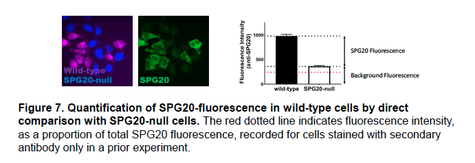
      Figure 3C: It is difficult to ascertain whether the gating on IL-17<SUP>+</SUP> cells is accurately identifying IL-17 producing cells. It is surprising, based on other published work, that the authors claim that almost half of CD45+CD11b-Ly6G- cells produce IL-17 in WT mice. It would be informative to show cell type-specific production of IL-17 in both WT and IFN-γ KO mice for comparison with the literature. Unstained/isotype controls for IL-17 staining should be shown. With this in mind, it is difficult to interpret the authors' claim that 80% of neutrophils produce IL-17.

      Thank you for the points above. We do agree that we were surprised to see ~50% of CD45<SUP>+</SUP> CD11b<SUP>-</SUP>Ly6G<SUP>-</SUP> cells producing IL-17. We have now done multiple experiments to confirm that this number is actually less than 1% (~90 cells) in the uninfected mice and less than 4% (~4000) in the Mtb-infected mice.

      Neutrophil-derived IL-17 production in Mtb-infected lungs is supported by two independent techniques in our current study: Flow Cytometry and Immunofluorescence assay. While  Neutrophil production of IL-17 is rarely studied in the context of TB, in several other settings it has been widely reported (Gonzalez-Orozco et al., 2019; Li et al., 2010; Ramirez-Velazquez et al., 2013). We consistently get >60% IL-17 positive cells in the CD11b<SUP>+</SUP> Ly6G<SUP>+</SUP> population, specifically in the infected samples. 

      To specifically address the reviewer’s concerns, we have now used an isotype control for IL17 staining and show the specificity of IL-17A antibody binding. The Author response image 1 is from the uninfected mice, 8 weeks age.

      Unfortunately, our efforts to establish an IL-17  ELISPOT assay from neutrophils were not very successful and need further standardisation. The new results are included in Fig. 3C-D and Fig. S2F-G in the revised manuscript.

      Author response image 1.

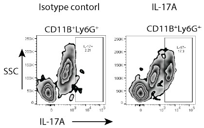
      Figure 3 D-H. Quantification of immunofluorescence microscopy should be provided.

      In the revised manuscript, we provide the quantification of IFA results.

      Figure 4: Effects on neutrophil numbers in IFN-γ Kos do not correlate with CFU reductions, suggesting there may be a neutrophilindependent mechanism.

      In the IFN-γ KO, we agree that the effect was less than dramatic. The immune dysfunction in the IFN-γ KO mice is too severe to see a strong reversal in the phenotype through interventions. 

      While we do not rule out any neutrophil-independent mechanism, in the context of following observations, neutrophil-dependent mechanisms certainly appear to play an important role-

      (a) Improved pathology and survival upon IL-17 neutralization, which further improves with the inclusion of celecoxib.

      (b) Loss of IL17<sup>+</sup>-Ly6G<sup>+</sup> cells upon IL-17 neutralization, which is further exacerbated when combined with celecoxib.

      (c) Significant reduction in PMN number (shown by FACS) without any major impact on Th17 cell population upon IL-17 neutralization.

      Finally, we believe some of the observations may become stronger once we characterize the specific sub-population among the Ly6G+ cells that correlates with pathology. For example, as shown in Figure 4I, FACS analysis of the Ly6G<sup>⁺</sup> cell population in Mtb-infected IFNγ<sup>⁻/⁻</sup> mice revealed a substantial subset of CD11b<sup>mid</sup> Ly6G<sup>ʰⁱ</sup> cells, indicative of an immature neutrophil population (Scapini et al., 2016). Efforts are currently underway to identify these important subpopulations.  

      Figure 4: Differences observed in the spleen cannot be connected to dissemination per se but instead could be a result of enhanced immune control in the spleen.

      Thank you for this important point. We have revised this section. The role of neutrophils in Mtb dissemination is an emerging area of research, with growing evidence suggesting that these cells contribute to the spread of Mtb beyond the lungs (Hult et al., 2021). We highlight that the observed correlation could be speculative at this juncture.

      Figure 4, 5: IL-17 neutralization alone has no effect on CFU in the lungs of Mtb-infected mice. While the combination of IL-17 neutralization and celecoxib has a very modest effect on CFU, the mechanism behind this observation is unclear. Further, the experiment shown has only 3 mice per group and it is unclear whether this (or any other) mouse experiment was repeated.

      For Fig. 4, the experiment was done with 3 mice/group. The IFN KO mice were used to help identify the mechanism. IL-17 neutralisation or Celecoxib treatment alone did not have any significant effect on the bacterial burden (in lungs or isolated PMNs). However, it did show a significant effect on the number of PMNs recruited. Combination of IL-17 neutralisation and celecoxib led to about a one-log decrease in CFU, which is significant.

      For Fig. 5, we used SR2211 instead of anti-IL-17 Ab for the experiment. This experiment had WT mice and 5 animals/group. Here, celecoxib and SR2211 alone showed a significant decline in PMN-resident Mtb pool as well as spleen burden. Only in the lungs, the impact of SR2211 alone was not significant.

      Figure 6: The decreases in CFU correlate with a decrease in neutrophils; nothing connects this to neutrophil production of IL-17.

      We now show quantification of observation in Fig. 5I, where in the WT mice, treatment with Celecoxib reduces the frequency of IL-17-producing Ly6G+ cells. In the revised manuscript, we also show direct evidence of SR2211 activity on BCG vaccine efficacy, which causes a significant decline in the Mtb burden in whole lung or in the isolated PMNs.

      Figure 7. The Human data shows that elevated neutrophil levels and elevated IL-17 levels are associated with treatment failure in TB patients. This is expected, and does not

      The literature lacks consensus in terms of a protective or pathological role of IL-17 in TB. Therefore, it was not expected to see higher IL-17 in patients who experienced relapse, death, or failed treatment outcomes. We do not have evidence from human subjects whether neutrophil derived IL-17 has a similar pathological role as observed in mice. However, higher IL-17 in failed outcome cases confirm the central theme that IL-17 is pathological in both human and mouse models.

      Reviewer #2 (Recommendations for the authors):

      (1) Survival of IFN-γ-/- Mice: The survival of IFN-γ-/- mice up to 100 days following a challenge with ~100 CFU of H37Rv is quite unusual. Have the authors checked PDIM expression in their Mtb strain, given that several studies report earlier mortality in these mice?

      As shown in Fig. 4F, H37Rv-infected IFN-γ⁻/⁻ mice survived up to a little over 80 days. These figures are not unusual in the light of the following:

      (1) In one study, IFNγ⁻/⁻ survived for about 40 days when the hypervirulent Mtb strain was used to infect these mice at 100-200 CFU using nose-only aerosol exposure (Nandi and Behar, 2011)

      (2) In yet another study, IFNγ⁻/⁻ mice survived for ~50 days, however, they used H37Rv at 1-3x10<sup>5</sup> CFU to infect through intravenous injection (Kawakami et al., 2004)

      Thus, compared with the above observations, where IFN-γ<sup>-/-</sup> mice survived for maximum 50 days due to hypervirulent infection or a very high dose infection, infection with H37Rv at ~100 CFU through the aerosol route and surviving for ~80 days is not unusual. The H37Rv cultures used in our study are always animal-passaged to ensure PDIM integrity.

      (2) Granuloma Scoring: The granuloma scores appear to represent the percentage of lesion area. Please clarify and, if necessary, amend this in the manuscript.

      The granuloma score is based on the calculation of the number of granulomatous infiltration and their severity. These are not % lesion area. We have added this detail in the revised manuscript.

      (3) Pathology Comparison in Figures 4F and 4G: Does the pathology shown in Figure 4G correspond to the same groups as in Figure 4F? The celecoxib group in Figure 4F and the WT group in Figure 4G seem to be missing. Please clarify.

      Figures 4F and 4G depict two independent experiments. For the time-to-death experiment, we had to leave the animals. The rest of the panels in Fig. 4 represent animals from the same experiment.

      (4) Effect of Celecoxib on Ly6G+ Cells: The authors demonstrated that celecoxib treatment reduces Ly6G+ cells and IL-17-producing Ly6G+ cells. Do Ly6G+ cells express EP2/EP4 receptors? Alternatively, could the reduction in IL-17-producing Ly6G+ cells be due to an improved bactericidal response in other innate cells? The authors should discuss this possibility.

      Yes, Ly6G<sup>⁺</sup> granulocytes express EP2/EP4 receptors (Lavoie et al., 2024), which mediate PGE₂ signaling. Prostaglandin E<sub>₂</sub> (PGE<sub>₂</sub>) is known to regulate neutrophil function and can enhance IL-17 production in various immune cells (Napolitani et al., 2009). However, the expression and functional role of EP2/EP4 receptors specifically on Ly6G<sup>⁺</sup> granulocytes in the context of Mtb infection require further investigation.

      The alternate suggestion by the reviewer that the reduction in IL-17-producing Ly6G<sup>⁺</sup> cells following celecoxib treatment could be attributed to an improved bactericidal response in other innate immune cells is attractive. While we did not experimentally rule out this possibility, since reduced IL-17 invariably associated with reduced neutrophil-resident Mtb population, a cell-autonomous mechanism operational in Ly6G+ granulocytes is a highly likely mechanism.  

      (5) Culture Conditions: The methods section indicates that bacteria were cultured in 7H9+ADC. Is there a specific reason why the Oleic acid supplement was not added, given that standard Mtb culture conditions typically use 7H9+OADC supplements? Please comment on this choice.

      It is a standard microbiological experimental procedure to use 7H9+ADC for broth culture, while 7H11+OADC for solid culture. Compared to broth culture, solid media are usually more stressful for bacteria because of hypoxia inside the growing colonies. Therefore, the media used are enriched in casein hydrolysate (like 7H11) and oleic acid (OADC).

      Reviewer #3 (Recommendations for the authors):

      Major suggestion: To really determine the role of neutrophil IL17 will require depletion studies and chimera experiments. These are clearly a major undertaking. I believe making significant re-writes to alter the conclusions or reanalyze any data to determine the role of nonhematopoietic and hematopoietic cells in IL17 is needed. If the conclusions are left as is, further experimentation is needed to fully support those conclusions.

      Thank you for the suggestion. We have embarked on the specific deletion studies; however, as mentioned, this is a major undertaking and will take time. As suggested, we have discussed the results in accordance with the strength of evidence currently provided.

      Eum, S.Y., J.H. Kong, M.S. Hong, Y.J. Lee, J.H. Kim, S.H. Hwang, S.N. Cho, L.E. Via, and C.E. Barry, 3rd. 2010. Neutrophils are the predominant infected phagocyGc cells in the airways of paGents with acGve pulmonary TB. Chest 137:122-128.

      Gonzalez-Orozco, M., R.E. Barbosa-Cobos, P. Santana-Sanchez, L. Becerril-Mendoza, L. Limon-

      Camacho, A.I. Juarez-Estrada, G.E. Lugo-Zamudio, J. Moreno-Rodriguez, and V. OrGzNavarrete. 2019. Endogenous sGmulaGon is responsible for the high frequency of IL-17Aproducing neutrophils in paGents with rheumatoid arthriGs. Allergy Asthma Clin Immunol 15:44.

      References

      Hult, C., J.T. Ma[la, H.P. Gideon, J.J. Linderman, and D.E. Kirschner. 2021. Neutrophil Dynamics Affect Mycobacterium tuberculosis Granuloma Outcomes and DisseminaGon. Front Immunol 12:712457.

      Kawakami, K., Y. Kinjo, K. Uezu, K. Miyagi, T. Kinjo, S. Yara, Y. Koguchi, A. Miyazato, K. Shibuya, Y. Iwakura, K. Takeda, S. Akira, and A. Saito. 2004. Interferon-gamma producGon and host protecGve response against Mycobacterium tuberculosis in mice lacking both IL-12p40 and IL-18. Microbes Infect 6:339-349.

      Lavoie, J.C., M. Simard, H. Kalkan, V. Rakotoarivelo, S. Huot, V. Di Marzo, A. Cote, M. Pouliot, and N. Flamand. 2024. Pharmacological evidence that the inhibitory effects of prostaglandin E2 are mediated by the EP2 and EP4 receptors in human neutrophils. J Leukoc Biol 115:1183-1189.

      Lee, J., S. Boyce, J. Powers, C. Baer, C.M. Sasse[, and S.M. Behar. 2020. CD11cHi monocyte-derived macrophages are a major cellular compartment infected by Mycobacterium tuberculosis. PLoS Pathog 16:e1008621.

      Li, L., L. Huang, A.L. Vergis, H. Ye, A. Bajwa, V. Narayan, R.M. Strieter, D.L. Rosin, and M.D. Okusa. 2010. IL-17 produced by neutrophils regulates IFN-gamma-mediated neutrophil migraGon in mouse kidney ischemia-reperfusion injury. J Clin Invest 120:331-342.

      Lovewell, R.R., C.E. Baer, B.B. Mishra, C.M. Smith, and C.M. Sasse[. 2021. Granulocytes act as a niche for Mycobacterium tuberculosis growth. Mucosal Immunol 14:229-241.

      Nandi, B., and S.M. Behar. 2011. RegulaGon of neutrophils by interferon-gamma limits lung inflammaGon during tuberculosis infecGon. The Journal of experimental medicine 208:22512262.

      Napolitani, G., E.V. Acosta-Rodriguez, A. Lanzavecchia, and F. Sallusto. 2009. Prostaglandin E2 enhances Th17 responses via modulaGon of IL-17 and IFN-gamma producGon by memory CD4+ T cells. Eur J Immunol 39:1301-1312.

      Ramirez-Velazquez, C., E.C. CasGllo, L. Guido-Bayardo, and V. OrGz-Navarrete. 2013. IL-17-producing peripheral blood CD177+ neutrophils increase in allergic asthmaGc subjects. Allergy Asthma Clin Immunol 9:23.

      Sadikot, R.T., H. Zeng, A.C. Azim, M. Joo, S.K. Dey, R.M. Breyer, R.S. Peebles, T.S. Blackwell, and J.W. Christman. 2007. Bacterial clearance of Pseudomonas aeruginosa is enhanced by the inhibiGon of COX-2. Eur J Immunol 37:1001-1009.

      Zheng, W., I.C. Chang, J. Limberis, J.M. Budzik, B.S. Zha, Z. Howard, L. Chen, and J.D. Ernst. 2023. Mycobacterium tuberculosis resides in lysosome-poor monocyte-derived lung cells during chronic infecGon. bioRxiv 

      Zheng, W., I.C. Chang, J. Limberis, J.M. Budzik, B.S. Zha, Z. Howard, L. Chen, and J.D. Ernst. 2024. Mycobacterium tuberculosis resides in lysosome-poor monocyte-derived lung cells during chronic infecGon. PLoS Pathog 20:e1012205.

    1. Reviewer #1 (Public review):

      Summary:

      The manuscript by Yang et al. investigates the relationship between multi-unit activity in the locus coeruleus, putatively noradrenergic locus coeruleus, hippocampus (HP), sharp-wave ripples (SWR), and spindles using multi-site electrophysiology in freely behaving male rats. The study focuses on SWR during quiet wake and non-REM sleep, and their relation to cortical states (identified using EEG recordings in frontal areas) and LC units.

      The manuscript highlights differential modulation of LC units as a function of HP-cortical communication during wake and sleep. They establish that ripples and LC units are inversely correlated to levels of arousal: wake, i.e., higher arousal correlates with higher LC unit activity and lower ripple rates. The authors show that LC neuron activity is strongly inhibited just before SWR is detected during wake. During non-REM sleep, they distinguish "isolated" ripples from SWR coupled to spindles and show that inhibition of LC neuron activity is absent before spindle-coupled ripples but not before isolated ripples, suggesting a mechanism where noradrenaline (NA) tone is modulated by HP-cortical coupling. This result has interesting implications for the roles of noradrenaline in the modulation of sleep-dependent memory consolidation, as ripple-spindle coupling is a mechanism favoring consolidation. The authors further show that NA neuronal activity is downregulated before spindles.

      Strengths:

      In continuity with previous work from the laboratory, this work expands our understanding of the activity of neuromodulatory systems in relation to vigilance states and brain oscillations, an area of research that is timely and impactful. The manuscript presents strong results suggesting that NA tone varies differentially depending on the coupling of HP SWR with cortical spindles. The authors place their findings back in the context of identified roles of HP ripples and coupling to cortical oscillations for memory formation in a very interesting discussion. The distinction of LC neuron activity between awake, ripple-spindle coupled events and isolated ripples is an exciting result, and its relation to arousal and memory opens fascinating lines of research.

      Weaknesses:

      I regretted that the paper fell short of trying to push this line of idea a bit further, for example, by contrasting in the same rats the LC unit-HP ripple coupling during exploration of a highly familiar context (as seemingly was the case in their study) versus a novel context, which would increase arousal and trigger memory-related mechanisms. Any kind of manipulation of arousal levels and investigation of the impact on awake vs non-REM sleep LC-HP ripple coordination would considerably strengthen the scope of the study.

      The main result shows that LC units are not modulated during non-REM sleep around spindle-coupled ripples (named spRipples, 17.2% of detected ripples); they also show that LC units are modulated around ripple-coupled spindles (ripSpindles, proportion of detected spindles not specified, please add). These results seem in contradiction; this point should be addressed by the authors.

      Results are displayed per recording session, with 20 sessions total recorded from 7 rats (2 to 8 sessions per rat), which implies that one of the rats accounts for 40% of the dataset. Authors should provide controls and/or data displayed as average per rat to ensure that results are now skewed by the weight of that single rat in the results.

      In its current form, the manuscript presents a lack of methodological detail that needs to be addressed, as it clouds the understanding of the analysis and conclusions. For example, the method to account for the influence of cortical state on LC MUA is unclear, both for the exact methods (shuffling of the ripple or spindle onset times) and how this minimizes the influence of cortical states; this should be better described. If the authors wish to analyze unit modulation as a function of cortical state, could they also identify/sort based on cortical states and then look at unit modulation around ripple onset? For the first part of the paper, was an analysis performed on quiet wake, non-REM sleep, or both?

    2. Author response:

      Reviewer #1 (Public review):

      Summary:

      The manuscript by Yang et al. investigates the relationship between multi-unit activity in the locus coeruleus, putatively noradrenergic locus coeruleus, hippocampus (HP), sharp-wave ripples (SWR), and spindles using multi-site electrophysiology in freely behaving male rats. The study focuses on SWR during quiet wake and non-REM sleep, and their relation to cortical states (identified using EEG recordings in frontal areas) and LC units.

      The manuscript highlights differential modulation of LC units as a function of HP-cortical communication during wake and sleep. They establish that ripples and LC units are inversely correlated to levels of arousal: wake, i.e., higher arousal correlates with higher LC unit activity and lower ripple rates. The authors show that LC neuron activity is strongly inhibited just before SWR is detected during wake. During non-REM sleep, they distinguish "isolated" ripples from SWR coupled to spindles and show that inhibition of LC neuron activity is absent before spindle-coupled ripples but not before isolated ripples, suggesting a mechanism where noradrenaline (NA) tone is modulated by HP-cortical coupling. This result has interesting implications for the roles of noradrenaline in the modulation of sleep-dependent memory consolidation, as ripple-spindle coupling is a mechanism favoring consolidation. The authors further show that NA neuronal activity is downregulated before spindles.

      Strengths:

      In continuity with previous work from the laboratory, this work expands our understanding of the activity of neuromodulatory systems in relation to vigilance states and brain oscillations, an area of research that is timely and impactful. The manuscript presents strong results suggesting that NA tone varies differentially depending on the coupling of HP SWR with cortical spindles. The authors place their findings back in the context of identified roles of HP ripples and coupling to cortical oscillations for memory formation in a very interesting discussion. The distinction of LC neuron activity between awake, ripple-spindle coupled events and isolated ripples is an exciting result, and its relation to arousal and memory opens fascinating lines of research.

      Weaknesses:

      I regretted that the paper fell short of trying to push this line of idea a bit further, for example, by contrasting in the same rats the LC unit-HP ripple coupling during exploration of a highly familiar context (as seemingly was the case in their study) versus a novel context, which would increase arousal and trigger memory-related mechanisms. Any kind of manipulation of arousal levels and investigation of the impact on awake vs non-REM sleep LC-HP ripple coordination would considerably strengthen the scope of the study.

      We agree that conducting specific behavioral tests before electrophysiological recordings, as well as manipulating arousal during the recording session, would strengthen the study. These experiments are planned for future work, and we will acknowledge this point in the discussion.

      The main result shows that LC units are not modulated during non-REM sleep around spindle-coupled ripples (named spRipples, 17.2% of detected ripples); they also show that LC units are modulated around ripple-coupled spindles (ripSpindles, proportion of detected spindles not specified, please add). These results seem in contradiction; this point should be addressed by the authors.

      We found that LC suppression was generally weak around both types of coupled events (spRipples and ripSpindles). Specifically, session-averaged spRipple-associated LC suppression reached a significance level (exceeding 95% CI) in 4 (n = 3 rats) out of 20 sessions (Line 177). The significant ripSpindle-associated LC suppression was observed in 3 (n = 2 animals) out of 20 sessions (Line 213). When comparing the modulation index (MI) around spRipples and ripSpindles, we found a significant correlation (Pearson r = 0.72, p = 0.0003). As shown in Author response image 1 below, the three sessions (blue square, MI < 95%CI) with significant ripSpindle-associated LC suppression coincide with those sessions showing LC modulation around spRipples. Although, the detection of coupled events was performed independently, some overlap can not be excluded. We will be happy to provide this additional information in the results section.

      Author response image 1.

      Results are displayed per recording session, with 20 sessions total recorded from 7 rats (2 to 8 sessions per rat), which implies that one of the rats accounts for 40% of the dataset. Authors should provide controls and/or data displayed as average per rat to ensure that results are now skewed by the weight of that single rat in the results.

      Since high-quality recordings from the LC in behaving rats are challenging and rare, we used all valid sessions for this study. In Author response image 2 below, we plotted the average MIs for each animal (A) and each session (B). The dashed lines indicate the mean ± 2 standard deviations across all sessions. The rat ID and number of sessions is indicated in parentheses in A. All animal-averaged MIs fall within this range, indicating that the MI distribution is not driven by a single animal (rat 1101, 8 sessions). The MIs of eight sessions from rat1101 are shown in grey-filled triangles (B). Comparison of the MI distribution for these eight sessions versus the remaining 12 sessions from six other animals revealed no significant difference (Kolmogorov-Smirnov test, p = 0.969). We will be happy to provide this additional information in the Results section.

      Author response image 2.

      In its current form, the manuscript presents a lack of methodological detail that needs to be addressed, as it clouds the understanding of the analysis and conclusions. For example, the method to account for the influence of cortical state on LC MUA is unclear, both for the exact methods (shuffling of the ripple or spindle onset times) and how this minimizes the influence of cortical states; this should be better described. If the authors wish to analyze unit modulation as a function of cortical state, could they also identify/sort based on cortical states and then look at unit modulation around ripple onset? For the first part of the paper, was an analysis performed on quiet wake, non-REM sleep, or both?

      As shown in Figure 3A and described in the main text (Lines 113–116), LC firing rate was negatively correlated with cortical arousal as quantified by Synchronisation Index (SI), whereas ripple rate was positively correlated with arousal. When computing LC activity (0.05 sec bins) aligned to the ripple onset over a longer time window ([–12, 12] sec), we observed a slow decrease in the LC firing rate beginning as early as 10 s before the ripple onset. In Author response image 3 below, a blue trace shows this slower temporal dynamic in a representative session. In addition to LC activity modulation at this relatively slow temporal scale, we also observed a much sharper drop in the LC firing rate ~ 2 s before the ripple onset. Considering two temporal scales, we hypothesized that slow modulation of LC activity might be related to fluctuations of the global brain state. Specifically, a higher SI (more synchronized cortical population activity) corresponded to a lower arousal state and reduced LC tonic firing; this brain state was associated with a higher ripple activity. Thus, slow LC modulation was likely driven by cortical state transitions. To correct for the influence of the global brain state on the LC/ripple temporal dynamics, we generated surrogate events by jittering the times of detected ripples (Lines 415–421). First, we confirmed that the cortical state did not differ around ripples and surrogate events (Figure 3C), while triggering the hippocampal LFP on the surrogate events lacked the ripple-specific frequency component (Figure 3B,). Thus, LC activity around surrogate evens captured its cortical state dependent dynamics (see orange trace in Author response image 3 below). Finally, to characterize state-independent ripple-related LC activity, we subtracted the state-related LC activity (orange trace in Author response image 3 below) from the ripple-triggered LC activity (blue trace). This yielded a corrected estimate of ripple-associated LC activity that was largely free from the confounding influence of cortical state transitions.

      Author response image 3.

      In the results subsection “LC-NE neuron spiking is suppressed around hippocampal ripples”, we reported LC modulation without accounting for the cortical state. The state-dependent effects were instead examined in the subsequent subsection, “Peri-ripple LC modulation depends on the cortical–hippocampal interaction,” where we characterized LC activity around ripples across different cortical states (quite awake and NREM sleep). We will provide more methodological details and a rationale for each analysis, as requested.

      Reviewer #2 (Public review):

      Summary:

      In this study, the authors studied the synchrony between ripple events in the Hippocampus, cortical spindles, and Locus Coeruleus spiking. The results in this study, together with the established literature on the relationship of hippocampal ripples with widespread thalamic and cortical waves, guided the authors to propose a role for Locus Coeruleus spiking patterns in memory consolidation. The findings provided here, i.e., correlations between LC spiking activity and Hippocampal ripples, could provide a basis for future studies probing the directional flow or the necessity of these correlations in the memory consolidation process. Hence, the paper provides enough scientific advances to highlight the elusive yet important role of Norepinephrine circuitry in the memory processes.

      Strengths:

      The authors were able to demonstrate correlations of Locus Coeruleus spikes with hippocampal ripples as well as with cortical spindles. A specific strength of the paper is in the demonstration that the spindles that activate with the ripples are comparatively different in their correlations with Locus Coeruleus than those that do not.

      Weaknesses:

      The claims regarding the roles of these specific interactions were mostly derived from the literature that these processes individually contribute to the memory process, without any evidence of these specific interactions being necessary for memory processes. There are also issues with the description of methods, validation of shuffling procedures, and unclear presentation and the interpretation of the findings, which are described in the points that follow. I believe addressing these weaknesses might improve and add to the strength of the findings.

      We believe that our responses to the Reviewer 1 and planned revisions as described above will adequately address the issues raised by the Reviewer 2. 

      Reviewer #3 (Public review):

      Summary:

      This manuscript examines how locus coeruleus (LC) activity relates to hippocampal ripple events across behavioral states in freely moving rats. Using multi-site electrophysiological recordings, the authors report that LC activity is suppressed prior to ripple events, with the magnitude of suppression depending on the ripple subtype. Suppression is stronger during wakefulness than during NREM sleep and is least pronounced for ripples coupled to spindles.

      Strengths:

      The study is technically competent and addresses an important question regarding how LC activity interacts with hippocampal and thalamocortical network events across vigilance states.

      Weaknesses:

      The results are interesting, but entirely observational. Also, the study in its current form would benefit from optimization of figure labeling and presentation, and more detailed result descriptions to make the findings fully interpretable. Also, it would be beneficial if the authors could formulate the narrative and central hypothesis more clearly to ease the line of reasoning across sections.

      We will do our best to optimize presentation, revise the main text and figure labelling. When appropriate, we will add specific hypotheses and a rationale for specific analyses.

      Comments:

      (1) Stronger evidence that recorded units represent noradrenergic LC neurons would reinforce the conclusions. While direct validation may not be possible, showing absolute firing rates (Hz) across quiet wake, active wake, NREM, and REM, and comparing them to published LC values, would help.

      We will provide the requested data in the revised manuscript.

      (2) The analyses rely almost exclusively on z-scored LC firing and short baselines (~4-6 s), which limits biological interpretation. The authors should include absolute firing rates alongside normalized values for peri-ripple and peri-spindle analyses and extend pre-event windows to at least 20-30 s to assess tonic firing evolution. This would clarify whether differences across ripple subtypes arise from ceiling or floor effects in LC activity; if ripples require LC silence, the relative drop will appear larger during high-firing wake states. This limitation should be discussed and, if possible, results should be shown based on unnormalized firing rates.

      We can provide absolute firing rates alongside normalized values for peri-ripple and peri-spindle analyses for isolated single LC units. However, we are reluctant to average absolute firing rates for multiunit activity, as it is unknown how many neurons contributed to each MUA recording. We can add the plots with extended pre-event windows ([–12, 12] sec). Please see our response to the Reviewer 1 about the two temporal scales of LC modulation.

      (3) Because spindles often occur in clusters, the timing of ripple occurrence within these clusters could influence LC suppression. Indicate whether this structure was considered or discuss how it might affect interpretation (e.g., first vs. subsequent ripples within a spindle cluster).

      We did not consider spindle clusters and classified the event as ripple coupled spindle if the ripple occurred between the spindle on- and offset. We will clarify this point in the Method section. 

      (4) While the observational approach is appropriate here, causal tests (e.g., optogenetic or chemogenetic manipulation of LC around ripple events and in memory tasks) would considerably strengthen the mechanistic conclusions. At a minimum, a discussion of how such approaches could address current open questions would improve the manuscript.

      We agree that conducting causal tests would strengthen the study. We will acknowledge in the discussion that our results shall inspire future studies addressing many open questions.

      (5) Please show how "Synchronization Index" (SI) differs quantitatively across behavioral states (wake, NREM, REM) and discuss whether it could serve as a state classifier. This would strengthen interpretations of the correlations between SI, ripple occurrence, and LC activity.

      We will add the plot showing the average SI values across behavioral states. Although SI could potentially serve as a classifier, we have chosen not to discuss this in detail to maintain focus in the discussion.

      (6) The current use of SI to denote a delta/gamma power ratio is unconventional, as "SI" typically refers to phase-locking metrics. Consider adopting a more standard term, such as delta/gamma power ratio. Similarly, it would be easier to follow if you use common terminology (AUC) to describe the drop in LC-MUA rather than using "MI" and "sub-MI".

      The ranges of delta and gamma bands might vary across studies; therefore, we prefer using SI, as defined here and in our previous publications (Yang, 2019; Novitskaya, 2012). We calculated the modulation index (MI) as the area under the curve of the peri-event time histogram within the 1 second preceding ripple onset. To avoid potential confusion with the AUC calculated over the entire signal window, we opted to use MI. 

      (7) The logic in Figure 3 is difficult to follow. The brain state (delta/gamma ratio) appears unchanged relative to surrogate events (3C), while LC activity that is supposedly negatively correlated to delta/gamma changes markedly (3D-E). Could this discrepancy reflect the low temporal resolution (4-s windows) used to calculate delta/gamma when the changes occur on a shorter time scale?

      Figure 3D and 3E show the 'state-corrected' ripple-related LC activity. Specifically, the cortical state related LC modulation was subtracted from the non-corrected ripple-associated LC activity. Please, see our detailed response to the Reviewer 1. We will revise the results and Figure 3 legend to clarify this point.

      (8) There are apparent inconsistencies between Figures 4B and 4C-D. In B, it seems that the difference between the 10th and 90th percentile is mostly in higher frequencies, but in C and D, the only significant difference is in the delta band.

      We will re-do this analysis and clarify this inconsistency.

      (9) Because standard sleep scoring is based on EEG and EMG signals, please include an example of sleep scoring alongside the data used for state classification. It would also be relevant to include the delta/gamma power ratio in such an example plot.

      We removed ‘standard’ and will add a supplementary Figure illustrating sleep scoring.

      (10) Can variability in modulation index (subMI) across ripple subsets reflect differences in recording quality? Please report and compare mean LC firing rates across subsets to confirm this is not a confounding factor.

      We will plot this result averaged per rat.

      (11) Figure 6B: If the brown trace represents LC-MUA activity around random time points, why would there be a coinciding negative peak as relative to real sleep spindles? Or is it the subtracted trace?

      We will clarify this point in the figure legend.

      (12) On page 8, lines 207-209, the authors write "Importantly, neither the LC-MUA rate nor SIs differed during a 2-sec time window preceding either group of spindles". It is unclear which data they refer to, but the statement seems to contradict Figure 6E as well as the following sentence: "Across sessions, MI values exceeded 95% CI in 17/20 datasets for isoSpindles and only 3/20 for ripSpindles". This should be clarified.

      We will clarify the description of this result.

      (13) The results in Figures 5C and 6F do not align. It seems surprising that ripple-coupled spindles show a considerably higher LC modulation than spindle-coupled ripples, as these events should overlap. Could the discrepancy be due to Z-score normalization as mentioned above? Please include a discussion of this to help the interpretation of the results.

      We will clarify this point in the revised manuscript. Please, also see our response to the Reviewer 1.

      (14) The text implies that 8 recordings came from one rat and two each from six others. This should be confirmed, and it should be explained how the recordings were balanced and analyzed across animals.

      Since high-quality recordings from LC in behaving animals are challenging and rare, we used all valid sessions. We will also present the main results averaged per rat, as also requested by the Reviewer 1.

    1. Tus respuestas ayudarán a implementar mejoras concretas en la enseñanza de Histología.AtrásEnviarBorrar formulario

      Percepción de justicia en las evaluaciones

    2. ¿Qué elementos de Anatomía encuentras MÁS DIFÍCILES?

      Anatomía? Sugiero que aquí vayan los nombres de las 6 unidades de aprendizaje y que vaya una escala de lickert para determinar la complejidad.

    1. Author response:

      The following is the authors’ response to the original reviews.

      Reviewer #1 (Public review):

      Summary:

      Syed et al. investigate the circuit underpinnings for leg grooming in the fruit fly. They identify two populations of local interneurons in the right front leg neuromere of ventral nerve cord, i.e. 62 13A neurons and 64 13B neurons. Hierarchical clustering analysis identifies 10 morphological classes for both populations. Connectome analysis reveals their circuit interactions: these GABAergic interneurons provide synaptic inhibition either between the two subpopulations, i.e., 13B onto 13A, or among each other, i.e., 13As onto other 13As, and/or onto leg motoneurons, i.e., 13As and 13Bs onto leg motoneurons. Interestingly, 13A interneurons fall into two categories, with one providing inhibition onto a broad group of motoneurons, being called "generalists", while others project to a few motoneurons only, being called "specialists". Optogenetic activation and silencing of both subsets strongly affect leg grooming. As well aas ctivating or silencing subpopulations, i.e., 3 to 6 elements of the 13A and 13B groups, has marked effects on leg grooming, including frequency and joint positions, and even interrupting leg grooming. The authors present a computational model with the four circuit motifs found, i.e., feed-forward inhibition, disinhibition, reciprocal inhibition, and redundant inhibition. This model can reproduce relevant aspects of the grooming behavior.

      Strengths:

      The authors succeeded in providing evidence for neural circuits interacting by means of synaptic inhibition to play an important role in the generation of a fast rhythmic insect motor behavior, i.e., grooming. Two populations of local interneurons in the fruit fly VNC comprise four inhibitory circuit motifs of neural action and interaction: feed-forward inhibition, disinhibition, reciprocal inhibition, and redundant inhibition. Connectome analysis identifies the similarities and differences between individual members of the two interneuron populations. Modulating the activity of small subsets of these interneuron populations markedly affects the generation of the motor behavior, thereby exemplifying their important role in generating grooming.

      We thank the reviewer for their thoughtful and constructive evaluation of our work. 

      Weaknesses:

      Effects of modulating activity in the interneuron populations by means of optogenetics were conducted in the so-called closed-loop condition. This does not allow for differentiation between direct and secondary effects of the experimental modification in neural activity, as feedforward and feedback effects cannot be disentangled. To do so, open loop experiments, e.g., in deafferented conditions, would be important. Given that many members of the two populations of interneurons do not show one, but two or more circuit motifs, it remains to be disentangled which role the individual circuit motif plays in the generation of the motor behavior in intact animals.

      Our optogenetic experiments show a role for 13A/B neurons in grooming leg movements – in an intact sensorimotor system - but we cannot yet differentiate between central and reafferent contributions. Activation of 13As or 13Bs disinhibits motor neurons and that is sufficient to induce walking/grooming. Therefore, we can show a role for the disinhibition motif.

      Proprioceptive feedback from leg movements could certainly affect the function of these reciprocal inhibition circuits. Given the synapses we observe between leg proprioceptors and 13A neurons, we think this is likely.

      Our previous work (Ravbar et al 2021) showed that grooming rhythms in dusted flies persist when sensory feedback is reduced, indicating that central control is possible. In those experiments, we used dust to stimulate grooming and optogenetic manipulation to broadly silence sensory feedback. We cannot do the same here because we do not yet have reagents to separately activate sparse subsets of inhibitory neurons while silencing specific proprioceptive neurons. More importantly, globally silencing proprioceptors would produce pleiotropic effects and severely impair baseline coordination, making it difficult to distinguish whether observed changes reflect disrupted rhythm generation or secondary consequences of impaired sensory input. Therefore, the reviewer is correct – we do not know whether the effects we observe are feedforward (central), feedback sensory, or both. We have included this in the revised results and discussion section to describe these possibilities and the limits of our current findings.

      Additionally, we have used a computational model to test the role of each motif separately and we show that in the results.

      Reviewer #2 (Public review):

      Summary:

      This manuscript by Syed et al. presents a detailed investigation of inhibitory interneurons, specifically from the 13A and 13B hemilineages, which contribute to the generation of rhythmic leg movements underlying grooming behavior in Drosophila. After performing a detailed connectomic analysis, which offers novel insights into the organization of premotor inhibitory circuits, the authors build on this anatomical framework by performing optogenetic perturbation experiments to functionally test predictions derived from the connectome. Finally, they integrate these findings into a computational model that links anatomical connectivity with behavior, offering a systems-level view of how inhibitory circuits may contribute to grooming pattern generation.

      Strengths:

      (1) Performing an extensive and detailed connectomic analysis, which offers novel insights into the organization of premotor inhibitory circuits.

      (2) Making sense of the largely uncharacterized 13A/13B nerve cord circuitry by combining connectomics and optogenetics is very impressive and will lay the foundation for future experiments in this field.

      (3) Testing the predictions from experiments using a simplified and elegant model.

      We thank the reviewer for their thoughtful and encouraging evaluation of our work. 

      Weaknesses:

      (1) In Figure 4, while the authors report statistically significant shifts in both proximal inter-leg distance and movement frequency across conditions, the distributions largely overlap, and only in Panel K (13B silencing) is there a noticeable deviation from the expected 7-8 Hz grooming frequency. Could the authors clarify whether these changes truly reflect disruption of the grooming rhythm? 

      We reanalyzed the dataset with Linear Mixed Models. We find significant differences in mean frequencies upon silencing these neurons but not upon activation. The experimental groups are also significantly more variable. We revised these panels with updated analysis. We think these data do support our interpretation that the grooming rhythms are disrupted. 

      More importantly, all this data would make the most sense if it were performed in undusted flies (with controls) as is done in the next figure.

      In our assay conditions, undusted flies groom infrequently. We used undusted flies for some optogenetic activation experiments, where the neuron activation triggers behavior initiation, but we chose to analyze the effect of silencing inhibitory neurons in dusted flies because dust reliably activates mechanosensory neurons and elicits robust grooming behavior enabling us to assess how manipulation of 13A/B neurons alters grooming rhythmicity and leg coordination.

      (2) In Figure 4-Figure Supplement 1, the inclusion of walking assays in dusted flies is problematic, as these flies are already strongly biased toward grooming behavior and rarely walk. To assess how 13A neuron activation influences walking, such experiments should be conducted in undusted flies under baseline locomotor conditions.

      We agree that there are better ways to assay potential contributions of 13A/13B neurons to walking. We intended to focus on how normal activity in these inhibitory neurons affects coordination during grooming, and we included walking because we observed it in our optogenetic experiments and because it also involves rhythmic leg movements. The walking data is reported in a supplementary figure because we think this merits further study with assays designed to quantify walking specifically. We will make these goals clearer in the revised manuscript and we are happy to share our reagents with other research groups more equipped to analyze walking differences.

      (3) For broader lines targeting six or more 13A neurons, the authors provide specific predictions about expected behavioral effects-e.g., that activation should bias the limb toward flexion and silencing should bias toward extension based on connectivity to motor neurons. Yet, when using the more restricted line labeling only two 13A neurons (Figure 4 - Figure Supplement 2), no such prediction is made. The authors report disrupted grooming but do not specify whether the disruption is expected to bias the movement toward flexion or extension, nor do they discuss the muscle target. This is a missed opportunity to apply the same level of mechanistic reasoning that was used for broader manipulations.

      Because we cannot unambiguously identify one of the neurons from our sparsest 13A splitGAL4 lines in FANC, we cannot say with certainty which motor neurons they target. That limits the accuracy of any functional predictions.  

      (4) Regarding Figure 5: The 70ms on/off stimulation with a slow opsin seems problematic. CsChrimson off kinetics are slow and unlikely to cause actual activity changes in the desired neurons with the temporal precision the authors are suggesting they get. Regardless, it is amazing that the authors get the behavior! It would still be important for the authors to mention the optogenetics caveat, and potentially supplement the data with stimulation at different frequencies, or using faster opsins like ChrimsonR.

      We were also intrigued by the behavioral consequences of activating these inhibitory neurons with CsChrimson. We appreciate the reviewer’s point that CsChrimson’s slow off-kinetics limit precise temporal control. To address this, we repeated our frequency analysis using a range of pulse durations (10/10, 50/50, 70/70, 110/110, and 120/120 ms on/off) and compared the mean frequency of proximal joint extension/flexion cycles across conditions. We found no significant difference in frequency (LLMS, p > 0.05), suggesting that the observed grooming rhythm is not dictated by pulse period but instead reflects an intrinsic property of the premotor circuit once activated. We now include these results in ‘Figure 5—figure supplement 1’ and clarify in the text that we interpret pulsed activation as triggering, rather than precisely pacing, the endogenous grooming rhythm. We continue to note in the manuscript that CsChrimson’s slow off-kinetics may limit temporal precision. We will try ChrimsonR in future experiments.

      Overall, I think the strengths outweigh the weaknesses, and I consider this a timely and comprehensive addition to the field.

      Reviewer #3 (Public review):

      Summary:

      The authors set out to determine how GABAergic inhibitory premotor circuits contribute to the rhythmic alternation of leg flexion and extension during Drosophila grooming. To do this, they first mapped the ~120 13A and 13B hemilineage inhibitory neurons in the prothoracic segment of the VNC and clustered them by morphology and synaptic partners. They then tested the contribution of these cells to flexion and extension using optogenetic activation and inhibition and kinematic analyses of limb joints. Finally, they produced a computational model representing an abstract version of the circuit to determine how the connectivity identified in EM might relate to functional output. The study, in its current form, makes an important but overclaimed contribution to the literature due to a mismatch between the claims in the paper and the data presented.

      Strengths:

      The authors have identified an interesting question and use a strong set of complementary tools to address it:

      (1) They analysed serial‐section TEM data to obtain reconstructions of every 13A and 13B neuron in the prothoracic segment. They manually proofread over 60 13A neurons and 64 13B neurons, then used automated synapse detection to build detailed connectivity maps and cluster neurons into functional motifs.

      (2) They used optogenetic tools with a range of genetic driver lines in freely behaving flies to test the contribution of subsets of 13A and 13B neurons.

      (3) They used a connectome-constrained computational model to determine how the mapped connectivity relates to the rhythmic output of the behavior.

      Weaknesses:

      The manuscript aims to reveal an instructive, rhythm-generating role for premotor inhibition in coordinating the multi-joint leg synergies underlying grooming. It makes a valuable contribution, but currently, the main claims in the paper are not well-supported by the presented evidence.

      Major points

      (1) Starting with the title of this manuscript, "Inhibitory circuits generate rhythms for leg movements during Drosophila grooming", the authors raise the expectation that they will show that the 13A and 13B hemilineages produce rhythmic output that underlies grooming. This manuscript does not show that. For instance, to test how they drive the rhythmic leg movements that underlie grooming requires the authors to test whether these neurons produce the rhythmic output underlying behavior in the absence of rhythmic input. Because the optogenetic pulses used for stimulation were rhythmic, the authors cannot make this point, and the modelling uses a "black box" excitatory network, the output of which might be rhythmic (this is not shown). Therefore, the evidence (behavioral entrainment; perturbation effects; computational model) is all indirect, meaning that the paper's claim that "inhibitory circuits generate rhythms" rests on inferred sufficiency. A direct recording (e.g., calcium imaging or patch-clamp) from 13A/13B during grooming - outside the scope of the study - would be needed to show intrinsic rhythmogenesis. The conclusions drawn from the data should therefore be tempered. Moreover, the "black box" needs to be opened. What output does it produce? How exactly is it connected to the 13A-13B circuit? 

      We modified the title to better reflect our strongest conclusions: “Inhibitory circuits control leg movements during Drosophila grooming”

      Our optogenetic activation was delivered in a patterned (70 ms on/off) fashion that entrains rhythmic movements, but this does not rule out the possibility that the rhythm is imposed externally. In the manuscript, we state that we used pulsed light to mimic a flexion-extension cycle and note that this approach tests whether inhibition is sufficient to drive rhythmic leg movements when temporally patterned. While this does not prove that 13A/13B neurons are intrinsic rhythm generators, it does demonstrate that activating subsets of inhibitory neurons is sufficient to elicit alternating leg movements resembling natural grooming and walking.

      Our goal with the model was to demonstrate that it is possible to produce rhythmic outputs with this 13A/B circuit, based on the connectome. The “black box” is a small recurrent neural network (RNN) consisting of 40 neurons in its hidden layer. The inputs are the “dust” levels from the environment (the green pixels in Figure 6I), the “proprioceptive” inputs (“efference copy” from motor neurons), and the amount of dust accumulated on both legs. The outputs (all positive) connect to the 13A neurons, the 13B neurons, and to the motor neurons. We refer to it as the “black box” because we make no claims about the actual excitatory inputs to these circuits. Its function is to provide input, needed to run the network, that reflects the distribution of “dust” in the environment as well as the information about the position of the legs.  

      The output of the “black box” component of the model might be rhythmic. In fact, in most instances of the model implementation this is indeed the case. However, as mentioned in the current version of the manuscript: “But the 13A circuitry can still produce rhythmic behavior even without those external inputs (or when set to a constant value), although the legs become less coordinated.” Indeed, when we refine the model (with the evolutionary training) without the “black box” (using a constant input of 0.1) the behavior is still rhythmic and sustained. Therefore, the rhythmic activity and behavior can emerge from the premotor circuitry itself without a rhythmic input.

      The context in which the 13A and 13B hemilineages sit also needs to be explained. What do we know about the other inputs to the motorneurons studied? What excitatory circuits are there? 

      We agree that there are many more excitatory and inhibitory, direct and indirect, connections to motor neurons that will also affect leg movements for grooming and walking. 13A neurons provide a substantial fraction of premotor input. For example, 13As account for ~17.1% of upstream synapses for one tibia extensor (femur seti) motor neuron and ~14.6% for another tibia extensor (femur feti) motor neuron. Our goal was to demonstrate what is possible from a constrained circuit of inhibitory neurons that we mapped in detail, and we hope to add additional components to better replicate the biological circuit as behavioral and biomechanical data is obtained by us and others.  

      Furthermore, the introduction ignores many decades of work in other species on the role of inhibitory cell types in motor systems. There is some mention of this in the discussion, but even previous work in Drosophila larvae is not mentioned, nor crustacean STG, nor any other cell types previously studied. This manuscript makes a valuable contribution, but it is not the first to study inhibition in motor systems, and this should be made clear to the reader.

      We thank the reviewer for this important reminder.  Previous work on the contribution of inhibitory neurons to invertebrate motor control certainly influenced our research. We have expanded coverage of the relevant history and context in our revised discussion.

      (2) The experimental evidence is not always presented convincingly, at times lacking data, quantification, explanation, appropriate rationales, or sufficient interpretation.

      We are committed to improving the clarity, rationale, and completeness of our experimental descriptions.  We have revisited the statistical tests applied throughout the manuscript and expanded the Methods.

      (3) The statistics used are unlike any I remember having seen, essentially one big t-test followed by correction for multiple comparisons. I wonder whether this approach is optimal for these nested, high‐dimensional behavioral data. For instance, the authors do not report any formal test of normality. This might be an issue given the often skewed distributions of kinematic variables that are reported. Moreover, each fly contributes many video segments, and each segment results in multiple measurements. By treating every segment as an independent observation, the non‐independence of measurements within the same animal is ignored. I think a linear mixed‐effects model (LMM) or generalized linear mixed model (GLMM) might be more appropriate.

      We thank the reviewer for raising this important point regarding the statistical treatment of our segmented behavioral data. Our initial analysis used independent t-tests with Bonferroni correction across behavioral classes and features, which allowed us to identify broad effects. However, we acknowledge that this approach does not account for the nested structure of the data. To address this, we re-analyzed key comparisons using linear mixed-effects models (LMMs) as suggested by the reviewer. This approach allowed us to more appropriately model within-fly variability and test the robustness of our conclusions. We have updated the manuscript based on the outcomes of these analyses.

      (4) The manuscript mentions that legs are used for walking as well as grooming. While this is welcome, the authors then do not discuss the implications of this in sufficient detail. For instance, how should we interpret that pulsed stimulation of a subset of 13A neurons produces grooming and walking behaviours? How does neural control of grooming interact with that of walking?

      We do not know how the inhibitory neurons we investigated will affect walking or how circuits for control of grooming and walking might compete. We speculate that overlapping pre-motor circuits may participate because both have similar extension flexion cycles at similar frequencies, but we do not have hard experimental data to support. This would be an interesting area for future research. Here, we focused on the consequences of activating specific 13A/B neurons during grooming because they were identified through a behavioral screen for grooming disruptions, and we had developed high-resolution assays and familiarity with the normal movements in this behavior.

      (5) The manuscript needs to be proofread and edited as there are inconsistencies in labelling in figures, phrasing errors, missing citations of figures in the text, or citations that are not in the correct order, and referencing errors (examples: 81 and 83 are identical; 94 is missing in text).

      We have proofread the manuscript to fix figure labeling, citation order, and referencing errors.

      Reviewing Editor Comments:

      In addition to the recommendations listed below, a common suggestion, given the lack of evidence to support that 13A and 13B are rhythm-generating, is to tone down the title to something like, for example, "Inhibitory circuits control leg movements during grooming in Drosophila" (or similar).

      We changed the title to Inhibitory circuits control leg movements during Drosophila  grooming

      Reviewer #1 (Recommendations for the authors):

      (1) Naming of movements of leg segments:

      The authors refer to movements of leg segments across the leg, i.e., of all joints, as "flexion" and "extension". For example, in Figure 4A and at many other places. This naming is functionally misleading for two reasons: (i) the anatomical organization of an insect leg differs in principle from the organization of the mammalian leg, which the manuscript often refers to. While the organization of a mammalian limb is planar the organization of the insect limb shows a different plane as compared to the body length axis (for detailed accounts see Ritzmann et al. 2004; Büschges & Ache, 2024); (ii) the reader cannot differentiate between places in the text, where "flexion" and "extension" refer to movements of the tibia of the femur-tibia joint, e.g. in the graphical abstract, in Figure 3 and its supplements, and other places, e.g. Figure 4 and its supplements, where these two words refer to movements of leg segments of other joints, e.g. thorax-coxa, coxa-trochanter and tarsal joints. The reviewer strongly suggests naming the movements of the leg segments according to the individual joint and its muscles.

      We accept this helpful suggestion. We now include a description of the leg segments and joints in the revised Introduction and refer to which leg segments we mean   

      “The adult Drosophila leg consists of serially arranged joints—bodywall/thoraco-coxal (Th-C), coxa–trochanter (C-Tr), trochanter–femur (Tr-F), femur–tibia (F-Ti), tibia–tarsus (Ti-Ta)—each powered by opposing flexor and extensor muscles that transmit force through tendons (Soler et al., 2004). The proximal joints, Th-C and C-Tr, mediate leg protraction–retraction and elevation–depression, respectively (Ritzmann et al., 2004; Büschges & Ache, 2025). The medial joint, F-Ti, acts as the principal flexion–extension hinge and is controlled by large tibia extensor motor neurons and flexor motor neurons (Soler et al., 2004; Baek and Mann 2009; Brierley et al., 2012; Azevedo et al., 2024; Lesser et al., 2024). By contrast, distal joints such as Ti-Ta and the tarsomeres contribute to fine adjustments, grasping, and substrate attachment (Azevedo et al., 2024).”

      We also clarified femur-tibia joints in the graphical abstract, modified Figure 3 legend and added joints at relevant places.

      (2)  Figures 3, 4, and 5 with supplements:

      The authors optogenetically silence and activate (sub)populations of 13A and 13B interneurons. Changes in frequency of movements and distance between legs or leg movements are interpreted as the effect of these experimental paradigms. No physiological recordings from leg motoneurons or leg muscles are shown. While I understand the notion of the authors to interpret a movement as the outcome of activity in a muscle, it needs to be remembered that it is well known that fast cyclic leg movements, including those for grooming, cannot be used to conclude on the underlying neural activity. Zakotnik et al. (2006) and others provided evidence that such fast cyclic movements can result from the interaction of the rhythmic activity of one leg muscle only, together with the resting tension of its silent antagonist. Given that no physiological recordings are presented, this needs to be mentioned in the discussion, e.g., in the section "Inhibitory Innervation Imbalance.......".

      Added studies from Heitler, 1974; Bennet-Clark, 1975; Zakotnik et al., 2006; Page et al., 2008 in discussion.

      (3) Introduction and Discussion:

      The authors refer extensively to work on the mammalian spinal cord and compare their own work with circuit elements found in the spinal cord. From the perspective of the reviewer this notion is in conflict with acknowledging prior research work on the role of inhibitory network interactions for other invertebrates and lower vertebrates: such are locust flight system (for feedforward inhibition, disinhibition), crustacean stomatogastric nervous system (reciprocal inhibition), clione swimming system (reciprocal inhibition, feedforward inhibition, disinhibition), leech swimming system (reciprocal inhibition, disinhibition, feedforward inhibition), xenopus swimming system (reciprocal inhibition). The next paragraph illustrates this criticism/suggestion for stick insect neural circuits for leg stepping.

      (4) Discussion:

      "Feedforward inhibition" and "Disinhibition": it is already been described that rhythmic activity of antagonistic insect leg motoneuron pools arises from alternating synaptic inhibition and disinhibition of the motoneurons from premotor central pattern generating networks, e.g., Büschges (1998); Büschges et al. (2004); Ruthe et al. (2024).

      We have added these references to the revised Discussion.

      (5) Circuit motifs of the simulation, i.e., mutual inhibition between interneurons and onto motoneurons and sensory feedback influences and pathways share similarities to those formerly used by studies simulating rhythmic insect leg movements, for example, Schilling & Cruse 2020, 2023 or Toth et al. 2012. For the reader, it appears relevant that the progress of the new simulation is explained in the light of similarities and differences to these former approaches with respect to the common circuit motifs used.

      We now put our work in the context of other models in the Discussion section: “Similar circuit motifs, namely reciprocal inhibitions between pre-motor neurons and the sensory feedback have been modeled before, in particular neuroWalknet, and such simple motifs do not require a separate CPG component to generate rhythmic behavior in these models (Schilling & Cruse 2020, 2023). However, our model is much simpler than the neuroWalknet - it controls a 2D agent operating on an abstract environment (the dust distribution), without physics. In real animals or complex mechanical models such as NeuroMechFly (Lobato-Rios et al), a more explicit central rhythm generation may be advantageous for the coordination across many more degrees of freedom.”

      Reviewer #2 (Recommendations for the authors):

      I might have missed this, but I couldn't find any mention of how the grooming command pathways, described by previous work from the authors' lab, recruit these predicted grooming pattern-generating neurons. This should be mentioned in the connectome analysis and also discussed later in the discussion.

      13A neurons are direct downstream targets of previously described grooming command neurons. Specifically, the antennal grooming command neuron aDN (Hampel et al., 2015) synapses onto two primary 13As (γ and α; 13As-i) that connect to proximal extensor and medial flexor motor neurons, as well as four other 13As (9a, 9c, 9i, 6e) projecting to body wall extensor motor neurons. The 13As-i also form reciprocal connections with 13As-ii, providing a potential substrate for oscillatory leg movements. aDN connects to homologous 13As on both sides, consistent with the bilateral coordination needed for antennal sweeping. 

      The head grooming/leg rubbing command neuron DNg12 (Guo et al., 2022)  synapses directly onto ~50 13As, predominantly those connected to proximal motor neurons. 

      While sometimes the structural connectivity suggests pathways for generating rhythmic movements, the extensive interconnections among command neurons and premotor circuits indicate that multiple motifs could contribute to the observed behaviors. Further work will be needed to determine how these inputs are dynamically engaged during normal grooming sequences. We have now added it to the discussion.

      I encourage the authors to be explicit about caveats wherever possible: e.g., ectopic expression in genetic tools, potential for other unexplored neurons as rhythm generators (rather than 13A/B), given that the authors never get complete silencing phenotypes, CsChrimson kinetics, neurotransmitter predictions, etc.

      We now explain these caveats as follows: Ectopic expression is noted in Figure 1—figure supplement 1, and we added the following to the Discussion: “While our experiments with multiple genetic lines labeling 13A/B neurons consistently implicate these cells in leg coordination, ectopic expression in some lines raises the possibility that other neurons may also contribute to this phenotype. In addition, other excitatory and inhibitory neural circuits, not yet identified, may also contribute to the generation of rhythmic leg movements. Future studies should identify such neurons that regulate rhythmic timing and their interactions with inhibitory circuits.”

      We also added a caveat regarding CsChrimson kinetics in the Results. Finally, our identification of these neurons as inhibitory is based on genetic access to the GABAergic population (we use GAD-spGAL4 as part of the intersection which targets them), rather than on predictions of neurotransmitter identity.

      Reviewer #3 (Recommendations for the authors):

      Detailed list of figure alterations:

      (1) Figure 1:

      (a) Figure 1B and Figure 1 - Figure Supplement 1 lack information on individual cells - how can we tell that the cells targeted are indeed 13A and 13B, and which ones they are? Since off-target expression in neighboring hemilineages isn't ruled out, the interpretation of results is not straightforward.

      The neurons labeled by R35G04-DBD and GAD1-AD are identified as 13A and 13B based on their stereotyped cell body positions and characteristic neurite projections into the neuropil, which match those of 13A and 13B neurons reconstructed in the FANC and MANC connectome. While we have not generated flip-out clones in this genotype, we do isolate 13A neurons more specifically later in the manuscript using R35G04-DBD intersected with Dbx-AD, and show single-cell morphology consistent with identified 13A neurons. The purpose of including this early figure was to motivate the study by showing that silencing this population, which includes 13A/13B neurons, strongly reduces grooming in dusted flies. 

      Regarding Figure 1—Figure Supplement 1:

      This figure showed the expression patterns of all lines used throughout the manuscript. Panels C and D illustrated lines with minimal to no ectopic expression. Panels A and B show neurons with posterior cell bodies that may correspond to 13A neurons not reconstructed in our dataset but described in Soffers et al., 2025 and Marin et al., 2025 and we have provided detailed information about all VNC expressions in the figure legend.

      (b) Figure 1D lacks explanation of boxplots, asterisks, genotypes/experimental design.

      Added.

      (c) Figures 1E-F and video 1 lack quantification, scale bars.

      Added quantification.

      (2) Figure 2:

      (a) Figure 2A, Figure 2 - Supplement 3: What are the details of the hierarchical clustering? What metric was used to decide on the number of clusters? 

      We have used FANC packages to perform NBLAST clustering (Azevedo et al., 2024, Nature). We now include the full protocol in Methods.  The details are as follows:

      We performed hierarchical clustering on pairwise NBLAST similarity scores computed using navis.nblast_allbyall(). The resulting similarity matrix was symmetrized by averaging it with its transpose, and converted into a distance matrix using the transformation:

      distance=(1−similarity)\text{distance} = (1 - \text{similarity})distance=(1−similarity)

      This ensures that a perfect NBLAST match (similarity = 1) corresponds to a distance of 0.

      Clustering was performed using Ward’s linkage method (method='ward' in scipy.cluster.hierarchy.linkage), which minimizes the total within-cluster variance and is well-suited for identifying compact, morphologically coherent clusters.

      We did not predefine the number of clusters. Instead, clusters were visualized using a dendrogram, where branch coloring is based on the default behavior of scipy.cluster.hierarchy.dendrogram(). By default, this function applies a visual color threshold at 70% of the maximum linkage distance to highlight groups of similar elements. In our dataset, this corresponded to a linkage distance of approximately 1–1.5, which visually separated morphologically distinct neuron types (Figures 2A and Figure 2—figure supplement 3A). This threshold was used only as a visual aid and not as a hard cutoff for quantitative grouping.

      The Methods section says that the classification "included left-right comparisons". What does that mean? What are the implications of the authors only having proofread a subset of neurons in T1L (see below)? 

      All adult leg motor neurons and 13A neurons (except one, 13A-ε) have neurite arbors restricted to the local, ipsilateral neuropil associated with the nearest leg.  Although 13B neurons have contralateral cell bodies, their projections are also entirely ipsilateral. The Tuthill Lab, with contributions from our group, focused proofreading efforts on the left front neuropil (T1L) in FANC. This is also where the motor neuron to muscle mapping has been most extensively done. We reconstructed/proofread the 13A and 13B neurons from the right side as well (T1R). We see similar clustering based on morphology and connectivity here as well.  

      Reconstructions lack scale bars and information on orientation (also in other figures), and the figures for the 13B analysis are not consistent with the main figure (e.g., labelling of clusters in panel B along x,y axes).

      Added.  

      (b) Figure 2B: Since the cosine similarity matrix's values should go from -1 to 1, why was a color map used ranging from 0 to 1? 

      While cosine similarity values can theoretically range from -1 to 1, in our case, all vector entries (i.e., synaptic weights) are non-negative, as they reflect the number of synapses from each 13A neuron to its downstream targets. This means all pairwise cosine similarities fall within the 0 to 1 range. 

      Why are some neurons not included in this figure, like 1g, 2b, 3c-f (also in Supplement 3)?

      The few 13A neurons that don’t connect to motor neurons are not shown in the figure.

      (c) Figures 2C and D: the overlaid neurites are difficult to distinguish from one another. If the point here is to show that each 13A neuron class innervates specific motor neurons, then this is not the clearest way of doing that. For instance, the legend indicates that extensors are labelled in red, and that MNs with the highest number of synapses are highlighted in red - does that work? I could not figure out what was going on. On a more general point: if two cells are connected, does that not automatically mean that they should overlap in their projection patterns?

      We intended these panels to illustrate that 13A neurons synapse onto overlapping regions of motor neurons, thereby creating a spatial representation of muscle targets. However, we agree that overlapping multiple neurons in a single flat projection makes the figure difficult to interpret. We have therefore removed Figures 2C and 2D.

      While neurons must overlap at least somewhere if they form a synaptic connection, the amount of their neurites that overlap can vary, and more extensive overlap suggests more possible connections. Because the synapses are computationally predicted, examining the overlap helps to confirm that these predictions are consistent.

      While connected neurons must overlap locally at their synaptic sites, they do not necessarily show extensive or spatially structured overlap of their projections. For example, descending neurons or 13B interneurons may form synapses onto motor neurons without exhibiting a topographically organized projection pattern. In contrast, 13A→MN connectivity is organized in a structured manner: specialist 13A neurons align with the myotopic map of MN dendrites, whereas generalist 13As project more broadly and target MN groups across multiple leg segments, reflecting premotor synergies. This spatial organization—combining both joint-specific and multi-joint representations—was a key finding we wished to highlight, and we have revised the Results text to make this clearer.

      (d) Figure 2 - Figure Supplement 1: Why are these results presented in a way that goes against the morphological clustering results, but without explanation? Clusters 1-3 seem to overlap in their connectivity, and are presented in a mixed order. Why is this ignored? Are there similar data for 13B?

      The morphological clusters 1–3 do exhibit overlapping connectivity, but this is consistent with both their anatomical similarity and premotor connectivity. Specifically, Cluster 1 neurons connect to SE and TrE motor neurons, Cluster 2 connects only to TrE motor neurons, and Cluster 3 targets multiple motor pools, including SE and TrE (Figure 2—Figure Supplement 1B). This overlap is also reflected in the high pairwise cosine similarity among Clusters 1–3 shown in Figure 2B. Thus, their similar connectivity profiles align with their proximity in the NBLAST dendrogram.

      Regarding 13B neurons: there is no clear correlation between morphological clusters and downstream motor targets, as shown in the cosine similarity matrix (Figure 2—figure supplement 3). Moreover, even premotor 13B neurons that fall within the same morphological cluster do not connect to the same set of motor neurons (Figure 3—figure supplement 1F). For example, 13B-2a connects to LTrM and tergo-trochanteral MNs, 13B-2b connects to TiF MNs, and 13B-2g connects to Tr-F, TiE, and tergo-T MNs. Together, these results demonstrate that 13A neurons are spatially organized in a manner that correlates with their motor neuron targets, whereas 13B neurons lack such spatially structured organization, suggesting distinct principles of connectivity for these two inhibitory premotor populations.

      (e) Figure 2 - Figure Supplement 2: A comparison is made here between T1R (proofread) and T1L (largely not proofread). A general point is made here that there are "similar numbers of neurons and cluster divisions". First, no quantitative comparison is provided, making it difficult to judge whether this point is accurate. Second, glancing at the connectivity diagram, I can identify a large number of discrepancies. How should we interpret those? Can T1L be proofread? If this is too much of a burden, results should be presented with that as a clear caveat.

      The 13A and 13B neurons in the T1L hemisegment are fully proofread (Lesser et al, 2024, current publication); the T1R has been extensively analyzed as well.  To compare the clustering and match identities of 13A and 13B neurons on the left and the right, We mirrored the 13A neurons from the left side and used NBLAST to match them with their counterparts on the right.

      While individual synaptic counts differ between sides in the FANC dataset (T1L generally showing higher counts), the number of 13A neurons, their clustering, and the overall patterns of connectivity are largely conserved between T1L and T1R.

      Importantly, each 13A cluster targets the same subset of motor neurons on both sides, preserving the overall pattern of connectivity. The largest divergence is seen in cluster 9, which shows more variable connectivity.  

      (f) Figure 2 - Figure Supplements 4 & 5: Why did the authors choose to present the particular cell type in Supplement 4?  Why are the cell types in Supplement 5 presented differently? Labels in Supplement 5 are illegible, but I imagine this is due to the format of the file presented to reviewers. Why are there no data for 13B?

      We chose to present the particular cell type in Supplement 4 because it corresponds to cell types targeted in the genetic lines used in our behavioral experiments. The 13A neuron shown is also one of the primary neurons in this lineage. This example illustrates its broader connectivity beyond the inhibitory and motor connections emphasized in the main figures.

      In Supplement 5, we initially aimed to highlight that the major downstream targets of 13A neurons are motor neurons. We have now removed this figure and instead state in the text that the major downstream targets are MNs.

      We did not present 13B neurons in the same format because their major downstream targets are not motor neurons. Instead, we emphasize their role in disinhibition and their connections to 13A neurons, as shown in a specific example in Figure 3—figure supplement 2. This 13B neuron also corresponds to a cell type targeted in the genetic line used in our behavioral experiments.

      (3) Figure 3:

      (a) Figure 3A: the collection of diagrams is not clear. I'd suggest one diagram with all connections included repeated for each subpanel, with each subpanel highlighting relevant connections and greying out irrelevant ones to the type of connection discussed. The nomenclature should be consistent between the figure and the legend (e.g., feedforward inhibition vs direct MN inhibition in A1.

      The intent of Figure 3A is to highlight individual circuit motifs by isolating them in separate panels. Including all connections in every sub panel would likely reduce clarity and make it harder to follow each motif. For completeness, we show the full set of connections together in Panel D. We updated the nomenclature as suggested. 

      (b) Figure 3B: Why was the medial joint discussed in detail? Do the thicknesses of the lines represent the number of synapses? There should be a legend, in that case. Why are the green edges all the same thickness? Are they indeed all connected with a similarly low number of synapses?

      We focused on the medial joint (femur-tibia joint) because it produces alternating flexion and extension of the tibia during both head sweeps and leg rubbing, which are the main grooming actions we analyzed. During head grooming, the tarsus is typically suspended in the air, so the cleaning action is primarily driven by tibial movements generated at the medial joint. 

      The thickness of the edges represents the number of synapses, and we have now clarified this in the legend. The green edges represent connections from 13B neurons, which were manually added to the graph, as described in the Methods section. 13B neurons are smaller than 13A neurons and form significantly fewer total downstream synapses. For example, the 13B neuron shown in Figure 3—figure supplement 2 makes a total of 155 synapses to all downstream neurons, with only 22 synapses to its most strongly connected partner, a 13A neuron. The relatively sparse connectivity of 13B neurons is shown in thinner or uniform edge weights in this graph.

      (C) Figure 3C: This is a potentially important panel, but the connections are difficult to interpret. Moreover, the text says, "This organizational motif applies to multiple joints within a leg as reciprocal connections between generalist 13A neurons suggest a role in coordinating multi-joint movements in synergy". To what extent is this a representative result? The figure also has an error in the legend (it is not labelled as 3C).

      This statement is true and based on the connectivity of these neurons. We now added

      “Data for 13A-MN connections shown in Figure 2—figure supplement 1 I9, I6, I7, H9, H4, and H5; 13A-13A connections shown in Figure 3—figure supplement 1C.” to the figure legend.

      Thanks, we fixed the labelling error.

      (d) Figure 3 - Figure Supplement 1: Panel A is very difficult to interpret. Could a hierarchical diagram be used, or some other representation that is easier to digest?

      Panel A provides a consolidated view of all upstream and downstream interconnections among individual 13A and 13B neurons, allowing readers to quickly assess which neurons connect to which others without having to examine all subpanels. For a hierarchical representation, we have provided individual neuron-level diagrams in Panels C–F. 

      (e) Figure 3 - Figure Supplement 2: Why was this cell type selected?

      We selected this 13B because it is involved in the disinhibition of 13A neurons and is also present in the genetic line used for our behavioral experiments. 

      (f) Figure 3 - Figure Supplement 3: The diagram is confusing, with text aligned randomly, and colors lacking some explanations. Legend has odd formatting.

      The diagram layout and text alignment are designed to reflect the logical grouping of proprioceptors, 13A neurons, and motor neurons. To improve clarity, we have added node colors, included a written explanation for edge colors, and corrected the formatting of the figure legend.

      (4) Figure 4:

      (a) Figure 4A: This has no quantification, poor labelling, and odd units (centiseconds?). The colours between the left and right panels also don't align.

      We have fixed these issues.

      (b) Figure 4D-K: The ranges on the different axes are not the same (e.g., y axis on box plots, x axis on histograms). This obscures the fact that the differences between experimental and control, which in many cases are not big, are not consistent between the various controls. Moreover, the data that are plotted are, as far as I can tell (which is also to say: this should be explained), one value per frame. With imaging at 100Hz, this means that an enormous number of values are used in each analysis. Very small differences can therefore be significant in a statistical sense. However, how different something is between conditions is important (effect size), and this is not taken int account in this manuscript. For instance, in 4D-J, the differences in the mean seem to be minimal. Should that not be taken into consideration? A point in case is panel D in Figure 4 - Figure Supplement 1: even with near identical distributions, a statistically significant difference is detected. The same applies to Figure 4 - Figure Supplements 1-3. Also, what do the boxes and whiskers in the box plots show, exactly?

      We have re-plotted all summary panels using linear mixed-effects models (LMMs) as suggested. In the updated plots, each dot represents the mean value for a single animal, and bar height represents the group mean. Whiskers indicate the 95% confidence interval around the group mean. This approach avoids inflating sample size by using per-frame values and provides a more accurate view of both variability and effect size. 

      (e) Figure 4 - Figure Supplement 1: There are 6 cells labelled in the split line; only 4 are shown in A3. Is cluster 6 a convincing match between EM and MCFO?

      We indeed report four neurons targeted by the split-GAL4 line in flip out clones. Generating these clones was technically challenging. In our sample (n=23), we may not have labeled all of the neurons.  Alternatively, two neurons may share very similar morphology and connectivity, making it difficult to tell them apart. We have added this clarification to the revised figure legend.

      It is interesting to see data on walking in panel K, but why were these analyses not done on any of the other manipulations? What defect produced the reduction in velocity, exactly? How should this be interpreted?

      Our primary focus was on grooming, but we did observe changes in walking, so we report illustrative examples. We initially included a panel showing increased walking velocity upon 13A activation, but this effect did not survive FDR correction and was removed in the revised version. We instead included data for 13A silencing which did not affect the frequency of joint movements during walking. However, spatial aspects of walking were affected: the distance between front leg tips during stance was reduced, indicating that although flies continued to walk rhythmically, the positioning of the legs was altered. This suggests that these specific 13A neurons may influence coordination and limb placement during walking without disrupting basic rhythmicity. As reviewer #2 also noted, dust may itself affect walking, so we have chosen not to further pursue this aspect in the current study.

      (f) Figure 4 - Figure Supplement 2: panel A is identical to Figure 1 - Figure Supplement 1C. This figure needs particular attention, both in content and style. Why present data on silencing these neurons in C-D, but not in E-F?

      We removed the panel Figure 1 - Figure Supplement 1C and kept it in Figure 4 - Figure Supplement 2 A. E-F also shows data on silencing, as C’.

      (g) Figure 4 - Figure Supplement 3: In panel B, the authors should more clearly demonstrate the identity of 4b and 4a. Why present such a limited number of parameters in F and G?

      The cells shown in panel B represent the best matches we could identify between the light-level expression pattern and EM reconstructions. In panels F and G, we focused on bout duration, as leg position/inter-leg distance and frequency were already presented (in Figure 4). Together, these parameters demonstrate the role of 13B neurons in coordinating leg movements. Maximum angular velocity of proximal joints was not significantly affected and is therefore not included.

      (5) Figure 5:

      (a) Figure 5B: Lacks a quantification of the periodic nature of the behavior, which is required to compare to experimental conditions, e.g., in panel C.

      Added

      (b) Figure 5C: Requires a quantification; stimulus dynamics need to be incorporated.

      Added

      (c) Figure 5D: More information is needed. Does "Front leg" mean "leg rub", and "Head" "head sweep"? How do the dynamics in these behaviors compare to normal grooming behavior?

      Yes, head grooming is head sweeps and Front leg grooming is leg rub. Comparison added, shown in 5E-F

      (d) Figure 5E: How should we interpret these plots? Do these look like normal grooming/walking?

      We have now included the comparison.

      (e) Figure 5F: Needs stats to compare it to 5B'.

      Done

      (6) Figure 6:

      (a) Figure 6A: I think the circuit used for the model is lacking the claw/hook extension - 13Bs connection. Any other changes? What is the rationale?

      13Bs upstream of these particular 13As do not receive significant connections from claw/hook neurons (there’s only one ~5 synapses connection from one hook extension to one 13B neurons, which we neglected for the modeling purpose). 

      (b) Figure 6B and C: Needs labels, legend; where is 13B?

      In the figure legend we now added: “The 13B neurons in this model do not connect to each other, receive excitatory input from the black box, and only project to the 13As (inhibitory). Their weight matrix, with only two values, is not shown.” We added the colorbar and corrected the color scheme.

      (c) Figure 6D-H: plots are very difficult to interpret. Units are also missing (is "Time" correct?).

      The units are indeed Time in frames (of simulation). We added this to the figure and the legend. We clarified the units of all variables in these panels. Corrected the color scheme and added their meaning to the legend text.

      (d) Figure 6I: I think the authors should consider presenting this in a different format.

      (e)  Figure 6 J and K (also Figure Supplement): lacks labels.

      We added labels for the three joints, increased the size of fonts for clarity, and added panel titles on the top.

      More specific suggestions:

      (1) It would be helpful if the titles of all figures reflected the take-away message, like in Figure 2.

      (2) "Their dendrites occupy a limited region of VNC, suggesting common pre-synaptic inputs" - all dendrites do, so I'd suggest rephrasing to be more precise.

      (3) "We propose that the broadly projecting primary neurons are generalists, likely born earlier, while specialists are mostly later-born secondary neurons" - this needs to be explained.

      We added the explanation.

      We propose that the broadly projecting primary neurons are generalists, likely born earlier, while specialists are mostly later-born secondary neurons. This is consistent with the known developmental sequence of hemilineages, where early-born primary neurons typically acquire larger arbors and integrate across broader premotor and motor targets, whereas later-born secondary neurons often have more spatially restricted projections and specialized roles[18,19,81,82,85]. Our morphological clustering supports this idea: generalist 13As have extensive axonal arbors spanning multiple leg segments, whereas specialist neurons are more narrowly tuned, connecting to a few MN targets within a segment. Thus, both their morphology and connectivity patterns align with the expectation from birth-order–dependent diversification within hemilineages.

      (4) "We did not find any correlation between the morphology of premotor 13B and motor connections" - this needs to be explained, as morphology constrains connectivity.

      We agree that morphology often constrains connectivity. However, in contrast to 13A neurons—where morphological clusters strongly predict MN connectivity—we did not observe such a correlation for 13B neurons. As we noted in our response to comment 2d, 13B neurons can form synapses onto MNs without exhibiting extensive or spatially structured overlap of their axonal projections with MN dendrites. This suggests that 13B→MN connectivity may be governed by more local, synapse-specific rules rather than by large-scale morphological positioning, in contrast to the spatially organized premotor map we observe for 13As.

      (5) "Based on their connectivity, we hypothesized that continuously activating them might reduce extension and increase flexion. Conversely, silencing them might increase extension and reduce flexion." - these clear predictions are then not directly addressed in the results that follow.

      We have now expanded this section.

      (6) "Thus, 13A neurons regulate both spatial and temporal aspects of leg coordination" "Together, 13A and 13B neurons contribute to both spatial and temporal coordination during grooming" - are these not intrinsically linked? This needs to be explained/justified.

      The spatial (leg positioning, joint angles) and temporal (frequency, rhythm) aspects are often linked, but they can be at least partially dissociated. This has been shown in other systems: for example, Argentine ants reduce walking speed on uneven terrain primarily by decreasing stride frequency while maintaining stride length (Clifton et al., 2020), and Drosophila larvae adjust crawling speed mainly by modulating cycle period rather than the amplitude of segmental contractions (Heckscher et al., 2012). Consistent with these findings, we observe that 13A neuron manipulation in dusted flies significantly alters leg positioning without changing the frequency of walking cycles. Thus, leg positioning can be perturbed while the number of extension–flexion cycles per second remains constant, supporting the view that spatial and temporal features are at least partially dissociable.

      (7) "Connectome data revealed that 13B neurons disinhibit motor pools (...) One of these 13B neurons is premotor, inhibiting both proximal and tibia extensor MN" - these are not possible at the same time.

      We show that the 13B population contains neurons with distinct connectivity motifs:

      some inhibit premotor 13A neurons (leading to disinhibition of motor pools), while others directly inhibit motor neurons. The split-GAL4 line we use labels three 13B neurons—two that inhibit the primary 13A neuron 13A-9d-γ (which targets proximal extensor and medial flexor MNs) and one that is premotor, directly inhibiting both proximal and tibia extensor MNs. Although these functions may appear mutually exclusive, their combined action could converge to a similar outcome: disinhibition of proximal extensor and medial flexor MNs while simultaneously inhibiting medial extensor MNs. This suggests that the labeled 13B neurons act in concert to bias the network toward a specific motor state rather than producing contradictory effects.

      (8) "we often observed that one leg became locked in flexion while the other leg remained extended, (indicating contribution from additional unmapped left right coordination circuits)." - Are these results not informative? I'd suggest the authors explain the implications of this more, rather than mentioning it within brackets like this.

      We agree with the reviewer that these results are highly informative. The observation that one leg can remain locked in flexion while the other stays extended suggests that additional left–right coordination circuits are engaged during grooming. This cross-talk is likely mediated by commissural interneurons downstream of inhibitory premotor neurons, which have not yet been systematically studied. Dissecting these circuits will require a dedicated project combining bilateral connectomic reconstruction, studying downstream targets of these commissural neurons, and functional interrogation, which is beyond the scope of the current study.

      (9) "Indeed, we observe that optogenetic activation of specific 13A and 13B neurons triggers grooming movements. We also discover that" - this phrasing suggests that this has already been shown.external

      We replaced ‘indeed’ with “Consistent with this connectivity,”

      (10) "But the 13A circuitry can still produce rhythmic behavior even without those  sensory inputs (or when set to a constant value), although the legs become less coordinated." - what does this mean?

      We can train (fine-tune) the model without the descending inputs from the “black box” and the behavior will still be rhythmic, meaning that our modeled 13A circuit alone can produce rhythmic behavior, i.e. the rhythm is not generated externally (by the “black box”). We added Figure 7 to the MS and re-wrote this paragraph. In the revised manuscript we now state: “But the 13A circuitry can still produce rhythmic behavior even without those excitatory inputs from the “black box” (or when set to a constant value), although the legs become less coordinated (because they are “unaware” of each other’s position at any time). Indeed, when we refine the model (with the evolutionary training) without the “black box” (using instead a constant input of 0.1) the behavior is still rhythmic although somewhat less sustained (Figure 7). This confirms that the rhythmic activity and behavior can emerge from the modeled pre-motor circuitry itself, without a rhythmic input.”

      (11) "However, to explore the possibility of de novo emergent periodic behavior (without the direct periodic descending input) we instead varied the model's parameters around their empirically obtained values." - why do the authors not show how the model performs without tuning it first? What are the changes exactly that are happening as a result of the tuning? Are there specific connections that are lost? Do I interpret Figure 6B and C correctly when I think that some connections are lost (e.g., an SN-MN connection)? How does that compare to the text, which states that "their magnitudes must be at least 80% of the empirical weights"?

      Without the fine-tuning we do not get any behavior (the activation levels saturate). So, we tolerate 20% divergence from the empirically established weights and we keep the signs the same. However, in the previous version we allowed the weights to decrease below 20% of the empirical weight (as long as the sign didn’t change) but not above (the signs were maintained and synapses were not added or removed). We thank the reviewer for observing this important discrepancy. In the current version we ensured that the model’s weights are bounded in both directions (the tolerance = 0.2), but we also partially relaxed the constraint on adjacency matrix re-scaling (see Methods, the “The fine-tuning of the synaptic weights” section, where we now clarify more precisely how the evolving model is fitted to the connectome constraints). We then re-ran the fine-tuning process. The Figure 6B and C is now corrected with the properly constrained model, as well as other panels in the figure.  We also applied a better color scheme (now, blue is inhibitory and red is excitatory) for Fig. 6B and C.

      (12) "Interestingly, removing 13As-ii-MN connections to the three MNs (second row of the 13A → MN matrices in Figures 6B and C) does not have much effect on the leg movement (data not shown). It seems sufficient for this model to contract only one of the two antagonistic muscles per joint, while keeping the other at a steady state." - this is not clear.

      We repeated this test with the newly fine-tuned model and re-wrote the result as follows:  “...when we remove just the 13A-i-MN connections (which control the flexors of the right leg) we likewise get a complete paralysis of the leg. However, removing the 13A-ii-MN (which control the extensors of the right leg) has only a modest effect on the leg movement. So, we need the 13A-i neurons to inhibit the flexors (via motor neurons), but not extensors, in order to obtain rhythmic movements.”

      (13) The Discussion needs to reference the specific Results in all relevant sections.

      We have revised the discussion to explicitly reference the specific results.

      (14) "Flexors and extensors should alternate" - there are circumstances in which flexors and extensors should co-contract. For instance, co-contraction modulates joint stiffness for postural stability and helps generate forces required for fast movements.

      Thanks for pointing this out. We added “However, flexor–extensor co-contraction can also be functionally relevant, such as for modulating joint stiffness during postural stabilization or for generating large forces required for fast movements (Zakotnik et al., 2006; Günzel et al., 2022; Ogawa and Yamawaki 2025). Some generalist 13A neurons could facilitate co-contraction across different leg segments, but none target antagonistic motor neurons controlling the same joint. Therefore, co-contraction within a single joint would require the simultaneous activation of multiple 13A neurons.”

      (15) "While legs alternate between extension and flexion, they remain elevated during grooming. To maintain this posture, some MNs must be continuously activated while their antagonists are inactivated." - this is not necessarily correct. Small limbs, like those of Drosophila, can assume gravity-independent rest angles (10.1523/JNEUROSCI.5510-08.2009).

      We added it to discussion

      (16) The discussion "Spatial Mapping of premotor neurons in the nerve cord" seems to me to be making obvious points, and does not need to be included.

      We have now revised this section to highlight the significance of 13A spatial organization, emphasizing premotor topographic mapping, multi-joint movement modules, and parallels to myotopic, proprioceptive, and vertebrate spinal maps.

      (17) Key point, albeit a small one: "Normal activity of these inhibitory neurons is critical for grooming" - the use of the word critical is problematic, and perhaps typical of the tone of the manuscript. These animals still groom when many of these neurons are manipulated, so what does "critical" really mean?

      In this instance, we now changed “critical” to “important”. We observed that silencing or activating a large number (>8) 13A neurons or few 13A and B neurons together completely abolishes grooming in dusted flies as flies get paralyzed or the limbs get locked in extreme poses. Therefore we think we have a justification for the statement that these neurons are critical for grooming.  These neurons may contribute to additional behaviors, and there may be partially redundant circuits that can also support grooming. We have revised the manuscript  with the intention of clarifying both what we have observed and the limits.

    1. Author response:

      The following is the authors’ response to the original reviews.

      Reviewer #1 (Public review):

      Summary:

      In this manuscript, the authors endeavor to capture the dynamics of emotion-related brain networks. They employ slice-based fMRI combined with ICA on fMRI time series recorded while participants viewed a short movie clip. This approach allowed them to track the time course of four non-noise independent components at an effective 2s temporal resolution at the BOLD level. Notably, the authors report a temporal sequence from input to meaning, followed by response, and finally default mode networks, with significant overlap between stages. The use of ICA offers a data-driven method to identify large-scale networks involved in dynamic emotion processing. Overall, this paradigm and analytical strategy mark an important step forward in shifting affective neuroscience toward investigating temporal dynamics rather than relying solely on static network assessments

      Strengths:

      (1) One of the main advantages highlighted is the improved temporal resolution offered by slice-based fMRI. However, the manuscript does not clearly explain how this method achieves a higher effective resolution, especially since the results still show a 2s temporal resolution, comparable to conventional methods. Clarification on this point would help readers understand the true benefit of the approach.

      (2) While combining ICA with task fMRI is an innovative approach to study the spatiotemporaldynamics of emotion processing, task fMRI typically relies on modeling the hemodynamic response (e.g., using FIR or IR models) to mitigate noise and collinearity across adjacent trials. The current analysis uses unmodeled BOLD time series, which might risk suffering from these issues.

      (3) The study's claims about emotion dynamics are derived from fMRI data, which are inherently affected by the hemodynamic delay. This delay means that the observed time courses may differ substantially from those obtained through electrophysiology or MEG studies. A discussion on how these fMRI-derived dynamics relate to - or complement - is critical for the field to understand the emotion dynamics.

      (4) Although using ICA to differentiate emotion elements is a convenient approach to tell a story, it may also be misleading. For instance, the observed delayed onset and peak latency of the 'response network' might imply that emotional responses occur much later than other stages, which contradicts many established emotion theories. Given the involvement of largescale brain regions in this network, the underlying reasons for this delay could be very complex.

      Concerns and suggestions:

      However, I have several concerns regarding the specific presentation of temporal dynamics in the current manuscript and offer the following suggestions.

      (1) One selling point of this work regarding the advantages of testing temporal dynamics is the application of slice-based fMRI, which, in theory, should improve the temporal resolution of the fMRI time course. Improving fMRI temporal resolution is critical for a research project on this topic. The authors present a detailed schematic figure (Figure 2) to help readers understand it. However, I have difficulty understanding the benefits of this method in terms of temporal resolution.

      (a) In Figure 2A, if we examine a specific voxel in slice 2, the slice acquisitions occur at 0.7s, 2.7s, and 4.7s, which implies a temporal resolution of 2s rather than 0.7s. I am unclear on how the temporal resolution could be 0.7s for this specific voxel. I would prefer that the authors clarify this point further, as it would benefit readers who are not familiar with this technology.

      We very much appreciate these concerns as they highlight shortcomings in our explanation of the method. Please note that the main explanation of the method (and comparison with expected HRF and FIR based methods) is done in Janssen et al. (2018, NeuroImage; see further explanations in Janssen et al., 2020). However, to make the current paper more selfcontained, we provided further explanation of the Slice-Based method in Figure 2. With respect to the specific concern of the reviewer, in the hypothetical example used in Figure 2, the temporal resolution of the voxel on slice 2 is 0.7s because it combines the acquisitions from stimulus presentations across all trials. Specifically, given the specific study parameters as outlined in Figures 2A and B, slice 2 samples the state of the brain exactly 0s after stimulus presentation on trial 1 (red color), 0.7s after stimulus presentation on trial 3 (green color), and 1.3s after stimulus presentation on trial 2 (yellow color). Thus after combining data acquisitions across these three 3 stimuli presentations, slice 2 has sampled the state of the brain at timepoints that are multiples of 0.7s starting from stimulus onset. This is why we say that the theoretical maximum temporal resolution is equal to the TR divided by the number of slices (in the example 2/3 = 0.7s, in the actual experiment 3/39 = 0.08s). In the current study we used temporal binning across timepoints to reduce the temporal resolution (to 2 seconds) and improve the tSNR.

      We have updated the legend of Figure 3 to more clearly explain this issue.

      (b) Even with the claim of an increased temporal resolution (0.7s), the actual data (Figure 3) still appears to have a 2s resolution. I wonder what specific benefit slice-based fMRI brings in terms of testing temporal dynamics, aside from correcting the temporal distortions that conventional fMRI exhibits.

      This is a good point. In the current experiment, the TR was 3s, but we extracted the fMRI signal at 2s temporal resolution, which means an increment of 33%. In this study we did not directly compare the impact of different temporal resolutions on the efficacy of detection of network dynamics. Indeed, we agree with the reviewer that there remain many unanswered questions about the issue of temporal resolution of the extracted fMRI signal and the impact on the ability to detect fMRI network dynamics. We think that questions such as those posed by the reviewer should be addressed in future studies that are directly focused on this issue. We have updated our discussion section (page 21-22) to more clearly reflect this point of view.

      (2) In task-fMRI, the hemodynamic response is usually estimated using a specific model (e.g., FIR, IR model; see Lindquist et al., 2009). These models are effective at reducing noise and collinearity across adjacent trials. The current method appears to be conducted on unmodeled BOLD time series.

      (a) I am wondering how the authors avoid the issues that are typically addressed by these HRF modeling approaches. For example, if we examine the baseline period (say, -4 to 0s relative to stimulus onset), the activation of most networks does not remain around zero, which could be due to delayed influences from the previous trial. This suggests that the current time course may not be completely accurate.

      We thank the reviewer for highlighting this issue. Let us start by reiterating what we stated above: That there are many issues related to BOLD signal extraction and fMRI network discovery in task-based fMRI that remain poorly understood and should be addressed in future work. Such work should explore, for example, the impact of using a FIR vs Slice-based method on the discovery of networks in task-fMRI. These studies should also investigate the impact of different types of baselines and baseline durations on the extraction of the BOLD signal and network discovery. For the present purposes, our goal was not to introduce a new technique of fMRI signal extraction, but to show that the slice-based technique, in combination with ICA, can be used to study the brain’s networks dynamics in an emotional task. In other words, while we clearly appreciate the reviewer’s concerns and have several other studies underway that directly address these concerns, we believe that such concerns are better addressed in independent research. See our discussion on page 21-22 that addresses this issue.

      (b) A related question: if the authors take the spatial map of a certain network and apply a modeling approach to estimate a time series within that network, would the results be similar to the current ICA time series?

      Interesting point. Typically in a modeling approach the expected HRF (e.g., the double gamma function) is fitted to the fMRI data. Importantly, this approach produces static maps of the fit between the expected HRF and the data. By contrast, model-free approaches such as FIR or slice-based methods extract the fMRI signal directly from the data without making apriori assumptions about the expected shape of the signal. These approaches do not produce static maps but instead are capable of extracting the whole-brain dynamics during the execution of a task (event-related dynamics). These data-driven approaches (FIR, SliceBased, etc) are therefore a necessary first step in the analyses of the dynamics of brain activity during a task. The subsequent step involves the analyses of these complex eventrelated brain dynamics. In the current paper we suggest that a straightforward way to do this is to use ICA which produces spatial maps of voxels with similar time courses, and hence, yields insights into the temporal dynamics of whole-brain fMRI networks. As we mentioned above, combining ICA with a high temporal resolution data-driven signal is new and there are many new avenues for research in this burgeoning new field.

      (3) Human emotion should be inherently fast to ensure survival, as shown in many electrophysiology and MEG studies. For example, the dynamics of a fearful face can occur within 100ms in subcortical regions (Méndez-Bértolo et al., 2016), and general valence and arousal effects can occur as early as 200ms (e.g., Grootswagers et al., 2020; Bo et al., 2022). In contrast, the time-to-peak or onset timing in the BOLD time series spans a much larger time range due to the hemodynamic delay. fMRI findings indeed add spatial precision to our understanding of the temporal dynamics of emotion, but could the authors comment on how the current temporal dynamics supplement those electrophysiology studies that operate on much finer temporal scales?

      We really like this point. One way that EEG and fMRI are typically discussed is that these two approaches are said to be complementary. While EEG is able to provide information on temporal dynamics, but not spatial localization of brain activity, fMRI cannot provide information on the temporal dynamics, but can provide insights into spatial localization. Our study most directly challenges the latter part of this statement. We believe that by using tasks that highlight “slow” cognition, fMRI can be used to reveal not only spatial but also temporal information of brain activity. The movie task that we used presumably relies on a kind of “slow” cognition that takes place on longer time scales (e.g., the construction of the meaning of the scene). Our results show that with such tasks, whole-brain networks with different temporal dynamics can be separated by ICA, at odds with the claim that fMRI is only good for spatial information. One avenue of future research would be to attempt such “slow” tasks directly with EEG and try to find the electrical correlates of the networks detected in the current study.

      We hope to have answered the concerns of the reviewer.

      (4) The response network shows activation as late as 15 to 20s, which is surprising. Could the authors discuss further why it takes so long for participants to generate an emotional response in the brain?

      We thank the reviewer for this question. Our study design was such that there was an initial movie clip that lasted 12.5s, which was then followed by a two-alternative forced-choice decision task (including a button press, 2.5s), and finally followed by a 10s rest period. We extracted the fMRI signal across this entire 25s period (actually 28s because we also took into account some uncertainty in BOLD signal duration). Network discovery using ICA then showed various networks with distinct time courses (across the 25s period), including one network (IC2 response) that showed a peak around 21s (see Figure 3). Given the properties of the spatial map (eg., activity in primary motor areas, Figure 4), as well as the temporal properties of its timecourse (e.g., peak close to the response stage of the task), we interpreted this network as related to generating the manual response in the two-alternative forced-choice decision task. Further analyses showed that this aspect of the task (e.g., deciding the emotion of the character in the movie clip) was also sensitive to the emotional content of the earlier movie clip (Figure 6 and 7).

      We have further clarified this aspect of our results (see pages 16-17). We thank the reviewer for pointing this out.

      (5) Related to 4. In many theories, the emotion processing stages-including perception, valuation, and response-are usually considered iterative processes (e.g., Gross, 2015), especially in real-world scenarios. The advantage of the current paradigm is that it incorporates more dynamic elements of emotional stimuli and is closer to reality. Therefore, one might expect some degree of dynamic fluctuation within the tested brain networks to reflect those potential iterative processes (input, meaning, response). However, we still do not observe much brain dynamics in the data. In Figure 5, after the initial onset, most network activations remain sustained for an extended period of time. Does this suggest that emotion processing is less dynamic in the brain than we thought, or could it be related to limitations in temporal resolution? It could also be that the dynamics of each individual trial differ, and averaging them eliminates these variations. I would like to hear the authors' comments on this topic.

      We thank the reviewer for this interesting question. We are assuming the reviewer is referring to Figure 3 and not Figure 5. Indeed what Figure 3 shows is the average time course of each detected network across all subjects and trial types. This figure therefore does not directly show the difference in dynamics between the different emotions. However, as we show in further analyses that examine how emotion modulates specific aspects of the fMRI signal dynamics (time to peak, peak value, duration) of different networks, there are differences in the dynamics of these networks depending on the emotion (Figure 6 and 7). Thus, our results show that different emotions evoked by movie clips differ in their dynamics. Obviously, generalizing this to say that in general, different emotions have different brain dynamics is not straightforward and would require further study (probably using other tasks, and other emotions). We have updated the discussion section as well as the caption of Figure 3 to better explain this issue (see also comments by reviewer 2).

      (6) The activation of the default mode network (DMN), although relatively late, is very interesting. Generally, one would expect a deactivation of this network during ongoing external stimulation. Could this suggest that participants are mind-wandering during the later portion of the task?

      Very good point. Indeed this is in line with our interpretation. The late activity of the default mode network could reflect some further processing of the previous emotional experience. More work is required to clarify this further in terms of reflective, mind-wandering or regulatory processing. We have updated our discussion section to better highlight this issue (see page 19).

      We thank the reviewer for their really insightful comments and suggestions!

      Reviewer #2 (Public review):

      Summary:

      This manuscript examined the neural correlates of the temporal-spatial dynamics of emotional processing while participants were watching short movie clips (each 12.5 s long) from the movie "Forrest Gump". Participants not only watched each film clip, but also gave emotional responses, followed by a brief resting period. Employing fMRI to track the BOLD responses during these stages of emotional processing, the authors found four large-scale brain networks (labeled as IC0,1,2,4) were differentially involved in emotional processing. Overall, this work provides valuable information on the neurodynamics of emotional processing.

      Strengths:

      This work employs a naturalistic movie watching paradigm to elicit emotional experiences. The authors used a slice-based fMRI method to examine the temporal dynamics of BOLD responses. Compared to previous emotional research that uses static images, this work provides some new data and insights into how the brain supports emotional processing from a temporal dynamics view.

      Thank you!

      Weaknesses:

      Some major conclusions are unwarranted and do not have relevant evidence. For example, the authors seemed to interpret some neuroimaging results to be related to emotion regulation. However, there were no explicit instructions about emotional regulation, and there was no evidence suggesting participants regulated their emotions. How to best interpret the corresponding results thus requires caution.

      We thank the reviewer for pointing this out. We have updated the limitations section of our Discussion section (page 20) to better qualify our interpretations.

      Relatedly, the authors argued that "In turn, our findings underscore the utility of examining temporal metrics to capture subtle nuances of emotional processing that may remain undetectable using standard static analyses." While this sentence makes sense and is reasonable, it remains unclear how the results here support this argument. In particular, there were only three emotional categories: sad, happy, and fear. These three emotional categories are highly different from each other. Thus, how exactly the temporal metrics captured the "subtle nuances of emotional processing" shall be further elaborated.

      This is an important point. We also discuss this limitation in the “limitations” section of our Discussion (page 20). We again thank the reviewer for pointing this out.

      The writing also contained many claims about the study's clinical utility. However, the authors did not develop their reasoning nor elaborate on the clinical relevance. While examining emotional processing certainly could have clinical relevance, please unpack the argument and provide more information on how the results obtained here can be used in clinical settings.

      We very much appreciate this comment. Note that we did not intend to motivate our study directly from a clinical perspective (because we did not test our approach on a clinical population). Instead, our point is that some researchers (e.g., Kuppens & Verduyn 2017; Waugh et al., 2015) have conceptualized emotional disorders frequently having a temporal component (e.g., dwelling abnormally long on negative thoughts) and that our technique could be used to examine if temporal dynamics of networks are affected in such disorders. However, as we pointed out, this should be verified in future work. We have updated our final paragraph (page 22) to more clearly highlight this issue. We thank the reviewer for pointing this out.

      Importantly, how are the temporal dynamics of BOLD responses and subjective feelings related? The authors showed that "the time-to-peak differences in IC2 ("response") align closely with response latency results, with sad trials showing faster response latencies and earlier peak times". Does this mean that people typically experience sad feelings faster than happy or fear? Yet this is inconsistent with ideas such that fear detection is often rapid, while sadness can be more sustained. Understandably, the study uses movie clips, which can be very different from previous work, mostly using static images (e.g., a fearful or a sad face). But the authors shall explicitly discuss what these temporal dynamics mean for subjective feelings.

      Excellent point! Our results indeed showed that sad trials had faster reaction times compared to happy and fearful trials, and that this result was reflected in the extracted time-to-peak measures of the fMRI data (see Figure 8D). To us, this primarily demonstrates that, as shown in other studies (e.g., Menon et al., 1997), that gross differences detected in behavioral measures can be directly recovered from temporal measures in fMRI data, which is not trivial. However, we do not think we are allowed to make interpretations of the sort suggested by the reviewer (and to be clear: we do not make such interpretations in the paper). Specifically, the faster reaction times on sad trials likely reflect some audio/visual aspect of the movie clips that result in faster reaction times instead of a generalized temporal difference in the subjective experience of sad vs happy/fearful emotions. Presumably the speed with which emotional stimuli influence the brain depends on the context. Perhaps future studies that examine emotional responses while controlling for the audio/visual experience could shed further light on this issue. We have updated the discussion section to address the reviewer’s concern.

      We thank the reviewer for the interesting points which have certainly improved our manuscript!

      Reviewer #1 (Recommendations for the authors):

      Minor:

      (1) Please add the unit to the y-axis in Figure 7, if applicable.

      Done. We have added units.

      (2) Adding a note in the legend of Figure 3 regarding the meaning of the amplitude of the timeseries would be helpful.

      Done. We have added a sentence further explaining the meaning of the timecourse fluctuations.

      Related references:

      (1) Lindquist, M. A., Loh, J. M., Atlas, L. Y., & Wager, T. D. (2009). Modeling the hemodynamic response function in fMRI: efficiency, bias, and mis-modeling. Neuroimage, 45(1), S187-S198.

      (2) Méndez-Bértolo, C., Moratti, S., Toledano, R., Lopez-Sosa, F., Martínez-Alvarez, R., Mah, Y. H., ... & Strange, B. A. (2016). A fast pathway for fear in human amygdala. Nature neuroscience, 19(8), 1041-1049.

      (3) Bo, K., Cui, L., Yin, S., Hu, Z., Hong, X., Kim, S., ... & Ding, M. (2022). Decoding the temporal dynamics of affective scene processing. NeuroImage, 261, 119532.

      (4) Grootswagers, T., Kennedy, B. L., Most, S. B., & Carlson, T. A. (2020). Neural signatures of dynamic emotion constructs in the human brain. Neuropsychologia, 145, 106535.

      (5) Gross, J. J. (2015). The extended process model of emotion regulation: Elaborations, applications, and future directions. Psychological inquiry, 26(1), 130-137.

    1. Reviewer #1 (Public review):

      Ejdrup, Gether and colleagues present a sophisticated simulation of dopamine (DA) dynamics based on a substantial volume of striatum with many DA release sites. The key observation is that reduced DA uptake rate in ventral striatum (VS) compared to dorsal striatum (DS) can produce an appreciable "tonic" level of DA in VS and not DS. In both areas they find that a large proportion of D2 receptors are occupied at "baseline"; this proportion increases with simulated DA cell phasic bursts but has little sensitivity to simulated DA cell pauses. They also examine, in a separate model, the effects of clustering dopamine transporters (DAT) into nanoclusters and say this may be a way of regulating tonic DA levels in VS. I found this work of interest and I think it will be useful to the community.

      The conclusion that even an unrealistically long (1s) and complete pause in DA firing has little effect on DA receptor occupancy is potentially very important. The ability to respond to DA pauses has been thought to be a key reason why D2 receptors (may) have high affinity. This simulation instead finds evidence that DA pauses may be useless, from the perspective of reward prediction error signals.

    2. Reviewer #2 (Public review):

      The work presents a model of dopamine release, diffusion and reuptake in a small (100 micrometer^2 maximum) volume of striatum. This extends previous work by this group and others by comparing dopamine dynamics in the dorsal and ventral striatum and by using a model of immediate dopamine-receptor activation inferred from recent dopamine sensor data. From their simulations the authors report three main conclusions: that ventral and dorsal striatum have consistently different distributions of dopamine; that dorsal striatum does not appear to have a clear "tonic" dopamine -- the sustained, relatively uniform concentration of dopamine driven by the constant 4Hz firing of dopamine neurons; and that D1 receptor activation is able to track rapid increases in dopamine concentration changes D2 receptor activation cannot -- and neither receptor-type's activation tracks pauses in pacemaker firing of dopamine neurons.

      The simulations of dorsal striatum will be of interest to dopamine aficionados as they throw doubt on the classic model of "tonic" and "phasic" dopamine actions, further show the disconnect between dopamine neuron firing and consequent release, and thus raise issues for the reward-prediction error theory of dopamine.

      There is some careful work here checking the dependence of results on the spatial volume and its discretisation. The simulations of dopamine concentration from pacemaker firing of dopamine neurons are checked over a range of values for key parameters. The model is good, the simulations are well done, and the evidence for robust differences between dorsal and ventral striatum dopamine concentration is good.

      There are a couple of weaknesses that suggest further work is needed to support the third conclusion of how DA receptors track dopamine concentration changes, before any strong conclusions are drawn about the implications for the reward prediction error theory of dopamine:

      effects of changes in affinity (EC50) are tested, and shown to be robust, but not of the receptors' binding (k_on) and unbinding (k_off) rate constants which are more crucial in setting the ability to track changes in concentration.

      bursts of dopamine were modelled as release from a cluster of local release sites (40), which is consistent with induced local release by e.g. cholinergic receptor activation, but the rate of release was modelled as the burst firing of dopamine neurons. Burst firing of dopamine neurons would produce a wide range of release site distributions, and are unlikely to be only locally clustered. Conversely, pauses in dopamine release were seemingly simulated as a blanket cessation of activity at all release sites, which implies a model of complete correlation between dopamine neurons. It would be good to have seen both release scenarios for both types of activity, as well as more nuanced models of phasic firing of dopamine neurons.

      That said, in releasing their code openly the authors have made it possible for others to extend this work to test the rate constants, the modelling of dopamine neuron bursting, and more.

    3. Author response:

      The following is the authors’ response to the original reviews.

      Reviewer #1 (Public review): 

      “Ejdrup, Gether, and colleagues present a sophisticated simulation of dopamine (DA) dynamics based on a substantial volume of striatum with many DA release sites. The key observation is that a reduced DA uptake rate in the ventral striatum (VS) compared to the dorsal striatum (DS) can produce an appreciable "tonic" level of DA in VS and not DS. In both areas they find that a large proportion of D2 receptors are occupied at "baseline"; this proportion increases with simulated DA cell phasic bursts but has little sensitivity to simulated DA cell pauses. They also examine, in a separate model, the effects of clustering dopamine transporters (DAT) into nanoclusters and say this may be a way of regulating tonic DA levels in VS. I found this work of interest and I think it will be useful to the community. At the same time, there are a number of weaknesses that should be addressed, and the authors need to more carefully explain how their conclusions are distinct from those based on prior models.

      We appreciate that the reviewer finds our work interesting and useful to the community. However, we acknowledge it is important to discuss how our conclusions are different from those reached based on previous model. Already in the original version of the manuscript we discussed our findings in relation to earlier models; however, this discussion has now been expanded. In particular, we would argue that our simulations, which included updated parameters, represent more accurate portrayals of in vivo conditions as it is now specifically stated in lines 466-487. Compared to previous models our data highlight the critical importance of different DAT expression across striatal subregions as a key determinant of differential DA dynamics and differential tonic levels in DS compared to VS. We find that these conclusions are already highlighted in the Abstract and Discussion. 

      (1) The conclusion that even an unrealistically long (1s) and complete pause in DA firing has little effect on DA receptor occupancy is potentially important. The ability to respond to DA pauses has been thought to be a key reason why D2 receptors (may) have high affinity. This simulation instead finds evidence that DA pauses may be useless. This result should be highlighted in the abstract and discussed more.“

      This is an interesting point. We have accordingly carried out new simulations across a range of D2R affinities to assess how this will affect the finding that even a long pause in DA firing has little effect on DR2 receptor occupancy. Interestingly, the simulations demonstrate that this finding is indeed robust across an order of magnitude in affinity, although the sensitivity to a one-second pause goes up as the affinity reaches 20 nM. The data are shown in a revised Figure S1H. For description of the results, please see revised text lines 195-197. The topic is now mentioned in the abstract as well as further commented in the Discussion in lines 500-504.

      “(2) The claim of "DAT nanoclustering as a way to shape tonic levels of DA" is not very well supported at present. None of the panels in Figure 4 simply show mean steady-state extracellular DA as a function of clustering. Perhaps mean DA is not the relevant measure, but then the authors need to better define what is and why. This issue may be linked to the fact that DAT clustering is modeled separately (Figure 4) to the main model of DA dynamics (Figures 1-3) which per the Methods assumes even distribution of uptake. Presumably, this is because the spatial resolution of the main model is too coarse to incorporate DAT nanoclusters, but it is still a limitation.”

      We agree with the reviewer that steady-state extracellular DA as a function of DAT clustering is a useful measure. We have therefore simulated the effects of different nanoclustering scenarios on this measure. We found that the extracellular concentrations went from approximately 15 nM for unclustered DAT to more than 30 nM in the densest clustering scenario. These results are shown in revised Figure 4F and described in the revised text in lines 337-349.

      Further, we fully agree that the spatial resolution of the main model is a limitation and, ideally, that the nanoclustering should be combined with the large-scale release simulations. Unfortunately, this would require many orders of magnitude more computational power than currently available.

      “As it stands it is convincing (but too obvious) that DAT clustering will increase DA away from clusters, while decreasing it near clusters. I.e. clustering increases heterogeneity, but how this could be relevant to striatal function is not made clear, especially given the different spatial scales of the models.”

      Thank you for raising this important point. While it is true that DAT clustering increases heterogeneity in DA distribution at the microscopic level, the diffusion rate is, in most circumstances, too fast to permit concentration differences on a spatial scale relevant for nearby receptors. Accordingly, we propose that the primary effect of DAT nanoclustering is to decrease the overall uptake capacity, which in turn increases overall extracellular DA concentrations. Thus, homogeneous changes in extracellular DA concentrations can arise from regulating heterogenous DAT distribution. An exception to this would be the circumstance where the receptor is located directly next to a dense cluster – i.e. within nanometers. In such cases, local DA availability may be more directly influenced by clustering effects. Please see revised text in lines 354-362 for discussion of this matter.  

      “(3) I question how reasonable the "12/40" simulated burst firing condition is, since to my knowledge this is well outside the range of firing patterns actually observed for dopamine cells. It would be better to base key results on more realistic values (in particular, fewer action potentials than 12).”

      We fully agree that this typically is outside the physiological range. The values are included in addition to more realistic values (3/10 and 6/20) to showcase what extreme situations would look like. 

      “(4) There is a need to better explain why "focality" is important, and justify the measure used.”

      We have expanded on the intention of this measure in the revised manuscript (please see lines 266-268).  Thank you for pointing out this lack of clarification.  

      “(5) Line 191: " D1 receptors (-Rs) were assumed to have a half maximal effective concentration (EC50) of 1000 nM" The assumptions about receptor EC50s are critical to this work and need to be better justified. It would also be good to show what happens if these EC50 numbers are changed by an order of magnitude up or down.”

      We agree that these assumptions are critical. Simulations on effective off-rates across a range of EC50 values has now been included in the revised version in Figure 1I and is referred to in lines 188-189.  

      “(6) Line 459: "we based our receptor kinetics on newer pharmacological experiments in live cells (Agren et al., 2021) and properties of the recently developed DA receptor-based biosensors (Labouesse & Patriarchi, 2021). Indeed, these sensors are mutated receptors but only on the intracellular domains with no changes of the binding site (Labouesse & Patriarchi, 2021)" 

      This argument is diminished by the observation that different sensors based on the same binding site have different affinities (e.g. in Patriarchi et al. 2018, dLight1.1 has Kd of 330nM while dlight1.3b has Kd of 1600nM).”

      We sincerely thank the reviewer for highlighting this important point. We fully recognize the fundamental importance of absolute and relative DA receptor kinetics for modeling DA actions and acknowledge that differences in affinity estimates from sensor-based measurements highlight the inherent uncertainty in selecting receptor kinetics parameters. While we have based our modeling decisions on what we believe to be the most relevant available data, we acknowledge that the choice of receptor kinetics is a topic of ongoing debate. Importantly, we are making our model available to the research community, allowing others to test their own estimates of receptor kinetics and assess their impact on the model’s behavior. In the revised manuscript, we have further elaborated the rationale behind our parameter choices. Please see revised text in lines in lines 177-178 of the Results section and in lines 481-486 of the Discussion. 

      “(7) Estimates of Vmax for DA uptake are entirely based on prior fast-scan voltammetry studies (Table S2). But FSCV likely produces distorted measures of uptake rate due to the kinetics of DA adsorption and release on the carbon fiber surface.”

      We fully agree that this is a limitation of FSCV. However, most of the cited papers attempt to correct for this by way of fitting the output to a multi-parameter model for DA kinetics. If newer literature brings the Vmax values estimated into question, we have made the model publicly available to rerun the simulations with new parameters.

      “(8) It is assumed that tortuosity is the same in DS and VS - is this a safe assumption?”

      The original paper cited does not specify which region the values are measured in. However, a separate paper estimates the rat cerebellum has a comparable tortuosity index (Nicholson and Phillips, J Physiol. 1981), suggesting it may be a rather uniform value across brain regions. This is now mentioned in lines 98-99 and the reference has been included. 

      “(9) More discussion is needed about how the conclusions derived from this more elaborate model of DA dynamics are the same, and different, to conclusions drawn from prior relevant models (including those cited, e.g. from Hunger et al. 2020, etc)”.

      As part of our revision, we have expanded the current discussion of our finding in the context of previous models in the manuscript in lines 466-487.

      Reviewer #2 (Public review): 

      The work presents a model of dopamine release, diffusion, and reuptake in a small (100 micrometers^2 maximum) volume of striatum. This extends previous work by this group and others by comparing dopamine dynamics in the dorsal and ventral striatum and by using a model of immediate dopamine-receptor activation inferred from recent dopamine sensor data. From their simulations, the authors report two main conclusions. The first is that the dorsal striatum does not appear to have a sustained, relatively uniform concentration of dopamine driven by the constant 4Hz firing of dopamine neurons; rather that constant firing appears to create hotspots of dopamine. By contrast, the lower density of release sites and lower rate of reuptake in the ventral striatum creates a sustained concentration of dopamine. The second main conclusion is that D1 receptor (D1R) activation is able to track dopamine concentration changes at short delays but D2 receptor activation cannot. 

      The simulations of the dorsal striatum will be of interest to dopamine aficionados as they throw some doubt on the classic model of "tonic" and "phasic" dopamine actions, further show the disconnect between dopamine neuron firing and consequent release, and thus raise issues for the reward-prediction error theory of dopamine. 

      There is some careful work here checking the dependence of results on the spatial volume and its discretisation. The simulations of dopamine concentration are checked over a range of values for key parameters. The model is good, the simulations are well done, and the evidence for robust differences between dorsal and ventral striatum dopamine concentration is good. 

      However, the main weakness here is that neither of the main conclusions is strongly evidenced as yet. The claim that the dorsal striatum has no "tonic" dopamine concentration is based on the single example simulation of Figure 1 not the extensive simulations over a range of parameters. Some of those later simulations seem to show that the dorsal striatum can have a "tonic" dopamine concentration, though the measurement of this is indirect. It is not clear why the reader should believe the example simulation over those in the robustness checks, for example by identifying which range of parameter values is more realistic.”

      We appreciate that the reviewer finds our work interesting and carefully performed.The reviewer is correct that DA dynamics, including the presence and level of tonic DA, are parameter-dependent in both the dorsal striatum (DS) and ventral striatum (VS). Indeed, our simulations across a broad range of biological parameters were intended to help readers understand how such variation would impact the model’s outcomes, particularly since many of the parameters remain contested. Naturally, altering these parameters results in changes to the observed dynamics. However, to derive possible conclusions, we selected a subset of parameters that we believe best reflect the physiological conditions, as elaborated in the manuscript. In response to the reviewer’s comment, we have placed greater emphasis on clarifying which parameter values we believe reflect the physiological conditions the most (see lines 155-157 and 254-255). Additionally, we have underscored that the distinction between tonic and non-tonic states is not a binary outcome but a parameter-dependent continuum (lines 222-225)—one that our model now allows researchers to explore systematically.  Finally, we have highlighted how our simulations across parameter space not only capture this continuum but also identify the regimes that produce the most heterogeneous DA signaling, both within and across striatal regions (lines 266-268).  

      “The claim that D1Rs can track rapid changes in dopamine is not well supported. It is based on a single simulation in Figure 1 (DS) and 2 (VS) by visual inspection of simulated dopamine concentration traces - and even then it is unclear that D1Rs actually track dynamics because they clearly do not track rapid changes in dopamine that are almost as large as those driven by bursts (cf Figure 1i).”

      We would like to draw the attention to Figure 1I, where the claim that D1R track rapid changes is supported in more depth (Figure S1 in original manuscript - moved to main figure to highlight this in the revised manuscript). According to this figure, upon coordinated burst firing, the D1R occupancy rapidly increased as diffusion no longer equilibrated the extracellular concentrations on a timescale faster than the receptors – and D1R receptor occupancy closely tracked extracellular DA with a delay on the order of tens of milliseconds. Note that the brief increases in [DA] from uncoordinated stochastic release events from tonic firing in Figure 1H are too brief to drive D1 signaling, as the DA concentration diffuses into the remaining extracellular space on a timescale of 1-5 ms. This is faster than the receptors response rate and does not lead to any downstream signaling according to our simulations. This means D1 kinetics are rapid enough to track coordinated signaling on a ~50 ms timescale and slower, but not fast enough to respond to individual release events from tonic activity.

      “The claim also depends on two things that are poorly explained. First, the model of binding here is missing from the text. It seems to be a simple bound-fraction model, simulating a single D1 or D2 receptor. It is unclear whether more complex models would show the same thing.”

      We realize that this is not made clear in the methods and, accordingly, we have updated the method section to elaborate on how we model receptor binding. The model simulates occupied fraction of D1R and D2R in every single voxel of the simulation space. Please see lines 546-555.

      “Second, crucial to the receptor model here is the inference that D1 receptor unbinding is rapid; but this inference is made based on the kinetics of dopamine sensors and is superficially explained - it is unclear why sensor kinetics should let us extrapolate to receptor kinetics, and unclear how safe is the extrapolation of the linear regression by an order of magnitude to get the D1 unbinding rate.”

      We chose to use the sensors because it was possible to estimate precise affinities/off-rates from the fluorescent measurements. Although there might some variation in affinities that could be attributable to the mutations introduced in the sensors, the data clearly separated D1R and D2R with a D1R affinity of ~1000 nM and a D2R affinity of ~7 nM (Labouesse & Patriarchi, 2021) consistent with earlier predictions of receptor affinities. From our assessment of the literature, we found that this was the most reasonable way to estimate affinities and thereby off-rates. Importantly, the model has been made publicly available, so should new measurements arise, the simulations can be rerun with tweaks to the input parameters. To address the concern, we have also expanded a bit on the logic applied in the updated manuscript (please see lines 177-178).

      Reviewing editor Comments : 

      The paper could benefit from a critical confrontation not only with existing modeling work as mentioned by the reviewers, but also with existing empirical data on pauses, D2 MSN excitability, and plasticity/learning.”

      We thank both the editor and the reviewers for their suggestions on how to improve the manuscript. We have incorporated further modelling on D1R and D2R response to pauses and bursts and expanded our discussion of the results in relation to existing evidence (please see our responses to the reviewers above and the revised text in the manuscript).

      Reviewer #1 (Recommendations for the authors): 

      “(1) Many figure panels are too small to read clearly - e.g. "cross-section over time" plots.”

      We agree with the reviewer and have increased the size of panels in several of the figures.

      (2) Supplementary Videos of the model in action might be useful (and fun to watch).”

      Great idea. We have generated videos of both bursts in the 3D projections and the resulting D1R and D2R occupancy in 2D. The videos are included as supplementary material as Videos S1 and S2 and referred to in the text of the revised manuscript.

      ” (3) Line 305: " Further, the cusp-like behaviour of Vmax in VS was independent of both Q and R%..." 

      It is not clear what the "cusp" refers to here.”

      We agree this is a confusing sentence. We have rewritten and eliminated the use of the vague “cusp” terminology in the manuscript.

      ” (4) Line 311: "We therefore reanalysed data from our previously published comparison of fibre photometry and microdialysis and found evidence of natural variations in the release-uptake balance of the mice (Figure 5F,G)" This figure seems to be missing altogether.”

      The manuscript missed “S” in the mentioned sentence to indicate a supplementary figure. We apologies for the confusion and have corrected the text.

      (5) Figure 1: 

      1b: need numbers on the color scale.”

      We have added numbers in the updated manuscript.

      ”1c: adding an earlier line (e.g. 2ms) could be helpful?”

      We have added a 2 ms line to aid the readers.

      ”1d: do the colors show DA concentration on the visible surfaces of the cube or some form of projection?”

      The colors show concentrations on the surface. We have expanded the text to clarify this.

      ”1e: is this "cross-section" a randomly-selected line (i.e. 1D) through the cube?”

      The cross-section is midway through the cube. We have clarified this in the text.

      ”1f: "density" misspelled.”

      We thank the reviewer for the keen eye. The error has been corrected.

      ”1g: color bars indicating stimulation time would be improved if they showed the individual stimulation pulses instead.”

      The burst is simulated as a Poisson distribution and individual pulses may therefore be misleading.

      ” Why does the burst simulation include all release sites in a 10x10x10µm cube? Please justify this parameter choice.

      1h: "1/10" - the "10" is meaningless for a single pulse, right?”

      Yes, we agree. 

      ”1i: is this the concentration for a single voxel? Or the average of voxels that are all 1µm from one specific release site?”

      Thank you for pointing out the confusing language. The figure is for a voxel containing a release site (with a voxel size of 1 um in diameter).

      The legend seems a bit different from the description in the main text ("within 1µm"). As it stands, I also can't tell whether the small DA peaks are related to that particular release site, or to others. 

      We have updated the text to clear up the confusing language.

      ” (6) Figure 2: 

      2h: I'm not sure that the "relative occupancy" normalized measure is the most helpful here.”

      We believe the figure aids to illustrate the sphere of influence on receptors from a single burst is greater in VS than DS, suggesting DS can process information with tighter spatial control. Using a relative measure allows for more accessible comparison of the sphere of influence in a single figure. 

      ” (7) Figure 3: 

      The schematics need improvement.

      3a – would be more useful if it corresponded better to the actual simulation (e.g. we had a spatial scale shown). 

      3d – is this really useful, given the number of molecules shown is so much lower than in the simulation? 

      3h, 3j – need more explanation, e.g. axis labels. ”

      The schematics are intended to quickly inform the readers what parameters are tuned in the following figures, and not to be exact representations. However, we agree Figures 3h and 3j need axis labels, and we have accordingly added these.

      (8) Figure 4: 

      4m, n were not clearly explained. 

      We agree and have elaborated the explanation of these figures in the manuscript (lines 374-377.

      ” (9) From Figure S1 it appears that the definition of "DS" and "VS" used is above and below the anterior commissure, respectively. This doesn't seem reasonable - many if not most studies of "VS" have examined the nucleus accumbens core, which extends above the anterior commissure. Instead, it seems like the DAT expression difference observed is primarily a difference between accumbens Shell and the rest of the striatum, rather than DS vs VS.”

      We assume that the reviewer refers to Figure S3 and not S1. First, we would like to highlight that we had mislabeled VMAT2 and DAT in Figure S3C (now corrected). Apologies for the confusion. Second, as for striatal subregions, we have intentionally not distinguished between different subregions of the ventral striatum. The majority of literature we base our parameters on do not specify between e.g., NAcC vs. NAcS or DLS vs. DMS. The four slices we examined in Figure 3A-C were not perfectly aligned in the accumbal region, and we therefore do not believe we can draw any conclusions between core and shell.

      Reviewer #2 (Recommendations for the authors): 

      (1) Modelling assumptions: 

      The burst activity simulations seem conceptually flawed. How were release sites assigned to the 150 neurons? The burst activity simulations such as Figure 1g show a spatially localised release, but this means either (1) the release sites for one DA neuron are all locally clustered, or (2) only some release sites for each DA neuron are receiving a burst of APs, those release sites are close together, and the DA neurons' other release sites are not receiving the burst. Either way, this is not plausible.”

      We apologize for the confusion; however, we disagree that the simulations seem conceptually flawed. It is important to note that the burst simulation is spatially restricted to investigate local DA dynamics and how well different parts of the striatum can gate spill-over and receptor activation. The conditions may mimic local action potentials generated by nicotinic receptor activation (see e.g. Liu et al. Science 2022 or Matityahu et al, Nature Comm 2023), We have accordingly expanded on this is the manuscript on lines 148-151.

      (2) Data and its reporting: 

      Comparison to May and Wightman data: if we're meant to compare DS and VS concentrations, then plot them together; what were the experimental results (just says "closely resembled the earlier findings")?”

      Unfortunately, the quantitative values of the May and Wightman (1989) data are not publicly available. We are therefore limited to visual comparison and cannot replot the values.

      ” Figures S3b and c do not agree: Figure S3b shows DAT staining dropping considerably in VS; Fig 3c does not, and neither do the quoted statistics.”

      We had accidentally mixed up the labels in Figure S3c. Thank you for spotting this. We have corrected this in the updated manuscript.

      ” How robust are the results of simulations of the same parameter set? Figures S3D and E imply 5 simulations per burst paradigm, but these are not described.”

      The bursts are simulated with a Poisson distribution as described in Methods under Three-dimensional finite difference model. This induces a stochastic variation in the simulations that mimics the empirical observations (see Dreyer et al., J. Neurosci., 2010).

      ” I found it rather odd that the robustness of the receptor binding results is not checked across the changes in model parameters. This seems necessary because most of the changes, such as increasing the quantal release or the number of sites, will obviously increase dopamine concentration, but they do not necessarily meaningfully increase receptor activation because of saturation (and, in more complex receptor binding models, because of the number of available receptors).”

      This is an excellent point. However, we decided not to address this in the present study as we would argue that such additional simulations are not a necessity for our main conclusions. Instead, we decided in the revised version to focus on simulations mirroring a range of different receptor affinities as described in detail above. 

      ” Figure 4H: how can unclustered simulations have a different concentration at the centre of a "cluster" than outside, when the uptake is homogenous? Why is clustering of DAT "efficient"? [line 359]”

      This is a great observation. The drop is compared to the average of the simulation space. Despite no clusters, the uniform scenario still has a concentration gradient towards the surface of the varicosity. We have elaborated on this in the manuscript on lines 346-349.

      ” The Discussion conclusions about what D1Rs and D2Rs cannot track are not tested in the paper (e.g. ramps). Either test them or make clear what is speculation.”

      An excellent point that some of the claims in the discussion were not fully supported. We have added a simulation with a chain of burst firings to highlight how the temporal integration differs between the two receptors and updated the wording in the discussion to exclude ramps as this was not explicitly tested. See lines 191-193 and Figure S1G.

      ” (3) Organisation of paper: 

      Consistency of terminology. These terms seem to be used to describe the same thing, but it is unclear if they are: release sites, active terminals (Table 1), varicosity density. Likewise: release probability, release fraction.”

      Thank you for pointing this out. We have revised the manuscript and cleared up terminology on release sites. However, release probability and release-capable fraction of varicosities are two separate concepts.

      ” The references to the supplementary figure are not in sequence, and the panels assigned to the supplemental figures seem arbitrary in what is assigned to each figure and their ordering. As Figures 1 and 2 are to be directly compared, so plot the same results in each. Figure S1F is discussed as a key result, but is in a supplemental figure. ”

      Thank you for identifying this. We have updated figure references and further moved Figure S1F into the main as we agree this is a main finding.

      ” The paper frequently reads as a loose collection of observations of simulations. For example, why look at the competitive inhibition of DA by cocaine [Fig 3H-I]? The nanoclustering of DAT (Figure 4) seems to be partial work from a different paper - it is unclear why the Vmax results warrant that detailed treatment here, especially as no rationale is offered for why we would want Vmax to change.”

      We apologize if the paper reads as a loose collection of observations of simulations. This is certainly not the case. As for the cocaine competition, we used this because this modulates the Km value for DA and because we wanted to examine how dependent the dopamine dynamics are to changing different parameters in the model (Km in this case). We noticed Vmax had a separate effect between DS and VS. Accordingly, we gave it particular focus because it is physiological parameter than be modified and, if modified, it can have potential large impact on striatal DA dynamics.  Importantly, it is well known that the DA transporter (DAT) is subject to cellular regulation of its surface expression e.g. by internalization /recycling and thereby of uptake capacity (Vmax). Furthermore, we demonstrate in the present study evidence that uptake capacity on a much faster time scale can be modulated by nanoclustering, which posits a potentially novel type of synaptic plasticity. We find this rather interesting and decided therefore to focus on this in the manuscript. 

      ” What are the axes in Figure 3H and Figure 3J?”

      We have updated the figures to include axis. Thank you for pointing out this omission.

      ” Much is made of the sensitivity to Vmax in VS versus DS, but this was hard work to understand. It took me a while to work out that Figure 3K was meant to indicate the range of Vmax that would be changed in VS and DS respectively. "Cusp-like behaviour" (line 305) is unclear.”

      We agree that the original language was unclear – including the terminology “cusplike behavior”. We have updated the description and cut the confusion terminology. See line 366.

      ” The treatment of highly relevant prior work, especially that of Hunger et al 2020 and Dreyer et al (2010, 2014), is poor, being dismissed in a single paragraph late in the Discussion rather than explicating how the current paper's results fit into the context of that work. The authors may also want to discuss the anticipation of their conclusions by Wickens and colleagues, including dopamine hotspots (https://doi.org/10.1016/j.tins.2006.12.003) and differences between DS and VS dopamine release (https://doi.org/10.1196/annals.1390.016).”

      We thank the reviewer for the suggested discussion points and have included and discussed references to the work by Wickens and colleagues (see lines 407-411 and 418-420).

      ” (4) Methods: 

      Clarify the FSCV simulations: the function I_FSCV was convolved with the simulated [DA] signal?”

      Yes. We have clarified this in the method section on lines 593-594.

    1. Author response:

      The following is the authors’ response to the original reviews.

      Reviewer #1 (Public review): 

      Summary: 

      The study by Gupta et al. investigates the role of mast cells (MCs) in tuberculosis (TB) by examining their accumulation in the lungs of M. tuberculosis-infected individuals, non-human primates, and mice. The authors suggest that MCs expressing chymase and tryptase contribute to the pathology of TB and influence bacterial burden, with MC-deficient mice showing reduced lung bacterial load and pathology. 

      Strengths: 

      (1) The study addresses an important and novel topic, exploring the potential role of mast cells in TB pathology. 

      (2) It incorporates data from multiple models, including human, non-human primates, and mice, providing a broad perspective on MC involvement in TB. 

      (3) The finding that MC-deficient mice exhibit reduced lung bacterial burden is an interesting and potentially significant observation. 

      Weaknesses: 

      (1) The evidence is inconsistent across models, leading to divergent conclusions that weaken the overall impact of the study. 

      The strength of the study is the use of multiple models including mouse, nonhuman primate as well as human samples. The conclusions have now been refined to reflect the complexity of the disease and the use of multiple models.

      (2) Key claims, such as MC-mediated cytokine responses and conversion of MC subtypes in granulomas, are not well-supported by the data presented.

      To address the reviewer’ s comments we will carry out further experimentation to strengthen the link between MC subtypes and cytokine responses. 

      (3) Several figures are either contradictory or lack clarity, and important discrepancies, such as the differences between mouse and human data, are not adequately discussed. 

      We will further clarify the figures and streamline the discussions between the different models used in the study. 

      (4) Certain data and conclusions require further clarification or supporting evidence to be fully convincing. 

      We will either provide clarification or supporting evidence for some of the key conclusions in the paper. 

      Reviewer #2 (Public review): 

      Summary: 

      The submitted manuscript aims to characterize the role of mast cells in TB granuloma. The manuscript reports heterogeneity in mast cell populations present within the granulomas of tuberculosis patients. With the help of previously published scRNAseq data, the authors identify transcriptional signatures associated with distinct subpopulations. 

      Strengths: 

      (1) The authors have carried out a sufficient literature review to establish the background and significance of their study. 

      (2) The manuscript utilizes a mast cell-deficient mouse model, which demonstrates improved lung pathology during Mtb infection, suggesting mast cells as a potential novel target for developing host-directed therapies (HDT) against tuberculosis. 

      Weaknesses: 

      (1) The manuscript requires significant improvement, particularly in the clarity of the experimental design, as well as in the interpretation and discussion of the results. Enhanced focus on these areas will provide better coherence and understanding for the readers. 

      The strength of the study is the use of multiple models including mouse, nonhuman primate as well as human samples. The conclusions have now been refined to reflect the complexity of the disease and the use of multiple models.

      (2) Throughout the manuscript, the authors have mislabelled the legends for WT B6 mice and mast cell-deficient mice. As a result, the discussion and claims made in relation to the data do not align with the corresponding graphs (Figure 1B, 3, 4, and S2). This discrepancy undermines the accuracy of the conclusions drawn from the results. 

      We apologize for the discrepancy which will be corrected in the revised manuscript 

      (3) The results discussed in the paper do not add a significant novel aspect to the field of tuberculosis, as the majority of the results discussed in Figure 1-2 are already known and are a re-validation of previous literature.

      This is the first study which has used mouse, NHP and human TB samples from Mtb infection to characterize and validate the role of MC in TB. We believe the current study provides significant novel insights into the role of MC in TB. 

      (4) The claims made in the manuscript are only partially supported by the presented data. Additional extensive experiments are necessary to strengthen the findings and enhance the overall scientific contribution of the work.

      We will either provide clarification or supporting evidence for some of the key conclusions in the paper.

      Reviewer #1 (Recommendations for the authors):

      In the study by Gupta et al., the authors report an accumulation of mast cells (MCs) expressing the proteases chymase and tryptase in the lungs of M. tuberculosis-infected individuals and non-human primates, as compared to healthy controls and latently infected individuals. They also MCs appear to play a pathological role in mice. Notably, MC-deficient mice show reduced lung bacterial burden and pathology during infection.

      While the topic is of interest, the study is overall quite preliminary, and many conclusions are not wellsupported by the presented data. The reliance on three different models, each suggesting divergent outcomes, weakens the ability to draw definitive conclusions. Specifically, the claim that "MCs (...) mediate cytokine responses to drive pathology and promote Mtb susceptibility and dissemination during TB" is not substantiated by the data.

      Major comments

      (1) In human samples, the authors conclude that "While MCTCs accumulated in early immature granulomas within TB lesions, MCCs accumulated in late granulomas in TB patients" and that MCTs "likely convert first to MCTCs in early granulomas before becoming MCCs in late mature granulomas with necrotic cores." However, Figure 1B shows the opposite. Furthermore, the assertion that MCTs "convert" into MCTCs is not justified by the data.

      Corrections have been made to the figures to ensure clarity for the reader. We demonstrate accumulation of tryptase-expressing MCs in healthy individuals, while the dual tryptase and chymaseexpressing MCs were seen in early granulomas, and only chymase-associated MCs were observed in late granulomas depicting more pathology of the disease. We have removed the line as advised by the reviewer.

      (2) In Figure 2 I and J, the panels do not demonstrate co-expression of chymase and tryptase in clusters 0, 1, and 3 in PTB samples, which contradicts the histology data. This discrepancy is left unaddressed and raises concerns about the conclusions drawn from Figures 1 and 2.

      We thank the reviewer for pointing this out. We revisited the data and now show the coexpression of the dual expressing cells in the data (Figure 2H). This discrepancy stemmed from the crossspecies nature of the dataset. It turns out the there is a considerable diversity in sequence similarity and tryptase function between human and NHPs (Trivedi et al., 2007). We explain this in the section now (line 313-364). Briefly, while humans express TPSG1 (encoding  tryptase) and TPSD1 (encoding  tryptase) and have the same gene name in NHP, the gene name for more widely expressed TPSAB1(encoding  /  tryptase) is different for NHP and the gene names are not shared as they are still predicated putative protein. The putative genes from NHP that map to human TPSAB1 is LOC699599 for M. mulatta and LOC102139613 for M. fasicularis, respectively. Thus, looking for TPSAB1 gene yielded no result in our previous analysis but examining these orthologous gene names, now phenocopy the results we see in the histology data. To strengthen our findings, we have now analyzed an additional single-cell dataset from the lungs of NHP M. fasicularis (Figure 2J-L) and found the co-expression of chymase and tryptase, adding an important validation to our histological findings.

      (3) Figure 2 serves more as a resource and contributes little to the core findings of the study. It might be better suited as supplementary material.

      We thank the reviewer for the suggestion; however, we believe that Figure 2 serves as an independent validation in a different species (NHP), showing heterogeneity in MCs across species in a TB model. The figure adds value as there are only a handful of studies (Tauber et al., 2023, Derakhshan et al., 2022, Cildir et al., 2021) but none in TB, describing MCs at single cell level, of which one is published from our group showing MC cluster in Mtb infected macaques (Esaulova et al., 2021). We feel strongly that dissecting MCs as specifically done here provides an important insight into the transcriptional heterogeneity of these cells linked to disease states. We have also added an additional NHP lung single cell dataset (Gideon et al., 2022) to complement our analysis, thus adding another validation, strengthening these findings. So, we believe in retaining the figure as an integral part of the main paper.

      (4) In lines 275-277, the data referenced should be shown to support the claims.

      We thank the reviewer for the suggestion. The text originally noted by the reviewer now appears in the revised manuscript at line 370-372 and the corresponding data has now been included as supplementary Figure S3. 

      (5) In Figure 3B, the difference between the two mouse strains becomes non-significant by day 150 pi, weakening the overall conclusion that MCs contribute to the bacterial burden.

      At 100 dpi, MC-deficient mice exhibit lower Mtb CFU in both the lung and spleen, indicating improved protection. By 150 dpi, lung CFU differences are no longer significant; however, dissemination to the spleen remains reduced in MC-deficient mice. Thus, the overall conclusion that MCs contribute to increased bacterial burden remains valid, particularly with respect to dissemination. This conclusion is further supported by new data showing that adoptive transfer of MCs into B6 Mtb-infected mice increased Mtb dissemination to the spleen (Figure 5E). 

      (6) Figures 3D and E are not particularly convincing.

      Figures 3D and 3E illustrate lung inflammation in MC-deficient mice compared to wild-type which more distinctly show that MC-deficient mice exhibit significantly less inflammation at 150 dpi, supporting the role of MCs in driving lung.

      (7) In Figures 4 and S3, the color coding in panels A-F appears incorrect but is accurate in G. This inconsistency is confusing.

      We thank the reviewer for noting this. The color coding has been corrected to ensure consistency across all figures.

      (8) In the mouse model, MCs seem to disappear during infection, in contrast to observations in human and macaque samples. This discrepancy is not discussed in the paper.

      We thank the reviewer for this important observation. In response, we performed a new analysis of lung MCs at baseline in wild-type and MC-deficient mice. Our data show that naïve wild-type lungs contain a small population of MCs, which is further reduced in MC-deficient mice. Following Mtb infection, MCs progressively accumulate in wild-type mice, whereas this accumulation is significantly impaired in MC-deficient mice. These new data are now included in Figure (Figure 4A) and also updated in the text (line 395-403).

      (9) In lines 306-307, data should be shown to support the claims.

      We thank the reviewer for the suggestion. The text originally noted by the reviewer now appears in the revised manuscript at line 399-400 and the corresponding data has now been included as supplementary Figure S4. 

      Minor comments

      (1) What does "granuloma-associated" cells mean in samples from healthy controls?

      We thank the reviewer for this point. The language has been revised to accurately refer to cells in the lung parenchyma in the Figure 1, rather than “granuloma associated” cells.

      (2) In line 229, it is unclear what "these cells" refers to.

      The phrase “these cells” refers to tryptase-expressing mast cells. This has now been clarified in the revised manuscript (line 276-277).

      (3) The citation of Figure 3A in lines 284-285 is misplaced in the text and should be corrected.

      The figure citation has been corrected in the text in the revised manuscript (lines 376-379).

      Reviewer #2 (Recommendations for the authors):

      (1) The data presented in Figure 1 seems to be a re-validation of the already known aspects of mast cells in TB granulomas. While distinct roles for mast cells in regulating Mtb infection have been reported, the manuscript appears to be a failed opportunity to characterize the transcriptional signatures of the distinct subsets and identify their role in previously reported processes towards controlling TB disease progression.

      We thank the reviewer for the insight. While it was not our intent to investigate the bulk transcriptome, owing to the high number of cells required to get enough RNA for transcriptomic sequencing, it is technically challenging due to the low abundance of mast cells during TB infection (Figure 2). The motivation for Figure 2, that we utilized a more sensitive transcriptomic analysis to find the different transcriptional states in the distinct TB disease states. We believe that this analysis captures the essence of what the reviewer and provides meaningful insights into mast cell heterogeneity during TB.

      (2) The experiments lack uniformity with respect to the strains of Mtb used for experimentation. For eg: Mtb strain HN878 was used for aerosol infection of mice while Mtb CDC1551 was used for macaques. If there were experimental constraints with respect to the choice, the same should be mentioned.

      We thank the reviewer for this comment. The Mtb strain usage has been consistent within each species: HN878 for mice and CDC1551 for non-human primates (NHPs), in line with prior studies from our lab. The species-specific choice reflects the differences in pathogenicity of these strains in mice versus NHPs. CDC1551, which exhibits lower virulence, allows the development of a macaque model that recapitulates human latent to chronic TB when administered via aerosol at low to moderate doses (Kaushal et al., 2015; Sharan et al., 2021; Singh et al., 2025). In contrast, the more virulent HN878 strain leads to severe disease and high mortality in NHPs and is therefore not suitable for these models. Using CDC1551 in macaques provides a controlled and clinically relevant platform to study immunological and pathophysiological mechanisms of TB, justifying its use in the current study. This explanation has now been added to the manuscript method section (lines 109-114).

      (3) Line 84- 85, the authors state that "Chymase positive MCs contribute to immune pathology and reduced Mtb control". Previous reports including Garcia-Rodriguez et al., 2021 associate high MCTCs with improved lung function. Additionally, in the macaques model of latent TB infection reported in the manuscript, the number of chymase-expressing MCs seems to significantly decrease. The authors should justify the same. 

      We thank the reviewer for this comment. In Garcia-Rodriguez et al., 2021, chymase-expressing MCs accumulate in fibrotic lung lesions. Fibrosis is a result of excessive inflammation in TB infection and is associated with lung damage. Similarly, in idiopathic pulmonary fibrosis, higher density and percentage of chymase-expressing MCs correlate positively with fibrosis severity (Andersson et al., 2011). In our study, although fibrosis was not directly assessed, chymase-positive MCs increased in late lung granulomas, consistent with advanced inflammatory disease. Therefore, our conclusion that chymaseproducing MCs contribute to lung pathology is justified and aligns with prior observations.

      (4) The manuscript would benefit from a brief description of the experimental conditions for the previously published scRNAseq data used in the current study.

      We thank the reviewer for the suggestion, and the information has been included in the final manuscript (lines 294-297) and represented as Figure 2A.

      (5) The authors have not mentioned the criteria used to categorize early and late granulomas in TB patients. A lucid description of the same is necessary.

      Based on reviewer’s comment the detailed categorization of early and late granulomas in TB patients is now included in the revised manuscript (line 256-260). Early granulomas: Discrete conglomerates of immune cells and resident stromal cells with defined borders and absence of central necrosis, and Late granulomas: Large and dense clusters of immune cells and resident cells with an evident necrotic center containing bacteria and dead neutrophils and lymphocytic infiltrating cells on the periphery of the necrotic center. MCs were measured in the periphery and inside early granulomas, while in the late granulomas, they were mainly quantified in the periphery.

      (6) The authors mention that "While MCTCs accumulated in early immature granulomas within TB lesions, MCCs accumulated in late granulomas in TB patients". While this is evident from the representative, the quantification in Figure 1B seems to indicate otherwise.

      We thank the reviewer for pointing this out. The labeling in the quantitative analysis shown in Figure 1B has been corrected in the revised manuscript to accurately reflect the accumulation of MC<sub>TC</sub>s in early granulomas and MC<sub>C</sub>s in late granulomas.

      (7) The labelling followed in Figures 3, 4 and S2 do not match with the discussion. Such errors should be rectified to minimize any ambiguity within the text of the manuscript.

      We thank the reviewer for noting this. The color coding has been corrected to ensure consistency across all figures.

      (8) The mast cell deficient mice model has a differential number of immune cells at the site of granuloma as reported in the manuscript. This could contribute to the altered mycobacterial survival and inflammation cytokine production in the lung and hence might not be a direct effect of mast cell depletion. The authors can consider reconstituting mast cell populations to analyze the mast cell function.

      We thank the reviewers for this suggestion. In the revised manuscript, we have adoptively transferred MCs into WT mice before Mtb challenge to assess if this would increase inflammation and Mtb CFU in the lung and spleen. Our results show that while lung inflammation was not impacted, we found that the dissemination to the spleen and the frequency of neutrophils in the lung were increased in WT mice that received MCs (Figure 5, lines 429-443).

      (9) Line 295- 297, the authors state "MCs continued to accumulate in the lung up to 100 dpi in CgKitWsh mice, following which the MC numbers decreased at later stages". However, the quantification in Figure 4A does not reflect the same. This should be addressed.

      In response to the reviewers' comments, we conducted a new analysis of lung MCs at baseline, comparing wild-type and MC-deficient mice. The revised data show that MC-deficient mice have fewer mast cells at baseline compared to B6 mice. Furthermore, mast cell numbers increase during infection, peaking at 100 days post-infection (dpi) and subsequently stabilize by 150 dpi. The revised data has been included in Figure 4A and text line 395-403.

      (10) Additionally, while the scRNAseq data reflects a lower production of TNF in pulmonary TB granulomas, the mice deficient in mast cells are discussed to have a lower production of proinflammatory cytokines.

      Mast cells increasing and contributing to the TB pathogenesis is the theme of the paper and as such we see and increase in the IFNG pathway genes and similar reduction in the production of pro- inflammatory cytokines. The relative decrease in the TNF pathway gene expression can be reconciled by the fact that less TNF gene expression in PTB could also represent loss of Mtb control and increased pathogenesis (Yuk et al., 2024), which is maintained in the LTBI/HC clusters. Higher bacterial burden of Mtb can also decrease the host TNF production, which is in line with what we observe here (Olsen et al., 2016, Reed et al., 2004, Kurtz et al., 2006).

      (11) The authors have not annotated Figure 2 I and J in the text while describing their results and interpretation.

      We thank the reviewer for noting this and the figure 2 has been revised and the results as pointed out have been added to the revised manuscript.

      (12) In line 284, the authors have discussed the results pertaining to Figure 3B, however, mentioned it as Figure 3A in the text.

      We thank the reviewer for noting this and the corrections have been made in the revised manuscript (lines 379-384).

      References

      ANDERSSON, C. K., ANDERSSON-SJOLAND, A., MORI, M., HALLGREN, O., PARDO, A., ERIKSSON, L., BJERMER, L., LOFDAHL, C. G., SELMAN, M., WESTERGREN-THORSSON, G. & ERJEFALT, J. S. 2011. Activated MCTC mast cells infiltrate diseased lung areas in cystic fibrosis and idiopathic pulmonary fibrosis. Respir Res, 12, 139.

      CILDIR, G., YIP, K. H., PANT, H., TERGAONKAR, V., LOPEZ, A. F. & TUMES, D. J. 2021. Understanding mast cell heterogeneity at single cell resolution. Trends Immunol, 42, 523-535.

      DERAKHSHAN, T., BOYCE, J. A. & DWYER, D. F. 2022. Defining mast cell differentiation and heterogeneity through single-cell transcriptomics analysis. J Allergy Clin Immunol, 150, 739-747.

      ESAULOVA, E., DAS, S., SINGH, D. K., CHORENO-PARRA, J. A., SWAIN, A., ARTHUR, L., RANGEL-MORENO, J., AHMED, M., SINGH, B., GUPTA, A., FERNANDEZ-LOPEZ, L. A., DE LA LUZ GARCIA-HERNANDEZ, M., BUCSAN, A., MOODLEY, C., MEHRA, S., GARCIA-LATORRE, E., ZUNIGA, J., ATKINSON, J., KAUSHAL, D., ARTYOMOV, M. N. & KHADER, S. A. 2021. The immune landscape in tuberculosis reveals populations linked to disease and latency. Cell Host Microbe, 29, 165-178 e8.

      GARCIA-RODRIGUEZ, K. M., BINI, E. I., GAMBOA-DOMINGUEZ, A., ESPITIA-PINZON, C. I., HUERTA-YEPEZ, S., BULFONE-PAUS, S. & HERNANDEZ-PANDO, R. 2021. Differential mast cell numbers and characteristics in human tuberculosis pulmonary lesions. Sci Rep, 11, 10687.

      GIDEON, H. P., HUGHES, T. K., TZOUANAS, C. N., WADSWORTH, M. H., 2ND, TU, A. A., GIERAHN, T. M., PETERS, J. M., HOPKINS, F. F., WEI, J. R., KUMMERLOWE, C., GRANT, N. L., NARGAN, K., PHUAH, J. Y., BORISH, H. J., MAIELLO, P., WHITE, A. G., WINCHELL, C. G., NYQUIST, S. K., GANCHUA, S. K. C., MYERS, A., PATEL, K. V., AMEEL, C. L., COCHRAN, C. T., IBRAHIM, S., TOMKO, J. A., FRYE, L. J., ROSENBERG, J. M., SHIH, A., CHAO, M., KLEIN, E., SCANGA, C. A., ORDOVAS-MONTANES, J., BERGER, B., MATTILA, J. T., MADANSEIN, R., LOVE, J. C., LIN, P. L., LESLIE, A., BEHAR, S. M., BRYSON, B., FLYNN, J. L., FORTUNE, S. M. & SHALEK, A. K. 2022. Multimodal profiling of lung granulomas in macaques reveals cellular correlates of tuberculosis control. Immunity, 55, 827846 e10.

      KAUSHAL, D., FOREMAN, T. W., GAUTAM, U. S., ALVAREZ, X., ADEKAMBI, T., RANGEL-MORENO, J., GOLDEN, N. A., JOHNSON, A. M., PHILLIPS, B. L., AHSAN, M. H., RUSSELL-LODRIGUE, K. E., DOYLE, L. A., ROY, C. J., DIDIER, P. J., BLANCHARD, J. L., RENGARAJAN, J., LACKNER, A. A., KHADER, S. A. & MEHRA, S. 2015. Mucosal vaccination with attenuated Mycobacterium tuberculosis induces strong central memory responses and protects against tuberculosis. Nat Commun, 6, 8533.

      KURTZ, S., MCKINNON, K. P., RUNGE, M. S., TING, J. P. & BRAUNSTEIN, M. 2006. The SecA2 secretion factor of Mycobacterium tuberculosis promotes growth in macrophages and inhibits the host immune response. Infect Immun, 74, 6855-64.

      OLSEN, A., CHEN, Y., JI, Q., ZHU, G., DE SILVA, A. D., VILCHEZE, C., WEISBROD, T., LI, W., XU, J., LARSEN, M., ZHANG, J., PORCELLI, S. A., JACOBS, W. R., JR. & CHAN, J. 2016. Targeting Mycobacterium tuberculosis Tumor Necrosis Factor Alpha-Downregulating Genes for the Development of Antituberculous Vaccines. mBio, 7.

      REED, M. B., DOMENECH, P., MANCA, C., SU, H., BARCZAK, A. K., KREISWIRTH, B. N., KAPLAN, G. & BARRY, C. E., 3RD 2004. A glycolipid of hypervirulent tuberculosis strains that inhibits the innate immune response. Nature, 431, 84-7.

      SHARAN, R., SINGH, D. K., RENGARAJAN, J. & KAUSHAL, D. 2021. Characterizing Early T Cell Responses in Nonhuman Primate Model of Tuberculosis. Front Immunol, 12, 706723.

      SINGH, D. K., AHMED, M., AKTER, S., SHIVANNA, V., BUCSAN, A. N., MISHRA, A., GOLDEN, N. A., DIDIER, P. J., DOYLE, L. A., HALL-URSONE, S., ROY, C. J., ARORA, G., DICK, E. J., JR., JAGANNATH, C., MEHRA, S., KHADER, S. A. & KAUSHAL, D. 2025. Prevention of tuberculosis in cynomolgus macaques by an attenuated Mycobacterium tuberculosis vaccine candidate. Nat Commun, 16, 1957.

      TAUBER, M., BASSO, L., MARTIN, J., BOSTAN, L., PINTO, M. M., THIERRY, G. R., HOUMADI, R., SERHAN, N., LOSTE, A., BLERIOT, C., KAMPHUIS, J. B. J., GRUJIC, M., KJELLEN, L., PEJLER, G., PAUL, C., DONG, X., GALLI, S. J., REBER, L. L., GINHOUX, F., BAJENOFF, M., GENTEK, R. & GAUDENZIO, N. 2023. Landscape of mast cell populations across organs in mice and humans. J Exp Med, 220.

      TRIVEDI, N. N., TONG, Q., RAMAN, K., BHAGWANDIN, V. J. & CAUGHEY, G. H. 2007. Mast cell alpha and beta tryptases changed rapidly during primate speciation and evolved from gamma-like transmembrane peptidases in ancestral vertebrates. J Immunol, 179, 6072-9.

      YUK, J. M., KIM, J. K., KIM, I. S. & JO, E. K. 2024. TNF in Human Tuberculosis: A Double-Edged Sword. Immune Netw, 24, e4.

    1. dweb.link This IPFS link is linking to a given state of a file it is immutable name for immutable content

      It give no indication of the context the folder structure where it was store when the hasn the Conted ID CID for the resource been created

      / 🧊/ ♖/ hyperpost/ ~/ indyweb/ 2025-11

      Peergos.link

      A Peergos secret link is one that can retrieve the resource identified by i. It is like IPNS that resolves an opque resource identifier to mutable content.

      Unlike IPFS it actually shows the folder trail for all its parents rooted at a Peergos Account's name

    1. Author response:

      The following is the authors’ response to the previous reviews

      Reviewer #1 (Public Review): 

      Summary:

      The authors of this study sought to define a role for IgM in responses to house dust mites in the lung. 

      Strengths: 

      Unexpected observation about IgM biology 

      Combination of experiments to elucidate function 

      Weaknesses: 

      Would love more connection to human disease 

      We thank the reviewer for these comments. At the time of this publication, we have not made a concrete link with human disease. While there is some anecdotal evidence of diseases such as Autoimmune glomerulonephritis, Hashimoto’s thyroiditis, Bronchial polyp, SLE, Celiac disease and other diseases in people with low IgM. Allergic disorders are also common in people with IgM deficiency, other studies have reported as high as 33-47%. The mechanisms for the high incidence of allergic diseases are unclear as generally, these patients have normal IgG and IgE levels. IgM deficiency may represent a heterogeneous spectrum of genetic defects, which might explain the heterogeneous nature of disease presentations.   

      Reviewer #2 (Public Review): 

      Summary: 

      The manuscript by Hadebe and colleagues describes a striking reduction in airway hyperresponsiveness in Igm-deficient mice in response to HDM, OVA and papain across the B6 and BALB-c backgrounds. The authors suggest that the deficit is not due to improper type 2 immune responses, nor an aberrant B cell response, despite a lack of class switching in these mice. Through RNA-Seq approaches, the authors identify few di]erences between the lungs of WT and Igm-deficient mice, but see that two genes involved in actin regulation are greatly reduced in IgM-deficient mice. The authors target these genes by CRISPR-Cas9 in in vitro assays of smooth muscle cells to show that these may regulate cell contraction. While the study is conceptually interesting, there are a number of limitations, which stop us from drawing meaningful conclusions. 

      Strengths:

      Fig. 1. The authors clearly show that IgMKO mice have striking reduced AHR in the HDM model, despite the presence of a good cellular B cell response. 

      Weaknesses: 

      Fig. 2. The authors characterize the cd4 t cell response to HDM in IGMKO mice.They have restimulated medLN cells with antiCD3 for 5 days to look for IL-4 and IL-13, and find no discernible di]erence between WT and KO mice. The absence of PBStreated WT and KO mice in this analysis means it is unclear if HDM-challenged mice are showing IL-4 or IL-13 levels above that seen at baseline in this assay. 

      We thank the Reviewer for this comment. We would like to mention that a very minimal level of IL-4 and IL-13 in PBS mice was detected. We have indicated with a dotted line on the Figure 2B to show levels in unstimulated or naïve cytokines. Please see Author response image 1 below from anti-CD3 stimulated cytokine ELISA data. The levels of these cytokines are very low (not detectable) and are not changed in control WT and IgM- KO mice challenge with PBS, this is also true for PMA/ionomycin-stimulated cells

      Author response image 1.

      The choice of 5 days is strange, given that the response the authors want to see is in already primed cells. A 1-2 day assay would have been better. 

      We agree with the reviewer that a shorter stimulation period would work. Over the years we have settled for 5-day re-stimulation for both anti-CD3 and HDM. We have tried other time points, but we consistently get better secretion of cytokines after 5 days. 

      It is concerning that the authors state that HDM restimulation did not induce cytokine production from medLN cells, since countless studies have shown that restimulation of medLN would induce IL-13, IL-5 and IL-10 production from medLN. This indicates that the sensitization and challenge model used by the authors is not working as it should. 

      We thank the reviewer for this observation. In our recent paper showing how antigen load a]ects B cell function, we used very low levels of HDM to sensitise and challenge mice (1 ug and 3 ug respectively). See below article, Hadebe et al., 2021 JACI. This is because Labs that have used these low HDM levels also suggested that antigen load impacts B cell function, especially in their role in germinal centres. We believe the reason we see low or undetectable levels of cytokines is because of this low antigen load sensitisation and challenge. In other manuscripts we have published or about to publish, we have shown that normal HDM sensitisation load (1 ug or 100 ug) and challenge (10 ug) do induce cytokine release upon restimulation with HDM. See the below article by Khumalo et al, 2020 JCI Insight (Figure 4A).

      Sabelo Hadebe*, Jermaine Khumalo, Sandisiwe Mangali, Nontobeko Mthembu, Hlumani Ndlovu, Amkele Ngomti, Martyna Scibiorek, Frank Kirstein, Frank Brombacher*. Deletion of IL-4Ra signalling on B cells limits hyperresponsiveness depending on antigen load. doi.org/10.1016/j.jaci.2020.12.635).

      Jermaine Khumalo, Frank Kirstein, Sabelo Hadebe*, Frank Brombacher*. IL-4Rα signalling in regulatory T cells is required for dampening allergic airway inflammation through inhibition of IL-33 by type 2 innate lymphoid cells. JCI Insight. 2020 Oct 15;5(20):e136206. doi: 10.1172/jci.insight.136206

      The IL-13 staining shown in panel c is also not definitive. One should be able to optimize their assays to achieve a better level of staining, to my mind. 

      We agree with the reviewer that much higher IL-13-producing CD4 T cells should be observed. We don’t think this is a technical glitch or non-optimal set-up as we see much higher levels of IL-13-producing CD4 T cells when using higher doses of HDM to sensitise and challenge, say between 7 -20% in WT mice (see Author response image 2 of lung stimulated with PMA/ionomycin+Monensin, please note this is for illustration purposes only and it not linked to the current manuscript, its merely to demonstrate a point from other experiments we have conducted in the lab).

      Author response image 2.

      In d-f, the authors perform a serum transfer, but they only do this once. The half life of IgM is quite short. The authors should perform multiple naïve serum transfers to see if this is enough to induce FULL AHR. 

      We thank the reviewer for this comment. We apologise if this was not clear enough on the Figure legend and method, we did transfer serum 3x, a day before sensitisation, on the day of sensitisation and a day before the challenge to circumvent the short life of IgM. In our subsequent experiments, we have now used busulfan to deplete all bone marrow in IgM-deficient mice and replace it with WT bone marrow and this method restores AHR (Figure 3B).

      This now appears in line 515 to 519 and reads

      Adoptive transfer of naïve serum

      Naïve wild-type mice were euthanised and blood was collected via cardiac puncture before being spun down (5500rpm, 10min, RT) to collect serum. Serum (200µL) was injected intraperitoneally into IgM-deficient mice. Serum was injected intraperitoneally at day -1, 0, and a day before the challenge with HDM (day 10).

      The presence of negative values of total IgE in panel F would indicate some errors in calculation of serum IgE concentrations. 

      We thank the reviewer for this observation. For better clarity, we have now indicated these values as undetected in Figure 2F, as they were below our detection limit.

      Overall, it is hard to be convinced that IgM-deficiency does not lead to a reduction in Th2 inflammation, since the assays appear suboptimal. 

      We disagree with the reviewer in this instance, because we have shown in 3 di]erent models and in 2 di]erent strains and 2 doses of HDM (high and low) that no matter what you do, Th2 remains intact. Our reason for choosing low dose HDM was based on our previous work and that of others, which showed that depending on antigen load, B cells can either be redundant or have functional roles. Since our interest was to tease out the role of B cells and specifically IgM, it was important that we look at a scenario where B cells are known to have a function (low antigen load). We did find similar findings at high dose of HDM load, but e]ects on AHR were not as strong, but Th2 was not changed, in fact in some instances Th2 was higher in IgM-deficient mice.

      Fig. 3. Gene expression di]erences between WT and KO mice in PBS and HDM challenged settings are shown. PCA analysis does not show clear di]erences between all four groups, but genes are certainly up and downregulated, in particular when comparing PBS to HDM challenged mice. In both PBS and HDM challenged settings, three genes stand out as being upregulated in WT v KO mice. these are Baiap2l1, erdr1 and Chil1. 

      Noted

      Fig. 4. The authors attempt to quantify BAIAP2L1 in mouse lungs. It is di]icult to know if the antibody used really detects the correct protein. A BAIAP2L1-KO is not used as a control for staining, and I am not sure if competitive assays for BAIAP2L1 can be set up. The flow data is not convincing. The immunohistochemistry shows BAIAP2L1 (in red) in many, many cells, essentially throughout the section. There is also no discernible di]erence between WT and KO mice, which one might have expected based on the RNA-Seq data. So, from my perspective, it is hard to say if/where this protein is located, and whether there truly exists a di]erence in expression between wt and ko mice. 

      We thank the reviewer for this comment. We are certain that the antibody does detect BAIAP2L1, we have used it in 3 assays, which we admit may show varying specificities since it’s a Polyclonal antibody. However, in our western blot (Figure 5A), the antibody detects a band at 56.7kDa, apart from what we think are isoforms. We agree that BAIAP2L1 is expressed by many cell types, including CD45+ cells and alpha smooth muscle negative cells and we show this in our Figure 5 – figure supplement 1A and B. Where we think there is a di]erence in expression between WT and IgM-deficient mice is in alpha-smooth muscle-positive cells. We have tested antibodies from di]erent companies (Proteintech and Abcam), and we find similar findings. We do not have access to BAIAP2L1 KO mice and to test specificity, we have also used single stain controls with or without secondary antibody and isotype control which show no binding in western blot and Immunofluorescence assays and Fluorescence minus one antibody in Flow cytometry, so that way we are convinced that the signal we are seeing is specific to BAIAP2L1.

      Here we have also added additional Flow cytometry images using anti-BAIAP2L1 (clone 25692-1-AP) from Proteintech

      Author response image 3.

      Figure similar to Figure 5C and Figure 5 -figure supplement 1A and B.

      Fig. 5 and 6. The authors use a single cell contractility assay to measure whether BAIAP2L1 and ERDR1 impact on bronchial smooth muscle cell contractility. I am not familiar with the assay, but it looks like an interesting way of analysing contractility at the single cell level.

      The authors state that targeting these two genes with Cas9gRNA reduces smooth muscle cell contractility, and the data presented for contractility supports this observation. However, the e]iciency of Cas9-mediated deletion is very unclear. The authors present a PCR in supp fig 9c as evidence of gene deletion, but it is entirely unclear with what e]iciency the gene has been deleted. One should use sequencing to confirm deletion. Moreover, if the antibody was truly working, one should be able to use the antibody used in Fig 4 to detect BAIAP2L1 levels in these cells. The authors do not appear to have tried this. 

      We thank the reviewer for these observations. We are in a process to optimise this using new polyclonal BAIAP2L1 antibodies from other companies, since the one we have tried doesn’t seem to work well on human cells via western blot. So hopefully in our new version, we will be able to demonstrate this by immunofluorescence or western blot.

      Other impressions: 

      The paper is lacking a link between the deficiency of IgM and the e]ects on smooth muscle cell contraction. 

      The levels of IL-13 and TNF in lavage of WT and IGMKO mice could be analysed. 

      We have measured Th2 cytokine IL-13 in BAL fluid and found no di]erences between IgM-deficient mice and WT mice challenged with HDM (Author response image 4 below). We could not detected TNF-alpha in the BAL fluid, it was below detection limit.

      Figure legend. IL-13 levels are not changed in IgM-deficient mice in the lung. Bronchoalveolar lavage fluid in WT or IgM-deficient mice sensitised and challenged with HDM. TNF-a levels were below the detection limit.

      Author response image 4.

      Moreover, what is the impact of IgM itself on smooth muscle cells? In the Fig. 7 schematic, are the authors proposing a direct role for IgM on smooth muscle cells? Does IgM in cell culture media induce contraction of SMC? This could be tested and would be interesting, to my mind. 

      We thank the Reviewer for these comments. We are still trying to test this, unfortunately, we have experienced delays in getting reagents such as human IgM to South Africa. We hope that we will be able to add this in our subsequent versions of the article. We agree it is an interesting experiment to do even if not for this manuscript but for our general understanding of this interaction at least in an in vitro system.

      Reviewer #3 (Public Review): 

      Summary: 

      This paper by Sabelo et al. describes a new pathway by which lack of IgM in the mouse lowers bronchial hyperresponsiveness (BHR) in response to metacholine in several mouse models of allergic airway inflammation in Balb/c mice and C57/Bl6 mice. Strikingly, loss of IgM does not lead to less eosinophilic airway inflammation, Th2 cytokine production or mucus metaplasia, but to a selective loss of BHR. This occurs irrespective of the dose of allergen used. This was important to address since several prior models of HDM allergy have shown that the contribution of B cells to airway inflammation and BHR is dose dependent. 

      After a description of the phenotype, the authors try to elucidate the mechanisms. There is no loss of B cells in these mice. However, there is a lack of class switching to IgE and IgG1, with a concomitant increase in IgD. Restoring immunoglobulins with transfer of naïve serum in IgM deficient mice leads to restoration of allergen-specific IgE and IgG1 responses, which is not really explained in the paper how this might work. There is also no restoration of IgM responses, and concomitantly, the phenotype of reduced BHR still holds when serum is given, leading authors to conclude that the mechanism is IgE and IgG1 independent. Wild type B cell transfer also does not restore IgM responses, due to lack of engraftment of the B cells. Next authors do whole lung RNA sequencing and pinpoint reduced BAIAP2L1 mRNA as the culprit of the phenotype of IgM-/- mice. However, this cannot be validated fully on protein levels and immunohistology since di]erences between WT and IgM KO are not statistically significant, and B cell and IgM restoration are impossible. The histology and flow cytometry seems to suggest that expression is mainly found in alpha smooth muscle positive cells, which could still be smooth muscle cells or myofibroblasts. Next therefore, the authors move to CRISPR knock down of BAIAP2L1 in a human smooth muscle cell line, and show that loss leads to less contraction of these cells in vitro in a microscopic FLECS assay, in which smooth muscle cells bind to elastomeric contractible surfaces. 

      Strengths: 

      (1) There is a strong reduction in BHR in IgM-deficient mice, without alterations in B cell number, disconnected from e]ects on eosinophilia or Th2 cytokine production.

      (2) BAIAP2L1 has never been linked to asthma in mice or humans 

      Weaknesses: 

      (1) While the observations of reduced BHR in IgM deficient mice are strong, there is insu]icient mechanistic underpinning on how loss of IgM could lead to reduced expression of BAIAP2L1. Since it is impossible to restore IgM levels by either serum or B cell transfer and since protein levels of BAIAP2L1 are not significantly reduced, there is a lack of a causal relationship that this is the explanation for the lack of BHR in IgMdeficient mice. The reader is unclear if there is a fundamental (maybe developmental) di]erence in non-hematopoietic cells in these IgM-deficient mice (which might have accumulated another genetic mutation over the years). In this regard, it would be important to know if littermates were newly generated, or historically bred along with the KO line. 

      We thank the reviewer for asking this question and getting us to think of this in a di]erent way. This prompted us to use a di]erent method to try and restore IgM function and since our animal facility no longer allows irradiation, we opted for busulfan. We present this data as new data in Figure 3. We had to go back and breed this strain and then generated bone marrow chimeras. What we have shown now with chimeras is that if we can deplete bone marrow from IgM-deficient mice and replace it with congenic WT bone marrow when we allow these mice to rest for 2 months before challenge with HDM (Figure 3 -figure supplement 1A-C) We also show that AHR (resistance and elastance) is partially restored in this way (Figure 3A and B) as mice that receive congenic WT bone marrow after chemical irradiation can mount AHR and those that receive IgM-deficient bone marrow, can’t mount AHR upon challenge with HDM. If the mice had accumulated an unknown genetic mutation in non-hematopoietic cells, the transfer of WT bone marrow would not make a di]erence. So, we don’t believe the colony could have gained a mutation that we are unaware of. We have also shipped these mice to other groups and in their hands, this strains still only behaves as an IgM only knockout mice. See their publication below.

      Mark Noviski, James L Mueller, Anne Satterthwaite, Lee Ann Garrett-Sinha, Frank Brombacher, Julie Zikherman 2018. IgM and IgD B cell receptors di]erentially respond to endogenous antigens and control B cell fate. eLife 2018;7:e35074. DOI: https://doi.org/10.7554/eLife.35074

      we have also added methods for bone marrow chimaeras and added results sections and new Figures related to these methods.

      Methods appear in line 521-532 of the untracked version of the article.

      Busulfan Bone marrow chimeras

      WT (CD45.2) and IgM<sup>-/-</sup> (CD45.2) congenic mice were treated with 25 mg/kg busulfan (Sigma-Aldrich, Aston Manor, South Africa) per day for 3 consecutive days (75 mg/kg in total) dissolved in 10% DMSO and Phosphate bu]ered saline (0.2mL, intraperitoneally) to ablate bone marrow cells. Twenty-four hours after last administration of busulfan, mice were injected intravenously with fresh bone marrow (10x10<sup>6</sup> cells, 100µL) isolated from hind leg femurs of either WT (CD45.1) or IgM<sup>-/-</sup> mice [33]. Animals were then allowed to complement their haematopoietic cells for 8 weeks. In some experiments the level of bone marrow ablation was assessed 4 days post-busulfan treatment in mice that did not receive donor cells. At the end of experiment level of complemented cells were also assessed in WT and IgM<sup>-/-</sup> mice that received WT (CD45.1) bone marrow. 

      Results appear in line 198-228 of the untracked version of the article

      Replacement of IgM-deficient mice with functional hematopoietic cells in busulfan mice chimeric mice restores airway hyperresponsiveness.

      We then generated bone marrow chimeras by chemical radiation using busulfan (Montecino-Rodriguez and Dorshkind, 2020). We treated mice three times with busulfan for 3 consecutive days and after 24 hrs transferred naïve bone marrow from congenic CD45.1 WT mice or CD45.2 IgM KO mice (Figure 3A and Figure 3 -figure supplement 1A). We showed that recipient mice that did not receive donor bone marrow after 4 days post-treatment had significantly reduced lineage markers (CD45<sup>+</sup>Sca-1<sup>+</sup>) or lineage negative (Lin<sup>-</sup>) cells in the bone marrow when compared to untreated or vehicle (10% DMSO) treated mice (Figure 3 -figure supplements 1B-C). We allowed mice to reconstitute bone marrow for 8 weeks before sensitisation and challenge with low dose HDM (Figure 3A). We showed that WT (CD45.2) recipient mice that received WT (CD45.1) donor bone marrow had higher airway resistance and elastance and this was comparable to IgM KO (CD45.2) recipient mice that received donor WT (CD45.1) bone marrow (Figure 3B). As expected, IgM KO (CD45.2) recipient mice that received donor IgM KO (CD45.2) bone marrow had significantly lower AHR compared to WT (CD45.2) or IgM KO (CD45.2) recipient mice that received WT (CD45.1) bone marrow (Figure 3B). We confirmed that the di]erences observed were not due to di]erences in bone marrow reconstitution as we saw similar frequencies of CD45.1 cells within the lymphocyte populations in the lungs and other tissues (Figure 3 -figure supplement 1D). We observed no significant changes in the lung neutrophils, eosinophils, inflammatory macrophages, CD4 T cells or B cells in WT or IgM KO (CD45.2) recipient mice that received donor WT (CD45.1/CD45.2) or IgM KO (CD45.2) bone marrow when sensitised and challenged with low dose HDM (Figure 3C).

      Restoring IgM function through adoptive reconstitution with congenic CD45.1 bone marrow in non-chemically irradiated recipient mice or sorted B cells into IgM KO mice (Figure 2 -figure supplement 1A) did not replenish IgM B cells to levels observed in WT mice and as a result did not restore AHR, total IgE and IgM in these mice (Figure 2 -figure supplements 1B-C). 

      The 2 new figures are Figure 3 which moved the rest of the Figures down and Figure 3- figure supplement 1AD), which also moved the rest of the supplementary figures down.

      Discussion appears in line 410-419 of the untracked version of the article.To resolve other endogenous factors that could have potentially influenced reduced AHR in IgM-deficient mice, we resorted to busulfan chemical irradiation to deplete bone marrow cells in IgM-deficient mice and replace bone marrow with WT bone marrow. While it is well accepted that busulfan chemical irradiation partially depletes bone marrow cells, in our case it was not possible to pursue other irradiation methods due to changes in ethical regulations and that fact that mice are slow to recover after gamma rays irradiation. Busulfan chemical irradiation allowed us to show that we could mostly restore AHR in IgM-deficient recipient mice that received donor WT bone marrow when challenged with low dose HDM.

      (2) There is no mention of the potential role of complement in activation of AHR, which might be altered in IgM-deficient mice   

      We thank the reviewer for this comment. We have not directly looked at complement in this instance, however, from our previous work on C3 knockout mice, there have been comparable AHR to WT mice under the HDM challenge.

      (3) What is the contribution of elevated IgD in the phenotype of the IgM-deficient mice. It has been described by this group that IgD levels are clearly elevated 

      We thank the reviewer for this question. We believe that IgD is essentially what drives partial class switching to IgG, we certainly have shown that in the case of VSV virus and Trypanosoma congolense and Trypanosoma brucei brucei that elevated IgD drive delayed but e]ective IgG in the absence of IgM (Lutz et al, 2001, Nature). This is also confirmed by Noviski et al., 2018 eLife study where they show that both IgM and IgD do share some endogenous antigens, so its likely that external antigens can activate IgD in a similar manner to prompt class switching.

      (4) How can transfer of naïve serum in class switching deficient IgM KO mice lead to restoration of allergen specific IgE and IgG1? 

      We thank the Reviewer for these comments, we believe that naïve sera transferred to IgM deficient mice is able to bind to the surface of B cells via IgM receptors (FcμR / Fcα/μR), which are still present on B cells and this is su]icient to facilitate class switching. Our IgM KO mouse lacks both membrane-bound and secreted IgM, and transferred serum contains at least secreted IgM which can bind to surfaces via its Fc portion. We measured HDM-specific IgE and we found very low levels, but these were not di]erent between WT and IgM KO adoptively transferred with WT serum. We also detected HDM-specific IgG1 in IgM KO transferred with WT sera to the same level as WT, confirming a possible class switching, of course, we can’t rule out that transferred sera also contains some IgG1. We also can’t rule out that elevated IgD levels can partially be responsible for class switched IgG1 as discussed above.

      In the discussion line 463-464, we also added the following

      “We speculate that IgM can directly activate smooth muscle cells by binding a number of its surface receptors including FcμR, Fcα/μR and pIgR (Liu et al., 2019; Nguyen et al., 2017b; Shibuya et al., 2000). IgM binds to FcμR strictly, but shares Fcα/μR and pIgR with IgA (Liu et al., 2019; Michaud et al., 2020; Nguyen et al., 2017b). Both Fcα/μR and pIgR can be expressed by non-structural cells at mucosal sites (Kim et al., 2014; Liu et al., 2019). We would not rule out that the mechanisms of muscle contraction might be through one of these IgM receptors, especially the ones expressed on smooth muscle cells(Kim et al., 2014; Liu et al., 2019). Certainly, our future studies will be directed towards characterizing the mechanism by which IgM potentially activates the smooth muscle.”

      We have discussed this section under Discussion section, line 731 to 757. In addition, since we have now performed bone marrow chimaeras we have further added the following in our discussion in line 410-419.

      To resolve other endogenous factors that could have potentially influenced reduced AHR in IgM-deficient mice, we resorted to busulfan chemical irradiation to deplete bone marrow cells in IgM-deficient mice and replace bone marrow with WT bone marrow. While it is well accepted that busulfan chemical irradiation partially depletes bone marrow cells, in our case it was not possible to pursue other irradiation methods due to changes in ethical regulations and that fact that mice are slow to recover after gamma rays irradiation. Busulfan chemical irradiation allowed us to show that we could mostly restore AHR in IgM-deficient recipient mice that received donor WT bone marrow when challenged with low dose HDM. 

      We removed the following lines, after performing bone marrow chimaeras since this changed some aspects. 

      Our efforts to adoptively transfer wild-type bone marrow or sorted B cells into IgMdeficient mice were also largely unsuccessful partly due to poor engraftment of wildtype B cells into secondary lymphoid tissues. Natural secreted IgM is mainly produced by B1 cells in the peritoneal cavity, and it is likely that any transfer of B cells via bone marrow transfer would not be su]icient to restore soluble levels of IgM<sup>3,10</sup>.

      (5) lpha smooth muscle antigen is also expressed by myofibroblasts. This is insu]iciently worked out. The histology mentions "expression in cells in close contact with smooth muscle". This needs more detail since it is a very vague term. Is it in smooth muscle or in myofibroblasts. 

      We appreciate that alpha-smooth muscle actin-positive cells are a small fraction in the lung and even within CD45 negative cells, but their contribution to airway hyperresponsiveness is major. We also concede that by immunofluorescence BAIAP2L1 seems to be expressed by cells adjacent to alpha-smooth muscle actin (Figure 5B), however, we know that cells close to smooth muscle (such as extracellular matrix and myofibroblasts) contribute to its hypertrophy in allergic asthma.

      James AL, Elliot JG, Jones RL, Carroll ML, Mauad T, Bai TR, et al. Airway Smooth Muscle Hypertrophy and Hyperplasia in Asthma. Am J Respir Crit Care Med [Internet]. 2012; 185:1058–64. Available from: https://doi.org/10.1164/rccm.201110-1849OC

      (6) Have polymorphisms in BAIAP2L1 ever been linked to human asthma? 

      No, we have looked in asthma GWAS studies, at least summary statistics and we have not seen any SNPs that could be associated with human asthma.

      (7) IgM deficient patients are at increased risk for asthma. This paper suggests the opposite. So the translational potential is unclear 

      We thank the reviewer for these comments. At the time of this publication, we have not made a concrete link with human disease. While there is some anecdotal evidence of diseases such as Autoimmune glomerulonephritis, Hashimoto’s thyroiditis, Bronchial polyp, SLE, Celiac disease and other diseases in people with low IgM. Allergic disorders are also common in people with IgM deficiency as the reviewer correctly points out, other studies have reported as high as 33-47%. The mechanisms for the high incidence of allergic diseases are unclear as generally, these patients have normal or higher IgG and IgE levels. IgM deficiency may represent a heterogeneous spectrum of genetic defects, which might explain the heterogeneous nature of disease presentations.

    1. Author response:

      The following is the authors’ response to the original reviews.

      Reviewer #1 (Public Review):

      Summary:

      In this study, the authors trained a variational autoencoder (VAE) to create a high-dimensional "voice latent space" (VLS) using extensive voice samples, and analyzed how this space corresponds to brain activity through fMRI studies focusing on the temporal voice areas (TVAs). Their analyses included encoding and decoding techniques, as well as representational similarity analysis (RSA), which showed that the VLS could effectively map onto and predict brain activity patterns, allowing for the reconstruction of voice stimuli that preserve key aspects of speaker identity.

      Strengths:

      This paper is well-written and easy to follow. Most of the methods and results were clearly described. The authors combined a variety of analytical methods in neuroimaging studies, including encoding, decoding, and RSA. In addition to commonly used DNN encoding analysis, the authors performed DNN decoding and resynthesized the stimuli using VAE decoders. Furthermore, in addition to machine learning classifiers, the authors also included human behavioral tests to evaluate the reconstruction performance.

      Weaknesses:

      This manuscript presents a variational autoencoder (VAE) to evaluate voice identity representations from brain recordings. However, the study's scope is limited by testing only one model, leaving unclear how generalizable or impactful the findings are. The preservation of identity-related information in the voice latent space (VLS) is expected, given the VAE model's design to reconstruct original vocal stimuli. Nonetheless, the study lacks a deeper investigation into what specific aspects of auditory coding these latent dimensions represent. The results in Figure 1c-e merely tested a very limited set of speech features. Moreover, there is no analysis of how these features and the whole VAE model perform in standard speech tasks like speech recognition or phoneme recognition. It is not clear what kind of computations the VAE model presented in this work is capable of. Inclusion of comparisons with state-of-the-art unsupervised or self-supervised speech models known for their alignment with auditory cortical responses, such as Wav2Vec2, HuBERT, and Whisper, would strengthen the validation of the VAE model and provide insights into its relative capabilities and limitations.

      The claim that the VLS outperforms a linear model (LIN) in decoding tasks does not significantly advance our understanding of the underlying brain representations. Given the complexity of auditory processing, it is unsurprising that a nonlinear model would outperform a simpler linear counterpart. The study could be improved by incorporating a comparative analysis with alternative models that differ in architecture, computational strategies, or training methods. Such comparisons could elucidate specific features or capabilities of the VLS, offering a more nuanced understanding of its effectiveness and the computational principles it embodies. This approach would allow the authors to test specific hypotheses about how different aspects of the model contribute to its performance, providing a clearer picture of the shared coding in VLS and the brain.

      The manuscript overlooks some crucial alternative explanations for the discriminant representation of vocal identity. For instance, the discriminant representation of vocal identity can be either a higher-level abstract representation or a lower-level coding of pitch height. Prior studies using fMRI and ECoG have identified both types of representation within the superior temporal gyrus (STG) (e.g., Tang et al., Science 2017; Feng et al., NeuroImage 2021). Additionally, the methodology does not clarify whether the stimuli from different speakers contained identical speech content. If the speech content varied across speakers, the approach of averaging trials to obtain a mean vector for each speaker-the "identity-based analysis"-may not adequately control for confounding acoustic-phonetic features. Notably, the principal component 2 (PC2) in Figure 1b appears to correlate with absolute pitch height, suggesting that some aspects of the model's effectiveness might be attributed to simpler acoustic properties rather than complex identity-specific information.

      Methodologically, there are issues that warrant attention. In characterizing the autoencoder latent space, the authors initialized logistic regression classifiers 100 times and calculated the tstatistics using degrees of freedom (df) of 99. Given that logistic regression is a convex optimization problem typically converging to a global optimum, these multiple initializations of the classifier were likely not entirely independent. Consequently, the reported degrees of freedom and the effect size estimates might not accurately reflect the true variability and independence of the classifier outcomes. A more careful evaluation of these aspects is necessary to ensure the statistical robustness of the results.

      We thank Reviewer #1 for their thoughtful and constructive comments. Below, we address the key points raised:

      New comparitive models. We agree there are still many open questions on the structure of the VLS and the specific aspects of auditory coding that its latent dimensions represent. The features tested in Figure 1c-e are not speech features, but aspects related to speaker identity: age, gender and unique identity. Nevertheless we agree the VLS could be compared to recent speech models (not available when we started this project): we have now included comparisons with Wav2Vec and HuBERT in the encoding section (new Figure 2-S3). The comparison of encoding results based on LIN, the VLS, Wav2Vec and HuBERT (new Fig2S3) indicates no clear superiority of one model over the others; rather, different sets of voxels are better explained by the different models. Interestingly all four models yielded best encoding results for the m and a TVA, indicating some consistency across models.

      On decoding directly from spectrograms. We have now added decoding results obtained directly from spectrograms, as requested in the private review. These are presented in the revised Figure 4, and allow for comparison with the LIN- and VLS-based reconstructions. As noted, spectrogram-based reconstructions sounded less vocal-like and faithful to the original, confirming that the latent spaces capture more abstract and cerebral-like voice representations.

      On the number and length of stimuli. The rationale for using a large number of brief, randomly spliced speech excerpts from different languages was to extract identity features independent of specific linguistic cues. Indeed, the PC2 could very well correlate with pitch; we were not able to extract reliable f0 information from the thousands of brief stimuli, many of which are largely inharmonic (e.g., fricatives), such that this assumption could not be tested empirically. But it would be relevant that the weight of PC2 correlates with pitch: although the average fundamental frequency of phonation is not a linguistic cue, it is a major acoustical feature differentiating speaker identities.

      Statistics correction.  To address the issue of potential dependence between multiple runs of logistic regression, we replaced our previous analysis with a Wilcoxon signedrank test comparing decoding accuracies to chance. The results remain significant across classifications, and the revised figure and text reflect this change.

      Reviewer #2 (Public Review):

      Summary:

      Lamothe et al. collected fMRI responses to many voice stimuli in 3 subjects. The authors trained two different autoencoders on voice audio samples and predicted latent space embeddings from the fMRI responses, allowing the voice spectrograms to be reconstructed. The degree to which reconstructions from different auditory ROIs correctly represented speaker identity, gender, or age was assessed by machine classification and human listener evaluations. Complementing this, the representational content was also assessed using representational similarity analysis. The results broadly concur with the notion that temporal voice areas are sensitive to different types of categorical voice information.

      Strengths:

      The single-subject approach that allows thousands of responses to unique stimuli to be recorded and analyzed is powerful. The idea of using this approach to probe cortical voice representations is strong and the experiment is technically solid.

      Weaknesses:

      The paper could benefit from more discussion of the assumptions behind the reconstruction analyses and the conclusions it allows. The authors write that reconstruction of a stimulus from brain responses represents 'a robust test of the adequacy of models of brain activity' (L138). I concur that stimulus reconstruction is useful for evaluating the nature of representations, but the notion that they can test the adequacy of the specific autoencoder presented here as a model of brain activity should be discussed at more length. Natural sounds are correlated in many feature dimensions and can therefore be summarized in several ways, and similar information can be read out from different model representations. Models trained to reconstruct natural stimuli can exploit many correlated features and it is quite possible that very different models based on different features can be used for similar reconstructions. Reconstructability does not by itself imply that the model is an accurate brain model. Non-linear networks trained on natural stimuli are arguably not tested in the same rigorous manner as models built to explicitly account for computations (they can generate predictions and experiments can be designed to test those predictions). While it is true that there is increasing evidence that neural network embeddings can predict brain data well, it is still a matter of debate whether good predictability by itself qualifies DNNs as 'plausible computational models for investigating brain processes' (L72). This concern is amplified in the context of decoding and naturalistic stimuli where many correlated features can be represented in many ways. It is unclear how much the results hinge on the specificities of the specific autoencoder architectures used. For instance, it would be useful to know the motivations for why the specific VAE used here should constitute a good model for probing neural voice representations.

      Relatedly, it is not clear how VAEs as generative models are motivated as computational models of voice representations in the brain. The task of voice areas in the brain is not to generate voice stimuli but to discriminate and extract information. The task of reconstructing an input spectrogram is perhaps useful for probing information content, but discriminative models, e.g., trained on the task of discriminating voices, would seem more obvious candidates. Why not include discriminatively trained models for comparison?

      The autoencoder learns a mapping from latent space to well-formed voice spectrograms. Regularized regression then learns a mapping between this latent space and activity space. All reconstructions might sound 'natural', which simply means that the autoencoder works. It would be good to have a stronger test of how close the reconstructions are to the original stimulus. For instance, is the reconstruction the closest stimulus to the original in latent space coordinates out of using the experimental stimuli, or where does it rank? How do small changes in beta amplitudes impact the reconstruction? The effective dimensionality of the activity space could be estimated, e.g. by PCA of the voice samples' contrast maps, and it could then be estimated how the main directions in the activity space map to differences in latent space. It would be good to get a better grasp of the granularity of information that can be decoded/ reconstructed.

      What can we make of the apparent trend that LIN is higher than VLS for identity classification (at least VLS does not outperform LIN)? A general argument of the paper seems to be that VLS is a better model of voice representations compared to LIN as a 'control' model. Then we would expect VLS to perform better on identity classification. The age and gender of a voice can likely be classified from many acoustic features that may not require dedicated voice processing.

      The RDM results reported are significant only for some subjects and in some ROIs. This presumably means that results are not significant in the other subjects. Yet, the authors assert general conclusions (e.g. the VLS better explains RDM in TVA than LIN). An assumption typically made in single-subject studies (with large amounts of data in individual subjects) is that the effects observed and reported in papers are robust in individual subjects. More than one subject is usually included to hint that this is the case. This is an intriguing approach. However, reports of effects that are statistically significant in some subjects and some ROIs are difficult to interpret. This, in my view, runs contrary to the logic and leverage of the single-subject approach. Reporting results that are only significant in 1 out of 3 subjects and inferring general conclusions from this seems less convincing.

      The first main finding is stated as being that '128 dimensions are sufficient to explain a sizeable portion of the brain activity' (L379). What qualifies this? From my understanding, only models of that dimensionality were tested. They explain a sizeable portion of brain activity, but it is difficult to follow what 'sizable' is without baseline models that estimate a prediction floor and ceiling. For instance, would autoencoders that reconstruct any spectrogram (not just voice) also predict a sizable portion of the measured activity? What happens to reconstruction results as the dimensionality is varied?

      A second main finding is stated as being that the 'VLS outperforms the LIN space' (L381). It seems correct that the VAE yields more natural-sounding reconstructions, but this is a technical feature of the chosen autoencoding approach. That the VLS yields a 'more brain-like representational space' I assume refers to the RDM results where the RDM correlations were mainly significant in one subject. For classification, the performance of features from the reconstructions (age/ gender/ identity) gives results that seem more mixed, and it seems difficult to draw a general conclusion about the VLS being better. It is not clear that this general claim is well supported.

      It is not clear why the RDM was not formed based on the 'stimulus GLM' betas. The 'identity GLM' is already biased towards identity and it would be stronger to show associations at the stimulus level.

      Multiple comparisons were performed across ROIs, models, subjects, and features in the classification analyses, but it is not clear how correction for these multiple comparisons was implemented in the statistical tests on classification accuracies.

      Risks of overfitting and bias are a recurrent challenge in stimulus reconstruction with fMRI. It would be good with more control analyses to ensure that this was not the case. For instance, how were the repeated test stimuli presented? Were they intermingled with the other stimuli used for training or presented in separate runs? If intermingled, then the training and test data would have been preprocessed together, which could compromise the test set. The reconstructions could be performed on responses from independent runs, preprocessed separately, as a control. This should include all preprocessing, for instance, estimating stimulus/identity GLMs on separately processed run pairs rather than across all runs. Also, it would be good to avoid detrending before GLM denoising (or at least testing its effects) as these can interact.

      We appreciate Reviewer #2’s careful reading and numerous suggestions for improving clarity and presentation. We have implemented the suggested text edits, corrected ambiguities, and clarified methodological details throughout the manuscript. In particular, we have toned down several sentences that we agree were making strong claims (L72, L118, L378, L380-381).

      Clarifications, corrections and additional information:

      We streamlined the introduction by reducing overly specific details and better framing the VLS concept before presenting specifics.

      Clarified the motivation for the age classification split and corrected several inaccuracies and ambiguities in the methods, including the hearing thresholds, balancing of category levels, and stimulus energy selection procedure.

      Provided additional information on the temporal structure of runs and experimental stimuli selection.

      Corrected the description of technical issues affecting one participant and ensured all acronyms are properly defined in the text and figure legends.

      Confirmed that audiograms were performed repeatedly to monitor hearing thresholds and clarified our use of robust scaling and normalization procedures.

      Regarding the test of RDM correlations, we clarified in the text that multiple comparisons were corrected using a permutation-based framework.

      Reviewer #3 (Public Review):

      Summary:

      In this manuscript, Lamothe et al. sought to identify the neural substrates of voice identity in the human brain by correlating fMRI recordings with the latent space of a variational autoencoder (VAE) trained on voice spectrograms. They used encoding and decoding models, and showed that the "voice" latent space (VLS) of the VAE performs, in general, (slightly) better than a linear autoencoder's latent space. Additionally, they showed dissociations in the encoding of voice identity across the temporal voice areas.

      Strengths:

      The geometry of the neural representations of voice identity has not been studied so far. Previous studies on the content of speech and faces in vision suggest that such geometry could exist. This study demonstrates this point systematically, leveraging a specifically trained variational autoencoder. 

      The size of the voice dataset and the length of the fMRI recordings ensure that the findings are robust.

      Weaknesses:

      Overall, the VLS is often only marginally better than the linear model across analysis, raising the question of whether the observed performance improvements are due to the higher number of parameters trained in the VAE, rather than the non-linearity itself. A fair comparison would necessitate that the number of parameters be maintained consistently across both models, at least as an additional verification step.

      The encoding and RSM results are quite different. This is unexpected, as similar embedding geometries between the VLS and the brain activations should be reflected by higher correlation values of the encoding model.

      The consistency across participants is not particularly high, for instance, S1 seemed to have demonstrated excellent performances, while S2 showed poor performance.

      An important control analysis would be to compare the decoding results with those obtained by a decoder operating directly on the latent spaces, in order to further highlight the interest of the non-linear transformations of the decoder model. Currently, it is unclear whether the non-linearity of the decoder improves the decoding performance, considering the poor resemblance between the VLS and brain-reconstructed spectrograms.

      We thank Reviewer #3 for their comments. In response:

      Code and preprocessed data are now available as indicated in the revised manuscript.

      While we appreciate the suggestion to display supplementary analyses as boxplots split by hemisphere, we opted to retain the current format as we do not have hypotheses regarding hemispheric lateralization, and the small sample size per hemisphere would preclude robust conclusions.

      Confirmed that the identities in Figure 3a are indeed ordered by age and have clarified this in the legend.

      The higher variance observed in correlations for the aTVA in Figure 3b reflects the small number of data points (3 participants × 2 hemispheres), and this is now explained.

      Regarding the cerebral encoding of gender and age, we acknowledge this interesting pattern. Prior work (e.g., Charest et al., 2013) found overlapping processing regions for voice gender without clear subregional differences in the TVAs. Evidence on voice age encoding remains sparse, and we highlight this novel finding in our discussion.

      We again thank the reviewers for their insightful comments, which have greatly improved the quality and clarity of our work.

      Reviewer #1 (Recommendations For The Authors):

      (1) A set of recent advances have shown that embeddings of unsupervised/self-supervised speech models aligned to auditory responses to speech in the temporal cortex (e.g. Wav2Vec2: Millet et al NeurIPS 2022; HuBERT: Li et al. Nat Neurosci 2023; Whisper: Goldstein et al.bioRxiv 2023). These models are known to preserve a variety of speech information (phonetics, linguistic information, emotions, speaker identity, etc) and perform well in a variety of downstream tasks. These other models should be evaluated or at least discussed in the study. 

      We fully agree - the pace of progress in this area of voice technology has been incredible. Many of these models were not yet available at the time this work started so we could not use them in our comparison with cerebral representations.

      We have now implemented Reviewer #1’s suggestion and evaluated Wav2Vec and HuBERT. The results are presented in supplementary Figure 2-S3. Correlations between activity predicted by the model and the real activity were globally comparable with those obtained with the LIN and VLS models. Interestingly both HuBERT and Wav2Vec yielded highest correlations in the mTVA, and to a lesser extent, the aTVA, as the LIN and VLS models.

      (2) The test statistics of the results in Fig 1c-e need to be revised. Given that logistic regression is a convex optimization problem typically converging to a global optimum, these multiple initializations of the classifier were likely not entirely independent. Consequently, the reported degrees of freedom and the effect size estimates might not accurately reflect the true variability and independence of the classifier outcomes. A more careful evaluation of these aspects is necessary to ensure the statistical robustness of the results. 

      We thank Reviewer #1 for pointing out this important issue regarding the potential dependence between multiple runs of the logistic regression model. To address this concern, we have revised our analyses and used a Wilcoxon signed-rank test to compare the decoding accuracy to chance level. The results showed that the accuracy was significantly above chance for all classifications (Wilcoxon signed-rank test, all W=15, p=0.03125). We updated Figure 1c-e and the corresponding text (L154-L155) to reflect the revised analysis. Because the focus of this section is to probe the informational content of the autoencoder’s latent spaces, and since there are only 5 decoding accuracy values per model, we dropped the inter-model statistical test.

      (3) In Line 198, the authors discuss the number of dimensions used in their models. To provide a comprehensive comparison, it would be informative to include direct decoding results from the original spectrograms alongside those from the VLS and LIN models. Given the vast diversity in vocal speech characteristics, it is plausible that the speaker identities might correlate with specific speech-related features also represented in both the auditory cortex and the VLS. Therefore, a clearer understanding of the original distribution of voice identities in the untransformed auditory space would be beneficial. This addition would help ascertain the extent to which transformations applied by the VLS or LIN models might be capturing or obscuring relevant auditory information.

      We have now implemented Reviewer #1’s suggestion. The graphs on the right panel b of revised Figure 4 now show decoding results obtained from the regression performed directly on the spectrograms, rather than on representations of them, for our two example test stimuli. They can be listened to and compared to the LIN- and VLS-based reconstructions in Supplementary Audio 2. Compared to the LIN and VLS, the SPEC-based reconstructions sounded much less vocal or similar to the original, indicating that the latent spaces indeed capture more abstract voice representations, more similar to cerebral ones.

      Reviewer #2 (Recommendations For The Authors): 

      L31: 'in voice' > consider rewording (from a voice?).

      L33: consider splitting sentence (after interactions). 

      L39: 'brain' after parentheses. 

      L45-: certainly DNNs 'as a powerful tool' extend to audio (not just image and video) beyond their use in brain models. 

      L52: listened to / heard. 

      L63: use second/s consistently. 

      L64: the reference to Figure 5D is maybe a bit confusing here in the introduction. 

      We thank Reviewer #2 for these recommendations, which we have implemented.

      L79-88: this section is formulated in a way that is too detailed for the introduction text (confusing to read). Consider a more general introduction to the VLS concept here and the details of this study later. 

      L99-: again, I think the experimental details are best saved for later. It's good to provide a feel for the analysis pipeline here, but some of the details provided (number of averages, denoising, preprocessing), are anyway too unspecific to allow the reader to fully follow the analysis. 

      Again, thank you for these suggestions for improving readability: we have modified the text accordingly.

      L159: what was the motivation for classifying age as a 2-class classification problem? Rather than more classes or continuous prediction? How did you choose the age split? 

      The motivation for the 2 age classes was to align on the gender classification task for better comparison. The cutoff (30 years) was not driven by any scientific consideration, but by practical ones, based on the median age in our stimulus set. This is now clarified in the manuscript (L149).

      L263: Is the test of RDM correlation>0 corrected for multiple comparisons across ROIs, subjects, and models?

      The test of RDM correlation>0 was indeed corrected for multiple comparisons for models using the permutation-based ‘maximum statistics’ framework for multiple comparison correction (described in Giordano et al., 2023 and Maris & Oostenveld, 2007). This framework was applied for each ROI and subject. It was described in the Methods (L745) but not clearly enough in the text—we thank Reviewer #2 and clarified it in the text (L246, L260-L261).

      L379: 'these stimuli' - weren't the experimental stimuli different from those used to train the V/AE? 

      We thank Reviewer #2 for spotting this issue. Indeed, the experimental stimuli are different from those used to train the models. We corrected the text to reflect this distinction (L84-L85).

      L443: what are 'technical issues' that prevented subject 3 from participating in 48 runs?? 

      We thank Reviewer #2 for pointing out the ambiguity in our previous statement. Participant 3 actually experienced personal health concerns that prevented them from completing the whole number of runs. We corrected this to provide a more accurate description (L442-L443).

      L444: participants were instructed to 'stay in the scanner'!? Do you mean 'stay still', or something? 

      We thank the Reviewer for spotting this forgotten word. We have corrected the passage (L444).

      L463: Hearing thresholds of 15 dB: do you mean that all had thresholds lower than 15 dB at all frequencies and at all repeated audiogram measurements? 

      We thank Reviewer #2 for spotting this error: we meant thresholds below 15dB HL. This has been corrected (L463). Indeed participants were submitted to several audiograms between fMRI sessions, to ensure no hearing loss could be caused by the scanner noise in these repeated sessions.

      L472: were the 4 category levels balanced across the dataset (in number of occurrences of each category combination)? 

      The dataset was fully balanced, with an equal number of samples for each combination of language, gender, age, and identity. Furthermore, to minimize potential adaptation effects, the stimuli were also balanced within each run according to these categories, and identity was balanced across sessions. We made this clearer in Main voice stimuli (L492-L496).

      L482: the test stimuli were selected as having high energy by the amplitude envelope. It is unclear what this means (how is the envelope extracted, what feature of it is used to measure 'high energy'?) 

      The selection of sounds with high energy was based on analyzing the amplitude envelope of each signal, which was extracted using the Hilbert transform and then filtered to refine the envelope. This envelope, which represents the signal's intensity over time, was used to measure the energy of each stimulus, and those that exceeded an arbitrary threshold were selected. From this pool of high-energy stimuli, likely including vowels, we selected six stimuli to be repeated during the scanning session, then reconstructed via decoding. This has been clarified in the text (L483-L484). 

      L500 was the audio filtered to account for the transfer function of the Sensimetrics headphones? 

      We did not perform any filtering, as the transfer function of the Sensimetrics is already very satisfactory as is. This has been clarified in the text (L503).

      L500: what does 'comfortable level' correspond to and was it set per session (i.e. did it vary across sessions)? 

      By comfortable we mean around 85 dB SPL. The audio settings were kept similar across sessions. This has been added to the text (L504).

      L526- does the normalization imply that the reconstructed spectrograms are normalized? Were the reconstructions then scaled to undo the normalization before inversion? 

      The paragraph on spectrogram standardization was not well placed inducing confusion. We have placed this paragraph in its more suitable location, in the Deep learning section (L545L550)

      L606: does the identity GLM model the denoised betas from the first GLM or simply the BOLD data? The text indicates the latter, but I suspect the former. 

      Indeed: this has been clarified (L601-L602).

      L704: could you unpack this a bit more? It is not easy to see why you specify the summing in the objective. Shouldn't this just be the ridge objective for a given voxel/ROI? Then you could just state it in matrix notation. 

      Thanks for pointing this out: we kept the formula unchanged but clarified the text, in particular specified that the voxel id is the ith index (L695).

      L716: you used robust scaling for the classifications in latent space but haven't mentioned scaling here. Are we to assume that the same applies?  

      Indeed we also used robust scaling here, this is now made clear (L710-L711).

      L720: Pearson correlation as a performance metric and its variance will depend on the choice of test/train split sizes. Can you show that the results generalize beyond your specific choices? Maybe the report explained variance as well to get a better idea of performance. 

      We used a standard 80/20 split. We think it is beyond the scope of this study to examine the different possible choices of splits, and prefer not to spend additional time on this point which we think is relatively minor.

      Could you specify (somewhere) the stimulus timing in a run? ISI and stimulus duration are mentioned in different places, but it would be nice to have a summary of the temporal structure of runs.

      This is now clarified at the beginning of the Methods section (L437-441)

      Reviewer #3 (Recommendations For The Authors):

      Code and data are not currently available. 

      Code and preprocessed data are now available (L826-827).

      In the supplementary material, it would be beneficial to present the different analyses as boxplots, as in the main text, but with the ROIs in the left and right hemispheres separated, to better show potential hemispheric effect. Although this information is available in the Supplementary Tables, it is currently quite tedious to access it. 

      Although we provide the complete data split by hemisphere in the Tables, we do not believe it is relevant to illustrate left/right differences, as we do not have any hypotheses regarding hemispheric lateralization–and we would be underpowered in any case to test them with only three points by hemisphere.

      In Figure 3a, it might be beneficial to order the identities by age for each gender in order to more clearly illustrate the structure of the RDMs,  

      The identities are indeed already ordered by increasing age: we now make this clear.

      In Figure 3b, the variance for the correlations for the aTVA is higher than in other regions, why? 

      Please note that the error bar indicates variance across only 6 data points (3 subjects x 2 hemispheres) such that some fluctuations are to be expected.

      Please make sure that all acronyms are defined, and that they are redefined in the figure legends. 

      This has been done.

      Gender and age are primarily encoded by different brain regions (Figure 5, pTVA vs aTVA). How does this finding compare with existing literature?

      This interesting finding was not expected. The cerebral processing of voice gender has been investigated by several groups including ours (Charest et al., 2013, Cerebral Cortex). Using an fMRI-adaptation design optimized using a continuous carry-over protocol and voice gender continua generated by morphing, we found that regions dealing with acoustical differences between voices of varying gender largely overlapped with the TVAs, without clear differentiation between the different subparts. Evidence for the role of the different TVAs in voice age processing remains scarce.

    1. Author response:

      The following is the authors’ response to the previous reviews.

      Reviewer #1 (Public review):

      Summary:

      In this descriptive study, Tateishi et al. report a Tn-seq based analysis of genetic requirements for growth and fitness in 8 clinical strains of Mycobacterium intracellulare Mi), and compare the findings with a type strain ATCC13950. The study finds a core set of 131 genes that are essential in all nine strains, and therefore are reasonably argued as potential drug targets. Multiple other genes required for fitness in clinical isolates have been found to be important for hypoxic growth in the type strain.

      Strengths:

      The study has generated a large volume of Tn-seq datasets of multiple clinical strains of Mi from multiple growth conditions, including from mouse lungs. The dataset can serve as an important resource for future studies on Mi, which despite being clinically significant remains a relatively understudied species of mycobacteria.

      Thank you for the comment on the significance of our manuscript on the basic research of non-tuberculous mycobacteria.

      Weaknesses:

      The primary claim of the study that the clinical strains are better adapted for hypoxic growth is yet to be comprehensively investigated. However, this reviewer thinks such an investigation would require a complex experimental design and perhaps forms an independent study

      Thank you for the comment on the issue of the claim of better adaptation for hypoxic growth in the clinical strains being not completely revealed. We agree the reviewer’s comment that comprehensive investigation of adaptation for hypoxic growth in the clinical strains should be a future project in terms of the complexity of an experimental design.

      Reviewer #4 (Public review):

      Summary:

      In this study Tateishi et al. used TnSeq to identify 131 shared essential or growth defect-associated genes in eight clinical MAC-PD isolates and the type strain ATCC13950 of Mycobacterium intracellulare which are proposed as potential drug targets. Genes involved in gluconeogenesis and the type VII secretion system which are required for hypoxic pellicle-type biofilm formation in ATCC13950 also showed increased requirement in clinical strains under standard growth conditions. These findings were further confirmed in a mouse lung infection model.

      Strengths:

      This study has conducted TnSeq experiments in reference and 8 different clinical isolates of M. intracellulare thus producing large number of datasets which itself is a rare accomplishment and will greatly benefit the research community

      Thank you for the comment on the significance of our manuscript on the basic research of non-tuberculous mycobacteria.

      Weaknesses:

      (1) A comparative growth study of pure and mixed cultures of clinical and reference strains under hypoxia will be helpful in supporting the claim that clinical strains adapt better to such conditions. This should be mentioned as future directions in the discussion section along with testing the phenotype of individual knockout strains.

      Thank you for the comment on the idea of a comparative growth assay of pure and mixed cultures of clinical and reference strains under hypoxia. We appreciate the idea that showing the phenomenon of advantage of bacterial growth of the clinical strains under hypoxia in mixed culture with the ATCC strain would be important to strengthen the claim of better adaptation for hypoxic growth in the clinical strains. However, co-culture conditions introduce additional variables, including inter-strain competition or synergy, which can obscure the specific contributions of hypoxic adaptation in each strain. Therefore, we consider that our current approach using monoculture growth curves under defined oxygen conditions offers a clearer interpretation of strain-specific hypoxic responses.

      Following the comment, we have added the mention of the mixed culture experiment and the growth assay using individual knockout strains as future directions (page 35 lines 614-632 in the revised manuscript).

      “We have provided the data suggesting the preferential hypoxic adaptation in clinical strains compared to the ATCC type strain by the growth assay of individual strains. To strengthen our claim, several experiments are suggested including mixed culture experiments of clinical and reference strains under hypoxia. However, co-culture conditions introduce additional variables, including inter-strain competition or synergy, which can obscure the specific contributions of hypoxic adaptation in each strain. Therefore, we took the current approach using monoculture growth curves under defined oxygen conditions, which offers a clearer interpretation of strainspecific hypoxic responses. Furthermore, one of the limitations of this study is the lack of validation of TnSeq results with individual gene knockouts. Contrary to the case of Mtb, the technique of constructing knockout mutants of slow-growing NTM including M. intracellulare has not been established long time. We have just recently succeeded in constructing the vector plasmids for making knockout mutants of M intracellulare (Tateishi. Microbiol Immunol. 2024). Growth assay of individual knockout strains of genes showing increased genetic requirements such as pckA, glpX, csd, eccC5 and mycP5 in the clinical strains is suggested to provide the direct involvement of these genes on the preferential hypoxic adaptation in clinical strains. We have a future plan to construct knockout mutants of these genes to confirm the involvement of these genes on preferential hypoxic adaptation.”

      Reference

      Tateishi, Y., Nishiyama, A., Ozeki, Y. & Matsumoto, S. Construction of knockoutmutants in Mycobacterium intracellulare ATCC13950 strain using a thermosensitive plasmid containing negative selection marker rpsL<sup>+</sup>. Microbiol Immunol 68, 339-347 (2024).

      (2) Authors should provide the quantitative value of read counts for classifying a gene as "essential" or "non-essential" or "growth-defect" or "growthadvantage". Merely mentioning "no insertions in all or most of their TA sites" or "unusually low read counts" or "unusually high low read counts" is not clear

      Thank you for the comment on the issue of not providing the quantitative value of read counts for classifying the gene essentiality. In this study, we used an Hidden Markov Model (HMM) to predict gene essentiality. The HMM does not classify the 4 gene essentiality uniquely by the quantitative number of read counts but uses a probabilistic model to estimate the state at each TA based on the read counts and consistency with adjacent sites (Ioerger. Methods Mol Biol 2022).

      The HMM uses consecutive data of read counts and calculates transition probability for predicting gene essentiality across the genome. The HMM allows for the clustering of insertion sites into distinct regions of essentiality across the entire genome in a statistically rigorous manner, while also allowing for the detection of growth-defect and growth-advantage regions. The HMM can smooth over individual outlier values (such as an isolated insertion in any otherwise empty region, or empty sites scattered among insertion in a non-essential region) and make a call for a region/gene that integrates information over multiple sites. The gene-level calls are made based on the majority call among the TA sites within each gene. The HMM automatically tunes its internal parameters (e.g. transition probabilities) to the characteristics of the input datasets (saturation and mean insertion counts) and can work over a broad range of saturation levels (as low as 20%) (DeJesus. BMC Bioinformatics 2013). Thus, HMM can represent the more nuanced ways the growth of an organism might be affected by the disruption of its genes (https://orca1.tamu.edu/essentiality/Tn-HMM/index.html)

      Thus, the prediction of gene essentiality by the HMM does not rely on the quantitative threshold of Tn insertion reads independently at each TA site, but rather it is the most probable states for the whole sequence taken together (computed using Vitebri algorithm). Of the statistical methods, the HMM is a standard method for predicting gene essentiality in TnSeq (Ioerger TR. Methods Mol Biol. 2022) since a substantial number of TnSeq studies adopt this method for predicting gene essentiality (Akusobi. mBio 2025, DeJesus. mBio 2017, Dragset mSystems 2019, Mendum. BCG Genomics 2019). The HMM can be applied in many bioinformatics fields such as profiling functional protein families, identifying functional domains, sequence motif discoveries and gene prediction.

      Taken together, we do not have the quantitative value of read counts for classifying gene essentiality by an HMM because the statistical methods for predicting gene essentiality do not uniquely use the quantitative value of read counts but use the transition of the read counts across the genome.

      Reference

      Ioerger TR. Analysis of Gene Essentiality from TnSeq Data Using Transit. Methods Mol Biol. 2022 ; 2377: 391–421. doi:10.1007/978-1-0716-1720-5_22.

      DeJesus MA, Ioerger TR (2013) A Hidden Markov Model for identifying essential and 5 growth-defect regions in bacterial genomes from transposon insertion sequencing data. BMC Bioinformatics 14:303 [PubMed: 24103077]

      Website by Ioerger: A Hidden Markov Model for identifying essential and growthdefect regions in bacterial genomes from transposon insertion sequencing data. https://orca1.tamu.edu/essentiality/Tn-HMM/index.html

      Akusobi. C. et al. Transposon-sequencing across multiple Mycobacterium abscessus isolates reveals significant functional genomic diversity among strains. mBio 6, e0337624 (2025).

      DeJesus, M.A. et al. Comprehensive essentiality analysis of the Mycobacterium tuberculosis genome via saturating transposon mutagenesis. mBio 8, e02133-16 (2017).

      Dragset, M.S., et al. Global assessment of Mycobacterium avium subsp. hominissuis genetic requirement for growth and virulence. mSystems 4, e00402-19 (2019). Mendum T.A., et al. Transposon libraries identify novel Mycobacterium bovis BCG genes involved in the dynamic interactions required for BCG to persist during in vivo passage in cattle. BMC Genomics 20, 431 (2019)

      (3) One of the major limitations of this study is the lack of validation of TnSeq results with individual gene knockouts. Authors should mention this in the discussion section.

      Thank you for the comment on the issue of the lack of validation of TnSeq results by using individual knockout mutants. We agree that the lack of validation of TnSeq results is one of the limitations of this study. We have just recently succeeded in constructing the vector plasmids for making knockout mutants of M intracellulare (Tateishi. Microbiol Immunol. 2024). We will proceed to the validation experiment of TnSeq-hit genes by constructing knockout mutants.

      Following the comment, we have added the description in the Discussion (page 35 lines 622-632 in the revised manuscript) as follows: “Furthermore, one of the limitations of this study is the lack of validation of TnSeq results with individual gene knockouts. Contrary to the case of Mtb, the technique of constructing knockout mutants of slow-growing NTM including M. intracellulare has not been established long time. We have just recently succeeded in constructing the vector plasmids for making knockout mutants of M intracellulare (Tateishi. Microbiol Immunol 2024). Growth assay of individual knockout strains of genes showing increased genetic requirements such as pckA, glpX, csd, eccC5 and mycP5 in the clinical strains is suggested to provide the direct involvement of these genes on the 6 preferential hypoxic adaptation in clinical strains. We have a future plan to construct knockout mutants of these genes to confirm the involvement of these genes on preferential hypoxic adaptation.”

      Reference

      Tateishi, Y., Nishiyama, A., Ozeki, Y. & Matsumoto, S. Construction of knockout mutants in Mycobacterium intracellulare ATCC13950 strain using a thermosensitive plasmid containing negative selection marker rpsL + . Microbiol Immunol 68, 339-347 (2024).

      Reviewer #5 (Public review):

      Summary:

      In the research article, "Functional genomics reveals strain-specific genetic requirements conferring hypoxic growth in Mycobacterium intracellulare" Tateshi et al focussed their research on pulmonary disease caused by Mycobacterium avium-intracellulare complex which has recently become a major health concern. The authors were interested in identifying the genetic requirements necessary for growth/survival within host and used hypoxia and biofilm conditions that partly replicate some of the stress conditions experienced by bacteria in vivo. An important finding of this analysis was the observation that genes involved in gluconeogenesis, type VII secretion system and cysteine desulphurase were crucial for the clinical isolates during standard culture while the same were necessary during hypoxia in the ATCC type strain.

      Strength of the study:

      Transposon mutagenesis has been a powerful genetic tool to identify essential genes/pathways necessary for bacteria under various in vitro stress conditions and for in vivo survival. The authors extended the TnSeq methodology not only to the ATCC strain but also to the recently clinical isolates to identify the differences between the two categories of bacterial strains. Using this approach they dissected the similarities and differences in the genetic requirement for bacterial survival between ATCC type strains and clinical isolates. They observed that the clinical strains performed much better in terms of growth during hypoxia than the type strain. These in vitro findings were further extended to mouse 7 infection models and similar outcomes were observed in vivo further emphasising the relevance of hypoxic adaptation crucial for the clinical strains which could be explored as potential drug targets.

      Thank you for the comment on the significance of our manuscript on the basic research of non-tuberculous mycobacteria.

      Weakness:

      The authors have performed extensive TnSeq analysis but fail to present the data coherently. The data could have been well presented both in Figures and text. In my view this is one of the major weakness of the study.

      Thank you for the comment on the issue of data presentation. Our point-by-point response to the Reviewer’s comments is shown below.

      Reviewer #5 (Recommendations for the authors):

      Major comments:

      (1) The result section could have been better organized by splitting into multiple sections with each section focusing on a particular aspect.

      Thank you for the comment on the organization of the section. We have split into multiple sections with each section focusing on a particular aspect as follows:

      (1) Common essential and growth-defect-associated genes representing the genomic diversity of M. intracellulare strains (page 6 lines 102-103 in the revised manuscript)

      (2) The sharing of strain-dependent and accessory essential and growth-defectassociated genes with genes required for hypoxic pellicle formation in the type strain ATCC13950 (page 8 lines 129-131 in the revised manuscript)

      (3) Partial overlap of the genes showing increased genetic requirements in clinical MAC-PD strains with those required for hypoxic pellicle formation in the type strain ATCC13950 (page 9 lines 151-153 in the revised manuscript)

      (4) Minor role of gene duplication on reduced genetic requirements in clinical MACPD strains (page 11 lines 184-185 in the revised manuscript)

      (5) Identification of genes in the clinical MAC-PD strains required for mouse lung infection (page 12 lines 210-211 in the revised manuscript) 8

      (6) Effects of knockdown of universal essential or growth-defect-associated genes in clinical MAC-PD strains (page 17 lines 305-306 in the revised manuscript)

      (7) Differential effects of knockdown of accessory/strain-dependent essential or growth-defect-associated genes among clinical MAC-PD strains (page 19 lines 325- 326 in the revised manuscript)

      (8) Preferential hypoxic adaptation of clinical MAC-PD strains evaluated with bacterial growth kinetics (page 21 lines 365-366 in the revised manuscript)

      (9) The pattern of hypoxic adaptation not simply determined by genotypes (page 22 line 386 in the revised manuscript)

      (2) The different strains that were used in the study, how they were isolated and some information on their genotypes could have been mentioned in brief in the main text and a table of different strains included as a supplementary table

      Thank you for the comment on the information on the clinically isolated strains used in this study. All clinical strains were isolated from sputum of MAC-PD patients (Tateishi. BMC Microbiol. 2021, BMC Microbiol. 2023). Sputum samples were treated by the standard method for clinical isolation of mycobacteria with 0.5% (w/v) Nacetyl-L-cysteine and 2% (w/v) sodium hydroxide and plated on 7H10/OADC agar plates. Single colonies were picked up for use in experiments as isolated strains.

      Following the comment, we have added the description on the information of the strains (page 37 lines 652-660 in the revised manuscript). “All eleven clinical strains from MAC-PD patients in Japan were isolated from sputum (Tateishi. BMC Microbiol 2021, BMC Microbiol 2023). Sputum samples were treated by the standard method for clinical isolation of mycobacteria with 0.5% (w/v) N-acetyl-L-cysteine and 2% (w/v) sodium hydroxide and plated on 7H10/OADC agar. Single colonies were picked up for use in experiments as isolated strains. Of these strains, ATCC13950, M.i.198, M.i.27, M018, M005 and M016 belong to the typical M. intracellulare (TMI) genotype and M001, M003, M019, M021 and MOTT64 belong to the M. paraintracellulare-M. indicus pranii (MP-MIP) genotype (Fig. 1, new Supplementary Table 1)”

      Moreover, we have added the Supplementary Table showing the information on genotypes of each strain and the purpose of the use of study strains as new Supplementary Table 1

      References

      Tateishi, Y. et al. Comparative genomic analysis of Mycobacterium intracellulare: implications for clinical taxonomic classification in pulmonary Mycobacterium aviumintracellulare complex disease. BMC Microbiol 21, 103 (2021). Tateishi, Y. et al. Virulence of Mycobacterium intracellulare clinical strains in a mouse model of lung infection - role of neutrophilic inflammation in disease severity. BMC Microbiol 23, 94 (2023).

      (3) As stated by the previous reviews, an explanation for the variation in the Tn insertion across different strains has not been provided and how they derive conclusions when the Tn frequency was not saturating.

      Thank you for the comment on how to predict gene essentiality from our TnSeq data under the variation in the Tn insertion reads with suboptimal levels of saturation without reaching full saturation of Tn insertion.

      As for the overcome of the Tn insertion variation, we normalized data by using Beta-Geometric correction (BGC), a non-linear normalization method. BGC normalizes the datasets to fit an “ideal” geometric distribution with a variable probability parameter ρ, and BGC improves resampling by reducing the skew. On TRANSIT software, we set the replicate option as Sum to combine read counts. And we normalized the datasets by Beta-Geometric correction (BGC) to reduce variabilities and performed resampling analysis by using normalized datasets to compare the genetic requirements between strains.

      Following the comment, we have explained the variation in the Tn insertion across different strains in the manuscript (pages 39-40, lines 700-708 in the revised manuscript). “The number of Tn insertion in our datasets varied between 1.3 to 5.8 million among strains. To reduce the variation in the Tn insertion across strains, we adopt a non-linear normalization method, Beta-Geometric correction (BGC). BGC normalizes the datasets to fit an “ideal” geometric distribution with a variable probability parameter ρ, and BGC improves resampling by reducing the skew. On TRANSIT software, we set the replicate option as Sum to combine read counts. And we normalized the datasets by BGC and performed resampling analysis by using normalized datasets to compare the genetic requirements between strains.”

      As for the issue of saturation levels of Tn insertion in our Tn mutant libraries, we made a description in the Discussion in the 1st version of the revised manuscript (pages 33-35 lines 592-613 in the 2nd version of the revised manuscript). The saturation of our Tn mutant libraries became 62-79% as follows: ATCC13950: 67.6%, M001: 72.9%, M003: 63.0%, M018: 62.4%, M019: 74.5%, M.i.27: 76.6%, M.i.198: 68.0%, MOTT64: 77.6%, M021: 79.9% by combining replicates. That is, we calculated gene essentiality from the Tn mutant libraries with 62-79% saturation in each strain. The levels of saturation of transposon libraries in our study are similar to the very recent TnSeq anlaysis by Akusobi where 52-80% saturation libraries (so-called “high-density” transposon libraries) are used for HMM and resampling analyses (Supplemental Methods Table 1[merged saturation] in Akusobi. mBio. 2025). The saturation of Tn insertion in individual replicates of our libraries is also comparable to that reported by DeJesus (Table S1 in mBio 2017). Thus, we consider that our TnSeq method of identifying essential genes and detecting the difference of genetic requirements between clinical MAC-PD strains and ATCC13950 is acceptable.

      As for the identification of essential or growth-defect-associated genes by an HMM analysis, we do not consider that we made a serious mistake for the classification of essentiality by an HMM method in most of the structural genes that encode proteins. Because, as DeJesus shows, the number essential genes identified by TnSeq are comparable in large genes possessing more than 10 TA sites between 2 and 14 TnSeq datasets, most of which seem to be structural genes (Supplementary Fig 2 in mBio 2017). If the reviewer intends to regard our libraries far less saturated due to the smaller replicates (n = 2 or 3) than the previous DeJesus’ and Rifat’s reports using 10-14 replicates obtained to acquire so-called “high-density” transposon libraries (DeJesus. mBio 2017, Rifat. mBio 2021), there is a possibility that not all genes could be detected as essential due to the incomplete 11 covering of Tn insertion at nonpermissive TA sites, especially the small genes including small regulatory RNAs. Even if this were the case, it would not detract from the findings of our current study

      As for the identification of genetic requirements by a resampling analysis, we consider that our data is acceptable because we compared the normalized data between strains whose saturation levels are similar to the previous report by Akusobi with “high-density” transposon libraries as mentioned above.

      References

      DeJesus, M.A., Ambadipudi, C., Baker, R., Sassetti, C. & Ioerger, T.R. TRANSIT--A software tool for Himar1 TnSeq analysis. PLoS Comput Biol 11, e1004401 (2015). Akusobi. C. et al. Transposon-sequencing across multiple Mycobacterium abscessus isolates reveals significant functional genomic diversity among strains. mBio 6, e0337624 (2025).

      DeJesus, M.A. et al. Comprehensive essentiality analysis of the Mycobacterium tuberculosis genome via saturating transposon mutagenesis. mBio 8, e02133-16 (2017).

      Rifat, D., Chen L., Kreiswirth, B.N. & Nuermberger, E.L.. Genome-wide essentiality analysis of Mycobacterium abscessus by saturated transposon mutagenesis and deep sequencing. mBio 12, e0104921 (2021).

      (4) ATCC strain is missing in the mouse experiment.

      Thank you for the comment on the necessity of setting ATCC13950 as a control strain of mouse TnSeq experiment. To set ATCC13950 as a control strain in mouse infection experiments would be ideal. However, we have proved that ATCC13950 is eliminated within 4 weeks of infection in mice (Tateishi. BMC Microbiol 2023). To perform TnSeq, it is necessary to collect colonies at least the number of TA sites mathematically (Realistically, colonies with more than the number of TA sites are needed to produce biologically robust data.). That means, it is impossible to perform in vivo TnSeq study using ATCC13950 due to the inability to harvest sufficient number of colonies.

      To make these things understood clearly, we have added the description of being unable to perform in vivo TnSeq in ATCC13950 in the result section (page 13 lines 221-222 in the revised manuscript).

      “(It is impossible to perform TnSeq in lungs infected with ATCC13950 because ATCC13950 is eliminated within 4 weeks of infection) (Tateishi. BMC Microbiol 2023)”

      Reference

      Tateishi, Y. et al. Virulence of Mycobacterium intracellulare clinical strains in a mouse model of lung infection - role of neutrophilic inflammation in disease severity. BMC Microbiol 23, 94 (2023).

      (5) The viability assays done in 96 well plate may not be appropriate given that mycobacterial cultures often clump without vigorous shaking. How did they control evaporation for 10 days and above?

      Thank you for the comment on the issue of viability assay in terms of bacterial clumping. As described in the Methods (page 44 lines 778-781 in the revised manuscript), we have mixed the culture containing 250 μL by pipetting 40 times to loosen clumping every time before sampling 4 μL for inoculation on agar plates to count CFUs. By this method, we did not observe macroscopic clumping or pellicles like of Mtb or M. bovis BCG as seen in statistic culture.

      We used inner wells for culture of bacteria in hypoxic growth assay. To control evaporation of the culture, we filled the distilled water in the outer wells and covered the plates with plastic lids. We cultured the plates with humidification at 37°C in the incubator.

      (6) Fig. 7a many time points have only two data points and in few cases. The Y axis could have been kept same for better comparison for all strains and conditions.

      Thank you for the comments on the data presentation of hypoxic growth assay in original Fig. 7a (new Fig 8a). The reason of many time points with only two data points is the close values of data in individual replicates. For example, the log10- transformed values of CFUs in ATCC13950 under aerobic culture are 4.716, 4.653, 4.698 at day 5, 4.949, 5.056, 4.954 at day 6, and 5.161, 5.190, 5.204 at day 8. We have added the numerical data of CFUs used for drawing growth curves as new Supplementary Table 19. Therefore, the data itself derives from three independent replicates.

      Following the comment, we have revised the data presentation in new Fig 8a (original Fig. 7a) by keeping the same maximal value of Y axis across all graphs. In addition, we have revised the legend to designate clearly how we obtained the data of growth curves as follows (page 63 lines 1107-1108 in the revised manuscript): “Data on the growth curves are the means of three biological replicates from one experiment. Data from one experiment representative of three independent 13 experiments (N = 3) are shown.”

      (7) The relevance of 7b is not well discussed and a suitable explanation for the difference in the profiles of M001 and MOTT64 between aerobic and hypoxia is not provided. Data representation should be improved for 7c with appropriate spacing.

      Thank you for the comments on the relevance of original Fig. 7b (new Fig. 8b). In order to compare the pattern of logarithmic growth curves between strains quantitatively, we focused on time and slope at midpoint. The time at midpoint is the timing of entry to logarithmic growth phase. The earlier the strain enters logarithmic phase, the smaller the value of the time at midpoint becomes.

      The two strains belonging to the MP-MIP subgroup, MOTT64 and M001 showed similar time at midpoint under aerobic conditions. However, the time at midpoint was significantly different between MOTT64 and M001 under hypoxia, the latter showing great delay of timing of entry to logarithmic phase. In contrast to the majority of the clinical strains that showed reduced growth rate at midpoint under hypoxia, neither strain showed such phenomenon under hypoxia. Although the implication in clinical situations has not been proven, strains without slow growth under hypoxia may have different (possibly strain-specific) mechanisms of hypoxic adaptation corresponding to the growth phenotypes under hypoxia.

      Following the comment, we have added the explanation on the difference in the profiles of M001 and MOTT64 between aerobic and hypoxia in the Discussion (page 31 lines 552-557, page 32 lines 562-567 in the revised manuscript). “The two strains belonging to the MP-MIP subgroup, MOTT64 and M001 showed similar time at midpoint under aerobic conditions. However, the time at midpoint was significantly different between MOTT64 and M001 under hypoxia, the latter showing great delay of timing of entry to logarithmic phase. In contrast to the majority of the clinical strains that showed slow growth at midpoint under hypoxia, neither strain showed such phenomenon.”.

      ” Our inability to construct knockdown strains in M001 and MOTT64 prevented us from clarifying the factors that discriminate against the pattern of hypoxic adaptation. Although the implication in clinical situations has not been proven, strains without slow growth under hypoxia may have different (possibly strainspecific) mechanisms of hypoxic adaptation corresponding to the growth phenotypes under hypoxia.”

      Following the comment, we have made the space between new Fig. 8b and 14 new Fig. 8c (original Fig. 7b and Fig. 7c).

      (8) Fig. 8a, the antibiotic sensitivity at early and later time points do not seem to correlate. Any explanation?

      Thank you for the comment on the uncorrelation of data of growth inhibition in knockdown strains of universal essential genes between early and later time points. The diminished effects of growth inhibition observed at Day 7 in knockdown strains may be due to the “escape” clones of knockdown strains under long-term culture by adding anhydrotetracycline (aTc) that induces sgRNA. As described in the Methods (pages 42-43 lines 754-758), we added aTc repeatedly every 48 h to maintain the induction of dCas9 and sgRNAs in experiments that extended beyond 48 h (Singh. Nucl Acid Res 2016). Such phenomenon has been reported by McNeil (Antimicrob Agent Chem. 2019) showing the increase in CFUs by day 9 with 100 ng/mL aTc with bacterial growth being detected between 2 and 3 weeks. These phenotypes of “escape” mutants is considered to be attributed to the promotor responsiveness to aTc.

      Nevertheless, except for gyrB in M.i.27, the effect of growth inhibition at Day 7 in knockdown strains of universal essential genes was 10-1 or less of comparative growth rates of knockdown strains to vector control strains (y-axis of original Fig. 8). In this study, we judged the positive level of growth inhibition as 10-1 or less of comparative growth rates of knockdown strains to vector control strains (y-axis of new Fig. 7). Thus, we consider that the CRISPR-i data overall validated the essentiality of these genes.

      References

      Singh A.K., et al. Investigating essential gene function in Mycobacterium tuberculosis using an efficient CRISPR interference system, Nucl Acid Res 44, e143 (2016) McNeil M.B. &, Cook, G.M. Utilization of CRISPR interference to validate MmpL3 as a drug target in Mycobacterium tuberculosis. Antimicrob Agent Chem 63, e00629-19 (2019)

      (9) Fig. 8b and c very data representation could have been improved. Some strains used in 7 are missing. The authors refer to technical challenge with respect to M001. Is it the same for others as well (MOTT64). The interpretation of data in result and discussion section is difficult to follow. Is the data subjected to statistical analysis?

      Thank you for the comment on data presentation in original Fig. 8b (new Fig 7b). As 15 mentioned in the Discussion (page 18 lines 316-31 in the revised manuscript), the reason of missing M001 and MOTT64 in CRISPR-i experiment in original Fig. 7 (new Fig. 8) was we were unable to construct the knockdown strains in M001 and MOTT64. We consider these are the same technical challenges between M001 and MOTT64.

      Following the comment, we have added the explanation of the technical challenge with respect to M001 and MOTT64 in the Discussion (page 32 lines 561- 566 in the revised manuscript). ”Our inability to construct knockdown strains in M001 and MOTT64 prevented us from clarifying the factors that discriminate against the pattern of hypoxic adaptation. Although the implication in clinical situations has not been proven, strains without slow growth under hypoxia may have different (possibly strain-specific) mechanisms of hypoxic adaptation corresponding to the growth phenotypes under hypoxia.”

      As for the interpretation of growth suppression in knockdown experiments described in original Fig. 8 (new Fig. 7), We judged the positive level of growth inhibition as 10-1 or less of comparative growth rates of knockdown strains to vector control strains (y-axis of new Fig. 7). We interpreted the results based on whether the level of growth inhibition was positive or not (i.e. the comparative growth rates of knockdown strains to vector control strains became below 10-1 or not). Since our aim was to investigate whether knockdown of the target genes in each strain leads to growth inhibition, we did not perform statistical analysis between strains or target genes.

      The major weakness of the study is the organization and data representation. It became very difficult to connect the role of gluconeogenesis, secretion system and others identified by authors to hypoxia, pellicle formation. The authors may consider rephrasing the results and discussion sections.

      Thank you for the comments on the issue of organization and data presentation. Following the comment, we have revised the manuscript to indicate the relevance of the role of gluconeogenesis, secretion system and others defined by us more clearly (page 23 lines 404-408 in the revised manuscript).

      “Because the profiles of genetic requirements reflect the adaptation to the environment in which bacteria habits, it is reasonable to assume that the increase of genetic requirements in hypoxia-related genes such as gluconeogenesis (pckA, glpX), type VII secretion system (mycP5, eccC5) and cysteine desulfurase (csd) play an important role on the growth under hypoxia-relevant conditions in vivo.”

      Following the comments, we have exchanged the order of data presentation as follows: in vitro TnSeq (pages 6-12 lines 102-208 in the revised manuscript) , Mouse TnSeq (pages 12-17 lines 210-303 in the revised manuscript), Knockdown experiment (pages 17-21 lines 305-363 in the revised manuscript), Hypoxic growth assay (pages 21-23 lines 365-408 in the revised manuscript).

      In association with the exchange of the order of data presentation, we have changed the order of the contents of the Discussion as follows: Preferential carbohydrate metabolism under hypoxia such as pckA and glpX (pages 24-26 lines 424-466 in the revised manuscript), Cysteine desulfurase gene (csd) (pages 26-27 lines 467-482 in the revised manuscript), Conditional essential genes in vivo such as type VII secretion system (pages 27-28 lines 483-497 in the revised manuscript), Knockdown experiment (pages 28-30 lines 498-536 in the revised manuscript), Hypoxic growth pattern (pages 30-32 lines 537-571 in the revised manuscript), Failure of assay using PckA inhibitors (pages 32-33 lines 572-578 in the revised manuscript), Transformation efficiencies (page 33 lines 579-591 in the revised manuscript), Saturation of Tn insertion (pages 33-35 lines 592-613 in the revised manuscript), Suggested future experiment plan (pages 35-36 lines 614-632 in the revised manuscript).

    1. Po roce 2020 došlo k násobnému nárůstu, který odráží především rozšíření programů SFŽP v oblasti energetických úspor a modernizace zdrojů tepla v domácnostech – zejména v souvislosti s implementací programu Nová zelená úsporám. 20152016201720182019202020212022202320240102030OdvětvíDávky pomoci v hmotné nouziDávky státní sociální podpory a dávky pěstounské péčeKomunální služby a územní rozvojOchrana ovzduší a klimatuOstatní činnost v oblasti bydlení, komunálních služeb a úz. rozv.Rozvoj bydlení a bytové hospodářstvíSlužby sociální prevenceZáležitosti těžebního průmyslu a energetikyVýdaje [mld. Kč].cls-1 {fill: #3f4f75;} .cls-2 {fill: #80cfbe;} .cls-3 {fill: #fff;}plotly-logomark {"x":{"data":[{"x":[2015,2016,2017,2018,2019,2020,2021,2022,2023,2024],"y":[3.1362012145199998,2.9167721326199998,2.42229314202,1.8933877991400001,1.5792528450799999,1.6272916878099999,1.76658297259,1.84017972437,1.694480889,1.6739637439999999],"text":["Rok: 2015 <br>Odvětví: Dávky pomoci v hmotné nouzi <br>Výdaje: 3.14 mld. Kč","Rok: 2016 <br>Odvětví: Dávky pomoci v hmotné nouzi <br>Výdaje: 2.92 mld. Kč","Rok: 2017 <br>Odvětví: Dávky pomoci v hmotné nouzi <br>Výdaje: 2.42 mld. Kč","Rok: 2018 <br>Odvětví: Dávky pomoci v hmotné nouzi <br>Výdaje: 1.89 mld. Kč","Rok: 2019 <br>Odvětví: Dávky pomoci v hmotné nouzi <br>Výdaje: 1.58 mld. Kč","Rok: 2020 <br>Odvětví: Dávky pomoci v hmotné nouzi <br>Výdaje: 1.63 mld. Kč","Rok: 2021 <br>Odvětví: Dávky pomoci v hmotné nouzi <br>Výdaje: 1.77 mld. Kč","Rok: 2022 <br>Odvětví: Dávky pomoci v hmotné nouzi <br>Výdaje: 1.84 mld. Kč","Rok: 2023 <br>Odvětví: Dávky pomoci v hmotné nouzi <br>Výdaje: 1.69 mld. Kč","Rok: 2024 <br>Odvětví: Dávky pomoci v hmotné nouzi <br>Výdaje: 1.67 mld. Kč"],"type":"scatter","mode":"lines","line":{"width":5.6692913385826778,"color":"rgba(17,49,68,1)","dash":"solid"},"hoveron":"points","name":"Dávky pomoci v hmotné nouzi","legendgroup":"Dávky pomoci v hmotné nouzi","showlegend":true,"xaxis":"x","yaxis":"y","hoverinfo":"text","frame":null},{"x":[2015,2016,2017,2018,2019,2020,2021,2022,2023,2024],"y":[9.1874478112700011,9.2896525793799984,8.6527129472500004,7.7153884478100005,7.1066980742899997,6.9721704018900006,6.64058688196,8.5408560970200007,17.890107087770001,20.330845674189998],"text":["Rok: 2015 <br>Odvětví: Dávky státní sociální podpory a dávky pěstounské péče <br>Výdaje: 9.19 mld. Kč","Rok: 2016 <br>Odvětví: Dávky státní sociální podpory a dávky pěstounské péče <br>Výdaje: 9.29 mld. Kč","Rok: 2017 <br>Odvětví: Dávky státní sociální podpory a dávky pěstounské péče <br>Výdaje: 8.65 mld. Kč","Rok: 2018 <br>Odvětví: Dávky státní sociální podpory a dávky pěstounské péče <br>Výdaje: 7.72 mld. Kč","Rok: 2019 <br>Odvětví: Dávky státní sociální podpory a dávky pěstounské péče <br>Výdaje: 7.11 mld. Kč","Rok: 2020 <br>Odvětví: Dávky státní sociální podpory a dávky pěstounské péče <br>Výdaje: 6.97 mld. Kč","Rok: 2021 <br>Odvětví: Dávky státní sociální podpory a dávky pěstounské péče <br>Výdaje: 6.64 mld. Kč","Rok: 2022 <br>Odvětví: Dávky státní sociální podpory a dávky pěstounské péče <br>Výdaje: 8.54 mld. Kč","Rok: 2023 <br>Odvětví: Dávky státní sociální podpory a dávky pěstounské péče <br>Výdaje: 17.89 mld. Kč","Rok: 2024 <br>Odvětví: Dávky státní sociální podpory a dávky pěstounské péče <br>Výdaje: 20.33 mld. Kč"],"type":"scatter","mode":"lines","line":{"width":5.6692913385826778,"color":"rgba(9,97,106,1)","dash":"solid"},"hoveron":"points","name":"Dávky státní sociální podpory a dávky pěstounské péče","legendgroup":"Dávky státní sociální podpory a dávky pěstounské péče","showlegend":true,"xaxis":"x","yaxis":"y","hoverinfo":"text","frame":null},{"x":[2018,2019,2020,2021,2022,2023,2024],"y":[1.67657141526,2.7964227882900001,3.15998356346,3.61070579615,2.8862273526500002,1.69988693084,0.82015937066],"text":["Rok: 2018 <br>Odvětví: Komunální služby a územní rozvoj <br>Výdaje: 1.68 mld. Kč","Rok: 2019 <br>Odvětví: Komunální služby a územní rozvoj <br>Výdaje: 2.8 mld. Kč","Rok: 2020 <br>Odvětví: Komunální služby a územní rozvoj <br>Výdaje: 3.16 mld. Kč","Rok: 2021 <br>Odvětví: Komunální služby a územní rozvoj <br>Výdaje: 3.61 mld. Kč","Rok: 2022 <br>Odvětví: Komunální služby a územní rozvoj <br>Výdaje: 2.89 mld. Kč","Rok: 2023 <br>Odvětví: Komunální služby a územní rozvoj <br>Výdaje: 1.7 mld. Kč","Rok: 2024 <br>Odvětví: Komunální služby a územní rozvoj <br>Výdaje: 0.82 mld. Kč"],"type":"scatter","mode":"lines","line":{"width":5.6692913385826778,"color":"rgba(2,146,144,1)","dash":"solid"},"hoveron":"points","name":"Komunální služby a územní rozvoj","legendgroup":"Komunální služby a územní rozvoj","showlegend":true,"xaxis":"x","yaxis":"y","hoverinfo":"text","frame":null},{"x":[2015,2016,2017,2018,2019,2020,2021,2022,2023,2024],"y":[1.6773676289600001,2.2493404589599999,3.1941818671500002,1.2126270560799999,2.1132997519700001,1.31701081322,0.97534286400000003,0.94263653754999999,2.2349673913600001,0.69131391674999998],"text":["Rok: 2015 <br>Odvětví: Ochrana ovzduší a klimatu <br>Výdaje: 1.68 mld. Kč","Rok: 2016 <br>Odvětví: Ochrana ovzduší a klimatu <br>Výdaje: 2.25 mld. Kč","Rok: 2017 <br>Odvětví: Ochrana ovzduší a klimatu <br>Výdaje: 3.19 mld. Kč","Rok: 2018 <br>Odvětví: Ochrana ovzduší a klimatu <br>Výdaje: 1.21 mld. Kč","Rok: 2019 <br>Odvětví: Ochrana ovzduší a klimatu <br>Výdaje: 2.11 mld. Kč","Rok: 2020 <br>Odvětví: Ochrana ovzduší a klimatu <br>Výdaje: 1.32 mld. Kč","Rok: 2021 <br>Odvětví: Ochrana ovzduší a klimatu <br>Výdaje: 0.98 mld. Kč","Rok: 2022 <br>Odvětví: Ochrana ovzduší a klimatu <br>Výdaje: 0.94 mld. Kč","Rok: 2023 <br>Odvětví: Ochrana ovzduší a klimatu <br>Výdaje: 2.23 mld. Kč","Rok: 2024 <br>Odvětví: Ochrana ovzduší a klimatu <br>Výdaje: 0.69 mld. Kč"],"type":"scatter","mode":"lines","line":{"width":5.6692913385826778,"color":"rgba(70,163,112,1)","dash":"solid"},"hoveron":"points","name":"Ochrana ovzduší a klimatu","legendgroup":"Ochrana ovzduší a klimatu","showlegend":true,"xaxis":"x","yaxis":"y","hoverinfo":"text","frame":null},{"x":[2015,2016,2017,2018,2019,2020,2021],"y":[0.66460017107000002,0.46405308710000004,0.19152440866000001,0,0,0,0],"text":["Rok: 2015 <br>Odvětví: Ostatní činnost v oblasti bydlení, komunálních služeb a úz. rozv. <br>Výdaje: 0.66 mld. Kč","Rok: 2016 <br>Odvětví: Ostatní činnost v oblasti bydlení, komunálních služeb a úz. rozv. <br>Výdaje: 0.46 mld. Kč","Rok: 2017 <br>Odvětví: Ostatní činnost v oblasti bydlení, komunálních služeb a úz. rozv. <br>Výdaje: 0.19 mld. Kč","Rok: 2018 <br>Odvětví: Ostatní činnost v oblasti bydlení, komunálních služeb a úz. rozv. <br>Výdaje: 0 mld. Kč","Rok: 2019 <br>Odvětví: Ostatní činnost v oblasti bydlení, komunálních služeb a úz. rozv. <br>Výdaje: 0 mld. Kč","Rok: 2020 <br>Odvětví: Ostatní činnost v oblasti bydlení, komunálních služeb a úz. rozv. <br>Výdaje: 0 mld. Kč","Rok: 2021 <br>Odvětví: Ostatní činnost v oblasti bydlení, komunálních služeb a úz. rozv. <br>Výdaje: 0 mld. Kč"],"type":"scatter","mode":"lines","line":{"width":5.6692913385826778,"color":"rgba(176,165,44,1)","dash":"solid"},"hoveron":"points","name":"Ostatní činnost v oblasti bydlení, komunálních služeb a úz. rozv.","legendgroup":"Ostatní činnost v oblasti bydlení, komunálních služeb a úz. rozv.","showlegend":true,"xaxis":"x","yaxis":"y","hoverinfo":"text","frame":null},{"x":[2015,2016,2017,2018,2019,2020,2021,2022,2023,2024],"y":[6.7056526725900003,6.1896334054099995,5.5863772922199999,5.4263460964599997,6.1337736404399994,6.9382058991499997,7.2597953133500006,6.96437401758,5.8336510214300006,4.9146220281000002],"text":["Rok: 2015 <br>Odvětví: Rozvoj bydlení a bytové hospodářství <br>Výdaje: 6.71 mld. Kč","Rok: 2016 <br>Odvětví: Rozvoj bydlení a bytové hospodářství <br>Výdaje: 6.19 mld. Kč","Rok: 2017 <br>Odvětví: Rozvoj bydlení a bytové hospodářství <br>Výdaje: 5.59 mld. Kč","Rok: 2018 <br>Odvětví: Rozvoj bydlení a bytové hospodářství <br>Výdaje: 5.43 mld. Kč","Rok: 2019 <br>Odvětví: Rozvoj bydlení a bytové hospodářství <br>Výdaje: 6.13 mld. Kč","Rok: 2020 <br>Odvětví: Rozvoj bydlení a bytové hospodářství <br>Výdaje: 6.94 mld. Kč","Rok: 2021 <br>Odvětví: Rozvoj bydlení a bytové hospodářství <br>Výdaje: 7.26 mld. Kč","Rok: 2022 <br>Odvětví: Rozvoj bydlení a bytové hospodářství <br>Výdaje: 6.96 mld. Kč","Rok: 2023 <br>Odvětví: Rozvoj bydlení a bytové hospodářství <br>Výdaje: 5.83 mld. Kč","Rok: 2024 <br>Odvětví: Rozvoj bydlení a bytové hospodářství <br>Výdaje: 4.91 mld. Kč"],"type":"scatter","mode":"lines","line":{"width":5.6692913385826778,"color":"rgba(245,158,14,1)","dash":"solid"},"hoveron":"points","name":"Rozvoj bydlení a bytové hospodářství","legendgroup":"Rozvoj bydlení a bytové hospodářství","showlegend":true,"xaxis":"x","yaxis":"y","hoverinfo":"text","frame":null},{"x":[2015,2016,2017,2018,2019,2020,2021,2022,2023,2024],"y":[0.017831,0.032006400999999997,0.023600388999999999,0.0082595670000000006,0.01070192675,0.10281950179999999,0.090053458209999993,0.013486108,0.014732843000000001,0.018406545],"text":["Rok: 2015 <br>Odvětví: Služby sociální prevence <br>Výdaje: 0.02 mld. Kč","Rok: 2016 <br>Odvětví: Služby sociální prevence <br>Výdaje: 0.03 mld. Kč","Rok: 2017 <br>Odvětví: Služby sociální prevence <br>Výdaje: 0.02 mld. Kč","Rok: 2018 <br>Odvětví: Služby sociální prevence <br>Výdaje: 0.01 mld. Kč","Rok: 2019 <br>Odvětví: Služby sociální prevence <br>Výdaje: 0.01 mld. Kč","Rok: 2020 <br>Odvětví: Služby sociální prevence <br>Výdaje: 0.1 mld. Kč","Rok: 2021 <br>Odvětví: Služby sociální prevence <br>Výdaje: 0.09 mld. Kč","Rok: 2022 <br>Odvětví: Služby sociální prevence <br>Výdaje: 0.01 mld. Kč","Rok: 2023 <br>Odvětví: Služby sociální prevence <br>Výdaje: 0.01 mld. Kč","Rok: 2024 <br>Odvětví: Služby sociální prevence <br>Výdaje: 0.02 mld. Kč"],"type":"scatter","mode":"lines","line":{"width":5.6692913385826778,"color":"rgba(241,135,56,1)","dash":"solid"},"hoveron":"points","name":"Služby sociální prevence","legendgroup":"Služby sociální prevence","showlegend":true,"xaxis":"x","yaxis":"y","hoverinfo":"text","frame":null},{"x":[2015,2016,2017,2018,2019,2020,2021,2022,2023,2024],"y":[0.70368427190999994,1.02549356101,1.58813889794,1.6295806145999998,1.8447968074100001,2.2908671036199997,2.8772400939499998,7.7262381892299992,29.393578740099997,33.00478224247],"text":["Rok: 2015 <br>Odvětví: Záležitosti těžebního průmyslu a energetiky <br>Výdaje: 0.7 mld. Kč","Rok: 2016 <br>Odvětví: Záležitosti těžebního průmyslu a energetiky <br>Výdaje: 1.03 mld. Kč","Rok: 2017 <br>Odvětví: Záležitosti těžebního průmyslu a energetiky <br>Výdaje: 1.59 mld. Kč","Rok: 2018 <br>Odvětví: Záležitosti těžebního průmyslu a energetiky <br>Výdaje: 1.63 mld. Kč","Rok: 2019 <br>Odvětví: Záležitosti těžebního průmyslu a energetiky <br>Výdaje: 1.84 mld. Kč","Rok: 2020 <br>Odvětví: Záležitosti těžebního průmyslu a energetiky <br>Výdaje: 2.29 mld. Kč","Rok: 2021 <br>Odvětví: Záležitosti těžebního průmyslu a energetiky <br>Výdaje: 2.88 mld. Kč","Rok: 2022 <br>Odvětví: Záležitosti těžebního průmyslu a energetiky <br>Výdaje: 7.73 mld. Kč","Rok: 2023 <br>Odvětví: Záležitosti těžebního průmyslu a energetiky <br>Výdaje: 29.39 mld. Kč","Rok: 2024 <br>Odvětví: Záležitosti těžebního průmyslu a energetiky <br>Výdaje: 33 mld. Kč"],"type":"scatter","mode":"lines","line":{"width":5.6692913385826778,"color":"rgba(237,113,99,1)","dash":"solid"},"hoveron":"points","name":"Záležitosti těžebního průmyslu a energetiky","legendgroup":"Záležitosti těžebního průmyslu a energetiky","showlegend":true,"xaxis":"x","yaxis":"y","hoverinfo":"text","frame":null}],"layout":{"margin":{"t":23.305936073059364,"r":7.3059360730593621,"b":24.690038964857905,"l":37.260273972602747},"paper_bgcolor":"rgba(255,255,255,1)","font":{"color":"rgba(0,0,0,1)","family":"","size":14.611872146118724},"xaxis":{"domain":[0,1],"automargin":true,"type":"linear","autorange":false,"range":[2014.55,2024.45],"tickmode":"array","ticktext":["2015","2016","2017","2018","2019","2020","2021","2022","2023","2024"],"tickvals":[2015,2016,2017,2018,2019,2020,2021,2022,2023,2024],"categoryorder":"array","categoryarray":["2015","2016","2017","2018","2019","2020","2021","2022","2023","2024"],"nticks":null,"ticks":"","tickcolor":null,"ticklen":3.6529680365296811,"tickwidth":0,"showticklabels":true,"tickfont":{"color":"rgba(77,77,77,1)","family":"","size":11.68949771689498},"tickangle":-45,"showline":false,"linecolor":null,"linewidth":0,"showgrid":true,"gridcolor":"rgba(235,235,235,1)","gridwidth":0,"zeroline":false,"anchor":"y","title":{"text":"","font":{"color":null,"family":null,"size":0}},"hoverformat":".2f"},"yaxis":{"domain":[0,1],"automargin":true,"type":"linear","autorange":false,"range":[-1.6502391121235001,34.655021354593501],"tickmode":"array","ticktext":["0","10","20","30"],"tickvals":[0,10,20,29.999999999999996],"categoryorder":"array","categoryarray":["0","10","20","30"],"nticks":null,"ticks":"","tickcolor":null,"ticklen":3.6529680365296811,"tickwidth":0,"showticklabels":true,"tickfont":{"color":"rgba(77,77,77,1)","family":"","size":11.68949771689498},"tickangle":-0,"showline":false,"linecolor":null,"linewidth":0,"showgrid":true,"gridcolor":"rgba(235,235,235,1)","gridwidth":0,"zeroline":false,"anchor":"x","title":{"text":"Výdaje [mld. Kč]","font":{"color":"rgba(0,0,0,1)","family":"","size":14.611872146118724}},"hoverformat":".2f"},"shapes":[{"type":"rect","fillcolor":null,"line":{"color":null,"width":0,"linetype":[]},"yref":"paper","xref":"paper","layer":"below","x0":0,"x1":1,"y0":0,"y1":1}],"showlegend":true,"legend":{"bgcolor":null,"bordercolor":null,"borderwidth":0,"font":{"color":"rgba(0,0,0,1)","family":"","size":11.68949771689498},"title":{"text":"Odvětví","font":{"color":null,"family":null,"size":0}},"orientation":"h"},"hovermode":"closest","barmode":"relative"},"config":{"doubleClick":"reset","modeBarButtonsToAdd":["hoverclosest","hovercompare"],"showSendToCloud":false},"source":"A","attrs":{"e303348632b":{"x":{},"y":{},"text":{},"colour":{},"type":"scatter"}},"cur_data":"e303348632b","visdat":{"e303348632b":["function (y) ","x"]},"highlight":{"on":"plotly_click","persistent":false,"dynamic":false,"selectize":false,"opacityDim":0.20000000000000001,"selected":{"opacity":1},"debounce":0},"shinyEvents":["plotly_hover","plotly_click","plotly_selected","plotly_relayout","plotly_brushed","plotly_brushing","plotly_clickannotation","plotly_doubleclick","plotly_deselect","plotly_afterplot","plotly_sunburstclick"],"base_url":"https://plot.ly"},"evals":[],"jsHooks":{"render":[{"code":"function(el){\n el.setAttribute('role','img');\n el.setAttribute('aria-label','Liniový graf výdajů státního rozpočtu na bydlení (včetně výdajů s nepřímým dopadem) v Česku v miliardách Kč podle odvětví. Zobrazuje se výše a složení výdajů na bydlení v čase od roku 2015. Popis dostupný v textu nad grafem v části Výdaje s nepřímým dopadem na bydlení.');\n }","data":null}]}}

      V NZÚ byly taky vyhlašovány výzvy na zateplení bytových domů (v období 14-23 za cca 1 mld. Kč), průměrné výdaje na jednu akci jsou výrazně vyšší než pro rodinné domy (cca 800 tis. Kč)

    2. Struktura výdajů

      Zvážil bych ještě doplnění informací o výdajích na bydlení v EU fondech, zejména výzvy na sociální bydlení (přímý dopad na bydlení) a pak je tam ještě IROP - Snížení energetické náročnosti v sektoru bydlení (nepřímý dopad)

    3. Investiční programy Ministerstva pro místní rozvoj a Státního fondu podpory investic

      Je tam ještě jeden investiční program, který byl spravovaný Všeobecnou pokladní zprávou.

      Jedná se o program 298D22 Akce financované z rozhodnutí Poslanecké sněmovny Parlamentu a Vlády ČR / 298D22300 Podpora výstavby a obnovy komunální infrastruktury

      Celkem 1,2 mld Kč v období 2016-2021, které šly zejména na rekonstrukce bytů v menších obcích.

    1. Reviewer #2 (Public review):

      Summary:

      Wang et al. engineered an optimized ACE2 mutant by introducing two mutations (T92Q and H374N) and fused this ACE2 mutant to human IgG1-Fc (B5-D3). Experimental results suggest that B5-D3 exhibits broad-spectrum neutralization capacity and confers effective protection upon intranasal administration in SARS-CoV-2-infected K18-hACE2 mice. Transcriptomic analysis suggests that B5-D3 induces early immune activation in lung tissues of infected mice. Fluorescence-based bio-distribution assay further indicates rapid accumulation of B5-D3 in the respiratory tract, particularly in airway macrophages. Further investigation shows that B5-D3 promotes viral phagocytic clearance by macrophages via an Fc-mediated effector function, namely antibody-dependent cellular phagocytosis (ADCP), while simultaneously blocking ACE2-mediated viral infection in epithelial cells. These results provide insights into improving decoy treatments against SARS-CoV-2 and other potential respiratory viruses.

      Strengths:

      The protective effect of this ACE2-Fc fusion protein against SARS-CoV-2 infection has been evaluated in a quite comprehensive way.

      Weaknesses:

      (1) The paper lacks an explanation regarding the reason for the combination of mutations listed in Supplementary Figure 2b. For example, for the mutations that enhance spike protein binding, B2-B6 does not fully align with the mutations listed in Table S1 of Reference 4, yet no specific criteria are provided. Second, for the mutations that abolished enzymatic activity, while D1 and D2, D3, D4, and D5 are cited from References 12, 11, and 33, respectively, the reason for combining D3 and D4 into A2, and D1 and D2 into A3 remains unexplained. It is also unclear whether some of these other possible combinations have been tested. Furthermore, for the B5-derived mutations, only double-mutant combinations with D1-D5 are tested, with no attempt made to evaluate triple mutations involving A2 or A3.

      (2) Figures 1b, 1d, and 1e lack statistical analyses, making it difficult to determine whether B5 and D3 exhibit significant advantages. For Wuhan-Hu-1 strain, B2 and B5 are similar, and for D614G strain, B2, B3, B4, B5, and B6 display comparable results. However, only the glycosylation-related single mutant B5 is chosen for further combinatorial constructs. Moreover, for VOC/VOI strains, B5 is superior to B5-D3; for the Alpha strain, B5-D4 and B5-D5 are superior to B5-D3; and for the Delta and Lambda strains, B5-D5 is superior to B5-D3. These observations further highlight the need for a clearer explanation of the selection strategy.

      (3) Figure 1e does not specify the construct form of the control hIgG1, namely whether it is an hIgG1 Fc fragment or a full-length hIgG1 protein. If the full-length form is used, the design of its Fab region should be clarified to ensure the accuracy and comparability of the experimental control.

      (4) In Figure 2a, all three PBS control mice died, whereas in Figure 2f, three out of five PBS control mice died, with the remaining showing gradual weight recovery. This discrepancy may reflect individual immune variations within the control groups, and it is necessary to clarify whether potential autoimmune factors could have affected the comparability of the results. Also, the mouse experiments suffer from insufficient sample sizes, which affects the statistical power and reliability of the results. In Figure 2a, each group contains only 4 replicates, one of which was used for lung tissue sampling. As a result, body weight monitoring data is derived from only 3 mice per group (the figure legend indicating n=4 should be corrected to n=3). Such a small sample size limits the robustness of the conclusions. Similarly, in Figure 2f, although each group has 5 replicates, body weight data are presented for only 4 mice, with no explanation provided for the exclusion of the fifth mouse. Furthermore, the lung tissue experiments in Figure 3a include only 3 replicates, which is also inadequate.

      (5) Compared to 6 hours, intranasal administration of B5-D3 at 24 hours before viral infection results in reduced protective efficacy. However, only survival and body weight data are provided, with no supporting evidence from virological assays such as viral titer measurement. Therefore, the long-term effectiveness lacks sufficient experimental validation.

      (6) In Figures 3b and 3c, viral spike (S) and nucleocapsid (N) RNA relative expression levels are quantified by qPCR. The results show significant individual variation within the B5-D3-LALA treatment group: one mouse exhibits high S and N expression, while the other two show low expression. Viral load levels are also inconsistent: two mice have high viral loads, and one has a low viral load. Due to this variability, the available data are insufficient to robustly support the conclusion.

      (7) Figure 3e: "H&E staining indicated alveolar thickening in all groups," including the Mock group. Since the Mock group did not receive virus or active drug treatment, this observed change may result from local tissue reaction induced by the intranasal inoculation procedure itself, rather than specific immune activation. A control group (no manipulation) should be set to rule out potential confounding effects of the experimental procedure on tissue morphology, thereby allowing a more accurate assessment of the drug's effects.

      (8) In Supplementary Figure 11b, a considerable number of alveolar macrophages (AMs) are observed in both the PBS and B5-D3 groups. This makes it difficult to determine whether the observed accumulation is specifically induced by B5-D3.

      (9) In the flow cytometry experiment shown in Figure 5, the PBS control group is not labeled with AF750, which necessarily results in a value of zero for "B5-D3+ cells" on the y-axis. An appropriate control (e.g., hIgG1-Fc labeled with AF750) should be included.

      (10) The Methods section: a more detailed description of the experimental procedures involving HIV p24 and SARS-CoV-2 should be included.

    1. Reviewer #2 (Public review):

      Summary:

      In this manuscript, Fan, Cohen, and Dam et al. conducted a follow-up study to their prior work on the ESCRT- and ALIX-binding region (EABR) mRNA vaccine platform that they developed. They tested in mice whether vaccines made in this format will have improved binding/neutralization antibody capacity over conventional antigens when used as a booster. The authors tested this in both monovalent (Wu1 only) or bivalent (Wu1 + BA.5) designs. The authors found that across both monovalent and bivalent designs, the EABR antigens had improved antibody titers than conventional antigens, although they observed dampened titers against Omicron variants, likely due to immune imprinting. Deep mutational scanning experiments suggested that the improvement of the EABR format may be due to a more diversified antibody response. Finally, the authors demonstrate that co-expression of multiple spike proteins within a single cell can result in the formation of heterotrimers, which may have potential further usage as an antigen.

      Strengths:

      (1) The experiments are conducted well and are appropriate to address the questions at hand. Given the significant time that is needed for testing of pre-existing immunity, due to the requirement of pre-vaccinated animals, it is a strength that the authors have conducted a thorough experiment with appropriate groups.

      (2) The improvement in titers associated with EABR antigens bodes well for its potential use as a vaccine platform.

      Weaknesses:

      As noted above, this type of study requires quite a bit of initial time, so the authors cannot be blamed for this, but unfortunately, the vaccine designs that were tested are quite outdated. BA.5 has long been replaced by other variants, and importantly, bivalent vaccines are no longer used. Testing of contemporaneous strains as well as monovalent variant vaccines would be desirable to support the study.

    1. https://www.sphinx-doc.org/ja/master/usage/restructuredtext/domains.html#info-field-lists

      MUST: リンク先のドキュメントが内容が無いです。変わったっぽいのでURLを変えてください

    1. Ejercicio 1. : Determinar las configuraciones estereoquímicas de los centros quirales en las biomoléculas que se muestran a continuación. Ejercicio 2. : ¿Debe el enantiómero (R) del malato tener una cuña sólida o discontinua para el enlace C-O en la figura siguiente? Ejercicio 3. : Usando cuñas sólidas o discontinuas para mostrar

      Cuál es la respuesta

    1. Note: This response was posted by the corresponding author to Review Commons. The content has not been altered except for formatting.

      Learn more at Review Commons


      Reply to the reviewers

      Note: This preprint has been reviewed by subject experts for Review Commons. Content has not been altered except for formatting.

      Reply to the Reviewers

      I thank the Referees for their...

      Referee #1

      1. The authors should provide more information when...

      Responses + The typical domed appearance of a hydrocephalus-harboring skull is apparent as early as P4, as shown in a new side-by-side comparison of pups at that age (Fig. 1A). + Though this is not stated in the MS 2. Figure 6: Why has only...

      Response: We expanded the comparison

      Minor comments:

      1. The text contains several...

      Response: We added...

      Referee #2

    2. Note: This preprint has been reviewed by subject experts for Review Commons. Content has not been altered except for formatting.

      Learn more at Review Commons


      Referee #3

      Evidence, reproducibility and clarity

      Meroni and colleagues present evidence that CIP2A is required to recruit the SMX complex to sites of replication stress in mitotic cells. Whilst the data generated when using U2OS cells seems to support a role for CIP2A in recruiting the SMX complex to sites of replication stress to facilitate MiDAS, as the authors point out, this pathway is not conserved in DLD1 cells. Although the authors suggest that this discrepancy in the data may relate to the fact that U2OS cells are ALT positive and the DLD1 cells are not, there is no experimental evidence to support this hypothesis. It would have been nice if the authors had backed up this hypothesis with data relating to how CIP2A regulates the SMX-MiDAS pathway in other ALT positive and negative cell lines. Taken together, after reading this manuscript, I am left wondering whether CIP2A is really important for SMX-dependent MiDAS or whether it is phenomenon that is found in some commonly used cancer cell lines and not others. Whilst it is important to publish conflicting results as they can explain why some research labs can reproduce published data and others can't, I think this manuscript would benefit from assessment of the role of CIP2A in mediating the recruitment of the SMX complex to carry out MiDAS in a variety of additional cancer cell lines and also non-cancer cell lines, such as RPE1-hTERT cells to obtain some sort of consensus about the importance of CIP2A in dealing with mitotic replication stress.

      Comments:

      1. Fig.2A-E: Can the authors comment on the difference in number of APH-induced FANCD2, SLX4, Mus81 and XPF foci in mitotic U2OS cells? Given that SLX4 should be recruiting both XPF and Mus81, there is a disparity between the numbers of mitotic foci given that there are approximately 30 FANCD3 foci per mitotic cell following APH treatment. Additionally, why do the XPF foci not increase after APH exposure?
      2. Fig.2G: I would say that the 'full rescue' of Mus81 foci in the CIP2A KO cells complemented with WT CIP2A is not hugely convincing since there is only a difference of 1-2 foci between the WT and CIP2A KO cells treated with APH.
      3. Fig.3A: I am not really sure how biologically meaningful a difference of 0.03-0.04 EdU foci per chromosome is when comparing BRCA2 KO DLD1 cells treated with control siRNA versus CIP2A siRNA. Would it not have been better to treat the BRCA2 KO DLD1 cells with APH?
      4. Fig.3H-I: Given that the reduction in MiDAS in the CIP2A KO cl.7 cell line is likely a clonal artifact not related to the loss of CIP2A, it is unclear how to interpret the data about the EdU foci pattern on chromosomes presented in Fig.3H-I and its relevance to CIP2A. Therefore, I am not sure this data really adds anything to the manuscript.
      5. Fig.4H: The difference in Mus81 foci per mitotic cell with/without the expression of B6L is only one focus per mitotic cell. Based on this, it is difficult to make any real conclusions about whether the TOPBP1-CIP2A interaction is really required for the recruitment of Mus81 to sites of mitotic replication stress.

      Significance

      As mentioned above, it is clear that the role of CIP2A in regulating the mitotic replication stress response by promoting recruitment of the SMX complex to sites of mitotic replication stress to promote MiDAS is complicated and may be specific to some cancer cell lines and not others. Whilst it is not clear what the underlying reason for this is, this manuscript would definitely benefit from additional analysis of this pathway in other cancer and non-cancer cell lines to obtain a consensus about the role of CIP2A.

      This manuscript would appeal to fundamental research scientists interested in understanding the mechanisms underlying DNA damage repair, the replication stress response and mitotic regulation.

    3. Note: This preprint has been reviewed by subject experts for Review Commons. Content has not been altered except for formatting.

      Learn more at Review Commons


      Referee #1

      Evidence, reproducibility and clarity

      Summary and Significance

      This is a timely and exciting study that provides us with some new molecular insights into mitotic DNA repair. It builds on previous studies that identified the CIP2A-TOPBP1 complex as a molecular tether that connects broken DNA ends that get transmitted from interphase into mitosis (PMID: 30898438, 35842428, 35842428). The results are also largely complementary with those of Martin et al. (BioRxiv preprint at https://doi.org/10.1101/2024.11.12.621593) and de Haan et al. (BioRxiv preprint at https://www.biorxiv.org/content/10.1101/2025.04.03.647079v1).

      The authors report three main findings, as summarized below.

      1) The CIP2A oncoprotein is involved in the cellular response to replication stress in mitosis.

      2) CIP2A is required for the recruitment of SLX4, MUS81, and XPF into foci during mitosis. SLX4 is a well-established protein scaffold for multiple DNA repair factors, including three structure-selective endonucleases called SLX1, MUS81-EME1, and XPF-ERCC1 that together, form the SMX tri-nuclease that removes DNA repair intermediates and chromosome entanglements during mitosis. In some cell lines, the SMX complex is required for mitotic DNA synthesis at sites of under-replicated DNA, thus ensuring complete DNA replication prior to cell division.

      3) The role(s) of CIP2A in MiDAS are cell line-dependent/context-dependent.

      In general, this is a solid body of microscopy-based work that includes appropriate cell models and experimental controls. The manuscript is well-written, and the data is presented coherently. The main findings will have important implications for researchers interested in mitotic DNA damage, genome stability, and cancer biology. After addressing the points below, I believe this manuscript will be suitable for publication.

      Major comments

      1) Figure 1C: The CIP2A-TOPBP1 PLA experiments are lacking critical controls, namely cells lacking or depleted of CIP2A and TOPBP1. These controls are necessary to provide confidence for the results presented in Figure 1C. If these controls are too expensive or time-demanding for the manuscript, then I recommend removing the PLA data from Figure 1C.

      2) In Figure 2, the authors conclude that the loss of SLX4, XPF, and MUS81 foci in CIP2A depleted cells is synonymous with the loss of recruitment to DNA lesions. However, I can think of many other reasons that could explain the loss of foci. For example, do the authors know that the proteins are expressed to similar levels in cells with and without CIP2A (this should be tested by a simple western blot). Along the same vein, a biochemical fractionation and western blot of the soluble vs chromatin-bound fraction would complement and substantiate their microscopy-based assays in Figure 2. If the fractionation is not possible, then the text should be adjusted accordingly.

      3) The experimental set-up in Figure 2 probes whether CIP2A mediates the recruitment of SMX subunits - SLX4, XPF, MUS81 - but not the SMX complex per se, which would require the study of SLX4 point mutants that selectively ablate the interactions with XPF or MUS81 (but not CIP2A). As such, I suggest that they rephrase their wording appropriately.

      4) Western blots must be provided to substantiate the experiments performed with siRNA (Figure 1G-J, Figure 2A-E and 2H, Figure 3A-D, Figure 5B-D). Similarly, the authors should provide western blots to confirm the BRCA2 and CIP2A statuses in their KO cell lines, as well as the complementation cell lines. In the absence of this information, it is difficult for someone to make an independent and meaningful interpretation of their data.

      5) Most of the data presented in this manuscript is derived from n = 2 biological replicates. All of the experiments reported in the study should be repeated for n = 3 biological replicates.

      6) Since the authors report the median of their data, they should also report the interquartile range or confidence interval to display the uncertainty.

      Minor comments

      1) The references can be improved by acknowledging some of the foundational papers on SLX4 and the SMX tri-nuclease.

      1.a) Page 3: Neither Minocherhomji et al. 2015 nor Pedersen et al. 2015 were the first to describe SLX4 as a scaffold for structure-selective endonucleases. The founding papers were published in 2009 (Svendsen et al. 2009, Munoz et al. 2009, Fekairi et al. 2009, Andersen et al. 2009) with important mechanistic studies on nuclease activation reported in 2013 (Wyatt et al. 2013, Castor et al. 2013) and 2017 (Wyatt et al. 2017).

      1.b) Page 6: The authors should cite Wyatt et al. 2013, alongside Castor et al. 2013 and Garner et al. 2013 since these 3 articles were published at similar times. They may also want to acknowledge previous work from the Hickson and Rosselli labs showing that XPF-ERCC1 and MUS81-EME1 are recruited to fragile sites in mitosis.

      2) To improve broad readability, the authors should remove the following abbreviations: Aph and WT.

      3) In several figures, the authors show that a given treatment causes a very small change in the number of foci observed per mitotic cell. Although the values may be statistically different, it is important that they discuss the biological significance of these small effects - for example, I am not convinced that a difference of 2-3 foci per cell is sufficient to induce a robust cellular response.

      4) The methods could be expanded to ensure reproducibility, particularly with respect to the drug treatments (e.g., timing, washes, etc.).

      Significance

      This is a timely and exciting study that provides us with some new molecular insights into mitotic DNA repair. It builds on previous studies that identified the CIP2A-TOPBP1 complex as a molecular tether that connects broken DNA ends that get transmitted from interphase into mitosis (PMID: 30898438, 35842428, 35842428). The results are also largely complementary with those of Martin et al. (BioRxiv preprint at https://doi.org/10.1101/2024.11.12.621593) and de Haan et al. (BioRxiv preprint at https://www.biorxiv.org/content/10.1101/2025.04.03.647079v1).

    1. Resections (ablative tumor surgery)

      ümörü tamamen çıkarmak için yapılan ablative cerrahi işlemlerdir. Bu işlem sırasında tümörle birlikte çevresindeki sağlıklı dokular da çıkarılır → büyük doku kayıpları ve maksillofasiyal defektlere yol açabilir.

    2. Maxillofacial Prosthetics is a branch of prosthodontics that involvesrehabilitation of patients with defects or disabilities that were presentwhen born or developed due to disease or trauma.

      Maksillofasiyal Protez, doğuştan mevcut olan veya hastalık ya da travma nedeniyle sonradan gelişen defekt veya engellere sahip hastaların rehabilitasyonuyla ilgilenen bir prostodonti dalıdır.

    Annotators

    1. Author response:

      The following is the authors’ response to the original reviews.

      Reviewer #1 (Public review):

      Summary

      This work provides important new evidence of the cognitive and neural mechanisms that give rise to feelings of shame and guilt, as well as their transformation into compensatory behavior. The authors use a well-designed interpersonal task to manipulate responsibility and harm, eliciting varying levels of shame and guilt in participants. The study combines behavioral, computational, and neuroimaging approaches to offer a comprehensive account of how these emotions are experienced and acted upon. Notably, the findings reveal distinct patterns in how harm and responsibility contribute to guilt and shame and how these factors are integrated into compensatory decision-making.

      Strengths

      (1) Investigating both guilt and shame in a single experimental framework allows for a direct comparison of their behavioral and neural effects while minimizing confounds.

      (2) The study provides a novel contribution to the literature by exploring the neural bases underlying the conversion of shame into behavior.

      (3) The task is creative and ecologically valid, simulating a realistic social situation while retaining experimental control.

      (4) Computational modeling and fMRI analysis yield converging evidence for a quotient-based integration of harm and responsibility in guiding compensatory behavior.

      We are grateful for your thoughtful summary of our work’s strengths and greatly appreciate these positive words.

      We would like to note that, in accordance with the journal’s requirements, we have uploaded both a clean version of the revised manuscript and a version with all modifications highlighted in blue.

      Weakness

      (1) Post-experimental self-reports rely both on memory and on the understanding of the conceptual difference between the two emotions. Additionally, it is unclear whether the 16 scenarios were presented in random order; sequential presentation could have introduced contrast effects or demand characteristics.

      Thank you for pointing out the two limitations of the experimental paradigm. We fully agree with your point. Participants recalled and reported their feelings of guilt and shame immediately after completing the task, which likely ensured reasonably accurate state reports. We acknowledge, however, that in-task assessments might provide greater precision. We opted against them to examine altruistic decision-making in a more natural context, as in-task assessments could have heightened participants’ awareness of guilt and shame and biased their altruistic decisions. Post-task assessments also reduced fMRI scanning time, minimizing discomfort from prolonged immobility and thereby preserving data quality.

      In the present study, assessing guilt and shame required participants to distinguish conceptually between the two emotions. Most research with adult participants has adopted this approach, relying on direct self-reports of emotional intensity under the assumption that adults can differentiate between guilt and shame (Michl et al., 2014; Wagner et al., 2011; Zhu et al., 2019). However, we acknowledge that this approach may be less suitable for studies involving children, who may not yet have a clear understanding of the distinction between guilt and shame.

      The limitations have been added into the Discussion section (Page 47): “This research has several limitations. First, post-task assessments of guilt and shame, unlike in-task assessments, rely on memory and may thus be less precise, although in-task assessments could have heightened participants’ awareness of these emotions and biased their decisions. Second, our measures of guilt and shame depend on participants’ conceptual understanding of the two emotions. While this is common practice in studies with adult participants (Michl et al., 2014; Wagner et al., 2011; Zhu et al., 2019), it may be less appropriate for research involving children.”

      We apologize for the confusion. The 16 scenarios were presented in a random order. We have clarified this in the revised manuscript (Page 13): “After the interpersonal game, the outcomes of the experimental trials were re-presented in a random order.”

      (2) In the neural analysis of emotion sensitivity, the authors identify brain regions correlated with responsibility-driven shame sensitivity and then use those brain regions as masks to test whether they were more involved in the responsibility-driven shame sensitivity than the other types of emotion sensitivity. I wonder if this is biasing the results. Would it be better to use a cross-validation approach? A similar issue might arise in "Activation analysis (neural basis of compensatory sensitivity)." 

      Thank you for this valuable comment. We replaced the original analyses with a leave-one-subject-out (LOSO) cross-validation approach, which minimizes bias in secondary tests due to non-independence (Esterman et al., 2010). The findings were largely consistent with the original results, except that two previously significant effects became marginally significant (one effect changed from P = 0.012 to P = 0.053; the other from P = 0.044 to P = 0.062). Although we believe the new results do not alter our main conclusions, marginally significant findings should be interpreted with caution. We have noted this point in the Discussion section (Page 48): “… marginally significant results should be viewed cautiously and warrant further examination in future studies with larger sample sizes.”

      In the revised manuscript, we have described the cross-validation procedure in detail and reported the corresponding results. Please see the Method section, Page 23: “The results showed that the neural responses in the temporoparietal junction/superior temporal sulcus (TPJ/STS) and precentral cortex/postcentral cortex/supplementary motor area (PRC/POC/SMA) were negatively correlated with the responsibility-driven shame sensitivity. To test whether these regions were more involved in responsibilitydriven shame sensitivity than in other types of emotion sensitivity, we implemented a leave-one-subject-out (LOSO) cross-validation procedure (e.g., Esterman et al., 2010). In each fold, clusters in the TPJ/STS and PRC/POC/SMA showing significant correlations with responsibility-driven shame sensitivity were identified at the group level based on N-1 participants. These clusters, defined as regions of interest (ROI), were then applied to the left-out participant, from whom we extracted the mean parameter estimates (i.e., neural response values). If, in a given fold, no suprathreshold cluster was detected within the TPJ/STS or PRC/POC/SMA after correction, or if the two regions merged into a single cluster that could not be separated, the corresponding value was coded as missing. Repeating this procedure across all folds yielded an independent set of ROI-based estimates for each participant. In the LOSO crossvalidation procedure, the TPJ/STS and PRC/POC/SMA merged into a single inseparable cluster in two folds, and no suprathreshold cluster was detected within the TPJ/STS in one fold. These instances were coded as missing, resulting in valid data from 39 participants for the TPJ/STS and 40 participants for the PRC/POC/SMA. We then correlated these estimates with all four types of emotion sensitivities and compared the correlation with responsibility-driven shame sensitivity against those with the other sensitivities using Z tests (Pearson and Filon's Z).” and Page 24: “To directly test whether these regions were more involved in one of the two types of compensatory sensitivity, we applied the same LOSO cross-validation procedure described above. In this procedure, no suprathreshold cluster was detected within the LPFC in one fold and within the TP in 27 folds. These cases were coded as missing, resulting in valid data from 42 participants for the bilateral IPL, 41 participants for the LPFC, and 15 participants for the TP. The limited sample size for the TP likely reflects that its effect was only marginally above the correction threshold, such that the reduced power in cross-validation often rendered it nonsignificant. Because the sample size for the TP was too small and the results may therefore be unreliable, we did not pursue further analyses for this region. The independent ROI-based estimates were then correlated with both guilt-driven and shame-driven compensatory sensitivities, and the strength of the correlations was compared using Z tests (Pearson and Filon's Z).”

      Please see the Results section, Pages 34 and 35: “To assess whether these brain regions were specifically involved in responsibility-driven shame sensitivity, we compared the Pearson correlations between their activity and all types of emotion sensitivities. The results demonstrated the domain specificity of these regions, by revealing that the TPJ/STS cluster had significantly stronger negative responses to responsibility-driven shame sensitivity than to responsibility-driven guilt sensitivity (Z = 2.44, P = 0.015) and harm-driven shame sensitivity (Z = 3.38, P < 0.001), and a marginally stronger negative response to harm-driven guilt sensitivity (Z = 1.87, P = 0.062) (Figure 4C; Supplementary Table 14). In addition, the sensorimotor areas (i.e., precentral cortex (PRC), postcentral cortex (POC), and supplementary motor area (SMA)) exhibited the similar activation pattern as the TPJ/STS (Figure 4B and 4C; Supplementary Tables 13 and 14).” and Page 35: “The results revealed that the left LPFC was more engaged in shame-driven compensatory sensitivity (Z = 1.93, P = 0.053), as its activity showed a marginally stronger positive correlation with shamedriven sensitivity than with guilt-driven sensitivity (Figure 5C). No significant difference was found in the Pearson correlations between the activity of the bilateral IPL and the two types of sensitivities (Supplementary Table 16). For the TP, the effective sample size was too small to yield reliable results (see Methods).”

      (1) Regarding the traits of guilt and shame, I appreciate using the scores from the subscales (evaluations and action tendencies) separately for the analyses (instead of a composite score). An issue with using the actions subscales when measuring guilt and shame proneness is that the behavioral tendencies for each emotion get conflated with their definitions, risking circularity. It is reassuring that the behavior evaluation subscale was significantly correlated with compensatory behavior (not only the action tendencies subscale). However, the absence of significant neural correlates for the behavior evaluation subscale raises questions: Do the authors have thoughts on why this might be the case, and any implications?

      We are grateful for this important comment. According to the Guilt and Shame Proneness Scale, trait guilt comprises two dimensions: negative behavior evaluations and repair action tendencies (Cohen et al., 2011). Behaviorally, both dimensions were significantly correlated with participants’ compensatory behavior (negative behavior evaluations: R = 0.39, P = 0.010; repair action tendencies: R = 0.33, P = 0.030). Neurally, while repair action tendencies were significantly associated with activity in the aMCC and other brain areas, negative behavior evaluations showed no significant neural correlates. The absence of significant neural correlates for negative behavior evaluations may be due to several factors. In addition to common explanations (e.g., limited sample size reducing the power to detect weak neural correlates or subtle effects obscured by fMRI noise), another possibility is that this dimension influences neural responses indirectly through intermediate processes not captured in our study (e.g., specific motivational states). We have added a discussion of the non-significant result to the revised manuscript (Page 47): “However, the neural correlates of negative behavior evaluations (another dimension of trait guilt) were absent. The reasons underlying the non-significant neural finding may be multifaceted. One possibility is that negative behavior evaluations influence neural responses indirectly through intermediate processes not captured in our study (e.g., specific motivational states).”

      In addition, to avoid misunderstanding, the revised manuscript specifies at the appropriate places that the neural findings pertain to repair action tendencies rather than to trait guilt in general. For instance, see Pages 46 and 47: “Furthermore, we found neural responses in the aMCC mediated the relationship between repair action tendencies (one dimension of trait guilt) and compensation… Accordingly, our fMRI findings suggest that individuals with stronger tendency to engage in compensation across various moral violation scenarios (indicated by their repair action tendencies) are more sensitive to the severity of the violation and therefore engage in greater compensatory behavior.”

      (2) Regarding the computational model finding that participants seem to disregard selfinterest, do the authors believe it may reflect the relatively small endowment at stake? Do the authors believe this behavior would persist if the stakes were higher?

      Additionally, might the type of harm inflicted (e.g., electric shock vs. less stigmatized/less ethically charged harm like placing a hand in ice-cold water) influence the weight of self-interest in decision-making?

      Taken together, the conclusions of the paper are well supported by the data. It would be valuable for future studies to validate these findings using alternative tasks or paradigms to ensure the robustness and generalizability of the observed behavioral and neural mechanisms.

      Thank you for these important questions. As you suggested, we believe that the relatively small personal stakes in our task (a maximum loss of 5 Chinese yuan) likely explain why the computational model indicated that participants disregarded selfinterest. We also agree that when the harm to others is less morally charged, people may be more inclined to consider self-interest in compensatory decision-making. Overall, the more stigmatized the harm and the smaller the personal stakes, the more likely individuals are to disregard self-interest and focus solely on making appropriate compensation.

      We have added the following passage to the Discussion section (Page 42): “Notably, in many computational models of social decision-making, self-interest plays a crucial role (e.g., Wu et al., 2024). However, our computational findings suggest that participants disregarded self-interest during compensatory decision-making. A possible explanation is that the personal stakes in our task were relatively small (a maximum loss of 5 Chinese yuan), whereas the harm inflicted on the receiver was highly stigmatized (i.e., an electric shock). Under conditions where the harm is highly salient and the cost of compensation is low, participants may be inclined to disregard selfinterest and focus solely on making appropriate compensation.”

      Reviewer #2 (Public review):

      Summary

      The authors combined behavioral experiments, computational modeling, and functional magnetic resonance imaging (fMRI) to investigate the psychological and neural mechanisms underlying guilt, shame, and the altruistic behaviors driven by these emotions. The results revealed that guilt is more strongly associated with harm, whereas shame is more closely linked to responsibility. Compared to shame, guilt elicited a higher level of altruistic behavior. Computational modeling demonstrated how individuals integrate information about harm and responsibility. The fMRI findings identified a set of brain regions involved in representing harm and responsibility, transforming responsibility into feelings of shame, converting guilt and shame into altruistic actions, and mediating the effect of trait guilt on compensatory behavior.

      Strengths

      This study offers a significant contribution to the literature on social emotions by moving beyond prior research that typically focused on isolated aspects of guilt and shame. The study presents a comprehensive examination of these emotions, encompassing their cognitive antecedents, affective experiences, behavioral consequences, trait-level characteristics, and neural correlates. The authors have introduced a novel experimental task that enables such a systematic investigation and holds strong potential for future research applications. The computational modeling procedures were implemented in accordance with current field standards. The findings are rich and offer meaningful theoretical insights. The manuscript is well written, and the results are clearly and logically presented.

      We are thankful for your considerate acknowledgment of our work’s strengths and truly value your positive comments.

      We would like to note that, in accordance with the journal’s requirements, we have uploaded both a clean version of the revised manuscript and a version with all modifications highlighted in blue.

      Weakness

      In this study, participants' feelings of guilt and shame were assessed retrospectively, after they had completed all altruistic decision-making tasks. This reliance on memorybased self-reports may introduce recall bias, potentially compromising the accuracy of the emotion measurements.

      Thank you for this crucial comment. We fully agree that measuring guilt and shame after the task may affect accuracy to some extent. However, because participants reported their emotions immediately after completing the task, we believe their recollections were reasonably accurate. In designing the experiment, we considered intask assessments, but this approach risked heightening participants’ awareness of guilt and shame and thereby interfering with compensatory decisions. After careful consideration, we ultimately chose post-task assessments of these emotions. A similar approach has been adopted in prior research on gratitude, where post-task assessments were also used (Yu et al., 2018).

      In the revised manuscript, we have specified the limitations of both post-task and intask assessments of guilt and shame (Page 47): “… post-task assessments of guilt and shame, unlike in-task assessments, rely on memory and may thus be less precise, although in-task assessments could have heightened participants’ awareness of these emotions and biased their decisions.”.

      In many behavioral economic models, self-interest plays a central role in shaping individual decision-making, including moral decisions. However, the model comparison results in this study suggest that models without a self-interest component (such as Model 1.3) outperform those that incorporate it (such as Model 1.1 and Model 1.2). The authors have not provided a satisfactory explanation for this counterintuitive finding. 

      Thank you for this important comment. In the revised manuscript, we have provided a possible explanation (Page 42): “Notably, in many computational models of social decision-making, self-interest plays a crucial role (e.g., Wu et al., 2024). However, our computational findings suggest that participants disregarded self-interest during compensatory decision-making. A possible explanation is that the personal stakes in our task were relatively small (a maximum loss of 5 Chinese yuan), whereas the harm inflicted on the receiver was highly stigmatized (i.e., an electric shock). Under conditions where the harm is highly salient and the cost of compensation is low, participants may be inclined to disregard self-interest and focus solely on making appropriate compensation.”

      The phrases "individuals integrate harm and responsibility in the form of a quotient" and "harm and responsibility are integrated in the form of a quotient" appear in the Abstract and Discussion sections. However, based on the results of the computational modeling, it is more accurate to state that "harm and the number of wrongdoers are integrated in the form of a quotient." The current phrasing misleadingly suggests that participants represent information as harm divided by responsibility, which does not align with the modeling results. This potentially confusing expression should be revised for clarity and accuracy.

      We sincerely thank you for this helpful suggestion and apologize for the confusion caused. We have removed expressions such as “harm and responsibility are integrated in the form of a quotient” from the manuscript. Instead, we now state more precisely that “harm and the number of wrongdoers are integrated in the form of a quotient.”

      However, in certain contexts we continue to discuss harm and responsibility. Introducing “the number of wrongdoers” in these places would appear abrupt, so we have opted for alternative phrasing. For example, on Page 3, we now write:

      “Computational modeling results indicated that the integration of harm and responsibility by individuals is consistent with the phenomenon of responsibility diffusion.” Similarly, on Page 49, we state: “Notably, harm and responsibility are integrated in a manner consistent with responsibility diffusion prior to influencing guilt-driven and shame-driven compensation.”

      In the Discussion, the authors state: "Since no brain region associated with social cognition showed significant responses to harm or responsibility, it appears that the human brain encodes a unified measure integrating harm and responsibility (i.e., the quotient) rather than processing them as separate entities when both are relevant to subsequent emotional experience and decision-making." However, this interpretation overstates the implications of the null fMRI findings. The absence of significant activation in response to harm or responsibility does not necessarily imply that the brain does not represent these dimensions separately. Null results can arise from various factors, including limitations in the sensitivity of fMRI. It is possible that more finegrained techniques, such as intracranial electrophysiological recordings, could reveal distinct neural representations of harm and responsibility. The interpretation of these null findings should be made with greater caution.

      Thank you for this reminder. In the revised manuscript, we have provided a more cautious interpretation of the results (Page 43): “Although the fMRI findings revealed that no brain region associated with social cognition showed significant responses to harm or responsibility, this does not suggest that the human brain encodes only a unified measure integrating harm and responsibility and does not process them as separate entities. Using more fine-grained techniques, such as intracranial electrophysiological recordings, it may still be possible to observe independent neural representations of harm and responsibility.”

      Reviewer #3 (Public review):

      Summary

      Zhu et al. set out to elucidate how the moral emotions of guilt and shame emerge from specific cognitive antecedents - harm and responsibility - and how these emotions subsequently drive compensatory behavior. Consistent with their prediction derived from functionalist theories of emotion, their behavioral findings indicate that guilt is more influenced by harm, whereas shame is more influenced by responsibility. In line with previous research, their results also demonstrate that guilt has a stronger facilitating effect on compensatory behavior than shame. Furthermore, computational modeling and neuroimaging results suggest that individuals integrate harm and responsibility information into a composite representation of the individual's share of the harm caused. Brain areas such as the striatum, insula, temporoparietal junction, lateral prefrontal cortex, and cingulate cortex were implicated in distinct stages of the processing of guilt and/or shame. In general, this work makes an important contribution to the field of moral emotions. Its impact could be further enhanced by clarifying methodological details, offering a more nuanced interpretation of the findings, and discussing their potential practical implications in greater depth.

      Strengths

      First, this work conceptualizes guilt and shame as processes unfolding across distinct stages (cognitive appraisal, emotional experience, and behavioral response) and investigates the psychological and neural characteristics associated with their transitions from one stage to the next.

      Second, the well-designed experiment effectively manipulates harm and responsibility - two critical antecedents of guilt and shame.

      Third, the findings deepen our understanding of the mechanisms underlying guilt and shame beyond what has been established in previous research.

      We truly appreciate your acknowledgment of our work’s strengths and your encouraging feedback.

      We would like to note that, in accordance with the journal’s requirements, we have uploaded both a clean version of the revised manuscript and a version with all modifications highlighted in blue.

      Weakness

      Over the course of the task, participants may gradually become aware of their high error rate in the dot estimation task. This could lead them to discount their own judgments and become inclined to rely on the choices of other deciders. It is unclear whether participants in the experiment had the opportunity to observe or inquire about others' choices. This point is important, as the compensatory decision-making process may differ depending on whether choices are made independently or influenced by external input.

      Thank you for pointing this out. We apologize for not making the experimental procedure sufficiently clear. Participants (as deciders) were informed that each decider performed the dot estimation independently and was unaware of the estimations made by the other deciders. We now have clarified this point in the revised manuscript (Pages 10 and 11): “Each decider indicated whether the number of dots was more than or less than 20 based on their own estimation by pressing a corresponding button (dots estimation period, < 2.5 s) and was unaware of the estimations made by other deciders”.

      Given the inherent complexity of human decision-making, it is crucial to acknowledge that, although the authors compared eight candidate models, other plausible alternatives may exist. As such, caution is warranted when interpreting the computational modeling results.

      Thank you for this comment. We fully agree with your opinion. Although we tried to build a conceptually comprehensive model space based on prior research and our own understanding, we did not include all plausible models, nor would it be feasible to do so. We acknowledge it as a limitation in the revised manuscript (Page 47): “... although we aimed to construct a conceptually comprehensive computational model space informed by prior research and our own understanding, it does not encompass all plausible models. Future research is encouraged to explore additional possibilities.”

      I do not agree with the authors' claim that "computational modeling results indicated that individuals integrate harm and responsibility in the form of a quotient" (i.e., harm/responsibility). Rather, the findings appear to suggest that individuals may form a composite representation of the harm attributable to each individual (i.e., harm/the number of people involved). The explanation of the modeling results ought to be precise.

      We appreciate your comment and apologize for the imprecise description. In the revised manuscript, we now use the expressions “… integrate harm and the number of wrongdoers in the form of a quotient.” and “… the integration of harm and responsibility by individuals is consistent with the phenomenon of responsibility diffusion.” For example, on Page 19, we state: “It assumes that individuals neglect their self-interest, have a compensatory baseline, and integrate harm and the number of wrongdoers in the form of a quotient.” On Page 3, we state: “Computational modeling results indicated that the integration of harm and responsibility by individuals is consistent with the phenomenon of responsibility diffusion.”

      Many studies have reported positive associations between trait gratitude, social value orientation, and altruistic behavior. It would be helpful if the authors could provide an explanation about why this study failed to replicate these associations.

      Thanks a lot for this important comment. We have now added an explanation into the revised manuscript (Page 47): “Although previous research has found that trait gratitude and SVO are significantly associated with altruistic behavior in contexts such as donation (Van Lange et al., 2007; Yost-Dubrow & Dunham, 2018) and reciprocity (Ma et al., 2017; Yost-Dubrow & Dunham, 2018), their associations with compensatory decisions in the present study were not significant. This suggests that the effects of trait gratitude and SVO on altruistic behavior are context-dependent and may not predict all forms of altruistic behavior.”

      As the authors noted, guilt and shame are closely linked to various psychiatric disorders. It would be valuable to discuss whether this study has any implications for understanding or even informing the treatment of these disorders.

      We are grateful for this advice. Although our study did not directly examine patients with psychological disorders, the findings offer insights into the regulation of guilt and shame. As these emotions are closely linked to various disorders, improving their regulation may help alleviate related symptoms. Accordingly, we have added a paragraph highlighting the potential clinical relevance (Pages 48 and 49): “Our study has potential practical implications. The behavioral findings may help counselors understand how cognitive interventions targeting perceptions of harm and responsibility could influence experiences of guilt and shame. The neural findings highlight specific brain regions (e.g., TPJ) as potential intervention targets for regulating these emotions. Given the close links between guilt, shame, and various psychological disorders (e.g., Kim et al., 2011; Lee et al., 2001; Schuster et al., 2021), strategies to regulate these emotions may contribute to symptom alleviation. Nevertheless, because this study was conducted with healthy adults, caution is warranted when considering applications to other populations.”

      Reviewer #1 (Recommendations for the authors):

      (1) Would it be interesting to explore other categories of behavior apart from compensatory behavior?

      Thanks a lot for this insightful question. We focused on a classic form of altruistic behavior, compensation. Future studies are encouraged to adapt our paradigm to examine other behaviors associated with guilt and/or shame, such as donation (Xu, 2022), avoidance (Shen et al., 2023), or aggression (Velotti et al., 2014). Please see Page 48: “Future research could combine this paradigm with other cognitive neuroscience methods, such as electroencephalography (EEG) or magnetoencephalography (MEG), and adapt it to investigate additional behaviors linked to guilt and shame, including donation (Xu, 2022), avoidance (Shen et al., 2023), and aggression (Velotti et al., 2014).”

      (2) Did the computational model account for the position of the block (slider) at the start of each decision-making response (when participants had to decide how to divide the endowment)? Or are anchoring effects not relevant/ not a concern?

      Thank you for this interesting question. In our task, the initial position of the slider was randomized across trials, and participants were explicitly informed of this in the instructions. This design minimized stable anchoring effects across trials, as participants could not rely on a consistent starting point. Although anchoring might still have influenced individual trial responses, we believe it is unlikely that such effects systematically biased our results, since randomization would tend to cancel them out across trials. Additionally, prior research has shown that when multiple anchors are presented, anchoring effects are reduced if the anchors contradict each other (Switzer

      III & Sniezek, 1991). Therefore, we did not attempt to model potential anchoring effects. Nevertheless, future research could systematically manipulate slider starting positions to directly examine possible anchoring influences. In the revised manuscript, we have added a brief clarification (Page 11): “The initial position of the block was randomized across trials, which helped minimize stable anchoring effects across trials.”

      (3) Was there a real receiver who experienced the shocks and received compensation? I think it is not completely clear in the paper.

      We are sorry for not making this clear enough. The receiver was fictitious and did not actually exist. We have supplemented the Methods section with the following description (Page 12): “We told the participant a cover story that the receiver was played by another college student who was not present in the laboratory at the time. … In fact, the receiver did not actually exist.”.

      (4) What was the rationale behind not having participants meet the receiver?

      Thank you for this question. Having participants meet the receiver (i.e., the victim), played by a confederate, might have intensified their guilt and shame and produced a ceiling effect. In addition, the current approach simplified the experimental procedure and removed the need to recruit an additional confederate. These reasons have been added to the Methods section (Page 12): “Not having participants meet the receiver helped prevent excessive guilt and shame that might produce a ceiling effect, while also eliminating the need to recruit an additional confederate.”

      Minor edits:

      (1) Line 49: "the cognitive assessment triggers them", I think a word is missing.

      (2) Line 227: says 'Slide' instead of 'Slider'.

      (3) Lines 867/868: "No brain response showed significant correlation with responsibility-driven guilt sensitivity, harm-driven shame sensitivity, or responsibilitydriven shame sensitivity." I think it should be harm-driven guilt sensitivity, responsibility-driven guilt sensitivity, and harm-driven shame sensitivity.

      (4) Supplementary Information Line 12: I think there is a typo ( 'severs' instead of 'serves')

      We sincerely thank you for patiently pointing out these typos. We have corrected them accordingly. 

      (1) “the cognitive assessment triggers them” has been revised to “the cognitive antecedents that trigger them” (Page 2).

      (2) “SVO Slide Measure” has been revised to “SVO Slider Measure” (Page 8).

      (3) “No brain response showed significant correlation with responsibility-driven guilt sensitivity, harm-driven shame sensitivity, or responsibility-driven shame sensitivity." has been revised to “No brain response showed significant correlation with harm-driven guilt sensitivity, responsibility-driven guilt sensitivity, and harm-driven shame sensitivity.” (Page 35).

      (4) “severs” has been revised to “serves” (see Supplementary Information). In addition, we have carefully checked the entire manuscript to correct any remaining typographical errors.

      Reviewer #2 (Recommendations for the authors):

      The statement that trait gratitude and SVO were measured "for exploratory purposes" would benefit from further clarification regarding the specific questions being explored.

      Thank you for this valuable suggestion. In the revised manuscript, we have illustrated the exploratory purposes (Page 9): “We measured trait gratitude and SVO for exploratory purposes. Previous research has shown that both are linked to altruistic behavior, particularly in donation contexts (Van Lange et al., 2007; Yost-Dubrow & Dunham, 2018) and reciprocity contexts (Ma et al., 2017; Yost-Dubrow & Dunham, 2018). Here, we explored whether they also exert significant effects in a compensatory context.”

      In the Methods section, the authors state: "To confirm the relationships between κ and guilt-driven and shame-driven compensatory sensitivities, we calculated the Pearson correlations between them." However, the Results section reports linear regression results rather than Pearson correlation coefficients, suggesting a possible inconsistency. The authors are advised to carefully check and clarify the analysis approach used.

      We thank you for the careful reviewing and apologize for this mistake. We used a linear mixed-effects regression instead of Pearson correlations for the analysis. The mistake has been revised (Page 25): “To confirm the relationships between κ and guiltdriven and shame-driven compensatory sensitivities, we conducted a linear mixedeffects regression. κ was regressed onto guilt-driven and shame-driven compensatory sensitivities, with participant-specific random intercepts and random slopes for each fixed effect included as random effects.”

      A more detailed discussion of how the current findings inform the regulation of guilt and shame would further strengthen the contribution of this study.

      Thank you for this suggestion. We have added a paragraph discussing the implications for the regulation of guilt and shame (Pages 48 and 49): “Our study has potential practical implications. The behavioral findings may help counselors understand how cognitive interventions targeting perceptions of harm and responsibility could influence experiences of guilt and shame. The neural findings highlight specific brain regions (e.g., TPJ) as potential intervention targets for regulating these emotions. Given the close links between guilt, shame, and various psychological disorders (e.g., Kim et al., 2011; Lee et al., 2001; Schuster et al., 2021), strategies to regulate these emotions may contribute to symptom alleviation. Nevertheless, because this study was conducted with healthy adults, caution is warranted when considering applications to other populations.”

      As fMRI provides only correlational evidence, establishing a causal link between neural activity and guilt- or shame-related cognition and behavior would require brain stimulation or other intervention-based methods. This may represent a promising direction for future research.

      Thank you for this advice. We also agree that it is important for future research to establish the causal relationships between the observed brain activity, psychological processes, and behavior. We have added a corresponding discussion in the revised manuscript (Pages 47 and 48): “… fMRI cannot establish causality. Future studies using brain stimulation techniques (e.g., transcranial magnetic stimulation) are needed to clarify the causal role of brain regions in guilt-driven and shame-driven altruistic behavior.”

      Reviewer #3 (Recommendations for the authors):

      It was mentioned that emotions beyond guilt and shame, such as indebtedness, may also drive compensation. Were any additional types of emotion measured in the study?

      Thank you for this question. We did not explicitly measure emotions other than guilt and shame. However, the parameter κ from our winning computational model captures the combined influence of various psychological processes on compensation, which may reflect the impact of emotions beyond guilt and shame (e.g., indebtedness). We acknowledge that measuring other emotions similar to guilt and shame may help to better understand their distinct contributions. This point has been added into the revised manuscript (Page 48): “… we did not explicitly measure emotions similar to guilt and shame (e.g., indebtedness), which would have been helpful for understanding their distinct contributions.”

      The experimental task is complicated, raising the question of whether participants fully understood the instructions. For instance, one participant's compensation amount was zero. Could this reflect a misunderstanding of the task instructions?

      Thanks a lot for this question. In our study, after reading the instructions, participants were required to complete a comprehension test on the experimental rules. If they made any mistakes, the experimenter provided additional explanations. Only after participants fully understood the rules and correctly answered all comprehension questions did they proceed to the main experimental task. We have clarified this procedure in the revised manuscript (Page 13): “Participants did not proceed to the interpersonal game until they had fully understood the experimental rules and passed a comprehension test.”

      Making identical choices across different trials does not necessarily indicate that participants misunderstood the rules. Similar patterns, where participants made the same choices across trials, have also been observed in previous studies (Zhong et al., 2016; Zhu et al., 2021).

      Reference

      Cohen, T. R., Wolf, S. T., Panter, A. T., & Insko, C. A. (2011). Introducing the GASP scale: a new measure of guilt and shame proneness. Journal of Personality and Social Psychology, 100(5), 947–966. https://doi.org/10.1037/a0022641

      Esterman, M., Tamber-Rosenau, B. J., Chiu, Y. C., & Yantis, S. (2010). Avoiding nonindependence in fMRI data analysis: Leave one subject out. NeuroImage, 50(2), 572–576. https://doi.org/10.1016/j.neuroimage.2009.10.092

      Kim, S., Thibodeau, R., & Jorgensen, R. S. (2011). Shame, guilt, and depressive symptoms: A meta-analytic review. Psychological Bulletin, 137(1), 68. https://doi.org/10.1037/a0021466

      Lee, D. A., Scragg, P., & Turner, S. (2001). The role of shame and guilt in traumatic events: A clinical model of shame-based and guilt-based PTSD. British Journal of Medical Psychology, 74(4), 451–466. https://doi.org/10.1348/000711201161109

      Ma, L. K., Tunney, R. J., & Ferguson, E. (2017). Does gratitude enhance prosociality?: A meta-analytic review. Psychological Bulletin, 143(6), 601–635. https://doi.org/10.1037/bul0000103

      Michl, P., Meindl, T., Meister, F., Born, C., Engel, R. R., Reiser, M., & Hennig-Fast, K. (2014). Neurobiological underpinnings of shame and guilt: A pilot fMRI study. Social Cognitive and Affective Neuroscience, 9(2), 150–157.

      Schuster, P., Beutel, M. E., Hoyer, J., Leibing, E., Nolting, B., Salzer, S., Strauss, B., Wiltink, J., Steinert, C., & Leichsenring, F. (2021). The role of shame and guilt in social anxiety disorder. Journal of Affective Disorders Reports, 6, 100208. https://doi.org/10.1016/j.jadr.2021.100208

      Shen, B., Chen, Y., He, Z., Li, W., Yu, H., & Zhou, X. (2023). The competition dynamics of approach and avoidance motivations following interpersonal transgression. Proceedings of the National Academy of Sciences, 120(40), e2302484120. https://doi.org/10.1073/pnas.230248412

      Switzer III, F. S., & Sniezek, J. A. (1991). Judgment processes in motivation: Anchoring and adjustment effects on judgment and behavior. Organizational Behavior and Human Decision Processes, 49(2), 208–229. https://doi.org/10.1016/0749-5978(91)90049-Y

      Van Lange, P. A. M., Bekkers, R., Schuyt, T. N. M., & Van Vugt, M. (2007). From games to giving: Social value orientation predicts donations to noble causes. Basic and Applied Social Psychology, 29(4), 375–384. https://doi.org/10.1080/01973530701665223

      Velotti, P., Elison, J., & Garofalo, C. (2014). Shame and aggression: Different trajectories and implications. Aggression and Violent Behavior, 19(4), 454–461. https://doi.org/10.1016/j.avb.2014.04.011

      Wagner, U., N’Diaye, K., Ethofer, T., & Vuilleumier, P. (2011). Guilt-specific processing in the prefrontal cortex. Cerebral Cortex, 21(11), 2461–2470. https://doi.org/10.1093/cercor/bhr016

      Wu, X., Ren, X., Liu, C., & Zhang, H. (2024). The motive cocktail in altruistic behaviors. Nature Computational Science, 4, 659–676. https://doi.org/10.1038/s43588-024-00685-6

      Xu, J. (2022). The impact of guilt and shame in charity advertising: The role of self- construal. Journal of Philanthropy and Marketing, 27(1). https://doi.org/10.1002/nvsm.1709

      Yost-Dubrow, R., & Dunham, Y. (2018). Evidence for a relationship between trait gratitude and prosocial behaviour. Cognition and Emotion, 32(2), 397–403. https://doi.org/10.1080/02699931.2017.1289153

      Yu, H., Gao, X., Zhou, Y., & Zhou, X. (2018). Decomposing gratitude: Representation and integration of cognitive antecedents of gratitude in the brain. Journal of Neuroscience, 38(21), 4886–4898. https://doi.org/10.1523/JNEUROSCI.2944-17.2018

      Zhong, S., Chark, R., Hsu, M., & Chew, S. H. (2016). Computational substrates of social norm enforcement by unaffected third parties. NeuroImage, 129, 95–104. https://doi.org/10.1016/j.neuroimage.2016.01.040

      Zhu, R., Feng, C., Zhang, S., Mai, X., & Liu, C. (2019). Differentiating guilt and shame in an interpersonal context with univariate activation and multivariate pattern analyses. NeuroImage, 186, 476486. https://doi.org/10.1016/j.neuroimage.2018.11.012

      Zhu, R., Xu, Z., Su, S., Feng, C., Luo, Y., Tang, H., Zhang, S., Wu, X., Mai, X., & Liu, C. (2021). From gratitude to injustice: Neurocomputational mechanisms of gratitude-induced injustice. NeuroImage, 245, 118730. https://doi.org/10.1016/j.neuroimage.2021.118730

    1. Author response:

      The following is the authors’ response to the original reviews.

      Public Reviews:

      Reviewer #1 (Public review):

      Summary:

      In this review, the author covered several aspects of the inflammation response, mainly focusing on the mechanisms controlling leukocyte extravasation and inflammation resolution.

      Strengths:

      This review is based on an impressive number of sources, trying to comprehensively present a very broad and complex topic.

      Weaknesses:

      (1) This reviewer feels that, despite the title, this review is quite broad and not centred on the role of the extracellular matrix.

      Since this review focuses on the whole extravasation journey of leukocyte, this topic is definitely quite broad and covers several related fields. The article highlights the involvement of extracellular matrices (ECM), which are important regulators in multiple phases of the process, as a common theme to thread together these related topics. In the revised manuscript, we have made further emphasis on the role of specific ECM where appropriate (see point 2 below) and reorganized the last section to fit to this theme (see point 3 below).

      (2) The review will benefit from a stronger focus on the specific roles of matrix components and dynamics, with more informative subheadings.

      ECM may exert their roles either as a collective structure or as individual components. In the latter case, though the concerned ECM are specifically named throughout the manuscript, they may not be sufficiently obvious since they were often not mentioned in subheadings. For sections discussing functions of a specific ECM protein or at least a specific class of ECM proteins, we have now included their names in the subheadings as well for clarity (section 5 and 8). For other sections discussing functions that involve ECM as a macrostructure, either in form of vascular basement membrane to enable force generation or contributing to the overall tissue stiffness to provide biophysical cues (section 7, 9-10), we have included the specific processes regulated in the subheadings like that in section 4.

      In the newly added discussion about the effects of matrikines on lymphocytes, we have also focused on the roles of specific ECM (PGP and versican; line 396-408). We hope these measures have made the subheadings more informative and provided better clarity of the roles of specific ECM components.

      (3) The macrophage phenotype section doesn't seem well integrated with the rest of the review (and is not linked to the ECM).

      Section 10-11 concerns how macrophage phenotypes affect the tissue fate following inflammation, that is, either to resolve inflammation and regenerate damages incurred or to sustain inflammation. This fate decision is an important aspect of this review: By furthering our understanding on the processes and mechanisms involved, we hope to gain the capability to properly control tissue outcomes in inflammatory diseases.

      In section 10, an emphasis is put on macrophage efferocytosis, for its documented efficiency to resolve tissue inflammation. Specific ECM components (type-V collagens and 𝑎2-laminins) could directly promote macrophage efferocytosis (line 494-499). On the other hand, changes in tissue stiffness, as a result of ECM turnover regulated by activities of leukocytes or other cell types like fibroblasts as described in section 9, also affects efferocytosis (line 504-507).

      We acknowledge that section 11 does not integrate well to the rest of the review, this section is now restructured. First, we describe how the ECM-regulated efferocytosis may be leveraged in disease modulation (line 522-529) and the need for a unified system to describe macrophage states for disease modulation (line 527-533) such that the responsible cell states for producing ECM regulators / effectors can be clarified (line 533-535). Given means to control macrophage cell states, this clarification will be useful to modulate pathologies involving ECM malfunctioning, that might be hinted by emergence or expansion of those responsible macrophage states in pathology (line 577-579, 581-585). Next, we provide historic background of efforts to establish such a unified descriptive platform for macrophage states (line 538-548) and describe the recent solution offered by MIKA. MIKA is a pan-tissue archive for tissue macrophage cell states based on meta-analysis of published single-macrophage transcriptomes, we have described the establishment, the latest development (Supplementary Data 1-4) and how the complex tissue macrophage states are segmented to core and tissue-specific identities under this framework (line 548-560, Figure 5A). Under this identity framework, expression of different ECM regulators discussed in this review (either the ECM per se, fibroblastic growth factors or proteases or protease inhibitors that regulate ECM turnover or matrikine production) are examined and linked to specific macrophage identities to offer insights of their potential relevance in pathologies (line 561-586, Figure 5B).

      (4) Table 1 is difficult to follow. It could be reformatted to facilitate reading and understanding

      We apologize for the complex setup. Table 1 is now reformatted to horizontal orientation to have enough space for the columns and reorganized for much easier comprehension.

      (5) Figure 2 appears very complex and broad.

      The original Figure 2 is now split to 2 separate figures (Figure 3-4). Since many processes of diverse natures influence tissue decision of resolution/inflammation, Figure 3 serves to outline and summarise these processes. Figure 4 now focuses on the regulation and tissue-resolving roles of macrophage efferocytosis, which specific ECM components (type-V collagens and 2-laminins) or tissue stiffness contribute to acquisition of this cell state. We hope this split can better focus the messages and ease understanding.

      (6) Spelling and grammar should be thoroughly checked to improve the readability.

      The manuscript is now proofread again, with corrections made throughout the text.

      Reviewer #2 (Public review):

      Summary:

      The manuscript is a timely and comprehensive review of how the extracellular matrix (ECM), particularly the vascular basement membrane, regulates leukocyte extravasation, migration, and downstream immune function. It integrates molecular, mechanical, and spatial aspects of ECM biology in the context of inflammation, drawing from recent advances. The framing of ECM as an active instructor of immune cell fate is a conceptual strength.

      Strengths:

      (1) Comprehensive synthesis of ECM functions across leukocyte extravasation and post-transmigration activity.

      (2) Incorporation of recent high-impact findings alongside classical literature.

      (3) Conceptually novel framing of ECM as an active regulator of immune function.

      (4) Effective integration of molecular, mechanical, and spatial perspectives.

      Weaknesses:

      (1) Insufficient narrative linkage between the vascular phase (Sections 2-6) and the in-tissue phase (Sections 7-10).

      A transition paragraph between these two phases is now added between Section 6 and Section 7 to provide a narrative that ECM interaction events during extravasation affect downstream leukocyte functions (line 300-307).

      (2) Underrepresentation of lymphocyte biology despite mention in early sections.

      Although lymphocytes follow a similar extravasation principle as described in earlier sections, their in-tissue activities differ much from innate leukocytes. Discussion of crosstalk amongst T cells, innate leukocytes and matrikines is now incorporated into section 8 (line 396-408). Functional effects of tissue stiffness on different T cell subsets are now discussed in section 9 (line 456-469).

      (3) The MIKA macrophage identity framework is only loosely tied to ECM mechanisms.

      The involved section 11 is now restructured to better integrate to the ECM topics with the associated Figure 3 changed to Figure 5. Specifically, under the MIKA framework, we have now linked specific macrophage identities to expression / production of ECM functional effectors or regulators discussed in this review to highlight their regulatory roles and potential relevance in pathologies. Reviewer #1 and #3 also have raised this issue, please refer to the response to point (3) of reviewer #1 for detailed description.

      (4) Limited discussion of translational implications and therapeutic strategies.

      Besides translational implications or therapeutic strategies included in the original manuscript (line 291-298, 375-377, 421-424, 427-429, 508-511, 512-516 of the current manuscript), we have now included additional discussion to enrich these aspects (line 356-358, line 396-398, 402-403, 428, 436-439, 467-469, 523-536, 579-586).

      (5) Overly dense figure insets and underdeveloped links between ECM carryover and downstream immune phenotypes.

      The original Figure 1 containing the insets is now split to Figure 1-2 to avoid too dense information fitting to a single figure and to better focus the message in each figure. To resolve the issue of overly dense insets, insets in Figure 1 are redrawn/ reorganized. The original Figure 1C is moved to Figure 2A. The inset showing platelet plugging, together with the issue of diapedesis overloading described in the original Figure 1B, is reorganized to Figure 2B. In this way, Figure 1 focuses on the vascular barrier organization, overview of extravasation, and the force related events during endothelial junctional remodelling. Figure 2 focuses on the low expression regions, and junctional sealing processes after diapedesis.

      We have now expanded discussion on ECM carryovers and their reported or implicated effects on downstream leukocyte functions (line 329-335).

      (6) Acronyms and some mechanistic details may limit accessibility for a broader readership.

      A glossary explaining specialized terms that may be confusing to readers of different fields is now included as Appendix 1 to broaden accessibility (line 977).

      Reviewer #3 (Public review):

      Summary & Strengths:

      This review by Yu-Tung Li sheds new light on the processes involved in leukocyte extravasation, with a focus on the interaction between leukocytes and the extracellular matrix. In doing so, it presents a fresh perspective on the topic of leukocyte extravasation, which has been extensively covered in numerous excellent reviews. Notably, the role of the extracellular matrix in leukocyte extravasation has received relatively little attention until recently, with a few exceptions, such as a study focusing on the central nervous system (J Inflamm 21, 53 (2024) doi.org/10.1186/s12950-024-00426-6) and another on transmigration hotspots (J Cell Sci (2025) 138 (11): jcs263862 doi.org/10.1242/jcs.263862). This review synthesizes the substantial knowledge accumulated over the past two decades in a novel and compelling manner.

      The author dedicates two sections to discussing the relevant barriers, namely, endothelial cell-cell junctions and the basement membrane. The following three paragraphs address how leukocytes interact with and transmigrate through endothelial junctions, the mechanisms supporting extravasation, and how minimal plasma leakage is achieved during this process. The subsequent question of whether the extravasation process affects leukocyte differentiation and properties is original and thought-provoking, having received limited consideration thus far. The consequences of the interaction between leukocytes and the extracellular matrix, particularly regarding efferocytosis, macrophage polarization, and the outcome of inflammation, are explored in the subsequent three chapters. The review concludes by examining tissue-specific states of macrophage identity.

      Weaknesses:

      Firstly, the first ten sections provide a comprehensive overview of the topic, presenting logical and well-formulated arguments that are easily accessible to a general audience. In stark contrast, the final section (Chapter 11) fails to connect coherently with the preceding review and is nearly incomprehensible without prior knowledge of the author's recent publication in Cell. Mol. Life Sci. CMLS 772 82, 14 (2024). This chapter requires significantly more background information for the general reader, including an introduction to the Macrophage Identity Kinetics Archive (MIKA), which is not even introduced in this review, its basis (meta-analysis of published scRNA-seq data), its significance (identification of major populations), and the reasons behind the revision of the proposed macrophage states and their further development.

      The issue of section 11 being not well-integrated to the rest of the review has also been pointed out by other reviewers. In response, this section and the associated Figure 3 are now restructured for better integration to the theme of ECM. In brief, we have now discussed the regulatory roles of specific macrophage identities under the MIKA framework on the ECM regulators described in this review. Please refer to the response to point (3) of reviewer #1 for further details.

      Regarding the difficulties in understanding the MIKA framework without prior knowledge of our previous work, first, we thank the reviewer for pointing out this issue and for making suggestion to better introduce the framework in a way easy to comprehend. Accordingly, in the current structure of section 11, we have described the rationales behind the needs of a common descriptive platform for tissue macrophage states (line 523-536), previous historic efforts (line 538-548), have introduced MIKA with mentions of the establishment and significance (line 548-555), and also have explained the rationales behind further development (line 555-560).

      Secondly, while the attempt to integrate a vast amount of information into fewer figures is commendable, it results in figures that resemble a complex puzzle. The author may consider increasing the number of figures and providing additional, larger "zoom-in" panels, particularly for the topics of clot formation at transmigration hotspots and the interaction between ECM/ECM fragments and integrins. Specifically, the color coding (purple for leukocyte α6-integrins, blue for interacting laminins, also blue for EC α6 integrins, and red for interacting 5-1-1 laminins) is confusing, and the structures are small and difficult to recognize.

      We apologize for the figures being too dense. Other reviewers have also raised this issue (see response to point (5) of reviewer #2 and response to point (5) of reviewer #1). The original Figure 1 and 2 are now reorganized to Figure 1-2 and 3-4 respectively, with insets also redrawn / expanded. Figure 1 now focuses on the vascular barrier organization, overview of extravasation, and the force related events during endothelial junctional remodelling. Figure 2 focuses on the low expression regions, and junctional sealing processes after diapedesis. Figure 3 serves to outline and summarise the diverse processes influencing tissue decision of resolution/inflammation. Figure 4 focuses on the regulation and tissue-resolving roles of macrophage efferocytosis. The original Figure 3, mainly concerning the methodological aspects of update of MIKA, is now integrated to Supplementary Data 1. This figure is now replaced as Figure 5 concerning the specific macrophage identities producing ECM effectors / regulators discussed in this review.

      The concerned colour-coding issue is now in Figure 2A. All integrins are now in sky blue and all laminins in red. VE-Cad is also in red but has a different size and shape than laminins. We hope these modifications have improved the figures avoiding confusion.

      Recommendations for the authors:

      As you will see, the reviewers thought your manuscript was interesting and timely. However, as part 11 and its corresponding Figure 3 seem somewhat detached from the rest of the manuscript, one recommendation would be to remove this part for improved clarity. Other recommendations can be found in the comments below.

      Reviewer #2 (Recommendations for the authors):

      (1) Improve narrative linkage between vascular extravasation (Sections 2-6) and in-tissue leukocyte activities (Sections 7-10) by adding explicit transition text that connects ECM changes during transmigration to downstream immune cell phenotypes.

      A transition paragraph is now added between section 6 and 7 (line 300-307).

      (2) Expand discussion of lymphocyte-ECM interactions, either within existing sections or as a dedicated subsection.

      We have now added discussion of the effects of matrikine on in vivo T cell traffic (line 396-409) and how T cell functions are regulated by tissue stiffness (line 457-466).

      (3) Strengthen integration of the MIKA macrophage identity framework with ECM-specific drivers (e.g., stiffness, matrikines) and reduce methodological detail in Fig. 3 to focus on biological relevance.

      We thank the reviewer for this recommendation and have adopted accordingly. First, the methodological details in the original Fig.3 is now integrated to Supplementary Data 1. This figure is now replaced as Fig.5 serving to examine different macrophage identities’ contribution to ECM effectors / regulators (specifically, ECM per se, growth factors for ECM-producing fibroblasts, proteases and protease inhibitors) discussed in earlier sections. Relevant texts are on line 561-586.

      (4) Consider adding a glossary of key terms (e.g., matrikines, efferocytosis) to aid accessibility.

      A glossary explaining selected terms that may be confusing to the general readership is now added as Appendix 1 (line 977).

      Reviewer #3 (Recommendations for the authors):

      The discussion of fibrosis as a significant consequence of inflammatory activity is currently limited to skin keloids and bleomycin-induced lung fibrosis. Considering the substantial clinical relevance, it would be beneficial to include a mention of the various forms of liver fibrosis resulting from chronic inflammation.

      Liver cirrhosis is now mentioned as further examples of stiffening tissues on line 428, 436-439.

      While the manuscript is generally well-written, there are several minor language issues that could be easily addressed by a native speaker during revisions. Some examples are listed below:

      We thank the reviewer for these very helpful suggestions. They are adopted with the relevant line number in the revised manuscript indicated below. In addition, the manuscript is proofread again, with other grammatical mistakes corrected throughout the text.

      (1) Line 40: ... proliferative pathogen, can be timely eliminated.

      line 40

      (2) Line 79: It may be worthwhile pointing out that while Claudin 5 expression is highest in the BBB, it is also relevant in the BRB and expressed at lower levels in peripheral ECs. Similarly, ZO-1 is widely found to be expressed in peripheral endothelial cells.

      Thanks for indicating this caution, it is now mentioned on line 79-82.

      (3) Line 82: affects leukocyte traffic and...

      line 84

      (4) Line 125: ..., both neutrophil and lymphocyte extravasation were reduced by ~60%

      line 125-126

      5) Line 128: The term "paracellular endothelial junction" is odd, as junctions are per se paracellular, i.e., between cells.

      line 129

      (6) Line 147: ... VE-Cadherin, in which the FRET signal vanishes.

      line 148

      (7) Line 186: "activation by direct leukocyte pressing" might be rephrased to be clearer, e.g. "it might as well be activated by mechanical force exerted by leukocytes like it is the case for Piezo-1."

      line 185-186

      (8) Line 216: The phrasing "knockout analogy" is somewhat unfortunate. I would suggest "...a4 ko mice consequently largely lack a5 low expression regions and the resulting reduction in leukocyte extravasation confirms the facilitating role of the low a5 expression regions."

      line 217-218

      (9) Line 219: ...how the low expression regions form / are formed in the first place... The term construction implies active planning.

      line 220

      (10) Line 278: ... thrombocytopenic mice ...

      line 279

      (11) Line 294: ... use platelets as a drug delivery vehicle ...

      line 295

      (12) Line 304: instead of "could have changed", use "might change"

      line 315

      (13) Line 320: at the level of the monocyte

      line 336-337

      (14) Line 324: ... consistent with ...

      line 340

      (15) Line 335: ... progenitors

      line 351

      (16) Line 432: ... a considerable number of apoptotic neutrophils has (been) accumulated

      line 480

      (17) Line 442: ..., which promote killing responses, cross activate other leukocytes ..., or reduce tissue availability...

      line 490-491

      (18) Line 453: ...This macrophage is responsive to BMP...

      This sentence is now rephrased on line 500-501.

      (19) Line 454: ...involved in forming S1 macrophages.

      line 502

      (20) Line 476: ...numerous pathologies...

      Points (20-22) concerns Section 11, which is now restructured (line 523-586).

      21) Line 492: ...macrophages acquiring phenotypes specific to their residence tissue.

      (22) Line 498: ...either - the tissue macrophage is of heterogeneous nature... or - tissue macrophages are of heterogeneous nature...

    1. do 100 km/h odporności na podmuchy wiatru przy zastosowaniu dodatkowych akcesoriów bezpieczeństwa. Bez zestawu – 50 km/h

      Do 100 km/h na takie podmuchy wiatru jest odporny namiot przy zastosowaniu dedykowanego zestawu kotwiącego. Bez zestawu - 50 km/h.

    2. Świetlówka działa na baterii nawet do 77 h. Wodoodporna, posiada funkcje „flash” i „powerbank”. Łatwy montaż oświetlenia do szabli namiotu za pomocą pasków z rzepami.

      Wstawić zdjęcie tente-dome-xpremium-2-1-scaled Poprawić opis, bo jest z ekspresów

    3. Kotwy i liny odciągowe

      Odporność na wiatr do 100 km/h Odporność namiotu na porywy wiatru do 100 km/h - przy użyciu dedykowanego zestawu kotwiącego - została potwierdzona obliczeniami statycznymi. Zdjęcie DSC_0377

    4. Łączenie ścian z dachem za pomocą zamków

      Zamienic na: Powiększone stopy Stalowe stopy z otworami do kotwienia gwarantują stabilność namiotu. Zdjęcie DSC_0365

    5. Jakie usprawnienia ma namiot kopułowy?

      Na czym polega wyjątkowość namiotu kopułowego? Albo Dlaczego namiot kopułowy jest tak wyjątkowy?

    1. Joint Public Review:

      Summary:

      Sha K et al aimed at identifying mechanism of response and resistance to castration in the Pten knock out GEM model. They found elevated levels of TNF overexpressed in castrated tumors associated to an expansion of basal-like stem cells during recurrence, which they show occurring in prostate cancer cells in culture upon enzalutamide treatment. Further, the authors carry on timed dependent analysis of the role of TNF in regression and recurrence to show that TNF regulates both processes. Similarly, CCL2, which the authors had proposed as a chemokine secreted upon TNF induction following enzalutamide treatment, is also shown elevated during recurrence and associate it to the remodeling of an immunosuppressive microenvironment through depletion of T cells and recruitment of TAMs.

      Strengths:

      The paper exploits a well stablished GEM model to interrogate mechanisms of response to standard of care treatment. This of utmost importance since prostate cancer recurrence after ADT or ARSi marks the onset of an incurable disease stage for which limited treatments exist. The work is relevant in the confirmation that recurrent prostate cancer is mostly an immunologically "cold" tumor with an immunosuppressive immune microenvironment.

      Comments on revised version:

      The Reviewing Editor has reviewed the response letter and revised manuscript and has the following recommendations (all text revisions) prior to the Version of Record.

      More information for Panel 4A:

      For the most part, the authors have addressed the statistical concerns raised in the initial review through inclusion of p values in the relevant figure legends. One important exception is Fig 4A which includes some of the most impactful data in the paper. The response letter and the new Fig4A legend refers to statistical in Supp Table 3. I could not find this in the package. Because this is such an important panel, I would urge the authors to include the statistics in the main figure. The display should include a fourth panel with castration alone, as requested by at least one reviewer.

      I would also urge the authors to place a schema of the experimental design at the top of the figure to clarify the timing of anti-TNF therapy and the fact that it is administered continuously rather than as a single dose (I was confused by this upon first reading). Last, it is hard to reconcile the curves in the day +3 panel with the conclusion that there is no effect (the red curve in particular).

      Include a model cartoon of the TNF switch:

      A key concept in the report is the concept of a "TNF switch". I recommend the authors include a model cartoon that lays out this out visually in an easily understandable format. The cartoon in Supp Fig 8 touches on this but is more biochemically focused and does not easily convey the "switch" concept.

      Add a "study limitations" paragraph at the end of the discussion:

      The authors noted that several other concerns expressed by the reviewers were considered beyond the scope of this report. These include the inclusion of additional tumor response endpoints beyond US-guided assessment of tumor volume (e.g., histology, proliferation markers, etc.) and the purely correlative association of macrophage and T cell infiltration with recurrence, in the absence of immune cell depletion experiments. To this point, the subheading "Immune suppression is a key consequence of increased tumor cell stemness" in the Discussion is too strongly worded.

      Similarly, there is no experimental proof that CCL2 from stroma (vs from tumor cell) is required for late relapse. Prior to formal publication, I suggest the authors include a "limitations of the study" paragraph at the end of the discussions that delineates several of these points.

      Other points:

      For concerns that several reviewers raised about basal versus luminal cells and stemness, the authors have modified the text to soften the conclusions and not assign specific lineage identities.

      The answer to the question regarding timing of castration (based on tumor size, not age) needs more detail. This is particularly relevant for the Hi-MYC model that is exquisitely castration sensitive and not known to relapse, except perhaps at very late time points (9-12 months). Surely the authors can include some information on the age range of the mice.

    2. Author response:

      The following is the authors’ response to the original reviews.

      Reviewer #1 (Public Review):

      Summary:

      Sha K et al aimed at identifying the mechanism of response and resistance to castration in the Pten knockout GEM model. They found elevated levels of TNF overexpressed in castrated tumors associated with an expansion of basal-like stem cells during recurrence, which they show occurring in prostate cancer cells in culture upon enzalutamide treatment. Further, the authors carry on a timed dependent analysis of the role of TNF in regression and recurrence to show that TNF regulates both processes. Similarly, CCL2, which the authors had proposed as a chemokine secreted upon TNF induction following enzalutamide treatment, is also shown to be elevated during recurrence and associated with the remodeling of an immunosuppressive microenvironment through depletion of T cells and recruitment of TAMs.

      Strengths:

      The paper exploits a well-established GEM model to interrogate mechanisms of response to standard-of-care treatment. This is of utmost importance since prostate cancer recurrence after ADT or ARSi marks the onset of an incurable disease stage for which limited treatments exist. The work is relevant in the confirmation that recurrent prostate cancer is mostly an immunologically "cold" tumor with an immunosuppressive immune microenvironment

      Weaknesses:

      While the data is consistent and the conclusions are mostly supported and justified, the findings overall are incremental and of limited novelty. The role of TNF and NF-kB signaling in tumor progression and the role of the CCL2-CCR2 in shaping the immunosuppressive microenvironment are well established.

      We contend there is novelty in: the experimental design; our finding of a TNF signaling ‘switch’ and the role of androgen-deprivation induced immunosuppression.    

      On the other hand, it is unclear why the authors decided to focus on the basal compartment when there is a wealth of literature suggesting that luminal cells are if not exclusively, surely one of the cells of origin of prostate cancer and responsible for recurrence upon antiandrogen treatment. As a result, most of the later shown data has to be taken with caution as it is not known if the same phenomena occur in the luminal compartment.

      While we appreciate the reviewer’s interest in the cancer stem cell biology occurring in the tumor in response to androgen deprivation, our focus in this report is identifying mechanisms that account for a switch in TNF signaling.  Specifically, our previous studies showed a rapid increase in TNF mRNA following castration (in the normal murine prostate) but in the current report we also observe an increase in TNF at late times post-castration (in a murine prostate cancer model).  We propose that the increase in TNF at late times is due to plasticity (increased stemness) in the tumor cell population, rather than - for example - a change in signal-driven TNF mRNA transcription.  While a possible mechanism is expansion of a recurrent tumor stem-cell population, a careful investigation is beyond the scope of this report.  Therefore, in the revised manuscript, we have altered the text in multiple places to indicate a suggestive, rather than definitive, role for tumor stem cells.  Indeed, we did include caveats regarding the role of tumor stem cells in the original discussion (lines 425-429 in the revised manuscript), and this is now made more explicit in the revised manuscript.   

      Reviewer #2 (Public Review):

      Summary:

      In this study, Sha and Zhang et al. reported that androgen deprivation therapy (ADT) induces a switch to a basal-stemness status, driven by the TNF-CCL2-CCR2 axis. Their results also reveal that enhanced CCL2 coincides with increased macrophages and decreased CD8 T cells, suggesting that ADT resistance may be related to the TNF/CCL2/CCR2-dependent immunosuppressive tumor microenvironment (TME). Overall, this is a very interesting study with a significant amount of data.

      Strengths:

      The strengths of the study include various clinically relevant models, cutting-edge technology (such as single-cell RNA-seq), translational potential (TNF and CCR2 inhibitors), and novel insights connecting stemness lineage switch to an immunosuppressive TME. Thus, I believe this work would be of significant interest to the field of prostate cancer and journal readership.

      Weaknesses:

      (1) One of the key conclusions/findings of this study is the ADT-induced basal-stemness lineage switch driving ADT resistance. However, most of the presented evidence supporting this conclusion only selects a couple of marker genes. What exacerbates this issue is that different basal-stemness markers were often selected with different results. For example, Figure S1A uses CD166/EZH2 as markers, while Figure S1B uses ITGb1/EZH2. In contrast, Figure 1D uses Sca1/CD49, and Figure 2B-C uses CD49/CD166. Since many basal-stemness lineage gene signatures have been previously established, the study should examine various basal-stemness gene signatures rather than a couple of selected markers. Moreover, why were none of the stemness/basal-gene signatures significantly changed in the GO enrichment analysis in Figure 6A/B?

      Mice and human cells express similar but also partially distinct prostate stem cell markers.  For example, Sca1 is predominantly used as a stem cell marker in mice but not in human prostate epithelial cells.  CD166 and CD49f are expressed in both human and murine prostate epithelium and therefore we used these in both sets of studies.  Also see the response to R1-2.

      (2) A related weakness is the lack of functional results supporting the stemness lineage switch. Although the authors present colony formation assay results, these could be influenced simply by promoted cell proliferation, which is not a convincing indicator of stemness. To support this key conclusion, widely accepted stemness assays, such as the prostasphere formation assay (in vitro) and Extreme Limiting Dilution Analysis (ELDA) xenograft assay (in vivo), should be carried out.

      See the response to R1-2 and R2-1, above.

      (3) Another significant concern is that this study uses concurrency to demonstrate a causal relationship in many key results, which is entirely different. For example, Figure S4A and S4B only show increased CCL2 and TNF secretion simultaneously, which cannot support that CCL2 is dependent on TNF. Similarly, Figure 5A only shows that CCL2 increased coincidently with a rise in TNF, which cannot support a causal relationship. To support the causal relationship of this conclusion, it is necessary to show that TNF-KO/KD would abolish the increased CCL2 secretion.

      Regarding Fig. S4A and S4B: We previously demonstrated (Sha et al, 2015; reference 10) that CCL2 secretion is dependent on TNF, in the same cell lines.  We have added additional data (new Fig. S4B) in this report to confirm this dependency.  

      Regarding Fig 5: In Fig 5B we demonstrated that the increase in CCL2-staining cells in recurrent tumors from castrated animals (the equivalent of human CRPC in our model) was significantly inhibited in animals receiving etanercept, demonstrating TNF dependency for CCL2 in this context.  

      While the use of TNF KO cell lines and animals could provide additional insights, the creation of such cell lines and tumor models is arduous.  Moreover, we previously demonstrated that administration of anti-TNF drugs such as etanercept are as effective as the KO phenotypes (Davis et al 2011; ref. 11).  

      (4) Some of the selective data presentations are not explained and are difficult to understand. For example, why does CD49 staining in Figure S3A have data for all four time points, while CD166 in Figure S3D only has data for the last time point (day 21)? Similarly, although several TNF_UP gene signatures were highlighted in Figure 4B, several TNF_DN signatures were also enriched in the same table, such as RUAN_RESPONSE_TO_TNF_DN. What is the explanation for these contrasting results?

      Regarding Fig. S3A and S3D: The cell-staining studies in Fig. S3 are confirmatory of the FACS studies in Figs. 2 and 3.  We were not able to stain all of the CD166 time-points for technical reasons (difficulty optimizing the automated staining protocol) but we were able to successfully stain key late time-points, so we have included this data in the supplementary figure.  There was no attempt to selectively present data; this was just a practical limitation of the time and funds that we could devote to confirmatory studies.   

      Regarding Fig 4B: The highlighting identifies a common (i.e., identical) group of gene sets in the two GSEA analyses, demonstrating that these very same gene sets are all up-regulated in one instance, and down-regulated in the other.  The ‘TNF DN’ genes were not identical in the two GSEA analyses and so we cannot draw any conclusions about these.  Note that we are scoring the TNF-related genes sets with the 10 largest (positive or negative) normalized enrichment scores (NES), and are not relying on DN or UP designations in the gene set name (identifier).  In this analysis up- and down-regulation refers to the sign and magnitude of the NES, not the gene set names.  

      Reviewer #3 (Public Review):

      Summary:

      The current manuscript evaluates the role of TNF in promoting AR targeted therapy regression and subsequent resistance through CCL2 and TAMs. The current evidence supports a correlative role for TNF in promoting cancer cell progression following AR inhibition. Weaknesses include a lack of descriptive methodology of the pre-clinical GEM model experiments and it is not well defined which cell types are impacted in this pre-clinical model which will be quite heterogenous with regards to cancer, normal, and microenvironment cells.

      Strengths:

      (1) Appropriate use of pre-clinical models and GEM models to address the scientific questions.

      (2) Novel finding of TNF and interplay of TAMs in promoting cancer cell progression following AR inhibition.

      (3) Potential for developing novel therapeutic strategies to overcome resistance to AR blockade.

      Weaknesses:

      (1) There is a lack of description regarding the GEM model experiments - the age at which mice experiments are started.

      Table S1 in the supplementary data summarizes the salient characteristics of the GEM models.  Note that as described in the M&M, we selected animals for experimental groups based on the tumor volume (determined by HFUS) and not based on the age of the mouse, since there is some variability in the kinetics of tumor growth in genetically identical mice, as shown by our HFUS observations of hundreds of mice harboring the genetic changes (PTEN loss, MYC gain) in the models we have studied most extensively.  Although admittedly an imperfect criteria, we reasoned that tumor volume would be the best surrogate criteria for tumor biology.  

      (2) Tumor volume measurements are provided but in this context, there is no discussion on how the mixed cancer and normal epithelial and microenvironment is impacted by AR therapy which could lead to the subtle changes in tumor volume.

      The reviewer’s criticism is well-founded - most of our studies involved bulk analysis, which makes it difficult to probe the cellular interactions within the TME.  Future studies - beyond the scope of this report - using single cell technical approaches - are needed to investigate these subtle changes.  We have added a statement to this effect to the manuscript (lines 464-468).

      (3) There are no readouts for target inhibition across the therapeutic pre-clinical trials or dosing time courses.

      The reviewer’s criticism is well-founded, since we cannot be 100% certain of drug delivery in the TNF and CCL2 blockade experiments.  Two points in this regard.  First, with the assistance of institutional veterinarian staff, we have had good success in training multiple scientists (PhD student, technicians) to deliver both biological and small molecule drugs i.p.  Second, the observation that the drugs did ‘work’ in most animals in well-defined experimental protocols strongly suggests that the delivery methodology is reliable.  If sporadic delivery failures do occur, this would tend to underestimate the magnitude of the ‘positive’ (i.e., blocking) effects rather than leading to false negatives.   

      (4) The terminology of regression and resistance appears arbitrary. The data seems to demonstrate a persistence of significant disease that progresses, rather than a robust response with minimal residual disease that recurs within the primary tumor.

      We explain our rationale for the criteria defining regression and recurrence in the M&M and in the legend to Table S2.  In the revised version of the manuscript, we now explicitly reference these descriptions in the relevant RESULTS section (lines 222-223).  Note that we use the term ‘recurrence’ rather than ‘resistance’ as the former does not necessarily imply a particular biological mechanism.  

      (5) It is unclear if the increase in basal-like stem cells is from normal basal cells or cancer cells with a basal stem-like property.

      See the response to R1-2 and R2-1.

      (6) In the Hi-MYC model, MYC expression is regulated by AR inhibition and is profoundly ARi responsive at early time points.

      We agree that this is the likely mechanism of castration-induced regression (so-called ‘MYC addiction’) but it is unclear what the reviewer’s concern is vis-a-vis our manuscript.  

      Reviewer #4 (Public Review):

      In this manuscript by Sha et al. the authors test the role of TNFa in modulating tumor regression/recurrence under therapeutic pressure from castration (or enzalutamide) in both in vitro and in vivo models of prostate cancer. Using the PTEN-null genetic mouse model, they compare the effect of a TNFα ligand trap, etanercept, at various points pre- and post-castration. Their most interesting findings from this experiment were that etanercept given 3 days prior to castration prevented tumor regression, which is a common phenotype seen in these models after castration, but etanercept given 1 day prior to castration prevented prostate cancer recurrence after castration. They go on to perform RNA sequencing on tumors isolated from either sham or castrate mice from two time points post-castration to study acute and delayed transcriptional responses to androgen deprivation. They found enrichment of gene sets containing TNF-targets which initially decrease post-castration but are elevated by 35 days, the time at which tumors recur. The authors conduct a similar set of experiments using human prostate cancer cell lines treated with the androgen receptor inhibitor enzalutamide and observe that drug treatment leads to cells with basal stem-like features that express high levels of TNF. They noticed that CCL2 levels correlate with changes in TNF levels raising the possibility that CCL2 might be a critical downstream effector for disease recurrence. To this end, they treated PTEN-null and hi-MYC castrated mice with a CCR2-antagonist (CCR2a) because CCR2 is one receptor of CCL2 and monitors tumor growth dynamics. Interestingly, upon treatment with CCR2a, tumors did not recur according to their measurements. They go on to demonstrate that the tumors pre-treated with CCR2a had reduced levels of putative TAMs and increased CTLs in the context of TNF or CCR2 inhibition providing a cellular context associated with disease regression. Lastly, they perform single-cell RNA sequencing to further characterize the tumor microenvironment post-castration and report that the ratio of CTLs to TAMs is lower in a recurrent tumor.

      While the concepts behind the study have merit, the data are incomplete and do not fully support the authors' conclusions. The author's definition of recurrence is subjective given that the amount of disease regression after castration is both variable (Figure 8) and relatively limited

      See the response to R3-4, above.

      particularly in the PTEN loss model. Critical controls are missing. For example, both drug experiments were completed without treating non-castrate plus drug controls

      In these experiments, we are investigating the effect of anti-TNF or anti-CCL2 therapy on the response to the castration.  The appropriate controls are castrated mice which received vehicle or no treatment.  The response of intact animals (with tumors still increasing in size) is not only irrelevant to the question we are asking, but also impractical, as the tumor size would be too large for mouse viability. 

      which raises the question of how specific these findings are to castration resistance. No validation was performed to ensure that either the TNF ligand trap or the CCR2 agonist was acting on target. 

      See the response to R3-3, above.

      The single-cell sequencing experiments were done without replicates which raises concern about its interpretation. 

      The goal in these experiments is to address a relatively narrow question concerning changes in a few key TAM-associated transcripts versus changes in a few CTL-associated transcripts.  This is not meant to provide rigorous single cell transcriptomic analysis that is required - for example - to definitely assess the levels of various cell populations.   As noted in R3-2 (and in the DISCUSSION , lines 467-468) future single cell analysis is ongoing, but beyond the scope of this manuscript.

      At a conceptual level, the authors say that a major cause of disease recurrence in the immunosuppressive TME, but provide little functional data that macrophages and T cells are directly responsible for this phenotype.   

      The requirement for CCL2-CCR2 signaling for recurrence suggests that TAMs drive recurrence, presumably due to immunosuppression in the TME.  However, CCR2 is expressed by other cell types.  Therefore, in future studies we will need to examine the response to additional inhibitors and also employ single cell ‘omics to more thoroughly characterize the changes in the cellular components of the tumor immune microenvironment.  Functional analysis of T-cell subsets is an even more formidable experimental challenge.  

      Statistical analyses were performed on only select experiments. 

      See the response to R1-3, below.

      In summary, further work is recommended to support the conclusions of this story.

      Reviewer #1 (Recommendations For The Authors):

      I suggest the authors address the following:

      (1) Throughout the figures, statistical analysis needs to be made clear including n numbers, replicates, and whether or not differences shown are statistically significant. These includes Figure 1c, and d,; Figure 2 A and B, Figure 3A; Figure 4A; Figure 5A, C and D; Figure 7B.

      We thank the reviewer for identifying these issues and we have inserted statistical analyses into the text as follows: 

      Figure 1C-D: Statistical analysis added to the legend of Fig. 1.  

      FIgure 2A: Statistical analysis added to the legend of Fig. 2.

      Figures 2B: These are representative FACS scatter plots –  the corresponding statistical analysis is shown in Fig. 2C (left panel).  

      Figure 3A: Statistical comparisons are not relevant to this figure – the data is presented to document the cell sorting enrichment process.

      Figure 4A and Figure 5C-D:  For the small n, categorical data sets related to the studies using GEM prostate cancer models shown in Figures 4A, 5C and 5D, we employed the exact binomial test to determine the Clopper-Pearson confidence interval for the proportion and Fisher’s exact test to determine the p-values and now present these analyses in a new Supplementary Table 3.  We have included this information in the M&M section and edited the Figure legends to direct the reader to the new Supplementary Table.  

      We would like to emphasize that the reported p-values are exact probabilities from Fisher’s exact test. Given the small sample sizes and the discrete nature of the distribution, these values should not be interpreted as if they strictly conform to conventional thresholds such as p<0.05. Instead, they represent the exact probability of observing data as extreme as (or more extreme than) what we obtained under the null hypothesis.

      Figure 5A: The legend of Fig. 5A was edited to clarify the statistical analysis.  

      Figure 7B: The differences in CD8+ T cells and F4/80 macrophages due to CCR2a-35d treatment were not statistically different (p>0.05) - we have now stated this explicitly in the figure legend.  

      (2) Several experiments either lack appropriate controls or the choice of data presentation is confusing. In Figure 4A vehicle controls should 

      We have not observed any effect of IP administration of vehicle in any experiments across multiple published studies employing these GEMMs, and so we conclude that the injection of vehicle is very unlikely to modify the outcome of these experiments.

      be included in the graphs and for ease of interpretation perhaps average tumor growth should be shown with individual tumor growth can be shown in the supplement. In Figure 5 the vehicle control is missing and in Figure 5D 4 out of 5 CX+vehicle tumors are said to have recurred but the trend line in the graph shows otherwise.

      We thank the reviewer for noting this issue - the color designations were inadvertently reversed in the legend text.  This error has been corrected in the revised version of the manuscript.  

      In Figure 8B flow cytometry would actually be more convincing than scRNAseq. If scRNAseq is chosen, a higher quality UMAP or t_SNE plot is needed with a broader color palette.

      We did consider the FACS approach suggested by the reviewer, but decided against it as we could not readily identify and validate a TAM-specific antibody to allow such measurements. 

      Reviewer #3 (Recommendations For The Authors):

      (1)  A clear description of the GEM model experiments will be helpful in interpreting the data as it is unclear what age the PTEN or MYC mice were when therapy was started. PTEN are generally intrinsically resistant to ARi whereas MYC are robustly sensitive.

      (2) Prostate organoid technology of the GEM prostate cell, and normal prostate cells may allow for a better evaluation of which basal stem-like cells are expressing TNF - dissecting out normal basal from cancer with basal-like properties.

      (3) Experiments to demonstrate targeting inhibition should be performed for AR and TNF inhibition. Especially across the spectrum of TNF blockade timing given the differences in proposed responsiveness over an acute change in dosing schedule.

      (4) Detailed histology and pathologic evaluation should be provided to characterize the impact on cancer and TME as well as normal prostate mixed in these tumors.

      (5) Prostate organoid development with genetic manipulation (PTEN ko) and transplant back into immunocompetent mice may provide experiments to prove causality and address the impact on the immune microenvironment.

      (6) The descriptive of regression and recurrence need to be defined as based on the kinetics and presented data this seems to be associated with minimal responsiveness and progression from a substantial volume of persistent cells.

      (7) The authors should also explore the impact of TNF inhibition on the cancer cell directly and evaluate downstream PI3K signaling.

      Responding to this set of recommendations:  A number of these recommendations (R3-7, -9, -12) are similar or identical to those already noted in Reviewer 3’s public review and have been addressed above.  The remaining recommendations (R3-8, -10, -11; organoids, histological approaches to the TME, etc.) are potentially interesting experimental approaches but beyond the scope of the current manuscript.  

      Reviewer #4 (Recommendations For The Authors):

      Major comments:

      (1) Figure 1A-B: While the decrease in tumor growth post-castration is apparent, the increase in tumor growth that has been designated as the point of androgen-independence is a mild increase from the 28 measurements and would benefit from statistical support. Further time points demonstrating that the tumors continue to increase in size would better support the claim that these tumors appropriately model disease recurrence.

      This data meets our criteria for recurrence (outlined in the M&M and in the legend to Table S2).

      (2) Figure 2A: Statistical analysis should be performed and why is this figure shown twice (also in the S2A right panel)?

      We added statistical analysis to the legend of Fig. 2A.  The data from Fig 2 (C4-2 cell line) is replicated in Supplementary Fig S2 to allow the reader to directly compare the response of the C4-2 cell line with the response of the LNCaP cell line.   

      (3) Figure 4A: Non-castrate + etan control is needed here. Also, the data should be statistically assessed.

      Regarding non-castrate controls, see our response to R4-2.  Statistical analysis has been added - see Supplementary Table S3.   

      (4) It appears that at least two of the mice shown in Figure 5C have the same level of disease recurrence as was demonstrated in Figure 1B, yet the analysis defines recurrence in 0/6 mice.

      Again, similar to R4-7, None of the mice in Figure 5C meet our criteria for recurrence (outlined in the M&M and in the legend to Table S2).

      (5) The text for Figure 5D states that vehicle-treated tumors (red) regress then recur while mice pre-treated with a CCR2 antagonist (blue) don't recur, but in the figure, these groups appear to be reversed. In addition, it would be good to have noncastrate + CCR2a control for Figure 5C and 5D.

      We corrected the labeling error in the legend to Figure 5.

      (6) It would be good to validate major RNAseq findings using orthogonal approaches.

      We agree that it is valuable to validate our findings but these experiments are beyond the scope of the manuscript

      (7) Figure 7B is quite puzzling. It appears to show the opposite of what was written.

      We thank the reviewer for bringing this error to our attention.  Our internal review of previous versions of the manuscript showed that the corresponding author (JJK) inadvertently mis-edited this figure when preparing the BioRxiv submission.  Figure 7B has been corrected and now aligns with the Results text. We have also appended a PDF documenting the editing error/ mistake.  

      (8) Figure 8: This experiment appears to have been done without replicates making the current interpretation questionable.

      A more detailed scRNAseq analysis of the GEMM response to castration (with replicated) is already underway.  The analysis in Fig. 8 includes 1000’s of cells, capturing the variation in mRNA levels.  However, it does not capture animal-to-animal variation.  Given the supporting role of this data in this manuscript, we believe that the single animal approach is adequate in this case.  

      (9) The level of detail included in the mechanism described in Figure S8 is not supported by the work shown.

      Fig. S8 is not presented as a summary of our findings but as a model that is consistent with our data - since it is by definition somewhat speculative, we present it in the supplementary data.   

      Minor Comments:

      (1) Figure 6S title is written incorrectly.

      We thank the reviewer for noticing this - we have corrected this in the revised manuscript.

      (2) Images shown in Figure S7C need scale bars.

      These images are at 40X magnification - this has been added to the legend.

    1. Reviewer #1 (Public review):

      Summary:

      This paper investigates the physical basis of epithelial invagination in the morphogenesis of the ascidian siphon tube. The authors observe changes in actin and myosin distribution during siphon tube morphogenesis using fixed specimens and immunohistochemistry. They discover that there is a biphasic change in the actomyosin localization that correlates with changes in cell shapes. Initially, there is the well-known relocation of actomyosin from the lateral sides to the apical surface of cells that will invaginate, accompanied by a concomitant lengthening of the central cells within the invagination, but not a lot of invagination. Coincident with a second, more rapid, phase of invagination, the authors see a relocalization of actomyosin back to the lateral sides of the cells. This 2nd "bidirectional" relocation of actin appears to be important because optogenetic inhibition of myosin in the lateral domain after the initial invaginations phase resulted in a block of further invagination. Although not noted in the paper, that the second phase of siphon invagination is dependent on actomyosin is interesting and important because it has been shown that during Drosophila mesoderm invagination that a second "folding" phase of invagination is independent of actomyosin contraction (Guo et al. elife 2022), so there appear to be important differences between the Drosophila mesoderm system and the ascidian siphon tube systems.

      Using the experimental data, the authors create a vertex model of the invagination, and simulations reveal a coupled mechanism of apicobasal tension imbalance and lateral contraction that creates the invagination. The resultant model appears to recapitulate many aspects of the observed cell behaviors, although there are some caveats to consider (described below).

      Strengths:

      The studies and presented results are well done and provide important insights into the physical forces of epithelial invagination, which is important because invaginations are how a large fraction of organs in multicellular organisms are formed.

      Weaknesses:

      (1) This reviewer has concerns about two aspects of the computational model. First, the model in Figure 5D shows a simulation of a flat epithelial sheet creating an invagination. However, the actual invagination is occurring in a small embryo that has significant curvature, such that nine or so cells occupy a 90-degree arc of the 360-degree circle that defines the embryo's cross-section (e.g., see Figure 1A). This curvature could have important effects on cell behavior.

      (2) The second concern about the model is that Figure 5 D shows the vertex model developing significant "puckering" (bulging) surrounding the invagination. Such "puckering" is not seen in the in vivo invagination (Figure 1A, 2A). This issue is not discussed in the text, so it is unclear how big an issue this is for the developed model, but the model does not recapitulate all aspects of the siphon invagination system.

      (3) In Figure 2A, Top View, and the schematic in Figure 2C, the developing invagination is surrounded by a ring of aligned cell edges characteristic of a "purse string" type actomyosin cable that would create pressure on the invaginating cells, which has been documented in multiple systems. Notably, the schematic in Figure 2C shows myosin II localizing to aligned "purse string" edges, suggesting the purse string is actively compressing the more central cells. If the purse string consistently appears during siphon invagination, a complete understanding of siphon invagination will require understanding the contributions of the purse string to the invagination process.

      (4) The introduction and discussion put the work in the context of work on physical forces in invagination, but there is not much discussion of how the modeling fits into the literature.

    2. Reviewer #2 (Public review):

      Summary:

      The authors propose that bidirectional translocation of actomyosin drives tissue invagination in Ciona siphon tube formation. They suggest a two-stage model where actomyosin first accumulates apically to drive a slow initial invagination, followed by translocation to lateral domains to accelerate the invagination process through cell shortening. They have shown that actomyosin activity is important for invagination - modulation of myosin activity through expression of myosin mutants altered the timing and speed of invagination; furthermore, optogenetic inhibition of myosin during the transition of the slow and fast stages disrupted invagination. The authors further developed a vertex model to validate the relationship between contractile force distribution and epithelial invagination.

      Strengths:

      (1) The authors employed various techniques to address the research question, including optogenetics, the use of MRLC mutants, and vertex modelling.

      (2) The authors provide quantitative analyses for a substantial portion of their imaging data, including cell and tissue geometry parameters as well as actin and myosin distributions. The sample sizes used in these analyses appear appropriate.

      (3) The authors combined experimental measurements with computer modeling to test the proposed mechanical models, which represents a strength of the study. It provides a framework to explore the mechanical principles underlying the observed morphogenesis.

      Weaknesses:

      (1) The concept of coordinated and sequential action of apical and lateral actomyosin in support of epithelial folding has been documented through a combination of experimental and modeling approaches in other contexts, such as ascidian endoderm invagination (PMID: 20691592) and gastrulation in Drosophila (PMIDs: 21127270, 22511944, 31273212). While the manuscript addresses an important question, related findings have been reported in these previous studies. This overlap reduces the degree of novelty, and it remains to be clarified how their work advances beyond these prior contributions.

      (2) One of the central statements made by the authors is that the translocation of actomyosin between the apical and lateral domains mediates invagination. The use of the term "translocation" infers that the same actomyosin structures physically move from one location to another location, which is not demonstrated by the data. Given the time scale of the process (several hours), it is also possible that the observed spatiotemporal patterns of actomyosin intensity result from sequential activation/assembly and inactivation/disassembly at specific locations on the cell cortex, rather than from the physical translocation of actomyosin structures over time.

      (3) Some aspects of the data on actomyosin localization require further clarification. (1) The authors state that actomyosin translocation is bidirectional, first moving from the lateral domain to the apical domain; however, the reduction of the lateral actomyosin at this step was not rigorously tested. (2) During the slow invagination stage, it is unclear whether myosin consistently localizes to the apical cell-cell borders or instead relocalizes to the medioapical domain, as suggested by the schematic illustration presented in Figure 2C. (3) It is unclear how many cells along the axis orthogonal to the furrow accumulate apical and lateral myosin.

      (4) The overexpression of MRLC mutants appears to be rather patchy in some cases (e.g., in Figure 3A, 17.0 hpf, only cells located at the right side of the furrow appeared to express MRLC T18ES19E). It is unclear how such patchy expression would impact the phenotype.

      (5) In the optogenetic experiment, it appears that after one hour of light stimulation, the apical side of the tissue underwent relaxation (comparing 17 hpf and 16 hpf in Figure 4B). It is therefore unclear whether the observed defect in invagination is due to apical relaxation or lack of lateral contractility, or both. Therefore, the phenotype is not sufficient to support the authors' statement that "redistribution of myosin contractility from the apical to lateral regions is essential for the development of invagination".

      (6) The vertex model is designed to explore how apical and lateral tensions contribute to distinct morphological outcomes. While the authors raise several interesting predictions, these are not further tested, making it unclear to what extent the model provides new insights that can be validated experimentally. In addition, modeling the epithelium as a flat sheet and not accounting for cell curvature is a simplification that may limit the model's accuracy. Finally, the model does not fully recapitulate the deeply invaginated furrow configuration as observed in a real embryo (comparing 18 hpf in Figure 5D and 18 hpf in Figure 1A) and does not fully capture certain mutant phenotypes (comparing 18 hpf in Figure 5F and 18 hpf in Figure 3B right panel).

    3. Author response:

      Reviewing Editor Comments:

      Based on the feedback from the reviewers, a focus on the following major points has the potential to improve the overall assessment of the significance of the findings and the strength of the evidence:

      (1) It would be helpful to clearly articulate how these findings advance the field beyond what has already been demonstrated or suggested in other systems.

      We will revise the Introduction and Discussion to better contextualize our findings. We will provide a careful comparison of the Ciona atrial siphon invagination with the other established systems to elucidate the unique aspects of our model. Highlighting our discovery of a novel bidirectional "lateral-apical-lateral" contractility as a distinct mechanical paradigm for sequential morphogenesis.

      (2) It would be helpful to clarify the meaning of "translocation" and more explicitly describe the temporal and spatial patterns of active myosin localization during the two steps of invagination.

      We will replace “translocation” with the more accurate and conservative term “redistribution” throughout the manuscript, including in the title. We will also revise the text in Result and Discussion sections to avoid overinterpretation. To provide a more explicit description of the spatiotemporal patterns, we will add new quantitative analyses of active myosin intensity from earlier time points (13-14 hpf) to rigorously support the initial lateral-to-apical redistribution phase. Then, we will add high-resolution top-view images to unambiguously show the ring-like localization of myosin at the apical cell-cell junctions during the initial stage. Finally, we will correct the schematic in Figure 2C to accurately reflect the predominant localization of active myosin at the apical cell-cell borders.

      (3) It would be helpful to explain how the optogenetic data support the conclusion that "redistribution of myosin contractility from the apical to lateral regions is essential for the development of invagination".

      We acknowledge the limitation of the original global inhibition experiment. We will perform additional experiments that combine optogenetic inhibition with subsequent immunostaining of the active myosin. By quantitatively comparing the distribution of actomyosin in light-stimulated versus dark-control embryos, we will be able to demonstrate whether the inhibition prevents the establishment of the lateral contractility domain. This will allow us to refine our conclusion.

      (4) It would be helpful to describe how the modeling work fits within the existing literature on modeling epithelial folding and to address discrepancies between the model and the actual biological observations, such as tissue curvature, limited invagination depth in the model, and the "puckering" surrounding the invagination. In addition, certain descriptions of the modeling results should be clarified, as suggested by Reviewer #3.

      We fully agree that we should discuss the existing theoretical work on epithelial folding more clearly. Clarifying how physical forces contribute to invagination is central to interprete the underlying mechanisms, and we appreciate the opportunity to better connect our framework to existing studies. In the revision, we will expand the Introduction and Discussion to place our model in the appropriate theoretical context and highlight how it relates to and differs from previous approaches. At the same time, we will extend the model to a curved geometric framework to more accurately reproduce the experimental observations, which will improve its predictive value. We will also revise the descriptions and schematic representations of the modeling results to enhance clarity and better align them with the biological data.

      (5) It would be helpful to elaborate on the methods for quantitative image analysis and statistical tests.

      We will thoroughly expand the Methods section to provide a detailed step-by-step description of image quantification procedures, including precise definitions of the apical, lateral, and basal domains used for intensity measurements and the measurement of cell surface areas and invagination depths.

      Reviewer #1 (Public review):

      Summary:

      This paper investigates the physical basis of epithelial invagination in the morphogenesis of the ascidian siphon tube. The authors observe changes in actin and myosin distribution during siphon tube morphogenesis using fixed specimens and immunohistochemistry. They discover that there is a biphasic change in the actomyosin localization that correlates with changes in cell shapes. Initially, there is the well-known relocation of actomyosin from the lateral sides to the apical surface of cells that will invaginate, accompanied by a concomitant lengthening of the central cells within the invagination, but not a lot of invagination. Coincident with a second, more rapid, phase of invagination, the authors see a relocalization of actomyosin back to the lateral sides of the cells. This 2nd "bidirectional" relocation of actin appears to be important because optogenetic inhibition of myosin in the lateral domain after the initial invaginations phase resulted in a block of further invagination. Although not noted in the paper, that the second phase of siphon invagination is dependent on actomyosin is interesting and important because it has been shown that during Drosophila mesoderm invagination that a second "folding" phase of invagination is independent of actomyosin contraction (Guo et al. elife 2022), so there appear to be important differences between the Drosophila mesoderm system and the ascidian siphon tube systems.

      Using the experimental data, the authors create a vertex model of the invagination, and simulations reveal a coupled mechanism of apicobasal tension imbalance and lateral contraction that creates the invagination. The resultant model appears to recapitulate many aspects of the observed cell behaviors, although there are some caveats to consider (described below).

      We sincerely thank you for this insightful comment and for bringing the important study by Guo et al. (2022) to our attention. We fully agree that a direct comparison between these two mechanisms is important of our findings. As you astutely point out, the fundamental difference lies in the autonomy and driving force of the second, rapid invagination phase. To highlight this important conceptual advance, we will add a dedicated paragraph in the Discussion section to explicitly discuss this point.

      Strengths:

      The studies and presented results are well done and provide important insights into the physical forces of epithelial invagination, which is important because invaginations are how a large fraction of organs in multicellular organisms are formed.

      Thank you for this positive assessment and for recognizing the significance of our work in elucidating the physical mechanisms underlying fundamental morphogenetic processes. We have striven to provide a comprehensive and rigorous analysis, and are grateful for this encouraging feedback.

      Weaknesses:

      (1) This reviewer has concerns about two aspects of the computational model. First, the model in Figure 5D shows a simulation of a flat epithelial sheet creating an invagination. However, the actual invagination is occurring in a small embryo that has significant curvature, such that nine or so cells occupy a 90-degree arc of the 360-degree circle that defines the embryo's cross-section (e.g., see Figure 1A). This curvature could have important effects on cell behavior.

      Thank you for bringing up the issue of tissue curvature. In this initial version of the model, we treated the tissue as flat because although the anterior epidermis indeed has significant curvature, the region that actually undergoes invagination occupies only a small arc of the embryo's cross-section—roughly 30-degree arc of the 360-degree circle. In addition, the embryo elongates anisotropically, and by 16.5 hpf the curvature has largely diminished (Fig.1A), leaving this local region effectively flattened. We agree that this simplification may overlook contributions from early curvature, and we will examine curvature changes more carefully in the data and incorporate curved geometry into the model to evaluate their impact.

      (2) The second concern about the model is that Figure 5 D shows the vertex model developing significant "puckering" (bulging) surrounding the invagination. Such "puckering" is not seen in the in vivo invagination (Figure 1A, 2A). This issue is not discussed in the text, so it is unclear how big an issue this is for the developed model, but the model does not recapitulate all aspects of the siphon invagination system.

      Thank you for pointing out the issue regarding the accuracy of the deformation pattern in our simulations. We do observe a mild puckering in vivo around 17 hpf (Fig. 1A), but it is clearly less pronounced than in the current model. The presence of such deformation suggests that bending stiffness of the epithelial sheet contributes to the mechanics of the invagination, which is included in our current model. While the discrepancy reflects limitations in our mechanical assumptions and geometric simplifications, including oversimplified interactions between the apical cell layer and the underlying basal cells, as well as the omission of tissue curvature. We will refine these aspects in the revised model to better reproduce the deformation patterns observed in vivo.

      (3) In Figure 2A, Top View, and the schematic in Figure 2C, the developing invagination is surrounded by a ring of aligned cell edges characteristic of a "purse string" type actomyosin cable that would create pressure on the invaginating cells, which has been documented in multiple systems. Notably, the schematic in Figure 2C shows myosin II localizing to aligned "purse string" edges, suggesting the purse string is actively compressing the more central cells. If the purse string consistently appears during siphon invagination, a complete understanding of siphon invagination will require understanding the contributions of the purse string to the invagination process.

      Thank you for this excellent observation. We agree that the ring-like actomyosin structure is a prominent feature during the initial stages of invagination, and its potential role warrants discussion. We carefully re-examined our data. Our analysis confirms that this myosin ring is most pronounced during the early initial invagination stage (approximately 13-14 hpf). This inward compression from the periphery would work in concert with apical constriction to help shape the initial invagination. However, this ring-like myosin pattern significantly diminishes in the accelerated invagination stage. We feel that the purse string may play a collaborative role in the early phase, however, its dissolution at the accelerated invagination stage indicates that Ciona atrial siphon invagination does not entirely rely on the sustained compression from the purse string of surrounding cells. These data will be included in the supplementary materials.

      (4) The introduction and discussion put the work in the context of work on physical forces in invagination, but there is not much discussion of how the modeling fits into the literature.

      We apologize for not providing sufficient context on how our theoretical framework relates to prior work on the mechanics of invagination. You are absolutely right that the Introduction and Discussion sessions should more clearly situate our model within the existing literature, including the classical formulations it builds upon and the more recent models that address similar morphogenetic processes. In the revision, we will expand this section to acknowledge relevant work, clarify how our approach connects to and differs from previous models, and explicitly discuss the strengths and limitations of our framework. We appreciate this helpful suggestion and will make these connections much clearer.

      Reviewer #2 (Public review):

      Summary:

      The authors propose that bidirectional translocation of actomyosin drives tissue invagination in Ciona siphon tube formation. They suggest a two-stage model where actomyosin first accumulates apically to drive a slow initial invagination, followed by translocation to lateral domains to accelerate the invagination process through cell shortening. They have shown that actomyosin activity is important for invagination - modulation of myosin activity through expression of myosin mutants altered the timing and speed of invagination; furthermore, optogenetic inhibition of myosin during the transition of the slow and fast stages disrupted invagination. The authors further developed a vertex model to validate the relationship between contractile force distribution and epithelial invagination.

      Thank you for your thoughtful and accurate summary of our work and for your constructive critique.

      Strengths:

      (1) The authors employed various techniques to address the research question, including optogenetics, the use of MRLC mutants, and vertex modelling.

      (2) The authors provide quantitative analyses for a substantial portion of their imaging data, including cell and tissue geometry parameters as well as actin and myosin distributions. The sample sizes used in these analyses appear appropriate.

      (3) The authors combined experimental measurements with computer modeling to test the proposed mechanical models, which represents a strength of the study. It provides a framework to explore the mechanical principles underlying the observed morphogenesis.

      We are grateful for your positive assessment of the multidisciplinary approaches, quantitative analyses, and the integration of modeling with experiments.

      Weaknesses:

      (1) The concept of coordinated and sequential action of apical and lateral actomyosin in support of epithelial folding has been documented through a combination of experimental and modeling approaches in other contexts, such as ascidian endoderm invagination (PMID: 20691592) and gastrulation in Drosophila (PMIDs: 21127270, 22511944, 31273212). While the manuscript addresses an important question, related findings have been reported in these previous studies. This overlap reduces the degree of novelty, and it remains to be clarified how their work advances beyond these prior contributions.

      We thank you for raising this important point regarding the novelty of our work and for directing us to the key literature on ascidian endoderm invagination (PMID: 20691592) and Drosophila gastrulation (PMIDs: 21127270, 22511944, 31273212). We agree with the reviewer that the sequential activation of contractility in different cellular domains is a fundamental mechanism driving epithelial morphogenesis, as elegantly demonstrated in these prior studies. Our work builds upon this foundational concept. However, we believe we reveals a novel and distinct mechanical model: The ascidian endoderm and the atrial siphon involve a sequential shift of actomyosin contractility. However, the spatial pattern and functional outcomes are fundamentally different. In the ascidian endoderm (PMID: 20691592), the transition is from apical constriction to basolateral contraction. Basolateral contraction works in concert with a persistent circumferential to overcome tissue resistance and drive invagination. In contrast, our study of the atrial siphon reveals a bidirectional actomyosin redistribution between the apical and lateral domains. The basal domain in our system appears to play a more passive, structural role. While, Drosophila gastrulation also involves apical and lateral myosin, the mechanisms and dependencies differ. As supported by recent work (Guo et al. elife 2022), ventral furrow invagination can proceed even when lateral contractility is compromised, indicating that it is not an absolute requirement. In our system, however, optogenetic inhibition and our vertex model strongly suggest that the acquisition of lateral contractility is essential for the accelerated invagination stage. We will revise the text to better articulate these points of distinction and novelty in the Introduction and Discussion sections.

      (2) One of the central statements made by the authors is that the translocation of actomyosin between the apical and lateral domains mediates invagination. The use of the term "translocation" infers that the same actomyosin structures physically move from one location to another location, which is not demonstrated by the data. Given the time scale of the process (several hours), it is also possible that the observed spatiotemporal patterns of actomyosin intensity result from sequential activation/assembly and inactivation/disassembly at specific locations on the cell cortex, rather than from the physical translocation of actomyosin structures over time.

      Your critique regarding the term "translocation" was well-founded. We will replace “translocation” with the more accurate and conservative term “redistribution” throughout the manuscript, including in the title. We will also revise the text in the Results and Discussion sections to avoid overinterpretation.

      (3) Some aspects of the data on actomyosin localization require further clarification. (1) The authors state that actomyosin translocation is bidirectional, first moving from the lateral domain to the apical domain; however, the reduction of the lateral actomyosin at this step was not rigorously tested. (2) During the slow invagination stage, it is unclear whether myosin consistently localizes to the apical cell-cell borders or instead relocalizes to the medioapical domain, as suggested by the schematic illustration presented in Figure 2C. (3) It is unclear how many cells along the axis orthogonal to the furrow accumulate apical and lateral myosin.

      Thank you for your insightful comments, which will help us significantly improve the clarity and rigor of our actomyosin localization analysis. To address the points raised, we will undertake several key revisions: First, we will add new quantitative analyses of active myosin intensity from earlier time points (13-14 hpf) to rigorously support the initial lateral-to-apical redistribution phase. Second, we will correct the schematic in Figure 2C to accurately reflect the predominant localization of active myosin at the apical cell-cell borders. Finally, we will clarify that the actomyosin redistribution occurs within a broader domain of approximately 15-20 cells in the invagination primordium, not being restricted to the single central cell on which our quantitative measurements were focused.

      (4) The overexpression of MRLC mutants appears to be rather patchy in some cases (e.g., in Figure 3A, 17.0 hpf, only cells located at the right side of the furrow appeared to express MRLC T18ES19E). It is unclear how such patchy expression would impact the phenotype.

      Thank you for your observation. We acknowledge that mosaic expression is common in Ciona electroporation. For all quantitative analyses, we only selected embryos in which the central cell, along with more than half of the surrounding cells in the primordium, showed clear expression of the plasmid.

      (5) In the optogenetic experiment, it appears that after one hour of light stimulation, the apical side of the tissue underwent relaxation (comparing 17 hpf and 16 hpf in Figure 4B). It is therefore unclear whether the observed defect in invagination is due to apical relaxation or lack of lateral contractility, or both. Therefore, the phenotype is not sufficient to support the authors' statement that "redistribution of myosin contractility from the apical to lateral regions is essential for the development of invagination".

      We agree that our optogenetic inhibition experiment does not distinguish between apical and lateral roles. To directly address this point, we will perform additional experiments in which we conduct the optogenetic inhibition and subsequently fix and stain the embryos for active myosin and F-actin. This will allow us to quantitatively compare the distribution of actomyosin in the light-stimulated experimental group versus the dark control group. We expect that light activation will have a more pronounced inhibitory effect on the lateral domains than on the apical domain, as the latter is naturally undergoing a reduction in contractility at this stage.

      (6) The vertex model is designed to explore how apical and lateral tensions contribute to distinct morphological outcomes. While the authors raise several interesting predictions, these are not further tested, making it unclear to what extent the model provides new insights that can be validated experimentally. In addition, modeling the epithelium as a flat sheet and not accounting for cell curvature is a simplification that may limit the model's accuracy. Finally, the model does not fully recapitulate the deeply invaginated furrow configuration as observed in a real embryo (comparing 18 hpf in Figure 5D and 18 hpf in Figure 1A) and does not fully capture certain mutant phenotypes (comparing 18 hpf in Figure 5F and 18 hpf in Figure 3B right panel).

      Thank you for raising these important points. We agree that several model predictions require stronger experimental grounding, and that the flat-sheet assumption is an oversimplification that likely contributes to the model not fully capturing certain morphological features. Our current simulations of myosin perturbation are largely consistent with the optogenetic experiments and the behavior of the myosin mutant. However, the predictions obtained by theoretically decoupling apical and lateral tension are difficult to validate experimentally, given the challenges of selectively manipulating these two components in vivo. Based on your helpful suggestions, we will extend the model to incorporate tissue curvature and examine how initial bending influences the mechanics of invagination, which we expect will improve the accuracy of the model’s morphological predictions.

      Reviewer #3 (Public review):

      Summary:

      In this manuscript by Qiao et al., the authors seek to uncover force and contractility dynamics that drive tissue morphogenesis, using the Ciona atrial siphon primordium as a model. Specifically, the authors perform a detailed examination of epithelial folding dynamics. Generally, the authors' claims were supported by their data, and the conceptual advances may have broader implications for other epithelial morphogenesis processes in other systems.

      Thank you for your positive summary and for recognizing the broader implications of our work.

      Strengths:

      The strengths of this manuscript include the variety of experimental and theoretical methods, including generally rigorous imaging and quantitative analyses of actomyosin dynamics during this epithelial folding process, and the derivation of a mathematical model based on their empirical data, which they perturb in order to gain novel insights into the process of epithelial morphogenesis.

      Thank you for highlighting the strengths of our multidisciplinary methodology.

      Weaknesses:

      There are concerns related to wording and interpretations of results, as well as some missing descriptions and details regarding experimental methods.

      We will revise the manuscript to address your concerns regarding wording and methodological details. Your feedback led us to improve clarity, precision, and the depth of methodological description throughout the text.

    1. Author response:

      The following is the authors’ response to the original reviews.

      Reviewer #1 (Public review)

      Summary: 

      In the paper, the authors investigate how the availability of genomic information and the timing of vaccine strain selection influence the accuracy of influenza A/H3N2 forecasting. The manuscript presents three key findings: 

      (1) Using real and simulated data, the authors demonstrate that shortening the forecasting horizon and reducing submission delays for sharing genomic data improve the accuracy of virus forecasting. 

      (2) Reducing submission delays also enhances estimates of current clade frequencies. 

      (3) Shorter forecasting horizons, for example, allowed by the proposed use of "faster" vaccine platforms such as mRNA, resulting in the most significant improvements in forecasting accuracy. 

      Strengths: 

      The authors present a robust analysis, using statistical methods based on previously published genetic-based techniques to forecast influenza evolution. Optimizing prediction methods is crucial from both scientific and public health perspectives. The use of simulated as well as real genetic data (collected between April 1, 2005, and October 1, 2019) to assess the effects of shorter forecasting horizons and reduced submission delays is valuable and provides a comprehensive dataset. Moreover, the accompanying code is openly available on GitHub and is well-documented. 

      Thank you for this summary! We worked hard to make this analysis robust, reproducible, and open source.

      Weaknesses: 

      While the study addresses a critical public health issue related to vaccine strain selection and explores potential improvements, its impact is somewhat constrained by its exclusive reliance on predictive methods using genomic information, without incorporating phenotypic data. The analysis remains at a high level, lacking a detailed exploration of factors such as the genetic distance of antigenic sites.

      We are glad to see this acknowledgment of the critical public health issue we've addressed in this project. The goal for this study was to test effects of counterfactual scenarios with realistic public health interventions and not to introduce methodological improvements to forecasting methods. The final forecasting model we analyzed in this study (lines 301-330 and Figure 6) was effectively an "oracle" model that produced the optimal forecast for each given current and future timepoint. We expect any methodological improvements to forecasting models to converge toward the patterns we observed in this final section of the results.

      We've addressed the reviewer's concerns in more detail in response to their numbered comments 4 and 5 below.

      Another limitation is the subsampling of the available dataset, which reduces several tens of thousands of sequences to just 90 sequences per month with even sampling across regions. This approach, possibly due to computational constraints, might overlook potential effects of regional biases in clade distribution that could be significant. The effect of dataset sampling on presented findings remains unexplored. Although the authors acknowledge limitations in their discussion section, the depth of the analysis could be improved to provide a more comprehensive understanding of the underlying dynamics and their effects.

      We have addressed this comment in the numbered comment 1 below.

      Suggestions to enhance the depth of the manuscript: 

      Thank you again for these thoughtful suggestions. They have encouraged us to revisit aspects of this project that we had overlooked by being too close to it and have helped us improve the paper's quality.

      (1) Subsampling and Sampling Strategies: It would be valuable to comment on the rationale behind the strong subsampling of the available GISAID data. A discussion of the potential effects of different sampling strategies is necessary. Additionally, assessing the stability of the results under alternative sequence sampling strategies would strengthen the robustness of the conclusions. 

      We agree with the reviewer's point that our subsampled sequences only represent a fraction of those available in the GISAID EpiFlu database and that a more complete representation would be ideal. We designed the subsampling approach we used in this study for two primary reasons.

      (1) First, we sought to minimize known regional and temporal biases in sequence availability. For example, North America and Europe are strongly overrepresented in the GISAID EpiFlu database, while Africa and Asia are underrepresented (Figure 1A). Additionally, the number of sequences in the database has increased every year since 2010, causing later years in this study period to be overrepresented compared to earlier years. A major limitation of our original forecasting model from Huddleston et al. 2020 is its inability to explicitly estimate geographic-specific clade fitnesses. Because of this limitation, we trained that original model on evenly subsampled sequences across space and time. We used the same approach in this study to allow us to reuse that previously trained forecasting model. Despite this strong subsampling approach, we still selected an average of 50% of all available sequences across all 10 regions and the entire study period (Figure 1B). Europe and North America were most strongly downsampled with only 7% and 8% of their total sequences selected for the study, respectively. In contrast, we selected 91% of all sequences from Southeast Asia.

      (2) Second, our forecasting model relies on the inference of time-scaled phylogenetic trees which are computationally intensive to infer. While new methods like CMAPLE (Ly-Trong et al. 2024) would allow us to rapidly infer divergence trees, methods to infer time trees still do not scale well to more than ~20,000 samples. The subsampling approach we used in this study allowed us to build the 35 six-year H3N2 HA trees we needed to test our forecasting model in a reasonable amount of time.

      We have expanded our description of this rationale for our subsampling approach in the discussion and described the potential effects of geographic and temporal biases on forecasting model predictions (lines 360-376). Our original discussion read:

      "Another immediate improvement would be to develop models that can use all available data in a way that properly accounts for geographic and temporal biases. Current models based on phylogenetic trees need to evenly sample the diversity of currently circulating viruses to produce unbiased trees in a reasonable amount of time. Models that could estimate sample fitness and compare predicted and future populations without trees could use more available sequence data and reduce the uncertainty in current and future clade frequencies."

      The section now reads:

      "Another immediate improvement would be to develop models that can use all available data in a way that properly accounts for geographic and temporal biases. For example, virus samples from North America and Europe are overrepresented in the GISAID EpiFlu database, while samples from Africa and Asia are underrepresented (McCarron et al. 2022). As new H3N2 epidemics often originate from East and Southeast Asia and burn out in North America and Europe (Bedford et al. 2015), models that do not account for this geographic bias are more likely to incorrectly predict the success of lower fitness variants circulating in overrepresented regions and miss higher fitness variants emerging from underrepresented regions. Additionally, the number of H3N2 HA sequences per year in the GISAID EpiFlu database has increased consistently since 2010, creating a temporal bias where any given season a model forecasts to will have more sequences available than the season from which forecasts occur. The model we used in this study does not explicitly account for geographic variability of viral fitness and relies on time-scaled phylogenetic trees which can be computationally costly to infer for large sample sizes. As a result, we needed to evenly sample the diversity of currently circulating viruses to produce unbiased trees in a reasonable amount of time. Models that could estimate viral fitness per geographic region without inferring trees could use more available sequence data and reduce the uncertainty in current and future clade frequencies."

      We also added a brief explanation of our subsampling method to the corresponding section of the methods (lines 411-415). These lines read:

      "This sampling approach accounts for known regional biases in sequence availability through time (McCarron et al. 2022) and makes inference of divergence and time trees computationally tractable. This approach also exactly matches our previous study where we first trained the forecast models used in this study (Huddleston et al. 2020), allowing us to reuse those previously trained models."

      Although our forecast model is limited to a small proportion of sequences that we evenly sample across regions and time, we agree that we could improve the robustness of our conclusions by repeating our analysis for different subsets of the available data. To assess the stability of the results under alternative sequence sampling strategies, we ran a second replicate of our entire analysis of natural H3N2 populations with three times as many sequences per month (270) than our original replicate. With this approach, we selected between 17% (Europe) and 97% (Southeast Asia) of all sequences per region with an average of 72% and median of 83% (Figure 1C). We compared the effects of realistic interventions for this high-density subsampling analysis with the effects from the original subsampling analysis (Figure 6). We have added the results from this analysis to the main text (lines 313-321) which now reads:

      "For natural A/H3N2 populations, the average improvement of the vaccine intervention was 1.1 AAs and the improvement of the surveillance intervention was 0.27 AAs or approximately 25% of the vaccine intervention. The average improvement of both interventions was only slightly less than additive at 1.28 AAs. To verify the robustness of these results, we replicated our entire analysis of A/H3N2 populations using a subsampling scheme that tripled the number of viruses selected per month from 90 to 270 (Figure 1—figure supplement 4C). We found the same pattern with this replication analysis, with average improvements of 0.93 AAs for the vaccine intervention, 0.21 AAs for the surveillance intervention, and 1.14 AAs for both interventions (Figure 6—figure supplement 2)."

      We updated our revised manuscript to include the summary of sequences available and subsampled as Figure 1—figure supplement 4 and the effects of interventions with the high-density analysis as Figure 6—figure supplement 2. For reference, we have included Figure 2 showing both the original Figure 6 (original subsampling) and Figure 6—figure supplement 2 (high-density subsampling).

      (2) Time-Dependent Effects: Are there time-dependent patterns in the findings? For example, do the effects of submission lag or forecasting horizon differ across time periods, such as [2005-2010, +2010-2015,2015-2018]? This analysis could be particularly interesting given the emergence of co-circulation of clades 3c.2 and 3c.3 around 2012, which marked a shift to less "linear" evolutionary patterns over many years in influenza A/H3N2. 

      This is an interesting question that we overlooked by focusing on the broader trends in the predictability of A/H3N2 evolution. The effects of realistic interventions that we report in Figure 6 span future timepoints of 2012-04-01 to 2019-10-01. Since H1N1pdm emerged in 2009 and 3c3 started cocirculating with 3c2 in 2012, we can't inspect effects for the specific epochs mentioned above. However, there have been many periods during this time span where the number of cocirculating clades varied in ways that could affect forecast accuracy. The streamgraph, Author response image 1, shows the variation in clade frequencies from the "full tree" that we used to define clades for A/H3N2 populations.

      Author response image 1.

      Streamgraph of clade frequencies for A/H3N2 populations demonstrating variability of clade cocirculation through time.

      We might expect that forecasting models would struggle to accurately predict future timepoints with higher clade diversity, since much of that diversity would not have existed at the time of the forecast. We might also expect faster surveillance to improve our ability to detect that future variation by detecting those variants at low frequency instead of missing them completely.

      To test this hypothesis, we calculated the Shannon entropy of clade frequencies per future timepoint represented in Figure 6 (under no submission lag) and plotted the change in optimal distance to the predicted future by the entropy per timepoint. If there was an effect of future clade complexity on forecast accuracy, we expected greater improvements from interventions to be associated with higher future entropy.

      There was a trend for some of the greatest improvements per intervention to occur at higher future clade entropy timepoints, but we didn’t find a strong relationship between clade entropy and improvement in forecast accuracy by any intervention (Figure 4). The highest correlation was for improved surveillance (Pearson r=0.24).

      We have added this figure to the revised manuscript as Figure 6—figure supplement 3 and updated the results (lines 321-323) to reflect the patterns we described above. The updated results (which partially includes our response to the next reviewer comment) read:

      "These effects of realistic interventions appeared consistent across the range of genetic diversity at future timepoints (Figure 6—figure supplement 3) and for future seasons occurring in both Northern and Southern Hemispheres (Figure 6—figure supplement 4)."

      (3) Hemisphere-Specific Forecasting: Do submission lags or forecasting horizons show different performance when predicting Northern versus Southern Hemisphere viral populations? Exploring this distinction could add significant value to the analysis, given the seasonal differences in influenza circulation.

      Similar to the question above, we can replot the improvements in optimal distances to the future for the realistic interventions, grouping values by the hemisphere that has an active season in each future timepoint. Much like we expected forecasts to be less accurate when predicting into a highly diverse season, we might also expect forecasts to be less accurate when predicting into a season for a more densely populated hemisphere. Specifically, we expected that realistic interventions would improve forecast accuracy more for Northern Hemisphere seasons than Southern Hemisphere seasons. For this analysis, we labeled future timepoints that occurred in October or January as "Northern" and those that occurred in April or July as "Southern". We plotted effects of interventions on optimal distances to the future by intervention and hemisphere.

      In contrast to our original expectation, we found a slightly higher median improvement for the Southern Hemisphere seasons under both of the interventions that improved the vaccine timeline (Figure 5). The median improvement for the combined intervention was 1.42 AAs in the Southern Hemisphere and 0.93 AAs in the Northern Hemisphere. Similarly, the improvement with the "improved vaccine" intervention was 1.03 AAs in the South and 0.74 AAs in the North. However, the range of improvements per intervention was greater for the Northern Hemisphere across all interventions. The median increase in forecast accuracy was similar for both hemispheres in the improved surveillance intervention, with a single Northern Hemisphere season showing an unusually greater improvement that was also associated with higher clade entropy (Figure 4). These results suggest that both an improved vaccine development timeline and more timely sequence submissions would most improve forecast accuracy for Southern Hemisphere seasons compared to Northern Hemisphere seasons.

      We have added this figure to the revised manuscript as Figure 6—figure supplement 4 and updated the results (lines 321-326) to reflect the patterns we described above. The new lines in the results read:

      "These effects of realistic interventions appeared consistent across the range of genetic diversity at future timepoints (Figure 6—figure supplement 3) and for future seasons occurring in both Northern and Southern Hemispheres (Figure 6—figure supplement 4). We noted a slightly greater median improvement in forecast accuracy associated with both improved vaccine interventions for the Southern Hemisphere seasons (1.03 and 1.42 AAs) compared to the Northern Hemisphere seasons (0.74 and 0.93 AAs)."

      (4) Antigenic Sites and Submission Delays: It would be interesting to investigate whether incorporating antigenic site information in the distance metric amplifies or diminishes the observed effects of submission delays. Such an analysis could provide a first glance at how antigenic evolution interacts with forecasting timelines. 

      This would be an interesting area to explore. One hypothesis along these lines would be that if 1) viruses with more substitutions at antigenic sites are more likely to represent the future population and 2) viruses with more antigenic substitutions originate in specific geographic locations and 3) submissions of sequences for those viruses are more likely to be lagged due to their geographic origin, then 4) decreasing submission lags should improve our forecasting accuracy by detecting antigenically-important sequences earlier. If there is not a direct link between viruses that are more likely to represent the future and higher submission lags, we would not expect to see any additional effect of reducing submission lags for antigenic sites. Based on our work in Huddleston et al. 2020, it is also not clear that assumption 1 above is consistently true, since the specific antigenic sites associated with high fitness change over time. In that earlier work, we found that models based on these antigenic (or "epitope") sites could only accurately predict the future when the relevant sites for viral success were known in advance. This result was shown by our "oracle" model which accurately predicted the future during the model validation period when it knew which sites were associated with success and failed to predict the future in the test period when the relevant sites for success had changed (Figure 6).

      To test the hypothesis above, we would need sequences to have submission lags that reflect their geographic origin. For this current study, we intentionally decoupled submission lags from geographic origin to allow inclusion of historical A/H3N2 HA sequences that were originally submitted as part of scientific publications and not as part of modern routine surveillance. As a result, the original submission dates for many sequences are unrealistically lagged compared to surveillance sequences.

      (5) Incorporation of Phenotypic Data: The authors should provide a rationale for their choice of a genetic-information-only approach, rather than a model that integrates phenotypic data. Previous studies, such as Huddleston et al. (2020, eLife), demonstrate that models combining genetic and phenotypic data improve forecasts of seasonal influenza A/H3N2 evolution. It would be interesting to probe the here observed effects in a more recent model.

      The primary goal of this study was not to test methodological improvements to forecasting models but to test the effects of realistic public health policy changes that could alter forecast horizons and sequence availability. Most influenza collaborating centers use a "sequence-first" approach where they sequence viral isolates first and use those sequences to prioritize viruses for phenotypic characterization (Hampson et al. 2017). The additional lag in availability of phenotypic data means that a forecasting model based on genetic and phenotypic data will necessarily have a greater lag in data availability than a model based on genetic data only. Since the policy changes we're testing in this study only affect the availability of sequence data and not phenotypic data, we chose to test the relative effects of policy changes on sequence-based forecasting models.

      We have updated the abstract (lines 18-26 and 30-32), introduction (lines 87-88), and discussion (lines 332-334) to emphasize the focus of this study on effects of policy changes. The updated abstract lines read as follows with new content in bold:

      "Despite continued methodological improvements to long-term forecasting models, these constraints of a 12-month forecast horizon and 3-month average submission lags impose an upper bound on any model's accuracy. The global response to the SARS-CoV-2 pandemic revealed that the adoption of modern vaccine technology like mRNA vaccines can reduce how far we need to forecast into the future to 6 months or less and that expanded support for sequencing can reduce submission lags to GISAID to 1 month on average. To determine whether these public health policy changes could improve long-term forecasts for seasonal influenza, we quantified the effects of reducing forecast horizons and submission lags on the accuracy of forecasts for A/H3N2 populations. We found that reducing forecast horizons from 12 months to 6 or 3 months reduced average absolute forecasting errors to 25% and 50% of the 12-month average, respectively. Reducing submission lags provided little improvement to forecasting accuracy but decreased the uncertainty in current clade frequencies by 50%. These results show the potential to substantially improve the accuracy of existing influenza forecasting models through the public health policy changes of modernizing influenza vaccine development and increasing global sequencing capacity."

      The updated introduction now reads:

      "These technological and public health policy changes in response to SARS-CoV-2 suggest that we could realistically expect the same outcomes for seasonal influenza."

      The updated discussion now reads:

      "In this work, we showed that realistic public health policy changes that decrease the time to develop new vaccines for seasonal influenza A/H3N2 and decrease submission lags of HA sequences to public databases could improve our estimates of future and current populations, respectively."

      We have also updated the introduction (lines 57-65) and the discussion (lines 345-348) to specifically address the use of sequence-based models instead of sequence-and-phenotype models. The updated introduction now reads:

      "For this reason, the decision process is partially informed by computational models that attempt to predict the genetic composition of seasonal influenza populations 12 months in the future (Morris et al. 2018). The earliest of these models predicted future influenza populations from HA sequences alone (Luksza and Lassig 2014, Neher et al. 2014, Steinbruck et al. 2014). Recent models include phenotypic data from serological experiments (Morris et al. 2018, Huddleston et al. 2020, Meijers et al. 2023, Meijers et al. 2025). Since most serological experiments occur after genetic sequencing (Hampson et al. 2017) and all forecasting models depend on HA sequences to determine the viruses circulating at the time of a forecast, sequence availability is the initial limiting factor for any influenza forecasts."

      The updated discussion now reads:

      "Since all models to date rely on currently available HA sequences to determine the clades to be forecasted, we expect that decreasing forecast horizons and submission lags will have similar relative effect sizes across all forecasting models including those that integrate phenotypic and genetic data."

      Reviewer #2 (Public review): 

      Summary: 

      The authors have examined the effects of two parameters that could improve their clade forecasting predictions for A(H3N2) seasonal influenza viruses based solely on analysis of haemagglutinin gene sequences deposited on the GISAID Epiflu database. Sequences were analysed from viruses collected between April 1, 2005 and October 1, 2019. The parameters they investigated were various lag periods (0, 1, 3 months) for sequences to be deposited in GISAID from the time the viruses were sequenced. The second parameter was the time the forecast was accurate over projecting forward (for 3,6,9,12 months). Their conclusion (not surprisingly) was that "the single most valuable intervention we could make to improve forecast accuracy would be to reduce the forecast horizon to 6 months or less through more rapid vaccine development". This is not practical using conventional influenza vaccine production and regulatory procedures. Nevertheless, this study does identify some practical steps that could improve the accuracy and utility of forecasting such as a few suggested modifications by the authors such as "..... changing the start and end times of our long-term forecasts. We could change our forecasting target from the middle of the next season to the beginning of the season, reducing the forecast horizon from 12 to 9 months.' 

      Strengths: 

      The authors are very familiar with the type of forecasting tools used in this analysis (LBI and mutational load models) and the processes used currently for influenza vaccine virus selection by the WHO committees having participated in a number of WHO Influenza Vaccine Consultation meetings for both the Southern and Northern Hemispheres. 

      Weaknesses: 

      The conclusion of limiting the forecasting to 6 months would only be achievable from the current influenza vaccine production platforms with mRNA. However, there are no currently approved mRNA influenza vaccines, and mRNA influenza vaccines have also yet to demonstrate their real-world efficacy, longevity, and cost-effectiveness and therefore are only a potential platform for a future influenza vaccine. Hence other avenues to improve the forecasting should be investigated. 

      We recognize that there are no approved mRNA influenza vaccines right now. However, multiple mRNA vaccines have completed phase 3 trials indicating that these vaccines could realistically become available in the next few years. A primary goal of our study was to quantify the effects of switching to a vaccine platform with a shorter timeline than the status quo. Our results should further motivate the adoption of any modern vaccine platform that can produce safe and effective vaccines more quickly than the egg-passaged standard. We have updated the introduction (lines 88-91) to note the mRNA vaccines that have completed phase 3 trials. The new sentence in the introduction reads:

      "Work on mRNA vaccines for influenza viruses dates back over a decade (Petsch et al. 2012, Brazzoli et al. 2016, Pardi et al. 2018, Feldman et al. 2019), and multiple vaccines have completed phase 3 trials by early 2025 (Soens et al. 2025, Pfizer 2022)."

      While it is inevitable that more influenza HA sequences will become available over time a better understanding of where new influenza variants emerge would enable a higher weighting to be used for those countries rather than giving an equal weighting to all HA sequences. 

      This is definitely an important point to consider. The best estimates to date (Russell et al. 2008, Bedford et al. 2015) suggest that most successful variants emerge from East or Southeast Asia. In contrast, most available HA sequence data comes from Europe and North America (Figure 1A). Our subsampling method explicitly tries to address this regional bias in data availability by evenly sampling sequences from 10 different regions including four distinct East Asian regions (China, Japan/Korea, South Asia, and Southeast Asia). Instead of weighting all HA sequences equally, this sampling approach ensures that HA sequences from important distinct regions appear in our analysis.

      We have updated our methods (lines 411-423) to better describe the motivation of our subsampling approach and proportions of regions sampled with our original approach (90 viruses per month) and a second high-density sampling approach (270 viruses per month). These new lines read:

      "This sampling approach accounts for known regional biases in sequence availability through time (McCarron et al. 2022) and makes inference of divergence and time trees computationally tractable. This approach also exactly matches our previous study where we first trained the forecast models used in this study (Huddleston et al. 2020), allowing us to reuse those previously trained models. With this subsampling approach, we selected between 7% (Europe) and 91% (Southeast Asia) of all available sequences per region across the entire study period with an average of 50% and median of 52% across all 10 regions (Figure 1—figure Supplement 4). To verify the reproducibility and robustness of our results, we reran the full forecasting analysis with a high-density subsampling scheme that selected 270 sequences per month with the same even sampling across regions and time as the original scheme. With this approach, we selected between 17% (Europe) and 97% (Southeast Asia) of all available sequences per region with an average of 72% sampled and a median of 83% (Figure 1—figure Supplement 4C)."

      We added Figure 1—figure Supplement 4 to document the regional biases in sequence availability and the proportions of sequences we selected per region and year.

      Also, other groups are considering neuraminidase sequences and how these contribute to the emergence of new or potentially predominant clades.

      We agree that accounting for antigenic evolution of neuraminidase is a promising path to improving forecasting models. We chose to focus on hemagglutinin sequences for several reasons, though. First, hemagglutinin is the only protein whose content is standardized in the influenza vaccine (Yamayoshi and Kawaoka 2019), so vaccine strain selection does not account for a specific neuraminidase. Additionally, as we noted in response to Reviewer 1 above, the goal of this study was to test effects of counterfactual scenarios with realistic public health interventions and not to introduce methodological improvements to forecasting models like the inclusion of neuraminidase sequences.

      We have updated the introduction to provide the additional context about hemagglutinin's outsized role in the current vaccine development process (lines 40-44):

      "The dominant influenza vaccine platform is an inactivated whole virus vaccine grown in chicken eggs (Wong and Webby, 2013) which takes 6 to 8 months to develop, contains a single representative vaccine virus per seasonal influenza subtype including A/H1N1pdm, A/H3N2, and B/Victoria (Morris et al., 2018), and for which only the HA protein content is standardized (Yamayoshi and Kawaoka, 2019)."

      We have updated the abstract (lines 18-26 and 30-32), introduction (lines 87-88), and discussion (lines 332-334) to emphasize our goal of testing effects of public health policy changes on forecasting accuracy rather than methodological changes. The updated abstract lines read as follows with new content in bold:

      "Despite continued methodological improvements to long-term forecasting models, these constraints of a 12-month forecast horizon and 3-month average submission lags impose an upper bound on any model's accuracy. The global response to the SARS-CoV-2 pandemic revealed that the adoption of modern vaccine technology like mRNA vaccines can reduce how far we need to forecast into the future to 6 months or less and that expanded support for sequencing can reduce submission lags to GISAID to 1 month on average. To determine whether these public health policy changes could improve long-term forecasts for seasonal influenza, we quantified the effects of reducing forecast horizons and submission lags on the accuracy of forecasts for A/H3N2 populations. We found that reducing forecast horizons from 12 months to 6 or 3 months reduced average absolute forecasting errors to 25% and 50% of the 12-month average, respectively. Reducing submission lags provided little improvement to forecasting accuracy but decreased the uncertainty in current clade frequencies by 50%. These results show the potential to substantially improve the accuracy of existing influenza forecasting models through the public health policy changes of modernizing influenza vaccine development and increasing global sequencing capacity."

      The updated introduction now reads:

      "These technological and public health policy changes in response to SARS-CoV-2 suggest that we could realistically expect the same outcomes for seasonal influenza."

      The updated discussion now reads:

      "In this work, we showed that realistic public health policy changes that decrease the time to develop new vaccines for seasonal influenza A/H3N2 and decrease submission lags of HA sequences to public databases could improve our estimates of future and current populations, respectively."

      Figure 1a. I don't understand why the orange dot 1-month lag appears to be on the same scale as the 3-month/ideal timeline. 

      We apologize for the confusion with this figure. Our original goal was to show how the two factors in our study design (forecast horizons and sequence submission lags) interact with each other by showing an example of 3-month forecasts made with no lag (blue), ideal lag (orange), and realistic lag (green). To clarify these two factors, we have removed the two lines at the 3-month forecast horizon for the ideal and realistic lags and have updated the caption to reflect this simplification. The new figure looks like this:

      The authors should expand on the line "The finding of even a few sequences with a potentially important antigenic substitution could be enough to inform choices of vaccine candidate viruses." While people familiar with the VCM process will understand the implications of this statement the average reader will not fully understand the implications of this statement. Not only will it inform but it will allow the early production of vaccine seeds and reassortants that can be used in conventional vaccine production platforms if these early predictions were consolidated by the time of the VCM. This is because of the time it takes to isolate viruses, make reassortants and test them - usually a month or more is needed at a minimum. 

      Thank you for pointing out this unclear section of the discussion. We have rewritten this section, dropping the mention of prospective measurements of antigenic escape which now feels off-topic and moving the point about early detection of important antigenic substitutions to immediately follow the description of the candidate vaccine development timeline. This new placement should clarify the direct causal relationship between early detection and better choices of vaccine candidates. The original discussion section read:

      "For example, virologists must choose potential vaccine candidates from the diversity of circulating clades well in advance of vaccine composition meetings to have time to grow virus in cells and eggs and measure antigenic drift with serological assays (Morris et al., 2018; Loes et al., 2024). Similarly, prospective measurements of antigenic escape from human sera allow researchers to predict substitutions that could escape global immunity (Lee et al., 2019; Greaney et al., 2022; Welsh et al., 2023). The finding of even a few sequences with a potentially important antigenic substitution could be enough to inform choices of vaccine candidate viruses."

      The new section (lines 386-391) now reads:

      "For example, virologists must choose potential vaccine candidates from the diversity of circulating clades months in advance of vaccine composition meetings to have time to grow virus in cells and eggs and measure antigenic drift with serological assays (Morris et al. 2018; Loes et al. 2024). Earlier detection of viral sequences with important antigenic substitutions could determine whether corresponding vaccine candidates are available at the time of the vaccine selection meeting or not."

      A few lines in the discussion on current approaches being used to add to just the HA sequence analysis of H3N2 viruses (ferret/human sera reactivity) would be welcome.

      We have added the following sentences to the last paragraph (lines 391-397) to note recent methodological advances in estimating influenza fitness and the relationship these advances have to timely genomic surveillance.

      "Newer methods to estimate influenza fitness use experimental measurements of viral escape from human sera (Lee et al., 2019; Welsh et al., 2024; Meijers et al., 2025; Kikawa et al., 2025), measurements of viral stability and cell entry (Yu et al., 2025), or sequences from neuraminidase, the other primary surface protein associated with antigenic drift (Meijers et al., 2025). These methodological improvements all depend fundamentally on timely genomic surveillance efforts and the GISAID EpiFlu database to identify relevant influenza variants to include in their experiments."

    1. eLife Assessment

      This manuscript reports on an FLIM-based calcium biosensor, G-CaFLITS. It represents an important contribution to the field of genetically-encoded fluorescent biosensors, and will serve as a practical tool for the FLIM imaging community. The paper provides convincing evidence of G-CaFLITS's photophysical properties and its advantages over previous biosensors such as Tq-Ca-FLITS. Although the benefits of G-Ca-FLITS over Tq-Ca-FLITS are limited by the relatively small wavelength shift, it presents some advantages in terms of compatibility with available instrumentation and brightness consistency.

    2. Reviewer #2 (Public review):

      Summary:

      Van der Linden et al. describe the addition of the T203Y mutation to their previously described fluorescence lifetime calcium sensor Tq-Ca-FLITS to shift the fluorescence to green emission. This mutation was previously described to similarly red-shift the emission of green and cyan FPs. Tq-Ca-FLITS_T203Y behaves as a green calcium sensor with opposite polarity compared with the original (lifetime goes down upon calcium binding instead of up). They then screen a library of variants at two linker positions and identify a variant with slightly improved lifetime contrast (Tq-Ca-FLITS_T203Y_V27A_N271D, named G-Ca-FLITS). The authors then characterize the performance of G-Ca-FLITS relative to Tq-Ca-FLITS in purified protein samples, in cultured cells, and in the brains of fruit flies.

      Strengths:

      This work is interesting as it extends their prior work generating a calcium indicator scaffold for fluorescent protein-based lifetime sensors with large contrast at a single wavelength, which is already being adopted by the community for production of other FLIM biosensors. This work effectively extends that from cyan to green fluorescence. While the cyan and green sensors are not spectrally distinct enough (~20-30nm shift) to easily multiplex together, it at least shifts the spectra to wavelengths that are more commonly available on commercial microscopes.

      The observations of organellar calcium concentrations were interesting and could potentially lead to new biological insight if followed up.

    3. Author response:

      The following is the authors’ response to the original reviews.

      Reviewer #1 (Public review):

      Summary:

      van der Linden et al. report on the development of a new green-fluorescent sensor for calcium, following a novel rational design strategy based on the modification of the cyan-emissive sensor mTq2-CaFLITS. Through a mutational strategy similar to the one used to convert EGFP into EYFP, coupled with optimization of strategic amino acids located in proximity of the chromophore, they identify a novel sensor, GCaFLITS. Through a careful characterization of the photophysical properties in vitro and the expression level in cell cultures, the authors demonstrate that G-CaFLITS combines a large lifetime response with a good brightness in both the bound and unbound states. This relative independence of the brightness on calcium binding, compared with existing sensors that often feature at least one very dim form, is an interesting feature of this new type of sensors, which allows for a more robust usage in fluorescence lifetime imaging. Furthermore, the authors evaluate the performance of G-CaFLITS in different subcellular compartments and under two-photon excitation in Drosophila. While the data appears robust and the characterization thorough, the interpretation of the results in some cases appears less solid, and alternative explanations cannot be excluded.

      Strengths:

      The approach is innovative and extends the excellent photophysical properties of the mTq2-based to more red-shifted variants. While the spectral shift might appear relatively minor, as the authors correctly point out, it has interesting practical implications, such as the possibility to perform FLIM imaging of calcium using widely available laser wavelengths, or to reduce background autofluorescence, which can be a significant problem in FLIM.

      The screening was simple and rationally guided, demonstrating that, at least for this class of sensors, a careful choice of screening positions is an excellent strategy to obtain variants with large FLIM responses without the need of high-throughput screening.

      The description of the methodologies is very complete and accurate, greatly facilitating the reproduction of the results by others, or the adoption of similar methods. This is particularly true for the description of the experimental conditions for optimal screening of sensor variants in lysed bacterial cultures.

      The photophysical characterization is very thorough and complete, and the vast amount of data reported in the supporting information is a valuable reference for other researchers willing to attempt a similar sensor development strategy. Particularly well done is the characterization of the brightness in cells, and the comparison on multiple parameters with existing sensors.

      Overall, G-CaFLITS displays excellent properties for a FLIM sensor: very large lifetime change, bright emission in both forms and independence from pH in the physiological range.

      Weaknesses:

      The paper demonstrates the application of G-CaFLITS in various cellular subcompartments without providing direct evidence that the sensor's response is not affected by the targeting. Showing at least that the lifetime values in the saturated state are similar in all compartments would improve the robustness of the claims.

      In some cases, the interpretation of the results is not fully convincing, leaving alternative hypotheses as a possibility. This is particularly the case for the claim of the origin of the strongly reduced brightness of G-CaFLITS in Drosophila. The explanation of the intensity changes of G-CaFLITS also shows some inconsistency with the basic photophysical characterization.

      While the claims generally appear robust, in some cases they are conveyed with a lack of precision. Several sentences in the introduction and discussion could be improved in this regard. Furthermore, the use of the signal-to-noise ratio as a means of comparison between sensors appears to be imprecise, since it is dependent on experimental conditions.

      We thank the reviewer for a thorough evaluation and for suggestions to improve our manuscript. We are happy with the recognition of the strengths of this work. The list with weaknesses has several valid points which will be addressed in a point-by-point reply and a revision.

      Reviewer #2 (Public review):

      Summary:

      Van der Linden et al. describe the addition of the T203Y mutation to their previously described fluorescence lifetime calcium sensor Tq-Ca-FLITS to shift the fluorescence to green emission. This mutation was previously described to similarly red-shift the emission of green and cyan FPs. Tq-Ca-FLITS_T203Y behaves as a green calcium sensor with opposite polarity compared with the original (lifetime goes down upon calcium binding instead of up). They then screen a library of variants at

      two linker positions and identify a variant with slightly improved lifetime contrast (TqCa-FLITS_T203Y_V27A_N271D, named G-Ca-FLITS). The authors then characterize the performance of G-Ca-FLITS relative to Tq-Ca-FLITS in purified protein samples, in cultured cells, and in the brains of fruit flies.

      Strengths:

      This work is interesting as it extends their prior work generating a calcium indicator scaffold for fluorescent protein-based lifetime sensors with large contrast at a single wavelength, which is already being adopted by the community for production of other FLIM biosensors. This work effectively extends that from cyan to green fluorescence. While the cyan and green sensors are not spectrally distinct enough (~20-30nm shift) to easily multiplex together, it at least shifts the spectra to wavelengths that are more commonly available on commercial microscopes.

      The observations of organellar calcium concentrations were interesting and could potentially lead to new biological insight if followed up.

      Weaknesses:

      (1) The new G-Ca-FLITS sensor doesn't appear to be significantly improved in performance over the original Tq-Ca-FLITS, no specific benefits are demonstrated.

      (2) Although it was admirable to attempt in vivo demonstration in Drosophila with these sensors, depolarizing the whole brain with high potassium is not a terribly interesting or physiological stimulus and doesn't really highlight any advantages of their sensors; G-Ca-FLITS appears to be quite dim in the flies.

      We thank the reviewer for a thorough evaluation and for suggestions to improve our manuscript. Although the spectral shift of the green variant is modest, we have added new data (figure 7) to the manuscript that demonstrates multiplex imaging of G-Ca-FLITS and Tq-Ca-FLITS.

      As for the listed weaknesses we respond here:

      (1) Although we agree that the performance in terms of dynamic range is not improved, the advantage of the green sensor over the cyan version is that the brightness is high in both states.

      (2) We agree that the performance of G-Ca-FLITS is disappointing in Drosophila. We feel that this is important data to report, and it makes it clear that Tq-Ca-FLITS is a better choice for this system. Depolarization of the entire brain was done to measure the maximal lifetime contrast.

      Reviewer #3 (Public review):

      Summary:

      The authours present a variant of a previously described fluorescence lifetime sensor for calcium. Much of the manuscript describes the process of developing appropriate assays for screening sensor variants, and thorough characterization of those variants (inherent fluorescence characteristics, response to calcium and pH, comparisons to other calcium sensors). The final two figures show how the sensor performs in cultured cells and in vivo drosophila brains.

      Strengths:

      The work is presented clearly and the conclusion (this is a new calcium sensor that could be useful in some circumstances) is supported by the data.

      Weaknesses:

      There are probably few circumstances where this sensor would facilitate experiments (calcium measurements) that other sensors would prove insufficient.

      We thank the reviewer for the evaluation of our manuscript. As for the indicated weakness, we agree that the main application of genetically encoded calcium biosensors is to measure qualitative changes in calcium. However, it can be argued that due to a lack of tools the absolute quantification has been very challenging. Now, thanks to large contrast lifetime biosensors the quantitative measurements are simplified, there are new opportunities, and the probe reported here is an improvement over existing probes as it remains bright in both states, further improving quantitative calcium measurements.

      Reviewer #1 (Recommendations for the authors):

      While the science in the paper appears solid, the methods well grounded and excellently documented, the manuscript would benefit from a revision to improve the clarity of the exposition. In particular:

      Part of the introduction appears like a patchwork of information with poor logical consequentiality. The authors rapidly pass from the impact of brightness on FLIM accuracy, to mitochondrial calcium in pathology, to the importance of the sensor's affinity, to a sentence on sensor's kinetics, to fluorescent dyes and bioluminescence, to conclude that sensors should be stable at mitochondrial pH. I highly recommend rewriting this part.

      We thank the referee for the comment and we have adjusted to introduction to better connect the parts and increase the logic. The updated introduction addresses all the feedback by the reviewers on different aspects of the introductory text, and we have removed the section on dyes and bioluminescence. We feel that the introduction is better structured now.

      The reference to particular amino acid positions would greatly benefit from including images of the protein structure in which the positions are highlighted, similar to what the same authors do in their fluorescent protein development papers. While in the case of sensors a crystal structure might be lacking, highlighting the positions with respect to an AlphaFold-generated structure or the structure of mTq2 might still be helpful.

      We appreciate this remark and we have added a sequence alignment of the FLITS probes to supplemental Figure S4. This shows the residues with number, and we have also highlighted the different domains, linkers and mutations. We think that this linear representation works better than a 3D structure (one issue is that alphafold fails to display the chromophore and it has usually poor confidence for linker residues).

      The use of SNR, as defined by the authors (mean of the lifetime divided by standard deviation) appears a poorly suited parameter to compare sensors, as it depends on the total number of collected photons and on the strength of the algorithms used to retrieve the lifetime value. In an extreme example, if one would collect uniform images with millions of photons per pixel, most likely SNR would be extremely good for all sensors in all states, irrespective of the fact that some states are dimmer (within reasonable limits). On the other hand, if the same comparison would be performed at a level of thousands or hundreds of photons per pixel, the effect of different brightness on the SNR would be much more dramatic. While in general I fully agree with the core concept of the paper, i.e. that avoiding low-brightness forms leads more easily to experiments with higher SNR, I would suggest to stick to comparing the sensors in terms of brightness and refer to SNR (if needed) only when describing the consequences on measurements.

      The reviewer is right that in absolute terms the SNR is not meaningful. In addition to acquisition time, it depends on expression levels. Yet, it is possible to compare the change in SNR between the apo- and saturated states, and that is what is shown in figure 5. We have added text to better explain that the change in SNR is relevant here:

      “The absolute SNR is not relevant here, as it will depend on the expression level and acquisition time. But since we have measured the two extremes in the same cells, we can evaluate how the SNR changes between these states for each separate probe”

      Some statements from the authors or aspects of the paper appear problematic:

      (1) "Additionally, the fluorescence of most sensors is a non-linear function of calcium concentration, usually with Hill coefficients between 2 and 3. This is ideal when the probe is used as a binary detector for increases in Ca2+ concentrations, but it makes robust quantification of low, or even intermediate, calcium concentrations extremely challenging."

      To the best of my knowledge, for all sensors the fluorescence response is a nonlinear function of calcium concentrations. If the authors have specific examples in mind in which this is not true, they should cite them specifically. Furthermore, the Hill coefficient defines the range of concentrations in which the sensor operates, while the fact that "low concentrations" might be hard to detect depends only on the dim fluorescence of some sensors in the unbound form.

      We agree with the reviewer that this part is not clearly written and confusing, as the sentence “Additionally, the fluorescence of most sensors is a non-linear function of calcium concentration, usually with Hill coefficients between 2 and 3” was not relevant in this section and so we removed it. Now it reads:

      “Many GECIs harboring a single fluorescent protein (FP), like GCaMPs, are optimized for a large intensity change, and have a (very) dim state when calcium levels are below the KD of the probe (Akerboom et al., 2013; Dana et al., 2019; Shen et al., 2018; Zhang et al., 2023; Zhao et al., 2011). This is ideal when the probe is used as a binary detector for increases in Ca2+ concentrations, but it makes robust quantification of low, or even intermediate, calcium concentrations extremely challenging”

      (2) "The affinity of a sensor is of major importance: a low KD can underestimate high concentrations and vice versa."

      It is not clear to me why the concentrations would be underestimated, rather than just being less precise. Also, if a calibration curve is plotted in linear scale rather than logarithmic scale, it appears that the precision problem is much more severe near saturation (where low lifetime changes result in large concentration changes) than near zero (where low concentration changes produce large lifetime changes).

      We agree that this could be better explained, what we meant to say that concentrations that are ~10x lower or higher than the KD cannot be precisely measured. See also our reply to the next comment.

      (3) "Differences can also arise due to the method of calibration, i.e. when the absolute minimum and maximum signal are not reached in the calibration procedure (Fernandez-Sanz et al., 2019)."

      Unless better explained, this appears obvious and not worth mentioning.

      What may be obvious to the reviewer (and to us) may not be obvious to the reader, and that’s why this is included. To make it clearer we rephrased this part as a list of four items:

      “Accurate determination of the affinity of a sensor is important and there are several issues that need to be considered during the calibration and the measurements: (i) the concentrations can only be measured with sufficient precision when it is in the range between 10x K<sub>D</sub> and 1/10x K<sub>D</sub>, (ii) the calibration is only valid when the two extremes are reached during the calibration procedure (Fernandez-Sanz et al., 2019), (iii) the sensor’s kinetics should be sufficiently fast enough to be able to track the calcium changes, and (iv) the biosensor should be compatible with the high mitochondrial pH of 8 (Cano Abad et al., 2004; Llopis et al., 1998).”

      (4) In the experiments depicted in Figure 6C the underlying assumption is that the sensor behaves in the same way independently of the compartment to which it is targeted. This is not necessarily the case. It would be valuable to see the plots of Figure 6C and D discussed in terms of lifetime. Is the saturating lifetime value the same in all compartments?

      This is a valid point and we have now included a plot with the actual lifetime data for each of the organelles (figure S15). 

      We have also added text to discuss this point: “We note that the underlying assumption of the quantification of organellar calcium concentrations is that the lifetime contrast is the same. This is broadly true for most of the measurements (Figure S15). Yet, there are also differences. It is currently unclear whether the discrepancies are due to differences in the physicochemical properties of the compartments, or whether there is a technical reason (the efficiency of ionomycin for saturating the biosensor in the different compartments is unknown, as far as we know). This is something that is worth revisiting. A related issue that deserves attention is the level of agreement between in vitro and in vivo calibrations.”

      (5) A similar problem arises for the observation of different calcium levels in peripheral mitochondria. In figure S11b, the values of the two lifetime components of a biexponential fit are displayed. Both the long and short components seem to be different. This is an interesting observation, as in an ideal sensor (in which the "long lifetime conformation" is the same whether the sensor is bound to the analyte or not, and similarly for the short lifetime one) those values should be identical. While it is entirely possible that this is not the case for G-CaFLITS, since the authors have conducted a calibration experiment using time-domain FLIM, could they show the behavior of the lifetimes and preamplitudes? Are the trends consistent with their interpretation of a different calcium level in the two mitochondrial populations?

      We have analyzed the calibration data from TCSPC experiments done with the Leica Stellaris. From these data (acquired at high photon counts as it is purified protein in solution), we infer that both the short and long lifetime do change as a function of calcium concentration. In particular the long lifetime shows a substantial change, which we cannot explain at this moment. We agree that this is interesting and may potentially give insight in the conformation changes that give rise to the lifetime change.

      The lifetime data of the mitochondria has been acquired with a different FLIM setup, but the trend is consistent, both the long and short lifetime decrease in the peripheral mitochondria that have a higher calcium concentration.

      Author response image 1

      (6) "The lifetime response of Tq-Ca-FLITS and the ΔF/F response of jGCaMP7f resembled each other, with both signals gradually increasing over the span of 3-4 minutes after we increased external [K+]; the two signals then hit a plateau for ~1 min, followed by a return to baseline and often additional plateaus (Figure 8B-C). By comparison, G-Ca-FLITS responses were more variable, typically exhibiting a smaller ramping phase and seconds-long spikes of activity rather than minutes-long plateaus (Figure 8C)."

      This statement does not appear fully consistent with the data in Figure 8. While in figure 8B it looks like GCaMP and mTq-CaFLITS have very similar profiles, these curves come from one single experiment out of a very variable dataset (see Figure 8C). If one would for example choose the second curve of GCaMP in Figure 8C, it would look very similar to the response of G-CaFLITS in figure 8B, and the argument would be reversed. How do the averages look like?

      Indeed, the dynamics of the responses are very variable and we do not want to draw attention to these differences in the dynamics, so we have removed the comparison. Instead, the difference in intensity change and lifetime contrast are of importance here. To answer the question of the reviewer, we have added a new panel (D) which shows the average responses for each of the GECIs.  

      (7) "Although the calibration is equipment independent under ideal conditions, and only needs to be performed once, we prefer to repeat the calibration for different setups to account for differences in temperature or pulse frequency."

      While I generally agree with the statement, it is imprecise. A change in temperature is generally expected to affect the Kd, so rather than "preferring to repeat", it is a requirement for accurate quantification at different concentrations. I am not sure I understand what the pulse frequency is in this context, and how it affects the Kd.

      We thank the referee for pointing out that our text is imprecise and confusing. What we meant to say is that we see differences between different set-ups and we have clarified this by changing the text. We have also added that it is “necessary” to repeat the calibration:

      “Although the calibration is equipment independent under ideal conditions, and only needs to be performed once, we do see differences between different set-ups. Therefore, it is necessary to repeat the calibration for different set-ups.”

      (8) "A recent effort to generate a green emitting lifetime biosensor used a GFP variant as a template (Koveal et al., 2022), and the resulting biosensor was pH sensitive in the physiological range. On the other hand, biosensors with a CFP-like chromophore are largely pH insensitive (van der Linden et al., 2021; Zhong et al., 2024)."

      The dismissal of the use of T-Sapphire as a pH independent template is inaccurate. The same group has previously reported other sensors (SweetieTS for glucose and Peredox for redox ratio) that are not pH sensitive. Furthermore, in Koveal et al. also many of the mTq2-based variants showed a pH response, suggesting that the pHdependence for the Lilac sensor might be more complex. Still, G-CaFLITS present advantages in terms of the possibility to excite at longer wavelengths, which could be mentioned instead.

      We only want to make the point that adding the T203Y mutation to Turquoise-based lifetime biosensors may be a good approach for generating pH insensitive green biosensors. There is no point in dismissing other green biosensors and we have changed the text to: “Since biosensors with a CFP-like chromophore are largely pH insensitive (van der Linden et al., 2021; Zhong et al., 2024), and we show here that the pH independence is retained for the Green Ca-FLITS, we expect that adding the T203Y mutation to a cyan sensor is a good approach for generating pH-insensitive green lifetime-based sensors.”

      (9) "Usually, a higher QY results in a higher intensity; however, in G-Ca-FLITS the open state has a differential shaped excitation spectrum which leads to a decreased intensity. These effects combined have resulted in a sensor where the two different states have a similar intensity despite displaying a large QY and lifetime contrast."

      This statement does not seem to reflect the excitation spectra of Figure 1. If this explanation would be true, wouldn't there be an isoemissive point in the excitation spectrum (i.e. an excitation wavelength at which emission intensity would not change)?

      The excitation spectra in figure 1 are not ideal for the interpretation as these are not normalized. The normalized spectra are shown in figure S10, but for clarity we show the normalized spectra here below as well. For the FD-FLIM experiments we used a 446 nm LED that excites the calcium bound state more efficiently. Therefore, the lower brightness due to a lower QY of the calcium bound state is compensated by increased excitation. So the limited change in intensity is excitation wavelength dependent. We have added a sentence to the discussion to stress this:

      “The smallest intensity change is obtained when the calcium-bound state is preferably excited (i.e. near 450 nm) and the effect is less pronounced when the probe is excited near its peak at 474 nm”   

      (10) "We evaluated the use of Tq-Ca-FLITS and G-Ca-FLITS for 2P-FLIM and observed a surprisingly low brightness of the green variant in an intact fly brain. This result is consistent with a study finding that red-shifted fluorescent-protein variants that are much brighter under one-photon excitation are, surprisingly, dimmer than their blue cousins in multi-photon microscopy (Molina et al., 2017). The responses of both probes were in line with their properties in single photon FLIM, but given the low brightness of G-Ca-FLITS under 2-photon excitation, the Tq-Ca-FLITS may be a better choice for 2P-FLIM experiments."

      The differences appear strikingly high, and it seems improbable that a reduction in two-photon absorption coefficient might be the sole cause. How can the authors rule out a problem in expression (possibly organism-specific)?

      The reviewers are correct that the changes in brightness between G-Ca-FLITS and Tq-Ca-FLITS may arise from changes in expression levels. It is difficult to calibrate for these changes explicitly without a stable reference fluorophore. However, both the G-Ca-FLITS and Tq-Ca-FLITS transgenic flies produced used the same plasmid backbone (the Janelia 20x-UAS-IVS plasmid), landed in the same insertion site (VK00005) of the same genetic background and were crossed to the same Janelia driver line (R60D05-Gal4), so at the level of the transcriptional machinery or genetic regulatory landscape the two lines are probably identical except for the few base pair differences between the G-Ca-FLITS and Tq-Ca-FLITS sequence. But the same level of transcription may not correspond to the same amount of stable protein in the ellipsoid body. So, we cannot rule out any organism-specific problems in expression. To examine the 2P excitation efficiency relative to 1P excitation efficiency, we have measured the fluorescence intensity of purified G-Ca-FLITS and Tq-Ca-FLITS on beads. See also response to reviewer 3 and supplemental figure S14

      Suggestions

      (1) The underlying assumption of any experiment using a biosensor is that the concentration of the biosensor should be roughly 2 orders of magnitude lower than the concentration of the analyte, otherwise the calibration equations do not hold. When measuring nM concentrations of calcium, this problem can be in principle very significant, as the concentration of the sensor in cells is likely in the low micromolar range. Calcium regulation by the cell should compensate for the problem, and the equations should hold. However, this might not hold true during experimental conditions that would disrupt this tight regulation. It might be a good thing to add a sentence to inform users about the limitations in interpreting calcium concentration data under such conditions.

      Good point. We have added this to the discussion: “All calcium indicators also act as buffers, and this limits the accuracy of the absolute measurements, especially for the lower calcium concentrations (Rose et al., 2014), as the expression of the biosensor is usually in the low micromolar range.”

      (2) Different methods of lifetime "averaging", such as intensity or amplitude-weighted lifetime in time domain FLIM or phase and modulation in frequency domain might lead to different Kd in the same calibration experiment. This is an underappreciated factor that might lead to errors by users. Since the authors conducted calibrations using both frequency and time-domain, it would be useful to mention this fact and maybe add a table in the Supporting Information with the minima, maxima and Kds calculated using different lifetime averaging methods.

      To avoid biases due to fitting we prefer to use the phasor plot, this can be used for both frequency and time-domain methods and we added a sentence to the discussion to highlight this: “We prefer to use the phasor analysis (which can be used for both frequency- and time-domain FLIM), as it makes no assumptions about the underlying decay kinetics.”

      (3) The origin of the redshift observed in G-CaFLITS is likely pi-stacking, similar to the EGFP-to-EYFP case. While previous studies suggest that for mTq2 based sensors a change in rigidity would lead to a change in the non-radiative rate, which would result in similar changes in quantum yield and (amplitude-weighted average) lifetime. If pi-stacking plays a role, there could be an additional change in the radiative rate (as suggested also by the change in absorption spectra). Could this play a role in the relation between brightness and lifetime in G-CaFLITS? Given the extensive data collected by the authors, it should be possible to comment on these mechanistical aspects, which would be useful to guide future design.

      We do appreciate this suggestion, but we currently do not have the data to answer this question. The inverted response that we observe, solely due to the introduction of the tyrosine is puzzling. Perhaps introduction of the mutation that causes the redshift in other cyan probes will provide more insight.

      Reviewer #2 (Recommendations for the authors):

      Specific points:

      The first section of Results is basically a description of how they chose the lysis conditions for screening in bacteria. I didn't see anything particularly novel or interesting about this, anyone working with protein expression in bacteria likely needs to optimize growth, lysis, purification, etc. This section should be moved to the Methods.

      As reviewer 1 lists the thorough documentation of this approach as one of the strengths, we prefer to keep it like this. We see this section as method development, rather than purely a method. When this section would be moved to methods, it remains largely invisible and we think that’s a shame. Readers that are not interested can easily skip this section.

      In the Results section Characterization of G-Ca-FLITS, the authors state "Here, the calcium affinity was KD = 339 nM, higher compared to the calibration at 37{degree sign}C. This is in line with the notion that binding strength generally increases with decreasing temperature." However, the opposite appears to be true - at 37C they measured a KD of 209 nM which would represent higher binding strength at higher temperature.

      Thanks for catching this, we’ve made a mistake. We rephrase this to “higher compared to the calibration at 37 ˚C. This is unexpected as it not in line with the notion that binding strength generally increases with decreasing temperature.”

      In Figure 8c, there should be a visual indicator showing the onset of application of high potassium, as there is in 8b.

      This is a good suggestion; a grey box is added to indicates time when high K+ saline was perfused.

      Reviewer #3 (Recommendations for the authors):

      I think the science of the manuscript is sound and the presentation is logical and clear. I have some stylistic recommendations.

      Supp Fig 1: The figure requires a bit of "eyeballing" to decide which conditions are best, and figuring out which spectra matched the final conditions took a little effort. Is there a way to quantify the fluorescence yield to better show why the one set of conditions was chosen? If it was subjective, then at least highlight the final conditions with a box around the spectra, making it a different colour, or something to make it stand out.

      Thanks for the comment; we added a green box.

      Supp Fig 3: Similar suggestion. Highlight the final variant that was carried forward (T203Y). The subtle differences in spectra are hard to discern when they are presented separately. How would it look if they were plotted all on one graph? Or if each mutant were presented as a point on a graph of Peak Em vs Peak Ex? Would T203Y be in the top right?

      We have added a light blue box for reference to make the differences clearer.

      Supp Fig 4 & Fig 1: Too much of the graph show the uninteresting tails of the spectra and condenses the interesting part. Plotting from 400 nm to 600 nm would be more informative.

      We appreciate the suggestion but disagree. We prefer to show the spectra in its entirety, including the tails. The data will be available so other plots can be made by anyone.

      Fig 3a: People who are not experts in lifetime analysis are probably not very familiar with the phase/modulation polar plot. There should be an additional sentence or two in the main text that _briefly_ describes the basis for making the polar plot and the transformation to the fractional saturation plot in 3B. I can't think of a good way to transform Eq 3 from Supp Info into a sentence, but that's what I think is needed to make this transformation clearer.

      We appreciate the suggestion and feel that it is well explained here:

      "The two extreme values (zero calcium and 39 μM free calcium) are located on different coordinates in the polar plot and all intermediate concentrations are located on a straight line between these two extremes. Based on the position in the polar plot, we determined the fraction of sensor in the calcium-bound state, while considering the intensity contribution of both states"  

      Fig 4: The figure is great, and I love the comparison of different calcium sensors. But where is Tq-Ca-FLITS? I get that this is a figure of green calcium sensors, but it would be nice to see Tq-Ca-FLITS in there as well. The G-Ca-FLITS is compared to Tq-Ca-FLITS in Fig 5. Maybe I'm just missing why the bottom panel of Fig 5 cannot be replotted and included in Fig 4.

      The point is that we compare all the data with identical filter sets, i.e. for green FPs.using these ex/em settings, the Tq probe would seriously underperform. Note that the data in fig. 5 is not normalized to a reference RFP and can therefore not be compared with data presented in figure 4.

      Fig 6: The BOEC data could easily be moved to Supp Figs. It doesn't contribute much relevant info.

      We are not keen of moving data to supplemental, as too often the supplemental data is ignored. Moreover, we think that the BOEC data is valuable (as BOEC are primary cells and therefore a good model of a healthy human cell) and deserves a place in the main manuscript.

      2P FLIM / Fig 8 / Fig S4: The lack of brightness of G-Ca-FLITS in the 2P FLIM of fruit fly brain could have been predicted with a 2P cross section of the purified protein. If the equipment to perform such measurements is available, it could be incorporated into Fig S4.

      Unfortunately, we do not have access to equipment that measures the 2P cross section. As an alternative, we compared the 2P excitation efficiency with 1P excitation efficiency. To this end, we have used beads that were loaded with purified G-Ca-FLITS or Tq-Ca-FLITS. We have evaluated the fluorescence intensity of the beads using 1P (460 nm) and 2P (920 nm) excitation. Although the absolute intensity cannot be compared (the G-Ca-FLITS beads have a lower protein concentration), we can compare the relative intensities when changing from 1P to 2P. The 2P excitation efficiency of G-Ca-FLITS is comparable (if not better) to that of Tq-Ca-FLITS. This excludes the option that the G-Ca-FLITS has poor 2P excitability. We will include this data as figure S12.

      We also have added text to the results: “We evaluated the relative brightness of purified Tq-Ca-FLITS and G-Ca-FLITS on beads by either 1-Photon Excitation (1PE) (at 460 nm) or 2-Photon Excitation (2PE) (at 920 nm) and observed a similar brightness between the two modes of excitations (figure S14). This shows that the two probes have similar efficiencies in 2PE and suggest that the low brightness of GCa-FLITS in Drosophila is due to lower expression or poor folding.” and discussion: “The responses of both probes were in line with their properties in single photon FLIM, but given the low brightness of G-Ca-FLITS under 2-photon excitation in Drosphila, the Tq-Ca-FLITS is a better choice in this system. Yet, the brightness of G-Ca-FLITS with 2PE at 920 nm is comparable to Tq-Ca-FLITS, so we expect that 2P-FLIM with G-Ca-FLITS is possible in tissues that express it well.”

    1. KSeF dla Przedsiębiorców: Uprawnienia i certyfikaty w Krajowym Systemie e-Faktur

      General summary

      • Obowiązek KSeF: Krajowy System e-Faktur (KSeF) wchodzi w życie 1 lutego 2024 roku. Należy już teraz nadawać uprawnienia dostępu.
      • Moduł Certyfikatów i Uprawnień (MCU): Jest to tymczasowe rozwiązanie do zarządzania uprawnieniami. Docelowo funkcjonalność trafi do aplikacji podatnika KSeF 2.0.
      • Metody Uwierzytelniania (Logowania) w KSeF:
        • Profil Zaufany (najczęściej stosowany).
        • Podpis kwalifikowany.
        • Pieczęć elektroniczna.
        • Certyfikat KSeF (najwygodniejszy w pracy z systemami księgowymi).
      • Identyfikator w KSeF: Najważniejszym adresem, gwarantującym dostarczenie faktury, jest numer NIP.
      • Uprawnienia Podstawowe: Można nadawać uprawnienia do wystawiania faktur, przeglądania faktur (kosztowych i przychodowych), przeglądania uprawnień (do nadawania/odbierania dalszych uprawnień) oraz przeglądania historii sesji.
      • Nadawanie Uprawnień dla Podmiotów Innych niż JDG (Spółki, Spółki Cywilne): Wymagane jest złożenie papierowego lub elektronicznego druku ZAF-FA (Zgłoszenie/aktualizacja/odwołanie administratora) w celu wyznaczenia pierwszej osoby (administratora) w systemie. Alternatywą jest Pieczęć Elektroniczna.
      • Uprawnienia dla Biura Rachunkowego: Przedsiębiorca może nadać uprawnienia konkretnemu podmiotowi (biuru rachunkowemu) z prawem do dalszego przekazywania uprawnień, co pozwala biuru na przydzielenie dostępu do klientów swoim pracownikom.
      • Certyfikaty KSeF: Są to dwuletnie "dowody tożsamości", które pozwalają na wygodne uwierzytelnianie się w KSeF (np. przez systemy księgowe bez każdorazowego logowania Profilem Zaufanym).
      • Ilość Certyfikatów: Można wygenerować dwa certyfikaty: jeden do uwierzytelniania w systemie, drugi do wystawiania faktur w trybie offline.
      • Generowanie Certyfikatu Podmiotu: Aby uzyskać certyfikat na spółkę (a nie na osobę fizyczną-administratora), konieczne jest posiadanie Pieczęci Elektronicznej do pierwszego uwierzytelnienia.
      • Certyfikat dla Księgowego: Księgowy korzysta z własnego certyfikatu (jako osoba fizyczna), który w połączeniu z nadanymi mu przez klienta uprawnieniami pozwala na dostęp do faktur klienta.
      • Faktury Zagraniczne: Faktury przychodowe dla kontrahentów zagranicznych (z NIP UE lub spoza UE) muszą być wystawiane w KSeF. Faktury kosztowe otrzymane od kontrahentów zagranicznych nie będą trafiać do KSeF.

      JDG summary

      📝 KSeF dla JDG (Profil IT): Kluczowe Informacje

      • Łatwość Dostępu dla JDG: Jako osoba fizyczna prowadząca JDG, masz automatyczny, pełny dostęp do KSeF (przy użyciu Profilu Zaufanego lub podpisu kwalifikowanego) bez konieczności składania formularza ZAF-FA czy innych formalności wstępnych.
      • Zarządzanie Uprawnieniami: Możesz samodzielnie i szybko nadawać uprawnienia innym osobom (np. księgowemu) bezpośrednio w systemie.
      • Automatyzacja (Certyfikaty KSeF): Kluczowe dla branży IT jest wykorzystanie Certyfikatów KSeF. Pełnią one funkcję tokenów służących do uwierzytelniania maszynowego (np. dla Twojego programu księgowego lub systemów, które zintegrujesz z KSeF). Certyfikaty są ważne 2 lata.
      • Dwa Certyfikaty: Możesz wygenerować dwa różne Certyfikaty KSeF: jeden do głównego uwierzytelniania, drugi dedykowany do generowania faktur w trybie offline (z kodem QR).
      • Fakturowanie Offline: Wystawienie faktury poza KSeF (offline) wymaga użycia certyfikatu KSeF i musi nastąpić wysyłka do KSeF najpóźniej następnego dnia roboczego.
      • Usługi Zagraniczne (Przychody): Faktury za usługi IT świadczone na rzecz kontrahentów zagranicznych (zarówno unijnych, jak i spoza UE) muszą być wystawiane w KSeF.
      • Koszty Zagraniczne: Faktury kosztowe, które otrzymujesz od zagranicznych dostawców (np. subskrypcje, sprzęt), nie są przesyłane do KSeF.

      Możesz już zacząć testować: https://pomoc.infakt.pl/hc/pl/articles/14972316754834-Integracja-z-KSeF-za-pomoc%C4%85-tokenu

    1. Graphical abstract

      Suggests I'm in an always high sleep pressure, with excellent LTP, but excessively and chronically elevated intracellular Cl. This creates string suspicion that Cl mediated lysosome acidification is broken. This is supported by LSD features, immunodeficiency features, acidosis features, HAGMA features. ..... Perhaps high intracellular cellular Cl causes extended Ca influx, thus causing excessive ATP efflux, thus causing ATP deficiency, thus causing ion saturation, swelling, microglia activation, ....

    1. penhora dos bens

      Tema 135/TST - Na vigência do Código de Processo Civil de 2015, é válida a penhora dos rendimentos (CPC, art. 833, inciso IV) para satisfação de crédito trabalhista, desde que observado o limite máximo de <u>50%</u> dos rendimentos líquidos e garantido o recebimento de, pelo menos, <u>um salário mínimo legal pelo devedor</u>.

      Obs.: Precedente vinculante estabeleceu 2 tetos para a penhora em dinheiro: - 1) 50% dos rendimentos líquidos; - 2) Garantia de manutenção de, ao menos, 1 salário-mínimo do devedor.

    2. compromisso

      Súmula nº 357/TST - TESTEMUNHA. AÇÃO CONTRA A MESMA RECLAMADA. SUSPEIÇÃO - Não torna suspeita a testemunha o simples fato de estar litigando ou de ter litigado contra o mesmo empregador.


      Tema 72/TST - A existência de ação contra o mesmo empregador, ainda que possua idêntica pretensão, não torna suspeita a testemunha, salvo quando o julgador se convencer da sua parcialidade mediante o exame da prova constante dos autos.


      Precedentes:

      • Nos termos da Súmula n.º 357 deste Tribunal Superior, o simples fato de estar litigando ou de ter litigado contra o mesmo empregador, não torna suspeita a testemunha, <u>ainda que</u> tenham os mesmos pedidos e sejam testemunhas recíprocas nos respectivos feitos. A suspeição somente se revela quando, comprovadamente, o Julgador se convencer da parcialidade, animosidade ou falta de isenção da testemunha, o que não ocorreu na hipótese. Recurso de revista conhecido e provido" (RRAg-10819-68.2020.5.03.0104, 1ª Turma, Relator Ministro Amaury Rodrigues Pinto Junior, Julgamento: 12/02/2025, Publicação: 17/02/2025).

      • Esta Corte tem o firme entendimento que a testemunha não se torna suspeita para depor pelo simples fato de estar litigando ou de ter litigado contra o mesmo empregador da parte autora, ainda que esteja <u>reivindicando pedido idêntico</u> ou com patrocínio do <u>mesmo advogado</u>. É o que se depreende da Súmula 357 do TST, segundo a qual: "Não torna suspeita a testemunha o simples fato de estar litigando ou de ter litigado contra o mesmo empregador". Desse modo, não havendo nos autos comprovação de que houve a troca de favores, a existência de reclamatória trabalhista não autoriza presumir o interesse direto da testemunha no desfecho da causa em favor do Autor. (...)" (Ag-AIRR-565-98.2020.5.19.0004, 3ª Turma, Relator Ministro Mauricio Godinho Delgado, DEJT 07/06/2024).

      • O simples fato de a testemunha exercer seu direito de ação, ainda que também esteja demandando contra a reclamada em ação com o mesmo objeto, não afasta a incidência da Súmula 357 do TST, que não excepciona tal hipótese. Recurso de revista não conhecido." (RR-138-28.2011.5.01.0066, 6ª Turma, Relator Ministro Augusto Cesar Leite de Carvalho, Julgamento: 11/06/2024, Publicação: 14/06/2024).

      • O único aresto paradigma colacionado para confronto de teses trata de situação fática diversa a impossibilitar a aplicação das razões de decidir ao caso concreto. Além disso, também não se vislumbra a contrariedade à Súmula 357 do TST, pois, não macula a isenção de ânimo da testemunha, ao ponto de retirar a neutralidade que se exige da prova testemunhal, o fato de a <u>testemunha ser advogada em outro processo</u> contra a mesma parte reclamada, bem como a situação de reclamante e testemunha terem ajuizados ação com identidade de pedidos em face do mesmo empregador e serem testemunhas recíprocas. Precedentes. Agravo conhecido e desprovido. (...)"Ag-E-ED-RRAg-1921-09.2013.5.10.0010, Subseção I Especializada em Dissídios Individuais, Relator Ministro Augusto Cesar Leite de Carvalho, DEJT 01/12/2023)..”.

    3. Art. 825

      Tema 64/TST

      • Não configura cerceio de defesa o ato de indeferir o adiamento da audiência una ou de instrução quando a parte, intimada previamente, não apresenta o rol de testemunhas, tampouco, diante da previsão de comparecimento espontâneo (art. 825, caput, da CLT), justifica a ausência

      Precedentes:

      • A Egrégia Turma decidiu consoante jurisprudência pacificada desta Corte, no sentido de que o indeferimento do pedido de adiamento da audiência, sem a prévia intimação das testemunhas, quando a parte, conquanto ciente do efeito preclusivo decorrente da não realização do ato processual relativo ao arrolamento prévio das testemunhas, não apresenta tempestivamente o referido rol, não configura o cerceamento do direito de defesa. Precedentes desta Subseção. Incide, portanto, o disposto no artigo 894, § 2º, da CLT. Correta a aplicação do referido óbice, mantém-se o decidido. Verificada, por conseguinte, a manifesta improcedência do presente agravo, aplica-se a multa prevista no artigo 1.021, § 4º, do Código de Processo Civil. Agravo interno conhecido e não provido (Ag-E-RR-100895-54.2016.5.01.0551, Subseção I Especializada em Dissídios Individuais, Relator Ministro Claudio Mascarenhas Brandao, DEJT 01/07/2022)

      • III. No caso vertente, o Tribunal Regional consignou expressamente que a parte reclamante, intimada a apresentar rol de testemunhas, quedou-se inerte. Corolário logico de seu silêncio foi a aplicação da preclusão temporal. Assentou ainda que, embora tenha a parte reclamante renovado tais protestos em razões finais e reiterado a insurgência em razões de recurso, a preclusão já havia se operado. Assim sendo, verifica-se que o acórdão regional declinou fundamentação devida e suficiente quanto às razões para se declarar a preclusão temporal, o que não caracteriza de modo algum cerceamento de defesa. Aplicação do brocardo latino : "dormientibus non sucurrit ius". IV. Decisão regional em conformidade com a jurisprudência atual e notória desta Corte Superior. Incidência do óbice do art. 896, § 7º, da CLT e da Súmula nº 333 do TST. V. Agravo interno de que se conhece e a que se nega provimento" (Ag-AIRR-1000902-57.2020.5.02.0614, 7ª Turma, Relator Ministro Evandro Pereira Valadao Lopes, DEJT 04/11/2022).

      • 11- Esse procedimento adotado objetiva evitar adiamentos desnecessários de audiências, com o escopo de concretizar o princípio da duração razoável do processo ( artigo 5°, LXXVIII, da Constituição Federal ). É fruto de intepretação teleológica do artigo 825 da CLT mediante a qual se conclui que a finalidade da norma é facultar à parte, em caso de resistência da testemunha de comparecer à audiência, a possibilidade de intimação ou até mesmo condução coercitiva desta, não fixando o legislador o momento a partir do qual se deve franquear à parte a intimação da testemunha, se na audiência ou previamente, por meio de notificação para apresentação de rol de testemunhas anteriormente à audiência una ou, como no caso, no prazo fixado na ata de audiência inicial com a determinação expressa da consequência ( preclusão ) para a hipótese de a parte comprometer-se a levar testemunha não arrolada à audiência subsequente e esta não comparecer. 12- Segundo o doutrinador Felipe Bernardes, o procedimento de intimar previamente as partes para apresentarem rol de testemunhas antes da audiência viabiliza-se pois a "interpretação teleológica do dispositivo gera a conclusão de que pouco importa que essa possibilidade de intimação seja concedida na audiência ou em momento prévio, desde que seja inequivocamente assegurada à parte " e conclui que "se a testemunha for arrolada e, requerida sua intimação, não comparecer injustificadamente, o interessado na sua oitiva pode requerer o adiamento da audiência e a condução coercitiva da testemunha; o indeferimento resulta em cerceamento de defesa. Já no caso em que a testemunha não é arrolada (e consequentemente não é intimada, e não comparece injustificadamente, a audiência não deve ser adiada, pois se presume que a parte desistiu da oitiva " (BERNARDES, Felipe. Manual de Processo do Trabalho. v. único. 4ª ed. rev. ampl. e atual. São Paulo: Editora JusPodivm, 2022, p. 575.) 13- A propósito, ao analisar e julgar um processo em que houve notificação para audiência una com determinação expressa para que a parte apresentasse antecipadamente o rol de testemunhas para intimação ou levasse suas testemunhas independentemente de intimação, a SBDI-1 do TST, em razão da determinação expressa e da ciência prévia das consequências decorrentes da ausência de testemunha em audiência, concluiu que não se configurou ofensa ao artigo 825 da CLT ou cerceamento de defesa no indeferimento do requerimento de adiamento de audiência para que fosse intimada a testemunha não arrolada e que não compareceu. (E-RR-1810-18.2012.5.15.0108, Subseção I Especializada em Dissídios Individuais, Redator Ministro Hugo Carlos Scheuermann, DEJT 20/04/2018). 14- Nessa perspectiva, o indeferimento do requerimento de adiamento de audiência para se proceder à oitiva da testemunha não arrolada e que faltou à audiência subsequente não viola o artigo 825 da CLT e não caracteriza cerceamento do direito de defesa. 15- Recurso de revista de que não se conhece.” (ARR-11201-76.2016.5.03.0112, 6ª Turma, Relatora Ministra Katia Magalhaes Arruda, DEJT 07/10/2022).

    4. Art. 466

      Tema 65/TST

      • A inadimplência ou cancelamento da compra pelo cliente não autoriza o empregador a estornar as comissões do empregado.

      Precedentes - 1. Em interpretação ao artigo 466 da CLT, a jurisprudência deste Tribunal firmou-se no sentido de não ser cabível o estorno de comissões pagas ao vendedor nos casos em que houve o cancelamento da compra ou inadimplemento por parte do cliente, em respeito ao princípio da alteridade, insculpido no artigo 2º da CLT, segundo o qual os riscos da atividade econômica devem ser suportados pelo empregador. Precedentes de todas as Turmas . 2. Nessa medida, impõe-se confirmar a decisão agravada, uma vez que as razões expendidas pelo agravante não logram demonstrar o apontado equívoco em relação a tal conclusão. Agravo conhecido e não provido" (Ag-ED-ARR-10427-91.2015.5.03.0173, 1ª Turma, Relator Ministro Hugo Carlos Scheuermann, DEJT 07/05/2021).

      • O Tribunal Regional manteve a sentença que indeferiu o pagamento de diferenças de comissões sob o fundamento de que a ausência de pagamento das verbas em virtude do cancelamento da compra ou vendas não faturadas não constitui procedimento ilícito. Contudo, o TST firmou o entendimento no sentido de que, uma vez ultimada a transação, é <u>indevido o estorno das comissões, ainda que haja inadimplência, cancelamento ou não faturamento da compra, em respeito ao princípio da alteridade</u>, segundo o qual os riscos da atividade econômica devem ser suportados pelo empregador. Precedentes. Recurso de revista conhecido e provido. (...)" (RRAg-11131-20.2017.5.03.0049, 2ª Turma, Relatora Ministra Maria Helena Mallmann, DEJT 27/05/2022).

      • jurisprudência consolidada desta Eg. Corte Superior é no sentido de que o cancelamento da venda pelo comprador não implica estorno da comissão do empregado, tendo em vista que o risco da atividade econômica é do empregador. Ademais, é firme o entendimento de que a transação é consumada quando ocorre acordo entre o comprador e o vendedor, sendo <u>irrelevante o cancelamento posterior</u>. Julgados. Recurso de Revista não conhecido" (RR-10194-82.2021.5.03.0012, 4ª Turma, Relatora Ministra Maria Cristina Irigoyen Peduzzi, DEJT 09/12/2022).


      Obs.: Vide que o precedente veicula a vedação de estorno de comissões de empregado na hipótese de inadimplência ou cancelamento. Acaso a hipótese seja <u>insolvência</u>, aí sim poderia haver o estorno na forma do art. 7º da Lei 3.207/57, norma essa que deve ser interpretada de forma restritiva.


      Tema 57/TST:

      • As comissões devidas ao empregado vendedor, em razão de vendas a prazo, devem incidir sobre o valor <u>total</u> da operação, incluídos os juros e demais encargos financeiros, salvo se houver pactuação em sentido contrário.
    5. Art. 192

      Tema 5/TST

      Questão Submetida a Julgamento: - ADICIONAL DE INSALUBRIDADE. OPERADORES DE TELEMARKETING. UTILIZAÇÃO DE FONES DE OUVIDOS. ANEXO 13 DA NR 15 DA PORTARIA Nº 3.214/78 DO MTE - Os operadores de telemarketing, que utilizam fones de ouvidos, têm direito ao recebimento de adicional de insalubridade nos termos do Anexo 13 da NR 15 da Portaria nº 3.214/78 do MTE?

      Tese Firmada: 1. O reconhecimento da insalubridade, para fins do percebimento do adicional previsto no artigo 192 da CLT, <u>não prescinde do enquadramento</u> da atividade ou operação na relação elaborada pelo Ministério do Trabalho ou da constatação de extrapolação de níveis de tolerância fixados para agente nocivo expressamente arrolado no quadro oficial.

      1. A atividade com utilização constante de fones de ouvido, tal como a de operador de telemarketing, não gera direito ao adicional de insalubridade, tão somente por equiparação aos serviços de telegrafia e radiotelegrafia, manipulação em aparelhos do tipo Morse e recepção de sinais em fones, para os fins do Anexo 13 da Norma Regulamentadora 15 da Portaria nº 3.214/78 do Ministério do Trabalho. Situação do Tema: TRANSITADO JULGADO
    6. d)

      Tema 70/TST

      • A ausência ou irregularidade no recolhimento dos depósitos de FGTS caracteriza descumprimento de obrigação contratual, nos termos do art. 483, "d", da CLT, suficiente para configurar a rescisão indireta do contrato de trabalho, sendo desnecessário o requisito da imediatidade.

      Tema 85/TST:

      • O descumprimento contratual contumaz relativo à ausência do pagamento de horas extraordinárias e a não concessão do intervalo intrajornada <u>autoriza</u> a rescisão indireta do contrato de trabalho, na forma do artigo 483, "d", da CLT.
    1. Author Response:

      Reviewer #1 (Public Review):

      The work by Wang et al. examined how task-irrelevant, high-order rhythmic context could rescue the attentional blink effect via reorganizing items into different temporal chunks, as well as the neural correlates. In a series of behavioral experiments with several controls, they demonstrated that the detection performance of T2 was higher when occurring in different chunks from T1, compared to when T1 and T2 were in the same chunk. In EEG recordings, they further revealed that the chunk-related entrainment was significantly correlated with the behavioral effect, and the alpha-band power for T2 and its coupling to the low-frequency oscillation were also related to behavioral effect. They propose that the rhythmic context implements a second-order temporal structure to the first-order regularities posited in dynamic attention theory.

      Overall, I find the results interesting and convincing, particularly the behavioral part. The manuscript is clearly written and the methods are sound. My major concerns are about the neural part, i.e., whether the work provides new scientific insights to our understanding of dynamic attention and its neural underpinnings.

      1) A general concern is whether the observed behavioral related neural index, e.g., alpha-band power, cross-frequency coupling, could be simply explained in terms of ERP response for T2. For example, when the ERP response for T2 is larger for between-chunk condition compared to within-chunk condition, the alpha-power for T2 would be also larger for between-chunk condition. Likewise, this might also explain the cross-frequency coupling results. The authors should do more control analyses to address the possibility, e.g., plotting the ERP response for the two conditions and regressing them out from the oscillatory index.

      Many thanks for the comment. In short, the enhancement in alpha power and cross-frequency coupling results in the between-cycle condition compared with those in the within-cycle condition cannot be accounted for by the ERP responses for T2.

      In general, the rhythmic stimulation in the AB paradigm prevents EEG signals from returning to the baseline. Therefore, we cannot observe typical ERP components purely related to individual items, except for the P1 and N1 components related to the stream onset, which reveals no difference between the two conditions and are trailed by steady-state responses (SSRs) resonating at the stimulus rate (Fig. R1).

      Fig. R1. ERPs aligned to stream onset. EEG signals were filtered between 1–30 Hz, baseline-corrected (-200 to 0 ms before stream onset) and averaged across the electrodes in left parieto-occipital area where 10-Hz alpha power showed attentional modulation effect.

      To further inspect the potential differences in the target-related ERP signals between the within- and between-cycle conditions, we plotted the target-aligned waveforms for these experimental conditions. As shown in Fig. R2, a drop of ERP amplitude occurred for both conditions around T2 onset, and the difference between these two conditions was not significant (paired t-test estimated on mean amplitude every 20 ms from 0 to 700 ms relative to T1 onset, p > .05, FDR-corrected).

      Fig. R2. ERPs aligned to T1 onset. EEG signals were filtered between 1–30 Hz, and baseline-corrected using signals -100 to 0 ms before T1 onset. The two dash lines indicate the onset of T1 and T2, respectively.

      Since there is a trend of enhanced ERP response for the between-cycle relative to the within-cycle condition during the period of 0 to 100 ms after T2 onset (paired t-test on mean amplitude, p =.065, uncorrected), we then directly examined whether such post-T2 responses contribute to the behavioral attentional modulation effect and behavior-related neural indices. Crucially, we did not find any significant correlation of such T2-related ERP enhancement with the behavioral modulation index (BMI), or with the reported effects of alpha power and cross-frequency coupling (PAC). Furthermore, after controlling for the T2-related ERP responses, there still remains a significant correlation between the delta-alpha PAC and the BMI (rpartial = .596, p = .019), which is not surprising given that the PAC is calculated based on an 800-ms time window covering more pre-T2 than post-T2 periods (see the response to point #4 for details) rather than around the T2 onset. Taken together, these results clearly suggest that the T2-related ERP responses cannot explain the attentional modulation effect and the observed behavior-related neural indices.

      2) The alpha-band increase for T2 is indeed contradictory to the well known inhibitory function of alpha-band in attention. How could a target that is better discriminated elicit stronger inhibitory response? Related to the above point, the observed enhancement in alpha-band power and its coupling to low-frequency oscillation might derive from an enhanced ERP response for T2 target.

      Many thanks for the comment. We have briefly discussed this point in the revised manuscript (page 18, line 477).

      A widely accepted function of alpha activity in attention is that alpha oscillations suppress irrelevant visual information during spatial selection (Kelly et al., 2006; Thut et al., 2006; Worden et al., 2000). However, it becomes a controversial issue when there exists rhythmic sensory stimulation at alpha-band, just like the situation in the current study where both the visual stream and the contextual auditory rhythm were emitted at 10 Hz. In such a case, alpha-band neural responses at the stimulation frequency can be interpreted as either passively evoked steady-state responses (SSR) or actively synchronized intrinsic brain rhythms. From the former perspective (i.e., the SSR view), an increase in the amplitude or power at the stimulus frequency may indicate an enhanced attentional allocation to the stimulus stream that may result in better target detection (Janson et al., 2014; Keil et al., 2006; Müller & Hübner, 2002). Conversely, the latter view of the inhibitory function of intrinsic alpha oscillations would produce the opposite prediction. In a previous AB study, Janson and colleagues (2014) investigated this issue by separating the stimulus-evoked activity at 12 Hz (using the same power analysis method as ours) from the endogenous alpha oscillations ranging from 10.35 to 11.25 Hz (as indexed by individual alpha frequency, IAF). Interestingly, they found a dissociation between these two alpha-band neural responses, showing that the RSVP frequency power was higher in non-AB trials (T2 detected) than in AB trials (T2 undetected) while the IAF power exhibited the opposite pattern. According to these findings, the currently observed increase in alpha power for the between-cycle condition may reflect more of the stimulus-driven processes related to attentional enhancement. However, we don’t negate the effect of intrinsic alpha oscillations in our study, as the current design is not sufficient to distinguish between these two processes. We have discussed this point in the revised manuscript (page 18, line 477). Also, we have to admit that “alpha power” may not be the most precise term to describe our findings of the stimulus-related results. Thus, we have specified it as “neural responses to first-order rhythms at 10 Hz” and “10-Hz alpha power” in the revised manuscript (see page 12 in the Results section and page 18 in the Discussion section).

      As for the contribution of T2-related ERP response to the observed effect of 10 Hz power and cross-frequency coupling, please refer to our response to point #1.

      References:

      Janson, J., De Vos, M., Thorne, J. D., & Kranczioch, C. (2014). Endogenous and Rapid Serial Visual Presentation-induced Alpha Band Oscillations in the Attentional Blink. Journal of Cognitive Neuroscience, 26(7), 1454–1468. https://doi.org/10.1162/jocn_a_00551

      Keil, A., Ihssen, N., & Heim, S. (2006). Early cortical facilitation for emotionally arousing targets during the attentional blink. BMC Biology, 4(1), 23. https://doi.org/10.1186/1741-7007-4-23

      Kelly, S. P., Lalor, E. C., Reilly, R. B., & Foxe, J. J. (2006). Increases in Alpha Oscillatory Power Reflect an Active Retinotopic Mechanism for Distracter Suppression During Sustained Visuospatial Attention. Journal of Neurophysiology, 95(6), 3844–3851. https://doi.org/10.1152/jn.01234.2005

      Müller, M. M., & Hübner, R. (2002). Can the Spotlight of Attention Be Shaped Like a Doughnut? Evidence From Steady-State Visual Evoked Potentials. Psychological Science, 13(2), 119–124. https://doi.org/10.1111/1467-9280.00422

      Thut, G., Nietzel, A., Brandt, S., & Pascual-Leone, A. (2006). Alpha-band electroencephalographic activity over occipital cortex indexes visuospatial attention bias and predicts visual target detection. The Journal of Neuroscience : The Official Journal of the Society for Neuroscience, 26(37), 9494–9502. https://doi.org/10.1523/JNEUROSCI.0875-06.2006

      Worden, M. S., Foxe, J. J., Wang, N., & Simpson, G. V. (2000). Anticipatory Biasing of Visuospatial Attention Indexed by Retinotopically Specific α-Bank Electroencephalography Increases over Occipital Cortex. Journal of Neuroscience, 20(6), RC63–RC63. https://doi.org/10.1523/JNEUROSCI.20-06-j0002.2000

      3) To support that it is the context-induced entrainment that leads to the modulation in AB effect, the authors could examine pre-T2 response, e.g., alpha-power, and cross-frequency coupling, as well as its relationship to behavioral performance. I think the pre-stimulus response might be more convincing to support the authors' claim.

      Many thanks for the insightful suggestion. We have conducted additional analyses.

      Following this suggestion, we have examined the 10-Hz alpha power within the time window of -100–0 ms before T2 onset and found stronger activity for the between-cycle condition than for the within-cycle condition. This pre-T2 response is similar to the post-T2 response except that it is more restricted to the left parieto-occipital cluster (CP3, CP5, P3, P5, PO3, PO5, POZ, O1, OZ, t(15) = 2.774, p = .007), which partially overlaps with the cluster that exhibits a delta-alpha coupling effect significantly correlated with the BMI. We have incorporated these findings into the main text (page 12, line 315) and the Fig. 5A of the revised manuscript.

      As for the coupling results reported in our manuscript, the coupling index (PAC) was calculated based on the activity during the second and third cycles (i.e., 400 to 1200 ms from stream onset) of the contextual rhythm, most of which covers the pre-T2 period as T2 always appeared in the third cycle for both conditions. Together, these results on pre-T2 10-Hz alpha power and cross-frequency coupling, as well as its relationship to behavioral performance, jointly suggest that the observed modulation effect is caused by the context-induced entrainment rather than being a by-product of post-T2 processing.

      4) About the entrainment to rhythmic context and its relation to behavioral modulation index. Previous studies (e.g., Ding et al) have demonstrated the hierarchical temporal structure in speech signals, e.g., emergence of word-level entrainment introduced by language experience. Therefore, it is well expected that imposing a second-order structure on a visual stream would elicit the corresponding steady-state response. I understand that the new part and main focus here are the AB effects. The authors should add more texts explaining how their findings contribute new understandings to the neural mechanism for the intriguing phenomena.

      Many thanks for the suggestion. We have provided more discussion in the revised manuscript (page 17, line 447).

      We have provided more discussion on this important issue in the revised manuscript (page 17, line 447). In brief, our study demonstrates how cortical tracking of feature-based hierarchical structure reframes the deployment of attentional resources over visual streams. This effect, distinct from the hierarchical entrainment to speech signals (Ding et al., 2016; Gross et al., 2013), does not rely on previously acquired knowledge about the structured information and can be established automatically even when the higher-order structure comes from a task-irrelevant and cross-modal contextual rhythm. On the other hand, our finding sheds fresh light on the adaptive value of the structure-based entrainment effect by expanding its role from rhythmic information (e.g., speech) perception to temporal attention deployment. To our knowledge, few studies have tackled this issue in visual or speech processing.

      References:

      Ding, N., Melloni, L., Zhang, H., Tian, X., & Poeppel, D. (2016). Cortical tracking of hierarchical linguistic structures in connected speech. Nature Neuroscience, 19(1), 158–164. https://doi.org/10.1038/nn.4186

      Gross, J., Hoogenboom, N., Thut, G., Schyns, P., Panzeri, S., Belin, P., & Garrod, S. (2013). Speech Rhythms and Multiplexed Oscillatory Sensory Coding in the Human Brain. PLoS Biol, 11(12). https://doi.org/10.1371/journal.pbio.1001752

      Reviewer #2 (Public Review):

      In cognitive neuroscience, a large number of studies proposed that neural entrainment, i.e., synchronization of neural activity and low-frequency external rhythms, is a key mechanism for temporal attention. In psychology and especially in vision, attentional blink is the most established paradigm to study temporal attention. Nevertheless, as far as I know, few studies try to link neural entrainment in the cognitive neuroscience literature with attentional blink in the psychology literature. The current study, however, bridges this gap.

      The study provides new evidence for the dynamic attending theory using the attentional blink paradigm. Furthermore, it is shown that neural entrainment to the sensory rhythm, measured by EEG, is related to the attentional blink effect. The authors also show that event/chunk boundaries are not enough to modulate the attentional blink effect, and suggest that strict rhythmicity is required to modulate attention in time.

      In general, I enjoyed reading the manuscript and only have a few relatively minor concerns.

      1) Details about EEG analysis.

      . First, each epoch is from -600 ms before the stimulus onset to 1600 ms after the stimulus onset. Therefore, the epoch is 2200 s in duration. However, zero-padding is needed to make the epoch duration 2000 s (for 0.5-Hz resolution). This is confusing. Furthermore, for a more conservative analysis, I recommend to also analyze the response between 400 ms and 1600 ms, to avoid the onset response, and show the results in a supplementary figure. The short duration reduces the frequency resolution but still allows seeing a 2.5-Hz response.

      Thanks for the comments. Each epoch was indeed segmented from -600 to 1600 ms relative to the stimulus onset, but in the spectrum analysis, we only used EEG signals from stream onset (i.e., time point 0) to 1600 ms (see the Materials and Methods section) to investigate the oscillatory characteristics of the neural responses purely elicited by rhythmic stimuli. The 1.6-s signals were zero-padded into a 2-s duration to achieve a frequency resolution of 0.5 Hz.

      According to the reviewer’s suggestion, we analyzed the EEG signals from 400 ms to 1600 ms relative to stream onset to avoid potential influence of the onset response, and showed the results in Figure 4. Basically, we can still observe spectral peaks at the stimulus frequencies of 2.5, 5 (the harmonic of 2.5 Hz), and 10 Hz for both power and ITPC spectrum. However, the peak magnitudes were much weaker than those of 1.6-s signals especially for 2.5 Hz, and the 2.5-Hz power did not survive the multiple comparisons correction across frequencies (FDR threshold of p < .05), which might be due to the relatively low signal-to-noise ratio for the analysis based on the 1.2-s epochs (only three cycles to estimate the activity at 2.5 Hz). Importantly, we did identify a significant cluster for 2.5 Hz ITPC in the left parieto-occipital region showing a positive correlation with the individuals’ BMI (Fig. R3; CP5, TP7, P5, P7, PO5, PO7, O1; r = .538, p = .016), which is consistent with the findings based on the longer epochs.

      Fig. R3. Neural entrainment to contextual rhythms during the period of 400–1600 ms from stream onset. (A) The spectrum for inter-trial phase coherence (ITPC) of EEG signals from 400 to 1600 ms after the stimulus onset. Shaded areas indicate standard errors of the mean. (B) The 2.5-Hz ITPC was significantly correlated with the behavioral modulation index (BMI) in a parieto-occipital cluster, as indicated by orange stars in the scalp topographic map.

      Second, "The preprocessed EEG signals were first corrected by subtracting the average activity of the entire stream for each epoch, and then averaged across trials for each condition, each participant, and each electrode." I have several concerns about this procedure.

      (A) What is the entire stream? It's the average over time?

      Yes, as for the power spectrum analysis, EEG signals were first demeaned by subtracting the average signals of the entire stream over time from onset to offset (i.e., from 0 to 1600 ms) before further analysis. We performed this procedure following previous studies on the entrainment to visual rhythms (Spaak et al., 2014). We have clarified this point in the “Power analysis” part of the Materials and Methods section (page 25, line 677).

      References:

      Spaak, E., Lange, F. P. de, & Jensen, O. (2014). Local Entrainment of Alpha Oscillations by Visual Stimuli Causes Cyclic Modulation of Perception. The Journal of Neuroscience, 34(10), 3536–3544. https://doi.org/10.1523/JNEUROSCI.4385-13.2014

      (B) I suggest to do the Fourier transform first and average the spectrum over participants and electrodes. Averaging the EEG waveforms require the assumption that all electrodes/participants have the same response phase, which is not necessarily true.

      Thanks for the suggestion. In an AB paradigm, the evoked neural responses are sufficiently time-locked to the periodic stimulation, so it is reasonable to quantify power estimate with spectral decomposition performed on trial-averaged EEG signals (i.e., evoked power). Moreover, our results of inter-trial phase coherence (ITPC), which estimated the phase-locking value across trials based on single-trial decomposed phase values, also provided supporting evidence that the EEG waveforms were temporally locked across trials to the 2.5-Hz temporal structure in the context session.

      Nevertheless, we also took the reviewer’s suggestion seriously and analyzed the power spectrum on the average of single-trial spectral transforms, i.e., the induced power, which puts emphasis on the intrinsic non-phase-locked activities. In line with the results of evoked power and ITPC, the induced power spectrum in context session also peaked at 2.5 Hz and was significantly stronger than that in baseline session at 2.5 Hz (t(15) = 4.186, p < .001, FDR-corrected with a p value threshold < .001). Importantly, Person correlation analysis also revealed a positive cluster in the left parieto-occipital region, indicating the induced power at 2.5 Hz also had strong relevance with the attentional modulation effect (P7, PO7, PO5, PO3; r = .606, p = .006). We have added these additional findings to the revised manuscript (page 11, line 288; see also Figure 4—figure supplement 1).

      2) The sequences are short, only containing 16 items and 4 cycles. Furthermore, the targets are presented in the 2nd or 3rd cycle. I suspect that a stronger effect may be observed if the sequence are longer, since attention may not well entrain to the external stimulus until a few cycles. In the first trial of the experiment, they participant may not have a chance to realize that the task-irrelevant auditory/visual stimulus has a cyclic nature and it is not likely that their attention will entrain to such cycles. As the experiment precedes, they learns that the stimulus is cyclic and may allocate their attention rhythmically. Therefore, I feel that the participants do not just rely on the rhythmic information within a trial but also rely on the stimulus history. Please discuss why short sequences are used and whether it is possible to see buildup of the effect over trials or over cycles within a trial.

      Thanks for the comments. Typically, to induce a classic pattern of AB effect, the RSVP stream should contain 3–7 distractors before the first target (T1), with varying lengths of distractors (0–7) between two targets and at least 2 items after the second target (T2). In our study, we created the RSVP streams following these rules, which allowed us to observe the typical AB effect that T2 performance was deteriorated at Lag 2 relative to that at Lag 8. Nevertheless, we agree with the reviewer that longer streams would be better for building up the attentional entrainment effect, as we did observe the attentional modulation effect ramped up as the stream proceeded over cycles, consistent with the reviewer’s speculation. In Experiments 1a (using auditory context) and 2a (using color-defined visual context), we adopted two sets of target positions—an early one where T2 appeared at the 6th or 8th position (in the 2nd cycle) of the visual stream, and a late one where T2 appeared at the 10th or 12th position (in the 3rd cycle) of the visual stream. In the manuscript, we reported T2 performance with all the target positions combined, as no significant interaction was found between the target positions and the experimental conditions (ps. > .1). However, additional analysis demonstrated a trend toward an increase of the attentional modulation effect over cycles, from the early to the late positions. As shown in Fig. R4, the modulation effect went stronger and reached significance for the late positions (for Experiment 1a, t(15) = 2.83, p = .013, Cohen’s d = 0.707; for Experiment 2a, t(15) = 3.656, p = .002, Cohen’s d = 0.914) but showed a weaker trend for the early positions (for Experiment 1a, t(15) = 1.049, p = .311, Cohen’s d = 0.262; for Experiment 2a, t(15) = .606, p = .553, Cohen’s d = 0.152).

      Fig. R4. Attentional modulation effect built up over cycles in Experiments 1a & 2a. Error bars represent 1 SEM; * p<0.05, ** p<0.01.

      However, we did not observe an obvious buildup effect across trials in our study. The modulation effect of contextual rhythms seems to be a quick process that the effect is evident in the first quarter of trials in Experiment 1a (for, t(15) = 2.703, p = .016, Cohen’s d = 0.676) and in the second quarter of trials in Experiment 2a (for, t(15) = 2.478, p = .026, Cohen’s d = 0.620.

      3) The term "cycle" is used without definition in Results. Please define and mention that it's an abstract term and does not require the stimulus to have "cycles".

      Thanks for the suggestion. By its definition, the term “cycle” refers to “an interval of time during which a sequence of a recurring succession of events or phenomena is completed” or “a course or series of events or operations that recur regularly and usually lead back to the starting point” (Merriam-Webster dictionary). In the current study, we stuck to the recurrent and regular nature of “cycle” in general while defined the specific meaning of “cycle” by feature-based periodic changes of the contextual stimuli in each experiment (page 5, line 101; also refer to Procedures in the Materials and Methods section for details). For example, in Experiment 1a, the background tone sequence changed its pitch value from high to low or vice versa isochronously at a rate of 2.5 Hz, thus forming a rhythmic context with structure-based cycles of 400 ms. Note that we did not use the more general term “chunk”, because arbitrary chunks without the regularity of cycles are insufficient to trigger the attentional modulation effect in the current study. Indeed, the effect was eliminated when we replaced the rhythmic cycles with irregular chunks (Experiments 1d & 1e).

      4) Entrainment of attention is not necessarily related to neural entrainment to sensory stimulus, and there is considerable debate about whether neural entrainment to sensory stimulus should be called entrainment. Too much emphasis on terminology is of course counterproductive but a short discussion on these issues is probably necessary.

      Thanks for the comments. As commonly accepted, entrainment is defined as the alignment of intrinsic neuronal activity to the temporal structure of external rhythmic inputs (Lakatos et al., 2019; Obleser & Kayser, 2019). Here, we are interested in the functional roles of cortical entrainment to the higher-order temporal structure imposed on first-order sensory stimulation, and used the term entrainment to describe the phase-locking neural responses to such hierarchical structure following literature on auditory and visual perception (Brookshire et al., 2017; Doelling & Poeppel, 2015). In our study, the consistent results of power and ITPC have provided strong evidence that neural entrainment at the structure level (2.5 Hz) is significantly correlated with the observed attentional modulation effect. However, this does not mean that the entrainment of attention is necessarily associated with neural entrainment to sensory stimulus in a broader context, as attention may also be guided by predictions based on non-isochronous temporal regularity without requiring stimulus-based oscillatory entrainment (Breska & Deouell, 2017; Morillon et al._2016).

      On the other hand, there has been a debate about whether the neural alignment to rhythmic stimulation reflects active entrainment of endogenous oscillatory processes (i.e., induced activity) or a series of passively evoked steady-state responses (Keitel et al., 2019; Notbohm et al., 2016; Zoefel et al., 2018). The latter process is also referred to as “entrainment in a broad sense” by Obleser & Kayser (2019). Given that a presented rhythm always evokes event-related potentials, a better question might be whether the observed alignment reflects the entrainment of endogenous oscillations in addition to evoked steady-state responses. Here we attempted to tackle this issue by measuring the induced power, which emphasizes the intrinsic non-phase-locked activity, in addition to the phase-locked evoked power. Specifically, we quantified these two kinds of activities with the average of single-trial EEG power spectra and the power spectra of trial-averaged EEG signals, respectively, according to Keitel et al. (2019). In addition to the observation of evoked responses to the contextual structure, we also demonstrated an attention-related neural tracking of the higher-order temporal structure based on the induced power at 2.5 Hz (see Figure 4—figure supplement 1), suggesting that the observed attentional modulation effect is at least partially derived from the entrainment of intrinsic oscillatory brain activity. We have briefly discussed this point in the revised manuscript (page 17, line 460).

      References:

      Breska, A., & Deouell, L. Y. (2017). Neural mechanisms of rhythm-based temporal prediction: Delta phase-locking reflects temporal predictability but not rhythmic entrainment. PLOS Biology, 15(2), e2001665. https://doi.org/10.1371/journal.pbio.2001665

      Brookshire, G., Lu, J., Nusbaum, H. C., Goldin-Meadow, S., & Casasanto, D. (2017). Visual cortex entrains to sign language. Proceedings of the National Academy of Sciences, 114(24), 6352–6357. https://doi.org/10.1073/pnas.1620350114

      Doelling, K. B., & Poeppel, D. (2015). Cortical entrainment to music and its modulation by expertise. Proceedings of the National Academy of Sciences, 112(45), E6233–E6242. https://doi.org/10.1073/pnas.1508431112

      Henry, M. J., Herrmann, B., & Obleser, J. (2014). Entrained neural oscillations in multiple frequency bands comodulate behavior. Proceedings of the National Academy of Sciences, 111(41), 14935–14940. https://doi.org/10.1073/pnas.1408741111

      Keitel, C., Keitel, A., Benwell, C. S. Y., Daube, C., Thut, G., & Gross, J. (2019). Stimulus-Driven Brain Rhythms within the Alpha Band: The Attentional-Modulation Conundrum. The Journal of Neuroscience, 39(16), 3119–3129. https://doi.org/10.1523/JNEUROSCI.1633-18.2019

      Lakatos, P., Gross, J., & Thut, G. (2019). A New Unifying Account of the Roles of Neuronal Entrainment. Current Biology, 29(18), R890–R905. https://doi.org/10.1016/j.cub.2019.07.075

      Morillon, B., Schroeder, C. E., Wyart, V., & Arnal, L. H. (2016). Temporal Prediction in lieu of Periodic Stimulation. Journal of Neuroscience, 36(8), 2342–2347. https://doi.org/10.1523/JNEUROSCI.0836-15.2016

      Notbohm, A., Kurths, J., & Herrmann, C. S. (2016). Modification of Brain Oscillations via Rhythmic Light Stimulation Provides Evidence for Entrainment but Not for Superposition of Event-Related Responses. Frontiers in Human Neuroscience, 10. https://doi.org/10.3389/fnhum.2016.00010

      Obleser, J., & Kayser, C. (2019). Neural Entrainment and Attentional Selection in the Listening Brain. Trends in Cognitive Sciences, 23(11), 913–926. https://doi.org/10.1016/j.tics.2019.08.004

      Zoefel, B., ten Oever, S., & Sack, A. T. (2018). The Involvement of Endogenous Neural Oscillations in the Processing of Rhythmic Input: More Than a Regular Repetition of Evoked Neural Responses. Frontiers in Neuroscience, 12. https://doi.org/10.3389/fnins.2018.00095

      Reviewer #3 (Public Review):

      The current experiment tests whether the attentional blink is affected by higher-order regularity based on rhythmic organization of contextual features (pitch, color, or motion). The results show that this is indeed the case: the AB effect is smaller when two targets appeared in two adjacent cycles (between-cycle condition) than within the same cycle defined by the background sounds. Experiment 2 shows that this also holds for temporal regularities in the visual domain and Experiment 3 for motion. Additional EEG analysis indicated that the findings obtained can be explained by cortical entrainment to the higher-order contextual structure. Critically feature-based structure of contextual rhythms at 2.5 Hz was correlated with the strength of the attentional modulation effect.

      This is an intriguing and exciting finding. It is a clever and innovative approach to reduce the attention blink by presenting a rhythmic higher-order regularity. It is convincing that this pulling out of the AB is driven by cortical entrainment. Overall, the paper is clear, well written and provides adequate control conditions. There is a lot to like about this paper. Yet, there are particular concerns that need to be addressed. Below I outline these concerns:

      1) The most pressing concern is the behavioral data. We have to ensure that we are dealing here with a attentional blink. The way the data is presented is not the typical way this is done. Typically in AB designs one see the T2 performance when T1 is ignored relative to when T1 has to be detected. This data is not provided. I am not sure whether this data is collected but if so the reader should see this.

      Many thanks for the suggestion. We appreciate the reviewer for his/her thoughtful comments. To demonstrate the AB effect, we did include two T2 lag conditions in our study (Experiments 1a, 1b, 2a, and 2b)—a short-SOA condition where T2 was located at the second lag of T1 (i.e., SOA = 200 ms), and a long-SOA condition where T2 appeared at the 8th lag of T1 (i.e., SOA = 800 ms). In a typical AB effect, T2 performance at short lags is remarkably impaired compared with that at long lags. In our study, we consistently replicated this effect across the experiments, as reported in the Results section of Experiment 1 (page 5, line 106). Overall, the T2 detection accuracy conditioned on correct T1 response was significantly impaired in the short-SOA condition relative to that in the long-SOA condition (mean accuracy > 0.9 for all experiments), during both the context session and the baseline session. More crucially, when looking into the magnitude of the AB effect as measured by (ACClong-SOA - ACCshort-SOA)/ACClong-SOA, we still obtained a significant attentional modulation effect (for Experiment 1a, t(15) = -2.729, p = .016, Cohen’s d = 0.682; for Experiment 2a, t(15) = -4.143, p <.001, Cohen’s d = 1.036) similar to that reflected by the short-SOA condition alone, further confirming that cortical entrainment effectively influences the AB effect.

      Although we included both the long- and short-SOA conditions in the current study, we focused on T2 performance in the short-SOA condition rather than along the whole AB curve for the following reasons. Firstly, for the long-SOA conditions, the T2 performance is at ceiling level, making it an inappropriate baseline to probe the attentional modulation effect. We focused on Lag 2 because previous research has identified a robust AB effect around the second lag (Raymond et al., 1992), which provides a reasonable and sensitive baseline to probe the potential modulation effect of the contextual auditory and visual rhythms. Note that instead of using multiple lags, we varied the length of the rhythmic cycles (i.e., a cycle of 300 ms, 400 ms, and 500 ms corresponding to a rhythm frequency of 3.3 Hz, 2.5 Hz, and 2 Hz, respectively, all within the delta band), and showed that the attentional modulation effect could be generalized to these different delta-band rhythmic contexts, regardless of the absolute positions of the targets within the rhythmic cycles.

      As to the T1 performance, the overall accuracy was very high, ranging from 0.907 to 0.972, in all of our experiments. The corresponding results have been added to the Results section of the revised manuscript (page 5, line 103). Notably, we did not find T1-T2 trade-offs in most of our experiments, except in Experiment 2a where T1 performance showed a moderate decrease in the between-cycle condition relative to that in the within-cycle condition (mean ± SE: 0.888 ± 0.026 vs. 0.933 ± 0.016, respectively; t(15) = -2.217, p = .043). However, by examining the relationship between the modulation effects (i.e., the difference between the two experimental conditions) on T1 and T2, we did not find any significant correlation (p = .403), suggesting that the better performance for T2 was not simply due to the worse performance in detecting T1.

      Finally, previous studies have shown that ignoring T1 would lead to ceiling-level T2 performance (Raymond et al., 1992). Therefore, we did not include such manipulation in the current study, as in that case, it would be almost impossible for us to detect any contextual modulation effect.

      References:

      Raymond, J. E., Shapiro, K. L., & Arnell, K. M. (1992). Temporary suppression of visual processing in an RSVP task: An attentional blink? Journal of Experimental Psychology: Human Perception and Performance, 18(3), 849–860. https://doi.org/10.1037/0096-1523.18.3.849

      2) Also, there is only one lag tested. The ensure that we are dealing here with a true AB I would like to see that more than one lag is tested. In the ideal situation a full AB curve should be presented that includes several lags. This should be done for at least for one of the experiments. It would be informative as we can see how cortical entrainment affects the whole AB curve.

      Many thanks for the suggestion. Please refer to our response to the point #1 for “Reviewer #3 (Public Review)”. In short, we did include two T2 lag conditions in our study (Experiments 1a, 1b, 2a and 2b), and the results replicated the typical AB effect. We have clarified this point in the revised manuscript (page 5, line 106).

      3) Also, there is no data regarding T1 performance. It is important to show that this the better performance for T2 is not due to worse performance in detecting T1. So also please provide this data.

      Many thanks for the suggestion. Please refer to our response to the point #1 or “Reviewer #3 (Public Review)”. We have reported the T1 performance in the revised manuscript (page 5, line 103), and the results didn’t show obvious T1-T2 trade-offs.

      4) The authors identify the oscillatory characteristics of EEG signals in response to stimulus rhythms, by examined the FFT spectral peaks by subtracting the mean power of two nearest neighboring frequencies from the power at the stimulus frequency. I am not familiar with this procedure and would like to see some justification for using this technique.

      According to previous studies (Nozaradan, 2011; Lenc e al., 2018), the procedure to subtract the average amplitude of neighboring frequency bins can remove unrelated background noise, like muscle activity or eye movement. If there were no EEG oscillatory responses characteristic of stimulus rhythms, the amplitude at a given frequency bin should be similar to the average of its neighbors, and thus no significant peaks could be observed in the subtracted spectrum.

      References:

      Lenc, T., Keller, P. E., Varlet, M., & Nozaradan, S. (2018). Neural tracking of the musical beat is enhanced by low-frequency sounds. Proceedings of the National Academy of Sciences, 115(32), 8221–8226. https://doi.org/10.1073/pnas.1801421115

      Nozaradan, S., Peretz, I., Missal, M., & Mouraux, A. (2011). Tagging the Neuronal Entrainment to Beat and Meter. The Journal of Neuroscience, 31(28), 10234–10240. https://doi.org/10.1523/JNEUROSCI.0411-11.2011

    1. Author Response:

      Evaluation Summary:

      This manuscript will be of interest to a broad audience of immunologists especially those studying host-pathogen interactions, mucosal immunology, innate immunity and interferons. The study reveals a novel role for neutrophils in the regulation of pathological inflammation during viral infection of the genital mucosa. The main conclusions are well supported by a combination of precise technical approaches including neutrophil-specific gene targeting and antibody-mediated inhibition of selected pathways.

      We would like to thank the reviewers for taking the time to review our manuscript, would also like to thank the editors for handling our manuscript. We are grateful for the positive response to our work and the thoughtful suggestions.

      Reviewer #1 (Public Review):

      Overall this is a well-done study, but some additional controls and experiments are required, as discussed below. The authors have done a considerable amount of work, resulting in quite a lot of negative data, and so should be commended for persistence to eventually identify the link between neutrophils with IL-18, though type I IFN signaling.

      Thank you! We appreciate the feedback and suggestions for strengthening the study.

      Major Comments:

      -A major conclusion of this manuscript is prolonged type I IFN production following vaginal HSV-2 infection, but the data presented herein did not actually demonstrate this. At 2 days post infection, IFN beta was higher (although not significantly) in HSV-2 infection, but much higher in HSV-1 infection compared to uninfected controls. At 5 days post infection the authors show mRNA data, but not protein data. If the authors are relying on prolonged type I IFN production, then they should demonstrate increased IFN beta during HSV-2 infection at multiple days after infection including 5dpi and 7dpi.

      We apologize for not including the IFN protein data and have now have provided this information in new Figure 3 and Figure 3 - Supplement 3. This new addition shows measurement of secreted IFNb in vaginal lavages at 4, 5 and 7 d.p.i., as well as total IFNb levels in vaginal tissue at 7 d.p.i..

      -Does the CNS viral load or kinetics of viral entry into the CNS differ in mice depleted of neutrophils, IFNAR cKO mice, or mice treated with anti- IL-18? Do neutrophils and/or IL-18 participate at all in neuronal protection from infection?

      To maintain the focus of our study on the host factors that contribute specifically to genital disease, we have not included discussion on viral dissemination into the PNS or CNS, especially as viral invasion of

      the CNS seems to be an infrequent occurrence during genital herpes in humans. However, we have performed some preliminary exploration of this interesting question, and find that viral invasion of the nervous system is unaltered in the absence of neutrophils. This is in accordance with the lack of antiviral neutrophil activity we have described in the vagina after HSV-2 infection. These preliminary data are provided below as a Reviewer Figure 1. We have not yet begun to investigate whether IL-18 modulates neuroprotection, but agree this is an important question to address in future studies.

      RFigure 1. Viral burden in the nervous system is similar in the presence or absence of neutrophils. Graphs show viral genomes measured by qPCR from the DRG, lower half of of the spinal cord and the brainstem at the indicated days post- infection.

      -In Figure 3 the authors show that neutrophil "infection" clusters 2 and 5 express high levels of ISGs. Only 4 of these ISGs are shown in the accompanying figures. Please list which ISGs were increased in neutrophils after both HSV-2 and HSV-1 infection, perhaps in a table. Were there any ISGs specifically higher after HSV-2 infection alone, any after HSV-1 infection alone?

      These tables listing differentially-expressed neutrophils ISGs during HSV-1 and HSV-2 have now been provided in new Figure 3 - Supplement 1, with complete lists of DEGs provided as Source Files for the same figure.

      -The authors claim that HSV-1 infection recruits non-pathogenic neutrophils compared to the pathogenic neutrophils recruited during HSV-2 infection. Can the authors please discuss if these differences in inflammation or transcriptional differences between the neutrophils in these two different infections could be due to differences in host response to these two viruses rather than differences in inflammation? Please elaborate on why HSV-1 used as opposed to a less inflammatory strain of HSV-2. Furthermore, does HSV-1 infection induce vaginal IL-18 production in a neutrophil-dependent fashion as well?

      These are excellent questions, and we have emphasized that differences in host responses against HSV-1 and HSV-2 likely lead to distinct inflammatory milieus that differentially affect neutrophil responses in lines 374-375 and 409-419. We completely agree that differences in neutrophil responses are likely due to distinct host responses against HSV-1 and HSV-2 and apologize for not making that clear. We have previously described some of the other differences in the immunological response against these two viruses (Lee et al, JCI Insight 2020). We would suggest that differences in the host response against these two viruses would naturally result in differences in the local inflammatory milieu, which then modulates neutrophil responses. Whether the transcriptomes of neutrophils beyond the immediate site of infection (outside the vagina) are different between HSV-1 and HSV-2 is currently an open question.

      As for why we used HSV-1 instead of a less inflammatory strain of HSV-2, we had originally been interested in trying to model the distinct disease outcomes that have previously been described during HSV-1 vs HSV-2 genital herpes in humans and thought this would be a relevant comparison. We have not yet examined infection with less inflammatory HSV-2 strains, but agree that this is a great idea. We have also not yet examined neutrophil-dependent IL-18 production in the context of HSV-1.

      Reviewer #2 (Public Review):

      This manuscript will be of interest to a broad audience of immunologists especially those studying host-pathogen interactions, mucosal immunology, innate immunity and interferons. The study reveals a novel role for neutrophils in the regulation of pathological inflammation during viral infection of the genital mucosa. The main conclusions are well supported by a combination of precise technical approaches including neutrophil-specific gene targeting and antibody-mediated inhibition of selected pathways.

      In this study by Lebratti, et al the authors examined the impact of neutrophil depletion on disease progression, inflammation and viral control during a genital infection with HSV-2. They find that removal of neutrophils prior to HSV-2 infection resulted in ameliorated disease as assessed by inflammatory score measurements. Importantly, they show that neutrophil depletion had no significant impact on viral burden nor did it affect the recruitment of other immune cells thus suggesting that the observed improvement on inflammation was a direct effect of neutrophils. The role of neutrophils in promoting inflammation appears to be specific to HSV-2 since the authors show that HSV-1 infection resulted in comparable numbers of neutrophils being recruited to the vagina yet HSV-1 infection was less inflammatory. This observation thus suggests that there might be functional differences in neutrophils in the context of HSV-2 versus HSV-1 infection that could underlie the distinct inflammatory outcomes observed in each infection. In ordered to uncover potential mechanisms by which neutrophils affect inflammation the authors examined the contributions of classical neutrophil effector functions such as NETosis (by studying neutrophil-specific PAD4 deficient mice), reactive oxygen species (using mice global defect in NADH oxidase function) and cytokine/phagocytosis (by studying neutrophil-specific STIM-1/STIM-2 deficient mice). The data shown convincingly ruled out a contribution by the neutrophil factors examined. The authors thus performed an unbiased single cell transcriptomic analysis of vaginal tissue during HSV-1 and HSV-2 infection in search for potentially novel factors that differentially regulate inflammation in these two infections. tSNE analysis of the data revealed the presence of three distinct clusters of neutrophils in vaginal tissue in mock infected mice, the same three clusters remained after HSV-1 infection but in response to HSV-2 only two of the clusters remained and showed a sustained interferon signature primarily driven by type I interferons (IFNs). In order to directly interrogate the impact of type I IFN on the regulation of inflammation the authors blocked type I IFN signaling (using anti IFNAR antibodies) at early or late times after infection and showed that late (day 4) IFN signaling was promoting inflammation while early (before infection) IFN was required for antiviral defense as expected. Importantly, the authors examined the impact of neutrophil-intrinsic IFN signaling on HSV-2 infection using neutrophil-specific IFNAR1 knockout mice (IFNAR1 CKO). The genetic ablation of IFNAR1 on neutrophils resulted in reduced inflammation in response to HSV-2 infection but no impact on viral titers; findings that are consistent with observations shown for neutrophil-depleted mice. The use of IFNAR1 CKO mice strongly support the importance of type I IFN signaling on neutrophils as direct regulators of neutrophil inflammatory activity in this model. Since type I IFNs induce the expression of multiple genes that could affect neutrophils and inflammation in various ways the authors set out to identify specific downstream effectors responsible for the observed inflammatory phenotype. This search lead them to IL-18 as possible mediator. They showed that IL-18 levels in the vagina during HSV-2 infection were reduced in neutrophil-depleted mice, in mice with "late" IFNAR blockade and in IFNAR1 CKO mice. Furthermore, they showed that antibody-mediated neutralization of IL-18 ameliorated the inflammatory response of HSV-2 infected mice albeit to a lesser extent that what was seen in IFNAR1 CKO. Altogether, the study presents intriguing data to support a new role for neutrophils as regulators of inflammation during viral infection via an IFN-IL-18 axis.

      In aggregate, the data shown support the author's main conclusions, but some of the technical approaches need clarification and in some cases further validation that they are working as intended.

      Thank you! We appreciate the enthusiasm for our work as well as the suggestions for improving our study.

      1) The use of anti-Ly6G antibodies (clone 1A8) to target neutrophil depletion in mice has been shown to be more specific than anti-Gr1 antibodies (which targets both monocytes and neutrophils) thus anti-Ly6G antibodies are a good technical choice for the study. Neutrophils are notoriously difficult to deplete efficiently in vivo due at least in part to their rapid regeneration in the bone marrow. In order to sustain depletion, previous reports indicate the need for daily injection of antibodies. In the current study the authors report the use of only one, intra-peritoneal injection (500 mg) of 1A8 antibodies and that this single treatment resulted in diminished neutrophil numbers in the vagina at day 5 after viral infection (Fig 1A). Data shown in figure 2B suggests that there are neutrophils present in the vagina of uninfected mice, that there is a significant increase in their numbers at day 2 and that their numbers remain fairly steady from days 2 to 5 after infection. In order to better understand the impact antibody-mediated depletion in this model the authors should have examined the kinetics of depletion from day 0 through 5 in the vaginal tissue after 1A8 injection as compared to the effect of antibodies in the periphery. These additional data sets would allow for a deeper understanding of neutrophil responses in the vagina as compared to what has been published in other models of infection at other mucosal sites.

      We agree and apologize for not providing this information in the original submission. Neutrophil depletion kinetics from the vagina have been shown in new Figure 1A, while depletion from the blood is shown in new Figure 1 - Supplement 1.

      2) The authors used antibody-mediated blockade as a means to interrogate the impact of type I IFNs and IL-18 in their model. The kinetics of IFNAR blockade were nicely explained and supported by data shown in supplementary figure 4. IFNAR blockade was done by intra-peritoneal delivery of antibodies at one day before infection or at day 4 after infection. When testing the role of IL-18 the authors delivered the blocking antibody intra-vaginally at 3 days post infection. The authors do not provide a rationale for changing delivery method and timing of antibody administration to target IL-18 relative to IFNAR signaling. Since the model presented argues for an upstream role for IFNAR as inducer of IL-18 it is unclear why the time point used to target IL-18 is before the time used for IFNAR.

      We thank Reviewer #2 for raising this point and apologize for not providing an explanation for the differences in antibody treatment regimens for modulating IFNAR and IL-18. As the anti-IL-18 mAb is a cytokine neutralizing antibody, we hypothesized that administering the antibody vaginally would help to concentrate the antibody at the relevant site of cytokine production and increase the potency of neutralization. This is in contrast to systemic administration of the anti-IFNAR1 mAb that acts to block signaling in the 'receiving' cell. We expect the anti-IFNAR1 mAb (given in much higher doses) to bind both circulating cells that are recruited to the site of infection as well as cells that are already at the site of infection. Similarly, we started the anti-IL-18 antibody treatment one day earlier to allow a presumably sufficient amount antibody to accumulate in the vagina. Our rationale has been included in the revised manuscript (lines 351-353). We are pleased to report, however, that we have conducted preliminary studies in which mice were treated beginning at 4 d.p.i. rather than 3 d.p.i., and observe similar trends. This data is provided below as Reviewer Figure 3.

      RFigure 3. Mice treated with anti-IL-18 mAb starting at 4 d.p.i. exhibit reduced disease severity. Mice were infected with HSV-2 and treated ivag with 100ug of anti-IL-18 on 4, 5 and 6 d.p.i.. Mice were monitored for disease until 7 d.p.i.. Data was analyzed by repeated measured two-way ANOVA with Geisser-Greenhouse correction and Bonferroni's multiple comparisons test.

      3) An open question that remains is the potential mechanism by which IL-18 is acting as effector cytokine of epithelial damage. As acknowledged by the authors the rescue seen in IFNAR1 CKO mice (Fig 5C) is more dramatic that targeting IL-18 (Fig 6D). It is thus very likely that IFNAR signaling on neutrophils is affecting other pathways. It would have been greatly insightful to perform a single cell RNA seq experiment with IFNAR CKO mice as done for WT mice in Fig 3. Such an analysis might would have provided a more thorough understanding of neutrophil-mediated inflammatory pathways that operate outside of classical neutrophil functions.

      We agree that the proposed scRNA-seq experiment comparing vaginal cells from IFNAR CKO and WT mice would be very interesting and insightful. Although a bit beyond the scope of the current manuscript, we are currently planning on performing these types of studies to better understand IFN-mediated regulation of inflammatory neutrophil functions.

      4) The inflammatory score scale used is nicely described in the methods and it took into consideration external signs of vaginal inflammation by visual observation. It would have been helpful to mention whether the inflammation scoring was done by individuals blinded to the experimental groups.

      This is an important point and we apologize for not making this clear. We have now provided this information in the methods section of the revised manuscript (lines 778).

      5) The presence of distinct clusters of neutrophils in the scRNA-seq data analysis is a fascinating observation that might suggest more diversity in neutrophils than what is currently appreciated. In this study, the authors do not provide a list of the genes expressed in each cluster within the data shown in the paper. Although the entire data set is deposited and publicly available, having the gene lists within the paper would have been helpful to provide a deeper understanding of the current study.

      The heterogeneity of the vaginal neutrophil population after HSV infection is indeed an unexpected finding. To provide a deeper understanding of these transcriptionally distinct clusters, we have now included complete lists of DEGs between the different clusters as Source Files for Figure 3.

      Reviewer #3 (Public Review):

      This paper examines the role of neutrophils, inflammatory immune cells, in disease caused by genital herpes virus infection. The experiments describe a role for type I interferon stimulation of neutrophils later in the infection that drives inflammation. Blockade of interferon, and to a lesser degree, IL-18 ameliorated disease. This study should be of interest to immunologists and virologists.

      This study sought to examine the role of neutrophils in pathology during mucosal HSV-2 infection in a mouse model. The data presented in this manuscript suggest that late or sustained IFN-I signals act on neutrophils to drive inflammation and pathology in genital herpes infection. The authors show that while depletion of neutrophils from mice does not impact viral clearance or recruitment of other immune cells to the infected tissue, it did reduce inflammation in the mucosa and genital skin. Single cell sequencing of immune cells from the infected mucosa revealed increased expression of interferon stimulated genes (ISGs) in neutrophils and myeloid cells in HSV-2 infected mice. Treatment of anti-IFNAR antibodies or neutrophil-specific IFNAR1 conditional knockout mice decreased disease and IL-18 levels. Blocking IL-18 also reduced disease, although these data show that other signals are likely to also be involved. It is interesting that viral titers and anti-viral immune responses were unaffected by IFNAR or IL-18 blockade when this treatment was started 3-4 days after infection, because data shown here (for IFN-I) and by others in published studies (for IFN-I or IL-18) have shown that loss of IFN-I or IL-18 prior to infection is detrimental.

      These data are interesting and show pathways (namely IFN-I and IL-18) that could be blocked to limit disease. While this suggests that IL-18 blockade might be an effective treatment for genital inflammation caused by HSV-2 infection, the utility of IL-18 blockade is still unclear, because the magnitude of the effect in this mouse model was less than IFNAR blockade. Additionally, further experiments, such as conditional loss of IL-18 in neutrophils, would be required to better define the role and source(s) of IL-18 that drive disease in this model.

      We thank the reviewer for the positive response and agree that additional studies would likely be necessary to fully understand the role of IL-18 during HSV-2 infection.

    1. Author Response

      Reviewer #1:

      The Lambowitz group has developed thermostable group II intron reverse transcriptases (TGIRTs) that strand switch and also have trans-lesion activity to provide a much wider view of RNA species analyzed by massively parallel RNA sequencing. In this manuscript they use several improvements to their methodology to identify RNA biotypes in human plasma pooled from several healthy individuals. Additionally, they implicate binding by proteins (RBPs) and nuclease-resistant structures to explain a fraction of the RNAs observed in plasma. Generally I find the study fascinating and argue that the collection of plasma RNAs described is an important tool for those interested in extracellular RNAs. I think the possibility that RNPs are protecting RNA fragments in circulation is exciting and fits with elegant studies of insects and plants where RNAs are protected by this mechanism and are transmitted between species.

      I have one major comment for the authors to consider. In my view the use of pooled plasma samples prevented the important opportunity to provide a glimpse on human variation in plasma RNA biotypes. This significantly limits the use of this information to begin addressing RNA biotypes as biomarkers. While I realize that data from multiple individuals represents a significant undertaking and may be beyond the scope of this manuscript, I urge the authors to do two things: (1) downplay the significance of the current study on the development of biomarkers in the current manuscript (e.g., in the abstract and discussion - e.g., "The ability of TGIRT-seq to simultaneously profile a wide variety of RNA biotypes in human plasma, including structured RNAs that are intractable to retroviral RTs, may be advantageous for identifying optimal combinations of coding and non-coding RNA biomarkers for human diseases."). (2) Carry out an analysis in multiple individuals - including racially diverse individuals - very important information will come of this - similar to C. Burge's important study in Nature ~2008 where it was clear that there is important individual variation in alternative splicing decisions - very likely genetically determined. This second suggestion could be added here or constitute a future manuscript.

      The identification of biomarkers in human plasma is an important application of this study, as was noted by reviewer 3 -- "Overall, this study provided a robust dataset and expanded picture of RNA biotypes one can detect in human plasma. This is valuable because the findings may have implications in biomarker identification in disease contexts." The present manuscript lays the foundation for such applications, which we have been carrying out in parallel. In one such study in collaboration with Dr. Naoto Ueno (MD Anderson), we used TGIRT-seq to identify combinations of mRNA and non-coding RNA biomarkers in FFPE-tumor slices, PBMCs and plasma from inflammatory breast cancer patients compared to non-IBC breast cancer patients and healthy controls (manuscript in preparation; data presented publicly in seminars), and in another, we explored the potential of using full-length excised intron (FLEXI) RNAs as biomarkers. In the latter study, we identified >8,000 FLEXI RNAs in different human cell lines and tissues and found that they are expressed in a cell-type specific manner, including hundreds of differences between matched tumor and healthy tissues from breast cancer patients and cell lines. A manuscript describing the latter findings was submitted for publication after this one and has been uploaded as a pertinent related manuscript. This new manuscript follows directly from the last sentence of the present manuscript and fully references the BioRxiv preprint currently under review for eLife.

      Reviewer #2:

      Yao et al used thermostable group II intron reverse transcriptase sequencing (TGIRT-seq) to study apheresis plasma samples. The first interesting discovery is that they had identified a number of mRNA reads with putative binding sites of RNA-binding proteins. A second interesting discovery from this work is the detection of full-length excised intron RNAs.

      I have the following comments:

      1) One doubt that I have is how representative is apheresis plasma when compared with plasma that one obtains through routine centrifugation of blood. The authors have reported the comparison of apheresis plasma versus a single male plasma in a previous publication. I think that to address this important question, a much increased number of samples would be necessary.

      Detailed comparison of plasma prepared by apheresis to that prepared by centrifugation would require a separate large-scale study, preferably by multiple laboratories using different methods to prepare plasma. However, our impression both from our findings and from the literature (Valbonesi et al. 2001, cited in the manuscript) is that apheresis-prepared plasma has very low levels of cellular contamination (required to meet clinical standards) compared to plasma prepared by centrifugation, even with protocols designed to minimize contamination from intact 4 or broken cell (e.g., preparing plasma from freshly drawn blood, centrifugation into a Ficoll cushion to minimize cell breakage, and carefully avoiding contamination from sedimented cells).

      We do have additional information about the degree of variation in protein-coding gene transcripts detected by TGIRT-seq in plasma samples prepared by centrifugation from five healthy females controls in our collaborative study with Dr. Naoto Ueno (M.D. Anderson; see above), and we have added it to the manuscript citing a manuscript in preparation with permission from Dr. Ueno (p. 10, beginning line 6 from bottom) as follows:

      “The identities and relative abundances of different protein-coding gene transcripts in the apheresis-prepared plasma were broadly similar to those in the previous TGIRT analysis of plasma prepared by Ficoll-cushion sedimentation of blood from a healthy male individual (Qin et al., 2016) (r = 0.62-0.80; Figure 3C) and between high quality plasma samples similarly prepared from five healthy females in a collaborative study with Dr. Naoto Ueno, M.D. Anderson (r = 0.53-0.67; manuscript in preparation).” See Author Response Image below.

      2) For the important conclusion of the presence of binding sites of RNA-binding proteins in a proportion of apheresis plasma mRNA molecules, the authors need to explore whether there is any systemic difference in terms of mapping quality (i.e. mapping quality scores in alignment results) between RBP binding sites and non-RBP binding sites, so that any artifacts of peaks caused by the alignment issues occurring in RNA-seq analysis could be revealed and solved subsequently. Furthermore, it would be prudent to perform immunoprecipitation experiments to confirm this conclusion in at least a proportion of the mRNA.

      We have added a figure panel comparing MAPQ scores for reads from peaks containing RBP-binding site to other long RNA reads (Figure 4–figure supplement 2A) and have added further details about the methods used to obtain peaks with high quality reads, including the following (p. 13, beginning line 3 from the bottom).

      “After further filtering to remove read alignments with MAPQ <30 (a cutoff that eliminates reads mapping equally well at more than one locus) or ≥5 mismatches from the mapped locus, we were left with 950 high confidence peaks ranging in size from 59 to 1,207 nt with ≥5 high quality read alignments at the peak maximum (Supplementary File).”

      3) In Fig. 2D, one can observe that there are clearly more RNA reads in TGIRT-seq located in the 1st exon of ACTB, compared with SMART-seq. Is there any explanation? Will this signal be called as a peak (a potential RBP binding site) in the peak calling analysis (MACS2)? Is ACTB supposed to be bound by a certain RBP?

      The higher coverage of the ACTB 5'-exon in the TGIRT-seq datasets reflects in part the more uniform 5' to 3' coverage of mRNA sequences by TGIRT-seq compared to SMART-seq, which is biased for 3'-mRNA sequences that have poly(A) tails (current Figure 3F). The signal in the first exon of ACTB was in fact called as a peak by MACS2 (peak ID#893, Supplementary file), which overlapped an annotated binding site for SERBP1 (see Supplementary File).

      4) For Fig 2A, it would be informative for the comparison of RNA yield and RNA size profile among different protocols if the author also added the results of TGIRT-seq.

      Figure 3D (previously Figure 2A) shows a bioanalyzer trace of PCR amplified cDNAs obtained by SMART-Seq. These cDNAs correspond to 3' mRNA sequences that have poly(A) tails and are not comparable to the bioanalyzer profiles of plasma RNA (Figure 1–figure supplement 1) or read span distributions in the TGIRT-seq datasets (Figure 1B), which are dominated by sncRNAs. The coverage plots for protein-coding gene transcripts show that TGIRT-seq captures mRNA fragments irrespective of length that span the entire mRNA sequence, whereas SMART-seq is biased for 3' sequences linked to poly(A) (Figure 3F). We also note that coverage plots and mRNAs detected by TGIRT-seq remain similar, even if the plasma RNA is chemically fragmented prior to TGIRT-seq library construction (Figure 3F and Figure 3–figure supplement 2).

      5) As shown in Figure 4 C (the track of RBP binding sites), it seems quite pervasive in some gene regions. How many RBP binding sites from public eCLIP-seq results are used for overlapping peaks present in TGIRT-seq of plasma RNA? What percentage of plasma RNA reads have fallen within RBP binding sites? Are those peaks present in TGRIT-seq significantly enriched in RBPs binding regions?

      Some of these points are addressed under Reviewer 1-comment #4. Additionally, we noted that 109 RBP-binding sites were searched in the original analysis, and we have now added further analyses for 150 RBPs currently available in ENCODE eCLIP datasets with and without irreproducible discovery rate (IDR) analysis (Figure 6 and Figure 6–figure supplement 1). We have also added a tab to the Supplementary File identifying the 109 and 150 RBPs whose binding sites were searched. The requested statistical analysis has been added in Figure 4–figure supplement 2C. The analysis shows that enrichment of RBP-binding site sequences in the 467 called peaks was statistically significant (p<0.001) (p. 14, para. 3, last sentence).

      6) Since there is a considerable portion of TGIRT-seq reads related to simple repeat, one possible reason is likely the high abundance of endogenous repeat-related RNA species in plasma. Nonetheless, have authors studied whether the ligation steps in TGIRT-seq have any biases (e.g. GC content) when analyzing human reference RNAs and spike ins (page 4, paragraph 2)?

      We have added a note to the manuscript indicating that although repeat RNAs constitute a high proportion of the called peaks, they do not constitute a similarly high proportion of the total RNA reads (Figure 1C; p. 18, para. 2, first sentence). The TGIRT-seq analysis of human reference RNAs and spike-ins showed that TGIRT-seq recapitulates the relative abundance of human transcripts and spike-in comparably to non-strand-specific TruSeq v2 and better than strand-specific TruSeq v3 (Nottingham et al. RNA 2016). Subsequently, we used miRNA reference sets for detailed analysis of TGIRT-seq biases, including developing a computer algorithm for bias correction based on a random forest regression model that provides insight into different factors that contribute to these biases (Xu et al. Sci. Report. 2019). Overall GC content does not make a significant contribution to TGIRT-seq biases (Figure 9 of Xu et al. Sci. Report, 2017). Instead, biases in TGIRT-seq are largely confined to the first three nucleotides at the 5'-end (due to bias of the thermostable 5' App DNA ligase used for 5' RNA-seq adapter addition) and the 3' nucleotide (due to TGIRT-template switching). These end biases are not expected to significantly impact the quantitation of repeat RNAs.

      7) As described in Figure 2 legend, there are 0.25 million deduplicated reads for TGIRT-seq reads assigned to protein-coding genes transcripts which are far less than 2.18 million reads for SMART-seq. The authors need to discuss whether the current protocol of TGIRT-seq would cause potential dropouts in mRNA analysis, compared with SMART-seq?

      We have added the following to the manuscript (p. 11, para. 1, line 15).

      “The larger number of mRNA reads compared to TGIRT-seq (0.28 million) largely reflects that SMART-seq selectively profiles polyadenylated mRNAs, while TGIRT-seq profiles mRNAs together with other more abundant RNA biotypes. In addition, ultra low input SMART-Seq is not strand-specific, resulting in redundant sense and antisense strand reads (Figure 3–figure supplement 1).”

      The manuscript contains the following statement regarding potential drop outs (p. 11, para. 2, line 1).

      “A scatter plot comparing the relative abundance of transcripts originating from different genes showed that most of the polyadenylated mRNAs detected in DNase I-treated plasma RNA by ultra low input SMART-Seq were also detected by TGIRT-seq at similar TPM values when normalized for protein-coding gene reads (r=0.61), but with some, mostly lower abundance mRNAs undetected either by TGIRT-seq or SMART-Seq, and with SMART-seq unable to detect non-polyadenylated histone mRNAs, which are relatively abundant in plasma (Figure 3E and Figure 3–figure supplement 1).”

      8) While scientific thought-provoking, the practical implication of the current work is still unclear. The authors have suggested that their work might have applications for biomarker development. Is it possible to provide one experimental example in the manuscript?

      We addressed the relevance of the manuscript to biomarker identification and noted parallel studies that supports this application in the response to reviewer 1--comment 1. We have also modified the final paragraph of the Discussion (p. 30, para. 2).

      “The ability of TGIRT-seq to simultaneously profile a wide variety of RNA biotypes in human plasma, including structured RNAs that are intractable to retroviral RTs, may be advantageous for identifying optimal combinations of coding and non-coding RNA biomarkers that could then be incorporated in target RNA panels for diagnosis and routine monitoring of disease progression and response to treatment. The finding that some mRNAs fragments persist in discrete called peaks suggests a strategy for identifying relatively stable mRNA regions that may be more reliably detected than other more labile regions in targeted liquid biopsies. Finally, we note that in addition to their biological and evolutionary interest, short full-length excised intron RNAs and intron RNA fragments, such as those identified here, may be uniquely well suited to serve as stable RNA biomarkers, whose expression is linked to that of numerous protein-coding genes."

      Reviewer #3:

      In this work, Yao and colleagues described transcriptome profiling of human plasma from healthy individuals by TGIRT-seq. TGIRT is a thermostable group II intron reverse transcriptase that offers improved fidelity, processivity and strand-displacement activity, as compared to standard retroviral RT, so that it can read through highly structured regions. Similar analysis was performed previously (ref. 20), but this study incorporated several improvements in library preparation including optimization of template switching condition and modified adapters to reduce primer dimer and introduce UMI. In their analysis, the authors detected a variety of structural RNA biotypes, as well as reads from protein-coding mRNAs, although the latter is in low abundance. Compared to SMART-Seq, TGIRT-seq also achieved more uniform read coverage across gene bodies. One novel aspect of this study is the peak analysis of TGIRT-seq reads, which revealed ~900 peaks over background. The authors found that these peaks frequently overlap with RBP binding sites, while others tend to have stable predicted secondary structures, which explains why these regions are protected from degradation in plasma. Overall, this study provided a robust dataset and expanded picture of RNA biotypes one can detect in human plasma. This is valuable because the findings may have implications in biomarker identification in disease contexts. On the other hand, the manuscript, in the current form, is relatively descriptive, and can be improved with a clearer message of specific knowledge that can be extracted from the data.

      Specific points:

      1) Several aspects of bioinformatics analysis can be clarified in more detail. For example, it is unclear how sequencing errors in UMI affect their de-duplication procedure. This is important for their peak analysis, so it should be explained clearly.

      We have added details of the procedure used for de-duplication to the following paragraph in Materials and methods (p. 35, para. 2).

      “Deduplication of mapped reads was done by UMI, CIGAR string, and genome coordinates (Quinlan, 2014). To accommodate base-calling and PCR errors and non-templated nucleotides that may have been added to the 3' ends of cDNAs during TGIRT-seq library preparation, one mismatch in the UMI was allowed during deduplication, and fragments with the same CIGAR string, genomic coordinates (chromosome start and end positions), and UMI or UMIs that differed by one nucleotide were collapsed into a single fragment. The counts for each read were readjusted to overcome potential UMI saturation for highly-expressed genes by implementing the algorithm described in (Fu et al., 2011), using sequencing tools (https://github.com/wckdouglas/sequencing_tools ).”

      Also, it is not described how exon junction reads (when mapped to the genome) are handled in peak calling, although the authors did perform complementary analysis by mapping reads to the reference transcriptome.

      We have added this to first sentence of the paragraph describing peak calling against the transcriptome reference (p. 16, line 4), which now reads as follows:

      "Peak calling against the human genome reference sequence might miss RBP-binding sites that are close to or overlap exon junctions, as such reads were treated by MACS2 as long reads that span the intervening intron."

      2) Overall, the authors provided convincing data that TGIRT-seq has advantages in detecting a wide range of RNA biotypes, especially structured RNAs, compared to other protocols, but these data are more confirmatory, rather than completely new findings (e.g., compared to ref. 20).

      As indicated in the response to Reviewer 1, comment 2, we modified the first paragraph of the Discussion to explicitly describe what is added by the present manuscript compared to Qin et al. RNA 2016 (p. 24, para. 2). Additionally, further analysis in response to the reviewers' comments resulted in the interesting finding that stress granule proteins comprised a high proportion of the RBPs whose binding sites were enriched in plasma RNAs (to our knowledge a completely new finding), consistent with a previously suggested link between RNP granules, EV packing, and RNA export (p. 16, last sentence; data shown in Figure 6 and Figure 6–figure supplement 1). Also highlighted in the Discussion p. 26, last sentence, continuing on p. 27).

      3) The peak analysis is more novel. The authors observed that 50% of peaks in long RNAs overlap with eCLIP peaks. However, there is no statistical analysis to show whether this overlap is significant or simply due to the pervasive distribution of eCLIP peaks. In fact, it was reported by the original authors that eCLIP peaks cover 20% of the transcriptome.

      We have added statistical analysis, which shows that the enrichment of RBP-binding sites in the 467 called peaks is statistically significant at p<0.001 (p. 14, para. 3, last sentence; Figure 4–Figure supplement 2C), as well as scatter plots identifying proteins whose binding sites were more highly represented in plasma than cellular RNAs or vice versa (p. 16, last two sentences; Figure 6 and Figure 6-figure supplement 1).

      Similarly, the authors found that a high proportion of remaining peaks can fold into stable secondary structures, but this claim is not backed up by statistics either.

      First, near the beginning of the paragraph describing these findings, we added the following to provide a guide as to what can and can't be concluded by RNAfold (p. 17, line 6 from the bottom).

      "To evaluate whether these peaks contained RNAs that could potentially fold into stable secondary structures, we used RNAfold, a tool that is widely used for this purpose with the understanding that the predicted structures remain to be validated and could differ under physiological conditions or due to interactions with proteins."

      Second, at the end of the same paragraph, we have added the requested statistics (p. 18, para. 1, last sentence).

      "Subject to the caveats above regarding conclusions drawn from RNAfold, simulations using peaks randomly generated from long RNA gene sequences indicated that enrichment of RNAs with more stable secondary structures (lower MFEs) in the called RNA peaks was statistically significant (p≤0.019; Figure 4–figure supplement 2D)."

      4) Ranking of RBPs depends on the total number of RBP binding sites detected by eCLIP, which is determined by CLIP library complexity and sequencing depth. This issue should be at least discussed.

      We have added scatter plots in Figure 6 and Figure 6–figure supplement 1, which show that the relative abundance of different RBP-binding sites detected in plasma differs markedly from that for cellular RNAs in the eCLIP datasets (both for the 109 RBPs searched initially and for 150 RBPs with or without irreproducible discovery rate (IDR) analysis from the ENCODE web site,) As mentioned in comments above, this analysis identified a number of RBP-binding sites that were substantially enriched in plasma RNAs compared to cellular RNAs or vice versa and led to what we think is the important new finding that plasma RNAs are enriched binding sites for a number of stress granule proteins (Figure 6 and Figure 6–figures supplement 1). We thank the reviewers for this and related comments that led to this additional analysis.

      5) Enrichment of RBP binding sites and structured RNA in TGIRT-seq data is certainly consistent with one's expectation. However, the paper can be greatly improved if the authors can make a clearer case of what is new that can be learned, as compared to eCLIP data or other related techniques that purify and sequence RNA fragments crosslinked to proteins. What is the additional, independent evidence to show the predicted secondary structures are real?

      Compared to CLIP and related methods, peak calling enables more facile identification of candidate RBPs and putatively structured RNAs for further analysis and may be particularly useful for the vanishingly small amounts of RNA present in plasma and other bodily fluids. New findings resulting from peak calling in the present manuscript include that plasma RNAs are enriched in binding sites for stress granule proteins (see above) and the discovery of a variety of novel RNAs, including the full-length excised intron RNAs first identified here and subsequently studied in cellular RNAs in the Yao et al. pertinent submitted manuscript. We also note that peak calling enables the identification of protein-protected and structured mRNA regions that are relatively stable in plasma and may be more reliably detected in targeted liquid biopsy assays than are more labile mRNA regions (p. 17, para. 1, last sentence; and p. 30, para. 2, beginning on line 5).

      6) The authors should probably discuss how alignment errors can potentially affect detection of repetitive regions.

      In the Empirical Bayes method that we used for the analysis of repeats, repeat sequences were quantified by aggregate counts irrespective of the genomic locus to which they mapped (Materials and methods, p. 38, para. 2, line 5), which should not be affected by alignment errors.

      7) Many figures are IGV screenshots, which can be difficult to follow. Some of them can probably be summarized to deliver the message better.

      Some IGV-based figures are crucial for showing key features of the RNAs that are called as peaks (e.g., the predicted secondary structures of the full-length excised intron RNAs and intron RNA fragments). However, in the process of reformatting, we have switched in and added non-IGV main text figures including Figure 2 (microbiome analysis), Figure 3 (TGIRT-seq versus SMART-Seq), Figure 4 (repeats), and Figure 6 (new figure comparing relative abundance of RBP-binding sites in plasma versus cells).

    1. Author Response:

      Reviewer #1 (Public Review):

      Strengths:

      1) The model structure is appropriate for the scientific question.

      2) The paper addresses a critical feature of SARS-CoV-2 epidemiology which is its much higher prevalence in Hispanic or Latino and Black populations. In this sense, the paper has the potential to serve as a tool to enhance social justice.

      3) Generally speaking, the analysis supports the conclusions.

      Other considerations:

      1) The clean distinction between susceptibility and exposure models described in the paper is conceptually useful but is unlikely to capture reality. Rather, susceptibility to infection is likely to vary more by age whereas exposure is more likely to vary by ethnic group / race. While age cohort are not explicitly distinguished in the model, the authors would do well to at least vary susceptibility across ethnic groups according to different age cohort structure within these groups. This would allow a more precise estimate of the true effect of variability in exposures. Alternatively, this could be mentioned as a limitation of the the current model.

      We agree that this would be an important extension for future work and have indicated this in the Discussion, along with the types of data necessary to fit such models:

      “Fourth, due to data availability, we have only considered variability in exposure due to one demographic characteristic; models should ideally strive to also account for the effects of age on susceptibility and exposure within strata of race and ethnicity and other relevant demographics, such as socioeconomic status and occupation \cite{Mulberry2021-tc}. These models could be fit using representative serological studies with detailed cross-tabulated seropositivity estimates.”

      2) I appreciated that the authors maintained an agnostic stance on the actual value of HIT (across the population & within ethnic groups) based on the results of their model. If there was available data, then it might be possible to arrive at a slightly more precise estimate by fitting the model to serial incidence data (particularly sorted by ethnic group) over time in NYC & Long Island. First, this would give some sense of R_effective. Second, if successive waves were modeled, then the shift in relative incidence & CI among these groups that is predicted in Figure 3 & Sup fig 8 may be observed in the actual data (this fits anecdotally with what I have seen in several states). Third, it may (or may not) be possible to estimate values of critical model parameters such as epsilon. It would be helpful to mention this as possible future work with the model.

      Caveats about the impossibility of truly measuring HIT would still apply (due to new variants, shifting use & effective of NPIs, etc….). However, as is, the estimates of possible values for HIT are so wide as to make the underlying data used to train the model almost irrelevant. This makes the potential to leverage the model for policy decisions more limited.

      We have highlighted this important limitation in the Discussion:

      “Finally, we have estimated model parameters using a single cross-sectional serosurvey. To improve estimates and the ability to distinguish between model structures, future studies should use longitudinal serosurveys or case data stratified by race and ethnicity and corrected for underreporting; the challenge will be ensuring that such data are systematically collected and made publicly available, which has been a persistent barrier to research efforts \cite{Krieger2020-ss}. Addressing these data barriers will also be key for translating these and similar models into actionable policy proposals on vaccine distribution and non-pharmaceutical interventions.”

      3) I think the range of R0 in the figures should be extended to go as as low as 1. Much of the pandemic in the US has been defined by local Re that varies between 0.8 & 1.2 (likely based on shifts in the degree of social distancing). I therefore think lower HIT thresholds should be considered and it would be nice to know how the extent of assortative mixing effects estimates at these lower R_e values.

      We agree this would be of interest and have extended the range of R0 values. Figure 1 has been updated accordingly (see below); we also updated the text with new findings: “After fitting the models across a range of $\epsilon$ values, we observed that as $\epsilon$ increases, HITs and epidemic final sizes shifted higher back towards the homogeneous case (Figure \ref{fig:model2}, Figure 1-figure supplement 4); this effect was less pronounced for $R_0$ values close to 1.”

      Figure 1: Incorporating assortativity in variable exposure models results in increased HITs across a range of $R_0$ values. Variable exposure models were fitted to NYC and Long Island serosurvey data.

      4) line 274: I feel like this point needs to be considered in much more detail, either with a thoughtful discussion or with even with some simple additions to the model. How should these results make policy makers consider race and ethnicity when thinking about the key issues in the field right now such as vaccine allocation, masking, and new variants. I think to achieve the maximal impact, the authors should be very specific about how model results could impact policy making, and how we might lower the tragic discrepancies associated with COVID. If the model / data is insufficient for this purpose at this stage, then what type of data could be gathered that would allow more precise and targeted policy interventions?

      We have conducted additional analyses exploring the important suggestion by the reviewers that social distancing could affect these conclusions. The text and figures have been updated accordingly:

      “Finally, we assessed how robust these findings were to the impact of social distancing and other non- pharmaceutical interventions (NPIs). We modeled these mitigation measures by scaling the transmission

      rate by a factor $\alpha$ beginning when 5\% cumulative incidence in the population was reached. Setting the duration of distancing to be 50 days and allowing $\alpha$ to be either 0.3 or 0.6 (i.e. a 70\% or 40\% reduction in transmission rates, respectively), we assessed how the $R_0$ versus HIT and final epidemic size relationships changed. We found that the $R_0$ versus HIT relationship was similar to in the unmitigated epidemic (Figure 1-figure supplement 5). In contrast, final epidemic sizes depended on the intensity of mitigation measures, though qualitative trends across models (e.g. increased assortativity leads to greater final sizes) remained true (Figure 1-figure supplement 6). To explore this further, we systematically varied $\alpha$ and the duration of NPIs while holding $R_0$ constant at 3. We found again that the HIT was consistent, whereas final epidemic sizes were substantially affected by the choice of mitigation parameters (Figure 1-figure supplement 7); the distribution of cumulative incidence at the point of HIT was also comparable with and without mitigation measures (Figure 2-figure supplement 8). The most stringent NPI intensities did not necessarily lead to the smallest epidemic final sizes, an idea which has been explored in studies analyzing optimal control measures \cite{Neuwirth2020- nb,Handel2007-ee}. Longitudinal changes in incidence rate ratios also were affected by NPIs, but qualitative trends in the ordering of racial and ethnic groups over time remained consistent (Figure 3- figure supplement 3).

      Figure 1-figure supplement 6: Final epidemic sizes versus $R_0$ in variable exposure models with mitigation measures for $\alpha = 0.3$ (top) and $\alpha = 0.6$ (bottom). NPIs were initiated when cumulative incidence reached 5\% in all models and continued for 50 days. Models were fitted to NYC and Long Island serosurvey data.

      Figure 1-figure supplement 7: Sensitivity analysis on the impact of intensity and duration of NPIs on final epidemic sizes. HIT values for the same mitigation parameters were 46.4 $\pm$ 0.5\% (range). The smallest final size, corresponding to $\alpha = 0.6$ and duration = 100, was 51\%. Census-informed assortativity models were fit to Long Island seroprevalence data. NPIs were initiated when cumulative incidence reached 5\% in all models.

      See points 1 and 2 above for examples of additional data required.

      Minor issues:

      -This is subjective but I found the words "active" and "high activity" to describe increases in contacts per day to be confusing. I would just say more contacts per day. It might help to change "contacts" to "exposure contacts" to emphasize that not all contacts are high risk.

      To clarify this, we have replaced instances of “activity level” (and similar) with “total contact rate”, indicating the total number of contacts per unit time per individual; e.g. “The estimated total contact rate ratios indicate higher contacts for minority groups such as Hispanics or Latinos and non-Hispanic Black people, which is in line with studies using cell phone mobility data \cite{Chang2020-in}; however, the magnitudes of the ratios are substantially higher than we expected given the findings from those studies.”

      We have also clarified our definition of contacts: “We define contacts to be interactions between individuals that allow for transmission of SARS-CoV-2 with some non-zero probability.”

      -The abstract has too much jargon for a generalist journal. I would avoid words like "proportionate mixing" & "assortative" which are very unique to modeling of infectious diseases unless they are first defined in very basic language.

      We have revised the abstract to convey these same concepts in a more accessible manner: “A simple model where interactions occur proportionally to contact rates reduced the HIT, but more realistic models of preferential mixing within groups increased the threshold toward the value observed in homogeneous populations.”

      -I would cite some of the STD models which have used similar matrices to capture assortative mixing.

      We have added a reference in the assortative mixing section to a review of heterogeneous STD models: “Finally, under the \textit{assortative mixing} assumption, we extended this model by partitioning a fraction $\epsilon$ of contacts to be exclusively within-group and distributed the rest of the contacts according to proportionate mixing (with $\delta_{i,j}$ being an indicator variable that is 1 when $i=j$ and 0 otherwise) \cite{Hethcote1996-bf}:”

      -Lines 164-5: very good point but I would add that members of ethnic / racial groups are more likely to be essential workers and also to live in multigenerational houses

      We have added these helpful examples into the text: “Variable susceptibility to infection across racial and ethnic groups has been less well characterized, and observed disparities in infection rates can already be largely explained by differences in mobility and exposure \cite{Chang2020-in,Zelner2020- mb,Kissler2020-nh}, likely attributable to social factors such as structural racism that have put racial and ethnic minorities in disadvantaged positions (e.g., employment as frontline workers and residence in overcrowded, multigenerational homes) \cite{Henry_Akintobi2020-ld,Thakur2020-tw,Tai2020- ok,Khazanchi2020-xu}.”

      -Line 193: "Higher than expected" -> expected by who?

      We have clarified this phrase: “The estimated total contact rate ratios indicate higher exposure contacts for minority groups such as Hispanics or Latinos and non-Hispanic Black people, which is in line with studies using cell phone mobility data \cite{Chang2020-in}; however, the magnitudes of the ratios are substantially higher than we expected given the findings from those studies.”

      -A limitation that needs further mention is that fact that race & ethnic group, while important, could be sub classified into strata that inform risk even more (such as SES, job type etc….)

      We agree and have added this to the Discussion: “Fourth, due to data availability, we have only considered variability in exposure due to one demographic characteristic; models should ideally strive to also account for the effects of age on susceptibility and exposure within strata of race and ethnicity and other relevant demographics, such as socioeconomic status and occupation \cite{Mulberry2021-tc}. These models could be fit using representative serological studies with detailed cross-tabulated seropositivity estimates.”

      Reviewer #2 (Public Review):

      Overall I think this is a solid and interesting piece that is an important contribution to the literature on COVID-19 disparities, even if it does have some limitations. To this point, most models of SARS-CoV-2 have not included the impact of residential and occupational segregation on differential group-specific covid outcomes. So, the authors are to commended on their rigorous and useful contribution on this valuable topic. I have a few specific questions and concerns, outlined below:

      We thank the reviewer for the supportive comments.

      1) Does the reliance on serosurvey data collected in public places imply a potential issue with left-censoring, i.e. by not capturing individuals who had died? Can the authors address how survival bias might impact their results? I imagine this could bring the seroprevalence among older people down in a way that could bias their transmission rate estimates.

      We have included this important point in the limitations section on potential serosurvey biases: “First, biases in the serosurvey sampling process can substantially affect downstream results; any conclusions drawn depend heavily on the degree to which serosurvey design and post-survey adjustments yield representative samples \cite{Clapham2020-rt}. For instance, because the serosurvey we relied on primarily sampled people at grocery stores, there is both survival bias (cumulative incidence estimates do not account for people who have died) and ascertainment bias (undersampling of at-risk populations that are more likely to self-isolate, such as the elderly) \cite{Rosenberg2020-qw,Accorsi2021-hx}. These biases could affect model estimates if, for instance, the capacity to self-isolate varies by race or ethnicity -- as suggested by associations of neighborhood-level mobility versus demographics \cite{Kishore2020- sy,Kissler2020-nh} -- leading to an overestimate of cumulative incidence and contact rates in whites.”

      2) It might be helpful to think in terms of disparities in HITs as well as disparities in contact rates, since the HIT of whites is necessarily dependent on that of Blacks. I'm not really disagreeing with the thrust of what their analysis suggests or even the factual interpretation of it. But I do think it is important to phrase some of the conclusions of the model in ways that are more directly relevant to health equity, i.e. how much infection/vaccination coverage does each group need for members of that group to benefit from indirect protection?

      We agree with this important point and indeed this was the goal, in part, of the analyses in Figure 2. We have added additional text to the Discussion highlighting this: “Projecting the epidemic forward indicated that the overall HIT was reached after cumulative incidence had increased disproportionately in minority groups, highlighting the fundamentally inequitable outcome of achieving herd immunity through infection. All of these factors underscore the fact that incorporating heterogeneity in models in a mechanism-free manner can conceal the disparities that underlie changes in epidemic final sizes and HITs. In particular, overall lower HIT and final sizes occur because certain groups suffer not only more infection than average, but more infection than under a homogeneous mixing model; incorporating heterogeneity lowers the HIT but increases it for the highest-risk groups (Figure \ref{fig:hitcomp}).”

      For vaccination, see our response to Reviewer #1 point 4.

      3) The authors rely on a modified interaction index parameterized directly from their data. It would be helpful if they could explain why they did not rely on any sources of mobility data. Are these just not broken down along the type of race/ethnicity categories that would be necessary to complete this analysis? Integrating some sort of external information on mobility would definitely strengthen the analysis.

      This is a great suggestion, but this type of data has generally not been available due to privacy concerns from disaggregating mobility data by race and ethnicity (Kishore et al., 2020). Instead, we modeled NPIs as mentioned in Reviewer #1 point 4, with the caveat that reduction in mobility was assumed to be identical across groups. We added this into the text explicitly as a limitation: “Third, we have assumed the impact of non-pharmaceutical interventions such as stay-at-home policies, closures, and the like to equally affect racial and ethnic groups. Empirical evidence suggests that during periods of lockdown, certain neighborhoods that are disproportionately wealthy and white tend to show greater declines in mobility than others \cite{Kishore2020-sy,Kissler2020-nh}. These simplifying assumptions were made to aid in illustrating the key findings of this model, but for more detailed predictive models, the extent to which activity level differences change could be evaluated using longitudinal contact survey data \cite{Feehan2020-ta}, since granular mobility data are typically not stratified by race and ethnicity due to privacy concerns \cite{Kishore2020-mg}.”

      Reviewer #3 (Public Review):

      Ma et al investigate the effect of racial and ethnic differences in SARS-CoV-2 infection risk on the herd immunity threshold of each group. Using New York City and Long Island as model settings, they construct a race/ethnicity-structured SEIR model. Differential risk between racial and ethnic groups was parameterized by fitting each model to local seroprevalence data stratified demographically. The authors find that when herd immunity is reached, cumulative incidence varies by more than two fold between ethnic groups, at approximately 75% of Hispanics or Latinos and only 30% of non-Hispanic Whites.

      This result was robust to changing assumptions about the source of racial and ethnic disparities. The authors considered differences in disease susceptibility, exposure levels, as well as a census-driven model of assortative mixing. These results show the fundamentally inequitable outcome of achieving herd immunity in an unmitigated epidemic.

      The authors have only considered an unmitigated epidemic, without any social distancing, quarantine, masking, or vaccination. If herd immunity is achieved via one of these methods, particularly vaccination, the disparities may be mitigated somewhat but still exist. This will be an important question for epidemiologists and public health officials to consider throughout the vaccine rollout.

      We thank the reviewer for the detailed and helpful summary and suggestions.

    1. Author Response

      Summary: A major tenet of plant pathogen effector biology has been that effectors from very different pathogens converge on a small number of host targets with central roles in plant immunity. The current work reports that effectors from two very different pathogens, an insect and an oomycete, interact with the same plant protein, SIZ1, previously shown to have a role in plant immunity. Unfortunately, apart from some technical concerns regarding the strength of the data that the effectors and SIZ1 interact in plants, a major limitation of the work is that it is not demonstrated that the effectors alter SIZ1 activity in a meaningful way, nor that SIZ1 is specifically required for action of the effects.

      We thank the editor and reviewers for their time to review our manuscript and their helpful and constructive comments. The reviews have helped us focus our attention on additional experiments to test the hypothesis that effectors Mp64 (from an aphid) and CRN83-152 (from an oomycete) indeed alter SIZ1 activity or function. We have revised our manuscript and added the following data:

      1) Mp64, but not CRN83-152, stabilizes SIZ1 in planta. (Figure 1 in the revised manuscript).

      2) AtSIZ1 ectopic expression in Nicotiana benthamiana triggers cell death from 3-4 days after agroinfiltration. Interestingly CRN83-152_6D10 (a mutant of CRN83-152 that has no cell death activity), but not Mp64, enhances the cell death triggered by AtSIZ1 (Figure 2 in the revised manuscript).

      For 1) we have added the following panel to Figure 1 as well as three biological replicates of the stabilisation assays in the Supplementary data (Fig S3):

      Figure 1 panel C. Stabilisation of SIZ1 by Mp64. Western blot analyses of protein extracts from agroinfiltrated leaves expressing combinations of GFP-GUS, GFP Mp64 and GFP-CRN83_152_6D10 with AtSIZ1-myc or NbSIZ1-myc. Protein size markers are indicated in kD, and equal protein amounts upon transfer is shown upon ponceau staining (PS) of membranes. Blot is representative of three biological replicates , which are all shown in supplementary Fig. S3. The selected panels shown here are cropped from Rep 1 in supplementary Fig. S3.

      For 2) we have added the folllowing new figure (Fig. 2 in the revised manuscript):

      Fig. 2. SIZ1-triggered cell death in N. benthamiana is enhanced by CRN83_152_6D10 but not Mp64. (A) Scoring overview of infiltration sites for SIZ1 triggered cell death. Infiltration site were scored for no symptoms (score 0), chlorosis with localized cell death (score 1), less than 50% of the site showing visible cell death (score 2), more than 50% of the site showing cell death (score 3). (B) Bar graph showing the proportions of infiltration sites showing different levels of cell death upon expression of AtSIZ1, NbSIZ1 (both with a C-terminal RFP tag) and an RFP control. Graph represents data from a combination of 3 biological replicates of 11-12 infiltration sites per experiment (n=35). (C) Bar graph showing the proportions of infiltration sites showing different levels of cell death upon expression of SIZ1 (with C-terminal RFP tag) either alone or in combination with aphid effector Mp64 or Phytophthora capsica effector CRN83_152_6D10 (both effectors with GFP tag), or a GFP control. Graph represent data from a combination of 3 biological replicates of 11-12 infiltration sites per experiment (n=35).

      Our new data provide further evidence that SIZ1 function is affected by effectors Mp64 (aphid) and CRN83-152 (oomycete), and that SIZ1 likely is a vital virulence target. Our latest results also provide further support for distinct effector activities towards SIZ1 and its variants in other species. SIZ1 is a key immune regulator to biotic stresses (aphids, oomycetes, bacteria and nematodes), on which distinct virulence strategies seem to converge. The mechanism(s) underlying the stabilisation of SIZ1 by Mp64 is yet unclear. However, we hypothesize that increased stability of SIZ1, which functions as an E3 SUMO ligase, leads to increased SUMOylation activity towards its substrates. We surmise that SIZ1 complex formation with other key regulators of plant immunity may underpin these changes. Whether the cell death, triggered by AtSIZ1 upon transient expression in Nicotiana benthamiana, is linked to E3 SUMO ligase activity remains to be investigated. Expression of AtSIZ1 in a plant species other than Arabidopsis may lead to mistargeting of substrates, and subsequent activation of cell death. Dissecting the mechanistic basis of SIZ1 targeting by distinct pathogens and pests will be an important next step in addressing these hypotheses towards understanding plant immunity.

      Reviewer #1:

      In this manuscript, the authors suggest that SIZ1, an E3 SUMO ligase, is the target of both an aphid effector (Mp64 form M. persicae) and an oomycete effector (CRN83_152 from Phytophthora capsica), based on interaction between SIZ1 and the two effectors in yeast, co-IP from plant cells and colocalization in the nucleus of plant cells. To support their proposal, the authors investigate the effects of SIZ1 inactivation on resistance to aphids and oomycetes in Arabidopsis and N. benthamiana. Surprisingly, resistance is enhanced, which would suggest that the two effectors increase SIZ1 activity.

      Unfortunately, not only do we not learn how the effectors might alter SIZ1 activity, there is also no formal demonstration that the effects of the effectors are mediated by SIZ1, such as investigating the effects of Mp64 overexpression in a siz1 mutant. We note, however, that even this experiment might not be entirely conclusive, since SIZ1 is known to regulate many processes, including immunity. Specifically, siz1 mutants present autoimmune phenotype, and general activation of immunity might be sufficient to attenuate the enhanced aphid susceptibility seen in Mp64 overexpressers.

      To demonstrate unambiguously that SIZ1 is a bona fide target of Mp64 and CRN83_152 would require assays that demonstrate either enhanced SIZ1 accumulation or altered SIZ1 activity in the presence of Mp64 and CRN83_152.

      The enhanced resistance upon knock-down/out of SIZ1 suggests pathogen and pest susceptibility requires SIZ1. We hypothesize that the effectors either enhance SIZ1 activity or that the effectors alter SIZ1 specificity towards substrates rather than enzyme activity itself. To investigate how effectors coopt SIZ1 function would require a comprehensive set of approaches and will be part of our future work. While we agree that this aspect requires further investigation, we think the proposed experiments go beyond the scope of this study.

      After receiving reviewer comments, including on the quality of Figure 1, which shows western blots of co-immunoprecipitation experiments, we re-analyzed independent replicates of effector-SIZ1 coexpression/ co-immunoprecipitation experiments. The reviewer rightly pointed out that in the presence of Mp64, SIZ1 protein levels increase when compared to samples in which either the vector control or CRN83-152_6D10 are co-infiltrated. Through carefully designed experiments, we can now affirm that Mp64 co-expression leads to increased SIZ1 protein levels (Figure 1C and Supplementary Figure S3, revised manuscript). Our results offer both an explanation of different SIZ1 levels in the input samples (original submission, Figure 1A/B) as well as tantalizing new clues to the nature of distinct effector activities.

      Besides, we were able to confirm a previous preliminary finding not included in the original submission that ectopic expression of AtSIZ1 in Nicotiana benthamiana triggers cell death (3/4 days after infiltration) and that CRN83-152_6D10 (which itself does not trigger cell death) enhances this phenotype.

      We have considered overexpression of Mp64 in the siz1 mutant, but share the view that the outcome of such experiments will be far from conclusive.

      In summary, we have added new data that further support that SIZ1 is a bonafide target of Mp64 and CRN83-152 (i.e. increased accumulation of SIZ1 in the presence of Mp64, and enhanced SIZ cell death activation in the presence of CRN83-152_6D10).

      Reviewer #2:

      The study provides evidence that an aphid effector Mp64 and a Phytophthora capsici effector CRN83_152 can both interact with the SIZ1 E3 SUMO-ligase. The authors further show that overexpression of Mp64 in Arabidopsis can enhance susceptibility to aphids and that a loss-of-function mutation in Arabidopsis SIZ1 or silencing of SIZ1 in N. benthamiana plants lead to increased resistance to aphids and P. capsici. On siz1 plants the aphids show altered feeding patterns on phloem, suggestive of increased phloem resistance. While the finding is potentially interesting, the experiments are preliminary and the main conclusions are not supported by the data.

      Specific comments:

      The suggestion that SIZ1 is a virulence target is an overstatement. Preferable would be knockouts of effector genes in the aphid or oomycete, but even with transgenic overexpression approaches, there are no direct data that the biological function of the effectors requires SIZ1. For example, is SIZ1 required for the enhanced susceptibility to aphid infestation seen when Mp64 is overexpressed? Or does overexpression of SIZ1 enhance Mp64-mediated susceptibility?

      What do the effectors do to SIZ1? Do they alter SUMO-ligase activity? Or are perhaps the effectors SUMOylated by SIZ1, changing effector activity?

      We agree that having effector gene knock-outs in aphids and oomycetes would be ideal for dissecting effector mediated targeting of SIZ1. Unfortunately, there is no gene knock-out system established in Myzus persicae (our aphid of interest), and CAS9 mediated knock-out of genes in Phytophthora capsici has not been successful in our lab as yet, despite published reports. Moreover, repeated attempts to silence Mp64, other effector and non-effector coding genes, in aphids (both in planta and in vitro) have not been successful thus far, in our hands. As detailed in our response to Reviewer 1, we considered the use of transgenic approaches not appropriate as data interpretation would become muddied by the strong immunity phenotype seen in the siz1-2 mutant.

      As stated before, we hypothesize that the effectors either enhance SIZ1 activity or alter SIZ1 substrate specificity. Mp64-induced accumulation of SIZ1 could form the basis of an increase in overall SIZ1 activity. This hypothesis, however, requires testing. The same applies to the enhanced SIZ1 cell death activation in the presence of CRN83-152_6D10.

      Whilst our new data support our hypothesis that effectors Mp64 and CRN83-152 affect SIZ1 function, how exactly these effectors trigger susceptibility, requires significant work. Given the substantial effort needed and the research questions involved, we argue that findings emanating from such experiments warrant standalone publication.

      While stable transgenic Mp64 overexpressing lines in Arabidopsis showed increased susceptibility to aphids, transient overexpression of Mp64 in N. benthamiana plants did not affect P. capsici susceptibility. The authors conclude that while the aphid and P. capsici effectors both target SIZ1, their activities are distinct. However, not only is it difficult to compare transient expression experiments in N. benthamiana with stable transgenic Arabidopsis plants, but without knowing whether Mp64 has the same effects on SIZ1 in both systems, to claim a difference in activities remains speculative.

      We agree that we cannot compare effector activities between different plant species. We carefully considered every statement regarding results obtained on SIZ1 in Arabidopsis and Nicotiana benthamiana. We can, however, compare activities of the two effectors when expressed side by side in the same plant species. In our original submission, we show that expression of CRN83 152 but not Mp64 in Nicotiana benthamiana enhances susceptibility to Phytophthora capsici. In our revised manuscript, we present new data showing distinct effector activities towards SIZ1 with regards to 1) enhanced SIZ1 stability and 2) enhanced SIZ1 triggered cell death. These findings raise questions as to how enhanced SIZ1 stability and cell death activation is relevant to immunity. We aim to address these critical questions by addressing the mechanistic basis of effector-SIZ1 interactions.

      The authors emphasize that the increased resistance to aphids and P. capsici in siz1 mutants or SIZ1 silenced plants are independent of SA. This seems to contradict the evidence from the NahG experiments. In Fig. 5B, the effects of siz1 are suppressed by NahG, indicating that the resistance seen in siz1 plants is completely dependent on SA. In Fig 5A, the effects of siz1 are not completely suppressed by NahG, but greatly attenuated. It has been shown before that SIZ1 acts only partly through SNC1, and the results from the double mutant analyses might simply indicate redundancy, also for the combinations with eds1 and pad4 mutants.

      We emphasized that siz1-2 increased resistance to aphids is independent of SA, which is supported by our data (Figure 5A). Still, we did not conclude that the same applies to increased resistance to Phytophthora capsici (Figure 5B). In contrast, the siz1-2 enhanced resistance to P. capsici appears entirely dependent on SA levels, with the level of infection on the siz1-2/NahG mutants even slightly higher than on the NahG line and Col-0 plants. We exercise caution in the interpretation of this data given the significant impact SA signalling appears to have on Phytophthora capsici infection.

      The reviewer commented on the potential for functional redundancy in the siz1-2 double mutants. Unfortunately, we are unsure what redundancy s/he is referring to. SNC1, EDS1, and PAD4 all are components required for immunity, and their removal from the immune signalling network (using the mutations in the lines we used here) impairs immunity to various plant pathogens. The siz1-2 snc1-11, siz1-2 eds1-2, and siz1-2 pad4-1 double mutants have similar levels of susceptibility to the bacterial pathogen Pseudomonas syringae when compared to the corresponding snc1-11, eds1-2 and pad4-1 controls (at 22oC). These previous observations indicate that siz1 enhanced resistance is dependent on these signalling components (Hammoudi et al., 2018, Plos Genetics).

      In contrast to this, we observed a strong siz1 enhanced resistance phenotype in the absence of snc1- 11, eds1 2 and pad4-1. Notably, the siz1-2 snc1-11 mutant does not appear immuno-compromised when compared to siz1-2 in fecundity assays, indicating that the siz1-2 phenotype is independent of SNC1. In our view, these data suggest that signalling components/pathways other than those mediated by SNC1, EDS1, and PAD4 are involved. We consider this to be an exciting finding as our data points to an as of yet unknown SIZ1-dependent signalling pathway that governs immunity to aphids.

      How do NahG or Mp64 overexpression affect aphid phloem ingestion? Is it the opposite of the behavior on siz1 mutants?

      We have not performed further EPG experiments on additional transgenic lines used in the aphid assay. These experiments are quite challenging and time consuming. Moreover, accommodating an experimental set-up that allows us to compare multiple lines at the same time is not straightforward. Considering that NahG did not affect aphid performance (Figure 5A), we do not expect to see an effect on phloem ingestion.

    1. Author Response

      1) Please comment on why many of the June samples failed to provide sufficient sequence information, especially since not all of them had low yields (supp table 2 and supp figure 5).

      An extended paragraph about experimental intricacies of our study has been added to the Discussion. It has also been also slightly restructured to give a better and wider overview of how future freshwater monitoring studies using nanopore sequencing can be improved (page 18, lines 343-359).

      We wish to highlight that all three MinION sequencing runs here analysed feature substantially higher data throughput than that of any other recent environmental 16S rRNA sequencing study with nanopore technology, as recently reviewed by Latorre-Pérez et al. (Biology Methods and Protocols 2020, doi:10.1093/biomethods/bpaa016). One of this work's sequencing runs has resulted in lower read numbers for water samples collected in June 2018 (~0.7 Million), in comparison to the ones collected in April and August 2018 (~2.1 and ~5.5 Million, respectively). While log-scale variabilities between MinION flow cell throughput have been widely reported for both 16S and shotgun metagenomics approaches (e.g. see Latorre-Pérez et al.), the count of barcode-specific 16S reads is nevertheless expected to be correlated with the barcode-specific amount of input DNA within a given sequencing run. As displayed in Supplementary Figure 7b, we see a positive, possibly logarithmic trend between the DNA concentration after 16S rDNA amplification and number of reads obtained. With few exceptions (April-6, April-9.1 and Apri-9.2), we find that sample pooling with original 16S rDNA concentrations of ≳4 ng/µl also results in the surpassing of the here-set (conservative) minimum read threshold of 37,000 for further analyses. Conversely, all June samples that failed to reach 37,000 reads did not pass the input concentration of 4 ng/µl, despite our attempt to balance their quantity during multiplexing.

      We reason that such skews in the final barcode-specific read distribution would mainly arise from small concentration measurement errors, which undergo subsequent amplification during the upscaling with comparably large sample volume pipetting. While this can be compensated for by high overall flow cell throughput (e.g. see August-2, August-9.1, August-9.2), we think that future studies with much higher barcode numbers can circumvent this challenge by leveraging an exciting software solution: real-time selective sequencing via “Read Until”, as developed by Loose et al. (Nature Methods 2016, doi:10.1038/nmeth.3930). In the envisaged framework, incoming 16S read signals would be in situ screened for the sample-barcode which in our workflow is PCR-added to both the 5' and 3' end of each amplicon. Overrepresented barcodes would then be counterbalanced by targeted voltage inversion and pore "rejection" of such reads, until an even balance is reached. Lately, such methods have been computationally optimised, both through the usage of GPUs (Payne et al., bioRxiv 2020, https://doi.org/10.1101/2020.02.03.926956) and raw electrical signals (Kovaka et al., bioRxiv 2020, https://doi.org/10.1101/2020.02.03.931923).

      2) It would be helpful if the authors could mention the amount (or proportion) of their sequenced 16S amplicons that provided species-level identification, since this is one of the advantages of nanopore sequencing.

      We wish to emphasize that we intentionally refrained from reporting the proportion of 16S rRNA reads that could be classified at species level, since we are wary of any automated species level assignments even if the full-length 16S rRNA gene is being sequenced. While we list the reasons for this below, we appreciate the interest in the theoretical proportion of reads at species level assignment. We therefore re-analyzed our dataset, and now also provide the ratio of reads that could be classified at species level using Minimap2 (pages 16-17, lines 308-314).

      To this end, we classified reads at species level if the species entry of the respective SILVA v.132 taxonomic ID was either not empty, or neither uncultured bacterium nor metagenome. Therefore, many unspecified classifications such as uncultured species of some bacterial genus are counted as species-level classifications, rendering our approach lenient towards a higher ratio of species level classifications. Still, the species level classification ratios remain low, on average at 16.2 % across all included river samples (genus-level: 65.6 %, family level: 76.6 %). The mock community, on the other hand, had a much higher species classification rate (>80 % in all three replicates), which is expected for a well-defined, well-referenced and divergent composition of only eight bacterial taxa, and thus re-validates our overall classification workflow.

      On a theoretical level, we mainly refrain from automated across-the-board species level assignments because: (1) many species might differ by very few nucleotide differences within the 16S amplicon; distinguishing these from nanopore sequencing errors (here ~8 %) remains challenging (2) reference databases are incomplete and biased with respect to species level resolution, especially regarding certain environmental contexts; it is likely that species assignments would be guided by references available from more thoroughly studied niches than freshwater

      Other recent studies have also shown that across-the-board species-level classification is not yet feasible with 16S nanopore sequencing, for example in comparison with Illumina data (Acharya et al., Scientific Reports 2019, doi:10.25405/data.ncl.9693533) which showed that “more reliable information can be obtained at genus and family level”, or in comparison with longer 16S-ITS-23S amplicons (Cusco et al., F1000Research 2019, doi: 10.12688/f1000research.16817.2), which “remarkably improved the taxonomy assignment at the species level”.

      3) It is not entirely clear how the authors define their core microbiome. Are they reporting mainly the most abundant taxa (dominant core microbiome), and would this change if you look at a taxonomic rank below the family level? How does the core compare, for example, with other studies of this same river?

      The here-presented core microbiome indeed represents the most abundant taxa, with relatively consistent profiles between samples. We used hierarchical clustering (Figure 4a, C2 and C4) on the bacterial family level, together with relative abundance to identify candidate taxa. Filtering these for median abundance > 0.1% across all samples resulted in 27 core microbiome families. To clarify this for the reader, we have added a new paragraph to the Material and Methods (section 2.7; page 29, lines 653-658).

      We have also performed the same analysis on the bacterial genus level and now display the top 27 most abundant genera (median abundance > 0.2%), together with their corresponding families and hierarchical clustering analysis in a new Supplementary Figure 4. Overall, high robustness is observed with respect to the families of the core microbiome: out of the top 16 core families (Figure 4b), only the NS11-12 marine group family is not represented by the top 27 most abundant genera (Supplementary Figure 4b). We reason that this is likely because its corresponding genera are composed of relatively poorly resolved references of uncultured bacteria, which could thus not be further classified.

      To the best of our knowledge, there are only two other reports that feature metagenomic data of the River Cam and its wastewater influx sources (Rowe et al., Water Science & Technology 2016, doi:10.2166/wst.2015.634; Rowe et al., Journal of Antimicrobial Chemotherapy 2017, doi:10.1093/jac/dkx017). While both of these primarily focus on the diversity and abundance of antimicrobial resistance genes using Illumina shotgun sequencing, they only provide limited taxonomic resolution on the river's core microbiome. Nonetheless, Rowe et al. (2016) specifically highlighted Sphingobium as the most abundant genus in a source location of the river (Ashwell, Hertfordshire). This genus belongs to the family of Sphingomonadaceae, which is also among the five most dominant families identified in our dataset. It thus forms part of what we define as the core microbiome of the River Cam (Figure 4b), and we have therefore highlighted this consistency in our manuscript's Discussion (page 17, lines 316-319).

      4) Please consider revising the amount of information in some of the figures (such as figure 2 and figure 3). The resulting images are tiny, the legends become lengthy and the overall impact is reduced. Consider splitting these or moving some information to the supplements.

      To follow this advice, we have split Figure 2 into two less compact figures. We have moved more detailed analyses of our classification tool benchmark to the supplement (now Supplementary Figure 1). Supplementary Figure 1 notably also contains a new summary of the systematic computational performance measurements of each classification tool (see minor suggestions).

      Moreover, we here suggest that the original Figure 3 may be divided into two figures: one to visualise the sequencing output, data downsampling and distribution of the most abundant families (now Figure 3), and the other featuring the clustering of bacterial families and associated core microbiome (now Figure 4). We think that both the data summary and clustering/core microbiome analyses are of particular interest to the reader, and that they should be kept as part of the main analyses rather than the supplement – however, we are certainly happy to discuss alternative ideas with the reviewers and editors.

      5) Given that the authors claim to provide a simple, fast and optimized workflow it would be good to mention how this workflow differs or provides faster and better analysis than previous work using amplicon sequencing with a MinION sequencer.

      Data throughput, sequencing error rates and flow cell stability have seen rapid improvements since the commercial release of MinION in 2015. In consequence, bioinformatics community standards regarding raw data processing and integration steps are still lacking, as illustrated by a thorough recent benchmark of fast5 to fastq format "basecalling" methods (Wick et al., Genome Biology 2019, doi: 10.1186/s13059-019-1727-y).

      Early on during our analyses, we noticed that a plethora of bespoke pipelines have been reported in recent 16S environmental surveys using MinION (e.g. Kerkhof et al., Microbiome 2017, 10.1186/s40168-017-0336-9; Cusco et al., F1000 Research 2018, 10.12688/f1000research.16817.2; Acharya et al., Scientific Reports 2019, 10.1038/s41598-019-51997-x; Nygaard et al., Scientific Reports 2020, doi: 10.1038/s41598-020-59771-0). This underlines a need for more unified bioinformatics standards of (full-length) 16S amplicon data treatment, while similar benchmarks exist for short-read 16S metagenomics approaches, as well as for nanopore shotgun sequencing (e.g. Ye et al., Cell 2019, doi: 10.1016/j.cell.2019.07.010; Latorre-Pérez et al., Scientific Reports 2020, doi:10.1038/s41598-020-70491-3).

      By adding a thorough speed and memory usage summary (new Supplementary Figure 1b), in addition to our (mis)classification performance tests based on both mock and complex microbial community analyses, we provide the reader with a broad overview of existing options. While the widely used Kraken 2 and Centrifuge methods provide exceptional speed, we find that this comes with a noticeable tradeoff in taxonomic assignment accuracy. We reason that Minimap2 alignments provide a solid compromise between speed and classification performance, with the MAPseq software offering a viable alternative should memory usage limitation apply to users.

      We intend to extend this benchmarking process to future tools, and to update it on our GitHub page (https://github.com/d-j-k/puntseq). This page notably also hosts a range of easy-to-use scripts for employing downstream 16S analysis and visualization approaches, including ordination, clustering and alignment tests.

      The revised Discussion now emphasises the specific advancements of our study with respect to freshwater analysis and more general standardisation of nanopore 16S sequencing, also in contrast to previous amplicon nanopore sequencing approaches in which only one or two bioinformatics workflows were tested (page 16, lines 297-306).

      They also mention that nanopore sequencing is an "inexpensive, easily adaptable and scalable framework" The term "inexpensive" doesn't seem appropriate since it is relative. In addition, they should also discuss that although it is technically convenient in some aspects compared to other sequencers, there are still protocol steps that need certain reagents and equipment that is similar or the same to those needed for other sequencing platforms. Common bottlenecks such as DNA extraction methods, sample preservation and the presence of inhibitory compounds should be mentioned.

      We agree with the reviewers that “inexpensive” is indeed a relative term, which needs further clarification. We therefore now state that this approach is “cost-effective” and discuss future developments such as the 96-sample barcoding kits and Flongle flow cells for small-scale water diagnostics applications, which will arguably render lower per-sample analysis costs in the future (page 18, lines 361-365).

      Other investigators (e.g. Boykin et al., Genes 2019, doi:10.3390/genes10090632; Acharya et al., Water Technology 2020, doi:10.1016/j.watres.2020.116112) have recently shown that the full application of DNA extraction and in-field nanopore sequencing can be achieved at comparably low expense: Boykin et al. studied cassava plant pathogens using barcoded nanopore shotgun sequencing, and estimated costs of ~45 USD per sample, while we calculate ~100 USD per sample in this study. Acharya et al. undertook in situ water monitoring between Birtley, UK and Addis Ababa, Ethiopia, estimated ~75-150 USD per sample and purchased all necessary equipment for ~10,000 GBP – again, we think that this lies roughly within a similar range as our (local) study's total cost of ~3,670 GBP (Supplementary Table 6).

      The revised manuscript now mentions the possibility of increasing sequencing yield by improving DNA extraction methods, by taking sample storage and potential inhibitory compounds into account in the planning phase (page 18, lines 348-352).

      Minor points:

      -Please include a reference to the statement saying that the river Cam is notorious for the "infections such as leptospirosis".

      There are indeed several media reports that link leptospirosis risk to the local River Cam (e.g. https://www.cambridge-news.co.uk/news/cambridge-news/weils-disease-river-cam-leptosirosis-14919008 or https://www.bbc.com/news/uk-england-cambridgeshire-29060018). As we, however, did not find a scientific source for this information, we have slightly adjusted the statement in our manuscript from referring to Cambridge to instead referring to the entire United Kingdom. Accordingly, we now cite two reports from Public Health England (PHE) about serial leptospirosis prevalence in the United Kingdom (page 13, lines 226-227).

      -Please check figure 7 for consistency across panels, such as shading in violet and labels on the figures that do not seem to correspond with what is stated in the legend. Please mention what the numbers correspond to in outer ring. Check legend, where it says genes is probably genus.

      Thank you for pointing this out. We have revised (now labelled) Figure 8 and removed all inconsistencies between the panels. The legend has also been updated, which now includes a description of the number labelling of the tree, and a clearer differentiation between the colour coding of the tree nodes and the background highlighting of individual nanopore reads.

      -Page 6. There is a "data not shown" comment in the text: "Benchmarking of the classification tools on one aquatic sample further confirmed Minimap2's reliable performance in a complex bacterial community, although other tools such as SPINGO (Allard, Ryan, Jeffery, & Claesson, 2015), MAPseq (Matias Rodrigues, Schmidt, Tackmann, & von Mering, 2017), or IDTAXA (Murali et al., 2018) also produced highly concordant results despite variations in speed and memory usage (data not shown)." There appears to be no good reason that this data is not shown. In case the speed and memory usage was not recorded, is advisable to rerun the analysis and quantify these variables, rather than mentioning them and not reporting them. Otherwise, provide an explanation for not showing the data please.

      This is a valid point, and we agree with the reviewers that it is worth properly following up on this initial observation. To this end, our revised manuscript now entails a systematic characterisation of the twelve tools' runtime and memory usage performance. This has been added as Supplementary Figure 1b and under the new Materials and Methods section 2.2.4 (page 26, lines 556-562), while the corresponding results and their implications are discussed on page 16, lines 301-306. Particularly with respect to the runtime measurements, it is worth noting that these can differ by several orders of magnitude between the classifiers, thus providing an additional clarification on our choice of the - relatively fast - Minimap2 alignments.

      -In Figure 4, it would be important to calculate if the family PCA component contribution differences in time are differentially significant. In Panel B, depicted is the most evident variance difference but what about other taxa which might not be very abundant but differ in time? One can use the fitFeatureModel function from the metagenomeSeq R library and a P-adjusted threshold value of 0.05, to validate abundance differences in addition to your analysis.

      To assess if the PC component contribution of Figure 5 (previously Figure 4) significantly differed between the three time points, we have applied non-parametric tests to all season-grouped samples except for the mock community controls. We first applied Kruskal-Wallis H-test for independent samples, followed by post-hoc comparisons using two-sided Mann-Whitney U rank tests.

      The Kruskal-Wallis test established a significant difference in PC component contributions between the three time points (p = 0.0049), with most of the difference stemming from divergence between April and August samples according to the post-hoc tests (p = 0.0022). The June sampled seemed to be more similar to the August ones (p = 0.66) than to the ones from April (p = 0.11), recapitulating the results of our hierarchical clustering analysis (Figure 4a).

      We have followed the reviewers' advice and applied a complementary approach, using the fitFeatureModel of metagenomeSeq to fit a zero-inflated log-normal mixture model of each bacterial taxon against the time points. As only three independent variables can be accounted for by the model (including the intercept), we have chosen to investigate the difference between the spring (April) and summer (June, August) months to capture the previously identified difference between these months. At a nominal P-value threshold of 0.05, this analysis identifies seven families to significantly differ in their relative composition between spring and summer, namely Cyanobiaceae, Armatimonadaceae, Listeriaceae, Carnobacteriaceae, Azospirillaceae, Cryomorphaceae, and Microbacteriaceae. Three out of these seven families were also detected by the PCA component analysis (Carnobacteriacaea, Azospirillaceae, Microbacteriaceae) and two more (Listeriacaea, Armatimonadaceae) occured in the top 15 % of that analysis (out of 357 families).

      This approach represents a useful validation of our principal component analysis' capture of likely seasonal divergence, but moreover allows for a direct assessment of differential bacterial composition across time points. We have therefore integrated the analysis into our manuscript (page 10, lines 184-186; Materials and Methods section 2.6, page 29, lines 641-647) – thank you again for this suggestion.

      -Page 12-13. In the paragraph: "Using multiple sequence alignments between nanopore reads and pathogenic species references, we further resolved the phylogenies of three common potentially pathogenic genera occurring in our river samples, Legionella, Salmonella and Pseudomonas (Figure 7a-c; Material and Methods). While Legionella and Salmonella diversities presented negligible levels of known harmful species, a cluster of reads in downstream sections indicated a low abundance of the opportunistic, environmental pathogen Pseudomonas aeruginosa (Figure 7c). We also found significant variations in relative abundances of the Leptospira genus, which was recently described to be enriched in wastewater effluents in Germany (Numberger et al., 2019) (Figure 7d)."

      Here it is important to mention the relative abundance in the sample. While no further experiments are needed, the authors should mention and discuss that the presence of DNA from pathogens in the sample has to be confirmed by other microbiology methodologies, to validate if there are viable organisms. Definitively, it is a big warning finding pathogen's DNA but also, since it is characterized only at genus level, further investigation using whole metagenome shotgun sequencing or isolation, would be important.

      We agree that further microbiological assays, particularly target-specific species isolation and culturing, would be essential to validate the presence of living pathogenic bacteria. Accordingly, our revised Discussion now contains a paragraph that encourages such experiments as part of the design of future studies (with a fully-equipped laboratory infrastructure); page 17, 338-341.

      -Page 15: "This might help to establish this family as an indicator for bacterial community shifts along with water temperature fluctuations."

      Temperature might not be the main factor for the shift. There could be other factors that were not measured that could contribute to this shift. There are several parameters that are not measured and are related to water quality (COD, organic matter, PO4, etc).

      We agree that this was a simplified statement, given our currently limited number of samples, and have therefore slightly expanded on this point (page 17, lines 323-325). It is indeed possible that differential Carnobacteriaceae abundances between the time point measurements may have arisen not as a consequence of temperature fluctuations (alone), but instead as a consequence of the observed hydrochemical changes like e.g. Ca2+, Mg2+, HCO3- (Figure 6b-c) or possible even water flow speed reductions (Supplementary Figure 6d).

      -"A number of experimental intricacies should be addressed towards future nanopore freshwater sequencing studies with our approach, mostly by scrutinising water DNA extraction yields, PCR biases and molar imbalances in barcode multiplexing (Figure 3a; Supplementary Figure 5)."

      Here you could elaborate more on the challenges, as mentioned previously.

      We realise that we had not discussed the challenges in enough detail, and the Discussion now contains a substantially more detailed description of these intricacies (page 18, lines 343-359).

    1. Author Response

      Reviewer #1:

      Summary:

      In this paper, the authors utilize CRISPR-Cas9 to generate two different DMD cell lines. The first is a DMD human myoblast cell line that lacks exon 52 within the dystrophin gene. The second is a DMD patient cell line that is missing miRNA binding sites within the regulatory regions of the utrophin gene, resulting in increased utrophin expression. Then, the authors proceeded to test antisense oligonucleotides and utrophin up-regulators in these cell lines.

      Overall opinion (expanded in more detail below).

      The paper suffers from the following weaknesses:

      1) The protocol used to generate the myoblast cell lines is rather inefficient and is not new.

      2) Many of the data figures are of low quality and are missing proper controls (detailed in points 5,7,10, 12, 13,14)

      Detailed critiques:

      1) The title needs to be changed. The method used by the authors is inefficient. The title should instead focus on the two cell lines generated.

      We appreciate the reviewer’s comments: thanks to them, we have realized the focus of the manuscript should be in the new models we described and less in the methodology used to create them.

      Originally, we wanted to share the problems we faced when applying new CRISPR/Cas9 edition techniques to myoblasts: our conversations with other researchers in the field confirmed that many were having similar problems. However, the reviewer is right in the fact that there are many ways around this problem. We do describe ours and we are working in a new version of the manuscript with additional data to characterize our new models further and where the method used to create them, although included, is not the main focus of the manuscript. In this new version we will change the title accordingly.

      2) Line 104: The authors declare that the efficiency of CRISPR/Cas9 is currently too low to provide therapeutic benefit for DMD in vivo. There are lots of papers that show efficient recovery of dystrophin in small and large animals following CRISPR/Cas9 therapy. The authors should cite them properly.

      Thank you for your appreciation. We have reviewed the literature again to include new evidences of efficient dystrophin recovery as well as other studies with lower efficiency.

      3) Figures 1, 2,3, and 4 can be merged into one figure.

      4) Figure 2A and 2B can be moved to supplementary.

      5) Figure 2C and 2D are not clear. Are the duplicates the same? Please invert the black and white colors of the blots.

      Thank you for your comments. We have inverted the colors of the blots and changed the marks used in figure 2C and 2D to clarify that duplicates are indeed the same sample, assayed in duplicates. We have also merged figures 1 and 4 and moved figures 2 and 3 to supplementary in this new version.

      6) Figure 3: In order to optimize the efficiency of myoblast transfection, the plasmids containing the Cas9 and the sgRNA should have different fluorophores (GFP and mCherry). This approach would increase the percentage of positive edited clones among the clones sorted.

      We think the reviewer may have misunderstood our methodology: we are not using a plasmid with the Cas9 and another with the sgRNA, we are using two plasmids, both containing Cas9 and each a different sgRNA. We did try to use two different plasmids, one expressing GFP and one expressing puromycin resistance, but we found out that single GFP positive cell selection plus puromycin selection was too inefficient. We could have tried with two different fluorophores, but we tested the tools we had in our hands first and were successful at obtaining enough clones to continue with their characterization, so we did so instead of a further optimization to our editing protocol.

      7) Figure 4A: In the text, the authors state that only 1 clone had the correct genomic edit, but from the PCR genotyping in this figure shows at least 2 positive clones (number 4 and 7).

      Thank you for your appreciation. As you said, we got two positive clones (as we also indicate in figure 3B) but we completed the full characterization of one of them (clone number 7= DMD-UTRN-Model). In the new version of the manuscript we explain this further.

      8) Figure 4C: The authors should address whether one or both copies of the UTRN gene was edited in their clones.

      Thank you for your comment. Both copies of the UTRN gene were edited in our clones. We have included this information both in the text and in the figure 4 legend.

      9) Figure 4 B and D: The authors should report the sequence below the electropherograms.

      Thank you for this correction, we have included the sequence under the electropherograms.

      10) Figure 5B: This western blot is of poor quality. Also, the authors should specify that the samples are differentiated myoblasts. Lastly, a standard protein should be included as a loading control.

      Thank you for your comment. Poor quality of dystrophin and utrophin western blots was the main reason to validate a new method in our laboratory to measure these proteins directly in cell culture (1) like an alternative to western blotting. Since then, the myoblot method has been routinely used by us and in collaboration with other groups and companies. We included the western blot as it is sometimes easier for those used to this technique to be able to assess a blot in which there is no dystrophin expression. As you pointed out, our samples were all differentiated myotubes, not myoblasts, and we have modified this accordingly. Thank you very much for pointing out this mistake

      On the other hand, as described in the methods, Revert TM 700 Total Protein Stain (Li-Cor) and alpha-actinin were included as standards in dystrophin and utrophin western blots, respectively.

      11) Figure 5E: We would like to see triplicates for the level of Utrophin expression.

      We thank the reviewer for his/her recommendation, but we do not consider western blotting a good quantitative technique, we have included western blots to show the expression/absence of protein at the same level. We have included many more replicates than needed to show at the level of utrophin by myoblots. We acknowledge that western blotting is the preferred method for some reviewers, so in the new version of our manuscript we clearly indicate the value we give to each technique, being myoblots our choice for quantification.

      12) Figure 6: A dystrophin western blot should be included to demonstrate protein recovery following antisense oligonucleotide treatment. Also, the RT-PCR data could be biased as you can have preferential amplification of shorter fragments.

      Thank you for your recommendation but as we have explained before, myoblots have been validated in our laboratory to replace western blot for accurate dystrophin quantification in cell culture.

      13) Figure 6A: Invert the black and white colors. The authors should also report the control sequences and sequences of the clones under the electropherograms.

      Thank you for your suggestion, we have inverted the colors and added the sequences under the electropherograms.

      14) Figure 6B: Control myoblasts should be included in figure 5C.

      Thank you for this correction, we will include control myoblasts in the new manuscript version.

      15) Figure S2A: Invert the black and white colors.

      Thank you for your suggestion, we have inverted the colors.

      Reviewer #2:

      The work from Soblechero-Martín et al reports the generation of a human DMD line deleted for exon 52 using CRISPR technology. In addition, the authors introduced a second mutation that leads to upregulation of utrophin, a protein similar to dystrophin, which has been considered as a therapeutic surrogate. The authors provide a careful description of the methodology used to generate the new cell line and have conducted meticulous evaluations to test the validity of the reagents.

      However, if the main purpose of this cell line is to perform drug or small molecule compound screenings, a single line might not be sufficient to draw robust conclusions. The generation of additional DMD lines in different genetic backgrounds using the reagents developed in this study will strengthen the work and will be of interest to the DMD field.

      Thank you for your appreciation. We think that a well characterized immortalized culture, like the one we describe is sufficient for compound screening, as described in other recently published studies (2), (3). About the other suggestion, we have indeed used our method to generate other cultures for collaborators, but they will be reported in their own publications, as they are interested in them as tools in their own research projects.

      Further, the future use of the edited DMD line with upregulated utrophin is unclear. The utrophin upregulation adds a complexity to this line that might complicate the assessment of screened compounds. In contrast, this line could be used to test if overexpression of utrophin generates myotubes that produce increased force compared to the control DMD line.

      We think we may have not explained our screening platform well enough. Our suggestion is to offer our newly generated culture ALONGSIDE the original unedited culture: the original is treated with potential drug candidates, while the new one may or may not be treated, if these drug candidates are thought to act by activating the edited region (see an example in the figure below). In this case, the new culture will be a reliable positive control to the effects that may be reported in the unedited cultures by the drug candidates. We will make this clear in the new version of the manuscript.

      Created with BioRender.com

      In summary, while there is support and enthusiasm for the techniques and methodological approach of the study, the future use of this single line might be dubious and could be strengthened if additional lines are generated.

      We share the reviewer’s enthusiasm for this approach, and we have included in the new version of the manuscript further characterization of this new cell culture that we think would demonstrate its usefulness better.

    1. Author Response

      Author Response refers to a revised version of the manuscript, Version 3, which was posted October 23, 2020.

      Summary:

      Serra-Marques, Martin et al. investigate the individual and cooperative roles of specific kinesins in transporting Rab6 secretory vesicles in HeLa cells using CRISPR and live-cell imaging. They find that both KIF5B and KIF13B cooperate in transporting Rab6 vesicles, but Eg5 and other kinesin-3s (KIF1B and KIF1C) are dispensable for Rab6 vesicle transport. They show that both KIF5B and KIF13B localize to these vesicles and coordinate their activities such that KIF5B is the main driver of the cargos on older, MAP7-decorated microtubules, and KIF13B takes over as the main transporter on freshly-polymerized microtubule ends that are largely devoid of MAP7. Interestingly, their data also indicate that KIF5B is important for controlling Rab6 vesicle size, which KIF13B cannot rescue. By analyzing subpixel localization of the motors, they find that the motors localize to the front of the vesicle when driving transport, but upon directional cargo switching, KIF5B localizes to the back of the vesicle when opposing dynein. Overall, this paper provides substantial insight into motor cooperation of cargo transport and clarifies the contribution of these distinct classes of motors during Rab6 vesicle transport.

      We thank the reviewers for their thoughtful and constructive suggestions, and for the positive feedback.

      Reviewer #1:

      In their manuscript, Serra-Marques, Martin, et al. investigate the individual and cooperative roles of specific kinesins in transporting Rab6 vesicles in HeLa cells using CRISPR and live-cell imaging. They find that both KIF5B and KIF13B cooperate in transporting Rab6 vesicles, but KIF5B is the main driver of transport. In these cells, Eg5 and other kinesin-3s (KIF1B and KIF1C) are dispensable for Rab6 vesicle transport. They find that both KIF5B and KIF13B are present on these vesicles and coordinate their activities such that KIF5B is the main driver of the cargos on older, MAP7-decorated MTs, and KIF13B takes over as the main transporter on freshly-polymerized MT ends that are largely devoid of MAP7. Interestingly, their data also indicate that KIF5B is important for controlling Rab6 vesicle size, which KIF13B cannot rescue. Upon cargo switching from anterograde to retrograde transport, KIF5B, but not KIF13B, engages in mechanical competition with dynein. Overall, this paper provides substantial insight into motor cooperation of cargo transport and clarifies the contribution of these distinct classes of motors during Rab6 vesicle transport. The experiments are well-performed and the data are of very high quality.

      Major Comments:

      1) In Figure 5, it is very interesting that only KIF5B opposes dynein. It would be informative to determine which kinesin was engaged on the Rab6 vesicle before the switch to the retrograde direction. Can the authors analyze the velocity of the run right before the switch to the retrograde direction? If the velocity corresponds with KIF5B (the one example provided seems to show a slow run prior to the switch), this could indicate that KIF5B opposes dynein more actively because KIF5B was the motor that was engaged at the time of the switch. Or if the velocity corresponds with KIF13B, this could indicate that KIF5B becomes specifically engaged upon a direction reversal. In any case, an analysis of the speed distributions before the switch would provide insight into vesicle movement and motor engagement before the change in direction.

      Directional switching was only analyzed in rescue experiments, where the vesicles were driven by either KIF5B alone or by KIF13B alone, and the speeds of vesicles were representative of these motors (please see panels on the right). The number of vesicle runs where two motors were detected simultaneously (KIF5B vs KIF13B in Figure 5G,H,J) were significantly lower, and therefore, unfortunately we could not perform the analysis of their directional switching with sufficient statistical power.

      2) One of the most interesting aspects of this paper is the different lattice preferences for KIF5B, which shows runs predominantly on "older" polymerized MTs decorated by MAP7, and for KIF13B, whose runs are predominantly restricted to newly polymerized MTs that lack MAP7. The results in Figure 8 suggest a potential switch from KIF5B to KIF13B motor engagement upon a change in lattice/MAP7 distribution. In general, do the authors observe the fastest runs at the cell periphery, where there should be a larger population of freshly polymerized MTs? For Figure 4E, are example 1 and example 2 in different regions of the cell?

      This is indeed a very interesting point and we have considered it carefully. As can be seen in Figure 8B (grey curve), vesicle speed remains relatively constant along the cell radius in control HeLa cells. We note, however, that our previous work has shown that in these cells microtubules are quite stable even at the cell periphery, due to the high activity of the CLASP-containing cortical microtubule stabilization complex (Mimori-Kiyosue et al., 2005, Journal of Cell Biology, PMID: 15631994; van der Vaart et al., 2013, Developmental Cell, PMID: 24120883). We therefore hypothesized that changes in vesicle speed distribution along the cell radius would be more obvious in cells with highly dynamic microtubule networks and performed a preliminary experiment in MRC5 human lung fibroblasts, which have a very sparse and dynamic microtubule cytoskeleton (Splinter et al., 2012, Molecular Biology of the Cell, PMID: 22956769). As shown in the figure below, we indeed found that vesicles move faster at the cell periphery. Even though these data are suggestive, characterization of this additional cell model goes beyond the scope of the current study, and we prefer not to include them in the manuscript.

      In Figure 4E, the two examples are from different cells, and were both recorded at the cell periphery. The difference in vesicle speeds reflects general speed variability.

      Do the authors think the intermediate speeds are a result of the motors switching roles? Additional discussion would help the reader interpret the results.

      Presence of intermediate speeds of cargos driven by multiple motors of two types is most clear in Figure 3F-H, where multiple and different ratios of KIF5B and KIF13B motors are recruited to peroxisomes. As can be seen in Fig. 3G, the kymographs in these conditions are “smooth” and no evidence of motor switching can be detected at this spatiotemporal resolution. On the other hand, it has been previously beautifully shown by the Verhey lab that when artificial cargos are driven by just two motor molecules of different nature, switching does occur (Norris et al., 2014, Journal of Cell Biology, PMID: 25365993). This point is emphasized on page 12 of the revised manuscript. These data suggest that motors working in teams show different properties, and more detailed biophysical analysis will be needed to understand them.

      Reviewer #2:

      The manuscript by Serra-Marques, Martin, et al provides a tour de force in the analysis of vesicle transport by different kinesin motor proteins. The authors generate cell lines lacking a specific kinesin or combination of kinesins. They analyze the distribution and transport of Rab6 as a marker of most, if not all, secretory vesicles and show that both KIF5B and KIF13B localize to these vesicles and describe the contribution of each motor to vesicle transport. They show that the motors localize to the front of the vesicle when driving transport whereas KIF5B localizes to the back of the vesicle when opposing dynein. They find that KIF5B is the major motor and its action on "old" microtubules is facilitated by MAP7 whereas KIF13B facilitates transport on "new" microtubules to bring vesicles to the cell periphery. The manuscript is well-written, the data are properly controlled and analyzed, and the results are nicely presented. There are a few things the authors could do to tie up loose ends but these would not change the conclusions or impact of the work and I only have a couple of clarifying questions.

      In Figure 2E, it seems like about half of the KIF5B events start at or near the Golgi whereas most of the KIF13B events are away from the Golgi? Did the authors find this to be generally true or just apparent in these example images?

      We sincerely apologize for the misunderstanding here. To automatically track the vesicles, we had to manually exclude the Golgi area. Moreover, only processive and not complete tracks are shown. Therefore, no conclusions can be made from these data on the vesicle exit from the Golgi. We have indicated this clearly in the Results (page 8) and Discussion (page 21) of the revised manuscript and included more representative images in the revised Figure 2E.

      In Figure 8G, the tracks for KIF13B-380 motility are difficult to see, which is surprising as KIF13B has been shown to be a superprocessive motor. Is this construct a dimer? If not, do the authors interpret the data as a high binding affinity of the monomer for new microtubules and if so, do they have any speculation on what could be the molecular mechanism? It appears as if KIF13B-380 and EB3 colocalize at the plus ends for a period of time before both are lost but then quickly replenished. Is this common?

      KIF13B-380 construct used here contains a leucine zipper from GCN4 and is therefore dimeric. In the revised version of the paper, we have indicated this more clearly in the Results section on page 17 of the revised manuscript. KIF13B-380 does show processive motility, although this is difficult to see close to the outermost microtubule tip as the motor tends to accumulate there. This does not necessarily correlate with a strong accumulation of EB3, likely because EB3 signal is more sensitive to the dynamic state of the microtubule (it diminishes when microtubule growth rate decreases). We now provide a kymograph in Fig. 8G where the processive motility of KIF13B-380 is clearer.

      Reviewer #3:

      Serra-Marques and co-authors use CRISPR/Cas9 gene editing and live-cell imaging to dissect the roles of kinesin-1 (KIF5) and kinesin-3 (KIF13) in the transport of Rab6-positive vesicles. They find that both kinesins contribute to the movement of Rab6 vesicles. In the context of recent studies on the effect of MAP7 and doublecortin on kinesin motility, the authors show that MAP7 is enriched on central microtubules corresponding to the preferred localization of constitutively-active KIF5B-560-GFP. In contrast, KIF13 is enriched on dynamic, peripheral microtubules marked by EB3.

      The manuscript provides needed insight into how multiple types of kinesin motors coordinate their function to transport vesicles. However, I outline several concerns about the analysis of vesicle and kinesin motility and its interpretation below.

      Major concerns:

      1) The metrics used to quantify motility are sensitive to tracking errors and uncertainty. The authors quantify the number of runs (Fig. 2D,F; 7C) and the average speed (Fig. 3A,B,D,E,H). The number of runs is sensitive to linking errors in tracking. A single, long trajectory is often misrepresented as multiple shorter trajectories. These linking errors are sensitive to small differences in the signal-to-noise ratio between experiments and conditions, and the set of tracking parameters used. The average speed is reported only for the long, processive runs (tracks>20 frames, segments<6 frames with velocity vector correlation >0.6). For many vesicular cargoes, these long runs represent <10% of the total motility. In the 4X-KO cells, it is expected there is very little processive motility, yet the average speed is higher than in control cells. Frame-to-frame velocities are often over-estimated due to the tracking uncertainty. Metrics like mean-squared displacement are less sensitive to tracking errors, and the velocity of the processive segments can be determined from the mean-squared displacement (see for example Chugh et al., 2018, Biophys. J.). The authors should also report either the average velocity of the entire run (including pauses), or the fraction of time represented by the processive segments to aid in interpreting the velocity data.

      Two stages of the described tracking and data processing are responsible for the extraction of processive runs: the “linking” method used during the tracking, and the “trajectory segmentation” method, applied to the obtained tracks. The detection and linking of vesicles have been performed using our previously published tracking method (Chenouard et al., 2014, Nature Methods, PMID: 24441936). Our linking method uses multi-frame data association, taking into account detections from four subsequent image frames in order to extend and create a trajectory at any given time. This allows for dealing with temporal disappearance of particles (missing detections) for 1-2 frames and avoiding creation of breaks in longer trajectories. The method is robust to noise, spurious and missing detections and had been fully evaluated in the aforementioned paper (Chenouard et al., 2014) showing excellent performance compared to other tracking methods.

      Having the trajectories describing the behavior of each particle, the track segmentation method had been applied to split each trajectory into a sequence of smaller parts (tracklets) describing processive runs and pieces of undirected (diffusive) motion. The algorithm that we used was validated earlier on an artificial dataset (please see Fig.S2e in Katrukha et al., Nat Commun 2017, PMID: 28322225). The chosen parameters were in the range where the algorithm provided less than 10% of false positives. Since the quantified and reported changes in the number of runs are six-fold (Fig.2D,F), we are quite certain that this estimated error (inherent to all automatic image analysis methods) does not affect our conclusions. Moreover, it is consistent with visual observations and manual analysis of representative movies.

      Further, we agree that frame-to-frame velocities are often somewhat over-estimated due to the tracking uncertainty. We are aware of such overestimation which is very difficult to avoid. In our case, we estimated (using a Monte Carlo simulation) that such overestimation will positively bias the average not more than 3-6%. Since we focus not on the absolute values of velocities, but rather on the comparison between different conditions, such biasing will be present in all estimates of average velocity and will not affect the presented conclusions.

      The usage of mean square displacement (MSD) to analyze trajectories containing both periods of processive runs and diffusive motion is confusing, since it represents average value over whole trajectories, resulting in the MSD slope which is in the range of 1.5 (i.e. between 1, diffusive and 2, processive; please see Fig.2c in Katrukha et al., 2017, Nature Communications, PMID: 28322225). Therefore, initial segmentation of trajectories is necessary, as it was performed in the paper by Chugh et al (Chugh et al., 2018, Biophysical Journal, PMID: 30021112; please see Fig.2e in that paper), suggested by the reviewer. In this paper the authors used an SCI algorithm, which is very similar to our analysis, relying on temporal correlations of velocities. Indeed, MSD analysis of only processive segments is less sensitive to tracking errors, but it reports an average velocity of the whole population of runs. This method is well suited if one would expect monodisperse velocity distribution (the case in Chugh et al, where single motor trajectories are analyzed). If there are subpopulations with different speeds (as we observed for Rab6 by manual kymograph analysis), this information will be averaged out. Therefore, we used histogram/distribution representations for our speed data, which in our opinion represents these data better.

      Finally, we fully agree with the reviewers that the fractions of processive/diffusive motion should be reported. In the revised version, we have added new plots to the revised manuscript (Figure 2G-I, Figure 2 - figure supplement 2G) illustrating these data for different conditions. Our data fully support the reviewer’s statement that processive runs represent less than 10% of total vesicle motility (new Figure 2G). As could be expected, the total time vesicles spent in processive motion and the percentage of trajectories containing processive runs strongly depended on the presence of the motors (new Figure 2H,I). However, within trajectories that did have processive segments, the percentage of processive movement was similar (new Figure 2I).

      We note that while our analysis is geared towards identification and characterization of processive runs (which was verified manually), analysis of diffusive movements poses additional challenges and is even more sensitive to linking errors. Therefore, we do not make any strong quantitative conclusions about the exact percentage and the properties of diffusive vesicle movements, and their detailed studies will require additional analytic efforts.

      2) The authors show that transient expression of either KIF13B or KIF5B partially rescues Rab6 motility in 4X-KO cells and that knock-out of KIF13B and KIF5B have an additive effect. They also analyze two vesicles where KIF13B and KIF5B co-localize on the same vesicle. The authors conclude that KIF13B and KIF5B cooperate to transport Rab6 vesicles. However, the nature of this cooperation is unclear. Are the motors recruited sequentially to the vesicles, or at the same time? Is there a subset of vesicles enriched for KIF13B and a subset enriched for KIF5B? Is motor recruitment dependent on localization in the cell? These open questions should be addressed in the discussion.

      Unfortunately, only fluorescent motors and not the endogenous ones can be detected on vesicles, so we cannot make any strong statements on this issue. Since KIF13B can compensate for the absence of KIF5B, it can be recruited to the vesicle when it emerges from the Golgi apparatus. However, in normal cells, KIF5B likely plays a more prominent role in pulling the vesicles from the Golgi, as Rab6 vesicles generated in the presence of KIF5B are larger (Figure 5I). We show in Figure 1G,H that KIF13B does not exchange on the vesicle and stays on the vesicle until it fuses with the plasma membrane. These data suggest that once recruited, KIF13B stays bound to the vesicle. Obtaining such data for KIF5B is more problematic because fewer copies of this motor are typically recruited to the vesicle (Figure 4B) and its signal is therefore weaker. Further research with endogenously tagged motors and highly sensitive imaging approaches will be needed to address the important open questions raised by the reviewer. We have added these points to the Discussion on pages 19 and 21 of the revised manuscript.

      3) The authors suggest that KIF5B transports Rab6 vesicles along centrally-located microtubules while KIF13B drives transport on peripheral microtubules. Is the velocity of Rab6 vesicles different on central and peripheral microtubules in control cells?

      As indicated in our answer to Major Comment 2 of Reviewer 1, we show in Figure 8B (grey curve) that vesicle speed remains relatively constant along the cell radius in control HeLa cells. We note, however, that our previous work has shown that in these cells microtubules are quite stable even at the cell periphery, due to the high activity of the CLASP-containing cortical microtubule stabilization complex (Mimori-Kiyosue et al., 2005, Journal of Cell Biology, PMID: 15631994; van der Vaart et al., 2013, Developmental Cell, PMID: 24120883). We therefore hypothesized that changes in vesicle speed distribution along the cell radius would be more obvious in cells with highly dynamic microtubule networks and performed a preliminary experiment in MRC5 human lung fibroblasts, which have a very sparse and dynamic microtubule cytoskeleton (Splinter et al., 2012, Molecular Biology of the Cell, PMID: 22956769). As shown in the figure above, we indeed found that vesicles move faster at the cell periphery.

      4) The imaging and tracking of fluorescently-labeled kinesins in cells as shown in Fig. 4 is impressive. This is often challenging as kinesin-3 forms bright accumulations at the cell periphery and there is a large soluble pool of motors, making it difficult to image individual vesicles. The authors should provide additional details on how they addressed these challenges. Control experiments to assess crosstalk between fluorescence images would increase confidence in the colocalization results.

      Imaging of vesicle motility was performed using TIRF microscopy focusing on regions where no strong motor accumulation was observed. We have little cross-talk between red and green channels, but channel cross talk in the three-color images shown in Figure 4E was indeed a potential concern. To address this potential issue, we performed the appropriate controls and added a new figure to the revised manuscript (Figure 4 – figure supplement 1). We conclude that we can reliably simultaneously detect blue, green and red channels without significant cross-talk on our microscope setup.

    1. Author Response

      Summary

      This manuscript examines how N-linked glycosylation regulates the binding of polysaccharide hyaluronan (HA) to cell surface receptor CD44, to conclude that multiple sites exist but are controlled by the nature of the glycosylation. The reviewers appreciated many aspects of the work, but they have raised serious concerns about the experimental and simulation design. The reviewers suggested that the proposed alternative binding site may not be biologically relevant, as the relevant CD44-HA interactions are multivalent and cannot be supported by that site. They also suggested that the findings are not well supported by the NMR experiments, which could have been extended to allow comparisons of the glycosylation patterns hypothesised. Moreover, the MD simulations, despite being considerable in size, were limited in sampling different possibilities without bias from the initial HA placement, and there is not enough data to convince the readers of thorough sampling and reproducibility.

      We understand the concerns raised in the review process. However, these concerns can be readily explained and fixed, as we explain below and are briefly introduced here.

      • Our data are compatible with the currently accepted multivalent interaction of hyaluronan with several CD44 receptors. The argument that our data goes against it stems from an unfortunate figure provided in the first version of the manuscript. This figure suggested that a bound hyaluronan would not be able to span the length the protein in the upright binding mode. That is not true. We now show another, and more relevant snapshot where the bound hyaluronan indeed spans the length of HABD. Hence, we show that multivalent interaction is not precluded by the upright binding mode.

      • We also clarify how our extensive simulation data were designed to avoid any bias. We admit that this was not obvious in the phrasing of our previous version.

      • Many of the raised issues stem from the lack of certain critical simulations. We have now added these simulations into the revision.

      Below we summarize the main issues raised by the reviewers, accompanied by our responses on how we have fixed them in the revised version of the manuscript.

      Reviewer #1

      The authors use MD simulations and NMR to study the cell surface adhesion receptor CD44 with the purpose of understanding the binding of carbohydrate polymer, hyaluronan (HA). In particular, this study focuses on the effects of N-glycosylation of the CD44 glycoprotein on potential HA binding. The authors previously proposed two lower affinity HA binding modes as alternatives to the primary mode seen in the crystal structure of the HA binding domain of CD44, driven by different arginine interactions, but overlapping with glycosylation sites that will affect HA binding. This study suggests that, because the canonical site appears blocked by glycans attached to the surface, HA would instead likely bind to an alternate parallel site with lower affinity, thus changing receptor affinity. The authors do not study HA binding to the glycosylated form directly, but undertake simulations of bound glycans to draw their conclusion. They do, however, place HA near the non-glycosylated CD44 in simulations, although it is not clear that MD sampling has been designed to provide unbiased observations of HA binding, or how the simulations help explain the NMR experiments.

      To better highlight the message, we left out a significant portion of our total simulation data from the initial version of the manuscript. We have now added e.g. simulations of HA binding to the glycosylated form into our revised manuscript. Furthermore, we are confident that our design of the simulation systems allows unbiased sampling of the binding surface. That is, the hyaluronan hexamers were initially placed several nanometres away from the protein surface. After this, they were allowed to spontaneously sample the space and find their respective binding sites during the course of the simulations. They were not placed into the binding sites manually. However, there was a one system with two HA hexamers from which the other was placed into the canonical binding groove. This was done to test where the freely floating hexamer would bind when the primary binding site is taken. These points are illustrated more clearly in the new version of the manuscript. Finally, all our simulation data is publicly available (see the DOIs provided in the paper).

      The data rely on libraries of MD simulation, which are substantial, with several replicas of a microsecond each. But what have these simulations really proved with reliability? Figure 2a shows that, while glycans stay roughly where they started, they are dynamic and cover much of the canonical HA binding site, which may be the case. From this the authors imply that the crystallographic site is significantly obstructed, the lower-affinity upright mode remains most accessible, and that the level of occlusion of the main site depends on the degree of glycosylation and size of the oligosaccharides. However, a full simulation of HA binding to this glycosylated surface was not attempted. It would have been good to see the glycans actually block unbiased simulation of canonical binding to the crystallographic site on long timescales (not being dislodged), but allow alternative binding to the parallel site, without initial placement there.

      Commenting both points 1.1 and 1.2, we cropped a large portion of our simulation data from the initial version of the manuscript in order to better highlight the current message. However, we do have extensive simulation data of hyaluronan binding spontaneously to CD44 with different glycosylation patterns. For example, see Figure A below where HA is bound to glycosylated CD44-HABD. These data have been carefully analysed and incorporated into the revised manuscript.

      Figure A. A representative binding pose between HA oligomer (dark red) and glycosylated (light blue, yellow, green, pink and purple) CD44-HABD (pale surface) extracted from our simulations.

      HA was, however, added to the non-glycosylated CD44-HABD surface in simulations, but no clear data is shown to illustrate the extent of sampling, convergence and reproducibility, beyond some statistical analysis of contacts. It seems a total of 30 microseconds of the non-glycosylated protein with 2 or 3 nearby HA placed was run, leading to contacts. But how well did these 30 simulations sample HA movement and relative binding to sites, if at all? Figure 4 suggests that the HA stay where they have been put. As the MD is the dominant source of data for the paper, the extent of sampling and how the outcomes depend on the initial placement of molecules requires proof. Was any sampling of HA movement, such as between canonical and alternative parallel conformations seen in MD?

      It is important to note that, in the non-glycosylated systems, the hyaluronan hexamers were initially placed several nanometres away from the protein surface. After this, they were allowed to spontaneously sample the space and find their respective binding sites during the course of the simulations. That is, they were not manually placed into the binding sites. We have changed the manuscript to better illustrate this key point.

      We have also made the simulation data publicly available (see the DOIs provided in the paper). After inspection of the simulations, we are confident that the reviewers will agree that the results are reliable and do not suffer from convergence problems that could compromise the message we provide.

      Moreover, we have even more simulation replicas ready with slightly different initial conditions that provide the same qualitative picture, see Figure B below (compare with Figure 4c in the original submission where one of the hyaluronan hexamers was initially placed in the crystallographic binding site). In these simulations, the hexamers have enhanced contacts with the crystallographic and upright mode residues despite being initially placed far from these binding sites. These simulations were already part of the manuscript.

      Figure B. Hyaluronate-perturbed residues in the simulations. The colored surface displays the probability of a given residue to be in contact with HA6 in our additional simulations, where three hyaluronan hexamers were placed in solution far from the binding site.

      The NMR is suggested to show that a short HA hexamer can bind to non-glycosylated CD44-HABD simultaneously in several modes at distinct binding sites, and that MD "correlates" with this. But is this MD biased by initial choices of where and how many HAs are placed, given HA movement is likely not well sampled?

      The hyaluronan hexamers were initially placed several nanometers away from the binding sites. They were not placed into these binding sites manually. During the simulations the hexamers displayed several binding and unbinding events as they were spontaneously sampling the space and finding their respective binding sites during the course of the simulations.

      While we saw multiple binding events to the proposed binding sites, the short size of the hyaluronan fragments was likely not enough for stable binding as the fragments often dissociated within few hundreds of nanoseconds. These points are now more clearly presented in the revised manuscript.

      No MD seems to have been used to examine the blocking or lack thereof by antibody MEM-85 in glycosylated or non-glycosylated CD44.

      This is not feasible using MD simulations, since the structure of the antibody is not available. Fortunately, there is no need for it, as we have direct and reliable experimental evidence using NMR as provided in the manuscript and in our previous work (Skerlova et.al. 2015; doi: 10.1016/j.jsb.2015.06.005). We therefore know where the antibody binds in CD44.

      Reviewer #2

      This manuscript is focused on understanding how N-linked glycosylation regulates the binding of the (very large) polysaccharide hyaluronan (HA) to its major cell surface receptor CD44, a question relevant, for example to the role of CD44 in mediating leukocyte migration in inflammation. The paper concludes that multiple binding sites for HA exist and that their occupancy is determined by the nature of the glycosylation, a suggestion first made by Teriete et al. (2004). The work is based on atomistic simulations with different glycan compositions and NMR spectroscopy on a non-glycosylated CD44 HA-binding domain (HABD) expressed in E. coli. While the question being researched is interesting and of biological relevance, there are flaws in the work.

      The relevance also stems from the increasing applicability of HA in many biomedical devices and treatment strategies, such as tissue scaffolds and HA-coated nanoparticles for targeted drug delivery. However, we respectfully disagree with the proposed flaws. We address these suggested issues point-by-point in sections 2.2–2.5.

      The paper describes how the well-established HA-binding site on CD44 (determined by a co-crystal structure; Banerji et al., 2007) is blocked by N-linked glycosylation (principally at N25 with a contribution from glycans at N100 and N110) and how certain glycans favour binding at a completely distinct binding site that lies perpendicular to the canonical 'crystallographic' binding site. This alternative 'upright' binding site, which has been proposed previously by the authors (Vuorio et al., 2017), needs further supporting experimental data.

      Indeed, a characterization of the upright mode can be found from (Vuorio et al., 2017. PloS CB. 13:7). This characterization is based on mircoseconds of unbiased MD simulation data as well as extensive free energy calculations. We for example analysed the most important interactions, orientations of the sugar rings, and binding affinities. These data indicate that while the upright binding mode is weaker than the canonical binding mode (Banerji et al., 2007), it has good shape complementarity between the protein, with e.g. most of the sugar rings lying flat on the surface of the protein, indicating that it might have biological relevance.

      The supporting experimental data is presented in the current publication. It has been improved and clarified for the revised version of the manuscript.

      Firstly, unlike the 'crystallographic' binding site that forms an open-ended shallow groove on the surface of the protein allowing polymeric HA to bind (and multivalent interactions to take place), the 'upright' binding site is closed at one end and can thus only accommodate the reducing end of the polysaccharide (as apparent from Appendix 1 Figure 1). Its configuration means that it would be impossible for this mode of binding to allow multivalent interactions with polymeric HA. This is a major problem since biologically relevant CD44-HA interactions are multivalent where a single HA polymer interacts with a large number of CD44 molecules (e.g. see Wolny et al., 2010 J. Biol. Chem. 285, 30170-30180). So even if this binding site existed, an interaction between a single CD44 molecule on the cell surface with the reducing terminus of an HA polymer would be exceptionally weak.

      We have data to show that our proposed secondary binding mode does not preclude multivalent CD44-hyaluronan interactions. This multivalent interaction, where a long hyaluronan binds simultaneously to several CD44 moieties, is important, and our secondary mode is compatible with it, see the new Figure C below. We acknowledge that our Figure 1 in the Appendix 1 was not sufficiently clear on this matter. That figure illustrated a structure of one possible CD44-hyaluronan complex obtained from just one of our simulations. However, we have a number of related CD44-hyaluronan complexes from other simulations where the bound ligand spans the full length of the protein, showing that the binding site can accommodate more than just the reducing end of the polysaccharide, and this is highlighted in the attached Figure C. Therefore, multivalent binding is not precluded by the upright binding mode. Unfortunately, the figure depicted in the SI of the original manuscript was misleading. To avoid this issue, it has been replaced in the revised manuscript.

      Figure C. The secondary CD44-hyaluronan binding mode.

      Secondly the NMR experiments performed in this study, purporting to provide evidence for multiple modes of binding, are problematic. Why weren't differentially glycosylated proteins used, i.e. where individual sites were mutated (e.g. +/- N25); this would have allowed comparisons of the glycosylation patterns hypothesised (based on the computer simulations) to favour the 'crystallographic' versus 'upright' modes.

      Indeed, NMR experiments with glycosylated material would be ideal, but obtaining the required quantities of isotopically labelled protein with a homogeneous glycosylation pattern is not possible even using the state-of-the-art technology. In addition, the substantially increased molecular weight of the glycosylated protein would be out of the experimental window accessible by NMR spectroscopy. We strongly believe that the message of the paper is already sustained by a combination of our observations based on NMR experiments and MD simulation techniques together with the available literature data as detailed in Appendix A (see below).

      While being aware of the difficulties of dealing with glycosylated CD44 using NMR, we designed a way to bypass this issue by combining multiple data from different experimental and simulation setups. All the data support the claims and conclusions made in our paper, see appendix A of this rebuttal. The existence of a weaker binding mode promoted upon glycosylation due to the primary binding site being covered is compatible with all available experimental and simulation data.

      Furthermore, previous NMR studies have shown that the binding of HA to CD44 causes a considerable number of chemical shift changes due to the induction of a large conformational change in the protein (Teriete et al., 2004; Banerji et al., 2007), making it very difficult to identify amino acids directly involved in HA binding based on the NMR data. Moreover, this conformational change has been fully characterised for mouse CD44 with structures available in the absence and presence of HA (Banerji et al., 2007); this information should have been used to inform the interpretation of the shift mapping. In fact, the way in which the shift mapping data are interpreted is simplistic and doesn't fully take account of the reasons that NMR spectra can exhibit different exchange regimes.

      We interpreted the NMR data very carefully. We are aware of the extent of conformational changes induced by HA binding in CD44-HABD, in fact, we identified them as a molecular mechanism underlying the mode of action for the MEM-85 antibody (Skerlova et.al. 2015; doi: 10.1016/j.jsb.2015.06.005). Therefore, we focused on the differential changes in the NMR signal positions of surface exposed residues upon titration with HA and MEM-85. We also observed different exchange regimes that allowed us to discriminate between different HA binding sites. We emphasized these points in the revised manuscript.

      Reviewer #3

      Vuorio and colleagues combine atomic resolution molecular dynamics simulations and NMR experiments to probe how glycosylation can bias binding of hyaluronan to one of several binding sites/modes on the CD44 hyaluronan binding domain. The results are of interest specifically to the field of CD44 biophysics and more generally to the broad field of glycosylation-dependent protein-ligand binding. The manuscript is clearly written, and the combination of data from computational and experimental methodologies is convincing. I especially commend the authors on the thorough molecular dynamics work, wherein they ran multiple simulations at microsecond timescale and tried different force fields to minimize the likelihood of their findings being an artifact of a particular force field.

      The use of multiple force fields was indeed meant to alleviate potential force field specific issues. Likewise, the use of multiple simulation repeats with different starting positions and randomized atom velocities were meant to provide comprehensive statistics, minimizing the chances of over-interpreting any isolated phenomena.

      Appendix A: Summary of the logic of the research procedure together with the experimental, simulation and literature results supporting each step.

      1) Non-glycosylated CD44 binds HA *(NMR experiments) *

      2) Non-glycosylated CD44 also binds HA in the presence of MEM-85 (NMR experiments)

      3) Glycosylated CD44s that bind HA do not bind HA in the presence of MEM-85 (from literature [J. Bajorath, B. Greenfield, S. B. Munro, A. J. Day, A. Aruffo, Journal of Biological Chemistry 273, 338 (1998).]).

      4) We show the MEM-85 binding site in non-glycosylated CD44 to be far from the canonical crystallographic binding region (NMR experiments). This MEM-85 binding site region is mostly inaccessible to typical N-glycans found in CD44 (MD simulation). Therefore, we expect that MEM-85 binds glycosylated CD44 in the same region. *(Our working hypothesis) *

      5) Taken together, the above points indicate that MEM-85 covers at least partially the relevant HA binding mode in glycosylated CD44, which has zero overlap with the crystallographic mode. This supports the idea of an alternative binding mode to the crystallographic mode which must be readily available for glycosylated CD44. (Our finding)

      6) Furthermore, heavily glycosylated CD44 variants cover a significant fraction of the crystallographic mode binding region (MD simulation), potentially making it unavailable for HA binding. This explains why non-glycosylated CD44 binds HA in the presence of MEM-85 (i.e., crystallographic mode is free), while glycosylated CD44 does not (i.e., crystallographic mode is covered with N-glycans). The upright region, on the other hand, experiences only minor coverage by the N-glycans in the glycosylated CD44 and is thus free to bind the ligand (MD simulations).

      7) Non-glycosylated CD44 binds HA simultaneously with the crystallographic mode and the upright mode when exposed to high concentrations of small hyaluronan hexamers *(NMR titration and MD simulations). *

      8) Pinpointing the position of the residues that experience the largest chemical shift during the titration experiments using non-glycosylated CD44 clearly shows the fingerprint of the canonical crystallographic mode but also a region compatible with our proposed upright mode (NMR titration experiments). These results are compatible with our simulations of several hyaluronan hexamers (MD simulation).

      9) Upright binding mode is accessible to hyaluronan binding in the glycosylated CD44 (MD simulations shown in this letter that could be included to the paper if deemed necessary).

      Glycosylation, and glycoscience in general, is one of the most challenging topics to understand in life sciences. We believe that our paper makes a very significant contribution to this area of research in the context of a central research problem and is exceptionally able to provide an atomic-level description of the HA-CD44 interaction under unambiguously known conditions.

    1. Author Response:

      Evaluation Summary:

      Since DBS of the habenula is a new treatment, these are the first data of its kind and potentially of high interest to the field. Although the study mostly confirms findings from animal studies rather than bringing up completely new aspects of emotion processing, it certainly closes a knowledge gap. This paper is of interest to neuroscientists studying emotions and clinicians treating psychiatric disorders. Specifically the paper shows that the habenula is involved in processing of negative emotions and that it is synchronized to the prefrontal cortex in the theta band. These are important insights into the electrophysiology of emotion processing in the human brain.

      The authors are very grateful for the reviewers’ positive comments on our study. We also thank all the reviewers for the comments which has helped to improve the manuscript.

      Reviewer #1 (Public Review):

      The study by Huang et al. report on direct recordings (using DBS electrodes) from the human habenula in conjunction with MEG recordings in 9 patients. Participants were shown emotional pictures. The key finding was a transient increase in theta/alpha activity with negative compared to positive stimuli. Furthermore, there was a later increase in oscillatory coupling in the same band. These are important data, as there are few reports of direct recordings from the habenula together with the MEG in humans performing cognitive tasks. The findings do provide novel insight into the network dynamics associated with the processing of emotional stimuli and particular the role of the habenula.

      Recommendations:

      How can we be sure that the recordings from the habenula are not contaminated by volume conduction; i.e. signals from neighbouring regions? I do understand that bipolar signals were considered for the DBS electrode leads. However, high-frequency power (gamma band and up) is often associated with spiking/MUA and considered less prone to volume conduction. I propose to also investigate that high-frequency gamma band activity recorded from the bipolar DBS electrodes and relate to the emotional faces. This will provide more certainty that the measured activity indeed stems from the habenula.

      We thank the reviewer for the comment. As the reviewer pointed out, bipolar macroelectrode can detect locally generated potentials, as demonstrated in the case of recordings from subthalamic nucleus and especially when the macroelectrodes are inside the subthalamic nucleus (Marmor et al., 2017). However, considering the size of the habenula and the size of the DBS electrode contacts, we have to acknowledge that we cannot completely exclude the possibility that the recordings are contaminated by volume conduction of activities from neighbouring areas, as shown in Bertone-Cueto et al. 2019. We have now added extra information about the size of the habenula and acknowledged the potential contamination of activities from neighbouring areas through volume conduction in the ‘Limitation’:

      "Another caveat we would like to acknowledge that the human habenula is a small region. Existing data from structural MRI scans reported combined habenula (the sum of the left and right hemispheres) volumes of ~ 30–36 mm3 (Savitz et al., 2011a; Savitz et al., 2011b) which means each habenula has the size of 2~3 mm in each dimension, which may be even smaller than the standard functional MRI voxel size (Lawson et al., 2013). The size of the habenula is also small relative to the standard DBS electrodes (as shown in Fig. 2A). The electrodes used in this study (Medtronic 3389) have electrode diameter of 1.27 mm with each contact length of 1.5 mm, and contact spacing of 0.5 mm. We have tried different ways to confirm the location of the electrode and to select the contacts that is within or closest to the habenula: 1.) the MRI was co-registered with a CT image (General Electric, Waukesha, WI, USA) with the Leksell stereotactic frame to obtain the coordinate values of the tip of the electrode; 2.) Post-operative CT was co-registered to pre-operative T1 MRI using a two-stage linear registration using Lead-DBS software. We used bipolar signals constructed from neighbouring macroelectrode recordings, which have been shown to detect locally generated potentials from subthalamic nucleus and especially when the macroelectrodes are inside the subthalamic nucleus (Marmor et al., 2017). Considering that not all contacts for bipolar LFP construction are in the habenula in this study, as shown in Fig. 2, we cannot exclude the possibility that the activities we measured are contaminated by activities from neighbouring areas through volume conduction. In particular, the human habenula is surrounded by thalamus and adjacent to the posterior end of the medial dorsal thalamus, so we may have captured activities from the medial dorsal thalamus. However, we also showed that those bipolar LFPs from contacts in the habenula tend to have a peak in the theta/alpha band in the power spectra density (PSD); whereas recordings from contacts outside the habenula tend to have extra peak in beta frequency band in the PSD. This supports the habenula origin of the emotional valence related changes in the theta/alpha activities reported here."

      We have also looked at gamma band oscillations or high frequency activities in the recordings. However, we didn’t observe any peak in high frequency band in the average power spectral density, or any consistent difference in the high frequency activities induced by the emotional stimuli (Fig. S1). We suspect that high frequency activities related to MUA/spiking are very local and have very small amplitude, so they are not picked up by the bipolar LFPs measured from contacts with both the contact area for each contact and the between-contact space quite large comparative to the size of the habenula.

      A

      B

      Figure S1. (A) Power spectral density of habenula LFPs across all time period when emotional stimuli were presented. The bold blue line and shadowed region indicates the mean ± SEM across all recorded hemispheres and the thin grey lines show measurements from individual hemispheres. (B) Time-frequency representations of the power response relative to pre-stimulus baseline for different conditions showing habenula gamma and high frequency activity are not modulated by emotional

      References:

      Savitz JB, Bonne O, Nugent AC, Vythilingam M, Bogers W, Charney DS, et al. Habenula volume in post-traumatic stress disorder measured with high-resolution MRI. Biology of Mood & Anxiety Disorders 2011a; 1(1): 7.

      Savitz JB, Nugent AC, Bogers W, Roiser JP, Bain EE, Neumeister A, et al. Habenula volume in bipolar disorder and major depressive disorder: a high-resolution magnetic resonance imaging study. Biological Psychiatry 2011b; 69(4): 336-43.

      Lawson RP, Drevets WC, Roiser JP. Defining the habenula in human neuroimaging studies. NeuroImage 2013; 64: 722-7.

      Marmor O, Valsky D, Joshua M, Bick AS, Arkadir D, Tamir I, et al. Local vs. volume conductance activity of field potentials in the human subthalamic nucleus. Journal of Neurophysiology 2017; 117(6): 2140-51.

      Bertone-Cueto NI, Makarova J, Mosqueira A, García-Violini D, Sánchez-Peña R, Herreras O, et al. Volume-Conducted Origin of the Field Potential at the Lateral Habenula. Frontiers in Systems Neuroscience 2019; 13:78.

      Figure 3: the alpha/theta band activity is very transient and not band-limited. Why refer to this as oscillatory? Can you exclude that the TFRs of power reflect the spectral power of ERPs rather than modulations of oscillations? I propose to also calculate the ERPs and perform the TFR of power on those. This might result in a re-interpretation of the early effects in theta/alpha band.

      We agree with the reviewer that the activity increase in the first time window with short latency after the stimuli onset is very transient and not band-limited. This raise the question that whether this is oscillatory or a transient evoked activity. We have now looked at this initial transient activity in different ways: 1.) We quantified the ERP in LFPs locked to the stimuli onset for each emotional valence condition and for each habenula. We investigated whether there was difference in the amplitude or latency of the ERP for different stimuli emotional valence conditions. As showing in the following figure, there is ERP with stimuli onset with a positive peak at 402 ± 27 ms (neutral stimuli), 407 ± 35 ms (positive stimuli), 399 ± 30 ms (negative stimuli). The flowing figure (Fig. 3–figure supplement 1) will be submitted as figure supplement related to Fig. 3. However, there was no significant difference in ERP latency or amplitude caused by different emotional valence stimuli. 2.) We have quantified the pure non-phase-locked (induced only) power spectra by calculating the time-frequency power spectrogram after subtracting the ERP (the time-domain trial average) from time-domain neural signal on each trial (Kalcher and Pfurtscheller, 1995; Cohen and Donner, 2013). This shows very similar results as we reported in the main manuscript, as shown in Fig. 3–figure supplement 2. These further analyses show that even though there were event related potential changes time locked around the stimuli onset, and this ERP did NOT contribute to the initial broad-band activity increase at the early time window shown in plot A-C in Figure 3. The figures of the new analyses and following have now been added in the main text:

      "In addition, we tested whether stimuli-related habenula LFP modulations primarily reflect a modulation of oscillations, which is not phase-locked to stimulus onset, or, alternatively, if they are attributed to evoked event-related potential (ERP). We quantified the ERP for each emotional valence condition for each habenula. There was no significant difference in ERP latency or amplitude caused by different emotional valence stimuli (Fig. 3–figure supplement 1). In addition, when only considering the non phase-locked activity by removing the ERP from the time series before frequency-time decomposition, the emotional valence effect (presented in Fig. 3–figure supplement 2) is very similar to those shown in Fig.3. These additional analyses demonstrated that the emotional valence effect in the LFP signal is more likely to be driven by non-phase-locked (induced only) activity."

      A

      B

      Fig. 3–figure supplement 1. Event-related potential (ERP) in habenula LFP signals in different emotional valence (neutral, positive and negative) conditions. (A) Averaged ERP waveforms across patients for different conditions. (B) Peak latency and amplitude (Mean ± SEM) of the ERP components for different conditions.

      Fig. 3–figure supplement 2. Non-phase-locked activity in different emotional valence (neutral, positive and negative) conditions (N = 18). (A) Time-frequency representation of the power changes relative to pre-stimulus baseline for three conditions. Significant clusters (p < 0.05, non-parametric permutation test) are encircled with a solid black line. (B) Time-frequency representation of the power response difference between negative and positive valence stimuli, showing significant increased activity the theta/alpha band (5-10 Hz) at short latency (100-500 ms) and another increased theta activity (4-7 Hz) at long latencies (2700-3300 ms) with negative stimuli (p < 0.05, non-parametric permutation test). (C) Normalized power of the activities at theta/alpha (5-10 Hz) and theta (4-7 Hz) band over time. Significant difference between the negative and positive valence stimuli is marked by a shadowed bar (p < 0.05, corrected for multiple comparison).

      References:

      Kalcher J, Pfurtscheller G. Discrimination between phase-locked and non-phase-locked event-related EEG activity. Electroencephalography and Clinical Neurophysiology 1995; 94(5): 381-4.

      Cohen MX, Donner TH. Midfrontal conflict-related theta-band power reflects neural oscillations that predict behavior. Journal of Neurophysiology 2013; 110(12): 2752-63.

      Figure 4D: can you exclude that the frontal activity is not due to saccade artifacts? Only eye blink artifacts were reduced by the ICA approach. Trials with saccades should be identified in the MEG traces and rejected prior to further analysis.

      We understand and appreciate the reviewer’s concern on the source of the activity modulations shown in Fig. 4D. We tried to minimise the eye movement or saccade in the recording by presenting all figures at the centre of the screen, scaling all presented figures to similar size, and presenting a white cross at the centre of the screen preparing the participants for the onset of the stimuli. Despite this, participants my still make eye movements and saccade in the recording. We used ICA to exclude the low frequency large amplitude artefacts which can be related to either eye blink or other large eye movements. However, this may not be able to exclude artefacts related to miniature saccades. As shown in Fig. 4D, on the sensor level, the sensors with significant difference between the negative vs. positive emotional valence condition clustered around frontal cortex, close to the eye area. However, we think this is not dominated by saccades because of the following two reasons:

      1.) The power spectrum of the saccadic spike artifact in MEG is characterized by a broadband peak in the gamma band from roughly 30 to 120 Hz (Yuval-Greenberg et al., 2008; Keren et al., 2010). In this study the activity modulation we observed in the frontal sensors are limited to the theta/alpha frequency band, so it is different from the power spectra of the saccadic spike artefact.

      2.) The source of the saccadic spike artefacts in MEG measurement tend to be localized to the region of the extraocular muscles of both eyes (Carl et al., 2012).We used beamforming source localisation to identify the source of the activity modulation reported in Fig. 4D. This beamforming analysis identified the source to be in the Broadmann area 9 and 10 (shown in Fig. 5). This excludes the possibility that the activity modulation in the sensor level reported in Fig. 4D is due to saccades. In addition, Broadman area 9 and 10, have previously been associated with emotional stimulus processing (Bermpohl et al., 2006), Broadman area 9 in the left hemisphere has also been used as the target for repetitive transcranial magnetic stimulation (rTMS) as a treatment for drug-resistant depression (Cash et al., 2020). The source localisation results, together with previous literature on the function of the identified source area suggest that the activity modulation we observed in the frontal cortex is very likely to be related to emotional stimuli processing.

      References:

      Yuval-Greenberg S, Tomer O, Keren AS, Nelken I, Deouell LY. Transient induced gamma-band response in EEG as a manifestation of miniature saccades. Neuron 2008; 58(3): 429-41.

      Keren AS, Yuval-Greenberg S, Deouell LY. Saccadic spike potentials in gamma-band EEG: characterization, detection and suppression. NeuroImage 2010; 49(3): 2248-63.

      Carl C, Acik A, Konig P, Engel AK, Hipp JF. The saccadic spike artifact in MEG. NeuroImage 2012; 59(2): 1657-67.

      Bermpohl F, Pascual-Leone A, Amedi A, Merabet LB, Fregni F, Gaab N, et al. Attentional modulation of emotional stimulus processing: an fMRI study using emotional expectancy. Human Brain Mapping 2006; 27(8): 662-77.

      Cash RFH, Weigand A, Zalesky A, Siddiqi SH, Downar J, Fitzgerald PB, et al. Using Brain Imaging to Improve Spatial Targeting of Transcranial Magnetic Stimulation for Depression. Biological Psychiatry 2020.

      The coherence modulations in Fig 5 occur quite late in time compared to the power modulations in Fig 3 and 4. When discussing the results (in e.g. the abstract) it reads as if these findings are reflecting the same process. How can the two effect reflect the same process if the timing is so different?

      As the reviewer pointed out correctly, the time window where we observed the coherence modulations happened quite late in time compared to the initial power modulations in the frontal cortex and the habenula (Fig. 4). And there was another increase in the theta band activities in the habenula area even later, at around 3 second after stimuli onset when the emotional figure has already disappeared. Emotional response is composed of a number of factors, two of which are the initial reactivity to an emotional stimulus and the subsequent recovery once the stimulus terminates or ceases to be relevant (Schuyler et al., 2014). We think these neural effects we observed in the three different time windows may reflect different underlying processes. We have discussed this in the ‘Discussion’:

      "These activity changes at different time windows may reflect the different neuropsychological processes underlying emotion perception including identification and appraisal of emotional material, production of affective states, and autonomic response regulation and recovery (Phillips et al., 2003a). The later effects of increased theta activities in the habenula when the stimuli disappeared were also supported by other literature showing that, there can be prolonged effects of negative stimuli in the neural structure involved in emotional processing (Haas et al., 2008; Puccetti et al., 2021). In particular, greater sustained patterns of brain activity in the medial prefrontal cortex when responding to blocks of negative facial expressions was associated with higher scores of neuroticism across participants (Haas et al., 2008). Slower amygdala recovery from negative images also predicts greater trait neuroticism, lower levels of likability of a set of social stimuli (neutral faces), and declined day-to-day psychological wellbeing (Schuyler et al., 2014; Puccetti et al., 2021)."

      References:

      Schuyler BS, Kral TR, Jacquart J, Burghy CA, Weng HY, Perlman DM, et al. Temporal dynamics of emotional responding: amygdala recovery predicts emotional traits. Social Cognitive and Affective Neuroscience 2014; 9(2): 176-81.

      Phillips ML, Drevets WC, Rauch SL, Lane R. Neurobiology of emotion perception I: The neural basis of normal emotion perception. Biological Psychiatry 2003a; 54(5): 504-14.

      Haas BW, Constable RT, Canli T. Stop the sadness: Neuroticism is associated with sustained medial prefrontal cortex response to emotional facial expressions. NeuroImage 2008; 42(1): 385-92.

      Puccetti NA, Schaefer SM, van Reekum CM, Ong AD, Almeida DM, Ryff CD, et al. Linking Amygdala Persistence to Real-World Emotional Experience and Psychological Well-Being. Journal of Neuroscience 2021: JN-RM-1637-20.

      Be explicit on the degrees of freedom in the statistical tests given that one subject was excluded from some of the tests.

      We thank the reviewers for the comment. The number of samples used for each statistics analysis are stated in the title of the figures. We have now also added the degree of freedom in the main text when parametric statistical tests such as t-test or ANOVAs have been used. When permutation tests (which do not have any degrees of freedom associated with it) are used, we have now added the number of samples for the permutation test.

      Reviewer #2 (Public Review):

      In this study, Huang and colleagues recorded local field potentials from the lateral habenula in patients with psychiatric disorders who recently underwent surgery for deep brain stimulation (DBS). The authors combined these invasive measurements with non-invasive whole-head MEG recordings to study functional connectivity between the habenula and cortical areas. Since the lateral habenula is believed to be involved in the processing of emotions, and negative emotions in particular, the authors investigated whether brain activity in this region is related to emotional valence. They presented pictures inducing negative and positive emotions to the patients and found that theta and alpha activity in the habenula and frontal cortex increases when patients experience negative emotions. Functional connectivity between the habenula and the cortex was likewise increased in this band. The authors conclude that theta/alpha oscillations in the habenula-cortex network are involved in the processing of negative emotions in humans.

      Because DBS of the habenula is a new treatment tested in this cohort in the framework of a clinical trial, these are the first data of its kind. Accordingly, they are of high interest to the field. Although the study mostly confirms findings from animal studies rather than bringing up completely new aspects of emotion processing, it certainly closes a knowledge gap.

      In terms of community impact, I see the strengths of this paper in basic science rather than the clinical field. The authors demonstrate the involvement of theta oscillations in the habenula-prefrontal cortex network in emotion processing in the human brain. The potential of theta oscillations to serve as a marker in closed-loop DBS, as put forward by the authors, appears less relevant to me at this stage, given that the clinical effects and side-effects of habenula DBS are not known yet.

      We thank the reviewers for the favourable comments about the implication of our study in basic science and about the value of our study in closing a knowledge gap. We agree that further studies would be required to make conclusions about the clinical effects and side-effects of habenula DBS.

      Detailed comments:

      The group-average MEG power spectrum (Fig. 4B) suggests that negative emotions lead to a sustained theta power increase and a similar effect, though possibly masked by a visual ERP, can be seen in the habenula (Fig. 3C). Yet the statistics identify brief elevations of habenula theta power at around 3s (which is very late), a brief elevation of prefrontal power a time 0 or even before (Fig. 4C) and a brief elevation of Habenula-MEG theta coherence around 1 s. It seems possible that this lack of consistency arises from a low signal-to-noise ratio. The data contain only 27 trails per condition on average and are contaminated by artifacts caused by the extension wires.

      With regard to the nature of the activity modulation with short latency after stimuli onset: whether this is an ERP or oscillation? We have now investigated this. In summary, by analysing the ERP and removing the influence of the ERP from the total power spectra, we didn’t observe stimulus emotional valence related modulation in the ERP, and the modulation related to emotional valence in the pure induced (non-phase-locked) power spectra was similar to what we have observed in the total power shown in Fig. 3. Therefore, we argue that the theta/alpha increase with negative emotional stimuli we observed in both habenula and prefrontal cortex 0-500 ms after stimuli onset are not dominated by visual or other ERP.

      With regard to the signal-to-noise ratio from only 27 trials per condition on average per participant: We have tried to clean the data by removing the trials with obvious artefacts characterised by increased measurements in the time domain over 5 times the standard deviation and increased activities across all frequency bands in the frequency domain. After removing the trials with artefacts, we have 27 trials per condition per subject on average. We agree that 27 trials per condition on average is not a high number, and increasing the number of trials would further increase the signal-to-noise ratio. However, our studies with EEG recordings and LFP recordings from externalised patients have shown that 30 trials was enough to identify reduction in the amplitude of post-movement beta oscillations at the beginning of visuomotor adaption in the motor cortex and STN (Tan et al., 2014a; Tan et al., 2014b). These results of motor error related modulation in the post-movement beta have been repeated by other studies from other groups. In Tan et al. 2014b, with simultaneous EEG and STN LFP measurements and a similar number of trials (around 30), we also quantified the time-course of STN-motor cortex coherence during voluntary movements. This pattern has also been repeated in a separate study from another group with around 50 trials per participant (Talakoub et al., 2016). In addition, similar behavioural paradigm (passive figure viewing paradigm) has been used in two previous studies with LFP recordings from STN from different patient groups (Brucke et al., 2007; Huebl et al., 2014). In both studies, a similar number of trials per condition around 27 was used. The authors have identified meaningful activity modulation in the STN by emotional stimuli. Therefore, we think the number of trials per condition was sufficient to identify emotional valence induced difference in the LFPs in the paradigm.

      We agree that the measurement of coherence can be more susceptible to noise and suffer from the reduced signal-to-noise ratio in MEG recording. In Hirschmann et al. 2013, 5 minutes of resting recording and 5 minutes of movement recording from 10 PD patients were used to quantify movement related changes in STN-cortical coherence and how this was modulated by levodopa (Hirschmann et al., 2013). Litvak et al. (2012) have identified movement-related changes in the coherence between STN LFP and motor cortex with recording with simultaneous STN LFP and MEG recordings from 17 PD patients and 20 trials in average per participant per condition (Litvak et al., 2012). With similar methods, van Wijk et al. (2017) used recordings from 9 patients and around on average in 29 trials per hand per condition, and they identified reduced cortico-pallidal coherence in the low-beta decreases during movement (van Wijk et al., 2017). So the trial number per condition participant we used in this study are comparable to previous studies.

      The DBS extension wires do reduce signal-to-noise ratio in the MEG recording. therefore the spatiotemporal Signal Space Separation (tSSS) method (Taulu and Simola, 2006) implemented in the MaxFilter software (Elekta Oy, Helsinki, Finland) has been applied in this study to suppress strong magnetic artifacts caused by extension wires. This method has been proved to work well in de-noising the magnetic artifacts and movement artifacts in MEG data in our previous studies (Cao et al., 2019; Cao et al., 2020). In addition, the beamforming method proposed by several studies (Litvak et al., 2010; Hirschmann et al., 2011; Litvak et al., 2011) has been used in this study. In Litvak et al., 2010, the artifacts caused by DBS extension wires was detailed described and the beamforming was demonstrated to effectively suppress artifacts and thereby enable both localization of cortical sources coherent with the deep brain nucleus. We have now added more details and these references about the data cleaning and the beamforming method in the main text. With the beamforming method, we did observe the standard movement-related modulation in the beta frequency band in the motor cortex with 9 trials of figure pressing movements, shown in the following figure for one patient as an example (Figure 5–figure supplement 1). This suggests that the beamforming method did work well to suppress the artefacts and help to localise the source with a low number of trials. The figure on movement-related modulation in the motor cortex in the MEG signals have now been added as a supplementary figure to demonstrate the effect of the beamforming.

      Figure 5–figure supplement 1. (A) Time-frequency maps of MEG activity for right hand button press at sensor level from one participant (Case 8). (B) DICS beamforming source reconstruction of the areas with movement-related oscillation changes in the range of 12-30 Hz. The peak power was located in the left M1 area, MNI coordinate [-37, -12, 43].

      References:

      Tan H, Jenkinson N, Brown P. Dynamic neural correlates of motor error monitoring and adaptation during trial-to-trial learning. Journal of Neuroscience 2014a; 34(16): 5678-88.

      Tan H, Zavala B, Pogosyan A, Ashkan K, Zrinzo L, Foltynie T, et al. Human subthalamic nucleus in movement error detection and its evaluation during visuomotor adaptation. Journal of Neuroscience 2014b; 34(50): 16744-54.

      Talakoub O, Neagu B, Udupa K, Tsang E, Chen R, Popovic MR, et al. Time-course of coherence in the human basal ganglia during voluntary movements. Scientific Reports 2016; 6: 34930.

      Brucke C, Kupsch A, Schneider GH, Hariz MI, Nuttin B, Kopp U, et al. The subthalamic region is activated during valence-related emotional processing in patients with Parkinson's disease. European Journal of Neuroscience 2007; 26(3): 767-74.

      Huebl J, Spitzer B, Brucke C, Schonecker T, Kupsch A, Alesch F, et al. Oscillatory subthalamic nucleus activity is modulated by dopamine during emotional processing in Parkinson's disease. Cortex 2014; 60: 69-81.

      Hirschmann J, Ozkurt TE, Butz M, Homburger M, Elben S, Hartmann CJ, et al. Differential modulation of STN-cortical and cortico-muscular coherence by movement and levodopa in Parkinson's disease. NeuroImage 2013; 68: 203-13.

      Litvak V, Eusebio A, Jha A, Oostenveld R, Barnes G, Foltynie T, et al. Movement-related changes in local and long-range synchronization in Parkinson's disease revealed by simultaneous magnetoencephalography and intracranial recordings. Journal of Neuroscience 2012; 32(31): 10541-53.

      van Wijk BCM, Neumann WJ, Schneider GH, Sander TH, Litvak V, Kuhn AA. Low-beta cortico-pallidal coherence decreases during movement and correlates with overall reaction time. NeuroImage 2017; 159: 1-8.

      Taulu S, Simola J. Spatiotemporal signal space separation method for rejecting nearby interference in MEG measurements. Physics in Medicine and Biology 2006; 51(7): 1759-68.

      Cao C, Huang P, Wang T, Zhan S, Liu W, Pan Y, et al. Cortico-subthalamic Coherence in a Patient With Dystonia Induced by Chorea-Acanthocytosis: A Case Report. Frontiers in Human Neuroscience 2019; 13: 163.

      Cao C, Li D, Zhan S, Zhang C, Sun B, Litvak V. L-dopa treatment increases oscillatory power in the motor cortex of Parkinson's disease patients. NeuroImage Clinical 2020; 26: 102255.

      Litvak V, Eusebio A, Jha A, Oostenveld R, Barnes GR, Penny WD, et al. Optimized beamforming for simultaneous MEG and intracranial local field potential recordings in deep brain stimulation patients. NeuroImage 2010; 50(4): 1578-88.

      Litvak V, Jha A, Eusebio A, Oostenveld R, Foltynie T, Limousin P, et al. Resting oscillatory cortico-subthalamic connectivity in patients with Parkinson's disease. Brain 2011; 134(Pt 2): 359-74.

      Hirschmann J, Ozkurt TE, Butz M, Homburger M, Elben S, Hartmann CJ, et al. Distinct oscillatory STN-cortical loops revealed by simultaneous MEG and local field potential recordings in patients with Parkinson's disease. NeuroImage 2011; 55(3): 1159-68.

      I doubt that the correlation between habenula power and habenula-MEG coherence (Fig. 6C) is informative of emotion processing. First, power and coherence in close-by time windows are likely to to be correlated irrespective of the task/stimuli. Second, if meaningful, one would expect the strongest correlation for the negative condition, as this is the only condition with an increase of theta coherence and a subsequent increase of theta power in the habenula. This, however, does not appear to be the case.

      The authors included the factors valence and arousal in their linear model and found that only valence correlated with electrophysiological effects. I suspect that arousal and valence scores are highly correlated. When fed with informative yet highly correlated variables, the significance of individual input variables becomes difficult to assess in many statistical models. Hence, I am not convinced that valence matters but arousal not.

      For the correlation shown in Fig. 6C, we used a linear mixed-effect modelling (‘fitlme’ in Matlab) with different recorded subjects as random effects to investigate the correlations between the habenula power and habenula-MEG coherence at an earlier window, while considering all trials together. Therefore the reported value in the main text and in the figure (k = 0.2434 ± 0.1031, p = 0.0226, R2 = 0.104) show the within subjects correlation that are consistent across all measured subjects. The correlation is likely to be mediated by emotional valence condition, as negative emotional stimuli tend to be associated with both high habenula-MEG coherence and high theta power in the later time window tend to happen in the trials with.

      The arousal scores are significantly different for the three valence conditions as shown in Fig. 1B. However, the arousal scores and the valence scores are not monotonically correlated, as shown in the following figure (Fig. S2). The emotional neutral figures have the lowest arousal value, but have the valence value sitting between the negative figures and the positive figures. We have now added the following sentence in the main text:

      "This nonlinear and non-monotonic relationship between arousal scores and the emotional valence scores allowed us to differentiate the effect of the valence from arousal."

      Table 2 in the main text show the results of the linear mixed-effect modelling with the neural signal as the dependent variable and the valence and arousal scores as independent variables. Because of the non-linear and non-monotonic relationship between the valence and arousal scores, we think the significance of individual input variables is valid in this statistical model. We have now added a new figure (shown below, Fig. 7) with scatter plots showing the relationship between the electrophysiological signal and the arousal and emotional valence scores separately using Spearman’s partial correlation analysis. In each scatter plot, each dot indicates the average measurement from one participant in one emotional valence condition. As shown in the following figure, the electrophysiological measurements linearly correlated with the valence score, but not with the arousal scores. However, the statistics reported in this figure considered all the dots together. The linear mixed effect modelling taking into account the interdependency of the measurements from the same participant. So the results reported in the main text using linear mixed effect modelling are statistically more valid, but supplementary figure here below illustrate the relationship.

      Figure S2. Averaged valence and arousal ratings (mean ± SD) for figures of the three emotional condition. (B) Scatter plots showing the relationship between arousal and valence scores for each emotional condition for each participant.

      Figure 7. Scatter plots showing how early theta/alpha band power increase in the frontal cortex (A), theta/alpha band frontal cortex-habenula coherence (B) and theta band power increase in habenula stimuli (C) changed with emotional valence (left column) and arousal (right column). Each dot shows the average of one participant in each categorical valence condition, which are also the source data of the multilevel modelling results presented in Table 2. The R and p value in the figure are the results of partial correlation considering all data points together.

      Page 8: "The time-varying coherence was calculated for each trial". This is confusing because coherence quantifies the stability of a phase difference over time, i.e. it is a temporal average, not defined for individual trials. It has also been used to describe the phase difference stability over trials rather than time, and I assume this is the method applied here. Typically, the greatest coherence values coincide with event-related power increases, which is why I am surprised to see maximum coherence at 1s rather than immediately post-stimulus.

      We thank the reviewer for pointing out this incorrect description. As the reviewer pointed out correctly, the method we used describe the phase difference stability over trials rather than time. We have now clarified how coherence was calculated and added more details in the methods:

      "The time-varying cross trial coherence between each MEG sensor and the habenula LFP was first calculated for each emotional valence condition. For this, time-frequency auto- and cross-spectral densities in the theta/alpha frequency band (5-10 Hz) between the habenula LFP and each MEG channel at sensor level were calculated using the wavelet transform-based approach from -2000 to 4000 ms for each trial with 1 Hz steps using the Morlet wavelet and cycle number of 6. Cross-trial coherence spectra for each LFP-MEG channel combination was calculated for each emotional valence condition for each habenula using the function ‘ft_connectivityanalysis’ in Fieldtrip (version 20170628). Stimulus-related changes in coherence were assessed by expressing the time-resolved coherence spectra as a percentage change compared to the average value in the -2000 to -200 ms (pre-stimulus) time window for each frequency."

      In the Morlet wavelet analysis we used here, the cycle number (C) determines the temporal resolution and frequency resolution for each frequency (F). The spectral bandwidth at a given frequency F is equal to 2F/C while the wavelet duration is equal to C/F/pi. We used a cycle number of 6. For theta band activities around 5 Hz, we will have the spectral bandwidth of 25/6 = 1.7 Hz and the wavelet duration of 6/5/pi = 0.38s = 380ms.

      As the reviewer noticed, we observed increased activities across a wide frequency band in both habenula and the prefrontal cortex within 500 ms after stimuli onset. But the increase of cross-trial coherence starts at around 300 ms. The increase of coherence in a time window without increase of power in either of the two structures indicates a phase difference stability across trials in the oscillatory activities from the two regions, and this phase difference stability across trials was not secondary to power increase.

      Reviewer #3 (Public Review):

      This paper describes the oscillatory activity of the habenula using local field potentials, both within the region and, through the use of MEG, in connection to the prefrontal cortex. The characteristics of this activity were found to vary with the emotional valence but not with arousal. Sheding light on this is relevant, because the habenula is a promising target for deep brain stimulation.

      In general, because I am not much on top of the literature on the habenula, I find difficult to judge about the novelty and the impact of this study. What I can say is that I do find the paper is well-written and very clear; and the methods, although quite basic (which is not bad), are sound and rigourous.

      We thank the reviewer for the positive comments about the potential implication of our study and on the methods we used.

      On the less positive side, even though I am aware that in this type of studies it is difficult to have high N, the very low N in this case makes me worry about the robustness and replicability of the results. I'm sure I have missed it and it's specified somewhere, but why is N different for the different figures? Is it because only 8 people had MEG? The number of trials seems also a somewhat low. Therefore, I feel the authors perhaps need to make an effort to make up for the short number of subjects in order to add confidence to the results. I would strongly recommend to bootstrap the statistical analysis and extract non-parametric confidence intervals instead of showing parametric standard errors whenever is appropriate. When doing that, it must be taken into account that each two of the habenula belong to the same person; i.e. one bootstraps the subjects not the habenula.

      We do understand and appreciate the concern of the reviewer on the low sample numbers due to the strict recruitment criteria for this very early stage clinical trial: 9 patients for bilateral habenula LFPs, and 8 patients with good quality MEGs. Some information to justify the number of trials per condition for each participant has been provided in the reply to the Detailed Comments 1 from Reviewer 2. The sample number used in each analysis was included in the figures and in the main text.

      We have used non-parametric cluster-based permutation approach (Maris and Oostenveld, 2007) for all the main results as shown in Fig. 3-5. Once the clusters (time window and frequency band) with significant differences for different emotional valence conditions have been identified, parametric statistical test was applied to the average values of the clusters to show the direction of the difference. These parametric statistics are secondary to the main non-parametric permutation test.

      In addition, the DICS beamforming method was applied to localize cortical sources exhibiting stimuli-related power changes and cortical sources coherent with deep brain LFPs for each subject for positive and negative emotional valence conditions respectively. After source analysis, source statistics over subjects was performed. Non-parametric permutation testing with or without cluster-based correction for multiple comparisons was applied to statistically quantify the differences in cortical power source or coherence source between negative and positive emotional stimuli.

      References:

      Maris E, Oostenveld R. Nonparametric statistical testing of EEG- and MEG-data. Journal of Neuroscience Methods 2007; 164(1): 177-90.

      Related to this point, the results in Figure 6 seem quite noisy, because interactions (i.e. coherence) are harder to estimate and N is low. For example, I have to make an effort of optimism to believe that Fig 6A is not just noise, and the result in Fig 6C is also a bit weak and perhaps driven by the blue point at the bottom. My read is that the authors didn't do permutation testing here, and just a parametric linear-mixed effect testing. I believe the authors should embed this into permutation testing to make sure that the extremes are not driving the current p-value.

      We have now quantified the coherence between frontal cortex-habenula and occipital cortex-habenula separately (please see more details in the reply to Reviewer 2 (Recommendations for the authors 6). The new analysis showed that the increase in the theta/alpha band coherence around 1 s after the negative stimuli was only observed between prefrontal cortex-habenula and not between occipital cortex-habenula. This supports the argument that Fig. 6A is not just noise.

    1. Note: This response was posted by the corresponding author to Review Commons. The content has not been altered except for formatting.

      Learn more at Review Commons


      Reply to the reviewers

      Manuscript number: RC-2025-03220

      Corresponding author(s): Ryusuke Niwa, Yuko Shimada-Niwa, and Wei Sun

      Dear Editors,

      We are pleased to submit our revised manuscript of RC-2025-03220R. The reviewers’ comments from Review Commons are presented in italic.

      For submission of our current revised manuscript, we provide two Word files, which are the “clean” and “Track-and-Change” files. Page and line numbers described below correspond to those of the “clean” file. The “Track-and-Change” file might be helpful for Reviewers to find what we have changed for the current revision.

      We hope that the revised version is now suitable for the next stage of evaluation.

      Sincerely,

      Ryusuke Niwa, Yuko Shimada-Niwa, and Wei Sun

      1. General Statements [optional]

      We sincerely thank the reviewers for their thoughtful feedback on our initial submission. Experiments that we will conduct and the revisions on the manuscript that have already been incorporated are detailed below in the point-by-point response. For this revised submission, two versions of the manuscript are provided: a clean copy and a tracked-changes file. Page and line numbers mentioned below refer to the clean version, while the tracked-changes file is intended to help reviewers easily identify the revisions made.

      In preparing the revision plan, we have included additional data, some of which were generated in collaboration with new contributors. Accordingly, we would like to propose adding Yuichi Shichino and Shintaro Iwasaki as co-authors to acknowledge their contributions.

      2. Description of the planned revisions__ __

      __

      - Also, the authors show that two different RNAi lines for NudC give the same defects - it would be good to know if the RNAi lines target the same or different sequences in the NudC transcripts. Alternatively, it would be equally good to show that trans-allelic combinations of NudC mutants have the same defects in the prothoracic glands and the salivary glands as the RNAi. Instead, they examine only overall body size, developmental delays and lethality in the trans-hetero allelic NudC mutants.

      Author response:

      In response to the second part of the criticism, we will further validate the observed phenotypes by examining tissue and nuclear size, chromosomal structure, and the levels of Fibrillarin and RpS6 proteins in the prothoracic glands and salivary glands of NudC mutants.

      __

      - It would be quite helpful to characterize the "5 blob" and "shortened polytene chromosome arm" defects shown in Figure 2 and Figure 6. Are these partially polytenized chromosomes or are large sections of the chromosomes missing or just underreplicated? What do the chromosomes look like if you lyse the nuclei, spread the chromosomes and stain with DAPI or Hoechst - this is a pretty standard practice and would reveal much more about the structure of the polytene chromosomes.

      Author response:

      To address these structural concerns more clearly, we plan to apply established protocols to obtain higher-resolution images and gather more detailed information on chromosome morphology.

      __ - Discussion, line 468. I don't think the authors have provided evidence of DNA damage. With the experiments they have shown, the chromosomes look abnormal - not clear what is abnormal.

      Author response:

      To further confirm DNA damage in NudC knockdown salivary gland cells, we plan to perform a TUNEL assay, which detects DNA fragmentation associated with damage.

      We would like to note that, in the current manuscript, we have shown that depletion of NudC, eIF5, RpLP0-like, or Nopp140 increased γH2Av levels, suggesting activation of the DNA damage response (Figures 6B and 6C).

      __

      *The authors claim that NudC has a dual role as a cell cycle/cytoskeleton regulator and as a ribosome biogenesis factor. However, because NudC knockdown reduces nuclear size and ploidy (Figures 1F and 2H-2I), the authors cannot exclude that decreased rDNA dosage and nucleolar volume contribute to reduced rRNA signals and that the effects seen are due to a NudC involvement in endoreplication, the rRNA reduction being a consequence of lower polyploidy. Different allelic combinations of NudC induce larval growth defects (Figure S5), consistent with a NudC role in endoreplication. To circumvent this, the authors could genetically modulate endocycle progression (e.g., E2F or Fzr overexpression) in the NudC RNAi background to test whether inducing endoreplication rescues rRNA production and nucleolar volume. This would establish causality between the endocycle state and rRNA output and clarify whether NudC's primary role is in RiBi or endocycle control. *

      Author response: In response to Reviewer #2’s suggestion, we plan to genetically modify the progression of the endocycle by inducing continuous expression of Cyclin E (CycE), E2F1, and Fzr in NudC RNAi salivary glands to test whether promoting endoreplication can restore rRNA production and nucleolar volume.

      In fact, we have attempted to rescue the developmental arrest in animals with NudC-deficient prothoracic glands (PGs) by inducing continuous expression of CycE. Two constructs, UAS-CycE-1 (BDSC#30725) and UAS-CycE-2 (BDSC#30924), were used. UAS-CycE-1 has previously been shown to rescue developmental arrest in PG-specific TOR loss-of-function animals (Ohhara, Kobayashi, and Yamanaka. PLoS Genetics 13 (1): e1006583, 2017). We introduced each construct into NudC knockdown PGs. However, continuous expression of CycE did not restore development (Figure A as shown below), suggesting that NudC functions in the polyploid cells extend beyond endocycle regulation. We do not currently plan to include the PG data shown in Figure A in the revised manuscript. We will evaluate whether it would be meaningful to present PG data alongside salivary gland results once we have obtained and analyzed data from the salivary gland rescue experiment.

      __Figure A. _Survival and developmental progression following continuous expression of CycE._ __Control (phtm>dicer2, +), NudC knockdown (phtm>dicer2, NudC RNAi), and NudC RNAi + CycE (phtm>dicer2, NudC RNAi, CycE) flies were analyzed at 10 days after hatching (10 dAH). Dead indicates dead larvae; L3 denotes third-instar larvae. Sample sizes (number of flies) are shown below each bar.

      __

      *The conclusion that NudC maintains rRNA levels is derived from salivary gland RNAi phenotypes with strong reductions in ITS1/ITS2 and 18S/28S signals (Figure 4B-4K) and reduced 28S by Northern (Figure 4L), plus corroboration in fat body cells (Figure S7). The authors verified knockdown using two independent RNAi lines for growth phenotypes and NudC::GFP reduction (Figure S2) and generated a UAS-FLAG::NudC transgene (Key Resources), but rRNA measurements were reported for only one RNAi line without rescue. Rescue of the rRNA phenotype by transgenic NudC re-expression, or replication of the rRNA decrease with a second, non-overlapping RNAi, would directly attribute the effect to NudC. In the absence of these standard validation controls, an off-target explanation remains plausible. *

      Author response:

      We plan to analyze rRNA FISH signals in salivary glands and fat bodies using a second, non-overlapping RNAi strain to confirm the reproducibility of the observed effects.

      __ - The authors report in Fig. 2 elevated γH2Av in SG cells upon NudC knockdown and interpret this as evidence of chromosome destabilization. They also state that apoptosis is not observed in Fig S10. However, the increase in γH2Av could reflect transient or early apoptotic events or other stress responses triggered by NudC depletion, rather than direct defects in endoreplication or genome stability. I suggest that the authors clarify this important point, for example, by co-expressing apoptotic inhibitors such as P35, or by using the TUNEL assay, which is more sensitive than anti-Caspase3 or Dcp1 antibodies.

      Author response:

      We plan to perform a TUNEL assay on salivary gland cells to evaluate apoptosis associated with NudC depletion.

      __ - Activation of the JNK pathway is often accompanied by apoptosis. It would strengthen the conclusions if the authors included a positive control to confirm that apoptosis is not induced under these experimental conditions, ensuring that the observed effects are specific to autophagy and not confounded by cell death.

      Author response:

      We will analyze pJNK and autophagy levels in animals expressing a constitutively-active form of hemipterous (hep) (hep[CA] ) under the control of fkh-GAL4 driver as a positive control. hep encodes the Drosophila JNK kinase, and it is well established that forced expression of hep[CA] induces JNK phosphorylation and activation.

      __ - In Figure S1, reduction of NudC in the fat body appears to induce a starvation-like phenotype, suggesting a potential impairment of metabolic or nutrient-sensing pathways. It would be important to determine whether modulation of nutrient-responsive signaling could rescue this phenotype. Specifically, have the authors examined whether activation of the TOR or PI3K pathways mitigates the effects of NudC knockdown? Assessing pathway activity (e.g., via phospho-S6K or phospho-Akt levels) or performing genetic rescue experiments with pathway activators could clarify whether the observed phenotypes are mediated through disrupted nutrient signaling rather than a secondary effect of general cellular stress. Such analyses could also provide a mechanistic explanation for the increased autophagy observed in these cells.

      Author response:

      1. We will analyze phospho-S6K levels in salivary glands and fat bodies by immunostaining.
      2. To activate the TOR pathway in NudC RNAi fat bodies, we will overexpress Rheb, an established upstream activator of the TOR pathway in Drosophila, which has been shown to robustly increase TOR signaling and S6K phosphorylation.

        __ - The current images of autophagic vesicles in the SG in Fig. 8B are not clearly visible and quantified. Considering the large size of these polyploid cells, higher-resolution images or alternative imaging approaches should be presented to better visualize and quantify autophagy. This would make the conclusions regarding enhanced autophagy more convincing. In addition, this data could be further strengthened by expanding the analysis of autophagy to other cell types. For example, examining autophagy in fat body cells, where autophagy plays a primary physiological role associated with rRNA accumulation (Fig. S7), rather than a reduction like in SG (Fig. 4), could provide a useful comparison for the function of NudC between polyploid cells.

      Author response:

      In response to the second part of the reviewer’s comment, we will conduct additional experiments using anti-Atg8a immunostaining and/or LysoTracker staining to analyze autophagy in NudC RNAi fat bodies and prothoracic glands. These experiments will help further characterize the cellular responses associated with NudC depletion.

      3. Description of the revisions that have already been incorporated in the transferred manuscript


      __

      -The title is a bit problematic since they haven't shown that NudC doesn't also affect normal mitotic cells - they only look at polyploid cells, but that doesn't mean normal mitotic cells are not also affected.

      Author response:

      In response to the suggestion from Reviewer #1, we have revised the title from “NudC moonlights in ribosome biogenesis and homeostasis in Drosophila melanogaster polyploid cells” to “NudC moonlights in ribosome biogenesis and homeostasis in polyploid cells of Drosophila melanogaster” to place greater emphasis on “polyploid cells.”

      Regarding mitotic cells, we have added new data in the revised manuscript (Figure S7; lines 249–256 and 417–418) demonstrating that NudC regulates apoptosis and stress responses in mitotic imaginal wing disc cells. However, as the main focus of our study remains polyploid cells, we have chosen to retain the emphasis in the title.

      __

      - Also, the authors show that two different RNAi lines for NudC give the same defects - it would be good to know if the RNAi lines target the same or different sequences in the NudC transcripts. Alternatively, it would be equally good to show that trans-allelic combinations of NudC mutants have the same defects in the prothoracic glands and the salivary glands as the RNAi. Instead, they examine only overall body size, developmental delays and lethality in the trans-hetero allelic NudC mutants.

      Author response:

      In response to the first half of criticism, the two RNAi lines used for NudC target distinct sequences. We have added the corresponding RNAi target sites to Figure S4A for clarity.

      __

      - Results: Lines 261 - 266. Seeing electron dense structures in TEMs and seeing increased Me31B staining by confocal imaging in the cytoplasm is insufficient evidence that the electron dense structures are P-bodies. They could be the P-bodies but they could also be aggregated ribosomes; there is insufficient evidence to "confirm" that they are P-bodies - maybe just say "suggests".

      Author response:

      In response to Reviewer #1’s suggestion, we have revised lines 261–262 to avoid using the word "confirm." The new sentence reads: “Immunostaining with the P-body marker Me31B reveals numerous cytoplasmic P-bodies in NudC-deficient SG cells,” which appears in lines 293–295.

      __

      - Abstract, lines 28 - 31. I think this gene has been identified before. The authors probably want to say they have discovered a role for this gene in RiBi.

      Author response:

      We have followed Reviewer #1’s suggestion and revised the sentence in lines 35–37 to: “In this study, we discovered a role for the gene NudC (nuclear distribution C, dynein complex regulator) in RiBi within polyploid cells of Drosophila melanogaster larvae.”

      __

      - Introduction, line 66. The protein is imported into the nucleus, where it localizes to the nucleolus - technically the protein is not imported into the nucleolus.

      Author response:

      To correct the misrepresentation in line 66, we have revised the sentence to: “RP mRNAs are synthesized by RNA polymerase II, and exported to the cytoplasm for translation. Then, RPs are imported into the nucleus, where they localize to the nucleolus.” in lines 70–73.

      __ - Introduction, line 70. To be comprehensive in the description of ribosome biogenesis, the authors may want to mention that the 40S and 60S subunits are then exported from the nucleus and form the 80S subunit in the cytoplasm during translation.

      Author response:

      To improve the representation, we have revised the sentences in lines 73 – 78 as follows: “Within the nucleolus, rRNAs and RPs assemble into pre-40S and pre-60S subunits. immature versions of the small (40S) and large (60S) subunits, respectively, that undergo maturation with numerous ribosome biogenesis factors (RBFs) (Greber, 2016). The 40S and 60S subunits are then transported separately to the cytoplasm, where they combine to form functional 80S ribosomes, capable of sustaining protein synthesis (Pelletier et al., 2018).”

      __ - Introduction, line 98. May want to cite paper showing that Minute mutations turn out to be mutations in individual ribosomal protein genes.

      Author response:

      As Reviewer #1 suggested, we have cited two, Marygold et al. (2007) entitled “The ribosomal protein genes and Minute loci of Drosophila melanogaster” and Recasens-Alvarez et al. (2021) entitled “Ribosomopathy-associated mutations cause proteotoxic stress that is alleviated by TOR inhibition” along with He et al. (2015). The inappropriate citation to Brehme (1939) has been removed.

      __ - Results, lines 292. Since they didn't knock down NudC in the fat body cells in this experiment, this comment seems irrelevant.

      Author response:

      We would like to clarify that the phenotype observed with fkh-GAL4-driven NudC RNAi was specific to salivary glands, and no obvious phenotypes were detected in the surrounding fat body cells, which do not express fkh-GAL4. In this context, the adjacent fat body cells serve as an internal control.

      In the revised manuscript, the sentence has been rewritten as: “In contrast, the fat body cells surrounding NudC-deficient SGs did not show this reduction (Figure S9),” in lines 323–324.

      __ - Figure 6A. Hoechst is misspelled.

      __

      - Fig. 2 I - Hoeschest should be Hoescht.

      Author response:

      We have fixed the error.

      __ *- Given that prothoracic gland (PG) size influences ecdysone production, the finding that NudC knockdown alters PG cell size, morphology, and cytoskeletal organization raises the possibility that ecdysone synthesis or signaling may also be affected. This, in turn, could explain the delayed maturation phenotype observed in Figure 1. I recommend testing whether ectopic activation of ecdysone signaling, for instance through 20-hydroxyecdysone (20E) supplementation, can rescue the defects in PG size and developmental timing. Such an experiment would strengthen the link between NudC function, PG morphology, and ecdysone-dependent developmental progression. *

      Author response:

      We have conducted experiments showing that developmental defects in NudC RNAi animals can be partially rescued by administering 20E. Approximately 32% of NudC RNAi larvae fed with 20E completed pupariation. These new data have been added to Figure S1B and are described in the main text (lines 165-168).

      Regarding PG size, our experiments show that PG growth remains inhibited following 20E administration (Figure B as shown below). This observation indicates that treatment with exogenous 20E does not restore PG growth in NudC RNAi animals, suggesting that other factors may be required for normal PG development beyond ecdysone supplementation.

      Because this analysis is not the main focus of our manuscript, we currently plan not to include these data in the revised manuscript.

      Figure B. Prothoracic gland (PG) size ____after 20E administration.

      To assess whether 20E supplementation could restore PG size, control (phtm>dicer2, +) and NudC RNAi (phtm>dicer2, NudC RNAi) larvae were transferred at 60 hours after hatching (hAH) to standard medium containing 20E dissolved in 100% ethanol. Control groups were transferred to medium containing the same volume of 100% ethanol at the same time point. PG size was quantified at the wandering stage. Sample sizes (number of glands) are shown below each bar. Bars represent mean ± SD. **p * *

      __ - Additionally, qRT-PCR can be performed to assess the expression levels of ecdysone precursors or target genes in whole larvae, serving as a readout of ecdysone activity, including dilp8, which is usually upregulated when ecdysone levels are reduced.

      Author response: To investigate ecdysone biosynthesis, Halloween genes including nvd, spok, sro, phm, dib, and sad were measured by conducting qRT-PCR. In NudC RNAi animals, nvd, sro and phm were suppressed at late L3 stage, indicating that NudC in the PG is required for ecdysone biosynthesis. The new data are described in Figure S1A and in the main text (lines 159-164) in the revised manuscript.

      __ - The current images of autophagic vesicles in the SG in Fig. 8B are not clearly visible and quantified. Considering the large size of these polyploid cells, higher-resolution images or alternative imaging approaches should be presented to better visualize and quantify autophagy. This would make the conclusions regarding enhanced autophagy more convincing.

      Author response:

      Regarding the image quality issue, we have provided improved images of anti-Atg8a immunostaining in the salivary gland mosaic clones (Figure 8B) and included additional data from SG-specific knockdown cells (Supplemental Figures S13A-S13F) to provided quantitative results.

      __ - Furthermore, including experiments in other cell types, such as imaginal disc cells, where apoptosis is more readily induced, would help determine whether the effects of NudC knockdown are specific to polyploid cells or are more broadly applicable.

      Author response: We found that apoptosis was observed in NudC RNAi wing discs. In the revised manuscript, we have included this data in Figure S7 and referenced it in the main text (lines 249–256).

      4. Description of analyses that authors prefer not to carry out

      __ - Results, lines 285 to 298. In situs with multiple probes that detect all parts of both the pre-rRNA and processed rRNA indicate that all are down in the SG in NudC knockdowns, but that the 18S and 28S rRNAs are down the internal transcribed spacers go up - can the authors explain or hypothesize how this could happen?

      Author response:

      As Reviewer #1 indicated, we indeed observed that internal transcribed spacer (ITS) levels decrease in NudC knockdown salivary glands, but increase in knockdown fat bodies. Our hypothesis is that, as noted in the Discussion (lines 529–534), ribosome abundance is typically linked to protein synthesis. Salivary gland cells, which are highly active in protein production, may be particularly sensitive to disruptions in ribosome biogenesis. Therefore, NudC may maintain appropriate levels of rRNA with its impact varying according to the specific regulatory mechanisms of each cell type. We do not have a further explanation for this phenomenon, and therefore we have retained the original sentences without adding new ones.

      __ - The data presented in Fig 4 show that NudC knockdown reduces pre-rRNA (ITS1/ITS2) and mature 18S/28S rRNAs in a tissue-specific manner. However, it remains unclear whether these reductions have functional consequences for ribosome assembly and translation. I recommend that the authors perform polysome profiling or an equivalent assay to assess the impact of NudC loss on actively translating ribosomes. This approach would provide a quantitative readout of translation efficiency and clarify whether the observed rRNA defects lead to impaired protein synthesis. Additionally, polysome profiling could help explain the tissue-specific differences observed between salivary glands and fat body cells.

      Author response:

      We performed ribosome fractionation using wild-type salivary glands and repeated the experiment three times with 56–62 gland pairs per sample. As shown in Figure C, the polyribosome peaks (grey lines) are not prominent, indicating that a much larger number of glands would be required for robust polysome profiling. Given that NudC RNAi salivary glands are significantly smaller than wild-type glands, collecting enough tissue for equivalent profiling would be technically difficult. Therefore, we concluded that obtaining sufficient RNAi samples for polysome profiling is extremely challenging, and these data have not been included in the revised manuscript.

      On the other hand, we would like to emphasize that we observed a significant reduction in O-propargyl puromycin (OPP) labeling in NudC-deficient salivary gland cells (Figure 3B), which provides strong evidence for reduced translational activity.

      __Figure C. Ribosomal fraction profiles of wild-type salivary glands. __Salivary glands from the late L3 larvae were dissected for analysis. Polyribosome peaks are indicated in grey. The number of salivary gland pairs used for each sample is shown above each bar.

    2. Note: This preprint has been reviewed by subject experts for Review Commons. Content has not been altered except for formatting.

      Learn more at Review Commons


      Referee #1

      Evidence, reproducibility and clarity

      Summary: This manuscript describes evidence for a role for the Nuclear distribution C dynein complex regulator (NudC) in ribosome biogenesis (RiBi) independent of its role in microtubule-associated dynein function.

      Evidence: NudC was picked up in a screen for genes affecting ecdysteroid biosynthesis, a process that occurs in the prothoracic gland (PG; an endocrine organ). In the absence of ecdysone, larvae fail to pupate. Consistent with this finding, the authors find that prothoracic RNAi knockdown of NudC results in a failure in pupation and a decrease in total PG size. They also show defects in polytene chromosome architecture and a mild decrease in overall DNA content. They then turn to the salivary gland (SG) to further characterize the phenotypes associated with NudC knockdown. First, they show that an endogenously tagged version of NudC is abundant in the cytosol and has very weak nuclear staining in the region of the nucleolus (marked by the very low levels of DAPI staining). Knockdown of NudC using RNAi results in reduced NudC-GFP staining, a reduction in SG size, and a reduction in nuclear size. They also find that the SG polytene chromosomes are abnormal and that the production of a SG glue protein as measured by Sgs3-GFP levels and electron dense secretory granules is significantly reduced with NudC knockdown. Interestingly, they also observe the presence of abundant virus-like particles in the nucleus (these structures are thought to originate from retrotransposons and are an indicator of stress). Consistent with increased cellular stress, the authors show activation of JNK signalling. Ultrastructural analysis reveals an abnormally organized ER with an apparent loss of ER-associated ribosomes. They do see other electron dense structures in the cytosol, which they provide evidence (see below) of being P-bodies (structures associated with mRNA). They show that, consistent with a decrease in ribosomes, protein translation is reduced. This is supported by FISH experiments where they show significant decreases in ribosomal RNA (rRNA) transcript levels and decreased translation. Seeing the significant decreases in rRNA levels prompted them to look at overall changes in gene expression, where they discovered that both ribosomal protein gene expression as well as expression of other genes involved in ribosome biogenesis (RiBi) are upregulated with knockdown of NudC. They confirm the changes in mRNA for two genes by showing that levels of the corresponding proteins are also upregulated based on immunostaining of SG cells in which NudC is knocked down. Linking NudC function to a response to defects in RiBi, they shown that SG knockdown of several ribosomal biogenesis factors (RBFs) have similar chromosome structural defects and result in an increase in expression of ribosomal protein genes and of NudC itself. Finally, they show that knock down of genes encoding proteins linked to NudC function in microtubule dynamics do not have any of the same phenotypes as knockdown of NudC and RBFs. Altogether, their data support a moonlighting function for NudC in ribosome biogenesis. Moreover, defects in RiBi wherein ribosomal RNAs are decreased seem to result in compensatory changes where both RBFs and ribosomal protein genes are upregulated.

      Major issues:

      The title is a bit problematic since they haven't shown that NudC doesn't also affect normal mitotic cells - they only look at polyploid cells, but that doesn't mean normal mitotic cells are not also affected.

      Also, the authors show that two different RNAi lines for NudC give the same defects - it would be good to know if the RNAi lines target the same or different sequences in the NudC transcripts. Alternatively, it would be equally good to show that trans-allelic combinations of NudC mutants have the same defects in the prothoracic glands and the salivary glands as the RNAi. Instead, they examine only overall body size, developmental delays and lethality in the trans-hetero allelic NudC mutants.

      Results: Lines 261 - 266. Seeing electron dense structures in TEMs and seeing increased Me31B staining by confocal imaging in the cytoplasm is insufficient evidence that the electron dense structures are P-bodies. They could be the P-bodies but they could also be aggregated ribosomes; there is insufficient evidence to "confirm" that they are P-bodies - maybe just say "suggests".

      It would be quite helpful to characterize the "5 blob" and "shortened polytene chromosome arm" defects shown in Figure 2 and Figure 6. Are these partially polytenized chromosomes or are large sections of the chromosomes missing or just underreplicated? What do the chromosomes look like if you lyse the nuclei, spread the chromosomes and stain with DAPI or Hoechst - this is a pretty standard practice and would reveal much more about the structure of the polytene chromosomes.

      Minor points:

      Abstract, lines 28 - 31. I think this gene has been identified before. The authors probably want to say they have discovered a role for this gene in RiBi.

      Introduction, line 66. The protein is imported into the nucleus, where it localizes to the nucleolus - technically the protein is not imported into the nucleolus.

      Introduction, line 70. To be comprehensive in the description of ribosome biogenesis, the authors may want to mention that the 40S and 60S subunits are then exported from the nucleus and form the 80S subunit in the cytoplasm during translation.

      Introduction, line 98. May want to cite paper showing that Minute mutations turn out to be mutations in individual ribosomal protein genes.

      Results, lines 285 to 298. In situs with multiple probes that detect all parts of both the pre-rRNA and processed rRNA indicate that all are down in the SG in NudC knockdowns, but that the 18S and 28S rRNAs are down the internal transcribed spacers go up - can the authors explain or hypothesize how this could happen?

      Results, lines 292. Since they didn't knock down NudC in the fat body cells in this experiment, this comment seems irrelevant.

      Discussion, line 468. I don't think the authors have provided evidence of DNA damage. With the experiments they have shown, the chromosomes look abnormal - not clear what is abnormal.

      Figure 6A. Hoechst is misspelled.

      Referee cross-commenting

      I think the other reviewers have valid criticisms. I think among the most critical issues to sort out is (1) what is wrong with the chromosomes, (2) are diploid tissues also affected, (3) are the RIBI phenotypes a primary or secondary consequence of nudC loss. I'm not sure how easy it is to do ribosomal profiling on tissues dissected from larvae as the third reviewer is suggesting.

      Significance

      It is a novel discovery that a protein regulating microtubule dynamics is moonlighting, presumably in the nucleolus, to regulate rRNA synthesis or stabilization. A little information regarding mechanism of action would make this a much more exciting paper - how does it do it? Right now, it is unclear whether rRNA synthesis or maintenance is being regulated and there are no hypotheses regarding how this protein localizes to nucleoli and exactly what it is doing there. Is it regulating all RNA Pol I-dependent transcription? Is it involved in processing or stabilizing rRNAs? The description of the chromosomal defects also fall short of satisfying. As is, this paper probably of most interest to those who study ribosome biogenesis - an important topic, but without more mechanistic insight, not so interesting to a more general audience.

      My expertise

      I am an experienced Drosophila biologist who is familiar with the system and who fully understands all of the experiments presented in this manuscript and the relevance of the findings.

    3. Note: This preprint has been reviewed by subject experts for Review Commons. Content has not been altered except for formatting.

      Learn more at Review Commons


      Referee #1

      Evidence, reproducibility and clarity

      Summary: This manuscript describes evidence for a role for the Nuclear distribution C dynein complex regulator (NudC) in ribosome biogenesis (RiBi) independent of its role in microtubule-associated dynein function.

      Evidence: NudC was picked up in a screen for genes affecting ecdysteroid biosynthesis, a process that occurs in the prothoracic gland (PG; an endocrine organ). In the absence of ecdysone, larvae fail to pupate. Consistent with this finding, the authors find that prothoracic RNAi knockdown of NudC results in a failure in pupation and a decrease in total PG size. They also show defects in polytene chromosome architecture and a mild decrease in overall DNA content. They then turn to the salivary gland (SG) to further characterize the phenotypes associated with NudC knockdown. First, they show that an endogenously tagged version of NudC is abundant in the cytosol and has very weak nuclear staining in the region of the nucleolus (marked by the very low levels of DAPI staining). Knockdown of NudC using RNAi results in reduced NudC-GFP staining, a reduction in SG size, and a reduction in nuclear size. They also find that the SG polytene chromosomes are abnormal and that the production of a SG glue protein as measured by Sgs3-GFP levels and electron dense secretory granules is significantly reduced with NudC knockdown. Interestingly, they also observe the presence of abundant virus-like particles in the nucleus (these structures are thought to originate from retrotransposons and are an indicator of stress). Consistent with increased cellular stress, the authors show activation of JNK signalling. Ultrastructural analysis reveals an abnormally organized ER with an apparent loss of ER-associated ribosomes. They do see other electron dense structures in the cytosol, which they provide evidence (see below) of being P-bodies (structures associated with mRNA). They show that, consistent with a decrease in ribosomes, protein translation is reduced. This is supported by FISH experiments where they show significant decreases in ribosomal RNA (rRNA) transcript levels and decreased translation. Seeing the significant decreases in rRNA levels prompted them to look at overall changes in gene expression, where they discovered that both ribosomal protein gene expression as well as expression of other genes involved in ribosome biogenesis (RiBi) are upregulated with knockdown of NudC. They confirm the changes in mRNA for two genes by showing that levels of the corresponding proteins are also upregulated based on immunostaining of SG cells in which NudC is knocked down. Linking NudC function to a response to defects in RiBi, they shown that SG knockdown of several ribosomal biogenesis factors (RBFs) have similar chromosome structural defects and result in an increase in expression of ribosomal protein genes and of NudC itself. Finally, they show that knock down of genes encoding proteins linked to NudC function in microtubule dynamics do not have any of the same phenotypes as knockdown of NudC and RBFs. Altogether, their data support a moonlighting function for NudC in ribosome biogenesis. Moreover, defects in RiBi wherein ribosomal RNAs are decreased seem to result in compensatory changes where both RBFs and ribosomal protein genes are upregulated.

      Major issues:

      The title is a bit problematic since they haven't shown that NudC doesn't also affect normal mitotic cells - they only look at polyploid cells, but that doesn't mean normal mitotic cells are not also affected.

      Also, the authors show that two different RNAi lines for NudC give the same defects - it would be good to know if the RNAi lines target the same or different sequences in the NudC transcripts. Alternatively, it would be equally good to show that trans-allelic combinations of NudC mutants have the same defects in the prothoracic glands and the salivary glands as the RNAi. Instead, they examine only overall body size, developmental delays and lethality in the trans-hetero allelic NudC mutants.

      Results: Lines 261 - 266. Seeing electron dense structures in TEMs and seeing increased Me31B staining by confocal imaging in the cytoplasm is insufficient evidence that the electron dense structures are P-bodies. They could be the P-bodies but they could also be aggregated ribosomes; there is insufficient evidence to "confirm" that they are P-bodies - maybe just say "suggests".

      It would be quite helpful to characterize the "5 blob" and "shortened polytene chromosome arm" defects shown in Figure 2 and Figure 6. Are these partially polytenized chromosomes or are large sections of the chromosomes missing or just underreplicated? What do the chromosomes look like if you lyse the nuclei, spread the chromosomes and stain with DAPI or Hoechst - this is a pretty standard practice and would reveal much more about the structure of the polytene chromosomes.

      Minor points:

      Abstract, lines 28 - 31. I think this gene has been identified before. The authors probably want to say they have discovered a role for this gene in RiBi.

      Introduction, line 66. The protein is imported into the nucleus, where it localizes to the nucleolus - technically the protein is not imported into the nucleolus.

      Introduction, line 70. To be comprehensive in the description of ribosome biogenesis, the authors may want to mention that the 40S and 60S subunits are then exported from the nucleus and form the 80S subunit in the cytoplasm during translation.

      Introduction, line 98. May want to cite paper showing that Minute mutations turn out to be mutations in individual ribosomal protein genes.

      Results, lines 285 to 298. In situs with multiple probes that detect all parts of both the pre-rRNA and processed rRNA indicate that all are down in the SG in NudC knockdowns, but that the 18S and 28S rRNAs are down the internal transcribed spacers go up - can the authors explain or hypothesize how this could happen?

      Results, lines 292. Since they didn't knock down NudC in the fat body cells in this experiment, this comment seems irrelevant.

      Discussion, line 468. I don't think the authors have provided evidence of DNA damage. With the experiments they have shown, the chromosomes look abnormal - not clear what is abnormal.

      Figure 6A. Hoechst is misspelled.

      Referee cross-commenting

      I think the other reviewers have valid criticisms. I think among the most critical issues to sort out is (1) what is wrong with the chromosomes, (2) are diploid tissues also affected, (3) are the RIBI phenotypes a primary or secondary consequence of nudC loss. I'm not sure how easy it is to do ribosomal profiling on tissues dissected from larvae as the third reviewer is suggesting.

      Significance

      It is a novel discovery that a protein regulating microtubule dynamics is moonlighting, presumably in the nucleolus, to regulate rRNA synthesis or stabilization. A little information regarding mechanism of action would make this a much more exciting paper - how does it do it? Right now, it is unclear whether rRNA synthesis or maintenance is being regulated and there are no hypotheses regarding how this protein localizes to nucleoli and exactly what it is doing there. Is it regulating all RNA Pol I-dependent transcription? Is it involved in processing or stabilizing rRNAs? The description of the chromosomal defects also fall short of satisfying. As is, this paper probably of most interest to those who study ribosome biogenesis - an important topic, but without more mechanistic insight, not so interesting to a more general audience.

      My expertise

      I am an experienced Drosophila biologist who is familiar with the system and who fully understands all of the experiments presented in this manuscript and the relevance of the findings.

    1. Author Response

      We thank the editors and the reviewers for a number of useful criticisms and suggestions, and for the opportunity given to us, as authors, to publicly reply to the comments. This is a useful exercise, which brings to the attention of the reader lights, but also shadows of the reviewing process, and that we hope will lead in future to develop a better approach to it. Here, we will reply to a number of selected issues which appear to us to be of particular relevance.

      Reviewer 1

      Reviewer 1 disqualifies our work altogether, based on her/his statement that: “In the paper by Mercurio et al, the authors examine the role of SOX2 in the development of mouse hippocampal dentate gyrus. Using conditionally mutant SOX2 mice the authors show that early, but not late, deletion of SOX2 leads to developmental impairments of the dentate gyrus. A drawback of their study is that these findings have been reported previously by the group (Favaro et al. 2009; Ferri et al. 2013).

      The statement reported in bold is simply not true. In Favaro et al. 2009 (Nat Neurosci 12:1248), we demonstrated that nes-Cre-mediated Sox2 deletion leads to defects in postnatal, but not embryonic, hippocampal neurogenesis. In Ferri et al. 2013 (Development 140:1250), we demonstrated that FoxG1Cre-mediated Sox2 deletion leads to defective development of the VENTRAL forebrain. The presence, at the end of gestation, of hippocampal defects was just mentioned in one sentence: - “the hippocampus, at E18.5, was severely underdeveloped (not shown)” (line 1, page 1253)-, and not analyzed any further. In the present work, we describe in detail, starting from E12.5, up to E18.5, how the hippocampal defect develops, and undertake a detailed study of downstream gene expression and cellular defects arising in mutants.

      It is unfortunate that the reviewer further insists on the same misleading, and unfounded statement – see her/his comment 3, highlighted in bold character: “the authors state "...remarkably, in the FoxG1-Cre cKO, the DG appears to be almost absent (Figure 2A).". The question is why this finding is remarkable as it already was published in (Ferri et al. 2013)”. As mentioned above, we only remark, in Ferri et al., that the hippocampus was severely underdeveloped (not shown).

      Reviewer 2

      Reviewer 2 states, already at the beginning: “I am concerned about a major confounding issue (see below).” ... “The authors rely on Foxg1-Cre for their main evidence that very early deletion of Sox2 leads to near loss of the dentate. However, it doesn't appear that the authors are aware that Foxg1 het mice have a fairly significant dentate phenotype (see this paper).”

      The reviewer refers to the fact that, to delete Sox2, we need to express a Cre gene “knocked-in” into the Foxg1 gene; hence, heterozygous and homozygous Sox2 deletions will be accompanied by heterozygous loss of Foxg1. If Foxg1 is important for hippocampus development, the absence of a Foxg1 allele will affect the phenotype.

      Unfortunately, the statement of the reviewer is subtly misleading, and leads the reader who has not checked the data reported in the cited paper (Shen et al., 2006) to erroneously believe that heterozygous loss of Foxg1 may be responsible for the effects that we report upon homozygous Sox2 deletion. In contrast to the statement made by the reviewer, the paper cited by the reviewer documents that, while heterozygous loss of Foxg1 leads to important POSTNATAL dentate gyrus abnormalities, the PRENATAL development of the dentate gyrus is essentially normal (Figure 6) (“a subtle and inconsistent defect” of the ventral blade observed in about 50% of the mice at E18.5, according to the authors of that paper). Compare “subtle and inconsistent defect” by Shen et al. with “fairly significant dentate phenotype”, as stated by the reviewer. As our paper is entirely focused on defects seen in PRENATAL development in Foxg1Cre; Sox2 mutants, the subtle and inconsistent defects seen by Shen et al. are in sharp contrast with the deep defects seen in embryonic development in our Foxg1Cre;Sox2-/- mutants, and in agreement with the similarity we observe between wild type and heterozygous Foxg1Cre;Sox2+/- embryos (page 5, lines 140-145, of the version of the Full Submission for publication on August 30). An example showing the comparison between a Wild type, a FoxG1 +/- heterozygote;Sox2+/- heterozygote and a FoxG1 heterozygote;Sox2-/- homozygote is now shown in the accompanying figure.

      Obviously the incorrect statement kills our paper by itself. If the reviewer had doubts, we could have provided plenty of additional data demonstrating the lack of significant differences between Foxg1CRE Sox2+/- and wild type (Sox2+/+) embryos, as we stated in our paper.

      There is an additional interesting comment by Reviewer 2 (see points 2 and 6). The reviewer argues that “The only two direct targets they find don't seem likely to be important players in the phenotypes they describe”. The Reviewer excludes the Gli3 gene (a direct Sox2 target, see Fig. 6), as a possible important player, in spite of the observation that Gli3 is decreased, at early developmental stages, in the cortical hem (Figure 5). The reviewer says “The Gli3 [mutation] phenotypes that have been published are quite distinct from this”. We object that the Gli3 phenotypes are indeed more severe than the phenotype of our mutant, and include failure to develop a dentate gyrus. However, this observation does not preclude the hypothesis that the decreased expression of Gli3 in our mutant is directly responsible for the phenotype we observe. The more severe phenotype of the Gli3 mutants is in fact due to a germ-line null mutation, whereas, in our Foxg1-Cre Sox2 mutants, we observe only a reduction of Gli3 expression, around E12.5 (Fig. 5), that is compatible with a less severe dentate gyrus phenotype. The Reviewer adds that Wnt3A, based on the phenotype of the knock-out mice, similar to that of our Sox2 deleted mice, is a more relevant gene, but it is not a direct target of Sox2. However, the fact that Wnt3A is apparently not directly regulated by Sox2 is not necessarily to be considered a “minus”; Sox2, being a transcription factor, is expected to directly regulate a multiplicity of genes, whose expression will affect the expression of other genes. Indeed, we presented in Fig 6D the hypothesis that decreased expression of Gli3 may contribute to decreased expression of Wnt3A, as already proposed by Grove et al. (1998) based on the observation that Gli3 null mutants lose the expression of Wnt3A (and other Wnt factors) from the cortical hem. The additional suggestion made by the Reviewer, in the context of the Wnt3A hypothesis, to investigate LEF1, as a potential direct Sox2 target, and its expression, is certainly interesting, but, as stated by the reviewer, LEF1 is downstream to Wnt3A, and, by itself, its hypothetical regulation by Sox2 would not explain the downregulation of Wnt3A. Moreover, we already have evidence that Sox2 does not directly regulate Wnt3A (unpublished).

      Reviewer 1 and 2

      Both Reviewer 1 and 2 have questions about the timing of Sox2 ablation in the Sox2 mutants obtained with the three different Cre deleters. As we state in the text (pages 4, 6), Foxg1-Cre deletes at E.9.5 (Ferri et al., 2013; Hébert and McConnell, 2000); Emx1-Cre deletes from E10.5 onwards, but not at E9.5 (Gorski et al., 2002; see also Shetty AS et al., PNAS 2013, E4913); Nestin-Cre deletes at later stages, around E12.5 (Favaro et al. 2009).

      Reviewer 3

      We thank Reviewer 3 for the useful considerations and suggestions, which constructively help to improve the paper.

      Evidence that Sox2+/-;FoxG1+/- hippocampi at E18.5 do not significantly differ from wild type (Sox2+/+, FoxG1+/+) controls. In contrast, Sox2-/-;FoxG1+/- hippocampi are severely defective. (A) GFAP immunofluorescence at E18.5 on coronal sections of control and FoxG1-Cre cKO hippocampi (controls n=6, mutants n=4). (B) In situ hybridization at E18.5 for NeuroD (controls n=4, mutants n=3) on coronal sections of control and FoxG1-Cre cKO hippocampi. Arrows indicate dentate gyrus (DG); note the strong decrease of the dentate gyrus, and the radial glia (GFAP) disorganization in cKO.<br /> The Sox2flox/flox genotype corresponds to wild type mice (Sox2+/+). The Sox2+/flox ; FoxG1Cre genotype corresponds to Sox2+/-; FoxG1+/- controls. The Sox2flox/flox ; FoxG1Cre genotype corresponds to Sox2-/-; FoxG1+/- mutants.

    1. Author Response

      Reviewer #1:

      Hutchings et al. report an updated cryo-electron tomography study of the yeast COP-II coat assembled around model membranes. The improved overall resolution and additional compositional states enabled the authors to identify new domains and interfaces--including what the authors hypothesize is a previously overlooked structural role for the SEC31 C-Terminal Domain (CTD). By perturbing a subset of these new features with mutants, the authors uncover some functional consequences pertaining to the flexibility or stability of COP-II assemblies.

      Overall, the structural and functional work appears reliable, but certain questions and comments should be addressed prior to publication. However, this reviewer failed to appreciate the conceptual advance that warrants publication in a general biology journal like eLIFE. Rather, this study provides a valuable refinement of our understanding of COP-II that I believe is better suited to a more specialized, structure-focused journal.

      We agree that in our original submission our description of the experimental setup, indeed similar to previous work, did not fully capture the novel findings of this paper. Rather than being simply a higher resolution structure of the COPII coat, in fact we have discovered new interactions in the COPII assembly network, and we have probed their functional roles, significantly changing our understanding of the mechanisms of COPII-mediated membrane curvature. In the revised submission we have included additional genetic data that further illuminate this mechanism, and have rewritten the text to better communicate the novel aspects of our work.

      Our combination of structural, functional and genetic analyses goes beyond refining our textbook understanding of the COPII coat as a simple ‘adaptor and cage’, but rather it provides a completely new picture of how dynamic regulation of assembly and disassembly of a complex network leads to membrane remodelling.

      These new insights have important implications for how coat assembly provides structural force to bend a membrane but is still able to adapt to distinct morphologies. These questions are at the forefront of protein secretion, where there is debate about how different types of carriers might be generated that can accommodate cargoes of different size.

      Major Comments: 1) The authors belabor what this reviewer thinks is an unimportant comparison between the yeast reconstruction of the outer coat vertex with prior work on the human outer coat vertex. Considering the modest resolution of both the yeast and human reconstructions, the transformative changes in cryo-EM camera technology since the publication of the human complex, and the differences in sample preparation (inclusion of the membrane, cylindrical versus spherical assemblies, presence of inner coat components), I did not find this comparison informative. The speculations about a changing interface over evolutionary time are unwarranted and would require a detailed comparison of co-evolutionary changes at this interface. The simpler explanation is that this is a flexible vertex, observed at low resolution in both studies, plus the samples are very different.

      We do agree that our proposal that the vertex interface changes over evolutionary time is speculative and we have removed this discussion. We agree that a co-evolutionary analysis will be enlightening here, but is beyond the scope of the current work.

      We respectfully disagree with the reviewer’s interpretation that the difference between the two vertices is due to low resolution. The interfaces are clearly different, and the resolutions of the reconstructions are sufficient to state this. The reviewer’s suggestion that the difference in vertex orientation might be simply attributable to differences in sample, such as inclusion of the membrane, cylindrical versus spherical morphology, or presence of inner coat components were ruled out in our original submission: we resolved yeast vertices on spherical vesicles (in addition to those on tubes) and on membrane-less cages. These analyses clearly showed that neither the presence of a membrane, nor the change in geometry (tubular vs. spherical) affect vertex interactions. These experiments are presented in Supplementary Fig 4 (Supplementary Fig. 3 in the original version). Similarly, we discount that differences might be due to the presence or absence of inner coat components, since membrane-less cages were previously solved in both conditions and are no different in terms of their vertex structure (Stagg et al. Nature 2006 and Cell 2008).

      We believe it is important to report on the differences between the two vertex structures. Nevertheless, we have shifted our emphasis on the functional aspects of vertex formation and moved the comparison between the two vertices to the supplement.

      2) As one of the major take home messages of the paper, the presentation and discussion of the modeling and assignment of the SEC31-CTD could be clarified. First, it isn't clear from the figures or the movies if the connectivity makes sense. Where is the C-terminal end of the alpha-solenoid compared to this new domain? Can the authors plausibly account for the connectivity in terms of primary sequence? Please also include a side-by-side comparison of the SRA1 structure and the CTD homology model, along with some explanation of the quality of the model as measured by Modeller. Finally, even if the new density is the CTD, it isn't clear from the structure how this sub-stoichiometric and apparently flexible interaction enhances stability. Hence, when the authors wrote "when the [CTD] truncated form was the sole copy of Sec31 in yeast, cells were not viable, indicating that the novel interaction we detect is essential for COPII coat function." Maybe, but could this statement be a leap to far? Is it the putative interaction essential, or is the CTD itself essential for reasons that remain to be fully determined?

      The CTD is separated from the C-terminus of the alpha solenoid domain by an extended domain (~350 amino acids) that is predicted to be disordered, and contains the PPP motifs and catalytic fragment that contact the inner coat. This is depicted in cartoon form in Figures 3A and 7, and discussed at length in the text. This arrangement explains why no connectivity is seen, or expected. We could highlight the C-terminus of the alpha-solenoid domain to emphasize where the disordered region should emerge from the rod, but connectivity of the disordered domain to the CTD could arise from multiple positions, including from an adjacent rod.

      The reviewer’s point about the essentiality of the CTD being independent of its interaction with the Sec31 rod, is an important one. The basis for our model that the CTD enhances stability or rigidity of the coat is the yeast phenotype of Sec31-deltaCTD, which resembles that of a sec13 null. Both mutants are lethal, but rescued by deletion of emp24, which leads to more easily deformable membranes (Čopič et al. Science 2012). We agree that even if this model is true, the interaction of the CTD with Sec31 that our new structure reveals is not proven to drive rigidity or essentiality. We have tempered this hypothesis and added alternative possibilities to the discussion.

      We have included the SRA1 structure in Supplementary Fig 5, as requested, and the model z-score in the Methods. The Z-score, as calculated by the proSA-web server is -6.07 (see figure below, black dot), and falls in line with experimentally determined structures including that of the template (PDB 2mgx, z-score = -5.38).

      img

      3) Are extra rods discussed in Fig. 4 are a curiosity of unclear functional significance? This reviewer is concerned that these extra rods could be an in vitro stoichiometry problem, rather than a functional property of COP-II.

      This is an important point, that, as we state in the paper, cannot be answered at the moment: the resolution is too low to identify the residues involved in the interaction. Therefore we are hampered in our ability to assess the physiological importance of this interaction. We still believe the ‘extra’ rods are an important observation, as they clearly show that another mode of outer coat interaction, different from what was reported before, is possible.

      The concern that interactions visualised in vitro might not be physiologically relevant is broadly applicable to structural biology approaches. However, our experimental approach uses samples that result from active membrane remodelling under near-physiological conditions, and we therefore expect these to be less prone to artefacts than most in vitro reconstitution approaches, where proteins are used at high concentrations and in high salt buffer conditions.

      4) The clashsccore for the PDB is quite high--and I am dubious about the reliability of refining sidechain positions with maps at this resolution. In addition to the Ramchandran stats, I would like to see the Ramachandran plot as well as, for any residue-level claims, the density surrounding the modeled side chain (e.g. S742).

      The clashscore is 13.2, which, according to molprobity, is in the 57th percentile for all structures and in the 97th for structures of similar resolutions. We would argue therefore that the clashscore is rather low. In fact, the model was refined from crystal structures previously obtained by other groups, which had worse clashscore (17), despite being at higher resolution. Our refinement has therefore improved the clashscore. During refinement we have chosen restraint levels appropriate to the resolution of our map (Afonine et al., Acta Cryst D 2018)

      The Ramachandran plot is copied here and could be included in a supplemental figure if required. We make only one residue-level claim (S742), the density for which is indeed not visible at our resolution. We claim that S742 is close to the Sec23-23 interface, and do not propose any specific interactions. Nevertheless we have removed reference to S742 from the manuscript. We included this specific information because of the potential importance of this residue as a site of phosphorylation, thereby putting this interface in broader context for the general eLife reader.

      img

      Minor Comments:

      1) The authors wrote "To assess the relative positioning of the two coat layers, we analysed the localisation of inner coat subunits with respect to each outer coat vertex: for each aligned vertex particle, we superimposed the positions of all inner coat particles at close range, obtaining the average distribution of neighbouring inner coat subunits. From this 'neighbour plot' we did not detect any pattern, indicating random relative positions. This is consistent with a flexible linkage between the two layers that allows adaptation of the two lattices to different curvatures (Supplementary Fig 1E)." I do not understand this claim, since the pattern both looks far from random and the interactions depend on molecular interactions that are not random. Please clarify.

      We apologize for the confusion: the pattern of each of the two coats are not random. Our sentence refers to the positions of inner and outer coats relative to each other. The two lattices have different parameters and the two layers are linked by flexible linkers (the 350 amino acids referred to above). We have now clarified the sentence.

      2) Related to major point #1, the author wrote "We manually picked vertices and performed carefully controlled alignments." I do now know what it means to carefully control alignments, and fear this suggests human model bias.

      We used different starting references for the alignments, with the precise aim to avoid model bias. For both vesicle and cage vertex datasets, we have aligned the subtomograms against either the vertex obtained from tubules, or the vertex from previously published membrane-less cages. In all cases, we retrieved a structure that resembles the one on tubules, suggesting that the vertex arrangement we observe isn’t simply the result of reference bias. This procedure is depicted in Supplementary Fig 4 (Supplementary Fig. 3 in the original manuscript), but we have now clarified it also in the methods section.

      3) Why do some experiments use EDTA? I may be confused, but I was surprised to see the budding reaction employed 1mM GMPPNP, and 2.5mM EDTA (but no Magnesium?). Also, for the budding reaction, please replace or expand upon the "the 10% GUV (v/v)" with a mass or molar lipid-to-protein ratio.

      We regret the confusion. As stated in the methods, all our budding reactions are performed in the presence of EDTA and Magnesium, which is present in the buffer (at 1.2 mM). The reason is to facilitate nucleotide exchange, as reported and validated in Bacia et al., Scientific Reports 2011.

      Lipids in GUV preparations are difficult to quantify. We report the stock concentrations used, but in each preparation the amount of dry lipid that forms GUVs might be different, as is the concentration of GUVs after hydration. However since we analyse reactions where COPII proteins have bound and remodelled individual GUVs, we do not believe the protein/lipid ratio influences our structures.

      4) Please cite the AnchorMap procedure.

      We cite the SerialEM software, and are not aware of other citations specifically for the anchor map procedure.

      5) Please edit for typos (focussing, functionl, others)

      Done

      Reviewer #2:

      The manuscript describes new cryo-EM, biochemistry, and genetic data on the structure and function of the COPII coat. Several new discoveries are reported including the discovery of an extra density near the dimerization region of Sec13/31, and "extra rods" of Sec13/31 that also bind near the dimerization region. Additionally, they showed new interactions between the Sec31 C-terminal unstructured region and Sec23 that appear to bridge multiple Sec23 molecules. Finally, they increased the resolution of the Sec23/24 region of their structure compared to their previous studies and were able to resolve a previously unresolved L-loop in Sec23 that makes contact with Sar1. Most of their structural observations were nicely backed up with biochemical and genetic experiments which give confidence in their structural observations. Overall the paper is well-written and the conclusions justified.

      However, this is the third iteration of structure determination of the COPII coat on membrane with essentially the same preparation and methods. Each time, there has been an incremental increase in resolution and new discoveries, but the impact of the present study is deemed to be modest. The science is good, but it may be more appropriate for a more specialized journal. Areas of specific concern are described below.

      As described above, we respectfully disagree with this interpretation of the advance made by the current work. This work improves on previous work in many aspects. The resolution of the outer coat increases from over 40A to 10-12A, allowing visualisation of features that were not previously resolved, including a novel vertex arrangement, the Sec31 CTD, and the outer coat ‘extra rods’. An improved map of the inner coat also allows us to resolve the Sec23 ‘L-loop’. We would argue that these are not just extra details, but correspond to a suite of novel interactions that expand our understanding of the complex COPII assembly network. Moreover, we include biochemical and genetic experiments that not only back up our structural observations but bring new insights into COPII function. As pointed out in response to reviewer 1, we believe our work contributes a significant conceptual advance, and have modified the manuscript to convey this more effectively.

      1) The abstract is vague and should be re-written with a better description of the work.

      We have modified the abstract to specifically outline what we have done and the major new discoveries of this paper.

      2) Line 166 - "Surprisingly, this mutant was capable of tubulating GUVs". This experiment gets to one of the fundamental unknown questions in COPII vesiculation. It is not clear what components are driving the membrane remodeling and at what stages during vesicle formation. Isn't it possible that the tubulation activity the authors observe in vitro is not being driven at all by Sec13/31 but rather Sec23/24-Sar1? Their Sec31ΔCTD data supports this idea because it lacks a clear ordered outer coat despite making tubules. An interesting experiment would be to see if tubules form in the absence of all of Sec13/31 except the disordered domain of Sec31 that the authors suggest crosslinks adjacent Sec23/24s.

      This is an astute observation, and we agree with the reviewer that the source of membrane deformation is not fully understood. We favour the model that budding is driven significantly by the Sec23-24 array. To further support this, we have performed a new experiment, where we expressed Sec31ΔN in yeast cells lacking Emp24, which have more deformable membranes and are tolerant to the otherwise lethal deletion of Sec13. While Sec31ΔN in a wild type background did not support cell viability, this was rescued in a Δemp24 yeast strain, strongly supporting the hypothesis that a major contributor to membrane remodelling is the inner coat, with the outer coat becoming necessary to overcome membrane bending resistance that ensues from the presence of cargo. We now include these results in Figure 1.

      However, we must also take into account the results presented in Fig. 6, where we show that weakening the Sec23-24 interface still leads to budding, but only if Sec13-31 is fully functional, and that in this case budding leads to connected pseudo-spherical vesicles rather than tubes. When Sec13-31 assembly is also impaired, tubes appear unstructured. We believe this strongly supports our conclusions that both inner and outer coat interactions are fundamental for membrane remodelling, and it is the interplay between the two that determines membrane morphology (i.e. tubes vs. spheres).

      To dissect the roles of inner and outer coats even further, we have done the experiment that the reviewer suggests: we expressed Sec31768-1114, but the protein was not well-behaved and co-purified with chaperones. We believe the disordered domain aggregates when not scaffolded by the structured elements of the rod. Nonetheless, we used this fragment in a budding reaction, and could not see any budding. We did not include this experiment as it was inconclusive: the lack of functionality of the purified Sec31 fragment could be attributed to the inability of the disordered region to bind its inner coat partner in the absence of the scaffolding Sec13-31 rod. As an alternative approach, we have used a version of Sec31 that lacks the CTD, and harbours a His tag at the N-terminus (known from previous studies to partially disrupt vertex assembly). We think this construct is more likely to be near native, since both modifications on their own lead to functional protein. We could detect no tubulation with this construct by negative stain, while both control constructs (Sec31ΔCTD and Nhis-Sec31) gave tubulation. This suggests that the cross-linking function of Sec31 is not sufficient to tubulate GUV membranes, but some degree of functional outer coat organisation (either mediated by N- or C-terminal interactions) is needed. It is also possible that the lack of outer coat organisation might lead to less efficient recruitment to the inner coat and cross-linking activity. We have added this new observation to the manuscript.

      3) Line 191 - "Inspecting cryo-tomograms of these tubules revealed no lozenge pattern for the outer 192 coat" - this phrasing is vague. The reviewer thinks that what they mean is that there is a lack of order for the Sec13/31 layer. Please clarify.

      The reviewer is correct, we have changed the sentence.

      4) Line 198 - "unambiguously confirming this density corresponds to 199 the CTD." This only confirms that it is the CTD if that were the only change and the Sec13/31 lattice still formed. Another possibility is that it is density from other Sec13/31 that only appears when the lattice is formed such as the "extra rods". One possibility is that the density is from the extra rods. The reviewer agrees that their interpretation is indeed the most likely, but it is not unambiguous. The authors should consider cross-linking mass spectrometry.

      We have removed the word ‘unambiguously’, and changed to ‘confirming that this density most likely corresponds to the CTD’. Nonetheless, we believe that our interpretation is correct: the extra rods bind to a different position, and themselves also show the CTD appendage. In this experiment, the lack of the CTD was the only biochemical change.

      5) In the Sec31ΔCTD section, the authors should comment on why ΔCTD is so deleterious to oligomer organization in yeast when cages form so abundantly in preparations of human Sec13/31 ΔC (Paraan et al 2018).

      We have added a comment to address this. “Interestingly, human Sec31 proteins lacking the CTD assemble in cages, indicating that either the vertex is more stable for human proteins and sufficient for assembly, or that the CTD is important in the context of membrane budding but not for cage formation in high salt conditions.”

      6) The data is good for the existence of the "extra rods", but significance and importance of them is not clear. How can these extra densities be distinguished from packing artifacts due to imperfections in the helical symmetry.

      Please also see our response to point 3 from reviewer 1. Regarding the specific concern that artefacts might be a consequence of imperfection in the helical symmetry, we would argue such imperfections are indeed expected in physiological conditions, and to a much higher extent. For this reason interactions seen in the context of helical imperfections are likely to be relevant. In fact, in normal GTP hydrolysis conditions, we expect long tubes would not be able to form, and the outer coat to be present on a wide range of continuously changing membrane curvatures. We think that the ability of the coat to form many interactions when the symmetry is imperfect might be exactly what confers the coat its flexibility and adaptability.

      7) Figure 5 is very hard to interpret and should be redone. Panels B and C are particularly hard to interpret.

      We have made a new figure where we think clarity is improved.

      8) The features present in Sec23/24 structure do not reflect the reported resolution of 4.7 Å. It seems that the resolution is overestimated.

      We report an average resolution of 4.6 Å. In most of our map we can clearly distinguish beta strands, follow the twist of alpha helices and see bulky side chains. These features typically become visible at 4.5-5A resolution. We agree that some areas are worse than 4.6 Å, as typically expected for such a flexible assembly, but we believe that the average resolution value reported is accurate. We obtained the same resolution estimate using different software including relion, phenix and dynamo, so that is really the best value we can provide. To further convince ourselves that we have the resolution we claim, we sampled EM maps from the EMDB with the same stated resolution (we just took the 7 most recent ones which had an associated atomic model), and visualised their features at arbitrary positions. For both beta strands and alpha helices, we do not feel our map looks any worse than the others we have examined. We include a figure here.

      img

      9) Lines 315/316 - "We have combined cryo-tomography with biochemical and genetic assays to obtain a complete picture of the assembled COPII coat at unprecedented resolution (Fig. 7)"

      10) Figure 7. is a schematic model/picture the authors should reference a different figure or rephrase the sentence.

      We now refer to Fig 7 in a more appropriate place.

      Reviewer #3:

      The manuscript by Hutchings et al. describes several previously uncharacterised molecular interactions in the coats of COP-II vesicles by using a reconstituted coats of yeast COPI-II. They have improved the resolution of the inner coat to 4.7A by tomography and subtomogram averaging, revealing detailed interactions, including those made by the so-called L-loop not observed before. Analysis of the outer layer also led to new interesting discoveries. The sec 31 CTD was assigned in the map by comparing the WT and deletion mutant STA-generated density maps. It seems to stabilise the COP-II coats and further evidence from yeast deletion mutants and microsome budding reconstitution experiments suggests that this stabilisation is required in vitro. Furthermore, COP-II rods that cover the membrane tubules in right-handed manner revealed sometimes an extra rod, which is not part of the canonical lattice, bound to them. The binding mode of these extra rods (which I refer to here a Y-shape) is different from the canonical two-fold symmetric vertex (X-shape). When the same binding mode is utilized on both sides of the extra rod (Y-Y) the rod seems to simply insert in the canonical lattice. However, when the Y-binding mode is utilized on one side of the rod and the X-binding mode on the other side, this leads to bridging different lattices together. This potentially contributes to increased flexibility in the outer coat, which maybe be required to adopt different membrane curvatures and shapes with different cargos. These observations build a picture where stabilising elements in both COP-II layers contribute to functional cargo transport. The paper makes significant novel findings that are described well. Technically the paper is excellent and the figures nicely support the text. I have only minor suggestions that I think would improve the text and figure.

      We thank the reviewer for helpful suggestions which we agree improve the manuscript.

      Minor Comments:

      L 108: "We collected .... tomograms". While the meaning is clear to a specialist, this may sound somewhat odd to a generic reader. Perhaps you could say "We acquired cryo-EM data of COP-II induced tubules as tilt series that were subsequently used to reconstruct 3D tomograms of the tubules."

      We have changed this as suggested

      L 114: "we developed an unbiased, localisation-based approach". What is the part that was developed here? It seems that the inner layer particle coordinates where simply shifted to get starting points in the outer layer. Developing an approach sounds more substantial than this. Also, it's unclear what is unbiased about this approach. The whole point is that it's biased to certain regions (which is a good thing as it incorporates prior knowledge on the location of the structures).

      We have modified the sentence to “To target the sparser outer coat lattice for STA, we used the refined coordinates of the inner coat to locate the outer coat tetrameric vertices”, and explain the approach in detail in the methods.

      L 124: "The outer coat vertex was refined to a resolution of approximately ~12 A, revealing unprecedented detail of the molecular interactions between Sec31 molecules (Supplementary Fig 2A)". The map alone does not reveal molecular interactions; the main understanding comes from fitting of X-ray structures to the low-resolution map. Also "unprecedented detail" itself is somewhat problematic as the map of Noble et al (2013) of the Sec31 vertex is also at nominal resolution of 12 A. Furthermore, Supplementary Fig 2A does not reveal this "unprecedented detail", it shows the resolution estimation by FSC. To clarify, these points you could say: "Fitting of the Sec31 atomic model to our reconstruction vertex at 12-A resolution (Supplementary Fig 2A) revealed the molecular interactions between different copies of Sec31 in the membrane-assembled coat.

      We have changed the sentence as suggested.

      L 150: Can the authors exclude the possibility that the difference is due to differences in data processing? E.g. how the maps amplitudes have been adjusted?

      Yes, we can exclude this scenario by measuring distances between vertices in the right and left handed direction. These measurements are only compatible with our vertex arrangement, and cannot be explained by the big deviation from 4-fold symmetry seen in the membrane-less cage vertices.

      L 172: "that wrap tubules either in a left- or right-handed manner". Don't they do always both on each tubule? Now this sentence could be interpreted to mean that some tubules have a left-handed coat and some a right-handed coat.

      We have changed this sentence to clarify. “Outer coat vertices are connected by Sec13-31 rods that wrap tubules both in a left- and right-handed manner.”

      L276: "The difference map" hasn't been introduced earlier but is referred to here as if it has been.

      We now introduce the difference map.

      L299: Can "Secondary structure predictions" denote a protein region "highly prone to protein binding"?

      Yes, this is done through DISOPRED3, a feature include in the PSIPRED server we used for our predictions. The reference is: Jones D.T., Cozzetto D. DISOPRED3: precise disordered region predictions with annotated protein-binding activity Bioinformatics. 2015; 31:857–863. We have now added this reference to the manuscript.

      L316: It's true that the detail in the map of the inner coat is unprecedented and the model presented in Figure 7 is partially based on that. But here "unprecedented resolution" sounds strange as this sentence refers to a schematic model and not a map.

      We have changed this by moving the reference to Fig 7 to a more appropriate place

      L325: "have 'compacted' during evolution" -> remove. It's enough to say it's more compact in humans and less compact in yeast as there could have been different adaptations in different organisms at this interface.

      We have changed as requested. See also our response to reviewer 1, point 1.

      L327: What's exactly meant by "sequence diversity or variability at this density".

      We have now clarified: “Since multiple charge clusters in yeast Sec31 may contribute to this interaction interface (Stancheva et al., 2020), the low resolution could be explained by the fact that the density is an average of different sequences.”

      L606-607: The description of this custom data processing approach is difficult to follow. Why is in-plane flip needed and how is it used here?

      Initially particles are picked ignoring tube directionality (as this cannot be assessed easily from the tomograms due to the pseudo-twofold symmetry of the Sec23/24/Sar1 trimer). So the in plane rotation of inner coat subunit could be near 0 or 180°. For each tube, both angles are sampled (in-plane flip). Most tubes result in the majority of particles being assigned one of the two orientations (which is then assumed as the tube directionality). Particles that do not conform are removed, and rare tubes where directionality cannot be determined are also removed. We have re-written the description to clarify these points: “Initial alignments were conducted on a tube-by-tube basis using the Dynamo in-plane flip setting to search in-plane rotation angles 180° apart. This allowed to assign directionality to each tube, and particles that were not conforming to it were discarded by using the Dynamo dtgrep_direction command in custom MATLAB scripts”

      L627: "Z" here refers to the coordinate system of aligned particles not that of the original tomogram. Perhaps just say "shifted 8 pixels further away from the membrane".

      Changed as requested.

      L642-643: How can the "left-handed" and "right-handed" rods be separated here? These terms refer to the long-range organisation of the rods in the lattice it's not clear how they were separated in the early alignments.

      They are separated by picking only one subset using the dynamo sub-boxing feature. This extracts boxes from the tomogram which are in set positions and orientation relative to the average of previously aligned subtomograms. From the average vertex structure, we sub-box rods at 4 different positions that correspond to the centre of the rods, and the 2-fold symmetric pairs are combined into the same dataset. We have clarified this in the text: “The refined positions of vertices were used to extract two distinct datasets of left and right-handed rods respectively using the dynamo sub-boxing feature.”

      Figure 2B. It's difficult to see the difference between dark and light pink colours.

      We have changed colours to enhance the difference.

      Figure 3C. These panels report the relative frequency of neighbouring vertices at each position; "intensity" does not seem to be the right measure for this. You could say that the colour bar indicates the "relative frequency of neighbouring vertices at each position" and add detail how the values were scaled between 0 and 1. The same applies to SFigure 1E.

      Changed as requested.

      Figure 4. The COP-II rods themselves are relatively straight, and they are not left-handed or right-handed. Here, more accurate would be "architecture of COPII rods organised in a left-handed manner". (In the text the authors may of course define and then use this shorter expression if they so wish.) Panel 4B top panel could have the title "left-handed" and the lower panel should have the title "right-handed" (for consistency and clarity).

      We have now defined left- and right-handed rods in the text, and have changed the figure and panel titles as requested.

    1. Author Response

      We thank the reviewers for their comments, which will improve the quality of our manuscript.

      Our study describes a novel approach to the identification of GTPase binding-partners. We recapitulated and augmented previous protein-protein interaction data for RAB18 and presented data validating some of our findings. In aggregate, our dataset suggested that RAB18 modulates the establishment of membrane contact sites and the transfer of lipid between closely apposed membranes.

      In the original version of our manuscript, we stated that we were exploring the possibility that RAB18 contributes to cholesterol biosynthesis by mobilizing substrates or products of the Δ8-Δ7 sterol isomerase emopamil binding protein (EBP). While our manuscript was under review, we profiled sterols in wild-type and RAB18-null cells and assayed cholesterol biosynthesis in a panel of cell lines (Figure 1).

      Figure 1

      Our new data show that an EBP-product, lathosterol, accumulates in RAB18-null cells (p<0.01). Levels of a downstream cholesterol intermediate, desmosterol, are reduced in these cells (p<0.01) consistent with impaired delivery of substrates to post-EBP biosynthetic enzymes (Figure 1A). Further, our preliminary data suggests that cholesterol biosynthesis is substantially reduced when RAB18 is absent or dysregulated (4 technical replicates, one independent experiment) (Figure 1B).

      Because of the clinical overlap between Micro syndrome and cholesterol biosynthesis disorders including Smith-Lemli-Opitz syndrome (SLOS; MIM 270400) and lathosterolosis (MIM 607330), our new findings suggest that impaired cholesterol biosynthesis may partly underlie Warburg Micro syndrome pathology. Therapeutic strategies have been developed for the treatment of SLOS and lathosterolosis, and so confirmation of our findings may spur development of similar strategies for Micro syndrome.

      Our new findings provide further functional validation of our methodology and support our interpretation of our protein interaction data.

      Response to Reviewer #1

      Reply to point 1)

      Tetracycline-induced expression of wild-type and mutant BirA*-RAB18 fusion proteins in the stable HEK293 cell lines was quantified by densitometry (Figure 2).

      Figure 2

      For the HEK293 BioID experiments, tetracycline dosage was adjusted to ensure comparable expression levels. We will include these data in supplemental material in an updated version of our manuscript.

      The localization of wild-type and mutant forms of RAB18 in HEK293 cells is somewhat different consistent with previous reports (Ozeki et al. 2005)(Figure 3).

      Figure 3

      We feel that this may reflect the differential localization of ‘active’ and ‘inactive’ RAB18, with wild-type RAB18 corresponding to a mixture of the two. We will include these data in supplemental material in an updated version of our manuscript.

      We acknowledge that the differential localization of wild-type and mutant BirA*-RAB18 might influence the compliment of proteins labeled by these constructs. Nevertheless, we feel that the RAB18(S22N):RAB18(WT) ratios are useful since they distinguish a number of previously-identified RAB18-interactors (manuscript, Figure 1B).

      Reply to point 2)

      For the HEK293 dataset, spectral counts are provided and for the HeLa dataset LFQ intensities were provided in the manuscript (manuscript, Tables S1 and S2 respectively). However, we did not find that these were useful classifiers for ranking functional interactions when used in isolation.

      The extent of labelling produced in a BioID experiment is not wholly determined by the kinetics of protein-protein associations. It is also influenced by, for example, protein abundance, the number and location of exposed surface lysine residues, and protein stability over the timcourse of labelling. We feel that RAB18(S22N):RAB18(WT) and GEF-null:wild-type ratios were helpful in controlling for these factors. Further, that our comparative approach was effective in highlighting known RAB18-interactors and in identifying novel ones.

      We acknowledge that our approach may omit some bona fide functional RAB18-interactions, but would argue that our aims were to augment existing functional RAB18-interaction data and avoid false-positives, rather than to emphasise completeness.

      Reply to point 3)

      We will include representative fluorescence images for the SEC22A, NBAS and ZW10 knockdown experiments in an updated version of our manuscript.

      Unfortunately, a suitable antibody for determining knockdown efficiency of SEC22A at the protein level is not commercially available. We will determine SEC22A knockdown efficiency at the mRNA level using qPCR.

      Reply to point 4)

      Expression levels of wild-type and mutant RAB18 in the stable CHO cell lines generated for this study were determined by Western blotting and found to be comparable (Figure 4).

      Figure 4

      We will include these data in supplemental material in an updated version of our manuscript.

      The levels of [14C]-CE were higher in RAB18(Gln67Leu) cells than in the other cell lines following loading with [14C]-oleate for 24 hours. We will amend the text to make this explicit. Our interpretation of the data is that ‘active’ RAB18 facilitates the mobilization of cholesterol. When cells are loaded with oleate, this promotes generation and storage of CE. Conversely, when cells are treated with HDL, it promotes more rapid efflux.

      Our new data implicating RAB18 in the mobilization of lathosterol supports our interpretation of our loading and efflux experiments. In the light of our new data showing that de novo cholesterol biosynthesis is impaired when RAB18 is absent or dysregulated, it will be interesting to determine whether cholesterol synthesis is increased in the RAB18(Gln67Leu) cells.

      Response to Reviewer #2

      Reply to point 1)

      We anticipate that the approach of comparative proximity biotinylation in GEF-null and wild-type cell lines will be broadly useful in small GTPase research.

      While RAB18 has previously been implicated in regulating membrane contacts, the identification of SEC22A as a RAB18-interactor adds to the previous model for their assembly.

      While ORP2 and INPP5B have previously been shown to mediate cholesterol mobilization, the novel finding that they both interact with RAB18 adds to this work. We argue that RAB18-ORP2-INPP5B functions in an analogous manner to ARF1-OSBP-SAC1 in mediating sterol exchange. The broad Rab-binding specificity of multiple OSBP-homologs, and that of multiple phosphoinositide phosphatase enzymes, suggests that this may be a common conserved relationship.

      Our new data indicating that RAB18 coordinates generation of sterol intermediates by EBP and their delivery to post-EBP biosynthetic enzymes reveals a new role for Rab proteins in lipid biogenesis. Most importantly, our new findings that RAB18 deficiency is associated with impaired cholesterol biogenesis suggest that Warburg Micro syndrome is a cholesterol biogenesis disorder. Further, that it may be amenable to therapeutic intervention.

      Reply to point 2)

      Recognising that the effect of RAB18 on cholesterol esterification and efflux could arise from various causes, we previously carried out Western blotting of the CHO cell lines for ABCA1 to determine whether this protein was involved (Figure 5).

      Figure 5

      Similar levels of ABCA1 expression in these lines suggests it is not. We will include these data in supplemental material in an updated version of our manuscript.

      We feel that our new data implicating RAB18 in lathosterol mobilization provides important insight into its role in cholesterol biogenesis. Further, it supports our previous suggestion that RAB18 mediates cholesterol mobilization.

      Reply to point 3)

      We agree that the established roles for ORP2, TMEM24/C2CD2L and PIP2 at the plasma membrane make this an extremely interesting area for future research; it is one we are actively investigating. However, we respectfully feel that to comprehensively explore the subcellular locations of RAB18-mediated sterol/PIP2 exchange requires another study and is beyond the scope of the present report.

      Response to Reviewer #3

      Reply to point 1)

      The RAB18-SPG20 interaction has already been validated with a co-immunoprecipitation experiment (Gillingham et al. 2014). We will update the text of our manuscript to make this more explicit, but do not feel it is necessary to recapitulate this work.

      We argue in the manuscript that RAB18 may coordinate the assembly of a non-canonical SNARE complex incorporating SEC22A, STX18, BNIP1 and USE1. However, this role may be mediated through prior interaction with the NBAS-RINT1-ZW10 (NRZ) tethering complex and the SM-protein SCFD2 rather than through a direct interaction. We therefore feel that a RAB18-SEC22A interaction may be difficult to validate by conventional means.

      The reciprocal experiments with BioID2(Gly40S)-SEC22A did provide tentative confirmation of the interaction together with evidence that a subset of SEC22A-interactions are attenuated when RAB18 is absent or dysregulated. In the light of our new findings reinforcing a role for RAB18 in sterol mobilization at membrane contact sites, it is interesting that one of these is DHRS7, an enzyme with steroids among its putative substrates.

      Reply to point 2)

      We previously analysed the localization of the BirA*-RAB18 fusion protein in HeLa cells (Figure 6).

      Figure 6

      It shows a reticular staining pattern consistent with the reported localization of RAB18 to the ER (Gerondopoulos et al. 2014; Ozeki et al. 2005). We will include these data in supplemental material in an updated version of our manuscript.

      Heterologous expression of the BirA*-RAB18 fusion protein in HeLa cells identified the interactions between RAB18 and EBP, ORP2 and INPP5B, for which we now have supportive functional evidence. Since the evidence for impaired lathosterol mobilization and cholesterol biosynthesis was derived from experiments on null-cells, in which endogenous protein expression is absent, we feel that rescue experiments are not necessary in the present study. However, such experiments could be highly useful in future studies.

      Reply to point 3)

      Our screening approach did use both a RAB3GAP-null:wild-type comparison (manuscript, Figure 2, Table S2) and also a RAB18(S22N):RAB18(WT) comparison (manuscript, Figure 1, Table S1). Differences should be expected between these datasets, since they used different cell lines and slightly different methodologies. Nevertheless, proteins identified in both datasets included the known RAB18 effectors NBAS, RINT1, ZW10 and SCFD2, and the novel potential effectors CAMSAP1 and FAM134B.

      There is prior evidence for 12 of the 25 RAB3GAP-dependent RAB18 interactions we identified (manuscript, Figure 2D). Among the 6 lipid modifying/mobilizing proteins found exclusively in our HeLa dataset, we previously presented direct evidence for the interaction of RAB18 with TMCO4. We now also have strong functional evidence for its interaction with EBP, ORP2 and INPP5B.

      Reply to point 4)

      It has been reported that knockdown of SEC22B does not affect the size distribution of lipid droplets (Xu et al. 2018) Figure 8H). Nevertheless, we will carry out qPCR experiments to determine whether the SEC22A siRNAs used in our study affect SEC22B expression. We have found that exogenous expression of SEC22A can cause cellular toxicity. Rescue experiments would therefore be difficult to perform.

      Reply to point 5)

      The background fluorescence measured in SPG20-null cells and presented in Figure 4B in the manuscript does not imply that the SPG20 antibody shows significant cross-reactivity. Rather, it reflects the fact that fluorescence intensity is recorded by our Operetta microscope in arbitrary units.

      Figure 7

      Above (Figure 7), is a version of the panel in which fluorescence from staining cells with only the secondary antibody is included (recorded in a previous experiment and expressed as a proportion of total SPG20 fluorescence in this experiment).

      We have found that comparative fluorescence microscopy is more sensitive than immunoblotting. The SPG20 antibody we used to stain the HeLa cells has previously been used in quantitative fluorescence microscopy (Nicholson et al. 2015).

      Furthermore, we showed corresponding, significantly reduced, expression of SPG20 in RAB18- and TBC1D20-null RPE1 cells, using quantitative proteomics (manuscript, Table S3).

      We acknowledge that quantification of SPG20 transcript levels would clarify the level at which it is downregulated and will carry out qPCR experiments accordingly.

      Reply to point 6)

      We interpret both the enhanced CE-synthesis following oleate-loading and the rapid efflux upon incubation with HDL (manuscript, Figure 7A) as resulting from increased cholesterol mobilization. Our new data implicating RAB18 in the mobilization of lathosterol support this interpretation.

      In the [3H]-cholesterol efflux assay (manuscript, Figure 7B) total [3H]-cholesterol loading at t=0 was 156392±8271 for RAB18(WT) cells, 168425±9103 for RAB18(Gln67Leu) cells and 148867±7609 (cpm determined through scintillation counting). Normalizing to total cellular radioactivity assured that differences in loading between replicates did not skew the results.

      The candidate effector likely to directly mediate cholesterol mobilization is ORP2. It has been shown that ORP2 overexpression drives cholesterol to the plasma membrane (Wang et al. 2019). Further, there is evidence for reduced plasma membrane cholesterol in ORP2-null cells (Wang et al. 2019).

      We previously carried out Western blotting of the CHO cell lines for ABCA1 to determine whether this protein was involved in altered efflux (Figure 5, above). Similar levels of ABCA1 expression in these lines suggests it is not. We will include these data in supplemental material in an updated version of our manuscript.

      References

      Gerondopoulos, A., R. N. Bastos, S. Yoshimura, R. Anderson, S. Carpanini, I. Aligianis, M. T. Handley, and F. A. Barr. 2014. 'Rab18 and a Rab18 GEF complex are required for normal ER structure', J Cell Biol, 205: 707-20.

      Gillingham, A. K., R. Sinka, I. L. Torres, K. S. Lilley, and S. Munro. 2014. 'Toward a comprehensive map of the effectors of rab GTPases', Dev Cell, 31: 358-73.

      Nicholson, J. M., J. C. Macedo, A. J. Mattingly, D. Wangsa, J. Camps, V. Lima, A. M. Gomes, S. Doria, T. Ried, E. Logarinho, and D. Cimini. 2015. 'Chromosome mis-segregation and cytokinesis failure in trisomic human cells', eLife, 4.

      Ozeki, S., J. Cheng, K. Tauchi-Sato, N. Hatano, H. Taniguchi, and T. Fujimoto. 2005. 'Rab18 localizes to lipid droplets and induces their close apposition to the endoplasmic reticulum-derived membrane', J Cell Sci, 118: 2601-11.

      Wang, H., Q. Ma, Y. Qi, J. Dong, X. Du, J. Rae, J. Wang, W. F. Wu, A. J. Brown, R. G. Parton, J. W. Wu, and H. Yang. 2019. 'ORP2 Delivers Cholesterol to the Plasma Membrane in Exchange for Phosphatidylinositol 4, 5-Bisphosphate (PI(4,5)P2)', Mol Cell, 73: 458-73 e7.

      Xu, D., Y. Li, L. Wu, Y. Li, D. Zhao, J. Yu, T. Huang, C. Ferguson, R. G. Parton, H. Yang, and P. Li. 2018. 'Rab18 promotes lipid droplet (LD) growth by tethering the ER to LDs through SNARE and NRZ interactions', J Cell Biol, 217: 975-95.

    1. Author Response

      Reviewer #1:

      This paper addresses the very interesting topic of genome evolution in asexual animals. While the topic and questions are of interest, and I applaud the general goal of a large-scale comparative approach to the questions, there are limitations in the data analyzed. Most importantly, as the authors raise numerous times in the paper, questions about genome evolution following transitions to asexuality inherently require lineage-specific controls, i.e. paired sexual species to compare with the asexual lineages. Yet such data are currently lacking for most of the taxa examined, leaving a major gap in the ability to draw important conclusions here. I also do not think the main positive results, such as the role of hybridization and ploidy on the retention and amount of heterozygosity, are novel or surprising.

      We agree with the reviewer that having the sexual outgroups would improve the interpretations; this is one of the points we make in our manuscript. Importantly however, all previous genome studies of asexual species focus on individual asexual lineages, generally without sexual species for comparison. Yet reported genome features have been interpreted as consequences of asexuality (e.g., Flot et al. 2013). By analysing and comparing these genomes, we can show that these features are in fact lineage-specific rather than general consequences of asexuality. Unexpectedly, we find that asexuals that are not of hybrid origin are largely homozygous, independently of the cellular mechanism underlying asexuality. This contrasts with the general view that cellular mechanisms such as central fusion (which facilitates heterozygosity retention between generation) promotes the evolutionary success of asexual lineages relative to mechanisms such as gamete duplication (which generate complete homozygosity) by delaying the expression of the recessive load. We also do not observe the expected relationship between cellular mechanism of asexuality and heterozygosity retention in species of hybrid origin. Thus we respectfully disagree that our results are not surprising. Reviewer #2 found our results “interesting” and a “potentially important contribution”, and reviewer #3 wrote that we “call into question the generality of the theoretical expectations, and suggest that the genomic impacts of asexuality may be more complicated than previously thought”.

      We also make it very clear that some of the patterns we uncover (e.g. low TE loads in asexual species) cannot be clearly evaluated with asexuals alone. Our study emphasizes the importance of the fact that asexuality is a lineage-level trait and that comparative analyses using asexuals requires lineage-level replication in addition to comparisons to sexual species.

      References

      Flot, Jean-François, et al. "Genomic evidence for ameiotic evolution in the bdelloid rotifer Adineta vaga." Nature 500.7463 (2013): 453-457.

      Reviewer #2:

      [...] Major Issues and Questions:

      1) The authors choose to refer to asexuality when describing thelytokous parthenogenesis. Asexuality is a very general term that can be confusing: fission, vegetative reproduction could also be considered asexuality. I suggest using parthenogenesis throughout the manuscript for the different animal clades studied here. Moreover, in thelytokous parthenogenesis meiosis can still occur to form the gametes, it is therefore not correct to write that "gamete production via meiosis... no longer take place" (lines 57-58). Fertilization by sperm indeed does not seem to take place (except during hybridogenesis, a special form of parthenogenesis).

      We will clarify more explicitly what asexuality refers to in our manuscript. Notably our study does not include species that produce gametes which are fertilized (which is the case under hybridogenesis, which sensu stricto is not a form of parthenogenesis). Even though many forms of parthenogenesis do indeed involve meiosis (something we explain in much detail in box 2), there is no production of gametes.

      2) The cellular mechanisms of asexuality in many asexual lineages are known through only a few, old cytological studies and could be inaccurate or incomplete (for example Triantaphyllou paper of 1981 of Meloidogyne nematodes or Hsu, 1956 for bdelloid rotifers). The authors should therefore mention in the introduction the lack of detailed and accurate cellular and genetic studies to describe the mode of reproduction because it may change the final conclusion.

      For example, for bdelloid rotifers the literature is scarce. However the authors refer in Supp Table 1 to two articles that did not contain any cytological data on oogenesis in bdelloid rotifers to indicate that A. vaga and A. ricciae use apomixis as reproductive mode. Welch and Meselson studied the karyotypes of bdelloid rotifers, including A. vaga, and did not conclude anything about absence or presence of chromosome homology and therefore nothing can be said about their reproduction mode. In the article of Welch and Meselson the nuclear DNA content of bdelloid species is measured but without any link with the reproduction mode. The only paper referring to apomixis in bdelloids is from Hsu (1956) but it is old and new cytological data with modern technology should be obtained.

      We will correct the rotifer citations and thank the reviewer for picking up the error. We agree that there are uncertainties in some cytological studies, but the same is true for genomic studies (which is why we base our analyses as much as possible on raw reads rather than assemblies because the latter may be incorrect). We in fact excluded cytological studies where the findings could not be corroborated. For example, we discarded the evidence for meiosis and diploidy by Handoo at al. 2004 for its incompatibility with genomic data because this study does not provide any verifiable evidence (there are no data or images, only descriptions of observations). We provide all the references in the supplementary material concerning the cytological evidence used.

      3) In the section on Heterozygosity, the authors compute heterozygosity from kmer spectra analysis from reads to "avoid biases from variable genome assembly qualities" (page 16). But such kmer analysis can be biased by the quality and coverage of sequencing reads. While such analyses are a legitimate tool for heterozygosity measurements, this argument (the bias of genome quality) is not convincing and the authors should describe the potential limits of using kmer spectra analyses.

      We excluded all the samples with unsuitable quality of data (e.g. one tardigrade species with excessive contamination or the water flea samples for insufficient coverage), and T. Rhyker Ranallo Benavidez, the author of the method we used, collaborated with us on the heterozygosity analyzes. However, we will clarify the limitations of the method for species with extremely low or high heterozygosity (see also comment 5 of this reviewer).

      4) The authors state that heterozygosity levels “should decay over time for most forms of meiotic asexuality". This is incorrect, as this is not expected with "central fusion" or with "central fusion automixis equivalent" where there is no cytokinesis at meiosis I.

      Our statement is correct. Note that we say “most” and not “all” because certain forms of endoduplication in F1 hybrids result in the maintenance of heterozygosity. Central fusion is expected to fully retain heterozygosity only if recombination is completely suppressed (see for example Suomalainen et al. 1987 or Engelstädter 2017).

      5) I do not fully agree with the authors’ statement that: "In spite of the prediction that the cellular mechanism of asexuality should affect heterozygosity, it appears to have no detectable effect on heterozygosity levels once we control for the effect of hybrid origins (Figure 2)." (page 17)

      The scaling on Figure 2 is emphasizing high values, while low values are not clearly separated. By zooming in on the smaller heterozygosity % values we may observe a bigger difference between the "asexuality mechanisms". I do not see how asexuality mechanism was controlled for, and if you look closely at intra group heterozygosity, variability is sometimes high.

      It is expected that hybrid origin leads to higher heterozygosity levels but saying that asexuality mechanism is not important is surprising: on Figure 2 the orange (central fusion) is always higher than yellow (gamete duplication).

      As we explain in detail in the text, the three comparatively high heterozygosity values under spontaneous origins of asexuality (“orange” points in the bottom left corner of the figure) are found in an only 40-year old clone of the Cape bee. Among species of hybrid origin, we see no correlation between asexuality mechanism and heterozygosity. These observations suggest that the asexuality mechanism may have an impact on genome-wide heterozygosity in recent incipient asexual lineages, but not in established asexual lineages.

      Also, the variability found within rotifers could be an argument against a strong importance of asexuality origin on heterozygosity levels: the four bdelloid species likely share the same origin but their allelic heterozygosity levels appears to range from almost 0 to almost 6% (Fig 2 and 3, however the heterozygosity data on Rotaria should be confirmed, see below).

      We prefer not using the data from rotifers for making such arguments, given the large uncertainty with respect to genome features in this group (including the possibility of octoploidy in some species which we describe in the supplemental information). One could even argue that the highly variable genome structure among rotifer species could indicate repeated transitions to asexuality and/or different hybridization events, but the available genome data would make all these arguments highly speculative.

      The authors’ main idea (i.e. asexuality origin is key) seems mostly true when using homoeolog heterozygosity and/or composite heterozygosity which is not what most readers will usually think as "heterozygosity". This should be made clear by the authors mostly because this kind of heterozygosity does not necessarily undergo the same mechanism as the one described in Box 2 for allelic heterozygosity. If homoeolog heterozygosity is sometimes not distinguishable from allelic heterozygosity, then it would be nice to have another box showing the mechanisms and evolution pattern for such cases (like a true tetraploid, in which all copies exist).

      The heterozygosity between homoeologs is always high in this study while it appears low between alleles, but since the heterozygosity between homeologs can only be measured when there is a hybrid origin, the only heterozygosity that can be compared between ALL the asexual groups is the one between alleles.

      By definition, homoeologs have diverged between species, while alleles have diverged within species. So indeed divergence between homoeologs will generally exceed divergence between alleles. We will consider adding expected patterns in perfect tetraploid species for Box 2.

      Both in the results and the conclusion the authors should not over interpret the results on heterozygosity. The variation in allelic heterozygosity could be small (although not in all asexuals studied) also due to the age of the asexual lineages. This is not mentioned here in the result/discussion section..

      We explain in section Overview of species and genomes studied that age effects are important but that we do not consider them quantitatively because age estimates are not available for the majority of asexual species in our paper.

      6) Regarding the section on Heterozygosity structure in polyploids

      There is inconsistency in many of the numbers. For example, A. vaga heterozygosity is estimated at 1.42% in Figure 1, but then appears to show up around 2% in Figure 2, and then becomes 2.4% on page 20. It is unclear is this is an error or the result of different methods.

      It is also unclear how homologs were distinguished from homeologs. How are 21 bp k-mers considered homologous? In the method section. the authors describe extracting unique k-mer pairs differing by one SNP, so does this mean that no more than one SNP was allowed to define heterozygous homologous regions? Does this mean that homologues (and certainly homoeologs) differing by more than 5% would not be retrieved by this method. If so, then It is not surprising that for A.vaga is classified as a diploid.

      Figure 1 a presents the values reported in the original genome studies, not our results. This is explained in the corresponding figure legend. Hence, 1.42 is the value reported by Flot at al. 2013. 2.4 is the value we measure and it is consistent in Figures 2 and 3.

      We used k-mer pairs differing by one SNP to estimate ploidy (smudgeplot). The heterozygosity estimates were estimated from kmer spectra (GenomeScope 2.0). The kmers that are found in 1n must be heterozygous between homologs, as the homoeolog heterozygosity would produce 2n kmers, We used the kmer approach to estimate heterozygosity in all other cases than homoeologs of rotifers, which were directly derived from the assemblies. We explain this in the legend to Figure 3, but we will add the information also to the Methods section for clarification.

      The result for A. ricciae is surprising and I am still not convinced by the octoploid hypothesis. In Fig S2. there is a first peak at 71x coverage that still could be mostly contaminants. It would be helpful to check the GC distribution of k-mers in the first haploid peak of A. ricciae to check whether there are contaminants. The karyotypes of 12 chromosomes indeed do not fit the octoploid hypothesis. I am also surprised by the 5.5% divergence calculated for A. ricciae, this value should be checked when eliminating potential contaminants (if any). In general, these kind of ambiguities will not be resolved without long-read sequencing technology to improve the genome assemblies of asexual lineages.

      We understand the scepticism of the reviewer regarding the octoploidy hypothesis, but it is important to note that we clearly present it as a possible explanation for the data that needs to be corroborated, i.e., we state that the data are better consistent with octo- than tetraploidy. Contamination seems quite unlikely, as the 71.1x peak represents nearly exactly half the coverage of the otherwise haploid peak (142x). Furthermore, the Smudgeplot analysis shows that some of the kmers from the 71x peak pair with genomic kmers of the main peaks. We also performed KAT analysis (not presented in the manuscript) showing that these kmers are also represented in the decontaminated assembly. We will add this clarification regarding possible contamination to the supplementary materials.

      7) Regarding the section on palindromes and gene conversion

      The authors screened all the published genomes for palindromes, including small blocks, to provide a more robust unbiased view. However, the result will be unbiased and robust if all the genomes compared were assembled using the same sequencing data (quality, coverage) and assembly program. While palindromes appear not to play a major role in the genome evolution of parthenogenetic animals since only few palindromes were detected among all lineages, mitotic (and meiotic) gene conversion is likely to take place in parthenogens and should indeed be studied among all the clades.

      We agree with the reviewer that gene conversion might be one of the key aspects of asexual genome evolution. Our study merely pointed out that genomes of asexual animals do not show organisation in palindromes, indicating that palindromes might not be of general importance in asexual genome evolution. Note also that we clearly point out that these analyses are biased by the quality of the available genome assemblies.

      8) Regarding the section on transposable elements

      The authors are aware that the approach used may underestimate the TEs present in low copy numbers, therefore the comparison might underestimate the TE numbers in certain asexual groups.

      Yes. We clearly explain this limitation in the manuscript. The currently available alternatives are based on assembled genomes, so the results are biased by the quality of the assemblies (and similarities to TEs in public databases) and our aim was to broadly compare genomes in the absence of assembly-generated biases.

      9) Regarding the section on horizontal gene transfer. For the HGTc analysis, annotated genes were compared to the UniRef90 database to identify non-metazoan genes and HGT candidates were confirmed if they were on a scaffold containing at least one gene of metazoan origin. While this method is indeed interesting, it is also biased by the annotation quality and the length of the scaffolds which vary strongly between studies.

      Yes, this is true and we explain many limitations in the supplemental information, but re-assembling and re-annotating all these genomes would be beyond reasonable computational possibilities.

      10) Regarding the use of GenomeScope2.0

      When homologues are very divergent (as observed in bdelloid rotifers) GenomeScope probably considers these distinct haplotypes as errors, making it difficult to model the haploid genome size and giving a high peak of errors in the GenomeScope profile. Moreover, due to the very divergent copies in A. vaga, GenomeScope indeed provides a diploid genome (instead of tetraploid).

      For A. vaga, the heterozygosity estimated par GenomeScope2.0. on our new sequencing dataset is 2% (as shown in this paper). This % corresponds to the heterozygosity between k-mers but does not provide any information on the heterogeneity in heterozygosity measurements along the genome. A limitation of GenomeScope2.0. (which the authors should mention here) is that it is assuming that the entire genome is following the same theoretical k-mer distribution.

      The model of estimating genome wide heterozygosity indeed assumes a random distribution of heterozygous loci and indeed is unable to estimate divergence over a certain threshold, which is the reason why we used genome assemblies for the estimation of divergence of homoeologs. Regarding estimates in all other genomes, the assumptions are unlikely to fundamentally change the output of the analysis. GenomeScope2 is described in detail in a recent paper (Ranallo-Benavidez et al. 2019), where the assumption that heterozygosity rates are constant across the genome is explicitly mentioned.

      References

      Engelstädter, Jan. "Asexual but not clonal: evolutionary processes in automictic populations." Genetics 206.2 (2017): 993-1009.

      Flot, Jean-François, et al. "Genomic evidence for ameiotic evolution in the bdelloid rotifer Adineta vaga." Nature 500.7463 (2013): 453-457.

      Handoo, Z. A., et al. "Morphological, molecular, and differential-host characterization of Meloidogyne floridensis n. sp.(Nematoda: Meloidogynidae), a root-knot nematode parasitizing peach in Florida." Journal of nematology 36.1 (2004): 20.

      Suomalainen, Esko, Anssi Saura, and Juhani Lokki. Cytology and evolution in parthenogenesis. CRC Press, 1987.

      Ranallo-Benavidez, Timothy Rhyker, Kamil S. Jaron, and Michael C. Schatz. "GenomeScope 2.0 and Smudgeplots: Reference-free profiling of polyploid genomes." BioRxiv (2019): 747568. 

      Reviewer #3:

      Jaron and collaborators provide a large-scale comparative work on the genomic impact of asexuality in animals. By analysing 26 published genomes with a unique bioinformatic pipeline, they conclude that none of the expected features due to the transition to asexuality is replicated across a majority of the species. Their findings call into question the generality of the theoretical expectations, and suggest that the genomic impacts of asexuality may be more complicated than previously thought.

      The major strengths of this work is (i) the comparison among various modes and origins of asexuality across 18 independent transitions; and (ii) the development of a bioinformatic pipeline directly based on raw reads, which limits the biases associated with genome assembly. Moreover, I would like to acknowledge the effort made by the authors to provide on public servers detailed methods which allow the analyses to be reproduced. That being said, I also have a series of concerns, listed below:

      We thank this reviewer for the relevant comments and for providing many constructive suggestions in the points below. We will take them into account for our final version of the manuscript.

      1) Theoretical expectations

      As far as I understand, the aim of this work is to test whether 4 classical predictions associated with the transition to asexuality and 5 additional features observed in individual asexual lineages hold at a large phylogenetic scale. However, I think that these predictions are poorly presented, and so they may be hardly understood by non-expert readers. Some of them are briefly mentioned in a descriptive way in the Introduction (L56 - 61), and with a little more details in the Boxes 1 and 2. However, the evolutive reasons why one should expect these features to occur (and under which assumptions) is not clearly stated anywhere in the Introduction (but only briefly in the Results & Discussion). I think it is important that the authors provide clear-cut quantitative expectations for each genomic feature analysed and under each asexuality origin and mode (Box 1 and 2). Also highlighting the assumptions behind these expectations will help for a better interpretation of the observed patterns.

      We will clarify the expectations for non expert readers.

      2) Mutation accumulation & positive selection

      A subtlety which is not sufficiently emphasized to my mind is that the different modes of asexuality encompass reproduction with or without recombination (Box 2), which can lead to very different genetic outcomes. For example, it has been shown that the Muller's ratchet (the accumulation of deleterious mutations in asexual populations) can be stopped by small amounts of recombination in large-sized populations (Charlesworth et al. 1993; 10.1017/S0016672300031086). Similarly a new recessive beneficial mutation can only segregate at a heterozygous state in a clonal lineage (unless a second mutation hits the same locus); whereas in the presence of recombination, these mutations will rapidly fix in the population by the formation of homozygous mutants (Haldane's Sieve, Haldane 1927; 10.1017/S0305004100015644). Therefore, depending on whether recombination occurs or not during asexual reproduction, the expectations may be quite different; and so they could deviate from the "classical predictions". In this regard, I would like to see the authors adjust their conclusions. Moreover, it is also not very clear whether the species analysed here are 100% asexuals or if they sometimes go through transitory sexual phases, which could reset some of the genomic effects of asexuality.

      Yes, the predictions regarding the efficiency of selection are indeed influenced by cellular modes of asexuality. Adding some details or at least a good reference would certainly increase the readability of the section. We thank the reviewer for this suggestion.

      3) Transposable elements

      I found the predictions regarding the amount of TEs expected under asexuality quite ambiguous. From one side, TEs are expected not to spread because they cannot colonize new genomes (Hickey 1982); but on the other side TEs can be viewed as any deleterious mutation that will accumulate in asexual genome due to the Muller's ratchet. The argument provided by the authors to justify the expectation of low TE load in asexual lineages is that "Only asexual lineages without active TEs, or with efficient TE suppression mechanisms, would be able to persist over evolutionary timescales". But this argument should then equally be applied to any other type of deleterious mutations, and so we won't be able to see Muller's ratchet in the first place. Therefore, not observing the expected pattern for TEs in the genomic data is not so surprising as the expectation itself does not seem to be very robust. I would like the authors to better acknowledge this issue, which actually goes into their general idea that the genomic consequences of asexuality are not so simple.

      Indeed, the survivorship bias should affect all genomic features. Nothing that is incompatible with the viability of the species will ever be observed in nature. Perhaps the difference between Muller’s ratchet and the dynamics of accumulation of transposable elements (TEs) is that TEs are expected to either propagate very fast or not at all (Dolgin and Charlesworth 2006), while the effects of Muller’s ratchet are expected to vary among different populations and cellular mechanisms of asexuality. We will rephrase the text to better reflect the complexity of the predicted consequences of TE dynamics.

      4) Heterozygosity

      Due to the absence of recombination, asexual populations are expected to maintain a high level of diversity at each single locus (heterozygosity), but a low number of different haplotypes. However, as presented by the authors in the Box 2, there are different modes of parthenogenesis with different outcomes regarding heterozygosity: (1) preservation at all loci; (2) reduction or loss at all loci; (3) reduction depending on the chromosomal position relative to the centromere (distal or proximal). Therefore, the authors could benefit from their genome-based dataset to explore in more detail the distribution of heterozygosity along the chromosomes, and further test whether it fits with the above predictions. If the differing quality of the genome assemblies is an issue, the authors could at least provide the variance of the heterozygosity across the genome. The mode #3 (i.e. central fusions and terminal fusions) would be particularly interesting as one would then be able to compare, within the same genome, regions with large excess vs. deficit of heterozygosity and assess their evolutive impacts.

      Moreover, the authors should put more emphasis on the fact that using a single genome per species is a limitation to test the subtle effects of asexuality on heterozygosity (and also on "mutation accumulation & positive selection"). These effects are better detected using population-based methods (i.e. with many individuals, but not necessarily many loci). For example, the FIS value of a given locus is negative when its heterozygosity is higher than expected under random mating, and positive when the reverse is true (Wright 1951; 10.1111/j.1469-1809.1949.tb02451.x).

      We agree with the reviewer that the analysis of the distribution of heterozygosity along the chromosomes would be very interesting. However, the necessary data is available only for the Cape honey bee, and its analysis has been published by Smith et al. 2018. Calculating the probability distribution of heterozygosities would be possible, but it would require SNP calling for each of the datasets. Such an analysis would be computationally intensive and prone to biases by the quality of the genome assemblies.

      5) Absence of sexual lineages

      A second limit of this work is the absence of sexual lineages to use as references in order to control for lineage-specific effects. I do not agree with the authors when they say that "the theoretical predictions pertaining to mutation accumulation, positive selection, gene family expansions, and gene loss are always relative to sexual species [...] and cannot be independently quantified in asexuals." I think that this is true for all the genomic features analysed, because the transition to asexuality is going to affect the genome of asexual lineages relative to their sexual ancestors. This is actually acknowledged at the end of the Conclusion by the authors.

      To give an example, the authors say that "Species with an intraspecific origin of asexuality show low heterozygosity levels (0.03% - 0.83%), while all of the asexual species with a known hybrid origin display high heterozygosity levels (1.73% - 8.5%)". Interpreting these low vs. high heterozygosity values is difficult without having sexual references, because the level of genetic diversity is also heavily influenced by the long term life history strategies of each species (e.g. Romiguier et al. 2014; 10.1038/nature13685).

      I understand that the genome of related sexual species are not available, which precludes direct comparisons with the asexual species. However, I think that the results could be strengthened if the authors provided for each genomic feature that they tested some estimates from related sexual species. Actually, they partially do so along the Result & Discussion section for the palindromes, transposable elements and horizontal gene transfers. I think that these expectations for sexual species (and others) could be added to Table 1 to facilitate the comparisons.

      Our statement "the theoretical predictions pertaining to mutation accumulation, positive selection, gene family expansions, and gene loss are always relative to sexual species [...] and cannot be independently quantified in asexuals." specifically refers to methodology: analyses to address these predictions require orthologs between sexual and asexual species. We fully agree that in addition to methodological constraints, comparisons to sexual species are also conceptually relevant - which is in fact one of the major points of our paper. We will clarify these points.

      6) Regarding statistics, I acknowledge that the number of species analysed is relatively low (n=26), which may preclude getting any significant results if the effects are weak. However, the authors should then clearly state in the text (and not only in the reporting form) that their analyses are descriptive. Also, their position regarding this issue is not entirely clear as they still performed a statistical test for the effect of asexuality mode / origin on TE load (Figure 2 - supplement 1). Therefore, I would like to see the same statistical test performed on heterozygosity (Figure 2).

      We will unify the sections and add an appropriate test everywhere where suited.

      7) As you used 31 individuals from 26 asexual species, I was wondering whether you make profit of the multi-sample species. For example, were the kmer-based analyses congruent between individuals of the same species?

      Unfortunately, some of the 31 individuals do not have publicly available reads (some of the root-knot nematode datasets are missing), others do not have sufficient quality (the coverage for some water flea samples is very low). Our analyses were consistent for the few cases where we have multiple datasets available.

      References

      Dolgin, Elie S., and Brian Charlesworth. "The fate of transposable elements in asexual populations." Genetics 174.2 (2006): 817-827.

      Smith, Nicholas MA, et al. "Strikingly high levels of heterozygosity despite 20 years of inbreeding in a clonal honey bee." Journal of evolutionary biology 32.2 (2019): 144-152.

    1. Author response:

      The following is the authors’ response to the original reviews.

      Reviewer #1 (Public review): 

      Summary: 

      Mancl et al. present cryo-EM structures of the Insulin Degrading Enzyme (IDE) dimer and characterize its conformational dynamics by integrating structures with SEC-SAXS, enzymatic activity assays, and all-atom molecular dynamics (MD) simulations. They present five cryo-EM structures of the IDE dimer at 3.0-4.1 Å resolution, obtained with one of its substrates, insulin, added to IDE in a 1:2 ratio. The study identified R668 as a key residue mediating the open-close transition of IDE, a finding supported by simulations and experimental data. The work offers a refined model for how IDE recognizes and degrades amyloid peptides, incorporating the roles of IDE-N rotation and charge-swapping events at the IDE-N/C interface. 

      Strengths: 

      The study by Mancl et al. uses a combination of experimental (cryoEM, SEC-SAXS, enzymatic assays) and computational (MD simulations, multibody analysis, 3DVA) techniques to provide a comprehensive characterization of IDE dynamics. The identification of R668 as a key residue mediating the open-to-close transition of IDE is a novel finding, supported by both simulations and experimental data presented in the manuscript. The work offers a refined model for how IDE recognizes and degrades amyloid peptides, incorporating the roles of IDE-N rotation and chargeswapping events at the IDE-N/C interface. The study identifies the structural basis and key residues for IDE dynamics that were not revealed by static structures. 

      Weaknesses: 

      Based on MD simulations and enzymatic assays of IDE, the authors claim that the R668A mutation in IDE affects the conformational dynamics governing the open-closed transition, which leads to altered substrate binding and catalysis. The functional importance of R668 would be substantiated by enzymatic assays that included some of the other known substrates of IDE than insulin such as amylin and glucagon. 

      We have included amyloid beta in our enzymatic assays, as shown in Figure 5D, and have updated the manuscript text accordingly. The R668A mutation results in a loss of dose-dependent competition with amyloid beta, but not with insulin. To further substantiate this unexpected finding, we plan to undertake a comprehensive biochemical characterization of the R668A mutation across a variety of substrates, followed by structural analysis of this mutant. However, these investigations are beyond the scope of the current study and, if successful, warrant a separate publication.

      It is unclear to what extent the force field (FF) employed in the MD simulations favors secondary structures and if the lack of any observed structural changes within the IDE domains in the simulations - which is taken to suggest that the domains behave as rigid bodies - stems from bias by the FF. 

      We utilized the widely adopted CHARMM36 force field, whose parameters have been validated by thousands of previous studies. As shown in Figure 2A, our simulations reveal small but noticeable fluctuations in intradomain RMSD values. However, after careful examination, we found that these changes do not correspond to any biologically meaningful motions based on previously reported structural and biophysical characterizations of IDE (e.g., Shen et al., Nature 2006; Noinaj et al., PLOS One 2011; McCord et al., PNAS 2013; Zhang et al., eLife 2018, and references therein).

      Reviewer #2 (Public review): 

      Summary: 

      The manuscript describes various conformational states and structural dynamics of the Insulin degrading enzyme (IDE), a zinc metalloprotease by nature. Both open and closed-state structures of IDE have been previously solved using crystallography and cryo-EM which reveal a dimeric organization of IDE where each monomer is organized into N and C domains. C-domains form the interacting interface in the dimeric protein while the two N-domains are positioned on the outer sides of the core formed by Cdomains. It remains elusive how the open state is converted into the closed state but it is generally accepted that it involves large-scale movement of N-domains relative to the C-domains. The authors here have used various complementary experimental techniques such as cryo-EM, SAXS, size-exclusion chromatography, and enzymatic assays to characterize the structure and dynamics of IDE protein in the presence of substrate protein insulin whose density is captured in all the structures solved. The experimental structural data from cryo-EM suffered from a high degree of intrinsic motion among the different domains and consequently, the resultant structures were moderately resolved at 3-4.1 Å resolution. A total of five structures were generated by cryo-EM. The authors have extensively used Molecular dynamics simulation to fish out important inter-subunit contacts which involve R668, E381, D309, etc residues. In summary, authors have explored the conformational dynamics of IDE protein using experimental approaches which are complemented and analyzed in atomic details by using MD simulation studies. The studies are meticulously conducted and lay the ground for future exploration of the protease structure-function relationship. 

      Reviewer #1 (Recommendations for the authors): 

      The manuscript reads well, however, there are minor details throughout that would tighten it up and, in some cases, make it easier to approach for a broader readership: 

      Abstract 

      (1) R668 is referred to by its one-letter code throughout the main text but referred to as arginine-668 in the abstract. The abstract should be corrected to R668. 

      This has been corrected.

      (2) The authors should consider reordering the significance of their work as it is listed at the end of the abstract. As the work first and foremost "offers the molecular basis of unfoldase activity of IDE and provides a new path forward towards the development of substrate-specific modulators of IDE activity" these should come before "the power of integrating experimental and computational methodologies to understand protein dynamics". 

      We have revised abstract substantially to incorporate the new findings. Consequently, the sentence for "the power of integrating experimental and computational methodologies to understand protein dynamics" has been removed.  

      Main text 

      (1) Cryo-EM is consistently referred to as cryoEM throughout the text. The commonly accepted format for referring to cryogenic electron microscopy is cryo-EM. The authors are asked to consider revising the text accordingly. 

      The text has been revised.

      (2) Introduction: The authors are asked to consider including a figure (panel) that provides the general reader with an overview of IDE architecture and topology as a point of reference in the introduction to understanding the pseudo symmetry in IDE, domains, and IDE-C relative to IDE-N, etc. This is relevant for reading most of the figures. 

      We have added a new figure 1 to provide the background and questions to be answered.

      (3) The authors should consider renaming some of the headers in the results section to include the main conclusion. For instance, "CryoEM structures of IDE in the presence of a sub-saturating concentration of insulin" is not really helpful for the reader to understand the work, while "R668A mediates IDE conformational dynamics in vitro" is. 

      The headings have been altered in an effort to be more informative.

      (4) It is unclear what the timescale for insulin cleavage is for IDE. Clearly, it is possible for the authors to capture an insulin-bound IDE from within the 7 million particles, but what is the chance of this? The authors emphasize the IDE:insulin ratio relative to previous experiments, but surely the kinetics would be the same in the two experiments that were presumably set up exactly the same way. In the context of this, the authors should disclose how concentrations were estimated experimentally. The authors are encouraged to touch upon the subject of time scales to tie up cryo-EM and enzyme experiments with MD simulations. 

      Both reviewers posted the question about time-scale relevant to IDE catalysis. In response to this request, we have revised the manuscript to address the relevance of key kinetic timescales. Specifically, we now discuss the open/closed transition (~0.1 second) and insulin cleavage (~2/sec), both established experimentally in prior studies (McCord et al PNAS 2013). 

      IDE concentrations were determined by spectrometry (Nanodrop and/or Bradford assay), and its purity was confirmed to be greater than 90% by SDS-PAGE. Insulin was purchased commercially, weighed, and dissolved in buffer, with its concentration subsequently verified using Nanodrop. Catalytically inactive IDE and insulin were mixed and incubated for at least 30 minutes. Given IDE’s low nanomolar affinity for insulin, and the sub-stoichiometric insulin concentrations used, sufficient time was allowed for insulin to bind IDE and remain bound.

      To distinguish between IDE’s unfoldase and protease activities, all structural analyses were performed in the presence of EDTA, which chelates catalytic zinc, thereby inactivating IDE. This approach inhibits the enzyme’s catalytic cycle and allows us to capture the fully unfolded state of insulin bound to IDE in its closed conformation, representing the endpoint of the reaction. Under these conditions, the only meaningful kinetic parameter available for investigation was the unfolding of insulin by IDE.

      To elaborate the interaction between IDE and insulin in the catalytically relevant time regime, we investigated IDE–insulin interactions within the millisecond time regime by rapidly mixing IDE with a large molar excess of insulin for approximately 120 milliseconds for the cryo-EM single particle analysis. Under these conditions, we observed that both IDE subunits in the dimer predominantly adopt open states, which are distinct from those previously reported. This observation suggests a potential mechanism of allostery in IDE function. 

      (5) It should be included in the main text that the data was processed with C1 symmetry and not just in Table 1. This is more useful information for understanding the study than the number of micrographs.  

      We have stated that the data was processed with C1 symmetry at the start of the results section.

      (6) The authors should consider adding speculation on what the approximately 6 million particles that did not yield a high-resolution structure represent. 

      In cryo-EM single particle analysis, particle selection is typically performed automatically using software such as Relion. Due to the low signal-to-noise ratio, many “junk particles”—originating from contaminants such as ice, impurities, aggregates, or incomplete particles—are inevitably included along with the particles of interest. It is standard practice to filter out these junk particles during data processing. In our case, we estimate that the majority of the 6 million particles are likely junk. However, we cannot fully exclude the possibility that some of these particles may originate from IDE and carry potentially useful information about its conformational heterogeneity. Nonetheless, current cryo-EM single particle analysis methods face significant challenges in objectively recovering and interpreting such particles.

      Reviewer #2 (Recommendations for the authors): 

      I have some minor comments regarding the manuscript which are given below. 

      (1) For O/O state, it will be great to see an explanation regarding why the values are dissimilar for 0.5 and 0.143 FSC. 

      All of our IDE structures (including previously published data) demonstrate a dip/plateau at moderate resolution in their FSCs. We interpret this an indicator of structural heterogeneity, as the dip/plateau is smallest in the pC/pC state, becomes larger when one of the subunits is open, and is largest when both subunits are open. Because both subunits within the O/O state are highly heterogeneous, the FSC dipped below the 0.5 threshold. Other states, such as the O/pO, display the same FSC trend, the dip remains slightly above the 0.5 threshold.

      (2) O/pO state is moderately resolved at 4.1 Å, but this state is populated with many particles (328,870). Can the resolution be improved by more extensive sorting of heterogenous particles which intrinsically causes misalignment amongst particles? 

      Unfortunately, no. As shown by the local resolution maps in Figure 1-figure supplement 1, the primary source of misalignment is the IDE-N region in the open subunit. We have found that IDE-N is nearly unconstrained in its conformational flexibility in the open state, and does not appear to adopt discrete states, our attempts to better classify particles have failed. We speculate that this may be a failing in kmeans cluster based classification, and this is part of the driving force behind our exploration of advanced methods of heterogeneity analysis.

      (3) Given the observation that capturing a substrate-bound open state is difficult, it can be assumed that the substrate capture in the catalytic cleft is a fast event. Please comment on the possible time frame of unfolding of substrate and catalysis. Can authors comment on any cryo-EM experiments that can deal with such a short time frame? If there is a possibility to include data from such experiments, then it may be considered.

      This has been addressed in conjunction with the previous reviewer’s comment (see above). Specifically, we now discuss the open/closed transition (~0.1 second) and insulin cleavage (~2/sec), both established experimentally in prior studies. Additionally, we investigated IDE–insulin interactions by rapidly mixing IDE with a large molar excess of insulin for approximately 120 milliseconds for the cryo-EM single particle analysis. Under these conditions, we observed that both IDE subunits in the dimer predominantly adopt open states, which are distinct from those previously reported. This observation suggests a potential mechanism of allostery in IDE function. 

      (4) How long was incubation time after adding any substrates, such as insulin? Can different incubation times be tested to generate additional information regarding other conformational states that lie in between open and closed states?  

      The incubation time for IDE with insulin prior to cryo-EM grid freezing was approximately 30 minutes. We agree that it would be exciting to explore shorter time frames to identify new conformational states. As discussed above, we have rapidly mixed IDE with a large molar excess of insulin for approximately 120 milliseconds for the cryo-EM single particle analysis. Under these conditions, we observed that both IDE subunits in the dimer predominantly adopt open states, which are distinct from those previously reported. This observation suggests a potential mechanism of allostery in IDE function.

      (5) A complex network of hydrogen bonding interaction initiated by R668 latching onto N-domain is mentioned in MD simulation studies but it is not clear why cryo-EM experiments did not capture such stabilized structures. 

      We believe that two main factors have prevented us from observing the hydrogen bonding network in our cryo-EM structures. The first factor is the requirement to freeze the sample in liquid ethane. According to the second law of thermodynamics, lowering the temperature reduces the effect of entropy. Our findings suggest that residue R668 interacts with several neighboring residues through a network of polar and electrostatic interactions, rather than being limited to a single partner. These interactions facilitate both the open-closed transitions and rotational movements between IDE-N and IDE-C. From a thermodynamic perspective, these interactions have both enthalpic and entropic components, and cooling the sample diminishes the entropic contribution. In line with this, we observe that the closed-state domains in our cryo-EM studies are positioned closer together than in our MD simulations, though not as tightly as in crystal structures of IDE. This implies that cryogenic data collection may constrain the interface between IDE-N and IDE-C, which can further alter the equilibrium for the network of R668 mediated interactions.

      Secondly, our cryo-EM structures represent ensemble averages of tens to hundreds of thousands of particles. MD simulations indicate that IDE-N and IDE-C can rotate relative to one another, resulting in considerable variability in residue interactions. However, the level of particle density in our cryo-EM data does not permit sufficiently fine classification to resolve these differences. As a result, distinct hydrogen bonding networks are likely averaged out in the ensemble structure, particularly in the case of R668, which is indicated to interact with multiple neighboring residues in the conformation-dependent manner. This averaging effect may also contribute to our inability to achieve resolutions below 3 Å.

      (6) Despite the observation that IDE is an intrinsically flexible protein, it seems probable that differently-sized substrates might reveal additional interaction networks formed by other novel key players apart from just R668. Will it be helpful to first try this computationally using MD simulations and then try to replicate this in cryo-EM experiments? If needed, additional simulation time may be added to the MD analysis. Please comment!  

      We agree that this is an exciting avenue to explore. Doubly so when considered in light of our R668A enzymatic results with amyloid beta. However, several challenges must be overcome before we can explore this direction effectively:

      (1) We lack experimental knowledge of the initial interaction event between IDE and substrate. All substrate-bound IDE structures have been obtained after unfolding and positioning for cleavage has occurred. Without a solid foundational model for the initial interaction event between IDE and substrate, the interpretation of subsequent MD simulations is open to question.

      (2) We have previously observed minimal effect of substrate on IDE in all-atom MD simulations. We believe that observable effects would require a much longer time scale than is currently achievable with all-atom MD, so have turned to Upside, a coarse-grained method to overcome these limitations, but Upside handles side chains with presumptive modeling, which prevent the identification of potential novel residue interactions.

      (3) Due to the conformational heterogeneity present within IDE cryo-EM datasets, we struggle to obtain sufficient resolution to clearly identify side chain interactions at the domain interface (see response to 5).

      Given these challenges, we plan to explore these directions in future manuscripts.

      (7) What is the possibility of water interaction networks and dynamism in this network to contribute to the overall dynamics of the protein in the presence and absence of substrates? How symmetric these networks be in the four domains of dimeric IDE? 

      This is an interesting idea that we have begun to explore, but consider to be outside the scope of this work. Currently, we do not have any MD simulations containing substrate with explicit solvent (Upside uses implicit solvent), and solvent atoms were removed from our all-atom simulations prior to analysis to speed up processing. That being said, preliminary WAXS data suggests that there may be a difference in water interaction interfaces between WT and R668A IDE, and this is a lead we plan to pursue in future work.

      (8) Line 214: Please fix the typo which wrongly describes closed = pO. 

      This is not a typo, but it is confusing. The pO state has previously been defined as the closed state of IDE lacking bound substrate as determined by cryo-EM. This differentiates the pO state from the pC state, where the pC state contains density indicative of bound substrate. As the MD simulations were conducted with the apo-state, the closed state the simulations were initialized from was the pO state structure, which represents the substrate-free closed state as determined by cryo-EM. We realize that this difference is probably unnecessary to the majority of readers, and have removed the (pO) specificity to avoid confusion.

      (9) It is not clear why a cryo-EM structure was not attempted for the R668A mutant. If the authors have tried to generate such a structure, it should be mentioned in the manuscript. Such a structure should yield more information when compared to SAXS experiments.

      We have not attempted to obtain a cryo-EM structure for the R668A mutant. Our SAXS analysis suggests a transition from a dominant O/pO state to a dominant O/O state. The O/O state is known to exhibit the highest degree of conformational heterogeneity, which severely limits structural insights. We are working to better handle the sample preparation of IDE and perform such analysis without the need to use Fab. We plan to further characterize IDE R668A biochemically and potentially explore other mutations that would provide insights in how IDE works. Armed with that, we will perform the structural analysis of such IDE mutant(s).

    1. Reviewer #3 (Public review):

      Summary:

      Here, Bykov et al move the bi-genomic split-GFP system they previously established to the genome-wide level in order to obtain a more comprehensive list of mitochondrial matrix and inner membrane proteins. In this very elegant split-GFP system, the longer GFP fragment, GFP1-10, is encoded in the mitochondrial genome and the shorter one, GFP11, is C-terminally attached to every protein encoded in the genome of yeast Saccharomyces cerevisiae. GFP fluorescence can therefore only be reconstituted if the C-terminus of the protein is present in the mitochondrial matrix, either as part of a soluble protein, a peripheral membrane protein or an integral inner membrane protein. The system, combined with high-throughput fluorescence microscopy of yeast cells grown under six different conditions, enabled the authors to visualize ca. 400 mitochondrial proteins, 50 of which were not visualised before and 8 of which were not shown to be mitochondrial before. The system appears to be particularly well suited for analysis of dually localized proteins and could potentially be used to study sorting pathways of mitochondrial inner membrane proteins.

      Strengths:

      Many fluorescence-based genome-wide screen were previously performed in yeast and were central to revealing the subcellular location of a large fraction of yeast proteome. Nonetheless, these screens also showed that tagging with full-length fluorescent proteins (FP) can affect both the function and targeting of proteins. The strength of the system used in the current manuscript is that the shorter tag is beneficial for detection of a number of proteins whose targeting and/or function is affected by tagging with full length FPs.

      Furthermore, the system used here can nicely detect mitochondrial pools of dually localized proteins. It is especially useful when these pools are minor and their signals are therefore easily masked by the strong signals coming from the major, nonmitochondrial pools of the proteins.

      Weaknesses:

      My only concern is that the biological significance of the screen performed appears limited. The dataset obtained is largely in agreement with several previous proteomic screens but it is, unfortunately, not more comprehensive than them, rather the opposite. For proteins that were identified inside mitochondria for the first time here or were identified in an unexpected location within the organelle, it remains unclear whether these localizations represent some minor, missorted pools of proteins or are indeed functionally important fractions and/or productive translocation intermediates. The authors also allude to several potential applications of the system but do little to explore any of these directions.

      Comments on revisions:

      The revised version of the manuscript submitted by Bykov et al addresses the comments and concerns raised by the Reviewers. It is a pity that the verification of the newly obtained data and its further biological exploration is apparently more challenging than perhaps anticipated.

    2. Author response:

      The following is the authors’ response to the original reviews.

      Reviewer #1 (Public Review):

      Summary:

      The study conducted by the Schuldiner's group advances the understanding of mitochondrial biology through the utilization of their bi-genomic (BiG) split-GFP assay, which they had previously developed and reported. This research endeavors to consolidate the catalog of matrix and inner membrane mitochondrial proteins. In their approach, a genetic framework was employed wherein a GFP fragment (GFP1-10) is encoded within the mitochondrial genome. Subsequently, a collection of strains was created, with each strain expressing a distinct protein tagged with the GFP11 fragment. The reconstitution of GFP fluorescence occurs upon the import of the protein under examination into the mitochondria.

      We are grateful for the positive evaluation. We would like to clarify that the bi-genomic (BiG) split-GFP assay was developed by the labs of H. Becker and Roza Kucharzyk by highly laborious construction of the strain with mtDNA-encoded GFP<sub>1-10</sub> (Bader et al, 2020). 

      Strengths:

      Notably, this assay was executed under six distinct conditions, facilitating the visualization of approximately 400 mitochondrial proteins. Remarkably, 50 proteins were conclusively assigned to mitochondria for the first time through this methodology. The strains developed and the extensive dataset generated in this study serve as a valuable resource for the comprehensive study of mitochondrial biology. Specifically, it provides a list of 50 "eclipsed" proteins whose role in mitochondria remains to be characterized.

      Weaknesses:

      The work could include some functional studies of at least one of the newly identified 50 proteins.

      In response to this we have expanded the characterization of phenotypic effects resulting from changing the targeting signal and expression levels of the dually localized Gpp1 protein and expanded the data in Fig. 3, panels H and I.

      Reviewer #2 (Public Review):

      The authors addressed the question of how mitochondrial proteins that are dually localized or only to a minor fraction localized to mitochondria can be visualized on the whole genome scale. For this, they used an established and previously published method called BiG split-GFP, in which GFP strands 1-10 are encoded in the mitochondrial DNA and fused the GFP11 strand C-terminally to the yeast ORFs using the C-SWAT library. The generated library was imaged under different growth and stress conditions and yielded positive mitochondrial localization for approximately 400 proteins. The strength of this method is the detection of proteins that are dually localized with only a minor fraction within mitochondria, which so far has hampered their visualization due to strong fluorescent signals from other cellular localizations. The weakness of this method is that due to the localization of the GFP1-10 in the mitochondrial matrix, only matrix proteins and IM proteins with their C-termini facing the matrix can be detected. Also, proteins that are assembled into multimeric complexes (which will be the case for probably a high number of matrix and inner membrane-localized proteins) resulting in the C-terminal GFP11 being buried are likely not detected as positive hits in this approach. Taking these limitations into consideration, the authors provide a new library that can help in the identification of eclipsed protein distribution within mitochondria, thus further increasing our knowledge of the complete mitochondrial proteome. The approach of global tagging of the yeast genome is the logical consequence after the successful establishment of the BiG split-GFP for mitochondria. The authors also propose that their approach can be applied to investigate the topology of inner membrane proteins, however, for this, the inherent issue remains that it cannot be excluded that even the small GFP11 tag can impact on protein biogenesis and topology. Thus, the approach will not overcome the need to assess protein topology analysis via biochemical approaches on endogenous untagged proteins.

      Reviewer #3 (Public Review):

      Summary:

      Here, Bykov et al move the bi-genomic split-GFP system they previously established to the genomewide level in order to obtain a more comprehensive list of mitochondrial matrix and inner membrane proteins. In this very elegant split-GFP system, the longer GFP fragment, GFP1-10, is encoded in the mitochondrial genome and the shorter one, GFP11, is C-terminally attached to every protein encoded in the genome of yeast Saccharomyces cerevisiae. GFP fluorescence can therefore only be reconstituted if the C-terminus of the protein is present in the mitochondrial matrix, either as part of a soluble protein, a peripheral membrane protein, or an integral inner membrane protein. The system, combined with high-throughput fluorescence microscopy of yeast cells grown under six different conditions, enabled the authors to visualize ca. 400 mitochondrial proteins, 50 of which were not visualised before and 8 of which were not shown to be mitochondrial before. The system appears to be particularly well suited for analysis of dually localized proteins and could potentially be used to study sorting pathways of mitochondrial inner membrane proteins.

      Strengths:

      Many fluorescence-based genome-wide screens were previously performed in yeast and were central to revealing the subcellular location of a large fraction of yeast proteome. Nonetheless, these screens also showed that tagging with full-length fluorescent proteins (FP) can affect both the function and targeting of proteins. The strength of the system used in the current manuscript is that the shorter tag is beneficial for the detection of a number of proteins whose targeting and/or function is affected by tagging with full-length FPs.

      Furthermore, the system used here can nicely detect mitochondrial pools of dually localized proteins. It is especially useful when these pools are minor and their signals are therefore easily masked by the strong signals coming from the major, nonmitochondrial pools of the proteins.

      Weaknesses:

      My only concern is that the biological significance of the screen performed appears limited. The dataset obtained is largely in agreement with several previous proteomic screens but it is, unfortunately, not more comprehensive than them, rather the opposite. For proteins that were identified inside mitochondria for the first time here or were identified in an unexpected location within the organelle, it remains unclear whether these localizations represent some minor, missorted pools of proteins or are indeed functionally important fractions and/or productive translocation intermediates. The authors also allude to several potential applications of the system but do little to explore any of these directions.

      We agree with the reviewer that a single method may not be used for the construction of the complete protein inventory of an organelle or its sub-compartment. We suggest that the value of our assay is in providing a complementary view to the existing data and approaches. For example, we confirm the matrix localization of several proteins that were only found in the two proteomic data and never verified before (Vögtle et al, 2017; Morgenstern et al, 2017). Given that proteomics is a very sensitive technique and false positives are hard to completely exclude, our complementary verification is valuable.

      Reviewer #1 (Recommendations for the authors):

      In my opinion, the manuscript can be published as it is, and I would expect that future work will advance the functional properties of the newly found mitochondrial proteins.

      We thank the reviewer for their positive evaluation

      Reviewer #2 (Recommendations for the authors)

      (1) Due to the localization of the GFP1-10 in the matrix, only matrix and IM proteins with C-termini facing the matrix can be detected, this should be added e.g. in the heading of the first results part and discussed earlier in the manuscript. In addition, the limitation that assembly into protein complexes will likely preclude detection of matrix and IM proteins needs to be discussed.

      To address the first point, we edited the title of the first section to only mention the visualization of the matrix-facing proteome and remove the words “inner membrane”. We also clarified early in the Results section that we only consider the matrix-facing C-termini by extending the sentence early in the results section “To compare our findings with published data, we created a unified list of 395 proteins that are observed with high confidence using our assay indicating that their C-terminus is positioned in the matrix (Fig. 2 – figure supplement 1B-D, Table S1).” (P. 6 Lines 1-3). Concluding the comparison with the earlier proteomic studies we also added the sentence “Many proteins are missing because their C-termini are facing the IMS” (P.8 Line 2). 

      To address the second point concerning the possible interference of the complex assembly and protein detection by our assay, we conducted an additional analysis. The analysis takes advantage of the protein complexes with known structures where we could estimate if the C-terminus with the GFP<sub>11</sub> tag would be available for GFP1-10 binding. We added the additional figure (Figure 3 – figure supplement 2) and following text in the Results section (P.7 Lines 22-34): 

      “To examine the influence of protein complex assembly on the performance of the BiG Mito-Split assay we analyzed the published structures of the mitoribosome and ATP synthase (Desai et al, 2017; Srivastava et al, 2018; Guo et al, 2017) and classified all proteins as either having C-termini in, or out of,  the complex. There was no difference between the “in” and “out” groups in the percentage observed in the BiG Mito-Split collection (Fig. 3 – figure supplement 2A) suggesting that the majority of the GFP11tagged proteins have a chance to interact with GFP1-10 before (or instead of) assembling into the complex. PCR and western blot verification of eight strains with the tagged complex subunits for which we observed no signal showed that mitoribosomal proteins were incorrectly tagged or not expressed, and the ATP synthase subunits Atp7, Atp19, and Atp20 were expressed (Fig. 3 – Supplement 2B). Atp19 and Atp20 have their C-termini most likely oriented towards the IMS (Guo et al, 2017) while Atp7 is completely in the matrix and may be the one example of a subunit whose assembly into a complex prevents its detection by the BiG Mito-Split assay.”

      We also consider related points on the interference of the tag and the influence of protein essentiality in the replies to points 3) and 12) of these reviews.

      (2) The imaging data is of high quality, but the manuscript would greatly benefit from additional analysis to support the claims or hypothesis brought forward by the authors. The idea that the nonmitochondrial proteins are imported due to their high sequence similarity to MTS could be easily addressed at least for some of these proteins via import studies, as also suggested by the authors.

      The idea that non-mitochondrial proteins may be imported into mitochondria due to occasional sequence similarity was recently demonstrated experimentally by (Oborská-Oplová et al, 2025). We incorporate this information in the Discussion section as follows (P. 14 Lines 10-16):

      “It was also recently shown that the r-protein uS5 (encoded by RPS2 in yeast) has a latent MTS that is masked by a special mitochondrial avoidance segment (MAS) preceding it (Oborská-Oplová et al, 2025). The removal of the MAS leads to import of uS5 into mitochondria killing the cells. The case of uS5 is an example of occasional similarity between an r-protein and an MTS caused by similar requirements of positive charges for rRNA binding and mitochondrial import. It remains unclear if other r-proteins have a MAS and if there are other mechanisms that protect mitochondria from translocation of cytosolic proteins.”

      We also conducted additional analysis to substantiate the claim that ribosomal (r)-proteins are similar in their physico-chemical properties to MTS-containing mitochondrial proteins. For this we chose not to use prediction algorithms like TartgetP and MitoFates that were already trained on the same dataset of yeast proteins to discriminate cytosolic and mitochondrial localization. Instead, we extended the analysis earlier made by (Woellhaf et al, 2014) and calculated several different properties such as charge, hydrophobicity, hydrophobic moment and amino acid content for mitochondrial MTS-containing proteins, cytosolic non-ribosomal proteins, and r-proteins. The analysis showed striking similarity of r-proteins and mitochondrial proteins. We incorporate a new Figure 3 – figure supplement 3 and the following text in the Results section (P. 8 Lines14-22): 

      “Five out of eight proteins are components of the cytosolic ribosome (r-proteins). In agreement with previous reports (Woellhaf et al, 2014) we find that their unique properties, such as charge, hydrophobicity and amino acid content, are indeed more similar to mitochondrial proteins than to cytosolic ones (Fig. 3 – figure supplement 3). Additional experiments with heterologous protein expression and in vitro import will be required to confirm the mitochondrial import and targeting mechanisms of these eight non-mitochondrial proteins. The data highlights that out of hundreds of very abundant proteins with high prediction scores only few are actually imported and highlights the importance of the mechanisms that help to avoid translocation of wrong proteins (Oborská-Oplová et al, 2025).”

      To further prove the possibility of r-protein import into mitochondria we aimed to clone the r-proteins identified in this work for cell-free expression and import into purified mitochondria. Despite the large effort, we have succeeded in cloning and efficiently expressing only Rpl23a (Author response image 1 A). Rpl23a indeed forms proteinase-protected fractions in a membrane potential-dependent manner when incubated with mitochondria. The inverse import dynamics of Rpl23a could be either indicative of quick degradation inside mitochondria or of background signal during the import experiments (Author response image 1.A). To address the r-protein degradation possibility, we measured how does GFP signal change in the BiG Mito-Split diploid collection strains after blocking cytosolic translation with cycloheximide (CHX). For this we selected Mrpl12a, that had one of the highest signals. We did not detect any drop in fluorescence signal for Rpl12a and the control protein Mrpl6 (Author response image 1 B). This might indicate the lack of degradation, or the degradation of the whole protein except GFP<sub>11</sub> that remains connected to GFP<sub>1-10</sub>. Due to time constrains we could not perform all experiments for the whole set of potentially imported r-proteins. Since more experiments are required to clearly show the mechanisms of mitochondrial r-protein import, degradation, and toxicity, or possible moonlighting functions (such as import into mitochondria derived from pim1∆ strain, degradation assays, fractionations, and analyses with antibodies for native proteins) we decided not to include this new data into the manuscript itself.

      Author response image 1.

      The import of r-proteins into mitochondria and their stability. (A) Rpl23 was synthesized in vitro (Input), radiolabeled, and imported into mitochondria isolated from BY4741 strain as described before (Peleh et al, 2015); the import was performed for 5,10, or 15 minutes and mitochondria were treated with proteinase K (PK) to degrade nonimported proteins; some reactions were treated with the mix of valinomycin, antimycin, and oligomycin (VAO) to dissipate mitochondrial membrane potential; the proteins were visualized by SDS-PAGE and autoradiography (B) The strains from the diploid BiG Mito-Split collection were grown in YPD to mid-logarithmic growth phase, then CHX was added to block translation and cell aliquots were taken from the culture and analyzed by fluorescence microscopy at the indicated time points. Scale bar is 5 µm.

      (3) The claim that the approach can be used to assess the topology of inner membrane proteins is problematic as the C-terminal tag can alter the biogenesis pathway of the protein or impact on the translocation dynamics (in particular as the imaging method applied here does not allow for analysis of dynamics). The hypothesis that the biogenesis route can be monitored is therefore far-reaching. To strengthen the hypothesis the authors should assess if the C-terminal GFP11 influences protein solubility by assessing protein aggregation of e.g. Rip1.

      We agree with the reviewer that the tag and assembly of GFP<sub>1-10/11</sub> can further complicate the assessment of topology of the IM proteins that already have complex biogenesis routes (lateral transfer, conservative, and a Rip1-specific Bcs1 pathway). To emphasize that the assessment of the steady state topology needs to be backed up by additional biochemical approaches, we edited the beginning of the corresponding Results sections as follows (P. 11 Lines 2-6): 

      “Studying membrane protein biogenesis requires an accurate way to determine topology in vivo. The mitochondrial IM is one of the most protein-rich membranes in the cell supporting a wide variety of TMD topologies with complex biogenesis pathways. We aimed to find out if our BiG Mito-Split collection can accurately visualize the steady-state localization of membrane protein C-termini protruding into the matrix or trap protein transport intermediates” (inserted text is underlined).

      The collection that we studied by microscopy is diploid and contains one WT copy of each 3xGFP<sub>11</sub>tagged gene. To assess the influence of the tag on the protein function we performed growth assays with haploid strains which have one 3xGFP<sub>11</sub>-tagged gene copy and no GFP<sub>1-10</sub>. We find that Rip13xGFP<sub>11</sub> displays slower growth on glycerol at 30˚C and even slower at 37˚C while tagged Qcr8, Qcr9, and Qcr10 grow normally (Author response image 2 A). Based on the growth assays and microscopy it is not possible to conclude whether the “Qcr” proteins’ biogenesis is affected by the tag. It may be that laterally sorted proteins are functional with the tag and constitute the majority while only a small portion is translocated into the matrix, trapped and visualized with GFP<sub>1-10</sub>. In case of Rip1 it was shown that C-terminal tag can affect its interaction with the chaperone Mzm1 and promote Rip1 aggregation (Cui et al, 2012). The extent of Rip1 function disruption can be different and depends on the tag. We hypothesize that our split-assay may trap the pre-translocation intermediate of Rip1 and can be helpful to study its interactors. To test this, we performed anti-GFP immune-precipitation (IP) using GFP-Trap beads (Author response image 2 B).

      Author response image 2.

      The influence of 3x-GFP11 on the function and processing of the inner membrane proteins. (A) Drop dilution assays with haploid strains from C-SWAT 3xGFP<Sub>11</sub> library on fermentative (YPD) and respiratory (YPGlycerol) media at different temperatures. (B) Immuno-precipitation with GFP-Trap agarose was performed on haploid strain that has only Rip1-3xGFP<sub>11</sub> and on the diploid strain derived from this haploid mated with BiG Mito-Split strain containing mtGFP<sub>1-10</sub> and WT untagged Rip1 using the lysis (1% TX-100) and washing protocols provided by the manufacturer; the total (T) and eluted with the Laemmli buffer (IP) samples were analyzed by immunoblotting with polyclonal rabbit antibodies against GFP (only visualizes GFP<Sub>11</sub> in these samples) and Rip1 (visualizes both tagged and WT Rip1). Polyclonal home-made rabbit antisera for GFP and Rip1 were kindly provided by Johannes Herrmann (Kaiserslautern) and Thomas Becker (Bonn); the antisera were diluted 1:500 for decorating the membranes.

      We find that the haploid strain with Rip1-3xGFP<sub>11</sub> contains not only mature (m) and intermediate (i) forms but also an additional higher Mw band that we interpreted as precursor that was not cleaved by MPP. WT Rip1 in the diploid added two more lower Mw bands: (m) and (i) forms of the untagged Rip1. IP successfully enriched GFP<sub>1-10</sub> fragment as visualized by anti-GFP staining. Interestingly only the highest Mw Rip1-3xGFP<sub>11</sub> band was also enriched when anti-Rip1 antibodies were used to analyze the samples. This suggests that Rip1 precursor gets completely imported and interacts with GFP<sub>1-10</sub> and can be pulled down. It is however not processed. Processed Rip1 is not interacting with GFP<sub>1-10</sub>. Based on the literature we expect all Rip1 in the matrix to be cleaved by MPP including the one interacting with GFP. Due to this discrepancy, we did not include this data in the manuscript. This is however clear that the assay may be useful to analyze biogenesis intermediates of the IM and matrix proteins. To emphasize this, we added information on the C-terminal tagging of Rip1 in the Results section (P. 11 Lines 18-20):

      “It was shown that a C-terminal tag on Rip1 can prevent its interaction with the chaperone Mzm1 and promote aggregation in the matrix (Cui et al, 2012). It is also possible that our assay visualizes this trapped biogenesis intermediate.”

      We also added a note on biogenesis intermediates in the Discussion (P. 14 Line 36 onwards): 

      “It is possible that the proteins with C-termini that are translocated into the IMS from the matrix side can be trapped by the interaction with GFP<sub>1-10</sub>. In that case, our assay can be a useful tool to study these pre-translocation intermediates.”

      (4) The hypothesis that the method can reveal new substrates for Bcs1 is interesting, and it would strongly increase the relevance for the scientific community if this would be directly tested, e.g. by deleting BCS1 and testing if more IM proteins are then detected by interaction with the matrix GFP110.

      we attempted to move the BiG Mito-Split assay into haploid strains where BCS1 and other factors can be deleted, however, this was not successful. Since this was a big effort (We cloned 10 potential substrate proteins but none of them were expressed) we decided not to pursue this further.

      (5) The screening of six different growth conditions reflects the strength of the high-throughput imaging readout. However, the interpretation of the data and additional follow-up on this is rather short and would be a nice addition to the present manuscript. In addition, one wonders, what was the rationale behind these six conditions (e.g. DTT treatment)? The direct metabolic shift from fermentation to respiration to boost mitochondrial biogenesis would be a highly interesting condition and the authors should consider adding this in the present manuscript.

      we agree with the reviewer that the analysis of different conditions is a strength of this work. However, we did not reveal any clear protein groups with strong conditional import and thus it was hard to select a follow-up candidate. The selection of conditions was partially driven by the technical possibilities: the media change is challenging on the robotic system; heat shock conditions make microscope autofocus unstable; library strain growth on synthetic respiratory media is very slow and the media cannot be substituted with rich media due to its autofluorescence. However, the usage of the spinning disc confocal microscope allowed us to screen directly in synthetic oleate media which has a lot of background on widefield systems due to oil micelles. We extended the explanation of condition choice as follows (P. 4 Line 34 onwards): 

      “The diploid BiG Mito-Split collection was imaged in six conditions representing various carbon sources and a diversity of stressors the cells can adapt to: logarithmic growth on glucose as a control carbon source and oleic acid as a poorly studied carbon source; post-diauxic (stationary) phase after growth on glucose where mitochondria, are more active and inorganic phosphate (Pi) depletion that was recently described to enhance mitochondrial membrane potential (Ouyang et al, 2024); as stress conditions we chose growth on glucose in the presence of 1 mM dithiothreitol (DTT) that might interfere with the disulfide relay system in the IMS, and nitrogen starvation as a condition that may boost biosynthetic functions of mitochondria. DTT and nitrogen starvation were earlier used for a screen with the regular C’-GFP collection (Breker et al, 2013). Another important consideration for selecting the conditions was the technical feasibility to implement them on automated screening setups.”

      Reviewer #3 (Recommendations for the authors )

      (6) This is a very elegant and clearly written study. As mentioned above, my only concern is that the biological significance of the obtained data, at this stage, is rather limited. It would have been nice if the authors explored one of the potential applications of the system they propose. For example, it should be relatively easy to analyze whether Cox26, Qcr8, Qcr9, or Qcr10 are new substrates of Bsc1, as the authors speculate.

      we thank the reviewer for their positive feedback. We addressed the biological application of the screen by including new data on metabolite concentrations in the strains where Gpp1 N-terminus was mutated leading to loss of the mitochondrial form. We added panels H and I to Figure 4, the new Supplementary Table S2 and appended the description of these results at the end of the third Results subsection (P. 10 Lines 19-35). Our data now show a role for the mitochondrial fraction of Gpp1 which adds mechanistic insight into this dually localized protein.

      We also were interested in the applications of our system to the study of mitochondrial import. However, the study of Cox26, Qcr8, Qcr9, and Qcr10 was not successful (also related to point 4, Reviewer #2). We thus decided to investigate the import mechanisms of the poorly studied dually localized proteins Arc1, Fol3, and Hom6 (related to Figure 4 of the original manuscript). To this end, we expressed these proteins in vitro, radiolabeled, and performed import assays with purified mitochondria. Arc1 was not imported, Fol3 and Hom6 gave inconclusive results (Author response image 3). Since it is known that even some genuine fully or dually localized mitochondrial proteins such as Fum1 cannot be imported in vitro post-translationally (Knox et al, 1998), we cannot draw conclusions from these experiments and left them out of the revised manuscript. Additional investigation is required to clarify if there exist special cytosolic mechanisms for the import of these proteins that were not reconstituted in vitro such as co-translational import.

      Author response image 3.

      In vitro import of poorly studies dually localized proteins. Arc1, Fol3, and Hom6 were cloned into pGEM4 plasmid, synthesized in vitro (Input), radiolabeled, and imported into mitochondria isolated from BY4741 strain as described before (Peleh et al, 2015); the import was performed for 5,10, or 15 minutes and mitochondria were treated with proteinase K (PK) to degrade non-imported proteins; some reactions were treated with the mix of valinomycin, antimycin, and oligomycin (VAO) to dissipate mitochondrial membrane potential. The proteins were separated by SDS-PAGE and visualized by autoradiography.

      Minor comments:

      (7) It is unclear why the authors used the six growth conditions they used, and why for example a nonfermentable medium was not included at all.

      we address this shortcoming in the reply to the previous point 5 (Reviewer #2).

      (8) Page 2, line 17 - "Its" should be corrected to "its".

      Changed

      (9) Page 2, line 25 to the end of the paragraph - the authors refer to the TIM complex when actually the TIM23 complex is probably meant. Also, it would be clearer if the TIM22 complex was introduced as well, especially in the context of the sentence stating that "the IM is a major protein delivery destination in mitochondria".

      This was corrected.

      (10) Page 5, line 35 - "who´s" should be corrected to "whose".

      This was corrected.

      (11) Page 9, line 5 - "," after Gpp1 should probably be "and".

      This was corrected.

      (12) Page 11 - the authors discuss in several places the possible effects of tags and how they may interfere with "expression, stability and targeting of proteins". Protein function may also be dramatically affected by tags - a quick look into the dataset shows that several mitochondrial matrix and inner membrane proteins that are essential for cell viability were not identified in the screen, likely because their function is impaired.

      we agree with the reviewer that the influence of tags needs to be carefully evaluated. This is not always possible in the context of whole genomic screens. Sometimes, yeast collections (and proteomic datasets) can miss well-known mitochondrial residents without a clear reason. To address this important point we conducted an additional analysis to look specifically at the essential proteins. We indeed found that several of the mitochondrial proteins that are essential for viability were absent from the collection at the start, but for those present, their essentiality did not impact the likelihood to be detected in our assay. To describe the analysis we added the following text and a Fig. 3 – figure supplement 2. Results now read (P.7 Lines 8-21): 

      “Next, we checked the two categories of proteins likely to give biased results in high-throughput screens of tagged collections: proteins essential for viability, and molecular complex subunits. To look at the first category we split the proteomic dataset of soluble matrix proteins (Vögtle et al. 2017) into essential and non-essential ones according to the annotations in the Saccharomyces Genome Database (SGD) (Wong et al, 2023). We found that there was no significant difference in the proportion of detected proteins in both groups (17 and 20 % accordingly), despite essential proteins being less represented in the initial library (Fig. 3 – figure supplement 2A). From the three essential proteins of the (Vögtle et al. 2017) dataset for which the strains present in our library but showed no signal, two were nucleoporins Nup57 and Nup116, and one was a genuine mitochondrial protein Ssc1. Polymerase chain reaction (PCR) and western blot verification showed that the Ssc1 strain was incorrect (Fig. 3 – figure supplement 2B). We conclude that essential proteins are more likely to be absent or improperly tagged in the original C’-SWAT collection, but the essentiality does not affect the results of the BiG Mito-Split assay.” 

      Discussion (P. 13 Lines 23-26): 

      “We did not find that protein complex components or essential proteins are more likely to be falsenegatives. However, some essential proteins were absent from the collection to start with (Fig. 3 – figure supplement 2A). Thus, a small tag allows visualization of even complex proteins.” 

      From our data it is difficult to estimate the effect of tagging on protein function. We also addressed the effect of tagging Rip1 as well as performed growth assays on the tagged small “Qcr proteins” in the reply to point 3 (Reviewer #2). It is also difficult to estimate the effect of GFP<sub>1-10</sub> and <sub>11</sub> complex assembly on protein function since the presence of functional, unassembled GFP<sub>11</sub> tagged pool cannot be ruled out in our assay. 

      Other changes

      Figure and table numbers changed after new data additions.

      A sentence added in the abstract to highlight the additional experiments on Gpp1 function: “We use structure-function analysis to characterize the dually localized protein Gpp1, revealing an upstream start codon that generates a mitochondrial targeting signal and explore its unique function.”

      The reference to the PCR verification (Fig. 3 – Supplement 2B) of correct tagging of Ycr102c was added to the Results section (P.8 Line 6), western blot verification added on.

      Added the Key Resources Table at the beginning of the Methods section.

      Small grammar edits, see tracked changes.

      References:

      Bader G, Enkler L, Araiso Y, Hemmerle M, Binko K, Baranowska E, De Craene J-O, Ruer-Laventie J, Pieters J, Tribouillard-Tanvier D, et al (2020) Assigning mitochondrial localization of dual localized proteins using a yeast Bi-Genomic Mitochondrial-Split-GFP. eLife 9: e56649

      Cui T-Z, Smith PM, Fox JL, Khalimonchuk O & Winge DR (2012) Late-Stage Maturation of the Rieske Fe/S Protein: Mzm1 Stabilizes Rip1 but Does Not Facilitate Its Translocation by the AAA ATPase Bcs1. Mol Cell Biol 32: 4400–4409

      Desai N, Brown A, Amunts A & Ramakrishnan V (2017) The structure of the yeast mitochondrial ribosome. Science 355: 528–531

      Guo H, Bueler SA & Rubinstein JL (2017) Atomic model for the dimeric FO region of mitochondrial ATP synthase. Science 358: 936–940

      Knox C, Sass E, Neupert W & Pines O (1998) Import into Mitochondria, Folding and Retrograde Movement of Fumarase in Yeast. J Biol Chem 273: 25587–25593

      Morgenstern M, Stiller SB, Lübbert P, Peikert CD, Dannenmaier S, Drepper F, Weill U, Höß P, Feuerstein R, Gebert M, et al (2017) Definition of a High-Confidence Mitochondrial Proteome at Quantitative Scale. Cell Rep 19: 2836–2852

      Oborská-Oplová M, Geiger AG, Michel E, Klingauf-Nerurkar P, Dennerlein S, Bykov YS, Amodeo S, Schneider A, Schuldiner M, Rehling P, et al (2025) An avoidance segment resolves a lethal nuclear–mitochondrial targeting conflict during ribosome assembly. Nat Cell Biol 27: 336–346

      Peleh V, Ramesh A & Herrmann JM (2015) Import of Proteins into Isolated Yeast Mitochondria. In Membrane Trafficking: Second Edition, Tang BL (ed) pp 37–50. New York, NY: Springer

      Srivastava AP, Luo M, Zhou W, Symersky J, Bai D, Chambers MG, Faraldo-Gómez JD, Liao M & Mueller DM (2018) High-resolution cryo-EM analysis of the yeast ATP synthase in a lipid membrane. Science 360: eaas9699

      Vögtle F-N, Burkhart JM, Gonczarowska-Jorge H, Kücükköse C, Taskin AA, Kopczynski D, Ahrends R, Mossmann D, Sickmann A, Zahedi RP, et al (2017) Landscape of submitochondrial protein distribution. Nat Commun 8: 290

      Woellhaf MW, Hansen KG, Garth C & Herrmann JM (2014) Import of ribosomal proteins into yeast mitochondria. Biochem Cell Biol 92: 489–498

    1. Note: This response was posted by the corresponding author to Review Commons. The content has not been altered except for formatting.

      Learn more at Review Commons


      Reply to the reviewers

      1. General Statements

      *We thank the reviewers for their valuable comments. A common suggestion by all reviewers was that the manuscript would benefit from restructuring. Following their recommendation we have restructured this manuscript to improve its readability. *

      2. Point-by-point description of the revisions

      __Reviewer #1 (Evidence, reproducibility and clarity (Required)): __ The paper from Louka et al. studies the function of Cep104 during the development of Xenopus embryos. They perform overexpression and knock down experiments and address the consequences on neural tube closure, on ciliogenesis, and MT stability and on apical intercalation. There is a lot of data presented on a wide range of topics. While the data on MTs tracks reasonably well with other reports on Cep104, there are some concerns regarding the quality of some of the data and the interpretations based on the experimental results.

      Specific Points: It is difficult to assess the effect on apical constriction with the data provided. Please show zoomed in higher mag images. Also this should be coupled with a quantification of cell number and proliferation rates, as it is possible that Cep104 mildly affects proliferation / cell division which could affect cell size. Overall this experiment is not really addressing apical constriction since there is no before and after data. Lots of things could affect apical surface area, most notably proliferation rates which one might predict would be affected by subtle changes to MT dynamics.

      __Response: __Following the reviewer's recommendation we now show zoomed in higher magnification images to more clearly demonstrate the larger cell surface area in the morpholino injected neural plate compared to the control non-injected side in the same embryo. We agree with the reviewer that defects in cell proliferation could affect the cell size. If the effect of Cep104 on the cell surface area is caused by defects in cell proliferation, then we would expect this phenotype to persist in other tissues such as the ectoderm. However, we show that this phenotype is specific to the neural plate. On the other hand, if the cell surface area defect is caused by defects in apical constriction, we would expect this phenotype to be stage specific. Following the reviewer's recommendation, we compared the surface area of neuroectoderm cells before and after extensive apical constriction takes. The new data is shown in Figure S2. Our results show no difference in the surface area of neuroectoderm cells in control tracer injected and morpholino injected neuroepithelial cells at stage 13, before extensive apical constriction whereas significant differences are observed in stage 15 embryos during which cells undergo apical constriction. This data strengthens our conclusion that downregulation of Cep104 affects apical constriction.

      "This defect was rescued with expression of exogenous human CEP104-GFP mRNA (300pg mRNA) (Figure 1D-E)." This was partially rescued as the control and the rescue are significantly different.

      __Response: __We thank the reviewer for this important clarification. We edited the text to more clearly reflect our data.

      I am unclear what is being depicted in Figure 1F and G. What is the intense red staining? Is that the blastopore? Which would imply that the stage of analysis is quite different between C and F which is concerning. The same stages should be used.

      __Response: __This is an image of the anterior most region of a stage 15 embryo. Occasionally some embryos do display intense phalloidin staining at the neural plate. We replaced the image with a more clear one and moved this data to Figure S2C.

      S1A has a boxed region as if there was going to be a zoomed in image, but there is not. It would be nice to see it zoomed in. While the localization is indeed at the base and tips of cilia the base looks too dispersed and big to be the basal body?

      __Response: __Following the reviewer's recommendation we now show a zoomed in image of a primary cilium. The boxed area in figure S2A shows the cilium that was used to generate the fluorescence intensity profile plot shown in S2B. The Cep104 signal at the basal body is much stronger compared to the ciliary tip signal. Exposure that allows simultaneous detection of both the base and the tip signal results in overexposure of the signal at the base. This is consistent with observations in primary cilia in cell culture (please refer to Figure 4 in Frikstad et al. 2019 and Figure 3 in Yamazoe et al 2020).

      In other systems the depletion of Cep104 decreases primary cilia length. While the authors claim that neural tube cilia are normal there is no quantification to support that and the provided image is hard to assess.

      __Response: __Following the reviewer's recommendation we now show quantifications of the length of floor plate cilia (Figure S3C). Floor plate cilia are longer than the cilia found elsewhere in the neural tube. This inherent variability in the length of cilia will likely prevent the detection of small changes in the cilium length elicited by downregulation of Cep104. Therefore, we chose to examine the length of floor plate cilia only, in control and morpholino injected cells. Our results show that downregulation of Cep104 leads to the formation of shorter floor plate cilia which is in agreement with published data in other systems.

      While the authors claim broad expression in humans and MO effects in cells without cilia, there is little data supporting the expression of Cep104 in the Xenopus cells being assayed (e.g. goblet cells).

      __Response: __We agree with the reviewer that there is little evidence supporting the expression of Cep104 in Xenopus goblet cells. Cep104 is a very low abundance protein and thus very difficult to detect it at endogenous levels For example, Ryniawec et al. (2023) raised an antibody against Drosophila Cep104 that failed to detect the native (endogenous) protein via western blot or immunofluorescence, but successfully recognized the overexpressed (transgenic) Cep104. A proteomic study by Peshkin et al. 2019 showed that Cep104 levels remain relatively constant throughout Xenopus development suggesting that this protein is expressed ubiquitously. This data is shown in Figure 4 where we plot the relative expression levels of Cep104 along with two motile cilia specific genes: hydin and RSPH9.

      The data in Figure 2 regarding the explants is difficult to understand and I think missing some key data. The text refers to the level of Gli increasing in the BF injected explants compared to uninjected explants, but the presentation of that is odd as the levels are normalized against uninjected rather than directly compared. And there are no stats for this key experiment. However, I think a bigger concern is the lack of information regarding the presence of cilia. While elongation and Sox2 expression are important they don't address if this tissue is similar to the neural tube in terms of cilia which is key to the interpretations.

      __Response: __Following the reviewer's recommendation we changed the presentation of this data. GLI1 levels are now normalized to XBF2 injected explants. The results are the same, Gli1 levels are 25% lower in morphant XBF2 explants (ttest pWe understand the reviewer's concern regarding the presence of cilia in the explants. To our knowledge there are currently no reports on the presence of cilia in the neural ectoderm in Xenopus. We have made several attempts to determine if cilia are present in this tissue during neurulation. However, we have not been able to detect cilia based on immunofluorescence staining for acetylated tubulin and Arl13b in the neural ectoderm. We conclude from this experiment that downregulation of Cep104 negatively affects hedgehog signaling and it remains to be addressed whether this is due to defects in primary cilia.

      The localization of Cep104 GFP in the epidermis and the neuroepithelium does not look similar as stated. Ones does not really see the punctate pattern in the neuroectoderm.

      Response: We thank the reviewer for pointing this out. To more clearly present this data we now show a plot of the fluorescence profile of Cep104-GFP along cell-cell junctions to demonstrate the punctate localization in the neuroepithelium.

      The experiments linking Cep104 to the tips of paused MTs is not particularly convincing. The depolymerization of MTs with nocodazole, will decrease all MTs as well as MT trafficking which could affect Cep104. Comparing this experiment with taxol treatment to stabilize MTs (and decrease dynamics) would be more convincing. Plus the image provided does not support the claim that the leftover EMTB is marked with Cep104.

      __Response: __Following the reviewer's recommendation we have examined the effect of taxol on the density of Cep104 apical puncta. We injected embryos with CEP104-GFP and EMTB-scarlet and exposed them to 20 μm taxol and imaged them live at stage 38. Embryos non treated with taxol served as the control. As shown in Figure S4 treatment with taxol led to an increase in the density of Cep104 puncta. This further supports our conclusion that Cep104 localizes to the ends of stable or paused microtubules. We also revised Figure 5 to more clearly show that Cep104 remains associated with the ends of nocodazole resistant EMTB labeled microtubules.

      The data in Figure 6 is very difficult to interpret / believe. The quantified effects on MTs are pretty subtle (which is fine...that is why you quantify), but the massive experimental variability questions the meaningfulness of those quantifications. In Fig 6B There are cells with lots of MTs right next to cells with no MTs and both have similar expression levels of Cep104. The staining just doesn't look consistent enough to accurately quantify. Also the effect of Nocodozole on MT stability is quite rapid, on the order of seconds to minutes, it is unclear what ON treatment with nocodazole would even be measuring since in that time there would be lots of secondary effects.

      __Response: __We thank the reviewer for this comment. Some cells in the epidermis lack apical microtubules as the reviewer correctly points out. Cells without strong apical microtubule staining are seen in both control and morpholino injected cells. Here we quantified the number of control and morphant cells per embryo that lack apical microtubules (DMSO treated embryos). Our results show that similar numbers of control and morphant cells per embryo appear to lack apical microtubules. We think that the heterogeneity in tubulin signal is not an artifact of immunofluorescence staining since these cells are adjacent to cells with clear tubulin staining. Although the source of this variability is still unknown, the fact that an equal number of control and morphant cells show this phenotype suggests that this is unlikely to be linked to the injections or drug treatment. Those cells were excluded from the quantifications shown in Figures 6C and 6D It is possible that these cells are preparing to enter mitosis.

      We think that the reviewer refers to the acute effects of nocodazole seen in cell cultures. However, in Xenopus tadpoles we didn't observe any effect on microtubules after short nocodazole treatment at low temperatures.

      The authors propose that overexpressing Cep104 would lead to stabilized MTs which is a reasonable hypothesis, however, they test this in multiciliated cells that already have a ton of acetylated MTs. If their hypothesis is correct it should lead to an increase in acetylated tubulin in non multiciliated cells which don't have much to begin with. This would be a marked improvement as the side projection quantification seems a little suspect as the analysis requires a precises ROI that eliminates the strong cilia acetylation staining. While I believe that could be done, the image provided looks as if it might cut off some of the apical surface which highlights the challenge.

      __Response: __Following the reviewer's recommendation, we examined the effect of Cep104 overexpression in non-MCCs on Xenopus epidermis. We show in Figure 7 that overexpression of Cep104 leads to a significant increase in the levels of acetylated tubulin in the cytoplasm of non-MCCs. We also show that overexpression of GFP alone did not have an effect on microtubule acetylation (Figure S5A). We moved the data on the cytoplasmic levels of acetylated microtubules in MCCs to figure S5B. We would like to clarify that the ROI to mark the cell body of MCCs was drawn right below the apical phalloidin signal to ensure that no signal derived from motile cilia will be included in the quantifications. A more detailed explanation of the quantification methods is included in this revised manuscript.

      Minor: Overall the color choice of images does not conform to the color blind favorable options that are becoming standard in the field. Also to the extent possible the colors should be consistent (e.g. Fig 4 A Cep104-GFP is green but in B it is red).

      __Response: __We thank the reviewer for this comment. We have changed the color choices in the figures to conform to the color blind.

      The recent Xenopus Cep104 paper was referenced with two references, and the wording of those two sentences was redundant.

      __Response: __We thank the reviewer for this comment. We edited the text accordingly.


      __Reviewer #2 (Evidence, reproducibility and clarity (Required)): __ This study by Louka et al., investigates the function of Cep104, a protein associated with Joubert syndrome, in Xenopus. Several aspects are studied at different scales. Loss of function of this protein suggests a role in neural tube closure, apical constriction, and HH signaling. Moving on in the study, the authors investigate the localization of Cep104 in the primary cilia of the neural tube before focusing on its localization in multiciliated cells. They then look at the consequences of loss of function on motile cilia and conclude that it plays a role in the length of the distal segment. They then show an association of Cep104 with cytoplasmic microtubules in non-multiciliated cells of the Xenopus epidermis. They then analyze the function of Cep104 on these microtubules and show that loss of Cep104 function increases the speed of EB1 comets. They then looked at the impact of loss of function on microtubule stability and finally the impact of gain of function. Finally, they returned to the multiciliated cells and described an intercalation defect that correlated with decreases in acetylated tubulin. I think that certain controls are missing and that the choice of illustrations should be reconsidered (better quality, appropriate zoom). In terms of form, the text is not easy to read and the manuscript would benefit from reformatting to highlight the logical links between the different experiences and avoid a catalog-like effect. I would advise the authors to revise their introduction to make it less disjointed and guide readers toward the questions addressed by the manuscript.

      Response: We thank the reviewer for the constructive criticism. We have revised the introduction to make it easier to read.

      Below are specific comments and remarks: Figure 1: Why the conclusion is a "delay" in neural tube closure? At what stage is this analyzed? Is there a recovery of NT closure at later stage? A: I would suggest to provide control picture of non-injected and tracer only injected embryos. B: Statistics are missing on the graph D: mention what was injected instead of "+ rescue". Close up picture would allow a better appreciation of the differences in surface area.

      Response: We thank the reviewer for this comment. The image shown in Figure 1A is from late neurula embryos, stage 18. We conclude that it is a delay in neural tube closure because the neural tube does close and the embryos develop to tailbud stages. To demonstrate the delay in neural tube closure we now include a time lapse sequence of a neurula stage embryo injected with the morpholino unilaterally which shows that the morpholino injected side moves towards the midline slower compared to the control uninjected side (movie 1). We also included a representative image of the dorsal side of a tailbud embryo injected unilaterally with the CEP104 morpholino to show that the neural tube has closed and the embryos develop to tailbud stages (figure S1D).

      Following the reviewer's recommendation, we also show images of embryos injected unilaterally with the tracer alone (Figure S2), we included the statistical analysis for graph 1D, revised image 1D to show that the embryo is injected with the morpholino and CEP104-GFP and provide close ups to allow for better appreciation of the differences in surface area.

      Figure S1: To illustrate the claim that cilia are not affected, it would be good to show injection of tracer alone and compare to tracer + morpholino. Also, to provide a measure of the cilia size.

      __Response: __Following the reviewer's recommendation we quantified the length of floor plate cilia in the neural tube of control and morpholino injected embryos. As explained in our response to a comment by reviewer 1, the floor plate cilia are longer than the cilia found elsewhere in the neural tube. This inherent variability in the length of cilia will likely prevent the detection of small changes in the cilium length elicited by downregulation of Cep104. Therefore, we chose to examine the length of floor plate cilia only in control and morpholino injected cells. Our results show that downregulation of Cep104 leads to the formation of shorter floor plate cilia which is in agreement with published data in other systems (Figure S3C).

      Figure 2: Please provide pictures to illustrate graph D.


      __Response: __The graph in Figure 2D shows RT-qPCR results for CEP104 in BF2 and BF2 and morpholino injected explants as compared to non-injected explants. We do not have a working antibody that would allow us to show the downregulation at the protein level.

      Figure 5: "Interestingly, most of the nocodazole-resistant stable microtubules were positive for Cep104 (Figure 5C, arrows). " The variation in density of Cep104-GFP signal is not visible on the pictures provided in C. I would suggest to show higher magnifications. Also, in the DMSO treated picture the Cep104GFP signal looks really different when compared to Cep104-GFP signal shown in B. Arrows should be reported on all channels. However, it not clear what we should see with this arrows. 5C: it seems that in nocodazole treated condition the Cep104-GFP is at the cilia base in MCCs which is different from the DMSO control condition. The basal body signal was not seen in the figure 3A which analyze the localization of Cep104-GFP in MCCs. Why not comment on this? Is it a phenotype on MCCs ?

      Response: __Following the reviewer's recommendation, we now show higher magnifications of the images shown in Figure 5C. We removed the arrows as most reviewers found them confusing. To demonstrate the presence of Cep104 at the ends of nocodazole resistant EMTB labeled microtubules we show zoomed images and a representative fluorescence intensity profile plot. __Figure 5B shows an image of a non-MCC whereas Figure 5C shows a larger area on the tadpole epidermis which includes both MCCs and non-MCCs. We thank the reviewer for pointing out that the localization of Cep104 in 5C looks different from 3A. We do not think this is a phenotype on MCCs. In Figure 3A we imaged only the tips of cilia which is why it looks different from 5C in which we imaged the apical surface of the cells as well. We disagree with the reviewer regarding the comment '5C: it seems that in nocodazole treated condition the Cep104-GFP is at the cilia base in MCCs which is different from the DMSO control condition'. The basal body localization of Cep104 is shown in the DMSO image as well. We hope that it will be clear in this revised figure.

      Figure 6: Intriguingly, morphant non-MCCs have significantly more mean β-tubulin signal compared to control non-MCCs in embryos treated with DMSO (Figure 6C). impossible to appreciate on the figures. Please specify on the figure what is considered as a morphant non-MCC versus a control non-MCC. The membrane-cherry positive cells (supposedly morphant? it has to be clarified show very heterogenous tubulin expression) If the point here is to show that microtubules are more sensitive to nocodazole in morphant cells as compared to control. I would suggest to show all conditions on a same graph. At least annotate more the graph for a self-explanatory figure (DMSO , Nocodazole).

      __Response: __We agree with the reviewer that it impossible to appreciate the difference in β-tubulin signal between control and morphant non-MCCs. Based on the quantifications of mean β-tubulin fluorescence intensity there is 5% difference in the fluorescence intensity between the two groups. Statistical analysis using t-test shows that although very small, this difference is statistically significant which is why we mention it in the manuscript. We have removed this statement and data from the revised manuscript because this is a very subtle phenotype, and it is beyond the scope of this experiment.

      Following the reviewer's recommendation, we clarify that mem-cherry positive cells contain the morpholino and mem-cherry negative cells are the control cells. We marked with a white asterisk the morphant non-MCCs. To address the heterogenous tubulin levels we provide quantifications which show that a similar number of control and morphant cells appear to lack microtubules. We think that the heterogeneity in tubulin signal is not an artifact of immunofluorescence staining since these cells are adjacent to cells with clear tubulin staining. Although the source of this variability is still unknown, the fact that an equal number of control and morphant cells show this phenotype suggests that this is unlikely to be linked to the injections or drug treatment. Those cells were excluded from the quantifications shown in figure 6. It is possible that these cells are preparing to enter mitosis. The reviewer is correct; the point of this experiment is to examine the effect of Cep104 downregulation on the sensitivity of microtubules to nocodazole. To more clearly present the results of this experiment we normalize the β-tubulin fluorescence Intensity in morphant cells to the one in control cells in the same embryo and we compare the normalized intensity in DMSO and nocodazole treated embryos.

      Figure 7: Statistics are missing on Graph B

      __ ____Response: __Following the reviewer's recommendation, we added the statistics on the graph.

      Comment on the text: "Cep104 signal shows the characteristic two dot pattern in motile cilia (Figure 3A) that was also observed in a recent study using Xenopus Cep10465 and in the cilia of Tetrahymena50. This is in agreement with a recent study showing the characteristic two dot pattern for Xenopus Cep104 as well66 " ref 65 and 66b are the same (Hong et al., preprint)

      __ ____Response: __We thank the reviewer for pointing this out. We edited the text to avoid repetition and corrected the references.

      "This data suggests that downregulation of CEP104 affects the stability of cytoplasmic microtubules." I would suggest a more precise conclusion by stating how is it affected? More stable? Less stable? Important for the follow-up demonstration.

      __ _Response: _We edited the text according to the reviewer's recommendation to precisely conclude that downregulation of Cep104 makes cytoplasmic microtubules less stable. __

      Movies: Please annotate properly movie 2 and 3 so the reader can know what he/she is looking.


      __Response: __Following the reviewer's comment, we revised the movie annotations to help the reader know what they are looking.


      __Reviewer #3 (Evidence, reproducibility and clarity (Required)): __ The manuscript entitled "Ciliary and non-ciliary functions of Cep104 in Xenopus" by Louka et al. investigate roles for the centriole and cilia tip protein Cep104 in Xenopus embryos. The authors show that depletion of Cep104 prevents neural tube closure due to inefficient apical constriction of neural cells and defective hedgehog signaling. Cep104 depletion also resulted in structural and functional ciliary defects in multi-ciliated cells. Surprisingly, the authors discover a role for Cep104 in stabilizing cytoplasmic microtubules in non-ciliated and multi-ciliated cells. Reduced microtubule stability in Cep104-depleted cells correlated with reduced apical intercalation of multi-ciliated cells in the epidermis.

      Overall, I find this manuscript difficult to understand because the experiments lack description of the findings within a normal developmental context and the findings are not developed into a cohesive narrative. I do find the study to be potentially impactful as the authors characterize Cep104 in a novel system (previous peer-reviewed studies have investigated Cep104 in human cell lines, Drosophila, zebrafish, Tetrahymena, and Chlamydomonas) with disease-relevant biology (neural development); however, mechanistic links are not properly explored. Over the course of their investigation, the authors made the novel finding that Cep104 controls the dynamics of cytoplasmic microtubules. However, this is not directly tested and potential pleiotropic effects of the developmental defects caused by Cep104 depletion confound the results.

      Response: We thank the reviewer for their comments. We tried to address this by restructuring the manuscript to describe the results in more detail within a normal developmental context.

      Major Critiques: The developmental context of experiments is not made clear. The authors use different tissues at varying developmental stages to perform experiments. However, these findings are not explored in depth and, therefore, the manuscript does not advance our understanding of Cep104's role in any of the processes explored.

      __ ____Response:__ We thank the reviewer for their comment. We took advantage of different tissues during Xenopus development to understand the cellular and molecular function of this protein in vivo. In this manuscript we show that Cep104 is involved in neural tube closure likely through its effect on apical constriction. Our data show that Cep104 is important for the stability of cytoplasmic microtubules and this is further demonstrated through its role in apical intercalation of multiciliated cells, a process known to depend on stable microtubules. Although our data do not advance our understanding on developmental processes such as apical constriction and MCC apical intercalation, they do improve our understanding of how Cep104 impacts cytoplasmic microtubules which has not been addressed in vivo yet.

      While the potential role of Cep104 in cytoplasmic microtubule regulation is intriguing, the experiments in the manuscript do not directly test this function. Because Cep104 depletion appears to have a profound developmental effect, it is difficult to interpret changes to EB1 velocity as directly attributed to Cep104 function. Additionally, the only evidence for Cep104 localization occurs in cells overexpressing human Cep104. The authors must directly visualize endogenous Cep104 to conclude microtubule or membrane localization, which they can also use to demonstrate Cep104 depletion in the morpholino experiments. Additionally, the assertion that Cep104 is binding plus-ends of cytoplasmic microtubules is not experimentally supported.

      __ ____Response: __Unfortunately, we cannot directly visualize endogenous Cep104 because there is no commercially available antibody that works in Xenopus. Cep104 is a very low abundance protein, and this is highlighted in the study by John M.Ryniawec et al. 2023, where they generated an antibody against the drosophila Cep104 which detected the GFP-tagged DmCep104 but failed to detect the endogenous protein. Given that the ciliary and basal body signal of Cep104 represents the cumulative signal from nine microtubules, one can appreciate the difficulty of observing the Cep104 signal in individual microtubules. None of the commercially available Cep104 antibodies that we have tested worked against the Xenopus protein in immunofluorescence or western blot experiments. We agree with the reviewer that we do not experimentally test the binding of Cep104 to the microtubule plus-end. This has been demonstrated by others. In Jiang et al. 2012 it was showed that GFP-Cep104 co-immunoprecipitates with GST-EB1 but not with GST-EB1 that lacks the tail which contains the SxIP binging motif. In Yamazoe et al. 2020 study it was shown that exogenous Cep104 co-immunoprecipitates with exogenous EB1 and Cep104 with mutated SxIP motif (SKNN) fails to co-immunoprecipitate with EB1. This shows that Cep104 interacts with EB1 through its SxIP motif. In addition, overexpression of Cep104 recruits Cep97 to microtubule tips suggesting that it acts as a +TIP protein. A recent study by Saunders et al. 2025 showed that in in vitro microtubule reconstitution assays, Cep104 could not autonomously bind the microtubule plus-end at low concentrations but in the presence of EB3 it could bind the microtubule plus-end and block microtubule polymerization at the same low concentration. This shows that Cep104 interacts with EB3, localizes to the microtubule plus-end and affects its dynamics in vitro. We added this information in the manuscript to more clearly show that the interaction of Cep104 and EB proteins is well documented. We anticipate that this interaction will hold true in all cell types where the two proteins are co-expressed.

      Additional Critiques: Figure S1. I only see the emergence of a shorter product after Cep104 depletion. Should PCR using Exon5-7 still work in successful knockdown? If not, then it is unclear what was quantified to determine Cep104 depletion as morpholino bands appear no different than control.

      __ ____Response: __We thank the reviewer for this comment. PCR using exon5-7 will not work when splice blocking by the morpholino takes place. This is a knockdown approach and the efficiency of the morpholino is about 90%. Upon completion of the RT-qPCR cycle the samples were analyzed by gel electrophoresis to demonstrate that 1) alternative splicing took place (see two products with exon 3-7 primers) and 2) the presence of a single product for all primer sets used.

      Figure 1A. Is this an example of an open or closed NTC? Show data used to determine the statement "no difference during convergent extension".

      __ ____Response: __This is an example of an embryo that was unilatterally injected with the morpholino. The left side is the control non-injected side and the right side is the morpholino injected. We added this information on the figure to make it more self-explanatory. In Figure 2 the elongation of the BF2 injected explants is due to convergent extension. The statement "no difference during convergent extension" was removed from the revised manuscript.

      Figure S2C. What does "Does not effect formation of cilia" mean? Does Cep104 depletion does not effect number, length, etc? Show quantitation used to determine this?

      __ ____Response:__ Following the reviewer's recommendation, we quantified the length of floor plate cilia in control and morpholino injected embryos. As mentioned in our response to reviewer 1 and 2, floor plate cilia are longer than the cilia found elsewhere in the neural tube. This inherent variability in the length of cilia will likely prevent the detection of small changes in the cilium length elicited by downregulation of Cep104. Therefore, we chose to examine the length of floor plate cilia only, in control and morpholino injected cells. Our results show that downregulation of Cep104 leads to the formation of shorter floor plate cilia which is in agreement with published data in other systems.

      Figure 5B. Along with strong Cep104 localization to membranes, there also appears to be strong EMTB localization. Is this also present in beta-tubulin immunostaining? Are these localizing to a cortical population of microtubules or to the membrane?

      __ ____Response: __We thank the reviewer for their comment. The Cep104 puncta at the cell periphery, are reduced/lost upon nocodazole treatment thus we conclude that Cep104 localizes to microtubules and not the cell membrane (Figure 5C, zoomed images). Of course, we cannot exclude the possibility that microtubules are required to target CEP104 to the plasma membrane. We edited the text to clearly state this conclusion.

      Figure 6C and 6D. These two panels have the same labels. The authors should denote that 6D is in nocodazole-treated explants.

      __ ____Response:__ We thank the reviewer for this comment. We edited this figure to more clearly present the results of this experiment: We normalized the β -tubulin levels in morphant cells to that of control cells in the same embryo (mosaic morphant embryos were used in this experiment). The graph shows the mean normalized β -tubulin levels per embryo treated with DMSO or nocodazole.

      Figure 7. What are Cep104 levels at stage 18-19?

      __ ____Response: __Following the reviewer's comment we now show the Cep104 protein expression levels during Xenopus development as reported on Xenbase (Figure 4). Cep104 is expressed at low levels from gastrulation to tailbud stages (Figure 4D).

    2. Note: This preprint has been reviewed by subject experts for Review Commons. Content has not been altered except for formatting.

      Learn more at Review Commons


      Referee #3

      Evidence, reproducibility and clarity

      The manuscript entitled "Ciliary and non-ciliary functions of Cep104 in Xenopus" by Louka et al. investigate roles for the centriole and cilia tip protein Cep104 in Xenopus embryos. The authors show that depletion of Cep104 prevents neural tube closure due to inefficient apical constriction of neural cells and defective hedgehog signaling. Cep104 depletion also resulted in structural and functional ciliary defects in multi-ciliated cells. Surprisingly, the authors discover a role for Cep104 in stabilizing cytoplasmic microtubules in non-ciliated and multi-ciliated cells. Reduced microtubule stability in Cep104-depleted cells correlated with reduced apical intercalation of multi-ciliated cells in the epidermis.

      Overall, I find this manuscript difficult to understand because the experiments lack description of the findings within a normal developmental context and the findings are not developed into a cohesive narrative. I do find the study to be potentially impactful as the authors characterize Cep104 in a novel system (previous peer-reviewed studies have investigated Cep104 in human cell lines, Drosophila, zebrafish, Tetrahymena, and Chlamydomonas) with disease-relevant biology (neural development); however, mechanistic links are not properly explored. Over the course of their investigation, the authors made the novel finding that Cep104 controls the dynamics of cytoplasmic microtubules. However, this is not directly tested and potential pleiotropic effects of the developmental defects caused by Cep104 depletion confound the results.

      Major Critiques:

      The developmental context of experiments is not made clear. The authors use different tissues at varying developmental stages to perform experiments. However, these findings are not explored in depth and, therefore, the manuscript does not advance our understanding of Cep104's role in any of the processes explored.

      While the potential role of Cep104 in cytoplasmic microtubule regulation is intriguing, the experiments in the manuscript do not directly test this function. Because Cep104 depletion appears to have a profound developmental effect, it is difficult to interpret changes to EB1 velocity as directly attributed to Cep104 function. Additionally, the only evidence for Cep104 localization occurs in cells overexpressing human Cep104. The authors must directly visualize endogenous Cep104 to conclude microtubule or membrane localization, which they can also use to demonstrate Cep104 depletion in the morpholino experiments. Additionally, the assertion that Cep104 is binding plus-ends of cytoplasmic microtubules is not experimentally supported.

      Additional Critiques:

      Figure S1. I only see the emergence of a shorter product after Cep104 depletion. Should PCR using Exon5-7 still work in successful knockdown? If not, then it is unclear what was quantified to determine Cep104 depletion as morpholino bands appear no different than control.

      Figure 1A. Is this an example of an open or closed NTC? Show data used to determine the statement "no difference during convergent extension".

      Figure S2C. What does "Does not effect formation of cilia" mean? Does Cep104 depletion does not effect number, length, etc? Show quantitation used to determine this?

      Figure 5B. Along with strong Cep104 localization to membranes, there also appears to be strong EMTB localization. Is this also present in beta-tubulin immunostaining? Are these localizing to a cortical population of microtubules or to the membrane?

      Figure 6C and 6D. These two panels have the same labels. The authors should denote that 6D is in nocodazole-treated explants.

      Figure 7. What are Cep104 levels at stage 18-19?

      Significance

      Overall, I find this manuscript difficult to understand because the experiments lack description of the findings within a normal developmental context and the findings are not developed into a cohesive narrative. I do find the study to be potentially impactful as the authors characterize Cep104 in a novel system (previous peer-reviewed studies have investigated Cep104 in human cell lines, Drosophila, zebrafish, Tetrahymena, and Chlamydomonas) with disease-relevant biology (neural development); however, mechanistic links are not properly explored. Over the course of their investigation, the authors made the novel finding that Cep104 controls the dynamics of cytoplasmic microtubules. However, this is not directly tested and potential pleiotropic effects of the developmental defects caused by Cep104 depletion confound the results.

    3. Note: This preprint has been reviewed by subject experts for Review Commons. Content has not been altered except for formatting.

      Learn more at Review Commons


      Referee #2

      Evidence, reproducibility and clarity

      This study by Louka et al., investigates the function of Cep104, a protein associated with Joubert syndrome, in Xenopus. Several aspects are studied at different scales. Loss of function of this protein suggests a role in neural tube closure, apical constriction, and HH signaling. Moving on in the study, the authors investigate the localization of Cep104 in the primary cilia of the neural tube before focusing on its localization in multiciliated cells. They then look at the consequences of loss of function on motile cilia and conclude that it plays a role in the length of the distal segment. They then show an association of Cep104 with cytoplasmic microtubules in non-multiciliated cells of the Xenopus epidermis. They then analyze the function of Cep104 on these microtubules and show that loss of Cep104 function increases the speed of EB1 comets. They then looked at the impact of loss of function on microtubule stability and finally the impact of gain of function. Finally, they returned to the multiciliated cells and described an intercalation defect that correlated with decreases in acetylated tubulin. I think that certain controls are missing and that the choice of illustrations should be reconsidered (better quality, appropriate zoom). In terms of form, the text is not easy to read and the manuscript would benefit from reformatting to highlight the logical links between the different experiences and avoid a catalog-like effect. I would advise the authors to revise their introduction to make it less disjointed and guide readers toward the questions addressed by the manuscript.

      Below are specific comments and remarks:

      Figure 1:

      Why the conclusion is a "delay" in neural tube closure? At what stage is this analyzed? Is there a recovery of NT closure at later stage? A: I would suggest to provide control picture of non-injected and tracer only injected embryos. B: Statistics are missing on the graph D: mention what was injected instead of "+ rescue". Close up picture would allow a better appreciation of the differences in surface area.

      Figure S1:

      To illustrate the claim that cilia are not affected, it would be good to show injection of tracer alone and compare to tracer + morpholino. Also, to provide a measure of the cilia size.

      Figure 2:

      Please provide pictures to illustrate graph D.

      Figure 5:

      "Interestingly, most of the nocodazole-resistant stable microtubules were positive for Cep104 (Figure 5C, arrows). " - The variation in density of Cep104-GFP signal is not visible on the pictures provided in C. I would suggest to show higher magnifications. Also, in the DMSO treated picture the Cep104GFP signal looks really different when compared to Cep104-GFP signal shown in B. Arrows should be reported on all channels. However, it not clear what we should see with this arrows. 5C: it seems that in nocodazole treated condition the Cep104-GFP is at the cilia base in MCCs which is different from the DMSO control condition. The basal body signal was not seen in the figure 3A which analyze the localization of Cep104-GFP in MCCs. Why not comment on this? Is it a phenotype on MCCs ? Figure 6: Intriguingly, morphant non-MCCs have significantly more mean β-tubulin signal compared to control non-MCCs in embryos treated with DMSO (Figure 6C). - impossible to appreciate on the figures. Please specify on the figure what is considered as a morphant non-MCC versus a control non-MCC. The membrane-cherry positive cells (supposedly morphant? it has to be clarified show very heterogenous tubulin expression)

      If the point here is to show that microtubules are more sensitive to nocodazole in morphant cells as compared to control. I would suggest to show all conditions on a same graph. At least annotate more the grap for a self-explanatory figure (DMSO , Nocodazole). Figure 7: Statistics are missing on Graph B Comment on the text: "Cep104 signal shows the characteristic two dot pattern in motile cilia (Figure 3A) that was also observed in a recent study using Xenopus Cep10465 and in the cilia of Tetrahymena50. This is in agreement with a recent study showing the characteristic two dot pattern for Xenopus Cep104 as well66 " - ref 65 and 66b are the same (Hong et al., preprint)

      "This data suggests that downregulation of CEP104 affects the stability of cytoplasmic microtubules." - I would suggest a more precise conclusion by stating how is it affected? More stable? Less stable? Important for the follow-up demonstration.

      Movies:

      Please annotate properly movie 2 and 3 so the reader can know what he/she is looking.

      Referees cross-commenting

      Similar feeling that reviews are consistent

      Significance

      This study investigates the role of the proprotein Cep104 in Xenopus. Cep104 is a protein associated with Joubert syndrome, whose role in primary cilia has been extensively documented. While its localization at the tip of motile cilia has also been reported, this study provides functional evidence for the role of Cep104 in motile cilia. In addition, the study looks at the role of Cep104 on non-cilial microtubules, which is the original aspect of the paper and may ultimately lead to a better understanding of Joubert syndrome. However, I believe that the evidence provided (controls, illustrations) needs to be improved. This paper will be of interest to a specialized audience with an interest in proteins associated with cilia and microtubules.

      I am a cell biologist specialized in the study of multiciliated cells using advanced imaging methods and Xenopus and mice as models. I believe my expertise was a perfect match for this manuscript.

    1. Do you think younger and older people are similar in what makes them happier at work and makes them committed to their companies? Do you think there are male-female differences? Explain your answers.

      aa