linked data backbones
linked data backbones for - information, - data models and - mappings
that connect - people, - things, and - insights.
Code and APIs optional.
linked data backbones
linked data backbones for - information, - data models and - mappings
that connect - people, - things, and - insights.
Code and APIs optional.
“
These curly quotes killed my code. I just copy-pasted the caption with quotes and got stuck in troubleshooting.
Why use tensor_parallel ... v.s. DeepSpeed and FairScale DeepSpeed has many parallelization strategies, but requires careful configuration tensor_parallel has one strategy that works with 1 line of code tensor_parallel works in a jupyter notebook v.s. MegatronLM MegatronLM has great tensor parallelism for one model architecture tensor_parallel has good parallelism for any architecture tensor_parallel is way easier to install v.s. parallelformers parallelformers is inference-only, tensor_parallel supports training v.s. alpa alpa is a powerful tool for automatic distributed training / inference in JAX tensor_parallel works with PyTorch v.s. Model.parallelize() both are easy to use, both fit large models in parallelize, one GPU works at a time in tensor_parallel, GPUs work in parallel In short, use tensor_parallel for quick prototyping on a single machine. Use DeepSpeed+Megatron or alpa for million-dollar training runs.
[!NOTE] 在小规模(一台机器)使用张量并行时,有什么好用的库?
flashcard
tensor_parallel
Using the functional profiles as input, we computed the pairwise FunUniFrac distances forT2D vs. HHS and performed MDS on the resulting pairwise distance matrices for visualization
is the code for this also in the linked github repo? I couldn't find it, but I think it's an interesting application. It would be nice if something similar could be implemented for sourmash taxonomy results
The pipeline is freely available and can be accessed here:https://github.com/KoslickiLab/funprofiler
I noticed that this repo doesn't have any unit tests and that the python script only contains 58 lines of code. Would it be possible to include this approach directly in sourmash?
Vous allez maintenant pouvoir enrichir le portfolio de Robbie Lens. Pour cela, vous devrez :remplacer les liens Twitter et Instagram en bas des pages "À propos" et "Accueil" par les icônes correspondantes ;insérer l'image de Robbie Lens sur la page d'accueil (le fichier s'appelle robbie-lens.png ) ;afficher tout en haut et tout en bas de la page le logo qui renvoie sur la page d'accueil grâce à un lien.Vous trouverez toutes les images nécessaires pour cet exercice directement dans la base de code, dans le dossier /images .Comme pour les chapitres précédents, vous trouverez la base de code pour démarrer l'exercice sur la branche P1C6-exercice, et la solution sur la branche P1C6-solution par ici !En résuméIl existe plusieurs formats d'images adaptés au Web : PNG, JPG…On insère une image avec la balise <img> .<img> doit obligatoirement comporter au moins ces deux attributs : src (source de l'image) et alt (courte description de l'image).Il est possible d'afficher une autre version d'une image grâce à un lien qui entoure l’image.Et voilà, vous avez maintenant terminé la première partie de ce cours : un grand bravo à vous ! Vous avez hâte de vous attaquer au CSS ? J’en suis sûr ! Mais avant de plonger dans le monde merveilleux de la mise en forme, passez le quiz ! #
mon code fonctionne mais n'est exactement écrit comme dans la solution GitHub, c grave docteur ? Après une 3è vérifs, j'ajoutais une ligne qui ne servait à rien. Voilà le code match.
To align with UNC Code, changes regarding what faculty can grieve.
New language: specifies that the grievance. The grievance "must allege that the decision was in violation of a right or privilege based on federal or state law, UNC Policy or Regulation, university policies or regulations, and that the faculty member was negatively affected by such a decision."
New language excludes grievances related to "disputes between faculty colleagues; between faculty and staff; between faculty and students"; and regarding decisions that don't "directly affect" the faculty member's employment, teaching loads/assignments, or resource decisions other than compensation."
To align with UNC Code, “personal malice” has been removed as an impermissible groundfor denial of promotion, tenure, and reappointment.
What's the deal here? (Ask if this means that "personal malice" is now a permissible grounds for denial of PTR.) What's the effect, and how is it operationalized?
WHOSE "malice" toward WHOM? Does this refer to the malice of the candidate or the malice of others toward the candidate?
LATEX source code
Q: why are they using the source code and not the text output?
paysage
Il me semble que c'est "voyage" dans le code téléchargé
Salesforce provides a set of cloud-based resources so you can build your own applications and websites easily, cheaply, and fast. This is where Salesforce Experience Cloud comes in. Experience Cloud allows you to create branded sites connected to your CRM without writing code, thereby addressing different purposes and achieving multiple online objectives. Eliminate worries about which infrastructure, operating systems, or development and deployment tools to use. With Experience Cloud, you have everything you need under one roof.
It's a user-friendly and cost-effective solution, not only from a development perspective but also makes it easier to deploy changes like adding site languages, access permissions etc.
Vous trouverez du code HTML dans le CodePen Quiz P1Q3
Dommage que le lien n'ouvre pas une nouvelle fenêtre ce qui éviterai de recommencer le quiz. Bon ça vas c'est deux questions à reprendre c'est pas très grave. Et ça a le mérite de voir qu'une amélioration est possible. En conclusion sur un plan pédagogique, c'est peut être une bonne chose.
27.2 Any Content, material, information or idea you post on or through theServices, or otherwise transmit to Shopee by any means (each, a"Submission"), is not considered confidential by Shopee and may bedisseminated or used by Shopee without compensation or liability to you forany purpose whatsoever, including, but not limited to, developing,manufacturing and marketing products. By making a Submission to Shopee,you acknowledge and agree that Shopee and/or other third parties mayindependently develop software, applications, interfaces, products andmodifications and enhancements of the same which are identical or similarin function, code or other characteristics to the ideas set out in yourSubmission. Accordingly, you hereby grant Shopee and its successors aperpetual, irrevocable, worldwide, non-exclusive, royalty-free, sub-licensableand transferable license to develop the items identified above, and to use,copy, distribute, republish, transmit, modify, adapt, create derivative worksof, publicly display, and publicly perform any Submission on, through or inconnection with the Services in any media formats and through any mediachannels, including, without limitation, for promoting and redistributing partof the Services (and its derivative works). This provision does not apply topersonal information that is subject to our privacy policy except to the extentthat you make such personal information publicly available on or through theServices
[Disagree] I disagree with this provision since this is unfair for the consumers. This provision raises privacy concerns for the consumers, as people who use Shopee to exchange ideas are not protected. This is because this provision gives Shopee an excessive amount of rights towards a person's idea are not even employed by them. This raises a flag regarding privacy concerns for the users.
27.2 Any Content, material, information or idea you post on or through theServices, or otherwise transmit to Shopee by any means (each, a"Submission"), is not considered confidential by Shopee and may bedisseminated or used by Shopee without compensation or liability to you forany purpose whatsoever, including, but not limited to, developing,manufacturing and marketing products. By making a Submission to Shopee,you acknowledge and agree that Shopee and/or other third parties mayindependently develop software, applications, interfaces, products andmodifications and enhancements of the same which are identical or similarin function, code or other characteristics to the ideas set out in yourSubmission. Accordingly, you hereby grant Shopee and its successors aperpetual, irrevocable, worldwide, non-exclusive, royalty-free, sub-licensableand transferable license to develop the items identified above, and to use,copy, distribute, republish, transmit, modify, adapt, create derivative worksof, publicly display, and publicly perform any Submission on, through or inconnection with the Services in any media formats and through any mediachannels, including, without limitation, for promoting and redistributing partof the Services (and its derivative works). This provision does not apply topersonal information that is subject to our privacy policy except to the extentthat you make such personal information publicly available on or through theServices.
[surprising/unexpected]
It was very surprising to find out that material or ideas posted in Shopee can be used and managed by them even without the knowledge of the owner that it is being used. Since we blindly click "accept" to these terms and conditions, this means that we are also technically giving Shopee the right to use our data and information publicly which could be very terrifying. Most especially, this would also probably be surprising for the sellers who use this platform as their content can be publicly used by Shopee without due credit or permission.
Reviewer #2 (Public Review):
This manuscript introduces an integrative framework for modelling and analysis in neuroscience called BrainPy. It describes the many tools and utilities for building a wide range of models with an accessible and extensible unified interface written in Python. Several illustrative examples are provided for common use cases, including how to extend the existing classes to incorporate new features, demonstrating its ease of use and adherence to Python's programming conventions for integrative modelling across multiple scales and paradigms. The provided benchmarks also demonstrate that despite the convenience of presenting a high-level interpreted language to the user, it provides orders of magnitude of computational speed-up relative to three popular alternative frameworks on the chosen simulations through the extensive use of several Just In Time compilers. Computational benchmarks are also provided to illustrate the speed-up gained from running the models on massively parallel processing hardware, including GPUs, suggesting leading computational performance across a wide range of use cases.
While the results presented are impressive, publishing further details of the benchmarks in an appendix would be helpful for evaluating the claims and the overall conclusion would be more convincing if the performance benefits were demonstrated on a wider selection of test cases. Unsatisfyingly, the authors gave up on making a direct comparison to Brian running on GPUs with GeNN which would have been a fairer comparison than CPU-based simulations. The code for the chosen benchmarks is also likely to be highly optimised by the authors for running on BrainPy but less so for the other platforms - a fairer test would be to invite the authors of the other simulators to optimise the same models and re-evaluate the benchmarks. Furthermore, the manuscript reads like an advertisement for the platform with very little discussion of its limitations, weaknesses, or directions for further improvement. A more frank and balanced perspective would strengthen the manuscript and give the reader greater confidence in the platform.
Since simulators wax and wane in popularity, it would be reassuring to see a roadmap for development with a proposed release cadence and a sustainable governance policy for the project. This would serve to both clearly indicate the areas of active development where community contributions would be most valuable and also to reassure potential users that the project is unlikely to be abandoned in the near future, ensuring that their time investment in learning to use the framework will not be wasted. Similarly, a complex set of dependencies, which need to be modified for BrainPy, will likely make the project hard to maintain and so a similar plan to those given for the CI pipeline and documentation generation for automation of these modifications would be a good addition. It is also important to periodically reflect on whether it still makes sense to combine all the disparate tools into one framework as the codebase grows and starts to strain under modifications required to maintain its unification.
Finally, a live demonstration would be a very useful addition to the project. For example, a Jupyter notebook hosted on mybinder.org or similar, and a fully configured Docker image, would each enable potential users to quickly experiment with BrainPy without having to install a stack of dependencies and troubleshoot version conflicts with their pre-existing setup. This would greatly lower the barrier to adoption and help to convince a larger base of modellers of the potential merits of BrainPy, which could be major, both in terms of the computational speed-up and ease of development for a wide range of modelling paradigms.
Reviewer #3 (Public Review):
The paper presents the novel neuro-simulator BrainPy, which introduces several new concepts compared to existing simulators such as NEST, Brian, or GeNN: 1) a modular and Pythonic interface, which avoids having to use a fixed set of neural/synaptic models or using a textual equation-oriented interface; 2) a common platform for simulation, training, and analysis; 3) the use of just-in-time compilation using JAX/XLA, allowing to transparently access CPU, GPU, and TPU platforms. While none of these features is new per se (apart from TPU support, as far as I know), their combination provides an interesting new direction for the design of neuro-simulators.
Overall, BrainPy is a nice and valuable addition to the already overwhelming list of neuro-simulators, which all have their own advantages and drawbacks and are diversely maintained. The main strengths of BrainPy are 1) its multi-scale modular interface and 2) the possibility for the user to transparently use various hardware platforms for the simulation. The paper succeeds in explaining those two aspects in a convincing manner. The paper is also very didactic in explaining the different strengths and weaknesses of the current simulators, as well as the benefits of JIT compilation.
One potential issue is that the scope of the neuro-simulator is not very clearly explained and the target audience is not well defined: is BrainPy primarily intended for computational neuroscientists or for neuro-AI practitioners? The simulator offers very detailed neural models (HH, fractional order models), classical point-models (LIF, AdEx), rate-coded models (reservoirs), but also deep learning layers (Conv, MaxPool, BatchNorm, LSTM). Is there an advantage to using BrainPy rather than PyTorch for purely deep networks? Is it possible to build hybrid models combining rate-coded reservoirs or convnets with a network of HH neurons? Without such a hybrid approach, it is unclear why the deep learning layers are needed. In terms of plasticity, only external training procedures are implemented (backpropagation, FORCE, surrogate gradients). No local plasticity mechanism (Hebbian learning for rate-coded networks, STDP and its variants for spiking networks) seems to be implemented, apart from STP. Is it a planned feature? Appendix 8 refers to `bp.synplast.STDP()`, but it is not present in the current code (https://github.com/brainpy/BrainPy/tree/master/brainpy/_src/dyn/synplast). Spiking networks without STDP are not going to be very useful to computational neuroscientists, so this suggests that the simulator targets primarily neuro-AI, i.e. AI researchers interested in using spiking models in a machine learning approach. However, it is unclear why they would be interested in HH or Morris-Lecar models rather than simpler LIF neurons.
A second weakness of the paper concerns the demos and benchmarks used to demonstrate the versatility and performance of BrainPy, which are not sufficiently described. In Fig. 4, it is for example not explained how the reservoirs are trained (only the readout weights, or also the recurrent ones? Using BPTT only makes sense when the recurrent weights are also trained.), nor how many neurons they have, what the final performance is, etc. The comparison with NEURON, NEST, and Brian2 is hard to trust without detailed explanations. Why are different numbers of neurons used for COBA and COBAHH? How long is the simulation in each setting? Which time is measured: the total time including compilation and network creation, or just the simulation time? Are the same numerical methods used for all simulators? It would also be interesting to discuss why the only result involving TPUs (Fig 8c) shows that it is worse than the V100 GPU. What could be the reason? Are there biologically-realistic networks that would benefit from a TPU? As the support for TPUs is a major selling point of BrainPy, it would be important to investigate its usage further.
How about an example that doesn't make you cringe: a piece of code known as Foo.java from conception through all its revisions to the most recent version maintains the same identity. We still call it Foo.java. To reference a specific revision or epoch is what Fielding is getting at with his "temporally varying member function MR(t), where revision r or time t maps to a set of spatial parts" stuff. In short, line 15 of Foo.java is just as much a part as version 15 of Foo.java, they just reference different subsets of its set of parts (one spatial and one temporal).
50% of memory on an Elasticsearch node is generally used for the JVM (Java Virtual Machine) heap
Elasticsearch is built on top of the Java Virtual Machine (JVM). The most critical part of memory allocation for Elasticsearch is the JVM heap memory. The heap memory is where Elasticsearch stores data structures, indexes, and caches.
The JVM is the runtime environment for Elasticsearch, and it's responsible for executing Elasticsearch's code and managing its memory. Allocating memory to the JVM is crucial because it affects Elasticsearch's performance and stability.
The Dean of Students Office addresses any violations to the code of conduct. They do so by first letting students know there was a potential violation, then they give the opportunity for the student to respond to these allegations, and finally the Dean of Students Office determines whether it is more likely than not that a violation has occurred
So here's a funny story. My first math exam was today. I'm an online student, so we have the honorlock extension. I took the exam in a study room at the library. I have discovered that I talk to myself a lot while working out math problems. One of the things that flags you for possible cheating is talking. I was so nervous afterwards. My grade wasn't immediately put in, so I think they may have had a proctor go back over my video...I hope I was entertaining! Also, I made a 90%!
I think that the website code started to feel like it had bitrotted, and so making new blog posts became onerous.
“What is the expected life span1 of your code?”
This is difficult to answer. Hopefully my company is successful and stays in business for a long time. If that's the case I'm still not sure that the code itself will have a long lifespan. If it's amenable to change I would expect it to be changed over and over in the coming years.
At a startup it's difficult to balance short-term needs with long-term aspirations.
Exceptionnellement pour cet exercice, la page a-propos.html a été déplacée dans un dossier dossier-demo
Il serait peut être mieux de dire aux personnes de déplacer la page pour faire l'exercice ? (mettre capture d'écran GitHub pour mieux comprendre ?) sauf si j'ai mal compris l'énoncé. Et cela permettrait d'enlever la phrase "sans déplacer les fichiers" dans les missions proposées juste en dessous. Indiquez une fois l'exercice fini de remettre le fichier "a propos" dans le même dossier pour la suite et revoir les liens de son code en conséquence
créer le paragraphe associé : "Photographe depuis plus de 5 ans, je réalise des reportages aux photos dynamiques et pertinentes pour vos projets de communication. Créativité, qualité, et sérénité pour vous ! Je gère tout, depuis la direction artistique, la réalisation du reportage, jusqu’à la livraison de vos photos retouchées, prêtes à l’emploi." ;
Il est possible de limiter le nombre de caractères par ligne afin que le code soit plus compact. Fixer une limite de ligne à 80 caractères est une bonne pratique. Voici la marche à suivre sur VsCode : WordWrapColumn
Author Response
The following is the authors’ response to the original reviews.
Editorial comments:
Comment 1 - Recommendations for the authors: please note that you control which revisions to undertake from the public reviews and recommendations for the authors.
We appreciate the feedback from the 3 Reviewers and Editor. We have enumerated each Reviewer comment and provide a detailed response. We endeavoured to include each suggestion into the revised manuscript. All changes in the manuscript are indicated in red font. In instances in which we respectfully disagree with the Reviewer, we have provided a fair rebuttal. We feel the comments from the Reviewers has significantly improved the clarity and quality of the manuscript.
Comment 2 - The revision process has demonstrated the value of your work, highlighting both its strengths and shortcomings. Importantly, it provides detailed and achievable suggestions for improving the current version of your contribution.
We thank the Reviewers and Editor for their time and expert input on our manuscript. We feel the suggestions from the Reviewers to address the shortcomings has resulted in a significantly improved manuscript.
Comment 3 - There is a general consensus among the reviewers on three key aspects. Firstly, the article would greatly benefit from a clearer layout of the experimental design and methodology, potentially including schematics to help readers comprehend the complexity and details of the study.
We appreciate the feedback from Reviewer 2 in particular. We have added a new schematic for Experiment 3 (see PUBLIC REVIEWS Reviewer #2 Comment 2). We have also revised the Results section by including subheadings and additional text to help explain the methods.
Comment 4 - Secondly, conducting a more comprehensive analysis of the available dataset, utilizing tools such as WGCNA to explore gene co-expression networks beyond specific genes, is recommended. Additionally, it is advised to exercise greater caution when discussing the limitations of the employed methods.
The suggestion for the WGCNA is excellent and very much appreciated. The revised manuscript includes WGCNA for both the MBH and pituitary gland. See Figures S3 & Table S6 and lines 166-182; 497-505).
Comment 5 - Thirdly, expanding the results section to create a more engaging narrative that guides readers through the numerous findings, and extending the discussion and conclusions to emphasize the ecological relevance of learning photoperiodic/seasonal responses and highlighting the presented model, would be valuable.
These were excellent suggestions that significantly improved the clarity and quality of the manuscript. The results section included several subheadings to help break up of the transitions across experiments. We have also significantly revised the introduction and discussion to include the ecological relevance and importance to consider sex as a factor in the interpretations.
Comment 6 - Finally, please pay close attention to the comment on the statistical analysis provided by Rev#2.
It is unclear why the Benjamini-Hochberg’s FDR analyses was suggested. The statistical test is a version of the Bonferroni test but is less stringent. We prefer to use conservative tests (i.e., Bonferroni correction). Moreover, the Bonferroni correction is the commonly used statistical tests in the field. To be consistent with the field and to be careful in our statistical approach, the revised manuscript did not change the post-hoc correction.
PUBLIC REVIEWS:
Reviewer #1:
Comment 1 - The authors investigated the molecular correlates in potential neural centers in the Japanese quail brain associated with photoperiod-induced life-history states. The authors simulated photoperiod to attain winter and summer-like physiology and samples of neural tissues at spring, and autumn life-history states, daily rhythms in transcripts in solstices and equinox, and lastly studies FSHb transcripts in the pituitary. The experiments are based on a series of changes in photoperiod and gave some interesting results. The experiment did not have a control for no change in photoperiod so it seems possible that endogenous rhythms could be another aspect of seasonal rhythms that lack in this study. The short-day group does not explain the endogenous seasonal response.
We thank the Reviewer for the fair assessment of the manuscript. The statement ‘the experiment did not have a control for no change in photoperiod’ is not clear to us. We think the Reviewer is arguing that prolonged constant photoperiod was not conducted to examine circannual timing in avian reproduction. The constant short photoperiod in Exp3 does provide the ability to examine the initial stages of interval timing. A different endogenous mechanism used by animals. The revised manuscript has clarified the different physiological responses.
Comment 2 - The manuscript would benefit from further clarity in synthesizing different sections. Additionally, there are some instances of unclear language and numerous typos throughout the manuscript. A thorough revision is recommended, including addressing sentence structure for improved clarity, reframing sentences where necessary, correcting typos, conducting a grammar check, and enhancing overall writing clarity.
We have incorporated the suggestions from both Reviewer 1 and Reviewer 2 that aimed to increase the clarity of the manuscript. We have provided detailed responses to each comment below and state how each comment was incorporated in the revised manuscript. We also had the manuscript reviewed by a colleague to help identify issues associated with sentence structure, grammar, and spelling.
Comment 3 - Data analysis needs more clarity particularly how transcriptome data explains different physiological measures across seasonal life-history states. It seems the discussion is built around a few genes that have been studied in other published literature on quail seasonal response. Extending results on the promotor of DEGs and building discussion is an extrapolating discussion on limited evidence and seems redundant.
A new statistical analysis (ie., WGCNA) was conducted to identify relations between photoperiod, physiology and transcripts. The focus on the few photoperiodic gene was kept in the discussion as the transcript expression is important to highlight the differences from the prevailing hypotheses and novel patterns of expression across seasonal timescales. See Figures S3 & Table S6 and lines 166-182; 497-505).
Comment 4 - Last, I wondered if it would be possible to add an ecological context for the frequent change in the photoperiod schedule and not take account of the endogenous annual response. Adding discussion on ecological relevance would make more sense.
This is an excellent suggestion. The introduction and discussion were substantially revised to include the ecological relevance.
Reviewer #2:
Comment 1 - This study is carefully designed and well executed, including a comprehensive suite of endpoint measures and large sample sizes that give confidence in the results. I have a few general comments and suggestions that the authors might find helpful.
We appreciate the Reviewers support for our manuscript. We have endeavoured to incorporate all suggestions in the revised manuscript.
Comment 2 - I found it difficult to fully grasp the experimental design, including the length of light treatment in the three different experiments (which appears to extend from 2 weeks up to 8 weeks). A graphical description of the experimental design along a timeline would be very helpful to the reader. I suggest adding the respective sample sizes to such a graphic, because this information is currently also difficult to keep track of.
We have created a new figure panel to address the Reviewer’s concern. See figure S4 panel ‘a’. The new schematic representation was designed to illustrate the similarity in experimental design used in Experiment 1 and Experiment 2. But clearly illustrates the extended short photoperiod manipulation (4 weeks and not 8 weeks). We added the sample sizes to initial drafts but felt the added text hindered the clarity of the schematic representation (particularly for Fig1a). The sample sizes for each experiment and treatment are provided in the raw data provided in the supplementary Table 1. For this reason, we have opted to not add the sample size to each diagram. We hope that the Reviewer will understand our perspective.
Comment 3 - The authors use a lot of terminology that is second nature to a chronobiologist but may be difficult for the general reader to keep track of. For example, what is the difference between "photoinducibility" and "photosensitivity"? Similarly, "vernal" and "autumnal" should be briefly explained at the outset, or maybe simply say "spring equinox" and "fall equinox."
This is a very helpful suggestion, and we thank the Reviewer. Two changes were made to the manuscript to address this comment. First, we revised the second introductory paragraph to describe the photoperiodic response and the terms used. Second, we have removed all reference to ‘vernal’ and replaced with ‘spring’. We opted to keep ‘autumn’ as the change to ‘fall’ did not provide the clarity of seasonal state in some statements (as fall is also used as a downward direction).
Comment 4 What was the rationale for using only male birds in this study? The authors may want to include a brief discussion on whether the expected results for females might be similar to or different from what they found in males, and why.
We agree with the Reviewer’s position that studies should include, or least describe, male and female biology. We have revised the text to address this comment. In the methods, we provide 2 sentences that state the photoperiodic response is the same for both male and females, and why males were selected. See lines (352-355). Then, in the discussion, we describe why females will be important to study how other supplementary environmental cues impact seasonal timing of reproduction. See lines (312-330; and 334-339).
Comment 5 - The authors used the Bonferroni correction method to account for multiple hypothesis testing of measures of testes mass, body mass, fat score, vimentin immunoreactivity and qPCR analyses in Study 1. I don't think Bonferroni is ever appropriate for biological data: these methods assume that all variables are independent of each other, an assumption that is almost never warranted in biology. In fact, the data show clear relationships between these endpoint measures. Alternatively, one might use Benjamini-Hochberg's FDR correction or various methods for calculating the corrected alpha level.
This concern is not clear to us. The Benjamini-Hochberg’s FDR is a slight modification of the Bonferroni correction. Moreover, the FDR is a less-stringent statistical test compared to the Bonferroni correction. We prefer to keep the Bonferroni approach to correct for multiple tests for two reasons. First, this test is commonly used in the field of chronobiology, and second, the Bonferroni correction is more conservative. We hope the Reviewer will appreciate our perspective to be consistent with the research field and higher stringency in our statistical approach.
Comment 6 - The graphical interpretations of the results shown in Figure 1n and Figure 3e, along with the hypothesized working model shown in Figure S5, might best be combined into a single figure that becomes part of the Discussion. As is, I do not think these interpretative graphics (which are well done and super helpful!) are appropriate for the Results section.
We appreciate the Reviewer’s suggestion. During the revision we developed a single figure to show the graphical representation for the respective experiments. Unfortunately, we found the single source to be very difficult to provide a clear description and overview of the findings. We feel that the interpretations, (admittedly unusual for Results section) are best placed in the respective figures that correspond to the different experiments.
Reviewer #3:
Comment 1a - It is well known that as seasonal day length increases, molecular cascades in the brain are triggered to ready an individual for reproduction. Some of these changes, however, can begin to occur before the day length threshold is reached, suggesting that short days similarly have the capacity to alter aspects of phenotype. This study seeks to understand the mechanisms by which short days can accomplish this task, which is an interesting and important question in the field of organismal biology and endocrinology.
We thank the Reviewer for their positive feedback.
Comment 1b - The set of studies that this manuscript presents is comprehensive and well-controlled. Many of the effects are also strong and thus offer tantalizing hints about the endo-molecular basis by which short days might stimulate major changes in body condition. Another strength is that the authors put together a compelling model for how different facets of an animal's reproductive state come "on line" as day length increases and spring approaches. In this way, I think the authors broadly fulfill their aims.
We thank the Reviewer for the positive support of our research and manuscript.
Comment 1c - I do, however, also think that there are a few weaknesses that the authors should consider, or that readers should consider when evaluating this manuscript. First, some of the molecular genetic analyses should be interpreted with greater caution. By bioinformatically showing that certain DNA motifs exist within a gene promoter (e.g., FSHbeta), one is not generating robust evidence that corresponding transcription factors actually regulate the expression of the gene in question. In fact, some may argue that this line of evidence only offers weak support for such a conclusion. I appreciate that actually running the laboratory experiments necessary to generate strong support for these types of conclusions is not trivial, and doing so may even be impossible. I would therefore suggest a clear admission of these limitations in the paper.
We agree with the Reviewer’s position. The transcription binding protein analyses was used as a means to identify potential factors involved in the regulation of transcript expression. We have written a new paragraph to address this comment. In the discussion, we that highlight the links between the well characterised circadian regulation of photoperiodic transcripts (e.g, D- & E-box elements and the photoperiodic control of TSHβ. We also indicate that our bioinformatic approach identified potentially new transcription binding motifs, and provide a clear admission and state that functional analyses are required to determine necessity of these pathways (e.g., MEF2). See lines 293-295.
Comment 2 - Second, I have another issue with the interpretation of data presented in Figure 3. The data show that FSHbeta increases in expression in the 8Lext group, suggesting that endogenous drivers likely act to increase the expression of this gene despite no change in day length. However, more robust effects are reported for FSHbeta expression in the 10v and 12v groups, even compared to the 8Lext group. Doesn't this suggest that both endogenous mechanisms and changes in day length work together to ramp up FSHbeta? The rest of the paper seemed to emphasize endogenous mechanisms and gloss over the fact that such mechanisms likely work additively with other factors. I felt like there was more nuance to these findings than the authors were getting into.
We agree with the Reviewer and a similar concern was raised by Reviewer 1. Our aim was to highlight that FSH expression increased in constant short photoperiod. We have revised the manuscript to address the concern raised by the Reviewer. We have added 2 sentences in the results to highlight the additive role of endogenous timing and photoperiodic effects on FSH expression (see lines 223-226). We have kept the text that describes endogenous increases in expression (e.g., FSH/GnRH) in response to short photoperiod in the manuscript as this observation is not influenced by long photoperiod.
Comment 3 - Third, studies 1 - 3 are well controlled; however, I'm left wondering how much of an effect the transitions in day length might have on the underlying molecular processes that mediate changes in body condition. While the changes in day length are themselves ecologically relevant, the transitions between day length states are not. How do we know, for example, that more gradual changes in day length that occur over long timespans do not produce different effects at the levels of the brain and body? This seemed especially relevant for study 3, where animals experience a rather sudden change in day length. I recognize that these experimental methods are well described in the literature, and they have been used by endocrinologists for a long time; nonetheless, I think questions remain.
There are two points raised in this comment. First, the effect of transition in day length on body condition. We are investigating the impact of photoperiodic transitions on body condition. The ongoing project has examined the changes in tissue lipid content and conducted transcriptomic analyses of multiple peripheral tissues involved in energy balance. Although we made an initial attempt to combine all the findings into a single manuscript, the large datasets resulted in an overwhelming manuscript that lacked clarity. Instead, we have opted for two manuscripts that focus on the respective physiological systems. Those data should be published shortly. We did expand the discussion by developing a single paragraph that focused on the pattern of POMC expression and changes in quail body mass and adipose tissue. See lines 300-311.
Second, the Reviewer raised the issue of more gradual changes in day length over longer timespans. The day length and duration of exposure selected was to replicate previously used photoperiod manipulations to ensure reproducibility in research programmes, and to reduce the impact of photoperiod history (see lines 367-369). The present manuscript is the first study in birds to examine multiple intervening (ie within the extreme long- and short-photoperiods) day length conditions and we feel this is a major and novel contribution to the field. We agree that other time points (e.g., 13L:11D), or quicker/longer timespans could provide additional insight into the molecular mechanisms that govern seasonal transitions in reproduction/energy balance. The question raised by the Reviewer requires the types of studies that use natural conditions from wild-caught animals (or semi-natural laboratory settings) and beyond the focus of the current manuscript.
Recommendations For The Authors:
Reviewer #1
Comment 1 - Abstract: Overall abstract needs more clarity in rationale, hypothesis, and result outcomes. How this study advances our knowledge in seasonal/ photoperiodic regulation of reproduction in birds. Particularly what knowledge gap FSHb results fill in.
We have substantially revised the abstract considering the Reviewer’s suggestions. The abstract has clarified the rationale, hypothesis and results outcomes. We have also added new introductory and concluding statements that place the work into a wider ecological context (as suggested below).
Comment 2 - In general the introduction needs more clarity and doesn't seem to cover the ecological relevance of learning photoperiodic/seasonal response.
We agree with the Reviewer the introduction could be improved. We have substantially revised the introduction with an aim to increase the clarity. This involved an addition on the ecological context, clarification of the photoperiodic states in birds, and a description of the general and specific objectives. Note we did not include an introduction to ‘learning’ of the photoperiodic response, as the term implies a cognitive component is involved which is incorrect. See lines (61-67, 71-74, 80-86, and 100-105).
Comment 3 - Line 58: What does the author mean by "future seasonal environment" Is it to introduce change in climate or future seasonal events? This sentence needs rephrasing and more clarity.
In response to Comment 2, we have revised the introductory paragraph and the sentence was removed from the text.
Comment 4 - Line 63: I would recommend the use of circannual rhythms with caution for the kind of experiments authors have proposed. The approach used here is beyond the scope of addressing circannual endogenous rhythms, which can be tested only independent of photoperiod change.
We agree with the Reviewer’s concern. The use of circannual rhythms was limited to the first paragraph (lines 56-63) only to introduce the concept of endogenous rhythmicity. We were careful to not use the term ‘circannual’ for the rest of the manuscript, as the Reviewer has indicated, would be inappropriate. We have retained the use of ‘endogenous program’ to refer to the molecular and physiological changes that can occur independent of photoperiod change (ie Experiment 3). In this case, the use of endogenous is appropriate as this form of timing adheres to an interval timer. We also provided a definition for interval timer and ecological examples to illustrate the difference between circannual rhythms and annual interval timer (see lines 71-74). We also reviewed the entire manuscript to ensure the distinction for the endogenous program was clear.
Comment 5 - Another aspect authors missed is that Quail is not an absolute photorefractory (Robinson and Follett, 1982).
We agree with the Reviewer that quail are not absolute photorefractory (but instead relative photorefractory). As our photoperiod manipulations do not address criterion 1, or criterion 2 of the avian photoperiodic response (MacDougall-Shackelton et al., 2009; see https://doi.org/10.1093/icb/icp048), we feel that adding the type of photorefractory response would be a distraction and reduce the clarity of the concepts/experimental design described in the manuscript.
Comment 6 - Line 223-234: "Chicks were raised under constant light and constant heat lamp". Constant photoperiod experienced during development raises concern on how this pretreatment would shape the adult seasonal response, which could be different in the seasonal response of birds raised in natural photoperiod. If this is correct, the results shown are not tenable for birds inhabiting the natural environment.
The light schedule used in our experiment is the most appropriate for laboratory reared chicks. The light schedule, use of an incubator and hatchery is commonly used in research laboratories. The procedure serves to increase the hatch rate and welfare of chicks. Undoubtedly there will be some early developmental programming effects on quail development. However, the gonadal response across all 3 experiments was consistent with the vast scientific literature on the avian photoperiodic response in both laboratory and wild birds. As the robust gonadal response clearly replicated previous studies, we are confident the results are tenable for birds inhabiting natural environments.
Comment 7 - Numerous studies done in mammals suggest that photoperiod experienced in the early life stage affects the circadian and seasonal response in adults (Ciarleglio et al., 2011, Perinatal photoperiod imprints the circadian clock, Nat Neurosceince; Stetson M., et al., 1986, Maternal transfer of photoperiodic information influences the photoperiodic response of prepubertal Djungarian hamsters).
We agree with the Reviewer that developmental programming in mammals is important for the photoperiodic response. However, there are vast differences between the avian and mammalian photoperiodic response. Critically, in mammals, the maternal transfer of information to the offspring is achieved via the melatonin hormone. Conversely, in birds, melatonin is not necessary, nor sufficient for photoperiodic time measurement (Juss et al., 1993; see https://doi.org/10.1098/rspb.1993.0121). It is not scientifically tenable to relate the mammalian and avian photoperiodic responses in adulthood based on early developmental programs. For this reason, we did not introduce or discuss developmental programming in our manuscript.
Comment 8 - Please give details on the month in which these birds were exposed to different short and long photoperiods. It is not clear in the method section. The birds experience long to short day transition and then back to long day in 16 weeks (~ 4 months). The annual cycle is ~12 months long in nature. Again, what is the ecological relevance of such an experimental paradigm. This could give some idea on photoperiodic response, but not on how the endogenous annual cycle would respond.
Birds were delivered in September 2019 and 2020. (We have added these details to the manuscript (see lines 351-352). We agree with the Reviewer that the ecological relevance of the experimental design is limited. Our focus was to use laboratory conditions and well characterised photoperiodic manipulations to examine the role of the environmental, initial predictive cue to time seasonal transitions in reproduction. The 2-week duration for each photoperiod state in Experiment 1 provides the ability to eliminate the impact of photoperiodic history (see lines 367-369; Stevenson et al., 2012a) and reduce the time necessary for the research project. As described above in Comment #4 – we did not examine the endogenous annual cycle – but instead focused on an endogenous interval timer. Experiment 3 was designed to best examine an endogenous interval timer.
Comment 9 - Line 251: "A jugular blood sample" Please rephrase this sentence and add 50 ul heparinized tubes
We thank the Reviewer for identifying this oversight. The text was changed accordingly.
Comment 10 - Line 259: The scale.....fat pads" - The sentence doesn't read correctly.
The sentence was revised accordingly.
Comment 11 - Line 274: Male.....six weeks. It is not clear from this sentence; what photoperiod birds were exposed to before transferring to 2 long days. Is it 16 or 14 LD.
The birds were held in 16L. The text has been revised accordingly.
Comment 12 - Line 276: It is not clear what is Home Office approved schedule 1. This may be a commonly used term for animal sacrifice protocol in UK and Europe. But it is not familiar jargon for the rest of the globe.
We apologise for the jargon. The text was revised to include the exact methods (decapitation followed by exsanguination).
Comment 13 - Line 277-284: Birds under SD for 4 weeks (8 Lext) is a bit confusing and particularly in the context of studying endogenous rhythm. Needs more clarity.
The text was revised to improve the clarity. The manuscript now states: ‘A subset of birds (n=6) was maintained in short day photoperiods for four more weeks (8Lext). This group of birds provided the ability to examine whether an endogenous increase in FSHβ expression would occur in constant short day photoperiod condition.’
Comment 14 - Line 322-323: Give RIN number (RNA integrity number) here which is a very common parameter to determine RNA degradation in RNAseq experiments. I guess, the MiniON is a portable sequencer and sequences one sample at a time. If this is true authors should consider any batch effect in sequencing and use it as a covariate in the model.
The RIN values from our extraction protocol reliably produce RIN values >9.0. The text now states: Isolated RNA reliably has RIN values >9.0 for both the mediobasal hypothalamus and pituitary gland. Our RIN values are well above the recommended 7.0 limit. The Reviewer is correct that MinION is portable, however, more than one sample can be run at a time. We stated in the text (lines 454-460) that birds were counterbalanced across Flow cells so that each sequencing run had 9 samples, one from each treatment group. Our counterbalancing approach and quality control steps prevented batch effects.
Comment 15 - Line 397-398: Adding quail or chicken-specific vimentin peptide pre-incubation with primary Ab will serve more confirming control. Omitting primary Ab doesn't address cross-reactive/ nonspecific binding issues.
We agree that a positive control (ie primary Ab) is the gold standard to support specificity of the antibody. Unfortunately, we have not found a supplier of the epitope for quail/chicken vimentin. We have conducted another in silico analysis an established that the sequences for the vimentin antibody is specific for vimentin. The next closest sequence alignment is only 68% for a protein that is not expressed in the brain. The immunoreactive pattern observed in our histology reproduces work from mammalian models in which the epitope is available. Therefore, we are confident that our immunoreactive signal for vimentin is specific. We have added the in silico analysis in the manuscript on lines 535-538.
Comment 16 - Line 430: Was the GLM model used for testing all variables? Running a statistical model to explain Differentially expressed genes, photoperiod, and physiological variables together will give a more conclusive outcome to explain the photoperiod effect and seasonal state.
A similar comment was raised by Reviewer 2. We have conducted a WGCNA analyses to examine the relationship between photoperiod, physiological variables and DEG. See Figures S3 & Table S6 and lines 166-182; 497-505).
Comment 17 - It is a bit unclear why the author used cherry-picking approach by talking about only a few genes that have been studied as key regulators of photoperiodic response in quail. What was the purpose of transcriptome? A better approach would have been to use a model to reduce the data (PCA) and explain the physiological response by regression against different PCs.
We agree with the Reviewer that other statistical approaches could be conducted, and other genes could be discussed. However, we focussed on the key regulators of the photoperiodic response in quail as these are the well characterised genes. It is important that our discussion focused on these transcripts as most do not conform to the predicted patterns of expression. We feel it is best that we keep the focus on these genes.
Comment 18 - TSHb result is inconsistent with past studies, where TSHb is the first responder gene on photoinduction. The author did not pay attention to explaining it further in the discussion.
We respectfully disagree with the Reviewer. Our results are consistent with past studies and show that TSHβ expression is a molecular marker of long day photoperiod. Our study does not examine photoinduction; which does not provide the ability to compare between our study and previous work (eg., Nakao et al., 2008; see doi: 10.1038/nature06738). We have revised the text in consideration of the concern raised by the Reviewer. The text now states ‘Previous reports established that TSHβ expression is significantly increased during the period of photoinducibility in quail (Nakao et al., 2008). Although the present study did not directly examine photoinduction, TSHβ expression was consistently elevated in long day photoperiod (i.e., 16L).’. (see lines 262-265).
Comment 19 - PRL result seems interesting and there could be more discussion in relation to the rise in PRL transcripts levels termination of breeding. Elaborating on PRL expression and breeding termination can add more information to the discussion.
This comment is not clear to us, and we would incorporate a clarified comment in a revised manuscript. The increased expression of prolactin does not occur during the termination of breeding. The increase in prolactin occurs during the vernal increase in photoperiod (ie 14L) but does not have a clear link with gonadal growth.
Comment 20 - Line 217-219: Based......respectively. Sounds like a big claim with less evidence.
We have removed the sentence from the discussion.
Comment 21 - Line 220-223: The .....Bird. The sentence is not clear about how this study would add to ecological studies. Need more clarity on the importance of such data.
The sentence was removed from the text.
Comment 22 - I think that it would be helpful to add a couple of caveats to provide more ecological context. First, the model is only based on males, and responses in females could be different.
We agree with the Reviewer there are undoubtedly sex differences in timing seasonal biology. However, the photoperiodic response (growth and regression) is similar in both males and females. Sex differences exist in response to supplementary environmental cues (e.g., temperature). Males were used in these studies as the gonadal response to changes in photoperiod manipulations are much larger compared to ovarian changes in females. The focus on males allows for fewer animals to be used in the experiments and greater statistical power. To address the Reviewers concern, we have added a paragraph in the discussion that describes the similarity in photoperiodic responses in males and females, and the importance of supplementary cues for full reproductive development in female birds. We also provide a couple sentences in the methods that describe the justification for only males in the present study. See lines (Methods 352-355; Discussion 312-330; and 334-339).
Comment 23 - Last, I wondered if it would be possible to add an ecological context for the frequent change in the photoperiod schedule and not take account of the endogenous annual response. Would the procedure simulate a similar kind of underlined molecular response for a bird under natural conditions responding to changing daylight cycles on an annual time frame?
The discussion was considerably revised to address the ecological relevance of the study, and findings. We have added a sentence at the beginning of the discussion to highlight that the laboratory-based approach and photoperiodic manipulations reliable replicate previous findings using semi-natural conditions (Robinson and Follett, 1982) (See lines 248-250). We have already reduced the focus on the endogenous annual response.
Reviewer #2:
Comment 1 - The writing is very terse and could benefit from a more narrating style, which would make it a lot easier for the reader to get through some of the very data-heavy text. Breaking up the Results with subheadings would also be helpful.
We appreciate the suggestion to add subheadings to the Results. We added 3 descriptive headings for each other studies conducted in the manuscript. We feel the added revision (e.g., ecological) has improved the narrative and made the manuscript accessible to the wider readership.
Comment 2 - The transcriptome analyses could be developed a bit more. First, using the limma package would allow the authors to apply a more complete model to the DEG analyses, which would likely be superior to EdgeR. Second, the authors may want to consider WGCNA or a similar approach to discover gene co-expression modules, and then examine whether any of the resulting module eigengenes co-vary with any morphological or physiological measures and/or vary rhythmically.
This is an excellent suggestion, and the new analyses was incorporated into the revised manuscript. Using the Langfelder and Horvath 2008 WCGNA package we conducted module-trait analyses to examine co-variation in our findings. These data are presented in Figure S# and lines 476-484. We agree that other DEG analyses would be useful; our main objectives was to use BioDare2.0 to identify rhythmic transcription in the seasonal transcriptomes. EdgR provides an excellent approach to identify transcripts and commonly used.
Comment 3 - In the Data and code availability statement (lines 226ff) the authors state that "all raw data are available in Extended data Table 1." However, they should be submitted to the GEO database or a similar public repository along with all relevant metadata. Also, and maybe I overlooked this, I did not see anywhere that the "R code used in Study 1 is freely available" (I was not sure what "the methods reference list" was supposed to refer to). Instead of stating that "the full R code used is available upon request" I suggest making all scripts available via GitHub or Dataverse, along with all non-omics data. The advantage of the latter platform is that a citable DOI is assigned to each upload.
The data are now available in the GEO database and can be accessed see GSE241775. We have added this information to the text. The R code is now provided as a Table S11 so that the reader can directly access the script.
Comment 4 - Line 191: Delete the extra "that"
We thank the Reviewer for identifying the oversight. We have revised the text accordingly.
Comment 5 - Line 24f: What does "pseudo-randomly" mean? Maybe "haphazardly" would be more appropriate here?
The term pseudo-randomly is used to describe the organized manner in which subjects are assigned to each treatment group. The aim is to ensure that a particular physiological variable, such as body mass, is evenly distributed across treatment groups. (Note although the term derived from the field of psychology). The aim is to reduce bias in the experiment due to an initial bias established when assigning treatment group. We are reluctant to replace pseudorandomly with haphazardly as the latter does not imply a logical organization. We have added text to help clarify the reason. The text now state: At the end of each photoperiodic treatment a subset of quail (n=12) body mass was used as a measure to pseudo randomly select birds for tissue collection and served to reduce the potential for unintentional bias.
Comment 6 - Figure 1e,j: The text indicates that 398 and 130 genes were "rhythmically expressed" in the MBH and pituitary, respectively, but considerably fewer genes are shown in the heatmaps in Figure 1e,j. How were these genes selected, and what was the rationale for doing so? Also, some autumnal and vernal expression patterns show some strong similarities (e.g., 16a and 16v in the MBH), which could be discussed. Consider showing the two heatmaps with the columns also hierarchically clustered in a supplementary figure.
We agree with the Reviewer that the full heatmap for the transcripts should be provided. The heat maps in Figure 1 are based on the transcripts with the most significant change; and were selected to provide a graphical representation that would be easily digested by the wide readership. We have created a new figure (ie. Fig. S1) that provides all the transcripts in heat maps for both the MBH and pituitary gland.
Reviewer #3:
Comment 1 I do not have too much to add to this section of my review. Broadly speaking, I would suggest that the authors address some of the concerns I highlight above, and integrate their thoughts into the paper more than they currently do. I think this is particularly important with respect to the limitations of many of the bioinformatic analyses.
We thank the reviewer for their input and time assessing the manuscript. We have revised the manuscript in many sections incorporating the suggestions by Reviewer 3 above, and Reviewers 1 and 2.
Comment 2 Some of the methods are also a little scant. For example, the qPCR analyses are not described in sufficient detail to replicate the study. What are the efficiencies? Were samples run in duplicate? What was the housekeeping control gene used? Was there only one, or were multiple housekeeping genes used?
We apologise for the oversight, the absence of information was a mistake that missed our previous early revisions. The revised manuscript includes all the requested information. Line 333 states that all samples were run in duplicate. The efficiency for each transcript was within the MIQE guidelines (indicated on line 342) and were within the 0.7 to 1.0 range. Actin and glyceraldehyde 3-phosphate dehydrogenase were used as the reference transcripts. The most stable reference transcript was used to calculate fold change in target gene expression (lines 343-345).
Author Response
The following is the authors’ response to the original reviews.
eLife assessment
In this important paper, the authors report a link between brumation and tissue size in frogs, summarizing convincing evidence that extended brumation is associated with smaller brain size and increased investment in reproduction-related tissues. The research will be of broad interest to ecologists, evolutionary biologists, and those interested in global change biology. While the dataset involves significant field work and advanced statistical analyses, the manuscript would benefit from more explanation of the models, including why frogs are a good model in which to address these questions, and from general improvement in the structure and conciseness.
We highly appreciate your positive assessment and that you considered our paper important and convincing.
Reviewer #1 (Public Review):
The authors have conducted lots of field work, lab work and statistical analysis to explore the effect of brumation on individual tissue investments, the evolutionary links between the relative costly tissue sizes, and the complex non-dependent processes of brain and reproductive evolution in anuran. The topic fits well within the scope of the journal and the manuscript is generally written well. The different parameters used in the present study will attract a board readership across ecology, zoology, evolution biology, and global change biology.
Thank you for your positive and supporting feedback.
Reviewer #2 (Public Review):
The authors set out to show how hibernation is linked to brain size in frogs. If there were broader aims it is hard to decipher them. The authors present an extremely impressive dataset and a thorough set of cutting-edge analyses. However not all details are well explained. The main result about hibernation and brain size is fairly convincing, but it is hard to think of broader implications for this study. Overall, the manuscript is very confusing and hard to follow.
Thank you for your compliments on our paper. As for your concerns, we have greatly revised our paper and, as we hope, improved its clarity. We have also added a few sentences to the conclusions to draw attention to potentially broader implications. Specifically, we describe how the focal traits of our study may all be affected by climate change. Differential constraints in necessary investments could be one of several reasons for the varying resilience to climate change between species in the same habitat.
Reviewer #1 (Recommendations For The Authors):
There are no issues on the availability of data and code.
Thank you.
Line 15: in the author contribution section, it seems that C.L.M. and J.P.Y are not in the author list.
These two authors are not part of this study. This was a mistake.
Line 24: I don't think it is vital or logical to address or compare too much on birds or mammals, which are not the focused taxa of the present study. Instead, it is better to clarify the reason why frogs and toads are ideal model taxon to this study.
The reason for comparisons with birds and mammals was that all hypotheses related to the various trade-offs tested here had been developed in these taxa. One of the points of our paper was that these needed validation beyond the two taxa, in addition to being tested against one another (each prediction had been developed in a specific group and typically in isolation of all other hypotheses).
Line 25-26: as the authors are shooting for eLife, as a general journal, it is not essential to provide the detailed methods in the abstract. But I think the authors need to strengthen the novelty of the work in the field here.
The strength of our study was that all traits were measured directly in our species, including estimates of hibernation duration. Prior studies used various proxies, categorial classification or datasets assembled from multiple sources. To us, this seemed like a sufficiently important advance in the field to mention it, but considering the reviewer’s comment, we have now removed it.
Line 28: "protracted brumation reduces brain size and instead promotes reproductive investments", as a correlative study, it is much more precise to change this sentence to a similar description as "protracted brumation is negatively correlated with brain size but is positively correlated with reproductive investments" here and related statements throughout the whole text.
We agree that, strictly speaking, a path analysis can only point toward possible causality and not provide hard evidence as experimental manipulation might. The wording may have been a bit too strong here in our attempt to minimize wordiness and because all our analyses combined very strongly pointed in this direction. However, we have now changed this as suggested even though it now reads almost as if we had done no more than conducting a simple correlation. We have further paid attention to the wording of our interpretations throughout the paper.
Line 32-33: it needs a bigger ending linking your main findings with the implication in understanding species response to the sustained environment change.
We have reworded the ending of the abstract to: “Our results provide novel insights into resource allocation strategies and possible constraints in trait diversification, which may have important implications for the adaptability of species under sustained environmental change.”
Line 63-68: this sentence is too long to understand and please simplify it.
We have split the sentence into two sentences.
Line 125-130: it is known that there are various frog reproductive modes (Crump et al. 2015) such as trade-offs between clutch size and egg size, different number of breeding during one year, etc. These different reproductive forms may also influence the brain size evolution with food availability and seasonal variations. Please clarify it.
Yes, anurans do have varying reproductive modes, but to us, there is no a priori reason to assume that such variation would have a direct effect on brain evolution. Rather, in our opinion, different reproductive modes would have indirect effects by affecting the environment in which reproduction occurs. For example, larvae developing under different environmental conditions (substrate, larval density, egg provisioning etc.) might affect developmental trajectories that could influence how resources are available and allocated to different organs, including the brain. Alternatively, reproductive modes could influence the choice of environment for reproduction, thereby possibly affecting mating strategies and ultimately trait investments associated with these strategies. Given we were asked to shorten our paper, we believe that ‘environmental effects’ remains broad enough to encompass such variation, thereby not necessitating disentangling the different, and likely primarily indirect, ways that reproductive modes could be linked to brain evolution. However, if the reviewer would find it important to go into such detail in the paper, we will be happy to do so.
Line 186-187: it is necessary to mention here that the authors also conducted sensitivity analyses to apply 2{degree sign}C or 4{degree sign}C below their experimentally derived as thresholds to test the robustness of the results to data uncertainty.
We have added “(details on methodology and various sensitivity analyses for validation in Material and Methods)” to indicate the different types of sensitivity analyses, which included more than simply 2 or 4°C difference.
Line 188: please change "In phylogenetic regressions" to "after controlling for phylogenetic autocorrelation/pseudo-replication" or similar sentence here.
Our focus here was the phylogenetically informed GLS model rather than phylogenetic control itself. In the latter case, it would still not be clear what type of model was conducted with such phylogenetic control. To avoid any shorthand, we have reworded for more precision: “We employed phylogenetic generalized least-squares (PGLS) models, …”
Line 177-287: please provide the exact variance explained by different predictor variables in brumation duration, individual tissue investments, and brain evolution. I also suggest that the authors need consider conducting multi-model inference-based model averaging analysis to test the relative importance of different variables. In addition, the present analyses did not include the interaction terms among variables, which may be more important than the effect of each individual factor.
There may be some misunderstanding as these models represent separate analyses for each predictor as indicated by the associated λ values (never more than one value per model). We conducted separate models to determine which variables might even play a role in explaining variation in the corresponding response variables. Based on relevant predictors, we then conducted path analyses rather than general multi-predictor analyses. The relative effect sizes are represented by the correlation coefficients (r values) in the tables.
Reviewer #2 (Recommendations For The Authors):
Why exactly are the pairwise comparisons positively correlated (fig. S5) and then negatively correlated (fig. 3). What is actually driving this difference? For the phylogenetic path analyses 26 candidate models are chosen without explanation. What theory or hypotheses are these based on?
We assume the reviewer is referring to the brain-body fat association. The two ‘pairwise’ analyses they mention were not the same. The correlation in Fig. S5 was a standard (albeit phylogenetically informed) partial correlation between the two focal tissues, controlling for SVL. By contrast, as described when introducing the analyses, negative associations were derived when additionally controlling for testes and hindlimb muscles, all of which deviated from isometry against body size. Here, the total mass of the four main tissues was divided by their proportional contribution to that mass in each species, then standardized for comparison across species. Since the total mass of these four tissues scaled directly with body size, larger-bodied species did not invest a proportion of their body to these tissues than smaller-bodied species, thus essentially rendering body size irrelevant for this analysis. However, the relative representation of the four traits changed between species such that more resources devoted to body fat was associated with a smaller brain, hence a negative relationship. Similarly, the multivariate analysis as well as the PCA also suggested similar trends when all four tissues were considered rather than purely pairwise comparisons.
Regarding the second comment: We indeed used 28 pre-defined predictions for our larger path analysis.
The authors haven't really provided much additional context either, and the discussion is almost entirely a rehash of the results section. I can't see the analysis code but this may be of use to people performing similar analyses.
It is true that the traits and core message of the Discussion relate directly to our results, but we believe that our Discussion provides the essential biological context to our findings and to how they are connected. We tried not to go on tangents or too much speculation as the many results provided enough material to discuss, with several different ways that we expanded the prior state-of-the-art in the field. However, we have now expanded the concluding paragraph to place our findings in the context of climate change, given that this could affect anurans and the different traits examined in many ways that are directly related to the current study. Yet, we decided to keep this short because such extrapolation of our findings
We indeed held off making the code available to the public in case dramatic changes to the paper were requested by the reviewers. However, it will be published.
Additional recommendations from the Reviewing Editor:
- One of the reviewers and I found the text a little difficult to follow. I suggest simplifying the paper by being more concise. For example, the introduction could be shortened into a 3-4 paragraphs of relevant text without overwhelming the reader. One of the reviewers wanted a better explanation of statistical models and I agree. The discussion could benefit from some structure - consider adding subheadings that would guide the reader as to the topic. Finally, the figures are difficult to see and should be made larger. For example, the graphs in Figure 1c could be on a panel below A and B so that readers can interpret the graph. In Figure 3 - the legend is far too small - please put above or below the graphs. In summary - I hope you consider a major re-write that would strengthen the accessibility of your paper to a broad audience.
We have substantially shortened the paper despite adding further details on models and a broader context to the Discussion. We also condensed the Introduction to about two thirds of the original word count. However, we did not think that shortening it even further or splitting it into 3-4 paragraphs would improve readability. We still considered it important to introduce with sufficient context all major hypotheses that were tested against one another, provide at least some information on what was or was not known about the evolution of the focal traits and their links to one another or the environmental variables. We also found it important to touch on the differences between our study organisms and those typically studied in the context of hibernation or brain evolution, as this could affect the predictions. Given the number of hypotheses and traits, cutting the number of paragraphs would have meant merging some of them into very long ones, which we did not consider helpful.
We further added short subheadings to the Discussion and adjusted the figures as requested.
Use the code samples given below to fetch the UPI account.
Kshetra: Which sample code?
Method 2: Install Visual Studio Code with apt
with apt
Dashboard What are my jobs? Show my jobs with budgets and actuals. What's the code for westheimer? How much budget is left on Glen Haven?
Those with disabilities often find ways to cope with their disability, that is, find ways to work around difficulties they encounter and seek out places and strategies that work for them
While this is super amazing and is so cool for people to overcome their disability, we should try to create jobs specifically for people with disabilities. Also when we are writing a code we should always take into account that there are people that have disabilities.
Nous pouvons utiliser le pseudosélecteur :active pour la remplir afin d'agrandir la barre à 100 % de largeur quand on clique sur le bouton “Charger
Ne serait il pas plus simple d'écrire directement: .btn { &:active + .progress { & .progress__bar { transform: scaleX(1); } } }
quelle est la différence avec le code du cours? merci
Author Response
We appreciate the editor's and reviewers' time to review our manuscript. We will work on the suggestions and have provided an initial assessment of what we can do for our revised submission.
Reviewer #1 (Public Review):
Summary:
This study aimed to investigate the effects of optically stimulating the A13 region in healthy mice and a unilateral 6-OHDA mouse model of Parkinson's disease (PD). The primary objectives were to assess changes in locomotion, motor behaviors, and the neural connectome. For this, the authors examined the dopaminergic loss induced by 6-OHDA lesioning. They found a significant loss of tyrosine hydroxylase (TH+) neurons in the substantia nigra pars compacta (SNc) while the dopaminergic cells in the A13 region were largely preserved. Then, they optically stimulated the A13 region using a viral vector to deliver the channelrhodopsine (CamKII promoter). In both sham and PD model mice, optogenetic stimulation of the A13 region induced pro-locomotor effects, including increased locomotion, more locomotion bouts, longer durations of locomotion, and higher movement speeds. Additionally, PD model mice exhibited increased ipsilesional turning during A13 region photoactivation. Lastly, the authors used whole-brain imaging to explore changes in the A13 region's connectome after 6-OHDA lesions. These alterations involved a complex rewiring of neural circuits, impacting both afferent and efferent projections. In summary, this study unveiled the pro-locomotor effects of A13 region photoactivation in both healthy and PD model mice. The study also indicates the preservation of A13 dopaminergic cells and the anatomical changes in neural circuitry following PD-like lesions that represent the anatomical substrate for a parallel motor pathway.
Strengths:
These findings hold significant relevance for the field of motor control, providing valuable insights into the organization of the motor system in mammals. Additionally, they offer potential avenues for addressing motor deficits in Parkinson's disease (PD). The study fills a crucial knowledge gap, underscoring its importance, and the results bolster its clinical relevance and overall strength.
The authors adeptly set the stage for their research by framing the central questions in the introduction, and they provide thoughtful interpretations of the data in the discussion section. The results section, while straightforward, effectively supports the study's primary conclusion the pro-locomotor effects of A13 region stimulation, both in normal motor control and in the 6-OHDA model of brain damage.
We thank the reviewer for their positive comments.
Weaknesses:
1) Anatomical investigation. I have a major concern regarding the anatomical investigation of plastic changes in the A13 connectome (Figures 4 and 5). While the methodology employed to assess the connectome is technically advanced and powerful, the results lack mechanistic insight at the cell or circuit level into the pro-locomotor effects of A13 region stimulation in both physiological and pathological conditions. This concern is exacerbated by a textual description of results that doesn't pinpoint precise brain areas or subareas but instead references large brain portions like the cortical plate, making it challenging to discern the implications for A13 stimulation. Lastly, the study is generally well-written with a smooth and straightforward style, but the connectome section presents challenges in readability and comprehension. The presentation of results, particularly the correlation matrices and correlation strength, doesn't facilitate biological understanding. It would be beneficial to explore specific pathways responsible for driving the locomotor effects of A13 stimulation, including examining the strength of connections to well-known locomotor-associated regions like the Pedunculopontine nucleus, Cuneiformis nucleus, LPGi, and others in the diencephalon, midbrain, pons, and medulla.
We considered two approaches initially. The first approach was to look at specific projections to the motor regions, focusing on the MLR. The second approach was to utilize a whole-brain analysis that is presented here. Given what we know about the zona incerta, especially its integrative role, we felt that a reasonable starting point was to examine the full connectome. The value of the whole-brain approach is that it provides a high-level overview of the afferents and efferents to the region. The changes in the brain that occur following Parkinson-like lesions, such as those in the nigrostriatal pathway, are known to be complex and can affect neighbouring regions such as the A13. Therefore, we wished to highlight the A13, which we considered a therapeutic target, and examine changes in connectivity that could occur following acute lesions affecting the SNc. We acknowledge that this study does not provide a causal link, but it presents the fundamental background information for subsequent hypothesis-driven, focused, region-specific analysis.
The terms provided were from the Allen Brain Atlas terminology and were presented as abbreviations. We have looked at other ways to present it, including a greater emphasis on raw numbers and highlighting motor-related subareas. We will rewrite the connectomics section to make it more accessible, reflecting the change in the figures.
Additionally, identifying the primary inputs to A13 associated with motor function would enhance the study's clarity and relevance.
This is a great point and could help simplify the whole-brain results. We can present the motor-related inputs and outputs as part of a new figure in the main paper and add accompanying text in the results section. This will help highlight possible therapeutic pathways. We can also enhance our discussion of these motor-related pathways. We will retain the entire dataset and present it in a supplementary table for those who are interested.
The study raises intriguing questions about compensatory mechanisms in Parkinson's disease and a new perspective on the preservation of dopaminergic cells in A13, despite the SNc degeneration, and the plastic changes to input/output matrices. To gain inspiration for a more straightforward reanalysis and discussion of the results, I recommend the authors refer to the paper titled "Specific populations of basal ganglia output neurons target distinct brain stem areas while collateralizing throughout the diencephalon from the David Kleinfeld laboratory." This could guide the authors in investigating motor pathways across different brain regions.
Thank you for the advice, and as pointed out, Kleinfeld’s group had a nice, focused presentation of their data. For the connectomic piece, we can certainly adopt their reporting style, which, as you point out, may highlight key motor-related regions. There are a few ideas here that we can explore further, as mentioned above.
2) Description of locomotor performance. Figure 3 provides valuable data on the locomotor effects of A13 region photoactivation in both control and 6-OHDA mice. However, a more detailed analysis of the changes in locomotion during stimulation would enhance our understanding of the pro-locomotor effects, especially in the context of 6-OHDA lesions. For example, it would be informative to explore whether the probability of locomotion changes during stimulation in the control and 6-OHDA groups. Investigating reaction time, speed, total distance, and even kinematic aspects during stimulation could reveal how A13 is influencing locomotion, particularly after 6-OHDA lesions. The laboratory of Whelan has a deep knowledge of locomotion and the neural circuits driving it so these features may be instructive to infer insights on the neural circuits driving movement. On the same line, examining features like the frequency or power of stimulation related to walking patterns may help elucidate whether A13 is engaging with the Mesencephalic Locomotor Region (MLR) to drive the pro-locomotor effects. These insights would provide a more comprehensive understanding of the mechanisms underlying A13-mediated locomotor changes in both healthy and pathological conditions.
Thank you for these suggestions. We will revise as suggested. We will provide additional and/or updated data in revised figures and text. We will also move Supplementary Figures S1 and S2, which present additional locomotor data, into the main text to partly address the reviewers' points.
Reviewer #2 (Public Review):
Summary:
The paper by Kim et al. investigates the potential of stimulating the dopaminergic A13 region to promote locomotor restoration in a Parkinson's mouse model. Using wild-type mice, 6-OHDA injection depletes dopaminergic neurons in the substantia nigra pars compacta, without impairing those of the A13 region and the ventral tegmentum area, as previously reported in humans. Moreover, photostimulation of presumably excitatory (CAMKIIa) neurons in the vicinity of the A13 region improves bradykinesia and akinetic symptoms after 6-OHDA injection. Whole-brain imaging with retrograde and anterograde tracers reveals that the A13 region undergoes substantial changes in the distribution of its afferents and projections after 6-OHDA injection. The study suggests that if the remodeling of the A13 region connectome does not promote recovery following chronic dopaminergic depletion, photostimulation of the A13 region restores locomotor functions.
Strengths:
Photostimulation of presumably excitatory (CAMKIIa) neurons in the vicinity of the A13 region promotes locomotion and locomotor recovery of wild-type mice 1 month after 6-OHDA injection in the medial forebrain bundle, thus identifying a new potential target for restoring motor functions in Parkinson's disease patients.
Weaknesses:
Electrical stimulation of the medial Zona Incerta, in which the A13 region is located, has been previously reported to promote locomotion (Grossman et al., 1958). Recent mouse studies have shown that if optogenetic or chemogenetic stimulation of GABAergic neurons of the Zona Incerta promotes and restores locomotor functions after 6-OHDA injection (Chen et al., 2023), stimulation of glutamatergic ZI neurons worsens motor symptoms after 6-OHDA (Lie et al., 2022).
Thank you - we will add this reference. It is useful as Grossman did stimulate the zona incerta in the cat and elicit locomotion, suggesting that stimulation of the area in normal mice has external validity. The area targeted by Chen et al. (2023) is in the lateral aspect of central/medial zona incerta, formed by dorsal and ventral zona incerta, which may account for the differing results. Our data were robust for stimulation of the medial aspect of the rostromedial zona incerta. The thigmotactic behaviour that we observed in our work that focused on CamKII neurons has not been observed with chemogenetic, optogenetic activation or with photoinhibition of GABAergic central/medial ZI (Chen et al. 2023).
Although CAMKIIa is a marker of presumably excitatory neurons and can be used as an alternative marker of dopaminergic neurons, behavioral results of this study raise questions about the neuronal population targeted in the vicinity of the A13 region. Moreover, if YFP and CHR2-YFP neurons express dopamine (TH) within the A13 region (Fig. 2), there is also a large population of transduced neurons within and outside of the A13 region that do not, thus suggesting the recruitment of other neuronal cell types that could be GABAergic or glutamatergic.
We found that CamKII transfection of the A13 region was extremely effective in promoting locomotor activity, which was critical for our work in exploring its possible therapeutic potential. We acknowledge that specific viral approaches that target the GABAergic, glutamatergic, and dopaminergic circuits would be very useful. The range of tools to target A13 dopaminergic circuits is more limited than the SNc, for example, because the A13 region lacks DAT, and TH-IRES-Cre approaches, while useful, are less specific than DAT-Cre mouse models. Intersectional approaches targeting multiple transmitters (glutamate & dopamine, for example) may be one solution as we do not expect that a single transmitter-specific pathway would work, as well as broad targeting of the A13 region. Recent work suggests that GABAergic neuron activation may have more general effects on behaviour rather than control of ongoing locomotor parameters. However, this is in contrast to recent work showing a positive valence effect of dopamine A13 activation on motivated food-seeking behavior, which differs from consummatory behavior observed with GABAergic modulation (Ye, Nunez, and Zhang 2023). Chemogenetic inactivation and ablation of dopaminergic A13 revealed that they contribute to grip strength and prehensile movements, uncoupling food-seeking grasping behavior from motivational factors (Garau et al. 2023). Overall, this suggests differing effects of GABA compared to DA and/or glutamatergic cell types, consistent with our effects of stimulating CamKII.
Regarding the analysis of interregional connectivity of the A13 region, there is a lack of specificity (the viral approach did not specifically target the A13 region), the number of mice is low for such correlation analyses (2 sham and 3 6-OHDA mice), and there are no statistics comparing 6-OHDA versus sham (Fig. 4) or contra- versus ipsilesional sides (Fig. 5). Moreover, the data are too processed, and the color matrices (Fig. 4) are too packed in the current format to enable proper visualization of the data. The A13 afferents/efferents analysis is based on normalized relative values; absolute values should also be presented to support the claim about their upregulation or downregulation.
Generally, papers using tissue-clearing imaging approaches have low sample sizes due to technical complexity and challenges. The technical challenges of obtaining these data were substantial in both collection and analysis. There are multiple technical complexities arising from dual injections (A13 and MFB coordinates) and targeting the area correctly. The A13 region is difficult to target as it spans only around 300 µm in the anterior-posterior axis. While clearing the brain takes weeks, and light-sheet imaging also takes time, the time necessary to analyze the tissue using whole-brain quantification is labor intensive, especially with a lack of a standardized analysis pipeline from atlas registrations, signal segmentations, and quantifications. The field is still relatively new, requiring additional time to refine pipelines.
Correlation matrices are often used in analyzing connectivity patterns on a brain-wide scale, as they can identify any observable patterns within a large amount of data. We used correlation matrices to display estimated correlation coefficients between the afferent and efferent proportions from one brain subregion to another across 251 brain regions in total in a pairwise manner (not for hypothesis testing). We provided descriptive statistics (mean and error bars) in Figure 5C and G. As mentioned in comments for Reviewer 1, we will also present data in a revised Figure 5 and/or a new figure that focuses specifically on motor-related pathways to provide information on possible therapeutic pathways. As suggested, absolute values will be shared in a supplemental table.
In the absence of changes in the number of dopaminergic A13 neurons after 6-OHDA injection, results from this correlation analysis are difficult to interpret as they might reflect changes from various impaired brain regions independently of the A13 region.
We acknowledge that models of Parkinson’s disease, particularly those using 6-OHDA, induce plasticity in various regions, which may subsequently affect A13 connectivity. Our aim is to emphasize the residual, intact A13 pathways that could serve as therapeutic targets in future investigations. This emphasis is pertinent in the context of potential clinical applications, as the overall input and output to the region fundamentally dictate the significance of the A13 region in lesioned nigrostriatal models. We agree with the reviewer that the changes certainly can be independent of A13; however, the fact that there was a significant change in the connectome post-6-OHDA injection and striatonigral degeneration is in and of itself important and important to document.
There is no causal link between anatomical and behavioral data, which raises questions about the relevance of the anatomical data.
This point was also addressed earlier in response to a comment from Reviewer 1. Focusing on specific motor pathways is one avenue to explore. However, given that the zona incerta acts as an integrative hub, we believed it is prudent to initially examine both afferent and efferent pathways using a brain-wide approach. For instance, without employing this methodology, the potential significance of cortical interconnectivity to the A13 region might not have been fully appreciated. As mentioned previously, we will place additional emphasis on motor-related regions in our revised paper, thereby enhancing the relevance of the anatomical data presented. With these modifications, we anticipate that our data will underscore specific motor-related targets for future exploration, employing optogenetic targeting to assess necessity and sufficiency.
Overall, the study does not take advantage of genetic tools accessible in the mouse to address the direct or indirect behavioral and anatomical contributions of the A13 region to motor control and recovery after 6-OHDA injection.
We acknowledge that our study has not specifically targeted neurons that express dopaminergic, glutamatergic, or GABAergic properties (refer to earlier comment for more detail). However, like others, we find that targeting one neuronal population often does not result in a pure transmitter phenotype. For instance, evidence suggests co-localization of dopamine neurons with a subpopulation of GABA neurons in the A13/medial zona incerta (Negishi et al. 2020). In the hypothalamus, research by Deisseroth and colleagues (Romanov et al. 2017) indicates the presence of multiple classes of dopamine cells, each containing different ratios of co-localized peptides and/or fast neurotransmitters. Consequently, we believe our work lays the foundation for the investigations suggested by the reviewer. Furthermore, if one considers this work in the context of a preclinical study to determine whether the A13 might be a target in human Parkinson's disease, the existing technology that could be utilized is deep brain stimulation (DBS) or electrical modulation, which would also affect different neuronal populations in a non-specific manner. While optogenetic stimulation therapy is longer term, using CamKII combined with the DJ hybrid AAV could be a translatable strategy for targeting A13 neuronal populations in non-human primates (Watakabe et al. 2015; Watanabe et al. 2020).
Reviewer #3 (Public Review):
Kim, Lognon et al. present an important finding on pro-locomotor effects of optogenetic activation of the A13 region, which they identify as a dopamine-containing area of the medial zona incerta that undergoes profound remodeling in terms of afferent and efferent connectivity after administration of 6-OHDA to the MFB. The authors claim to address a model of PD-related gait dysfunction, a contentious problem that can be difficult to treat with dopaminergic medication or DBS in conventional targets. They make use of an impressive array of technologies to gain insight into the role of A13 remodeling in the 6-OHDA model of PD. The evidence provided is solid and the paper is well written, but there are several general issues that reduce the value of the paper in its current form, and a number of specific, more minor ones. Also, some suggestions, that may improve the paper compared to its recent form, come to mind.
Thank you for the suggestions and careful consideration of our work - it is appreciated.
The most fundamental issue that needs to be addressed is the relation of the structural to the behavioral findings. It would be very interesting to see whether the structural heterogeneity in afferent/effects projections induced by 6-OHDA is related to the degree of symptom severity and motor improvement during A13 stimulation.
As mentioned in comments for Reviewer 1, we will be highlighting motor-related A13 pathways in a revised Figure 5 and/or a new figure. We hope that our work will provide a roadmap for future studies to disentangle divergent or convergent A13 pathways that are involved in different or all PD-related motor symptoms. Because we could not measure behavioural change in the same animals studied with the anatomic study (essentially because the optrode would have significantly disrupted the connectome we are measuring), we cannot directly compare behaviour to structure.
The authors provide extensive interrogation of large-scale changes in the organization of the A13 region afferent and efferent distributions. It remains unclear how many animals were included to produce Fig 4 and 5. Fig S5 suggests that only 3 animals were used, is that correct? Please provide details about the heterogeneity between animals. Please provide a table detailing how many animals were used for which experiment. Were the same animals used for several experiments?
The behavioral set and the anatomical set were necessarily distinct. In the anatomical experiments, we employed both anterograde and retrograde viral approaches to target the afferent and efferent A13 populations with fluorescent proteins. For the behavioral approach, a single ChR2 opsin was utilized to photostimulate the A13 region; hence combining the two populations was not feasible. We were also concerned that the optrode itself would interfere with connectomics. A lower number of animals were used for the whole-brain work due to technical limitations described earlier. We will provide more details regarding numbers we can identify as a table and text.
While the authors provide evidence that photoactivation of the A13 is sufficient in driving locomotion in the OFT, this pro-locomotor effect seems to be independent of 6-OHDA-induced pathophysiology. Only in the pole test do they find that there seems to be a difference between Sham vs 6-OHDA concerning the effects of photoactivation of the A13. Because of these behavioral findings, optogenic activation of A13 may represent a gain of function rather than disease-specific rescue. This needs to be highlighted more explicitly in the title, abstract, and conclusion.
We agree with the reviewer that this aspect needs to be highlighted more. Optogenetic activation of A13 may represent a gain of function in both healthy and 6-OHDA mice, highlighting a parallel descending motor pathway that remains intact. 6-OHDA lesions have multiple effects on motor and cognitive function. This makes a single pathway unlikely to rescue all deficits observed in 6-OHDA models. We can say that the lack of locomotion observed in 6-OHDA models can be reversed by A13 region stimulation. We have discussed some aspects of the gain of function possibility but will augment this in other areas of the paper as well, as suggested.
The authors claim that A13 may be a possible target for DBS to treat gait dysfunction. However, the experimental evidence provided (in particular the lack of disease-specific changes in the OFT) seems insufficient to draw such conclusions. It needs to be highlighted that optogenetic activation does not necessarily have the same effects as DBS (see the recent review from Neumann et al. in Brain: https://pubmed.ncbi.nlm.nih.gov/37450573/). This is important because ZI-DBS so far had very mixed clinical effects. The authors should provide plausible reasons for these discrepancies. Is cell-specificity, which only optogenetic interventions can achieve, necessary? Can new forms of cyclic burst DBS achieve similar specificity (Spix et al, Science 2021)? Please comment.
Thank you for the useful comments - we will update our discussion accordingly.
Our study highlights a parallel motor pathway provided by the A13 region that remains intact in 6-OHDA mice and can be sufficiently driven to rescue the hypolocomotor pathology observed in the OFT and overcome bradykinesia and akinesia. The photoactivation of ipsilesional A13 also has an overall additive effect on ipsiversive circling, representing a gain of function on the intact side that contributes to the magnitude of overall motor asymmetry against the lesioned side. The effects of DBS are rather complex, ranging from micro-, meso-, to macro-scales, involving activation, inhibition, and informational lesioning, and network interactions. This could contribute to the mixed clinical effects observed with ZI-DBS, in addition to differences in targeting and DBS programming among the studies (see review (Ossowska 2019)). Also the DBS studies targeting ZI have never targeted the rostromedial ZI which extends towards the hypothalamus and contains the A13. Furthermore, DBS and electrical stimulation of neural tissue, in general, are always limited by current spread and lower thresholds of activation of axons (e.g., axons of passage), both of which can reduce the specificity of the true therapeutic target. Optogenetic studies have provided mechanistic insights that could be leveraged in overcoming some of the limitations in targeting with conventional DBS approaches. Spix et al. (2021) provided an interesting approach highlighting these advancements. They devised burst stimulation to facilitate population-specific neuromodulation within the external globus pallidus. Moreover, they found a complementary role for optogenetics in exploring the pathway-specific activation of neurons activated by DBS. To ascertain whether A13 DBS may be a viable therapy for PD gait, it will be necessary to perform many more preclinical experiments, and tuning of DBS parameters could be facilitated by optogenetic stimulation in these murine models.
In a recent study, Jeon et al (Topographic connectivity and cellular profiling reveal detailed input pathways and functionally distinct cell types in the subthalamic nucleus, 2022, Cell Reports) provided evidence on the topographically graded organization of STN afferents and McElvain et al. (Specific populations of basal ganglia output neurons target distinct brain stem areas while collateralizing throughout the diencephalon, 2021, Neuron) have shown similar topographical resolution for SNr efferents. Can a similar topographical organization of efferents and afferents be derived for the A13/ ZI in total?
The ZI can be subdivided into four subregions in the antero-posterior axis: rostral (ZIr), dorsal (ZId), ventral (ZIv), and caudal (ZIc) regions. The dorsal and ventral ZI is also referred together as central/medial/intermediate ZI. There are topographical gradients in different cell types and connectivity across these subregions (see reviews: (Mitrofanis 2005; Monosov et al. 2022; Ossowska 2019). Recent work by Yang and colleagues (2022) demonstrated a topographical organization among the inputs and outputs of GABAergic (VGAT) populations across four ZI subregions. Given that A13 region encompasses a smaller portion (the medial aspect) of both rostral and medial/central ZI (three of four ZI subregions) and coexpress VGAT, A13 region likely falls under rostral and intermediate medial ZI dataset found in Yang et al. (2022). With our data, we would not be able to capture the breadth of topographical organization shown in Yang et al (2022).
In conclusion, this is an interesting study that can be improved by taking into consideration the points mentioned above.
Reviewer #1 (Recommendations For The Authors):
1) Figure 2 indeed presents valuable information regarding the effects of A13 region photoactivation. To enhance the comprehensiveness of this figure and gain a deeper understanding of the neurons driving the pro-locomotor effect of stimulation, it would be beneficial to include quantifications of various cell types:
• cFos-Positive Cells/TH-Positive Cells: it can help determine the impact of A13 stimulation on dopaminergic neurons and the associated pro-locomotor effect in the healthy condition and especially in the context of Parkinson's disease (PD) modeling.
• cFos-Positive Cells /TH-Negative Cells: Investigating the number of TH-negative cells activated by stimulation is also important, as it may reveal non-dopaminergic neurons that play a role in locomotor responses. Identifying the location and characteristics of these TH-negative cells can provide insights into their functional significance.
Incorporating these quantifications into Figure 2 would enhance the figure's informativeness and provide a more comprehensive view of the neuronal populations involved in the locomotor effects of A13 stimulation.
Agreed - we will add quantification and create graphs to present the data in Figure 2.
2) Refer to Figure 3. In the main text (page 5) when describing the animal with 6-OHDA the wrong panels are indicated. It is indicated in Fgure 2A-E but it should be replaced with 3A-E. Please do that.
Will be done
Reviewer #2 (Recommendations For The Authors):
Abstract
Page 1: Inhibitory or lesion studies will be necessary to support the claim that the global remodeling of afferent and efferent projections of the A13 region highlights the Zona Incerta's role as a crucial hub for the rapid selection of motor function.
We believe that overall, there is quite a bit of evidence that the zona incerta is a hub for afferent/efferents. Mitrofanis (2005) and, more recently, Wang et al. (2020) summarize some of the evidence. Yang (2022) illustrates that the zona incerta shows multiple inputs to GABAergic neurons and outputs to diverse regions. Recent work suggests that the zona incerta contributes to various motor functions such as hunting, exploratory locomotion, and integrating multiple modalities (Zhao et al. 2019; Wang et al. 2019; Monosov et al. 2022; Chometton et al. 2017). We will update our paper to reflect these references.
Introduction
Page 2, paragraph 2: "However, little attention has been placed on the medial zona incerta (mZI), particularly the A13, the only dopamine-containing region of the rostral ZI" Is the A13 region located in the rostral or medial ZI or both?
It should have been written “rostromedial” ZI. The A13 is located in the medial aspect of rostromedial ZI. We will update the introduction.
Page 2, para 3: Li et al (2021) used a mini-endoscope to record the GCaMP6 signal. Masini and Kiehn, 2022 transiently blocked the dopaminergic transmission; they never used 6-OHDA. Please correct through the text.
We will correct this.
Page 2, para 4: the A13 connectome encompasses the cerebral cortex,... MLR. The MLR is a functional region, correct this for the CNF and PPN.
Thank you, we will correct this.
Page 3, the last paragraph of the introduction could be clarified by presenting the behavioral data first, followed by the anatomy.
We will correct this.
Figure 1 is nice and clear, and well summarizes the experimental design.
Thank you.
Figure 2 shows an example of the extent of the ChR2-YFP expression and the position of an optical fiber tip above the dopaminergic A13 region from a mouse. Without any quantification, these images could be included in Figure 1. Despite a very small volume (36.8nL) of AAV, the extent of ChR2-YFP expression is quite large and includes dopaminergic and unidentified neurons within the A13 region but also a large population of unidentified neurons outside of it, thus raising questions about the volume and the types of neurons recruited.
This is an important consideration. As mentioned previously, we will provide more information on viral spread and optrode location. The issue of viral spread is complex and depends on factors including tissue type, serotype, and promotor of the virus. Li et al. (2021), for example, used different virus serotypes and promotors, injecting 150 nL, whereas we used AAV DJ, injecting 36.8nL. AAV-DJ is a hybrid viral type consisting of multiple serotypes. It has a high transduction efficiency, which leads to greater gene delivery than single-serotype AAV viral constructs (Mao et al. 2016). A secondary consideration regarding translation was that AAV-DJ could effectively transduce non-primate neurons (Watanabe et al. 2020). We have addressed the issue of neurons recruited earlier and will provide c-Fos quantification to illustrate the extent of co-localization with TH.
Anatomical reconstruction of the extent of the ChR2-YFP expression and the location of the tip of the optical fiber will be necessary to confirm that ChR2-YFP expression was restricted to the A13 region.
We will provide additional information regarding viral spread, ferrule tip placement, and c-fos cell counts.
Page 5, 1st para: Double-check the references, as not all of them are 6-OHDA injections in the MLF.
Will correct.
Page 5, 1st para, 4th line: Replace ferrule with optical canula or fiber.
Will correct.
Page 5, 1st para, 9th line: Replace Figure 2 with Figure 3.
Will correct.
Page 5, 2nd para: About the refractory decrease in traveled distance by sham-ChR2 mice: is this significant?
It was not significant (Figure S1, 1-way RM ANOVA: F5,25 = 0.486, P = 0.783)). We will update this.
Figure 3 showing behavioral assessments is nice, but the stats are not always clear. In Fig 3A, are each of the off and on boxes 1 minute long? The figure legend states the test lasts 1 min, but isn't it 4 minutes? In Figure 3B-E and 3J-M, what are the differences? Do the stats identify a significant difference only during the stimulation phase? Fig. 3F-I are nice and could have been presented as primary examples prior to data analysis in Fig. 3B-E. Group labels above the graph would help.
Yes, the off-on boxes are 1 minute long. We will correct the error in the legend. Great suggestion for F-I - we will move them ahead of the summary figures.
Fig. 3L-M, what do PreSur, Post, and Ferrule mean? I assume that Ferrule refers to mice tested with the optical fiber without stimulation, whereas Stim. refers to the stimulation. It would be helpful to standardize the format of stats in Fig. 3B-E and 3-J-M. What are time points a, b, and c referring to?
We will do this.
Figure S2A: the higher variability in 6-OHDA-YFP mice in comparison to 6-OHDA-ChR2 mice prior to stimulation suggests that 6-OHDA-YFP mice were less impaired. Why use boxplots only for these data? Would a pairwise comparison be more appropriate?
Data did not follow a normal distribution and thus, were plotted as box and whiskers with the horizontal line through the box indicating the group median, interquartile range indicated by the limits of the box, and group minimum and maximum indicated by the whiskers. And indeed, a non-parametric equivalent of paired t-test (Wilcoxon signed-rank test) was used.
Fig. S2B: add the statistical marker.
Will do
Page 7, para 1, line 8: to add "in comparison to 6-OHDA-YFP and YFP mice" to during photostimulation... (Figure 3E).
Will do
Page 7, para 3, line 5: about larger improvement, replace "sham ChR2" with "6-OHDA."
Will do
Page 8, para 1, line 4: Perier et al., 2000 reported that 6-OHDA injection increased the firing frequency of the ZI over a month.
We will add that time frame. Agreed, it is shorter than the behavioral work, which was started 3 weeks after 6-OHDA injection.
Page 8, para 2, line 1: Since the results were expected, add some references.
Will do
Page 8, para 3, line 4. Double-check the reference.
Will correct and update
Page 8: About large-scale changes in the A13 region, the relevance of correlation matrices is difficult to grasp. Analysis of local connectivity would have been more informative in the context of GABAergic and glutamatergic neurons of the ZI in the vicinity of the A13 region.
We will explore alternative methods to present the data.
Page 8, para 3, line: given Fig. 2, there is concern about the claim that only the A13 region was targeted. The time of the analysis after 6-OHDA should be mentioned. Some sections of the paragraph could be moved to methods.
As mentioned earlier, we will provide additional information regarding viral spread, ferrule tip placement, and c-fos cell counts. We will mention analysis time after 6-OHDA and update Figure 1a to include this.
Fig. 4: The color code helps the reader visualize distribution differences. However, statistical analyses comparing 6-OHDA versus sham should be included. Quantification per region would greatly help readers visualize the data and support the conclusion. The relationship between the type of correlation (positive or negative) and absolute change (increase or decrease) is unknown in the current format, which limits the interpretation of the data. Moreover, examples of raw images of axons and cells should be presented for several brain regions. The experimental design with a timeline, as in Fig. 1, would be helpful. The legend for Fig. 4 is a bit long. Some sections are very descriptive, whereas others are more interpretive.
We will explore alternative methods of presenting the data, as suggested in a previous comment. Should we retain the correlation matrix, we will incorporate the reviewer’s suggestions.
Page 10, para 1, line 1: add "afferent" to "changes in -afferent and- projection patterns."
Will do
Page 10, para 1, line 9: remove the 2nd "compared to sham" in the sentence.
Will do
10, para 1, line 10: remove "coordinated" in "several regions showed a coordinated reduction in afferent density." We cannot say anything about the timing of events, as there is only info at 1 month.
Will do
Page 10, para 2: the section should be written in the past tense.
Will do
Page 13, para 2, the last sentence is overstated. Please remove "cells" and refer to the A13 region instead.
Will do
About differential remodelling of the A13 region connectome: Figure 5C and 5G: The proportion of total afferents ipsi- and contralateral to 6-OHDA injection argues that the A13 region primarily receives inputs from the cortical plate and the striatum. Unfortunately, there are no statistics.
Due to the small sample size, we provided descriptive statistics (mean and error bars) in Figure 5C and G. As mentioned in comments for Reviewers 1 and 2, we will revise Figure 5 to present data focusing on motor-related pathways to provide clarity. In addition, absolute values will be shared in a supplemental table.
Figure 5 D and 5H: Changes in the proportion of total afferents/projections are relatively modest (less than 10% of the whole population for the highest changes). There is no standard deviation for these data and no statistics. Do they reflect real changes or variability from the injection site?
The changes are relatively modest (less than 10%) since a small brain region usually provides a very small proportion of total input (McElvain et al. 2021; Yang et al. 2022). The changes in the proportions reflect real differences between average proportions observed in sham and 6-OHDA mice. The variability in the total labeling of neurons and fibers was minimized by normalizing individual regional counts against total counts found in each individual animal.
Fig 5F and H: The example in F shows a huge decrease in the striatum, but H indicates only a 2% change, which makes the example not very representative. Absolute values would be helpful.
While a 2% change may seem small, it represents a relatively large change in the A13 efferent connectome. To provide further clarity, we will provide absolute values as suggested in our new supplemental table.
Figure 6 is inaccurate and unnecessary.
Agree - it is too simplistic. We will remove it and replace it with one outlined in comments to Reviewer 1.
Discussion
Although interesting, the discussion is too long.
We will make it more concise in the revised paper.
Page 12: para 2. If the A13 region has a pro-locomotor effect and has therapeutical potential; the claim about its plasticity relies on Fig. 4 and 5, which have a limited scope in the current analysis and presentation (see comments above).
We will revise the paper per the comments above and then update this accordingly.
Methods
Page 17, para 1: include the stereotaxic coordinates of the optical cannula above the A13 region.
We will include this information.
References
Chen, Fenghua, Junliang Qian, Zhongkai Cao, Ang Li, Juntao Cui, Limin Shi, and Junxia Xie. 2023. “Chemogenetic and Optogenetic Stimulation of Zona Incerta GABAergic Neurons Ameliorates Motor Impairment in Parkinson’s Disease.” iScience 26 (7). https://doi.org/10.1016/j.isci.2023.107149.
Chometton, S., K. Charrière, L. Bayer, C. Houdayer, G. Franchi, F. Poncet, D. Fellmann, and P. Y. Risold. 2017. “The Rostromedial Zona Incerta Is Involved in Attentional Processes While Adjacent LHA Responds to Arousal: C-Fos and Anatomical Evidence.” Brain Structure & Function 222 (6): 2507–25.
Garau, Celia, Jessica Hayes, Giulia Chiacchierini, James E. McCutcheon, and John Apergis-Schoute. 2023. “Involvement of A13 Dopaminergic Neurons in Prehensile Movements but Not Reward in the Rat.” Current Biology: CB, October. https://doi.org/10.1016/j.cub.2023.09.044.
Li, Zhuoliang, Giorgio Rizzi, and Kelly R. Tan. 2021. “Zona Incerta Subpopulations Differentially Encode and Modulate Anxiety.” Science Advances 7 (37): eabf6709.
Mao, Yingying, Xuejun Wang, Renhe Yan, Wei Hu, Andrew Li, Shengqi Wang, and Hongwei Li. 2016. “Single Point Mutation in Adeno-Associated Viral Vectors -DJ Capsid Leads to Improvement for Gene Delivery in Vivo.” BMC Biotechnology 16 (January): 1.
McElvain, Lauren E., Yuncong Chen, Jeffrey D. Moore, G. Stefano Brigidi, Brenda L. Bloodgood, Byung Kook Lim, Rui M. Costa, and David Kleinfeld. 2021. “Specific Populations of Basal Ganglia Output Neurons Target Distinct Brain Stem Areas While Collateralizing throughout the Diencephalon.” Neuron 109 (10): 1721–38.e4.
Mitrofanis, J. 2005. “Some Certainty for the ‘Zone of Uncertainty’? Exploring the Function of the Zona Incerta.” Neuroscience 130 (1): 1–15.
Monosov, Ilya E., Takaya Ogasawara, Suzanne N. Haber, J. Alexander Heimel, and Mehran Ahmadlou. 2022. “The Zona Incerta in Control of Novelty Seeking and Investigation across Species.” Current Opinion in Neurobiology 77 (December): 102650.
Negishi, Kenichiro, Mikayla A. Payant, Kayla S. Schumacker, Gabor Wittmann, Rebecca M. Butler, Ronald M. Lechan, Harry W. M. Steinbusch, Arshad M. Khan, and Melissa J. Chee. 2020. “Distributions of Hypothalamic Neuron Populations Coexpressing Tyrosine Hydroxylase and the Vesicular GABA Transporter in the Mouse.” The Journal of Comparative Neurology 528 (11): 1833–55.
Ossowska, Krystyna. 2019. “Zona Incerta as a Therapeutic Target in Parkinson’s Disease.” Journal of Neurology. https://doi.org/10.1007/s00415-019-09486-8.
Romanov, Roman A., Amit Zeisel, Joanne Bakker, Fatima Girach, Arash Hellysaz, Raju Tomer, Alán Alpár, et al. 2017. “Molecular Interrogation of Hypothalamic Organization Reveals Distinct Dopamine Neuronal Subtypes.” Nature Neuroscience 20 (2): 176–88.
Spix, Teresa A., Shruti Nanivadekar, Noelle Toong, Irene M. Kaplow, Brian R. Isett, Yazel Goksen, Andreas R. Pfenning, and Aryn H. Gittis. 2021. “Population-Specific Neuromodulation Prolongs Therapeutic Benefits of Deep Brain Stimulation.” Science 374 (6564): 201–6.
Wang, Xiyue, Xiaolin Chou, Bo Peng, Li Shen, Junxiang J. Huang, Li I. Zhang, and Huizhong W. Tao. 2019. “A Cross-Modality Enhancement of Defensive Flight via Parvalbumin Neurons in Zona Incerta.” eLife 8 (April). https://doi.org/10.7554/eLife.42728.
Wang, Xiyue, Xiao-Lin Chou, Li I. Zhang, and Huizhong Whit Tao. 2020. “Zona Incerta: An Integrative Node for Global Behavioral Modulation.” Trends in Neurosciences 43 (2): 82–87.
Watakabe, Akiya, Masanari Ohtsuka, Masaharu Kinoshita, Masafumi Takaji, Kaoru Isa, Hiroaki Mizukami, Keiya Ozawa, Tadashi Isa, and Tetsuo Yamamori. 2015. “Comparative Analyses of Adeno-Associated Viral Vector Serotypes 1, 2, 5, 8 and 9 in Marmoset, Mouse and Macaque Cerebral Cortex.” Neuroscience Research 93 (April): 144–57.
Watanabe, Hidenori, Hiromi Sano, Satomi Chiken, Kenta Kobayashi, Yuko Fukata, Masaki Fukata, Hajime Mushiake, and Atsushi Nambu. 2020. “Forelimb Movements Evoked by Optogenetic Stimulation of the Macaque Motor Cortex.” Nature Communications 11 (1): 3253.
Yang, Yang, Tao Jiang, Xueyan Jia, Jing Yuan, Xiangning Li, and Hui Gong. 2022. “Whole-Brain Connectome of GABAergic Neurons in the Mouse Zona Incerta.” Neuroscience Bulletin 38 (11): 1315–29.
Ye, Qiying, Jeremiah Nunez, and Xiaobing Zhang. 2023. “Zona Incerta Dopamine Neurons Encode Motivational Vigor in Food Seeking.” bioRxiv : The Preprint Server for Biology, June. https://doi.org/10.1101/2023.06.29.547060.
Zhao, Zheng-Dong, Zongming Chen, Xinkuan Xiang, Mengna Hu, Hengchang Xie, Xiaoning Jia, Fang Cai, et al. 2019. “Zona Incerta GABAergic Neurons Integrate Prey-Related Sensory Signals and Induce an Appetitive Drive to Promote Hunting.” Nature Neuroscience 22 (6): 921–32.
Reviewer #2 (Public Review):
Summary<br /> This paper expands on the literature on spatial metamers, evaluating different aspects of spatial metamers including the effect of different models and initialization conditions, as well as the relationship between metamers of the human visual system and metamers for a model. The authors conduct psychophysics experiments testing variations of metamer synthesis parameters including type of target image, scaling factor, and initialization parameters, and also compare two different metamer models (luminance vs energy). An additional contribution is doing this for a field of view larger than has been explored previously.
General Comments<br /> Overall, this paper addresses some important outstanding questions regarding comparing original to synthesized images in metamer experiments and begins to explore the effect of noise vs image seed on the resulting syntheses. While the paper tests some model classes that could be better motivated, and the results are not particularly groundbreaking, the contributions are convincing and undoubtedly important to the field. The paper includes an interesting Voronoi-like schematic of how to think about perceptual metamers, which I found helpful, but for which I do have some questions and suggestions. I also have some major concerns regarding incomplete psychophysical methodology including lack of eye-tracking, results inferred from a single subject, and a huge number of trials. I have only minor typographical criticisms and suggestions to improve clarity. The authors also use very good data reproducibility practices.
Specific Comments
Experimental Setup<br /> Firstly, the experiments do not appear to utilize an eye tracker to monitor fixation. Without eye tracking or another manipulation to ensure fixation, we cannot ensure the subjects were fixating the center of the image, and viewing the metamer as intended. While the short stimulus time (200ms) can help minimize eye movements, this does not guarantee that subjects began the trial with correct fixation, especially in such a long experiment. While Covid-19 did at one point limit in-person eye-tracked experiments, the paper reports no such restrictions that would have made the addition of eye-tracking impossible. While such a large-scale experiment may be difficult to repeat with the addition of eye tracking, the paper would be greatly improved with, at a minimum, an explanation as to why eye tracking was not included.
Secondly, many of the comparisons later in the paper (Figures 9,10) are made from a single subject. N=1 is not typically accepted as sufficient to draw conclusions in such a psychophysics experiment. Again, if there were restrictions limiting this it should be discussed. Also (P11) Is subject sub-00 is this an author? Other expert? A naive subject? The subject's expertise in viewing metamers will likely affect their performance.
Finally, the number of trials per subject is quite large. 13,000 over 9 sessions is much larger than most human experiments in this area. The reason for this should be justified.
Model<br /> For the main experiment, the authors compare the results of two models: a 'luminance model' that spatially pools mean luminance values, and an 'energy model' that spatially pools energy calculated from a multi-scale pyramid decomposition. They show that these models create metamers that result in different thresholds for human performance, and therefore different critical scaling parameters, with the basic luminance pooling model producing a scaling factor 1/4 that of the energy model. While this is certain to be true, due to the luminance model being so much simpler, the motivation for the simple luminance-based model as a comparison is unclear.
The authors claim that this luminance model captures the response of retinal ganglion cells, often modeled as a center-surround operation (Rodieck, 1964). I am unclear in what aspect(s) the authors claim these center-surround neurons mimic a simple mean luminance, especially in the context of evidence supporting a much more complex role of RGCs in vision (Atick & Redlich, 1992). Why do the authors not compare the energy model to a model that captures center-surround responses instead? Do the authors mean to claim that the luminance model captures only the pooling aspects of an RGC model? This is particularly confusing as Figures 6 and 9 show the luminance and energy models for original vs synth aligning with the scaling of Midget and Parasol RGCs, respectively. These claims should be more clearly stated, and citations included to motivate this. Similarly, with the energy model, the physiological evidence is very loosely connected to the model discussed.
Prior Work:<br /> While the explorations in this paper clearly have value, it does not present any particularly groundbreaking results, and those reported are consistent with previous literature. The explorations around critical eccentricity measurement have been done for texture models (Figure 11) in multiple papers (Freeman 2011, Wallis, 2019, Balas 2009). In particular, Freeman 20111 demonstrated that simpler models, representing measurements presumed to occur earlier in visual processing need smaller pooling regions to achieve metamerism. This work's measurements for the simpler models tested here are consistent with those results, though the model details are different. In addition, Brown, 2023 (which is miscited) also used an extended field of view (though not as large as in this work). Both Brown 2023, and Wallis 2019 performed an exploration of the effect of the target image. Also, much of the more recent previous work uses color images, while the author's exploration is only done for greyscale.
Discussion of Prior Work:<br /> The prior work on testing metamerism between original vs. synthesized and synthesized vs. synthesized images is presented in a misleading way. Wallis et al.'s prior work on this should not be a minor remark in the post-experiment discussion. Rather, it was surely a motivation for the experiment. The text should make this clear; a discussion of Wallis et al. should appear at the start of that section. The authors similarly cite much of the most relevant literature in this area as a minor remark at the end of the introduction (P3L72).
White Noise:<br /> The authors make an analogy to the inability of humans to distinguish samples of white noise. It is unclear however that human difficulty distinguishing samples of white noise is a perceptual issue- It could instead perhaps be due to cognitive/memory limitations. If one concentrates on an individual patch one can usually tell apart two samples. Support for these difficulties emerging from perceptual limitations, or a discussion of the possibility of these limitations being more cognitive should be discussed, or a different analogy employed.
Relatedly, in Figure 14, the authors do not explain why the white noise seeds would be more likely to produce syntheses that end up in different human equivalence classes.
It would be nice to see the effect of pink noise seeds, which mirror the power spectrum of natural images, but do not contain the same structure as natural images - this may address the artifacts noted in Figure 9b.
Finally, the authors note high-frequency artifacts in Figure 4 & P5L135, that remain after syntheses from the luminance model. They hypothesize that this is due to a lack of constraints on frequencies above that defined by the pooling region size. Could these be addressed with a white noise image seed that is pre-blurred with a low pass filter removing the frequencies above the spatial frequency constrained at the given eccentricity?
Schematic of metamerism:<br /> Figures 1,2,12, and 13 show a visual schematic of the state space of images, and their relationship to both model and human metamers. This is depicted as a Voronoi diagram, with individual images near the center of each shape, and other images that fall at different locations within the same cell producing the same human visual system response. I felt this conceptualization was helpful. However, implicitly it seems to make a distinction between metamerism and JND (just noticeable difference). I felt this would be better made explicit. In the case of JND, neighboring points, despite having different visual system responses, might not be distinguishable to a human observer.
In these diagrams and throughout the paper, the phrase 'visual stimulus' rather than 'image' would improve clarity, because the location of the stimulus in relation to the fovea matters whereas the image can be interpreted as the pixels displayed on the computer.
Other<br /> The authors show good reproducibility practices with links to relevant code, datasets, and figures.
For starters, if you are seeking to use a green financial instrument to finance your data construction project anywhere in the world, and have European investors, then the Taxonomy Climate Delegated Act (TCDA) will apply. This requires the operator to implement 106 of the EU Code of Conduct for Data Centre (Energy Efficiency) best practices as well as undertake various other activities
Oh, this is new to me - if you want the cheap money, yo need to meet the ECOCDC
Which abilities are expected of people, and therefore what things are considered disabilities, are socially defined. Different societies and groups of people make different assumptions about what people can do, and so what is considered a disability in one group, might just be “normal” in another.
It reminded me of the video I have watched before about an Indian software engineer. He worked for Microsoft and talked about the experience to code as someone with disability.
on considère que c'est une mauvaise pratique qui rend le code délicat à maintenir.
Est-ce vrai ? Ou bien est-ce juste une considération ?
Pour consulter le code du corrigé de l’exercice, vous pouvez cliquer sur le fichier index.html ou cliquer en haut à droite sur le bouton vert Code pour le télécharger (“download”). Vous pourrez alors l’ouvrir depuis votre ordinateur avec l’éditeur Visual Studio Code (que vous avez normalement téléchargé au début de ce chapitre).Pour consulter le code du corrigé de l’exercice, vous pouvez cliquer sur le fichier index.html ou cliquer en haut à droite sur le bouton vert Code pour le télécharger (“download”). Vous pourrez alors l’ouvrir depuis votre ordinateur avec l’éditeur Visual Studio Code (que vous avez normalement téléchargé au début de ce chapitre).
Doublon
When we’ve been accessing Reddit through Python and the “PRAW” code library. The praw code library works by sending requests across the internet to Reddit, using what is called an “application programming interface” or API for short. APIs have a set of rules for what requests you can make, what happens when you make t
So based on my understanding, the code of import draw is basically function like calling a house keeper to tell him to do something. The whole draw thing is just a bridge or transformer.
When we’ve been accessing Reddit through Python and the “PRAW” code library. The praw code library works by sending requests across the internet to Reddit, using what is called an “application programming interface” or API for short. APIs have a set of rules for what requests you can make, what happens when you make the request, and what information you can get back.
Using Python with the PRAW library to access Reddit is a powerful way to interact with the platform programmatically. It's interesting to note that PRAW leverages Reddit's API, which essentially serves as a bridge for communication between your code and the Reddit servers. Understanding how APIs work and the rules they follow is crucial for efficient data retrieval and interaction with online services like Reddit. It's a testament to the versatility and potential of programming when combined with APIs like Reddit's to automate tasks and gather data.
When we’ve been accessing Reddit through Python and the “PRAW” code library. The praw code library works by sending requests across the internet to Reddit, using what is called an “application programming interface” or API for short. APIs have a set of rules for what requests you can make, what happens when you make the request, and what information you can get back. If you are interested in learning more about what you can do with praw and what information you can get back, you can look at the official documentation for those. But be warned they are not organized in a friendly way for newcomers and take some getting used to to figure out what these documentation pages are talking about. So, if you are interested, you can look at the praw library documentation to find out what the library can do (again, not organized in a beginner-friendly way). You can learn a little more by clicking on the praw models and finding a list of the types of data for each of the models, and a list of functions (i.e., actions) you can do with them.
In discussing how to access Reddit using Python and the "PRAW" code library, the chapter emphasizes the essential function that APIs play in making this procedure possible. Reddit's API is used by PRAW to send internet queries, and it establishes the guidelines for request kinds, responses, and data extraction. In addition to warning that it might not be user-friendly for novices and might require considerable acclimation, the text suggests that individuals who are interested in learning more about PRAW contact the official documentation. Although it reiterates that the organization of the documentation may not be immediately novice-friendly, it provides insights into PRAW's capabilities and data retrieval, particularly by investigating the praw models, their associated data types, and the accessible functions.
document.addEventListener('DOMContentLoaded', ()=>{ all your code })
Create an event listener for the DOM after it loads.
Author Response
The following is the authors’ response to the original reviews.
We thank the editor and the reviewers for their very useful and constructive comments. We went through the list and gladly received all their suggestions. The reviewers mostly pointed to minor revisions in the text, and we acted on all of those. The one suggestion that required major work was the one raised in point 13, about the processing pipeline being unconvincingly scattered between different tools (R → Python → Matlab). I agree that this was a major annoyance, and I am happy to say we have solved it integrating everything in a recent version of the ethoscopy software (available on biorxiv with DOI https://www.biorxiv.org/content/10.1101/2022.11.28.517675v2 and in press with Bioinformatics Advances). End users will now be able to perform coccinella analysis using ethoscopy only, thus relying on nothing else but Python as their data analysis tool. This revised version of the manuscript now includes two Jupyter Notebooks as supplementary material with a “pre-cooked” sample recipe of how to do that. This should really simplify adoption and provides more details on the pipeline used for phenotyping.
Please find below a point-by-point description of how we incorporated all the reviewers’ excellent suggestions.
Recommendations for the authors: please note that you control which, if any, revisions, to undertake
1) Line 38: "collecting data simultaneously from a large number of individuals with no or limited human intervention" is a bit misleading, as the entire condition the individuals are put in are highly modified by humans and most times "unnatural". I understand the point that once the animals are placed in these environments, then recording takes place without intervention, but it would be nice to rephrase this so that it reflects more accurately what is happening.
We have now rephrased this into the following (L39):
Collecting data simultaneously from a large number of individuals, which can remain undisturbed throughout recording.
2) Line 63: please add a reference to the Ethoscopes so that readers can easily find it.
Done.
2b) And also add how much they cost and the time needed to build them, as this will allow readers to better compare the proposed system against other commercially available ones.
This information is available on the ethoscope manual website (http://lab.gilest.ro/ethoscope). The price of one ethoscope, provided all necessary tools are available, is around ~£75 and the building time very much depends on the skillset of the builder and whether they are building their first ethoscope or subsequent ones. In our experience, building and adopting ethoscopes for the first time is not any more time-expensive than building a (e.g.) deeplabcut setup for the first time. We have added this information to L81
Ethoscopes are open source and can be manufactured by a skilled end-user at a cost of about £75 per machine, mostly building on two off-the-shelf component: a Raspberry Pi microcomputer and a Raspberry Pi NoIR camera overlooking a bespoke 3D printed arena hosting freely moving flies.
3) Line 88: The authors describe that in the current setting, their system is capable of an acquisition rate of 2.2 frames per second (FPS). Would reducing the resolution of the PiCamera allow for higher FPS? I raise this point because the authors state that max velocity over a ten second window is a good feature for classifying behaviors. However, if animals move much faster than the current acquisition rate, they could, for instance, be in position X, move about and be close to the initial position when the next data point is acquired, leading to a measured low max velocity, when in fact the opposite happened. I think it would be good to add a statement addressing this (either data from the literature showing that the low FPS does not compromise data acquisition, or a test where increasing greatly FPS leads to the same results).
We have previously performed a comparison of data analysed using videos captured at different FPSs, which is published in Quentin Geissman’s doctoral Thesis (2018, DOI: https://doi.org/10.25560/69514 ) in chapter 2, section 2.8.3, figure 2.9 ). We have now added this work as one of the references at L95 (reference 19).
4) Still on the low FPS, would a Raspberry Pi 4 help with the sampling rate? Given that they are more powerful than the RPi3 used in the paper?
It would, but it would be a minor increase, leading from 2.2 to probably 3-5 FPS. A significantly higher number of FPSs would be best achieved by lowering the camera’s resolution, as the reviewer’s suggested, or by operating offline. I think the interesting point being implied by the reviewers is that, for Drosophila, the current limits of resolution are more than sufficient. For other animals, perhaps moving more abruptly, they may not. The reviewer is right that we should add a line of caveat about this. We now do so in the discussion, lines 215-224.
Coccinella is a reductionist tool, not meant to replace the behavioural categorization that other tools can offer but to complement it. It relies on raspberry PIs as main acquisition devices, with associated advantages and limitations. Ethoscopes are inexpensive and versatile but have limitations in terms of computing power and acquisition rates. Their online acquisition speed is fast enough to successfully capture the motor activity of different species of Drosophilae28, but may not be sufficient for other animals moving more swiftly, such as zebrafish larvae. Moreover, coccinella cannot apply labels to behaviour (“courting”, “lounging”, “sipping”, “jumping” etc.) but it can successfully identify large behavioural phenotypes and generate unbiased hypothesis on how behaviour – and a nervous system at large – can be influenced by chemicals, genetics, artificial manipulations in general.
5) Along the same line of thought, would using a simple webcam (with similar specs to the PiCamera - ELP has cameras that operate on infrared and are quite affordable too) connected to a more powerful computer lead to higher FPS? - The reason for the question about using a simple webcam is that this would make your system more flexible (especially useful in the current shortage of RPi boards on the market) lowering the barrier for others to use it, increasing the chances for adoption.
Completely bypassing ethoscopes would require the users to setup their own tracking solution, with a final result that may or may not match what we describe here. If a greater temporal resolution is necessary, the easiest way to achieve more FPSs would be to either decrease camera resolution or use the Pis to take videos offline and then process those videos at a later stage. The combination of these two would give FPS acquisition of 60 fps at 720p, which is the maximum the camera can achieve. We now made this clear at lines 83-92.
The temporal and spatial resolution of the collected images depends on the working modality the user chooses. When operating in offline mode, ethoscopes are capable to acquire 720p videos at 60 fps, which is a convenient option with fast moving animals. In this study, we instead opted for the default ethoscope working settings, providing online tracking and realtime parametric extraction, meaning that images are analysed by each raspberry Pi at the very moment they were acquired (Figure 1b). This latter modality limits the temporal resolution of information being processed (one frame every 444 ms ± 127 ms, equivalent to 2.2 fps on a Raspberry Pi3 at a resolution of 1280x960 pixels with each animal being constricted in an ellipse measuring 25.8 ± 1.4 x 9.85 ±1.4 pixels - Figure 1a) but provides the most affordable and high-throughput solution, dispensing the researcher from organising video storage or asynchronous video processing for animals tracking.
6) One last point about decreasing use barrier and increasing adoption: Would it be possible to use DeepLabCut (DLC) to simply annotate each animal (instead of each body part) and feed the extracted data into your current analysis with coccinella? This way different labs that already have pipelines in place that use DLC would have a much easier time in testing and eventually switching to coccinella? I understand that extracting simple maximal velocity this way would be an overkill, but the trade-off would again be a lowering of the adoption barrier.
It would certainly be possible to calculate velocity from the whole animal pose measurement and then use this with HCTSA or Catch22, thus mimicking the coccinella pipeline, but it would be definitely overkilled, as the reviewers correctly points out. Given that we are trying to make an argument about high-throughput data acquisition I would rather not suggest this option in the manuscript.
7) Line 96: The authors state that once data is collected, it is put through a computational frameworkthat uses 7700 tests described in the literature so that meaningful discriminative features are found. I think it would be interesting to expand a bit on the explanation of how this framework deals multiple comparison/multiple testing issues.
We always use the full set of features on aggregate to train a classifier (e.g., TS_Classify in HCTSA) and that means no correction is necessary because the trained classifier only ever makes a single prediction (only one test is performed), so as long as it is done correctly (e.g., proper separation of training and test sets, etc.) then multiple hypothesis correction is not appropriate. This has been confirmed with the HCTSA/Catch22 author (Dr Ben Fulcher, personal communication). We have added a clarifying sentence about this to the methods (L315-318)
8) It would be nice to have a couple of lines explaining the choice of compounds used for testing and also why in some tests, 17 compounds were used, while in others 40, and then 12? I understand how much work it must be in terms of experiment preparation and data collection for these many flies and compounds, but these changes in the compounds used for testing without a more detailed explanation is suboptimal.
This is another good point. We have now added this information to the methods, in a section renamed “choice, handling and preparation of drugs” L280-285, which now reads like this:
The initial preliminary analysis was conducted using a group of 12 compounds “proof of principle” compounds and a solvent control. These compounds were initially used to compare both the video method and ethoscope method. After testing these initial compounds, it was found that the ethoscope methodology was more successful, and then the compound list was expanded to 17 (including the control) only using the ethoscope method. As a final test, we included additional compounds for a single concentration, bringing up the total to 40 (including control), also for the ethoscope method.
9) Line 119 states: "A similar drop in accuracy was observed using a smaller panel of 12 treatments (Supplementary Figure 2a)". It is actually Supplementary Figure 1c.
Thank you for noticing that! Now corrected. The Supplementary figures have also been renamed to obey eLife’s expected nomenclature (both Figure 1 – Figure supplements)
10) In some places the language seems a little outlandish and should either be removed or appropriately qualified. a- Lines 56-59 pose three questions that are either rhetorical or ill-posed. For example, "...minimal amount of information...behavior" implies there is a singular response but the response depends on many details such as to what degree do the authors want to "classify behavior".
Yes, those were meant as rhetorical questions indeed, but we prefer to keep them in, because we are hoping to generate this type of thoughts with the readers. These are concepts that may not be so obvious to someone who is just looking to apply an existing tool and may spring some reflection about what kind of data do they really want/need to acquire.
b) Some of the criticisms leveled at the state-of-the-art methods are probably unwarranted because the goals of the different approaches are different. The current method does not yield the type of rich information that DeepLabCut yields. So, depending on the application DeepLabCut may be the method of choice. The authors of the current manuscript should more clearly state that.
In the introduction and discussion we do try to stress that coccinella is not meant to replace tools like DLC. We have now added more emphasis to this concept, for instance to L212:
[tools like deeplabcut] are ideal – and irreplaceable – to identify behavioural patterns and study fine motor control but may be undue for many other uses.
And L215:
Coccinella is a reductionist tool not meant to replace the behavioural categorization that other tools can offer but to complement it
11) The application to sleep data appears suddenly in the manuscript. The authors should attempt to make with text change a smoother transition from drug screen to investigation into sleep.
I agree with this observation. We have now tried to add a couple of sentences to contextualise this experiment and hopefully make the connection appear more natural. Ultimately, this is a proof-ofprinciple example anyway so hopefully the reader will take it for what it is (L169).
Finally, to push the system to its limit, we asked coccinella to find qualitative differences not in pharmacologically induced changes in activity, but in a type of spontaneous behaviour mostly characterised by lack of movement: sleep. In particular, we wondered whether coccinella could provide biological insights comparing conditions of sleep rebound observed after different regimes of sleep deprivation. Drosophila melanogaster is known to show a strong, conserved homeostatic regulation of sleep that forces flies to recover at least in part lost sleep, for instance after a night of forceful sleep deprivation.
11b) Additionally, the beginning section of sleep experiments talks about sleep depth yet the conclusion drawn from sleep rebound says more about the validity of the current 5 min definition of sleep than about sleep depth. If this conclusion was misunderstood, it should be clarified. If it was not, the beginning text of the sleep section should be tailored to better fit the conclusion.
I am afraid we did not a good job at explaining a critical aspect here: the data fed to coccinella are the “raw” activity data, in which we are not making any assumption on the state of the animal. In other words, we do not use the 5-minutes at this or any other point to classify sleep and wakening. Nevertheless, coccinella picks the 300 seconds threshold as the critical one for discerning the two groups. This is interesting because it provides a full agnostic confirmation of the five minutes rule in D. melanogaster. We recognise this was not necessarily obvious from the text and now added a clarification at L189-201:
However, analysis of those same animals during rebound after sleep deprivation showed a clear clustering, segregating the samples in two subsets with separation around the 300 seconds inactivity trigger (Figure 3d). This result is important for two reasons: on one hand, it provides, for the third time, strong evidence that the system is not simply overfitting data of nought biological significance, given that it could not perform any better than a random classifier on the baseline control. On the other hand, coccinella could find biologically relevant differences on rebound data after different regimes of sleep deprivation. Interestingly enough, the 300 seconds threshold that coccinella independently identified has a deep intrinsic significance for the field, for it is considered to be the threshold beyond which flies lose arousal response to external stimuli, defining a “sleep quantum” (i.e.: the minimum amount of time required for transforming inactivity bouts into sleep bouts23,24,28). Coccinella’s analysis ran agnostic of the arbitrary 5-minutes threshold and yet identified the same value as the one able to segregate the two clusters, thus providing an independent confirmation of the fiveminutes rule in D. melanogaster.
12) Line 227: (standard food) - please add a link to a protocol or a detailed description on what is "standard food". This way others can precisely replicate what you are using. This is not my field, but I have the impression that food content/composition for these animals makes big changes in behaviour?
Yes, good point. We have now added the actual recipe to the methods L240:
Fly lines were maintained on a 12-hour light: 12-hour dark (LD) cycle and raised on polenta and yeast-based fly media (agar 96 g, polenta 240 g, fructose 960 g and Brewer’s yeast 1,200 g in 12 litres of water).
13) Data acquisition and processing: please add links to the code used.
Both the code and the raw data used to generate all the figures have been uploaded on Zenodo and available through their repository. Zenodo has a limit of 50GB per uploaded dataset so we had to split everything into two files, with two DOIs, given in the methods (L356, section “code and availability” - DOIs: 10.5281/zenodo.7335575 and 10.5281/zenodo.7393689). We have now also created a landing page for the entire project at http://lab.gilest.ro/coccinella and linked that landing page in the introduction (L64).
13b) Also your pipeline seems to use three different programming languages/environments... Any chance this could be reduced? Maybe there are R packages that can convert csv to matlab compatible formats, so you can avoid the Python step? (nothing against using the current pipeline per se, I am just thinking that for usability and adoption by other labs, the smaller amount of languages, the better?
This is a very important suggestion that highlights a clear limitation of the pipeline. I am happy to say that we worked on this and solved the problem integrating the Python version of Catch22 into the ethoscopy software. This means the two now integrate, and the entire analysis can be run within the Python ecosystem. HCTSA does not have a Python package unfortunately but we still streamlined the process so that one only has to go from Python to Matlab without passing through R. To be honest, Catch22 is the evolution of HCTSA and performs really well so I think that is what most users will want to use. We provide two supplementary notebooks to guide the reader through the process. One explains how to go from ethoscope data to an HCTSA compatible mat file. The other explains how ethoscope data integrate with Catch22 and provides many more examples than the ones found in the paper figures.
14) There are two sections named "References" (which are different from each other) on the manuscript I received and also on BioRxiv. Should one of them be a supplementary reference? Please correct it. I spent a bit of time trying to figure out why cited references in the paper had nothing to do with what was being described...
The second list of references actually applied only to the list of compounds in the supplementary table 1. When generating a collated PDF this appeared at the end of the document and created confusion. We have now amended the heading of that list in the following way, to read more appropriately:
People in the antiwork subreddit found the website where Kellogg’s posted their job listing to replace the workers. So those Redditors suggested they spam the site with fake applications, poisoning the job application data, so Kellogg’s wouldn’t be able to figure out which applications were legitimate or not (we could consider this a form of trolling). Then Kellogg’s wouldn’t be able to replace the striking workers, and they would have to agree to better working conditions. Then Sean Black, a programmer on TikTok saw this and decided to contribute by creating a bot that would automatically log in and fill out applications with random user info, increasing the rate at which he (and others who used his code) could spam the Kellogg’s job applications:
I feel like this version of data poisoning is very interesting. It’s a way for others to stand against the power and have a way to control the situation. Without having to go out and protest they can just sabotaged their job listing so they have no other way of making money.
https://www.youtube.com/watch?v=ux1GXpzXt0U
Yet another PKM Guru channel. A mixture of (he says) Tiago Forte (BASB, CODE), zettelkasten, and PKM.
Uses Craft, Canva, Figma, Spotify (for ambient focus).
He's actively creating/using some of the words and definitions of others, but also creating his own "system" definition. (hubs, etc.) He redefines Forte's C.O.D.E. to give it his own spin: Capture, Connect, Create Share.
He's got a subtle proselytizing Christian underlying message. Mentions Bible. Has hat with word "WRSHP". "Adding value to someone else's life" by sharing. Personal conversation is important to him (proselytizing). Speaking at his church about what "God has put in his heart."
Turning notes into "diamonds"
There's an outline of a system here, but he doesn't show actual practice, which is possibly the most important part, otherwise it may be unusable theory. To be able to do this system, I think, one would need to already be conversant in what is going on generally in the space or have Forte's system under control. By this point, what is Wheeler's real contribution other than a small example?
meh....
32:00 - Writing abstracts (and using transclusion)
Obsidian for Academic Publishing - A Walkthrough with Jason Yuh (4)
Al interior de su nota de capítulo, Jason hace resúmenes (algo sumamente importante) y divide en headers cada subcapítulo, junto con el número de la página.
Dentro de cada header, están en guiones (bullets) el número de la página seguido de un breve resumen o nota rápida – apuntes de lo que le interesa, un poco à la Luhmann.
En el número de página utiliza la "f", que en castellano sería la "s", de following o subsecuente.
En cada número(s) de página(s), Jason dice que se ha entrenado para atrapar el argumento principal o la premisa de la sección, para hacerlo en niveles de párrafos, y que cuando a veces no es disciplinado, lo hace al nivel de la sección, o al menos al nivel del capítulo.
Jason también utiliza apuntes al estilo: "skimmed mostly from 36-46". Para dejar en claro la huella de lo que leyó, pero también de lo que no leyó.
Tiene una nota "global" llamada "Abstracts", donde están todos los resúmenes de todos los artículos que ha leído.
Porque Jason hace abstracts de cada artículo que lee. Si hay uno ya hecho, lo copia y pega... Pero escribe siempre su propio resumen, en sus propias palabras, para retener mejor lo que leyó.
Su principal enfoque al momento de hacer un abstract:
Sobre el tercer punto, es importante que abajo del abstract siempre pone un code-block (o cualquier cosa que sea visual funciona, que cambie el color y llame la atención), donde escribe cómo se relaciona el abstract con su investigación.
Jason dice que seguramente olvidará el artículo en pocas horas... Pero que el code-block le ayuda a recordar por qué ese artículo es importante para él y para su investigación.
Utiliza también la opción de "embedding" para poner los abstracts + code-blocks de cada capítulo en su nota principal del libro.
¿Cómo, en fin, Jason hace sus abstracts? Pregunta Anthony.
Jason intenta escribirlo sin mirar a las notas, solo de la memoria, para resumir todo lo que acaba de leer en un solo párrafo. Y después de escribir, revisa, sección por sección, para ver si se olvidó de algo o si escribió mal algo. Edita su abstract, elimina, añade y modifica cosas...
Toillustrate this principle, an HTML page typically provides the user with a num-ber of affordances, such as to navigate to a different page by clicking a hyperlinkor to submit an order by filling out and submitting an HTML form. Performingany such action transitions the application to a new state, which provides theuser with a new set of affordances. In each state, the user’s browser retrievesan HTML representation of the current state from a server, but also a selec-tion of next possible states and the information required to construct the HTTPrequests to transition to those states. Retrieving all this information throughhypermedia allows the application to evolve without impacting the browser, andallows the browser to transition seamlessly across servers. The use of hyperme-dia and HATEOAS is central to reducing coupling among Web components, andallowed the Web to evolve into an open, world-wide, and long-lived system.In contrast to the above example, when using a non-hypermedia Web service(e.g., an implementation of CRUD operations over HTTP), developers have tohard-code into clients all the knowledge required to interact with the service.This approach is simple and intuitive for developers, but the trade-off is thatclients are then tightly coupled to the services they use (hence the need for APIversioning).
Author Response
The following is the authors’ response to the original reviews.
We thank the reviewers for recognizing the importance of our work and for their insightful suggestions. A point-by-point response to their comments is listed underneath each reviewer’s section.
Reviewer #1 (Recommendations For The Authors):
Major comments
1) Have the authors optimized the expression level of dCas9? I cannot find this information in this paper or in their 2021 paper. It is important to avoid the toxicity phenomenon that occurs when using guide RNAs that share specific five base seed sequences (referred to as 'bad seeds').
Cui L., Vigouroux A., Rousset F., Varet H., Khanna V., Bikard D. A CRISPRi screen in E. coli reveals sequence-specific toxicity of dCas9. Nat. Commun. 2018; 9:1912.
Rostain W., Grebert T., Vyhovskyi D., Thiel Pizarro P., Tshinsele-Van Bellingen G., Cui1 L., Bikard D. Cas9 off-target binding to the promoter of bacterial genes leads to silencing and toxicity. Nucleic Acids Research, 2023, gkad170.
2) One guide per gene is highly unusual given that different guides block the RNA polymerase with different efficiency. This was even shown by the Machner lab in the Legionella context in Figure 1c of Ellis et al. 2021 for sidM and vipD. Typically, genes need three guides minimum to ensure that the gene of interest is knocked down fully unless it is not possible as the gene is too small and/or it is difficult to find an NGG sequence. The authors have used one guide per effector, how can they be sure that each gene is knocked down? The Machner lab themselves in Figure 3c of Ellis et al. 2021 shows not all genes targeted using multiplex CRISPRi are equally efficiently knocked down. Please justify why only one guide per gene was chosen and add controls to validate the results. The authors themselves state that the strategy of one guide may be problematic. Lines 315-316 it reads... A possible explanation was the incomplete knockdown of a seemingly important process.
3) Given what the Machner lab observed about spacer location in Ellis et al. 2021 would it not make more sense to take one set of redundant effectors and make multiplex randomized CRISPRi with them in different locations? For Figure 1 at least.
4) Following infection, it seems that the bacteria were not plated onto antibiotic media, so it is not known how well the plasmid harboring guides is kept through infection.
Specific comments
A) The first results paragraph describes the set-up of 10-plex synthesized CRISPR arrays, where 10 effector encoding genes of specific gene families are selected. The rationale of the choice of these genes is not given. Please explain.
B) Please also add some biological data on what these genes code for, and what is their known or predicted function. It is not very informative and exciting to have tables of lpg numbers without any knowledge of what these genes code for and why they were selected, at least some.
C) Figure 1 A Why are only some of the MC arrays shown? Please, at least include in supplementary the others. Again one array in detail would be more informative, showing true knockdown of all genes by qPCR and ideally by western blot.
D) I am not convinced that the gene silencing efficiency qPCR comparison is done in the correct way. In my opinion, each of the genes to be knocked down should be tested against the expression of a control gene e.g. rpoS and then these results should be compared and not the results of empty plasmid or CRISPR array containing plasmid directly. L. pneumophila are very sensitive to growth conditions and inoculum, thus the two strains might not be completely at the same growth stage when being compared which can impact the results.
E) Figure 1 B As stated in general comment number 4, the authors do not appear to plate onto antibiotic so we don't know how well the plasmid harboring the guides is kept through infection. The sustained presence of the guide is particularly important for CRISPRi.
F) The authors found only a few growth phenotypes and mainly this was due to single genes and not combinations of genes. This might again be due to the fact that only one guide per gene was used. How do the authors know that all genes targeted were indeed knocked down?
G) Line 119 Alternatively, the genes were not 100% all knocked down, escaping the knockdown effect expected. Could authors take three genes with three guides each and look at impact instead of only one?
H) The authors then develop the randomized multiplexed arrays and chose to test 44 TME encoding genes. Line 141 Justify why these effectors were chosen in the text.
I) Unfortunately, the method is not clearly described, and many parts are complicated and the text needs to be re-read several times to be understood (lines 150 - 166). Please re-write to better explain to the reader. In line 156 the authors point to a supplementary note 1. This information should be in the main text.
J) What is the copy number of the CRISPR plasmid? Please add in the Material and Method section also the origin of this plasmid.
Figure 2
K) In the paper (line 154-160) and the extra notes, it states that authors attempt to size select CRISPR arrays. However, this is not apparent in Figure 2 schematic. Or are the authors stating that plasmids only containing one guide were selected out? However, line 312 would suggest not. Please clarify
L) A limiting factor in making multiplex guide CRISPR, as the authors are trying to establish in this study, is cloning of multiple guides. In the pre-determined CRISPR arrays in this study, the guides were synthesized. For the randomized multiplex CRISPR in this study, the authors adapt a Golden Gate cloning method to generate multiple sgRNAs in the Cas9 vector. A similar protocol was established in the below paper. Please add this reference.
Zuckermann, M.; Hlevnjak, M.; Yazdanparast, H.; Zapatka, M.; Jones, D.T.W.; Lichter, P.; Gronych, J. A novel cloning strategy for one-step assembly of multiplex CRISPR vectors. Sci. Rep. 2018
M) As the authors note, Zuckermann et al. similarly note that plex of 3 or 4 is most common and above 5 is rare. This thus appears to still be the limiting step of multiplex CRISPR technology. Please discuss
Figure 4
N) The idea of multiplexed CRISPRi seq to address the biological phenomenon of redundancy is an interesting one, however, I am missing the in-depth functional characterization and discussion of at least one of the redundant functions discovered. Please add.
Figure5/6
O) As noted above, the strength of the experiments is undermined by how CRISPRi is set up. Having an average multiplex of 2 or three and again only using one guide per gene weakens the study and the results obtained. Furthermore, as stated in general comment number 4, the authors do not appear to plate onto antibiotic so again, we don't know how well the plasmid harboring the guides is kept through infection. The sustained presence of the guide is particularly important for CRISPRi. Please add a validation that the guides are all present.
Response to Reviewer #1
We are grateful to the reviewers for their insightful comments and suggestions on how to further improve the manuscript.
Regarding the issue of ‘bad seed sequences’ (comment #1), we had previously evaluated the expression level of dcas9 (plotted in Figure 1b of the 2021 Communications Biol paper) and tuned our induction conditions accordingly (40 ng/mL as described in the Methods). Since all strains used in this study express dcas9 from the chromosome, not a plasmid, this eliminates the possibility of fluctuations in expression levels due to variabilities in plasmid copy numbers.
In the rare event that toxicity by any given guide occurs, we would expect that guide to already be underrepresented or missing in the input pool following 24+ hours of CRISPRi induction during axenic growth. Our data, now discussed in the manuscript (Lines 211-216 and Figure S2), revealed that this was not the case and that all guide-encoding spacers were present in roughly equal amounts (median of >5000 occurrences). As with any knockdown study, the creation of true chromosome deletions was performed throughout as to alleviate the issue of false positives.
Regarding comments #2, #3, and specific comments made under point F, G, and O, on the topic of using single vs. multiple guides, we agree that there are circumstances under which using more than one guide per target may be advantageous, for example when attempting to delete a gene from mammalian cells using conventional CRISPR engineering. In the study described here, this is not the case. In fact, we did create a second array library with alternative guides targeting the same group of genes at locations other than the “optimal location” identified in our 2021 paper and found that these “sub-optimal” guides were inefficient for identifying critical effectors as described in Supplemental Note S1 under the heading “Sub-optimal annealing sites” (Lines 919+). These data suggest that adding sub-optimal guides to the arrays of optimal guides might ‘poison’ the arrays and limit rather than enhance their ability to identify gene combinations.
Regarding comment #2, #3, and specific comments made under point C, F, and G, on the topic of confirming efficient gene knockdown for the identification of critical genes, we remind Reviewer 1 that we did confirm knockdown of 60 of the target genes of the 10-plex screen to be at least 2-fold, with an average fold repression of one order of magnitude or more (Figure 1A). While knockdown of every gene in every 10-plex construct would be an unprecedented ask of any published CRISPR screen, we believe that these 60 genes provide a large enough sampling of all guides to elucidate the range of knockdown to be expected by our CRISPRi platform. As with other knockdown technologies, such as RNAi, there is no expectation of accomplishing complete knockdown for any given target. Hence, the data in Figure 1A suggest that the lack of identifying critical genes using pre-determined 10-plex arrays was not due to a lack of knockdown efficiency, but rather the difficulty to accurately predict redundancy within a cohort of uncharacterized genes, accentuating the need for array randomization with MuRCiS.
On the topic of antibiotic use for plasmid selection (comments #4, E and O), we would like to clarify that the CRISPR plasmids were selected by thymidine prototrophy, not antibiotic resistance, and we apologize for not making this clearer. The laboratory strain Lp02 is a thymidine auxotroph (thyA-) L. pneumophila variant, and plasmid retention is routinely achieved by including the thymidine biosynthesis gene (thyA) on the plasmid backbone. Only with a plasmid bearing the thyA gene can L. pneumophila grow on CYE (thymidine-) plates. Our use of vectors bearing thyA and plating on CYE plates is described in the Methods section. Further, in Figure 7 of our 2021 paper, we show that CRISPR plasmids are efficiently retained by Lp02 for the duration of a 48-hour infection, resulting in efficient multi-gene knockdown even at the end of the intracellular growth experiment.
Regarding comments A and B, on publishing the biological data used to classify genes in gene families for 10-plex silencing, we do not consider it critical to provide additional information beyond the broad classification (e.g. kinases, phosphatases, etc) described in Table S1. Structural predictions constantly change due to continuously evolving databases. Our initial analyses were made in 2015 using HHPRED Hidden-Markov models and, in all likelihood, those predictions have been refined since then. Moreover, with the recent advent of Alphafold, anyone interested in learning more about select effectors from our list is advised to simply access the most recent functional predictions directly on the Alphafold webpage (https://alphafold.ebi.ac.uk/). We clarify how predictions were made on Lines 97-101.
Regarding specific comment D, on our method for qPCR normalization and comparison, we point Reviewer 1 to the Methods section (Lines 460+) where we describe that data obtained from each CRISPRi strain were in fact normalized to the levels of rpsL prior to comparing them to the normalized data from the strain with the empty control plasmid. This normalization to rpsL, a gene encoding a ribosomal protein, also corrects for growth differences between samples.
Regarding specific comment H, the justification for studying 44 transmembrane effector-encoding genes was driven by the fact that activities mediated by transmembrane proteins are difficult (though not impossible) to be replaced by cytosolic proteins, for example the transport of metabolites across the LCV membrane. And since transmembrane regions can be predicted with high confidence, we decided to probe this group of TMEs for synthetic lethality with the randomized CRISPRi approach as proof-of-concept. To make this clearer, we have added more detail to the text (Lines 151-155).
Regarding specific comment I, we have further simplified the description of the cloning technique to increase clarity (Lines 156+). The information listed under Supplemental Note S1, though informative, is not critical for the overall understanding of this highly technical section, and since the reviewer already considered this section to be difficult to follow, we would prefer to not further complicate the text by including these non-essential details.
Regarding the origin of the CRISPRi plasmid (specific comment J), we point Reviewer 1 to the reference (Hammer BK and Swanson MS (Mol Microbiol 1999)) listed in Table S10: Strains and Plasmids Used in this Study.
Regarding specific comment K and O, on the clarity of depicting the CRISPR array size selection process, we have updated the Figure 2 schematic. Reviewer 1 is correct in that despite our best efforts to exclude short CRISPR arrays, inevitably some 1-plex arrays remained in our input vector pool. Still, the average length of all arrays used in our pilot study exceeded three crRNA-encoding spacers. Further, having a population of 1- or 2-plex arrays in our libraries did allow us to pin-point the most critical effectors of a larger arrays within the same MuRCiS experiment (Table S5 and Table S7), a strength of MuRCiS as described in the discussion (Lines 378+).
Regarding specific comment L, we appreciate Reviewer 1’s suggestion of an additional reference and we have added it to the manuscript as reference #23 (Line 71). While this reference does use a Golden Gate strategy to build a multiplex array, that array was not randomized but had a predefined order. Hence, our assembly method is unique due to its randomization.
Regarding specific comment M, on array length cloning limitations, we agree with the conclusion of Zuckermann in Figure 1d of their article that longer inserts are generally harder to get into vector backbones. The challenge of cloning longer inserts is a common phenomenon of general biology and is not unique to cloning CRISPR arrays. We have altered the wording in our manuscript to better describe the intrinsic competition between short and long inserts during cloning (Lines 162-164).
Regarding specific comment N, we second Reviewer 1’s desire to learn more about the critical effector pairs discovered here. With that said, the goal of this manuscript is to report the development of a novel MuRCiS pipeline to identify these critical pairs. Biochemical and molecular investigations of the encoded protein pairs are on-going and will be the topic of a future manuscript.
Reviewer #2 (Recommendations For The Authors):
Specific points
1) The effector repertoire of L. pneumophila seems to have evolved in response to the plethora of potential protozoan hosts (PMID: 31988381). To further assess evolutionary aspects of the vast L. pneumophila effector arsenal, it would be interesting to test the single and double effector mutant strains (Fig. 5FG, Fig. 6EF) for growth in protozoa other than A. castellanii.
2) Most CRISPR arrays comprising genes encoding functionally similar proteins or encoding evolutionarily conserved proteins did not substantially affect intracellular growth of L. pneumophila (Fig. 1B). This rather surprising result should be further discussed.
3) l. 118/119: "Similar results ..., where none of the MC arrays ..." This statement should be phrased more precisely, since some CRISPR arrays did indeed have an effect on intracellular growth of L. pneumophila in U937 macrophages, while none affected intracellular growth in A. castellanii (Fig. 1B).
4) Typos:
l. 852: ... (arbitrarily set to -100).
l. 862: ... Legionella-containing vacuole (LCV).
l. 895: ... and so we would recommend ...
Regarding point 1, we thank Reviewer 2 for the suggestion of testing effector mutants in different hosts. While the primary purpose of the current manuscript was to optimize the MuRCiS platform, future studies using this technology to investigate specific biological questions related to Legionella infection would certainly benefit from including more than one amoebaean species.
Regarding point 2, we agree that the lack of substantial growth defects seems surprising. Yet only two of the seven core effectors (found in all Legionella sp.), lpg2300 and mavN, individually attenuated Legionella intracellular growth when deleted (Burstein 2016 Nat Genetics; Isaac et al., 2015 PNAS). Thus, we hypothesize that the functions many effectors fulfil are of such importance for intracellular survival that that redundancy reaches beyond the boundary of conservation or like-function. We have added a statement emphasizing this at the end of the Figure 1 results section (Line 122-125).
Regarding points 3 and 4, we thank Reviewer 2 for catching these errors and have corrected where needed in the text.
-l. 852 (now Line 874): … (arbitrarily set to -100,000) is correct for Figure 6E.
obs_name = observatories[df_noaa["site_code"][0].lower()]
J'ai scrap la fonction pour trouver le nom, dans un fichier il n'y aura qu'un seul code, donc je regarde celui de la première ligne et avec le dictionnaire j'ai directement son nom (pas besoin de mapping de dictionnaire).
ECMA-262 grammar
So, at minimum, we won't get any syntax errors. But the semantics of the constructs we use means that it's a valid expectation that the browser itself can execute this code itself—even though it is not strictly JS—because the expected semantics here conveniently overlap with some of JS's semantics.
Our main here is an immediately invoked function expression, so it runs as soon as it is encountered. An IIFE is used here since the triple script dialect has certain prohibitions on the sort of top-level code that can appear in a triple script's global scope, to avoid littering the namespace with incidental values.
Emphasize that this corresponds to the main familiar from other programming systems—that triple scripts doesn't just permit arbitrary use of IIFEs at the top level, so long as you write them that way. This is in fact the correct way to denote the program entry point; it's special syntax.
The code labelled the "program entry point" (containing the main function) is referred to as shunting block.
Preface this with "In the world of triple scripts"?
Also, we can link to the wiki article for shunting blocks.
Note that by starting with LineChecker.prototype.getStats before later moving on to LineChecker.analyze, we're not actually practicing top-down programming here...
achine language is the encoding of instructions in binary so that they can be directly executed by the computer.
machine language is binary code. Assembly language is slightly different way to show low-level languages.
Now, you can add <hr> (horizontal rule) elements into the list of select options and they will appear as separators to help visually break up the options
Reviewer #2 (Public Review):
In this study, researchers aim to understand the computational principles behind attention allocation in goal-directed reading tasks. They explore how deep neural networks (DNNs) optimized for reading tasks can predict reading time and attention distribution. The findings show that attention weights in transformer-based DNNs predict reading time for each word. Eye tracking reveals that readers focus on basic text features and question-relevant information during initial reading and rereading, respectively. Attention weights in shallow and deep DNN layers are separately influenced by text features and question relevance. Additionally, when readers read without a specific question in mind, DNNs optimized for word prediction tasks can predict their reading time. Based on these findings, the authors suggests that attention in real-world reading can be understood as a result of task optimization.
Strengths of the Methods and Results:<br /> The present study employed stimuli consisting of paragraphs read by middle and high school students, covering a wide range of diverse topics. This choice ensured that the reading experience for participants remained natural, ultimately enhancing the ecological validity of the findings and conclusions.
In Experiments 1-3, participants were instructed to read questions before the text, while in Experiment 4 participants were instructed to read questions after the text. This deliberate manipulation allowed the paper to assess how different reading task conditions influence reading and eye movements.
Weaknesses of the Methods and Results:
While the study benefits from several strengths, it is important to acknowledge its limitations. Notably, recent months have seen significant advancements in Deep Neural Network (DNN) models, including the development of models such as GPT-3.5 and GPT-4, which have demonstrated remarkable capabilities in tasks resembling human cognition, like Theory of Mind. However, as the code for these cutting-edge models was not publicly accessible, they were unable to evaluate whether the attention mechanisms in the most up-to-date DNN models could provide improved predictions for human eye-movement data. This constraint represents a limitation in the investigation.
The methods and data presented in this study are valuable for gaining insights into the psychological mechanisms of reading. Moreover, the data provided in this paper may prove instrumental in enhancing the performance of future DNN models.
Reviewer #2 (Public Review):
Summary:<br /> In this manuscript, "KinCytE- a Kinase to Cytokine Explorer to Identify Molecular Regulators and Potential Therapeutic", the authors present a web resource, KinCytE, that lets researchers search for kinase inhibitors that have been shown to affect cytokine and chemokine release and signaling networks. I think it's a valuable resource that has a lot of potential and could be very useful in deciding on statistical analysis that might precede lab experiments.
Opportunities:<br /> With the release of the manuscript and the code base in place, I hope the authors continue to build upon the platform, perhaps by increasing the number of cell types that are probed (beyond macrophages). Additionally, when new drug-response data becomes available, perhaps it can be used to further validate the findings. Overall, I see this as a great project that can evolve.
Strengths:<br /> The site contains valuable content, and the structure is such that growing that content should be possible.
Weaknesses:<br /> Only based on macrophage experiments, would be nice to have other cell types investigated, but I'm sure that will be remedied with some time.
We could try looking at the source code for the PRAW library to try and make sure the library we are using isn’t doing anything bad, but no programmer can be expected to read through all the libraries they use. Th
I believe it is relatively common for hacked Minecraft clients (the market is big for "enhancing" gameplay) to also include token loggers hidden away in their code, making login information accessible for the hacked client developers. I think one of the main things that helps gamers interested in installing a safe cracked client is auditors who have time to review everything. Another thing that would probably help is trusting open-source software, since other developers could provide input easily.
Social engineering, where they try to gain access to information or locations by tricking people. For example: Phishing attacks, where they make a fake version of a website or app and try to get you to enter your information or password into it. Some people have made malicious QR codes to take you to a phishing site. Many of the actions done by the con-man Frank Abagnale, which were portrayed in the movie Catch Me If You Can
Social engineering is the most powerful way to steal other people's information, scuh as sending fake url or link to people's email to get their ip info. Or making fake QR code. Also can get other people's info from mailing address or shipping address.
There’s a cost to using dependencies. New versions are released, APIs change, and it takes time and effort to make sure your own code remains compatible with them. And the cost accumulates over time. It would be one thing if I planned to continually work on this code; it’s usually simple enough to migrate from one version of a depenency to the next. But I’m not planning to ever really touch this code again unless I absolutely need to. And if I do ever need to touch this code, I really don’t want to go through multiple years’ worth of updates all at once.
The corollary: you can do that (make it once and never touch it again) if you are using the "native substrate" of the WHATWG/W3C Web platform. Breaking changes in "JavaScript" or "browsers" are rarely actually that. They're project/organizational failures one layer up—someone (who doesn't control users' Web browsers and how they work) decided to stop maintaining something or published a new revision but didn't commit to doing it in a backwards compatible way (and someone decided to build upon that, anyway).
although they happened to be built with HTML, CSS and JS, these examples were content, not code. In other words, they’d be handled more or less the same as any image or video I would include in my blog posts. They should be portable to any place in which I can render HTML.
Trial CODE FOR RECORDING AND PLAYING AUDIO SIMULTANEOUSLY
Real time
SD card slow
// Set the waveform1 object to generate a sine wave
Frequency domain, 0.5 phase 180 degree shift.
Only code check, not for use.
SD card save to memory and fetch data and channel output to speaker after multiplying with reverse function.
The juxtaposition of both classification systems, the Borges list and the ethnicity list #1–10, makes the ethnicity code from the UK trial appear silly or out of context. Making something like the ethnicity code seem strange is an anthropological endeavor into the implicit politics of classifications and hierarchies that are not explicit when used in what might be considered a “proper” context. Whereas Borges’ list was intentionally exaggerated to make a point about the arbitrariness of classification systems, the classification list from the StandUP clinical trial in the United Kingdom was intended to order ethnicities for the production of scientific knowledge.
Valdez points out the arbitrary nature of ethnic classification systems.
- if (!(typeof data === 'string' || Buffer.isBuffer(data))) { + if (!(typeof data === 'string' || isUint8Array(data))) {
Better yet, just don't write code like this to begin with.
code leveraging Buffer-specific methods needs polyfilling, preventing many valuable packages from being browser-compatible
... so don't rely on it.
If the methods are helpful then reimplement them (as a library, even) and use that in your code. When passing data to code that you don't control, use the underlying ArrayBuffer instance.
The very mention of polyfilling here represents a fundamental misapprehension about how to structure a codebase and decide which abstractions to rely on and which ones not to...
In the above code, we ran a polarity_scores function on the sentence and pulled out the compound result. In this case it came back as 0.941, which is close to 1 and indicates a positive statement.
I'm struggling to understand how this works - primarily how the number is generated. I understand that it's using the word "love" and "hate" but what determines how powerful they are and... quite frankly no one talks like they do in the examples. It'll probably make more sense reading further but it does seem kind of silly to me.
t would also train in code and programming literacy, empoweringstudents to be able not only to read and unpack, but also to assess therelevance of computer language choices in the di˙erent settings theymight encounter. Guidance in heritage selection mechanisms would alsobe part of it
It's a bit the Matthew Kirschenbaum argument.... and the ongoing discussion whether one needs to be / can be expert in everything or can share/pool responsibility and expertises
Reviewer #1 (Public Review):
Summary<br /> This work contains 3 sections. The first section describes how protein domains with SQ motifs can increase the abundance of a lacZ reporter in yeast. The authors call this phenomenon autonomous protein expression-enhancing activity, and this finding is well supported. The authors show evidence that this increase in protein abundance and enzymatic activity is not due to changes in plasmid copy number or mRNA abundance, and that this phenomenon is not affected by mutants in translational quality control. It was not completely clear whether the increased protein abundance is due to increased translation or to increased protein stability.
In section 2, the authors performed mutagenesis of three N-terminal domains to study how protein sequence changes protein stability and enzymatic activity of the fusions. These data are very interesting, but this section needs more interpretation. It is not clear if the effect is due to the number of S/T/Q/N amino acids or due to the number of phosphorylation sites.
In section 3, the authors undertake an extensive computational analysis of amino acid runs in 27 species. Many aspects of this section are fascinating to an expert reader. They identify regions with poly-X tracks. These data were not normalized correctly: I think that a null expectation for how often poly-X track occur should be built for each species based on the underlying prevalence of amino acids in that species. As a result, I believe that the claim is not well supported by the data.
Strengths<br /> This work is about an interesting topic and contains stimulating bioinformatics analysis. The first two sections, where the authors investigate how S/T/Q/N abundance modulates protein expression level, is well supported by the data. The bioinformatics analysis of Q abundance in ciliate proteomes is fascinating. There are some ciliates that have repurposed stop codons to code for Q. The authors find that in these proteomes, Q-runs are greatly expanded. They offer interesting speculations on how this expansion might impact protein function.
Weakness<br /> At this time, the manuscript is disorganized and difficult to read. An expert in the field, who will not be distracted by the disorganization, will find some very interesting results included. In particular, the order of the introduction does not match the rest of the paper.
In the first and second sections, where the authors investigate how S/T/Q/N abundance modulates protein expression levels, it is unclear if the effect is due to the number of phosphorylation sites or the number of S/T/Q/N residues. The authors also do not discuss if the N-end rule for protein stability applies to the lacZ reporter or the fusion proteins.
The most interesting part of the paper is an exploration of S/T/Q/N-rich regions and other repetitive AA runs in 27 proteomes, particularly ciliates. However, this analysis is missing a critical control that makes it nearly impossible to evaluate the importance of the findings. The authors find the abundance of different amino acid runs in various proteomes. They also report the background abundance of each amino acid. They do not use this background abundance to normalize the runs of amino acids to create a null expectation from each proteome. For example, it has been clear for some time (Ruff, 2017; Ruff et al., 2016) that Drosophila contains a very high background of Q's in the proteome and it is necessary to control for this background abundance when finding runs of Q's. The authors could easily address this problem with the data and analysis they have already collected. However, at this time, without this normalization, I am hesitant to trust the lists of proteins with long runs of amino acid and the ensuing GO enrichment analysis.
Ruff KM. 2017. Washington University in St.<br /> Ruff KM, Holehouse AS, Richardson MGO, Pappu RV. 2016. Proteomic and Biophysical Analysis of Polar Tracts. Biophys J 110:556a.
Each community produced its own Gemara which have been preserved as two different multi-volume sets: the Talmud Yerushalmi includes the Mishnah and the Gemara Gemara <audio src="https://www.myjewishlearning.com/wp-content/uploads/2017/03/gemara.mp3" controls> Your browser does not support the <code>audio</code> element. </audio> Pronounced: guh-MAHR-uh, Origin: Aramaic, a compendium of rabbinic writings and discussions from the first few centuries of the Common Era. The Talmud comprises Gemara and the Mishnah, a code of law on which the Gemara elaborates. produced by the sages of the Land of Israel, and the Talmud Bavli includes the Mishnah and the Gemara of the Babylonian Jewish sages.
I wonder how different they are
This is because the Mishnah is not a code of Jewish law; it is a study book of law. As the Mishnah itself describes, in a rare self-reflective comment: Why are the opinions of the minority included with the opinions of the majority even though the law is not like them? So that a later court can examine their words and rely upon them? (Mishnah Eduyot 1:3). While one could determine law based upon the Mishnah, its intention was to train the sages in thinking through the legal issues that inform the halacha halacha <audio src="https://www.myjewishlearning.com/wp-content/uploads/2017/03/halacha.mp3" controls> Your browser does not support the <code>audio</code> element. </audio> Pronounced: hah-lah-KHAH or huh-LUKH-uh, Origin: Hebrew, Jewish law. (Jewish law).
This is soo on brand for a Jewish ancient text
the Mishnah Mishnah <audio src="https://www.myjewishlearning.com/wp-content/uploads/2017/03/mishnah.mp3" controls> Your browser does not support the <code>audio</code> element. </audio> Pronounced: MISH-nuh, Origin: Hebrew, code of Jewish law compiled in the first centuries of the Common Era. Together with the Gemara, it makes up the Talmud. is an edited record of the complex body of material known as oral Torah Torah <audio src="https://www.myjewishlearning.com/wp-content/uploads/2017/02/torah.mp3" controls> Your browser does not support the <code>audio</code> element. </audio> Pronunced: TORE-uh, Origin: Hebrew, the Five Books of Moses. that was transmitted in the aftermath of the destruction of the Second Temple in 70 CE.
The MIshnah is oral torah
The majority of the Jews refused to quit. One element in this community reacted with overwhelming despair. The Talmud Talmud <audio src="https://www.myjewishlearning.com/wp-content/uploads/2017/03/talmud.mp3" controls> Your browser does not support the <code>audio</code> element. </audio> Pronounced: TALL-mud, Origin: Hebrew, the set of teachings and commentaries on the Torah that form the basis for Jewish law. Comprised of the Mishnah and the Gemara, it contains the opinions of thousands of rabbis from different periods in Jewish history. speaks of “mourners of Zion”who would neither eat meat nor drink wine. They rejected any possibility of normal life and chose not to marry or have children. Simple human activities–having a child, getting married, doing acts of kindness in a community–are sustained only by enormous levels of faith and life affirmation, and trust in ultimate meaning. Considering the tragedy and the threat that still hung over the Jewish community, these people felt they simply could not go on with life as usual. Yet by refusing to live normally, they harnessed despair into a force for action: to make an all-out effort to restore the Temple. Only rebuilding the sanctuary could reduce the terrible angst and restore life to normal.
This shows the strength of Jewish people
Sans concurrent, les films grand public ont codé l’érotisme selon le langage de l’ordre patriarcal dominant.
TRÈS IMPORTANT
These social techniques for code review can be remarkably effective. In one study conducted at IBM (Jones, 1991), code inspection found 65% of the known coding errors and 25% of the known documentation errors, whereas testing found only 20% of the coding errors and none of the documentation errors. The code inspection process may be more effective than walkthroughs. One study (Fagan, 1976) found that code inspections resulted in code with 38% fewer failures, compared to code walkthroughs.
这让我想起来,小的时候大家遇到难题一起讨论的样子
we think that a more critical code+data literacy is needed to deal and build a common world that is, increasingly, mediated by data and code.
En un mundo y nuestras realidades cada vez más atravesadas por la tecnología, este tipo de propuestas son necesarias para crear nuevas formas de comunicación y codificación del conocimiento.
ésormais méta-logiciel d’une complexité immense
Oui, et les nouveaux monopoles: Chrome est en train de distancier Firefox sur l'implémentation de fonctionnalité CSS indispensable au print (oprhans/widows, hyphenate-limit-chars, ect.) Ce qui fait quœn se retrouve à devoir utiliser Chrome. On a le même problème: le navigateur web est un logiciel sur lequel on ne peut pas intervenir parce que le code est trop complexe et nous n'avons pas les compétences pour le modifier
La place prépondérante de Paged.js dans les projets dits de web to print ne marque-t-elle pas une forme d’institutionnalisation de telles pratiques ?
haha cette phrase me fait un peu rire quand on sait à quel point on galère en coulisse. Je trouve qu'il manque aussi une question par rapport à tout ce que tu as développé plus haut sur les pratiques des designers graphiques utlisant le code: est-ce que ces nouvelles pratiques peuvent être soutenable s'il y a pas une communauté qui se forme et partage un outil commun ? à vouloir toujours être un pas de côté et rejeter des choses qui sont construites par une plus grande communauté on s'épuise. Sans parler à leur place mais au détour de conversations avec elles: Marianne est partie de Luuse pour cette raison, Stéphanie est partie d'OSP aussi parce que c'est épuisant de maintenir un outil pour sa propre pratique sans qu'il y ait plus de contributeur. La question de l'institutionnalisation est différente de la question du nombre de personne qui utilise et participe au développement de l'outil (la communauté). Pour moi, il n'y a pas forcément institutionnalisation parce que l'outil est utilisé par un plus grand nombre de personnes. Le fait qu'une plus grande utilisation est vue négativement par certain.es me rend vraiment triste (on m'a déjà dit: 'j'utilise pas Paged.js parce que c'est déjà maintream"). Pourquoi ne pas vouloir participer à la construction d'une communauté qui développe un outil ensemble ? Il me semble que ça rend les pratiques plus fortes. Vouloir être radical à tout prix et rejeter toute forme d''organisation' (plutôt qu'insitutionnalisation), est-ce une bonne chose en soi ? est-ce vraiment un positionnement intéressant quand on se revendique du mouvement de la culture du libre ? Si tu poses la question de l'instiutionnalisation et d'uniformisation, il me semble que tu dois aussi poser la question inverse (que je n'arrive pas forcément bien à formuler). Nous avons aussi besoin de productions techniques partagées et de standard pour travailler ensemble. Comment les designers graphiques peuvent ils défendre une forme de collaboration et de communauté de pratiques s'ils rejettent une standardisation (à ne pas confondre avec uniformisation). Il y a bien des bonnes pratiques dans le code, la façon de structurer ses sites pour pouvoir collaborer à plus grande échelle. C'est aussi ça la culture de la programmation dont se revendique les graphistes.
PS: je fais mes commentaires au fur et à mesure donc désolé si tu reviens sur ça ensuite. Et mon commentaire est long parce que ça me tient à cœur ^^ Et en fait ça m'attriste un peu que tu cites Paged.js pour la première fois et aue tu mettes directement mettre une phrase un peu négative derrière (même si la question est légitime)
Dans l’essai qui suit cette introduction, Silvio Lorusso apporte un regard critique bienvenu, distinguant deux postures antagonistes : apprendre à programmer ou programmer pour apprendre. Il y a une certaine pression économique, les compétences en programmation étant attendue par une société qui a besoin d’ouvriers du code plutôt que de bricoleurs créatifs. Silvio Lorusso insiste à juste titre sur la tension entre la programmation vue comme un gain de temps pour des opérations d’habitude longues, et la programmation comme processus d’apprentissage nécessairement lent : This is the paradox of creative coding: the coding part is supposed to make things faster, the creative part requires that things go slowly. (Citation: Lorusso, 2021, p. 32) Lorusso, S. (2021). Learn to Code vs. Code to Learn: Creative Coding Beyond the Economic Imperative. Dans Graphic Design in the Post-Digital Age: A Survey of Practices Fueled by Creative Coding. (First edition, pp. 25–34). Onomatopee. La programmation, dans le cas du design graphique, est donc une pratique qui permet de repenser l’usage de l’informatique plus que d’automatiser toute sorte de tâches.
💛
alors que la mise en place de scripts ou de programmes est une voie plus atteignable
des scripts et des programmes dans un certains langages : javascript, Python, mais on ne code pas en C++ ou go
and numerical evaluation of Eq. (6)within seconds on a laptop computer.
Hmm, wonder if supplemental info has this code.
Aujourd’hui, l’article L. 121-4-1 du code de l’éducation inclut lapromotion de la santé parmi les objectifs et les missions du service public del’enseignement
Le contentieux du droit au logement opposable se caractérise quant à lui par des modalités d’exécution ne bénéficiantpas directement au bénéficiaireLe code de la construction et de l’habitation prévoit que le demandeur qui a été reconnu comme prioritaire et devant être logé d’urgence peutdéposer un recours devant la juridiction administrative. Le président du tribunal administratif peut alors ordonner à l’Etat de fournir un logement audemandeur et assortir cette injonction d’une astreinte.Toutefois, l’injonction ne débouche que rarement sur une proposition de logement à court terme, compte tenu du déficit structurel de logementssociaux. Et le montant de l’astreinte est versé au « fonds national d’accompagnement vers et dans le logement, deux fois par an, jusqu’à exécutionde la décision. Ce mécanisme favorise la construction de logement sociaux, mais demeure très largement incompris par les demandeurs et susciteun contentieux indemnitaire mettant en cause la responsabilité de l’Etat.Parallèlement au renforcement des outils dont dispose le juge de l’exécution (par exemple, la faculté de prononcer d’office des injonctions et desastreintes), l’amélioration du dernier kilomètre passe, notamment pour les contentieux de masse, par un respect plus rigoureux par l’administrationdes délais qui lui sont impartis et par l’allocation de moyens humains suffisants.
i love this game because it is fun and it helps me to code
Browser engines integrate a Wasm virtual machine, usually called a Wasm runtime, which can run the Wasm binary instructions. There are compiler toolchains (like Emscripten) that can compile source code to the Wasm target. This allows for legacy applications to be ported to a browser and directly communicate with the JS code that runs in client-side Web applications.
Explanation on how Wasm runs in browsers
Note: This rebuttal was posted by the corresponding author to Review Commons. Content has not been altered except for formatting.
Learn more at Review Commons
We would like to thank all reviewers for their careful evaluation of our manuscript and their thoughtful feedback, which we could use to improve its quality significantly.
Reviewer #1 (Evidence, reproducibility and clarity):
Summary: This study addresses the problem of what is the optimal ribosome composition in terms of relative RNA and protein content, to ensure optimal growth rate and minimal energy waste. The RNA-world hypothesis suggests that primitive ribosomes were RNA-only objects, and in fact this would appear to be very advantageous from an energetic point of view, since RNA synthesis requires a much lower energy expenditure than protein synthesis. Yet a large fraction of present-day ribosome mass is protein, ranging from 30% to nearly 70% depending on the organism. The authors hypothesize that one of the main functions of ribosomal proteins is to stabilize the RNA and to protect it against degradation. According to their idea, the fast degradation of a protein-free rRNA would offset the energetic advantage given by its cheaper synthesis. To test the hypothesis, they developed a mathematical model whereby to evaluate the optimal ribosome composition under a number of different conditions.
Major comments: The paper is well-written and very readable. I am not an expert of mathematical modelling, so I cannot go into the details of the model presented. As a biologist, I can say that the conclusion arrived at are reasonable and well-justified.
We thank the reviewer for the positive evaluation.
Perhaps the point of view is rather narrow, since ribosomal proteins are known to be important not only for RNA protection and ribosome stability, but also to ensure the accuracy of decoding and, in certain contexts, to allow the ribosomes to interact with other cellular ligands. The authors make only very slight reference to these questions, so it would be worthwhile to further comment on them.
Thank you for your suggestion. To address it, we expanded the discussion as follows:<br /> "Finally, we need to consider that ribosomal proteins may play other roles in the cells, especially in eukaryotic organisms. Ribosomal proteins participate in translation processes, for example, binding of translation factors, release of tRNA, and translocation. They may also affect the fidelity of translation (Nikolay et al., 2015). Furthermore, they play roles in various cellular processes such as cell proliferation, apoptosis, DNA repair, cell migration and others (Kisly and Tamm, 2023). These additional functions might have conferred evolutionary fitness advantages. Nevertheless, the primary role of ribosomal proteins seems to be stabilization and folding of rRNA (Nikolay et al., 2015; Kisly and Tamm, 2023)."
Furthermore, their explanation of why ribosome composition should be so different in different organisms (e.g. protein-poor bacterial ribosomes versus protein-rich archaeal ones) is not entirely convincing. For instance, they suggest that archaea may have protein-richer ribosomes than bacteria because they live in extreme environments, thus needing a further aid to stabilize the organelle. While this may be a factor, one must point out that non-extremophilic archaea (e.g. methanogens) have protein-rich ribosomes, making it obvious that other factors must be at play.<br />
We appreciate the reviewer's feedback. Ribosome composition is indeed complex and influenced by various factors. While extreme environments (may) contribute to protein-rich ribosomes in archaea, it's important to note that not all archaea share this characteristic. Some, like Halobacteriales, Methanomicrobiales, and Methanobacteriales, have ribosomes with protein content similar to bacteria.
Furthermore, there are species in both archaea and bacteria with low protein content in their ribosomes despite extreme habitats. This suggests that alternative strategies, possibly involving specific sequence variants in the rRNA (Nissley et al., 2023), play a role in stabilizing ribosomes. In our model, these findings would correspond to a decreased kdegmax. However, these sequence variants are not universal.
Amils et al. (1993) suggest that protein-rich ribosomes in archaea are (more) ancient and proteins may have been lost in some species, possibly to favor higher growth rates (and in agreement with our theoretical analysis). An intriguing avenue for further research would be a phylogenetic analysis of archaeal evolution to investigate the emergence of different ribosome compositions.
To address your concerns, we added the following paragraph to the discussion:<br /> "Additionally, some extremophilic organisms, such as the bacteria Chloroflexus aurantiacus or Fervidobacterium islandicum, exhibit ribosomes with lower protein content (approximately 40%) compared to extremophilic archaea (50%). It has been suggested that protein-rich ribosomes can be traced back to the oldest phylogenetic lineages, with some ribosomal proteins being lost over time (Amils et al., 1993; Acca et al., 1993). Organisms with lower protein content in their ribosomes may have evolved alternative strategies to thrive in extreme conditions. Examples of such strategies include the presence of specific rRNA sequence variants or base modifications, as recently discussed by Nissley et al. (2023).
Moreover, certain archaeal species, such as those from Methanobacteriales or Halobacteriales, have transitioned to milder environmental conditions and subsequently shed unnecessary ribosomal proteins (Acca et al., 1993; Amils et al., 1993).
To gain a comprehensive understanding of ribosome evolution in response to changing conditions, a thorough phylogenetic analysis is warranted. This analysis should be complemented by measurements of growth rate, translation rate, RNA degradation rate, among other parameters, to delineate the order of protein loss or gain, and the emergence of sequence variations and base modifications."
Minor comments: none in particular. Referencing is adequate, text is clear and the figures are clear and well-organized.
Thank you.
Reviewer #1 (Significance):
As I stated above, the main weakness of this study may be that it concentrates overwhelmingly on a single problem, i.e. the energetic cost of adding proteins to an RNA-only ancestral ribosome. On the other hand, this is a question seldom addressed when talking about ribosome composition, which indeed makes this paper valuable and interesting. The authors expand and advance a previous study of the same kind (to which they make ample reference).
Although rather specialized, I think this paper, in its general conclusions, may be of interest to most of those working in the field of protein synthesis and ribosome evolution.
Referee's keywords: archaea, ribosome evolution, translation, translation initiation
Reviewer #2 (Evidence, reproducibility and clarity):
The authors explore a mathematical model to rationalize the variable RNA content in ribosomes across species. The mathematical model particularly considers the idea that the protein-to-RNA ratio in ribosomes emerges as a consequence of faster rRNA than r-protein synthesis coupled with a faster degradation of rRNA. This is an interesting analysis. The idea is well explained and the math of the model is overall well explained. Overall, I thus support publication of this analysis.
We thank the reviewer for the positive evaluation.
However, while reading the manuscript I was continuously wondering about two major aspects which, I suggest, should be considered more prominently in the text:
- How clear is it that rRNA is more unstable than r-protein?
- Why should the translation rate (the speed with which ribosomes assemble new proteins) not be highly dependent on the ribosome-to-protein ratio (with some intermediate ratio ensuring efficient synthesis and efficient translation?
Currently these points are considered briefly in the discussion part. I suggest that these points should at least be discussed more prominently in the introduction. I further appreciate any more detailed thoughts the authors have on these questions.
Finally, I think the discussion section would benefit strongly from a more detailed consideration of possible future experiments. Which data is needed to probe the idea? What types of experiments could be performed to probe the model.
We added a paragraph to the discussion with suggestions for experiments:<br /> "There are still many open questions about ribosome biogenesis and evolution. Our model could guide future experiments. There are a few studies that assessed the effect of individual rP deletions in E. coli, for example mutation in S10 increased RNA degradation (Kuwano et al., 1977), and mutation in L6 lead to disrupted ribosomal assembly (Shigeno et al., 2016). A systematic knock-out screen of all ribosomal proteins could be done (as in Shoji et al. (2011)), complemented with quantification of RNA degradation and misfolding.
In case of extremophilic organisms with protein-rich ribosomes, temperature sensitivity could also be assessed. We would expect that deletion of the extra proteins would cause growth defects only at high temperatures.
Furthermore, after removal of proteins from archaeal protein-rich ribosomes, laboratory evolution could be performed to see whether growth rate increases beyond wild-type.
Comprehensive datasets, akin to the work of Bremer and Dennis in 2008 for E. coli, should be generated for non-standard organisms by measuring various parameters such as transcription and translation rates, ribosome and RNAP activities, and other relevant factors.
Finally, as mentioned earlier, phylogenetic analysis or ribosome evolution across different species and environments could be done."
More detailed comments:
Regarding i: rRNA is pretty stable compared to other RNA types in the cell. The authors argue it is unstable. The specific question then seems to become how stable rRNA is compared to r-protein? Generally, proteins are also stable, but what data is available to support that r-proteins are more stable than rRNA?
While rRNA that is already integrated into a ribosome is stable, nascent RNA may be susceptible to degradation (Jain, 2018). It has been observed that even during exponential growth, some rRNA is degraded (Gausing, 1997; Jain 2018) and the degradation rate increases if ribosome assembly is delayed (Jain, 2018). This suggests that rRNA that is synthesized in excess cannot be stored and used later. Furthermore, when rRNA is overexpressed in excess of rPs, it is rapidly degraded (half life 15-70 min) (Siehnel and Morgan, 1985).
On the other hand, the turnover of proteins is negligible (Bremer and Dennis 2008), and most ribosomal proteins can exist in a free form without RNA. For example, under starvation/in stationary phase, rRNA is degraded, but most proteins are stable and can be reused later (Reier et al., 2022; Deutscher, 2003).
The precise mechanisms of the rRNA instability are not clear. The simplest explanation is that rRNA that is not protected by rPs is attacked by RNases. Another option is that rRNA without proteins is difficult to fold and can get trapped in misfolded states. These are then degraded as a part of quality control. The model developed in this paper allows for both of these mechanisms.
We added these references to the discussion:<br /> "In order to explain a mixed (RNA+protein) ribosome, we consider rRNA degradation in our extended model, thereby increasing the costs for RNA synthesis. While rRNA that is already integrated into a ribosome is stable, nascent RNA may be susceptible to degradation (Jain, 2018). Indeed, it has been experimentally observed that even at maximum growth rate, 10% of newly synthesized rRNA is degraded (Gausing, 1977), and the degradation rate increases if ribosome assembly is delayed (Jain, 2018). Furthermore, when rRNA is overexpressed in excess of rPs, it is rapidly degraded (Siehnel and Morgan, 1985). Due to the extremely high rates at which rRNA is synthesized, errors become inevitable, necessitating the action of quality control enzymes such as polynucleotide phosphorylase (PNPase) and RNase R to ensure ribosome integrity (Dos Santos et al., 2018). The absence of the RNases results in the accumulation of rRNA fragments, ultimately leading to cell death (Cheng and Deutscher, 2003; Jain, 2018).
In contrast, protein turnover is negligible (Bremer & Dennis, 2008), and most ribosomal proteins can exist without rRNA and can be reused (Reier et al., 2022; Deutscher, 2003). Therefore, we do not consider protein degradation in our model."
Regarding ii: Building on their model results, the authors rationalize the highly varying RNA-to-protein ratio in ribosomes across species. The model considers a non-varying rate with which ribosomes synthesize new proteins. This is briefly discussed in the discussion section. However, this appears to be a major assumption that, I think, should be stated clearly stated earlier in the text, including the abstract and introduction. Second, I wonder how the authors then rationalize variations in translation rate across species. Translation rates and the speeds with which ribosomes are varying strongly across species (indicated for example well by the change in the slope between ribosome content/rRNA and growth rate - slope in Fig. 2A). Why could the rRNA-to-protein ratio not be important in playing a role here?
We decided not to consider the effect of rRNA/protein ratio in ribosomes on translation rate mainly because it is not clear in what way it affects it. Proteins are better catalysts than rRNA. Yet, eukaryotic ribosomes which have higher protein content, have lower translation rates. For archaea and mitochondria, we were not able to find data but it is unlikely that the translation rates are faster because the growth rates are not faster.
We added a paragraph to the introduction that explains our assumption:<br /> "We focus on the primary role of ribosomal proteins, which is stabilizing rRNA (by preventing its degradation or misfolding).
Ribosome protein content might also affect other parameters, such as translation rate. Proteins are generally better catalysts than RNA (Jeffares et al., 1998), but the ribosome's catalytic core is formed by rRNA (Tirumalai et al., 2021) and operates at a relatively slow catalytic rate compared to typical enzymes. This suggests that there is little evolutionary pressure to increase the catalytic rate. Furthermore, ribosomes with the lowest protein content, like the E. coli ribosome, exhibit the highest translation rates (Bonven and Gulløv, 1979; Hartl and Hayer-Hartl, 2009; Bremer and Dennis, 2008). Therefore, we do not consider the impact on translation rate in this study."
And a sentence to the abstract:<br /> "In this study, we develop a (coarse-grained) mechanistic model of a self-fabricating cell and validate it under various growth conditions. Using resource balance analysis (RBA), we examine how the maximum growth rate varies with ribosome composition, assuming that all kinetic parameters remain independent of ribosome composition."
More minor point, but I was also not sure about the justification that ribosome mass is constant (line 111). The mass of an amino acid and a nucleotide is quite different. Why should overall mass matter, and not for example the number of amino acids and proteins. I think it also would be good here to motivate the assumption better early on instead of commenting on it in the discussion section.
Thank you for your suggestion. We agree with the reviewer that we should make our assumption of keeping the ribosome mass constant, which we used for simplicity, clearer from the beginning. Therefore, we have added the following statement to the introduction:<br /> "For simplicity, we assume a constant ribosome mass."
Reviewer #2 (Significance):
Protein synthesis by ribosomes is a major determinant of the rate with which microbes and other fast growing cells accumulate biomass. To better understand cell growth it is thus essential to better understand the makeup of ribosomes. Széliová et al present a mathematical model to entertain the idea that the varying RNA content in ribosomes across species is a consequence of RNA degradation. The model makes clear predictions which can guide future experiments.
Reviewer #4 (Evidence, reproducibility and clarity):
Summary
In this manuscript, Széliová et al. used a simple self-replicating cell model to study why the ribosome consists of both RNA and protein from an economic point of view. Their base model predicts an RNA-only ribosome, which is not surprising since the smaller RNAP has a higher turnover number compared to the larger ribosome. When rRNA instability is included, the model predicts an "RNA+Protein" ribosome. In particular, the predicted ribosome composition is comparable to the measured ribosome composition when strong cooperative binding of ribosomal proteins to rRNA is considered. The authors conclude that the maximal growth rate is achieved by the real ribosome composition when rRNA instability is taken into account.
Major comments:
- The authors modeled the rRNA degradation rate as a function of the concentration of fully assembled ribosomes (equation 5). However, only partially assembled ribosomes are susceptible to RNase, and they make up only a small fraction of total ribosomes. The majority of ribosomes are fully assembled. In addition, the turnover number obtained from Fazal et al. (2015) and used here is the degradation rate of double-stranded RNA, not the fully assembled ribosomes, which have a stable tertiary structure. In my opinion, the rRNA degradation rate should be modeled as a function of the concentration of partially assembled ribosomes (i.e., pre-R in Figure 7) rather than the concentration of fully assembled ribosomes.
We agree with the reviewer that the way we model the process is not entirely biologically accurate. The problem is that even if we add the assembly intermediates, their concentration would be zero as they do not catalyze any reaction (similarly to the metabolites). Therefore, the degradation rate would also always be zero. Given the current modeling setup, the obvious proxy for the intracellular rRNA concentration is the rRNA concentration in the (assembled) ribosome, c_R*(1-x_rP).
- Compared to the work by Kostinski and Reuveni (2020), the authors have made an improvement by avoiding the use of constant ribosome allocation to ribosomal protein (Φ_rP^R) and RNAP (Φ_RNAP^R), allowing these parameters to vary with predicted growth rates (by changing 𝑥_rP). This is indeed important, as bacteria are very likely to adjust these parameters in response to different growth conditions. However, certain other growth rate-dependent parameters are still treated as constants (or treated as nutrient-specific parameters) across predicted growth rates under given conditions. For example, experiments have shown that the fraction of active RNAP (f_RNAP^act) and the ribosome elongation rate (k_R^el) are growth rate-dependent (Bremer and Dennis, 1996). In contrast, when the authors predict the maximum growth rate by changing 𝑥_rP, f_RNAP^act and k_R^el are held constant regardless of the predicted growth rates.
The fraction of active RNAP (f_RNAP^act) was growth-rate dependent in all our simulations (see Table 2), only the fraction of active ribosomes (f_R^act) was kept constant according to Bremer and Dennis, 1996 & 2008.
We decided to keep the elongation rate (k_R^el) constant similar to Scott et al. 2010 (their explanation is in the supplementary material “Correlation [1] and the control of ribosome synthesis”).
We reran the simulations with variable k_R^el. It has no impact on the predictions of optimal ribosome composition. However, the linear dependence of RNA/protein ratio is less steep and predicts an offset at zero growth rate.
We added the results to the supplementary material and the following text to the results section (for the base model):<br /> "…the base model correctly recovers the well-known linear dependence of the RNA to protein ratio and growth rate (Scott et al. 2010), see Figure 2a, but not the offset at zero growth rate, since our model does not contain any non-growth associated processes and we assume constant translation elongation rate kelR as in Scott et al. (2010). At low growth rate, kelR decreases, most likely because of the lower availability of the required substrates (Bremer and Dennis, 2008; Dai et al., 2016). Interestingly, when we use variable kelR, we observe a nonzero offset (Appendix 1, Figure 2)."
and in a later section:<br /> "Using variable or constant kelR has no impact on the predicted optimal ribosome composition. As in the base model, variable kelR leads to predicted non-zero offset of RNA/protein ratio at zero growth rate (Appendix 1, Figure 6)."
- _If amino acids or nucleotides are provided in the media, the cell does not have to synthesize all of them de novo. However, the model assumes that the cell always synthesizes all amino acids or nucleotides de novo for growth on growth on amino acid-supplemented media or on LB. This problem could in principle be solved by assuming very fast kinetics of the metabolic reactions in these media, but that should be discussed in the manuscript. Furthermore, why does the turnover number for EAA depend on the growth rate while that of ENT is constant?<br /> > _
We focused on the “enzyme” EAA because it forms a significant fraction of the proteome. However, for consistency, we now also made ENT turnover number depend on growth rate. It made no significant impact on the simulation results.
We agree with the reviewer that the model is currently very simplified and the enzymes ENT and EAA are used even in the media supplemented with AAs/NTs. However, these enzymes represent lumped pathways that aim to take into account not only AA/NT synthesis but also the different ‘nutrient efficiencies’ of the carbon sources (as in Scott et al. 2010). Therefore, to approximate these effects we increase the kcat of EAA (and now also ENT) with growth rate.
We added a paragraph to the results section to explain these simplifications:<br /> "We used parameters from E. coli grown in six different media. Three of them are rich media (Gly+AA, Glc+AA, LB) where amino acids (and nucleotides) are provided so cells only have to express the corresponding transporters instead of the synthesis pathways. In our model, the enzymes ENT and EAA represent lumped pathways for glycolysis and nucleotide / amino acid synthesis, and we only consider one type of transporter. Therefore, to model the changing `nutrient quality' of the different media (inspired by Scott et al. 2010), we assume that turnover numbers of EAA and ENT increase with growth rate."
- All parameters related to transcription (RNAP) and translation (ribosome) used in this manuscript are adopted from Kostinski and Reuveni (2020), which are slightly modified based on Bremer and Dennis' research (1996, 2008). However, the authors changed some of the original parameters or data points, but did not provide explanations for these changes:
(a) The original data depicted a growth rate-dependent translation elongation rate, but Table 2 presents it as a constant value.
Please see the reply to point 2 above.
(b) Figure 2b displays five experimental data points, as opposed to the six data points in the original dataset and other figures in this manuscript.
The values for the transcription rate were taken from Bremer and Dennis’s paper from 1996 which only contains five growth rates. We updated the Figure 2b – it now displays data from Bremer and Dennis 2008 for six growth rates.
(c) The model does not consider the fraction of RNAP transcribing rRNA (Φ_rRNA^RNAP), except in Appendix Figure 4. In the original data (Bremer and Dennis 1996), the fraction of RNAP transcribing rRNA increases dramatically with growth rate; however, in this study, it remains constant at 1.
Our goal was to keep the model as simple as possible and keep the number of required parameters to a minimum. We only included the figure in the supplementary material because it does not change the conclusions, even though it makes the predictions quantitatively better. In the future we would like to achieve this improvement by expanding the model (with mRNA, tRNA, non-specific RNAP binding to DNA etc.). We added a sentence to the discussion to point out again how the results are affected if Φ_rRNA^RNAP is included, and how this parameter could be mechanistically included in the model in the future.
"Furthermore, incorporating other types of RNA (mRNA, tRNA) and energy metabolism, or even constructing a genome-scale RBA model (Hu et al., 2020), will likely lead to more quantitative predictions of fluxes and growth rate. A strong indication of this is that including a variable RNAP allocation into the model leads to quantitatively better predictions (see Appendix 1, Figure 5). Therefore, in the future, we aim to model RNAP allocation mechanistically. This will involve for example adding other RNA species (mRNA, tRNA), and considering non-specifically bound RNAP which is a significant fraction of RNAP (Klumpp and Hwa, 2008)."
Furthermore, Φ_rRNA^RNAP was first introduced in line 205 but was not explained until line 337.
We added an explanation to the sentence in line 205:<br /> "If we consider RNAP allocation to rRNA (k_RNAP^el^bar = k_RNAP^el f_act^RNAP Φ_rRNA^RNAP, where Φ_rRNA^RNAP is the fraction of RNAP allocated to the synthesis of rRNA), the results get closer to the experimental data (Appendix 1, Figure 5)."
The value(s) of Φ_rRNA^RNAP for Appendix Figure 4 are also missing from this manuscript.
We added the missing values to the figure caption.
- How, exactly, is the unit of flux converted to mmol g-1 h-1?
We are not exactly sure what the reviewer means by this question. As an example of unit conversion, we provide an explanation for the conversion of literature RNAP fluxes. The RNAP fluxes predicted by the model are in mmol g^-1 h^-1. The RNAP fluxes in Bremer and Dennis (2008) were in nt min^-1 cell^-1. To convert them to mmol g^-1 h^-1, we used the values of dry mass/cell from Bremer and Dennis (2008) and the number of nucleotides in rRNA (the stoichiometric coefficient n_rRNA). The code for the conversion is available on GitHub (https://github.com/diana-sz/RiboComp) in the script fluxes_vs_growth_rate.py.
- What is the (dry) mass constraint and how is it defined? In the manuscript, both the second equation in line 101 and the bottom row of Table 1 are dry mass constraint(s). Why are they different? Furthermore, why is the right-hand side of the second equation in line 101 a dimensionless 1, and how does the last row of Table 1 result in the unit of growth rate, time^(-1)?
These are two forms of the same constraint. We added a paragraph to the methods section that explains how to convert the equations (capacity constraints, dry mass constraint) into the form in Table 1.
In the first form of the equation, ⍵Tc = 1, the units of ⍵ are g/mmol, and the units of c are mmol/g, so they cancel out.
The rows in Table 1 are multiplied by the vector of fluxes, so we get ⍵C [g/mmol] * vIC [mmol/gh] = μ [1/h].
- The concentrations of all components that serve as "substrates" will be zero when growth rate is maximized, as these molecules do not catalyze any reactions, nor do they influence reaction kinetics in the model. These "0" concentration components are C, AA, NT, rP, and rRNA. Why are these concentrations even included in the model?
The reviewer is correct in pointing out that these species have zero concentrations at maximum growth, and it would be possible to simplify the model accordingly. However, we have chosen not to merge these reactions to maintain clarity in distinguishing between metabolic and macromolecular synthesis processes. Additionally, while we currently use the model to predict optimal behavior, it is not inherently limited to this purpose, as it can equally describe sub-optimal states (as in Figure 2b). Finally, if needed, we can easily introduce minimum concentration constraints (e.g. obtained from measurements) for any of these species without affecting our overall arguments.
Minor comments:
- Questions regarding Figure 2:
(a) The explanation of Figure 2a is unclear. Intuitively, I assumed that it was a comparison between model predictions and experimental data, with the points representing experimental data and the line representing predictions; and the authors wrote in the figure legend "The points represent maximum growth rates in six experimental conditions". However, the growth rates shown in the figure do not match the original experimental data. Are all the data in the figure predictions?
Yes, the points are predictions and the line is a linear fit. We changed the figure caption as follows:<br /> "The model predicts a linear relationship between RNA to protein ratio and growth rate. The points represent the predicted maximum growth rates in six experimental conditions (Table 2). The line is a linear fit."
(b) Figure 2b is difficult to understand. This figure shows the non-optimal solutions of the model. It is unclear how these solutions are achieved and why there are three lines in the figure.
We expanded the figure caption to make it clearer:<br />
"Alternative RNAP fluxes at different non-optimal growth rates in glucose minimal medium. These are obtained by varying the growth rate step by step from zero to maximum and enumerating all solutions (elementary growth vectors as defined in Müller et al. (2022)) for each growth rate. The grey and blue lines are the alternative solutions. The blue line corresponds to solutions, where rRNA and ribosomes do not accumulate (constraints rRNA' andcap R' in Table 1 are limiting)."
- Table 1 is also difficult to understand. While the stoichiometric constraints can be easily derived, the capacity constraints and the dry mass constraint cannot be easily derived from related equations from the text.
We added a paragraph into the methods section that explains how to convert the equations (capacity constraints, dry mass constraint) into matrix form.
- As the authors ask a question in the title, they should provide an explicit answer in the abstract.
We added a sentence to the abstract:<br /> "Our model highlights the importance of RNA instability. If we neglect it, RNA synthesis is always ``cheaper' than protein synthesis, leading to an RNA-only ribosome at maximum growth rate. However, when we account for RNA turnover, we find that a mixed ribosome composed of RNA and proteins maximizes growth rate."
- The authors should cite a seminal modeling paper, which was the first to examine resource allocation in simplified self-replicating cell systems (Molenaar et al. 2009, Molecular Systems Biology 5:323).
The citation was added.
- The meaning of v is not consistently defined throughout the manuscript. It refers to the fluxes of enzymatic reactions in some instances, but in other contexts, it refers to the fluxes of the entire network of enzymatic reactions and protein synthesis reactions (Figure 1, Equation 1, and Line 386).
We have made the notation more consistent. When we refer to the fluxes of the entire network we now use v_tot instead of v.
- Line 85, it might be difficult to interpret "RNAP fluxes" as the flux of rRNA synthesis without reading the subsequent text.
_We added the explanation in brackets.<br /> "_We validate the model by predicting RNAP fluxes (rRNA synthesis fluxes)."
- Typo in line 102-103. "...protein fluxes 𝒘" → "...protein synthesis fluxes 𝒘".
Thank you for spotting that, we added the missing word.
- Line 104, f_RNAP^act and f_R^act are not explained in the text; and their biological significance cannot be understood from their names in Table 2 ("RNAP activity" and "Ribosome activity").
We added a sentence that explains these parameters:<br /> "f_RNAP^act is the fraction of actively transcribing RNAPs, and f_R^act is the fraction of actively translating ribosomes."
- Notion "**" in Table 2. The coupling between transcription and translation means the coupling of "mRNA" transcription and translation, not rRNA. At least in E. coli, the transcription rate of rRNA is faster than that of mRNA.
The transcription rate of the archaeal RNAP was determined in vitro. To our knowledge, data for transcription rates of rRNA vs. mRNA in vivo are not available. Therefore, the translation rate is only a very rough estimate.
- Is the citation correct in line 136? I didn't find related information in Bremer and Dennis' paper after a quick scan.
We corrected the citation. Additionally, we added references that indicate that if rRNA is transcribed in excess of available r-proteins, it gets rapidly degraded:<br /> "In fact, the accumulation of free rRNA in a cell is biologically not realistic as it is bound by rPs already during transcription (Rodgers and Woodson, 2021). Furthermore, if rRNA is expressed in excess of rPs, it is rapidly degraded (Siehnel and Morgan, 1985)."
- Lines 136-138. The statement is not accurate, as the fraction of inactive ribosomes increases with decreasing growth rate in E. coli (Dai et al. 2016, Nat Microbiol 2, 16231). If the studied growth rates are relatively high, it is acceptable to use a constant active ribosome fraction as an approximation, but this approximation should be made explicit.
We used the fractions of active ribosomes as reported in Bremer and Dennis, 2008 which are constant between growth rates of 0.4-2.1 1/h. In Dai et al. 2016, it was similarly observed that above the growth rate of ~0.5 1/h, the active fraction is quite constant. We rephrase the text to make it more accurate:<br /> "For the growth rates studied here (0.4-2.1 1/h), the fraction of inactive ribosomes stays roughly constant at 15-20% (Bremer and Dennis, 1996, 2008; Dai et al., 2016). In our model, we have already incorporated this fraction using the effective translation elongation rate (k_R^el^bar = k_R^el*f_R^act). However, below the growth rate of ~0.5 1/h, the fraction of active ribosomes rapidly decreases (Dai et al. 2016)."
- The citation in line 142 is not accurate. It should be (Bremer and Dennis, 1996).
We corrected the citation.
- Lines 192-193: "six" different growth media, not five.
Thank you for pointing that out, we corrected it.
- Line 287: The statement "... translation rate does not increase in ribosomes with a higher protein content" could be misinterpreted as discussing translation elongation rate changes with different protein content in ribosomal protein mutant strains in a given species. It should be rephrased to remove ambiguity.
We rephrased the sentence as follows:<br /> "…translation rate does not increase in ribosomes from different species which have higher protein content."
- Parameters for the three panels in Figure 8 are missing.
The parameters used for mitochondria are the same as for E. coli in glucose minimal media. The only difference is that a fraction of rPs can be imported. We added a sentence to the figure caption to clarify this:<br /> "The model can be adjusted to predict mitochondrial protein-rich ribosome composition. All parameters used for the simulation of mitochondria are the same as for E. coli in glucose minimal media, except a fraction of rPs can be imported for free from the cytoplasm and does not have to be synthesized. For simplicity, we assumed that 1/3 of rPs are imported. (In reality, almost all rPs are imported, but mitochondria make additional proteins to provide energy for the whole cell.)"
Reviewer #4 (Significance):
Strengths: Why the ribosome is composed of RNA and protein parts is a fundamental biological question. This manuscript proposes a very interesting hypothesis, arguing that the mixed ribosome composition results from rRNA instability. To test their hypothesis, the authors parameterize a simplified self-replicating cell model with realistic parameters. The model is first developed/parameterized for E. coli, and it could be easily adapted to other organisms with higher ribosomal protein content.
Limitations: The main limitations of this manuscript lie in the development of the model, especially the modeling of rRNA degradation and the use of constant values for growth rate-dependent parameters.
Advances: (1) This manuscript proposes a new hypothesis that rRNA instability is a universal factor that influences the ribosome composition across living organisms. (2) Compared to Kostinski and Reuveni's work, the authors have made certain improvements by including adjustable ribosome allocation to RNA and ribosomal protein when maximizing growth rate, which may lead to more realistic conclusions.
Audience: This work will be of interest to people in the field of theoretical biology, computational biology, and evolution, as well as to researchers studying ribosome structure and function.
Areas of expertise: Microbial systems biology, computational biology, and prokaryotic genomics.
While the interface among services is HTTP, the networking is not. In fact, there is no networking! Unlike the typical “microservice architecture,” where services communicate over a network and can suffer from latency or interruption, service bindings are a zero-cost abstraction. When you deploy a service, we build a dependency graph of its service bindings, then package all of those services into a single deployment. When one service invokes another, there is no network delay; the request is executed immediately.This zero-cost model enables teams to share and reuse code within their organizations, without sacrificing latency or performance.
But the government was so slow in issuing specifications that the firm did not start writing software code until this spring, according to people familiar with the process.
This spring being 2013, roughly 1 year and a half or so
Reviewer #2 (Public Review):
This work provides a new tool (H3-Opt) for the prediction of antibody and nanobody structures, based on the combination of AlphaFold2 and a pre-trained protein language model, with a focus on predicting the challenging CDR-H3 loops with enhanced accuracy than previously developed approaches. This task is of high value for the development of new therapeutic antibodies. The paper provides an external validation consisting of 131 sequences, with further analysis of the results by segregating the test sets into three subsets of varying difficulty and comparison with other available methods. Furthermore, the approach was validated by comparing three experimentally solved 3D structures of anti-VEGF nanobodies with the H3-Opt predictions
Strengths:<br /> The experimental design to train and validate the new approach has been clearly described, including the dataset compilation and its representative sampling into training, validation and test sets, and structure preparation. The results of the in silico validation are quite convincing and support the authors' conclusions.
The datasets used to train and validate the tool and the code are made available by the authors, which ensures transparency and reproducibility, and allows future benchmarking exercises with incoming new tools.
Compared to AlphaFold2, the authors' optimization seems to produce better results for the most challenging subsets of the test set.
Weaknesses:<br /> The scope of the binding affinity prediction using molecular dynamics is not that clearly justified in the paper.
Some parts of the manuscript should be clarified, particularly the ones that relate to the experimental validation of the predictions made by the reported method. It is not absolutely clear whether the experimental validation is truly a prospective validation. Since the methodological aspects of the experimental determination are not provided here, it seems that this may not be the case. This is a key aspect of the manuscript that should be described more clearly.
Some Figures would benefit from a more clear presentation.
In 2016, when Donald Trump was running a campaign to be the US President, one twitter user pointed out that you could see which of the Tweets on Donald Trump’s Twitter account were posted from an Android phone and which from an iPhone, and that the tone was very different. A data scientist decided to look into it more and found: “My analysis … concludes that the Android and iPhone tweets are clearly from different people, “posting during different times of day and using hashtags, links, and retweets in distinct ways, “What’s more, we can see that the Android tweets are angrier and more negative, while the iPhone tweets tend to be benign announcements and pictures. …. this lets us tell the difference between the campaign’s tweets (iPhone) and Trump’s own (Android).” (Read more in this article from The Guardian) Note: we can no longer run code to check this ourselves because first, Donald Trump’s account was suspended in January 2021 for inciting violence, then when Elon Musk decided to reinstate Donald Trump’s account (using a Twitter poll as an excuse, but how many of the votes were bots?), Elon Musk also decided to remove the ability to look up a tweet’s source.
A Twitter user pointed out a stark contrast in tone between tweets sent from his Android phone and his iPhone in 2016, during Donald Trump's presidential campaign. A data scientist then carried out an analysis, which made evident the differences between the two groups of tweets. The investigation showed that these tweets were posted at various times of the day, by various people, and made unique use of links, hashtags, and retweets. Notably, tweets from the iPhone mostly consisted of positive announcements and pictures, but tweets from the Android handset were more critical and angry. This difference made it possible to distinguish between Trump's personal tweets, which are normally posted from an Android handset, and campaign-related tweets, which are usually posted from an iPhone. Regretfully, the capacity
How do you notice yourself changing how you express yourself in different situations, particularly on social media? Do you feel like those changes or expressions are authentic to who you are, do they compromise your authenticity in some way? { requestKernel: true, binderOptions: { repo: "binder-examples/jupyter-stacks-datascience", ref: "master", }, codeMirrorConfig: { theme: "abcdef", mode: "python" }, kernelOptions: { kernelName: "python3", path: "./ch06_authenticity" }, predefinedOutput: true } kernelName = 'python3'
The phrase context collapse reminds me of in- and out-groups in sociology. In-groups hold superiority and individuals usually belong identify with, while out-groups are the lesser or different group and treated inferiorly. This happens so often, especially with adolescents and wanting to fit in more. It's relatable because everyone's felt the need to adjust to a group to fit in, especially to minority groups because of the need to code-switch.
Note: This rebuttal was posted by the corresponding author to Review Commons. Content has not been altered except for formatting.
Learn more at Review Commons
The paper provides models of essential complexes formed in bacteria. These models have been predicted by AlphaFold2 and in some of the models, information from existing experimental structures is utilized. The predicted models have been calculated based on standard workflow procedures which are explained in detail and can be reproduced by others. The figures are informative and clear.
We are grateful for the reviewer's insightful comments, which have significantly contributed to improve our manuscript.
Suggestions for improvement:
The PDB accession codes of the experimental structures should be providedb. A comparison of the predicted models with the experimental structures should be provided (e.g. same orientation, superposition). In Fig. 6 for example, a figure with superposition or use of the same orientation would be more informative.
As suggested by the reviewer, we have included a new table (Table 1) listing all experimental structures discussed in the main text, with the corresponding PDB codes. All predictions are listed in Supplementary File 1. For instances with available PDB codes, we compared the predicted structures to the experimental ones (new Supplementary Figure 3). In Fig. 6, the structures were difficult to superimpose because the subunits in the complexes have different relative orientations. To help comparing both models, we have added a schematic representation (new Fig. 6c).
The paper will certainly generate many hypotheses based on the predicted models. In this respect, it would be useful for a wide audience in the bioscience field. However, the discussed models will need experimental verification by various techniques, such as X-ray crystallography, cryo-EM, SAXS, and structural proteomics. A more thorough analysis of the literature may help to improve the paper in this respect.
We acknowledge the reviewer's emphasis on the importance of experimental verification of the predicted models. We have conducted a thorough analysis of the literature to identify instances where experimental verification could complement our predictions. We identified several mutations in BirA, documented in the literature, that affect its interaction with AccB. __In BirA mutations M310L and P143T were found to induce a superrepressor phenotype (BirA lacks the capacity to biotinylate AccB). These mutations do not significantly affect the BirA active site, but can destabilize the BirA-AccB interface. __We have added this information in the main text. Also, we investigated whether our complexes have known crosslinks in the xlinkdb database(https://xlinkdb.gs.washington.edu/xlinkdb/). We found information for five of our predicted complexes. In all cases, the distance restraints identified by crosslinking (crosslinked lysines are ~15Å apart) are compatible with our models. We have incorporated these references into a new table in Supplementary File 1. Unfortunately, we could not find more information in the xlinkdb that can be used to further validate our complexes.
Supplementary table. Selected binary complexes modeled by AF2 whose structure is experimentally verified by cross-linking mass spectrometry.
Protein 1
Protein 2
Peptide 1
Pepitde 2
Species
acca
accd
VNMLQYSTYSVISPEGCASILWKSADK
IKSNITPTR
E. coli
dnak
grpe
DDDVVDAEFEEVKDKK
VKAEMENLR
E. coli
rpob
rpoc
GKTHSSGK
KGLADTALK
E. coli
bama
bamd
TVDIKPAR
DVSYLKVAYQNFVDLIR
A. baumannii
secd
secf
ILGKTANLEFR
MPSEDPELGKK
P. aeruginosa
This study attempts to identify the 'essential interactome' through combining information in presence/absence genomics across bacteria, information in the STRING database, and predictions from alpha-fold. Overall, the strategy is clear, and I do not have concerns about reproducibility and clarity.
We value the reviewer's constructive evaluation of our manuscript and we would like to thank the reviewer's feedback as it has significantly helped us in improving our manuscript.
Strengths: Clever approach to get at the essential interactome.
Weaknesses: Putative impact. It is clear why understanding which interactions are present are important. But even as the authors suggest, interactions are dynamic and there are plenty of other tools that people could use to find interactions (including AA Coev that the authors themselves cite). The counter argument the authors bring up is the high false positive rate of interactions that is solved by this method. While true, the stringency criteria for what constitutes an interaction in this paper is remarkably high: each protein within the interaction needs to be essential, and needs to have a high confidence score in STRING, and then there is a hyperparameter that dictates the level at which AlphaFold 2 is providing confident answers. In this sense, this is less about an 'essential' interactome, and more about an interactome that is present with the highest true positive rate (trading off with the ability to discover new interactions at a reasonable breadth).
We appreciate the reviewer's insights concerning the stringency criteria for defining interactions. Here, we provide a detailed justification for our selection criteria and show how it aligns with our goal of identifying high-confidence interactions.
Methods
AUPRCa
*SGPPI *
0.422
Profppikernelb
0.359
PIPRc
0.342
PIPE2b
0.220
SigProdb
0.264
a AUPRC denotes the average AUPRC value of 10-fold cross-validation.
It is clear from the data that such methods are not mature enough to be used as confident predictors. Hence, we decided to resort to validated interactions in the String database, which is one of the most comprehensive PPI databases__. In this revised version, we have expanded our data set to include all experimentally labeled interactions in the String database, even those with a low probability (experimental score > 0.15). The addition of these new interactions __increased the total number of interactions tested from 1089 to 1402 and generated 38 new models for Gram-negative species (13 with high accuracy) and 275 new models for Gram-positive bacteria (18 with high accuracy). All interactions are now included in the Supplementary File 1 and high accuracy models will be deposited on Model Archive after acceptance.
Alphafold (AF2) criterion for complex prediction. Although AF2 has its limitations, its accuracy in predicting bacterial complexes is consistently high. In various benchmarking studies, AF2 Multimer accurately predicted between 70-75% of tested complexes, with almost 90% of them being of medium-to-high quality (Evans et al., Yin et al., 2022). While there might be some minor deviations, AF2 can largely capture the bacterial essential interactome accurately. In the revised version, we compare pDockQ and pDockQ2 metrics with our ipTM criterion to define confident models. We observed that both pDockQ and pDockQ2 metrics were capable of identifying highly reliable complexes, but also disregarded actual complexes (Supplementary Figure 1). Thus, we decided to retain our initial criterion, based on ipTM scores, which is consistent with other authors who used similar ipTM thresholds to model bacterial interactions (e.g., O’Reilly et al., 2023).
In summary, although our methodology has inherent limitations, we believe that our approach is sound and can give a comprehensive and realistic view of the bacterial essential interactome. We hope that these new insights further substantiate our approach.
I don't know of too many studies that use AlphaFold 2 in this way. This was clever. However, there are plenty of studies that use phylogenomic information to infer interactions. In this sense, the core idea of the paper is not intrinsically novel.
We thank the reviewer for valuing our approach. Although other methods have been used to predict interactomes, our study, to the best of our knowledge, provides the first high-quality essential interactome for bacteria. We used experimental data (analysis of single deletion mutants) to define the essential interactions in bacteria. Other methods, either using phylogenomic information and/or deep learning tools to infer interactions, have a poor performance, as illustrated in the preceding table. Often, these methods yield a high number of interactions and, in many cases, show a bias towards overrepresented entries in the positive databases used to train the predictors (Macho Rendón et al., 2022). Also, while other methods lack detailed structural insights into the interactions, we offer structural models for every interaction tested.
Overall, I do feel this would be worth publishing as an expose of AF2 is capable of. I'm not sure of the impact it will have on researchers, however.
We appreciate the reviewer's positive feedback on our manuscript. Using AF2, we identified key interactions using only gene deletion mutant data. __This manuscript reveals new insights into the assembly of essential bacterial complexes, providing specific structural details to understand their stability and function. Additionally, __our work seeks to establish a methodology applicable to all bacterial species, guiding future research in this field. The approach taken in this study may expand drug targeting opportunities and accelerate the development of more effective antibiotics aimed to disrupt these essential interactions. In conclusion, the impact of the paper lies in its novel use of Alphafold2 to understand essential bacterial protein interactions, providing key insights into assembly mechanisms, and identifying new potential drug targets.
The selection of "essential" interactions is a bit arbitrary, given that their main criterion for selection is that both proteins are essential. Unfortunately, it's not always clear where the essential protein data is coming from. Authors cite Mateus et al. (ref 15) as source for E. coli, but I don't see an explicit list of essential genes in this paper (nor its supplement). For Pseudomonas the citation doesn't contain author information and for Acinetobacter essentiality only seems to refer to "essentiality" in the lung.
As a minimum, the author should provide a table with summary statistics for the essential proteins they are using, as this is the basis for the whole paper. Such a table should include the names of the species, the number of genes that are considered as essential, a very brief characterization of how essentiality was determined and the source for this information. For instance, are the genes listed in the Supplementary File congruent with the genes in the Database of Essential Genes (DEG) for these organisms? Finally, authors should indicate in that table which (essential) protein pairs are conserved across species, as this is another one of their selection criteria. Conservation is not necessary for an essential interaction, but it certainly makes it more likely.
We understand the reviewer's concerns regarding the selection of essential interactions and the need for a more thorough description of the sources of essential protein data. To address these concerns in the revised manuscript:
Author should also state whether they have verified that none of the random pairs are in the positive set.
We thank the reviewer for this comment. We certainly checked that none of the random pairs was present in the positive dataset. This clarification has now been added to the methods section.
This is also relevant because authors "retrieved all high-confidence PPIs between these proteins from the STRING database" which provides compound scores for interactions but that has often little to do with physical interactions (given that the scores factor in co-expression and several other criteria). In fact, I find STRING scores difficult to interpret for that very reason.
We appreciate the reviewer's comment to the use of combined interaction scores from the STRING database. We agree with the reviewer that STRING combined scores are somehow difficult to interpret because they combine different evidence of interaction. We decided to use the STRING combined scores to include interactions that may not have direct experimental evidence but are probable to interact according to other information (e.g., co-expression). However, to further examine the interactome we have also included in the revised version all interactions with experimental evidence in String to complete our interactome. As mentioned in the response to Reviewer 1, __we expanded the tested interactions from 1089 to 1402. This resulted in 38 new models for Gram-negative species, with 13 being highly accurate, and 275 for Gram-positive bacteria, of which 18 were highly accurate. All interactions are now included in the Supplementary File 1 __and high accuracy models will be deposited on the Model Archive after acceptance.
The authors "reasoned that a given interaction would only be essential if and only if both proteins forming the complex are essential" - this sounds reasonable but doesn't capture synthetically lethal (genetic) interactions, that is, interactions between two proteins that are both non-essential but are essential in combination. Admittedly, I don't have a number of how many such cases exist, but there are such cases in the literature (e.g. Hannum et al. 2009, PLoS Genet 5[12]: e1000782, for yeast).
We thank the reviewer for bringing this point into discussion. We acknowledge that our reasoning does not capture synthetic lethality, which occurs when the loss of one of two individual genes has no effect on cell survival, but the simultaneous loss of both leads to cell death. In this case, the two genes or proteins are non-essential individually but become essential in combination. To cover synthetic lethality, we retrieved all synthetically lethal interactions found in Escherichia coli, strain K12-BW25113 from the Mlsar database and included them in our pipeline. We identified 28 synthetically lethal PPIs (involving 45 proteins) and we modeled them with AF2. Only two interactions displayed an ipTM score > 0.6 (nadA-pncB and nuoG-purA). Hence, the number of interactions due to synthetic lethality seems to contribute low to the overall interactome. We believe that synthetic lethal partners often function in parallel or compensatory pathways, rather than directly interacting with each other. For example, in yeast, the genes RAD9 and RAD24 are synthetic lethal. RAD9 is involved in cell cycle checkpoints, while RAD24 is involved in DNA damage response. They function in related pathways but do not encode proteins that directly interact with each other. Hence, finding specific examples of proteins that are both synthetic lethal and directly interact might be challenging as the synthetic lethal relationship often reveals functional rather than physical interactions.
Apart from that, one could question the selection method more generally, given that for a biological process always essential and non-essential proteins work together, so I wonder why the authors didn't include additional proteins known to be involved in specific processes as this could make their predictions much more biologically meaningful.
We agree with the reviewer that accessory proteins are important to understand the biological context of interactions. In fact, in several sections of our manuscript, we included accessory proteins to fully describe the essential complexes. For example, in the cell division complex, we incorporated proteins like MreCD-RodZ from the elongasome to enhance the structural context of the interactions. However, a comprehensive explanation of all identified interactions and accessory proteins would extend beyond the scope of this manuscript and further lengthen an already extensive document. In our study, we sought to describe the fundamental interactions for both Gram-negative and Gram-positive bacteria. We anticipate that our findings will prompt additional research to confirm our hypotheses and enhance knowledge of these protein complexes within the proper cellular context.
In any case, to understand their choice better, authors should provide a table (in the main text) summarizing the proteins they actually analyze and discuss in more detail in their models. This would allow a reader to see which proteins are considered essential and which ones are missing. I would organize this by function / pathway / process, so these proteins are listed in a functional context.
We added Table 1 in the main text, listing all interactions described in the text. Table 1 includes the proteins involved in each complex, the ipTM score of the interaction, whether a PDB code is available for comparison and the functional classification of the interaction.
With regard to docking, please also discuss why you focus on iPTM, as there are other derived metrics from AF2 scores, such as pdockq based on if_plddt (e. g. Bryant et al, 2022), as well as external metrics to AF2 (physics-based methods such as Rosetta). Another option may be a modified versions of AF2 multimer, such as AFSample, which produces a greater diversity of models, allowing for more "shots on goal" and ultimately a higher success rate, assuming one has a reliable QC filter (I wonder how those compares to iPTM).
We did not use AFsample because is a very expensive computational approach that would require too many resources for the batch prediction of more than 1.400 complexes. AFsample generates 240x models, and including the extra recycles, the overall timing is around 1,000x more costly than the baseline. However, we acknowledge that using other metrics can be useful to further evaluate our models. Hence, we investigated how pDockQ and pDockQ2 metrics compare with ipTM score. We observed that pDockQ hardly correlates with ipTM (R = 0.328) whereas the improved metric pDockQ2 correlates much better (R = 0.649). All complexes described in the manuscript, which have an ipTM score higher than our threshold (0.6), have also a pDockQ2 score higher than 0.23, except for six interactions that have a lower pDockQ2 score. However, these scores improve when the interactions are modeled with accessory proteins in the complex. This somehow suggests that the ipTM metric better captures binary interactions when these are excluded from their context. __It is possible however, that pDockQ scores are better in discriminating false positive interactions than ipTM scores. Based on the strong correlation between the two metrics and the observation that ipTM may better capture binary interactions, we decided to keep our method in the manuscript. Other authors have employed analogous ipTM thresholds to model bacterial interactions (e.g., O’Reilly et al., 2023). Notwithstanding, __we also included pDockQ and pDockQ2 metrics in Supplementary File 1, so readers can evaluate complexes based on these metrics.
Minor comments:
1, 3rd last line: "the essential interactome is a potentially powerful strategy to [...] identify new targets for discovering new antibiotics"
Figures and figure legends need to be explicit which species is represented (ideally with a Uniprot ID) and which structure was predicted by alphafold and which one has an experimental structure. Known structures should be indicated in a table, as suggested above.
Figure 5: LptF is too dark when printed, so a lighter color may be better.
Figure 6: The cryoEM and alphafold structures look quite different, so please discuss discrepancies between them (in terms of prediction or cryEM modeling). A schematic may be helpful to illustrate the differences in more clarity.
Figure 7: LolC is also too dark when printed. Make lighter.
Maybe in some cases it may be worthwhile looking at Consurf structures to see if the predicted inferfaces are indeed more conserved than the non-conserved parts.
We thank the reviewer for his/her insightful feedback on our manuscript. We have addressed all these comments as follows:
The main significance of this study is its potential use for a better understanding of the protein complexes described in more detail (and the fact that alphafold can be applied in a similar fashion to many other complexes). This is why the individual sections need to be evaluated to process-specific experts (disclaimer: I have only worked on some of the complexes, but I am not an expert on any of them). I wonder if it would make more sense to break out some of the sections on individual complexes into separate papers, and then discuss them in more detail and with more context from previous studies. Complexes such as the divisome have a huge body of literature and it may be worth reviewing which structures are known and which ones are not. However, the dynamic and labile nature of these complexes have made it difficult for both crystallography as well as modeling to get a good structural understanding, but some of the models proposed here may be useful for overcoming some of these hurdles.
We appreciate the reviewer's suggestion. While we acknowledge the complexity of some of the individual complexes, such as the divisome, and the wealth of existing literature, we believe that the current manuscript provides a valuable comprehensive view on how AF2 can be used to predict essential protein complexes in bacteria. In our opinion, dividing the manuscript in separate pieces might dilute its scope. Nonetheless, we are exploring in our laboratory the interactions detailed in the manuscript, aiming to further expand the knowledge on these important complexes and their potential as targets for new antimicrobials.
References:
Bai J, Dai Y, Farinha A, et al. Essential Gene Analysis in Acinetobacter baumannii by High-Density Transposon Mutagenesis and CRISPR Interference. J Bacteriol. 2021; 203(12):e0056520.
Evans R, O’Neill M, Pritzel A, et al. Protein complex prediction with AlphaFold-Multimer.
bioRxiv. 2021; 2021.10.04.463034.
Huang Y, Wuchty S, Zhou Y, Zhang Z. SGPPI: structure-aware prediction of protein-protein interactions in rigorous conditions with graph convolutional network. Brief Bioinform. 2023; 24(2):bbad020
Macho Rendón J, Rebollido-Ríos R, Torrent Burgas M. HPIPred: Host-pathogen interactome prediction with phenotypic scoring. Comput Struct Biotechnol J. 2022; 20:6534-6542.
O'Reilly FJ, Graziadei A, Forbrig C, et al. Protein complexes in cells by AI-assisted structural proteomics. Mol Syst Biol. 2023; 19(4):e11544.
Potvin, E., Lehoux, D.E., Kukavica-Ibrulj, I., et al. In vivo functional genomics of Pseudomonas aeruginosa for high-throughput screening of new virulence factors and antibacterial targets. Environmental Microbiology. 2003; 5: 1294-1308.
Wang N, Ozer EA, Mandel MJ, Hauser AR. Genome-wide identification of Acinetobacter baumannii genes necessary for persistence in the lung. mBio. 2014; 5(3):e01163-14.
Yin, R, Feng, BY, Varshney, A, Pierce, BG. Benchmarking AlphaFold for protein complex modeling reveals accuracy determinants. Protein Science. 2022; 31(8):e4379.
Humans are brilliant at finding patterns, and we use pattern recognition to increase the efficiency of our cognitive processing. We also respond to patterns and absorb patterns of speech production and style of dress from the people around us.
Similar to the idea of code switching discussed in the previous chapter. This aptitude for recognizing patterns is also why it's easy for a troll to disrupt the stability of those practices. Interesting to see how this notion of "trolling" can be used to disrupt structures that may be seen in a negative light, such as the K-Pop protest example. Despite its inherent connotations, many things on social media such as trolls and bots come down to perspective, which is why considering multiple ethical frameworks are beneficial.
Engelmann, Claire. Hey Ballet Dress Code...let’s Talk About Queerness. 2017.
Is this a book? article?
How do I remove VS Code & settings from Ubuntu?
![]()
Author Response
Reviewer #1 (Public Review):
Summary:
Rai1 encodes the transcription factor retinoic acid-induced 1 (RAI1), which regulates expression of factors involved in neuronal development and synaptic transmission. Rai1 haploinsufficiency leads to the monogenic disorder Smith-Magenis syndrome (SMS), which is associated with excessive feeding, obesity and intellectual disability. Consistent with findings in human subjects, Rai1+/- mice and mice with conditional deletion of Rai1 in Sim+ neurons, which are abundant in the paraventricular nucleus (PVN), exhibit hyperphagia, obesity and increased adiposity. Furthermore, RAI1-deficient mice exhibit reduced expression of brain-derived neurotrophic factor (BDNF), a satiety factor essential for the central control of energy balance. Notably, overexpression of BDNF in PVN of RAI1-deficient mice mitigated their obesity, implicating this neurotrophin in the metabolic dysfunction these animals exhibit. In this follow up study, Javed et al. interrogated the necessity of RAI1 in BDNF+ neurons promoting metabolic health.
Consistent with previous reports, the authors observed reduced BDNF expression in the hypothalamus of Rai1+/- mice. Moreover, proteomics analysis indicated impairment in neurotrophin signaling in the mutants. Selective deletion of Rai1 in BDNF+ neurons in the brain during development resulted in increased body weight, fat mass and reduced locomotor activity and energy expenditure without changes in food intake. There was also a robust effect on glycemic control, with mutants exhibiting glucose intolerance. Selective depletion of RAI1 in BDNF+ neurons in PVN in adult mice also resulted in increased body weight, reduced locomotor activity, and glucose intolerance without affecting food intake. Blunting RAI1 activity also leads to increases and decreases in the inhibitory tone and intrinsic excitability, respectively, of BDNF+ neurons in the PVN.
Strengths:
Overall, the experiments are well designed and multidisciplinary approaches are employed to demonstrate that RAI1 deficits in BDNF+ neurons diminish hypothalamic BDNF signaling and produce metabolic dysfunction. The most significant advance relative to previous reports is the finding from electrophysiological studies showing that blunting RAI1 activity leads to increases and decreases the inhibitory tone and intrinsic excitability, respectively, of BDNF+ neurons in the PVN. Furthermore, that intact RAI1 function is required in BDNF+ neurons for the regulation of glucose homeostasis.
Weaknesses:
Some of the data need to be reconciled with previous findings by others. For example, the authors report that more than 50% of BDNF+ neurons in PVN also express pTrkB whereas about 20% of pTrkB+ cells contain BDNF, raising the possibility that autocrine mechanisms might be at play. This is in conflict with a previous study by An et al, (2015) showing that these cell populations are largely non-overlapping in the PVN.
We fully agree with this assessment. Given the difficulty of using immunostaining to characterize the expression of membrane proteins in vivo, and the specificity of the pTrkB antibody in different tissues remains unknown, it is difficult to interpret the signals we observed. We have excluded the data because the histological analysis of p-TRKB and BDNF autocrine/paracrine signalling is not a focus of the present study. Future studies using a more advanced genetic method (i.e., Ntrk2CreER/+; Ai9 mouse line as used by An et al., 2015) is more suitable and should be used in the future to investigate the function of Rai1 in the TRKB+ neurons.
Another issue that deserves more in-depth discussion is that diminished BDNF function appears to play a minor part driving deficits in energy balance regulation. Accordingly, both global central depletion of Rai1 in BDNF+ neurons during development and deletion of Rai1 in BDNF+ neurons in the adult PVN elicited modest effects on body weight (less than 18% increase) and did not affect food intake. This contrasts with mice with selective Bdnf deletion in the adult PVN, which are hyperphagic and dramatically obese (90% heavier than controls). Therefore, the results suggest that deficits in RAI1 in PVN or the whole brain only moderately affect BDNF actions influencing energy homeostasis and that other signaling cascades and neuronal populations play a more prominent role driving the phenotypes observed in Rai1+/- mice, which are hyperphagic and 95% heavier than controls. The results from the proteomic analysis of hypothalamic tissue of Rai1 mutant mice and controls could be useful in generating alternative hypotheses. Depleting RAI1 in BDNF+ neurons had a robust effect compromising glycemic control. However, as the approach does not necessarily impact BDNF exclusively, there should be a larger discussion of alternative mechanisms.
We thank the reviewer for these insightful comments. We want to highlight that global deletion of Rai1 from BDNF neurons did induce food intake increase in male mice (Fig 2figure supplement 4K). We have incorporated the following paragraphs into the discussion section.
Lines 364-384: “Notably, mice lacking one copy of Rai1 in the BDNF-producing cells do not exhibit obesity, whereas SMS patients and SMS mice show pronounced obesity (Burns et al., 2010; Huang et al., 2016; Smith et al., 2005). This indicates that although reduced Bdnf expression and BDNF-producing neurons contribute to regulating body weight, additional molecular changes and other hypothalamic populations also play important roles in regulating body weight homeostasis in SMS. Our RPPA data suggest that mTOR signalling is also misregulated in addition to the reduced activation of the neurotrophin downstream cascades. Hypothalamic mTORC1 is crucial to regulate glucose release from the liver, peripheral lipid metabolism, and insulin sensitivity (Burke et al., 2017; Caron et al., 2016; Smith et al., 2015), while mTORC2 regulates glucose tolerance and fat mass (Kocalis et al., 2014). How the impaired mTOR signalling contributes to energy homeostasis defects in SMS and the therapeutic potential of targeting this pathway to treat SMS-related obesity remains unclear and warrants future investigation.
What additional Rai1-dependent hypothalamic cell types residing in brain regions other than PVH regulate obesity in SMS? Other important cell types such as TRKB neurons within the PVH (An et al., 2020) and several RAI1-expressing hypothalamic nuclei including the arcuate nucleus, ventromedial nucleus of the hypothalamus (VMH), and lateral hypothalamus all play important roles in regulating energy homeostasis. POMC- and AGRP-expressing neurons within the arcuate nucleus are known to regulate food intake and glucose and insulin homeostasis (Quarta et al., 2021; Vohra et al., 2022). Therefore, Rai1 function in these neurons could contribute to obesity in SMS, a topic that awaits future investigation.”
Reviewer #2 (Public Review):
Understanding disease conditions often yields valuable insights into the physiological regulation of biological functions, as well as potential therapeutic approaches. In previous investigations, the author's research group identified abnormal expression of brain-derived neurotrophic factor (BDNF) in the hypothalamus of a mouse model exhibiting Smith-Magenis syndrome (SMS), which is caused by heterozygous mutations of the Rai1 gene. Human SMS is associated with distinct facial characteristics, sleep disturbances, behavioral issues, and intellectual disabilities, often accompanied by obesity. Conditional knockout (cKO) of the Bdnf gene from the paraventricular hypothalamus (PVH) in mice led to hyperphagic obesity, while overexpression of the Bdnf gene in the PVH of Rai1 heterozygous mice restored the SMS-like obese phenotype. Based on these preceding findings, the authors of the present study discovered that homozygous Rai1 cKO restricted to Bdnf-expressing cells, or Rai1 gene knockdown solely in Bdnf-positive neurons in the PVH, induced obesity along with intricate alterations in adipose tissue composition, energy expenditure, locomotion, feeding patterns, and glucose tolerance, some of which varied between sexes. Additionally, the authors demonstrated that a brain-penetrating drug capable of activating the TrkB pathway, a downstream signaling pathway of BDNF, partially alleviated the SMS-like obesity phenotype in female mice with Rai1 heterozygous mutations. Although the specific (neural) cell type responsible for this TrkB signaling remains an open question, the present study unequivocally highlights the importance of Rai1 gene function in PVH Bdnf neurons for the obesity phenotype, providing valuable insights into potential therapeutic strategies for managing obesity associated with SMS.
In the proteomic analysis (Fig. 1), the authors elucidated that multiple phospho-protein signaling pathways, including Akt and mTOR pathways, exhibited significant attenuation in the SMS model mice. Of significance, the manifestation of haploinsufficiency of the Rai1 gene exclusively within the BDNF+ cells demonstrated negligible impact on body weight (Fig. 2supple 3D), despite observing a reduction in BDNF levels in the heterozygous Rai1 mutant (Fig. 1A). Conversely, the homozygous Rai1 cKO in the BDNF+ cells prominently displayed an obesity phenotype, suggesting substantial dissimilarities in the gene expression profiles between Rai1 heterozygous and homozygous conditions within the BDNF+ cell population. It would be advantageous to precisely identify the responsible differentially expressed genes, possibly including Bdnf itself, in the homozygous cKO model. The observed reduction in the excitability of PVH BDNF+ cells (Fig. 3) is presumably attributed to aberrant gene expression other than Bdnf itself, which may serve as a prospective target for gene expression analysis. Notably, the Rai1 homozygous cKO mice in BDNF+ cells exhibited some sexual dimorphisms in feeding and energy expenditures, as evidenced by Fig. 2 and related figures. Exploring the potential relevance of these sexual differences to human SMS cases and investigating the underlying cellular/molecular mechanisms in the future would provide valuable insights.
Although the CRISPR-mediated knockdown of the Rai1 gene (Fig. 4) appears to be highly effective, given the broad transduction of AAV serotype 9, it may be helpful to exclude the possibility of other brain regions adjacent to the PVH, such as the DMH or VMH, being affected by this viral procedure. If the PVH-specificity is established, the majority of Rai1 cKO effects in Bdnf+ cells are primarily attributed to PVH-Bdnf+ cells based on the similarity of phenotypes observed. With regards to the apparent rescue of the body weight phenotype in Rai1 heterozygous mutants using a selective TrkB activator, the specific biological processes, and neurons responsible for this effect remain unclear to this reviewer. Elucidating these aspects would be significant when considering potential applications to human SMS cases.
We appreciate the reviewer's insightful comments. We agree that the logical next step would be to identify the profile of the differentially expressed genes in our homozygous conditional knockout model. We have included the following paragraphs in the discussion.
Lines 364-384: “Notably, mice lacking one copy of Rai1 in the BDNF-producing cells do not exhibit obesity, whereas SMS patients and SMS mice show pronounced obesity (Burns et al., 2010; Huang et al., 2016; Smith et al., 2005). This indicates that although reduced Bdnf expression and BDNF-producing neurons contribute to regulating body weight, additional molecular changes and other hypothalamic populations also play important roles in regulating body weight homeostasis in SMS. Our RPPA data suggest that mTOR signalling is also misregulated in addition to the reduced activation of the neurotrophin downstream cascades. Hypothalamic mTORC1 is crucial to regulate glucose release from the liver, peripheral lipid metabolism, and insulin sensitivity (Burke et al., 2017; Caron et al., 2016; Smith et al., 2015), while mTORC2 regulates glucose tolerance and fat mass (Kocalis et al., 2014). How the impaired mTOR signalling contributes to energy homeostasis defects in SMS and the therapeutic potential of targeting this pathway to treat SMS-related obesity remains unclear and warrants future investigation.
What additional Rai1-dependent non-PVH hypothalamic cell types regulate obesity in SMS? Other important cell types such as TRKB neurons within the PVH (An et al., 2020) and several RAI1expressing hypothalamic nuclei including the arcuate nucleus, ventromedial nucleus of the hypothalamus (VMH), and lateral hypothalamus all play important roles in regulating energy homeostasis. POMC- and AGRP-expressing neurons within the arcuate nucleus are known to regulate food intake and glucose and insulin homeostasis (Quarta et al., 2021; Vohra et al., 2022). Therefore, Rai1 function in these neurons could contribute to obesity in SMS, a topic that awaits future investigation.”
Lines 409-418: “It is plausible that RAI1 regulates the expression of genes encoding inward rectifier K+ channels, which regulate neuronal activity and potentially energy homeostasis. For instance, KIR6 (a family of ATP-sensitive potassium channels, KATP) is widely expressed in the hypothalamus. Deleting the hypothalamic KIR6.2 subunit impairs KATP channel function and glucose tolerance (Miki et al., 2001; Parton et al., 2007). Moreover, reduced expression of hypothalamic GIRK4 (encoding an inwardly rectifying potassium channel) causes obesity (Perry et al., 2008). GABAergic neurotransmission from arcuate AGRP-expressing neurons to the PVH neurons is important to increase appetite by favouring hyperphagia (Atasoy et al., 2012). Disrupting the composition of these ion channels could contribute to reduced PVHBDNF neuronal firing, which awaits further investigations.”
Moreover, to facilitate the future exploration of the potential relevance of sexual differences to human SMS cases, we have incorporated the following explanation in the discussion section.
Lines 419-426: “Female mice with a conditional knockout of Rai1 from BDNF-producing neurons do not display a noteworthy difference in food intake. Conversely, their male counterparts exhibit a significant increase in food intake. Although SMS individuals of both genders tend to overeat, male patients who are obese show significantly higher food consumption than their female counterparts (Gandhi et al., 2022). This observation raises the possibility that Rai1 regulates eating behaviours through multiple cell types in the hypothalamus and that a male-specific involvement of BDNF-producing neurons in regulating food intake, potentially provides a neurobiological basis for the observed pattern in SMS patients (Gandhi et al., 2022).”
To exclude the possibility of other brain regions adjacent to the PVH (such as VMH and arcuate nucleus) being affected by our AAV-CRISPR-mediated Rai1 knockout, we have analyzed other hypothalamic regions including VMH and arcuate nucleus from the same slides used to confirm PVH viral expression and we confirmed that the AAV was not expressed in these regions. We have incorporated a representative image (Figure 4 suppl 1F) depicting limiting AAV expression in these nuclei.
Regarding LM22A-4: It is possible that LM22A-4 functions directly through binding to TRKB or indirectly engages TRKB downstream molecules through activating other receptors such as GPCR. LM22A-4 appears to engage neurotrophin downstream PI3KAKT pathway, which was identified by our RPPA analysis to be downregulated in the hypothalamus of Rai1-deficient mice. Reduced AKT activity is associated with insulin resistance and obesity in mice. Restoration of functional activity of AKT by LM22A-4 could be the primary mode of action for this drug in the brain. However, since we observed that this drug only partially rescued the body weight defect, future research exploring more potent TrkB agonists or utilizing a combination therapy that targets both the neurotrophin and mTOR pathways might yield improved responses to the pharmacological interventions. We have included the following paragraph in the discussion:
Lines 451-461: “ We recognize that while several in vivo studies have demonstrated the potential of LM22A-4 in targeting neurotrophin downstream signalling (Kron et al., 2014; Li et al., 2017), an in vitro analysis failed to demonstrate the ability of LM22A-4 to activate TrkB directly (Boltaev et al., 2017). Therefore, the precise mechanism by which LM22A-4 enhances AKT cascades in the mammalian brain remains unclear and awaits further investigations. In the hypothalamus of SMS mice, LM22A-4 could indirectly engage neurotrophin downstream PI3KAKT pathway through the G protein-coupled receptor-dependent transactivation of the TRKB receptor (Domeniconi & Chao, 2010) or other unknown mechanisms. Moreover, while LM22A4 may have potential side effects, we found that wild-type mice treated with LM22A-4 did not show a further decrease in body weight, suggesting limited side effects regarding body weight regulation.”
Overall, the present study represents a valuable addition to the authors' series of high-quality molecular genetic investigations into the in vivo functions of the Rai1 gene. This reviewer particularly commends their diligent efforts to enhance our comprehension of SMS and contribute to the future development of more effective therapies for this syndrome.
We thank the reviewer for finding our study valuable in advancing the understanding of RAI1 function.
Reviewer #3 (Public Review):
Summary:
Smith-Magenis syndrome (SMS) is associated with obesity and is caused by deletion or mutations in one copy of the Rai1 gene which encodes a transcriptional regulator. Previous studies have shown that Bdnf gene expression is reduced in the hypothalamus of Rai1 heterozygous mice. This manuscript by Javed et al. further links SMS-associated obesity with reduced Bdnf gene expression in the PVH.
Strengths:
The authors show that deletion of the Rai1 gene in all BDNF-expressing cells or just in the PVH BDNF neurons postnatally caused obesity. Interestingly, mutant mice displayed sexual dimorphism in the cause for the obesity phenotype. Overall, the data are well presented and convincing except the data from LM22A-4.
Weaknesses:
1) The most serious concern is about data from LM22A-4 administration experiments (Figure 5 and associated supplemental figures). A rigorous study has demonstrated that LM22A-4 does not activate TrkB (Boltaev et al., Science Signaling, 2017), which is consistent with unpublished results from many labs in the neurotrophin field. It is tricky to interpret body weight data from pharmacological studies because compounds always have some side effects, which can reduce body weight non-specifically.
We thank this reviewer for their valuable comments. Indeed, the precise mechanism by which LM22A-4 exerts its effect is not entirely clear and there has been mixed evidence regarding its identity as a TRKB agonist in vitro. We have refrained from stating LM22A-4 as a partial agonist of TRKB, and instead have focused on highlighting the potential of this drug in activating neurotrophin downstream signalling through increasing AKT phosphorylation in vivo. We have modified the title to remove TRKB, and the following changes have been made in the discussion:
Lines 451-461: “ We recognize that while several in vivo studies have demonstrated the potential of LM22A-4 in targeting neurotrophin downstream signalling (Kron et al., 2014; Li et al., 2017), an in vitro analysis failed to demonstrate the ability of LM22A-4 to activate TrkB directly (Boltaev et al., 2017). Therefore, the precise mechanism by which LM22A-4 enhances AKT cascades in the mammalian brain remains unclear and awaits further investigations. In the hypothalamus of SMS mice, LM22A-4 could indirectly engage neurotrophin downstream PI3KAKT pathway through the G protein-coupled receptor-dependent transactivation of the TRKB receptor (Domeniconi & Chao, 2010) or other unknown mechanisms. Moreover, while LM22A4 may have potential side effects, we found that wild-type mice treated with LM22A-4 did not show a further decrease in body weight, suggesting limited side effects regarding body weight regulation.”
2) The resolution of all figures are poor, and thus I could not judge the quality of the micrographs.
We have updated with higher resolution images.
3) Citation of the literature is not precise. The study by An et al. (2015) shows that deletion of the Bdnf gene in the PVH leads to obesity due to increased food intake and reduced energy expenditure (not just hyperphagic obesity; Line 72). Furthermore, the study by Unger et al. (2017) carried out Bdnf deletion in the VMH and DMH using AAV-Cre and did not discuss SF1 neurons at all (Line 354). The two studies by Yang et al. (Mol Endocrinol, 2016) and Kamitakahara et al. (Mol Metab, 2015) did use SF1-Cre to delete the Bdnf gene and did not observe any obesity phenotype.
We thank the reviewer for bringing this to our attention. We have revised the text to ensure accurate representation of the cited publications. The following changes have been made: Lines 348-350: “ Although BDNF is required in the VMH and DMH to regulate body weight (Unger et al., 2007), embryonic deletion of Bdnf from the SF1-lineage populations including the VMH did not result in obesity (Kamitakahara et al., 2016; Yang et al., 2016).”
4) Animal number is not described in many figure legends.
We thank the reviewer for pointing it out. We have revised the manuscript to incorporate the missing animal numbers.
Reviewer #1 (Recommendations For The Authors):
Additional points:
1) The data provided indicating increased inhibitory tone onto BDNF neurons in PVN of Rai1 mutant mice are not convincing that inhibitory drive is significantly affected.
We have modified the sentences as follows, we have also deleted these conclusions from the abstract and discussion:
Lines 215-220: “We observed a slight rightward shift of the probability of miniature inhibitory postsynaptic current (mIPSC) frequency in cKO PVHBDNF neurons, although the average frequency (Fig 3K) was not significantly different between groups. The probability of mIPSC amplitude also showed a right shift without a significant change (Fig 3L, Figure 3—figure supplement 1D). However, we observes a significant increased area under the curve (Fig 3M).”
2) Fig. 3C - Was outlier analysis performed for these data? One of the data points for the control group looks like an outlier that might be skewing the data.
We performed an outlier analysis and found that indeed one data point was an outlier, after removing this data point, the data remained statistically significant (*p<0.05) and the new manuscript has been updated.
Reviewer #2 (Recommendations For The Authors):
1) The manuscript would benefit from improved usage and precise descriptions of statistics. The authors often provided only general statements such as "one or two-way ANOVA" without specifying the exact statistical tests used. It is important to differentiate between one-way and two-way ANOVA, particularly when using the latter, by clearly indicating the within-group effects and interaction effects. The representation of p-values associated with ANOVA using asterisks requires clarification, specifying which statistics indicate ANOVA results and which ones correspond to post hoc analysis. It is advisable to assess the normality of the distribution before employing t-tests or consider non-parametric comparisons such as Wilcoxon's rank sum test if normality assumptions are not met. Additionally, it is essential to specify whether the tests are one-sided or two-sided and whether they are paired or unpaired. In some figure panels, such as Fig. 2H and K, the statistical tests used were not indicated at all.
We have clarified the exact statistical tests in the figure legend for each figure.
2) Rearranging the figures to facilitate a direct comparison of the sexual phenotypes (Fig. 2 and Fig. 2-supple 4) within the same figures would greatly improve reader comprehension.
We have decided to keep the figure arrangement because of the focus on female mice in the main figures.
3) To improve the comprehension of the figures and text, the following points should be addressed:
- Fig. 1D: The definition of the expression level in the color code is not clear.
Explanation for the color code has been added in the method section.<br /> Lines 652-656: “The vertical axis of the dendrogram represents the dissimilarity (measured as distance) between protein expressions, and the horizontal axis represents the individual test samples. The colour code (ranging from red to yellow to green) specifies the expression levels of different proteins, where red indicates nifies low expression, yellow indicates intermediate expression, and green indicates high expression.”
- Fig. 1F: One parenthesis is missing from the figure label.
Fixed
- Fig. 2C: It is unclear why there are so many dots for just n = 3 animals. It would be better to specify the conditions or use "animals" as a unit of measurement.
The dots represent percentage cells quantified per sliced from 3 animals. It has been clarified in the figures.
- Fig. 2F: There seems to be an unnecessary label "I" in the middle of the panel.
Fixed
- It is not completely clear if the data in Fig. 2E-L were all obtained at 26 weeks of age.
To clarify, following line has been added to the method section:
Lines 517-518: “After the 25th week, mice were subjected to body composition analysis.”
- In Fig. 2-Supple 1, the legend should read "G-J." Additionally, please provide a definition for the arrowheads.
Line 1086: “yellow arrowheads indicate Ai9 marked BDNF cells co-expressing endogenous BDNF.”
- It is not completely clear if the data in Fig. 3 were all obtained from female mice.
It is explained in the legend of Fig 3.
- The description of the number of animals seems to be missing in Fig. 4
The description for the number of animals has been added in the figure legend. Line 1004: “(Ctrl group: n=5, Exp group: n =5)”
- On line 280-281, "Fig 4A." should be corrected to "Fig. 5A."
Corrected.
- In Fig. 5C-E, it is uncertain if multiple pairwise comparisons for three groups are statistically appropriate. At the very least, multiple comparisons should be corrected.
We performed two-way ANOVA where mean body weight of age-matched groups were compared with each other (i.e. between control saline-injected and SMS saline-injected, SMS saline-injected and LM22A-4 -saline injected, and Control saline-injected and SMS LM22A-4 injected). We used Šidák’s multiple comparisons test, where statistical significance was indicated with p<0.05, p < 0.01, p<0.001, **p < 0.0001. We have clarified this in the figure 5 legends.
- The unit of measurement should be standardized across figures, if possible, to facilitate better side-by-side comparisons. For example, most bodyweight figures use "g" (grams), but "mg" (milligrams) is used in Fig. 5.
All measurements are corrected to be consistent (in grams).
- It is unclear if nM (not mM) of glucose was actually measured in the glucose tolerance test (Fig. 2L and Fig. 4L).
Fixed.
Reviewer #3 (Recommendations For The Authors):
1) The authors can remove the LM22A-4 data without much detrimental effects on the conclusion of the manuscript. Otherwise, the authors have to demonstrate that LM22A-4 activates TrkB, does not have any toxicity, and does not cause aversion.
We thank this reviewer the valuable comments and we acknowledge the valid concern. Indeed, the precise mechanism by which LM22A-4 exert its effects is not clear and there has been mixed opinions regarding its function as TRKB agonist in in-vitro assays. To clarify, we have refrained from stating LM22A-4 as a partial agonist of TRKB, and instead have focused on highlighting the potential of this drug in activating neurotrophin downstream signalling through increased AKT phosphorylation, in-vivo.
We have also modified the title of our article to exclude the word “TRKB Signalling”. The new title is as follows:
“Smith-Magenis syndrome protein RAI1 regulates body weight homeostasis through hypothalamic BDNF-producing neurons and neurotrophin downstream signalling”
2) Line 50: "40% > 95th percentile weight, 40% > 85th percentile weight" should be "40% > 95th percentile weight, 80% > 85th percentile weight".
Corrected.
3) Abbreviations for brain-derived neurotrophic factor: Bdnf for gene and BDNF for protein.
Abbreviations have been corrected throughout the manuscript.
4) Need to specify the animal age when viruses were injected into the PVH to inactivate the Bdnf gene.
Line 235: Virus was injected at 3 weeks of age. It has been specified in the main text.
5) Line 832: "3 technical triplicates" can be simplified as "3 technical repeats" because 3 and triplicates are redundant.
Corrected.
6) Figure 2B: The "O" in cKO is misplaced.
Fixed.
7) Figure 3: The black legends in E and F should include Ctrl.
Fixed in the Figure 3.
Author Response
The following is the authors’ response to the original reviews.
eLife assessment
This useful manuscript challenges the utility of current paradigms for estimating brain-age with magnetic resonance imaging measures, but presents inadequate evidence to support the suggestion that an alternative approach focused on predicting cognition is more useful. The paper would benefit from a clearer explication of the methods and a more critical evaluation of the conceptual basis of the different models. This work will be of interest to researchers working on brain-age and related models.
Response: Thank you so much for providing high-quality reviews on our manuscript. We revised the manuscript to address all of the reviewers’ comments and provided full responses to each of the comments below.
Briefly, regarding clearer explanations of the methods, we added additional analyses (e.g., commonality analyses on ridge regression and on multiple regressions with a quadratic term for chronological age) to address some of the concerns and additional details in text and figures to ensure that the reader can fully understand our methodological procedures. Regarding the critical evaluation of the conceptual basis of the different models, we added discussions to help with interpretations and the scope of the generalisability of our findings. For instance, as opposed to treating Brain Cognition and Brain Age as separate biomarkers and comparing them in the ability to explain fluid cognition, we now treated the capability of Brain Cognition in capturing fluid cognition as the upper limit of Brain Age’s capability in capturing fluid cognition. In other words, we now examined the extent to which Brain Age missed the variation in the brain MRI that could explain fluid cognition (for this particular issue, please see our response to Reviewer 3 Public Review #4).
Reviewer 1:
This is a reasonably good paper and the use of a commonality analysis is a nice contribution to understanding variance partitioning across different covariates. I have some comments that I believe the authors ought to address which mostly relate to clarity and interpretation.
Reviewer 1 Public Review #1:
First, from a conceptual point of view, the authors focus exclusively on cognition as a downstream outcome. I would suggest the authors nuance their discussion to provide broader considerations of the utility of their method and on the limits of interpretation of brain-age models more generally. Further, I think that since brain-age models by construction confound relevant biological variation with the accuracy of the regression models used to estimate them, there may be limits to the interpretation of (e.g.) the brain-age gap is as a dimensionless biomarker. This has also been discussed elsewhere (see e.g. https://academic.oup.com/brain/article/143/7/2312/5863667). I would suggest that the authors consider and comment on these issues.
Response: Thank you Reviewer 1 for pointing out these important issues. We addressed them in our response to Reviewer 1 Recommendations For The Authors #1 (see below).
Reviewer 1 Public Review #2
Second, from a methods perspective, there is not a sufficient explanation of the methodological procedures in the current manuscript to fully understand how the stacked regression models were constructed. Stacked models can be prone to overfitting when combined with cross-validation. This is because the predictions from the first-level models (i.e. the features that are provided to the second level 'stacked' models) contain information about the training set and the test set. If cross-validation is not done very carefully (e.g. using multiple hold-out sets), information leakage can easily occur at the second level. Unfortunately, there is not a sufficient explanation of the methodological procedures in the current manuscript to fully understand what was actually done. Please provide more information to enable the reader to better understand the stacked regression models. If the authors are not using an approach that fully preserves training and test separability, they need to do so.
Response: Thank you Reviewer 1. We addressed this issue in our response to Reviewer 1 Recommendations For The Authors #2 (see below). Briefly, we now made it clearer that training models for both non-stacked and stacked models did not involve the test set, ensuring that there was no data leakage between training and test sets.
Reviewer 1 Public Review #3
Please also provide an indication of the different regression strengths that were estimated across the different models and cross-validation splits. Also, how stable were the weights across splits?
Response: Thank you Reviewer 1. We addressed this issue in our response to Reviewer 1 Recommendations For The Authors #3 (see below).
Reviewer 1 Public Review #4:
Please provide more details about the task designs, MRI processing procedures that were employed on this sample in addition to the regression methods, and bias-correction methods used. For example, there are several different parameterisations of the elastic net, please provide equations to describe the method used here so that readers can easily determine how the regularisation parameters should be interpreted.
Response: Thank you Reviewer 1. We addressed this issue in our response to Reviewer 1 Recommendations For The Authors #5-#6. Briefly, we followed your advice and add all of the suggested details.
Reviewer 2 (Public Review):
Reviewer 2 Public Review Overall:
In this study, the authors aimed to evaluate the contribution of brain-age indices in capturing variance in cognitive decline and proposed an alternative index, brain-cognition, for consideration. The study employs suitable data and methods, albeit with some limitations, to address the research questions. A more detailed discussion of methodological limitations in relation to the study's aims is required. For instance, the current commonality analysis may not sufficiently address potential multicollinearity issues, which could confound the findings. Importantly, given that the study did not provide external validation for the indices, it is unclear how well the models would perform and generalize to other samples. This is particularly relevant to their novel index, brain-cognition, given that brain-age has been validated extensively elsewhere. In addition, the paper's rationale for using elastic net, which references previous fMRI studies, seemed somewhat unclear. The discussion could be more nuanced and certain conclusions appear speculative.
Response Thank you for your encouragement. We have now added discussion of methodological limitations (see below). Regarding potential multicollinearity issues, we addressed this comment using Ridge regressions (see our response to Reviewer 2 Recommendations For The Authors #2). Regarding external validation, we now added discussions about how consistency between our results and several recent studies that investigated similar issues with Brain Age in different populations (see Reviewer 2 Recommendations For The Authors #1). Regarding Brain Cognition, we also added previous studies showing similarly high prediction for cognition functioning (Dubois et al., 2018; Pat, Wang, Anney, et al., 2022; Rasero et al., 2021; Sripada et al., 2020; Tetereva et al., 2022; for review, see Vieira et al., 2022). We added a discussion about Elastic Net (see Reviewer 1 Recommendations For The Authors #6)
Discussion
“There are several potential limitations of this study. First, we conducted an investigation relying only on one dataset, the Human Connectome Project in Aging (HCP-A) (Bookheimer et al., 2019). While HCP-A used state-of-the-art MRI methodologies, covered a wide age range from 36 to 100 years old and used several task-fMRI from different tasks that are harder to find in other bigger databases (e.g., UK Biobank from Sudlow et al., 2015), several characteristics of HCP-A might limit the generalisability of our findings. For instance, the tasks used in task-based fMRI in HCP-A are not used widely in clinical settings (Horien et al., 2020). This might make it challenging to translate the approaches used here. Similarly, HCP-A also excluded participants with neurological conditions, possibly making their participants not representative of the general population. Next, while HCP-A’s sample size is not small (n=725 and 504 people, before and after exclusion, respectively), other datasets provide a much larger sample size (Horien et al., 2020). Similarly, HCP-A does not include younger populations. But as mentioned above, a study with a larger sample in older adults (Cole, 2020) and studies in younger populations (8-22 years old) (Butler et al., 2021; Jirsaraie, Kaufmann, et al., 2023) also found small effects of the adjusted Brain Age Gap in explaining cognitive functioning. And the disagreement between the predictive performance of age-prediction models and the utility of Brain Age found here is largely in line with the findings across different phenotypes seen in a recent systematic review (Jirsaraie, Gorelik, et al., 2023).”
Reviewer 2 Public Review #1:
The authors aimed to evaluate how brain-age and brain-cognition indices capture cognitive decline (as mentioned in their title) but did not employ longitudinal data, essential for calculating 'decline'. As a result, 'cognition-fluid' should not be used interchangeably with 'cognitive decline,' which is inappropriate in this context.
Response Thank you for raising this issue. We now no longer used the word ‘cognitive decline’.
Reviewer 2 Public Review #2:
In their first aim, the authors compared the contributions of brain-age and chronological age in explaining variance in cognition-fluid. Results revealed much smaller effect sizes for brain-age indices compared to the large effects for chronological age. While this comparison is noteworthy, it highlights a well-known fact: chronological age is a strong predictor of disease and mortality. Has the brain-age literature systematically overlooked this effect? If so, please provide relevant examples. They conclude that due to the smaller effect size, brain-age may lack clinical significance, for instance, in associations with neurodegenerative disorders. However, caution is required when speculating on what brain-age may fail to predict in the absence of direct empirical testing. This conclusion also overlooks extant brain-age literature: although effect sizes vary across psychiatric and neurological disorders, brain-age has demonstrated significant effects beyond those driven by chronological age, supporting its utility.
Response For aim 1, we focused our claims on cognitive functioning and not on any clinical significance for neurodegenerative disorders. We now made it clearer that the small effects of the Corrected Brain Age Gap in explaining fluid cognition of aging individuals found here are consistent with a study with a larger sample in older adults (Cole, 2020) and studies in younger populations (8-22 years old) (Butler et al., 2021; Jirsaraie, Kaufmann, et al., 2023).
We believe this issue of the utility of brain age on cognitive functioning vs neurological/psychological disorders requires another consideration, namely the discrepancy in the training and test samples typically used for studies focusing on neurological/psychological disorders. We made this point in the discussion now (see below).
Discussion
“There is a notable difference between studies investigating the utility of Brain Age in explaining cognitive functioning, including ours and others (e.g., Butler et al., 2021; Cole, 2020, 2020; Jirsaraie, Kaufmann, et al., 2023) and those explaining neurological/psychological disorders (e.g., Bashyam et al., 2020; Rokicki et al., 2021). That is, those Brain Age studies focusing on neurological/psychological disorders often build age-prediction models from MRI data of largely healthy participants (e.g., controls in a case-control design or large samples in a population-based design), apply the built age-prediction models to participants without vs. with neurological/psychological disorders and compare Brain Age indices between the two groups. This means that age-prediction models from Brain Age studies focusing on neurological/psychological disorders might be under-fitted when applied to participants with neurological/psychological disorders because they were built from largely healthy participants. And thus the difference in Brain Age indices between participants without vs. with neurological/psychological disorders might be confounded by the under-fitted age-prediction models (i.e., Brain Age may predict chronological age well for the controls, but not for those with a disorder). On the contrary, our study and other Brain Age studies focusing on cognitive functioning often build age-prediction models from MRI data of largely healthy participants and apply the built age-prediction models to participants who are also largely healthy. Accordingly, the age-prediction models for explaining cognitive functioning do not suffer from being under-fitted. We consider this as a strength, not a weakness of our study.”
Reviewer 2 Public Review #3:
The second aim's results reveal a discrepancy between the accuracy of their brain-age models in estimating age and the brain-age's capacity to explain variance in cognition-fluid. The authors suggest that if the ultimate goal is to capture cognitive variance, brain-age predictive models should be optimized to predict this target variable rather than age. While this finding is important and noteworthy, additional analyses are needed to eliminate potential confounding factors, such as correlated noise between the data and cognitive outcome, overfitting, or the inclusion of non-healthy participants in the sample. Optimizing brain-age models to predict the target variable instead of age could ultimately shift the focus away from the brain-age paradigm, as it might optimize for a factor differing from age.
Response We discussed the issue regarding the discrepancy between the accuracy of their brain-age models in estimating age and the brain-age's capacity to explain variance in fluid cognition in our response to Reviewer 3 Public Review #9 (see below). This issue is found to be widespread in a recent systematic review (Jirsaraie, Gorelik, et al., 2023). We now provided several strategies to mitigate this issue to improve the utility of Brain Age in explaining other phenotypes based on our current work and others, using different MRI modalities as well as modelling techniques (Bashyam et al., 2020; Jirsaraie, Kaufmann, et al., 2023; Rokicki et al., 2021).
Regarding potential confounding factors, we are not sure what the reviewer meant by “correlated noise between the data and cognitive outcome”. The current study, for instance, used ICA-FIX (Glasser et al., 2016) to remove noise in functional MRI. It is unclear how much ‘noise’ is still left and might confound our findings. More importantly, we are not sure how to define ‘noise’ as referred to by Reviewer 2 here. As for overfitting, we used nested cross-validation to ensure that training and test sets were separate from each other (see Reviewer 1 Recommendations For The Authors #2). If overfitting happened as suggested, we should see a ‘lower’ predictive performance of age-prediction and cognitive-prediction models since the models would fit well with the training set but would not generalise well to the test set. This is not what we found. The predictive performance of our age-prediction and cognitive-prediction models was high and consistent with the literature. Regarding the inclusion of non-healthy participants in the sample, we discussed this above in our response to Reviewer 2 Public Review #2).
Reviewer 2 Public Review #4:
While a primary goal in biomarker research is to obtain indices that effectively explain variance in the outcome variable of interest, thus favouring models optimized for this purpose, the authors' conclusion overlooks the potential value of 'generic/indirect' models, despite sacrificing some additional explained variance provided by ad-hoc or 'specific/direct' models. In this context, we could consider brain-age as a 'generic' index due to its robust out-of-sample validity and significant associations across various health outcome variables reported in the literature. In contrast, the brain-cognition index proposed in this study is presumed to be 'specific' as, without out-of-sample performance metrics and testing with different outcome variables (e.g., neurodegenerative disease), it remains uncertain whether the reported effect would generalize beyond predicting cognition-fluid, the same variable used to condition the brain-cognition model in this study. A 'generic' index like brain-age enables comparability across different applications based on a common benchmark (rather than numerous specific models) and can support explanatory hypotheses (e.g., "accelerated ageing") since it is grounded in its own biological hypothesis. Generic and specific indices are not mutually exclusive; instead, they may offer complementary information. Their respective utility may depend heavily on the context and research or clinical question.
Response Thank you Reviewer 2 for pointing out this important issue. Reviewer 1 (Recommendations For The Authors #4) and Reviewer 3 (Public Review #4) bought up a similar issue. We agreed with Reviewer 2 that both 'specific/direct' index and Brain Age as a 'generic/indirect' index have merit in their own right. We made a discussion about this issue in our response to Reviewer 3 Public Review #4 (please see this response below).
Briefly, in the revision, as opposed to treating Brain Cognition and Brain Age as separate biomarkers and comparing them, we treated the capability of Brain Cognition in capturing fluid cognition as the upper limit of Brain Age’s capability in capturing fluid cognition. In other words, we now examined the extent to which Brain Age missed the variation in the brain MRI that could explain fluid cognition. We also made a discussion about using our commonality approach to test for this missing variation in future work:
Discussion
“Finally, researchers should test how much Brain Age miss the variation in the brain MRI that could explain fluid cognition or other phenotypes of interest. As demonstrated here, one straightforward method is to build a prediction model using a phenotype of interest as the target (e.g., fluid cognition) and incorporate the predicted value of this model (e.g., Brain Cognition), along with Brain Age and chronological age, into a multiple regression for commonality analyses. The unique effect of this predicted value will inform the missing variation in the brain MRI from Brain Age. If this unique effect is large, then researchers might need to reconsider whether using Brain Age is appropriate for a particular phenotype of interest.”
Reviewer 2 Public Review #5:
The study's third aim was to evaluate the authors' new index, brain-cognition. The results and conclusions drawn appear similar: compared to brain-age, brain-cognition captures more variance in the outcome variable, cognition-fluid. However, greater context and discussion of limitations is required here. Given the nature of the input variables (a large proportion of models in the study were based on fMRI data using cognitive tasks), it is perhaps unsurprising that optimizing these features for cognition-fluid generates an index better at explaining variance in cognition-fluid than the same features used to predict age. In other words, it is expected that brain-cognition would outperform brain-age in explaining variance in cognition-fluid since the former was optimized for the same variable in the same sample, while brain-age was optimized for age. Consequently, it is unclear if potential overfitting issues may inflate the brain-cognition's performance. This may be more evident when the model's input features are the ones closely related to cognition, e.g., fMRI tasks. When features were less directly related to cognitive tasks, e.g., structural MRI, the effect sizes for brain-cognition were notably smaller (see 'Total Brain Volume' and 'Subcortical Volume' models in Figure 6). This observation raises an important feasibility issue that the authors do not consider. Given the low likelihood of having task-based fMRI data available in clinical settings (such as hospitals), estimating a brain-cognition index that yields the large effects discussed in the study may be challenged by data scarcity.
Response Given the use of nested cross-validation, we do not consider the good predictive performance of Brain Cognition found here as overfitting. In fact, we found a similar level of predictive performance of Brain Cognition on another database with younger participants in the past (Tetereva et al., 2022). However, we agreed with Reviewer 2 that the prediction of fluid cognition might be driven by MRI modalities that are different from those that drive the prediction of chronological age. In our own work with other age groups, including young adults (Tetereva et al., 2022) and children (Pat, Wang, Anney, et al., 2022), cognitive functioning seems to be predicted well from task-based functional MRI. And Reviewer 2 is right that task-based fMRI is not commonly used in clinics, making it harder to translate our results. However, given our results, clinicians should be encouraged to use task-based fMRI if their goal is to predict cognitive functioning. Nevertheless, as suggested, we listed data scarcity as one of the limitations of our approach.
Discussion “For instance, the tasks used in task-based fMRI in HCP-A are not used widely in clinical settings (Horien et al., 2020). This might make it challenging to translate the approaches used here.”
Reviewer 2 Public Review #6:
This study is valuable and likely to be useful in two main ways. First, it can spur further research aimed at disentangling the lack of correspondence reported between the accuracy of the brain-age model and the brain-age's capacity to explain variance in fluid cognitive ability. Second, the study may serve, at least in part, as an illustration of the potential pros and cons of using indices that are specific and directly related to the outcome variable versus those that are generic and only indirectly related.
Response We are thankful for the encouragement. For the discrepancy between the predictive performance of age-prediction models and the utility of Brain Age indices as a biomarker for fluid cognition, we made a detailed discussion in our response to Reviewer 3 Public Review #9. More specifically, to ensure that readers can benefit from our findings, we made suggestions on how to ensure the utility of Brain Age indices as a biomarker for other phenotypes by drawing from our own strategy, as well as strategies used by Rokicki and colleagues (2021), Jirsaraie and colleagues (2023) and Bashyam and colleagues (2020).
As for the pros and cons between generic vs specific biomarkers, we made a detailed discussion in our response to Reviewer 3 Public Review #4. We also made some suggestions on how to make use of the difference in the ability between generic vs specific biomarkers (see Reviewer 2 Public Review #4, above).
Reviewer 2 Public Review #7:
Overall, the authors effectively present a clear design and well-structured procedure; however, their work could have been enhanced by providing more context for both the brain-age and brain-cognition indices, including a discussion of key concepts in the brain-age paradigm, which acknowledges that chronological age strongly predicts negative health outcomes, but crucially, recognizes that ageing does not affect everyone uniformly. Capturing this deviation from a healthy norm of ageing is the key brain-age index. This lack of context was mirrored in the presentation of the four brain-age indices provided, as it does not refer to how these indices are used in practice. In fact, there is no mention of a more common way in which brain-age is implemented in statistical analyses, which involves the use of brain-age delta as the variable of interest, along with linear and non-linear terms of age as covariates. The latter is used to account for the regression-to-the-mean effect. The 'corrected brain-age delta' the authors use does not include a non-linear term, which perhaps is an additional reason (besides the one provided by the authors) as to why there may be small, but non-zero, common effects of both age and brain-age in the 'corrected brain-age delta' index commonality analysis. The context for brain-cognition was even more limited, with no reference to any existing literature that has explored direct brain-cognitive markers, such as brain-cognition.
Response Regarding Brain Age and negative health outcomes, we addressed this in our response to Reviewer 1 Recommendations For The Authors #1 (see below). Briefly, we now discussed (1) the consistency between our findings on fluid cognition and other recent works on negative health outcomes, (2) the differences between Brain Age studies focusing on negative health outcomes vs. cognitive functioning and (3) suggested solutions to optimise the utility of brain age for both cognitive functioning and negative health outcomes.
Regarding how Brain Age was used in practice, we addressed this in our response to Reviewer 3 Public Review #2 (see below). Our argument resonates Butler and colleagues’ (2021) suggestion that the common practice for Brain Age analysis should be re-evaluated: “The MBAG and performance on the complex cognition tasks were not associated (r = .01, p = 0.71). These results indicate that the association between cognition and the BAG are driven by the association between age and cognitive performance. As such, it is critical that readers of past literature note whether or not age was controlled for when testing for effects on the BAG, as this has not always been common practice (e.g., Beheshti et al., 2018; Cole, Underwood, et al., 2017; Franke et al., 2015; Gaser et al., 2013; Liem et al., 2017; Nenadi c et al., 2017; Steffener et al., 2016). (p. 4097).”
Importantly, we also implemented “brain-age delta as the variable of interest, along with linear and non-linear terms of age as covariates” in our additional analyses along with other implementations (see Reviewer 2 Recommendations For The Authors #3). Of particular note, we found that adding a non-linear term (i.e., a quadratic term for chronological age) barely changed the results of commonality analyses.
We now wrote this paragraph to recommend how future research should implement Brain Age:
Discussion
“First, they have to be aware of the overlap in variation between Brain Age and chronological age and should focus on the contribution of Brain Age over and above chronological age. Using Brain Age Gap will not fix this. Butler and colleagues (2021) recently highlighted this point, “These results indicate that the association between cognition and the BAG are driven by the association between age and cognitive performance. As such, it is critical that readers of past literature note whether or not age was controlled for when testing for effects on the BAG, as this has not always been common practice (p. 4097).” Similar to their recommendation (Butler et al., 2021), we suggest future work focus on Corrected Brain Age Gap or, better, unique effects of Brain Age indices after controlling for chronological age in multiple regressions. In the case of fluid cognition, the unique effects might be too small to be clinically meaningful as shown here and previously (Butler et al., 2021; Jirsaraie, Kaufmann, et al., 2023). “
Regarding brain cognition, we now expanded our explanation about Brain Cognition on how it might be relevant to Brain Age and on Brain Cognition’s predictive performance found previously.
Introduction
“Third and finally, certain variation in the brain MRI is related to fluid cognition, but to what extent does Brain Age not capture this variation? To estimate the variation in the brain MRI that is related to fluid cognition, we could build prediction models that directly predict fluid cognition (i.e., as opposed to chronological age) from brain MRI data. Previous studies found reasonable predictive performances of these cognition-prediction models, built from certain MRI modalities (Dubois et al., 2018; Pat, Wang, Anney, et al., 2022; Rasero et al., 2021; Sripada et al., 2020; Tetereva et al., 2022; for review, see Vieira et al., 2022). Analogous to Brain Age, we called the predicted values from these cognition-prediction models, Brain Cognition. The strength of an out-of-sample relationship between Brain Cognition and fluid cognition reflects variation in the brain MRI that is related to fluid cognition and, therefore, indicates the upper limit of Brain Age’s capability in capturing fluid cognition. Consequently, the unique effects of Brain Cognition that explain fluid cognition beyond Brain Age and chronological age indicate what is missing from Brain Age -- the amount of co-variation between brain MRI and fluid cognition that cannot be captured by Brain Age.”
Discussion
“Third, by introducing Brain Cognition, we showed the extent to which Brain Age indices were not able to capture the variation of brain MRI that is related to fluid cognition. Brain Cognition, from certain cognition-prediction models such as the stacked models, has relatively good predictive performance, consistent with previous studies (Dubois et al., 2018; Pat, Wang, Anney, et al., 2022; Rasero et al., 2021; Sripada et al., 2020; Tetereva et al., 2022; for review, see Vieira et al., 2022).”
Reviewer 2 Public Review #8:
While this paper delivers intriguing and thought-provoking results, it would benefit from recognizing the value that both approaches--brain-age indices and more direct, specific markers like brain-cognition--can contribute to the field.
Response Thank you so much for recognising the value of our work. As we mentioned above in our response to Reviewer 2 Public Review #4 and #6, we made some suggestions on how to make use of the difference in the ability between generic vs specific biomarkers.
Reviewer 3 (Public Review):
Reviewer 3 Public Review Overall:
The main question of this article is as follows: "To what extent does having information on brain-age improve our ability to capture declines in fluid cognition beyond knowing a person's chronological age?" While this question is worthwhile, considering that there is considerable confusion in the field about the nature of brain-age, the authors are currently missing an opportunity to convey the inevitability of their results, given how brain-age and the brain-age gap are calculated. They also argue that brain-cognition is somehow superior to brain-age, but insufficient evidence is provided in support of this claim.
Response We addressed the concerns below. The inevitability of our results is not obvious to many researchers who might be interested in Brain Age. We hope our findings might make many issues surrounding Brain Age more obvious, and we now make many suggestions on how to address some of these issues. We no longer argue that Brain Cognition is superior to Brain Age (Reviewer 3 Public Review #4). Rather, we treated the capability of Brain Cognition in capturing fluid cognition as the upper limit of Brain Age’s capability in capturing fluid cognition. We used the unique effects of Brain Cognition that explain fluid cognition beyond Brain Age and chronological age to indicate how much Brain Age misses the variation in the brain MRI that could explain fluid cognition.
Specific comments follow:
Reviewer 3 Public Review #1:
- "There are many adjustments proposed to correct for this estimation bias" (p3). Regression to the mean is not a sign of bias. Any decent loss function will result in over-predicting the age of younger individuals and under-predicting the age of older individuals. This is a direct result of minimizing an error term (e.g., mean squared error). Therefore, it is inappropriate to refer to regression to the mean as a sign of bias. This misconception has led to a great deal of inappropriate analyses, including "correcting" the brain age gap by regressing out age.
Response: Thank you so much for raising this issue. We used the word ‘bias’ following many articles in the field. For instance,
de Lange and Cole (2020) wrote: “brain-age estimation also involves a frequently observed bias: brain age is overestimated in younger subjects and underestimated in older subjects, while brain age for participants with an age closer to the mean age (of the training dataset) are predicted more accurately (Cole, Le, Kuplicki, McKinney, Yeh, Thompson, Paulus, Investigators, et al., 2018, Liang, Zhang, Niu, 2019, Niu, Zhang, Kounios, Liang, 2019, Smith, Vidaurre, Alfaro-Almagro, Nichols, Miller, 2019).”
Cole (2020) wrote: “As recent research has highlighted a proportional bias in brain-age calculation, whereby the difference between chronological age and brain-predicted age is negatively correlated with chronological age (Le et al., 2018, Liang et al., 2019, Smith et al., 2019), an age-bias correction procedure was used. This entailed calculating the regression line between age (predictor) and brain-predicted age (outcome) in the training set, then using the slope (i.e., coefficient) and intercept of that line to adjust brain-predicted age values in the testing set (by subtracting the intercept and then dividing by the slope). After applying the age-bias correction the brain-predicted age difference (brain-PAD) was calculated; chronological age subtracted from brain-predicted age.”
Beheshiti and colleagues (2019) used bias in their title: “Bias-adjustment in neuroimaging-based brain age frameworks: a robust scheme”
More recently, Cumplido-Mayoral and colleagues (2023) wrote: “As recent research has shown that brain-age estimation involves a proportional bias (de Lange et al., 2020a; Le et al., 2018; Liang et al., 2019; Smith et al., 2019), we applied a well-established age-bias correction procedure to our data (de Lange et al., 2020a; Le et al., 2018).”
Still, we agree with Reviewer 3 that using ‘bias’ might lead to misinterpretation. As Butler and colleagues (Butler et al., 2021) pointed out, ”It is important to note that regression toward the mean is not a failure, but a feature, of regression and related methods.“ We rewrote the paragraph and clarified the “regression towards the mean” issue. We no longer used the word “bias” here:
Introduction
“Note researchers often subtract chronological age from Brain Age, creating an index known as Brain Age Gap (Franke & Gaser, 2019). A higher value of Brain Age Gap is thought to reflect accelerated/premature aging. Yet, given that Brain Age Gap is calculated based on both Brain Age and chronological age, Brain Age Gap still depends on chronological age (Butler et al., 2021). If, for instance, Brain Age was based on prediction models with poor performance and made a prediction that everyone was 50 years old, individual differences in Brain Age Gap would then depend solely on chronological age (i.e., 50 minus chronological age). Moreover, Brain Age is known to demonstrate the “regression towards the mean” phenomenon (Stigler, 1997). More specifically, because Brain Age is a predicted value of a regression model that predicts chronological age, Brain Age is usually shrunk towards the mean age of samples used for training the model (Butler et al., 2021; de Lange & Cole, 2020; Le et al., 2018). Accordingly, Brain Age predicts chronological age more accurately for individuals who are closer to the mean age while overestimating younger individuals’ chronological age and underestimating older individuals’ chronological age. There are many adjustments proposed to correct for the age dependency, but the outcomes tend to be similar to each other (Beheshti et al., 2019; de Lange & Cole, 2020; Liang et al., 2019; Smith et al., 2019). These adjustments can be applied to Brain Age and Brain Age Gap, creating Corrected Brain Age and Corrected Brain Age Gap, respectively. Corrected Brain Age Gap in particular is viewed as being able to control for age dependency (Butler et al., 2021). Here, we tested the utility of different Brain Age calculations in capturing fluid cognition, over and above chronological age.”
Reviewer 3 Public Review #2:
- "Corrected Brain Age Gap in particular is viewed as being able to control for both age dependency and estimation biases (Butler et al., 2021)" (p3). This summary is not accurate as Butler and colleagues did not use the words "corrected" and "biases" in this context. All that authors say in that paper is that regressing out age from the brain age gap - which is referred to as the modified brain age gap (MBAG) - makes it so that the modified brain age gap is not dependent on age, which is true. This metric is meaningless, though, because it is the variance left over after regressing out age from residuals from a model that was predicting age. If it were not for the fact that regression on residuals is not equivalent to multiple regression (and out of sample estimates), MBAG would be a vector of zeros. Upon reading the Methods, I noticed that the authors use a metric from Le et al. (2018) for the "Corrected Brain Age Gap". If they cite the Butler et al. (2021) paper, I highly recommend sticking with the same notation, metrics and terminology throughout. That would greatly help with the interpretability of the present manuscript, and cross-comparisons between the two.
Response: We thank Reviewer 3 for pointing out the issues surrounding our choices of wording: "corrected" and "biases". We share the same frustration with Reviewer 3 in that different brain-age articles use different terminologies, and we tried to make sure our readers understand our calculations of Brain Age indices in order to compare our results with previous work.
We commented on the word “bias” in our response to Reviewer 3 Public Review #1 above and refrained from using this word in the revised manuscript. Here we commented on the use of the word “Corrected Brain Age Gap". And by doing so, we clarified how we calculated it.
Reviewer 3 is right that we cited the work of Butler and colleagues (2021), but wasn’t accurate to say that we used “a metric from Le et al. (2018) for the "Corrected Brain Age Gap". We, instead, used a method described in de Lange and Cole’s (2020) work. We now added equations to explain this method in our Materials and Method section (see below).
It is important to note that Butler and colleagues (2021) did not come up with any adjustment methods. Instead, Butler and colleagues (2021) discussed three adjustment methods:
1) A method proposed by Beheshiti and colleagues (2019). Butler and colleagues (2021) called the result of this method, Modified Brain Age Gap (MBAG). Importantly, Butler and colleagues (2021) discouraged the use of this method due to “researchers misinterpreting the reduced variability of the MBAG as an improvement in prediction accuracy.” Accordingly in our article, we performed methods (2) and (3) below.
2) A method proposed by de Lange and Cole (2020). We used this method in our article (see below for the equations). Briefly, we first fit a regression line predicting the Brain Age from a chronological age in each training set. We then used the slope and intercept of this regression line to adjust Brain Age in the corresponding test set, resulting in an adjusted index of Brain Age. Butler and colleagues (2021) called this index, “Revised Predicted Age.”, while de Lange and Cole’s (2020) originally called this Corrected Brain Age, “Corrected Predicted Age”. Butler and colleagues (2021) then subtracted the chronological age from this index and called it, “Revised Brain Age Gap (RBAG)”. We would like to follow the original terminology, but we do not want to use the word “Predicted Age” since chronological age can be predicted by other variables beyond the brain. We then settled with the word, "Corrected Brain Age" and “Corrected Brain Age Gap". We listed the terminologies used in the past in our article (see below).
3) A method proposed by Le and colleagues (2018). Here, Butler and colleagues (2021) referred to one of the approaches done by Le and colleagues: “include age as a regressor when doing follow-up analyses.” Essentially this is what we did for the commonality analysis. Le and colleagues (2018)’ approach is the same as examining the unique effects of Brain Age in a multiple regression analysis with Chronological Age and Brain Age as regressors.
While indexes from de Lange and Cole’s (2020) and Le and colleagues’ (2018) methods show poor performance in capturing fluid cognition in the current work, we need to stress that many research groups do not believe that these methods are meaningless. In fact, de Lange and Cole’s method (2020) is one of the most commonly implemented methods that can be seen elsewhere (e.g., Cole et al., 2020; Cumplido-Mayoral et al., 2023; Denissen et al., 2022). This index just does not seem to work well in the case of fluid cognition.
Here is how we described how we calculated Brain Age indexes in the revised manuscript:
Methods
“ Brain Age calculations: Brain Age, Brain Age Gap, Corrected Brain Age and Corrected Brain Age Gap In addition to Brain Age, which is the predicted value from the models predicting chronological age in the test sets, we calculated three other indices to reflect the estimation of brain aging. First, Brain Age Gap reflects the difference between the age predicted by brain MRI and the actual, chronological age. Here we simply subtracted the chronological age from Brain Age:
Brain Age Gapi = Brain Agei - chronological agei , (2)
where i is the individual. Next, to reduce the dependency on chronological age (Butler et al., 2021; de Lange & Cole, 2020; Le et al., 2018), we applied a method described in de Lange and Cole’s (2020), which was implemented elsewhere (Cole et al., 2020; Cumplido-Mayoral et al., 2023; Denissen et al., 2022):
In each outer-fold training set: Brain Agei = 0 + 1 chronological agei + εi, (3)
Then in the corresponding outer-fold test set: Corrected Brain Agei = (Brain Agei - 0)/1, (4)
That is, we first fit a regression line predicting the Brain Age from a chronological age in each outer-fold training set. We then used the slope (1) and intercept (0) of this regression line to adjust Brain Age in the corresponding outer-fold test set, resulting in Corrected Brain Age. Note de Lange and Cole (2020) called this Corrected Brain Age, “Corrected Predicted Age”, while Butler (2021) called it “Revised Predicted Age.”
Lastly, we computed Corrected Brain Age Gap by subtracting the chronological age from the Corrected Brain Age (Butler et al., 2021; Cole et al., 2020; de Lange & Cole, 2020; Denissen et al., 2022):
Corrected Brain Age Gap = Corrected Brain Age - chronological age, (5)
Note Cole and colleagues (2020) called Corrected Brain Age Gap, “brain-predicted age difference (brain-PAD),” while Butler and colleagues (2021) called this index, “Revised Brain Age Gap”.
Reviewer 3 Public Review #3:
- "However, the improvement in predicting chronological age may not necessarily make Brain Age to be better at capturing Cognitionfluid. If, for instance, the age-prediction model had the perfect performance, Brian Age Gap would be exactly zero and would have no utility in capturing Cognitionfluid beyond chronological age" (p3). I largely agree with this statement. I would be really careful to distinguish between brain-age and the brain-age gap here, as the former is a predicted value, and the latter is the residual times -1 (i.e., predicted age - age). Therefore, together they explain all of the variance in age. Changing the first sentence to refer to the brain-age gap would be more accurate in this context. The brain-age gap will never be exactly zero, though, even with perfect prediction on the training set, because subjects in the testing set are different from the subjects in the training set.
Response: Thank you so much for pointing this out. We agree to change “Brain Age” to “Brain Age Gap” in the mentioned sentence.
Reviewer 3 Public Review #4:
- "Can we further improve our ability to capture the decline in cognitionfluid by using, not only Brain Age and chronological age, but also another biomarker, Brain Cognition?". This question is fundamentally getting at whether a predicted value of cognition can predict cognition. Assuming the brain parameters can predict cognition decently, and the original cognitive measure that you were predicting is related to your measure of fluid cognition, the answer should be yes. Upon reading the Methods, it became clear that the cognitive variable in the model predicting cognition using brain features (to get predicted cognition, or as the authors refer to it, brain-cognition) is the same as the measure of fluid cognition that you are trying to assess how well brain-cognition can predict. Assuming the brain parameters can predict fluid cognition at all, it is then inevitable that brain-cognition will predict fluid cognition. Therefore, it is inappropriate to use predicted values of a variable to predict the same variable.
Response: Thank you Reviewer 3 for pointing out this important issue. Reviewer 1 (Recommendations For The Authors #4) and Reviewer 2 (Public Review #4) bought up a similar issue. While Reviewer 3 felt that “it is inappropriate to use predicted values of a variable to predict the same variable,“ Reviewer 2 viewed Brain Cognition as a 'specific/direct' index and Brain Age as a 'generic/indirect' index. And both have merit in their own right.
Similar to Reviewer 2, we believe that the specific index is as important and has commonly been used elsewhere in the context of biomarkers. For instance, to obtain neuroimaging biomarkers for Alzheimer’s, neuroimaging researchers often build a predictive model to predict Alzheimer's diagnosis (Khojaste-Sarakhsi et al., 2022). In fact, outside of neuroimaging, polygenic risk scores (PRSs) in genomics are often used following “to use predicted values of a variable to predict the same variable” (Choi et al., 2020). For instance, a PRS of ADHD that indicates the genetic liability to develop ADHD is based on genome-wide association studies of ADHD (Demontis et al., 2019).
Still, we now agreed that it may not be fair to compare the performance of a specific index (Brain Cognition) and a generic index (Brain Age) directly (as pointed out by Reviewer 3 Public Review #6 below). Accordingly, in the revision, as opposed to treating Brain Cognition and Brain Age as separate biomarkers and comparing them, we treated the capability of Brain Cognition in capturing fluid cognition as the upper limit of Brain Age’s capability in capturing fluid cognition. In other words, the strength of an out-of-sample relationship between Brain Cognition and fluid cognition reflects variation in the brain MRI that is related to fluid cognition. And consequently, the unique effects of Brain Cognition that explain fluid cognition beyond Brain Age and chronological age indicate what is missing from Brain Age -- the amount of co-variation between brain MRI and fluid cognition that cannot be captured by Brain Age. According to Reviewer 2, a generic index (Brain Age) “sacrificed some additional explained variance provided” compared to a specific index (Brain Cognition). Here, we used the commonality analyses to quantify how much scarifying was made by Brain Age. See below for the re-conceptualisation of Brain Age vs. Brain Cognition in the revision:
Abstract
“Lastly, we tested how much Brain Age missed the variation in the brain MRI that could explain fluid cognition. To capture this variation in the brain MRI that explained fluid cognition, we computed Brain Cognition, or a predicted value based on prediction models built to directly predict fluid cognition (as opposed to chronological age) from brain MRI data. We found that Brain Cognition captured up to an additional 11% of the total variation in fluid cognition that was missing from the model with only Brain Age and chronological age, leading to around a 1/3-time improvement of the total variation explained.”
Introduction:
“Third and finally, certain variation in the brain MRI is related to fluid cognition, but to what extent does Brain Age not capture this variation? To estimate the variation in the brain MRI that is related to fluid cognition, we could build prediction models that directly predict fluid cognition (i.e., as opposed to chronological age) from brain MRI data. Previous studies found reasonable predictive performances of these cognition-prediction models, built from certain MRI modalities (Dubois et al., 2018; Pat, Wang, Anney, et al., 2022; Rasero et al., 2021; Sripada et al., 2020; Tetereva et al., 2022; for review, see Vieira et al., 2022). Analogous to Brain Age, we called the predicted values from these cognition-prediction models, Brain Cognition. The strength of an out-of-sample relationship between Brain Cognition and fluid cognition reflects variation in the brain MRI that is related to fluid cognition and, therefore, indicates the upper limit of Brain Age’s capability in capturing fluid cognition. Consequently, the unique effects of Brain Cognition that explain fluid cognition beyond Brain Age and chronological age indicate what is missing from Brain Age -- the amount of co-variation between brain MRI and fluid cognition that cannot be captured by Brain Age.”
“Finally, we investigated the extent to which Brain Age indices missed the variation in the brain MRI that could explain fluid cognition. Here, we tested Brain Cognition’s unique effects in multiple regression models with a Brain Age index, chronological age and Brain Cognition as regressors to explain fluid cognition.“
Discussion
“Third, how much does Brain Age miss the variation in the brain MRI that could explain fluid cognition? Brain Age and chronological age by themselves captured around 32% of the total variation in fluid cognition. But, around an additional 11% of the variation in fluid cognition could have been captured if we used the prediction models that directly predicted fluid cognition from brain MRI.
“Third, by introducing Brain Cognition, we showed the extent to which Brain Age indices were not able to capture the variation of brain MRI that is related to fluid cognition. Brain Cognition, from certain cognition-prediction models such as the stacked models, has relatively good predictive performance, consistent with previous studies (Dubois et al., 2018; Pat, Wang, Anney, et al., 2022; Rasero et al., 2021; Sripada et al., 2020; Tetereva et al., 2022; for review, see Vieira et al., 2022). We then examined Brain Cognition using commonality analyses (Nimon et al., 2008) in multiple regression models having a Brain Age index, chronological age and Brain Cognition as regressors to explain fluid cognition. Similar to Brain Age indices, Brain Cognition exhibited large common effects with chronological age. But more importantly, unlike Brain Age indices, Brain Cognition showed large unique effects, up to around 11%. The unique effects of Brain Cognition indicated the amount of co-variation between brain MRI and fluid cognition that was missed by a Brain Age index and chronological age. This missing amount was relatively high, considering that Brain Age and chronological age together explained around 32% of the total variation in fluid cognition. Accordingly, if a Brain Age index was used as a biomarker along with chronological age, we would have missed an opportunity to improve the performance of the model by around one-third of the variation explained.”
Reviewer 3 Public Review #5:
- "However, Brain Age Gap created from the lower-performing age-prediction models explained a higher amount of variation in Cognitionfluid. For instance, the top performing age-prediction model, "Stacked: All excluding Task Contrast", generated Brain Age and Corrected Brain Age that explained the highest amount of variation in Cognitionfluid, but, at the same time, produced Brian Age Gap that explained the least amount of variation in Cognitionfluid" (p7). This is an inevitable consequence of the following relationship between predicted values and residuals (or residuals times -1): y=(y-y ̂ )+y ̂. Let's say that age explains 60% of the variance in fluid cognition, and predicted age (y ̂) explains 40% of the variance in fluid cognition. Then the brain age gap (-(y-y ̂)) should explain 20% of the variance in fluid cognition. If by "Corrected Brain Age" you mean the modified predicted age from Butler et al (2021), the "Corrected Brain Age" result is inevitable because the modified predicted age is essentially just age with a tiny bit of noise added to it. From Figure 4, though, this does not seem to be the case, because the lower left quadrant in panel (a) should be flat and high (about as high as the predictive value of age for fluid cognition). So it is unclear how "Corrected Brain Age" is calculated. It looks like you might be regressing age out of brain-age, though from your description in the Methods section, it is not totally clear. Again, I highly recommend using the terminology and metrics of Butler et al (2021) throughout to reduce confusion. Please also clarify how you used the slope and intercept. In general, given how brain-age metrics tend to be calculated, the following conclusion is inevitable: "As before, the unique effects of Brain Age indices were all relatively small across the four Brain Age indices and across different prediction models" (p10).
Response: We agreed that the results are ‘inevitable’ due to the transformations from Brain Age to other Brain Age indices. However, the consequences of these transformations may not be very clear to readers who are not very familiar with Brain Age literature and to the community at large who think about the implications of Brain Age. This is appreciated by Reviewer 1, who mentioned “While the main message will not come as a surprise to anyone with hands-on experience of using brain-age models, I think it is nonetheless an important message to convey to the community.”
Note we made clarifications on how we calculated each of the Brain Age indices above (see<br /> Reviewer 3 Public Review #2), including how we used the slope and intercept. We chose the terminology closer to the one originally used by de Lange and Cole (2020) and now listed many terminologies others have used to refer to this transformation.
Reviewer 3 Public Review #6:
"On the contrary, the unique effects of Brain Cognition appeared much larger" (p10). This is not a fair comparison if you do not look at the unique effects above and beyond the cognitive variable you predicted in your brain-cognition model. If your outcome measure had been another metric of cognition other than fluid cognition, you would see that brain-cognition does not explain any additional variance in this outcome when you include fluid cognition in the model, just as brain-age would not when including age in the model (minus small amounts due to penalization and out-of-sample estimates). This highlights the fact that using a predicted value to predict anything is worse than using the value itself.
Response Please see our response to Reviewer 3 Public Review #4 above. Briefly, we no long made this comparison. Instead, we now viewed the unique effects of Brain Cognition as a way to test how much Brain Age missed the variation in the brain MRI that could explain fluid cognition.
Reviewer 3 Public Review #7:
"First, how much does Brain Age add to what is already captured by chronological age? The short answer is very little" (p12). This is a really important point, but the paper requires an in-depth discussion of the inevitability of this result, as discussed above.
Response We agree that the tight relationship between Brain Age and chronological age is inevitable. We mentioned this from the get-go in the introduction:
Introduction “Accordingly, by design, Brain Age is tightly close to chronological age. Because chronological age usually has a strong relationship with fluid cognition, to begin with, it is unclear how much Brain Age adds to what is already captured by chronological age.”
To make this point obvious, we quantified the overlap between Brain Age and chronological age using the commonality analysis. We hope that our effort to show the inevitability of this overlap can make people more careful when designing studies involving Brain Age.
Reviewer 3 Public Review #8:
"Third, do we have a solution that can improve our ability to capture Cognitionfluid from brain MRI? The answer is, fortunately, yes. Using Brain Cognition as a biomarker, along with chronological age, seemed to capture a higher amount of variation in Cognitionfluid than only using Brain Age" (p12). I suggest controlling for the cognitive measure you predicted in your brain-cognition model. This will show that brain-cognition is not useful above and beyond cognition, highlighting the fact that it is not a useful endeavor to be using predicted values.
Response This point is similar to Reviewer 3 Public Review #6. Again please see our response to Reviewer 3 Public Review #4 above. Briefly, we no long made this comparison and said whether Brain Cognition is ‘better’ than Brain Age. Instead, we now viewed the unique effects of Brain Cognition as a way to test how much Brain Age missed the variation in the brain MRI that could explain fluid cognition.
Reviewer 3 Public Review #9:
"Accordingly, a race to improve the performance of age-prediction models (Baecker et al., 2021) does not necessarily enhance the utility of Brain Age indices as a biomarker for Cognitionfluid. This calls for a new paradigm. Future research should aim to build prediction models for Brian Age indices that are not necessarily good at predicting age, but at capturing phenotypes of interest, such as Cognitionfluid and beyond" (p13). I whole-heartedly agree with the first two sentences, but strongly disagree with the last. Certainly your results, and the underlying reason as to why you found these results, calls for a new paradigm (or, one might argue, a pre-brain-age paradigm). As of now, your results do not suggest that researchers should keep going down the brain-age path. While it is difficult to prove that there is no transformation of brain-age or the brain-age gap that will be useful, I am nearly sure this is true from the research I have done. If you would like to suggest that the field should continue down this path, I suggest presenting a very good case to support this view.
Response Thank you for your comments on this issue.
Since the submission of our manuscript, other researchers also made a similar observation regarding the disagreement between the predictive performance of age-prediction models and the utility of Brain Age. For instance, in their systematic review, Jirasarie and colleagues (2023, p7) wrote this statement, “Despite mounting evidence, there is a persisting assumption across several studies that the most accurate brain age models will have the most potential for detecting differences in a given phenotype of interest. As a point of illustration, seven of the twenty studies in this review only evaluated the utility of their most accurate model, which in all cases was trained using multimodal features. This approach has also led to researchers to exclusively use T1-weighted and diffusion-weighted MRI scans when developing brain age models36 since such modalities have been shown to have the largest contribution to a model’s predictive power.2,67 However, our review suggests that model accuracy does not necessarily provide meaningful insight about clinical utility (e.g., detection of age-related pathology). Taken with prior studies,16,17 it appears that the most accurate models tend to not be the most useful.”
We now discussed the disagreement between the predictive performance of age-prediction models and the utility of Brain Age, not only in the context of cognitive functioning (Jirsaraie, Kaufmann, et al., 2023) but also in the context of neurological/psychological disorders (Bashyam et al., 2020; Rokicki et al., 2021). Following Reviewer 3’s suggestion, we also added several possible strategies to mitigate this problem of Brain Age, used by us and other groups. Please see below.
Discussion:
“This discrepancy between the predictive performance of age-prediction models and the utility of Brain Age indices as a biomarker is consistent with recent findings (for review, see Jirsaraie, Gorelik, et al., 2023), both in the context of cognitive functioning (Jirsaraie, Kaufmann, et al., 2023) and neurological/psychological disorders (Bashyam et al., 2020; Rokicki et al., 2021). For instance, combining different MRI modalities into the prediction models, similar to our stacked models, often lead to the highest performance of age-prediction models, but does not likely explain the highest variance across different phenotypes, including cognitive functioning and beyond (Jirsaraie, Gorelik, et al., 2023).”
“Next, researchers should not select age-prediction models based solely on age-prediction performance. Instead, researchers could select age-prediction models that explained phenotypes of interest the best. Here we selected age-prediction models based on a set of features (i.e., modalities) of brain MRI. This strategy was found effective not only for fluid cognition as we demonstrated here, but also for neurological and psychological disorders as shown elsewhere (Jirsaraie, Gorelik, et al., 2023; Rokicki et al., 2021). Rokicki and colleagues (2021), for instance, found that, while integrating across MRI modalities led to age-prediction models with the highest age-prediction performance, using only T1 structural MRI gave age-prediction models that were better at classifying Alzheimer’s disease. Similarly, using only cerebral blood flow gave age-prediction models that were better at classifying mild/subjective cognitive impairment, schizophrenia and bipolar disorder.
As opposed to selecting age-prediction models based on a set of features, researchers could also select age-prediction models based on modelling methods. For instance, Jirsaraie and colleagues (2023) compared gradient tree boosting (GTB) and deep-learning brain network (DBN) algorithms in building age-prediction models. They found GTB to have higher age-prediction performance but DBN to have better utility in explaining cognitive functioning. In this case, an algorithm with better utility (e.g., DBN) should be used for explaining a phenotype of interest. Similarly, Bashyam and colleagues (2020) built different DBN-based age-prediction models, varying in age-prediction performance. The DBN models with a higher number of epochs corresponded to higher age-prediction performance. However, DBN-based age-prediction models with a moderate (as opposed to higher or lower) number of epochs were better at classifying Alzheimer’s disease, mild cognitive impairment and schizophrenia. In this case, a model from the same algorithm with better utility (e.g., those DBN with a moderate epoch number) should be used for explaining a phenotype of interest. Accordingly, this calls for a change in research practice, as recently pointed out by Jirasarie and colleagues (2023, p7), “Despite mounting evidence, there is a persisting assumption across several studies that the most accurate brain age models will have the most potential for detecting differences in a given phenotype of interest”. Future neuroimaging research should aim to build age-prediction models that are not necessarily good at predicting age, but at capturing phenotypes of interest.”
Reviewer #1 (Recommendations For The Authors):
In this paper, the authors evaluate the utility of brain age derived metrics for predicting cognitive decline using the HCP aging dataset by performing a commonality analysis in a downstream regression. The main conclusion is that brain age derived metrics do not explain much additional variation in cognition over and above what is already explained by age. The authors propose to use a regression model trained to predict cognition ('brain-cognition') as an alternative that explains more unique variance in the downstream regression.
This is a reasonably good paper and the use of a commonality analysis is a nice contribution to understanding variance partitioning across different covariates. While the main message will not come as a surprise to anyone with hands-on experience of using brain-age models, I think it is nonetheless an important message to convey to the community. With that said, I have some comments that I believe the authors ought to address before publication.
Reviewer 1 Recommendations For The Authors #1:
First, from a conceptual point of view, the authors focus exclusively on cognition as a downstream outcome. This is undeniably important, but is only one application area for brain age models. They are also used for example to provide biomarkers for many brain disorders. What would the results presented here have to say about these application areas? Further, I think that since brain-age models by construction confound relevant biological variation with the accuracy of the regression models used to estimate them, my own opinion about the limits of interpretation of (e.g.) the brain-age gap is as a dimensionless biomarker. This has also been discussed elsewhere (see e.g. https://academic.oup.com/brain/article/143/7/2312/5863667). I would suggest the authors nuance their discussion to provide considerations on these issues.
Response Thank you Reviewer 1 for pointing out two important issues.
The first issue was about applications for brain disorders. We now made a detailed discussion about this, which also addressed Reviewer 3 Public Review #9. Briefly, we now bought up
1) the consistency between our findings on fluid cognition and other recent works on brain disorders,
2) under-fitted age-prediction models from Brain Age studies focusing on neurological/psychological disorders when applied to participants with neurological/psychological disorders because the age-prediction models were built from largely healthy participants,
and 3) suggested solutions we and others made to optimise the utility of Brain Age for both cognitive functioning and brain disorders.
Discussion:
“This discrepancy between the predictive performance of age-prediction models and the utility of Brain Age indices as a biomarker is consistent with recent findings (for review, see Jirsaraie, Gorelik, et al., 2023), both in the context of cognitive functioning (Jirsaraie, Kaufmann, et al., 2023) and neurological/psychological disorders (Bashyam et al., 2020; Rokicki et al., 2021). For instance, combining different MRI modalities into the prediction models, similar to our stacked models, often lead to the highest performance of age-prediction models, but does not likely explain the highest variance across different phenotypes, including cognitive functioning and beyond (Jirsaraie, Gorelik, et al., 2023).”
“There is a notable difference between studies investigating the utility of Brain Age in explaining cognitive functioning, including ours and others (e.g., Butler et al., 2021; Cole, 2020, 2020; Jirsaraie, Kaufmann, et al., 2023) and those explaining neurological/psychological disorders (e.g., Bashyam et al., 2020; Rokicki et al., 2021). That is, those Brain Age studies focusing on neurological/psychological disorders often build age-prediction models from MRI data of largely healthy participants (e.g., controls in a case-control design or large samples in a population-based design), apply the built age-prediction models to participants without vs. with neurological/psychological disorders and compare Brain Age indices between the two groups. This means that age-prediction models from Brain Age studies focusing on neurological/psychological disorders might be under-fitted when applied to participants with neurological/psychological disorders because they were built from largely healthy participants. And thus, the difference in Brain Age indices between participants without vs. with neurological/psychological disorders might be confounded by the under-fitted age-prediction models (i.e., Brain Age may predict chronological age well for the controls, but not for those with a disorder). On the contrary, our study and other Brain Age studies focusing on cognitive functioning often build age-prediction models from MRI data of largely healthy participants and apply the built age-prediction models to participants who are also largely healthy. Accordingly, the age-prediction models for explaining cognitive functioning do not suffer from being under-fitted. We consider this as a strength, not a weakness of our study.”
“Next, researchers should not select age-prediction models based solely on age-prediction performance. Instead, researchers could select age-prediction models that explained phenotypes of interest the best. Here we selected age-prediction models based on a set of features (i.e., modalities) of brain MRI. This strategy was found effective not only for fluid cognition as we demonstrated here, but also for neurological and psychological disorders as shown elsewhere (Jirsaraie, Gorelik, et al., 2023; Rokicki et al., 2021). Rokicki and colleagues (2021), for instance, found that, while integrating across MRI modalities led to age-prediction models with the highest age-prediction performance, using only T1 structural MRI gave age-prediction models that were better at classifying Alzheimer’s disease. Similarly, using only cerebral blood flow gave age-prediction models that were better at classifying mild/subjective cognitive impairment, schizophrenia and bipolar disorder. As opposed to selecting age-prediction models based on a set of features, researchers could also select age-prediction models based on modelling methods. For instance, Jirsaraie and colleagues (2023) compared gradient tree boosting (GTB) and deep-learning brain network (DBN) algorithms in building age-prediction models. They found GTB to have higher age-prediction performance but DBN to have better utility in explaining cognitive functioning. In this case, an algorithm with better utility (e.g., DBN) should be used for explaining a phenotype of interest. Similarly, Bashyam and colleagues (2020) built different DBN-based age-prediction models, varying in age-prediction performance. The DBN models with a higher number of epochs corresponded to higher age-prediction performance. However, DBN-based age-prediction models with a moderate (as opposed to higher or lower) number of epochs were better at classifying Alzheimer’s disease, mild cognitive impairment and schizophrenia. In this case, a model from the same algorithm with better utility (e.g., those DBN with a moderate epoch number) should be used for explaining a phenotype of interest. Accordingly, this calls for a change in research practice, as recently pointed out by Jirasarie and colleagues (2023, p7), “Despite mounting evidence, there is a persisting assumption across several studies that the most accurate brain age models will have the most potential for detecting differences in a given phenotype of interest”. Future neuroimaging research should aim to build age-prediction models that are not necessarily good at predicting age, but at capturing phenotypes of interest.”
The second issue was about “the brain-age gap as a dimensionless biomarker.” We are not so clear on what the reviewer meant by “the dimensionless biomarker.” One possible meaning of the “dimensionless biomarker” is the fact that Brain Age from the same algorithm and same modality can be computed, such that Brain Age can be tightly fit or loosely fit with chronological age. This is what Bashyam and colleagues (2020) did in the article Reviewer 1 referred to. We now wrote about this strategy in the above paragraph in the Discussion.
Alternatively, “the dimensionless biomarker” might be something closer to what Reviewer 2 viewed Brain Age as a “generic/indirect” index (as opposed to a 'specific/direct' index in the case of Brain Cognition) (see Reviewer 2 Public Review #4). We discussed this in our response to Reviewer 3 Public Review #4.
Reviewer 1 Recommendations For The Authors #2:
Second, from a methods perspective, I am quite suspicious of the stacked regression models the authors are using to combine regression models and I suspect they may be overfit. In my experience, stacked models are very prone to overfitting when combined with cross-validation. This is because the predictions from the first level models (i,e. the features that are provided to the second-level 'stacked' models) contain information about the training set and the test set. If cross-validation is not done very carefully (e.g. using multiple hold-out sets), information leakage can easily occur at the second level. Unfortunately, there is not sufficient explanation of the methodological procedures in the current manuscript to fully understand what was done. First, please provide more information to enable the reader to better understand the stacked regression models and if the authors are not using an approach that fully preserves training and test separability, please do so.
Response: We would like to thank Reviewer 1 for the suggestion. We now made it clearer in texts and new figure (see below) that we used nested cross-validation to ensure no information leakage between training and test sets. Regarding the stacked models more specifically, the hyperparameters of the stacked models were tuned in the same inner-fold CV as the non-stacked model (see Figure 7 below). That is, training models for both non-stacked and stacked models did not involve the test set, ensuring that there was no data leakage between training and test sets.
Methods:
“To compute Brain Age and Brain Cognition, we ran two separate prediction models. These prediction models either had chronological age or fluid cognition as the target and standardised brain MRI as the features (Denissen et al., 2022). We used nested cross-validation (CV) to build these models (see Figure 7). We first split the data into five outer folds. We used five outer folds so that each outer fold had around 100 participants. This is to ensure the stability of the test performance across folds. In each outer-fold CV, one of the outer folds was treated as a test set, and the rest was treated as a training set, which was further divided into five inner folds. In each inner-fold CV, one of the inner folds was treated as a validation set and the rest was treated as a training set. We used the inner-fold CV to tune for hyperparameters of the models and the outer-fold CV to evaluate the predictive performance of the models.
In addition to using each of the 18 sets of features in separate prediction models, we drew information across these sets via stacking. Specifically, we computed predicted values from each of the 18 sets of features in the training sets. We then treated different combinations of these predicted values as features to predict the targets in separate “stacked” models. The hyperparameters of the stacked models were tuned in the same inner-fold CV as the non-stacked model (see Figure 7). That is, training models for both non-stacked and stacked models did not involve the test set, ensuring that there was no data leakage between training and test sets. We specified eight stacked models: “All” (i.e., including all 18 sets of features), “All excluding Task FC”, “All excluding Task Contrast”, “Non-Task” (i.e., including only Rest FC and sMRI), “Resting and Task FC”, “Task Contrast and FC”, “Task Contrast” and “Task FC”. Accordingly, in total, there were 26 prediction models for Brain Age and Brain Cognition.
Reviewer 1 Recommendations For The Authors #3:
Third, the authors standardize the elastic net regression coefficients post-hoc. Why did the authors not perform the more standard approach of standardizing the covariates and responses, prior to model estimation, which would yield standardized regression coefficients (in the classical sense) by construction? Please also provide an indication of the different regression strengths that were estimated across the different models and cross-validation splits. Also, how stable were the weights across splits?
Response For model fitting, we did not “standardize the elastic net regression coefficients post-hoc.” Instead, we did all of the standardisation steps prior to model fitting (see Methods below). For regression strengths across different models and cross-validation splits, we now provided predictive performance at each of the five outer-fold test sets in Figure 1 (below). As you may have seen, the predictive performance was quite stable across the cross-validation splits.
For visualising feature importance, We originally only standardised the elastic net regression coefficients post-hoc, so that feature importance plots were in the same scale across folds. However, as mentioned by Reviewer 3 (Recommendations for the Authors #7, below), this might make it difficult to interpret the directionality of the coefficients. In the revised manuscript, we refitted the Elastic Net model to the full dataset without splitting them into five folds and visualised the coefficients on brain images (see below).
Methods
“We controlled for the potential influences of biological sex on the brain features by first residualising biological sex from brain features in each outer-fold training set. We then applied the regression of this residualisation to the corresponding test set. We also standardised the brain features in each outer-fold training set and then used the mean and standard deviation of this outer-fold training set to standardise the test set. All of the standardisation was done prior to fitting the prediction models.”
“To understand how Elastic Net made a prediction based on different brain features, we examined the coefficients of the tuned model. Elastic Net coefficients can be considered as feature importance, such that more positive Elastic Net coefficients lead to more positive predicted values and, similarly, more negative Elastic Net coefficients lead to more negative predicted values (Molnar, 2019; Pat, Wang, Bartonicek, et al., 2022). While the magnitude of Elastic Net coefficients is regularised (thus making it difficult for us to interpret the magnitude itself directly), we could still indicate that a brain feature with a higher magnitude weights relatively stronger in making a prediction. Another benefit of Elastic Net as a penalised regression is that the coefficients are less susceptible to collinearity among features as they have already been regularised (Dormann et al., 2013; Pat, Wang, Bartonicek, et al., 2022).
Given that we used five-fold nested cross validation, different outer folds may have different degrees of ‘’ and ‘l_1 ratio’, making the final coefficients from different folds to be different. For instance, for certain sets of features, penalisation may not play a big part (i.e., higher or lower ‘’ leads to similar predictive performance), resulting in different ‘’ for different folds. To remedy this in the visualisation of Elastic Net feature importance, we refitted the Elastic Net model to the full dataset without splitting them into five folds and visualised the coefficients on brain images using Brainspace (Vos De Wael et al., 2020) and Nilern (Abraham et al., 2014) packages. Note, unlike other sets of features, Task FC and Rest FC were modelled after data reduction via PCA. Thus, for Task FC and Rest FC, we, first, multiplied the absolute PCA scores (extracted from the ‘components_’ attribute of ‘sklearn.decomposition.PCA’) with Elastic Net coefficients and, then, summed the multiplied values across the 75 components, leaving 71,631 ROI-pair indices.”
Reviewer 1 Recommendations For The Authors #4:
I do not really find it surprising that the level of unique explained variance provided by a brain-cognition model is higher than a brain-age model, given that the latter is considerably more accurate (also, in view of the comment above). As such I would recommend to tone down the claims about the utility of this method, also because it is only really applicable to one application area for brain age.
Response Thank you for bringing this issue to our attention. We have now toned down the claims about the utility of Brain Cognition and importantly treated the capability of Brain Cognition in capturing fluid cognition as the upper limit of Brain Age’s capability in capturing fluid cognition. Please see Reviewer 3 Public Review #4 above for a detailed discussion about this issue.
Reviewer 1 Recommendations For The Authors #5:
Please provide more details about the task designs and MRI processing procedures that were employed on this sample so that the reader is not forced to dig through the publications from the consortia contributing the data samples used. For example, comments such as "Here we focused on the pre-processed task fMRI files with a suffix "_PA_Atlas_MSMAll_hp0_clean.dtseries.nii." are not particularly helpful to readers not already familiar with this dataset.
Response Thank you so much for pointing out this important point on the clarity of the description of our MRI methodology. We now added additional details about the data processing done by the HCP-A and by us. We, for instance, explained the meaning of the HCP-A suffix “"_PA_Atlas_MSMAll_hp0_clean.dtseries.nii”. Please see below.
Methods
“HCP-A provides details of parameters for brain MRI elsewhere (Bookheimer et al., 2019; Harms et al., 2018). Here we used MRI data that were pre-processed by the HCP-A with recommended methods, including the MSMALL alignment (Glasser et al., 2016; Robinson et al., 2018) and ICA-FIX (Glasser et al., 2016) for functional MRI. We used multiple brain MRI modalities, covering task functional MRI (task fMRI), resting-state functional MRI (rsfMRI) and structural MRI (sMRI), and organised them into 19 sets of features.
Sets of Features 1-10: Task fMRI contrast (Task Contrast)
Task contrasts reflect fMRI activation relevant to events in each task. Bookheimer and colleagues (2019) provided detailed information about the fMRI in HCP-A. Here we focused on the pre-processed task fMRI Connectivity Informatics Technology Initiative (CIFTI) files with a suffix, “_PA_Atlas_MSMAll_hp0_clean.dtseries.nii.” These CIFTI files encompassed both the cortical mesh surface and subcortical volume (Glasser et al., 2013). Collected using the posterior-to-anterior (PA) phase, these files were aligned using MSMALL (Glasser et al., 2016; Robinson et al., 2018), linear detrended (see https://groups.google.com/a/humanconnectome.org/g/hcp-users/c/ZLJc092h980/m/GiihzQAUAwAJ) and cleaned from potential artifacts using ICA-FIX (Glasser et al., 2016).
To extract Task Contrasts, we regressed the fMRI time series on the convolved task events using a double-gamma canonical hemodynamic response function via FMRIB Software Library (FSL)’s FMRI Expert Analysis Tool (FEAT) (Woolrich et al., 2001). We kept FSL’s default high pass cutoff at 200s (i.e., .005 Hz). We then parcellated the contrast ‘cope’ files, using the Glasser atlas (Gordon et al., 2016) for cortical surface regions and the Freesurfer’s automatic segmentation (aseg) (Fischl et al., 2002) for subcortical regions. This resulted in 379 regions, whose number was, in turn, the number of features for each Task Contrast set of features.
HCP-A collected fMRI data from three tasks: Face Name (Sperling et al., 2001), Conditioned Approach Response Inhibition Task (CARIT) (Somerville et al., 2018) and VISual MOTOR (VISMOTOR) (Ances et al., 2009). First, the Face Name task (Sperling et al., 2001) taps into episodic memory. The task had three blocks. In the encoding block [Encoding], participants were asked to memorise the names of faces shown. These faces were then shown again in the recall block [Recall] when the participants were asked if they could remember the names of the previously shown faces. There was also the distractor block [Distractor] occurring between the encoding and recall blocks. Here participants were distracted by a Go/NoGo task. We computed six contrasts for this Face Name task: [Encode], [Recall], [Distractor], [Encode vs. Distractor], [Recall vs. Distractor] and [Encode vs. Recall].
Second, the CARIT task (Somerville et al., 2018) was adapted from the classic Go/NoGo task and taps into inhibitory control. Participants were asked to press a button to all [Go] but not to two [NoGo] shapes. We computed three contrasts for the CARIT task: [NoGo], [Go] and [NoGo vs. Go].
Third, the VISMOTOR task (Ances et al., 2009) was designed to test simple activation of the motor and visual cortices. Participants saw a checkerboard with a red square either on the left or right. They needed to press a corresponding key to indicate the location of the red square. We computed just one contrast for the VISMOTOR task: [Vismotor], which indicates the presence of the checkerboard vs. baseline.
Sets of Features 11-13: Task fMRI functional connectivity (Task FC)
Task FC reflects functional connectivity (FC ) among the brain regions during each task, which is considered an important source of individual differences (Elliott et al., 2019; Fair et al., 2007; Gratton et al., 2018). We used the same CIFTI file “_PA_Atlas_MSMAll_hp0_clean.dtseries.nii.” as the task contrasts. Unlike Task Contrasts, here we treated the double-gamma, convolved task events as regressors of no interest and focused on the residuals of the regression from each task (Fair et al., 2007). We computed these regressors on FSL, and regressed them in nilearn (Abraham et al., 2014). Following previous work on task FC (Elliott et al., 2019), we applied a highpass at .008 Hz. For parcellation, we used the same atlases as Task Contrast (Fischl et al., 2002; Glasser et al., 2016). We computed Pearson’s correlations of each pair of 379 regions, resulting in a table of 71,631 non-overlapping FC indices for each task. We then applied r-to-z transformation and principal component analysis (PCA) of 75 components (Rasero et al., 2021; Sripada et al., 2019, 2020). Note to avoid data leakage, we conducted the PCA on each training set and applied its definition to the corresponding test set. Accordingly, there were three sets of 75 features for Task FC, one for each task. “
Reviewer 1 Recommendations For The Authors #6:
Similarly, please be more specific about the regression methods used. There are several different parameterisations of the elastic net, please provide equations to describe the method used here so that readers can easily determine how the regularisation parameters should be interpreted. The same goes for the methods used for correcting bias, e.g. what is "de Lange and Cole's (2020) 5th equation"?
Response Thank you. We now made a detailed description of Elastic Net including its equation (see below). We also added more specific details about the methods used for correcting bias in Brain Age indices (see our response to Reviewer 3 Public Review #2 above).
Methods:
“For the machine learning algorithm, we used Elastic Net (Zou & Hastie, 2005). Elastic Net is a general form of penalised regressions (including Lasso and Ridge regression), allowing us to simultaneously draw information across different brain indices to predict one target variable. Penalised regressions are commonly used for building age-prediction models (Jirsaraie, Gorelik, et al., 2023). Previously we showed that the performance of Elastic Net in predicting cognitive abilities is on par, if not better than, many non-linear and more-complicated algorithms (Pat, Wang, Bartonicek, et al., 2022; Tetereva et al., 2022). Moreover, Elastic Net coefficients are readily explainable, allowing us the ability to explain how our age-prediction and cognition-prediction models made the prediction from each brain feature (Molnar, 2019; Pat, Wang, Bartonicek, et al., 2022) (see below).
Elastic Net simultaneously minimises the weighted sum of the features’ coefficients. The degree of penalty to the sum of the feature’s coefficients is determined by a shrinkage hyperparameter ‘’: the greater the , the more the coefficients shrink, and the more regularised the model becomes. Elastic Net also includes another hyperparameter, ‘l_1 ratio’, which determines the degree to which the sum of either the squared (known as ‘Ridge’; l_1 ratio=0) or absolute (known as ‘Lasso’; l_1 ratio=1) coefficients is penalised (Zou & Hastie, 2005). The objective function of Elastic Net as implemented by sklearn (Pedregosa et al., 2011) is defined as: argmin_ ((|(|y-X|)|_2^2)/(2×n_samples )+α×l_1 _ratio×|(||)|_1+0.5×α×(1-l_1 _ratio)×|(|w|)|_2^2 ), (1) where X is the features, y is the target, and is the coefficient. In our grid search, we tuned two Elastic Net hyperparameters: using 70 numbers in log space, ranging from .1 and 100, and l_1-ratio using 25 numbers in linear space, ranging from 0 and 1.”
Additional minor points:
Reviewer 1 Recommendations For The Authors #7:
- Please provide more descriptive figure legends, especially for Figs 5 and 6. For example, what do the boldface numbers reflect? What do the asterisks reflect?
Response Thank you for the suggestion. We made changes to the figure legends to make it clearer what the numbers and asterisks reflect.
Reviewer 1 Recommendations For The Authors #8:
- Perhaps this is personal thing, but I find the nomenclature cognition_{fluid} to be quite awkward. Why not just define FC as an acronym?
Response Thank you for the suggestion. We now used the word ‘fluid cognition’ throughout the manuscript.
Reviewer #2 (Recommendations For The Authors):
Suggestions for improved or additional experiments, data or analyses.
Reviewer 2 Recommendations For The Authors #1:
• Since the study did not provide external validation for the indices, it is unclear how well the models would perform and generalize to other samples. Therefore, it is recommended to conduct out-of-sample testing of the models.
Response Thank you for the suggestion. We now added discussions about how consistency between our results and several recent studies that investigated similar issues with Brain Age in different populations, e.g., large samples of older adults in Uk Biobank (Cole, 2020) and younger populations (Butler et al., 2021; Jirsaraie, Kaufmann, et al., 2023), and in a broader context, extending to neurological and psychological disorders (for review, see Jirsaraie, Gorelik, et al., 2023). Please see below.
Please also noted that all of the analyses done were out-of-sample. We used nested cross-validation to evaluate the predictive performance of age- and cognition-prediction models on the outer-fold test sets, which are out-of-sample from the training sets (please see Reviewer 1 Recommendations For The Authors #2). Similarly, we also conducted all of the commonality analyses on the outer-fold test sets.
Discussion
“The small effects of the Corrected Brain Age Gap in explaining fluid cognition of aging individuals found here are consistent with studies in older adults (Cole, 2020) and younger populations (Butler et al., 2021; Jirsaraie, Kaufmann, et al., 2023). Cole (2020) studied the utility of Brain Age on cognitive functioning of large samples (n>17,000) of older adults, aged 45-80 years, from the UK Biobank (Sudlow et al., 2015). He constructed age-prediction models using LASSO, a similar penalised regression to ours and applied the same age-dependency adjustment to ours. Cole (2020) then conducted a multiple regression explaining cognitive functioning from Corrected Brain Age Gap while controlling for chronological age and other potential confounds. He found Corrected Brain Age Gap to be significantly related to performance in four out of six cognitive measures, and among those significant relationships, the effect sizes were small with a maximum of partial eta-squared at .0059. Similarly, Jirsaraie and colleagues (2023) studied the utility of Brain Age on cognitive functioning of youths aged 8-22 years old from the Human Connectome Project in Development (Somerville et al., 2018) and Preschool Depression Study (Luby, 2010). They built age-prediction models using gradient tree boosting (GTB) and deep-learning brain network (DBN) and adjusted the age dependency of Brain Age Gap using Smith and colleagues’ (2019) method. Using multiple regressions, Jirsaraie and colleagues (2023) found weak effects of the adjusted Brain Age Gap on cognitive functioning across five cognitive tasks, five age-prediction models and the two datasets (mean of standardised regression coefficient = -0.09, see their Table S7). Next, Butler and colleagues (2021) studied the utility of Brain Age on cognitive functioning of another group of youths aged 8-22 years old from the Philadelphia Neurodevelopmental Cohort (PNC) (Satterthwaite et al., 2016). Here they used Elastic Net to build age-prediction models and applied another age-dependency adjustment method, proposed by Beheshti and colleagues (2019). Similar to the aforementioned results, Butler and colleagues (2021) found a weak, statistically non-significant correlation between the adjusted Brain Age Gap and cognitive functioning at r=-.01, p=.71. Accordingly, the utility of Brain Age in explaining cognitive functioning beyond chronological age appears to be weak across age groups, different predictive modelling algorithms and age-dependency adjustments.“
“This discrepancy between the predictive performance of age-prediction models and the utility of Brain Age indices as a biomarker is consistent with recent findings (for review, see Jirsaraie, Gorelik, et al., 2023), both in the context of cognitive functioning (Jirsaraie, Kaufmann, et al., 2023) and neurological/psychological disorders (Bashyam et al., 2020; Rokicki et al., 2021). For instance, combining different MRI modalities into the prediction models, similar to our stacked models, often lead to the highest performance of age-prediction models, but does not likely explain the highest variance across different phenotypes, including cognitive functioning and beyond (Jirsaraie, Gorelik, et al., 2023). “
“Third, by introducing Brain Cognition, we showed the extent to which Brain Age indices were not able to capture the variation of brain MRI that is related to fluid cognition. Brain Cognition, from certain cognition-prediction models such as the stacked models, has relatively good predictive performance, consistent with previous studies (Dubois et al., 2018; Pat, Wang, Anney, et al., 2022; Rasero et al., 2021; Sripada et al., 2020; Tetereva et al., 2022; for review, see Vieira et al., 2022). We then examined Brain Cognition using commonality analyses (Nimon et al., 2008) in multiple regression models having a Brain Age index, chronological age and Brain Cognition as regressors to explain fluid cognition. Similar to Brain Age indices, Brain Cognition exhibited large common effects with chronological age. But more importantly, unlike Brain Age indices, Brain Cognition showed large unique effects, up to around 11%. The unique effects of Brain Cognition indicated the amount of co-variation between brain MRI and fluid cognition that was missed by a Brain Age index and chronological age. This missing amount was relatively high, considering that Brain Age and chronological age together explained around 32% of the total variation in fluid cognition. Accordingly, if a Brain Age index was used as a biomarker along with chronological age, we would have missed an opportunity to improve the performance of the model by around one-third of the variation explained. “
“There is a notable difference between studies investigating the utility of Brain Age in explaining cognitive functioning, including ours and others (e.g., Butler et al., 2021; Cole, 2020, 2020; Jirsaraie, Kaufmann, et al., 2023) and those explaining neurological/psychological disorders (e.g., Bashyam et al., 2020; Rokicki et al., 2021). That is, those Brain Age studies focusing on neurological/psychological disorders often build age-prediction models from MRI data of largely healthy participants (e.g., controls in a case-control design or large samples in a population-based design), apply the built age-prediction models to participants without vs. with neurological/psychological disorders and compare Brain Age indices between the two groups. This means that age-prediction models from Brain Age studies focusing on neurological/psychological disorders might be under-fitted when applied to participants with neurological/psychological disorders because they were built from largely healthy participants. And thus, the difference in Brain Age indices between participants without vs. with neurological/psychological disorders might be confounded by the under-fitted age-prediction models (i.e., Brain Age may predict chronological age well for the controls, but not for those with a disorder). On the contrary, our study and other Brain Age studies focusing on cognitive functioning often build age-prediction models from MRI data of largely healthy participants and apply the built age-prediction models to participants who are also largely healthy. Accordingly, the age-prediction models for explaining cognitive functioning do not suffer from being under-fitted. We consider this as a strength, not a weakness of our study.”
Reviewer 2 Recommendations For The Authors #2:
• Employ Variance Inflation Factor (VIF) to empirically test for multicollinearity.
Response Given high common effects between many of the regressors in the models (e.g., between Brain Age and chronological age), VIF will be high, but this is not a concern for the commonality analysis. We showed now that applying the commonality analysis to multiple regressions allowed us to have robust results against multicollinearity, as demonstrated elsewhere (Ray-Mukherjee et al., 2014, Using commonality analysis in multiple regressions: A tool to decompose regression effects in the face of multicollinearity). Specifically, using the multiple regressions by themselves without the commonality analysis, researchers have to rely on beta estimates, which are strongly affected by multicollinearity (e.g., a phenomenon known as the Suppression Effect). However, by applying the commonality analysis on top of multiple regressions, researchers can then rely on R2 estimates, which are less affected by multicollinearity. This can be seen in our case (Figure 5 and 6) where Brain Age indices had the same unique effects regardless of the level of common effects they had with chronological age (e.g., Brain Age vs. Corrected Brain Age Gap from stacked models).
To directly demonstrate the robustness of the current commonality analysis regarding multicollinearity, we applied the commonality analysis to Ridge regressions (see Supplementary Figures 3 and 5 below). Ridge regression is a method designed to deal with multicollinearity (Dormann et al., 2013). As seen below, the results from commonality analyses applied to Ridge regressions are closely matched with our original results.
Methods
“Note to ensure that the commonality analysis results were robust against multicollinearity (Ray-Mukherjee et al., 2014), we also repeated the same commonality analyses done here on Ridge regression, as opposed to multiple regression. Ridge regression is a method designed to deal with multicollinearity (Dormann et al., 2013). See Supplementary Figure 3 for the Ridge regression with chronological age and each Brain Age index as regressors and Supplementary Figure 5 for the Ridge regression with chronological age, each Brain Age and Brain Cognition index as regressors. Briefly, the results from commonality analyses applied to Ridge regressions are closely matched with our results done using multiple regression.”
Reviewer 2 Recommendations For The Authors #3:
• Incorporate non-linearities in the correction of brain-age indices, such as separate terms in the regression or statistical analyses.
Response Thank you for the suggestion. We now added a non-linear term of chronological age in our multiple-regression models explaining fluid cognition (see Supplementary Figure 4 and 6 below). Originally we did not have the quadratic term for chronological age in our model since the relationship between chronological age and fluid cognition was relatively linear (see Figure 1 above). Accordingly, as expected, adding the quadratic term for chronological age as suggested did not change the pattern of the results of the commonality analyses.
Methods
“Similarly, to ensure that we were able to capture the non-linear pattern of chronological age in explaining fluid cognition, we added a quadratic term of chronological age to our multiple-regression models in the commonality analyses. See Supplementary Figure 4 for the multiple regression with chronological age, square chronological age and each Brain Age index as regressors and Supplementary Figure 6 for the multiple regression with chronological age, square chronological age, each Brain Age index and Brain Cognition as regressors. Briefly, adding the quadratic term for chronological age did not change the pattern of the results of the commonality analyses.”
Reviewer 2 Recommendations For The Authors #4:
• It would be helpful to include the complete set of results in the appendix - for instance, the statistical significance for each component for the final commonality analysis.
Response Figures 5 and 6 (see above) already have asterisks to reflect the statistical significance of the unique effects. Because of this, we do not believe we need more figures/tables in the appendix to show statistical significance.
Recommendations for improving the writing and presentation.
Reviewer 2 Recommendations For The Authors #5:
• The authors are encouraged to refrain from using terms such as 'fortunately', 'unfortunately', and 'unsettling', as they may appear inappropriate when referring to empirical findings.
Response We agree with this suggestion and no long used those words.
Reviewer 2 Recommendations For The Authors #6:
• It would be helpful to clarify in the methods that you end up with 5 test folds.
Response We now made a clarification why we chose 5 test folds.
Methods
“We used nested cross-validation (CV) to build these models (see Figure 7). We first split the data into five outer folds. We used five outer folds so that each outer fold had around 100 participants. This is to ensure the stability of the test performance across folds.”
Minor corrections to the text and figures.
Reviewer 2 Recommendations For The Authors #7:
• Why use months, not years for chronological age? This seems inappropriate given the age range.
Response We originally used months since they were units used in our prediction modelling. However, to make the figures easier to understand, we now used years.
Reviewer 2 Recommendations For The Authors #8:
• The formatting, especially regarding the text embedded within the figures, could benefit from significant improvements.
Response Thank you for the suggestion. We made changes to the text embedded within the figures. They should be more readable now
Reviewer 2 Recommendations For The Authors #9:
• The legend for the neuroimaging feature labels is missing, and the captions are incomplete.
Response Please see Figure 2 above. We now revised by adding the letter L and R for the laterality of the brain images. We made some changes to the captions to make sure they are complete.
Reviewer 2 Recommendations For The Authors #10:
• Figure 5's caption: SD has a missing decimal point).
Response The numbers are not SD. The numbers to the left of the figure represent the unique effects of chronological age in %, the numbers in the middle of the figure represent the common effects between chronological age and Brain Age index in %, and the numbers to the right of the figure represent the unique effects of Brain Age Index in %. We now used the same one decimal point for these number
Reviewer #3 (Recommendations For The Authors):
The main question of this article is as follows: “To what extent does having information on Brain Age improve our ability to capture declines in fluid cognition beyond knowing a person’s chronological age?” While this question is worthwhile, considering most of the field is confused about the nature of brain age, the authors are currently missing an opportunity to convey the inevitability of their results given how Brain Age and the Brain Age Gap are calculated. They also misleadingly convey that Brain Cognition is somehow superior to Brain Age. If the authors work on conveying the inevitability of their results and redo (or remove) their section on Brain Cognition, I can see how their results would be enlightening to the general neuroimaging community that is interested in the concept of brain age. See below for specific critiques.
Response Please see our response to Reviewer 3 Public Review Overall. Note we no longer argue that Brain Cognition is superior to Brain Age (Reviewer 3 Public Review #4). Rather, we treated the capability of Brain Cognition in capturing fluid cognition as the upper limit of Brain Age’s capability in capturing fluid cognition. We used the unique effects of Brain Cognition that explain fluid cognition beyond Brain Age and chronological age to indicate how much Brain Age misses the variation in the brain MRI that could explain fluid cognition.
Reviewer 3 Recommendations For The Authors #1:
“There are many adjustments proposed to correct for this estimation bias” (p3) → Regression to the mean is not a sign of bias. Any decent loss function will result in over- predicting the age of younger individuals and under-predicting the age of older individuals. This is a direct result of minimizing an error term (e.g., mean squared error). Therefore, it is inappropriate to refer to regression to the mean as a sign of bias. This misconception has led to a great deal of inappropriate analyses, including “correcting” the brain age gap by regressing out age.
Response Please see our response to Reviewer 3 Public Review#1
Reviewer 3 Recommendations For The Authors #2:
“Corrected Brain Age Gap in particular is viewed as being able to control for both age dependency and estimation biases (Butler et al., 2021).” (p3) → This summary is not accurate as Butler and colleagues did not use the words "corrected" and "biases" in this context. All that authors say in that paper is that regressing out age from the brain age gap - which is referred to as the modified brain age gap (MBAG) - makes it so that the modified brain age gap is not dependent on age, which is true. This metric is meaningless, though, because it is the variance left over after regressing out age from residuals from a model that was predicting age. If it were not for the fact that regression on residuals is not equivalent to multiple regression (and out of sample estimates), MBAG would be a vector of zeros. Upon reading your Methods, I noticed that you are using a metric for Le et al. (2018) for your “Corrected Brain Age Gap”. If they cite the Butler et al. (2021) paper, I highly recommend sticking with the same notation, metrics and terminology throughout. That would greatly help with the interpretability of your paper, and cross-comparisons between the two.
Response Please see our response to Reviewer 3 Public Review #2.
Reviewer 3 Recommendations For The Authors #3:
“However, the improvement in predicting chronological age may not necessarily make Brain Age to be better at capturing Cognitionfluid. If, for instance, the age-prediction model had the perfect performance, Brian Age Gap would be exactly zero and would have no utility in capturing Cognitionfluid beyond chronological age.” (p3) → I largely agree with this statement. I would be really careful to distinguish between Brain Age and the Brain Age Gap here, as the former is a predicted value, and the latter is the residual times -1 (predicted age - age). Therefore, together they explain all of the variance in age. If you change the first sentence to refer to the Brain Age Gap, this statement makes more sense. The Brain Age Gap will never be exactly zero, though, even with perfect prediction on the training set, because subjects in the testing set are different from the subjects in the training set.
Response Please see our response to Reviewer 3 Public Review #3.
Reviewer 3 Recommendations For The Authors #4:
“Can we further improve our ability to capture the decline in cognitionfluid by using, not only Brain Age and chronological age, but also another biomarker, Brain Cognition?” → This question is fundamentally getting at whether a predicted value of cognition can predict cognition. Assuming the brain parameters can predict cognition decently, and the original cognitive measure that you were predicting is related to your measure of fluid cognition, the answer should be yes. This seems like an uninteresting question to me. Upon reading your Methods, it became clear that the cognitive variable in the model predicting cognition using brain features (to get predicted cognition, or as you refer to it, Brain Cognition) is the same as the measure of fluid cognition that you are trying to assess how well Brain Cognition can predict. Assuming the brain parameters can predict fluid cognition at all, of course Brain Cognition will predict fluid cognition. This is inevitable. You should never use predicted values of a variable to predict the same variable.
Response Please see our response to Reviewer 3 Public Review #4.
Reviewer 3 Recommendations For The Authors #5:
“We also examined if these better-performing age-prediction models improved the ability of Brain Age in explaining Cognitionfluid.” → Improved above and beyond what?
Response We referred to if better-performing age-prediction models improved the ability of Brain Age in explaining fluid cognition over and above lower-performing age-prediction models. We made changes to the Introduction to clarify this change.
Reviewer 3 Recommendations For The Authors #6:
Figure 1 b & c → It is a little difficult to read the text by the horizontal bars in your plots. Please make the text smaller so that there is more space between the words vertically, or even better, make the plots slightly bigger. Please also put the predicted values on the y-axis. This is standard practice for displaying regression results. To make more room, you can get rid of your rPearson or your R2 plot, considering the latter is simply the square of the former. If you want to make it clear that the association is positive between all of your variables, I would keep rPearson.
Response Thank you so much for the suggestions.
1) We now made sure that the text by the horizontal bars in Figure 1b and c is readable.
2) Note in prediction model/machine-learning literature, it is more common to plot observed/real values on the y-axis. Here is the logic of our practice: values in the x-axis are the predicted values based on the model, and we would like to see if the changes in the predicted values correspond to the changes in the observed/real value in the y-axis.
3) Regarding Pearson correlation vs R2, please note that we wrote ”for R2, we used the sum of squares definition (i.e., R2 = 1 – (sum of squares residuals/total sum of squares)) per a previous recommendation (Poldrack et al., 2020).” As such, R2 is NOT the square of the Pearson correlation. In fact, in Poldrack and colleages’s “Establishment of Best Practices for Evidence for Prediction” paper (2020), they discourage 1) the use of Pearson correlation by itself and 2) the use of the correlation coefficient square as R2 (as opposed to sum of squares definition):
“It is common in the literature to use the correlation between predicted and actual values as a measure of predictive performance; of the 64 studies in our literature review that performed prediction analyses on continuous outcomes, 30 reported such correlations as a measure of predictive performance. This reporting is problematic for several reasons. First, correlation is not sensitive to scaling of the data; thus, a high correlation can exist even when predicted values are discrepant from actual values. Second, correlation can sometimes be biased, particularly in the case of leave-one-out cross-validation. As demonstrated in Figure 4, the correlation between predicted and actual values can be strongly negative when no predictive information is present in the model. A further problem arises when the variance explained (R2) is incorrectly computed by squaring the correlation coefficient. Although this computation is appropriate when the model is obtained using the same data, it is not appropriate for out-of-sample testing23; instead, the amount of variance explained should be computed using the sum-of-squares formulation (as implemented in software packages such as scikit-learn).”
“A further problem arises when the variance explained (R2) is incorrectly computed by squaring the correlation coefficient. Although this computation is appropriate when the model is obtained using the same data, it is not appropriate for out-of-sample testing23; instead, the amount of variance explained should be computed using the sum-of-squares formulation (as implemented in software packages such as scikit-learn).”
Accordingly, we decided to keep both R2 and Pearson correlation (along with MAE) in our Figure 1.
Reviewer 3 Recommendations For The Authors #7:
Figure 2 “We calculated feature importance by, first, standardizing Elastic Net weights across brain features of each set of features from each test fold.” → What do you mean by “standardize” here? Rescale to be mean 0, variance 1? If so, this seems like a misleading transformation, because it gives the impression that the relationships are negative, when they are not necessarily. Also, why did you choose to use elastic net weights in any form as measures of effect size (or importance)? The raw values are inherently penalized, which means they are under-estimates of the true effect size. It would be more meaningful (and less biased) to plot the raw correlations.
Response For the first question regarding standardisation, we addressed this issue in our response to Reviewer 1 Recommendations For The Authors #3. Briefly, we agreed with Reviewer 3 that standardisation (with mean = 0, SD = 1) might make it difficult to interpret the directionality of the coefficients. For visualising feature importance in the revised manuscript, we refitted the Elastic Net model to the full dataset without splitting them into five folds and visualised the coefficients on brain images (see below).
For the second question regarding why using Elastic Net coefficients as feature importance (as opposed to correlations), we need to mention the goal of feature importance: to understand how the model makes a prediction based on different brain features (Molnar, 2019). Correlations between a target and each brain feature do not achieve this. Instead, they will show univariate/marginal relationships between a target and a brain feature. What we want to visualise is how the model made a prediction, which in the case of Elastic Net, the prediction is based on the sum of the features’ coefficients. In other words, the multivariate models (including Elastic Net) focus on marginal relationships that take into account all brain features within each set of features.
Elastic Net coefficients can be considered as feature importance, such that more positive Elastic Net coefficients lead to more positive predicted values and, similarly, more negative Elastic Net coefficients lead to more negative predicted values (Molnar, 2019; Pat, Wang, Bartonicek, et al., 2022). While the magnitude of Elastic Net coefficients is regularised (thus making it difficult for us to interpret the magnitude itself directly), we could still indicate that a brain feature with a higher magnitude weights relatively stronger in making a prediction. Another benefit of Elastic Net as a penalised regression is that the coefficients are less susceptible to collinearity among features as they have already been regularised (Dormann et al., 2013; Pat, Wang, Bartonicek, et al., 2022).
Reviewer 3 Recommendations For The Authors #8:
Figure 3 → Again, what exactly do you mean by “standardised” here?
Response It means mean subtraction followed by the division by an SD. Though we no longer applies standardisation for feature importance. See our response to Reviewer 1 Recommendations For The Authors #3 and Reviewer 3 Recommendations For The Authors #7.
Reviewer 3 Recommendations For The Authors #9:
“However, Brain Age Gap created from the lower-performing age-prediction models explained a higher amount of variation in Cognitionfluid. For instance, the top performing age-prediction model, “Stacked: All excluding Task Contrast”, generated Brain Age and Corrected Brain Age that explained the highest amount of variation in Cognitionfluid, but, at the same time, produced Brian Age Gap that explained the least amount of variation in Cognitionfluid.” (p7) → Yes, but you did not need to run any models to show this, considering it is an inevitable consequence of the following relationship between predicted values and residuals (or residuals times -1): 𝑦 = (𝑦 − 𝑦% ) + 𝑦% . Let’s say that age explains 60% of the variance in fluid cognition, and predicted age ( 𝑦% ) explains 40% of the variance in fluid cognition. Then the brain age gap (−(𝑦 − 𝑦% )) should explain 20% of the variance in fluid cognition. If by “Corrected Brain Age” you mean the modified predicted age from the Butler paper, the “Corrected Brain Age” result is inevitable because the modified predicted age is essentially just age with a tiny bit of noise added to it. From Figure 4, though, this does not seem to be the case, because the lower left quadrant in panel a should be flat and high (about as high as the predictive value of age for fluid cognition). So how are you calculating “Corrected Brain Age”? It looks like you might be regressing age out of Brain Age, though from your description the Methods (How exactly do you use the slope and intercept? You need equation of you are going to stick with this terminology), it is not totally clear. I highly recommend using terminology and metrics from the Butler et al. (2021) paper throughout to reduce confusion.
Response Please see our response to Reviewer 3 Public Review #5
Reviewer 3 Recommendations For The Authors #10:
“On the contrary, an amount of variation in Cognitionfluid explained by Corrected Brain Age Gap was relatively small (maximum R2 = .041) across age-prediction models and did not relate to the predictive performance of the age-prediction models.” (p7) → If by “Corrected Brain Age Gap” you mean MBAG from The Butler paper, yes, this is also inevitable, considering MBAG would be a vector of zeros if it were not for regression on residuals (and out of sample estimates), as I mentioned earlier. Also, it is not clear why you used “on the contrary” as a transition here.
Response Please see our response to Reviewer 3 Public Review #2 for the ‘MBAG’ term. Briefly, we didn’t use Butler and colleagues' (2021) MBAG, but rather we used the method described in de Lange and Cole’s (2020), which was called RBAG by Butler and colleagues.
de Lange and Cole’s (2020) method, was commonly implemented elsewhere (Cole et al., 2020; Cumplido-Mayoral et al., 2023; Denissen et al., 2022). Accordingly, researchers who use Brain Age do not usually view this method as capturing a meaningless biomarker. Yet, the small effects of the Corrected Brain Age Gap in explaining fluid cognition of aging individuals found here are consistent with studies in older adults (Cole, 2020) and younger populations (Butler et al., 2021; Jirsaraie, Kaufmann, et al., 2023) (see our response to Reviewer 2 Recommendations For The Authors #1).
“On the contrary” refers to the fact that the other three Brain Age indices (i.e., those that did not account for the relationship between Brain Age and chronological age) showed a much higher amount of variation in fluid cognition explained. As mentioned above (our response to Reviewer 2 Public Review #7), our argument resonates Butler and colleagues’ (2021) suggestion (p. 4097): “As such, it is critical that readers of past literature note whether or not age was controlled for when testing for effects on the BAG, as this has not always been common practice (e.g., Beheshti et al., 2018; Cole, Underwood, et al., 2017; Franke et al., 2015; Gaser et al., 2013; Liem et al., 2017; Nenadi c et al., 2017; Steffener et al., 2016)”.
Reviewer 3 Recommendations For The Authors #11:
“As before, the unique effects of Brain Age indices were all relatively small across the four Brain Age indices and across different prediction models.” (p10) → Yes, again, this is inevitable considering how they are calculated. You can show these analyses to demonstrate your results in data, if you want, but ignoring the inevitability given how these variables are calculated is misleading.
Response Accounting for the relationship between Brain Age and chronological age when examining the utility of Brain Age is not misleading. Similar to previous recommendations (Butler et al., 2021; Le et al., 2018), we believe that not doing so is misleading. That is, without accounting for the relationship between Brain Age and chronological age, Brain Age will likely explain the same variation of the phenotype of interest as chronological age. Please see our response to Reviewer 3 Recommendations For The Authors #18 below.
Reviewer 3 Recommendations For The Authors #12:
“On the contrary, the unique effects of Brain Cognition appeared much larger.” (p10) → This is not a fair comparison if you don’t look at the unique effects above and beyond the cognitive variable you predicted (fluid cognition) in your Brain Cognition model. When you do this, you will see that Brain Cognition is useless when you include fluid cognition in the model, just as Brain Age would be in predicting age when you include age in the model. This highlights the fact that using predicted values of a metric to predict that metric is a pointless path to take, and that using a predicted value to predict anything is worse than using the value itself.
Response Please see our response to Reviewer 3 Public Review #6.
Reviewer 3 Recommendations For The Authors #13:
“First, how much does Brain Age add to what is already captured by chronological age? The short answer is very little.” (p12) → This is a really important point, but your paper requires an in-depth discussion of the inevitability of this result, which I have discussed previously in this review.
Response Please see our response to Reviewer 3 Public Review #7.
Reviewer 3 Recommendations For The Authors #14:
“Second, do better-performing age-prediction models improve the ability of Brain Age to capture Cognitionfluid? Unfortunately, the answer is no.” (p12) → You need to be clear that you are talking about above and beyond age here.
Response Thank you so much for your suggestion. We now made the change to this sentence accordingly.
Discussion
“Second, do better-performing age-prediction models improve the utility of Brain Age to capture fluid cognition above and beyond chronological age? The answer is also no.”
Reviewer 3 Recommendations For The Authors #15:
“Third, do we have a solution that can improve our ability to capture Cognitionfluid from brain MRI? The answer is, fortunately, yes. Using Brain Cognition as a biomarker, along with chronological age, seemed to capture a higher amount of variation in Cognitionfluid than only using Brain Age.” (p12) → Again, try controlling for the cognitive measure you predicted in your Brain Cognition model. This will show that Brain Cognition is not useful above and beyond cognition, highlighting the fact that it is not a useful endeavor to be using predicted values.
Response Please see our response to Reviewer 3 Public Review #8.
Reviewer 3 Recommendations For The Authors #16:
“Accordingly, a race to improve the performance of age-prediction models (Baecker et al., 2021) does not necessarily enhance the utility of Brain Age indices as a biomarker for Cognitionfluid. This calls for a new paradigm. Future research should aim to build prediction models for Brian Age indices that are not necessarily good at predicting age, but at capturing phenotypes of interest, such as Cognitionfluid and beyond.” (p13) → I whole-heartedly agree with the first two sentences, and strongly disagree with the last. Certainly your results, and the underlying reason as to why you found these results, calls for a new paradigm (or, one might argue, a pre-brain age paradigm). They do not, however, suggest that we should keep going down the Brain Age path. In fact, I think it should be abandoned all together. While it is difficult to prove that there is no transformation of Brain Age or the Brain Age Gap that will be useful, I am nearly sure this is true from the research I have done. Therefore, if you would like to suggest that the field should continue down this path, you need to present a very good case to support this view.
Response Please see our response to Reviewer 3 Public Review #9.
Reviewer 3 Recommendations For The Authors #17:
“Perhaps this is because the estimation of the influences of chronological age was done in the training set.” (p13) → I believe this is the case, and it is testable. Try re-running your analyses where parameters are estimated and performance is evaluated on the same data.
Response Yes, we agreed with this. Based on the equations we used, this is inevitable.
Reviewer 3 Recommendations For The Authors #18:
“Similar to a previous recommendation (Butler et al., 2021), we suggest focusing on Corrected Brain Age Gap.” (p13) → To be clear, the authors did not use the term “Corrected” because it is very misleading. The authors also did not suggest that we proceed with any brain age metric; rather they mentioned that the modified brain age gap is independent of age. Note the following passage: “Further, the interpretability of the modified brain age gap (MBAG) itself is limited by the fact that it is a prediction error from a regression to remove the effects of age from a residual obtained through a regression to predict age. By virtue of these limitations, we suggest that the modified version may not provide useful information about precocity or delay in brain development. In light of this, as well as the complexities associated with interpretations of the BAG and its dependence on age, we suggest that further methodological and theoretical work is warranted.” I recognize that that this statement is hedged, as is often required in the publication process, but I am all but certain that MBAG/BAG/modified predicted age are useless constructs. Therefore, if you are going to suggest that people continue to use them, opposed to suggesting that further methodological or theoretical work is warranted, you need to make a strong case, which you did not try to make here. If anything, your results support abandoning the age- prediction endeavor altogether.
Response Please see our response to Reviewer 3 Public Review #2 for the term. Briefly, we didn’t use Butler and colleagues’ (2021) MBAG, but rather RBAG. This index was originally described in de Lange and Cole’s (2020), and has now been implemented elsewhere (Cole et al., 2020; Cumplido-Mayoral et al., 2023; Denissen et al., 2022).
We do not intend to encourage people to abandon the Brain Age endeavour altogether. However, we made main three suggestions for future research on Brain Age to ensure its utility. First, they should account for the relationship between Brain Age and chronological age either using Corrected Brain Age Gap (or other similar adjustments) or, better, examining the unique effects of Brain Age indices after controlling for chronological age through commonality analyses (see below). This is similar to the suggestion made by Le and colleagues (2018) and later rephased by Butler and colleagues (2021). More specifically, Le and colleagues (2018) mentioned (p. 10): “Based on our observations in both real and simulated data, we recommend that the relationship between chronological age and BrainAGE should be accounted for. The two methods proposed in this study are either: (1) regress age on BrainAGE, producing BrainAGER, which is centered on 0 regardless of a participant's actual age or (2) include age as a regressor when doing follow-up analyses.”
Second, we suggested that researchers should not select age-prediction models based solely on age-prediction performance (see our response to Reviewer 1 Recommendations For The Authors #1).
Third, we suggested that researchers should test how much Brain Age miss the variation in the brain MRI that could explain fluid cognition or other phenotypes of interest (see our response to Reviewer 2 Public Review #4).
Discussion
“What does it mean then for researchers/clinicians who would like to use Brain Age as a biomarker? First, they have to be aware of the overlap in variation between Brain Age and chronological age and should focus on the contribution of Brain Age over and above chronological age. Using Brain Age Gap will not fix this. Butler and colleagues (2021) recently highlighted this point, “These results indicate that the association between cognition and the BAG are driven by the association between age and cognitive performance. As such, it is critical that readers of past literature note whether or not age was controlled for when testing for effects on the BAG, as this has not always been common practice (p. 4097).” Similar to previous recommendations (Butler et al., 2021; Le et al., 2018), we suggest future work should account for the relationship between Brain Age and chronological age, either using Corrected Brain Age Gap (or other similar adjustments) or, better, examining unique effects of Brain Age indices after controlling for chronological age through commonality analyses. Note we prefer using unique effects over beta estimates from multiple regressions, given that unique effects do not change as a function of collinearity among regressors (Ray-Mukherjee et al., 2014). In our case, Brain Age indices had the same unique effects regardless of the level of common effects they had with chronological age (e.g., Brain Age vs. Corrected Brain Age Gap from stacked models). In the case of fluid cognition, the unique effects might be too small to be clinically meaningful as shown here and previously (Butler et al., 2021; Cole, 2020; Jirsaraie, Kaufmann, et al., 2023).”
Reviewer 3 Recommendations For The Authors #19:
“To compute Brain Age and Brain Cognition, we ran two separate prediction models. These prediction models either had chronological age or Cognitionfluid as the target.” (p16) → You should make it clear in the main text of your paper that the cognition variable in your Brain Cognition models is the same as what you refer to as Cognitionfluid. Some of your analyses would have been much more reasonable if you had two different measures of cognition.
Response Thank you so much for the suggestion. We believe, given the re-conceptualisation of Brain Cognition as the main text
Introduction
“certain variation in the brain MRI is related to fluid cognition, but to what extent does Brain Age not capture this variation? To estimate the variation in the brain MRI that is related to fluid cognition, we could build prediction models that directly predict fluid cognition (i.e., as opposed to chronological age) from brain MRI data.”
Reviewer 3 Recommendations For The Authors #20:
“We controlled for the potential influences of biological sex on the brain features by first residualizing biological sex from brain features in the training set.” (p16) → Why? Your question is about prediction, not causal inference.
Response While the question is about prediction, we still would like to, as much as possible, be confident about what kind of information we drew from. Here we focused on brain data and controlled for other variables that might not be neuronal. For instance, we controlled for movement and physiological noise using ICA-FIX (Glasser et al., 2016). Following conventional practices in brain-based predictive modelling, we also treated biological sex as another sort of noise (Vieira et al., 2022). The difference between movement/physiological noise and biological sex is that the former varies across TRs, and the latter varies across individuals. Thus we controlled for movement and physiological noise within each participant and controlled for biological sex within a group of participants who belonged to the same training set.
Reviewer 3 Recommendations For The Authors #20:
“Lastly, we computer Corrected Brain Age Gap by subtracting the chronological age from the Corrected Brain Age (Butler et al., 2021; Le et al., 2018).” (p17) → The modified brain age gap in that paper is the residuals from regressing BAG on age (see equation 6). I highly recommend using that terminology and notation throughout to provide consistency and interpretability across papers.
Response Please see our response to Reviewer 3 Public Review #2 for the term.
Reviewer 3 Recommendations For The Authors #21: Equations (pgs 17-19) → Please use statistical notation instead of pseudo-R code.
Response We rewrote all of the equations using statistical notations.
References
Abraham, A., Pedregosa, F., Eickenberg, M., Gervais, P., Mueller, A., Kossaifi, J., Gramfort, A., Thirion, B., & Varoquaux, G. (2014). Machine learning for neuroimaging with scikit-learn. Frontiers in Neuroinformatics, 8, 14. https://doi.org/10.3389/fninf.2014.00014
Ances, B. M., Liang, C. L., Leontiev, O., Perthen, J. E., Fleisher, A. S., Lansing, A. E., & Buxton, R. B. (2009). Effects of aging on cerebral blood flow, oxygen metabolism, and blood oxygenation level dependent responses to visual stimulation. Human Brain Mapping, 30(4), 1120–1132. https://doi.org/10.1002/hbm.20574
Bashyam, V. M., Erus, G., Doshi, J., Habes, M., Nasrallah, I. M., Truelove-Hill, M., Srinivasan, D., Mamourian, L., Pomponio, R., Fan, Y., Launer, L. J., Masters, C. L., Maruff, P., Zhuo, C., Völzke, H., Johnson, S. C., Fripp, J., Koutsouleris, N., Satterthwaite, T. D., … on behalf of the ISTAGING Consortium, the P. A. disease C., ADNI, and CARDIA studies. (2020). MRI signatures of brain age and disease over the lifespan based on a deep brain network and 14 468 individuals worldwide. Brain, 143(7), 2312–2324. https://doi.org/10.1093/brain/awaa160
Beheshti, I., Nugent, S., Potvin, O., & Duchesne, S. (2019). Bias-adjustment in neuroimaging-based brain age frameworks: A robust scheme. NeuroImage: Clinical, 24, 102063. https://doi.org/10.1016/j.nicl.2019.102063
Bookheimer, S. Y., Salat, D. H., Terpstra, M., Ances, B. M., Barch, D. M., Buckner, R. L., Burgess, G. C., Curtiss, S. W., Diaz-Santos, M., Elam, J. S., Fischl, B., Greve, D. N., Hagy, H. A., Harms, M. P., Hatch, O. M., Hedden, T., Hodge, C., Japardi, K. C., Kuhn, T. P., … Yacoub, E. (2019). The Lifespan Human Connectome Project in Aging: An overview. NeuroImage, 185, 335–348. https://doi.org/10.1016/j.neuroimage.2018.10.009
Butler, E. R., Chen, A., Ramadan, R., Le, T. T., Ruparel, K., Moore, T. M., Satterthwaite, T. D., Zhang, F., Shou, H., Gur, R. C., Nichols, T. E., & Shinohara, R. T. (2021). Pitfalls in brain age analyses. Human Brain Mapping, 42(13), 4092–4101. https://doi.org/10.1002/hbm.25533 Choi, S. W., Mak, T. S.-H., & O’Reilly, P. F. (2020). Tutorial: A guide to performing polygenic risk score analyses. Nature Protocols, 15(9), Article 9. https://doi.org/10.1038/s41596-020-0353-1
Cole, J. H. (2020). Multimodality neuroimaging brain-age in UK biobank: Relationship to biomedical, lifestyle, and cognitive factors. Neurobiology of Aging, 92, 34–42. https://doi.org/10.1016/j.neurobiolaging.2020.03.014
Cole, J. H., Raffel, J., Friede, T., Eshaghi, A., Brownlee, W. J., Chard, D., De Stefano, N., Enzinger, C., Pirpamer, L., Filippi, M., Gasperini, C., Rocca, M. A., Rovira, A., Ruggieri, S., Sastre-Garriga, J., Stromillo, M. L., Uitdehaag, B. M. J., Vrenken, H., Barkhof, F., … Group, M. study. (2020). Longitudinal Assessment of Multiple Sclerosis with the Brain-Age Paradigm. Annals of Neurology, 88(1), 93–105. https://doi.org/10.1002/ana.25746
Cumplido-Mayoral, I., García-Prat, M., Operto, G., Falcon, C., Shekari, M., Cacciaglia, R., Milà-Alomà, M., Lorenzini, L., Ingala, S., Meije Wink, A., Mutsaerts, H. J., Minguillón, C., Fauria, K., Molinuevo, J. L., Haller, S., Chetelat, G., Waldman, A., Schwarz, A. J., Barkhof, F., … OASIS study. (2023). Biological brain age prediction using machine learning on structural neuroimaging data: Multi-cohort validation against biomarkers of Alzheimer’s disease and neurodegeneration stratified by sex. ELife, 12, e81067. https://doi.org/10.7554/eLife.81067
de Lange, A.-M. G., & Cole, J. H. (2020). Commentary: Correction procedures in brain-age prediction. NeuroImage: Clinical, 26, 102229. https://doi.org/10.1016/j.nicl.2020.102229
Demontis, D., Walters, R. K., Martin, J., Mattheisen, M., Als, T. D., Agerbo, E., Baldursson, G., Belliveau, R., Bybjerg-Grauholm, J., Bækvad-Hansen, M., Cerrato, F., Chambert, K., Churchhouse, C., Dumont, A., Eriksson, N., Gandal, M., Goldstein, J. I., Grasby, K. L., Grove, J., … Neale, B. M. (2019). Discovery of the first genome-wide significant risk loci for attention deficit/hyperactivity disorder. Nature Genetics, 51(1), Article 1. https://doi.org/10.1038/s41588-018-0269-7
Denissen, S., Engemann, D. A., De Cock, A., Costers, L., Baijot, J., Laton, J., Penner, I., Grothe, M., Kirsch, M., D’hooghe, M. B., D’Haeseleer, M., Dive, D., De Mey, J., Van Schependom, J., Sima, D. M., & Nagels, G. (2022). Brain age as a surrogate marker for cognitive performance in multiple sclerosis. European Journal of Neurology, 29(10), 3039–3049. https://doi.org/10.1111/ene.15473
Dormann, C. F., Elith, J., Bacher, S., Buchmann, C., Carl, G., Carré, G., Marquéz, J. R. G., Gruber, B., Lafourcade, B., Leitão, P. J., Münkemüller, T., McClean, C., Osborne, P. E., Reineking, B., Schröder, B., Skidmore, A. K., Zurell, D., & Lautenbach, S. (2013). Collinearity: A review of methods to deal with it and a simulation study evaluating their performance. Ecography, 36(1), 27–46. https://doi.org/10.1111/j.1600-0587.2012.07348.x
Dubois, J., Galdi, P., Paul, L. K., & Adolphs, R. (2018). A distributed brain network predicts general intelligence from resting-state human neuroimaging data. Philosophical Transactions of the Royal Society B: Biological Sciences, 373(1756), 20170284. https://doi.org/10.1098/rstb.2017.0284
Elliott, M. L., Knodt, A. R., Cooke, M., Kim, M. J., Melzer, T. R., Keenan, R., Ireland, D., Ramrakha, S., Poulton, R., Caspi, A., Moffitt, T. E., & Hariri, A. R. (2019). General functional connectivity: Shared features of resting-state and task fMRI drive reliable and heritable individual differences in functional brain networks. NeuroImage, 189, 516–532. https://doi.org/10.1016/j.neuroimage.2019.01.068
Fair, D. A., Schlaggar, B. L., Cohen, A. L., Miezin, F. M., Dosenbach, N. U. F., Wenger, K. K., Fox, M. D., Snyder, A. Z., Raichle, M. E., & Petersen, S. E. (2007). A method for using blocked and event-related fMRI data to study “resting state” functional connectivity. NeuroImage, 35(1), 396–405. https://doi.org/10.1016/j.neuroimage.2006.11.051
Fischl, B., Salat, D. H., Busa, E., Albert, M., Dieterich, M., Haselgrove, C., van der Kouwe, A., Killiany, R., Kennedy, D., Klaveness, S., Montillo, A., Makris, N., Rosen, B., & Dale, A. M. (2002). Whole Brain Segmentation. Neuron, 33(3), 341–355. https://doi.org/10.1016/S0896-6273(02)00569-X
Franke, K., & Gaser, C. (2019). Ten Years of BrainAGE as a Neuroimaging Biomarker of Brain Aging: What Insights Have We Gained? Frontiers in Neurology, 10, 789. https://doi.org/10.3389/fneur.2019.00789
Glasser, M. F., Smith, S. M., Marcus, D. S., Andersson, J. L. R., Auerbach, E. J., Behrens, T. E. J., Coalson, T. S., Harms, M. P., Jenkinson, M., Moeller, S., Robinson, E. C., Sotiropoulos, S. N., Xu, J., Yacoub, E., Ugurbil, K., & Van Essen, D. C. (2016). The Human Connectome Project’s neuroimaging approach. Nature Neuroscience, 19(9), 1175–1187. https://doi.org/10.1038/nn.4361
Glasser, M. F., Sotiropoulos, S. N., Wilson, J. A., Coalson, T. S., Fischl, B., Andersson, J. L., Xu, J., Jbabdi, S., Webster, M., Polimeni, J. R., Van Essen, D. C., & Jenkinson, M. (2013). The minimal preprocessing pipelines for the Human Connectome Project. NeuroImage, 80, 105–124. https://doi.org/10.1016/j.neuroimage.2013.04.127
Gordon, E. M., Laumann, T. O., Adeyemo, B., Huckins, J. F., Kelley, W. M., & Petersen, S. E. (2016). Generation and Evaluation of a Cortical Area Parcellation from Resting-State Correlations. Cerebral Cortex, 26(1), 288–303. https://doi.org/10.1093/cercor/bhu239
Gratton, C., Laumann, T. O., Nielsen, A. N., Greene, D. J., Gordon, E. M., Gilmore, A. W., Nelson, S. M., Coalson, R. S., Snyder, A. Z., Schlaggar, B. L., Dosenbach, N. U. F., & Petersen, S. E. (2018). Functional Brain Networks Are Dominated by Stable Group and Individual Factors, Not Cognitive or Daily Variation. Neuron, 98(2), 439-452.e5. https://doi.org/10.1016/j.neuron.2018.03.035
Harms, M. P., Somerville, L. H., Ances, B. M., Andersson, J., Barch, D. M., Bastiani, M., Bookheimer, S. Y., Brown, T. B., Buckner, R. L., Burgess, G. C., Coalson, T. S., Chappell, M. A., Dapretto, M., Douaud, G., Fischl, B., Glasser, M. F., Greve, D. N., Hodge, C., Jamison, K. W., … Yacoub, E. (2018). Extending the Human Connectome Project across ages: Imaging protocols for the Lifespan Development and Aging projects. NeuroImage, 183, 972–984. https://doi.org/10.1016/j.neuroimage.2018.09.060
Horien, C., Noble, S., Greene, A. S., Lee, K., Barron, D. S., Gao, S., O’Connor, D., Salehi, M., Dadashkarimi, J., Shen, X., Lake, E. M. R., Constable, R. T., & Scheinost, D. (2020). A hitchhiker’s guide to working with large, open-source neuroimaging datasets. Nature Human Behaviour, 5(2), 185–193. https://doi.org/10.1038/s41562-020-01005-4
Jirsaraie, R. J., Gorelik, A. J., Gatavins, M. M., Engemann, D. A., Bogdan, R., Barch, D. M., & Sotiras, A. (2023). A systematic review of multimodal brain age studies: Uncovering a divergence between model accuracy and utility. Patterns, 4(4), 100712. https://doi.org/10.1016/j.patter.2023.100712
Jirsaraie, R. J., Kaufmann, T., Bashyam, V., Erus, G., Luby, J. L., Westlye, L. T., Davatzikos, C., Barch, D. M., & Sotiras, A. (2023). Benchmarking the generalizability of brain age models: Challenges posed by scanner variance and prediction bias. Human Brain Mapping, 44(3), 1118–1128. https://doi.org/10.1002/hbm.26144
Khojaste-Sarakhsi, M., Haghighi, S. S., Ghomi, S. M. T. F., & Marchiori, E. (2022). Deep learning for Alzheimer’s disease diagnosis: A survey. Artificial Intelligence in Medicine, 130, 102332. https://doi.org/10.1016/j.artmed.2022.102332
Le, T. T., Kuplicki, R. T., McKinney, B. A., Yeh, H.-W., Thompson, W. K., Paulus, M. P., Tulsa 1000 Investigators, Aupperle, R. L., Bodurka, J., Cha, Y.-H., Feinstein, J. S., Khalsa, S. S., Savitz, J., Simmons, W. K., & Victor, T. A. (2018). A Nonlinear Simulation Framework Supports Adjusting for Age When Analyzing BrainAGE. Frontiers in Aging Neuroscience, 10. https://www.frontiersin.org/articles/10.3389/fnagi.2018.00317
Liang, H., Zhang, F., & Niu, X. (2019). Investigating systematic bias in brain age estimation with application to post-traumatic stress disorders. Human Brain Mapping, 40(11), 3143–3152. https://doi.org/10.1002/hbm.24588
Luby, J. L. (2010). Preschool Depression: The Importance of Identification of Depression Early in Development. Current Directions in Psychological Science, 19(2), 91–95. https://doi.org/10.1177/0963721410364493
Molnar, C. (2019). Interpretable Machine Learning. A Guide for Making Black Box Models Explainable. https://christophm.github.io/interpretable-ml-book/
Nimon, K., Lewis, M., Kane, R., & Haynes, R. M. (2008). An R package to compute commonality coefficients in the multiple regression case: An introduction to the package and a practical example. Behavior Research Methods, 40(2), 457–466. https://doi.org/10.3758/BRM.40.2.457
Pat, N., Wang, Y., Anney, R., Riglin, L., Thapar, A., & Stringaris, A. (2022). Longitudinally stable, brain‐based predictive models mediate the relationships between childhood cognition and socio‐demographic, psychological and genetic factors. Human Brain Mapping, hbm.26027. https://doi.org/10.1002/hbm.26027
Pat, N., Wang, Y., Bartonicek, A., Candia, J., & Stringaris, A. (2022). Explainable machine learning approach to predict and explain the relationship between task-based fMRI and individual differences in cognition. Cerebral Cortex, bhac235. https://doi.org/10.1093/cercor/bhac235
Pedregosa, F., Varoquaux, G., Gramfort, A., Michel, V., Thirion, B., Grisel, O., Blondel, M., Prettenhofer, P., Weiss, R., Dubourg, V., Vanderplas, J., Passos, A., Cournapeau, D., Brucher, M., Perrot, M., & Duchesnay, É. (2011). Scikit-learn: Machine Learning in Python. Journal of Machine Learning Research, 12(85), 2825–2830.
Poldrack, R. A., Huckins, G., & Varoquaux, G. (2020). Establishment of Best Practices for Evidence for Prediction: A Review. JAMA Psychiatry, 77(5), 534–540. https://doi.org/10.1001/jamapsychiatry.2019.3671
Rasero, J., Sentis, A. I., Yeh, F.-C., & Verstynen, T. (2021). Integrating across neuroimaging modalities boosts prediction accuracy of cognitive ability. PLOS Computational Biology, 17(3), e1008347. https://doi.org/10.1371/journal.pcbi.1008347
Ray-Mukherjee, J., Nimon, K., Mukherjee, S., Morris, D. W., Slotow, R., & Hamer, M. (2014). Using commonality analysis in multiple regressions: A tool to decompose regression effects in the face of multicollinearity. Methods in Ecology and Evolution, 5(4), 320–328. https://doi.org/10.1111/2041-210X.12166
Robinson, E. C., Garcia, K., Glasser, M. F., Chen, Z., Coalson, T. S., Makropoulos, A., Bozek, J., Wright, R., Schuh, A., Webster, M., Hutter, J., Price, A., Cordero Grande, L., Hughes, E., Tusor, N., Bayly, P. V., Van Essen, D. C., Smith, S. M., Edwards, A. D., … Rueckert, D. (2018). Multimodal surface matching with higher-order smoothness constraints. NeuroImage, 167, 453–465. https://doi.org/10.1016/j.neuroimage.2017.10.037
Rokicki, J., Wolfers, T., Nordhøy, W., Tesli, N., Quintana, D. S., Alnæs, D., Richard, G., de Lange, A.-M. G., Lund, M. J., Norbom, L., Agartz, I., Melle, I., Nærland, T., Selbæk, G., Persson, K., Nordvik, J. E., Schwarz, E., Andreassen, O. A., Kaufmann, T., & Westlye, L. T. (2021). Multimodal imaging improves brain age prediction and reveals distinct abnormalities in patients with psychiatric and neurological disorders. Human Brain Mapping, 42(6), 1714–1726. https://doi.org/10.1002/hbm.25323
Satterthwaite, T. D., Connolly, J. J., Ruparel, K., Calkins, M. E., Jackson, C., Elliott, M. A., Roalf, D. R., Hopson, R., Prabhakaran, K., Behr, M., Qiu, H., Mentch, F. D., Chiavacci, R., Sleiman, P. M. A., Gur, R. C., Hakonarson, H., & Gur, R. E. (2016). The Philadelphia Neurodevelopmental Cohort: A publicly available resource for the study of normal and abnormal brain development in youth. NeuroImage, 124, 1115–1119. https://doi.org/10.1016/j.neuroimage.2015.03.056
Smith, S. M., Vidaurre, D., Alfaro-Almagro, F., Nichols, T. E., & Miller, K. L. (2019). Estimation of brain age delta from brain imaging. NeuroImage, 200, 528–539. https://doi.org/10.1016/j.neuroimage.2019.06.017
Somerville, L. H., Bookheimer, S. Y., Buckner, R. L., Burgess, G. C., Curtiss, S. W., Dapretto, M., Elam, J. S., Gaffrey, M. S., Harms, M. P., Hodge, C., Kandala, S., Kastman, E. K., Nichols, T. E., Schlaggar, B. L., Smith, S. M., Thomas, K. M., Yacoub, E., Van Essen, D. C., & Barch, D. M. (2018). The Lifespan Human Connectome Project in Development: A large-scale study of brain connectivity development in 5–21 year olds. NeuroImage, 183, 456–468. https://doi.org/10.1016/j.neuroimage.2018.08.050
Sperling, R. A., Bates, J. F., Cocchiarella, A. J., Schacter, D. L., Rosen, B. R., & Albert, M. S. (2001). Encoding novel face-name associations: A functional MRI study. Human Brain Mapping, 14(3), 129–139. https://doi.org/10.1002/hbm.1047
Sripada, C., Angstadt, M., Rutherford, S., Kessler, D., Kim, Y., Yee, M., & Levina, E. (2019). Basic Units of Inter-Individual Variation in Resting State Connectomes. Scientific Reports, 9(1), Article 1. https://doi.org/10.1038/s41598-018-38406-5
Sripada, C., Angstadt, M., Rutherford, S., Taxali, A., & Shedden, K. (2020). Toward a “treadmill test” for cognition: Improved prediction of general cognitive ability from the task activated brain. Human Brain Mapping, 41(12), 3186–3197. https://doi.org/10.1002/hbm.25007
Stigler, S. M. (1997). Regression towards the mean, historically considered. Statistical Methods in Medical Research, 6(2), 103–114. https://doi.org/10.1177/096228029700600202
Sudlow, C., Gallacher, J., Allen, N., Beral, V., Burton, P., Danesh, J., Downey, P., Elliott, P., Green, J., Landray, M., Liu, B., Matthews, P., Ong, G., Pell, J., Silman, A., Young, A., Sprosen, T., Peakman, T., & Collins, R. (2015). UK Biobank: An Open Access Resource for Identifying the Causes of a Wide Range of Complex Diseases of Middle and Old Age. PLOS Medicine, 12(3), e1001779. https://doi.org/10.1371/journal.pmed.1001779
Tetereva, A., Li, J., Deng, J. D., Stringaris, A., & Pat, N. (2022). Capturing brain‐cognition relationship: Integrating task‐based fMRI across tasks markedly boosts prediction and test‐retest reliability. NeuroImage, 263, 119588. https://doi.org/10.1016/j.neuroimage.2022.119588
Vieira, B. H., Pamplona, G. S. P., Fachinello, K., Silva, A. K., Foss, M. P., & Salmon, C. E. G. (2022). On the prediction of human intelligence from neuroimaging: A systematic review of methods and reporting. Intelligence, 93, 101654. https://doi.org/10.1016/j.intell.2022.101654
Vos De Wael, R., Benkarim, O., Paquola, C., Lariviere, S., Royer, J., Tavakol, S., Xu, T., Hong, S.-J., Langs, G., Valk, S., Misic, B., Milham, M., Margulies, D., Smallwood, J., & Bernhardt, B. C. (2020). BrainSpace: A toolbox for the analysis of macroscale gradients in neuroimaging and connectomics datasets. Communications Biology, 3(1), 103. https://doi.org/10.1038/s42003-020-0794-7
Woolrich, M. W., Ripley, B. D., Brady, M., & Smith, S. M. (2001). Temporal Autocorrelation in Univariate Linear Modeling of FMRI Data. NeuroImage, 14(6), 1370–1386. https://doi.org/10.1006/nimg.2001.0931
Zou, H., & Hastie, T. (2005). Regularization and variable selection via the elastic net. Journal of the Royal Statistical Society: Series B (Statistical Methodology), 67(2), 301–320. https://doi.org/10.1111/j.1467-9868.2005.00503.x
Author Response
We thank the reviewers for their suggestions. We are confident in the model that predicts odor vs odor (OCT-MCH) preference using calcium activity, but we acknowledge the relative weakness of the model that predicts odor (OCT) vs air preference. We are preparing an updated manuscript that will prioritize our interpretation of the OCT-MCH results and more fully document uncertainties around our estimates of prediction capacity.
Reviewer #1 (Public Review):
Summary: The authors seek to establish what aspects of nervous system structure and function may explain behavioral differences across individual fruit flies. The behavior in question is a preference for one odor or another in a choice assay. The variables related to neural function are odor responses in olfactory receptor neurons or in the second-order projection neurons, measured via calcium imaging. A different variable related to neural structure is the density of a presynaptic protein BRP. The authors measure these variables in the same fly along with the behavioral bias in the odor assays. Then they look for correlations across flies between the structure-function data and the behavior.
Strengths: Where behavioral biases originate is a question of fundamental interest in the field. In an earlier paper (Honegger 2019) this group showed that flies do vary with regard to odor preference, and that there exists neural variation in olfactory circuits, but did not connect the two in the same animal. Here they do, which is a categorical advance, and opens the door to establishing a correlation. The authors inspect many such possible correlations. The underlying experiments reflect a great deal of work, and appear to be done carefully. The reporting is clear and transparent: All the data underlying the conclusions are shown, and associated code is available online.
We are glad to hear the reviewer is supportive of the general question and approach.
Weaknesses: The results are overstated. The correlations reported here are uniformly small, and don't inspire confidence that there is any causal connection. The main problems are
We are working on a revision that overhauls the interpretations of the results. We recognize that the current version inadequately distinguishes the results that we have high confidence in (specifically, PC2 of our Ca++ data as a predictor of OCT-MCH preference) versus results that are suggestive but not definitive (such as the PC1 of Ca++ data as a predictor of Air-OCT preference).
It’s true that the correlations are small, with r2 values typically in the 0.1-0.2 range. That said, we would call it a victory if we could explain 10 to 20% of the variance of a behavior measure, captured in a 3 minute experiment, with a circuit correlate. This is particularly true because, as the reviewer notes, the behavioral measurement is noisy.
1) The target effect to be explained is itself very weak. Odor preference of a given fly varies considerably across time. The systematic bias distinguishing one fly from another is small compared to the variability. Because the neural measurements are by necessity separated in time from the behavior, this noise places serious limits on any correlation between the two.
This is broadly correct, though to quibble, it’s our measurement of odor preference which varies considerably over time. We are reasonably confident that the more variance in our measurements can be attributed to sampling error than changes to true preference over time. As evidence, the correlation in sequential measures of individual odor preference, with delays of 3 hours or 24 hours, are not obviously different. We are separately working on methodological improvements to get more precise estimates of persistent individual odor preference, using averages of multiple, spaced measurements. This is promising, but beyond the scope of this study.
2) The correlations reported here are uniformly weak and not robust. In several of the key figures, the elimination of one or two outlier flies completely abolishes the relationship. The confidence bounds on the claimed correlations are very broad. These uncertainties propagate to undermine the eventual claims for a correspondence between neural and behavioral measures.
We are broadly receptive to this criticism. The lack of robustness of some results comes from the fundamental challenge of this work: measuring behavior is noisy at the individual level. Measuring Ca++ is also somewhat noisy. Correlating the two will be underpowered unless the sample size is huge (which is impractical, as each data point requires a dissection and live imaging session) or the effect size is large (which is generally not the case in biology). In the current version we tried to in some sense to avoid discussing these challenges head-on, instead trying to focus on what we thought were the conclusions justified by our experiments with sample sizes ranging from 20 to 60. We are working on a revision that is more candid about these challenges.
That said, we believe the result we view as the most exciting — that PC2 of Ca++ responses predicts OCT-MCH preference — is robust. 1) It is based on a training set with 47 individuals and a test set composed of 22 individuals. The p-value is sufficiently low in each of these sets (0.0063 and 0.0069, respectively) to pass an overly stringent Bonferonni correction for the 5 tests (each PC) in this analysis. 2) The BRP immunohistochemistry provides independent evidence that is consistent with this result — PC2 that predicts behavior (p = 0.03 from only one test) and has loadings that contrast DC2 and DM2. Taken together, these results are well above the field-standard bar of statistical robustness.
In the revision we are working on, we are explicit that this is the (one) result we have high confidence in. We believe this result convincingly links Ca++ and behavior, and warrants spotlighting. We have less confidence in other results, and say so, and we hope this addresses concerns about overstating our results.
3) Some aspects of the statistical treatment are unusual. Typically a model is proposed for the relationship between neuronal signals and behavior, and the model predictions are correlated with the actual behavioral data. The normal practice is to train the model on part of the data and test it on another part. But here the training set at times includes the testing set, which tends to give high correlations from overfitting. Other times the testing set gives much higher correlations than the training set, and then the results from the testing set are reported. Where the authors explored many possible relationships, it is unclear whether the significance tests account for the many tested hypotheses. The main text quotes the key results without confidence limits.
Our primary analyses are exactly what the reviewer describes, scatter plots and correlations of actual behavioral measures against predicted measures. We produced test data in separate experiments, conducted weeks to months after models were fit on training data. This is more rigorous than splitting into training and test sets data collected in a single session, as batch/environmental effects reduce the independence of data collected within a single session.
We only collected a test set when our training set produced a promising correlation between predicted and actual behavioral measures. We never used data from test sets to train models. In our main figures, we showed scatter plots that combined test and training data, as the training and test partitions had similar correlations.
We are unsure what the reviewer means by instances where we explored many possible relationships. The greatest number of comparisons that could lead to the rejection of a null hypothesis was 5 (corresponding to the top 5 PCs of Ca++ response variation or Brp signal). We were explicit that the p-values reported were nominal. As mentioned above, applying a Bonferroni correction for n=5 comparisons to either the training or test correlations from the Ca++ to OCT-MCH preference model remains significant at alpha=0.05.
Our revision will include confidence limits.
Reviewer #2 (Public Review):
Summary:
The authors aimed to identify the neural sources of behavioral variation in a decision between odor and air, or between two odors.
Strengths:
-The question is of fundamental importance.
-The behavioral studies are automated, and high-throughput.
-The data analyses are sophisticated and appropriate.
-The paper is clear and well-written aside from some strong wording.
-The figures beautifully illustrate their results.
-The modeling efforts mechanistically ground observed data correlations.
We are glad to read that the reviewer sees these strengths in the study. We hope the forthcoming revision will address the strong wording.
Weaknesses:
-The correlations between behavioral variations and neural activity/synapse morphology are (i) relatively weak, (ii) framed using the inappropriate words "predict", "link", and "explain", and (iii) sometimes non-intuitive (e.g., PC 1 of neural activity).
Taking each of these points in turn: i) It would indeed be nicer if our empirical correlations are higher. One quibble: we primarily report relatively weak correlations between measurements of behavior and Ca++/Brp. This could be the case even when the correlation between true behavior and Ca++/Brp is higher. Our analysis of the potential correlation between latent behavioral and Ca++ signals was an attempt to tease these relationships apart. The analysis suggests that there could, in fact, be a high underlying correlation between behavior and these circuit features (though the error bars on these inferences are wide).
ii) We are working to guarantee that all such words are used appropriately. “Predict” can often be appropriate in this context, as a model predicts true data values. Explain can also be appropriate, as X “explaining” a portion of the variance of Y is synonymous with X and Y being correlated. We cannot think of formal uses of “link,” and are revising the manuscript to resolve any inappropriate word choice.
iii) If the underlying biology is rooted in non-intuitive relationships, there’s unfortunately not much we can do about it. We chose to use PCs of our Ca++/Brp data as predictors to deal with the challenge of having many potential predictors (odor-glomerular responses) and relatively few output variables (behavioral bias). Thus, using PCs is a conservative approach to deal with multiple comparisons. Because PCs are just linear transformations of the original data, interpreting them is relatively easy, and in interpreting PC1 and PC2, we were able to identify simple interpretations (total activity and the difference between DC2 and DM2 activation, respectively). All in all, we remain satisfied with this approach as a means to both 1) limit multiple comparisons and 2) interpret simple meanings from predictive PCs.
-No attempts were made to perturb the relevant circuits to establish a causal relationship between behavioral variations and functional/morphological variations.
We did conduct such experiments, but we did not report them because they had negative results that we could not definitively interpret. We used constitutive and inducible effectors to alter the physiology of ORNs projecting to DC2 and DM2. We also used UAS-LRP4 and UAS-LRP4-RNAi to attempt to increase and decrease the extent of Brp puncta in ORNs projecting to DC2 and DM2. None of these manipulations had a significant effect on mean odor preference in the OCT-MCH choice, which was the behavioral focus of these experiments. We were unable to determine if the effectors had the intended effects in the targeted Gal4 lines, particularly in the LRP experiments, so we could not rule out that our negative finding reflected a technical failure. We are reviewing these results to determine if they warrant including as a negative finding in the revision.
We believe that even if these negative results are not technical failures, they are not necessarily inconsistent with the analyses correlating features of DC2 and DM2 to behavior. Specifically, we suspect that there are correlated fluctuations in glomerular Ca++ responses and Brp across individuals, due to fluctuations in the developmental spatial patterning of the antennal lobe. Thus, the DC2-DM2 predictor may represent a slice/subset of predictors distributed across the antennal lobe. This would also explain how we “got lucky” to find two glomeruli as predictors of behavior, when were only able to image a small portion of the glomeruli. In analyses we did not report, we explored this possibility using the AL computational model. We are likely to include this interpretation in the revised discussion.
Reviewer #3 (Public Review):
Churgin et. al. seeks to understand the neural substrates of individual odor preference in the Drosophila antennal lobe, using paired behavioral testing and calcium imaging from ORNs and PNs in the same flies, and testing whether ORN and PN odor responses can predict behavioral preference. The manuscript's main claims are that ORN activity in response to a panel of odors is predictive of the individual's preference for 3-octanol (3-OCT) relative to clean air, and that activity in the projection neurons is predictive of both 3-OCT vs. air preference and 3-OCT vs. 4-methylcyclohexanol (MCH). They find that the difference in density of fluorescently-tagged brp (a presynaptic marker) in two glomeruli (DC2 and DM2) trends towards predicting behavioral preference between 3-oct vs. MCH. Implementing a model of the antennal lobe based on the available connectome data, they find that glomerulus-level variation in response reminiscent of the variation that they observe can be generated by resampling variables associated with the glomeruli, such as ORN identity and glomerular synapse density.
Strengths:
The authors investigate a highly significant and impactful problem of interest to all experimental biologists, nearly all of whom must often conduct their measurements in many different individuals and so have a vested interest in understanding this problem. The manuscript represents a lot of work, with challenging paired behavioral and neural measurements.
Weaknesses:
The overall impression is that the authors are attempting to explain complex, highly variable behavioral output with a comparatively limited set of neural measurements…
We would say that we are attempting to explain a simple, highly variable behavioral measure with a comparatively limited set of neural measurements. I.e. we make no claims to explain the complex behavioral components of odor choice, like locomotion, reversals at the odor boundary, etc.
Given the degree of behavioral variability they observe within an individual (Figure 1- supp 1) which implies temporal/state/measurement variation in behavior, it's unclear that their degree of sampling can resolve true individual variability (what they call "idiosyncrasy") in neural responses, given the additional temporal/state/measurement variation in neural responses.
We are confident that different Ca++ recordings are statistically different. This is borne out in the analysis of repeated Ca++ recordings in this study, which finds that the significant PCs of Ca++ variation contain 77% of the variation in that data. That this variation is persistent over time and across hemispheres was assessed in Honegger & Smith, et al., 2019. We are thus confident that there is true individuality in neural responses (Note, we prefer not to call it “individual variability” as this could refer to variability within individuals, not variability across individuals.) It is a separate question of whether individual differences in neural responses bear some relation to individual differences in behavioral biases. That was the focus of this study, and our finding of a robust correlation between PC2 of Ca++ responses and OCT-MCH preference indicates a relation. Because behavior and Ca++ were collected with an hours-to-day long gap, this implies that there are latent versions of both behavioral bias and Ca++ response that are stable on timescales at least that long.
The statistical analyses in the manuscript are underdeveloped, and it's unclear the degree to which the correlations reported have explanatory (causative) power in accounting for organismal behavior.
With respect, we do not think our statistical analyses are underdeveloped, though we acknowledge that the detailed reviewer suggestions included the helpful suggestion to include uncertainty in the estimation of confidence intervals around the point estimate of the strength of correlation between latent behavioral and Ca++ response states. We are considering those suggestions and anticipate responding to them in the revision.
It is indeed a separate question whether the correlations we observed represent causal links from Ca++ to behavior (though our yoked experiment suggests there is not a behavior-to-Ca++ causal relationship — at least one where odor experience through behavior is an upstream cause). We attempted to be precise in indicating that our observations are correlations. That is why we used that word in the title, as an example. In the revision, we are working to make sure this is appropriately reflected in all word choice across the paper.
Reviewer #1 (Public Review):
Summary: The authors seek to establish what aspects of nervous system structure and function may explain behavioral differences across individual fruit flies. The behavior in question is a preference for one odor or another in a choice assay. The variables related to neural function are odor responses in olfactory receptor neurons or in the second-order projection neurons, measured via calcium imaging. A different variable related to neural structure is the density of a presynaptic protein BRP. The authors measure these variables in the same fly along with the behavioral bias in the odor assays. Then they look for correlations across flies between the structure-function data and the behavior.
Strengths: Where behavioral biases originate is a question of fundamental interest in the field. In an earlier paper (Honegger 2019) this group showed that flies do vary with regard to odor preference, and that there exists neural variation in olfactory circuits, but did not connect the two in the same animal. Here they do, which is a categorical advance, and opens the door to establishing a correlation. The authors inspect many such possible correlations. The underlying experiments reflect a great deal of work, and appear to be done carefully. The reporting is clear and transparent: All the data underlying the conclusions are shown, and associated code is available online.
Weaknesses: The results are overstated. The correlations reported here are uniformly small, and don't inspire confidence that there is any causal connection. The main problems are<br /> 1. The target effect to be explained is itself very weak. Odor preference of a given fly varies considerably across time. The systematic bias distinguishing one fly from another is small compared to the variability. Because the neural measurements are by necessity separated in time from the behavior, this noise places serious limits on any correlation between the two.<br /> 2. The correlations reported here are uniformly weak and not robust. In several of the key figures, the elimination of one or two outlier flies completely abolishes the relationship. The confidence bounds on the claimed correlations are very broad. These uncertainties propagate to undermine the eventual claims for a correspondence between neural and behavioral measures.<br /> 3. Some aspects of the statistical treatment are unusual. Typically a model is proposed for the relationship between neuronal signals and behavior, and the model predictions are correlated with the actual behavioral data. The normal practice is to train the model on part of the data and test it on another part. But here the training set at times includes the testing set, which tends to give high correlations from overfitting. Other times the testing set gives much higher correlations than the training set, and then the results from the testing set are reported. Where the authors explored many possible relationships, it is unclear whether the significance tests account for the many tested hypotheses. The main text quotes the key results without confidence limits.
Da Vinci Code
I'm still a bit unsure of what the Da Vinci Code is
Redis sophisticated data structures enable you to develop applications with fewer lines of elegant code to store, access, and use your data and enable powerful and speedy in-memory processing.
复杂的,优雅的,迅速的
Specifically, this method provides 1) a general spatio-temporal view of scene encoding over an entire set of images, thereby allowing visualization ofthe general coding strategy over time, and 2) a scene-specific spatiotemporal view to visualizethe various transformations that each scene undergoes over time. Further, this technique offersa rich source of spatiotemporal data to explore a wide variety of questions concerning the vari-ous transformational states of visual coding once thought impossible to address with EEGmeasures.Fig 1. Example DETI maps from the image-general analysis at different time points. The movie version of this figure can be downloaded here https://pbsc.colgate.edu/~bchansen/HansenGreeneField2021/HansenGreeneField_Figure1_Movie.mp4. The left-hand column shows a topographical map of the posterior electrodes,illustrating the variation of DETI maps across that scalp region. On the right-hand side, each column shows the spatiotemporal evolution of the visual code for differentelectrodes (each row corresponds to the time given on the left-hand side). The color bar shows the spatial frequency tuning peak (in cycles per degree; cpd) of the encoderthat was mapped to each pixel in the DETI maps. Note that the maps are circular because the stimuli were windowed with a circular window (see Materials & Methods).https://doi.org/10.1371/journal.pcbi.1009456.g001PLOS COMPUTATIONAL BIOLOGYDynamic electrode-to-Image (DETI) mappingPLOS Computational Biology | https://doi.org/10.1371/journal.pcbi.1009456 September 27, 2021 3 / 34
WHY THIS METHOD - what it provides
visual code varies in a location-specific manner, likely reflecting that neuralprocessing prioritizes different features at different image locations over time
depending on the image, the order of neurons responding to its features varies?
Set-AzVirtualNetwork
if you get any errors with this code, it's because you chose the wrong parameters file in the step above!!
Lab files
These files are found from a zip https://github.com/MicrosoftLearning/AZ-140-Configuring-and-Operating-Microsoft-Azure-Virtual-Desktop - click on Code and then download the zip file. You can do quite a lot of the first lab outside of learnondemand environment, so you can save your files on your computer and inside learnondemand.
The individualistic property morality of the present day is beginning to seem very obviously paralysing and oppressive. In criticising the quality of sexual relationships modern man is doing far more than rejecting the outdated forms of behaviour of the current moral code
the individualist lonely man!
The champions of bourgeois individualism say that we ought to destroy all the hypocritical restrictions of the obsolete code of sexual behaviour.
also fundamentally disagrees with them
npm - EPERM: operation not permitted on Windows
got this when running as root on ubuntu WSL while running code as /mnt/c/Users/Testr/AppData/Local/Programs/Microsoft\ VS\ Code/ ..
once su-d to user npx create-apprun-app my-app
The ISOSDB and pseudoR pipeline is freely available at https://github.com/joshuakirsch/pseudoR.
I really appreciate you putting your code on Github! And for specifying the dependency versions. The documentation looks really nice. So awesome. One suggestion- it might be nice to organize yours scripts/ databases into folders to make the repo a little cleaner
access your Ubuntu development environment in WSL is using Visual Studio Code via the built in Remote extension
access Ubunto
Working with Visual Studio Code on Ubuntu on WSL2
Working with Visual Studio Code on Ubuntu on WSL2
VS Code Remote Development
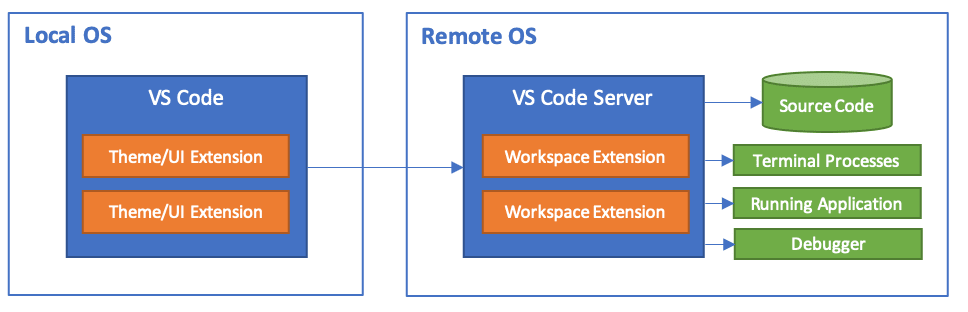
Reviewer #3 (Public Review):
Summary:<br /> The authors generate and characterize two phosphospecific antisera for FFA2 receptor and claim a "bar code" difference between white fat and Peyers patches.
Strengths:<br /> The question is interesting and the antibody characterization is convincing.
Weaknesses:<br /> The mass spectrometry analysis is not convincing because the method is not quantitative (no SILAC, TMT, internal standards etc). Figure 1 shows single tryptic peptides with one and two phosphorylation fragmentations as claimed, but there is no data testing the abundance of these so the differences claimed between cell treatment conditions are not established.
The blot analysis cannot distinguish 296/7 but it does convincingly show an agonist increase. Can the authors clarify why the amount of constitutive phosphorylation is much higher in the example blot in Figure 2 than in Figure 3? It would be helpful to quantify this across more than one example, like in Figures 4 and 5 for tissue.
Compound 101 is shown in Figure 2 to block barrestin recruitment. I agree this suggests phosphorylation mediated by GRK2/3 but this is not tested. The new antibodies should be good for this so I don't understand why the indirect approach.
The conditions used to inhibit dephosphorylation are not specified, the method only says "phosphatase inhibitors". How do the authors know that low P at 306/7 in white fat is not a result of dephosphorylation during sample preparation? If these sites are GRK2/3 dependent (see above) then does adipose tissue lack this GRK?
The easiest way to install Visual Studio Code for Debian/Ubuntu based distributions is to download and install the .deb package (64-bit), either through the graphical software center if it's available, or through the command line with:
sudo apt install ./<file>.deb
Install Visual Code Binary on Linux
Howell agreed with the Copyright Office and said human authorship is a "bedrock requirement of copyright" based on "centuries of settled understanding."
Human authorship is key thats why I believe the humans that wrote the code for the AI should have the right to copyright what the AI creates. You can argue that it is an extension of their original creation.
calls are routedto the system by area code —meaning someone based in New York, but whose phone has a Massachusetts areacode, will be routed to a Massachusetts call center.
First area of struggle. Causing big issues for call center staff.
Numbers# Numbers are normally stored in two different ways: Integer: whole numbers like 5, 37, -10, and 0 Floating point numbers: these can represent decimals like: 0.75, -1.333, and 3 x 10 ^ 8 Fig. 4.5 The number of replies, retweets, and likes can be represented as integer numbers (197.8K can be stored as a whole number like 197,800).# Click to see example Python code # Save an integer value in a variable called num_tweet_likes num_tweet_likes = 197800 # Save an integer value in a variable called max_tweet_length max_tweet_length = 280 # Save a floating point number in a variable called average_tweet_length average_tweet_length = 133.5 Copy to clipboard When computers store numbers, there are limits to how much space is can be used to save each number. This limits how big (or small) the numbers can be, and causes rounding with floating-point numbers. Additionally, programming languages might include other ways of storing numbers, such as fractions, complex numbers, or limited number sets (like only positive integers). Strings (Text)# Computers typically store text by dividing the text into characters (the individual letters, spaces, numerals, punctuation marks, emojis, and other symbols). These characters are then stored in order and called strings (that is a bunch of characters strung together, like in Fig. 4.6 below). Fig. 4.6 A physical string of the characters: “H”, “A”, “P”, “P”, “Y”, ” “, “B”, “I”, “R”, “T”, “H”, “D”, “A”, “Y”. (image source)# In our example tweet, we can see some different pieces of information that might be represented with strings: Fig. 4.7 The user name, twitter handle, and the tweet text can all be represented with strings.#
it's interesting how programming languages have interesting or different words for basic grammar structures in our language. For example, strings is essentially words, phrases or sentences. A boolean is a dichotomy (I had to search that up) or just a simple T/F in our language. And floating point numbers are non-integers.
le menu Inspect à droit
Il n'y a plus de bouton inspect dans le menu de droite, pour avoir le code rapidement, il faut apparemment se mettre en mode dev. Ensuite le code css est directement dans la barre de droite
In the above code our for loop runs a block of code that has four statements, each doing a print. You’ll notice we added an extra blank print which makes a blank line and helps us see in the output what each loop did.
My friend had learned how to loop with "for loop" in another course and told me it was a very handy code. I've always wanted to learn how to use "for". Here I learned that after using "for", I need to use "print" to show my answer.
what does -mcmodel=medany mean这选择了medium-any code model。这意味着程序和它静态定义的symbol必须在2GB范围
[!NOTE]
gcc --mcmodel=medany表示什么?flashcard
程序和它静态定义的symbol必须在2GB范围内
Reviewer #2 (Public Review):
Summary:
Guan and colleagues address the question of how a single neuroblast produces a defined number of progeny, and what influences its decommissioning. The focus of the experiments are two well-studied RNA-binding proteins: Imp and Syp. The Authors find that these factors play an important role in determining the number of neurons in their preferred model system of VNC motor neurons coming from a single lineage (LinA/15) by separate functions taking place at specific stages of development of this lineage: influencing the life-span of the LinA neuroblast to control its timely decommissioning and functioning in the Late-born post-mitotic neurons to influence cell death after the appropriate number of progeny is generated. The post-mitotic role of Imp/Syp in regulating programmed-cell death (PCD) is also correlated with a specific code of key transcription factors that are suspected to influence neuronal identity, linking the fate of neuronal survival with its specification. This paper addresses a wide scope of phenotypes related to the same factors, thus providing an intriguing demonstration of how the nervous system is constructed by context-specific changes in key developmental regulators.
The bulk of conclusions drawn by the authors are supported by careful experimental evidence, and the findings are a useful addition to an important topic in developmental neuroscience.
Strengths:
A major strength is the use of a genetic labeling tool that allows the authors to specifically analyze and manipulate one neuronal lineage. This allows for simultaneous study of both the progenitors and post-mitotic progeny. As a result the paper conveys a lot of useful information for this particular neuronal lineage. Furthermore addressing the association of cell fate specification, taking advantage of this lab's extensive prior work in the system, with developmentally-regulated programmed cell-death is an important contribution to the field.<br /> Beyond Imp/Syp, additional characterization of this model system is provided in characterizing a previously unrecognized death of a hemilineage in early-born neurons.
Weaknesses:
The main observations that distinguish this study from others that have investigated Imp/Syp in the fly nervous system is the role played in late-born post-mitotic neurons to regulate programmed cell-death. This is an important and plausible (based on the presented findings) newly discovered role for these proteins. However the precision of experiments is not particularly strong, which limits the authors claims. The genetic strategy used to manipulate Imp/Syp or the TF code appears to be done throughout the entire lineage, or all neuronal progeny, and not restricted to only the late born cells. Can the authors rule out survival of the early born hemi-lineage normally fated to die? Therefore statements such as this: To further investigate this possibility, we used the MARCM technique to change the TF code<br /> of last-born MNs without affecting the expression of Imp and Syp<br /> should be qualified to specify that the result is obtained by misexpressing these factors throughout the entire lineage.
The authors make an observation that differs from other systems in which Imp/Syp have been studied: that the expression of the two proteins appears to be independent and not influenced by cross-regulation. However there is a lack of investigation as to what effect this may have on how Imp/Syp regulate temporal identity. A key implication of the previously observed cross-regulation in the fly mushroom body is that the ratio of Imp/Syp could change over the life of the NB which would permit different neuronal identities. Without cross-regulation, do the authors still observe a gradient in the expression pattern of time? Because the data is presented with Imp and Syp stained in different brain samples, and without quantification across different stages, this is unclear. The authors use the term 'gradient' but changes in levels of these factors are not evident from the presented data.
Someone in another country would have to try to find a way to indicate that they aren’t in the United States even though there is no clear place to indicate that. If this is a form for shipping to people in the US only, then this limitation might make sense.
I think this is a good point that shines light on a bigger issue. People making technology and social media have biases that they are using to make code. A lot of people being this point up when there is evidence of ai being racist and that’s only possible by human error wether that is intentional or not.
Data collection and storage can go wrong in other ways as well, with incorrect or erroneous options. Here are some screenshots from a thread of people collecting strange gender selection forms:
Although this may be seen as an error on the developer's end, it was a common occurrence among many sign-up applications on the internet in the past and is still prevalent in certain areas such as video games, where only 'male' or 'female' are provided as gender identities. Nevertheless, just as we accept others in society, coders need to consider these things when designing their code.
Now, there are many reasons one might be suspicious about utilitarianism as a cheat code for acting morally, but let’s assume for a moment that utilitarianism is the best way to go. When you undertake your utility calculus, you are, in essence, gathering and responding to data about the projected outcomes of a situation. This means that how you gather your data will affect what data you come up with. If you have really comprehensive data about potential outcomes, then your utility calculus will be more complicated, but will also be more realistic. On the other hand, if you have only partial data, the results of your utility calculus may become skewed. If you think about the potential impact of a set of actions on all the people you know and like, but fail to consider the impact on people you do not happen to know, then you might think those actions would lead to a huge gain in utility, or happiness.
This passage provides an interesting perspective on utilitarianism and the role of data in the context of making moral decisions. It emphasizes the importance of having all the necessary information when using utilitarianism. Moreover, the text also raises a point about considering the interests of people we may not know personally. In our society, the consequences of our actions extend beyond our immediate circles and failing to account for these broader implications can lead to skewed moral judgments. It serves as a reminder that the moral choices we make based on utilitarianism are only as good as the data we have access to.
Now, there are many reasons one might be suspicious about utilitarianism as a cheat code for acting morally, but let’s assume for a moment that utilitarianism is the best way to go.
I actually really like the idea of utilitarianism. I think of it more as a guiding philosophy than anything else. Simply put for the most part I try to act in way that satisfies the most people. I try to take other peoples opinions into consideration when I make decisions. It's like looking at things in the third person. I believe this text book really discounts this philosophy and says it's too complicated or biased. You do not have to follow it exactly in order to use it.
So all data that you might find is a simplification. There are many seemingly simple questions that in some situations or for some people, have no simple answers, questions like:
I find it interesting how simplifying data always results in some form of bias towards a certain factor. As mentioned in the examples, there are many extraneous factors that influence answers to questions that cannot be captured by computers. Though the simplification of data can speed up the code, we lose the complexity of the data in the process.
The Constantine Codex
Is this the source material for the Da Vinci Code?
"western" biblical materials from "exotic" lands;
While not necessarily related to the Da Vinci Code, this reminds me of the Indiana Jones series with the famous line being "it belongs in a museum". It makes me question the justifications provided by museums and individuals for claiming cultural and historical artifacts as "exotic" and putting them on display for people to see.
Total cost of ownership (TCO) addresses the total cost of software development from inception to sun setting. In 2011, the CRASH report stated the total cost of ownership for software code was $18/Line of Code (LOC). Of this, it is generally accepted that the majority of this cost is related to the maintenance of the software after its initial creation, with estimates ranging from 60-90%.
$18 /LOC
peer-to-peer code hosting network.
code0hosting network
Radicle is a sovereign peer-to-peer network for code collaboration, built on top of Git.
from : https://hyp.is/ICaWMGamEe6B599t4jNMiw/github.com/avasdao/nexa-garden

for : use utf8 icons to indicate type/intent
achieve this using trailmarks intentional plain text mark in notation in vanilla HTML content
🌟 Usage 🌃 JSON 🌠 DAG-JSON 🌌 DAG-CBOR 🐾 Next steps 🥅 Purpose and goals 🏃♀️ Getting Started 📗 Project Docs 📒 API Docs 📐 System diagram 🏭 Code Structure 📣 Project status 🛣️ Roadmap 👫 Get involved 🤲 Contribute 🛍️ Notable Consumers/Users 🌞 Branding 🏭 Code Structure 📗 Project Docs 📒 API Docs 📐 System diagram 📣 Project status 🛣️ Roadmap 👫 Get involved 🤲 Contribute 🛍️ Notable Consumers/Users 🌞 Branding

Author Response
The following is the authors’ response to the original reviews.
Reviewer #1 (Public Review):
Sun and co-authors have determined the crystal structures of EHEP with/without phlorotannin analog, TNA, and akuBGL. Using the akuBGL apo structure, they also constructed model structures of akuBGL with phlorotannins (inhibitor) and laminarins (substrate) by docking calculation. They clearly showed the effects of TNA on akuBGL activity with/without EHEP and resolubilization of the EHEP-phlorotannin (eckol) precipitate under alkaline conditions (pH >8). Based on this knowledge, they propose the molecular mechanism of the akuBGL- phlorotannin/laminarin-EHEP system at the atomic level. Their proposed mechanism is useful for further understanding of the defensive-offensive association between algae and herbivores. However, there are several concerns, especially about structural information, that authors should address.
Thank you for reviewing our manuscript. We addressed all comments below.
1) TNA binding to EHEP
The electron densities could not show the exact conformations of the five gallic acids of TNA, as the authors mentioned in the manuscript. On the other hand, the authors describe and discuss the detailed interaction between EHEP and TNA based on structural information. The above seems contradictory. In addition, the orientation of TNA, especially the core part, in Fig. 4 and PDB (8IN6) coordinates seem inconsistent. The authors should redraw Fig. 4 and revise the description accordingly to be slightly more qualitative.
We apologize for the mistake with the PDB file. We forgot to re-upload the final coordinate file of 8IN6, which had been modified according to the requirement of the PDB instructions. We have now re-uploaded the correct PDB file. We carefully checked Fig. 4 (Fig.3 in the revised version), which used the final coordinate file of 8IN6.
2) Two domains of akuBGL
The authors concluded that only the GH1D2 domain affects its catalytic activity from a detailed structural comparison and the activity of recombinant GH1D1. That conclusion is probably reasonable. However, the recombinant GH1D2 (or GH1D1+GH1D2) and inactive mutants are essential to reliably substantiate conclusions. The authors failed to overexpress recombinant GH1D2 using the E. coli expression system. Have the authors tried GH1D1+GH1D2 expression and/or other expression systems?
By referencing other BGLs (six samples were expressed by using E. coli, and one was expressed by using Pichia), we only tried the overexpression of akuBGL, GH1D1, GH1D2, and GH1D1+GH1D2 in E. coli expression system using several different vectors. As the reviewer mentioned that inactive mutants are essential to substantiate our conclusion reliably, it will be tried further to use yeast or cell expression systems to confirm our conclusion. We added these limitations as “Future assay of GH1D2 and inactive mutants is the complement to validate the molecular mechanism of akuBGL” in the discussion (Line 343-345)
3) Inhibitor binding of akuBGL
The authors constructed the docking structure of GH1D2 with TNA, phloroglucinol, and eckol because they could not determine complex structures by crystallography. The molecular weight of akuBGL would also allow structure determination by cryo-EM, but have the authors tried it? In addition, the authors describe and discuss the detailed interaction between GH1D2 and TNA/phloroglucinol/eckol based on docking structures. The authors should describe the accuracy of the docking structures in more detail, or in more qualitative terms if difficult.
Yes, it is possible to try cryo-EM for obtaining the structure of akuBGL complexed with the ligand. However, we didn’t try because 110 kDa akuBGL consists of two 55 kDa GH1Ds linked by along loop, and we worried that ligand may not be visualized using cryo-EM.
Following the comment, we added the description of the accuracy of the docking structures as “Those docking scores corroborated well with the inhibition activity toward akuBGL, that TNA had a more robust inhibition activity than phloroglucinol, indicating that the docking results are reasonable.” (Line 322-324)
Reviewer #2 (Public Review):
In this study the authors try to understand the interaction of a 110 kDa ß-glucosidase from the mollusk Aplysia kurodai, named akuBGL, with its substrate, laminarin, the main storage polysaccharide in brown algae. On the other hand, brown algae produce phlorotannin, a secondary metabolite that inhibits akuBGL. The authors study the interaction of phlorotannin with the protein EHEP, which protects akuBGL from phlorotannin by sequestering it in an insoluble complex.
The strongest aspect of this study is the outstanding crystallographic structures they obtained, including akuBGL (TNA soaked crystal) structure at 2.7 Å resolution, EHEP structure at 1.15 Å resolution, EHEP-TNA complex at 1.9 Å resolution, and phloroglucinol soaked EHEP structure at 1.4 Å resolution. EHEP structure is a new protein fold, constituting the major contribution of the study.
We thank you for reviewing our manuscript.
The drawback on EHEP structure is that protein purification, crystallization, phasing and initial model building were published somewhere else by the authors, so this structure is incremental research and not new.
We have published the results of protein purification, crystallization, phasing, and initial model building for determining structure but have yet to give the structure since further structural refinement is indispensable. Such published data in [Acta F] is a service for obtaining the structure.
We believe that the structure of the EHEP holds great importance, and it is the first time to publish.
Most of the conclusions are derived from the analysis of the crystallographic structures. Some of them are supported by other experimental data, but remain incomplete. The impossibility to obtain recombinant samples, implying that no mutants can be tested, makes it difficult to confirm some of the claims, especially about the substrate binding and the function of the two GH1Ds from akuBGL.
As mentioned by the reviewer, mutant analysis would be the best way to substantiate our conclusions. However, it is challenging to obtain recombinant samples, although we tried to overexpress them (akuBGL, GH1D1, GH1D2, and GH1D1+GH1D2). So, we did the structural comparison, and docking simulation to propose the molecular mechanism. We added these limitations as “Further assay of GH1D2 and inactive mutants is the complement to validate the molecular mechanism of akuBGL” in the discussion part (Line 343-345).
The authors hypothesize from their structure that the interaction of EHEP with phlorotannins might be pH dependent. Then they succeed to confirm their hypothesis, showing they can recover EHEP from precipitates at alkaline pH, and that the recovered EHEP can be reutilized.
A weakness in the model is raised by the fact that the stoichiometry of the complex EHEP:TNA is proposed to be 1:1, but in Figure 1 they show that 4 µM of EHEP protects akuBGL from 40 µM TNA, meaning EHEP sequesters more TNA than expected, this should be addressed in the manuscript.
The assay experiment in figure1 does not directly provide the stoichiometric ratio of EHEP: TNA because the activity assay system consists of substrate of akuBGL, akuBGL, TNA, and EHEP, which involves multiple equilibration processes: akuBGL⇋ substrate, akuBGL⇋TNA, and EHEP ⇋TNA. To avoid misunderstanding, we added the descriptions of ″As this activity assay system involves multiple equilibration processes: akuBGL⇋substrate, akuBGL⇋TNA, and EHEP ⇋TNA.″(Line 120-121).
The authors study the interaction of akuBGL with different ligands using docking. This technique is good for understanding the possible interaction between the two molecules but should not be used as evidence of binding affinity. This implies that the claims about the different binding affinities between laminarin and the inhibitors should be taken out of the preprint.
Following the suggestion, we deleted the descriptions about the difference in binding affinity with docking scores at the last paragraph of [Inhibitor binding of akuBGL].
In the discussion section there is a mistake in the text that contradicts the results. It is written "EHEP-TNA could not dissolve in the buffer of pH > 8.0" but the result obtained is the opposite, the precipitate dissolved at alkaline pH.
We apologize for this mistake and corrected it to " EHEP–TNA could dissolve in the buffer of pH > 8.0." (Line 394).
Solving a new protein fold, as the authors report for EHEP, is relevant to the community because it contributes to the understanding of protein folding. The study is also relevant dew to the potential biotechnological application of the system in biofuel production. The understanding on how an enzyme as akuBGL can discriminate between substrates is important for the manipulation of such enzyme in terms of improving its activity or changing its specificity. The authors also provide with preliminary data that can be used by others to produce the proteins described or to design a strategy to recover EHEP from precipitates with phlorotannin at industrial scales.
In general methods are not carefully described, the section should be extended to improve the manuscript.
Following the comment, we added the method descriptions
Recombinant GH1D1 domain expression and purification in [EHEP and akuBGL preparation].
Sections of [recomGH1D1 activity assay], and [N-terminal sequencing of akuBGL]
More details of resolubiliztion of EHEP and activity in [Resolubilization of the EHEP–eckol precipitate].
Reviewer #3 (Public Review):
The manuscript by Sun et al. reveals several crystal structures that help underpin the offensivedefensive relationship between the sea slug Aplysia kurodai and algae. These centre on TNA (a algal glycosyl hydrolase inhibitor), EHEP (a slug protein that protects against TNA and like compounds) and BGL (a glycosyl hydrolase that helps digest algae). The hypotheses generated from the crystal structures herein are supported by biochemical assays.
The crystal structures of apo and TNA-bound EHEP reveals the binding (and thus protection) mechanism. The authors then demonstrate that the precipitated EHEP-TNA complex can be resolubilised at an alkaline pH, potentially highlighting a mechanism for EHEP recycling in the A. kurodai midgut. The authors also present the crystal structures of akuBGL, a beta-glucosidase utilised by Aplysia kurodai to digest laminarin in algae into glucose. The structure revealed that akuBGL is composed of two GH1 domains, with only one GH1 domain having the necessary residue arrangement for catalytic activity, which was confirmed via hydrolytic activity assays. Docking was used to assess binding of the substrate laminaritetraose and the inhibitors TNA, eckol and phloroglucinol to akuBGL. The docking studies revealed that the inhibitors bound akuBGL at the glycone-binding suggesting a competitive inhibition mechanism. Overall, most of the claims made in this work are supported by the data presented.
We thank you very much for reviewing our manuscript.
Reviewer #1 (Recommendations For The Authors):
• Fig. 3 should be moved to the Supplements because acetylation modification at the N-terminus is not essential for the function of EHEP.
Following the recommendation, we moved Fig.3 to Supplements (Fig. S2).
• EHEP2 is processed at 1.4 Å resolution, however, the statistics at highest resolution shell indicate you can process at higher resolution. Why 1.4 Å resolution?
We tried to process this dataset at the higher resolution at 1.35 Å, and the completeness and I/sigma of the highest resolution shell reduced to 88.9% and 2.16, respectively. The parameter of I/sigma is OK, but the completeness reduced seriously. So, we set a cutoff of 1.4 Å.
• Fig. S1A should be revised to include the gallic acid numbers (1, 2, 3, 4, 6) and the 3.0 σ map. >
As presented in Fig. S1A, the omitted map (fo–fc map) of the ligand TNA, countered at 2.0 σ, showed that gallic acid 2 has poor density, and gallic acid 4 has weak density. Moreover, the TNA is relatively big to EHEP (7.5 %), and the omitted map countered 3.0 σ could not clearly show gallic acids. So, we keep the map at 2.0 σ in Fig. S3A.
• The authors should provide more information on "co-cage-1 nucleant".
Our lab is currently publishing a paper that provides detailed information on the co-cage-1 nucleant, including components, synthesis, nucleation mechanism, and application. Once the paper is published, we will cite it in this manuscript.
Reviewer #2 (Recommendations For The Authors):
- Is the word "offence" the appropriate word for referring to the activity of EHEP? Is this word used in the literature for this system? I find it confusing but might be because I am not in the specific topic.
In the field of prey–predator, the defense–offensive is commonly used.<br /> According to Charles D. Amsler's book ″Algal Chemical ecology″, Herbivore offensive is the traits that allow herbivores to increase feeding rates on algae. Therefore, in our opinion, the offensive is appropriate.
Taking into consideration that I am not an English language expert I find the writing of the manuscript could be improved in general. Here are some lines as examples of where the grammar could be better:
Line 193: "decrement of the loop part"
Following the comment, we corrected it to "decrease of the loop part" (Line 197).
Line 199: there is a typographical error.
We apologize for our mistake and corrected it to “EHEP” (Line 202).
Line 205-206: "only hydrophobically interacted with"
Following the comment, we modified it to "only interacted hydrophobically with EHEP" (Line 209)
Line 224: "phlorotannin–precipitate activity"
Following the comment, we modified it to “phlorotannin-precipitate activity” (Line 227).
Line 232: "without the N-terminal 25 residues"
Following the comment, we modified it to "lacked the N-terminal 25 residues" (Line 236).
Line 353: "bound" should be "bind"
We apologize for our mistake and modified it (Line 356).
Line 359: "predator mammals"
We apologize for our mistake and modified it to "predatory mammals" (Line 363).
Line 363: "at an alkaline pH of insect midgut"
Following the comment, we modified it to "at the alkaline pH of the insect midgut" (Line 367).
Line 370: "nonstructural proteins" means "unstructured proteins"?
Yes, unfolding proteins, we modified to "unfolding proteins with randomly coils" (Line 374).
Line 374: "similar strategy with mammals"
Following the comment, we modified it to "similar strategy to mammals" (Line 379).
Line 403: "to forming"
We apologize for our mistake and modified it to "to form" (Line 404).
Line 404: "considered no binding"
We apologize for our mistake and modified it to "considered not binding" (Line 405).
Line 406: "activity pocket" means the active site?
Yes, we modified it to "active site" (Line 407).
Line 424: "step purification"
Following the comment, we corrected it to "one step for purification" (Line 425).
Line 431
Following the comment, we corrected it to “To verify whether the chemical modifications which was indicated by previous study affects” (Line 432-433).
Line 812: there is typographical error
We apologize for our mistakes, and corrected it to Tris-HCl” for all “Tris–HCl (Line 878~).
Line 223: eckol is not mentioned in the text and appears for the first time in the figure caption.
Following the comment, we added “eckol” in the first section of the [Result] (Line 117).
The paragraph between lines 271 and 280 is disconnected from the previous one and it is not about results, it should be at the discussion section.
Following the comment, we moved them to the discussion part (Line 335-343).
Line 324: "the three inhibitors inhibited": this claim should be corrected to "the three inhibitors interacted", since the word inhibited would imply the authors measured activity experimentally.
We modified it as the comment. (Line 325).
Line 392: "could not dissolve" is contradicting the result.
We apologize for our mistake and corrected it to "could dissolve" (Line 394).
They describe acetylation but they try overexpressing in E. coli, could it be that they needed to express the construct in a system where they would get the acetylation? At least this should be discussed in the text.
Because our sample of EHEP with acetylation was purified from the natural source of the digestive fluid of A.kurodai, we only need to express EHEP without acetylation. Following the comment, we modified the descriptions to clarify it in the section (Lines 170-173 and 177-179).
“Consistent with the molecular weight results obtained using MALDI–TOF MS, the apo structure2 (1.4 Å resolution) clearly showed that the cleaved N-terminus of Ala21 underwent acetylation, demonstrating that EHEP is acetylated in A. kurodai digestive fluid.”
"To explore whether acetylation affects the protective effects of EHEP on akuBGL, we used the E. coli expression system to obtain the unmodified recomEHEP (A21–K229)."
From the text it is not clear in which biological context the brown algae meet the attack by the hydrolase, the information is spread all over the manuscript, it should be clearly described at the introduction.
When the brown algae are consumed as food by sea hare A. kurodai, they meet the attack by the hydrolase akuBGL. Following the comment, we clear the descriptions in the introduction part as below (Line 42-45).
″In brown algae Eisenia bicyclis, laminarin is a major storage carbohydrate, constituting 20%–30% of algae dry weight. The sea hare Aplysia kurodai, a marine gastropod, preferentially feeds on the E. bicyclis with its 110 and 210 kDa β-glucosidases (akuBGLs), hydrolyzing the laminarin and releasing large amounts of glucose.″
Affinity ranking based on docking is not reliable, the differences in free energy are in the same order of magnitude. I would recommend erasing this claim since it is not fundamental to the study. Another option would be to determine affinities experimentally.
We agree with the comment and removed the text about affinity ranking with docking scores.
Figure 1: relative activity is not defined. HPLC data should be shown as supplementary material.
Following the comment, we added the definition of relative activity and the HPLC data as Fig. S1 in the revised version.
Figure 4: Sephacryl resin is mentioned here but not described in the methods.
Following the comment, we added the description in the methods (Line 515).
Protein N-terminal sequencing analysis should be described in the methods.
Following the comment, we added the sequencing analysis in the methods (Line 476-483).
Figure S1 C: it should be specified how the surface electrostatic potential at different pH was calculated.
Following the comment, we added the descriptions of how the surface electrostatic potential at different pH was calculated in the figure legend of Fig. S2 of the revised version (Line 876-877).
Since the authors are capable of producing good amounts of akuBGL and have already conducted glycosidase activity assays using ONPG, it would not be difficult for them to run some kinetics experiments for the enzyme in the presence of the different inhibitors to confirm their hypothesis derived from the docking calculations.
As mentioned by the reviewer, kinetics experiments are the best way to confirm our hypothesis derived from docking calculations. However, the yield of akuBGL purification from the digestive fluid of sea hare A.kurodai is quite difficult. We could not obtain a sufficient sample of akuBGL to conduct the kinetic experiments. So, we stopped at docking simulation in this study. We added such limitations of ″Future kinetic experiments are required to validate quantitatively the competitive inhibition of phlorotannin against akuBGL″ (Line 359-360).
Some citations are missing in the discussion section, for example in lines 362, 364 and 396.
Following the comment, we added the citations.
Reviewer #3 (Recommendations For The Authors):
Please see comments/suggestions below for revisions.
Line 176-178 - Text explains that recombEHEP precipitated after incubation with TNA to a comparable level to natural EHEP. However, figure 3B shows no comparison between recombinant and natural EHEP.
As the reviewer suggested, we repeated the binding assay of recomEHEP to confirm the precipitation with TNA and added a precipitation result of natural EHEP (Fig. S2B right) for comparing.
Line 223 - The work presented in Figure S1E goes partway towards demonstrating the activity of resolubilised EHEP. This claim would be strengthened if resolubilised EHEP was used in the akuBGL Galactoside hydrolytic activity assay and is then seen to rescue akuBGL activity in the presence of TNA.
Yes, our claim would be strengthened by adding resolubilized EHEP to akuBGL assay in the presence of TNA. Since we have obtained and presented the relationship between the precipitating of EHEP with TNA and the rescuing akuBGL activity from TNA, we only used the precipitation to demonstrate the activity of resolubilized EHEP.
Line 380-384 - Here it is discussed how TNA simultaneously binds to three EHEP molecules thus crosslinking them. It is then proposed that this could be the mechanism of precipitation. However, it is noted that TNA is soaked into crystals, therefore it is likely that this lattice exists whether TNA is present or not (this absolutely needs to be mentioned in the text). It would be possible to test this mechanism through mutagenesis. If the sites where TNA packs in between chains of EHEP were mutated to prevent crosslinking, it could then be determined whether crosslink-null EHEP can still precipitate TNA.
As the review mentioned, we do not have enough experiments to propose that the TNA-crosslink may cause the EHEP-TNA precipitation. So, we deleted the discussion of the TNA crosslink and the corresponding figure.
All docked models need to be deposited (perhaps modelarchive.org) and this resource referred to in the text.
The structures in modelarchive.org site are either homology models or de novo. We think the docked model is out of this site. So, we did not deposit them.
The x-ray data table contains data previously published in the referenced Acta cryst publication. What is eLife policy on this "double use" of data?
We apologize for our mistake, and deleted the SAD data in Table 1.
Minor points
Line 26 - use "apo akuBGL" so as not to infer a tannic-acid bound form of this also >
Following the comment, we modified it to “apo akuBGL” (Line 26).
Line 48 - The sentence currently reads as A. kurodai is being digested.
Following the comment, we modified it to “by A. kurodai” (Line 48).
Line 49-50 & Line 65-66 - Both these lines make the same point about the impact of phlorotannin inhibition on the use of brown algae as feedstocks for biofuel, please remove one.
Following the comment, we deleted the line 49-50.
Line 115 - This needs attention as its an unusual opening sentence
Following the comment, we modified it o “Phlorotannin, a type of tannin, is a chemical defense metabolite of brown algae.” (Line 114).
Line 130 - Should the EHEP concentration be 3.96 µM not 3.36?
We apologize for our mistake 3.36 is correct, and we corrected the X-axis label in Fig.1B.
Line 133 - consider using "non-recombinant" rather than "natural"
To distinguish between non-recombinant and recombinant samples, we used “EHEP” and “akuBGL” as purified from the native source and recomEHEP and recomakuBGL as the samples overexpressed from E. coli in this manuscript. So, we added the definition in [Introduction] (Line 100-101).
Line 134 - "The residues A21-V227 of A21-K229..." This sentence could be written more clearly.
Following the comment, we re-wrote it to “The residues A21–V227 in purified EHEP (1–20 aa were cleaved during maturation) were built” (Line 135-136).
Line 136 - switch "appropriately visualized" for "tracable"?
Following the comment, we modified it to “built” (Line 136).
Line 158 - use "70% of backbone in a loop conformation" >
We modified as the comment (Line 159-160).
Line 184 - reword "map showed an electron density blob". (Map showed positive electron density)
Following the comment, we modified it to “map showed the electron density” (Line 188).
Line 193-194 - Is EHEP really more stable when bound to TNA? It is not shown experimentally? It is difficult to see which loop changes. Is the difference a result of crystal packing? Please switch "decrement" for another term
The regions with conformation change between EHEP and EHEP–TNA are close to TNA but not at the intermolecular interface. As the reviewer mentioned, we could not clarify the EHEP stability depended on TNA-binding, and deleted the descriptions in the second paragraph of [TNA binding to EHEP].
Following the comment, we redraw Fig. S1B (Fig. S3B in the revised version) to show the conformation changes clearly. We also modified "decrement" to "decrease" (Line 197).
Fig S1B - Can an extra figure be added to show the secondary differences more clearly? >
We redraw this figure (Fig. S3B) using closeup view to show the differences.
Line 212-213 - There is a slight discrepancy between the text and Figure 4B. Gallic acid 4 interacts with P201 and gallic acid 6 interacts with P77.
We apologize for our mistake in the text. and corrected it to “gallic acid4 and 6 showed alkyl–π interaction with P201 and P77, respectively” (Line 216).
Figure 4D - Change x axis from tube number to elution volume. Both chromatograms could also be superimposed for interpretability.
Since we used raw data from the experiment, we kept the x-axis in tube number with additional “2.7 ml/tube” information (Fig.3D).
Line 229 - Please change "there was no blob of TNA in the electron density" to there was no electron density for TNA or something similar.
Following comment, we modified it to “there was no electron density of TNA or something similar in the 2Fo–Fc and Fo–Fc map” (Line 232).
Line 231 - asymmetric unit is a more standard term (also in Fig S2 legend)
We modified as the comment (Line 235 and 885).
Line 234-235 - Reword "the residues L26-P978 of L26-N994" to make it more concise. >
Following the comment, we deleted “of L26-N994” (Line 239).
Lines 296-299 could be written more carefully - pi stacking with what? >
We apologize for our mistake and corrected it to CH–𝜋 (Line 293).
Line 349 - which putatively enables it to......
We modified it as the commend (Line 353 in the revised manuscript).
Line 370 - "nonstructural" is the wrong term because they remain structured - use something akin to non-classical secondary structure
Following the comment, we modified it to“are unfolding proteins with randomly coils in solution " (Line 374)
Throughout - use phenix autobuild, not autobuil
We apologize for our mistakes and corrected them throughout the manuscript.
Figure 1 - the graphs would be more interpretable with all data points shown overlaid
The two graphs in Figure 1 showed two experiments with different reaction conditions. Figure 1A presents various TNA concentrations, while Figure 1B maintains a constant concentration of 40 μM for TNA with varying EHEP concentrations. So, overlaying the graphs is not feasible. Therefore, we would like to keep them separated and added the reaction condition in figure legend.
Figure 4 - in part D add an extra statement outlining what the S-100 analysis demonstrated
S-100 analysis is using a gel filtration column with Sephacryl S-100 media. We added an extra statement in the method and the legend (Fig. 3, Lines 515 and 879).
Figure 5 (and elsewhere) - the structures referred to need a PDB code and reference given in legend
Following the comment, we checked the manuscript carefully and added PDB code to the referred structures.
Fig S1 - please add an additional panel showing part D but in proper structure form, not schematic shapes
Since we do not have enough experiments to validate the TNA-crosslink, we deleted the discussion of the TNA crosslink and Fig. S1D.
Figure sig 4 - Text contains in depth information of side chain hydrogen bonding and π-π interactions between akuBGL and laminarittrose. However, the figure only shows a surface model. Consider adding a figure showing these interactions.
Following the suggestion, we added a closeup view to show these detailed interactions (Fig. S6B).
Escaping the cycle of reincarnation requires the individual to realize that atman is brahman and to live well or in accordance with dharma, observing the code of conduct as prescribed by scripture, and karma, actions and deeds.
What I take away here is that the people of Brahman think that reincarnation is very bad thing and the way the propose to escape it is by living in accordance with dharma.
Code of Ethics
This has a lot negative language about what not to do, instead of what should be done.
Note: Your site will not receive template updates from Squarespace when Developer Mode is enabled, and you will not be able to switch templates. Additionally, note that using Git or SFTP will not allow you to run server-side code.
This confused me but makes sense because you're essentially branching off the main template so no more updates that's fine
RING STRUCTURE
Ivan writes about a concept called "Ring Structure". This is a way of organizing and linking different elements or components in a system.
In simpler terms, imagine you have a bunch of different objects (like points and lines in a drawing program like Sketchpad). You want to keep track of how these objects are related to each other. For example, you might want to know all the lines that end at a particular point.
To do this, Ivan uses a "ring structure". Each object has a "string of pointers" - basically a list of references to other objects. This list is circular - the last item in the list points back to the first item. This makes it easy to move forwards and backwards through the list.
Each object has two "registers" or slots for keeping track of these relationships. One slot is for the object itself, and the other is for the list of related objects.
Ivan uses the terms "hen" and "chicken" to describe these slots. The "hen" is the object itself, and the "chicken" is the list of related objects.
Here's a simple Python code example to illustrate this concept:
```python class Point: def init(self): self.hen = self self.chickens = []
class Line: def init(self, point1, point2): self.hen = self self.chickens = [point1, point2] point1.chickens.append(self) point2.chickens.append(self) ```
In this example, a Point object has a hen that refers to itself and a list of chickens that will contain any Line objects that end at this point. When a Line is created, it adds itself to the chickens list of its end points.
The "ring structure" is a way to organize and link different elements in a system, making it easier to find and update related elements.
Reviewer #3 (Public Review):
Summary:<br /> In this article, Fox and colleagues describe the results of a novel and innovative task, coupled with a modified computational model, to explore pure directed exploration (not quite a pun, but intended nonetheless). In their task, participants make a series of discrete choices, importantly with no reward feedback, to navigate a nested series of rooms in a virtual environment. The initial 2-door choice is used as the primary probe and the complexity of the series of rooms behind each choice is used as the critical independent variable. The authors find that, as the number of follow-up options behind a door increases, "good" participants are more likely to choose the door that leads to the more complex choices. As the depth of the search increased (i.e. the room with the most doors was presented "farther" down the search), these same participants were less likely to choose the door leading to the more complex route. Finally, these same "good" participants showed an initial boost in preference towards the more complex exploration option after a few learning episodes that settled down after about 10 episodes, with a modest reliable preference towards the more complex route. This reflected the fact that information value decays over time in stable situations. Using an adaptation of standard Q-learning, with a proxy of information value being substituted for reward value, the authors show how their model can qualitatively capture most of the observed experimental effects, although with some critical differences in the temporal dynamics of learning, suggesting that the memory horizon for humans is longer than in the adapted Q-learning model.
Strengths:<br /> 1. Clever experimental design<br /> The novel task is really clever and gets around many of the limitations for understanding directed exploration that have plagued prior research (which typically involve some use of reward feedback). Finding a way to provide direct information that can be experimentally manipulated, without needing to provide any explicit reward feedback, makes this one of the few pure exploration tasks that I am aware of.
2. Compelling results<br /> The effect of manipulating choice complexity and depth on initial choice probability for "good" directed learners seems fairly strong, as do the learning dynamics. The heterogeneity in exploration style across participants is also interesting and brings up more questions that are useful for follow-up research.
3. Simple model<br /> The computational model used is a simple adaptation of standard reinforcement learning models, specifically Q-learning models. This is elegant as it doesn't require major changes in the dynamics of learning, simply a revision of the variables going into the update. The simplicity of this change, coupled with the ability to capture the results of the "good" directed explorers makes a strong case that information seeking and reward-seeking may share common underlying mechanisms (as shown previously by Kobayashi, K., & Hsu, M. (2019). Common neural code for reward and information value. Proceedings of the National Academy of Sciences, 116(26), 13061-13066.).
Weaknesses:
1. "Good" vs. "poor"<br /> There is an odd circularity, and implicit value judgment, in the classification of participants into "good" and "poor" directed explorers. The logic, based on the visit-counter model of directed exploration, is that the probability of repeating a choice (at the initial decision trial) should be low for directed explorers vs. random explorers. Doing the median split on repetition probability seems intuitively fine here, but it does bring up two issues. First, the labels "good" vs. "poor" seem arbitrarily judgemental, after all random exploration is a viable exploration strategy in many contexts. Would "directed" vs. "random" be more appropriate labels based on how the decision was made to categorize participants? Second, how much of the "good" participant performance is driven by the extreme non-repeaters? For example, if a tertiary split was performed instead of a binary median split, would the middle group show a weaker version of the effects seen in the "good" group or appear more like the "poor" group?
2. Characterization of information value<br /> The authors discuss primarily methods that can be summarized by visit counters as a description for all directed exploration models. However, that doesn't seem to be a good summary of the overall literature in this space. There are also entropy-based approaches, that quantify information value based on the statistics of the feedback. For example, in machine learning methods like the KL divergence are often used to represent the information value of a channel. A few such papers are highlighted below. Now it is entirely possible that these approaches can be extrapolated to simple visit-count approaches, but I am unaware of anything showing this. I think it would be good to broaden the discussion on directed exploration models beyond visit-counter methods like UCB, highlighting the other methods used to promote directed exploration.
Houthooft, R., Chen, X., Duan, Y., Schulman, J., De Turck, F., & Abbeel, P. (2016). Vime: Variational information maximizing exploration. Advances in neural information processing systems, 29.
Eysenbach, B., Gupta, A., Ibarz, J., & Levine, S. (2018). Diversity is all you need: Learning skills without a reward function. arXiv preprint arXiv:1802.06070.
Hazan, E., Kakade, S., Singh, K., & Van Soest, A. (2019, May). Provably efficient maximum entropy exploration. In International Conference on Machine Learning (pp. 2681-2691). PMLR.
3. Model vetting<br /> The model used to simulate the behavioral results is interesting and intuitive. However, there seem to be some things left on the table and unresolved. First, the definition of information value (E) that is maximized is assumed to satisfy the same constraints as typical reward does in the Bellman solution for reinforcement learning. This is the only way it can be substituted into the typical Q-learning method. Is that true here?
Second, the advantage of these simpler computational-level models is that they can be effectively fit to behavior. The model outlined in the paper has only a few free parameters (some of which can be fixed for convenience purposes). Was there an attempt to fit each participant's data into the model? This would be a powerful way of highlighting where exactly the differences between the "good" and "bad" participants arise.
Reviewer #2 (Public Review):
Summary: After manually labelling 144 human adult hemispheres in the lateral parieto-occipital junction (LPOJ), the authors 1) propose a nomenclature for 4 previously unnamed highly variable sulci located between the temporal and parietal or occipital lobes, 2) focus on one of these newly named sulci, namely the ventral supralateral occipital sulcus (slocs-v) and compare it to neighbouring sulci to demonstrate its specificity (in terms of depth, surface area, gray matter thickness, myelination, and connectivity), 3) relate the morphology of a subgroup of sulci from the region including the slocs-v to the performance in a spatial orientation task, demonstrating behavioural and morphological specificity. In addition to these results, the authors propose an extended reflection on the relationship between these newly named landmarks and previous anatomical studies, a reflection about the slocs-v related to functional and cytoarchitectonic parcellations as well as anatomic connectivity and an insight about potential anatomical mechanisms relating sulcation and behaviour.
Strengths:<br /> - To my knowledge, this is the first study addressing the variable tertiary sulci located between the superior temporal sulcus (STS) and intra-parietal sulcus (IPS).<br /> - This is a very comprehensive study addressing altogether anatomical, architectural, functional and cognitive aspects.<br /> - The definition of highly variable yet highly reproducible sulci such as the slocs-v feeds the community with new anatomo-functional landmarks (which is emphasized by the provision of a probability map in supp. mat., which in my opinion should be proposed in the main body).<br /> - The comparison of different features between the slocs-v and similar sulci is useful to demonstrate their difference.<br /> - The detailed comparison of the present study with state of the art contextualises and strengthens the novel findings.<br /> - The functional study complements the anatomical description and points towards cognitive specificity related to a subset of sulci from the LPOJ<br /> - The discussion offers a proposition of theoretical interpretation of the findings<br /> - The data and code are mostly available online (raw data made available upon request).
Weaknesses:<br /> - While three independent raters labelled all hemispheres, one single expert finalized the decision. Because no information is reported on the inter-rater variability, this somehow equates to a single expert labelling the whole cohort, which could result in biased labellings and therefore affect the reproducibility of the new labels.<br /> - 3 out of the 4 newly labelled sulci are only described in the very first part and never reused. This should be emphasized as it is far from obvious at first glance of the article.<br /> - The tone of the article suggests a discovery of these 4 sulci when some of them have already been reported (as rightfully highlighted in the article), though not named nor studied specifically. This is slightly misleading as I interpret the first part of the article as a proposition of nomenclature rather than a discovery of sulci.<br /> - The article never mentions the concept of merging of sulcal elements and the potential effect it could have on the labelling of the newly named variable sulci.<br /> - The definition of the new sulci is solely based on their localization relative to other sulci which are themselves variable (e.g. the 3rd branch of the STS can show different locations and different orientation, potentially affecting the definition of the slocs-v). This is not addressed in the discussion.<br /> - The new sulci are only defined in terms of localization relative to other sulci, and no other property is described (general length, depth, orientation, shape...), making it hard for a new observer to take labelling decisions in case of conflict.<br /> - The very assertive tone of the article conveys the idea that these sulci are identifiable certainly in most cases, when by definition these highly variable tertiary sulci are sometimes very difficult to take decisions on.<br /> - I am not absolutely convinced with the labelling proposed of a previously reported sulcus, namely the posterior intermediate parietal sulcus.
Assuming that the labelling of all sulci reported in the article is reproducible, the different results are convincing and in general, this study achieves its aims in defining more precisely the sulcation of the LPOJ and looking into its functional/cognitive value. This work clearly offers a finer understanding of sulcal pattern in this region, and lacks only little for the new markers to be convincingly demonstrated. An overall coherence of the labelling can still be inferred from the supplementary material which support the results and therefore the conclusions, yet, addressing some of the weaknesses listed above would greatly enhance the impact of this work. This work is important to the understanding of sulcal variability and its implications on functional and cognitive aspects.
Reviewer #2 (Public Review):
Summary<br /> Recent evidence indicates that cells of the navigation system representing different directions and whole spatial routes fire in a rhythmic alternation during 5-10 Hz (theta) network oscillation (Brandon et al., 2013, Kay et al., 2020). This phenomenon of theta cycle skipping was also reported in broader circuitry connecting the navigation system with the cognitive control regions (Jankowski et al., 2014, Tang et al., 2021). Yet nothing was known about the translation of these temporally separate representations to midbrain regions involved in reward processing as well as the hypothalamic regions, which integrate metabolic, visceral, and sensory signals with the descending signals from the forebrain to ensure adaptive control of innate behaviors (Carus-Cadavieco et al., 2017). The present work aimed to investigate theta cycle skipping and alternating representations of trajectories in the lateral septum, neurons of which receive inputs from a large number of CA1 and nearly all CA3 pyramidal cells (Risold and Swanson, 1995). While spatial firing has been reported in the lateral septum before (Leutgeb and Mizumori, 2002, Wirtshafter and Wilson, 2019), its dynamic aspects have remained elusive. The present study replicates the previous findings of theta-rhythmic neuronal activity in the lateral septum and reports a temporal alternation of spatial representations in this region, thus filling an important knowledge gap and significantly extending the understanding of the processing of spatial information in the brain. The lateral septum thus propagates the representations of alternative spatial behaviors to its efferent regions. The results can instruct further research of neural mechanisms supporting learning during goal-oriented navigation and decision-making in the behaviourally crucial circuits entailing the lateral septum.
Strengths<br /> To this end, cutting-edge approaches for high-density monitoring of neuronal activity in freely behaving rodents and neural decoding were applied. Strengths of this work include comparisons of different anatomically and probably functionally distinct compartments of the lateral septum, innervated by different hippocampal domains and projecting to different parts of the hypothalamus; large neuronal datasets including many sessions with simultaneously recorded neurons; consequently, the rhythmic aspects of the spatial code could be directly revealed from the analysis of multiple spike trains, which were also used for decoding of spatial trajectories; and comparisons of the spatial coding between the two differently reinforced tasks.
Weaknesses<br /> Possible in principle, with the present data across sessions, longitudinal analysis of the spatial coding during learning the task was not performed. Without using perturbation techniques, the present approach could not identify the aspects of the spatial code actually influencing the generation of behaviors by downstream regions.
有以下几种方法可以配置javac的编码方式:方法一:在vscode的设置中,找到"code-runner.executorMap",然后修改"java"的值为"cd方法一:在vscode的设置中,找到"code-runner.executorMap",然后修改"java"的值为"cd$dir && javac -encoding UTF-8 $fileName && java $fileNameWithoutExt"。这样就可以$dir && javac -encoding UTF-8 $fileName && java $fileNameWithoutExt"。这样就可以让code-runner插件在运行java代码时使用UTF-8编码。让code-runner插件在运行java代码时使用UTF-8编码。
我用了第一个方法,因为它比较通用,只要是run java代码都可以生效
library(dplyr) # for data wrangling
should be a line of code?
"DeepDream - a code example for visualizing Neural Networks".
This is a real source: https://blog.research.google/2015/07/deepdream-code-example-for-visualizing.html?m=1
With all languages (including programming languages), you combine pieces of the language together according to specific rules in order to create meaning. For example: Consider this sentence in English:
I have never coded before (except briefly using scratch.mit in elementary school). As such, I find this idea of treating coding as a language (like English) very interesting. Essentially, I can structure code through various rules and laws to give it proper meaning. Just like how English has certain laws regarding things like punctuation, verb tenses, etc.; what it looks like is programming has their own set of laws that will govern how I write code.
I have never coded before (except briefly using scratch.mit in elementary school). As such, I find this idea of treating coding as a language (like English) very interesting. Essentially, I can structure code through various rules and laws to give it proper meaning. Just like how English has certain laws regarding things like punctuation, verb tenses, etc.; what it looks like is programming has their own set of laws that will govern how I write code.
Note that sometimes people use “bots” to mean inauthentically run accounts, such as those run by actual humans, but are paid to post things like advertisements or political content. We will not consider those to be bots, since they aren’t run by a computer.
Actually, and I may be wrong, the bots referred to in this paragraph, can be ran by computers. Now, it may be unlikely and is usually ran by a human being, but there have been sometimes where I've seen inauthentically ran accounts being ran by some type of source code.
Page 3- "Sign-in sheets can document how many or who attended an activity." Weirton Elementary is so large, and I was always amazed on how one of how secretary was able to read all parent signatures to document attendance. One of our principals created a QR code this year for Open House. When parents came to open house, they could sign in using the QR code. This was more convenient for parents, great for documenting attendance, and a time saver for our secretary.
Its code base is open-source—publicly available for anyone to download and comment on—and subject to peer review.
It's not. The codebase used in production is not the same codebase they put on github and pretend to maintain.
Psuedocode is intended to be easier to read and write. Pseudocode is often used by programmers to plan how they want their programs to work, and once the programmer is somewhat confident in their pseudocode, they will then try to write it in actual programming language code.
Due to its reflection of human language, to what extent may the structure of Psuedocode's ability to be easily understood fluctuate amongst written languages? I am curious regarding the lingual context of its development may have influenced its structure, or if so is more so tailored towards computer binaries.
Psuedocode is intended to be easier to read and write. Pseudocode is often used by programmers to plan how they want their programs to work, and once the programmer is somewhat confident in their pseudocode, they will then try to write it in actual programming language code.
This is a tool that I recognized during my learning in CSE 142. Although I personally didn't use it a ton, I would highly recommend it for beginner coders. Coding languages aren't directly self-explanatory, which is why people often use pseudocode and comments in their programs.
A human computer running a cooking program. In other words: “someone following a recipe” (but probably not a dumpling recipe)
I had never thought of computer programming in terms of mundane actions before as computers and humans have lived very mutually exclusive lives in my mind. However, this comparison is quite accurate and upon reading the rest of this section, being a newbie to coding, the process does not seem as intimidating or complicated as I previously thought, particularly the part on conditionals and code blocks.
Psuedocode is intended to be easier to read and write. Pseudocode is often used by programmers to plan how they want their programs to work, and once the programmer is somewhat confident in their pseudocode, they will then try to write it in actual programming language code.
I learned psuedocode when i took CSE121 class. Psuedocode serves as a blueprint for translating the code's logic into an actual programming language. For me, it is pretty useful since it helps me to think about problem more comprehensive and efficient especially when the problem is hard.
In this example, some clever protesters have made a donkey perform the act of protest: walking through the streets displaying a political message. But, since the donkey does not understand the act of protest it is performing, it can’t be rightly punished for protesting.
I can see the logic behind this reasoning and I agree with it quite well. I view this as technology or bots being the donkey and the protestors as being the programmers. Its not the donkey that's protesting it is simply "following instructions" just like a bot reads code.
The reason eval is there is because when you need it, when you really need it, there are no substitutes. There's only so much you can do with creative method dispatching, after all, and at some point you need to execute arbitrary code.
But this way of displaying a variable will only work if it is the last line of code in the code block. So if I write a bunch of variables on their own lines, only the last one will be displayed:
This is so interesting and I never knew this about Python and I wonder if there is a specific reason for why the language developers decided to only display the last variable when a list of them is written out consecutively. I can imagine this would make some aspects of debugging easier.
magic(bool, dict, or str, optional) The bool controls whether we try to auto-instrument your script, capturing basic details of your run without you having to add more wandb code. (default: False) You can also pass a dict, json string, or yaml filename.
[!NOTE]
wandb中,要自动记录基本信息,可以使用?flashcard
wandb.init(magic=...)
the radical left
Code for anyone outside their ideological camp.
When one of us ran the program, who made those reddit posts (me? you? the bot?)? Notice that there are at least three times of actions for posting reddit post with this bot, one is when the code was originally written, another is when the code was modified, and and the other is when the code is run. These could even be done by different people. How do you divide out responsibility for a bots actions between the person writing the code and the person running the program?
When the bot post in social media, is us or the programmer made those reddit posts, because the bots doesn't have any sence of independence. Human manipulate the bots and the programs to post any infomartion on the internet, which means if we are trying to divide out responsibility for bot action, human would have the most responsibility.
Note: This preprint has been reviewed by subject experts for Review Commons. Content has not been altered except for formatting.
Learn more at Review Commons
In this work, the authors generate a multi-omic dataset (RNA, proteomic and metabolomic) from fibroblast cell-lines of human and bat origins, in study of the specific differences in bat that allows them to have a good cancer resistance and longevity. They specifically focus on metabolic differences between humans and bats. They perform differential analysis followed by GO enrichment analysis to highlight differences related to the electron transport chain both at the level of RNA and protein abundance. They then use FBA sampling and specific constraints to propose an hypothesis of reverse direction of the second complex of the ETC, as well as better resistance to ROS, which they support with several subsequent experiments.
Overall, the paper is very well written, the findings are presented clearly and efficiently. For the most part, the assumption and limits of the study are clearly stated by the author (notably with respect to the limits of using only cell lines). In my opinion, the goal of the paper, which is presented as a stepping stone into further characterisation of the metabolic differences between human and bat for potential oncological research benefits, is clearly stated and appropriate.
There are however several points that I think are important to address inorder to improve the quality of the scientific work and its interest for the rest of the scientific community.
Major
The authors state:<br /> "We then set the lower bound of the PaLung Complex I reaction flux to a value equal to 70% of its theoretical maximum. Similarly, we set the upper bound of the WI-38 Complex I reaction at a value equal to 30% of its theoretical maximum value. This ensured that the PaLung model would have higher flux through the Complex I reaction, in comparison to the WI-38 model."
How do the results hold with different thresholds ? Are these findings robust with e.g. in ranges between 10 to 50% (90-50%) (instead of only 30% and 70%). Furthermore, the histogram figures doesnt seem to reflect a 70% of maximum lower bound for complex I (threshold at a value of 30 seems like extremity of tail).
Number of differentially expressed genes is extremely high because such cutoffs are not really meaningful given the comparison between two organisms. No need to refer to the 6247 above cutoff as differentially regulated genes (see: https://elevanth.org/blog/2023/07/17/none-of-the-above/ and https://daniel-saunders-phil.github.io/imagination_machine/posts/if-none-of-the-above-then-what/ for pointers toward current best practice in biological statistics). Enough to simply note that 6247 are above the cutoffs, which suggest a drastic (and expected) difference in expression profiles between the two organisms.
Please highlight the RNA and proteomic analysis assumption and present results within those boundaries (e.g. how are the transcript matched between human and bat, the use of human gene ontologies, etc...). Are the human GO set definitions relevant in bat (it is a common practice with mice and rats, are bats close ?)?
Are oxphos and hypoxia responses the most extreme pathway scores in the GSEA ? Instead of barcode plots that are generally not a very useful use of figure space, use fig 1C to show the top e.g.20 (positive and negative) pathway scores so that we can see how much those two actually stand out. Same for the proteomic analysis. Also, need to show an unbiased side by side comparison of the pathway enrichments for RNA and proteomic, the reported results in main text and figures are too cherry picked to be of interest as they stand.
Finally, and very importantly, please upload ALL the code used for the analysis, with instructions to run it and all the required inputs and source files. The computational analysis is only as credible as it is easy to reproduce.
Minor
Introduce GeTMM, what are its key specificities ?
Fig 1C code bar plot useless, simply report ES and NES and pathway absolute rank in text.
Report Foldchange/p-value/rank of complex-I members and other genes of interest for the narrative of the paper.
Referees cross-commenting
I also think the comments from the other reviewers are appropriate.
In my opinion, the goal of the paper, which is presented as a stepping stone into further characterisation of the metabolic differences between human and bat for potential oncological research benefits, is clearly stated and appropriate.
Broadly interesting for oncological research.
My espertise is multi-omic data analysis and integration with prior knowledge in the context of complexe diseases.
Author Response
The following is the authors’ response to the original reviews.
Summary of changes
I thank the reviewers for their thorough feedback on this paper and providing me with such a detailed list of recommendations. I have been able to incorporate many of their suggestions, which I believe has greatly improved this paper.
The most important changes:
• I added comparisons to the lexicon- and rule-based sentiment algorithms TextBlob and VADER to Supplementary Fig. 4. This shows the superiority of ChatGPT in scoring the sentiment of scientific texts compared to existing and already-validated tools for sentiment analysis based on natural language processing. [Suggestion Reviewer 2]
• I added the measure intra-class correlation to Fig. 3b, emphasizing the inconsistency in sentiment scores across different reviews of the same paper. [Suggestion Reviewer 3]
• I added Supplementary Fig. 6, in which I directly propose different experiments to test the causes of the observed gender effects on peer review. [Suggestion Reviewer 3]
• I further studied the issue of variability in responses by ChatGPT (Supplementary Fig. 2), and learned that this has greatly improved in the latest version of ChatGPT (for Version Aug 3, 2023, R2 values of 0.99 (sentiment) and 0.86 (politeness) were reached). I show these findings in Supplementary Fig. 2. [Suggestions Reviewers 1 and 3]
• Throughout the manuscript (most notably in the Abstract and Discussion), I emphasize that this is a proof-of-concept study, and make suggestions on how to scale this up across journals and fields. I also toned down certain claims given the relatively small sample size of this study, including in the abstract. I also more prominently and elaborately discuss the limitations of the study in the Discussion section. [Suggestions Reviewers 1, 2 and 3]
• I made many smaller changes to text, figures and references on the basis of the reviewers’ comments. [Suggestions Reviewers 1, 2 and 3]
Notably, Reviewer 3 has provided me with a very detailed list of recommendations for follow-up experiments. I appreciate their ideas, and I am currently considering different options for future work. Specifically I am looking to team up with a journal to perform the experiments laid out in Supplementary Fig. 6 of the new paper, to study whether I can find evidence of bias across rejected and accepted papers. As suggested by this reviewer, I am also looking into ways to automate data collection using APIs, and by utilizing the rapidly expanding databases for transparent peer review.
Based on this preprint, I have received messages from academics that are interested in using generative AI to study scientific texts. By revising this manuscript, I hope to provide them with the tools to concurrently expand the analysis of peer review into different scientific disciplines and journals.
Reviewer #1 (Public review)
Strengths:
The innovative method is the biggest strength of this article. Moreover, the method can be implemented across fields and disciplines. I myself would like to see this method implemented in a grander scale. The author invested a lot of effort in data collection and I especially commend that ChatGPT assessed the reviews twice, to ensure greater objectivity.
I want to thank this reviewer for commending the innovative methodology of this study. I appreciate that this reviewer would like to see this methodology implemented at a grander scale, which is a view that I share. I initially only included Neuroscience papers, because I was uncertain whether I would be able to properly assess the reviews from different scientific disciplines (and thus judge whether ChatGPT was able to provide plausible scores).
The reviewers have provided me with a list of potential follow-up experiments, and I am currently considering different options for future work. Specifically I am looking to team up with a journal to perform the experiments laid out in (the new) Supplementary Fig. 6 of the new paper, to study whether I can find evidence of bias across rejected and accepted manuscript of a journal. In addition, as suggested by Reviewer #3, I am looking into ways to automate data collection using APIs, and by utilizing the rapidly expanding databases for transparent peer review. Importantly, based on this preprint, I have received messages from academics that are interested in using generative AI to study scientific texts. By revising this manuscript now, I hope to provide them with the tools to concurrently expand the analysis of peer review into different scientific disciplines and journals.
The comments I received from the different reviewers made me realize that I did not describe the intent of this paper well enough in the original submission. I rewrote much of the Abstract, to emphasize the proof-of-concept nature of this study, and rewrote the Discussion to focus more on the limitations of the study.
Weaknesses:
I have several concerns regarding the methodology of the article. The first relates to the fact that the sample is not random. The selection of journal and inclusion and exclusion criteria do not contribute well to the strength of the evidence.
Indeed, the inclusion of only accepted manuscript from a single journal is the biggest caveat of this paper. I have re-written much of the Abstract to emphasize that this is a proof-of-concept paper, hoping that other researchers concurrently expand this method to larger and more diverse datasets.
An important methodological fact is that the correlation between the two assessments of peer reviews was actually lower than we would expect (around 0.72 and 0.3 for the different linguistic characteristics). If the ChatGPT gave such different scores based on two assessments, should it not be sound to do even more assessments and then take the average?
This was a great recommendation by this reviewer, and a point also raised by Reviewer #3. Based on their suggestion, I looked into how each additional iteration of scoring would reduce the variability of scoring for a subset of papers (thus being able to advice users on an optimal number of iterations).
Interestingly, I observed that ChatGPT has become significantly more reliable in providing sentiment and politeness scores in recent versions. For the latest version (ChatGPT Aug 3, 2023), R2 = 0.992 for sentiment and R2 = 0.859 for politeness were reached for two subsequent iterations of scoring. Unfortunately, OpenAI does not allow access to previous version of ChatGPT, so the current dataset could not be re-scored. Yet, based on these data, there may no longer be a need for people to perform repeated scoring. I show these data in Supplementary Fig. 2, as I believe this is very useful information for people who are interested in using this tool.
Reviewer #1 (Recommendations to author)
I had some difficulties reading the article, so it would maybe help to structure the article more (e.g. In the introduction there are three aims stated, so the Statistical Analysis section could be divided in three sections, and instead of the link to figures, the author could state which variables were analysed in a specific manner) to be easier to comprehend the details. Also, I found on one place that the sample consisted of 572 reviews, and on other that it was 558.
These are very good points. I re-wrote the statistical analysis for clarity (Page 7 of the manuscript). The 558 reviews was a mistake from my part, as I forgot to include the fourth review for the 14 papers that received four reviews in the histograms of Fig. 2b and the accompanying text. This has been updated.
For figures 1a and 1b it could be considered to enter the table instead of several figures.
I thank the reviewer for pointing this out. I tried this suggestion, but I found it to reduce the readability of the paper. As an alternative, I now provide an Excel spreadsheet with all the raw data, so people can find all the characteristics of the included papers.
99.8% of the reviews analysed were assessed as polite. This is, in my opinion, extremely important finding, which shows that reviewers are still holding to certain degree of standards in communication, and it can be mentioned in the abstract.
I very much agree with this reviewer; this has now been added to the Abstract.
In results you state that QS World Ranking is "imperfect" measure. When stating that in the results section, it poses the question why it is used in the study, so maybe it is more suitable for the discussion.
This point is well taken. Even though the QS World Ranking score is imperfect, I still think it can be useful, as a rough proxy of perceived prestige of an institution. I now removed this “imperfect measure” statement from the Results section, and moved it to the Discussion (Page 5).
In the Results section, instead of using only p values, please add measures of effect (correlations, mean differences), to make it easier to place in the context.
For the significant effects of Fig. 4, I have added these to the figure legends. Please note that the used statistical tests are non-parametric, so I reported the Hodges-Lehmann differences (which is the median of all possible pairwise differences between observations from the two groups).
I think the results interpretation should be softened a bit, or the limitations of the study should be placed as the second paragraph in the discussion, since this was only specific journal with specific subfield.
I agree with this reviewer that the relatively small sample size of this paper demands more careful wording. Throughout the manuscript, I have toned down claims, and emphasized the “proof of concept” nature of this study (for example in the Abstract). I also moved the limitations section to the second paragraph of the Discussion, and elaborate more on the study’s caveats.
Methods:
The measure Review time was assessed from submission to acceptance, but this does not need to be review time since it takes a lot of time sometimes to find reviewers. that needs to be stated as the limitation.
This point is well taken. I changed this to “Paper acceptance time” in Fig. 3 and the accompanying text.
Gender name determination methods differed between the assessment of the first authors and the last authors, and that needs stronger explanation.
I appreciate this reviewer raising this point, which has also been raised by Reviewer #3. For this paper, I have carefully weighed the pros and cons of automated versus manual gender determination. Initially, my intention was to rely only on a programmatic method to identify authors' names. However, I came to realize that there were inaccuracies in senior author gender predictions made by ChatGPT/Genderize. This was evident to me due to my personal familiarity with some of these authors, either because they are famous or through personal interactions. It seemed problematic to me to proceed with this analysis knowing that these misclassifications would introduce unnecessary variability to the dataset.
The advantage of the relatively small sample size in this study was the opportunity to manually perform this task, rather than being fully dependent on algorithms. While I attempted manual gender identification for the first author as well, this was way more challenging due to their limited online presence. The discrepancy in gender identification accuracy between first and senior authors did not go unnoticed, and I acknowledge the issue it presents. I also recognize that, unlike senior authors, reviewers may not necessarily be familiar with the first authors of the papers they evaluate, as indicated in the original submission of this paper. In light of this, I sought input from several PIs who often serve as reviewers. Their feedback confirmed that they typically possess knowledge of senior authors' identities, for example through conferences, whereas the same is not true for first authors. Yet, this may be different for other scientific disciplines, where the pool of reviewers might be bigger.
Notably, for future studies I may make a different decision, especially when I use larger datasets that require me to automate the process.
I also realize that my rationale for the different methods of gender determination was not explained well enough in the original submission; I now explain my reasoning more elaborately on Page 7 on the manuscript.
For sentiment analysis: Please state based on what the GPT made a decision? Which program? (e.g. for gender it used genderize.io)
This has been added to Page 7.
Finally, your entire analysis can be made reproducible (since everything is publicly available). You can share ChatGPT chats as online materials with variables entered with the dataset analysed and the code. This would increase the credibility of the findings.
I will make the entire raw dataset available through the eLife website, including all reviews and their scores.
Reviewer #2 (Public review)
Strengths include:
1) Given the variability in responses from ChatGPT, the author pooled two scores for each review and demonstrated significant correlation between these two iterations. He confirmed also reasonable scoring by manipulating reviews. Finally, he compared a small subset (7 papers) to human scorers and again demonstrated correlation with sentiment and politeness.
2) The figures are consistently well presented and informative. Figure 2C nicely plots the scores with example reviews. The supplementary data are also thoughtful and include combination of first/last author genders. It is interesting that first author female last author male has the lowest score.
3) A series of detailed analysis including breaking down reviews by subfield (interesting to see the wide range of reviewer sentiment/politeness scores in computational papers), institution, and author's name and inferred gender using Genderize. The author suggests that peer review to blind the reviewers to authors' gender may be helpful to mitigating the impoliteness seen.
Thank you.
Weaknesses include:
1) This study does not utilize any of the wide range of Natural Language Processing (NLP) sentiment analysis tools. While the author did have a small subset reviewed by human scorers, the paper would be strengthened by examining all the reviews systematically using some of the freely available tools (for example, many resources are available through Hugging Face [https:// huggingface.co/blog/sentiment-analysis-python ]). These methods have been used in previous examinations of review text analysis (Luo et al. 2022. Quantitative Science Studies 2:1271-1295). Why use ChatGPT rather than these older validated methods? How does ChatGPT compare to these established methods? See also: colab.research.google.com/drive/ 1ZzEe1lqsZIwhiSv1IkMZdOtjPTSTlKwB?usp=sharing
This was a great recommendation by this reviewer, and I have tested ChatGPT against TextBlob and VADER, the two algorithms also used by the Luo et al. study — see Supplementary Fig. 4. Perhaps unsurprisingly, these algorithms performed very poorly at scoring sentiment of the reviews. Please note that I also tested these two algorithms at scoring individual sentences, Tweets and Amazon reviews, which it did very well (i.e., the software package was working correctly). Thus, ChatGPT is better at scoring scientific texts than TextBlob and VADER, likely because these algorithms struggle with finding where in the review the sentiment is conveyed. I now discuss this on Pages 1, 3 and 4 of the manuscript.
2) The author's claim in the last paragraph that his study is proof of concept for NLP to analyze peer review fails to take into account the array of literature already done in this domain. The statement in the introduction that past reports (only three citations) have been limited to small dataset sizes is untrue (Ghosal et al. 2022. PLoS One 17:e0259238 contains over 1000 peer review documents, including sentiment analysis) and reflects a lack of review on the topic before examining this question.
I thank this reviewer for pointing me to this very useful study. I regret missing this one in my initial submission; I now discuss this paper in Pages 1 and 5 of the manuscript.
3) The author acknowledges the limitation that only papers under neuroscience were evaluated. Why not scale this method up to other fields within Nature Communications? Cross-field analysis of the features of interest would examine if these biases are present in other domains.
I share this reviewer’s opinion that it would be very interesting to expand this analysis to different subfields. I initially only included Neuroscience papers, because I was uncertain whether I would be able to properly assess the reviews from different scientific disciplines (and thus judge whether ChatGPT was able to provide plausible scores). The different reviewers have provide me with a list of potential follow-up experiments, and I am currently considering different options for future work, including expanding into different fields within Nature Communications. Additionally, I am looking to team up with a journal to perform the experiments laid out in (the new) Supplementary Fig. 6 of the new paper, to study whether I can find evidence of bias across rejected and accepted manuscript papers of a journal. I am also looking into ways to automate data collection using APIs, and by utilizing the rapidly expanding databases for transparent peer review. Yet, based on this preprint, I have received messages from academics that are interested in using generative AI to study scientific texts. By revising this manuscript now, I hope to provide them with the tools to concurrently expand the analysis of peer review into different scientific disciplines and journals.
The comments I received from the different reviewers made me realize that I did not describe the intent of this paper well enough in the original submission. I rewrote much of the Abstract, to emphasize the proof-of-concept nature of this study, and rewrote the Discussion to focus more on the limitations of the study.
Reviewer #3 (Public review)
Strengths:
On the positive side, I thought the use of ChatGPT to score the sentiment of text was novel and interesting, and I was largely convinced by the parts of the methods which illustrate that the AI provides broadly similar sentiment and politeness scores to humans who were asked to rank a sub-set of the reviews. The paper is mostly clear and well-written, and tackles a question of importance and broad interest (i.e. the potential for bias in the peer review process, and the objectivity of peer review).
Thank you.
Weaknesses:
The sample size and scope of the paper are a bit limited, and I have written a long list of recommendations/critiques covering diverse aspects including statistical/inferential issues, missing references, and suggestions for other material that could be included that would greatly increase the usefulness of the paper. A major limitation is that the paper focuses on published papers, and thus is a biased sample of all the reviews that were written, which prevents the paper properly answering the questions that it sets out to answer (e.g. is peer review repeatable, fair and objective).
I very much appreciate this reviewer taking the time to provide me with such a detailed list of recommendations. Below, I will respond to this list in a point-by-point manner.
Reviewer #3 (Recommendations to author)
My main issues with the paper are that it is not very ambitious, and gave me the impression the aim was to write the first paper using ChatGPT to address this question, rather than to conduct the most thorough and informative investigation that would have been feasible (many obvious questions that could be addressed are not tackled, since the sample size is small and restricted). There are also issues with selection bias, and the statistical analysis, that have possibly led to erroneous inferences and greatly limit what conclusions can be drawn from the analysis. I hope my comments of use in further improving the paper.
The repeatability of ChatGPT when calculating the two linguistic characteristics is low. Taking the average of multiple assessments is one way to deal with this. To verify that taking the average of, say, 5 scores gives a repeatable score, the author could consider calculating 10 scores for a set of 20-30 reviews, calculating two scores for each review using the first 5 and second 5 ChatGPT ratings, and then calculating repeatability across the 20-30 reviews. It is important to demonstrate that ChatGPT is sufficiently repeatable for this new method to be useful.<br /> Also, it might be possible to automate this process a bit to save time - e.g. the author could change the ChatGPT prompt, like "please rate the politeness of this review from -100 to +100, do it 10 times independently, and print your 10 ratings as well as their average". Hopefully the AI is smart enough to provide 10 independently-computed ratings this way, saving the need to copypaste the prompt into the chat box 10 times per review.
This was a great recommendation by this reviewer, and a point also raised by Reviewer #1. Based on their suggestion, I looked into how each additional iteration of scoring would reduce the variability of scoring for a subset of papers (thus being able to advice users on an optimal number of iterations). I also tested this Reviewer’s suggestion to ask ChatGPT to score many times, and give separate scores for each iteration — this worked very well.
Interestingly, I observed that ChatGPT has become significantly more reliable in providing sentiment and politeness scores in recent versions. For the latest version (ChatGPT Aug 3, 2023), R2 = 0.992 for sentiment and R2 = 0.859 for politeness were reached for two subsequent iterations of scoring. Unfortunately, OpenAI does not allow access to previous version of ChatGPT, so the current dataset could not be re-scored. Yet, based on these data, there may no longer be a need for people to perform repeated scoring. I show these data in Supplementary Fig. 2, as I believe this is very useful information for people who are interested in using this tool.
To my mind, the main reason to use an AI instead of one or more human readers to rank the sentiment/politeness of peer reviews is to save time, and thereby allow this study to have a larger sample size than would be feasible using human readers. With this in mind, why did you choose to download only 200 papers, all from the discipline of Neuroscience, and only from Nature Communications? It seems like it would be relatively easy to download papers from many more journals, fields of research, or time periods if using AI-based methods, and in fact it would have been feasible (though fairly laborious) for one person to read and classify the sentiment of the reviews for 200 papers.
As well as providing more precise estimates of the parameters you are interested in (e.g. the consistency of reviews, and the size of the difference in reviewer sentiment between author genders), expanding the sample beyond this small set of papers would allow you to address other interesting questions. For example, you could ask whether the patterns observed for neuroscience are similar to those in other research disciplines, whether Nature Comms is representative of all journals (given there are other journals with public reviews), and you could test whether the male-female differences have become greater or smaller over time (e.g. by comparing the male-female differences observed in the past to the effect size observed in 2022-23). Additionally, the main analyses in this paper would have higher statistical power - for example, you only include 53 papers with a female senior author, giving you quite low power/ precision to estimate the gender difference in the average sentiment of reviews (given the high variance in sentiment between papers).
I want to thank this reviewer for taking the time about possible ways to increase the impact of this work. I agree, these are all great suggestions, and there are many possibilities to apply ChatGPTbased natural language processing to scientific peer review. Respectfully, I chose to continue with publishing this work in the form of a proof-of-concept paper, because I currently do not have the resources to perform this (quite labor intensive) study. Below I will explain my reasoning, that I also shared with Reviewers #1 and #2.
I initially only included Neuroscience papers, because I was uncertain whether I would be able to properly assess the reviews from different scientific disciplines (and thus judge whether ChatGPT was able to provide plausible scores). The different reviewers have provide me with a list of potential follow-up experiments, and I am currently considering different options for future work, including expanding into different fields within Nature Communications. Additionally, I am looking to team up with a journal to perform the experiments laid out in (the new) Supplementary Fig. 6 of the new paper, to study whether I can find evidence of bias across rejected and accepted manuscript papers of a journal. I am also looking into ways to automate data collection using APIs, and by utilizing the rapidly expanding databases for transparent peer review. Yet, based on this preprint, I have received messages from academics that are interested in using generative AI to study scientific texts. By revising this manuscript now, I hope to provide them with the tools to concurrently expand the analysis of peer review into different scientific disciplines and journals. The comments I received from the different reviewers made me realize that I did not describe the intent of this paper well enough in the original submission. I rewrote much of the Abstract, to emphasize the proof-of-concept nature of this study, and rewrote the Discussion to focus more on the limitations of the study.
Also, if you could include some reviews of papers that were reviewed double-blind, you could test whether the gender-related differences in peer reviews are ameliorated by double-blind reviewing. Nature Comms (and many other journals with open review) do have some double-blinded papers, and there is evidence that that double-blinding is preferentially selected by authors who think they will experience discrimination in the peer review process (DOI: 10.1186/s41073-018-0049-z), and also that double-blinding does ameliorate bias (DOI: 10.1111/1365-2435.14259), so this seems very relevant to the ideas under study here.
I note that the PLOS journals allow open peer review, and there is an API for PLOS which one can use to download the reviews for a given paper (e.g. try this query to get to the XML file of a paper which has open peer review: http://journals.plos.org/plosone/article/file?id=10.1371/ journal.pone.0239518&type=manuscript). Using an API could allow this project to be scaled up, because you can programmatically search for the papers with open reviews, download those reviews using the API and some code, and then score them using the same ChatGPT-based methods used for Nature Comms. Also, Publons recently merged with Web of Science (Clarivate), and you can now read all the open peer reviews on Web of Science for papers which had open review (e.g. for this paper: https://www-webofscience-com.napier.idm.oclc.org/wos/woscc/fullrecord/WOS:000615934800001). It would be possible to write to Web of Science, request access to their data or search engine, and programmatically download many thousands of papers and their associated reviews, and then use ChatGPT or a similar AI to score them all (especially if you can pass the reviews to ChatGPT for scoring programmatically, instead of manually copy-pasting the reviews into the chat box one at a time as it appears was done in the present study).
These are great suggestions, and I have different plans for follow-up studies, including the use of APIs to download large batches of peer reviews. The analyses in this paper have been performed in February of this year, even before the ChatGPT API had been released, which did not let me automate the process at that time. As a result, these analyses have been performed manually. I realize that the field is moving rapidly, and that there are now different options to scale this up quickly.
I plan on using the suggestions from this Reviewer for follow-up experiment in a next paper, and publish this revision as a proof-of-concept paper. In this way, different researchers can optimally use ChatGPT-based sentiment analyses for similar studies without a delay.
As you acknowledge, there is a selection bias in this study, since you only include papers that were ultimately published in Nature Comms (missing reviews of papers that were rejected). This is a really big limitation on the usefulness of some of your analyses. For example, you found no relationship between author institutional prestige and reviewer sentiment. This could be evidence of a fair and impartial review process (which seems unlikely!), or it could be a direct result of selection bias (specifically a "collider bias", like the famous example involving height and skill among professional basketball players). The likelihood that a paper is published is positively related both to its quality and the prestige held by the authors, we might expect a flatter (or even negative) correlation between prestige and reviewer sentiment among papers that were published than among the whole set of papers (like how the correlation between height and speed/skill is less positive among NBA players than among the general population, since both height and speed/skill provide advantages in basketball).
I agree with this reviewer that the selection bias is a major limitation of this study. I rewrote much of the Abstract and Discussion to tone down claims, and more prominently discuss the limitations of this study. I also made several suggestions for follow-up experiments.
In the section "Consistency across reviewers", you write that there was little similarity between review sentiment scores from different reviewers from the same paper, and then write "This surprising result indicates high levels of disagreement between the reviewers' favorability of a paper, suggesting that the peer review process is subjective." However I disagree with this conclusion for three reasons:
- Firstly, your dataset only includes papers that were published, and thus there is a selection bias against manuscripts where both/all reviewers disliked the paper - the removal of this (probably large) set of reviews will add a (potentially very strong) downward bias to your estimate of how consistent the review process is (since you are missing all those papers where the reviewers agreed). I think that one cannot properly answer the question "are reviewers consistent in their appraisals" without having access to papers that were rejected as well as those that were accepted.
I agree with this reviewer that there is a selection bias in this study, which I acknowledged throughout the initial submission of this manuscript. Indeed, having access to reviews of rejected papers will greatly increase my confidence in this finding. However, if there is consistency across reviewers in the entire pool of (post-review rejected+accepted) manuscripts, some of that has to trickle down into the pool of accepted papers. The correlation between sentiment scores of the different reviewers is so strikingly low (or even absent) that I simply cannot envision a way in which there is consistency across reviewers in the pre-editioral decision stage. Yet, I realize that this point is debatable. Therefore, I changed the phrasing of the Discussion section, including the following sentence:
That being said, the extremely low (or even absent) relation between how different reviewers scored the same paper was striking, at least to this author.
- Secondly, the method used to assess whether the reviews for each paper tend to be similar (shown in Figure 3b) does not fully utilize the information contained in the data and could be replaced with another method. (In the paper 3 univariate regressions compare the sentiment scores for R1 vs R2, R1 vs R3, and R2 vs R3, which needlessly splits up the data in the case of papers with more than 2 reviewers, reducing power.) You could instead calculate the intraclass correlation coefficient (aka 'repeatability'), to determine what proportion of the variance in sentiment scores is between vs within papers (I suggest using the excellent R package rptR for this). Note that the sentiment scores are not normally distributed, and so regular regression (as you used) or one-way ANOVA (which you might be tempted to use for the ICC calculation) are not ideal - consider using a GLM or transformation (the rptR package automates the tricky calculation of repeatability for generalized models).
I thank this reviewer for pointing me towards this option. I added this analysis to Fig. 3b, which confirmed the inconsistency in sentiment scores for reviews of the same paper (ICC = 0.055). As suggested by this reviewer, I decided to perform the ICC on log-transformed data, as ICC calculation is very sensitive to non-normally distributed data.
- Thirdly, an alternative and very plausible hypothesis for this lack of similarity (besides peer review being highly subjective) is that ChatGPT is estimating the "true sentiment" of a review (i.e. what the reviewer intended to say) with some amount of error (e.g. due to limitations/biases in the AI, or reviewers struggling to make themselves understood due to issues such as writing in a second language, typos, or writing under time pressure), which dilutes the similarly in the estimated sentiment of the reviews. In other words, if the true sentiment values are strongly correlated, but there is random error in how those values are estimated by ChatGPT, then the correlation between reviewer scores for each paper will tend to zero as the error tends to infinity. Furthermore a nebulous quality like "sentiment" cannot be fully summarised in a single variable running from -100 to +100, and if you had used a more multi-dimensional classification system for the reviews (or qualitative assessment by human readers) you might have found that there is a bit more correspondence (I'm speculating here, but I think you cannot really exclude this and the paper doesn't mention this limitation).
This point is well taken. I added caveats to the Discussion section on Page 5. Altogether, after taking these caveats into account, I do believe that this analysis convincingly demonstrates subjectivity in the peer review of this subset of papers. That said, I hope that my re-written discussion and additional analysis have added the necessary nuance to this point.
In Figure 3C, you write "Contribution of paper scores to review time". This strongly implies to the reader that the sentiment scores inferred for the reviews have a causal effect on the review time. This is imprecise writing (since the scores were calculated by you after the papers were published, and thus cannot be causal - you mean that the actual reviews affected the review time, not the scores), but more importantly you cannot infer any causality here since your dataset is observational/correlational. You could fix this by re-phrasing to emphasise this, e.g. "Statistical associations between paper scores and review time".
This is a very good point raised by this reviewer. I have corrected the phrasing so it no longer implies causality.
For the analysis shown in Figure 4d and Figure 4e, I am not certain what you mean by "data split per lowest/median/highest sentiment score". This is ambiguous, and I am also not sure what the purpose of this analysis is or what it shows - I suggest re-writing for greater clarity (and ideally providing the code used in all your analyses) and perhaps revising the analysis. Additionally, an important missing piece of information from this analysis (and most analyses in the paper) is the effect size. For example, you don't report what is the difference in politeness score and sentiment score between male and female authors, and what is the SE and 95% CIs for this difference. From eyeballing the figure, it looks like the difference in politeness is about 4 points on your 200point scale - this is small in absolute terms, but might be quite large in relative terms given that "politeness score" usually hovered around a small part of the full 200-point scale. What is this as a standardised effect size (i.e. in terms of standard deviations, as captured by effect sizes like Cohen's d and Hedges' g)? Calculating this (and its 95% CIs) would allow you to say whether the difference between genders is a "big effect", and give an idea of your confidence in your effect size estimate and any inferences drawn from it. You even discuss the effect size in your discussion, so it would help to calculate the standardised effect size. If you're not familiar with effect size and why it's useful, I found this paper very instructive: https://onlinelibrary.wiley.com/ doi/abs/10.1111/j.1469-185X.2007.00027.x
I agree with this reviewer that this phrasing was ambiguous. I now rephrased this on Page 4 of the manuscript:
To study whether these more impolite reviews for female first authors were due to an overall lower politeness score, or due to one or some of the reviewers being more impolite, I split the reviews for each paper by its lowest/median/highest politeness score. I observed that the lower politeness scores for first authors with a female name was driven by significantly lower low and median scores (Fig. 4d, bottom panel). Thus, the least polite reviews a paper received were even more impolite for papers with a female first author.
I also added effect sizes of the significant effects from Fig. 4 to its figure legend. Please note that the used statistical tests are non-parametric, so I reported the Hodges-Lehmann differences (which is the median of all possible pairwise differences between observations from the two groups).
"Double-blind peer review has been debated before, but has come under scrutiny for various reasons" - this is vague and unhelpful. I think it's worthwhile to properly engage with the debate and the substantial body of evidence in your paper, given your main focus is on potential bias in the review process based on authors' identities (e.g. gender, institutional prestige).
I thank the reviewer for pointing this out. I rephrased this sentence to indicate that there is evidence that it helps to remove certain forms of bias (Page 5):
To address this issue, double-blind peer review, where the authors' names are anonymized, could be implemented. Evidence suggests that this is useful in removing certain forms of bias from reviewing8,9, but has thus far not been widely implemented, perhaps because some studies have cast doubt on its merits21,22.
I have also added a Supplementary Fig. 6 to this paper, in which I lay out how my tool can be used to study bias by applying it to single- and double-blinded reviews (see also my answer to the other question about this topic below).
On a related note, in the first paragraph, when discussing the potential of single-blind review to allow reviewers to essentially discriminate against papers by women, there is a key missing citation. This year, the first truly experimental test of this hypothesis was published (DOI: 10.1111/1365-2435.14259); a journal conducted a randomised controlled trial in which submitted manuscripts were reviewed either single- or double-blind. They found no effect of author gender on reviewer ratings or editorial decisions (though there was an effect of review type on success rate of authors from different countries). It would be better to cite this instead of reference 6, which as you acknowledge is methodologically flawed. This paper is also worth a read given your focus on Nature journals: DOI: 10.1186/s41073-018-0049-z.
This point is well taken. I now cite this paper (citation #8) and rephrased this part of the Introduction (Page 1).
"Another - arguably more simple - solution [compared to double-blind peer review] could be for reviewers to be more mindful of their language use." Here, you seem to be saying that we don't need to blind author names during peer reviewers, because it would simpler if all reviewers were simply nicer! I object to this because A) double-blind review is easy to implement, and greatly reduces the opportunity to tune the review to the author's identity (and there is some experimental evidence that it works in this regard), and B) it seems like wishful thinking to say that we don't need to implement measures that reduce the scope for bias, because all reviewers could instead stop using impolite language.
This is a very valuable comment. I rephrased this to emphasize that this is an additional measure.
"reviewers may want to use ChatGPT to extract a politeness score for their review before submitting" Yes, that's an interesting idea, and I can imagine that some (probably small) proportion of reviewers will be interested in doing this. But I think you should think bigger about wholesale changes to the review system that are possible because of AI like ChatGPT. For example, the submission platforms where reviewers submit their reviewers (e.g. ScholarOne, Manuscript Central) could be updated to use AI to pre-screen draft reviews, and issue a warning to reviewers, like "Our AI assistant has indicated that the writing in this review might be impolite (example phrases here) - would you like to edit your review before you submit it?" Also, reviewcredit platforms like Publons could display not only the number of reviews that someone wrote, but an AI-generated assessment of how constructive, detailed, and polite their reviews are (this would help nudge people into writing better reviews, and also give credit where it's due to careful reviewers, which is part of the aim of Publons and similar platforms). This is just off the top of my head - there are many other good ideas about how AI could transform the peer review process. Indeed, AI is already good enough to generate quite useful peer reviews and constructive criticism of draft papers, and will surely get better at this... this surely has lots of implications for science publishing over the coming decades.
These are great suggestions for implementation of this tool. I now end the first paragraph of the Discussion (Page 4) with the following sentence:
Such an automated language analysis of peer reviews can be used in different ways, such as afterthe-fact analyses (as has been done here), providing writing support for reviewers (for example by implementation in the journal submission portal), or by helping editors pick the best papers or most constructive reviewers.
"Further research is required to investigate the reasons behind this effect and to identify in what level of the academic system these differences emerge." Here you could mention what this research would be - I think you'd need the full sample of reviewed papers, not just those that were accepted. Spell out what analyses would be required to test and falsify the various (very plausible and interesting) competing hypotheses that you mention for the male-female difference in sentiment scores.
Great point. I added a Supplementary Fig. 6, in which I show a visual depiction of the experiments that can be performed to answer these questions.
"areas of concern were discovered within the academic publishing system that require immediate attention. One such area is the inconsistency between the reviews of the same paper, highlighting the need for greater standardization in the peer review process." I disagree here. I think it is natural for there to sometimes be differences in how two or more reviewers rate the quality of a paper, even if the peer review process were carefully standardised (e.g. via the use of a detailed "peer review form", which helps guide reviewers to comment on all important aspects of the paper - some journals use these). This is because reviewers differ in their experience, expertise, or interests, and so some reviewers will catch mistakes that others miss, or request stylistic changes that others would not. More broadly, it's often not possible to write a version of the paper that satisfies all possible reviewers.
I re-phrased part of the Discussion on Page 5 to indicate other sources of inter-reviewer variability. Specifically, I mention that some variability in sentiment can be expected based on the different backgrounds of the reviewers:
Notably, some level of variability may be expected, for example due to different backgrounds, experiences, and biases of the reviewers. In addition, ChatGPT may not always reliably assess a reviews sentiment, adding some spurious inter-reviewer variability.
Yet, as also mentioned in my response to one of the previous questions, I still find the the extremely low levels of consistency striking, even after taking these possible sources of interreviewer variability into account.
"the maximum score an institution could receive was 100 (in 2023 this was Massachusetts Institute of Technology)" - this seems unnecessary information (just mention the score runs from 0-100).
I agree with this reviewer that this was unnecessary information. This has been removed.
"reviewers are generally familiar with the senior author of papers they review and thus are likely aware of their gender identity." This seems like a strong assumption, and you don't provide any evidence for it Speaking personally, as a reviewer and journal editor I am often not familiar with the senior author, or I am familiar with the first author - I am not sure how often I know the senior author but not the first author or vice versa. It's also not always the case that the first author is a junior scientist and the last author a senior, famous one, as you imply. I suggest that you use the same approach to score the gender of both author positions, namely inferring their gender programmatically from their name (I agree that generally the important thing for the purposes of this study is the gender that reviewers will infer from the name, not the author's actual gender, and so gender estimation from first names is the correct approach).
I appreciate this reviewer raising this point, and I have carefully weighed the pros and cons of both approaches. Initially, my intention was to rely only on a programmatic method to identify authors' names. However, I came to realize that there were inaccuracies in senior author gender predictions made by ChatGPT/Genderize. This was evident to me due to my personal familiarity with some of these authors, either because they are famous or through personal interactions. It seemed problematic to me to proceed with this analysis knowing that these misclassifications would introduce unnecessary variability to the dataset.
The advantage of the relatively small sample size in this study was the opportunity to manually perform this task, rather than being fully dependent on algorithms. While I attempted manual gender identification for the first author as well, this was way more challenging due to their limited online presence. The discrepancy in gender identification accuracy between first and senior authors did not go unnoticed, and I acknowledge the issue it presents. I also recognize that, unlike senior authors, reviewers may not necessarily be familiar with the first authors of the papers they evaluate, as indicated in the original submission of this paper. In light of this, I sought input from several PIs who often serve as reviewers. Their feedback confirmed that they typically possess knowledge of senior authors' identities, for example through conferences, whereas the same is not true for first authors. Yet, this may be different for other scientific disciplines, where the pool of reviewers might be bigger.
Notably, for future studies I may make a different decision, especially when I use larger datasets that require me to automate the process. I now more elaborately explain why I made this decision on Page 7 of the manuscript.
In the Abstract, you write "suggesting a gender disparity in academic publishing". This part of the sentence contains no information about what you think is the cause of the male/female difference, and no further interpretation of its ramifications, so I think you can just remove it (because "disparity" just means a difference, so you are effectively saying something redundant like "there was a difference between papers with male and female senior authors, suggesting there is a difference")
I thank the reviewer for pointing this out. I replaced the latter part of this sentence with “(…) for which I discuss potential causes.”, which I think is better than a short summary of potential causes which may lack the nuance that such a topic deserves.
For private dining enquiries please email: info@gauthiersoho.co.uk Opening Hours Open for Dinner: Tues-Sat 5-9.30pm Open for Lunch: Sat 12.30pm Sunday & Monday - Closed Dress Code Dress code for the restaurant is smart casual. Have you been recommended? If you have been recommended by a friend or associate, we’d love to thank them. Please leave the name of the person who recommended you in the “special requests” box on OpenTable or mention it when calling.
The booking page is well defined and explained about the timing and the venue and the specialities which can be provided.
Confucianism (another link)# Being and becoming an exemplary person (e.g., benevolent; sincere; honoring and sacrificing to ancestors; respectful to parents, elders and authorities, taking care of children and the young; generous to family and others). These traits are often performed and achieved through ceremonies and rituals (including sacrificing to ancestors, music, and tea drinking), resulting in a harmonious society.
Confucianism, an ancient philosophical ethic originating in China, has always been a part of my life due to the beliefs instilled by my Korean parents since I was little. Despite its age, this concept continues to hold a strong presence in Korean culture and other societies, where it is highly regarded as a fundamental social code.
3D scans of runestones enable researchers to gain a close-up view of traces of the carving process. This means they can tell the carving technique of the different rune stones apart. Every experienced stonemason holds his chisel at a certain angle and strikes the hammer with a specific force: this is visible in the angle of the traces of the carving and the distance between them. The motor function developed in such work is individual.
Just as the idea of "hand" in morse code or handwriting or typewriting analysis differentiates operators, the same sort of identification process can be done for stonemasons, carvers, and inscribers.
Color Vision is Coarse
Lowpass: processing everything below a particular frequency (color)
**Slide not included, showing same face at diff. spatial frequencies
Reviewer #2 (Public Review):
The manuscript by Escobedo et al. is an interesting investigation addressing the involvement of a lesser-studied brain region/neuron population (SUM glutamate neurons that project to the POA and other places) in active coping and locomotor behavior. The authors present data that this small population of glutamate neurons is an important circuit hub recruited for active coping but not overall locomotion by employing several behavioral tests. The manuscript is straightforward and potentially interesting, but the strength of the evidence and the significance of the paper as a whole is limited due to some lack of rigor with regards to 1) validation and quantification of anatomical tracing data that serve as a basis for the behavioral testing, 2) the use of statistics, 3) sex as a biological variable, 4) genotype differences between experimental and control groups in behavioral tests, and other concerns laid out below.
1) These are very difficult, small brain regions to hit, and it is commendable to take on the circuit under investigation here. However, there is no evidence throughout the manuscript that the authors are reliably hitting the targets and the spread is comparable across experiments, groups, etc., decreasing the significance of the current findings. There are no hit/virus spread maps presented for any data, and the representative images are cropped to avoid showing the brain regions lateral and dorsal to the target regions. In images where you can see the adjacent regions, there appears expression of cell bodies (such as Supp 6B), suggesting a lack of SuM specificity to the injections.
2) In addition, the whole brain tracing is very valuable, but there is very little quantification of the tracing. As the tracing is the first several figures and supp figure and the basis for the interpretation of the behavior results, it is important to understand things including how robust the POA projection is compared to the collateral regions, etc. Just a rep image for each of the first two figures is insufficient, especially given the above issue raised. the combination of validation of the restricted expression of viruses, rep images, and quantified tracing would add rigor that made the behavioral effects have more significance.
For example, in Fig 2, how can one be sure that the nature of the difference between the nonspecific anterograde glutamate neuron tracing and the Sum-POA glutamate neuron tracing is real when there is no quantification or validation of the hits and expression, nor any quantification showing the effects replicate across mice? It could be due to many factors, such as the spread up the tract of the injection in the nonspecific experiment resulting in the labeling of additional regions, etc.
Relatedly, in Supp 4, why isn't C normalized to DAPI, which they show, or area? Similar for G -what is the mcherry coverage/expression, and why isn't Fos normalized to that?
3) The authors state that they use male and female mice, but they do not describe the n's for each experiment or address sex as a biological variable in the design here. As there are baseline sex differences in locomotion, stress responses, etc., these could easily factor into behavioral effects observed here.
4) In a similar vein as the above, the authors appear to use mice of different genotypes (however the exact genotypes and breeding strategy are not described) for their circuit manipulation studies without first validating that baseline behavioral expression, habituation, stress responses are not different. Therefore, it is unclear how to interpret the behavioral effects of circuit manipulation. For example in 7H, what would the VGLUT2-Cre mouse with control virus look like over time? Time is a confound for these behaviors, as mice often habituate to the task, and this varies from genotype to genotype. In Fig 8H, it looks like there may be some baseline differences between genotypes- what is normal food consumption like in these mice compared to each other? Do Cre+ mice just locomote and/or eat less? This issue exists across the figures and is related to issues of statistics, potential genotype differences, and other experimental design issues as described, as well as the question about the possibility of a general locomotor difference (vs only stress-induced). In addition, the authors use a control virus for the control groups in VGAT-Cre manipulation studies but do not explain the reasoning for the difference in approach.
5) The statistics used throughout are inappropriate. The authors use serial Mann-Whitney U tests without a description of data distributions within and across groups. Further, they do not use any overall F tests even though most of the data are presented with more than two bars on the same graph. Stats should be employed according to how the data are presented together on a graph. For example, stats for pre-stim, stim, and post-stim behavior X between Cre+ and Cre- groups should employ something like a two-way repeated measures ANOVA, with post-hoc comparisons following up on those effects and interactions. There are many instances in which one group changes over time or there could be overall main effects of genotype. Not only is serially using Mann-Whitney tests within the same panel misleading and statistically inaccurate, but it cherry-picks the comparisons to be made to avoid more complex results. It is difficult to comprehend the effects of the manipulations presented without more careful consideration of the appropriate options for statistical analysis.
Conceptual:<br /> 6) What does the signal look like at the terminals in the POA? Any suggestion from the data that the projection to the POA is important?
7) Is this distinguishing active coping behavior without a locomotor phenotype? For example, Fig. 5I and other figure panels show a distance effect of stimulation (but see issues raised about the genotype of comparison groups). In addition, locomotor behavior is not included for many behaviors, so it is hard to completely buy the interpretation presented.
8) What is the role of GABA neurons in the SuM and how does this relate to their function and interaction with glutamate neurons? In Supp 8, GABA neuron activation also modulates locomotion and in Fig 7 there is an effect on immobility, so this seems pretty important for the overall interpretation and should probably be mentioned in the abstract.
Questions about figure presentation:<br /> 9) In Fig 3, why are heat maps shown as a single animal for the first couple and a group average for the others? Why is the temporal resolution for J and K different even though the time scale shown is the same? What is the evidence that these signal changes are not due to movement per se?
10) In Fig 4, the authors carefully code various behaviors in mice. While they pick a few and show them as bars, they do not show the distribution of behaviors in Cre- vs Cre+ mice before manipulation (to show they have similar behaviors) or how these behaviors shift categories in each group with stimulation. Which behaviors in each group are shifting to others across the stim and post-stim periods compared to pre-stim?<br /> Of note, issues of statistics, genotype, and SABV are important here. For example, the hint that treading/digging may have a slightly different pre-stim basal expression, it seems important to first evaluate strain and sex differences before interpreting these data.
11) Why do the authors use 10 Hz stimulation primarily? is this a physiologically relevant stim frequency? They show that they get effects with 1 Hz, which can be quite different in terms of plasticity compared to 10 Hz.
12) In Fig 5A-F, it is unclear whether locomotion differences are playing a role. Entrances (which are low for both groups) are shown but distance traveled or velocity are not.
In B, there is no color in the lower left panel. where are these mice spending their time? How is the entirety of the upper left panel brighter than the lower left? If the heat map is based on time distribution during the session, there should be more color in between blue and red in the lower left when you start to lose the red hot spots in the upper left, for example. That is, the mice have to be somewhere in apparatus. If the heat map is based on distance, it would seem the Cre- mice move less during the stim.
13) By starting with 1 hz, are the experimenters inducing LTD in the circuit? what would happen if you stop stimming after the first epoch? Would the behavioral effect continue? What does the heat map for the 1 hz stim look like?
Relatedly, it is a lot of consistent stimulation over time and you likely would get glutamate depletion without a break in the stim for that long.
14) In Fig 6, the authors show that the Cre- mice just don't do the task, so it is unclear what the utility of the rest of the figure is (such as the PR part). Relatedly, the pause is dependent on the activation, so isn't C just the same as D? In G and H, why is a subset of Cre+ mice shown? Why not all mice, including Cre- mice?
15) In Fig 7, what does the GCaMP signal look like if aligned to the onset of immobility? It looks like since the hindpaw swimming is short and seems to precede immobility, and the increase in the signal is ramping up at the onset of hindpaw swimming, it may be that the calcium signal is aligned with the onset of immobility. What does it look like for swimming onset? In I, what is the temporal resolution for the decrease in immobility? Does it start prior to the termination of the stim, or does it require some elapsed time after the termination, etc?
Author Response
The following is the authors’ response to the original reviews.
Reviewer #1 (Recommendations For The Authors):
p. 5, l. 87-90: The control of flgM by OmrA/B (PMID 32133913) and the antisense RNA to flhD (PMID 36000733) are other examples of known regulatory RNAs that impact the flagellar regulon.
We thank the reviewer for pointing out these references and have added citations to them (page 5, lines 87-91).
p.11/Fig. 3: it is intriguing that ArcZ and RprA, two of the rpoS-activating sRNAs, repress lrhA. I realize that it is outside of the scope of this study, but have the authors considered the possibility that ArcZ or McaS could have a role in the previously reported repression of rpoS by LrhA (PMID 16621809)?
We agree that it is intriguing that ArcZ and RprA, two of the rpoS-activating sRNAs, repress lrhA, and added mention of this regulatory connection (page 12, lines 247-250).
p. 13/l. 272: I do not understand why the authors say that "r-proteins were almost exclusively found in chimeras with MotR and FliX and no other sRNAs...", given that several other chimeras between r-prot and other sRNAs are found
While some r-proteins encoding genes were found with other sRNAs in RIL-seq datasets, MotR and FliX generally had the highest numbers. The text was revised to better describe the RIL-seq data for r-proteins interaction partners (page 14, lines 291-295), and a new panel showing the S10 operon with all the interacting sRNAs was added to Figure 3—figure supplement 1B.
Fig. 4 and 5: One possible improvement would be to more systematically assess the effect of base-pairing mutants of the sRNAs, such as MotRM1 or FliXM1 on fliC and rps/rpl genes in vivo. This is especially important for the mutants that affected the sRNA effects in the in vitro probing assays, such as UhpU-M2, MotR-M1 and FliX-S-M1 on fliC (Fig. S7)
As suggested, we examined fliC mRNA levels across growth in motR-M1 and fliX-M1 chromosomal mutants. The results of these northern assays, now shown in Figure 8—figure supplement 1, are consistent with our model as we observed delayed expression of fliC mRNA in motR-M1 background and premature expression in fliX-M1 background (page 21, lines 444446, 449-453).
Fig. 5: it may be worth including a schematic of the whole S10 operon to highlight its length and its organization?
As suggested, a schematic representation of the S10 operon was added to Figure 3—figure supplement 1 with a summary of the RIL-seq data for this operon.
Probing data (Fig. 5, S7 and S9): in general, it is difficult to differentiate the thin and thick brackets, and what is indicated by the dashed brackets is not always clear. Maybe using a color-code instead could help? Highlighting the predicted pairing regions on the different gels could be useful as well.
We thank the reviewer for this suggestion and color-coded the brackets (Figure 5, Figure 4figure supplement 2, and Figure 5-figure supplement 2). The correspondences to regions of predicted pairing are described in the figures legends.
Fig. S10: The experimental evidence used to support FliX-dependent degradation of the rpsS mRNA is indirect (primer extension to observe higher levels of cleavage intermediates). It would be nice to be able to observe a decrease in the mRNA levels as well, either by Northern, or primer extension from a region more distant to the FliX pairing site.
The S10 operon is long (~5 KB). We have tried multiple probes for this mRNA and detect many bands with each, likely due to extensive regulation of this operon. We think teasing out the origin of the different bands to appropriately interpret changes in patterns will require a significant amount of work.
legend of Fig. S10: from the gel, it seems that only the plasmids differ in the samples, and it is not clear where the data corresponding to the WT strain mentioned in the legend is shown
The samples shown in this figure are all for the indicated plasmids in the WT strain. We corrected the figure legend.
Table S1: please define the NOR (normalized odds ratio?)
The definition of Normalized Odds Ratio was added to the legend of Supplementary file 1.
Reviewer #2 (Recommendations For The Authors):
Major comments:
Figure 1B. Please add a negative control (which could be in the supplementary section) from a large section showing transcripts that are not directly influenced by Hfq.
We think the flgKLO browser in this figure serves as a negative control; flgK and flgL clearly are not enriched on Hfq in contrast to FlgO. Figure 1B was generated using published datasets that are easily accessible to the readers at a genome browser and show many other examples of transcripts that are not influenced by Hfq: https://genome.ucsc.edu/cgi-bin/hgTracks?hubUrl=https://hpc.nih.gov/~NICHD- core0/storz/trackhubs/ecoli_rilseq/hub.hub.txt&hgS_loadUrlName=https://hpc.nih.gov/~NICHDcore0/storz/trackhubs/ecoli_rilseq/session.txt&hgS_doLoadUrl=submit
Line 158. MotR* is a more abundant version of [the constitutively overexpressed] MotR. Is there a Northern or qPCR to confirm this? While I understand the relevance of these mutated constructs, their high expression can lead to artefactual effects.
This is a valuable point and therefore we provided a northern blot to document the relative levels of MotR and MotR* (Figure 2—figure supplement 1A).
Figure 2. The overexpression of MotR/MotR* from a plasmid is increasing the number of flagella. However, when the MotR gene is deleted, is there a reduction of the number of flagella? Same question with FliX: what happens when the fliX gene is deleted? According to the model described in the manuscript, we should expect fewer flagella in ΔmotR background and an increased number of flagella in ΔfliX background. Both Figure 2 and Figure 8 would benefit from additional experiments with deleted motR and fliX genes.
We agree that experiments regarding the endogenous effects of endogenous sRNAs are important. We provided such data in Figure 8 and Figure 8—figure supplement 1 for MotR and FliX in a variety of assays: flagella numbers by electron microscopy, motility and competition assays, expression of flagellar genes by RT-qPCR and western analysis. The chromosomallyexpressed MotR-M1 and FliX-M1 base pairing mutants did show the expected phenotypes of reduced and increased numbers of flagella, respectively (Figure 8A-B). As suggested by reviewer 1, we added northern analysis that examined fliC mRNA levels across growth in motRM1 and fliX-M1 chromosomal mutants. The results of these northern assays are consistent with our model as we observed delayed expression of fliC mRNA in motR-M1 background and premature expression in fliX-M1 background. We went to the trouble of constructing strains carrying point mutations in the chromosomal copies of these genes rather than deletions to avoid interfering with the expression of motA and fliC given that MotR and FliX encompass the 5’ and 3’ UTRs, respectively.
Figure 3 is key to demonstrating the sRNAs pairing with their specific targets and potential effect on bacterial swimming. However, these results would be more relevant with endogenous expression of the sRNAs and demonstration of their effects on the same targets. A Northern blot showing the overproduced sRNA level compared to endogenous sRNA level could help us appreciate the expression ratio.
The levels of the UhpU, MotR and FliX expressed from the overexpression plasmids are at least 100-fold higher than the endogenous levels. Thus, we agree that assays of chromosomal deletion/point mutants are important experiments. We did construct chromosomal uhpU-M1 and uhpU∆seed sequence mutants. However, under the conditions assayed, the uhpU chromosomal mutations did not result in observable effects on motility or FlhD-SPA protein levels. It is possible we would be able to detect differences between the wild type and uhpU chromosomal mutant strains under different growth conditions or in different assays, but this would require a significant amount of work. For many other sRNA chromosomal mutations have no or only subtle effects, suggesting redundancy between sRNAs or sRNA roles in fine tuning gene expression.
Figure 4. In panel B, the empty plasmid pZE alone seems to positively affect the flagellin expression when compared to the WT background. This can also be seen in Figure 4C. There is no fliC signal with empty plasmid pBR* but a strong fliC signal with empty plasmid pZE. Maybe the authors can explain this in the manuscript.
With respect to panel B and Figure 4—figure supplement 1A, we agree that there is some variation between the levels of flagellin in the WT and pZE control samples, possibly due to the addition of antibiotic to the pZE culture. We added quantification of the bands in Figure 4— figure supplement 1 to better document the changes in flagellin levels.
With respect to panel C, the pBR samples were collected in crl+ background while the pZE samples were collected in crl- background, which explains the lack of fliC signal in the pBR control sample. This is now noted in the figure legend.
In lines 154-157, the justification for using two plasmids is described. An IPTG-inducible Plac promoter, the pBR*, is used because the constitutive overexpression of UhpU is resulting in mutated UhpU clones. These observations suggest a toxic expression level of UhpU that the cell can only tolerate when the UhpU RNA is somewhat deactivated by mutations. This does not seem like a detail and could be discussed further.
We agree with the reviewer that this observation is important and now mention that it suggests at a critical UhpU role (page 8, lines 160-163).
Figure 5E and I. While the bindings of MotR on rpsJ and Flix-S on rpsS are clear, the resolution of both gels in the areas of binding (upper part of both gels) could be improved.
We found it tricky to choose the mRNA fragments for the in vitro structure probing for the regions of predicted pairing internal to CDSs. Given that we hoped to retain native RNA folding, we chose long fragments; for rpsJ, we started with the +1 of S10 leader and for rpsS, we started 147 nt into the CDS, a region that overlaps the region that was cloned to the rpsS-rplV-gfp fusion. Consequently, the region of base pairing is in the upper part of both gels. The gels were already run for an unusually long time. Thus, we do not think the resolution could be improved further. Nevertheless, we think the region of protection is evident for both mRNAs.
Minor comments:
Fig 1B. The promoter symbols are extremely small, please increase the size.
As suggested, we have enlarged the promoter symbols in Figure 1B as well as in Figure 3A.
Line 211. "the lrhA mRNA has an unusually long 5´ UTR". How long exactly?
The 5’ UTR of the lrhA mRNA is 371 nt long. This is now mentioned in the text (page 11, line 224)
Line 320. Should "Fig 9C" be "Fig S9C" instead?
We thank the reviewer for noticing this typo. Callouts to supplementary figures have now been renumbered per eLife format.
Line 384. Something seems to be missing in the sentence "a representative combined class 2 and 3 promoter".
The sentence has been modified to clarify the designation (page 19, lines 409-411).
Reviewer #3 (Recommendations For The Authors):
Recommendation to clarify/strengthen the presentation of science in the paper:
Lines 102-103: Can the authors provide some more information on how the sRNAs were initially discovered to be potentially sigma-28 dependent and selected?
As suggested, we expanded the section discussing the discovery and the selection of these sRNAs (page 6, lines 104-109).
Lines 192-193: It would be helpful to provide a bit more information in the main text about what are the different RIL-seq data sets (18 in total).
As suggested, we now provide more details about the different RIL-seq datasets we used in the analysis (page 10, lines 202-205).
It would be helpful to specify the criteria for "top" interactions in targets retrieved from RIL-seq data (Table S1 and text, e.g., line 273): e.g. number of conditions, number of chimeras, etc.
As suggested, we now more explicitly specify the criteria for selecting targets to characterize (page 10, lines 205-206).
Fig. 4B/ S6 and line 242: The flagellin amount in the empty vector control (pZE) looks higher than in WT, and the stated effect of MotR/MotR* OE on flagellin is not very clear from the blot. The "cross-reacting band" above flagellin also seems to vary among strains. Could the authors include a quantification of flagellin protein amount and normalize relative to a housekeeping protein (e.g., GroEL), instead of Ponceau S as loading control?
We agree that there is some variation between the levels of flagellin in the WT and pZE control sample, possibly due to the addition of antibiotic to the pZE culture. We added quantification of the bands in Figure 4—figure supplement 1 to better document the changes in flagellin levels.
Figure legends: It would be helpful to have a bit more information about the method used/displayed image rather than stating results in the legends.
As suggested, we now provide a bit more information about the methods used/displayed image in the figure legends to allow for easier comprehension of the data presented in the figures (while trying to balance this with the length of the legends).
Fig. 2: Please include a scale for all electron microscopy images or, if it is the same for all panels, state it in the figure legend. Moreover, the same image is used for the pZE control in panel C, E and Figure S4A/C. It would be better to show different fields of bacteria for the pZE sample.
As is now mentioned in the legends to Figure 2, Figure 2—figure supplement 2, and Figure 8, the same scale was used for all panels. We thought it was better to show the same image for the pZE control in the different panels to emphasize that these samples were all analyzed on the same day.
Fig. 2: The sRNA OE strains seem to show some heterogeneity in cell length (pZE-MotR) or width (pZE-FliX). The authors could, e.g., check whether this is a phenotype correlated to sRNA OE by quantifying these parameters for different fields and comparing to WT or comment on this in the text if this is not consistently seen.
We also were intrigued by the slightly different sizes and widths of cells in the EM images. However, our statistical analysis did not reveal significant differences between the different samples. We now comment on this (page 53, lines 1178-1179).
As a follow-up to this study, it would be interesting to assess the impact of MotR and FliX regulation of ribosomal protein synthesis on overall ribosome activity (e.g., via Ribo-seq), also considering that antitermination regulates rRNA transcription. In the case of MotR, the authors suggest that MotR upregulation of S10 protein might not only impact antitermination, but also lead to the formation of more active ribosomes that would increase flagellar protein synthesis (lines 359-362). However, in the RNA-seq performed in OE MotR* several transcripts encoding rRNA and ribosomal proteins are significantly downregulated compared to EVC (Supplementary Table S2). Could the authors comment on this?
We share the reviewer’s enthusiasm for follow-up work and thank for the suggested experiments. We hope we will be able to decipher the full mechanism of MotR and FliX action on ribosomal protein synthesis in future experiments. The observation that some ribosomal protein-coding gene levels are reduced in the RNA-seq experiment with overexpression of MotR* is interesting but we do not have an explanation other than the fact that the samples were collected early in exponential growth. We now mention the observation in the text (page 19, lines 404-407).
Considering that OE of the WT MotR appears to increase fliC mRNA abundance but has no strong impact on flagellin protein levels, can the authors speculate what is the physiological relevance of MotR* for flagellin production?
We agree that while we do see significant increases in the flagella number and fliC mRNA abundance with MotR and MotR* overexpression, the western analysis did not reveal a striking increase in flagellin levels and also wonder how MotR strongly increases the flagella number, which requires flagellin subunits, but only has a weak effect on the intercellular levels of flagellin. One possibility explanation is that it is more difficult to see significant increases for a protein whose levels are high to begin with. These points are now discussed (page 13, lines 264-269).
Fig. 4C: The pZE samples seem to show variable expression of fliC mRNA although the samples are collected at the same timepoints. Try to clarify in the text.
The northern membrane on the bottom was exposed for a longer time due to the lower fliC mRNA levels in the samples with FliX overexpression. We now note these differences in the legends to Figure 4 and Figure 4—figure supplement 1.
Fig. 7/S13: While a volcano plot for MotR is shown in Fig. 7A, quantification of GFP reporter fusion regulation is shown for MotR. Quantifications of MotR are shown in Fig. S13. Maybe swap the figures.
Given that the data for MotR are in the supplement figures for all other figures we would also like to retain this distribution for Figure 7 (aside from the volcano plot since this experiment was only carried out for MotR).
Lines 135-136 (Fig. S1B): on the northern blots, only sRNA levels of MotR are comparable between rich and minimal media (excluding M63 G6P and M63 gal). Most other sRNA seem to be more abundantly expressed in minimal media conditions compared to LB. Maybe rephrase.
As suggested, the text was revised to point out the differences in the sRNA levels for cells grown in different growth media (page 7, lines 140-144).
Lines 229-234: this paragraph seems not directly connected to the aims of the study (i.e., no effect on motility tested of these other sRNAs) and could be removed (or moved to discussion).
We appreciate the reviewer’s suggestion but, considering Reviewer 1’s comments, think that showing the regulation of lrhA by other sRNAs has value in highlighting the complexity of the regulatory circuit. We have revised the text to incorporate Reviewer 1’s suggestions and better explain why these results are intriguing (page 12, lines 247-250).
Line 200 and Fig. S5: For FlgO sRNA only one target was identified in RIL-seq. This gene could be specified and labeled in Fig. S5 and the text. Does FlgO also bind ProQ?
We now mention the single FlgO target (gatC) detected in four datasets (page 10, lines 213215). In Figure 3—figure supplement 1, we labeled only targets that we followed up with in the current study. Therefore, to be consistent, we prefer not to label gatC in the FlgO plot. FlgO was found to co-immunoprecipitate with ProQ but at much lower levels than with Hfq, and to have very few RNA partners (Melamed et al., 2020).
Lines 493-498: It is mentioned that the four sRNAs were also detected in recent RIL-seq experiments of Salmonella and EPEC. Are any of the here identified targets also found in other species or was none detected as analyses were carried out under conditions that do not favor flagella expression?
The targets identified in this study were not detected in the Salmonella and EPEC RIL-seq datasets. However, the Salmonella and EPEC experiments were carried out under different growth conditions. Based on the sequence conservation of the Sigma 28-dependent sRNAs across several bacterial species (Figure 8—figure supplement 2), we do think overlapping targets will be found in other bacterial species under the appropriate growth conditions.
The strongest evidence of MotR dependent target regulation is the one on rpsJ, which does not necessarily require the additional experiments with MotR. Since the authors were able to show upregulation of the rpsJ-gfp reporter upon OE of MotR WT, it would have strengthened the results if they performed the experiments in Fig. S8C with MotR WT. Similary as an increase of flagella number was seen with OE of MotR WT in Fig. 2A, the effect of the OE S10∆loop could be compared to OE MotR instead of OE MotR (Fig. 6A). At least if would be helpful, to briefly comment on why MotR* was used instead of MotR WT for these experiments.
As suggested, we state MotR was used in some assays given the stronger effects for some phenotypes (page 10, lines 196-197). We think, given that we established MotR and MotR cause the same effects, with increased intensity for the latter, it is reasonable to use MotR* in some of the experiments.
p. lines 482-491 and 508-511: The authors discuss that both UhpU sRNAs and RsaG sRNA from S. aureus are derived from the 3'UTR of uhpT, but conclude there is no overlap regarding flagella regulation, suggesting independent evolution of these sRNAs. However, the authors also mention that UhpU sRNA has many additional targets beyond LhrA involved in carbon and nutrient metabolism. Thus, maybe regulation of metabolic traits could be a conserved theme and function for UhpU and RsaG? Maybe try to comment on or better connect these two parts in the discussion.
As suggested, we now comment on the possibility of the regulation of metabolic traits being a conserved theme and function for UhpU and RsaG (page 24, lines 520-527).
Check the text for consistency regarding the use of italics for gene names (e.g., legend of Figs. 7 and 8)
The text was corrected.
Please introduce abbreviations, e.g., G6P (line 139), REP (line 150), ARN (line 258), NOR/U (Table S1 legend)
As suggested, we now introduce the abbreviations for G6P (page 7, line 142), REP (page 8, lines 155-156), and NOR (Supplementary file 1 legend). Regarding ARN, these sequences are already written in parentheses in the same sentence. However, we revised this to “ARN motif sequences” (page 13, line 278).
Fig. S1A: Highlight REP sequence mentioned in text (line 150).
REP sequences are now highlighted in gray in Figure 1—figure supplement 1A.
Fig. S1C: It would be helpful to list number nt positions on the sRNAs based on full-length transcripts.
The corresponding positions based on the full-length transcripts have also been added to this figure.
Fig. S2: Adjust the position of UhpU-S label.
UhpU-S label position was adjusted.
Fig. S6: Include UhpU in the figure title.
UhpU was added to the title.
Fig. S10: It would be helpful to indicate on the figure (or state more clearly in the legend) which RNA was extracted from WT or ΔfliCX background.
The samples shown in the Figure are all in a WT strain. We corrected the figure legend accordingly.
Line 290: the effect is on flagella number, not motility.
This typo is now corrected (page 15, line 312).
Fig. S8: One-way ANOVA (panel A legend)
This typo is now corrected (page 64, line 1433).
Line 320: Fig. S9C instead of 9C
We thank the reviewer for noticing the typo. The numbering of the supplementary figures has now been changed to the eLife format.
It would be helpful to add reference for statement in line 57.
A reference to (Fitzgerald et al., 2014) was added as suggested.
Add PMID:32133913 as reference for post-transcriptional regulation of the flagellar regulon in the introduction (lines 87-91)
The indicated reference was added as suggested (page 5, lines 87-91).
Legend Fig. S6: expand view -> expanded view
This typo is now corrected (page 63, line 1406).
line 513: sRNA -> sRNAs
This typo is now corrected (page 25, line 549).
Fig. 8G: Maybe include lrhA as target of UhpU sRNA at top of the cascade.
As suggested lrhA has been added as a target of UhpU at the top of the cascade.
compromising side of the compromising/conditioning divide, whilethe second argue that a suitably non-arbitrary form of law belongs onthe conditioning side of that distinction.
Differences in how Non-Interference and Non-Domination view the legal code
mcause CSR寄存器 当发生异常时,mcause CSR中被写入一个指示导致异常的事件的代码,如果事件由中断引起,则置上Interrupt位,Exception Code字段包含指示最后一个异常的编码
[!NOTE]
mstatusCSR 有什么功能?flashcard
- 第一位表示是否中断(0 表示异常)
- 其他位是 "Exception Code"
INFECTIOUS DISEASE Download Section PDF Listen +++ ++ Of the thousands of species of viruses, bacteria, fungi, and parasites, only a tiny portion is involved in disease of any kind. These are called pathogens. There are plant pathogens, animal pathogens, and fish pathogens, as well as the subject of this book, human pathogens. Among pathogens, there are degrees of potency called virulence, which sometimes makes drawing the dividing line between benign and virulent microorganisms difficult. Pathogens are associated with disease with varying frequency and severity. Yersinia pestis, the cause of plague, causes fulminant disease and death in 50% to 75% of persons who come in contact with it. Therefore, it is highly virulent. Understanding the basis of these differences in virulence is a fundamental goal of this book. The better students of medicine understand how a pathogen causes disease, the better they will be prepared to intervene and help their patients. ++ Pathogens are rare Virulence varies greatly ++ For any pathogen, the basic aspects of how it interacts with the host to produce disease can be expressed in terms of its epidemiology, pathogenesis, and immunity. Usually, our knowledge of one or more of these topics is incomplete. It is the task of the physician to relate these topics to the clinical aspects of disease and be prepared for new developments which clarify, or in some cases, alter them. We do not know everything, and not all of what we believe we know is correct. +++ EPIDEMIOLOGY ++ Epidemiology is the “who, what, when, and where” of infectious diseases. The power of the science of epidemiology was first demonstrated by Semmelweis, who by careful analysis of statistical data alone determined how streptococcal puerperal fever is transmitted. He even devised a means to prevent transmission (handwashing) decades before the organism itself (Streptococcus pyogenes) was discovered. Since then, each organism has built its own profile of vital statistics. Some agents are transmitted by air, some by food, and others by insects; many spread by the person-to-person route. Figure 1–5 presents some of the variables in this regard. Some agents occur worldwide, and others only in certain geographic locations or ecologic circumstances. Knowing how an organism gains access to its victim and spreads is crucial to understanding the disease. It is also essential in discovering the emergence of “new” diseases, whether they are truly new (HIV, Covid-19) or just recently discovered (Legionnaires disease). Solving mysterious outbreaks or recognizing new epidemiologic patterns have often pointed the way to the isolation of new agents. ++ FIGURE 1–5. Infection overview. The sources and potential sites of infection are shown. Infection may be endogenous from the internal flora or exogenous from the sources shown around the outside. Graphic Jump LocationView Full Size| Favorite Figure |Download Slide (.ppt) ++ Each agent has its own mode of spread ++ Epidemic spread and disease are facilitated by malnutrition, poor socioeconomic conditions, natural disasters, and hygienic inadequacy. Epidemics, caused by the introduction of new organisms of unusual virulence, often result in high morbidity and mortality rates. We are currently witnessing a new and extended Covid-19 pandemic, but the prospect of recurrence of old pandemic infections (influenza, cholera) remains. Modern times and technology have introduced new wrinkles to epidemiologic spread. Air travel has allowed diseases to leap continents even when they have very short incubation periods. The efficiency of the food industry has sometimes backfired when the distributed products are contaminated with infectious agents. The outbreaks of hamburger-associated E coli O157:H7 bloody diarrhea and hemolytic uremic syndrome are examples. The nature of massive meat-packing facilities allowed organisms from infected cattle on isolated farms to be mixed with other meat and distributed rapidly and widely. By the time outbreaks were recognized, cases of disease were widespread, and tons of meat had to be recalled. In simpler times, local outbreaks from the same source might have been detected and contained more quickly. ++ Poor socioeconomic conditions foster infection Modern society may facilitate spread ++ Of course, the most ominous and uncertain epidemiologic threat of these times is not amplification of natural transmission but the specter of unnatural, deliberate spread. Anthrax is a disease uncommonly transmitted by direct contact with animals or animal products. Under natural conditions, it produces a nasty, but not usually life-threatening, ulcer. The inhalation of human-produced aerosols of anthrax spores could produce a lethal pneumonia on a massive scale. Smallpox is the only disease officially eradicated from the world. It took place sufficiently long ago that most of the population has never been exposed or immunized and is, thus, vulnerable to its reintroduction. We do not know whether infectious bioterrorism will work on the scale contemplated by its perpetrators; however, in the case of anthrax, we do know that sophisticated systems have been designed to attempt it. We hope never to learn whether bioterrorism will work on a large scale. ++ Anthrax and smallpox are new bioterrorism threats +++ PATHOGENESIS ++ When a potential pathogen reaches its host, features of the organism determine whether or not disease ensues. The primary reason pathogens are so few in relation to the microbial world is that being successful at producing disease is a very complicated process. Multiple features, called virulence factors, are required to persist, cause disease, and escape to repeat the cycle. The variations are many, but the mechanisms used by many pathogens have now been dissected at the molecular level. ++ Pathogenicity is multifactorial ++ The first step for any pathogen is to attach and persist at whatever site it gains access. This usually involves specialized surface molecules or structures that correspond to receptors on human cells. Because human cells were not designed to receive the microorganisms, the pathogens are often exploiting some molecule important for some other essential function of the cell. For some toxin-producing pathogens, this attachment alone may be enough to produce disease. For most pathogens, it just allows them to persist long enough to proceed to the next stage—invasion into or beyond the surface mucosal cells. For viruses, invasion of cells is essential, because they cannot replicate on their own. Invading pathogens must also be able to adapt to a new milieu. For example, the nutrients and ionic environment of the cell surface differ from those inside the cell or in the submucosa. Some of the steps in pathogenesis at the cellular level are illustrated in Figure 1–6. ++ FIGURE 1–6. Infection cellular view. Left. A virus is attaching to the cell surface but can replicate only within the cell. Middle. A bacterial cell attaches to the surface, invades, and spreads through the cell to the bloodstream. Right. A bacterial cell attaches and injects proteins into the cell. The cell is disrupted while the organism remains on the surface. Graphic Jump LocationView Full Size| Favorite Figure |Download Slide (.ppt) ++ Pathogens have molecules that bind to host cells Invasion requires adaptation to new environments ++ Persistence and even invasion do not necessarily translate immediately to disease. The invading organisms must disrupt function in some way. For some, the inflammatory response they stimulate is enough. For example, a lung alveolus filled with neutrophils responding to the presence of S pneumoniae loses its ability to exchange oxygen. The longer a pathogen can survive in the face of the host response, the greater the compromise in host function. Most pathogens do more than this. Destruction of host cells through the production of digestive enzymes, toxins, or intracellular multiplication is among the more common mechanisms. Other pathogens operate by altering the function of a cell without injury. Diphtheria is caused by a bacterial toxin that blocks protein synthesis inside the host cell. Details of the molecular mechanism for this action are illustrated in Figure 1–7. Some viruses cause the insertion of molecules in the host cell membrane, which causes other host cells to attack it. The variations are diverse and fascinating. ++ FIGURE 1–7. Action of diphtheria toxin, molecular view. The toxin-binding (B) portion attaches to the cell membrane, and the complete molecule enters the cell. In the cell, the A subunit dissociates and catalyzes a reaction that ADP-ribosylates (ADPR) and, thus, inactivates elongation factor 2 (EF-2). This factor is essential for ribosomal reactions at the acceptor and donor sites, which transfer triplet code from messenger RNA (mRNA) to amino acid sequences via transfer RNA (tRNA). Inactivation of EF-2 stops building of the polypeptide chain. Graphic Jump LocationView Full Size| Favorite Figure |Download Slide (.ppt) ++ Inflammation alone can result in injury Cells may be destroyed or their function altered +++ IMMUNITY ++ Although the science of immunology is beyond the scope of this book, understanding the immune response to infection (see Chapter 2) is an important part of appreciating pathogenic mechanisms. In fact, one of the most important virulence attributes any pathogen can have is an ability to neutralize the immune response to it in some way. Some pathogens attack the immune effector cells, and others undergo changes that evade the immune response. The old observation that there seems to be no immunity to gonorrhea turns out to be an example of the latter mechanism. Neisseria gonorrhoeae, the causative agent of gonorrhea, undergoes antigenic variation of important surface structures so rapidly that antibodies directed against the bacteria become irrelevant. ++ Evading the immune response is a major feature of virulence ++ For each pathogen, the primary interest is whether there is natural immunity and, if so, whether it is based on cell-mediated (TH1, CMI) or humoral (TH2, antibody) mechanisms. Humoral and CMI responses are broadly stimulated with most infections, but the specific response to a particular molecular structure is usually dominant in mediating immunity to reinfection. For example, the repeated nature of strep throat (group A streptococcus) in childhood is not due to antigenic variation as described above for gonorrhea. The antigen against which protective antibodies are directed (M protein) is stable, but naturally exists in more than 80 types. Each type requires its own specific antibody. Thus, even with a strong immune response the gauntlet is great. Identifying the specific molecular structure against which the protective immune response is directed is particularly important for devising preventive vaccines. ++ Antibody or cell-mediated mechanisms may be protective +++ CLINICAL ASPECTS OF INFECTIOUS DISEASE +++ Manifestations ++ Fever, pain, and swelling are the universal signs of infection. Beyond this, the particular organs involved and the speed of the process dominate the signs and symptoms of disease. Cough, diarrhea, and mental confusion represent disruption of three different body systems. On the basis of clinical experience, physicians have become familiar with the range of behavior of the major pathogens. However, signs and symptoms overlap considerably. Skilled physicians use this knowledge to begin a deductive process leading to a list of suspected pathogens and a strategy to make a specific diagnosis and provide patient care. Through the probability assessment, an understanding of how the diseases work is a distinct advantage in making the correct decisions. ++ Body system(s) involved dictate clinical approach +++ Diagnosis ++ A major difference between infectious and other diseases is that the probabilities just described can be specifically resolved, often overnight. Most microorganisms can be isolated from the patient, grown in artificial culture, and identified. Others can be seen microscopically or detected by measuring the specific immune response to the pathogen. Preferred modalities for diagnosis of each agent have been developed and are available in clinics, hospitals, and public health laboratories all over the world. Empiric diagnosis made on the basis of clinical findings can be confirmed and the treatment plan modified accordingly. New methods which detect molecular or genomic markers of the agent are now realizing much greater application for rapid, specific diagnosis. ++ Disease-causing microbes can be identified by culture or genomics +++ Treatment ++ Over the past 80+ years, therapeutic tools of remarkable potency and specificity have become available for the treatment of bacterial infections. These include all the antibiotics and an array of synthetic chemicals that kill or inhibit the infecting organism but have minimal or acceptable toxicity for the host. Antibacterial agents exploit the structural and metabolic differences between microbial and human eukaryotic cells to provide the selectivity necessary for good antimicrobial therapy. Penicillin, for example, interferes with the synthesis of the bacterial cell wall, a structure that has no analog in human cells. There are fewer antifungal and antiprotozoal agents because the eukaryotic cells of the host and those of the parasite have metabolic and structural similarities. Nevertheless, hosts and parasites do have some significant differences, and effective therapeutic agents have been discovered or developed to exploit them. ++ Antibiotics are directed at structures of bacteria not present in host ++ Specific therapeutic attack on viral disease has posed more complex problems, because of the intimate involvement of viral replication with the metabolic and replicative activities of the cell. However, recent advances in molecular virology have identified specific viral targets that can be attacked. Scientists have developed successful antiviral agents, including those that interfere with viral attachment, the liberation of viral nucleic acid from its protective protein coat, or with the processes of viral nucleic acid synthesis and replication. The successful development of new agents for human immunodeficiency virus has involved targeting enzymes coded by the virus genome. ++ Antivirals target unique virus-coded enzymes ++ The success of the “antibiotic era” has been clouded by the development of resistance by the organisms. The mechanisms involved are varied but, most often, involve a mutational alteration in the enzyme, ribosome site, or other target against which the antimicrobial is directed. In some instances, organisms acquire new enzymes or block entry of the antimicrobial to the cell. Many bacteria produce enzymes that directly inactivate antibiotics. To make the situation worse, the genes involved are readily spread by promiscuous genetic mechanisms. New agents that are initially effective against resistant strains have been developed, but resistance by new mechanisms usually follows. The battle is by no means lost, but it has become a never-ending policing action. ++ Resistance complicates therapy Mechanisms include mutation and inactivation +++ Prevention ++ The goal of the scientific study of any disease is its prevention. In the case of infectious diseases, this has involved public health measures and immunization. The public health measures depend on knowledge of transmission mechanisms and on interfering with them. Water disinfection, food preparation, insect control, handwashing, and a myriad of other measures prevent humans from coming in contact with infections agents. Immunization relies on knowledge of immune mechanisms and designing vaccines that stimulate protective immunity. ++ Public health and immunization are primary preventive measures ++ Immunization follows two major strategies—live vaccines and inactivated vaccines. The former uses live organisms that have been modified (attenuated) so they do not produce disease, but still stimulate a protective immune response. Such vaccines have been effective, but they carry the risk that the vaccine strain itself may cause disease. This event has been observed with the live oral polio vaccine. Although this rarely occurs, it has caused a shift back to the original Salk inactivated vaccine. This issue has reemerged with a debate over strategies for the use of smallpox immunization to protect against bioterrorism. This vaccine uses vaccinia virus, a cousin of smallpox, and its potential to produce disease on its own has been recognized since its original use by Jenner in 1798. Serious disease would be expected primarily in immunocompromised individuals (eg, from cancer chemotherapy or AIDS), who represent a significantly larger part of the population than when smallpox immunization was stopped in the 1970s. Could immunization cause more disease than it prevents? Despite the claims of those who oppose the use of all vaccines as “unnatural,” the risk/benefit ratio of all currently licensed vaccines is greatly on the positive side. ++ Attenuated strains stimulate immunity Live vaccines rarely cause disease ++ The safest immunization strategy is the use of organisms that have been killed or, better yet, killed and purified to contain only the immunizing component. This approach requires much better knowledge of pathogenesis and immune mechanisms. Vaccines for meningitis use the polysaccharide capsule of the bacterium, and vaccines for diphtheria and tetanus use only a formalin-inactivated protein toxin. Pertussis (whooping cough) immunization has undergone a transition in this regard. The original killed whole-cell vaccine was effective, but it caused a significant incidence of side effects. A purified vaccine containing pertussis toxin and a few surface components has reduced side effects, but its efficacy compared with the previous vaccine is now in question. ++ Purified components are safe vaccines ++ The newest approaches for vaccines require neither live organisms nor killed, purified ones. As the entire genomes of more and more pathogens are being reported, an entirely genetic strategy is emerging. Armed with knowledge of molecular pathogenesis and immunity and the tools of genomics and proteomics, scientists can now synthesize an immunogenic protein without ever growing the organism itself. Two of the most successful new Covid-19 vaccines use coded messenger RNA (mRNA) which instructs human cells to produce the immunogen. Such ideas would have astonished even the great microbiologists of the last two centuries. ++ Vaccines can be genetically engineered ++ SUMMARY Infectious diseases remain as important and fascinating as ever. Where else do we find the emergence of new diseases, together with improved understanding of the old ones? At a time when the revolution in molecular biology and genetics has brought us to the threshold of new and novel means of infection control, the perpetrators of bioterrorism threaten us with diseases we have already conquered. Meeting this challenge requires a secure knowledge of the pathogenic organisms and how they produce disease, as well as an understanding of the clinical aspects of these diseases. In the collective judgment of the authors, this book presents the principles and facts required for students of medicine to understand the most important infectious diseases.
Infectious disease Pathogens are viruses ,bacteria ,fungi and parasites. Degree of potency called virulence ,which divide line between benign and virulent microorganisms. sources and potential sites of infection are skin ,capillary ,respiratory tract and alimentary tract. Epidermic spread and disease are caused by malnutrition ,poor socioeconomic conditons, natural distasters and hygienic in adequaency.
The
We need to replace the image text on the left
MoxieBot
What is the deadline to apply?
According to our website, the deadline to apply is March 23. You’ll need our school code as well. It’s 39859. Good luck!
Thank you, Moxie!
You're welcome. I'm here to serve
SharedWorker technology
share a "thread" between all the browser tabs open on the same CryptPad instance. Code that concerns all CryptPad applications can be placed at this level to avoid running it once in each tab.
if the function declaration is reactive, then Svelte will redeclare the function everytime something within it changes, which makes the function rerun in the markup
```svelte
<script> $: giveMeSomething = () => { //... some code return something } </script> <div id="app"> {giveMeSomething()} </div>```
For the C language, the asm keyword is a GNU extension. When writing C code that can be compiled with -ansi and the -std options that select C dialects without GNU extensions, use __asm__ instead of asm (see Alternate Keywords). For the C++ language, asm is a standard keyword, but __asm__ can be used for code compiled with -fno-asm.
[!NOTE] C 内联汇编的关键词是什么?
flashcard
asm需要 GNU 标准库支持__asm__更为通用
for: animal communication, AI - animal communication, bioacoustic
title: BEAN: The Benchmark of Animal Sounds
author
Abstract
Dismount-VHD -Path "C:\Allfiles\Labs\04\MSIXVhds\$appName.vhd" -Confirm:$false
you will need to add the line $appName="XmlNotepad" above as we overwrote the whole code for step 6 or alternatively overtype $appName.vhd with XmlNotepad.vhd
target
make this into code formatting
Reviewer #2 (Public Review):
Summary:<br /> The manuscript by David et al. describes a novel image segmentation method, implementing Local Moran's method, which determines whether the value of a datapoint or a pixel is randomly distributed among all values, in differentiating pixel clusters from the background noise. The study includes several proof-of-concept analyses to validate the power of the new approach, revealing that implementation of Local Moran's method in image segmentation is superior to threshold-based segmentation methods commonly used in analyzing confocal images in neuroanatomical studies.
Strengths:<br /> Several proof-of-concept experiments are performed to confirm the sensitivity and validity of the proposed method. Using composed images with varying levels of background noise and analyzing them in parallel with the Local Moran's or a Threshold-Based Method (TBM), the study is able to compare these approaches directly and reveal their relative power in isolating clustered pixels.
Similarly, dual immuno-electron microscopy was used to test the biological relevance of a colocalization that was revealed by Local Moran's segmentation approach on dual-fluorescent labeled tissue using immuno-markers of the axon terminal and a membrane-protein (Figure 5). The EM revealed that the two markers were present in terminals and their post-synaptic partners, respectively. This is a strong approach to verify the validity of the new approach for determining object-based colocalization in fluorescent microscopy.
The methods section is clear in explaining the rationale and the steps of the new method (however, see the weaknesses section). Figures are appropriate and effective in illustrating the methods and the results of the study. The writing is clear; the references are appropriate and useful.
Weaknesses:<br /> While the steps of the mathematical calculations to implement Local Moran's principles for analyzing high-resolution images are clearly written, the manuscript currently does not provide a computation tool that could facilitate easy implementation of the method by other researchers. Without a user-friendly tool, such as an ImageJ plugin or a code, the use of the method developed by David et al by other investigators may remain limited.
Code
Where's the code?
Sanctions for a code of conduct violation are different depending on the severity of the violation, and can range from taking a workshop to expulsion.
Cheating is not worth having an expulsion on your record, because that's a guaranteed way to blacklist your name from all the public Universities here.
Comments:
Idk
1) Yes. The researchers stated descriptive statistics were used to analyze the survey responses and explained how the specific code was developed and applied to the data.
What about the analysis process of the interviews?
2) Idk?
3) Idk?
4) Idk?
5) Idk?
6) No. The researchers never critically examined their own role, potential bias, or influence during the analysis and selection of data for presentation.
Inform your customers using your Customer Identifiers about adding new beneficiary in their bank accounts with new Customer Identifier details (Bank Account, IFSC Code), which retains the same bank account number but features an updated IFSC code.
this sentence is a bit confusing. can we simplify this?
The migration process will encompass all current customer identifiers. Post-migration, the new IFSC code will be displayed on the Dashboard and also provided through the API, alongside reference to the original IFSC code.
The migration process will encompass all current Customer Identifiers. Post-migration, the new IFSC code will be displayed on the Dashboard and provided through the API alongside a reference to the original IFSC code.
Existing Smart Collect Customer Identifiers associated with unregulated merchants (defined below) will undergo a transition to our new banking partner, Axis Bank. Though the account number associated with these customer identifiers remains unchanged, the previous IFSC code will be superseded by a new one. It is imperative for you to communicate this change to your customers, directing them to utilise the updated IFSC code for subsequent payments.
Existing Smart Collect Customer Identifiers associated with unregulated merchants will undergo a transition to our new banking partner, Axis Bank. Though the account number associated with these customer identifiers remains unchanged, the previous IFSC code will be replaced with a new one. You must communicate this change to your customers, directing them to use the updated IFSC code for subsequent payments.
In Python, you can add a comment by using the # symbol. Python will ignore everything on a line that comes after the #. But human programmers will often look for the meaning of the program in these comments.
I think it's pretty interesting that with just a single symbol you can make Python disregard any line of code that you wish. I wonder how code developers were able to dictate the rules that a coding language follows since often times it feels like we're constantly adjusting to the sundry coding rules rather than it being the other way around.
Besides that ffscreencast can act as an ffmpeg command generator. Every available option can also just show the corresponding ffmpeg command instead of executing it. Non-ffmpeg commands, such as how the camera resolution is pulled and others can also be shown instead of being executed.
sual Angle & Spatial Frequency
Note: This rebuttal was posted by the corresponding author to Review Commons. Content has not been altered except for formatting.
Learn more at Review Commons
Point-by-point response to reviewers, including our plans for the revision:
Review____er #1 (Evidence, reproducibility and clarity (Required)):
* Summary: In this manuscript by the Sanson group, Lye and colleagues try to definitively answer the question of whether pulling forces from the ventral mesoderm have significant effects on convergent extension in the Drosophila germband (germband extension). While germband extension does occur in mutant embryos lacking mesoderm invagination, it has long been an open question in the field as to whether ventral pulling forces from the mesoderm have significant effects (positive or negative) on cell intercalation during germband extension. To definitely address this question, Lye and colleagues generated high-quality, directly comparable datasets from wild-type and twist mutant embryos, and then systematically assessed nearly all aspects of cell intercalation, myosin recruitment, and tissue elongation over time. They demonstrate that pulling forces from the ventral mesoderm have negligible impacts on the course of germband extension. While there are indeed some interesting differences between wild-type and twist embryos with respect to cell intercalation and myosin recruitment, such differences are relatively minor. They conclude that the events of germband extension neither require nor are strongly affected by external forces from the mesoderm. While this is largely a negative results paper, I believe that it should be published and that it will be an impactful paper within the field. Namely, it will settle once and for all the question of whether mesoderm invagination is required for optimal germband extension in the early Drosophila embryo, and it suggests that tissues are largely autonomous developmental units that are buffered from outside mechanical inputs.*
* It seems to me that the one obvious omission from this paper is a general measure of convergent extension over time. I think it would be useful to the reader to include some measure of change in tissue aspect ratio over time between wild-type and twist embryos. This could be included in Figure 5 or 6. *
We are happy to include a graph with what we call “tissue strain rate”, which measures the deformation of the germ-band in the direction of extension (along AP) over time, and propose to add it as a panel in Supplementary Figure 6. Note that in our measures, the “tissue” strain rate is decomposed into contributions from two cell behaviors, the “cell intercalation” strain rate and the “cell shape” strain rate (Blanchard et al., 2009). “Tissue” and “cell shape” strain rate are directly measured, and “cell intercalation” strain rate is what remains when “cell shape” strain rate is removed from “tissue” strain rate. The “cell intercalation” strain rate calculated in that way is a “continuous” measure of cell intercalation, measuring the progressive shearing of cells during convergent extension. We also use a “discrete” measure of cell intercalation, which measures the number of cell neighbor exchanges, also called T1 swaps. We found that both “continuous” and “discrete” measures of cell intercalation are unchanged in twist mutant compared to wild-type embryos (Fig. 6F and 6E, respectively). In contrast, we find that the “cell shape” strain rate is increased in twist mutants (Fig. 5B and Fig. 5S1A). Consistent with this finding, the “tissue” strain rate is also increased in twist mutants (see graph below).
Otherwise, I have no major comments on the experimental approach or the findings of this manuscript. It seems to me a straightforward and systematic approach for determining whether mesoderm invagination affects germband extension. I do have several minor comments that should be addressed prior to publication (below).
*Minor comments: *
*I understand why cells would initially stretch more along the DV axis in wild-type embryos compared with twist embryos, but why do cells become so much more stretched along the AP axis (and become smaller apically) after 10 minutes of GBE in wild type compared with twist (Figure 2C and E). *
*I think this is an interesting and non-intuitive result that would warrant a bit of explanation/conjecture. *
This is not what Fig. 2C and E show, and we realize now that our schematics on the graphs might have been confusing. We will work on those to improve their clarity (or remove them), and also review our text.
Figure 2C shows how cells deform along DV (cell shape strain rate projected onto the DV axis). So the graph does not show that the cells are elongating in AP, as only the DV component of the strain rate is shown in this figure. In the wild type, the DV strain rate is positive (the cells are elongating in DV) at developmental times when the mesoderm invaginate (from about -10 minutes to until 7.5 minutes). The DV strain shows an acceleration until about 5 mins, then decelerates, crossing the x-axis to become negative at 7.5 minutes. From this timepoint and until the end of GBE, the DV strain rate is negative (the cells are contracting along DV). Mirroring the positive section of the curve, the DV contraction of the cells accelerate until about 12 mins and then slows down. The strong rate of DV contraction between 7.5 and 20 mins could in part be due to the endoderm invagination pulling in the orthogonal direction (AP) and helping the cells regaining a more isotropic shape. We could add a mention about this in the discussion.
In Figure 2E, the rate of change in cell area follows a similar time course in the wild type, showing that the cells are increasing their areas until about 10 mins (positive values) and then reduce their areas again until the end of GBE (negative values). Note that the graph does not show raw (instantaneous) cell areas as suggested by the comment, but rather a rate of change.
So in wild type, the cells get stretched by the invaginating mesoderm, and once the mesoderm is not pulling anymore, the cells appear to relax back. As there is no stretching in twist mutants, there is no equivalent relaxation of the cells along DV. Note that in twist, there is a milder increase in cell area in the first 15 mins of GBE (Fig. 2E). This could again be caused by the pull from endoderm invagination stretching the cells along AP, which, as we have shown before, increases both cell shape strain rates along AP and cell areas (Butler et al., 2009). So the pull from endoderm invagination (along AP) will have an impact on cell area rates of change and possibly also, indirectly, on DV cell shape strain rates, in both twist and wild type embryos, during most of GBE. Therefore cell area and DV cell shape strain rates are affected by more than one process during GBE. In this paper, we are focusing on the impact of mesoderm invagination, which happens around the start of GBE, so have focused our analysis of the graphs in the results section to this period, and the differences between wildtype and *twist. *
*I don't understand how you are defining cell orientation in Figure 2G. How are you choosing the cell axis that you are then comparing with the body axis? Is it the long axis, or something more complicated than that? I think you should briefly provide this information in the results section. If it is included in the methods, I wasn't able to locate it. *
Yes, it is the orientation of the long axis of the cell relative to the antero-posterior embryonic axis. We will clarify this in the text, in particular in the Methods, and also try improve our schematics.
Figure 2: Since you have the space, it might help the reader if you simply wrote out "strain rate" for panels B, D, and F, rather that used the abbreviation "SR." Thank you for this suggestion, we will reduce use of abbreviations where space permits.
*Please ensure that all axis labels are fully visible in the final figures. In several figures, the Y-axis labels were cut off (e.g., Fig 2I, 4A, 4D, 6B, 6C). *
These were visible to us in our submitted version, but of course we will ensure everything is visible on the final version.
*Where space permits, I would suggest using fewer abbreviations in axis labels to increase readability of the figures (e.g., in Figures 3H or 4D). *
Thank you for this suggestion, will do.
* In Figure 7, I would move the wild-type panels to the left and the twist panels to the right. I think it is more conventional to describe the normal wild-type scenarios first, and then contrast the mutant state.*
Will do.
To be consistent with the literature, "wildtype" should be hyphenated (wild-type) when used as an adjective, or two separate words (wild type) when used as a noun. Thank you, we will change this.
Review*er #1 (Significance (Required)): *
* Advance: The advances in this manuscript are largely methodological, but the experiments and analyses are quite rigorous and allow the authors to make strong conclusions concerning their hypotheses. Their findings are based on a high-quality collection of movies from control and twist mutant embryos expressing a cell membrane marker and knock-in GFP-tagged myosin. Importantly, I think the researchers were correct in choosing to analyze twist single-mutant embryos (as opposed to snail or twist, snail double-mutant embryos), as the overall embryo geometry of these mutants is fairly similar to wild-type embryos, allowing the researchers to directly compare cell behaviors and myosin dynamics during germband extension. This approach also allows them to avoid indirect effects on the germband due to a completely non-internalized mesoderm. *
*
Audience: The primary audience for this article will be basic science researchers working in the early Drosophila embryo who are interested in the interplay between the germband and neighboring tissues. Secondary audiences will include developmental biologists more broadly who are interested in biomechanical coupling (or in this case decoupling) of neighboring tissues. *
*
Describe your expertise: I have been a Drosophila developmental geneticist for over twenty years, and I have been working directly on Drosophila germband extension for over a decade. I have published numerous papers and reviews in this field, and I am very familiar with the genetic backgrounds and types of experimental analyses used in this manuscript. Therefore, I believe I am highly qualified to serve as a reviewer for this manuscript.*
Review____er #2 (Evidence, reproducibility and clarity (Required)):
*
In the present manuscript, Lye et al. describe a highly detailed quantification of cell shape changes during germband extension in Drosophila melanogaster early embryo. During this process, ectodermal tissue contracts along the dorso-ventral axis, simultaneously expanding along the perpendicular antero-posterior direction, migrating from the ventral to the dorsal surface of the embryo as it extends. This important morphogenetic event is preceded by ventral furrow formation when mesodermal tissue (located in the ventral part of the embryo) contracts along the dorso-ventral axis and invaginates into the embryonic interior. The study compares cell shape dynamics in the wildtype Drosophila with that in the twist mutant, which largely lacks mesoderm and does not form ventral furrow. The major motivation of the study is to examine whether cellular behaviors and myosin recruitment in the ectoderm is cell autonomous, or if those cellular behaviors depend on mechanical interactions between mesoderm and ectoderm.*
The authors first examine whether transcriptional patterning of key genes involved in germband extension is different between the wildtype and the twist mutant and find no significant difference. Next, the authors thoroughly quantify cellular behaviors and patterns of myosin recruitment in the two genetic backgrounds. A number of different measures are investigated, notably the rate of change in the degree of cellular asymmetry, rate of cell area change, rate of change of cell orientation, differences in myosin recruitment to cell edges of various orientation, as well as the rates of growth, shrinkage, and re-orientation of the various cellular interfaces. It is thoroughly documented how these quantities change as a function of developmental timing and spatial position within the embryo. These data serve basis for quantitative comparison between cellular dynamics in the two genetic backgrounds considered.*
Overall, the study shows that cellular behaviors observed in the ectoderm are largely the same during the period of time following ventral furrow formation, as would be expected if those cellular behaviors were predominantly cell autonomous and not dependent on stresses generated in the mesoderm.*
The data presented in the manuscript are of excellent quality and presentation is very clear.
Minor comments: none *
* Reviewer #2 (Significance (Required)): *
* I find that the study provides a thorough quantification of cell behaviors in a widely studied important model of morphogenesis. The work may be of particular interest for future model-to-data comparison, perhaps providing a basis for future modeling work. I therefore certainly think that this work warrants publication.*
*The work is pretty much entirely observational, and for most part provides a more detailed documentation/quantification of previous findings. I do not think it is appropriate for high profile publication. *
We are not sure which evidence the reviewer is referring to here specifically. We agree that the single mutants twist or snail, or the double twist snail mutants do extend their germ-band. However, the question we are asking here, is how well do they extend their germband and to answer this question, quantitation is needed. The first quantitation of GBE were performed by (Irvine and Wieschaus, 1994). While they quantified GBE in various mutant contexts, they did not perform quantitation for snail, twist, or twist snail mutants. Instead, they refer to these mutants once in p839, with the following sentence: ”Additionally, twist and snail mutant embryos, which lack mesoderm, extend their germbands almost normally (Leptin and Grunewald, 1990; Simpson, 1983)*.” *
Following these earlier qualitative observations, various studies have quantified different aspects of GBE in mesoderm invagination mutants, with contradictory results. For example, some studies, including from our own lab, report a reduction in cell intercalation in the absence of mesoderm invagination (Butler et al., 2009; Wang et al., 2020), but there have also been reports that tissue extension and T1-transistions occur normally (Farrell et al., 2017)(see also introduction of our manuscript). These contradictory results have motivated our present study, and we have implemented rigorous comparison between wild type and mesoderm invagination mutants, being careful i) to check that the regions analyzed were comparable in terms of cell fate, and ii) to control for any confounding effects between experiments (see also response to reviewer 4, main question 2). We have also considered which mesoderm invagination mutants to use. We rejected snail or twist snail mutants because the absence of snail means that the mesodermal cells do not contract and thus stay at the surface of the embryo, which changes the spatial configuration of the embryo considerably and would make a fair quantitative comparison very difficult. Instead, we decided to use twist mutants, as in those, cell contractions still happen so the cells do not take as much space at the surface of the embryo, but the contractions are uncoordinated which means that there is no invagination (and we demonstrate here, no significant pulling on the ectoderm). We note that reviewer 1 highlights the merit of settling the question of the impact of mesoderm invagination on GBE and the pertinence of choosing twist mutants versus the alternatives (see also response to reviewer 4, suggestion 1).
__Review____er #3 (Evidence, reproducibility and clarity (Required)): __
During morphogenesis, the final shape of the tissue is not only dictated by mechanical forces generated within the tissue but can also be impacted by mechanical contributions from surrounding tissues. The way and extent to which tissue deformation is influenced by tissue-extrinsic forces are not well understood. In this work, Lye et al. investigated the potential influence of Drosophila mesoderm invagination on germband extension (GBE), an epithelial convergent extension process occurring during gastrulation. Drosophila GBE is genetically controlled by the AP patterning system, which determines planar polarized enrichment of non-muscle myosin II along the DV-oriented adherens junctions. Myosin contractions drive shrinking of DV-oriented junctions into 4-way vertices, followed by formation of new, AP-oriented junctions. This process results in cell intercalation, which causes tissue convergence along the DV-axis and extension along the AP-axis. In addition, GBE is facilitated by tissue-extrinsic pulling forces produced by invagination of the posterior endoderm. Interestingly, some recent studies suggest that the invagination of the mesoderm, which occurs immediately prior to GBE, also facilitates GBE. In the proposed mechanism, invaginating mesoderm pulls on the germband tissue along the DV-axis; the resulting strain of the germband cells generates a mechanotransduction effect that promotes myosin II recruitment to the DV-oriented junctions, thereby facilitating cell intercalation. Here, the authors revisited this proposed mechanotransduction effect using quantitative live imaging approaches. By comparing the wildtype embryos with twist mutants that fail to undergo mesoderm invagination, the authors show that although the DV-oriented strain of the germband cells was greatly reduced in the absence of mesoderm pulling, this defect had a negligible impact on junctional myosin density, myosin planar polarity, the rate of junction shrinkage or the rate of cell intercalation during GBE. A mild increase in the rate of new junction extension and a slight defect in cell orientation were observed in twist mutants, but these differences did not cause obvious defects in cell intercalation. The authors conclude that myosin II-mediated cell intercalation during GBE is robust to the extrinsic mechanical forces generated by mesoderm pulling.
* *Overall, I found that the results described here are very interesting and of high quality. The data acquisition and analyses were elegantly performed, statistics were appropriately used, and the manuscript was clearly written. However, there are a few points where some further explanation or clarification is necessary, as detailed below: *
-For myosin quantification, the authors state that "Background signal was subtracted by setting pixels of intensities up to 5 percentile set to zero for each timepoint" [Line826]. The rationale for selecting 5 percentile as the threshold for background should be explained. Also, how does this background value change over time? *
*
For our normalization method, we stretched the intensity histogram of images to use the full dynamic range for quantification and enable meaningful comparison of intensities between different movies. The 5th percentile was chosen to set to zero intensity as this removed background signal without removing any structured Myosin signal (i.e., non-uniform, low level fluorescence - this was assessed by eye). We will provide some before and after normalization images at different timepoints to illustrate this (See reviewer 3, minor point 4 below). Since the cytoplasmic signal is uniform, it is difficult to discern from true ‘background’, therefore some cytoplasmic signal might be set to zero with this method, but all medial and junctional Myosin structures will still be visible and have none-zero intensity values. However, since cytoplasm takes up a large majority of pixels in the image, and we only set 5% of pixels to zero, the majority of the cytoplasm will have non-zero pixel values. ‘Background’ changes increases slightly as Myosin II levels increase in general over time, as expected from the embryo accumulating Myosin II as they develop.
-The authors mention that "Intensities varied slightly between experiments due to differences in laser intensity and therefore histograms of pixel intensities were stretched" [Line828]. The method of intensity justification should be justified. For example, does this normalization result in similar cytoplasmic myosin intensity between control and twist mutant embryos?
As stated above, we stretched the intensity histogram of images to enable meaningful comparison of intensities between different movies, as stretching the histograms would bring Myosin II structures of similar intensities into the same pixel value range. We chose to stretch histograms using a reference timepoint (30 minutes, the latest timepoint analyzed), rather than on a per timepoint basis, because we saw a general increase in Myosin II over time, and we wanted to ensure that this increase was preserved in our analysis.
Note that we quantify Myosin from 2 µm above to 2 µm below the level of the adherens junctions (see Methods), not throughout the entire cell, and therefore we have no true measure of cytoplasmic Myosin. However, we can plot non-membrane Myosin from this same apicobasal position in the cell. Non-membrane Myosin will include both the cytoplasmic signal and the Myosin II medial web (see above). When plotting these, we find that Myosin II intensities in this pool are similar in wildtype and twist (see graph below, dotted lines show standard deviations), confirming that that we are not inappropriately brightening one set of images compared to the other (e.g., twist versus wildtype).
Finally, our observations of rate of junction shrinkage and intercalation are consistent with our Myosin II quantification results (see Figures 4A, 4D and 6F). This further validates our methods.
*
*
- A previous study demonstrates that the accumulation of junctional myosin is substantially reduced in twist mutant embryos compared to the wild type (Gustafson et al., 2022). In that work, junctional myosin was quantified as (I_junction - I_cytoplasm)/I_cytoplasm. In contrast, the cytoplasmic myosin intensity does not appear to be subtracted from the quantification in this study. How much of the difference in the conclusions of the two studies can be explained by this difference in myosin quantification?
As explained above, we choose to normalize our data by stretching histograms, rather than subtracting and dividing intensities between different pools of Myosin. The setting pixels of intensities up to 5 percentiles set to zero for each will have a similar effect to subtracting a small fraction of the cytoplasmic pool. We note that the intensity measurements in (Gustafson et al., 2022) are in the apical-top 5µm of the cell, and therefore their ‘cytoplasmic’ signal is likely to also include the apical medial web of Myosin. Also, after subtraction they use division by the cytoplasmic intensity in an attempt to bring pixel intensities between different movies into a comparable range, whereas we do this by stretching the histograms themselves (see above). We carefully designed our method to preserve the increase in Myosin levels that we see over time in our post-normalization data. This is something that their method of normalization would not be predicted to capture, if their ‘cytoplasmic’ signal increase over time as well as their junctional signal. Indeed, in FigS6D of their paper, Myosin II levels do not appear to increase over time in these (presumably normalized) images.
Additionally, we note that in (Gustafson et al., 2022), not all Myosin II is fluorescently tagged since they use a sqhGFP transgene located on the balancer chromosome. This means that the line they use will have a pool of exogeneous Myosin tagged with GFP (expressed from the CyO balancer) and a pool of endogenous Myosin (expressed from the sqh gene on the X chromosome. It is not known whether endogenous and exogeneous GFP-tagged Myosin II will be recruited equally to cell junctions when in competition with each other. Therefore, in their genetic background, the ratio of junctional/cytoplasmic sqhGFP might not reflect the true ratio. To avoid this potential caveat, in our study we have used a new knock-in of Myosin, which tags the sqh gene at the endogenous locus (Proag et al., 2019). The line is homozygous viable and thus all the molecules of Myosin II Regulatory Light Chain (encoded by sqh), and thus the Myosin II mini-filaments, are labelled with GFP.
Additionally, we note that when comparing their images of Myosin II in wildtype and twist (Figure 5D and D’), the overall Myosin signal appears reduced in twist mutants (including in the head and posterior midgut, which is outside the area that they are claiming Myosin II is recruited in response to mesoderm invagination). This suggests that Myosin II is generally reduced in their twist mutants (or images thereof), which is not expected and might indicate issues with their methods.
Therefore differences in the methods may explain the discrepancies between studies. Importantly, we have quantified junctional shrinkage rates and intercalation, and our analysis of these rates is consistent with our Myosin II quantification results (see above).
-The authors used the tissue flow data to register the myosin channel and the membrane channel, which were acquired at slightly different times. The accuracy of this channel registration should be demonstrated.
As stated in our methods: “the channel registration was corrected post-acquisition in order that information on the position of interfaces in the Gap43 channel could be used to locate them in the Myosin channel. Therefore the local flow of cell centroids between successive pairs of time frames in the Gap43 channel is used to give each interface/vertex pixel a predicted flow between frames. A fraction of this flow is applied, equal to the Myosin II to Gap43 channel time offset, divided by the frame interval. Because cells deform as well as flow, the focal cell’s cell shape strain rate is also applied, in the same fractional manner as above.”
The images in Figure 3C and C’ show the Myosin II, with quantified membrane Myosin superimposed on the image as a color-code. Images in Figure 3B and B’ show the (normalized) Myosin II. Comparison of these images demonstrates that the channel registration is accurate. We will add a reference to these images in the methods.
We do not see a reduction in the speed of GBE as reported by (Gustafson et al., 2022), we will add “tissue strain rate” graphs to demonstrate this. On the contrary, we find a slight increase in the “tissue strain rate”, because there is a slight increase in the “cell shape strain rate” contributing to extension (while “cell intercalation strain rate” is unchanged). See also response to Reviewer 1 (major comment) .
It has been previously shown that contractions of medioapical myosin in germband cells also contribute to cell intercalation. The authors should explain why medioapical myosin was not included in the comparison between wildtype and twist mutant embryos. *
*
Indeed, it has been shown that there is a flow of medial Myosin towards the junctions (Rauzi et al., 2010). However, and as described in that paper, this flow ‘feeds’ the enrichment of Myosin II at shrinking junctions, and thus the junctional Myosin II can be taken as a readout of polarized Myosin II behavior. Additionally, medial flows are more technically challenging to quantify, especially when quantification is required in a large number of cells as is the case for our study.
Importantly, our junctional Myosin II and junctional shrinkage rate results are consistent with each other, therefore it is very unlikely that analyzing medial Myosin II would lead us to form a different conclusion. We will add a sentence to explain why we chose to quantify junctional, and not medial, Myosin II.
*Minor points: *
The cyan cells highlight tracked mesodermal and mesectodermal cells, which are not included in the analysis. The low number of mesodermal cells highlighted at 10mins germband extension is because mesodermal and mesectodermal cells are not always tracked successfully at this time. Note that the legend includes a note that ‘”Unmarked cells are poorly tracked and excluded from the analysis”. Also see Methods: “Note on number of cells in movies, for notes on changes to the number of tracked ectodermal cells throughout the timecourse of the movies.”
Fig. 1-S2: the vnd band in panel A appears to be much narrower than in panel B. *
*
These are fixed embryos, therefore this could be (at least partially) due to slight differences in exact developmental age of the embryo. Note that we wanted to check that vnd and ind are expressed in the correct places in the ectoderm. We were motivated to check this because the width of mesoderm is reduced in twist, so we thought it was important to verify that there is not a population of ‘ectodermal’ cells with a strange fate (i.e., negative for both vnd and ind). Our experiments show that vnd abuts the mesoderm/mesectoderm in twist as in wildtype, and that the cells immediately lateral to the vnd cell population express ind as expected.
It is possible that there is a slight difference in the number of vnd cells in twist mutants compared to wildtype, but we see no differences in Myosin II bipolarity that would coincide with the vnd/ind boundary (Fig3-S1). Therefore, this would not change the interpretation of our results. Counting the number of rows of vnd cells prior to any cell intercalation (the number of rows will reduce as cells intercalate) would be technically challenging as the lateral border of vnd expression is hard to discern at this time due to lower levels of vnd expression laterally within the vnd expression domain.
The schematic in Fig. 2J suggests that at the onset of mesoderm pulling the germband cells have a uniform angle of rotation (towards bottom right). Is this the case?*
*
No, this schematic is purely supposed to show that as cells stretch, they also reorient. Note that we will review our schematics in Fig. 2 to increase clarity (see response to reviewer 1, first minor comment).
We will add some examples of before and after normalization images to this section. We will also review the Methods to improve the text’s clarity.
Thank you for this, the step size was 1µm. We will add this information.
This image is a 2D representation of the Gap43Cherry signal at the level of the adherens junctions extracted for tracking, not a simple confocal z-slice. When viewing these representations, you can see lines showing borders between where information from different z-stacks was used for the tracking layer. Unfortunately, our software does not allow us to remove these lines, but they do not affect tracking, quantification etc.
Reviewer #3 (Significance (Required)):
While most previous work on tissue mechanics and morphogenesis focuses on tissue-intrinsic mechanical input, recent studies have started to emphasize the contribution of tissue-extrinsic forces. An important challenge in understanding the function of tissue-extrinsic forces lies in the difficulties in properly comparing the wild type and the mutant samples that disrupt extrinsic forces, in particular when cell fate specification is altered in the mutants. In this work, the authors addressed this challenge by employing a number of approaches to warrant a parallel comparison between genotypes, including examining the AP- and DV-patterning of the tissue, selecting sample regions with comparable cell fate for analysis, and carefully aligning the stage of the movies. With these approaches, the authors provide compelling evidence to support their main conclusions. By teasing apart the role of the intrinsic genetic program and the extrinsic tissue forces, the work provides important clarifications on the function of mesoderm pulling in GBE and adds new insights into this well-studied tissue morphogenetic process. This work should be of interest to the broad audience of epithelial morphogenesis, tissue mechanics and myosin mechanobiology.
Review____er #4 (Evidence, reproducibility and clarity (Required)):
*Lye and colleagues investigate the impact of tissue-tissue interactions on morphogenesis. Specifically, they ask how disrupting mesoderm internalization affects convergence and extension of the ectoderm (germband) in Drosophila embryos. Using twi mutants in which mesoderm invagination fails, the authors find that the invagination of the mesoderm deforms germband cells, but does not significantly contribute to patterning, cell alignment, myosin polarization and cell-cell contact disassembly (which drive germband convergence). The authors find modest effects of mesoderm invagination on new junction formation and orientation (which drive extension), but these changes do not have a significant effect on germband elongation. The authors conclude that germband extension is robust to external forces from the invagination of the mesoderm. *
*MAIN 1. The authors clearly show that myosin density is not different in wild-type and twi mutant embryos, and subsequently argue that the pulling force from the mesoderm does not elicit a mechanosensitive response in early germband extension. But if the cell density is constant, doesn't that mean that the longer, DV-oriented interfaces in the wild type accumulate more total myosin than their shorter counterparts in twi mutants? Assuming that the total number of myosin molecules per cell is not greater in the wild type, wouldn't increased total myosin at the membrane suggest a response to the increased deformation? Certainly the cells are able to maintain the same cell density despite the pulling force from the mesoderm, so can the authors rule out a mechanosensing mechanism? *
We do not rule out a mechanosensing mechanism. We agree the total Myosin at stretched interfaces is higher than at unstretched interfaces and proposed a homeostatic mechanism to maintain Myosin II density on the cortex upon rapid stretching (summarized in Fig. 7). Indeed it is possible that this mechanism could itself be due to mechanosensitive recruitment of Myosin II (though there are also other possibilities). We have tried to address this in our discussion (under “Mechanisms regulating Myosin II density at the cortex and consequences for cell intercalation” and “Restoration of DV cell length after being stretched by mesoderm invagination”), but we will amend the wording the make the possibility of mechanosensitive recruitment of Myosin II to maintain cortical density more explicit.
*What happens to the Gap43mCherry signal? From Figure 2A, it seem to be diluted ventrally in the wild type as compared to twi mutants? Comparing myosin and Gap43 dynamics may shed light on whether myosin accumulates more or less than one would expect simply on the basis of having longer contacts. *
We quantify the density of Myosin, rather than the total amount. Therefore, the length of the contact should not matter. The suggestion of comparing Myosin density to Gap43Cherry density is in principle a good one, as it would allow us to compare a protein which is not diluted as cell contact length increases (Myosin) to one which appears to be (Gap43). However, it is not essential for the conclusions that we make. However, in practice quantifying the Gap43Cherry signal would not be straightforward on our existing movies due to the imaging parameters used. We capture the Gap43Cherry channel (but not the Myosin channel) with a ‘spot noise reducer’ tuned on in the camera software, due to very occasional bright spot noise, which confuses the tracking software. Therefore, our Gap43Cherry signal is manipulated during acquisition and to quantify from these images would not be appropriate. Therefore, we would have to acquire, track and quantify some new movies, which is not possible within the timeframe of a revision.
In summary, we think that we have sufficient evidence from our analysis that Myosin II is not diluted upon junctional stretching without comparing to quantification of Gap43Cherry, and the time investment required to quantify the Gap43Cherry would not be worthwhile as it would require more data to be acquired and processed.
We are happy to add more information about these discrepancies in the discussion. In a nutshell, we think that these discrepancies arise from the challenges of comparing wildtype and twist mutant embryos relative to each other, and as a consequence we have made various improvements to our methods since (Butler et al., 2009). These improvements included using markers that would be expressed at the same levels in wildtype and twist embryos. Additionally, we did not use overexpressed cadherin-FPs (namely, the ubi-CadGFP transgene), which may have confounding effects, and we used a knock-in sqhGFP to ensure we could all Myosin II molecules were labelled by GFP. We also carefully controlled the temperature at which we acquired the movies, standardized the level at which to track cells and quantify Myosin between movies, as well as improving the accuracy of our image segmentation and cell type identification since our previous study (Butler et al., 2009). See also response to reviewer 2.
*Have the authors considered analyzing their results as time series rather than comparing individual time points? Or perhaps integrating the different metrics over the duration of germband extension (e.g. using areas under the curve)? That way they would not have to arbitrarily decide if significant differences in a few time points should or not be interpreted as significant overall differences. *
For graphs plotted against time of germband extension, we do not think it is appropriate to analyze as a time series rather than comparing individual time points, since different developmental events (such as mesoderm invagination) occur at different times. For graphs plotted against time to/from cell neighbor swap, these can also change over time (e.g., ctrd-ctrd orientation, Fig6D). Therefore we do not feel that it appropriate to run statistical analyses as a timeseries for these comparisons either. Statistically cut-offs are by their nature arbitrary. We have tried to highlight non-significant trends throughout the text (including for Fig4A&B), in addition to stating where we see significant differences to highlight where there may be minor (but not significant) differences.
While the number of cells analyzed is impressive, the number of embryos is relatively low, particularly for the wild type (only four embryos analyzed). If I understood correctly (if not, please clarify) the authors ran their statistics using cells and not embryos as their measurement unit. But I could not find any evidence that cells from the same embryo can be considered as independent measurements. This could be easily done by demonstrating that the variance of any of the measurements (e.g. elongation, area change rate, etc.) for cells in an embryo is comparable to that calculated when mixing cells from different embryos. *
*
We do not simply use the number of cells as an n for our experiments. We use a mixed effects model for our statistics as previously (Butler et al., 2009; Finegan et al., 2019; Lye et al., 2015; Sharrock et al., 2022; Tetley et al., 2016). This estimates the P value associated with a fixed effect of differences between genotypes, allowing for random effects contributed by differences between embryos within a given genotype. We will make sure that this is clear in the Methods.
MINOR 1. Figure 4D: the authors show no difference in the proportion of neighbor swaps per minute between wild-type and twi- mutant embryos. But how about the absolute number of neighbour swaps per minute? Does that change in twi mutants (and if so, why?).
The number of interfaces involved in a T1 swap are expressed as a proportion of the total number of DV-oriented interfaces for all tracked ectodermal germband cells, to take account of differences in the number of tracked cells between different timepoints and different movies. Presenting the absolute number of swaps per minute could lead to misleading interpretations.
Thank you, we will amend so that both measures are expressed in the same units.
Thank you, and apologies for this oversight, we will add these references__.__
SUGGESTIONS 1. While I appreciate the arguments that the authors provide to use twi mutants rather than sna mutants or twi sna double mutants, as the authors indicate, in twi mutants there is still contractility in the mesoderm (albeit not ratcheted). Therefore, it is possible that contractile pulses from the mesoderm in twi mutants could still facilitate cell alignment and polarization of myosin in the germband. Given the previous results from the Zallen lab using twi sna double mutants (see above) this is unlikely to be the case, but the findings in this manuscript would be significantly stronger if they included similar analysis in the double mutants.
We had concerns about using sna or twi sna double mutants due to the large amount of space the un-internalized mesoderm takes up on the exterior of the embryo. This concern is also shared by reviewer 1 “Importantly, I think the researchers were correct in choosing to analyze twist single-mutant embryos (as opposed to snail or twist, snail double-mutant embryos), as the overall embryo geometry of these mutants is fairly similar to wild-type embryos, allowing the researchers to directly compare cell behaviors and myosin dynamics during germband extension. This approach also allows them to avoid indirect effects on the germband due to a completely non-internalized mesoderm.” * In addition to this concern, imaging of snail or twist snail* embryos by confocal imaging to include the ventral midline (which is required to define embryonic axes) is problematic as the un-constricted mesodermal cells occupy virtually all the field of view, leaving very few ectodermal cells to analyze.
Whilst we acknowledge that there are some (un-ratcheted) contractions of mesodermal cells in twist mutants, we have clearly shown that there is no DV stretch and very little reorientation of cells. Therefore, any residual contractile activity in the mesodermal cells of twist mutants does not appear to have a mechanical impact on the ectoderm. We cannot exclude the possibility that there is some transmission of forces between contracting cells of the mesoderm and the ectoderm in twist mutants. However, our evidence suggests that the large tissue scale force that transmits to the ectoderm from the invaginating mesoderm is missing in twist mutants, and it was the effects of that force that we wished to investigate (See also response to reviewer 2).
Review*er #4 (Significance (Required)): *
*This is an interesting study, with careful quantitative analysis of cellular and subcellular dynamics. The results follow previous findings from Jennifer Zallen and the authors themselves. The Zallen lab showed that cell alignment, myosin polarization and germband extension are normal in sna twi mutants [Fernandez-Gonzalez et al., 2009], a result that the authors fail to cite. The results in the present manuscript are similar, but the analysis is much more in depth here, so the findings by Lye and colleagues certainly warrant publication. *
We did not specifically cite this result from (Fernandez-Gonzalez et al., 2009), because the subject of their study is the formation of multicellular rosettes, not whether a pull from mesoderm affects Myosin II polarity and cell intercalation. The formation of multicellular rosettes occurs later in germband extension, and therefore these results are not directly relevant to our study. Additionally, their measures of alignment are defined as linkage to other approximately DV oriented interfaces, rather than directly measuring orientation compared to the embryonic axes as we do here, as a different question is being addressed. Specifically, the quoted sna twi experiment is interpreted as extrinsic forces from the mesoderm not being required for linkage of Myosin enriched DV-oriented interfaces together. Myosin II quantification is more rudimentary with edges being assigned as Myosin positive or Myosin negative, as opposed to quantifying the density of Myosin on each interface and we cannot see any comparison of Myosin II quantification between wildtype and twist embryos.
So, although the results are consistent with each other, they are not directly comparable due to methods used and we are happy that the reviewer acknowledges that our analysis is more in depth, which was necessary to address the specific questions that we investigate in our study.
In general, there have been inconsistencies in results between previous studies, leading reviewer one to recognize that *“…it should be published and that it will be an impactful paper within the field. Namely, it will settle once and for all the question of whether mesoderm invagination is required for optimal germband extension in the early Drosophila embryo.” *The high amount of conflicting information in the literature led us to not exhaustively describe individual findings, but we will ensure the results from the Zallen lab are appropriately cited.
However, there are a number of experimental points that I think need to be addressed to solidify the manuscript, particularly in terms of statistical analysis.
Please see more details above (main points 3 and 4) regarding specific concerns about experimental points and statistics. Additionally, we note that reviewer 3 states “statistics were appropriately used”, and our statistical methods are the same as we have used in previous studies comparing live imaging data (Butler et al., 2009; Finegan et al., 2019; Lye et al., 2015; Sharrock et al., 2022; Tetley et al., 2016).
__REFERENCES
__
Blanchard, G. B., Kabla, A. J., Schultz, N. L., Butler, L. C., Sanson, B., Gorfinkiel, N., Mahadevan, L. and Adams, R. J. (2009). Tissue tectonics: morphogenetic strain rates, cell shape change and intercalation. Nat Methods 6, 458-464.
Butler, L. C., Blanchard, G. B., Kabla, A. J., Lawrence, N. J., Welchman, D. P., Mahadevan, L., Adams, R. J. and Sanson, B. (2009). Cell shape changes indicate a role for extrinsic tensile forces in Drosophila germ-band extension. Nat Cell Biol 11, 859-864.
Farrell, D. L., Weitz, O., Magnasco, M. O. and Zallen, J. A. (2017). SEGGA: a toolset for rapid automated analysis of epithelial cell polarity and dynamics. Development 144, 1725-1734.
Fernandez-Gonzalez, R., Simoes Sde, M., Roper, J. C., Eaton, S. and Zallen, J. A. (2009). Myosin II dynamics are regulated by tension in intercalating cells. Dev Cell 17, 736-743.
Finegan, T. M., Hervieux, N., Nestor-Bergmann, A., Fletcher, A. G., Blanchard, G. B. and Sanson, B. (2019). The tricellular vertex-specific adhesion molecule Sidekick facilitates polarised cell intercalation during Drosophila axis extension. PLoS Biol 17, e3000522.
Gustafson, H. J., Claussen, N., De Renzis, S. and Streichan, S. J. (2022). Patterned mechanical feedback establishes a global myosin gradient. Nat Commun 13, 7050.
Irvine, K. D. and Wieschaus, E. (1994). Cell intercalation during Drosophila germband extension and its regulation by pair-rule segmentation genes. Development 120, 827-841.
Leptin, M. and Grunewald, B. (1990). Cell shape changes during gastrulation in Drosophila. Development 110, 73-84.
Lye, C. M., Blanchard, G. B., Naylor, H. W., Muresan, L., Huisken, J., Adams, R. J. and Sanson, B. (2015). Mechanical Coupling between Endoderm Invagination and Axis Extension in Drosophila. PLoS Biol 13, e1002292.
Proag, A., Monier, B. and Suzanne, M. (2019). Physical and functional cell-matrix uncoupling in a developing tissue under tension. Development 146.
Rauzi, M., Lenne, P. F. and Lecuit, T. (2010). Planar polarized actomyosin contractile flows control epithelial junction remodelling. Nature 468, 1110-1114.
Sharrock, T. E., Evans, J., Blanchard, G. B. and Sanson, B. (2022). Different temporal requirements for tartan and wingless in the formation of contractile interfaces at compartmental boundaries. Development 149.
Simpson, P. (1983). Maternal-Zygotic Gene Interactions during Formation of the Dorsoventral Pattern in Drosophila Embryos. Genetics 105, 615-632.
Tetley, R. J., Blanchard, G. B., Fletcher, A. G., Adams, R. J. and Sanson, B. (2016). Unipolar distributions of junctional Myosin II identify cell stripe boundaries that drive cell intercalation throughout Drosophila axis extension. Elife 5.
Wang, X., Merkel, M., Sutter, L. B., Erdemci-Tandogan, G., Manning, M. L. and Kasza, K. E. (2020). Anisotropy links cell shapes to tissue flow during convergent extension. Proc Natl Acad Sci U S A 117, 13541-13551.
The Sanskrit word vimāna (विमान) literally means "measuring out, traversing" or "having been measured out". Monier Monier-Williams defines vimāna as "a car or a chariot of the gods, any self-moving aerial car sometimes serving as a sea
"firedept code ... is it the 4H club?"
hey berdra are you ryan?