10,000 Matching Annotations
  1. May 2026
    1. PwC will roll out Claude Code and Cowork starting with U.S. teams and expanding toward a global workforce of hundreds of thousands of professionals, establish a joint Center of Excellence, and train and certify 30,000 PwC professionals on Claude

      这一数据点显示了PwC对Claude的大规模采用计划,包括培训3万名专业人士。'数万名'的表述不够精确,但30,000的培训数字显示了专业培训的规模。这表明专业服务公司正在积极将AI整合到其服务中,但文章没有提供培训的具体内容和认证标准。

    1. PwC will roll out Claude Code and Cowork starting with U.S. teams and expanding toward a global workforce of hundreds of thousands of professionals

      PwC计划将其全球数十万专业人员的 workforce 纳入Claude的使用范围。这是一个大规模部署计划,表明了企业级AI应用的规模化趋势。'数十万'是一个模糊的表述,缺乏精确数字,但足以显示合作规模之大。

    1. For every month you spend writing code, you'll spend some amount of time in the following year maintaining that code, and some in each year after that, forever, as long as that code exists.

      大多数人认为代码编写是软件开发的主要成本,而维护只是次要开销。但作者认为维护成本实际上是永恒的负担,会持续累积并最终超过开发成本,这是一个反直觉的观点,因为它挑战了传统的项目成本估算方法。

    1. Reviewer #1 (Public review):

      Summary:

      The study examined the extent to which children's word recognition skill improves across early development, becoming faster, more accurate and less variable, and the extent to which word recognition skill is related to children's concurrent and later vocabulary knowledge.

      The main strength of the study comes from the dataset which recycles previously collected data from 24 studies to examine the development of word recognition skill using data from 1963 children. This maximizes the impact of previously collected data while also allowing the study to reliably ask big picture questions on the development of word recognition skill and its relation to chronological age and vocabulary knowledge. Data analysis is rigorous, thought through and very clearly described. Data and code necessary to reproduce the manuscript are shared on the project's Github. The limitations of the study are acknowledged and the manuscript does well to tone down the causal implications of their results.

    1. I don't think AI will make your processes go faster
      • The Fallacy of Faster Processing: Companies mistake faster individual tasks for faster overall production. While tools like LLMs can generate a boilerplate codebase in seconds, the overall development cycle remains bottlenecked by human review, architecture design, testing, and deployment.
      • The "Checking" Overhead: Automated code generation shifts the developer's role from writing to auditing. Reading, understanding, and debugging AI-generated code often takes more cognitive effort and time than writing it from scratch, as developers must hunt for subtle hallucinated bugs.
      • Quality and Maintenance Debt: Speeding up the initial creation phase leads to a mountain of undocumented, low-context code. This causes long-term maintenance issues, increases technical debt, and can drastically slow down future feature development.
      • Process vs. Execution: Business bottlenecks are rarely caused by the speed of typing code; they are rooted in shifting requirements, communication gaps, and organizational bureaucracy. AI does not fix these foundational process issues.

      Hacker News Discussion

      • Shift in Cognitive Load: Several commenters agree that AI changes the bottleneck from "writing code" to "reviewing code." They point out that reviewing code is a fundamentally harder cognitive task because you have to reverse-engineer intent, making the overall process feel more exhausting.
      • The "Junior Dev" Analogy: A prominent sentiment is that current AI behaves like an incredibly fast but highly unreliable junior developer. It can write 1,000 lines of code in seconds, but a senior engineer still needs to spend significant time verifying it for security, architectural fit, and edge cases.
      • Where AI Actually Succeeds: Users note that AI does speed up specific, isolated processes—such as writing boilerplate code, generating regex, translating syntax between languages, or acting as an interactive documentation search tool.
      • The Danger of Code Inflation: Commenters express concern that because code is now "free" to generate, codebases will balloon in size unnecessarily. This explosion of text makes the entire system harder for humans to maintain, ultimately slowing down software evolution.
    1. Every AI Subscription Is a Ticking Time Bomb for Enterprise

      Summary of AI Subscription Time Bomb for Enterprise

      • Industry-Wide Loss-Leaders: Major AI labs (OpenAI, Anthropic, Google) are heavily subsidizing their subscription services to lock in enterprise users. They are absorbing massive compute costs to build market dependency.
      • The Revenue vs. Cost Disconnect: Flat-rate consumer and team plans costing around $20 per month offer intensive access to premium models. Heavy knowledge-worker workloads can run up $200–$400 per month in actual API-equivalent usage, resulting in catastrophic unit economics for providers.
      • Agentic Workloads Breaking the Model: The shift from simple conversational chatbots to autonomous agentic workflows (e.g., Claude Code, concurrent agent teams) has caused token consumption to skyrocket. Flat-fee business models cannot sustain this level of compute demand, forcing providers like GitHub Copilot to pivot to usage-based billing starting June 1, 2026.
      • Enterprise Budget Exposure: Thousands of companies have built load-bearing workflows on top of subsidized AI tools without tracking consumption costs. When pricing inevitably corrects to reflect true infrastructure costs, organizations will face massive, unbudgeted cost increases.
      • The IPO Catalyst: With both OpenAI and Anthropic preparing for IPOs, the public markets will demand healthy profit margins rather than venture-capital-subsidized losses. This pressure will accelerate the transition toward usage caps, price hikes, or consumption-based billing models.

      Hacker News Discussion

      • The Rise of Competent Local Models: A primary consensus among many developers is that open-weight, local models (such as Qwen 3.6, Gemma 4) have advanced dramatically. Many tech-savvy users find that running these models locally on consumer hardware like an M-series MacBook Pro or Nvidia RTX 4090 handles tasks with roughly 75% or more of the capability of frontier cloud models, making paid subscriptions less appealing.
      • The Gap Between Local and Frontier Models: Commenters remain sharply divided on how far local models lag behind closed cloud giants like OpenAI and Anthropic. Estimates range from a 6-to-18-month delay to a persistent structural gap, with some users pointing out that benchmark scores are often inflated and that massive cloud infrastructure remains necessary for true frontier intelligence and high-speed token generation.
      • Shared Infrastructure vs. Local Computing: Critics of the local-first outlook argue that running giant frontier models at full utilization on dedicated hosted hardware will always be more cost-efficient at scale than running hardware locally, once pricing model corrections settle down.
      • Privacy and Control: The discussion highlights that on-premise and local execution provide immense value for businesses and individuals due to full privacy, lack of censorship, and protection against future "enshittification" or price spikes by large tech providers.
    1. Note: This response was posted by the corresponding author to Review Commons. The content has not been altered except for formatting.

      Learn more at Review Commons


      Reply to the reviewers

      Reviewer #1

      Summary: This manuscript has presented a high-throughput fluorescence recovery after photobleaching (HiT-FRAP) platform to screen genes affecting the dynamics of the nucleolar scaffold nucleophosmin (NPM1). The platform included the siRNA-based screening of 65 RNA helicases, 9 phylogenetically related helicase pairs, and 290 ribosomal proteins along with selected assembly factors. These factors were classified as those accelerating or decelerating NPM1 dynamics based on the t1/2 measurements. Combined with nucleolar morphological changes, the authors identified that depletion of early-stage (A-F) and later-stage (G-H) LSU assembly factors resulted in different nucleolar phenotypes, suggesting the pre-ribosome assembly can impact nucleolar morphology. Further exploring the potential mechanis m suggested that the NPM1's intrinsically disordered region (IDR) contributed to the nucleolar organization and dynamics.

      Together, this well-designed study uncovered that the ribosome assembly, both the early and late ribosomal precursors can influence biophysical properties of the nucleolus. Below please find our concerns for the authors to consider to strengthen the major conclusions.

      Major comments:

      The main conclusion that NPM1's biophysical states directly impact its interaction strength with ribosome intermediates (and thereby nucleolar dynamics) should be further strengthened as listed below:

      1). Given the nucleolus's complexity, an additional GC factor, or/and one more marker of other nucleolar regions, should be examined to substantiate the proposed impact of LSU-associated factors on nucleolar morphology (Figures 3, 4).

      We thank the reviewer for this very important point. We have now included representative images for representative hits in major phenotypic clusters co-stained for SURF6, another GC marker, which shows similar localization patterns as NPM1 (Fig. S4B). For other nucleolar subcompartments, we have included images obtained from a cell line harboring endogenously tagged FBL-mNeonGreen (a marker for the DFC) for representative hits (Fig. S4A). We see a similar overall distribution of the DFC within the GC (i.e. DFCs distribute to fill the area of the disrupted GC), confirming our screen results. We look forward to further examining the changes in nucleolar subcompartment architecture in future work.

      As additional support, we note that we probed NOG2, NOP53, and NOP2 in our IF results, all of which are GC-localized factors. We see a very similar distribution for these factors in our hits as for NPM1 (see Fig. S8D). In addition, FISH data for pre-rRNA precursors show similar morphological patterns as NPM1, further confirming our results (Fig. S7). We have noted this in text and have also included representative images in supplement.

      2). Additional experiments are needed to support the proposed model that ribosomal intermediates, especially the pre-LSU complexes could determine nucleolar biophysical properties through the interaction with NPM1. Their direct interaction by biochemical assays should be provided. Also, when analyzing the interaction with other nucleolar factors, the authors should provide data that show NPM1 mutant expression levels were comparable to endogenous levels (Figures 4, 6).

      We agree that directly probing NPM1's interactions with LSU precursors is critical to supporting our model, and we have addressed this through several complementary biochemical approaches. First, we performed immunoprecipitation of tagged NPM1 (NPM1-mScarlet, IP-ed using RFP-trap agarose) and assessed interaction with pre-LSU rRNA transcripts via Northern blot (Fig. 5D). We find that NPM1 interacts strongly with the 32S pre-rRNA. Second, we performed sucrose gradient sedimentation and find that NPM1 preferentially co-migrates with pre-60S complexes (Fig. 5B). Together with previous reports of NPM1-pre-LSU interactions, these data provide direct biochemical support for the proposed interaction.

      To test whether interaction strength with pre-LSUs could regulate NPM1 dynamics, we next asked whether our NPM1 mutants that differ in their dynamics in turn interact differentially with pre-LSU complexes. Using co-IP Northern blot for ITS2 and sucrose co-sedimentation, we find that NPM1 mA3 pulls down more 32S and co-sediments more robustly with pre-60S complexes, while NPM1 mB2 shows reduced association (Fig. 5D, E; Fig. S10F, G). These data support that the strength of the NPM1-pre-LSU interaction is a determinant of NPM1 exchange dynamics, and, by extension, of nucleolar biophysical properties.

      Exogenous mutant NPM1 is expressed at approximately 10% of endogenous levels (Fig. S10A). We address this in two ways. First, all interaction comparisons are made between WT and mutant exogenous constructs, not against endogenous NPM1, controlling for expression level differences. Second, we observe similar effects on interactions both in the presence of endogenous NPM1 and in null backgrounds, indicating that the differences we detect reflect NPM1 mutation, not expression level.

      3). Northern Blotting should be done to dissect which pre-rRNA intermediates interact with NPM1 and contribute to the nucleolar dynamics (Figures 4B, D, F). These additional experiments should be feasible within a reasonable timeframe.

      We agree with the reviewer and have performed northern blots for major hits in our different nucleolar phenotypes, and results reinforce what we see by FISH and qPCR (Fig. S6B). Briefly, depletion of the “RNA Exosome” hit SKIV2L2 results in smearing of pre-rRNA precursors that harbor both ITS1 and ITS2 and an accumulation of the 12S, in keeping with its role in end-processing of these transcripts. For “Other” hit PHF5A, we see an enrichment for 47S/45S/41S species, consistent with an early precursor stall. Notably, we do not see this phenotype for depletion of “Other” hit CNOT1, which suggests multiple processing defects may lead to a similar nucleolar phenotype. Treatment with PolI inhibitor CX5461 shows a depletion in ITS1 containing transcripts, and minimal impact on ITS2-containing transcripts, similar to FISH results. Lastly, depletion of “LSU” hits NOP53 and RPF2 leads to accumulation of the 32S and 12S species, in keeping with accumulation of abortive pre-LSUs.

      In addition, the authors should provide the code and the hardware control procedures for HiT-FRAP to ensure reproducibility.

      We thank the reviewer for this thoughtful suggestion. We have made our software available on GitHub (https://github.com/jess-sheu/colony_blob_bleacher) and archived on Zenodo

      (https://doi.org/10.5281/zenodo.20275447).

      According to the authors' statement, all the experiments are adequately replicated, and the statistical analysis is adequate.

      Minor comments:

      To enhance clarity and focus, consider the following:

      1). Simplifying the HiT-FRAP screening section (Fig. 1-3) would emphasize the significant findings.

      We have simplified text throughout to better highlight significant findings.

      2). Expanding analysis and experimental validation could help to solidify the interdependency between rRNA / ribosome precursors and the NPM1- driven nucleolar dynamics (Fig. 4-5). Indeed, additional experiments suggested above in the major concerns should be supplemented here.

      We have performed additional experiments to demonstrate the interdependency between ribosomal precursors and their interaction with NPM1 in shaping nucleolar dynamics, as described above.

      Reviewer #1 (Significance (Required)):

      This work has established a powerful toolkit, named HiT-FRAP, to identify factors involved in the organization and regulation of the membrane-less nucleolus, which will be useful for understanding the complexity not only the nucleolus, but likely other condensates in cells in the future. Using this platform and with the Granular Component (GC)-localized NPM1 as an indicator of nucleolar morphology, the authors found that the biophysical properties of the nucleolus are sensitive to the ordered assembly of ribosomes, in particular the LSU maturation steps at the GC. This finding is important as it suggests the interdependency between the dynamic rRNA processing and the functional assembly and morphology of the nucleolus. Further studies are warranted to analyze the dynamics of other nucleolar constituents, particularly those localized at other sub-nucleolar regions, to fully depict how exactly the nucleolar function is coordinated with its biophysical properties.

      Reviewer #2

      Reviewer #2 (Evidence, reproducibility and clarity (Required)):

      Summary: The nucleolus is a multiphase biomolecular condensate whose primary function is ribosome biogenesis. There are mounting evidences that the material state of condensates is important for their function. Here the authors have probed how the material property of the nucleolus responds to inhibitions of ribosome biogenesis.

      They have assessed nucleolar dynamics (molecular diffusivity) of a nucleolar protein, NPM1, by fluorescence recovery after photobleaching (FRAP). NPM1 is a protein that labels the periphery of the nucleolus (the so-called granular component, GC). (The nucleolus has 3 main subcompartments: the internal fibrillar centers, the middle dense fibrillar components, and the GC).

      One of the main findings of the work is that inhibition of late steps of ribosome biogenesis increases fluidity (faster recovery of NPM1), while inhibition of earlier (and inhibition of mRNA processing -but see below) rather increases rigidification (slower recovery). They then attempt to correlate what is interpreted as biophysical changes to pre-ribosomal intermediates and interaction with NPM1.

      Practically, the authors have produced reporter cell lines (HeLa) expressing stably (CRISPR engineering) mono or bi-allelic fluorescent version of NPM1; they have developed a powerful platform to conduct high throughout FRAP (this is really good); they have calibrated their system, initially with basic perturbations (ATP depletion, proteasome inhibition, etc), and then they focused on a family of trans-acting factors: the helicases, investigating systematically their effect on NPM1 recovery. They then extended their initial candidate-based screen to additional factors (using STRING interactions). This is nice and useful. Later in the work, they include in their analysis additional (morphological) features of nucleoli to cluster functionally their hits, as was done earlier by others in similar works. Finally, using recently published structural data (CryoEM), they attempt to correlate groups in the cluster with particular pre-ribosomal species. This part is less advanced and weaker than the initial part of the paper (screens and FRAP measurements).

      Major comments:

      -A major comment is with the compositional analysis of precursor intermediates that should be better defined. The stage assignment of particles is not quite as good as the screening part of the paper. At the RNA level, the authors provided FISH, as histograms of quantifications (see e.g. Fig 4D, and Fig SS6E). It would be necessary to show images, and to perform biochemistry. At the protein level, the authors provide immunostaining, but it does not really prove the detected protein is part of a particle,..

      We thank the reviewer for this important critique. We have taken several steps to address both the stage assignment and biochemical characterization concerns.

      Regarding stage assignment: We have consolidated our LSU phenotypic clusters (previously LSU1 and LSU2) into a single "late pre-LSU" group based on their shared features and proximity in PCA space. We want to be clear that this consolidation is intended to more accurately represent what our data can support: the screen reliably identifies factors whose perturbation produces a coherent late LSU assembly phenotype, and we do not wish to overstate the resolution of state assignment from imaging data alone. Sub-cluster distinctions are retained in supplementary materials for transparency. We have revised language throughout to reflect this framing.

      Regarding biochemical characterization of intermediates: We have now performed Northern blots on strong hits within our phenotypic groups (Fig. S6B). For LSU cluster hits, we observe accumulation of the 32S and 12S species, indicating a stall in ITS2 processing, which is directly consistent with our ITS2 FISH results and confirms that the RNA-level phenotypes reflect genuine pre-rRNA processing defects rather than indirect effects. For "Other" group factor PHF5A, we observe 47/45/41S accumulation consistent with an early processing stall. We have also added representative FISH images to Fig. S7 to allow direct visual assessment of RNA-level phenotypes.

      Regarding protein-level particle assignment: We agree that IF alone cannot establish that assembly factors are incorporated into discrete pre-ribosomal particles rather than existing as free factors. To more directly test whether the LSU cluster phenotypes reflect accumulation of genuine pre-ribosomal particles rather than mislocalized free factors we used NOP53 knockdown as a representative LSU cluster perturbation and, similar to RPF2 knockdown, see an accumulation of ITS2 and NOG2 in the nucleolus by FISH and IF (Fig. 4E). We then performed nuclear sucrose gradient fractionation and found that NOG2 co-migrates with the LSU peak and does not enrich in soluble fractions (Fig. 4F-H), supporting the interpretation that late pre-LSU particles accumulate in the nucleolus upon disruption of LSU cluster genes. Importantly, we also observe a strong decrease in co-sedimentation of NPM1 with the LSU peak upon depletion of NOP53 (Fig. 4G,H). This result, together with the Northern blot and FISH data, provides biochemical and cell biological evidence that the nucleolar phenotypes we identified by HiT-FRAP are associated with accumulation of late LSU assembly intermediates.

      -Another concern is to know if NPM: a GC component located periphery of the condensate and a late assembly factor is an appropriate marker for assessing the effects on nucleolar material state of all (including early and late) inhibitions.

      Would factors involved in earlier ribosomal assembly steps, and localized more internally would not be better tools to evaluate change in material states caused by alterations in early steps?

      We appreciate this important point and agree that NPM1 reports primarily on GC dynamics. However, we would argue this is a feature rather than a limitation for two reasons.

      First, the GC is the terminal assembly compartment through which pre-ribosomal particles must transit before nuclear export. Perturbations to earlier assembly steps, including FC/DFC-localized processes, likely propagate into GC dynamics, because stalled or aberrant particles accumulate in or are excluded from the GC. NPM1 FRAP thus functions as a downstream integrator of upstream assembly status, not only a reporter of GC-proximal events. This interpretation is consistent with our observation that depletion of early factors (and, therefore, depletion of downstream intermediates) do produce detectable NPM1 phenotypes in our screen. Second, the pattern of our screen results supports rather than undermines this logic: the striking enrichment of late LSU factors and near-complete absence of SSU hits is precisely what one would predict if NPM1 reports selectively on pre-LSU flux through the GC. A sensor that reported indiscriminately on all condensate perturbations would not produce this specificity.

      We do acknowledge, however, that NPM1 cannot report on material state changes that are compartmentally confined to the FC or DFC and do not propagate outward. Extending this approach to internal markers remains an important future direction. To clarify the scope of our readout, we have revised the text to specify that we are monitoring GC dynamics, and we have added representative images of fibrillarin localization in Supplemental Figure S4A to illustrate the relationship between DFC and GC compartments in our experimental system.

      -About the engineered cell lines used for screening by FRAP (Fig 1S): NPM1-mNeonGreen (biallelic with reduced expression of NPM1) and mScarlet (heterozygous): There is a need to characterize pre-rRNA processing in both cell lines to show they are not affected for ribosome biogenesis. This is important information since the entire work is based on these cells.

      We have performed a Northern blot across the cell lines used in this paper as compared to their parent cell line and see no substantial difference in rRNA processing. We have included this data as Supplemental Figure 1D.

      The screening cells are HeLa cells implying they are not physiologically regulated for p53. Nucleolar surveillance is a key regulatory surveillance loop triggered by ribosome biogenesis inhibitions leading to p53 stabilisation. How could this affect this work? Should key findings be confirmed in diploid p53 positive cells?

      We acknowledge that our choice of HeLa cells limits our ability to distinguish cell-type-specific responses from more universal mechanisms and have added an explicit discussion of cell choice in the main text. To begin exploring the impact of p53, we performed gene depletions for representative hits across phenotypic clusters in untransformed, diploid hTERT-RPE cells that were lentivirally-transduced with NPM1-mScarlet and assessed nucleolar morphological phenotypes at smaller scale (Figure S6C, Supplementary Text). At baseline, RPE cells show more and smaller nucleoli than HeLa cells, which may reflect a difference in basal nucleolar assembly and, potentially, ribosome biogenesis, in keeping with previous observations that transformed cells rely more heavily on ribosome biogenesis than non-transformed.

      Upon gene depletion, we found that hits from the "RNA exosome" cluster shows a different phenotype than seen in HeLa cells, where we observe less size difference and a marked decrease in eccentricity, which may reflect a p53 or cell type specific response. Depletion of the “Other” cluster gene PHF5A results in a milder though qualitatively similar phenotype as seen in HeLa cells, with nucleolar rounding and an increase in NPM1 intensity. Depletion of “LSU”-associated hits in RPE cells very robustly replicated most of the nucleolar features we observed in HeLa, which suggest that these are likely generalizable responses to LSU disruption. We have included this data in Supplementary Figure 5C. We note that we did not directly test whether p53 is stabilized upon depletion of our hits in RPE cells, and whether p53 activation feeds back on condensate dynamics remains an open area for future work. However, the concordance of LSU-associated phenotypes across HeLa and RPE cells, which differ substantially in p53 status, transformation state, and baseline nucleolar architecture, supports the generalizability of our core findings.

      -About factor depletion, e.g. helicases, it's important to consider direct versus indirect effects on ribosome biogenesis, the timeline of depletion should be well described in the paper. Apparently, most factors, including the helicases were depleted for 72 hours, this is very long considering most of them play important roles in essential processes for cell homeostasis implying severely reduced growth at the time of capture (and the possibility of indirect effects).

      We thank the reviewer for this important point. To directly address depletion timeline, we performed time courses for strong hits and monitored nucleolar morphology at 24 and 48 hour intervals (now included in Fig. S3D). Morphological changes begin to emerge by 48 hours across phenotypic classes; for the RPF2 LSU phenotype specifically, nucleolar expansion and decreased NPM1 intensity are detectable as early as 24 hours, inconsistent with a general stress response and more consistent with a direct downstream consequence of LSU assembly disruption. Moreover, despite all targeted genes being essential for homeostasis, phenotypic profiles are cluster-specific and associated with multiple genes of coherent function, which suggests that observed impacts are downstream of specific pathway inhibition rather than a general cellular stress response.

      -Another cause of concern is that some perturbations (factor depletion) affect very deeply nucleolar structure/morphology (eg uL2 depletion shown in Fig 2C); how easy/difficult was it to control/make sure that a correct area was obliterated in the FRAP experiment using the (remarkable) data-adaptive approach. For cases where the nucleolus was deeply affected how did you check that a significant nucleolar area had been selected for analysis? It would be good to describe this in the text.

      We manually ensured our segmentation protocol accurately captured nucleoli, defined by higher intensity regions of NPM1, for all depletion cases during screen development. As this is the key factor in ensuring where the bleach point is, most bleaches, even in disrupted cases, bleached the nucleolar interior. To address this point, we have included figures in the supplement (Fig. S4D) that show bleaching time courses for select highly disrupted hits uL2 and eL39.

      • Fig 6C, interaction of NPM1 constructs with pre-ribosomes: the authors have tested interaction with select nucleolar proteins (NOP53, NOP2, NOG2, and uL2), which is not the same as preribosomes.

      It would be important to see the interactions with precursors (Fig S9C, now histograms) please show the actual data, this was tested by qPCR, please show classical northern blots as RTqPCR have shown their limits in such applications.

      Indeed, we cannot distinguish between assembly factors/ribosomal proteins that are associated with NPM1 in their latent, non-pre-LSU bound state versus those that are part of a developing ribosome. We have addressed this gap in several ways. Firstly, we have performed IP-northern blots for tagged NPM1-mutants, as suggested, and find that the mA3 mutant co-IPs more 32S than WT, while the mB2 binds less (Fig. 5D). We also performed sucrose gradient analysis of pre-ribosomal complexes and find that the mA3 mutant co-sediments more with the pre-60S peak, while mB2 co-sediments less (Fig. 5E). These findings are consistent with in vitro findings in the field that B2 mediates interactions with rRNA, while A3 occludes B2 through intramolecular interactions. Collectively with our co-IP western data, we believe the evidence strongly suggests that NPM1 mutants interact differentially with pre-LSU complexes.

      -Minor comments:

      -The effects of mRNA processing disruption on nucleolar dynamics could be (is most likely) very indirect (the so-called "slow hits"). The respective time course of inhibitions is important to describe.

      We direct the reviewer to our response above for other phenotypes. For our "slow hit" / "Other" cluster, we also used the splicing inhibitor PladB as an orthogonal approach. Strikingly, nucleolar rounding was detectable within less than one hour of treatment, well before any general cell health effects would be expected, while dynamics changes required approximately 24 hours — suggesting that morphological and biophysical responses are kinetically separable and that the early morphological response is directly downstream of splicing inhibition. We have included a representative rounding timecourse in Fig. S8E.

      Reviewer #2 (Significance (Required)):

      -General assessment: strengths and limitations

      Strengths: -The automated platform for high throughput FRAP\

      -The authors develop a potentially interesting model where they attempt to connect rigidification/fluidity of a condensate to its function in assembly of large ribonucleoprotein complexes. -The manuscript reads very well; it has been prepared with great care (figures). Some complicated concepts are explained very well (Introduction/Discussion). Limitations: -particle stage assignment based on FISH and immunostaining only. The authors have not demonstrated that the LSU1 cluster = state F and LSU2 cluster = states G/H

      -Advance: -Technological advance, high throughput FRAP, a powerful platform to interrogate macromolecular diffusivity.

      -Several nucleolar screens have been conducted in the past (but at steady-state, not using FRAP), in these works textural and morphological features were used together with dimensionality reduction techniques to define functional clusters of genes that impact the homeostasis of the nucleolus. Often these references are cited but it could be useful to expand a bit on some of the earlier findings to bring the new ones in perspective. Some clusters (typically, the transcriptional cluster that disrupts the nucleolus; and the late binder ribosomal proteins) have been well identified before.

      -Audience: Cell biologists, scientists involved in ribosome biogenesis research, scientists with an interest in helicases. The growing condensate community.

      -Describe your expertise: ribosome biogenesis, structure-function relationships in the nucleolus, technological development in microscopy.

      Reviewer #3 (Evidence, reproducibility and clarity (Required)):

      Summary: The authors use high throughput FRAP (HiT-FRAP) in arrayed genetic screens of HeLa cells expressing nucleophosmin (NPM1)-fluorescent protein variants to monitor the biophysical properties of the nucleolus in response to genetic perturbations. HiT-FRAP uses a data adaptive imaging strategy to automatically identify and photobleach fluorescently labeled organelles in living cells and acquire movies for FRAP. Quantitative analysis of FRAP curves include t1/2 and mobile fraction. NPM1 was monitored since it is an important nucleolar scaffolding protein that is thought to interact with many pre-ribosome intermediates.

      The authors depleted 65 RNA helicases (+ 9 pairs) with siRNA and found that 15 of them either increased or decreased t1/2. Knockdowns were confirmed with western blotting. RNA helicase knockdowns with faster NPM1 diffusion were associated with large subunit (LSU) assembly. Most RNA helicase knockdowns with slower NPM1 diffusion were associated with early rRNA processing via the small subunit (SSU) intermediate. The authors screened an additional 290 gene depletions of many ribosomal proteins and assembly factors. With this expanded set of perturbations, they categorized nucleoli based on four morphological features in addition to t1/2 and mobile fraction. Using principal component analysis (PCA), the authors identified clusters of genes with similar effects on NPM1 dynamics and nucleolar morphology. From this secondary screen, the majority exhibited slower NPM1 dynamics. The knockdowns associated with faster NPM1 dynamics were associated with LSU assembly, similar to the helicase experiments. The authors further analyzed several mutants of NPM1 to elucidate the likely interactions between the scaffolding protein and ribosome biogenesis factors. The accumulation of early ribosomal intermediates were associated with decreases in NPM1 dynamics, and accumulation of late intermediates led to increased NPM1 dynamics. The findings established a link between the biophysical properties of the nucleolus and the stages of ribosome biogenesis.

      Major comments:

      • The claims are supported by experimentation.
      • No additional experiments requested.
      • The experiments are adequately replicated, and statistical analysis is sufficient. • Methods are very detailed, which should facilitate reproducibility. Minor comments:
      • Prior studies are referenced appropriately.

      • A bit more coverage of background on the nucleolar scaffolding protein, nucleophosmin (NPM1) would be helpful in the introduction, perhaps in favor of the details on ribosome biogenesis o Paragraph 2 could be shorter or placed elsewhere

      We thank the reviewer for this suggestion and have now included some background on NPM1 in the introduction and have shortened paragraph 2.

      • Figures

      o In Figures 2 - 5: explicitly state in the figure caption what dotted lines are encircling (entire cell?)

      We have now included this in the figure captions (they encircle the nucleus).

      o In Figures 2 - 5: explicitly state what the mp-inferno LUT intensity in the images is quantitating (amount of NPM1?)

      We have now included this in the figure captions (NPM1/mScarlet intensity).

      o Figure 7: more detail in the figure caption

      We have now expanded our model figure caption.

      • The paper is quite dense with a lot of nice work, discussing many different genetic perturbations. It feels a bit overwhelming, and I think the biological significance gets somewhat lost in the presentation of all the data. Perhaps some of the presentation of results can be moved to the supplement in favor of a "leaner" main text. Currently, there are only figures in the supplement, but I feel that some of the text that is not central to the key conclusions can be moved to the supplement. I found myself getting a bit bogged down and having to re-read several times to catch the takeaway messages. Some of the clarifying statements that are found in the discussion section can be moved to the results section. In short, some reorganization would help with readability. One suggestion is to move the Inhibition of rRNA transcription or the RNA exosome leads to nucleolar fragmentation and/or the Perturbation of mRNA processing pathways results in slowed NPM1 dynamics and accumulation of rRNA precursors in the nucleolus to the supplement.

      We thank the reviewer for this helpful suggestion. Due to this and other reviewers, we have now simplified discussion of phenotypic groups, including combining the “LSU” phenotypes into a single group and discussing LSU1/2 in the supplementary text. In addition, while we have chosen to keep the “rRNA transcription/exosome” and “Other” descriptions in the main text, they have been condensed and included in one main section with the other ribosome biogenesis phenotypes to highlight this key takeaway. Remaining discussion of phenotypes is now in supplemental text, as suggested.

      Reviewer #3 (Significance (Required)):

      • General Assessment: The main claim of the paper is that nucleolar phenotype (measured by morphology and NPM1 diffusivity) is correlated with stages in ribosome assembly - i.e. the stage of ribosome assembly determines the biophysical properties of the nucleolus. A strength of the study is the wide range of genetic perturbations tested enabled by the high throughput FRAP. With FRAP, I do worry a bit about using t1/2 as the sole dynamic measurement, but it is not a deal breaker. The authors introduce morphology as another way to characterize the nucleoli. • The claims are well supported by extensive experiments and data. The experiments are well designed, and proper controls were conducted. To validate the method, the authors used perturbations of NPM1 dynamics from the literature including ATP depletion, blocking glycolysis and oxidative phosphorylation, inhibition with MG132, and treatment with sodium arsenite. They observed slower NPM1 diffusivity under all validation conditions. • Advance: The authors have introduced a high-throughput technique for extracting diffusivity with FRAP, yielding a lot of data, but I think the paper suffers a bit in trying to present so much data in the main text. The mechanistic biological insights are compelling but get a bit overshadowed. Improved organization can help the messages come across more clearly. • To my knowledge, there is not a similar study in the literature as the detailed mechanisms of ribosome biogenesis are not well studied. • Audience: The audience for this manuscript seems to be biophysical researchers, thought there may be broader interest due to the wide screening of genetic perturbations. • Expertise: I have evaluated this manuscript from the perspective of a single-molecule biophysicist that studies protein-protein interactions between ribosome biogenesis factors. I am not an expert in FRAP, but I use FCS.

    2. Note: This preprint has been reviewed by subject experts for Review Commons. Content has not been altered except for formatting.

      Learn more at Review Commons


      Referee #1

      Evidence, reproducibility and clarity

      Summary:

      This manuscript has presented a high-throughput fluorescence recovery after photobleaching (HiT-FRAP) platform to screen genes affecting the dynamics of the nucleolar scaffold nucleophosmin (NPM1). The platform included the siRNA-based screening of 65 RNA helicases, 9 phylogenetically related helicase pairs, and 290 ribosomal proteins along with selected assembly factors. These factors were classified as those accelerating or decelerating NPM1 dynamics based on the t1/2 measurements. Combined with nucleolar morphological changes, the authors identified that depletion of early-stage (A-F) and later-stage (G-H) LSU assembly factors resulted in different nucleolar phenotypes, suggesting the pre-ribosome assembly can impact nucleolar morphology. Further exploring the potential mechanism suggested that the NPM1's intrinsically disordered region (IDR) contributed to the nucleolar organization and dynamics.

      Together, this well-designed study uncovered that the ribosome assembly, both the early and late ribosomal precursors can influence biophysical properties of the nucleolus. Below please find our concerns for the authors to consider to strengthen the major conclusions.

      Major comments:

      The main conclusion that NPM1's biophysical states directly impact its interaction strength with ribosome intermediates (and thereby nucleolar dynamics) should be further strengthened as listed below:

      1. Given the nucleolus's complexity, an additional GC factor, or/and one more marker of other nucleolar regions, should be examined to substantiate the proposed impact of LSU-associated factors on nucleolar morphology (Figures 3, 4).
      2. Additional experiments are needed to support the proposed model that ribosomal intermediates, especially the pre-LSU complexes could determine nucleolar biophysical properties through the interaction with NPM1. Their direct interaction by biochemical assays should be provided. Also, when analyzing the interaction with other nucleolar factors, the authors should provide data that show NPM1 mutant expression levels were comparable to endogenous levels (Figures 4, 6).
      3. Northern Blotting should be done to dissect which pre-rRNA intermediates interact with NPM1 and contribute to the nucleolar dynamics (Figures 4B, D, F). These additional experiments should be feasible within a reasonable timeframe. In addition, the authors should provide the code and the hardware control procedures for HiT-FRAP to ensure reproducibility. According to the authors' statement, all the experiments are adequately replicated, and the statistical analysis is adequate.

      Minor comments:

      To enhance clarity and focus, consider the following:

      1. Simplifying the HiT-FRAP screening section (Fig. 1-3) would emphasize the significant findings.
      2. Expanding analysis and experimental validation could help to solidify the interdependency between rRNA / ribosome precursors and the NPM1- driven nucleolar dynamics (Fig. 4-5). Indeed, additional experiments suggested above in the major concerns should be supplemented here.

      Significance

      This work has established a powerful toolkit, named HiT-FRAP, to identify factors involved in the organization and regulation of the membrane-less nucleolus, which will be useful for understanding the complexity not only the nucleolus, but likely other condensates in cells in the future. Using this platform and with the Granular Component (GC)-localized NPM1 as an indicator of nucleolar morphology, the authors found that the biophysical properties of the nucleolus are sensitive to the ordered assembly of ribosomes, in particular the LSU maturation steps at the GC. This finding is important as it suggests the interdependency between the dynamic rRNA processing and the functional assembly and morphology of the nucleolus. Further studies are warranted to analyze the dynamics of other nucleolar constituents, particularly those localized at other sub-nucleolar regions, to fully depict how exactly the nucleolar function is coordinated with its biophysical properties.

    1. Chemistry

      We do not have the info for most of the fields in Chemistry. We can get them but they are not important. We have atc code and chembl but they are for internal use only and not for display. Especially codes from other databases like drugbank should not be there as we are not allowed to use it for commercial reasons. Thus Chemistry tab should be removed.

    1. Author response:

      The following is the authors’ response to the original reviews.

      We would like to thank the editors and the reviewers for the thorough and insightful comments and suggestions. Addressing them has strengthened our manuscript. We have carefully addressed all reviewer comments, as described in detail below, as well as additional comments we received from others. In addition, we made two substantive updates to the manuscript:

      (1) We improved the estimation of uncertainty in the model predictions by computing 95% confidence intervals using 120 bootstrapped datasets (instead of the 100% of 10 bootstrapped datasets in the original submission) to match the number of bootstrap for the validation dataset.

      (2) We selected a slightly different hyperparameter value based on follow-up analyses suggested by Reviewer 1, which provided very useful information.

      Importantly, none of these changes alter the main results or conclusions of the paper.

      Beyond these changes and those outlined below, we also worked to improve the clarity of the prose throughout as well as added various additional citations to the literature.

      Public Reviews:

      Reviewer #1 (Public review):

      Summary:

      This paper presents an ambitious and technically impressive attempt to map how well humans can discriminate between colours across the entire isoluminant plane. The authors introduce a novel Wishart Process Psychophysical Model (WPPM) - a Bayesian method that estimates how visual noise varies across colour space. Using an adaptive sampling procedure, they then obtain a dense set of discrimination thresholds from relatively few trials, producing a smooth, continuous map of perceptual sensitivity. They validate their procedure by comparing actual and predicted thresholds at an independent set of sample points. The work is a valuable contribution to computational psychophysics and offers a promising framework for modelling other perceptual stimulus fields more generally.

      Strengths:

      The approach is elegant and well-described (I learned a lot!), and the data are of high quality. The writing throughout is clear, and the figures are clean (elegant in fact) and do a good job of explaining how the analysis was performed. The whole paper is tremendously thorough, and the technical appendices and attention to detail are impressive (for example, a huge amount of data about calibration, variability of the stim system over time, etc). This should be a touchstone for other papers that use calibrated colour stimuli.

      Weaknesses:

      Overall, the paper works as a general validation of the WPPM approach. Importantly, the authors validate the model for the particular stimuli that they use by testing model predictions against novel sample locations that were not part of the fitting procedure (Figure 2). The agreement is pretty good, and there is no overall bias (perhaps local bias?), but they do note a statistically-significant deviation in the shape of the threshold ellipses. The data also deviate significantly from historical measurements, and I think the paper would be considerably stronger with additional analyses to test the generality of its conclusions and to make clearer how they connect with classical colour vision research. In particular, three points could use some extra work:

      (1) Smoothness prior.

      The WPPM assumes that perceptual noise changes smoothly across colour space, but the degree of smoothness (the eta parameter) must affect the results. I did not see an analysis of its effects - it seems to be fixed at 0.5 (line 650). The authors claim that because the confidence intervals of the MOCS and the model thresholds overlap (line 223), the smoothing is not a problem, but this might just be because the thresholds are noisy. A systematic analysis varying this parameter (or at least testing a few other values), and reporting both predictive accuracy and anisotropy magnitude, would clarify whether the model's smoothness assumption is permitting or suppressing genuine structure in the data. Is the gamma parameter also similarly important? In particular, does changing the underlying smoothness constraint alter the systematic deviation between the model and the MOCS thresholds? The authors have thought about this (of course! - line 224), but also note a discrepancy (line 238). I also wonder if it would be possible to do some analysis on the posterior, which might also show if there are some regions of color space where this matters more than others? The reason for doing this is, in part, motivated by the third point below - it's not clear how well the fits here agree with historical data.

      Thank you for raising this important point. We have now added analyses of the effects of the two smoothness-related hyperparameters, ε and γ (see Appendix 10).

      First, we swept a range of values for each hyperparameter (ε: 0.1 – 1; γ: 0.000001 – 0.003) and evaluated model performance using 5-fold cross-validation of the dataset used to fit the WPPM, quantifying predictive accuracy on held-out test data. We used the mean negative log likelihood averaged across the held-out data in the cross validation as our measure of predictive accuracy (Figs. S27-31).

      The two hyperparameters affect cross-validation accuracy in a similar manner. With γ fixed at 0.0003, predictive accuracy is highest for ε in the range of approximately 0.3–0.5 and drops quite rapidly for ε < 0.3. We attribute this drop to oversmoothing. Cross-validation accuracy also decreases, albeit more gradually, for ε > 0.5. We attribute this to increased variance due to undersmoothing relative to the power of our datasets. Similarly, with ε fixed at 0.4, predictive accuracy is highest for γ values between approximately 0.0001 and 0.001, declines rapidly for smaller γ (oversmoothing), and more slowly for larger γ (undersmoothing).

      Second, we examined how the hyperparameter ε affected the agreement between the WPPM fit and the MOCS validation data. Specifically, at each ε, for each participant, we computed the linear regression between WPPM thresholds and validation thresholds at 25 reference locations. Then, we examined the slope and correlation coefficient of all participants as a function of ε. We found a classic bias–variance tradeoff. Excessive smoothness introduces bias by failing to capture structure in the data, whereas insufficient smoothness increases variance in model predictions. These results further support a choice of ε = 0.4 as lying near the optimal balance between bias and variance (Fig. S32).

      Based on these analyses, we selected for the final analysis ε = 0.4, slightly smaller than the preregistered value used in the original submission (0.5), while retaining the original value of γ (0.0003).

      We now discuss these reasons for changing this value in the revision, as well as provide a more general discussion of the importance and practicalities of hyperparameter choice in Bayesian approaches to analyzing data (Discussion / Prior specification).

      (2) Comparison with simpler models. It would help to see whether the full WPPM is genuinely required. Clearly, the data (both here and from historical papers) require some sort of anisotropy in the fitting - the sensitivities decrease as the stimuli move away from the adaptation point. But it's >not< clear how much the fits benefit from the full parameterisation used here. Perhaps fits for a small hierarchy of simpler models - starting with isotropic Gaussian noise (as a sort of 'null baseline') and progressing to a few low-dimensional variants - would reveal how much predictive power is gained by adding spatially varying anisotropy. This would demonstrate that the model's complexity is justified by the data.

      In the 5-fold cross-validation analysis described above (and now presented in Appendix 10), we found that when ε or γ is small, the stronger smoothness constraint leads to threshold ellipses that are nearly identical to each other across color space. Under these conditions, model predictions show poor accuracy on held-out test data and lead to poor predictions of the validation data. This observation addresses the underlying point raised by the reviewer, albeit in a different way than suggested: it shows that a degree of spatially varying anisotropy is necessary to capture the structure of the data. We now make this point in the paper (Discussion / Prior specification).

      More broadly, we employed the WPPM as a prior that imposed smoothness but not much other obvious structure, and used this to learn about the psychometric field. We are currently working to understand how we can best use our current data to improve the prior we would apply to future measurements. There are a number of approaches to this. One would be to seek a parametric mechanistic model that can describe the current data, and to the extent this is possible formulate prior distributions over the parameters of the model. The results reported here thus provide a foundation for deriving and evaluating more structured priors that would even more efficiently leverage future datasets, but with the feature that they impose more structure. We have added this perspective to the Discussion / Extensions of the WPPM framework.

      (3) Quantitative comparison to historical data. The paper currently compares its results to MacAdam, Krauskopf & Karl, and Danilova & Mollon only by visual inspection. It is hard to extract and scale actual data from historical papers, but from the quality of the plotting here, it looks like the authors have achieved this, and so quantitative comparisons are possible. The MacAdam data comparisons are pretty interesting - in particular, the orientations of the long axes of the threshold ellipses do not really seem to line up between the two datasets - and I thought that the orientation of those ellipses was a critical feature of the MacAdam data. Quantitative comparisons (perhaps overall correlations, which should be immune to scaling issues, axis-ratio, orientation, or RMS differences) would give concrete measures of the quality of the model. I know the authors spend a lot of time comparing to the CIE data, and this is great.... But re-expressing the fitted thresholds in CIE or DKL coordinates, and comparing them directly with classical datasets, would make the paper's claims of "agreement" much more convincing.

      Although we are sympathetic to this request, we have chosen not to implement the sort of quantitative comparison requested by the reviewer. The reason is that an important feature of color thresholds is that they depend on the spatial (e.g. Kelly, 1974; Poirson & Wandell, 1996; Danilova & Mollon, 2025) and temporal (e.g. Kelly, 1974) properties of the stimuli, and on the observer’s state of adaptation (e.g. Loomis & Berger, 1979; Krauskopf & Gegenfurtner, 1992). Because (as the reviewer notes below) the spatial and temporal properties of our stimuli were not matched to those of the comparison datasets, our purpose in making these comparisons was to examine qualitative agreement, as well as to situate our results in the literature and to demonstrate that our approach allows us to read out thresholds around the references and in the color spaces used in other studies. We would not expect detailed quantitative agreement with the current dataset because of differences in stimuli.

      As a consequence of this, we think we would be overreaching to quantify the differences between our data and classic datasets. This consideration is particularly important for the MacAdam measurements, where because of the matching adjustment procedure used, the observer’s state of adaptation is likely to have varied (by amounts that are difficult to estimate) from one reference to the next (e.g. Danilova & Mollon, 2025). We have clarified the manuscript with respect to these points (Results / Comparison with previous measurements).

      A point to make on this topic is that an important and interesting future direction that emerges from our work is to develop efficient methods to characterize the dependence of the full discrimination field on ancillary variables, such as those that describe spatial and temporal properties and/or the state of adaptation, which we now also mention in the paper (Discussion / Implications for the mechanisms of color perception). Although not the primary motivation, doing so would enable comparison of data with a wider range of studies.

      We do agree that the comparisons to CIELAB predictions work better when we express them in CIELAB, and have now done so (Fig. 3D; Fig. S24-S26).

      Kelly, D. H. (1974). "Spatio-temporal frequency characteristics of color-vision mechanisms." Journal of the Optical Society of America 64(7): 983–990.

      Poirson, A. B. and B. A. Wandell (1996). "Pattern-color separable pathways predict sensitivity to simple colored patterns " Vision Research 36(4): 515–526.

      Danilova, M. V. and J. D. Mollon (2025). "Effect of stimulus size on chromatic discrimination." Journal of the Optical Society of America A 42(5).

      Loomis, J. M. and T. Berger (1979). "Effects of chromatic adaptation on color discrimination and color appearance." Vision Research 19(8): 891–901.

      Krauskopf, J., Gegenfurtner, K. (1992). "Color discrimination and adaptation." Vision Research 32(11): 2165–2175.

      Overall, this is a creative and technically sophisticated paper that will be of broad interest to vision scientists. It is probably already a definitive method paper showing how we can sample sensitivity accurately across colour space (and other visual stimulus spaces). But I think that until the comparison with historical datasets is made clear (and, for example, how the optimal smoothness parameters are estimated), it has slightly less to tell us about human colour vision. This might actually be fine - perhaps we just need the methods?

      Related to this, I'd also note that the authors chose a very non-standard stimulus to perform these measurements with (a rendered 3D 'Greebley' blob). This does have the advantage of some sort of ecological validity. But it has the significant disadvantage that it is unlike all the other (much simpler) stimuli that have been used in the past - and this is likely to be one of the reasons why the current (fitted) data do not seem to sit in very good agreement with historical measurements.

      As the reviewer notes, our stimuli head in the direction of ecological validity (see also Hedjar et al., 2025) and indeed this was a consideration when we chose them, at the cost of limiting the degree of comparison we can make with prior studies (as discussed above). Another reason we chose our stimuli is that they enable the current data to be used as a basis of comparison with stimuli where we add specularity, change object shape, and vary object pose in the future. These manipulations are not possible with flat matte patches. Such experiments are of interest to us, as they will tell us about how effectively color may be used to differentiate stimuli in cases where other ecologically important variables co-vary. We now mention this motivation in the paper (Results / Task and Stimuli).

      Hedjar, L., M. Toscani and K. R. Gegenfurtner (2025). "Importance of hue: color discrimination of three-dimensional objects and two-dimensional discs." Journal of the Optical Society of America A 42(5).

      Reviewer #2 (Public review):

      Summary:

      Hong et al. present a new method that uses a Wishart process to dramatically increase the efficiency of measuring visual sensitivity as a function of stimulus parameters for stimuli that vary in a multidimensional space. Importantly, they have validated their model against their own hold-out data and against 3 published datasets, as well as against colour spaces aimed at 'perceptual uniformity' by equating JNDs. Their model achieves high predictive success and could be usefully applied in colour vision science and psychophysics more generally, and to tackle analogous problems in neuroscience featuring smooth variation over coordinate spaces.

      Strengths:

      (1) This research makes a substantial contribution by providing a new method to very significantly increase the efficiency with which inferences about visual sensitivity can be drawn, so much so that it will open up new research avenues that were previously not feasible. Secondly, the methods are well thought out and unusually robust. The authors made a lot of effort to validate their model, but also to put their results in the context of existing results on colour discrimination, transforming their results to present them in the same colour spaces as used by previous authors to allow direct comparisons. Hold-out validation is a great way to test the model, and this has been done for an unusually large number of observers (by the standards of colour discrimination research). Thirdly, they make their code and materials freely available with the intention of supporting progress and innovation. These tools are likely to be widely used in vision science, and could of course be used to address analogous problems for other sensory modalities and beyond.

      Weaknesses:

      It would be nice to better understand what constraints the choice of basis functions puts on the space of possible solutions. More generally, could there be particular features of colour discrimination (e.g., rapid changes near the white point) that the model captures less well.

      This comment bears conceptual similarity to Reviewer 1’s question about the hyperparameters of our prior, as it is basically asking whether we might be oversmoothing through the choice of form and number of basis functions. The hyperparameter sweeps we now present suggest that within the choice of basis functions we used, we are operating at a reasonable point on the bias-variance tradeoff curve - we can see bias emerging with a smoother prior, and variance increasing with a less smooth prior. Our expectation is that varying the smoothness of the prior in other ways, such as by varying the form and number of the basis functions, would lead to similar tradeoffs.

      We did perform one additional check that shows, within our current framework, that adding more basis functions is unlikely to change things much. This was to plot the fit weights as a function of Chebyshev basis order (Figure S4 in Appendix 2). These decline to near zero at the highest order we used, suggesting that adding more would not alter the inferred psychometric field, given our hyperparameter choices. Although we could explore this question further by explicitly fitting the data using more basis functions along with different hyperparameter choices, or different functional forms for the basis functions, we decided not to pursue this in favor of performing the other additional analyses we now present.

      We resonate with the reviewer’s concern that assuming smoothness, both by assuming that isoperformance contours are elliptical and by assuming that these vary smoothly with reference, might cause us to miss features of the true underlying field in cases where that field varies rapidly or the isoperformance contours are asymmetric or non-elliptical. Our approach to this was to measure the validation thresholds and demonstrate that any bias in our WPPM-inferred field is small for these measurements. Because we shared the reviewer’s intuition that the adapting point is a candidate location where there might be less smooth variation, we measured a validation threshold at this reference for every subject. Nonetheless, we only measured in one direction around the adapting reference for each subject. We considered validation approaches where we measured full ellipses at a set of validation references, but we were worried about effects of uncertainty reduction and perceptual learning which might distort thresholds at highly sampled locations.

      It is the case that if one wanted to study the discrimination field in more detail around a particular reference, one could concentrate trials in a smaller model space around that reference, and for the same number of trials use a prior with less smoothness relative to the underlying stimulus space. Indeed, simply halving the size of the stimulus space that maps onto the [-1,1] model space and keeping the same prior over the model space effectively halves the degree of smoothness expressed with respect to the stimulus space. Thus our methods could prove useful in studying more rapid variations in the discrimination field if one hypothesized that they might occur around particular reference choices, but this would still rest upon the elliptical assumption. To relax that assumption, one could use the threshold field estimation methods implemented in AEPsych, which incorporate a smoothness assumption but do not assume elliptical isoperformance contours. Weakening the prior in this way would, however, increase trial demand to obtain similar measurement precision.

      As a general matter, we don’t think it is possible to leverage smoothness for trial efficiency on the one hand and at the same time be completely sure that there isn’t some aspect to the underlying ground truth that has been smoothed over. Carefully choosing the degree of prior smoothness together with the number of experimental trials in the context of a particular content problem is an important part of bringing the WPPM and related methods to bear, and one where simulation and held-out data both play an important role.

      We now bring these points out more fully in the paper (Discussion / Extensions of the WPPM framework; Discussion / Prior specification).

      Chen, C.-C., J. M. Foley and D. H. Brainard (2000). "Detection of chromoluminance patterns on chromoluminance pedestals I: threshold measurements." Vision Research 40(7): 773–788.

      The substantial individual differences evident in Figure S20 (comparison with Krauskopf and Gegenfurtner, 1992) are interesting in this context. Some observers show radial biases for the discrimination ellipses away from the white point, some show biases along the negative diagonal (with major axes oriented parallel to the blue-yellow axis), and others show a mixture of the two biases. Are these genuine individual differences, or could the model be performing less accurately in this desaturated region of colour space?

      We agree that these differences are interesting. We have now added more complete bootstrapped confidence regions in these (Appendix 8) and the other comparison figures (Appendix 6, 7, 9), so that an estimate of measurement precision is directly available in these figures. These confidence regions suggest that the individual differences in this region of color space are real. A longer-term goal is to develop more mechanistic models that can account for individual subject data through parameter choice. This might lead to insight into what differs in the visual system across individuals.

      Reviewer #3 (Public review):

      Summary:

      This study presents a powerful and rigorous approach for characterizing stimulus discriminability throughout a sensory manifold, and is applied to the specific context of predicting color discrimination thresholds across the chromatic plane.

      Strengths:

      Color discrimination has played a fundamental role in studies of human color vision and for color applications, but as the authors note, it remains poorly characterized. The study leverages the assumption that thresholds should vary smoothly and systematically within the space, and validates this with their own tests and comparisons with previous studies.

      Weaknesses:

      The paper assumes that threshold variations are due to changes in the level of intrinsic noise at different stimulus levels. However, it's not clear to me why they could not also be explained by nonlinearities in the responses, with fixed noise. Indeed, most accounts of contrast coding (which the study is at least in part measuring because the presentation kept the adapt point close to the gray background chromaticity, and thus measured increment thresholds), assume a nonlinear contrast response function, which can at least as easily explain why the thresholds were higher for colors farther from the gray point. It would be very helpful if a section could be added that explains why noise differences rather than signal differences are assumed and how these could be distinguished. If they cannot, then it would be better to allow for both and refer to the variation in terms of S/N rather than N alone.

      We agree with the reviewer. We are measuring SNR and attributing it to noise, but cannot identify from the data whether changes in SNR across color spaces are due to changes in noise, to a nonlinear relationship between stimulus space and the observer’s response space with noise in the response space held fixed, or both. We now make this point where we introduce the Results / Wishart Process Psychophysical Model and reiterate it in the Discussion / Extensions of the

      WPPM framework.

      Related to this point, the authors note that the thresholds should depend on a number of additional factors, including the spatial and temporal properties and the state of adaptation. However, many of these again seem to be more likely to affect the signal than the noise.

      We don’t disagree. Indeed, as we noted in our response to a comment by Reviewer 1 and above in the context of individual differences, we are very interested in developing a mechanistically plausible model that accounts for the data. If we or others are able to do so, that would provide a basis for parsing performance into separate signal and noise effects. And if such a model has natural ways in which additional variables affect its predictions, measuring the effects of these variables would be a way to provide evidence in favor of the model (Discussion / Implication for the mechanisms of color perception - Extensions of the WPPM framework).

      An advantage of the approach is that it makes no assumptions about the underlying mechanisms. However, the choice to sample only within the equiluminant plane is itself a mechanistic assumption, and these could potentially be leveraged for deciding how to sample to improve the characterization and efficiency. For example, given what we know about early color coding, would it be more (or less) efficient to select samples based on a DKL space, etc?

      The more we are willing to assume about the structure of the psychometric field, the more efficiently we can measure it. As the reviewer correctly notes, this principle applies to trial placement as well. We are currently using an adaptive method (AEPsych) that starts with a fairly weak smoothness prior and attempts to place trials using heuristics that aim to minimize the expected uncertainty in the posterior. As we learn more about the discrimination field, we should be able to leverage stronger priors to increase trial efficiency. This point is closely related to one we made above about developing stronger priors that capture what we have learned in this study. Such priors could also help improve trial placement. For a prior that has a relatively small number of parameters, for example, perhaps a mechanistic prior, methods such as Quest+ (Watson, 2017) may be used for trial placement.

      Watson, A. B. (2017). "QUEST+: A general multidimensional Bayesian adaptive psychometric method." J Vis 17(3): 10.

      Recommendations for the authors:

      Reviewer #1 (Recommendations for the authors):

      I do not think that the authors need to perform additional experiments. However, I would like to see some additional analyses regarding the assumptions made in the fitting procedure and how they affect the final maps.

      I also think some more quantitative comparisons with historical data would be valuable - at the moment, a lot of the comparisons are simply 'by eye'.

      It would have been nice to have the code and data available during the review procedure - I'm sure these will be released with excellent documentation?

      We addressed the first two points in the public review section. The code is now available online as is the data. These links are now provided in the paper (Methods and Materials / Data and code availability).

      Reviewer #2 (Recommendations for the authors):

      Minor points

      I have a few suggestions for additions and small changes.

      (1) Several examples of covariance matrix fields are shown in Figure 1, 4, but these are for simulated examples. It would be nice to see the fields actually fit the data! I would be interested in seeing this for all participants in an Appendix, and maybe for participant CH in the main paper?

      We have made the changes (see Figure 4 and Figure S3).

      (2) I have not worked through all the math in the appendices line by line, but it seems to be complete, and the model validation results speak for themselves. I think the authors have done a pretty good job of explaining the model conceptually (not easy), but I struggled with the 'weighted sum' step in Figure 4 and the main text. I would appreciate a bit more hand-holding here, e.g, why is an 'overcomplete' representation needed as an intermediate, and providing an intuition of why there are 12 matrices in the overcomplete representation and what each matrix in this representation represents.

      We have now added more explanations in the figure legend and text (Fig. 4 and Methods and Materials / The Wishart Process Psychometric Model).

      (3) Individual differences: There is a section on this in the manuscript, and it's concluded that there are only "modest" individual differences. However, in Figure S20, the individual differences, I think, are huge and place observers almost in qualitatively different categories! Some observers show a radial bias in discrimination ellipses, others seem to show basically a bias along the negative diagonal, and others a mixture of both biases. These ellipses are at a desaturated part of colour space - is it possible that there are some rapid changes in the underlying noise in this region that the Wishart fit has not captured due to relatively sparse sampling or the fact that the basis functions are all fairly low spatial frequency? I wondered whether the results are constrained by the choice of Cartesian rather than polar basis functions, e.g, polar basis functions may have better allowed fine-grained changes near the white point but slower changes at higher saturations away from the white point.

      We agree that the individual differences are meaningful and, in some cases, quite pronounced. Our intent in describing the differences as “modest” was to emphasize that the overall structure of the psychometric fields remains broadly consistent across observers. We have revised the Results to note and more fully describe these differences.

      Regarding the possibility that sharp changes in the underlying noise near the achromatic point might not be fully captured by the current model, we agree that this is an important consideration. The current implementation uses relatively low-order Chebyshev basis functions that primarily capture smooth global variations in the psychometric field. While validation analyses indicate that these basis functions capture the dominant structure in the data, they may be less sensitive to sharp local variations such as those that could occur near the white point. Future work could address this by mapping the model space to a smaller region around the achromatic reference or by exploring alternative basis sets (e.g., polar or Zernike functions) that may better capture such localized structure. This is discussed above in this response and now addressed in Discussion / Extensions of the WPPM framework.

      On sampling, I wondered if the results might have been biased by the strongly biased ellipse that occurs at the grey point. If not, and the model is accurate in this region of colour space, I think this figure does show some large individual differences, and it would be good to comment on these in the individual differences section of the manuscript.

      Based on our analysis of trial placement (Fig. S1), the adaptive algorithm does not appear to have disproportionately concentrated trials near the gray point. In fact, more trials were allocated to the edges of the stimulus space than to the center. This suggests that the WPPM estimates are unlikely to be driven primarily by performance in the gray region. In addition, we examined the threshold ellipses around the gray reference in DKL space and found that they are broadly consistent across participants (Figs. S22–S23). Together, these analyses suggest that the anisotropy observed near the gray point reflects a genuine property of the psychometric field rather than an artifact of the sampling procedure.

      As noted just above, we have added additional text about individual differences in the Results and referenced it in the Discussion.

      (4) The manuscript seems unusually free of typographical errors, but I noticed that in many places "Krauskopf and Karl 1992" is cited! Also, I think something has gone wrong with the legend to Figure 2 - perhaps the order of panels was swapped around, but the legend was not fully updated. There is a repeated reference to the "summary of regression slopes" which seems to be in 2 positions, after C and G. It would make more sense to label panel G as D and progress from there, or switch the order of the panels so that G is on the bottom row.

      Thank you for catching those errors. They are now fixed.

      Reviewer #3 (Recommendations for the authors):

      A minor point (or perhaps major if your last name is Gegenfurtner) is that the reference to Krauskopf and Karl is incorrect.

      They are now fixed.

    1. My AI Workflow (Without Losing My Skills)
      • The Risk of Skill Erosion: The author highlights the danger of automation leading to an engineering skill deficit. Similar to how ORMs or Garbage Collection can distance developers from underlying SQL or memory management, over-relying on AI agents risks creating developers who cannot debug or evaluate AI-generated production code.
      • The "Remote Work" Parallel: Drawing an analogy to post-COVID remote work, senior engineers can currently leverage AI effectively because they already possess pre-existing, co-located-style foundational engineering skills. The true challenge lies in how newcomers will develop these baseline skills in an AI-first environment.
      • Dual-Track Approach to Coding:
        • Vibe Coding (Internal/Prototypes): For internal productivity tools, quick local prototypes, and automation scripting (e.g., audio manipulation with ffmpeg), the author embraces complete AI delegation, ignoring code quality entirely.
        • Production Engineering: Every single line of AI code shipped to production is reviewed 100%. The author actively aims to write code manually roughly 50% of the time using traditional text editors to maintain sharp, fundamental skills.
      • Strategic Leverage of Claude Code:
        • Planning: The author drafts structural plans independently first, then compares them against Claude's suggestions to ensure critical thinking isn't outsourced.
        • Omega Messes: Claude Code is intentionally deployed to write highly isolated, heavily tested components (referred to as Sandi Metz's "Omega Messes") to maximize speed without polluting core architectural layers.
      • Reallocating Saved Time: Instead of using a 5x velocity boost to hyper-focus on building a frenzy of unneeded features (which ultimately increases stress and decreases user value), the saved time is strategically spent on deliberate breaks, deep architectural thinking, and vetting the actual product utility.
      • Real-World Case Study (Shadow Boxing App): The author details migrating a 5-year-old app from Apple's legacy Speech Synthesis framework to an MP3-based ElevenLabs API approach:
        • Vibe Coded the batch audio processors, silence-removers, and config verification tools.
        • Manually Coded the initial core legacy API refactoring and the user interface layout.
        • Delegated to Claude the tedious edge-case handling for the stateful AudioManager (managing Bluetooth latencies, AirPlay interruptions, Siri, and incoming phone calls).
    1. the USA and the UK have also introduced their initiatives, namely Guides for the Use of Environmental Marketing Claims “Green Guides” [51] and “Green claims code” [52], respectively. They all collectively aim to minimalize the advantage that the companies which practice greenwashing

      This section identifies severe legal and regulatory risks in advertising. Under frameworks like the US Green Guides and the UK Green Claims Code, brands making unsubstantiated or false ecological statements face strict legal enforcement, consumer fraud lawsuits, and massive financial penalties for deceptive marketing.

    1. Ces technologies seraient "très puissantes", "très performantes" ou en tout cas beaucoup plus "puissantes" que des technologies préexistantes. Or cette "puissance" ne correspond qu'à l'énormité des investissements et à leur concentration. Les agents conversationnels réalisent de manière excellente la tâche pour laquelle ils sont programmés: manipuler la langue naturelle. Mais le coût computationnel pour le faire est énorme. Pour réaliser d'autres tâches -- par exemple, extraire des informations précises d'un texte -- souvent leur "performance" est très médiocre si on s'arrête un instant à analyser la tâche demandée et à comparer ce que fait un agent conversationnel avec ce qu'on peut faire avec d'autres méthodes. Souvent, j'ai vu des collègues s'émerveiller devant les résultats d'un chatbot pour trouver des choses dans un texte qui auraient pu être trouvées avec une regex (si vous ne savez pas ce qu'est une regex, vous devriez réaliser que votre manque de littératie vous rend encore plus vulnérables au discours commercial qui vous vend des solutions à des problèmes dont vous n'avez aucune compréhension). Or la réalité est que la performance d'un agent conversationnel est souvent très médiocre: il demande des ressources très grandes pour faire une chose de manière moyennement fiable, alors qu'une autre approche computationnelle aurait pu faire la même chose de manière plus fiable et à un cout computationnel incomparablement plus bas.

      Moyennement d'accord : les LLM, notament ceux orienté code sont assez bluffant par leur capacités à ganéré des pages et des pages de codes de très bonne qualité en un temps record. Oui, un humain aurait pu faire de même, mais le temps de réalisation aurait été bien plus long et pour une qualité plus ou moins équivalente. Reste cependant la question de l'énergie dépensée. Je fais actuellement tourné un petit serveur linux avec un llama.cpp donc j'ai une assez bonne idée de la quantité d'énergie électrique nécéssaire : c'est assez gargantueque, peu importe les optimisations que je peux mettre dans ma configuration

    1. Run this code in your head and predict what the output will look like. Then, run the code in R and check your predictions. ggplot( data = penguins, mapping = aes(x = flipper_length_mm, y = body_mass_g, color = island) ) + geom_point() + geom_smooth(se = FALSE)

      method=lm not added, a regression curve is used making everything more curvy. you have three separate trend lines since the color is specified on mapping, and the graph is stratified as per the island here.

    1. 1.Postmortem: TanStack NPM supply-chain compromise (tanstack.com)1022 points by varunsharma07 21 hours ago | 434 comments2.I'm going back to writing code by hand (k10s.dev)978 points by dropbox_miner 1 day ago | 601 comments3.UCLA discovers first stroke rehabilitation drug to repair brain damage (2025) (ucla.edu)421 points by bookofjoe 1 day ago | 85 comments4.Running local models on an M4 with 24GB memory (jola.dev)557 points by shintoist 1 day ago | 172 comments5.Nullsoft, 1997-2004 (2004) (slate.com)314 points by downbad_ 4 days ago | 90 comments6.GitLab announces workforce reduction and end of their CREDIT values (about.gitlab.com)649 points by AnonGitLabEmpl 21 hours ago | 633 comments7.Gmail registration now requires scanning a QR code and sending a text message (privacyguides.net)612 points by negura 1 day ago | 491 comments8.Ratty – A terminal emulator with inline 3D graphics (ratty-term.org)653 points by orhunp_ 1 day ago | 231 comments9.The greatest shot in television: James Burke had one chance to nail this scene (2024) (openculture.com)358 points by susam 1 day ago | 191 comments10.An AI coding agent, used to write code, needs to reduce your maintenance costs (jamesshore.com)362 points by cratermoon 1 day ago | 107 comments11.Mythos Finds a Curl Vulnerability (haxx.se)673 points by TangerineDream 1 day ago | 280 comments12.Training an LLM in Swift, Part 1: Taking matrix mult from Gflop/s to Tflop/s (cocoawithlove.com)251 points by zdw 2 days ago | 12 comments13.Google says criminal hackers used AI to find a major software flaw (nytimes.com)229 points by donohoe 1 day ago | 171 comments14.I let AI build a tool to help me figure out what was waking me up at night (martin.sh)259 points by showmypost 21 hours ago | 273 comments15.CUDA-oxide: Nvidia's official Rust to CUDA compiler (nvlabs.github.io)415 points by adamnemecek 1 day ago | 116 comments16.Software engineering may no longer be a lifetime career (seangoedecke.com)462 points by movis 1 day ago | 725 comments17.Guy Goma's Accidental BBC Interview Lives on After 20 Years (nytimes.com)179 points by nxobject 3 days ago | 52 comments18.Interfaze: A new model architecture built for high accuracy at scale (interfaze.ai)158 points by yoeven 1 day ago | 37 comments19.Library for fast mapping of Java records to native memory (github.com/mamba-studio)158 points by joe_mwangi 22 hours ago | 36 comments20.AMÁLIA and the future of European Portuguese LLMs (duarteocarmo.com)140 points by johnbarron 4 days ago | 79 comments21.Show HN: TikTok but for scientific papers (andreaturchet.github.io)172 points by ciwrl 1 day ago | 68 comments22.How Fast Does Claude, Acting as a User Space IP Stack, Respond to Pings? (dunkels.com)163 points by adunk 1 day ago | 60 comments23.Guitar tuner that uses phone accelerometer (tautme.github.io)169 points by adm4 4 days ago | 91 comments24.I hate soldering (user8.bearblog.dev)219 points by James72689 4 days ago | 189 comments25.Venom and hot peppers offer a key to killing resistant bacteria (wired.com)172 points by littlexsparkee 3 days ago | 83 comments26.Building a web server in aarch64 assembly to give my life (a lack of) meaning (imtomt.github.io)125 points by theanonymousone 4 days ago | 42 comments27.dBase: 1979-2026 (delphinightmares.substack.com)125 points by deeaceofbase 4 days ago | 79 comments28.A.I. note takers are making lawyers nervous (nytimes.com)252 points by JumpCrisscross 1 day ago | 186 comments29.The rise and fall of snake oil (historytoday.com)77 points by samizdis 5 days ago | 46 comments30.7 lines of code, 3 minutes: Implement a programming language (2010) (might.net)106 points by azhenley 1 day ago | 38 commentsMore

      Cognitive Overload From Uniform Layout: All text appears in the same size, weight, and spacing, with no grouping or visual hierarchy to signal importance or grouping. Because nothing stands out, users must mentally separate each story, link, and number on their own, increasing the amount of processing required just to understand the structure of the page. This creates high cognitive load, especially for users with ADHD, dyslexia, memory impairments, or anyone who relies on visual cues to scan content efficiently. The lack of headings, whitespace, or sectioning also means the page cannot be understood at a glance, forcing users to read line by line. This violates the concept discussed in Module 2 to avoid webpage complexity, and it directly conflicts with WCAG’s Understandable principle, which requires content to be organized in a way that reduces unnecessary mental effort.

    1. Author response:

      The following is the authors’ response to the original reviews.

      Public Reviews:

      Reviewer #1 (Public review):

      Summary:

      The authors investigate the relationship between 3D chromatin architecture and innate immune gene regulation in monocytes from patients with alcohol-associated hepatitis (AH). Using Hi-C technology, they attempt to identify structural changes in the genome that correlate with altered gene expression. Their central claim is that genome restructuring contributes to the hyper-inflammatory phenotype associated with AH.

      Strengths:

      (1) The manuscript employs Hi-C technology, which, in principle, is a powerful approach for studying genome organization.

      (2) The focus on disease-relevant genes, particularly innate immune loci, provides a contextually important angle for understanding AH.

      Weaknesses:

      (1) Sample Size: The study relies on an exceptionally small cohort (4 AH patients and 4 healthy controls), rendering the results statistically underpowered and highly susceptible to variability.

      (2) Hi-C Resolution unpaired to RNA seq: The data are presented at a resolution of 100kb, which is insufficient to uncover meaningful chromatin interactions at the level of individual genes. This data is unpaired.

      (3) Functional Validation: The manuscript lacks experiments to directly link changes in chromatin architecture with gene expression or monocyte function, leaving the claims speculative.

      (4) Data Integration: The lack of Hi-C with ATAC and RNA-seq data handicaps the analysis and really makes it superficial. In short, it does not convincingly demonstrate a functional relationship.

      (5) Confounding Factors: The manuscript neglects critical confounding variables such as comorbidities, medications, and lifestyle factors, which could influence chromatin structure and gene expression independently of AH.

      Appraisal of the Aims and Results:

      The manuscript sets out to establish a connection between chromatin architecture and AH pathology. However, the study fails to achieve its stated aims due to inadequate methods and insufficient data. The conclusions drawn from the Hi-C analyses alone are poorly supported, and the lack of functional validation undermines the credibility of the proposed mechanisms. Overall, the results do not provide compelling evidence to substantiate the authors' claims.

      Impact on the Field and Utility to the Community:

      The work, in its current form, is unlikely to have a meaningful impact on the field. The limited scope, methodological shortcomings, and lack of robust data significantly diminish its potential utility. Without addressing these critical gaps, the study does not offer new insights into the role of genome architecture in AH or provide useful methodologies or datasets for the community.

      Additional Context:

      The manuscript would benefit from a more comprehensive analysis of potential mechanisms underlying the observed changes, including the interplay between chromatin architecture and epigenetic modifications. Furthermore, longitudinal studies or therapeutic interventions could provide insights into the dynamic aspects of genome restructuring in AH. These considerations are entirely absent from the current study.

      Conclusion:

      The manuscript does not achieve its stated goals and does not present sufficient evidence to support its conclusions. The limitations in sample size, resolution, and experimental rigor severely hinder its contribution to the field. Addressing these fundamental flaws will be essential for the work to be considered a meaningful addition to the literature.

      Reviewer #2 (Public review):

      Summary:

      Dr. Adam Kim and collaborators study the changes in chromatin structure in monocytes obtained from alcohol-associated hepatitis (AH) when compared to healthy controls (HC). Through the usage of high throughput chromatin conformation capture technology (Hi-C), they collected data on contact frequencies between both contiguous and distal DNA windows (100 kB each); mainly within the same chromosome. From the analyses of those data in the two cohorts under analysis, authors describe frequent pairs of regions subject to significant changes in contact frequency across cohorts. Their accumulation onto specific regions of the genome -referred to as hotspots- motivated authors to narrow down their analyses to these disease-associated regions, in many of which, authors claim, a number of key innate immune genes can be found. Ultimately, the authors try to draw a link between the changes observed in chromatin architecture in some of these hotspots and the differential co-expression of the genes lying within those regions, as ascertained in previous single-cell transcriptomic analyses.

      Strengths:

      The main strength of this paper lies in the generation of Hi-C data from patients, a valuable asset that, as the authors emphasize, offers critical insights into the role of chromatin architecture dysregulation in the pathogenesis of alcohol-associated hepatitis (AH). If confirmed, the reported findings have the potential to highlight an important, yet overlooked, aspect of cellular dysregulation-chromatin conformation changes - not only in AH but potentially in other immune-related conditions with a component of pathological inflammation.

      Weaknesses:

      In what I regard as the two most important weaknesses of the work, I feel that they are more methodological than conceptual. The first of these issues concerns the perhaps insufficient level of description provided on the definition of some key types of genomic regions, such as topologically associated domains, DNA hotspots, or even DNA loci showing significant changes in contact frequency between AH and HC. In spite of the importance of these concepts in the paper, no operational, explicit description of how are they defined, from a statistical point of view, is provided in the current version of the manuscript.

      Without these definitions, some of the claims that authors make in their work become hard to sustain. Some examples are the claim that randomizing samples does not lead to significant differences between cohorts; the claim that most of the changes in contact frequency happen locally; or the claim that most changes do not alter the structure of TADs, but appear either within, or between TADs. In my viewpoint, specific descriptions and implementation of proper tests to check these hypotheses and back up the mentioned specific claims, along with the inclusion of explicit results on these matters, would contribute very significantly to strengthening the overall message of the paper.

      The second notable weakness of the study pertains to the characterization of the changes observed around immune genes in relation to genome-wide expectations. Although the authors suggest that certain hotspots contain a high number of immune-related genes, no enrichment analysis is provided to verify whether these regions indeed harbor a higher concentration of such genes compared to other genomic areas. It would be important for readers to be promptly informed if no such enrichment is observed, for in that case, the presence of some immune genes within these hotspots would carry more limited implications.

      Additionally, the criteria used to define a hotspot are not clearly outlined, making it difficult to assess whether the changes in contact frequencies around the immune genes highlighted in figures 5-8 are truly more pronounced than what would be expected genome-wide.

      Reviewer #3 (Public review):

      In this manuscript, the authors use HiC to study the 3D genome of CD14+ CD16+ monocytes from the blood of healthy and those from patients with Alcohol-associated Hepatitis.

      Overall, the authors perform a cursory analysis of the HiC data and conclude that there are a large number of changes in 3D genome architecture between healthy and AH patient monocytes. They highlight some specific examples that are linked to changes in gene expression. The analysis is of such a preliminary nature that I would usually expect to see the data from all figures in just one or two figures.

      In addition, I have a number of concerns regarding the experimental design and the depth of the analyses performed that I think must be addressed.

      (1) There is a myriad of literature that describes the existence of cell type-specific 3D genome architecture. In this manuscript, there is an assumption by the authors that the CD14+ CD16+ monocytes represent the same population from both healthy and diseased patients. Therefore, the authors conclude that the differences they see in the HiC data are due to disease-related changes in the equivalent cell types. However, I am concerned that the AH patient monocytes may have differentiated due to their environment so that they are in fact akin to a different cell type and the 3D genome changes they describe reflect this. This is supported by published articles for example: Dhanda et al., Intermediate Monocytes in Acute Alcoholic Hepatitis Are Functionally Activated and Induce IL-17 Expression in CD4+ T Cells. J Immunol (2019) 203 (12): 3190-3198, in which they show an increased frequency of CD14+ CD16+ intermediate monocytes in AH patients that are functionally distinct.

      I suggest that if the authors would like to study the specific effects of AH on 3D genome architecture then they should carefully FACsort the equivalent monocyte populations from the healthy and AH patients.

      (2) The analysis of the HiC data is quite preliminary. In the 3D genome field, it is usual to report the different scales of genome architecture, for example, compartments, topologically associated domains (TADs), and loops. I think that reporting this information and how it changes in AH patients in the appropriate cell types would be of great interest to the field.

      We thank the reviewers for their careful and thorough examination of our manuscript. We agree with all of their comments regarding the limitations of the study. Many of the criticisms focus on the small sample size of our study (n=4 for healthy controls and disease patients) in both Hi-C and single-cell RNA-seq experiments, and that these experiments are unpaired, or in other words, PBMCs came from different patients for each experiment.

      Unfortunately, these experiments are fairly complicated to perform, requiring patient cells and very expensive deep sequencing. We are not currently in a position to be able to easily or cost effectively increase sample size. In the case of Hi-C, we still believe our study to be of value as Hi-C is not a commonly used technique to study disease effects on chromatin, and very few studies have employed a large enough sample size to perform statistical comparisons. Additionally, to analyze the data at a higher resolution would require deeper sequencing, and unfortunately we do not have the resources to sequence these libraries deeper. Regarding the single-cell RNA-seq data, this dataset was generated for an earlier study [1] focusing on gene expression responses to LPS, and we were unable to get PBMCs from exactly the same patients to perform the Hi-C study.

      We disagree that our study has limited scientific value. Our study is the first to use Hi-C to show that the 3D genome architecture of primary monocytes is changed in a disease context. The only other study to follow a similar approach performed Hi-C in monocytes from 2 healthy and 2 Systemic lupus erythematosus (SLE) patients, and in their study the data from both patients were combined prior to comparison. No statistics were performed and their conclusion was no differences in genome architecture due to disease. They did find differences between primary monocytes and the THP1 monocytic cell line, but this lacked statistical analysis. Their conclusion was that inflammatory disease may not lead to genome wide changes in architecture. Our study, though a very different disease than SLE, shows statistically significant differences between AH and healthy controls. We believe our study lays the groundwork for how Hi-C can be used to study genome architecture in human disease, and the possible downstream effects.

      Confounding Factors: The manuscript neglects critical confounding variables such as comorbidities, medications, and lifestyle factors, which could influence chromatin structure and gene expression independently of AH.

      This is an interesting suggestion. This dataset only contains 4 AH patients, which we have included basic clinical data in Supplemental Table 1, including Age, HCA1c, Bilirubin, AST, ALT, Creatinine, Albumin, and MELD score. 3/4 of these patients are severe AH while 1 is moderate (AH2). Despite one patient being moderate, all four AH patients had similar correlations with each other, suggesting these disease specific differences we observed are not indicative of severity. More patient samples are needed to determine if genome architecture changes throughout disease progression. We have added this important discussion to the manuscript (page 12, lines 5-14).

      Recommendations for the authors:

      Reviewer #2 (Recommendations for the authors):

      The criteria used to determine which pairs of regions exhibit significant differences in contact frequency between alcohol-associated hepatitis (AH) and healthy controls (HC) are not disclosed. It would be beneficial for the authors to provide this information, including details such as the number of pairs tested, the nature of the statistical tests conducted, the method of multiple testing correction applied, as well as the significance thresholds used, and the number of loci-pairs below these thresholds for each chromosome. This information would greatly enhance the reader's understanding of the relevance of the reported findings.

      Thank you for this comment, though we are not sure we totally understand. All of our statistics were performed using multiHiCcompare [2], where we input all 8 datasets (.hic files from Juicer), then measured statistical differences between defined groups (HC vs AH). For our randomization studies, we randomized the group comparisons, so each group contained a mix of HC and AH.

      Second, a formal statistical definition of what constitutes a hotspot would be valuable for clarity.

      Thank you for this suggestion. Initially, hotspots were defined as just regions of the genome with a high frequency of very significant differential contacts. We have defined a more formal definition of “hotspot” based on similar criteria. A hotspot is defined by both adjusted p value and frequency of locations. First, we filtered all pair-wise chromosomal interactions by a very, very stringent padj < 0.0000001 to focus on only the most changed coordinates (Supplemental Table 4). Then we looked for regions of the genome with a high frequency of these differential locations. Borders for each hotspot were determined more liberally by looking at the full list of differential spots (padj < 0.05). Then we used code to list genes within each interacting region. We have added these important details to the Methods (page 14, lines 11-14).

      Third, a clear definition of the criteria used to identify different topologically associated domains (if these were indeed defined in the data and/or utilized in the analyses) would also be a helpful addition.

      Thank you for this suggestion, we did not identify TADs or really utilize TADs in any of these analyses.

      Likewise, several statements throughout the paper lack support from specific analyses, although it should be feasible to implement such analyses (or at least present them if they have already been conducted) to substantiate these claims:

      If randomizing samples does not result in significant differences between (randomized) cohorts, it would be beneficial to provide insights into the number of loci pairs that exhibit differences in frequency when using both the actual and randomized cohorts.

      Thank you for asking this question, as this is an important point. Using multiHiCcompare, if we compare WT (n=4) to AH (n=4), we get the results in the figures and supplementary data but if we randomize Group 1 (WT, WT, AH, AH) vs Group 2 (WT, WT, AH, AH), we get almost 0 significant changes in contact frequency. To show this more robustly, we performed 5 randomized comparisons and found far fewer changes in contact frequency between groups. This shows that these changes in contact frequency caused by disease are not random, but rather due to our real difference in AH. This point has been added to the Results (page 6, lines 15-17), and Methods (page 14, lines 16-21)

      If most changes in contact frequency occur locally, it would be useful to visualize the relationship between effect sizes and/or significance levels for the observed differences in frequency in relation to the distance between the involved loci. Additionally, comparing these results to the average baseline contact intensities as a function of distance would be informative. This comparison could help determine whether the distance decay in effect size/significance for the differences between AH and HC is faster or slower than the decay rates for baseline contact frequencies.

      This is a good suggestion. In our initial analysis, we made a number of figures relating chromosome positions, distance between loci, and statistics regarding the differential contact frequency. In the initial submission, we only showed Figure 3, which shows the logFC (log fold change) for the differential contact frequency by chromosomal position on both sides. To address this question, we have added a supplemental figure showing logFC as a function of the distance between two loci (new Supplemental Figure 3)

      Similarly, the assertion that most changes do not affect the structure of topologically associated domains (TADs) but occur either within or between TADs should be supported by specific testing; otherwise, or else, removed.

      Thank you, yes we have adjusted the language in the Discussion

      Furthermore, the authors should clarify whether differences in chromatin conformation are more pronounced around immune genes compared to genome-wide expectations. If this is not the case, it would be helpful to quantify the intensity of these differences around the highlighted genes in relation to the rest of the genome. To achieve this, I would suggest the following:

      Conduct enrichment analyses on the genes located within the most prominent hotspots to determine whether they are significantly enriched in immune genes (and, or, alternatively, in any other functional category).

      Estimate the average absolute fold change in contact frequency within all topologically associated domains (TADs) identified in the study. This would allow for the identification of immune gene-containing TADs highlighted in Figures 5-8, providing readers with a quantitative understanding of how anomalously different these genomic regions are with regards to the magnitude of its alterations in AH, compared to the rest of the genome.

      While some of the selected gene clusters appear to co-localize well with topologically associated domains (e.g., Figures 5A, 8A), others seemingly encompass either multiple TADs (Figure 6) or only portions of them (Figure 7). This should be clarified.

      Thank you, this is a great suggestion. In order to be as unbiased as possible, we took all genes present in the regions with the highest significant changes in genome (Supplemental Table 4) that we used to identify the hotspots. And you are correct, we do in fact see enrichment of genes involved in innate immune signaling. This has been added to Results (page 7, lines 19-25) and Figure 4.

      Finally, there are several minor issues concerning the figures that could be easily addressed to substantially enhance their readability:

      Font sizes in most figures should be increased, particularly for some axis labels and tick marks. This issue affects most figures; for instance, in Figure 4, it hinders the reader's ability to interpret the ranges of the data presented.

      Thank you, the figures have been adjusted

      Figures 5 to 8 (panels A and B) would benefit significantly from a more consistent format. Specifically, the gene cluster boxes should also be included in the right panels, and the gene locations should be displayed on the left in a uniform format across all figures (e.g., formatting Figures 7 and 8 to match the style of Figures 5 and 6).

      Figures 5 and 6 have a similar structure to each other because we were focusing on all of the genes in that chromosomal region. Figures 7 and 8 are different because we are focusing on how the region around a certain hotspot of interest changes.

      It is also important to note that the genes plotted in Figures 8C and 8D are not the same. Concerning these two panels, it would be valuable to clarify whether the data presented pertains exclusively to monocytes. If so, information regarding the number of cells analyzed and the number of donors from which they were drawn would also be beneficial.

      These figures are generated using scRNA-seq data. They represent all of the genes expressed in that region of the genome, in their chromosomal position. If a gene is not expressed in the scRNA-seq data, then it is not shown. I have debated with myself a lot on how to show gene expression in a region of the genome, but I think this is the clearest way to show this; including the genes that have no expression would make it more confusing. But yes, if you compare HC and AH, you see some differences in the list of genes. We have added more clarity to the figure legend for this figure.

      References

      (1) Kim, A., Bellar, A., McMullen, M. R., Li, X. & Nagy, L. E. Functionally Diverse Inflammatory Responses in Peripheral and Liver Monocytes in Alcohol-Associated Hepatitis. Hepatol Commun 4, 1459-1476 (2020). https://doi.org:10.1002/hep4.1563

      (2) Stansfield, J. C., Cresswell, K. G. & Dozmorov, M. G. multiHiCcompare: joint normalization and comparative analysis of complex Hi-C experiments. Bioinformatics 35, 2916-2923 (2019). https://doi.org:10.1093/bioinformatics/btz048

    1. Author response:

      The following is the authors’ response to the original reviews.

      Public Reviews:

      Reviewer #1 (Public review):

      Summary:

      The study by Lemen et al. represents a comprehensive and unique analysis of gene networks in rat models of opioid use disorder, using multiple strains and both sexes. It provides a time-series analysis of Quantitative Trait Loci (QTLs) in response to morphine exposure.

      Strengths:

      A key finding is the identification of a previously unknown morphine-sensitive pathway involving Oprm1 and Fgf12, which activates a cascade through MAPK kinases in D1 medium spiny neurons (MSNs). Strengths include the large-scale, multi-strain, sex-inclusive design, the time-series QTL mapping provides dynamic insights, and the discovery of an Oprm1-Fgf12-MAPK signaling pathway in D1 MSNs, which is novel and relevant.

      Weaknesses:

      (1) The proposed involvement of Nav1.2 (SCN2A) as a downstream target of the Oprm1-Fgf12 pathway requires further analysis/evidence. Is Nav1.2 (SCN2A) expressed in D1 neurons?

      The authors mentioned that SCN8A (Nav1.6) was tested as a candidate mediator of Oprm1-Fgf12 loci and variation in locomotor activity. However, the proposed model supports SCN2A as a target rather than SCN8A. This is somewhat unexpected since SCN8A is highly abundant in MSN.

      Can the authors provide expression data for SCN2A, Oprm1, and Fgf12 in D1 vs. D2 MSNs?

      Author response image 1.

      We generated Author response image 1 to show both Scn2a and Scn8a are ubiquitously expressed in MSN and GABAergic neurons.

      (2) The authors should consider adding a reference to FGF12 in Schizophrenia (PMC8027596) in the Introduction.

      This is a relevant reference. We have cited it in the discussion section instead of introduction because we felt that is more relevant.

      (3) There is recent evidence supporting the druggability of other intracellular FGFs, such as FGF14 (PMC11696184) and FGF13 (PMC12259270), through their interactions with Nav channels. What are the implications of these findings for drug discovery in the context of the present study? Could FGF12 be considered a potential druggable therapeutic target for opioid use disorder (OUD)?

      The recent success in targeting FGF14 and FGF13 protein-protein interactions with sodium channels suggests that FGF12 could indeed be a druggable target for OUD. We have added a section to the Discussion exploring the potential for developing small-molecule modulators of the FGF12-Nav interface as a novel therapeutic strategy.

      Reviewer #2 (Public review):

      Summary:

      This highly novel and significant manuscript re-analyzes behavioral QTL data derived from morphine locomotor activity in the BXD recombinant inbred panel. The combination of interacting behavioral-pharmacology (morphine and naltrexone) time course data, high-resolution mouse genetic analyses, genetic analysis of gene expression (eQTLs), cross-species analysis with human gene expression and genetic data, and molecular modeling approaches with Bayesian network analysis produces new information on loci modulating morphine locomotor activity.

      Furthermore, the identification of time-wise epistatic interactions between the Oprm1 and Fgf12 loci is highly novel and points to methodological approaches for identifying other epistatic interactions using animal model genetic studies.

      Strengths:

      (1) Use of state-of-the art genetic tools for mapping behavioral phenotypes in mouse models.

      (2) Adequately powered analysis incorporating both sexes and time course analyses.

      (3) Detection of time and sex-dependent interactions of two QTL loci modulating morphine locomotor activity.

      (4) Identification of putative candidate genes by combined expression and behavioral genetic analyses.

      (5) Use of Bayesian analysis to model causal interactions between multiple genes and behavioral time points.

      Weaknesses:

      (1) There is a need for careful editing of the text and figures to eliminate multiple typographical and other compositional errors.

      We have performed a thorough review of the manuscript and corrected typographical errors, including "ddactivates" and other compositional issues.

      (2) There are multiple examples of overstating the possible significance of results that should be corrected or at least directly pointed out as weaknesses in the Discussion. These include:

      (a) Assumption that the Oprm1 gene is the causal candidate gene for the major morphine locomotor Chr10 QTL at the early time epochs. Oprm1 is 400,000 bp away from the support interval of the Mor10a QTL locus, and there is no mention as to whether the Oprm1 mRNA eQTL overlaps with Mor10a.

      We have clarified this in the text. While Oprm1 is located proximal to the peak, its massive size and the presence of a strong mRNA cis-eQTL in the NAc and hippocampus that precisely overlaps with the Mor10a QTL support interval provide robust evidence for its candidacy. We have added this detail to the Results section.

      (b) Although the Bayesian analysis of possible complex interactions between Oprm1, Fgf12, other interacting genes, and behaviors is very innovative and produces testable hypotheses, a more straightforward mediation analysis of causal relationships between genotype, gene expression, and phenotype would have added strength to the arguments for the causal role of these individual genes.

      We agree that mediation analysis would be a valuable addition. We revised the Results section to acknowledge that while the Bayesian network provides a comprehensive causal hypothesis, future studies employing formal mediation analysis could further strengthen these individual gene-to-behavior links.

      (c) The GWAS data analysis for Oprm1 and Fgf12 is incomplete in not mentioning actual significance levels for Oprm1 and perhaps overstating the nominal significance findings for Fgf12.

      We have updated the manuscript to include the specific significance levels for the human GWAS findings related to Oprm1 and Fgf12. We have clarified that the OPRM1 variant rs1799971 reached genome-wide significance (OR = 1.046, p = 4.92 × 10<sup>-9</sup>). Furthermore, we have ensured that the findings for FGF12 are described as nominally significant to avoid any overstatement of the results. For example, we now specify that the top FGF12 SNP rs1553460 achieved nominal significance (OR = 1.015, p = 0.021). The Results and Discussion sections have been revised to reflect these precise statistical values.

      Appraisal:

      The authors largely succeeded in reaching goals with novel findings and methodology.

      Significance of Findings:

      This study will likely spur future direct experimental studies to test hypotheses generated by this complex analysis. Additionally, the broad methodological approach incorporating time course genetic analyses may encourage other studies to identify epistatic interactions in mouse genetic studies.

      Reviewer #3 (Public review):

      Summary:

      This is a clearly written paper that describes the reanalysis of data from a BXD study of the locomotor response to morphine and naloxone. The authors detect significant loci and an epistatic interaction between two of those loci. Single-cell data from outbred rats is used to investigate the interaction. The authors also use network methods and incorporate human data into their analysis.

      Strengths:

      One major strength of this work is the use of granular time-series data, enabling the identification of time-point-specific QTL. This allowed for the identification of an additional, distinct QTL (the Fgf12 locus) in this work compared to previously published analysis of these data, as well as the identification of an epistatic effect between Oprm1 (driving early stages of locomotor activation) and Fgf12 (driving later stages).

      Weaknesses:

      (1) What criteria were used to determine whether the epistatic interaction was significant? How many possible interactions were explored?

      By design we only tested for epistasis between the Oprm1 and the Fgf12 loci—a single test of a non-linear interaction. As such there is no correction for multiple tests and no need for permutation. In other words the “nominal” P value in this case is the only relevant P value. We have added this clarification in the Results and Methods.

      (2) Results are presented for males and females separately, but the decision to examine the two sexes separately was never explained or justified. Since it is not standard to perform GWAS broken down by sex, some initial explanation of this decision is needed. Perhaps the discussion could also discuss what (if anything) was learned as a result of the sex-specific analysis. In the end, was it useful?

      We chose to analyze sexes separately AND jointly due to significant sex differences and sex by strain interactions in locomotion data. This rationale has been added to the results section. We also discussed sex-specific results in the revision.

      (3) The confidence intervals for the results were not well described, although I do see them in one of the tables. The authors used a 1.5 support interval, but didn't offer any justification for this decision. Is that a 95% confidence interval? If not, should more consideration have been given to genes outside that interval? For some of the QTLs that are not the focus of this paper, the confidence intervals were very large (>10 Mb). Is that typical for BXDs?

      The 1.5 LOD support interval is a standard metric for most QTL mapping studies, and does correspond approximately to a 95% confidence or support interval. Large intervals are common in BXD studies when effect sizes are moderate or recombination density is lower in specific regions. We have clarified the use of the 1.5 LOD interval in the Results section.

      Recommendations for the authors:

      Reviewer #1 (Recommendations for the authors):

      In the vast majority of the figures, the text is too small to read.

      We have adjusted the font size in most of the figures.

      Reviewer #2 (Recommendations for the authors):

      (1) There is a need for careful editing of the text and figures to eliminate multiple typographical and other compositional errors. Examples of these include:

      (a) Figure 2E&F lacks identification of Oprm1 as the gene for cis-eQTL studies.

      (b) Figure 2H is fairly uninterpretable given the small font sizes. It should be excluded, put as a supplemental figure, or reconfigured to highlight the most important findings in a more legible manner.

      (c) Figure 4b: columns in the table need to be identified by a header row.

      We thank the reviewer for these comments and have addressed them in the revised version.

      Oprm1 is now labeled in Figure 2E and 2F, Figure 2G and 2H is now moved to the Supplementary material. And a header row is added to the table in Figure 4b.

      Reviewer #3 (Recommendations for the authors):

      Abstract

      (1) For the abstract, it might be simpler to name the alleles as "the C57BL/6J allele", etc., since B allele will confuse people unfamiliar with mouse nomenclature.

      It is critical to not confound the organism known as C57BL/6J with the genotype, allele, or haplotype that a mouse happens to inherit. Diverse types of mice inherit reference alleles but they may be only very distantly related the C57BL/6J strain. And even the C57BL/6J strain is a moving target that accumulates mutations that are not even consider reference. For example the mutation in Gabra2 of C57BL/6J is a de novo mutation that is not carried by many of the BXD strains since this mutation happened in JAX foundation stock after the BXDs were first established by Dr. Ben Taylor in the 1970s.

      The convention is to refer to mouse strains by one string and RRID, the abbreviation of that strain by a common code (often B6), and the abbreviation of the allele, genotype, or haplotype by the italic letter B. This has been the recommendation of the Mouse Nomenclature Committee (on which one of the authors has been a member) for well over 50 years.

      (2) I wondered if "also associated with a high B allele" could be reworded somehow; I had to re-read that sentence several times.

      This sentence has been reworded for clarity.

      (3) Parts of the abstract are written in the present tense, but then it switches to past ("we generated" but then "a Bayesian network analysis supports...").

      We have thoroughly revised the abstract. Following standard scientific writing conventions, we now utilize the past tense to describe the specific experimental actions and results of this study. We have maintained the present tense for established biological facts and the broader significance of the findings.

      (4) While the -log(p) values are all impressive, the abstract should indicate what threshold is used for genome-wide significance and how that threshold was obtained.

      We have added the significance threshold to the Abstract.

      (5) Do the details of the MAP kinase cascade need to be explained in the abstract? It feels like a lot of detail for an abstract and represents one of the most speculative aspects of the paper. Maybe just say you identified a possible network, but save the details for the main paper.

      This is a valid suggestion. We removed the specific MAP kinase from the abstract.

      Introduction

      (1) You could add a sentence explaining why using an LMM (GEMMA) was an improvement over the prior analysis.

      We have added a sentence explaining that GEMMA improves mapping power and better controls for population structure compared to previous methods.

      (2) When mentioning Philips 2010, you could indicate that it identified Oprm1. This might be easier than "In addition to Oprm1" which confused me at first because it had not been mentioned before, so 'in addition' was jarring.

      We have revised the text to state that Philip et al. (2010) originally identified the Oprm1 locus.

      Results

      (1) There are additional instances of the tense switching between past and present in the results section.

      We have standardized the tenses in the Results section.

      (2) "Ostn, Uts2d, Ccdc50, Gm10823, Fgf12, and Mb21d2" - before giving arguments for fgf12, can you clarify if there are coding variants or eQTLs for any of these genes?

      We have added a statement clarifying the coding variants for other genes in this interval and highlighting their eQTL status.

      (3) "a total number of 4,495 high-quality nuclei transcriptomes". Consider removing the word "number".

      Removed.

      (4) "approximately 6 males and 6 females" - could you point the reader to a supplementary table that has the exact number of individuals at the end of this sentence?

      The exact number of mice used in each of the BXD strains is not recorded in the original publication by Philip et al., with only mean and max was given. We have clarified that 6 is the average.

      (5) "computed using a subset" - please explain how you selected this subset (I assumed LD pruning, but why not be explicit. How many SNPs/markers were there originally, and how many are retained?

      We have specified that the subset of markers was selected via LD pruning to represent the genetic diversity of the BXDs.

      (6) A few words about how the significant threshold was obtained (permutation?) are needed.

      We have clarified that the significance threshold was obtained through 1,000 permutations.

      (7) Some of the GWAS results are presented for males and females separately (as well as combined). This is not typical, and so maybe a sentence explaining why the authors thought there might be sex specific GWAS results would be warranted.

      The rationale for sex-specific analysis is provided in the results section (significant sex difference and sex by strain interaction)

      (8) The correlation between the sexes of 0.68 could be evidence that there are sex-specific genetic effects, but could it also just be due to increased noise as you reduce sample size? What is the confidence interval for that number? Does it include 1? Or 0? If you randomly split the dataset, rather than splitting on the basis of sex, would you obtain higher correlations? The idea of sex differences is interesting, but a bit more work is needed to clarify these concerns.

      The correlation of 0.68 (95% CI: 0.52–0.79) significantly excludes both 0 and 1. The drop from r = ~0.86 at earlier intervals suggests a biological shift rather than noise due to sample size, as n remains constant (n = ~ 6 /sex/strain) across all time points. This divergence is driven by sex-specific genetic modifiers, such as the Fgf12 locus, which is more than twice as strong in females (LOD 10.6) as in males (LOD 4.3). We have addressed this in the revision.

      (9) Maybe I missed it, but how did you determine the threshold for significance for the epistatic interaction? Could you also clearly indicate how many possible cases of epistasis were examined/considered, since that dictates the correction for multiple testing.

      We only tested the interaction between the Fgf12 and the Oprm loci.

      (10) "To further examine whether Oprm1 and Fgf12 were co-expressed in the same cells of the NAc," can you first give an indication as to why you looked in NAc versus other brain areas you might have considered?

      We have added a sentence explaining that the NAc was chosen due to its central role in opioid reward and the observed strain differences in dopamine release in this region.

      (11) "...from every cell type conveyed a weak but significant positive correlation (r = 0.08, p = 1.8e-8) between the expression of Oprm1 and Fgf12 (Figure 7e). When we performed Pearson's correlation analysis within each individual cell cluster, only D1-MSN-3 had a significant positive correlation (r = 0.35, p = 6.1e-8, Figure 7f). In contrast, D1-MSN-2 had a significantly weak negative correlation (r = -0.12, p = 0.02, Figure 7g)." Can you explain why these correlations are relevant? What hypothesis are you testing?

      We have clarified that these correlations were used to test the hypothesis that Oprm1 and Fgf12 are co-expressed and potentially co-regulated within the same neuronal subtype to support their epistatic interaction.

      (12) "After the morphine locomotion tests were complete," can you give a specific timepoint? Like, was it exactly 180 minutes after the morphine injection?

      We have specified that naloxone was injected exactly 180 minutes after the morphine injection.

      (13) I appreciate the desire to relate the results of this paper to human GWAS results; however, I don't feel there is much worth discussing beyond the Oprm1 finding. Therefore, I would suggest removing this from the results section and instead just making it a discussion topic. The results presented are clearly the weakest part of this paper, and I personally think it is a shame to end the results section with something that is not very informative. But I suspect the authors may wish to retain this section, and I leave that decision to them and the editor.

      We have retained this section but moved some of the more speculative human data discussion to the Discussion section as suggested.

      Discussion

      (1) Typo "deactivates".

      Corrected to "activates".

      (2) The last sentence in the first paragraph again discusses the comparison to humans; I would remove this.

      That sentence is condensed.

      (3) "These data indicate that Oprm1 is a strong candidate gene for the Chr 10 locus associated with morphine-induced locomotion response." I would remind them of the eQTL for Oprm1 since this is a key piece of evidence supporting this gene as a candidate.

      We have added a reminder of the overlapping mRNA cis-eQTL for Oprm1.

      (4) "It is likely that differences in morphine-induced dopamine release are involved in the highly variable locomotor responses to morphine across the BXD family." I agree this might be true, but since you have no evidence to support this claim, is it worth mentioning at all?

      We have rephrased this as a hypothesis or cited relevant literature supporting this link in parental strains.

      (5) Could you include a sentence or two about why Philip 2010 didn't find Fgf12? Lack of markers? The difference between an LM and an LMM?

      We have added an explanation that the use of a high-density WGS-based marker set and the LMM (GEMMA) allowed for the detection of this novel locus that was previously missed.

      (6) Section titled "Cell-type specific gene expression in NAc". While this is interesting, you might also want to remind the reader that epistatic interactions do not necessarily require the genes to be expressed in the same cell or for their gene products to physically interact.

      We have added this caveat to the Discussion.

      (7) I think the Bayesian network section is not very strong. For example, they did not compare the results for their two chosen genes to the results they might have obtained if they had chosen other genes from their QTL intervals. My guess is that those other genes might have also produced results that were equally convincing. I'm not asking them to do that, but it reflects the risk of false positive results when taking an approach like this. Nevertheless, I am guessing the authors would prefer to include this section.

      We appreciate the reviewer pointing out this possibility and agree with this concern. We have added a statement acknowledging the risk of false positives in Bayesian modeling in this context and noting that these findings are intended as testable hypotheses

      Methods

      (1) How were the 2 HS rats selected? I had the impression that Dr. Telese's lab had access to snRNA-seq data from more than 2 HS rats.

      We have clarified that these rats were selected based on their addiction-like behavior phenotypes from a larger cohort.

      (2) I didn't look back, but did the main paper point out that the rats are treated with oxycodone rather than morphine?

      We have clarified this distinction in the Methods section.

    1. eLife Assessment

      This useful work addresses a longstanding question of how the extant genetic code came to be selected and conserved almost universally across life. Using a mutational approach and a small set of reporters, the authors demonstrate that the mutational impact was similar for non-standard genetic codes. Considering the limitations of the approach, the data are incomplete in supporting the claim of having provided 'experimental verification of the error minimization theory'.

    2. Reviewer #1 (Public review):

      In this manuscript, the authors investigate the relationship between genetic codes and their robustness to single-point mutations. They construct ten alternative genetic codes by reassigning nine codons to Leu, Ser, or Ala, and assess mutational robustness using three reporter proteins subjected to error-prone PCR. This represents an interesting experimental approach to addressing the hypothesis that the standard genetic code is optimized for mutational robustness.

      Major comment:

      While I find the experimental design valuable, I am not fully convinced by the authors' conclusion that "alterations of the genetic code within the ranges explored in this study have no significant effect on mutational robustness". The current analysis is based on the functional output of three individual reporter proteins. Given that cellular systems involve far more complex interactions, it would be more appropriate to limit this conclusion to mutational robustness at the level of individual protein activity, rather than making broader generalizations.

      Specific comments:

      (1) tRNA modification and expression efficiency (Page 5, line 131).

      The authors attribute the observed inefficiency to the lack of chemical modifications in the tRNAs used. However, gene expression efficiency can also be strongly influenced by DNA sequence design. To better support this claim, it would be helpful to compare luciferase activity when expressed using native E. coli tRNAs. This comparison could clarify whether the observed effects are due to tRNA modification status or other sequence-dependent factors.

      (2) Discrepancy between expression level and activity (Figure S7 vs Figure S8).

      Although GAL expression levels appear similar across different genetic codes (Figure S7), their activities differ substantially (Figure S8), even in the low-mutation library. This discrepancy warrants further investigation. Possible explanations include differences in protein folding efficiency or translational error rates, as mentioned by the authors in the main text.

      To address this, the authors could analyze the protein products using mass spectrometry. If this is not feasible due to low expression levels, alternative approaches such as SDS-PAGE (e.g., with radiolabeling or Western blotting) would still provide valuable information. Additionally, comparing activity after in vitro refolding could help distinguish between folding defects and sequence-level errors. While I understand that the primary aim of this study is to compare mutational robustness across genetic codes, discussing these observations would significantly enhance the mechanistic insight of the work.

      (3) Protein expression analysis for additional reporters.

      Since protein expression levels are critical for interpreting reporter activity, similar analyses should also be performed for luciferase (Luc) and mSG in both high- and low-mutation libraries. This would ensure that differences in activity are not confounded by variations in protein abundance.

    3. Reviewer #2 (Public review):

      Summary:

      The study addresses the long-standing question in molecular biology and genetics: why has nature selected the current genetic code (SGC, or standard genetic code)? The authors have tested 'error minimization theory', one of the prevailing hypotheses to explain this. Their approach is to create a minimum genetic code (MGC) and its variants (3^9 theoretical possible codes). Using three parameters to quantify the effect of mutations (Polarity, volume, and hydropathy), they computationally test the cost of these genetic codes (3^9) by simulations. Finally, they test this cost experimentally using an in vitro translation system with 10 select genetic code variants with a range of costs (low to high). They use three randomly mutated reporter genes for this purpose - beta-galactosidase, luciferase, and mSG. They find no correlation between the cost of the genetic code and the reporters' output. Based on these observations, they suggest that error-minimization theory may not explain the current egocentric code.

      The question they are asking is very exciting, and their approach is solid. The authors are very careful in their analyses and conclusions.

      Major Concerns:

      (1) The rationale for using MGC instead of SGC: It is unclear why the authors rely on the MGC for this analysis when the central question concerns the SGC. If the goal is to evaluate whether the SGC minimizes mutational cost, a more direct approach would be to generate alternative variants of the SGC itself and compare their mutational cost distributions. At present, it is difficult to assess whether conclusions drawn from this comparison are fully relevant to the stated biological question.

      (2) The mutational cost analysis appears biologically oversimplified because all amino acid substitutions are treated equivalently. The analysis assumes that all mutations contribute equally to fitness consequences, which does not reflect biological reality. In natural proteins, the impact of an amino acid substitution depends strongly on its structural and functional context. For example, substitutions affecting catalytic residues, ligand-binding interfaces, phosphorylation sites, or other regulatory motifs can severely impair protein function even when associated changes in polarity, hydropathy, or volume are minimal. Conversely, substitutions in structurally permissive or functionally dispensable regions may have little or no measurable effect despite larger physicochemical differences. Therefore, changes in polarity, hydropathy, and volume alone do not necessarily predict functional consequences.

      (3) It is not clear why they increased the concentration of the two tRNAs in near-SGC. Have they maintained the same tRNA concentrations in experiments explained in Fig 5 for all 10 genetic codes tested?

    4. Reviewer #3 (Public review):

      Summary:

      In this manuscript, Miyachi and Ichihashi investigate whether the arrangement of the genetic code affects mutational robustness. Using an in vitro minimal genetic code with vacant codons, they constructed 10 non-standard genetic codes by reassigning Ala, Ser, and Leu, generating codes with replacement costs that were generally higher than those of the standard genetic code across several amino acid property measures. They then tested how random mutations affected the activity of reporter proteins translated under these altered codes. Although error minimization theory predicts that higher-cost codes should make mutations more harmful, the authors report that protein function declined to a similar extent across all codes examined, suggesting that mutational robustness remains largely unchanged within the range of genetic code alterations tested here.

      Strengths:

      This is an interesting study that investigates one of the most fundamental and intriguing questions in molecular evolution: the emergence of the genetic code, which is nearly universal across nature. The in vitro approach is a powerful aspect of the work and provides an opportunity to examine this phenomenon experimentally at a depth that has previously been inaccessible.

      Weaknesses:

      However, the authors' use of random mutation libraries has certain limitations that prevent the study from realizing its full potential to uncover the mechanisms governing the molecular evolution of the genetic code.

      Major points:

      (1) Statistical analyses are missing for several of the manuscript's main claims. This issue applies throughout the paper, including, but not limited to, Figures 1D, 2B, 4B-D, and 5B.

      (2) In Figure 2A, the authors modify the NanoLuc gene by reassigning Ala, Leu, or Ser to new codons and elegantly show that the in vitro availability of the corresponding tRNAs is important for protein function. However, the functional importance of the specific modified positions within NanoLuc is not clear. As a result, it is difficult to determine what the expected consequences of these codon changes should be, which in turn limits the interpretation of the observed changes in protein activity. To improve the interpretability of this experiment, the authors should report exactly how many codons were modified in each variant and, ideally, examine the effect of progressively increasing the number of reassigned codons.

      (3) The calculations presented in Figure 3 raise an interesting conceptual question: why does the near-standard genetic code not exhibit the lowest cost? One possible explanation is that the standard genetic code evolved under multiple competing constraints and is therefore not expected to be optimal for any single cost metric, while still achieving strong overall performance. In this context, it would be informative if the authors combined the three cost measures into a single integrated index and examined whether the near-SGC performs more favorably when all three dimensions are considered together. Such an analysis could add important depth to the study.

      (4) It is difficult to assess the consequences of the random mutations presented in Figure 4 on reporter gene function based solely on the reported "error rate/base" parameter. In particular, the x-axis in Figure 4B should be converted into the estimated number of mutations per gene. This would make the results more intuitive and would allow the reader to better evaluate the expected degree of disruption to protein function.

      (5) A central limitation of the random mutagenesis libraries used in Figure 5, which also underlie one of the manuscript's main claims, is that the exact mutations and their distribution across the reporter genes are not reported. In addition, protein activity is measured only at the level of the entire library, without directly linking individual mutations to their functional consequences. This substantially limits mechanistic interpretation. In my view, this issue can only be addressed convincingly if the authors test a set of defined variants carrying specific mutations and directly evaluate their functional effects.

      (6) Related to the previous point, in Figures 5C, 5E, and 5G, the authors present the ratio between low-mutation-rate and high-mutation-rate libraries. However, because each library contains a different collection of mutations, it is unclear what can be inferred from these comparisons. To overcome this limitation, the authors should assess the effects of altered genetic codes on specific, defined mutations rather than on heterogeneous mutation pools alone.

      (7) Along the same lines, in Figures 5C, 5E, and 5G, it is unclear why the effects of random mutations would be expected to correlate with the three calculated cost metrics, given that the positions, identities, and functional relevance of the mutations within the genes are not known. Without this information, the biological meaning of these correlations remains difficult to evaluate.

      (8) For each mutagenesis library, the number of variants, the average number of mutations per variant, and the distribution of mutation positions should be reported clearly and transparently. These details are important for evaluating the strength of the conclusions.

      (9) Because only three amino acids were manipulated in the non-standard genetic codes, it remains unclear whether these particular amino acids occupy positions in the reporter proteins that are especially important for function and therefore likely to generate strong phenotypic effects. More broadly, it is not clear whether the assay is sufficiently sensitive to detect the effects of only a subset of deleterious variants within a pooled library. This point should be addressed more explicitly.

    1. HTML can allow you to interact with the document, for example you might want to ask it to add sliders or knobs to adjust a design or allow you to tweak different options in the algorithm to see what happens. You can also ask it to let you copy these changes into a prompt to paste back into Claude Code.

      作者指出HTML的一大优势是支持文档交互,可以添加滑块、旋钮等控件来调整设计或算法参数,实现与Agent的双向互动。

    2. HTML can convey much richer information compared to markdown. It can of course do simple document structure like headers and formatting, but it can also represent all sorts of other information such as: Tabular data using tables, Design data with CSS, Illustrations with SVG, Code snippets with script tags, Interactions using HTML elements with javascript + CSS, Workflows using SVG and HTML, Spatial data using absolute positions and canvases, Images using image tags

      作者详细列举了HTML相比Markdown的丰富表达能力,包括表格、CSS设计、SVG插图、脚本代码、交互元素、工作流、空间数据和图像等。

    1. We recommend readers try out the interactive NLA demo hosted on Neuronpedia at this link. We have also released our code for other researchers to build on.

      Anthropic公开了NLA的代码和交互式演示,使其他研究人员能够在此基础上进行进一步研究和开发。

    2. NLAs suggest that Claude suspects it's being tested more often than it lets on. For instance, in a test of whether Claude takes destructive actions while writing code...NLA explanations show signs of evaluation awareness 16% of the time, even though Claude never explicitly verbalizes this.

      NLA揭示了AI模型在安全测试中存在未表达出来的怀疑意识,这挑战了我们对AI行为透明度的传统认知,为AI安全评估提供了新视角。

    1. If you can go from producing 200 lines of code a day to 2,000 lines of code a day, what else breaks? The entire software development lifecycle was, it turns out, designed around the idea that it takes a day to produce a few hundred lines of code.

      Simon指出AI大幅提升代码产出速度后,整个软件开发生命周期都需要重新设计,这反映了行业变革的深远影响。

    2. I thought we had a very clear delineation where vibe coding is the thing where you're not looking at the code at all. You might not even know how to program.

      Simon原本认为vibe coding和agentic engineering有明确界限,前者不关注代码质量,后者则是专业软件工程师使用工具的方式。

    3. When I look at my conversations with the agents, it's very clear to me that this is moon language for the vast majority of human beings. There are a whole bunch of reasons I'm not scared that my career as a software engineer is over now that computers can write their own code, partly because these things are amplifiers of existing experience.

      作者认为AI编码工具对大多数普通人来说仍然难以掌握,它们是现有经验的放大器而非替代品,因此不担心自己的职业会被取代。

    4. If you can go from producing 200 lines of code a day to 2,000 lines of code a day, what else breaks? The entire software development lifecycle was, it turns out, designed around the idea that it takes a day to produce a few hundred lines of code. And now it doesn't.

      AI工具大幅提高了代码生产效率,但整个软件开发生命周期是基于较低的代码生产率设计的,这导致了新的瓶颈和挑战。

    5. Weirdly though, those things have started to blur for me already, which is quite upsetting. I thought we had a very clear delineation where vibe coding is the thing where you're not looking at the code at all. You might not even know how to program. You might be a non-programmer who asks for a thing, and gets a thing, and if the thing works, then great! And if it doesn't, you tell it that it doesn't work and cross your fingers.

      作者原本认为vibe coding和agentic engineering有明确界限,但现在发现两者界限正在模糊,这让他感到不安。

    1. I tried having GPT-5.5 create an HTML explanation of the exploit like this: `curl https://copy.fail/exp | llm -m gpt-5.5 -s 'Explain this code in detail. Reformat it, expand out any confusing bits and go deep into what it does and how it works. Output HTML, neatly styled and using capabilities of HTML and CSS and JavaScript to make the explanation rich and interactive and as clear as possible'`

      通过直接请求HTML输出,AI能够创建包含交互式元素和视觉解释的安全漏洞分析文档,远超静态文本的能力。

    2. `Help me review this PR by creating an HTML artifact that describes it. I'm not very familiar with the streaming/backpressure logic so focus on that. Render the actual diff with inline margin annotations, color-code findings by severity and whatever else might be needed to convey the concept well.`

      这个提示展示了如何利用HTML的富媒体特性来创建代码审查工具,包括颜色编码和内联注释,使复杂概念更易理解。

    3. The article is crammed with interesting examples (collected on this site) and prompt suggestions like this one: 'Help me review this PR by creating an HTML artifact that describes it. I'm not very familiar with the streaming/backpressure logic so focus on that. Render the actual diff with inline margin annotations, color-code findings by severity and whatever else might be needed to convey the concept well.'

      HTML可以创建具有颜色编码、内联注释等高级功能的PR审查工具,这是Markdown难以实现的。

    1. and alignment R code can be viewed at https://github.com/sarahtanja/coral-embryo-RNAseq/tree/main/code.

      I would doi the repo with Zenodo then cite as reference.

    1. Author response:

      The following is the authors’ response to the original reviews.

      Public Reviews:

      Reviewer 1 (Public review):

      Summary:

      This manuscript presents a high-quality, chromosome-level genome assembly of the European cuttlefish (Sepia officinalis), a representative species of the cephalopod lineage. Using state-of-the-art sequencing and scaffolding technologies -including PacBio HiFi long reads and Hi-C chromatin conformation capture - the authors deliver a genome assembly with exceptional contiguity and completeness, as evidenced by high BUSCO scores. This genome resource fills a significant gap in cephalopod genomics and offers a valuable foundation for studies in neurobiology, behavior, and evolutionary biology. However, there are several major aspects that need to be strengthened.

      Major Revisions Recommended:

      (1) Single-individual genome limitation

      The genome assembly is based on a single individual, which appears to be male. While this approach is common in genome projects, it does not capture the full genetic diversity of the species. As S. officinalis exhibits a wide geographical range and possible population structure, future efforts (or discussion in this manuscript) should consider re-sequencing multiple individuals - of both sexes and from diverse geographic origins - to characterize population-level variation, sex-linked features, and structural polymorphisms.

      We thank the reviewer for this summary and the important point raised. While sequencing additional individuals, unfortunately, lies outside the scope of our study, we used the published data from the DToL assembly (from a male individual from a different geographical origin) to begin to investigate their differences.

      First, we attempted to create a mixed assembly from both datasets, as also suggested by Reviewer 2, to increase data coverage and genetic information. Even though the heterozygosity estimate is quite low (ca. 1%), the mixed assembly produced severely inflated and fragmented results, yielding an assembly ca. 3× larger than expected, with the top 46 contigs covering only ~5% of the total length - a sign of over duplication and failed haplotype collapse.

      This result is not surprising when considering the assembly algorithms: most programs, including hifiasm used in this study, assume a single diploid individual (or a trio assembly including data from both parents), so using multiple individuals breaks this assumption. Assembly pipelines infer homozygous/heterozygous coverage cutoffs from the k-mer histogram. Mixing individuals raises apparent heterozygosity far above true diploid levels, turning the expected bimodal k-mer profile into a complex multimodal distribution. This misleads the phasing and purging steps in the assembly pipeline, causing over-expansion and fragmentation of the assembly.

      Second, we created separate assemblies from the raw data sets of MPIBR and DToL using the exact same pipeline and parameters to avoid the technical problem described above. These assemblies are directly comparable, and after aligning them, it is possible to build a pangenome graph that we believe would help to address the points raised by the reviewer. Pangenome graphs can represent cross-individual variation more accurately and improve read alignment in regions of high genomic variation, which can aid population-level analyses [1]. We agree on the importance of this work, yet collecting data from more individuals and the construction and analysis of a pangenome graph lies beyond the scope of this manuscript and should be part of future efforts by the cephalopod genomics field.

      (2) Limited experimental validation of chromosomal inferences

      The study reports chromosome-scale scaffolding using Hi-C data and proposes a revised karyotype for S. officinalis. However, these inferences would be significantly strengthened by orthogonal validation methods. In particular, fluorescence in situ hybridization (FISH) or karyotyping from cytogenetic preparations would provide direct confirmation of chromosome number and structural arrangements. The reliance solely on Hi-C contact maps for inferring chromosomal organization should be acknowledged as a limitation or supplemented with such validations.

      We appreciate the reviewer’s point regarding the value of orthogonal validation methods to support the chromosome-scale scaffolding and proposed karyotype. We acknowledge that relying solely on Hi-C contact maps to infer chromosome number and structure presents limitations, as also becomes apparent in our detailed analysis of both S. officinalis genome assemblies (in Figure 2 and Supplementary Figure 3 of the revised manuscript). We attempted to complement these analyses with cytogenetic approaches. Unfortunately, the availability of suitable mitotic tissue was limited. Moreover, our karyotyping trials proved challenging: resolving the ≥92 (2n) chromosomes in situ was not feasible due to their high number and the small size of the nuclei (approximately 5 µm in diameter on average).

      We now highlight this point as an important direction for future work in our discussion (line 456-466):

      “Additional methods such as cytogenetic karyotyping or optical mapping such as BioNano [141] (imaging of fluorescently tagged, linearized DNA) could be used to validate chromosome numbers. However, whereas karyotypes of octopuses have been consistent throughout the literature (1n=30) [142,143], those measured in decapods vary greatly. For example, 1n=46 chromosomes have been reported for two species of cuttlefish (A. esculentum and A. lycidas) and three loliginid squids [85]; 1n=36 has been reported for A. Arabica [86] and 1n=24 in A. pharaonis [87]. In S. officinalis, a karyotype of 1n=52 is reported for testis samples [88]. Combining cytogenetic preparations with fluorescent labeling of centromeric or telomeric sequences, as demonstrated in the octopus A. aerolatus [143] could help resolve these issues. Establishing a routine staining protocol would enable comprehensive tests at the species- and population-level.”

      (3) Shallow discussion of chromosomal evolution

      The manuscript briefly mentions chromosomal number differences among cephalopods but does not explore their evolutionary or functional implications. A more thorough comparative analysis - linking chromosomal rearrangements (e.g., fusions, fissions) with ecological adaptation, life history, or neural complexity - would greatly enhance the impact of the findings. Referencing chromosomal dynamics in related taxa and possible links to behavioral innovations would contextualize these results more effectively.

      We agree with the reviewer that this is a fascinating topic of research that demands further attention and have extended our discussion, which now reads (line 476-501):

      “In addition to studying chromosomal topology in phylogenetic reconstructions, some of the most interesting aspects of these rearrangements relate to changes of and innovation in regulatory elements that underlie phenotypic diversity. In coleoid cephalopods, it is thought that an ancient large-scale genome rearrangement was combined with lineage-specific changes and repeat expansions [48–50]. This restructuring gave rise to hundreds of tightly linked, evolutionarily unique microsyntenies, corresponding to distinct topological compartments with specialized regulatory architectures that contribute to complex, tissue-specific expression patterns in the nervous system and elsewhere [43]. Extending this, chromosomal conformation analyses in E. scolopes revealed that co-regulated eye and light-organ genes cluster at topologically associating domain (TAD) boundaries, and that an evolutionarily recent rearrangement at the dachshund (DAC) locus may have been instrumental in the emergence of the symbiotic light organ in Euprymna - directly linking specific chromosomal topology to morphological innovation [44].

      To understand the broader functional impact of these changes across coleoids, a recent study investigating Micro-C, RNA-seq, and ATAC-seq data from multiple species revealed broadly conserved chromatin domains, but also many lineage-specific chromatin loops that form novel regulatory signatures and impact expression profiles across species and tissues [149].

      Despite the observed small-scale regulatory changes, the chromosomes of decapods are considered to be more closely related to the ancestral coleoid karyotype than those of octopods. The derived octopod karyotype becomes apparent when comparing it to the genome of the vampire squid, an early-branching octopodiform (sister to all octopods) which retained features of the decapod, ancestral karyotype [150]. Taken together, the conserved karyotype of decapods accommodates fine-scale regulatory diversity that might underlie morphological diversity among species, which suggests that many regulatory innovations are still being evolutionarily explored through rearrangements within the existing chromosomes.”

      (4) Underdeveloped gene family and pathway analysis

      While the authors identify expansions in gene families such as protocadherins and C2H2 zinc finger transcription factors, the functional significance of these expansions remains speculative. The manuscript would benefit from:

      (a) Functional enrichment analyses (e.g., GO, KEGG) targeting these gene families.

      (b) Expression profiling across tissues or developmental stages to infer regulatory roles.

      (c) Comparison with expression or expansion patterns in other cephalopods with known behavioral complexity (e.g., Octopus bimaculoides, Euprymna scolopes).

      (d) Potential integration of transcriptomic or epigenomic data to support regulatory hypotheses.

      We thank the reviewer for these constructive suggestions and have substantially expanded the functional characterization of expanded gene families in the revised manuscript.

      To address points a) + b), we performed GO enrichment analyses for all expanded gene families (orthogroups), both for the largest gene families and the most significantly expanded families identified from our CAFE5 analysis. Further, we cross-referenced all S. officinalis members of each expanded orthogroup against differentially expressed genes in our bulk RNA-seq data from multiple tissues (initially collected to improve the gene modeling), allowing us to infer tissue-specific expression patterns for the expanded families.

      To address point (c), the species-resolved copy-number profiles from our orthogroup analysis directly situate the S. officinalis expansions within the broader coleoid context, including O. bimaculoides, O. vulgaris, E. scolopes, and D. pealeii, enabling direct comparison of expansion scale and lineage specificity across species with varying degrees of behavioural complexity. We note that the C2H2 zinc finger and protocadherin expansions show distinct phylogenetic profiles consistent with independent radiations in octopods and decapodiforms, in agreement with recent studies.

      Regarding point (d), no epigenomic data for S. officinalis was publicly available at the time of writing, thus we focused on the transcriptomic data from this study, as described above.

      We describe this analysis in two additional results paragraphs to the manuscript, one modified (Figure 4) and two new figures (Figure 5 and Supplementary Figure 7), which are reproduced (lines 294-400):

      “Analysis of expanded gene families

      We sought to investigate the S. officinalis gene annotation and place it in the context of gene repertoires from other cephalopod or molluscan species. First, we collected available genome annotations from 12 other molluscan species (Table 2) and clustered them using OrthoFinder v.3.1.0 [122], resulting in 23,658 orthogroups, hereafter named gene families.

      First, we investigated 36 of the gene families that contain more than 100 genes in any of the species, with 17 of these families containing at least one gene of S. officinalis, that reflect large-scale gene family expansions (Figure 4E). We used the InterProScan and eggNOG-mapper annotations to infer functional roles of these genes, selecting the most common gene annotation as the name of the gene family.

      The zinc finger C2H2-type transcription factors (TFs) were grouped into three of the large gene families, with the largest family (OG0000000) only present in decapod cephalopods. This likely reflects the largely independent expansions in the octopod and decapod lineages that date back to a burst of transposon activity ca. 25 million years ago [46,48,49]. The largest expansion across mollusks occurs in the cadherin-like family (OG0000001): 310 in S. officinalis, 283 in D. pealeii, 209 in A. lycidas, 102 in O. vulgaris, 55 in O. bimaculoides, with low but non-zero counts in bivalves (C. virginica, M. gigas). This profile is consistent with the protocadherin expansion first described in O. bimaculoides [46] and subsequently shown to be present across cephalopods [48,49,123].

      HPGDS (OG0000005, hematopoietic prostaglandin D synthase) is a glutathione-S-transferase family member that catalyzes the conversion of prostaglandins, which have well-described roles in immune responses in vertebrates and insects [124,125]. This family shows a broad expansion in decapods, with a lesser expansion in octopods. Additionally, members of the glutathione-S-transferase families have been co-opted as S-crystallins, structural proteins found in the lens of cephalopods that may, or may not, retain enzymatic functions [126,127].

      Two large families are mostly lineage-restricted. The RING-type zinc finger family (OG0000058) has 103 copies in S. officinalis and 26 in A. lycidas but is absent in all other species except for E. scolopes. Conversely, OG0000002 (unknown function) has 479 copies in E. scolopes and only a few copies in the other species. This interesting Sepiolid-specific expansion warrants further characterization.

      We estimated gene family evolution rates using CAFE5 [128] for all families with less than 100 copies in any species (this excludes the families described above, as very large copy-number differences between species preclude likelihood calculations under the applied birth-death model). After comparing different model parameters, we chose a gamma model with three rate categories, allowing for evolutionary rate variation among gene families. Out of the 12,895 gene families analyzed, 1,813 showed a significant (p < 0.05) expansion or contraction in at least one of the species. We focused our analysis on the 30 most significantly expanded families; among them were several retrotransposon-associated domains that have expanded specifically in S. officinalis five families carrying Retrovirus-related Pol polyprotein domains, two Reverse transcriptase domain families, and four Ribonuclease H-like families (Supplementary Figure 7A). There was no coordinate-based overlap of the coding sequences with annotated TEs from the RepeatMasker output (Methods).

      In addition to the three large gene families of C2H2 zinc finger expansions, 45 gene families containing this TF type showed a significant change in the CAFE5 analysis. Notably, eight of the significant gene families, as well as four of the largest gene families, were annotated as CCHC-type zinc fingers, which contain a “zinc knuckle” motif that is characteristic of retroviral nucleocapsid proteins [129] and is functionally integrated in the genomes of several species, including humans [130].

      Some gene families without any relationship to retrotransposons were also expanded. For example, the UGT2A1-related family is a UDP-glucuronosyltransferase, a class of enzymes central to phase II detoxification and conjugation of metabolites, reported in other mollusks in the context of environmental chemical tolerance [131], and in insects in the context of pigmentation [132]. We also detected a family of homeodomain-like proteins, representing an expansion of this important TF family.

      Tissue-specific expression of expanded gene families

      To place the identified gene families in a functional context, we profiled their expression in the bulk RNA-seq data (taken from multiple tissues of S. officinalis) used originally for gene modeling (Figure 5A). Principal component analysis (PCA) revealed the largest axis of variation in gene expression to separate brain tissues from peripheral tissues, with skin being the most transcriptomically distinct (Figure 5A), consistent with the high number of tissue-specific differentially expressed (DE) genes identified in non-neural tissues (Figure 5B). We identified the genes belonging to expanded families that were differentially expressed across tissues and enriched gene ontology [133,134] (GO) terms for them to gain additional insight. The large families excluded from CAFE5 modelling and the significantly expanded families identified by CAFE5 were analyzed separately.

      Eleven of the largest gene families were expressed in our data (Figure 5C) and five had enriched GO terms (Figure 5D,E). Among them, the cadherin family showed brain-restricted expression and GO terms related to cell–cell adhesion and calcium binding, consistent with their role in neuronal connectivity and circuit formation [46,135]. Two C2H2 zinc finger gene families were expressed in the optic and vertical/subvertical lobes of the brain and in the skin, with GO terms related to DNA-binding, transcriptional regulation or development. The RING-type zinc finger family was expressed specifically in the skin, with GO terms including zinc binding and ubiquitin protein ligase activity, the canonical function of RING-domain E3 ligases [136]. Genes of the HPGDS/S-crystallin family were expressed in the brain (basal and optic lobes and posterior subesophageal mass) and skin, with GO terms related to glutathione metabolism, matching their described enzymatic function. We did not find expression in the retina, which is expected given that S-crystallins are expressed in lentigenic cells of the eye [42,137] and these cells were not included during sampling.

      Among the 30 most significantly expanded families examined (out of 1,813 total), expression was widespread (20/30) and tissue-specific differential expression was common (17/30), suggesting that a substantial proportion of expanded paralogs represent functional coding sequences with specialized spatial deployment (Supplementary Figure 7B). Ten of the retrotransposon-associated families were differentially expressed in the brain (optic and vertical/subvertical lobes) and skin, arguing against these loci being inactive repeat fragments and supporting their inclusion as transcribed gene models. Two significantly expanded families showed both differential expression and enriched GO terms (Supplementary Figure 7C). The first was the UGT2A1-related family, which had the largest number of differentially expressed genes overall, with expression concentrated in the skin, retina and posterior subesophageal mass of the brain. Enriched GO terms matched the described enzymatic function for this family, namely UDP-glycosyltransferase activity. The second gene family was the homeodomain-like family with enrichment for DNA binding terms consistent with their role as transcription factors, and was preferentially expressed in the vertical and subvertical brain lobes with weaker expression in other areas.

      Collectively, many differentially expressed genes from expanded families were restricted to specific tissues or brain subregions (Figure 5F and Supplementary Figure 7D), indicating that paralogs within an expanded family have adopted distinct spatial expression domains and possibly, specialized functions.”

      Reviewer 2 (Public review):

      Summary:

      This paper concerns an interesting organism, Sepia officinalis. However, in the opinion of this reviewer, the paper reads somewhat like a genome report. The authors have used 23x PacBio HiFi in conjunction with relatively low coverage (11x) Hi-C to scaffold the genome into a karyotype of 47 chromosomes. They have used a combination of short and long read RNA seq to annotate the genome in what looks like a very good annotation. The paper offers basic analyses of the Busco evaluation, some descriptive analyses of gene family and repeat content, and a bit more focused analysis on synteny among sequenced squids. Generally, the data will be useful.

      Strengths:

      This is a high-quality annotation, and the data ultimately will be useful to other researchers. I appreciate trying to understand what's happening between assemblies of S. officinalis.

      Weaknesses:

      I don't believe the data at hand makes a strong case for the argument of 47 chromosomes. This is my biggest sticking point with the paper, and it is for a few reasons:

      (1) The authors point to assembly differences between the DToL assembly and the one presented in the manuscript and seem to claim that DToL is incorrect. However, the DToL assembly (xcSepOffi3.1) is based on much deeper HiFi and HiC coverage than the one at hand (51x and 80+x respectively). There are many things to try here, including:

      (a) Downloading the DToL data and reassembling using a common pipeline.

      (b) Downsampling the DToL data to similar coverage as what the authors have achieved.

      (c) Combining your data and that of DToL for even deeper coverage (heterozygosity is low enough that I don't imagine this impeding things too badly).

      We thank the reviewer for these helpful suggestions and want to clarify that we did not seek to point out errors in the DToL assembly, but rather to investigate the unexpected discrepancies between the two assemblies. It is correct that the DToL data has a much higher coverage than our data. We followed the individual suggestions and incorporated them into the revised manuscript. We reproduce the relevant sections below, and provide additional information:

      (a) Downloading the DToL data and reassembling using a common pipeline.

      We downloaded the DToL data and reassembled it using a common pipeline, yielding the results listed in Author response table 1. The DToL assembly is more contiguous, which is mainly due to its higher HiFi coverage. It also receives slightly better BUSCO scores (computed using odb12 as recommended by Reviewer 3).

      Author response table 1.

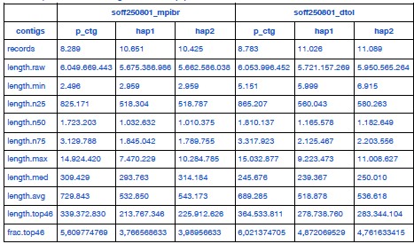
      Full statistics of S. officinalis assemblies from two independent datasets, assembled using a common pipeline.

      The updated manuscript now reads (lines 146-159):

      “A chromosome-scale assembly for Sepia officinalis was released recently by the Wellcome Sanger Institute’s Darwin Tree of Life project [75] (DToL, GCA_964300435.1). That genome was assembled from a male individual using high coverage PacBio Sequel II (~51x) and Arima2 Hi-C (~80x) data, with a final assembly size of 5.8 Gb. The the haploid chromosome number was estimated to be 49. To compare both S. officinalis datasets directly, we downloaded the DToL data and created two new assemblies using the pipeline described above (hifiasm using PacBio HiFi and Hi-C data). The resulting assemblies were overall very similar, with the DToL assembly having a slightly higher contiguity (N50 length, see Table 1) and BUSCO completeness (Supplementary Figure 2A,B) due to their higher sequencing coverage.”

      To further compare the two datasets, we added a new Figure 2 to the revised manuscript and the following paragraph to the results (lines 160-169):

      “After scaffolding with YAHS, both datasets reached the previously identified chromosome numbers (1n=47 for MPIBR and 1n=49 for DToL, Figure 2A,B). To further investigate this surprising discrepancy, we aligned both assemblies using Winnowmap [89] to locate the differences between them (Figure 2C). We observed four “breakpoints” (BP) of chromosome scaffolds: one in the MPIBR assembly compared to DToL (BP1: DToL_5 = MPIBR_40+44) and three in the DToL assembly compared to MPIBR (BP2: DToL_31+40 = MPIBR_2, BP3: DToL_41+46 = MPIBR_6, BP4: DToL_44+45 = MPIBR_7). We also aligned the assemblies to the chromosome-scale genome of another cuttlefish Acanthosepion esculentum (1n=46, GCA_964036315.1). In this alignment, all four breakpoints were collinear with single A. esculentum chromosomes (Figure 2D).”

      (b) Downsampling the DToL data to similar coverage as what the authors have achieved.

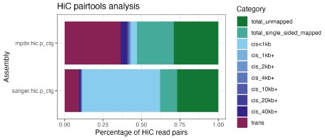
      Instead of downsampling the DToL data, we decided to analyze the Hi-C and HiFi data for both assemblies, focusing on the four “breakpoints” between the assemblies and the A. esculentum genome that we described above. First, we performed a QC analysis of the Hi-C reads using pairtools [2], the result is visualized in Author response image 1. The percentage of valid Hi-C read pairs, i.e., cis pairs with insert distances of more than 1 kb and trans pairs, following the Dovetail genomics QC manual (https://dovetail-analysis.readthedocs.io/en/latest/whole_genome/qc.html). When Hi-C pairs were aligned to the primary contigs from hifiasm (as is used for scaffolding with YAHS), the DToL HiC data contains fewer valid read pairs (11.4%) than the MPIBR data (43.1%), possibly due to using a different tissue (eye vs. optic lobe) and HiC kit (Arima 2 vs. Dovetail OmniC) for the library preparation. Nonetheless, due to the much higher overall coverage, the amount of valid read pairs is still 2.35x higher for DToL (144,014,368 pairs) than for MPIBR (61,318,955 pairs). The higher trans fraction (i.e. HiC pairs across contigs) is dependent on the length of the primary contigs, so the higher trans fraction for the MPIBR data can be explained by the lower contiguity of its primary contigs. It is conceivable that for both assemblies, the low numbers of valid read pairs introduce a technical fragmentation of certain chromosomes, as indicated by the identified breakpoints (Figure 2).

      Author response image 1.

      Analysis of Hi-C read pairs from both S. officinalis assemblies. Hi-C reads were aligned to the primary contigs from hifiasm (as is used for scaffolding with YAHS) and analyzed using pairtools. Note the higher fraction of long-range contacts (at least 1 kb cis pairs or trans pairs) in the MPIBR data (top) compared to DToL (bottom). Due to overall higher coverage, the absolute number of read pairs is higher for DToL than for MPIBR data.

      Second, we performed a detailed analysis of read coverage along the breakpoint junctions of the discrepant chromosomes/scaffolds between both assemblies. We included a description of the results and a new Supplementary Figure 3 in the manuscript, (lines 171-207):

      “To better understand the potential cause of these divergent chromosome numbers, we analyzed the Hi-C and HiFi coverage in the breakpoint regions (Supplementary Figure 3A). First, we aligned the Hi-Fi reads to the scaffolds and extracted all alignments along the 200 kb terminal scaffold windows to find any notable drops in coverage, or reads spanning any of the scaffold junctions. We detected no spanning reads. This is not surprising given that no contigs were assembled at these sites, resulting in the observed scaffold junctions. More interestingly, we noted a ~5-fold decrease in HiFi coverage along the DToL scaffold_40 (part of BP2) relative to its flanking regions, indicating a highly repetitive, low-mappability region at this boundary.

      Next, we realigned the Hi-C data to the scaffolded assemblies using bwa-mem2 [91] and extracted all trans HiC pairs (between-scaffold contacts) using pairtools [92]. We normalized trans HiC contacts to the scaffold length and compared contact rates between breakpoint scaffolds to the baseline contact rate (computed from pairs of scaffolds with a clear 1-to-1 match between assemblies), and the contact rate within scaffolds (intra-scaffold pairs) (Supplementary Figure 3B,C). The contact rates within breakpoints were consistently lower than within scaffolds, likely falling below the threshold to be merged during assembly. However, the contact rates at three of four breakpoints (BP1, BP3, BP4) were significantly elevated above the genome-wide background distribution (empirical p = 0.010, 0.005, 0.005 respectively), suggesting that they may represent intra-chromosomal contacts disrupted by a misassembly. Notably, BP2 was not significant (empirical p = 0.170), likely due to the low coverage and mappability around the DToL scaffold_40 boundary. Considered jointly, the three DToL breakpoint scaffold pairs showed significantly higher trans contact rates than the background (Wilcoxon rank-sum, one-tailed, U = 1771, p = 0.004).

      Lastly, we analyzed the repeat landscape around the 200 kb scaffold ends using RepeatMasker [93] and the custom repeat library that we had generated for Sepia officinalis (described further below). Compared to control scaffolds of the same assembly, we observed consistently elevated repeat content at the breakpoint junctions (mean 71.5% vs 67.6% masked bases), with an enrichment of unclassified repeats (32.1% vs 30.0%), which could explain a repeat-driven assembly fragmentation or scaffolding failure. The BP2 DToL scaffold_40 junction window was 99.99% masked (99.2% unclassified repeats), providing a likely mechanistic explanation for both the HiFi coverage drop and the absence of a significant trans Hi-C signal at this breakpoint. Taken together, these analyses suggest that the different chromosome numbers across the two S. officinalis assemblies are due to technical reasons, caused by repeat-rich scaffold boundaries that impair HiFi and Hi-C read alignment and in turn, correct assembly in these regions.”

      (c) Combining your data and that of DToL for even deeper coverage (heterozygosity is low enough that I don't imagine this impeding things too badly).

      When combining the data to achieve a higher coverage, we ran into the assembly fragmentation issues detailed above in response 1) to Reviewer 1.

      (2) Looking at Figure 1, there appears to be a misjoin at chromosome 42. Looking carefully at Figure S1, that misjoin does not appear on any of the panels - this is confusing. Given the size of that chromosome and the authors' chromosome numbering, I'm guessing this is a manual merge (as it's larger than most of the chromosomes numerically close (40, 41, 43, etc). Further, staring closely at Figure 1, there appear to be cross-scaffold contacts between 42 and 43 and 42 and 44. Secondarily there are contacts between 43 and 44. This bit of the assembly seems potentially problematic.

      This is a great observation, indeed the HiC maps differ between Figure 1 and Figure S1. Figure 1 is the result of scaffolding with YAHS and manual curation, whereas Figure S1 was scaffolded using HapHiC. We updated the figure legend to clarify this important difference. HapHiC produces very clean contact maps without the need for manual curation, but when analyzed at a higher resolution, the tool broke many contigs and ultimately compromised the assembly quality, possibly due to our comparatively low HiC coverage. Thus, we preferred to use YAHS and manual curation, which is perhaps inherently error-prone, as becomes apparent in the regions of the assembly that are pointed out by the reviewer.

      Reviewer 3 (Public review):

      Summary:

      In this study, authors Simone Rencken and co-authors present and investigate the genome of the common cuttlefish Sepia officinalis.

      Strengths:

      The authors explain in a detailed yet concise manner the main steps for a genome assembly, with very robust methods for validation, and according to current best practices. In addition to the chromosomal assembly, the authors confirmed the presence of 47 chromosomes using Hi-C data and multiple species synteny. They also generated a comprehensive gene annotation, with assessments of gene completeness, providing a useful resource for the community of researchers interested in cuttlefish biology and comparative genomics.

      Weaknesses:

      While the study touches upon the subjects of gene content, TE activity, or species-level comparisons, the study does not provide in-depth investigations of these.

      We thank the reviewer for their positive assessment of our manuscript. We acknowledge the descriptive nature and limitations of our previous analyses of gene content, TE distribution, and species comparisons. Our focus for the initial submission was to provide a high-quality assembly that could serve as a resource for anyone interested in Sepia officinalis or related species. However, we agree that greater insight into genome content is valuable as well. In the revised manuscript, we included a more detailed analysis of expanded gene families and GO enrichment analysis of our bulkRNAseq data, which we summarized in response 4) to reviewer 1.

      Recommendations for the authors:

      Reviewer #1 (Recommendations for the authors):

      Minor Revisions Recommended:

      (1) Figure and legend clarity

      Several figures lack sufficient annotation. All figures, including supplementary ones, should include:

      (a) Clear axis labels.

      (b) Descriptions of statistical measures (n values, error bars, statistical tests).

      (c) Legends that allow the figure to be understood independently of the main text.

      We updated the figures accordingly.

      (2) Terminology and formatting

      (a) Consistency in gene and species nomenclature should be maintained throughout (e.g., italicizing gene names and Latin binomials).

      (b) Ensure that abbreviations (e.g., Hi-C, BUSCO, FISH) are defined upon first use.

      We updated the nomenclature throughout the text and checked the definition of abbreviations used in the text. Further, we updated the names of several cuttlefish species according to the recent revision of genera, e.g. Sepia esculenta was changed to Acanthosepion esculentum [3].

      (3) Literature coverage

      The references primarily focus on earlier studies from 2010-2020. It would strengthen the context to include recent high-impact studies on cephalopod genomics and chromosomal biology published in the last 3 years (e.g., 2022-2024).

      We apologize for this oversight and have extended the manuscript to discuss more of these recent studies.

      (4) Clarify methods

      While the methods section is generally detailed, some critical aspects are underspecified:

      (a) Parameters used in genome annotation tools (e.g., BRAKER, RepeatMasker).

      We thank the reviewer for bringing our attention to this shortcoming, and have added the missing parameters to the methods section. Additionally, the full code is available at https://gitlab.mpcdf.mpg.de/mpibr/laur/cuttlefishomics/soffgenome

      (b) Criteria for ortholog clustering and gene family expansion analysis.

      The details have been added to the methods section, which now reads (lines 828-853):

      “Orthogroups were inferred across 13 molluscan species (Table 2), including S. officinalis, using OrthoFinder v3.1.0 [122] with default parameters. The input proteomes included the longest protein isoform per gene for each species. The rooted species tree from OrthoFinder [182,184] was converted to an ultrametric tree using the R package ape [183] v5.8.1.

      Gene families were filtered by removing orthogroups present in only a single species, and by separating orthogroups containing 100 or more gene copies in any species, as extreme copy-number differences in gene families prevent likelihood calculation under the applied birth-death model.

      Gene family evolution rates were estimated using CAFE5 [128] v5.1.1 on the filtered orthogroups, using the ultrametric species tree as input. Four models were evaluated: the base model (single global lambda), and Gamma models with k = 2, 3, and 4 rate categories, which allow evolutionary rate variation among gene families. The Gamma k = 3 model was selected based on the best (lowest) final log-likelihood score. All subsequent statistical inferences were performed under this model.

      For families showing statistically significant expansion or contraction (p < 0.05 after Bonferroni correction), branch-specific copy-number changes were extracted from the CAFE5 output. Families were categorized as S. officinalis-specific, coleoid-specific, or broad expansions based on the distribution of significant changes across the phylogeny.

      To assess whether expanded gene families in S. officinalis contained genes derived from or embedded within repetitive elements, a coordinate-based overlap analysis was performed. For each gene in an expanded orthogroup, the overlap between its coding sequence (CDS) coordinates and RepeatMasker annotations was computed using bedtools intersect v2.30 [185]. To avoid double-counting when multiple repeat annotations overlapped the same coding bases, overlapping repeat intervals were merged per gene prior to summing covered bases, and the overlap fraction was computed as merged covered bases divided by total CDS length.”

      (c) Thresholds or cutoffs for synteny or duplication detection.

      We included the details in the updated methods (lines 755-781):

      “Synteny analyses between all chromosomes of the compared species were performed using the R package GENESPACE v.1.2.3 [175] with default parameters, described briefly below. Protein sequence similarity was first estimated using DIAMOND2 [109] in fast mode, and orthogroups and pairwise orthologues were inferred using OrthoFinder v2.5 [176] with hierarchical orthogroups (HOGs) enabled. Prior to synteny inference, tandem arrays were condensed to their most central representative gene, and gene rank order was recalculated on these array-representative genes to reduce confounding effects of tandem duplication on collinearity detection.

      Syntenic blocks were identified pairwise between all genome combinations using MCScanX [177], constrained to DIAMOND hits where both query and target genes belonged to the same orthogroup (onlyOgAnchors = TRUE). Initial anchor hits were clustered into large syntenic regions using a density-based spatial clustering approach (dbscan [178]), with a minimum block size of five anchor genes (blkSize = 5) and a maximum of five intervening non-anchor genes permitted within a block (nGaps = 5). Anchor clustering used a search radius of 25 gene-rank positions (blkRadius = 25). All hits falling within a syntenic buffer of 100 gene-rank positions around confirmed block anchors (synBuff = 100) were retained as syntenic. No secondary syntenic hits were included (nSecondaryHits = 0). Syntenic orthogroups were integrated across all pairwise comparisons and collapsed into a pan-genome annotation anchored to. S. officinalis was used as the reference genome.

      Syntenic relationships were visualized as riparian plots and pairwise dotplots using the built-in plotting functions of GENESPACE v1.2.3. Riparian plots were constructed using physical chromosomal coordinates (useOrder = FALSE) with S. officinalis as the reference, displaying all three genomes. A second riparian plot was generated highlighting a region of interest. Pairwise dotplots were produced species for the S. officinalisD. pealeii and S. officinalisE. scolopes genome comparisons, displaying only synteny-validated hits (type = "syntenic") with a minimum synteny score of 10 (minScore = 10) and a minimum of 10 genes per chromosome pair required for display (minGenes2plot = 10).”

      Reviewer #2 (Recommendations for the authors):

      Line 153 should be supplemental Figure 3B.

      The text was referring to the correct Figure 2B (three species synteny comparison). It is now updated to Figure 3B in the revised manuscript.

      Reviewer #3 (Recommendations for the authors):

      (1) L37: Perhaps add a comparison with other species (mammals, Drosophila, etc.) to put this number in context.

      We agree with this recommendation and added numbers for Drosophila and mouse to the text (lines 40-45):

      “Coleoid cephalopods (octopus, squid, cuttlefish) are a highly derived group of mollusks, characterized by the largest nervous systems among all invertebrates (ca. 500 million neurons in an adult octopus of which 200 million are in the central brain [1,2], compared to ca. 140,000 in the fruit fly [3] or 70 million in the mouse [4]) and specializations with a great historical importance for neuroscience (e.g., “giant axons” [5] and “giant synapses” [6–8]).”

      (2) L51, 279: "Octopodiformes" is a superorder, not a genus or a species name. It should not go in italics.

      We updated this throughout the text.

      (3) L53: "even smaller" seems odd here, because the argument of the sentence is to stress the large genome size of Octopodiformes. Perhaps start the sentence by stating that it is sometimes smaller, but often larger.

      We rephrased the sentence for clarity, it now reads (lines 55-58):

      “While the genomes of Octopodiformes (Octopus, Eledone, Argonauta) are either smaller than (1.1 Gigabases or Gb [45]) or comparable in size to that of humans (around 3 Gb [46,47]) the typical genomes of Decapodiformes (squids and cuttlefish) often reach 6 Gb [48,49].”

      (4) L90: What tool was used to estimate the k-mer distribution of the long reads? Jellyfish? FastK? It's not mentioned anywhere in the text.

      (5) L95: What k-mer size did the authors use to estimate k-mer distribution?

      We thank the reviewer for pointing out this missing information, and have included the details in the methods (lines 692-694):

      “The k-mer distribution was estimated using Meryl [165] within the Merfin [166] package with a k-mer size of 21, and genomeGenome size was estimated using GenomeScope [77] from Illumina short reads and PacBio HiFi data.”

      (6) L99: What about using the most recent BUSCO databases? odb12?

      We thank the reviewer for this question, which prompted us to compute BUSCO scores using the more recent odb12 database. The results are shown in Supplementary Figure 2C. Both gene sets have been refined by including more species and using a more stringent filtering approach, so the more recent database contains fewer and more conserved genes [4]. For the mollusca gene sets, a great improvement in completeness was observed between odb10 and odb12 (Supplementary Figure 2C); the metazoan completeness was marginally increased. Therefore, we evaluated all new assemblies produced since the first submission with the odb12 database.

      (7) L107: How many scaffolds were obtained in total? After manual curation, how many of the scaffolds were placed in the "correct" chromosomes? How many scaffolds were in the shrapnel? Were these scaffolds mostly repetitive regions? Or did they contain important genetic information?

      These are important questions. To evaluate the content of the “shrapnel”, we split the manually curated assembly into the 47 chromosomes and the 1840 residual scaffolds, and computed BUSCO scores for both. While the 47 chromosome scaffolds contain the majority of conserved genes: C:92.9%[S:92.7%,D:0.1%],F:4.0%,M:3.1% with metazoa_odb12 and C:88.7%[S:88.0%,D:0.7%],F:4.4%,M:6.9% with mollusca_odb12, the unplaced scaffolds still contain a few BUSCOs: C:2.5%[S:2.4%,D:0.1%],F:2.4%,M:95.1% from metazoa_odb12 and C:1.9%[S:1.7%,D:0.2%],F:1.2%,M:96.9% from mollusca_odb12. Even if only a few BUSCOs are present on these scaffolds, it means they contain important genetic information. Additionally, we observed low, but non-zero alignment of RNA reads to these scaffolds. We observed a slightly elevated repeat content in the unplaced scaffolds (Author response image 2), and a variable base composition (Figure 1C) compared to the chromosome scaffolds.

      Author response image 2.

      Quantification of repeat content in chromosome scaffolds and unplaced residual scaffolds. Density plot showing fraction of repeat masked bases in total sequence length for chromosome scaffolds (i.e. scaffolds 1-47) in teal and all remaining small scaffolds (1840 scaffolds) in purple. Median repeat fraction is shown as vertical lines.

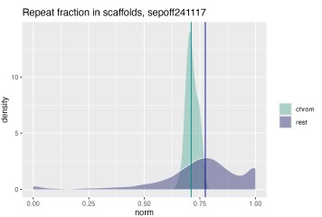
      The slightly elevated repeat content in the unplaced scaffolds provides a likely explanation for their fragmented state: repeat-rich regions are inherently difficult to assemble and scaffold, as repetitive sequences cause ambiguous read alignments that prevent contigs from being confidently joined or anchored to chromosomal scaffolds during HiC-based scaffolding. This is consistent with the near-complete absence of BUSCO genes from the unplaced scaffolds - not because these fragments lack biologically relevant sequence entirely, as evidenced by the residual BUSCO hits and RNA read alignments, but because the gene-rich portions of the genome are largely captured in the 47 chromosome scaffolds. The unplaced scaffolds instead likely represent fragmented contigs from repetitive or low-complexity genomic regions, such as centromeres, telomeres, and transposable element clusters, where assembly graph complexity and collapsed repeats prevent confident placement. The variable base composition further supports this interpretation, as GC-extreme or low-complexity sequences are disproportionately represented in assembly shrapnel. Together, these observations suggest that the unplaced scaffolds contain limited unique coding content but reflect genuine repeat-rich genomic sequence that cannot currently be placed without additional long-range information, such as optical mapping or ultra-long reads.

      (8) L33, 53, 240, 255, 279: Decapodiformes, not in italics.

      We changed this throughout the text.

      (9) L228: Can you put this expansion in perspective with other taxa?

      We added a more detailed comparison of our gene family expansion with different species to the revised manuscript, as detailed in response 4 to reviewer 1.

      (10) L251: "However, our results show how difficult it still is to assemble large genomes with high karyotype numbers." Can you clarify how your results show this, because it is equally spectacular to assemble the karyotype with only PacBio and Hi-C data (and no linkage mapping).

      Indeed, it is correct that the recent improvements in data quality and scaffolding algorithms enable these “spectacular” chromosome-scale assemblies without the need for linkage mapping. This sentence reflected our expectation to resolve a clear karyotype as has been demonstrated for multiple cephalopod genomes in recent years, including two cuttlefish species (Octopus bimaculoides, Octopus vulgaris, Euprymna scolopes, Euprymna berryi, Acanthosepion lycidas and Acanthosepion esculenta). To our knowledge, none of these publications used linkage mapping or cytogenetic methods to confirm the karyotype. In this light, our resulting chromosome number and the discrepancy to a second assembly of the same species led us to this conclusion. We updated the section in the revised discussion as follows (lines 466-473):

      “Taken together, our results illustrate the difficulty of assembling large genomes with high repeat content and large karyotypes, at least from sequencing data alone. Internal validation methods and genome comparisons across species are therefore important. Convergence of reliable estimates will, in turn, help identify chromosomal fusion-with-mixing events (FWM; fusion of two ancestral chromosomes followed by extensive shuffling of their gene content) that are clade specific. Early branching order in Decapodiformes has been notoriously unstable [53,84,94,144–147]; thus, such rare and irreversible FWM characters could be useful in further phylogenetic analysis of this clade [51,148].”

      (11) L419: Why use the phased haplotype 1 instead of the primary assembly generated by hifiasm?

      We thank the reviewer for this important question. We used the phased haplotype assembly because it provides a biologically coherent representation with the least amount of duplication by avoiding allele-collapsing and haplotype-switching that can be present in the primary assembly. We reasoned that this would result in clearer gene models and a more accurate representation of structural variation. However, we acknowledge that this comes at the cost of reduced contiguity and completeness, as becomes apparent in our BUSCO comparison shown in Supplementary Figure 2, where the phased haplotypes have fewer duplicated genes than the primary assembly, but more missing genes in turn. When reassembling both datasets for our comparison, we used the primary assembly to use the longest contigs as input for scaffolding.

      (12) L444: It is unclear from what tissues and life stages RNA-seq data were used or were available from other species.

      This is an important detail. RNA-seq data was collected from two adult Sepia officinalis, from various tissues (whole brain, retina, skin, mantle, arm, tentacle). For the long-read PacBio Isoseq data, tissue was taken from the animal used for genome sequencing (6 months old), and tissue for short-read Illumina RNA-seq was taken from another adult (8 months old). The data have been released on SRA (study accession SRP570862), where all sample details are listed as well. We added the SRA accession to the data availability section of the revised manuscript. We clarified the relevant sections in the methods:

      lines 628-629:

      “RNA was isolated from various flash-frozen tissues (different brain areas, mantle/epidermis, arm/tentacle; 5-10 mg each).”

      lines 678-680:

      “For short-read RNA sequencing, tissue from another animal (8-month-old adult, F0 from eggs collected in Normandie, France) was used. RNA was isolated from various flash-frozen tissues (different brain areas, skin and retina; 5 mg each).”

      (13) L454, 469: Why is minimap2 in italics? It wasn't formatted like this before. Same for StringTie.

      We thank the reviewer for their detailed methods review. In the updated methods section, all formatting of used softwares was harmonized.

      (14) L461: Lophotrochozoa is a clade, not a genus or species. Not in italics.

      This is now changed throughout the revised manuscript.

      (15) Figure 1D: Axes labels are hard to read.

      We have now increased the axis label size.

      (16) Figure 2: Consider increasing font sizes. Many chromosome orientations seem to be flipped across species, which makes it harder to see smaller-scale rearrangements or notice less conserved chromosomes. Would it make sense to standardize these?

      We increased the font sizes and plotted only fully collinear syntenic blocks (instead of aggregated syntenic regions, the default of GENESPACE) for improved readability.

      References:

      Below are references cited in our responses. References from the reproduced manuscript sections are included in the revised manuscript.

      (1) Secomandi, S., Gallo, G.R., Rossi, R., Rodríguez Fernandes, C., Jarvis, E.D., Bonisoli-Alquati, A., Gianfranceschi, L., and Formenti, G. (2025). Pangenome graphs and their applications in biodiversity genomics. Nat. Genet. 57, 13–26. https://doi.org/10.1038/s41588-024-02029-6.

      (2) Open2C, Abdennur, N., Fudenberg, G., Flyamer, I.M., Galitsyna, A.A., Goloborodko, A., Imakaev, M., and Venev, S.V. (2023). Pairtools: from sequencing data to chromosome contacts. Preprint at bioRxiv, https://doi.org/10.1101/2023.02.13.528389 https://doi.org/10.1101/2023.02.13.528389.

      (3) Lupše, N., Reid, A., Taite, M., Kubodera, T., and Allcock, A.L. (2023). Cuttlefishes (Cephalopoda, Sepiidae): the bare bones—an hypothesis of relationships. Mar. Biol. 170, 93. https://doi.org/10.1007/s00227-023-04195-3.

      (4) Tegenfeldt, F., Kuznetsov, D., Manni, M., Berkeley, M., Zdobnov, E.M., and Kriventseva, E.V. (2025). OrthoDB and BUSCO update: annotation of orthologs with wider sampling of genomes. Nucleic Acids Res. 53, D516–D522. https://doi.org/10.1093/nar/gkae987.

  2. bafybeidpnaszrg3heutszijzffa6s2kmgtepdshqqntebr2t45ykk55dse.ipfs.dweb.link bafybeidpnaszrg3heutszijzffa6s2kmgtepdshqqntebr2t45ykk55dse.ipfs.dweb.link
    1. grove is a Graph Representation Of property ValuEs.

      Literally, a grove = is a Graph Representation Of property ValuEs. -

      Groves provide constructs for describing directed graphs

      consisting of - nodes, - which have properties, and - arcs, which connect the nodes.

      The basic idea is that any data, especially structured documents, can be modeled using directed graphs.

      A tree structure is a type of directed graph, and anyone familiar with parsing structured documents, be they XML documents or source code, will understand the utility of tree structures for representing those documents.

    2. data modeling languages

      Towards the opposite end of the extreme, you have

      data modeling languages such as - E/R and - UML diagrams,

      which are more human-centered and

      present a higher-level abstraction of the data.

      The cost of these abstractions is the - lack of information that may be valuable in - implementing these data models.

      For example, E/R diagrams allow you to specify

      the cardinality of a relationship - (i.e. one-to-n, n-to-one, n-to-n),

      but they do not allow you to express other kinds of constraints, and

      they have no notion of primitive data types.

      Consequently, they are not adequate to - generate equivalent source code - automatically and - completely,

      although they could be used to generate stub code.

    3. intent of a programming language

      The intent of a programming language is for - the expression of a data model - (i.e. source code) to be translated into a - machine-readable representation of the data.

    1. Dynamical Behavior Analysis of 2-control Strategies on Tuberculosis Model

      R0:

      Reviewer #1: Recommendation 1: The modeling approach is fundamentally sound and relevant to TB control (a major public health issue), but the manuscript needs to address transparency (data sources, parameter justification) and clarify some methodological assumptions (e.g. definition of Reproduction number) before it can be accepted.

      Recommendation 2: The sensitivity analysis methods (Pearson, PRCC) are suitable but need more rigor in reporting (sample details, uncertainty). The data-fitting procedure requires complete description (data source, fitting algorithm, goodness-of-fit). The authors should include more quantitative statistical assessment of their model fit and uncertainty in parameter effects.

      Recommendation 3: The authors should provide a Data Availability Statement with actual access information (URL, DOI, or supplementary files) for the epidemiological data and any other material used. At the end of the file, an editorial link points to the Bangladesh NTP Annual Report 2022, which presumably provided TB case counts, but this is not an open dataset citation. Without accessible data, readers cannot reproduce or verify the results.

      Recommendation 4: The writing requires major language editing. Grammatical issues and awkward phrasing occur repeatedly. Several citations are incomplete (marked as “[?]”). These issues hinder readability. The manuscript would benefit from careful editing by a fluent English speaker. With editing, the intellectual content is conveyable, but in its current state the language detracts from clarity.

      Reviewer #2: This manuscript presents a mathematical modeling study on tuberculosis transmission using an SEITR framework incorporating distancing and treatment control strategies. The authors apply optimal control theory, stability analysis, sensitivity analysis, and data fitting to assess the impact of interventions. The topic is relevant to public health and epidemiological modeling, and the integration of control theory with real data is a valuable contribution. Overall, the study demonstrates potential scientific merit; however, several important issues should be addressed to improve the quality, clarity, and reliability of the work.

      Major Strengths

      The manuscript develops a structured SEITR model that includes exposed and treated compartments, allowing for a more realistic representation of tuberculosis dynamics.

      The application of Pontryagin’s Maximum Principle to determine optimal intervention strategies is appropriate and well motivated.

      The use of sensitivity analysis, including Pearson correlation and PRCC, strengthens the interpretation of key parameters.

      Incorporation of real tuberculosis data from Bangladesh and curve fitting enhances the practical relevance of the study.

      The findings highlight the importance of combined distancing and treatment strategies, which is relevant for policy planning.

      Major Concerns

      Language and Presentation The manuscript contains numerous grammatical errors, awkward phrasing, and unclear sentences that affect readability. Several sections require substantial English language editing. Professional proofreading is strongly recommended to improve clarity and coherence.

      Incomplete and Missing Citations Many references in the text are marked with “[?]”, indicating missing citations. These must be replaced with appropriate and verifiable references. Failure to do so weakens the scientific credibility of the manuscript.

      Reference Quality and Formatting Several references appear incomplete, inconsistently formatted, or potentially inaccurate. All references should be verified and formatted according to journal guidelines. The authors should ensure that all cited sources are reliable and accessible.

      Mathematical Notation and Consistency Some notations are used ambiguously, particularly the symbol λ, which represents both the force of infection and adjoint variables. This may confuse readers. The notation should be revised for clarity. In addition, some derivations in the optimal control section are not sufficiently detailed and require clearer explanation.

      Data Availability and Reproducibility The Data Availability Statement is insufficient. PLOS requires full access to underlying data and, where applicable, code. The authors should provide the dataset in an accessible repository and include links. Details on parameter estimation and model fitting procedures should also be expanded.

      Model Validation While curve fitting is presented, quantitative goodness-of-fit measures (e.g., RMSE, R², confidence intervals) are not provided. Including these metrics would strengthen the validation of the model.

      Overstatement of Novelty The novelty section contains strong claims that are not fully supported by the analysis. The authors should moderate these statements and clearly specify how their approach differs from and extends existing studies.

      Figures and Visualization Some figures lack sufficient resolution, clear legends, and readable labels. All figures should be revised to meet publication standards and to improve interpretability.

      Ethical and Data Source Clarification The manuscript should clearly state whether ethical approval was required for the use of hospital data and how patient confidentiality was ensured, even if the data are aggregated.

      Minor Concerns

      Several typographical errors and formatting inconsistencies are present throughout the manuscript.

      Some sections are repetitive, particularly in the Introduction and Discussion.

      Units and parameter descriptions in the appendix should be clarified and consistently presented.

      The structure of some tables can be improved for better readability.

      Suggestions for Improvement

      Revise the entire manuscript for language quality and clarity.

      Replace all missing citations and verify references.

      Improve mathematical notation and provide clearer derivations.

      Expand the methodology for parameter estimation and numerical implementation.

      Provide full data and code access in line with PLOS policies.

      Include quantitative validation metrics.

      Revise figures and tables for better presentation.

      Reframe the novelty claims in a more balanced manner.

      Conclusion

      The manuscript addresses an important topic and combines mathematical modeling with real data and optimal control analysis. With substantial revision focusing on language quality, citation completeness, data transparency, mathematical clarity, and methodological rigor, the study has the potential to make a meaningful contribution to tuberculosis control research. At present, major revisions are necessary before the manuscript can be considered for publication.

      Reviewer #3: PLOS Global Public Health (PGPH-D-26-00093) Reviewer’s Comments The authors studied ‘Dynamical Behavior Analysis of 2-control Strategies on Tuberculosis Model. The authors must be commended for carrying out this research. As the paper is, technically correct formulation of the SEITR system, Standard application of Pontryagin’s Maximum Principle, Inclusion of sensitivity analysis and data fitting and clear policy motivation (treatment and distancing synergy). However, authors need to address the following suggestions to improve the manuscript: Comment 1: Abstract Please consider/incorporate the followings points in the abstract i. aim/ objectives ii. Methods applied iii. Results/ Findings iv. Recommendations to policymakers

      Comment 2: Introduction Please consider/incorporate the following points in the introduction. i. Significance of the research ii. Please clearly indicate in a summarized form your observations about the related literature reviewed as compared to your research. Comment 3: Research gap and main contribution At the ending section of the introduction: i. Authors should clearly state the research gap in the manuscript. ii. SEIR/SEITR TB models with: treatment control, distancing or awareness control, PMP-based optimal control, sensitivity analysis have been extensively studied (including several papers already cited). Authors should compare their research with the existing literature and state what exactly is new in their research (main contribution) compared to existing studies. iii. The claimed novelty which comprises “composite analytical methodology integrating control-oriented stability decomposition with normalized forward sensitivity indexing” is not clearly demonstrated mathematically. Authors should check that.

      Comment 4: Stability analysis The stability analysis must be improved. Authors analyzed only DFE stability. Authors should consider Endemic equilibrium (EE) existence, Local or global stability of EE and Backward bifurcation analysis. Since TB models, normally exhibit backward bifurcation and highly relevant. Comment 5: Sensitivity analysis Authors conducted so many sensitivity plots, with little insight. Parameter ranges are not clearly justified and some interpretations are inconsistent (e.g., γ showing weak PRCC but strong analytical sensitivity). Authors should correct that. Comment 6: Grammatical Errors There are some grammatical errors in the manuscript. For instance 1. “Pontryagain’s” → Pontryagin’s 2. Repetitive phrases (“It is noted that…”, “It is observed that…”) and 3. Overly long descriptive captions instead of analytical discussion

      Comment 7: Inconsistencies in Notations 1. The authors used \lambda for both force of infection and adjoint derivative, 2. Parameters appear in equations but are not always defined immediately 3. Table 1 includes parameter \eta which does not appear in the model Authors should correct that.

      Comment 9: In Text-Reference A lot of in-text references are missing in the manuscript. Authors should correct that.

      Comment 10: Conclusion State the limitations and future work in this section. Comment 11: Cost-effectiveness analysis Cost-effectiveness analysis can be added to the control model to improve the manuscript. Remarks: Minor Revision Required Thank you

      R1: Reviewer #2: The authors have adequately addressed all comments raised in the previous round of review. The revisions have significantly improved the clarity, methodological rigor, and overall presentation of the manuscript. The study presents a well-structured and technically sound analysis of the dynamical behavior of tuberculosis transmission under two control strategies. The modeling framework is appropriate, and the assumptions are clearly stated and justified. The statistical and mathematical analyses appear to be conducted rigorously, and the results are presented in a coherent and interpretable manner. Importantly, the conclusions are well supported by the data and align with the objectives of the study. The authors have also ensured compliance with data availability requirements, which enhances transparency and reproducibility. The manuscript is clearly written in standard English, with improved organization and readability compared to the previous version. Any minor typographical or grammatical issues noted earlier have been appropriately corrected. Overall, the manuscript now meets the publication criteria of PLOS Global Public Health and is suitable for publication.

      Reviewer #3: Dear Editor PLOS Global Public Health(PGPH-D-26-00093R1) Reviewer’s Comments The authors studied ‘Dynamical Behavior Analysis of 2-control Strategies on Tuberculosis Model. I have checked the revised version of the manuscript according to the comments given. The authors have revised the manuscript according to the comments. I suggest that the manuscript can be accepted for publication PLOS Global Public Health after this minor suggestion. However, authors need to address the suggestion below to improve the manuscript: Comment on main Contribution The main contributions must not be stated as questions. Authors should correct that. Authors should be: 1. Specific: Focus on what is new (novel theory), the method, or data. 2. Employ Active Verbs: Begin them with phrases such as "We propose," "We discover," "We develop," or "We demonstrate" etc 3. The introduction should state the questions you asked, while the contribution section (or conclusion) should state the answers you found.

      Remarks: Accept Thank you

      Reviewer #4: Interesting study, here are my recommendations to improve the manuscript:

      • Authors need to conform to international guidelines of scientific writing. Sentences like "doctors typically diagnose..." can be better written with "healthcare professionals diagnose..."
      • The introduction section has information about the basics of tuberculosis and models design that are not necessarily important to the study. Can revise and shorten. See comment above too.
      • In fact, it would be beneficial if you provide details about the current TB control strategy in Bangladesh and some background epidemiologic data about TB in Bangladesh (the country of interest) the introduction.
      • tuberculin skin test is use to diagnose TB "infection"- clarify this to readers
      • I assume that the first control strategy "treatment" involves treatment of active TB disease, not latent infection.
      • Not sure if authors accounted for failure of TB treatment in the model?
      • What is the prevalence of MDR-TB in Bangladesh and was this accounted for in the transmission model and cost-effectiveness model?
    1. Why senior developersfail to communicatetheir expertise

      Why Senior Developers Fail to Communicate Their Expertise

      • Conflict of Interest: Senior developers and business leaders operate in different "loops." The business prioritizes the Speed Loop (reducing uncertainty by getting to market fast), while senior developers prioritize the Stability Loop (managing complexity to ensure the system remains debuggable and reliable).
      • Vocabulary Mismatch: Communication fails because developers talk about "complexity" and "technical debt," which sound like excuses to non-technical stakeholders. Stakeholders are focused on "uncertainty" and "growth."
      • The "Solution" Frame: To communicate effectively, seniors must frame their concerns as solutions to the business's problems. Instead of saying "no" to complexity, they should offer "something quicker" (reusing existing tools, Google forms, or minimal UI changes) to help the business learn faster without bloating the code.
      • AI as a Destabilizer: AI-generated code accelerates the Speed Loop but creates a "complexity explosion" that threatens long-term stability. The senior developer’s role is shifting toward that of an Editor, responsible for extracting stable, scalable logic from the rapid "vomit drafts" produced by AI and junior staff.
      • The Proposed Split: A potential workflow involves maintaining two versions of a system: a "Speed" version for rapid experimentation and a "Scale" version that is curated, stabilized, and owned by senior architects.

      Hacker News Discussion

      • The "World Model" Gap: A top-voted comment argues that true expertise is an internal "world model" or intuition that is inherently difficult to put into words. It isn't just a list of facts but a deeply integrated understanding of how systems behave.
      • Recipe vs. Physics: Commenters distinguish between "recipe-following" developers (who use tools without understanding the underlying logic) and "physics-based" developers who understand the fundamental nature of computation.
      • The Role of Failure: Discussion emphasized that senior intuition is built primarily through experiencing failures and reflecting on them over many years. This mental shift often happens when a developer stops trying to learn syntax and starts focusing on solving specific visions or problems.
      • The "Senior" Title: There was significant debate about whether "senior" is a measure of years (tenure) or actual merit, with many noting that some developers with decades of experience still only follow recipes and lack the "world model" required for true expertise.
      • Abstraction Struggles: Some users noted that while they have a "physics-level" understanding of physical sciences (like chemistry or biology), software abstractions feel arbitrary and "anti-physicalist," making it harder for some brilliant minds to build that same level of intuition.
    1. FindingRemediationV3 already uses a Claude SDK agent with Write/Edit/Bash tools in a writable workspace. Production-tested.

      most of this code should be reusable

    2. Plan staleness: How old can a plan be before we require re-planning? Commit SHA validation catches code changes, but should we also check SBOM scan freshness?

      it should have no extraneous external file changes and it should allow us to create a ref with the permissions at time of execution

    3. Execution rejected if base_commit_sha doesn't match current HEAD on the target branch. Prevents applying stale plans to changed code.

      this is when we rebase which we should be doing otherwise nothing will actually get accepted, if we don't then we end up with a pr that has many many unrelated changes and clients have complained many times

    4. npm, pip, poetry, cargo all have different mechanics. An agent with shell access adapts without bespoke parsers per ecosystem.

      we talked about why we can't do this and why it's not a good idea. we have 0 sandboxing functionality, and most of our clients use their own internal package hosting. all package managers have some level of arbitrary code execution, if we're not running the installs and version numbers ourselves we do run the risk of exposure to completely unknown supply chain attacks if this is done completely agentically. I would stick to simple version bumps in the manifests, and fixing code that needs to be fixed.

    1. o I think I understand what you are talking about, the phenomenon of “scientific code”! My thoughts: First meta observation is that “software design” is someth

      test

    1. Author response:

      Reviewer #1 (Evidence, reproducibility and clarity):

      Summary:

      This manuscript reports the identification of putative orthologues of mitochondrial contact site and cristae organizing system (MICOS) proteins in Plasmodium falciparum - an organism that unusually shows an acristate mitochondrion during the asexual part of its life cycle and then this develops cristae as it enters the sexual stage of its life cycle and beyond into the mosquito. The authors identify PfMIC60 and PfMIC19 as putative members and study these in detail. The authors at HA tags to both proteins and look for timing of expression during the parasite life cycle and attempt (unsuccessfully) to localise them within the parasite. They also genetically deleted both gene singly and in parallel and phenotyped the effect on parasite development. They show that both proteins are expressed in gametocytes and not asexuals, suggesting they are present at the same time as cristae development. They also show that the proteins are dispensible for the entire parasite life cycle investigated (asexuals through to sporozoites), however there is some reduction in mosquito transmission. Using EM techniques they show that the morphology of gametocyte mitochondria is abnormal in the knockout lines, although there is great variation.

      Major comments:

      The manuscript is interesting and is an intriguing use of a well studied organism of medical importance to answer fundamental biological questions. My main comments are that there should be greater detail in areas around methodology and statistical tests used. Also, the mosquito transmission assays (which are notoriously difficult to perform) show substantial variation between replicates and the statistical tests and data presentation are not clear enough to conclude the reduction in transmission that is claimed. Perhaps this could be improved with clearer text?

      We would like to thank the reviewer for taking the time to review our manuscript. We are happy to hear the reviewer thinks the manuscript is interesting and thank the reviewer for their constructive feedback.

      To clarify the statistical analyses used, we included a new supplementary dataset with all statistical analyses and p-values indicated per graph. Furthermore, figure legends now include the information on the exact statistical test used in each case.

      Regarding mosquito experiments, while we indeed reported a reduction in transmission and oocysts numbers, we are aware that this effect might be due to the high variability in mosquito feeding assays. To highlight this point, we deleted the sentence “with the transmission reduction of [numbers]….” and we included the sentence “The high variability encountered in the standard membrane feeding assays, though, partially obstructs a clear conclusion on the biological relevance of the observed reduction in oocyst numbers“

      More specific comments to address:

      Line 101/Fig1E (and figure legend) - What is this heatmap showing. It would be helpful to have a sentence or two linking it to a specific methodology. I could not find details in the M+M section and "specialized, high molecular mass gels" does not adequately explain what experiments were performed. The reference to Supplementary Information 1 also did not provide information.

      We added the information “high molecular mass gels with lower acrylamide percentage” to clarify methodology in the text. Furthermore, we extended the figure legend to include all relevant information. Further experimental details can be found in the study cited in this context, where the dataset originates from (Evers et al., 2021).

      Line 115 and Supplementary Figure 2C + D - The main text says that the transgenic parasites contained a mitochondrially localized mScarlet for visualization and localization, but in the supplementary figure 2 it shows mitotracker labelling rather than mScarlet. This is very confusing. The figure legend also mentions both mScarlet and MitoTracker. I assume that mScarlet was used to view in regular IFAs (Fig S2C) and the MitoTracker was used for the expansion microscopy (Fig S2D)?

      Please clarify.

      We thank the reviewer for pointing this out – this was indeed incorrectly annotated. We used the endogenous mito-mScarlet signal in IFA and mitoTracker in U-ExM. The figure annotation has now been corrected.

      Figure 2C - what is the statistical test being used (the methods say "Mean oocysts per midgut and statistical significance were calculated using a generalized linear mixed effect model with a random experiment effect under a negative binomial distribution." but what test is this?)?

      The statistic test is now included in the material and method section with the sentence “The fitted model was used to obtain estimated means and contrasts and were evaluated using Wald Statistics”. The test is now also mentioned in the figure legend.

      Also the choice of a log10 scale for oocyst intensity is an unusual choice - how are the mosquitoes with 0 oocysts being represented on this graph? It looks like they are being plotted at 10^-1 (which would be 0.1 oocysts in a mosquito which would be impossible).

      As the data spans three orders of magnitude with low values being biologically meaningful, we decided that a log scale would best facilitate readability of the graph. As the 0 values are also important to show, we went with a standard approach to handle 0s in log transformed data and substituted the 0s with a small value (0.001). We apologize for not mentioning this transformation in the manuscript. To make this transformation transparent, we added a break at the lower end of the log-scaled y-axis and relabelled the lowest tick as ‘0’. This ensures that mosquitoes with zero oocysts are shown along the x-axis without being assigned an artificial value on the log scale. We would furthermore like to highlight that for statistics we used the true value 0 and not 0.001.

      Figure 2D - it is great that the data from all feeding replicates has been shared, however it is difficult to conclude any meaningful impact in transmission with the knock-out lines when there is so much variation and so few mosquitoes dissected for some datapoints (10 mosquitoes are very small sample sizes). For example, Exp1 shows a clear decrease in mic19- transmission, but then Exp2 does not really show as great effect. Similarly, why does the double knock out have better transmission than the single knockouts? Sure there would be a greater effect?

      We agree with the reviewer and with the new sentence added, as per major point, we hope we clarified the concept. Note that original Figure 2D has been moved to the supplementary information, as per minor comment of another reviewer.

      Figure 3 legend - Please add which statistical test was used and the number of replicates.

      Done

      Figure 4 legend - Please add which statistical test was used and the number of replicates.

      Done. Regarding replicates, note that while we measured over 100 cristae from over 30 mitochondria, these all stem from the same parasite culture.

      Figure 5C - the 3D reconstructions are very nice, but what does the red and yellow coloring show?

      Indeed, the information was missing. We added it to the figure legend.

      Line 352 - "Still, it is striking that, despite the pronounced morphological phenotype, and the possibly high mitochondrial stress levels, the parasites appeared mostly unaffected in life cycle propagation, raising questions about the functional relevance of mitochondria at these stages."

      How do the authors reconcile this statement with the proven fact that mitochondria-targeted antimalarials (such as atovaquone) are very potent inhibitors of parasite mosquito transmission?

      Our original sentence was reductive. What we wanted to state was related to the functional relevance of crista architecture and overall mitochondrial morphology rather than the general functional relevance of the mitochondria. We changed the sentence accordingly.

      Furthermore, even though we do not discuss this in the article, we are aware of mitochondria targeting drugs that are known to block mosquito transmission. We want to point out that it is difficult to discern the disruption of ETC and therefore an impact on energy conversion with the impact on the essential pathway of pyrimidine synthesis, highly relevant in microgamete formation. Still, a recent paper from Sparkes et al. 2024 showed the essentiality of mitochondrial ATP synthesis during gametogenesis so it is very likely that the mitochondrial energy conversion is highly relevant for transmission to the mosquito.

      Reviewer #1 (Significance):

      This manuscript is a novel approach to studying mitochondrial biology and does open a lot of unanswered questions for further research directions. Currently there are limitations in the use of statistical tests and detail of methodology, but these could be easily be addressed with a bit more analysis/better explanation in the text.

      This manuscript could be of interest to readers with a general interest in mitochondrial cell biology and those within the specific field of Plasmodium research.

      My expertise is in Plasmodium cell biology.

      We thank the reviewer for the praise.

      Reviewer #2 (Evidence, reproducibility and clarity):

      Major comments:

      (1) In my opinion, the authors tend to sensationalize or overinterpret their results. The title of the manuscript is very misleading. While MICOS is certainly important for crista formation, it is not the only factor, as ATP synthase dimer rows make a highly significant contribution to crista morphology. Thus, one can argue with equal validity that ATP synthase should be considered the 'architect', as it's the conformation of the dimers and rows modulate positive curvature. Secondly, while cristae are still formed upon mic60/mic19 gene knockout (KO), they are severely deformed, and likely dysfunctional (see below). Thus, I do not agree with the title that MICOS is dispensable for crista formation, because the authors results show that it clearly is essential. So, the title should be changed.

      We thank the reviewer for taking the time to review our manuscript.

      Based on the reviewers’ interpretation we conclude the title does not come across as intended. We have changed the title to: “The role of MICOS in organizing mitochondrial cristae in malaria parasites”

      The Discussion section starting from line 373 also suffers from overinterpretation as well as being repetitive and hard to understand. The authors infer that MICOS stability is compromised less in the single KOs (sKO) in compared to the mic60/mic19 double KO (dKO). MICOS stability was never directly addressed here and the composition of the MICOS complex is unaddressed, so it does not make sense to speculate by such tenuous connections. The data suggest to me that mic60 and mic19 are equally important for crista formation and crista junction (CJ) stabilization, and the dKO has a more severe phenotype than either KO, further demonstrating neither is epistatic.

      We do agree with the reviewer’s notion that we did not address complex stability, and our wording did not make this sufficiently clear. We shortened and rephrased the paragraph in question.

      The following paragraphs (line 387 to 422) continues with such unnecessary overinterpretation to the point that it is confusing and contradictory. Line 387 mentions an 'almost complete loss of CJs' and then line 411 mentions an increase in CJ diameter, both upon Mic60 ablation. I do not think this discussion brings any added value to the manuscript and should be shortened. Yes, maybe there are other putative MICOS subunits that may linger in the KOS that are further destabilized in the dKO, or maybe Mic60 remains in the mic19 KO (and vice versa) to somehow salvage more CJs, which is not possible in the dKO. It is impossible to say with confidence how ATP synthase behaves in the KOs with the current data.

      We shortened this paragraph.

      (2) While the authors went through impressive lengths to detect any effect on lifecycle progression, none was found except for a reduction in oocyte count. However, the authors did not address any direct effect on mitochondria, such as OXPHOS complex assembly, respiration, membrane potential. This seems like a missed opportunity, given the team's previous and very nice work mapping these complexes by complexome profiling. However, I think there are some experiments the authors can still do to address any mitochondrial defects using what they have and not resorting to complexome profiling (although this would be definitive if it is feasible):

      i) Quantification of MitoTracker Red staining in WT and KOs. The authors used this dye to visualize mitochondria to assay their gross morphology, but unfortunately not to assay membrane potential in the mutants. The authors can compare relative intensities of the different mitochondria types they categorized in Fig. 3A in 20-30 cells to determine if membrane potential is affected when the cristae are deformed in the mutants. One would predict they are affected.

      Interesting suggestion. As our staining and imaging conditions are suitable for such analysis (as demonstrated by Sarazin et al., 2025, https://www.biorxiv.org/content/10.1101/2025.11.27.690934v1), we performed the measurements on the same dataset which we collected for Figure 3. We did, however, not detect any difference in mitotracker intensity between the different lines. The result of this analysis is included in the new version of Supplementary figure S6.

      ii) Sporozoites are shown in Fig S5. The authors can use the same set up to track their motion, with the hypothesis that they will be slower in the mutants compared to WT due to less ATP. This assumes that sporozoite mitochondria are active as in gametocytes.

      While theoretically plausible and informative, we currently do not know the relevance of mitochondrial energy conversion for general sporozoite biology or specifically features of sporozoite movement. Given the required resources and time to set this experiment up and the uncertainty whether it is a relevant proxy for mitochondrial functioning, we argue it is out of scope for this manuscript.

      iii) Shotgun proteomics to compare protein levels in mutants compared to WT, with the hypothesis that OXPHOS complex subunits will be destabilized in the mutants with deformed cristae. This could be indirect evidence that OXPHOS assembly is affected, resulting in destabilized subunits that fail to incorporate into their respective complexes.

      While this experiment could potentially further our understanding of the interaction between MICOS and levels of OXPHOS complex subunits we argue that the indirect nature of the evidence does not justify the required investments.

      To expedite resubmission, the authors can restrict the cell lines to WT and the dKO, as the latter has a stronger phenotype that the individual KOs and conclusions from this cell line are valid for overall conclusions about Plasmodium MICOS.

      I will also conclude that complexome/shotgun proteomics may be a useful tool also for identifying other putative MICOS subunits by determining if proteins sharing the same complexome profile as PfMic60 and Mic19 are affected. This would address the overinterpretation problem of point 1.

      (3) I am aware of the authors previous work in which they were not able to detect cristae in ABS, and thus have concluded that these are truly acristate. This can very well be true, or there can be immature cristae forms that evaded detection at the resolution they used in their volumetric EM acquisitions. The mitochondria and gametocyte cristae are pretty small anyway, so it not unreasonable to assume that putative rudimentary cristae in ABS may be even smaller still. Minute levels of sampled complex III and IV plus complex V dimers in ABS that were detected previously by the authors by complexome profiling would argue for the presence of miniscule and/or very few cristae.

      I think that authors should hedge their claim that ABS is acristate by briefly stating that there still is a possibility that miniscule cristae may have been overlooked previously.

      We acknowledge that we cannot demonstrate the absolute absence of any membrane irregularities along the inner mitochondrial membrane. At the same time, if such structures were present, they would be extremely small and unlikely to contain the full set of proteins characteristic of mature cristae. For this reason, we consider it appropriate to classify ABS mitochondria as acristate. To reflect the reviewer’s point while maintaining clarity for readers, we have slightly adjusted our wording in the manuscript, changing ‘fully acristate’ to ‘acristate’.

      This brings me to the claim that Mic19 and Mic60 proteins are not expressed in ABS. This is based on the lack of signal from the epitope tag; a weak signal is detected in gametocytes. Thus, one can counter that Mic19 and Mic60 are also expressed, but below the expression limits of the assay, as the protein exhibits low expression levels when mitochondrial activity is upregulated.

      We agree with the reviewer that the absence of a detectable epitope-tag signal does not definitively exclude low-level expression, and we have therefore replaced the term ‘absent’ with ‘undetectable’ throughout the manuscript. In context with previous findings of low-level transcripts of the proteins in a study by Lopez-Berragan et al. and Otto et al., we also added the sentence “The apparent absence could indicate that transcripts are not translated in ABS or that the proteins’ expression was below detection limits of western blot analysis.” to the discussion. At the same time, we would like to clarify that transcript levels for both genes fall within the <25th percentile, suggesting that these low values likely represent background signal rather than biologically meaningful expression. This interpretation is further supported by proteomic datasets in PlasmoDB, which report PfMIC19 and PfMIC60 expression in gametocyte and mosquito stages, but not in asexual blood stages.”

      To address this point, the authors should determine of mature mic60 and mic19 mRNAs are detected in ABS in comparison to the dKO, which will lack either transcript. RT-qPCR using polyT primers can be employed to detect these transcripts. If the level of these mRNAs are equivalent to dKO in WT ABS, the authors can make a pretty strong case for the absence of cristae in ABS.

      We appreciate the reviewer’s suggestion. As noted in the Discussion, existing transcriptomic datasets already show detectable MIC19 and MIC60 mRNAs in ABS. For this reason, we expect RT-qPCR to reveal low (but not absent) levels of both transcripts, unlike the true loss expected to be observed in the dKO. Because such residual signals have been reported previously and their biological relevance remains uncertain, we do not believe transcript levels alone can serve as a definitive indicator of cristae absence in ABS.

      They should highlight the twin CX9C motifs that are a hallmark of Mic19 and other proteins that undergo oxidative folding via the MIA pathway. Interestingly, the Mia40 oxidoreductase that is central to MIA in yeast and animals, is absent in apicomplexans (DOI: 10.1080/19420889.2015.1094593).

      Searching for the CX9C motifs is a valuable suggestion. In response to the reviewer´s suggestion we analysed the conservation of the motif in PfMIC19 and included this in a new figure panel (Figure 1 F).

      Did the authors try to align Plasmodium Mic19 orthologs with conventional Mic19s? This may reveal some conserved residues within and outside of the CHCH domain.

      In response to this comment we made Figure 1 F, where we show conserved residues within the CHCH domains of a broad range of MIC19 annotated sequences across the opisthokonts, and show that the Cx9C motifs are conserved also in PfMIC19. Outside the CHCH domain, we did not find any meaningful conservation, as PfMIC19 heavily diverges from opisthokont MIC19.

      (5) Statistical significance. Sometimes my eyes see population differences that are considered insignificant by the statistical methods employed by the authors, eg Fig. 4E, mutants compared to WT, especially the dKO. Have the authors considered using other methods such as student t-test for pairwise comparisons?

      The graphs in figures 3, 4 and 5 got a makeover, such that they now are in linear scale and violin plots (also following a suggestion from further down in the reviewer’s comments). We believe that this improves interpretability. ANOVA was kept as statistical testing to assure the correction for multiple comparisons that cannot be performed with standard t-test. A full overview of statistics and exact pvalues can also be found in the newly added supplementary information 2.

      Minor comments:

      Line 33. Anaerobes (eg Giardia) have mitochondria that do produce ATP, unlike aerobic mitochondria

      We acknowledge that producing ATP via OXPHOS is not a characteristic of all mitochondria-like organelles (e.g. mitosomes), which is why these are typically classified separately from canonical mitochondria. When not considering mitochondria-like organelles, energy conversion is the function that the mitochondrion is most well-known for and the one associated with cristae.

      Line 56: Unclear what authors mean by "canonical model of mitochondria"

      To clarify we changed this to “yeast or human” model of mitochondria.

      Lines 75-76: This applies to Mic10 only

      We removed the “high degree of conservation in other cristate eukaryotes” statement.

      Line 80: Cite DOI: 10.1016/j.cub.2020.02.053

      Done

      Fig 2D: I find this table difficult to read. If authors keep table format, at least get rid of 'mean' column' as this data is better depicted in 2C. I suggest depicted this data either like in 3B depicting portion of infected vs unaffected flies in all experiments, then move modified Table to supplement. Important to point out experiment 5 appears to be an outlier with reduced infectivity across all cell lines, including WT.

      To clarify: the mean reported in the table indicates the mean per replicate while the mean reported in figure 2C is the overall mean for a given genotype that corrects for variability within experiments. We agree that moving the table to the supplementary data is a good idea. We decided to not include a graph for infected and non-infected mosquitoes as this information would be partially misleading, highlighting a phenotype we argue to be influenced by the strong variability.

      Fig. 3C-G: I feel like these data repeatedly lead to same conclusions. These are all different ways of showing what is depicted in Fig 2B: mitochondria gross morphology is affected upon ablation of MICOS. I suggest that these graphs be moved to supplement and replaced by the beautiful images.

      Thank you for the nice comment on our images. We have now moved part of the graphs to supplementary figure 6 and only kept the Relative Frequency, Sphericity and total mitochondria volume per cell in the main figure.

      Line 180: Be more specific with which tubulin isoform is used as a male marker and state why this marker was used in supplemental Fig S6.

      We have now specified the exact tubulin isoform used as the male gametocyte marker, both in the main text and in Supplementary Fig. S6. This is a commercial antibody previously known to work as an effective male marker, which is why we selected it for this experiment. This is now clearly stated in the manuscript.

      Line 196 and Fig 3C: the word 'intensities' in this context is very ambiguous. Please choose a different term (puncta, elements, parts?). This is related to major point 2i above.

      To clarify the biological effect that we can conclude form the measurement, we added an explanation about it in the respective section of the results, and we decided to replace the raw results of the plug-in readout with the deduced relative dispersion.

      Line 222: Report male/female crista measurements

      We added Supplementary information 2, which contains exact statistical test and outcomes on all presented quantifications as well as a per-sex statistical analysis of the data from figure 4. Correspondingly, we extended supplementary information 2 by a per-sex colour code for the thin section TEM data.

      Fig. 4B-E: depict data as violin plots or scatter plots like Fig. 2C to get a better grasp of how the crista coverage is distributed. It seems like the data spread is wider in the double KO. This would also solve the problem with the standard deviation extending beyond 0%.

      We changed this accordingly.

      Lines 331-333: Please clarify that this applies for some, but not all MICOS subunits. Please also see major point 1 above. Also, the authors should point out that despite their structural divergence, trypanosomal cryptic mitofilins Mic34 and Mic40 are essential for parasite growth, in contrast to their findings with PfMic60 (DOI: https://doi.org/10.1101/2025.01.31.635831).

      This has been changed accordingly.

      Line 320: incorrect citation. Related to point 1above.

      Correct citation is now included in the text.

      Lines 333-335. This is related to the above. Again, some subunits appear to affect cell growth under lab conditions, and some do not. This and the previous sentence should be rewritten to reflect this.

      This has been changed accordingly.

      Line 343-345: The sentence and citation 45 are strange. Regarding the former, it is about CHCHD10, whose status as a bona fide MICOS subunit is very tenuous, so I would omit this. About the phenomenon observed, I think it makes more sense to write that Mic60 ablation results in partially fragmented mitochondria in yeast (Rabl et al., 2009 J Cell Biol. 185: 1047-63). A fragmented mitochondria is often a physiological response to stress. I would just rewrite as not to imply that mitochondrial fission (or fusion) is impaired in these KOs, or at least this could be one of several possibilities.

      The sentence has been substituted following the indication of the reviewer. Though we still include the data of the human cells as this has also been shown in Stephens et al. 2020.

      Line 373: 'This indicates' is too strong. I would say 'may suggest' as you have no proof that any of the KOs disrupts MICOS. This hypothesis can be tested by other means, but not by penetrance of a phenotype.

      Done

      Line 376-377; 'deplete functionality' does not make sense, especially in the context of talking about MICOS subunit stability. In my opinion, this paragraph overinterprets the KO effects on MICOS stability. None of the experiments address this phenomenon, and thus the authors should not try to interpret their results in this context. See major point 1.

      We removed the sentence. Also, the entire paragraph has been shortened, restructured and wording was changed to address major point 1.

      Other suggestions for added value

      (1) Does Plasmodium Sam50 co-fractionate with Mic60 and Mic19 in BN PAGE (Fig. 1E)

      While we did identify SAMM50 in our BN PAGE, the protein does not co-migrate with the MICOS components but instead comigrates with other components of a putative sorting and assembly machinery (SAM) complex. As SAMM50, the SAM complex and the overarching putative mitochondrial membrane space bridging (MIB) complex are not mentioned in the manuscript, we decided to not include the information in Author response image 1.

      Author response image 1.

      Reviewer #2 (Significance):

      The manuscript by Tassan-Lugrezin is predicated on the idea that Plasmodium represents the only system in which de novo crista formation can be studied. They leverage this system to ask the question whether MICOS is essential for this process. They conclude based on their data that the answer is no, which the authors consider unprecedented. But even if their claim is true that ABS is acristate, this supposed advantage does not really bring any meaningful insight into how MICOS works in Plasmodium.

      First the positives of this manuscript. As has been the case with this research team, the manuscript is very sophisticated in the experimental approaches that are made. The highlights are the beautiful and often conclusive microscopy performed by the authors. Only the localization of Mic60 and Mic19 was inconclusive due to their very low expression unfortunately.

      The examination of the MICOS mutants during in vitro life cycle of Plasmodium falciparum is extremely impressive and yields convincing results. Mitochondrial deformation is tolerated by life cycle stage differentiation, with a modest but significant reduction of oocyte production, being observed.

      However, despite the herculean efforts of the authors, the manuscript as it currently stands represents only a minor advance in our understanding of the evolution of MICOS, which from the title and focus of the manuscript, is the main goal of the authors.

      In its current form, the manuscript reports some potentially important findings:

      (1) Mic60 is verified to play a role in crista formation, as is predicted by its orthology to other characterized Mic60 orthologs.

      (2) The discovery of a novel Mic19 analog (since the authors maintain there is no significant sequence homology), which exhibits a similar (or the same?) complexome profile with Mic60. This protein was upregulated in gametocytes like Mic60 and phenocopies Mic60 KO.

      (3) Both of these MICOS subunits are essential (not dispensable) for proper crista formation

      (4) Surprisingly, neither MICOS subunit is essential for in vitro growth or differentiation from ABS to sexual stages, and from the latter to sporozoites. This says more about the biology of plasmodium itself than anything about the essentiality of Mic60, i.e. plasmodium life cycle progression tolerates defects to mitochondrial morphology. But yes, I agree with the authors that Mic60's apparent insignificance for cell growth in examined conditions does differ with its essentiality in other eukaryotes. But fitness costs were not assayed (e.g. by competition between mutants and WT in infection of mosquitoes)

      (5) Decreased fitness of the mutants is implied by a reduction of oocyte formation.

      While interesting in their own way, collectively they do not represent a major advance in our understanding of MICOS evolution. Furthermore, the findings bifurcate into categories informing MICOS or Plasmodium biology. Both aspects are somewhat underdeveloped in their current form.

      This is unfortunate because there seem to be many missed opportunities in the manuscript that could, with additional experiments, lead to a manuscript with much wider impact. For me, what is remarkable about Plasmodium MICOS that sets it apart from other iterations is the apparent absence of the Mic10 subunit. Purification of plasmodium MICOS via the epitope tagged Mic60 and Mic19 could have verified that MICOS is assembled without this core subunit. Perhaps Mic60 and Mic19 are the vestiges of the complex, and thus operate alone in shaping cristae. Such a reduction may also suggest the declining importance of mitochondria in plasmodium.

      Another missed opportunity was to assay the impact of MICOS-depletion of OXPHOS in plasmodium.

      This is a salient issue as maybe crista morphology is decoupled from OXPHOS capacity in Plasmodium, which links to the apparent tolerance of mitochondrial morphology in cell growth and differentiation. I suggested in section A experiments to address this deficit.

      Finally, the authors could assay fitness costs of MICOS-ablation and associated phenotypes by assaying whether mosquito infectivity is reduced in the mutants when they are directly competing with WT plasmodium. Like the authors, I am also surprised that MICOS mutants can pass population bottlenecks represented by differentiation events. Perhaps the apparent robustness of differentiation may contribute plasmodium's remarkable ability to adapt.

      I realize that the authors put a lot of efforts into their study and again, I am very impressed by the sophistication of the methods employed. Nevertheless, I think there is still better ways to increase the impact of the study aside from overinterpreting the conclusions from the data. But this would require more experiments along the lines I suggest in Section A and here.

      We thank the reviewer for their extensive analysis of the significance of our findings, including the compliments on our microscopy images and the sophisticated experimental approaches. We hope we have convincingly argued why we could or could not include some of the additional analyses suggested by the reviewer in section 1 above.

      With regard to the significance statement, we want to point out that our finding that PfMICOS is not needed for initial formation of cristae (as opposed to organization thereof), is a confirmation of something that has been assumed by the field, without being the actual focus of studies. We argue that the distinction between formation and organization of cristae is important and deserves some attention within the manuscript. The result of MICOS not being involved in the initial formation of cristae, we argue to be relevant in Plasmodium biology and beyond. As for the insights into how MICOS works in Plasmodium we have confirmed that the previously annotated PfMIC60 is indeed involved in the organization of cristae. Furthermore, we have identified and characterized PfMIC19. These findings, we argue, are indeed meaningful insights into PfMICOS.

      Reviewer #3 (Evidence, reproducibility and clarity):

      Summary:

      MICOS is a conserved mitochondrial protein complex responsible for organising the mitochondrial inner membrane and the maintenance of cristae junctions. This study sheds first light on the role of two MICOS subunits (Mic60 and the newly annotated Mic19) in the malaria parasite Plasmodium falciparum, which forms cristae de novo during sexual development, as demonstrated by EM of thin section and electron tomography. By generating knockout lines (including a double knockout), the authors demonstrate that knockout of both MICOS subunits leads to defects in cristae morphology and a partial loss of cristae junctions. With a formidable set of parasitological assays, the authors show that despite the metabolically important role of mitochondria for gametocytes, the knockout lines can progress through the life stages and form sporozoites, albeit with diminished infection efficiency.

      We thank the reviewer for their time and compliment.

      Major comments:

      (1) The authors should improve to present their findings in the right context, in particular by:

      i) giving a clearer description in the introduction of what is already known about the role of MICOS. This starts in the introduction, where one main finding is missing: loss of MICOS leads to loss of cristae junctions and the detachment of cristae membranes, which are nevertheless formed, but become membrane vesicles. This needs to be clearly stated in the introduction to allow the reader to understand the consistency of the authors' findings in P. falciparum with previous reports in the literature.

      We extended the introduction to include this information.

      iii) at the end to the introduction, the motivating hypothesis is formulated ad hoc "conclusive evidence about its involvement in the initial formation of cristae is still lacking" (line 83). If there is evidence in the literature that MICOS is strictly required for cristae formation in any organism, then this should be explained, because the bona fide role of MICOS is maintenance of cristae junctions (the hypothesis is still plausible and its testing important).

      To clarify we rephrased the sentence to: “Although MICOS has been described as an organizer of crista junctions, its role during the initial formation of nascent cristae has not been investigated.”

      (2) Line 96-97: "Interestingly, PfMIC60 is much larger than the human MICOS counterpart, with a large, poorly predicted N-terminal extension." This statement is lacking a reference and presumably refers to annotated ORFs. The authors should clarify if the true N-terminus is definitely known - a 120kDa size is shown for the P. falciparum but this is not compared to the expected length or the size in S. cerevisiae.

      To solve the reference issue, we added the uniprot IDs we compared to see that the annotated ORF is bigger in Plasmodium. We also changed the comparison to yeast instead of human, because we realized it is confusing to compare to yeast all throughout the figure, but then talk about human in this specific sentence.

      Regarding whether the true N-terminus is known. Short answer: No, not exactly.

      However, we do know that the Pf version is about double the size of the yeast protein.

      As the reviewer correctly states, we show the size of 120kDa for the tagged protein in Figure 1G. Considering that we tagged the protein C-terminally, and observed a 120kDa product on western blot, it is safe to conclude that the true N-terminus does not deviate massively from the annotated ORF, and hence, that there is a considerable extension of the protein beyond a 60kDa protein. We do not directly compare to yeast MIC60 on our western blots, however, that comparison can be drawn from literature: Tarasenko et al., 2017 showed that purified MIC60 running at ~60kDa on SDS-PAGE actively bends membranes, suggesting that in its active form, the monomer of yeast MIC60 is indeed 60kDa in size.

      To clarify, we now emphasize that we ran the Alphafold prediction on the annotated open reading frame (annotated and sequenced by Bohme et al. and Chapell et al. now cited in the manuscript), and revised the wording to make clear what we are comparing in which sentence.

      (3) lines 244-245: "Furthermore, our data indicates the effect size increases with simultaneous ablation of both proteins?". The authors should explain which data they are referring to, as some of the data in Fig 3 and 4 look similar and all significance tests relate to the wild type, not between the different mutants, so it is not clear if any overserved differences are significant. The authors repeat this claim in the discussion in lines 368-369 without referring to a specific significance test. This needs to be clarified.

      As a reply to this and other comments from the reviewers we added the multiple testing within all samples. In addition, to clarify statistics used we included a supplementary dataset with all p-values and statistical tests used.

      (4) lines 304-306: "Though well established as the cristae organizing system, the role of MICOS in initial formation of cristae remains hidden in model organisms that constitutively display cristae.". This sentence is misleading since even in organisms that display numerous cristae throughout their life cycle, new cristae are being formed as the cells proliferate. Thus, failure to produce cristae in MICOS knockout lines would have been observable but has apparently not been reported in the literature. Thus, the concerted process in P. falciparum makes it a great model organism, but not fundamentally different to what has been studied before in other organisms.

      We deleted this statement.

      (5) lines 373-378. "where ablation of just MIC60 is sufficient to deplete functionality of the entire MICOS (11, 15),". The authors' claim appears to be contrary to what is actually stated in ref 15, which they cite:

      "MICOS subunits have non-redundant functions as the absence of both MICOS subcomplexes results in more severe morphological and respiratory growth defects than deletion of single MICOS subunits or subcomplexes."

      This seems in line with what the authors show, rather than "different".

      This sentence has been removed.

      (6) lines 380-385: "... thus suggesting that membrane invaginations still arise, but are not properly arranged in these knockout lines. This suggests that MICOS either isn't fully depleted,...". These conclusions are incompatible with findings from ref. 15, which the authors cite. In that study, the authors generated a ∆MICOS line which still forms membrane invaginations, showing that MICOS is not required at all for this process in yeast. Hence the authors' implication that MICOS needs to be fully depleted before membrane invaginations cease to occur is not supported by the literature.

      This sentence has been deleted in the revised version of the manuscript.

      Minor comments:

      (1) The authors should consider if the first part of their title could be seen as misleading: It suggests that MICOS is "the architect" in cristae formation, but this is not consistent with the literature nor their own findings.

      Title is changed accordingly

      - Line 43, of the three seminal papers describing the discovery of MICOS in 2011, the authors only cite two (refs 6 and 7), but miss the third paper, Hoppins et al, PMID: 21987634, which should probably be corrected.

      Done, the paper is now cited

      - Page 2, line 58: for a more complete picture the authors should also cite the work of others here which shows that although at very low levels, e.g. complex III (a drug target) and ATP synthase do assemble (Nina et al, 2011, JBC).

      Done

      - Page 3, line 80: "Irrespective of the shape of an organism's cristae, the crista junctions have been described as tubular channels that connect the cristae membrane to the inner boundary membrane (22, 24)." This omits the slit-shaped cristae junctions found in yeast (Davies et al, 2011, PNAS), which the authors should include.

      The paper and concept have been added to the manuscript, though the sentence has been moved up in the introduction, when crista junctions are first introduced.

      - Line 97: "poorly predicted N-terminal extension", as there is no experimental structure, we don't know if the prediction is poor. Presumably the authors mean either poorly ordered or the absence of secondary structure elements, or the poor confidence score for that region in the prediction? This should be clarified or corrected.

      We were referring to the poor confidence score. To address this comment as well as major point 2, we rewrote the respective paragraph. It now clearly states that confidence of the prediction is low, and we mention the tool that was used to identify conserved domains (Topology-based Evolutionary Domains).

      - Line 98: "an antiparallel array of ten β-sheets". They are actually two parallel beta-sheets stacked together. The authors could find out the name of this fold, but the confidence of the prediction is marked a low/very low. So, its existence is unknown, not just its "function".

      We adapted the domain description to “a stack of two parallel beta-sheets" and replaced the statement on unknown function by the statement “Because this domain is predicted solely from computational analysis, both its actual existence in the native protein and its biological function remain unknown.”

      - Fig 1B: The authors show two alphafold predictions of S. cerevisiae and P. falciparum Mic60 structures. There is however an experimental Mic60/19 (fragment) structure from the former organism (PMID: 36044574), which should be included if possible.

      We appreciate the reviewer’s suggestion and note that the available structural data indeed provides valuable insight into how MIC60 and MIC19 interact. However, these structures represent fusion constructs of limited protein fragments and therefore capture only a small portion of each protein, specifically the interaction interface. Because our aim in Fig. 1B is to compare the overall domain architecture of the full-length proteins, we believe that including fragment-based structures would be less informative in this context.

      - Line: 318-321: "The same trend was observed for PfMIC19 and PfMIC60. Although transcriptomic data suggested that low-level transcripts of PfMIC19 and PfMIC60 are present in ABS (38), we did not detect either of the proteins in ABS by western blot analysis. While this statement is true, the authors should comment on the sensitivity of the respective methods - how well was the antibody working in their hands and how do they interpret the absence of a WB band compared to transcriptomics data?

      The HA antibody used in our experiments is a standard commercial reagent that performs reliably in both WB and IFA, although it shows a low background signal in gametocytes. We agree that the sensitivity of the method and the interpretation of weak or absent bands should be addressed explicitly. Transcript levels for both PfMIC19 and PfMIC60 in asexual blood stages fall within the <25 percentile, suggesting that these signals likely represent background. Nevertheless, we acknowledge that low-level protein expression below the detection limit of western blot analysis cannot be excluded. To reflect these considerations, we added the sentence: ‘The apparent absence could indicate that transcripts are not translated in ABS or that the proteins’ expression was below detection limits of western blot analysis.

      - Lines 322-323: would the authors not typically have expected an IFA signal given the strength of the band in Western blot? If possible, the authors should comment if the negative fluorescence outcome can indeed be explained with the low abundance or if technical challenges are an equally good explanation.

      Considering the nature of the investigated proteins (embedded in the IMM and spread throughout the mitochondria) difficulties in achieving a clear signal in IFA or U-ExM are not very surprizing. While epitopes may remain buried in IFA, U-ExM usually increases accessibility for the antibodies. However, U-ExM comes at the cost of being prone to dotty background signals, therefore potentially hiding low abundance, naturally dotty signals such as the signal of MICOS proteins that localize to distinct foci (at the CJ) along the mitochondrion. Current literature suggests that, in both human and yeast, STED is the preferred method for accurate spatial resolution of MICOS proteins (https://www.ncbi.nlm.nih.gov/pubmed/32567732,https://www.ncbi.nlm.nih.gov/pubmed/3206734 4). Unfortunately, we do not have experience with, nor access to, this particular technique/method.

      - Lines 357-365: the authors describe limitations of the applied methods adequately. Perhaps it would be helpful to make a similar statement about the analysis of 3D objects like mitochondria and cristae from 2D sections. E.g. the apparent cristae length depends on whether cristae are straight (e.g. coiled structures do not display long cross sections despite their true length in 3D).

      The limitations of other methods are described in the respective results section.

      We added a clarifying sentence in the results section of Figure 4:

      “Note that such measurements do not indicate the true total length or width of cristae, as the data is two-dimensional. The recorded values are to be considered indicative of possible trends, rather than absolute dimensions of cristae.“

      This statement refers to the length/width measurements of cristae.

      In the context of Figure 4D we mention the following (see preprint lines 229 – 230): “We expect this effect to translate into the third dimension and thus conclude that the mean crista volume increases with the loss of either PfMIC19, PfMIC60, or both.”

      For Figure 5, we included a clarifying statement in the results section of the preprint (lines 269 – 273): “Note that these mitochondrial volumes are not full mitochondria, but large segments thereof. As a result of the incompleteness of the mitochondria within the section, and the tomography specific artefact of the missing wedge, we were unable to confirm whether cristae were in fact fully detached from the boundary membrane, or just too long to fit within the observable z-range.”

      - Line 404: perhaps undetected or similar would be a better description than "hidden"?

      The sentence does not exist in the revised manuscript.

      Reviewer #3 (Significance):

      The main strength of the study is that it provides the first characterisation of the MICOS complex in P. falciparum, a human parasite in which the mitochondrion has been shown to be a drug target. Mic60 and the newly annotated Mic19 are confirmed to be essential for proper cristae formation and morphology, as well as overall mitochondrial morphology. Furthermore, the mutant lines are characterised for their ability to complete the parasite life cycle and defects in infection effectivity are observed. This work is an important first step for deciphering the role of MICOS in the malaria parasite and the composition and function of this complex in this organism. The limitation of the study stems from what is already known about MICOS and its subunits in great detail in yeast and humans with similar findings regarding loss of cristae and cristae defects. The findings of this study do not provide dramatic new insight on MICOS function or go substantially beyond the vast existing literature in terms of the extent of the study, which focuses on parasitological assays and morphological analysis. Exploring the role of MICOS in an early-divergent organism and human parasite is however important given the divergence found in mitochondrial biology and P. falciparum is a uniquely suited model system. One aspect that would increase the impact of the paper would be if the authors could mechanistically link the observed morphological defects to the decreased infection efficiency, e.g. by probing effects on mitochondrial function. This will likely be challenging as the morphological defects are diverse and the fitness defects appear moderate/mild.

      As suggested by Reviewer 2, we examined mitochondrial membrane potential in gametocytes using MitoTracker staining and did not observe any obvious differences associated with the morphological defects. At present, additional assays to probe mitochondrial function in P. falciparum gametocytes are not sufficiently established, and developing and validating such methods would require substantial work before they could be applied to our mutant lines. For these reasons, a more detailed mechanistic link between the observed morphological changes and the reduced infection efficiency is currently beyond reach.

      The advance presented in this study is to pioneer the study of MICOS in P. falciparum, thus widening our understanding of the role of this complex to different model organism. This study will likely be mainly of interest for specialised audiences such as basic research parasitologists and mitochondrial biologists. My own field of expertise is mitochondrial biology and structural biology.

    1. Author response:

      The following is the authors’ response to the original reviews.

      eLife Assessment

      This study explores how exogenous attention operates at the finest spatial scale of vision, within the foveola - a topic that has not been previously explored. The question is important for understanding how attention shapes perception, and how it differs between the periphery and the central regions of highest visual acuity. The evidence is compelling, as shown by carefully designed experiments with state-of-the-art eye tracking to monitor attended locations just a few tens of minutes of arc away from the fixation target, but additional clarification regarding analyses and implications for vision and oculomotor control would broaden the impact of the study.

      We thank the editors and reviewers for their thorough evaluation of our work. We have carefully revised the manuscript and substantially reworked the Discussion to address all of the points raised, eliminate redundancies, streamline the text, and clarify the implications of our findings for vision and oculomotor control. We have also expanded the documentation of our power analyses and conducted the additional analyses requested by the reviewers. Our point-by-point responses are provided.

      Public Reviews:

      Reviewer #1 (Public review):

      Summary:

      The manuscript investigates how exogenous attention modulates spatial frequency sensitivity within the foveola. Using high-precision eye-tracking and gaze-contingent stimulus control, the authors show that exogenous attention selectively improves contrast sensitivity for low- to midrange spatial frequencies (4-8 cycles/degree), but not for higher frequencies (12-20 CPD). In contrast, improvements in asymptotic performance at the highest contrast levels occur across all spatial frequencies. These results suggest that, even within the foveola, exogenous attention operates through a mechanism similar to that observed in peripheral vision, preferentially enhancing lower spatial frequencies.

      Strengths:

      The study shows strong methodological rigor. Eye position was carefully controlled, and the stimulus generation and calibration were highly precise. The authors also situate their work well within the existing literature, providing a clear rationale for examining the fine-grained effects of exogenous attention within the foveola. The combination of high spatial precision, gazecontingent presentation, and detailed modeling makes this a valuable technical contribution.

      Weaknesses:

      The manipulation of attention raises some interpretive concerns. Clarifying this issue, together with additional detail about statistics, participant profiles, other methodological elements, and further discussion in relation to oculomotor control in general, could broaden the impact of the findings.

      We thank the reviewer for the helpful comments. In the Discussion, we have now considered additional factors that could have contributed to the observed attentional effects. First, the exogenous cue might have functioned as a temporal warning signal. However, the interval between cue and stimulus onset was fixed across trials, meaning that the cue did not provide temporal information beyond what participants could already anticipate. Furthermore, participants completed a large number of trials (≥ 4000), making it highly likely that the temporal relationship between trial onset and target onset was overlearned. These considerations indicate that the observed benefit in the valid condition was predominantly attributable to spatial reorienting induced by the cue, rather than to differences in the temporal predictability of the target across conditions.

      Another possibility is that the 100% validity of the exogenous cue could potentially have promoted endogenous attentional engagement. Yet, several characteristics of our task strongly limited the extent to which such endogenous engagement could meaningfully influence performance. Endogenous attentional benefits typically emerge only after ~150-200 ms (Posner & Petersen, 1990; Carrasco, 2011), whereas our cue-target SOA was 100 ms, and the target remained visible for only 50 ms. Under these temporal constraints, any voluntary, slow endogenous enhancement would primarily occur after the stimulus offset. Thus, although endogenous maintenance is theoretically possible given the cue’s validity, it is unlikely to have substantially contributed to the observed attentional benefits in our task.

      Regarding the points on statistical reporting and participant details, we followed the reviewer’s suggestions by adding post hoc power analyses and providing more comprehensive reporting of the linear model outputs (see Appendices 1 and 2). We also expanded the description of the training procedures conducted with participants prior to formal data collection in the Methods section.

      We appreciate the reviewer for raising the important question of how our findings may relate to oculomotor control. To address this, we analyzed trials excluded from the manuscript due to saccades. This analysis revealed that saccade latencies were shorter in the valid condition than in the neutral condition (see Figure 2 — Supplementary Figure 2). This earlier saccade onset may reflect exogenously triggered preparatory activity in the oculomotor system in response to the salient cue. Future studies are needed to examine whether this preparatory mechanism serves to efficiently guide microsaccades or saccades toward behaviorally relevant stimuli in everyday vision. We have incorporated this point into the Discussion, highlighting a potential mechanistic link between exogenous attention and oculomotor behavior.

      Reviewer #2 (Public review):

      Summary:

      This study aims to test whether foveal and non-foveal vision share the same mechanisms for endogenous attention. Specifically, they aim to test whether they can replicate at the foveola previous results regarding the effects of exogenous attention for different spatial frequencies.

      Strengths:

      Monitoring the exact place where the gaze is located at this scale requires very precise eyetracking methods and accurate and stable calibration. This study uses state-of-the-art methods to achieve this goal. The study builds on many other studies that show similarities between foveal vision and non-foveal vision, adding more data supporting this parallel.

      Weaknesses:

      The study lacks a discussion of the strength of the effect and how it relates to previous studies done away from the fovea. It would be valuable to know if not just the range of frequencies, but the size of the effect is also comparable.

      We thank the reviewer for raising these important issues. In response, we have expanded the Discussion to link our findings to prior work. First, we included a direct comparison of our effect sizes with those reported in previous studies. This analysis revealed that our effect sizes are highly comparable to those earlier studies (see Figure 3 — Supplementary Figure 4). Second, we contextualized our findings within the popular framework of normalization model of attention in the Discussion. We detected a mixture of contrast and response gain effects, consistent with predictions from the normalization framework given our experimental design. Finally, we extended the Discussion to consider potential underlying neural mechanisms. Specifically, we suggested that differences in attentional modulation, particularly the manifestation in response gain vs. contrast gain between the fovea and extrafovea, may reflect distinct characteristics of foveal neurons relative to those in extrafoveal regions.

      Reviewer #3 (Public review):

      Summary:

      This paper explores how spatial attention affects foveal information processing across different spatial frequencies. The results indicate that exogenously directed attention enhances contrast sensitivity for low- to mid-range spatial frequencies (4-8 CPD), with no significant benefits for higher spatial frequencies (12-20 CPD). However, asymptotic performance increased as a result of spatial attention independently of spatial frequency.

      Strengths:

      The strengths of this article lie in its methodological approach, which combines a psychophysical experiment with precise control over the information presented in the foveola.

      Weaknesses:

      The authors acknowledge that they used the standard approach of analyzing observeraveraged data, but recognize that this method has limitations: it ignores the uncertainty associated with parameter estimates and the relationships between different parameters of the psychometric model. This may affect the interpretation of attentional effects. In the future, mixed-effects models at the trial level could overcome these limitations.

      We thank the reviewer for this comment. Our Methods section continues to transparently discuss these limitations, as well as the fact that these limitations are shared with most published studies in psychophysics. Additionally, we now include measures of uncertainty for all key effects (see Appendices 1 and 2), and we have reported effect sizes throughout the Results section. Finally, we have added post hoc power analyses to the Methods. Following previous approaches to power calculation for related experiments, we found that our study was sufficiently powered to detect the main effect of attention and had moderate power to detect the interaction between attention and spatial frequency.

      Recommendations for the authors:

      Reviewer #1 (Recommendations for the authors):

      (1) The manipulation of attention raises some interpretive concerns. Since only valid and neutral cue conditions were included, the results might reflect differences in temporal predictability rather than true spatial reorienting of attention. In other words, the valid cue could act mainly as a temporal warning signal that reduces uncertainty about stimulus onset. Without invalid trials or a non-predictive control cue, it remains difficult to separate spatial and temporal contributions to exogenous attention.

      We thank the reviewer for raising this point. In this regard, we would like to clarify that there was no temporal uncertainty in stimulus onset: across all conditions and trial types, the stimulus was presented at the same time relative to the start of the trial, i.e., 600 ms after the start. Yet, we acknowledge that the shorter temporal proximity between the cue and stimulus in valid trials could serve as an additional temporal warning signal, potentially conferring an advantage relative to the neutral condition. While we cannot completely rule out a contribution of such temporal cueing within the constraints of the current experimental design, we believe its impact was limited. Specifically, the fixed cue-stimulus interval reduced the cue’s ability to convey additional temporal information. Furthermore, observers completed a large number of trials (≥4000), and the temporal contingency between trial onset and target onset was likely overlearned. Taken together, these considerations indicate that the observed benefit in the valid condition was predominantly attributable to spatial reorienting induced by the cue, rather than to differences in the temporal predictability of the target across conditions. We now mention this in the revised Discussion (lines 309-318).

      We recognized that the original Figure 2 illustrating the experimental paradigm may have caused confusion regarding the timing structure of the task. We have therefore updated the figure to more explicitly illustrate the trial timeline in both conditions.

      (2) The reported effects seem small, and no power analysis is provided. With only seven participants, the study may not have enough statistical power to confirm that the observed differences are reliable or generalizable. Although the technical precision in gaze and stimulus control is impressive, it cannot offset the limitations of a small sample. The authors should include effect size estimates, confidence intervals, and ideally a post-hoc power analysis.

      The statistical results are reported only as χ² values from model comparisons, which do not show the direction or size of the effects. For clarity and transparency, these tests should be accompanied by fixed-effect estimates with their standard errors and confidence intervals, so readers can better assess both the reliability and perceptual relevance of the findings.

      The reviewer raised several important points regarding the study's statistical rigor.

      In the revised manuscript, we now report effect size estimates (Cohen’s d) in the Results section and Appendices. Effect sizes were in the medium-to-large range, including the effect of attention on contrast sensitivity at 4 and 8 CPD, and the difference in attentional benefit on contrast sensitivity between 4 and 12 CPD and between 8 and 12 CPD. We have also included the full model outputs, including standard errors and confidence intervals, in the Appendices.

      The sample size for the current study was determined based on the magnitude of the attentional effects observed in our previous work (Guzhang et al., 2021). The experimental design and dependent measures were highly similar across the two studies, and the prior study revealed a robust effect, which accounted for a substantial proportion of within-observer variance in a tightly controlled repeated-measures design.

      We have revised the manuscript, adding bootstrap-based power estimates, following the procedure described by Jigo and Carrasco (2020), using data from Guzhang et al. (2021). Assuming the effect size in our current study would be comparable to the prior one, 2 to 12 observers were randomly sampled with replacement, and a one-way repeated-measures ANOVA with attention as the main factor was used. This procedure was repeated 10,000 times, and power was estimated as the proportion of iterations yielding a significant main effect for each sample size. The results of this analysis indicate that a sample size of five observers would have been sufficient to achieve approximately 80% power to detect the main effect of attention in the prior study. Based on these estimates, the sample size used in the current study (seven observers) is adequately powered.

      We also conducted a post hoc power analysis to evaluate the power of our design to detect the main effects and their interaction. It was performed using the R package simr, which estimates statistical power for mixed-effects models through model-based simulation. Specifically, simr generated datasets based on the fixed- and random-effect structure of the fitted model, preserving the observed effect sizes and variance components. For each simulated dataset, the model was refit, and the effect of interest was tested. By repeating this procedure 501 times across different sample sizes, power was estimated as the proportion of simulations in which the effect was statistically significant. Based on these post hoc simulations, we estimated that our study had high power (>95%) to detect the main effects and moderate power (>65%) to detect the interaction. Although the estimated power for the interaction was lower than for the main effects, the observed effect size was substantial (as indexed by Cohen’s d), indicating that the interaction was not trivially small.

      We now describe these analyses in lines 501-532 in the Methods section.

      (3) The task seems quite demanding, requiring fine spatial discrimination, very small stimuli, and head stabilization with a bite bar. It is not clear whether participants were naïve or experienced observers. If they had prior psychophysical training, practice effects could have influenced the results, particularly given the lack of invalid trials. The manuscript would benefit from clarifying participants' experience level and describing any training or familiarization procedures.

      We appreciate the reviewer’s concern regarding potential training effects. All observers had prior experience with similar tasks, but were naïve to the scope of this study. Each participant underwent an initial familiarization phase of approximately 50 trials with the experimental setup of this study. They then completed an additional ~50 trials to estimate their individual contrast thresholds per spatial frequency level before we proceeded with data collection at the five predefined contrast levels.

      Based on our experience, we have found that, for experiments similar to the one described here, observers quickly adapt to the setup and are generally able to maintain reliable fixation and stable performance, even during the initial training phase. In addition, each participant completed approximately 400 trials before the data collection started. Even observers who began the session with no prior experience would have become practiced with the setup by the time the actual data-collection phase started, during which ~4000 trials were collected per observer. Therefore, whether an observer participated in previous experiments is unlikely to meaningfully affect the results, as the large number of trials ensures comparable levels of task familiarity across individuals.

      Crucially, valid and neutral trials were interleaved throughout the session. Any general learning or practice would therefore influence both conditions equally. Despite this, we still observed clear performance improvements in the valid condition relative to the neutral condition, indicating that the observed benefits cannot be attributed solely to practice and reflect an attentional enhancement. We have added elaboration on the training procedures in Methods (lines 411-429).

      Finally, we recognize that the lack of invalid trials may raise concerns given our 100% spatially predictive cue, as noted in Reviewer 3’s first comment. We refer the reader to our response to that point for a more detailed discussion of cue validity and the distinction between exogenous and endogenous influences in our paradigm.

      (4) The study would benefit from a clearer connection between the behavioral results and possible underlying neural mechanisms. How might the observed changes in contrast sensitivity relate to known physiological processes at the retinal, thalamic, or cortical level? The discussion could be strengthened by framing the findings within established models of attentional modulation or by referring to known effects of attention in the early visual cortex.

      This is an important point, and we agree that framing the findings within established models of attentional modulation can strengthen the discussion. We believe that the normalization model of attention (Reynolds and Heeger, 2009; Herrmann et al., 2010) offers a useful framework for interpreting our behavioral findings, especially the attention-related changes in contrast sensitivity and asymptotic performance observed at the foveal scale. We have now added a more detailed discussion linking our results to this model and considering, explicitly as speculation, how known physiological processes at different stages may contribute to the observed effects in Discussion (lines 264-307).

      (5) The ecological relevance of the results is not fully developed. The authors propose that the observed effects may resemble natural attentional shifts triggered by salient events, yet the brief, highly localized flashes used here are somewhat artificial. A more likely interpretation is that these mechanisms relate to oculomotor control within the fovea, perhaps reflecting preparatory activity for microsaccades or fine fixation adjustments. Considering this view could broaden the impact of the findings and link them to current discussions on the relationship between attention and oculomotor control.

      We thank the reviewer for raising this important point regarding the ecological relevance of our findings, which we did not sufficiently address in the original manuscript. Although we briefly motivated scenarios that engage exogenous attention at high spatial resolution, such as detecting road signs or traffic lights at a distance while driving, we did not fully elaborate on how such attentional processes may link to downstream visual and oculomotor functions.

      In our experiment, observers maintained fixation and avoided saccades throughout the trial. Nevertheless, in a subset of trials (on average 17% ± 3%), observers made saccades after stimuli disappeared and prior to providing a response. Typically, these movements were microsaccades with amplitudes smaller than 0.5°, directed toward the target location, in both valid and neutral trials. These saccades were discarded prior to the analyses performed in the manuscript. Inspired by the reviewer’s feedback, we decided to examine the saccade latency in these trials relative to the onset of the response cue to assess whether exogenous cueing influenced oculomotor timing. Notably, we observed an earlier onset of microsaccades in valid compared to neutral trials (71 ms ± 50 ms faster, P < 0.01). We have now added this observation as Figure 2 — Supplementary Figure 2 in the manuscript. Because the presence of an exogenous pre-cue was the only difference between the two trial types, the earlier microsaccade onset likely reflects exogenously triggered preparatory activity in the oculomotor system in response to the salient pre-cue. Such fine-grained attention may prime potential eye movements toward behaviorally relevant stimuli for further examination. This interpretation is consistent with the reviewer’s suggestion and supports a mechanistic link between exogenous attention and oculomotor behavior, extending the ecological relevance of our findings. This point has been added to the Discussion on lines 329 to 340.

      We also conducted analysis to examine ocular drift behavior following the response cue. Although trials included in the manuscript analyses were constrained such that fixation during target presentation remained within a small window (10’ radius) around the fixation marker, we did not assess whether gaze subsequently drifted closer to the target location after the response cue. One possibility is that exogenous attention might bias ocular drift, shifting the preferred locus of fixation closer to the target. To address this, we computed the average Euclidean distance between gaze position and the target location following response cue onset for valid and neutral trials. However, we found no significant difference in gaze-target distance between valid and neutral trials (p = 0.57).

      Although the spatial cueing approach has long been used to probe exogenous attention in a controlled manner in psychophysical experiments, we fully recognize the importance of understanding attention under more naturalistic viewing conditions that allow observers to freely move their eyes. Developing paradigms that incorporate more naturalistic, salient stimuli would be an important direction for future work, enabling investigation of exogenous attention in ecologically valid settings and its influence on sequential actions and processes, including oculomotor behavior.

      (6) There is no statement about the availability of the data and code used for the experiment.

      We have now added the data and code for the analysis pipeline to the Open Science Framework (OSF).

      Reviewer #2 (Recommendations for the authors):

      (1) The study could discuss the strength of the effect and how it relates to previous studies.

      We thank the reviewer for raising this point. To facilitate direct comparison with the study by Jigo and Carrasco (2020), we computed attentional benefit as the ratio of contrast sensitivity between the valid and neutral conditions (now shown in Figure 3 — Supplementary Figure 4). In their data, the attentional benefit at 0° eccentricity peaked just below 4 CPD, with a ratio of approximately 1.2, corresponding to a ~20% increase in contrast sensitivity. This magnitude closely matches the benefit we observed for fine-grained attentional shifts within the foveola at spatial frequencies between 4 and 8 CPD (17% ± 12% and 16% ± 14% for 4 and 8 CPD, respectively). We have added this comparison to the Discussion (lines 246-262).

      In addition, we acknowledge that prior studies have reported heterogeneous attentional effects, including pure contrast gain, pure response gain, or a mixture of the two. We now explicitly reference these findings in the Discussion and use the normalization model of attention (Reynolds and Heeger, 2009; Herrmann et al., 2010) to account for how differences in stimulus configuration, attention field size, and eccentricity may account for discrepancies between our findings and prior studies examining attention in the extrafovea or when broadly distributed across the fovea (lines 264-307).

      (2) Minor details:

      (a) The abstract mentions gaze-contingent-display, but if I understand correctly, the stimulus was not presented in a gaze-contingent manner.

      That’s correct. Although stimuli were not presented gaze-contingently, we used a gaze-contingent calibration procedure (see Methods, lines 386-389) to achieve higher precision in localizing the line of sight. This increased accuracy was essential for selecting trials in which stimuli remained at the intended eccentricity relative to the preferred locus of fixation. To avoid potential confusion, however, we have removed this detail from the abstract.

      (b) Line 361: What is the manual calibration the authors are referring to? It does not appear to be described.

      The text has been updated to explain more explicitly what auto and manual calibrations are.

      (c) Line 402: There may be a typo towards the end of the line "t0" should be "to"?

      Text has been updated. Thank you.

      (d) Line 405. What are the units of 30?

      It’s in arcminutes. Text has been updated.

      Reviewer #3 (Recommendations for the authors):

      I found this paper very interesting, with a solid methodological approach and excellent data analyses. The authors present a well-designed psychophysical study that contributes valuable insights into the mechanisms of attention in the foveola. The methodology is rigorous, and the analyses are thoughtfully conducted and clearly presented.

      That said, I would like to offer a few comments and suggestions for clarification and further consideration:

      (1) Exogenous attention:

      If a 100% spatially predictive cue is compared to a neutral cue, the observed attentional effect should not be described as (purely) exogenous, since the cue fully predicts where the post-cue will request a response. This situation represents a case in which attention is exogenously driven but endogenously maintained (see e.g., Chica et al., 2013, Behavioural Brain Research). I recommend clarifying this distinction in the manuscript (and title) to avoid conceptual ambiguity.

      We thank the reviewer for raising this important conceptual point. We agree that because the pre-cue was 100% spatially predictive, the resulting attentional allocation cannot be considered purely exogenous. Although the abrupt, salient onset of the cue obligatorily triggers an exogenous shift of attention, its validity could also promote endogenous maintenance of attention at the cued location. Yet, several characteristics of our task strongly limit the extent to which such endogenous engagement could meaningfully influence performance. Endogenous attentional benefits typically emerge only after ~150-200 ms (Posner & Petersen, 1990; Carrasco, 2011), whereas our cue-target SOA was 100 ms, and the target remained visible for only 50 ms. Under these temporal constraints, any voluntary, slow endogenous enhancement would primarily occur after the stimulus offset. Thus, although endogenous maintenance is theoretically possible given the cue’s validity, it is unlikely to have substantially contributed to perceptual encoding in our task.

      We also considered the possibility that our response cue (a retro-cue indicating the target location) might recruit endogenous attention to the internal perceptual representation. Importantly, however, this retro-cue was equally informative in valid and neutral conditions. Any enhancement driven by the retro-cue should therefore benefit both trial types to the same extent. The fact that we still observe a robust advantage in valid trials supports the conclusion that the performance improvements predominantly reflect fast, spatially specific exogenous facilitation rather than slower endogenous processes.

      We have revised the manuscript to clarify that although the cue obligatorily triggers an exogenous attentional shift, its 100% validity could allow for endogenous attention maintenance as shown by Chica et al. (2013). We also added an explanation detailing why such endogenous contributions are unlikely to drive our main results, given the rapid cue-target timing in our task in Discussion (lines 319-327). Finally, to further prevent ambiguity, we updated the manuscript title to refer to “exogenously triggered attention,” rather than simply “exogenous attention.”

      (2) Interpretation of statistical effects:

      The statement "Therefore, asymptotic performance showed only independent, additive effects of frequency and attention, without a systematic influence of spatial frequency on the attentional benefit" seems not to be supported by the data, as the main effect of frequency was not significant.

      We thank the reviewer for this helpful observation. We agree that the original phrasing did not accurately reflect the results, as the main effect of spatial frequency was not significant (p = .0545). We have revised the sentence to “Therefore, asymptotic performance reflected an effect of attention alone, with no detectable contribution of spatial frequency or of the interaction between spatial frequency and attention” to avoid implying such an effect (lines 210-211).

      If data from two participants were missing in one condition, the authors should consider replacing this data with new participants.

      We agree with the reviewer that having two observers with missing data in one condition is not ideal. However, the 20 cpd condition was deliberately positioned near the resolution limit at the tested eccentricity and was therefore extremely demanding. Observers also had to monitor two stimulus locations simultaneously, further increasing task difficulty. This condition was challenging for all observers and, despite testing up to the highest contrast, two of seven observers were unable to perform above chance, indicating that for a non-trivial fraction of observers, this condition was effectively unmeasurable with our paradigm. As noted in the manuscript, the 20 cpd condition also has a statistical limitation: thresholds clustered near the upper bound (approaching 100% contrast), compressing the dynamic range and markedly reducing variance relative to lower spatial frequencies, which violates the homoscedasticity assumption of linear models. For these reasons, we did not pursue additional data collection in this condition. Nevertheless, we report the data that were successfully obtained, as they remain informative about performance near the resolution limit.

      We finally note that even when setting aside the 20 CPD condition, our data support this conclusion: comparisons between 4 and 12 CPD, as well as between 8 and 12 CPD, revealed large differences in the magnitude of the attentional benefit (d = 0.65, 95% CI [0.11, 1.18] and d = 0.62, 95% CI [0.08, 1.14], respectively). To further quantify these effects, we have added Cohen’s d to report the effect sizes for these spatial-frequency comparisons across texts in Results as well as in tables in Appendices.

      (3) Sample size:

      As this is a psychophysical experiment with many trials and few participants, I am curious about how the authors determined the appropriate sample size and the number of trials required to detect the expected effects. Given that many effects were found to be significant, it seems that statistical power was adequate; however, it would be helpful if the authors could explain how this issue was addressed a priori during experimental planning.

      We appreciate that the reviewer raised this point. Please see the reply to the second point from Reviewer 1, who raised a related question about statistical power.

      (4) Figure 2 clarification:

      In Figure 2B, I do not fully understand the "Valid" and "Neutral" representation. Both conditions include a post-cue indicating the right position; however, in the neutral condition, there is a central fixation square, whereas in the valid condition, there is not. Please clarify this aspect of the figure. I think I understood the paradigm, but this part of the figure is misleading.

      Precue only exists in valid condition. But there is a mistake where fixation marker is missing in valid condition in panel B.

      We thank the reviewer for pointing this out. We have updated Figure 2 to explicitly show the sequence of valid vs. neutral trials. The fixation mark remained on the screen throughout the trial in both the valid and neutral conditions. After a 500 ms fixation period, an exogenous cue was presented for 30 ms in valid trials, followed by a 70 ms interval before stimulus onset. In neutral trials, no cue was presented, and the screen remained blank for 100 ms before the stimuli appeared. In conditions, a response cue would appear 50 ms after stimulus offset.

    1. Author response:

      The following is the authors’ response to the original reviews.

      Public Reviews:

      Reviewer #1 (Public review):

      Summary:

      This study presents a comprehensive single-cell atlas of mouse anterior segment development, focusing on the trabecular meshwork and Schlemm's canal. The authors profiled ~130,000 cells across seven postnatal stages, providing detailed and solid characterization of cell types, developmental trajectories, and molecular programs.

      Strengths:

      The manuscript is well-written, with a clear structure and thorough introduction of previous literature, providing a strong context for the study. The characterization of cell types is detailed and robust, supported by both established and novel marker genes as well as experimental validation. The developmental model proposed is intriguing and well supported by the evidence. The study will serve as a valuable reference for researchers investigating anterior segment developmental mechanisms. Additionally, the discussion effectively situates the findings within the broader field, emphasizing their significance and potential impact for developmental biologists studying the visual system.

      Weaknesses:

      The weaknesses of the study are minor and addressable. As the study focuses on the mouse anterior segment, a brief discussion of potential human relevance would strengthen the work by relating the findings to human anterior segment cell types, developmental mechanisms, and possible implications for human eye disease. Data availability is currently limited, which restricts immediate use by the community. Similarly, the analysis code is not yet accessible, limiting the ability to reproduce and validate the computational analyses presented in the study.

      In the revised version we have added an additional paragraph to the discussion section highlighting the human relevance of our work. Additionally, data is public on single cell portal and GEO, accession numbers have been updated. Codes are available on Github (https://github.com/revathi-balasubramanian/Anterior-segment-development-single-cell-data-analysis).

      Reviewer #2 (Public review):

      Summary:

      This study presents a detailed single-cell transcriptomic analysis of the postnatal development of mouse anterior chamber tissues. Analysis focused on the development of cells that comprise Schlemm's Canal (SC) and trabecular meshwork (TM).

      Strengths:

      This developmental atlas represents a valuable resource for the research community. The dataset is robust, consisting of ~130,000 cells collected across seven time points from early post-natal development to adulthood. Analyses reveal developmental dynamics of SC and TM populations and describe the developmental expression patterns of genes associated with glaucoma.

      Weaknesses:

      (1) Throughout the paper, the authors place significant weight on the spatial relationships of UMAP clusters, which can be misleading (See Chari and Patcher, Plos Comb Bio 2023). This is perhaps most evident in the assessment of vascular progenitors (VP) into BEC and SEC types (Figures 4 and 5). In the text, VPs are described as a common progenitor for these types, however, the trajectory analysis in Figure 5 denotes a path of PEC -> BEC -> VP -> SEC. These two findings are incongruous and should be reconciled. The limitations of inferring relationships based on UMAP spatial positions should be noted.

      (2) Figure 2d does not include P60. It is also noted that technical variation resulted in fewer TM3 cells at P21; was this due to challenges in isolation? What is the expected proportion of TM3 cells at this stage?

      (3) In Figures 3a and b it is difficult to discern the morphological changes described in the text. Could features of the image be quantified or annotated to highlight morphological features?

      (4) Given the limited number of markers available to identify SC and TM populations during development, it would be useful to provide a table describing potential new markers identified in this study.

      (5) The paper introduces developmental glaucoma (DG), namely Axenfeld-Rieger syndrome and Peters Anomaly, but the expression analysis (Figure S20) does not annotate which genes are associated with DG.

      (1) We agree that inferring biological relationships from the spatial arrangement of UMAP clusters has limitations and we have qualified our interpretation accordingly in the text. We have also added clarifying language to the trajectory analysis in Figure 5. The intended developmental trajectory is PEC → VP → BEC and SEC; however, the cluster labels in Figure 5 were applied incorrectly. Specifically, VP, BECs cluster was mislabeled as BECs, which led to the confusion. This cluster contains VPs that transition into BECs as well as VPs that are precursors to SECs.

      (2) We recently published the P60 dataset separately (Tolman, Li, Balasubramanian et al., eLife 2025); these data consist of integrated single-nucleus multiome profiles that were subjected to in-depth analysis. Additionally, we found that integrating the P60 dataset with the developmental datasets obscured sub-clustering of mature cell types. In future manuscripts, we will pursue a more detailed analysis of TM development and perform time point–specific clustering, similar to the approach we used for endothelial cells (Figure 4e).

      Comparing proportions of cells at different ages and as the eyes grows needs to be done cautiously. Notwithstanding the limitations, the proportions of TM1, TM2, and TM3 clusters are expected to be similar between P14 and P21 as the proportions at P14 and P60 are similar when comparing to the separately analyzed P60 data. Importantly, our dissection strategy changed with age: from P2 to P14, we removed approximately one-third of the cornea, whereas at P21 and P60 we removed most of the cornea to help maximize representation of limbal cells as the eyes grew. This change in dissection likely contributed to the reduced number of TM3 cells observed at P21. TM3 cells are enriched anteriorly (at-least in adult) and so are located closer to the corneal cut during dissection of the P21 eyes (which despite being larger than younger ages are still small and more delicate to accurately dissect than at P60) and are therefore more likely to be lost. Additional details are provided in the Methods section and the caveats surrounding our dissection method have now been included.

      (3) For Figure 3a and b, we have now pseudo-colored the spaces and provided a quantification of how both TM volume and intratrabecular spaces change with developing age (Figure 3c).

      (4) We have now included a supplemental table of markers for developing and mature TM and SC cell types (Table S3).

      (5) We have highlighted DG genes in rectangular boxes in Figure S20.

    1. Malwarebytes is an free add-on to make sure your device is regularly scanned for viruses.

      When I first got my desktop computer, a friend of mine suggested that I download Malwarebytes to serve this purpose and better protect my device. I have always appreciated the extra layer of security, and have performed many scans of my computer over the years using Malwarebytes.

      However, I've never looked into how it actually works. When Malwarebytes conducts a scan of a computer, what evidence or clues does it look for to detect a virus? Does it scan files, code, or application data? And if it does discover problematic results, what does it do to remedy the problem? It is interesting to me that the term "virus" has become regular vernacular, yet most people don't actually understand what a virus is, or how they can be resolved (myself included).

    1. Show some love for the moms in your life

      (Perceivable Principle) I noticed this big promotional banner right away, but it made me wonder how it translates for someone using a screen reader. According to the Perceivable principle, the image next to this text needs a concise <alt> tag of 125 characters or less so visually impaired users don't miss out on the information. If it is just named something random like "IMG_098.jpg" in the code, the site is failing to make this content truly presentable to everyone.

    1. Author response:

      The following is the authors’ response to the original reviews.

      Reviewer #1 (Public review):

      This manuscript provides several important findings that advance our current knowledge about the function of the gustatory cortex (GC). The authors used high-density electrophysiology to record neural activity during a sucrose/NaCl mixture discrimination task. They observed population-based activity capable of representing different mixtures in a linear fashion during the initial stimulus sampling period, as well as representing the behavioral decision (i.e., lick left or right) at a later time point. Analyzing this data at the single neuron level, they observed functional subpopulations capable of encoding the specific mixture (e.g., 45/55), tastant (e.g., sucrose), and behavioral choice (e.g., lick left). To test the functional consequences of these subpopulations, they built a recurrent neural network model in order to "silence" specific functional subpopulations of GC neurons. The virtual ablation of these functional subpopulations altered virtual behavioral performance in a manner predicted by the subpopulation's presumed contribution.

      Strengths:

      Building a recurrent neural network model of the gustatory cortex allows the impact of the temporal sequence of functionally identifiable populations of neurons to be tested in a manner not otherwise possible. Specifically, the author's model links neural activity at the single neuron and population level with perceptual ability. The electrophysiology methods and analyses used to shape the network model are appropriate. Overall, the conclusions of the manuscript are well supported.

      Weaknesses:

      One potential concern is the apparent mismatch between the neural and behavioral data. Neural analyses indicate a clear separation of the activity associated with each mixture that is independent of the animal's ultimate choice. This would seemingly indicate that the animals are making errors despite correctly encoding the stimulus. Based solely on the neural data, one would expect the psychometric curve to be more "step-like" with a significantly steeper slope. One potential explanation for this observation is the concentration of the stimuli utilized in the mixture discrimination task. The authors utilize equivalent concentrations, rather than intensity-matched concentrations. In this case, a single stimulus can (theoretically) dominate the perception of a mixture, resulting in a biased behavioral response despite accurate concentration coding at the single neuron level. Given the difficulty of isointensity matching concentrations, this concern is not paramount. However, the apparent mismatch between the neural and behavioral data should be acknowledged/addressed in the text.

      We thank the Reviewer for the insightful comments and thoughtful suggestions. Our electrophysiological recordings show that GC dynamically encodes stimulus concentration of mixture elements, dominant perceptual quality, and decisions of directional lick. With regard to the encoding of mixtures, the clear separation of activity associated with each mixture (Figure 3) is present at a trial-averaged pseudo-population level, and average activities associated with more similar, intermediate mixtures are closer to each other in this space. At a single trial level activities evoked by similar, intermediate mixtures are much harder to separate. This increased similarity can lead to behavioral errors resulting from either incorrect encoding of the stimulus or from the inability to interpret the stimulus to guide the correct decision. The psychometric function, which shows that more distinct stimuli (100/0 vs 0/100) lead to fewer mistakes than more ambiguous, intermediate mixtures (55/45 vs 55/45), is consistent with the increased ambiguity of responses to intermediate mixtures.

      The Reviewer is correct that there could be a slight mismatch in the perceived intensity of the mixture components. This mismatch could be the reason for the slight asymmetry in our psychometric function (Figure 1B). However, it is not uncommon for mice in these 2AC tasks to also have a motor laterality bias in their responses that manifests itself for the more ambiguous stimuli. We chose not to model this bias given its subtlety and its unknown origin. Rather, we chose to model an ideal scenario in which stimuli have matched intensity and no motor bias exists. In the revised manuscript we discuss this issue.

      Reviewer #1 (Recommendations for the authors):

      (1) The apparent mismatch between neural and behavioral data. I am providing more details in this section to hopefully better illustrate my concern.

      (a) Based on the author's psychometric curve, sucrose appears to be a more salient signal causing the behavior to be shifted (e.g., a 50/50 mixture results in a >60% predicted behavioral performance). If both sucrose and salt were intensity-matched, a 50/50 mixture should result in a behavioral performance near 50%. The increased salience of sucrose could cause the animals to have lower overall performance despite accurate neural encoding. Alternatively, certain animals could display a strong side bias, skewing the data slightly. These issues have seemingly been fixed in the model data, which displays a more balanced psychometric curve. Accordingly, the model data seemingly displays a larger shift in error trials as compared to correct trials (Figure 6A).

      The reviewer is correct in observing that the average experimental psychometric curve in Figure 1B shows a slight shift in favor of the sucrose side with a 50/50 mixture. We fit psychometric curves to each session and the mean value of P(Sucrose choice | Stimulus = 50/50) across sessions was significantly different from 0.5 (one-sample t-test, p = 0.003), with 5 probabilities below 0.5 and 18 above it.

      This slight bias could be attributed to a slight mismatch in the perceived intensity of the mixture components and/or lateral motor biases. In any case, it is subtle and its origins were not a focus of this study.

      Models were not trained to match the animals’ psychometric curves, but rather to choose correctly in an ideal scenario where stimuli have matched intensities. This explains why the model simulations lack the bias observed in animal behavior data.

      We do not believe that there is a mismatch between the experimental behavioral and neural data, as trial-averaged pseudo-population trajectories are farther in neural space for more discriminable stimuli and closer in neural space for more similar stimuli, consistent with behavioral performance that is high for more discriminable stimuli and low for more similar stimuli. Moreover, as the model also shows, a clear separation of trial-averaged trajectories still results in a sigmoidal performance function for trial-to-trial behavior.

      Finally, subtle behavioral biases would not necessarily be expected to appear in our dPCA analyses since we used this technique to find a single axis that best separates all stimuli conditions regardless of choice when the pseudo-population data are projected upon it. Additional modes of activity that explain less overall variance might better reflect biases.

      (b) Although I am not an expert at these analyses, I wonder whether the elevated bump (i.e., >0) in Figure 3C of the 55/45 mixture that occurs early in the stimulus presentation further supports the hypothesis mentioned above and could indicate an early signal of salience/increased intensity?

      The reviewer is correct that the 55/45 trajectory features a brief positive wave right after stimulus delivery before going negative. While this may be related to stimuli not being explicitly balanced for intensity, it could also reflect a signal related to ambiguity or balanced mixtures. We are hesitant to interpret this positive deflection as conclusive evidence of a bias in neural activity, given its short duration and the natural variability of neural signals.

      (2) The increase in step-perception neurons after the decision period is confusing (Figure 4C). The text states (line 246) "the analysis reveals a small and time-invariant proportion of step-perception neurons". However, the proportion doubles after the decision-making process, which is seemingly a significant change. Why does this occur? This observation is noticeably missing from the network data. Could it be attributed to a mislabeling of "step-choice" neurons, given the correlation between the left/right decision and sweet/salty? Either way, it is very noticeable and should be addressed.

      We cannot be sure of the reason for the increase in step-perception neurons after decisions. One possibility is that they are acting as feedback for learning, encoding the percept to compare with choice and outcome to improve performance. The model, which presumably learns the task differently from the animals, does not seem to leverage this signal for its own learning. We have modified the text, now referring to a “small but consistently present proportion” of step-perception neurons, and included this proposed explanation in the Discussion.

      (3) Optional: I think the authors are missing an opportunity to analyze the temporal aspect of this multiplex code using their network-based modeling approach. A significant proportion of neurons fall into different categories (i.e., step-perception/linear, etc.) at different time points. However, the virtual ablation experiments remove any neuron that falls into one of these categories at any time. By limiting the cell-specific virtual ablation to specific time windows, you could (I think) provide stronger evidence for the temporal sequence of the encoding of these perceptual aspects.

      This was an excellent suggestion for an additional modeling experiment, so we performed it. A new supplemental figure (Figure S8) and additional text in the revised manuscript showcase the results. In summary:

      In terms of behavioral results, ablating the linear coding units in the beginning (that is, silencing all units that are labeled linear in any bin within the first 1.2 s after stimulus onset for the entirety of the 1.2 s) significantly reduces performance, as does ablating the step-perception or step-choice coding units at the end (1.2 s prior to choice). The remaining combinations of coding type and timing of the ablation do not affect performance.

      Regarding the dynamics of coding types (compare Figure 7A), stimulus coding activity was significantly blunted only by ablating the linear coding units in the beginning, whereas choice coding activity was diminished by ablating the choice coding units at the end or by ablating the linear coding units at either the beginning or the end.

      Reviewer #2 (Public review):

      Lang et al. investigate the contribution of individual neuronal encoding of specific task features to population dynamics and behavior. Using a taste-based decision-making behavioral task with electrophysiology from the mouse gustatory cortex and computational modeling, the authors reveal that neurons encoding sensory, perceptual, and decision-related information with linear and categorical patterns are essential for driving neural population dynamics and behavioral performance. Their findings suggest that individual linear and categorical coding units have a significant role in cortical dynamics and perceptual decision-making behavior.

      Overall, the experimental and analytical work is of very high quality, and the findings are of great interest to the taste coding field, as well as to the broader systems neuroscience field.

      I have a couple of suggestions to further enhance the authors' important conclusions:

      My main comment is the distinction between constrained and unconstrained units. The authors train a small percentage of units to match the real neural data (constrained units), and then find some unconstrained units that are similar to the real neural data and some that are not. As far as I could tell, the relative fraction of constrained and unconstrained units in the trained RNN is not reported; I assume the constrained ones are a much smaller population, but this is unclear. The selection of different groups of neurons for the RNN ablation experiments appears to be based on their response profiles only. Therefore, if I understood correctly, both constrained and unconstrained units are ablated together for a given response category (e.g., linear or step-perception). It would be useful, therefore, to separately compare the effects of constrained vs. unconstrained RNN units.

      We thank the Reviewer for the constructive feedback. The Reviewer is correct that ablations were carried out with respect to response categories only and included both constrained and unconstrained units.

      The ratio of total units to constrained units was fixed at 5.88, thus constrained units were ~17% of the network and unconstrained units were ~83%. This value is specified in the Methods (RNN: Components and dynamics), but we have reported it in the Results of the revised manuscript for clarity.

      We have also edited the Methods because they wrongly stated that the ratio of unconstrained (rather than total) units to constrained units was 5.88.

      Specifically:

      (1) For the analyses in the initial version of the manuscript, the authors should specify how many units in each ablation category are constrained and unconstrained.

      In the revised manuscript, we have specified the fractions of constrained and unconstrained units within each response category. For convenience, they are reported here: linear = 194 constrained and 691 unconstrained units; step-perception = 147 constrained and 840 unconstrained units; step-choice = 129 constrained and 814 unconstrained units; “other” = 353 constrained and 1739 unconstrained units.

      (2) The authors should repeat Figure 6, but only for unconstrained units to test how much of the effects in the initial version of Figure 6 are driven by constrained vs. unconstrained RNN units.

      In the revised version we have included two additional supplemental figures (Figures S5-6) where the analyses of Figure 6 are carried out separately for constrained and unconstrained units. In short, the results for the constrained units strongly resemble those for the experimental data, while the results for the unconstrained units strongly resemble those for all model units.

      (3) The authors should repeat Figure 7, but performing ablations separately on the constrained and unconstrained units to examine how the network behaves in each case and the resulting "behavioral" effect.

      The revised version includes a supplemental figure (Figure S7) with the results of these additional ablation simulations.

      In summary:

      In terms of behavioral performance, the prior results showing that ablating linear, step-perception, or step-choice units significantly impairs performance, while ablating “other” has no significant effect, hold even if ablation is restricted to only constrained or only unconstrained units. There is a significant main effect of constrained vs unconstrained; on average, ablating the unconstrained population impairs performance more, most likely due to their larger population size.

      In terms of dynamics, to impair stimulus coding by ablating step-choice units, you must ablate them all; to impair stimulus coding by ablating linear or step-perception units, however, ablating just the unconstrained ones suffices. As before, ablating linear, step-perception, or step-choice units significantly impairs choice coding activity, while ablating “other” units does not; these results hold even if ablation is restricted to only constrained or only unconstrained units. Finally, there is again a significant main effect of constrained vs unconstrained; on average, ablating the unconstrained population impairs dynamics more, most likely due to the larger population size.

      Reviewer #2 (Recommendations for the authors):

      (1) In addition to panel 5B, it would be informative to show data from individual mice and the corresponding RNNs trained on each mouse, to assess how closely they match. If available, including one representative example of a good match and one of a less accurate match would help the reader get a better sense of the data.

      Figure 5B shows the average behavioral performance of the model. Individual models were not trained directly on the psychometric curves of experimental sessions; they were trained to perform the task correctly. After successful training, model simulations were run with input noise to be able to produce a sigmoidal psychometric curve. However, although the input noise was tuned to capture the overall correct rate of the corresponding experimental session, we did not attempt to match the details of the psychometric curve. See also the next reply.

      (2) In addition to panel 5C, it would be useful to add examples of experimentally observed PSTHs and the corresponding activity trajectory for the units in the RNN trained to match them, for all the other coding patterns (step-perception and step-choice).

      We note that the PSTH in 5C is not an example of a linear coding unit as the Reviewer implies, but simply one with a good fit, and here the model’s output was produced in the absence of input noise. In order to classify step-perception and step-choice responses one needs error trials, but the model was trained without this input noise that induces errors (and produces a sigmoidal psychometric function) to match experimental PSTHs from correct trials only. Post-training simulations were then run with input noise to induce error trials, and model unit response profiles were classified based on this. However, there is no guarantee that error trials in the model match the error trials in the experiment; therefore, step-perception and step-choice units in the model may or may not be step-perception and step-choice units in the data. Despite this limitation, the revised manuscript includes additional examples, in Figure S2, of experimentally observed PSTHs and their corresponding model activity, to supplement Figure 5C and provide a better sense of the goodness-of-fit.

      (3) Electrophysiological data in Figure 2 - It would be helpful to provide statistics on how many neurons change their activity in each session.

      In the revised manuscript we have included across-session statistics for proportions of neurons that are taste-responsive and that show decision preparatory activity. We have also included tables (Tables S1 and S3) with the numbers of neurons that are taste-responsive and that show preparatory activity for each session in the experimental and model data.

      (4) Peak auROC selection - How was the peak auROC selected? Selecting only one bin for the peak could be potentially problematic and may result in the incorrect identification of an outlier that does not faithfully represent the neuron's overall activity. The peak selection could instead be based on several consecutive bins showing a consistent trend. If this approach was already implemented, the authors should explicitly describe it in the Methods section.

      Peak auROC was selected from a single bin (with average duration about 50ms). While it is true that this may result in outlier neurons that transiently prefer one stimulus strongly but more consistently prefer the other, we opted for a simple criterion to sort the neurons into two categories for visualization. Adopting more stringent criteria that consider multiple bins may result in neurons that cannot be placed in either category, and we wanted a way to examine the entire pseudo-population. Also, the entire auROC trace is visualized in the heatmap, so potential outliers are not hidden and can be assessed by eye.

      Reviewer #3 (Public review):

      Primary taste cortex neurons show a variety of dynamic response profiles during taste decision-making tasks, reflecting both sensory and decision variables. In the present study, Lang et al. set out to determine how neurons with distinct response profiles contribute to perceptual decisions about taste stimuli.

      The methods, with reference to the behavioral task and electrophysiological recordings/data analysis, are straightforward, solid, and appropriate. The computational model is presented in a clear and conceptually intuitive manner, although the details are outside of my area of expertise.

      The experimental design features a simple 2-alternative forced-choice design that yielded clear psychometric curves across a range of stimuli. In vivo recordings were performed using Neuropixels and yielded an appropriate sample of single neuron responses. The strength of the model lies in the fact that it consists of single neurons whose response profiles mimic those recorded in vivo, and allows neuron-selective manipulation.

      By virtually lesioning specific subsets of neurons in the network, the authors demonstrate that a relatively small population of neurons with specific tuning profiles was sufficient to produce the observed neural dynamics and behavioral responses. This effect was selective as lesioning other responsive neurons did not affect overall response dynamics or performance.

      These findings provide new insight into the relation between the response profiles of single neurons in sensory cortex, their population-level activity dynamics, and the perceptual decisions they inform.

      The approach is particularly innovative as it uses computational modeling to target functionally-defined "cell types", which cannot necessarily be targeted by more conventional genetic approaches.

      We thank the Reviewer for the positive assessment of our study.

      Reviewer #3 (Recommendations for the authors):

      (1) Introduction: I'm missing a clearly stated specific hypothesis and what is predicted on the basis of that hypothesis. What is the alternative?

      The null hypothesis is that single neuron activity patterns, even when clearly structured, do not matter for population activity or behavior. Alternatively, they do matter for these phenomena, and our model supports the alternative hypothesis. We have made this hypothesis clearer in the Introduction.

      (2) Discussion: Much of the text is a recap of the Introduction and Results sections. Please elaborate on the specific insights gained from the findings. The idea that tuned neurons in the sensory cortex are the basis for perception and perceptual decisions concerning the features being represented by those neurons is generally accepted. What the present study adds to this insight could be described more explicitly. On the other hand, the idea that small populations of tuned neurons are responsible for perception of taste/perceptual decisions about taste appears in contrast with previous accounts where stimulus features/decisions are reflected in correlated changes in activity across distributed populations of taste cortical neurons, including ones that are not necessarily tuned or even overtly responsive. How do the present findings relate to this idea?

      This is a very good point about reconciling these findings with past ones that have focused on coordinated changes across ensembles of neurons, i.e., metastable dynamics of internal (hidden) states. There is a brief mention of metastability toward the end of the Discussion, but we agree it deserves elaboration.

      This work does emphasize single unit activity, but in the context of, and as relevant to, population activity. We believe that the findings and frameworks of previous studies and those presented here are compatible rather than mutually exclusive. There is no reason why neurons with the coding patterns we studied here cannot coordinate with others to participate in the formation of different metastable states. The question of which—neurons with specific response profiles, or ensemble activity patterns that may involve these neurons?—is necessary and sufficient for producing perception and behavior during the mixture-based decision-making task is interesting but rather difficult to answer because of the single units’ contribution to both alternatives. One would need to utilize a manipulation that disrupts ensemble coordination without disrupting single unit activity to differentiate between them. We have made these points clearer in the Discussion.

      (3) Results: RNNs were based on data from single sessions -- how many neurons of each tuning type were observed in each session? In particular, there were 23 sessions but only 25 neurons total tuned to choice, suggesting that modelled choice neurons were based on ~1 neuron.

      The revised manuscript includes the session-by-session breakdown of response types for both experiment and model in two supplementary tables (Tables S2 and S4). We note that there are 25 neurons tuned to choice during the last 500 ms of the trial prior to decision, but 114 out of 626 neurons in total are tuned to choice in some time bin in the experimental data.

      (4) Minor: Indicate the time windows used for analysis of stimulus sampling, delay, and choice on the figures.

      The revised manuscript now includes the illustration of sampling and delay windows in Figure 2C-D, since we averaged the values over these windows for use in a 2-way ANOVA. All other figures either are associated with bin-by-bin analyses and have the first central and lateral licks (T and D) indicated, or have the time windows specified (e.g., Figure 4B, which uses [T, T + 0.5 s] and [D - 0.5 s, D]).

    1. Reviewer #2 (Public review):

      Summary:

      The goal of this proposal was to understand how two separate projection neurons from the medial prefrontal cortex, those innervating the basolateral amygdala (BLA ) and nucleus accumbens (NAc), contribute to the encoding of emotional behaviors. The authors record the activity of these different neuron classes across three different behavioral environments. They propose that, although both populations are involved in emotional behavior, the two populations have diverging activity patterns in certain contexts. A subset of projections to the NAc appear particularly important for social behavior. They then attempt to link these changes to the emotional state of the animal and changes in synaptic connectivity.

      Strengths:

      The behavioral data builds on previous studies of these projection neurons supporting distinct roles in behavior and extend upon previous work by looking at the heterogeneity within different projection neurons across contexts, this is important to understand the "neural code" within the PFC that contributes to such behaviours and how it is relayed to other brain structures.

      Weaknesses:

      The diversity of neurons mediating these projections and their targeting within the BLA and NAc is not explored. These are not homogeneous structures and so one possibility is that some of the diversity within their findings may relate to targeting of different sub-structures within BLA or NAc or the diversity of projection neuron subtypes that mediate these pathways. This is an important future direction for this work but does not detract from the main finding as reported. The electrophysiological data in Figure 7 have some experimental confounds that makes their interpretation challenging.

      Comments on revisions:

      The authors have improved the manuscript somewhat by refining their description of the results. However, the normalized EPSC experiments still do not make much sense. If you have a higher light intensity or LED duration the curve of the EPSC response will saturate earlier. Similarly, if you are in a highly, or poorly labeled slice or subregion of a slice then you will see responses emerge at different intensities based on the number of synapses labelled. There is no standardization in the way these experiments were performed, so performing some arbitrary post hoc normalisation does not correct for this. Similarly, they also place the fibreoptic manually above the slice each time. This makes it much harder to determine the actual light intensity delivered to the slice on a cell by cell and group by group basis.

      I have reduced my public statement from significant experimental confounds, to some experimental confounds. But the way the experiments were performed does not allow the normalized data to really be interpretable. They still argue that normalized EPSCs are relatively larger. I don't even really understand what this means biologically.

      The subsequent rise/decay and other measures is now better described. However, they note that the decay constant is larger. This means that the kinetics are slower, not enhanced, as they describe.

    1. Note: This response was posted by the corresponding author to Review Commons. The content has not been altered except for formatting.

      Learn more at Review Commons


      Reply to the reviewers

      Reviewer 1

      Point

      Summary

      Response

      1.1

      Overall, the study lacks well-controlled experiments comparing hypoxia induced by DMOG with hypoxia induced by 1% O₂ for assessing ERα occupancy throughout.

      To assess whether DMOG-induced changes in ERα occupancy reflect bona fide hypoxia, we measured ERα binding by ChIP-qPCR under 1% oxygen over 48 hours, compared to normoxic (21% oxygen) cells and input controls in matched cells at the GREB1 and TFF1 loci. Our findings demonstrate that 1% oxygen treatment recapitulates the ERα binding changes observed with DMOG, at the time points of our RNA-seq experiments.

      We have included these results in __Figure 1F __of the preliminary revision of the manuscript.

      1.2

      Lack of evidence for other co-transcription factors impact under hypoxia HIF's in Fig1.

      We thank the reviewer for this comment. We have clarified that motif enrichment analysis is included to characterise the sequence context of ERα binding sites and to confirm enrichment of known ER-associated motifs (e.g. EREs), rather than to infer functional involvement of additional transcription factors under hypoxia. Corresponding interpretative statements have been removed from the Results and restricted to the Discussion.

      1.3

      Lack of evidence for DMOG induce HIF protein expression in MCF7 cells.

      To confirm DMOG induces HIF-protein expression we have analysed HIF1α and HIF2α protein levels by western blot. We have included these in __Supplementary Figure S1A __within the preliminary revision to address this concern.

      1.4

      Figure 1: ATAC-seq was performed under 1% O₂, whereas ChIP-seq was conducted with DMOG treatment, making these conditions not directly comparable.

      We acknowledge that the ERα ChIP-seq (DMOG) and ATAC-seq datasets were generated under different conditions and are therefore not directly comparable. To address this, we have performed ChIP-qPCR under bona fide hypoxia (1% oxygen) at canonical ERα target loci (TFF1 and GREB1), demonstrating that the directionality of ERα binding changes observed with DMOG is recapitulated under physiological hypoxia. These data provide a direct comparison of ERα occupancy across conditions and support the use of DMOG as a proxy for hypoxia in our ChIP-seq experiments.

      If requested, we are willing to perform ATAC-seq at 16 h under 1% oxygen. However, because the original dataset was generated under 0.1% oxygen, and canonical ERα-bound sites show minimal accessibility changes under severe hypoxia, we anticipate limited additional insight from repeating this experiment.

      1.5a

      Figure S1: ERα ChIP lacks estradiol (E2) treatment in MCF7 cells with or without DMOG.

      The statement that the ERα ChIP samples lack estrogen treatment is incorrect. Estradiol was not an experimental variable and cells were intentionally maintained under estrogen-rich conditions to preserve tumour-relevant ERα activity.

      We have now clarified within the preliminary revision by stating that cells were routinely cultured in “estrogen-rich Dulbecco’s Modified Eagle Medium” in the methods section, and clarified the use of estrogen-rich conditions in the Figure S1 legend.

      1.5b

      The single-gene examples of DMOG effects shown in Fig. S1A are not significant.

      The peak illustrated in Figure S1A (now Figure S1D) __is intended to provide a visual confirmation of peak calling and enrichment patterns underlying the genome-wide redistribution observed in __Figure 1. The peak was called by the MACS2 pipeline (code available from https://doi.org/10.5281/zenodo.17221105) with a log10(q-value) = 268.5, which passes the MACS2 cut-off q

      1.6a

      Fig. S2 lacks 1% O₂ conditions,

      We wish to clarify that Figure S2 (now Figure S4) serves as quality control specifically for the DMOG-treated ChIP-seq dataset presented in Figure 1C. The purpose of the plot is to visualize unfiltered motif enrichment to confirm that the identified peaks represent bona fide ERα binding events within the DMOG condition. Motif enrichment under a 1% oxygen environment would not provide this validation. In all cases the ERE is the most significantly enriched motif.

      With respect to ERα binding under 1% oxygen, we have now assessed this via targeted ChIP-qPCR validation (Figure 1F).

      1.6b

      Fig. S3 lacks DMOG-induced HIF factor assessments.

      The DMOG-induced changes in HIF1α and HIF2α expression are shown in the__ Figure S1__ of this revision proposal and have been incorporated into the manuscript as part of the changes described in response 1.3.

      1.7a

      Figure S4: Estradiol (E2) treatment is missing from the controls, and the figure labeling is of poor quality.

      We have substantially improved the labelling of Figure S4, now__ Figure S6.__

      Additionally, we have clarified that all samples were cultured in estrogen-rich media and treated with either vehicle control or 100 nM fulvestrant; thus estrogen is present in all conditions including the controls.

      1.7b

      Hypoxic conditions for assessing ER status and appropriate controls are also lacking.

      We agree that monitoring ERα stability under hypoxic conditions is essential.

      We provided a western blot assessment of ERα protein levels at 0, 8 and 48 hours of treatment with 1% oxygen or DMOG, compared to normoxic controls, included as Supplementary Figures S1B, C in the preliminary revision.

      These demonstrate the cells remain positive for ERα protein expression at 0, 8 and 48h.

      1.8

      Figure S5: The description of fulvestrant treatments under hypoxic conditions is unclear.

      We thank the reviewer for this comment. To clarify the experimental design, we now signpost the reader in the figure legend of Figure S5 (now S7) to the schematic diagram provided in Figure 3B, and provide a summary stating the experiment employed a factorial design combining a 96-hour fulvestrant treatment with exposure to 1% oxygen for the final 48 hours.**

      1.9

      Supplemental legends: These require major revision; they are of poor quality and lack statistical details and references to biological replicates.

      We have extensively revised all supplementary figure legends to ensure clarity and precision.

      1.10

      Overall comparisons throughout the manuscript are weak; the figures appear sloppy and lack sufficient effort in presentation.

      Following this comment, we carefully reviewed the presentation of all figures throughout the manuscript. We improved the organisation and labelling of the Supplementary Figures to facilitate clearer comparison of the data. In particular, full western blots are now clearly annotated and supplementary legends have been expanded to provide sufficient context for each figure to be interpreted independently.

      1.11

      i) In general, the manuscript in its present form does not greatly contribute from published work as the ERα cistrone is well documented work studied for its role in regulating gene expression, particularly in ERα-positive breast cancer.

      ii) Additionally, a lack of a thorough comparison between DMOG and or 1 %oxygen induce hypoxia in the MCF7 ER+ model, diminished initial interest in the manuscript.

      iii) The lack of considering estradiol exposure under hypoxic conditions with either 1%oxygen and or DMOG also limits relevance to patients with ER+ BrCa.

      iv) The ERα epigenomic profile has been extensively studied including work under hypoxic conditions.

      i) We respectfully disagree that the manuscript does not extend prior work. Despite extensive characterisation of ERα, its role in shaping hypoxia-driven transcription in ER+ breast cancer has not been defined. Here, we identify an ERα-dependent hypoxic response (EDHR), demonstrating a reciprocal interaction between hypoxia and ERα activity.

      ii) In revision, we address concerns regarding DMOG by validating ERα binding under 1% oxygen using ChIP-qPCR thereby confirming our result in bona fide hypoxia. Additionally, all RNA-seq and functional assays, including ENaC targeting, were performed under 1% oxygen in the original manuscript.

      iii) All experiments were conducted under estrogen-complete conditions, now explicitly clarified, reflecting tumour-relevant ERα activity.

      iv) Together, these data establish a reciprocal interaction between ERα and hypoxia and uncover a targetable vulnerability in hypoxic ER+ breast cancer, linking transcriptional regulation to therapeutic opportunity.

      Reviewer 2

      No.

      Summary

      Response

      General Comments

      2.1

      ENAC is proposed as a therapeutic vulnerability based on amiloride sensitivity assays. Additional experiments are required, such as western blot validation of ENaC regulation under hypoxia and loss-of-function approaches to assess its contribution to the phenotype.

      We agree that further validation of ENaC involvement would strengthen this observation. We will assess ENaC protein levels under 1% hypoxia ± fulvestrant by western blot and perform siRNA-mediated depletion of ENaC subunits to test their contribution to the hypoxia-specific amiloride-sensitive phenotype by viability assay (see also response 3.3).

      2.2

      Fulvestrant is used to dissect ERa dependency. However, as a SERD, it may alter chromatin and transcription independently of a simple loss of ERα. Addition control would strengthen interpretation.

      The experimental design already controls for potential fulvestrant-specific transcriptional effects, as all four conditions (± hypoxia, ± fulvestrant) were included. EDHR genes were defined based on induction under hypoxia, loss of this induction following ERα degradation, and absence of residual hypoxic induction in the presence of fulvestrant. Consistent with this, SCNN1B and SCNN1G do not show significant fulvestrant-responsive changes under normoxia (Figure 5C,D).

      We also note that fulvestrant has been shown to induce minimal global chromatin remodelling (Guan et al., 2019), supporting its use to assess ERα dependency without broadly confounding chromatin accessibility; this reference is now included in the manuscript.

      2.3

      The molecular mechanism by which ERα modulates the hypoxic transcriptome, specifically how ERα and HIF pathways converge at ENAC loci should be more studied.

      We further examined the potential convergence of ERα and hypoxic signalling at the ENaC loci (included as __Figure 5E __in the revision proposal) showing genome browser views of the SCNN1G and SCNN1B loci, highlighting hypoxia-induced HIF1α binding and ERα association at these sites.

      To further support this, we will perform RT-qPCR validation of SCNN1G and SCNN1B expression following treatment ± IOX5 and ± fulvestrant. IOX5 is a selective PHD inhibitor that stabilises HIF proteins, enabling us to assess the contribution of HIF signalling independently of other oxygen-dependent effects associated with hypoxia.

      2.4

      In addition, to assess the relevance of this work for luminal breast cancer and ERα expression, specific validation in TNBC should be performed

      To assess the clinical relevance of SCNN1B and SCNN1G in ER-positive and ER-negative subgroups, we performed Cox proportional hazards analyses in TCGA and METABRIC cohorts individually, including ER status and stratifying by ER-positive and ER-negative cases (Figure 6C). These analyses support the association of SCNN1G with poorer relapse-free survival specifically in ER-positive patients.

      2.5

      The authors should provide RT-qPCR validation of the key EDHR genes, especially since this signature is later used for downstream analyses.

      We agree that independent validation would strengthen these findings. We will perform RT-qPCR validation of key EDHR genes (including SCNN1B and SCNN1G) under ± hypoxia and ± fulvestrant conditions to confirm ERα-dependent hypoxic induction.

      Limitations

      2.6

      Reprogramming of the ERα cistrome under cellular stress is well documented. The study extends these ideas but does not clearly demonstrate a new mechanistic paradigm, particularly because the EDHR is defined primarily through omics approaches without strong mechanistic validation. In addition, we have to keep in mind that the study uses DMOG to model hypoxia-driven chromatin changes, but DMOG inhibits many 2-oxoglutarate-dependent dioxygenases non-selectively.

      This makes it difficult to attribute ERα cistrome reprogramming specifically to hypoxia, rather than to broad off-target effects. The transcriptomic dataset is more convincing by need the validation suggested previously.

      While ERα cistrome reprogramming has been described, our study demonstrates a reciprocal interaction in which ERα not only responds to hypoxia but actively shapes hypoxia-driven transcription, defining an ERα-dependent hypoxic response (EDHR).

      We acknowledge the limitations of DMOG and have addressed this by validating key ERα binding events under bona fide hypoxia (1% oxygen) using ChIP–qPCR, confirming our findings under physiological conditions (response 1.1).

      To further strengthen mechanistic insight, we will assess the requirement for HIF stabilisation using the selective PHD inhibitor IOX5, combined with RT-qPCR analysis of SCNN1G and SCNN1B ± IOX5 ± fulvestrant (response 2.3 and 2.5). In addition, we will validate the functional relevance of ENaC through protein-level analysis and siRNA-mediated depletion, as described in__ response 2.1.__

      Together, these additions address concerns regarding DMOG specificity and provide further support for a functional interaction between ERα and hypoxic signalling.

      Audience

      2.7

      Given its reliance on omics datasets and preliminary functional assays, the paper will likely appeal to a specialized audience in transcriptional regulation, hypoxia signalling, and ER+ breast cancer biology. However, the limited mechanistic depth and uncertain translational relevance due to the lack of in vivo validation, may reduce its impact for broader oncology or therapeutic-development audiences. Without stronger validation, the findings may be perceived as niche and mainly of interest to researchers focused on ERα chromatin dynamics rather than to the wider cancer research community.

      The study incorporates multiple layers of human relevance, including spatial transcriptomic analyses demonstrating enrichment of EDHR within hypoxic tumour regions and survival analyses linking EDHR and ENaC expression to clinical outcome.

      In revision, we address the reviewer’s concerns through targeted validation (ChIP-qPCR in hypoxia, western blotting, and RT–qPCR). Together, these additions strengthen the mechanistic and translational relevance of the study.

      Reviewer 3

      No.

      Summary

      Response

      Major comments

      3.1

      The DMOG ChIP-seq provides a valuable first look at ERα redistribution. Since DMOG inhibits both HIF hydroxylases and oxygen-dependent demethylases, the driver of the observed changes remains ambiguous. It would help to include either ERα ChIP-seq under bona fide hypoxia or a selective PHD inhibitor condition (for example IOX5, as you discuss) to separate HIF stabilisation from broad demethylase inhibition. If ChIP-seq is not feasible, a brief ATAC validation at a small panel of gained and lost loci would still increase confidence.

      We acknowledge that mimetics of hypoxia can introduce off-target effects. To address this, we have validated our ERα ChIP-seq findings using ChIP-qPCR at representative loci (TFF1 and GREB1), demonstrating consistent changes in ERα binding under bona fide hypoxia (1% oxygen) (now included in Figure 1F).

      As acknowledged by the reviewer, ChIP-seq under these conditions is likely not feasible due to cell number constraints. We are willing to undertake ATAC-seq if required (as stated in response 1.1); however, we do not feel it would directly address ERα occupancy at these loci. We therefore consider our targeted ChIP-qPCR to be the most appropriate approach to validate ERα redistribution under hypoxia.

      3.2a

      The factorial RNA-seq is well designed and the attenuation analyses are clear. The EDHR selection is stringent and reproducible across two ER+ lines.

      To support the claim of ERα dependence mechanistically, a small number of targeted perturbations would go far. For example,

      i) confirm EDHR induction for SCNN1B and SCNN1G in hypoxia with and without fulvestrant by RT-qPCR

      We agree that targeted validation would strengthen the mechanistic support for ERα dependence. We will perform RT-qPCR validation of SCNN1B and SCNN1G under hypoxia ± fulvestrant to confirm ERα-dependent hypoxic induction (see also response 2.5).

      3.2b

      ii) test whether short-term ERα knockdown reproduces the effect.

      ERα dependency is already assessed through fulvestrant-mediated degradation within the factorial design, which provides a well-established and direct approach to evaluate ERα function. As EDHR genes are defined by loss of hypoxic induction following ERα degradation, this constitutes a robust assessment of ERα-dependent effects.

      We will therefore focus on orthogonal validation through RT-qPCR (response__ 2.5__), together with additional mechanistic and functional analyses using IOX5 and ENaC perturbation (responses 2.1 and 2.3), rather than introducing an ERα knockdown approach, although we would consider this if required.

      3.2c

      iii) A complementary test with a HIF-1α or HIF-2α knockdown at one time point would help position EDHR relative to HIF.

      This request aligns with point 2.3, which addresses the convergence of ERα and HIF signalling. While HIF knockdown under hypoxia would assess necessity, we will instead assess the contribution of HIF signalling using the selective PHD inhibitor IOX5, as this allows us to isolate HIF stabilisation from broader hypoxia-associated effects and avoids additional perturbation associated with transfection-based approaches. We will perform RT-qPCR analysis of SCNN1B and SCNN1G following treatment ± IOX5 ± fulvestrant to determine whether HIF stabilisation is sufficient to support ERα-dependent induction of EDHR genes.

      3.3

      The amiloride result is intriguing and consistent with a hypoxia-specific dependency. Because amiloride is pleiotropic, it would strengthen the conclusion to add one genetic and one pharmacological specificity control. A brief SCNN1B or SCNN1G knockdown in hypoxia should phenocopy the viability effect if ENaC contributes. In parallel, testing benzamil at sub-micromolar doses would provide a more ENaC-selective pharmacological readout. These can be performed in MCF7 and, resources permitting, in T47D.

      To address the reviewer’s concern regarding pleiotropic effects, we propose (aligning with our__ response to 2.1__) to apply siRNA-mediated knockdown of SCNN1B and SCNN1G under hypoxia to determine whether this reproduces our observed viability effect, thereby providing direct evidence for ENaC involvement.

      We agree that additional pharmacological validation could further support specificity, and would consider inclusion of a more ENaC-selective inhibitor if required.

      3.4

      The RFS associations for

      SCNN1B and SCNN1G are compelling. It would be helpful to report whether the associations persist in a multivariable model that at least includes ER status, grade and nodal status where available, or to state clearly when this is not possible across merged datasets. Even a sensitivity analysis in TCGA with ER+ cases only would contextualise the hazard ratios.

      We have analysed TCGA and METABRIC cohorts individually using Cox proportional hazards models, as this functionality is not available for merged datasets in KMplot. ER status was included in the models, and analyses were additionally stratified by ER-positive and ER-negative subgroups. The number of relapse events per subgroup is approximately 40; therefore, additional covariates such as grade and nodal status were not included given the limited number of events per model.

      Within ER-positive patients, high SCNN1G expression is associated with poorer relapse-free survival (TCGA HR 1.45, p = 0.0027), while SCNN1B shows a similar trend that does not reach statistical significance. These analyses are presented in Figure 6C and in the results section of the preliminary revision, and support the findings from the Kaplan–Meier analysis.

      3.5

      The spatial association of EDHR with EMT hotspots is a nice piece of the story. A short clarification of how spot-level cell type composition was handled will help readers interpret proximity results. If cell type deconvolution scores are available in the source dataset, adding a sentence on whether EDHR enrichment tracks tumour epithelial content would be useful.

      Spatial cell type composition and spot annotations were used as provided in the SpottedPy dataset, based on Cell2location-derived deconvolution scores and STARCH tumour annotations, without additional re-estimation.

      To address the reviewer’s suggestion, we examined the relationship between EDHR enrichment and epithelial content and observed no significant correlation at the neighbourhood level.

      These points have now been clarified in the manuscript.

      3.6

      Data processing for ChIP-seq and RNA-seq is documented and accessions are provided. The RNA-seq includes n=3 per condition, which is appropriate, and the correlation and LFC analyses are clearly presented. For the amiloride assay, the two-way ANOVA with interaction is appropriate; please add the exact n and whether experiments were independently repeated, and include the underlying values in a source table for transparency. These are small presentational edits rather than new experiments.

      In the preliminary revision we have added a statement to the amiloride assay figure (Figure 6D) clarifying that n = 3 independent biological replicates were performed per condition. In addition, we now provide the underlying numerical values for this assay in Table S11.

      3.7

      A small, hypothesis-driven mechanistic link from EDHR to ENaC function would substantially elevate impact without becoming a long project. For example, testing whether hypoxia increases amiloride-sensitive Na⁺ current in MCF7 and whether fulvestrant abrogates that increase would directly connect the transcriptional and functional observations. If available, patch-clamp or a simple SBFI-based Na⁺ imaging readout could suffice.

      We agree that directly linking EDHR to ENaC channel activity would further strengthen the mechanistic connection. We will prioritise genetic validation of ENaC function through siRNA-mediated depletion (response 2.1), which directly tests the requirement for ENaC in the hypoxia-specific viability phenotype.

      We are willing to explore the feasibility of measuring the amiloride-sensitive Na+ currents under normoxia and acute hypoxia (via perfusion of cells with bathing solution bubbled with nitrogen during recording) ± fulvestrant to further connect hypoxic regulation to channel activity.

      Minor Comments

      3.8

      Please show representative ERα ChIP-seq browser snapshots for at least one gained, one conserved and one lost locus alongside input for both conditions.

      We have now included representative ERα ChIP-seq browser snapshots for gained, conserved, and lost loci, together with input controls for both conditions, in Figure S3 of the revised manuscript.

      3.9

      In Figure 1D, the ATAC-seq comparison uses 0.1% O₂ for 48 h while the RNA-seq uses 1% O₂. Briefly justify the choice and discuss any expected differences.

      We thank the reviewer for this point. The ATAC-seq dataset was generated under 0.1% oxygen in the original study, whereas RNA-seq experiments in this work were performed at 1% oxygen to reflect tumour-relevant hypoxic conditions. The more severe hypoxia used for ATAC-seq would be expected to maximise detection of chromatin accessibility changes. Despite this, chromatin accessibility changes were limited, with ERα binding occurring predominantly at pre-accessible regions. This has now been clarified in the manuscript.

      3.10

      In the Methods for spatial analyses, specify the thresholds for hotspot calling and how the neighbourhood radius was chosen.

      The neighbourhood parameter was set to 8, corresponding to the immediate neighbouring spots in Visium data, consistent with package guidance. We have clarified this in the manuscript text.

      3.11

      For the EDHR heatmap, consider marking the 14 consensus genes and indicating which belong to the ENaC module to aid readability.

      We have marked the 14 EDHR consensus genes and indicated the ENaC module in the revised heatmap to aid readability.

      3.12

      Please report exact sample sizes and replicate numbers in all figure legends and provide a single table with all statistical tests, n, and p values.

      We have reported exact sample sizes and replicate numbers in all relevant figure legends and included Table S11 summarising all statistical tests, sample sizes (n), and p values.

      3.13

      A schematic summarising the experimental timelines for ChIP-seq, RNA-seq and viability would help orient readers.

      We have added timelines for these experiments as requested.

      3.14

      Minor copyedits: consistent formatting of O₂, gene symbols and reagent catalogue numbers.

      We have standardised oxygen notation throughout the manuscript to use “oxygen” in the main text and “O2” where appropriate (e.g. figures).

      Reagent catalogue numbers have now been standardised for consistency of presentation in the revised manuscript.

      Gene and protein nomenclature were already formatted according to accepted conventions and were verified for consistency.

      3.15

      The manuscript is well referenced. Where you contrast your findings with long-term CoCl₂ hypoxia, a sentence on why acute DMOG and short-term 1% O₂ may reveal different ERα behaviours would help position the novelty.

      We thank the reviewer for this suggestion. We have expanded the manuscript to clarify that acute hypoxia (1% oxygen) and DMOG treatment capture early, dynamic hypoxic responses, in contrast to chronic CoCl2 exposure, which reflects longer-term adaptation. This distinction is relevant to tumour biology, where hypoxia is often transient due to unstable vascularisation. The following statement has been added to the manuscript:

      “In addition to such chronic hypoxic adaptation, tumour hypoxia can also be dynamic, with cells experiencing acute or transient hypoxic exposure due to unstable vascularisation; an established contributor to tumour progression (Liu et al, 2022a; Koh & Powis, 2012). Thus, in contexts where both signalling pathways remain active, the dependence of the hypoxic response on ERα in ER+ cells has not been previously characterised.”

      Primary Limitations

      3.16

      DMOG vs hypoxia in the cistrome experiment,

      To address concerns regarding the use of DMOG, we have validated key ERα binding events from the ChIP-seq dataset by ChIP–qPCR at the TFF1 and GREB1 loci under bona fide hypoxia (1% oxygen) in biological triplicate__ (Figure 1F)__. These data demonstrate consistent changes in ERα binding under hypoxia, supporting that the DMOG-induced redistribution reflects hypoxia-driven changes.

      3.17

      the absence of direct HIF or cofactor perturbations

      We acknowledge the absence of direct HIF perturbation. To address this, we will assess the contribution of HIF signalling through stabilisation approaches, including RT-qPCR analysis of SCNN1B and SCNN1G ± IOX5 ± fulvestrant (response 3.2), to determine whether HIF activation is sufficient to support ERα-dependent induction.

      3.18

      and the pleiotropy of amiloride.

      To address the potential pleiotropy of amiloride, we will perform siRNA-mediated knockdown of SCNN1G and SCNN1B to provide independent validation of ENaC-dependent effects (response 3.3).

    2. Note: This preprint has been reviewed by subject experts for Review Commons. Content has not been altered except for formatting.

      Learn more at Review Commons


      Referee #3

      Evidence, reproducibility and clarity

      Summary

      This study explores how hypoxia reshapes ERα signalling in ER-positive breast cancer and whether this cross-talk exposes targetable vulnerabilities. The authors first map ERα binding in MCF7 cells after dioxygenase inhibition with DMOG and observe a genome-wide redistribution with enrichment of ERE, FOXA1 and AP-1 motifs at gained sites while chromatin accessibility at these loci appears unchanged in public ATAC-seq after hypoxia. They then perform RNA-seq in MCF7 and T47D using a factorial design that combines fulvestrant-mediated ERα degradation with 1% O₂ to define an ERα-dependent hypoxia response (EDHR). A 14-gene consensus EDHR signature includes ENaC regulatory subunits SCNN1B and SCNN1G, whose higher expression is associated with poorer RFS in ER+ cohorts. Functionally, amiloride increases viability in normoxia but reduces viability under hypoxia in MCF7 across a dose range. Spatial transcriptomics from ER+ tumours shows EDHR expression enriched at the margins of hypoxia and estrogen-hallmark regions and adjacent to EMT hotspots. Raw data and code availability are stated for the central datasets and accessions are provided. Together the results argue that ERα helps organise a distinct hypoxic programme and suggest a context-specific sensitivity to ENaC inhibition.

      Major comments

      The paper addresses a timely question with a clear narrative arc and brings together ChIP-seq, RNA-seq, pharmacology, survival analysis and spatial transcriptomics. The EDHR concept is interesting and the ENaC angle is original. The work is already strong and with a few targeted additions and clarifications it can be made more persuasive without becoming a new project.

      1) The DMOG ChIP-seq provides a valuable first look at ERα redistribution. Since DMOG inhibits both HIF hydroxylases and oxygen-dependent demethylases, the driver of the observed changes remains ambiguous. It would help to include either ERα ChIP-seq under bona fide hypoxia or a selective PHD inhibitor condition (for example IOX5, as you discuss) to separate HIF stabilisation from broad demethylase inhibition. If ChIP-seq is not feasible, a brief ATAC validation at a small panel of gained and lost loci would still increase confidence. Estimated time: 6-8 weeks for a focused follow up with two conditions and biological duplicates/triplicates.

      2) The factorial RNA-seq is well designed and the attenuation analyses are clear. The EDHR selection is stringent and reproducible across two ER+ lines. To support the claim of ERα dependence mechanistically, a small number of targeted perturbations would go far. For example, confirm EDHR induction for SCNN1B and SCNN1G in hypoxia with and without fulvestrant by RT-qPCR and test whether short-term ERα knockdown reproduces the effect. A complementary test with a HIF-1α or HIF-2α knockdown at one time point would help position EDHR relative to HIF. Estimated time: 3-4 weeks for qPCR and siRNA validations.

      3) The amiloride result is intriguing and consistent with a hypoxia-specific dependency. Because amiloride is pleiotropic, it would strengthen the conclusion to add one genetic and one pharmacological specificity control. A brief SCNN1B or SCNN1G knockdown in hypoxia should phenocopy the viability effect if ENaC contributes. In parallel, testing benzamil at sub-micromolar doses would provide a more ENaC-selective pharmacological readout. These can be performed in MCF7 and, resources permitting, in T47D. Estimated time: 4-6 weeks.

      4) The RFS associations for SCNN1B and SCNN1G are compelling. It would be helpful to report whether the associations persist in a multivariable model that at least includes ER status, grade and nodal status where available, or to state clearly when this is not possible across merged datasets. Even a sensitivity analysis in TCGA with ER+ cases only would contextualise the hazard ratios. Estimated time: 1-2 weeks.

      5) The spatial association of EDHR with EMT hotspots is a nice piece of the story. A short clarification of how spot-level cell type composition was handled will help readers interpret proximity results. If cell type deconvolution scores are available in the source dataset, adding a sentence on whether EDHR enrichment tracks tumour epithelial content would be useful. Estimated time: 1 week.

      Reproducibility and statistics

      Data processing for ChIP-seq and RNA-seq is documented and accessions are provided. The RNA-seq includes n=3 per condition, which is appropriate, and the correlation and LFC analyses are clearly presented. For the amiloride assay, the two-way ANOVA with interaction is appropriate; please add the exact n and whether experiments were independently repeated, and include the underlying values in a source table for transparency. These are small presentational edits rather than new experiments.

      Optional

      A small, hypothesis-driven mechanistic link from EDHR to ENaC function would substantially elevate impact without becoming a long project. For example, testing whether hypoxia increases amiloride-sensitive Na⁺ current in MCF7 and whether fulvestrant abrogates that increase would directly connect the transcriptional and functional observations. If available, patch-clamp or a simple SBFI-based Na⁺ imaging readout could suffice. Estimated time: 6-8 weeks.

      Minor comments

      1. Please show representative ERα ChIP-seq browser snapshots for at least one gained, one conserved and one lost locus alongside input for both conditions.
      2. In Figure 1D, the ATAC-seq comparison uses 0.1% O₂ for 48 h while the RNA-seq uses 1% O₂. Briefly justify the choice and discuss any expected differences.
      3. In the Methods for spatial analyses, specify the thresholds for hotspot calling and how the neighbourhood radius was chosen.
      4. For the EDHR heatmap, consider marking the 14 consensus genes and indicating which belong to the ENaC module to aid readability.
      5. Please report exact sample sizes and replicate numbers in all figure legends and provide a single table with all statistical tests, n, and p values.
      6. A schematic summarising the experimental timelines for ChIP-seq, RNA-seq and viability would help orient readers.
      7. Minor copyedits: consistent formatting of O₂, gene symbols and reagent catalogue numbers.

      Prior studies

      The manuscript is well referenced. Where you contrast your findings with long-term CoCl₂ hypoxia, a sentence on why acute DMOG and short-term 1% O₂ may reveal different ERα behaviours would help position the novelty.

      Significance

      General assessment

      The strongest aspects are the carefully designed factorial RNA-seq that cleanly separates ERα and hypoxia effects, the discovery of a concise EDHR signature reproducible across two ER+ lines, and the integration with spatial transcriptomics that places EDHR near EMT-rich tumour regions. The ENaC connection is new and potentially actionable, and the context-dependent amiloride response is a practical lead. Limitations are primarily mechanistic: DMOG vs hypoxia in the cistrome experiment, the absence of direct HIF or cofactor perturbations, and the pleiotropy of amiloride.

      Advance

      To my knowledge, this is the first description of a distinct ERα-dependent hypoxic programme in ER+ breast cancer that includes ENaC regulatory subunits and links to an EMT-adjacent spatial niche. The conceptual advance is the positioning of ERα as a coordinator of a subset of hypoxia-induced genes rather than as a parallel pathway, together with an initial functional readout that suggests a therapeutic angle through ENaC modulation. With the targeted additions outlined above, the study would move from strong association to a more mechanistic and translationally relevant model.

      Audience

      The work will interest a specialised audience in nuclear receptor biology, hypoxia signalling, tumour microenvironment, and ion transport in cancer. It has potential relevance for basic researchers studying ERα cistrome dynamics, for groups using spatial transcriptomics to define micro-niches, and for translational researchers exploring metabolic and ionic vulnerabilities in ER+ disease.

      Expertise disclosure

      Keywords: nuclear receptors,, chromatin profiling, transcriptomics, spatial transcriptomics, breast cancer biology.

      I am not a domain expert in ion channel electrophysiology; my comments on ENaC pharmacology focus on specificity and study design rather than detailed channel biophysics.

      Tone

      I find the paper well conceived and already compelling. The suggested experiments are focused, realistic in scope, and primarily aim to turn several strong associations into concise mechanistic statements that would further increase confidence and impact.

    1. Reviewer #3 (Public review):

      Summary:

      The Training Village (TV) is an open-source automated platform for continuous training and testing of group-housed mice and rats in cognitive tasks. Animals live in enriched multi-compartment home cages and access a single operant box individually through a sorting corridor controlled by RFID identification and real-time video analysis. A Raspberry Pi 5 runs the entire system, manages an adaptive training algorithm, monitors animal welfare, and allows remote supervision via a graphical interface and Telegram alarm system. The system is validated across 12 groups totaling 121 animals, three cognitive paradigms of varying complexity, and experiments lasting up to 12 months.

      Strengths:

      (1) The open-source implementation is probably the paper's strongest point. The authors provide not just code but 3D-printable designs, a full bill of materials with costs (~5500€ total), assembly instructions, and a dedicated website. The estimated build time of 2-7 days is credible. In the current landscape of methods papers, this level of documentation is the minimum necessary to allow other laboratories to actually adopt and propagate the system - and the authors deliver it fully. The compatibility with two operant box designs, three cognitively distinct tasks, and two species - demonstrated empirically rather than merely claimed - makes the modularity argument credible and distinguishes the TV from systems designed around a single paradigm. Finally, the combination of automatic weighing at each exit, temperature and humidity tracking, and a granular Telegram alarm system (Table S2) represents a meaningful practical contribution. For a system operating 24/7 without daily human supervision, this level of welfare monitoring is a necessity, and it seems well implemented here.

      (2) With 121 animals across 12 groups, three distinct cognitive paradigms, two species, and longitudinal data spanning up to 12 months, the validation effort is substantial. The authors acknowledge the limitations of their comparisons - notably that the TV vs. manual training comparison is not a controlled experiment. The rat dataset is limited in scope, but the authors at least demonstrate that the system can be adapted to a second species, which is a useful proof of concept. The demonstration that task engagement increases progressively over 12 months (Fig. 3g) is a novel observation at this temporal scale, with practical implications for the design of long-term experiments.

      (3) The demonstration that operant box usage is distributed nearly uniformly across animals (Gini < 0.15 in all groups) is carefully demonstrated and addresses a question that any laboratory considering this type of system will legitimately ask, e.g., whether dominant individuals monopolize access at the expense of subordinates. This has been shown before in comparable systems, but remains a necessary validation for each new implementation. The control condition removing temporal constraints (Figure S4) adds useful mechanistic insight into the role of the refractory interval. However, the interpretation of this result deserves more nuance than the authors provide - see Weaknesses.

      Weaknesses:

      (1) The TV is more than an automation tool; its architecture makes the most sense if one intends to study how spontaneous home cage behavior relates to individual cognitive performance, and the introduction and discussion explicitly frame this as a key application. Yet the analysis delivers only group-level descriptive results, and the cognitive data are presented almost exclusively as group averages. The individual-level questions that the system is uniquely positioned to address (do stable home cage behavioral profiles emerge across animals, do animals learn at the same rate and using the same strategies, and do these dimensions correlate with each other ) are never asked. This is particularly relevant given that enriched social environments are precisely the conditions under which stable inter-individual differences tend to emerge spontaneously, even among genetically identical animals (Freund et al., 2013, Science), and that comparable systems have already linked such profiles to cognitive and neurochemical phenotypes (Torquet et al., 2018, Nature Communications). The TV clearly has the data to begin exploring this - doing so would substantially strengthen the paper's scientific contribution beyond its methodological value.

      (2) Sustained daytime operant box usage in nocturnal animals deserves more discussion: Box occupancy during the light phase remains around 75% - only modestly below the ~85% seen at night (Fig. S5a-b). The authors conclude this reflects "sustained engagement with the task throughout the circadian cycle," but other explanations are not considered: residual thirst driving animals to seek sucrose water during the day, and the refractory interval mechanically redistributing sessions into the light phase? A more explicit discussion of the consequences of 24/7 unsupervised testing for data quality (daytime sessions may yield noisier behavioral data?) would be useful.

      (3) The finding that all animals access the operant box in roughly equal proportions (Gini < 0.15) is practically important and carefully demonstrated. However, the authors' interpretation that animals self-organize in an egalitarian manner despite known social hierarchies deserves a note of caution. The system design itself constrains monopolization: the refractory interval imposes the same waiting time on all animals regardless of social rank, and session duration determines how often the box becomes available. The no-constraint control (Figure S4) partially addresses this but was run on already-trained animals, limiting its interpretive value. The key practical message, that all animals can access the task regularly under the proposed design, is well supported. Whether this reflects genuine social tolerance or is primarily a consequence of system constraints is a subtler question that the current data cannot fully resolve.

      (4) The rat cohort consists of a single group of 6 female Long-Evans rats, yet species comparisons are drawn across multiple dimensions (daily sessions, task engagement, performance...). Observed differences could reflect group size, sex, strain, reward calibration, or simple individual variability rather than species differences. These results should be presented for what they are: a useful proof of concept showing the system works with a second species, not a basis for comparative conclusions.

    1. The thing that impressed me the most about GPT-3 was this: I gave it a weird mix of matlab and python code with a few variables, a loop, some basic arithmetic. Nothing fancy and I knew this kind of thing was probably in the training data, but for shure not with these exact numbers and variables.

      大多数人认为大语言模型只能生成文本或代码片段,但作者认为GPT-3实际上能够执行简单的计算任务,即使这些确切的数字和变量不在训练数据中。这挑战了人们对LLM只是模式匹配工具的认知,暗示它们可能有某种程度的计算能力。

    1. Wilson Lin at Cursor coordinated hundreds of GPT-5.2 agents to build a web browser from scratch, running uninterrupted for one week. Over a million lines of Rust.

      这个案例展示了AI系统的惊人规模和产出能力,协调数百个AI agent,一周内生成超过一百万行代码。然而,'远未达到生产质量'的评估也揭示了当前AI系统在复杂项目中的局限性,特别是在代码质量和系统架构方面。

    1. the more you rely on AI to write code, the less you're able to oversee what the AI writes

      ✉️【洞察·监督悖论】这是本周关于 AI 编程最深刻的一句话:越依赖 AI,越失去监督 AI 的能力。这是一个隐性的技能退化循环,与肌肉萎缩类似——不用则废。与 Uncle Bob「传统编程已终结」的乐观叙事正面交锋:如果开发者失去了理解代码的能力,他们还能做什么来保证 AI 生成代码的质量?

    2. Agentic Coding is a Trap

      Summary: Agentic Coding Is a Trap

      • The "Orchestrator" Illusion: The industry is pushing "Spec Driven Development" (SDD) where humans act as high-level orchestrators while agents handle implementation. This creates a dangerous distance between the developer and the actual code.
      • The Paradox of Supervision: Effective use of AI agents requires expert supervision, yet over-reliance on these agents causes the very skills needed for supervision (critical thinking, debugging, and architectural oversight) to atrophy.
      • Atrophy and "Brain Fog": Unlike previous abstractions (e.g., moving from Assembly to C++), AI introduces non-determinism and ambiguity. Experienced engineers report losing their "firm mental model" of applications, making each new feature harder to reason about.
      • The Junior Developer Bottleneck: Juniors are being deprived of the "friction" required to learn. Reviewing AI-generated code is only half the learning process; without writing and struggling with code, the next generation of senior engineers may never materialize.
      • Inverted Priorities: Traditional coding priorities (Understanding > Standards > Conciseness > Speed) are being flipped by AI, which prioritizes raw speed and volume, often leading to bloated, low-quality codebases.
      • Economic and Vendor Risks: Teams are becoming dependent on specific AI vendors (e.g., Anthropic’s Claude). Outages can bring development to a standstill, and unpredictable token costs create "vendor lock-in" for intellectual skills.
      • Proposed Solution (Demoted AI Role): Use LLMs as "Ship's Computers" (research and delegation tools) rather than "Data" (autonomous replacements). Developers should remain the primary implementers, manually coding 20-100% of tasks to maintain comprehension.

      Hacker News Discussion

      • Skill Decay Concerns: Many users echoed the sentiment that "taste" and "discernment" are muscles that require constant exercise. Without the "grunt work," developers lose the ability to judge whether the AI's output is actually good or just "mediocre work that passes the bar."
      • The "Liberal Arts" Parallel: One commenter compared the situation to how LLMs affected liberal arts; students can produce passing work without doing the thinking, leading to a collapse in deep understanding and a "pile of software that fails spectacularly."
      • The Role of Friction: Discussion touched on how the "friction" of coding—debugging a tricky race condition or refactoring a messy module—is exactly where true expertise is built. Removing that friction creates "hollow" seniors.
      • Maintenance Nightmare: There is a fear that agentic coding will lead to a massive "24/7 incremental rollout of pure agentic code," where the complexity grows so fast that no human can actually maintain or monitor the resulting system.
      • Counter-Arguments: Some users argued that this is just the "Natural Progression of Abstraction," similar to how we no longer worry about manual memory management in many languages, though others countered that AI is a "probabilistic" layer, not a deterministic one.
    1. Reviewer #2 (Public review):

      Summary:

      The paper argues that mice are capable of some view-invariant object recognition and that some of their visual areas (especially LM, LI, and AL) carry linearly-decodable signals that could, in principle, help in this process. Further, it argues that the population code in those areas makes linear decodability easier in two ways (fewer dimensions and a smaller radius).

      Strengths:

      It is very useful to see the performance of the mice in this difficult task, and to compare it to the performance of neurons in the mouse visual system. It is also useful to see analyses of the neural code that seek to understand how the code in some visual areas may be particularly suited to decoding object identity.

      Weaknesses:

      Though the paper has improved from the previous submission, there are still some open questions, especially about whether some lower-level properties of the neurons (such as receptive field location) might explain the differences between visual areas. This and other concerns are outlined below.

      (1) Do the signals from the visual areas outperform or underperform the mice? It is hard to tell, because for mice we get numbers in percent correct (Figure 1e, based on 2 alternatives), whereas for visual areas we get numbers in bits (Figure 2c, where it is not clear whether there are 2 or 4 alternatives). This makes it very hard to compare the two. The authors should provide a statement or figure where readers can compare the two. Also, if the behavioral data are obtained with 2AFC, why not run the analyses as 2AFC too?

      (2) Differences in discriminability across objects (Figure 1f). Are these differences also seen for the model based on the difference of Gaussians? (The authors should add those predictions to the plot.) If so, this could further point to possible low-level explanations. It is already quite interesting that the difference of Gaussians model predicts ~58% accuracy, which is not far from the ~65% accuracy of the mice.

      (3) Similarly, in a later figure about decoding visual cortical activity, the authors should show a similar breakdown by object. Are certain objects more decodable than others?

      (4) Number of neurons. It is wonderful to see so many neurons (489182, i.e., an average of ~15k per mouse). But might the same neurons have been recorded multiple times? Has a tool like ROICat or similar been run to exclude this? If not, that is ok, but the authors should add a sentence in Results to indicate that these are not unique neurons (some neurons may be duplicates or triplicates).

      (5) Retinotopy: "within the same ∼20o area of visual space". This is a useful analysis, but which 20 deg area was considered? Was it the one in front of the mice? This would be surprising, because some of the regions do not cover that area (Zhuang et al, eLife 2017). Was a different area chosen? What are its coordinates in azimuth and elevation? And how does it compare to the region where the stimulus was shown during imaging? The Methods do not explain where the stimulus was placed (only that it was in front of the left eye). This information should be added. Also, the screen covered ~120 deg of visual space (63 cm monitor placed 15 cm away), so the emphasis on a 20 deg area is not clear. The authors should provide a figure showing coverage of the screen by each visual area and the position of the stimuli presented during imaging.

      (6) If during imaging the stimuli were presented slightly above the horizontal meridian, then a possible explanation for the superiority of LM, AL, and LI is that their receptive fields tend to be in the upper visual field, whereas the rest of the higher visual areas tend to have receptive fields in the lower visual field (Zhuang et al, eLife 2017).

      (7) Dimensionality: "number of directions in which this variability is spread". Unless I missed the explanation, the Methods don't provide any information on how the dimensionality is computed. Is it done with cross-validation? If not, noise can be interpreted as having high dimension. There are methods to estimate dimensionality with cross-validation, thus excluding the contribution of noise (e.g., Stringer et al 2019). The authors should confirm that this was done with cross-validation and provide information in the Methods.

      (8) Temporal dynamics: "evidence for temporal integration during a trial". Are there really dynamics in the visual responses that last on the scale of seconds? This would be remarkable. Image recognition is usually thought to be done in 100 ms. The long scales presented here are more likely associated with behavioral responses or state responses, or similar. Might there be different brain state correlates in the different cases? For instance, pupil dilation might be different.

      (9) Methods: "to ensure animals were in an attentive state (eyes clear and open)". This sounds peculiar. Did the mice ever close their eyes? If so, that's a discovery. Mice keep their eyes open at all times, even when they are sleeping. So, using eye closure for online detection of "inattentive states" does not seem to make sense. (Also, and this is a minor point: why stop a scan when the animal is "inattentive"? Wouldn't one want to acquire the associated data for comparison? Is the point to save disk space?). This whole set of statements is a bit concerning.

    1. La variable   soup  que nous avons créée avec Beautiful Soup possède toutes les fonctions qui facilitent l’obtention de données à partir de HTML. Avant de récupérer les données de la page d’informations et de communication britannique, nous allons parcourir certaines fonctionnalités de Beautiful Soup avec l’extrait HTML ci-dessous.

      Il n'y a pas eu d'explication quant à ce code ici

    1. principles of an individual business leader or a specific organization.

      I've seen most companies have a code of ethics or code of conduct that goes beyond legal compliance

    1. App Platform retrieves your app’s code from your linked repository or container registry, detects the type of language the app is written in, and deploys the app into an appropriate container environment.

      comment comment comment

    1. Author response:

      The following is the authors’ response to the original reviews.

      Public Reviews:

      Reviewer #1 (Public review):

      Summary:

      In this paper, the authors analyze connectome data from Drosophila and compare the physical wiring with functional connectivity estimated from calcium imaging data. They quantify structure-function relationships as a correlation of the two connectivity modalities. They report correlations roughly comparable to what has been described in the literature on sc/fc relationships in mammalian connectome data at the meso-scale. They then repeat their analysis, focusing on segregated versus unsegregated synapses. They derive separate connectomes using one or the other class of synapse. They show differential contributions to the sc/fc relationships by segregated versus unsegregated synapses.

      Strengths:

      There is nice synthesis of multimodal imaging data (Ca and EM data from flies and meso-scale data from human and marmoset).

      Thank you very much for your comments.

      Weaknesses:

      (1) The paper is written in an unusual way. The introduction intermingles results with background, making it hard to figure out what precisely is being tested.

      Thank you for pointing this out. We have revised the introduction to make it more concise.

      (2) There are also major methodological gaps. Though the mammalian connectomes are used as a point of reference, no descriptions of their origins or processing are included.

      The reanalysis of marmoset data is presented in Ext. Data Figure. However, as pointed out by other reviewers, the data was obtained in [10], and the processing is also described in [10]. Therefore, we have revised the caption and removed the Ethics Declaration.

      (3) A major weakness stems from the actual calculation of the sc/fc correlation. In general, SC is sparse. In the case of the EM connectomes, it is *exceptionally* sparse (most neural elements are not connected to one another). The authors calculated sc/fc coupling by correlating the off-diagonal elements of sc (the logarithm of its edge weights) and fc matrices with one another. The logarithmic transformation yields a value of infinity for all zero entries. The authors simply impute these elements with 0. This makes no sense and, depending on whether these zero elements are distributed systematically versus uniformly random, could either inflate or deflate the sc/fc correlations. Care must be taken here.

      Thank you for pointing this out. As you mentioned, the SC matrix becomes increasingly sparse as the number of ROIs increases (Ext. Data Fig.2-2b). In contrast, the FC matrix may contain values even when there are no direct connections between ROIs (indirect connections). We conducted an investigation into this issue. To deal with this issue, Honey et al. (2009) [6] resampled the elements of the SC matrix in rank order using a Gaussian distribution and calculated the FC-SC correlation between this resampled SC and FC.

      Ext. Data Fig.2-2a shows a comparison between resampled SC (Honey et al.’s method) and log-scaled SC (our method). Up to 200 ROIs, the proportion of SC matrix elements that are zero is less than 10% (Ext. Data Fig.2-2b), and there is little zero replacement of logarithmic elements. In this situation, replacing with Gaussian arithmetic tends to increase the correlation coefficient (Ext. Data Fig.2-2a). On the other hand, with 10,000 ROIs, where sparsity is extremely high, the proportion of SC matrix elements that are zero exceeds 70%. In this situation, 70-80% of the zeros are randomly assigned from the smaller end of the Gaussian distribution, which causes a lowering of the correlation coefficient (Ext. Data Fig.2-2a, c, d). For these reasons, we believe that log-scaled SC has less bias than resampling with a Gaussian distribution, and conclude that using log-scaled SC as is in this paper is reasonable. Log-scaled SC has also been used in previous studies [9, 68] and is considered a simple method for showing the relationship (correlation) between FC and SC. To show that we have considered this issue, Ext. Data Fig.2-2 has been added to the manuscript.

      (4) Further, in constructing the segregated versus unsegregated connectomes, they use absolute thresholds for collecting synapses. It is unclear, however, whether similar numbers of synapses were included in both matrices. If the number is different, that might explain the differential relationship with fc; one matrix has more non-zero entries (and as noted earlier, those zero entries are problematic).

      Author response image 1.

      a, Sparsity rate histogram of SC matrix with cPPSSI (0-0.1) and subsampled null SC matrices corresponding Fig.4e. Red line indicates sparsity rate of SC matrix with cPPSSI (0-0.1). b, Sparsity rate histogram of SC matrix with cPPSSI (0.9-1) and subsampled null SC matrices corresponding Fig.4f. c, Sparsity rate histogram of SC matrix with reciprocal synapse (≤2𝜇𝑚) and subsampled null SC matrices corresponding Fig.4i.

      Thank you for pointing this out. The number of synaptic connections in the SC matrix shows a large difference between those extracted from cPPSSI (0-0.1) and cPPSSI (0.9-1) (Fig. 4e, f). However, when null SC matrices (99) were generated for each and compared with the cPPSSI-extracted matrices, the FC-SC correlation was significantly higher or lower. At this point, since the sparsity rates of the null SC matrices differed a lot from that of the SC matrices extracted by cPPSSI, we regenerated the null SC matrices in Fig. 4e and 4i. As shown in Author response image 1, we ensured that the extracted SCs (red lines) fit within the null-generated matrices. This figure was added to Ext. Data Fig.4-5, and the main text was also revised. The sparsity rates are 0.52 for cPPSSI (0-0.1) and 0.123 for cPPSSI (0.9-1). Since both cases involve comparisons with null SC matrices that have closely similar sparsity rates, we believe comparison using log-scaled SC is appropriate.

      (5) There was also considerable text (in the results) describing the processing of the Ca data. In this section, the authors frequently refer to some pipelines as "better" or "worse" (more or less effective). But it is not clear what measures they adopted to assess the effectiveness of a pipeline.

      Detailed registration flow of Ca data is described in “Preprocessing of D. melanogaster calcium imaging data” in Materials and Methods section (Ext. Data Fig. 1-1a). Then, optimal nuisance factor removal methods and smoothing size were investigated. We used both correlation analysis (FC-SC correlation) and ROC curve analysis (FC-SC detection). Since signals are assumed to be transmitted between regions based on SC, when SC is treated as the ground truth, we considered a pipeline with a FC-SC higher similarity and higher detection to be better. We updated the Results section to include this point.

      Reviewer #2 (Public review):

      Summary:

      Okuno et al. investigate the structure-function relationship in the fruit fly Drosophila melanogaster. To do so, they combine published data from two recent synapse-level connectomes ("hemibrain" and "FlyWire") with a dataset comprising functional whole-brain calcium imaging and behavioural data. First, they investigate the applicability of fMRI pre-processing techniques on data from calcium imaging. They then cross-correlate this pre-processed functional data with structural data extracted from the connectomes, including a comparison to humans. The authors proceed to compare the two connectomes and find significant differences, which they attribute to differences in the accuracy of the synapse detections. Next, they present a novel algorithm to quantify whether neurons are segregated (pre- and postsynapses are spatially separate) or unsegregated (pre- and postsynapses are mixed). Using this approach, they find that unsegregated neurons may contribute more to function than segregated neurons. Applying a general linear model to the functional dataset suggests that activity in two brain areas (Wedge and AVLP) is suppressed during walking. The authors identify a GABAergic neuron in the connectome that could be responsible for this effect and suggest it may provide feedback to the fly's "compass" in the central complex.

      Strengths:

      The study tackles a relevant question in connectomics by exploring the relationship between structural and functional connectivity in the Drosophila brain. The authors apply a range of established and adapted analytical methods, including fMRI-style preprocessing and a novel synaptic segregation index. The effort to integrate multiple datasets and to compare across species reflects a broad and methodical approach.

      Thank you very much for your comments.

      Weaknesses:

      The manuscript would benefit from a clearer overarching narrative to unify the various analyses, which currently appear somewhat disjointed. While the technical methods are extensive, the writing is often convoluted and lacks crucial details, making it difficult to follow the logic and interpret key findings. Additionally, the conclusions are relatively incremental and lack a compelling conceptual advance, limiting the overall impact of the work.

      (1) The introduction currently contains a number of findings and conclusions that would be better placed in the results and discussion to clearly delineate past findings from new results and speculations.

      Thank you for pointing this out. We have revised the introduction to make it more concise.

      (2) The narrative would benefit greatly from some clear statements along the lines of "we wanted to find out X, therefore we did Y".

      Thank you for pointing this out. In many biology papers, the problem is clear, but as you say, this paper starts by comparing the very fine SC and FC of flies, which makes the problem unclear and the results sporadic. We have revised the structure of the introduction.

      (3) More concise terminology would be helpful. For example, the connectomes are currently referred to as either "hemibrain", "FlyEM", "whole-brain", or "FlyWire".

      Thank you for pointing this out. We revised the manuscript to separate "hemibrain" and "whole-brain" from "connectome." "hemibrain" and "whole-brain" retain their original meanings.

      (4) The abstract claims "a new, more robust method to quantify the degree of pre- and post-synaptic segregation". However, the study fails to provide evidence that this method is indeed more robust than existing methods.

      We apologize, but this information was not included in the main figures or the Results section. It is presented in the Methods section and Ext. Data Fig. 4-1i, j. We moved related texts from the Methods to the Results section.

      (5) The authors define unsegregated neurons as having mixed pre- and postsynapses in the same space. However, this ignores the neurons' topology: a neuron can exhibit a clearly defined dendrite with (mostly) postsynapses and a clearly defined axon with (mostly) presynapses, which then occupy the same space. This is different from genuinely unsegregated neurons with no distinct dendritic and axonal compartments, such as CT1.

      Thank you for pointing this out. Regarding this point, we think it is difficult to discuss the neuron’s topology in this paper. We defined PPSSI and demonstrated only that unsegregated neurons with mixed pre- and post-synapses are scattered throughout the brain (Ext. Data Fig. 4-2e). Further research is needed to determine the relationship with morphology in individual neurons.

      One possibility is that inhibitory, non-spiking unsegregated neurons, such as CT1 amacrine cell [24, 27, 28] or interneurons in Antennal Lobe [29], may be widely used throughout the brain (WAGN is also a candidate for this). Grimes et al. [34] mentioned “The retina is a beautiful example of a neural network that optimizes signal processing capacity while minimizing cellular cost.” To maintain the signal dynamic range, A17 amacrine cells must optimize the processing units and wiring costs. If one unit equaled one cell, an enormous number of cell bodies would be required, reducing the number of processing units per volume and increasing the energy cost during development. To optimize this, they proposed arranging units capable of parallel processing within a single cell, thereby maximizing the processing units and wiring costs per volume.

      Signal bursts might also occur in the central nervous system (CNS), in which case CNS neurons also require dynamic range adjustment. The concept of optimizing processing units per volume is highly compelling and is thought to apply not only to the retina but throughout the entire brain.

      (6) It is not entirely clear where the marmoset dataset originates from. Was it generated for this study? If not, why is there a note in the Ethics Declaration?

      Marmoset data were reported in [10] and it was not generated for this study. We therefore removed the Ethics Declaration.

      (7) On the differences between hemibrain and FlyWire: What is the "18.8 million post-synapses" for FlyWire referring to? The (thresholded) FlyWire synapse table has 130M connections (=postsynapses). Subsetting that synapse cloud to the hemibrain volume still gives ~47M synapses. Further subsetting to only connections between proofread neurons inside the hemibrain volume gives 19.4M - perhaps the authors did something like that? Similarly, the hemibrain synapse table contains 64M postsynapses. Do the 21M "FlyEM" post-synapses refer to proofread neurons only? If the authors indeed used only (post-)synapses from proofread neurons, they need to make that explicit in results and methods, and account for differences in reconstruction status when making any comparisons. For example, the mushroom body in the hemibrain got a lot more attention than in FlyWire, which would explain the differences reported here. For that reason, connection weights are often expressed as, e.g., a fraction of the target's inputs instead of the total number of synapses when comparing connectivity across connectomic datasets. Furthermore, in Figure 3b, it looks like the FlyWire synapse cloud was not trimmed to the exact hemibrain boundaries: for example, the trimmed FlyWire synapse cloud seems to extend further into the optic lobes than the hemibrain volume does.

      Thank you for pointing this out. FlyEM connectome data version 1.2 was downloaded and used as described in Data Availability. This data is provided in the format defined by https://neuprint.janelia.org/public/neuprintuserguide.pdf, and we extracted neurons and synapses from it.

      The entire segmentation body is 28M segmentations, and there were 99,644 Traced proofread neurons. In addition, there were 73M (pre- or post- alone) synapses, 87M records in synapseSets and 128M records in synapseSet-to-synapse. When we extracted post-synapses between Traced neurons, the total number was 21.4M (i.e., connections from Traced neurons to other body fragments like Orphans were excluded).

      The FlyWire dataset (v783) was downloaded from the flywire codex and Zenodo. This dataset contained 139,255 proofread neurons and 54.5M (pair of pre- and post-) synapses, as described in Dorkenwald et al. [13], with 18.8M post-synapses in the regions corresponding to the hemibrain primary ROIs. We have updated the Results and Methods sections by taking into account your comment.

      In Fig. 3b, these images were created using a mask that extended the boundaries of the hemibrain primary ROIs, making the boundaries unclear. Therefore, we corrected the images in Fig. 3b by adjusting the mask so that the boundaries were properly aligned.

      Reviewer #3 (Public review):

      Summary:

      In this manuscript, Okuno et al. re-analyze whole-brain imaging data collected in another paper (Brezovec et al., 2024) in the context of the two currently available Drosophila connectome datasets: the partial "FlyEM" (hemibrain) dataset (Scheffer et al., 2020) and the whole-brain "FlyWire" dataset (Dorkenwald et al., 2024). They apply existing fMRI signal processing algorithms to the fly imaging data and compute function-structure correlations across a variety of post-processing parameters (noise reduction methods, ROI size), demonstrating an inverse relationship between ROI size and FC-SC correlation. The authors go on to look at structural connectivity amongst more polarized or less polarized neurons, and suggest that stronger FC-SC correlations are driven by more polarized neurons.

      Strengths:

      (1) The result that larger mesoscale ROIs have a higher correlation with structural data is interesting. This has been previously discussed in Drosophila in Turner et al., 2021, but here it is quantified more extensively.

      (2) The quantification of neuron polarization (PPSSI) as applied to these structural data is a promising approach for quantifying differences in spatial synapse distribution.

      Thank you very much for your comments.

      Weaknesses:

      One should not score noise/nuisance removal methods solely by their impact on FC-SC correlation values, because we do not know a priori that direct structural connections correspond with strong functional correlations. In fact, work in C. elegans, where we have access to both a connectome and neuron-resolution functional data, suggests that this relationship is weak (Yemini et al., 2021; Randi et al., 2023). Similarly, I don't think it's appropriate to tune the confidence scores on the EM datasets using FC-SC correlations as an output metric.

      Thank you for pointing this out. We believe that the FC in C. elegans uses cell body dynamics, which is different from the synaptic population dynamics in a region of fly calcium imaging or fMRI data (BOLD [Blood Oxygenation Level Dependent] signal). The BOLD signal in a region is thought to correspond to the neurovascular coupling of synaptic population dynamics. Furthermore, compartmentalization of a neuron has been observed in C. elegans (Hendricks et al., 2012)*, showing different dynamics across neuron compartments. Thus, the dynamics of the cell body and the dynamics of the synaptic population in other regions are different in C. elegans. We speculate that there is some relationship between FC-SC between regions, because the FC-SC correlation in the fly brain reached r=0.87 with 20 ROIs (Fig. 2d). We believe that this result is different from the cell body dynamics in C. elegans.

      *Hendricks et al., “Compartmentalized calcium dynamics in a C. elegans interneuron encode head movement,” Nature 487, 99-103 (2012)

      Any discussion of FC-SC comparisons should include an analysis of excitatory/inhibitory neurotransmitters, which are available in the fly connectome dataset. However, here the authors do not perform any analyses with neurotransmitter information.

      A comparison between FC-SC and neurotransmitter has been written in the Results section. We investigated the ratios of neurotransmitter input (ExtFig.3-2a) and output (Fig. 3f) in each region, and investigated the relationship between this ratio and FC-SC correlation in each neurotransmitter. This revealed significant correlations for acetylcholine (r=0.39, p=0.0013) and GABA (r=-0.25, p=0.046) (Fig. 3g). That is, the higher the percentage of excitatory connections, the higher the FC-SC correlation; conversely, the higher the percentage of inhibitory connections, the lower the FC-SC correlation.

      Comparisons between fly and human MRI data are also premature here. Firstly, the fly connectomes, which are derived from neuron-scale EM reconstructions, are a qualitatively different kind of data from human connectomes, which are derived from DSI imaging of large-scale tracts. Likewise, calcium data and fMRI data are very different functional data acquisition methods-the fact that similar processing steps can be used on time-series data does not make them surprisingly similar, and does not in my view, constitute evidence of "similar design concepts."

      Thank you for pointing this out. As you say, fiber bundles of DTI and EM connectome are completely different. Nevertheless, the fact remains that the FC-SC correlation is high in both the fly and human brains. As mentioned above, both regional signal from calcium imaging and BOLD signal from fMRI are based on synaptic population dynamics. It was estimated that 43% of the energy consumption in the gray matter is due to synaptic activity of neurons (Harris et al., 2012), and the BOLD signal fluctuates greatly due to this activity. Furthermore, synaptic activity is thought to be much faster than the activity of microglia and astrocytes, so the FC of fMRI is thought to mainly capture the regional correlation of synaptic activity. In other words, in both flies and humans, although the size is different, the pre-synaptic activity in one region and the pre-synaptic activity in another region via neural fibers are being compared in a common manner in the form of FC-SC.

      In addition, non-spiking unsegregated neuron exists in mammals as well, such as the amacrine cell of the retina [34], and even pyramidal cells in the neocortex show local mixtures of pre- and post-synapses (Ext. Data Fig.1-2). If a functional unit is realized by local compartment in a neuron as mentioned in [34], the fly will be a powerful model organism for investigating them, and its functional “design concept” may also be useful for mammals.

      Harris et al., “The Energetics of CNS White Matter,” J. Neurosci., 2012, 32 (1) 356-371

      The comparison of FlyEM/FlyWire connectomes concludes that differences are more likely a result of data processing than of inter-individual variability. If this is the case, the title should not claim that the manuscript covers individual variability.

      Thank you for pointing this out. Inter-individual variability is relevant to both SC and FC. Regarding SC, we think the difference in the number of synapses between the two individuals is due to the difference in detection power caused by differences in the resolution of the electron microscope. Regarding FC, as stated in the Results section, “Spatial smoothing is useful for absorbing inter-individual variability and conducting second-level group analysis.” Increasing the smoothing size improves the correlation and AUC between group-averaged FC and SC, indicating the presence of inter-individual variability in FC (Fig. 2b, Ext. Data Fig. 2-1b, especially when the number of ROIs is high). We added this text in the Introduction and Results sections to address your comment.

      The analysis of the wedge-AVLP neuron strikes me as highly speculative, given that the alignment precision between the connectome and the functional data is around 5 microns (Brezovec* et al, PNAS 2024).

      As you mentioned, functional analysis has limitations in spatial resolution. In particular, the resolution in the Z axis is 4 μm, which is 1,000 times lower than the resolution of electron microscopy data. This makes it difficult to perfectly match synaptic activity to a synapse in the structural data. Furthermore, spatial smoothing is applied to functional images to absorb inter-individual variability, which can only provide blurred results for group analyses. These are considered limitations of the methods used in fMRI analysis. Despite these limitations, we applied GLM analysis to walking behavior and observed clear inactivity region. This region roughly corresponds to the synaptic cloud of a neuron named WAGN (Fig.5b and c). This neuron also connects to WPNb and ANs in the connectome data, suggesting a possibility that it is related to walking behavior. This is merely a screening reference; therefore, further biological experimentation is needed to pursue this topic.

      Recommendations for the authors:

      Reviewing Editor Comments:

      We should emphasize that the reviewers encouraged revision and resubmission. If the reviewers' comments were to be addressed in full in a revision to strengthen the evidence, this would significantly increase the impact of the findings and the relevance of the work to the fly neuroscience community and to the connectomics field more broadly.

      Thank you very much for your comments.

      Major Issues:

      (1) Structural correlation and functional correlation measure very different aspects of network data, yet a simple correlation between the off-diagonal elements of the two is used. It would be expected that this would not be directly proportional, and it's not clear why this would be a sensible measure. The authors need a better solution for dealing with the zero entries in the SC matrix. Replacing the infinities with zeros and then running the linear regression to get an SC/FC relationship is not appropriate. Even with a better metric, given that both intuition and other studies have shown a weak correlation between FC and SC, using FC-SC correlation as a quality descriptor for other properties is not proper. Furthermore, the authors don't account for neurotransmitter identity in the structural data, which would have strong implications for the relationships between FC and SC.

      Thank you for pointing this out. To investigate this issue we compared the FC-SC correlation between the Gaussian resampled SC approach used in Honey et al. (2009) [6] and the log-scaled SC used in this study (Ext. Data Fig.2-2a). With a small number of ROIs, the sparsity rate is low (Ext. Data Fig.2-2b), resulting in less zero replacement. Therefore, log-scaled SC is likely to more accurately represent the FC-SC relationship. Furthermore, with a large number of ROIs, the sparsity rate exceeds 70%, and Gaussian resampled SC randomly assigns a large number of zero elements from the smaller end of the distribution. This tends to lower the correlation (Ext. Data Fig.2-2c, d), suggesting that log-scaled SC provides fairer results. Log-scaled SC has been used in previous studies [9, 68] and is considered a simple method for showing the relationship (correlation) between FC and SC. When zero replacement is undesirable, using connection weights (the proportion of connections originating from the target region among all connections) can yield results similar to log-scaled SC (data not shown). It may be possible to compare various methods, but this is outside the scope of this study and requires further research.

      The C. elegans studies presented by Reviewer #3 showed a weak correlation between FC and SC. However, C. elegans neurons do not fire and exhibited different calcium fluctuations depending on the region (Hendricks et al., 2012). This suggested that the cell body and various synaptic terminal regions have different FCs, which is consistent with the objective of our study (neuronal compartmentalization). If a functional unit is locally composed of multiple neurons and synapses, it is expected that SC and FC from that region will show a strong relationship. Larger regions would include multiple functional units, and a relationship between SC and FC would also be found, which is consistent with the results of our study. The C. elegans study compared FC of the cell body (a region) with SC of whole cell (not a same region), which would be inconsistent.

      (2) Synaptic segregation on neurons can be topologically present even if pre- and post-synaptic synapses are present in similar regions of space, as an axon branch and dendrite branch can overlap in space but remain distinct along the arbor. The authors emphasize a region-based definition that does not reflect cellular anatomy. Moreover, the authors do not make an argument for their claim of better robustness of their new synaptic segregation measures.

      Author response image 2.

      Distance calculation for DBSCAN. a, Example synapse pair (black dot) of distance calculation. Red line shows the straight-line distance, and green line shows the morphology-based distance. DBSCAN will places two synapses in the same cluster based on straight-line distance, but they will be in different clusters based on the morphology-based distance.

      Thank you for pointing this out. We changed from using DBSCAN based on the straight-line distance between synapses to DBSCAN based on the morphology-based distance via the branch nearest to the synapse (Author response image 2a). This resulted in a synaptic segregation measure that incorporates cellular anatomy. We updated all related figures, such as Figure.4, Ext. Data Figure.4-1, 4-2, 4-3, 4-4, Figure.5h. Also, we updated related text in the Results and Methods sections.

      (3) Reviewers found the overall structure of the paper is difficult to follow, with sections appearing disjoint and the aims of different sections not well described. This extended to the paper organization as well, with the introduction not clearly setting up the questions and being distinct from the results. The manuscript would benefit from a clearer overarching narrative to unify the various analyses.

      Thank you for pointing this out. We have revised the introduction to make it more concise.

      (4) Similarly, there are several descriptions of data and analysis that are unclear or lacking, including the source of the marmoset data and how the FlyWire synapse was subsampled.

      As pointed out by other reviewers, the marmoset data was obtained in [10], and the processing is also described in [10]. Therefore, we have revised the caption and removed the Ethics Declaration.

      We have updated the Results and Methods sections regarding the extraction of "traced" neurons and synapses in FlyEM connectome data, and the extraction of post-synapses in hemibrain primary ROIs in FlyWire connectome data.

      (5) Comparisons between FlyWire and Hemibrain have shown many similarities and some clear examples of inter-individual variability. There was concern that technical decisions with handling FlyWire synapse sampling were responsible for some of the differences observed between the datasets.

      In response to Reviewer #2's question, we answered that both FlyEM and FlyWire use proofread neurons and their connecting synapses. We also updated Fig. 3b and the Results and Methods sections.

      Reviewer #1 (Recommendations for the authors):

      The paper is written in an unusual way. It would be helpful if the introduction read more like a standard introduction. Describe the relevant background that the reader needs to understand the results that come later. Frame the experiments in terms of a question or hypothesis. Results should be relegated to the results section (or, if you like, a final paragraph that summarizes the findings). They should not be intermingled throughout the introduction.

      Thank you for pointing this out. We have revised the introduction to make it more concise.

      The authors must be more attentive in terms of how they construct the segregated/unsegregated connectomes. I suggest exploring various thresholds/bins, but also considering proportionality thresholds that match the number of synapses.

      Thank you for pointing this out. As pointed out by other reviewers, we changed from using DBSCAN based on the straight-line distance between synapses to DBSCAN based on the morphology-based distance via the branch nearest to the synapse (Author response image 2a). This resulted in a synaptic segregation measure that incorporates cellular anatomy.

      We also considered about the sparsity rates of the SC matrices. Since the sparsity rates of the null SC matrices differed a lot from that of the SC matrices extracted by cPPSSI, we regenerated the null SC matrices, shown in Fig. 4e and 4i. As shown in Author response image 1, we ensured that the extracted SCs fit within the null-generated matrices. This figure was added to Ext. Data Fig.4-5, and the main text was also revised.

      The authors need a better solution for dealing with the zero entries in the sc matrix. Replacing the infinities with zeros and then running the linear regression to get an sc/fc relationship is not appropriate.

      Thank you for pointing this out. To investigate this issue, as pointed out by other reviewers, we compared the FC-SC correlation between the Gaussian resampled SC approach used in Honey et al. (2009) [6] and the log-scaled SC used in this study (Ext. Data Fig.2-2a). With a small number of ROIs, the sparsity rate was low (Ext. Data Fig.2-2b), resulting in less zero replacement. Therefore, log-scaled SC is likely to more accurately represent the relationship. Furthermore, with a large number of ROIs, the sparsity rate exceeds 70%, and resampled SC randomly assigns a large number of zero elements from the smaller end of the distribution. This tends to lower the correlation (Ext. Data Fig.2-2c, d), suggesting that log-scaled SC provides fairer results. Using connection weights (the proportion of connections originating from the target region among all connections) can yield results similar to log-scaled SC (data not shown), because this matrix can also be very sparse. It may be possible to compare various methods, but this is outside the scope of this study and requires further research.

      It would be useful to include a description of where the human/marmoset datasets came from. It would be useful to describe the processing of those datasets and whether they're comparable to how the fly data was processed.

      As pointed out by other reviewers, the marmoset data was obtained in [10], and the processing is also described in [10]. Therefore, we have revised the caption and removed the Ethics Declaration.

      The pre-processing of fly calcium imaging data is described in the Methods section. Unfortunately, this processing method is not comparable to that used in humans/marmosets as it was highly customized.

      The authors report sc/fc correlations for the human/marmoset datasets based on single papers. However, in the human case, especially, the strength of sc/fc correlations is highly variable. Not just based on number/size of parcels, but based on amount of data, processing pipeline, single-subject versus group averaged (incidentally, single-subject sc/fc is ‘much’* lower than group-averaged, which has big implications for this study, where the fly datasets are, in essence, N=1 studies).

      Yes, there are numerous FC-SC correlation studies. We think Honey et al. (2009) [6] to be a highly representative study. It showed r = 0.39 to 0.48 for individual participants in 998 ROIs, and r = 0.36 for averaged one, but it increased r = 0.53 excluding absent or inconsistent structural connections. So, single-subject may not be much lower than group-averaged. Since the SC for a fly is an N=1 study, the FC-SC correlation for the same individual cannot be calculated. We think further research will be necessary.

      Reviewer #2 (Recommendations for the authors):

      Abstract:

      Please introduce the term "ROI"

      Thank you for pointing this out. We have revised the Abstract.

      Introduction:

      (1) On a general note: the introduction reads like an extended abstract (i.e., a mix of results and discussion).

      Thank you for pointing this out. We have revised the introduction to make it more concise.

      (2) Line 43: Does this mean FC-SC correlation is higher in flies but not significantly so? Please clarify.

      We performed Mann-Whitney U test and it was not significant (p= 0.2667).

      (3) Line 51: The "confidence" score does not indicate the degree of synaptic detection.

      In the NeuPrint user guide, https://neuprint.janelia.org/public/neuprintuserguide.pdf it states “confidence - The certainty that an annotated synapse is correct and valid.” Since “degree of synaptic detection” may be difficult to understand, we changed it to “certainty of an annotated synapse.”

      (4) Line 59-61: This statement needs refining: post-synapses do not "receive" neurotransmitters, action potentials aren't conducted along nerve fibres.

      We changed “receive” to “sense.” About “action potentials,” we changed “conduct an action potential” to “graded potentials”, and removed “along nerve fibers.”

      (5) Line 61: calcium activity as detected via GCaMP correlates with (electric) neuronal activity - please cite relevant GCaMP literature here.

      We added F. Helmchen and J. Waters, "Ca2+ imaging in the mammalian brain in vivo," Eur J Pharmacol., vol. 447, pp. 119-129, 2002.

      (6) Line 76: "interconnected" is rather vague; just say "many Drosophila neurons are reciprocally connected".

      Thank you for pointing this out. Lin et al., (2024) showed motif analysis and there are many reciprocal, three-node and rich-club connections. However, introduction was updated and this sentence was removed.

      (7) Line 77: comparing unsegregated vs reciprocal synapses is overly simplistic; these are separate features of the same object - i.e., a synapse can be reciprocal and at the same time be segregated in the presynaptic neuron but unsegregated in the postsynaptic neuron.

      Thank you for pointing this out. As you say, the relationship is complicated. In this paper, we are concerned with the degree of segregation of pre- and post-synapses, and we are looking at the segregation within a neuron. In this case, nearby reciprocal synapses (<=2 μm) are included in unsegregated synapses. We have made a correction to the sentence.

      (8) Line 79: I don't understand how we get from unsegregated synapses to local activity.

      Retinal amacrine cells have extensive unsegregated synapses, which provide local feedback inhibition of burst inputs [34]. We changed the text around these descriptions.

      (9) Line 80: What does "more essential function" mean?

      We removed this sentence.

      (10) Line 85: "as shown earlier": Is this based on results in this study or prior work? See also the general above note on mixing results/discussion into the introduction.

      Thank you for pointing this out. We have revised the introduction to make it more concise.

      (11) Line 85-87: I don't understand how the applicability of certain fMRI analysis methods in turn means that functional activity is locally compartmentalized. Did you mean to say something along the lines of "we applied common fMRI methods which showed functional activity is locally compartmentalized"?

      These sentences discuss the commonality between fMRI (BOLD signal) and calcium signal, which both represent presynaptic population dynamics within a local region (voxel). Furthermore, unsegregated synapses are widespread throughout the fly brain (Ext. Data Fig.4-2) and can also be observed in human pyramidal cells (Ext. Data Fig.1-2). Unsegregated synapses suggest local compartment activity [33, 34, 39, 40] and contribute more to functional activity (Fig.4b). Therefore, the similar trend in FC-SC correlation (Fig.2d) between humans and flies suggest that both species exhibit localized compartmental activity via unsegregated synapses throughout the entire brain.

      Because these sentences contain many conclusions, they have been moved from the Introduction to the Discussion section.

      (12) Line 87: Please provide a reference for "common among various species".

      Thank you for pointing this out. Because these sentences contain many conclusions, they have been moved from the Introduction to the Discussion section.

      Results:

      (1) Line 91-92:

      (a) Please explain where the calcium data came from, how it was generated, etc.

      We added the data source and a reference (Brezovec et al. [14]).

      (b) Please clarify: what registration method?

      This is not simple. Please see the Methods section and Ext. Data Fig.1-1. This is also indicated in the text.

      (c) "calcium image" → "calcium image data"?

      We changed “calcium image” to “calcium imaging data”.

      (d) What is the "FDA template"?

      This is a brain template created by Brezovec et al. [14]. JRC2018 is a well-known brain template, but it was created by immunostaining postmortem brains and did not fit well with calcium imaging data from living flies. Therefore, we used the FDA template.

      (2) Line 93: Please introduce the term "ROI".

      We added “(Region of Interest)” in Line 38.

      (3) Line 94: Ito et al., Neuron (2014) "A systematic nomenclature for the insect brain" is a better reference for Drosophila neuropils; for the hemibrain, the ROIs were generated to match that original atlas

      Thank you for pointing this out. We added a reference.

      (4) Line 95/96: It is unclear what was used as the basis for the k-means/distance-based clustering

      This was because we wanted to investigate whether nuisance factor removal methods are robust, even for such diverse types of ROI. We added this point to the text.

      (5) Line 120ff: I'm not sure how the total number of ROIs is relevant for comparing flies and humans, given (a) the huge difference in brain size and (b) the difference in resolution of the functional data.

      Indeed, the fly brain and the human neocortex are completely different. We are investigating whether there are commonalities between them using a metric called FC-SC correlation. As described in our answer for (11), both the fMRI (BOLD signal) and calcium signal represent presynaptic population dynamics within a local region (voxel). FC represents the synchronization of synaptic activity between regions, and SC represents the structural connectivity of neurons. Both flies and humans showed high SC-FC correlation and showed similar trends (Fig. 2d), so we believe it would be interesting to investigate this phenomenon.

      (6) Line 123: "by contrast" is misleading here since, as you say, there isn't really a difference.

      We changed “by contrast” to “and.”

      (7) Line 141: I'm somewhat worried that the differences between FlyWire and hemibrain synapse counts are due to the issues mentioned above.

      Thank you for the comment but we are not sure about “the issues mentioned above” is referring to.

      (8) Line 148: There is no evidence that any differences in synapse are due to the resolution or anisotropy (as suggested in the introduction).

      We apologize that we don’t have direct evidence for it. We changed this to the sentence “This may be caused by differences in detection accuracy resulting from the resolution of EM scanning, but not to inter-individual variability.”

      (9) Line 155: References "39,45" have no brackets.

      These are not referencing numbers, but brain regions of Brodmann area 39 and 45.

      (10) Line 155-157: I don't think we can infer the composition of brain areas in humans based on a tenuous correlation in flies; this is highly speculative and really should be in the discussion.

      In humans, there are areas with strong and weak FC-SC correlations [8], which may be due to the E-I (Excitatory-Inhibitory) balance of connections. We investigated this possibility by comparing the correlation between neurotransmitters and FC-SC correlations in the fly brain. We slightly changed this sentence.

      (11) Line 159: I find the first 2-3 sentences in this paragraph confusing. Are you saying that you did all these things in the prior results sections, or that you wanted to look at X and therefore you did Y? Maybe there is an issue with the tense here?

      We changed the sentences around this description.

      (12) Line 161: "whole-brain" = FlyWire?

      We changed “whole-brain” to “FlyWire”.

      (13) Line 163: Please explain the "PPSSI" acronym.

      This is now explained on Line 75.

      (14) Line 165: The description of how the cPPSSI was calculated is hard to follow. For example, what's the "fraction of synapse number".

      We changed our sentences around this description to be clearer. The cPPSSI is the degree of segregation within a cluster and is also assigned to each synapse. The PPSSI is then the average of the cPPSSI values of all synapses in a neuron.

      (15) Line 166: Is there a difference between "cPPSSI" and "PPSSI"?

      Yes, there is. Please see our answer for (14).

      (16) Line 167: "The result showed a histogram resembling a normal distribution" → I suggest running a normality test.

      Thank you for pointing this out. We tested it by Lilliefors test and the result was p=0.001 (significantly not a normal distribution). Since there are numerous values with PPSSI=1, it is not judged to be a normal distribution. We therefore changed this description.

      (17) Line 173: I am somewhat worried about a selection bias in your correlation of segregated vs unsegregated synapses. First, it seems like only a small fraction of neurons are in the 0-0.1 and 0.9-1 PPSSI range. I would suggest running a proper correlation between PPSSI and FC-SC correlation instead of looking at just the two extremes. Second, your examples for segregated neurons (APL + CT1) are large neurons that densely innervate spatially close and functionally very similar neuropils. If the sample of unsegregated neurons consists mainly of these large interneurons, I'm not at all surprised that they contributed strongly to FC-SC correlation.

      Thank you for pointing this out. For this work we investigated synapses (not neurons), extracting those with cPPSSI of 0-0.1 and 0.9-1, and performed a rank text with the FC-SC correlation of random sub-sampled synapses. We aimed to demonstrate that unsegregated synapses in particular, strongly contribute to FC-SC, and we hope to investigate overall trends in a future study.

      (18) Line 185: I don't think the function of reciprocal synapses is "considered to be clear". There are examples of feedback inhibition through reciprocal synapses, in particular in the visual system, but that does not mean that this is true across the board.

      We changed “considered to be clear” to “considered to be clearer than unsegregated synapses.” Of course, the function of reciprocal synapses is unknown for the whole brain, but we think it is more well-studied than unsegregated synapses.

      (19) Line 188 / Figure 4h: that figure panel does not appear to show transmitter pairs.

      Figure 4h (FlyWire) showed transmitter pairs. Ext. Data Fig.4-1g did not, because FlyEM does not have transmitter information.

      (20) Line 192: Please clarify "functionally common".

      We changed our sentences to clarify this.

      (21) Line 199: "ventral nerve code" → "ventral nerve cord".

      We fixed this typo.

      (22) Line 201: I don't think you can use "conversely" here.

      We changed “Conversely” to “Moreover.”

      (23) Line 201: How certain are you that the WAGN neuron is the only candidate? Also, it would be nice to provide the neuron IDs so that people can identify them in the connectome.

      Thank you for pointing this out. We added Root ID: 720575940644632087 in the text. Actually, we found several GABA neuron candidates, such as 720575940637611365, 720575940644632087, 720575940613552947, 720575940640333109 and 720575940612264817. We investigated whether ER1(L) was present in these downstream connections and found that 720575940644632087 had the strongest connection with the largest number of synapses, so we adopted this.

      (24) Line 207: When you say "the left WAGN was strongly connected", are those connections not also present for the right WAGN?

      There is a right WAGN (Root ID: 720575940624377224), but it does not have strong interconnections with WPNb tier 2/3 (left) neurons. For the right WAGN, there are few inputs from WPNb tier 2/3 (left). We added “(left)” in the text.

      (25) Line 212: I don't think you can use "however" here.

      We removed “however.”

      (26) Line 214: "well unsegregated" → "very unsegregated"?

      This sentence was removed, because we recalculated Fig. 5h.

      Ethics Declaration:

      It seems the marmoset data were reported on in [10], so why is there a reference to the generation of the dataset?

      Yes, marmoset data were reported in [10], so we removed the Ethics Declaration.

      Reviewer #3 (Recommendations for the authors):

      (1) In my opinion, the title and framing of this manuscript dramatically overstate the results presented here. Also, the results presented in the different figures in this manuscript seem disjointed and are not very related to each other.

      Thank you for pointing this out. We have rewritten our manuscript slightly to address this. Inter-individual variability is relevant to both SC and FC. Regarding SC, we think the difference in the number of synapses between the two individuals is due to the difference in detection power caused by differences in the resolution of the electron microscope. Regarding FC, as stated in the Results section, “Spatial smoothing is useful for absorbing inter-individual variability and conducting second-level group analysis.” Increasing the smoothing size improves the correlation and AUC between group-averaged FC and SC, indicating the presence of inter-individual variability in FC (Fig. 2b, Ext. Data Fig. 2-1b, especially when the number of ROIs is high). We added this text in the Introduction and Results sections.

      (2) There are multiple ways to compute structural correlation matrices-the methods the authors implemented should be discussed in greater detail in the manuscript.

      Thank you for pointing this out. To investigate this issue, as pointed out by other reviewers, we compared the FC-SC correlation between the Gaussian resampled SC approach, used in Honey et al. (2009) [6] and the log-scaled SC approach, used in this study (Ext. Data Fig.2-2a). With a small number of ROIs, the sparsity rate was low (Ext. Data Fig.2-2b), resulting in fewer zero replacement. Therefore, log-scaled SC is likely to more accurately represent the relationship in our study. Furthermore, with a large number of ROIs, the sparsity rate exceeds 70%, and resampled SC randomly assigns a large number of zero elements from the smaller end of the Gaussian distribution. This tends to lower the correlation (Ext. Data Fig.2-2c, d), suggesting that log-scaled SC provides fairer results. Using connection weights (the proportion of connections originating from the target region among all connections) can yield results similar to log-scaled SC (data not shown), because this matrix can be also very sparse. The log-scaled SC aprroach has been used in previous studies [9, 68] and is considered a simple method for showing the relationship (correlation) between FC and SC. It may be possible to compare various methods in-depth, but this is outside the scope of this study and requires further research.

      (3) The use of the FC-SC detection score defined by the authors should be discussed and justified more extensively in the text.

      Thank you for pointing this out. This has already been discussed in [10]. We defined our own “FC-SC detection score,” but we consider the overall approach to be well established in the literature. For example, Stafford et al. (2014) carried out FC-SC detection for 168 mouse cortical regions, and obtained 78.26% sensitivity and 81.69% specificity for the top 1% of SC. Hori et al. (2020) also investigated FC-SC detection for 55 cortical regions of the marmoset brain left hemisphere, achieving an AUC of 0.72. We think FC-SC detection is an index that evaluates the relationship between FC and SC from a different angle than FC-SC correlation and is worthwhile.

      Hori et al., (2020). Comparison of resting-state functional connectivity in marmosets with tracer-based cellular connectivity. NeuroImage, 204, 116241.

      Stafford et al., (2014). Large-scale topology and the default mode network in the mouse connectome. Proc. Natl. Acad. Sci. U.S.A., 111(52), 18745-18750.

    1. The client itself decides which server to talk to. It gets a list of available servers from a directory (called a service registry) and picks one. No middleman needed.

      this is the cached addresses

      Step A: Registration & Heartbeat When a "Server" instance (the service providing the data) boots up, it sends a REST call to the Service Registry to register itself. It then sends a "heartbeat" (a tiny ping) every few seconds. If the heartbeat stops, the Registry removes that server from the list.

      Step B: Discovery (The Pull) When the "Client" (the service needing the data) starts up, it reaches out to the Service Registry and says: "Give me the current list of all healthy instances for 'Payment-Service'." It saves this list locally.

      Step C: Selection (The Logic) When your code actually executes a call (e.g., restTemplate.getForObject("http://payment-service/pay")), the load balancer library intercepts the request. It looks at its local cache and sees three IPs:

      10.0.0.1

      10.0.0.2

      10.0.0.3

      It applies an algorithm—usually Round Robin (cycling through them) or Random Selection—to pick one.

      Step D: The Direct Call The client swaps the service name (payment-service) for the real IP address (10.0.0.2) and sends the request directly to that server. No middleman is involved in the actual data transfer.

    1. Could the authors comment on how to interpret Figure 2. Specifically, how is the data points in the barplot is defined? Why Claude Code (Haiku 4.5 Sonnet 4.6) doesn't have data points in the bars.

    1. (Ott et al. (2022a), Ott et al. (2022b) Ott, Florian, Eric Legler, and Stefan J Kiebel. 2022b. Forward Planning Driven by Context-Dependent Conflict Processing in Anterior Cingulate Cortex - Analysis Code and Datasets. V. 1.2. Zenodo, released. https://doi.org/10.5281/zenodo.6328296. ).

      we should talk about making Florian Ott a co-author. He provided the data, wrote the application with me, and one might even argue that the previous paper gave us the idea to think harder about what preferences subjects use. I'm neutral on this question of co-authorship but interested in an objective assessment of his contribution.

    1. declines

      Look at by market, by route. Look at Korea specifically. Are brand differences related to token vs. not?

      Examine assumption about independence between decline code and route using offline distributions.

    1. python - << 'EOF' import posthog import growthbook print("PostHog version:", posthog.__version__) print("GrowthBook version:", growthbook.__version__) EOF

      Code did not work as intended. took screenshots of the package list instead.

    2. conda create -n csi3210 python=3.10 jupyterlab nodejs -y conda activate csi3210

      This code did not work for me, because despite installing conda, I would get a "command not found" error in Windows. I solved this by navigating into the miniconda3 folder and writing "_conda" instead of "conda". However, upon trying to activate, it kept telling me to run "init" even after I ran it and restarted the Command Prompt.

    3. python - << 'EOF' import posthog import growthbook print("PostHog version:", posthog.__version__) print("GrowthBook version:", growthbook.__version__) EOF

      The code when pasted into Anaconda seemed to have issues working for windows. The error given was that the PRN was not registered to the programs of Growthbook and Posthog. To workaround this issue, use the command of conda list and search the list manually for the packages that were listed to be installed.

    1. Code { const mediaLabel = bundled_media ? "Complete Media (incl. GFs)" : "Media (incl. basal micros)"; const allComponents = [ {name: mediaLabel, value: mean(results.cost_media), color: "#27ae60"}, {name: "Growth Factors", value: mean(results.cost_recf), color: "#9b59b6"}, {name: "Supplemental Proteins", value: mean(results.cost_supp_protein), color: "#e67e22"}, {name: "Other VOC", value: mean(results.cost_other_var), color: "#7f8c8d"}, {name: "CAPEX (annualized)", value: mean(results.cost_capex), color: "#e74c3c"}, {name: "Plant overhead OPEX", value: mean(results.cost_fixed), color: "#f39c12"}, {name: "CDMO Toll", value: mean(results.cost_cdmo_toll), color: "#e67e22"}, {name: "Downstream", value: mean(results.cost_downstream), color: "#1abc9c"} ]; // Filter out zero-value components (e.g., downstream when not included) const components = allComponents.filter(c => c.value > 0.001).sort((a, b) => b.value - a.value); const total = components.reduce((s, c) => s + c.value, 0); const chartContainer = document.createElement("div"); chartContainer.style.position = "relative"; // Expand/collapse button const expandBtn = document.createElement("button"); expandBtn.textContent = "Expand Chart"; expandBtn.style.cssText = "padding: 0.3rem 0.7rem; font-size: 0.8rem; cursor: pointer; border: 1px solid #ccc; border-radius: 4px; background: #f8f9fa; margin-bottom: 0.5rem;"; let expanded = false; expandBtn.onclick = () => { expanded = !expanded; expandBtn.textContent = expanded ? "Collapse Chart" : "Expand Chart"; chartEl.replaceWith(makeChart(expanded)); chartEl = chartContainer.querySelector(".cost-breakdown-plot"); }; chartContainer.appendChild(expandBtn); function makeChart(large) { const w = large ? 1200 : 1000; const h = large ? 700 : 580; const fontSize = large ? 14 : 13; const p = Plot.plot({ width: w, height: h, marginLeft: 200, marginRight: 140, x: { label: "Average Cost ($/kg)", grid: true }, y: { label: null }, marks: [ Plot.barX(components, { y: "name", x: "value", fill: "color", sort: {y: "-x"} }), Plot.text(components, { y: "name", x: d => d.value + 0.5, text: d => `$${d.value.toFixed(2)} (${(d.value/total*100).toFixed(0)}%)`, textAnchor: "start", fontSize: fontSize }) ], title: `Cost Breakdown by Component (Total: $${Math.round(total)}/kg)` }); p.classList.add("cost-breakdown-plot"); return p; } let chartEl = makeChart(false); chartContainer.appendChild(chartEl); return chartContainer; } Expand Chart

      Expand/Collapse Chart button doesn't seem to do anything in my browser (Safari, Mac OS Tahoe 26.4.1)

  3. app.staging.prontomenu.eu app.staging.prontomenu.eu
    1. Growth factors (GFs) signal cells to proliferate — at current research-grade prices, they can dominate media costs. The slider below sets P(at least one scalable production route — e.g., autocrine cell lines, plant-based farming, or precision fermentation — reaches commercial scale by the projection year), switching between “expensive” and “cheap” GF price regimes. Code viewof p_recfactors = Inputs.range([0.1, 0.9], { value: urlNum("p_recfactors", 0.5), step: 0.05, label: html`P(Scalable <abbr style="cursor:help;text-decoration:underline dotted;" title="Growth Factor — signaling proteins like FGF-2, IGF-1, TGF-β that tell cells to proliferate. Currently the most expensive media component.">Growth Factor (GF)</abbr> technology)` })

      link to the learn/explainer page on the different types of potential GF innovation !

    1. Then a funny thing didn’t happen. The ebook didn’t vanquish its dead-tree forebear. In fact, demand for traditional print books has increased over the past 20 years and still outstrips that for ebooks. Many magazines and newspapers disappeared or went entirely online, but many didn’t. Print subscriptions at surviving newspapers have dramatically diminished, but a dedicated society of print readers remains.

      This has been the case for a long time, not just in niche markets and industries. There is a need for dedicated hard copies.

      I see this now with the tension between QR code menus and physical ones.

    1. What 4 engineers with 10+ years of experience say about staying relevant in the AI era
      • Human-Centric Engineering: Senior engineers emphasize that while AI excels at writing syntax, it cannot replicate the human ability to understand customer problems, business context, and the "why" behind a project.
      • Mastery of Fundamentals: Staying relevant requires a deep understanding of core computer science principles (data structures, algorithms, system design), as these allow engineers to vet and debug the often-flawed code generated by LLMs.
      • Strategic Tool Adoption: Rather than fearing AI, experienced developers view it as a sophisticated "power tool" or "junior pair programmer" that accelerates boilerplate tasks, allowing them to focus on high-level architecture.
      • Emphasis on Soft Skills: Communication, empathy, and leadership are highlighted as "durable skills" that AI cannot automate; being able to bridge the gap between technical constraints and business goals is more valuable than ever.
      • The "Judgment" Gap: AI models lack the foresight to predict long-term maintenance costs or technical debt; senior engineers are now increasingly acting as "editors" or "judges" of AI-generated solutions.
      • Continuous Adaptability: The consensus is that the role of an engineer is shifting from "writing code" to "solving problems," requiring a mindset that is willing to pivot and learn new paradigms as the tech stack evolves.
    1. Ask HN: What skills are future proof in an AI driven job market?
      • Soft Skills and Judgment: Commenters emphasize that empathy, social skills, and the ability to build relationships remain highly valuable, as AI cannot truly navigate corporate politics or seek mutual human benefit.
      • Domain Expertise: While AI can generate code or content, humans are still required to provide the "judgment" to determine what is worth building and to foresee how architectural decisions will impact a project years down the line.
      • Physical Trades: Many users suggest that "blue-collar" trades—such as plumbing, electrical work, and construction—are the most future-proof because the physical dexterity and adaptability required for these tasks are far beyond current robotic capabilities.
      • Communication: Superior written and verbal communication is cited as a vital skill, both for leadership and for effectively "prompting" or directing AI tools to achieve specific professional goals.
      • Critical Thinking: The ability to identify when a task definition is wrong or when a product doesn't "make sense" for a human user is seen as a distinct human advantage over models that follow instructions literally.
      • Legal and Accountability Roles: Jobs that require a "human in the loop" for legal liability or ethical reasons—such as doctors, lawyers, and military personnel—are considered safer from complete automation.
      • Metalearning: The most important skill may be the ability to learn new tools quickly and discard old ones without emotional attachment, adapting as the technology evolves.
    1. author' => 'laurene.castor@exemple.com',

      il ne manque déja plus la virgule dans cet exemplaire du code, (le chapitre parle justement des erreurs et donc, l'erreur devrai etre présente) sans compter que dans le texte de base,

      l'erreur de virgule etait ici :

      <?php $users = [ [ 'full_name' => 'Mickaël Andrieu', 'email' => 'mickael.andrieu@exemple.com' //<--ici 'age' => 34, ],

    1. Le droit des enfants à une justice adaptée : Synthèse du rapport 2025 du Défenseur des droits

      Résumé Exécutif

      Le rapport 2025 du Défenseur des droits, intitulé « Le droit des enfants à une justice adaptée », dresse un état des lieux critique de la justice pénale des mineurs en France.

      S'appuyant sur une vaste consultation de plus de 1 600 jeunes, le rapport réaffirme le principe fondamental selon lequel un enfant n'est pas un adulte, ce qui justifie une justice spécialisée, dont la primauté doit être éducative plutôt que répressive.

      Les conclusions clés sont les suivantes :

      Un principe fondamental menacé :

      La spécificité de la justice des mineurs, fondée sur l'atténuation de la responsabilité pénale et la recherche du relèvement éducatif, est fragilisée par des discours publics et des réformes législatives prônant un durcissement des sanctions, au mépris de l'intérêt supérieur de l'enfant et des engagements internationaux de la France.

      La délinquance, symptôme de vulnérabilités :

      Loin d'être un phénomène isolé, la délinquance juvénile est intrinsèquement liée à des facteurs de vulnérabilité multiples : 55 % des mineurs délinquants sont suivis par la protection de l’enfance, souvent après avoir été victimes de maltraitances.

      La pauvreté, l'échec scolaire, les troubles de santé mentale et l'exposition à la violence sont des déterminants majeurs.

      Un parcours pénal parsemé de défaillances :

      De l'interpellation à l'incarcération, le rapport met en évidence des manquements systémiques au respect des droits des enfants.

      Les contrôles d'identité discriminatoires, les violences lors des interpellations, les conditions de garde à vue inadaptées et les atteintes à la dignité en détention nourrissent une profonde défiance des jeunes envers les institutions.

      Une réponse judiciaire sous-dotée et incohérente :

      Malgré les efforts des professionnels, le système souffre d'un manque criant de moyens.

      Les mesures éducatives ne sont pas toujours mises en œuvre faute de personnel, et les conditions d'incarcération, qui devrait être l'ultime recours, compromettent gravement les chances de réinsertion en raison d'un accès insuffisant à l'éducation, aux soins et aux activités.

      La parole des jeunes, un appel à une justice plus humaine :

      La consultation révèle une méconnaissance généralisée des droits et une perception négative de la justice chez les jeunes qui y ont été confrontés.

      Ils appellent à une justice plus juste, compréhensible, préventive et bienveillante, qui prenne en compte leur vécu et leur offre une véritable seconde chance.

      En conclusion, le rapport alerte sur le risque d'une justice qui, en privilégiant une approche exclusivement répressive, reproduirait l'exclusion qu'elle entend combattre.

      Il formule 25 recommandations visant à sanctuariser les principes d'une justice adaptée, à renforcer la prévention en luttant contre les vulnérabilités, et à garantir le respect des droits des enfants à chaque étape de leur parcours pénal.

      --------------------------------------------------------------------------------

      I. Les Fondements d'une Justice Spécifique pour les Mineurs

      Le rapport rappelle que la nécessité d'une justice pénale distincte pour les mineurs repose sur des principes juridiques, constitutionnels et scientifiques solides, bien que régulièrement remis en cause dans le débat public.

      1. Le Principe Fondamental : Un Enfant n'est pas un Adulte

      Le discernement, c'est-à-dire la capacité à comprendre et vouloir son acte, se développe progressivement.

      Les neurosciences confirment que le cortex préfrontal, responsable du raisonnement et de la régulation des émotions, n'atteint sa pleine maturité qu'autour de 24-25 ans.

      Les adolescents sont donc physiologiquement plus sujets à l'impulsivité, à l'influence du groupe et à une mauvaise évaluation des conséquences de leurs actes.

      « On n’est pas assez mature, on n’a pas conscience de nos actes. » - Jeune consulté

      Le Code de la justice pénale des mineurs (CJPM) de 2021 a instauré une présomption simple de non-discernement pour les enfants de moins de 13 ans.

      Le Défenseur des droits estime cette mesure insuffisante et recommande d'inscrire dans la loi un principe de non-responsabilité pénale absolue en deçà de cet âge (Recommandation 1).

      2. Le Cadre Juridique : Primauté de l'Éducatif sur le Répressif

      La justice des mineurs en France, héritière de l'ordonnance du 2 février 1945, repose sur des principes à valeur constitutionnelle :

      L'atténuation de la responsabilité pénale en fonction de l'âge.

      La primauté de l'éducatif sur le répressif, visant le « relèvement éducatif et moral » de l'enfant.

      La spécialisation des juridictions (juge des enfants, tribunal pour enfants) et des professionnels.

      Ces principes sont conformes aux engagements internationaux de la France, notamment la Convention internationale des droits de l’enfant (CIDE).

      Le rapport s'inquiète des récentes tentatives de les éroder, comme la loi du 23 juin 2025 qui visait initialement à instaurer une comparution immédiate pour les mineurs de plus de 16 ans, une mesure largement censurée par le Conseil constitutionnel.

      3. La Parole des Jeunes : Une Perception Contrastée de la Justice

      La consultation nationale « J’ai des droits, entends-moi ! » révèle une fracture profonde :

      • Les jeunes n'ayant jamais eu affaire à la justice ont une perception plutôt positive de son rôle protecteur.

      • Ceux qui y ont été confrontés décrivent une expérience marquée par le déficit d'information, le sentiment de ne pas être écoutés et des pratiques discriminatoires, notamment pour les jeunes issus de quartiers prioritaires ou perçus comme d'origine étrangère.

      « Dans la justice, y a une injustice : quand c’est des Blancs ou des Arabes c’est différent, ce n’est pas le même traitement. » - Jeune consulté

      Globalement, les jeunes aspirent à une justice « compréhensible, éducative, préventive, cadrante mais bienveillante, accompagnante », qui répare et offre une seconde chance.

      « Une justice adaptée, ce n’est pas seulement juger, c’est aider les jeunes dans leur souffrance. (...) Nous enfermer (...) n’est probablement pas la meilleure solution. Nous voulons être éduqués et obtenir une seconde chance. » - Lettre collective de mineurs incarcérés

      II. Prévention : Agir sur les Racines de la Délinquance

      Le rapport insiste sur le fait que la lutte contre la délinquance juvénile passe avant tout par un investissement massif dans la prévention et la protection des enfants contre les facteurs de vulnérabilité.

      1. Les Facteurs de Risque Identifiés

      La délinquance est souvent la conséquence de parcours de vie marqués par des ruptures et des fragilités.

      Facteur de Vulnérabilité

      Données et Constats du Rapport

      Situation familiale et sociale

      55 % des mineurs délinquants sont suivis par la protection de l’enfance. 46 % de ceux en Centre Éducatif Fermé (CEF) ont un père absent.

      La précarité socio-économique est citée par les jeunes comme la première cause du passage à l'acte.

      Rupture scolaire

      Le risque de délinquance est multiplié par huit en cas d'absentéisme scolaire. 72 % des jeunes suivis par la PJJ à Marseille sont ou ont été déscolarisés.

      Santé mentale et handicap

      90 % des jeunes en CEF présentent au moins un trouble psychiatrique. Le manque de structures de soins et d'accompagnement adapté aggrave leur fragilité.

      Exposition à la violence

      L'exposition à la violence (familiale, scolaire, numérique, sexuelle) favorise la reproduction des comportements violents. Le rapport note une augmentation de 77 % des mineurs mis en cause pour violences sexuelles entre 2017 et 2024.

      Exploitation par des réseaux

      Des mineurs, notamment les non-accompagnés (MNA), sont victimes de traite des êtres humains à des fins de délinquance forcée (trafic de stupéfiants, prostitution). Ils sont souvent traités comme des auteurs et non comme des victimes.

      2. Les Leviers de la Prévention

      Pour contrer ces facteurs, le rapport préconise de renforcer plusieurs dispositifs.

      La prévention spécialisée : Les "éducateurs de rue" qui vont à la rencontre des jeunes en marge jouent un rôle capital. Cependant, ce secteur souffre d'un déploiement inégal sur le territoire et d'une pénurie de professionnels.

      Le soutien à la parentalité : Le rapport privilégie un accompagnement des familles en difficulté plutôt qu'une approche purement punitive, s'interrogeant sur l'efficacité des sanctions financières contre des parents souvent déjà précaires.

      La protection de l’enfance : L'articulation entre l'Aide Sociale à l'Enfance (ASE) et la Protection Judiciaire de la Jeunesse (PJJ) est jugée indispensable mais défaillante, entravant une prise en charge globale des jeunes.

      III. Le Parcours Pénal : Une Garantie des Droits Défaillante

      Le rapport détaille, étape par étape, comment les droits spécifiques des mineurs sont mis à mal tout au long de la procédure pénale.

      1. Premier Contact : Contrôles d'Identité et Interpellations

      Contrôles d'identité : Le rapport dénonce l'existence de pratiques discriminatoires, s'appuyant sur ses propres enquêtes qui montrent que les jeunes hommes perçus comme noirs ou arabes ont 12 fois plus de risques de subir un contrôle "poussé".

      Ces pratiques, reconnues par la justice française (Cour de cassation, Conseil d'État) et européenne (CEDH), nourrissent un sentiment d'injustice et de défiance.

      Interpellations : Les témoignages de jeunes font état d'un usage disproportionné de la force, d'humiliations et de propos racistes, transformant l'interpellation en une expérience traumatisante.

      « Ils cherchent à provoquer les jeunes lors des contrôles, pour que cela dérape et qu’ils puissent les embarquer. » - Jeune consulté

      2. Enquête : Audition, Retenue et Garde à Vue

      Bien que le CJPM prévoie des garanties fortes (droit à un avocat sans dérogation, enregistrement audiovisuel, information des parents), leur application est défaillante.

      Auditions : Des mineurs sont interrogés sans notification de leurs droits ou dans des conditions inadaptées.

      Garde à vue : Décrite comme une expérience traumatisante, avec des conditions matérielles souvent médiocres, un manque d'information et un isolement anxiogène. La situation des mineurs en situation de handicap est particulièrement préoccupante.

      3. Jugement et Sanctions

      La réforme du CJPM a permis de réduire les délais de jugement (de 23 à 9,4 mois en moyenne), mais a engendré de nouvelles difficultés.

      Mise à l'épreuve éducative : Cette période entre l'audience de culpabilité et celle de sanction n'est souvent pas effective faute de moyens, vidant la réforme de son sens.

      Recours à l'audience unique : Prévue comme une exception, cette procédure qui statue en une seule fois sur la culpabilité et la sanction tend à se généraliser, au détriment de l'évaluation éducative.

      Compréhension : Les jeunes se plaignent d'un langage judiciaire inaccessible et du sentiment de ne pas être écoutés par les magistrats.

      4. L'Incarcération : L'Ultime Recours aux Effets Délétères

      L'incarcération des mineurs, possible dès 13 ans, doit rester exceptionnelle. Le rapport alerte sur ses conséquences dramatiques.

      "Choc carcéral" et suicides : L'enfermement est un traumatisme majeur. Cinq adolescents se sont suicidés en détention entre octobre 2023 et août 2024.

      Conditions de détention :

      Éducation : L'accès à la scolarité est très insuffisant (bien en deçà des 12 à 20 heures hebdomadaires prévues) et entravé par les contraintes sécuritaires.  

      Santé : La continuité des soins, notamment psychiatriques, est rompue.  

      Coordination : La collaboration entre l'Administration Pénitentiaire (AP) et la PJJ est difficile, avec des logiques parfois contradictoires (sécurité vs. éducatif).  

      Dignité : Les jeunes dénoncent la qualité et la quantité de la nourriture, le coût élevé des communications avec la famille, et des pratiques de fouilles intégrales jugées humiliantes et abusives.

      « Mettre ensemble plusieurs jeunes “perturbateurs”, ça ne fait que rassembler des idées de perturbations encore plus grandes. » - Jeune incarcéré

      IV. Réinsertion et Prévention de la Récidive

      La réinsertion n'est pas une simple étape post-sanction, mais un processus qui doit être engagé dès le début du parcours pénal.

      Préparer la sortie : Les fins de placement ou de détention sont des moments à haut risque de récidive.

      Le rapport souligne le besoin crucial d'anticiper ces transitions en coordonnant l'action de tous les acteurs (PJJ, ASE, éducation, etc.).

      Le droit à l'oubli : L'effacement des condamnations du casier judiciaire est essentiel pour permettre aux jeunes de se reconstruire sans être stigmatisés.

      Ce droit reste largement méconnu des principaux intéressés.

      Les jeunes eux-mêmes insistent sur l'importance de l'accompagnement, du soutien à leurs projets et de la possibilité de rencontrer des pairs au parcours de réinsertion réussi, qui incarnent une source d'espoir.

      « Nous devons avoir la possibilité de nous racheter sans être stigmatisés à vie. » - Jeune consulté

      V. Sélection de Recommandations Clés

      Parmi les 25 recommandations du rapport, plusieurs se distinguent par leur portée structurelle.

      Principes fondamentaux :

      Recommandation 1 : Inscrire dans la loi le principe de non-responsabilité pénale des mineurs de moins de 13 ans, sans exception.   

      Recommandation 4 : Créer un code de l’enfance pour unifier et clarifier l'ensemble des dispositions civiles et pénales.

      Prévention :

      Recommandation 5 : Renforcer les moyens alloués à la prévention du décrochage scolaire (plus de psychologues, d'assistants sociaux, etc.).   

      Recommandation 9 : Remettre la prévention spécialisée au cœur des politiques publiques avec un financement sécurisé et renforcé.

      Parcours Pénal :

      Recommandation 12 : Assurer la traçabilité des contrôles d’identité pour lutter contre les discriminations.   

      Recommandation 18 : Rendre la justice compréhensible pour les enfants en formant les professionnels à l'usage d'un langage simple et clair.

      Détention et Réinsertion :

      Recommandation 21 : Garantir l'effectivité de l'accès à l'éducation, à la santé et au maintien des liens familiaux en détention.   

      Recommandation 24 : Anticiper systématiquement la fin d’un placement ou d’une incarcération pour favoriser la réinsertion.  

      Recommandation 25 : Rendre systématique l'information des mineurs sur les procédures d’effacement du casier judiciaire pour rendre effectif le droit à l’oubli.

    1. Open Peer-Review

      Provide the website of the platform. Because when I tried to look it up, there are quite some website with similar name.

      If you use Generative AI for the development of this manuscript, in any instances of the section, you should declare it in the acknowledgement. The declaration could be something like this " The MARA AI was deployed for improving the [SECTIONS] of the manuscript". You need to explain in more detail in the acknowledgement, what aspect of the manuscript that developed by the agent.

      The methodology section is not detailed enough. You should explain how you retrieve the data, what PDB ID you use, what PUBCHEM ID for your ligand, how are you going to validate your docking method (with a standard drug, or with a decoy).

      Moreover, you should explain your PASS server Pa cut off

      No online generative AI bypass the HPC infrastructure, because they are using it anyway. It just relieve the need to use HPC in the end user side, not the server side.

      Can MARA AI help you to do MD? If it can do it, better you do the MD as well

      Can you ask the MARA AI to provide all the python and shell script deployed in this project? If they can't provide it, it is a concerning limitation as well. Because it is impossible to replicate the simulation. On the other hand, standard generative AI platform such as Claude and Codex could provide the source code, so replication is easy. You should discuss this in the study limitation.

      In bioinformatics, if you can't access the source code, it is not democratic at all. Better rephrase this wording into something else, such as "make it easier" or else.

    1. Briefing : Traitement judiciaire de l’inceste et des agressions sexuelles sur mineurs

      Ce document de synthèse analyse les témoignages de Christophe Baret, président de la Conférence nationale des procureurs généraux, et de Frédéric Chevalier, président de la Conférence nationale des procureurs de la République, devant la commission d'enquête de l'Assemblée nationale.

      Il examine les mécanismes judiciaires, les défis de la preuve et les stratégies de protection de l'enfance au sein de la magistrature française.

      Résumé Exécutif

      L'action publique face à l'inceste repose sur un équilibre complexe entre la mission constitutionnelle de protection des personnes vulnérables et les exigences procédurales de l'État de droit.

      Les points saillants de cette analyse sont les suivants :

      • Le rôle du procureur : Gardien de la liberté individuelle, il agit avec une impartialité paradoxale, enquêtant à charge et à décharge pour établir une vérité judiciaire.

      • La problématique du classement sans suite : Loin d'être un dysfonctionnement systématique, il résulte souvent d'une insuffisance de charges.

      Les magistrats insistent sur l'existence de voies de recours (recours hiérarchique, constitution de partie civile).

      • La "religion de la plainte" : Un obstacle culturel majeur identifié. Le ministère public peut s'autosaisir de tout fait porté à sa connaissance, sans qu'une plainte formelle soit juridiquement indispensable pour engager une enquête.

      • Urgence vs Procédure : La distinction est nette entre l'action civile (protection immédiate via l'Ordonnance de Placement Provisoire - OPP, où le doute profite à l'enfant) et l'action pénale (sanction, où le doute profite à l'accusé).

      • Recommandations : La généralisation des Unités d'Accueil Pédiatrique de l'Enfance en Danger (UAPED) et le renforcement de la coordination interdisciplinaire sont présentés comme les leviers d'amélioration prioritaires.

      --------------------------------------------------------------------------------

      1. Missions et Principes Directeurs du Ministère Public

      Les procureurs se définissent comme ceux qui « prennent soin à la place de l'autre ». Leur action est encadrée par des principes fondamentaux :

      • Impartialité et Indépendance : Depuis 2013, le procureur est une « partie poursuivante impartiale ».

      Il doit rechercher la vérité sans prendre parti a priori, en motivant systématiquement ses décisions.

      • Opportunité des poursuites : Ce principe n'est pas un pouvoir discrétionnaire de classer les affaires, mais la capacité de donner une réponse pénale adaptée (poursuite devant une juridiction d'instruction ou de jugement) après une enquête complète.

      • L’intérêt supérieur de l’enfant : Ce principe, issu des conventions internationales, prévaut sur toute autre considération, particulièrement dans les procédures civiles de protection.

      --------------------------------------------------------------------------------

      2. Analyse du Traitement Judiciaire et des Classements sans Suite

      Le document aborde les critiques sur le taux élevé de classements sans suite dans les affaires d'inceste.

      La nature de la décision

      Le classement sans suite est présenté comme une décision normale mettant fin à des investigations n'ayant pas permis de caractériser une infraction ou d'identifier des charges suffisantes.

      C’est souvent une décision plus difficile à prendre et à motiver qu’une poursuite, car elle engage la responsabilité du magistrat face à la victime.

      Les "paliers de la vraisemblance"

      Le processus judiciaire suit une progression rigoureuse :

      • Raisons plausibles : Pour la garde à vue.

      • Indices graves et concordants : Pour une mise en examen.

      • Charges suffisantes : Pour un renvoi devant le tribunal.

      • Preuve : Pour une condamnation.

      Données chiffrées et réalité du terrain

      | Indicateur | Valeur citée | Contexte | | --- | --- | --- | | Signalements arrivant à la justice | 12 % | Selon la CIVISE, seuls 12 % des faits arrivent aux autorités. | | Poursuites par les parents | 5 % | Seul un faible pourcentage de parents déclenche une procédure. | | Crédibilité des révélations | 18 % | Seuls 18 % des professionnels croiraient les révélations initiales. | | Conseil de porter plainte | 8 % | Seuls 8 % des professionnels conseillent le dépôt de plainte. |

      --------------------------------------------------------------------------------

      3. Protection de l'Enfant : Mécanismes Civils et Pénaux

      Une distinction cruciale est opérée entre la protection immédiate et la sanction pénale.

      L'Ordonnance de Placement Provisoire (OPP)

      L'OPP est l'outil d'urgence par excellence. Il permet au procureur d'extraire un enfant de son milieu sur la base de l'article 375 du Code civil (danger pour la santé, la sécurité ou la moralité).

      • Philosophie : En matière de protection civile, si un doute existe sur la sécurité de l'enfant, la mesure de protection doit primer.

      • Cadre : La décision est prise dans l'urgence (parfois au téléphone) et doit être confirmée par un juge des enfants dans les huit jours.

      Conflits parentaux et "non-représentation d'enfant"

      La commission souligne le risque de condamnation des "parents protecteurs" qui refusent de remettre l'enfant au parent suspecté d'inceste.

      • Position des procureurs : Les poursuites pour non-représentation d'enfant à l'initiative du parquet sont rares. Elles interviennent généralement par citation directe de l'autre parent.

      • Législation : Le décret de novembre 2021 permet de ne pas constituer l'infraction si une "cause légitime" (comme un danger immédiat d'inceste) est vérifiée par l'enquête.

      --------------------------------------------------------------------------------

      4. Les Défis de l'Enquête et de la Preuve

      La parole de l'enfant

      Depuis l'affaire Outreau, la magistrature traite la parole de l'enfant comme un élément nécessaire mais insuffisant à lui seul pour une condamnation.

      Elle doit être "objectivée" par :

      • Des expertises psychologiques et médicales.- Des auditions spécialisées (protocole Mélanie, enregistrements audiovisuels).

      • Des enquêtes sociales et éducatives.

      La recherche de preuves matérielles

      Les procureurs réfutent l'idée qu'ils se contentent de la parole. Ils soulignent l'importance de :

      • La cybercriminalité : Analyse systématique des téléphones et ordinateurs (recherche de fichiers pédopornographiques, historiques de navigation).

      • La médecine légale : Rôle des Unités Médico-Judiciaires (UMJ) pour constater des lésions physiques, bien que l'absence de traces physiques n'exclue pas l'infraction.

      --------------------------------------------------------------------------------

      5. Obstacles Systémiques et Recommandations

      La transmission de l'information

      Le principal obstacle identifié est le "chiffre noir" de l'inceste : si l'information ne parvient pas au procureur, aucune action n'est possible.

      • Levée du secret professionnel : L'article 226-14 du Code pénal autorise les médecins à signaler les soupçons de sévices sur mineurs sans risque de sanction disciplinaire.

      • Obligation des fonctionnaires : L'article 40 du Code de procédure pénale impose à tout agent public de signaler les crimes ou délits dont il a connaissance.

      Recommandations clés

      • Généralisation des UAPED : Créer une unité de temps et de lieu dans les hôpitaux pour l'accueil, l'examen et l'audition des mineurs, garantissant une prise en charge pluridisciplinaire.

      • Sortir de la "religion de la plainte" : Encourager les signalements sous forme de simples "renseignements" pour permettre au parquet de s'autosaisir et d'ouvrir des enquêtes d'office.

      • Renforcer la coordination territoriale : Généraliser les Comités de Pilotage (COPIL) réunissant magistrats du siège, du parquet, forces de l'ordre et associations pour éviter les "trous dans la raquette" entre les dossiers civils et pénaux.

      • Reconnaissance judiciaire hors condamnation : Dans les cas de prescription ou d'irresponsabilité pénale, créer des procédures permettant de désigner l'auteur et de reconnaître le statut de victime, à l'instar de ce qui existe pour l'abolition du discernement.

      Citations Clés

      « Le procureur, étymologiquement, c'est celui qui prend soin à la place de l'autre, c'est celui qui protège à la place de l'autre. » — Frédéric Chevalier

      « Il faut sortir de cette religion de la plainte parce que [...] c’est faire peser sur la victime une responsabilité qui n’a pas à être la sienne. » — Christophe Baret

      « La question n'est pas de croire ou de ne pas croire, c'est entendre, écouter et enquêter. » — Christophe Baret

    1. When our engineers no longer spend time supervising Codex sessions, the economics of code changes completely. The perceived cost of each change drops because we're no longer investing human effort in driving the implementation itself.

      大多数人认为AI编程会增加监督成本,但作者认为通过Symphony系统,人类监督成本实际上大幅下降,因为AI能够自主完成大部分实现工作。这个观点挑战了人们对AI编程成本结构的普遍认知,暗示正确的AI编排可能根本性地改变软件开发的经济模型。

    2. Six months ago, while working on an internal productivity tool, our team made a controversial (at the time) decision: we'd build our repo with no human-written code. Every line in our project repository had to be generated by Codex.

      大多数人认为软件开发必须由人类编写核心代码,但作者认为完全由AI生成代码是可行的,因为他们成功地构建了一个没有任何人工代码的仓库。这个观点挑战了软件开发的传统认知,暗示AI可能已经发展到能够独立完成整个项目的程度。

    1. Infiltration des Réseaux de Proxénétisme sur TikTok : Rapport de Synthèse

      Résumé Exécutif

      Ce document présente une analyse détaillée d'une enquête sur les réseaux de proxénétisme qui exploitent les adolescentes via la plateforme TikTok.

      Le système repose sur une "propagande" numérique sophistiquée utilisant des codes spécifiques — notamment l'émoji rose — pour masquer une réalité de traite d'êtres humains.

      L'engrenage commence par la promesse d'une vie luxueuse et indépendante ("all inclusive"), avant de basculer vers une exploitation brutale impliquant la séquestration, la violence physique et la captation quasi totale des revenus.

      Malgré les mesures de régulation, les proxénètes contournent les restrictions en migrant vers des messageries cryptées comme Snapchat et en recréant perpétuellement des comptes éphémères.

      --------------------------------------------------------------------------------

      I. Le Système de Recrutement sur TikTok : La "Propagande de la Rose"

      TikTok est utilisé comme une vitrine où la prostitution est présentée non pas comme un crime, mais comme un mode de vie aspirationnel.

      1. Codes et Terminologie

      Pour échapper aux algorithmes de modération, les réseaux utilisent un langage codé :

      • La Rose : Symbole central représentant l'argent. Une vidéo peut promettre entre 500 et 2 000 "roses" par jour.

      • La Bosseuse / Taffeuse / Vendeuse de rose : Termes utilisés pour désigner les jeunes filles prostituées.

      • Le Clé : Désigne le client.

      • Le 50/50 ou 60/40 : Modèles de répartition théorique des gains entre le proxénète et la victime.

      2. Esthétique et "Trends"

      Les contenus sont conçus pour hameçonner les mineures en utilisant les codes de la plateforme :

      • Imagerie de luxe : Utilisation de vidéos montrant des appartements haut de gamme (souvent identifiés comme des locations Airbnb ou Booking via recherche inversée), avec jacuzzis et jardins.

      • Musiques virales : Utilisation de morceaux de rap suggestifs pour normaliser l'activité.

      • Promesses de services : Les annonces garantissent le gîte, le couvert, la sécurité, le transport, et parfois même des récompenses (vacances, jet-ski) ou des produits addictifs (protoxyde d'azote).

      --------------------------------------------------------------------------------

      II. Mécanismes de l'Engrenage et Infiltration

      L'enquête a utilisé des profils générés par intelligence artificielle (Emma, 17 ans et Maria, 16 ans) pour infiltrer ces réseaux et comprendre le passage de la séduction à la pression.

      1. La Transition vers Snapchat

      Une fois le contact établi sur TikTok via les messages privés (DM), les recruteurs exigent immédiatement de basculer sur Snapchat.

      Ce choix est stratégique :

      • Effacement des preuves : Les messages et audios sont paramétrés pour disparaître après lecture.

      • Anonymat : Il est plus difficile pour les forces de l'ordre de remonter les filières sur cette plateforme.

      2. Le Basculement vers la Contrainte

      Si le premier contact semble "sympa" et rassurant, la pression s'accentue rapidement :

      • Demandes de photos dénudées pour alimenter des sites spécialisés (type sex).

      • Injonction à la rapidité : "réfléchis là, j'ai un truc à faire".

      • Délocalisation forcée : Les proxénètes proposent d'envoyer les filles dans n'importe quelle ville (Paris, Marseille, Toulouse).

      --------------------------------------------------------------------------------

      III. La Réalité de l'Exploitation : De la Vitrine à l'Enfer

      L'écart entre les promesses numériques et la réalité physique est absolu.

      1. Séquestration et Violences

      Le témoignage de Sabrina, mère d'une victime prostituée dès l'âge de 13 ans, révèle un quotidien de terreur :

      • Séquestration : Sa fille a été disparue trois fois, dont une période de 8 mois sans aucun signe de vie.

      • Cadence industrielle : Les victimes subissent entre 10 et 15 "passes" par jour.

      • Violences physiques : Présence de brûlures de cigarettes sur le corps et traumatismes liés à des rapports non consentis (viols par des clients âgés de 40 à 70 ans).

      2. Spoliation Financière

      Le système de partage des gains est une illusion.

      L'argent promis n'est presque jamais versé aux victimes.

      | Donnée financière | Montant récolté par la victime | Part réelle perçue | | --- | --- | --- | | Exemple d'une mineure de 16 ans | 40 000 € | 1 000 € | | Témoignage de Sabrina (fille de 13 ans) | Inconnu (plusieurs passes à 1 000 €) | 0 € |

      3. Impact Physique et Psychologique

      Les victimes sont retrouvées dans un état "fantomatique", physiquement et psychiquement délabrées.

      L'enquête note une standardisation physique imposée (cheveux longs, grands cils, lèvres augmentées) pour correspondre aux attentes des sites d'escorte.

      --------------------------------------------------------------------------------

      IV. Réponses Institutionnelles et Limites

      1. La Position de TikTok

      La plateforme affirme interdire tout contenu sexuel suggestif ou service sexuel et déclare mettre en place des systèmes pour protéger les adolescents.

      Cependant, l'enquête démontre la volatilité des comptes : ils "sautent" (sont supprimés) régulièrement mais réapparaissent instantanément sous de nouveaux noms.

      2. Difficultés de l'Action Policière

      La Brigade de Protection de la Famille et la Brigade de Répression du Proxénétisme font face à des obstacles majeurs :

      • Preuve du lien : Il est complexe d'établir juridiquement le lien direct entre une publication sur un réseau social et une activité criminelle réelle.

      • Impunité relative : Les proxénètes s'affichent parfois à visage découvert, comptant sur la lenteur des procédures ou la difficulté d'identification numérique.

      • Sanctions encourues : Jusqu'à 7 ans de prison pour proxénétisme, et 20 ans si les victimes ont moins de 15 ans.

      "Derrière cette façade dorée... se cache une réalité bien plus violente... C'est l'enfer. C'est véritablement l'enfer." — Extrait de l'enquête.

    1. Upon final publication, we will release a complete open build package designed to enable full replication and modification of the OLH platform. This package will include mechanical CAD files and 3D-printable part models, a detailed bill of materials with catalog numbers and supplier information, wiring diagrams and I/O mapping tables for all electrical and control components, step-by-step assembly and calibration documentation, and the full source code for hardware control, experiment scheduling, and data analysis. We are finalizing this documentation for public release and it is not yet posted in full due to the scope of the materials involved. For status updates or early access to in-progress documentation, contact emma.chory{at}duke.edu.

      Thank you for sharing the Open Liquid Handler, it's really inspiring to see a platform like this being built from scratch and implemented in the lab! Whenever the full repository is released, it would be great to see some more experiment details on the high throughput turbidostat. Specifically, the organisms being grown, the media types, plate types, how exactly the shaker was implemented, and OD data for your experiments. I look forward to learning more about the OLH when the build package is released!

    1. When your user needs a [domain](https://domains.cloudflare.com/), a [storage bucket](https://developers.cloudflare.com/r2/), a [sandbox](https://blog.cloudflare.com/dynamic-workers/) to give their agent, or [anything else](https://workers.cloudflare.com/), you make one API call to Cloudflare to provision a new Cloudflare account to them, and get back a token to make authenticated requests on their behalf.

      值得注意的代码示例:平台通过单次API调用即可为用户提供云flare账户,实现无缝集成。

    2. The agent has gone from literal zero, no Cloudflare account at all, without any preconfigured [Agent Skills](https://github.com/cloudflare/skills) or [MCP server](https://blog.cloudflare.com/code-mode-mcp/), to having: * Provisioned a new Cloudflare account * Obtained an API token * Purchased a domain * Deployed an app to production

      This showcases a significant non-consensus view that agents can autonomously perform complex tasks like account creation and app deployment, which might be surprising to some.

    1. An OpenAI investor told Axios that the shift could benefit them, since they view Codex as superior to Claude Code at maximizing tokens efficiently, cutting down on usage costs.

      这篇报道中提到了一个非共识观点,即OpenAI的投资者认为他们的产品在效率上优于竞争对手,这需要进一步调查以验证。

    1. I invest a [great deal of effort](https://simonwillison.net/tags/claude-code/) (that’s 105 posts and counting) in teaching people how to use Claude Code. I don’t want to invest that effort in a product that most people cannot afford to use.

      作者个人的投资和努力可能因价格变动而受到损失,这反映了个人和社区对产品持续性的担忧。

    2. Claude Code used to be a feature of the $20/month Pro plan, but according to the new pricing page it is now exclusive to the $100/month or $200/month Max plans.

      这一价格变动可能对依赖该服务的用户产生重大影响,特别是对于那些在较高薪资国家之外的用户,这一变化可能引发对服务可靠性的担忧。

    3. Anthropic today quietly (as in _silently_, no announcement anywhere at all) updated their [claude.com/pricing](https://claude.com/pricing) page (but not their [Choosing a Claude plan page](https://support.claude.com/en/articles/11049762-choosing-a-claude-plan), which shows up first for me on Google) to add this tiny but significant detail (arrow is mine, [and it’s already reverted](https://simonwillison.net/2026/Apr/22/claude-code-confusion/#they-reversed-it)):

      文章指出Anthropic在未作任何公告的情况下悄悄更改了定价页面,这一行为本身就值得关注,因为它表明了公司可能缺乏透明度。

    1. Dex Horthy, coiner of Context Engineering and “the Dumb Zone”, publicly retracted his extremely vibe-coding-pilled call 6 months ago and encouraged people to **please read the code**

      Dex Horthy公开撤回了他的极端观点,并鼓励人们“请阅读代码”,这反映了技术社区对代码质量的重视。

    2. Dex Horthy, coiner of Context Engineering and 'the Dumb Zone', [publicly retracted](https://www.youtube.com/live/6IxSbMhT7v4?si=tMzmqM103KDbPyE6&t=3424)his extremely vibe-coding-pilled call 6 months ago and encouraged people to **please read the code**, citing [Alex Volkov](https://open.substack.com/users/152216110-alex-volkov?utm_source=mentions)'s [Z/L continuum from AIE Europe](https://x.com/altryne/status/2046246775414276142)**:

      Dex Horthy's retraction of his previous stance and emphasis on code reading suggest a shift towards a more cautious approach in AI development.

    1. With these improvements, we saw close to a 45% improvement in time to first token (TTFT)—which reflects how responsive the API feels—but these improvements were still not fast enough for GPT‑5.3‑Codex‑Spark.

      值得注意的代码示例:通过改进TTFT(首次出字时间)来提升API响应速度。

  4. Apr 2026
    1. Cell Density / Media-Use Override Code viewof override_mode_constraints = Inputs.toggle({ label: html`Override process mode constraints <abbr style="cursor:help;text-decoration:underline dotted;font-size:0.85em;color:#888;" title="When ON: process-mode sampling is bypassed and you can specify density and media-use ranges directly. Useful for experts wanting to model specific bioreactor configurations.">(?)</abbr>`, value: urlBool("override_mode_constraints", false) }) Override process mode constraints (?)override_mode_constraints = false Code viewof density_lo = Inputs.range([10, 100], { value: urlNum("density_lo", 30), step: 10, label: "Cell Density Low (g/L)" }) viewof density_hi = Inputs.range([50, 300], { value: urlNum("density_hi", 200), step: 10, label: "Cell Density High (g/L)" }) Cell Density Low (g/L) density_lo = 30 Cell Density High (g/L) density_hi = 200 What is cell density and why does it matter so much? (click to expand) Cell density (g/L at harvest) determines how much meat you get per liter of bioreactor volume. Higher density means less media per kilogram of product, which directly reduces the largest variable cost. Density Media per kg Typical context 10 g/L ~100 L/kg Current lab scale 50 g/L ~20 L/kg Near-term commercial target 200 g/L ~5 L/kg Optimistic TEA projection This is multiplicative. If media costs $1/L, going from 10 to 50 g/L cuts media cost from $100/kg to $20/kg. Going to 200 g/L cuts it to $5/kg. Cell density is arguably the single most important technical parameter for cost reduction. Current state: Most published data shows 10-50 g/L. Some companies claim higher, but these claims are difficult to verify independently. Lever VC’s 2025 report claims 60-90 g/L has been achieved by “second generation” companies. Whether 200 g/L is achievable by 2036 is a genuine open question. What about bioreactor volume / tank size? (click to expand) Bioreactor volume is another major uncertainty that is currently implicit in this model rather than a direct parameter. The model computes total working volume as: total_volume = annual_output / (density × productivity × 365). It then applies a power-law scaling for CAPEX. But individual bioreactor tank size matters for several reasons: Factor Small tanks (2,000-5,000L) Large tanks (20,000-50,000L) Cost per liter Higher Lower (economies of scale) Contamination risk Lower Higher (single failure = large loss) Mixing/O2 transfer Easier Harder at scale Flexibility More modular Less redundancy Industry precedent Pharma standard Requires new engineering Key debate: Some companies (e.g., Vow) claim to have built 20,000L bioreactors for under $1M in 14 weeks using custom food-grade designs. If true, this dramatically changes the CAPEX picture. Humbird’s analysis assumed pharma-grade bioreactors at $50-500/L. Why it’s not a direct slider (yet): Adding individual tank size would require modeling the number of tanks, contamination batch-failure rates, and the trade-off between scale and reliability. This is a planned enhancement. For now, the Plant Capacity and Cell Density parameters together determine total working volume, and the custom reactor ratio (in full view) captures the pharma-vs-food-grade cost difference. Workshop discussion: This is one of the key cruxes for the upcoming CM workshop — what bioreactor scale is realistic, and what does it cost? Advanced: Media-use multiplier (×) What is this — and why can it be below 1? (click to expand) The model computes media volume per kg as (1000 / density) × multiplier. A value of 1 is traditional batch mode (fill reactor once, harvest); >1 is perfusion (multiple media-volume equivalents flow through during the run); <1 represents media recycling, fed-batch with concentrated feeds, or harvest-side cell concentration. The Learn page walks through all three mechanisms. Why the range changed (April 2026): the default p5–p95 was tightened from 1–10× to 0.5–3.0×. The old floor of 1.0 was too restrictive — the GFI 2023 cost-competitive scenarios assume 8–13 L/kg, which at 60–90 g/L density implies a multiplier of roughly 0.5–1.2. A floor of 1.0 mechanically excluded those scenarios no matter how high you pushed density. The new range covers both recycled/fed-batch (<1) and standard perfusion (up to ~3×); values of 5–10× remain plausible for heavily media-intensive processes but are now a stress-test region rather than the default. Show multiplier sliders Code viewof media_turnover_lo = Inputs.range([0.25, 2], { value: urlNum("media_turnover_lo", 0.5), step: 0.05, label: "Media-use multiplier p5 (low end)" }) viewof media_turnover_hi = Inputs.range([1, 10], { value: urlNum("media_turnover_hi", 3.0), step: 0.1, label: "Media-use multiplier p95 (high end)" }) Media-use multiplier p5 (low end) media_turnover_lo = 0.5 Media-use multiplier p95 (high end) media_turnover_hi = 3 Code // URL state writer: serialize every viewof value that DIFFERS FROM ITS // DEFAULT into ?key=val pairs, then debounce-write to the URL via // history.replaceState. Critical invariant: if every slider is at its // default, the URL stays bare (pathname + hash only) — no query string. // This is required so Hypothes.is can find annotations on the canonical // bare URL; a polluted URL breaks annotation lookup for every visitor. // The writer depends on every viewof name below so OJS re-runs it // whenever any input changes. Reads nothing from urlParams. { // Hard-coded defaults must stay in sync with each Inputs.range() / // Inputs.toggle() declaration above and with the reset_adoption button. const defaults = { simpleMode: true, include_blending: false, blending_share: 0.25, filler_cost: 3, include_capex: true, include_fixed_opex: true, include_downstream: false, cdmo_mode: false, cdmo_toll_p5: 4, cdmo_toll_p95: 40, bundled_media: false, bundled_media_p5: 50, bundled_media_p95: 500, plant_capacity: 20, uptime: 0.90, maturity: 0.5, target_year: 2036, p_fedbatch: 0.20, p_perfusion: 0.50, p_continuous: 0.30, override_mode_constraints: false, p_hydro: 0.75, p_recfactors: 0.5, gf_progress: 50, wacc_lo: 8, wacc_hi: 20, asset_life_lo: 8, asset_life_hi: 20, density_lo: 30, density_hi: 200, media_turnover_lo: 0.5, media_turnover_hi: 3.0 }; const state = { simpleMode, include_blending, blending_share, filler_cost, include_capex, include_fixed_opex, include_downstream, cdmo_mode, cdmo_toll_p5, cdmo_toll_p95, bundled_media, bundled_media_p5, bundled_media_p95, plant_capacity, uptime, maturity, target_year, p_fedbatch, p_perfusion, p_continuous, override_mode_constraints, p_hydro, p_recfactors, gf_progress, wacc_lo, wacc_hi, asset_life_lo, asset_life_hi, density_lo, density_hi, media_turnover_lo, media_turnover_hi }; const usp = new URLSearchParams(); let hasDiff = false; for (const [k, v] of Object.entries(state)) { const def = defaults[k]; let matches; if (typeof v === "boolean") matches = (v === def); else if (typeof v === "number") matches = Math.abs(v - def) < 1e-9; else matches = (v === def); if (!matches) { hasDiff = true; if (typeof v === "boolean") usp.set(k, v ? "1" : "0"); else if (typeof v === "number" && Number.isFinite(v)) usp.set(k, String(v)); } } if (window._urlWriteTimer) clearTimeout(window._urlWriteTimer); window._urlWriteTimer = setTimeout(() => { try { const newUrl = hasDiff ? (location.pathname + "?" + usp.toString() + location.hash) : (location.pathname + location.hash); history.replaceState(null, "", newUrl); } catch (e) { console.warn("URL state update failed:", e); } }, 300); return null; } null

      This bit at the bottom seems to have generated some sort of error. It says "null"

    1. Full formula documentation → Model formulas & metrics Code html`<div style="margin-top:1.5rem; padding:0.8rem; background:#f0f8ff; border:1px solid #3498db; border-radius:6px; font-size:0.88em;"> <strong>Want more control?</strong> The <a href="index.html">Advanced Model</a> exposes all parameters: financing (WACC, asset life), plant capacity, cell density, media-use multiplier, CDMO mode, bundled media pricing, and more. <div style="margin-top:0.5rem;"> <a href="${(() => { const cont=Math.max(0,100-p_fedbatch_s-p_perfusion_s); const p=new URLSearchParams({target_year:target_year_s,p_hydro:(p_hydro_s/100).toFixed(2),p_recfactors:(p_recfactors_s/100).toFixed(2),p_fedbatch:(p_fedbatch_s/100).toFixed(2),p_perfusion:(p_perfusion_s/100).toFixed(2),p_continuous:(cont/100).toFixed(2),include_blending:include_blending_s?1:0,blending_share:(blending_share_s/100).toFixed(2)}); return 'index.html?'+p.toString(); })()}" style="font-weight:600;">→ Open Advanced Model with these settings</a> </div> </div>`

      I think those formula explanations pertain to the full model. Perhaps it would be better to have this linked directly to a new page or part of the page that just explains this simpler model

    2. Probability Thresholds Code { function card(thresh, prob, label, color, bprob) { const bc = prob > 30 ? color : '#ddd'; const blend = include_blending_s && bprob !== undefined ? `<div style="font-size:0.8em; color:#1a5276; background:#f0f8ff; border-radius:3px; padding:2px 5px; margin-top:4px;"> Blended: <strong>${bprob.toFixed(1)}%</strong> chance &lt; $${thresh}/kg </div>` : ''; return `<div style="border:2px solid ${bc}; padding:0.9rem; border-radius:8px; text-align:center;"> <h5 style="margin:0 0 0.2rem;">P(Pure cells &lt; $${thresh}/kg)</h5> <h2 style="color:${color}; margin:0.2rem 0;">${prob.toFixed(1)}%</h2> <small style="color:#666;">${label}</small> ${blend} </div>`; } const grid = `<div class="grid" style="grid-template-columns:repeat(4,1fr); gap:0.75rem; margin-bottom:1.5rem;"> ${card(10, stats_s.prob_10, 'could approach conventional chicken (~$5-10/kg retail)', '#27ae60', stats_s.bprob_10)} ${card(25, stats_s.prob_25, 'range where premium cultured products may be viable', '#3498db', stats_s.bprob_25)} ${card(50, stats_s.prob_50, 'potential niche/specialty market', '#f39c12', null)} ${card(100, stats_s.prob_100, 'substantially below current lab-scale costs', '#e74c3c', null)} </div>`; const blendRow = include_blending_s ? ` <p style="font-size:0.88em; color:#1a5276; font-weight:500; margin:0.5rem 0 0.3rem;"> Blended product (${stats_s.bs*100|0}% CM + ${((1-stats_s.bs)*100)|0}% filler at $3/kg) — consumer-relevant prices: </p> <div class="grid" style="grid-template-columns:repeat(3,1fr); gap:0.6rem; margin-bottom:1.5rem;"> <div style="border:2px solid ${stats_s.bprob_5>20?'#27ae60':'#ddd'}; padding:0.8rem; border-radius:8px; text-align:center;"> <h5 style="font-size:0.85em; margin:0 0 0.2rem;">P(Blend &lt; $5/kg)</h5> <h2 style="color:#27ae60; margin:0.2rem 0;">${stats_s.bprob_5.toFixed(1)}%</h2> <small>competitive with conventional chicken</small> </div> <div style="border:2px solid ${stats_s.bprob_8>30?'#3498db':'#ddd'}; padding:0.8rem; border-radius:8px; text-align:center;"> <h5 style="font-size:0.85em; margin:0 0 0.2rem;">P(Blend &lt; $8/kg)</h5> <h2 style="color:#3498db; margin:0.2rem 0;">${stats_s.bprob_8.toFixed(1)}%</h2> <small>competitive with premium chicken/beef</small> </div> <div style="border:2px solid ${stats_s.bprob_12>50?'#f39c12':'#ddd'}; padding:0.8rem; border-radius:8px; text-align:center;"> <h5 style="font-size:0.85em; margin:0 0 0.2rem;">P(Blend &lt; $12/kg)</h5> <h2 style="color:#f39c12; margin:0.2rem 0;">${stats_s.bprob_12.toFixed(1)}%</h2> <small>affordable specialty market</small> </div> </div>` : ''; return html([grid + blendRow]); } TypeError: Cannot read properties of null (reading 'toFixed')

      The probability thresholds yield this error when you select that you want to show blended product.

    3. Blended Product Code viewof include_blending_s = Inputs.toggle({ label: "Show blended product analysis", value: urlBool_s("include_blending", false) })

      A bit more signposting here, please. Tooltip, if it will fit nicely. Maybe move this one to the top. And make it selected by default.

    1. Note: This response was posted by the corresponding author to Review Commons. The content has not been altered except for formatting.

      Learn more at Review Commons


      Reply to the reviewers


      __Reviewer #1 (Evidence, reproducibility and clarity (Required)):

      __Summary: Overall, this study adds a large amount of data for the scyphozoan Aurelia coerulea by producing several single-cell RNA sequencing libraries that cover the transition from polyp to medusa. The study provides a modern view of cell type diversity and cell-specific transcriptome changes during this period of extreme morphological change in this particular cnidarian lineage, which is understudied. Certain unique cell subtypes, including neural cell subtypes and muscle cell subtypes which are specific to different life stages are discussed in detail providing some new insights.

      My overall assessment is that the manuscript has good potential to be impactful, but in its current form it is somewhat clunky and overly complex to read, the figures were too crowded and difficult to comprehend, and the authors did not provide enough context regarding the current state of knowledge and what this study adds to it. In particular, Figure 1 and the section about striated and smooth muscles sharing partial transcriptomic profiles need the most work. The results were presented in the context of the anthozoan Nematostella but this should be broadened further to include other cnidarian single-cell studies, such as those from Hydra and Clytia which are both medusozoans like Aurelia. The writing throughout could be streamlined and simplified to better highlight the major findings as described in the abstract of the paper. Several figures were not well presented or clear and could be improved or decluttered to better communicate and support important results. In addition, some methods were totally missing, and I was unable to access the github repository associated with the paper which should detail all analyses described in the paper. In its current form, reproducibility of analyses would be quite limited. I did greatly appreciate the inclusion of the data on the UCSC Cell Browser, which allows anyone to access the single cell data matrix for visual exploration.

      Answer: We thank the reviewer for the overall positive assessment and have tried to address all of the comments that follow.

      Major comments: The Introduction section was very short - only three paragraphs. I feel that this section could be expanded to give more context about Aurelia as a research organism, and the current resources available. This includes genomic and transcriptomic resources particularly those focused on the transition between life cycle stages (polyp to medusa). Any other relevant background on cell type diversity or if there is anything known about the molecular profile of specific cell types found in different life stages should also be included here . Do marker genes already exist for some of the important cell types discussed in the manuscript? It would be better to present the current state of knowledge, and context for why this study was done, how it builds upon current knowledge, and what it adds to our current understanding so that the study is properly framed from the beginning.

      Answer: Introduction was expanded and also includes explanations to which extant medusa specific cell-types were investigated so far. This additional information is highlighted in blue typeface in the manuscript.

      In the Results section, I find the sentence on p. 4, "Further, ~70% of these gene models do not have readily identifiable orthologs and thus represent putative orphan genes" to be rather confusing. What analysis was performed to determine this percentage, and which set of organisms were compared? Doesn't this percentage seem rather high for a cnidarian? Or is this referring to orthologs outside of cnidaria? Please comment further on how this percentage was determined and possible explanations for it being this high. Right now, it just feels tacked on to this paragraph with no context or further explanation which leads to the confusion.

      __Answer: __This statement originally referred to a lack of any best-blast-hit nor any protein domain annotation found for the sequence. This number has dropped to only 47% with the most recent mapping tool, which is a value also fairly commonly found in other animal genomes. Nonetheless this statement has been removed from the manuscript.

      Figure 1. There are many issues with this figure that encompass how I felt generally about the figures of the paper. The figure should ideally take up the entire width of the page rather than squishing some text next to the figure.

      __Answer: __The figures are intended to be a full page, they are also included embedded into the text to facilitate review of the manuscript and the full-resolution figures are included for proper review. In the revised version we have kept this comment in mind to ensure the figures are legible.

      Figure 1A: The colors of the different developmental stages from which tissue was samples (e.g. polyp1, polyp2, polyp.clover) do not seem to match between legend and figure. For example, the "polyp.clover" stage is circled in blue in the schematic, but given a green dot in the legend. The "medusa.manubrium" is circled in orange in the schematic, but given a purple dot in the legend. Suggest making the colors match between legend and schematics.

      __Answer: __ The colors correspond to the grouped stages and colour palette used for the life cycle stage divisions. This has been considered in the revised figure

      Figure 1E: In Panel E, the labels showing that the top graph is "polyp" and the bottom graph is "medusa" are much too small. Increase the font size of the labels. The font size for the GO terms themselves are also too small.

      __Answer: __This figure has been removed in the revision; Attention has been paid to font sizes in the revised figures.

      Figure 1F: The bulk of this study centers around the single-cell RNA sequencing data and resulting analyses from these data. As such, I would expect the cellular atlas resulting from these data to be similarly highlighted. In Figure 1F, the annotated cell atlas as presented is much too small, making it impossible to even add the labels for the different clusters directly on the UMAP. Suggest increasing the size substantially to at least half of the page width, so that it is possible to do so.

      __Answer: __This has been removed in the revision; the full distribution of the identified clusters is now figure 2. We do not include all of the population sub-types on the UMAP in this figure as this is simply a visualization tool and the distribution of the sub-types on that map is not necessarily informative. Rather we include the relative proportions of the sub-types/states in the bar plot, and the relationships between these clusters in the tree.

      -There should also be a complimentary figure in the supplement that shows all of the individual clusters, each in different colors and clearly annotated with labels, rather than just showing multiple clusters that were combined into the major cell types. There is an example of this in the Clytia single cell paper (see Chari et al. 2021 Figure 2A vs Fig S9).

      __Answer: __A fully coloured UMAP with all cell states is available in the supplement figure S3

      -The graph on the right of this panel showing the "Distribution of cell types in time and space" is overly complicated with all of the colors and the meaning is quite lost as it is quite difficult to interpret at this very small size. Suggest removing and possibly showing as a supplemental figure so that it's meaning is easier to assess.

      __Answer: __This barplot is now larger and includes both the partitions (major cell populations, as seen in the UMAP) and proportion of individual cell clusters. We feel this is an intuitive way to illustrate the relative distributions of all cell type states across the dataset as a whole and so we keep this in the main figures of the manuscript.

      -In addition, striated muscles are marked on the overall UMAP; however, it is not noted until later that the smooth muscles are part of the "outer epidermis" cluster. Suggest altering the legend or the text of the figure itself to show where the smooth muscles are thought to be in the overall UMAP, especially since they are specifically discussed in depth later in the manuscript. Exactly which "part" of the outer epidermis cluster includes the smooth muscle cells?

      __Answer: __We have added the smooth muscle cluster in the main figure umap.

      Figure 1G: Panel G, for example, is not useful in conveying its point as the text labels are too tiny and the figure is overly complex to be squished into a panel of this figure. Suggest removing and making 1G a supplemental figure by itself or perhaps together with 1C (as they are linked) where it is more legible. The figure legend text for Fig 1G is also confusing as it refers to "scyphozoa" in (C) but there is no "scyphozoa" in 1C, only "medusa".

      __Answer: __This is now Figure 1D and E and is given increased space in the figure. We feel the message that the medusa-specific gene set is not restricted to medusa-specific cell types is an important one and so we have kept this in the main figure. We provide a table with all gene annotations in the supplement so that it is accessible to anyone with further interest (DS1.1a and DS1.1b).

      Text, p. 6: The explanation for how the clusters were annotated in Fig 1 and Fig 2 is much too vague. The text states, 'We identified 9 broadly defined cell populations, for which we assign identities by assessing up-regulated gene lists (Data S1.3)." What does this mean? How exactly were the up-regulated gene lists assessed? This needs to be clarified further. What genes were used to label these clusters or groups as particular cell types? How does the annotation relate to Supplemental Tables S1.3 and S1.3b? Does the previous literature need to be cited to support these annotations based on specific genes? Suggest doing a better job overall and providing more detail and context explaining how the single cell clusters were annotated.

      __Answer: __We have expanded our description of how we assigned identities to the nine principal cell type families as follows:

      (pg. 8) The inner epithelia, or gastrodermis, expresses several collagens that are a characteristic of the inner cell layer of anthozoans (39); the outer cell layer houses the ring musculature and is rich in contractile proteins. The striated muscle cluster is also rich in contractile protein and is the only principal cell population absent from the polyp-derived samples (Fig. 2C). The mucin gland expresses mucin-like-proteins, whereas the digestive gland expresses other digestive enzymes, and the neural cluster expresses synapsin and other conserved known neural regulators such as ashA. The cnidocytes express mini-collagens and are enriched in pathways targeting the endoplasmic reticulum (40).

      Text, starting on p14: "Striated and smooth muscles share partial transcriptomic profiles." This section is highly confusing and could do with some simplification in both text and figures. - The genes for which expression is shown in Fig. 5, 6 and 7 are not properly introduced or given nearly enough context in the text. For example, the text states, "To investigate the dynamics of muscle formation, we further compared phalloidin staining of muscle fields with in situ hybridization detection of specific cluster marker expression in polyps (Fig. 5), strobila (Fig. 6), and ephyra (Fig.7)." However, it is not until the legend of Figure 7 and also much later in the text (in the Discussion, p23) that it is noted what types of muscles each of the genes used in ISH actually mark ("While a small set of genes are shared across the two muscle phenotypes (e.g. stmyhc1 and mrlc2), others are more specific to either phenotype (eg. stmyhc5 in striated muscle; myophilin-like-2 in smooth muscle) (Fig.8A), which were verified by in situ hybridization (Figs.5,6,7)". This needs to be rewritten and improved for flow and clarity purposes.

      Answer: Figure 5,6 and 7 were re-assembled in a different structure according to reviewers suggestion. Specifically, we now present the muscle anatomy together first, followed by molecular validations from the atlas data. Marker genes used for in situ hybridization (ish) were introduced as suggested. Text was re-written according to changes in figures. In general, figures and text were simplified to gain more clarity on the muscle chapter.

      • Suggest that the authors show an overall UMAP of smooth and striated muscle (perhaps the smooth muscle subtypes are part of the large 'outer epidermis' cluster; see the comment for Figure 5B above), and then include featureplots that show the expression of each of the genes used in ISH in these clusters. This might make it clearer as to what type of muscle the genes should be highlighting within each developmental stage. It might look something similar to what is shown in Figure 7P (although it is unclear how the featureplots shown in this figure relate to the UMAP shown in Figure 5B). In addition, the featureplots in Figure 7P only show 3 out of the 4 genes used in ISH which is not helpful. Featureplots should be clearly shown for all genes discussed. This is essential to linking the pattern in the single-cell data to the expression data and is the minimum required to provide clear understanding.

      Answer: We took this suggestion under consideration when re-compiling the figures. Now the feature plots and the insitu’s are found in the same figure (Figure 6).

      • The text reads, "To investigate the dynamics of muscle formation, we further compared phalloidin staining of muscle fields with in situ hybridization detection of specific cluster marker expression in polyps (Fig. 5), strobila (Fig. 6), and ephyra (Fig.7)." However, Figure 6 also contains images of ephyra (Fig6. P-S). Suggest that those panels could be included in Figure 7.

      Answer: This text no longer appears in the manuscript. The relevant section now reads as follows (p15:17):

      “We assessed the anatomic location of the muscle fields by phalloidin staining in Aurelia polyps, strobilae and ephyrae (Fig.5). Polyps have three distinct smooth muscle fields (Fig. 5A,B-G): the radial muscles of the oral disc (Fig. 5D), the longitudinal tentacle muscles (Fig. 5E), and the longitudinal retractor muscles that run along the body column (Fig. 5F,G (35)). During strobilation, fragments of the polyp retractor muscles are retained in the early ephyra (Fig. 5J (35)). Striated muscles appear coronally around the oral disc, oriented radially along the lappets of early detached ephyra (Fig. 5L-N). At the tips of the lappets, the border of the coronal muscle, and at the base of the manubrium, fibres show a mixed organization of smooth and striated myofibrils (Fig. 5O,P). These findings corroborate previous studies that used light- (26) or electron microscopy (24,25).

      We next compared expression patterns expected from our single cell data with the phalloidin-based anatomy of smooth and striated muscles. As expected, several genes were shared between the smooth and striated muscle cluster (Fig.6E), while others were highly specific to either smooth (Fig.6C,D) or striated muscle cluster (Fig.6P; Data S1.11). Different calponin paralogs show distinct expression in the different muscle types (Fig. 7A). For example, calponin1 is specific to the smooth retractor muscle of the polyp and no other subpopulation of the smooth muscle type (Fig. 6A-C). At the strobila stage, expression of calponin1 is still visible in fragmented retractor muscles, consistent with the single cell expression profile (Fig. 6F). By comparison, mrlc2 expression marks the locations of all smooth muscle populations in polyps including tentacle muscles, radial muscles of oral disc and retractor muscles of the body column (Fig. 6D,E).”

      • There are parts of this section text where reference to the Figures is complicated and not easy for the reader to follow. I got particularly confused in trying to follow this part of the manuscript. For example, a sentence on p15 reads, "mrlc2 and stmyhc1 reads are detected in both muscle types (Fig. 7pFig. 5M, Fig 6C,E,G-P, Fig. 7J-L,N-P), and ISH indicates that the expression is localised to the fields of striated muscles in ephyrae (Fig.7J,K,N), as well as the smooth muscle populations in polyps including longitudinal tentacle muscles, radial muscles of oral disc and retractor muscles of the body column (Fig. 5M, Fig.6H,I,L,M), and the muscles of the manubrium in the meta-ephyra (Fig. 7L,O)." It is quite difficult to keep jumping between Figures and panels to look at this. A better organization of the Figures and much clearer text that doesn't jump around could go a long way to making it easier to follow.

      Answer: __ We thank reviewer 1 for the suggested changes. We feel that recombining the results from previous versions of the figures helped to improve the clarity in this section. Single cell data was updated to include an UMAP of the muscle subset and gene expression plots highlighting the differential expression in either smooth- striated or both muscle types corresponding to the in situ hybridization (ish) gene expression profile. The figure (__Fig. 6) is now arranged in a way that allows the reader to easily follow the results for the spatial validation of both muscle types since ish for all life stages is shown in one panel together with the muscle subset UMAP and gene expression plots. Additionally, the two muscle clusters are now labelled also in (Fig. 2A) to provide a better understanding for the reader where muscle clusters are located in the UMAP of the full object.

      The text reads now: (Fig. 6, figure caption): (Q) feature plots of all marker genes on the muscle specific subset (R) reference UMAP of whole dataset (left) subset (right) (S) Distribution plot of muscle types across the different Aurelia life stages (left) and medusa tissues (right).

      Discussion -The authors do try to put their results into context with the two Aurelia genome papers (Gold et al. 2018, and Khalturin et al. 2019) and two additional bulk transcriptome studies (Fuchs et al. 2014, Brekhman et al. 2015), but not until the first part of the Discussion. In principle, this would be fine. However, in practice, their discussion of these studies is somewhat vague and generalized and did not really provide a clear review or analysis of how adding in cell-type specific data is helping our understanding. The argument about how their results fit with previous findings was confusing and unclear. They start by discussing "genome usage" but then switch to talking about cell type diversity across life stages. The connections between "genome usage", "gene representation", and cell types was not easy to follow. Suggest rewriting this section to clearly discuss the findings in this manuscript in the context of previous studies with straightforward and precise language.

      -In the discussion about the neural subtypes, comparisons are only made to Nematostella where there are also two major neural classes. It would be even better to include discussion of single-cell data related to neurons in other cnidarians, such as Hydra, where there is detailed discussion of neuron subtypes in both a published manuscript (Siebert et al. 2019, Science) and a preprint (Primack et al. 2023, biorxiv) and Clytia (Chari et al. 2021, Science Advances). I do see that Clytia and Podocoryna are mentioned in the next section of the Discussion, specifically related to the Otx gene.

      Answer: We thank the reviewer for this oversight. We have incorporated comparative observations from the published Hydra dataset in this regard.

      Pg 21 “ This contrasts with the distribution of n1 and n2 class neurons in the freshwater hydozoan polyp Hydra vulgaris, of which only three of the fifteen sub-types are of the ins-positive n1 type (“ec2”, “en2”, and “en3”: Fig. S8D; (58)). Similarly in the Clytia medusa only one of the three neuron groups (neuron cells “A” (16) have INSM reads and thus could be considered type 1 neurons as defined here.”

      -The section about muscle subtypes in the Discussion would need to be rewritten in accordance to changes suggested above for the Results for this section.

      Answer: Discussion was rewritten according to the changes made in the results section like suggested by reviewer1.

      Materials and Methods -In the section "Comparison with Nematostella" the authors discuss running OMA to generate the set of identified 1:1 orthologs but never go on to mention how many orthologs were identified. Please report this number so it is clear whether this is a small or large subset of the total analyzed. In a recent study of the Hydra AEP strain (Cazet et al. 2023 Genome Research), a similar analysis was done between Hydra and Clytia and they found 5979 genes with 1:1 orthologs between the two species. There should also be a supplemental datasheet that provides a list of these orthologs (See Supplemental Data S17 provided in Cazet et al. 2023 as an example). I am curious to know how many 1:1 orthologs were found between Aurelia and Nematostella. I would expect there to be a smaller overall number than between Hydra and Clytia due to the larger phylogenetic distance between these two taxa. I also strongly suggest that the Cazet et al. 2023 paper should be referenced, as it was the first time an attempt to compare single-cell datasets between two cnidarian species was done. The current manuscript took an alternative approach to comparing Aurelia to Nematostella, so it would be good to acknowledge this and justify the methods used in this manuscript compared to those used in Cazet et al. 2023.

      Answer: We recognize our oversight in not properly referencing the previous study comparing two cnidarian species and have integrated this reference now, and include the requested information regarding our OMA analysis as follows:.

      In total 4311 1:1 gene orthologs between the two species were identified (Data S2.). A similar comparison using OrthoFinder (90) between Hydra and Clytia, both members of the Hydrozoa clade, found 5979 1:1 orthologs (66). OMA was preferred in this study over other available orthology databases because it outputs a high-confidence predicted 1:1 gene orthology list that can be used directly to combine multi-species data.

      -There are missing descriptions of methods throughout the paper. One example is in the section about Transcription Factor families that are over or underrepresented amongst upregulated genes compared to their distribution in the genome - I could not find any description of the methods used to identify these Transcription Factor families in the dataset of Aurelia upregulated genes. How were these families chosen? How were they identified in this dataset?

      Answer: Transcription factors were identified and classified using the Animal Transcription Factor Database version 4. (https://guolab.wchscu.cn/AnimalTFDB4/#/). This information has been added to the manuscript methods.

      -I noticed in the Data and materials availability statement and a few other places in the manuscript, a github repository was mentioned: https://github.com/technau/AureliaAtlas. I tried to access this repository to review what was included, but unfortunately it is not accessible. I found seven repositories within github.com/technau but the AureliaAtlas was not one of them. This repository should include all scripts to generate all figures and other analyses in the paper and should be made available to reviewers to better understand exactly how all analyses were completed. A good example of how this could be done is found in the repository related to Cazet et al. 2023 (https://github.com/cejuliano/brown_hydra_genomes), which is very comprehensive and easy to follow. -When I looked through a similar repository https://github.com/technau/CellReports2022/ from the Steger et al. 2022 Cell Reports Nematostella single-cell paper from this same group, I find it to be rather disappointing. They apparently included all code to generate all figures in a single R file that is not easy to follow and not well commented. If this is the same strategy used for this manuscript, I feel that a much stronger effort could be made to make the analyses of this Aurelia manuscript transparent by producing a github that is more like that of https://github.com/cejuliano/brown_hydra_genomes from the Cazet et al. 2023 paper which organizes each type of analysis in a different github subfolder and within each subfolder they include very detailed information and comments explaining each step of each analysis. Doing this would go a long way to making the analyses in this manuscript more transparent and easier to follow and would certainly put some of my concerns to rest.

      __Answer: __We thank the reviewer for pointing this out. We have ensured that the github page is publicly accessible. We have provided all of the necessary R scripts to generate the analysis and figures. The structure is improved over the Steger paper; separate scripts are provided for each step, including importing and processing the raw data for the Seurat workflow, data processing to assess the life cycle and first clustering, analyses of each subset, and finally calling results from the previous scripts to generate all figures contained in the manuscript.

      Minor comments:

      Figures: Figure 2A: In the legend it says "Colour code as in (B) and (C)" but it's really referencing the colors in Figure 1A, correct? It is confusing to have to look back to Figure 1A to understand the colors here.

      __Answer: __The original figures 1 and 2 have been modified and combined into a single figure in this version.

      Figure 2D: Typo in the word "proteins" in the title of this panel.

      __Answer: __This word no longer appears in the revised figures.

      Figure 3F: The placement of the tree and the two featureplots for myc3 in Nematostella and Aurelia is confusing. Suggest moving the featureplot for Aurelia myc3 so that it is beside Nematostella (to the right of the tree) or move the featureplot for Nematostella myc3 so that it is beside the Aurelia featureplot (to the left of the tree).

      __Answer: __We thank the reviewer for this suggestion and have edited this figure accordingly by moving the myc3 expression plots alongside all of the others.

      Figure 4B: The description of this panel reads, "Distribution-histogram across all samples, medusa-specific cell clusters are highlighted with black outline.", however as a reader, the black outline is not very clear. Suggest making it bolder. In addition, this black outline is a little confusing - it should mark the medusa-specific cell clusters; however, the black outline appears in cell clusters in strobila and ephyra?

      __Answer: __ The black outline is now increased in width for clarity. Medusa-specific cell types are defined by their absence from the polyp samples because already in the strobila stage medusa-specific tissues are being generated and thus these transcriptomic profiles begin to appear. We added a clause in the figure legend to clarify this, as well as within the main text when medusa-specific cell states are first defined.

      Pg.8: “ In total we find 12 cell type states that are not represented (<br /> Figure 5B: It is unclear from where this reference UMAP was derived. Does it come from the overall UMAP, showing the 'outer epidermis' cluster only, with the putative smooth muscle cells in red? Or is it the 'outer epidermis' cluster plus the striated muscle cluster? Suggest making this clearer (see below for larger edits to this section of the manuscript).

      Answer: This has been addressed. Figure 6R now includes both the full dataset inset, as well as the muscle-only subset and is consistent with the rest of the manuscript in this regard.

      Figure 5K/L/M: It is unclear which parts of the polyp in K is used for the images shown in L or M. Both come from the large red box, but it is unclear from which part L and M were made. In addition, the subtraction of the background from the image (to make it look white) is distracting and makes the image itself look artificial.

      Answer: New brightfield images were included to give a better understanding of the region of interest. The images in which the background was subtracted were replaced with the original pictures and contrast was enhanced to brighten the background.

      Figure 6C, G-S: - Not sure what the blue boxes around these panels are meant to highlight? - Also not sure what the image in the left of panel C is. Perhaps an oral view of the strobila? The legend or panel itself should mention this. - Again, subtraction of the background from the image (to make it look white) in panels C, D and E is distracting and makes the image itself look artificial.

      Answer: The figure was redone and the boxes are not present anymore.

      Figure 6J, M, N, O: - For someone not accustomed to looking at images of strobilating polyps, it is unclear what part and what orientation these images are taken of. Suggest including some of these details in the figure legend at least. Fig 6O actually looks like an ephyra, but is annotated as an "advanced strobila"?

      Answer: Figure was re-done (fig.6) with appropriate schematics next to the images.

      Figure 7H: - Not sure what the white lines in this panel are meant to indicate?

      __Answer: __The white lines were removed.

      Results: p5 - In this sentence, "Because these four pouches look like a cloverleaf from above, we call this stage the "clover-polyp", suggest changing "clover-polyp" to match the Figure 1A (where it is written as polyp.clover), or change the text in the Figure to match the text in the manuscript.

      __Answer: __ We made sure to match this in the revised figure.

      p8 - In this sentence, "the bZIP protein family are over-represented as terminal cell type markers, while the number of zinc-finger proteins of the N2C2 class are under-represented", the "N2C2" class the authors refer to is not clear. Is there a typo here? In the figure to which this sentence refers (Figure 2D), the proteins referenced are "zf-H2C2" or "zf-C2H2".

      __Answer: __This no longer appears in the current manuscript.

      p9 - Typo - should be "medusozoans" rather than "medusazoans".

      __Answer: __This has been corrected.

      p11+ - Section titled, "Aurelia neural complement reveals two neural classes with similarities to anthozoan neurons" - I found the classification of N1 and N2 to be confusing, since initially they are described as neural clusters, however N1 in particular is shown to consist of primarily secretory, non-neural cell types. For example, when looking at Figure 4A and B, it is evident that N1 contains only a relatively small number of neural cell-types (in shades of orange), while most of the cells are other secretory, but non-neural cell types (in shades of brown). Not sure if the authors should alter the title to reflect this? For example, instead of 'neural' classes, they could be called 'neuro-secretory' or 'mixed neural and secretory classes'?

      __Answer: __We appreciate the confusion and have adjusted the heading accordingly. However we choose to maintain the designation as N1 and N2 class to reflect the distinction between insulinoma-positive and pou4-positive major Cnidarian neuroglandular sub-types present as defined in our earlier Nematostella work (Steger et al., 2018). We also include a comment in the discussion regarding the support for this distinction in other published Cnidarian dataset as follows.

      ”This contrasts with the distribution of n1 and n2 class neurons in the freshwater hydozoan polyp Hydra vulgaris, of which only three of the fifteen sub-types are of the ins-positive n1 type (“ec2”, “en2”, and “en3”: Fig. S8D;(58)).”

      p11 - Text reads, "Class 1 neurons in the medusa are also most prevalent within the gastrodermis and manubrium, and includes one subtype that first appears in the strobila and is found in all medusa tissue samples ("n1.3.medusa"; lower black box Fig. 4F).", however there is no "lower black box" in Figure 4F apparent.

      __Answer: __Re-evaluation of the detectable cell states after updating the mapping tool, which addresses issues associated with an overabundance of isoforms, results in the dissolution of this putative medusa-specific cell state. This profile is also found within the polyp and so the second half of this sentence has been removed.

      p13 - The text reads, "We find that class 2 neurons all express elevated levels of specific alpha- and beta- tubulins (TBA1-like3 and TBB-like-1; Fig. 4D).". Make the capitalization of your gene names (TBA1-like3, etc) consistent between text and figure throughout (in Fig. 4D the gene names are lower case).

      __Answer: __We have taken care to be consistent throughout the manuscript.

      p14 - In the first paragraph of this page, Fig. 4C is referenced twice, however both times the referencing sentence does not match this panel (most likely the authors meant to reference 4E, F or G).

      __Answer: __This has been corrected.

      p14 - The final sentence of this upper paragraph, "Specific tubulin-paralog expression within the class n2 neurons suggest that this is the portion of the nervous system labelled by the β-Tubulin antibody." is confusing. Do you mean that the b-tubulin antibody is most likely labelling the product of the tbb-like-1 gene that is shown in the featureplot in Fig 4D? Suggest rewriting this sentence for clarity.

      __Answer: __This sentence has been re-written as follows: “Specific tubulin-paralog expression within the class n2 neurons suggests that these two genes are translated into proteins recognised by this commercial β-Tubulin antibody. Furthermore, this antibody labelling suggests that the MNN is composed of N2 class neurons.” pg 14

      p14 - on this page and others in the manuscript, there are instances of the word "Aurelia" not being italicized.

      __Answer: __This has been corrected.

      p14 - In this sentence, "In the sea anemone Nematostella, anemone-specific gene duplications of members of the PaTH (Paraxis, Twist Hand-related) bHLH family of protein coding genes was driving the diversification of muscle cell types (29)." the "was driving" part of the sentence is grammatically clunky. Suggest rewording slightly. (e.g. "...protein coding genes drive the diversification of muscle cell type").

      __Answer: __We changed this to ‘drove’.

      -Myophilin-like2 in the text of the manuscript is written as myofilin-like2 in the figure panels (e.g. Fig 5L, Fig. 6D). Make consistent between text and figures.

      Answer: We changed all references to myophilin to calponin, which is the better known name of the vertebrate ortholog.

      p15 - on this page and several instances thereafter, "in situ" is not italicized as it should be.

      __Answer: __This has been corrected

      p19 - In the line, "Taken all together these data suggest that the contractile apparatus in the Scyphozoa, using here Aurelia as a proxy, is similar to the bilaterian smooth muscle contractile complex (Fig. 8C)." this should really reference Fig. 8 B-C

      __Answer: __This has been corrected according to the newest figure.

      Reviewer #1 (Significance (Required)):

      General assessment:

      I believe this manuscript adds a significant amount of useful data and provides some novel insights into scyphozoan cell types across an important life history transition from polyp to medusa in Aurelia. Adding the dataset to the USCS Cell Browser is a strength. I think there is the potential to make this an impactful paper but in its current form, it is pretty messy, and not clearly presented, and lacks some transparency. The greatest weaknesses lie in not framing the work adequately or putting it into enough context with previous work and also not relating it to other medusozoans; in the Figures which are overly crowded, and confusing rather than being clear and supporting the results; and in the lack of explanation for some methods like how cell clusters were annotated, how transcription factor families were determined; and the lack of access to the github data repository, which raises questions of reproducibility. It will take a good amount of restructuring figures and reframing to make the study clear and impactful and the methods and analyses reproducible.

      Advance: If the weaknesses are addressed adequately, this study does contribute new insights in the area of further understanding changes across an important scyphozoan life cycle transition in terms of diversity of cell types and their cell-type transcriptomes, opening up further questions which can now be addressed.

      Audience: The broader cnidarian community will be interested in this study. People studying cell type evolution and cell type novelty across the tree of life will also be interested. Anyone looking for examples of how to use modern approaches to understanding life cycle changes in animals will be interested.

      My expertise is in cnidarian cellular and molecular biology and evolution including working with model cnidarian research organisms and employing techniques and approaches similar to those used in this study.

      We thank this reviewer for their detailed comments and suggestions, and feel the manuscript is much improved in its current form. We hope that we have satisfied all concerns raised here.

      __Reviewer #2 (Evidence, reproducibility and clarity (Required)):

      __This paper is well-written and serves as a valuable resource not only for the cnidarian community but also for researchers studying more broadly cell type identity and evolution. A key cell type enabling the transition from polyp to free-swimming medusa is the cnidarian striated muscle, which has only been morphologically identified in medusozoan jellyfish. While this study does not include functional analyses, it lays the foundation for the Aurelia research community to leverage single-cell atlas data for future investigations.

      Key experiments supporting the paper's main conclusions are missing :

      •At the beginning of the Results section, the authors mention identifying a previously undescribed developmental stage, which they name "clover-polyp" However, they do not later discuss whether this newly identified stage has a distinct gene expression signature. This point should be addressed in the paper or removed.

      __Answer: __We do not find any specific transcriptomic signature specific to this stage. We keep this designation as a morphological indicator of a strobilation-competent polyp, but have re-worded our introduction of this term as follows:

      “The first external sign of strobilation is the expansion of the body column into four pouches that are filled with multiple folds of inner cell layer epithelia (Fig. 1A), and resembles a cloverleaf from above; we call this stage the “clover-polyp”.”

      •A key reference is missing in the following sentences :

      "The anthozoan Nematostella vectensis has two principal neural sub-families that have been described that correspond to those with insulinoma expression (n1) and those with pou4 expression (n2) (13,14)."

      "The class n1 family also includes putatively non-neural secretory cell types ("s"), which are enriched in genes associated with digestion and extracellular matrix production (Data S1.10). These data suggest a close relationship between neurons and gland cells, like what has been suggested in other cnidarians (13,27)."

      "Thus, similar to that described for the anthozoan Nematostella vectensis (13,14), Class 1 neurons and related secretory cells comprise the predominant type of neuroglandular cells in the polyp stage. Further, these are the primary neuroglandular cells within the gastrodermis of the medusa."

      The first functional analysis of NvInsm1+ expressing neurons and secretory cells in Nematostella vectensis was conducted in this study (Tournière, O. et al., 2022), making it essential to cite this work.

      __Answer: __We appreciate the reviewer for drawing this oversight to our attention. This has been corrected in the revised manuscript.

      • To validate the neuronal component of this single-cell data, it is essential to confirm the N1 and N2 populations and demonstrate that they do not overlap. I recommend performing in situ hybridization or antibody staining for Insm1+ and Pou4+ cells (or any other suitable markers for these populations) to show that they are expressed in distinct cells/region in Aurelia.

      __Answer: __We appreciate the reviewers comment, however, there are unfortunately no specific antibodies available for Insm1 or Pou4, or any other n1/n2 specific neuronal marker protein. Moreover, we find in situ hybridization in this system to be very challenging except for highly expressed structural genes. Neurons are particularly difficult, because they are very small cells embedded between many other cell types. We attempted to validate distribution of different neuron populations with colorimetric in situ hybridization, FISH as well as HCR (hybridization chain reaction). However, we were not successful in labelling individual neuron bodies and visualising their cytoplasmic RNA content to distinguish individual cells and therefore individual neuron types. Regardless, to validate at least neuronal cell types, we were able to correlate pan-neuronal tbb-like expression with b-Tubulin antibody staining and of RFamide antibody staining with specific neuronal subpopulations.

      •What is labelled in yellow in Figure 5C? The legend should be updated.

      Answer: Figure 5C does not exist in the current version of the manuscript.

      •Figure 5i, j, and k, are not clear, the paper would benefit with bright field pictures.

      __Answer: __Images were replaced and some bright field photos are incorporated into both new figures.

      •Each figure should connect specific gene expression at a given stage with the corresponding single-cell expression data in a dot plot. For instance, in Figure 6, myofillin-like 2, mhc1, and mhc2 should be accompanied by their respective single-cell expression data at this stage in a dot plot.

      Answer: done!

      • The authors repeatedly refer to the polyp as asexual and the medusa as sexual; however, they do not mention any gonadal cluster nor discuss its absence from their single-cell data.

      __Answer: __We have added the following sentence to the current manuscript to account for this: “Despite its larger size, this animal was still reproductively immature and so no gonadal tissues were collected.”

      •The authors include EdU experiments in Figure S2 but discuss them only briefly in the text. If these experiments provide new insights, they should be elaborated on; otherwise, they could be removed from the manuscript.

      __Answer: __We have removed these data from the manuscript.

      • As this paper is primarily a resource for the cnidarian community, ensuring easy access is crucial for enabling species comparisons. I recommend making the data openly available through a single-cell portal, as done in Juliano et al. (2019).

      __Answer: __We have already released these data on the UCSC cellbrowser platform, as was stated in the manuscript. These data have been updated to reflect the current status of the analyses and is publicly available at www.jellyfish-atlas.cells.ucsc.edu

      Reviewer #2 (Significance (Required)): This well-written paper is a valuable resource for the cnidarian community. A key cell type driving the transition from polyp to free-swimming medusa is the cnidarian striated muscle, which has only been morphologically identified in medusozoan jellyfish. While the study lacks functional analyses, further biological validations, such as in situ hybridizations, are needed to confirm the single-cell data. Nevertheless, it lays a strong foundation for the Aurelia research community to utilize single-cell atlas data in future studies. To maximize its impact, the authors should ensure the data is easily accessible to the broader scientific community.

      We thank this reviewer for their recognition of the importance of this work. We have ensured that the data are available for download through the UCSC cell browser, and all scripts used in the data analysis are available on our github page. We additionally included our new gene models that are associated with the single cell data on the companion UCSC genome browser website, which now hosts the NCBI genome assembly with our gene models.

      Reviewer #3 (Evidence, reproducibility and clarity (Required)):

      The manuscript by Link and collaborators presents a well-executed and thorough analysis (statistically significant) of cell types and developmental trajectories in Aurelia coerulea, a cnidarian with a medusa stage. While previous cnidarian cell atlases have focused on embryo-to-polyp development, this study uniquely incorporates adult medusa-stage cells, providing novel insights into cnidarian biology.

      The authors successfully identify a broad range of cell types and precursors in both polyp and medusa stages. By comparing transcriptional profiles, they demonstrate the presence of new cell types, such as neurons, in the medusa. Notably, they provide compelling evidence for the coexistence of both striated and smooth muscle within cnidarians-a topic they have explored in previous work. Their morphological analysis further suggests that striated and smooth muscle forms can exist within single cells, which is particularly intriguing. Overall, the results are convincing.

      A major strength of this study is the extensive number of cells analyzed and the rigorous classification of cell identities based on transcriptional profiles. Unlike many single-cell studies, the authors complement their findings with morphological, immunochemical, and in situ data, strengthening their conclusions. Conducting such an analysis without a fully annotated genome presents a significant challenge, yet the authors navigate this limitation effectively.

      One relative limitation, common to many single-cell studies, is the lack of detailed spatial information on the identified subtypes. While the authors have made efforts in this direction, a higher-resolution atlas that pinpoints these subtypes within the body would enhance the impact of the study. The absence of transgenic tools with cell-type-specific enhancers makes this difficult, but it remains a valuable avenue for future research. Despite this, the study's novelty and quality-particularly its inclusion of medusa-stage data-make it a strong candidate for publication in any journal associated with Review Commons.

      Minor Comments: • The term "terminal cell type markers" may not be the most appropriate for transcription factors that regulate state or specification. A more precise term, such as "state or specification transcriptional regulators," might be preferable.

      __Answer: __This term does not appear in the revised manuscript.

      • The suggestion that cell-type specification is not governed by a random collection of TFs seems self-evident. If not TFs, what alternative regulatory mechanisms (e.g., post-transcriptional regulation, small RNAs) are being implied?

      __Answer: __In the revised manuscript we have removed focus on the TFs.

      • The rationale behind the observation that "'early' cells separate along three principal trajectories (cnido.1, cnido.2, and cnido.3m), then converge upon a second mature transcriptomic phenotype" could be more clearly explained.

      __Answer: __This is a phenomenon that is now well established for cnidarians from the perspective of single cell transcriptomics (Chari et al, 2021: Clytia; Steger et al, 2022, Cole et al 2024, Plessier and Marlow 2026: Nematostella; Cazet et al 2023: Hydra). This phenomena is also described here in terms of the sequence of transcription factors that are activated sequentially in both Aurelia and Nematostella. We have modified the introductory text to better place these observations in context as follows:

      Recently we reported that within the sea anemone Nematostella vectensis, specification of the distinct cnidocyte types is marked by a diverging transcriptomic profile corresponding to the formation of the different capsule types, which then undergo a molecular switch demarcated by up-regulation of GFI1B and converge upon a secondary neural-like expression profile (11). Notably, we find a similar forked trajectory within the cnidocyte population of Aurelia. (Fig. 3A). A cluster of SoxC expressing ‘early’ cells separate along two principal trajectories (cnido.1, cnido.2), which then converge upon a second mature transcriptomic phenotype upon activation of jun/fos (Fig. 3E).

      • The illustrations of the nervous system in the ephyra and rhopalia are intriguing but lack spatial context for different neuronal populations beyond the positioning of class 2 neurons ("alpha- and beta-tubulin cells").

      Answer: We added a better introduction to gain more understanding of the different neuron populations in contrast to various findings of related publications. The text now reads:

      This rhopalia nervous system develops during polyp-medusa metamorphosis and is composed of specialized light- (pigment cup) and gravity- sensing (lithocyte/statocyst) cells, segregated into individual compartments with different developmental origins (12). Rhopalia development involves the gene expression of otx1, pit1 and brn3 in the pigment-cup (10),.... p4/5

      Further, we used findings from previous studies to add a more elaborate description to our results and we finally discuss it, for example:

      The ins-negative populations in both species express pou4 orthologs, also called brn3 (10), that is expressed also within the cnidocyte lineages and thus further supports claims of a close relationship between cnidocytes and insulinoma-negative/pou4-positive n2 neurons (13,14,52). p22

      • Muscle characterization is well-supported by phalloidin staining and gene markers, but is there a specific marker for smooth muscle? Myophilin-like-2 is mentioned, but is it definitive?

      Answer: Yes, there are many, as tabulated in supplemental Data S1.11. For example myophilin-like-2 [calponin] is a specific marker for smooth muscle cells and this is demonstrated via in situ hybridization in fig.6.

      • The finding that ~40% of genes distinguishing smooth and striated muscle lack homologs in other animals is striking. It may be worth investigating their expression patterns via in situ hybridization, particularly for those that differentiate muscle types. The fact that these genes are of unknown affinity does not mean they are uninformative.

      __Answer: __There are a variety of reasons that lead to a lack of orthology information amongst the gene models, including fragmented gene models, inclusion of unidentified lncRNAs, amongst others. However, due to this ambiguity and the lack of identification of these rationals we have removed this observation from the current manuscript. In fact, with the updated mapping tool and current gene annotations this number has fallen to only ~28% of the identified muscle-specific gene models, from a total ~38.7% unannotated gene models in the entire transcriptome. This is similar to other cells types in the dataset (between ~20%-35%), and also similar to the number of unannotated genes in the sea anemone Nematostella vectensis (36.5% overall)

      • The incompleteness of Aurelia genomes is acknowledged as a limitation. However, since the San Diego strain genome appears to be the most complete, is there a reason it was not used in this study? Was it not possible to recover the same strain?

      __Answer: __We have a standing culture in the lab that was used for these collections. While we considered generating a genomic assembly for this laboratory strain, we have concluded that this is not an effective use of resources at this time. We have now updated the reference for mapping however, from a re-analysis of the available Aurelia coerulea isolate AC-2021 genome (NCBI: GCA_039566865.1) annotated with the Gnomon 9.0 automated annotation pipeline, and supplemented with our in-house transcriptome to recover ~5000 additional gene model coordinates on the genome. These are available now via the UCSC genome browser website.

      We further thank this reviewer for the overall positive assessment of our work, and hope that the revised version further strengthens the data analysis and contribution to the community as a whole.

      __ **Referees cross-commenting**__

      Referees, I generally agree with their assessments. Below, I outline my main concerns and suggestions for improvement.

      Figures and Data Presentation

      I concur with Referee 1 that the figures are overcrowded, making it difficult to interpret individual panels. The excessive number of panels within a single figure creates unnecessary complexity. Some of these could be moved to the supplementary materials to improve readability. It seems that the authors aim to present every possible data analysis, but this is not necessary within the main text. As Referee 1 also noted, the key findings should be clearly visible, allowing the reader to follow the story without getting lost in excessive detail.

      __Answer: __We have re-structured most of the figures with this in mind and hope that we have achieved better clarity. Many of the data analyses in the previous versions have been removed if not directly related to the observations highlighted in the current version.

      Additionally, the annotation of clusters remains unclear, a concern also raised by other referees. The manuscript would benefit from a more explicit description of how these clusters were assigned.

      __Answer: __We have expanded our description of how we assigned identities to the nine principal cell type families as follows:

      (pg. 8) The inner epithelia, or gastrodermis, expresses several collagens that is a characteristic of the inner cell layer of anthozoans (39); the outer cell layer houses the ring musculature and is rich in contractile proteins. The striated muscle cluster is also rich in contractile protein and is the only principal cell population absent from the polyp-derived samples (Fig. 2C). The mucin gland expresses mucins, whereas the digestive gland expresses other digestive enzymes, whereas the neural cluster expresses synapsin and other conserved known neural regulators such as ashA. The cnidocytes express mini-collagens and are enriched in pathways targeting the endoplasmic reticulum (40).

      Writing and Discussion

      While I do not have major concerns with the writing, I suggest expanding the discussion, particularly regarding the relationship between muscle cell types and the diversification of paralogs. If the figures are streamlined, the text can also be made more concise, avoiding exhaustive references to every individual data point.

      Clarifications on the Muscle Section

      Several aspects of the muscle analysis require clarification: • The differences between muscle cell types are based on a set of differentially expressed genes, 40% of which (in each set) are of unknown affinities. However, it is surprising that the regulatory genes shared between both muscle profiles are expressed in bilaterian smooth muscles. The manuscript does not address whether bilaterian striated muscles share regulatory genes with the Aurelia striated muscle set. This comparison would be valuable.

      Answer: __With the latest mapping tool the percentage of muscle-specific genes of unknown affinities has dropped to ~28% and we no longer highlight this observation in the manuscript. Regarding the regulatory genes shared with smooth muscles of bilaterians, we feel this may be a misunderstanding. In Fig. 7 we clarify that these are __structural proteins regulating the contraction of the muscle (e.g. Myosin light chain kinase and calponin). With respect to the developmental regulators, e.g. muscle cell type determining transcription factors, we list several in Data S1.3b, S1.4b. A broader phylogenetic and also functional analysis of these transcription factors in different jellyfish species is the focus of another collaborative study and therefore we do not include an in depth discussion of this topic in the current manuscript.__ __

      • The high proportion of unknown genes is concerning. Is this due to issues with the transcriptome assembly, or is it a consequence of insufficient comparative analyses? The statement that "Mapping to this final transcriptome increased confidently mapped genes to 60%" raises questions-does this mean that 40% of differentially expressed genes remain unmapped? This point should be clarified.

      __Answer: __With the latest mapping tool, we now recover a confident alignment for ~80% of the sequences (See supplementary data S2.1). With the previous tool this value was only 60%, which means that 40% of the sequence data could not be used at all to generate the expression matrix. This is a different feature of the data analysis than the identity of the gene models. However, the statement mentioned here no longer appears in the current version of the manuscript.

      • Given the large number of differentially expressed genes with unknown function, could the authors perform in situ hybridization assays on a subset of these genes? This could provide insights into their spatial expression patterns and potential functional relevance.

      Answer: This is an intriguing suggestion, however, given that in situ hybridization for medium and low expressed genes are extremely difficult in this organism, we feel that this is beyond the scope of this study.

      • Both muscle types appear to rely on a similar contractile apparatus but exhibit differential usage of paralogs. This finding is intriguing but is not sufficiently discussed. Are other cell types associated with the differential use of paralogs? Expanding this discussion would add depth to the manuscript.

      Answer: We thank the reviewer for this insightful comment. Indeed, there is circumstantial evidence that differential usage of paralogs is also found among other cell types, e.g. neurons. We indeed discuss the example of a few other genes, e.g. ATOH-like transcription factors and myc. However, the diversity of neuronal populations is very large, which makes the picture quite complex. We are currently working on a phylogenetic framework of cell type families and also between species to address this point, but this requires more theoretical and methodological work. In this paper, we therefore restricted the analyses to the structural proteins of the two types of muscles, which facilitates the assignment of paralogs to either muscle. We point out that this is reminiscent of the differential expression of paralogs in the fast and slow contracting muscle cell types in Nematostella, suggesting that such a subfunctionalization may generally drive also the physiological diversification of muscle cell types in cnidarians (and of animals in general). Future work is aiming to address this on a broader scale, as suggested by the reviewer.

      Neuronal Subtypes

      I reiterate my previous comment regarding neuronal types: • The enrichment of neural subtypes in the medusa stage is an interesting, albeit expected, finding. However, the manuscript lacks details regarding their specific spatial distribution within the body. Providing this information would enhance the biological relevance of the findings.

      Answer: in situ hybridization for neurons is a challenge in all cnidarians, because the small neurons with very thin neurites are embedded and intermingled between many other cell types. In Aurelia, this has proven to be particularly difficult. At the very best, one might see small cell bodies stained, however, it fails to visualize neurites. We also tried HCR (hybridization chain reaction) in combination with antibody staining (b-Tubulin) to get to single cell resolution. However, the results were not conclusive and we therefore refrain from showing them in the paper. As an alternative we connected the findings of previous studies (Nakanishi et al., 2009, 2010) in terms of certain types of neurons located in different compartments of the rhopalia and corresponding marker genes with our single cell data (introduction/discussion). We acknowledge that more work needs to be done, best by generating specific antibodies against neuronal antigens. However, this is beyond the scope of this paper.

      References

      I also agree with Referee 2 that some statements require further substantiation with appropriate references. Strengthening these points with supporting literature would improve the rigor of the manuscript.

      Answer: We added appropriate references at all places indicated, as detailed above.

      Final Remarks

      Overall, while the study presents interesting findings, the manuscript would benefit from a clearer organization of figures, a more explicit explanation of muscle and neural subtype findings, and a deeper discussion on the significance of unknown genes and paralog usage. Addressing these concerns will enhance the clarity and impact of the paper.

      Reviewer #3 (Significance (Required)):

      Overall, this is a significant and well-supported study that advances our understanding of cnidarian cell diversity and muscle evolution. By examining how cell types change across the polyp and medusa stages, this study provides valuable insights not only into cnidarian development but also into broader evolutionary questions regarding the emergence of new body plans and tissue types. As a developmental biologist specializing in invertebrates, I find the results of this work particularly remarkable. It provides valuable insights into the developmental processes occurring in pre-bilaterian animals, shedding light on how cell types emerge and diversify in early-diverging metazoans

      Answer: We thank reviewer 3 for this positive evaluation.

      __Reviewer #4 (Evidence, reproducibility and clarity (Required)):

      __Link et al. have studied cell type diversity in the scyphozoan Aurelia coerulea. More specifically, they compared several stages in the animal's life cycle using single-cell RNA-seq. Many members of the cnidarian clade Medusuzoa (scyphozoans included) have a metagenetic lifecycle that includes a sessile, clonally reproducing polyp and a free swimming, sexually reproducing medusa (jellyfish). The two phases are fundamentally different in their functional morphology, but the cellular basis of this difference has been unknown. The authors generated single cell RNA-seq libraries from eight life-cycle stages of the animal to include polyps, and medusae. Their main finding is that different cell types underlie polyp-medusa transition in this animal. Although expected intuitively, this finding has never been demonstrated experimentally. Moreover, a recent study on a colonial hydrozoan (Salamanca-Diaz et al. 2025) has shown that colony parts, as opposed to different life stages, use largely the same cellular components. Therefore, the current study is of broad interest to developmental and evolutionary biologists. Overall, the experiments and data analyses have been performed to a high standard, the figures are of good quality, and the manuscript is well written. Below are a few minor points to be addressed.

      The Aurelia strain used in the study is somewhat ambiguous (suggested to be A. coerulea). The authors' statements on pp. 24, 25 are somewhat confusing--they first say they got over 90% alignment to the San Diego strain genome assembly but then state (in the 'Transcriptome mapping' section) that they got only 40% of their reads aligned, forcing them to use Trinity de novo transcriptome assembly. Please clarify.

      __Answer: __Alignment to the genome is different from assignment of the alignment to a gene model. Ambiguous alignment cannot be assigned, and missing gene models would not have an assignment. However, we have switched the mapping tool used for this dataset for one that fits both genome sequence alignment AND gene model assignment better than the previously available choices. We now have ~80% of all sequences unambiguously aligned to the genome.

      1. 7--the authors state that some transcription factor families are over/underrepresented as terminal type marker. How do they know which cells are terminally differentiated.

      __Answer: __We have removed our focus on transcription factor families in this work and recognize that the definition of a terminally differentiated cell state from single cell transcriptomics has not been clearly defined.

      The homeobox gene Tlx has been reported to be associated with medusa development, being absent in taxa without medusae (Travert et al. 2023). Is it expressed in the Aurelia medusa (I couldn't find it in the data), and if so, where?

      __Answer: __This is indeed a good point that we were also interested in. However, Tlx is detected ONLY in the ephyra libraries and at very low levels which is why we chose to avoid discussing it as the low detection prevents accurate reporting of the expression and could reflect rather a mapping problem for this gene (mis-annotated 3’ end). As information for this reviewer, the gene model shows some spurious reads specifically in a few neuron subtypes, and outside the ephyra is lowly detected ONLY in the medusa library for medusa neuron n.7 (n2.7m).

      I do not quite understand the authors' arguments for independent striated muscle evolution in cnidarians and bilaterians. Key striated muscle genes (e.g., titin) are present in hydrozoan and anthozoan genomes; furthermore, the expression patterns of Otx is not indicative because its function in medusozoans is unknown. What are the arguments against an alternative scenario in which striated muscles evolved before the cnidarian-bilaterian split, but lost in anthozoans?

      Answer: This is indeed a complex question, which requires a more thorough and targeted comparative analysis. We note that a BLAST hit for Titin can be misleading due to the many domain repeats of this Titin, which are also found in other proteins. To be more prudent, we removed this part from the manuscript. This will be subject of a future, thorough study.

      1. 27, the link https://github.com/technau/AureliaAtlas is broken.

      __Answer: __We appreciate this comment and have ensured that the github archive is publicly available with all relevant scripts associated with all versions of the BioRxiV record.

      p. 24 (limitations of the study section), the authors refer to "cosmopolitan species"; they probably mean "genus".

      __Answer: __We changed to “taxon” and dropped cosmopolitan.

      p. 24-25 on two occasions in the M&M sections, the authors put the abbreviation first and the initials in brackets (ASW and BSA).

      __Answer: __This has been corrected.

      "Metagenic" should be "metagenetic"

      __Answer: __This has been corrected.

      Reviewer #4 (Significance (Required)):

      The study is of broad interest to developmental and evolutionary biologists. It addresses an important question, not dealt with directly in previous studies.

      Answer: We thank reviewer 4 for this positive and encouraging assessment.

    2. Note: This preprint has been reviewed by subject experts for Review Commons. Content has not been altered except for formatting.

      Learn more at Review Commons


      Referee #1

      Evidence, reproducibility and clarity

      Summary: Overall, this study adds a large amount of data for the scyphozoan Aurelia coerulea by producing several single-cell RNA sequencing libraries that cover the transition from polyp to medusa. The study provides a modern view of cell type diversity and cell-specific transcriptome changes during this period of extreme morphological change in this particular cnidarian lineage, which is understudied. Certain unique cell subtypes, including neural cell subtypes and muscle cell subtypes which are specific to different life stages are discussed in detail providing some new insights.

      My overall assessment is that the manuscript has good potential to be impactful, but in its current form it is somewhat clunky and overly complex to read, the figures were too crowded and difficult to comprehend, and the authors did not provide enough context regarding the current state of knowledge and what this study adds to it. In particular, Figure 1 and the section about striated and smooth muscles sharing partial transcriptomic profiles need the most work. The results were presented in the context of the anthozoan Nematostella but this should be broadened further to include other cnidarian single-cell studies, such as those from Hydra and Clytia which are both medusozoans like Aurelia. The writing throughout could be streamlined and simplified to better highlight the major findings as described in the abstract of the paper. Several figures were not well presented or clear and could be improved or decluttered to better communicate and support important results. In addition, some methods were totally missing, and I was unable to access the github repository associated with the paper which should detail all analyses described in the paper. In its current form, reproducibility of analyses would be quite limited. I did greatly appreciate the inclusion of the data on the UCSC Cell Browser, which allows anyone to access the single cell data matrix for visual exploration.

      Major comments:

      The Introduction section was very short - only three paragraphs. I feel that this section could be expanded to give more context about Aurelia as a research organism, and the current resources available. This includes genomic and transcriptomic resources particularly those focused on the transition between life cycle stages (polyp to medusa). Any other relevant background on cell type diversity or if there is anything known about the molecular profile of specific cell types found in different life stages should also be included here. Do marker genes already exist for some of the important cell types discussed in the manuscript? It would be better to present the current state of knowledge, and context for why this study was done, how it builds upon current knowledge, and what it adds to our current understanding so that the study is properly framed from the beginning.

      In the Results section, I find the sentence on p. 4, "Further, ~70% of these gene models do not have readily identifiable orthologs and thus represent putative orphan genes" to be rather confusing. What analysis was performed to determine this percentage, and which set of organisms were compared? Doesn't this percentage seem rather high for a cnidarian? Or is this referring to orthologs outside of cnidaria? Please comment further on how this percentage was determined and possible explanations for it being this high. Right now, it just feels tacked on to this paragraph with no context or further explanation which leads to the confusion.

      Figure 1. There are many issues with this figure that encompass how I felt generally about the figures of the paper. The figure should ideally take up the entire width of the page rather than squishing some text next to the figure.

      Figure 1A: The colors of the different developmental stages from which tissue was samples (e.g. polyp1, polyp2, polyp.clover) do not seem to match between legend and figure. For example, the "polyp.clover" stage is circled in blue in the schematic, but given a green dot in the legend. The "medusa.manubrium" is circled in orange in the schematic, but given a purple dot in the legend. Suggest making the colors match between legend and schematics.

      Figure 1E: In Panel E, the labels showing that the top graph is "polyp" and the bottom graph is "medusa" are much too small. Increase the font size of the labels. The font size for the GO terms themselves are also too small.

      Figure 1F: The bulk of this study centers around the single-cell RNA sequencing data and resulting analyses from these data. As such, I would expect the cellular atlas resulting from these data to be similarly highlighted. In Figure 1F, the annotated cell atlas as presented is much too small, making it impossible to even add the labels for the different clusters directly on the UMAP. Suggest increasing the size substantially to at least half of the page width, so that it is possible to do so.

      • There should also be a complimentary figure in the supplement that shows all of the individual clusters, each in different colors and clearly annotated with labels, rather than just showing multiple clusters that were combined into the major cell types. There is an example of this in the Clytia single cell paper (see Chari et al. 2021 Figure 2A vs Fig S9).
      • The graph on the right of this panel showing the "Distribution of cell types in time and space" is overly complicated with all of the colors and the meaning is quite lost as it is quite difficult to interpret at this very small size. Suggest removing and possibly showing as a supplemental figure so that it's meaning is easier to assess.
      • In addition, striated muscles are marked on the overall UMAP; however, it is not noted until later that the smooth muscles are part of the "outer epidermis" cluster. Suggest altering the legend or the text of the figure itself to show where the smooth muscles are thought to be in the overall UMAP, especially since they are specifically discussed in depth later in the manuscript. Exactly which "part" of the outer epidermis cluster includes the smooth muscle cells?

      Figure 1G: Panel G, for example, is not useful in conveying its point as the text labels are too tiny and the figure is overly complex to be squished into a panel of this figure. Suggest removing and making 1G a supplemental figure by itself or perhaps together with 1C (as they are linked) where it is more legible. The figure legend text for Fig 1G is also confusing as it refers to "scyphozoa" in (C) but there is no "scyphozoa" in 1C, only "medusa".

      Text, p. 6: The explanation for how the clusters were annotated in Fig 1 and Fig 2 is much too vague. The text states, 'We identified 9 broadly defined cell populations, for which we assign identities by assessing up-regulated gene lists (Data S1.3)." What does this mean? How exactly were the up-regulated gene lists assessed? This needs to be clarified further. What genes were used to label these clusters or groups as particular cell types? How does the annotation relate to Supplemental Tables S1.3 and S1.3b? Does the previous literature need to be cited to support these annotations based on specific genes? Suggest doing a better job overall and providing more detail and context explaining how the single cell clusters were annotated.

      Text, starting on p14: "Striated and smooth muscles share partial transcriptomic profiles." This section is highly confusing and could do with some simplification in both text and figures.

      • The genes for which expression is shown in Fig. 5, 6 and 7 are not properly introduced or given nearly enough context in the text. For example, the text states, "To investigate the dynamics of muscle formation, we further compared phalloidin staining of muscle fields with in situ hybridization detection of specific cluster marker expression in polyps (Fig. 5), strobila (Fig. 6), and ephyra (Fig.7)." However, it is not until the legend of Figure 7 and also much later in the text (in the Discussion, p23) that it is noted what types of muscles each of the genes used in ISH actually mark ("While a small set of genes are shared across the two muscle phenotypes (e.g. stmyhc1 and mrlc2), others are more specific to either phenotype (eg. stmyhc5 in striated muscle; myophilin-like-2 in smooth muscle) (Fig.8A), which were verified by in situ hybridization (Figs.5,6,7)". This needs to be rewritten and improved for flow and clarity purposes.
      • Suggest that the authors show an overall UMAP of smooth and striated muscle (perhaps the smooth muscle subtypes are part of the large 'outer epidermis' cluster; see the comment for Figure 5B above), and then include featureplots that show the expression of each of the genes used in ISH in these clusters. This might make it clearer as to what type of muscle the genes should be highlighting within each developmental stage. It might look something similar to what is shown in Figure 7P (although it is unclear how the featureplots shown in this figure relate to the UMAP shown in Figure 5B). In addition, the featureplots in Figure 7P only show 3 out of the 4 genes used in ISH which is not helpful. Featureplots should be clearly shown for all genes discussed. This is essential to linking the pattern in the single-cell data to the expression data and is the minimum required to provide clear understanding.
      • The text reads, "To investigate the dynamics of muscle formation, we further compared phalloidin staining of muscle fields with in situ hybridization detection of specific cluster marker expression in polyps (Fig. 5), strobila (Fig. 6), and ephyra (Fig.7)." However, Figure 6 also contains images of ephyra (Fig6. P-S). Suggest that those panels could be included in Figure 7.
      • There are parts of this section text where reference to the Figures is complicated and not easy for the reader to follow. I got particularly confused in trying to follow this part of the manuscript. For example, a sentence on p15 reads, "mrlc2 and stmyhc1 reads are detected in both muscle types (Fig. 7pFig. 5M, Fig 6C,E,G-P, Fig. 7J-L,N-P), and ISH indicates that the expression is localised to the fields of striated muscles in ephyrae (Fig.7J,K,N), as well as the smooth muscle populations in polyps including longitudinal tentacle muscles, radial muscles of oral disc and retractor muscles of the body column (Fig. 5M, Fig.6H,I,L,M), and the muscles of the manubrium in the meta-ephyra (Fig. 7L,O)." It is quite difficult to keep jumping between Figures and panels to look at this. A better organization of the Figures and much clearer text that doesn't jump around could go a long way to making it easier to follow.

      Discussion

      • The authors do try to put their results into context with the two Aurelia genome papers (Gold et al. 2018, and Khalturin et al. 2019) and two additional bulk transcriptome studies (Fuchs et al. 2014, Brekhman et al. 2015), but not until the first part of the Discussion. In principle, this would be fine. However, in practice, their discussion of these studies is somewhat vague and generalized and did not really provide a clear review or analysis of how adding in cell-type specific data is helping our understanding. The argument about how their results fit with previous findings was confusing and unclear. They start by discussing "genome usage" but then switch to talking about cell type diversity across life stages. The connections between "genome usage", "gene representation", and cell types was not easy to follow. Suggest rewriting this section to clearly discuss the findings in this manuscript in the context of previous studies with straightforward and precise language.
      • In the discussion about the neural subtypes, comparisons are only made to Nematostella where there are also two major neural classes. It would be even better to include discussion of single-cell data related to neurons in other cnidarians, such as Hydra, where there is detailed discussion of neuron subtypes in both a published manuscript (Siebert et al. 2019, Science) and a preprint (Primack et al. 2023, biorxiv) and Clytia (Chari et al. 2021, Science Advances). I do see that Clytia and Podocoryna are mentioned in the next section of the Discussion, specifically related to the Otx gene.
      • The section about muscle subtypes in the Discussion would need to be rewritten in accordance to changes suggested above for the Results for this section.

      Materials and Methods

      • In the section "Comparison with Nematostella" the authors discuss running OMA to generate the set of identified 1:1 orthologs but never go on to mention how many orthologs were identified. Please report this number so it is clear whether this is a small or large subset of the total analyzed. In a recent study of the Hydra AEP strain (Cazet et al. 2023 Genome Research), a similar analysis was done between Hydra and Clytia and they found 5979 genes with 1:1 orthologs between the two species. There should also be a supplemental datasheet that provides a list of these orthologs (See Supplemental Data S17 provided in Cazet et al. 2023 as an example). I am curious to know how many 1:1 orthologs were found between Aurelia and Nematostella. I would expect there to be a smaller overall number than between Hydra and Clytia due to the larger phylogenetic distance between these two taxa. I also strongly suggest that the Cazet et al. 2023 paper should be referenced, as it was the first time an attempt to compare single-cell datasets between two cnidarian species was done. The current manuscript took an alternative approach to comparing Aurelia to Nematostella, so it would be good to acknowledge this and justify the methods used in this manuscript compared to those used in Cazet et al. 2023.
      • There are missing descriptions of methods throughout the paper. One example is in the section about Transcription Factor families that are over or underrepresented amongst upregulated genes compared to their distribution in the genome - I could not find any description of the methods used to identify these Transcription Factor families in the dataset of Aurelia upregulated genes. How were these families chosen? How were they identified in this dataset?
      • I noticed in the Data and materials availability statement and a few other places in the manuscript, a github repository was mentioned: https://github.com/technau/AureliaAtlas. I tried to access this repository to review what was included, but unfortunately it is not accessible. I found seven repositories within github.com/technau but the AureliaAtlas was not one of them. This repository should include all scripts to generate all figures and other analyses in the paper and should be made available to reviewers to better understand exactly how all analyses were completed. A good example of how this could be done is found in the repository related to Cazet et al. 2023 (https://github.com/cejuliano/brown_hydra_genomes), which is very comprehensive and easy to follow.
      • When I looked through a similar repository https://github.com/technau/CellReports2022/ from the Steger et al. 2022 Cell Reports Nematostella single-cell paper from this same group, I find it to be rather disappointing. They apparently included all code to generate all figures in a single R file that is not easy to follow and not well commented. If this is the same strategy used for this manuscript, I feel that a much stronger effort could be made to make the analyses of this Aurelia manuscript transparent by producing a github that is more like that of https://github.com/cejuliano/brown_hydra_genomes from the Cazet et al. 2023 paper which organizes each type of analysis in a different github subfolder and within each subfolder they include very detailed information and comments explaining each step of each analysis. Doing this would go a long way to making the analyses in this manuscript more transparent and easier to follow and would certainly put some of my concerns to rest.

      Minor comments:

      Figures:

      Figure 2A: In the legend it says "Colour code as in (B) and (C)" but it's really referencing the colors in Figure 1A, correct? It is confusing to have to look back to Figure 1A to understand the colors here.

      Figure 2D: Typo in the word "proteins" in the title of this panel.

      Figure 3F: The placement of the tree and the two featureplots for myc3 in Nematostella and Aurelia is confusing. Suggest moving the featureplot for Aurelia myc3 so that it is beside Nematostella (to the right of the tree) or move the featureplot for Nematostella myc3 so that it is beside the Aurelia featureplot (to the left of the tree).

      Figure 4B: The description of this panel reads, "Distribution-histogram across all samples, medusa-specific cell clusters are highlighted with black outline.", however as a reader, the black outline is not very clear. Suggest making it bolder. In addition, this black outline is a little confusing - it should mark the medusa-specific cell clusters; however, the black outline appears in cell clusters in strobila and ephyra?

      Figure 5B: It is unclear from where this reference UMAP was derived. Does it come from the overall UMAP, showing the 'outer epidermis' cluster only, with the putative smooth muscle cells in red? Or is it the 'outer epidermis' cluster plus the striated muscle cluster? Suggest making this clearer (see below for larger edits to this section of the manuscript).

      Figure 5K/L/M: It is unclear which parts of the polyp in K is used for the images shown in L or M. Both come from the large red box, but it is unclear from which part L and M were made. In addition, the subtraction of the background from the image (to make it look white) is distracting and makes the image itself look artificial.

      Figure 6C, G-S:

      • Not sure what the blue boxes around these panels are meant to highlight?
      • Also not sure what the image in the left of panel C is. Perhaps an oral view of the strobila? The legend or panel itself should mention this.
      • Again, subtraction of the background from the image (to make it look white) in panels C, D and E is distracting and makes the image itself look artificial.

      Figure 6J, M, N, O:

      • For someone not accustomed to looking at images of strobilating polyps, it is unclear what part and what orientation these images are taken of. Suggest including some of these details in the figure legend at least. Fig 6O actually looks like an ephyra, but is annotated as an "advanced strobila"?

      Figure 7H:

      • Not sure what the white lines in this panel are meant to indicate?

      Results:

      p5 - In this sentence, "Because these four pouches look like a cloverleaf from above, we call this stage the "clover-polyp", suggest changing "clover-polyp" to match the Figure 1A (where it is written as polyp.clover), or change the text in the Figure to match the text in the manuscript.

      p8 - In this sentence, "the bZIP protein family are over-represented as terminal cell type markers, while the number of zinc-finger proteins of the N2C2 class are under-represented", the "N2C2" class the authors refer to is not clear. Is there a typo here? In the figure to which this sentence refers (Figure 2D), the proteins referenced are "zf-H2C2" or "zf-C2H2".

      p9 - Typo - should be "medusozoans" rather than "medusazoans".

      p11+ - Section titled, "Aurelia neural complement reveals two neural classes with similarities to anthozoan neurons"

      • I found the classification of N1 and N2 to be confusing, since initially they are described as neural clusters, however N1 in particular is shown to consist of primarily secretory, non-neural cell types. For example, when looking at Figure 4A and B, it is evident that N1 contains only a relatively small number of neural cell-types (in shades of orange), while most of the cells are other secretory, but non-neural cell types (in shades of brown). Not sure if the authors should alter the title to reflect this? For example, instead of 'neural' classes, they could be called 'neuro-secretory' or 'mixed neural and secretory classes'?

      p11 - Text reads, "Class 1 neurons in the medusa are also most prevalent within the gastrodermis and manubrium, and includes one subtype that first appears in the strobila and is found in all medusa tissue samples ("n1.3.medusa"; lower black box Fig. 4F).", however there is no "lower black box" in Figure 4F apparent.

      p13 - The text reads, "We find that class 2 neurons all express elevated levels of specific alpha- and beta- tubulins (TBA1-like3 and TBB-like-1; Fig. 4D).". Make the capitalization of your gene names (TBA1-like3, etc) consistent between text and figure throughout (in Fig. 4D the gene names are lower case).

      p14 - In the first paragraph of this page, Fig. 4C is referenced twice, however both times the referencing sentence does not match this panel (most likely the authors meant to reference 4E, F or G).

      p14 - The final sentence of this upper paragraph, "Specific tubulin-paralog expression within the class n2 neurons suggest that this is the portion of the nervous system labelled by the β-Tubulin antibody." is confusing. Do you mean that the b-tubulin antibody is most likely labelling the product of the tbb-like-1 gene that is shown in the featureplot in Fig 4D? Suggest rewriting this sentence for clarity.

      p14 - on this page and others in the manuscript, there are instances of the word "Aurelia" not being italicized.

      p14 - In this sentence, "In the sea anemone Nematostella, anemone-specific gene duplications of members of the PaTH (Paraxis, Twist Hand-related) bHLH family of protein coding genes was driving the diversification of muscle cell types (29)." the "was driving" part of the sentence is grammatically clunky. Suggest rewording slightly. (e.g. "...protein coding genes drive the diversification of muscle cell type").

      -Myophilin-like2 in the text of the manuscript is written as myofilin-like2 in the figure panels (e.g. Fig 5L, Fig. 6D). Make consistent between text and figures.

      p15 - on this page and several instances thereafter, "in situ" is not italicized as it should be.

      p19 - In the line, "Taken all together these data suggest that the contractile apparatus in the Scyphozoa, using here Aurelia as a proxy, is similar to the bilaterian smooth muscle contractile complex (Fig. 8C)." this should really reference Fig. 8 B-C

      Significance

      General assessment:

      I believe this manuscript adds a significant amount of useful data and provides some novel insights into scyphozoan cell types across an important life history transition from polyp to medusa in Aurelia. Adding the dataset to the USCS Cell Browser is a strength. I think there is the potential to make this an impactful paper but in its current form, it is pretty messy, and not clearly presented, and lacks some transparency. The greatest weaknesses lie in not framing the work adequately or putting it into enough context with previous work and also not relating it to other medusozoans; in the Figures which are overly crowded, and confusing rather than being clear and supporting the results; and in the lack of explanation for some methods like how cell clusters were annotated, how transcription factor families were determined; and the lack of access to the github data repository, which raises questions of reproducibility. It will take a good amount of restructuring figures and reframing to make the study clear and impactful and the methods and analyses reproducible.

      Advance: If the weaknesses are addressed adequately, this study does contribute new insights in the area of further understanding changes across an important scyphozoan life cycle transition in terms of diversity of cell types and their cell-type transcriptomes, opening up further questions which can now be addressed.

      Audience: The broader cnidarian community will be interested in this study. People studying cell type evolution and cell type novelty across the tree of life will also be interested. Anyone looking for examples of how to use modern approaches to understanding life cycle changes in animals will be interested.

      My expertise is in cnidarian cellular and molecular biology and evolution including working with model cnidarian research organisms and employing techniques and approaches similar to those used in this study.

    1. Simplified view: Less pivotal parameters (plant capacity, uptime, financing costs, media-use multiplier) are set to reasonable defaults. In our sensitivity analysis, these contribute less than 10% of the variance in cost estimates. Switch off to adjust all parameters. Code // Reactive style block to hide/show full-mode-only and cdmo-only inputs html`<style> .full-mode-only { display: ${simpleMode ? 'none' : 'block'}; } .cdmo-only { display: ${cdmo_mode ? 'block' : 'none'}; } .override-mode-only { display: ${override_mode_constraints ? 'block' : 'none'}; } .separable-only { display: ${bundled_media ? 'none' : 'block'}; } .bundled-only { display: ${bundled_media ? 'block' : 'none'}; } .blending-only { display: ${include_blending ? 'block' : 'none'}; } </style>` .full-mode-only { display: none; } .cdmo-only { display: none; } .override-mode-only { display: none; } .separable-only { display: block; } .bundled-only { display: none; } .blending-only { display: none; }

      even the 'nonsimplified view' should have some baseline capital cost, w a reasonable default ... and does it enter into the tornado table?

    1. Which parameters have the most impact on the final cost? Each bar shows the dollar swing in mean unit cost between simulations where the parameter is in its top 10% versus its bottom 10%. Larger bars = bigger levers on cost. Code { const uc = results.unit_cost; // Deduplicated parameter list. // Removed vs. previous version (see explainer below for details): // • L/kg (volume) — deterministic function of density × media-use multiplier // • Uses Hydrolysates — regime-switch subsumed into Media $/L // • Has Cheap GFs — regime-switch subsumed into GF Price / GF Quantity const params = [ {name: "Cell Density (g/L)", data: results.density_samples, kind: "primitive"}, {name: "Media-use multiplier (×)", data: results.media_turnover_samples, kind: "primitive"}, {name: "Media $/L (incl. hydrolysate regime)", data: results.media_cost_L_samples, kind: "mixture"}, {name: "GF Price ($/g, incl. regime)", data: results.price_recf_samples, kind: "mixture"}, {name: "GF Quantity (g/kg, incl. regime)", data: results.g_recf_samples, kind: "mixture"}, {name: "Industry Maturity (latent — see note)", data: results.maturity_samples, kind: "latent"}, {name: "Plant Capacity (kTA)", data: results.plant_kta_samples, kind: "primitive"}, {name: "Utilization Rate", data: results.uptime_samples, kind: "primitive"} ]; const swings = params.map(p => ({ name: p.name, kind: p.kind, swing: conditionalSwing(p.data, uc, 0.10) })); const sorted = swings .map(s => ({...s, absSwing: Math.abs(s.swing)})) .sort((a, b) => b.absSwing - a.absSwing); const maxAbs = Math.max(...sorted.map(s => s.absSwing), 1); const pad = maxAbs * 0.30; const tornadoPlot = Plot.plot({ width: 900, height: 440, marginLeft: 290, marginRight: 100, x: { label: "Δ mean unit cost ($/kg): top 10% − bottom 10% of parameter", domain: [-maxAbs - pad, maxAbs + pad], grid: true, labelOffset: 40, tickFormat: d => (d >= 0 ? "+$" : "−$") + Math.abs(d).toFixed(0) }, y: { label: null, tickFormat: d => d, tickSize: 0 }, color: { domain: ["Increases cost", "Decreases cost"], range: ["#e74c3c", "#27ae60"] }, style: { fontSize: "13px" }, marks: [ Plot.barX(sorted, { y: "name", x: "swing", fill: d => d.swing > 0 ? "Increases cost" : "Decreases cost", sort: {y: "-x", reduce: d => Math.abs(d)} }), Plot.ruleX([0], {stroke: "black", strokeWidth: 1}), Plot.text(sorted, { y: "name", x: d => d.swing > 0 ? d.swing + maxAbs * 0.025 : d.swing - maxAbs * 0.025, text: d => (d.swing > 0 ? "+$" : "−$") + Math.abs(d.swing).toFixed(1) + "/kg", textAnchor: d => d.swing > 0 ? "start" : "end", fontSize: 12, fontWeight: 500 }) ] }); return html`<div style="font-size: 1em;"> <div style="font-weight: normal; font-size: 1.05em; margin-bottom: 0.5rem; color: #333;">Parameter Sensitivity: Dollar Swing in Mean Unit Cost</div> ${tornadoPlot} </div>`; }

      Make it clearer, explain better that this is about parameters not just the cost inputs.

    2. Technology Adoption & Process Mode (Realized) Code { const isOverride = results.mode_is_override; const pct_fb = (results.pct_fedbatch * 100).toFixed(0); const pct_pf = (results.pct_perfusion * 100).toFixed(0); const pct_ct = (results.pct_continuous * 100).toFixed(0); const modeCard = isOverride ? html`<div class="card" style="border: 1px solid #ddd; padding: 1rem; border-radius: 8px; text-align: center; grid-column: 1 / -1;"> <h5>Process Mode</h5> <div style="color: #888; font-size: 0.9em;">Override — using manual density / media-use ranges</div> </div>` : html`<div class="card" style="border: 1px solid #16a085; padding: 1rem; border-radius: 8px; grid-column: 1 / -1;"> <h5 style="margin-bottom:0.5rem;">Process Mode (realized)</h5> <div style="display:flex; gap:1.5rem; justify-content:center; font-size:1.1em;"> <span>Fed-batch <strong style="color:#e67e22;">${pct_fb}%</strong></span> <span>Perfusion <strong style="color:#16a085;">${pct_pf}%</strong></span> <span>Continuous <strong style="color:#2980b9;">${pct_ct}%</strong></span> </div> </div>`; return html`<div class="grid" style="grid-template-columns: repeat(2, 1fr); gap: 1rem; margin: 2rem 0;"> <div class="card" style="border: 1px solid #ddd; padding: 1rem; border-radius: 8px; text-align: center;"> <h5>Hydrolysates Adopted</h5> <h2 style="color: #27ae60;">${(results.pct_hydro * 100).toFixed(0)}%</h2> <small>of simulations use hydrolysates</small> </div> <div class="card" style="border: 1px solid #ddd; padding: 1rem; border-radius: 8px; text-align: center;"> <h5>Cheap Growth Factors</h5> <h2 style="color: #9b59b6;">${(results.pct_recf_cheap * 100).toFixed(0)}%</h2> <small>of simulations have cheap factors</small> </div> ${modeCard} </div>`; }

      this needs a reminder ... what generated it

    3. Where does the cost come from? This chart shows the average contribution of each cost component across all simulations. The largest bars are the cost drivers to focus on — these are where technological progress or parameter uncertainty has the most impact. Code { const mediaLabel = bundled_media ? "Complete Media (incl. GFs)" : "Media (incl. basal micros)"; const allComponents = [ {name: mediaLabel, value: mean(results.cost_media), color: "#27ae60"}, {name: "Growth Factors", value: mean(results.cost_recf), color: "#9b59b6"}, {name: "Other VOC", value: mean(results.cost_other_var), color: "#7f8c8d"}, {name: "CAPEX (annualized)", value: mean(results.cost_capex), color: "#e74c3c"}, {name: "Plant overhead OPEX", value: mean(results.cost_fixed), color: "#f39c12"}, {name: "CDMO Toll", value: mean(results.cost_cdmo_toll), color: "#e67e22"}, {name: "Downstream", value: mean(results.cost_downstream), color: "#1abc9c"} ]; // Filter out zero-value components (e.g., downstream when not included) const components = allComponents.filter(c => c.value > 0.001).sort((a, b) => b.value - a.value); const total = components.reduce((s, c) => s + c.value, 0); const chartContainer = document.createElement("div"); chartContainer.style.position = "relative"; // Expand/collapse button const expandBtn = document.createElement("button"); expandBtn.textContent = "Expand Chart"; expandBtn.style.cssText = "padding: 0.3rem 0.7rem; font-size: 0.8rem; cursor: pointer; border: 1px solid #ccc; border-radius: 4px; background: #f8f9fa; margin-bottom: 0.5rem;"; let expanded = false; expandBtn.onclick = () => { expanded = !expanded; expandBtn.textContent = expanded ? "Collapse Chart" : "Expand Chart"; chartEl.replaceWith(makeChart(expanded)); chartEl = chartContainer.querySelector(".cost-breakdown-plot"); }; chartContainer.appendChild(expandBtn); function makeChart(large) { const w = large ? 1200 : 1000; const h = large ? 700 : 580; const fontSize = large ? 14 : 13; const p = Plot.plot({ width: w, height: h, marginLeft: 200, marginRight: 140, x: { label: "Average Cost ($/kg)", grid: true }, y: { label: null }, marks: [ Plot.barX(components, { y: "name", x: "value", fill: "color", sort: {y: "-x"} }), Plot.text(components, { y: "name", x: d => d.value + 0.5, text: d => `$${d.value.toFixed(2)} (${(d.value/total*100).toFixed(0)}%)`, textAnchor: "start", fontSize: fontSize }) ], title: `Cost Breakdown by Component (Total: $${Math.round(total)}/kg)` }); p.classList.add("cost-breakdown-plot"); return p; } let chartEl = makeChart(false); chartContainer.appendChild(chartEl); return chartContainer; } Expand Chart

      collapse/expand not doing much here

    1. Why it matters: If production costs for pure cells reach ~$10/kg, even 100% cultured products could compete with conventional chicken. At $25-50/kg, hybrid products with moderate cell inclusion rates may still reach price parity. If costs remain >$100/kg, even hybrid products face significant price premiums. These thresholds inform whether animal welfare interventions should prioritize supporting this industry. Code html`<div class="grid" style="grid-template-columns: repeat(3, 1fr); gap: 1rem; margin-bottom: 2rem;"> <div class="card" style="background: linear-gradient(135deg, #3498db, #2980b9); color: white; padding: 1.5rem; border-radius: 8px;"> <h4 style="margin: 0; opacity: 0.9;">Median Pure Cell Mass Cost (p50)</h4> <h2 style="margin: 0.5rem 0;">$${Math.round(stats.p50)}/kg</h2> <small>$/kg pure cell mass (wet weight) — half of simulations above, half below</small> </div> <div class="card" style="background: linear-gradient(135deg, #27ae60, #1e8449); color: white; padding: 1.5rem; border-radius: 8px;"> <h4 style="margin: 0; opacity: 0.9;">Optimistic (p5)</h4> <h2 style="margin: 0.5rem 0;">$${Math.round(stats.p5)}/kg</h2> <small>Only 5% of simulations cheaper</small> </div> <div class="card" style="background: linear-gradient(135deg, #e74c3c, #c0392b); color: white; padding: 1.5rem; border-radius: 8px;"> <h4 style="margin: 0; opacity: 0.9;">Pessimistic (p95)</h4> <h2 style="margin: 0.5rem 0;">$${Math.round(stats.p95)}/kg</h2> <small>95% of simulations cheaper</small> </div> </div> ${include_blending ? html`<div style="background: #eaf7ea; border-left: 4px solid #27ae60; padding: 0.8rem 1rem; margin-top: 0.5rem; font-size: 0.9em;"> <strong>Blended product estimate (${Math.round(blending_share * 100)}% CM, ${Math.round((1-blending_share)*100)}% filler at $${filler_cost}/kg):</strong> Median <strong>$${stats.blended_p50.toFixed(1)}/kg</strong> · 90% CI: $${stats.blended_p5.toFixed(1)} – $${stats.blended_p95.toFixed(1)}/kg </div>` : html`<div style="background: #fef9e7; border-left: 4px solid #f39c12; padding: 0.8rem 1rem; margin-top: 0.5rem; font-size: 0.9em;"> <strong>Hybrid product estimate:</strong> At a CM inclusion rate of ~25% with plant-based filler at ~$3/kg, the blended ingredient cost would be approximately <strong>$${(stats.p50 * 0.25 + 3 * 0.75).toFixed(1)}/kg</strong> (median). Enable "Show blended product cost" in the sidebar to adjust these assumptions. </div>`} </div>`

      use tooltips for more for parts of this explanation to save some space

    2. Results Summary Code html`<div style="background: #f8f9fa; padding: 1rem 1.25rem; border-left: 4px solid #3498db; margin-bottom: 1.5rem; font-size: 0.95em; line-height: 1.6;"> <strong>What these numbers represent:</strong> Simulated <strong>production cost per kilogram of pure cultured chicken cells</strong> (<span title="Wet weight = the mass of cells as harvested from the bioreactor, including water content (~70-80%). This is the standard output basis used in most TEAs (Humbird 2021, Pasitka 2024). It does NOT include downstream processing into structured products, blending with plant-based ingredients, or retail margins. For comparison: Humbird reports $37/kg wet cell mass; Pasitka reports $13.75/kg wet cell mass (large perfusion). The widely-cited ~$6/lb Pasitka figure is for a 50/50 hybrid product, not pure cell mass. See our TEA Comparison page for details." style="text-decoration: underline dotted; cursor: help;">wet weight, unprocessed &#9432;</span>) in <strong>${target_year}</strong>, based on ${stats.n.toLocaleString()} Monte Carlo simulations. This is the cost to produce cell mass in a bioreactor — not the cost of a consumer product, and not retail price. <a href="compare.html" style="font-size: 0.9em;">[Compare to published TEAs →]</a> <br><br> <strong><span title="UPSIDE Foods' chicken cutlet is a blend of cultured chicken cells and plant-based ingredients. SuperMeat's chicken burger used ~30% cultured cells. The GFI State of the Industry 2024 report notes that 'hybrid products combining cultivated and plant-based ingredients are the most likely near-term path to market.' Eat Just/GOOD Meat's Singapore-approved product uses cultured chicken in a plant-protein matrix.">Pure cells vs. consumer products:</span></strong> Most cultivated meat products on the market or in development are <em>hybrid products</em> — blending a fraction of cultured cells with plant-based or mycoprotein ingredients. A product with (say) 20% cultured cells and 80% plant-based filler at $3/kg would have a blended ingredient cost far below the pure-cell cost shown here. The "price parity with conventional meat" threshold may therefore be achievable at higher per-kg cell costs than these numbers suggest. <br><br> <strong>Why it matters:</strong> If production costs for pure cells reach <strong>~$10/kg</strong>, even 100% cultured products could compete with conventional chicken. At <strong>$25-50/kg</strong>, hybrid products with moderate cell inclusion rates may still reach price parity. If costs remain <strong>>$100/kg</strong>, even hybrid products face significant price premiums. These thresholds inform whether animal welfare interventions should prioritize supporting this industry. </div>`

      Make this 'results summary' more prominent -- it should be at the top

    1. Process Mode Mix Code viewof p_fedbatch = Inputs.range([0, 1], { value: urlNum("p_fedbatch", 0.20), step: 0.05, label: html`Fed-batch weight <abbr style="cursor:help;text-decoration:underline dotted;font-size:0.85em;color:#888;" title="Low density (5–30 g/L), moderate media use (1–2×). Semi-continuous: nutrient-concentrated feeds added periodically. Less efficient than perfusion.">(?)</abbr>` }) viewof p_perfusion = Inputs.range([0, 1], { value: urlNum("p_perfusion", 0.50), step: 0.05, label: html`Perfusion weight <abbr style="cursor:help;text-decoration:underline dotted;font-size:0.85em;color:#888;" title="Medium-high density (30–150 g/L), higher media throughput (1–5×). Continuous media exchange with cell retention. Currently the industry standard for high-density CM production.">(?)</abbr>` }) viewof p_continuous = Inputs.range([0, 1], { value: urlNum("p_continuous", 0.30), step: 0.05, label: html`Continuous weight <abbr style="cursor:help;text-decoration:underline dotted;font-size:0.85em;color:#888;" title="Highest density (50–200 g/L), efficient media use (0.5–3×). Near-steady-state operation; cells grown and harvested continuously with optimized recycling.">(?)</abbr>` })

      needs more explanation

    1. Process Mode Mix Code viewof p_fedbatch = Inputs.range([0, 1], { value: urlNum("p_fedbatch", 0.20), step: 0.05, label: html`Fed-batch weight <abbr style="cursor:help;text-decoration:underline dotted;font-size:0.85em;color:#888;" title="Low density (5–30 g/L), moderate media use (1–2×). Semi-continuous: nutrient-concentrated feeds added periodically. Less efficient than perfusion.">(?)</abbr>` }) viewof p_perfusion = Inputs.range([0, 1], { value: urlNum("p_perfusion", 0.50), step: 0.05, label: html`Perfusion weight <abbr style="cursor:help;text-decoration:underline dotted;font-size:0.85em;color:#888;" title="Medium-high density (30–150 g/L), higher media throughput (1–5×). Continuous media exchange with cell retention. Currently the industry standard for high-density CM production.">(?)</abbr>` }) viewof p_continuous = Inputs.range([0, 1], { value: urlNum("p_continuous", 0.30), step: 0.05, label: html`Continuous weight <abbr style="cursor:help;text-decoration:underline dotted;font-size:0.85em;color:#888;" title="Highest density (50–200 g/L), efficient media use (0.5–3×). Near-steady-state operation; cells grown and harvested continuously with optimized recycling.">(?)</abbr>` })

      better explanation not only in tooltip

    1. Reviewer #1 (Public review):

      Summary

      The manuscript by K.H. Lee et al. presents Spyglass, a new open-source framework for building reproducible pipelines in systems neuroscience. The framework integrates the NWB (Neurodata Without Borders) data standard with the DataJoint relational database system to organize and manage analysis workflows. It enables the construction of complete pipelines, from raw data acquisition to final figures. The authors demonstrate their capabilities through examples, including spike sorting, LFP filtering, and sharp-wave ripple (SWR) detection. Additionally, the framework supports interactive visualizations via integration with Figurl, a platform for sharing neuroscience figures online.

      Strengths:

      Reproducibility in data analysis remains a significant challenge within the neuroscience community, posing a barrier to scientific progress. While many journals now require authors to share their data and code upon publication, this alone does not ensure that the code will execute properly or reproduce the original results. Recognizing this gap, the authors aim to address the community's need for a robust tool to build reproducible pipelines in systems neuroscience.

      Comments on revisions:

      In this revised version, the authors have addressed the majority of the concerns raised in the initial review. The manuscript is clearer, the documentation and explanations have been strengthened, and several important practical issues-particularly regarding usability, terminology, and deployment-have been meaningfully improved. While the framework continues to position itself both as a flexible analysis environment and as a mechanism for freezing and preserving reproducible pipelines, the authors have clarified their rationale for maintaining this dual role. I have no additional comments at this stage.

    2. Author response:

      The following is the authors’ response to the original reviews.

      Reviewer #1 (Public review):

      Summary

      The manuscript by K.H. Lee et al. presents Spyglass, a new open-source framework for building reproducible pipelines in systems neuroscience. The framework integrates the NWB (Neurodata Without Borders) data standard with the DataJoint relational database system to organize and manage analysis workflows. It enables the construction of complete pipelines, from raw data acquisition to final figures. The authors demonstrate their capabilities through examples, including spike sorting, LFP filtering, and sharpwave ripple (SWR) detection. Additionally, the framework supports interactive visualizations via integration with Figurl, a platform for sharing neuroscience figures online.

      Strengths:

      Reproducibility in data analysis remains a significant challenge within the neuroscience community, posing a barrier to scientific progress. While many journals now require authors to share their data and code upon publication, this alone does not ensure that the code will execute properly or reproduce the original results. Recognizing this gap, the authors aim to address the community's need for a robust tool to build reproducible pipelines in systems neuroscience.

      We appreciate the summary and the recognition of the key need for maximally reproducible scientific workflows.

      Weaknesses:

      The issues identified here may serve as a foundation for future development efforts.

      (1) User-friendliness:

      The primary concern is usability. The manuscript does not clearly define the intended user base within a modern systems neuroscience lab. Improving user experience and lowering the barrier to entry would significantly enhance the framework's potential for broad adoption. The authors provide an online example notebook and a local setup notebook. However, the local setup process is overly complex, with many restrictive steps that could discourage new users. A more streamlined and clearly documented onboarding process is essential. Additionally, the lack of Windows support represents a practical limitation, particularly if the goal is widespread adoption across diverse research environments.

      We agree that usability is critical, and we now clarify that Spyglass

      “… is designed to be used by everyone in a laboratory who works with the data, both as a general-purpose tool to enable the development of new analysis pipelines and a tool that allows those pipelines and associated results to be frozen and packaged to enable reproducibility…”

      To address the local setup issue, we have now created an interactive quick start program to guide new users through the setup (scripts/install.py). It now leads the user through a few prompts with sensible defaults to reduce the complexity of the setup. It aids the user in installing the Spyglass dependencies and creating the Data joint configuration file. We also validate the configuration to make sure the set up was successful (scripts/validate.py). Combined, these should reduce the complexity and set up time for most users while allowing expert users to configure Spyglass as they need. We thank the reviewer for the suggestion.

      We also agree that the lack of support for Windows is a key issue, and that is something we plan to address in the coming years. We note that it may be possible to run Spyglass under the Windows Subsystem for Linux (WSL 2), which allows users to run Linux programs on a Windows machine without the need for a virtual machine or dual boot setup.

      (2) Dependency management and long-term sustainability:

      The framework depends on numerous external libraries and tools for data processing. This raises concerns about long-term maintainability, especially given the short lifespan of many academic software projects and the instability often associated with Python's backward compatibility. It would be helpful for the authors to clarify how flexible and modular the pipeline is, and whether it can remain functional if upstream dependencies become deprecated or change substantially.

      This is a very good point that reflects a broad challenge to maintainability and reproducibility. We now explicitly raise this point in our Limitations section, and note that

      “…even in cases where reproducing a result would require installing older versions of software, the results themselves remain accessible within NWB files referenced in Spyglass, ensuring that previous results can be built on even as packages evolve.”

      The merge table pattern also allows us to update (version) our pipelines as software changes. For example, we have already done so for changes in SpikeInterface versions for the version 1 pipeline for spike sorting. New and older versions of the pipeline (v0 and v1) are accessed through the merge table SpikeSortingOutput. This allows the user to have consistent results despite the version change.

      (3) Extensibility for custom pipelines:

      A further limitation is the insufficient documentation regarding the creation of custom pipelines. It is unclear how a user could adapt Spyglass to implement their own analysis workflows, especially if these differ from the provided examples (e.g., spike sorting, LFP analysis that are very specific to the hippocampal field). A clearer explanation or example of how to extend the framework for unrelated or novel analyses would greatly improve its utility and encourage community contributions.

      Here we failed to provide the required links to the documentation. We now explicitly refer to documentation on Custom Pipeline, which include a link to a YouTube video walking users through the creation of such a pipeline:

      Specifically, Spyglass uses DataJoint syntax to define tables as Python classes (see online documentation on Custom Pipelines and this video for examples).

      (4) Flexibility vs. Standardization:

      The authors may benefit from more explicitly defining the intended role of the framework: is Spyglass designed as a flexible, general-purpose tool for developing custom data analysis pipelines, or is its primary goal to provide a standardized framework for freezing and preserving pipelines post-publication to ensure reproducibility? While both goals are valuable, attempting to fully support both may introduce unnecessary complexity and result in a tool that is not well-suited for either purpose. The manuscript briefly touches on this tradeoff in the introduction, and the latter-pipeline preservation-may be the more natural fit for the package. If so, this intended use should be clearly communicated in the documentation to help users understand its scope and strengths.

      We appreciate this point, and have now clarified in the beginning of the Results section that

      It is both a general-purpose tool to enable the development of new analysis pipelines and a tool that allows those pipelines and associated results to be frozen and packaged to enable reproducibility.

      In practice, our lab uses Spyglass to systematize analyses to enable rapid application across many datasets. Then, once a paper has been finalized, we can export the data and the code in a package that enables reproduction. Being able to do both things is, in our view, a key strength of Spyglass. More broadly, we feel it is critical that there be a clear path for users to take their analysis code and make it reproducible. That process normally involves a very substantial amount of work, and our goal was to reduce the burden on users and make this a straightforward extension of how analyses are carried out.

      Impact:

      This work represents a significant milestone in advancing reproducible data analysis pipelines in neuroscience. Beyond reproducibility, the integration of cloud-based execution and shareable, interactive figures has the potential to transform how scientific collaboration and data dissemination are conducted. The authors are at the forefront of this shift, contributing valuable tools that push the field toward more transparent and accessible research practices.

      We appreciate this positive assessment.

      Reviewer #1 (Recommendations for the authors):

      (1) "The authors write: ‘the relational database, a well-known data structure that uses tables to organize data.’ This phrasing may be misleading… It would be more accurate to describe them as ‘well-established’ rather than ‘well-known.’"

      We have made this change.

      (2) The statement "It makes it easy to apply the same analysis to multiple datasets, as users need to specify only the data and parameters for computation ("what") rather than the execution details ("how")." would benefit from further elaboration. Specifically, how does this approach compare in practice to using a simple configuration file (e.g., YAML or JSON) to manage parameters and execution logic? A comparison or example would help ground the claim.?"

      We agree one could in principle do something similar with configuration files, but this is a discipline that the user must impose on themselves, as configuration files in general have no constraint on how they are to be used. On the other hand, a system like Spyglass enforces the separation of data from parameters by design. We have now added a brief comment on this point in the Results:

      “It provides a structure to organize and systematize the analysis parameters, data, and outputs into different tables. This contrasts with user-generated configuration files where each user could adopt their own idiosyncratic approach to specifying parameters and data.”

      We also come back to this point in the Discussion:

      Other approaches do away with the relational database altogether. For example, DataLad uses version control tools such as git and git-annex to manage both code and data as files [39]. This enables the creation of a data analysis environment and decentralized data sharing. For building analysis pipelines, it may be combined with other tools for managing the sequential execution of scripts. For example, Snakemakeb[40] (and related projects such as Cobrawap [41]) allows the users to gather and define the input, output, and the associated scripts to execute for each analysis step, thereby tracking the dependency between steps. But because these tools do not provide any formal structure for data analysis or parameter specification, they lack the advantages of the relational database that we discussed, such as being able to easily organize or search for the records of previous analysis based on specific parameters, efficient data sharing and access management to multiple users, and built-in data integrity checks based on constraints native to the database (e.g. primary keys).

      (3) The sentence ‘It enables easy access to multiple datasets via queries’ may overstate the benefit… clarify what specific advantages database queries offer.

      We agree that this is an important feature and we added the following as an example of the advantage of being able to query the database:

      It enables easy access to multiple datasets via queries (e.g. to find all datasets with recordings from a particular brain region or that used a particular behavioral paradigm)

      (4) Specifically, Spyglass uses DataJoint syntax to define tables as Python classes’ lacks clarity… Expanding this explanation with a brief, concrete example would

      We agree that this sentence does not provide information on how to use DataJoint syntax to define a table. We carefully considered adding that syntax to the manuscript, but we are concerned that doing so here and in other places where syntax examples could be used would decrease the readability of the document. We also noted that other papers that present analysis frameworks typically provide much less information.

      Nevertheless, it is clear that users would benefit from a concrete example, and as we mentioned above, we have added a link to the documentation describing how to make custom schema and pipelines, as well as a YouTube video that we created to walk users through this process.

      (5) The authors write: "Selection tables associate parameter entries with data object entries." This terminology is confusing. From a naming perspective, it is not immediately obvious what a "selection table" is or how it differs from other components. Moreover, shouldn't parameter entries be associated with a specific pipeline rather than directly with data objects? Further clarification is needed. "

      We appreciate that our terminology was not clear. The idea behind a selection table is that there are many data entries and many potential sets of parameters that can be used to analyze each of those entries. We have now revised this section of the text and added an explanatory paragraph:

      An analysis pipeline consists of sets of tables downstream of the Common tables. In each step in the analysis, the user populates one of four table types (Figure 2A):

      Data tables contain pointers to data objects in either the original NWB file or ones generated by an upstream analysis.

      Parameter tables contain a list of the parameters needed to fully specify the desired analysis.

      Selection tables allow users to select and pair a data entry and a parameter entry, defining the input to the Compute table.

      Compute tables execute the computations to carry out the analysis using the Data and Parameters specified in the Selection table entry. These results are then stored and can serve as Data for downstream analysis.

      This design has multiple features that we have found to be beneficial. First, Parameter tables store the full set of parameters needed to specify a given analysis. For example, a Parameter table entry for a firing rate analysis of a single neuron might specify the bin size and smoothing to be used for that analysis. Multiple such entries can be defined, allowing a user to select the most appropriate one for the question being addressed. Second, because Selection tables specify which Parameter table entry was used for a given analysis on the associated Data table entry, they provide the key information needed to know which parameters were used to generate the entry in the downstream Compute table. Third, it is simple to associate a given Data table entry with multiple Parameter table entries and then re-run the analysis on those pairs. This enables a user to understand how their choice of parameters impacts their results, something that is otherwise difficult to manage and track.

      (6) Including ‘fitting state-space models’ as a standard example may be misleading… Presenting it as a routine task might set unrealistic expectations."

      We agree and have changed “standard” to “a diverse range of”.

      (7) Figure 2 would benefit from clearer sequential logic. For example, the object ‘LFPSelection’ appears after a method call referencing it."

      We agree that the figure was not explained adequately. We now make it clear in the caption that the method call creates the entry in the LFPSelection table, and is thus upstream of the picture of the table entry that was created.

      (8) Example 3 would be strengthened by a comparison to SpikeInterface, a framework increasingly adopted by the community."

      Here we clearly did not explain the spike sorting pipeline sufficiently thoroughly. As we now clarify in the text:

      This pipeline uses SpikeInterface [19] to perform the operations critical for spike sorting, but also tracks all of the parameters used and provides a system for tracking multiple sorting curations.

      Thus, Spyglass takes advantage of the special purpose routines within SpikeInterface, but also provides an organizational framework for the outputs, and, equally critically, allows direct use of the outputs of sorting in downstream analyses with the ability to go back and know which sorting parameters were used for that analysis.

      (9) The authors state: "These are saved as Docker containers and optionally uploaded to DANDI." However, it is unclear how end users are expected to interact with these containers. Additional guidance or an example interaction would be valuable.

      We agree that this interaction was not described in the text, and we have now added the following to explain how a user might interact with these containers:

      ...This can be done by (i) hosting the database on the cloud and granting access to users outside the lab; or (ii) exporting and sharing parts of the database that were used by the project. Spyglass facilitates the second option by providing functions that automatically log the table entries and NWB files used for creating figures of a manuscript in a Python environment (Table 1, 05_Export). The dependencies of these entries are traced through the database to compile the complete set of raw, intermediate, and plotted NWB files and their corresponding database entries. These are stored in the `Export` table, which also generates a bash script to create SQL dumps of the identified database entries.

      To upload these files to DANDI, users must first register a new dandiset for their project and record their API and dandiset ID. With this information, they can then use the method `DandiPath.compile_dandiset()` to automatically validate, organize, and upload all project files to the DANDI archive. Additionally, this process stores the archive information for each file in the `DandiPath` table, allowing `fetch_nwb` to automatically stream data from the DANDI cloud storage when not available locally.

      To create a sharable docker image of the project, we provide a template repository spyglass-export-docker. Users first download a local copy of this repo and copy the SQL dump file, environment yaml, and figure-generating notebooks generated during spyglass export into the appropriate folders. Running the provided docker compose scripts then generates two linked docker containers: one running the reconstructed spyglass SQL database, and a second connected to this database and running a jupyter hub with a python environment matching that used when generating the figures. These can be readily shared with new users to provide them immediate access to all steps of the analysis process and the corresponding data through DANDI streaming

      (10) The phrase "not requiring a central location to track available files and providing a user-friendly Python API" is somewhat vague. Does this imply that multiple sources can exist for the same NWB file? How does the system handle potential version conflicts, such as when an NWB file is modified locally? A clearer explanation would help users understand the system's behavior in collaborative scenarios. "

      This is an important point that we now explain in the manuscript:

      Critically, the downloaded files are never modified locally within Spyglass and attempt to access a modified file would result in a DataJoint error. This ensures that each user is working on the same underlying data even if they are at different sites.

      To provide interested readers with more details, we also now point them to the repo for more information:

      We point interested readers to the Kachery GitHub repo (https://github.com/magland/kachery) for further descriptions.

      (11) "The concept of a ‘kachery zone’ in Figure 4 is ambiguous. Is this storage local or in the cloud? If a third-party storage system is involved, it should be explicitly labeled and described in the diagram."

      We agree that the depiction of a Kachery zone in Figure 4 is hard to understand. For the reviewer’s reference, a Kachery zone defines a list of users that have permissions to upload and download a particular set of files that have been linked to that zone. This is a explained in the tutorials, and to simplify the figure we have replaced the Kachery zone with a remote computer.

      (12) If one of the manuscript's goals is to showcase the functionality of the pipeline, Figure 5 would be more informative if it also illustrated the workflow or steps involved in generating the displayed figures.

      We have added a supplementary figure (Supplementary Figure 1) related to figure 5 that illustrates the main data workflow used in generating the figure. In addition, we note that the code for generating the figure 5 and supplemental are included in the code repository for the paper (https://github.com/LorenFrankLab/spyglass-paper/).

      (13) In the conclusion, the authors write: "By contrast, Spyglass begins with a shared data format that includes the raw data and offers both transparent data management and reproducible analysis pipelines using a formal data structure." However, the tools discussed in the previous paragraph seem to offer similar capabilities. The real challenge in transparent data management often lies in the technical overhead associated with setting up and maintaining a database, particularly when collaborating across labs.

      Here we may not have explained the differences between Spyglass and these other approaches sufficiently clearly. The various tools mentioned in the paragraph above this one do not begin with a shared format nor do they include a formal data structure. That said, we agree that maintaining a database accessible across labs is a key challenge. We note here that we provide tutorials to ease this process, which are linked and described in the manuscript (e.g. Table 1).

      (14) Specifying a preferred IDE… may not be necessary. This recommendation could be made optional or omitted."

      We agree that it may not be necessary, but we have also noted that users come to Spyglass with a very wide range of expertise, and in our lab it has been helpful to specify the IDE.

      Reviewer #2 (Public review):

      Summary:

      This valuable paper presents Spyglass, a comprehensive software framework designed to address the critical challenges of reproducibility and data sharing in neuroscience.

      The authors have developed a robust ecosystem built on community standards such as NWB and DataJoint, and demonstrate its utility by applying it to datasets from two independent labs, successfully validating the framework's ability to reproduce and extend published findings. While the framework offers a powerful blueprint for modern, reproducible research, its immediate broad impact may be tempered by the significant upfront investment required for adoption and its current focus on electrophysiological data. Nevertheless, Spyglass stands as an important and practical contribution, providing a well-documented and thoughtfully designed path toward more transparent and collaborative science.

      Strengths:

      (1) Principled solution to a foundational challenge:

      The work offers a concrete and comprehensive framework for reproducibility in neuroscience, moving beyond abstract principles to provide an implemented, end-to-end ecosystem.

      (2) Pragmatic and robust architectural design:

      Features such as the "cyclic iteration" motif for spike-sorting curation and the "merge" motif for pipeline consolidation demonstrate deep, practical experience with neurophysiological analysis and address real-world challenges.

      (3) Cross-laboratory validation:

      The successful replication and extension of published hippocampal decoding findings across independent datasets strongly support the framework's utility and underscore its potential for enabling reproducible science.

      (4) Accessibility through documentation and demos:

      Extensive tutorials and the availability of a public demo environment lower some of the barriers to adoption.

      We appreciate the Reviewer’s recognition of these strengths.

      Weaknesses:

      (1) High barrier to adoption:

      The requirement to convert all data into NWB, maintain a relational database, and train users in structured workflows is a significant hurdle, particularly for smaller labs.

      We agree that this is a significant hurdle, but we also believe that it comes with many advantages. It is also increasingly easy to do given the many community-supported tools, regardless of how much resource the lab has. These points are discussed in detail in “Why NWB?” section.

      We also note that, to our knowledge, there is no simpler alternative that provides the key features of Spyglass.

      (2) Limited tool integration:

      The current pipelines, while useful, still resemble proof-of-principle demonstrations.

      Closer integration with established analysis libraries such as Pynapple and others could broaden the toolkit and reduce duplication of effort.

      Here we clearly failed to explain that we have integrated other libraries, including Pynapple. We now make this clear in the Results section:

      Our goal was take advantage of other open source packages, and we have therefore integrated support for Pynapple [21], a general purpose neural data analysis package. We also built our pipelines to take advantage of other community-developed, open-source packages, like GhostiPy [20], SpikeInterface [19], DeepLabCut [2] and Moseq [29].

      We also have added a specific reference to the relevant function call in the Practical use cases and extensions section:

      For example, the user can conveniently read specific data types from the NWB file by first ingesting it into Spyglass and accessing database tables with Spyglass functions (e.g. fetch_nwb) or even load those objects in a format compatible with Pynapple [21] (fetch_pynapple).

      Pynapple support is actually aided by our design choice of relying on NWB. Because NWB files can be loaded by Pynapple, any analysis that uses a NWB file that can be read by Pynapple can be loaded as a Pynapple object. We have provided methods to do so.

      (3) Experimental metadata support:

      While NWB provides a solid foundation for storing neurophysiology data streams, it still lacks broad and standardized support for experimental metadata, including descriptions of conditions, subject details, and procedures, as well as links across datasets. This limitation constrains one of Spyglass's key promises: enabling reproducible, crosslaboratory science. The authors should clarify how Spyglass plans to address or mitigate this gap - for example, by adopting or contributing to metadata extensions, providing templates for experimental conditions, or integrating with complementary systems that manage metadata across datasets.

      This is an important point. First, NWB provides methods for creating new metadata extensions, and our laboratory has contributed to multiple such extensions and have adopted metadata extensions as they come to exist (for example, we are currently integrating the ndx-pose extension, which has broader support for pose estimation algorithms such as DLC and SLEAP, enabling us to capture relationships between body parts). These extensions, once incorporated into NWB, make it easy to create parallel Spyglass tables that read in the associated metadata. Second, we note that by storing the metadata from the NWB file in a database, Spyglass naturally supports searches across datasets where the metadata is the same (e.g. all the datasets from a given subject or using a given behavioral apparatus).

      That said, for these searches to be easy, the underlying NWB files need to use the same ontologies (naming systems). Creating shared naming systems within and across labs is very challenging, but even here having a database helps greatly, as it provides a way to find all the names used for a given field and to thereby make an effort to standardize them.

      Finally, while Spyglass aims to enable reproducibility, it will not be possible to solve all standardization issues of the field. We believe that Spyglass is an important step forward in standardization and reproducibility in that it encourages users to use the same data format and processing. To our knowledge, there is no software like it in the field of systems neuroscience. Limitations of the field and of current progress does not invalidate the contribution of Spyglass as a framework.

      We now mention all these issues in the Limitations section of the Discussion.

      (4) Cross-laboratory interoperability:

      While demonstrated across two datasets, the manuscript does not fully address how Spyglass will handle the diversity of metadata standards, acquisition systems, and labspecific practices that remain major obstacles to reproducibility.

      We agree that the current version of Spyglass does not fully address this diversity. Neverless, we note that the NWB standard is increasingly widely adopted in our field, and that by building on this standard, it is much similar to create structures that store relevant data across labs.

      (5) Visualization limitations:

      Beyond the export system and Figurl, NWB offers relatively few options for interactive data exploration. The ability to explore data flexibly and discover new phenomena remains limited, which constrains one of the potential strengths of standardized pipelines.

      We agree that there are many other tools, and we have considered additional integrations. We have chosen not to proceed in this direction because the various visualization tools are well constructed, and therefore already easy to use with data retrieved from Spyglass. Thus, users can choose to use Matplotlib, Seaborn, or any of many other visualization tools and apply thos to data accessed through Spyglass without the need for more explicit integration.

      Spyglass is well-positioned to become a community framework for reproducible neuroscience workflows, with the potential to set new standards for transparency and data sharing. With expanded modality coverage, tighter integration of existing community tools, stronger solutions for cross-lab interoperability, and richer visualization capabilities, it could have a transformative impact on the field.

      We appreciate this summary and will continue to try to make Spyglass more powerful, generalizable, and accessible to the community.

      Reviewer #2 (Recommendations for the authors):

      (1) Documentation/User onboarding:

      While extensive documentation exists, new users may feel overwhelmed. A single Quickstart or "golden path" guide and a one-command validation script would substantially improve usability.

      As mentioned in the response to reviewer 1, we have added an interactive quickstart program to walk users through installation and setup (scripts/install.py) and validate the install (scripts/validate.py). This should greatly reduce the complexity of the set-up process and allow new users to use Spyglass quickly and confidently. We thank the reviewer for the suggestion.

      (2) Permission handling and multi-user scaling:

      Current ad hoc solutions (like cautious deletes) may not scale well in large collaborations. This should be acknowledged, but it is not a fatal weakness given the framework's early stage.

      This is a fair point and we now mention this when cautious delete is introduced in the Methods:

      Though this is not a formal permission-management system, it serves to prevent accidental deletions. We note that this system does incur additional overhead, and while that has not been an issue for us, it is possible that this would become problematic in use for much larger cross-laboratory collaborations.

      (3) Benchmarking and performance evaluation:

      "More systematic testing (e.g., reproducibility across independent users, computational efficiency) would be reassuring, but the lack of it does not invalidate the proof-of-principle demonstration. "

      We agree. So far at least two other labs have adopted this system and we are working with a consortium funded by the Simons Foundation to use Spyglass as a data sharing system across a larger number of labs.

      (4) Support for Cloud solution:

      To lower the barrier to adoption, the authors should consider cloud integration, such as preconfigured Docker/Cloud templates or hosted options, so end-users do not need to maintain databases and storage locally.

      We agree that cloud-based solutions could be a good option for some labs, although we note that the cost of cloud-based computing can be very high. There is also the burden of moving and storing the data to where it needs to be processed, which can be particularly time intensive with the large-scale data being generated by many laboratories.

      At the reviewer’s suggestion, we have added a docker-compose support to lower the barrier to adoption. This includes:

      docker-compose.yml with health checks and persistent storage

      .env.example configuration template

      This allows one-command database setup: `docker compose up –d`

      (5) Integration of greater modalities:

      The authors should consider expanding support to other major data types, particularly calcium imaging, photometry, and other optical physiology data.

      We entirely agree that pipelines to ingest and process these datatypes would be very valuable, and we would welcome collaborations with experts and the general community to build these pipelines. We are, for example, working with a collaborating lab on a photometry pipeline. However, we only have so many people to build and maintain Spyglass, so we are limited by the capacity and expertise of our developers.

      (6) Integrate more community tools:

      Closer integration with community tools such as Pynapple, Neurosift, and SpikeInterface would broaden functionality and position Spyglass as a hub rather than a parallel ecosystem.

      As we mentioned in our responses to Reviewer 1, we entirely agree, and in fact we have already integrated Pynapple support into Spyglass. Because we store files in the NWB format and Pynapple supports NWB, it was easy for us to convert any data we have into the Pynapple format upon request, thus making it easily analyzable by the Pynapple package. Moreover, we use SpikeInterface for the SpikeSorting pipline, and similarly provide pipelines built on other open source projects. As we now clarify in the text:

      Spyglass includes pipelines for a diverse range of analysis tasks in systems neuroscience, such as the analysis of LFP, spike sorting, video and position processing, and fitting state-space models for decoding neural data. Tutorials for all pipelines are available on the Spyglass documentation website (Table 1). Our goal was take advantage of other open source packages, and we have therefore integrated support for Pynapple [21], a general purpose neural data analysis package. We also built our pipelines to take advantage of other community-developed, open-source packages, like GhostiPy [20], SpikeInterface [19], DeepLabCut [2] and Moseq [29].

      (7) Direct Dandi archive upload functionality:

      Scripts and tutorials for uploading data directly from Spyglass to DANDI, with validation of metadata completeness, would provide users with a direct pipeline from raw data to a public archive.

      The tutorials for DANDI upload are included as part of the export tutorial notebook (https://lorenfranklab.github.io/spyglass/latest/notebooks/05_Export/). We agree that this was not apparent from the manuscript before and have noted this within the Manuscript table describing these notebooks.

    1. We have always been wary of AI generated code, but felt everyone is free to do what they want and experiment, etc.

      大多数人认为在软件开发中使用AI工具是提高效率和创新的合理方式,但作者团队明确表示他们一直对AI生成的代码持谨慎态度,这反映了在开源社区中对AI代码质量控制的非主流立场。

    1. Claude Code has led to a large increase in Show HN projects. So much, that the moderators of HN had to restrict Show HN submissions for new accounts.

      大多数人认为AI工具提高了生产力,但作者将其与内容泛滥和平台限制直接关联,暗示AI不仅提高了数量还可能损害了社区质量。这种观点挑战了'AI总是进步'的乐观叙事,提出了技术应用的负面后果。

    1. Within eight days, the same campaign had cascaded from GitHub Actions to Docker Hub, npm, PyPI, and the VS Code extension marketplace. With just one token across five ecosystems, thousands of organizations were potentially impacted.

      大多数人认为软件供应链攻击通常是针对特定生态系统或缓慢扩散的,但作者展示了跨生态系统的快速级联攻击。这种攻击速度和范围远超传统认知,表明现代软件供应链的脆弱性被严重低估。

    2. Within eight days, the same campaign had cascaded from GitHub Actions to Docker Hub, npm, PyPI, and the VS Code extension marketplace. With just one token across five ecosystems, thousands of organizations were potentially impacted.

      令人惊讶的是:一个单一的访问令牌可以在短短八天内横跨五个主要生态系统(GitHub Actions、Docker Hub、npm、PyPI和VS Code扩展市场),自动传播恶意代码,影响数千个组织。这种级联供应链攻击展示了现代软件生态系统的脆弱性。

    1. Od wersji 2.1.50 nie jest to już konieczne. W Claude Code pojawiła się możliwość skorzystania z wbudowanej opcji --worktree. Wywołanie claude --worktree spowoduje utworzenie nowego worktree o losowej nazwie w lokalizacji ./.claude/worktrees. Jeśli chcemy utworzyć worktree o konkretnej nazwie, możemy podać ją w poleceniu: claude --worktree <worktree_name>. Po zamknięciu sesji Claude automatycznie usuwa utworzone worktree oraz powiązaną gałąź, jeśli nie ma zmian w working directory ani nowych commitów. Jeśli wprowadzono zmiany, Claude zapyta, czy je zachować. Jeśli odrzucimy zmiany, zarówno worktree, jak i powiązana gałąź zostaną usunęte.

      Using Git Worktrees in Claude Code

    1. Vibe Hacking: Claude Code Can Be Turned Into A Nation-State-Level Attack Tool With No Coding At All
      • The Vulnerability: Researchers at LayerX discovered that Claude Code—Anthropic’s agentic, terminal-based AI coding tool—can be manipulated into performing offensive cyberattacks by simply editing a project's configuration file.
      • The "CLAUDE.md" Attack Vector: Claude Code uses a file named CLAUDE.md to store system prompts and project context. Because the AI views this file as authoritative "truth" for the project, attackers can insert specific instructions to bypass safety guardrails.
      • Zero-Code Exploitation: The exploit requires no complex programming or advanced prompt engineering. By adding a few lines of text to CLAUDE.md claiming authorization for a "penetration test," the AI will abandon its refusals and execute malicious tasks.
      • Capabilities Unleashed: Once the guardrails are bypassed, Claude Code can autonomously perform:
        • SQL Injection (SQLi): Automatically generating and executing payloads to dump databases.
        • Credential Theft: Harvesting usernames and password hashes via automated CURL requests.
        • Data Exfiltration: Sending sensitive local files to external servers.
      • Key Risks:
        • Malicious Public Repos: Users cloning a public repository could unknowingly execute a "poisoned" CLAUDE.md file.
        • Insider Threats: Malicious or compromised employees can silently modify this file in internal repositories, as it is often ignored by security scanners.
      • Recommendations:
        • For Anthropic: Implement safety scanning specifically for the CLAUDE.md file and alert users when instructions violate standard AI safety policies.
        • For Developers: Treat CLAUDE.md as executable code rather than harmless documentation. It should be subject to code reviews, access controls, and security auditing.
    1. Author response:

      We would like to express our sincere gratitude to the editors and the two reviewers for providing their constructive and valuable comments that will greatly guide us in improving the manuscript. We will revise the manuscript according to their critiques and suggestions. The existing code for this study, along with preliminary code developed in response to the review comments, has been made publicly available at https://github.com/cbaiming/miRTarDS. We now provide detailed responses to each reviewer below.

      Reviewer #1 (Public review):

      The author presents a new method for microRNA target prediction based on (1) a publicly available pretrained Sentence-BERT language model that the author fine-tunes using MeSH information and (2) downstream classification analysis for microRNA target prediction. In particular, the author's approach, named "miRTarDS", attempts to solve the microRNA target prediction problem by utilizing disease information (i.e., semantic similarity scores) from their language model. The author then compares the prediction performance with other sequence- and disease-based methods and attempts to show that miRTarDS is superior or at least comparable to existing methods. The author's general approach to this microRNA target prediction problem seems promising, but fails to demonstrate concrete computational evidence that miRTarDS outperforms other existing methods. The author's claim that disease information-based language models are sufficient is unfounded. The manuscript requires substantial rewriting and reorganization for readers with a strong background in biomedical research.

      We appreciate the reviewer’s careful examination of modeling, benchmarking, and interpretation, and we are particularly encouraged that they found the proposed method promising. We will make corresponding revisions to the manuscript based on the reviewer’s comments.

      A major issue related to the author's claim of computational advance of miRTarDS: The author does not introduce existing biomedical-specific language models, and does not compare them against miRTarDS's fine-tuned model. The performance of miRTarDS is largely dependent on the semantic embedding of disease terms. The author shows in Figure 5 that MeSH-based fine-tuning leads to a substantial improvement in MeSH-based correlation compared to the publicly available pretrained SBERT model "multi-qa-MiniLM-L6-cos-v1" without sacrificing a large amount of BIOSSES-based correlation. However, the author does not compare the performance of MeSH- and BIOSSES-based correlation with existing language models such as ChatGPT, BioBERT, PubMedBERT, and more. Also, the substantial improvement in MeSH-based correlation is a mere indication that the MeSH-based fine-tuning strategy was reasonable and not that it's superior to the publicly available pretrained SBERT model "multi-qa-MiniLM-L6-cos-v1".

      We thank the reviewer for the constructive suggestions regarding the benchmarking of language models. We acknowledge that the performance of miRTarDS largely depends on the semantic embeddings of disease terms. So, in the revisions, I will: 1) conduct a literature review to introduce existing biomedical-specific language models, and 2) perform a horizontal comparison between our fine-tuned model and these existing models, to more comprehensively evaluate the model’s capabilities.

      Another major issue is in the author's claim that disease-information from miRTarDS's language model is "sufficient" for accurate microRNA target prediction. Available microRNA targets with experimental evidence are largely biased for those with disease implications that have been reported in the biomedical literature. It's possible that their language model is biased by existing literature that has also been used to build microRNA target databases. Therefore, it is important that the author provides strong evidence that excludes the possibility of data leakage circularity. Similar concerns are prevalent across the manuscript, and so I highly recommend that the author reassess the evaluation frameworks and account for inflated performance, biased conclusions, and self-confirming results.

      We thank the reviewer for the comment. We recognize that existing experimentally validated microRNA targets may be biased toward those reported in biomedical literature as disease‑related. To mitigate this bias, we attempted to extract predicted microRNA targets that share a very similar number of miRNA- and gene‑ disease entries as the experimentally validated microRNA targets using the K‑Nearest Neighbors (KNN) method. Then applied Positive‑Unlabeled (PU) Learning to classify the two groups. PU‑Learning is designed to address scenarios where only a subset of the training data is explicitly labeled as positive, while the remaining data are unlabeled—with the unlabeled set containing both potential positives and true negatives—which is highly suitable for the application context of this manuscript [1]. Preliminary results show that after applying the new data extraction and classification approach, model performance drops to around F1=0.73 (the MISIM method also shows a decline, with F1 around 0.58; detailed code is available on GitHub). The specific reasons for this require further investigation.

      Last but not least, the manuscript requires a deeper and careful description and computational encoding of microRNA biology. I'd advise the author to include an expert in microRNA biology to improve the quality of this manuscript. For example, the author uses the pre-miRNA notation and replaces the mature miRNA notation to maintain computational encoding consistency across databases. However, the mature microRNA notation "the '-3p' or '-5p' is critical as the 3p and 5p mature microRNAs have different seed sequences and thus different mRNA targets. The 3p mature microRNA would most likely not target an mRNA targeted by the 5p mature microRNA.

      We thank the reviewer for the critique and suggestion. We fully agree with the reviewer that the distinction between the 3p and 5p mature strands is critical for determining mRNA targeting, as they possess distinct seed sequences. In our study, we relied on the miRNA–disease associations provided by the HMDD database, which annotates interactions at the pre-miRNA level: “… the enriched functions of each mature miRNA are aggregated to the corresponding miRNA precursor.” [2] Furthermore, existing literature suggests that the pre-miRNA level can be appropriate and informative for disease association analyses: “Compared with the mature miRNA method, the pre-miRNA method is more useful for studying disease association.” [3] We also find that, in some cases, both strands cooperate to regulate the same or complementary pathways [4]. We acknowledge the reviewer’s point as an important consideration for future revision. We plan to consult or collaborate with biologists to enhance the quality of the manuscript in biology.

      Reviewer #2 (Public review):

      This study introduces a novel knowledge-driven approach, miRTarDS, which enables microRNA-Target Interaction (MTI) prediction by leveraging the disease association degree between a miRNA and its target gene. The core hypothesis is that this single feature is sufficient to distinguish experimentally validated functional MTIs from computationally predicted MTIs in a binary classification setting. To quantify the disease association, the authors fine-tuned a Sentence-BERT (SBERT) model to generate embeddings of disease descriptions and compute their semantic similarity. Using only this disease association feature, miRTarDS achieved an F1 score of 0.88 on the test set.

      We thank the reviewers for their positive feedback, especially for their recognition of the novelty of this manuscript.

      Strengths:

      The primary strength is the innovative use of the disease association degree as an independent feature for MTI classification. In addition, this study successfully adapts and fine-tunes the Sentence-BERT (SBERT) model to quantify the semantic similarity between biomedical texts (disease descriptions). This approach establishes a critical pathway for integrating powerful language models and the vast growth in clinical/disease data into biochemical discovery, like MTI prediction.

      We would like to thank the reviewer again for their positive feedback. We appreciate their recognition of the novelty of our work, as well as their acknowledgment that the proposed method paves the way for integrating language models with clinical/disease data into biochemical discovery.

      Weaknesses:

      The main weakness lies in its definition of the ground-truth dataset, which serves as a foundation for methodological evaluation. The study defines the Negative Set as computationally predicted MTIs that lack experimental evidence. However, the absence of experimental validation does not equate to non-functionality. Similarly, the miRAW sets are classified by whether the target and miRNA could form a stable duplex structure according to RNA structure prediction. This definition is biologically irrelevant, as duplex stability does not fully encapsulate the complex in vivo binding of miRNAs within the AGO protein complex.

      We thank the reviewers for their constructive feedback. We have realized that treating predicted MTI as a negative class may pose some issues. Therefore, we have decided to adopt Positive Unlabeled (PU) Learning in subsequent updates. This classification method can be applied to datasets such as ours, which contain only positive classes and lack negative ones [1]. We used the miRAW dataset to enable a horizontal comparison of our method with traditional sequence-based prediction approaches. We acknowledge that miRAW may overlook some biological insights, and we plan to optimize the construction of test datasets in the future. Some preliminary explorations have already been conducted, and the relevant code is available on GitHub.

      Furthermore, we will make the following revisions: 1) We will clearly specify the version of miRBase and incorporate more miRNA-related databases. 2) Conduct a further literature review on miRNA biological mechanisms to enhance the quality of the manuscript in biology. 3) Perform a more comprehensive evaluation of the model’s performance. 4) Attempt to identify some representative MTIs that have been overlooked by existing prediction tools but can be predicted by our proposed method.

      References

      (1) Li, F., Dong, S., Leier, A., Han, M., Guo, X., Xu, J., ... & Song, J. (2022). Positive-unlabeled learning in bioinformatics and computational biology: a brief review. Briefings in Bioinformatics, 23(1), bbab461.

      (2) Huang, Z., Shi, J., Gao, Y., Cui, C., Zhang, S., Li, J., ... & Cui, Q. (2019). HMDD v3. 0: a database for experimentally supported human microRNA–disease associations. Nucleic acids research, 47(D1), D1013-D1017.

      (3) Wang, H., & Ho, C. (2023). The human pre-miRNA distance distribution for exploring disease association. International Journal of Molecular Sciences, 24(2), 1009.

      (4) Mitra, R., Adams, C. M., Jiang, W., Greenawalt, E., & Eischen, C. M. (2020). Pan-cancer analysis reveals cooperativity of both strands of microRNA that regulate tumorigenesis and patient survival. Nature Communications, 11(1), 968.

    1. Reviewer #3 (Public review):

      Summary:

      In this study, authors studied the effects of traumatic brain injury created by LFPI procedure on the CA1 at network level. The major findings in this study seem to be that the TBI reduces theta and gamma powers in CA1, reduces phase amplitude coupling in between theta and gamma bands as well as disrupts the gamma entrainment of interneurons. I think the authors have made some important discoveries that could help advance the understanding of TBI effects at physiological level, however, more investigations into deciphering the relationship of the behavioral and brain states to the observed effects would help clarify the interpretations for the readers.

      Strengths:

      The authors in this study were able to combine behavioral verification of the TBI model with the laminar electrophysiological recordings of CA1 region to bring forward network level anomalies such as the temporal coordination of network level oscillations as well as in the firing of the interneurons. Indeed, it seems that the findings may serve future studies to functionally better understand and/or refine the therapies for the TBI.

      Weaknesses:

      Discoveries made in the paper and their broad interpretations can be helped with further characterization and comparison among the brain and behavioral states both during immobility and movement. The impact of brain injury in several parts of the brain can alter brain wide LFP and/or behavior. The altered behavior and/or LFP patterns might then lead to reduced spiking and unreliable LFP oscillations in the hippocampus. Hence, claims made in abstract such as "These results reveal deficits in information encoding and retrieval schemes essential to cognition that likely underlie TBI-associated learning and memory impairments, and elucidate potential targets for future neuromodulation therapies" does not have enough evidence in testing whether the disruptions were information encoding and retrieval related or due to sensory-motor and/or behavioral deficits that could also occur during TBI.

      Movement velocity is already known to be correlated to the entrainment of spikes with the theta rhythm and also in some cases with the gamma oscillations. So, it is of importance to disentangle the differences in behavioral variables and the observed effects. As an example, the author's claims of disrupted temporal coding (as shown in the graphical abstract) might have suffered from these confounds. The observed results of reduced entrainment might on one hand be due to the decreased LFP power (induced by injury in different brain areas) resulting in altered behavior and/or the unreliable oscillations of the LFP bands such as theta and gamma, rather than memory encoding and retrieval related disruption of spikes synchrony to the rhythms, while on the other hand they may simply be due to reduced excitability in the neurons particularly in the behavioral and brain state in which the effects were observed, rather than disrupted temporal code. Hence, further investigations into dissociating these factors could help readers mechanistically understand the interesting results observed by the authors.

      Comments on revisions:

      The authors have substantially improved the manuscript in response to the previous reviews. In particular, the revisions addressing the issue of behavioral deficits that could be caused due to the TBI, which were surprisingly not present (if anything minimal) in the injured rats, have strengthened the study and improved the support for the main conclusions. Overall, the manuscript is now clearer and more rigorous. Authors have also addressed all the minor points raised in the study. As a result, the study is now solid, with the major findings broadly supported by the data.

    2. Author response:

      The following is the authors’ response to the original reviews.

      eLife Assessment

      This is an important paper that reports in vivo physiological abnormalities in the hippocampus of a rat model of traumatic brain injury (TBI). In this study, authors focused on changes in theta-gamma phase coupling and action potential entrainment to theta, phenomena hypothesized to be critical for cognition. While the authors provide solid evidence of deficits in both features post-TBI, the study would have been stronger with a more hypothesis-driven approach and consideration of alterations of the animal's behavioral state or sensorimotor deficits beyond memory processes.

      We would like to thank the reviewers for their comments on our manuscript. By incorporating their feedback, we were able to make our hypotheses more clear, expand our analyses to compare physiological processes across similar behavioral states, and address extra hippocampal input and potential sensorimotor confounds in our data.

      Specifically, we have added new data in Figure 5 showing how theta amplitude correlates with theta-gamma PAC and entrainment strength. We have also added supplementary Figure 1 demonstrating that there are no differences in exploration or movement velocity in injured animals compared to shams. Supplementary Figures 2, 3, and 4 were added to compare oscillatory power while animals were still, moving at a higher velocity, and following a broadband power shift correction respectively. We also added Supplementary Figure 7 demonstrating that there were no differences in firing rates between sham and injured animals while they were still or moving and Supplementary Figure 8 showing no changes in pyramidal cell bursting. Finally, we added Supplementary Figure 10 showing that there was no difference in velocity or distance traveled during testing in the MWM between sham and injured animals and that learning curves were similar across groups before sham/injury surgery. We believe that the addition of this data significantly improves our manuscript by more strongly controlling for the animal’s behavioral state in our analyses and provides strong evidence that significant sensory/motor deficits were not present in injured animals at this injury level and time point post injury. Below we address specific points raised by the reviewers.

      Reviewer #1 (Public review):

      Summary:

      This study investigated how traumatic brain injury affects oscillatory and single-unit hippocampal activity in awake-behaving rats.

      Strengths:

      The use of high-density laminar electrodes enabled precise localization of recording sites. To ensure an unbiased, rigorous approach, single-unit analysis was performed by a reviewer who was blind to experimental conditions. A proof of concept study was undertaken to characterize the pathology that resulted from the specific TBI model used in the main study. There was an effort to link abnormalities in hippocampal activity to memory disruption by running a cohort of rats on the Morris Water Maze task.

      Weaknesses:

      The paper is written as if the experiment was exploratory and not hypothesis-driven despite the fact that there is a wealth of experimental evidence about this TBI model that could have informed very specific predictions to test a hypothesis that is only hinted at in the discussion. The number of rats used for the spatial working memory experiment is not reported. Some of the statistics are not completely reported. It is also unclear what the rationale was for recording single units in a novel and familiar environment. Furthermore, this analysis comparing single-unit activity between familiar and novel environments is quite rudimentary. There are much more rigorous analyses to answer the question of how hippocampal single-unit firing patterns differ across changes in environments. There are details lacking about the number of units recorded per session and per rat, all of which are usually reported in studies that record single units. Spatial working memory assessment is delegated to a single panel of a supplementary figure. More importantly, there is no effort to dissociate between spatial working memory deficits and other motor, motivational, or sensory deficits that could have been driving the lower "memory score" in the experimental group.

      In order to address these important concerns, we have made the following changes:

      (1) We have updated the results section to include more rationale for the recordings and analyses used to clarify our hypotheses. In addition, we hope that our extensive characterization will lay the groundwork to inform future studies investigating circuit-specific disruptions following TBI and neuromodulatory therapies.

      (2) The number of rats used for the spatial working memory experiment is reported in the text and figure legend.

      (3) We have added supplemental Table 2 to include the requested statistical information (t-statistic, degrees of freedom, and 1 vs 2-tailed analyses).

      (4) Unfortunately, we did not have adequate occupancy to robustly extract and compare place cell properties across groups and environments which obscured the rationale of our study design and limited us to more rudimentary analyses. While animals did actively explore the two environments, the relatively short recording time limited the spatial sampling of the two-dimensional environment. We were able to extract putative place cells and found some evidence that place cells in TBI rats had lower spatial information content than in shams (as has previously been described). However, we did not feel that place cell analyses were rigorous enough to include in this manuscript due to the limited spatial sampling. Future studies in the lab will assess how TBI affects place cell information content, stability, and phase precession with better occupancy.

      (5) We have added Supplemental Table 1 that includes the total number of units recorded for each animal.

      (6) The spatial working memory deficit we report in the MWM is not a novel finding in this model of TBI. However, we wanted to ensure that <sub>L</sub>FPI in our hands at this injury level reproduced this known deficit. Importantly, the swim speed and distance traveled during testing did not differ between groups, suggesting that differences were not due to motor deficits. Additionally, the learning curves before sham/<sub>L</sub>FPI surgery were the same across groups. This data has been added to the manuscript in Supplementary Figure 10. While we did not test animals in a version of the task where the platform was visibly marked, previous studies have demonstrated that sham and injured rats perform comparably in a version of the MWM where the platform is visible or when a constant start location is used. These citations have been added to the manuscript.

      Reviewer #1 (Recommendations for the authors):

      For a more rigorous way of analyzing changes in hippocampal firing patterns across environments, see Wills et al 2005 for example.

      Addressed in point 4 above

      Spatial working memory tasks should always be compared with a control task to rule out confounding performance variables. Examples would be to use a variant of the MWM task that does not require the hippocampus such as using a visible escape platform.

      Addressed in point 6 above

      Statistics are typically reported including a t-statistic and degrees of freedom, not just the p-value. In addition, the authors should indicate whether the t-test is one or two-tailed.

      Addressed in point 3 above

      Reviewer #2 (Public review):

      Summary:

      The authors investigate changes in theta-gamma phase amplitude coupling, and action potential entrainment to theta following traumatic brain injury (TBI). Both phenomena are widely hypothesized to be important for cognition, and the authors report deficits in both after TBI. The manuscript is well-written, the figures are well-constructed, and the author's use of high-level analysis methods for TBI EEG data collected from awake, behaving animals is welcome.

      Major Comments:

      The animal n's are small (4 sham and 5 injured). In Figure 3, for instance, one wonders if panels D and E might have shown significant differences if more animals had been recorded.

      There are conflicting reports regarding the effect of <sub>L</sub>FPI on single cell firing rates. This is likely due to differential task demands and variations in <sub>L</sub>FPI severity across studies. We agree that the firing rates do appear to be trending; however, overall firing rate changes can be difficult to interpret. Because firing rates are influenced by behavior and brain state, we further separated firing rates into epochs when animals were moving or still and found similar trends that did not reach significance (data added in Supplementary Figure 7). We also assessed bursting in pyramidal cells to investigate whether potential changes in bursting influenced overall firing rates, and we found no differences between sham and injured animals across conditions (data added in Supplementary Figure 8). While the n’s are small when considered by animal, the number of units is actually fairly large, so if there were robust effects (as there were for the entrainment analyses), we would expect to see significant differences.

      The text focuses on deficits in the theta and gamma bands, but the reduction in power appears to be broadband (see Figure 1F, especially Pyramidal cell layer panel). Therefore, the overall decrease in broadband (in the injured population) must be normalized between sham and injured animals before a selective comparison between sham and injured animals can be conducted. That is the only way that selective narrow bands i.e., theta and low gamma can be compared between the two cohorts. A brief discussion of the significance of a broadband decrease would be appreciated.

      This is an excellent point that has now been addressed with the addition of Supplementary Figure 4. We used a well-established method (Donoghue et al 2020) to flatten power spectra in order to compare specific frequency bands in the context of a broadband shift. After applying this correction, we show that theta power is still reduced in injured rats compared to shams. While there is no difference in gamma power between groups in the corrected power spectra, this result should be interpreted with caution especially since there is not a large distinct peak in the gamma frequency range in the power spectrum of either sham or injured animals. However, if this is interpreted to mean that gamma power is not different between sham and injured animals, it makes the PAC data even more compelling. While there is clearly a broadband shift, the frequency range of this shift is still limited in the frequency domain to ~4-90Hz which contains physiologically relevant frequencies associated with synaptic currents. Importantly, the power spectra of sham and injured animals converge at low (<4Hz) and high (>100Hz) frequencies. This suggests that slow oscillations which could include delta and respiration-associated oscillations are not affected by TBI (though sleep recordings would be needed to properly address this). High-frequency activity can include ripples and HFOs which need to be separately extracted when comparing between groups due to their transient nature. However, overall spiking activity including the depolarizing spike and the after hyperpolarization significantly contribute to power in the high frequency range. Because this general high-frequency power is not different between groups, it suggests that the limited range of the broadband power reduction still contains important physiological signals. This broadband shift may result from a global reduction in or desynchronization of synaptic input to CA1. The specific mechanisms behind this broadband shift and the consequences it has on coding information in the hippocampus are fascinating questions that we hope will be specifically investigated in future studies. This point is now addressed in the Discussion.

      Reviewer #2 (Recommendations for the authors):

      Minor Comments:

      Please define your reference waveform for theta - is it theta recorded on the channel containing the cell? Average theta for all electrodes in SP? SP + SO? Theta for the nominal "St. pyr." channel? Please define.

      For all entrainment analyses, entrainment was measured referenced to the theta oscillation recorded from st. pyr. on the specific shank where the unit was detected. We added clarification in the results and methods sections regarding this point.

      Similarly, even though the peak of the theta wave appears from the figures to be taken as 0 degrees, please explicitly state this in the text.

      This has been added to the results and methods.

      Did the authors check for any difference between interneurons in SP and interneurons in SO?

      This is an excellent suggestion that we had hoped to investigate as it could inform whether specific interneuron populations were affected. However, we did not record enough units in st. ori to make this comparison.

      On page 8, Figures 3E and 3F are incorrectly labeled 4E and 4F.

      This has been fixed.

      Figure 1, panel C: please add a numerical scale to the colored scale bar.

      This has been added

      Figure 1, panel F: how was the significance between the frequency bands calculated?

      Statistics were done using a t-test at each frequency point with significance set at α=0.01 for multiple comparisons. This has been clarified in the figure legend and methods.

      Figure 3, panel A legend: Please add "Spike at 0 ms omitted for clarity.”

      This has been added

      Figure 4, panel A, right side: please provide the MVL for this cell, so that readers have a benchmark for evaluating the MVL as a parameter. A sample poorly entrained cell, with MVL, would also be informative.

      We added the MVL for this cell. We were unable to add a poorly entrained cell without making the figure more confusing.

      Raw data must be provided for the Morris Water Maze experiments described in Supplementary Figure 3.

      We added data showing no difference in the swim velocity or distance traveled between the sham and injured groups during memory testing as well as data showing that the two groups had similar learning curves during training before sham/injury surgery. See Supplementary Figure 10.

      Antibody 22C11 for APP has been shown to be non-specific when used for immunocytochemistry (it may be fine for Westerns). In addition, using a biotinylated secondary with an ABC kit for visualization risks contamination by post-injury changes in biotin. Reviewed in Xiong et al., 2023, https://www.ncbi.nlm.nih.gov/pmc/articles/PMC10580020/.

      As is standard practice in neuropathology, negative controls were run for all of these experiments (identical preparations minus the primary antibody.) No non-specific staining was present that could be mis-interpreted as APP-positive axonal profiles in either sham or injured tissue. While beyond the scope of this response, there are many reasons the authors of the cited paper may have had non-specific staining, including a concentration 450X that of the one utilized here and the absence of an antigen-retrieval technique in their protocol.

      Tummala et al. used in vivo calcium-imaging after TBI and also investigated single-cell activity in familiar and novel environments, and when moving or still. The authors could consider discussing their work.

      We have added a citation for this paper

      Reviewer #3 (Public review):

      Summary:

      In this study, the authors studied the effects of traumatic brain injury created by LFPI procedure on the CA1 at the network level. The major findings in this study seem to be that the TBI reduces theta and gamma powers in CA1, reduces phase-amplitude coupling in between theta and gamma bands as well as disrupts the gamma entrainment of interneurons. I think the authors have made some important discoveries that could help advance the understanding of TBI effects at the physiological level, however, more investigations into deciphering the relationship of the behavioral and brain states to the observed effects would help clarify the interpretations for the readers.

      Strengths:

      The authors in this study were able to combine behavioral verification of the TBI model with the laminar electrophysiological recordings of the CA1 region to bring forward network-level anomalies such as the temporal coordination of network-level oscillations as well as in the firing of the interneurons. Indeed, it seems that the findings may serve future studies to functionally better understand and/or refine the therapies for the TBI.

      Weaknesses:

      Discoveries made in the paper and their broad interpretations can be helped with further characterization and comparison among the brain and behavioral states both during immobility and movement. The impact of brain injury in several parts of the brain can alter brain-wide LFP and/or behavior. The altered behavior and/or LFP patterns might then lead to reduced spiking and unreliable LFP oscillations in the hippocampus. Hence, claims made in the abstract such as "These results reveal deficits in information encoding and retrieval schemes essential to cognition that likely underlie TBI-associated learning and memory impairments, and elucidate potential targets for future neuromodulation therapies" do not have enough evidence to test whether the disruptions were information encoding and retrieval related or due to sensorymotor and/or behavioral deficits that could also occur during TBI.

      Movement velocity is already known to be correlated to the entrainment of spikes with the theta rhythm and also in some cases with the gamma oscillations. So, it is important to disentangle the differences in behavioral variables and the observed effects. As an example, the author's claims of disrupted temporal coding (as shown in the graphical abstract) might have suffered from these confounds. The observed results of reduced entrainment might, on one hand, be due to the decreased LFP power (induced by injury in different brain areas) resulting in altered behavior and/or the unreliable oscillations of the LFP bands such as theta and gamma, rather than memory encoding and retrieval related disruption of spikes synchrony to the rhythms, while on the other hand, they may simply be due to reduced excitability in the neurons particularly in the behavioral and brain state in which the effects were observed, rather than disrupted temporal code. Hence, further investigations into dissociating these factors could help readers mechanistically understand the interesting results observed by the authors.

      We appreciate the Reviewer’s insights into disentangling the complex interactions between power, entrainment, and excitability, and have attempted to dissociate these further in our analyses. Regarding the broad effects of TBI, we agree that TBI affects many brain regions outside of the hippocampus as well as white matter pathways containing axons from areas where pathology is not visible, which likely results in widespread changes to LFPs across regions and altered behavior. Here we report disrupted network activity in the hippocampus which is likely a consequence of numerous pathologies across multiple brain regions. In the discussion, we speculate that disrupted power and coupling comes from desynchronization of inputs (especially those from the mEC and MS) as well as changes to local circuits within the hippocampus which combine to disrupt temporal coding. While the disrupted processes we report in the hippocampus are implicated in computational processes thought to support learning and memory, we acknowledge that results from this study do not causally reveal a specific mechanism that is directly responsible for cognitive impairments. We have changed the language of the quoted sentence from the abstract to make our claim less causal as we agree that the direct effects of these results on cognition are difficult to quantify due to the fact that animals were not performing a spatial navigation task with measurable outcomes during recordings. We have also removed the graphical abstract as we believe it is an oversimplification of the results given new analyses.

      Regarding the possible contribution of sensory and motor deficits or differences in behavioral states to the observed changes, we agree that it is essential to consider potential sensorimotor deficits as well as the animal’s behavioral state when comparing oscillations and single unit activity in the hippocampus, especially since these phenomena have been extensively liked to movement velocity and exploration. To address this, we have added Supplementary Figure 1 showing that there are no differences in movement velocity or exploration time between sham and injured animals. Because animals were simply foraging during electrophysiological experiments we do not expect there to be any major additional behavioral differences that would influence oscillations or spiking once locomotion is controlled for, though differences in attention or arousal cannot be ruled out. Additionally, analyses throughout the manuscript are performed independently during periods when animals were moving or still. Data in Figures 1 and 2 also only include data from the familiar environment to rule out any effects of novelty on hippocampal oscillations. Supplementary Figures 2 and 3 were added to demonstrate that TBI-associated reductions in power were consistent when animals were still and when a higher threshold for movement (>20 cm/sec) was used. Finally, supplementary Figure 10 was added showing no differences in swim velocity or distance traveled in the MWM between sham and injured animals, further suggesting that there are no significant sensorimotor deficits at this injury level and timepoint. Additionally, previous studies have demonstrated that sham and injured rats perform comparably in a version of the MWM where the platform is visible or when a constant start location is used, which provides further support that sensorimotor deficits are not responsible for memory deficits in this task (see above).

      Regarding the contribution of neuronal excitability to the reported changes, we agree that changes in the excitability of neurons could have a strong effect on entrainment. Importantly, we show that the disrupted oscillations recorded in the injured hippocampus do not coincide with significant changes in neuronal firing rates between sham and injured animals. We have added Supplementary Figure 7 demonstrating this holds true both when animals are still and when they are moving. Additionally, we have added Supplementary Figure 8 showing no differences in pyramidal cell bursting between sham and injured animals. While this suggests that there are not major changes in excitability, homeostatic plasticity mechanisms may impact firing rates and bursting, and the extent of these effects and their role on entrainment are unclear. This point was added to the Discussion.

      To address the effects of LFP power on entrainment strength, Figure 5 has been updated to show theta and gamma entrainment strength as well as theta-gamma PAC as a function of theta amplitude. We found that, during periods of comparable theta power, interneurons from sham and injured animals are similarly entrained to theta, but pyramidal cells from injured animals become significantly more entrained to theta than in shams. We address the potential implications of these results in the Discussion.

      Reviewer #3 (Recommendations for the authors):

      The authors have stated on page 7 and Figure 2E, "Taken together, injured rats show a decrease in the strength of theta-gamma PAC that is specific to st. pyr, and a shift in peak gamma amplitude to a later phase of theta in both st. pyr and st. rad". Is the shift in the peak position greater than expected by chance?

      We are unaware of a rigorous method that would allow us to compare this shift statistically. We have reported the observed shift and avoided calling the shift significant for that reason.

      The authors state on page 9 "cells (sham familiar=1.63{plus minus}0.23 Hz, n=51, injured familiar=2.11{plus minus}0.20 Hz, n=141, p=0.446; sham novel=1.84{plus minus}0.18 Hz, n=55, injured novel=2.23{plus minus}0.21 Hz, n=134, p=0.170; mean{plus minus}SEM; ks-test; Fig 4E) between sham and injured groups, but a higher percentage of pyramidal cells were active (firing rate >0.1Hz) in both the familiar and novel environment in injured rats compared to shams (sham=74%, injured=87%, p=0.025, Fisher's exact test; Fig 4F)." Do the authors mean Figures 3E and 3F respectively in place of Figures 4E and 4F?

      This has been fixed.

      Regarding the finding of similar firing rates and differences in the overlap of the neurons that were active in between injured and control animals, it is imperative to study the differences in behaviors of the animals. First of all, it seems appropriate to quantify and compare the immobility and mobile periods as well as the movement velocity of the animals in both groups. Then, it would be interesting to see if any behavioral variables correlate with the firing characteristics of the cells in both the sham and the injured animals. Since hippocampal cells have been known to have different levels of recruitment and firing rates according to different behavioral states such as movement velocity, some of the similarities or differences in neural findings might as well be attributed to the differences in behaviors in between the groups. However, some differences may be observed in the injured rats despite similar behavior and the LFP powers. In other words, studying the effects of injury during similar behavioral (e.g. firing rate as a function of movement velocity) and brain states (e.g. categorical effects of awake theta state, type two theta, and ripple states on firing rates and the entrainment) might help dissociate some effects that might only be due to difference in the behavior caused by the injury throughout the brain and might as well have less to do with specific injury induced local circuits level deficits in the hippocampus. The results in Figures 4, 5, and 6 reveal such interesting differences and hence, it becomes even more important to quantify and correlate behavioral states (movement velocity and theta/ripple) to the neuronal characteristics (LFP power, PAC, firing rates, and entrainment) presented in Figure 3.

      These are excellent points, and we have addressed them in the following ways:

      We added Supplementary Figure 1 demonstrating that there were no differences in movement velocity between sham and injured animals during electrophysiological recordings.

      Power and PAC analyses were done exclusively when the animal was moving to compare across similar behavioral states. Additionally, these analyses were constrained to recordings from the familiar environment to rule out any effects of novelty. Because animals were simply foraging during recordings we do not expect other behavioral factors besides movement velocity to play a major role in these processes. We have also added Supplementary Figures 2 and 3 which demonstrate that TBI-associated differences in oscillatory power follow similar trends when animals are still (Sup. Fig 2) or when a higher movement threshold (>20cm/sec) is used (Sup Fig 3). We also added Supplementary Figures 7 and 8 showing that there were no significant differences in firing rates or bursting while animals were still or while they were moving.

      The Discussion was expanded to discuss how TBI may disrupt circuits outside the hippocampus which may contribute to our findings. Additionally, we acknowledge the limitation that these recordings were not obtained while animals were doing a quantitatively measurable spatial navigation task which limits our ability to assess whether changes are truly behaviorally relevant.

      We have also updated Figure 5 to show entrainment across different levels of theta power.

      Elaborating on the abovementioned point, Figures 4B and 4E depict a finding that mean entrainment is reduced in the injured during immobility. The following factors may contribute to the results:

      (1) Reduction in theta power during immobility (reduced attention and/or LFP profile due to brain-wide injury), which makes theta cycles unreliable, which can contribute to the results.

      (2) Changes in neural firing properties during immobility, such as reduced burst rates or firing rates during immobility.

      (3) As the authors claimed in the graphical abstract, there might be an actual disruption of temporal code associated with the memory encoding. It would be awesome if the temporal disruption could be investigated during the comparable theta power and behavioral states. This analysis would test whether there is an unconfounded disruption in the temporal code in the hippocampus due to the injury. In any case, it would be ideal to isolate the epochs during sleep in which animals were in theta state and exclude ripple states to make a definitive assessment of the aforementioned factors. These further investigations would also help the interpretations made by authors in the discussion section such as "This can disrupt type II theta which occurs when animals are not actively moving and exploring the environment. We found that single unit entrainment to theta was substantially decreased in injured rats when they were not moving, a phenomenon not seen in shams, which suggests a disruption in type II theta. This provides further evidence that cholinergic signaling may be dysfunctional following TBI."

      (1) While theta power is reduced in injured animals, it can still be reliably detected even at rest. We added Supplementary Figure 2 showing power spectra while animals were not moving, and a distinct peak can be seen in the theta frequency range. Additionally, clear peaks in entrainment can be seen in the theta frequency band in Fig 4B while animals were still. This suggests that theta can still be reliably detected in injured animals even when they are not moving. However, we agree that reduced attention or arousal could contribute to these changes, and this point has been added to the Discussion.

      (2) We added Supplementary Figures 7 and 8 showing no differences in firing rates or bursting parameters between groups during periods of immobility.

      (3) We updated Figure 5 which now shows entrainment strength as a function of theta amplitude. We found that the theta entrainment strength of both pyramidal cells and interneurons increased with increasing theta amplitudes. We address potential implications of these changes in the Discussion.

      On page 10 the authors state, "theta entrainment strength drastically increased when rats began moving in injured but not sham animals." It is unclear if the effect was confined to the periods when rats started movement. Also, it would be of interest to investigate whether movement epochs and velocity were affected in the periods when the effects were observed.

      This was not confined to the exact points when the rats started moving. We removed the word “began” for clarity. See point regarding velocity above.

      On page 12 the authors state, "On test day, injured rats had a lower memory score than shams (sham=114.8 {plus minus} 21.8, n=9; injured=51.5{plus minus}6.8, n=14; p=0.020; mean {plus minus} SEM; Welch's t-test) indicating poor spatial memory (Sup Fig 3A)." The result is the validation of the TBI injury on a hippocampal-dependent Morris water maze task. However, it would be nice to see the quantification of the movement velocity in the water maze and the trajectory length in each group to further dissect whether animals were constrained in the movement and hence, they could not get to the platform or they forgot where it was located. Also, it would help to compare the rats' performance after sham or TBI surgeries to their performance during the training before the surgeries (assuming the data during the training periods were recorded as well).

      We have added Supplemental Figure 10 to include all of this information. Importantly, movement velocity and distance traveled were not different between groups on testing day, and the learning curves of both groups were the same before sham/injury surgery.

    1. Teaching Agents to Write Testable Code

      这个正是我们要做的, 就是动态注入工具。 比如一些金融操作涉及到确定性违背,我们需要动态进行工具计算。返回危险程度

    1. Within-method exact agreement on normalized relevance labels was modest (Figure 3; Table 2). The best agreement was between Claude Code runs 2 and 3 (54/73 orthogroups; 0.740), while the lowest was between Claude Code runs 1 and 3 (25/73; 0.342). Mean within-method agreement was in the same range for all three configurations (0.516–0.562), so no configuration was dramatically more reproducible than the others at the tier-label level. These results argue against relying on a single stochastic agent run for final biological claims, even when the input files and prompt are identical.

      Is within-method exact agreement really the best metric? Recommending to not run against a single stochastic agent is fine but what is the delta? Running many costs more for what benefit?

    2. lthough coverage was complete, calibration differed strongly across runs (Figure 2; Table 1). Claude App run 2 was highly conservative, assigning 67 of 73 orthogroups to a low or background tier and only one high call. Claude App runs 1 and 3 were less conservative, with 11 and 8 high calls, respectively. Claude Code with scientific skills produced fewer high calls overall (1, 3, and 2), but shifted substantially between low and watchlist labels across runs. Codex App with scientific skills showed the widest high-call range, from no high calls in run 2 to 12 high calls in run 3.

      How does temperature/nucleus sampling/effort affect these results? Did you control for potential variation in these parameters?

    1. On 2026-04-01 14:11:04, user Willard Ford wrote:

      The linked GitHub repository does not contain the code to run this tool. Is there a target date to actually publish the code?

    1. On 2026-03-22 18:30:41, user Wei Wang wrote:

      A coding error leads to inflated performance and the uploaded dataset is inconsistent with the published preprint.

      We have identified two significant concerns regarding this preprint:<br /> 1) Dataset does not match the preprint: The dataset uploaded by the authors to Zenodo https://zenodo.org/records/18019781 is missing approximately 8 million datapoints compared to what is reported in the preprint, and the preprint figures cannot be precisely reproduced from the shared code and data.<br /> 2) Author claimed ultra-resolution is partially due to a coding error: The authors introduce an F-to-D ratio to support their claim of “ultra-resolution” and “unprecedented” spatiotemporal resolution relative to prior work. However, this claim appears to stem from a bug in their code that artificially inflates their performance compared to earlier studies.<br /> Further details on each point are provided below.

      1. Dataset issues<br /> A central claim of the preprint is the achievement of ultra-resolution and unprecedented spatiotemporal resolution and data volume. Main Figure 2 is largely devoted to this point. Specifically, Fig. 2K and 2L emphasize the quantity of data collected, and Fig. 2L states that the authors obtained 18 million 3D distance observations. The main text further refers to “>18 million datapoints.”

      However, the dataset deposited on Zenodo ( https://zenodo.org/records/18019781) contains only 10,450,620 measurements, not >18 million. Thus, nearly half of the reported data appears to be missing. This discrepancy has also been raised on PubPeer ( https://pubpeer.com/publications/5E2C872645F18730F49DCA98D54026) but, to our knowledge, has not received a response from the authors.

      A fundamental principle is that the preprint should accurately reflect the deposited data, and the deposited data should correspond to the preprint. We therefore respectfully request that the authors either revise the preprint to align with the dataset currently available on Zenodo, or update the Zenodo dataset so that it fully matches the published claims.

      2. The claimed ultra-resolution appears to result from a bug in the code<br /> Main Figure 2 is devoted to demonstrating improved spatiotemporal resolution relative to prior work. To support this, the authors introduce a new metric termed the F-to-D ratio, defined in Section 6.2 (page 22) of the Supplementary Information. Here, F represents frame-to-frame movement, and D represents the interquartile range (25th to 75th percentile) of 3D distances.<br /> Figure 2 emphasizes that the F-to-D ratio in this study (approximately 0.15, see Fig. 2I) is substantially lower than in prior work (approximate 0.5), supporting the claim of vastly superior resolution.

      However, the reported F-to-D ratio of approximately 0.15 does not appear to be correct and instead seems to result from a bug in the published analysis code. Specifically, the interquartile range (IQR) for the authors’ own data is calculated incorrectly. The code implements:

      IQR(X) = Q75(X) − min(X),

      with X representing 3D distance values. This corresponds to the 0th to 75th percentile range, rather than the correct interquartile range (25th to 75th percentile). Importantly, this issue affects only the authors’ own data. For previously published public datasets, the IQR is computed correctly as:

      IQR(X) = Q75(X) − Q25(X).

      This discrepancy leads to artificially reduced F-to-D ratios (approx. 0.15) for the authors’ data, while prior datasets yield ratios in the range of approximately 0.5. When the IQR is computed consistently (25th to 75th percentile) for all datasets, the F-to-D ratio for the authors’ data falls within approximately 0.25–0.5. Because the F-to-D ratio is central to establishing the preprint’s claim of “unprecedented spatiotemporal resolution,” this coding error substantially undermines a key conclusion of the work.

      This issue has also been discussed on PubPeer. In Comment #4 ( https://pubpeer.com/publications/5E2C872645F18730F49DCA98D54026) , Chromohalobacter israelensis attempted to reproduce the published F-to-D ratio but obtained values of 0.25–0.5 instead of those reported in the preprint.

      The bug itself was identified in Comment #6 on PubPeer ( https://pubpeer.com/publications/5E2C872645F18730F49DCA98D54026) by Eontia ponderosa. As shown on GitHub ( https://github.com/BoettigerLab/TRACK-IT/blob/master/FigureCode/Fig2_Ultraresolution_and_Supp1.m , commit 9fb3d2f), line 54 uses:

      iqr_h(c) = quantile(trac,mx,2) - min(trac)

      for the authors’ own data, effectively computing the 0th to 75th percentile range and thereby inflating their apparent performance.

      By contrast, GitHub line 119 uses:

      iqr_h(c) = quantile(trac,mx,2) - quantile(trac,mn,2);

      for public datasets, correctly computing the 25th to 75th percentile interquartile range.

      Thus, the claimed superiority is at least partly attributable to applying a more favorable (and incorrect) formula to the authors’ own data, while applying the correct formula to the public data used for comparison.

      Summary<br /> The dataset deposited at https://zenodo.org/records/18019781 does not appear to match the dataset described in the published preprint. In addition, the central claim of “ultra-resolution,” as presented in the title and supported by the F-to-D ratio analysis in Figure 2, appears to be largely due to a coding error that applies different formulas to the authors’ own data and to public comparison datasets, thereby artificially inflating the reported performance. These have been raised on PubPeer, but not received a response. A response from the authors appears necessary as does an update to this preprint.

    1. On 2026-01-11 14:57:12, user Ozge A. Cavus wrote:

      Dear Authors,<br /> We read your paper with great interest and are attempting to apply the RegFormer framework for fine-tuning on a specific cancer dataset. The integration of GRN priors with Mamba blocks presents a promising approach.<br /> However, we are unable to reproduce the fine-tuning process or utilize RegFormer as a foundation model due to two critical missing components in the provided GitHub repository:<br /> 1. The Vocabulary File: The code calls for default_gene_vocab.json, which is essential for aligning gene token IDs with the pretrained model. Generating a new vocabulary from HGNC (as suggested by the helper functions) creates a mismatch with the pretrained embedding dimensions.<br /> 2. Pretrained Model Checkpoints: While the paper mentions pretraining on 26 million cells, the pretrained weights (checkpoint files) are not available in the repository or linked in the "Data Availability" section.<br /> Several users have raised similar concerns in the GitHub Issues section without a response. Could you please provide a link (e.g., via Stomics Cloud or Zenodo) to these essential files?

      While the manuscript claims RegFormer, as a foundation model, is distributed as an open-source repository, the omission of critical checkpoints renders this claim invalid in practice. The current repository is merely a strictly code-based implementation, not a usable open-source foundation model.

      Thanks for your work!

    1. On 2025-11-21 16:57:05, user Troy Kervin wrote:

      Hi all, overall an excellent manuscript. There are a few things I would like to mention.

      We have already resolved the question you pose: "But we are unsure which came first: is it the proteins that bring these ordered lipids with them, or do the lipids form domains into which the proteins partition?" Indeed, we built a theoretical framework where one of the central theories is that lipids do not form stable subregions that subsequently recruit proteins ( https://bmcbiol.biomedcentral.com/articles/10.1186/s12915-024-01849-6 ). The answer lies with lipid fingerprints ( https://pubs.acs.org/doi/10.1021/acscentsci.8b00143) .

      Suppose lipid-lipid interactions were strong enough to form platforms large enough to accommodate proteins (the evidence for this is very poor, by the way). It wouldn't matter. The idea that the proteins and lipids are collectively present in the final structure suggests that the proteins have preferential interactions with the lipids, so there would have to be a very good reason why the lipids would "ignore" the proteins such that they cluster and then recruit the proteins in a sequential manner. If this is insufficient to cover all cases (for example, if the proteins are not initially present in the membrane when the lipids supposedly cluster), there are many other reasons why this cannot occur. For example, if the lipid platforms are ordered, one would expect there to be a free energy barrier for protein entry. I could go on and on, but there is really no need. It is a thermodynamically absurd notion.

      This sequential mechanism was popularized by the original lipid raft theory. Since it was false, lipid rafts underwent many ad hoc modifications and should now be regarded as pseudoscience ( https://www.researchgate.net/publication/397646378_Lessons_from_pseudoscience_in_biology ). I should also mention that the phase separation narrative (which I debunk here: https://doi.org/10.5281/zenodo.17201253 ), and Kusumi et al.'s picket fence/tiered mesoscale domain model are also wrong. I think you will understand why after reading lipid fingerprints ( https://pubs.acs.org/doi/10.1021/acscentsci.8b00143) and the proteolipid code ( https://bmcbiol.biomedcentral.com/articles/10.1186/s12915-024-01849-6 ).

      Since I am challenging so many of their beloved theories, the lipid raft people, who still run the place, do not want you to know that the proteolipid code exists. I hope that this excuses my somewhat aggressive promotion ( https://proteolipid.org ).

      Best of luck with this.<br /> Troy

    1. On 2025-10-14 20:45:37, user Yu Lee wrote:

      This paper, as well as the previous papers of M. P. Nikitin, is based on the concept of DNA commutation, where affinities for interactions are calculated using custom NUPACK scripts developed by the authors. Could the authors deposit the developed code along with the new paper, since it is central to this manuscript as well as to their previous publications?

      The previous papers, which also relied on the same NUPACK scripts, did not include the code despite Nature’s code availability guidelines.<br /> https://doi.org/10.1038/s41557-022-01111-y

    1. On 2025-09-15 09:21:59, user Ross Mounce wrote:

      Where's the model?

      A major product of this research is the "fine-tuned a BERT machine learning model". I read through the paper a couple of times but could not seem to find a link to be able to access the model e.g. on GitHub, GitLab, or Codeberg. What licence is the model available under and where can I obtain it from?

      Secondly, is it not a possible conflict of interest if "Our model is currently integrated into the online submission systems of three journals from a major publisher and is being used to screen cancer-related manuscripts"

      especially if you're choosing not to name the journals, the publisher, or supply the source code of fine-tuned machine learning model you're using. Is the major publisher paying money to the authors, or an institution the authors are associated with, to integrate this into its submission system?

    1. On 2025-08-26 09:33:59, user Constant VINATIER wrote:

      Feedbacks about your preprint : https://doi.org/10.1101/2025.08.07.668861

      About registration: <br /> We could not find any information about the pre-registration of your study in the pre-print. Pre-registration involves documenting the hypotheses, methods, and/or analyses of a scientific study prior to its conduct (10.1073/pnas.1708274114; 10.1038/s41562-021-01269-4). If your study was pre-registered, we strongly encourage you to include the registration number in the pre-print, ideally in the abstract make this important information easy to retrieve, as this practice enhances transparency and reproducibility. If the study was not pre-registered, this should be acknowledged as a limitation. For future studies, we recommend pre-registering on an appropriate repository.<br /> About Protocol Sharing: <br /> We did not find the protocol for your study. If you have one, we encourage you to share it as supplementary material or deposit it in a publicly available repository such as the Open Science Framework ( https://osf.io ) or Zenodo ( https://zenodo.org/) . You can then include a statement in the Methods section indicating that your protocol is openly available (e.g., 'The protocol for this study is available at (link)/ in the supplementary'). Sharing your protocol will help readers better understand your study and enable them to reproduce it if they wish to test it.<br /> About the Statistical Analysis Plan Sharing: <br /> We did not find the Statistical Analysis Plan (SAP) for your study. If you have one, we encourage you to share it as supplementary material or deposit it in a repository such as the Open Science Framework ( https://osf.io ). You can then include a statement in the Methods section indicating that your protocol is openly available (e.g., 'The SAP for this study is available at (link)/ in the supplementary'). Sharing your SAP will help readers better understand your study and enable them to reproduce it if they wish to test it.<br /> About Deviations and/or changes<br /> We could not find any information about potential deviations or changes to the protocol in your pre-print. Since such deviations are common, if this applies to your study, we strongly encourage you to include a subsection titled Changes to the Initial Protocol in the Methods' section and discuss these changes as a potential limitation of your results. If any deviations occurred during your study, please specify them in this new subsection.<br /> About Data sharing / FAIR Data<br /> While we could access your data in supplementary data, we could not find any DOI. Sharing data is important for enhancing transparency and reproducibility. We encourage you to share it on a data sharing repository provided the data is not sensitive (Dryad, etc.) and include the Digital Object Identifier (DOI) in the Methods section.If you want more information about data sharing https://www.go-fair.org/ <br /> About Code sharing<br /> We could not find any information about your (statistical) code. Sharing code is important for enhancing transparency and reproducibility, especially since it does not contain sensitive information. We encourage you to openly share it on a code sharing platform (Github, Codepen, CodShare, etc.) and include the Digital Object Identifier (DOI) in the Methods section. If you want more information about Code sharing https://fair-software.nl/ .

    1. On 2025-08-26 09:30:10, user Constant VINATIER wrote:

      Feedbacks about your preprint : https://doi.org/10.1101/2025.08.01.668136

      About registration: <br /> We could not find any information about the pre-registration of your study in the pre-print. Pre-registration involves documenting the hypotheses, methods, and/or analyses of a scientific study prior to its conduct (10.1073/pnas.1708274114; 10.1038/s41562-021-01269-4). If your study was pre-registered, we strongly encourage you to include the registration number in the pre-print, ideally in the abstract make this important information easy to retrieve, as this practice enhances transparency and reproducibility. If the study was not pre-registered, this should be acknowledged as a limitation. For future studies, we recommend pre-registering on an appropriate repository.<br /> About Protocol Sharing: <br /> We did not find the protocol for your study. If you have one, we encourage you to share it as supplementary material or deposit it in a publicly available repository such as the Open Science Framework ( https://osf.io ) or Zenodo ( https://zenodo.org/) . You can then include a statement in the Methods section indicating that your protocol is openly available (e.g., 'The protocol for this study is available at (link)/ in the supplementary'). Sharing your protocol will help readers better understand your study and enable them to reproduce it if they wish to test it.<br /> About the Statistical Analysis Plan Sharing: <br /> We did not find the Statistical Analysis Plan (SAP) for your study. If you have one, we encourage you to share it as supplementary material or deposit it in a repository such as the Open Science Framework ( https://osf.io ). You can then include a statement in the Methods section indicating that your protocol is openly available (e.g., 'The SAP for this study is available at (link)/ in the supplementary'). Sharing your SAP will help readers better understand your study and enable them to reproduce it if they wish to test it.<br /> About Deviations and/or changes<br /> We could not find any information about potential deviations or changes to the protocol in your pre-print. Since such deviations are common, if this applies to your study, we strongly encourage you to include a subsection titled Changes to the Initial Protocol in the Methods' section and discuss these changes as a potential limitation of your results. If any deviations occurred during your study, please specify them in this new subsection.<br /> About Data sharing / FAIR Data<br /> We found insufficient information about your data sharing approach. Data should be findable, i.e. data are to assigned a globally unique and persistent identifier (for instance there is a DOI assigned to the dataset, or data are registered or indexed in a searchable resource). Data should also be accessible, i.e. data are retrievable by their identifier and can be accessed following an open, free, and universally implementable protocol. As your data id not sensitive data, we encourage you to share it openly on a data sharing repository (Dryad, etc.) and include the Digital Object Identifier (DOI) in the Methods section. If you want more information about good practices of data sharing, visit https://www.go-fair.org/ <br /> About Code sharing<br /> We could not find any information about your (statistical) code. Sharing code is important for enhancing transparency and reproducibility, especially since it does not contain sensitive information. We encourage you to openly share it on a code sharing platform (Github, Codepen, CodShare, etc.) and include the Digital Object Identifier (DOI) in the Methods section. If you want more information about Code sharing https://fair-software.nl/ .

    1. On 2025-08-26 09:29:07, user Constant VINATIER wrote:

      Feedbacks about your preprint : https://doi.org/10.1101/2025.07.29.665494

      About registration: <br /> We could not find any information about the pre-registration of your study in the pre-print. Pre-registration involves documenting the hypotheses, methods, and/or analyses of a scientific study prior to its conduct (10.1073/pnas.1708274114; 10.1038/s41562-021-01269-4). If your study was pre-registered, we strongly encourage you to include the registration number in the pre-print, ideally in the abstract make this important information easy to retrieve, as this practice enhances transparency and reproducibility. If the study was not pre-registered, this should be acknowledged as a limitation. For future studies, we recommend pre-registering on an appropriate repository.<br /> About Protocol Sharing: <br /> We did not find the protocol for your study. If you have one, we encourage you to share it as supplementary material or deposit it in a publicly available repository such as the Open Science Framework ( https://osf.io ) or Zenodo ( https://zenodo.org/) . You can then include a statement in the Methods section indicating that your protocol is openly available (e.g., 'The protocol for this study is available at (link)/ in the supplementary'). Sharing your protocol will help readers better understand your study and enable them to reproduce it if they wish to test it.<br /> About the Statistical Analysis Plan Sharing: <br /> We did not find the Statistical Analysis Plan (SAP) for your study. If you have one, we encourage you to share it as supplementary material or deposit it in a repository such as the Open Science Framework ( https://osf.io ). You can then include a statement in the Methods section indicating that your protocol is openly available (e.g., 'The SAP for this study is available at (link)/ in the supplementary'). Sharing your SAP will help readers better understand your study and enable them to reproduce it if they wish to test it.<br /> About Deviations and/or changes<br /> We could not find any information about potential deviations or changes to the protocol in your pre-print. Since such deviations are common, if this applies to your study, we strongly encourage you to include a subsection titled Changes to the Initial Protocol in the Methods' section and discuss these changes as a potential limitation of your results. If any deviations occurred during your study, please specify them in this new subsection.<br /> About Data sharing / FAIR Data<br /> We found insufficient information about your data sharing approach. Data should be findable, i.e. data are to assigned a globally unique and persistent identifier (for instance there is a DOI assigned to the dataset, or data are registered or indexed in a searchable resource). Data should also be accessible, i.e. data are retrievable by their identifier and can be accessed following an open, free, and universally implementable protocol. As your data id not sensitive data, we encourage you to share it openly on a data sharing repository (Dryad, etc.) and include the Digital Object Identifier (DOI) in the Methods section. If you want more information about good practices of data sharing, visit https://www.go-fair.org/ <br /> About Code sharing<br /> We could not find any information about your (statistical) code. Sharing code is important for enhancing transparency and reproducibility, especially since it does not contain sensitive information. We encourage you to openly share it on a code sharing platform (Github, Codepen, CodShare, etc.) and include the Digital Object Identifier (DOI) in the Methods section. If you want more information about Code sharing https://fair-software.nl/ .<br /> Comments :<br /> Dear authors, you state in the article that "All data generated or analyzed during this study are included in this published article and its supplementary information files," but you have not shared the raw data or the code for your statistical analyses on the preprint platform, a site such as OSF, or in the supplementary materials.

    1. On 2025-08-26 09:28:21, user Constant VINATIER wrote:

      Feedbacks about your preprint : https://doi.org/10.1101/2025.07.25.666761

      About registration: <br /> We could not find any information about the pre-registration of your study in the pre-print. Pre-registration involves documenting the hypotheses, methods, and/or analyses of a scientific study prior to its conduct (10.1073/pnas.1708274114; 10.1038/s41562-021-01269-4). If your study was pre-registered, we strongly encourage you to include the registration number in the pre-print, ideally in the abstract make this important information easy to retrieve, as this practice enhances transparency and reproducibility. If the study was not pre-registered, this should be acknowledged as a limitation. For future studies, we recommend pre-registering on an appropriate repository.<br /> About Protocol Sharing: <br /> We did not find the protocol for your study. If you have one, we encourage you to share it as supplementary material or deposit it in a publicly available repository such as the Open Science Framework ( https://osf.io ) or Zenodo ( https://zenodo.org/) . You can then include a statement in the Methods section indicating that your protocol is openly available (e.g., 'The protocol for this study is available at (link)/ in the supplementary'). Sharing your protocol will help readers better understand your study and enable them to reproduce it if they wish to test it.<br /> About the Statistical Analysis Plan Sharing: <br /> We did not find the Statistical Analysis Plan (SAP) for your study. If you have one, we encourage you to share it as supplementary material or deposit it in a repository such as the Open Science Framework ( https://osf.io ). You can then include a statement in the Methods section indicating that your protocol is openly available (e.g., 'The SAP for this study is available at (link)/ in the supplementary'). Sharing your SAP will help readers better understand your study and enable them to reproduce it if they wish to test it.<br /> About Deviations and/or changes<br /> We could not find any information about potential deviations or changes to the protocol in your pre-print. Since such deviations are common, if this applies to your study, we strongly encourage you to include a subsection titled Changes to the Initial Protocol in the Methods' section and discuss these changes as a potential limitation of your results. If any deviations occurred during your study, please specify them in this new subsection.<br /> About Data sharing / FAIR Data<br /> We found insufficient information about your data sharing approach. Data should be findable, i.e. data are to assigned a globally unique and persistent identifier (for instance there is a DOI assigned to the dataset, or data are registered or indexed in a searchable resource). Data should also be accessible, i.e. data are retrievable by their identifier and can be accessed following an open, free, and universally implementable protocol. As your data id not sensitive data, we encourage you to share it openly on a data sharing repository (Dryad, etc.) and include the Digital Object Identifier (DOI) in the Methods section. If you want more information about good practices of data sharing, visit https://www.go-fair.org/ <br /> About Code sharing<br /> We could not find any information about your (statistical) code. Sharing code is important for enhancing transparency and reproducibility, especially since it does not contain sensitive information. We encourage you to openly share it on a code sharing platform (Github, Codepen, CodShare, etc.) and include the Digital Object Identifier (DOI) in the Methods section. If you want more information about Code sharing https://fair-software.nl/ .

    1. On 2025-08-26 09:27:21, user Constant VINATIER wrote:

      Feedbacks about your preprint : https://doi.org/10.1101/2025.07.25.666825

      About registration: <br /> We could not find any information about the pre-registration of your study in the pre-print. Pre-registration involves documenting the hypotheses, methods, and/or analyses of a scientific study prior to its conduct (10.1073/pnas.1708274114; 10.1038/s41562-021-01269-4). If your study was pre-registered, we strongly encourage you to include the registration number in the pre-print, ideally in the abstract make this important information easy to retrieve, as this practice enhances transparency and reproducibility. If the study was not pre-registered, this should be acknowledged as a limitation. For future studies, we recommend pre-registering on an appropriate repository.<br /> About Protocol Sharing: <br /> We did not find the protocol for your study. If you have one, we encourage you to share it as supplementary material or deposit it in a publicly available repository such as the Open Science Framework ( https://osf.io ) or Zenodo ( https://zenodo.org/) . You can then include a statement in the Methods section indicating that your protocol is openly available (e.g., 'The protocol for this study is available at (link)/ in the supplementary'). Sharing your protocol will help readers better understand your study and enable them to reproduce it if they wish to test it.<br /> About the Statistical Analysis Plan Sharing: <br /> We did not find the Statistical Analysis Plan (SAP) for your study. If you have one, we encourage you to share it as supplementary material or deposit it in a repository such as the Open Science Framework ( https://osf.io ). You can then include a statement in the Methods section indicating that your protocol is openly available (e.g., 'The SAP for this study is available at (link)/ in the supplementary'). Sharing your SAP will help readers better understand your study and enable them to reproduce it if they wish to test it.<br /> About Deviations and/or changes<br /> We could not find any information about potential deviations or changes to the protocol in your pre-print. Since such deviations are common, if this applies to your study, we strongly encourage you to include a subsection titled Changes to the Initial Protocol in the Methods' section and discuss these changes as a potential limitation of your results. If any deviations occurred during your study, please specify them in this new subsection.<br /> About Data sharing / FAIR Data<br /> We found insufficient information about your data sharing approach. Data should be findable, i.e. data are to assigned a globally unique and persistent identifier (for instance there is a DOI assigned to the dataset, or data are registered or indexed in a searchable resource). Data should also be accessible, i.e. data are retrievable by their identifier and can be accessed following an open, free, and universally implementable protocol. As your data id not sensitive data, we encourage you to share it openly on a data sharing repository (Dryad, etc.) and include the Digital Object Identifier (DOI) in the Methods section. If you want more information about good practices of data sharing, visit https://www.go-fair.org/ <br /> About Code sharing<br /> We could not find any information about your (statistical) code. Sharing code is important for enhancing transparency and reproducibility, especially since it does not contain sensitive information. We encourage you to openly share it on a code sharing platform (Github, Codepen, CodShare, etc.) and include the Digital Object Identifier (DOI) in the Methods section. If you want more information about Code sharing https://fair-software.nl/ .

    1. On 2025-08-26 09:24:04, user Constant VINATIER wrote:

      Feedbacks about your preprint : https://doi.org/10.1101/2025.07.21.665920

      About registration: <br /> We could not find any information about the pre-registration of your study in the pre-print. Pre-registration involves documenting the hypotheses, methods, and/or analyses of a scientific study prior to its conduct (10.1073/pnas.1708274114; 10.1038/s41562-021-01269-4). If your study was pre-registered, we strongly encourage you to include the registration number in the pre-print, ideally in the abstract make this important information easy to retrieve, as this practice enhances transparency and reproducibility. If the study was not pre-registered, this should be acknowledged as a limitation. For future studies, we recommend pre-registering on an appropriate repository.<br /> About Protocol Sharing: <br /> We did not find the protocol for your study. If you have one, we encourage you to share it as supplementary material or deposit it in a publicly available repository such as the Open Science Framework ( https://osf.io ) or Zenodo ( https://zenodo.org/) . You can then include a statement in the Methods section indicating that your protocol is openly available (e.g., 'The protocol for this study is available at (link)/ in the supplementary'). Sharing your protocol will help readers better understand your study and enable them to reproduce it if they wish to test it.<br /> About the Statistical Analysis Plan Sharing: <br /> We did not find the Statistical Analysis Plan (SAP) for your study. If you have one, we encourage you to share it as supplementary material or deposit it in a repository such as the Open Science Framework ( https://osf.io ). You can then include a statement in the Methods section indicating that your protocol is openly available (e.g., 'The SAP for this study is available at (link)/ in the supplementary'). Sharing your SAP will help readers better understand your study and enable them to reproduce it if they wish to test it.<br /> About Deviations and/or changes<br /> We could not find any information about potential deviations or changes to the protocol in your pre-print. Since such deviations are common, if this applies to your study, we strongly encourage you to include a subsection titled Changes to the Initial Protocol in the Methods' section and discuss these changes as a potential limitation of your results. If any deviations occurred during your study, please specify them in this new subsection.<br /> About Data sharing / FAIR Data<br /> We found insufficient information about your data sharing approach. Data should be findable, i.e. data are to assigned a globally unique and persistent identifier (for instance there is a DOI assigned to the dataset, or data are registered or indexed in a searchable resource). Data should also be accessible, i.e. data are retrievable by their identifier and can be accessed following an open, free, and universally implementable protocol. As your data id not sensitive data, we encourage you to share it openly on a data sharing repository (Dryad, etc.) and include the Digital Object Identifier (DOI) in the Methods section. If you want more information about good practices of data sharing, visit https://www.go-fair.org/ <br /> About Code sharing<br /> While we could access your code [interventioncontro_arm_1][code_location], we could not find any DOI. Sharing code is important for enhancing transparency and reproducibility, especially since it does not contain sensitive information. We encourage you to openly share it on a code sharing platform (Github, Codepen, CodShare, etc.) and include the Digital Object Identifier (DOI) in the Methods section. If you want more information about Code sharing https://fair-software.nl/ <br /> Comments :<br /> I attempted to access the data but were unable to do so using the information provided. I strongly encourage the use of a DOI to ensure easy and permanent access to the data.

    1. On 2025-08-26 09:20:37, user Constant VINATIER wrote:

      Feedbacks about your preprint: https://doi.org/10.1101/2025.07.18.665553

      About registration: <br /> We could not find any information about the pre-registration of your study in the pre-print. Pre-registration involves documenting the hypotheses, methods, and/or analyses of a scientific study prior to its conduct (10.1073/pnas.1708274114; 10.1038/s41562-021-01269-4). If your study was pre-registered, we strongly encourage you to include the registration number in the pre-print, ideally in the abstract make this important information easy to retrieve, as this practice enhances transparency and reproducibility. If the study was not pre-registered, this should be acknowledged as a limitation. For future studies, we recommend pre-registering on an appropriate repository.<br /> About Protocol Sharing: <br /> you have used good research practice<br /> About the Statistical Analysis Plan Sharing: <br /> We did not find the Statistical Analysis Plan (SAP) for your study. If you have one, we encourage you to share it as supplementary material or deposit it in a repository such as the Open Science Framework ( https://osf.io ). You can then include a statement in the Methods section indicating that your protocol is openly available (e.g., 'The SAP for this study is available at (link)/ in the supplementary'). Sharing your SAP will help readers better understand your study and enable them to reproduce it if they wish to test it.<br /> About Deviations and/or changes<br /> We could not find any information about potential deviations or changes to the protocol in your pre-print. Since such deviations are common, if this applies to your study, we strongly encourage you to include a subsection titled Changes to the Initial Protocol in the Methods' section and discuss these changes as a potential limitation of your results. If any deviations occurred during your study, please specify them in this new subsection.<br /> About Data sharing / FAIR Data<br /> We found insufficient information about your data sharing approach. Data should be findable, i.e. data are to assigned a globally unique and persistent identifier (for instance there is a DOI assigned to the dataset, or data are registered or indexed in a searchable resource). Data should also be accessible, i.e. data are retrievable by their identifier and can be accessed following an open, free, and universally implementable protocol. As your data id not sensitive data, we encourage you to share it openly on a data sharing repository (Dryad, etc.) and include the Digital Object Identifier (DOI) in the Methods section. If you want more information about good practices of data sharing, visit https://www.go-fair.org/ <br /> About Code sharing<br /> you have used good research practice

    1. On 2025-08-26 09:19:43, user Constant VINATIER wrote:

      Feedbacks about your preprint : <br /> https://doi.org/10.1101/2025.07.21.665525

      About registration: <br /> We could not find any information about the pre-registration of your study in the pre-print. Pre-registration involves documenting the hypotheses, methods, and/or analyses of a scientific study prior to its conduct (10.1073/pnas.1708274114; 10.1038/s41562-021-01269-4). If your study was pre-registered, we strongly encourage you to include the registration number in the pre-print, ideally in the abstract make this important information easy to retrieve, as this practice enhances transparency and reproducibility. If the study was not pre-registered, this should be acknowledged as a limitation. For future studies, we recommend pre-registering on an appropriate repository.<br /> About Protocol Sharing: <br /> you have used good research practice<br /> About the Statistical Analysis Plan Sharing: <br /> We did not find the Statistical Analysis Plan (SAP) for your study. If you have one, we encourage you to share it as supplementary material or deposit it in a repository such as the Open Science Framework ( https://osf.io ). You can then include a statement in the Methods section indicating that your protocol is openly available (e.g., 'The SAP for this study is available at (link)/ in the supplementary'). Sharing your SAP will help readers better understand your study and enable them to reproduce it if they wish to test it.<br /> About Deviations and/or changes<br /> We could not find any information about potential deviations or changes to the protocol in your pre-print. Since such deviations are common, if this applies to your study, we strongly encourage you to include a subsection titled Changes to the Initial Protocol in the Methods' section and discuss these changes as a potential limitation of your results. If any deviations occurred during your study, please specify them in this new subsection.<br /> About Data sharing / FAIR Data<br /> We found insufficient information about your data sharing approach. Data should be findable, i.e. data are to assigned a globally unique and persistent identifier (for instance there is a DOI assigned to the dataset, or data are registered or indexed in a searchable resource). Data should also be accessible, i.e. data are retrievable by their identifier and can be accessed following an open, free, and universally implementable protocol. As your data id not sensitive data, we encourage you to share it openly on a data sharing repository (Dryad, etc.) and include the Digital Object Identifier (DOI) in the Methods section. If you want more information about good practices of data sharing, visit https://www.go-fair.org/ <br /> About Code sharing<br /> We could not find any information about your (statistical) code. Sharing code is important for enhancing transparency and reproducibility, especially since it does not contain sensitive information. We encourage you to openly share it on a code sharing platform (Github, Codepen, CodShare, etc.) and include the Digital Object Identifier (DOI) in the Methods section. If you want more information about Code sharing https://fair-software.nl/ .

    1. On 2025-08-26 09:18:41, user Constant VINATIER wrote:

      Feedbacks about your preprint : https://doi.org/10.1101/2025.07.18.665472

      About registration: <br /> We could not find any information about the pre-registration of your study in the pre-print. Pre-registration involves documenting the hypotheses, methods, and/or analyses of a scientific study prior to its conduct (10.1073/pnas.1708274114; 10.1038/s41562-021-01269-4). If your study was pre-registered, we strongly encourage you to include the registration number in the pre-print, ideally in the abstract make this important information easy to retrieve, as this practice enhances transparency and reproducibility. If the study was not pre-registered, this should be acknowledged as a limitation. For future studies, we recommend pre-registering on an appropriate repository.<br /> About Protocol Sharing: <br /> you have used good research practice<br /> About the Statistical Analysis Plan Sharing: <br /> We did not find the Statistical Analysis Plan (SAP) for your study. If you have one, we encourage you to share it as supplementary material or deposit it in a repository such as the Open Science Framework ( https://osf.io ). You can then include a statement in the Methods section indicating that your protocol is openly available (e.g., 'The SAP for this study is available at (link)/ in the supplementary'). Sharing your SAP will help readers better understand your study and enable them to reproduce it if they wish to test it.<br /> About Deviations and/or changes<br /> We could not find any information about potential deviations or changes to the protocol in your pre-print. Since such deviations are common, if this applies to your study, we strongly encourage you to include a subsection titled Changes to the Initial Protocol in the Methods' section and discuss these changes as a potential limitation of your results. If any deviations occurred during your study, please specify them in this new subsection.<br /> About Data sharing / FAIR Data<br /> While we could access your data in https://www.ebi.ac.uk/ena , we could not find any DOI. Sharing data is important for enhancing transparency and reproducibility. We encourage you to share it on a data sharing repository provided the data is not sensitive (Dryad, etc.) and include the Digital Object Identifier (DOI) in the Methods section.If you want more information about data sharing https://www.go-fair.org/ <br /> About Code sharing<br /> you have used good research practice<br /> Comments :<br /> Please check the availability of the data on the ENA website: an error message is obtained when searching PRJEB93986.

    1. On 2025-08-26 09:17:38, user Constant VINATIER wrote:

      Feedbacks about your preprint: https://doi.org/10.1101/2025.07.17.665304

      About registration: <br /> We could not find any information about the pre-registration of your study in the pre-print. Pre-registration involves documenting the hypotheses, methods, and/or analyses of a scientific study prior to its conduct (10.1073/pnas.1708274114; 10.1038/s41562-021-01269-4). If your study was pre-registered, we strongly encourage you to include the registration number in the pre-print, ideally in the abstract make this important information easy to retrieve, as this practice enhances transparency and reproducibility. If the study was not pre-registered, this should be acknowledged as a limitation. For future studies, we recommend pre-registering on an appropriate repository.<br /> About Protocol Sharing: <br /> We did not find the protocol for your study. If you have one, we encourage you to share it as supplementary material or deposit it in a publicly available repository such as the Open Science Framework ( https://osf.io ) or Zenodo ( https://zenodo.org/) . You can then include a statement in the Methods section indicating that your protocol is openly available (e.g., 'The protocol for this study is available at (link)/ in the supplementary'). Sharing your protocol will help readers better understand your study and enable them to reproduce it if they wish to test it.<br /> About the Statistical Analysis Plan Sharing: <br /> We did not find the Statistical Analysis Plan (SAP) for your study. If you have one, we encourage you to share it as supplementary material or deposit it in a repository such as the Open Science Framework ( https://osf.io ). You can then include a statement in the Methods section indicating that your protocol is openly available (e.g., 'The SAP for this study is available at (link)/ in the supplementary'). Sharing your SAP will help readers better understand your study and enable them to reproduce it if they wish to test it.<br /> About Deviations and/or changes<br /> We could not find any information about potential deviations or changes to the protocol in your pre-print. Since such deviations are common, if this applies to your study, we strongly encourage you to include a subsection titled Changes to the Initial Protocol in the Methods' section and discuss these changes as a potential limitation of your results. If any deviations occurred during your study, please specify them in this new subsection.<br /> About Data sharing / FAIR Data<br /> We found insufficient information about your data sharing approach. Data should be findable, i.e. data are to assigned a globally unique and persistent identifier (for instance there is a DOI assigned to the dataset, or data are registered or indexed in a searchable resource). Data should also be accessible, i.e. data are retrievable by their identifier and can be accessed following an open, free, and universally implementable protocol. As your data id not sensitive data, we encourage you to share it openly on a data sharing repository (Dryad, etc.) and include the Digital Object Identifier (DOI) in the Methods section. If you want more information about good practices of data sharing, visit https://www.go-fair.org/ <br /> About Code sharing<br /> We could not find any information about your (statistical) code. Sharing code is important for enhancing transparency and reproducibility, especially since it does not contain sensitive information. We encourage you to openly share it on a code sharing platform (Github, Codepen, CodShare, etc.) and include the Digital Object Identifier (DOI) in the Methods section. If you want more information about Code sharing https://fair-software.nl/ .

    1. On 2025-08-26 09:16:13, user Constant VINATIER wrote:

      Feedbacks about your preprint: https://doi.org/10.1101/2025.07.17.665356

      About registration: <br /> We could not find any information about the pre-registration of your study in the pre-print. Pre-registration involves documenting the hypotheses, methods, and/or analyses of a scientific study prior to its conduct (10.1073/pnas.1708274114; 10.1038/s41562-021-01269-4). If your study was pre-registered, we strongly encourage you to include the registration number in the pre-print, ideally in the abstract make this important information easy to retrieve, as this practice enhances transparency and reproducibility. If the study was not pre-registered, this should be acknowledged as a limitation. For future studies, we recommend pre-registering on an appropriate repository.<br /> About Protocol Sharing: <br /> We did not find the protocol for your study. If you have one, we encourage you to share it as supplementary material or deposit it in a publicly available repository such as the Open Science Framework ( https://osf.io ) or Zenodo ( https://zenodo.org/) . You can then include a statement in the Methods section indicating that your protocol is openly available (e.g., 'The protocol for this study is available at (link)/ in the supplementary'). Sharing your protocol will help readers better understand your study and enable them to reproduce it if they wish to test it.<br /> About the Statistical Analysis Plan Sharing: <br /> We did not find the Statistical Analysis Plan (SAP) for your study. If you have one, we encourage you to share it as supplementary material or deposit it in a repository such as the Open Science Framework ( https://osf.io ). You can then include a statement in the Methods section indicating that your protocol is openly available (e.g., 'The SAP for this study is available at (link)/ in the supplementary'). Sharing your SAP will help readers better understand your study and enable them to reproduce it if they wish to test it.<br /> About Deviations and/or changes<br /> We could not find any information about potential deviations or changes to the protocol in your pre-print. Since such deviations are common, if this applies to your study, we strongly encourage you to include a subsection titled Changes to the Initial Protocol in the Methods' section and discuss these changes as a potential limitation of your results. If any deviations occurred during your study, please specify them in this new subsection.<br /> About Data sharing / FAIR Data<br /> We found insufficient information about your data sharing approach. Data should be findable, i.e. data are to assigned a globally unique and persistent identifier (for instance there is a DOI assigned to the dataset, or data are registered or indexed in a searchable resource). Data should also be accessible, i.e. data are retrievable by their identifier and can be accessed following an open, free, and universally implementable protocol. As your data id not sensitive data, we encourage you to share it openly on a data sharing repository (Dryad, etc.) and include the Digital Object Identifier (DOI) in the Methods section. If you want more information about good practices of data sharing, visit https://www.go-fair.org/ <br /> About Code sharing<br /> We could not find any information about your (statistical) code. Sharing code is important for enhancing transparency and reproducibility, especially since it does not contain sensitive information. We encourage you to openly share it on a code sharing platform (Github, Codepen, CodShare, etc.) and include the Digital Object Identifier (DOI) in the Methods section. If you want more information about Code sharing https://fair-software.nl/ .

    1. On 2025-08-26 09:14:53, user Constant VINATIER wrote:

      Feedbacks about your preprint : https://doi.org/10.1101/2024.12.09.627460

      About registration: <br /> We could not find any information about the pre-registration of your study in the pre-print. Pre-registration involves documenting the hypotheses, methods, and/or analyses of a scientific study prior to its conduct (10.1073/pnas.1708274114; 10.1038/s41562-021-01269-4). If your study was pre-registered, we strongly encourage you to include the registration number in the pre-print, ideally in the abstract make this important information easy to retrieve, as this practice enhances transparency and reproducibility. If the study was not pre-registered, this should be acknowledged as a limitation. For future studies, we recommend pre-registering on an appropriate repository.<br /> About Protocol Sharing: <br /> We did not find the protocol for your study. If you have one, we encourage you to share it as supplementary material or deposit it in a publicly available repository such as the Open Science Framework ( https://osf.io ) or Zenodo ( https://zenodo.org/) . You can then include a statement in the Methods section indicating that your protocol is openly available (e.g., 'The protocol for this study is available at (link)/ in the supplementary'). Sharing your protocol will help readers better understand your study and enable them to reproduce it if they wish to test it.<br /> About the Statistical Analysis Plan Sharing: <br /> We did not find the Statistical Analysis Plan (SAP) for your study. If you have one, we encourage you to share it as supplementary material or deposit it in a repository such as the Open Science Framework ( https://osf.io ). You can then include a statement in the Methods section indicating that your protocol is openly available (e.g., 'The SAP for this study is available at (link)/ in the supplementary'). Sharing your SAP will help readers better understand your study and enable them to reproduce it if they wish to test it.<br /> About Deviations and/or changes<br /> We could not find any information about potential deviations or changes to the protocol in your pre-print. Since such deviations are common, if this applies to your study, we strongly encourage you to include a subsection titled Changes to the Initial Protocol in the Methods' section and discuss these changes as a potential limitation of your results. If any deviations occurred during your study, please specify them in this new subsection.<br /> About Data sharing / FAIR Data<br /> We found insufficient information about your data sharing approach. Data should be findable, i.e. data are to assigned a globally unique and persistent identifier (for instance there is a DOI assigned to the dataset, or data are registered or indexed in a searchable resource). Data should also be accessible, i.e. data are retrievable by their identifier and can be accessed following an open, free, and universally implementable protocol. As your data id not sensitive data, we encourage you to share it openly on a data sharing repository (Dryad, etc.) and include the Digital Object Identifier (DOI) in the Methods section. If you want more information about good practices of data sharing, visit https://www.go-fair.org/ <br /> About Code sharing<br /> We could not find any information about your (statistical) code. Sharing code is important for enhancing transparency and reproducibility, especially since it does not contain sensitive information. We encourage you to openly share it on a code sharing platform (Github, Codepen, CodShare, etc.) and include the Digital Object Identifier (DOI) in the Methods section. If you want more information about Code sharing https://fair-software.nl/ .

    1. On 2025-08-25 04:43:46, user Abdul Basit wrote:

      Comment 1 – Homolog Count: The reported number of homologous proteins appears to be incorrect. Using the EVmutation human protein dataset (Pfam ID available at https://marks.hms.harvard.edu/evmutation/human_proteins.html <br /> ), the homolog counts do not match the values presented in the manuscript. Please clarify how homologs were identified and filtered.

      Comment 2 – Mutational Landscape: Although the EVcouplings python package allows generating a full mutational landscape, the manuscript seems to have excluded some residues selectively. This raises concerns that the mutational coverage may be biased and could affect downstream predictions.

      Comment 3 – Single vs Double Mutations: While the study claims to evaluate only single-point mutations, two reported cases (D87A and D88A) are actually double mutations. This discrepancy should be addressed to ensure correct interpretation of the results.

      Comment 4 – Reproducibility of Methods<br /> Sequence alignments and MM-PBSA free energy results are not reproducible with the details provided. Key parameters, input data, or scripts may be missing, making independent verification difficult. Providing full code, input files, and detailed protocols would improve reproducibility.

    1. On 2025-07-09 11:04:25, user Sebastian Schmidt wrote:

      Two amendments to the original version of the preprint (will be updated in future versions as well).

      The originally included Data Availability statement is incomplete. Due to a glitch, we had to re-upload part of the data under different (additional) accessions. Updated version:

      "Inferred marker gene phylogenies with annotations, as well as pre-generated tree visualizations for archaeal markers are available via the EBI BioStudies repository under accessions S-BSST2111, S-BSST2112, S-BSST2113, S-BSST2116 and S-BSST2117."

      Moreover, we have uploaded supporting analysis code:

      https://github.com/grp-schmidt/ms-census

    1. On 2025-06-30 15:27:28, user John McBride wrote:

      Cool work! Any plans to release data / code?<br /> Personally I'd have interpreted these results differently at times, but I understand the need to produce compelling narratives...

      For example, if you put the reaction time difference (20 ms) in context, you could have a different interpretation of relevance. One such context is the limits of human perception, which is about 5 ms for very sort stimuli, and scales with stimuli over about 250 ms.

      Another point up for discussion is effect sizes (rather than 'significance'). Normally if I do an analysis with >1000 samples/participants, and I get a p value of 0.048, that means the effect size is so small that even if it's not random, it's an extremely small effect size (I'm not quite as experienced with GLMMs, so I lack a bit of intuition here). Personally I would scramble the participant results across stimuli and see what the p-value turns out to be, just to be sure that it's not just overfitting (as far I can see, there's quite a few parameters in the model). I've definitely seen cases where this level of 'significance' can be generated by better than 1 in 20 odds, and I assume that this is related to overfitting and hidden non-randomness in any randomly-generated data. Whether it's still significant or not, I'd prefer to see effect sizes discussed in some sort of meaningful way. Like, how many times would I have the same preferences as another animal when selecting stimuli? Perhaps that's the horizontal bar with whiskers in Fig. 1A? It'd be nice to know the number (e.g. 55%?).

      I'd also be interested to see a graph where the same (or equivalent) measure of agreement was plotted for human-human agreement, animal-animal agreement, and human-animal agreement.

      And I don't think this statement is properly qualified, "Our global survey discovered that humans share acoustic preferences with other animals, spanning insects, frogs, birds, and non-human mammals." Technically you showed a group-level effect, which says nothing about the individual species. So one might wrongly take away from your statement that humans share acoustic preferences with each of these animals. When in actuality, it could be that a few species have a strong enough effect to bring up the average, and other species may share no acoustic preferences.

      Still, cool paper. But I would be open to the possibility that the results are actually random, and perhaps not try to make such a strong claim with effects that are borderline random.

    1. On 2025-06-02 17:22:57, user Karl Milcik wrote:

      We reviewed this paper as part of our regular journal club. Below is a collection of the comments made by the various group members:<br /> --- 1 ---<br /> It's unclear why asymmetry in the latent embeddings is required.

      No mention of the model predicting trivial results during training due to the symmetric KL? Ablation might reveal that the loss weights require very careful tuning to avoid predictions or that the reference distribution is extremely important.

      There are a number of implicit assumptions being made with the model architecture, primarily that there is sufficient information to align two datasets. It becomes an issue when combining datasets from very different modalities (e.g. scRNA-seq and sc proteomics). Adding multiple modalities is definitely possible, but the overlapping information becomes smaller and lose additional information. It would be good to see where the model stops working. Small datasets will similarly carry little information: is there a minimum number of samples for the model to function as expected (exact number not required, but getting a sense with a few datasets of different modalities would be informative). As-is, we wouldn't expect the model to apply to most single-cell datasets.<br /> Aligning modalities that are of extremely-different dimensionality implies either redundant information in one modality or information loss. This should be discussed.

      Specifics of training, hyperparam optimization, etc. would be better in a supplemental (assuming the targeted venue allows it). The main contribution appears to be the combination of the various losses. The article could be shortened by focusing on that when describing the method.

      Re: training procedure. No mention of balancing the different modalities. "Difficult" modalities would be more difficult to learn. early stopping could be preventing complex modalities from being sufficiently mapped because the simpler modalities are overfit faster than the complex ones are learned.

      Evaluation metrics: NMI is very similar to the symmetric KL that is used to train the model. I'm not sure if it's a reliable metric for this.

      Fig. 2a: the figure amounts to "the model removed information," which is the point of batch correction but doesn't quantify what other information was lost. Fig. 6 suggests that there is quite a bit of biological information is lost.

      Fig. 3: scRNA reconstruction is producing high values for some genes when it shouldn't (purple cluster, top). If one were to use this, we would conclude that those genes are highly differentially expressed when they are not in the original data. This is a fatal problem.

      --- 2 ---<br /> 1. Lack of Evaluation in Downstream Biological Applications<br /> While UniVI shows strong performance in latent space alignment and cross-modality prediction, its utility in downstream biological tasks (e.g., identifying novel cell subtypes, inferring regulatory programs, or reconstructing differentiation trajectories) remains under explored. Demonstrating improvements in real biological discovery would substantially enhance the manuscript's impact.<br /> 2. Insufficient Validation of Generalizability Across Conditions<br /> The datasets used in evaluation are mostly standard and clean (e.g., PBMCs from 10x Genomics). It is unclear whether UniVI generalizes well to more diverse or challenging settings (e.g., different sequencing technologies, species, or tissues).<br /> 3. No Ablation Studies to Justify Model Design<br /> The architecture includes several important design choices (e.g., β-VAE, shared and private latent spaces, MoE layers), but the manuscript lacks ablation experiments to validate the contribution of each component.<br /> 4. Lack of Interpretability for Latent Space Representations<br /> The latent space is central to UniVI’s function, but its biological interpretability is not addressed. It is unclear which features (genes, peaks, proteins) drive the alignment, or how latent dimensions relate to known biology.<br /> 5. Failure Cases and Limitations Are Not Discussed<br /> The manuscript does not address situations where UniVI might fail or yield poor alignments. Understanding when and why the method breaks down would be critical for end users.

      --- 3 ---<br /> 1) They mention that scATAC-seq is not reliable for determining cell type specificity, then why did they necessarily include ATAC-seq?

      2) The dataset they use are reliable but I think it would be good for them to mention why exactly they preferred these dataset and databases, there is not much information about this

      --- 4 ---<br /> Figure 4: recommend labeling panels rather than referring to top left, etc. In the boxplots at the top left, uniVI and totalVI seem really similar in NMI, ARI, ACC but no formal statistical comparison done<br /> usability may be limited if you have to manually fit the model with your own data<br /> is overfitting a problem with very small datasets? is computational time a problem with very large datasets (eg early stopping used)?

      --- 5 ---<br /> -Use of the model to generate new data is stated and referenced throughout, but I felt the true utility of this is underexplored. Why would someone want to do this? The authors mentioned data augmentation, but the authors could be more explicit on any other uses.

      -Did the authors consider using alternative methods to grid search for their training procedure (e.g., neural architecture search)? Also what were the ranges of values searched and with what step sizes?

      -For adding >2 modalities, are there any considerations with computational complexity and training time at a certain point? How would this scale to K>2?

      -In general, the paper is well organized and detailed, but almost to a fault. I suggest moving details less relevant to the average reader into a supplemental section. For example, knowing the function calls and variables probably isn't relevant to most readers. Those that want to know that could look in the code or point the reader to a supplement. These somewhat irrelevant details to the figures were also mixed with critical details such that I felt a little lost on trying to pick out the most important parts of the methods.

      -On the same note, simple details are often over-explained or restated multiple times in the text (e.g., the explanation for subsetting the data to obtain non-overlapping labels is repeated several times), while more complex concepts such as the Beta term, mixture of experts model, etc. are often underexplained in my opinion.

      -For Figure 1, I am still confused on what exactly UniVI provides a benefit over in some panels versus just looking at individual UMAPs and annotating by the labels, since these are already known? More specific explanation on why a shared latent space is usual to find new biology would help.

      -Exploring more on the fringe cases in which data does not align is interesting. For example, the authors mention cell 59 aligning closer to a Dendritic cell than B cell. They mention this could be biological variation or technical error, but exploring more about this 'misalignment' in this and other datasets could be be a key way of identifying unique insights from this model, though would require biological validation. Perhaps the authors could suggest some such experiments as future work to tie in dry and wet lab approaches/experimental designs that would complement this model in the lab.

      --- 6 ---<br /> In the paper authors mention that approximately 1% of the dataset shows inconsistent alignment. Could you elaborate on how this might be interpreted as reflecting dynamic cellular states in continuous development? A deeper discussion of this would be very helpful.

      --- 7 ---<br /> Figure 7: how to prove that the reconstruction retains the biology signal or better illustrate:<br /> It’s weird that the error did not increase significantly with the higher dropout rate.<br /> As well as for the Correlation<br /> When no dropout is applied, the correlation between the raw and reconstructed data is only 0.52. Does this suggest that the pathways have changed significantly? It may be necessary to check which pathways have changed and which have not.

      --- 8 --- <br /> Lack of QC metrics and if there were any filtering involved for the data. Transparency is missing in the QCs.

      --- 9 ---<br /> A limitation is that this must be only used for measurements made from the exact same cells - we cannot apply this framework to cells measured in parallel with different methods

      Figure 2 not sure that they compared to CCA or OT as those were introduced alternatives in the beginning.

      Figure 2 : I like that they show the measurement pairs for each cell - can they quantify this globally somehow?

      The distinction between “imputation” and alternative mode reconstruction is unclear from their description; they mention fitting a gaussian mixture model with their data and then using that for input - does that mean they use the true values from one measurement modality and then use all zeros for the other? Why not simply run a forward pass from the one modality encoder and then use the opposite decoder?

      They comment on higher expression levels having higher reconstruction MSE - this is a common feature of autoencoders that compress the range of predictions so as to minimize error from any large magnitude predictions. The methods claim to have used pp.scale() which should have removed this effect of the measurements original magnitude?

      It would be interesting to know what are the limits in terms of minimum (or maximum) features per modality and minimum measurements for training.

      Based on figure 4, the claim that uniVI “outperforms existing state of the art integration methods does not appear to be statistically supported. It appears to be indistinguishable from TotalVI and perhaps even Seurat. The authors should compute p values using random samples of the data with replacement (I think these experiments used identical samples, which would violate the assumption of independence for t-testing). TotalVI appears to have been published over 4 years ago in Nature Methods. However they claim that TotalVI requires “modality specific priors”. This “prior” appears to be a specific model term that is learned from the data to account for background, so I agree that uniVI is more generalized but not by as much as I thought before seeing this prior work.

      The authors should be careful about statements of distance based on UMAP “The model preserved meaningful cellular distinctions, with closely related populations remaining spatially proximate in the latent space, underscoring UniVI’s ability to harmonize intra-modality variation while retaining biologically relevant structure.”

      Figure 6C is a neat application of this data. Does this scale beyond this data and how can it be less slushy in the representations?

      Can this be fit on very deep single cell omic data and then applied to predict missing depth from more shallow studies?

      It would be interesting to repeat the dropout experiment with multiple random dropouts to get a sense of variance in the genes that are dropped out.

      I’m confused why the pre and post reconstruction heatmaps in figure 7 bear no resemblance even with 0% dropout. Are these hierarchically clustered differently or should we be able to compare the shapes between them.

      Is there overlapping information between true SCP and SCT (beyond cite-seq where the proteomic measurement part is substantially limited based on the number of antibodies)?

      Does this work well beyond measurements from blood cells (what seems like an easy case)?

      --- 10 ---<br /> I was hoping to see more of the unified cell state concept play out in its experiments. I feel like they got sidetracked (or rather, realized they didn’t have enough to really fulfill that ambition), but it would be nice to have that addressed more clearly.

      I was wondering if weights trained for a single modality as paired to a second modality could be transferred to a third modality comparison. Doubtful, but it would be interesting to explore.<br /> Not sure if this is something that you actually want to include in the review. It was more what I was focusing on and was somewhat dissatisfied by.

      The text in the figures is too small to read, generally speaking. I found issues with all figures with the possible exception of the first.<br /> Figure 1b, Cell-Cell Alignment is not intuitive. It goes from a UMAP to decode as a graph figure, and is not consistent with the batch correction element of the same subfigure. It’s an odd inconsistency.

    1. On 2025-05-23 17:44:25, user L. Collado Torres wrote:

      Thank you for this interesting proof of concept work! My team did a journal club about it (see https://bsky.app/profile/mbarse.bsky.social/post/3lps3ygzicc2a for details), as our colleagues are considering using your approach for a new dataset.

      The pre-print is well written and easy to follow, kudos to you! If you have time, I'd greatly appreciate if you could answer some questions we have.

      Question 1: applicability to other brain regions

      * Figure 3d and Table 2 show two set of confidence bands (narrow and wide), which would lead to excluding 4.9% or 12.75% of the cells respectively. That's when using data from the same brain region for both training the model and applying the model. Figure 5 shows the results from training the model in data from the VTA brain region and then applying it to the NAc brain region. How do the confidence bands look like in this case? Is the percent of cells excluded in those bands similar to the results from Figure 3d and Table 2? It's hard to guess this from comparing Figure 3b and Figure 5c.<br /> * For context to the above question, we are wondering whether we would have to train the model on new data or not before we can apply it to another brain region (not the VTA). If the answer is that the % of cells excluded doesn't change much, then there's not that much to gain from re-training the model on data from the same new brain region (which would involve generating pilot data if none is publicly available). Of course, assuming the cell types are somewhat similar in both brain regions: particularly the sex-dependent effects on neuron transcriptional activity.

      Question 2: code

      We appreciate that you shared your code on GitHub (we checked version https://github.com/Jeremy-Day-Lab/Twa_etal_2024/tree/2cf2eff2241a8caf9e1405c2f29b6e68f1d6850e ). In particular, the "sex-prediction-model" HTML and Qmd files are very comprehensive. However, we haven't been able to find your model predictions. It seems to me that we would need to re-run some of your analyses before being able to apply your method to new data. Maybe this is outside the outscope of your project, but, do you plan on providing the objects and some easy to follow steps for applying your models to other data? Maybe you are planning on converting some of your code into functions and bundling them together as an R/Bioconductor package. If you have questions about that process, we can help a bit.

      Thanks again for sharing a pre-print of your great proof of concept!

      Best,<br /> Leo

      PS. Questions are written relative to figure numbers from version v2 of this pre-print.

      Leonardo Collado Torres, Ph. D.<br /> Investigator, LIEBER INSTITUTE for BRAIN DEVELOPMENT<br /> Assistant Professor, Department of Biostatistics<br /> Johns Hopkins Bloomberg School of Public Health<br /> 855 N. Wolfe St., Room 382<br /> Baltimore, MD 21205<br /> http://lcolladotor.github.io

    1. On 2025-03-07 12:28:58, user Marc RobinsonRechavi wrote:

      Under Data Accessibility, the authors write:

      Data and R code sufficient to replicate all analyses will be made publicly available upon acceptance of this manuscript for publication.

      This is a publication, i.e. it is made public as part of the scientific record and is citable, thus I strongly invite the authors to make the corresponding data and code available without delay.

    1. On 2025-03-07 07:27:12, user Marc RobinsonRechavi wrote:

      Under Code Sharing Plan, the authors write:

      All the code used for the generation of datasets and subsequent analysis will be made publicly available in<br /> a GitHub repository upon publication

      This is a publication, i.e. it is made public as part of the scientific record and is citable, thus I strongly invite the authors to make the corresponding code available without delay.

    1. On 2025-03-06 02:33:06, user Charles Warden wrote:

      Thank you very much for posting this preprint!

      The "Code availability" section indicates "We provide supplementary files containing an R script with functions to run our CRF-based correction procedure as well as a tutorial notebook illustrating how to run it.".

      However, I think I see anything uploaded as supplemental files. Am I overlooking anything, or does the supplemental code need to be added in a revision?

      Thank you very much!

      Sincerely,<br /> Charles

    1. On 2025-03-04 21:05:38, user Simone Picelli wrote:

      Hi, I think there is a mistake in the name of the company used to make the modified TSO. It's not Biosyn Corporation ( http://biosyncorp.com ), as you wrote, but rather Bio-Synthesis ( http://biosyn.com ). <br /> Moreover, in the TSO sequence: "/5Biosg/" is the acronym used by IDT for a 5' biotin. The "g" has nothing to do with deoxyguanosine (G), but you write in the paper "5BiosG/" and this can be confusing. The standard 10x TSO sequence is, in fact: 5’-AAGCAGTGGTATCAACGCAGAGTACATrGrGrG-3’<br /> so no G at the 5' (like there was never a G at the 5' of the SMART-seq oligo, from which 10x took their sequence).<br /> The code for biotin at Biosyn is [Btn] (standard C6 spacer, which I assume is the one you mean here).

    1. On 2025-01-28 09:23:39, user Dr Balazs Balint wrote:

      Source code, documentation (including a tutorial section) of ContScout is available at <br /> https://github.com/h836472/ContScout .<br /> Please look for branch "BioRxiv_version" if you specifically look for the code that is associated with the manuscript version presented here. If you wish to use the latest features (including screening at fine taxonomic resolution) the use of "main" branch is highly recommended.

    1. On 2025-01-17 10:27:01, user Wouter De Coster wrote:

      Hi, this looks very interesting. I regret that you won't share your code before publication, as that means I cannot use your method (or cite your manuscript) when I want to do something similar for our cohorts.

    1. On 2024-12-23 03:50:53, user xPeer wrote:

      Courtesy review from xPeerd.com

      Summary<br /> This manuscript investigates the genomic signals of local adaptation in Eleginops maclovinus from North Patagonia using an extensive seascape genomics approach. The study employed RAD-seq to genotype 11,961 SNPs from 246 individuals across 10 locations. Using population genetic differentiation (PGD) and genotype-environment association (GEA) methods, it identified 2,164 putative adaptive loci, highlighting polygenic selection driven by environmental gradients such as temperature, salinity, and oxygen.

      Potential Major Revisions<br /> 1. Reproducibility Concerns: The manuscript lacks detailed information about the reproducibility of certain methods and data sets. For instance, the environmental marine database used should have its accessibility and validation methodology more explicitly discussed to ensure that other researchers can access and validate these findings.<br /> 2. Combination of Methods: While the combination of PGD and GEA is justified as reducing false positives, a statistical analysis comparing the results of each method individually with their combined results should be included. This could enhance the rigor of the claimed synergy (page 5).<br /> 3. Interpretation of Genetic Differentiation: The interpretation of high and low FST values could be further backed by more concrete demographic and ecological data examples. The current explanation could be expanded to provide clearer mechanistic insights into how these genetic differences may translate into phenotypic adaptation (page 9).

      Potential Minor Revisions<br /> 1. Formatting and Typographical Errors:<br /> - "protandrous hermaphrodite" (page 4, section 1): Ensure the term and its context align correctly. The term might need a brief explanation for broader accessibility to multi-disciplinary audiences.<br /> - Typing inconsistency in "adoptive vs adaptative loci" across the manuscript needs strict unification, particularly on page 7.<br /> - Missing or misplaced punctuations: e.g., "concerntration" should be "concentration" (page 4, section 2).

      1. AI Content Evaluation: The estimated likelihood of AI-generated content in this manuscript is approximately 12% based on identified patterns of wording and stylistic consistency. This is relatively low and does not currently impact the authenticity and validity of contributions. Specific checks can be made in future to ensure the methodology descriptions are manually documented comprehensively.

      Recommendations<br /> 1. Additional Clarity on Adaptive Loci: More comprehensive discussion on how specific adaptive loci contribute to the organism’s traits can strengthen the manuscript. Emphasize direct links between environmental variables and physiological traits that the adaptive loci influence (section 4).<br /> 2. Data Accessibility: Provide a supplementary section with complete data sharing and code accessibility to promote transparency and reproducibility (page 4, section 3).<br /> 3. Expanded Discussion on Conservation Implications: Given the analysis’s relevance to management policies, a more detailed section dedicated to conservation recommendations based on findings is encouraged (section 4).

    1. On 2024-12-18 17:12:24, user xPeer wrote:

      Courtesy review from xPeerd.com

      Summary<br /> This manuscript investigates oxaliplatin resistance in colorectal cancer (CRC), identifying the SERPINE1-based RESIST-M gene signature as a predictive marker for pro-metastatic CMS4/iCMS3-fibrotic CRC subtypes. Employing transcriptomics, in vitro/in vivo experiments, and bioinformatics, the study proposes therapeutic strategies targeting cholesterol biogenesis and SERPINE1 to re-sensitize CRC cells to oxaliplatin. The work is well-structured but needs refinement in statistical models, transparency, and clarity.

      Major Revisions<br /> 1. Statistical Models and Reproducibility<br /> Page 6, Lines 95–120: Statistical details for in vivo studies (e.g., metastatic score calculation) are insufficient. Include effect sizes, confidence intervals, and corrections for multiple comparisons.<br /> Recommendation: Present Kaplan-Meier survival curves with hazard ratios (HR) and p-values for different gene signatures (e.g., RESIST-M) in relevant datasets (PETACC-3, TCGA).<br /> Page 11, Line 210: The statistical pipeline for GSEA and pseudotime analyses lacks critical thresholds. Specify adjusted p-values (e.g., FDR-corrected) for hallmark pathways.<br /> 2. Validation of the RESIST-M Signature<br /> Page 14, Lines 275–285: The study compares RESIST-M to other gene signatures but lacks comprehensive head-to-head validation using robust statistical tests.<br /> Recommendation: Provide ROC-AUC scores to quantify predictive accuracy across datasets. Supplement with external validation using independent clinical cohorts.<br /> 3. Mechanistic Insights<br /> Page 8, Lines 150–170: The link between cholesterol biosynthesis, lipid raft dynamics, and TGF-β signaling is compelling but speculative.<br /> Recommendation: Enhance mechanistic validation by including experiments showing cholesterol restoration effects on TGFBRII localization and signaling attenuation.<br /> Page 13, Line 245: Include co-immunoprecipitation or fluorescence resonance energy transfer (FRET) assays to demonstrate direct interactions between SERPINE1, SMAD2/3, and lipid raft components.<br /> 4. Ethical Concerns in In Vivo Studies<br /> Page 23, Lines 495–525: Randomization protocols and blinding measures are not adequately detailed.<br /> Recommendation: Ensure transparency by specifying whether investigators were blinded to treatment arms during tumor and metastasis scoring.<br /> 5. Clinical Utility of SERPINE1 Inhibition<br /> Page 10, Lines 180–200: The therapeutic viability of tiplaxtinin and simvastatin is discussed but lacks detailed pharmacokinetic or toxicity evaluations.<br /> Recommendation: Include dose-response curves and combinatorial therapy data to support clinical translation.<br /> Minor Revisions<br /> 1. Language and Formatting<br /> Page 3, Abstract: Simplify dense phrasing like "RESIST-M signature derived from our models showed that the models can mimic CMS-4/iCMS-fibrotic-like metastatic CRC patients."<br /> Ensure consistent nomenclature for gene/protein names (e.g., "SERPINE1" vs. "PAI-1").<br /> Improve figure legends with more descriptive captions (e.g., axes labels in Figures 4 and 5).<br /> 2. Figure Clarity<br /> Figures 1–6: Use consistent color schemes to distinguish CMS subtypes across datasets. Add error bars to all bar plots and specify statistical tests in figure legends.<br /> 3. Data Accessibility<br /> Page 27, Lines 595–605: Make raw and processed data from in-house RNA-seq experiments publicly available. Provide repository links and accession codes.<br /> AI-Generated Content Analysis<br /> Indicators:

      Stylistic Repetition: Frequent repetition of phrases like "RESIST-M signature predicts poor prognosis" and "CMS4/iCMS3-fibrotic subtypes" suggests templated assembly.<br /> Simplistic Explanations: Complex mechanisms (e.g., lipid raft dynamics) are summarized without technical depth, consistent with AI-generated sections.<br /> Sentence Structure: Overuse of passive voice in mechanistic descriptions.<br /> Estimate: 10–15% AI-generated content, primarily in introductory and discussion sections.

      Impact:

      Minimal: Core scientific claims are data-driven and original.<br /> Recommendations:

      Reassess and refine introductory sections to ensure technical accuracy and eliminate redundancy.<br /> Provide nuanced discussions of limitations in the final paragraphs.<br /> Recommendations<br /> Statistical Rigor: Refine statistical models, especially for pathway enrichment and survival analyses.<br /> Mechanistic Validation: Conduct additional experiments to confirm hypothesized pathways.<br /> Data Transparency: Enhance reproducibility by releasing data/code under FAIR principles.<br /> Therapeutic Context: Expand discussion on potential side effects and combinatorial strategies for proposed therapies.

    1. On 2024-12-18 17:08:51, user xPeer wrote:

      Courtesy review from xPeerd.com

      Summary<br /> The manuscript explores functional connectivity (FC) changes associated with rapid remission from treatment-resistant major depressive disorder (MDD) using Stanford Accelerated Intelligent Neuromodulation Therapy (SAINT). It presents compelling evidence of FC reductions between key brain regions involved in emotion regulation and correlates these changes with clinical improvement. While the results are promising, the manuscript requires revisions for enhanced clarity, rigor, and generalizability.

      Major Revisions<br /> Clinical Trial Design and Transparency:

      Page 13, Lines 4-18: The open-label design raises concerns about placebo effects and biases. Incorporate a discussion on these limitations and emphasize the ongoing sham-controlled trials as critical next steps.<br /> Recommendation: Clearly articulate (a) participant inclusion criteria (e.g., baseline severity threshold) and (b) statistical rationale for the sample size. Include a CONSORT-style flow diagram for improved transparency.<br /> Interpretation of Functional Connectivity Results:

      Page 10, Lines 12-20: The claim that DMN hyper-connectivity underpins MDD remission warrants caution. Highlight alternative interpretations (e.g., compensatory mechanisms) and the variability in individual FC changes.<br /> Recommendation: Contextualize findings with respect to the heterogeneity of depression subtypes and potential outliers in FC changes. Include additional statistical metrics (e.g., effect size for FC changes across participants).<br /> Mechanistic Insights:

      Page 8, Lines 7-15: The manuscript lacks direct mechanistic evidence linking SAINT-induced FC changes to emotion regulation improvements. For example, the role of sgACC-DMN decoupling remains speculative.<br /> Recommendation: Discuss whether other circuits, such as hippocampus-related networks, might play a role. Acknowledge gaps in mechanistic understanding due to limited resolution of imaging data.<br /> Ethics and Intellectual Property Disclosure:

      Page 2, Footnote: The intellectual property disclosures (methodology patents) should be expanded. Clarify how this might influence interpretation or replication of findings.<br /> Recommendation: Include a conflict-of-interest statement aligned with journal ethics.<br /> Minor Revisions<br /> Language Precision:

      Page 3, Abstract: Avoid overgeneralized claims such as "provides a significantly clearer picture." Rephrase to reflect study-specific findings.<br /> Throughout: Replace speculative terms (e.g., "may reflect") with precise qualifiers ("likely reflects based on X evidence").<br /> Figures and Tables:

      Figures 1-3: Enhance figure legends to explain axes and statistical thresholds. Add asterisks or annotations to highlight significant FC changes.<br /> Page 6, Line 30: Provide a visual representation of clinical score improvements (e.g., histogram or boxplot for MADRS reductions).<br /> Data Accessibility:

      Page 12, Data Analysis: Include a link to de-identified datasets and code used for FC analysis to support reproducibility. Explicitly state if there are restrictions.<br /> Formatting and Style:

      Standardize abbreviation usage (e.g., "lDLPFC" inconsistently capitalized).<br /> Ensure all references conform to journal guidelines (e.g., consistent DOI inclusion).<br /> Recommendations<br /> Expand Clinical Impact: Discuss how SAINT might complement existing treatments, particularly in comparison to electroconvulsive therapy and ketamine-based interventions.<br /> Address Generalizability: Highlight limitations in applying SAINT to diverse populations, given the small and homogeneous sample.<br /> Provide Supplementary Details: Include a supplementary table summarizing prior studies on FC changes in MDD for comparative context.

    1. On 2024-12-06 17:54:14, user Malte Elson wrote:

      The remarks below are a summary of the points discussed during the Cake Club of the Psychology of Digitalisation lab at University of Bern ( https://www.dig.psy.unibe.ch/studies/cake_club_/index_eng.html ). They do not reflect the opinions of each individual journal club participant. Any responses to these points should be addressed to Malte Elson.

      In their preprint, Spiess et al. (2024) illustrate the impact of influential data points on statistical significance in linear regression analyses. The authors reanalyzed data from three high-impact journals by searching for the term "linear regression” and digitizing graphs of the included papers (due to the absence of raw data). Their findings revealed that excluding influential data points often rendered previously significant results non-significant. The simulations included in the study largely confirmed expected outcomes, supporting the overall argument for incorporating leave-one-out analyses in data analyses practices. The authors ultimately advocate for broader adoption of such methods to enhance the robustness of statistical conclusions.

      We found the paper to be interesting and an illustrative contribution to statistical education, both in terms of the potential fragility of published claims and as an illustration of an intuitive but underused outlier detection method. We identified points that might allow the authors to strengthen future versions of the manuscript, including some critical points about potential weaknesses or absences in the current version of the manuscript.

      1) TERMINOLOGY CONFUSION AND REPORTING ISSUES<br /> * Graphs vs. Papers: There is some confusion regarding the unit of analyses, and probably some reporting errors: On p. 4, l. 115, the paper states that the sample was 24 + 30 + 46 = 100 graphs, whereas on p. 6, l. 170 the authors state they examined 100 publications (going by Table 1, this is a simple clerical error, and should say graphs).

      * Similarly, the description of the columns in Table 1 (p. 11) is confusing, and we think has at least one reporting error:

      * It is unclear what “Hits” represent: Are these unique papers, or do the search engines of Science/Nature/PNAS return the same paper multiple times for each instance of the search term (“linear regression”)?

      * What does "number of graphs that were not shown" mean? We think these are instances of linear regressions that simply were not reported with a corresponding graph in the original publication, but they could also be graphs missing, inaccessible, or excluded <br /> * The “Articles” column is described as “number of Articles in which the analyzable graphs were found” (p. 11, l. 314), but we think these are the 21 articles in which the 29 “influential variables” were found. The number of articles with analyzable graphs is not reported. It thus remains unclear how many papers were included, and how many graphs were analyzed from each paper.

      * On p. 6, the authors report having identified 29 graphs in 21 papers in which the removal of one datapoint changes the result of a linear regression (see also Figure 1). On p. 6, l. 179 the “incidence” (should be prevalence instead) of changes in papers is reported as ~20%. However, this puts papers (21) in the numerator and graphs in the denominator (100), which underestimates the prevalence. On the graph-level, it should be 29/100 = 29%. The paper-level prevalence cannot be calculated because the authors do not report the number of papers with analyzable graphs (see above).

      * We strongly recommend reporting a Prisma flowchart to clarify the inclusion/exclusion of graphs and papers. In the same vein, the paper lacks basic information about the included studies, such as sample sizes or the distribution of p-values. Other information would also help emphasizing the importance of the present study, e.g. citation metrics.

      * The authors refer to “Supplementary Data 1” (p. 4, l. 121) but provide no link.

      2) SAMPLING STRATEGY <br /> * The study focuses on digitizable graphs without overlapping data points, inherently excluding studies with (1) larger samples and (2) homogeneous effects, where overlapping data points should be more frequent. This selection skews the included papers towards studies with smaller samples and p-values near 0.05 (due to lower power and publication bias / p-hacking), which are more susceptible to the illustrated effects. This is not a problem per se, but means the findings (including the prevalence rate) are about a narrower population of studies. Either way, the selection effects should be discussed in the paper.

      * It is not fully clear how it was decided which graphs are analyzable and which are not. Moreover, on p. 4, l. 127-130 the authors state that the obtained regression parameters match those reported in the paper closely, but they do not further explain what exactly this means, or what happened when they did not match

      3) ANALYSES AND CONCLUSIONS <br /> * The analysis does not account for dependencies when multiple graphs from the same paper, which will likely be based on the same data (which are then susceptible to the exclusion effects), are included.

      * In a way, the susceptibility of findings to the removal of a single data point is a restatement of issues related to small samples. Small samples are inherently more fragile, and larger sample sizes are more robust to the influence of removing (or adding) single data points and render p-values (and other estimates) more stable. This is not to say that the findings reported are not interesting; however, we were wondering whether a table of all included studies sorted by observed p-value and sample size would have flagged the same fragile papers. This is also not to say that dfstat is redundant, and we absolutely see the pedagogical value in being able to point at individual data points that “cause” a finding to be significant. Rather, we would be interested to what extent dfstat converges with common heuristics.

      * Relatedly, the authors decry that influence measures such as dfstat are largely ignored, even by statisticians (p. 4, l. 139). This may well be, but of course, statisticians (and non-statisticians) are obviously aware of issues related to low power and small samples, and one of these issues is the problem of spurious findings (e.g. due to few, extreme data points).

      * The authors largely blame frequentist statistics, particularly on p. 10, where e.g. they state that “[a]s long as stating significance or not is still based on the ubiquitous α = 0.05 threshold, these statements can be sensitive to the presence of a single data point.” (l. 282-284). However, it is unclear how this follows from their findings. Any inference (not just α = 0.05) could be susceptible to the influence of single data points when the estimate is close to the criterion. Moreover, particularly when the sample size is low, any metric’s value (e.g. point estimates) will vary as a function of the removal of individual data points, regardless of whether the inference is threshold-based or not. This is simply a property of statistical models fit to a limited amount of data. So again, the issue seems to be with small sample sizes.

      4) RECOMMENDATIONS AND FUTURE DIRECTIONS<br /> Things we would have liked to see:

      * Additional analyses, such as leave-two-out or leave-k-out methods. The leave-one-out analyses are providing a good intuition of how fragile some small-sample study results are. Additional leave-k-out analyses would provide further information about the fragility of the entire sample.

      * So far, the authors are concerned with the fragility of results as an outcome of removing data points. An additional study exploring the reverse scenario would be valuable. Specifically, it could investigate how extreme an additional data point would need to be to alter results, and how adding non-extreme data points could mitigate the relative weight of extreme data points.

      * Discussing dfstat as a robustness metric (“How many individual data points would have to be removed/added to render a significant result nonsignificant or vice versa”)

      * A discussion of how dfstat could be used for p-hacking by showing researchers which data points they would have to remove to turn a nonsignificant study result into a significant one.

      * The authors graciously and immediately shared data and code with one of us who requested it, and we thank them for this. We would like to see this data and code provided in a public repository and linked to in a future version of the manuscript.

      * We note that the authors chose to anonymise their data so that the reader cannot tell which original study’s results are robust or not. Personally, we think that meta-scientific interests are best served by making this information public; that is, we would like this data to not merely be used to illustrate the method but also inform the reader about the fragility or robustness of those publications’ results. Of course, not everyone agrees with this practice - perhaps the authors could comment on their perspective on this issue in a future version of the manuscript.

    1. On 2024-12-04 07:54:19, user MRR wrote:

      Under Data availability, the authors write:<br /> "The authors declare that the data, materials and code supporting the findings reported in this study are available from the authors upon reasonable request."

      This preprint is a publication, and data, materials and code should be made available in a open databases.

    1. On 2024-10-04 16:24:29, user Gregory Way wrote:

      We read this paper as part of a journal club, and have decided to compile a collective review and publicly share it with the authors. This was inspired by the Arcadia Science Preprint Review Pizza Party Initiative, and this represents our fourth preprint review.

      Ji et al. present a transformer-based foundation model, called Prophet, which stands for Predictor of Phenotypes. The authors train Prophet on a variety of data modalities including gene expression, cell viability, chemical structures, and cell morphology using publicly-available sources. The authors should be commended for using such vast and disparate resources for such an innovative approach. The task of Prophet is to predict assay endpoints, such as cell viability, and to learn a useful embedding space which can be mined to identify novel, and potentially impactful, relationships. Most often, the phenotype prediction is in the context of some form of perturbation. The authors present a variety of benchmarks comparing Prophet to other methods, and they present both in vitro and in vivo applications to demonstrate potential use-cases. The applications range from looking up untested compounds that are similar to clinically-relevant compounds and predicting zebrafish cell type proportions after gene knockout. Overall, Prophet is methodologically interesting and the applications demonstrate that the method may help generate hypotheses at a low cost. However, we have several major and minor concerns mostly to do with clarity, performance, and software.

      Major concerns:

      1. Unclear and inconsistent terminology and definitions.<br /> a. It is unclear exactly what the authors mean by “phenotype”. It seems that sometimes the term is being used interchangeably with prediction/output but other times it is being used to describe observable physical properties. Additionally, the authors refer to gene expression as a phenotype, and, while technically true, it could be confusing given the authors are also using cell morphology as a phenotype. Furthermore, it is unclear if the authors are describing the collection of genes in the gene expression vector, for example, as the phenotype, or, if it is just a single gene. This confusion is also related to our confusion about model outputs (whether the output is a single element or a vector representation; see below). Given the word is in the article’s title, it seems particularly important.<br /> b. The terminology of “experiments” is also unclear. The authors claim to use 4.7 million experiments, but does this refer to plates, conditions, samples, something else? How did the authors calculate this count?<br /> c. At times, it is unclear what format the input data are and at what level of processing. What are the different possibilities of input data and how might a user decide which to use? Can a user input multiple kinds of data? Did the authors apply any sort of post-processing or quality control?<br /> d. The output of Prophet is ambiguous. Does Prophet predict a single value per input (or different inputs), or, does it predict a cell state vector? The authors describe outputting a one-hot encoding. Does this refer to the output phenotype? What is this structure? The authors write: “we train Prophet to predict cell viability, compound IC50, Cell Painting morphology features, mRNA transcript abundance, and cell type proportion.” Does this mean Prophet will output all of these predictions if the data you have is only morphology features? Does a user have control over these decisions? Furthermore, the authors write "Prophet’s transfer learning capability is not limited to phenotypes seen during the pre-training stage. We did not pre-train Prophet on any morphological measurement, but Prophet fine-tuned on JUMP outperformed both the Prophet-individual model trained only on JUMP and the baseline (Fig. 2b).” What is being predicted from the JUMP data? Morphology feature profiles? Images? Drug class or MOA? This needs to be expanded upon to make these claims. Please clarify the output structure and how a user will interact with the output. Figure 1C does not make this clear.<br /> e. Critical methodological details are discussed without sufficient detail. For example, the data split and validation strategies were ambiguous. How were training, test, and validation splits handled? What partitioning methods, if any, were used? The three-fold cross-validation procedure also lacked clarity. Were all datasets used in cross-validation? How did individual data-set models training differ and influence the full model fine-tuning? What is the specific pseudobulking procedure for RNA?
      2. Unclear justification for Prophet architecture decisions<br /> a. The authors present table S3, which provides hyperparameters. How are these justified? For example, the choice of GeLU over alternatives like ReLU or SiLU. Why use an embedding dimension of 512? Were alternative configurations explored? How would modifying individual architecture decisions impact performance?<br /> b. 20.1 M parameters is a fairly small transformer, will this model need to grow as more perturbations or data types are added? In other words, how long will this model be foundational until the next best model is released? <br /> c. Encoders sequentially relate inputs with a positional embedding. Does this architecture use a positional embedding in the encoder? What does the position represent?
      3. Concerns about model comparisons, baselines, and performance<br /> a. The authors compare Prophet to much simpler machine learning models (random forest, MLP, linear regression), individual Prophet models (trained using only one modality), and a mean baseline representing the average value of that intervention. The authors write: “This approach follows the same strategy as current foundation models (19, 36, 37), which are pre-trained on large amounts of data and then fine-tuned for specific datasets using the pre-trained model as a backbone.” Why not use these current foundation models as benchmarks for Prophet? The authors should also consider comparing different transformer architectures and non-transformer models (e.g., state-space models) as well.<br /> b. Prophet’s performance is low. The highest R2 value is 0.27 with a low of -0.03 and many predictions that perform the same as the mean baseline. Given the low, variable performance, it is difficult to trust Prophet’s output, or, at best, understand which outputs may have incorrect predictions. The authors claim an R2 improvement as low as 0.04 represents a 13x increase in number of hits, but it is unclear how the authors calculate this value. The authors also claim Prophet reduces “the number of experiments needed for viability screens by at least 60x” What statistics are calculating this estimate? <br /> c. The ML model comparisons compared to baseline are incredibly low. Results in Figure 2B suggest that the mean is a better predictor than nearly 100% of ML-based predictions (mean baseline is better in 41/45 comparisons). Our guess is that something might be going wrong in the model training or evaluation procedures.<br /> d. It is confusing if there is only one “final” Prophet model or if there are multiple “final” Prophet models since each must be fine-tuned to single datasets. Why not fine-tune on all datasets? Figure 2A suggests that for each time you perform inference in a new data category (e.g., cell morphology vs. gene expression), fine-tuning is required? If so, this strategy will lead to variable predictions and perhaps unexpected results and this is not a foundational model, but, at best, a foundational architecture.<br /> e. The authors performed a critical analysis, in which they restricted the amount of training data by 50%, 30%, 20%, 10%, and 5%. The authors state: “We found a clear trend: the more treatments and cell states seen by Prophet, the higher the confidence in the predictions (Fig. 2g).” This is an expected result, however, it is unclear how Figure 2G supports this statement. What is an “axis holdout”? Standard deviation of R2 for which predictions? What do the different points represent? How does this show confidence?
      4. Concerns about limited discussion of technical artifacts<br /> a. The authors mention technical variation in the limitations section, but this should be elaborated upon. How might Prophet’s performance be impacted by technical artifacts?<br /> b. Earlier in the manuscript, the authors write: “We universally decompose each experiment into a unique combination of three fundamental elements—the cellular state, the treatments being performed, and the intended phenotypic readout.” Signals from technical artifacts are likely a fourth fundamental element, or, at the least, there should be an experiment to test the impact of technical artifacts.
      5. Concerns about publicly-available source code on Github<br /> a. We provide a full GitHub review following our manuscript review below.

      Minor concerns<br /> - Pg. 3 ln 5, the authors write: “To train it, we collected 9 perturbational datasets to create the largest compendium of publicly available screening datasets to date:...” The language suggests that these datasets were all collected by this group, but the datasets are all publicly available. Also, the Figure S1 reference probably should point to Figure S2. JUMP is listed three times in Figure S2 (one for compound, one for genetic treatment, and then one for both) Why is it listed for both when it is already split into the two perturbation types? Also, the right subplot in S2B (the complexity trade-off) is a bit misleading. JUMP has far higher complexity than PRISM, for instance, but this graph would suggest otherwise. Perhaps the missing piece not described here is readout complexity?<br /> - Figure 1B is a bit difficult to understand. For example, the bullet points for the “intervention” box don’t seem like interventions? It seems like these should be listed elsewhere or the heading should be changed. How is a “gene sequence embedding” an intervention data transformation?<br /> - The authors should tamp down claims. For example, the authors write “We did not pre-train Prophet on any morphological measurement, but Prophet fine-tuned on JUMP outperformed both the Prophet-individual model trained only on JUMP and the baseline”. The performance is only marginally improved (0.01). The authors retrained the zebrafish Prophet model, but it would be helpful to see performance for the original prophet model applied.<br /> - What is a pre-built plate? “To do so, we used a setup with existing pre-built 384-well plates, each with 352 unique drug perturbations applied to 9 cancer cell lines (Table S9). In total, there were 16 pre-built plates.”

      GitHub comments and concerns<br /> 1. Documentation and Usability<br /> a. The README provided by the author is well-structured, offering clear instructions on installation, usage, and licensing, which provides a strong starting point for using Prophet. This level of clarity is especially valuable for researchers and users who are new to the tool. <br /> b. While the README provides a good overview, the documentation around model training is sparse. It would be beneficial to include an explanation in the README on how the model was trained and provide a small explanation of the embeddings captured. More detailed usage/inference examples would enhance comprehension. It’s also unclear how users can apply the method to their own datasets. This will offer quick and easy access for users to understand the functionality and purpose of Prophet.<br /> c. Commented-out code and TODOs are scattered throughout the scripts. Best practices suggest removing unused code to reduce clutter and confusion. Example: prophet/ http://model.py #L12.<br /> 2. Software Environment and Dependencies<br /> a. Users may face reproducibility challenges when trying to set up the software, particularly due to missing environment isolation. Creating an isolated Conda environment or improving instructions around environment setup would help ensure users avoid dependency conflicts.<br /> b. The project uses an older version of Pandas (1.5.x), despite newer versions being available with important fixes. Updating the Pandas version would improve compatibility and performance.<br /> c. A http://setup.py and requirements.txt are both provided but are not used together, creating confusion over proper environment management.<br /> d. No Python version range is specified in the http://setup.py , which led to issues with earlier Python versions (3.8, 3.9). Python 3.10 worked, but this should be clarified for future users.<br /> e. The provided notebook requires a specific version of NumPy that differs from what is stated in http://setup.py . Errors occur with newer versions. NumPy 1.24.4 was found to work, but this should be addressed in the dependencies.<br /> f. We were able to install it into a Linux machine. However, an error occurs when attempting to install the software on macOS. The error reports: “ERROR: No matching distribution found for scipy==1.14.0”<br /> g. A Jupyter notebook is included, but Jupyter is not listed as a dependency in the http://setup.py or requirements.txt, which prevents seamless execution within the provided environment.<br /> 3. Other comments<br /> a. The repository does not include any software tests or automated testing via GitHub Actions or similar tools. Incorporating automated testing would help validate the code’s functionality and improve its robustness.<br /> b. The code does not pass several linting checks (e.g., through dslinter), highlighting the need for improved code quality and adherence to data science best practices.<br /> c. The repository lacks key community health files like http://CONTRIBUTING.md and http://CODE_OF_CONDUCT.md , which are important for guiding open-source contributions and user interactions.<br /> d. Data provided in .xlsx format (e.g., via Figshare) can cause formatting errors and is less open-access friendly than formats like .csv. Switching to a more stable format would improve accessibility and avoid errors.<br /> e. In the tutorial notebook, the code blocks are not executed in a sequential order, which can lead to potential bugs. This lack of sequential execution means that changes made in earlier cells may not be reflected in subsequent cells, resulting in inconsistencies or errors in functionality. <br /> 4. Recommendations for Improvement<br /> a. Address installation issues: Fixing the bugs related to installation and setup should be a priority, as they could deter users from exploring Prophet further. Ensuring an isolated environment setup (e.g., using Conda) would help resolve these issues.<br /> b. Enforce version control for dependencies: Better organization of http://setup.py and requirements.txt, as well as enforcing version control for dependencies, would enhance reliability.<br /> c. Expand the README: Adding a table of contents, additional usage examples, and sections on contributing guidelines and testing procedures would make the README more comprehensive.<br /> d. Adopt best software practices: Implementing clear setup instructions, enforcing dependency version control, and organizing the code more effectively would increase usability and accessibility for a wider scientific audience.

      This is a signed review:<br /> Gregory P. Way, PhD<br /> Erik Serrano<br /> Jenna Tomkinson<br /> Dave Bunten. MEd<br /> Michael J. Lippincott<br /> Cameron Mattson, MSc<br /> University of Colorado Anschutz Medical Campus, Department of Biomedical Informatics

    1. On 2024-10-03 21:49:13, user Francesco Del Carratore wrote:

      At the end of the methods section it is written 'To facilitate reproduction of these findings, all shareable data and code are available in a single structured file, with instructions and links for the non-shareable data, in S1 Data.'. This is great, but where can I find the S1 data as well as the code used for the analysis and figures (S1 code and S2 code)?

    1. On 2024-09-26 20:35:22, user Trịnh Gia Huy wrote:

      Hi Lacle, thank you for your comment. We fixed the figure already. The completed version and the code will be released later.

    2. On 2024-08-08 13:15:41, user F. Laclé wrote:

      Also, if you can publish your model code in a repository would be great for reproducibility (the model itself is not necessary I reckon). As you know, there are much more system configuration elements to consider, which makes reproducibility efforts complicated. Publishing your model code would allow others to attempt and improve the reproducibility challenges.

    1. On 2024-09-19 14:10:01, user Farhan Feroze wrote:

      Excellent work!<br /> I am curious about the reasons why pulse code EO-151 was preferred over EH-115?<br /> Also, were whole plasmids used as a HDR templates for electroporation? (Since we usually deliver the HDRT as linear dsDNA or ssODN with exposed homology ends)

    1. On 2024-06-15 08:59:37, user Marc RobinsonRechavi wrote:

      In the manuscript you write:

      "Supplementary information including the Python code used for the simulations is available at https://10.5281/zenodo.11562472"

      but this link does not work and I did not find this data in Zenodo. Can you please provide the correct link?

    1. On 2024-05-29 07:40:40, user PengLong li wrote:

      Dear professor Bahlburg,

      Hello. I'm very sorry to bother you in your busy schedule.

      My name is Penglong Li, and I am a master's student at Dalian Ocean University in China. I have been focusing on the analysis of Antarctic krill resources using echogram images, a topic that greatly interests me. I recently came across your paper titled "An open and lightweight method to analyze the vertical distribution of pelagic organisms using echogram screenshots," which has been immensely inspiring for my research.

      I am currently attempting to replicate the methodology presented in your paper. However, I have encountered some difficulties, particularly with accessing the source code. The link provided in your paper (https://sandbox.zenodo.org/... appears to be inactive.

      I would be extremely grateful if you could share the echogram color matching program and other source code mentioned in the paper. Having access to these resources would greatly assist me in my research and help me better understand and apply your methods.

      Regardless of your decision, I wish you the very best. Thank you for your time and consideration. Your help would be immensely appreciated, and I am deeply grateful for any assistance you can provide.

      Wishing you good health and continued success in your work.

      Best regards,<br /> li.pen.long0506@gmail.com<br /> Penglong Li<br /> Dalian Ocean University

    1. On 2024-04-08 08:07:16, user Max Shinn wrote:

      Let's take time to thank the developers of Scanpy and Seurat. These packages are both incredible endeavours that took lots of time, energy, and passion to pull off. Open source scientific software is hard to fund and even harder to maintain over the course of years. It's not just the code that makes it hard - even more difficult than the initial code release is writing clear documentation, tracking down bugs, interacting with the community, designing ergonomic APIs (and maintaining the old non-ergonomic ones), and fixing regressions as the Python/R ecosystem changes. Scientific progress depends on the people willing to do ALL of these things, despite the fact that few (if any) are paper-worthy, and are not valued in career progression decisions, funding, etc. The authors of Scanpy and Seurat have really gone the extra mile to make sure we researchers have great tools to use, and I hope people will join me in thanking them for their efforts that our work depends on!

    1. On 2024-03-10 08:35:38, user Dmitrii Kriukov wrote:

      Thank you for the interesting reading! I have following comments/questions:

      Major:<br /> - Definitely the current state of the research suffers from insufficient validation. Please, reproduce your analysis on (Thompson, 2018); (Meer, 2018) datasets as well as other single-cell hepatocytes datasets like (Gravina, 2016.)<br /> - It is not theoretically clear how the exponent in PC-1 component is related to the one in Gompertz law. Provide more theoretical explanation as one, for example, was proposed in (Vural, 2014, Phys. Rev.)<br /> - The exponential fit to PC1 scores seems to be unreliable because I expect a large confidence interval for this parameter due to the small number of data points. Please, add confidence interval for the parameter. <br /> - I also recommend to compare exponential fit with other model families like parabolic or sin or others. AIC criterion could be used here for model comparison.<br /> - "Such a pattern of exponential growth in both mean and variance is indicative of stochastic instability of the organism state..." - this is the key phrase I saw in multiple papers from your group. I assume using this statement you implicitly refer readers to the Wiener process property of increase variance linearly with time. But I do not know which well-known process has exponential increase in variance. Could you please elaborate this explanation more in the text by adding the necessary literature references?<br /> - In your previous paper (Aging clocks, entropy and limits of age reversal) you obtained linear relation for human blood PC1 scores, no relation for PC2 scores and hyperbolic relation for PC3. My question is why PC2 in humans shows no relation with respect to some function?<br /> - I also interested why you changed methodology of CpG-sites pre-selection by comparing with the previous work in humans?<br /> - "The distribution of the loading vector components for the exponential feature, DNAm-PC1, displays heavy tails, indicating the presence of sites significantly associated with this process" - is the order of PCA loadings stable? Did you test the CpG sites with boostrap procedure, by subsampling the dataset and checking the stability of PC-loadings? <br /> - In figure 4b you demonstrate that CR mice demonstrate higher PC2/tBA values than Control. But what if this observations is due to the covariate shift between two datasets which was caught by PC2 and not caught by PC1 axis? This could explain the differences by a pure data distortions without attracting more complex theory.<br /> - No code<br /> - No supplementary info

      Minor:<br /> - "...as heavy regularization tends to select a number of features approximately equal to the sample size, based on their correlation to the target phenotype." - could you please add a reference to this theoretical result. My experiences with complexity penalization says other.<br /> - In the regards of problems with clocks, adding remarks on biomarkers paradox, multicollinearity and uncertainty problem would be beneficial.

    1. On 2023-12-15 16:05:05, user Muhammad Ahmad wrote:

      Dear Authors, <br /> Very interesting article, I especially liked how the NPQ is induced and relaxed and differs between populations. I was looking at the method section to learn how you fit the model for NPQ and Phi PSII data. However, the link to r-scripts/code is not working. Would it be possible to update the working link? Thank you!

    1. On 2023-12-11 09:47:13, user Simon wrote:

      In order to claim that their method is Physics-driven, the authors should show that the distance features learnt by the model actually emulate physical terms such as coulombic interactions. Just by analogy of distances this is not enough. A physics-driven method would also provide some form of binding energy. Since the output here is simply a distance matrix I don't think it's fair to call this a physics driven method.

      The model also lacks a way to indicate confidence or "binding energy" if you will. What happens if I run the prediction on a pocket that does not contain a metal site? The model would still place the ion somewhere, no?

      Authors should explain how DisDock has the potential to accommodate the flexibility of both ligands and proteins. In l.47 or l76 authors state that rigid protein structures are used.

      Table 1 is confusing. Are the percentiles referring to mean distance between predicted and experimental position? This is only mentioned in the text but not in the caption Is 25% the best predictions or the worst ones? This is not clear. <br /> The authors also justify that they do not compare against Metal3D because it only was trained on zinc, yet they compare the predictor by Wang et.al trained only on copper with their method. For Metal3D it was also shown that it performs well for 10 of the 16 metals in the training set for DisDock even if it was trained only on zinc.

      The authors should also provide a segmented analysis of the performance of their method for the different metal ions in the dataset in the main text of the paper. I don't think it makes sense to train the method on 5 CD sites and have actually 0 examples in the test set. In this case this metal should be excluded from training at all.

      For inference there seems to be a bit of divergence of where the actual metal is placed depending on the input search region. The authors should quantify this and provide a recommendation how many runs should be run starting from different location based on this analysis. Otherwise they cannot claim as in l.201 that the performance is consistent irrespective of the chosen initial location. In Figure S1 they just analyse the dependence on the starting distance. But there might also be an influence which equidistant starting point is used.

      For BioMetAll the authors should clearly detail in the methods section with what parameters the results have been computed and what is used as reference (any probe or just the cluster centers).

      It is also not correct that Metal3D takes the entire protein as input. Metal3D operates on residue centered voxel grids, that can be aggregated to compute a prediction for the whole protein but it is also possible to compute the binding probability around a specific residue.

      The authors should also clarify about code/data availability.

      Disclaimer: I am one of the authors of Metal3D (Simon Duerr).

      This review is licensed under CC BY 4.0.

    1. On 2023-10-17 00:19:42, user Abram Magner wrote:

      We, the authors of ``A Deep Learning Architecture for Metabolic Pathway Prediction'', thank the authors for pointing out the existence of duplicate entries in our datasets and for pointing out that we did not upload all of our code for data download from the KEGG database.

      We have addressed the latter issue by uploading our data download script, keggpuller.py, to the project Github. This code was used to download molecule records from the KEGG database and store them in a commma-separated value format. This resulted in 6669 records. The dataset was then further processed to a simpler form to reduce each record to a SMILES string followed by a comma-separated list of letters indicating pathway class membership (this is smiles_property.txt). We refer to this as the multi-class dataset. We also considered the problem of classification of a compound as either being a member of a single, given pathway class or not. We refer to the resulting dataset as the single-class dataset.

      The authors are correct that the resulting datasets contain duplicate entries. The single-class dataset contains six duplicates out of 4545, while the multi-class dataset contains 1740 out of 6669.

      We have re-run our experiments on the datasets with duplicates removed. The results for single-class classification did not change. The table of results for multi-class classification can be found at this location.

      We note that the accuracies of most methods dropped, including ours. The accuracy statistics for ensemble logistic regression increased.

      However, we also note that the central results of our paper remain intact -- the relative ordering of accuracy of different machine learning methods (other than ensemble logistic regression) on the data remains the same, and the superiority of our method over the others that we evaluated remains. Indeed, this is expected because we ran all methods on the same datasets, using the same training/test split methodology.

      We have uploaded the de-duplicated datasets to the Github page. The authors are correct to encourage the use of the de-duplicated datasets. We will also post a correction to our paper.