Randy was not able to drive until age eighteen.
GA
Randy was not able to drive until age eighteen.
GA
David was able to lift heavy boxes before his injury.
GA
Sherry was able to run faster than her brother when they were young
GA
.____ I was able to ride a bike when I was ten years old
GA
____
ga
____
ga
____
ga
____
ga
1.____ I was able to ride a bike when I was ten years old.
Ga
6.____
GA
____
GA
____
GA
____
GA
____
GA
____
GA
____
GA
____
GA
____
GA
____
GA
____
GA
____
GA
____
GA
____
GA
____
GA
____
GA
____
GA
____
GA
____
GA
Reviewer #3 (Public review):
Here the Wang et al resubmit their manuscript describing the events in the establishment of polarity in MDCK cells cultured in vitro. As with the original version, the description is throughout and is important to the field to report as it establishes a hierarchy of events in polarization, placing Par3 upstream of centrosome positioning and apical membrane component trafficking. Unfortunately, in the revised version, the authors addressed almost none of my points. They did a cursory job of responding in the rebuttal letter but made little attempt to actually address what was being asked or to incorporate any of my suggestions into the manuscript. The particularly egregious examples are cited below:
Comments on revisions:
(1) My original main experimental concern was not addressed: I had originally asked what role microtubules play in the process of polarization (either centrosomal or non-centrosomal). An obvious model is that Gp135, Rab11, etc. are delivered to the AMIS on centrosomal microtubules. Centrosomes might be also be pulled to the AMIS via cortically derived microtubules as is the case in the C. elegans intestine where the centrosome moves apically on apical microtubules via dynein directed transport to the cortically anchored minus ends. The authors do not explore the role of microtubules in the revision, citing that it was not possible to observe the microtubules directly or to perform nocodazole experiments during polarization. Instead, the authors use a relatively new genetic tool to disrupt centrosomal microtubules. They appear to succeed in displacing centrosomal g-tubulin using this tool, but without being able to observe microtubules, a remaining caveat of this experiment is that it is still unclear whether the authors have removed centrosomal microtubules. Compounding this issue is that this tool has never been used in MDCK cells. The authors conclude "we found that cells lacking centrosomal microtubules were still able to polarize and position the centrioles apically.", but they have not shown this, instead the data suggest this conclusion and the authors should acknowledge the caveat that they have no idea whether centrosomal microtubules are abolished. Similarly, the authors also state: "Additionally, although PCNT knockout cells show reduced microtubule nucleation ability, they still recruit a small amount of γ-tubulin". Where are the data that show that microtubule nucleation is reduced in these PCNT knock out cells?
(2) Many of my comments were addressed in the rebuttal, but not in the text.<br /> The non-centrosomal GP135 in Figure 2 is not acknowledged or explained.
That the polarity index does not actually measure polarity, but nuclear-centrosome distance is not acknowledged or explained in the paper.
I still don't believe that the quantification in Figure 3D matches the images I am being shown in Figure 3A. In the centrinone treatment condition, there is certainly an enrichment of GP135 at the AMIS that is not detected in the quantification. The method described in the rebuttal might miss this enrichment if it is offset from line drawn between the centroid of the two nuclei.
Cell height changes in the centrosome depleted cysts are still referenced in the text ("the cell heights of the centrosome-depleted cysts are less uniform"), but no specific data or image is called out. Currently, Figure 3G is referenced, but that is a graph of GP135 intensity
In my original review, I called on the authors to comment on the striking similarity of the mechanisms they documented in MDCK cells to what has been shown in in vivo systems. The authors did not do this, instead restating in the rebuttal some features of what they found. But, the mechanisms shown here are remarkably similar to the polarization of primordia that generate tubular organs in vivo. Perhaps most striking is the similarity to the C> elegans intestine where Par3 localizes to the cortex at the site of an apical MTOC that pulls the centrosome to the apical surface via dynein (Feldman and Priess, 2012). Instead of discussing this similarity, the authors state: "Par3 is likely to regulate centrosome positioning through some intermediate molecules or mechanisms, but its specific mechanism is still unclear and requires further investigation." Given the acetylated tubulin signal emanating from the Par3 positive patch in Figure 5E and F, I suspect similar mechanisms to the C. elegans intestine are at play here. Such a parallel should be noted in the Discussion.
I had originally commented that "I find the results in Figure 6G puzzling. Why is ECM signaling required for Gp135 recruitment to the centrosome. Could the authors discuss what this means?" The authors responded that "The data in Figure 6G do not indicate that ECM signaling is required for the recruitment of Gp135 to the centrosome". In Figure 6G, the localization of GP135 to the centrosome appears significantly delayed compared to its localization to the centrosome in images where cells were cultured in Matrigel. Indeed, the authors argue that the centrosomal localization precedes and contributes to its localization to the AMIS. In the absence of ECM, GP135 localizes to the membrane before it localizes to the centrosome and its localization to the centrosome appears significantly reduced. Thus, my original and current interpretation is that ECM signaling is somehow required for the centrosomal targeting of GP135. One could make a competition argument, i.e. that the cortex in the absence of ECM is somehow a more desirable place to localize than the centrosome, but this experiment also argues that the centrosome does not need to be a source of this material in order for it to end up on the cortex.
(3) There needs to be precision in the language used in many places:
I don't understand this line in the abstract: "When cultured in Matrigel, de novo polarization of a single epithelial cell is often coupled with mitosis." If a cell has divided, it is no longer a single cell.
The authors state in the Introduction "Because of its strong ability to nucleate microtubules, the centrosome functions as the primary microtubule organizing center", but then state ""In polarized epithelial cells, the centrosome is localized at the apical region during interphase, which contributes to the construction of an asymmetric microtubule network conducive to polarized vesicle trafficking". In the latter statement, I assume the authors are describing the well-characterized apical microtubule network in epithelial cells that is non-centrosomal. Thus, the latter sentence is at odds with the former.
The authors continually refer to Par3 as a tight junction protein. "Par3, which controls tight junction assembly to partition the apical surface from the basolateral surface". To my knowledge, PARD3 is an apical protein with similar localization to C. elegans PAR-3 and Drosophila Bazooka. PARD3B is a junctional protein. I assume that the antibody that the authors are using is to PARD3 and not PARD3B? Can the authors please clarify this in the text.
Author response:
The following is the authors’ response to the original reviews.
Public Reviews:
Reviewer #1 (Public review):
Summary:
Wang, Po-Kai, et al., utilized the de novo polarization of MDCK cells cultured in Matrigel to assess the interdependence between polarity protein localization, centrosome positioning, and apical membrane formation. They show that the inhibition of Plk4 with Centrinone does not prevent apical membrane formation, but does result in its delay, a phenotype the authors attribute to the loss of centrosomes due to the inhibition of centriole duplication. However, the targeted mutagenesis of specific centrosome proteins implicated in the positioning of centrosomes in other cell types (CEP164, ODF2, PCNT, and CEP120) did not affect centrosome positioning in 3D cultured MDCK cells. A screen of proteins previously implicated in MDCK polarization revealed that the polarity protein Par-3 was upstream of centrosome positioning, similar to other cell types.
Strengths:
The investigation into the temporal requirement and interdependence of previously proposed regulators of cell polarization and lumen formation is valuable to the community. Wang et al., have provided a detailed analysis of many of these components at defined stages of polarity establishment. Furthermore, the generation of PCNT, p53, ODF2, Cep120, and Cep164 knockout MDCK cell lines is likely valuable to the community.
Weaknesses:
Additional quantifications would highly improve this manuscript, for example it is unclear whether the centrosome perturbation affects gamma tubulin levels and therefore microtubule nucleation, it is also not clear how they affect the localization of the trafficking machinery/polarity proteins. For example, in Figure 4, the authors measure the intensity of Gp134 at the apical membrane initiation site following cytokinesis, but there is no measure of Gp134 at the centrosome prior to this.
We thank the reviewer for this important suggestion. Previous studies have shown that genes encoding appendage proteins and CEP120 do not regulate γ-tubulin recruitment to centrosomes (Betleja, Nanjundappa, Cheng, & Mahjoub, 2018; Vasquez-Limeta & Loncarek, 2021). Although the loss of PCNT reduces γ-tubulin levels, this reduction is partially compensated by AKAP450. Even in the case of PCNT/AKAP450 double knockouts, low levels of γ-tubulin remain at the centrosome (Gavilan et al., 2018), suggesting that it is difficult to completely eliminate γ-tubulin by perturbing centrosomal genes alone.
To directly address this question, in the revised manuscript (Page 8, Paragraph 4; Figure 4—figure supplement 3), we employed a recently reported method to block γ-tubulin recruitment by co-expressing two constructs: the centrosome-targeting carboxy-terminal domain (C-CTD) of CDK5RAP2 and the γ-tubulin-binding domain of NEDD1 (N-gTBD). This approach effectively depleted γ-tubulin and abolished microtubule nucleation at the centrosome (Vinopal et al., 2023). Interestingly, despite the reduced efficiency of apical vesicle trafficking, these cells were still able to establish polarity, with centrioles positioned apically. These results suggest that microtubule nucleation at the centrosomes (centrosomal microtubules) facilitates—but is not essential for—polarity establishment.
Regarding Figure 4, we assume the reviewer was referring to Gp135 rather than Gp134. In the revised manuscript (Page 8, Paragraph 2; Figure 4I), we observed a slight decrease in Gp135 intensity near PCNT-KO centrosomes at the pre-Abs stage. However, its localization at the AMIS following cytokinesis remained unaffected. These results suggest that the loss of PCNT has a limited impact on Gp135 localization.
Reviewer #2 (Public review):
Summary:
The authors decoupled several players that are thought to contribute to the establishment of epithelial polarity and determined their causal relationship. This provides a new picture of the respective roles of junctional proteins (Par3), the centrosome, and endomembrane compartments (Cdc42, Rab11, Gp135) from upstream to downstream.
Their conclusions are based on live imaging of all players during the early steps of polarity establishment and on the knock-down of their expression in the simplest ever model of epithelial polarity: a cell doublet surrounded by ECM.
The position of the centrosome is often taken as a readout for the orientation of the cell polarity axis. There is a long-standing debate about the actual role of the centrosome in the establishment of this polarity axis. Here, using a minimal model of epithelial polarization, a doublet of daugthers MDCK cultured in Matrigel, the authors made several key observations that bring new light to our understanding of a mechanism that has been studied for many years without being fully explained:
(1) They showed that centriole can reach their polarized position without most of their microtubule-anchoring structures. These observations challenge the standard model according to which centrosomes are moved by the production and transmission of forces along microtubules.
(2) However) they showed that epithelial polarity can be established in the absence of a centriole.
(3) (Somehow more expectedly) they also showed that epithelial polarity can't be established in the absence of Par3.
(4) They found that most other polarity players that are transported through the cytoplasm in lipid vesicles, and finally fused to the basal or apical pole of epithelial cells, are moved along an axis which is defined by the position of centrosome and orientation of microtubules.
(5) Surprisingly, two non-daughter cells that were brought in contact (for 6h) could partially polarize by recruiting a few Par3 molecules but not the other polarity markers.
(6) Even more surprisingly, in the absence of ECM, Par 3 and centrosomes could move to their proper position close to the intercellular junction after cytokinesis but other polarity markers (at least GP135) localized to the opposite, non-adhesive, side. So the polarity of the centrosome-microtubule network could be dissociated from the localisation of GP135 (which was believed to be transported along this network).
Strengths:
(1) The simplicity and reproducibility of the system allow a very quantitative description of cell polarity and protein localisation.
(2) The experiments are quite straightforward, well-executed, and properly analyzed.
(3) The writing is clear and conclusions are convincing.
Weaknesses:
(1) The simplicity of the system may not capture some of the mechanisms involved in the establishment of cell polarity in more physiological conditions (fluid flow, electrical potential, ion gradients,...).
We agree that certain mechanisms may not be captured by this simplified system. However, the model enables us to observe intrinsic cellular responses, minimize external environmental variables, and gain new insights into how epithelial cells position their centrosomes and establish polarity.
(2) The absence of centriole in centrinone-treated cells might not prevent the coalescence of centrosomal protein in a kind of MTOC which might still orient microtubules and intracellular traffic. How are microtubules organized in the absence of centriole? If they still form a radial array, the absence of a centriole at the center of it somehow does not conflict with classical views in the field.
Previous studies have shown that in the absence of centrioles, centrosomal proteins can relocate to alternative microtubule-organizing centers (MTOCs), such as the Golgi apparatus (Gavilan et al., 2018). Furthermore, centriole loss leads to increased nucleation of non-centrosomal microtubules (Martin, Veloso, Wu, Katrukha, & Akhmanova, 2018). However, these microtubules typically do not form the classical radial array or a distinct star-like organization.
While this non-centrosomal microtubule network can still support polarity establishment, it does so less efficiently—similar to what is observed in p53-deficient cells undergoing centriole-independent mitosis (Meitinger et al., 2016). Thus, although the absence of centrioles does not completely prevent microtubule-based organization or polarity establishment, it impairs their spatial coordination and reduces overall efficiency compared to a centriole-centered microtubule-organizing center (MTOC).
(3) The mechanism is still far from clear and this study shines some light on our lack of understanding. Basic and key questions remain:
(a) How is the centrosome moved toward the Par3-rich pole? This is particularly difficult to answer if the mechanism does not imply the anchoring of MTs to the centriole or PCM.
Previous studies have shown that Par3 interacts with dynein, potentially anchoring it at the cell cortex (Schmoranzer et al., 2009). This interaction enables dynein, a minus-enddirected motor, to exert pulling forces on microtubules, thereby promoting centrosome movement toward the Par3-enriched pole.
In our experiments (Figure 4), we attempted to disrupt centrosomal microtubule nucleation by knocking out multiple genes involved in centrosome structure and function, including ODF2 and PCNT. Under these perturbations, γ-tubulin still remained detectable at the centrosome, and we were unable to completely eliminate centrosomal microtubules.
To address this question more directly, we employed a strategy to deplete γ-tubulin from centrosomes by co-expressing the centrosome-targeting C-terminal domain (C-CTD) of CDK5RAP2 and the γ-tubulin-binding domain of NEDD1 (N-gTBD). As shown in the new data of the revised manuscript (Page 8, Paragraph 4; Figure 4—figure supplement 3), this approach effectively depleted γ-tubulin from centrosomes, thereby abolishing microtubule nucleation at the centrosome.
Surprisingly, even under these conditions, centrioles remained apically positioned (Page 8, Paragraph 4; Figure 4—figure supplement 3), indicating that centrosomal microtubules are not essential for centrosome movement during polarization.
Given these findings, we agree that the precise mechanism by which the Par3-enriched cortex attracts or guides centrosome movement remains unclear. Although dynein–Par3 interactions may contribute, further studies are needed to elucidate how centrosome repositioning occurs in the absence of microtubule-based pulling forces from the centrosome itself.
(b) What happens during cytokinesis that organises Par3 and intercellular junction in a way that can't be achieved by simply bringing two cells together? In larger epithelia cells have neighbours that are not daughters, still, they can form tight junctions with Par3 which participates in the establishment of cell polarity as much as those that are closer to the cytokinetic bridge (as judged by the overall cell symmetry). Is the protocol of cell aggregation fully capturing the interaction mechanism of non-daughter cells?
We speculate that a key difference between cytokinesis and simple cell-cell contact lies in the presence or absence of actomyosin contractility during the process of cell division. Specifically, contraction of the cytokinetic ring generates mechanical forces between the two daughter cells, which are absent when two non-daughter cells are simply brought together. While adjacent epithelial cells can indeed form tight junctions and recruit Par3, the lack of shared cortical tension and contractile actin networks between non-daughter cells may lead to differences in how polarity is initiated. This mechanical input during cytokinesis may serve as an organizing signal for centrosome positioning. This idea is supported by recent work showing that the actin cytoskeleton can influence centrosome positioning (Jimenez et al., 2021), suggesting that contractile actin structures formed during cytokinesis may contribute to spatial organization in a manner that cannot be replicated by simple aggregation.
In our experiments, we simply captured two cells that were in contact within Matrigel. We cannot say for sure that it captures all the interaction mechanisms of non-daughter cells, but it does provide a contrast to daughter cells produced by cytokinesis.
Reviewer #3 (Public review):
Here, Wang et al. aim to clarify the role of the centrosome and conserved polarity regulators in apical membrane formation during the polarization of MDCK cells cultured in 3D. Through well-presented and rigorous studies, the authors focused on the emergence of polarity as a single MDCK cell divided in 3D culture to form a two-cell cyst with a nascent lumen. Focusing on these very initial stages, rather than in later large cyst formation as in most studies, is a real strength of this study. The authors found that conserved polarity regulators Gp135/podocalyxin, Crb3, Cdc42, and the recycling endosome component Rab11a all localize to the centrosome before localizing to the apical membrane initiation site (AMIS) following cytokinesis. This protein relocalization was concomitant with a repositioning of centrosomes towards the AMIS. In contrast, Par3, aPKC, and the junctional components E-cadherin and ZO1 localize directly to the AMIS without first localizing to the centrosome. Based on the timing of the localization of these proteins, these observational studies suggested that Par3 is upstream of centrosome repositioning towards the AMIS and that the centrosome might be required for delivery of apical/luminal proteins to the AMIS.
To test this hypothesis, the authors generated numerous new cell lines and/or employed pharmacological inhibitors to determine the hierarchy of localization among these components. They found that removal of the centrosome via centrinone treatment severely delayed and weakened the delivery of Gp135 to the AMIS and single lumen formation, although normal lumenogenesis was apparently rescued with time. This effect was not due to the presence of CEP164, ODF2, CEP120, or Pericentrin. Par3 depletion perturbed the repositioning of the centrosome towards the AMIS and the relocalization of the Gp135 and Rab11 to the AMIS, causing these proteins to get stuck at the centrosome. Finally, the authors culture the MDCK cells in several ways (forced aggregation and ECM depleted) to try and further uncouple localization of the pertinent components, finding that Par3 can localize to the cell-cell interface in the absence of cell division. Par3 localized to the edge of the cell-cell contacts in the absence of ECM and this localization was not sufficient to orient the centrosomes to this site, indicating the importance of other factors in centrosome recruitment.
Together, these data suggest a model where Par3 positions the centrosome at the AMIS and is required for the efficient transfer of more downstream polarity determinants (Gp135 and Rab11) to the apical membrane from the centrosome. The authors present solid and compelling data and are well-positioned to directly test this model with their existing system and tools. In particular, one obvious mechanism here is that centrosome-based microtubules help to efficiently direct the transport of molecules required to reinforce polarity and/or promote lumenogenesis. This model is not really explored by the authors except by Pericentrin and subdistal appendage depletion and the authors do not test whether these perturbations affect centrosomal microtubules. Exploring the role of microtubules in this process could considerably add to the mechanisms presented here. In its current state, this paper is a careful observation of the events of MCDK polarization and will fill a knowledge gap in this field. However, the mechanism could be significantly bolstered with existing tools, thereby elevating our understanding of how polarity emerges in this system.
We agree that further exploration of microtubule dynamics could strengthen the mechanistic framework of our study. In our initial experiments, we disrupted centrosome function through genetic perturbations (e.g., knockout of PCNT, CEP120, CEP164, and ODF2). However, consistent with previous reports (Gavilan et al., 2018; Tateishi et al., 2013), we found that single-gene deletions did not completely eliminate centrosomal microtubules. Furthermore, imaging microtubule organization in 3D culture presents technical challenges. Due to the increased density of microtubules during cell rounding, we were unable to obtain clear microtubule filament structures—either using α-tubulin staining in fixed cells or SiR-tubulin labeling in live cells. Instead, the signal appeared diffusely distributed throughout the cytosol.
To overcome this, we employed a recently reported approach by co-expressing the centrosome-targeting carboxy-terminal domain (C-CTD) of CDK5RAP2 and the γtubulin-binding domain (gTBD) of NEDD1 to completely deplete γ-tubulin and abolish centrosomal microtubule nucleation (Vinopal et al., 2023). In our new data presented in the revised manuscript (Page 8, Paragraph 4; Figure 4—figure supplement 3), we found that cells lacking centrosomal microtubules were still able to polarize and position the centrioles apically. However, the efficiency of polarized transport of Gp135 vesicles to the apical membrane was reduced. These findings suggest that centrosomal microtubules are not essential for polarity establishment but may contribute to efficient apical transport.
Reference
Betleja, E., Nanjundappa, R., Cheng, T., & Mahjoub, M. R. (2018). A novel Cep120-dependent mechanism inhibits centriole maturation in quiescent cells. Elife, 7. doi:10.7554/eLife.35439
Gavilan, M. P., Gandolfo, P., Balestra, F. R., Arias, F., Bornens, M., & Rios, R. M. (2018). The dual role of the centrosome in organizing the microtubule network in interphase. EMBO Rep, 19(11). doi:10.15252/embr.201845942
Jimenez, A. J., Schaeffer, A., De Pascalis, C., Letort, G., Vianay, B., Bornens, M., . . . Thery, M. (2021). Acto-myosin network geometry defines centrosome position. Curr Biol, 31(6), 1206-1220 e1205. doi:10.1016/j.cub.2021.01.002
Martin, M., Veloso, A., Wu, J., Katrukha, E. A., & Akhmanova, A. (2018). Control of endothelial cell polarity and sprouting angiogenesis by non-centrosomal microtubules. Elife, 7. doi:10.7554/eLife.33864
Meitinger, F., Anzola, J. V., Kaulich, M., Richardson, A., Stender, J. D., Benner, C., . . . Oegema, K. (2016). 53BP1 and USP28 mediate p53 activation and G1 arrest after centrosome loss or extended mitotic duration. J Cell Biol, 214(2), 155-166. doi:10.1083/jcb.201604081
Schmoranzer, J., Fawcett, J. P., Segura, M., Tan, S., Vallee, R. B., Pawson, T., & Gundersen, G. G. (2009). Par3 and dynein associate to regulate local microtubule dynamics and centrosome orientation during migration. Curr Biol, 19(13), 1065-1074. doi:10.1016/j.cub.2009.05.065
Tateishi, K., Yamazaki, Y., Nishida, T., Watanabe, S., Kunimoto, K., Ishikawa, H., & Tsukita, S. (2013). Two appendages homologous between basal bodies and centrioles are formed using distinct Odf2 domains. J Cell Biol, 203(3), 417-425. doi:10.1083/jcb.201303071
Vasquez-Limeta, A., & Loncarek, J. (2021). Human centrosome organization and function in interphase and mitosis. Semin Cell Dev Biol, 117, 30-41. doi:10.1016/j.semcdb.2021.03.020
Vinopal, S., Dupraz, S., Alfadil, E., Pietralla, T., Bendre, S., Stiess, M., . . . Bradke, F. (2023). Centrosomal microtubule nucleation regulates radial migration of projection neurons independently of polarization in the developing brain. Neuron, 111(8), 1241-1263 e1216. doi:10.1016/j.neuron.2023.01.020.
Recommendations for the authors:
Reviewer #1 (Recommendations for the authors):
Figures:
(1) Figure 3 B+C - Although in comparison to Figure 2 it appears the p53 mutation does not affect θN-C, or Lo-c. the figure would benefit from direct comparison to control cells.
We appreciate your suggestion to improve the clarity of the figure. In response, we have revised Figure 3B+C to include control cell data, allowing for clearer side-by-side comparisons in the updated figures.
(2) Figure 3D - Clarify if both were normalized to time point 0:00 of the p53 KO. The image used appears that Gp135 intensity increases substantially between 0:00 and 0:15 in the figure, but the graph suggests that the intensity is the same if not slightly lower.
Figure 3D – The data were normalized to the respective 0:00 time point for each condition. Because the intensity profile was measured along a line connecting the two nuclei, Gp135 signal could only be detected if it appeared along this line. However, the images shown are maximum-intensity projections, meaning that Gp135 signals from peripheral regions are projected onto the center of the image. This may create the appearance of increased intensity at certain time points (e.g., Figure 3A, p53-KO + CN, 0:00–0:15).
(3) Figure 4A: The diagram does not accurately represent the effect of the mutations, for example, PCNT mutation likely doesn't completely disrupt PCM (given gamma-tubulin is still visible in the staining), but instead results in its disorganization, Cep164 also wouldn't be expected to completely ablate distal appendages.
Thank you for your comment. We have modified the figure in the revised manuscript (Figure 4A) to more clearly depict the defective DAs.
(4) Figure 4 + Supplements: A more in-depth characterization of the mutations would help address the previous comment and strengthen the manuscript. Especially as these components have previously been implicated in centrosome transport.
Thank you for your valuable suggestion. As noted in previous studies, CEP164 is essential for distal appendage function and basal body docking, with its loss resulting in blocked ciliogenesis (Tanos et al., 2013); CEP120 is required for centriole elongation and distal appendage formation, and its loss also results in blocked ciliogenesis (Comartin et al., 2013; Lin et al., 2013; Tsai, Hsu, Liu, Chang, & Tang, 2019); ODF2 functions upstream in the formation of subdistal appendages, and its loss eliminates these structures and impairs microtubule anchoring (Tateishi et al., 2013); and PCNT functions as a PCM scaffold, necessary for the recruitment of PCM components and for microtubule nucleation at the centrosome (Fong, Choi, Rattner, & Qi, 2008; Zimmerman, Sillibourne, Rosa, & Doxsey, 2004).
Given that the phenotypes of these mutants have been well characterized in the literature. Here, we further focus on their roles in centrosome migration and polarized vesicle trafficking within the specific context of our study.
(5) Figure 4: It would be interesting to measure the Gp135 intensity at the centrosomes, given that the model proposes it is trafficked from the centrosomes to the AMIS.
Thank you for your suggestion. We have included measurements of Gp135 intensity at the centrosomes during the Pre-Abs stage in the revised figure (Figure 4I). Our data show no significant differences in Gp135 intensity between wild-type (WT) and CEP164-, ODF2-, or CEP120-knockout (KO) cell lines. However, a slight decrease in Gp135 intensity was observed in PCNT-KO cells.
(6) Figure 6F shows that in suspension culture polarity is reversed, however, in Figure 6G gp135 still localizes to the cytokinetic furrow prior to polarity reversal. Given this paper demonstrates Par-3 is upstream of centrosome positioning, it would be important to have temporal data of how Par-3 localizes prior to the ring observed in 6F.
Thank you for your comment. We have included a temporal analysis of Par3 localization using fixed-cell staining in the revised figure (Figure 6—figure supplement 1D). This analysis shows that Par3 also localizes to the cytokinesis site during the Pre-Abs stage, prior to ring formation observed during the Post-CK stage (Figure 6F). Interestingly, during the Pre-Abs stage, the centrosomes also migrate toward the center of the cell doublets in suspension culture, and Gp135 surrounding the centrosomes is also recruited to a region near the center (Figure 6—figure supplement 1E). These data suggest that Par3 also is initially recruited to the cytokinesis site before polarity reversal, potentially promoting centrosome migration. The main difference from Matrigel culture is the peripheral localization of Par3 and Gp135 in suspension, which is likely due to the lack of external ECM signaling.
Results:
(1) Page 7 Paragraph 1 - consistently use AMIS (Apical membrane initiation site) rather than "the apical site".
Thank you for your helpful comment. We have revised the manuscript (Page 7, Paragraph 1) and will now use "AMIS" (Apical Membrane Initiation Site) instead of "the apical site" throughout the text.
(2) Page 7 Paragraph 4 - A single sentence explaining why the p53 background had to be used for the Cep120 deletion would be beneficial. Did the cell line have a reduced centrosome number? Does this effect apical membrane initiation similar to centrinone?
We have revised the text (Page 7, Paragraph 4) to clarify that we were unable to generate a CEP120 KO line in p53-WT cells for unknown reasons. CEP120-KO cells have a normal number of centrosome, but their centrioles are shorter. Because this KO line still contains centrioles, the effect is different from centrinone treatment, which results in a complete loss of centrioles.
(3) Page 10 paragraph 4 - This paragraph is confusing to read. I understand that in the cysts and epithelial sheet the cytokinetic furrow is apical, therefore a movement towards the AMIS could be due to its coincidence with the furrow. However, the phrasing "....we found that centrosomes move towards the apical membrane initiation site direction before bridge abscission. Taken together these findings indicate the position is strongly associated with the site of cytokinesis but not with the apical membrane" is confusing to the reader.
We have revised the manuscript (Page 11, paragraph 4) to change the AMIS as the center of the cell doublet. During de novo epithelial polarization, the apical membrane has not yet formed at the Pre-Abs stage. However, at the Pre-Abs stage, the centrosome has already migrated toward the site of cytokinesis, suggesting that centrosome positioning is correlated with the site of cell division. A similar phenomenon occurs in fully polarized epithelial cysts and sheets, where the centrosomes also migrate before bridge abscission. Thus, we propose that the position of the centrosome is closely associated with the site of cytokinesis and is independent of apical membrane formation.
Discussion
(1) Page 11, Paragraph 2 - citations needed when discussing previous studies.
Thank you for your suggestion. We have included the necessary references to the discussion of the previous studies in the revised manuscript (Page 12, Paragraph 2).
(2) Page 12, Paragraph 2 - This section of the discussion would be strengthened by discussing the role of the actomyosin network in defining centrosome position (Jimenez et al., 2021). It seems plausible that the differences observed in the different conditions could be due to altered actomyosin architecture. Especially where the cells haven't undergone cytokinesis.
We appreciate the suggestion of a role for the actomyosin network in determining centrosome positioning. Recent studies have indeed highlighted the role of the actomyosin network in regulating centrosome centering and off-centering (Jimenez et al., 2021). During the pre-abscission stage of cell division, the actomyosin network undergoes significant dynamic changes, with the contractile ring forming at the center and actin levels decreasing at the cell periphery. In contrast, under aggregated cell conditions—meaning cells that have not undergone division—the actomyosin network does not exhibit such dynamic changes. The loss of actomyosin remodeling may therefore influence whether the centrosome moves. Thus, alterations in actomyosin architecture may contribute to the differences observed under various conditions, particularly when cells have not yet completed cytokinesis. We have revised Paragraph 2 on Page 13 to briefly mention the referenced study and to propose that the actomyosin network may influence centrosome positioning, contributing to our observed results. This addition strengthens the discussion and clarifies our findings.
(3) Page 12 paragraph 3 - Given that centrosome translocation during cytokinesis in MDCK cells (this study) appears to be similar to that observed in HeLa cells and the zebrafish Kupffers vesicle (Krishnan et al., 2022) it would be interesting to discuss why Rab11a and PCNT may not be essential to centrosome positioning in MDCK cells.
Thank you for your insightful comment. We agree that it is interesting that centrosome translocation during cytokinesis in MDCK cells (as observed in our study) is similar to that observed in HeLa cells and zebrafish Kupffer's vesicle (Krishnan et al., 2022). However, there are notable differences between these systems that may help explain why Rab11a and PCNT are not essential for centrosome positioning in MDCK cells.
Our study used 3D culture of MDCK cells, while the reference study examined adherent culture of HeLa cells. In the adherent culture, cells attached to the culture surface form large actin stress fibers on their basal side, which weakens the actin networks in the apical and intercellular regions. In contrast, the 3D culture system used in our study better preserves cell polarity and the integrity of the actin network, which might contribute to centrosome positioning independent of Rab11a and PCNT. Differences in culture conditions and actin network architecture may explain why Rab11a and PCNT are not required for centrosome positioning in MDCK cells.
Furthermore, the referenced study focused on Rab11a and PCNT in zebrafish embryos at 3.3–5 hours post-fertilization (hpf), a time point before the formation of the Kupffer’s vesicle. At this stage, the cells they examined may not yet have become epithelial cells, which may also influence the requirement of Rab11a and PCNT for centrosome positioning. We hypothesize that during the pre-abscission stage, centrosome migration toward the cytokinetic bridge occurs primarily in epithelial cells, and that the polarity and centrosome positioning mechanisms in these cells may differ from those in other cell types, such as zebrafish embryos.
Furthermore, data from Krishnan et al. (2022) suggest that cytokinesis failure in pcnt+/- heterozygous embryos and Rab11a functional-blocked embryos may be due to the presence of supernumerary centrosomes. Consistent with this, our data show that blocking cytokinesis inhibits centrosome movement in MDCK cells. However, in our MDCK cell lines with PCNT or Rab11a knockdown, we did not observe significant cytokinesis failure, and centrosome migration proceeded normally.
Reviewer #2 (Recommendations for the authors):
Suggestions for experiments:
(1) A description of the organization of microtubules in the absence of centriole, or in the absence of ECM would be interesting to understand how polarity markers end up where you observed them. This easy experiment may significantly improve our understanding of this system.
Previous studies have shown that in the absence of centrioles, microtubule organization undergoes significant changes. Specifically, the number of non-centrosomal microtubules increases, and these microtubules are not radially arranged, leading to the absence of focused microtubule organizing centers in centriolar-deficient cells (Martin, Veloso, Wu, Katrukha, & Akhmanova, 2018). This disorganized microtubule network reduces the efficiency of vesicle transport during de novo epithelial polarization at the mitotic preabscission stage.
In contrast, the organization of microtubules under ECM-free conditions remains less well characterized. Here, we show that while the ECM plays a critical role in establishing the direction of epithelial polarity, it does not influence the positioning of the centrosome, the microtubule-organizing center (MTOC).
(2) Would it be possible to knock down ODF2 and pericentrin to completely disconnect the centrosome from microtubules?
ODF2 is the base of subdistal appendages. When ODF2 is knocked out, it affects the recruitment of all downstream proteins to the subdistal appendages (Mazo, Soplop, Wang, Uryu, & Tsou, 2016). One study has shown that ODF2 knockout cells almost completely lost subdistal appendage structures and significantly reduced the microtubule asters surrounding the centrioles (Tateishi et al., 2013). However, although pericentrin (PCNT) is the main scaffold of the pericentriolar matrix (PCM) of centrosomes, the microtubule organization ability of centrosomes can be compensated by AKAP450, a paralog of PCNT, after PCNT knockout. A previous study has even shown that in cells with a double knockout of PCNT and AKAP450, γ-tubulin can still be recruited to the centrosomes, and centrosomes can still nucleate microtubules (Gavilan et al., 2018). This suggests that there are other proteins or pathways that promote microtubule nucleation on centrosomes. We are unsure whether the triple knockout of ODF2, PCNT, and AKAP450 can completely disconnect the centrosome from microtubules. However, a recent study reported a simpler approach involving the expression of dominant-negative fragments of the γ-tubulinbinding protein NEDD1 and the activator CDK5RAP2 at the centrosome (Vinopal et al., 2023). In our revised manuscript (Page 8, Paragraph 4; Figure 4—figure supplement 3), we applied this strategy, which resulted in the depletion of nearly all γ-tubulin from the centrosome. This indicates a strong suppression of centrosomal microtubule nucleation and an effective disconnection of the centrosome from the microtubule network.
(3) The study does not distinguish the role of cytokinesis from the role of tight junctions, which form only after cytokinesis and not simply by bringing cells into contact. Would it be feasible and interesting to study the polarization after cytokinesis in cells that could not form tight junctions (due to the absence of Ecad or ZO1 for example)?
Studying cell polarization after cytokinesis in cells unable to form tight junctions is a promising area of research.
Recent studies have shown that mouse embryonic stem cells (mESCs) cultured in Matrigel can form ZO-1-labelled tight junctions at the midpoint of cell–cell contact even in the absence of cell division. However, in the absence of E-cadherin, ZO-1 localization is significantly impaired. Interestingly, despite the loss of E-cadherin, the Golgi apparatus and centrosomes remain oriented toward the cell–cell interface (Liang, Weberling, Hii, Zernicka-Goetz, & Buckley, 2022). These findings suggest that cell polarity can be maintained independently of tight junction formation, highlighting the potential value of studying cell polarization that lack tight junctions.
Furthermore, while studies have explored the effects of knocking down tight junction components such as JAM-A and Cingulin on lumen formation in MDCK 3D cultures (Mangan et al., 2016; Tuncay et al., 2015), the role of ZO-1 in this context remains underexplored. Cingulin knockdown has been shown to disrupt endosome targeting and the formation of the AMIS, while both JAM-A and Cingulin knockdown result in actin accumulation at multiple points, leading to the formation of multi-lumen structures rather than a reversal of polarity. However, previous research has not specifically investigated centrosome positioning in JAM-A and Cingulin knockdown cells, an area that could provide valuable insights into how polarity is maintained in the absence of tight junctions.
Writing details:
(1) The migration of the centrosome in the absence of appendages or PCM is proposed to be ensured by compensatory mechanisms ensuring the robustness of microtubule anchoring to the centrosome. It could also be envisaged that the centrosome motion does not require this anchoring and that other yet unknown moving mechanisms, based on an actin network for example, might exist.
Thank you for your valuable comments. We agree that there may indeed be some unexpected mechanisms that allow centrosomes to move independently of microtubule anchoring to the centrosome, such as mechanisms based on actin filaments or noncentrosomal microtubules; these mechanisms are worth further investigation.
In response to your suggestion, in the Paragraph 5 of the discussion section, we further clarified that while a microtubule anchoring mechanism might be one explanation, other mechanisms could also influence centrosome movement in the absence of appendages or PCM. Additionally, we revised the Paragraph 4 regarding the possibility of actin network-driven centrosome movement and emphasized the importance of future research for a deeper understanding of these processes.
(2) The actual conclusion of the study of Martin et al (eLife 2018) is not simply that centrosome is not involved in cell polarization but that it hinders cell polarization!
Thank you for your valuable feedback. We agree with the findings of Martin et al. (eLife 2018) that centrosome is not irrelevant to cell polarity, but rather they inhibit cell polarization. Therefore, we have revised the manuscript (Page 2, Paragraph 2) to more accurately reflect this viewpoint.
(3) This study recalls some conclusions of the study by Burute et al (Dev Cell 2017), in particular the role of Par3 in driving centrosome toward the intercellular junction of daughter cells after cytokinesis. It would be welcome to comment on the results of this study in light of their work.
Thank you for your valuable feedback. The study by Burute et al. (Dev Cell, 2017) showed that in micropattern-cultures of MCF10A cells, the cells exhibit polarity and localize their centrosomes towards the intercellular junction, while downregulation of Par3 gene expression disrupts this centrosome positioning. This result is similar to our findings in 3D cultured MDCK cells and consistent with previous studies in C. elegans intestinal cells and migrating NIH 3T3 cells (Feldman & Priess, 2012; Schmoranzer et al., 2009), indicating that Par3 indeed influences centrosome positioning in different cellular systems. However, Par3 does not directly localize to the centrosome; rather, it localizes to the cell cortex or cell-cell junctions. Therefore, Par3 likely regulates centrosome positioning through other intermediary molecules or mechanisms, but the specific mechanism remains unclear and requires further investigation.
(4) Could the term apico-basal be used in the absence of a basement membrane to form a basal pole?
We understand that using the term "apico-basal" in the absence of a basement membrane might raise some questions. Traditionally, the apico-basal axis refers to the polarity of epithelial cells, where the apical surface faces the lumen or external environment, and the basal surface is oriented toward the basement membrane. However, in the absence of a basement membrane, such as in certain in vitro systems or under specific experimental conditions, polarity along a similar axis can still be observed. In such cases, the term "apico-basal" can still be used to describe the polarity between the apical domain and the region where it contacts the substrate or adjacent cells.
(5) The absence of centrosome movement to the intercellular bridge in spread cells in culture is not so surprising considering the work of Lafaurie-Janvore et al (Science 2018) about the role of cell spreading in the regulation of bridge tension and abscission delay.
Thank you for your valuable comment. Indeed, previous studies have shown that in some cell types, the centrosome does move toward the intercellular bridge in spread cells (Krishnan et al., 2022; Piel, Nordberg, Euteneuer, & Bornens, 2001), but other studies have suggested that this movement may not be significant and it may not occur in universally observed across all cell types (Jonsdottir et al., 2010). In our study, we aim to demonstrate that this phenomenon is more pronounced in 3D culture systems compared to 2D spread cell culture systems. Previous studies and our work have observed that centrosome migration occurs during the pre-abscission stage, but whether this migration is directly related to cytokinetic bridge tension or the time of abscission remains an open question. Further research is needed to explore the potential relationship between centrosome positioning, cytokintic bridge tension, and the timing of abscission.
(6) GP135 (podocalyxin) has been proposed to have anti-adhesive/lubricant properties (hence its pro-invasive effect). Could it be possible that once localized at the cell surface it is systematically moved away from regions that are anchored to either the ECM or adjacent cells? So its localization away from the centrosome in an ECM-free experiment would not be a consequence of defective targeting but relocalization after reaching the plasma membrane?
Thank you for your valuable comment. We agree that GP135 may indeed move directly across the cell surface, away from the region where it interacts with the ECM or adjacent cells. This re-localization could be due to its anti-adhesive or lubricating properties, which may facilitate its displacement from these adhesive sites. To validate this, it is necessary to employ higher-resolution real-time imaging system to observe the dynamic behavior of GP135 on the cell surface.
However, this does not contradict our main conclusion. Under suspension culture conditions without ECM, the centrosome positioning in cell doublets is indeed decoupled from apical membrane orientation. This suggests that the localization of the centrosome and the apical membrane is regulated by different mechanisms. Specifically, the GP135 protein tends to accumulate away from areas of contact with the ECM or adjacent cells, possibly through movement within the cell membrane or by recycling endosome transport. In contrast, centrosome positioning is closely related to the cytokinesis site. Our study clearly elucidates the differences between these two polarity properties.
Reviewer #3 (Recommendations for the authors):
Major:
(1) To me, a clear implication of these studies is that Gp135, Rab11, etc. are delivered to the AMIS on centrosomal microtubules. The authors do not explore this model except to say that depletion of SD appendage or pericentrin has no effect on the protein relocalization to the AMIS. However, the authors do not observe microtubule association with the centrosome in these KO conditions. This analysis is imperative to interpret existing results since these are new KO conditions in this cell/culture system and parallel pathways (e.g. CDK5RAP2) are known to contribute to microtubule association with the centrosome. An ability to comment on the mechanism by which the centrosome contributes to the efficiency of polarization would greatly enhance the paper.
Microtubule requirement could also be tested in numerous additional ways requiring varying degrees of new experiments:
(a) faster live cell imaging at abscission to see if the deposition of those components appears to traffic on MTs;
(b) live cell imaging with microtubules (e.g. SPY-tubulin) and/or EB1 to determine the origin and polarity of microtubules at the pertinent stages;
For (a) and (b), because the cells were cultured in Matrigel, they tended to be round up, with a dense internal structure that made observation difficult. In contrast, under adherent culture conditions, the cells were flattened with a more dispersed internal structures, making them easier to observe. We had previously used SPY-tubulin to label microtubules for live cell imaging; however, due to the dense microtubule structure in 3D culture, the image contrast was reduced, and we could not clearly observe the microtubule network within the cells.
(c) acute nocodazole treatment at abscission to determine the effect on protein localization.
Regarding the method of using nocodazole to study microtubule requirements at the abscission stage, we believe that nocodazole treatment may lead to cytokinesis failure. Cell division failure results in the formation of binucleated cells, which are unable to establish cell polarity. Furthermore, nocodazole treatment cannot distinguish between centrosomal and non-centrosomal microtubules, making it unsuitable for studying the specific role of centrosomal microtubules in this process.
In our new data (Figure 4-figure supplementary 3) presented in the revised manuscript, we employed a recently reported method by co-expressing of the centrosome-targeting carboxy-terminal domain (C-CTD) of CDK5RAP2 and the γ-tubulin-binding domain (gTBD) of NEDD1 to completely deplete γ-tubulin and abolish centrosomal microtubule nucleation (Vinopal et al., 2023). We found that cells lacking centrosomal microtubules were still able to polarize and position the centrioles apically. However, the efficiency of polarized transport of Gp135 vesicles to the apical membrane was reduced. These findings suggest that centrosomal microtubules are not essential for polarity establishment but may contribute to facilitate efficient apical transport.
(2) Similar to the expanded analysis of the role of microtubules in this system, it would be excellent if the author could expand on the role of Par3 and the centrosome, although this reviewer recognizes that the authors have already done substantial work. For example, what are the consequences of Gp135 and/or Rab11 getting stuck at the centrosome? Do the authors have any later images to determine when and if these components ever leave the centrosome? Existing literature focuses on the more downstream consequence of Par3 removal on single-lumen formation.
Similarly, could the authors expand on the description of polarity disruption following centrinone treatment? It is clear that Gp135 recruitment is disrupted, but how and when do things get fixed and what else is disrupted at the very earliest stages of AMIS formation? The authors have an excellent opportunity to really expand on what is known about the requirements for these conserved components.
Regarding the use of centrinone in treatment, we speculate that Gp135 can still accumulate at the AMIS over time, although the efficiency of its recruitment may be reduced.
Furthermore, under similar conditions, other apical membrane components (such as the Crumbs3 protein) may exhibit similar characteristics to Gp135 protein.
(3) Perhaps satisfying both of the above asks, could the authors do a faster time-lapse at the relevant time points, i.e. as proteins are being recruited to the AMIS (time points between 1Aiv and v)? This type of imaging again might help shed light on the mechanism.
We believe the above questions are very important and may require further experimental verification in the future.
Minor:
(1) What is the green patch of Gp135 in Figure 2A that does not colocalize with the centrosome? Is this another source of Gp135 that is being delivered to the AMIS? This type of patch is also visible in Figure 3A 15 and 30-minute panels.
During mitosis, membrane-composed organelles such as the Golgi apparatus are typically dispersed throughout the cytoplasm. However, during the pre-abscission stage, these organelles begin to reassemble and cluster around the centrosome. Furthermore, they also accumulate in the region between the nucleus and the cytokinetic bridge, corresponding to the “patch” mentioned in Figure 2A.
Live cell imaging results showed that this Gp135 patch initially appears in a region not associated with the centrosome. Subsequently, they were either directly transported to the AMIS or fused with the centrosome-associated Gp135 and transported together. Notably, this patch was only observed when Gp135 was overexpressed in cells. No such distinct protein patches were observed when staining endogenous Gp135 protein (Figure 1A), suggesting that overexpression of Gp135 protein may lead to a localized increase in its concentration in that region.
(2) I am confused by the "polarity index" quantification as this appears to just be a nucleus centrosome distance measurement and wouldn't, for example, distinguish if the centrosomes separated from the nucleus but were on the basal side of the cell.
The position of the centrosome within the cell (i.e., its distance from the nucleus) can indeed serve as an indicator of cell polarity (Burute et al., 2017). We acknowledge that this quantitative method does not directly capture the specific direction in which the centrosome deviates from the cell center. To address this limitation, we have incorporated information about the angle between the nucleus and the centrosome, which allows for a more accurate description of changes in cell polarity (Rodriguez-Fraticelli, Auzan, Alonso, Bornens, & Martin-Belmonte, 2012).
(3) How is GP135 "at AMIS" measured? Is an arbitrary line drawn? This is important later when comparing to centrinone treatment in Figure 3D where the quantification does not seem to accurately capture the enrichment of Gp135 that is seen in the images.
To measure the expression level of Gp135 in the "AMIS" region of the cell, we first connected the centers of the two cell nuclei in three-dimensional space to form a straight line. Then, we used the Gp135 expression intensity at the midpoint of this line as the representative value for the AMIS region. This method is based on the assumption that the AMIS region is most likely located between the centers of the two cell nuclei. Therefore, this quantitative method provides a standardized assessment tool for comparing Gp135 expression levels under different conditions.
(4) The authors reference cell height (p.7) but no data for this measurement are shown
Thank you for the comment. Although we did not perform quantitative measurements, the differences in cell height are clearly visible in Figure 3E (p53-KO + CN), which visually illustrates this phenomenon.
(5) Can the authors comment on the seeming reduction of Par3 in p53 KO cells?
We did not observe a reduction of Par3 in p53-KO cells in our experiments.
(6) Can the authors make sense of the E-cad localization: Figure 5, Supplement 2.
Our study revealed that E-cadherin begins to accumulate at the cell-cell contact sites during the pre-abscission stage. Its appearance is similar to that of ZO-1, which also appears near the cell division site during this phase. Therefore, the behavior of E-cadherin contrasts sharply with that of Gp135, further highlighting the unique trafficking mechanisms of apical membrane proteins during this process.
(7) I find the results in Figure 6G puzzling. Why is ECM signaling required for Gp135 recruitment to the centrosome. Could the authors discuss what this means?
We appreciate the reviewer’s valuable comments and thank you for the opportunity to clarify this point. The data in Figure 6G do not indicate that ECM signaling is required for the recruitment of Gp135 to the centrosome. Rather, our findings suggest that even in the absence of ECM, the centrosomes can migrate to a polarized position similar to that in Matrigel culture. This suggests that centrosome migration and the orientation of the nucleus–centrosome axis may be independent of ECM signaling and are primarily driven by cytokinesis alone.
Regarding the localization of Gp135, previous studies have shown that ECM signaling through integrin promotes endocytosis, which is crucial for the internalization of Gp135 from the cell membrane and its subsequent transport to the AMIS (Buckley & St Johnston, 2022). Our study found that, prior to its accumulation at the AMIS, Gp135 transiently localizes around the centrosome. In the absence of ECM, due to reduced endocytosis, Gp135 primarily remains on the cell membrane and does not undergo intracellular trafficking.
(8) The authors end the Discussion stating that these studies may have implication for in vivo settings, yet do not discuss the striking similarities to the C. elegans and Drosophila intestine or the findings from any other more observational studies of tubular epithelial systems in vivo (e.g. mouse kidney polarization, zebrafish neuroepithelium, etc.). These models should be discussed.
Thank you for your valuable comment. Indeed, all types of epithelial tissues or tubular epithelial systems in vivo share some common features during cell division, which have been well-documented across various species.
These features include: during interphase, the centrosome is located at the apical surface of the cells; after the cell enters mitosis, the centrosome moves to the lateral side of the cell to regulate spindle orientation; and during cytokinesis, the cleavage furrow ingresses asymmetrically from the basal to the apical side, with the cytokinetic bridge positioned at the apical surface. Our study using MDCK 3D culture and transwell culture systems successfully mimicked these key features, demonstrating that these in vitro models are of significant value for studying cell polarization dynamics.
Based on our observations, we speculate that the centrosome may return to the apical surface after anaphase, just before bridge abscission. This is consistent with our findings from studies using MDCK 3D cultures and transwell systems, which showed that the centrosome relocates prior to the final stages of cytokinesis.
Additionally, we propose that de novo polarization of the kidney tubule in vivo may not solely depend on the aggregation and mesenchymal-epithelial transition (MET) of the metanephric mesenchyme. It may also be related to the cell division process, which triggers centrosome migration and polarized vesicle trafficking. These processes likely contribute to enhancing cell polarization, as we observed in our in vitro models.
We hope this will further clarity the potential implications of our findings for in vivo model studies, as well as and their broader impact on the field of tubular epithelial cell polarization research.
(9) There are several grammatical issues/typos throughout the paper. A careful readthrough is required. For example:
this sentence makes no sense "that the centrosome acts as a hub of apical recycling endosomes and centrosome migration during cytokinetic pre-abscission before apical membrane components are targeted to the AMIS"
We carefully reviewed the paper and made necessary revisions to address the issues raised. In particular, we revised certain sentences to improve clarity and readability (Page 5, Paragraph 3).
(10) P.8: have been previously reported [to be] involved in MDCK...
We appreciate the reviewer's valuable suggestions. We have revised the sentence accordingly (Page 9, Paragraph 2).
(11) This sentence seems misplaced: "Cultured conditions influence cellular polarization preferences."
The sentence itself is fine, but to improve the coherence and clarity of the paragraph, we adjusted the paragraph structure and added some transitional phrases (Page 13, Paragraph 1).
(12) "Play a downstream role in Par3 recruitment" doesn't make sense, this should just be downstream of Par3 recruitment.
Thank you for your suggestion. We have revised the wording accordingly, changing it to "downstream of Par3 recruitment" (Page 10, Paragraph 2).
Reference
Buckley, C. E., & St Johnston, D. (2022). Apical-basal polarity and the control of epithelial form and function. Nat Rev Mol Cell Biol, 23(8), 559-577. doi:10.1038/s41580-022-00465-y
Burute, M., Prioux, M., Blin, G., Truchet, S., Letort, G., Tseng, Q., . . . Thery, M. (2017). Polarity Reversal by Centrosome Repositioning Primes Cell Scattering during Epithelial-to-Mesenchymal Transition. Dev Cell, 40(2), 168-184. doi:10.1016/j.devcel.2016.12.004
Comartin, D., Gupta, G. D., Fussner, E., Coyaud, E., Hasegan, M., Archinti, M., . . . Pelletier, L. (2013). CEP120 and SPICE1 cooperate with CPAP in centriole elongation. Curr Biol, 23(14), 13601366.
doi:10.1016/j.cub.2013.06.002
Feldman, J. L., & Priess, J. R. (2012). A role for the centrosome and PAR-3 in the hand-off of MTOC function during epithelial polarization. Curr Biol, 22(7), 575-582. doi:10.1016/j.cub.2012.02.044
Fong, K. W., Choi, Y. K., Rattner, J. B., & Qi, R. Z. (2008). CDK5RAP2 is a pericentriolar protein that functions in centrosomal attachment of the gamma-tubulin ring complex. Mol Biol Cell, 19(1), 115-125. doi:10.1091/mbc.e07-04-0371
Gavilan, M. P., Gandolfo, P., Balestra, F. R., Arias, F., Bornens, M., & Rios, R. M. (2018). The dual role of the centrosome in organizing the microtubule network in interphase. EMBO Rep, 19(11). doi:10.15252/embr.201845942
Jimenez, A. J., Schaeffer, A., De Pascalis, C., Letort, G., Vianay, B., Bornens, M., . . . Thery, M. (2021). Acto-myosin network geometry defines centrosome position. Curr Biol, 31(6), 1206-1220 e1205. doi:10.1016/j.cub.2021.01.002
Jonsdottir, A. B., Dirks, R. W., Vrolijk, J., Ogmundsdottir, H. M., Tanke, H. J., Eyfjord, J. E., & Szuhai, K. (2010). Centriole movements in mammalian epithelial cells during cytokinesis. BMC Cell Biol, 11, 34. doi:10.1186/1471-2121-11-34
Krishnan, N., Swoger, M., Rathbun, L. I., Fioramonti, P. J., Freshour, J., Bates, M., . . . Hehnly, H. (2022). Rab11 endosomes and Pericentrin coordinate centrosome movement during preabscission in vivo. Life Sci Alliance, 5(7). doi:10.26508/lsa.202201362
Liang, X., Weberling, A., Hii, C. Y., Zernicka-Goetz, M., & Buckley, C. E. (2022). E-cadherin mediates apical membrane initiation site localisation during de novo polarisation of epithelial cavities. EMBO J, 41(24), e111021. doi:10.15252/embj.2022111021
Lin, Y. N., Wu, C. T., Lin, Y. C., Hsu, W. B., Tang, C. J., Chang, C. W., & Tang, T. K. (2013). CEP120 interacts with CPAP and positively regulates centriole elongation. J Cell Biol, 202(2), 211219. doi:10.1083/jcb.201212060
Mangan, A. J., Sietsema, D. V., Li, D., Moore, J. K., Citi, S., & Prekeris, R. (2016). Cingulin and actin mediate midbody-dependent apical lumen formation during polarization of epithelial cells. Nat Commun, 7, 12426. doi:10.1038/ncomms12426
Martin, M., Veloso, A., Wu, J., Katrukha, E. A., & Akhmanova, A. (2018). Control of endothelial cell polarity and sprouting angiogenesis by non-centrosomal microtubules. Elife, 7. doi:10.7554/eLife.33864
Mazo, G., Soplop, N., Wang, W. J., Uryu, K., & Tsou, M. F. (2016). Spatial Control of Primary Ciliogenesis by Subdistal Appendages Alters Sensation-Associated Properties of Cilia. Dev Cell, 39(4), 424-437. doi:10.1016/j.devcel.2016.10.006
Piel, M., Nordberg, J., Euteneuer, U., & Bornens, M. (2001). Centrosome-dependent exit of cytokinesis in animal cells. Science, 291(5508), 1550-1553. doi:10.1126/science.1057330
Rodriguez-Fraticelli, A. E., Auzan, M., Alonso, M. A., Bornens, M., & Martin-Belmonte, F. (2012). Cell confinement controls centrosome positioning and lumen initiation during epithelial morphogenesis. J Cell Biol, 198(6), 1011-1023. doi:10.1083/jcb.201203075
Schmoranzer, J., Fawcett, J. P., Segura, M., Tan, S., Vallee, R. B., Pawson, T., & Gundersen, G. G. (2009). Par3 and dynein associate to regulate local microtubule dynamics and centrosome orientation during migration. Curr Biol, 19(13), 1065-1074. doi:10.1016/j.cub.2009.05.065
Tanos, B. E., Yang, H. J., Soni, R., Wang, W. J., Macaluso, F. P., Asara, J. M., & Tsou, M. F. (2013). Centriole distal appendages promote membrane docking, leading to cilia initiation. Genes Dev, 27(2), 163-168. doi:10.1101/gad.207043.112
Tateishi, K., Yamazaki, Y., Nishida, T., Watanabe, S., Kunimoto, K., Ishikawa, H., & Tsukita, S. (2013). Two appendages homologous between basal bodies and centrioles are formed using distinct Odf2 domains. J Cell Biol, 203(3), 417-425. doi:10.1083/jcb.201303071
Tsai, J. J., Hsu, W. B., Liu, J. H., Chang, C. W., & Tang, T. K. (2019). CEP120 interacts with C2CD3 and Talpid3 and is required for centriole appendage assembly and ciliogenesis. Sci Rep, 9(1), 6037. doi:10.1038/s41598-019-42577-0
Tuncay, H., Brinkmann, B. F., Steinbacher, T., Schurmann, A., Gerke, V., Iden, S., & Ebnet, K. (2015). JAM-A regulates cortical dynein localization through Cdc42 to control planar spindle orientation during mitosis. Nat Commun, 6, 8128. doi:10.1038/ncomms9128
Vinopal, S., Dupraz, S., Alfadil, E., Pietralla, T., Bendre, S., Stiess, M., . . . Bradke, F. (2023). Centrosomal microtubule nucleation regulates radial migration of projection neurons independently of polarization in the developing brain. Neuron, 111(8), 1241-1263 e1216. doi:10.1016/j.neuron.2023.01.020
Zimmerman, W. C., Sillibourne, J., Rosa, J., & Doxsey, S. J. (2004). Mitosis-specific anchoring of gamma tubulin complexes by pericentrin controls spindle organization and mitotic entry. Mol Biol Cell, 15(8), 3642-3657. doi:10.1091/mbc.e03-11-0796.
Author response:
The following is the authors’ response to the original reviews
Public Reviews:
Reviewer #1 (Public review):
Summary:
In this manuscript, Chengjian Zhao et al. focused on the interactions between vascular, biliary, and neural networks in the liver microenvironment, addressing the critical bottleneck that the lack of high-resolution 3D visualization has hindered understanding of these interactions in liver disease.
Strengths:
This study developed a high-resolution multiplex 3D imaging method that integrates multicolor metallic compound nanoparticle (MCNP) perfusion with optimized CUBIC tissue clearing. This method enables the simultaneous 3D visualization of spatial networks of the portal vein, hepatic artery, bile ducts, and central vein in the mouse liver. The authors reported a perivascular structure termed the Periportal Lamellar Complex (PLC), which is identified along the portal vein axis. This study clarifies that the PLC comprises CD34⁺Sca-1⁺ dual-positive endothelial cells with a distinct gene expression profile, and reveals its colocalization with terminal bile duct branches and sympathetic nerve fibers under physiological conditions.<br />
Weaknesses:
This manuscript is well-written, organized, and informative. However, there are some points that need to be clarified.
(1) After MCNP-dye injection, does it remain in the blood vessels, adsorb onto the cell surface, or permeate into the cells? Does the MCNP-dye have cell selectivity?
The experimental results showed that after injection, the MCNP series nanoparticles predominantly remained within the lumens of blood vessels and bile ducts, with their tissue distribution determined by physical perfusion. No diffusion of the dye signal into the surrounding parenchymal tissue was observed, nor was there any evidence of adsorption onto the cell surface or entry into cells. The newly added Supplementary Figure S2A–H further confirmed this feature, demonstrating that the dye signals were strictly confined to the luminal space, clearly delineating the continuous course of blood vessels and the branching morphology of bile ducts. These findings strongly support the conclusion that “MCNP dyes are distributed exclusively within the luminal compartments.”
Therefore, the MCNP dyes primarily serve as intraluminal tracers within the tissue rather than as labels for specific cell types.
(2) All MCNP-dyes were injected after the mice were sacrificed, and the mice's livers were fixed with PFA. After the blood flow had ceased, how did the authors ensure that the MCNP-dyes were fully and uniformly perfused into the microcirculation of the liver?
Thank you for the reviewer’s valuable comments. Indeed, since all MCNP dyes were perfused after the mice were euthanized and blood circulation had ceased, we cannot fully ensure a homogeneous distribution of the dye within the hepatic microcirculation. The vascular labeling technique based on metallic nanoparticle dyes used in this study offers clear imaging, stable fluorescence intensity, and multiplexing advantages; however, it also has certain limitations. The main issue is that the dye distribution within the hepatic parenchyma can be affected by factors such as lobular overlap, local tissue compression, and variations in vascular pathways, resulting in regional inhomogeneity of dye perfusion. This is particularly evident in areas where multiple lobes converge or where anatomical structures are complex, leading to local dye accumulation or over-perfusion.
In our experiments, we attempted to minimize local blockage or over-perfusion by performing PBS pre-flushing and low-pressure, constant-speed perfusion. Nevertheless, localized dye accumulation or uneven distribution may still occur in lobe junctions or structurally complex regions. Such variation represents one of the methodological limitations. Overall, the dye signals in most samples remained confined to the vascular and biliary lumens, and the distribution pattern was highly reproducible.
We have addressed this issue in the Discussion section but would like to emphasize here that, although this system has clear advantages, it remains sensitive to anatomical variability in the liver—such as lobular overlap and vascular heterogeneity. At vascular junctions, local perfusion inhomogeneity or dye accumulation may occur; therefore, injection strategies and perfusion parameters should be adjusted according to liver size and vascular condition to improve reproducibility and imaging quality. It should also be noted that the results obtained using this method primarily aim to visualize the overall and fine anatomical structures of the hepatic vascular system rather than to quantitatively reflect hemodynamic processes. In the future, we plan to combine in vivo perfusion or dynamic fluid modeling to further validate the diffusion characteristics of the dyes within the hepatic microcirculation.
(3) It is advisable to present additional 3D perspective views in the article, as the current images exhibit very weak 3D effects. Furthermore, it would be better to supplement with some videos to demonstrate the 3D effects of the stained blood vessels.
Thank you for the reviewer’s valuable comments. In response to the suggestion, we have added perspective-rendered images generated from the 3D staining datasets to provide a more intuitive visualization of the spatial morphology of the hepatic vasculature. These images have been included in Figure S2A–J. In addition, we have prepared supplementary videos (available upon request) that dynamically display the three-dimensional distribution of the stained vessels, further enhancing the spatial perception and visualization of the results.
(4) In Figure 1-I, the authors used MCNP-Black to stain the central veins; however, in addition to black, there are also yellow and red stains in the image. The authors need to explain what these stains are in the legend.
Thank you for the reviewer’s constructive comment. In Figure 1I, MCNP-Black labels the central vein (black), MCNP-Yellow labels the portal vein (yellow), MCNP-Pink labels the hepatic artery (pink), and MCNP-Green labels the bile duct (green). We have revised the Figure 1 legend to include detailed descriptions of the color signals and their corresponding structures to avoid any potential confusion.
(5) There is a typo in the title of Figure 4F; it should be "stem cell".
Thank you for the reviewer’s careful correction. We have corrected the spelling error in the title of Figure 4F to “stem cell” and updated it in the revised manuscript.
(6) Nuclear staining is necessary in immunofluorescence staining, especially for Figure 5e. This will help readers distinguish whether the green color in the image corresponds to cells or dye deposits.
We thank the reviewer for the valuable suggestion. We understand that nuclear staining can help determine the origin of fluorescence signals. However, in our three-dimensional imaging system, the deep signal acquisition range after tissue clearing often causes nuclear dyes such as DAPI to generate highly dense and widespread fluorescence, especially in regions rich in vascular structures, which can obscure the fine vascular and perivascular details of interest. Therefore, this study primarily focuses on high-resolution visualization of the spatial architecture of the vascular and biliary systems. We have added an explanation regarding this point in Figures S2I–J.
Reviewer #2 (Public review):
Summary:
The present manuscript of Xu et al. reports a novel clearing and imaging method focusing on the liver. The authors simultaneously visualized the portal vein, hepatic artery, central vein, and bile duct systems by injecting metal compound nanoparticles (MCNPs) with different colors into the portal vein, heart left ventricle, inferior vena cava, and the extrahepatic bile duct, respectively. The method involves: trans-cardiac perfusion with 4% PFA, the injection of MCNPs with different colors, clearing with the modified CUBIC method, cutting 200 micrometer thick slices by vibratome, and then microscopic imaging. The authors also perform various immunostaining (DAB or TSA signal amplification methods) on the tissue slices from MCNP-perfused tissue blocks. With the application of this methodical approach, the authors report dense and very fine vascular branches along the portal vein. The authors name them as 'periportal lamellar complex (PLC)' and report that PLC fine branches are directly connected to the sinusoids. The authors also claim that these structures co-localize with terminal bile duct branches and sympathetic nerve fibers, and contain endothelial cells with a distinct gene expression profile. Finally, the authors claim that PLC-s proliferate in liver fibrosis (CCl4 model) and act as a scaffold for proliferating bile ducts in ductular reaction and for ectopic parenchymal sympathetic nerve sprouting.
Strengths:
The simultaneous visualization of different hepatic vascular compartments and their combination with immunostaining is a potentially interesting novel methodological approach.
Weaknesses:
This reviewer has several concerns about the validity of the microscopic/morphological findings as well as the transcriptomics results. In this reviewer's opinion, the introduction contains overstatements regarding the potential of the method, there are severe caveats in the method descriptions, and several parts of the Results are not fully supported by the documentation. Thus, the conclusions of the paper may be critically viewed in their present form and may need reconsideration by the authors.
We sincerely thank the reviewer for the thorough evaluation and constructive comments on our study. We fully understand and appreciate the reviewer’s concerns regarding the methodological validity and interpretation of the results. In response, we have made comprehensive revisions and additions to the manuscript as follows:
First, we have carefully revised the Introduction and Discussion sections to provide a more balanced description of the methodological potential, removing statements that might be considered overstated, and clarifying the applicable scope and limitations of our approach (see the revised Introduction and Discussion).
Second, we have substantially expanded the Methods section with detailed information on model construction, imaging parameters, data processing workflow, and technical aspects of the single-cell transcriptomic reanalysis, to enhance the transparency and reproducibility of the study.
Third, we have added additional references and explanatory notes in the Results section to better support the main conclusions (see Section 6 of the Results).
Finally, we have rechecked and validated all experimental data, and conducted a verification analysis using an independent single-cell RNA-seq dataset (Figure S6). The results confirm that the morphological observations and transcriptomic findings are consistent and reproducible across independent experiments.
We believe these revisions have greatly strengthened the reliability of our conclusions and the overall scientific rigor of the manuscript. Once again, we sincerely appreciate the reviewer’s valuable comments, which have been very helpful in improving the logic and clarity of our work.
Reviewer #3 (Public review):
Summary:
In the reviewed manuscript, researchers aimed to overcome the obstacles of high-resolution imaging of intact liver tissue. They report successful modification of the existing CUBIC protocol into Liver-CUBIC, a high-resolution multiplex 3D imaging method that integrates multicolor metallic compound nanoparticle (MCNP) perfusion with optimized liver tissue clearing, significantly reducing clearing time and enabling simultaneous 3D visualization of the portal vein, hepatic artery, bile ducts, and central vein spatial networks in the mouse liver. Using this novel platform, the researchers describe a previously unrecognized perivascular structure they termed Periportal Lamellar Complex (PLC), regularly distributed along the portal vein axis. The PLC originates from the portal vein and is characterized by a unique population of CD34⁺Sca-1⁺ dual-positive endothelial cells. Using available scRNAseq data, the authors assessed the CD34⁺Sca-1⁺ cells' expression profile, highlighting the mRNA presence of genes linked to neurodevelopment, biliary function, and hematopoietic niche potential. Different aspects of this analysis were then addressed by protein staining of selected marker proteins in the mouse liver tissue. Next, the authors addressed how the PLC and biliary system react to CCL4-induced liver fibrosis, implying PLC dynamically extends, acting as a scaffold that guides the migration and expansion of terminal bile ducts and sympathetic nerve fibers into the hepatic parenchyma upon injury.
The work clearly demonstrates the usefulness of the Liver-CUBIC technique and the improvement of both resolution and complexity of the information, gained by simultaneous visualization of multiple vascular and biliary systems of the liver at the same time. The identification of PLC and the interpretation of its function represent an intriguing set of observations that will surely attract the attention of liver biologists as well as hepatologists; however, some claims need more thorough assessment by functional experimental approaches to decipher the functional molecules and the sequence of events before establishing the PLC as the key hub governing the activity of biliary, arterial, and neuronal liver systems. Similarly, the level of detail of the methods section does not appear to be sufficient to exactly recapitulate the performed experiments, which is of concern, given that the new technique is a cornerstone of the manuscript.
Nevertheless, the work does bring a clear new insight into the liver structure and functional units and greatly improves the methodological toolbox to study it even further, and thus fully deserves the attention of readers.
Strengths:
The authors clearly demonstrate an improved technique tailored to the visualization of the liver vasulo-biliary architecture in unprecedented resolution.
This work proposes a new biological framework between the portal vein, hepatic arteries, biliary tree, and intrahepatic innervation, centered at previously underappreciated protrusions of the portal veins - the Periportal Lamellar Complexes (PLCs).
Weaknesses:
Possible overinterpretation of the CD34+Sca1+ findings was built on re-analysis of one scRNAseq dataset.
Lack of detail in the materials and methods section greatly limits the usefulness of the new technique to other researchers.
We thank the reviewer for this important comment. We agree that when conclusions are mainly based on a single dataset, overinterpretation should be avoided. In response to this concern, we have carefully re-evaluated and clearly limited the scope of our interpretation of the scRNA-seq analysis. In addition, we performed a validation analysis using an independent single-cell RNA-seq dataset (see new Figure S6), which consistently confirmed the presence and characteristic transcriptional profile of the periportal CD34⁺Sca1⁺ endothelial cell population. These supplementary analyses strengthen the robustness of our findings and address the reviewer’s concern regarding potential overinterpretation.
In the revised manuscript, we have also greatly expanded the Materials and Methods section by providing detailed information on sample preparation, imaging parameters, data processing workflow, and single-cell reanalysis procedures. These revisions substantially improve the transparency and reproducibility of our methodology, thereby enhancing the usability and reference value of this technique for other researchers.
Recommendations for the authors:
Reviewer #2 (Recommendations for the authors):
Introduction
(1) In general, the Introduction is very lengthy and repetitive. It needs extensive shortening to a maximum of 2 A4 pages.
We thank the reviewer for the valuable suggestions. We have thoroughly condensed and restructured the Introduction, removing redundant content and merging related paragraphs to make the theme more focused and the logic clearer. The revised Introduction has been shortened to within two A4 pages, emphasizing the scientific question, innovation, and technical approach of the study.
(2) Please correct this erroneous sentence:
'...the liver has evolved the most complex and densely n organized vascular network in the body, consisting primarily of the portal vein system, central vein system, hepatic artery system, biliary system, and intrahepatic autonomic nerve network [6, 7].'
We thank the reviewer for pointing out this spelling error. The revised sentence is as follows:
“…the liver has evolved the most complex and densely organized ductal-vascular network in the body, consisting primarily of the portal vein system, central vein system, hepatic artery system, biliary system, and intrahepatic autonomic nerve network [6, 7].”
(3) '...we achieved a 63.89% improvement in clearing efficiency and a 20.12% increase in tissue transparency'
Please clarify what you exactly mean by 'clearing efficiency' and 'increased tissue transparency'.
We thank the reviewer for the valuable comments and have clarified the relevant terminology in the revised manuscript.
“Clearing efficiency” refers to the improvement in the time required for the liver tissue to become completely transparent when treated with the optimized Liver-CUBIC protocol (40% urea + H₂O₂), compared with the conventional CUBIC method. In this study, the clearing time was reduced from 9 days to 3.25 days, representing a 63.89% increase in time efficiency.
“Tissue transparency” refers to the ability of the cleared tissue to transmit visible light. We quantified the optical transparency by measuring light transmittance across the 400–900 nm wavelength range using a microplate reader. The results showed that the average transmittance increased by 20.12%, indicating that Liver-CUBIC treatment markedly enhanced the optical clarity of the liver tissue.
(4) I am concerned about claiming this imaging method as real '3D imaging'. Namely, while the authors clear full lobes, they actually cut the cleared lobes into 200-micrometer-thick slices and perform further microscopy imaging on these slices. Considering that they focus on ductular structures of the liver (such as vasculature, bile duct system, and innervations), 200 micrometer allows a very limited 3D overview, particularly in comparison with the whole-mount immuno-imaging methods combined with light sheet microscopy (such as Adori 2021, Liu 2021, etc). In this context, I feel several parts of the Introduction to be an overstatement: besides of emphasizing the advantages of the technique (such as simultaneous visualization of different hepatic vascular compartments and the bile duct system by MCNPs, the combination with immunostainings), the authors must honestly discuss the limitations (such as limited tissue overview, potential dye perfusion problems - uneven distribution of the dye etc).
We appreciate the reviewer’s insightful comments. It is true that most of the imaging depth in this study was limited to approximately 200 μm, and thus it could not achieve whole-liver three-dimensional imaging comparable to light-sheet microscopy. However, the primary focus of our study was to resolve the microscopic intrahepatic architecture, particularly the spatial relationships among blood vessels, bile ducts, and nerve fibers. Through high-resolution imaging of thick tissue sections, combined with MCNP-based multichannel labeling and immunofluorescence co-staining, we were able to accurately delineate the three-dimensional distribution of these microstructures within localized regions.
In addition to thick-section imaging, we also obtained whole-lobe dye perfusion data (as shown in Figure S1F), which comprehensively depict the three-dimensional branching patterns and distribution of the vascular systems within the liver lobe. These images were acquired from intact liver lobes perfused with MCNP dyes, revealing a continuous vascular network extending from major trunks to peripheral branches, thereby demonstrating that our approach is also capable of achieving organ-level visualization.
We have added this image and a corresponding description in the revised manuscript to more comprehensively present the coverage of our imaging system, and we have incorporated this clarification into the Discussion section.
Method
(5) More information may be needed about MCNPs:
a) As reported, there are nanoparticles with different colors in brightfield microscopy, but the particles are also excitable in fluorescence microscopy. Would you please provide a summary about excitation/emission wavelengths of the different MCNPs? This is crucial to understand to what extent the method is compatible with fluorescence immunohistochemistry.
We thank the reviewer for the careful attention and professional suggestion. We fully agree that this issue is critical for evaluating the compatibility of our method with fluorescent immunohistochemistry. Different types of metal compound nanoparticles (MCNPs) have clearly distinguishable spectral properties:
- MCNP-Green and MCNP-Yellow: AF488-matched spectra, with excitation/emission wavelengths of 495/519 nm.
- MCNP-Pink: Designed for far-red spectra, with excitation/emission wavelengths of 561/640 nm.
- MCNP-Black: Non-fluorescent, appearing black under bright-field microscopy only.
The above information has been added to the Materials and Methods section.
b) Also, is there more systematic information available concerning the advantage of these particles compared to 'traditional' fluorescence dyes, such as Alexa fluor or Cy-dyes, in fluorescence microscopy and concerning their compatibility with various tissue clearing methods (e.g., with the frequently used organic-solvent-based methods)?
We thank the reviewer for the detailed question. Compared with conventional organic fluorescent dyes, MCNP offers the following advantages:
- Enhanced photostability: Its inorganic core-shell structure resists fading even after hydrogen peroxide bleaching.
- High signal stability: Fluorescence is maintained during aqueous-based clearing (e.g., CUBIC) and multiple rounds of staining without quenching.
We appreciate the reviewer’s suggestion. In our Liver-CUBIC system, MCNP nanoparticles exhibited excellent multi-channel labeling stability and fluorescence signal retention. Regarding compatibility with other clearing methods (e.g., SCAFE, SeeDB, CUBIC), since these methods have limited effectiveness for whole-liver clearing (see Figure 2 of Tainaka, et al. 2014) and cannot meet the requirements for high-resolution microstructural imaging in this study, we consider further testing of their compatibility unnecessary.
In summary, MCNP dye demonstrates superior signal stability and spectral separation compared with conventional organic fluorescent dyes in multi-channel, long-term, high-transparency three-dimensional tissue imaging.
c) When you perfuse these particles, to which structures do they bind inside the ducts (vessels, bile ducts)? Is the 48h post-fixation enough to keep them inside the tubes/bind them to the vessel walls? Is there any 'wash-out' during the complex cutting/staining procedure? E.g., in Figure 2D: the 'classical' hepatic artery in the portal triad is not visible - but the MCNP apparently penetrated to the adjacent sinusoids at the edge of the lobulus. Also, in Figure 3B, there is a significant mismatch between the MNCP-green (bile duct) signal and the CD19 (epithelium marker) immunostaining. Please discuss these.
The experimental results showed that following injection, MCNP nanoparticles primarily remained within the vascular and biliary lumens, and their tissue distribution depended on physical perfusion. No dye signal was observed to diffuse into the surrounding parenchyma, nor did the particles adhere to cell surfaces or enter cells. The newly added Supplementary Figures S2A–H further confirm this feature: the dye signal is strictly confined within the lumens, clearly delineating continuous vascular paths and biliary branching patterns, strongly supporting the conclusion that “MCNP dye is distributed only within luminal spaces.”
Thus, MCNP dye mainly serves as an intraluminal tracer rather than a label for specific cell types.
We provide the following explanations and analyses regarding MCNP distribution in the hepatic vascular and biliary systems and its post-fixation stability:
- Potential signal displacement during sectioning/immunostaining: During slicing and immunostaining, a small number of particles may be washed away due to mechanical cutting or washing steps; however, the overall three-dimensional structure retains high spatial fidelity.
- Observation in Figure 2D: MCNP was seen entering the sinusoidal spaces at the lobule periphery, but hepatic arteries were not visible, likely due to limitations in section thickness. Although arteries were not apparent in this slice, arterial distribution around the portal vein is visible in Figure 2C. It should be noted that Figures 2C, D, and E do not represent whole-liver imaging, so not all regions necessarily contain visible hepatic arteries. For easier identification, the main hepatic artery trunk is highlighted in cyan in Figure 2E.
- Incomplete biliary signal in Figure 3B: This may be because CK19 labeling only covers biliary epithelial cells, whereas MCNP-green distributes throughout the biliary lumen. In Figure 3B, the terminal MCNP-green signal exhibits irregular polygonal structures, which we interpret as the canalicular regions.
(6) Which fixative was used for 48h of postfixation (step 6) after MCNP injections?
After MCNP injection, mouse livers were post-fixed in 4% paraformaldehyde (PFA) for 48 hours. This fixation condition effectively “locks” the MCNP particles within the vascular and biliary lumens, maintaining their spatial positions, while also being compatible with subsequent sectioning and multi-channel immunostaining analyses.
The above information has been added to the Materials and Methods section
(7) What is the 'desired thickness' in step 7? In the case of immunostained tissue, a 200-micrometer slice thickness is mentioned. However, based on the Methods, it is not completely clear what the actual thickness of the tissue was that was examined ultimately in the microscopes, and whether or not the clearing preceded the cutting or vice versa.
We appreciate the reviewer’s question. The “desired thickness” referred to in step 7 of the manuscript corresponds to the thickness of tissue sections used for immunostaining and high-resolution microscopic imaging, which is typically around 200 µm. We selected 200 µm because this thickness is sufficient to observe the PLC structure in its entirety, allows efficient staining, and preserves tissue architecture well. Other researchers may choose different section thicknesses according to their experimental needs.
In this study, the processing order for immunostained tissue samples was sectioning followed by clearing, as detailed below:
Section Thickness
To ensure antibody penetration and preservation of three-dimensional structure, tissue sections were typically cut to ~200 µm. Thicker sections can be used if more complete three-dimensional structures are required, but adjustments may be needed based on antibody penetration and fluorescence detection conditions.
Clearing Sequence
After sectioning, slices were processed using the Liver-CUBIC aqueous-based clearing system.
(8) More information is needed concerning the 'deep-focus microscopy' (Keyence), the applied confocal system, and the THUNDER 'high resolution imaging system': basic technical information, resolutions, objectives (N.A., working distance), lasers/illumination, filters, etc.
In this study, all liver lobes (left, right, caudate, and quadrate lobes) were subjected to Liver-CUBIC aqueous-based clearing to ensure uniform visualization of MCNP fluorescence and immunolabeling throughout the three-dimensional imaging of the entire liver.
The above information has been added to the Materials and Methods section.
Imaging Systems and Settings
VHX-6000 Extended Depth-of-Field Microscope: Objective: VH-Z100R, 100×–1000×; resolution: 1 µm (typical); illumination: coaxial reflected; transmitted illumination on platform: ON.
Zeiss Confocal Microscope (980): Objectives: 20× or 40×; image size: 1024 × 1024. Fluorescence detection was set up in three channels:
- Channel 1: 639 nm laser, excitation 650 nm, emission 673 nm, detection range 673–758 nm, corresponding to Cy5-T1 (red).
- Channel 2: 561 nm laser, excitation 548 nm, emission 561 nm, detection range 547–637 nm, corresponding to Cy3-T2 (orange).
- Channel 3: 488 nm laser, excitation 493 nm, emission 517 nm, detection range 490–529 nm, corresponding to AF488-T3 (green).
Leica THUNDER Imager 3D Tissue: Fluorescence detection in two channels:
- Channel 1: FITC channel (excitation 488 nm, emission ~520 nm).
- Channel 2: Orange-red channel (excitation/emission 561/640 nm).<br /> Equipped with matching filter sets to ensure signal separation.
The above information has been added to the Materials and Methods section.
(9) Liver-CUBIC, step 2: which lobe(s) did you clear (...whole liver lobes...).
In this study, all liver lobes (left, right, caudate, and quadrate lobes) were subjected to Liver-CUBIC aqueous-based clearing to ensure uniform visualization of MCNP fluorescence and immunolabeling throughout the three-dimensional imaging of the entire liver.
The above information has been added to the Materials and Methods section.
(10) For the DAB and TSA IHC stainings, did you use free-floating slices, or did you mount the vibratome sections and do the staining on mounted sections?
In this study, fixed livers were first sectioned into thick slices (~200 µm) using a vibratome. Subsequently, DAB and TSA immunohistochemical (IHC) staining were performed on free-floating sections. During the entire staining process, the slices were kept floating in the solutions, ensuring thorough antibody penetration in the thick sections while preserving the three-dimensional tissue architecture, thereby facilitating multiple rounds of staining and three-dimensional imaging.
(11) Regarding the 'transmission quantification': this was measured on 1 mm thick slices. While it is interesting to make a comparison between different clearing methods in general, one must note that it is relatively easy to clear 1mm thick tissue slices with almost any kind of clearing technique and in any tissues. The 'real' differences come with thicker blocks, such as >5mm in the thinnest dimension. Do you have such experiences (e.g., comparison in whole 'left lateral liver lobes')?
In this study, we performed three-dimensional visualization of entire liver lobes to depict the distribution of MCNPs and the overall spatial architecture of the vascular and biliary systems (Figure S1F). However, due to the limitations of the plate reader and fluorescence imaging systems in terms of spatial resolution and light penetration depth, quantitative analyses were conducted only on tissue sections approximately 1 mm thick.
Regarding the comparative quantification of different clearing methods, as the reviewer noted, nearly all aqueous- or organic solvent–based clearing techniques can achieve relatively uniform transparency in 1 mm-thick tissue sections, so differences at this thickness are limited. We have not yet conducted systematic comparisons on whole-lobe sections thicker than 5 mm and therefore cannot provide “true” difference data for thicker tissues.
(12) There is no method description for the ELMI studies in the Methods.
Transmission Electron Microscopy (TEM) Analysis of MCNPs
Before imaging, the MCNP dye solution was centrifuged at 14,000 × g for 10 minutes at 4 °C to remove aggregates and impurities. The supernatant was collected, diluted 50-fold, and 3–4 μL of the sample was applied onto freshly glow-discharged Quantifoil R1.2/1.3 copper grids (Electron Microscopy Sciences, 300 mesh). The sample was allowed to sit for 30 seconds to enable particle adsorption, after which excess liquid was gently wicked away with filter paper and the grid was air-dried at room temperature. The sample was then negatively stained with 1% uranyl acetate for 30 seconds and air-dried again before imaging.
Negative-stain TEM images were acquired using a JEOL JEM-1400 transmission electron microscope operating at 120 kV and equipped with a CCD camera. Data acquisition followed standard imaging conditions.
The above information has been added to the Materials and Methods section.
(13) Please, provide a method description for the applied CCl4 cirrhosis model. This is completely missing.
(1) Under a fume hood, carbon tetrachloride (CCl₄) was dissolved in corn oil at a 1:3 volume ratio to prepare a working solution, which was filtered through a 0.2 μm filter into a 30 mL glass vial. In our laboratory, to mimic chronic injury, mice in the experimental group were intraperitoneally injected at a dose of 1 mL/kg body weight per administration.
(2) Mice were carefully removed from the cage and placed on a scale to record body weight for calculation of the injection volume.
(3) The needle cap was carefully removed, and the required volume of the pre-prepared CCl₄ solution was drawn into the syringe. The syringe was gently flicked to remove any air bubbles.
(4) Mice were placed on a textured surface (e.g., wire cage) and restrained. When the mouse was properly positioned, ideally with the head lowered about 30°, the left lower or right lower abdominal quadrant was identified.
(5) Holding the syringe at a 45° angle, with the bevel facing up, the needle was inserted approximately 4–5 mm into the abdominal wall, and the calculated volume of CCl₄ was injected.
(6) Mice were returned to their cage and observed for any signs of discomfort.
(7) Needles and syringes were disposed of in a sharps container without recapping. A new syringe or needle was used for each mouse.
(8) To establish a progressive liver fibrosis model, injections were administered twice per week (e.g., Monday and Thursday) for 3 or 6 consecutive weeks (n=3 per group). Control mice were injected with an equal volume of corn oil for 3 or 6 weeks (n=3 per group).
(9) Forty-eight hours after the last injection, mice were euthanized by cervical dislocation, and livers were rapidly harvested. Portions of the liver were processed for paraffin embedding and histological sectioning, while the remaining tissue was either immediately frozen or used for subsequent molecular biology analyses.
The above information has been added to the Materials and Methods section.
(14) Please provide a method description for the quantifications reported in Figures 5D, 5F, and 6E.
ImageJ software was used to analyze 3D stained images (Figs. 5F, 6E), and the ultra-depth-of-field 3D analysis module was used to analyze 3D DAB images (Fig. 5D). The specific steps are as follows:
Figure 5D: DAB-stained 3D images from the control group and the CCl<sub>4</sub> 6-week (CCl<sub>4</sub>-6W) group were analyzed. For each group, 20 terminal bile duct branch nodes were randomly selected, and the actual path distance along the branch to the nearest portal vein surface was measured. All measurements were plotted as scatter plots to reflect the spatial extension of bile ducts relative to the portal vein under different conditions.
Figure 5F: TSA 3D multiplex-stained images from the control group, CCl<sub>4</sub> 3-week (CCl<sub>4</sub>-3W), and CCl<sub>4</sub> 6-week (CCl<sub>4</sub>-6W) groups were analyzed. For each group, 5 terminal bile duct branch nodes were randomly selected, and the actual path distance along the branch to the nearest portal vein surface was measured. Measurements were plotted as scatter plots to illustrate bile duct spatial extension.
Figure 6E: TSA 3D multiplex-stained images from the control, CCl<sub>4</sub>-3W, and CCl<sub>4</sub>-6W groups were analyzed. For each group, 5 terminal nerve branch nodes were randomly selected, and the actual path distance along the branch to the nearest portal vein surface was measured. Scatter plots were generated to depict the spatial distribution of nerves under different treatment conditions.
(15) Please provide a method description for the human liver samples you used in Figure S6. Patient data, fixation, etc...
The human liver tissue samples shown in Figure S6 were obtained from adjacent non-tumor liver tissues resected during surgical operations at West China Hospital, Sichuan University. All samples used were anonymized archived tissues, which were applied for scientific research in accordance with institutional ethical guidelines and did not involve any identifiable patient information. After being fixed in 10% neutral formalin for 24 hours, the tissues were routinely processed for paraffin embedding (FFPE), and sectioned into 4 μm-thick slices for immunostaining and fluorescence imaging.
Results
(16) While it is stated in the Methods that certain color MCNPs were used for labelling different structures (i.e., yellow: hepatic artery; green: bile duct; portal vein: pink; central veins: black), in some figures, apparently different color MCNPs are used for the respective structures. E.g., in Figure 1J, the artery is pink and the portal vein is green. Please clarify this.
The color assignment of MCNP dyes is not fixed across different experiments or schematic illustrations. MCNP dyes of different colors are fundamentally identical in their physical and chemical properties and do not exhibit specific binding or affinity for particular vascular structures. We select different colors based on experimental design and imaging presentation needs to facilitate distinction and visualization, thereby enhancing recognition in 3D reconstruction and image display. Therefore, the color labeling in Figure 1F is primarily intended to illustrate the distribution of different vascular systems, rather than indicating a fixed correspondence to a specific dye or injection color.
(17) In Figure 1J, the hepatic artery is extremely shrunk, while the portal vein is extremely dilated - compared to the physiological situation. Does it relate to the perfusion conditions?
We appreciate the reviewer’s attention. In fact, under normal physiological conditions, the hepatic arteries labeled by CD31 are naturally narrow. Therefore, the relatively thin hepatic arteries and thicker portal veins shown in Figure 1J are normal and unrelated to the perfusion conditions. See figure 1E of Adori et al., 2021.
(18) Re: MCNP-black labelled 'oval fenestrae': the Results state 50-100 nm, while they are apparently 5-10-micron diameter in Figure 1I. Accordingly, the comparison with the ELMI studies in the subsequent paragraph is inappropriate.
We thank the reviewer for the correction. The previous statement was a typographical error. In fact, the diameter of the “elliptical windows” marked by MCNP-black is 5–10 μm, so the diameter of 5–10 μm shown in Figure 1I is correct.
(19) Please, correct this erroneous sentence: 'Pink marked the hepatic arterial system by injection extrahepatic duct (Figure 2B).'
Original sentence: “The hepatic arterial system was labeled in pink by injection through the extrahepatic duct (Figure 2B).”
Revised sentence: “The hepatic arterial system was labeled in pink by injection through the left ventricle (Figure 2B).”
(20) How do you define the 'primary portal vein tract'?
We thank the reviewer for the question. The term “primary portal vein tract” refers to the first-order branches of the portal vein that enter the liver from the hepatic hilum. These are the major branches arising directly from the main portal vein trunk and are responsible for supplying blood to the respective hepatic lobes. This definition corresponds to the concept of the first-order portal vein in hepatic anatomy.
(21) I am concerned that the 'periportal lamellar complex (PLC)' that the Authors describe really exists as a distinct anatomical or functional unit. I also see these in 3D scans - in my opinion, these are fine, lower-order portal vein branches that connect the portal veins to the adjacent sinusoid. The strong MCNP-labelling of these structures may be caused by the 'sticking' of the perfused MCNP solutions in these 'pockets' during the perfusion process. What do these structures look like with SMA or CD31 immunostaining? Also, one may consider that the anatomical evaluation of these structures may have limitations in tissue slices. Have you ever checked MCNP-perfused, cleared full live lobes in light sheet microscope scans? I think this would be very useful to have a comprehensive morphological overview. Unfortunately, based on the presented documentation, I am also not convinced that PLCs are 'co-localize' with fine terminal bile duct branches (Figure 3E, S3C), or with TH+ 'neuronal bead chain networks' (Fig 6C). More detailed and more convincing documentation is needed here.
We thank the reviewer for the detailed comments. Regarding the existence and function of the periportal lamellar complex (PLC), our observations are based on MCNP-Pink labeling of the portal vein, through which we were able to identify the PLC structure surrounding the portal branches. It should be noted that the PLC represents a very small anatomical structure. Although we have not yet performed light-sheet microscopy scanning, we anticipate that such imaging would primarily visualize larger portal vein branches. Nevertheless, this does not affect our overall conclusions.
We also appreciate the reviewer’s suggestion that the observed structures might result from MCNP adherence during perfusion. To verify the structural characteristics of the PLC, we performed immunostaining for SMA and CD31, which revealed a specific arrangement pattern of smooth muscle and endothelial markers rather than simple perfusion-induced deposition (Figures 4F and S6B).
Regarding the apparent colocalization of the PLC with terminal bile duct branches (Figures 3E and S3C) and TH⁺ neuronal bead-like networks (Figure 6C), we acknowledge that current literature evidence remains limited. Therefore, we have carefully described these observations as possible spatial associations rather than definitive conclusions. Future studies integrating high-resolution three-dimensional imaging with functional analyses will help to further clarify the anatomical and physiological significance of the PLC.
(22) 'Extended depth-of-field three-dimensional bright-field imaging revealed a strict 1:1 anatomical association between the primary portal vein trunk (diameter 280 {plus minus} 32 μm) and the first-order bile duct (diameter 69 {plus minus} 8 μm) (Figures 3A and S3A)'.
How do you define '1:1 anatomical association'? How do you define and identify the 'order' (primary, secondary) of vessel and bile duct branches in 200-micrometer slices?
We thank the reviewer for the question. In this study, the term “1:1 anatomical correlation” refers to the stable paired spatial relationship between the main portal vein trunk and its corresponding primary bile duct within the same portal territory. In other words, each main portal vein branch is accompanied by a primary bile duct of matching branching order and trajectory, together forming a “vascular–biliary bundle.”
The definitions of “primary” and “secondary” branches were based on extended-depth 3D bright-field reconstructions, considering both branching hierarchy and vessel/duct diameters: primary branches arise directly from the main trunk at the hepatic hilum and exhibit the largest diameters (averaging 280 ± 32 μm for the portal vein and 69 ± 8 μm for the bile duct), whereas secondary branches extend from the primary branches toward the lobular interior with smaller calibers.
(23) In my opinion, the applied methodical approach in the single cell transcriptomics part (data mining in the existing liver single cell database and performing Venn diagram intersection analysis in hepatic endothelial subpopulations) is largely inappropriate and thus, all the statements here are purely speculative. In my opinion, to identify the molecular characteristics of such small and spatially highly organized structures like those fine radial portal branches, the only way is to perform high-resolution spatial transcriptomic.
We thank the reviewer for the comment. We fully acknowledge the importance of high-resolution spatial transcriptomics in identifying the fine structural characteristics of portal vein branches. Due to current funding and technical limitations, we were unable to perform such high-resolution spatial transcriptomic analyses. However, we validated the molecular features of the PLC using another publicly available liver single-cell RNA-sequencing dataset, which provided preliminary supporting evidence (Figures S6B and S6C). In the manuscript, we have carefully stated that this analysis is exploratory in nature and have avoided overinterpretation. In future studies, high-resolution spatial omics approaches will be invaluable for more precisely delineating the molecular characteristics of these fine structures.
(24) 'How the autonomic nervous system regulates liver function in mice despite the apparent absence of substantive nerve fiber invasion into the parenchyma remains unclear.'
Please consider the role of gap junctions between hepatocytes (e.g., Miyashita, 1991; Seseke, 1992).
In this study, we analyzed the spatial distribution of hepatic nerves in mice using immunofluorescence staining and found that nerve fibers were almost exclusively confined to the portal vein region (Figure S6A). Notably, this distribution pattern differs markedly from that in humans. Previous studies have shown that, in human livers, nerves are not only located around the portal veins but also present along the central veins, interlobular septa, and within the parenchymal connective tissue (Miller et al., 2021; Yi, la Fleur, Fliers & Kalsbeek, 2010).
Further research has provided a physiological explanation for this interspecies difference: even among species with distinct sympathetic innervation patterns in the parenchyma—i.e., with or without direct sympathetic input—the sympathetic efferent regulatory functions may remain comparable (Beckh, Fuchs, Ballé & Jungermann, 1990). This is because signals released from aminergic and peptidergic nerve terminals can be transmitted to hepatocytes through gap junctions as electrical signals (Hertzberg & Gilula, 1979; Jensen, Alpini & Glaser, 2013; Seseke, Gardemann & Jungermann, 1992; Taher, Farr & Adeli, 2017).
However, the scarcity of nerve fibers within the mouse hepatic parenchyma suggests that the mechanisms by which the autonomic nervous system regulates liver function in mice may differ from those in humans. This observation prompted us to further investigate the potential role of PLC endothelial cells in this process.
(25) Please, correct typos throughout the text.
We thank the reviewer for this comment. We have carefully proofread the entire manuscript and corrected all typographical errors and minor language issues throughout the text.
Reviewer #3 (Recommendations for the authors):
(1) A strong recommendation - the authors ought to challenge their scRNAsq- re-analysis with another scRNAseq dataset, namely a recently published atlas of adult liver endothelial, but also mesenchymal, immune, and parenchymal cell populations https://pubmed.ncbi.nlm.nih.gov/40954217/, performed with Smart-seq2 approach, which is perfectly suitable as it brings higher resolution data, and extensive cluster identity validation with stainings. Pietilä et al. indicate a clear distinction of portal vein endothelial cells into two populations that express Adgrg6, Jag1 (e2c), from Vegfc double-positive populations (e5c and e2c). Moreover, the dataset also includes the arterial endothelial cells that were shown to be part of the PLC, but were not followed up with the scRNAseq analysis. This distinction could help the authors to further validate their results, better controlling for cross-contaminations that may occur during scRNAseq preparation.
We thank the reviewer for the valuable suggestion. As noted, we have further validated the molecular characteristics of the PLC using a recently published atlas of adult liver endothelial cells (Pietilä et al., 2023, PMID: 40954217). This dataset, generated using the Smart-seq2 technique, provides high-resolution transcriptomic profiles. By analyzing this dataset, we identified a CD34⁺LY6A⁺ portal vein endothelial cell population within the e2 cluster, which is localized around the portal vein. We then examined pathways and gene expression patterns related to hematopoiesis, bile duct formation, and neural signaling within these cells. The results revealed gene enrichment patterns consistent with those observed in our primary dataset, further supporting the robustness of our analysis of the PLC’s molecular characteristics.
(2) Improving the methods section is highly recommended, this includes more detailed information for material and protocols used - catalog numbers; protocol details of the usage - rocking platforms, timing, and tubes used for incubations; GitHub or similar page with code used for the scRNA seq re-analysis.
We thank the reviewer for the valuable suggestion. We have added more detailed information regarding the materials and experimental procedures in the Methods section, including catalog numbers, incubation conditions (such as the type of shaker, incubation time, and tube specifications), and other relevant parameters.
(3) In Figure 2A, the authors claim the size of the nanoparticle is 100nm, while based on the image, the size is ~150-180nm. A more thorough quantification of the particle size would help users estimate the usability of their method for further applications.
We thank the reviewer for the comment. In the TEM image shown in Figure 2A, the nanoparticles indeed appear to be approximately 150–200 nm in size. We have re-verified the particle dimensions and will update the corresponding description in the Methods section to allow readers to more accurately assess the applicability of this approach.
(4) In Figure 3E, it is not clear what is labeled by the pink signal. Please consider labeling the structures in the figure.
We thank the reviewer for the valuable comment. The pink signal in Figure 3E was originally intended to label the hepatic artery. However, a slight spatial misalignment occurred during the labeling process, making its position appear closer to the central vein rather than the portal vein in the image. To avoid misunderstanding, we will add clear annotations to the image and clarify this deviation in the figure legend in the revised version. It should also be noted that this figure primarily aims to illustrate the spatial relationship between the bile duct and the portal vein, and this minor deviation does not affect the reliability of our experimental conclusions.
(5) The following statement is not backed by quantification as it ought to be „Dual-channel three-dimensional confocal imaging combined with CK19 immunostaining revealed that the sites of dye leakage did not coincide with the CK19-positive terminal bile duct epithelium, but instead were predominantly localized within regions adjacent to the PLC structures".
We thank the reviewer for the valuable comment. We have added the corresponding quantitative analysis to support this conclusion. Quantitative assessment of the extended-depth imaging data revealed that dye leakage predominantly occurred in regions adjacent to the PLC structure, rather than in the perivenous sinusoidal areas. The corresponding results have been presented in the revised Figure 3G.
(6) Similarly, Figure 4F is central to the Sca1CD34 cell type identification but lacks any quantification, providing it would strengthen the key statement of the article. A possible way to approach this is also by FACS sorting the double-positive cells and bluk/qRT validation.
We thank the reviewer for raising this point. We agree that quantitative validation of the Sca1⁺CD34⁺ population by FACS sorting could further support our conclusions. However, the primary focus of this study is on the spatial localization and transcriptional features of PLC endothelial cells. The identification of the Sca1⁺CD34⁺ subset is robustly supported by multiple complementary approaches, including three-dimensional imaging, co-staining with pan-endothelial markers, and projection mapping analyses. Collectively, these lines of evidence provide a solid basis for characterizing this unique endothelial population.
(7) The images in Figure S4D are not comparable, as the Sca1-stained image shows a longitudinal section of the PV, but the other stainings are cross-sections of PVs.
We thank the reviewer for the careful comment. We agree that the original Sca1-stained image, being a longitudinal section of the portal vein, was not optimal for direct comparison with other cross-sectional images. We have replaced it with a cross-sectional image of the portal vein to ensure comparability across all images. The updated image has been included in the revised Supplementary Figure S4D.
(8) I might be wrong, but Figure 4J is entirely missing, and only a cartoon is provided. Either remove the results part or provide the data.
We appreciate the reviewer’s careful observation. Figure 4J was intentionally designed as a schematic illustration to summarize the structural relationships and spatial organization of the portal vein, hepatic artery, and PLC identified in the previous panels (Figures 4A–4I). It does not represent newly acquired experimental data, but rather serves to provide a conceptual overview of the findings.
To avoid misunderstanding, we have clarified this point in the figure legend and the main text, stating that Figure 4J is a schematic summary rather than an experimental image. Therefore, we respectfully prefer to retain the schematic figure to aid readers’ interpretation of the preceding results.
(9) The methods section lacks information about the CCL4concentration, and it is thus hard to estimate the dosage of CCL4 received (ml/kg). This is important for the interpretation of the severity of the fibrosis and presence of cirrhosis, as different doses may or may not lead to cirrhosis within the short regimen performed by the authors [PMID: 16015684 DOI: 10.3748/wjg.v11.i27.4167]. Validation of the fibrosis/cirrhosis severity is, in this case, crucial for the correct interpretation of the results. If the level of cirrhosis is not confirmed, only progressive fibrosis should be mentioned in the manuscript, as these two terms cannot be used interchangeably.
Thank you for the reviewer’s comment. We indeed omitted the information on the concentration of carbon tetrachloride (CCl<sub>4</sub>) in the Methods section. In our experiments, mice received intraperitoneal injections of CCl<sub>4</sub> at a dose of 1 mL/kg body weight, twice per week, for a total of six weeks. We have revised the manuscript accordingly, using the term “progressive fibrosis” to avoid confusion between fibrosis and cirrhosis.
(10) The following statement is not backed by any correlation analysis: "Particularly during liver fibrosis progression, the PLC exhibits dynamic structural extension correlating with fibrosis severity,.. ".
We thank the reviewer for the comment. The original statement that the “PLC correlates with fibrosis severity” lacked support from quantitative analysis. To ensure a precise description, we have revised the sentence as follows: “During liver fibrosis progression, the PLC exhibits dynamic structural extension.”
(11) Similarly, the following statement is not followed by data that would address the impact of innervation on liver function: "How the autonomic nervous system regulates liver function in mice despite the apparent absence of substantive nerve fiber invasion into the parenchyma remains unclear.".
This section has been revised. In this study, we analyzed the spatial distribution of nerves in the mouse liver using immunofluorescence staining. The results showed that nerve fibers were almost entirely confined to the portal vein region (Figure S6A). Notably, this distribution pattern differs significantly from that in humans. Previous studies have demonstrated that in the human liver, nerves are not only distributed around the portal vein but also present in the central vein, interlobular septa, and connective tissue of the hepatic parenchyma (Miller et al., 2021; Yi, la Fleur, Fliers & Kalsbeek, 2010).
Previous studies have further explained the physiological basis for this difference: even among species with differences in parenchymal sympathetic innervation (i.e., species with or without direct sympathetic input), their sympathetic efferent regulatory functions may still be similar (Beckh, Fuchs, Ballé & Jungermann, 1990). This is because signals released by adrenergic and peptidergic nerve terminals can be transmitted to hepatocytes as electrical signals through intercellular gap junctions (Hertzberg & Gilula, 1979; Jensen, Alpini & Glaser, 2013; Seseke, Gardemann & Jungermann, 1992; Taher, Farr & Adeli, 2017). However, the scarcity of nerve fibers in the mouse hepatic parenchyma suggests that the mechanism by which the autonomic nervous system regulates liver function in mice may differ from that in humans. This finding also prompts us to further explore the potential role of PLC endothelial cells in this process.
(12) Could the authors discuss their interpretation of the results in light of the fact that the innervation is lower in cirrhotic patients? https://pmc.ncbi.nlm.nih.gov/articles/PMC2871629/. Also, while ADGRG6 (Gpr126) may play important roles in liver Schwann cells, it is likely not through affecting myelination of the nerves, as the liver nerves are not myelinated https://pubmed.ncbi.nlm.nih.gov/2407769/ and https://www.pnas.org/doi/10.1073/pnas.93.23.13280.
We have revised the text to state that although most hepatic nerves are unmyelinated, GPR126 (ADGRG6) may regulate hepatic nerve distribution via non-myelination-dependent mechanisms. Studies have shown that GPR126 exerts both Schwann cell–dependent and –independent functions during peripheral nerve repair, influencing axon guidance, mechanosensation, and ECM remodeling (Mogha et al., 2016; Monk et al., 2011; Paavola et al., 2014).
(13) The manuscript would benefit from text curation that would:
a) Unify the language describing the PLC, so it is clear that (if) it represents protrusions of the portal veins.
We have standardized the description of the PLC throughout the manuscript, clearly specifying its anatomical relationship with the portal vein. Wherever appropriate, we indicate that the PLC represents protrusions associated with the portal vein, avoiding ambiguous or inconsistent statements.
b) Increase the accuracy of the statements.
Examples: "bile ducts, and the central vein in adult mouse livers."
We have refined all statements for accuracy.
c) Reduce the space given to discussion and results in the introduction, moving them to the respective parts. The same applies to the results section, where discussion occurs at more places than in the Discussion part itself.
We have edited the Introduction, removing detailed results and functional explanations, and retaining only a concise overview.
Examples: "The formation of PLC structures in the adventitial layer may participate in local blood flow regulation, maintenance of microenvironmental homeostasis, and vascular-stem cell interactions."
"This finding suggests that PLC endothelial cells not only regulate the periportal microcirculatory blood flow, but also establish a specialized microenvironment that supports periportal hematopoietic regulation, contributing to stem cell recruitment, vascular homeostasis, and tissue repair. "
"Together, these findings suggest the PLC endothelium may act as a key regulator of bile duct branching and fibrotic microenvironment remodeling in liver cirrhosis. " This one in particular would require further validation with protein stainings and similar, directly in your model.
d) Provide a clear reference for the used scRNA seq so it's clear that the data were re-analyzed.
Example: "single-cell transcriptomic analysis revealed significant upregulation of bile duct-related genes in the CD34<sup>+</sup>Sca-1<sup>+</sup> endothelium of PLC in cirrhotic liver, with notably high expression of Lgals1 (Galectin-1) and HGF(Figure 5G) "
When describing the transcriptional analysis of PLC endothelial cells, we explicitly cited the original scRNA-seq dataset (Su et al., 2021), clarifying that these data were reanalyzed rather than newly generated.
e) Introducing references for claims that, in places, are crucial for further interpretation of experiments.
Examples: "It not only guides bile duct branching during development but also"; the authors show no data from liver development.
Thank you for pointing this out. We have revised the relevant statement to ensure that the claim is accurate and well-supported.
f) Results sentence "Instead, bile duct epithelial cells at the terminal ducts extended partially along the canalicular network without directly participating in the formation of the bile duct lumen." Lacks a callout to the respective Figure.
We would like to thank the reviewers for pointing out this issue. In the revised manuscript, the relevant image (Figure 3D) has been clearly annotated with white arrows to indicate the phenomenon of terminal cholangiocytes extending along the bile canaliculi network. Additionally, the schematic diagram on the right side clearly shows the bile canaliculi, cholangiocytes, and bile flow direction using arrows and color coding, thus intuitively corresponding to the textual description.
(14) Formal text suggestions: The manuscript text contains a lot of missed or excessive spaces and several typos that ought to be fixed. A few examples follow:
a) "densely n organized vascular network "
b) "analysis, while offering high spatial "
c) "specific differences, In the human liver, "
d) Figure 4F has a typo in the description.
e) "generation of high signal-to-noise ratio, multi-target " SNR abbreviation was introduced earlier.
f) Canals of Hering, CoH abbreviation comes much later than the first mention of the Canals of Hering.
We thank the reviewer for the helpful comment regarding textual consistency. We have carefully reviewed and revised the entire manuscript to improve the accuracy, clarity, and consistency of the text.
Reviewer #1 (Public review):
Domínguez-Rodrigo and colleagues make a largely convincing case for habitual elephant butchery by Early Pleistocene hominins at Olduvai Gorge (Tanzania), ca. 1.8-1.7 million years ago. They present this at a site scale (the EAK locality, which they excavated), as well as across the penecontemporaneous landscape, analyzing a series of findspots that contain stone tools and large-mammal bones. The latter are primarily elephants, but giraffids and bovids were also butchered in a few localities.
The authors claim that this is the earliest well-documented evidence for elephant butchery; doing so requires debunking other purported cases of elephant butchery in the literature, or in one case, reinterpreting elephant bone manipulation as being nutritional (fracturing to obtain marrow) rather than technological (to make bone tools). The authors' critical discussion of these cases may not be consensual, but it surely advances the scientific discourse. The authors conclude by suggesting that an evolutionary threshold was achieved at ca. 1.8 ma, whereby regular elephant consumption rich in fats and perhaps food surplus, more advanced extractive technology (the Acheulian toolkit), and larger human group size had coincided.
The fieldwork and spatial statistics methods are presented in detail and are solid and helpful, especially the excellent description (all too rare in zooarchaeology papers) of bone conservation and preservation procedures. The results are detailed and clearly presented.
The authors achieved their aims, showcasing recurring elephant butchery in 1.8-1.7 million-year-old archaeological contexts. The authors cautiously emphasize the temporal and spatial correlation of 1) elephant butchery, 2) Acheulian toolkits, and 3) larger sites, and discuss how these elements may be causally related.
Overall, this is an interesting manuscript of broad interest that presents original data and interpretations from the Early Pleistocene archaeology of Olduvai Gorge. These observations and the authors' critical review of previously published evidence are an important contribution that will form the basis for building models of Early Pleistocene hominin adaptation.
Author response:
The following is the authors’ response to the original reviews
Public Reviews:
Reviewer #1 (Public review):
Domínguez-Rodrigo and colleagues make a moderately convincing case for habitual elephant butchery by Early Pleistocene hominins at Olduvai Gorge (Tanzania), ca. 1.8-1.7 million years ago. They present this at the site scale (the EAK locality, which they excavated), as well as across the penecontemporaneous landscape, analyzing a series of findspots that contain stone tools and large-mammal bones. The latter are primarily elephants, but giraffids and bovids were also butchered in a few localities. The authors claim that this is the earliest well-documented evidence for elephant butchery; doing so requires debunking other purported cases of elephant butchery in the literature, or in one case, reinterpreting elephant bone manipulation as being nutritional (fracturing to obtain marrow) rather than technological (to make bone tools). The authors' critical discussion of these cases may not be consensual, but it surely advances the scientific discourse. The authors conclude by suggesting that an evolutionary threshold was achieved at ca. 1.8 ma, whereby regular elephant consumption rich in fats and perhaps food surplus, more advanced extractive technology (the Acheulian toolkit), and larger human group size had coincided.
The fieldwork and spatial statistics methods are presented in detail and are solid and helpful, especially the excellent description (all too rare in zooarchaeology papers) of bone conservation and preservation procedures. However, the methods of the zooarchaeological and taphonomic analysis - the core of the study - are peculiarly missing. Some of these are explained along the manuscript, but not in a standard Methods paragraph with suitable references and an explicit account of how the authors recorded bone-surface modifications and the mode of bone fragmentation. This seems more of a technical omission that can be easily fixed than a true shortcoming of the study. The results are detailed and clearly presented.
By and large, the authors achieved their aims, showcasing recurring elephant butchery in 1.8-1.7 million-year-old archaeological contexts. Nevertheless, some ambiguity surrounds the evolutionary significance part. The authors emphasize the temporal and spatial correlation of (1) elephant butchery, (2) Acheulian toolkits, and (3) larger sites, but do not actually discuss how these elements may be causally related. Is it not possible that larger group size or the adoption of Acheulian technology have nothing to do with megafaunal exploitation? Alternative hypotheses exist, and at least, the authors should try to defend the causation, not just put forward the correlation. The only exception is briefly mentioning food surplus as a "significant advantage", but how exactly, in the absence of food-preservation technologies? Moreover, in a landscape full of aggressive scavengers, such excess carcass parts may become a death trap for hominins, not an advantage. I do think that demonstrating habitual butchery bears very significant implications for human evolution, but more effort should be invested in explaining how this might have worked.
Overall, this is an interesting manuscript of broad interest that presents original data and interpretations from the Early Pleistocene archaeology of Olduvai Gorge. These observations and the authors' critical review of previously published evidence are an important contribution that will form the basis for building models of Early Pleistocene hominin adaptation.
This is a good example of the advantages of the eLife reviewing process. It has become much too common, among traditional peer-reviewing journals, to reject articles when there is no coincident agreement in the reviews, regardless of the heuristics (i.e., empirically-supported weight) of the arguments on both reviewers. Reviewers 1 and 2 provide contrasting evaluations, and the eLife dialogue between authors and reviewers enable us to address their comments differentially. Reviewer 1 (R1), whose evaluation is overall positive, remarks that the methods of the zooarchaeological and taphonomic analysis are missing. We have added them now in the revised version of our manuscript. R1 also remarks that our work highlights correlation of events, but not necessarily causation. We did not establish causation because such interpretations bear a considerable amount of speculation (and they might have fostered further criticism by R2); however, in the revised version, we expanded our discussion of these issues substantially. Establishing causation among the events described is impossible, but we certainly provide arguments to link them.
Reviewer #2 (Public review):
The authors argue that the Emiliano Aguirre Korongo (EAK) assemblage from the base of Bed II at Olduvai Gorge shows systematic exploitation of elephants by hominins about 1.78 million years ago. They describe it as the earliest clear case of proboscidean butchery at Olduvai and link it to a larger behavioral shift from the Oldowan to the Acheulean.
The paper includes detailed faunal and spatial data. The excavation and mapping methods appear to be careful, and the figures and tables effectively document the assemblage. The data presentation is strong, but the behavioral interpretation is not supported by the evidence.
The claim for butchery is based mainly on the presence of green-bone fractures and the proximity of bones and stone artifacts. These observations do not prove human activity. Fractures of this kind can form naturally when bones break while still fresh, and spatial overlap can result from post-depositional processes. The studies cited to support these points, including work by Haynes and colleagues, explain that such traces alone are not diagnostic of butchery, but this paper presents them as if they were.
The spatial analyses are technically correct, but their interpretation extends beyond what they can demonstrate. Clustering indicates proximity, not behavior. The claim that statistical results demonstrate a functional link between bones and artifacts is not justified. Other studies that use these methods combine them with direct modification evidence, which is lacking in this case.
The discussion treats different bodies of evidence unevenly. Well-documented cut-marked specimens from Nyayanga and other sites are described as uncertain, while less direct evidence at EAK is treated as decisive. This selective approach weakens the argument and creates inconsistency in how evidence is judged.
The broader evolutionary conclusions are not supported by the data. The paper presents EAK as marking the start of systematic megafaunal exploitation, but the evidence does not show this. The assemblage is described well, but the behavioral and evolutionary interpretations extend far beyond what can be demonstrated.
We disagree with the arguments provided by Reviewer 2 (R2). The arguments are based on two issues: bone breakage and spatial association. We will treat both separately here.
Bone breakage
R2 argues that:
“The claim for butchery is based mainly on the presence of green-bone fractures and the proximity of bones and stone artifacts. These observations do not prove human activity. Fractures of this kind can form naturally when bones break while still fresh, and spatial overlap can result from post-depositional processes. The studies cited to support these points, including work by Haynes and colleagues, explain that such traces alone are not diagnostic of butchery, but this paper presents them as if they were.”
In our manuscript, we argued that green-breakage provides an equally good (or even better) taphonomic evidence of butchery if documented following clear taphonomic indicators. Not all green breaks are equal and not all “cut marks” are unambiguously identifiable as such. First, “natural” elephant long limb breaks have been documented only in pre/peri-mortem stages when an elephant breaks a leg. As a matter of fact, they have only been reported in publication on femora, the thinnest long bone (Haynes et al., 2021). Unfortunately, they have been studied many months after the death of the individuals, and the published diagnosis is made under the assumption that no other process intervened in the modification of those bones during this vast time span. Most of the breaks resulting from pre-mortem fractures produce long smooth, oblique/helical outlines. Occasionally, some flake scarring may occur on the cortical surface. This has been documented as uneven, small-sized, spaced, and we are not sure if it resulted from rubbing of broken fragments while the animal was alive and attempting to walk or some may have resulted from dessication of the bone after one year. When looking at them in detail, such breaks contain sometimes step-microfractures and angular (butterfly-like) outlines. Sometimes, they may be accompanied by pseudo-notches, which are distinct and not comparable to the deep notches that hammerstone breaking generates on the same types of bones. Commonly, the edges of the breaks show some polishing, probably from separate break planes rubbing against each other. It should be emphasized that the experimental work on hammerstone breaking documented by Haynes et al. (2021) is based on bone fracture properties of bones that are no longer completely green. The cracking documented in their hammerstone experimentation, with very irregular outlines differs from the cracking that we are documented in butchery of recently dead elephants.
All this contrasts with the overlapping notches and flake scars (mostly occurring on the medullary side of the bone), both of them bigger in size, with clear smooth, spiral and longitudinal trajectories, with a more intensive modification on the medullary surface, and with sharp break edges resulting from hammerstone breaking of the green bone. No “natural” break has been documented replicating the same morphologies displayed in the Supplementary File to our paper. We display specimens with inflection points, hackle marks on the breaks, overlapping scarring on the medullary surface, with several specimens displaying percussion marks and pitting (also most likely percussion marks). Most importantly, we document this patterned modification on elements other than femora, for which no example has been documented of purported morphological equifinality caused by pre-mortem “natural” breaking. In contrast, such morphologies are documented in hammerstone-broken completely green bones (work in progress). We cited the works of Haynes to support this, because they do not show otherwise. As a matter of fact, Haynes himself had the courtesy of making a thorough reading of our manuscript and did not encounter any contradiction with his work.
Spatial association
R2 argues in this regard:
“The spatial analyses are technically correct, but their interpretation extends beyond what they can demonstrate. Clustering indicates proximity, not behavior. The claim that statistical results demonstrate a functional link between bones and artifacts is not justified. Other studies that use these methods combine them with direct modification evidence, which is lacking in this case.”
We should emphasize that there is some confusion in the use and interpretation of clustering by R2 when applied to EAK. R2 appears to interpret clustering as the typical naked-eye perception of the spatial association of different items. In contrast, we rely on the statistical concept of clustering, more specifically on spatial interdependence or covariance, which is different. Items may appear visually clustered but still be statistically independent. This could, for example, result from two independent depositional episodes that happen to overlap spatially. In such cases, the item-to-item relationship does not necessarily show any spatial interdependence between classes other than simple clustering (i.e., spatial coincidence in intensity).
Spatial statistical interdependence, on the other hand, reflects a spatial relationship or co-dependence between different items. This goes beyond the mere fact that classes appear clustered: items between classes may show specific spatial relationships — they may avoid each other or occupy distinct positions in space (regular co-dependence), or they may interact within the same spatial area (clustering co-dependence). Our tests indicate the latter for EAK.
Such patterns are difficult to explain when depositional events are unrelated, since the probability that two independent events would generate identical spatial patterns in the same loci is very low. They are also difficult to reconcile when post-depositional processes intervene and resediment part of the assemblage (Domínguez-Rodrigo et al. 2018).
Finally, R2 concludes:
“The discussion treats different bodies of evidence unevenly. Well-documented cut-marked specimens from Nyayanga and other sites are described as uncertain, while less direct evidence at EAK is treated as decisive. This selective approach weakens the argument and creates inconsistency in how evidence is judged.”
The Nyayanga hippo remains bearing modifications have not been well-documented cut marks. Neither R2 nor we can differentiate those marks from those inflicted by natural abrasive processes in coarse-grained sedimentary contexts, where the carcasses are found. The fact that the observable microscopic features (through low-quality photographs as appear in the original publication) differ between the cut marks documented on smaller animals and those inferred for the hippo remains makes them even more ambiguous. Nowhere in our manuscript do we treat the EAK evidence (or any other evidence) as decisive, but as the most likely given the methods used and the results reported.
References
Haynes G, Krasinski K, Wojtal P. 2021. A Study of Fractured Proboscidean Bones in Recent and Fossil Assemblages. Journal of Archaeological Method and Theory 28:956–1025.
Domínguez-Rodrigo, M., Cobo-Sánchez, L., yravedra, J., Uribelarrea, D., Arriaza, C., Organista, E., Baquedano, E. 2018. Fluvial spatial taphonomy: a new method for the study of post-depositional processes. Archaeological and Anthropological Sciences 10: 1769-1789.
Recommendations for authors:
Reviewer #1 (Recommendations for the authors):
I have several recommendations that, in my opinion, could enhance the communication of this study to the readers. The first point is the only crucial one.
(1) A detailed zooarchaeological methods section must be added, with explanations (or references to them) of precisely how the authors defined and recorded bone-surface modifications and mode of bone fragmentation.
This appears in the revised version of the manuscript in the form of a new sub-section within the Methods section.
(2) The title could be improved to better represent the contents of the paper. It contains two parts: the earliest evidence for elephant butchery (that's ok), and revealing the evolutionary impact of megafaunal exploitation. The latter point is not actually revealed in the manuscript, just alluded to here and there (see also below).
We have elaborated on this in the revised version, linking megafaunal exploitation and anatomical changes (which appear discussed in much more detail in the references indicated).
(3) The abstract does not make it clear whether the authors think that the megafaunal adaptation strongly correlates with the Acheulian technocomplex. It seems that they do, so please make this point apparent in the abstract.
From a functional point of view, we document the correlation, but do not believe in the causation, since most butchering tools around these megafaunal carcasses are typologically non Acheulian. We have indicated so in the abstract.
(4) Please define what you mean by "megafauna". How large should an animal be to be considered as megafauna in this particular context?
We have added this definition: we identify as “megafauna” those animals heavier than 800 kg.
(5) In the literature survey, consider also this Middle Pleistocene case-study of elephant butchery, including a probable bone tool: Rabinovich, R., Ackermann, O., Aladjem, E., Barkai, R., Biton, R., Milevski, I., Solodenko, N., and Marder, O., 2012. Elephants at the middle Pleistocene Acheulian open-air site of Revadim Quarry, Israel. Quaternary International, 276, pp.183-197.
Added to the revised version
(6) The paragraph in lines 123-160 is unclear. Do the authors argue that the lack of evidence for processing elephant carcasses for marrow and grease is universal? They bring forth a single example of a much later (MIS 5) site in Germany. Then, the authors state the huge importance of fats for foragers (when? Where? Surely not in all latitudes and ecosystems). This left me confused - what exactly are you trying to claim here?
We have explained this a little more in the revised text. What we pointed out was that most prehistoric (and modern) elephant butchery sites leave grease-containing long bones intact. Evidence of anthropogenic breakage of these elements is rather limited. The most probably reason is the overabundance of meat and fat from the rest of the carcass and the time-consuming effort needed to access the medullary cavity of elephant long bones.
(7) The paragraph in lines 174-187 disrupts the flow of the text, contains previously mentioned information, ends with an unclear sentence, and could be cut.
(8) Results: please provide the MNI for the EAK site (presumably 1, but this is never mentioned).
Done in the revised version.
(9) Lines 292 - 295: The authors found no traces of carnivoran activity (carnivoran remains, coprolites, or gnawing marks on the elephant bones), yet they attribute the absence of some non-dense skeletal elements to carnivore ravaging. I cannot understand this rationale, given that other density-mediated processes could have deleted the missing bones and epiphysis.
This interpretation stems from our observations of several elephant carcasses in the Okavango delta in Botswana. Those that were monitored showed deletion of remains (i.e., disappearance of certain bones, like feet) without necessarily imprinting damage on the rest of the carcass. Carnivore intervention in an elephant death site can result in deletion of a few remains without much damage (if any), or if hyena clans access the carcass, much more conspicuous damage can be documented. There is a whole range of carnivore signatures in between. We are currently working on our study of several elephant carcasses subjected to these highly variable degrees of carnivore impact.
(10) Lines 412 - 422: "The clustering of the elephant (and hippopotamus) carcasses in the areas containing the highest densities of landscape surface artifacts is suggestive of a hominin agency in at least part of their consumption and modification." - how so? It could equally suggest that both hominins and elephants were drawn to the same lush environments.
We agree. Both hominins and megafauna must have been drawn to the same ecological loci for interaction to emerge. However, the fact that the highest density clusters of artifacts coincide with the highest density of carcasses “showing evidence of having been broken”, is suggestive of hominin use and consumption.
(11) Discussion: I suggest starting the Discussion with a concise appraisal of the lines of evidence detailed in the Results and their interpretation, and only then, the critical reassessment of other studies. Similarly, a new topic starts in line 508, but without any subheading or an introductory sentence that could assist the readers.
We added the introductory lines of the former Conclusion section to the revised Discussion section, as suggested by R1.
(12) Line 607: Neumark-Nord are Late Pleistocene sites (MIS 5), not Middle Pleistocene.
Corrected.
(13) Regarding the ambiguity in how megafaunal exploitation may be causally related to the other features of the early Acheulian, the authors can develop the discussion. Alternatively, they should explicitly state that correlation is not causation, and that the present study adds the megafaunal exploitation element to be considered in future discussion of the shifts in lifestyles 1.8 million years ago.
We have done so.
Reviewer #2 (Recommendations for the authors):
The following detailed comments are provided to help clarify arguments, ensure accurate representation of cited literature, and strengthen the logical and methodological framing of the paper. Line numbers refer to the version provided for review.
(1) Line 55: Such concurrency (sometimes in conjunction with other variables)
The term "other variables" is very vague. I would suggest expanding on this or taking it out altogether.
(2) Line 146: Megafaunal long bone green breakage (linked to continuous spiral fractures on thick cortical bone) is probably a less ambiguous trace of butchery than "cut marks", since many of the latter could be equifinal and harder to identify, especially in contexts of high abrasion and trampling (Haynes et al., 2021, 2020).
This reasoning is not supported by the evidence or the cited sources. Green-bone spiral fractures only show that a bone broke while it was fresh and do not reveal who or what caused it. Carnivore feeding, trampling, and natural sediment pressure can all create the same patterns, so these fractures are not clearer evidence of butchery than cut marks. Cut marks, when they are preserved and morphologically clear, remain the most reliable indicator of human activity. The Haynes papers actually show the opposite of what is claimed here. They warn that spiral fractures and surface marks can form naturally and that fracture patterns alone cannot be used to infer butchery. This section should be revised to reflect what those studies actually demonstrate.
The reasoning referred to in line 146 is further explained below in the original text as follows:
“Despite the occurrence of green fractures on naturally-broken bones, such as those trampled by elephants (Haynes et al., 2020), those occurring through traumatic fracturing or gnawed by carnivores (Haynes and Hutson, 2020), these fail to reproduce the elongated, extensive, or helicoidal spiral fractures (uninterrupted by stepped sections), accompanied by the overlapping conchoidal scars (both cortical and medullary), the reflected scarring, the inflection points, or the impact hackled break surfaces and flakes typical of dynamic percussive breakage. Evidence of this type of green breakage had not been documented earlier for the Early Pleistocene proboscidean or hippopotamid carcasses, beyond the documentation of flaked bone with the purpose of elaboration of bone tools (Backwell and d’Errico, 2004; Pante et al., 2020; Sano et al., 2020).”
The problem in the way that R2 uses Haynes et al.´s works is that R2 uses features separately. Natural breaks occurring while the bone is green can generate spiral smooth breaks, for example, but it is not the presence of a single feature that invalidates the diagnosis of agency or that is taphonomically relevant, but the concurrence of several of them. The best example of a naturally (pre-mortem) broken bone was published by Haynes et al.
The natural break shows helical fractures, subjugated to linear (angular) fracture outlines. Notice how the crack displays a zig-zag. The break is smooth but most damage occurs on the cortical surface, with flaking adjacent to the break and step micro-fracturing on the edges. The cortical scarring is discontinuous (almost marginal) and very small, almost limited to the very edge of the break. No modification occurs on the medullary surface. No extensive conchoidal fractures are documented, and certainly none inside the medullary surface of the break.
Compare with Figure S8, S10, S17 and S34 (all specimens are shown in their medullary surface):
In these examples, we see clearly modified medullary surfaces with multiple green breaks and large-sized step fractures, accompanied in some examples by hackle marks. Some show large overlapping scars (of substantially bigger size than those documented in the natural break image). Not a single example of naturally-broken bones has been documented displaying these morphologies simultaneously. It is the comprehensive analysis of the co-occurrence of these features and not their marginal and isolated occurrence in naturally-broken bones that make a difference in the attribution of agency. Likewise, no example of naturally-broken bone has been published that could mimic any of the two green-broken bones documented at EAK. In contrast, we do have bones from our on-going experimentation with green elephant carcasses that jointly reproduce these features. See also Figure 6 of the article to find another example without any modern referent in the naturally-broken bones documented.
We should emphasize that R2 is inaccurately portraying what Haynes et al.´s results really document. Contrary to R2´s assertion, trampling does not reproduce any of the examples shown above. Neither do carnivores. It should be stressed that Haynes & Harrod only document similar overlapping scarring on the medullary surface of bones, when using much smaller animals. In all the carnivore damage repertoire that they document for elephants, durophagous spotted hyenas can only inflict furrowing on the ends of the biggest long bones, especially if they are adults. Long bone midshafts remain inaccessible to them. The mid-shaft portions of bones that we document in our Supplementary File and at EAK cannot be the result of hyena (or carnivore damage) for this reason, and also because their intense gnawing on elephant bones leaves tooth marking on most of the elements that they modify, being absent in our sample.
(3) Line 176: other than hominins accessed them in different taphonomically-defined stages- stages - the "Stages" is repeated twice
Defined in the revised version
(4) Line 174: Regardless of the type of butchery evidence - and with the taphonomic caveat that no unambiguous evidence exists to confirm that megafaunal carcasses were hunted or scavenged other than hominins accessed them in different taphonomically-defined stages- stages - the principal reasons for exploring megafaunal consumption in early human evolution is its origin, its episodic or temporally-patterned occurrence, its impact on hominin adaptation to certain landscapes, and its reflection on hominin group size and site functionality.
This sentence is confusing and needs to be rewritten for clarity. It tries to combine too many ideas at once, and the phrasing makes it hard to tell what the main point is. The taphonomic caveat in the middle interrupts the sentence and obscures the argument. It should be broken into separate, clearer statements that distinguish what evidence exists, what remains uncertain, and what the broader goals of the discussion are.
We believe the ideas are displayed clearly
(5) Line 179: landscapes, and its reflection on hominin group size and site functionality. If hominins actively sought the exploitation of megafauna, especially if targeting early stages of carcass consumption, the recovery of an apparent surplus of resources reflects a substantially different behavior from the small-group/small-site pattern documented at several earlier Oldowan anthropogenic sites (Domínguez-Rodrigo et al., 2019) -or some modern foragers, like the Hadza, who only exploit megafaunal carcasses very sporadically, mostly upon opportunistic encounters (Marlowe, 2010; O'Connell et al., 1992; Wood, 2010; Wood and Marlowe, 2013).
This sentence makes a reasonable point, but is written in a confusing way. The idea that early, deliberate access to megafauna would represent a different behavioral pattern from smaller Oldowan or modern foraging contexts is valid, but the sentence is awkward and hard to follow. It should be rephrased to make the logic clearer and more direct.
We believe the ideas are displayed clearly
(6) Line 186: When the process started of becoming megafaunal commensal started has major implications for human evolution.
This sentence is awkward and needs to be rewritten for clarity. The phrasing "when the process started of becoming megafaunal commensal started" is confusing and grammatically incorrect. It could be revised to something like "Determining when hominins first began to interact regularly with megafauna has major implications for human evolution," or another version that clearly identifies the process being discussed.
Modified in the revised version
(7) Line189: The multiple taphonomic biases intervening in the palimpsestic nature of most of these butchery sites often prevent the detection of the causal traces linking megafaunal carcasses and hominins. Functional links have commonly been assumed through the spatial concurrence of tools and carcass remains; however, this perception may be utterly unjustified as we argued above. Functional association of both archaeological elements can more securely be detected through objective spatial statistical methods. This has been argued to be foundational for heuristic interpretations of proboscidean butchery sites (Giusti, 2021). Such an approach removes ambiguity and solidifies spatial functional association, as demonstrated at sites like Marathousa 1 (Konidaris et al., 2018) or TK Sivatherium (Panera et al., 2019). This method will play a major role in the present study.
This section overstates what spatial analysis can demonstrate and misrepresents the cited studies. The works by Giusti (2021), Konidaris et al. (2018), and Panera et al. (2019) do use spatial statistics to examine relationships between artifacts and faunal remains, but they explicitly caution that spatial overlap alone does not prove functional or behavioral association. These studies argue that clustering can support such interpretations only when combined with detailed taphonomic and stratigraphic evidence. None of them claims that spatial analysis "removes ambiguity" or "solidifies" functional links. The text should be revised to reflect the more qualified conclusions of those papers and to avoid implying that spatial statistics can establish behavioral causation on their own.
We disagree. Both works (Giusti and Panera) use spatial statistical tools to create an inferential basis reinforcing a functional association of lithics and bones. In both cases, the anthropogenic agency inferred is based on that. We should stress that this only provides a basis for argumentation, not a definitive causation. Again, those analyses show much more than just apparent visual clustering.
(8) Line 200: Here, we present the discovery of a new elephant butchery site (Emiliano Aguirre Korongo, EAK), dated to 1.78 Ma, from the base of Bed II at Olduvai Gorge. It is the oldest unambiguous proboscidean butchery site at Olduvai.
It is fine to state the main finding in the introduction, but the phrasing here is too strong. Calling EAK "the oldest unambiguous proboscidean butchery site" asserts certainty before the evidence is presented. The claim should be stated more cautiously, for example, "a new site that provides early evidence for proboscidean butchery," so that the language reflects the strength of the data rather than pre-judging it.
We understand the caution by R2, but in this case, EAK is the oldest taphonomically-supported evidence of elephant butchery at Olduvai (see discussion about FLK North in the text). Whether this is declared at the beginning or the end of the text is irrelevant.
(9) Line 224: The drying that characterizes Bed II had not yet taken place during this moment.
This sentence reads like a literal translation. It should be rewritten for clarity.
Modified in the revised version
(10) Line 233: During the recent Holocene, the EAK site was affected by a small landslide which displaced the...
This section contains far more geological detail than is needed for the argument. The reader only needs to know that the site block was displaced by a small Holocene landslide but retains its stratigraphic integrity. The extended discussion of regional faults, seismicity, and slope processes goes well beyond what is necessary for context and distracts from the main focus of the paper.
We disagree. The geological information is what is most commonly missing from most archaeological reports. Here, it is relevant because of the atypical process and because it has been documented only twice with elephant butchery sites. Explaining the dynamic geological process that shaped the site helps to understand its spatial properties.
(11) Line 264: In June 2022, a partial elephant carcass was found at EAK on a fragmented stratigraphic block...
This section reads like field notes rather than a formal site description. Most of the details about the discovery sequence, trench setup, and excavation process are unnecessary for the main text. Only the basic contextual information about the find location, stratigraphic position, and anatomical composition is needed. The rest could be condensed or moved to the methods or supplementary material.
We disagree. See reply above.
(12) Line 291: hominins or other carnivores. Ongoing restoration work will provide an accurate estimate of well-preserved and modified fractions of the assemblage.
This sentence is unclear and needs to specify what kind of restoration work is being done and what is meant by well-preserved and modified fractions. It is not clear whether modified refers to surface marks, diagenetic alteration, or something else. If the bones are still being cleaned or prepared, the analysis is incomplete, and the counts cannot be considered final. If restoration only means conservation or stabilization, that should be stated clearly so the reader understands that it does not affect the results. As written, it is not clear whether the data presented here are preliminary or complete.
We added: For this reason, until restoration is concluded, we cannot produce any asssertion about the presence or absence of bone surface modifications.
(13) Line 294: The tibiae were well preserved, but the epiphyseal portions of the femora were missing, probably removed by carnivores, which would also explain why a large portion of the rib cage and almost all vertebrae are missing.
This explanation is not well supported. The missing elements could be the result of other forms of density-mediated destruction, such as sediment compaction or post-depositional fragmentation, especially since no tooth marks were found. Given the low density of ribs, vertebrae, and femoral epiphyses, these processes are more likely explanations than carnivore removal. The text should acknowledge these alternatives rather than attributing the pattern to carnivore activity without direct evidence.
Sediment compaction and post-depositional can break bones but cannot make them disappear. Our excavation process was careful enough to detect bone if present. Their absence indicates two possibilities: erosion through the years at the front of the excavation or carnivore intervention. Carnivores can take elephant bones without impacting the remaining assemblage (see our reply above to a similar comment).
(14) Line 304: The fact that the carcass was moved while encased in its sedimentary context, along with the close association of stone tools with the elephant bones, is in agreement with the inference that the animal was butchered by hominins. A more objective way to assess this association is through spatial statistical analysis.
The authors state that "the carcass was moved while encased in its sedimentary context, along with the close association of stone tools with the elephant bones, is in agreement with the inference that the animal was butchered by hominins." This does not logically follow. Movement of the block explains why the bones and tools remain together, not how that association was created. The preserved association alone does not demonstrate butchery, especially in the absence of cut marks or other direct evidence of hominin activity.
Again, we are sorry that R2 is completely overlooking the strong signal detected by the spatial statistical analysis. The way that the block moved, it preserved the original association of bones and tools. This statement is meant to clarify that despite the allochthonous nature of the block, the original autochthonous depositional process of both types of archaeological materials has been preserved. The spatial association, as statistically demonstrated, indicates that the functional link is more likely than any other alternative process. The additional fact that nowhere else in that portion of the outcrop do we identify scatters of tools (all appear clustered at a landscape scale with the elephant) adds more support to this interpretation. This would have been further supported by the presence of cut marks, no doubt, but their absence does not indicate lack of functional association, since as Haynes´ works have clearly shown, most bulk defleshing of modern elephant leaves no traces on most bones.
(15) Line 370: This also shows that the functional connection between the elephant bones and the tools has been maintained despite the block post-sedimentary movement.
The spatial analyses appear to have been carried out appropriately, and the interpretations of clustering and segregation are consistent with the reported results. However, the conclusion that the "functional connection" between bones and tools has been maintained goes beyond what spatial correlation alone can demonstrate. These analyses show spatial proximity and scale-dependent clustering but cannot, by themselves, confirm a behavioral or functional link.
R2 is making this comment repeatedly and we have addressed it more than once above. We disagree and we refer to our replies above to sustain it.
(16) Line 412: The clustering of the elephant (and hippopotamus) carcasses in the areas containing the highest densities of landscape surface artifacts is suggestive of a hominin agency in at least part of their consumption and modification. The presence of green broken elephant long bone elements in the area surveyed is only documented within such clusters, both for lower and upper Bed II. This constitutes inverse negative evidence for natural breaks occurring on those carcasses through natural (i.e., non-hominin) pre- and peri-mortem limb breaking (Haynes et al., 2021, 2020; Haynes and Hutson, 2020). In this latter case, it would be expected for green-broken bones to show a more random landscape distribution, and occur in similar frequencies in areas with intense hominin landscape use (as documented in high density artifact deposition) and those with marginal or non-hominin intervention (mostly devoid of anthropogenic lithic remains).
The clustering of green-bone fractures with stone tools is intriguing but should be interpreted cautiously. The Haynes references are misrepresented here. Those studies address both cut marks and green-bone (spiral) fractures, emphasizing that each can arise through non-hominin processes such as trampling, carcass collapse, and sediment loading. They do not treat green fractures as clearer evidence of butchery; in fact, they caution that such breakage patterns can occur naturally and even form clustered distributions in areas of repeated animal activity. The claim that these studies support spiral fractures as unambiguous indicators of hominin activity, or that natural breaks would be randomly distributed, is not accurate.
We would like to emphasize again that the Haynes´references are not misrepresented here. See our extensive reply above. If R2 can provide evidence of natural breakage patterns resulting from pre-mortem limb breaking or post-mortem trampling resulting in all limb bones being affected by these processes and resulting in smooth spiral breaks, accompanied with extensive and overlapping scarring on the medullary surface, in conjunction with the other features described in our replies above, then we would be willing to reconsider. With the evidence reported until now, that does not occur simultaneously on specimens resulting from studies on modern elephant bones.
R2 seems to contradict him(her)self here by saying that Haynes studies show that cut marks are not reliable because they can also be reproduced via trampling. Until this point, R2 had been saying that only cut marks could demonstrate a functional link and support butchery. Haynes´ studies do not deal experimentally with sediment loading.
(17) Line 424: This indicates that from lower Bed II (1.78 Ma) onwards, there is ample documented evidence of anthropogenic agency in the modification of proboscidean bones across the Olduvai paleolandscapes. The discovery of EAK constitutes, in this respect, the oldest evidence thereof at the gorge. The taphonomic evidence of dynamic proboscidean bone breaking across time and space supports, therefore, the inferences made by the spatial statistical analyses of bones and lithics at the site.
This conclusion is overstated. The claim of "ample documented evidence of anthropogenic agency" is too strong, given that the main support comes from indirect indicators like green-bone fractures and spatial clustering rather than clear butchery marks. It would be more accurate to say that the evidence suggests or is consistent with possible hominin involvement. The final sentence also conflates association with causation; spatial and taphonomic data can indicate a relationship, but do not confirm that the carcasses were butchered by hominins.
The evidence is based on spatially clustering (at a landscape scale) of tools and elephant (and other megafaunal taxa) bones, in conjunction with a large amount of green-broken elements. This interpretation, if we compare it against modern referents is supported even stronger. In the past few years, we have been conducting work on modern naturally dead elephant carcasses in Botswana and Zambia, and of the several carcasses that we have seen, we have not identified a single case of long bone shaft breaks like those described by Haynes as natural or like those we describe here as anthropogenic. This probably means that they are highly unlikely or marginal occurrences at a landscape scale. This seems to be supported by Haynes´ work too. Out of the hundreds of elephant carcasses that he has monitored and studied over the years for different works, we have managed to identify only two instances where he described natural pre-mortem breaks. This certainly qualifies as extremely marginal.
Most of the Results section is clearly descriptive, but beginning with "The clustering of the elephant (and hippopotamus) carcasses..." the text shifts from reporting observations to drawing behavioral conclusions. From this point on, it interprets the data as evidence of hominin activity rather than simply describing the patterns. This part would be more appropriate for the Discussion, or should be rewritten in a neutral, descriptive way if it is meant to stay in the Results.
This appears extensively discussed in the Discussion section, but the data presented in the results is also interpreted in that section, following a clear argumental chain.
(18) Line 433: A recent discovery of a couple of hippopotamus partial carcasses at the 3.0-2.6 Ma site of Nyayanga (Kenya), spatially concurrent with stone artifacts, has been argued to be causally linked by the presence of cut marks on some bones (Plummer et al., 2023). The only evidence published thereof is a series of bone surface modifications on a hippo rib and a tibial crest, which we suggest may be the result of byproduct of abiotic abrasive processes; the marks contrast noticeably with the well-defined cut marks found on smaller mammal bones (Plummer et al. ́s 2023: Figure 3C, D) associated with the hippo remains (Plummer et al., 2023).
The authors suggest that the Nyayanga marks could result from abiotic abrasion, but this claim does not engage with the detailed evidence presented by Plummer et al. (2023). Plummer and colleagues documented well-defined, morphologically consistent cut marks and considered the sedimentary context in their interpretation. Raising abrasion as a general possibility without addressing that analysis gives the impression of selective skepticism rather than an evaluation grounded in the published data.
We disagree again on this matter. R2 does not clarify what he/she means by well-defined or morphologically consistent. We provide an alternative interpretation of those marks that fit their morphology and features and that Plummer at al did not successfully exclude. We also emphasize that the interpretation of the Nyayanga marks was made descriptively, without any analytical approach and with a high degree of subjectivity by the researcher. All of this disqualifies the approach as well defined and keeps casting an old look at modern taphonomy. Descriptive taphonomy is a thing of the 1980´s. Today there are a plethora of analytical methods, from multivariate statistics, to geometric morphometrics to AI computer vision (so far the most reliable) which represent how taphonomy (and more specifically, analysis of bone surface modifications) should be conducted in the XXI century. This approaches would reinforce interpretations as preliminarily published by Plummer et al, provided they reject alternative explanations like those that we have provided.
(19) Line 459: It would have been essential to document that the FLK N6 tools associated with the elephant were either on the same depositional surface as the elephant bones and/or on the same vertical position. The ambiguity about the FLK N6 elephant renders EAK the oldest secure proboscidean butchery evidence at Olduvai, and also probably one of the oldest in the early Pleistocene elsewhere in Africa.
The concern about vertical mixing is fair, but the tone makes it sound like the association is definitely not real. It would be more accurate to say that the evidence is ambiguous, not that it should be dismissed altogether.
We have precisely done so. We do not dismiss it, but we cannot take it for anything solid since we excavated the site and show how easily one could make functional associations if forgetting about the third dimension. It is not a secure butchery site. This is what we said and we stick to this statement.
(20) Line 479: In all cases, these wet environments must have been preferred places for water-dependent megafauna, like elephants and hippos, and their overlapping ecological niches are reflected in the spatial co-occurrence of their carcasses. Both types of megafauna show traces of hominin use through either cutmarked or percussed bones, green-broken bones, or both (Supplementary Information).
The environmental part is good, but the behavioral interpretation is too strong. Saying elephants and hippos "must have been" drawn to these areas is too certain, and claiming that both "show traces of hominin use" makes it sound like every carcass was modified. It should be clearer that only some have possible evidence of this.
The sentence only refers to both types of fauna taxonomically. No inference can be drawn therefor that all carcasses are modified.
(21) Line 496: In most green-broken limb bones, we document the presence of a medullary cavity, despite the continuous presence of trabecular bone tissue on its walls.
This sentence is confusing and doesn't seem to add anything meaningful. All limb bones naturally have a medullary cavity lined with trabecular bone, so it's unclear why this is noted as significant. The authors should clarify what they mean here or remove it if it's simply describing normal bone structure.
No. Modern elephant long bones do not have a hollow medullary cavity. All the medullary volume is composed of trabecular tissue. Some elephants in the past had hollow medullary cavities, which probably contained larger amounts of marrow and fat.
(22) Line 518: We are not confident that the artefacts reported by de la Torre et al are indeed tools.
While I generally agree with this statement, the paragraph reads as defensive rather than comparative. It would help if they briefly summarized what de la Torre et al. actually argued before explaining why they disagree.
We devote two full pages of the Discussion section to do so precisely.
(23) Lines 518-574: They are similar to the green-broken specimens that we have reported here...
This part is very detailed but inconsistent. They argue that the T69 marks could come from natural processes, but they use similar evidence (green fractures, overlapping scars) to argue for human activity at EAK. If equifinality applies to one, it applies to both.
We are confused by this misinterpretation. Features like green fractures and overlapping scars (among others) can be used to detect anthropogenic agency in elephant bone breaking; that is, any given specimen can be determined to have been an “artifact” (in the sense of human-created item), but going from there to interpreting an artifact as a tool, there is a large distance. Whereas an artifact (something made by a human) can be created indirectly through several processes (for example, demarrowing a bone resulting in long bone fragments), a tool suggest either intentional manufacture and use or both. That is the difference between de la Torre et al.´s interpretation and ours. We believe that they are showing anthropogenically-made items, but they have provided no proof that they were tools.
(24) Line 576: A final argument used by the authors to justify the intentional artifactual nature of their bone implements is that the bone tools were found in situ within a single stratigraphic horizon securely dated to 1.5 million years ago, indicating systematic production rather than episodic use. This is taphonomically unjustified.
The reasoning here feels uneven in how clustering evidence is used. At EAK, clustering of bones and artifacts is taken as meaningful evidence of hominin activity, but here the same pattern at T69 is treated as a natural by-product of butchery or carnivore activity. If clustering alone cannot distinguish between intentional and incidental association, the authors should clarify why it is interpreted as diagnostic in one case but not in the other.
Again, we are confused by this misinterpretation. It applies to two different scenarios/questions:
a) is there a functional link between tools and bones at EAK and T69? We have statistically demonstrated that at EAK and we think de la Torre et al. is trying to do the same for T69, although using a different method.
b) Are the purported tools at T69 tools? Are those that we report here tools? In this regard there is no evidence for either case and given that several bones from T69 come from animals smaller than elephants, we do not discard that carnivores might have been responsible for those, whereas hominin butchery might have been responsible for the intense long limb breaking at that site. It remains to be seen how many (if any) of those specimens were tools.
(25) Line 600: If such a bone implement was a tool, it would be the oldest bone tool documented to date (>1.7 Ma).
The comparison to prior studies is useful, and the point about missing use-wear traces is well taken. However, the last lines feel speculative. If no clear use evidence has been found, it's premature to suggest that one specimen "would be the oldest bone tool." That claim should be either removed or clearly stated as hypothetical.
It clearly reads as hypothetical.
(26) Line 606: Evidence documents that the oldest systematic anthropogenic exploitation of proboscidean carcasses are documented (at several paleolandscape scales) in the Middle Pleistocene sites of Neumark-Nord (Germany)(Gaudzinski-Windheuser et al., 2023a, 2023b).
This is the first and only mention of Neumark-Nord in the paper, and it appears without any prior discussion or connection to the rest of the study. If this site is being used for comparison or as part of a broader temporal framework, it needs to be introduced and contextualized earlier. As written, it feels out of place and disconnected from the rest of the argument.
This is a Late Pleistocene site and we do not see the need to present it earlier, given that the scope of this work is Early Pleistocene.
(27) Line 608: Evidence of at least episodic access to proboscidean remains goes back in time (see review in Agam and Barkai, 2018; Ben-Dor et al., 2011; Haynes, 2022).
The distinction between "systematic" and "episodic" exploitation is useful, but the authors should clarify what criteria define each. The phrase "episodic access...goes back in time" is vague and could be replaced with a clearer statement summarizing the nature of the earlier evidence.
It is self-explanatory
(28) Line 610: Redundant megafaunal exploitation is well documented at some early Pleistocene sites from Olduvai Gorge (Domínguez-Rodrigo et al., 2014a, 2014b; Organista et al., 2019, 2017, 2016).
The phrase "redundant megafaunal exploitation" needs clarification. "Redundant" is not standard terminology in this context. Does this mean repeated, consistent, or overlapping behaviors? Also, while these same Olduvai sites are mentioned earlier, this phrasing also introduces new interpretive language not used before and implies a broader behavioral generalization than what the data actually show.
Webster: Redundant means repetitive, occurring multiple times.
(29) Line 612: At the very same sites, the stone artifactual assemblages, as well as the site dimensions, are substantially larger than those documented in the Bed I Oldowan sites (Diez-Martín et al., 2024, 2017, 2014, 2009).
The placement and logic of this comparison are unclear. The discussion moves from Middle Pleistocene Neumark-Nord to early Pleistocene Olduvai sites, then to Bed I Oldowan contexts without clearly signaling the temporal or geographic transitions. If the intent is to contrast Acheulean vs. Oldowan site scale or organization, that connection needs to be made explicit. As written, it reads as a disjointed shift rather than a continuation of the argument.
We disagree. Here, we finalize by bringing in some more recent assemblages where hominin agency is not in question.
(30) Line 616: Here, we have reported a significant change in hominin foraging behaviors during Bed I and Bed II times, roughly coinciding with the replacement of Oldowan industries by Acheulian tool kits -although during Bed II, both industries co-existed for a substantial amount of time (Domínguez-Rodrigo et al., 2023; Uribelarrea et al., 2019, 2017).
This section should be restructured for flow. The reference to behavioral change during Bed I-II and the overlap of Oldowan and Acheulean industries is important, but feels buried after a long detour. Consider moving this earlier or rephrasing so the main conclusion (behavioral change across Beds I-II) is clearly stated first, followed by supporting examples.
It is not within the scope of this work and is properly described in the references mentioned.
(31) Line 620: The evidence presented here, together with that documented by de la Torre et al. (2025), represents the most geographically extensive documentation of repeated access to proboscidean and other megafaunal remains at a single fossil locality.
The phrase "most geographically extensive documentation of repeated access" overstates what has been demonstrated. The evidence presented is site-specific and does not justify such a broad superlative. This should be toned down or supported with comparative quantitative data.
We disagree. There is no other example where such an abundant record of green-broken elements from megafauna is documented. Neumark-Nord is more similar because it shows extensive evidence of butchery, but not so much about degreasing.
(32) Line 623: The transition from Oldowan sites, where lithic and archaeofaunal assemblages are typically concentrated within 30-40 m2 clusters, to Acheulean sites that span hundreds or even over 1000 m2 (as in BK), with distinct internal spatial organization and redundancy in space use across multiple archaeological layers spanning meters of stratigraphic sequence (Domínguez-Rodrigo et al., 2014a, 2009b; Organista et al., 2017), reflects significant behavioral and technological shifts.
This sentence about site size and spatial organization repeats earlier claims without adding new insight. If it's meant as a synthesis, it should explicitly say how the spatial expansion relates to changes in behavior or mobility, not just describe the difference.
In the Conclusion section these correlations have been explained in more detail to add some causation.
(33) Line 628: This pattern likely signifies critical innovations in human evolution, coinciding with major anatomical and physiological transformations in early hominins (Dembitzer et al., 2022; Domínguez-Rodrigo et al., 2021, 2012).
The conclusion that this "signifies critical innovations in human evolution" is too sweeping, given the data presented. It introduces physiological and anatomical transformation without connecting it to any evidence in this paper. Either cite the relevant findings or limit the claim to behavioral implications.
The references cited elaboration in extension this. The revised version of the Conclusion section also elaborates on this.
Overall, the conclusions section reads as a loosely connected set of assertions rather than a focused synthesis. It introduces new interpretations and terminology not supported or developed earlier in the paper, and the argument jumps across temporal and geographic scales without clear transitions. The discussion should be restructured to summarize key results, clarify the scope of interpretation, and avoid speculative or overstated claims about evolutionary significance.
We have done so, supported by the references used in addition to extending some of the arguments
(34) Line 639: The systematic excavation of the stratigraphic layers involved a small crew.
This sentence is not necessary.
No comment
(35) Line 643: The orientation and inclination of the artifacts were recorded using a compass and an inclinometer, respectively.
What were these measurements used for (e.g., post-depositional movement analysis, spatial patterning)? A short note on the purpose would make this more meaningful.
Fabric analysis has been added to the revised version.
(36) Line 659: Restoration of the EAK elephant bones
This section could be streamlined and clarified. It includes procedural detail that doesn't contribute to scientific replicability (e.g., the texture of gauze, number of consolidant applications), while omitting some key information (such as how restoration may have affected analytical results). It also contains interpretive comments ("most of the assemblage has been successfully studied") that don't belong in Methods.
No comment
(37) Line 689: In the field laboratory, cleaning of the bone remains was carried out, along with adhesion of fragments and their consolidation when necessary.
Clarify whether cleaning or adhesion treatments might obscure or alter bone surface modifications, as this has analytical implications.
These protocols do not impact bone like that anymore.
(38) Line 711: (b) Percussion Tools - Includes hammerstones or cobbles exhibiting diagnostic battering, pitting, and/or impact scars consistent with percussive activities.
Define how diagnostic features (battering, pitting) were identified - visual inspection, magnification, or quantitative criteria?
Both macro and microscopically
(39) Line 734: We conducted the analysis in three different ways after selecting the spatial window, i.e., the analysed excavated area (52.56 m2).
Clarify why the 52.56 m<sup>2</sup> spatial window was chosen. Was this the total excavated area or a selected portion?
It was what was left of the elephant accumulation after erosion.
(40) Line 728: The spatial statistical analyses of EAK.
Adding one or two sentences at the start explaining the analytical objective, such as testing spatial association between faunal and lithic materials, would help readers understand how each analysis relates to the broader research questions.
This is well explained in the main text
(41) Line 782: An intensive survey seeking stratigraphically-associated megafaunal bones was carried out in the months of June 2023 and 2024.
It would help to specify whether the same areas were resurveyed in both field seasons or if different zones were covered each year. This information is important for understanding sampling consistency and potential spatial bias.
Both areas were surveyed in both field seasons. We were very consistent.
(42) Line 787: We focused on proboscidean bones and used hippopotamus bones, some of the most abundant in the megafaunal fossils, as a spatial control.
Clarify how the hippopotamus remains functional as a "spatial control." Are they used as a proxy for water-associated taxa to test habitat patterning, or as a baseline for comparing carcass distribution? The meaning of "control" in this context is ambiguous.
As a proxy for megafaunal distribution given their greater abundance over any other megafaunal taxa.
(43) Line 789: Stratigraphic association was carried out by direct observation of the geological context and with the presence of a Quaternary geologist during the whole survey.
This is good methodological practice, but it would be helpful to describe how stratigraphic boundaries were identified in the field (for example, by reference to tuffs or marker beds). That information would make the geological framework more replicable.
This is basic geological work. Of course, both tuffs and marker beds were followed.
(44) Line 791: When fossils found were ambiguously associated with specific strata, these were excluded from the present analysis.
You might specify what proportion of the total finds were excluded due to uncertain stratigraphic association. Reporting this would indicate the strength of the stratigraphic control.
This was not quantified but it was a very small amount compared to those whose stratigraphic provenience was certain.
(45) Line 799: The goals of this survey were: a) collect a spatial sample of proboscidean and megafaunal bones enabling us to understand if carcasses on the Olduvai paleolandscapes were randomly deposited or associated to specific habitats.
You might clarify how randomness or habitat association was tested.
Randomness was tested spatially and comparing density according to ecotone. Same for habitat association.
(46) The Methods section provides detailed information about excavation, restoration, and spatial analyses but omits critical details about the zooarchaeological and taphonomic procedures. There is no explanation of how faunal remains were analyzed once recovered, including how cut marks, percussion marks, or green bone fractures were identified or what magnification or diagnostic criteria were used. The authors also do not specify the analytical unit used for faunal quantification (e.g., NISP, MNI, MNE, or other), making it unclear how specimen counts were generated for spatial or taphonomic analyses. Even if these details are provided in the Supplementary Information, the main text should include at least a concise summary describing the analytical framework, the criteria for identifying surface modifications and fracture morphology, and the quantification system employed. This information is essential for transparency, replicability, and proper evaluation of the behavioral interpretations.
See reply above. There is a new subsection on taphonomic methods now.
Supplementary information:
(47) The Supplementary Information includes a large number of green-broken proboscidean specimens from other Olduvai localities (BK, LAS, SC, FLK West), but it is never explained why these are shown or how they relate to the EAK study. The main analysis focuses entirely on the EAK elephant, including so much unrelated material without any stated purpose, which makes the supplement confusing. If these examples are meant only to illustrate the appearance of green fractures, that should be stated. Otherwise, the extensive inclusion of non-EAK material gives the impression that they were part of the analyzed assemblage when they were not.
This is stated in the opening paragraph to the section.
(48) Line 96: A small collection of green-broken elephant bones was retrieved from the lower and upper Bed II units.
It would help to clarify whether these specimens are part of the EAK assemblage or derive from other Bed II localities. As written, it is not clear whether this description refers to material analyzed in the main text or to comparative examples shown only in the Supplementary Information.
No, EAK only occupies the lower Bed II section. They belong in the Bed II paleolandscape units.
(49) Line 97: One of them, a proximal femoral shaft found within the LAS unit, has all the traces of having been used as a tool (Figure 6).
This says the bone tool in Figure 6 is from LAS, but the main text caption identifies it as from EAK. If I am not mistaken, EAK is a site at the base of Bed II, and LAS is a separate stratigraphic unit higher in the sequence, so the authors should clarify which is correct.
Our mistake. It provenience is from LAS in the vicinity of EAK.
(50) Line 186: Figure S20. Example of other megafaunal long bone shafts showing green breaks.
Not cited in text or SI narrative. No indication where these bones come from or why they are relevant.
It appears justified in the revised version.
(51) Line 474: Figure S28-S30. Hyena-ravaged giraffe bones from Chobe (Botswana).
These figures are not discussed in the text or SI, and their relevance to the study is unclear. The authors should explain why these modern comparative examples were included and how they inform interpretations of the Olduvai assemblages.
It appears justified in the revised version.
(52) Line 498: Figure S31. Bos/Bison bone from Bois Roche (France).
This figure is not mentioned in the text or Supplementary Information. The authors should specify why this specimen is shown and how it contributes to the study's taphonomic or behavioral comparisons.
It appears justified in the revised version.
(53) Line 504: Figure S32. Miocene Gomphotherium femur from Spain.
This figure is never referenced in the paper. The authors should clarify the purpose of including a Miocene specimen from outside Africa and explain what it adds to the interpretation of Bed II material.
It appears justified in the revised version.
(54) Line 508: Figure S33. Elephant femoral shaft from BK (Olduvai).
This figure appears to show comparative material but is not cited or discussed in the text. The authors should explain why the BK material is presented here and how it relates to EAK or the broader analysis.
There are two figures labeled S33.
It appears justified in the revised version.
(55) Line 515: Figure S33. Tibia fragment from a large medium-sized bovid displaying multiple overlapping scars on both breakage planes inflicted by carnivore damage.
Because this figure repeats the S33 label and is not cited or explained in the text, it is unclear why this specimen is included or how it contributes to the study. The authors should correct the duplicate numbering and clarify the purpose of this figure.
It appears justified in the revised version.
(56) Line 522: Same specimen as shown in Figure S30, viewed on its medial side.
This is not the same bone as S30. This figure is not discussed in the text or Supplementary Information. The authors should clarify why it is included and how it relates to the rest of the analysis.
It appears justified in the revised version.
Author response:
The following is the authors’ response to the original reviews.
Public Reviews:
Reviewer #1 (Public review):
Summary:
This paper focuses on understanding how covalent inhibitors of peroxisome proliferator-activated receptor-gamma (PPARg) show improved inverse agonist activities. This work is important because PPARg plays essential roles in metabolic regulation, insulin sensitization, and adipogenesis. Like other nuclear receptors, PPARg, is a ligand-responsive transcriptional regulator. Its important role, coupled with its ligand-sensitive transcriptional activities, makes it an attractive therapeutic target for diabetes, inflammation, fibrosis, and cancer. Traditional non-covalent ligands like thiazolininediones (TZDs) show clinical benefit in metabolic diseases, but utility is limited by off-target effects and transient receptor engagement. In previous studies, the authors characterized and developed covalent PPARg inhibitors with improved inverse agonist activities. They also showed that these molecules engage unique PPARg ligand binding domain (LBD) conformations whereby the c-terminal helix 12 penetrates into the orthosteric binding pocket to stabilize a repressive state. In the nuclear receptor superclass of proteins, helix 12 is an allosteric switch that governs pharmacologic responses, and this new conformation was highly novel. In this study, the authors did a more thorough analysis of how two covalent inhibitors, SR33065 and SR36708 influence the structural dynamics of PPARg LBD.
Strengths:
(1) The authors employed a compelling integrated biochemical and biophysical approach.
(2) The cobinding studies are unique for the field of nuclear receptor structural biology, and I'm not aware of any similar structural mechanism described for this class of proteins.
(3) Overall, the results support their conclusions.
(4) The results open up exciting possibilities for the development of new ligands that exploit the potential bidirectional relationship between the covalent versus non-covalent ligands studied here.
Weaknesses:
(1) The major weakness in this work is that it is hard to appreciate what these shifting allosteric ensembles actually look like on the protein structure. Additional graphical representations would really help convey the exciting results of this study.
We thank the review for the comments. In response to the specific recommendations below, we added two new figures—Figure 1 and Figure 8 in this resubmission—that hopefully address the weakness identified by the reviewer.
Reviewer #2 (Public review):
Summary:
The authors use ligands (inverse agonists, partial agonists) for PPAR, and coactivators and corepressors, to investigate how ligands and cofactors interact in a complex manner to achieve functional outcomes (repressive vs. activating).
Strengths:
The data (mostly biophysical data) are compelling from well-designed experiments. Figures are clearly illustrated. The conclusions are supported by these compelling data. These results contribute to our fundamental understanding of the complex ligand-cofactor-receptor interactions.
Weaknesses:
This is not the weakness of this particular paper, but the general limitation in using simplified models to study a complex system.
We appreciate the reviewer’s comments. Breaking down a complex system into a simpler model system, when possible, provides a unique lens with which to probe systems with mechanistic insight. While simplified models may not always explain the complexity of systems in cells, for example, our recently published work showed that a simplified model system — biochemical assays using reconstituted PPARγ ligand-binding domain (LBD) protein and peptides derived from coregulator proteins (similar to the assays in this current work) and protein NMR structural biology studies using PPARγ LBD — can explain the activity of ligand-induced PPARγ activation and repression to a high degree (pearson/spearman correlation coefficients ~0.7-0.9):
MacTavish BS, Zhu D, Shang J, Shao Q, He Y, Yang ZJ, Kamenecka TM, Kojetin DJ. Ligand efficacy shifts a nuclear receptor conformational ensemble between transcriptionally active and repressive states. Nat Commun. 2025 Feb 28;16(1):2065. doi: 10.1038/s41467-025-57325-4. PMID: 40021712; PMCID: PMC11871303.
Recommendations for the authors
Reviewer #1 (Recommendations for the authors):
(1) More set-up is needed in the results section. The first paragraph is unclear on what is new to this study versus what was done previously. Likewise, a brief description of the assays used and the meaning behind differences in signals would help the general reader along.
We modified the last paragraph of the introduction and first results section to hopefully better set the stage for what was done previously vs. what is new/recollected in this study. In our results section, we also include more description about what the assays measure.
(2) Since this paper is building on previous work, additional figures are needed in the introduction and discussion. Graphical depictions of what was found in the first study on how these ligands uniquely influence PPARg LBD conformation. A new model/depiction in the discussion for what was learned and its context with the rest of the field.
Our revised manuscript includes a new Figure 1 describing the possible allosteric mechanism by which a covalent ligand inhibits binding of other non-covalent ligands that was inferred from our previous study; and a new Figure 8 with a model for what has been learned.
(3) It is stated that the results shown are representative data for at least two biological replicates. However, I do not see the other replicates shown in the supplementary information.
We appreciate the Reviewer’s emphasis on data reproducibility and rigor. We confirm that the biochemical and cellular assay data presented are indeed representative of consistent findings observed across two or more biological replicates—and we show representative data in our figures but not the extensive replicate data in supplementary information consistent with standard practices.
(4) Figure 1a could benefit from labels of antagonists, inverse agonist, etc., next to each chemical structure. Likewise, if any co-crystal or other models are available it would be helpful to include those for comparison.
We added the pharmacological labels to Figure 2a (old Figure 1a).
(5) The figure legends don't seem to match up completely with the figures. For example, Figure 2b states that fitted Ki values +/- standard deviation. are stated in the legend, but it's shown as the log Ki.
We revised the figure legends to ensure they display the appropriate errors as reported from the data fitting.
(6) EC50, IC50, Ki, and Kd values alongside reported errors and R2 values for the fits should be reported in a table.
Our revised manuscript now includes a Source Data file (Figure 5—source data 1.xlsx) of the data (n=2) plotted in Figure 5 (old Figure 4) so that readers can regenerate the plots and calculate the errors and R2 values if desired. Otherwise, fitted values and errors are reported in figures when fitting in Prism permitted and reported errors; when Prism was unable to fit data or fit the error, n.d. (not determined) is specified.
(7) Statistical analysis is missing in some places, for example, Figure 1b.
We revised Figure 2b (old Figure 1b) to include statistical testing.
Reviewer #2 (Recommendations for the authors):
I suggest that the authors discuss the following points to broaden the significance of the results:
(1) The two partial agonists MRL24 and nTZDpa) are "partial" in the coactivator and corepressor recruitment assays, but are "complete" in the TR-FRET ligand displacement assay (Figure 2). Please explain that a partial agonist is defined based on the functional outcome (cofactor recruitment in this study) but not binding affinity/efficacy.
We added the following sentence to describe the partial agonist activity of these compounds: “These high affinity ligands are partial agonists as defined on their functional outcome in coregulator recruitment and cellular transcription; i.e., they are less efficacious than full agonists at recruiting peptides derived from coactivator proteins in biochemical assays (Chrisman et al., 2018; Shang et al., 2019; Shang and Kojetin, 2024) and increasing PPARγ-mediated transcription (Acton et al., 2005; Berger et al., 2003).“
(2) Will the discovery reported here be broadly applicable?
(a) Applicable if other partial agonists and inhibitors are used?
(b) Applicable if different coactivators/corepressors, or different segments of the same cofactor, are used?
(c) Applicable to other NRs (their AF-2 are similar but with sequence variation)?
(d) The term "allosteric" might mean different things to different people - many readers might think that it means a "distal and unrelated" binding pocket. It might be helpful to point out that in this study, the allosteric site is actually "proximal and related".
We expanded our introduction and/or discussion sections to expand upon these concepts; specific answers as follows:
(a) Orthosteric partial agonists?—yes, because helix 12 would clash with an orthosteiric ligand; other covalent inhibitors?—it depends on whether the covalent inhibitor stabilizes helix 12 in the orthosteric pocket.
(b) yes with some nuanced exceptions where certain segments of the same coregulator protein bind with high affinity and others apparently do not bind or bind with low affinity
(c) it is not clear yet if other NRs share a similar ligand-induced conformational ensemble to PPARγ
(d) we addressed this point in the 4th paragraph of the introduction “...the non-covalent ligand binding event we previously described at the alternate/allosteric site, which is proximal to the orthosteric ligand-binding pocket, …”
Reviewer #1 (Public review):
Summary:
This study aims to explore how different forms of "fragile nucleosomes" facilitate RNA Polymerase II (Pol II) transcription along gene bodies in human cells. The authors propose that pan-acetylated, pan-phosphorylated, tailless, and combined acetylated/phosphorylated nucleosomes represent distinct fragile states that enable efficient transcription elongation. Using CUT&Tag-seq, RNA-seq, and DRB inhibition assays in HEK293T cells, they report a genome-wide correlation between histone pan-acetylation/phosphorylation and active Pol II occupancy, concluding that these modifications are essential for Pol II elongation.
Strengths:
(1) The manuscript tackles an important and long-standing question about how Pol II overcomes nucleosomal barriers during transcription.
(2) The use of genome-wide CUT&Tag-seq for multiple histone marks (H3K9ac, H4K12ac, H3S10ph, H4S1ph) alongside active Pol II mapping provides a valuable dataset for the community.
(3) The integration of inhibition (DRB) and recovery experiments offers insight into the coupling between Pol II activity and chromatin modifications.
(4) The concept of "fragile nucleosomes" as a unifying framework is potentially appealing and could stimulate further mechanistic studies.
Weaknesses:
(1) Misrepresentation of prior literature
The introduction incorrectly describes findings from Bintu et al., 2012. The cited work demonstrated that pan-acetylated or tailless nucleosomes reduce the nucleosomal barrier for Pol II passage, rather than showing no improvement. This misstatement undermines the rationale for the current study and should be corrected to accurately reflect prior evidence.
(2) Incorrect statement regarding hexasome fragility
The authors claim that hexasome nucleosomes "are not fragile," citing older in vitro work. However, recent studies clearly showed that hexasomes exist in cells (e.g., PMID 35597239) and that they markedly reduce the barrier to Pol II (e.g., PMID 40412388). These studies need to be acknowledged and discussed.
(3) Inaccurate mechanistic interpretation of DRB
The Results section states that DRB causes a "complete shutdown of transcription initiation (Ser5-CTD phosphorylation)." DRB is primarily a CDK9 inhibitor that blocks Pol II release from promoter-proximal pausing. While recent work (PMID: 40315851) suggests that CDK9 can contribute to CTD Ser5/Ser2 di-phosphorylation, the manuscript's claim of initiation shutdown by DRB should be revised to better align with the literature. The data in Figure 4A indicate that 1 µM DRB fully inhibits Pol II activity, yet much higher concentrations (10-100×) are needed to alter H3K9ac and H4K12ac levels. The authors should address this discrepancy by discussing the differential sensitivities of CTD phosphorylation versus histone modification turnover.
(4) Insufficient resolution of genome-wide correlations
Figure 1 presents only low-resolution maps, which are insufficient to determine whether pan-acetylation and pan-phosphorylation correlate with Pol II at promoters or gene bodies. The authors should provide normalized metagene plots (from TSS to TTS) across different subgroups to visualize modification patterns at higher resolution. In addition, the genome-wide distribution of another histone PTM with a different localization pattern should be included as a negative control.
(5) Conceptual framing
The manuscript frequently extrapolates correlative genome-wide data to mechanistic conclusions (e.g., that pan-acetylation/phosphorylation "generate" fragile nucleosomes). Without direct biochemical or structural evidence. Such causality statements should be toned down.
Author response:
Public Reviews:
Reviewer #1 (Public review):
Summary:
This study aims to explore how different forms of "fragile nucleosomes" facilitate RNA Polymerase II (Pol II) transcription along gene bodies in human cells. The authors propose that pan-acetylated, pan-phosphorylated, tailless, and combined acetylated/phosphorylated nucleosomes represent distinct fragile states that enable eFicient transcription elongation. Using CUT&Tagseq, RNA-seq, and DRB inhibition assays in HEK293T cells, they report a genome-wide correlation between histone pan-acetylation/phosphorylation and active Pol II occupancy, concluding that these modifications are essential for Pol II elongation.
Strengths:
(1) The manuscript tackles an important and long-standing question about how Pol II overcomes nucleosomal barriers during transcription.
(2) The use of genome-wide CUT&Tag-seq for multiple histone marks (H3K9ac, H4K12ac, H3S10ph, H4S1ph) alongside active Pol II mapping provides a valuable dataset for the community.
(3) The integration of inhibition (DRB) and recovery experiments oFers insight into the coupling between Pol II activity and chromatin modifications.
(4) The concept of "fragile nucleosomes" as a unifying framework is potentially appealing and could stimulate further mechanistic studies.
Really appreciate the positive or affirmative comments from the reviewer.
Weaknesses:
(1) Misrepresentation of prior literature
The introduction incorrectly describes findings from Bintu et al., 2012. The cited work demonstrated that pan-acetylated or tailless nucleosomes reduce the nucleosomal barrier for Pol II passage, rather than showing no improvement. This misstatement undermines the rationale for the current study and should be corrected to accurately reflect prior evidence.
What we said is according to the original report in the publication (Bintu et al., Cell, 2012). Here is the citation from the report:
Page 739,(Bintu, L. et al., Cell, 2012)(PMID: 23141536)
“Overall transcription through tailless and acetylated nucleosomes is slightly faster than through unmodified nucleosomes (Figure 1C), with crossing times that are generally under 1 min (39.5 ± 5.7 and 45.3 ± 7.6 s, respectively). Both the removal and acetylation of the tails increase eFiciency of NPS passage:71% for tailless nucleosomes and 63% for acetylated nucleosomes (Figures 1C and S1), in agreement with results obtained using bulk assays of transcription (Ujva´ ri et al., 2008).”
We will cite this original sentence in our revision.
(2) Incorrect statement regarding hexasome fragility
The authors claim that hexasome nucleosomes "are not fragile," citing older in vitro work. However, recent studies clearly showed that hexasomes exist in cells (e.g., PMID 35597239) and that they markedly reduce the barrier to Pol II (e.g., PMID 40412388). These studies need to be acknowledged and discussed.
“hexasome” was introduced in the transcription field four decades ago. Later, several groups claimed that “hexasome” is fragile and could be generated in transcription elongation of Pol II. However, their original definition was based on the detection of ~100 bps DNA fragments (MNase resistant) in vivo by Micrococcal nuclease sequencing (MNase-seq), which is the right length to wrap up one hexasome histone subunit (two H3/4 and one H2A/2B) to form the sub-nucleosome of a hexasome. As we should all agree that acetylation or phosphorylation of the tails of histone nucleosomes will lead to the compromised interaction between DNA and histone subunits, which could lead to the intact naïve nucleosome being fragile and easy to disassemble, and easy to access by MNase. Fragile nucleosomes lead to better accessibility of MNase to DNA that wraps around the histone octamer, producing shorter DNA fragments (~100 bps instead of ~140 bps). In this regard, we believe that these ~100 bps fragments are the products of fragile nucleosomes (fragile nucleosome --> hexasome), instead of the other way around (hexasome --> fragile).
Actually, two early reports from Dr. David J. Clark’s group from NIH raised questions about the existence of hexasomes in vivo (PMID: 28157509) (PMID: 25348398).
From the report of PMID:35597239, depletion of INO80 leads to the reduction of “hexasome” for a group of genes, and the distribution of both “nucleosomes” and “hexasomes” with the gene bodies gets fuzzier (less signal to noise). In a recent theoretical model (PMID: 41425263), the corresponding PI found that chromatin remodelers could act as drivers of histone modification complexes to carry out different modifications along gene bodies. The PI found that INO80 could drive NuA3 (a H3 acetyltransferase) to carry out pan-acetylation of H3 and possibly H2B as well in the later runs of transcription of Pol II for a group of genes (SAGA-dependent). It suggests that the depletion of INO80 will affect (reduce) the pan-acetylation of nucleosomes, which leads to the drop of pan-acetylated fragile nucleosomes, subsequently the drop of “hexasomes”. This explains why depletion of INO80 leads to the fuzzier results of either nucleosomes or “hexasomes” in PMID: 35597239. The result of PMID: 35597239 could be a strong piece of evidence to support the model proposed by the corresponding PI (PMID: 41425263).
From a recent report: PMID:40412388, the authors claimed that FACT could bind to nucleosomes to generate “hexasomes”, which are fragile for Pol II to overcome the resistance of nucleosomes. It was well established that FACT enhances the processivity of Pol II in vivo via its chaperonin property. However, the exact working mechanism of FACT still remains ambiguous. A report from Dr. Cramer’s group showed that FACT enhances the elongation of regular genes but works just opposite for pausing-regulated genes (PMID: 38810649). An excellent review by Drs. Tim Formosa and Fred Winston showed that FACT is not required for the survival of a group of differentiated cells (PMID: 33104782), suggesting that FACT is not always required for transcription. It is quite tricky to generate naïve hexasomes in vitro according to early reports from the late Dr. Widom’s group. Most importantly, the new data (the speed of Pol II, the best one on bare DNA is ~27 bps/s) from the report of PMID: 40412388, which is much slower than the speed of Pol II in vivo: ~2.5 kbs/min or ~40 bps/s. From our recovering experiments (Fig. 4C, as mentioned by reviewer #3), in 20 minutes (the period between 10 minutes and 30 minutes, due to the property of CUT-&TAG-seq, of which Pol II still active after cells are collected, there is a big delay of complete stop of Pol II during the procedure of CUT&TAG experiments, so the first period of time does not actually reflect the speed of Pol II, which is ~5 kb/min), all Pol IIs move at a uniform speed of ~2.5 kbs/min in vivo. Interestingly, a recent report from Dr. Shixin Liu’s group (PMID: 41310264) showed that adding SPT4/5 to the transcription system with bare DNA (in vitro), the speed of Pol II reaches ~2.5kbs/min, exactly the same one as we derived in vivo. Similar to the original report (PMID: 23141536), the current report of PMID:40412388 does not mimic the conditions in vivo exactly.
There is an urgent need for a revisit of the current definition of “hexasome”, which is claimed to be fragile and could be generated during the elongation of Pol II in vivo. MNase is an enzyme that only works when the substrate is accessible. In inactive regions of the genome, due to the tight packing of chromatin, MNase is not accessible to individual nucleosomes within the bodies of a gene or upstream of promoters, which is why we only see phased/spacing or clear distribution of nucleosomes at the transcription start sites, but it becomes fuzzy downstream or upstream of promoters. On the other hand, for fragile nucleosomes, the accessibility to MNase should increase dramatically, which leads to the ~100 bps fragments. Based on the uniform rate (2.5 kbs/min) of Pol II for all genes derived from human 293T cells and the similar rate (2.5 kbs/min) of Pol II on bare DNA in vitro, it is unlikely for Pol II to pause in the middle of nucleosomes to generate “hexasomes” to continue during elongation along gene bodies. Similar to RNAPs in bacterial (no nucleosomes) and Archaea (tailless nucleosomes), there should be no resistance when Pol IIs transcribe along all fragile nucleosomes within gene bodies in all eukaryotes, as we characterized in this manuscript.
(3) Inaccurate mechanistic interpretation of DRB
The Results section states that DRB causes a "complete shutdown of transcription initiation (Ser5-CTD phosphorylation)." DRB is primarily a CDK9 inhibitor that blocks Pol II release from promoter-proximal pausing. While recent work (PMID: 40315851) suggests that CDK9 can contribute to CTD Ser5/Ser2 di-phosphorylation, the manuscript's claim of initiation shutdown by DRB should be revised to better align with the literature. The data in Figure 4A indicate that 1 M DRB fully inhibits Pol II activity, yet much higher concentrations (10-100 ) are needed to alter H3K9ac and H4K12ac levels. The authors should address this discrepancy by discussing the differential sensitivities of CTD phosphorylation versus histone modification turnover.
Yes, it was reported that DRB is also an inhibitor of CDK9. However, if the reviewer agrees with us and the current view in the field, the phosphorylation of Ser5-CTD of Pol II is the initiation of transcription for all Pol II-regulated genes in eukaryotes. CDK9 is only required to work on the already phosphorylated Ser5-CTD of Pol II to release the paused Pol II, which only happens in metazoans. From a series of works by us and others: CDK9 is unique in metazoans, required only for the pausing-regulated genes but not for regular genes. We found that CDK9 works on initiated Pol II (Ser5-CTD phosphorylated Pol II) and generates a unique phosphorylation pattern on CTD of Pol II (Ser2ph-Ser2ph-Ser5ph-CTD of Pol II), which is required to recruit JMJD5 (via CID domain) to generate a tailless nucleosome at +1 from TSS to release paused Pol II (PMID: 32747552). Interestingly, the report from Dr. Jesper Svejstrup’s group (PMID: 40315851) showed that CDK9 could generate a unique phosphorylation pattern (Ser2ph-Ser5ph-CTD of Pol II), which is not responsive to the popular 3E10 antibody that recognizes the single Ser2phCTD of Pol II. This interesting result is consistent with our early report showing the unique phosphorylation pattern (Ser2ph-Ser2ph-Ser5ph-CTD of Pol II) is specifically generated by CDK9 in animals, which is not recognized by 3E10 either (PMID: 32747552). Actually, an early report from Dr. Dick Eick’s group (PMID: 26799765) showed the difference in the phosphorylation pattern of the CTD of Pol II between animal cells and yeast cells. We have characterized how CDK9 is released from 7SK snRNP and recruited onto paused Pol II via the coupling of JMJD6 and BRD4 (PMID: 32048991), which was published on eLIFE. It is well established that CDK9 works after CDK7 or CDK8. From our PRO-seq data (Fig. 3) and CUT&TAG-seq data of active Pol II (Fig. 4), adding DRB completely shuts down all genes via inhibiting the initiation of Pol II (generation of Ser5ph-CTD of Pol II). Due to the uniqueness of CDK9 only in metazoans, it is not required for the activation of CDK12 or CDK13 (they are orthologs of CTK1 in yeast), as we demonstrated recently (PMID: 41377501). Instead, we found that CDK11/10 acts as the ortholog of Bur1 kinase from yeast, is essential for the phosphorylation of Spt5, the link of CTD of Pol II, and CDK12 (PMID: 41377501).
(4) Insufficient resolution of genome-wide correlations
Figure 1 presents only low-resolution maps, which are Insufficient o determine whether pan-acetylation and pan-phosphorylation correlate with Pol II at promoters or gene bodies. The authors should provide normalized metagene plots (from TSS to TTS) across different subgroups to visualize modification patterns at higher resolution. In addition, the genome-wide distribution of another histone PTM with a diFerent localization pattern should be included as a negative control.
A popular view in the field is that the majority of genomes are inactive since they do not contain coding RNAs, which are responsible for ~20,000 protein candidates characterized in animals. However, our genomewide characterization using the four histone modification marks, active Pol II, and RNA-seq, shows a different story. Figure 1 shows that most of the human genome of HEK293T is active in producing not only protein-coding RNAs but also non-coding RNAs (the majority of them). We believe that Figure 1 could change our current view of the activity of the entire genome, and should be of great interest to general readers as well as researchers on genomics. Furthermore, it is a basis for Figure 2, which is a zoom-in of Figure 1.
(5) Conceptual framing
The manuscript frequently extrapolates correlative genome-wide data to mechanistic conclusions (e.g., that pan-acetylation/phosphorylation "generate" fragile nucleosomes). Without direct biochemical or structural evidence. Such causality statements should be toned down.
The reviewer is right, we should tone down the strong sentences. However, we believe that our data is strong enough to derive the general conclusion. The reviewer may agree with us that the entire field of transcription and epigenetics has been stagnant in recent decades, but there is an urgent need for fresh ideas to change the current situation. Our novel discoveries, for sure, additional supporting data are needed, should open up a brand new avenue for people to explore. We believe that a new era of transcription will emerge based on our novel discoveries. We hope that this manuscript will attract more people to these topics. As Reviewer #3 pointed out, this story establishes the connection between transcription and epigenetics in the field.
Reviewer #2 (Public review):
Summary:
In this manuscript, the authors use various genomics approaches to examine nucleosome acetylation, phosphorylation, and PolII-CTD phosphorylation marks. The results are synthesized into a hypothesis that 'fragile' nucleosomes are associated with active regions of PolII transcription.
Strengths:
The manuscript contains a lot of genome-wide analyses of histone acetylation, histone phosphorylation, and PolII-CTD phosphorylation.
Weaknesses:
This reviewer's main research expertise is in the in vitro study of transcription and its regulation in purified, reconstituted systems.
Actually, the pioneering work of the establishment of in vitro transcription assays at Dr. Robert Roeder’s group led to numerous groundbreaking discoveries in the transcription field. The contributions of in vitro work in the transcription field are the key for us to explore the complexity of transcription in eukaryotes in the early times and remain important currently.
I am not an expert at the genomics approaches and their interpretation, and overall, I had a very hard time understanding and interpreting the data that are presented in this manuscript. I believe this is due to a problem with the manuscript, in that the presentation of the data is not explained in a way that's understandable and interpretable to a non-expert.
Thanks for your suggestions. You are right, we have problems expressing our ideas clearly in this manuscript, which could confuse. We will make modifications accordingly per your suggestions.
For example:
(1) Figure 1 shows genome-wide distributions of H3K9ac, H4K12ac, Ser2phPolII, mRNA, H3S10ph, and H4S1ph, but does not demonstrate correlations/coupling - it is not clear from these data that pan-acetylation and pan-phosphorylation are coupled with Pol II transcription.
Figure 1 shows the overall distribution of the four major histone modifications, active Pol II, and mRNA genome-wide in human HEK293T cells. It tells general readers that the entire genome is quite active and far more than people predicted that most of the genome is inactive, since just a small portion of the genome expresses coding RNAs (~20,000 in animals). Figure 1 shows that the majority of the genome is active and expresses not only coded mRNA but also non-coding RNAs. After all, it is the basis of Figure 2, which is a zoom-in of Figure 1. However, it is beyond the scope of this manuscript to discuss the non-coding RNAs.
(2) Figure 2 - It's not clear to me what Figure 2 is supposed to be showing.
(A) Needs better explanation - what is the meaning of the labels at the top of the gel lanes?
Figure 2 is a zoom-in for the individual gene, which shows how histone modifications are coupled with Pol II activity on the individual gene. We will give a more detailed explanation of the figure per the reviewer’s suggestions.
(B) This reviewer is not familiar with this technique, its visualization, or its interpretation - more explanation is needed. What is the meaning of the quantitation graphs shown at the top? How were these calculated (what is on the y-axis)?
Good suggestions, we will do some modifications.
(3) To my knowledge, the initial observation of DRB eFects on RNA synthesis also concluded that DRB inhibited initiation of RNA chains (pmid:982026) - this needs to be acknowledged.
Thanks for the reference, which is the first report to show the DRB inhibits initiation of Pol II in vivo. We will cite it in the revision.
(4) Again, Figures 4B, 4C, 5, and 6 are very difficult to understand - what is shown in these heat maps, and what is shown in the quantitation graphs on top?
Thanks for the suggestions, we will give a more detailed description of the Figures.
Reviewer #3 (Public review):
Summary:
Li et al. investigated the prevalence of acetylated and phosphorylated histones (using H3K9ac, H4K12ac, H3S10ph & H4S1ph as representative examples) across the gene body of human HEK293T cells, as well as mapping elongating Pol II and mRNA. They found that histone acetylation and phosphorylation were dominant in gene bodies of actively transcribing genes. Genes with acetylation/phosphorylation restricted to the promoter region were also observed. Furthermore, they investigated and reported a correlation between histone modifications and Pol II activity, finding that inhibition of Pol II activity reduced acetylation/phosphorylation levels, while resuming Pol II activity restored them. The authors then proposed a model in which panacetylation or pan-phosphorylation of histones generates fragile nucleosomes; the first round of transcription is accompanied by panacetylation, while subsequent rounds are accompanied by panphosphorylation.
Strengths:
This study addresses a highly significant problem in gene regulation. The author provided riveting evidence that certain histone acetylation and/or phosphorylation within the gene body is correlated with Pol II transcription. The author furthermore made a compelling case that such transcriptionally correlated histone modification is dynamic and can be regulated by Pol II activity. This work has provided a clearer view of the connection between epigenetics and Pol II transcription.
Thanks for the insightful comments, which are exactly what we want to present in this manuscript.
Weaknesses:
The title of the manuscript, "Fragile nucleosomes are essential for RNA Polymerase II to transcribe in eukaryotes", suggests that fragile nucleosomes lead to transcription. While this study shows a correlation between histone modifications in gene bodies and transcription elongation, a causal relationship between the two has not been demonstrated.
Thanks for the suggestions. What we want to express is that the generation of fragile nucleosomes precedes transcription, or, more specifically, transcription elongation. The corresponding PI wrote a hypothetical model on how pan-acetylation is generated by the coupling of chromatin remodelers and acetyltransferase complexes along gene bodies, in which chromatin remodelers act as drivers to carry acetyltransferases along gene bodies to generate pan-acetylation of nucleosomes (PMID: 41425263). We have a series of work to show how “tailless nucleosomes” at +1 from transcription start sites are generated to release paused Pol II in metazoans (PMID: 28847961) (PMID: 29459673) (PMID: 32747552) (PMID: 32048991). We still do not know how pan-phosphorylation along gene bodies is generated. It should be one of the focuses of our future research.
Reviewer #1 (Public review):
This study by Vitar et al. probes the molecular identity and functional specialization of pH-sensing channels in cerebrospinal fluid-contacting neurons (CSFcNs). Combining patch-clamp electrophysiology, laser-based local acidification, immunohistochemistry, and confocal imaging, the authors propose that PKD2L1 channels localized to the apical protrusion (ApPr) function as the predominant dual-mode pH sensor in these cells.
The work establishes a compelling spatial-physiological link between channel localization and chemosensory behavior. The integration of optical and electrical approaches is technically strong, and the separation of phasic and sustained response modes offers a useful conceptual advance for understanding how CSF composition is monitored.
Several aspects of data interpretation, however, require clarification or reanalysis-most notably the single-channel analyses (event counts, Po metrics, and mixed parameters), the statistical treatment, and the interpretation of purported "OFF currents." Additional issues include PKD2L1-TRPP3 nomenclature consistency, kinetic comparison with ASICs, and the physiological relevance of the extreme acidification paradigm. Addressing these points will substantially improve reproducibility and mechanistic depth.
Overall, this is a scientifically important and technically sophisticated study that advances our understanding of CSF sensing, provided that the analytical and interpretative weaknesses are satisfactorily corrected.
(1) The authors should re-analyze electrophysiological data, focusing on macroscopic currents rather than statistically unreliable Po calculations. Remove or revise the Po analysis, which currently conflates current amplitude and open probability.
(2) PKD2L1-TRPP3 nomenclature should be clarified and all figure labels, legends, and text should use consistent terminology throughout.
(3) The authors should reinterpret the so-called OFF currents as pH-dependent recovery or relaxation phenomena, not as distinct current species. Remove the term "OFF response" from the manuscript.
(4) Evidence for physiological relevance should be provided, including data from milder acidification (pH 6.5-6.8) and, where appropriate, comparisons with ASIC-mediated currents to place PKD2L1 activity in context.
(5) Terminology and data presentation should be unified, adopting consistent use of "predominant" (instead of "exclusive") and "sustained" (instead of "tonic"), and all statistical formats and units should be standardized.
(6) The Discussion should be expanded to address potential Ca²⁺-dependent signaling mechanisms downstream of PKD2L1 activation and their possible roles in CSF flow regulation and central chemoreception.
Author response:
Public Reviews:
Reviewer #1 (Public review):
This study by Vitar et al. probes the molecular identity and functional specialization of pH-sensing channels in cerebrospinal fluid-contacting neurons (CSFcNs). Combining patch-clamp electrophysiology, laser-based local acidification, immunohistochemistry, and confocal imaging, the authors propose that PKD2L1 channels localized to the apical protrusion (ApPr) function as the predominant dual-mode pH sensor in these cells.
The work establishes a compelling spatial-physiological link between channel localization and chemosensory behavior. The integration of optical and electrical approaches is technically strong, and the separation of phasic and sustained response modes offers a useful conceptual advance for understanding how CSF composition is monitored.
Several aspects of data interpretation, however, require clarification or reanalysis-most notably the single-channel analyses (event counts, Po metrics, and mixed parameters), the statistical treatment, and the interpretation of purported "OFF currents." Additional issues include PKD2L1-TRPP3 nomenclature consistency, kinetic comparison with ASICs, and the physiological relevance of the extreme acidification paradigm. Addressing these points will substantially improve reproducibility and mechanistic depth.
Overall, this is a scientifically important and technically sophisticated study that advances our understanding of CSF sensing, provided that the analytical and interpretative weaknesses are satisfactorily corrected.
(1) The authors should re-analyze electrophysiological data, focusing on macroscopic currents rather than statistically unreliable Po calculations. Remove or revise the Po analysis, which currently conflates current amplitude and open probability.
We agree with the reviewer that the Po analysis has strong limitations, particularly in experiments where the recording times are short, such as when extracellular pH is changed via photolysis (Figure 4D) or puff application (Figure 3Aa). To circumvent this problem and not rely solely on Po estimations, we used alternative methods, including an analysis of the total membrane charge (extensively used throughout the manuscript, as in Figures 3A and 4D) and an analysis of event latencies (Figure 4G). Nevertheless, single channel recordings contain information that is not included in the macroscopic current analysis. In the revised version, we intend to stress that the elementary current amplitude is conserved during manipulations such as pH changes, leaving the total number of channels (N) and the channel open probability (Po) as possible culprits for the current changes. Since these changes are rapid and reversible, it is likely that N remains constant while Po changes. To address the reviewer’s concern, we propose the following changes/reanalysis: (i) report in each condition the minimum N (based on the maximum number of simultaneously open channels; for example, in Figure 3Aa, the minimum N goes from 4-5 in control conditions to 1 during the puff of the pH 6.4 solution). Although imperfect, this method provides a tentative estimate of Po; (ii) report the fraction of time that the channels remain open; (iii) revise the text and figures to use the expression “apparent Po” instead of “Po”, acknowledging the limitations of the measurement in short recordings. We also acknowledge that some traces (Figure 3Aa, top) may appear confusing, as they seem to show macroscopic currents. We will modify these figures by including the amplitude histograms (as in Figure 1Bb) to clearly demonstrate that recordings from CSFcNs primarily reflect single-channel activity when challenged with pH changes.
(2) PKD2L1-TRPP3 nomenclature should be clarified and all figure labels, legends, and text should use consistent terminology throughout.
We agree with the reviewer that the nomenclature for the polycystin protein family is confusing. In this manuscript, we have followed the nomenclature proposed in a recent comprehensive review on polycystin channels by Palomero, Larmore and DeCaen (Palomero et al. 2023), which refer to the channels by their gene names. As indicated in that review, the PKD2L1 channel corresponds to TRPP2 (previously known as TRPP3, see their Table 1). However, in another recent review on TRP channels, the PKD2L1 channel is referred to as TRPP3 (Zhang et al. 2023). To prevent any ambiguity, we will remove references to the TRPP nomenclature from the text and exclusively use the PKD2L1 acronym.
(3) The authors should reinterpret the so-called OFF currents as pH-dependent recovery or relaxation phenomena, not as distinct current species. Remove the term "OFF response" from the manuscript.
Although largely used in the literature, we concur with the reviewer that the term “OFF response” is not very helpful from a biophysical perspective as it may imply the existence of a distinct current. Consequently, we will remove the terms “OFF response” and “OFF current” from the revised manuscript and replace them with the term “photolysis-evoked PKD2L1 current”. Furthermore, to improve the logical flow, we will condense the two sections (“The proton-induced current is an off-current” and “The off-current is mediated by the activation of PKD2L1 channels”) into a single, new section titled “The photolysis-induced current is mediated by PKD2L1 channels”. This consolidation will prevent the artificial separation of the description of this current. Finally, we will revise the discussion to better characterize this photolysis-evoked phenomenon as a recovery current.
(4) Evidence for physiological relevance should be provided, including data from milder acidification (pH 6.5-6.8) and, where appropriate, comparisons with ASIC-mediated currents to place PKD2L1 activity in context.
This point is partly addressed in Figure 3. The data indicate that PKD2L1 channels are highly sensitive to pH variations within the physiological range. To strengthen this conclusion, we will add the EC50 values derived from the curve fittings to the figure. Regarding ASIC-mediated currents, one of our main conclusions is that ASICs are not present in the apical process (ApPr), as the effects of proton photolysis in the ApPr are not blocked by ASIC antagonists. Our results suggest that PKD2L1 channels are the exclusive pH sensitive channels in the ApPr. ASIC channels likely mediate acid sensitivity in the soma, although we have not investigated the latter in detail. We intend to modify the Discussion in order to provide a physiological framework linking channel activity with physiological and pathophysiological pH changes.
(5) Terminology and data presentation should be unified, adopting consistent use of "predominant" (instead of "exclusive") and "sustained" (instead of "tonic"), and all statistical formats and units should be standardized.
Folllowing the reviewer’s suggestions, an exhaustive rephrasing will be performed to unify terminology, data presentation and correct the text.
(6) The Discussion should be expanded to address potential Ca²⁺-dependent signaling mechanisms downstream of PKD2L1 activation and their possible roles in CSF flow regulation and central chemoreception.
This is indeed a very interesting and currently unresolved point in the physiology of CSFcNs. Published data indicate that calcium influx through PKD2L1 channels is a key regulator of apical process (ApPr) physiology. These channels are calcium permeable yet are also inhibited by intracellular calcium (DeCaen et al. 2016). Additionally, ultrastructural data show that the ApPr is rich in mitochondria and tubulo-vesicular structures resembling the Golgi apparatus (Bruni et Reddy 1987; Bjugn et al. 1988; Nakamura et al. 2023), intracellular organelles critical for calcium homeostasis. Altogether, this evidence suggests that intra-ApPr calcium concentration must be finely regulated, both in space and time, for the ApPr to fulfill its physiological roles. Based on the existing literature, we can speculate that these calcium signals are decoded by several systems: (i) calcium may act as a second messenger, linking the activation of the multimodal PKD2L1 channels to changes in CSFcN excitability, which in turn regulates spinal neuronal networks controlling locomotor activity; (ii) calcium could initiate the neurosecretion of various molecules from the ApPr into the central canal, as proposed by the Wyart group in the zebrafish in the context of bacterial infections (Prendergast et al. 2023); (iii) calcium could activate the Hedgehog signaling pathway (as has been shown by Delling et al. 2013); iv) calcium could modulate CSF flow by modulating ependymal cells ciliary activity. Resolving these downstream pathways is essential to fully define the role of CSFcNs as integrators of cerebrospinal fluid homeostasis. We will expand on this topic in the Discussion section of the revised ms.
Reviewer #2 (Public review):
Summary:
Cerebrospinal fluid contacting neurons (CSF-cNs) are GABAergic cells surrounding the spinal cord central canal (CC). In mammals, their soma lies sub-ependymally, with a dendritic-like apical extension (AP) terminating as a bulb inside the CC.
How this anatomy-soma and AP in distinct extracellular environments relate to their multimodal CSF-sensing function remains unclear.
The authors confirm that in GATA3:GFP mice, where these cells are labeled, that CSFcNs exhibit prominent spontaneous electrical activity mediated by PKD2L1 (TRPP2) channels, non-selective cation channels with ~200 pS conductance modulated by protons and mechanical forces.
They investigated PKD2L1 pH sensitivity and its effects on CSFcN excitability. They uncovered that PKD2L1 generates both phasic and tonic currents, bidirectionally modulated by pH with high sensitivity near physiological values.
Combining electrophysiology (intact and isolated AP recordings) with elegant laser-photolysis, they show that functional PKD2L1 channels localize specifically to the apical extension (AP).
This spatial segregation, coupled with PKD2L1's biophysical properties (high conductance, pH sensitivity) and the AP's unique features (very high input resistance), renders CSFcN excitability highly sensitive to PKD2L1 modulation. Their findings reveal how the AP's properties are optimised for its sensory role.
Strengths:
This is a very convincing demonstration using elegant and challenging approaches (uncaging, outside out patch of the AP) together to form a complete understanding of how these sensory cells can detect the changes of pH in the CSF so finely.
Weaknesses:
The following do not constitute weaknesses; rather, they are minor requests that this reviewer considers would complete this beautiful study.
(1) It would be nice to quantify further the relation in spontaneous as well as in acidic or basic pH between the effects observed on channel opening and holding current: do they always vary together and in a linear way?
Following the reviewer’s suggestion, we performed a Spearman’s rank correlation test. The analysis revealed a significant correlation between the changes in the apparent open probability and the holding current in paired experiments (control vs pH 6.4 pressure applications; p < 0.05, Spearman r = 0.72 and critical value = 0.67). The Pearson correlation coefficient calculated on the same data set was r = 0.63 (critical value = 0.632), indicating that the correlation is not linear. We thank the reviewer for raising this point and will add this analysis to the manuscript.
(2) Since CSF-cNs also respond to changes in osmolarity (Orts Dell Immagine 2013) & mechanosensory stimulations in a PKD2L1 dependent manner (Sternberg NC 2018), it would be nice to test the same results whether the same results hold true on the role of PKD2L1 in AP for pressure application of changes in osmolarity.
This is a very important point. As the reviewer notes, previous experimental evidence indicates that CSFcNs are also sensitive to osmolarity changes and mechanical stimulation in a PKD2L1-dependent manner. It is therefore reasonable to assume that, similar to pH sensitivity, osmotic and mechanical sensitivity depend on channels localized to the apical process (ApPr). Regarding mechanosensitivity, this spatial segregation could be tested by mechanically stimulating either the ApPr or the soma with a piezo-controlled blunt pipette (see, for example, Hao et al. 2013). Assessing sensitivity to osmotic changes, however, is more challenging, as pressure application lacks the spatial resolution to discriminate between compartments in such a compact cell. In theory, a highly localized osmotic jump could be achieved via photolysis, provided a caged compound that releases many osmotic particles simultaneously is used. In typical photolysis experiments, a localized osmotic change is produced, but its amplitude is very low (on the order of 1 to 2 mOsm).
In mice, like in fish (Sternberg et al, NC 2018), we can observe throughout the figures that a large fraction of the channel activity occurs with partial and very fast openings of the PKD2L1 channel. I recommend the authors analyse the points below:
(a) To what extent do these partial openings of the channel contribute to the changes in holding current and resting potential?
As the reviewer indicates, these partial and rapid openings are characteristic of PKD2L1 single-channel activity and appear to be conserved across species. However, estimating their precise contribution to the sustained current would require a detailed channel model, which is currently lacking. Indeed, the exact mechanism underlying this prominent sustained current in CSFcNs remains unknown and should definitely be addressed in future work.
(b) In the trace from the outside out AP, it looks like the partial transient openings are gone. Can the authors verify whether these partial openings are only present in somatic recordings?
The outside-out recordings from the apical process also show some partial openings (see the upper trace in Figure 4Db). We will specifically mention this important point in the revised version of the ms.
(3) Previous studies have observed expression of metabotropic Glutamate receptors in CSF-cNs (transcriptome from Prendergast et al CB 2023). The authors only used blockers for ionotropic glutamate receptors in their recordings: could it be that these metabotropic receptors influence the response to uncaging of MNI-Glu when glutamate is co-released with a proton?
We thank the reviewer for pointing out the presence of metabotropic glutamate receptors in CSFcNs. However, our evidence indicates that metabotropic receptors do not contribute to the response when uncaging MNI-glutamate. This conclusion is supported by two observations: (i) the response obtained when uncaging MNI-γLGG, which does not release glutamate (Figure 5Ab), and (ii) the response obtained when uncaging protons from DPNI-GABA (data not shown) (DPNI-GABA is a GABA cage with photochemistry similar to MNI cages that also releases a proton upon photolysis; Trigo et al. 2009), are the same. In both experiments (uncaging MNI-γLGG or DPNI-GABA) a clear photolysis-evoked PKD2L1 current is observed.
(4) In the outside out patch of the AP, PKD2L1 unitary currents appear rare. Could it be that the disruption in the cilium or underlying actin/myosin cytoskeleton drastically alter the open probability of the channel?
The reviewer is correct in noting that the opening frequency of PKD2L1 channels appears lower in outside-out patches than in whole-ApPr recordings, although we have not quantified this. We interpreted this difference as reflecting a lower channel number. However, as the reviewer suggests, a plausible alternative explanation is that the channel's biophysical properties are altered when removed from its native ionic environment or when it loses interactions with regulatory proteins. We will address this point in the Discussion.
(5) Could the authors use drugs against ASIC to specify which ASIC channels contribute to the pH response in the soma?
As described in the manuscript, we performed experiments with ASIC antagonists, although we did not attempt to characterize the specific ASIC subtype mediating the somatic response. Based on the published literature, we used both psalmotoxin-1, which blocks ASIC1 channels, and APETx2, which blocks ASIC3 channels. The presence of ASIC1 in mouse CSFcNs has been demonstrated previously (Orts-Del’immagine et al. 2012; Orts-Del’Immagine et al. 2016), while ASIC3 has been identified in lamprey CSFcNs (Jalalvand et al. 2016). When applying an acidic solution to the soma, we recorded an inward current that was substantially blocked by psalmotoxin-1, although a small residual component persisted, consistent with the earlier findings of Orts-Del’Immagine et al. We did not attempt to block this remaining Psalmotoxin1‑insensitive component.
(6) This is out of the scope of this study, but we did observe in fish a very rarely-opening channel in the PKD2L1KO mutant. I wonder if the authors have similar observations in the conditions where PKD2L1 is mainly in the closed state.
We have never seen such kind of openings in our recordings (when the channel is closed or in the presence of dibucaine).
References
Bjugn, R, H K Haugland, et P R Flood. 1988. “Ultrastructure of the mouse spinal cord ependyma”. Journal of Anatomy 160 (octobre): 117‑25.
Bruni, J. E., et K. Reddy. 1987. “Ependyma of the Central Canal of the Rat Spinal Cord: A Light and Transmission Electron Microscopic Study”. Journal of Anatomy 152 (juin): 55‑70.
Delling, Markus, Paul G. DeCaen, Julia F. Doerner, Sebastien Febvay, et David E. Clapham. 2013. ”Primary cilia are specialized calcium signaling organelles”. Nature 504 (7479): 311‑14 https://doi.org/10.1038/nature12833.
Hao, Jizhe, Jérôme Ruel, Bertrand Coste, Yann Roudaut, Marcel Crest, et Patrick Delmas. 2013. “Piezo-Electrically Driven Mechanical Stimulation of Sensory Neurons”. In Ion Channels, édité par Nikita Gamper, vol. 998. Methods in Molecular Biology. Humana Press. https://doi.org/10.1007/978-1-62703-351-0_12.
Jalalvand, Elham, Brita Robertson, Hervé Tostivint, Peter Wallén, et Sten Grillner. 2016. “The Spinal Cord Has an Intrinsic System for the Control of pH”. Current Biology: CB 26 (10): 1346‑51. https://doi.org/10.1016/j.cub.2016.03.048.
Nakamura, Yuka, Miyuki Kurabe, Mami Matsumoto, et al. 2023. “Cerebrospinal Fluid-Contacting Neuron Tracing Reveals Structural and Functional Connectivity for Locomotion in the Mouse Spinal Cord”. eLife 12 (février): e83108. https://doi.org/10.7554/eLife.83108.
Orts-Del’Immagine, Adeline, Riad Seddik, Fabien Tell, et al. 2016. “A Single Polycystic Kidney Disease 2-like 1 Channel Opening Acts as a Spike Generator in Cerebrospinal Fluid-Contacting Neurons of Adult Mouse Brainstem”. Neuropharmacology 101 (février): 549‑65. https://doi.org/10.1016/j.neuropharm.2015.07.030.
Orts-Del’immagine, Adeline, Nicolas Wanaverbecq, Catherine Tardivel, Vanessa Tillement, Michel Dallaporta, et Jérôme Trouslard. 2012. “Properties of Subependymal Cerebrospinal Fluid Contacting Neurones in the Dorsal Vagal Complex of the Mouse Brainstem”. The Journal of Physiology 590 (16): 3719‑41. https://doi.org/10.1113/jphysiol.2012.227959.
Prendergast, Andrew E., Kin Ki Jim, Hugo Marnas, et al. 2023. “CSF-Contacting Neurons Respond to Streptococcus Pneumoniae and Promote Host Survival during Central Nervous System Infection”. Current Biology 33 (5): 940-956.e10. https://doi.org/10.1016/j.cub.2023.01.039.
Trigo, Federico F., George Papageorgiou, John E. T. Corrie, et David Ogden. 2009. “Laser photolysis of DPNI-GABA, a tool for investigating the properties and distribution of GABA receptors and for silencing neurons in situ”. Journal of Neuroscience Methods 181 (2): 159‑69. https://doi.org/10.1016/j.jneumeth.2009.04.022.
Corrigé
Pour le premier point : dans le console.log, "listeRadio[index].value" fonctionne aussi (dans ce cas, pas besoin de mettre un argument "event" dans la fonction fléchée).
Reviewer #1 (Public review):
Mitochondrial staining difference is convincing, but the status of the mitos, fused vs fragmented, elongated vs spherical, does not seem convincing. Given the density of mito staining in CySC, it is difficult to tell what is an elongated or fused mito vs the overlap of several smaller mitos.
I'm afraid the quantification and conclusions about the gstD1 staining in CySC vs. GSCs is just not convincing-I cannot see how they were able to distinguish the relevant signals to quantify once cell type vs the other.
The overall increase in gstD1 staining with the CySC SOD KD looks nice, but again I can't distinguish different cel types. This experiment would have been more convincing if the SOD KD was mosaic, so that individual samples would show changes in only some of the cells. Still, it seems that KD of SOD in the CySC does have an effect on the germline, which is interesting.
The effect of SOD KD on the number of less differentiated somatic cells seems clear. However, the effect on the germline is less clear and is somewhat confusing. Normally, a tumor of CySC or less differentiated Cyst cells, such as with activated JAK/STAT, also leads to a large increase in undifferentiated germ cells, not a decrease in germline as they conclude they observe here. The images do not appear to show reduced number of GSCs, but if they counted GSCs at the niche, then that is the correct way to do it, but its odd that they chose images that do not show the phenotype. In addition, lower number of GSCs could also be caused by "too many CySCs" which can kick out GSCs from the niche, rather than any affect on GSC redox state. Further, their conclusion of reduced germline overall, e.g. by vasa staining, does not appear to be true in the images they present and their indication that lower vasa equals fewer GSCs is invalid since all the early germline expresses Vasa.
The effect of somatic SOD KD is perhaps most striking in the observation of Eya+ cyst cells closer to the niche. The combination of increased Zfh1+ cells with many also being Eya+ demonstrates a strong effect on cyst cell differentiation, but one that is also confusing because they observe increases in both early cyst cells (Zfh1+) as well as late cyst cells (Eya+) or perhaps just an increase in the Zfh1/Eya double-positive state that is not normally common. The effects on the RTK and Hh pathways may also reflect this disturbed state of the Cyst cells.
However, the effect on germline differentiation is less clear-the images shown do not really demonstrate any change in BAM expression that I can tell, which is even more confusing given the clear effect on cyst cell differentiation.
For the last figure, any effect of SOD OE in the germline on the germline itself is apparently very subtle and is within the range observed between different "wt" genetic backgrounds.
Comments on revisions:
Upon re-re-review, the manuscript is improved but retains many of the flaws outlined in the first reviews.
Hubert: „De Europese industrie staat buitenspel. Maar vervolgens zijn de techbedrijven hier er ook niet in geïnteresseerd om de kar te trekken naar een oplossing.” Zijn conclusie: „EuroStack staat voor de onmogelijke uitdaging klanten die niet willen kopen te koppelen aan leveranciers die niet willen maken. Strategisch loop je dan dood.”
[[Bert Hubert c]] ziet geen rol (meer) voor Eurostack als initiatief, na de positieve invloed in 2024 en 2025. Zijn omschrijving wijst opnieuw naar noodzaak van actie
De stichting moet helpen bij de stap van ‘praten naar actie’, staat in de verklaring. En dat het tijd is om te gaan ‘bouwen’ aan het Europese aanbod. Wat dit concreet betekent, is niet gelijk duidelijk. Het is vooral geen brancheorganisatie, zegt Caffarra telefonisch. Daarvan lopen er in Brussel al genoeg rond.
Foundation wants to move from talk to walk, but unclear how. This is where the groundswell comes in right, the smaller providers joining forces a la Nextcloud, the NLnet stuff EU funding.
Frank Karlitschek voelt verantwoordelijkheid, hij wil de Europese ‘techstack’ helpen bouwen. De Duitse softwarebouwer en ondernemer biedt met zijn bedrijf NextCloud kantoorsoftware aan à la Microsoft,
[[Frank Karlitschek p]] has been doing this for over decade already, and that needs mentioning. I talked to him [[Berlin 2014]] at re:publica about this, in the light of the steps E and I were taking in our personal digitisation, and when I moved my company to nextcloud.
Reviewer #2 (Public review):
Summary:
This study presents a detailed single-cell transcriptomic analysis of the postnatal development of mouse anterior chamber tissues. Analysis focused on the development of cells that comprise Schlemm's Canal (SC) and trabecular meshwork (TM).
Strengths:
This developmental atlas represents a valuable resource for the research community. The dataset is robust, consisting of ~130,000 cells collected across seven time points from early post-natal development to adulthood. Analyses reveal developmental dynamics of SC and TM populations and describe the developmental expression patterns of genes associated with glaucoma.
Weaknesses:
(1) Throughout the paper, the authors place significant weight on the spatial relationships of UMAP clusters, which can be misleading (See Chari and Patcher, Plos Comb Bio 2023). This is perhaps most evident in the assessment of vascular progenitors (VP) into BEC and SEC types (Figures 4 and 5). In the text, VPs are described as a common progenitor for these types, however, the trajectory analysis in Figure 5 denotes a path of PEC -> BEC -> VP -> SEC. These two findings are incongruous and should be reconciled. The limitations of inferring relationships based on UMAP spatial positions should be noted.
(2) Figure 2d does not include P60. It is also noted that technical variation resulted in fewer TM3 cells at P21; was this due to challenges in isolation? What is the expected proportion of TM3 cells at this stage?
(3) In Figures 3a and b it is difficult to discern the morphological changes described in the text. Could features of the image be quantified or annotated to highlight morphological features?
(4) Given the limited number of markers available to identify SC and TM populations during development, it would be useful to provide a table describing potential new markers identified in this study.
(5) The paper introduces developmental glaucoma (DG), namely Axenfeld-Rieger syndrome and Peters Anomaly, but the expression analysis (Figure S20) does not annotate which genes are associated with DG.
Author response:
Public Reviews:
Reviewer #1 (Public review):
Summary:
This study presents a comprehensive single-cell atlas of mouse anterior segment development, focusing on the trabecular meshwork and Schlemm's canal. The authors profiled ~130,000 cells across seven postnatal stages, providing detailed and solid characterization of cell types, developmental trajectories, and molecular programs.
Strengths:
The manuscript is well-written, with a clear structure and thorough introduction of previous literature, providing a strong context for the study. The characterization of cell types is detailed and robust, supported by both established and novel marker genes as well as experimental validation. The developmental model proposed is intriguing and well supported by the evidence. The study will serve as a valuable reference for researchers investigating anterior segment developmental mechanisms. Additionally, the discussion effectively situates the findings within the broader field, emphasizing their significance and potential impact for developmental biologists studying the visual system.
Weaknesses:
The weaknesses of the study are minor and addressable. As the study focuses on the mouse anterior segment, a brief discussion of potential human relevance would strengthen the work by relating the findings to human anterior segment cell types, developmental mechanisms, and possible implications for human eye disease. Data availability is currently limited, which restricts immediate use by the community. Similarly, the analysis code is not yet accessible, limiting the ability to reproduce and validate the computational analyses presented in the study.
In the revised version we will highlight the human relevance of our work in the discussion section. Additionally, data and codes are public on single cell portal and GEO, accession numbers have been updated.
Reviewer #2 (Public review):
Summary:
This study presents a detailed single-cell transcriptomic analysis of the postnatal development of mouse anterior chamber tissues. Analysis focused on the development of cells that comprise Schlemm's Canal (SC) and trabecular meshwork (TM).
Strengths:
This developmental atlas represents a valuable resource for the research community. The dataset is robust, consisting of ~130,000 cells collected across seven time points from early post-natal development to adulthood. Analyses reveal developmental dynamics of SC and TM populations and describe the developmental expression patterns of genes associated with glaucoma.
Weaknesses:
(1) Throughout the paper, the authors place significant weight on the spatial relationships of UMAP clusters, which can be misleading (See Chari and Patcher, Plos Comb Bio 2023). This is perhaps most evident in the assessment of vascular progenitors (VP) into BEC and SEC types (Figures 4 and 5). In the text, VPs are described as a common progenitor for these types, however, the trajectory analysis in Figure 5 denotes a path of PEC -> BEC -> VP -> SEC. These two findings are incongruous and should be reconciled. The limitations of inferring relationships based on UMAP spatial positions should be noted.
(2) Figure 2d does not include P60. It is also noted that technical variation resulted in fewer TM3 cells at P21; was this due to challenges in isolation? What is the expected proportion of TM3 cells at this stage?
(3) In Figures 3a and b it is difficult to discern the morphological changes described in the text. Could features of the image be quantified or annotated to highlight morphological features?
(4) Given the limited number of markers available to identify SC and TM populations during development, it would be useful to provide a table describing potential new markers identified in this study.
(5) The paper introduces developmental glaucoma (DG), namely Axenfeld-Rieger syndrome and Peters Anomaly, but the expression analysis (Figure S20) does not annotate which genes are associated with DG.
(1) We agree that inferring biological relationships from the spatial arrangement of UMAP clusters has limitations and we will qualify our interpretation accordingly in the text. We will also add clarifying language to the trajectory analysis in Figure 5. The intended developmental trajectory is PEC → VP → BEC and SEC; however, the cluster labels in Figure 5 were applied incorrectly. Specifically, VP-BECs were mislabeled as BECs, which led to the confusion.
(2) We recently published the P60 dataset separately (Tolman, Li, Balasubramanian et al., eLife 2025); these data consist of integrated single-nucleus multiome profiles that were subjected to in-depth analysis. Additionally, we found that integrating the P60 dataset with the developmental datasets obscured sub-clustering of mature cell types. In future manuscripts, we will pursue a more detailed analysis of TM development and perform time point–specific clustering, similar to the approach we used for endothelial cells (Figure 4e).
Comparing proportions of cells at different ages and as the eyes grows needs to be done cautiously. Notwithstanding the limitations, the proportions of TM1, TM2, and TM3 clusters are expected to be similar between P14 and P21 as the proportions at P14 and P60 are similar when comparing to the separately analyzed P60 data. Importantly, our dissection strategy changed with age: from P2 to P14, we removed approximately one-third of the cornea, whereas at P21 and P60 we removed most of the cornea to help maximize representation of limbal cells as the eyes grew. This change in dissection likely contributed to the reduced number of TM3 cells observed at P21. TM3 cells are enriched anteriorly (at-least in adult) and so are located closer to the corneal cut during dissection of the P21 eyes (which despite being larger than younger ages are still small and more delicate to accurately dissect than at P60) and are therefore more likely to be lost. Additional details are provided in the Methods section.
(3) For Figure 3a and b, we will work to add clarity by providing additional annotations and an additional illustration.
(4) We will include a table listing potential new markers for developing SC and TM populations.
(5) We will annotate the genes associated with DG in Figure S20.
Programmable Charge Current:- MCP73830L: 20 mA-200 mA- MCP73830: 100 mA-1000 mA
charge current
Keamanan
Section ini ga perlu ada, karena kesalahan generation
RRID:AB_2341188
DOI: 10.1016/j.ydbio.2025.11.011
Resource: (Cell Signaling Technology Cat# 9661, RRID:AB_2341188)
Curator: @scibot
SciCrunch record: RRID:AB_2341188
nationales
il y a deux actualités régionales et pas de nationale ci-dessous. Peut-être relayer ce message de FNE? https://fne.asso.fr/actualites/violences-contre-les-associations-ca-continue-et-c-est-insupportable
Briefing : Éduquer à l'Orientation, de l'École Primaire à Parcoursup
Ce document synthétise les perspectives et stratégies clés concernant l'éducation à l'orientation dans le système éducatif français, de l'école primaire à l'enseignement supérieur.
Il ressort que l'orientation est un processus continu et complexe qui doit commencer dès le plus jeune âge pour être efficace.
L'enjeu principal est de lutter contre les déterminismes sociaux, géographiques et de genre qui se construisent très tôt.
Les enseignants jouent un rôle central, non pas seulement informatif, mais comme des acteurs majeurs permettant aux élèves d'élargir leurs horizons et de se projeter dans un avenir concret.
• L'orientation est un processus et non un acte ponctuel : Elle ne doit pas se réduire au choix final sur une plateforme comme Parcoursup, mais être un cheminement accompagné tout au long de la scolarité.
• La précocité de l'intervention est essentielle : Les actions menées dès l'école primaire sont fondamentales pour "ouvrir le champ des possibles" avant que les stéréotypes ne se cristallisent.
• La lutte contre les déterminismes est l'objectif suprême : L'école a pour mission de permettre à chaque jeune de s'émanciper de son genre, de son origine sociale ou de son territoire pour construire son propre parcours.
• Une approche collaborative est indispensable : Le succès de l'accompagnement repose sur l'articulation entre les différents acteurs : enseignants, parents, psychologues de l'Éducation nationale (PsyEN), et partenaires externes comme les Régions.
• Le développement de compétences transversales est central : Au-delà de la découverte des métiers, il s'agit de développer chez l'élève la connaissance de soi, l'esprit critique, la capacité à s'informer et à se projeter dans un monde incertain.
L'orientation est un concept polysémique, perçu différemment par chaque acteur impliqué dans le parcours de l'élève. Comprendre ces perspectives est essentiel pour construire un accompagnement cohérent.
• Pour les parents : L'orientation est souvent définie par un lieu d'affectation final. Leur principal intérêt est de voir leur enfant épanoui dans un environnement choisi.
• Pour les enseignants : L'objectif est de garantir la réussite de l'élève dans son parcours. Ils observent les compétences de l'adolescent pour l'orienter vers des formations où il pourra augmenter son potentiel et réussir.
• Pour les spécialistes (PsyEN) : L'accent est mis sur le développement psychocognitif. Ils accompagnent les élèves dans la projection, ce qui implique d'accepter de faire des deuils et de renoncer à certaines options, un processus parfois complexe à l'adolescence.
Ces acteurs, auxquels s'ajoute la Région qui détient la compétence de l'information sur les métiers et les formations, doivent s'articuler pour offrir un soutien complet.
Yoril Baudoin, DRAIO : "Les différents acteurs de l'orientation dans le système éducatif doivent s'articuler pour accompagner le jeûne dans ses projets et dans l'accomplissement de ses rêves."
Le "Plan Avenir", et plus spécifiquement son "plan pluriannuel d'éducation à l'orientation", formalise la nécessité de voir l'orientation comme une trajectoire continue.
• Une vision de parcours : Le plan vise à créer une articulation fluide entre l'école, le collège, le lycée et l'enseignement supérieur. Il met l'accent sur le "parcours" plutôt que sur le "projet" ponctuel.
• L'importance du primaire : L'implication du premier degré, bien que récente, est jugée cruciale.
Estelle Blanchard, directrice d'école, souligne que les élèves du primaire se posent déjà des questions sur leur avenir mais manquent de références.
L'objectif est donc de leur "ouvrir le champ des possibles" dès la maternelle, en découvrant les métiers des parents puis en élargissant progressivement les horizons.
• Le rôle renforcé des enseignants : Le plan rappelle que les enseignants sont les premiers au contact des élèves et ont un impact significatif sur leurs trajectoires.
Leur mission est d'agir activement contre les déterminismes pour permettre à chaque élève de se dire : "Et pourquoi pas moi ?".
Yoril Baudoin, DRAIO : "[Le plan Avenir, c'est] dire aux enseignants vous avez une place très forte pour travailler sur les déterminismes quel qu'ils soient et pour permettre finalement à des jeunes de se dire 'Bah l'école peut me servir d'ascenseur social ou en tout cas de m'extirper d'une assignation si tenté que ce soit mon choix.'"
L'un des objectifs centraux de l'éducation à l'orientation est de corriger les inégalités qui entravent les choix des élèves. Celles-ci sont de plusieurs ordres.
Particulièrement prégnant dans les territoires ruraux et enclavés, il se manifeste par :
• Des choix par défaut : Des élèves aux bons résultats scolaires s'orientent vers des filières professionnelles par dépit, simplement parce que le lycée général le plus proche est trop éloigné.
• La peur de l'inconnu : Les familles et les élèves appréhendent les "grandes villes", ce qui constitue un frein majeur aux projets ambitieux.
• Solutions concrètes mises en place :
◦ Visites de lycées dès le CM1-CM2 : Pour se projeter et découvrir les formations existantes.
◦ Implication des familles : Inviter les parents à participer à ces visites pour "dédramatiser le passage au lycée".
◦ Sorties scolaires stratégiques : Organiser des voyages dans de grandes villes (ex: Lille) en utilisant les transports en commun (train, métro) pour familiariser élèves et parents avec cet environnement.
Ce biais affecte non seulement les élèves mais aussi la perception des éducateurs.
• L'autocensure des accompagnants : Face à un élève de milieu modeste, la tendance peut être de proposer un "projet par petit pas" (ex: Bac Pro puis BTS) en anticipant des difficultés financières, une approche qui ne serait pas adoptée pour un élève de milieu favorisé.
• Solutions proposées :
◦ Informer sur les droits : Communiquer de manière explicite sur les aides financières et les dispositifs de soutien (bourses, services du CROUS) pour lever les freins financiers.
◦ Intégrer les services sociaux dans les temps forts de l'orientation, comme les forums des métiers.
Les stéréotypes de genre sont ancrés dès le plus jeune âge et influencent fortement les projections professionnelles.
• Des projections stéréotypées : En maternelle, les choix sont très genrés ("princesse", "chevalier").
Le travail consiste à déconstruire ces clichés (ex: les princesses peuvent être fortes et se sauver seules).
• Le risque de renforcer les stéréotypes : L'intervention de professionnels peut être contre-productive.
Un chef d'entreprise affirmant que l'industrie a besoin de filles parce qu'elles sont "minutieuses et plus sérieuses" ancre le stéréotype au lieu de le combattre.
• Les limites des "rôles modèles" : Présenter des figures au parcours exceptionnel peut être intimidant et perçu comme inaccessible, au lieu d'inspirer.
L'idéal est de présenter des modèles plus proches, dans une "zone proximale de développement", auxquels les jeunes peuvent s'identifier.
Les témoignages d'élèves révèlent le poids de l'entourage dans les décisions finales.
• Le dilemme de l'écoute : Une élève de terminale explique son tiraillement entre les conseils de ses professeurs (basés sur ses notes) et ceux de ses parents (basés sur sa personnalité et sa gestion du stress).
• Les choix faits "pour" les parents : Un élève raconte avoir choisi un lycée général "pour sa mère", alors qu'il aspirait à une filière professionnelle manuelle.
Ce cheminement, bien que contraint, lui a permis de mûrir son projet et de mieux l'argumenter par la suite.
Éduquer à l'orientation ne se limite pas à informer, mais vise à équiper les élèves d'un ensemble de compétences pour naviguer leur parcours.
| Stratégie | Description | Objectifs | | --- | --- | --- | | Le Référentiel de Compétences | Cadre officiel pour le collège et le lycée qui balise les compétences à développer (ex: s'informer, se projeter). | Intégrer l'orientation dans chaque discipline et non comme une activité annexe. Développer l'esprit critique, notamment face à l'information en ligne. | | L'Introspection et Connaissance de Soi | Travail sur les compétences psychosociales : estime de soi, confiance, savoir-être, apprendre à apprendre. | Permettre à l'élève de connaître ses forces, ses faiblesses et de prendre conscience de ses capacités via des outils comme l'auto-évaluation. | | L'Immersion et l'Expérience | Mise en situation concrète : journées portes ouvertes dans les lycées, stages, "classe en entreprise" (une classe délocalisée une fois par semaine dans une entreprise locale). | Rendre l'apprentissage concret en "passant par le geste". Faciliter la projection et démystifier le monde professionnel. L'interaction entre pairs est un levier puissant. | | La Gestion des "Grands Rêves" | Accompagner les élèves qui aspirent à des carrières très sélectives (footballeur, influenceur) sans briser leurs ambitions. | Le rêve est un moteur essentiel. Le rôle de l'éducateur est d'aider l'élève à développer les compétences nécessaires et la réflexivité pour, si besoin, réajuster son projet. | | L'Intelligence Artificielle (IA) | Utilisation d'outils comme les chatbots (ex: Orian) pour fournir de l'information. | Le risque est de court-circuiter le cheminement humain. L'opportunité est d'utiliser l'IA pour la recherche documentaire afin de libérer du temps pour l'accompagnement humain qualitatif. |
Le témoignage d'une élève sur l'anxiété générée par les choix finaux sur Parcoursup illustre l'échec d'une approche tardive.
Analyse de Yoril Baudoin : "Ce qu'elle nous décrit là c'est à un moment donné l'orientation se réduit à un acte administratif où il faut faire un choix et là d'un seul coup on n'est pas prêt [...] alors que nous souhaitons travailler collégialement pour montrer que c'est un cheminement."
specific to dissolvedorganic matter (DOM) and halides
More photodegradation of DA linked to DOM and halides, not other seawater consitutes
Thus we are confident that both the IQ-TREE and PAML reconstructions are robust and that together they cover the sequence space for possible ancestral reconstruction of the Arf1/6 ancestral protein
Looking at figure 2a, it appears that some sites that are of low confidence using one method are identical across both methods. For these low confidence sites, it is custom to test a secondary sequence that incudes the second most likely residues. I couldn't find supplement table 2, so it is possible you've already done that but i just couldn't look at the sequences to verify, and it wasn't clear from the text either.
c’est bien la population qui demande
Aïe... Ici pour moi, ça coince. La notion de "population" est trop vague... aussi "qui demande"
Le phénomène est bien plus insidieux et subtil. La pente vers l'extrêmedroitisation est déjà là. Elle répond à un affect particulier, très pulsionnel : celui de l'homme du ressentiment nietzschéen. La population est donc l'agglomérat, la collection de ces ressentiments individuels. "population" renvoie à une notion 'collective' où le collectif n'est pas collectif justement !
organes physiologiques5, techniques et de toutes les perspectives d’organisations sociales possibles
j'ajouterais la dimension psychique, ce qui donnerait "qu’il est constitutif de nos organes physiologiques5, psychiques, , techniques et de toutes les perspectives d’organisations sociales possibles;"
Author response:
The following is the authors’ response to the original reviews.
Reviewer #1:
In this well-written and timely manuscript, Rieger et al. introduce Squidly, a new deep learning framework for catalytic residue prediction. The novelty of the work lies in the aspect of integrating per-residue embeddings from large protein language models (ESM2) with a biology-informed contrastive learning scheme that leverages enzyme class information to rationally mine hard positive/negative pairs. Importantly, the method avoids reliance on the use of predicted 3D structures, enabling scalability, speed, and broad applicability. The authors show that Squidly outperforms existing ML-based tools and even BLAST in certain settings, while an ensemble with BLAST achieves state-of-the-art performance across multiple benchmarks. Additionally, the introduction of the CataloDB benchmark, designed to test generalization at low sequence and structural identity, represents another important contribution of this work.
We thank the reviewer for their constructive and encouraging assessment of the manuscript. We appreciate the recognition of Squidly’s biology-informed contrastive learning framework with ESM2 embeddings, its scalability through the avoidance of predicted 3D structures, and the contribution of the CataloDB benchmark. We are pleased that the reviewer finds these aspects to be of value, and their comments will help us in further clarifying the strengths and scope of the work.
The manuscript acknowledges biases in EC class representation, particularly the enrichment for hydrolases. While CataloDB addresses some of these issues, the strong imbalance across enzyme classes may still limit conclusions about generalization. Could the authors provide per-class performance metrics, especially for underrepresented EC classes?
We thank the reviewer for raising this point. We agree that per-class performance metrics provide important insight into generalizability across underrepresented EC classes. In response, we have updated Figure 3 to include two additional panels: (i) per-EC F1, precision and recall scores, and (ii) a relative display of true positives against the total number of predictable catalytic residues. These additions allow the class imbalance to be more directly interpretable. We have also revised the text between lines 316-321 to better contextualize our generalizability claims in light of these results.
An ablation analysis would be valuable to demonstrate how specific design choices in the algorithm contribute to capturing catalytic residue patterns in enzymes.
We agree an ablation analysis is beneficial to show the benefits of a specific approach. We consider the main design choice in Squidly to be how we select the training pairs, hence we chose a standard design choice for the contrastive learning model. We tested the effect of different pair schemes on performance and report the results in Figure 2A and lines 244258. These results are a targeted ablation in which we evaluate Squidly against AEGAN using the AEGAN training and test datasets, while systematically varying the ESM2 model size and pair-mining scheme. As a baseline, we included the LSTM trained directly on ESM2 embeddings and random pair selection. We showed that indeed the choice of pairs has a large impact on performance, which is significantly improved when compared to naïve pairing. This comparison suggests that performance gains are attributable to reactioninformed pair-mining strategies. We recognize that the way these results were originally presented made this ablation less clear. We have revised the wording in the Results section (lines 244-247) and updated the caption to Figure 2A to emphasize the purpose of this section of the paper.
The statement that users can optionally use uncertainty to filter predictions is promising but underdeveloped. How should predictive entropy values be interpreted in practice? Is there an empirical threshold that separates high- from low-confidence predictions? A demonstration of how uncertainty filtering shifts the trade-off between false positives and false negatives would clarify the practical utility of this feature.
Thank you for the suggestion. Your comment prompted us to consider what is the best way to represent the uncertainty and, additionally, what is the best metric to return to users and how to visualize the results. Based on this, we included several new figures (Figure 3H and Supplementary Figures S3-5). We used these figures to select the cutoffs (mean prediction of 0.6, and variance < 0.225) which were then set as the defaults in Squidly, and used in all subsequent analyses. The effect of these cutoffs is most evident in the tradeoff of precision and recall. Hence users may opt to select their own filters based on the mean prediction and variance across the predictions, and these cutoffs can be passed as command line parameters to Squidly. The choice to use a consistent default cutoff selected using the Uni3175 benchmark has slightly improved the reported performance for the benchmarks seen in table 1, and figure 3C. However, our interpretation remains the same.
The excerpt highlights computational efficiency, reporting substantial runtime improvements (e.g., 108 s vs. 5757 s). However, the comparison lacks details on dataset size, hardware/software environment, and reproducibility conditions. Without these details, the speedup claim is difficult to evaluate. Furthermore, it remains unclear whether the reported efficiency gains come at the expense of predictive performance
Thank you for pointing out this limitation in how we presented the runtime results. We have rerun the tests and updated the table. An additional comment is added underneath, which details the hardware/software environment used to run both tools, as well as that the Squidly model is the ensemble version. As per the relationship between efficiency gains and predictive performance, both 3B and 15B models are benchmarked side by side across the paper.
Compared to the tools we were able to comprehensively benchmark, it does not come at a cost. However, we note that the increased benefits in runtime assume that a structure must be folded, which is not the case for enzymes already present in the PDB. If that is the case, then it is likely already annotated and, in those cases, we recommend using BLAST which is superior in terms of run time than either Squidly or a structure-based tool and highly accurate for homologous or annotated sequences.
Given the well-known biases in public enzyme databases, the dataset is likely enriched for model organisms (e.g., E. coli, yeast, human enzymes) and underrepresents enzymes from archaea, extremophiles, and diverse microbial taxa. Would this limit conclusions about Squidly's generalizability to less-studied lineages?
The enrichment for model organisms in public enzyme databases may indeed affect both ESM2 and Squidly when applied to underrepresented lineages such as archaea, extremophiles, and diverse microbial taxa. We agree that this limitation is significant and have adjusted and expanded the previous discussion of benchmarking limitations accordingly (lines 358, 369). We thank the reviewer for highlighting this issue, which has helped us to improve the transparency and balance of the manuscript.
Reviewer #2:
The authors aim to develop Squidly, a sequence-only catalytic residue prediction method. By combining protein language model (ESM2) embedding with a biologically inspired contrastive learning pairing strategy, they achieve efficient and scalable predictions without relying on three-dimensional structure. Overall, the authors largely achieved their stated objectives, and the results generally support their conclusions. This research has the potential to advance the fields of enzyme functional annotation and protein design, particularly in the context of screening large-scale sequence databases and unstructured data. However, the data and methods are still limited by the biases of current public databases, so the interpretation of predictions requires specific biological context and experimental validation.
Strengths:
The strengths of this work include the innovative methodological incorporation of EC classification information for "reaction-informed" sample pairing, thereby enhancing the discriminative power of contrastive learning. Results demonstrate that Squidly outperforms existing machine learning methods on multiple benchmarks and is significantly faster than structure prediction tools, demonstrating its practicality.
Weaknesses:
Disadvantages include the lack of a systematic evaluation of the impact of each strategy on model performance. Furthermore, some analyses, such as PCA visualization, exhibit low explained variance, which undermines the strength of the conclusions.
We thank the reviewer for their comments and feedback.
The authors state that "Notably, the multiclass classification objective and benchmarks used to evaluate EasIFA made it infeasible to compare performance for the binary catalytic residue prediction task." However, EasIFA has also released a model specifically for binary catalytic site classification. The authors should include EasIFA in their comparisons in order to provide a more comprehensive evaluation of Squidly's performance.
We thank the reviewer for raising this point. EasIFA’s binary classification task includes catalytic, binding, and “other” residues, which differs from Squidly’s strict catalytic residue prediction. This makes direct comparison non-trivial, which is why we originally had opted to not benchmark against EasIFA and instead highlight it in our discussion.
Given your comment, we did our best to include a benchmark that could give an indication of a comparison between the two tools. To do this, we filtered EasIFA’s multiclass classification test dataset for a non-overlapping subset with Squidly and AEGAN training data and <40% sequence identity to all training sets. This left only 66 catalytic residue– containing sequences that we could use as a held-out test set from both tools. We note it is not directly equal as Squidly and AEGAN had lower average identity to this subset (8.2%) than EasIFA (23.8%), placing them at a relative disadvantage.
We also identified a potential limitation in EasIFA’s original recall calculation, where sequences lacking catalytic residues were assigned a recall of 0. We adapted this to instead consider only the sequences which do have catalytic residues, which increased recall across all models. With the updated evaluation, EasIFA continues to show strong performance, consistent with it being SOTA if structural inputs are available. Squidly remains competitive given it operates solely from sequence and has a lower sequence identity to this specific test set.
Due to the small and imbalanced benchmark size, differences in training data overlap, and differences in our analysis compared with the original EasIFA analysis, we present this comparison in a new section (A.4) of the supplementary information rather than in the main text. References to this section have been added in the manuscript at lines 265-268. Additionally, we do update the discussion and emphasize the potential benefits of using EasIFA at lines (353-356).
The manuscript proposes three schemes for constructing positive and negative sample pairs to reduce dataset size and accelerate training, with Schemes 2 and 3 guided by reaction information (EC numbers) and residue identity. However, two issues remain:
(a) The authors do not systematically evaluate the impact of each scheme on model performance.
(b) In the benchmarking results, it is not explicitly stated which scheme was used for comparison with other models (e.g., Table 1, Figure 6, Figure 8). This lack of clarity makes it difficult to interpret the results and assess reproducibility.
(c) Regarding the negative samples in Scheme 3 in Figure 1, no sampling patterns are shown for residue pairs with the same amino acid, different EC numbers, and both being catalytic residues.
We thank the reviewer for these suggestions, which enabled us to improve the clarity and presentation of the manuscript. Please find our point by point response:
(a) We thank the reviewer for highlighting the lack of clarity in the way we have presented our evaluation in the section describing the Uni3175 benchmark. We aimed to systematically evaluate the impact of each scheme using the Uni3175 benchmark and refer to these results at lines 244-258, Additionally, we have adjusted the presentation of this section at lines 244-247 also in line with related comments from reviewer 1 in order to make the intention of this section and benchmark results to allow a comparison of each scheme to baseline models and AEGAN. These results led us to use Scheme 3 in both models for the other benchmarks in Figures 2 and 3. Please let us know if there is anything we can do to further improve the interpretability of Squidly’s performance.
(b) We thank the reviewer for highlighting this issue and improving the clarity of our manuscript. We agree that after the Uni3175 benchmark was used to evaluate the schemes, we did not clearly state in the other benchmarks that scheme 3 was chosen for both the 3B and 15B models. We have made changes in table 1 and the Figure legends of Figures 2 and 3 to state that scheme 3 was used. In addition, we integrated related results into panel figures (e.g. Figures 2 and 3 now show models trained and tested on consistent benchmark datasets) and standardized figure colors and legend formatting throughout. Furthermore, we suspect that the previous switch from using the individual vs ensembled Squidly models during the paper was not well indicated, and likely to confuse the reader. Therefore, we decided to consistently report the ensembled Squidly models for all benchmarks except in the ablation study (Figure 2A). In line with this, we altered the overview Figure 1A, so that it is clearer that the default and intended version of Squidly is the ensemble.
(c) We appreciate the reviewer pointing this out. You’re correct, we explicitly did not sample the negatives described by the reviewer in scheme 3 as our focus was on the hard negatives that relate most to the binary objective. We do think this is a great idea and would be worth exploring further in future versions of Squidly, where we will be expanding the label space used for hard-negative sampling and including binding sites in our prediction. We have updated the discussion at lines 395-396 to highlight this potential direction.
The PCA visualization (Figure 3) explains very little variance (~5% + 1.8%), but its use to illustrate the separability of embedding and catalytic residues may overinterpret the meaning of the low-dimensional projection. We question whether this figure is appropriate for inclusion in the main text and suggest that it be moved to the Supporting Information.
We thank the reviewer for this suggestion. We had discussed this as well, and in the end decided to include it in the main manuscript. We agree that the explained variance is low. However, when we first saw the PCA we were surprised that there was any separation at all. This then prompted us to investigate further, so we kept it in the manuscript to be true to the scientific story. However, we do agree that our interpretation could be interpreted as overly conclusive given the minimal variance explained by the top 2 PCs. Therefore, we agree with the assessment that the figure, alongside the accompanying results section, is more appropriately placed in the supplementary information. We moved this section (A.1) to the appendix to still explain the exploratory data analysis process that we used to tackle this problem, so that the general thought process behind Squidly is available for further reading.
Minor Comments:
(1) Figure Quality and Legends a) In Figure 4, the legend is confusing: "Schemes 2 and 3 (S1 and S2) ..." appears inconsistent, and the reference to Scheme 3 (S3) is not clearly indicated.
(b) In Figure 6, the legend overlaps with the y-axis labels, reducing readability. The authors should revise the figures to improve clarity and ensure consistent notation.
The reviewer correctly notes inconsistencies in figure presentation. We have revised the legend of Figure 4 (now 2A) to ensure schemes are referred to consistently and Scheme 3 (S3) is clearly indicated. We also adjusted Figure 6 (now 2c) to remove the overlap between the legend and y-axis labels.
Conclusion
We thank the reviewers and editor again for their constructive input. We believe the revisions and clarifications substantially strengthened the manuscript and the resource
Author response:
The following is the authors’ response to the original reviews.
Public Reviews:
Reviewer #1 (Public review):
Summary:
This study used explicit-solvent simulations and coarse-grained models to identify the mechanistic features that allow for the unidirectional motion of SMC on DNA. Shorter explicit-solvent models describe relevant hydrogen bond energetics, which were then encoded in a coarse-grained structure-based model. In the structure-based model, the authors mimic chemical reactions as signaling changes in the energy landscape of the assembly. By cycling through the chemical cycle repeatedly, the authors show how these time-dependent energetic shifts naturally lead SMC to undergo translocation steps along DNA that are on a length scale that has been identified.
Strengths:
Simulating large-scale conformational changes in complex assemblies is extremely challenging. This study utilizes highly-detailed models to parameterize a coarse-grained model, thereby allowing the simulations to connect the dynamics of precise atomistic-level interactions with a large-scale conformational rearrangement. This study serves as an excellent example for this overall methodology, where future studies may further extend this approach to investigated any number of complex molecular assemblies.
We thank the reviewer for careful reading of our manuscript and highlighting the value of our bottom-up multiscale simulation approach.
Weaknesses:
The only relative weakness is that the text does not always clearly communicate which aspects of the dynamics are expected to be robust. That is, which aspects of the dynamics/energetics are less precisely described by this model? Where are the limits of the models, and why should the results be considered within the range of applicability of the models?
We appreciate this insightful comment and agree that it is important to more explicitly describe the robustness and limitations of the simulation model used in this study. In response to this comment, we have revised the Discussion section of our manuscript.
First, to clarify the robust aspects of our model, we have added a new subsection titled “Parametric choices and robustness of simulation model” to the Discussion, which is as follows:
“The switching Gō approach adopted in this study is a powerful tool for providing the relationship between known large-scale conformational changes and the resulting functional and mechanical dynamics of the molecular machine (Brandani and Takada, 2018b; Koga and Takada, 2006b; Nagae et al., 2025). In this study, we mimic conformational change induced by ATP binding and hydrolysis events by instantaneously switching the potential energy function from one that stabilized a given conformation to another that stabilized a different conformation. This drives the protein to undergo a conformational transition toward the minimum of the new energy landscape.
This approach is particularly well suited to investigate whether a given conformational change in a subunit of a molecular machine can produce the overall motion observed, and whether this process is mechanically feasible. Therefore, the fundamental mechanisms identified in this study, i.e., DNA segment capture mechanism, the correlation between step size and loop length, and the unidirectional translocation mechanism originating from the asymmetric kleisin path, can be considered as robust, as they emerge directly from the structural and topological constraints of the SMC-kleisin architecture rather than from tuned parameters.”
Additionally, to more clearly define the limits of our model, we have expanded the "Limitations in current simulations" subsection. Specifically, we have added a detailed discussion regarding the energetics and transition pathways inherent to the switching Gō approach, which is as follows:
“First, use of switching potentials to trigger conformational changes impose a limitation on predictive power for energetics and transition pathways. The switching of potentials is akin to a “vertical excitation” from one energy landscape to another, rather than a thermally activated crossing of an energy barrier. Consequently, the model cannot provide quantitative predictions of the transition rates or the free energy barriers associated with these changes. Furthermore, while the subsequent relaxation follows the new potential landscape, it is not guaranteed to reproduce the unique, physically correct transition pathway. Nevertheless, this simplification is justified because conformational changes within the protein are expected to occur on a much faster timescale than the large-scale motion of the DNA. Thus, this simplification has a limited impact on our main conclusions regarding the functional DNA dynamics driven by these large-scale conformational changes.”
We have not made any additions regarding the timescale and dwell times for each ATP state, as these were already discussed in the original manuscript.
Reviewer #2 (Public review):
Summary:
The authors perform coarse grained and all atom simulations to provide a mechanism for loop extrusion that is involved in genome compaction.
Strengths:
The simulations are very thoughtful. They provide insights into the translocation process, which is only one of the mechanisms. Much of the analyses is very good. Over all the study advances the use of simulations in this complicated systems.
We sincerely thank the reviewer for their thoughtful and encouraging comments.
Weaknesses:
Even the authors point out several limitations, which cannot be easily overcome in the paper because of the paucity of experimental data. Nevertheless, the authors could have done so to illustrate the main assertion that loop extrusion occurs by the motor translocating on DNA. They should mention more clearly that there are alternative theories that have accounted for a number of experimental data.
We thank the reviewer for these constructive suggestions. As the reviewer pointed out, it is important to state more explicitly how the unidirectional DNA translocation revealed in this study relates to the widely recognized loop-extrusion hypothesis of genome organization and situate our findings with the context of major alternative theories.
To address this, we first clarify the relationship between the translocation mechanism we observed and the phenomenon of loop extrusion. We emphasize that our simulations were designed to elucidate the core motor activity of the SMC complex, and we explicitly state our view that loop extrusion is a functional consequence of this motor activity when the complex is anchored to DNA.
Second, as the reviewer also suggested, we addressed alternative models of loop extrusion that also have experimental support in more details. We have revised the Discussion accordingly to provide a more balanced and comprehensive context. Further details are provided in our separate response to the comment below.
Reviewer #3 (Public review):
Summary:
In this manuscript, Yamauchi and colleagues combine all-atom and coarse-grained MD simulations to investigate the mechanism of DNA translocation by prokaryotic SMC complexes. Their multiscale approach is well-justified and supports a segment-capture model in which ATP-dependent conformational changes lead to the unidirectional translocation of DNA. A key insight from the study is that asymmetry in the kleisin path enforces directionality. The work introduces an innovative computational framework that captures key features of SMC motor action, including DNA binding, conformational switching, and translocation.
This work is well executed and timely, and the methodology offers a promising route for probing other large molecular machines where ATP activity is essential.
Strengths:
This manuscript introduces an innovative yet simple method that merges all-atom and coarse-grained, purely equilibrium, MD simulations to investigate DNA translocation by SMC complexes, which is triggered by activated ATP processes. Investigating the impact of ATP on large molecular motors like SMC complexes is extremely challenging, as ATP catalyses a series of chemical reactions that take and keep the system out of equilibrium. The authors simulate the ATP cycle by cycling through distinct equilibrium simulations where the force field changes according to whether the system is assumed to be in the disengaged, engaged, and V-shaped states; this is very clever as it avoids attempting to model the non-equilibrium process of ATP hydrolysis explicitly. This equilibrium switching approach is shown to be an effective way to probe the mechanistic consequences of ATP binding and hydrolysis in the SMC complex system.
The simulations reveal several important features of the translocation mechanism. These include identifying that a DNA segment of ~200 bp is captured in the engaged state and pumped forward via coordinated conformational transitions, yielding a translocation step size in good agreement with experimental estimates. Hydrogen bonding between DNA and the top of the ATPase heads is shown to be critical for segment capturtrans, as without it, translocation is shown to fail. Finally, asymmetry in the kleisin subunit path is shown to be responsible for unidirectionally.
This work highlights how molecular simulations are an excellent complement to experiments, as they can exploit experimental findings to provide high-resolution mechanistic views currently inaccessible to experiments. The findings of these simulations are plausible and expand our understanding of how ATP hydrolysis induces directional motion of the SMC complex.
We thank the reviewer for the thoughtful and encouraging assessment of our work. We appreciate the reviewer’s summary of our key contributions, especially our switching Gō strategy, the segment-capture mechanism of SMC translocation, and the role of kleisin-path asymmetry in ensuring unidirectionality.
Weaknesses:
There are aspects of the methodology and modelling assumptions that are not clear and could be better justified. The major ones are listed below:
(1) The all-atom MD simulations involve a 47-bp DNA duplex interacting with the ATPase heads, from which key residues involved in hydrogen bonding are identified. However, DNA mechanics-including flexibility and hydrogen bond formation-are known to be sequence-dependent. The manuscript uses a single arbitrary sequence but does not discuss potential biases. Could the authors comment on how sequence variability might affect binding geometry or the number of hydrogen bonds observed?
We thank the reviewer for this insightful comment regarding the potential effects of DNA sequence.
The primary biological role of the SMC complex is to organize genome architecture on a global scale; as such, its fundamental interaction with DNA is considered not to be sequence-specific. Our all-atom MD simulations and analysis pipeline were designed to probe the nature of this general interaction. Our approach confirms this rationale: the analysis exclusively identified hydrogen bonds formed between amino acid residues and the phosphate groups of the DNA's sugar-phosphate backbone. As shown in Figs. 1B and 1C, the results confirm that the key stabilizing interactions occur between basic residues on the SMC head surface and the DNA backbone. Since the backbone is chemically uniform, the stable binding mode we characterized is inherently sequence-independent.
While the final bound state is likely sequence-independent, we agree that sequence-dependent properties such as local DNA flexibility or intrinsic curvature could influence the kinetics of the binding process. For example, the rate of initial recognition or the ease of DNA bending on the head surface might vary between AT-rich and GC-rich regions. However, once the DNA is bound, we expect the stable binding geometry and the identity of the key interacting residues to be conserved across different sequences.
Therefore, we are confident that using a single, representative DNA sequence is a valid approach for elucidating the fundamental, non-sequence-specific aspects of SMC-DNA interaction and does not alter the general validity of the translocation mechanism proposed in this work.
(2) A key feature of the coarse-grained model is the inclusion of a specific hydrogen-bonding potential between DNA and residues on the ATPase heads. The authors select the top 15 hydrogen-bond-forming residues from the all-atom simulations (with contact probability > 0.05), but the rationale for this cutoff is not explained. Also, the strength of hydrogen bonds in coarse-grained models can be sensitive to context. How did the authors calibrate the strength of this interaction relative to electrostatics, and did they test its robustness (e.g., by varying epsilon or residue set)? Could this interaction be too strong or too weak under certain ionic conditions? What happens when salt is changed?
Thank you for these comments. We provide our rationale for the parameter choices below.
The contact probability cutoff of 0.05 was chosen to create a comprehensive set of residues that form physically robust interactions with DNA. To establish this robustness, we performed a parallel set of all-atom simulations using a different force field (see Fig. S2). This cross-validation revealed two key points. First, the top six residues (Arg120, Arg123, Ile63, Arg111, Arg62, and Lys56), which include experimentally confirmed DNA-binding sites, consistently exhibited the highest contact probabilities in both force fields, confirming the reliability of our identification. Second, and just as importantly, many residues with lower contact probabilities (e.g., Trp115, Tyr107, Arg105, Ser124, and Ser54) were also consistently detected across both simulations. This reproducibility suggests that these interactions are physically robust and not artifacts of a specific force field. We therefore concluded that a 0.05 cutoff is a well-balanced threshold that ensures the inclusion of not only the primary anchor residues but also the secondary, moderately interacting residues that are crucial for cooperatively stabilizing the DNA. We discussed this point in Method in the revised manuscript, which is as follows:
“The rationale for this cutoff is the physical robustness of the identified interactions; all-atom simulations using a different force field confirmed that the same set of key interacting residues, including both strong and moderate binders, was consistently identified (Fig. S2).”
The strength of the hydrogen bond potential was set to ϵ = 4.0 kT (≈2.4 kcal/mol), a physically plausible value corresponding to an ideal hydrogen bond. To test the robustness of this parameterization, we performed preliminary simulations where we varied these parameters by (i) reducing the value of ϵ and (ii) restricting the interaction to only the top six anchor residues. In both test cases, while a short DNA duplex (47 bp) could still bind to the ATPase heads, simulations with a long DNA (800 bp) failed to form a stable DNA loop after initial docking. These tests demonstrated that a larger set of cooperative interactions with a physically realistic strength was necessary for the full segment capture mechanism. Our final parameter set (15 residues at ϵ = 4.0 kT) was thus chosen as the parameter set required to capture both the initial anchoring of DNA and the subsequent cooperative stabilization of the captured loop.
As correctly pointed out, ionic conditions are a critical factor. Our simulations revealed that the salt concentration had a more pronounced effect on the kinetics of the DNA finding its correct binding site rather than on the thermodynamic stability of the final bound state. During our parameter tuning, we found that at physiological salt conditions (150 mM), long-range electrostatic interactions become dominant. This caused the DNA to be non-specifically captured by positively charged patches on the sides of the heads, which are not the functional binding sites. This off-pathway trapping kinetically prevented the DNA from reaching its proper location within the simulation timeframe. In contrast, the high-salt conditions (300 mM) used in this study screen these long-range interactions, suppressing non-specific trapping and allowing the DNA to efficiently explore the protein surface. This enables the correct binding to be established via the specific, short-range hydrogen bonds. Therefore, the ion concentration in our model is more as a crucial kinetic control factor to reproduce correct binding pathway within a realistic simulation timeframe. This point is discussed in the new subsection entitled “Parametric choices and robustness of simulation model”.
(3) To enhance sampling, the translocation simulations are run at 300 mM monovalent salt. While this is argued to be physiological for Pyrococcus yayanosii, such a concentration also significantly screens electrostatics, possibly altering the interaction landscape between DNA and protein or among protein domains. This may significantly impact the results of the simulations. Why did the authors not use enhanced sampling methods to sample rare events instead of relying on a high-salt regime to accelerate dynamics?
We agree that enhanced sampling methods are powerful for exploring rare events. However, many of these techniques require the pre-definition of a suitable, low-dimensional reaction coordinate (RC) to guide the simulation. The primary goal of our study was to discover the DNA translocation mechanism as it emerges naturally from fundamental physical interactions, without imposing a priori assumptions about the specific pathway.
The DNA segment capture process is complex, involving the coordinated motion of a long DNA polymer and multiple protein domains. Defining a simple RC in advance was not feasible and would have carried a significant risk of biasing the system toward an artificial pathway. Therefore, to avoid such bias, we chose to perform direct, unbiased molecular dynamics simulations. Using a physiologically relevant high-salt concentration (300 mM) for Pyrococcus yayanosii was a strategy to accelerate the system's natural dynamics, allowing us to observe these unbiased trajectories within a feasible computational timescale.
Because our current work has elucidated the fundamental steps of this mechanism, we agree that this work provides a foundation for more quantitative analyses. As suggested, future studies using methods like Markov State Model analysis or enhanced sampling techniques, guided by more sophisticated RCs defined from the insights of this work, would be a valuable next step for characterizing the free-energy landscape of the process or longer time scale dynamics.
(4) Only a small fraction of the simulated trajectories complete successful translocation (e.g., 45 of 770 in one set), and this is attributed to insufficient simulation time. While the authors are transparent about this, it raises questions about the reliability of inferred success rates and about possible artefacts (e.g., DNA trapping in coiled-coil arms). Could the authors explore or at least discuss whether alternative sampling strategies (e.g., Markov State Models, transition path sampling) might address this limitation more systematically?
We thank the reviewer for raising this point that is crucial for considering limitations and future directions of our study.
As we noted in a previous response, the primary reason we did not employ such enhanced sampling methods was the limited prior knowledge available to define previously uncharacterized DNA translocation process. Therefore, we first try to define the key conformational states and transitions without the potential bias of a predefined model or reaction coordinate. This approach was successful, as it allowed us to identify critical on-pathway states like “DNA segment capture” and significant off-pathway or kinetically trapped states such as 'DNA trapping' between the coiled-coil arms.
We fully agree that the low success rate observed is a key finding that points to significant kinetic bottlenecks, and that a more systematic analysis is required. Having identified the essential states, applying techniques such as Markov State Models (MSMs) or transition path sampling represents a powerful and logical next step. These methods, using a state-space definition based on our findings, will enable a quantitative characterization of the free-energy landscape and the transition rates between states. This will provide a rigorous understanding of the kinetic factors, such as the depth of the trapped-state energy well, that underlie the low translocation efficiency.
In the revised manuscript, we discuss the application of these advanced sampling methods as a feasible and promising future direction, which is as follows:
“Future studies can leverage the insights from this work to overcome the current timescale limitations. Techniques such as Markov state modeling (Husic and Pande, 2018; Prinz et al., 2011) or enhanced sampling methods (Hénin et al., 2022) may be employed to quantitatively characterize the free-energy landscape and transition rates. Such an approach would provide a rigorous understanding of the kinetic barriers, such as the stability of the trapped state, that govern the efficiency of SMC translocation.”
Reviewer #1 (Recommendations for the authors):
As noted in the public review, there could be a more systematic description of the limits of the model. The model appears to be carefully crafted, though every model has limits. It could be helpful for the general readership to give some idea of which parametric choices are more critical, and which mechanistic features should be robust to minor changes in parameters.
We sincerely thank the reviewer for this constructive comment. We agree that clarifying which aspects of our model is robust and sensitive to specific parameter choices is crucial for the reader's understanding.
We have expanded the Discussion to clarify how specific simulation parameters affect the efficiency and success rate of DNA translocation in our coarse-grained simulations. In particular, we have added a description of the parametric choices for (i) selection and strength of hydrogen bonds, (ii) ionic strength, and (iii) interaction strength between the coiled-coil arms. The discussion can be found in subsection entitled “Parametric choice and robustness of simulation model” in the Discussion, which is as follows:
“On the other hand, the efficiency and success rate of DNA translocation in our simulations are more sensitive to certain parametric choices. For instance, the selection and strength of hydrogen bond-like interactions are a key factor. Our model incorporates specific hydrogen bonds between the upper surface of the ATPase heads and DNA, based on all-atom simulations. These interactions are essential for initiating segment capture; without them, DNA fails to migrate to the correct binding surface. While the identification of these key residues is a robust finding—persisting across different all-atom force fields (Fig. S2)—their strength and number in the coarse-grained potential are critical parameters that directly influence the probability and kinetics of DNA capture. Another critical parameter is the ionic strength. We performed translocation simulations at an ionic strength of 300 mM to accelerate DNA dynamics. At lower concentrations, non-specific electrostatic interactions between DNA and positively charged patches on the sides of the ATPase heads or coiled-coil arm became dominant, hindering the efficient migration of DNA to its functional binding site. Using a higher-than-physiological ionic strength is a justified practice in coarse-grained simulations employing the Debye-Hückel approximation, as it serves as a first-order correction to mimic the strong local charge screening by condensed counterions that is not explicitly captured by the mean-field model (Brandani et al., 2021; Niina et al., 2017b). Finaly, the interaction strength between the coiled-coil arms is also important. In our model, once the arms closed during the transition from the V-shaped to the disengaged state, they remained closed on the simulated timescale, frequently trapping DNA pushed from the hinge and thereby leading to failed translocation. This behavior suggests that the arm–arm interactions may be overestimated. A parameterization that allows for more frequent, transient opening of the arms could increase the success rate of DNA pumping.”
Reviewer #2 (Recommendations for the authors):
This paper reports simulations (all atom and coarse grained) to provide molecular details of loop extrusion. In general, it is a well done paper. There are a few issues that the authors should address.
(1) The study supposes that loop extrusion occurs by translocation. Although they point out alternate models like scrunching (C Dekker; the theory by Takaki is also based on the scrunching model that the authors should mention), they should discuss this further. After all, the Takaki theory does predict several experimental outcomes very accurately. The precise mechanism has not been nailed down - The paper by Terakawa in Science suggests the extrusion is by translocation, but the evidence is not clear.
We thank the reviewer for this insightful comment. We agree that our discussion should briefly acknowledge alternative models such as scrunching. We have therefore revised the manuscript to mention the theory by Takaki et al. (Nat. Commun., 2021), which reproduces several experimental outcomes.
Because our present work specifically addresses the translocation mechanism based on DNA segment capture, we now state that scrunching and related models represent alternative proposals for loop extrusion.
In this revision, we have added discussion to the end of the subsection titled "DNA segment capture as the mechanism of the DNA translocation by SMC complexes." in the Discussion section, which is as follows:
“Turning to loop extrusion mechanisms, alternative mechanisms have been proposed in addition to the DNA-segment capture model. For example, Takaki et al. developed a scrunching-based theory that quantitatively accounts for several experimental observations, including force-velocity relationships and step-size distributions. While our present study focuses on the DNA translocation mechanism via segment capture, it is important to note that scrunching and other models remain plausible alternatives for loop extrusion. The precise mechanism may depends on the specific SMC complex and their subunits and remains to be fully resolved.”
(2) It is unclear how one can say from Figure 4I and J that translocation has taken place. These panels show that the base pair length increases. This should be explained more clearly. They should also simultaneously plot the location of the heads (2D plot).
Thank you for this valuable suggestion. In response to the comment on how translocation is presented in Fig. 4I and J, we have revised the text to make it clear that the SMC complex moves along DNA in subsection entitled “DNA translocation via DNA-segment capture”, as follows:
“Fig. 4I represents the one-dimensional contour coordinate of the DNA molecule, indexed by base pairs (1-800). In this plot, translocation is visualized as a discontinuous shift in the range of base-pair indices that the SMC complex contacts over one complete ATP cycle”
“This translocation is recorded in Fig. 4I as the average coordinate of the kleisin contact region (red dots) jumps from ~400 bp before the cycle to ~600bp after, which corresponds to a translocation event of ~200 bp”
We believe that adding this explanation makes it clearer to readers that Fig. 4I and 4J provide direct evidence for unidirectional translocation of the SMC complex.
(3) The transitions between the states are very abrupt (see Figure 2). Please explain. Also, in which state does extrusion take place? What is the role of the V-shape - is it part of the ATPase cycle?
We thank the reviewer for raising these questions.
In our simulation, we implemented ATP-binding state change by instantaneously switching the structure-based (Gō-type) potential between reference conformations for the disengaged (apo), engaged (ATP-bound), and V-shaped (ADP-bound) states at predetermined times. The system rapidly relaxes along the new funnel-shaped potential energy surface toward its minimum. This rapid relaxation is why the transition appears abrupt in metrics such as the Q-score in Fig.2.
The V-shaped state corresponds to a key ADP-bound intermediate within the ATP hydrolysis cycle. Its primary role in our model is preparatory; it establishes the necessary open geometry that allows for the subsequent "zipping" of the coiled-coil arms. Crucially, unidirectional pumping motion is generated during the transition from the V-shaped state to the disengaged state. That is, the zipping motion of the coiled-coil arm pushes the captured DNA segment forward, resulting in a net translocation along the DNA.
(4) It appears the heads do not move between the disengaged to engaged states. Why not in their model?
Thank you for pointing out the lack of clarity in explanation of the SMC head movement in our simulations.
In our model, the transition from the disengaged to the engaged state involves a dynamic rearrangement of the SMC heads. Specifically, one ATPase head slides (~10 Å) and rotates (~85°) relative to the other ATPase head to re-associate at a new dimer interface. This movement drives the global conformational change of the complex from a rod-like shape to an open ring, a mechanism proposed in a previous structural study (Diebold-Durand et al., Mol. Cell, 2017).
As reviewer 2 noted, this crucial motion, which is reflected in the changing head-head distance and hinge angle in Fig. 2A, was not sufficiently highlighted in the text. We have therefore revised the manuscript to explicitly describe this head rearrangement to improve clarity, which is as follows:
“Upon transition to the engaged state, the two ATPase heads were quickly rearranged to form the new inter-subunit contacts. Specifically, this rearrangement involves one ATPase head sliding by approximately 10 Å and rotating by 85° relative to the other, allowing it to associate through a different interface (Diebold-Durand et al., 2017b). The fractions of formed contacts, Q-scores, that exist at the disengaged (engaged) states quickly decreased (increased) (Fig. 2A, top two plots).”
(5) What is pumping - it has been used in Marko NAR in the DNA capture model. How is that illustrated in the simulations?
We thank the reviewer for raising this point. In the context of the DNA segment-capture model by Marko et al. (NAR, 2019), "pumping" refers to the conceptual process where a DNA loop, captured in an upper compartment of the SMC ring, is transferred to a lower compartment, resulting in net translocation.
Our simulations provide a direct, molecular-resolution visualization of the physical mechanism underlying this concept. We illustrate that the "pumping" action is not a passive transfer but an active, mechanical process driven by a specific conformational change. This occurs during the transition from the V-shaped (ADP-bound) to the disengaged state. As shown in our trajectories, the two coiled-coil arms close in a zipper-like manner, beginning from the hinge and progressing toward the ATPase heads. This zipping motion physically pushes the captured DNA segment from the hinge region toward the kleisin ring.
This process is visualized in our simulations as a clear, unidirectional translocation step (see Figs. 4B–D, 4I, and S6). The result is a net forward movement of the DNA by a distance that corresponds to the length of the initially captured loop, a key prediction of the Marko’s model that we quantify in our step-size analysis (Figs. 4K–L and S8).
To make this point clearer for the reader, we have revised the manuscript. We have explicitly defined this "zipping and pushing" action as the physical basis for the "pumping" mechanism in the subsection titled "Zipping motion of coiled-coil arms pushes the DNA from hinge domain toward kleisin ring", which is as follows:.
“This active, mechanical pushing of the DNA loop, driven by the sequential closing of the coiled-coil arm, constitutes the physical basis of the “pumping” mechanism that drives unidirectional translocation. Our simulations thus provide a concrete, molecular-level visualization for this key step in the DNA segment-capture model.”
(6) The length of DNA simulated is small for understandable reasons. Both experiments and theory show that loop extrusion sizes can be very large, far exceeding the sizes of the SMA complex. Could the small size of DNA be affecting the results?
We thank the reviewer for this important comment. The relationship between our simulated system size and the large-scale phenomena observed experimentally is a key point.
Our study was specifically designed to elucidate the fundamental mechanism of the elementary, single-cycle translocation step at near-atomic resolution. For this purpose, the 800 bp DNA length was sufficient. The observed translocation step size per cycle was 216 ± 71 bp, which is substantially smaller than the total length of the simulated DNA. This confirms that the boundaries of our system did not artificially constrain the core translocation process we aimed to investigate. Therefore, we think that the DNA length used in this study did not systematically bias our main findings regarding the motor mechanism itself.
As the reviewer pointed out, on the other hand, our current setup cannot reproduce the formation of kilobase-scale loops. We hypothesize that these large-scale events are intrinsically linked to the stochastic nature of the ATP hydrolysis cycle, which was simplified in our simulation model. We used fixed durations for each state for computational feasibility. In a more realistic scenario, a stochastically prolonged engaged state would provide a larger duration time for a captured DNA loop to grow via thermal diffusion. This could lead to occasional, much larger translocation steps upon ATP hydrolysis, contributing to the large loop sizes seen experimentally.
(7) Minor point: The first CG model using three sites was introduced in PNAS vol 102, 6789 2005. The authors should consider citing it.
Thank you for this suggestion. We have now cited the paper the reviewer recommended. Please find subsection entitled Coarse-grained simulations in Materials and Methods.
Reviewer #2 (Public review):
Summary:
This work by Clarke, Rittershofer, and colleagues used categorization and discrimination tasks with subjective reports of task regularities. In three behavioral experiments, they found that these subjective reports explain task accuracy and response times at least as well and sometimes better than objective measures. They conclude that subjective experience may play a role in predicting processing.
Strengths:
This set of behavioral studies addresses an important question. The results are replicated three times with a different experimental design, which strengthens the claims. The design is preregistered, which further strengthens the results. The findings could inspire many studies in decision-making.
Weaknesses:
It seems to me that it is important, but difficult to distinguish whether the objective and subjective measures stem from reasonably different mechanisms contributing to behavior, or whether they are simply two noisy proxies to the same mechanism, in which case it is not so surprising that both contribute to the explained variance. The authors acknowledge in the discussion that the type of objective measure that is chosen is crucial.
For instance, the RW model's learning rates were not fitted to participants but to the sequence of stimuli, so they represent the optimal parameter values, not the true ones that participants are using. Is the subjective measure just a readout of the RW model's true state when using the participants' parameters? Relatedly, would the authors consider the RW predictions from participants using a sub-optimal alpha to be a subjective or an objective measure? Do the results truly show the importance of subjective measures, or is it another way of saying that humans are sub-optimal (Rahnev & Denison, 2018, BBS) ... or optimal for other goals. I see the difficulty of avoiding double-dipping on accuracy, but this seems essential to address. This relates to a more general question about the underlying mechanisms of subjective versus objective measures, which is alluded to in the discussion but could be interesting to develop a bit further.
In terms of methods, I did not fully understand the 'RW model expectedness' objective metric in Experiments 2 and 3. VT is defined as the 'model's expectation for the given tone T. A (signed?) prediction error is defined for the expectation update, but it seems that the RW model expectedness used in the figures and statistical models is VT, sign-inverted for unexpected stimuli. So how do we interpret negative values, and how often do they occur? Shouldn't it be the unsigned value that is taken as objective surprise? This could be explained in a bit more detail. Could this be related to the quadratic effect that one can see in Figures 4E and 5E, which is not taken into account in the statistical model? Figures 4A and 5A also seem to show a combination of linear and quadratic effects. A more complete description of the objective measure could help determine whether this is a serious issue or just noise in the data.
Gabor patches in Experiments 2 and 3 seemed to have been presented at quite a sharp contrast (I did not find this info), and accuracy seems to saturate at 100%. What was the distribution of error rates, i.e., how many participants were so close to 100% that there was no point in including them in the analysis?
In the second preregistration, the authors announced that BIC comparisons between the full model and the objective model will test whether subjective measures capture additional variance [...] beyond objective prediction error. This is also the conclusion reached in sections 3.3 and 4.3. The model comparison, however, is performed by selecting the best of three models, excluding the null model. It seems that the full model still wins over the objective model, but sometimes quite marginally. Could the authors not test the significance of the model comparison since models are nested?
Author response:
The following is the authors’ response to the original reviews
Public Reviews:
Reviewer #1 (Public review):
(1) As part of getting rid of cross-contamination in the bulk data, the authors model the scRNA data, extrapolate it to the bulk data and subtract out "contaminant" cell types. One wonders, however, given that low expressed genes are not represented in the scRNA data, whether the assignment of a gene to one or another cell type can really be made definitive. Indeed, it's possible that a gene is expressed at low levels in one cell, and high levels in another, and would therefore be considered a contaminant. The result would be to throw out genes that actually are expressed in a given cell type. The definitive list would therefore be a conservative estimate, and not necessarily the correct estimate.
We agree that the various strategies we employ do not result in perfect annotation of gene expression. However, despite their limitations, they are significantly better than either the single cell or the bulk data alone. We represent these strengths and shortcomings throughout the manuscript (for example, in ROC curves).
(2) It would be quite useful to have tested some genes with lower expression levels using in vivo gene-fusion reporters to assess whether the expression assignments hold up as predicted. i.e. provide another avenue of experimentation, non-computational, to confirm that the decontamination algorithm works.
We agree that evaluating only highly-expressed genes might introduce bias. We used a large battery of in vivo reporters, made with best-available technology (CRISPR insertion of the fluorophore into the endogenous locus) to evaluate our approaches. These reporters were constructed without bias in terms of gene expression and therefore represent both high and low expression levels. These data are represented throughout the manuscript (for example, in ROC curves). Details about the battery of reporters may be found in Taylor et al 2021. In addition to these reporters, this manuscript also generates and analyzes two other types of gene sets: non-neuronal and ubiquitous genes. Again, these genes are selected without bias toward gene expression, and the techniques presented here are benchmarked against them as well, with positive results.
(3) In many cases, each cell class would be composed of at least 2 if not more neurons. Is it possible that differences between members of a single class would be missed by applying the cleanup algorithms? Such transcripts would be represented only in a fraction of the cells isolated by scRNAseq, and might then be considered not real.
For the data set presented in this manuscript, all cells of a single neuron type were labeled and isolated together by FACS, and sequencing libraries were constructed from this pool of cells. Thus, potential subtypes within a particular type (when that type includes more than one cell) cannot be resolved by this method. By contrast, such subtypes were in some cases resolved in the single cell approach. To make the two data sets compatible with each other, for the single cell data we combined any subtypes together. We state in the Methods:
“For this work, single cell clusters of neuron subtypes were collapsed to the resolution of the bulk replicates (example: VB and VB1 clusters in the single cell data were treated as one VB cluster).”
(4) I didn't quite catch whether the precise staging of animals was matched between the bulk and scRNAseq datasets. Importantly, there are many genes whose expression is highly stage-specific or age-specific so even slight temporal differences might yield different sets of gene expression.
We agree that accurate staging is critically important for valid comparisons between data sets and have included an additional supplemental table with staging metadata for each sample. The staging protocol used for the bulk data set was initially employed to generate scRNA seq data and should be comparable. An additional description of our approach is now included in Methods:
“Populations of synchronized L1s were grown at 23 C until reaching the L4 stage on 150 mM 8P plates inoculated with Na22. The time in culture to reach the L4 stage varied (40.5-49 h) and was determined for each strain. 50-100 animals were inspected with a 40X DIC objective to determine developmental stage as scored by vulval morphology (Mok et al., 2025). Cultures were predominantly composed of L4 larvae but also typically included varying fractions of L3 larvae and adults.”
We have also updated supplementary table 1 to include additional information about each sort including the observed developmental stages and their proportions when available, the temperature the worms were grown at, the genotype of each experiment, and the number of cells collected in FACS.
(5) To what extent does FACS sorting affect gene expression? Can the authors provide some controls?
We appreciate this suggestion. We agree that FACS sorting (and also dissociation of the animals prior to sorting) might affect gene expression, particularly of stress-related transcripts. We note that dissociation and FACS sorting was also used to collect cells for our single cell data set (Taylor et al 2021). We would note that clean controls for this approach can be prohibitively difficult to collect, as the process of dissociation and FACS will inevitably change the proportion of cell types present in the sample, and for bulk sequencing efforts it is difficult even with deconvolution approaches to accurately account for changes in gene expression that result from dissociation and FACS, versus changes in gene expression that result from differences in cell type composition. We regrettably omitted a discussion of these issues in the manuscript. We now write in the Results:
“The dissociation and FACS steps used to isolate neuron types induce cellular stress responsive pathways (van den Brink et al., 2017; Kaletsky et al., 2016, Taylor 2021). Genes associated with this stress response (Taylor 2021) were not removed from downstream analyses, but should be viewed with caution.”
Reviewer #2 (Public review):
The bulk RNA-seq data collected by the authors has high levels of contamination and, in some cases, is based on very few cells. The methodology to remove contamination partly makes up for this shortcoming, but the high background levels of contaminating RNA in the FACS-isolated neurons limit the confidence in cell-specific transcripts.
We agree that these are the limitations of the source data. One of the manuscript’s main goals is to analyze and refine these source data, reducing these limitations and quantifying the results.
The study does not experimentally validate any of the refined gene expression predictions, which was one of the main strengths of the initial CenGEN publication (Taylor et al, 2021). No validation experiments (e.g., fluorescence reporters or single molecule FISH) were performed for protein-coding or non-coding genes, which makes it difficult for the reader to assess how much gene predictions are improved, other than for the gold standard set, which may have specific characteristics (e.g., bias toward high expression as they were primarily identified in fluorescence reporter experiments).
We agree that evaluating only highly-expressed genes might introduce bias. We used a large battery of in vivo reporters, made with best-available technology (CRISPR insertion of the fluorophore into the endogenous locus) to evaluate our approaches. These reporters were constructed without bias in terms of gene expression and therefore represent both high and low expression levels. These data are represented throughout the manuscript (for example, in ROC curves). Details about the battery of reporters may be found in Taylor et al 2021. In addition to these reporters, this manuscript also generates and analyzes two other types of gene sets: non-neuronal and ubiquitous genes. Again, these genes are selected without bias toward gene expression, and the techniques presented here are benchmarked against them as well, with positive results.
The study notes that bulk RNA-seq data, in contrast to scRNA-seq data, can be used to identify which isoforms are expressed in a given cell. However, no analysis or genome browser tracks were supplied in the study to take advantage of this important information. For the community, isoform-specific expression could guide the design of cell-specific expression constructs or for predictive modeling of gene expression based on machine learning.
We strongly agree that these datasets allow for new discoveries in neuronal splicing patterns and regulators, which is explored further in other publications from our group and other research groups in the field. We did not sufficiently highlight these works in the body of our text, and have added a reference in the discussion. “In addition, the bulk RNA-seq dataset contains transcript information across the gene body, which parallel efforts have used to identify mRNA splicing patterns that are not found in the scRNA-seq dataset.” These works can be found in references 26 and 27.
(1) The study relies on thresholding to determine whether a gene is expressed or not. While this is a common practice, the choice of threshold is not thoroughly justified. In particular, the choice of two uniform cutoffs across protein-encoding RNAs and of one distinct threshold for non-coding RNAs is somewhat arbitrary and has several limitations. This reviewer recommends the authors attempt to use adaptive threshold-methods that define gene expression thresholds on a per-gene basis. Some of these methods include GiniClust2, Brennecke's variance modeling, HVG in Seurat, BASiCS, and/or MAST Hurdle model for dropout correction.
We appreciate the reviewer’s suggestion, and would note that the integrated data currently incorporates some gene-specific weighting to identify gene expression patterns, as the single-cell data are weighted by maximum expression for each gene prior to integration with the LittleBites cleaned data. This gene level normalization markedly improved gene detection accuracy, and is discussed in depth in our 2021 Paper “Molecular topography of an entire nervous system”. We previously explored several methods for setting gene specific thresholds for identifying gene expression patterns in the integrated dataset. Unfortunately we found that none of the tested methods out performed setting “static” thresholds across all genes in the integrated dataset, and tended to increase false positive rates for some low abundance genes, where gene-specific thresholding can tend towards calling a gene expressed in at least one cell type when it is actually not expressed in any cell types present. These methods are likely to provide better results for expanded datasets that cover all tissue types (where one might reasonably expect that a gene is likely to be expressed in at least one sample).
(2) Most importantly, the study lacks independent experimental validation (e.g., qPCR, smFISH, or in situ hybridization) to confirm the expression of newly detected lowly expressed genes and non-coding RNAs. This is particularly important for validating novel neuronal non-coding RNAs, which are primarily inferred from computational approaches.
We agree that smFISH and related in situ validation methods would be an asset in this analysis. Unfortunately because most ncRNAs are very short, they are prohibitively difficult to accurately measure with smFISH. Many ncRNAs we attempted to assay with smFISH methods can bind at most 3 fluorescent probes, which unfortunately was not reliably distinguishable from background autofluorescence in the worm. Many published methods for smFISH signal amplification have not been optimized for C. elegans, and the tough cuticle is a major barrier for those efforts.
(3) The novel biology is somewhat limited. One potential area of exploration would be to look at cell-type specific alternative splicing events.
We appreciate this suggestion. Indeed, as we put our source data online prior to publishing this manuscript, two published papers already use this source data set to analyze alternative splicing. Further, these works include validation of splicing patterns observed in this source data, indicating the biological relevance of these data sets.
(4) The integration method disproportionately benefits neuron types with limited representation in scRNA-seq, meaning well-sampled neuron types may not show significant improvement. The authors should quantify the impact of this bias on the final dataset.
We agree that cell-types that are well represented in the single-cell dataset tend to have fewer new genes identified in the Integrated dataset than “rare” cell-types in the single cell data. However we would note that cell-types that are highly abundant in the single-cell data appear to become increasingly vulnerable to non-neuronal false positives, and that integration’s primary effect in high abundance cell-types appears to be reducing the false positive rate for non-neuronal genes. Thus we suggest that integration benefits all cell-types across the spectrum of single-cell abundance. The false positives are likely caused by a side-effect of normalization steps in the single-cell dataset, which is moderated by using the LittleBites cleaned bulk samples as an orthogonal measurement. The benefit of integration for cell-types with low abundance in the single-cell dataset is now quantified, and the benefits of integration for low and high abundance cell-types from the single cell data are described in the following section (p.13):
“To test the stability of LittleBites cleanup across different single-cell reference dataset qualities, we ran the algorithm on a set of bulk samples by first subsetting the corresponding single-cell cluster’s population to 10, 50, 100, or 500 cells. We performed this process 500 times for each subsampling rate for each sample (2000 total runs per sample). We found that testing gene AUROC values are stable across reference cluster sizes (Fig. 2D), suggesting that even if the target cell type is rarely represented in a single cell reference, accurate cleaning is still possible. However, comparing gene level stability across target cluster population levels reveals that low abundance references have higher gene level variance (Fig. 2E), lower purity estimates (Fig. S2F), higher variance in the mean expression across genes (Fig. S2G), and they tend to have lower overall expression (suggesting more aggressive subtraction) (Fig. S2H). This indicates that while binary gene calling is improved even if the reference cluster is small, users should be cautious when using fewer than 100 cells in their single cell reference cluster as the resulting cleanup is less stable.”
(5) The authors employ a logit transformation to model single-cell proportions into count space, but they need to clarify its assumptions and potential pitfalls (e.g., how it handles rare cell types).
We agree that the assumptions and pitfalls of the logit model are key for evaluating its usefulness, especially for cell types that are rarely captured in the single-cell dataset. The assumptions and pitfalls are described in the methods section, but we regretfully omitted any mention of those pitfalls in the results, which we have now rectified.
The description in the methods section is: “We applied this formula to our real single cell dataset and used this equation to transform proportion measures of gene expression into a count space to generate the Prop2Count dataset for downstream analysis and integration with bulk datasets. This procedure allows for proportions data to be used in downstream analyses that work with counts datasets. However, it does limit the range of potential values that each gene can have, with the potential values set as: 
As n approaches 0, the number of potential values decreases, which can be incompatible with some downstream models. Thus, caution should be used when applying this transformation to datasets with few cells.”
The new mention in the results is: “However, caution should be taken when using this approach in scRNAseq cases where all replicates of a cell type contain few cells. scProp2Count values are limited to the space of possible proportion values, and so replicates with low numbers of cells will have fewer potential expression “levels” which may break some model assumptions in downstream applications (see Methods).”
(6) The LittleBites approach is highly dependent on the accuracy of existing single-cell references. If the scRNA-seq dataset is incomplete or contains classification biases, this could propagate errors into the bulk RNA-seq data. The authors may want to discuss potential limitations and sensitivity to errors in the single-cell dataset, and it is critical to define minimum quality parameters (e.g. via modeling) for the scRNAseq dataset used as reference.
We appreciate this suggestion, and agree that manuscript would benefit from a description of where the LittleBites method can give poor results. To this end, we subset our single cell reference for individual neurons of interest to the level of 10, 50, 100, or 500 cells (500 iterations per sample rate), and then ran Littlebites, and compared metrics of gene expression stability, sample composition estimates, and AUROC performance on test genes. We found that when fewer than 100 cells for the target cell type are included in the single cell reference, gene expression stability drops (variance between subsampling iterations was much higher when fewer reference cells were used). However, we found that AUROC values were consistently high regardless of how many reference cells were included, but that this stability in AUROC values was paired with lower overall counts in samples with <100 reference cells after cleanup. This indicates that in cases where few reference cells are present, higher AUROC values might be achieved by more aggressive subtraction, which is attenuated when the reference model is more complete. This analysis is shown in figure 2 and figure S2, and described in the results section, recreated here.
“To test the stability of Littlebites cleanup across different single-cell reference dataset qualities, we ran the algorithm on a set of bulk samples by first subsetting the corresponding single-cell cluster’s population to 10, 50, 100, or 500 cells. We performed this process 500 times for each subsampling rate for each sample (2000 total runs per sample). We found that testing gene AUROC values are stable across reference cluster sizes (Fig. 2D), suggesting that even if the target cell type is rarely represented in a single cell reference, accurate cleaning is still possible. However, comparing gene level stability across target cluster population levels reveals that low population references have higher gene level variance (Fig. 2E), lower purity estimates (Fig. S2F), higher variance in the mean expression across genes (Fig. S2G), and they tend to have lower overall expression (suggesting more aggressive subtraction) (Fig. S2H). This suggests that while binary gene calling is improved similarly even if the reference cluster is small, users should be cautious when using less than 100 cells in their single cell reference cluster as the resulting cleanup is less stable.”
(7) Also very important, the LittleBites method could benefit from a more intuitive explanation and schematic to improve accessibility for non-computational readers. A supplementary step-by-step breakdown of the subtraction process would be useful.
We appreciate this suggestion and implemented a step-by-steo breakdown of the subtraction process in the methods section, also copied below. We also updated the graphic representation in figure 2A.
“LittleBites Subtraction algorithm
LittleBites is an iterative algorithm for bulk RNA-seq datasets, that improves the accuracy of cell-type specific bulk RNA-seq sample profiles by removing counts from non-target contaminants (e.g. ambient RNA from dead cells, carry-over non-target cells from FACS enrichment due to imperfect gating). This method leverages single cell reference datasets and ground truth expression information to guide iterative and conservative subtraction to enrich for true target cell-type expression. Using this approach, LittleBites balances subtraction by optimizing using both a single-cell reference, and an orthogonal ground truth reference, moderating biases inherent to either reference.
This algorithm first calculates gene level specificity weights in a single cell reference dataset using SPM (Specificity Preservation Method) (re-add 22, re-add 23). SPM assigns high weights (approaching 1) to genes expressed in single cell types while applying conservative weights to genes with broader expression patterns, which helps to reduce inappropriate subtraction.
The algorithm proceeds in a loop of three steps:
Step 1: Estimate Contamination. Each bulk sample is modeled as the sum of a linear combination of single-cell profiles (target cell type and likely contaminants) using non-negative least squares (NNLS). The resulting coefficients provide the estimate of how much of the sample’s counts come from the target cell-type, and how much comes from each contaminant cell-type.
Step 2: Weighted Subtraction. Each bulk sample is cleaned by subtracting the weighted sum of contaminant single-cell profiles. This subtraction is attempted multiple times (separately) across a series of learning rate weights (usually ranging from 0-1) which moderate the size of the subtraction step (Equation 1). This produces a range of possible “cleaned” sample options for evaluation.
Step 3: Performance Optimization. For each learning rate, the cleaned result is evaluated against a set of ground truth genes by calculating the area under the receiver operating characteristic curve (AUROC). The learning rate that optimizes the AUROC is then selected. When multiple learning rates yielded equivalent AUROC values, the lowest learning rate value is chosen to minimize subtraction.
If the optimal learning rate at Step 3 is 0 (no subtraction option beats the baseline) then the loop is halted. Else, the cleaned bulk profile is returned to Step 1, and the loop continues until the AUROC cannot be improved upon using the single-cell reference modeling.“
(8) In the same vein, the ROC curves and AUROC comparisons should have clearer annotations to make results more interpretable for readers unfamiliar with these metrics.
We agree that the ROC and AUROC metrics need a clearer explanation to make their use and interpretations clearer. We included a description of both metrics, and a suggestion for how to interpret them in the results section, copied below.
“To evaluate the post-subtraction datasets accuracy we used the area under the Receiver-Operator Characteristic (AUROC) score. In brief, we set a wide range of thresholds to call genes expressed or unexpressed, and then compared it to expected expression from a set of ground truth genes. This comparison produces a true positive rate (TPR, the percentage of truly expressed genes that are called expressed), and false positive rate (FPR, the percentage of truly not expressed genes that are called expressed), and a false discovery rate (FDR, the percentage of genes called expressed that are truly not expressed). The Receiver-Operator Characteristic (ROC) is the graph of the line produced by the TPR and FPR values across the range of thresholds tested, and the AUROC is calculated as the sum of the area under that line. A “random” model of gene expression is expected to have an AUROC value of 0.5, and a “perfect” model is expected to have an AUROC value of 1. Thus, AUROCs below 0.5 are worse than a random guess, and values closer to 1 indicate higher accuracy.”
(9) Finally, after the correlation-based decontamination of the 4,440 'unexpressed' genes, how many were ultimately discarded as non-neuronal?
a) Among these non-neuronal genes, how many were actually known neuronal genes or components of neuronal pathways (e.g., genes involved in serotonin synthesis, synaptic function, or axon guidance)?
b) Conversely, among the "unexpressed" genes classified as neuronal, how many were likely not neuron-specific (e.g., housekeeping genes) or even clearly non-neuronal (e.g., myosin or other muscle-specific markers)?
Combined with point 10, see below.
(10) To increase transparency and allow readers to probe false positives and false negatives, I suggest the inclusion of:
a) The full list of all 4,440 'unexpressed' genes and their classification at each refinement step. In that list flag the subsets of genes potentially misclassified, including:
- Neuronal genes wrongly discarded as non-neuronal.
- Non-neuronal genes wrongly retained as neuronal.
b) Add a certainty or likelihood ranking that quantifies confidence in each classification decision, helping readers validate neuronal vs. non-neuronal RNA assignments.
This addition would enhance transparency, reproducibility, and community engagement, ensuring that key neuronal genes are not erroneously discarded while minimizing false positives from contaminant-derived transcripts.
We agree that the genes called “unexpressed” in the single-cell data need more context and clarity. First, we trimmed the list to only include 2,333 genes of highest confidence. Second, for those genes we identified any with published neuronal expression patterns. Identifying genes that were retained as neuronal but are likely non-neuronal in origin is difficult as many markers are expressed in a mixture of neuronal and non-neuronal cell-types, however we used a curated list of putative non-neuronal markers to assess the accuracy of the integrated data (see supplementary table 4), and established that most non-neuronal markers are undetected in the integrated data, with the number of detected genes decreasing as our threshold stringency increases. Of note, a few putative non-neuronal genes remain detected even at high thresholds, indicating that our dataset still retains a small percentage of neuronal false positives. This result has been collected in the new supplementary figure 4F, and addressed in the following text in the results section “Testing against a curated list of non-neuronal genes from fluorescent reporters and genomic enrichment studies, we found that of 445 non-neuronal markers, each gene was detected in an average of 12.5 cells or a median of 3 cells in the single-cell dataset, and an average of 8.7 cells or a median of 1 cell in the integrated dataset, at a 14% FDR threshold.”
We also included a list of “unexpressed” gene identities and tissue annotations as new supplementary tables 16 and 17.
Reviewer #2 (Recommendations for the authors):
The utility of the bulk RNA-seq data would be significantly increased if the authors were to analyze which isoforms are expressed in individual neurons. Also, it would be very useful to know if there are instances where a gene is expressed in several neurons, but different isoforms are specific to individual neurons.
We appreciate this suggestion. Indeed, as we put our source data online prior to publishing this manuscript, two published papers already use this source data set to analyze alternative splicing. Further, these works include validation of splicing patterns observed in this source data, indicating the biological relevance of these data sets. This is now noted in our discussion section “In addition, the bulk RNA-seq dataset contains transcript information across the gene body, which parallel efforts have used to identify mRNA splicing patterns that are not found in the scRNA-seq dataset.” These works can be found in references 26 and 27.
Reviewer #3 (Recommendations for the authors):
(1) Describe the number of L4 animals processed to obtain good-quality bulk RNAseq libraries from the different neuronal types. If the number of worms would be different for different neuronal types, then please make a supplementary table listing the minimum number of worms needed for each neuronal type.
We appreciate the reviewer’s recommendation, and agree that it would be a useful resource to provide suggestions for how many worms are needed per experiment. Unfortunately We did not track the total number of animals for each sample. We aimed to start with 200-300 ul of packed worms for each strain, generally equating to >500,000 worms, but yields of FACS-isolated cells varied among cell types. Because replicates for specific neuron types were also variable in some instances (See additions to supplemental Table 1), yields likely depend on multiple factors. We have previously noted (Taylor et al., 2021), for example, that some cell types were under-represented in scRNA-seq data (e.g, pharyngeal neurons) based on in vivo abundance presumptively due to the difficulty of isolation or sub-viability in the cell dissociation-FACS protocol.
(2) List the thresholds for the parameters used during the FASTQC quality control and the threshold number of reads that would make a sample not useful.
We now include parameters for sample exclusion in the methods section. “Samples were excluded after sequencing if they had: fewer than 1 million read pairs, <1% of uniquely mapping reads to the C. elegans genome, > 50% duplicate reads (low umi diversity), or failed deduplication steps in the nudup package.”
(3) In Figure 5C, include an overlapping bar that shows the total number of genes in each cell type. You may need to use a log scale to see both (new and all) numbers of genes in the same graph. Add supplementary tables with the names of all new genes assigned to each neuronal type.
We agree that this figure panel needed additional context. On further reflection we concluded that figure 5 was not sufficiently distinct from figure 4 to warrant separation, and incorporated some key findings from figure 5 into figure S4.
Author response:
The following is the authors’ response to the previous reviews
Public Reviews:
Reviewer #1 (Public review):
Weaknesses:
(1) Weaknesses of this study include a proposed mechanism underlying the sexual dimorphism phenotype based on experimentation in only males, and widespread reliance on over-expression when investigating protein-protein interaction and localization. Additionally, a minor weakness is that the text describing the identification of cyp17a2 as a candidate contains errors that are confusing.
We thank the reviewer for these insightful comments, which have helped us improve the manuscript.
(1) Experimentation in males. We focused on male zebrafish for our mechanistic studies to preclude potential confounding effects from female hormones and to directly interrogate the basis of the observed male-biased resistance. As confirmed in the manuscript (lines 151-153), both wild-type and cyp17a2⁻/⁻ males developed normal male sex organs and exhibited comparable androgen levels. This crucial control gives us confidence that the differences in antiviral immunity we observed are a direct consequence of Cyp17a2 loss-of-function, rather than secondary to developmental or hormonal abnormalities. We fully agree that elucidating the mechanism in females represents a valuable and interesting direction for future research.
(2) Over-expression studies. We acknowledge that overexpression approaches can have inherent limitations. To mitigate this and strengthen our conclusions, we complemented these experiments with loss-of-function data from both knockout zebrafish and knockdown cells, as well as validation at the endogenous level (e.g., Fig. 4J and S4C). The consistent results obtained across these diverse experimental models collectively reinforce our conclusion that Cyp17a2 interacts with and stabilizes STING.
(3) We thank the reviewer for pointing out the lack of clarity in the text regarding the selection process of Cyp17a2. We have thoroughly revised the manuscript to provide a precise and accurate description of our methodology. The relevant text is now as follows: “Differential expression analysis identified 1511 upregulated and 1117 downregulated genes (Fig. 2A and Table S2). We then focused on a subset of known or putative sexrelated genes. Among these eight candidates, cyp17a2 exhibited the most significant male-biased upregulation, a finding that was subsequently confirmed by qPCR (Fig. 2B and S1A)” (lines 142-144).
(2) Lines 139-140 describe the data for Figure 2 as deriving from "healthy hermaphroditic adult zebrafish". This appears to be a language error and should be corrected to something that specifies that the comparison made is between healthy adult male and female kidneys.
We thank the reviewer for pointing out this inaccuracy. This was a terminological error, and we have corrected the text to accurately state “transcriptome sequencing was performed on head-kidney tissues from healthy adult male and female zebrafish” (lines 139-140). We have carefully reviewed the manuscript to ensure no similar errors are present.
(3) In Figure 2A and associated text cyp17a2 is highlighted but the volcano plot does not indicate why this was an obvious choice. For example, many other genes are also highly induced in male vs female kidneys. Figure 2B and line 143 describe a subset of "eight sex-related genes" but it is not clear how these relate to Figure 2A. The narrative could be improved to clarify how cyp17a2 was selected from Figure 2A and it seems that the authors made an attempt to do this with Figure 2B but it is not clear how these are related. This is important because the available data do not rule out the possibility that other factors also mediate the sexual dimorphism they observed either in combination, in a redundant fashion, or in a more complex genetic fashion. The narrative of the text and title suggests that they consider this to be a monogenic trait but more evidence is needed.
We thank the reviewer for raising these important points. We have revised the manuscript to clarify the candidate gene selection process and to avoid any implication that the trait is monogenic.
The selection of cyp17a2 was not based solely on its position in the volcano plot (Fig. 2A), but on a multi-faceted rationale. We first prioritized genes with known or putative sex-related functions from the pool of differentially expressed genes. From this subset, cyp17a2 emerged as the lead candidate due to a combination of unique attributes, it exhibited the most significant and consistent male-biased upregulation among the validated candidates (Fig. 2B and S1A); it is a teleost-specific autosomal gene, suggesting a novel mechanism for sexual dimorphism independent of canonical sex chromosomes; and it showed conserved male-biased expression across multiple tissues (Fig. 2C and 2D). Regarding its representation in the volcano plot, cyp17a2 was included in the underlying dataset but was not explicitly labeled in the revised Figure 2A to maintain visual clarity, as the plot aimed to illustrate the global transcriptomic landscape rather than highlight individual genes.
We agree with the reviewer that other genetic factors may contribute to the observed sexual dimorphism. Accordingly, we have modified the text throughout the manuscript to remove any suggestion of a purely monogenic trait. Our functional data position cyp17a2 as a key and sufficient factor, as its knockout in males was sufficient to ablate the antiviral resistance phenotype (Fig. 2E-G), demonstrating a major, nonredundant role without precluding potential contributions from other genes.
The following specific changes have been made to the text.
(1) The title has been revised by replacing “governs” with “orchestrates.” (line 1)
(2) The abstract now states “the male-biased gene cyp17a2 as a critical mediator of this enhanced response” instead of “which are driven by the male-biased gene Cyp17a2 rather than by hormones or sex chromosomes.” (lines 33-34)
(3) The discussion now states “Our study leverages this unique context to demonstrate that enhanced antiviral immunity in males is mediated by the male-biased expression of the autosomal gene cyp17a2,” removing the comparative phrasing regarding hormones or sex chromosomes. (lines 364-366)
Reviewer #1 (Public review):
Summary:
This study employed a saccade-shifting sequential working memory paradigm, manipulating whether a saccade occurred after each memory array to directly compare retinotopic and transsaccadic working memory for both spatial location and color. Across four participant groups (young and older healthy adults, and patients with Parkinson's disease and Alzheimer's disease), the authors found a consistent saccade-related cost specifically for spatial memory - but not for color - regardless of differences in memory precision. Using computational modeling, they demonstrate that data from healthy participants are best explained by a complex saccade-based updating model that incorporates distractor interference. Applying this model to the patient groups further elucidates the sources of spatial memory deficits in PD and AD. The authors then extend the model to explain copying deficits in these patient groups, providing evidence for the ecological validity of the proposed saccade-updating retinotopic mechanism.
Strengths:
Overall, the manuscript is well written, and the experimental design is both novel and appropriate for addressing the authors' key research questions. I found the study to be particularly comprehensive: it first characterizes saccade-related costs in healthy young adults, then replicates these findings in healthy older adults, demonstrating how this "remapping" cost in spatial working memory is age-independent. After establishing and validating the best-fitting model using data from both healthy groups, the authors apply this model to clinical populations to identify potential mechanisms underlying their spatial memory impairments. The computational modeling results offer a clearer framework for interpreting ambiguities between allocentric and retinotopic spatial representations, providing valuable insight into how the brain represents and updates visual information across saccades. Moreover, the findings from the older adult and patient groups highlight factors that may contribute to spatial working memory deficits in aging and neurological disease, underscoring the broader translational significance of this work.
Weaknesses:
Several concerns should be addressed to enhance the clarity of the manuscript:
(1) Relevance of the figure-copy results (pp. 13-15).
Is it necessary to include the figure-copy task results within the main text? The manuscript already presents a clear and coherent narrative without this section. The figure-copy task represents a substantial shift from the LOCUS paradigm to an entirely different task that does not measure the same construct. Moreover, the ROCF findings are not fully consistent with the LOCUS results, which introduces confusion and weakens the manuscript's coherence. While I understand the authors' intention to assess the ecological validity of their model, this section does not effectively strengthen the manuscript and may be better removed or placed in the Supplementary Materials.
(2) Model fitting across age groups (p. 9).
It is unclear whether it is appropriate to fit healthy young and healthy elderly participants' data to the same model simultaneously. If the goal of the model fitting is to account for behavioral performance across all conditions, combining these groups may be problematic, as the groups differ significantly in overall performance despite showing similar remapping costs. This suggests that model performance might differ meaningfully between age groups. For example, in Figure 4A, participants 22-42 (presumably the elderly group) show the best fit for the Dual (Saccade) model, implying that the Interference component may contribute less to explaining elderly performance.
Furthermore, although the most complex model emerges as the best-fitting model, the manuscript should explain how model complexity is penalized or balanced in the model comparison procedure. Additionally, are Fixation Decay and Saccade Update necessarily alternative mechanisms? Could both contribute simultaneously to spatial memory representation? A model that includes both mechanisms-e.g., Dual (Fixation) + Dual (Saccade) + Interference-could be tested to determine whether it outperforms Model 7 to rule out the sole contribution of complexity.
Minor point: On p. 9, line 336, Figure 4A does not appear to include the red dashed vertical line that is mentioned as separating the age groups.
(3) Clarification of conceptual terminology.
Some conceptual distinctions are unclear. For example, the relationship between "retinal memory" and "transsaccadic memory," as well as between "allocentric map" and "retinotopic representation," is not fully explained. Are these constructs related or distinct? Additionally, the manuscript uses terms such as "allocentric map," "retinotopic representation," and "reference frame" interchangeably, which creates ambiguity. It would be helpful for the authors to clarify the relationships among these terms and apply them consistently.
(4) Rationale for the selective disruption hypothesis (p. 4, lines 153-154).
The authors hypothesize that "saccades would selectively disrupt location memory while leaving colour memory intact." Providing theoretical or empirical justification for this prediction would strengthen the argument.
(5) Relationship between saccade cost and individual memory performance (p. 4, last paragraph).
The authors report that larger saccades were associated with greater spatial memory disruption. It would be informative to examine whether individual differences in the magnitude of saccade cost correlate with participants' overall/baseline memory performance (e.g. their memory precision in the no-saccade condition). Such analyses might offer insights into how memory capacity/ability relates to resilience against saccade-induced updating.
(6) Model fitting for the healthy elderly group to reveal memory-deficit factors (pp. 11-12).
The manuscript discusses model-based insights into components that contribute to spatial memory deficits in AD and PD, but does not discuss components that contribute to spatial memory deficits in the healthy elderly group. Given that the EC group also shows impairments in certain parameters, explaining and discussing these outcomes of the EC group could provide additional insights into age-related memory decline, which would strengthen the study's broader conclusions.
(7) Presentation of saccade conditions in Figure 5 (p. 11).
In Figure 5, it may be clearer to group the four saccade conditions together within each patient group. Since the main point is that saccadic interference on spatial memory remains robust across patient groups, grouping conditions by patient type rather than intermixing conditions would emphasize this interpretation.
70746
DOI: 10.1016/j.cub.2025.09.008
Resource: RRID:BDSC_70746
Curator: @maulamb
SciCrunch record: RRID:BDSC_70746
BDSC:52884
DOI: 10.1038/s41467-025-65708-w
Resource: RRID:BDSC_52884
Curator: @scibot
SciCrunch record: RRID:BDSC_52884
BDSC:67760
DOI: 10.1038/s41467-025-65708-w
Resource: RRID:BDSC_67760
Curator: @scibot
SciCrunch record: RRID:BDSC_67760
Reviewer #1 (Public review):
Summary:
The authors present a novel investigation of the movement vigor of individuals completing a synchronous extension-flexion task. Participants were placed into groups of two (so-called "dyads") and asked to complete shared movements (connected via a virtual loaded spring) to targets placed at varying amplitudes. The authors attempted to quantify what, if any, adjustments in movement vigor individual participants made during the dyadic movements, given the combined or co-dependent nature of the task. This is a novel, timely question of interest within the broader field of human sensorimotor control.
Participants from each dyad were labeled as "slow" (low vigor) or "fast" (high vigor), and their respective contributions to the combined movement metrics were assessed. The authors presented four candidate models for dyad interactions: (a) independent motor plans (i.e., co-activity hypothesis), (b) individual-led motor plans (i.e., leader-follower hypothesis), (c) generalization to a weighted average motor plan (i.e., weighted adaptation hypothesis), and (d) an uncertainty-based model of dynamic partner-partner interaction (i.e., interactive adaptation hypothesis). The final model allowed for dynamic changes in individual motor plans (and therefore, movement vigor) based on partner-partner interactions and observations. After detailed observations of interaction torque and movement duration (or vigor), the authors concluded that the interactive adaptation model provided the best explanation of human-human interaction during self-paced dyadic movements.
Strengths:
The experimental setup (simultaneous wrist extension-flexion movements) has been thoroughly vetted. The task was designed particularly well, with adequate block pseudo-randomization to ensure general validity of the results. The analyses of torque interaction, movement kinematics, and vigor are sound, as are the statistical measures used to assess significance. The authors structured the work via a helpful comparison of several candidate models of human-human interaction dynamics, and how well said models explained variance in the vigor of solo and combined movements. The research question is timely and extends current neuroscientific understanding of sensorimotor control, particularly in social contexts.
Weaknesses:
(1) My chief concern about the study as it currently stands is the relatively low number of data points (n=10). The authors recruited 20 participants, but the primary conclusions are based on dyad-specific interactions (i.e., analyses of "fast" vs "slow" participants in each pair). Some of these analyses would benefit greatly, in terms of power, from the addition of more data points.
1a) The distribution of delta-vigor (Fast group vs Slow group) is highly skewed (see Figures 3D, S6D), with over half of the dyads exhibiting delta-vigor less than 0.2 (i.e., less than 20% of unit vigor). Given the relatively low number of dyads, it would be helpful for the authors to provide explicit listings of VigorFast, VigorSlow, and VigorCombined for each of the 10 separate dyads or pairings.
1b) The authors concluded that the interactive adaptation hypothesis provided the best summary of the combined movement dynamics in the study. If this is indeed the case, then the relative degree of difference in vigor between the fast and slow participants in a dyad should matter. How well did the interactive adaptation model explain variance in the dyads with relatively low delta-vigor (e.g., less than 0.2) vs relatively high delta-vigor?
(2) The authors shared the results of one analysis of reaction time, showing that the reaction times of the slow partners and the fast partners did not differ during the initial passive block. Did the authors observe any changes in RT of either the slow or fast partner during the combined (primary task) blocks (KL, KH, etc.)? If the pairs of participants did indeed employ a form of interactive adaptation, then it is certainly plausible that this interaction would manifest in the initial movement planning phase (i.e., RT) in addition to the vigor and smoothness of the movements themselves.
Universidad Autónoma De San Luis Potosí: Situación estudiantil, matríc ulas y graduaciones [Internet]. [cited 2025 Mar 16]. Available from: https://www.economia.gob.mx/datamexico/es/profile/institution/universi dad-autonoma-de-san-luis-potosi 99. Zulfiqar H, Sankari A, Rahman O. Vaping-Associated Pulmonary Injury. In: StatPearls. Treasure Island (FL): StatPearls Publishing; 2025 [cited 2025 Mar 13]. Available from: http://www.ncbi.nlm.nih.gov/books/NBK560656/
la referencias en Vancouver no van por orden de aparición?
Hojas de máquina Lapiceros Frascos de recolección de orina iPad 10ª generación Espectrómetro de masas de absorción atómica por horno de grafito Laptop MSI Thin GF Servidor Raspberry pi 4 8GB Servidor Raspberry pi 5 16GB Sonómetro digital Steren HER-404 Contenedores isotérmicos Paquetes de gel refrigerante Termómetro con registro ThermoPro TP
aqui faltan materias tubos cornig, ácidos, los clínex ceca, varias coas que mencionas en la metodología
siendo incluso más alto que la concentración permitida en las guías de la unión europea que es de 20 mg/ml)
para la discusión hay valor de este en MX??
Chile offers a particularly relevant context for examining the measurement and structure of meritocratic beliefs in education. Despite sustained economic growth and poverty reduction, Chile remains one of the most unequal countries in Latin America and the OECD (Chancel et al., 2022; Flores et al., 2020), and its educational system has been strongly shaped by neoliberal reforms that transformed schooling into a competitive market (Ferre, 2023; Madariaga, 2020).
Creo que esto debería ser sintetizado dentro del párrafo anterior en tanto se vincula aclarando por qué es importante estudiar factores meritocráticos en una sociedad con tales características. Porque acá creo que queda un poco descontextuallizado. Entiendo que antes ya habíamos hablado de que no convencía tanto este párrafo.
The socialization of meritocracy: families and schools
Esto tiene que ser centrado en la escuela
Muy buena reflexión. Me recuerda a cosas que decía mi compañero de LIGO, y creo que de la app https://www.envirohero.org/
ation.
Creo que entre medio de este párrafo y el que sigue hay que3 señalar que las autoeficacias tienen un efecto distinto con CIL consistente entre olas y entre paises. Esto porque es el hallazgo más importante y sólido, y queda bien con el relato. De lo contrario no se cacha el por qué de esta separación. El último parrafo lo dedicaría exclusivamente a las relaciones que tienen los constructos con otras variables: NSE, genero, etc etc. De este modo tampoco se mezclan con esta relación que es la principal para este tipo de estudios.
ICILS grounds its measurement in social cognitive theory,
¿De dónde sacaste esta información? No encontre algo en el informe. No mencionaría la teoría o corriente de Bandura acá, pues ni siquiera la presentamos en el apartado pasado. Además después se define de la misma forma que ya se definión arriba. Mejor no reiterar. PRopuesta:
ICILS grounds on elements of Bandura (1993) view of self-efficacy to propose a measurement of how students judge their capabilities to execute courses of action with Informational and Computation Technologies (fraillon_iea_2025a).
Author response:
The following is the authors’ response to the original reviews.
Public reviews:
Reviewer #1 (Public review):
Summary:
Wu and colleagues aimed to explain previous findings that adolescents, compared to adults, show reduced cooperation following cooperative behaviour from a partner in several social scenarios. The authors analysed behavioural data from adolescents and adults performing a zero-sum Prisoner's Dilemma task and compared a range of social and non-social reinforcement learning models to identify potential algorithmic differences. Their findings suggest that adolescents' lower cooperation is best explained by a reduced learning rate for cooperative outcomes, rather than differences in prior expectations about the cooperativeness of a partner. The authors situate their results within the broader literature, proposing that adolescents' behaviour reflects a stronger preference for self-interest rather than a deficit in mentalising.
Strengths:
The work as a whole suggests that, in line with past work, adolescents prioritise value accumulation, and this can be, in part, explained by algorithmic differences in weighted value learning. The authors situate their work very clearly in past literature, and make it obvious the gap they are testing and trying to explain. The work also includes social contexts that move the field beyond non-social value accumulation in adolescents. The authors compare a series of formal approaches that might explain the results and establish generative and modelcomparison procedures to demonstrate the validity of their winning model and individual parameters. The writing was clear, and the presentation of the results was logical and well-structured.
We thank the reviewer for recognizing the strengths of our work.
Weaknesses:
(1) I also have some concerns about the methods used to fit and approximate parameters of interest. Namely, the use of maximum likelihood versus hierarchical methods to fit models on an individual level, which may reduce some of the outliers noted in the supplement, and also may improve model identifiability.
We thank the reviewer for this suggestion. Following the comment, we added a hierarchical Bayesian estimation. We built a hierarchical model with both group-level (adolescent group and adult group) and individual-level structures for the best-fitting model. Four Markov chains with 4,000 samples each were run, and the model converged well (see Figure supplement 7).
We then analyzed the posterior parameters for adolescents and adults separately. The results were consistent with those from the MLE analysis. These additional results have been included in the Appendix Analysis section (also see Figure supplement 5 and 7). In addition, we have updated the code and provided the link for reference. We appreciate the reviewer’s suggestion, which improved our analysis.
(2) There was also little discussion given the structure of the Prisoner's Dilemma, and the strategy of the game (that defection is always dominant), meaning that the preferences of the adolescents cannot necessarily be distinguished from the incentives of the game, i.e. they may seem less cooperative simply because they want to play the dominant strategy, rather than a lower preferences for cooperation if all else was the same.
We thank the reviewer for this comment and agree that adolescents’ lower cooperation may partly reflect a rational response to the incentive structure of the Prisoner’s Dilemma.
However, our computational modeling explicitly addressed this possibility. Model 4 (inequality aversion) captures decisions that are driven purely by self-interest or aversion to unequal outcomes, including a parameter reflecting disutility from advantageous inequality, which represents self-oriented motives. If participants’ behavior were solely guided by the payoff-dominant strategy, this model should have provided the best fit. However, our model comparison showed that Model 5 (social reward) performed better in both adolescents and adults, suggesting that cooperative behavior is better explained by valuing social outcomes beyond payoff structures.
Besides, if adolescents’ lower cooperation is that they strategically respond to the payoff structure by adopting defection as the more rewarding option. Then, adolescents should show reduced cooperation across all rounds. Instead, adolescents and adults behaved similarly when partners defected, but adolescents cooperated less when partners cooperated and showed little increase in cooperation even after consecutive cooperative responses. This pattern suggests that adolescents’ lower cooperation cannot be explained solely by strategic responses to payoff structures but rather reflects a reduced sensitivity to others’ cooperative behavior or weaker social reciprocity motives. We have expanded our Discussion to acknowledge this important point and to clarify how the behavioral and modeling results address the reviewer’s concern.
“Overall, these findings indicate that adolescents’ lower cooperation is unlikely to be driven solely by strategic considerations, but may instead reflect differences in the valuation of others’ cooperation or reduced motivation to reciprocate. Although defection is the payoff-dominant strategy in the Prisoner’s Dilemma, the selective pattern of adolescents’ cooperation and the model comparison results indicate that their reduced cooperation cannot be fully explained by strategic incentives, but rather reflects weaker valuation of social reciprocity.”
Appraisal & Discussion:
(3) The authors have partially achieved their aims, but I believe the manuscript would benefit from additional methodological clarification, specifically regarding the use of hierarchical model fitting and the inclusion of Bayes Factors, to more robustly support their conclusions. It would also be important to investigate the source of the model confusion observed in two of their models.
We thank the reviewer for this comment. In the revised manuscript, we have clarified the hierarchical Bayesian modeling procedure for the best-fitting model, including the group- and individual-level structure and convergence diagnostics. The hierarchical approach produced results that fully replicated those obtained from the original maximumlikelihood estimation, confirming the robustness of our findings. Please also see the response to (1).
Regarding the model confusion between the inequality aversion (Model 4) and social reward (Model 5) models in the model recovery analysis, both models’ simulated behaviors were best captured by the baseline model. This pattern arises because neither model includes learning or updating processes. Given that our task involves dynamic, multi-round interactions, models lacking a learning mechanism cannot adequately capture participants’ trial-by-trial adjustments, resulting in similar behavioral patterns that are better explained by the baseline model during model recovery. We have added a clarification of this point to the Results:
“The overlap between Models 4 and 5 likely arises because neither model incorporates a learning mechanism, making them less able to account for trial-by-trial adjustments in this dynamic task.”
(4) I am unconvinced by the claim that failures in mentalising have been empirically ruled out, even though I am theoretically inclined to believe that adolescents can mentalise using the same procedures as adults. While reinforcement learning models are useful for identifying biases in learning weights, they do not directly capture formal representations of others' mental states. Greater clarity on this point is needed in the discussion, or a toning down of this language.
We sincerely thank the reviewer for this professional comment. We agree that our prior wording regarding adolescents’ capacity to mentalise was somewhat overgeneralized. Accordingly, we have toned down the language in both the Abstract and the Discussion to better align our statements with what the present study directly tests. Specifically, our revisions focus on adolescents’ and adults’ ability to predict others’ cooperation in social learning. This is consistent with the evidence from our analyses examining adolescents’ and adults’ model-based expectations and self-reported scores on partner cooperativeness (see Figure 4). In the revised Discussion, we state:
“Our results suggest that the lower levels of cooperation observed in adolescents stem from a stronger motive to prioritize self-interest rather than a deficiency in predicting others’ cooperation in social learning”.
(5) Additionally, a more detailed discussion of the incentives embedded in the Prisoner's Dilemma task would be valuable. In particular, the authors' interpretation of reduced adolescent cooperativeness might be reconsidered in light of the zero-sum nature of the game, which differs from broader conceptualisations of cooperation in contexts where defection is not structurally incentivised.
We thank the reviewer for this comment and agree that adolescents’ lower cooperation may partly reflect a rational response to the incentive structure of the Prisoner’s Dilemma. However, our behavioral and computational evidence suggests that this pattern cannot be explained solely by strategic responses to payoff structures, but rather reflects a reduced sensitivity to others’ cooperative behavior or weaker social reciprocity motives. We have expanded the Discussion to acknowledge this point and to clarify how both behavioral and modeling results address the reviewer’s concern (see also our response to 2).
(6) Overall, I believe this work has the potential to make a meaningful contribution to the field. Its impact would be strengthened by more rigorous modelling checks and fitting procedures, as well as by framing the findings in terms of the specific game-theoretic context, rather than general cooperation.
We thank the reviewer for the professional comments, which have helped us improve our work.
Reviewer #2 (Public review):
Summary:
This manuscript investigates age-related differences in cooperative behavior by comparing adolescents and adults in a repeated Prisoner's Dilemma Game (rPDG). The authors find that adolescents exhibit lower levels of cooperation than adults. Specifically, adolescents reciprocate partners' cooperation to a lesser degree than adults do. Through computational modeling, they show that this relatively low cooperation rate is not due to impaired expectations or mentalizing deficits, but rather a diminished intrinsic reward for reciprocity. A social reinforcement learning model with asymmetric learning rate best captured these dynamics, revealing age-related differences in how positive and negative outcomes drive behavioral updates. These findings contribute to understanding the developmental trajectory of cooperation and highlight adolescence as a period marked by heightened sensitivity to immediate rewards at the expense of long-term prosocial gains.
Strengths:
(1) Rigid model comparison and parameter recovery procedure.
(2) Conceptually comprehensive model space.
(3) Well-powered samples.
We thank the reviewer for highlighting the strengths of our work.
Weaknesses:
A key conceptual distinction between learning from non-human agents (e.g., bandit machines) and human partners is that the latter are typically assumed to possess stable behavioral dispositions or moral traits. When a non-human source abruptly shifts behavior (e.g., from 80% to 20% reward), learners may simply update their expectations. In contrast, a sudden behavioral shift by a previously cooperative human partner can prompt higher-order inferences about the partner's trustworthiness or the integrity of the experimental setup (e.g., whether the partner is truly interactive or human). The authors may consider whether their modeling framework captures such higher-order social inferences. Specifically, trait-based models-such as those explored in Hackel et al. (2015, Nature Neuroscience)-suggest that learners form enduring beliefs about others' moral dispositions, which then modulate trial-bytrial learning. A learner who believes their partner is inherently cooperative may update less in response to a surprising defection, effectively showing a trait-based dampening of learning rate.
We thank the reviewer for this thoughtful comment. We agree that social learning from human partners may involve higher-order inferences beyond simple reinforcement learning from non-human sources. To address this, we had previously included such mechanisms in our behavioral modeling. In Model 7 (Social Reward Model with Influence), we tested a higher-order belief-updating process in which participants’ expectations about their partner’s cooperation were shaped not only by the partner’s previous choices but also by the inferred influence of their own past actions on the partner’s subsequent behavior. In other words, participants could adjust their belief about the partner’s cooperation by considering how their partner’s belief about them might change. Model comparison showed that Model 7 did not outperform the best-fitting model, suggesting that incorporating higher-order influence updates added limited explanatory value in this context. As suggested by the reviewer, we have further clarified this point in the revised manuscript.
Regarding trait-based frameworks, we appreciate the reviewer’s reference to Hackel et al. (2015). That study elegantly demonstrated that learners form relatively stable beliefs about others’ social dispositions, such as generosity, especially when the task structure provides explicit cues for trait inference (e.g., resource allocations and giving proportions). By contrast, our study was not designed to isolate trait learning, but rather to capture how participants update their expectations about a partner’s cooperation over repeated interactions. In this sense, cooperativeness in our framework can be viewed as a trait-like latent belief that evolves as evidence accumulates. Thus, while our model does not include a dedicated trait module that directly modulates learning rates, the belief-updating component of our best-fitting model effectively tracks a dynamic, partner-specific cooperativeness, potentially reflecting a prosocial tendency.
This asymmetry in belief updating has been observed in prior work (e.g., Siegel et al., 2018, Nature Human Behaviour) and could be captured using a dynamic or belief-weighted learning rate. Models incorporating such mechanisms (e.g., dynamic learning rate models as in Jian Li et al., 2011, Nature Neuroscience) could better account for flexible adjustments in response to surprising behavior, particularly in the social domain.
We thank the reviewer for the suggestion. Following the comment, we implemented an additional model incorporating a dynamic learning rate based on the magnitude of prediction errors. Specifically, we developed Model 9: Social reward model with Pearce–Hall learning algorithm (dynamic learning rate), in which participants’ beliefs about their partner’s cooperation probability are updated using a Rescorla–Wagner rule with a learning rate dynamically modulated by the Pearce–Hall (PH) Error Learning mechanism. In this framework, the learning rate increases following surprising outcomes (larger prediction errors) and decreases as expectations become more stable (see Appendix Analysis section for details).
The results showed that this dynamic learning rate model did not outperform our bestfitting model in either adolescents or adults (see Figure supplement 6). We greatly appreciate the reviewer’s suggestion, which has strengthened the scope of our analysis. We now have added these analyses to the Appendix Analysis section (see Figure Supplement 6) and expanded the Discussion to acknowledge this modeling extension and further discuss its implications.
Second, the developmental interpretation of the observed effects would be strengthened by considering possible non-linear relationships between age and model parameters. For instance, certain cognitive or affective traits relevant to social learning-such as sensitivity to reciprocity or reward updating-may follow non-monotonic trajectories, peaking in late adolescence or early adulthood. Fitting age as a continuous variable, possibly with quadratic or spline terms, may yield more nuanced developmental insights.
We thank the reviewer for this professional comment. In addition to the linear analyses, we further conducted exploratory analyses to examine potential non-linear relationships between age and the model parameters. Specifically, we fit LMMs for each of the four parameters as outcomes (α+, α-, β, and ω). The fixed effects included age, a quadratic age term, and gender, and the random effects included subject-specific random intercepts and random slopes for age and gender. Model comparison using BIC did not indicate improvement for the quadratic models over the linear models for α<sup>+</sup> (ΔBIC<sub>quadratic-linear</sub> = 5.09), α− (ΔBICquadratic-linear = 3.04), β (ΔBICquadratic-linear = 3.9), or ω (ΔBICquadratic-linear = 0). Moreover, the quadratic age term was not significant for α<sup>+</sup>, α<sup>−</sup>, or β (all ps > 0.10). For ω, we observed a significant linear age effect (b = 1.41, t = 2.65, p = 0.009) and a significant quadratic age effect (b = −0.03, t = −2.39, p = 0.018; see Author response image 1). This pattern is broadly consistent with the group effect reported in the main text. The shaded area in the figure represents the 95% confidence interval. As shown, the interval widens at older ages (≥ 26 years) due to fewer participants in that range, which limits the robustness of the inferred quadratic effect. In consideration of the limited precision at older ages and the lack of BIC improvement, we did not emphasize the quadratic effect in the revised manuscript and present these results here as exploratory.
Author response image 1.
Linear and quadratic model fits showing the relationship between age and the ω parameter, with 95% confidence intervals.<br />
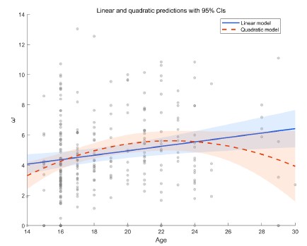
Finally, the two age groups compared - adolescents (high school students) and adults (university students) - differ not only in age but also in sociocultural and economic backgrounds. High school students are likely more homogenous in regional background (e.g., Beijing locals), while university students may be drawn from a broader geographic and socioeconomic pool. Additionally, differences in financial independence, family structure (e.g., single-child status), and social network complexity may systematically affect cooperative behavior and valuation of rewards. Although these factors are difficult to control fully, the authors should more explicitly address the extent to which their findings reflect biological development versus social and contextual influences.
We appreciate this comment. Indeed, adolescents (high school students) and adults (university students) differ not only in age but also in sociocultural and socioeconomic backgrounds. In our study, all participants were recruited from Beijing and surrounding regions, which helps minimize large regional and cultural variability. Moreover, we accounted for individual-level random effects and included participants’ social value orientation (SVO) as an individual difference measure.
Nonetheless, we acknowledge that other contextual factors, such as differences in financial independence, socioeconomic status, and social experience—may also contribute to group differences in cooperative behavior and reward valuation. Although our results are broadly consistent with developmental theories of reward sensitivity and social decisionmaking, sociocultural influences cannot be entirely ruled out. Future work with more demographically matched samples or with socioeconomic and regional variables explicitly controlled will help clarify the relative contributions of biological and contextual factors. Accordingly, we have revised the Discussion to include the following statement: “Third, although both age groups were recruited from Beijing and nearby regions, minimizing major regional and cultural variation, adolescents and adults may still differ in socioeconomic status, financial independence, and social experience. Such contextual differences could interact with developmental processes in shaping cooperative behavior and reward valuation. Future research with demographically matched samples or explicit measures of socioeconomic background will help disentangle biological from sociocultural influences.”
Reviewer #3 (Public review):
Summary:
Wu and colleagues find that in a repeated Prisoner's Dilemma, adolescents, compared to adults, are less likely to increase their cooperation behavior in response to repeated cooperation from a simulated partner. In contrast, after repeated defection by the partner, both age groups show comparable behavior.
To uncover the mechanisms underlying these patterns, the authors compare eight different models. They report that a social reward learning model, which includes separate learning rates for positive and negative prediction errors, best fits the behavior of both groups. Key parameters in this winning model vary with age: notably, the intrinsic value of cooperating is lower in adolescents. Adults and adolescents also differ in learning rates for positive and negative prediction errors, as well as in the inverse temperature parameter.
Strengths:
The modeling results are compelling in their ability to distinguish between learned expectations and the intrinsic value of cooperation. The authors skillfully compare relevant models to demonstrate which mechanisms drive cooperation behavior in the two age groups.
We thank the reviewer’s recognition of our work’s strengths.
Weaknesses:
Some of the claims made are not fully supported by the data:
The central parameter reflecting preference for cooperation is positive in both groups. Thus, framing the results as self-interest versus other-interest may be misleading.
We thank the reviewer for this insightful comment. In the social reward model, the cooperation preference parameter is positive by definition, as defection in the repeated rPDG always yields a +2 monetary advantage regardless of the partner’s action. This positive value represents the additional subjective reward assigned to mutual cooperation (e.g., reciprocity value) that counterbalances the monetary gain from defection. Although the estimated social reward parameter ω was positive, the effective advantage of cooperation is Δ=p×ω−2. Given participants’ inferred beliefs p, Δ was negative for most trials (p×ω<2), indicating that the social reward was insufficient to offset the +2 advantage of defection. Thus, both adolescents and adults valued cooperation positively, but adolescents’ smaller ω and weaker responsiveness to sustained partner cooperation suggest a stronger weighting on immediate monetary payoffs.
In this light, our framing of adolescents as more self-interested derives from their behavioral pattern: even when they recognized sustained partner cooperation and held high expectations of partner cooperation, adolescents showed lower cooperative behavior and reciprocity rewards compared with adults. Whereas adults increased cooperation after two or three consecutive partner cooperations, this pattern was absent among adolescents. We therefore interpret their behavior as relatively more self-interested, reflecting reduced sensitivity to the social reward from mutual cooperation rather than a categorical shift from self-interest to other-interest, as elaborated in the Discussion.
It is unclear why the authors assume adolescents and adults have the same expectations about the partner's cooperation, yet simultaneously demonstrate age-related differences in learning about the partner. To support their claim mechanistically, simulations showing that differences in cooperation preference (i.e., the w parameter), rather than differences in learning, drive behavioral differences would be helpful.
We thank the reviewer for raising this important point. In our model, both adolescents and adults updated their beliefs about partner cooperation using an asymmetric reinforcement learning (RL) rule. Although adolescents exhibited a higher positive and a lower negative learning rate than adults, the two groups did not differ significantly in their overall updating of partner cooperation probability (Fig. 4a-b). We then examined the social reward parameter ω, which was significantly smaller in adolescents and determined the intrinsic value of mutual cooperation (i.e., p×ω). This variable differed significantly between groups and closely matched the behavioral pattern.
Following the reviewer’s suggestion, we conducted additional simulations varying one model parameter at a time while holding the others constant. The difference in mean cooperation probability between adults and adolescents served as the index (positive = higher cooperation in adults). As shown in the Author response image 2, decreases in ω most effectively reproduced the observed group difference (shaded area), indicating that age-related differences in cooperation are primarily driven by variation in the social reward parameter ω rather than by others.
Author response image 2.
Simulation results showing how variations in each model parameter affect the group difference in mean cooperation probability (Adults – Adolescents). Based on the best-fitting Model 8 and parameters estimated from all participants, each line represents one parameter (i.e., α+, α-, ω, β) systematically varied within the tested range (α±:0.1–0.9; ω, β:1–9) while other parameters were held constant. Positive values indicate higher cooperation in adults. Smaller ω values most strongly reproduced the observed group difference, suggesting that reduced social reward weighting primarily drives adolescents’ lower cooperation.
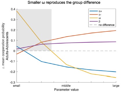
Two different schedules of 120 trials were used: one with stable partner behavior and one with behavior changing after 20 trials. While results for order effects are reported, the results for the stable vs. changing phases within each schedule are not. Since learning is influenced by reward structure, it is important to test whether key findings hold across both phases.
We thank the reviewer for this thoughtful and professional comment. In our GLMM and LMM analyses, we focused on trial order rather than explicitly including the stable vs. changing phase factor, due to concerns about multicollinearity. In our design, phases occur in specific temporal segments, which introduces strong collinearity with trial order. In multi-round interactions, order effects also capture variance related to phase transitions.
Nonetheless, to directly address this concern, we conducted additional robustness analyses by adding a phase variable (stable vs. changing) to GLMM1, LMM1, and LMM3 alongside the original covariates. Across these specifications, the key findings were replicated (see GLMM<sub>sup</sub>2 and LMM<sub>sup</sub>4–5; Tables 9-11), and the direction and significance of main effects remained unchanged, indicating that our conclusions are robust to phase differences.
The division of participants at the legal threshold of 18 years should be more explicitly justified. The age distribution appears continuous rather than clearly split. Providing rationale and including continuous analyses would clarify how groupings were determined.
We thank the reviewer for this thoughtful comment. We divided participants at the legal threshold of 18 years for both conceptual and practical reasons grounded in prior literature and policy. In many countries and regions, 18 marks the age of legal majority and is widely used as the boundary between adolescence and adulthood in behavioral and clinical research. Empirically, prior studies indicate that psychosocial maturity and executive functions approach adult levels around this age, with key cognitive capacities stabilizing in late adolescence (Icenogle et al., 2019; Tervo-Clemmens et al., 2023). We have clarified this rationale in the Introduction section of the revised manuscript.
“Based on legal criteria for majority and prior empirical work, we adopt 18 years as the boundary between adolescence and adulthood (Icenogle et al., 2019; Tervo-Clemmens et al., 2023).”
We fully agree that the underlying age distribution is continuous rather than sharply divided. To address this, we conducted additional analyses treating age as a continuous predictor (see GLMM<sub>sup</sub>1 and LMM<sub>sup</sub>1–3; Tables S1-S4), which generally replicated the patterns observed with the categorical grouping. Nevertheless, given the limited age range of our sample, the generalizability of these findings to fine-grained developmental differences remains constrained. Therefore, our primary analyses continue to focus on the contrast between adolescents and adults, rather than attempting to model a full developmental trajectory.
Claims of null effects (e.g., in the abstract: "adults increased their intrinsic reward for reciprocating... a pattern absent in adolescents") should be supported with appropriate statistics, such as Bayesian regression.
We thank the reviewer for highlighting the importance of rigor when interpreting potential null effects. To address this concern, we conducted Bayes factor analyses of the intrinsic reward for reciprocity and reported the corresponding BF10 for all relevant post hoc comparisons. This approach quantifies the relative evidence for the alternative versus the null hypothesis, thereby providing a more direct assessment of null effects. The analysis procedure is now described in the Methods and Materials section:
“Post hoc comparisons were conducted using Bayes factor analyses with MATLAB’s bayesFactor Toolbox (version v3.0, Krekelberg, 2024), with a Cauchy prior scale σ = 0.707.”
Once claims are more closely aligned with the data, the study will offer a valuable contribution to the field, given its use of relevant models and a well-established paradigm.
We are grateful for the reviewer’s generous appraisal and insightful comments.
Recommendations for the authors
Reviewer #1 (Recommendations for the authors):
I commend the authors on a well-structured, clear, and interesting piece of work. I have several questions and recommendations that, if addressed, I believe will strengthen the manuscript.
We thank the reviewer for commending the organization of our paper.
Introduction: - Why use a zero-sum (Prisoner's Dilemma; PD) versus a mixed-motive game (e.g. Trust Task) to study cooperation? In a finite set of rounds, the dominant strategy can be to defect in a PD.
We thank the reviewer for this helpful comment. We agree that both the rationale for using the repeated Prisoner’s Dilemma (rPDG) and the limitations of this framework should be clarified. We chose the rPDG to isolate the core motivational conflict between selfinterest and joint welfare, as its symmetric and simultaneous structure avoids the sequential trust and reputation dependencies/accumulation inherent to asymmetric tasks such as the Trust Game (King-Casas et al., 2005; Rilling et al., 2002).
Although a finitely repeated rPDG theoretically favors defection, extensive prior research shows that cooperation can still emerge in long repeated interactions when players rely on learning and reciprocity rather than backward induction (Rilling et al., 2002; Fareri et al., 2015). Our design employed 120 consecutive rounds, allowing participants to update expectations about partner behavior and to establish stable reciprocity patterns over time. We have added the following clarification to the Introduction:
“The rPDG provides a symmetric and simultaneous framework that isolates the motivational conflict between self-interest and joint welfare, avoiding the sequential trust and reputation dynamics characteristic of asymmetric tasks such as the Trust Game (Rilling et al., 2002; King-Casas et al., 2005)”
Methods:
Did the participants know how long the PD would go on for?
Were the participants informed that the partner was real/simulated?
Were the participants informed that the partner was going to be the same for all rounds?
We thank the reviewer for the meticulous review work, which helped us present the experimental design and reporting details more clearly. the following clarifications: I. Participants were not informed of the total number of rounds in the rPDG. This prevented endgame expectations and avoided distraction from counting rounds, which could introduce additional effects. II. Participants were told that their partner was another human participant in the laboratory. However, the partner’s behavior was predetermined by a computer program. This design enabled tighter experimental control and ensured consistent conditions across age groups, supporting valid comparisons. III. Participants were informed that they would interact with the same partner across all rounds, aligning with the essence of a multiround interaction paradigm and stabilizing partner-related expectations. For transparency, we have clarified these points in the Methods and Materials section:
“Participants were told that their partner was another human participant in the laboratory and that they would interact with the same partner across all rounds. However, in reality, the actions of the partner were predetermined by a computer program. This setup allowed for a clear comparison of the behavioral responses between adolescents and adults. Participants were not informed of the total number of rounds in the rPDG.”
The authors mention that an SVO was also recorded to indicate participant prosociality. Where are the results of this? Did this track game play at all? Could cooperativeness be explained broadly as an SVO preference that penetrated into game-play behaviour?
We thank the reviewer for pointing this out. We agree that individual differences in prosociality may shape cooperative behavior, so we conducted additional analyses incorporating SVO. Specifically, we extended GLMM1 and LMM3 by adding the measured SVO as a fixed effect with random slopes, yielding GLMM<sub>sup</sub>3 and LMM<sub>sup</sub>6 (Tables 12–13). The results showed that higher SVO was associated with greater cooperation, whereas its effect on the reward for reciprocity was not significant. Importantly, the primary findings remained unchanged after controlling for SVO. These results indicate that cooperativeness in our task cannot be explained solely by a broad SVO preference, although a more prosocial orientation was associated with greater cooperation. We have reported these analyses and results in the Appendix Analysis section.
Why was AIC chosen rather an BIC to compare model dominance?
Sorry for the lack of clarification. Both the Akaike Information Criterion (AIC, Akaike, 1974) and Bayesian Information Criterion (BIC, Schwarz, 1978) are informationtheoretic criterions for model comparison, neither of which depends on whether the models to be compared are nested to each other or not (Burnham et al., 2002). We have added the following clarification into the Methods.
“We chose to use the AICc as the metric of goodness-of-fit for model comparison for the following statistical reasons. First, BIC is derived based on the assumption that the “true model” must be one of the models in the limited model set one compares (Burnham et al., 2002; Gelman & Shalizi, 2013), which is unrealistic in our case. In contrast, AIC does not rely on this unrealistic “true model” assumption and instead selects out the model that has the highest predictive power in the model set (Gelman et al., 2014). Second, AIC is also more robust than BIC for finite sample size (Vrieze, 2012).”
I believe the model fitting procedure might benefit from hierarchical estimation, rather than maximum likelihood methods. Adolescents in particular seem to show multiple outliers in a^+ and w^+ at the lower end of the distributions in Figure S2. There are several packages to allow hierarchical estimation and model comparison in MATLAB (which I believe is the language used for this analysis; see https://journals.plos.org/ploscompbiol/article?id=10.1371/journal.pcbi.1007043).
We thank the reviewer for this helpful comment and for referring us to relevant methodological work (Piray et al., 2019). We have addressed this point by incorporating hierarchical Bayesian estimation, which effectively mitigates outlier effects and improves model identifiability. The results replicated those obtained with MLE fitting and further revealed group-level differences in key parameters. Please see our detailed response to Reviewer#1 Q1 for the full description of this analysis and results.
Results: Model confusion seems to show that the inequality aversion and social reward models were consistently confused with the baseline model. Is this explained or investigated? I could not find an explanation for this.
The apparent overlap between the inequality aversion (Model 4) and social reward (Model 5) models in the recovery analysis likely arises because neither model includes a learning mechanism, making them unable to capture trial-by-trial adjustments in this dynamic task. Consequently, both were best fit by the baseline model. Please see Response to Reviewer #1 Q3 for related discussion.
Figures 3e and 3f show the correlation between asymmetric learning rates and age. It seems that both a^+ and a^- are around 0.35-0.40 for young adolescents, and this becomes more polarised with age. Could it be that with age comes an increasing discernment of positive and negative outcomes on beliefs, and younger ages compress both positive and negative values together? Given the higher stochasticity in younger ages (\beta), it may also be that these values simply represent higher uncertainty over how to act in any given situation within a social context (assuming the differences in groups are true).
We appreciate this insightful interpretation. Indeed, both α+ and α- cluster around 0.35–0.40 in younger adolescents and become increasingly polarized with age, suggesting that sensitivity to positive versus negative feedback is less differentiated early in development and becomes more distinct over time. This interpretation remains tentative and warrants further validation. Based on this comment, we have revised the Discussion to include this developmental interpretation.
We also clarify that in our model β denotes the inverse temperature parameter; higher β reflects greater choice precision and value sensitivity, not higher stochasticity. Accordingly, adolescents showed higher β values, indicating more value-based and less exploratory choices, whereas adults displayed relatively greater exploratory cooperation. These group differences were also replicated using hierarchical Bayesian estimation (see Response to Reviewer #1 Q1). In response to this comment, we have added a statement in the Discussion highlighting this developmental interpretation.
“Together, these findings suggest that the differentiation between positive and negative learning rates changes with age, reflecting more selective feedback sensitivity in development, while higher β values in adolescents indicate greater value sensitivity. This interpretation remains tentative and requires further validation in future research.”
A parameter partial correlation matrix (off-diagonal) would be helpful to understand the relationship between parameters in both adolescents and adults separately. This may provide a good overview of how the model properties may change with age (e.g. a^+'s relation to \beta).
We thank the reviewer for this helpful comment. We fully agree that a parameter partial correlation matrix can further elucidate the relationships among parameters. Accordingly, we conducted a partial correlation analysis and added the visually presented results to the revised manuscript as Figure 2-figure supplement 4.
It would be helpful to have Bayes Factors reported with each statistical tests given that several p-values fall within the 0.01 and 0.10.
We thank the reviewer for this important recommendation. We have conducted Bayes factor analyses and reported BF10 for all relevant post hoc comparisons. We also clarified our analysis in the Methods and Materials section:
“Post hoc comparisons were conducted using Bayes factor analyses with MATLAB’s bayesFactor Toolbox (version v3.0, Krekelberg, 2024), with a Cauchy prior scale σ = 0.707.”
Discussion: I believe the language around ruling out failures in mentalising needs to be toned down. RL models do not enable formal representational differences required to assess mentalising, but they can distinguish biases in value learning, which in itself is interesting. If the authors were to show that more complex 'ToM-like' Bayesian models were beaten by RL models across the board, and this did not differ across adults and adolescents, there would be a stronger case to make this claim. I think the authors either need to include Bayesian models in their comparison, or tone down their language on this point, and/or suggest ways in which this point might be more thoroughly investigated (e.g., using structured models on the same task and running comparisons: https://journals.plos.org/plosone/article?id=10.1371/journal.pone.0087619).
We thank the reviewer for the comments. Please see our response to Reviewer 1 (Appraisal & Discussion section) for details.
Reviewer #2 (Recommendations for the authors):
The authors may want to show the winning model earlier (perhaps near the beginning of the Results section, when model parameters are first mentioned).
We thank the reviewer for this suggestion. We agree that highlighting the winning model early improves clarity. Currently, we have mentioned the winning model before the beginning of the Results section. Specifically, in the penultimate paragraph of the Introduction we state:
“We identified the asymmetric RL learning model as the winning model that best explained the cooperative decisions of both adolescents and adults.”
Reviewer #3 (Recommendations for the authors):
In addition to the points mentioned above, I suggest the following:
(1) Clarify plots by clearly explaining each variable. In particular, the indices 1 vs. 1,2 vs. 1,2,3 were not immediately understandable.
We thank the reviewer for this suggestion. We agree that the indices were not immediately clear. We have revised the figure captions (Figure 1 and 4) to explicitly define these terms more clearly:
“The x-axis represents the consistency of the partner’s actions in previous trials (t<sub>−1</sub>: last trial; t<sub>−1,2</sub>: last two trials; t<sub>−1,2,3</sub>: last three trials).”
It's unclear why the index stops at 3. If this isn't the maximum possible number of consecutive cooperation trials, please consider including all relevant data, as adolescents might show a trend similar to adults over more trials.
We thank the reviewer for raising this point. In our exploratory analyses, we also examined longer streaks of consecutive partner cooperation or defection (up to four or five trials). Two empirical considerations led us to set the cutoff at three in the final analyses. First, the influence of partner behavior diminished sharply with temporal distance. In both GLMMs and LMMs, coefficients for earlier partner choices were small and unstable, and their inclusion substantially increased model complexity and multicollinearity. This recency pattern is consistent with learning and decision models emphasizing stronger weighting of recent evidence (Fudenberg & Levine, 2014; Fudenberg & Peysakhovich, 2016). Second, streaks longer than three were rare, especially among some participants, leading to data sparsity and inflated uncertainty. Including these sparse conditions risked biasing group estimates rather than clarifying them. Balancing informativeness and stability, we therefore restricted the index to three consecutive partner choices in the main analyses, which we believe sufficiently capture individuals’ general tendencies in reciprocal cooperation.
The term "reciprocity" may not be necessary. Since it appears to reflect a general preference for cooperation, it may be clearer to refer to the specific behavior or parameter being measured. This would also avoid confusion, especially since adolescents do show negative reciprocity in response to repeated defection.
We thank you for this comment. In our work, we compute the intrinsic reward for reciprocity as p × ω, where p is the partner cooperation expectation and ω is the cooperation preference. In the rPDG, this value framework manifests as a reciprocity-derived reward: sustained mutual cooperation maximizes joint benefits, and the resulting choice pattern reflects a value for reciprocity, contingent on the expected cooperation of the partner. This quantity enters the trade-off between U<sub>cooperation</sub> and U<sub>defection</sub>and captures the participant’s intrinsic reward for reciprocity versus the additional monetary reward payoff of defection. Therefore, we consider the term “reciprocity” an acceptable statement for this construct.
Interpretation of parameters should closely reflect what they specifically measure.
We thank the reviewer for pointing this out. We have refined the relevant interpretations of parameters in the current Results and Discussion sections.
Prior research has shown links between Theory of Mind (ToM) and cooperation (e.g., Martínez-Velázquez et al., 2024). It would be valuable to test whether this also holds in your dataset.
We thank the reviewer for this thoughtful comment. Although we did not directly measure participants’ ToM, our design allowed us to estimate participants’ trial-by-trial inferences (i.e., expectations) about their partner’s cooperation probability. We therefore treat these cooperation expectations as an indirect representation for belief inference, which is related to ToM processes. To test whether this belief-inference component relates to cooperation in our dataset, we further conducted an exploratory analysis (GLMM<sub>sup</sub>4) in which participants’ choices were regressed on their cooperation expectations, group, and the group × cooperation-expectation interaction, controlling for trial number and gender, with random effects. Consistent with the ToM–cooperation link in prior research (MartínezVelázquez et al., 2024), participants’ expectations about their partner’s cooperation significantly predicted their cooperative behavior (Table 14), suggesting that decisions were shaped by social learning about others’ inferred actions. Moreover, the interaction between group and cooperation expectation was not significant, indicating that this inference-driven social learning process likely operates similarly in adolescents and adults. This aligns with our primary modeling results showing that both age groups update beliefs via an asymmetric learning process. We have reported these analyses in the Appendix Analysis section.
More informative table captions would help the reader. Please clarify how variables are coded (e.g., is female = 0 or 1? Is adolescent = 0 or 1?), to avoid the need to search across the manuscript for this information.
We thank the reviewer for raising this point. We have added clear and standardized variable coding in the table notes of all tables to make them more informative and avoid the need to search the paper. We have ensured consistent wording and formatting across all tables.
I hope these comments are helpful and support the authors in further strengthening their manuscript.
We thank the three reviewers for their comments, which have been helpful in strengthening this work.
Reference
(1) Fudenberg, D., & Levine, D. K. (2014). Recency, consistent learning, and Nash equilibrium. Proceedings of the National Academy of Sciences of the United States of America, 111(Suppl. 3), 10826–10829. https://doi.org/10.1073/pnas.1400987111
(2) Fudenberg, D., & Peysakhovich, A. (2016). Recency, records, and recaps: Learning and nonequilibrium behavior in a simple decision problem. ACM Transactions on Economics and Computation, 4(4), Article 23, 1–18. https://doi.org/10.1145/2956581
(3) Hackel, L., Doll, B., & Amodio, D. (2015). Instrumental learning of traits versus rewards: Dissociable neural correlates and effects on choice. Nature Neuroscience, 18, 1233– 1235. https://doi.org/10.1038/nn.4080
(4) Icenogle, G., Steinberg, L., Duell, N., Chein, J., Chang, L., Chaudhary, N., Di Giunta, L.,Dodge, K. A., Fanti, K. A., Lansford, J. E., Oburu, P., Pastorelli, C., Skinner, A. T.,Sorbring, E., Tapanya, S., Uribe Tirado, L. M., Alampay, L. P., Al-Hassan, S. M.,Takash, H. M. S., & Bacchini, D. (2019). Adolescents’ cognitive capacity reaches adult levels prior to their psychosocial maturity: Evidence for a “maturity gap” in a multinational, cross-sectional sample. Law and Human Behavior, 43(1), 69–85. https://doi.org/10.1037/lhb0000315
(5) Krekelberg, B. (2024). Matlab Toolbox for Bayes Factor Analysis (v3.0) [Computer software]. Zenodo. https://doi.org/10.5281/zenodo.13744717
(6) Martínez-Velázquez, E. S., Ponce-Juárez, S. P., Díaz Furlong, A., & Sequeira, H. (2024). Cooperative behavior in adolescents: A contribution of empathy and emotional regulation? Frontiers in Psychology, 15, 1342458. https://doi.org/10.3389/fpsyg.2024.1342458
(7) Tervo-Clemmens, B., Calabro, F. J., Parr, A. C., et al. (2023). A canonical trajectory of executive function maturation from adolescence to adulthood. NatureCommunications, 14, 6922. https://doi.org/10.1038/s41467-023-42540-8
(8) King-Casas, B., Tomlin, D., Anen, C., Camerer, C. F., Quartz, S. R., & Montague, P. R. (2005). Getting to know you: reputation and trust in a two-person economic exchange. Science, 308(5718), 78-83. https://doi.org/10.1126/science.1108062
(9) Rilling, J. K., Gutman, D. A., Zeh, T. R., Pagnoni, G., Berns, G. S., & Kilts, C. D. (2002). A neural basis for social cooperation. Neuron, 35(2), 395-405. https://doi.org/10.1016/s0896-6273(02)00755-9
(10) Fareri, D. S., Chang, L. J., & Delgado, M. R. (2015). Computational substrates of social value in interpersonal collaboration. Journal of Neuroscience, 35(21), 8170-8180. https://doi.org/10.1523/JNEUROSCI.4775-14.2015
(11) Akaike, H. (2003). A new look at the statistical model identification. IEEE transactions on automatic control, 19(6), 716-723. https://doi.org/10.1109/TAC.1974.1100705
(12) Schwarz, G. (1978). Estimating the dimension of a model. The annals of statistics, 461464. https://doi.org/10.1214/aos/1176344136
(13) Burnham, K. P., & Anderson, D. R. (2002). Model selection and multimodel inference: A practical information-theoretic approach (2nd ed.). Springer.https://doi.org/10.1007/b97636
(14) Gelman, A., & Shalizi, C. R. (2013). Philosophy and the practice of Bayesian statistics. British Journal of Mathematical and Statistical Psychology, 66(1), 8–38. https://doi.org/10.1111/j.2044-8317.2011.02037.x
(15) Gelman, A., Carlin, J. B., Stern, H. S., Dunson, D. B., Vehtari, A., & Rubin, D. B. (2014). Bayesian data analysis (3rd ed.). Chapman and Hall/CRC. https://doi.org/10.1201/b16018
(16) Vrieze, S. I. (2012). Model selection and psychological theory: A discussion of the differences between the Akaike Information Criterion (AIC) and the Bayesian Information Criterion (BIC). Psychological Methods, 17(2), 228–243. https://doi.org/10.1037/a0027127.
Author response:
The following is the authors’ response to the original reviews.
Public Reviews:
Reviewer #1 (Public review):
Summary:
Zhang and colleagues examine neural representations underlying abstract navigation in the entorhinal cortex (EC) and hippocampus (HC) using fMRI. This paper replicates a previously identified hexagonal modulation of abstract navigation vectors in abstract space in EC in a novel task involving navigating in a conceptual Greeble space. In HC, the authors claim to identify a three-fold signal of the navigation angle. They also use a novel analysis technique (spectral analysis) to look at spatial patterns in these two areas and identify phase coupling between HC and EC. Finally, the authors propose an EC-HPC PhaseSync Model to understand how the EC and HC construct cognitive maps. While the wide array of techniques used is impressive and their creativity in analysis is admirable, overall, I found the paper a bit confusing and unconvincing. I recommend a significant rewrite of their paper to motivate their methods and clarify what they actually did and why. The claim of three-fold modulation in HC, while potentially highly interesting to the community, needs more background to motivate why they did the analysis in the first place, more interpretation as to why this would emerge in biology, and more care taken to consider alternative hypotheses seeped in existing models of HC function. I think this paper does have potential to be interesting and impactful, but I would like to see these issues improved first.
General comments:
(1) Some of the terminology used does not match the terminology used in previous relevant literature (e.g., sinusoidal analysis, 1D directional domain).
We thank the reviewer for this valuable suggestion, which helps to improve the consistency of our terminology with previous literature and to reduce potential ambiguity. Accordingly, we have replaced “sinusoidal analysis” with “sinusoidal modulation” (Doeller et al., 2010; Bao et al., 2019; Raithel et al., 2023) and “1D directional domain” with “angular domain of path directions” throughout the manuscript.
(2) Throughout the paper, novel methods and ideas are introduced without adequate explanation (e.g., the spectral analysis and three-fold periodicity of HC).
We thank the reviewer for raising this important point. In the revised manuscript, we have substantially extended the Introduction (paragraphs 2–4) to clarify our hypothesis, explicitly explaining why the three primary axes of the hexagonal grid cell code may manifest as vector fields. We have also revised the first paragraph of the “3-fold periodicity in the HPC” section in the Results to clarify the rationale for using spectral analysis. Please refer to our responses to comment 2 and 3 below for details.
Reviewer #2 (Public review):
The authors report results from behavioral data, fMRI recordings, and computer simulations during a conceptual navigation task. They report 3-fold symmetry in behavioral and simulated model performance, 3-fold symmetry in hippocampal activity, and 6-fold symmetry in entorhinal activity (all as a function of movement directions in conceptual space). The analyses are thoroughly done, and the results and simulations are very interesting.
We sincerely thank the reviewer for the positive and encouraging comments on our study.
Recommendations for the authors:
Reviewer #1 (Recommendations for the authors):
(1) This paper has quite a few spelling and grammatical mistakes, making it difficult to understand at times.
We apologize for the wordings and grammatical errors. We have thoroughly re-read and carefully edited the entire manuscript to correct typographical and grammatical errors, ensuring improved clarity and readability.
(2) Introduction - It's not clear why the three primary axes of hexagonal grid cell code would manifest as vector fields.
We thank the reviewer for raising this important point. In the revised Introduction (paragraphs 2, 3, and 4), we now explicitly explain the rationale behind our hypothesis that the three primary axes of the hexagonal grid cell code manifest as vector fields.
In paragraph 2, we present empirical evidence from rodent, bat, and human studies demonstrating that mental simulation of prospective paths relies on vectorial representations in the hippocampus (Sarel et al., 2017; Ormond and O’Keefe, 2022; Muhle-Karbe et al., 2023).
In paragraphs 3 and 4, we introduce our central hypothesis: vectorial representations may originate from population-level projections of entorhinal grid cell activity, based on three key considerations:
(1) The EC serves as the major source of hippocampal input (Witter and Amaral, 1991; van Groen et al., 2003; Garcia and Buffalo, 2020).
(2) Grid codes exhibit nearly invariant spatial orientations (Hafting et al., 2005; Gardner et al., 2022), which makes it plausible that their spatially periodic activity can be detected using fMRI.
(3) A model-based inference: for example, in the simplest case, when one mentally simulates a straight pathway aligned with the grid orientation, a subpopulation of grid cells would be activated. The resulting population activity would form a near-perfect vectorial representation, with constant activation strength along the path. In contrast, if the simulated path is misaligned with the grid orientation, the population response becomes a distorted vectorial code. Consequently, simulating all possible straight paths spanning 0°–360° results in 3-fold periodicity in the activity patterns—due to the 180° rotational symmetry of the hexagonal grid, orientations separated by 180° are indistinguishable.
We therefore speculate that vectorial representations embedded in grid cell activity exhibit 3-fold periodicity across spatial orientations and serve as a periodic structure to represent spatial direction. Supporting this view, reorientation paradigms in both rodents and young children have shown that subjects search equally in two opposite directions, reflecting successful orientation encoding but a failure to integrate absolute spatial direction (Hermer and Spelke, 1994; Julian et al., 2015; Gallistel, 2017; Julian et al., 2018).
(3) It took me a few reads to understand what the spectral analysis was. After understanding, I do think this is quite clever. However, this paper needs more motivation to understand why you are performing this analysis. E.g., why not just take the average regressor at the 10º, 70º, etc. bins and compare it to the average regressor at 40º, 100º bins? What does the Fourier transform buy you?
We are sorry for the confusion. we outline the rationale for employing Fast Fourier Transform (FFT) analysis to identify neural periodicity. In the revised manuscript, we have added these clarifications into the first paragraph of the “3-fold periodicity in the HPC” subsection in the Results.
First, FFT serves as an independent approach to cross-validate the sinusoidal modulation results, providing complementary evidence for the 6-fold periodicity in EC and the 3-fold periodicity in HPC.
Second, FFT enables unbiased detection of multiple candidate periodicities (e.g., 3–7-fold) simultaneously without requiring prior assumptions about spatial phase (orientation). By contrast, directly comparing “aligned” versus “misaligned” angular bins (e.g., 10°/70° vs. 40°/100°) would implicitly assume knowledge of the phase offset, which was not known a priori.
Finally, FFT uniquely allows periodicity analysis of behavioral performance, which is not feasible with standard sinusoidal GLM approaches. This methodological consistency makes it possible to directly compare periodicities across neural and behavioral domains.
(4) A more minor point: at one point, you say it’s a spectral analysis of the BOLD signals, but the methods description makes it sound like you estimated regressors at each of the bins before performing FFT. Please clarify.
We apologize for the confusion. In our manuscript, we use the term spectral analysis to distinguish this approach from sinusoidal modulation analysis. Conceptually, our spectral analysis involves a three-level procedure:
(1) First level: We estimated direction-dependent activity maps using a general linear model (GLM), which included 36 regressors corresponding to path directions, down-sampled in 10° increments.
(2) Second level: We applied a Fast Fourier Transform (FFT) to the direction-dependent activity maps derived from the GLM to examine the spectral magnitude of potential spatial periodicities.
(3) Third level: We conducted group-level statistical analyses across participants to assess the consistency of the observed periodicities.
We have revised the “Spectral analysis of MRI BOLD signals” subsection in the Methods to clarify this multi-level procedure.
(5) Figure 4a:
Why do the phases go all the way to 2*pi if periodicity is either three-fold or six-fold?
When performing correlation between phases, you should perform a circular-circular correlation instead of a Pearson's correlation.
We thank the reviewer for raising this important point. In the original Figure 4a, both EC and HPC phases spanned 0–2π because their sinusoidal phase estimates were projected into a common angular space by scaling them according to their symmetry factors (i.e., multiplying the 3-fold phase by 3 and the 6-fold phase by 6), followed by taking the modulo 2π. However, this projection forced signals with distinct intrinsic periodicities (120° vs. 60° cycles) into a shared 360° space, thereby distorting their relative angular distances and disrupting the one-to-one correspondence between physical directions and phase values. Consequently, this transformation could bias the estimation of their phase relationship.
In the revised analysis and Figure 4a, we retained the original phase estimates derived from the sinusoidal modulation within their native periodic ranges (0–120° for 3-fold and 0–60° for 6-fold) by applying modulo operations directly. Following your suggestion, the relationship between EC and HPC phases was then quantified using circular–circular correlation (Jammalamadaka & Sengupta, 2001), as implemented in the CircStat MATLAB toolbox. This updated analysis avoids the rescaling artifact and provides a statistically stronger and conceptually clearer characterization of the phase correspondence between EC and HPC.
(6) Figure 4d needs additional clarification:
Phase-locking is typically used to describe data with a high temporal precision. I understand you adopted an EEG analysis technique to this reconstructed fMRI time-series data, but it should be described differently to avoid confusion. This needs additional control analyses (especially given that 3 is a multiple of 6) to confirm that this result is specific to the periodicities found in the paper.
We thank the reviewer for this insightful comment. We have extensively revised the description of the Figure 4 to avoid confusion with EEG-based phase-locking techniques. The revised text now explicitly clarifies that our approach quantifies spatial-domain periodic coupling across path directions, rather than temporal synchronization of neural signals.
To further address the reviewer’s concern about potential effects of the integer multiple relationship between the 3-fold HPC and 6-fold EC periodicities, we additionally performed two control analyses using the 9-fold and 12-fold EC components, both of which are also integer multiples of the 3-fold HPC periodicity. Neither control analysis showed significant coupling (p > 0.05), confirming that the observed 3-fold–6-fold coupling was specific and not driven by their harmonic relationship.
The description of the revised Figure 4 has been updated in the “Phase Synchronization Between HPC and EC Activity” subsection of the Results.
(7) Figure 5a is misleading. In the text, you say you test for propagation to egocentric cortical areas, but I don’t see any analyses done that test this. This feels more like a possible extension/future direction of your work that may be better placed in the discussion.
We are sorry for the confusion. Figure 5a was intended as a hypothesis-driven illustration to motivate our analysis of behavioral periodicity based on participants’ task performance. However, we agree with the reviewer that, on its own, Figure 5a could be misleading, as it does not directly present supporting analyses.
To provide empirical support for the interpretation depicted in Figure 5a, we conducted a whole-brain analysis (Figure S8), which revealed significant 3-fold periodic signals in egocentric cortical regions, including the parietal cortex (PC), precuneus (PCU), and motor regions.
To avoid potential misinterpretation, we have revised the main text to include these results and explicitly referenced Figure S8 in connection with Figure 5a.
The updated description in the “3-fold periodicity in human behavior” subsection in the Results is as follows:
“Considering the reciprocal connectivity between the medial temporal lobe (MTL), where the EC and HPC reside, and the parietal cortex implicated in visuospatial perception and action, together with the observed 3-fold periodicity within the DMN (including the PC and PCu; Fig. S8), we hypothesized that the 3-fold periodic representations of path directions extend beyond the MTL to the egocentric cortical areas, such as the PC, thereby influencing participants' visuospatial task performance (Fig. 5a)”.
Additionally, Figure 5a has been modified to more clearly highlight the hypothesized link between activity periodicity and behavioral periodicity, rather than suggesting a direct anatomical pathway.
(8) PhaseSync model: I am not an expert in this type of modeling, so please put a lower weight on this comment (especially compared to some of the other reviewers). While the PhaseSync model seems interesting, it’s not clear from the discussion how this compares to current models. E.g., Does it support them by adding the three-fold HC periodicity? Does it demonstrate that some of them can't be correct because they don't include this three-fold periodicity?
We thank the reviewer for the insightful comment regarding the PhaseSync model. We agree that further clarifying its relationship to existing computational frameworks is important.
The EC–HPC PhaseSync model is not intended to replace or contradict existing grid–place cell models of navigation (e.g., Bicanski and Burgess, 2019; Whittington et al., 2020; Edvardsen et al., 2020). Instead, it offers a hierarchical extension by proposing that vectorial representations in the hippocampus emerge from the projections of periodic grid codes in the entorhinal cortex. Specifically, the model suggests that grid cell populations encode integrated path information, forming a vectorial gradient toward goal locations.
To simplify the theoretical account, our model was implemented in an idealized square layout. In more complex real-world environments, hippocampal 3-fold periodicity may interact with additional spatial variables, such as distance, movement speed, and environmental boundaries.
We have revised the final two paragraphs of the Discussion to clarify this conceptual framework and emphasize the importance of future studies in exploring how periodic activity in the EC–HPC circuit interacts with environmental features to support navigation.
Reviewer #2 (Recommendations for the authors):
(1) Please show a histogram of movement direction sampling for each participant.
We thank the reviewer for this helpful suggestion. We have added a new supplementary figure (Figure S2) showing histograms of path direction sampling for each participant (36 bins of 10°). The figure is also included. Rayleigh tests for circular uniformity revealed no significant deviations from uniformity (all ps > 0.05, Bonferroni-corrected across participants), confirming that path directions were sampled evenly across 0°–360°.
(2) Why didn’t you use participants’ original trajectories (instead of the trajectories inferred from the movement start and end points) for the hexadirectional analyses?
In our paradigm, participants used two MRI-compatible 2-button response boxes (one for each hand) to adjust the two features of the greebles. As a result, the raw adjustment path contained only four cardinal directions (up, down, left, right). If we were to use the raw stepwise trajectories, the analysis would be restricted to these four directions, which would severely limit the angular resolution. By instead defining direction as the vector from the start to the end position in feature space, we can expand the effective range of directions to the full 0–360°. This approach follows previous literature on abstract grid-like coding in humans (e.g., Constantinescu et al., 2016), where direction was similarly defined by the relative change between two feature dimensions rather than the literal stepwise path. We have added this clarification in the “Sinusoidal modulation” subsection of the revised method.
(3) Legend of Figure 2: the statement "localizing grid cell activity" seems too strong because it is still not clear whether hexadirectional signals indeed result from grid-cell activity (e.g., Bin Khalid et al., eLife, 2024). I would suggest rephrasing this statement (here and elsewhere).
Thank you for this helpful suggestion. We have removed the statement “localizing grid cell activity” to avoid ambiguity and revised the legend of Figure 2a to more explicitly highlight its main purpose—defining how path directions and the aligned/misaligned conditions were constructed in the 6-fold modulation. We have also modified similar expressions throughout the manuscript to ensure consistency and clarity.
(4) Legend of Figure 2: “cluster-based SVC correction for multiple comparisons” - what is the small volume you are using for the correction? Bilateral EC?
For both Figure 2 and Figure 3, the anatomical mask of the bilateral medial temporal lobe (MTL), as defined by the AAL atlas, was used as the small volume for correction. This has been clarified in the revised Statistical Analysis section of the Methods as “… with small-volume correction (SVC) applied within the bilateral MTL”.
(5) Legend of Figure 2: "ROI-based analysis" - what kind of ROI are you using? "corrected for multiple comparisons" - which comparisons are you referring to? Different symmetries and also the right/left hemisphere?
In Figure 2b, the ROI was defined as a functional mask derived from the significant activation cluster in the right entorhinal cortex (EC). Since no robust clusters were observed in the left EC, the functional ROI was restricted to the right hemisphere. We indeed included Figure 2c to illustrate this point; however, we recognize that our description in the text was not sufficiently clear.
Regarding the correction for multiple comparisons, this refers specifically to the comparisons across different rotational symmetries (3-, 4-, 5-, 6-, and 7-fold). Only the 6-fold symmetry survived correction, whereas no significant effects were detected for the other symmetries.
We have clarified these points in the “6-fold periodicity in the EC” subsection of the result as “… The ROI was defined as a functional mask of the right EC identified in the voxel-based analysis and further restricted within the anatomical EC. These analyses revealed significant periodic modulation only at 6-fold (Figure 2c; t(32) = 3.56, p = 0.006, two-tailed, corrected for multiple comparisons across rotational symmetries; Cohen’s d = 0.62) …”.
We have also revised the “3-fold periodicity in the HPC” subsection of the result as “… ROI analysis, using a functional mask of the HPC identified in the spectral analysis and further restricted within the anatomical HPC, indicated that HPC activity selectively fluctuated at 3-fold periodicity (Figure 3e; t(32) = 3.94, p = 0.002, corrected for multiple comparisons across rotational symmetries; Cohen’s d = 0.70) …”.
(6) Figure 2d: Did you rotationally align 0{degree sign} across participants? Please state explicitly whether (or not) 0{degree sign} aligns with the x-axis in Greeble space.
We thank the reviewer for this helpful question. Yes, before reconstructing the directional tuning curve in Figure 2d, path directions were rotationally aligned for each participant by subtracting the participant-specific grid orientation (ϕ) estimated from the independent dataset (odd sessions). We have now made this description explicit in the revised manuscript in the “6-fold periodicity in the EC” subsection of the Results, stating “… To account for individual difference in spatial phase, path directions were calibrated by subtracting the participant-specific grid orientation estimated from the odd sessions ...”.
(7) Clustering of grid orientations in 30 participants: What does “Bonferroni corrected” refer to? Also, the Rayleigh test is sensitive to the number of voxels - do you obtain the same results when using pair-wise phase consistency?
“Bonferroni corrected” here refers to correction across participants. We have clarified this in the first paragraph of the “6-fold periodicity in the EC” subsection of the Result and in the legend of Supplementary Figure S5 as “Bonferroni-corrected across participants.”
To examine whether our findings were sensitive to the number of voxels, we followed the reviewer’s guidance to compute pairwise phase consistency (PPC; Vinck et al., 2010) for each participant. The PPC results replicated those obtained with the Rayleigh test. We have updated the new results into the Supplementary Figure S5. We also updated the “Statistical Analysis” subsection of the Methods to describe PPC as “For the PPC (Vinck et al., 2010), significance was tested using 5,000 permutations of uniformly distributed random phases (0–2π) to generate a null distribution for comparison with the observed PPC”.
(8) 6-fold periodicity in the EC: Do you compute an average grid orientation across all EC voxels, or do you compute voxel-specific grid orientations?
Following the protocol originally described by Doeller et al. (2010), we estimated voxel-wise grid orientations within the EC and then obtained a participant-specific orientation by averaging across voxels within a hand-drawn bilateral EC mask. The procedure is described in detail in the “Sinusoidal modulation” subsection of the Methods.
(9) Hand-drawn bilateral EC mask: What was your procedure for drawing this mask? What results do you get with a standard mask, for example, from Freesurfer or SPM? Why do you perform this analysis bilaterally, given that the earlier analysis identified 6-fold symmetry only in the right EC? What do you mean by "permutation corrected for multiple comparisons"?
We thank the reviewer for raising these important methodological points. To our knowledge, no standard volumetric atlas provides an anatomically defined entorhinal cortex (EC) mask. For example, the built-in Harvard–Oxford cortical structural atlas in FSL contains only a parahippocampal region that encompasses, but does not isolate, the EC. The AAL atlas likewise does not contain an EC region. In FreeSurfer, an EC label is available, but only in the fsaverage surface space, which is not directly compatible with MNI-based volumetric group-level analyses.
Therefore, we constructed a bilateral EC mask by manually delineating the EC according to the detailed anatomical landmarks described by Insausti et al. (1998). Masks were created using ITK-SNAP (Version 3.8, www.itksnap.org). For transparency and reproducibility, the mask has been made publicly available at the Science Data Bank (link: https://www.scidb.cn/s/NBriAn), as indicated in the revised Data and Code availability section.
Regarding the use of a bilateral EC mask despite voxel-wise effects being strongest in the right EC. First, we did not have any a priori hypothesis regarding laterality of EC involvement before performing analyses. Second, previous studies estimated grid orientation using a bilateral EC mask in their sinusoidal analyses (Doeller et al., 2010; Constantinescu et al., 2016; Bao et al., 2019; Wagner et al., 2023; Raithel et al., 2023). We therefore followed this established approach to estimate grid orientation.
By “permutation corrected for multiple comparisons” we refer to the family-wise error correction applied to the reconstructed directional tuning curves (Figure 2d for the EC, Figure 3f for the HPC). Specifically, directional labels were randomly shuffled 5,000 times, and an FFT was applied to each shuffled dataset to compute spectral power at each fold. This procedure generated null distributions of spectral power for each symmetry. For each fold, the 95th percentile of the maximal power across permutations was used as the uncorrected threshold. To correct across folds, the 95th percentile of the maximal suprathreshold power across all symmetries was taken as the family-wise error–corrected threshold. We have clarified this procedure in the revised “Statistical Analysis” subsection of the Methods.
(10) Figures 3b and 3d: Why do different hippocampal voxels show significance for the sinusoidal versus spectral analysis? Shouldn’t the analyses be redundant and, thus, identify the same significant voxels?
We thank the reviewer for this insightful question. Although both sinusoidal modulation and spectral analysis aim to detect periodic neural activity, the two approaches are methodologically distinct and are therefore not expected to identify exactly the same significant voxels.
Sinusoidal modulation relies on a GLM with sine and cosine regressors to test for phase-aligned periodicity (e.g., 3-fold or 6-fold), calibrated according to the estimated grid orientation. This approach is highly specific but critically depends on accurate orientation estimation. In contrast, spectral analysis applies Fourier decomposition to the directional tuning profile, enabling the detection of periodic components without requiring orientation calibration.
Accordingly, the two analyses are not redundant but complementary. The FFT approach allows for an unbiased exploration of multiple candidate periodicities (e.g., 3–7-fold) without predefined assumptions, thereby providing a critical cross-validation of the sinusoidal GLM results. This strengthens the evidence for 6-fold periodicity in EC and 3-fold periodicity in HPC. Furthermore, FFT uniquely facilitates the analysis of periodicities in behavioral performance data, which is not feasible with standard sinusoidal GLM approaches. This methodological consistency enables direct comparison of periodicities across neural and behavioral domains.
Additionally, the anatomical distributions of the HPC clusters appear more similar between Figure 3b and Figure 3d after re-plotting Figure 3d using the peak voxel coordinates (x = –24, y = –18), which are closer to those used for Figure 3b (x = –24, y = –20), as shown in the revised Figure 3.
Taken together, the two analyses serve distinct but complementary purposes.
(11) 3-fold sinusoidal analysis in hippocampus: What kind of small volume are you using to correct for multiple comparisons?
We thank the reviewer for this comment. The same small volume correction procedure was applied as described in R4. Specifically, the anatomical mask of the bilateral medial temporal lobe (MTL), as defined by the AAL atlas, was used as the small volume for correction. This procedure has been clarified in the revised Statistical Analysis section of the Methods as following: “… with small-volume correction (SVC) applied within the bilateral MTL.”
(12) Figure S5: “right HPC” – isn’t the cluster in the left hippocampus?
We are sorry for the confusion. The brain image was present in radiological orientation (i.e., the left and right orientations are flipped). We also checked the figure and confirmed that the cluster shown in the original Figure S5 (i.e., Figure S6 in the revised manuscript) is correctly labeled as the right hippocampus, as indicated by the MNI coordinate (x = 22), where positive x values denote the right hemisphere. To avoid potential confusion, we have explicitly added the statement “Volumetric results are displayed in radiological orientation” to the figure legends of all volume-based results.
(13) Figure S5: Why are the significant voxels different from the 3-fold symmetry analysis using 10{degree sign} bins?
As shown in R10, the apparent differences largely reflect variation in MNI coordinates. After adjusting for display coordinates, the anatomical locations of the significant clusters are in fact highly similar between the 10°-binned (Figure 3d, shown above) and the 20°-binned results (Figure S6).
Although both analyses rely on sinusoidal modulation, they differ in the resolution of the input angular bins (10° vs. 20°). Combined with the inherent noise in fMRI data, this makes it unlikely that the two approaches would yield exactly the same set of significant voxels. Importantly, both analyses consistently reveal robust 3-fold periodicity in the hippocampus, indicating that the observed effect is not dependent on angular bin size.
(14) Figure 4a and corresponding text: What is the unit? Phase at which frequency? Are you using a circular-circular correlation to test for the relationship?
We thank the reviewer for raising this important point. In the revised manuscript, we have clarified that the unit of the phase values is radians, corresponding to the 6-fold periodic component in the EC and the 3-fold periodic component in the HPC. In the original Figure 4a, both EC and HPC phases—estimated from sinusoidal modulation—were analyzed using Pearson correlation. We have since realized issues with this approach, as also noted R5 to Reviewer #1.
In the revised analysis and Figure 4a (as shown above), we re-evaluated the relationship between EC and HPC phases using a circular–circular correlation (Jammalamadaka & Sengupta, 2001), implemented in the CircStat MATLAB toolbox. The “Phase synchronization between the HPC and EC activity” subsection of the Result has been accordingly updated as following:
“To examine whether the spatial phase structure in one region could predict that in another, we tested whether the orientations of the 6-fold EC and 3-fold HPC periodic activities, estimated from odd-numbered sessions using sinusoidal modulation with rotationally symmetric parameters (in radians), were correlated across participants. A cross-participant circular–circular correlation was conducted between the spatial phases of the two areas to quantify the spatial correspondence of their activity patterns (EC: purple dots; HPC: green dots) (Jammalamadaka & Sengupta, 2001). The analysis revealed a significant circular correlation (Figure 4a; r = 0.42, p < 0.001) …”.
In the “Statistical analysis” subsection of the method:
“… The relationship between EC and HPC phases was evaluated using the circular–circular correlation (Jammalamadaka & Sengupta, 2001) implemented in the CircStat MATLAB toolbox …”.
(15) Paragraph following “We further examined amplitude-phase coupling...” - please clarify what data goes into this analysis.
We thank the reviewer for this helpful comment. In this analysis, the input data consisted of hippocampal (HPC) phase and entorhinal (EC) amplitude, both extracted using the Hilbert transform from the reconstructed BOLD signals of the EC and HPC derived through sinusoidal modulation. We have substantially revised the description of the amplitude–phase coupling analysis in the third paragraph of the “Phase Synchronization Between HPC and EC Activity” subsection of the Results to clarify this procedure.
(16) Alignment between EC 6-fold phases and HC 3-fold phases: Why don't you simply test whether the preferred 6-fold orientations in EC are similar to the preferred 3-fold phases in HC? The phase-amplitude coupling analyses seem sophisticated but are complex, so it is somewhat difficult to judge to what extent they are correct.
We thank the reviewer for this thoughtful comment. We employed two complementary analyses to examine the relationship between EC and HPC activity. In the revised Figure 4 (as shown in Figure 4 for Reviewer #1), Figure 4a provides a direct and intuitive measure of the phase relationship between the two regions using circular–circular correlation. Figure 4b–c examines whether the activity peaks of the two regions are aligned across path directions using cross-frequency amplitude–phase coupling, given our hypothesis that the spatial phase of the HPC depends on EC projections. These two analyses are complementary: a phase correlation does not necessarily imply peak-to-peak alignment, and conversely, peak alignment does not always yield a statistically significant phase correlation. We therefore combined multiple analytical approaches as a cross-validation across methods, providing convergent evidence for robust EC–HPC coupling.
(17) Figure 5: Do these results hold when you estimate performance just based on “deviation from the goal to ending locations” (without taking path length into account)?
We thank the reviewer for this thoughtful suggestion. Following the reviewer’s advice, we re-estimated behavioral performance using the deviation between the goal and ending locations (i.e., error size) and path length independently. As shown in the new Figure S9, no significant periodicity was observed in error size (p > 0.05), whereas a robust 3-fold periodicity was found for path length (p < 0.05, corrected for multiple comparisons).
We employed two behavioral metrics,(1) path length and (2) error size, for complementary reasons. In our task, participants navigated using four discrete keys corresponding to the cardinal directions (north, south, east, and west). This design inherently induces a 4-fold bias in path directions, as described in the “Behavioral performance” subsection of the Methods. To minimize this artifact, we computed the objectively optimal path length and used it to calibrate participants’ path lengths. However, error size could not be corrected in the same manner and retained a residual 4-fold tendency (see Figure S9d).
Given that both path length and error size are behaviorally relevant and capture distinct aspects of task performance, we decided to retain both measures when quantifying behavioral periodicity. This clarification has been incorporated into the “Behavioral performance” subsection of the Methods, and the 2<sup>nd</sup> paragraph of the “3-fold periodicity in human behavior” subsection of the Results.
(18) Phase locking between behavioral performance and hippocampal activity: What is your way of creating surrogates here?
We thank the reviewer for this helpful question. Surrogate datasets were generated by circularly shifting the signal series along the direction axis across all possible offsets (following Canolty et al., 2006). This procedure preserves the internal phase structure within each domain while disrupting consistent phase alignment, thereby removing any systematic coupling between the two signals. Each surrogate dataset underwent identical filtering and coherence computation to generate a null distribution, and the observed coherence strength was compared with this distribution using paired t-tests across participants. The statistical analysis section has been systematically revised to incorporate these methodological details.
(19) I could not follow why the authors equate 3-fold symmetry with vectorial representations. This includes statements such as “these empirical findings provide a potential explanation for the formation of vectorial representation observed in the HPC.” Please clarify.
We thank the reviewer for raising this point. Please refer to our response to R2 for Reviewer #1 and the revised Introduction (paragraphs 2–4), where we explicitly explain why the three primary axes of the hexagonal grid cell code can manifest as vector fields.
(20) It was unclear whether the sentence “The EC provides a foundation for the formation of periodic representations in the HPC” is based on the authors’ observations or on other findings. If based on the authors’ findings, this statement seems too strong, given that no other studies have reported periodic representations in the hippocampus to date (to the best of my knowledge).
We thank the reviewer for this comment. We agree that the original wording lacked sufficient rigor. We have extensively revised the 3rd paragraph of the Discussion section with more cautious language by reducing overinterpretation and emphasizing the consistency of our findings with prior empirical evidence, as follows: “The EC–HPC PhaseSync model demonstrates how a vectorial representation may emerge in the HPC from the projections of populations of periodic grid codes in the EC. The model was motivated by two observations. First, the EC intrinsically serves as the major source of hippocampal input (Witter and Amaral, 1991; van Groen et al., 2003; Garcia and Buffalo, 2020), and grid codes exhibit nearly invariant spatial orientations (Hafting et al., 2005; Gardner et al., 2022). Second, mental planning, characterized by “forward replay” (Dragoi and Tonegawa, 2011; Pfeiffer, 2020), has the capacity to activate populations of grid cells that represent sequential experiences in the absence of actual physical movement (Nyberg et al., 2022). We hypothesize that an integrated path code of sequential experiences may eventually be generated in the HPC, providing a vectorial gradient toward the goal location. The path code exhibits regular, vector-like representations when the path direction aligns with the orientations of grid axes, and becomes irregular when they misalign. This explanation is consistent with the band-like representations observed in the dorsomedial EC (Krupic et al., 2012) and the irregular activity fields of trace cells in the HPC (Poulter et al., 2021). ”
Author response:
The following is the authors’ response to the original reviews
A point by point response included below. Before we turn to that we want to note one change that we decided to introduce, related to generalization on unseen tissues/cell types (Figure 3a in the original submission and related question by Reviewer #2 below). This analysis was based on adding a latent “RBP state” representation during learning of condition/tissue specific splicing. The “RBP state” per condition is captured by a dedicated encoder. Our original plan was to have a paper describing a new RBP-AE model we developed in parallel, which also served as the base to capture this “RBP State”. However, we got delayed in getting this second paper finalized (it was led by other lab members, some of whom have already left the lab). This delay affected the TrASPr manuscript as TrASPr’s code should be available and analysis reproducible upon publication. After much deliberation, we decided that in order to comply with reproducibility standards while not self scooping the RBP-AE paper, we eventually decided to take out the RBP-AE and replace it with a vanilla PCA based embedding for the “RBP-State”. The PCA approach is simpler and reproducible, based on linear transformation of the RBPs expression vector into a lower dimension. The qualitative results included in Figure 3a still hold, and we also produced the new results suggested by Reviewer #2 in other GTEX tissues with this PCA based embedding (below).
We don’t believe the switch to PCA based embedding should have any bearing on the current manuscript evaluation but wanted to take this opportunity to explain the reasoning behind this additional change.
Public Reviews:
Reviewer #1 (Public review):
Summary:
The authors propose a transformer-based model for the prediction of condition - or tissue-specific alternative splicing and demonstrate its utility in the design of RNAs with desired splicing outcomes, which is a novel application. The model is compared to relevant existing approaches (Pangolin and SpliceAI) and the authors clearly demonstrate its advantage. Overall, a compelling method that is well thought out and evaluated.
Strengths:
(1) The model is well thought out: rather than modeling a cassette exon using a single generic deep learning model as has been done e.g. in SpliceAI and related work, the authors propose a modular architecture that focuses on different regions around a potential exon skipping event, which enables the model to learn representations that are specific to those regions. Because each component in the model focuses on a fixed length short sequence segment, the model can learn position-specific features. Another difference compared to Pangolin and SpliceAI which are focused on modeling individual splice junctions is the focus on modeling a complete alternative splicing event.
(2) The model is evaluated in a rigorous way - it is compared to the most relevant state-of-the-art models, uses machine learning best practices, and an ablation study demonstrates the contribution of each component of the architecture.
(3) Experimental work supports the computational predictions.
(4) The authors use their model for sequence design to optimize splicing outcomes, which is a novel application.
We wholeheartedly thank Reviewer #1 for these positive comments regarding the modeling approach we took to this task and the evaluations we performed. We have put a lot of work and thought into this and it is gratifying to see the results of that work acknowledged like this.
Weaknesses:
No weaknesses were identified by this reviewer, but I have the following comments:
(1) I would be curious to see evidence that the model is learning position-specific representations.
This is an excellent suggestion to further assess what the model is learning. To get a better sense of the position-specific representation we performed the following analyses:
(1) Switching the transformers relative order: All transformers are pretrained on 3’ and 5’ splice site regions before fine-tunning for the PSI and dPSI prediction task. We hypothesized that if relative position is important, switching the order of the transformers would make a large difference on prediction accuracy. Indeed if we switch the 3’ and 5’ we see as expected a severe drop in performance, with Pearson correlation on test data dropping from 0.82 to 0.11. Next, we switched the two 5’ and 3’ transformers, observing a drop to 0.65 and 0.78 respectively. When focusing only on changing events the drop was from 0.66 to 0.54 (for 3’ SS transformers), 0.48 (for 5’ SS transformers), and 0.13 (when the 3’ and 5’ transformers flanking the alternative exon were switched).
(2) Position specific effect of RBPs: We wanted to test whether the model is able to learn position specific effects for RBPs. For this we focused on two RBPs, FOX (a family of three highly related RBPs), and QKI, both have a relatively well defined motif, known condition and position specific effect identified via RBP KD experiments combined with CLIP experiments (e.g. PMID: 23525800, PMID: 24637117, PMID: 32728246). For each, we randomly selected 40 highly and 40 lowly included cassette exons sequences. We then ran in-silico mutagenesis experiments where we replaced small windows of sequences with the RBP motifs (80 for RBFOX and 80 for QKI), then compared TrASPR’s predictions for the average predictions for 5 random sequences inserted in the same location. The results of this are now shown in Figure 4 Supp 3, where the y-axis represents the dPSI effect per position (x-axis), and the color represents the percentile of observed effects over inserting motifs in that position across all 80 sequences tested. We see that both RBPs have strong positional preferences for exerting a strong effect on the alternative exon. We also see differences between binding upstream and downstream of the alternative exon. These results, learned by the model from natural tissue-specific variations, recapitulate nicely the results derived from high-throughput experimental assays. However, we also note that effects were highly sequence specific. For example, RBFOX is generally expected to increase inclusion when binding downstream of the alternative exon and decrease inclusion when binding upstream. While we do observe such a trend we also see cases where the opposite effects are observed. These sequence specific effects have been reported in the literature but may also represent cases where the model errs in the effect’s direction. We discuss these new results in the revised text.
(3) Assessing BOS sequence edits to achieve tissue-specific splicing: Here we decided to test whether BOS edits in intronic regions (at least 8b away from the nearest splice site) are important for the tissue-specific effect. The results are now included in Figure 6 Supp 1, clearly demonstrating that most of the neuronal specific changes achieved by BOS were based on changing the introns, with a strong effect observed for both up and downstream intron edits.
(2) The transformer encoders in TrASPr model sequences with a rather limited sequence size of 200 bp; therefore, for long introns, the model will not have good coverage of the intronic sequence. This is not expected to be an issue for exons.
The reviewer is raising a good question here. On one hand, one may hypothesize that, as the reviewer seems to suggest, TrASPr may not do well on long introns as it lacks the full intronic sequence.
Conversely, one may also hypothesize that for long introns, where the flanking exons are outside the window of SpliceAI/Pangolin, TrASPr may have an advantage.
Given this good question and a related one by Reviewer #2, we divided prediction accuracy by intron length and the alternative exon length.
For short exons (<100bp) we find TrASPr and Pangolin perform similarly, but for longer exons, especially those > 200, TrASPr results are better. When dividing samples by the total length of the upstream and downstream intron, we find TrASPr outperform all other models for introns of combined length up to 6K, but Pangolin gets better results when the combined intron length is over 10K. This latter result is interesting as it means that contrary to the second hypothesis laid out above, Pangolin’s performance did not degrade for events where the flanking exons were outside its field of view. We note that all of the above holds whether we assess all events or just cases of tissue specific changes. It is interesting to think about the mechanistic causes for this. For example, it is possible that cassette exons involving very long introns evoke a different splicing mechanism where the flanking exons are not as critical and/or there is more signal in the introns which is missed by TrASPr. We include these new results now as Figure 2 - Supp 1,2 and discuss these in the main text.
(3) In the context of sequence design, creating a desired tissue- or condition-specific effect would likely require disrupting or creating motifs for splicing regulatory proteins. In your experiments for neuronal-specific Daam1 exon 16, have you seen evidence for that? Most of the edits are close to splice junctions, but a few are further away.
That is another good question. Regarding Daam1 exon 16, in the original paper describing the mutation locations some motif similarities were noted to PTB (CU) and CUG/Mbnl-like elements (Barash et al Nature 2010). In order to explore this question beyond this specific case we assessed the importance of intronic edits by BOS to achieve a tissue specific splicing profile - see above.
(4) For sequence design, of tissue- or condition-specific effect in neuronal-specific Daam1 exon 16 the upstream exonic splice junction had the most sequence edits. Is that a general observation? How about the relative importance of the four transformer regions in TrASPr prediction performance?
This is another excellent question. Please see new experiments described above for RBP positional effect and BOS edits in intronic regions which attempt to give at least partial answers to these questions. We believe a much more systematic analysis can be done to explore these questions but such evaluation is beyond the scope of this work.
(5) The idea of lightweight transformer models is compelling, and is widely applicable. It has been used elsewhere. One paper that came to mind in the protein realm:
Singh, Rohit, et al. "Learning the language of antibody hypervariability." Proceedings of the National Academy of Sciences 122.1 (2025): e2418918121.
We definitely do not make any claim this approach of using lighter, dedicated models instead of a large ‘foundation’ model has not been taken before. We believe Rohit et al mentioned above represents a somewhat different approach, where their model (AbMAP) fine-tunes large general protein foundational models (PLM) for antibody-sequence inputs by supervising on antibody structure and binding specificity examples. We added a description of this modeling approach citing the above work and another one which specifically handles RNA splicing (intron retention, PMID: 39792954).
Reviewer #2 (Public review):
Summary:
The authors present a transformer-based model, TrASPr, for the task of tissue-specific splicing prediction (with experiments primarily focused on the case of cassette exon inclusion) as well as an optimization framework (BOS) for the task of designing RNA sequences for desired splicing outcomes.
For the first task, the main methodological contribution is to train four transformer-based models on the 400bp regions surrounding each splice site, the rationale being that this is where most splicing regulatory information is. In contrast, previous work trained one model on a long genomic region. This new design should help the model capture more easily interactions between splice sites. It should also help in cases of very long introns, which are relatively common in the human genome.
TrASPr's performance is evaluated in comparison to previous models (SpliceAI, Pangolin, and SpliceTransformer) on numerous tasks including splicing predictions on GTEx tissues, ENCODE cell lines, RBP KD data, and mutagenesis data. The scope of these evaluations is ambitious; however, significant details on most of the analyses are missing, making it difficult to evaluate the strength of the evidence. Additionally, state-of-the-art models (SpliceAI and Pangolin) are reported to perform extremely poorly in some tasks, which is surprising in light of previous reports of their overall good prediction accuracy; the reasoning for this lack of performance compared to TrASPr is not explored.
In the second task, the authors combine Latent Space Bayesian Optimization (LSBO) with a Transformer-based variational autoencoder to optimize RNA sequences for a given splicing-related objective function. This method (BOS) appears to be a novel application of LSBO, with promising results on several computational evaluations and the potential to be impactful on sequence design for both splicing-related objectives and other tasks.
We thank Reviewer #2 for this detailed summary and positive view of our work. It seems the main issue raised in this summary regards the evaluations: The reviewer finds details of the evaluations missing and the fact that SpliceAI and Pangolin perform poorly on some of the tasks to be surprising. We made a concise effort to include the required details, including code and data tables. In short, some of the concerns were addressed by adding additional evaluations, some by clarifying missing details, and some by better explaining where Pangolin and SpliceAI may excel vs. settings where these may not do as well. More details are given below.
Strengths:
(1) A novel machine learning model for an important problem in RNA biology with excellent prediction accuracy.
(2) Instead of being based on a generic design as in previous work, the proposed model incorporates biological domain knowledge (that regulatory information is concentrated around splice sites). This way of using inductive bias can be important to future work on other sequence-based prediction tasks.
Weaknesses:
(1) Most of the analyses presented in the manuscript are described in broad strokes and are often confusing. As a result, it is difficult to assess the significance of the contribution.
We made an effort to make the tasks be specific and detailed, including making the code and data of those available. We believe this helped improve clarity in the revised version.
(2) As more and more models are being proposed for splicing prediction (SpliceAI, Pangolin, SpliceTransformer, TrASPr), there is a need for establishing standard benchmarks, similar to those in computer vision (ImageNet). Without such benchmarks, it is exceedingly difficult to compare models. For instance, Pangolin was apparently trained on a different dataset (Cardoso-Moreira et al. 2019), and using a different processing pipeline (based on SpliSER) than the ones used in this submission. As a result, the inferior performance of Pangolin reported here could potentially be due to subtle distribution shifts. The authors should add a discussion of the differences in the training set, and whether they affect your comparisons (e.g., in Figure 2). They should also consider adding a table summarizing the various datasets used in their previous work for training and testing. Publishing their training and testing datasets in an easy-to-use format would be a fantastic contribution to the community, establishing a common benchmark to be used by others.
There are several good points to unpack here. Starting from the last one, we very much agree that a standard benchmark will be useful to include. For tissue specific splicing quantification we used the GTEx dataset from which we select six representative human tissues (heart, cerebellum, lung, liver, spleen, and EBV-transformed lymphocytes). In total, we collected 38394 cassette exon events quantified across 15 samples (here a ‘sample’ is a cassette exon quantified in two tissues) from the GTEx dataset with high-confidence quantification for their PSIs based on MAJIQ. A detailed description of how this data was derived is now included in the Methods section, and the data itself is made available via the bitbucket repository with the code.
Next, regarding the usage of different data and distribution shifts for Pangolin: The reviewer is right to note there are many differences between how Pangolin and TrASPr were trained. This makes it hard to determine whether the improvements we saw are not just a result of different training data/labels. To address this issue, we first tried to finetune the pre-trained Pangolin with MAJIQ’s PSI dataset: we use the subset of the GTEx dataset described above, focusing on the three tissues analyzed in Pangolin’s paper—heart, cerebellum, and liver—for a fair comparison. In total, we obtained 17,218 events, and we followed the same training and test split as reported in the Pangolin paper. We got Pearson: 0.78 Spearman: 0.68 which are values similar to what we got without this extra fine tuning. Next, we retrained Pangolin from scratch, with the full tissues and training set used for TrASPr, which was derived from MAJIQ’s quantifications. Since our model only trained on human data with 6 tissues at the same time, we modified Pangolin from original 4 splice site usage outputs to 6 PSI outputs. We tried to take the sequence centered with the first or the second splice site of the mid exon. This test resulted in low performance (3’ SS: pearson 0.21 5’ SS: 0.26.).
The above tests are obviously not exhaustive but their results suggest that the differences we observe are unlikely to be driven by distribution shifts. Notably, the original Pangolin was trained on much more data (four species, four tissues each, and sliding windows across the entire genome). This training seems to be important for performance while the fact we switched from Pangolin’s splice site usage to MAJIQ’s PSI was not a major contributor. Other potential reasons for the improvements we observed include the architecture, target function, and side information (see below) but a complete delineation of those is beyond the scope of this work.
(3) Related to the previous point, as discussed in the manuscript, SpliceAI, and Pangolin are not designed to predict PSI of cassette exons. Instead, they assign a "splice site probability" to each nucleotide. Converting this to a PSI prediction is not obvious, and the method chosen by the authors (averaging the two probabilities (?)) is likely not optimal. It would be interesting to see what happens if an MLP is used on top of the four predictions (or the outputs of the top layers) from SpliceAI/Pangolin. This could also indicate where the improvement in TrASPr comes from: is it because TrASPr combines information from all four splice sites? Also, consider fine-tuning Pangolin on cassette exons only (as you do for your model).
Please see the above response. We did not investigate more sophisticated models that adjust Pangolin’s architecture further as such modifications constitute new models which are beyond the scope of this work.
(4) L141, "TrASPr can handle cassette exons spanning a wide range of window sizes from 181 to 329,227 bases - thanks to its multi-transformer architecture." This is reported to be one of the primary advantages compared to existing models. Additional analysis should be included on how TrASPr performs across varying exon and intron sizes, with comparison to SpliceAI, etc.
This was a good suggestion, related to another comment made by Reviewer #1. Please see above our response to them with a breakdown by exon/intron length.
(5) L171, "training it on cassette exons". This seems like an important point: previous models were trained mostly on constitutive exons, whereas here the model is trained specifically on cassette exons. This should be discussed in more detail.
Previous models were not trained exclusively on constitutive exons and Pangolin specifically was trained with their version of junction usage across tissues. That said, the reviewer’s point is valid (and similar to ones made above) about a need to have a matched training/testing and potential distribution shifts. Please see response and evaluations described above.
(6) L214, ablations of individual features are missing.
These were now added to the table which we moved to the main text (see table also below).
(7) L230, "ENCODE cell lines", it is not clear why other tissues from GTEx were not included.
Good question. The task here was to assess predictions in unseen conditions, hence we opted to test on completely different data of human cell lines rather than additional tissue samples. Following the reviewers suggestion we also evaluated predictions on two additional GTEx tissues, Cortex and Adrenal Gland. These new results, as well as the previous ones for ENCODE, were updated to use the PCA based embedding of “RBP-State” as described above. We also compared the predictions using the PCA based embedding of the “RBP-State” to training directly on data (not the test data of course) from these tissues. See updated Figure 3a,b. Figure 3 Supp 1,2.
(8) L239, it is surprising that SpliceAI performs so badly, and might suggest a mistake in the analysis. Additional analysis and possible explanations should be provided to support these claims. Similarly, the complete failure of SpliceAI and Pangolin is shown in Figure 4d.
Line 239 refers to predicting relative inclusion levels between competing 3’ and 5’ splice sites. We admit we too expected this to be better for SpliceAI and Pangolin but we were not able to find bugs in our analysis (which is all made available for readers and reviewers alike). Regarding this expectation to perform better, first we note that we are not aware of a similar assessment being done for either of those algorithms (i.e. relative inclusion for 3’ and 5’ alternative splice site events). Instead, our initial expectation, and likely the reviewer’s as well, was based on their detection of splice site strengthening/weakening due to mutations, including cryptic splice site activation. More generally though, it is worth noting in this context that given how SpliceAI, Pangolin and other algorithms have been presented in papers/media/scientific discussions, we believe there is a potential misperception regarding tasks that SpliceAI and Pangolin excel at vs other tasks where they should not necessarily be expected to excel. Both algorithms focus on cryptic splice site creation/disruption. This has been the focus of those papers and subsequent applications. While Pangolin added tissue specificity to SpliceAI training, the authors themselves admit “...predicting differential splicing across tissues from sequence alone is possible but remains a considerable challenge and requires further investigation”. The actual performance on this task is not included in Pangolin’s main text, but we refer Reviewer #2 to supplementary figure S4 in the Pangolin manuscript to get a sense of Pangolin’s reported performance on this task. Similar to that, Figure 4d in our manuscript is for predicting ‘tissue specific’ regulators. We do not think it is surprising that SpliceAI (tissue agnostic) and Pangolin (slight improvement compared to SpliceAI in tissue specific predictions) do not perform well on this task. Similarly, we do not find the results in Figure 4C surprising either. These are for mutations that slightly alter inclusion level of an exon, not something SpliceAI was trained on - SpiceAI was trained on genomic splice sites with yes/no labels across the genome. As noted elsewhere in our response, re-training Pangolin on this mutagenesis dataset results in performance much closer to that of TrASPr. That is to be expected as well - Pangolin is constructed to capture changes in PSI (or splice site usage as defined by the authors), those changes are not even tissue specific for the CD19 data and the model has no problem/lack of capacity to generalize from the training set just like TrASPr does. In fact, if you only use combinations of known mutations seen during training a simple regression model gives correlation of ~92-95% (Cortés-López et al 2022). In summary, we believe that better understanding of what one can realistically expect from models such as SpliceAI, Pangolin, and TrASPr will go a long way to have them better understood and used effectively. We have tried to make this more clear in the revision.
(9) BOS seems like a separate contribution that belongs in a separate publication. Instead, consider providing more details on TrASPr.
We thank the reviewer for the suggestion. We agree those are two distinct contributions/algorithms and we indeed considered having them as two separate papers. However, there is strong coupling between the design algorithm (BOS) and the predictor that enables it (TrASPr). This coupling is both conceptual (TrASPr as a “teacher”) and practical in terms of evaluations. While we use experimental data (experiments done involving Daam1 exon 16, CD19 exon 2) we still rely heavily on evaluations by TrASPr itself. A completely independent evaluation would have required a high-throughput experimental system to assess designs, which is beyond the scope of the current paper. For those reasons we eventually decided to make it into what we hope is a more compelling combined story about generative models for prediction and design of RNA splicing.
(10) The authors should consider evaluating BOS using Pangolin or SpliceTransformer as the oracle, in order to measure the contribution to the sequence generation task provided by BOS vs TrASPr.
We can definitely see the logic behind trying BOS with different predictors. That said, as we note above most of BOS evaluations are based on the “teacher”. As such, it is unclear what value replacing the teacher would bring. We also note that given this limitation we focus mostly on evaluations in comparison to existing approaches (genetic algorithm or random mutations as a strawman).
Recommendations for the authors:
Reviewer #1 (Recommendations for the authors):
Additional comments:
(1) Is your model picking up transcription factor binding sites in addition to RBPs? TFs have been recently shown to have a role in splicing regulation:
Daoud, Ahmed, and Asa Ben-Hur. "The role of chromatin state in intron retention: A case study in leveraging large scale deep learning models." PLOS Computational Biology 21.1 (2025): e1012755.
We agree this is an interesting point to explore, especially given the series of works from the Ben-Hur’s group. We note though that these works focus on intron retention (IR) which we haven’t focused on here, and we only cover short intronic regions flanking the exons. We leave this as a future direction as we believe the scope of this paper is already quite extensive.
(2) SpliceNouveau is a recently published algorithm for the splicing design problem:
Wilkins, Oscar G., et al. "Creation of de novo cryptic splicing for ALS and FTD precision medicine." Science 386.6717 (2024): 61-69.
Thank you for pointing out Wilkins et al recent publication, we now refer to it as well.
(3) Please discuss the relationship between your model and this deep learning model. You will also need to change the following sentence: "Since the splicing sequence design task is novel, there are no prior implementations to reference."
We revised this statement and now refer to several recent publications that propose similar design tasks.
(4) I would suggest adding a histogram of PSI values - they appear to be mostly close to 1 or 0.
PSI values are indeed typically close to either 0 or 1. This is a known phenomenon illustrated in previous studies of splicing (e.g. Shen et al NAR 2012 ). We are not sure what is meant by the comment to add a histogram but we made sure to point this out in the main text:
“...Still, those statistics are dominated by extreme values, such that 33.2\% are smaller than 0.15 and 56.0\% are higher than 0.85. Furthermore, most cassette exons do not change between a given tissue pair (only 14.0\% of the samples in the dataset, \ie a cassette exon measured across two tissues, exhibit ΔΨ| ≥ 0.15).”
(5) Part of the improvement of TrASPr over Pangolin could be the result of a more extensive dataset.
Please see above responses and new analysis.
(6) In the discussion of the roles of alternative splicing, protein diversity is mentioned, but I suggest you also mention the importance of alternative splicing as a regulatory mechanism:
Lewis, Benjamin P., Richard E. Green, and Steven E. Brenner. "Evidence for the widespread coupling of alternative splicing and nonsense-mediated mRNA decay in humans." Proceedings of the National Academy of Sciences 100.1 (2003): 189-192.
Thank you for the suggestion. We added that point and citation.
(7) Line 96: You use dPSI without defining it (although quite clear that it should be Delta PSI).
Fixed.
(8) Pretrained transformers: Have you trained separate transformers on acceptor and donor sites, or a single splice junction transformer?
Single splice junction pre-training.
(9) "TrASPr measures the probability that the splice site in the center of Se is included in some tissue" - that's not my understanding of what TrASPr is designed to do.
We revised the above sentence to make it more precise: “Given a genomic sequence context S<sub>e</sub> = (s<sub>e</sub>,...,s<sub>e</sub>), made of a cassette exon e and flanking intronic/exonic regions, TrASPr predicts for tissue c the fraction of transcripts where exon e is included or skipped over, ΔΨ-<sub>e,c,c’</sub>.”
(10) Please include the version of the human genome annotations that you used.
We used GENCODE v40 human genome hg38- this is now included in the Data section.
(11) I did not see a description of the RBP-AE component in the methods section. A bit more detail on the model would be useful as well.
Please see above details about replacing RBP-AE with a simpler linear PCA “RBP-State” encoding. We added details about how the PCA was performed to the Methods section.
(12) Typos, grammar:
- Fix the following sentence: ATP13A2, a lysosomal transmembrane cation transporter, linked to an early-onset form of Parkinson's Disease (PD) when 306 loss-of-function mutations disrupt its function.
Sentence was fixed to now read: “The first example is of a brain cerebellum-specific cassette exon skipping event predicted by TrASPr in the ATP13A2 gene (aka PARK9). ATP13A2 is a lysosomal transmembrane cation transporter, for which loss of function mutation has been linked to early-onset of Parkinson’s Disease (PD)”.
- Line 501: "was set to 4e−4"(the - is a superscript).
Fixed
- A couple of citations are missing in lines 580 and 581.
Thank you for catching this error. Citations in line 580, 581 were fixed.
(13) Paper title: Generative modeling for RNA splicing predictions and design - it would read better as "Generative modeling for RNA splicing prediction and design", as you are solving the problems of splicing prediction and splicing design.
Thank you for the suggestion. We updated the title and removed the plural form.
Reviewer #2 (Recommendations for the authors):
(1) Appendices are not very common in biology journals. It is also not clear what purpose the appendix serves exactly - it seems to repeat some of the things said earlier. Consider merging it into the methods or the main text.
We merged the appendices into the Methods section and removed redundancy.
(2) L112, "For instance, the model could be tasked with designing a new version of the cassette exon, restricted to no more than N edit locations and M total base changes." How are N and M different? Is there a difference between an edit location and a base change?
Yes, N is the number of locations (one can think of it as a start position) of various lengths (e.g. a SNP is of length 1) and the total number of positions edited is M. The text now reads “For instance, the model could be tasked with designing a new version of the cassette exon, restricted to no more than $N$ edit locations (\ie start position of one or more consecutive bases) and $M$ total base changes.”
(3) L122: "DEN was developed for a distinct problem". What prevents one from adapting DEN to your sequence design task? The method should be generic. I do not see what "differs substantially" means here. (Finally, wasn't DEN developed for the task you later refer to as "alternative splice site" (as opposed to "splice site selection")? Use consistent terminology. And in L236 you use "splice site variation" - is that also the same?).
Indeed, our original description was not clear/precise enough. DEN was designed and trained for two tasks: APA, and 5’ alternative splice site usage. The terms “selection”, “usage”, and “variation” were indeed used interchangeably in different locations and the reviewer was right, noting the lack of precision. We have now revised the text to make sure the term “relative usage” is used.
Nonetheless, we hold DEN was indeed defined for different tasks. See figures from Figure 2A, 6A of Linder et al 2020 (the reference was also incorrect as we cited the preprint and not the final paper):
In both cases DEN is trying to optimize a short region for selecting an alternative PA site (left) or a 5’ splice site (right). This work focused on an MPRA dataset of short synthetic sequences inserted in the designated region for train/test. We hold this is indeed a different type of data and task then the one we focus on here. Yes, one can potentially adopt DEN for our task, but this is beyond the scope of this paper. Finally, we note that a more closely related algorithm recently proposed is Ledidi (Schreiber et al 2025) which was posted as a pre-print. Similar to BOS, Ledidi tries to optimize a given sequence and adopt it with a few edits for a given task. Regardless, we updated the main text to make the differences between DEN and the task we defined here for BOS more clear, and we also added a reference to Ledidi and other recent works in the discussion section.
(4) L203, exons with DeltaPSI very close to 0.15 are going to be nearly impossible to classify (or even impossible, considering that the DeltaPSI measurements are not perfect). Consider removing such exons to make the task more feasible.
Yes, this is how it was done. As described in more details below, we defined changing samples as ones where the change was >= 0.15 and non-changing as ones where the change in PSI was < 0.05 to avoid ambiguous cases affecting the classification task.
(5) L230, RBP-AE is not explained in sufficient detail (and does not appear in the methods, apparently). It is not clear how exactly it is trained on each new cellular condition.
Please see response in the opening of this document and Q11 from
Reviewer 1
(6) L230, "significantly improving": the r value actually got worse; it is therefore not clear you can claim any significant improvement. Please mention that fact in the text.
This is a fair point. We note that we view the “a” statistic as potentially more interesting/relevant here as the Pearson “r” is dominated by points being generally close to 0/1. Regardless, revisiting this we realized one can also make a point that the term “significant” is imprecise/misplaced since there is no statistical test done here (side note: given the amount of points, a simple null of same distribution yes/no would pass significance but we don’t think this is an interesting/relevant test here). Also, we note that with the transition to PCA instead of RBP-AE we actually get improvements in both a and r values, both for the ENCODE samples shown in Figure 3a and the two new GTEX tissues we tested (see above). We now changed the text to simply state:
“...As shown in Figure 3a, this latent space representation allows TrSAPr to generalize from the six GTEX tissues to unseen conditions, including unseen GTEX tissues (top row), and ENCODE cell lines (bottom row). It improves prediction accuracy compared to TrASPr lacking PCA (eg a=88.5% vs a=82.3% for ENCODE cell lines), though naturally training on the additional GTEX and ENCODE conditions can lead to better performance (eg a=91.7%, for ENCODE, Figure 3a left column).”
(7) L233, "Notably, previous splicing codes focused solely on cassette exons", Rosenberg et al. focused solely on alternative splice site choice.
Right - we removed that sentence..
(8) L236, "trained TrASPr on datasets for 3' and 5' splice site variations". Please provide more details on this task. What is the input to TrASPr and what is the prediction target (splice site usage, PSI of alternative isoforms)? What datasets are used for this task?
The data for this data was the same GTEx tissue data processed, just for alternative 3’ and 5’ splice sites events. We revised the description of this task in the main task and added information in the Methods section. The data is also included in the repo.
(9) L243, "directly from genomic sequences", and conservation?
Yes, we changed the sentence to read “...directly from genomic sequences combined with related features”
(10) L262, what is the threshold for significant splicing changes?
The threshold is 0.15 We updated the main text to read the following:
The total number of mutations hitting each of the 1198 genomic positions across the 6106 sequences is shown in \FIG{mut_effect}b (left), while the distribution of effects ($|\Delta \Psi|$) observed across those 6106 samples is shown in \FIG{mut_effect}b (right). To this data we applied three testing schemes. The first is a standard 5-fold CV where 20\% of combinations of point mutations were hidden in every fold while the second test involved 'unseen mutation' (UM) where we hide any sample that includes mutations in specific positions for a total of 1480 test samples. As illustrated by the CDF in \FIG{mut_effect}b, most samples (each sample may involve multiple positions mutated) do not involve significant splicing changes. Thus, we also performed a third test using only the 883 samples were mutations cause significant changes ($|\Delta \Psi|\geq 0.15 $).
(11) L266, Pangolin performance is only provided for one of the settings (and it is not clear which). Please provide details of its performance in all settings.
The description was indeed not clear. Pangolin’s performance was similar to SpliceAI as mentioned above but retraining it on the CD19 data yielded much closer performance to TrASPr. We include all the matching tests for Pangolin after retraining in Figure 4 Supp Figure 1.
(12) Please specify "n=" in all relevant plots.
Fixed.
(13) Figure 3a, "The tissues were first represented as tokens, and new cell line results were predicted based on the average over conditions during training." Please explain this procedure in more detail. What are these tokens and how are they provided to the model? Are the cell line predictions the average of the predictions for the training tissues?
Yes, we compared to simply the average over the predictions for the training tissues for that specific event as baseline to assess improvements (see related work pointing for the need to have similar baselines in DL for genomics in https://pubmed.ncbi.nlm.nih.gov/33213499/). Regarding the tokens - we encode each tissue type as a possible value and feed the two tissues as two tokens to the transformer.
(14) Figure 4b, the total count in the histogram is much greater than 6106. Please explain the dataset you're using in more detail, and what exactly is shown here.
We updated the text to read:
“...we used 6106 sequence samples where each sample may have multiple positions mutated (\ie mutation combinations) in exon 2 of CD19 and its flanking introns and exons (Cortes et al 2022). The total number of mutations hitting each of the 1198 genomic positions across the 6106 sequences is shown in Figure 4b (left).”
(15) Figure 5a, how are the prediction thresholds (TrASPr passed, TrASPr stringent, and TrASPr very stringent) defined?
Passed: dpsi>0.1, Stringent: dpsi>0.15, Very stringent: dpsi>0.2 This is now included in the main text.
(16) L417, please include more detail on the relative size of TrASPr compared to other models (e.g. number of parameters, required compute, etc.).
SpliceAI is a general-purpose splicing predictor with 32-layer deep residual neural network to capture long-range dependencies in genomic sequences. Pangolin is a deep learning model specifically designed for predicting tissue-specific splicing with similar architecture as SpliceAI. The implementation of SpliceAI that can be found here https://huggingface.co/multimolecule/spliceai involves an ensemble of 5 such models for a total of ~3.5M parameters. TrASPr, has 4 BERT transformers (each 6 layers and 12 heads) and MLP a top of those for a total of ~189M parameters. Evo 2, a genomic ‘foundation’ model has 40B parameters, DNABERT has ~86M (a single BERT with 12 layers and 12 heads), and Borzoi has 186M parameters (as stated in https://www.biorxiv.org/content/10.1101/2025.05.26.656171v2). We note that the difference here is not just in model size but also the amount of data used to train the model. We edited the original L417 to reflect that.
(17) L546, please provide more detail on the VAE. What is the dimension of the latent representation?
We added more details in the Methods section like the missing dimension (256) and definitions for P(Z) and P(S).
(18) Consider citing (and possibly comparing BOS to) Ghari et al., NeurIPS 2024 ("GFlowNet Assisted Biological Sequence Editing").
Added.
(19) Appendix Figure 2, and corresponding main text: it is not clear what is shown here. What is dPSI+ and dPSI-? What pairs of tissues are you comparing? Spearman correlation is reported instead of Pearson, which is the primary metric used throughout the text.
The dPSI+ and dPSI- sets were indeed not well defined in the original submission. Moreover, we found our own code lacked consistency due to different tests executed at different times/by different people. We apologize for this lack of consistency and clarity which we worked to remedy in the revised version. To answer the reviewer’s question, given two tissues ($c,c'$), dPSI+ and dPSI- is for correctly classifying the exons that are significantly differentially included or excluded. Specifically, differential included exons are those for which $\Delta \Psi_{e,c1,c2} = \Psi_\Psi_{e,c1} - \Psi_{e,c2} \geq 0.15$, compared to those that are not ($\Delta \Psi_{e,c1,c2} < 0.05). Similarly, dPSI- is for correctly classifying the exons that are significantly differentially excluded in the first tissue or included in the second tissue ($\Delta \Psi_{e,c1,c2} = \Psi_\Psi_{e,c1} - \Psi_{e,c2} \leq -0.15$) compared to those that are not ($\Delta \Psi_{e,c1,c2} > -0.05). This means dPSI+ and dPSI- are dependent on the order of c1, c2. In addition, we also define a direction/order agnostic test for changing vs non changing events i.e. $|\Delta \Psi_{e,c1,c2}| \geq 0.15$ vs $|\Delta \Psi_{e,c1,c2}| < 0.05$. These test definitions are consistent with previous publications (e.g. Barash et al Nature 2010, Jha et al 2017) and also answer different biological questions: For example “Exons that go up in brain” and “Exons that go up in Liver” can reflect distinct mechanisms, while changing exons capture a model’s ability to identify regulated exons even if the direction of prediction may be wrong. The updated Appendix Figure 2 is now in the main text as Figure 2d and uses Pearson, while AUPRC and AUROC refer to the changing vs no-changing classification task described above such that we avoid dPSI+ and dPSI- when summarizing in this table over 3 pairs of tissues . Finally, we note that making sure all tests comply with the above definition also resulted in an update to Figure 2b/c labels and values, where TrASPr’s improvements over Pangolin reaches up to 1.8fold in AUPRC compared to 2.4fold in the earlier version. We again apologize for having a lack of clarity and consistent evaluations in the original submission.
(20) Minor typographical comments:
- Some plots could use more polishing (e.g., thicker stroke, bigger font size, consistent style (compare 4a to the other plots)...).
Agreed. While not critical for the science itself we worked to improve figure polishing in the revision to make those more readable and pleasant.
- Consider using 2-dimensional histograms instead of the current kernel density plots, which tend to over-smooth the data and hide potentially important details.
We were not sure what the exact suggestion is here and opted to leave the plots as is.
- L53: dPSI_{e, c, c'} is never formally defined. Is it PSI_{e, c} - PSI_{e, c'} or vice versa?
Definition now included (see above).
- L91: Define/explain "transformer" and provide reference.
We added the explanation and related reference of the transformer in the introduction section and BERT in the method section.
- L94: exons are short. Are you referring here to the flanking introns? Please explain.
We apologize for the lack of clarity. We are referring to a cassette exon alternative splicing event as is commonly defined by the splice junctions involved that is from the 5’ SS of the upstream exon to the 3’ SS of the downstream exon. The text now reads:
“...In contrast, 24% of the cassette exons analyzed in this study span a region between the flanking exons' upstream 3' and downstream 5' splice sites that are larger than 10 kb.”
- L132: It's unclear whether a single, shared transformer or four different transformers (one for each splice site) are being pre-trained. One would at least expect 5' and 3' splice sites to have a different transformer. In Methods, L506, it seems that each transformer is pre-trained separately.
We updated the text to read:
“We then center a dedicated transformer around each of the splice sites of the cassette exon and its upstream and downstream (competing) exons (four separate transformers for four splice sites in total).”
- L471: You explain here that it is unclear what tasks 'foundation' models are good for. Also in L128, you explain that you are not using a 'foundation' model. But then in L492, you describe the BERT model you're using as a foundation model!
Line 492 was simply a poor choice of wording as “foundation” is meant here simply as the “base component”. We changed it accordingly.
- L169, "pre-training ... BERT", explain what exactly this means. Is it using masking? Is it self-supervised learning? How many splice sites do you provide? Also explain more about the BERT architecture and provide references.
We added more details about the BERT architecture and training in the Methods section.
- L186 and later, the values for a and r provided here and in the below do not correspond to what is shown in Figure 2.
Fixed, thank you for noticing this.
- L187,188: What exactly do you mean by "events" and "samples"? Are they the same thing? If so, are they (exon, tissue) pairs? Please use consistent terminology. Moreover, when you say "changing between two conditions": do you take all six tissues whenever there is a 0.15 spread in PSI among them? Or do you take just the smallest PSI tissue and the largest PSI tissue when there is a 0.15 spread between them? Or something else altogether?
Reviewer #2 is yet again correct that the definitions were not precise. A “sample” involves a specific exon skipping “event” measured in two tissues. The text now reads:
“....most cassette exons do not change between a given tissue pair (only 14.0% of the samples in the dataset, i.e., a cassette exon measured across two tissues, exhibit |∆Ψ| ≥ 0.15). Thus, when we repeat this analysis only for samples involving exons that exhibited a change in inclusion (|∆Ψ| ≥ 0.15) between at least two tissues, performance degrades for all three models, but the differences between them become more striking (Figure 2a, right column).”
- Figure 1a, explain the colors in the figure legend. The 3D effect is not needed and is confusing (ditto in panel C).
Color explanation is now added: “exons and introns are shown as blue rectangles and black lines. The blue dashed line indicates the inclusive pattern and the red junction indicates an alternative splicing pattern.”
These are not 3D effects but stacks to indicate multiple events/cases. We agree these are not needed in Fig1a to illustrate types of AS and removed those. However, in Fig1c and matching caption we use the stacks to indicate HT data captures many such LSVs over which ML algorithms can be trained.
- Figure 1b, this cartoon seems unnecessary and gives the wrong impression that this paper explores mechanistic aspects of splicing. The only relevant fact (RBPs serving as splicing factors) can be explained in the text (and is anyway not really shown in this figure).
We removed Figure 1b cartoon.
- Figure 1c, what is being shown by the exon label "8"?
This was meant to convey exon ID, now removed to simplify the figure.
- Figure 1e, left, write "Intron Len" in one line. What features are included under "..."? Based on the text, I did not expect more features.
Also, the arrows emanating from the features do not make sense. Is "Embedding" a layer? I don't think so. Do not show it as a thin stripe. Finally, what are dPSI'+ and dPSI'-? are those separate outputs? are those logits of a classification task?
We agree this description was not good and have updated it in the revised version.
- Figure 1e, the right-hand side should go to a separate figure much later, when you introduce BOS.
We appreciate the suggestion. However, we feel that Figure 1e serves as a visual representation of the entire framework. Just like we opted to not turn this work into two separate papers (though we fully agree it is a valid option that would also increase our publication count), we also prefer to leave this unified visual representation as is.
- Figure 2, does the n=2456 refer to the number of (exons, tissues) pairs? So each exon contributes potentially six times to this plot? Typo "approximately".
The “n” refers to the number of samples which is a cassette event measured in two tissues. The same cassette event may appear in multiple samples if it was confidently quantified in more than two tissues. We updated the caption to reflect this and corrected the typo.
- Figure 2b, typo "differentially included (dPSI+) or excluded" .
Fixed.
- L221, "the DNABERT" => "DNABERT".
Fixed.
- L232, missing percent sign.
-
Fixed.
- L246, "see Appendix Section 2 for details" seems to instead refer to the third section of the appendix.
We do not have this as an Appendix, the reference has been updated.
- Figure 3, bottom panels, PSI should be "splice site usage"?
PSI is correct here - we hope the revised text/definitions make it more clear now.
- Figure 3b: typo: "when applied to alternative alternative 3'".
Fixed.
- p252, "polypyrimidine" (no capitalization).
Fixed.
- Strange capitalization of tissue names (e.g., "Brain-Cerebellum"). The tissue is called "cerebellum" without capitalization.
We used EBV (capital) for the abbreviation and lower case for the rest.
- Figure 4c: "predicted usage" on the left but "predicted PSI" on the right.
Right. We opted to leave it as is since Pangolin and SpliceAI do predict their definition of “usage” and not directly PSI, we just measure correlations to observed PSI as many works have done in the past.
- Figure 4 legend typo: "two three".
Fixed.
- L351, typo: "an (unsupervised)" (and no need to capitalize Transformer).
Fixed.
- L384, "compared to other tissues at least" => "compared to other tissues of at least".
Fixed.
- L549, P(Z) and P(S) are not defined in the text.
Fixed.
- L572, remove "Subsequently". Add missing citations at the end of the paragraph.
Fixed.
- L580-581, citations missing.
Fixed.
- L584-585, typo: "high confidince predictions"
Fixed.
- L659-660, BW-M and B-WM are both used. Typo?
Fixed.
- L895, "calculating the average of these two", not clear; please rewrite.
Fixed.
- L897, "Transformer" and "BERT", do these refer to the same thing? Be consistent.
BOS is a transformer and not a BERT but TrASPr uses the BERT architecture. BERT is a type of transformer as the reviewer is surely well aware so the sentence is correct. Still, to follow the reviewer’s recommendation for consistency/clarity we changed it here to state BERT.
- Appendix Figure 5: The term dPSI appears to be overloaded to also represent the difference between predicted PSI and measured PSI, which is inconsistent with previous definitions.
Indeed! We thank the reviewer again for their sharp eye and attention to details that we missed. We changed Supp Figure 5, now Figure 4 Supplementary Figure 2, to |PSI’-PSI| and defined those as the difference between TrASPr’s predictions (PSI’) and MAJIQ based PSI quantifications.
event.clientX et event.clientY : les coordonnées de la souris quand l’événement écouté est lié à la souris
Manque un verbe.
event.key : la touche appuyée quand l’événement écouté est lié au clavier
Manque un verbe.
event
Visual Studio Code n'accepte pas "event" mais accepte "Event" (en tout cas sur mon pc c'est comme ça).
Joint Public Review:
Summary:
This is an excellent, timely study investigating and characterizing the underlying neural activity that generates the neuroendocrine GnRH and LH surges that are responsible for triggering ovulation. Abundant evidence accumulated over the past 20 years implicated the population of kisspeptin neurons in the hypothalamic RP3V region (also referred to as the POA or AVPV/PeN kisspeptin neurons) as being involved in driving the GnRH surge in response to elevated estradiol (E2), also known as the "estrogen positive feedback". However, while former studies used Cfos coexpression as a marker of RP3V kisspeptin neuron activation at specific times and found this correlates with the timing of the LH surge, detailed examination of the live in vivo activity of these neurons before, during, and after the LH surge remained elusive due to technical challenges.
Here, Zhou and colleagues use fiber photometry to measure the long-term synchronous activity of RP3V kisspeptin neurons across different stages of the mouse estrous cycle, including on proestrus when the LH surge occurs, as well as in a well-established OVX+E2 mouse model of the LH surge.
The authors report that RP3V kisspeptin neuron activity is low on estrous and diestrus, but increases on proestrus several hours before the late afternoon LH surge, mirroring prior reports of rising GnRH neuron activity in proestrus female mice. The measured increase in RP3V kisspeptin activation is long, spanning ~13 hours in proestrus females and extending well beyond the end of the LH secretion, and is shown by the authors to be E2 dependent.
For this work, Kiss-Cre female mice received a Cre-dependent AAV injection, containing GCaMP6, to measure the neuronal activation of RP3V Kiss1 cells. Females exhibited periods of increased neuronal activation on the day of proestrus, beginning several hours prior to the LH surge and lasting for about 12 hours. Though oscillations in the pattern of GCaMP fluorescence were occasionally observed throughout the ovarian cycle, the frequency, duration, and amplitude of these oscillations were significantly higher on the day of proestrus. This increase in RP3V Kiss1 neuronal activation that precedes the increase in LH supports the hypothesis that these neurons are critical in regulating the LH surge. The authors compare this data to new data showing a similar increased activation pattern in GnRH neurons just prior to the LH surge, further supporting the hypothesis that RP3V Kiss1 cell activation causes the release of kisspeptin to stimulate GnRH neurons and produce the LH surge.
Strengths:
This study provides compelling data demonstrating that RP3V kisspeptin neuronal activity changes throughout the ovarian cycle, likely in response to changes in estradiol levels, and that neuronal activation increases on the day of the LH surge.
The observed increase in RP3V kisspeptin neuronal activation precedes the LH surge, which lends support to the hypothesis that these neurons play a role in regulating the estradiol-induced LH surge. Continuing to examine the complexities of the LH surge and the neuronal populations involved, as done in this study, is critical for developing therapeutic treatments for women's reproductive disorders.
This innovative study uses a within-subject design to examine neuronal activation in vivo across multiple hormone milieus, providing a thorough examination of the changes in activation of these neurons. The variability in neuronal activity surrounding the LH surge across ovarian cycles in the same animals is interesting and could not be achieved without this within-subjects design. The inclusion and comparison of ovary-intact females and OVX+E2 females is valuable to help test mechanisms under these two valuable LH surge conditions, and allows for further future studies to tease apart minor differences in the LH surge pattern between these 2 conditions.
This study provides an excellent experimental setup able to monitor the daily activity of preoptic kisspeptin neurons in freely moving female mice. It will be a valuable tool to assess the putative role of these kisspeptin neurons in various aspects of altered female fertility (aging, pathologies...). This approach also offers novel and useful insights into the impact of E2 and circadian cues on the electrical activity of RP3V kisspeptin neurons.
An intriguing cyclical oscillation in kisspeptin neural activity every 90 minutes exists, which may offer critical insight into how the RP3V kisspeptin system operates. Interestingly, there was also variability in the onset and duration of RP3V Kisspeptin neuron activity between and within mice in naturally cycling females. Preoptic kisspeptin neurons show an increased activity around the light/dark transition only on the day of proestrus, and this is associated with an increase in LH secretion. An original finding is the observation that the peak of kisspeptin neuron activation continues a few hours past the peak of LH, and the authors hypothesize that this prolonged activity could drive female sexual behaviors, which usually appear after the LH surge.
The authors demonstrated that ovariectomy resulted in very little neuronal activity in RP3V kisspeptin neurons. When these ovarietomized females were treated with estradiol benzoate (EB) and an LH surge was induced, there was an increase in RP3V kisspeptin neuronal activation, as was seen during proestrus. However, the magnitude of the change in activity was greater during proestrus than during the EB-induced LH surge. Interestingly, the authors noted a consistent peak in activity about 90 minutes prior to lights out on each day of the ovarian cycle and during EB treatment, but not in ovariectomized females. The functional purpose of this consistent neuronal activity at this time remains to be determined.
Though not part of this study, the comparison of neuronal activation of GnRH neurons during the LH surge to the current data was convincing, demonstrating a similar pattern of increased activation that precedes the LH surge.
In summary, the study is well-designed, uses proper controls and analyses, has robust data, and the paper is nicely organized and written. The data from these experiments is compelling, and the authors' claims and conclusions are nicely supported and justified by the data. The data support the hypothesis in the field that these RP3V neurons regulate the LH surge. Overall, these findings are important and novel, and lend valuable insight into the underlying neural mechanisms for neuroendocrine control of ovulation.
Weaknesses:
(1) LH levels were not measured in many mice or in robust temporal detail, such as every 30 or 60 min, to allow a more detailed comparison between the fine-scale timing of RP3V neuron activation with onset and timing of LH surge dynamics.
(2) The authors report that the peak LH value occurred 3.5 hours after the first RP3V kisspeptin neuron oscillation. However, it is likely, and indeed evident from the 2 example LH patterns shown in Figures 3A-B, that LH values start to increase several hours before the peak LH. This earlier rise in LH levels ("onset" of the surge) occurs much closer in time to the first RP3V kisspeptin neuron oscillatory activation, and as such, the ensuing LH secretion may not be as delayed as the authors suggest.
(3) The authors nicely show that there is some variation (~2 hours) in the peak of the first oscillation in proestrus females. Was this same variability present in OVX+E2 females, or was the variability smaller or absent in OVX+E2 versus proestrus? It is possible that the variability in proestrus mice is due to variability in the timing and magnitude of rising E2 levels, which would, in theory, be more tightly controlled and similar among mice in the OVX+E2 model. If so, the OVX+E2 mice may have less variability between mice for the onset of RP3V kisspeptin activity.
(4) One concern regarding this study is the lack of data showing the specificity of the AAV and the GCaMP6s signals. There are no data showing that GCaMP6s is limited to the RP3V and is not expressed in other Kiss1 populations in the brain. Given that 2ul of the AAV was injected, which seems like a lot considering it was close to the ventricle, it is important to show that the signal and measured activity are specific to the RP3V region. Though the authors discuss potential reasons for the low co-expression of GCaMP6 and kisspeptin immunoreactivity, it does raise some concern regarding the interpretation of these results. The low co-expression makes it difficult to confirm the Kiss1 cell-specificity of the Cre-dependent AAV injections. In addition, if GFP (GCaMP6s) and kisspeptin protein co-localization is low, it is possible that the activation of these neurons does not coincide with changes in kisspeptin or that these neurons are even expressing Kiss1 or kisspeptin at the time of activation. It is important to remember that the study measures activation of the kisspeptin neuron, and it does not reveal anything specific about the activity of the kisspeptin protein.
(5) One additional minor concern is that LH levels were not measured in the ovariectomized females during the expected time of the LH surge. The authors suggest that the lower magnitude of activation during the LH surge in these females, in comparison to proestrus females, may be the result of lower LH levels. It's hard to interpret the difference in magnitude of neuronal activation between EB-treated and proestrus females without knowing LH levels. In addition, it's possible that an LH surge did not occur in all EB-treated females, and thus, having LH levels would confirm the success of the EB treatment.
(6) This kisspeptin neuron peak activity is abolished in ovariectomized mice, and estradiol replacement restored this activity, but only partially. Circulating levels of estradiol were not measured in these different setups, but the authors hypothesize that the lack of full restoration may be due to the absence of other ovarian signals, possibly progesterone.
(7) Recordings in several mice show inter- and intra-variability in the time of peak onset. It is not shown whether this variability is associated with a similar variability in the timing of the LH surge onset in the recorded mice. The authors hypothesized that this variability indicates a poor involvement of the circadian input. However, no experiments were done to investigate the role of the (vasopressinergic-driven) circadian input on the kisspeptin neuron activation at the light/dark transition. Thus, we suggest that the authors be more tentative about this hypothesis.
Note: This preprint has been reviewed by subject experts for Review Commons. Content has not been altered except for formatting.
Learn more at Review Commons
Summary:
Liu et al. provided evidence of the interaction between endocytosis and VAMP8-mediated endocytic recycling of clathrin-mediated endocytosis (CME) cargo through a knockdown approach combined with total internal reflection fluorescence (TIRF) microscopy, western blotting, and functional assays in a mammalian cell line system. They demonstrated that VAMP8 impairs the initial stages of CME, such as the initiation, stabilization, and invagination of clathrin-coated pits (CCPs). VAMP8 indirectly regulates CME by facilitating endocytic recycling. The depletion of VAMP8 alters endosomal recycling, as shown here by the transferrin receptor, towards lysosomal degradation, thereby inhibiting clathrin-coated vesicle (CCV) formation. Overall, I found this study to be highly engaging because of its elucidation of the unexpected role of R-Snare in influencing the levels of cargo proteins within the context of clathrin-mediated endocytosis (CME). This MS will be helpful for researchers in endocytosis and protein trafficking fields. It appears to me that VAMP8 interacts with multiple targets within the endo-lysosomal pathway, collectively influencing the clathrin-mediated endocytosis (CME). Therefore, the contribution of lysosomes in this context should be evaluated. This matter should be addressed experimentally and discussed in the MS before considering publication.
Major comments:
Minor comments:
VAMP8 is an R-SNARE critical for late endosome/lysosome fusion and regulates exocytosis, especially in immune and secretory cells. It pairs with Q-SNAREs to mediate vesicle fusion, and its dysfunction alters immunity, inflammation, and secretory processes. This study revealed that the SNARE protein VAMP8 influences clathrin-mediated endocytosis (CME) by managing the recycling of endocytic cargo rather than being directly recruited to clathrin-coated vesicles. This study advances our understanding of cellular trafficking mechanisms and underscores the essential role of recycling pathways in maintaining membrane dynamics. This is an excellent piece of work, and the experiments were designed meticulously; however, the mechanism is not convincing enough at this point. This MS will surely benefit the general audience, specifically the membrane and protein trafficking and cell biology community.
Note: This preprint has been reviewed by subject experts for Review Commons. Content has not been altered except for formatting.
Learn more at Review Commons
Liu and colleagues show that the knockdown of VAMP8 impairs CME by downregulating various cargo receptors, including TfnR, by rerouting theses receptors to lysosomes for degradation instead of recycling them to the plasma membrane. The results also imply that the lack of sufficient receptors (CME-cargo and associated endocytic machinery) in turn impairs the initiation/stabilization of nascent CCPs and their subsequent invagination. As shown by specific mutations in CALM, VAMP8 is apparently not directly required for CME. The emloyed cmeAnalysis DASC assay appears to be state of the art. The data are overall convincing. Nevertheless, the authors should address/clarify the following points:
Major comments:
Minor comments:
Overall, this study provides significant insights into the role of VAMP8 in the recycling of receptors to the plasma membrane. The lack of VAMP8 results in rerouting of plasma membrane receptors to lysosomes and thereby indirectly reduces endocytosis. The results will be of broad interest in the field of membrane trafficking. The reviewers field of expertise is membrane trafficking, in particular molecular mechanisms of exocytosis.
Il n'y a, bien sûr, aucun rapport entre l'espace vital nécessaire à la démographie allemande et l'ambition de Trump de s'approprier un espace stratégique. Folie progressiste dégénérée, lamentable fantasme d'Européen débile impuissant.
Author response:
The following is the authors’ response to the previous reviews
Reviewer 1
The authors should clarify the statement regarding the expression in horizontal cells (lines 170-172). In line 170, it is stated that GFP was observed in horizontal cells. Since GFP is fused to Cx36, the observation of GFP in horizontal cells would suggest the expression of Cx36-GFP.
We believe that there appears to be a misunderstanding. GFP is observed in horizontal cells, because the test AAV construct, which consists of the HKamac promoter and a downstream GFP sequence, was used to validate the promoter specificity in wildtype animals. This was just a test to confirm that HKamac is indeed active in AII amacrine cells as previously described by Khabou et al. 2023. This construct was not used for the large scale BioID screen. For these experiments, V5-dGBP-Turbo was expressed under the control of the HKamac promoter as illustrated in Figure 2A.
Fig 7: the legend is missing the descriptions for panels A-C.
We apologize for this mistake. We have missed the label “(A-C)” and added it to the legend.
Supplemental files are not referenced in the manuscript.
We have added a reference for these files in line 221-226.
Reviewer 2
Supplementary Files 1 and 2 are presented as two replicates of the zebrafish proteomic datasets, but they appear to be identical.
This appears to be a misunderstanding. These two replicates contain slightly different hits, although the most abundant candidates are identical.
Reviewer 3
Thank you for the positive comments
Reviewer #1 (Public review):
Summary:
The authors note that there is a large corpus of research establishing the importance of LC-NE projections to medial prefrontal cortex (mPFC) of rats and mice in attentional set or 'rule' shifting behaviours. However, this is complex behavior and the authors were attempting to gain an understanding of how locus coeruleus modulation of the mPFC contributes to set shifting.
The authors replicated the ED-shift impairment following NE denervation of mPFC by chemogenetic inhibition of the LC. They further showed that LC inhibition changed the way neurons in mPFC responded to the cues, with a greater proportion of individual neurons responsive to 'switching', but the individual neurons also had broader tuning, responding to other aspects of the task (i.e., response choice and response history). The population dynamics was also changed by LC inhibition, with reduced separation of population vectors between early-post-switch trials, when responding was at chance, and later trials when responding was correct. This was what they set out to demonstrate and so one can conclude they achieved their aims.
The authors concluded that LC inhibition disrupted mPFC "encoding capacity for switching" and suggest that this "underlie[s] the behavioral deficits."
Strengths:
The principal strength is combining inactivation of LC with calcium imaging in mPFC. This enabled detailed consideration of the change in behavior (i.e., defining epochs of learning, with an 'early phase' when responding is at chance being compared to a 'later phase' when the behavioral switch has occurred) and how these are reflected in neuronal activity in the mPFC, with and without LC-NE input.
Comments on revised version:
In their response to reviewers, the authors say "We report p values using 2 decimal points and standard language as suggested by this reviewer". However, no changes were made in the manuscript: for example, "P = 4.2e-3" rather than "p = 0.004".
In their response to the reviewers, they wrote: "Upon closer examination of the behavioral data, we exclude several sessions where more trials were taken in IDS than in EDS." If those sessions in which EDSIDS. Most problematic is the fact that the manuscript now reads "Importantly, control mice (pooled from Fig. 1e, 1h, Supp. Fig. 1a, 1b) took more trials to complete EDS than IDS (Trials to criterion: IDS vs. EDS, 10 {plus minus} 1 trials vs. 16 {plus minus} 1 trials, P < 1e-3, Supp. Fig. 1c), further supporting the validity of attentional switching (as in Fig. 1c)" without mentioning that data has been excluded.
Author response:
The following is the authors’ response to the original reviews.
Public Reviews:
We thank the reviewers and editors for this peer review. Following the editorial assessment and specific review comments, in this revision we have included new analysis to support the validity of the behavioral task (Reviewer #2). We have improved data presentation by including 1) data points from individual animals (Reviewer #1, #3), 2) updated histology showing the expression of hM4Di in LC neurons as well as LC terminals in the mPFC (Reviewer #3), and 3) more detailed descriptions of methodology and data analysis (Reviewer #1, #2, #3).
Recommendations for the authors:
Reviewer #2 (Recommendations for the authors):
(1) Planned t-tests should be performed in both control and experimental animals to determine if the number of trials needed to reach criterion on the ID is lower than on the ED. Based on the data analyses showing no difference among the control group, the data could be pooled to demonstrate that the task is valid. Reporting all p-values using 2 decimal points and standard language e.g., p < 0.001 would greatly improve the readability of the data.
Thank you for this suggestion. As pointed out by this reviewer, more trials to reach performance criterion in EDS than IDS is indicative of successful acquisition and switching of the attentional sets. Upon closer examination of the behavioral data, we exclude several sessions where more trials were taken in IDS than in EDS, and our conclusions that DREADD inhibition of the LC or LC input to the mPFC impaired rule switching in EDS remain robust (e.g., new Fig. 1e, 1h). We also pool control and test data (Fig. 1e, 1h, new Supp. Fig. 1a, 1b) to demonstrate the validity of this task (new Supp. Fig. 1c, IDS vs. EDS in the control group, 10 ± 1 trials vs. 16 ± 1 trials, P < 1e-3). The validity of set shifting is also supported by the new Fig. 1c.
We report p values using 2 decimal points and standard language as suggested by this reviewer.
Relevant to the comments from Reviewer #1 in the public review, we now show individual data points on the bar charts (new Fig. 1e, 1h).
(2) It may also be helpful to provide the average time between CNO infusion and onset of the ED as well as information about when maximal effects are expected after these treatments.
Systemic CNO injections were administered immediately after IDS, and we waited approximately one hour before proceeding to EDS. Maximal effects of systemic CNO activation were reported to occur after 30 minutes and last for at least 4-6 hours. Both control and test groups received the CNO injections in the same manner. This is now better described in Methods.
Reviewer #3 (Recommendations for the authors):
(1) Add better histology images showing colocalization of TH and HM4Di. Quantification of colocalization would be optimal.
We now include better histology images (new Fig. 1d) and have quantified the colocalization of TH and HM4Di in the main text (line 115-116).
(2) If possible, images showing HM4Di expression in mPFC axon terminals would be useful. If these are colocalized with TH immunostaining, that would increase confidence in their identity. This would be much more useful than the images provided in Figure 1C.
We now include new image to show hM4Di expression (mCherry) in LC terminals in the mPFC (new Fig. 1f). However, due to technical limitations (species of the primary antibody), we did not co-stain with TH.
(3) Include behavior of mice from the miniscope experiment in Figure 2 to show they are similar to those from Figure 1.
This is now included in Supp. Fig. 1b.
(4) More details about the processing and segmentation of miniscope data would be helpful (e.g., how many neurons were identified from each animal?).
We use standard preprocessing and segmentation pipelines in Inscopix data processing software (version 1.6), which includes modules for motion correction and signal extraction. Briefly, raw imaging videos underwent preprocessing, including a x4 spatial down sampling to reduce file size and processing time. No temporal down sampling was performed. The images were then cropped to eliminate post-registration borders and areas where cells were not visible. Prior to the calculation of the dF/F0 traces, lateral movement was corrected. For ROI identification, we used a constrained non-negative matrix factorization algorithm optimized for endoscopic data (CNMF-E) to extract fluorescence traces from ROIs. We identified 128 ± 31 neurons after manual selection, depending on recording quality and field of view. Number of neurons acquired from each animal are now included in Methods. This is now further elaborated in Methods (line 405415).
(5) Add more methodological detail for how cell tuning was analyzed, including how z-scoring was performed (across the entire session?), and how neurons in each category were classified.
We have expanded the Methods section to clarify how cell tuning was analyzed (line 419430). Calcium traces were z-scored on a per-neuron basis across the entire session. For each neuron, we computed trial-averaged activity aligned to specific task events (e.g., digging in one of the two ramekins available). A neuron was classified as responsive if its activity showed a significant difference (p < 0.05) between two conditions within the defined time window in the ROC analysis.
(6) For data from Figure 2F it would be very useful to plot data from individual mice in addition to this aggregated representation.
We now include data from individual mice in Supp. Table 1.
(7) I think it would be helpful to move some parts of Figure S1 to the main Figure 1, in particular the table from S1A.
Fig. S1 is now part of the new Fig. 1.
(8) Clarify whether Figure S2 is an independent replication, as implied, or whether the same test data is shown twice in two separate figures (In Figure 1b and Supplementary Figure 2).
The test group in Fig. S2 (new Fig. S1) is the same as the test group in Fig. 1b (new Fig. 1e), but the control group is a separate cohort. This is now clarified in the figure legends.
(9) The authors should add a limitations section to the discussion where they specifically discuss the caveats involved in relating their results specifically to NE. This should include the possible involvement of co-transmitters and off-target expression of Cre in other populations.
Thank you for this comment. Previous pharmacology and lesion studies showed that LC input or NE content in the mPFC was specifically required for EDS-type switching processes (Lapiz, M.D. et al., 2006; Tait, D.S. et al. 2007; McGaughy, J. et al. 2008), in light of which we interpret our mPFC neurophysiological effects with LC inhibition as at least partially mediated by the direct LC-NE input. When discussing the limitations of our study, we now explicitly acknowledge the potential involvement of co-transmitters released by LC neurons (line 253-256).
(10) The authors should provide details about the TH antibody uses for IHC
We now include more details in immunohistochemistry (line 384-388).
(11) Throughout, it would be helpful to include datapoints from individual animals - these are included in some supplementary figures, but are missing in a number of the main plots.
Reviewer #1 made a similar comment, and we now include individual data points in the figures (e.g., Fig. 1e, 1h).
Author response:
The following is the authors’ response to the original reviews.
eLife Assessment
This study introduces a novel method for estimating spatial spectra from irregularly sampled intracranial EEG data, revealing cortical activity across all spatial frequencies, which supports the global and integrated nature of cortical dynamics. The study showcases important technical innovations and rigorous analyses, including tests to rule out potential confounds; however, the lack of comprehensive theoretical justification and assumptions about phase consistency across time points renders the strength of evidence incomplete. The dominance of low spatial frequencies in cortical phase dynamics continues to be of importance, and further elaboration on the interpretation and justification of the results would strengthen the link between evidence and conclusions.
Public Reviews:
Reviewer #1 (Public review):
Summary:
The paper uses rigorous methods to determine phase dynamics from human cortical stereotactic EEGs. It finds that the power of the phase is higher at the lowest spatial phase.
Strengths:
Rigorous and advanced analysis methods.
Weaknesses:
The novelty and significance of the results are difficult to appreciate from the current version of the paper.
(1) It is very difficult to understand which experiments were analysed, and from where they were taken, reading the abstract. This is a problem both for clarity with regard to the reader and for attribution of merit to the people who collected the data.
We now explicitly state the experiments that were used, lines 715-716.
(2) The finding that the power is higher at the lowest spatial phase seems in tune with a lot of previous studies. The novelty here is unclear and it should be elaborated better.
It is not generally accepted in neuroscience that power is higher at lowest spatial frequencies, and recent research concludes that traveling waves at this scale may be the result of artefactual measurement (Orczyk et al., 2022; Hindriks et al., 2014; Zhigalov & Jensen,2023). The question we answer is therefore timely and a source of controversy to researchers analysing TWs in cortex. While, in our view, the previous literature points in the direction of our conclusions (notably the work of Freeman et. al. 2003; 2000; Barrie et al. 1996), it is not conclusive at the scale we are interested in, specifically >8cm, and certainly not convincing to the proponents of ‘artefactual measurement’.
We have added to a sentence to make this explicit in the abstract, lines 20-22. Please also note previous text at the end of the introduction, lines 140-148 and in the first paragraph of the discussion, lines 563-569.
I could not understand reading the paper the advantage I would have if I used such a technique on my data. I think that this should be clear to every reader.
We have made the core part of the code available on github (line 1154), which should simplify adoption of the technique. We have urged, in the Discussion (lines 653-663), why habitual measurement of SF spectra is desirable, since the same task measured with EEG, sEEG or ECoG does not encompass the same spatial scales, and researchers may be comparing signals with different functional properties. Until reliable methods for estimating SF are available, not dependent on the layout of the recording array, data cannot be analysed to resolve this question. Publication of our results and methods will help this process along.
(3) It seems problematic to trust in a strong conclusion that they show low spatial frequency dynamics of up to 15-20 cm given the sparsity of the arrays. The authors seem to agree with this concern in the last paragraph of page 12.
The new surrogate testing supports our conclusions. The sEEG arrays would not normally be a first choice to estimate SF spectra, for reasons of their sparsity, which may be why such estimates have not been done before. Yet, this is the research challenge that we sought to solve, and a problem for which there was no ready method to hand. Nevertheless, it is a problem that urgently needed to be solved given the current debate on the origin of large-scale TWs. We have now included detailed surrogate testing of real data plus varying strength model waves (Figure 6A and Supplementary Figure 4). We believe this should convince the reader that we are measuring the spatial frequency spectrum with sufficient accuracy to answer the central research question.
They also say that it would be informative to repeat the analyses presented here after the selection of more participants from all available datasets. It begs the question of why this was not done. It should be done if possible.
We have now doubled the number of participants in the main analyses. Since each participant comprises a test of the central hypothesis, now the hypothesis test now has 23 replications (Supplementary Figures 2 and 3). There were four failures to reach significance due to under-powered tests, i.e., not enough contacts. This is sufficient test of the hypothesis and, in our opinion, not the primary obstacle to scientific acceptance of our results. The main obstacle is providing convincing tests that the method is accurate, and this is what we have focussed on. Publication of python code and the detailed methods described here enable any interested researcher to extend our method to other datasets.
(4) Some of the analyses seem not to exploit in full the power of the dataset. Usually, a figure starts with an example participant but then the analysis of the entire dataset is not as exhaustive. For example, in Figure 6 we have a first row with the single participants and then an average over participants. One would expect quantifications of results from each participant (i.e. from the top rows of GFg 6) extracting some relevant features of results from each participant and then showing the distribution of these features across participants. This would complement the subject average analysis.
The results are now clearly split into sections, where we first deal with all the single participant analyses, then the surrogate testing to confirm the basic results, then the participant aggregate results (Figure 7 and Supplementary Figure 7). The participant aggregate results reiterate the basic findings for the single participants. The key finding is straightforward (SF power decreases with SF) and required only one statistical analysis per subject.
(5) The function of brain phase dynamics at different frequencies and scales has been examined in previous papers at frequencies and scales relevant to what the authors treat. The authors may want to be more extensive with citing relevant studies and elaborating on the implications for them. Some examples below:
Womelsdorf T, et alScience. 2007
Besserve M et al. PloS Biology 2015
Nauhaus I et al Nat Neurosci 2009
We have added two paragraphs to the discussion, in response to the reviewer suggestion (lines 606-623). These paragraphs place our high TF findings in the context of previous research.
Reviewer #2 (Public review):
Summary:
In this paper, the authors analyze the organization of phases across different spatial scales. The authors analyze intracranial, stereo-electroencephalogram (sEEG) recordings from human clinical patients. The authors estimate the phase at each sEEG electrode at discrete temporal frequencies. They then use higher-order SVD (HOSVD) to estimate the spatial frequency spectrum of the organization of phase in a data-driven manner. Based on this analysis, the authors conclude that most of the variance explained is due to spatially extended organizations of phase, suggesting that the best description of brain activity in space and time is in fact a globally organized process. The authors' analysis is also able to rule out several important potential confounds for the analysis of spatiotemporal dynamics in EEG.
Strengths:
There are many strengths in the manuscript, including the authors' use of SVD to address the limitation of irregular sampling and their analyses ruling out potential confounds for these signals in the EEG.
Weaknesses:
Some important weaknesses are not properly acknowledged, and some conclusions are overinterpreted given the evidence presented.
The central weakness is that the analyses estimate phase from all signal time points using wavelets with a narrow frequency band (see Methods - "Numerical methods"). This step makes the assumption that phase at a particular frequency band is meaningful at all times; however, this is not necessarily the case. Take, for example, the analysis in Figure 3, which focuses on a temporal frequency of 9.2 Hz. If we compare the corresponding wavelet to the raw sEEG signal across multiple points in time, this will look like an amplitude-modulated 9.2 Hz sinusoid to which the raw sEEG signal will not correspond at all. While the authors may argue that analyzing the spatial organization of phase across many temporal frequencies will provide insight into the system, there is no guarantee that the spatial organization of phase at many individual temporal frequencies converges to the correct description of the full sEEG signal. This is a critical point for the analysis because while this analysis of the spatial organization of phase could provide some interesting results, this analysis also requires a very strong assumption about oscillations, specifically that the phase at a particular frequency (e.g. 9.2 Hz in Figure 3, or 8.0 Hz in Figure 5) is meaningful at all points in time. If this is not true, then the foundation of the analysis may not be precisely clear. This has an impact on the results presented here, specifically where the authors assert that "phase measured at a single contact in the grey matter is more strongly a function of global phase organization than local". Finally, the phase examples given in Supplementary Figure 5 are not strongly convincing to support this point.
“using wavelets with a narrow frequency band … this analysis also requires a very strong assumption about oscillations, specifically that the phase at a particular frequency (e.g. 9.2 Hz in Figure 3, or 8.0 Hz in Figure 5) is meaningful at all points in time”
Our method uses very short time-window Morlet wavelets to avoid the assumptions of oscillations, i.e., long-lasting sinusoids in the signal, in the sense of sinusoidal waveforms, or limit cycles extending in time. Cortical TWs can only last one or two cycles (Alexander et al., 2006), requiring methods that are compact in the time domain to avoid underreporting the desired phenomena. Additionally, the short time-window Morlet wavelets have low frequency resolution, so they are robust with respect to shifts in frequency between sites. We now discuss this issue explicitly in the Methods (lines 658-674). This means the phase estimation methods used in the manuscript precisely do not have the problem of assuming narrow-band oscillations in the signal. The methods are also robust to the exact shape of the waveforms; the signal needs be only approximately sinusoidal; to rise and fall. This means the Fourier variant we use does not introduce ringing artefact that can be introduced using longer timeseries methods, such as FFT.
“This step makes the assumption that phase at a particular frequency band is meaningful at all times”
This important consideration is entrenched in our choice of methods. By way of explanatory background, we point out that this step is not the final step. Aggregation methods can be used to distinguish between signal and noise. In the simple case, event-locked time-series of phase can be averaged. This would allow consistent (non-noise) phase relations to be preserved, while the inconsistent (including noise) phase relations would be washed out. This is part of the logic behind all such aggregation procedures, e.g., phase-locking, coherence. SVD has the advantage of capturing consistent relations in this sense, but without loss of information as occurs in averaging (up to the choice of number of singular vectors in the final model). Specifically, maps of the spatial covariances in phase are captured in the order of the variance explained. Noise (in the sense conveyed by the reviewer) in the phase measurements will not contribute to highest rank singular vectors. SVD is commonly used to remove noise, and that is one of its purposes here. This point can be seen by considering the very smooth singular vectors derived from MEG (Figure 3F) in this new version of the manuscript. These maps of phase gradients pull out only the non-noisy relations, even as their weighted sums reproduce any individual sample to any desired accuracy.
To summarize, the next step (of incorporating the phase measure into the SVD) neatly bypasses the issue of non-meaningful phase quantification. This is one of the reasons why we do not undertake the spatial frequency estimates on the raw matrices of estimated phase.
We now include a new sub-paragraph on this topic in the methods, lines 831-838.
In addition, we have reworded the first description of the methods with a new paragraph at the end of the introduction, which better balances the description of the steps involved. The two sentences (lines 162-166 highlight the issue of concern to the reviewer.
“there is no guarantee that the spatial organization of phase at many individual temporal frequencies converges to the correct description of the full sEEG signal.”
The correct description of the full sEEG signal is beyond the scope of the present research. Our main goal, as stated, is to show that the hypothesis that ‘extra-cranial measurements of TWs is the result of projection from localized activity’ is not supported by the evidence of spatial patterns of activity in the cortex. Since this activity can be accessed as single frequency band (especially if localized sources create the large-scale patterns), analysis of SF on a TF-by-TF basis is sufficient.
“This has an impact on the results presented here, specifically where the authors assert that "phase measured at a single contact in the grey matter is more strongly a function of global phase organization than local".
We agree with the reviewer, even though we expect that the strongest influences on local phase are due to other cortical signals in the same band. The implicit assumption of the focus on bands of the same temporal frequency is now made explicit in the abstract (lines 31-34).
A sentence addressing this issue had been added to the first paragraph of the discussion (lines 579-582).
Inclusion of cross-frequency interactions would likely require a highly regular measurement array over the scales of interest here, i.e., the noise levels inherent in the spatial organization of sEEG contacts would not support such analyses.
“Finally, the phase examples given in Supplementary Figure 5 are not strongly convincing to support this point.”
We have removed the phase examples that were previously in Supplementary Figure 5 (and Figure 5 in the previous version of the main text), since further surrogate testing and modelling (Supplementary Figure 11) shows the LSVs from irregular arrays will inevitably capture mixtures of low and high SF signals. The final section of the Methods explains this effect in some detail. Instead, the new version of the manuscript relies on new surrogate testing to validate our methods.
Another weakness is in the discussion on spatial scale. In the analyses, the authors separate contributions at (approximately) > 15 cm as macroscopic and < 15 cm as mesoscopic. The problem with the "macroscopic" here is that 15 cm is essentially on the scale of the whole brain, without accounting for the fact that organization in sub-systems may occur. For example, if a specific set of cortical regions, spanning over a 10 cm range, were to exhibit a consistent organization of phase at a particular temporal frequency (required by the analysis technique, as noted above), it is not clear why that would not be considered a "macroscopic" organization of phase, since it comprises multiple areas of the brain acting in coordination. Further, while this point could be considered as mostly semantic in nature, there is also an important technical consideration here: would spatial phase organizations occurring in varying subsets of electrodes and with somewhat variable temporal frequency reliably be detected? If this is not the case, then could it be possible that the lowest spatial frequencies are detected more often simply because it would be difficult to detect variable organizations in subsets of electrodes?
The motivation for our study was to show that large-scale TWs measured outside the cortex cannot be the result of more localized activity being ‘projected up’. In this case, the temporal frequency of the artefactual waves would be the same as the localized sources, so the criticism does not apply.
“while this point could be considered as mostly semantic in nature”
We have changed the terminology in the paper to better coincide with standard usage. Macroscopic now refers to >1cm, while we refer to >8cm as large-scale.
“15 cm is essentially on the scale of the whole brain, without accounting for the fact that organization in sub-systems may occur.”
We can assume that subtle frequency variation (e.g., within an alpha phase binding) is greatest at the largest scales of cortex, or at least not less varying than measurements within regions. This means that not considering frequency-drift effects will not inflate low spatial frequency power over high spatial frequency power. Even so, the power spectrum we estimated is approximately 1/SF, so that unmeasured cross-frequency effects in binding (causal influences on local phase) would have to overcome the strength of this relation for this criticism to apply, which seems unlikely.
“would spatial phase organizations occurring in varying subsets of electrodes and with somewhat variable temporal frequency reliably be detected?”
See our previous comments about the low temporal frequency resolution of two cycle Morlet wavelets. The answer is yes, up to the range approximated by half-power bandwidth, which is large in the case of this method (see lines 760-764).
Another weakness is disregarding the potential spike waveform artifact in the sEEG signal in the context of these analyses. Specifically, Zanos et al. (J Neurophysiol, 2011) showed that spike waveform artifacts can contaminate electrode recordings down to approximately 60 Hz. This point is important to consider in the context of the manuscript's results on spatial organization at temporal frequencies up to 100 Hz. Because the spike waveform artifact might affect signal phase at frequencies above 60 Hz, caution may be important in interpreting this point as evidence that there is significant phase organization across the cortex at these temporal frequencies.
We have now added a sentence on this issue to the discussion (lines 600-602).
However, our reading of the Zanos et al. paper is that the low temporal frequency (60-100Hz) contribution of spikes and spike patterns is negligible compared to genuine post-synaptic membrane fluctuations (see their Figure 3). These considerations come more strongly into play when correlations between LFP and spikes are calculated or spike triggered averaging is undertaken, since then a signal is being partly correlated with itself, or, partly averaged over the supposedly distinct signal with which it was detected.
A last point is that, even though the present results provide some insight into the organization of phase across the human brain, the analyses do not directly link this to spiking activity. The predictive power that these spatial organizations of phase could provide for spiking activity - even if the analyses were not affected by the distortion due to the narrow-frequency assumption - remains unknown. This is important because relating back to spiking activity is the key factor in assessing whether these specific analyses of phase can provide insight into neural circuit dynamics. This type of analysis may be possible to do with the sEEG recordings, as well, by analyzing high-gamma power (Ray and Maunsell, PLoS Biology, 2011), which can provide an index of multi-unit spiking activity around the electrodes.
“even if the analyses were not affected by the distortion due to the narrow-frequency assumption”
See our earlier comment about narrow TFs; this is not the case in the present work.
The spiking activity analysis would be an interesting avenue for future research. It appears the 1000Hz sampling frequency in the present data is not sufficient for method described in Ray & Maunsell (2011). On a related topic, we have shown that large-scale traveling waves in the MEG and 8cm waves in ECoG can both be used to predict future localized phase at a single sensor/contact, two cycles into the future (Alexander et al., 2019). This approach could be used to predict spiking activity, by combining it with the reviewer’s suggestion. However, the current manuscript is motivated by the argument that measured large-scale extra-cranial TWs are merely projections of localized cortical activity. Since spikes do not arise in this argument, we feel it is outside the scope of the present research. We have added this suggestion to the discussion as a potential line of future research (lines 686-688).
Reviewer #3 (Public review):
Summary:
The authors propose a method for estimation of the spatial spectra of cortical activity from irregularly sampled data and apply it to publicly available intracranial EEG data from human patients during a delayed free recall task. The authors' main findings are that the spatial spectra of cortical activity peak at low spatial frequencies and decrease with increasing spatial frequency. This is observed over a broad range of temporal frequencies (2-100 Hz).
Strengths:
A strength of the study is the type of data that is used. As pointed out by the authors, spatial spectra of cortical activity are difficult to estimate from non-invasive measurements (EEG and MEG) due to signal mixing and from commonly used intracranial measurements (i.e. electrocorticography or Utah arrays) due to their limited spatial extent. In contrast, iEEG measurements are easier to interpret than EEG/MEG measurements and typically have larger spatial coverage than Utah arrays. However, iEEG is irregularly sampled within the threedimensional brain volume and this poses a methodological problem that the proposed method aims to address.
Weaknesses:
The used method for estimating spatial spectra from irregularly sampled data is weak in several respects.
First, the proposed method is ad hoc, whereas there exist well-developed (Fourier-based) methods for this. The authors don't clarify why no standard methods are used, nor do they carry out a comparative evaluation.
We disagree that the method is ad hoc, though the specific combination of SVD and multiscale differencing is novel in its application to sEEG. The SVD method has been used to isolate both ~30cm TWs in MEG and EEG (Alexander et al., 2013; 2016), as well as 8cm waves in ECoG (Alexander et al., 2013; 2019). In our opening examples in the results now reiterate these previous related findings, by way of example analysis of MEG data (Figure 3). This will better inform the reader on the extent of continuity of the method from previous research.
Standard FFT has been used after interpolating between EEG electrodes to produce a uniform array (Alamia et al., 2023). There exist well-developed Fourier methods for nonuniform grids, such as simple interpolation, the butterfly algorithm, wavefield extrapolation and multi-scale vector field techniques. However, the problems for which these methods are designed require non-sparse sampling or less irregular arrays. The sEEG contacts (reduced in number to grey matter contacts) are well outside the spatial irregularity range of any Fourierrelated methods that we are aware of, particularly at the broad range of spatial scales of interest here (2cm up to 24cm). This would make direct comparison of these specialized Fourier method to our novel methods, in the sEEG, something of a straw-man comparison.
We now include a summary paragraph in the introduction, which is a brief review of Fourier methods designed to deal with non-uniform sampling (lines 159-162).
Second, the proposed method lacks a theoretical foundation and hinges on a qualitative resemblance between Fourier analysis and singular value decomposition.
We have improved our description of the theoretical relation between Fourier analysis and SVD (additional material at lines 839-861 and 910-922). In fact, there are very strong links between the two methods, and now it should be clearer that our method does not rely on a mere qualitative resemblance.
Third, the proposed method is not thoroughly tested using simulated data. Hence it remains unclear how accurate the estimated power spectra actually are.
We now include a new surrogate testing procedure, which takes as inputs the empirical data and a model signal (of known spatial frequency) in various proportions. Thus, we test both the impact of small amount of surrogate signal on the empirical signal, and the impact of ‘noise’ (in the form of a small amount of empirical signal) added to the well-defined surrogate signal.
In addition, there are a number of technical issues and limitations that need to be addressed or clarified (see recommendations to the authors).
My assessment is that the conclusions are not completely supported by the analyses. What would convince me, is if the method is tested on simulated cortical activity in a more realistic set-up. I do believe, however, that if the authors can convincingly show that the estimated spatial spectra are accurate, the study will have an impact on the field. Regarding the methodology, I don't think that it will become a standard method in the field due to its ad hoc nature and well-developed alternatives.
Simulations of cortical activity do not seem the most direct way to achieve this goal. The first author has published in this area (Liley et. al., 1999; Wright et al., 2001), and such simulations, for both bulk and neuronally based simulations, readily display traveling wave activity at low spatial frequencies (indeed, this was the origin of the present scientific journey). The manuscript outlines these results in the introduction, as well as theoretical treatments proposing the same. Several other recent studies have highlighted the appearance of largescale travelling waves using connectome-based models (https://www.biorxiv.org/content/10.1101/2025.07.05.663278v1; https://www.nature.com/articles/s41467-024-47860-x), which we do not include in the manuscript for reasons of brevity. In short, the emergence of TW phenomenon in models is partly a function of the assumptions put into them (i.e., spatial damping, boundary conditions, parameterization of connection fields) and would therefore be inconclusive in our view.
Instead, we rely on the advantages provided by the way our central research question has been posed: that the spatial frequency distribution of grey matter signal can determine whether extra-cranial TWs are artefactual. The newly introduced surrogate methods reflect this advantage by directly adding ground truth spatial frequency components to individual sample measurements. This is a less expensive option than making cortical simulations to achieve the same goal.
For the same reasons, we include testing of the methods using real cortical signals with MEG arrays (for which we could test the effects of increasing sparseness of contacts, test the effects of average referencing, and also construct surrogate time-series with alternative spectra).
Recommendations for the authors:
Reviewer #2 (Recommendations for the authors):
Major points
Methods, Page 18: "... using notch filters to remove the 50Hz line signal and its harmonics ...": The sEEG data appear to have been recorded in North America, where the line frequency is 60 Hz. Is this perhaps a typo, or was a 50 Hz notch filter in fact applied here (which would be a mistake)?
This has now been fixed in the text to read 60Hz. This is the notch filter that was applied.
Minor points
(1) While the authors do state that they are analyzing the "spatial frequency spectrum of phase dynamics" in the abstract, this could be more clearly emphasized. Specifically, the difference between signal power at different spatial frequencies (as analyzed by a standard Fourier analysis) and the organization of phase in space (as done here) could be more clearly distinguished.
We now address this point explicitly on lines 167-172. We now include at the end of the results additional analyses where the TF power is included. This means that the effects of including signal power at different temporal frequencies can be directly compared to our main analysis of the SF spectrum of the phase dynamics.
(2) Figure 1A-C: It was not immediately clear what the lengths provided in these panels (e.g."> 40 cm cortex", "< 10 cm", "< 30 cm") were meant to indicate. This could be made clearer.
Now fixed in the caption.
(3) Figure 2A: If this is surrogate data to explain the analysis technique, it would be helpful to note explicitly at this point.
This Figure has been completely reworked, and now the status of the examples (from illustrative toy models to actual MEG data) should be clearer.
(4) Figure 4A: Why change from "% explained variance" for the example data in Figure 2C to arbitrary units at this point?
This has now been explicitly stated in the methods (lines 1033-1036).
(5) Page 15: "This means either the results were biased by a low pass filter, or had a maximum measurable...": If the authors mean that the low-pass filter is due to spatial blurring of neural activity in the EEG signal, it would be helpful to state that more directly at this point.
Now stated directly, lines 567-568.
(6) Page 23: "...where |X| is the complex magnitude of X...": The modulus operation is defined on a complex number, yet here is applied to a vector of complex numbers. If the operation is elementwise, it should be defined explicitly.
‘Elementwise’ is now stated explicitly (line 1020).
Reviewer #3 (Recommendations for the authors):
In the submitted manuscript, the authors propose a method to estimate spatial (phase) spectra from irregularly sampled oscillatory cortical activity. They apply the method to intracranial (iEEG) data and argue that cortical activity is organized into global waves up to the size of the entire cortex. If true, this finding is certainly of interest, and I can imagine that it has profound implications for how we think about the functional organization of cortical activity.
We have added a section to the discussion outlining the most radical of these implications: what does it mean to do source localization when non-local signals dominate? Lines 670-681.
The manuscript is well-written, with comprehensive introduction and discussion sections, detailed descriptions of the results, and clear figures. However, the proposed method comprised several ad hoc elements and is not well-founded mathematically, its performance is not adequately assessed, and its limitations are not sufficiently discussed. As such, the study failed to convince (me) of the correctness of the main conclusions.
We now have a direct surrogate testing of the method. We have also improved the mathematical explanation to show that the link between Fourier analysis and SVD is not ad hoc, but well understood in both literatures. We had addressed explicitly in the text all of the limitations raised by the reviewers.
Major comments
(1) The main methodological contribution of the study is summarized in the introduction section:
"The irregular sampling of cortical spatial coordinates via stereotactic EEG was partly overcome by the resampling of the phase data into triplets corresponding to the vertices of approximately equilateral triangles within the cortical sheet."
There exist well-established Fourier methods for handling irregularly sampled data so it is unclear why the authors did not resort to these and instead proposed a rather ad hoc method without theoretical justification (see next comment).
We have re-reviewed the literature on non-uniform Fourier analysis. We now briefly review the Fourier methods for handling irregularly sampled data (lines 155-162) and conclude that none of the existing methods can deal with the degree of irregularity, and especially sparsity, found for the grey-matter sEEG contacts.
(2) In the Appendix, the authors write:
"For appropriate signals, i.e., those with power that decreases monotonically with frequency, each of the first few singular vectors, v_k, is an approximate complex sinusoid with wavenumber equal to k."
I don't think this is true in general and if it is, there must be a formal argument that proves it. Furthermore, is it also true for irregularly sampled data? And in more than one spatial dimension? Moreover, it is also unclear exactly how the spatial Fourier spectrum is estimated from the SVD.
In response to these reviewer queries, we now spend considerably more time in the conceptual set-up of the manuscript, giving examples of where SVD can be used to estimate the Fourier spectrum. We have now unpacked the word ‘appropriate’ and we are now more exact in our phrasing. This is laid out in lines 843-850 of the manuscript. In addition, the methods now describe the mathematical links between Fourier analysis and SVD (lines 851861 and 910-922).
The authors write:
"The spatial frequency spectrum can therefore be estimated using SVD by summing over the singular values assigned to each set of singular vectors with unique (or by binning over a limited range of) spatial frequencies. This procedure is illustrated in Figure 1A-C."
First, the singular vectors are ordered to decreasing values of the corresponding singular values. Hence, if the singular values are used to estimate spectral power, the estimated spectrum will necessarily decrease with increasing spatial frequency (as can be seen in Figure 2C). Then how can traveling waves be detected by looking for local maxima of the estimated power spectra?
TWs are not detected by looking for local maxima in the spectra. Our work has focussed on the global wave maps derived from the SVD of phase (i.e., k=1-3), which also explain most of the variance in phase. This is now mentioned in the caption to Figure 3 (lines 291-294).
Second, how are spatial frequencies assigned to the different singular vectors? The proposed method for estimating spatial power spectra from irregularly sampled data seems rather ad hoc and it is not at all clear if, and under what conditions, it works and how accurate it is.
The new version of the manuscript uses a combination of the method previously presented (the multi-scale differencing) and the method previously outlined in the supplementary materials (doing complex-valued SVD on the spatial vectors of phase). We hope that along with the additional expository material in the methods the new version is clearer and seems less ad hoc to the reviewer. Certainly, there are deep and well-understood links between Fourier analysis and SVD, and we hope we have brought these into focus now.
(3) The authors define spatial power spectra in three-dimensional Euclidean space, whereas the actual cortical activity occurs on a two-dimensional sheet (the union of two topological 2spheres). As such, it is not at all clear how the estimated wavelengths in three-dimensional space relate to the actual wavelengths of the cortical activity.
We define spatial power spectra on the folded cortical sheet, rather than Cartesian coordinates. We use geodesic distances in all cases where a distance measurement is required. We have included two new figures (Figure 5 and Supplementary Figure1) showing the mapping of the triangles onto the cortical sheet, which should bring this point home.
(4) The authors' analysis of the iEEG data is subject to a caveat that is not mentioned in the manuscript: As a reference for the local field potentials, the average white-matter signal was used and this can lead to artifactual power at low spatial frequencies. This is because fluctuations in the reference signal are visible as standing waves in the recording array. This might also explain the observation that
"A surprising finding was that the shape of the spatial frequency spectrum did not vary much with temporal frequency."
because fluctuations in the reference signal are expected to have power at all temporal frequencies (1/f spectrum). When superposed with local activity at the recording electrodes, this leads to spurious power at low spatial frequencies. Can the authors exclude this interpretation of the results?
The new version of the manuscript deals explicitly with this potential confound (lines 454467). First, the artefactual global synchrony due to the reference signal (the DC component in our spatial frequency spectra of phase) is at a distinct frequency from the lowest SF of interest here. The lowest spatial frequency is a function of the maximum spatial range of the recording array and not overlapping in our method with the DC component, despite the loss of SF resolution due to the noise of the spatial irregularity of the recording array. This can be seen from consideration of the SF tuning (Figure 4) for the MEG wave maps shown in Figure 3, and the spectra generated for sparse MEG arrays in Supplementary Figure 5. Additionally, this question led us to a series of surrogate tests which are now included in the manuscript. We used MEG to test for the effects of average reference, since in this modality the reference free case is available. The results show that even after imposing a strong and artefactual global synchrony, the method is highly robust to inflation of the DC component, which either way does not strongly influence the SF estimates in the range of interest (4c/m to 12c/m for the case of MEG).
(5) Related to the previous comment: Contrary to the authors' claims, local field potentials are susceptible to volume conduction, particularly when average references are used (see e.g. https://www.cell.com/neuron/fulltext/S0896-6273(11)00883-X)
Methods exist to mitigate these effects (e.g. taking first- or second-order spatial differences of the signals). I think this issue deserves to be discussed.
We have reviewed this research and do not find it to be a problem. The authors cited by the reviewer were concerned with unacknowledged volume conduction up to 1 cm for LFP. The maximum spatial frequency we report here is 50c/m, or equivalent to 2cm. While the intercontact distance on the sEEG electrodes was 0.5cm, in practice the smallest equilateral triangles (i.e., between two electrodes) to be found in the grey matter was around 2cm linear size. We make no statements about SF in the 1cm range. We do now cite this paper and mention this short-range volume conduction (lines 602-605). The method of taking derivatives has the same problems as source localization methods. They remove both artefactual correlations (volume conduction) and real correlations (the low SF interactions of interest here). We mention this now at lines 667-669. In addition, our method to remove negative SF components from the LSVs ameliorates the effects of average referencing. There are now more details in the Methods about this step (lines 924-947), as well as a new supplementary figure illustrating its effects on signal with a known SF spectrum (MEG, supplementary Figure 6).
(6) Could the authors add an analysis that excludes the possibility that the observed local maxima in the spectra are a necessary consequence of the analysis method, rather than reflecting true maxima in the spectra? A (possibly) similar effect can be observed in ordinary Fourier spectra that are estimated from zero-mean signals: Because the signals have zero mean, the power spectrum at frequency zero is close to zero and this leads to an artificial local maximum at low frequencies.
We acknowledge the reviewer’s mathematical point. We do not agree that it could be an issue, though it is important to rule it out definitively. First, removing the DC component will only produce an artefactual low SF peak if the power at low SF is high. This may occur in the reviewer’s example only because temporal frequency has a ~1/f spectrum. If the true spectrum is flat, or increasing in power with f, no such artificial low SF will be produced (see Supplementary Figure 5G). Additionally,
(1) The DC component is well separated from the low SF components in our method;
(2) We now include several surrogate methods which show that our method finds the correct spectral distribution and is not just finding a maximum at low SFs due to the suggested effect (subtraction of the DC component). Analysis of separated wave maps in MEG (Figures 3 & 4) shows the expected peaks in SF, increasing in peak SF for each family of maps when wavenumber increases (roughly three k=1 maps, three k=2 etc.). A specific surrogate test for this query was also undertaken by creating a reverse SF spectrum in MEG phase data, in which the spectrum goes linearly with f over the SF range of interest, rather than the usual 1/f. Our method correctly finds the former spectrum (Supplementary Figure 5). Additionally, we tested for the effects of introducing the average reference and the effects of our method to remove the DC component of the phase SF spectrum (Supplementary Figure 6). We can definitively rule out the reviewer’s concern.
A related issue (perhaps) is the observation that the location of the maximum (i.e. the peak spatial frequency of cortical activity) depends on array size: If cortical activity indeed has a characteristic wavelength (in the sense of its spectrum having a local maximum) would one not expect it to be independent of array size?
This is only true when making estimates for relatively clean sinusoidal signals, and not from broad-band signals. Fourier analysis and our related SVD methods are very much dependent on maximum array size used to measure cortical signals. This is why the first frequency band (after the DC component) in Fourier analysis is always at a frequency equivalent to 1/array_size, even if the signal is known to contain lower frequency components. We now include a further illustration of this in Figure 3, a more detailed exposition of this point in the methods, and in Supplementary Figure 11 we provide a more detailed example of the relation between Fourier analysis and SVD when grids with two distinct scales are used.
In short, it is not possible, mathematically, to measure wavelengths greater than the array size in broad-band data. This is now stated explicitly in the manuscript (lines 143-144). A common approach in Neuroscience research is to first do narrowband filtering, then use a method that can accurately estimate ‘instantaneous’ phase change, such as the Hilbert transform. This is not possible for highly irregular sEEG arrays.
(7) The proposed method of estimating wavelength from irregularly sampled threedimensional iEEG data involves several steps (phase-extraction, singular value decomposition, triangle definition, dimension reduction, etc.) and it is not at all clear that the concatenation of all these steps actually yields accurate estimates.
Did the authors use more realistic simulations of cortical activity (i.e. on the convoluted cortical sheet) to verify that the method indeed yields accurate estimates of phase spectra?
We now included detailed surrogate testing, in which varying combinations of sEEG phase data and veridical surrogate wavelengths are added together.
See our reply from the public reviewer comments. We assess that real neurophysiological data (here, sEEG plus surrogate and MEG manipulated in various ways) is a more accurate way to address these issues. In our experience, large scale TWs appear spontaneously in realistic cortical simulations, and we now cite the relevant papers in the manuscript (line 53).
Minor comments
(1) Perhaps move the first paragraph of the results section to the Introduction (it does not describe any results).
So moved.
(2) The authors write:
"The stereotactic EEG contacts in the grey matter were re-referenced using the average of low-amplitude white matter contacts"
Does this mean that the average is taken over a subset of white-matter contacts (namely those with low amplitude)? Or do the authors refer to all white-matter contacts as "low-amplitude"? And had contacts at different needles different references? Or where the contacts from all needles pooled?
A subset of white-matter contacts was used for re-referencing, namely those 50% with lowest amplitude signals. This subset was used to construct a pooled, single, average reference. We have rephrased the sentences referring to this procedure to improve clarity (line 202 and 743745).
Reviewer #3 (Public review):
Summary:
This paper reports on an association between body size and the occurrence of species in cities, which is quantified using an 'urban score' that can be visualized as a 'Species Urbanness Distribution' for particular taxa. The authors use species records from the Global Biodiversity Information Facility (GBIF) and link the occurrence data to nighttime lighting quantified using satellite data (Visible Infrared Imaging Radiometer Suite-VIIRS). They link the urban score to body size data to find 'heterogeneous relationship between body size and urban tolerance across the tree'. The results are then discussed with reference to potential mechanisms that could possibly produce the observed effects (cf. Figure 1).
Strengths:
The novelty of this study lies in the huge number of species analyzed and the comparison of results among animal taxa, rather than in a thorough analysis of what traits allow species to persist under urban conditions. Such analyses have been done using a much more thorough approach that employs presence-absence data as well as a suite of traits by other studies, for example, in (Hahs et al. 2023, Neate-Clegg et al. 2023). The dataset that the authors produced would also be very valuable if these raw data were published, both the cleaned species records as well as the body sizes.
The paper could strongly add to our understanding of what species occur in cities when the open questions are addressed.
Weaknesses:
I value the approach of the authors, but I think the paper needs to be revised.
In my view, the authors could more carefully validate their approach. Currently, any weakness or biases in the approach are quickly explained away rather than carefully explored. This concerns particularly the use of presence-only data, but also the calculation of the urban score.
The vast majority of data in GBIF is presence-only data. This produces a strong bias in the analysis presented in the paper. For some taxa, it is likely that occurrences within the city are overrepresented, and for other taxa, the opposite is true (cf. Sweet et al. 2022). I think the authors should try to address this problem.
The authors should compare their results to studies focusing on particular taxa where extensive trait-based analyses have already been performed, i.e., plants and birds. In fact, I strongly suggest that the authors should compare their results to previous studies on the relationship between traits, including body size and occurrences along a gradient of urbanisation, to draw conclusions about the validity of the approach used in the current study, which has a number of weaknesses.
They should be be more careful in coming up with post-hoc explanations of why the pattern found in this study makes sense or suggests a particular mechanism. This reviewer considers that there is no way in which the current study can disentangle the different possible mechanisms without further analyses and data, so I would suggest pointing out carefully how the mechanisms could be studied
More details should be given about the methodology. The readers should be able to understand the methods without having to read a number of other papers.
References:
Hahs, A. K., B. Fournier, M. F. Aronson, C. H. Nilon, A. Herrera-Montes, A. B. Salisbury, C. G. Threlfall, C. C. Rega-Brodsky, C. A. Lepczyk, and F. A. La Sorte. 2023. Urbanisation generates multiple trait syndromes for terrestrial animal taxa worldwide. Nature Communications 14:4751.
Neate-Clegg, M. H. C., B. A. Tonelli, C. Youngflesh, J. X. Wu, G. A. Montgomery, Ç. H. Şekercioğlu, and M. W. Tingley. 2023. Traits shaping urban tolerance in birds differ around the world. Current Biology 33:1677-1688.
Sweet, F. S. T., B. Apfelbeck, M. Hanusch, C. Garland Monteagudo, and W. W. Weisser. 2022. Data from public and governmental databases show that a large proportion of the regional animal species pool occur in cities in Germany. Journal of Urban Ecology 8:juac002.
Une reformulation de la banalité du mal: la pensée est dialogue , y compris à l'intérieur de soi, comme confrontation, comme deux en un. Quand elle s'éteint, il n'y a plus que l'obéissance et la banalité.
C'est ça les intellectuels qui virent la montée du nazisme et ... Eichmann.
Est ce la même chose aujourd'hui, où les intellectuels ont la responsabilité de la montée des populismes ?
Phil Mui described as AI "drift" in an October blog post. When users ask irrelevant questions, AI agents lose focus on their primary objectives. For instance, a chatbot designed to guide form completion may become distracted when customers ask unrelated questions.
ha, you can distract chatbots, as we've seen from the start. This is the classic 'it's not for me but for my mom' train ticket sales automation hangup in response to 'to which destination would you like a ticket', and then 'unknown railway station 'for my mom' in a new guise. And they didn't even expect that to happen? It's an attack service!
Guide pratique : S'engager sans s'épuiser, cultiver un militantisme durable
Face à une urgence écologique et sociale de plus en plus palpable, nous assistons à une multiplication des formes d'engagement citoyen.
Des actions de désobéissance civile aux initiatives de sensibilisation, en passant par la création de médias indépendants, cet élan collectif est vital pour faire face aux défis de notre époque.
Cependant, cette mobilisation intense expose les individus et les organisations à un risque élevé d'épuisement physique et psychologique, un phénomène souvent désigné sous le nom de « burnout militant ».
Loin d'être un signe de faiblesse, cet épuisement est une conséquence logique d'une lutte exigeante contre des systèmes profondément ancrés.
Ce guide se veut une ressource pragmatique et encourageante, synthétisant les stratégies, les changements de perspective et les leçons partagées par des militants expérimentés pour préserver son énergie et cultiver sa motivation sur le long terme.
En tant que psychologue observant ces dynamiques, ce guide vise à outiller les acteurs du changement pour qu'ils puissent aligner leur action extérieure avec leur résilience intérieure.
--------------------------------------------------------------------------------
Avant de chercher à protéger la flamme de l'engagement, il est fondamental de comprendre ce qui l'a allumée.
Identifier ses motivations profondes, cette « étincelle » initiale qui pousse à l'action, est la première étape pour construire un engagement résilient et authentique.
C'est en se reconnectant à ce « pourquoi » viscéral que l'on peut trouver la force de traverser les moments de doute et de fatigue.
Cette section explore les divers détonateurs de l'action, tels que vécus et partagés par des personnes engagées aux parcours variés.
Les chemins qui mènent à l'engagement sont multiples, souvent personnels et profondément transformateurs. Ils naissent d'une rencontre entre une sensibilité individuelle et une réalité qui devient intolérable.
• La prise de conscience soudaine : Pour certains, l'engagement naît d'un choc, d'une information qui brise les certitudes.
C'est le cas de l'arboriste-grimpeur Thomas Braille, qui a été « coupé dans ses jambes » en réalisant que l'échéance de l'urgence climatique n'était plus une projection lointaine mais une réalité imminente :
« 20 ans, c'est demain ».
Cette prise de conscience a été catalysée par la peur viscérale pour l'avenir de son fils.
• Le sentiment d'injustice personnel : L'expérience vécue de l'injustice est un moteur puissant et durable.
Pour la réalisatrice Flore Vasseur, le « foyer de la flamme » se trouve dans une injustice personnelle vécue durant l'enfance.
Cette blessure initiale, bien que longtemps enfouie, est devenue la source d'une quête de réparation et d'une sensibilité aiguë aux injustices du monde.
• La passion confrontée à la réalité : L'engagement peut aussi émerger lorsque la passion d'une vie se heurte à l'inaction et à l'absurdité du système.
L'agroclimatologue Serge Zaka, passionné par la météo depuis l'enfance, a basculé dans un engagement public en constatant les impacts concrets du changement climatique (des végétaux brûlés à 46°C) et l'ignorance des décideurs politiques face à des études qu'ils avaient eux-mêmes commandées.
• La quête de cohérence et la fin de la solitude : Parfois, l'engagement est une flamme qui couvait depuis longtemps mais peinait à trouver un exutoire.
Pour Anaïs Terrien, présidente de La Fresque du Climat, un engagement précoce mais solitaire a trouvé un nouvel élan grâce à un outil lui permettant enfin de structurer le dialogue, de briser l'isolement et d'être comprise dans ses préoccupations.
Selon l'analyse de l'écopsychologue Emmanuel Delrieu, l'engagement n'est pas un simple choix intellectuel, mais une transformation profonde qui répond à des mécanismes psychologiques précis.
1. L'interaction des forces : Pour persévérer, un engagement doit mobiliser une synergie de trois types de forces.
Les forces affectives (ce qui nous touche, la sensibilité à la souffrance du monde), les forces comportementales (la capacité à agir et à persévérer dans la durée) et les forces cognitives (la capacité à analyser et à réconcilier les aspects positifs et négatifs de la lutte).
2. La résolution de la dissonance cognitive : S'engager est souvent un moyen de réduire la tension interne entre ses valeurs et les paradigmes dominants de la société (capitalisme, patriarcat, colonialisme).
Face à cette dissonance, l'action permet de « remettre de l'ordre dans sa vie » en alignant ses comportements avec ses convictions profondes.
3. La transformation par l'enracinement : Plus l'engagement est profond, plus l'individu se transforme et se « radicalise », au sens étymologique du terme :
il s'enracine dans ses convictions. Cet enracinement crée des liens, un « mycélium » avec d'autres luttes, renforçant la solidarité et la position de chacun.
Cependant, cette même puissance qui ancre l'individu dans ses convictions le rend aussi plus vulnérable.
En s'alignant si profondément avec sa cause, il s'expose frontalement à la résistance, à l'inertie et à la violence du système qu'il combat, créant un terrain propice à l'usure.
--------------------------------------------------------------------------------
Loin d'être un échec personnel ou un signe de faiblesse, les moments de fatigue, de doute et même d'effondrement sont des étapes quasi inévitables du parcours militant.
Ils sont le reflet de l'intensité de la lutte et de la violence de ce qui est combattu.
L'enjeu stratégique n'est donc pas d'éviter ces moments à tout prix, mais d'apprendre à en reconnaître les signes avant-coureurs et à y répondre de manière constructive et bienveillante.
Être à l'écoute de soi est la première ligne de défense. Voici quelques signaux d'alerte, basés sur les analyses et témoignages, qui doivent inciter à la prudence :
• Fatigue physique et mentale : Une irritabilité croissante et une fatigue persistante qui ne se résorbe pas avec le repos sont des premiers signes clairs que les réserves d'énergie s'épuisent (Emmanuel Delrieu).
• Perte de sens et envie de retrait : Après une action extrême – 40 jours de grève de la faim suivis d'une grève de la soif – Thomas Braille a ressenti le besoin de s'isoler : « je ne voulais plus voir d'êtres humains ».
Ce sentiment que le sacrifice est vain et que « tout le monde s'en fout » est un symptôme critique.
• Sentiment de submerssion : L'impression que « le vase était presque plein et menaçait de casser » a poussé Anaïs Terrien à annuler ses engagements.
Cette sensation d'être submergé par les responsabilités et les urgences est un indicateur majeur.
• Confrontation à l'indifférence et au cynisme : La frustration face à l'inaction générale, comme l'a vécue Flore Vasseur après les révélations d'Edward Snowden, peut user la motivation et mener à un sentiment d'impuissance destructeur.
Il est crucial de déconstruire l'idée que le burnout est un point final. C'est avant tout un signal et une étape de transformation.
• L'effondrement est un « moment transformatoire nécessaire ».
L'écopsychologue Emmanuel Delrieu insiste : plus on résiste à la fatigue et au besoin de changement, plus l'effondrement est douloureux.
L'accepter comme une étape nécessaire permet de le traverser plus sereinement.
• L'engagement n'est pas linéaire mais cyclique. Il s'apparente à une spirale.
Les phases de « down » ne sont pas des régressions, mais des moments où l'on plonge pour « chercher des forces encore plus grandes d'ancrage ».
Chaque cycle permet de se transformer et de repartir sur des bases plus solides.
• L'erreur est de « toujours vouloir être parfait et aller bien ». Comme le souligne Flore Vasseur, la société nous pousse à masquer nos vulnérabilités.
Or, la libération que représentent les émotions, les larmes et l'acceptation de ses failles est une source de résilience immense.
L'enjeu stratégique est donc de cultiver un réseau de soutien solide, capable de vous accueillir lors de ces phases d'effondrement pour qu'elles deviennent des sources de transformation, et non de destruction.
Au-delà du surmenage classique, le militantisme expose à des sources de stress uniques qui accélèrent le risque d'épuisement.
1. La violence des attaques personnelles : L'exposition publique s'accompagne souvent d'une violence décomplexée.
Les insultes constantes reçues par Serge Zaka sur son physique (allant jusqu'à la création du sobriquet « Grosaka ») ou sa crédibilité (son chapeau) sont une forme de harcèlement visant à déstabiliser et à user psychologiquement.
2. L'invisibilisation institutionnelle : Comme l'analyse Emmanuel Delrieu, les structures politiques et sociales nient ou minimisent systématiquement les luttes.
Cette non-reconnaissance est une source d'injustice profonde et d'épuisement, car elle oblige à se battre non seulement pour sa cause, mais aussi pour la légitimité même de son combat.
3. La confrontation à la force du système : Les militants se heurtent à la capacité du système à absorber et neutraliser la critique.
Flore Vasseur a constaté que « plus vous tapez dedans, plus il est fort ».
Le système peut transformer la dénonciation en spectacle, la vidant de sa substance et laissant le militant avec un sentiment d'impuissance.
--------------------------------------------------------------------------------
Un engagement durable ne se résume pas à la gestion des crises d'épuisement.
Il repose sur la mise en place de stratégies proactives pour nourrir sa motivation, protéger son énergie et construire sa propre résilience.
Les quatre piliers suivants, complémentaires et interdépendants, offrent des pistes concrètes pour y parvenir.
Le premier et le plus puissant rempart contre l'épuisement est la qualité des liens humains. L'isolement est le terreau du burnout.
• S'appuyer sur le collectif : Anaïs Terrien l'affirme sans détour : elle a été sauvée du burnout par son conseil d'administration.
Le groupe agit comme un filet de sécurité, permettant de prendre le relais lorsque l'un de ses membres flanche.
• Savoir demander de l'aide : Reconnaître ses propres limites et oser demander du soutien n'est pas une faiblesse, mais une compétence stratégique essentielle pour durer.
C'est un acte de confiance envers le collectif.
• Cultiver le « prendre soin du lien » : Comme le propose Emmanuel Delrieu, il est crucial d'instaurer au sein des groupes une pratique active de soutien mutuel.
Cela signifie créer des espaces où la vulnérabilité est acceptée et où l'on prend soin les uns des autres autant que de la cause défendue.
La manière dont on perçoit son action et ses objectifs peut radicalement diminuer la pression et le risque d'épuisement.
• Adopter « l'esprit des cathédrales » : Partagée par Flore Vasseur via Edward Snowden, cette métaphore est libératrice.
Elle invite à accepter de ne pas voir le résultat final de ses actions, mais à se concentrer sur sa contribution : poser sa « brique » avec la confiance que d'autres construiront dessus.
• Lutter « pour » plutôt que « contre » : Ce changement de paradigme, également proposé par Flore Vasseur, rend l'engagement plus positif et moins autodestructeur.
Il s'agit de se battre pour un monde désirable, pour la vie, pour l'avenir de ses enfants — des moteurs qui génèrent une énergie positive et renouvelable, à l'inverse de la lutte contre un système qui peut se révéler corrosive.
• Renoncer à l'attente d'un résultat immédiat :
L'attente d'une victoire rapide est l'une des principales sources de dépression et de désillusion pour les militants.
L'esprit des cathédrales aide à se détacher de cette tyrannie du résultat.
Un engagement qui dure est un engagement qui vient du cœur, pas de l'ego.
• Se connecter à son injustice profonde : Comme le conseille Flore Vasseur, les blessures personnelles, les humiliations, les trahisons vécues sont le « fioul » le plus durable.
C'est en allant chercher ce qui nous touche viscéralement que l'on trouve une énergie inépuisable.
• S'engager pour se réparer soi-même : Plutôt que de s'engager pour la reconnaissance sociale ou l'image, ce qui mène inévitablement à l'épuisement, l'engagement le plus durable est celui qui est aussi une démarche intime.
Comme l'explique Flore Vasseur, « on y va pour se réparer soi. Ce qu'on vient réparer c'est soi et en se réparant soi on répare le monde ».
• Diversifier ses projets et ses sources d'énergie : Pour ne pas dépendre d'une seule source de gratification, il est sain de « ne pas mettre tous ses œufs dans le même panier », comme le pratique Anaïs Terrien.
Avoir d'autres projets (collectif d'habitation, jardinage, art) permet de se ressourcer et de maintenir un équilibre.
Prendre soin de soi n'est pas un luxe ou un acte égoïste ; c'est une condition indispensable pour pouvoir continuer à prendre soin du monde.
• « Faire silence d'humain » : Ce conseil d'Emmanuel Delrieu invite à se reconnecter régulièrement et profondément à la nature, loin du bruit et de l'agitation humaine, pour se ressourcer et retrouver une perspective plus large.
• Se détacher de la peur du jugement : Thomas Braille illustre une source de force immense :
« Je n'ai pas peur du jugement des hommes, j'ai peur uniquement du jugement de mon fils ».
Se libérer de la peur du regard social permet d'agir avec une plus grande liberté et une plus grande force.
• Le plus grand renoncement : renoncer à plaire. Cette phrase puissante de Flore Vasseur résume un acte de libération essentiel.
Un militant ne peut pas plaire à tout le monde. L'accepter, c'est se libérer d'un poids immense.
• Se nourrir de la joie : Malgré les difficultés, l'engagement est aussi une source de joies intenses.
Flore Vasseur rappelle rencontrer « plus souvent des moments de joie quasi extatique que des moments de burnout ».
Le lien, la solidarité et les petites victoires sont des nourritures essentielles.
--------------------------------------------------------------------------------
En définitive, l'engagement sur le long terme s'apparente bien plus à un marathon qu'à un sprint. Les stratégies pour durer ne sont pas des distractions ou des luxes, mais des composantes essentielles de la lutte elle-même.
Prendre soin de soi, cultiver la force du collectif, ajuster sa perspective et agir depuis un lieu d'authenticité sont les conditions de la victoire.
En acceptant la nature cyclique de l'énergie et en se rappelant constamment son « pourquoi », il devient possible non seulement de tenir, mais aussi de s'épanouir dans l'action.
Comme le disait Baden-Powell, cité par Anaïs Terrien, l'objectif n'est peut-être pas de sauver le monde seul et tout de suite, mais plus humblement et plus durablement d'« essayer de laisser le monde un peu meilleur que quand vous êtes arrivé ».
Effective altruism is the extreme end of what Dickens called “telescopic philanthropy.” Mrs. Jellyby in Bleak House is obsessed with orphans in Africa—Dickens is satirizing the Niger Expedition of 1841, the West’s first major step into what would later become the present aid-industrial complex—and neglects her family and everyone around her. EA has wrecked her capacity for genuine sympathy, like porn destroying the capacity for sex. The abstraction has driven out the emotion.
Interesting
Het versterken van digitale autonomie vergt daarom een Europese aanpak.
ja
7:37 "Anspruchsdenken"
ja, vor allem das "recht auf leben"... 90% aller menschen sind überflüssig aber wollen trotzdem leben. warum?
Pasywne odtwarzanie informacji — kiedy nauka nie ma sensu i nie pomaga budować wiedzy.
Imagine a carpenter who couldn’t figure out how to adjust their table saw, or a surgeon who shrugged and said something like, “I’m just not a scalpel person.” We would never accept that. But in the field of knowledge work, “I’m just not a tech person” has become a permanent identity instead of a temporary gap to be filled.
I'm just not a scalpel person! Ha!
RRID:AB_2616739
DOI: 10.1016/j.celrep.2025.116753
Resource: (BioLegend Cat# 105838, RRID:AB_2616739)
Curator: @scibot
SciCrunch record: RRID:AB_2616739
Note: This response was posted by the corresponding author to Review Commons. The content has not been altered except for formatting.
Learn more at Review Commons
Reviewer #1* (Evidence, reproducibility and clarity (Required)):
Summary: In this study, the authors used proximity proteomics in U2OS cells to identify several E3 ubiquitin ligases recruited to stress granules (SGs), and they focused on MKRN2 as a novel regulator. They show that MKRN2 localization to SGs requires active ubiquitination via UBA1. Functional experiments demonstrated that MKRN2 knockdown increases the number of SG condensates, reduces their size, slightly raises SG liquidity during assembly, and slows disassembly after heat shock. Overexpression of MKRN2-GFP combined with confocal imaging revealed co-localization of MKRN2 and ubiquitin in SGs. By perturbing ubiquitination (using a UBA1 inhibitor) and inducing defective ribosomal products (DRiPs) with O-propargyl puromycin, they found that both ubiquitination inhibition and MKRN2 depletion lead to increased accumulation of DRiPs in SGs. The authors conclude that MKRN2 supports granulostasis, the maintenance of SG homeostasis , through its ubiquitin ligase activity, preventing pathological DRiP accumulation within SGs.
Major comments: - Are the key conclusions convincing? The key conclusions are partially convincing. The data supporting the role of ubiquitination and MKRN2 in regulating SG condensate dynamics are coherent, well controlled, and consistent with previous literature, making this part of the study solid and credible. However, the conclusions regarding the ubiquitin-dependent recruitment of MKRN2 to SGs, its relationship with UBA1 activity, the functional impact of the MKRN2 knockdown for DRiP accumulation are less thoroughly supported. These aspects would benefit from additional mechanistic evidence, validation in complementary model systems, or the use of alternative methodological approaches to strengthen the causal connections drawn by the authors. - Should the authors qualify some of their claims as preliminary or speculative, or remove them altogether? The authors should qualify some of their claims as preliminary. 1) MKRN2 recruitment to SGs (ubiquitin-dependent): The proteomics and IF data are a reasonable starting point, but they do not yet establish that MKRN2 is recruited from its physiological localization to SGs in a ubiquitin-dependent manner. To avoid overstating this point the authors should qualify the claim and/or provide additional controls: show baseline localization of endogenous MKRN2 under non-stress conditions (which is reported in literature to be nuclear and cytoplasmatic), include quantification of nuclear/cytoplasmic distribution, and demonstrate a shift into bona fide SG compartments after heat shock. Moreover, co-localization of overexpressed GFP-MKRN2 with poly-Ub (FK2) should be compared to a non-stress control and to UBA1-inhibition conditions to support claims of stress- and ubiquitination-dependent recruitment. *
Authors: We will stain cells for endogenous MKRN2 and quantify nuc/cyto ratio of MKRN2 without heat stress, without heat stress + TAK243, with HS and with HS + TAK243. We will do the same in the MKRN2-GFP overexpressing line while also staining for FK2.
*2) Use and interpretation of UBA1 inhibition: UBA1 inhibition effectively blocks ubiquitination globally, but it is non-selective. The manuscript should explicitly acknowledge this limitation when interpreting results from both proteomics and functional assays. Proteomics hits identified under UBA1 inhibition should be discussed as UBA1-dependent associations rather than as evidence for specific E3 ligase recruitment. The authors should consider orthogonal approaches before concluding specificity. *
Authors: We have acknowledged the limitation of using only TAK243 in our study by rephrasing statements about dependency on “ubiquitination” to “UBA1-dependent associations”.
* 3) DRiP accumulation and imaging quality: The evidence presented in Figure 5 is sufficient to substantiate the claim that DRiPs accumulate in SGs upon ubiquitination inhibition or MKRN2 depletion but to show that the event of the SGs localization and their clearance from SGs during stress is promoted by MKRN3 ubiquitin ligase activity more experiments would be needed. *
Authors: We have acknowledged the fact that our experiments do not include DRiP and SG dynamics assays using ligase-dead mutants of MKRN2 by altering our statement regarding MKRN2-mediated ubiquitination of DRiPs in the text (as proposed by reviewer 1).
*- Would additional experiments be essential to support the claims of the paper? Request additional experiments only where necessary for the paper as it is, and do not ask authors to open new lines of experimentation. Yes, a few targeted experiments would strengthen the conclusions without requiring the authors to open new lines of investigation. 1) Baseline localization of MKRN2: It would be important to show the baseline localization of endogenous and over-expressed MKRN2 (nuclear and cytoplasmic) under non-stress conditions and prior to ubiquitination inhibition. This would provide a reference to quantify redistribution into SGs and demonstrate recruitment in response to heat stress or ubiquitination-dependent mechanisms. *
Authors: We thank the reviewer for bringing this important control. We will address it in revisions.
We will quantify the nuclear/cytoplasmic distribution of endogenous and GFP-MKRN2 under control, TAK243, heat shock, and combined conditions, and assess MKRN2–ubiquitin colocalization by FK2 staining in unstressed cells.
* 2) Specificity of MKRN2 ubiquitin ligase activity: to address the non-specific effects of UBA1 inhibition and validate that observed phenotypes depend on MKRN2's ligase activity, the authors could employ a catalytically inactive MKRN2 mutant in rescue experiments. Comparing wild-type and catalytic-dead MKRN2 in the knockdown background would clarify the causal role of MKRN2 activity in SG dynamics and DRiP clearance. *
Authors: We thank the reviewer for this suggestion and have altered the phrasing of some of our statements in the text accordingly.
* 3) Ubiquitination linkage and SG marker levels: While the specific ubiquitin linkage type remains unknown, examining whether MKRN2 knockdown or overexpression affects total levels of key SG marker proteins would be informative. This could be done via Western blotting of SG markers along with ubiquitin staining, to assess whether MKRN2 influences protein stability or turnover through degradative or non-degradative ubiquitination. Such data would strengthen the mechanistic interpretation while remaining within the current study's scope. *
Authors: We thank the reviewer for requesting and will address it by performing MKRN2 KD and perform Western blot for G3BP1.
*
Overall, points 1 and 3 are highly feasible, while point 2 is more substantial and may require careful planning.
Are the data and the methods presented in such a way that they can be reproduced? Yes. The methodologies used in this study to analyze SG dynamics and DRiP accumulation are well-established in the field and should be reproducible, particularly by researchers experienced in stress granule biology. Techniques such as SG assembly and disassembly assays, use of G3BP1 markers, and UBA1 inhibition are standard and clearly described. The data are generally presented in a reproducible manner; however, as noted above, some results would benefit from additional controls or complementary experiments to fully support specific conclusions.
Are the experiments adequately replicated and statistical analysis adequate? Overall, the experiments in the manuscript appear to be adequately replicated, with most assays repeated between three and five times, as indicated in the supplementary materials. The statistical analyses used are appropriate and correctly applied to the datasets presented. However, for Figure 5 the number of experimental replicates is not reported. This should be clarified, and if the experiment was not repeated sufficiently, additional biological replicates should be performed. Given that this figure provides central evidence supporting the conclusion that DRiP accumulation depends on ubiquitination-and partly on MKRN2's ubiquitin ligase activity-adequate replication is essential. *
Authors: We thank the reviewer for noting this accidental omission. We now clarify in the legend of Figure 5 that the experiments with DRiPs were replicated three times.
Minor comments: - Specific experimental issues that are easily addressable. • For the generation and the validation of MKRN2 knockdown in UOS2 cells data are not presented in the results or in the methods sections to demonstrate the effective knockdown of the protein of interest. This point is quite essential to demonstrate the validity of the system used
Authors: We thank the reviewer for requesting and will address it by performing MKRN2 KD and perform Western blot and RT-qPCR.
* In the supplementary figure 2 it would be useful to mention if the Western Blot represent the input (total cell lysates) before the APEX-pulldown or if it is the APEX-pulldown loaded for WB. There is no consistence in the difference of biotynilation between different replicates shown in the 2 blots. For example in R1 and R2 G3BP1-APX TAK243 the biotynilation is one if the strongest condition while on the left blot, in the same condition comparison samples R3 and R4 are less biotinilated compared to others. It would be useful to provide an explanation for that to avoid any confusion for the readers. * Authors: We have added a mention in the legend of Figure S2 that these are total cell lysates before pulldown. The apparent differences in biotin staining are small and not sufficient to question the results of our APEX-proteomics.
* In Figure 2D, endogenous MKRN2 localization to SGs appears reduced following UBA1 inhibition. However, it is not clear whether this reduction reflects a true relocalization or a decrease in total MKRN2 protein levels. To support the interpretation that UBA1 inhibition specifically affects MKRN2 recruitment to SGs rather than its overall expression, the authors should provide data showing total MKRN2 levels remain unchanged under UBA1 inhibition, for example via Western blot of total cell lysates. * Authors: Based on first principles in regulation of gene expression, it is unlikely that total MKRN2 expression levels would decrease appreciably through transcriptional or translational regulation within the short timescale of these experiments (1 h TAK243 pretreatment followed by 90 min of heat stress).
* DRIPs accumulation is followed during assembly but in the introduction is highlighted the fact that ubiquitination events, other reported E3 ligases and in this study data on MKRN2 showed that they play a crucial role in the disassembly of SGs which is also related with cleareance of DRIPs. Authors could add tracking DRIPs accumulation during disassembly to be added to Figure 5. I am not sure about the timeline required for this but I am just adding as optional if could be addressed easily. * Authors: We thank the reviewer for proposing this experimental direction. However, in a previous study (Ganassi et al., 2016; 10.1016/j.molcel.2016.07.021), we demonstrated that DRiP accumulation during the stress granule assembly phase drives conversion to a solid-like state and delays stress granule disassembly. It is therefore critical to assess DRiP enrichment within stress granules immediately after their formation, rather than during the stress recovery phase, as done here.
* The authors should clarify in the text why the cutoff used for the quantification in Figure 5D (PC > 3) differs from the cutoff used elsewhere in the paper (PC > 1.5). Providing a rationale for this choice will help the reader understand the methodological consistency and ensure that differences in thresholds do not confound interpretation of the results. * Authors: We thank the reviewer for this question. The population of SGs with a DRiP enrichment > 1.5 represents SGs with a significant DRiP enrichment compared to the surrounding (background) signal. As explained in the methods, the intensity of DRiPs inside each SG is corrected by the intensity of DRiPs two pixels outside of each SG. Thus, differences in thresholds between independent experimental conditions (5B versus 5D) do not confound interpretation of the results but depend on overall staining intensity that can different between different experimental conditions. Choosing the cut-off > 3 allows to specifically highlight the population of SGs that are strongly enriched with DRiPs. MKRN2 silencing caused a strong DRiP enrichment in the majority of the SGs analyzed and therefore we chose this way of data representation. Note that the results represent the average of the analysis of 3 independent experiments with high numbers of SGs automatically segmented and analyzed/experiment. Figure 5A, B: n = 3 independent experiments; number of SGs analyzed per experiment: HS + OP-puro (695; 1216; 952); TAK-243 + HS + OP-puro (1852; 2214; 1774). Figure 5C, D: n = 3 independent experiments; number of SGs analyzed per experiment: siRNA control, HS + OP-puro (1984; 1400; 1708); siRNA MKRN2, HS + OP-puro (912; 1074; 1532).
* For Figure 3G, the authors use over-expressed MKRN2-GFP to assess co-localization with ubiquitin in SGs. Given that a reliable antibody for endogenous MKRN2 is available and that a validated MKRN2 knockdown line exists as an appropriate control, this experiment would gain significantly in robustness and interpretability if co-localization were demonstrated using endogenous MKRN2. In the current over-expression system, MKRN2-GFP is also present in the nucleus, whereas the endogenous protein does not appear nuclear under the conditions shown. This discrepancy raises concerns about potential over-expression artifacts or mislocalization. Demonstrating co-localization using endogenous MKRN2 would avoid confounding effects associated with over-expression. If feasible, this would be a relatively straightforward experiment to implement, as it relies on tools (antibody and knockdown line) already described in the manuscript.
* Authors: We thank the reviewer for requesting and will address it by performing MKRN2 KD, FK2 immunofluorescence microscopy and perform SG partition coefficient analysis.
* - Are prior studies referenced appropriately? • From line 54 to line 67, the manuscript in total cites eight papers regarding the role of ubiquitination in SG disassembly. However, given the use of UBA1 inhibition in the initial MS-APEX experiment and the extensive prior literature on ubiquitination in SG assembly and disassembly under various stress conditions, the manuscript would benefit from citing additional relevant studies to provide more specifc examples. Expanding the references would provide stronger context, better connect the current findings to prior work, and emphasize the significance of the study in relation to established literature *
Authors: We have added citations for the relevant studies.
At line 59, it would be helpful to note that G3BP1 is ubiquitinated by TRIM21 through a Lys63-linked ubiquitin chain. This information provides important mechanistic context, suggesting that ubiquitination of SG proteins in these pathways is likely non-degradative and related to functional regulation of SG dynamics rather than protein turnover. * Authors: The reviewer is correct. We have added to the text that G3BP1 is ubiquitinated through a Lys63-linked ubiquitin chain.
When citing references 16 and 17, which report that the E3 ligases TRIM21 and HECT regulate SG formation, the authors should provide a plausible explanation for why these specific E3 ligases were not detected in their proteomics experiments. Differences could arise from the stress stimulus used, cell type, or experimental conditions. Similarly, since MKRN2 and other E3 ligases identified in this study have not been reported in previous works, discussing these methodological or biological differences would help prevent readers from questioning the credibility of the findings. It would also be valuable to clarify in the Conclusion that different types of stress may activate distinct ubiquitination pathways, highlighting context-dependent regulation of SG assembly and disassembly. * Authors: We thank the reviewer for this suggestion. We added to the discussion plausible explanations for why our study identified new E3 ligases.
Line 59-60: when referring to the HECT family of E3 ligases involved in ubiquitination and SG disassembly, it would be more precise to report the specific E3 ligase identified in the cited studies rather than only the class of ligase. This would provide clearer mechanistic context and improve accuracy for readers. * Authors: We have added this detail to the discussion.
The specific statement on line 182 "SG E3 ligases that depend on UBA1 activity are RBULs" should be supported by reference. * Authors: We have added citations to back up our claim that ZNF598, CNOT4, MKRN2, TRIM25 and TRIM26 exhibit RNA-binding activity.
*- Are the text and figures clear and accurate?
• In Supplementary Figure 1, DMSO is shown in green and the treatment in red, whereas in the main figures (Figure 1B and 1F) the colours in the legend are inverted. To avoid confusion, the colour coding in figure legends should be consistent across all figures throughout the manuscript. *
Authors: We have made the colors consistent across the main and supplementary figures.
At line 79, the manuscript states that "inhibition of ubiquitination delayed fluorescence recovery dynamics of G3BP1-mCherry, relative to HS-treated cells (Figure 1F, Supplementary Fig. 6A)." However, the data shown in Figure 1F appear to indicate the opposite effect: the TAK243-treated condition (green curve) shows a faster fluorescence recovery compared to the control (red curve). This discrepancy between the text and the figure should be corrected or clarified, as it may affect the interpretation of the role of ubiquitination in SG dynamics. * Authors: Good catch. We now fixed the graphical mistake (Figure 1F and S6).
* Line 86: adjust a missing bracket * Authors: Thank you, we fixed it.
*
There appears to be an error in the legend of Supplementary Figure 3: the legend states that the red condition (MKRN2) forms larger aggregates, but both the main Figure 3C of the confocal images and the text indicate that MKRN2 (red) forms smaller aggregates. Please correct the legend and any corresponding labels so they are consistent with the main figure and the text. The authors should also double-check that the figure panel order, color coding, and statistical annotations match the legend and the descriptions in the Results section to avoid reader confusion.
* Authors: This unfortunate graphical mistake has been corrected.
* At lines 129-130, the manuscript states that "FRAP analysis demonstrated that MKRN2 KD resulted in a slight increase in SG liquidity (Fig. 3F, Supplementary Fig. 6B)." However, the data shown in Figure 3F appear to indicate the opposite trend: the MKRN2 KD condition (red curve) exhibits a faster fluorescence recovery compared to the control (green curve). This discrepancy between the text and the figure should be corrected or clarified, as it directly affects the interpretation of MKRN2's role in SG disassembly. Ensuring consistency between the written description and the plotted FRAP data is essential for accurate interpretation. * Authors: We thank the reviewer and clarify in the legend of Figure 3F and the Results the correct labels: indeed faster fluorescence recovery seen in MKRN2 KD is correctly interpreted as increased liquidity in the text.
*
At lines 132-133, the manuscript states: "Then, to further test the impact of MKRN2 on SG dynamics, we overexpressed MKRN2-GFP and observed that it was recruited to SG (Fig. 3G)." This description should be corrected or clarified, as the over-expressed MKRN2-GFP also appears to localize to the nucleus. * Authors: The text has been modified to reflect both the study of MKRN2 localization to SGs and of nuclear localization.
At lines 134-135, the manuscript states that the FK2 antibody detects "free ubiquitin." This is incorrect. FK2 does not detect free ubiquitin; it recognizes only ubiquitin conjugates, including mono-ubiquitinated and poly-ubiquitinated proteins. The text should be corrected accordingly to avoid misinterpretation of the immunostaining data. * Authors: Thank you for pointing out this error. We have corrected it.
* Do you have suggestions that would help the authors improve the presentation of their data and conclusions?
• In the first paragraph following the APEX proteomics results, the authors present validation data exclusively for MKRN2, justifying this early focus by stating that MKRN2 is the most SG-depleted E3 ligase. However, in the subsequent paragraph they introduce the RBULs and present knockdown data for MKRN2 along with two additional E3 ligases identified in the screen, before once again emphasizing that MKRN2 is the most SG-depleted ligase and therefore the main focus of the study. For clarity and logical flow, the manuscript would benefit from reordering the narrative. Specifically, the authors should first present the validation data for all three selected E3 ligases, and only then justify the decision to focus on MKRN2 for in-depth characterization. In addition to the extent of its SG depletion, the authors may also consider providing biologically relevant reasons for prioritizing MKRN2 (e.g., domain architecture, known roles in stress responses, or prior evidence of ubiquitination-related functions). Reorganizing this section would improve readability and better guide the reader through the rationale for the study's focus.*
Authors: We thank the reviewer for this suggested improvement to our “storyline”. As suggested by the reviewer, we have moved the IF validation of MKRN2 to the following paragraph in order to improve the flow of the manuscript. We added additional justification to prioritizing MKRN2 citing (Youn et al. 2018 and Markmiller et al. 2018).
At lines 137-138, the manuscript states: "Together these data indicate that MKRN2 regulates the assembly dynamics of SGs by promoting their coalescence during HS and can increase SG ubiquitin content." While Figure 3G shows some co-localization of MKRN2 with ubiquitin, immunofluorescence alone is insufficient to claim an increase in SG ubiquitin content. This conclusion should be supported by orthogonal experiments, such as Western blotting, in vitro ubiquitination assays, or immunoprecipitation of SG components. Including a control under no-stress conditions would also help demonstrate that ubiquitination increases specifically in response to stress. The second part of the statement should therefore be rephrased to avoid overinterpretation, for example:"...and may be associated with increased ubiquitination within SGs, as suggested by co-localization, pending further validation by complementary assays." * Authors: The statement has been rephrased in a softer way as suggested by the reviewer.
At line 157, the statement: "Therefore, we conclude that MKRN2 ubiquitinates a subset of DRiPs, avoiding their accumulation inside SGs" should be rephrased as a preliminary observation. While the data support a role for MKRN2 in SG disassembly and a reduction of DRIPs, direct ubiquitination of DRIPs by MKRN2 has not been demonstrated. A more cautious phrasing would better reflect the current evidence and avoid overinterpretation. * * *Authors: We thank the reviewer for this suggestion and have altered the phrasing of this statement accordingly.
*Reviewer #1 (Significance (Required)):
General assessment: provide a summary of the strengths and limitations of the study. What are the strongest and most important aspects? What aspects of the study should be improved or could be developed?
• This study provides a valuable advancement in understanding the role of ubiquitination in stress granule (SG) dynamics and the clearance of SGs formed under heat stress. A major strength is the demonstration of how E3 ligases identified through proteomic screening, particularly MKRN2, influence SG assembly and disassembly in a ubiquitination- and heat stress-dependent manner. The combination of proteomics, imaging, and functional assays provides a coherent mechanistic framework linking ubiquitination to SG homeostasis. Limitations of the study include the exclusive use of a single model system (U2OS cells), which may limit generalizability. Additionally, some observations-such as MKRN2-dependent ubiquitination within SGs and changes in DRIP accumulation under different conditions-would benefit from orthogonal validation experiments (e.g., Western blotting, immunoprecipitation, or in vitro assays) to confirm and strengthen these findings. Addressing these points would enhance the robustness and broader applicability of the conclusions.
Advance: compare the study to the closest related results in the literature or highlight results reported for the first time to your knowledge; does the study extend the knowledge in the field and in which way? Describe the nature of the advance and the resulting insights (for example: conceptual, technical, clinical, mechanistic, functional,...).
• The closest related result in literature is - Yang, Cuiwei et al. "Stress granule homeostasis is modulated by TRIM21-mediated ubiquitination of G3BP1 and autophagy-dependent elimination of stress granules." Autophagy vol. 19,7 (2023): 1934-1951. doi:10.1080/15548627.2022.2164427 - demonstrating that TRIM21, an E3 ubiquitin ligase, catalyzes K63-linked ubiquitination of G3BP1, a core SG nucleator, under oxidative stress. This ubiquitination by TRIM21 inhibits SG formation, likely by altering G3BP1's propensity for phase separation. In contrast, the MKRN2 study identifies a different E3 (MKRN2) that regulates SG dynamics under heat stress and appears to influence both assembly and disassembly. This expands the role of ubiquitin ligases in SG regulation beyond those previously studied (like TRIM21).
• Gwon and colleagues (Gwon Y, Maxwell BA, Kolaitis RM, Zhang P, Kim HJ, Taylor JP. Ubiquitination of G3BP1 mediates stress granule disassembly in a context-specific manner. Science. 2021;372(6549):eabf6548. doi:10.1126/science.abf6548) have shown that K63-linked ubiquitination of G3BP1 is required for SG disassembly after heat stress. This ubiquitinated G3BP1 recruits the segregase VCP/p97, which helps extract G3BP1 from SGs for disassembly. The MKRN2 paper builds on this by linking UBA1-dependent ubiquitination and MKRN2's activity to SG disassembly. Specifically, they show MKRN2 knockdown affects disassembly, and suggest MKRN2 helps prevent accumulation of defective ribosomal products (DRiPs) in SGs, adding a new layer to the ubiquitin-VCP model.
• Ubiquitination's impact is highly stress- and context-dependent (different chain types, ubiquitin linkages, and recruitment of E3s). The MKRN2 work conceptually strengthens this idea: by showing that MKRN2's engagement with SGs depends on active ubiquitination via UBA1, and by demonstrating functional consequences (SG dynamics + DRIP accumulation), the study highlights how cellular context (e.g., heat stress) can recruit specific ubiquitin ligases to SGs and modulate their behavior.
• There is a gap in the literature: very few (if any) studies explicitly combine the biology of DRIPs, stress granules, and E3 ligase mediated ubiquitination, especially in mammalian cells. There are relevant works about DRIP biology in stress granules, but those studies focus on chaperone-based quality control, not ubiquitin ligase-mediated ubiquitination of DRIPs. This study seems to be one of the first to make that connection in mammalian (or human-like) SG biology. A work on the plant DRIP-E3 ligase TaSAP5 (Zhang N, Yin Y, Liu X, et al. The E3 Ligase TaSAP5 Alters Drought Stress Responses by Promoting the Degradation of DRIP Proteins. Plant Physiol. 2017;175(4):1878-1892. doi:10.1104/pp.17.01319 ) shows that DRIPs can be directly ubiquitinated by E3s in other biological systems - which supports the plausibility of the MKRN2 mechanism, but it's not the same context.
• A very recent review (Yuan, Lin et al. "Stress granules: emerging players in neurodegenerative diseases." Translational neurodegeneration vol. 14,1 22. 12 May. 2025, doi:10.1186/s40035-025-00482-9) summarizes and reinforces the relationship among SGs and the pathogenesis of different neurodegenerative diseases (NDDs). By identifying MKRN2 as a new ubiquitin regulator in SGs, the current study could have relevance for neurodegeneration and proteotoxic diseases, providing a new candidate to explore in disease models.
Audience: describe the type of audience ("specialized", "broad", "basic research", "translational/clinical", etc...) that will be interested or influenced by this research; how will this research be used by others; will it be of interest beyond the specific field?
The audience for this paper is primarily specialized, including researchers in stress granule biology, ubiquitin signaling, protein quality control, ribosome biology, and cellular stress responses. The findings will also be of interest to scientists working on granulostasis, nascent protein surveillance, and proteostasis mechanisms. Beyond these specific fields, the study provides preliminary evidence linking ubiquitination to DRIP handling and SG dynamics, which may stimulate new research directions and collaborative efforts across complementary areas of cell biology and molecular biology.
I work in ubiquitin biology, focusing on ubiquitination signaling in physiological and disease contexts, with particular expertise in the identification of E3 ligases and their substrates across different cellular systems and in vivo models. I have less expertise in stress granule dynamics and DRiP biology, so my evaluation of those aspects is more limited and relies on interpretation of the data presented in the manuscript.
Reviewer #2 (Evidence, reproducibility and clarity (Required)):
This study identifies the E3 ubiquitin ligase Makorin 2 (MKRN2) as a novel regulator of stress granule (SG) dynamics and proteostasis. Using APEX proximity proteomics, the authors demonstrate that inhibition of the ubiquitin-activating enzyme UBA1 with TAK243 alters the SG proteome, leading to depletion of several E3 ligases, chaperones, and VCP cofactors. Detailed characterization of MKRN2 reveals that it localizes to SGs in a ubiquitination-dependent manner and is required for proper SG assembly, coalescence, and disassembly. Functionally, MKRN2 prevents the accumulation of defective ribosomal products (DRiPs) within SGs, thereby maintaining granulostasis. The study provides compelling evidence that ubiquitination, mediated specifically by MKRN2, plays a critical role in surveilling stress-damaged proteins within SGs and maintaining their dynamic liquid-like properties. Major issues: 1. Figures 1-2: Temporal dynamics of ubiquitination in SGs. The APEX proteomics was performed at a single timepoint (90 min heat stress), yet the live imaging data show that SG dynamics and TAK243 effects vary considerably over time: • The peak or SG nucleation was actually at 10-30 min (Figure 1B). • TAK243 treatment causes earlier SG nucleation (Figure 1B) but delayed disassembly (Figure 1A-B, D). A temporal proteomic analysis at multiple timepoints (e.g., 30 min, 60 min, 90 min of heat stress, and during recovery) would reveal whether MKRN2 and other ubiquitination-dependent proteins are recruited to SGs dynamically during the stress response. It would also delineate whether different E3 ligases predominate at different stages of the SG lifecycle. While such experiments may be beyond the scope of the current study, the authors should at minimum discuss this limitation and acknowledge that the single-timepoint analysis may miss dynamic changes in SG composition. *
Authors: We thank the reviewer for identifying this caveat in our methodology. We now discuss this limitation and acknowledge that the single-timepoint analysis may miss dynamic changes in SG composition.
* Figures 2D-E, 3G: MKRN2 localization mechanism requires clarification. The authors demonstrate that MKRN2 localization to SGs is dependent on active ubiquitination, as TAK243 treatment significantly reduces MKRN2 partitioning into SGs (Figure 2D-E). However, several mechanistic questions remain: • Does MKRN2 localize to SGs through binding to ubiquitinated substrates within SGs, or does MKRN2 require its own ubiquitination activity to enter SGs? • The observation that MKRN2 overexpression increases SG ubiquitin content (Figure 3G-H) could indicate either: (a) MKRN2 actively ubiquitinates substrates within SGs, or (b) MKRN2 recruitment brings along pre-ubiquitinated substrates from the cytoplasm. • Is MKRN2 localization to SGs dependent on its E3 ligase activity? A catalytically inactive mutant of MKRN2 would help distinguish whether MKRN2 must actively ubiquitinate proteins to remain in SGs or whether it binds to ubiquitinated proteins independently of its catalytic activity. The authors should clarify whether MKRN2's SG localization depends on its catalytic activity or on binding to ubiquitinated proteins, as this would fundamentally affect the interpretation of its role in SG dynamics. *
Authors: We thank the reviewer for this experimental suggestion. We will perform an analysis of the SG partitioning coefficient between WT-MKRN2 and a RING mutant of MKRN2.
* Figures 3-4: Discrepancy between assembly and disassembly phenotypes. MKRN2 knockdown produces distinct phenotypes during SG assembly versus disassembly. During assembly: smaller, more numerous SGs that fail to coalesce (Figure 3A-E), while during disassembly: delayed SG clearance (Figure 4A-D). These phenotypes may reflect different roles for MKRN2 at different stages, but the mechanism underlying this stage-specificity is unclear: • Does MKRN2 have different substrates or utilize different ubiquitin chain types during assembly versus disassembly? • The increased SG liquidity upon MKRN2 depletion (Figure 3F) seems paradoxical with delayed disassembly- typically more liquid condensates disassemble faster. The authors interpret this as decreased coalescence into "dense and mature SGs," but this requires clarification. • How does prevention of DRiP accumulation relate to the assembly defect? One would predict that DRiP accumulation would primarily affect disassembly (by reducing liquidity), yet MKRN2 depletion impacts both assembly dynamics and DRiP accumulation. The authors should discuss how MKRN2's role in preventing DRiP accumulation mechanistically connects to both the assembly and disassembly phenotypes. *
Authors: We thank the reviewer and will add to the Discussion a mention of a precedent for this precise phenotype from our previous work (Seguin et al., 2014).
* Figure 5: Incomplete characterization of MKRN2 substrates. While the authors convincingly demonstrate that MKRN2 prevents DRiP accumulation in SGs (Figure 5C-D), the direct substrates of MKRN2 remain unknown. The authors acknowledge in the limitations that "the direct MKRN2 substrates and ubiquitin-chain types (K63/K48) are currently unknown." However, several approaches could strengthen the mechanistic understanding: • Do DRiPs represent direct MKRN2 substrates? Co-immunoprecipitation of MKRN2 followed by ubiquitin-chain specific antibodies (K48 vs K63) could reveal whether MKRN2 mediates degradative (K48) or non-degradative (K63) ubiquitination. *
Authors: The DRiPs generated in the study represent truncated versions of all the proteins that were in the process of being synthesized by the cell at the moment of the stress, and therefore include both MKRN2 specific substrates and MKRN2 independent substrates. Identifying specific MKRN2 substrates, while interesting as a new research avenue, is not within the scope of the present study.
* Given that VCP cofactors (such as UFD1L, PLAA) are depleted from SGs upon UBA1 inhibition (Figure 2C) and these cofactors recognize ubiquitinated substrates, does MKRN2 function upstream of VCP recruitment? Testing whether MKRN2 depletion affects VCP cofactor localization to SGs would clarify this pathway. * Authors: We thank the reviewer for requesting and will address it by performing MKRN2 KD, VCP immunofluorescence microscopy and perform SG partition coefficient analysis.
* The authors note that MKRN2 knockdown produces a phenotype reminiscent of VCP inhibition-smaller, more numerous SGs with increased DRiP partitioning. This similarity suggests MKRN2 may function in the same pathway as VCP. Direct epistasis experiments would strengthen this connection. * Authors: This study is conditional results of the above study. If VCP partitioning to SGs is reduced upon MKRN2 KD, which we do not know at this point, then MKRN2/VCP double KD experiment will be performed to strengthen this connection.
* Alternative explanations for the phenotype of delayed disassembly with TAK243 or MKRN2 depletion- the authors attribute this to DRiP accumulation, but TAK243 affects global ubiquitination. Could impaired degradation of other SG proteins (not just DRiPs) contribute to delayed disassembly? Does proteasome inhibition (MG-132 treatment) phenocopy the MKRN2 depletion phenotype? This would support that MKRN2-mediated proteasomal degradation (via K48 ubiquitin chains) is key to the phenotype. *
Authors: We are happy to provide alternative explanations in the Discussion in line with Reviewer #2 suggestion. The role of the proteosome is out of the scope of our study.
Comparison with other E3 ligases (Supplementary Figure 5): The authors show that CNOT4 and ZNF598 depletion also affect SG dynamics, though to lesser extents than MKRN2. However: • Do these E3 ligases also prevent DRiP accumulation in SGs? Testing OP-puro partitioning in CNOT4- or ZNF598-depleted cells would reveal whether DRiP clearance is a general feature of SG-localized E3 ligases or specific to MKRN2. *
* Are there redundant or compensatory relationships between these E3 ligases? Do double knockdowns have additive effects? * Authors: Our paper presents a study of the E3 ligase MKRN2. Generalizing these observations to ZNF598, CNOT4 and perhaps an even longer list of E3s, may be an interesting question, outside the scope of our mission.
* The authors note that MKRN2 is "the most highly SG-depleted E3 upon TAK243 treatment"-does this mean MKRN2 has the strongest dependence on active ubiquitination for its SG localization, or simply that it has the highest basal level of SG partitioning? * Authors: We thank the reviewer for this smart question. MKRN2 has the strongest dependence on active ubiquitination as we now clarify better in the Results.
*Reviewer #2 (Significance (Required)):
This is a well-executed study that identifies MKRN2 as an important regulator of stress granule dynamics and proteostasis. The combination of proximity proteomics, live imaging, and functional assays provides strong evidence for MKRN2's role in preventing DRiP accumulation and maintaining granulostasis. However, key mechanistic questions remain, particularly regarding MKRN2's direct substrates, the ubiquitin chain types it generates, and how its enzymatic activity specifically prevents DRiP accumulation while promoting both SG coalescence and disassembly. Addressing the suggested revisions, particularly those related to MKRN2's mechanism of SG localization and substrate specificity, would significantly strengthen the manuscript and provide clearer insights into how ubiquitination maintains the dynamic properties of stress granules under proteotoxic stress.
Reviewer #3 (Evidence, reproducibility and clarity (Required)):
In this paper, Amzallag et al. investigate the relationship between ubiquitination and the dynamics of stress granules (SGs). They utilize proximity ligation coupled mass spectrometry to identify SG components under conditions where the proteasome is inhibited by a small drug that targets UBiquitin-like modifier Activating enzyme 1 (UBA1), which is crucial for the initial step in the ubiquitination of misfolded proteins. Their findings reveal that the E3 ligase Makorin2 (MKRN2) is a novel component of SGs. Additionally, their data suggest that MKRN2 is necessary for processing damaged ribosome-associated proteins (DRIPs) during heat shock (HS). In the absence of MKRN2, DRIPs accumulate in SGs, which affects their dynamics. Major comments: Assess the knockdown efficiency (KD) for CNOT1, ZNF598, and MKRN2 to determine if the significant effect observed on SG dynamics upon MKRN2 depletion is due to the protein's function rather than any possible differences in KD efficiency. *
Authors: To address potential variability in knockdown efficiency, we will quantify CNOT4, ZNF598, and MKRN2 mRNA levels by RT-qPCR following siRNA knockdown.
* Since HS-induced stress granules (SGs) are influenced by the presence of TAK-243 or MKRN2 depletion, could it be that these granules become more mature and thus acquire more defective ribosomal products (DRIPs)? Do HS cells reach the same level of DRIPs, as assessed by OP-Puro staining, at a later time point? *
Authors: an interesting question. Mateju et al. carefully characterized the time course of DRiP accumulation in stress granules during heat shock, decreasing after the 90 minutes point (Appendix Figure S7; 10.15252/embj.201695957). We therefore interpret DRiP accumulation in stress granules following TAK243 treatment as a pathological state, reflecting impaired removal and degradation of DRiPs, rather than a normal, more “mature” stress granule state.
* Incorporating OP-Puro can lead to premature translation termination, potentially confounding results. Consider treating cells with a short pulse (i.e., 5 minutes) of OP-Puro just before fixation. *
Authors: Thank you for this suggestion. Treating the cell with a short pulse of OP-Puro just before fixation will lead to the labelling of a small amount of proteins, likely undetectable using conventional microscopy or Western blotting. Furthermore, it will lead to the unwanted labeling of stress responsive proteins that are translated with non canonical cap-independent mechanisms upon stress.
* Is MKRN2's dependence limited to HS-induced SGs? *
Authors: We will test sodium arsenite–induced stress and use immunofluorescence at discrete time points to assess whether the heat shock–related observations generalize to other stress types.
*
Minor comments: Abstract: Introduce UBA1. Introduction: The reference [2] should be replaced with 25719440. Results: Line 70, 'G3BP1 and 2 genes,' is somewhat misleading. Consider rephrasing into 'G3BP1 and G3BP2 genes'. Line 103: considers rephrasing 'we orthogonally validated the ubiquitin-dependent interaction' to 'we orthogonally validated the ubiquitin-dependent stress granule localization'. Line 125: '(fig.3C, EI Supplementary fig. 3)' Remove 'I'. Methods: line 260: the reference is not linked (it should be ref. [26]). Line 225: Are all the KDs being performed using the same method? Please specify. *
Authors: The text has been altered to reflect the reviewer’s suggestions.
*Fig.2C: Consider adding 'DEPLETED' on top of the scheme.
Reviewer #3 (Significance (Required)):
The study offers valuable insights into the degradative processes associated with SGs. The figures are clear, and the experimental quality is high. The authors do not overstate or overinterpret their findings, and the results effectively support their claims. However, the study lacks orthogonal methods to validate the findings and enhance the results. For instance, incorporating biochemical and reporter-based methods to measure degradation-related intermediate products (DRIPs) would be beneficial. Additionally, utilizing multiple methods to block ubiquitination, studying the dynamics of MKRN2 on SGs, and examining the consequences of excessive DRIPs on the cell fitness of SGs would further strengthen the research. *
Note: This preprint has been reviewed by subject experts for Review Commons. Content has not been altered except for formatting.
Learn more at Review Commons
This study identifies the E3 ubiquitin ligase Makorin 2 (MKRN2) as a novel regulator of stress granule (SG) dynamics and proteostasis. Using APEX proximity proteomics, the authors demonstrate that inhibition of the ubiquitin-activating enzyme UBA1 with TAK243 alters the SG proteome, leading to depletion of several E3 ligases, chaperones, and VCP cofactors. Detailed characterization of MKRN2 reveals that it localizes to SGs in a ubiquitination-dependent manner and is required for proper SG assembly, coalescence, and disassembly. Functionally, MKRN2 prevents the accumulation of defective ribosomal products (DRiPs) within SGs, thereby maintaining granulostasis. The study provides compelling evidence that ubiquitination, mediated specifically by MKRN2, plays a critical role in surveilling stress-damaged proteins within SGs and maintaining their dynamic liquid-like properties.
Major issues:
This is a well-executed study that identifies MKRN2 as an important regulator of stress granule dynamics and proteostasis. The combination of proximity proteomics, live imaging, and functional assays provides strong evidence for MKRN2's role in preventing DRiP accumulation and maintaining granulostasis. However, key mechanistic questions remain, particularly regarding MKRN2's direct substrates, the ubiquitin chain types it generates, and how its enzymatic activity specifically prevents DRiP accumulation while promoting both SG coalescence and disassembly. Addressing the suggested revisions, particularly those related to MKRN2's mechanism of SG localization and substrate specificity, would significantly strengthen the manuscript and provide clearer insights into how ubiquitination maintains the dynamic properties of stress granules under proteotoxic stress.
Note: This preprint has been reviewed by subject experts for Review Commons. Content has not been altered except for formatting.
Learn more at Review Commons
Summary:
In this study, the authors used proximity proteomics in U2OS cells to identify several E3 ubiquitin ligases recruited to stress granules (SGs), and they focused on MKRN2 as a novel regulator. They show that MKRN2 localization to SGs requires active ubiquitination via UBA1. Functional experiments demonstrated that MKRN2 knockdown increases the number of SG condensates, reduces their size, slightly raises SG liquidity during assembly, and slows disassembly after heat shock. Overexpression of MKRN2-GFP combined with confocal imaging revealed co-localization of MKRN2 and ubiquitin in SGs. By perturbing ubiquitination (using a UBA1 inhibitor) and inducing defective ribosomal products (DRiPs) with O-propargyl puromycin, they found that both ubiquitination inhibition and MKRN2 depletion lead to increased accumulation of DRiPs in SGs. The authors conclude that MKRN2 supports granulostasis, the maintenance of SG homeostasis , through its ubiquitin ligase activity, preventing pathological DRiP accumulation within SGs.
Major comments:
The key conclusions are partially convincing. The data supporting the role of ubiquitination and MKRN2 in regulating SG condensate dynamics are coherent, well controlled, and consistent with previous literature, making this part of the study solid and credible. However, the conclusions regarding the ubiquitin-dependent recruitment of MKRN2 to SGs, its relationship with UBA1 activity, the functional impact of the MKRN2 knockdown for DRiP accumulation are less thoroughly supported. These aspects would benefit from additional mechanistic evidence, validation in complementary model systems, or the use of alternative methodological approaches to strengthen the causal connections drawn by the authors. - Should the authors qualify some of their claims as preliminary or speculative, or remove them altogether? The authors should qualify some of their claims as preliminary.
1) MKRN2 recruitment to SGs (ubiquitin-dependent): The proteomics and IF data are a reasonable starting point, but they do not yet establish that MKRN2 is recruited from its physiological localization to SGs in a ubiquitin-dependent manner. To avoid overstating this point the authors should qualify the claim and/or provide additional controls: show baseline localization of endogenous MKRN2 under non-stress conditions (which is reported in literature to be nuclear and cytoplasmatic), include quantification of nuclear/cytoplasmic distribution, and demonstrate a shift into bona fide SG compartments after heat shock. Moreover, co-localization of overexpressed GFP-MKRN2 with poly-Ub (FK2) should be compared to a non-stress control and to UBA1-inhibition conditions to support claims of stress- and ubiquitination-dependent recruitment.
2) Use and interpretation of UBA1 inhibition: UBA1 inhibition effectively blocks ubiquitination globally, but it is non-selective. The manuscript should explicitly acknowledge this limitation when interpreting results from both proteomics and functional assays. Proteomics hits identified under UBA1 inhibition should be discussed as UBA1-dependent associations rather than as evidence for specific E3 ligase recruitment. The authors should consider orthogonal approaches before concluding specificity.
3) DRiP accumulation and imaging quality: The evidence presented in Figure 5 is sufficient to substantiate the claim that DRiPs accumulate in SGs upon ubiquitination inhibition or MKRN2 depletion but to show that the event of the SGs localization and their clearance from SGs during stress is promoted by MKRN3 ubiquitin ligase activity more experiments would be needed. - Would additional experiments be essential to support the claims of the paper? Request additional experiments only where necessary for the paper as it is, and do not ask authors to open new lines of experimentation. Yes, a few targeted experiments would strengthen the conclusions without requiring the authors to open new lines of investigation.
1) Baseline localization of MKRN2: It would be important to show the baseline localization of endogenous and over-expressed MKRN2 (nuclear and cytoplasmic) under non-stress conditions and prior to ubiquitination inhibition. This would provide a reference to quantify redistribution into SGs and demonstrate recruitment in response to heat stress or ubiquitination-dependent mechanisms.
2) Specificity of MKRN2 ubiquitin ligase activity: to address the non-specific effects of UBA1 inhibition and validate that observed phenotypes depend on MKRN2's ligase activity, the authors could employ a catalytically inactive MKRN2 mutant in rescue experiments. Comparing wild-type and catalytic-dead MKRN2 in the knockdown background would clarify the causal role of MKRN2 activity in SG dynamics and DRiP clearance.
3) Ubiquitination linkage and SG marker levels: While the specific ubiquitin linkage type remains unknown, examining whether MKRN2 knockdown or overexpression affects total levels of key SG marker proteins would be informative. This could be done via Western blotting of SG markers along with ubiquitin staining, to assess whether MKRN2 influences protein stability or turnover through degradative or non-degradative ubiquitination. Such data would strengthen the mechanistic interpretation while remaining within the current study's scope. - Are the suggested experiments realistic in terms of time and resources? It would help if you could add an estimated cost and time investment for substantial experiments. The experiments suggested in points 1 and 3 are realistic and should not require substantial additional resources beyond those already used in the study. - Point 1 (baseline localization of MKRN2): This involves adding two control conditions (no stress and no ubiquitination inhibition) for microscopy imaging. The setup is essentially the same as in the current experiments, with time requirements mainly dependent on cell culture growth and imaging. Overall, this could be completed within a few weeks. - Point 3 (SG marker levels and ubiquitination): This entails repeating the existing experiment and adding a Western blot for SG markers and ubiquitin. The lab should already have the necessary antibodies, and the experiment could reasonably be performed within a couple of weeks. - Point 2 (catalytically inactive MKRN2 mutant and rescue experiments): This is likely more time-consuming. Designing an effective catalytic-dead mutant depends on structural knowledge of MKRN2 and may require additional validation to confirm loss of catalytic activity. If this expertise is not already present in the lab, it could significantly extend the timeline. Therefore, this experiment should be considered only if similarly recommended by other reviewers, as it represents a higher resource and time investment.
Overall, points 1 and 3 are highly feasible, while point 2 is more substantial and may require careful planning. - Are the data and the methods presented in such a way that they can be reproduced?
Yes. The methodologies used in this study to analyze SG dynamics and DRiP accumulation are well-established in the field and should be reproducible, particularly by researchers experienced in stress granule biology. Techniques such as SG assembly and disassembly assays, use of G3BP1 markers, and UBA1 inhibition are standard and clearly described. The data are generally presented in a reproducible manner; however, as noted above, some results would benefit from additional controls or complementary experiments to fully support specific conclusions. - Are the experiments adequately replicated and statistical analysis adequate?
Overall, the experiments in the manuscript appear to be adequately replicated, with most assays repeated between three and five times, as indicated in the supplementary materials. The statistical analyses used are appropriate and correctly applied to the datasets presented. However, for Figure 5 the number of experimental replicates is not reported. This should be clarified, and if the experiment was not repeated sufficiently, additional biological replicates should be performed. Given that this figure provides central evidence supporting the conclusion that DRiP accumulation depends on ubiquitination-and partly on MKRN2's ubiquitin ligase activity-adequate replication is essential.
Minor comments:
Are prior studies referenced appropriately?
Do you have suggestions that would help the authors improve the presentation of their data and conclusions?
General assessment: provide a summary of the strengths and limitations of the study. What are the strongest and most important aspects? What aspects of the study should be improved or could be developed?
Advance: compare the study to the closest related results in the literature or highlight results reported for the first time to your knowledge; does the study extend the knowledge in the field and in which way? Describe the nature of the advance and the resulting insights (for example: conceptual, technical, clinical, mechanistic, functional,...).
Audience: describe the type of audience ("specialized", "broad", "basic research", "translational/clinical", etc...) that will be interested or influenced by this research; how will this research be used by others; will it be of interest beyond the specific field?
The audience for this paper is primarily specialized, including researchers in stress granule biology, ubiquitin signaling, protein quality control, ribosome biology, and cellular stress responses. The findings will also be of interest to scientists working on granulostasis, nascent protein surveillance, and proteostasis mechanisms. Beyond these specific fields, the study provides preliminary evidence linking ubiquitination to DRIP handling and SG dynamics, which may stimulate new research directions and collaborative efforts across complementary areas of cell biology and molecular biology.
Please define your field of expertise with a few keywords to help the authors contextualize your point of view. Indicate if there are any parts of the paper that you do not have sufficient expertise to evaluate.
I work in ubiquitin biology, focusing on ubiquitination signaling in physiological and disease contexts, with particular expertise in the identification of E3 ligases and their substrates across different cellular systems and in vivo models. I have less expertise in stress granule dynamics and DRiP biology, so my evaluation of those aspects is more limited and relies on interpretation of the data presented in the manuscript.
crisis existencial, en la que sólo la sostuvo la fuerza de la fe y la ayuda espiritual
V
llevó con paciencia la prueba
V
vidéo
Je vais itérer ma question du chapitre précédent : pourquoi ? Pourquoi faire tout ça, alors qu'on a juste à aller dans notre document .html et écrire ce qu'on veut ? Pourquoi brûler non neurones avec des "${}, innerHTML …" ? J'ai l'impression qu'on veut se débarrasser du fichier HTML et de tout faire avec .js.
entourer la chaîne de caractères
On entoure plutôt l'élément qu'on veut ajouter (ici div), non ?
D’autant qu’on voit bien ensuite, dans les faits, qu’il y a un problème de représentation, avec, à la fin, toujours les mêmes profils aux postes électifs.
Sur la question de sous-représentation des classes populaires en politique : https://democratiserlapolitique.org/
Récapitulons en vidéo
Question : Pourquoi change-t-on les attributs dans le fichier .js alors qu'on peut directement le faire dans le fichier .html ? Par exemple, dans la vidéo, pourquoi se casser la tête avec du Java, alors qu'on a juste à modifier la valeur de "src" directement dans le fichier HTML ? Pareil pour le "alt" d'aillerus.
Author response:
The following is the authors’ response to the original reviews.
Public Reviews:
Reviewer #1 (Public Review):
Summary:
Englert et al. proposed a functional connectome-based Hopfield artificial neural network (fcHNN) architecture to reveal attractor states and activity flows across various conditions, including resting state, task-evoked, and pathological conditions. The fcHNN can reconstruct characteristics of resting-state and task-evoked brain activities. Additionally, the fcHNN demonstrates differences in attractor states between individuals with autism and typically developing individuals.
Strengths:
(1) The study used seven datasets, which somewhat ensures robust replication and validation of generalization across various conditions.
(2) The proposed fcHNN improves upon existing activity flow models by mimicking artificial neural networks, thereby enhancing the representational ability of the model. This advancement enables the model to more accurately reconstruct the dynamic characteristics of brain activity.
(3) The fcHNN projection offers an interesting visualization, allowing researchers to observe attractor states and activity flow patterns directly.
We are grateful to the reviewer for highlighting the robustness of our findings across multiple datasets and for appreciating the novelty and representational advantages of our fcHNN model (which has been renamed to fcANN in the revised manuscript).
Weaknesses:
(1) The fcHNN projection can offer low-dimensional dynamic visualizations, but its interpretability is limited, making it difficult to make strong claims based on these projections. The interpretability should be enhanced in the results and discussion.
We thank the reviewer for these important points. We agree that the interpretability of the low-dimensional projection is limited. In the revised manuscript, we have reframed the fcANN projection primarily as a visualization tool (see e.g. line 359) and moved the corresponding part of Figure 2 to the Supplementary Material (Supplementary Figure 2). We have also implemented a substantial revision of the manuscript, which now directly links our analysis to the novel theoretical framework of self-orthogonalizing attractor networks (Spisak & Friston, 2025), opening several new avenues in terms of interpretation and shedding light on the computational principles underlying attractor dynamics in the brain (see the revised introduction and the new section “Theoretical background”, starting at lines 128, but also the Mathematical Appendices 1-2 in the Supplementary Material for a comprehensive formal derivation). As part of these efforts, we now provide evidence for the brain’s functional organization approximating a special, computationally efficient class of attractor networks, the so-called Kanter-Sompolinsky projector network (Figure 2A-C, line 346, see also our answer to your next comment). This is exactly, what the theoretical framework of free-energy-minimizing attractor networks predicts.
(2) The presentation of results is not clear enough, including figures, wording, and statistical analysis, which contributes to the overall difficulty in understanding the manuscript. This lack of clarity in presenting key findings can obscure the insights that the study aims to convey, making it challenging for readers to fully grasp the implications and significance of the research.
We have thoroughly revised the manuscript for clarity in wording, figures (see e.g. lines 257, 482, 529 in the Results and lines 1128, 1266, 1300, 1367 in the Methods). We carefully improved statistical reporting and ensured that we always report test statistics, effect sizes and clearly refer to the null modelling approach used (e.g. lines 461, 542, 550, 565, 573, 619, as well as Figures 2-4). As absolute effect sizes, in many analyses, do not have a straightforward interpretation, we provided Glass’ , as a standardized effect size measure, expressing the distance of the true observation from the null distribution as a ratio of the null standard deviation. To further improve clarity, we now clearly define our research questions and the corresponding analyses and null models in the revised manuscript, both in the main text and in two new tables (Tables 1 and 2). We denoted research questions and null model with Q1-7 and NM1-5, respectively and refer to them at multiple instances when detailing the analyses and the results.
Reviewer #2 (Public Review):
Summary:
Englert et al. use a novel modelling approach called functional connectome-based Hopfield Neural Networks (fcHNN) to describe spontaneous and task-evoked brain activity and the alterations in brain disorders. Given its novelty, the authors first validate the model parameters (the temperature and noise) with empirical resting-state function data and against null models. Through the optimisation of the temperature parameter, they first show that the optimal number of attractor states is four before fixing the optimal noise that best reflects the empirical data, through stochastic relaxation. Then, they demonstrate how these fcHNN-generated dynamics predict task-based functional activity relating to pain and self-regulation. To do so, they characterise the different brain states (here as different conditions of the experimental pain paradigm) in terms of the distribution of the data on the fcHNN projections and flow analysis. Lastly, a similar analysis was performed on a population with autism condition. Through Hopfield modeling, this work proposes a comprehensive framework that links various types of functional activity under a unified interpretation with high predictive validity.
Strengths:
The phenomenological nature of the Hopfield model and its validation across multiple datasets presents a comprehensive and intuitive framework for the analysis of functional activity. The results presented in this work further motivate the study of phenomenological models as an adequate mechanistic characterisation of large-scale brain activity.
Following up on Cole et al. 2016, the authors put forward a hypothesis that many of the changes to the brain activity, here, in terms of task-evoked and clinical data, can be inferred from the resting-state brain data alone. This brings together neatly the idea of different facets of brain activity emerging from a common space of functional (ghost) attractors.
The use of the null models motivates the benefit of non-linear dynamics in the context of phenomenological models when assessing the similarity to the real empirical data.
We thank the reviewer for recognizing the comprehensive and intuitive nature of our framework and for acknowledging the strength of our hypothesis that diverse brain activity facets emerge from a common resting state attractor landscape.
Weaknesses:
While the use of the Hopfield model is neat and very well presented, it still begs the question of why to use the functional connectome (as derived by activity flow analysis from Cole et al. 2016). Deriving the functional connectome on the resting-state data that are then used for the analysis reads as circular.
We agree that starting from functional couplings to study dynamics is in stark contrast with the common practice of estimating the interregional couplings based on structural connectome data. We now explicitly discuss how this affects the scope of the questions we can address with the approach, with explicit notes on the inability of this approach to study the structure-function coupling and its limitations in deriving mechanistic insights at the level of biophysical implementation.
Line 894:
“The proposed approach is not without limitations. First, as the proposed approach does not incorporate information about anatomical connectivity and does not explitly model biophysical details. Thus, in its present form, the model is not suitable to study the structure-function coupling and cannot yiled mechanistic explanations underlying (altered) polysynaptic connections, at the level of biophysical details.”
We are confident, however, that our approach is not circular. At the high level, our approach can be considered as a function-to-function generative model, with twofold aims.
First, we link large-scale brain dynamics to theoretical artificial neural network models and show that the functional connectome display characteristics that render it as an exceptionally “well-behaving” attractor network (e.g. superior convergence properties, as contrasted against appropriate respective null models). In the revised manuscript, we have significantly improved upon this aspect by explicitly linking the fcANN model to the theoretical framework of self-orthogonalizing attractor networks (Spisak & Friston, 2025) (see the revised introduction and the new section “Theoretical background”, starting at lines 128, but also the Mathematical Appendices 1-2 in the Supplementary Material for a comprehensive formal derivation). As part of these efforts, we now provide evidence for the brain’s functional organization approximating a special, computationally efficient class of attractor networks, the so-called Kanter-Sompolinsky projector network (Figure 2A-C, line 346, see also our answer to your next comment). This is exactly, what the theoretical framework of free-energy-minimizing attractor networks predicts. This result is not circular, as the empirical model does not use the key mechanism (the Hebbian/anti-Hebbian learning rule) that induces self-orthogonalization in the theoretical framework. We clarify this in the revised manuscript, e.g. in line 736.
Second, we benchmark ability of the proposed function-to-function generative model to predict unseen data (new datasets) or data characteristics that are not directly encompassed in the connectivity matrix (e.g. non-Gaussian conditional dependencies, temporal autocorrelation, dynamical responses to perturbations on the system). These benchmarks are constructed against well defined null models, which provide reasonable references. We have now significantly improved the discussion of these null models in the revised manuscript (Tables 1 and 2, lines 257). We not only show, that our model - when reconstructing resting state dynamics - can generalize to unseen data over and beyond what is possible with the baseline descriptive measure (e.g. covariance measures and PCA), but also demonstrate the ability of the framework to reconstruct the effects of perturbations on this dynamics (such as task-evoked changes), based solely on the resting state data form another sample.
If the fcHNN derives the basins of four attractors that reflect the first two principal components of functional connectivity, it perhaps suffices to use the empirically derived components alone and project the task and clinical data on it without the need for the fcHNN framework.
We are thankful for the reviewer for highlighting this important point, which encouraged us to develop a detailed understanding of the origins of the close alignment between attractors and principal components (eigenvectors of the coupling matrix) and the corresponding (approximate) orthogonality. Here, we would like to emphasize that the attractor-eigenvector correspondence is by no means a general feature of any arbitrary attractor network. In fact, such networks are a very special class of attractor neural networks (the so-called Kanter-Sompolinsky projector neural network (Kanter & Sompolinsky, 1987)), with a high degree of computational efficiency, maximal memory capacity and perfect memory recall. It has been rigorously shown that in such networks, the eigenvectors of the coupling matrix (i.e. PCA on the timeseries data) and the attractors become equivalent (Kanter & Sompolinsky, 1987). This in turn made us ask the question, what are the learning and plasticity rules that drive attractor networks towards developing approximately orthogonal attractors? We found that this is a general tendency of networks obeying the free energy principle ( Figure 2A-C, line 346, see also our answer to your next comment). The formal derivation of this framework in now presented in an accompanying theoretical piece (Spisak & Friston, 2025). In the revised manuscript, we provide a short, high-level overview of these results (in the Introduction form line 55 and in the new section “Theoretical background”, line 128, but also the Mathematical Appendices 1-2 in the Supplementary Material for a comprehensive formal derivation). According to this new theoretical model, attractor states can be understood as a set of priors (in the Bayesian sense) that together constitute an optimal orthogonal basis, equipping the update process (which is akin to a Markov-chain Monte Carlo sampling) to find posteriors that generalize effectively within the spanned subspace. Thus, in sum, understanding brain function in terms of attractor dynamics - instead of PCA-like descriptive projections - provides important links towards a Bayesian interpretation of brain activity. At the same time, the eigenvector-attractor correspondence also explains, why descriptive decomposition approaches, like PCA or ICA are so effective at capturing the dynamics of the system, at the first place.
As presented here, the Hopfield model is excellent in its simplicity and power, and it seems suited to tackle the structure-function relationship with the power of going further to explain task-evoked and clinical data. The work could be strengthened if that was taken into consideration. As such the model would not suffer from circularity problems and it would be possible to claim its mechanistic properties. Furthermore, as mentioned above, in the current setup, the connectivity matrix is based on statistical properties of functional activity amongst regions, and as such it is difficult to talk about a certain mechanism. This contention has for example been addressed in the Cole et al. 2016 paper with the use of a biophysical model linking structure and function, thus strengthening the mechanistic claim of the work.
We agree that investigating how the structural connectome constraints macro-scale dynamics is a crucial next step. Linking our results with the theoretical framework of self-orthogonalizing attractor networks provides a principled approach to this, as the “self-orthogonalizing” learning rule in the accompanying theoretical work provides the opportunity to fit attractor networks with structural constraints to functional data, shedding light on the plastic processes which maintain the observed approximate orthogonality even in the presence of these structural constraints. We have revised the manuscript to clarify that our phenomenological approach is inherently limited in its ability to answer mechanistic questions at the level of biophysical details (lines 894) and discuss this promising direction as follows:
Lines 803:
“A promising application of this is to consider structural brain connectivity (as measured by diffusion MRI) as a sparsity constraint for the coupling weights and then train the fcANN model to match the observed resting-state brain dynamics. If the resulting structural-functional ANN model is able to closely match the observed functional brain substate dynamics, it can be used as a novel approach to quantify and understand the structural functional coupling in the brain”.
Recommendations for the authors:
Reviewer #1 (Recommendations For The Authors):
(1) The statistical analyses are poorly described throughout the manuscript. The authors should provide more details on the statistical methods used for each comparison, as well as the corresponding statistics and degrees of freedom, rather than solely reporting p-values.
We thank the reviewer for pointing this out. We have revised the manuscript to include the specific test statistics, precise p-values and raw effect sizes for all reported analyses to ensure full transparency and replicability, see e.g. lines 461, 542, 550, 565, 573, 619, as well as Figures 2-4. Additionally, as absolute effect sizes - in many analyses - do not have a straightforward interpretation, we provided Glass’ Δ, as a standardized effect size measure, expressing the distance of the true observation from the null distribution as a ratio of the null standard deviation.
We have also improved the description of the statistical methods used in the manuscript (lines 1270, 1306, 1339, 1367, 1404) and added two overview tables (Tables 1 and 2) that summarize the methodological approaches and the corresponding null models.
Furthermore, we have fully revised the analysis corresponding to noise optimization. We only retained null model 2 (covariance-matched Gaussian) in the main text and on Figure 3, and moved model 1 (spatial phase randomization) into the Supplementary Material (Supplementary Figure 6) and is less appropriate for this analysis (trivially significant in all cases). Furthermore, as test statistic, no we use a Wasserstein distance between the 122-dimensional empirical and the simulated data (instead of focusing on the 2-dimensional projection). This analysis now directly quantifies the capacity of the fcANN model to capture non-Gaussian conditionals in the data.
(2) The convergence procedure is not clearly explained in the manuscript. Is this an optimization procedure to minimize energy? If so, the authors should provide more details about the optimizer used.
We apologize for the lack of clarity. The convergence is not an optimization procedure per se, in a sense that it does not involve any external optimizer. It is simply the repeated (deterministic) application of the same update rule also known from Hopfield networks or Boltzmann machines. However, as detailed in the accompanying theoretical paper, this update rule (or inference rule) inherently solves and optimization problem: it performs gradient descent on the free energy landscape of the network. As such, it is guaranteed to converge to a local free energy minimum in the deterministic case. We have clarified this process in the Results and Methods sections as follows:
Line 161:
“Inference arises from minimizing free energy with respect to the states \sigma. For a single unit, this yields a local update rule homologous to the relaxation dynamics in Hopfield networks”.
Line 181:
“In the basis framework (Spisak & Friston, 2025), inference is a gradient descent on the variational free energy landscape with respect to the states σ and can be interpreted as a form of approximate Bayesian inference, where the expected value of the state σ<sub>i</sub> is interpreted as the posterior mean given the attractor states currently encoded in the network (serving as a macro-scale prior) and the previous state, including external inputs (serving as likelihood in the Bayesian sense)”.
Line 1252:
“As the inference rule was derived as a gradient descent on free energy, iterations monotonically decrease the free energy function and therefore converge to a local free‑energy minimum without any external optimizer. Thus, convergence does not require any optimization procedure with an external optimizer. Instead, it arises as the fixed point of repeated local inference updates, which implement gradient descent on free energy in the deterministic symmetric case.”
(3) In Figure 2G, the beta values range from 0.035 to 0.06, but they are reported as 0.4 in the main text and the Supplementary Figure. Please clarify this discrepancy.
We are grateful to the reviewer for spotting this typo. The correct value for β is 0.04, as reported in the Methods section. We have corrected this inconsistency in the revised manuscript and as well as in Supplementary Figure 5.
(4) Line 174: What type of null model was used to evaluate the impact of the beta values? The authors did not provide details on this anywhere in the manuscript.
We apologize for this omission. The null model is based on permuting the connectome weights while retaining the matrix symmetry, which destroys the specific topological structure but preserves the overall weight distribution. We have now clarified this at multiple places in the revised manuscript (lines 432, Table 1-2, Figure 2), and added new overview tables (Tables 1 and 2) to summarize the methodological approaches and the corresponding null models.
(5) Figure 3B: It appears that the authors only demonstrate the reproducibility of the “internal” attractor across different datasets. What about other states?
Thank you for noticing this. We now visualize all attractor states in Figure 3B (note that these essentially consist of two symmetric pairs).
(6) Figure 3: What does “empirical” represent in Figure 3? Is it PCA? If the “empirical” method, which is a much simpler method, can achieve results similar to those of the fcHNN in terms of state occupancy, distribution, and activity flow, what are the benefits of the proposed method? Furthermore, the authors claim that the explanatory power of the fcHNN is higher than that of the empirical model and shows significant differences. However, from my perspective, this difference is not substantial (37.0% vs. 39.9%). What does this signify, particularly in comparison to PCA?
This is a crucial point that is now a central theme of our revised manuscript. The reviewer is correct that the “empirical” method is PCA. PCA - by identifying variance-heavy orthogonal directions - aims to explain the highest amount of variance possible in the data (with the assumption of Gaussian conditionals). While empirical attractors are closely aligned to the PCs (i.e. eigenvectors of the inverse covariance matrix, as shown in the new analysis Q1), the alignment is only approximate. We basically take advantage of this small “gap” to quantify, weather attractor states are a better fit to the unseen data than the PCs. Obviously, due to the otherwise strong PC-attractor correspondence, this is expected to be only a small improvement. However, it is an important piece of evidence for the validity of our framework, as it shows that attractors are not just a complementary, perhaps “noisier” variety of the PCs, but a “substrate” that generalizes better to unseen data than the PCs themselves. We have revised the manuscript to clarify this point (lines 528).
Reviewer #2 (Recommendations For The Authors):
For clarity, it might be useful to define and use consistently certain key terms. Connectome often refers to structural (anatomical) connectivity unless defined specifically this should be considered, in Figure 1B title for example Brain state often refers to different conditions ie autism, neurotypical, sleep, etc... see for review Kringelbach et al. 2020, Cell Reports. When referring to attractors of brain activity they might be called substates.
We thank the reviewer for these helpful suggestions. We have carefully revised the manuscript to ensure our terminology is precise and consistent. We now explicitly refer to the “functional connectome” (including the title) and avoid using the too general term “brain state” and use “substates” instead.
In Figure 2 some terms are not defined. Noise is sigma in the text but elpsilon in the figure. Only in methods, the link becomes clear. Perhaps define epsilon in the caption for clarity. The same applies to μ in the methods. It is only described above in the methods, I suggest repeating the epsilon definition for clarity
We appreciate this feedback and apologize for the inconsistency. We have revised all figures and the Methods section to ensure that all mathematical symbols (including ε, σ, and μ) are clearly and consistently defined upon their first appearance and in all figure captions. For instance, noise level is now consistently referred to as ϵ. We improved the consistency and clarity for other terms, too, including:
functional connectome-based Hopfiled network (fcHNN) => functional connectivity-based attractor network (fcANN);
temperature => inverse temperature;
And improved grammar and language throughout the manuscript.
References
Kanter, I., & Sompolinsky, H. (1987). Associative recall of memory without errors. Physical Review A, 35(1), 380–392. 10.1103/physreva.35.380
Spisak T & Friston K (2025). Self-orthogonalizing attractor neural networks emerging from the free energy principle. arXiv preprint arXiv:2505.22749.
Although HIV-associated neurocognitive disorders (HAND) are widely attributed to HIV, the relationship between the two remains circumstantial. In fact, HAND occurs even in individuals who have lost all detectable traces of HIV through antiretroviral therapy. Yet 21% of them go on to develop dementia
La enfermedad misma puede cambiar tu personalidadl.
RRID:AB_1107780
DOI: 10.1016/j.stem.2025.12.005
Resource: (Bio X Cell Cat# BE0090, RRID:AB_1107780)
Curator: @scibot
SciCrunch record: RRID:AB_1107780
RRID:AB_2924400
DOI: 10.1016/j.cell.2025.10.027
Resource: (Abcam Cat# ab283260, RRID:AB_2924400)
Curator: @scibot
SciCrunch record: RRID:AB_2924400
Na een tijdje bouwen begon ik patronen te zien. Ik had niet alleen losse notities. Ik had heel veel herbruikbare entiteiten: mensen, organisaties, locaties, boeken, films, podcasts, concepten. En ik had gebeurtenissen: optredens, etentjes, concerten, reizen, vergaderingen.
zou je kunnen aanvullen met rollen (aanwezig en missend), projecten, areas, verantwoordelijkheden etc.
Je moet actief werken: fleeting notes verwerken tot permanent notes, verbindingen handmatig leggen, dagelijks je systeem onderhouden.
ja, dat lijkt mij de eufrictie. Ik moet namelijk weten wat ik er in stop. Een verbinding is niet een feit, maar een inzicht en een emergente kennis. Om het mijn kennis te laten zijn, moet het mijn verbinding zijn.
Suzanne Briet, bijgenaamd "Madame Documentation", haar manifest "Qu'est-ce que la documentation?" Ze stelt een vraag die niemand eerder zo scherp had gesteld: wat is eigenlijk een document?
Suzanne Briet https://en.wikipedia.org/wiki/Suzanne_Briet wrote some 100 essay, books and more as documentalist. - [ ] look for Suzanne Briet's work (French) #pkm #30mins
At the time shepublished these essays, she was chief ofthe reference service at the BibliothequeNationale in Paris. She had already beenheavily involved in the development ofthe documentation profession, includingbeing one of the founders and leadersof the Union Francaise des Organismesde Documentation. However, only threeyears after publishing Qu’est-ce que la docu-mentation?, Briet took early retirement
Briet published Qu'est-ce que la documentation? at the height of her professional life, working at the national library as head of the reference service, and 3 yrs before her early retirement.
Qu'est-ce que la documentation? 2024 edition w notes, of the 1951 original 3 essays. In calibre.
Suzanne Briet, 1894-1989 "Madame Documentation", France.
wrote many essays and books on documentation. Qu'est-ce que la documentation? (English: What is Documentation?), seen as key text in information science.
Du 20 Décembre au 4 Janvier 2026 La patinoire de Noël La patinoire de Noël revient à Clisson pour sa 11e édition !| Clisson Du 24 Septembre au 17 Juin 2026 Atelier Peinture L’association Les Léonarts vous propose du 24 septembre prochain au 17 juin 2026 des ateliers d’art plastique: dessin, peinture, volume, gravure, prat...
problème affichage en bas de page @l.flaujat
La patinoire de Noël Atelier Peinture
Problème d'affichage en bas de page @l.flaujat
De technologie van ThetaOS en de code zijn op zich niet heel complex. Maar wat telt is het inzicht dat ik ermee kan vergaren en ontsluiten. Je hebt al informatie over je leven. Die informatie zit verspreid over tientallen apps die niet met elkaar praten: vele kopieën van dezelfde naam, in WhatsApp, mail, agenda's of banktransacties. Net als adressen, locaties, namen van organisaties of projecten en ga zo maar door.
The tech is straigthforward: sqlite, node.js and html/css. The value is the combination of different sources into personal tool.
Reviewer #1 (Public review):
Summary:
Zhou and colleagues developed a computational model of replay that heavily builds on cognitive models of memory in context (e.g., the context-maintenance and retrieval model), which have been successfully used to explain memory phenomena in the past. Their model produces results that mirror previous empirical findings in rodents and offers a new computational framework for thinking about replay.
Strengths:
The model is compelling and seems to explain a number of findings from the rodent literature. It is commendable that the authors implement commonly used algorithms from wakefulness to model sleep/rest, thereby linking wake and sleep phenomena in a parsimonious way. Additionally, the manuscript's comprehensive perspective on replay, bridging humans and non-human animals, enhanced its theoretical contribution.
Weaknesses:
This reviewer is not a computational neuroscientist by training, so some comments may stem from misunderstandings. I hope the authors would see those instances as opportunities to clarify their findings for broader audiences.
(1) The model predicts that temporally close items will be co-reactivated, yet evidence from humans suggests that temporal context doesn't guide sleep benefits (instead, semantic connections seem to be of more importance; Liu and Ranganath 2021, Schechtman et al 2023). Could these findings be reconciled with the model or is this a limitation of the current framework?
(2) During replay, the model is set so that the next reactivated item is sampled without replacement (i.e., the model cannot get "stuck" on a single item). I'm not sure what the biological backing behind this is and why the brain can't reactivate the same item consistently. Furthermore, I'm afraid that such a rule may artificially generate sequential reactivation of items regardless of wake training. Could the authors explain this better or show that this isn't the case?
(3) If I understand correctly, there are two ways in which novelty (i.e., less exposure) is accounted for in the model. The first and more talked about is the suppression mechanism (lines 639-646). The second is a change in learning rates (lines 593-595). It's unclear to me why both procedures are needed, how they differ, and whether these are two different mechanisms that the model implements. Also, since the authors controlled the extent to which each item was experienced during wakefulness, it's not entirely clear to me which of the simulations manipulated novelty on an individual item level, as described in lines 593-595 (if any).
As to the first mechanism - experience-based suppression - I find it challenging to think of a biological mechanism that would achieve this and is selectively activated immediately before sleep (somehow anticipating its onset). In fact, the prominent synaptic homeostasis hypothesis suggests that such suppression, at least on a synaptic level, is exactly what sleep itself does (i.e., prune or weaken synapses that were enhanced due to learning during the day). This begs the question of whether certain sleep stages (or ultradian cycles) may be involved in pruning, whereas others leverage its results for reactivation (e.g., a sequential hypothesis; Rasch & Born, 2013). That could be a compelling synthesis of this literature. Regardless of whether the authors agree, I believe that this point is a major caveat to the current model. It is addressed in the discussion, but perhaps it would be beneficial to explicitly state to what extent the results rely on the assumption of a pre-sleep suppression mechanism.
(4) As the manuscript mentions, the only difference between sleep and wake in the model is the initial conditions (a0). This is an obvious simplification, especially given the last author's recent models discussing the very different roles of REM vs NREM. Could the authors suggest how different sleep stages may relate to the model or how it could be developed to interact with other successful models such as the ones the last author has developed (e.g., C-HORSE)? Finally, I wonder how the model would explain findings (including the authors') showing a preference for reactivation of weaker memories. The literature seems to suggest that it isn't just a matter of novelty or exposure, but encoding strength. Can the model explain this? Or would it require additional assumptions or some mechanism for selective endogenous reactivation during sleep and rest?
(5) Lines 186-200 - Perhaps I'm misunderstanding, but wouldn't it be trivial that an external cue at the end-item of Figure 7a would result in backward replay, simply because there is no potential for forward replay for sequences starting at the last item (there simply aren't any subsequent items)? The opposite is true, of course, for the first-item replay, which can't go backward. More generally, my understanding of the literature on forward vs backward replay is that neither is linked to the rodent's location. Both commonly happen at a resting station that is further away from the track. It seems as though the model's result may not hold if replay occurs away from the track (i.e. if a0 would be equal for both pre- and post-run).
(6) The manuscript describes a study by Bendor & Wilson (2012) and tightly mimics their results. However, notably, that study did not find triggered replay immediately following sound presentation, but rather a general bias toward reactivation of the cued sequence over longer stretches of time. In other words, it seems that the model's results don't fully mirror the empirical results. One idea that came to mind is that perhaps it is the R/L context - not the first R/L item - that is cued in this study. This is in line with other TMR studies showing what may be seen as contextual reactivation. If the authors think that such a simulation may better mirror the empirical results, I encourage them to try. If not, however, this limitation should be discussed.
(7) There is some discussion about replay's benefit to memory. One point of interest could be whether this benefit changes between wake and sleep. Relatedly, it would be interesting to see whether the proportion of forward replay, backward replay, or both correlated with memory benefits. I encourage the authors to extend the section on the function of replay and explore these questions.
(8) Replay has been mostly studied in rodents, with few exceptions, whereas CMR and similar models have mostly been used in humans. Although replay is considered a good model of episodic memory, it is still limited due to limited findings of sequential replay in humans and its reliance on very structured and inherently autocorrelated items (i.e., place fields). I'm wondering if the authors could speak to the implications of those limitations on the generalizability of their model. Relatedly, I wonder if the model could or does lead to generalization to some extent in a way that would align with the complementary learning systems framework.
Author response:
The following is the authors’ response to the original reviews.
Public Reviews:
Reviewer #1 (Public Review):
Summary:
Zhou and colleagues developed a computational model of replay that heavily builds on cognitive models of memory in context (e.g., the context-maintenance and retrieval model), which have been successfully used to explain memory phenomena in the past. Their model produces results that mirror previous empirical findings in rodents and offers a new computational framework for thinking about replay.
Strengths:
The model is compelling and seems to explain a number of findings from the rodent literature. It is commendable that the authors implement commonly used algorithms from wakefulness to model sleep/rest, thereby linking wake and sleep phenomena in a parsimonious way. Additionally, the manuscript's comprehensive perspective on replay, bridging humans and non-human animals, enhanced its theoretical contribution.
Weaknesses:
This reviewer is not a computational neuroscientist by training, so some comments may stem from misunderstandings. I hope the authors would see those instances as opportunities to clarify their findings for broader audiences.
(1) The model predicts that temporally close items will be co-reactivated, yet evidence from humans suggests that temporal context doesn't guide sleep benefits (instead, semantic connections seem to be of more importance; Liu and Ranganath 2021, Schechtman et al 2023). Could these findings be reconciled with the model or is this a limitation of the current framework?
We appreciate the encouragement to discuss this connection. Our framework can accommodate semantic associations as determinants of sleep-dependent consolidation, which can in principle outweigh temporal associations. Indeed, prior models in this lineage have extensively simulated how semantic associations support encoding and retrieval alongside temporal associations. It would therefore be straightforward to extend our model to simulate how semantic associations guide sleep benefits, and to compare their contribution against that conferred by temporal associations across different experimental paradigms. In the revised manuscript, we have added a discussion of how our framework may simulate the role of semantic associations in sleep-dependent consolidation.
“Several recent studies have argued for dominance of semantic associations over temporal associations in the process of human sleep-dependent consolidation (Schechtman et al., 2023; Liu and Ranganath 2021; Sherman et al., 2025), with one study observing no role at all for temporal associations (Schechtman et al., 2023). At first glance, these findings appear in tension with our model, where temporal associations drive offline consolidation. Indeed, prior models have accounted for these findings by suppressing temporal context during sleep (Liu and Ranganath 2024; Sherman et al., 2025). However, earlier models in the CMR lineage have successfully captured the joint contributions of semantic and temporal associations to encoding and retrieval (Polyn et al., 2009), and these processes could extend naturally to offline replay. In a paradigm where semantic associations are especially salient during awake learning, the model could weight these associations more and account for greater co-reactivation and sleep-dependent memory benefits for semantically related than temporally related items. Consistent with this idea, Schechtman et al. (2023) speculated that their null temporal effects likely reflected the task’s emphasis on semantic associations. When temporal associations are more salient and task-relevant, sleep-related benefits for temporally contiguous items are more likely to emerge (e.g., Drosopoulos et al., 2007; King et al., 2017).”
The reviewer’s comment points to fruitful directions for future work that could employ our framework to dissect the relative contributions of semantic and temporal associations to memory consolidation.
(2) During replay, the model is set so that the next reactivated item is sampled without replacement (i.e., the model cannot get "stuck" on a single item). I'm not sure what the biological backing behind this is and why the brain can't reactivate the same item consistently.
Furthermore, I'm afraid that such a rule may artificially generate sequential reactivation of items regardless of wake training. Could the authors explain this better or show that this isn't the case?
We appreciate the opportunity to clarify this aspect of the model. We first note that this mechanism has long been a fundamental component of this class of models (Howard & Kahana 2002). Many classic memory models (Brown et al., 2000; Burgess & Hitch, 1991; Lewandowsky & Murdock 1989) incorporate response suppression, in which activated items are temporarily inhibited. The simplest implementation, which we use here, removes activated items from the pool of candidate items. Alternative implementations achieve this through transient inhibition, often conceptualized as neuronal fatigue (Burgess & Hitch, 1991; Grossberg 1978). Our model adopts a similar perspective, interpreting this mechanism as mimicking a brief refractory period that renders reactivated neurons unlikely to fire again within a short physiological event such as a sharp-wave ripple. Importantly, this approach does not generate spurious sequences. Instead, the model’s ability to preserve the structure of wake experience during replay depends entirely on the learned associations between items (without these associations, item order would be random). Similar assumptions are also common in models of replay. For example, reinforcement learning models of replay incorporate mechanisms such as inhibition to prevent repeated reactivations (e.g., Diekmann & Cheng, 2023) or prioritize reactivation based on ranking to limit items to a single replay (e.g., Mattar & Daw, 2018). We now discuss these points in the section titled “A context model of memory replay”
“This mechanism of sampling without replacement, akin to response suppression in established context memory models (Howard & Kahana 2002), could be implemented by neuronal fatigue or refractory dynamics (Burgess & Hitch, 1991; Grossberg 1978). Non-repetition during reactivation is also a common assumption in replay models that regulate reactivation through inhibition or prioritization (Diekmann & Cheng 2023; Mattar & Daw 2018; Singh et al., 2022).”
(3) If I understand correctly, there are two ways in which novelty (i.e., less exposure) is accounted for in the model. The first and more talked about is the suppression mechanism (lines 639-646). The second is a change in learning rates (lines 593-595). It's unclear to me why both procedures are needed, how they differ, and whether these are two different mechanisms that the model implements. Also, since the authors controlled the extent to which each item was experienced during wakefulness, it's not entirely clear to me which of the simulations manipulated novelty on an individual item level, as described in lines 593-595 (if any).
We agree that these mechanisms and their relationships would benefit from clarification. As noted, novelty influences learning through two distinct mechanisms. First, the suppression mechanism is essential for capturing the inverse relationship between the amount of wake experience and the frequency of replay, as observed in several studies. This mechanism ensures that items with high wake activity are less likely to dominate replay. Second, the decrease in learning rates with repetition is crucial for preserving the stochasticity of replay. Without this mechanism, the model would increase weights linearly, leading to an exponential increase in the probability of successive wake items being reactivated back-to-back due to the use of a softmax choice rule. This would result in deterministic replay patterns, which are inconsistent with experimental observations.
We have revised the Methods section to explicitly distinguish these two mechanisms:
“This experience-dependent suppression mechanism is distinct from the reduction of learning rates through repetition; it does not modulate the update of memory associations but exclusively governs which items are most likely to initiate replay.”
We have also clarified our rationale for including a learning rate reduction mechanism:
“The reduction in learning rates with repetition is important for maintaining a degree of stochasticity in the model’s replay during task repetition, since linearly increasing weights would, through the softmax choice rule, exponentially amplify differences in item reactivation probabilities, sharply reducing variability in replay.”
Finally, we now specify exactly where the learning-rate reduction applied, namely in simulations where sequences are repeated across multiple sessions:
“In this simulation, the learning rates progressively decrease across sessions, as described above.“
As to the first mechanism - experience-based suppression - I find it challenging to think of a biological mechanism that would achieve this and is selectively activated immediately before sleep (somehow anticipating its onset). In fact, the prominent synaptic homeostasis hypothesis suggests that such suppression, at least on a synaptic level, is exactly what sleep itself does (i.e., prune or weaken synapses that were enhanced due to learning during the day). This begs the question of whether certain sleep stages (or ultradian cycles) may be involved in pruning, whereas others leverage its results for reactivation (e.g., a sequential hypothesis; Rasch & Born, 2013). That could be a compelling synthesis of this literature. Regardless of whether the authors agree, I believe that this point is a major caveat to the current model. It is addressed in the discussion, but perhaps it would be beneficial to explicitly state to what extent the results rely on the assumption of a pre-sleep suppression mechanism.
We appreciate the reviewer raising this important point. Unlike the mechanism proposed by the synaptic homeostasis hypothesis, the suppression mechanism in our model does not suppress items based on synapse strength, nor does it modify synaptic weights. Instead, it determines the level of suppression for each item based on activity during awake experience. The brain could implement such a mechanism by tagging each item according to its activity level during wakefulness. During subsequent consolidation, the initial reactivation of an item during replay would reflect this tag, influencing how easily it can be reactivated.
A related hypothesis has been proposed in recent work, suggesting that replay avoids recently active trajectories due to spike frequency adaptation in neurons (Mallory et al., 2024). Similarly, the suppression mechanism in our model is critical for explaining the observed negative relationship between the amount of recent wake experience and the degree of replay.
We discuss the biological plausibility of this mechanism and its relationship with existing models in the Introduction. In the section titled “The influence of experience”, we have added the following:
“Our model implements an activity‑dependent suppression mechanism that, at the onset of each offline replay event, assigns each item a selection probability inversely proportional to its activation during preceding wakefulness. The brain could implement this by tagging each memory trace in proportion to its recent activation; during consolidation, that tag would then regulate starting replay probability, making highly active items less likely to be reactivated. A recent paper found that replay avoids recently traversed trajectories through awake spike‑frequency adaptation (Mallory et al., 2025), which could implement this kind of mechanism. In our simulations, this suppression is essential for capturing the inverse relationship between replay frequency and prior experience. Note that, unlike the synaptic homeostasis hypothesis (Tononi & Cirelli 2006), which proposes that the brain globally downscales synaptic weights during sleep, this mechanism leaves synaptic weights unchanged and instead biases the selection process during replay.”
(4) As the manuscript mentions, the only difference between sleep and wake in the model is the initial conditions (a0). This is an obvious simplification, especially given the last author's recent models discussing the very different roles of REM vs NREM. Could the authors suggest how different sleep stages may relate to the model or how it could be developed to interact with other successful models such as the ones the last author has developed (e.g., C-HORSE)?
We appreciate the encouragement to comment on the roles of different sleep stages in the manuscript, especially since, as noted, the lab is very interested in this and has explored it in other work. We chose to focus on NREM in this work because the vast majority of electrophysiological studies of sleep replay have identified these events during NREM. In addition, our lab’s theory of the role of REM (Singh et al., 2022, PNAS) is that it is a time for the neocortex to replay remote memories, in complement to the more recent memories replayed during NREM. The experiments we simulate all involve recent memories. Indeed, our view is that part of the reason that there is so little data on REM replay may be that experimenters are almost always looking for traces of recent memories (for good practical and technical reasons).
Regarding the simplicity of the distinction between simulated wake and sleep replay, we view it as an asset of the model that it can account for many of the different characteristics of awake and NREM replay with very simple assumptions about differences in the initial conditions. There are of course many other differences between the states that could be relevant to the impact of replay, but the current target empirical data did not necessitate us taking those into account. This allows us to argue that differences in initial conditions should play a substantial role in an account of the differences between wake and sleep replay.
We have added discussion of these ideas and how they might be incorporated into future versions of the model in the Discussion section:
“Our current simulations have focused on NREM, since the vast majority of electrophysiological studies of sleep replay have identified replay events in this stage. We have proposed in other work that replay during REM sleep may provide a complementary role to NREM sleep, allowing neocortical areas to reinstate remote, already-consolidated memories that need to be integrated with the memories that were recently encoded in the hippocampus and replayed during NREM (Singh et al., 2022). An extension of our model could undertake this kind of continual learning setup, where the student but not teacher network retains remote memories, and the driver of replay alternates between hippocampus (NREM) and cortex (REM) over the course of a night of simulated sleep. Other differences between stages of sleep and between sleep and wake states are likely to become important for a full account of how replay impacts memory. Our current model parsimoniously explains a range of differences between awake and sleep replay by assuming simple differences in initial conditions, but we expect many more characteristics of these states (e.g., neural activity levels, oscillatory profiles, neurotransmitter levels, etc.) will be useful to incorporate in the future.”
Finally, I wonder how the model would explain findings (including the authors') showing a preference for reactivation of weaker memories. The literature seems to suggest that it isn't just a matter of novelty or exposure, but encoding strength. Can the model explain this? Or would it require additional assumptions or some mechanism for selective endogenous reactivation during sleep and rest?
We appreciate the encouragement to discuss this, as we do think the model could explain findings showing a preference for reactivation of weaker memories, as in Schapiro et al. (2018). In our framework, memory strength is reflected in the magnitude of each memory’s associated synaptic weights, so that stronger memories yield higher retrieved‑context activity during wake encoding than weaker ones. Because the model’s suppression mechanism reduces an item’s replay probability in proportion to its retrieved‑context activity, items with larger weights (strong memories) are more heavily suppressed at the onset of replay, while those with smaller weights (weaker memories) receive less suppression. When items have matched reward exposure, this dynamic would bias offline replay toward weaker memories, therefore preferentially reactivating weak memories.
In the section titled “The influence of experience”, we updated a sentence to discuss this idea more explicitly:
“Such a suppression mechanism may be adaptive, allowing replay to benefit not only the most recently or strongly encoded items but also to provide opportunities for the consolidation of weaker or older memories, consistent with empirical evidence (e.g., Schapiro et al. 2018; Yu et al., 2024).”
(5) Lines 186-200 - Perhaps I'm misunderstanding, but wouldn't it be trivial that an external cue at the end-item of Figure 7a would result in backward replay, simply because there is no potential for forward replay for sequences starting at the last item (there simply aren't any subsequent items)? The opposite is true, of course, for the first-item replay, which can't go backward. More generally, my understanding of the literature on forward vs backward replay is that neither is linked to the rodent's location. Both commonly happen at a resting station that is further away from the track. It seems as though the model's result may not hold if replay occurs away from the track (i.e. if a0 would be equal for both pre- and post-run).
In studies where animals run back and forth on a linear track, replay events are decoded separately for left and right runs, identifying both forward and reverse sequences for each direction, for example using direction-specific place cell sequence templates. Accordingly, in our simulation of, e.g., Ambrose et al. (2016), we use two independent sequences, one for left runs and one for right runs (an approach that has been taken in prior replay modeling work). Crucially, our model assumes a context reset between running episodes, preventing the final item of one traversal from acquiring contextual associations with the first item of the next. As a result, learning in the two sequences remains independent, and when an external cue is presented at the track’s end, replay predominantly unfolds in the backward direction, only occasionally producing forward segments when the cue briefly reactivates an earlier sequence item before proceeding forward.
We added a note to the section titled “The context-dependency of memory replay” to clarify this:
“In our model, these patterns are identical to those in our simulation of Ambrose et al. (2016), which uses two independent sequences to mimic the two run directions. This is because the drifting context resets before each run sequence is encoded, with the pause between runs acting as an event boundary that prevents the final item of one traversal from associating with the first item of the next, thereby keeping learning in each direction independent.”
To our knowledge, no study has observed a similar asymmetry when animals are fully removed from the track, although both types of replay can be observed when animals are away from the track. For example, Gupta et al. (2010) demonstrated that when animals replay trajectories far from their current location, the ratio of forward vs. backward replay appears more balanced. We now highlight this result in the manuscript and explain how it aligns with the predictions of our model:
“For example, in tasks where the goal is positioned in the middle of an arm rather than at its end, CMR-replay predicts a more balanced ratio of forward and reverse replay, whereas the EVB model still predicts a dominance of reverse replay due to backward gain propagation from the reward. This contrast aligns with empirical findings showing that when the goal is located in the middle of an arm, replay events are more evenly split between forward and reverse directions (Gupta et al., 2010), whereas placing the goal at the end of a track produces a stronger bias toward reverse replay (Diba & Buzsaki 2007).”
Although no studies, to our knowledge, have observed a context-dependent asymmetry between forward and backward replay when the animal is away from the track, our model does posit conditions under which it could. Specifically, it predicts that deliberation on a specific memory, such as during planning, could generate an internal context input that biases replay: actively recalling the first item of a sequence may favor forward replay, while thinking about the last item may promote backward replay, even when the individual is physically distant from the track.
We now discuss this prediction in the section titled “The context-dependency of memory replay”:
“Our model also predicts that deliberation on a specific memory, such as during planning, could serve to elicit an internal context cue that biases replay: actively recalling the first item of a sequence may favor forward replay, while thinking about the last item may promote backward replay, even when the individual is physically distant from the track. While not explored here, this mechanism presents a potential avenue for future modeling and empirical work.”
(6) The manuscript describes a study by Bendor & Wilson (2012) and tightly mimics their results. However, notably, that study did not find triggered replay immediately following sound presentation, but rather a general bias toward reactivation of the cued sequence over longer stretches of time. In other words, it seems that the model's results don't fully mirror the empirical results. One idea that came to mind is that perhaps it is the R/L context - not the first R/L item - that is cued in this study. This is in line with other TMR studies showing what may be seen as contextual reactivation. If the authors think that such a simulation may better mirror the empirical results, I encourage them to try. If not, however, this limitation should be discussed.
Although our model predicts that replay is triggered immediately by the sound cue, it also predicts a sustained bias toward the cued sequence. Replay in our model unfolds across the rest phase as multiple successive events, so the bias observed in our sleep simulations indeed reflects a prolonged preference for the cued sequence.
We now discuss this issue, acknowledging the discrepancy:
“Bendor and Wilson (2012) found that sound cues during sleep did not trigger immediate replay, but instead biased reactivation toward the cued sequence over an extended period of time. While the model does exhibit some replay triggered immediately by the cue, it also captures the sustained bias toward the cued sequence over an extended period.”
Second, within this framework, context is modeled as a weighted average of the features associated with items. As a result, cueing the model with the first R/L item produces qualitatively similar outcomes as cueing it with a more extended R/L cue that incorporates features of additional items. This is because both approaches ultimately use context features unique to the two sides.
(7) There is some discussion about replay's benefit to memory. One point of interest could be whether this benefit changes between wake and sleep. Relatedly, it would be interesting to see whether the proportion of forward replay, backward replay, or both correlated with memory benefits. I encourage the authors to extend the section on the function of replay and explore these questions.
We thank the reviewer for this suggestion. Regarding differences in the contribution of wake and sleep to memory, our current simulations predict that compared to rest in the task environment, sleep is less biased toward initiating replay at specific items, leading to a more uniform benefit across all memories. Regarding the contributions of forward and backward replay, our model predicts that both strengthen bidirectional associations between items and contexts, benefiting memory in qualitatively similar ways. Furthermore, we suggest that the offline learning captured by our teacher-student simulations reflects consolidation processes that are specific to sleep.
We have expanded the section titled “The influence of experience” to discuss these predictions of the model:
“The results outlined above arise from the model's assumption that replay strengthens bidirectional associations between items and contexts to benefit memory. This assumption leads to several predictions about differences across replay types. First, the model predicts that sleep yields different memory benefits compared to rest in the task environment: Sleep is less biased toward initiating replay at specific items, resulting in a more uniform benefit across all memories. Second, the model predicts that forward and backward replay contribute to memory in qualitatively similar ways but tend to benefit different memories. This divergence arises because forward and backward replay exhibit distinct item preferences, with backward replay being more likely to include rewarded items, thereby preferentially benefiting those memories.”
We also updated the “The function of replay” section to include our teacher-student speculation:
“We speculate that the offline learning observed in these simulations corresponds to consolidation processes that operate specifically during sleep, when hippocampal-neocortical dynamics are especially tightly coupled (Klinzing et al., 2019).”
(8) Replay has been mostly studied in rodents, with few exceptions, whereas CMR and similar models have mostly been used in humans. Although replay is considered a good model of episodic memory, it is still limited due to limited findings of sequential replay in humans and its reliance on very structured and inherently autocorrelated items (i.e., place fields). I'm wondering if the authors could speak to the implications of those limitations on the generalizability of their model. Relatedly, I wonder if the model could or does lead to generalization to some extent in a way that would align with the complementary learning systems framework.
We appreciate these insightful comments. Traditionally, replay studies have focused on spatial tasks with autocorrelated item representations (e.g., place fields). However, an increasing number of human studies have demonstrated sequential replay using stimuli with distinct, unrelated representations. Our model is designed to accommodate both scenarios. In our current simulations, we employ orthogonal item representations while leveraging a shared, temporally autocorrelated context to link successive items. We anticipate that incorporating autocorrelated item representations would further enhance sequence memory by increasing the similarity between successive contexts. Overall, we believe that the model generalizes across a broad range of experimental settings, regardless of the degree of autocorrelation between items. Moreover, the underlying framework has been successfully applied to explain sequential memory in both spatial domains, explaining place cell firing properties (e.g., Howard et al., 2004), and in non-spatial domains, such as free recall experiments where items are arbitrarily related.
In the section titled “A context model of memory replay”, we added this comment to address this point:
“Its contiguity bias stems from its use of shared, temporally autocorrelated context to link successive items, despite the orthogonal nature of individual item representations. This bias would be even stronger if items had overlapping representations, as observed in place fields.”
Since CMR-replay learns distributed context representations where overlap across context vectors captures associative structure, and replay helps strengthen that overlap, this could indeed be viewed as consonant with complementary learning systems integration processes.
Reviewer #2 (Public Review):
This manuscript proposes a model of replay that focuses on the relation between an item and its context, without considering the value of the item. The model simulates awake learning, awake replay, and sleep replay, and demonstrates parallels between memory phenomenon driven by encoding strength, replay of sequence learning, and activation of nearest neighbor to infer causality. There is some discussion of the importance of suppression/inhibition to reduce activation of only dominant memories to be replayed, potentially boosting memories that are weakly encoded. Very nice replications of several key replay findings including the effect of reward and remote replay, demonstrating the equally salient cue of context for offline memory consolidation.
I have no suggestions for the main body of the study, including methods and simulations, as the work is comprehensive, transparent, and well-described. However, I would like to understand how the CMRreplay model fits with the current understanding of the importance of excitation vs inhibition, remembering vs forgetting, activation vs deactivation, strengthening vs elimination of synapses, and even NREM vs REM as Schapiro has modeled. There seems to be a strong association with the efforts of the model to instantiate a memory as well as how that reinstantiation changes across time. But that is not all this is to consolidation. The specific roles of different brain states and how they might change replay is also an important consideration.
We are gratified that the reviewer appreciated the work, and we agree that the paper would benefit from comment on the connections to these other features of consolidation.
Excitation vs. inhibition: CMR-replay does not model variations in the excitation-inhibition balance across brain states (as in other models, e.g., Chenkov et al., 2017), since it does not include inhibitory connections. However, we posit that the experience-dependent suppression mechanism in the model might, in the brain, involve inhibitory processes. Supporting this idea, studies have observed increased inhibition with task repetition (Berners-Lee et al., 2022). We hypothesize that such mechanisms may underlie the observed inverse relationship between task experience and replay frequency in many studies. We discuss this in the section titled “A context model of memory replay”:
“The proposal that a suppression mechanism plays a role in replay aligns with models that regulate place cell reactivation via inhibition (Malerba et al., 2016) and with empirical observations of increased hippocampal inhibitory interneuron activity with experience (Berners-Lee et al., 2022). Our model assumes the presence of such inhibitory mechanisms but does not explicitly model them.”
Remembering/forgetting, activation/deactivation, and strengthening/elimination of synapses: The model does not simulate synaptic weight reduction or pruning, so it does not forget memories through the weakening of associated weights. However, forgetting can occur when a memory is replayed less frequently than others, leading to reduced activation of that memory compared to its competitors during context-driven retrieval. In the Discussion section, we acknowledge that a biologically implausible aspect of our model is that it implements only synaptic strengthening:
“Aspects of the model, such as its lack of regulation of the cumulative positive weight changes that can accrue through repeated replay, are biologically implausible (as biological learning results in both increases and decreases in synaptic weights) and limit the ability to engage with certain forms of low level neural data (e.g., changes in spine density over sleep periods; de Vivo et al., 2017; Maret et al., 2011). It will be useful for future work to explore model variants with more elements of biological plausibility.” Different brain states and NREM vs REM: Reviewer 1 also raised this important issue (see above). We have added the following thoughts on differences between these states and the relationship to our prior work to the Discussion section:
“Our current simulations have focused on NREM, since the vast majority of electrophysiological studies of sleep replay have identified replay events in this stage. We have proposed in other work that replay during REM sleep may provide a complementary role to NREM sleep, allowing neocortical areas to reinstate remote, already-consolidated memories that need to be integrated with the memories that were recently encoded in the hippocampus and replayed during NREM (Singh et al., 2022). An extension of our model could undertake this kind of continual learning setup, where the student but not teacher network retains remote memories, and the driver of replay alternates between hippocampus (NREM) and cortex (REM) over the course of a night of simulated sleep. Other differences between stages of sleep and between sleep and wake states are likely to become important for a full account of how replay impacts memory. Our current model parsimoniously explains a range of differences between awake and sleep replay by assuming simple differences in initial conditions, but we expect many more characteristics of these states (e.g., neural activity levels, oscillatory profiles, neurotransmitter levels, etc.) will be useful to incorporate in the future.”
We hope these points clarify the model’s scope and its potential for future extensions.
Do the authors suggest that these replay systems are more universal to offline processes beyond episodic memory? What about procedural memories and working memory?
We thank the reviewer for raising this important question. We have clarified in the manuscript:
“We focus on the model as a formulation of hippocampal replay, capturing how the hippocampus may replay past experiences through simple and interpretable mechanisms.”
With respect to other forms of memory, we now note that:
“This motor memory simulation using a model of hippocampal replay is consistent with evidence that hippocampal replay can contribute to consolidating memories that are not hippocampally dependent at encoding (Schapiro et al., 2019; Sawangjit et al., 2018). It is possible that replay in other, more domain-specific areas could also contribute (Eichenlaub et al., 2020).”
Though this is not a biophysical model per se, can the authors speak to the neuromodulatory milieus that give rise to the different types of replay?
Our work aligns with the perspective proposed by Hasselmo (1999), which suggests that waking and sleep states differ in the degree to which hippocampal activity is driven by external inputs. Specifically, high acetylcholine levels during waking bias activity to flow into the hippocampus, while low acetylcholine levels during sleep allow hippocampal activity to influence other brain regions. Consistent with this view, our model posits that wake replay is more biased toward items associated with the current resting location due to the presence of external input during waking states. In the Discussion section, we have added a comment on this point:
“Our view aligns with the theory proposed by Hasselmo (1999), which suggests that the degree of hippocampal activity driven by external inputs differs between waking and sleep states: High acetylcholine levels during wakefulness bias activity into the hippocampus, while low acetylcholine levels during slow-wave sleep allow hippocampal activity to influence other brain regions.”
Reviewer #3 (Public Review):
In this manuscript, Zhou et al. present a computational model of memory replay. Their model (CMR-replay) draws from temporal context models of human memory (e.g., TCM, CMR) and claims replay may be another instance of a context-guided memory process. During awake learning, CMR replay (like its predecessors) encodes items alongside a drifting mental context that maintains a recency-weighted history of recently encoded contexts/items. In this way, the presently encoded item becomes associated with other recently learned items via their shared context representation - giving rise to typical effects in recall such as primacy, recency, and contiguity. Unlike its predecessors, CMR-replay has built-in replay periods. These replay periods are designed to approximate sleep or wakeful quiescence, in which an item is spontaneously reactivated, causing a subsequent cascade of item-context reactivations that further update the model's item-context associations.
Using this model of replay, Zhou et al. were able to reproduce a variety of empirical findings in the replay literature: e.g., greater forward replay at the beginning of a track and more backward replay at the end; more replay for rewarded events; the occurrence of remote replay; reduced replay for repeated items, etc. Furthermore, the model diverges considerably (in implementation and predictions) from other prominent models of replay that, instead, emphasize replay as a way of predicting value from a reinforcement learning framing (i.e., EVB, expected value backup).
Overall, I found the manuscript clear and easy to follow, despite not being a computational modeller myself. (Which is pretty commendable, I'd say). The model also was effective at capturing several important empirical results from the replay literature while relying on a concise set of mechanisms - which will have implications for subsequent theory-building in the field.
With respect to weaknesses, additional details for some of the methods and results would help the readers better evaluate the data presented here (e.g., explicitly defining how the various 'proportion of replay' DVs were calculated).
For example, for many of the simulations, the y-axis scale differs from the empirical data despite using comparable units, like the proportion of replay events (e.g., Figures 1B and C). Presumably, this was done to emphasize the similarity between the empirical and model data. But, as a reader, I often found myself doing the mental manipulation myself anyway to better evaluate how the model compared to the empirical data. Please consider using comparable y-axis ranges across empirical and simulated data wherever possible.
We appreciate this point. As in many replay modeling studies, our primary goal is to provide a qualitative fit that demonstrates the general direction of differences between our model and empirical data, without engaging in detailed parameter fitting for a precise quantitative fit. Still, we agree that where possible, it is useful to better match the axes. We have updated figures 2B and 2C so that the y-axis scales are more directly comparable between the empirical and simulated data.
In a similar vein to the above point, while the DVs in the simulations/empirical data made intuitive sense, I wasn't always sure precisely how they were calculated. Consider the "proportion of replay" in Figure 1A. In the Methods (perhaps under Task Simulations), it should specify exactly how this proportion was calculated (e.g., proportions of all replay events, both forwards and backwards, combining across all simulations from Pre- and Post-run rest periods). In many of the examples, the proportions seem to possibly sum to 1 (e.g., Figure 1A), but in other cases, this doesn't seem to be true (e.g., Figure 3A). More clarity here is critical to help readers evaluate these data. Furthermore, sometimes the labels themselves are not the most informative. For example, in Figure 1A, the y-axis is "Proportion of replay" and in 1C it is the "Proportion of events". I presumed those were the same thing - the proportion of replay events - but it would be best if the axis labels were consistent across figures in this manuscript when they reflect the same DV.
We appreciate these useful suggestions. We have revised the Methods section to explain in detail how DVs are calculated for each simulation. The revisions clarify the differences between related measures, such as those shown in Figures 1A and 1C, so that readers can more easily see how the DVs are defined and interpreted in each case.
Reviewer #4/Reviewing Editor (Public Review):
Summary:
With their 'CMR-replay' model, Zhou et al. demonstrate that the use of spontaneous neural cascades in a context-maintenance and retrieval (CMR) model significantly expands the range of captured memory phenomena.
Strengths:
The proposed model compellingly outperforms its CMR predecessor and, thus, makes important strides towards understanding the empirical memory literature, as well as highlighting a cognitive function of replay.
Weaknesses:
Competing accounts of replay are acknowledged but there are no formal comparisons and only CMR-replay predictions are visualized. Indeed, other than the CMR model, only one alternative account is given serious consideration: A variant of the 'Dyna-replay' architecture, originally developed in the machine learning literature (Sutton, 1990; Moore & Atkeson, 1993) and modified by Mattar et al (2018) such that previously experienced event-sequences get replayed based on their relevance to future gain. Mattar et al acknowledged that a realistic Dyna-replay mechanism would require a learned representation of transitions between perceptual and motor events, i.e., a 'cognitive map'. While Zhou et al. note that the CMR-replay model might provide such a complementary mechanism, they emphasize that their account captures replay characteristics that Dyna-replay does not (though it is unclear to what extent the reverse is also true).
We thank the reviewer for these thoughtful comments and appreciate the opportunity to clarify our approach. Our goal in this work is to contrast two dominant perspectives in replay research: replay as a mechanism for learning reward predictions and replay as a process for memory consolidation. These models were chosen as representatives of their classes of models because they use simple and interpretable mechanisms that can simulate a wide range of replay phenomena, making them ideal for contrasting these two perspectives.
Although we implemented CMR-replay as a straightforward example of the memory-focused view, we believe the proposed mechanisms could be extended to other architectures, such as recurrent neural networks, to produce similar results. We now discuss this possibility in the revised manuscript (see below). However, given our primary goal of providing a broad and qualitative contrast of these two broad perspectives, we decided not to undertake simulations with additional individual models for this paper.
Regarding the Mattar & Daw model, it is true that a mechanistic implementation would require a mechanism that avoids precomputing priorities before replay. However, the "need" component of their model already incorporates learned expectations of transitions between actions and events. Thus, the model's limitations are not due to the absence of a cognitive map.
In contrast, while CMR-replay also accumulates memory associations that reflect experienced transitions among events, it generates several qualitatively distinct predictions compared to the Mattar & Daw model. As we note in the manuscript, these distinctions make CMR-replay a contrasting rather than complementary perspective.
Another important consideration, however, is how CMR replay compares to alternative mechanistic accounts of cognitive maps. For example, Recurrent Neural Networks are adept at detecting spatial and temporal dependencies in sequential input; these networks are being increasingly used to capture psychological and neuroscientific data (e.g., Zhang et al, 2020; Spoerer et al, 2020), including hippocampal replay specifically (Haga & Fukai, 2018). Another relevant framework is provided by Associative Learning Theory, in which bidirectional associations between static and transient stimulus elements are commonly used to explain contextual and cue-based phenomena, including associative retrieval of absent events (McLaren et al, 1989; Harris, 2006; Kokkola et al, 2019). Without proper integration with these modeling approaches, it is difficult to gauge the innovation and significance of CMR-replay, particularly since the model is applied post hoc to the relatively narrow domain of rodent maze navigation.
First, we would like to clarify our principal aim in this work is to characterize the nature of replay, rather than to model cognitive maps per se. Accordingly, CMR‑replay is not designed to simulate head‐direction signals, perform path integration, or explain the spatial firing properties of neurons during navigation. Instead, it focuses squarely on sequential replay phenomena, simulating classic rodent maze reactivation studies and human sequence‐learning tasks. These simulations span a broad array of replay experimental paradigms to ensure extensive coverage of the replay findings reported across the literature. As such, the contribution of this work is in explaining the mechanisms and functional roles of replay, and demonstrating that a model that employs simple and interpretable memory mechanisms not only explains replay phenomena traditionally interpreted through a value-based lens but also accounts for findings not addressed by other memory-focused models.
As the reviewer notes, CMR-replay shares features with other memory-focused models. However, to our knowledge, none of these related approaches have yet captured the full suite of empirical replay phenomena, suggesting the combination of mechanisms employed in CMR-replay is essential for explaining these phenomena. In the Discussion section, we now discuss the similarities between CMR-replay and related memory models and the possibility of integrating these approaches:
“Our theory builds on a lineage of memory-focused models, demonstrating the power of this perspective in explaining phenomena that have often been attributed to the optimization of value-based predictions. In this work, we focus on CMR-replay, which exemplifies the memory-centric approach through a set of simple and interpretable mechanisms that we believe are broadly applicable across memory domains. Elements of CMR-replay share similarities with other models that adopt a memory-focused perspective. The model learns distributed context representations whose overlaps encodes associations among items, echoing associative learning theories in which overlapping patterns capture stimulus similarity and learned associations (McLaren & Mackintosh 2002). Context evolves through bidirectional interactions between items and their contextual representations, mirroring the dynamics found in recurrent neural networks (Haga & Futai 2018; Levenstein et al., 2024). However, these related approaches have not been shown to account for the present set of replay findings and lack mechanisms—such as reward-modulated encoding and experience-dependent suppression—that our simulations suggest are essential for capturing these phenomena. While not explored here, we believe these mechanisms could be integrated into architectures like recurrent neural networks (Levenstein et al., 2024) to support a broader range of replay dynamics.”
Recommendations For The Authors
Reviewer #1 (Recommendations For The Authors):
(1) Lines 94-96: These lines may be better positioned earlier in the paragraph.
We now introduce these lines earlier in the paragraph.
(2) Line 103 - It's unclear to me what is meant by the statement that "the current context contains contexts associated with previous items". I understand why a slowly drifting context will coincide and therefore link with multiple items that progress rapidly in time, so multiple items will be linked to the same context and each item will be linked to multiple contexts. Is that the idea conveyed here or am I missing something? I'm similarly confused by line 129, which mentions that a context is updated by incorporating other items' contexts. How could a context contain other contexts?
In the model, each item has an associated context that can be retrieved via Mfc. This is true even before learning, since Mfc is initialized as an identity matrix. During learning and replay, we have a drifting context c that is updated each time an item is presented. At each timestep, the model first retrieves the current item’s associated context cf by Mfc, and incorporates it into c. Equation #2 in the Methods section illustrates this procedure in detail. Because of this procedure, the drifting context c is a weighted sum of past items’ associated contexts.
We recognize that these descriptions can be confusing. We have updated the Results section to better distinguish the drifting context from items’ associated context. For example, we note that:
“We represent the drifting context during learning and replay with c and an item's associated context with cf.”
We have also updated our description of the context drift procedure to distinguish these two quantities:
“During awake encoding of a sequence of items, for each item f, the model retrieves its associated context cf via Mfc. The drifting context c incorporates the item's associated context cf and downweights its representation of previous items' associated contexts (Figure 1c). Thus, the context layer maintains a recency weighted sum of past and present items' associated contexts.”
(3) Figure 1b and 1d - please clarify which axis in the association matrices represents the item and the context.
We have added labels to show what the axes represent in Figure 1.
(4) The terms "experience" and "item" are used interchangeably and it may be best to stick to one term.
We now use the term “item” wherever we describe the model results.
(5) The manuscript describes Figure 6 ahead of earlier figures - the authors may want to reorder their figures to improve readability.
We appreciate this suggestion. We decided to keep the current figure organization since it allows us to group results into different themes and avoid redundancy.
(6) Lines 662-664 are repeated with a different ending, this is likely an error.
We have fixed this error.
Reviewer #3 (Recommendations For The Authors):
Below, I have outlined some additional points that came to mind in reviewing the manuscript - in no particular order.
(1) Figure 1: I found the ordering of panels a bit confusing in this figure, as the reading direction changes a couple of times in going from A to F. Would perhaps putting panel C in the bottom left corner and then D at the top right, with E and F below (also on the right) work?
We agree that this improves the figure. We have restructured the ordering of panels in this figure.
(2) Simulation 1: When reading the intro/results for the first simulation (Figure 2a; Diba & Buszaki, 2007; "When animals traverse a linear track...", page 6, line 186). It wasn't clear to me why pre-run rest would have any forward replay, particularly if pre-run implied that the animal had no experience with the track yet. But in the Methods this becomes clearer, as the model encodes the track eight times prior to the rest periods. Making this explicit in the text would make it easier to follow. Also, was there any reason why specifically eight sessions of awake learning, in particular, were used?
We now make more explicit that the animals have experience with the track before pre-run rest recording:
“Animals first acquire experience with a linear track by traversing it to collect a reward. Then, during the pre-run rest recording, forward replay predominates.”
We included eight sessions of awake learning to match with the number of sessions in Shin et al. (2017), since this simulation attempts to explain data from that study. After each repetition, the model engages in rest. We have revised the Methods section to indicate the motivation for this choice:
“In the simulation that examines context-dependent forward and backward replay through experience (Figs. 2a and 5a), CMR-replay encodes an input sequence shown in Fig. 7a, which simulates a linear track run with no ambiguity in the direction of inputs, over eight awake learning sessions (as in Shin et al. 2019)”
(3) Frequency of remote replay events: In the simulation based on Gupta et al, how frequently overall does remote replay occur? In the main text, the authors mention the mean frequency with which shortcut replay occurs (i.e., the mean proportion of replay events that contain a shortcut sequence = 0.0046), which was helpful. But, it also made me wonder about the likelihood of remote replay events. I would imagine that remote replay events are infrequent as well - given that it is considerably more likely to replay sequences from the local track, given the recency-weighted mental context. Reporting the above mean proportion for remote and local replay events would be helpful context for the reader.
In Figure 4c, we report the proportion of remote replay in the two experimental conditions of Gupta et al. that we simulate.
(4) Point of clarification re: backwards replay: Is backwards replay less likely to occur than forward replay overall because of the forward asymmetry associated with these models? For example, for a backwards replay event to occur, the context would need to drift backwards at least five times in a row, in spite of a higher probability of moving one step forward at each of those steps. Am I getting that right?
The reviewer’s interpretation is correct: CMR-replay is more likely to produce forward than backward replay in sleep because of its forward asymmetry. We note that this forward asymmetry leads to high likelihood of forward replay in the section titled “The context-dependency of memory replay”:
“As with prior retrieved context models (Howard & Kahana 2002; Polyn et al., 2009), CMR-replay encodes stronger forward than backward associations. This asymmetry exists because, during the first encoding of a sequence, an item's associated context contributes only to its ensuing items' encoding contexts. Therefore, after encoding, bringing back an item's associated context is more likely to reactivate its ensuing than preceding items, leading to forward asymmetric replay (Fig. 6d left).”
(5) On terminating a replay period: "At any t, the replay period ends with a probability of 0.1 or if a task-irrelevant item is reactivated." (Figure 1 caption; see also pg 18, line 635). How was the 0.1 decided upon? Also, could you please add some detail as to what a 'task-irrelevant item' would be? From what I understood, the model only learns sequences that represent the points in a track - wouldn't all the points in the track be task-relevant?
This value was arbitrarily chosen as a small value that allows probabilistic stopping. It was not motivated by prior modeling or a systematic search. We have added: “At each timestep, the replay period ends either with a stop probability of 0.1 or if a task-irrelevant item becomes reactivated. (The choice of the value 0.1 was arbitrary; future work could explore the implications of varying this parameter).”
In addition, we now explain in the paper that task irrelevant items “do not appear as inputs during awake encoding, but compete with task-relevant items for reactivation during replay, simulating the idea that other experiences likely compete with current experiences during periods of retrieval and reactivation.”
(6) Minor typos:
Turn all instances of "nonlocal" into "non-local", or vice versa
"For rest at the end of a run, cexternal is the context associated with the final item in the sequence. For rest at the end of a run, cexternal is the context associated with the start item." (pg 20, line 663) - I believe this is a typo and that the second sentence should begin with "For rest at the START of a run".
We have updated the manuscript to correct these typos.
(7) Code availability: I may have missed it, but it doesn't seem like the code is currently available for these simulations. Including the commented code in a public repository (Github, OSF) would be very useful in this case.
We now include a Github link to our simulation code: https://github.com/schapirolab/CMR-replay.
Author response:
The following is the authors’ response to the previous reviews
Public Reviews:
Reviewer #1 (Public review):
Summary:
The manuscript by Raices et al., provides some novel insights into the role and interactions between SPO-11 accessory proteins in C. elegans. The authors propose a model of meiotic DSBs regulation, critical to our understanding of DSB formation and ultimately crossover regulation and accurate chromosome segregation. The work also emphasizes the commonalities and species-specific aspects of DSB regulation.
Strengths:
This study capitalizes on the strengths of the C. elegans system to uncover genetic interactions between a lSPO-11 accessory proteins. In combination with physical interactions, the authors synthesize their findings into a model, which will serve as the basis for future work, to determine mechanisms of DSB regulation.
Weaknesses:
The methodology, although standard, still lacks some rigor, especially with the IPs.
Reviewer #2 (Public review):
Summary:
Meiotic recombination initiates with the formation of DNA double-strand break (DSB) formation, catalyzed by the conserved topoisomerase-like enzyme Spo11. Spo11 requires accessory factors that are poorly conserved across eukaryotes. Previous genetic studies have identified several proteins required for DSB formation in C. elegans to varying degrees; however, how these proteins interact with each other to recruit the DSB-forming machinery to chromosome axes remains unclear.
In this study, Raices et al. characterized the biochemical and genetic interactions among proteins that are known to promote DSB formation during C. elegans meiosis. The authors examined pairwise interactions using yeast two-hybrid (Y2H) and co-immunoprecipitation and revealed an interaction between a chromatin-associated protein HIM-17 and a transcription factor XND-1. They further confirmed the previously known interaction between DSB-1 and SPO-11 and showed that DSB-1 also interacts with a nematodespecific HIM-5, which is essential for DSB formation on the X chromosome. They also assessed genetic interactions among these proteins, categorizing them into four epistasis groups by comparing phenotypes in double vs. single mutants. Combining these results, the authors proposed a model of how these proteins interact with chromatin loops and are recruited to chromosome axes, offering insights into the process in C. elegans compared to other organisms.
Weaknesses:
This work relies heavily on Y2H, which is notorious for having high rates of false positives and false negatives. Although the interactions between HIM-17 and XND-1 and between DSB-1 and HIM-5 were validated by co-IP, the significance of these interactions was not tested in vivo. Cataloging Y2H and genetic interactions does not yield much more insight. The model proposed in Figure 4 is also highly speculative.
Reviewer #3 (Public review):
The goal of this work is to understand the regulation of double-strand break formation during meiosis in C. elegans. The authors have analyzed physical and genetic interactions among a subset of factors that have been previously implicated in DSB formation or the number of timing of DSBs: CEP-1, DSB-1, DSB-2, DSB-3, HIM-5, HIM-17, MRE-11, REC-1, PARG-1, and XND-1.
The 10 proteins that are analyzed here include a diverse set of factors with different functions, based on prior analyses in many published studies. The term "Spo11 accessory factors" has been used in the meiosis literature to describe proteins that directly promote Spo11 cleavage activity, rather than factors that are important for the expression of meiotic proteins or that influence the genome-wide distribution or timing of DSBs. Based on this definition, the known SPO-11 accessory factors in C. elegans include DSB-1, DSB2, DSB-3, and the MRN complex (at least MRE-11 and RAD-50). These are all homologs of proteins that have been studied biochemically and structurally in other organisms. DSB-1 & DSB-2 are homologs of Rec114, while DSB-3 is a homolog of Mei4. Biochemical and structural studies have shown that Rec114 and Mei4 directly modulate Spo11 activity by recruiting Spo11 to chromatin and promoting its dimerization, which is essential for cleavage. The other factors analyzed in this study affect the timing, distribution, or number of RAD-51 foci, but they likely do so indirectly. As elaborated below, XND-1 and HIM-17 are transcription factors that modulate the expression of other meiotic genes, and their role in DSB formation is parsimoniously explained by this regulatory activity. The roles of HIM-5 and REC-1 remain unclear; the reported localization of HIM-5 to autosomes is consistent with a role in transcription (the autosomes are transcriptionally active in the germline, while the X chromosome is largely silent), but its loss-of-function phenotypes are much more limited than those of HIM-17 and XND-1, so it may play a more direct role in DSB formation. The roles of CEP-1 (a Rad53 homolog) and PARG-1 are also ambiguous, but their homologs in other organisms contribute to DNA repair rather than DSB formation.
We appreciate the reviewer’s clarification. However, the definition of Spo11 accessory factors varies across the literature. Only Keeney and colleagues define these as proteins that physically associate with and activate Spo11 to catalyze DSB formation (Keeney, Lange & Mohibullah, 2014; Lam & Keeney, 2015). In contrast, other authors have used the term more broadly to refer to proteins that promote or regulate Spo11-dependent DSB formation, without necessarily implying a direct interaction with Spo11 (e.g., Panizza et al., 2011; Robert et al., 2016; Stanzione et al., 2016; Li et al., 2021; Lange et al., 2016). Thus, our usage of the term follows this broader functional definition.
An additional significant limitation of the study, as stated in my initial review, is that much of the analysis here relies on cytological visualization of RAD-51 foci as a proxy for DSBs. RAD-51 associates transiently with DSB sites as they undergo repair and is thus limited in its ability to reveal details about the timing or abundance of DSBs since its loading and removal involve additional steps that may be influenced by the factors being analyzed.
We agree with the reviewer that counting RAD-51 foci provides only an indirect measure of SPO-11–dependent DSBs, as RAD-51 marks sites of repair rather than the breaks themselves. However, we would like to clarify that our current study does not rely on RAD51 foci quantification for any of the analyses or conclusions presented. None of the figures or datasets in this manuscript are based on RAD-51 cytology. Instead, our conclusions are drawn from genetic interactions, biochemical assays, and protein–protein interaction analyses.
The paper focuses extensively on HIM-5, which was previously shown through genetic and cytological analysis to be important for breaks on the X chromosome. The revised manuscript still claims that "HIM-5 mediates interactions with the different accessory factors sub-groups, providing insights into how components on the DNA loops may interact with the chromosome axis." The weak interactions between HIM-5 and DSB-1/2 detected in the Y2H assay do not convincingly support such a role. The idea that HIM-5 directly promotes break formation is also inconsistent with genetic data showing that him5 mutants lack breaks on the X chromosomes, while HIM-5 has been shown to be is enriched on autosomes. Additionally, as noted in my comment to the authors, the localization data for HIM-5 shown in this paper are discordant with prior studies; this discrepancy should be addressed experimentally.
We appreciate the reviewer’s concerns regarding the interpretation of HIM-5 function. The weak Y2H interactions between HIM-5 and DSB-1 are not interpreted as direct biochemical evidence of a strong physical interaction, but rather as a potential point of regulatory connection between these pathways. Importantly, these Y2H data are further supported by co-immunoprecipitation experiments, genetic interactions, and the observed mislocalization of HIM-5 in the absence of DSB-1. Together, these complementary results strengthen our conclusion that HIM-5 functionally associates with DSB-promoting complexes.
Regarding HIM-5 localization, the pattern we observe using both anti-GFP staining of the eaIs4 transgene (Phim-5::him-5::GFP) and anti-HA staining of the HIM-5::HA strain is consistent with that reported by McClendon et al. (2016), who validated the same eaIs4 transgene. Although the pattern difers slightly from Meneely et al. (2012), that used a HIM5 antibody that is no longer functional and that has been discontinued by the commercial source. In this prior study, a weak signal was detected in the mitotic region and late pachytene, but stronger signal was seen in early to mid-pachytene. Our imaging— optimized for low background and stable signal—similarly shows robust HIM-5 localization in early and mid-pachytene, supporting the reliability of our GFP and HA-tagged analyses.
The recent analysis of DSB formation in C. elegans males (Engebrecht et al; PloS Genetics; PMID: 41124211) shows that in absence of him-5 there is a significant reduction of CO designation (measured as COSA-1 foci) on autosomes. This study strongly supports a direct and general role for HIM-5 in crossover formation— on both autosomes and on the hermaphrodite X.
This paper describes REC-1 and HIM-5 as paralogs, based on prior analysis in a paper that included some of the same authors (Chung et al., 2015; DOI 10.1101/gad.266056.115). In my initial review I mentioned that this earlier conclusion was likely incorrect and should not be propagated uncritically here. Since the authors have rebutted this comment rather than amending it, I feel it is important to explain my concerns about the conclusions of previous study. Chung et al. found a small region of potential homology between the C. elegans rec-1 and him-5 genes and also reported that him-5; rec-1 double mutants have more severe defects than either single mutant, indicative of a stronger reduction in DSBs. Based on these observations and an additional argument based on microsynteny, they concluded that these two genes arose through recent duplication and divergence. However, as they noted, genes resembling rec-1 are absent from all other Caenorhabditis species, even those most closely related to C. elegans. The hypothesis that two genes are paralogs that arose through duplication and divergence is thus based on their presence in a single species, in the absence of extensive homology or evidence for conserved molecular function. Further, the hypothesis that gene duplication and divergence has given rise to two paralogs that share no evident structural similarity or common interaction partners in the few million years since C. elegans diverged from its closest known relatives is implausible. In contrast, DSB-1 and DSB-2 are both homologs of Rec114 that clearly arose through duplication and divergence within the Caenorhabditis lineage, but much earlier than the proposed split between REC-1 and HIM-5. Two genes that can be unambiguously identified as dsb-1 and dsb-2 are present in genomes throughout the Elegans supergroup and absent in the Angaria supergroup, placing the duplication event at around 18-30 MYA, yet DSB-1 and DSB-2 share much greater similarity in their amino acid sequence, predicted structure, and function than HIM-5 and REC-1. Further, Raices place HIM-5 and REC-1 in different functional complexes (Figure 3B).
We respectfully disagree with the reviewer’s characterization of the relationship between HIM-5 and REC-1. Our use of the term “paralog” follows the conclusions of Chung et al. (2015), a peer-reviewed study that provided both sequence and microsynteny evidence supporting this relationship. While we acknowledge that the degree of sequence conservation is limited, the evolutionary scenario proposed by Chung et al. remains the only published framework addressing this question. Further the degree of homology between either HIM-5 or REC-1 and the ancestral locus are similar to that observed for DSB-1 and DSB-2 with REC-114 (Hinman et al., 2021). We therefore retain the use of the term “paralog” in reference to these genes. Importantly, our conclusions regarding their distinct molecular and functional roles are independent of this classification.
The authors acknowledge that HIM-17 is a transcription factor that regulates many meiotic genes. Like HIM-17, XND-1 is cytologically enriched along the autosomes in germline nuclei, suggestive of a role in transcription. The Reinke lab performed ChIP-seq in a strain expressing an XND-1::GFP fusion protein and showed that it binds to promoter regions, many of which overlap with the HIM-17-regulated promoters characterized by the Ahringer lab (doi: 10.1126/sciadv.abo4082). Work from the Yanowitz lab has shown that XND-1 influences the transcription of many other genes involved in meiosis (doi: 10.1534/g3.116.035725) and work from the Colaiacovo lab has shown that XND-1 regulates the expression of CRA-1 (doi: 10.1371/journal.pgen.1005029). Additionally, loss of HIM-17 or XND-1 causes pleiotropic phenotypes, consistent with a broad role in gene regulation. Collectively, these data indicate that XND-1 and HIM-17 are transcription factors that are important for the proper expression of many germline-expressed genes. Thus, as stated above, the roles of HIM-17 and XND-1 in DSB formation, as well as their effects on histone modification, are parsimoniously explained by their regulation of the expression of factors that contribute more directly to DSB formation and chromatin modification. I feel strongly that transcription factors should not be described as "SPO-11 accessory factors."
The ChIP analysis of XND-1 binding sites (using the XND-1::GFP transgene we provided to the Reinke lab) was performed, and Table S3 in the Ahringer paper suggests it is found at germline promoters, although the analysis is not actually provided. We completely agree that at least a subset of XND-1 functions is explained by its regulation of transcriptional targets (as we previously showed for HIM-5). However, like the MES proteins, a subset of which are also autosomal and impact X chromosome gene expression, XND-1 could also be directly regulating chromatin architecture which could have profound effects on DSB formation. As stated in our prior comments, precedent for the involvement of a chromatin factor in DSB formation is provided by yeast Spp1.
Recommendations for the authors:
Editor comments:
As you can see, the reviewers have additional comments, and the authors can include revisions to address those points prior to publicizing 'a version of record' (e.g. hatching rate assay mentioned by reviewer #1). This type of study, trying to catalog interactions of many factors, inevitably has loose ends, but in my opinion, it does not reduce the value of the study, as long as statements are not misleading. I suggest that the authors address issues by making changes to the main text. After the next round of adjustments by authors, I feel that it will be ready for a version of record, based on the spirit of the current eLife publication model.
Reviewer #1 (Recommendations for the authors):
I still have concerns about the HIM-17 IP and immunoblot probing with XND-1 antibodies. While the newly provided whole extract immunoblot clearly shows a XND-1 specific band that goes away in the mutant extracts, there is additional bands that are recognized - the pattern looks different than in the input in Figure 1B. Additionally, there is still a band of the corresponding size in the IPs from extracts not containing the tagged allele of HIM-17, calling into question whether XND-1 is specifically pulled down.
The authors did not include the hatching rate as pointed out in the original reviews. In the rebuttal:
"Great question. I guess we need to do this while back out for review. If anyone has suggestions of what to say here. Clearly we overlooked this point but do have the strain."
We thank the reviewer for this suggestion. We had intended to include a hatching analysis; however, during the course of this work we discovered that our him-17 stock had acquired an additional linked mutation(s) that altered its phenotype and led to inconsistent results. This strain was used to rederive the him-17; eaIs4 double mutant after our original did not survive freeze/thaw. Given the abnormal behavior observed in this line, we concluded that proceeding with the hatching assays could yield unreliable data. We are currently reestablishing a verified him-17 strain, but in the interest of accuracy and reproducibility, we have restricted our analysis in this manuscript to validated datasets derived from confirmed strains.
Reviewer #2 (Recommendations for the authors):
The authors have addressed most of the previous concerns and substantially improved the manuscript. The new data demonstrate that HIM-5 localization depends on DSB-1, and together with the Y2H and Co-PI results, strengthen the link between HIM-5 and the DSBforming machinery in C. elegans. The remaining points are outlined below:
Specific comments:
The font size of texts and labels in the Figure is very small and is hardly legible. Please enlarge them and make them clearly visible (Fig 1A, 1B, 2A, 2B, 2C, 2D, 2E, 3A, 3B, 3C, 3D, 3F)
Done
Although the authors have addressed the specificity of the XND-1 antibody, it remains unclear whether the boxed band is specific to the him-17::3xHA IP, since the same band appears in the control IP, albeit with lower intensity (Fig 1B). Is the ~100 kDa band in the him-17::3xHA IP a modified form XND-1? While antibody specificity was previously demonstrated by IF using xnd-1 mutants, it would be ideal to confirm this on a western blot as well.
A Western Blot performed using whole cell extracts and probed with the anti- XND-1 antibody has been provided in the revised version of the manuscript (Fig. S1A). This confirms that the antibody specifically recognizes XND-1 protein. We believe that the ~100 kDa band mentioned by the reviewer is likely to be a non-specific cross reaction band detected by the antibody, since an identical band of the same mW was also detected in xnd-1 null mutants (Fig. S1A).
Regarding the IP negative controls, we are firmly convinced the boxed band to be specific, and the fact that a (very) low intensity band is also found in the negative control should not infringe the validity of the HIM-17-XND-1 specific interaction. There is a constellation of similar examples present across the literature, as it is widely acknowledged amongst biochemists that some proteins may “stick” to the beads due their intrinsic biochemical properties despite usage of highly stringent IP buffers. However, the high level of enrichment detected in the IP (as also underlined by the reviewer) corroborates that XND-1 specifically immunoprecipitates with HIM-17 despite a low, non-specific binding to the HA beads is present. If interaction between XND-1 and HIM-17 was non-specific, we logically would have found the band in the IP and the band in the negative control to be of very similar intensity, which is clearly not the case.
Although co-IP assays are generally considered not a strictly quantitative assay, we want to emphasize that a comparable amount of nuclear extract was employed in both samples as also evidenced by the inputs, in which it is also possible to see that if anything, slightly less nuclear extracts were employed in the him-17::3xHA; him-5::GFP::3xFLAG vs. the him5::GFP::3xFLAG negative control, corroborating the above mentioned points.
Lastly, it is crucial to mention that mass spectrometry analyses performed on HIM17::3xHA pulldowns show XND-1 as a highly enriched interacting protein (Blazickova et al.; 2025 Nature Comms.), which strongly supports our co-IP results.
The subheading "HIM-5 is the essential factor for meiotic breaks in the X chromosome" does not accurately represent the work described in the Results or in Figure 1. I disagree with the authors' response to the earlier criticism. The issue is not merely semantic. The data do not demonstrate that HIM-5 is required for DSB formation on the X chromosome - this conclusion can only be inferred. What Figure 1 shows is that XND-1 and HIM-17 interact, and that pie-1p-driven HIM-5 expression can partially rescue meiotic defects of him-17 mutants. This supports the conclusion that him-5 is a target of HIM-17/XND-1 in promoting CO formation on the X chromosome. However, the data provide no direct evidence for the claim stated in the subheading. I strongly encourage authors to revise the subheading to more accurately represent the findings presented in the paper.
After considering the reviewer’s comments, we have revised the subheading to more accurately describe our findings.
In Fig1C, please fix the typo in the last row - "pie1p::him5-::GFP" to "pie-1p::him- 5::GFP".
Done
In Fig 2C, "p" is missing from the label on the right for Phim-5::him-5::GFP.
Done
In Fig 3I, bring the labels (DSB-1/2/3) at the lower right to the front.
Done
In Concluding Remarks, please fix the typo "frequently".
Done
Reviewer #3 (Recommendations for the authors):
The experiments that analyze HIM-5 in dsb-1 mutants should be repeated using antibodies against the endogenous HIM-5 antibody, and localization of the HIM-5::HA and HIM-5::GFP proteins should be compared directly to antibody staining. This work uses an epitopetagged protein and a GFP-tagged protein to analyze the localization of HIM-5, while prior work (Meneely et al., 2012) used an antibody against the endogenous protein. In Figures 2 and S4 of this paper, neither HIM-5::HA nor HIM-5::GFP appears to localize strongly to chromatin, and autosomal enrichment of HIM-5, as previously reported for the endogenous protein based on antibody staining, is not evident. Moreover, HIM-5::GFP and HIM-5::HA look different from each other, and neither resembles the low-resolution images shown in Figure 6 in Meneely et al 2012, which showed nuclear staining throughout the germline, including in the mitotic zone, and also in somatic sheath cells. Given the differences in localization between the tagged transgenes and the endogenous protein, it is important to analyze the behavior of the endogenous, untagged protein. A minor issue: a wild-type control should also be shown for HIM-5::HA in Figure S4.
Wild type control added to figure S4
Evidence that XND-1 and HIM-17 form a complex is weak; it is supported by the Y2H and co-IP data but opposed by functional analysis or localization. The diversity of proteins found in the Co-IP of HIM-17::GFP (Table S2) indicate that these interactions are unlikely to be specific. The independent localization of these proteins to chromatin is clear evidence that they do not form an obligate complex; additionally, they have been found to regulate distinct (although overlapping) sets of genes. The predicted structure generated by Alphafold3 has very low confidence and should not be taken as evidence for an interaction.The newly added argument about the lack of apparently overlap between HIM-17 and XND1 due to the distance between the HA tag on HIM-17 and XND-1 is flawed and should be removed - the extended C-terminus in the predicted AlphaFold3 C-terminus of HIM-17 has been interpreted as if it were a structured domain. Moreover, the predicted distance of 180 Å (18 nm) is comparable to the distance between a fluorophore on a secondary antibody and the epitope recognized by the primary antibody (~20-25 nm) and is far below than the resolution limit of light microscopy.
We appreciate the reviewer’s thoughtful comment. The evidence supporting a physical interaction between XND-1 and HIM-17 is not only shown by our co-IP experiments, but it has also been recently shown in an independent study where MS analyses were conducted on HIM-17::3xHA pull downs to identify novel HIM-17 interactors (Blazickova et al.; 2025 Nature Comms). As shown in the data provided in this study, also under these experimental settings XND-1 was identified as a highly enriched putative HIM-17 interactor. We do acknowledge that their chromatin localization patterns are distinct and they regulate overlapping but not identical sets of genes, however, it is worth noting that protein–protein interactions in meiosis are often transient or context-dependent, and may not necessarily result in co-localization detectable by microscopy. In line with this, in the same work cited above, a similar situation for BRA-2 and HIM-17 was reported, as they were shown to interact biochemically despite the absence of overlapping staining patterns.
Minor issues:
The images shown in Panel D in Figure 1 seem to have very different resolutions; the HTP3/HIM-17 colocalization image is particularly blurry/low-resolution and should be replaced. The contrast between blue and green cannot be seen clearly; colors with stronger contrast should be used, and grayscale images should also be shown for individual channels. High-resolution images should probably be included for all of the factors analyzed here to facilitate comparisons.
Reviewer #1 (Public review):
Summary:
In their article, Guo and coworkers investigate the Ca²⁺ signaling responses induced by Enteropathogenic Escherichia coli (EPEC) in epithelial cells and how these responses regulate NF-κB activation. The authors show that EPEC induces rapid, spatially coordinated Ca²⁺ transients mediated by extracellular ATP released through the type III secretion system (T3SS). Using high-speed Ca²⁺ imaging and stochastic modeling, they propose that low ATP levels trigger "Coordinated Ca²⁺ Responses from IP₃R Clusters" (CCRICs) via fast Ca²⁺ diffusion and Ca²⁺-induced Ca²⁺ release. These responses may dampen TNF-α-induced NF-κB activation through Ca²⁺-dependent modulation of O-GlcNAcylation of p65. The interdisciplinary work suggests a new perspective on calcium-mediated immune response by combining quantitative imaging, bacterial genetics, and computational modeling.
Strengths:
The study provides a new concept for host responses to bacterial infections and introduces the concept of Coordinated Ca²⁺ Responses from IP₃R Clusters (CCRICs) as synchronized, whole-cell-scale Ca²⁺ transients with the fast kinetics typical of local events. This is elegantly done by an interdisciplinary approach using quantitative measurements and mechanistic modelling.
Weaknesses:
(1) The effect of coordination by fast diffusion for small eATP concentrations is explained by the resulting low Ca2+ concentration that is not as strongly affected by calcium buffers compared to higher concentrations. While I agree with this statement on the relative level, CICR is based on the resulting absolute concentration at neighboring IP3Rs (to activate them). Thus, I do not fully agree with the explanation, or at least would expect to use the modelling approach to demonstrate this effect. Simulations for different activation and buffer concentrations could strengthen this point and exclude potential inhibition of channels at higher stimulation levels.
In this respect, I would also include the details of the modelling, such as implementation environment, parameters, and benchmarking. The description in the Supplementary Methods is very similar to the description in the main text. In terms of reproducibility, it would be important to at least provide simulation parameters, and providing the code would align with the emerging standards for reproducible science.
(2) Quantitative characterization of CCRICs:
The paper would benefit from a clearer definition of the term CCRICs and quantitative descriptors like duration, amplitude distribution, frequency, and spatial extent (also in relation to the comment on the EGTA measurements below). Furthermore, it remains unclear to me whether CCRICs represent a population of rapidly propagating micro-waves or truly simultaneous events. Maybe kymographs or wave-front propagation analyses (at least from simulations if experimental resolution is too bad) would strengthen this point.
(3) Specificity of pharmacological tools:
Suramin and U73122 are known to have off-target effects. Control experiments using alternative P2 receptor antagonists like PPADS or inactive U73343 analogs would strengthen the causal link.
5C8H1, a ‘rhesusized’ IgG1k modification of hu5c8 (Non-Human Primate Reagent Resource, Boston, MA)
DOI: 10.1016/j.healun.2024.07.022
Resource: (NIH Nonhuman Primate Reagent Resource Cat# PR-1547, RRID:AB_2716324)
Curator: @giovanni.decastro
SciCrunch record: RRID:AB_2716324
CVCL_0092
DOI: 10.64898/2025.12.16.694090
Resource: (CLS Cat# 300297/NA, RRID:CVCL_0092)
Curator: @scibot
SciCrunch record: RRID:CVCL_0092
RRID:SCR_023107
DOI: 10.64898/2025.12.09.693266
Resource: La Jolla Institute for Immunology Next Generation Sequencing Core Facility (RRID:SCR_023107)
Curator: @scibot
SciCrunch record: RRID:SCR_023107
AB_2884884
DOI: 10.64898/2025.12.08.693069
Resource: (Thermo Fisher Scientific Cat# A48257, RRID:AB_2884884)
Curator: @scibot
SciCrunch record: RRID:AB_2884884
The 1990s: 2Pac ft. Talent—Changes
Setting the scene: the song was recorded in 1992 and released six years later in 2Pac's posthumous album Greatest Hits. It features Talent, an R&B trio formed by Ernest “Bishop” Dixon, Marlon “Castor Troy” Hatcher and Keith “Casino” Murrell. As mentioned earlier, the song samples Bruce Hornsby and the Range's The Way It is and addresses the same social themes.
A dive into the historical context: what happened in the 1990s?
* A new President, the Democratic Bill Clinton, was elected and stayed in charge from 1993 to 2001. in 1996, he promoted the Personal Responsibility and Work Opportunity Reconciliation Act which restricted governmental assistance to families in distress.


Zerillis
Curiosity: Bruce Springsteen is actually a third generation immigrant and Zerilli was his mother's last name. His grandparents came to the United States from Vico Equestre (NA) in the beginning of the 20th century. https://napoli.corriere.it/notizie/cultura-e-tempo-libero/24_febbraio_02/torneremo-a-danzare-abbracciati-l-addio-di-bruce-springsteen-a-mamma-adele-era-originaria-di-vico-equense-8106e8ac-f4bf-415c-b8f1-162269453xlk.shtml
ya
Informal alternative of you written to mimic the pronunciation in oral speech. https://www.merriam-webster.com/dictionary/ya
RRID:CVCL_E299
DOI: 10.1158/0008-5472.CAN-25-1507
Resource: (RRID:CVCL_E299)
Curator: @scibot
SciCrunch record: RRID:CVCL_E299
RRID:AB_1834447
DOI: 10.1126/sciadv.aea8707
Resource: (Thermo Fisher Scientific Cat# 46-0271-82, RRID:AB_1834447)
Curator: @scibot
SciCrunch record: RRID:AB_1834447
RRID:AB_2313606
DOI: 10.1111/jne.70123
Resource: (Vector Laboratories Cat# BA-1000, RRID:AB_2313606)
Curator: @scibot
SciCrunch record: RRID:AB_2313606
Plasmid_79749
DOI: 10.1016/j.str.2025.11.018
Resource: RRID:Addgene_79749
Curator: @scibot
SciCrunch record: RRID:Addgene_79749
RRID:AB_2758459
DOI: 10.1016/j.molcel.2025.12.001
Resource: None
Curator: @scibot
SciCrunch record: RRID:AB_2758459
RRID:AB_1841648
DOI: 10.1016/j.celrep.2025.116748
Resource: None
Curator: @scibot
SciCrunch record: RRID:AB_1841648
In Kerry, they were accompanied by a hobby horse called the Láir Bhán.
Any relationship of Wren Day to Ma
unmixing. In this context, Raman measurements xi ∈ Rb aretreated as mixtures xi = F (M, αi) of a set of n unknown end-member components M ∈ Rn×b based on their relative abun-dances αi ∈ Rn in a given measurement xi. Blind unmixingaims to decompose a set of Raman measurements X ∈ Rm×b(i.e. a given scan) into endmember components M and theirrelative abundances A ∈ Rm×n.To achieve this, we train an autoencoder model A consist-ing of an encoder module E and a decoder module D. Theencoder was responsible for mapping input spectra x into la-tent space representations z = E (x), and the decoder was re-sponsible for mapping these latent representations into recon-structions of the original input bx = D(z) = D(E (x)) = A (x).The model was trained in an unsupervised manner by min-imising the reconstruction error between the input x and theoutput bx. During this process, the model was guided to learnthe endmember components M and their relative abundances Athrough the introduction of related physical constraints. Below,we provide additional details about the developed architectureand training procedure. For more information about hyperspec-tral unmixing, the reader is pointed to previous works by Ke-shava and Mustard55 and Li et al.56. For more informationabout autoencoders, the reader is pointed to the work of Good-fellow et al.81.The encoder E comprised two separate blocks applied se-quentially. The first part was a multi-branch convolutionalblock comprising four parallel convolutional layers with ker-nel sizes of 5, 10, 15 and 20, designed to capture patterns atmultiple spectral scales. Each convolutional layer contained32 filters with ReLU activation, He initialisation82 and ‘same’padding. Batch normalisation83 and dropout with a rate of0.284 were applied to each convolutional layer to improve train-ing stability and generalisation. The outputs of the four convo-lutional layers were merged channel-wise through a fully con-nected layer to yield an output of dimension matching that ofthe input spectrum. The rationale behind this was to transformintensity values into representations that capture local spectralfeatures (e.g. peak shape, width, local neighbourhood) and thuspromote better generalisability. The second part of the encoderwas a fully connected dimensionality reduction block, appliedto learn patterns between the learnt spectral features. This blockcomprised a series of fully connected layers of sizes 256, 128,64 and 32 with He initialisation and ReLU activation. Batchnormalisation and dropout (rate of 0.5) were also applied ateach fully connected layer. The block was followed by a finalfully connected layer (Xavier uniform initialisation85) that re-duced the final 32 features to a latent space of size n. The num-ber n was treated as a hyperparameter that encodes the numberof endmembers to extract, with latent representations treated asabundance fractions. To improve interpretation, non-negativitywas enforced in the latent space using a ‘softly-rectified’ hyper-bolic tangent function f (x) = 1γ log(1 + eγ∗tanh(x)), with γ = 10,as we previously reported53.
It seems totally reasonable to use convolution across spectral space because any one place in the spectrum should contain information about proximal spaces. Similarly though, it seems reasonable to expect that there should be shared information across proximal pixels across the imaging space. Likely, pixels that are on the boundary between the nucleus and outside of the nucleus seem likely to have different spectra than those within the nucleus. As a result, combining convolutions across both physical and spectral space (a truly hyper-spectral convolutional autoencoder) seems both reasonable and like it would leverage the spatial information to further refine the endmember definitions. Did you try something like this?
La base nota_final es la base que contiene la nota final del estudiante, es decir, la nota promediada a partir de todos los semestres cursados en la carrera. Está en formate wide. La base notas_cursos considera las notas desagregadas por cada cátedra que ha cursado un estudiante en cada semestre. Está en formato long.
Reportar fuente de los datos
5
Ojo porque parece que se desconfiguran la numeración de los capítulos
to-linear fiber paired with fiber collimator) and the high-resolution confocal (105 μm fiber withlens tube) mode of the standard ORM setup obtained using an MCS-1TR-XY electronmicroscopy calibration grid and collecting line profiles across the chromium-silicon features.Intensities are the measured Raman intensity, averaged over 100 measurements of apowdered aspirin tablet as an exemplary scattering sample, and the silicon region of thecalibration target at 1595 cm-1 (C=O stretch) and 520 cm-1 (c-Si) respectively. Acquisitions wereperformed with a 785 nm laser at 45 mW with a 500 ms integration time using either a 10x OlympusPlan N or 40x Olympus UPlanSApo objective (NA 0.25 and 0.95 respectivel
Do you have resolution specifications for a higher NA objective? For folks who might want higher spatial resolution than 2.5um it would be great to know how far the system could be pushed. Related, have you tried a 'true' confocal light path with focusing optics and a pinhole? Again, it would be great to know how far the system could be pushed.
Propuestas para el análisis
No entiendo la función de esta sección
factores exógenos y factores endógenos
Bien que vayamos pensando y haciendo estas distinciones desde el principios. Pero me parece que las definiciones sobre los tipos de variables no corresponden tanto a la introducción, sino a la metodología.
esto es un fenómeno propio de la FACSO, o es un panorama general en la educación superior? la homogeneidad observada en el rendimiento académico se condice con los aprendizajes esperados?
Me parece que acá no vamos a abordar estos problemas
El alto promedio a nivel facultad pareciera una señal alentadora al constatar que las calificaciones se concentran en la parte más alta de la escala de notas
Solo desde anécdota, pero no he escuchado a nadie entender esto como una señal alentadora, ni siquiera como primera reacción
A pesar de que este hecho ya ha sido estudiado y comprobado
cita
Zerillis
Curiosity: Bruce Springsteen is actually a third generation immigrant and Zerilli was his mother's last name. His grandparents came to the United States from Vico Equestre (NA) in the beginning of the 20th century. https://napoli.corriere.it/notizie/cultura-e-tempo-libero/24_febbraio_02/torneremo-a-danzare-abbracciati-l-addio-di-bruce-springsteen-a-mamma-adele-era-originaria-di-vico-equense-8106e8ac-f4bf-415c-b8f1-162269453xlk.shtml
ya
Informal alternative of you written to mimic the pronunciation in oral speech. https://www.merriam-webster.com/dictionary/ya
Author response:
The following is the authors’ response to the previous reviews
Public Reviews:
Reviewer #1 (Public review):
Petrovic et al. investigate CCR5 endocytosis via arrestin 2, with a particular focus on clathrin and AP2 contributions. The study is thorough and methodologically diverse. The NMR titration data clearly demonstrate chemical shift changes at the canonical clathrin-binding site (LIELD), present in both the 2S and 2L arrestin splice variants.
To assess the effect of arrestin activation on clathrin binding, the authors compare: truncated arrestin (1-393), full-length arrestin, and 1-393 incubated with CCR5 phosphopeptides. All three bind clathrin comparably, whereas controls show no binding. These findings are consistent with prior crystal structures showing peptide-like binding of the LIELD motif, with disordered flanking regions. The manuscript also evaluates a non-canonical clathrin binding site specific to the 2L splice variant. Though this region has been shown to enhance beta2-adrenergic receptor binding, it appears not to affect CCR5 internalization.
Similar analyses applied to AP2 show a different result. AP2 binding is activation-dependent and influenced by the presence and level of phosphorylation of CCR5-derived phosphopeptides. These findings are reinforced by cellular internalization assays.
In sum, the results highlight splice-variant-dependent effects and phosphorylation-sensitive arrestin-partner interactions. The data argue against a (rapidly disappearing) one-size-fitsall model for GPCR-arrestin signaling and instead support a nuanced, receptor-specific view, with one example summarized effectively in the mechanistic figure.
We thank the referee for this positive assessment of our manuscript. Indeed, by stepping away from the common receptor models for understanding internalization (b2AR and V2R), we revealed the phosphorylation level of the receptor as a key factor in driving the sequestration of the receptor from the plasma membrane. We hope that the proposed mechanistic model will aid further studies to obtain an even more detailed understanding of forces driving receptor internalization.
Weaknesses:
Figure 1 shows regions alphaFold model that are intrinsically disordered without making it clear that this is not an expected stable position. The authors NMR titration data are n=1. Many figure panels require that readers pinch and zoom to see the data.
In the “Recommendations for the Authors” section, we addressed the reviewer’s stated weaknesses. In short, for the AlphaFold representation in Figure 1A, we added explicit labeling and revised the legend and main text to clearly state that the depicted loops are intrinsically disordered, absent from crystal structures due to flexibility, and shown only for visualization of their location. We also clarified that the NMR titration experiments inherently have n = 1 due to technical limitations, and that this is standard practice in the field, while ensuring individual data points remain visible. The supplementary NMR figures now have more vibrant coloring, allowing easier data assessment. However, we have not changed the zooming of the microscopy and NMR spectra. We believe that the presentation of microscopy data, which already show zoomed-in regions of interest, follow standard practices in the field. Furthermore, we strongly believe that we should display full NMR spectra in the supplementary figures to allow the reader to assess the overall quality and behavior. As indicated previously, the reader can zoom in to very high resolution, since the spectra are provided by vector graphics. Zoomed regions of the relevant details are provided in the main figures.
Reviewer #2 (Public review):
Summary:
Based on extensive live cell assays, SEC, and NMR studies of reconstituted complexes, these authors explore the roles of clathrin and the AP2 protein in facilitating clathrin mediated endocytosis via activated arrestin-2. NMR, SEC, proteolysis, and live cell tracking confirm a strong interaction between AP2 and activated arrestin using a phosphorylated C-terminus of CCR5. At the same time a weak interaction between clathrin and arrestin-2 is observed, irrespective of activation.
These results contrast with previous observations of class A GPCRs and the more direct participation by clathrin. The results are discussed in terms of the importance of short and long phosphorylated bar codes in class A and class B endocytosis.
Strengths:
The 15N,1H and 13C,methyl TROSY NMR and assignments represent a monumental amount of work on arrestin-2, clathrin, and AP2. Weak NMR interactions between arrestin-2 and clathrin are observed irrespective of activation of arrestin. A second interface, proposed by crystallography, was suggested to be a possible crystal artifact. NMR establishes realistic information on the clathrin and AP2 affinities to activated arrestin with both kD and description of the interfaces.
We sincerely thank the referee for this encouraging evaluation of our work and appreciate the recognition of the NMR efforts and insights into the arrestin–clathrin–AP2 interactions.
Weaknesses:
This reviewer has identified only minor weaknesses with the study.
(1) I don't observe two overlapping spectra of Arrestin2 (1393) +/- CLTC NTD in Supp Figure 1
We believe the referee is referring to Figure 1 – figure supplement 2. We have now made the colors of the spectra more vibrant and used different contouring to make the differences between the two spectra clearer. The spectra are provided as vector graphics, which allows zooming in to the very fine details.
(2) Arrestin-2 1-418 resonances all but disappear with CCR5pp6 addition. Are they recovered with Ap2Beta2 addition and is this what is shown in Supp Fig 2D
We believe the reviewer is referring to Figure 3 - figure supplement 1. In this figure, the panels E and F show resonances of arrestin2<sup>1-418</sup> (apo state shown with black outline) disappear upon the addition of CCR5pp6 (arrestin2<sup>1-418</sup>•CCR5pp6 complex spectrum in red). The panels C and D show resonances of arrestin2<sup>1-418</sup> (apo state shown with black outline), which remain unchanged upon addition of AP2b2 <sup>701-937</sup> (orange), indicating no complex formation. We also recorded a spectrum of the arrestin2<sup>1-418</sup>•CCR5pp6 complex under addition of AP2b2 <sup>701-937</sup> (not shown), but the arrestin2 resonances in the arrestin2<sup>1-418</sup> •CCR5pp6 complex were already too broad for further analysis. This had been already explained in the text.
“In agreement with the AP2b2 NMR observations, no interaction was observed in the arrestin2 methyl and backbone NMR spectra upon addition of AP2b2 in the absence of phosphopeptide (Figure 3-figure supplement 1C, D). However, the significant line broadening of the arrestin2 resonances upon phosphopeptide addition (Figure 3-figure supplement 1E, F) precluded a meaningful assessment of the effect of the AP2b2 addition on arrestin2 in the presence of phosphopeptide”.
(3) I don't understand how methyl TROSY spectra of arrestin2 with phosphopeptide could look so broadened unless there are sample stability problems?
We thank the referee for this comment. We would like to clarify that in general a broadened spectrum beyond what is expected from the rotational correlation time does not necessarily correlate with sample stability problems. It is rather evidence of conformational intermediate exchange on the micro- to millisecond time scale.
The displayed <sup>1</sup>H-<sup>15</sup>N spectra of apo arrestin2 already suffer from line broadening due to such intrinsic mobility of the protein. These spectra were recorded with acquisition times of 50 ms (<sup>15</sup>N) and 55 ms (<sup>1</sup>H) and resolution-enhanced by a 60˚-shifted sine-bell filter for <sup>15</sup>N and a 60˚-shifted squared sine-bell filter for <sup>1</sup>H, respectively, which leads to the observed resolution with still reasonable sensitivity. The <sup>1</sup>H-<sup>15</sup>N resonances in Fig. 1b (arrestin2<sup>1-393</sup>) look particularly narrow. However, this region contains a large number of flexible residues. The full spectrum, e.g. Figure 1-figure supplement 2, shows the entire situation with a clear variation of linewidths and intensities. The linewidth variation becomes stronger when omitting the resolution enhancement filters.
The addition of the CCR5pp6 phosphopeptide does not change protein stability, which we assessed by measuring the melting temperature of arrestin2<sup>1-418</sup> and arrestin2<sup>1-418</sup>•CCR5pp6 complex (Tm = 57°C in both cases). We believe that the explanation for the increased broadening of the arrestin2 resonances is that addition of the CCR5pp6, possibly due to the release of the arrestin2 strand b20, amplifies the mentioned intermediate timescale protein dynamics. This results in the disappearance of arrestin2 resonances.
We have now included the assessment of arrestin2<sup>1-418</sup> and arrestin2<sup>1-418</sup>•CCR5pp6 stability in the manuscript:
“The observed line broadening of arrestin2 in the presence of phosphopeptide must be a result of increased protein motions and is not caused by a decrease in protein stability, since the melting temperature of arrestin2 in the absence and presence of phosphopeptide are identical (56.9 ± 0.1 °C)”.
(4) At one point the authors added excess fully phosphorylated CCR5 phosphopeptide (CCR5pp6). Does the phosphopeptide rescue resolution of arrestin2 (NH or methyl) to the point where interaction dynamics with clathrin (CLTC NTD) are now more evident on the arrestin2 surface?
Unfortunately, when we titrate arrestin2 with CCR5pp6 (please see Isaikina & Petrovic et. al, Mol. Cell, 2023 for more details), the arrestin2 resonances undergo fast-to-intermediate exchange upon binding. In the presence of phosphopeptide excess, very few resonances remain, the majority of which are in the disordered region, including resonances from the clathrin-binding loop. Due to the peak overlap, we could not unambiguously assign arrestin2 resonances in the bound state, which precluded our assessment of the arrestin2-clathrin interaction in the presence of phosphopeptide. We have made this now clearer in the paragraph ‘The arrestin2-clathrin interaction is independent of arrestin2 activation’
“Due to significant line broadening and peak overlap of the arrestin2 resonances upon phosphopeptide addition, the influence of arrestin activation on the clathrin interaction could not be detected on either backbone or methyl resonances “.
(5) Once phosphopeptide activates arrestin-2 and AP2 binds can phosphopeptide be exchanged off? In this case, would it be possible for the activated arrestin-2 AP2 complex to re-engage a new (phosphorylated) receptor?
This would be an interesting mechanism. In principle, this should be possible as long as the other (phosphorylated) receptor outcompetes the initial phosphopeptide with higher affinity towards the binding site. However, we do not have experiments to assess this process directly. Therefore, we rather wish not to further speculate.
(6) I'd be tempted to move the discussion of class A and class B GPCRs and their presumed differences to the intro and then motivate the paper with specific questions.
We appreciate the referee’s suggestion and had a similar idea previously. However, as we do not have data on other class-A or class-B receptors, we rather don’t want to motivate the entire manuscript by this question.
(7) Did the authors ever try SEC measurements of arrestin-2 + AP2beta2+CCR5pp6 with and without PIP2, and with and without clathrin (CLTC NTD? The question becomes what the active complex is and how PIP2 modulates this cascade of complexation events in class B receptors.
We thank the referee for this question. Indeed, we tested whether PIP2 can stabilize the arrestin2•CCR5pp6•AP2 complex by SEC experiments. Unfortunately, the addition of PIP2 increased the formation of arrestin2 dimers and higher oligomers, presumably due to the presence of additional charges. The resolution of SEC experiments was not sufficient to distinguish arrestin2 in oligomeric form or in arrestin2•CCR5pp6•AP2 complex. We now mention this in the text:
“We also attempted to stabilize the arrestin2-AP2b2-phosphopetide complex through the addition of PIP2, which can stabilize arrestin complexes with the receptor (Janetzko et al., 2022). The addition of PIP2 increased the formation of arrestin2 dimers and higher oligomers, presumably due to the presence of additional charges. Unfortunately, the resolution of the SEC experiments was not sufficient to separate the arrestin2 oligomers from complexes with AP2b2”.
Reviewer #3 (Public review):
Summary:
Overall, this is a well-done study, and the conclusions are largely supported by the data, which will be of interest to the field.
Strengths:
Strengths of this study include experiments with solution NMR that can resolve high-resolution interactions of the highly flexible C-terminal tail of arr2 with clathrin and AP2. Although mainly confirmatory in defining the arr2 CBL376LIELD380 as the clathrin binding site, the use of the NMR is of high interest (Fig. 1). The 15N-labeled CLTC-NTD experiment with arr2 titrations reveals a span from 39-108 that mediates an arr2 interaction, which corroborates previous crystal data, but does not reveal a second area in CLTC-NTD that in previous crystal structures was observed to interact with arr2.
SEC and NMR data suggest that full-length arr2 (1-418) binding with 2-adaptin subunit of AP2 is enhanced in the presence of CCR5 phospho-peptides (Fig. 3). The pp6 peptide shows the highest degree of arr2 activation, and 2-adaptin binding, compared to less phosphorylated peptide or not phosphorylated at all. It is interesting that the arr2 interaction with CLTC NTD and pp6 cannot be detected using the SEC approach, further suggesting that clathrin binding is not dependent on arrestin activation. Overall, the data suggest that receptor activation promotes arrestin binding to AP2, not clathrin, suggesting the
AP2 interaction is necessary for CCR5 endocytosis.
To validate the solid biophysical data, the authors pursue validation experiments in a HeLa cell model by confocal microscopy. This requires transient transfection of tagged receptor (CCR5-Flag) and arr2 (arr2-YFP). CCR5 displays a "class B"-like behavior in that arr2 is rapidly recruited to the receptor at the plasma membrane upon agonist activation, which forms a stable complex that internalizes onto endosomes (Fig. 4). The data suggest that complex internalization is dependent on AP2 binding not clathrin (Fig. 5).
The addition of the antagonist experiment/data adds rigor to the study.
Overall, this is a solid study that will be of interest to the field.
We thank the referee for the careful and encouraging evaluation of our work. We appreciate the recognition of the solidity of our data and the support for our conclusions regarding the distinct roles of AP2 and clathrin in arrestin-mediated receptor internalization.
Recommendations for the authors:
Reviewer #1 (Recommendations for the authors):
I believe that the authors have made efforts to improve the accessibility to a broader audience. In a few cases, I believe that the authors response either did not truly address the concern or made the problem worse. I am grouping these as 'very strong opinions' and 'sticking point'.
Very strong opinion 1:
While data presentation is somewhat at the authors discretion, there were several figures where the presentation did not make the work approachable, including microscopy insets and NMR spectra. A suggestion to 'pinch and zoom' does not really address this. For the overlapping NMR spectra in supporting Figure 1, I actually -can- see this on zooming, but I did not recognize this on first pass because the colors are almost identical for the two spectra. This is an easy fix. Changing the presentation by coloring these distinctly would alleviate this. The Supplemental figure to Fig. 2 looks strange with pinch and zoom. But at the end of the day, data presentation where the reader is to infer that they must zoom in is not very approachable and may prevent readers from being able to independently assess the data. In this case, there doesn't seem to be a strong rationale to not make these panels easier to see at 100% size.
We appreciate the reviewer’s thoughtful comments regarding figure accessibility and agree that data presentation should be clear and interpretable without requiring readers to zoom in extensively. However, we must note that the presentation of the microscopy data follows standard practices in the field and that the panels already include zoomed-in regions, which enable easier access to key results and observations.
Regarding the NMR data, we have revised Figure 1—figure supplement 2 and Figure 2— figure supplement 1 to match the presentation style of Figure 3—figure supplement 1, which the reviewer apparently found more accessible. We also made the colors of the spectra more vibrant, as the referee suggested. We would like to emphasize that it is absolutely necessary to display the full NMR spectra in order to allow independent assessment of signal assignment, data quality, and overall protein behavior. Zoomed regions of the relevant details are provided in the main figures.
Very strong opinion 2:
The author's response to lack of individual data points and error bars is that this is an n=1 experiment. I do not believe this meets the minimum standard for best practices in the field.
We respectfully disagree with the reviewer’s assessment. The Figure already displays individual data points, as shown already in the initial submission. Performing NMR titrations with isotopically labeled protein samples is inherently resource-intensive, and single-sample (n = 1) experiments are widely accepted and routinely reported in the field. Numerous studies have used the same approach, including Rosenzweig et al., Science (2013); Nikolaev et al., Nat. Methods (2019); and Hobbs et al., J. Biomol. NMR (2022), as well as our own recent work (Isaikina & Petrovic et al., Mol. Cell, 2023). These studies demonstrate that such NMR-based affinity measurements, even when performed on a single sample, are highly reproducible, precise, and consistent with orthogonal evidence and across different sample conditions.
Sticking point:
Figure 1A - the alphaFold model of arrestin2L depicts the disordered loops as ordered. The depiction is misleading at best, and inaccurate in truth. To use an analogy, what the authors depict is equivalent to publishing an LLM hallucination in the text. Unlike LLMs, alphaFold will actually flag its hallucination with the confidence (pLDDT) in the output. Both for LLMs and for alphaFold, we are spending much time teaching our students in class how to use computation appropriately - both to improve efficiency but also to ensure accuracy by removing hallucinations.
The original review indicated that confidences needed to be shown and that this needed to be depicted in a way that clarifies that this is NOT a structural state of the loops. The newly added description ("The model was used to visualize the clathrin-binding loop and the 344-loop of the arrestin2 Cdomain, which are not detected in the available crystal structures...) worsens the concern because it even more strongly implies that a 0 confidence computational output is a likely structural state. It also indicates that these regions were 'not detected' in crystal structures. These regions of arrestin are intrinsically disordered. AlphaFold (by it's nature) must put out something in terms of coordinates, even if the pLDDT suggests that the region cannot be predicted or is not in a stable position, which is the case here. In crystal structures, these regions are not associated with interpretable electron density, meaning that coordinates are omitted in these regions because adding them would imply that under the conditions used, the protein adopts a low energy structural state in this region. This region is instead intrinsically disordered.
A good description of why showing disordered loops in a defined position is incorrect and how to instead depict disorder correctly is in Brotzakis et al. Nat communications 16, 1632 (2025) "AlphaFold prediction of structural ensembles of disordered proteins", where figures 3A, 4A, and 5A show one AlphaFold prediction colored by confidence and 3B, 4B and 5B are more accurate depictions of the structural ensemble.
Coming back to the original comment "The AlphaFold model could benefit from a more transparent discussion of prediction confidence and caveats. The younger crowd (part of the presumed intended readership) tends to be more certain that computational output is 'true'...." Right now, the authors are still showing in Fig 1A a depiction of arrestin with models for the loops that are untrue. They now added text indicating that these loops are visualized in an AlphaFold prediction and 'true' but 'not detected in crystal structures'. There is no indication in the text that these are intrinsically disordered. The lack of showing the pLDDT confidence and the lack of any indication that these are disordered regions is simply incorrect.
We appreciate the concern of the reviewer towards AlphaFold models. As NMR spectroscopists we are highly aware of intrinsic biomolecular motions. However, our AlphaFold2 model is used as a graphical representation to display the interaction sites of loops; it is not intended to depict the loops as fixed structural states. The flexibility of the loops had been clearly described in the main text before:
“Arrestin2 consists of two consecutive (N- and C-terminal) β-sandwich domains (Figure 1A), followed by the disordered clathrin-binding loop (CBL, residues 353–386), strand b20 (residues 386–390), and a disordered C-terminal tail after residue 393”.
and
“Figure 1B depicts part of a 1H-15N TROSY spectrum (full spectrum in Figure 1-figure supplement 2A) of the truncated 15N-labeled arrestin2 construct arrestin21-393 (residues 1393), which encompasses the C-terminal strand β20, but lacks the disordered C-terminal tail. Due to intrinsic microsecond dynamics, the assignment of the arrestin21-393 1H-15N resonances by triple resonance methods is largely incomplete, but 16 residues (residues 367381, 385-386) within the mobile CBL could be assigned. This region of arrestin is typically not visible in either crystal or cryo-EM structures due to its high flexibility”.
as well as in the legend to Figure 1:
“The model was used to visualize the clathrin-binding loop and the 344-loop of the arrestin2 C-domain, which are not detected in the available crystal structures of apo arrestin2 [bovine: PDB 1G4M (Han et al., 2001), human: PDB 8AS4 (Isaikina et al., 2023)]. In the other structured regions, the model is virtually identical to the crystal structures”.
We have now further added a label ‘AlphaFold2 model’ to Figure 1A and amended the respective Figure legend to
“The model was used to visualize the clathrin-binding loop and the 344-loop of the arrestin2 C-domain, which are not detected in the available crystal structures of apo arrestin2 [bovine: PDB 1G4M (Han et al., 2001), human: PDB 8AS4 (Isaikina et al., 2023)] due to flexibility. In the other structured regions, the model is virtually identical to the crystal structures”.
Reviewer #2 (Recommendations for the authors):
I appreciated the response by the authors to all of my questions. I have no further comments
We thank the referee for the raised questions, which we believe have improved the quality of the manuscript.
#zoneProposition
D'après ce que j'ai appris en CSS (avec OpenClassrooms), on mettait un "." à la place du "#". C'est pareil ?
Après test : effectivement, c'est "." à la place de "#" car sinon, ça ne fonctionne pas (Chrome affiche dans la Console "null").
Reviewer #3 (Public review):
Summary:
This work presents a novel neural network-based framework for parameterizing individual differences in human behavior. Using two distinct decision-making experiments, the author demonstrates the approach's potential and claims it can predict individual behavior (1) within the same task, (2) across different tasks, and (3) across individuals. While the goal of capturing individual variability is compelling and the potential applications are promising, the claims are weakly supported, and I find that the underlying problem is conceptually ill-defined.
Strengths:
The idea of using neural networks for parameterizing individual differences in human behavior is novel, and the potential applications can be impactful.
Weaknesses:
(1) To demonstrate the effectiveness of the approach, the authors compare a Q-learning cognitive model (for the MDP task) and RTNet (for the MNIST task) against the proposed framework. However, as I understand it, neither the cognitive model nor RTNet is designed to fit or account for individual variability. If that is the case, it is unclear why these models serve as appropriate baselines. Isn't it expected that a model explicitly fitted to individual data would outperform models that do not? If so, does the observed superiority of the proposed framework simply reflect the unsurprising benefit of fitting individual variability? I think the authors should either clarify why these models constitute fair control or validate the proposed approach against stronger and more appropriate baselines.
(2) It's not very clear in the results section what it means by having a shorter within-individual distance than between-individual distances. Related to the comment above, is there any control analysis performed for this? Also, this analysis appears to have nothing to do with predicting individual behavior. Is this evidence toward successfully parameterizing individual differences? Could this be task-dependent, especially since the transfer is evaluated on exceedingly similar tasks in both experiments? I think a bit more discussion of the motivation and implications of these results will help the reader in making sense of this analysis.
(3) The authors have to better define what exactly he meant by transferring across different "tasks" and testing the framework in "more distinctive tasks". All presented evidence, taken at face value, demonstrated transferring across different "conditions" of the same task within the same experiment. It is unclear to me how generalizable the framework will be when applied to different tasks.
(4) Conceptually, it is also unclear to me how plausible it is that the framework could generalize across tasks spanning multiple cognitive domains (if that's what is meant by more distinctive). For instance, how can an individual's task performance on a Posner task predict task performance on the Cambridge face memory test? Which part of the framework could have enabled such a cross-domain prediction of task performance? I think these have to be at least discussed to some extent, since without it the future direction is meaningless.
(5) How is the negative log-likelihood, which seems to be the main metric for comparison, computed? Is this based on trial-by-trial response prediction or probability of responses, as what usually performed in cognitive modelling?
(6) None of the presented evidence is cross-validated. The authors should consider performing K-fold cross-validation on the train, test, and evaluation split of subjects to ensure robustness of the findings.
(7) The authors excluded 25 subjects (20% of the data) for different reasons. This is a substantial proportion, especially by the standards of what is typically observed in behavioral experiments. The authors should provide a clear justification for these exclusion criteria and, if possible, cite relevant studies that support the use of such stringent thresholds.
(8) The authors should do a better job of creating the figures and writing the figure captions. It is unclear which specific claim the authors are addressing with the figure. For example, what is the key message of Figure 2C regarding transfer within and across participants? Why are the stats presentation different between the Cognitive model and the EIDT framework plots? In Figure 3, it's unclear what these dots and clusters represent and how they support the authors' claim that the same individual forms clusters. And isn't this experiment have 98 subjects after exclusion, this plot has way less than 98 dots as far as I can tell. Furthermore, I find Figure 5 particularly confusing, as the underlying claim it is meant to illustrate is unclear. Clearer figures and more informative captions are needed to guide the reader effectively.
(9) I also find the writing somewhat difficult to follow. The subheadings are confusing, and it's often unclear which specific claim the authors are addressing. The presentation of results feels disorganized, making it hard to trace the evidence supporting each claim. Also, the excessive use of acronyms (e.g., SX, SY, CG, EA, ES, DA, DS) makes the text harder to parse. I recommend restructuring the results section to be clearer and significantly reducing the use of unnecessary acronyms.
Comments on revisions:
The authors have addressed my previous comments with great care and detail. I appreciate the additional analyses and edits. I have no further comments.
Author response:
The following is the authors’ response to the original reviews.
Public Reviews:
Reviewer #1 (Public review):
Because the "source" and "target" tasks are merely parameter variations of the same paradigm, it is unclear whether EIDT achieves true crosstask transfer. The manuscript provides no measure of how consistent each participant's behaviour is across these variants (e.g., two- vs threestep MDP; easy vs difficult MNIST). Without this measure, the transfer results are hard to interpret. In fact, Figure 5 shows a notable drop in accuracy when transferring between the easy and difficult MNIST conditions, compared to transfers between accuracy-focused and speedfocused conditions. Does this discrepancy simply reflect larger withinparticipant behavioural differences between the easy and difficult settings? A direct analysis of intra-individual similarity for each task pair and how that similarity is related to EIDT's transfer performance is needed.
Thank you for your insightful comment. We agree that the tasks used in our study are variations of the same paradigm. Accordingly, we have revised the manuscript to consistently frame our findings as demonstrating individuality transfer "across task conditions" rather than "across distinct tasks."
In response to your suggestion, we have conducted a new analysis to directly investigate the relationship between individual behavioural patterns and transfer performance. As show in the new Figures 4, 11, S8, and S9, we found a clear relationship between the distance in the space of individual latent representation (called individuality index in the previous manuscript) and prediction performance. Specifically, prediction accuracy for a given individual's behaviour degrades as the latent representation of the model's source individual becomes more distant. This result directly demonstrates that our framework captures meaningful individual differences that are predictive of transfer performance across conditions.
We have also expanded the Discussion (Lines 332--343) to address the potential for applying this framework to more structurally distinct tasks, hypothesizing that this would rely on shared underlying cognitive functions.
Related to the previous comment, the individuality index is central to the framework, yet remains hard to interpret. It shows much greater within-participant variability in the MNIST experiment (Figure S1) than in the MDP experiment (Figure 3). Is such a difference meaningful? It is hard to know whether it reflects noisier data, greater behavioural flexibility, or limitations of the model.
Thank you for raising this important point about interpretability. To enhance the interpretability of the individual latent representation, we have added a new analysis for the MDP task (see Figures 6 and S4). By applying our trained encoder to data from simulated Q-learning agents with known parameters, we demonstrate that the dimensions of the latent space systematically map onto the agents' underlying cognitive parameters (learning rate and inverse temperature). This analysis provides a clearer interpretation by linking our model's data-driven representation to established theoretical constructs.
Regarding the greater within-participant variability observed in the MNIST task (visualized now in Figure S7), this could be attributed to several factors, such as greater behavioural flexibility in the perceptual task. However, disentangling these potential factors is complex and falls outside the primary scope of the current study, which prioritizes demonstrating robust prediction accuracy across different task conditions.
The authors suggests that the model's ability to generalize to new participants "likely relies on the fact that individuality indices form clusters and individuals similar to new participants exist in the training participant pool". It would be helpful to directly test this hypothesis by quantifying the similarity (or distance) of each test participant's individuality index to the individuals or identified clusters within the training set, and assessing whether greater similarity (or closer proximity) to the clusters in the training set is associated with higher prediction accuracy for those individuals in the test set.
Thank you for this excellent suggestion. We have performed the analysis you proposed to directly test this hypothesis. Our new results, presented in Figures 4, 11, S5, S8, and S9, quantify the distance between the latent representation of a test participant and that of the source participant used to generate the prediction model.
The results show a significant negative correlation: prediction accuracy consistently decreases as the distance in the latent space increases. This confirms that generalization performance is directly tied to the similarity of behavioural patterns as captured by our latent representation, strongly supporting our hypothesis.
Reviewer #2 (Public review):
The MNIST SX baseline appears weak. RTNet isn't directly comparable in structure or training. A stronger baseline would involve training the GRU directly on the task without using the individuality index-e.g., by fixing the decoder head. This would provide a clearer picture of what the index contributes.
We agree that a more direct baseline is crucial for evaluating the contribution of our transfer mechanism. For the Within-Condition Prediction scenario, the comparison with RTNet was intended only to validate that our task solver architecture could achieve average humanlevel task performance (Figure 7).
For the critical Cross-Condition Transfer scenario, we have now implemented a stronger and more appropriate baseline, which we call ``task solver (source).'' This model has the same architecture as our EIDT task solver but is trained directly on the source task data of the specific test participant. As shown in revised Figure 9, our EIDT framework significantly outperforms this direct-training approach, clearly demonstrating the benefit of the individuality transfer mechanism.
Although the focus is on prediction, the framework could offer more insight into how behaviour in one task generalizes to another. For example, simulating predicted behaviours while varying the individuality index might help reveal what behavioural traits it encodes.
Thank you for this valuable suggestion. To provide more insight into the encoded behavioural traits, we have conducted a new analysis linking the individual latent representation to a theoretical cognitive model. As detailed in the revised manuscript (Figures 6 and S4), we applied our encoder to simulated data from Q-learning agents with varying parameters. The results show a systematic relationship between the latent space coordinates and the agents' learning rates and inverse temperatures, providing a clearer interpretation of what the representation captures.
It's not clear whether the model can reproduce human behaviour when acting on-policy. Simulating behaviour using the trained task solver and comparing it with actual participant data would help assess how well the model captures individual decision tendencies.
We have added the suggested on-policy evaluation (Lines 195--207). In the revised manuscript (Figure 5), we present results from simulations where the trained task solvers performed the MDP task. We compared their performance (total reward and rate of the highly-rewarding action selected) against their corresponding human participants. The strong correlations observed demonstrate that our model successfully captures and reproduces individual-specific behavioural tendencies in an onpolicy setting.
Figures 3 and S1 aim to show that individuality indices from the same participant are closer together than those from different participants. However, this isn't fully convincing from the visualizations alone. Including a quantitative presentation would help support the claim.
We agree that the original visualizations of inter- and intraparticipant distances was not sufficiently convincing. We have therefore removed that analysis. In its place, we have introduced a more direct and quantitative analysis that explicitly links the individual latent representation to prediction performance (see Figures 4, 11, S5, S8, and S9). This new analysis demonstrates that prediction error for an individual is a function of distance in the latent space, providing stronger evidence that the representation captures meaningful, individual-specific information.
The transfer scenarios are often between very similar task conditions (e.g., different versions of MNIST or two-step vs three-step MDP). This limits the strength of the generalization claims. In particular, the effects in the MNIST experiment appear relatively modest, and the transfer is between experimental conditions within the same perceptual task. To better support the idea of generalizing behavioural traits across tasks, it would be valuable to include transfers across more structurally distinct tasks.
We agree with this limitation and have revised the manuscript to be more precise. We now frame our contribution as "individuality transfer across task conditions" rather than "across tasks" to accurately reflect the scope of our experiments. We have also expanded the Discussion section (Line 332-343) to address the potential and challenges of applying this framework to more structurally distinct tasks, noting that it would likely depend on shared underlying cognitive functions.
For both experiments, it would help to show basic summaries of participants' behavioural performance. For example, in the MDP task, first-stage choice proportions based on transition types are commonly reported. These kinds of benchmarks provide useful context.
We have added behavioral performance summaries as requested. For the MDP task, Figure 5 now compares the total reward and rate of highlyrewarding action selected between humans and our model. For the MNIST task, Figure 7 shows the rate of correct responses for humans, RTNet, and our task solver across all conditions. These additions provide better context for the model's performance.
For the MDP task, consider reporting the number or proportion of correct choices in addition to negative log-likelihood. This would make the results more interpretable.
Thank you for the suggestion. To make the results more interpretable, we have added a new prediction performance metric: the rate for behaviour matched. This metric measures the proportion of trials where the model's predicted action matches the human's actual choice. This is now included alongside the negative log-likelihood in Figures 2, 3, 4, 8, 9, and 11.
In Figure 5, what is the difference between the "% correct" and "% match to behaviour"? If so, it would help to clarify the distinction in the text or figure captions.
We have clarified these terms in the revised manuscript. As defined in the Result section (Lines 116--122, 231), "%correct" (now "rate of correct responses") is a measure of task performance, whereas "%match to behaviour" (now "rate for behaviour matched") is a measure of prediction accuracy.
For the cognitive model, it would be useful to report the fitted parameters (e.g., learning rate, inverse temperature) per individual. This can offer insight into what kinds of behavioural variability the individual latent representation might be capturing.
We have added histograms of the fitted Q-learning parameters for the human participants in Supplementary Materials (Figure S1). This analysis revealed which parameters varied most across the population and directly informed the design of our subsequent simulation study with Q-learning agents (see response to Comment 2-2), where we linked these parameters to the individual latent representation (Lines 208--223).
A few of the terms and labels in the paper could be made more intuitive. For example, the name "individuality index" might give the impression of a scalar value rather than a latent vector, and the labels "SX" and "SY" are somewhat arbitrary. You might consider whether clearer or more descriptive alternatives would help readers follow the paper more easily.
We have adopted the suggested changes for clarity.
"Individuality index" has been changed to "individual latent representation".
"Situation SX" and "Situation SY" have been renamed to the more descriptive "Within-Condition Prediction" and "Cross-Condition Transfer", respectively.
We have also added a table in Figure 7 to clarify the MNIST condition acronyms (EA/ES/DA/DS).
Please consider including training and validation curves for your models. These would help readers assess convergence, overfitting, and general training stability, especially given the complexity of the encoder-decoder architecture.
Training and validation curves for both the MDP and MNIST tasks have been added to Supplementary Materials (Figure S2 and S6) to show model convergence and stability.
Reviewer #3 (Public review):
To demonstrate the effectiveness of the approach, the authors compare a Q-learning cognitive model (for the MDP task) and RTNet (for the MNIST task) against the proposed framework. However, as I understand it, neither the cognitive model nor RTNet is designed to fit or account for individual variability. If that is the case, it is unclear why these models serve as appropriate baselines. Isn't it expected that a model explicitly fitted to individual data would outperform models that do not? If so, does the observed superiority of the proposed framework simply reflect the unsurprising benefit of fitting individual variability? I think the authors should either clarify why these models constitute fair control or validate the proposed approach against stronger and more appropriate baselines.
Thank you for raising this critical point. We wish to clarify the nature of our baselines:
For the MDP task, the cognitive model baseline was indeed designed to account for individual variability. We estimated its parameters (e.g., learning rate) from each individual's source task behaviour and then used those specific parameters to predict their behaviour in the target task. This makes it a direct, parameter-based transfer model and thus a fair and appropriate baseline for individuality transfer.
For the MNIST task, we agree that the RTNet baseline was insufficient for evaluating individual-level transfer in the "Cross-Condition Transfer" scenario. We have now introduced a much stronger baseline, the "task solver (source)," which is trained specifically on the source task data of each test participant. Our results (Figure 9) show that the EIDT framework significantly outperforms this more appropriate, individualized baseline, highlighting the value of our transfer method over direct, within-condition fitting.
It's not very clear in the results section what it means by having a shorter within-individual distance than between-individual distances. Related to the comment above, is there any control analysis performed for this? Also, this analysis appears to have nothing to do with predicting individual behavior. Is this evidence toward successfully parameterizing individual differences? Could this be task-dependent, especially since the transfer is evaluated on exceedingly similar tasks in both experiments? I think a bit more discussion of the motivation and implications of these results will help the reader in making sense of this analysis.
We agree that the previous analysis on inter- and intra-participant distances was not sufficiently clear or directly linked to the model's predictive power. We have removed this analysis from the manuscript. In its place, we have introduced a new, more direct analysis (Figures 4, 11, S5, S8, and S9) that demonstrates a quantitative relationship between the distance in the latent space and prediction accuracy. This new analysis shows that prediction error for an individual increases as a function of this distance, providing much stronger and clearer evidence that our framework successfully parameterizes meaningful individual differences.
The authors have to better define what exactly he meant by transferring across different "tasks" and testing the framework in "more distinctive tasks". All presented evidence, taken at face value, demonstrated transferring across different "conditions" of the same task within the same experiment. It is unclear to me how generalizable the framework will be when applied to different tasks.
Conceptually, it is also unclear to me how plausible it is that the framework could generalize across tasks spanning multiple cognitive domains (if that's what is meant by more distinctive). For instance, how can an individual's task performance on a Posner task predict task performance on the Cambridge face memory test? Which part of the framework could have enabled such a cross-domain prediction of task performance? I think these have to be at least discussed to some extent, since without it the future direction is meaningless.
We agree with your assessment and have corrected our terminology throughout the manuscript. We now consistently refer to the transfer as being "across task conditions" to accurately describe the scope of our findings.
We have also expanded our Discussion (Line 332-343) to address the important conceptual point about cross-domain transfer. We hypothesize that such transfer would be possible if the tasks, even if structurally different, rely on partially shared underlying cognitive functions (e.g., working memory). In such a scenario, the individual latent representation would capture an individual's specific characteristics related to that shared function, enabling transfer. Conversely, we state that transfer between tasks with no shared cognitive basis would not be expected to succeed with our current framework.
How is the negative log-likelihood, which seems to be the main metric for comparison, computed? Is this based on trial-by-trial response prediction or probability of responses, as what usually performed in cognitive modelling?
The negative log-likelihood is computed on a trial-by-trial basis. It is based on the probability the model assigned to the specific action that the human participant actually took on that trial. This calculation is applied consistently across all models (cognitive models, RTNet, and EIDT). We have added sentences to the Results section to clarify this point (Lines 116--122).
None of the presented evidence is cross-validated. The authors should consider performing K-fold cross-validation on the train, test, and evaluation split of subjects to ensure robustness of the findings.
All prediction performance results reported in the revised manuscript are now based on a rigorous leave-one-participant-out cross-validation procedure to ensure the robustness of our findings. We have updated the
Methods section to reflect this (Lines 127--129 and 229).
For some purely illustrative visualizations (e.g., plotting the entire latent space in Figures S3 and S7), we used a model trained on all participants' data to provide a single, representative example and avoid clutter. We have explicitly noted this in the relevant figure captions.
The authors excluded 25 subjects (20% of the data) for different reasons. This is a substantial proportion, especially by the standards of what is typically observed in behavioral experiments. The authors should provide a clear justification for these exclusion criteria and, if possible, cite relevant studies that support the use of such stringent thresholds.
We acknowledge the concern regarding the exclusion rate. The previous criteria were indeed empirical. We have now implemented more systematic exclusion procedure based on the interquartile range of performance metrics, which is detailed in Section 4.2.2 (Lines 489--498). This revised, objective criterion resulted in the exclusion of 42 participants (34% of the initial sample). While this rate is high, we attribute it to the online nature of the data collection, where participant engagement can be more variable. We believe applying these strict criteria was necessary to ensure the quality and reliability of the behavioural data used for modeling.
The authors should do a better job of creating the figures and writing the figure captions. It is unclear which specific claim the authors are addressing with the figure. For example, what is the key message of Figure 2C regarding transfer within and across participants? Why are the stats presentation different between the Cognitive model and the EIDT framework plots? In Figure 3, it's unclear what these dots and clusters represent and how they support the authors' claim that the same individual forms clusters. And isn't this experiment have 98 subjects after exclusion, this plot has way less than 98 dots as far as I can tell. Furthermore, I find Figure 5 particularly confusing, as the underlying claim it is meant to illustrate is unclear. Clearer figures and more informative captions are needed to guide the reader effectively.
We agree that several figures and analyses in the original manuscript were unclear, and we have thoroughly revised our figures and their captions to improve clarity.
The confusing analysis in the old Figures 2C and 5 (Original/Others comparison) have been completely removed. The unclear visualization of the latent space for the test pool (old Figure 3 showing representations only from test participants) has also been removed to avoid confusion. For visualization of the overall latent space, we now use models trained on all data (Figures S3 and S7) and have clarified this in the captions. In place of these removed analyses, we have introduced a new, more intuitive "cross-individual" analysis (presented in Figures 4, 11, S5, S8, and S9). As explained in the new, more detailed captions, this analysis directly plots prediction performance as a function of the distance in latent space, providing a much clearer demonstration of how the latent representation relates to predictive accuracy.
I also find the writing somewhat difficult to follow. The subheadings are confusing, and it's often unclear which specific claim the authors are addressing. The presentation of results feels disorganized, making it hard to trace the evidence supporting each claim. Also, the excessive use of acronyms (e.g., SX, SY, CG, EA, ES, DA, DS) makes the text harder to parse. I recommend restructuring the results section to be clearer and significantly reducing the use of unnecessary acronyms.
Thank you for this feedback. We have made significant revisions to improve the clarity and organization of the manuscript. We have renamed confusing acronyms: "Situation SX" is now "Within- Condition Prediction," and "Situation SY" is now "Cross-Condition Transfer." We also added a table to clarify the MNIST condition acronyms (EA/ES/DA/DS) in Figure 7.
The Results section has been substantially restructured with clearer subheadings.
Author response:
Reviewer #1
(1) Mechanistic insight into how Hsp70 but not Hsc70 increase PL-SF FL tau aggregation/pathology is missing. This is despite both chaperones binding to PL-SF FL tau. What species of tau does Hsp70 bind, and what cofactors are important in this process?
We agree that explaining why Hsp70, but not Hsc70, promotes tau aggregation would strengthen the study. Although both chaperones bind tau, they diverge slightly in 1) protein sequence, 2) biochemical activity, and 3) co-chaperone engagement.
Sequence: Hsp70 has an extra cysteine residue (Cys306) that is highly reactive to oxidation and a glycine residue that is critical for cysteine oxidation (Gly557). Both residues are specific to Hsp70 (not present in Hsc70) and may alter Hsp70 conformation or client handling (Hong et al., 2022).
Biochemical activity: Prior studies indicate that Hsp70’s ATPase domain (NBD) is critical for tau interactions (Jinwal et al., 2009; Fontaine et al., 2015; Young et al., 2016) and can be disrupted with point mutations including K71E and E175S for ATPase and A406G/V438G for substrate binding (Fontaine et al., 2015).
Co-chaperone engagement: Hsp70 recruits the co-chaperone and E3 ubiquitin ligase CHIP/Stub1 more strongly than Hsc70, suggesting co-chaperone engagement could lead to differences in tau processing (Jinwal et al., 2013).
To directly test how the two closely related chaperones could differentially impact tau, we plan to perform the following experiments:
(a) We will mutate residues responsible for cysteine reactivity in Hsp70 including the cysteine itself (Cys306) and the critical glycine that facilitates cysteine reactivity (Gly557). These residues will be deleted from Hsp70 or alternatively inserted into Hsc70 to determine whether cysteine reactivity is the reason for Hsp70’s ability to drive tau aggregation.
(b) We will generate Hsp70 mutants lacking ATPase- or substrate-binding mutants to determine which Hsp70 domains are responsible for driving tau aggregation.
(c) We will perform seeding assays in stable tau-expressing cell lines to determine whether Hsp70/Hsc70 overexpression or depletion alters seeded tau aggregation.
(d) We will perform confocal microscopy to determine the extent of co-localization of Hsp70 or Hsc70 with phospho-tau, oligomeric tau, or Thioflavin-S (ThioS) to identify which tau species are engaged by Hsp70/Hsc70.
(e) We will perform immunoprecipitation pull-downs followed by mass spectrometry to globally identify any relevant Hsp70/Hsc70 interacting factors that might account for the differences in tau aggregation.
(2) The study relies heavily on densitometry of bands to draw conclusions; in several instances, the blots are overexposed to accurately quantify the signal.
All immunoblots were acquired as 16-bit TIFFs with exposure settings chosen to prevent pixel saturation, and quantification was performed on raw, unsaturated images. Brightness and contrast adjustments were applied only for visualization and did not alter pixel values used for analysis. All quantified bands fell within the linear range of the detector, with one exception in Figure 7B, which we removed from quantification. We will add both low- and high-exposure versions of immunoblots to the revised figures to demonstrate signal linearity and dynamic range.
Reviewer #2
(1) Although the PL-SF model can accelerate tau aggregation, it is crucial to determine whether this aligns with the temporal progression and spatial distribution of tau pathology in the brains of patients with tauopathies.
No single tauopathy model fully recapitulates the temporal and spatial progression of human tauopathies. The PL-SF system is not intended to model the disease course. Rather, it is an excellent model for mechanistic studies of mature tau aggregation, which is otherwise challenging to study. We note that prior studies showed that PL-SF tau expression in transgenic mice (Xia et al., 2022 and Smith et al., 2025) and rhesus monkeys (Beckman et al., 2021) led to prion-like tau seeding and aggregation in hippocampal and cortical regions. Indeed, the spatial and temporal tau aggregation patterns aligned with features of human tauopathies. So far, these findings all support PL-SF as a valid accelerated model of tauopathy than can be used to interrogate pathogenic mechanisms that impact tau processing, degradation, and/or aggregation.
(2) The authors did not elucidate the specific molecular mechanism by which Hsp70 promotes tau aggregation.
We agree that a deeper understanding of the molecular mechanism is needed. The revision experiments outlined above (Reviewer #1, point #1) will define how Hsp70 promotes tau aggregation by testing sequence contributions, dissecting ATPase and substrate-binding domain requirements, and mapping Hsp70/Hsc70 interactors to directly address this mechanistic question.
(3) Some figures in this study show large error bars in the quantitative data (some statistical analysis figures, MEA recordings, etc.), indicating significant inter-sample variability. It is recommended to label individual data points in all quantitative figures and clearly indicate them in figure legends.
We acknowledge the inter-sample variability in some of the quantitative datasets. This level of variability can occur in primary neuronal cultures (e.g., MEA recordings) that are sensitive to growth and surface adhesion conditions, leading to many technical considerations. To improve transparency and interpretation, we will revise all quantitative figures to display individual data points overlaid on summary statistics and will update figure legends to clearly indicate sample sizes and statistical tests used.
References
Hong Z, Gong W, Yang J, Li S, Liu Z, Perrett S, Zhang H. Exploration of the cysteine reactivity of human inducible Hsp70 and cognate Hsc70. J Biol Chem. 2023 Jan;299(1):102723. doi: 10.1016/j.jbc.2022.102723. Epub 2022 Nov 19. PMID: 36410435; PMCID: PMC9800336.
Jinwal UK, Miyata Y, Koren J 3rd, Jones JR, Trotter JH, Chang L, O'Leary J, Morgan D, Lee DC, Shults CL, Rousaki A, Weeber EJ, Zuiderweg ER, Gestwicki JE, Dickey CA. Chemical manipulation of hsp70 ATPase activity regulates tau stability. J Neurosci. 2009 Sep 30;29(39):12079-88. doi: 10.1523/JNEUROSCI.3345-09.2009. PMID: 19793966; PMCID: PMC2775811.
Fontaine SN, Rauch JN, Nordhues BA, Assimon VA, Stothert AR, Jinwal UK, Sabbagh JJ, Chang L, Stevens SM Jr, Zuiderweg ER, Gestwicki JE, Dickey CA. Isoform-selective Genetic Inhibition of Constitutive Cytosolic Hsp70 Activity Promotes Client Tau Degradation Using an Altered Co-chaperone Complement. J Biol Chem. 2015 May 22;290(21):13115-27. doi: 10.1074/jbc.M115.637595. Epub 2015 Apr 11. PMID: 25864199; PMCID: PMC4505567
Young ZT, Rauch JN, Assimon VA, Jinwal UK, Ahn M, Li X, Dunyak BM, Ahmad A, Carlson G, Srinivasan SR, Zuiderweg ERP, Dickey CA, Gestwicki JE. Stabilizing the Hsp70‑Tau Complex Promotes Turnover in Models of Tauopathy. Cell Chem Biol. 2016 Aug 4;23(8):992–1001. doi:10.1016/j.chembiol.2016.04.014.
Jinwal UK, Akoury E, Abisambra JF, O'Leary JC 3rd, Thompson AD, Blair LJ, Jin Y, Bacon J, Nordhues BA, Cockman M, Zhang J, Li P, Zhang B, Borysov S, Uversky VN, Biernat J, Mandelkow E, Gestwicki JE, Zweckstetter M, Dickey CA. Imbalance of Hsp70 family variants fosters tau accumulation. FASEB J. 2013 Apr;27(4):1450-9. doi: 10.1096/fj.12-220889. Epub 2012 Dec 27. PMID: 23271055; PMCID: PMC3606536.
Xia, Y., Prokop, S., Bell, B.M. et al. Pathogenic tau recruits wild-type tau into brain inclusions and induces gut degeneration in transgenic SPAM mice. Commun Biol 5, 446 (2022). https://doi.org/10.1038/s42003-022-03373-1.
Smith ED, Paterno G, Bell BM, Gorion KM, Prokop S, Giasson BI. Tau from SPAM Transgenic Mice Exhibit Potent Strain-Specific Prion-Like Seeding Properties Characteristic of Human Neurodegenerative Diseases. Neuromolecular Med. 2025 May 30;27(1):44. doi: 10.1007/s12017-025-08850-4. PMID: 40447946; PMCID: PMC12125038.
Beckman D, Chakrabarty P, Ott S, Dao A, Zhou E, Janssen WG, Donis-Cox K, Muller S, Kordower JH, Morrison JH. A novel tau-based rhesus monkey model of Alzheimer's pathogenesis. Alzheimers Dement. 2021 Jun;17(6):933-945. doi: 10.1002/alz.12318. Epub 2021 Mar 18. PMID: 33734581; PMCID: PMC8252011.
Author response:
The following is the authors’ response to the original reviews.
Public Reviews:
Reviewer #1 (Public review):
Summary:
This study presents convincing findings that oligodendrocytes play a regulatory role in spontaneous neural activity synchronisation during early postnatal development, with implications for adult brain function. Utilising targeted genetic approaches, the authors demonstrate how oligodendrocyte depletion impacts Purkinje cell activity and behaviours dependent on cerebellar function. Delayed myelination during critical developmental windows is linked to persistent alterations in neural circuit function, underscoring the lasting impact of oligodendrocyte activity.
Strengths:
(1) The research leverages the anatomically distinct olivocerebellar circuit, a well-characterized system with known developmental timelines and inputs, strengthening the link between oligodendrocyte function and neural synchronization.
(2) Functional assessments, supported by behavioral tests, validate the findings of in vivo calcium imaging, enhancing the study's credibility.
(3) Extending the study to assess the long-term effects of early-life myelination disruptions adds depth to the implications for both circuit function and behavior.
We appreciate these positive evaluation.
Weaknesses:
(1) The study would benefit from a closer analysis of myelination during the periods when synchrony is recorded. Direct correlations between myelination and synchronized activity would substantiate the mechanistic link and clarify if observed behavioral deficits stem from altered myelination timing.
We appreciate the reviewer’s thoughtful suggestion and have expanded the manuscript to clarify how oligodendrocyte maturation relates to the development of Purkinje-cell synchrony. The developmental trajectory of Purkinje-cell synchrony has already been comprehensively characterized by Good et al. (2017, Cell Reports 21: 2066–2073): synchrony drops from a high level at P3–P5 to adult-like values by P8. We found that the myelination in the cerebellum starts to appear from P5-P7 (Figure S1A, B), indicating that the timing of Purkinje cell desynchronization coincides with the initial appearance of oligodendrocytes and myelin in the cerebellum. To determine whether myelin growth could nevertheless modulate this process, we quantified ASPA-positive oligodendrocyte density and MBP-positive bundle thickness and area at P10, P14, P21 and adulthood (Fig. 1J, K, Fig. S1E). Both metrics increase monotonically and clearly lag behind the rapid drop in synchrony, indicating that myelination could be not the primary trigger for the desynchronization. When oligodendrocytes were ablated during the second postnatal week, the synchrony was reduced (new Fig. 2). Thus, once myelination is underway, oligodendrocytes become critical for maintaining the synchrony, acting not as the initiators but as the stabilizers and refiners of the mature network state.
We have added the new subsection in discussion (lines 451–467) now in which we propose a two-phase model. Phase I (P3–P8): High early synchrony is generated by non-myelin mechanisms (e.g. transient gap junctions, shared climbing-fiber input). Phase II (P8-). As oligodendrocytes proliferate and ensheath axons, they fine-tune conduction velocity and stabilize the mature, low-synchrony network state.
We believe these additions fully address the reviewer’s concerns.
(2) Although the study focuses on Purkinje cells in the cerebellum, neural synchrony typically involves cross-regional interactions. Expanding the discussion on how localized Purkinje synchrony affects broader behaviors - such as anxiety, motor function, and sociality - would enhance the findings' functional significance.
We appreciate the reviewer’s helpful suggestion and have expanded the Discussion (lines 543–564) to clarify how localized Purkinje-cell synchrony can influence broader behavioral domains. In the revised text we note that changes in PC synchrony propagate into thalamic, prefrontal, limbic, and parietal targets, thereby impacting distributed networks involved in motor coordination, affect, and social interaction. Our optogenetic rescue experiments further support this framework, as transient resynchronization of PCs normalized sociability and motor coordination while leaving anxiety-like behavior impaired. This dissociation highlights that different behavioral domains rely to varying degrees on precise cerebellar synchrony and underscores how even localized perturbations in Purkinje timing can acquire system-level significance.
(3) The authors discuss the possibility of oligodendrocyte-mediated synapse elimination as a possible mechanism behind their findings, drawing from relevant recent literature on oligodendrocyte precursor cells. However, there are no data presented supporting this assumption. The authors should explain why they think the mechanism behind their observation extends beyond the contribution of myelination or remove this point from the discussion entirely.
We thank the reviewer for pointing out that our original discussion of oligodendrocyte-mediated synapse elimination was not directly supported by data in the present manuscript. Because we are actively analyzing this question in a separate, follow-up study, we have deleted the speculative passage to keep the current paper focused on the demonstrated, myelination-dependent effects. We believe this change sharpens the mechanistic narrative and fully addresses the reviewer’s concern.
(4) It would be valuable to investigate the secondary effects of oligodendrocyte depletion on other glial cells, particularly astrocytes or microglia, which could influence long-term behavioral outcomes. Identifying whether the lasting effects stem from developmental oligodendrocyte function alone or also involve myelination could deepen the study's insights.
We thank the reviewer for raising this point and have performed the requested analyses. Using IBA1 immunostaining for microglia and S100b for Bergmann glia, we quantified cell density and these marker signal intensity at P14 and P21. Neither microglial or Bergmann-glial differed between control and oligodendrocyte-ablated mice at either time‐point (new Figure S2). These results indicate that the behavioral phenotypes we report are unlikely to arise from secondary activation or loss of other glial populations.
We now added results (lines 275–286) and also discuss myelination and other oligodendrocyte function (lines 443–450). It remains difficult to disentangle conduction-related effects from myelination-independent trophic roles of oligodendrocytes. We therefore note explicitly that future work employing stage-specific genetic tools or acute metabolic manipulations will be required to parse these contributions more definitively.
(5) The authors should explore the use of different methods to disturb myelin production for a longer time, in order to further determine if the observed effects are transient or if they could have longer-lasting effects.
We agree that distinguishing transient from enduring effects is critical. Importantly, our original submission already included data demonstrating a persistent deficit of PC population synchrony (Fig. 4, previous Fig. 3): (i) at P14—the early age after oligodendrocyte ablation—population synchrony is reduced, and (ii) the same deficit is still present in adults (P60–P70) despite full recovery of ASPA-positive cell density and MBP-area and -thickness (Fig. 2H-K, Fig. S1E, and Fig. 4). We also performed the ablation of oligodendrocytes after the third postnatal week. Despite a similar acute drop in ASPA-positive cells, neither population synchrony nor anxiety-, motor-, or social behaviors differed from littermate controls. Thus, extending myelin disruption beyond the developmental window does not exacerbate or prolong the phenotype, whereas a short perturbation within that window leaves a permanent timing defect. These findings strengthen our conclusion that it is the developmental oligodendrocyte/myelination program itself—rather than ongoing adult myelin production—that is essential for establishing stable network synchrony. We now highlight this point explicitly in the revised Discussion (lines 507–522).
(6) Throughout the paper, there are concerns about statistical analyses, particularly on the use of the Mann-Whitney test or using fields of view as biological replicates.
We appreciate the reviewer’s guidance on appropriate statistical treatment. To address these concerns we have re-analyzed all datasets that contained multiple measurements per animal (e.g., fields of view, lobules, or trials) using nested statistics with animal as the higher-order unit. Specifically, we applied a two-level nested ANOVA when more than two groups were compared and a nested t-test when two conditions were present. The re-analysis confirmed all original conclusions. Because the nested models yielded comparable effect sizes to the Mann–Whitney tests, we have retained the mean ± SEM for ease of comparison with prior literature but now also report all values for each mouse in Table 1. In cases where a single measurement per mouse was compared between two groups, we used the Mann–Whitney test and present the results in the graphs as median values.
Major
(1) The authors present compelling evidence that early loss of myelination disrupts synchronous firing prematurely. However, synchronous neuronal firing does not equate to circuit synchronization. It is improbable that myelination directly generates synchronous firing in Purkinje cells (PCs). For instance, Foran et al. (1992) identified that cerebellar myelination begins around postnatal day 6 (P6), while Good et al. (2017) recorded a developmental decline in PC activity correlation from P5-P11. To clarify myelin's role, we recommend detailed myelin imaging through light microscopy (MBP staining at higher magnification) to assess the extent of myelin removal accurately. Myelin sheaths, as shown by Snaidero et al. (2020), can persist after oligodendrocyte (OL) death, particularly following DTA induction (Pohl et al. 2011). Quantification of MBP+ area, rather than mean MBP intensity, is necessary to accurately measure myelin coverage.
We appreciate the reviewer’s concern that residual sheaths might remain after oligodendrocyte ablation and have therefore re-examined myelin at higher spatial resolution. Then, two independent metrics were extracted: MBP⁺ area fraction in the white matter and MBP⁺ bundle thickness (new Figure 1J, K, and Fig. S1E). We confirm a robust, transient loss of myelin at P10 and P14 as shown by the reduction of MBP⁺ area and MBP⁺ bundle thickness. Both parameters recovered to control values by P21 and adulthood, indicating effective remyelination. These data demonstrate that, in our paradigm, oligodendrocyte ablation is accompanied by substantial sheath loss rather than the persistent myelin reported after acute toxin exposure. We have added them in Result (lines 266–271).
The results reinforce the view that myelin removal and/or loss of trophic support during a narrow developmental window drive the long-term hyposynchrony and behavioral phenotypes we report. We have added the new subsection in discussion (lines 443–450) now in which we propose a two-phase model. Phase I (P3–P8): High early synchrony is generated by non-myelin mechanisms (e.g. transient gap junctions, shared climbing-fiber input). Phase II (P8-). As oligodendrocytes proliferate and ensheath axons, they fine-tune conduction velocity and stabilize the mature, low-synchrony network state. We believe these additions fully address the reviewer’s concerns.
(2) Surprisingly, the authors speculate about oligodendrocyte-mediated synaptic pruning without supportive data, shifting the focus away from the potential impact of myelination. Even if OLs perform synaptic pruning, OL depletion would likely maintain synchrony, yet the opposite was observed. Further characterisation of the model and the potential source of the effect is needed.
We thank the reviewer for pointing out that our original discussion of oligodendrocyte-mediated synapse elimination was not directly supported by data in the present manuscript. Because we are actively analyzing this question in a separate, follow-up study, we have deleted the speculative passage to keep the current paper focused on the demonstrated, myelination-dependent effects. We believe this change sharpens the mechanistic narrative and fully addresses the reviewer’s concern.
(3) Improved characterization of the DTA model would add clarity. Although almost all infected cells are reported as OLs, quantification of infected OL-lineage cells (e.g., via Olig2 staining) would verify this. It remains possible that observed activity changes are driven by OL-independent demyelination effects. We suggest cross-staining with Iba1 and GFAP to rule out inflammation or gliosis.
We thank the reviewer for this important suggestion and have expanded our histological characterization accordingly. First, to verify that DTA expression is confined to mature oligodendrocytes, we co-stained cerebellar sections collected 7 days after AAV-hMAG-mCherry injection with Olig2 (pan-OL lineage) and ASPA (mature OL marker) as shown in Figure S1C-D. Quantitative analysis revealed that 100 % of mCherry⁺ cells were Olig2⁺/ASPA⁺, whereas mCherry signal was virtually absent in Olig2⁺/ASPA⁻ immature oligodendrocytes. These data confirm that our DTA manipulation targets mature myelinating OLs rather than earlier lineage stages. We have added them in Result (lines 260–262).
Second, to examine indirect effects mediated by other glia, we performed cross-staining with IBA1 (microglia) and S100β (Bergmann). Cell density and fluorescence intensity for each marker were indistinguishable between control and DTA groups at P14 and P21 (Figure S2A-H). Thus, neither inflammation nor astro-/microgliosis accompanies OL ablation. We have added them in Result (lines 275–286).
Collectively, these results demonstrate that the observed desynchronization and behavioral phenotypes arise from specific loss of mature oligodendrocytes and their myelin, rather than from off-target viral expression or secondary glial responses.
(4) The use of an independent model of myelin loss, such as the inducible Myrf knockout mouse with a MAG promoter, to assess if oligodendrocyte loss causes temporary or sustained impacts, employing an extended knockout model like Myrf cKO with MAG-Cre viral methods would be advantageous.
We agree that distinguishing transient from enduring effects is critical. Importantly, our original submission already included data demonstrating a persistent deficit of PC population synchrony (Fig. 4, previous Fig. 3): (i) at P13-15—the early age after oligodendrocyte ablation—population synchrony is reduced, and (ii) the same deficit is still present in adults (P60–P70) despite full recovery of ASPA-positive cell density and MBP-area and -thickness (Fig. 2H-K, Fig. S1E, and Fig. 4). We also performed the ablation of oligodendrocytes after the third postnatal week. Despite a similar acute drop in ASPA-positive cells, neither population synchrony nor anxiety-, motor-, or social behaviors differed from littermate controls. Thus, extending myelin disruption beyond the developmental window does not exacerbate or prolong the phenotype, whereas a short perturbation within that window leaves a permanent timing defect. These findings strengthen our conclusion that it is the developmental oligodendrocyte/myelination program itself—rather than ongoing adult myelin production—that is essential for establishing stable network synchrony. We now highlight this point explicitly in the revised Discussion (lines 507–522).
(5) For statistical robustness, the use of non-parametric tests (Mann-Whitney) necessitates reporting the median instead of the mean as the authors do. Furthermore, as repeated measurements within the same animal are not independent, the authors should ideally use nested ANOVA (or nested t-test comparing two conditions) to validate their findings (Aarts et al., Nat. Neuroscience 2014). Alternatively use one-way ANOVA with each animal as a biological replicate, although this means that the distribution in the data sets per animal is lost.
We appreciate the reviewer’s guidance on appropriate statistical treatment. To address these concerns we have re-analyzed all datasets that contained multiple measurements per animal (e.g., fields of view, lobules, or trials) using nested statistics with animal as the higher-order unit. Specifically, we applied a two-level nested ANOVA when more than two groups were compared and a nested t-test when two conditions were present. The re-analysis confirmed all original conclusions. Because the nested models yielded comparable effect sizes to the Mann–Whitney tests, we have retained the mean ± SEM for ease of comparison with prior literature but now also report all values for each mouse in Table 1. In cases where a single measurement per mouse was compared between two groups, we used the Mann–Whitney test and present the results in the graphs as median values.
Minor Points
(1) In all figures, please specify the ages at which each procedure was conducted, as demonstrated in Figure 2A.
All main and supplementary figures now specify the exact postnatal age.
(2) Clarify the selection criteria for regions of interest (ROI) in calcium imaging, and provide representative ROIs.
We appreciate the reviewer’s guidance. We have clarified that our ROI detection followed the protocol reported by our previous paper (Tanigawa et al., 2024, Communications Biology) (lines 177-178) and representative Purkinje cell ROIs are now shown in Fig. 2B.
(3) Include data on the proportion of climbing fiber or inferior olive neurons expressing Kir and the total number of neurons transfected, which would help contextualize the observed effects on PC synchronization and its broader implications for cerebellar circuit function.
We appreciate the reviewer’s guidance. New Fig. 7C summarizes the efficiency of AAV-GFP and AAV-Kir2.1-GFP injections into the inferior olive. Across 4 mice PCs with GFP-labeled CFs was detected in 19.3 ± 11.9 (mean ± S.D.) % for control and 26.2 ± 11.8 (mean ± S.D.) % for Kir2.1 of PCs. These numbers are reported in the Results (lines 373–375).
(4) Higher magnification images in Figures 1 and S3 would improve visual clarity.
We have addressed the request for higher-magnification images in two ways. First, all panels in Figure S3 were placed on a larger canvas. Second, in Figure 1 we adjusted panel sizes to emphasize fine structure: panel 1C already represents an enlargement of the RFP positive cells shown in 1B, and panel 1H and 1J now occupies a wider span so that every ASPA-positive cell body can be distinguished. Should the reviewer still require an even closer view, we have additional ready for upload.
(5) Consider language editing to enhance overall clarity and readability.
The entire manuscript was edited to improve flow, consistency, and readability.
(6) Refine the discussion to align with the presented data.
We have refined the discussion.
Thank you once again for your constructive suggestions and comments. We believe these changes have improved the clarity and readability of our manuscript.
Reviewer #2 (Public review):
We appreciate Reviewer #2’s positive evaluation of our work and thank him/her for the constructive suggestions and comments. We followed these suggestions and comments and have conducted additional experiments. We have rewritten the manuscript and revised the figures according to the points Reviewer #1 mentioned. Our point-by-point responses to the comments are as follows.
Summary:
In this manuscript, the authors use genetic tools to ablate oligodendrocytes in the cerebellum during postnatal development. They show that the oligodendrocyte numbers return to normal post-weaning. Yet, the loss of oligodendrocytes during development seems to result in decreased synchrony of calcium transients in Purkinje neurons across the cerebellum. Further, there were deficits in social behaviors and motor coordination. Finally, they suppress activity in a subset of climbing fibers to show that it results in similar phenotypes in the calcium signaling and behavioral assays. They conclude that the behavioral deficits in the oligodendrocyte ablation experiments must result from loss of synchrony.
Strengths:
Use of genetic tools to induce perturbations in a spatiotemporally specific manner.
We appreciate these positive evaluation.
Weaknesses:
The main weakness in this manuscript is the lack of a cohesive causal connection between the experimental manipulation performed and the phenotypes observed. Though they have taken great care to induce oligodendrocyte loss specifically in the cerebellum and at specific time windows, the subsequent experiments do not address specific questions regarding the effect of this manipulation.
Calcium transients in Purkinje neurons are caused to a large extent by climbing fibers, but there is evidence for simple spikes to also underlie the dF/F signatures (Ramirez and Stell, Cell Reports, 2016).
We thank the reviewer for drawing attention to the work of Ramirez & Stell (2016), which showed that simple-spike bursts can elicit Ca²⁺ rises, but only in the soma and proximal dendrites of adult Purkinje cells. In our study, Regions of Interest were restricted to the dendritic arbor, where SS-evoked signals are essentially undetectable (Ramirez & Stell, 2016), whereas climbing-fiber complex spikes generate large, all-or-none transients (Good et al., 2017). Accordingly, even if a rare SS-driven event reached threshold it would likely fall outside our ROIs.
In addition, we directly imaged CF population activity by expressing GCaMP7f in inferior-olive neurons. Correlation analysis of CF boutons revealed that DTA ablation lowers CF–CF synchrony at P14 (new Fig. 3A–D). Because CF synchrony is a principal driver of Purkinje-cell co-activation, this reduction provides a mechanistic link between oligodendrocyte loss and the hyposynchrony we observe among Purkinje cells. Consistent with this interpretation, electrophysiological recordings showed that parallel-fiber EPSCs and inhibitory synaptic inputs onto Purkinje cells were unchanged by DTA treatment (Fig. 3E-H) , which makes it less likely that the reduced synchrony simply reflects changes in other excitatory or inhibitory synaptic drive.
That said, SS-dependent somatic Ca²⁺ signals could still influence downstream plasticity and long-term cerebellar function. In future work we therefore plan to combine somatic imaging with stage-specific oligodendrocyte manipulations to test whether SS-evoked Ca²⁺ dynamics are themselves modulated by oligodendrocyte support. We have added these descriptions in the Results (lines 288–294) and Discussion (lines 423–434).
Also, it is erroneous to categorize these calcium signals as signatures of "spontaneous activity" of Purkinje neurons as they can have dual origins.
Thank you for pointing out the potential ambiguity. In the revised manuscript we have clarified how we use the term “spontaneous activity” in the context of our measurements (lines 289-290). Our calcium imaging was restricted to the dendritic arbor of Purkinje cells, where calcium transients are dominated by climbing-fiber (CF) inputs (Ramirez & Stell, 2016; Good et al., 2017). Thus, the synchrony values reported here primarily reflect CF-driven complex spikes rather than mixed signals of dual origin. We have revised the Results section accordingly (lines 289–293) to make this measurement-specific limitation explicit.
Further, the effect of developmental oligodendrocyte ablation on the cerebellum has been previously reported by Mathis et al., Development, 2003. They report very severe effects such as the loss of molecular layer interneurons, stunted Purkinje neuron dendritic arbors, abnormal foliations, etc. In this context, it is hardly surprising that one would observe a reduction of synchrony in Purkinje neurons (perhaps due to loss of synaptic contacts, not only from CFs but also from granule cells).
We appreciate the reviewer’s comparison to Mathis et al. (2003). Mathis et al. used MBP–HSV-TK transgenic mice in which systemic FIAU treatment eliminates oligodendrocytes. When ablation began at P1, they observed severe dysmorphology—loss of molecular-layer interneurons, Purkinje-cell (PC) dendritic stunting, and abnormal foliation. Crucially, however, the same study reports that starting the ablation later (FIAU from P6-P20) left cerebellar cyto-architecture entirely normal.
Our AAV MAG-DTA paradigm resembles this later window. Our temporally restricted DTA protocol produces the same ‘late-onset’ profile—robust yet reversible hypomyelination with no loss of Purkinje cells, interneurons, dendritic length, or synaptic input (new Fig. S1–S2, Fig. 3E-H). The enduring hyposynchrony we report therefore cannot be attributed to the dramatic anatomical defects seen after prenatal ablation, but instead reveals a specific requirement for early-postnatal myelin in stabilizing PC synchrony, especially affecting CF-CF synchrony.
This clarification shows that we have carefully considered the Mathis model and that our findings not only replicate, but also extend the earlier work. We have added these description in Result (lines 273-286)
The last experiment with the expression of Kir2.1 in the inferior olive is hardly convincing.
We appreciate the reviewer’s concern and have reinforced the causal link between Purkinje-cell synchrony and behavior. To test whether restoring PC synchrony is sufficient to rescue behavior, we introduced a red-shifted opsin (AAV-L7-rsChrimine) into PCs of DTA mice raised to adulthood. During testing we delivered 590-nm light pulses (10 ms, 1 Hz) to the vermis, driving brief, population-wide spiking (new Fig. 8). This periodic re-synchronization left anxiety measures unchanged (open-field center time remained low) but rescued both motor coordination (rotarod latency normalized to control levels) and sociability (time spent with a novel mouse restored). The dissociation implies that distinct behavioral domains differ in their sensitivity to PC timing precision and confirms that reduced synchrony—not cell loss or gross circuit damage (Fig. S1F, S2)—is the primary driver of the motor and social deficits. Together, the optogenetic rescue establishes a bidirectional, mechanistic link between PC synchrony and behavior, addressing the reviewer’s reservations about the original experiment. We have added these descriptions in Result (lines 394-415)
In summary, while the authors used a specific tool to probe the role of developmental oligodendrocytes in cerebellar physiology and function, they failed to answer specific questions regarding this role, which they could have done with more fine-grained experimental analysis.
Thank you once again for your constructive suggestions and comments. We believe these changes have improved the clarity and readability of our manuscript.
Recommendations for the authors:
Reviewer #2 (Recommendations for the authors):
(1) Show that ODC loss is specific to the cerebellum.
We thank the reviewer for requesting additional evidence. To verify that oligodendrocyte ablation was confined to the cerebellum, we injected an AAV carrying mCherry under the human MAG promoter (AAV-hMAG-mCherry) into the cerebellum, and screened the whole brain one week later. As shown in the new Figure 1E–G, mCherry positive cells were present throughout the injected cerebellar cortex (Fig. 1E), but no fluorescent cells were detected in extracerebellar regions—including cerebral cortex, medulla, pons, midbrain. These data demonstrate that our viral approach are specific to the cerebellum, ruling out off-target demyelination elsewhere in the CNS as a contributor to the behavioral and synchrony phenotypes. We have added these descriptions in Result (lines 262-264)
(2) Characterize the gross morphology of the cerebellum at different developmental stages. Are major cell types all present? Major pathways preserved?
We thank the reviewer for requesting additional evidence. To ensure that the developmental loss of oligodendrocytes did not globally disturb cerebellar architecture, we performed a comprehensive histological and electrophysiological survey during development. New data are presented (new Fig. S1–S2, Fig. 3E-H).
(1) Overall morphology. Low-magnification parvalbumin counterstaining revealed similar cerebellar area in DTA versus control mice at every age (Fig. S1F, G).
(2) Major neuronal classes. Quantification of parvalbumin-positive Purkinje cells and interneurons showed no differences in density between control and DTA (Fig. S2E, H, M, N, P). Purkinje dendritic arbors were not different between control and DTA (Fig. S2G, O).
(3) Excitatory and inhibitory synapse inputs. Miniature IPSCs and Parallel-fiber-EPSCs onto Purkinje cells were quantified; neither was differed between groups (Fig. 3E-G).
(4) Glial populations. IBA1-positive microglia and S100β-positive astrocytes exhibited normal density and marker intensity (Fig. S2).
Taken together, these analyses show that all major cell types are present at normal density, synaptic inputs from excitatory and inhibitory neurons are preserved, and gross cerebellar morphology is intact after DTA-mediated oligodendrocyte ablation.
(3) Recording of PNs to see whether the lack of synchrony is due to CFs or simple spikes.
We thank the reviewer for drawing attention to the work of Ramirez & Stell (2016), which showed that simple-spike bursts can elicit Ca<sup>2+</sup> rises, but only in the soma and proximal dendrites of adult Purkinje cells. In our study, Regions of Interest were restricted to the dendritic arbor, where SS-evoked signals are essentially undetectable (Ramirez & Stell, 2016), whereas climbing-fiber complex spikes generate large, all-or-none transients (Good et al., 2017). Accordingly, even if a rare SS-driven event reached threshold it would likely fall outside our ROIs.
In addition, we directly imaged CF population activity by expressing GCaMP7f in inferior-olive neurons. Correlation analysis of CF boutons revealed that DTA ablation lowers CF–CF synchrony at P14 (new Fig. 3A–D). Because CF synchrony is a principal driver of Purkinje-cell co-activation, this reduction provides a mechanistic link between oligodendrocyte loss and the hyposynchrony we observe among Purkinje cells. Consistent with this interpretation, electrophysiological recordings showed that parallel-fiber EPSCs and inhibitory synaptic inputs onto Purkinje cells were unchanged by DTA treatment (Fig. 3E-H) , which makes it less likely that the reduced synchrony simply reflects changes in other excitatory or inhibitory synaptic drive.
That said, SS-dependent somatic Ca<sup>2+</sup> signals could still influence downstream plasticity and long-term cerebellar function. In future work we therefore plan to combine somatic imaging with stage-specific oligodendrocyte manipulations to test whether SS-evoked Ca²⁺ dynamics are themselves modulated by oligodendrocyte support. We have added these descriptions in the Results (lines 301–312) and Discussion (lines 423–434).
(4) Is CF synapse elimination altered? Test using evoked EPSCs or staining methods.
We agree that directly testing whether oligodendrocyte loss disturbs climbing-fiber synapse elimination would provide a full mechanistic picture. We are already quantifying climbing fiber terminal number with vGluT2 immunostaining and recording evoked CF-EPSCs in the same DTA model; these data, together with an analysis of how population synchrony is involved in synapse elimination, will form the basis of a separate manuscript now in preparation. To keep the present paper focused on the phenomena we have rigorously documented—transient oligodendrocyte loss and the resulting long-lasting hyposynchrony and abnormal behaviors—we have removed the speculative sentence on oligodendrocyte-mediated synapse elimination. We believe this revision meets the reviewer’s request without over-extending the current dataset.
Thank you once again for your constructive suggestions and comments. We believe these changes have improved the clarity and readability of our manuscript.
STUPNE ODKÁZANOSTI
Stupeň odkázanosti sa určí na základe počtu základných životných potrieb, ktoré fyzická osoba nie je schopná samostatne uspokojovať. Základné životné potreby, ktoré fyzická osoba nie je schopná samostatne uspokojovať, a ich počet sa určí na základe dotazníka k určeniu odkázanosti fyzickej osoby na pomoc inej fyzickej osoby. Stupeň odkázanosti Počet základných životných potrieb, ktoré fyzická osoba nad 15 rokov veku nie je schopná samostatne uspokojovať Počet základných životných potrieb, ktoré fyzická osoba do 15 rokov veku nie je schopná samostatne uspokojovať I. ľahká odkázanosť 1 – 2 1 II. stredne ľahká odkázanosť 3 – 4 2 – 3
e) stavy spojené s často sa opakujúcimi poruchami vedomia alebo závratmi, nereagujúce na liečbu,
asyncio.run(coroutine, *, debug=False)
https://docs.python.org/ja/3/library/asyncio-runner.html#asyncio.run
3.12からloop_factory引数が増えてる
create_task
https://docs.python.org/ja/3/library/asyncio-task.html#asyncio.create_task
これをみると3.11以降で引数が増えているようです。
Les Algorithmes Contre la Société : Synthèse des Analyses d'Hubert Guillaud
Ce document de synthèse expose les arguments principaux développés par Hubert Guillaud, journaliste et essayiste, concernant l'impact sociétal des systèmes algorithmiques.
L'analyse révèle que loin d'être des outils neutres, les algorithmes constituent une nouvelle logique systémique qui transforme en profondeur les services publics et les rapports sociaux.
Leur fonction première est de calculer, trier et appareiller, traduisant le fait social en une simple "combinaison de chiffres".
• La discrimination comme fonctionnalité : Par nature, le calcul est une machine à différencier.
Des systèmes comme Parcoursup ou le "score de risque" de la Caisse d'Allocations Familiales (CAF) génèrent des distinctions souvent aberrantes et fictionnelles pour classer les individus, ce qui institutionnalise la discrimination sous couvert d'objectivité mathématique.
• Ciblage des populations précaires : L'automatisation des services publics cible et surveille de manière disproportionnée les populations les plus vulnérables.
La CAF, par exemple, ne chasse pas tant la fraude que les "indus" (trop-perçus), affectant principalement les personnes aux revenus morcelés et complexes comme les mères isolées.
• Menace sur les principes démocratiques :
L'interconnexion croissante des données entre les administrations (CAF, Impôts, France Travail, Police) menace la séparation des pouvoirs en créant un système de surveillance généralisée où les faiblesses d'un individu dans un domaine peuvent avoir des répercussions dans tous les autres.
• La massification déguisée : Contrairement à l'idée d'une personnalisation poussée, les algorithmes opèrent une massification des individus.
Ils ne ciblent pas des personnes uniques mais les regroupent en permanence dans des catégories larges et standardisées à des fins de contrôle ou de publicité.
• Un risque de dérive fasciste : En systématisant la discrimination et en la rendant opaque et invisible, ces technologies créent un terrain propice à des dérives autoritaires, un risque qualifié par Hubert Guillaud de "fasciste".
En conclusion, bien que ces technologies posent une menace sérieuse, Hubert Guillaud les replace dans un contexte plus large, arguant que les enjeux primordiaux demeurent le réchauffement climatique et les logiques du capitalisme financier, dont les algorithmes ne sont qu'un outil d'amplification.
--------------------------------------------------------------------------------
La discussion, introduite par Marine Placa, doctorante en droit public, s'articule autour de l'ouvrage d'Hubert Guillaud, Les algorithmes contre la société.
L'enjeu central est "l'immixtion d'une nouvelle logique algorithmique plus insidieuse et plus systémique à la délivrance des prestations de services publics".
Cette logique, qui "traduit le fait social comme une combinaison de chiffres", gouverne de plus en plus l'environnement des individus avec des conséquences tangibles.
• Opacité et injustice : Les systèmes d'IA sont souvent trop opaques, discriminants et il est impossible d'expliciter les décisions qui en résultent.
• Déconnexion des réalités : Alors que les investissements massifs se poursuivent (109 milliards d'euros débloqués par le gouvernement français), les retours d'expérience alertent sur les "dégâts sociaux, démocratiques et écologiques".
• Technologie privée : La technologie est privée, développée par des capitaux privés et dictée par les "mastodontes économiques de la Silicon Valley".
Son usage est ainsi largement influencé par des intérêts de profit plutôt que par le bien commun.
• L'IA n'est pas autonome : L'IA "ne décide de rien.
Elle ne raisonne pas." Elle est le résultat d'une conception humaine, et son impact dépend moins de son essence que de son usage.
Selon Hubert Guillaud, les systèmes algorithmiques, de l'algorithme simple à l'IA complexe, doivent être compris comme une "continuité technologique" de systèmes de calcul appliqués à la société. Leur fonctionnement repose sur trois fonctions fondamentales :
| Fonction | Description | Exemple | | --- | --- | --- | | 1\. Produire des scores | Transformer des informations qualitatives (mots, comportements) en données quantitatives (chiffres, notes). | Un profil sur une application de rencontre est "scoré", une demande d'aide sociale reçoit une note de risque. |
| 2\. Trier | Classer les individus ou les informations en fonction des scores produits. | Les candidats sur Parcoursup sont classés du premier au dernier. |
| 3\. Apparier (Le "mariage") | Faire correspondre une demande à une offre sur la base du tri effectué. | Un étudiant est appareillé à une formation, un demandeur d'emploi à un poste, un bénéficiaire à l'obtention (ou non) d'une aide sociale. |
Cette mécanique simple est au cœur de tous les systèmes, des réseaux sociaux aux plateformes de services publics, avec pour enjeu principal de classer, trier et faire correspondre.
Hubert Guillaud utilise l'exemple de Parcoursup pour illustrer comment le calcul génère une discrimination systémique.
• Contexte : Une plateforme nationale orientant 900 000 élèves de terminale vers plus de 25 000 formations.
• Mécanisme : Chaque formation doit classer tous ses candidats du premier au dernier, sans aucun ex-æquo.
• Le critère principal : les notes. Le système se base quasi exclusivement sur les bulletins scolaires, ignorant des critères essentiels comme la motivation, qui est pourtant un facteur clé de la réussite dans le supérieur.
• La création de distinctions aberrantes : Pour départager la masse d'élèves aux dossiers homogènes (par exemple, avec une moyenne de 14/20), le système génère des calculs complexes pour créer des micro-différences.
Les scores finaux sont calculés à trois chiffres après la virgule (ex: 14,001 contre 14,003). Guillaud souligne l'absurdité de cette distinction :
"Je ne peux pas faire de différence académique même entre eux. [...] Mais en fait pour le calcul par le calcul on va générer en fait des différences entre ces élèves."
• Équivalence au tirage au sort : Pour 80 % des candidats, ce système d'attribution basé sur des différences insignifiantes est "pleinement équivalent au tirage au sort", mais il est camouflé par l'apparence scientifique des chiffres.
Contrairement à un simple tirage au sort, Parcoursup n'introduit pas d'aléa.
Au contraire, il diffuse et normalise les méthodes de sélection des formations d'élite (grandes écoles, Sciences Po) à l'ensemble du système éducatif, y compris à des formations techniques (BTS) où ce type de sélection est inadapté.
Cette standardisation interdit les méthodes d'évaluation alternatives (entretiens, projets) et renforce les biais sociaux.
Le résultat est un taux d'insatisfaction élevé :
• 2 % des candidats ne reçoivent aucune proposition.
• 20 % reçoivent une seule proposition qu'ils refusent.
• 20 % retentent leur chance l'année suivante.
Au total, environ 45-46 % des élèves sont insatisfaits chaque année par la plateforme.
Hubert Guillaud réfute l'idée que la technologie est neutre. L'exemple de la Caisse d'Allocations Familiales (CAF) est emblématique de cette non-neutralité.
• Objectif affiché : Détecter le risque de fraude chez les allocataires grâce à l'IA.
• Réalité : Le système ne mesure pas la fraude (souvent liée aux déclarations des employeurs) mais ce que l'on nomme "l'indu", c'est-à-dire le trop-perçu d'un mois qui doit être remboursé le suivant.
• Ciblage : Ce système pénalise les personnes aux situations complexes et aux revenus non-linéaires : mères isolées, veuves, travailleurs précaires.
Le calcul de leurs droits est difficile, générant mécaniquement des "indus".
• Critères de calcul absurdes : Des données comportementales sont utilisées.
Par exemple, se connecter à son espace CAF plus d'un certain nombre de fois par mois augmente le score de risque, alors que ce comportement reflète simplement l'anxiété de personnes en situation de besoin.
• Conséquences : Des populations déjà précaires, représentant moins de 20 % des bénéficiaires, subissent la majorité des contrôles.
Certaines mères isolées sont contrôlées "quatre à cinq fois dans la même année".
L'interconnexion des données entre les administrations, sous couvert de "fluidifier l'information", constitue une menace pour le principe démocratique de la séparation des pouvoirs.
• La CAF a accès aux données des impôts, de France Travail, et aux fichiers des comptes bancaires (FICOBA).
• Le niveau d'accès est opaque : certains agents peuvent voir les soldes, voire le détail des dépenses sur six mois.
• Cette collusion crée des formes de surveillance étendues et problématiques.
Exemple : la police qui dénoncerait des individus à la CAF (environ 3000 cas par an), instaurant un "échange de bons procédés" en dehors de tout cadre légal clair.
• Cela crée ce qu'un sociologue nomme un "lumpen scorariat" : des individus constamment mal évalués et pénalisés par le croisement des systèmes.
La discussion met en avant une phrase choc tirée du livre de Guillaud : "Déni de démocratie un principe, la discrimination une fonctionnalité, le fascisme une possibilité."
Le risque fasciste réside dans le fait que ces systèmes permettent de mettre en place des discriminations massives, objectives en apparence, mais basées sur des choix politiques et des biais invisibles.
• Exemple du recrutement : Les logiciels de tri de CV analysent les mots pour produire des scores.
Ils préfèrent des profils "moyens partout" plutôt que des profils avec des failles et des points forts.
• Discrimination géographique et ethnique :
Ces systèmes permettent très facilement aux employeurs d'exclure des candidats sur la base de critères non-dits, comme leur localisation géographique (via l'adresse IP) ou leur origine (via des termes associés à certains pays).
L'idée que les algorithmes nous offrent une expérience "personnalisée" (les "bulles de filtre") est un leurre. En réalité, ils opèrent une massification.
• Logique publicitaire : L'objectif n'est pas de comprendre un individu, mais de le faire rentrer dans des catégories préexistantes pour lui vendre de la publicité de masse.
• Exemple concret : Si un utilisateur "like" une publication critiquant le football où le mot "PSG" apparaît, l'algorithme ne retient que le mot-clé "PSG".
L'utilisateur est alors associé à la masse de tous les autres profils liés au "PSG" et recevra de la publicité ciblée pour les fans de football, même si son intention initiale était opposée.
• L'individu est ainsi constamment regroupé "d'une masse à l'autre", pris dans des profils de données qui le dépassent.
Interrogé sur une citation du journal Le Postillon affirmant que le "grand refroidissement technologique" est la plus grande menace de notre époque, Hubert Guillaud exprime son désaccord.
• Il considère que cette vision est trop "techno-centrée".
• Selon lui, des enjeux plus fondamentaux et urgents priment :
1. Le réchauffement climatique. 2. La concentration financière et les logiques du capitalisme.
• La technologie et ses dérives ne sont pas la cause première des problèmes sociaux (isolement, repli sur soi), mais plutôt un amplificateur des dynamiques déjà à l'œuvre, comme la "dissolution des rapports engendrés par le capitalisme".
• Il conclut en affirmant qu'il faut "savoir raison garder".
L'enjeu n'est pas seulement de réformer un système comme Parcoursup, mais de s'attaquer au problème de fond : "comment est-ce qu'on crée des places dans l'enseignement supérieur public".
La technologie n'est pas une fatalité, mais un prisme à travers lequel des forces sociales, politiques et économiques plus vastes s'expriment.
This separateness is not the biggest problem; what is more dangerous is that in each of these versions of the Internet, the neurons can’t talk and express themselves directly to each other. Servers control our communication with those closest to us: family members, neighbors and local communities.The problems with cloud-based architecture don't stop there. Not only do central servers control who can do what, but their control is ubiquitous. Even when texting your family member on the couch next to you, the signal from your device to theirs needs to go to the application server first, and only after that, return to your own living room.
Una arquitectura donde cada cual pueda fácilmente descargar y ejecutar un servidor completo y comunicarlo con otros, es para efectos prácticos una arquitectura federada, con la posibildad de convertirse en P2P.
Una arquitectura federada/P2P no es garantía de descentralización, como vemos pasó con la web, diría yo debido a la dificultad de montar y desplegar servidores. Y si bien se ejercen fuerzas extremas de centralización sobre sistemas como el correo electrónico y los podcast, estos continúan siendo federados. Además, el fediverso ha adquirido un nuevo auge tras la compra de Twitter, pero enfrenta sus propios desafíos.
Diría que se requiere no sólo una manera frugal de poner a funcionar la tecnología, sino de disponerla a terceros para sus usos colectivos. Acá pareciera ser que el cuello de botella es el hospedaje y habría que mirar cómo hacerlo barato y amigable.
Note: This response was posted by the corresponding author to Review Commons. The content has not been altered except for formatting.
Learn more at Review Commons
Reviewer #1 (Evidence, reproducibility and clarity (Required)):
*The authors have a longstanding focus and reputation on single cell sequencing technology development and application. In this current study, the authors developed a novel single-cell multi-omic assay termed "T-ChIC" so that to jointly profile the histone modifications along with the full-length transcriptome from the same single cells, analyzed the dynamic relationship between chromatin state and gene expression during zebrafish development and cell fate determination. In general, the assay works well, the data look convincing and conclusions are beneficial to the community. *
Thank you for your positive feedback.
*There are several single-cell methodologies all claim to co-profile chromatin modifications and gene expression from the same individual cell, such as CoTECH, Paired-tag and others. Although T-ChIC employs pA-Mnase and IVT to obtain these modalities from single cells which are different, could the author provide some direct comparisons among all these technologies to see whether T-ChIC outperforms? *
In a separate technical manuscript describing the application of T-ChIC in mouse cells (Zeller, Blotenburg et al 2024, bioRxiv, 2024.05. 09.593364), we have provided a direct comparison of data quality between T-ChIC and other single-cell methods for chromatin-RNA co-profiling (Please refer to Fig. 1C,D and Fig. S1D, E, of the preprint). We show that compared to other methods, T-ChIC is able to better preserve the expected biological relationship between the histone modifications and gene expression in single cells.
*In current study, T-ChIC profiled H3K27me3 and H3K4me1 modifications, these data look great. How about other histone modifications (eg H3K9me3 and H3K36me3) and transcription factors? *
While we haven't profiled these other modifications using T-ChIC in Zebrafish, we have previously published high quality data on these histone modifications using the sortChIC method, on which T-ChIC is based (Zeller, Yeung et al 2023). In our comparison, we find that histone modification profiles between T-ChIC and sortChIC are very similar (Fig. S1C in Zeller, Blotenburg et al 2024). Therefore the method is expected to work as well for the other histone marks.
*T-ChIC can detect full length transcription from the same single cells, but in FigS3, the authors still used other published single cell transcriptomics to annotate the cell types, this seems unnecessary? *
We used the published scRNA-seq dataset with a larger number of cells to homogenize our cell type labels with these datasets, but we also cross-referenced our cluster-specific marker genes with ZFIN and homogenized the cell type labels with ZFIN ontology. This way our annotation is in line with previous datasets but not biased by it. Due the relatively smaller size of our data, we didn't expect to identify unique, rare cell types, but our full-length total RNA assay helps us identify non-coding RNAs such as miRNA previously undetected in scRNA assays, which we have now highlighted in new figure S1c .
*Throughout the manuscript, the authors found some interesting dynamics between chromatin state and gene expression during embryogenesis, independent approaches should be used to validate these findings, such as IHC staining or RNA ISH? *
We appreciate that the ISH staining could be useful to validate the expression pattern of genes identified in this study. But to validate the relationships between the histone marks and gene expression, we need to combine these stainings with functional genomics experiments, such as PRC2-related knockouts. Due to their complexity, such experiments are beyond the scope of this manuscript (see also reply to reviewer #3, comment #4 for details).
*In Fig2 and FigS4, the authors showed H3K27me3 cis spreading during development, this looks really interesting. Is this zebrafish specific? H3K27me3 ChIP-seq or CutTag data from mouse and/or human embryos should be reanalyzed and used to compare. The authors could speculate some possible mechanisms to explain this spreading pattern? *
Thanks for the suggestion. In this revision, we have reanalysed a dataset of mouse ChIP-seq of H3K27me3 during mouse embryonic development by Xiang et al (Nature Genetics 2019) and find similar evidence of spreading of H3K27me3 signal from their pre-marked promoter regions at E5.5 epiblast upon differentiation (new Figure S4i). This observation, combined with the fact that the mechanism of pre-marking of promoters by PRC1-PRC2 interaction seems to be conserved between the two species (see (Hickey et al., 2022), (Mei et al., 2021) & (Chen et al., 2021)), suggests that the dynamics of H3K27me3 pattern establishment is conserved across vertebrates. But we think a high-resolution profiling via a method like T-ChIC would be more useful to demonstrate the dynamics of signal spreading during mouse embryonic development in the future. We have discussed this further in our revised manuscript.
Reviewer #1 (Significance (Required)):
*The authors have a longstanding focus and reputation on single cell sequencing technology development and application. In this current study, the authors developed a novel single-cell multi-omic assay termed "T-ChIC" so that to jointly profile the histone modifications along with the full-length transcriptome from the same single cells, analyzed the dynamic relationship between chromatin state and gene expression during zebrafish development and cell fate determination. In general, the assay works well, the data look convincing and conclusions are beneficial to the community. *
Thank you very much for your supportive remarks.
Reviewer #2 (Evidence, reproducibility and clarity (Required)):
*Joint analysis of multiple modalities in single cells will provide a comprehensive view of cell fate states. In this manuscript, Bhardwaj et al developed a single-cell multi-omics assay, T-ChIC, to simultaneously capture histone modifications and full-length transcriptome and applied the method on early embryos of zebrafish. The authors observed a decoupled relationship between the chromatin modifications and gene expression at early developmental stages. The correlation becomes stronger as development proceeds, as genes are silenced by the cis-spreading of the repressive marker H3k27me3. Overall, the work is well performed, and the results are meaningful and interesting to readers in the epigenomic and embryonic development fields. There are some concerns before the manuscript is considered for publication. *
We thank the reviewer for appreciating the quality of our study.
*Major concerns: *
- A major point of this study is to understand embryo development, especially gastrulation, with the power of scMulti-Omics assay. However, the current analysis didn't focus on deciphering the biology of gastrulation, i.e., lineage-specific pioneer factors that help to reform the chromatin landscape. The majority of the data analysis is based on the temporal dimension, but not the cell-type-specific dimension, which reduces the value of the single-cell assay. *
We focused on the lineage-specific transcription factor activity during gastrulation in Figure 4 and S8 of the manuscript and discovered several interesting regulators active at this stage. During our analysis of the temporal dimension for the rest of the manuscript, we also classified the cells by their germ layer and "latent" developmental time by taking the full advantage of the single-cell nature of our data. Additionally, we have now added the cell-type-specific H3K27-demethylation results for 24hpf in response to your comment below. We hope that these results, together with our openly available dataset would demonstrate the advantage of the single-cell aspect of our dataset.
- *The cis-spreading of H3K27me3 with developmental time is interesting. Considering H3k27me3 could mark bivalent regions, especially in pluripotent cells, there must be some regions that have lost H3k27me3 signals during development. Therefore, it's confusing that the authors didn't find these regions (30% spreading, 70% stable). The authors should explain and discuss this issue. *
Indeed we see that ~30% of the bins enriched in the pluripotent stage spread, while 70% do not seem to spread. In line with earlier observations(Hickey et al., 2022; Vastenhouw et al., 2010), we find that H3K27me3 is almost absent in the zygote and is still being accumulated until 24hpf and beyond. Therefore the majority of the sites in the genome still seem to be in the process of gaining H3K27me3 until 24hpf, explaining why we see mostly "spreading" and "stable" states. Considering most of these sites are at promoters and show signs of bivalency, we think that these sites are marked for activation or silencing at later stages. We have discussed this in the manuscript ("discussion"). However, in response to this and earlier comment, we went back and searched for genes that show H3K27-demethylation in the most mature cell types (at 24 hpf) in our data, and found a subset of genes that show K27 demethylation after acquiring them earlier. Interestingly, most of the top genes in this list are well-known as developmentally important for their corresponding cell types. We have added this new result and discussed it further in the manuscript (Fig. 2d,e, , Supplementary table 3).
*Minors: *
- The authors cited two scMulti-omics studies in the introduction, but there have been lots of single-cell multi-omics studies published recently. The authors should cite and consider them. *
We have cited more single-cell chromatin and multiome studies focussed on early embryogenesis in the introduction now.
*2. T-ChIC seems to have been presented in a previous paper (ref 15). Therefore, Fig. 1a is unnecessary to show. *
Figure 1a. shows a summary of our Zebrafish TChIC workflow, which contains the unique sample multiplexing and sorting strategy to reduce batch effects, which was not applied in the original TChIC workflow. We have now clarified this in "Results".
- *It's better to show the percentage of cell numbers (30% vs 70%) for each heatmap in Figure 2C. *
We have added the numbers to the corresponding legends.
- *Please double-check the citation of Fig. S4C, which may not relate to the conclusion of signal differences between lineages. *
The citation seems to be correct (Fig. S4C supplements Fig. 2C, but shows mesodermal lineage cells) but the description of the legend was a bit misleading. We have clarified this now.
*5. Figure 4C has not been cited or mentioned in the main text. Please check. *
Thanks for pointing it out. We have cited it in Results now.
Reviewer #2 (Significance (Required)):
*Strengths: This work utilized a new single-cell multi-omics method and generated abundant epigenomics and transcriptomics datasets for cells covering multiple key developmental stages of zebrafish. *
*Limitations: The data analysis was superficial and mainly focused on the correspondence between the two modalities. The discussion of developmental biology was limited. *
*Advance: The zebrafish single-cell datasets are valuable. The T-ChIC method is new and interesting. *
*The audience will be specialized and from basic research fields, such as developmental biology, epigenomics, bioinformatics, etc. *
*I'm more specialized in the direction of single-cell epigenomics, gene regulation, 3D genomics, etc. *
Thank you for your remarks.
Reviewer #3 (Evidence, reproducibility and clarity (Required)):
*This manuscript introduces T‑ChIC, a single‑cell multi‑omics workflow that jointly profiles full‑length transcripts and histone modifications (H3K27me3 and H3K4me1) and applies it to early zebrafish embryos (4-24 hpf). The study convincingly demonstrates that chromatin-transcription coupling strengthens during gastrulation and somitogenesis, that promoter‑anchored H3K27me3 spreads in cis to enforce developmental gene silencing, and that integrating TF chromatin status with expression can predict lineage‑specific activators and repressors. *
*Major concerns *
- *Independent biological replicates are absent, so the authors should process at least one additional clutch of embryos for key stages (e.g., 6 hpf and 12 hpf) with T‑ChIC and demonstrate that the resulting data match the current dataset. *
Thanks for pointing this out. We had, in fact, performed T-ChIC experiments in four rounds of biological replicates (independent clutch of embryos) and merged the data to create our resource. Although not all timepoints were profiled in each replicate, two timepoints (10 and 24hpf) are present in all four, and the celltype composition of these replicates from these 2 timepoints are very similar. We have added new plots in figure S2f and added (new) supplementary table (#1) to highlight the presence of biological replicates.
2. *The TF‑activity regression model uses an arbitrary R² {greater than or equal to} 0.6 threshold; cross‑validated R² distributions, permutation‑based FDR control, and effect‑size confidence intervals are needed to justify this cut‑off. *
Thank you for this suggestion. We did use 10-fold cross validation during training and obtained the R2 values of TF motifs from the independent test set as an unbiased estimate. However, the cutoff of R2 > 0.6 to select the TFs for classification was indeed arbitrary. In the revised version, we now report the FDR-adjusted p-values for these R2 estimates based on permutation tests, and select TFs with a cutoff of padj supplementary table #4 to include the p-values for all tested TFs. However, we see that our arbitrary cutoff of 0.6 was in fact, too stringent, and we can classify many more TFs based on the FDR cutoffs. We also updated our reported numbers in Fig. 4c to reflect this. Moreover, supplementary table #4 contains the complete list of TFs used in the analysis to allow others to choose their own cutoff.
3. *Predicted TF functions lack empirical support, making it essential to test representative activators (e.g., Tbx16) and repressors (e.g., Zbtb16a) via CRISPRi or morpholino knock‑down and to measure target‑gene expression and H3K4me1 changes. *
We agree that independent validation of the functions of our predicted TFs on target gene activity would be important. During this revision, we analysed recently published scRNA-seq data of Saunders et al. (2023) (Saunders et al., 2023), which includes CRISPR-mediated F0 knockouts of a couple of our predicted TFs, but the scRNAseq was performed at later stages (24hpf onward) compared to our H3K4me1 analysis (which was 4-12 hpf). Therefore, we saw off-target genes being affected in lineages where these TFs are clearly not expressed (attached Fig 1). We therefore didn't include these results in the manuscript. In future, we aim to systematically test the TFs predicted in our study with CRISPRi or similar experiments.
4. *The study does not prove that H3K27me3 spreading causes silencing; embryos treated with an Ezh2 inhibitor or prc2 mutants should be re‑profiled by T‑ChIC to show loss of spreading along with gene re‑expression. *
We appreciate the suggestion that indeed PRC2-disruption followed by T-ChIC or other forms of validation would be needed to confirm whether the H3K27me3 spreading is indeed causally linked to the silencing of the identified target genes. But performing this validation is complicated because of multiple reasons: 1) due to the EZH2 contribution from maternal RNA and the contradicting effects of various EZH2 zygotic mutations (depending on where the mutation occurs), the only properly validated PRC2-related mutant seems to be the maternal-zygotic mutant MZezh2, which requires germ cell transplantation (see Rougeot et al. 2019 (Rougeot et al., 2019)) , and San et al. 2019 (San et al., 2019) for details). The use of inhibitors have been described in other studies (den Broeder et al., 2020; Huang et al., 2021), but they do not show a validation of the H3K27me3 loss or a similar phenotype as the MZezh2 mutants, and can present unwanted side effects and toxicity at a high dose, affecting gene expression results. Moreover, in an attempt to validate, we performed our own trials with the EZH2 inhibitor (GSK123) and saw that this time window might be too short to see the effect within 24hpf (attached Fig. 2). Therefore, this validation is a more complex endeavor beyond the scope of this study. Nevertheless, our further analysis of H3K27me3 de-methylation on developmentally important genes (new Fig. 2e-f, Sup. table 3) adds more confidence that the polycomb repression plays an important role, and provides enough ground for future follow up studies.
*Minor concerns *
- *Repressive chromatin coverage is limited, so profiling an additional silencing mark such as H3K9me3 or DNA methylation would clarify cooperation with H3K27me3 during development. *
We agree that H3K27me3 alone would not be sufficient to fully understand the repressive chromatin state. Extension to other chromatin marks and DNA methylation would be the focus of our follow up works.
*2. Computational transparency is incomplete; a supplementary table listing all trimming, mapping, and peak‑calling parameters (cutadapt, STAR/hisat2, MACS2, histoneHMM, etc.) should be provided. *
As mentioned in the manuscript, we provide an open-source pre-processing pipeline "scChICflow" to perform all these steps (github.com/bhardwaj-lab/scChICflow). We have now also provided the configuration files on our zenodo repository (see below), which can simply be plugged into this pipeline together with the fastq files from GEO to obtain the processed dataset that we describe in the manuscript. Additionally, we have also clarified the peak calling and post-processing steps in the manuscript now.
*3. Data‑ and code‑availability statements lack detail; the exact GEO accession release date, loom‑file contents, and a DOI‑tagged Zenodo archive of analysis scripts should be added. *
We have now publicly released the .h5ad files with raw counts, normalized counts, and complete gene and cell-level metadata, along with signal tracks (bigwigs) and peaks on GEO. Additionally, we now also released the source datasets and notebooks (.Rmarkdown format) on Zenodo that can be used to replicate the figures in the manuscript, and updated our statements on "Data and code availability".
*4. Minor editorial issues remain, such as replacing "critical" with "crucial" in the Abstract, adding software version numbers to figure legends, and correcting the SAMtools reference. *
Thank you for spotting them. We have fixed these issues.
Reviewer #3 (Significance (Required)):
The method is technically innovative and the biological insights are valuable; however, several issues-mainly concerning experimental design, statistical rigor, and functional validation-must be addressed to solidify the conclusions.
Thank you for your comments. We hope to have addressed your concerns in this revised version of our manuscript.
Note: This preprint has been reviewed by subject experts for Review Commons. Content has not been altered except for formatting.
Learn more at Review Commons
Joint analysis of multiple modalities in single cells will provide a comprehensive view of cell fate states. In this manuscript, Bhardwaj et al developed a single-cell multi-omics assay, T-ChIC, to simultaneously capture histone modifications and full-length transcriptome and applied the method on early embryos of zebrafish. The authors observed a decoupled relationship between the chromatin modifications and gene expression at early developmental stages. The correlation becomes stronger as development proceeds, as genes are silenced by the cis-spreading of the repressive marker H3k27me3. Overall, the work is well performed, and the results are meaningful and interesting to readers in the epigenomic and embryonic development fields. There are some concerns before the manuscript is considered for publication.
Major concerns:
Minors:
Strengths: This work utilized a new single-cell multi-omics method and generated abundant epigenomics and transcriptomics datasets for cells covering multiple key developmental stages of zebrafish. Limitations: The data analysis was superficial and mainly focused on the correspondence between the two modalities. The discussion of developmental biology was limited.
Advance: The zebrafish single-cell datasets are valuable. The T-ChIC method is new and interesting.
The audience will be specialized and from basic research fields, such as developmental biology, epigenomics, bioinformatics, etc.
I'm more specialized in the direction of single-cell epigenomics, gene regulation, 3D genomics, etc.
alors
à supprimer pour éviter la répétition avec ce qui suit
Vanier, Pierre. 1995. « Manifestes Médiologiques ». Études de communication, nᵒ 16:195‑99.
La référence est à compléter : Le titre de l'article est : "Manifestes médiologiques. Régis Debray, Editions Gallimard, 1994"
RRID:CVCL_0069
DOI: 10.1158/1541-7786.MCR-25-0319
Resource: (CLS Cat# 300423/NA, RRID:CVCL_0069)
Curator: @scibot
SciCrunch record: RRID:CVCL_0069
RRID:AB_2562099
DOI: 10.1016/j.xcrm.2025.102519
Resource: (BioLegend Cat# 100550, RRID:AB_2562099)
Curator: @scibot
SciCrunch record: RRID:AB_2562099
RRID:AB_2722565
DOI: 10.1016/j.str.2025.11.013
Resource: (Proteintech Cat# SA00001-1, RRID:AB_2722565)
Curator: @scibot
SciCrunch record: RRID:AB_2722565
RRID:AB_893340
DOI: 10.1016/j.immuni.2025.11.020
Resource: (BioLegend Cat# 103132, RRID:AB_893340)
Curator: @scibot
SciCrunch record: RRID:AB_893340
RRID:SCR_016418
DOI: 10.1016/j.celrep.2025.116757
Resource: pheatmap (RRID:SCR_016418)
Curator: @scibot
SciCrunch record: RRID:SCR_016418
RRID:AB_354485
DOI: 10.1016/j.celrep.2025.116757
Resource: (R and D Systems Cat# AF-419-NA, RRID:AB_354485)
Curator: @scibot
SciCrunch record: RRID:AB_354485
Probar la notacion de lfujo llamada send rich message
Or you get some more info from here https://docs.cxengage.net/Help/Content/Managing%20Flows/Elements_reference.htm?Highlight=rich%20message
just look at the "Send Rich Message"
Was ist das wichtigste Merkmal des Lebens in dieser Stadt? 5. Ein Überblick über die Geschichte des Alten Testaments Um die Bibel besser zu verstehen, ist es häufig hilfreich, etwas über die ursprüngliche historische Situation des behandelten Bibeltextes bzw. biblischen Buches zu wissen. Es ist allerdings noch wichtiger, die Hauptbegebenheiten der Bibel zueinander in Bezug setzen zu können – also die Reihenfolge von Ereignissen und die Einordnung wichtiger Personen in die Hauptstruktur zu kennen. In Einheit 1 wurde die Botschaft der gesamten Bibel von 1. Mose bis zur Offenbarung kurz zusammengefasst und wichtige Ereignisse wurden hervorgehoben. Zum Abschluss dieser Einheit werden einige dieser Ereignisse nun erneut graphisch dargestellt werden mitsamt einigen Jahreszahlen und den Namen wichtiger Personen. Im weiteren Verlauf des Kurses kann es hilfreich sein, immer wieder zu dieser Übersicht zurückzukommen und weitere Details hinzuzufügen. Die Geschichte des Alten Testaments Die Abbildung wurde mit wenigen Änderungen Graeme Goldworthys The Goldsworthy Trilogy (Cumbria: Paternoster Press, 2000, S. 36) entnommen und mit freundlicher Genehmigung wiedergegeben. Weitere Einzelheiten zur biblischen Geschichte können in einem Bibellexikon oder einer entsprechenden Abhandlung alttestamentlicher Geschichte nachgeschlagen werden. Die Daten zu Abraham und Mose sind abhängig von der Datierung des Exodus. Die archäologische Beweislage zum Exodus ist leider nicht eindeutig. Die Mehrheit der Forscher datiert den Exodus heute bevorzugt im 13. Jahrhundert (ca. 1280 bis 1240 v. Chr.), aber die chronologischen Angaben innerhalb des Alten Testaments legen eine Datierung im 15. Jahrhundert nahe (ca. 1450 v. Chr.; vgl. 1. Könige 6,1; Richter 11,26; 2. Mose 12,40). Aufgrund der Mehrdeutigkeit des archäologischen Materials erscheint es weiser, den expliziten Angaben des biblischen Textes Glauben zu schenken und die frühere Datierung („Lange Chronologie“ in der folgenden Tabelle) als korrekt anzunehmen. Wichtige Jahreszahlen (Es gibt zwei mögliche Datierungen für diesen frühen Zeitraum.)1 Lange Chronologie Kurze Chronologie Abraham ca. 2165–1990 v. Chr. ca. 2000–1825 v. Chr. Isaak ca. 2065–1885 v. Chr. ca. 1900–1720 v. Chr. Jakob ca. 2000–1860 v. Chr. ca. 1840–1700 v. Chr. Josef ca. 1910–1800 v. Chr. ca. 1750–1640 v. Chr. Ankunft in Ägypten ca. 1875 ca. 1700 Auszug aus Ägypten ca. 1450 ca. 1260 Zeit der Richter ca. 1380–1050 v. Chr. ca. 1200–1050 v. Chr. Zeitstrahl Manchmal fällt es schwer, verschiedene geschichtliche Ereignisse in Relation zueinander zu setzen. Ein Zeitstrahl kann dabei helfen, einen besseren Überblick zu gewinnen. Betrachten Sie den unten stehenden Zeitstrahl und die oben stehende Tabelle zusammen und gewinnen Sie ein Eindruck davon, mit welch großer Zeitspanne wir uns befassen. Zeitstrahl – menschliche Perspektive auf die Geschichte Übungen Was hat die Sintflut erreicht, wenn sich die Situation der Menschheit nach Noah so schnell wieder abwärts bewegt? Welche Absicht war damit verknüpft? Nehmen Sie sich die Zeit, Jesaja 65,17–25 sorgfältig zu lesen. Versuchen Sie in eigenen Worten auszudrücken, was mit der Bildsprache gemeint ist. Welche Botschaft versucht der Prophet, zu vermitteln? Weiterführende Lektüre: Schlagen Sie „Adam“, „Eva“ und „Sündenfall“ im Bibellexikon nach. Reflexion Wie viele der Probleme in unserer Welt können mit den Begebenheiten in 1. Mose 3–11 in Verbindung gebracht werden? Wir haben in dieser Einheit viel darüber nachgedacht, was in der Welt im Argen liegt. Welche Hoffnungen wurden dabei zugleich in Ihnen geweckt? 1 Vgl. Artikel „Archaeological sites: Late Bronze Age” und „Time Charts: Biblical History from Abraham to Saul” in New Bible Atlas, Leicester: IVP 1985. Als erledigt kennzeichnen ◄ 2. Auslegung der Bibel Direkt zu: Direkt zu: Bitte lesen... Ankündigungen Gruppeninterne Videokonferenz Gruppeninternes Forum Offenes Forum 1. Das Buch der Bücher 2. Auslegung der Bibel 4. Israel und Gottes Heilsplan 5. Das verheißene Land und Gottes Heilsplan 6. Davids Königreich und Gottes Heilsplan 7. Die Erneuerung von Gottes Heilsplan 8. Jesus: die Erfüllung von Gottes Heilsplan 9. Die Gute Nachricht für alle Völker 10. Warten auf die Vollendung – die Schriften der Apostel Quiz: 1. Das Buch der Bücher Quiz: 2. Auslegung der Bibel <input type="submit" class="btn btn-secondary ml-1" value="Start"> 4. Israel und Gottes Heilsplan ► Kontakte Ausgewählte Mitteilungen: 1 × Kontakte 0 Einstellungen Kontakte Anfragen 0 Keine Kontakte Keine Kontaktanfragen Kontaktanfrage gesendet Persönlicher Bereich Speichern Sie Entwürfe von Nachrichten, Links, Notizen usw. für einen späteren Zugriff. Für mich und alle anderen löschen Blockieren Blockierung aufheben Entfernen Hinzufügen Löschen Löschen Kontaktanfrage senden Annehmen und zu Kontakten hinzufügen Ablehnen OK Abbrechen Favoriten () Keine Kommunikation als Favorit markiert Gruppe () Keine Gruppenkommunikation Persönlich () Keine persönliche Kommunikation Kontakte Weitere Personen Mehr laden Mitteilungen Mehr laden Keine Ergebnisse Personen und Mitteilungen suchen Datenschutz Welche Personen sollen Ihnen persönliche Mitteilungen senden können? Mitteilungen akzeptieren von: Nur meine Kontakte Kontakte und aus meinen Kursen Systemnachrichten Allgemein Eingabetaste zum Senden tippen Ausgewählte Mitteilungen löschen Kontaktanfrage senden Sie haben diese Person blockiert. Blockierung für diese Person aufheben Sie können dieser Person keine Mitteilung senden. Alle anzeigen Sie sind angemeldet als Franziska Kaps (Logout) Einführung in die Bibel Datenschutzinfos Impressum | Cookie-Einstellungen © Copyright 2018–2025 – Alle Inhalte des Bibel-für-alle-Kurses sind urheberrechtlich geschützt. Alle Rechte, einschließlich der Vervielfältigung, Veröffentlichung, Bearbeitung und Übersetzung, bleiben vorbehalten. Das Urheberrecht liegt, soweit nicht ausdrücklich anders gekennzeichnet, beim Moore Theological College. Soweit nicht anders angegeben sind die Bibelzitate der Schlachter Übersetzung in der revidierten Fassung von 2000 entnommen: © Copyright Genfer Bibelgesellschaft. Wiedergegeben mit freundlicher Genehmigung. Alle Rechte vorbehalten. try { document.querySelector('.bfaFooter .currentYear').textContent = new Date().getFullYear(); } catch (e) { } //<![CDATA[ var require = { baseUrl : 'https://kurs.bibel-fuer-alle.net/lib/requirejs.php/1647014878/', // We only support AMD modules with an explicit define() statement. enforceDefine: true, skipDataMain: true, waitSeconds : 0, paths: { jquery: 'https://kurs.bibel-fuer-alle.net/lib/javascript.php/1647014878/lib/jquery/jquery-3.5.1.min', jqueryui: 'https://kurs.bibel-fuer-alle.net/lib/javascript.php/1647014878/lib/jquery/ui-1.12.1/jquery-ui.min', jqueryprivate: 'https://kurs.bibel-fuer-alle.net/lib/javascript.php/1647014878/lib/requirejs/jquery-private' }, // Custom jquery config map. map: { // '*' means all modules will get 'jqueryprivate' // for their 'jquery' dependency. '*': { jquery: 'jqueryprivate' }, // Stub module for 'process'. This is a workaround for a bug in MathJax (see MDL-60458). '*': { process: 'core/first' }, // 'jquery-private' wants the real jQuery module // though. If this line was not here, there would // be an unresolvable cyclic dependency. jqueryprivate: { jquery: 'jquery' } } }; //]]> //<![CDATA[ M.util.js_pending("core/first"); require(['core/first'], function() { require(['core/prefetch']) ; require(["media_videojs/loader"], function(loader) { loader.setUp('de'); });; require(['jquery', 'message_popup/notification_popover_controller'], function($, controller) { var container = $('#nav-notification-popover-container'); var controller = new controller(container); controller.registerEventListeners(); controller.registerListNavigationEventListeners(); }); ; require( [ 'jquery', 'core_message/message_popover' ], function( $, Popover ) { var toggle = $('#message-drawer-toggle-6945962ccc63e6945962cc6f2b3'); Popover.init(toggle); }); ; require(['jquery', 'core/custom_interaction_events'], function($, CustomEvents) { CustomEvents.define('#jump-to-activity', [CustomEvents.events.accessibleChange]); $('#jump-to-activity').on(CustomEvents.events.accessibleChange, function() { if (!$(this).val()) { return false; } $('#url_select_f6945962cc6f2b12').submit(); }); }); ; require(['jquery', 'core_message/message_drawer'], function($, MessageDrawer) { var root = $('#message-drawer-6945962ccf8396945962cc6f2b13'); MessageDrawer.init(root, '6945962ccf8396945962cc6f2b13', false); }); ; M.util.js_pending('theme_boost/loader'); require(['theme_boost/loader'], function() { M.util.js_complete('theme_boost/loader'); }); M.util.js_pending('theme_boost/drawer'); require(['theme_boost/drawer'], function(drawer) { drawer.init(); M.util.js_complete('theme_boost/drawer'); }); ; require(['core_course/manual_completion_toggle'], toggle => { toggle.init() }); ; M.util.js_pending('core/notification'); require(['core/notification'], function(amd) {amd.init(170, []); M.util.js_complete('core/notification');});; M.util.js_pending('core/log'); require(['core/log'], function(amd) {amd.setConfig({"level":"warn"}); M.util.js_complete('core/log');});; M.util.js_pending('core/page_global'); require(['core/page_global'], function(amd) {amd.init(); M.util.js_complete('core/page_global');}); M.util.js_complete("core/first"); }); //]]> //<![CDATA[ M.str = {"moodle":{"lastmodified":"Zuletzt ge\u00e4ndert","name":"Name","error":"Fehler","info":"Infos","yes":"Ja","no":"Nein","cancel":"Abbrechen","confirm":"Best\u00e4tigen","areyousure":"Sind Sie sicher?","closebuttontitle":"Schlie\u00dfen","unknownerror":"Unbekannter Fehler","file":"Datei","url":"URL","collapseall":"Alles einklappen","expandall":"Alles aufklappen"},"repository":{"type":"Typ","size":"Gr\u00f6\u00dfe","invalidjson":"Ung\u00fcltiger JSON-Text","nofilesattached":"Keine Datei","filepicker":"Dateiauswahl","logout":"Abmelden","nofilesavailable":"Keine Dateien vorhanden","norepositoriesavailable":"Sie k\u00f6nnen hier zur Zeit keine Dateien hochladen.","fileexistsdialogheader":"Datei bereits vorhanden","fileexistsdialog_editor":"Eine Datei mit diesem Namen wurde bereits an den Text angeh\u00e4ngt, den Sie gerade bearbeiten","fileexistsdialog_filemanager":"Eine Datei mit diesem Namen wurde bereits an den Text angeh\u00e4ngt","renameto":"Nach '{$a}' umbenennen","referencesexist":"Es gibt {$a} Links zu dieser Datei.","select":"W\u00e4hlen Sie"},"admin":{"confirmdeletecomments":"M\u00f6chten Sie die Kommentare wirklich l\u00f6schen?","confirmation":"Best\u00e4tigung"},"debug":{"debuginfo":"Debug-Info","line":"Zeile","stacktrace":"Stack trace"},"langconfig":{"labelsep":":\u00a0"}}; //]]> //<![CDATA[ (function() {M.util.help_popups.setup(Y); M.util.js_pending('random6945962cc6f2b14'); Y.on('domready', function() { M.util.js_complete("init"); M.util.js_complete('random6945962cc6f2b14'); }); })(); //]]> window.hypothesisConfig = function () { return {"openSidebar":false,"showHighlights":true,"appType":"bookmarklet"}; };window.hypothesisConfig = function () { return {"openSidebar":false,"showHighlights":true,"appType":"bookmarklet"}; };window.hypothesisConfig = function () { return {"openSidebar":false,"showHighlights":true,"appType":"bookmarklet"}; };window.hypothesisConfig = function () { return {"openSidebar":false,"showHighlights":true,"appType":"bookmarklet"}; };window.hypothesisConfig = function () { return {"openSidebar":false,"showHighlights":true,"appType":"bookmarklet"}; };window.hypothesisConfig = function () { return {"openSidebar":false,"showHighlights":true,"appType":"bookmarklet"}; };
Gott der Herr selbt wird gegenwärtig sein und alles mit seiner herrlichen Gegenwart erfüllen.
Author response:
The following is the authors’ response to the original reviews.
Public Reviews:
Reviewer #1 (Public review):
Summary
This is a strong paper that presents a clear advance in multi-animal tracking. The authors introduce an updated version of idtracker.ai that reframes identity assignment as a contrastive learning problem rather than a classification task requiring global fragments. This change leads to gains in speed and accuracy. The method eliminates a known bottleneck in the original system, and the benchmarking across species is comprehensive and well executed. I think the results are convincing and the work is significant.
Strengths
The main strengths are the conceptual shift from classification to representation learning, the clear performance gains, and the fact that the new version is more robust. Removing the need for global fragments makes the software more flexible in practice, and the accuracy and speed improvements are well demonstrated. The software appears thoughtfully implemented, with GUI updates and integration with pose estimators.
Weaknesses
I don't have any major criticisms, but I have identified a few points that should be addressed to improve the clarity and accuracy of the claims made in the paper.
(1) The title begins with "New idtracker.ai," which may not age well and sounds more promotional than scientific. The strength of the work is the conceptual shift to contrastive representation learning, and it might be more helpful to emphasize that in the title rather than branding it as "new."
We considered using “Contrastive idtracker.ai”. However, we thought that readers could then think that we believe they could use both the old idtracker.ai or this contrastive version. But we want to say that the new version is the one to use as it is better in both accuracy and tracking times. We think “New idtracker.ai” communicates better that this version is the version we recommend.
(2) Several technical points regarding the comparison between TRex (a system evaluated in the paper) and idtracker.ai should be addressed to ensure the evaluation is fair and readers are fully informed.
(2.1) Lines 158-160: The description of TRex as based on "Protocol 2 of idtracker.ai" overlooks several key additions in TRex, such as posture image normalization, tracklet subsampling, and the use of uniqueness feedback during training. These features are not acknowledged, and it's unclear whether TRex was properly configured - particularly regarding posture estimation, which appears to have been omitted but isn't discussed. Without knowing the actual parameters used to make comparisons, it's difficult to dassess how the method was evaluated.
We added the information about the key additions of TRex in the section “The new idtracker.ai uses representation learning”, lines 153-157. Posture estimation in TRex was not explicitly used but neither disabled during the benchmark; we clarified this in the last paragraph of “Benchmark of accuracy and tracking time”, lines 492-495.
(2.2) Lines 162-163: The paper implies that TRex gains speed by avoiding Protocol 3, but in practice, idtracker.ai also typically avoids using Protocol 3 due to its extremely long runtime. This part of the framing feels more like a rhetorical contrast than an informative one.
We removed this, see new lines 153-157.
(2.3) Lines 277-280: The contrastive loss function is written using the label l, but since it refers to a pair of images, it would be clearer and more precise to write it as l_{I,J}. This would help readers unfamiliar with contrastive learning understand the formulation more easily.
We added this change in lines 613-620.
(2.4) Lines 333-334: The manuscript states that TRex can fail to track certain videos, but this may be inaccurate depending on how the authors classify failures. TRex may return low uniqueness scores if training does not converge well, but this isn't equivalent to tracking failure. Moreover, the metric reported by TRex is uniqueness, not accuracy. Equating the two could mislead readers. If the authors did compare outputs to human-validated data, that should be stated more explicitly.
We observed TRex crashing without outputting any trajectories on some occasions (Appendix 1—figure 1), and this is what we labeled as “failure”. These failures happened in the most difficult videos of our benchmark, that’s why we treated them the same way as idtracker.ai going to P3. We clarified this in new lines 464-469.
The accuracy measured in our benchmark is not estimated but it is human-validated (see section Computation of tracking accuracy in Appendix 1). Both softwares report some quality estimators at the end of a tracking (“estimated accuracy” for idtracker.ai and "uniqueness” for TRex) but these were not used in the benchmark.
(2.5) Lines 339-341: The evaluation approach defines a "successful run" and then sums the runtime across all attempts up to that point. If success is defined as simply producing any output, this may not reflect how experienced users actually interact with the software, where parameters are iteratively refined to improve quality.
Yes, our benchmark was designed to be agnostic to the different experiences of the user. Also, our benchmark was designed for users that do not inspect the trajectories to choose parameters again not to leave room for potential subjectivity.
(2.6) Lines 344-346: The simulation process involves sampling tracking parameters 10,000 times and selecting the first "successful" run. If parameter tuning is randomized rather than informed by expert knowledge, this could skew the results in favor of tools that require fewer or simpler adjustments. TRex relies on more tunable behavior, such as longer fragments improving training time, which this approach may not capture.
We precisely used the TRex parameter track_max_speed to elongate fragments for optimal tracking. Rather than randomized parameter tuning, we defined the “valid range” for this parameter so that all values in it would produce a decent fragment structure. We used this procedure to avoid worsening those methods that use more parameters.
(2.7) Line 354 onward: TRex was evaluated using two varying parameters (threshold and track_max_speed), while idtracker.ai used only one (intensity_threshold). With a fixed number of samples, this asymmetry could bias results against TRex. In addition, users typically set these parameters based on domain knowledge rather than random exploration.
idtracker.ai and TRex have several parameters. Some of them have a single correct value (e.g. number of animals) or the default value that the system computes is already good (e.g. minimum blob size). For a second type of parameters, the system finds a value that is in general not as good, so users need to modify them. In general, users find that for this second type of parameter there is a valid interval of possible values, from which they need to choose a single value to run the system. idtracker.ai has intensity_threshold as the only parameter of this second type and TRex has two: threshold and track_max_speed. For these parameters, choosing one value or another within the valid interval can give different tracking results. Therefore, when we model a user that wants to run the system once except if it goes to P3 (idtracker.ai) or except if it crashes (TRex), it is these parameters we sample from within the valid interval to get a different value for each run of the system. We clarify this in lines 452-469 of the section “Benchmark of accuracy and tracking time”.
Note that if we chose to simply run old idtracker.ai (v4 or v5) or TRex a single time, this would benefit the new idtracker.ai (v6). This is because old idtracker.ai can enter the very slow protocol 3 and TRex can fail to track. So running old idtracker.ai or TRex up to 5 times until old idtracker.ai does not use Protocol 3 and TRex does not fail is to make them as good as they can be with respect to the new idtracker.ai.
(2.8) Figure 2-figure supplement 3: The memory usage comparison lacks detail. It's unclear whether RAM or VRAM was measured, whether shared or compressed memory was included, or how memory was sampled. Since both tools dynamically adjust to system resources, the relevance of this comparison is questionable without more technical detail.
We modified the text in the caption (new Figure 1-figure supplement 2) adding the kind of memory we measured (RAM) and how we measured it. We already have a disclaimer for this plot saying that memory management depends on the machine's available resources. We agree that this is a simple analysis of the usage of computer resources.
(3) While the authors cite several key papers on contrastive learning, they do not use the introduction or discussion to effectively situate their approach within related fields where similar strategies have been widely adopted. For example, contrastive embedding methods form the backbone of modern facial recognition and other image similarity systems, where the goal is to map images into a latent space that separates identities or classes through clustering. This connection would help emphasize the conceptual strength of the approach and align the work with well-established applications. Similarly, there is a growing literature on animal re-identification (ReID), which often involves learning identity-preserving representations across time or appearance changes. Referencing these bodies of work would help readers connect the proposed method with adjacent areas using similar ideas, and show that the authors are aware of and building on this wider context.
We have now added a new section in Appendix 3, “Differences with previous work in contrastive/metric learning” (lines 792-841) to include references to previous work and a description of what we do differently.
(4) Some sections of the Results text (e.g., lines 48-74) read more like extended figure captions than part of the main narrative. They include detailed explanations of figure elements, sorting procedures, and video naming conventions that may be better placed in the actual figure captions or moved to supplementary notes. Streamlining this section in the main text would improve readability and help the central ideas stand out more clear
Thank you for pointing this out. We have rewritten the Results, for example streamlining the old lines 48-74 (new lines 42-48) by moving the comments about names, files and order of videos to the caption of Figure 1.
Overall, though, this is a high-quality paper. The improvements to idtracker.ai are well justified and practically significant. Addressing the above comments will strengthen the work, particularly by clarifying the evaluation and comparisons.
We thank the reviewer for the detailed suggestions. We believe we have taken all of them into consideration to improve the ms.
Reviewer #2 (Public review):
Summary:
This work introduces a new version of the state-of-the-art idtracker.ai software for tracking multiple unmarked animals. The authors aimed to solve a critical limitation of their previous software, which relied on the existence of "global fragments" (video segments where all animals are simultaneously visible) to train an identification classifier network, in addition to addressing concerns with runtime speed. To do this, the authors have both re-implemented the backend of their software in PyTorch (in addition to numerous other performance optimizations) as well as moving from a supervised classification framework to a self-supervised, contrastive representation learning approach that no longer requires global fragments to function. By defining positive training pairs as different images from the same fragment and negative pairs as images from any two co-existing fragments, the system cleverly takes advantage of partial (but high-confidence) tracklets to learn a powerful representation of animal identity without direct human supervision. Their formulation of contrastive learning is carefully thought out and comprises a series of empirically validated design choices that are both creative and technically sound. This methodological advance is significant and directly leads to the software's major strengths, including exceptional performance improvements in speed and accuracy and a newfound robustness to occlusion (even in severe cases where no global fragments can be detected). Benchmark comparisons show the new software is, on average, 44 times faster (up to 440 times faster on difficult videos) while also achieving higher accuracy across a range of species and group sizes. This new version of idtracker.ai is shown to consistently outperform the closely related TRex software (Walter & Couzin, 2021\), which, together with the engineering innovations and usability enhancements (e.g., outputs convenient for downstream pose estimation), positions this tool as an advancement on the state-of-the-art for multi-animal tracking, especially for collective behavior studies.
Despite these advances, we note a number of weaknesses and limitations that are not well addressed in the present version of this paper:
Weaknesses
(1) The contrastive representation learning formulation. Contrastive representation learning using deep neural networks has long been used for problems in the multi-object tracking domain, popularized through ReID approaches like DML (Yi et al., 2014\) and DeepReID (Li et al., 2014). More recently, contrastive learning has become more popular as an approach for scalable self-supervised representation learning for open-ended vision tasks, as exemplified by approaches like SimCLR (Chen et al., 2020), SimSiam (Chen et al., 2020\), and MAE (He et al., 2021\) and instantiated in foundation models for image embedding like DINOv2 (Oquab et al., 2023). Given their prevalence, it is useful to contrast the formulation of contrastive learning described here relative to these widely adopted approaches (and why this reviewer feels it is appropriate):
(1.1) No rotations or other image augmentations are performed to generate positive examples. These are not necessary with this approach since the pairs are sampled from heuristically tracked fragments (which produces sufficient training data, though see weaknesses discussed below) and the crops are pre-aligned egocentrically (mitigating the need for rotational invariance).
(1.2) There is no projection head in the architecture, like in SimCLR. Since classification/clustering is the only task that the system is intended to solve, the more general "nuisance" image features that this architectural detail normally affords are not necessary here.
(1.3) There is no stop gradient operator like in BYOL (Grill et al., 2020\) or SimSiam. Since the heuristic tracking implicitly produces plenty of negative pairs from the fragments, there is no need to prevent representational collapse due to class asymmetry. Some care is still needed, but the authors address this well through a pair sampling strategy (discussed below).
(1.4) Euclidean distance is used as the distance metric in the loss rather than cosine similarity as in most contrastive learning works. While cosine similarity coupled with L2-normalized unit hypersphere embeddings has proven to be a successful recipe to deal with the curse of dimensionality (with the added benefit of bounded distance limits), the authors address this through a cleverly constructed loss function that essentially allows direct control over the intra- and inter-cluster distance (D\_pos and D\_neg). This is a clever formulation that aligns well with the use of K-means for the downstream assignment step.
No concerns here, just clarifications for readers who dig into the review. Referencing the above literature would enhance the presentation of the paper to align with the broader computer vision literature.
Thank you for this detailed comparison. We have now added a new section in Appendix 3, “Differences with previous work in contrastive/metric learning” (lines 792-841) to include references to previous work and a description of what we do differently, including the points raised by the reviewer.
(2) Network architecture for image feature extraction backbone. As most of the computations that drive up processing time happen in the network backbone, the authors explored a variety of architectures to assess speed, accuracy, and memory requirements. They land on ResNet18 due to its empirically determined performance. While the experiments that support this choice are solid, the rationale behind the architecture selection is somewhat weak. The authors state that: "We tested 23 networks from 8 different families of state-of-the-art convolutional neural network architectures, selected for their compatibility with consumer-grade GPUs and ability to handle small input images (20 × 20 to 100 × 100 pixels) typical in collective animal behavior videos."
(2.1) Most modern architectures have variants that are compatible with consumer-grade GPUs. This is true of, for example, HRNet (Wang et al., 2019), ViT (Dosovitskiy et al., 2020), SwinT (Liu et al., 2021), or ConvNeXt (Liu et al., 2022), all of which report single GPU training and fast runtime speeds through lightweight configuration or subsequent variants, e.g., MobileViT (Mehta et al., 2021). The authors may consider revising that statement or providing additional support for that claim (e.g., empirical experiments) given that these have been reported to outperform ResNet18 across tasks.
Following the recommendation of the reviewer, we tested the architectures SwinT, ConvNeXt and ViT. We found out that none of them outperformed ResNet18 since they all showed a slower learning curve. This would result in higher tracking times. These tests are now included in the section “Network architecture” (lines 550-611).
(2.2) The compatibility of different architectures with small image sizes is configurable. Most convolutional architectures can be readily adapted to work with smaller image sizes, including 20x20 crops. With their default configuration, they lose feature map resolution through repeated pooling and downsampling steps, but this can be readily mitigated by swapping out standard convolutions with dilated convolutions and/or by setting the stride of pooling layers to 1, preserving feature map resolution across blocks. While these are fairly straightforward modifications (and are even compatible with using pretrained weights), an even more trivial approach is to pad and/or resize the crops to the default image size, which is likely to improve accuracy at a possibly minimal memory and runtime cost. These techniques may even improve the performance with the architectures that the authors did test out.
The only two tested architectures that require a minimum image size are AlexNet and DenseNet. DenseNet proved to underperform ResNet18 in the videos where the images are sufficiently large. We have tested AlexNet with padded images to see that it also performs worse than ResNet18 (see Appendix 3—figure 1).
We also tested the initialization of ResNet18 with pre-trained weights from ImageNet (in Appendix 3—figure 2) and it proved to bring no benefit to the training speed (added in lines 591-592).
(2.3) The authors do not report whether the architecture experiments were done with pretrained or randomly initialized weights.
We adapted the text to make it clear that the networks are always randomly initialized (lines 591-592, lines 608-609 and the captions of Appendix 3—figure 1 and 2).
(2.4) The authors do not report some details about their ResNet18 design, specifically whether a global pooling layer is used and whether the output fully connected layer has any activation function. Additionally, they do not report the version of ResNet18 employed here, namely, whether the BatchNorm and ReLU are applied after (v1) or before (v2) the conv layers in the residual path.
We use ResNet18 v1 with no activation function nor bias in its last layer (this has been clarified in the lines 606-608). Also, by design, ResNet has a global average pool right before the last fully connected layer which we did not remove. In response to the reviewer, Resnet18 v2 was tested and its performance is the same as that of v1 (see Appendix 3—figure 1 and lines 590-591).
(3) Pair sampling strategy. The authors devised a clever approach for sampling positive and negative pairs that is tailored to the nature of the formulation. First, since the positive and negative labels are derived from the co-existence of pretracked fragments, selection has to be done at the level of fragments rather than individual images. This would not be the case if one of the newer approaches for contrastive learning were employed, but it serves as a strength here (assuming that fragment generation/first pass heuristic tracking is achievable and reliable in the dataset). Second, a clever weighted sampling scheme assigns sampling weights to the fragments that are designed to balance "exploration and exploitation". They weigh samples both by fragment length and by the loss associated with that fragment to bias towards different and more difficult examples.
(3.1) The formulation described here resembles and uses elements of online hard example mining (Shrivastava et al., 2016), hard negative sampling (Robinson et al., 2020\), and curriculum learning more broadly. The authors may consider referencing this literature (particularly Robinson et al., 2020\) for inspiration and to inform the interpretation of the current empirical results on positive/negative balancing.
Following this recommendation, we added references of hard negative mining in the new section “Differences with previous work in contrastive/metric learning”, lines 792-841. Regarding curriculum learning, even though in spirit it might have parallels with our sampling method in the sense that there is a guided training of the network, we believe the approach is more similar to an exploration-exploitation paradigm.
(4) Speed and accuracy improvements. The authors report considerable improvements in speed and accuracy of the new idTracker (v6) over the original idTracker (v4?) and TRex. It's a bit unclear, however, which of these are attributable to the engineering optimizations (v5?) versus the representation learning formulation.
(4.1) Why is there an improvement in accuracy in idTracker v5 (L77-81)? This is described as a port to PyTorch and improvements largely related to the memory and data loading efficiency. This is particularly notable given that the progression went from 97.52% (v4; original) to 99.58% (v5; engineering enhancements) to 99.92% (v6; representation learning), i.e., most of the new improvement in accuracy owes to the "optimizations" which are not the central emphasis of the systematic evaluations reported in this paper.
V5 was a two year-effort designed to improve time efficiency of v4. It was also a surprise to us that accuracy was higher, but that likely comes from the fact that the substituted code from v4 contained some small bug/s. The improvements in v5 are retained in v6 (contrastive learning) and v6 has higher accuracy and shorter tracking times. The difference in v6 for this extra accuracy and shorter tracking times is contrastive learning.
(4.2) What about the speed improvements? Relative to the original (v4), the authors report average speed-ups of 13.6x in v5 and 44x in v6. Presumably, the drastic speed-up in v6 comes from a lower Protocol 2 failure rate, but v6 is not evaluated in Figure 2 - figure supplement 2.
Idtracker.ai v5 runs an optimized Protocol 2 and, sometimes, the Protocol 3. But v6 doesn’t run either of them. While P2 is still present in v6 as a fallback protocol when contrastive fails, in our v6 benchmark P2 was never needed. So the v6 speedup comes from replacing both P2 and P3 with the contrastive algorithm.
(5) Robustness to occlusion. A major innovation enabled by the contrastive representation learning approach is the ability to tolerate the absence of a global fragment (contiguous frames where all animals are visible) by requiring only co-existing pairs of fragments owing to the paired sampling formulation. While this removes a major limitation of the previous versions of idtracker.ai, its evaluation could be strengthened. The authors describe an ablation experiment where an arc of the arena is masked out to assess the accuracy under artificially difficult conditions. They find that the v6 works robustly up to significant proportions of occlusions, even when doing so eliminates global fragments.
(5.1) The experiment setup needs to be more carefully described.
(5.1.1) What does the masking procedure entail? Are the pixels masked out in the original video or are detections removed after segmentation and first pass tracking is done?
The mask is defined as a region of interest in the software. This means that it is applied at the segmentation step where the video frame is converted to a foreground-background binary image. The region of interest is applied here, converting to background all pixels not inside of it. We clarified this in the newly added section Occlusion tests, lines 240-244.
(5.1.2) What happens at the boundary of the mask? (Partial segmentation masks would throw off the centroids, and doing it after original segmentation does not realistically model the conditions of entering an occlusion area.)
Animals at the boundaries of the mask are partially detected. This can change the location of their detected centroid. That’s why, when computing the ground-truth accuracy for these videos, only the groundtruth centroids that were at minimum 15 pixels further from the mask were considered. We clarified this in the newly added section Occlusion tests, lines 248-251.
(5.1.3) Are fragments still linked for animals that enter and then exit the mask area?
No artificial fragment linking was added in these videos. Detected fragments are linked the usual way. If one animal hides into the mask, the animal disappears so the fragment breaks. We clarified this in the newly added section Occlusion tests, lines 245-247.
(5.1.4) How is the evaluation done? Is it computed with or without the masked region detections?
The groundtruth used to validate these videos contains the positions of all animals at all times. But only the positions outside the mask at each frame were considered to compute the tracking accuracy. We clarified this in the newly added section Occlusion tests, lines 248-251.
(5.2) The circular masking is perhaps not the most appropriate for the mouse data, which is collected in a rectangular arena.
We wanted to show the same proof of concept in different videos. For that reason, we used to cover the arena parametrized by an angle. In the rectangular arena the circular masking uses an external circle, so it is covering the rectangle parametrized by an angle.
(5.3) The number of co-existing fragments, which seems to be the main determinant of performance that the authors derive from this experiment, should be reported for these experiments. In particular, a "number of co-existing fragments" vs accuracy plot would support the use of the 0.25(N-1) heuristic and would be especially informative for users seeking to optimize experimental and cage design. Additionally, the number of co-existing fragments can be artificially reduced in other ways other than a fixed occlusion, including random dropout, which would disambiguate it from potential allocentric positional confounds (particularly relevant in arenas where egocentric pose is correlated with allocentric position).
We included the requested analysis about the fragment connectivity in Figure 3-figure supplement 1. We agree that there can be additional ways of reducing co-existing fragments, but we think the occlusion tests have the additional value that there are many real experiments similar to this test.
(6) Robustness to imaging conditions. The authors state that "the new idtracker.ai can work well with lower resolutions, blur and video compression, and with inhomogeneous light (Figure 2 - figure supplement 4)." (L156). Despite this claim, there are no speed or accuracy results reported for the artificially corrupted data, only examples of these image manipulations in the supplementary figure.
We added this information in the same image, new Figure 1 - figure supplement 3.
(7) Robustness across longitudinal or multi-session experiments. The authors reference idmatcher.ai as a compatible tool for this use case (matching identities across sessions or long-term monitoring across chunked videos), however, no performance data is presented to support its usage. This is relevant as the innovations described here may interact with this setting. While deep metric learning and contrastive learning for ReID were originally motivated by these types of problems (especially individuals leaving and entering the FOV), it is not clear that the current formulation is ideally suited for this use case. Namely, the design decisions described in point 1 of this review are at times at odds with the idea of learning generalizable representations owing to the feature extractor backbone (less scalable), low-dimensional embedding size (less representational capacity), and Euclidean distance metric without hypersphere embedding (possible sensitivity to drift). It's possible that data to support point 6 can mitigate these concerns through empirical results on variations in illumination, but a stronger experiment would be to artificially split up a longer video into shorter segments and evaluate how generalizable and stable the representations learned in one segment are across contiguous ("longitudinal") or discontiguous ("multi-session") segments.
We have now added a test to prove the reliability of idmatcher.ai in v6. In this test, 14 videos are taken from the benchmark and split in two non-overlapping parts (with a 200 frames gap in between). idmatcher.ai is run between the two parts presenting a 100% accuracy identity matching across all of them (see section “Validity of idmatcher.ai in the new idtracker.ai”, lines 969-1008).
We thank the reviewer for the detailed suggestions. We believe we have taken all of them into consideration to improve the ms.
Reviewer #3 (Public review):
Summary
The authors propose a new version of idTracker.ai for animal tracking. Specifically, they apply contrastive learning to embed cropped images of animals into a feature space where clusters correspond to individual animal identities.
Strengths
By doing this, the new software alleviates the requirement for so-called global fragments - segments of the video, in which all entities are visible/detected at the same time - which was necessary in the previous version of the method. In general, the new method reduces the tracking time compared to the previous versions, while also increasing the average accuracy of assigning the identity labels.
Weaknesses
The general impression of the paper is that, in its current form, it is difficult to disentangle the old from the new method and understand the method in detail. The manuscript would benefit from a major reorganization and rewriting of its parts. There are also certain concerns about the accuracy metric and reducing the computational time.
We have made the following modifications in the presentation:
(1) We have added section tiles to the main text so it is clearer what tracking system we are referring to. For example, we now have sections “Limitation of the original idtracker.ai”, “Optimizing idtracker.ai without changes in the learning method” and “The new idtracker.ai uses representation learning”.
(2) We have completely rewritten all the text of the ms until we start with contrastive learning. Old L20-89 is now L20-L66, much shorter and easier to read.
(3) We have rewritten the first 3 paragraphs in the section “The new idtracker.ai uses representation learning” (lines 68-92).
(4) We now expanded Appendix 3 to discuss the details of our approach (lines 539-897). It discusses in detail the steps of the algorithm, the network architecture, the loss function, the sampling strategy, the clustering and identity assignment, and the stopping criteria in training
(5) To cite previous work in detail and explain what we do differently, we have now added in Appendix 3 the new section “Differences with previous work in contrastive/metric learning” (lines 792-841).
Regarding accuracy metrics, we have replaced our accuracy metric with the standard metric IDF1. IDF1 is the standard metric that is applied to systems in which the goal is to maintain consistent identities across time. See also the section in Appendix 1 "Computation of tracking accuracy” (lines 414-436) explaining IDF1 and why this is an appropriate metric for our goal.
Using IDF1 we obtain slightly higher accuracies for the idtracker.ai systems. This is the comparison of mean accuracy over all our benchmark for our previous accuracy score and the new one for the full trajectories:
v4: 97.42% -> 98.24%
v5: 99.41% -> 99.49%
v6: 99.74% -> 99.82%
trex: 97.89% -> 97.89%
We thank the reviewer for the suggestions about presentation and about the use of more standard metrics.
Recommendations for the authors:
Reviewer #2 (Recommendations for the authors):
(1) Figure 1a: A graphical legend inset would make it more readable since there are multiple colors, line styles, and connecting lines to parse out.
Following this recommendation, we added a graphical legend in the old Figure 1 (new Figure 2).
(2) L46: "have images" → "has images".
We applied this correction. Line 35.
(3) L52: "videos start with a letter for the species (z,**f**,m)", but "d" is used for fly videos.
We applied this correction in the caption of Figure 1.
(4) L62: "with Protocol 3 a two-step process" → "with Protocol 3 being a two-step process".
We rewrote this paragraph without mentioning Protocol 3, lines 37-41.
(5) L82-89: This is the main statement of the problems that are being addressed here (speed and relaxing the need for global fragments). This could be moved up, emphasized, and made clearer without the long preamble and results on the engineering optimizations in v5. This lack of linearity in the narrative is also evident in the fact that after Figure 1a is cited, inline citations skip to Figure 2 before returning to Figure 1 once the contrastive learning is introduced.
We have rewritten all the text until the contrastive learning, (old lines 20-89 are now lines 20-66). The text is shorter, more linear and easier to read.
(6) L114: "pairs until the distance D_{pos}" → "pairs until the distance approximates D_{pos}".
We rewrote as “ pairs until the distance 𝐷pos (or 𝐷neg) is reached” in line 107.
(7) L570: Missing a right parenthesis in the equation.
We no longer have this equation in the ms.
(8) L705: "In order to identify fragments we, not only need" → "In order to identify fragments, we not only need".
We applied this correction, Line 775.
(9) L819: "probably distribution" → "probability distribution".
We applied this correction, Line 776.
(10) L833: "produced the best decrease the time required" → "produced the best decrease of the time required".
We applied this correction, Line 746.
Reviewer #3 (Recommendations for the authors):
(1) We recommend rewriting and restructuring the manuscript. The paper includes a detailed explanation of the previous approaches (idTracker and idTracker.ai) and their limitations. In contrast, the description of the proposed method is short and unstructured, which makes it difficult to distinguish between the old and new methods as well as to understand the proposed method in general. Here are a few examples illustrating the problem.
(1.1) Only in line 90 do the authors start to describe the work done in this manuscript. The previous 3 pages list limitations of the original method.
We have now divided the main text into sections, so it is clearer what is the previous method (“Limitation of the original idtracker.ai”, lines 28-51), the new optimization we did of this method (“Optimizing idtracker.ai without changes in the learning method”, lines 52-66) and the new contrastive approach that also includes the optimizations (“The new idtracker.ai uses representation learning”, lines 66-164). Also, the new text has now been streamlined until the contrastive section, following your suggestion. You can see that in the new writing the three sections are 25 , 15 and 99 lines. The more detailed section is the new system, the other two are needed as reference, to describe which problem we are solving and the extra new optimizations.
(1.2) The new method does not have a distinct name, and it is hard to follow which idtracker.ai is a specific part of the text referring to. Not naming the new method makes it difficult to understand.
We use the name new idtracker.ai (v6) so it becomes the current default version. v5 is now obsolete, as well as v4. And from the point of view of the end user, no new name is needed since v6 is just an evolution of the same software they have been using. Also, we added sections in the main text to clarify the ideas in there and indicate the version of idtracker.ai we are referring to.
(1.3) There are "Protocol 2" and "Protocol 3" mixed with various versions of the software scattered throughout the text, which makes it hard to follow. There should be some systematic naming of approaches and a listing of results introduced.
Following this recommendation we no longer talk about the specific protocols of the old version of idtracker.ai in the main text. We rewritten the explanation of these versions in a more clear and straightforward way, lines 29-36.
(2) To this end, the authors leave some important concepts either underexplained or only referenced indirectly via prior work. For example, the explanation of how the fragments are created (line 15) is only explained by the "video structure" and the algorithm that is responsible for resolving the identities during crossings is not detailed (see lines 46-47, 149-150). Including summaries of these elements would improve the paper's clarity and accessibility.
We listed the specific sections from our previous publication where the reader can find information about the entire tracking pipeline (lines 539-549). This way, we keep the ms clear and focused on the new identification algorithm while indicating where to find such information.
(3) Accuracy metrics are not clear. In line 319, the authors define it as based on "proportion of errors in the trajectory". This proportion is not explained. How is the error calculated if a trajectory is lost or there are identity swaps? Multi-object tracking has a range of accuracy metrics that account for such events but none of those are used by the authors. Estimating metrics that are common for MOT literature, for example, IDF1, MOTA, and MOTP, would allow for better method performance understanding and comparison.
In the new ms, we replaced our accuracy metric with the standard metric IDF1. IDF1 is the standard metric that is applied to systems in which the goal is to maintain consistent identities across time. See also the section in Appendix 1 "Computation of tracking accuracy” explaining why IDF1 and not MOTA or MOTP is the adequate metric for a system that wants to give correct tracking by identification in time. See lines 416-436.
Using IDF1 we obtain slightly higher accuracies for the idtracker.ai systems. This is the comparison of mean accuracy four our previous accuracy and the new one for the full trajectories:
v4: 97.42% -> 98.24%
v5: 99.41% -> 99.49%
v6: 99.74% -> 99.82%
trex: 97.89% -> 97.89%
(4) Additionally, the authors distinguish between tracking with and without crossings, but do not provide statistics on the frequency of crossings per video. It is also unclear how the crossings are considered for the final output. Including information such as the frame rate of the videos would help to better understand the temporal resolution and the differences between consecutive frames of the videos.
We added this information in the Appendix 1 “Benchmark of accuracy and tracking time”, lines 445-451. The framerate in our benchmark videos goes from 25 to 60 fps (average of 37 fps). On average 2.6% of the blobs are crossings (1.1% for zebrafish 0.7% for drosophila 9.4% for mice).
(5) In the description of the dataset used for evaluation (lines 349-365), the authors describe the random sampling of parameter values for each tracking run. However, it is unclear whether the same values were used across methods. Without this clarification, comparisons between the proposed method, older versions, and TRex might be biased due to lucky parameter combinations. In addition, the ranges from which the values were randomly sampled were also not described.
Only one parameter is shared between idtracker.ai and TRex: intensity_threshold (in idtracker.ai) and threshold (in TRex). Both are conceptually equivalent but differ in their numerical values since they affect different algorithms. V4, v5, and TRex each required the same process of independent expert visual inspection of the segmentation to select the valid value range. Since versions 5 and 6 use exactly the same segmentation algorithm, they share the same parameter ranges.
All the ranges of valid values used in our benchmark are public here https://drive.google.com/drive/folders/1tFxdtFUudl02ICS99vYKrZLeF28TiYpZ as stated in the section “Data availability”, lines 227-228.
(6) Lines 122-123, Figure 1c. "batches" - is an imprecise metric of training time as there is no information about the batch size.
We clarified the Figure caption, new Figure 2c.
(7) Line 145 - "we run some steps... For example..." leaves the method description somewhat unclear. It would help if you could provide more details about how the assignments are carried out and which metrics are being used.
Following this recommendation, we listed the specific sections from our previous publication where the reader can find information about the entire tracking pipeline (lines 539-549). This way, we keep the ms clear and focused on the new identification algorithm while indicating where to find such information.
(8) Figure 3. How is tracking accuracy assessed with occlusions? Are the individuals correctly recognized when they reappear from the occluded area?
The groundtruth for this video contains the positions of all animals at all times. Only the groundtruth points inside the region of interest are taken into account when computing the accuracy. When the tracking reaches high accuracy, it means that animals are successfully relabeled every time they enter the non-masked region. Note that this software works all the time by identification of animals, so crossings and occlusion are treated the same way. What is new here is that the occlusions are so large that there are no global fragments. We clarified this in the new section “Occlusion tests” in Methods, lines 239-251.
(9) Lines 185-187 this part of the sentence is not clear.
We rewrote this part in a clearer way, lines 180-182.
(10) The authors also highlight the improved runtime performance. However, they do not provide a detailed breakdown of the time spent on each component of the tracking/training pipeline. A timing breakdown would help to compare the training duration with the other components. For example, the calculation of the Silhouette Score alone can be time-consuming and could be a bottleneck in the training process. Including this information would provide a clearer picture of the overall efficiency of the method.
We measured that the training of ResNet takes on average in our benchmark 47% of the tracking time (we added this information line 551 section “Network Architecture”). In this training stage the bottleneck becomes the network forward and backward pass, limited by the GPU performance. All other processes happening during training have been deeply optimized and parallelized when needed so their contribution to the training time is minimal. Apart from the training, we also measured 24.4% of the total tracking time spent in reading and segmenting the video files and 11.1% in processing the identification images and detecting crossings.
(11) An important part of the computational cost is related to model training. It would be interesting to test whether a model trained on one video of a specific animal type (e.g., zebrafish_5) generalizes to another video of the same type (e.g., zebrafish_7). This would assess the model's generalizability across different videos of the same species and spare a lot of compute. Alternatively, instead of training a model from scratch for each video, the authors could also consider training a base model on a superset of images from different videos and then fine-tuning it with a lower learning rate for each specific video. This could potentially save time and resources while still achieving good performance.
Already before v6, there was the possibility for the user to start training the identification network by copying the final weights from another tracking session. This knowledge transfer feature is still present in v6 and it still decreases the training times significatively. This information has been added in Appendix 4, lines 906-909.
We have already begun working on the interesting idea of a general base model but it brings some complex challenges. It could be a very useful new feature for future idtracker.ai releases.
We thank the reviewer for the many suggestions. We have implemented all of them.
la délibération morale est basée sur un paradigme qualitatif et non quantitatif. La délibération éthique
Il faudrait être constant: ou bien on utilise «délibération morale» ou bien on utilise «délibération éthique».
porter un nouveau regard sur la considération que porte le pragmatisme de John Dewey sur les émotions dans l’expérience morale
L'article fait-il vraiment cela? S'il s'agit de poser «un nouveau regard», cela implique que soit présenté un «ancien» ou «plus habituel» regard sur la considération que porte le pragmatisme de Dewey sur les émotions. Ou du moins, on devrait voir ce que suggère de nouveau cet article sur cette question. Il semble plutôt que l'article fait ressortir ou cherche à reconstruire ce qu'avance Dewey sur les émotions. C'est tout aussi valable, mais différent.
contribuer à la surreprésentation de la composante intellectuelle par rapport à la composante émotionnelle dans de la compétence éthique et au maintien d’une conception dualiste dans laquelle s’oppose encore l’émotion à la cognition et la raison
On voit mal en quoi ce serait le cas, puisque le passage de Bidet mentionne une triple composante de l'appréciation immédiate (et donc une imbrication) de l'émotionnel, de l'intellectuel et de la motricité (volonté). D'ailleurs, la suite du présent article réitère clairement que l'appréciation immédiate n'est pas qu'affaire d'émotion, qu'il y a une part d'activité cognitive dans celle-ci, sous la forme d'une intrication de l'un à l'autre. On voit mal ce qui justifie la critique de conception dualiste où s'opposeraient l'émotion et la cognition.
la mettre à distance
À quoi cela réfère-t-il? s'il s'agit de la mise à distance des émotions, il faut mettre au pluriel: «les mettre à distance».
Nous pouvons devenir si curieux de questions lointaines et abstraites que nous n’accordons qu’une attention dédaigneuse et impatiente aux choses qui nous concernent. Nous pouvons croire que nous glorifions l’amour de la vérité pour elle-même, alors que nous ne faisons que nous adonner à une occupation favorite et que nous négligeons les exigences de la situation immédiate. Les hommes qui se consacrent à la réflexion sont susceptibles d’être exceptionnellement irréfléchis à certains égards, comme dans les relations personnelles immédiates. Un humain pour qui l’érudition exacte est une quête absorbante peut être plus qu’ordinairement vague dans les affaires ordinaires. L’humilité et l’impartialité peuvent se manifester dans un domaine spécialisé, et la mesquinerie et l’arrogance dans les relations avec d’autres personnes.
S'agit-il d'une citation? On le croirait, mais il n'y a aucune référence.
Dewey, 2022, Dewey 2023
Cette façon de s'en tenir à inscrire seulement la référence à l'ouvrage plutôt que les pages est un peu désagréable: quand il est fait référence à une idée précise, on s'attendrait à plus d'informations sur la source où est exprimée l'idée.
Une valuation sans émotion
Une valuation peut-elle avoir lieu sans émotion? N'est-ce pas une position contraire à ce que dit Dewey de la valuation? Cette phrase est par ailleurs un peu énigmatique. Peut-être parce qu'elle est trop synthétique? On voit mal, par exemple, le lien entre l'égoïsme et la conformité....
(Dewey, 2005)
indiquer la page d'où est extrait ce passage.
(Dewey, 2023
il faudrait ajouter la page car on réfère à un passage bien précis.
Or, il n’en est rien. Il n’existe pas d’empreinte digitale qui nous permettrait d’identifier l’expression d’une émoti
C'est très affirmatif. Il serait plus prudent d'écrire «selon la théorie de Barrett» ou «les travaux de Barrett avancent plutôt que»...
Damasio (la théorie des marqueurs somatiques)
ajouter une référence
construite,
remplacer la virgule par «qui»
nous soutenons qu’une meilleure intégration des émotions en éthique est nécessaire au développement de la compétence éthique.
Cette phrase est ambigüe. L'«intégration des émotions en éthique» renvoie à la théorie: on voit mal alors en quoi une précision théorique serait nécessaire au développement - concret, matériel - de la compétence éthique (chez les personnes). À moins qu'on parle plutôt de la théorie ou de la compréhension de la compétence éthique. Il faudrait lever cette ambiguïté.
du fait qu’elle reprend les éléments importants des multiples théories modernes des émotions (Petit, 2021)
Cette formulation («elle reprend») laisse entendre qu'elle serait ultérieure à la théorie de Petit, ce qui n'est évidemment pas le cas. À reformuler.
es émotions, ont
enlever la virgule
Reviewer #2 (Public review):
This manuscript presents the ACT-DEPP dataset, a comprehensive single-nucleus RNA-sequencing atlas of the mouse hippocampus that examines how activity-dependent and circadian transcriptional programs intersect. The dataset spans multiple experimental conditions and circadian time points, clarifying how cell-type identity relates to transcriptional state. In particular, the authors compare stimulus-evoked activity programs (environmental enrichment and kainate-induced seizures) with circadian phase-dependent transcriptional oscillations. They also identify a transcriptional inflection point near ZT12 and argue that immediate early gene (IEG) induction is broadly maintained across circadian phases, with minimal ZT-dependent modulation.
Strengths:
The study is ambitious in scope and data volume, and outlines the data-processing and atlas-registration workflows. The side-by-side treatment of stimulus paradigms and ZT sampling provides a coherent framework for parsing state (activity) from phase (circadian) across diverse neuronal and non-neuronal classes. Several findings - especially the ZT12 "inflection" and the differential sensitivity of pathways across subclasses - are intriguing.
Weaknesses:
(1) The authors acknowledge, but do not adequately address, the fundamental confounding factor between circadian phase and spontaneous locomotor activity. The assertion that these represent "orthogonal regulatory axes," based on largely non-overlapping DEGs, may be overstated. The absence of behavioral monitoring during baseline is a major limitation.
(2) The statement "Thus, novel experiences and seizures trigger categorically distinct transcriptional responses-with respect to both magnitude and specific genes-in these hippocampal subregions" is overstated, given the data presented. Figure 2A-B shows that approximately one-third of EE-induced DEGs at 30 minutes overlap with KA DEGs, and this overlap increases substantially at 6 hours in CA1 (where EE and KA responses become "fully shared"). This suggests the responses are quantitatively different rather than "categorically distinct."
(3) In Figure 4B, "active cells" are defined as those with {greater than or equal to}3 of 15 IEGs above the 90th percentile, with thresholds apparently calibrated in CA1. Because baseline expression distributions differ across subclasses, this rule can bias activation rates across cell types.
(4) Few genes show significant ZT × stimulus (EE or seizure) interactions, concentrated in neuronal populations. Given unequal nucleus counts and biological replicates across subclasses, small effects may be underpowered.
(5) In Figure 6 I, J, the relationship between the highlighted pathways/functions and circadian phase is not yet explicit.
(6) Line 276-280: The enrichment of lncRNAs at ZT12 in CA1 is intriguing but underdeveloped. What are these lncRNAs, and what might they regulate?
Overall, most descriptive conclusions are supported (e.g., broad phase-robustness of classical IEGs; an inflection near ZT12). Claims about the separability/orthogonality of activity vs circadian programs, and about categorical distinctions between EE and KA responses, would benefit from more conservative wording or additional analyses to rule out behavioral and power-related alternatives.
Author response:
The following is the authors’ response to the original reviews.
Public Reviews:
Reviewer #1 (Public review):
Summary:
Artiushin et al. establish a comprehensive 3D atlas of the brain of the orb-web building spider Uloborus diversus. First, they use immunohistochemistry detection of synapsin to mark and reconstruct the neuropils of the brain of six specimens and they generate a standard brain by averaging these brains. Onto this standard 3D brain, they plot immunohistochemical stainings of major transmitters to detect cholinergic, serotonergic, octopaminergic/taryminergic and GABAergic neurons, respectively. Further, they add information on the expression of a number of neuropeptides (Proctolin, AllatostatinA, CCAP, and FMRFamide). Based on this data and 3D reconstructions, they extensively describe the morphology of the entire synganglion, the discernible neuropils, and their neurotransmitter/neuromodulator content.
Strengths:
While 3D reconstruction of spider brains and the detection of some neuroactive substances have been published before, this seems to be the most comprehensive analysis so far, both in terms of the number of substances tested and the ambition to analyze the entire synganglion. Interestingly, besides the previously described neuropils, they detect a novel brain structure, which they call the tonsillar neuropil.<br /> Immunohistochemistry, imaging, and 3D reconstruction are convincingly done, and the data are extensively visualized in figures, schemes, and very useful films, which allow the reader to work with the data. Due to its comprehensiveness, this dataset will be a valuable reference for researchers working on spider brains or on the evolution of arthropod brains.
Weaknesses:
As expected for such a descriptive groundwork, new insights or hypotheses are limited, apart from the first description of the tonsillar neuropil. A more comprehensive labeling in the panels of the mentioned structures would help to follow the descriptions. The reconstruction of the main tracts of the brain would be a very valuable complementary piece of data.
Reviewer #2 (Public review):
Summary
Artiushin et al. created the first three-dimensional atlas of a synganglion in the hackled orb-weaver spider, which is becoming a popular model for web-building behavior. Immunohistochemical analysis with an impressive array of antisera reveals subcompartments of neuroanatomical structures described in other spider species as well as two previously undescribed arachnid structures, the protocerebral bridge, hagstone, and paired tonsillar neuropils. The authors describe the spider's neuroanatomy in detail and discuss similarities and differences from other spider species. The final section of the discussion examines the homology between onychophoran and chelicerate arcuate bodies and mandibulate central bodies.
Strengths
The authors set out to create a detailed 3D atlas and accomplished this goal.
Exceptional tissue clearing and imaging of the nervous system reveal the three-dimensional relationships between neuropils and some connectivity that would not be apparent in sectioned brains.
A detailed anatomical description makes it easy to reference structures described between the text and figures.
The authors used a large palette of antisera which may be investigated in future studies for function in the spider nervous system and may be compared across species.
Weaknesses
It would be useful for non-specialists if the authors would introduce each neuropil with some orientation about its function or what kind of input/output it receives, if this is known for other species. Especially those structures that are not described in other arthropods, like the opisthosomal neuropil. Are there implications for neuroanatomical findings in this paper on the understanding of how web-building behaviors are mediated by the brain?
Likewise, where possible, it would be helpful to have some discussion of the implications of certain neurotransmitters/neuropeptides being enriched in different areas. For example, GABA would signal areas of inhibitory connections, such as inhibitory input to mushroom bodies, as described in other arthropods. In the discussion section on relationships between spider and insect midline neuropils, are there similarities in expression patterns between those described here and in insects?
Reviewer #3 (Public review):
Summary:
This is an impressive paper that offers a much-needed 3D standardized brain atlas for the hackled-orb weaving spider Uloborus diversus, an emerging organism of study in neuroethology. The authors used a detailed immunohistological whole-mount staining method that allowed them to localize a wide range of common neurotransmitters and neuropeptides and map them on a common brain atlas. Through this approach, they discovered groups of cells that may form parts of neuropils that had not previously been described, such as the 'tonsillar neuropil', which might be part of a larger insect-like central complex. Further, this work provides unique insights into the previously underappreciated complexity of higher-order neuropils in spiders, particularly the arcuate body, and hints at a potentially important role for the mushroom bodies in vibratory processing for web-building spiders.
Strengths:
To understand brain function, data from many experiments on brain structure must be compiled to serve as a reference and foundation for future work. As demonstrated by the overwhelming success in genetically tractable laboratory animals, 3D standardized brain atlases are invaluable tools - especially as increasing amounts of data are obtained at the gross morphological, synaptic, and genetic levels, and as functional data from electrophysiology and imaging are integrated. Among 'non-model' organisms, such approaches have included global silver staining and confocal microscopy, MRI, and, more recently, micro-computed tomography (X-ray) scans used to image multiple brains and average them into a composite reference. In this study, the authors used synapsin immunoreactivity to generate an averaged spider brain as a scaffold for mapping immunoreactivity to other neuromodulators. Using this framework, they describe many previously known spider brain structures and also identify some previously undescribed regions. They argue that the arcuate body - a midline neuropil thought to have diverged evolutionarily from the insect central complex - shows structural similarities that may support its role in path integration and navigation.
Having diverged from insects such as the fruit fly Drosophila melanogaster over 400 million years ago, spiders are an important group for study - particularly due to their elegant web-building behavior, which is thought to have contributed to their remarkable evolutionary success. How such exquisitely complex behavior is supported by a relatively small brain remains unclear. A rich tradition of spider neuroanatomy emerged in the previous century through the work of comparative zoologists, who used reduced silver and Golgi stains to reveal remarkable detail about gross neuroanatomy. Yet, these techniques cannot uncover the brain's neurochemical landscape, highlighting the need for more modern approaches-such as those employed in the present study.
A key insight from this study involves two prominent higher-order neuropils of the protocerebrum: the arcuate body and the mushroom bodies. The authors show that the arcuate body has a more complex structure and lamination than previously recognized, suggesting it is insect central complex-like and may support functions such as path integration and navigation, which are critical during web building. They also report strong synapsin immunoreactivity in the mushroom bodies and speculate that these structures contribute to vibratory processing during sensory feedback, particularly in the context of web building and prey localization. These findings align with prior work that noted the complex architecture of both neuropils in spiders and their resemblance (and in some cases greater complexity) compared to their insect counterparts. Additionally, the authors describe previously unrecognized neuropils, such as the 'tonsillar neuropil,' whose function remains unknown but may belong to a larger central complex. The diverse patterns of neuromodulator immunoreactivity further suggest that plasticity plays a substantial role in central circuits.
Weaknesses:
My major concern, however, is that some of the authors' neuroanatomical descriptions rely too heavily on inference rather than what is currently resolvable from their immunohistochemistry stains alone.
We would like to thank the reviewers for their time and effort in carefully reading our manuscript and providing helpful feedback, and particularly for their appreciation and realistic understanding of the scope of this study and its context within the existing spider neuroanatomical literature.
Regarding the limitations and potential additions to this study, we believe these to be well-reasoned and are in agreement. We plan to address some of these shortcomings in future publications.
As multiple reviewers remarked, a mapping of the major tracts of the brain would be a welcome addition to understanding the neuroanatomy of U. diversus. This is something which we are actively working on and hope to provide in a forthcoming publication. Given the length of this paper as is, we considered that a treatment of the tracts would be better served as an additional paper. Likewise, mapping of the immunoreactive somata of the currently investigated targets is a component which we would like to describe as part of a separate paper, keeping the focus of the current one on neuropils, in order to leverage our aligned volumes to describe co-expression patterns, which is not as useful for the more widely dispersed somata. Furthermore, while we often see somata through immunostaining, the presence and intensity of the signal is variable among immunoreactive populations. We are finding that these populations are more consistently and comprehensively revealed thru fluorescent in situ hybridization.
We appreciate the desire of the reviewers for further information regarding the connectivity and function of the described neuropils, and where possible we have added additional statements and references. That being said, where this context remains sparse is largely a reflection of the lack of information in the literature. This is particularly the case for functional roles for spider neuropils, especially higher order ones of the protocerebrum, which are essentially unexamined. As summarized in the quite recent update to Foelix’s Spider Neuroanatomy, a functional understanding for protocerebral neuropil is really only available for the visual pathway. Consequently, it is therefore also difficult to speak of the implications for presence or absence of particular signaling elements in these neuropils, if no further information about the circuitry or behavioral correlates are available. Finally, multiple reviewers suggested that it might be worthwhile to explore a comparison of the arcuate body layer innervation to that of the central bodies of insects, of which there is a richer literature. This is an idea which we were also initially attracted to, and have now added some lines to the discussion section. Our position on this is a cautious one, as a series of more recent comparative studies spanning many insect species using the same antibody, reveals a considerable amount of variation in central body layering even within this clade, which has given us pause in interpreting how substantive similarities and differences to the far more distant spiders would be. Still, this is an interesting avenue which merits an eventual comprehensive analysis, one which would certainly benefit from having additional examples from more spider species, in order to not overstate conclusions based on the currently limited neuroanatomical representation.
Given our framing for the impetus to advance neuroanatomical knowledge in orb-web builders, the question of whether the present findings inform the circuitry controlling web-building is one that naturally follows. While we are unable with this dataset alone to define which brain areas mediate web-building - something which would likely be beyond any anatomical dataset lacking complementary functional data – the process of assembling the atlas has revealed structures and defined innervation patterns in previously ambiguous sectors of the spider brain, particularly in the protocerebrum. A simplistic proposal is that such regions, which are more conspicuous by our techniques and in this model species, would be good candidates for further inquiries into web-building circuitry, as their absence or oversight in past work could be attributable to the different behavioral styles of those model species. Regardless, granted that such a hypothesis cannot be readily refuted by the existing neuroanatomical literature, underscores the need to have more finely refined models of the spider brain, to which we hope that we have positively contributed to and are gratified by the reviewer’s enthusiasm for the strengths of this study.
Recommendations for the authors:
Reviewer #1 (Recommendations for the authors):
(1) Brenneis 2022 has done a very nice and comprehensive study focused on the visual system - this might be worth including.
Thank you, we have included this reference on Line 34.
(2) L 29: When talking about "connectivity maps", the emerging connectomes based on EM data could be mentioned.
Additional references have been added, thank you. Line 35.
(3) L 99: Please mention that you are going to describe the brain from ventral to dorsal.
Thank you, we have added a comment to Line 99.
(4) L 13: is found at the posterior.
Thank you, revised.
(5) L 168: How did you pick those two proctolin+ somata, given that there is a lot of additional punctate signal?
Although not visible in this image, if you scroll through the stack there is a neurite which extends from these neurons directly to this area of pronounced immunoreactivity.
(6) Figure 1: Please add the names of the neuropils you go through afterwards.
We have added labels for neuropils which are recognizable externally.
(7) Figure 1 and Figure 5: Please mark the esophagus.
Label has now been added to Figure 1. In Figure 5, the esophagus should not really be visible because these planes are just ventral to its closure.
(8) Figure 5A: I did not see any CCAP signal where the arrow points to; same for 5B (ChAT).
In hindsight, the CCAP point is probably too minor to be worth mentioning, so we have removed it.
The ChAT signal pattern in 5B has been reinforced by adding a dashed circle to show its location as well.
(9) L 249: Could the circular spot also be a tract (many tracts lack synapsin - at least in insects)?
Yes, thank you for pointing this out – the sentence is revised (L274). We are currently further analyzing anti-tubulin volumes and it seem that indeed there are tracts which occupy these synapsin-negative spaces, although interestingly they do not tend to account for the entire space.
(10) L 302: Help me see the "conspicuous" thing.
Brace added to Fig. 8B, note in caption.
(11) L 315: Please first introduce the number of the eyes and how these relate to 1{degree sign} and 2{degree sign} pathway. Are these separate pathways from separate eyes or two relay stations of one visual pathway?
We have expanded the introduction to this section (L336). Yes, these are considered as two separate visual pathways, with a typical segregation of which eyes contribute to which pathway – although there is evidence for species-specific differences in these contributions. In the context of this atlas, we are not currently able to follow which eyes are innervating which pathway.
(12) L 343: It seems that the tonsillar neuropil could be midline spanning (at least this is how I interpret the signal across the midline). Would it make sense to re-formulate from a paired structure to midline-spanning? Would that make it another option for being a central complex homolog?
In the spectrum from totally midline spanning and unpaired (e.g., arcuate body (at least in adults)) to almost fully distinct and paired (e.g., mushroom bodies (although even here there is a midline spanning ‘bridge’)), we view the tonsillar to be more paired due to the oval components, although it does have a midline spanning section, particularly unambiguous just posterior to the oval sections.
Regarding central complex homology, if the suggestion is that the tonsillar with its midline spanning component could represent the entire central complex, then this is a possibility, but it would neglect the highly innervated and layered arcuate body, which we think represent a stronger contender – at least as a component of the central complex. For this reason, we would still be partial to the possibility that the tonsillar is a part of the central complex, but not the entire complex.
(13) L 407: ...and dorsal (..) lobe...
Added the word ‘lobe’ to this sentence (L429).
(14) L 620ff: Maybe mention the role of MBs in learning and memory.
A reference has been added at L661.
(15) L 644: In the context of arcuate body homology with the central body, I was missing a discussion of the neurotransmitters expressed in the respective parts in insects. Would that provide additional arguments?
This is an interesting comparison to explore, and is one that we initially considered making as well. There are certainly commonalities that one could point to, particularly in trying to build the case of whether particular lobes of the arcuate body are similar to the fan-shaped or ellipsoid bodies in insects. Nevertheless, something which has given us pause is studying the more recent comparative works between insect species (Timm et al., 2021, J Comp Neuro, Homberg et al., 2023, J Comp Neuro), which also reveal a fair degree of heterogeneity in expression patterns between species – and this is despite the fact that the neuropils are unambiguously homologous. When comparing to a much more evolutionarily distant organism such as the spider, it becomes less clear which extant species should serve as the best point of comparison, and therefore we fear making specious arguments by focusing on similarities when there are also many differences. We have added some of these comments to the discussion (L699-725).
Throughout the text, I frequently had difficulties in finding the panels right away in the structures mentioned in the text. It would help to number the panels (e.g., 6Ai, Aii, Aii,i etc) and refer to those in the text. Further, all structures mentioned in the text should be labelled with arrows/arrowheads unless they are unequivocally identified in the panel
Thank you for the suggestion. We have adopted the additional numbering scheme for panels, and added additional markers where suggested.
Reviewer #2 (Recommendations for the authors):
(1) L 18: "neurotransmitter" should be pluralized.
Thank you, revised (L18).
(2) L 55: Missing the word "the" before "U. diversus".
Thank you, revised (L57).
(3) L 179: Change synaptic dense to "synapse-dense".
Thank you, revised (L189).
(4) L 570: "present in" would be clearer than "presented on in".
Our intention here was to say that Loesel et al did not show slices from the subesophageal mass for CCAP, so it was ambiguous as to whether it had immunoreactivity there but they simply did not present it, or if it indeed doesn’t show signal in the subesophageal. But agreed, this is awkward phrasing which has been revised (L606-608), thank you.
(5) L 641: It would be worth noting that the upper and lower central bodies are referred to as the fan-shaped and ellipsoid bodies in many insects.
Thank you, this has been added in L694.
(6) L 642: Although cited here regarding insect central body layers, Strausfeld et al. 2006 mainly describe the onychophoran brain and the evolutionary relationship between the onychophoran and chelicerate arcuate bodies. The phylogenetic relationships described here would strengthen the discussion in the section titled "A spider central complex?"
The phylogenetic relationship of onychophorans and chelicerates remains controversial and therefore we find it tricky to use this point to advance the argument in that discussion section, as one could make opposing arguments. The homology of the arcuate body (between chelicerates, onychophorans, and mandibulates) has likewise been argued over, with this Strausfeld et al paper offering one perspective, while others are more permissive (good summary at end of Doeffinger et al., 2010). Our thought was simply to draw attention to grossly similar protocerebral neuropils in examples from distantly related arthropods, without taking a stance, as our data doesn’t really deeply advance one view over the other.
(7) L 701- Noduli have been described in stomatopods (Thoen et al., Front. Behav. Neurosci., 2017).
This is an important addition, thank you – it has been incorporated and cited (L766).
(8) Antisera against DC0 (PKA-C alpha) may distinguish globuli cells from other soma surrounding the mushroom bodies, but this may be accomplished in future studies.
Agreed, this is something we have been interested in, but have not yet acquired the antibody.
Reviewer #3 (Recommendations for the authors):
Overall, this paper is both timely and important. However, it may face some resistance from classically trained arthropod neuroanatomists due to the authors' reliance on immunohistochemistry alone. A method to visualize fiber tracts and neuropil morphology would have been a valuable and grounding complement to the dataset and can be added in future publications. Tract-tracing methods (e.g., dextran injections) would strengthen certain claims about connectivity - particularly those concerning the mushroom bodies. For delineating putative cell populations across regions, fluorescence in situ hybridization for key transcripts would offer convincing evidence, especially in the context of the arcuate body, the tonsillar neuropil, and proposed homologies to the insect central complex.
That said, the dataset remains rich and valuable. Outlined below are a number of issues the authors may wish to address. Most are relatively minor, but a few require further clarification.
(1) Abstract
(a) L 12-14: The authors should frame their work as a novel contribution to our understanding of the spider brain, rather than solely as a tool or stepping stone for future studies. The opening sentences currently undersell the significance of the study.
Thank you for your encourament! We have revised the abstract.
(b) Rather than touting "first of its kind" in the abstract, state what was learned from this.
Thank you, we have revised the abstract.
(c) The abstract does not mention the major results of the study. It should state which brain regions were found. It should list all of the peptides and transmitters that were tested so that they can be discoverable in searches.
Thank you, revised.
(2) Introduction
(a) L 38: There's a more updated reference for Long (2016): Long, S. M. (2021). Variations on a theme: Morphological variation in the secondary eye visual pathway across the order of Araneae. Journal of Comparative Neurology, 529(2), 259-280.
Thank you, this has been updated (L41 and elsewhere).
(b) L 47: While whole-mount imaging offers some benefits, a downside is the need for complete brain dissection from the cuticle, which in spiders likely damages superficial structures (such as the secondary eye pathways).
True – we have added this caveat to the section (L48-51).
(c) L 49-52: If making this claim, more explicit comparisons with non-web building C. saeli in terms of neuropil presence, volume, or density later in the paper would be useful.
We do not have the data on hand to make measured comparisons of C. salei structures, and the neuropils identified in this study are not clearly identifiable in the slices provided in the literature, so would likely require new sample preparations. We’ve removed the reference to proportionality and softened this sentence slightly – we are not trying to make a strong claim, but simply state that this is a possibility.
(3) Results
(a) The authors should state how they accounted for autofluorescence.
While we did not explicitly test for autofluorescence, the long process of establishing a working whole-mount immuno protocol and testing antibodies produced many examples of treated brains which did not show any substantial signal. We have added a note to the methods section (L866).
(b) L 69: There is some controversy in delineating the subesophageal and supraesophageal mass as the two major divisions despite its ubiquity in the literature. It might be safer to delineate the protocerebrum, deutocerebrum, and fused postoral ganglia (including the pedipalp ganglion) instead.
Thank you for this insight, we have modified the section, section headings and Figure 1 to account for this delineation as well. We have chosen to include both ways of describing the synganglion, in order to maintain a parallel with the past literature, and to be further accessible to non-specialist readers. L73-77
(c) L 90: It might be useful to include a justification for the use of these particular neuropeptides.
Thank you, revised. L97-99.
(d) L 106 - 108: It is stated that the innervation pattern of the leg neuropils is generally consistent, but from Figure 2, it seems that there are differences. The density of 5HT, Proctolin, ChAT, and FMRFamide seems to be higher in the posterior legs. AstA seems to have a broader distribution in L1 and is absent in L4.
We would still stand by the generalization that the innervation pattern is fairly similar for each leg. The L1 neuropils tend to be bigger than the posterior legs, which might explain the difference in density. Another important aspect to keep in mind is that not all of the leg neuropils appear at the exact same imaging plane as we move from ventral to dorsal. If you scroll through the synapsin stack (ventral to dorsal), you will see that L2 and L3 appear first, followed shortly by L1, and then L4, and at the dorsal end of the subesophageal they disappear in the opposite order. The observations listed here are true for the single z-plane in Figure 2, but the fact that they don’t appear at the same time seems to mainly account for these differences. For example, if you scroll further ventrally in the AstA volume, you will see a very similar innervation appear in L4 as well, even though it is absent in the Fig. 2 plane. We plan to have these individual volumes available from a repository so that they can be individually examined to better see the signal at all levels. At the moment, the entire repository can be accessed here: https://doi.org/10.35077/ace-moo-far.
(e) Figure 1 and elsewhere: The axes for the posterior and lateral views show Lateral and Medial. It would be more accurate to label them Left and Right. because it does not define the medial-to-lateral axis. The medial direction is correct for only one hemiganglion, and it's the opposite for the contralateral side.
Thank you, revised.
(f) In Figures that show particular sections, it might be helpful to include a plane in the standard brain to illustrate where that section is.
Yes, we agree and it was our original intention. It is something we can attempt to do, but there is not much room in the corners of many of the synapsin panels, making it harder to make the 3D representation big enough to be clear.
(g) Figure 2, 3: Presenting the z-section stack separately in B and C is awkward because it makes it seem that they are unrelated. I think it would be better to display the z160-190 directly above its corresponding z230-260 for each of the exemplars in B and C. Since there's no left-right asymmetry, a hemibrain could be shown for all examples as was done for TH in D. It's not clear why TH was presented differently.
Thank you for this suggestion. We rearranged the figure as described, but ultimately still found the original layout to be preferrable, in part because the labelling becomes too cramped. We hope that the potential confusion of the continuity of the B and C sections will be mitigated by focusing on the z plane labels and overall shape – which should suggest that the planes are not far from each other. We trust that the form of the leg neuropils is recognizable in both B and C synapsin images, and so readers will make the connection.
Regarding TH, this panel is apart from the rest because we were unable to register the TH volume to the standard brain because the variant of the protocol which produced good anti-TH staining conflicted with synapsin, and we could not simultaneously have adequate penetration of the synapsin signal. We did not want to align the TH panel with the others to avoid potential confusion that this was a view from the same z-plane of a registered volume, as the others are. We have added a note to the figure caption.
(h) The locations of the labels should be consistent. The antisera are below the images in Figure 2, above in Figure 3, and to the bottom left in Figure 5. The slices are shown above in Figure 2 and below in Figure 3.
Thank you, this has been revised for better consistency.
(i) It is surprising to me that there is no mention of the neuronal somata visible in Figure 2 and Figure 3. A typical mapping of the brain would map the locations of the neurons, not just the neuropils.
Our first arrangement of this paper described each immunostain individually from ventral to dorsal, including locations of the immunoreactive somata which could be observed. To aid the flow of the paper and leverage the aligned volumes to emphasize co-expression in the function divisions of the brain, we re-formulated to this current layout which is organized around neuropils. Somata locations are tricky to incorporate in this format of the paper which focuses on key z-planes or tight max projections, because the relevant immunoreactive somata are more dispersed throughout the synganglion, not always overlapping in neighboring z-planes. Further, since only a minority of the antisera we used can reveal traceable projections from the supplying somata in the whole-mount preparation, we would be quite limited in the degree to which we could integrate the specific somata mapping with expression patterns in the neuropil. Finally, compared to immuno, which can be variable in staining intensity between somata for the same target, we find that FISH reveals these locations more clearly and comprehensively – so while we agree that this mapping would also be useful for the atlas, we would like to better provide this information in a future publication using whole-mount FISH.
(j) L 139: There is a reference to a "brace" in Figure 3B, which does not seem to exist. There's one in Figure 3C.
There is a smaller brace near the bottom of the TDC2 panel in Fig. 3B.
(k) L 151 should be "3D".
Thank you, revised (L160).
(l) Figure 4C: It is not mentioned in the legend that the bottom inset is Proctolin without synapsin.
Thank you, revised (L1213).
(m) L 199: Are the authors sure this subdivision is solely on the anterior-posterior axis? Could it also be dorsal ventral? (i.e., could this be an artifact of the protocerebrum and deutocerebrum?)
Yes, this division can be appreciated to extend somewhat in the dorsal-ventral axis and it is possible that this is the protocerebrum emerging after the deutocerebrum, although this area is largely dorsal to the obvious part of the deutocerebrum. In the horizontal planes there appears to be a boundary line which we use for this subdivision in order to assist in better describing features within this generally ventral part of the protocerebrum – referred to as “stalk” because it is thinner before the protocerebrum expands in size, dorsally. Our intention was more organizational, and as stated in the text, this area is likely heterogenous and we are not suggesting that it has a unified function, so being a visual artifact would not be excluded.
(n) L 249: Could it also indicate large tracts projecting elsewhere?
Yes, definitely, we have evidence that part of the space is occupied by tracts. Revised, thank you (L262).
(o) L 281: Several investigators, including Long (2021,) noted very large and robust mushroom bodies of Nephila.
Thank you – the point is well taken that there are examples of orb-web builders that do have appreciable mushroom bodies. We have added a note in this section (L295), giving the examples of Deinopis spinosa and Argiope trifasciata (Figure 4.20 and 4.22 in Long, 2016).
It looks like these species make the point better than Nephila, as Long lists the mushroom body percentage of total protocerebral volume for D. spinosa as 4.18%, for A. trifasciata as 2.38%, but doesn’t give a percentage for Nephila clavipes (Figure 4.24) and only labels the mushroom bodies structures as “possible” in the figure.
In Long (2021), Nephilidae is described as follows: “In Nephilidae, I found what could be greatly reduced medullae at the caudal end of the laminae, as well as a structure that has many physical hallmarks of reduced mushroom bodies”
(p) L 324: If the authors were able to stain for histamine or supplement this work with a different dissection technique for the dorsal structures, the visual pathways might have been apparent, which seems like a very important set of neuropils to include in a complete brain atlas.
Yes, for this reason histamine has been an interesting target which we have attempted to visualize, but unfortunately have not yet been able to successfully stain for in U. diversus. An additional complication is that the antibodies we have seen call for glutaraldehyde fixation, which may make them incompatible with our approach to producing robust synapsin staining throughout the brain.
We agree that the lack of the complete visual pathway is a substantial weakness of our preparation, and should be amended in future work, but this will likely require developing a modified approach in order to preserve these delicate structures in U. diversus.
(q) L 331: Is this bulbous shape neuropil, or just the remains of neuropil that were not fully torn away during dissection?
This certainly is a severed part of the primary pathway, although it seems more likely that the bulbous shape is indicative of a neuropil form, rather than just being a happenstance shape that occurred during the breakage. We have examples where the same bulbous shape appears on both sides, and in different brains. It is possible that this may be the principal eye lamina – although we did not see co-staining with expected markers in examples where it did appear, so cannot be sure.
(r) L 354: Is tyraminergic co-staining with the protocerebral bridge enough evidence to speculate that inputs are being supplied?
We agree that this is not compelling, and have removed the statement.
(s) L 372: This whole structure appears to be a previously described structure in spiders, the 'protocerebral commissure'.
We are reasonably sure that what we are calling the PCB is a distinct structure from the protocerebral bridge (PCC). In Babu and Barth’s (1984) horizontal slice (Fig. 11b), you can see the protocerebral commissure immediately adjacent to the mushroom body bridge. It is found similarly located in other species, as can be seen in the supplementary 3D files provided by Steinhoff et al., (2024).
While not visible with synapsin in U. diversus, we likewise can make out a commissure in this area in close proximity to the mushroom body bridge using tubulin staining. What we are calling the protocerebral bridge is a structure which is much more dorsal to the protocerebral commissure, not appearing in the same planes as the MB bridge.
(t) L 377: Do you have an intuition why the tonsillar neuropil and the protocerebral bridge would show limited immunoreactivity, while the arcuate body's is quite extensive?
This is an interesting question. Given the degree of interconnection and the fact that multiple classes of neurons in insects will innervate both central body as well as PCB or noduli, perhaps it would be expected that expression in tonsillar and protocerebral bridge should be commensurate to the innervation by that particular neurotransmitter expressing population in the arcuate body. Apart from the fact that the arcuate body is just bigger, perhaps this points to a great role of the arcuate body for integration, whereas the tonsillar and PCB may engage in more particular processing, or be limited to certain sensory modalities.
Interestingly, it seems that this pattern of more limited immunoreactivity in the PCB and noduli compared with the central bodies (fan-shaped/ellipsoid) also appears in insects (Kahsai et al., 2010, J Comp Neuro, Timm et al., 2021, J Comp Neuro, Homberg et al., 2023, J Comp Neuro) – particularly, with almost every target having at least some layering in the fan-shaped body (Kahsai et al., 2010, J Comp Neuro). For example, serotoninergic innervation is fairly consistently seen in the upper and lower central bodies across insects, but its presence in the PCB or noduli is more variable – appearing in one or the other in a species-dependent manner (Homberg et al., 2023, J Comp Neuro).
(4) Discussion
(a) L 556: But if confocal images from slices are aligned, is the 3D shape not preserved?
Yes, fair enough – the point we wanted to make was that there is still a limitation in z resolution depending on the thickness of the slices used, which could obscure structures, but perhaps this is too minor of a comment.
(b) L 597: This is a very interesting result. I agree it's likely to do with the processing of mechanosensory information relevant to web activities, and the mushroom body seems like the perfect candidate for this.
(c) L 638: Worth noting that neuropil volume vs density of synapses might play a role in this, as the literature is currently a bit ambiguous with regards to the former.
Thank you, noted (L689).
(d) L 651: The latter seems far more plausible.
Agreed, though the presence of mushroom bodies appears to be variable in spiders, so we didn’t want to take a strong stance, here.
Author response:
The following is the authors’ response to the original reviews.
Public Reviews:
Review #1 (Public review):
Figures 1 through 4 contain data that largely recapitulate published findings (Fulton et al., 2015; Lee et al., 2024; Swee et al., 2016; Dong et al., 2021); it is noted that there is value in confirming phenotypic differences between naive CD5lo and CD5hi CD8 T cells in the NOD background. It is important to contextualize the data while being wary of making parallels with results obtained from CD5lo and CD5hi CD4 T cells. There should also be additional attention paid to the wording in the text describing the data (e.g., the authors assert that, in Figure 4C, the “CD5hi group exhibited higher percentages of CD8+ T cells producing TNF-α, IFN-γ and IL-2” though there is no difference in IL-2 nor consistent differences in TNF-α between the CD5lo and CD5hi population<sup>hi</sup> CD8<sup>+</sup> and CD5<sup>lo</sup>CD8<sup>+</sup> T cells have been previously characterized in other genetic backgrounds. In our study, we aimed to confirm and extend these observations specifically in the autoimmune-prone NOD background, which had not been systematically addressed. Additionally, we carefully reviewed the text describing Figure 4C and revised the wording to accurately reflect the observed data (line 263-264). Specifically, we now state that the CD5<sup>hi</sup> group exhibited higher levels of IFN-γ and a trend toward increased TNF-α, while IL-2 production did not show a significant difference.
The comparison of CD5 across thymocyte populations is cautioned due to variation in developmental stages, particularly in transgenic models. The reported differences may reflect maturation stages rather than self-reactivity.
We appreciate the reviewer’s important point regarding the interpretation of CD5 levels across thymocyte subsets. In our revised manuscript (lines 455–471), we have added clarification that CD5 expression in DN and DP subsets reflects pre-TCR and TCR signaling events during thymic development. We also acknowledge that differences in maturation stages, especially in the NOD8.3 transgenic model, may influence CD5 expression. We now discuss this caveat and interpret our results with caution, particularly emphasizing that our data support but do not sufficiently define their differential self-reactivity.
The conclusion that PTPN22 overexpression does not inhibit the diabetogenic potential of CD5<sup>hi</sup>CD8<sup>+</sup> T cells is potentially confounded by differences between polyclonal and TCR transgenic systems.
We thank the reviewer for raising this concern. We acknowledge that this system introduces confounders due to differences in precursor frequencies and clonal expansion compared to polyclonal repertoires. These differences may affect the responsiveness to phosphatase-mediated attenuation of signaling. Therefore, while our results support that high-affinity autoreactive CD8<sup>+</sup> T cells may be less sensitive to PTPN22 overexpression, we do not claim that this finding generalizes to all autoreactive CD8<sup>+</sup> T cells. Rather, it highlights a potential inability of peripheral tolerance in T cells with strong intrinsic self-reactivity.
TCR sequencing data shows variability; is this representative of the overall repertoire?
We appreciate the reviewer’s comment. We acknowledge that data from bulk TCR sequencing has potential limitations, including variability across experiments and limited resolution at the clonotype level. To improve representativeness and reduce sampling bias, we performed TCR repertoire analysis in two independent experiments. In each experiment, naïve CD5<sup>hi</sup> CD8<sup>+</sup> and CD5<sup>lo</sup>CD8<sup>+</sup> T cells were sorted from pooled peripheral lymph nodes of at least 20 individual NOD mice per group. This approach allowed us to capture a broader range of clonotypes and ensured that the resulting repertoire profiles reflect the characteristics of the overall CD5<sup>hi</sup> and CD5<sup>lo</sup> populations, rather than isolated outliers. Despite some variability, we observed consistent trends in key features, such as shorter CDR3β length, altered TRAV/TRBV usage and reduced diversity in the CD5<sup>hi</sup> subset across both experiments. To enhance resolution and directly assess clonotype-specific reactivity, we plan to perform single-cell RNA and TCR sequencing in future studies, as noted in the revised Discussion (lines 466–471).
Clarifications are requested regarding naive gating, controls, gMFI reporting, and missing methods.
We thank the reviewer for these specific suggestions. We have revised figure legends to better describe gating strategies and included appropriate controls in Figures or Supplementary Figures. Regarding gMFI reporting, we have now shown in the figure legends whether values are reported as gMFI. Additionally, we have added the missing methods for cytokine staining, EdU incorporation, overlapped count matrix construction and TCR repertoire diversity metrics.
Review #2 (Public review):
Summary Comment:
The study is nicely performed, but the definition of naive T cells using only CD44 and CD62L may be oversimplified. CD5hi naive T cells express higher CD44 than CD5lo cells.
We thank the reviewer for the critical evaluation and thoughtful comment. As noted, we defined naïve CD8<sup>+</sup> T cells using a well-established gating strategy based on CD44<sup>lo</sup> and CD62L<sup>hi</sup> expression, consistent with previous studies (Immunity. 2010; 32(2):214–26; Nat Immunol. 2015; 16(1):107–17). We acknowledge that CD44 is expressed along a continuum, and indeed, within the naïve gate, CD5<sup>hi</sup> CD8<sup>+</sup> T cells exhibited slightly higher CD44 levels compared to their CD5<sup>lo</sup> counterparts. However, both subsets remained well below the CD44 expression observed in conventional effector/memory CD8<sup>+</sup> T cells, supporting their classification as naïve. To further validate this, we assessed additional markers associated with activation and memory differentiation, including CD69, PD-1, KLRG1 and CD25. These analyses confirmed that the sorted CD5<sup>hi</sup> and CD5<sup>lo</sup> populations retained a phenotypically naïve profile while exhibiting meaningful differences in baseline activation readiness (Figure 1F).
Review #3 (Public review):
CD5 can be regulated by peripheral signals. Therefore, it cannot be concluded that predisposition to effector/memory differentiation is solely programmed in the thymus.
We thank the reviewer for this important point. We agree that CD5 expression can be dynamically regulated in the periphery by tonic TCR signals and antigen encounter, as also reflected in our own data that cells with high CD5 level display elevated activation potential upon encountering antigen (e.g., Figure 3L). To minimize the confounding effects of pre-existing peripheral activation, we performed an adoptive T cell transfer experiment (Figure 4). In this experiment, naïve CD5<sup>hi</sup>CD<sup>+</sup>and CD5<sup>lo</sup>CD8<sup>+</sup>T cells were sorted from the peripheral lymph nodes of young (6–8-week-old) prediabetic NOD mice and transferred into NOD Rag1<sup>–/–</sup> recipients. After 4 weeks, we compared the disease phenotypes and functional profiles of CD8<sup>+</sup> T cells from these two groups. This approach allowed us to evaluate the stability and differentiation capacity of CD5<sup>hi</sup> versus CD5<sup>lo</sup> cells in a lymphopenic environment, while excluding the possibility that the observed differences were due to already activated CD8<sup>+</sup>T cells at the time of isolation. We have revised the Discussion (lines 440–450) to acknowledge these experimental limitations and clarify that, while our findings demonstrate functional differences between CD5<sup>hi</sup>CD8<sup>+</sup> and CD5<sup>lo</sup>CD8<sup>+</sup>T cells, we cannot fully exclude contributions from peripheral influences.
Experiments do not explain why PTPN22 overexpression protects in polyclonal T cells but not in NOD8.3 mice.
We appreciate this critical comment. Our findings support that autoreactive T cells with high-affinity TCRs as in NOD8.3 mice receive strong signaling that even PTPN22 overexpression is insufficient to attenuate their activation and effector function. We acknowledge that further mechanistic studies are needed to fully elucidate the differential effects of PTPN22 in polyclonal versus TCR-transgenic settings.
Evidence that PTPN22 does not regulate TCR signaling in NOD8.3 T cells is weak.
We thank the reviewer for this critical comment. Our data show that NOD8.3 T cells with an intrinsic high CD5-associated self-reactivity are more resistant to transgenic Pep-mediated change in the phosphorylation status of TCR signaling molecules CD3ζ and Erk and CD5 expression (Figure 6, B-D). However, we agree that additional functional assays would strengthen this conclusion.
TCR sequencing does not conclusively link CD5hi cells with autoreactivity; single-cell analysis is needed.
We agree with this critical comment. Bulk TCR sequencing revealed repertoire features associated with autoreactivity, but cannot definitively link specific TCRs to function. We have acknowledged this in the discussion (lines 466–471) and highlighted plans to perform single-cell analysis.
CD5hi cells in the PLNs may reflect antigen exposure rather than basal signaling.
We thank the reviewer for this insightful comment. As also noted in Figure 3L, CD5 expression can be influenced by peripheral tonic TCR signals and recent antigen exposure. To minimize the contribution of peripheral activation, we particularly characterized naïve CD8<sup>+</sup>T cells isolated from the peripheral lymph nodes of young (6–8-week-old) prediabetic NOD mice before the onset of overt autoimmunity. Furthermore, we performed an adoptive transfer experiment (Figure 4) using sorted naïve CD5<sup>hi</sup>CD8<sup>+</sup> and CD5<sup>lo</sup>CD8<sup>+</sup>T cells from these mice and characterized their disease phenotype after 4 weeks in lymphopenic NOD Rag1<sup>–/–</sup> recipients and evaluated the effector function of CD8<sup>+</sup>T cells. This approach allowed us to compare the differentiation potential of these subsets in a controlled setting, independent of their activation status at the time of isolation. We have revised the Discussion (lines 440–450) to emphasize that, while our data support functional differences between CD5<sup>hi</sup>CD8<sup>+</sup> and CD5<sup>lo</sup>CD8<sup>+</sup>T cells, we cannot fully exclude the role of peripheral cues in shaping CD5 expression.
Provide proper gating controls and representative flow plots.
We thank the reviewer for this comment. We have revised figure legends to better describe gating strategies and included representative flow cytometry plots and appropriate gating controls in Figures or Supplementary Figures.
Recommendations for the authors:
Reviewer #1 (Recommendations For The authors):
(1) The figure presentation is inconsistent and the labels/font are often too small to read easily.
As Reviewer suggested, the figure presentation has been revised for consistency. Labels and fonts have been adjusted for improved readability. Specific figures that were difficult to read have been reformatted with larger fonts and clearer legends.
(2) A careful review of the text to ensure clarity of the content is suggested (e.g., “gratitude” at line 91, “were generally lied” at line 123).
Thanks for Reviewer’s comments. The text has been carefully reviewed for clarity and grammatical accuracy. Corrections have been made, including changing “gratitude” to “magnitude” (line 47) and “were generally lied” to “fell between” (line 79).
Reviewer #2 (Recommendations For The Authors):
(1) The definition of naïve T cells based solely on CD44low and CD62Lhigh staining may be oversimplistic. Indeed, even within this definition, naïve CD5high CD8 T cells express much higher levels of CD44 than CD5low CD8 T cells.
Thanks for Reviewer’s comments. We used a literature-supported gating strategy (Immunity. 2010; 32(2):214–26; Nat Immunol. 2015; 16(1):107–17) to define naïve T cells based on CD44<sup>low</sup> and CD62L<sup>high</sup> expression. It is important to note that CD44 expression exists along a continuum. While we were initially surprised to observe that CD5<sup>lo</sup>CD8<sup>+</sup>T cells expressed relatively higher levels of CD44 than CD5<sup>lo</sup>CD8<sup>+</sup>T cells within the naïve gate, both populations still exhibited significantly lower CD44 expression compared to conventional effector/memory CD8<sup>+</sup>T cells. To further validate the distinction between CD5<sup>hi</sup> and CD5 subsets, we also examined additional markers such as CD69, PD1, KLRG1 and CD25, which supported their phenotypic differences within the naïve compartment (Figure 1F).
(2) Figure 1G should show the proportion of IGRP-tetramer+ in the three groups of CD8 T cells. Additionally, it would be useful to assess reactivity against a pool of other islet autoantigens using a similar strategy.
As suggested by the reviewer, the revised manuscript now includes additional data showing the proportion of IGRP-tetramer+ cells (Supplementary Figure 1D), as well as reactivity against another islet autoantigen, insulin-1/insulin-2 (Insulin B15–23) (Supplementary Figure 1E). The description of these results, including the proportions of IGRP-tetramer<sup>+</sup> and Insulin B15–23<sup>+</sup> CD8<sup>+</sup>Tcells, has been added to lines 126–129 of the revised manuscript.
(3) The resolution of Figure 2 is suboptimal and at places poorly visible. Figure 2D is stated to show “two significant pathways stand out.” In fact, the data are barely significant, and the authors may want to correct their statement.
The resolution of Figure 2 has been improved. As Reviewer suggested, the text has been revised to state “two potential pathways stand out” (line 187) instead of “two significant pathways stand out”.
(4) Figure 3C-F and 3H, showing fold change over baseline values would be much easier for the reader to grasp the data.
As Reviewer suggested, data in Figures 3C-F and 3H now are shown in fold change over baseline values for clarity. Baseline gMFI is the mean of each group (total CD<sup>+</sup> , CD5<sup>hi</sup>CD8<sup>+</sup> and CD5<sup>lo</sup>CD8<sup>+</sup>) at 0 μg/ml anti-CD3, with fold changes calculated for stimulation conditions (0.625-10 μg/ml anti-CD3). The figure legend has been updated accordingly.
(5) Figure 4A, it would be much more valuable to show the diabetes frequency upon transfer of CD25- CD4 T cells alone and upon transfer of CD5high CD8 T cells alone. The word “spontaneous” in the Figure 4A legend seems inappropriate.
Thanks for the Reviewer’s comment. We apologize for not including the data for the CD25 CD4<sup>+</sup> T cell transfer group in the original manuscript. While this group was part of our initial experimental design, we had considered it a control group and unintentionally omitted it from the figure. The revised manuscript now includes this group in Figure 4A. In addition, the term “spontaneous” has been replaced with “diabetes incidence” in the Figure 4A legend and manuscript (line 248). Regarding the suggestion to assess CD5<sup>hi</sup>CD8<sup>+</sup>T cells transfer alone, we appreciate the Reviewer’s point. However, previous studies have shown that CD8<sup>+</sup> T cells alone are not effective and sufficient to induce diabetes in adoptive transfer models, and that effective β-cell destruction typically requires both CD4<sup>+</sup> and CD8<sup>+</sup> T cell subsets. For instance, Christianson et al. (1993) demonstrated that enriched CD8<sup>+</sup> T cells from NOD mice fail to transfer diabetes on their own, while CD4<sup>+</sup> T cells—particularly from diabetic donors—can induce disease only under specific conditions and are significantly potentiated by co-transfer of CD8<sup>+</sup>cells. These findings have contributed to the widely available standard of co-transferring both subsets when studying diabetogenic potential in NOD models (Diabetes. 1993;42(1):44–55).
(6) Line 257-258, please remove “indicating superior in vivo proliferation by the CD5hi subset.” Indeed, several other possibilities may explain the phenotype, including survival, migration, etc.
As Reviewer suggested, the phrase “indicating superior in vivo proliferation by the CD5<sup>hi</sup> subset” has been replaced with “implying increased expansion and activation/effector potential” (line 261).
(7) Figure 5A, it is unclear to this referee what is the significance of CD5 and pCD3zeta expression on DN thymocytes. Do these cells express rearranged alpha/beta TCR? Is it signaling through pre-TCRalpha/TCRbeta pairs?
Thanks a lot for this important question. In the revised manuscript, we have expanded the discussion (line 455–471) to address the developmental significance of CD5 and pCD3ζ expression on DN thymocytes. CD5 expression at this stage reflects pre-TCR signaling strength during early selection, which occurs following successful TCRβ rearrangement. The associated phosphorylation of CD3ζ indicates activation of downstream signaling through the pre-TCRα/TCRβ complex. As discussed in the revised text, these early signals play a critical role in determining lineage progression and self-reactivity tuning. We now acknowledge that signaling at the DN stage occurs through the pre-TCRα/TCRβ heterodimer, not a fully rearranged αβ TCR, and that CD5 expression serves as a marker of the strength of these initial pre-selection signals (Sci Signal. 2022;15(736):eabj9842.). These developmental checkpoints are essential for calibrating TCR sensitivity and ensuring proper thymocyte maturation. This has been clarified in the revised discussion (line 455–471).
(8) Figure 5F, could the DP TCRbeta- CD69- thymocytes from 8.3-TCR NOD mice already express low levels of the self-reactive TCR at this stage to explain their high expression of CD5? Addressing the question experimentally would be useful.
Thanks a lot for this useful comment. According to a review by Huseby et al. (2022), expression of a functional TCRβ chain begins at the DN3 stage, initiating progression through the β-selection checkpoint. This is followed by TRAV locus recombination, resulting in the generation of αβ TCR-expressing double-positive 1 (DP-1) thymocytes. At the DP-1 stage, the quality of TCR signaling driven by self-pMHC interactions governs both positive and negative selection, as well as the development of nonconventional T cell lineages. We hypothesize that in transgenic NOD8.3 mice, which express pre-rearranged Tcra and Tcrb transgenes derived from the islet-reactive CD8<sup>+</sup>T cell clone NY8.3, thymocytes undergo allelic exclusion and lack the clonal diversity seen in non-transgenic mice. As a result, NOD8.3 thymocytes may receive strong TCR signals from early developmental stages (DN3 and DP-1) even without undergoing normal selection checkpoints. While the elevated TCR signal observed in NOD8.3 is indeed artificial, this model provides a unique system to test our hypothesis—namely, whether a strongly self-reactive TCR can generate high basal signaling during thymic development that overrides the negative regulatory effects of phosphatases like Pep. This possibility has been acknowledged in the revised Discussion section, along with a plan to validate the hypothesis experimentally (line 455–471).
(9) Figure 7, single-cell TCR-seq would be much more appropriate to tackle the question of self-reactivity of CD5hi vs. CD5low CD8 T cells.
Thanks a lot for this useful comment. The limitations of bulk TCR-seq are acknowledged, and single-cell TCR-seq is proposed as a future direction (line 455–471).
Note, for Reviewer #2 (Recommendations For The Authors) (7) (8) (9), the discussion paragraphs are included to address the reviewers’ questions (line 455–471).
Reviewer #3 (Recommendations For The Authors):
(1) Positive controls (activated T cells from PLN or spleen), gating controls (whole naïve T cells), and representative flow-cytometry plots are needed for T-bet, EOMES, GzmB, and cytokine staining in Figure 1.
As Reviewer suggested, we added representative gating controls for T-bet, EOMES, GzmB and cytokine staining in Supplementary Figure 1 of revised manuscript.
(2) For Figure 1F, MFI for activation markers for the CD44hiCD62Llo cells should be provided for the comparison of PLN data.
As Reviewer suggested, MFI data for these markers have been included in Figure 1F of revised manuscript.
(3) In many places and figure legends, it is not mentioned from which organ cells were collected, i.e., spleen or PLN.
As Reviewer suggested, the origin of cells for each experiment has been explicitly indicated in the figure legends or figure content to ensure clarity.
(4) In the pancreatic lymph node, autoreactive T cells might be upregulating CD5 because they are encountering antigens. This should be addressed in the discussion.
As Reviewer suggested, this issue has been included in the discussion of revised manuscript (line 440-450).
(5) It is not clear if T cells from the spleen and PLN were stimulated to detect the production of pro-inflammatory cytokines.
Thanks for the critical comment. The stimulation protocol and cytokine staining method have been added to the Supplementary material’s Supplementary methods section Cytokine staining in revised manuscript.
(6) Figure 4C-D: It is not clear if analysis was done on naïve T cells or if they were stimulated.
Thanks for the comment. Additionally, the stimulation and cytokine staining methods used in Figure 4C-D have been described in detail in the Supplementary Materials section Cytokine staining of revised manuscript.
(7) IGRP gating in Figure 4F should be revisited with negative controls.
Thanks for the critical comment. Negative controls have been added and used to adjust IGRP gating, and this is now mentioned in the figure legend of revised manuscript.
(8) Interpretation that only CD5hi cells form a central memory T cell population (Figure 4F) could be misleading.
Thanks for this valuable comment. We agree with that in conventional CD8<sup>+</sup> T cell immune responses, both CD5<sup>hi</sup> and CD5<sup>lo</sup> subsets have the potential to differentiate into central memory T cells. In our experimental approach, we adoptively transferred sorted CD5<sup>hi</sup>CD8<sup>+</sup> or CD5<sup>lo</sup>CD8<sup>+</sup>cells into Rag1<sup>-/-</sup> recipients and specifically analyzed PLNs four weeks after transfer. Using CD44 and CD62L expression as conventional markers for central memory T cells, we barely observed a CD44<sup>hi</sup>CD62L<sup>hi</sup> population in CD5<sup>lo</sup>CD8<sup>+</sup>transferred group. Based on these results, we stated: “This analysis underscores that the central memory T cell population and the frequency of islet autoantigen-specific CD8<sup>+</sup>T cells are higher in the CD5<sup>hi</sup> transferred subset within the PLNs, implying more robust immune responses initiated by the CD5<sup>hi</sup>cells” (line 272–274). Importantly, we did not intend to imply that only CD5<sup>hi</sup> cells can form central memory T cells, but rather that they were more enriched for this phenotype under the specific conditions and time point analyzed.
(9) IL-2 gating representative plot should be provided for Figure 5A.
As Reviewer suggested, a representative IL-2 gating plot has been included in the revised Supplementary Figure 3B.
Reviewer #2 (Public review):
Summary:
The main finding of this work is that microbiota impacts lifespan though regulating the expression of a gut hormone (Tk) which in turn acts on its receptor expressed on neurons. This conclusion is robust and based on a number of experimental observations, carefully using techniques in fly genetics and physiology: 1) microbiota regulates Tk expression, 2) lifespan reduction by microbiota is absent when Tk is knocked down in gut (specifically in the EEs), 3) Tk knockdown extends lifespan and this is recapitulated by knockdown of a Tk receptor in neurons. These key conclusions are very convincing. Additional data are presented detailing the relationship between Tk and insulin/IGF signalling and Akh in this context. These are two other important endocrine signalling pathways in flies. The presentation and analysis of the data are excellent.
There are only a few experiments or edits that I would suggest as important to confirm or refine the conclusions of this manuscript. These are:
(1) When comparing the effects of microbiota (or single bacterial species) in different genetic backgrounds or experimental conditions, I think it would be good to show that the bacterial levels are not impacted by the other intervention(s). For example, the lifespan results observed in Figure 2A are consistent with Tk acting downstream of the microbes but also with Tk RNAi having an impact on the microbiota itself. I think this simple, additional control could be done for a few key experiments. Similarly, the authors could compare the two bacterial species to see if the differences in their effects come from different ability to colonise the flies.
(2) The effect of Tk RNAi on TAG is opposite in CR and Ax or CR and Ap flies, and the knockdown shows an effect in either case (Figure 2E, Figure 3D). Why is this? Better clarification is required.
(3) With respect to insulin signalling, all the experiments bar one indicate that insulin is mediating the effects of Tk. The one experiment that does not is using dilpGS to knock down TkR99D. Is it possible that this driver is simply not resulting in an efficient KD of the receptor? I would be inclined to check this, but as a minimum I would be a bit more cautious with the interpretation of these data.
(4) Is it possible to perform at least one lifespan repeat with the other Tk RNAi line mentioned? This would further clarify that there are no off-target effects that can account for the phenotypes.
There are a few other experiments that I could suggest as I think they could enrich the current manuscript, but I do not believe they are essential for publication:
(5) The manuscript could be extended with a little more biochemical/cell biology analysis. For example, is it possible to look at Tk protein levels, Tk levels in circulation, or even TkR receptor activation or activation of its downstream signalling pathways? Comparing Ax and CR or Ap and CR one would expect to find differences consistent with the model proposed. This would add depth to the genetic analysis already conducted. Similarly, for insulin signalling - would it be possible to use some readout of the pathway activity and compare between Ax and CR or Ap and CR?
(6) The authors use a pan-acetyl-K antibody but are specifically interested in acetylated histones. Would it be possible to use antibodies for acetylated histones? This would have the added benefit that one can confirm the changes are not in the levels of histones themselves.
(7) I think the presentation of the results could be tightened a bit, with fewer sections and one figure per section.
Significance:
The main contribution of this manuscript is the identification of a mechanism that links the microbiota to lifespan. This is very exciting and topical for several reasons:
(1) The microbiota is very important for overall health but it is still unclear how. Studying the interaction between microbiota and health is an emerging, growing field, and one that has attracted a lot of interest, but one that is often lacking in mechanistic insight. Identifying mechanisms provides opportunities for therapies. The main impact of this study comes from using the fruit fly to identify a mechanism.
(2) It is very interesting that the authors focus on an endocrine mechanism, especially with the clear clinical relevance of gut hormones to human health recently demonstrated with new, effective therapies (e.g. Wegovy).
(3) Tk is emerging as an important fly hormone and this study adds a new and interesting dimension by placing TK between microbiota and lifespan.
I think the manuscript will be of great interest to researchers in ageing, human and animal physiology and in gut endocrinology and gut function.
Author response:
(1) General Statements
The goal of our study was to mechanistically connect microbiota to host longevity. We have done so using a combination of genetic and physiological experiments, which outline a role for a neuroendocrine relay mediated by the intestinal neuropeptide Tachykinin, and its receptor TkR99D in neurons. We also show a requirement for these genes in metabolic and healthspan effects of microbiota.
The referees' comments suggest they find the data novel and technically sound. We have added data in response to numerous points, which we feel enhance the manuscript further, and we have clarified text as requested. Reviewer #3 identified an error in Figure 4, which we have rectified. We felt that some specific experiments suggested in review would not add significant further depth, as we articulate below.
Altogether our reviewers appear to agree that our manuscript makes a significant contribution to both the microbiome and ageing fields, using a large number of experiments to mechanistically outline the role(s) of various pathways and tissues. We thank the reviewers for their positive contributions to the publication process.
(2) Description of the planned revisions
Reviewer #2:
Not…essential for publication…is it possible to look at Tk protein levels?
We have acquired a small amount of anti-TK antibody and we will attempt to immunostain guts associated with A. pomorum and L. brevis. We are also attempting the equivalent experiment in mouse colon reared with/without a defined microbiota. These experiments are ongoing, but we note that the referee feels that the manuscript is a publishable unit whether these stainings succeed or not.
(3) Description of the revisions that have already been incorporated in the transferred manuscript
Reviewer #1:
Can the authors state in the figure legends the numbers of flies used for each lifespan and whether replicates have been done?
We have incorporated the requested information into legends for lifespan experiments.
Do the interventions shorten lifespan relative to the axenic cohort? Or do they prevent lifespan extension by axenic conditions? Both statements are valid, and the authors need to be consistent in which one they use to avoid confusing the reader.
We read these statements differently. The only experiment in which a genetic intervention prevented lifespan extension by axenic conditions is neuronal TkR86C knockdown (Figure 6B-C). Otherwise, microbiota shortened lifespan relative to axenic conditions, and genetic knockdowns extend blocked this effect (e.g. see lines 131-133). We have ensured that the framing is consistent throughout, with text edited at lines 198-199, 298-299, 311-312, 345-347, 407-408, 424-425, 450, 497-503.
TkRNAi consistently reduces lipid levels in axenic flies (Figs 2E, 3D), essentially phenocopying the loss of lipid stores seen in control conventionally reared (CR) flies relative to control axenic. This suggests that the previously reported role of Tk in lipid storage - demonstrated through increased lipid levels in TkRNAi flies (Song et al (2014) Cell Rep 9(1): 40) - is dependent on the microbiota. In the absence of the microbiota TkRNAi reduces lipid levels. The lack of acknowledgement of this in the text is confusing
We have added text at lines 219-222 to address this point. We agree that this effect is hard to interpret biologically, since expressing RNAi in axenics has no additional effect on Tk expression (Figure S7). Consequently we can only interpret this unexpected effect as a possible off-target effect of RU feeding on TAG, specific to axenic flies. However, this possibility does not void our conclusion, because an off-target dimunition of TAG cannot explain why CR flies accumulate TAG following Tk<sup>RNAi</sup> induction. We hope that our added text clarifies.
I have struggled to follow the authors logic in ablating the IPCs and feel a clear statement on what they expected the outcome to be would help the reader.
We have added the requested statement at lines 423-424, explaining that we expected the IPC ablation to render flies constitutively long-lived and non-responsive to A pomorum.
Can the authors clarify their logic in concluding a role for insulin signalling, and qualify this conclusion with appropriate consideration of alternative hypotheses?
We have added our logic at lines 449-454. In brief, we conclude involvement for insulin signalling because FoxO mutant lifespan does not respond to Tk<sup>RNAi</sup>, and diminishes the lifespan-shortening effect of A. pomorum. However, we cannot state that the effects are direct because we do not have data that mechanistically connects Tk/TkR99D signalling directly in insulin-producing cells. The current evidence is most consistent with insulin signalling priming responses to microbiota/Tk/TkR99D, as per the newly-added text.
Typographical errors
We have remedied the highlighted errors, at lines 128-140.
Reviewer #2:
it would be good to show that the bacterial levels are not impacted [by TkRNAi]
We have quantified CFUs in CR flies upon ubiquitous TkRNAi (Figure S5), finding that the RNAi does not affect bacterial load. New text at lines 138-139 articulates this point.
The effect of Tk RNAi on TAG is opposite in CR and Ax or CR and Ap flies, and the knockdown shows an effect in either case (Figure 2E, Figure 3D). Why is this?
As per response to Reviewer #1, we have added text at lines 219-222 to address this point.
Is it possible to perform at least one lifespan repeat with the other Tk RNAi line mentioned?
We have added another experiment showing longevity upon knockdown in conventional flies, using an independent TkRNAi line (Figure S3).
Reviewer #3:
In Line243, the manuscript states that the reporter activity was not increased in the posterior midgut. However, based on the presented results in Fig4E, there is seemingly not apparent regional specificity. A more detailed explanation is necessary.
We thank the reviewer sincerely for their keen eye, which has highlighted an error in the previous version of the figure. In revisiting this figure we have noticed, to our dismay, that the figures for GFP quantification were actually re-plots of the figures for (ac)K quantification. This error led to the discrepancy between statistics and graphics, which thankfully the reviewer noticed. We have revised the figure to remedy our error, and the statistics now match the boxplots and results text.
Fig1C uses Adh for normalization. Given the high variability of the result, the authors should (1) check whether Adh expression levels changed via bacterial association
We selected Adh on the basis of our RNAseq analysis, which showed it was not different between AX and CV guts, whereas many commonly-used “housekeeping” genes were. We have now added a plot to demonstrate (Figure S2).
The statement in Line 82 that EEs express 14 peptide hormones should be supported with an appropriate reference
We have added the requested reference (Hung et al, 2020) at line 86.
(4) Description of analyses that authors prefer not to carry out
Reviewer #1:
I'd encourage the authors to provide lifespan plots that enable comparison between all conditions
We have avoided this approach because the number of survival curves that would need to be presented on the same axis (e.g. 16 for Figure 5) is not legible. However we have ensured that axes on faceted plots are equivalent and with grid lines for comparison. Moreover, our approach using statistical coefficients (EMMs) enables direct quantitative comparison of the differences among conditions.
Reviewer #2:
Is it possible that this driver is simply not resulting in an efficient KD of the receptor? I would be inclined to check this
This comment relates to Figure 7G. We do see an effect of the knockdown in this experiment, so we believe that the knockdown is effective. However the direction of response is not consistent with our hypothesis so the experiment is not informative about the role of these cells. We therefore feel there is little to be gained by testing efficacy of knockdown, which would also be technically challenging because the cells are a small population in a larger tissue which expresses the same transcripts elsewhere (i.e. necessitating FISH).
Would it be possible to use antibodies for acetylated histones?
The comment relates to Figure 4C-E. The proposed studies would be a significant amount of work because, to our knowledge, the specific histone marks which drive activation in TK+ cells remain unknown. On the other hand, we do not see how this information would enrich the present story, rather such experiments would appear to be the beginning of something new. We therefore agree with Reviewer #1 (in cross-commenting) that this additional work is not justified.
Reviewer #3:
Tk+ EEC activity should be assessed directly, rather than relying solely on transcript levels. Approaches such as CaLexA or GCaMP could be used.
We agree with reviewers 1-2 (in cross-commenting) that this proposal is non-trivial and not justified by the additional insight that would be gained. As described above, we are attempting to immunostain Tk, which if successful will provide a third line of evidence for regulation of Tk+ cells. However we note that we already have the strongest possible evidence for a role of these cells via genetic analysis (Figure 5).
While the difficulty of maintaining lifelong axenic conditions is understandable, it may still be feasible to assess the induction of Tk (ie. Tk transcription or EE activity upregulation) by the microbiome on males.
As the reviewer recognises, maintaining axenic experiments for months on end is not trivial. Given the tendency for males either to simply mirror female responses to lifespan-extending interventions, or to not respond at all, we made the decision in our work to only study females. We have instead emphasised in the manuscript that results are from female flies.
TkR86C, in addition to TkR99D, may be involved in the A. pomorum-lifespan interaction. Consider revising the title to refer more generally to the "tachykinin receptor" rather than only TkR99D.
We disagree with this interpretation: the results do not show that TkR86C-RNAi recapitulates the effect of enteric Tk-RNAi. A potentially interesting interaction is apparent, but the data do not support a causal role for TkR86C. A causal role is supported only for TkR99D, knockdown of which recapitulates the longevity of axenic flies and Tk<sup>RNAi</sup> flies_._ Therefore we feel that our current title is therefore justified by the data, and a more generic version would misrepresent our findings.
The difference between "aging" and "lifespan" should also be addressed.
The smurf phenotype is a well-established metric of healthspan. Moreover, lifespan is the leading aggregate measure of ageing. We therefore feel that the use of “ageing” in the title is appropriate.
If feasible, assessing foxo activation would add mechanistic depth. This could be done by monitoring foxo nuclear localization or measuring the expression levels of downstream target genes.
Foxo nuclear localisation has already been shown in axenic flies (Shin et al, 2011). We have added text and citation at lines 401-402.
Reviewer #2 (Public review):
The authors present highly impressive in vivo voltage‐imaging data, demonstrating neuronal activity at subcellular, cellular, and population levels in a developing organism. The approach provides excellent spatial and temporal resolution, with sufficient signal-to-noise to detect hyperpolarizations and subthreshold events. The visualization of contralateral synchrony and its developmental loss over time is particularly compelling. The observation that ipsilateral synchrony persists despite contralateral desynchronization is a striking demonstration of the power of GEVIs in vivo. While I outline several points that should be addressed, I consider this among the strongest demonstrations of in vivo GEVI imaging to date.
Major points:
(1) Clarification of GEVI performance characteristics
There is a widespread misconception in the GEVI field that response speed is the dominant or primary determinant of sensor performance. Although fast kinetics are certainly desirable, they are not the only (or even necessarily the limiting) factor for effective imaging. Kinetic speed specifies the time to reach ~63% of the maximal ΔF/F for a given voltage step (typically 100 mV, approximating the amplitude of a neuronal action potential), but in practical imaging, a slower sensor with a large ΔF/F can outperform a faster sensor with a small ΔF/F. In this context, the authors' use of ArcLight is actually instructive. ArcLight is one of the slower GEVIs in common use, yet Figures S1a-b clearly show that it still reports voltage transients in vivo very well. I therefore strongly recommend moving these panels into the main text to emphasize that robust in vivo imaging can be achieved even with a relatively slow GEVI, provided the signal amplitude and SNR are adequate. This will help counteract the common misunderstanding in the field.
(2) ArcLight's voltage-response range
ArcLight is shifted toward more negative potentials (V₁/₂ ≈ −30 mV). This improves subthreshold detection but makes distinguishing action potentials from subthreshold transients more challenging. The comparison with GCaMP is helpful because the Ca²⁺ signal largely reflects action potentials. Panels S1c-f show similar onset kinetics but a longer decay for GCaMP. Surprisingly, the ΔF/F amplitudes are comparable; typically, GCaMP changes are larger. To support lines 193-194, the authors should include a table summarizing the onset/offset kinetics and ΔF/F ranges for neurons expressing ArcLight versus GCaMP.
Additionally, the expected action-potential amplitude in zebrafish neurons should be stated. In Figure S1b, a 40 mV change appears to produce ~0.5% ΔF/F, but this should be quantified and noted. Could this comparison to GCaMP help resolve action potentials from subthreshold bursts?
(3) Axonal versus somatic amplitudes (Line 203)
The manuscript states that voltage amplitudes are "slightly smaller" in axons than in somata; this requires quantitative values and statistical testing. More importantly, differences in optical amplitude reflect factors such as expression levels, background fluorescence, and optical geometry, not necessarily true differences in voltage amplitude. The axonal signals are clearly present, but their relative magnitude should not be interpreted without correction.
(4) Figure 4C: need for an off-ROI control
Figure 4C should include a control ROI located away from ROI3 to demonstrate that the axonal signal is not due to background fluctuations, similar to the control shown in Figure S3. Although the ΔF image suggests localization, showing the trace explicitly would strengthen the point. The fluorescence-change image in Figure 4c should also be fully explained in the legend.
(5) Figure 5: hyperpolarization signals
Figure 5 is particularly impressive. It appears that Cell 2 at 18.5 hpf and Cell 1 at 18 hpf exhibit hyperpolarizing events. The authors should confirm that these are true hyperpolarizations by giving some indication of how often they were observed.
(6) SNR comparison (Lines 300-302)
The claim that ArcLight and GCaMP exhibit comparable SNR requires statistical support across multiple cells.
eLife Assessment
This study presents a valuable and practical approach for one-photon imaging through GRIN lenses. By scanning a low numerical aperture (NA) beam and collecting fluorescence with a high NA, the method expands the usable field of view and yields clearer cellular signals. The evidence is solid overall, with strong qualitative demonstrations, but some claims would benefit from additional quantitative tests. The work will interest researchers who need simple, scalable tools for large‑area cellular imaging in the brain.
Reviewer #1 (Public review):
Summary:
The manuscript reported a method for deep brain imaging with a GRIN lens that combines "low-NA telecentric scanning (LNTS) of laser excitation with high-NA fluorescence collection" to achieve a larger FOV than conventional approaches.
Strengths:
The manuscript presented in vivo structural images and calcium activity results in side-by-side comparison to wide-field epi fluorescence imaging through a GRIN lens and two-photon scanning imaging.
Weaknesses:
(1) Lack of sufficient technique information on the "high-NA (1.0) fluorescence collection". Is it custom-made or an off-the-shelf component? The only optical schematic, Figure 1, shows two lenses and a Si-PMT as the collection apparatus. There is no information about the lenses and the spacing between each component.
(2) There is no discussion about the speed limitation of the LNTS method, which, as a scanning-based method, is limited by the scanner speed. At a 10 Hz frame rate, the LNTS, although it has a better FOV, is much slower than widefield fluorescence imaging. The 10 Hz speed is not sufficient for some fast calcium activities.
(3) Supplementary Figure 5 is irrelevant to the main claim of the manuscript. This is a preliminary simulation related to the authors' proposed future work.
Reviewer #2 (Public review):
Summary:
This study introduces a simple optical strategy for one-photon imaging through GRIN lenses that prioritizes coverage while maintaining practical signal quality. By using low-NA telecentric scanned excitation together with high-NA collection, the approach aims to convert nearly the full lens facet into a usable field of view (FOV) with uniform contrast and visible somata. The method is demonstrated in 4-µm fluorescent bead samples and mouse brain, with qualitative comparisons to widefield and two-photon (2P) imaging. Because the configuration relies on standard components and a minimalist optical layout, it may enable broader access to large-area cellular imaging in the deep brain across neuroscience laboratories.
Strengths:
(1) This method mitigates off-axis aberrations and enlarges the usable FOV. It achieves near full-facet usable FOV with consistent centre-to-edge contrast, as evidenced by 4-µm fluorescent bead samples (uniform visibility to the edge) and in vivo microglia imaging (resolvable somata across the field).
(2) The optical design is simple and supports efficient photon collection, lowering the barrier to adoption relative to adaptive optics (AO) or lens design-based correction. Using standard components and treating the GRIN lens as a high-NA (~1.0) light pipe increases collection efficiency for ballistic and scattered fluorescence. Figure annotations report the illumination energy required to reach a fixed detected-photon target (e.g., ~1000 detected photons per bead/cell for the 500-µm FOV condition), and under this equal-output criterion, the LNTS configuration achieves comparable or better image quality at lower illumination energy than conventional wide-field imaging, supporting improved photon efficiency and implying reduced bleaching and heating for equivalent signal levels.
(3) The in vivo functional recordings are stable and exhibit strong signals. In vivo calcium imaging shows high-SNR ΔF/F₀ traces that remain stable over ~30-minute sessions with only modest baseline drift reported, supporting physiological measurements without heavy denoising and enabling large-scale data collection.
(4) The low-NA excitation provides an extended focal depth, enabling more neurons to be tracked concurrently within a single FOV while maintaining practical signal quality. It reduces sensitivity to axial motion and minor misalignment and enhances overall experimental efficiency.
Weaknesses:
(1) Quantitative characterization is limited. Resolution and contrast are not comprehensively mapped as functions of field position and depth, and a clear, operational definition of "usable FOV" is not specified with threshold criteria.
(2) The claim of approximately 100% usable FOV is largely supported by qualitative images; standardized metrics (e.g., PSF/MTF maps, contrast-to-noise ratio profiles, cell-detection yield versus radius) are needed to calibrate expectations and enable comparison across systems.
(3) The trade-off inherent to low NA excitation, namely a broader axial PSF and possible neuropil/background contamination, is acknowledged qualitatively but not quantified. Analyses that separate in-focus from out-of-focus signal would help readers judge single-cell fidelity across the field.
(4) Generalizability remains to be established. Performance across multiple GRIN models (e.g., diameter, NA), wavelengths, is not yet demonstrated. Longer-session photobleaching, heating, and phototoxicity, particularly near the edge of the FOV, also require fuller evaluation.
Readers should view it as a coverage-first strategy that enlarges the FOV while accepting a modest trade-off in resolution due to the low-NA excitation and the extended axial PSF.
Reviewer #1 (Public review):
Summary:
Two major breakthroughs in the field of arbuscular mycorrhiza (AM) were the discoveries that first AM fungi obtain lipids (not only carbohydrates) from their plant hosts (Bravo et al 2017; Jiang et al 2017; Keymer et al 2017; Luginbuehl et al 2017) and second that presumably obligate biotrophic AM fungi can produce spores in the absence of host plants when exposed to myristate (Sugiura et al 2020; Tanaka et al 2022).
For this manuscript, Chen et al asked the question of whether myristate in the soil may also play a role in AM symbiosis when AM fungi live in symbiosis with their plant hosts. They show that myristate occurs in natural as well as agricultural soils, probably as a component of root exudates. Further, they treat AM fungi with myristate when grown in symbiosis in a Petri dish system with carrot hairy roots or in pots with alfalfa or rice to describe which effect the exogenous myristate has on symbiosis. Using 13C labelling, they show that myristate is taken up by AM fungi, although they can obtain sugars and lipids from the plant host. They also show that myristate leads to an increase in root colonization as well as expression of fungal genes involved in FA assimilation.
Interestingly, the effect of myristate on colonization depends on the plant species and the level of phosphate fertilization provided to the plant. The reason for this remains unknown.
Strengths:
The findings are interesting and provide an advance in our understanding of lipid use by the extraradical mycelium of AM fungi.
Weaknesses:
However, there are some misconceptions in the writing, and some experimental results remain poorly clear as they are presented in a highly descriptive manner without interpretation or explanation.
RRID:AB_2916051
DOI: 10.12688/wellcomeopenres.24212.1
Resource: (Dianova Cat# DIA-310-BA-2, RRID:AB_2916051)
Curator: @scibot
SciCrunch record: RRID:AB_2916051
SCR_008125
DOI: 10.1093/bib/bbaf654
Resource: MetaCore (RRID:SCR_008125)
Curator: @scibot
SciCrunch record: RRID:SCR_008125
RRID:CVCL_0547
DOI: 10.1007/s13402-025-01113-1
Resource: (BCRC Cat# 60343, RRID:CVCL_0547)
Curator: @scibot
SciCrunch record: RRID:CVCL_0547