**Summary ** 1) This isn’t nostalgia — it’s a structural change in childhood space

The essay argues that across history and cultures, kids have naturally carved out autonomous zones (streets, empty lots, forests, corners of towns) where they own time and space away from adults. That’s not a random pattern — it’s deeply human behavior. The Browser

The disappearance of these spaces isn’t just kids playing less. It’s a loss of a psychological environment where children make sense of the world on their own terms.

Insight: It reframes the problem from “kids spend more time inside” to “children are being structurally excluded from public life,” not by kids’ choices, but by how adult society is organized.

2) The cause is more built environment + social patterns than screens

The author pushes back against the common idea that the internet is the big culprit. Instead, he points to car-dependent suburbs, families spread far apart, and modern work patterns (parents not at home, schedules tightly managed), making free interaction physically harder. aman.bh

Insight: Technology is a symptom of isolation, not the root cause. The real bottlenecks are:

towns designed without gathering places

kids physically separated from peers

reliance on cars over walking/biking

3) Modern “play” is not truly play

There’s a distinction made between:

Structured activities (sports practice, classes with adults)

Unstructured peer play (kids deciding what to do, how to do it, together)

The latter is what’s disappearing. Organized activities fill time, but don’t create the same kind of autonomy and peer culture that spontaneous play does. aman.bh

Insight: If all your child’s social interactions are planned by adults, the dynamic changes — it becomes supervision, not co-participation.

4) Internet/online spaces are a child-managed arena

One reason kids gravitate online is because it’s one of the only unsupervised social spaces left. They aren’t free in the physical world, so they find agency where adults are less present (forums, chats, games). The Browser

New angle: The internet isn’t the cause of isolation — it’s a response to it. Kids go where they can control interactions without adult oversight.

5) The core issue isn’t “kids vs screens” — it’s where childhood autonomy can exist

This reframes the whole debate from blaming technologies to asking:

Where in the modern city can children act independently?

And the answer the essay hints at is: almost nowhere — so kids create their own spaces, even if imperfect.

Insight: Autonomy isn’t earned by limiting devices. It’s earned by restoring real-world environments where children can make choice, risk, negotiation, and friendship happen without adult orchestration.

6) Play functions as a designed culture, not an activity

When the essay references he “wishes children had forests,” he’s pointing to a deeper truth: What matters isn’t a physical object (forest) — it’s the freedom to explore, innovate, and improvise with peers.

Insight: Play loses value when it’s designed by adults for kids (e.g., programs, classes) and gains value when it’s designed by kids for themselves.

7) This problem isn’t just a “kids issue” — it’s a community design failure

The commentary makes it clear that the conditions limiting play — distance, traffic fears, suburban sprawl — are not random. They’re outcomes of how cities and societies organize:

roads instead of paths

fences instead of common spaces

schedules instead of unstructured time

Insight: If you want kids to have autonomy, you have to change the adult world — it’s not something kids can generate on their own.

Author response:

The following is the authors’ response to the original reviews.

Public reviews:

Reviewer #1 (Public review):

In this important study, the authors characterized the transformation of neural representations of olfactory stimuli from the primary sensory cortex to multisensory regions in the medial temporal lobe and investigated how they were affected by non-associative learning. The authors used high-density silicon probe recordings from five different cortical regions while familiar vs. novel odors were presented to a head-restrained mouse. This is a timely study because unlike other sensory systems (e.g., vision), the progressive transformation of olfactory information is still poorly understood. The authors report that both odor identity and experience are encoded by all of these five cortical areas but nonetheless some themes emerge. Single neuron tuning of odor identity is broad in the sensory cortices but becomes narrowly tuned in hippocampal regions. Furthermore, while experience affects neuronal response magnitudes in early sensory cortices, it changes the proportion of active neurons in hippocampal regions. Thus, this study is an important step forward in the ongoing quest to understand how olfactory information is progressively transformed along the olfactory pathway.

The study is well-executed. The direct comparison of neuronal representations from five different brain regions is impressive. Conclusions are based on single neuronal level as well as population level decoding analyses. Among all the reported results, one stands out for being remarkably robust. The authors show that the anterior olfactory nucleus (AON), which receives direct input from the olfactory bulb output neurons, was far superior at decoding odor identity as well as novelty compared to all the other brain regions. This is perhaps surprising because the other primary sensory region - the piriform cortex - has been thought to be the canonical site for representing odor identity. A vast majority of studies have focused on aPCx, but direct comparisons between odor coding in the AON and aPCx are rare. The experimental design of this current study allowed the authors to do so and the AON was found to convincingly outperform aPCx. Although this result goes against the canonical model, it is consistent with a few recent studies including one that predicted this outcome based on anatomical and functional comparisons between the AON-projecting tufted cells vs. the aPCx-projecting mitral cells in the olfactory bulb (Chae, Banerjee et. al. 2022). Future experiments are needed to probe the circuit mechanisms that generate this important difference between the two primary olfactory cortices as well as their potential causal roles in odor identification.

The authors were also interested in how familiarity vs. novelty affects neuronal representation across all these brain regions. One weakness of this study is that neuronal responses were not measured during the process of habituation. Neuronal responses were measured after four days of daily exposure to a few odors (familiar) and then some other novel odors were introduced. This creates a confound because the novel vs. familiar stimuli are different odorants and that itself can lead to drastic differences in evoked neural responses. Although the authors try to rule out this confound by doing a clever decoding and Euclidian distance analysis, an alternate more straightforward strategy would have been to measure neuronal activity for each odorant during the process of habituation.

Reviewer #2 (Public review):

This manuscript investigates how olfactory representations are transformed along the cortico-hippocampal pathway in mice during a non-associative learning paradigm involving novel and familiar odors. By recording single-unit activity in several key brain regions (AON, aPCx, LEC, CA1, and SUB), the authors aim to elucidate how stimulus identity and experience are encoded and how these representations change across the pathway.

The study addresses an important question in sensory neuroscience regarding the interplay between sensory processing and signaling novelty/familiarity. It provides insights into how the brain processes and retains sensory experiences, suggesting that the earlier stations in the olfactory pathway, the AON aPCx, play a central role in detecting novelty and encoding odor, while areas deeper into the pathway (LEC, CA1 & Sub) are more sparse and encodes odor identity but not novelty/familiarity. However, there are several concerns related to methodology, data interpretation, and the strength of the conclusions drawn.

Strengths:

The authors combine the use of modern tools to obtain high-density recordings from large populations of neurons at different stages of the olfactory system (although mostly one region at a time) with elegant data analyses to study an important and interesting question.

Weaknesses:

(1) The first and biggest problem I have with this paper is that it is very confusing, and the results seem to be all over the place. In some parts, it seems like the AON and aPCx are more sensitive to novelty; in others, it seems the other way around. I find their metrics confusing and unconvincing. For example, the example cells in Figure 1C show an AON neuron with a very low spontaneous firing rate and a CA1 with a much higher firing rate, but the opposite is true in Figure 2A. So, what are we to make of Figure 2C that shows the difference in firing rates between novel vs. familiar odors measured as a difference in spikes/sec. This seems nearly meaningless. The authors could have used a difference in Z-scored responses to normalize different baseline activity levels. (This is just one example of a problem with the methodology.)

We appreciate the reviewer’s concerns regarding clarity and methodology. It is less clear why all neurons in a given brain area should have similar firing rates. Anatomically defined brain areas typically comprise of multiple cell types, which can have diverse baseline firing rates. Since we computed absolute firing rate differences per neuron (i.e., novel vs. familiar odor responses within the same neuron), baseline differences across neurons do not have a major impact.

The suggestion to use Z-scores instead of absolute firing rate differences is well taken. However, Z-scoring assumes that the underlying data are normally distributed, which is not the case in our dataset. Specifically, when analyzing odor-evoked firing rates on a per-neuron basis, only 4% of neurons exhibit a normal distribution. In cases of skewed distributions, Z-scoring can distort the data by exaggerating small variations, leading to misleading conclusions. We acknowledge that different analysis methods exist, we believe that our chosen approach best reflects the properties of the dataset and avoids potential misinterpretations introduced by inappropriate normalization techniques.

(2) There are a lot of high-level data analyses (e.g., decoding, analyzing decoding errors, calculating mutual information, calculating distances in state space, etc.) but very little neural data (except for Figure 2C, and see my comment above about how this is flawed). So, if responses to novel vs. familiar odors are different in the AON and aPCx, how are they different? Why is decoding accuracy better for novel odors in CA1 but better for familiar odors in SUB (Figure 3A)? The authors identify a small subset of neurons that have unusually high weights in the SVM analyses that contribute to decoding novelty, but they don't tell us which neurons these are and how they are responding differently to novel vs. familiar odors.

We performed additional analyses to address the reviewer’s feedback (Figures 2C-E and lines 118-132) and added more single-neuron data (Figures 1, S3 and S4).

(3) The authors call AON and aPCx "primary sensory cortices" and LEC, CA1, and Sub "multisensory areas". This is a straw man argument. For example, we now know that PCx encodes multimodal signals (Poo et al. 2021, Federman et al., 2024; Kehl et al., 2024), and LEC receives direct OB inputs, which has traditionally been the criterion for being considered a "primary olfactory cortical area". So, this terminology is outdated and wrong, and although it suits the authors' needs here in drawing distinctions, it is simplistic and not helpful moving forward.

We appreciate the reviewer’s concern regarding the classification of brain regions as “primary sensory” versus “multisensory.” Of note, the cited studies (Poo et al., 2021; Federman et al., 2024; Kehl et al., 2024) focus on posterior PCx (pPCx), while our recordings were conducted in very anterior section of anterior PCx. The aPCx and pPCx have distinct patterns of connectivity, both anatomically and functionally. To the best of our knowledge, there is no evidence for multimodal responses in aPCx, whereas there is for LEC, CA1 and SUB. Furthermore, our distinction is not based on a connectivity argument, as the reviewer suggests, but on differences in the α-Poisson ratio (Figure 1E and F).

To avoid confusion due to definitions of what constitutes a “primary sensory” region, we adopted a more neutral description throughout the manuscript.

(4) Why not simply report z-scored firing rates for all neurons as a function of trial number? (e.g., Jacobson & Friedrich, 2018). Figure 2C is not sufficient.

Regarding z-scores, please see response to 1). We further added a figure showing responses of all neurons to novel stimuli (using ROC instead of z-scoring, as described previously (e.g. Cohen et al. Nature 2012). We added the following figure to the supplementary for the completeness of the analysis (S2E).

For example, in the Discussion, they say, "novel stimuli caused larger increases in firing rates than familiar stimuli" (L. 270), but what does this mean?

This means that on average, the population of neurons exhibit higher firing rates in response to novel odors compared to familiar ones.

Odors typically increase the firing in some neurons and suppress firing in others. Where does the delta come from? Is this because novel odors more strongly activate neurons that increase their firing or because familiar odors more strongly suppress neurons?

We thank the reviewer for this valuable feedback and extended the characterization of firing rate properties, including a separate analysis of neurons i) significantly excited by odorants, ii) significantly inhibited by odorants and iii) not responsive to odorants. We added the analysis and corresponding discussion to the main manuscript (Figures 2C-E and lines 118-132)

(5) Lines 122-124 - If cells in AON and aPCx responded the same way to novel and familiar odors, then we would say that they only encode for odor and not at all for experience. So, I don't understand why the authors say these areas code for a "mixed representation of chemical identity and experience." "On the other hand," if LEC, CA1, and SUB are odor selective and only encode novel odors, then these areas, not AON and aPCx, are the jointly encoding chemical identity and experience. Also, I do not understand why, here, they say that AON and PCx respond to both while LEC, CA1, and SUB were selective for novel stimuli, but the authors then go on to argue that novelty is encoded in the AON and PCx, but not in the LEC, CA1, and SUB.

We appreciate the reviewer’s request for clarification. Throughout the brain areas we studied, odorant identity and experience can be decoded. However, the way information is represented is different between regions. We acknowledge that that “mixed” representation is a misleading term and removed it from the manuscript.

In AON and aPCx, neurons significantly respond to both novel and familiar odors. However, the magnitude of their responses to novel and familiar odors is sufficiently distinct to allow for decoding of odor experience (i.e., whether an odor is novel or familiar). Moreover, novelty engages more neurons in encoding the stimulus (Figure 2D). In neural space, the position of an odor’s representation in AON and aPCx shifts depending on whether it is novel or familiar, meaning that experience modifies the neural representation of odor identity. This suggests that in these regions the two representations are intertwined.

In contrast, some neurons in LEC, CA1, and SUB exhibit responses to novel odors, but few neurons respond to familiar odors at all. This suggests a more selective encoding of novelty.

(6) Lines 132-140 - As presented in the text and the figure, this section is poorly written and confusing. Their use of the word "shuffled" is a major source of this confusion, because this typically is the control that produces outcomes at the chance level. More importantly, they did the wrong analysis here. The better and, I think, the only way to do this analysis correctly is to train on some of the odors and test on an untrained odor (i.e., what Bernardi et al., 2021 called "cross-condition generalization performance"; CCGP).

We appreciate the feedback and thank the reviewer for the recommendation to implement cross-condition generalization performance (CCGP) as used in Bernardi et al., 2020. We acknowledge that the term "shuffled" may have caused confusion, as it typically refers to control analyses producing chance-level outcomes. In our case, by "shuffling" we shuffled the identity of novel and familiar odors to assess how much the decoder relies on odor identity when distinguishing novelty. This test provided insight into how novelty-based structure exists within neural activity beyond random grouping but does not directly assess generalization.

As suggested, we used CCGP to measure how well novelty-related representations generalize across different odors. Our findings show that in AON and aPCx, novelty-related information is indeed highly generalizable, supporting the idea that these regions encode novelty in a less odor-selective manner (Figure 2K).

Reviewer #3 (Public review):

In this manuscript, the authors investigate how odor-evoked neural activity is modulated by experience within the olfactory-hippocampal network. The authors perform extracellular recordings in the anterior olfactory nucleus (AON), the anterior piriform (aPCx) and lateral entorhinal cortex (LEC), the hippocampus (CA1), and the subiculum (SUB), in naïve mice and in mice repeatedly exposed to the same odorants. They determine the response properties of individual neurons and use population decoding analyses to assess the effect of experience on odor information coding across these regions.

The authors' findings show that odor identity is represented in all recorded areas, but that the response magnitude and selectivity of neurons are differentially modulated by experience across the olfactory-hippocampal pathway.

Overall, this work represents a valuable multi-region data set of odor-evoked neural activity. However, limitations in the interpretability of odor experience of the behavioral paradigm, and limitations in experimental design and analysis, restrict the conclusions that can be drawn from this study.

Recommendations for the authors:

Reviewer #1 (Recommendations for the authors):

Some suggestions, in no particular order, to further improve the manuscript:

(1) The example neuronal responses for CA1 and SUB in Figure 1 are not very inspiring. To my eyes, the odor period response is not that different from the baseline period. In general, a thorough characterization of firing rate properties during the odor period between the different brain regions would be informative.

We thank the reviewer for this valuable feedback. We have replaced the example neurons from CA1 and SUB in Figure 1C. We further extended the characterization of firing rate properties, including a separate analysis of neurons i) significantly excited by odorants, ii) significantly inhibited by odorants and iii) not responsive to odorants. We added the analysis and corresponding discussion to the main manuscript (Figures 2C-E and lines 118-132)

(2) For the summary in Figure 1, why not show neuronal responses as z-scored firing rates as opposed to auROC?

We chose to use auROC instead of z-scored firing rates due to the non-normality of the dataset, which can distort results when using z-scores. Specifically, z-scoring can exaggerate small deviations in neurons with low responsiveness, potentially leading to misleading conclusions. auROC provides a more robust measure of response change that is less sensitive to these distortions because it does not assume any specific distribution. This approach has been used previously (e.g. Cohen et al. 2012, Nature).

(3) To study novelty, the authors presented odorants that were not used during four days of habituation. But this design makes it hard to dissociate odor identity from novelty. Why not track the response of the same odorants during the habituation process itself?

We respectfully disagree with the argument that using different stimuli as novel and familiar constitutes a confound in our analysis. In our study, we used multiple different, structurally dissimilar single molecule chemicals which were randomly assigned to novel and familiar categories in each animal. If individual stimuli did cause “drastic differences in evoked neural responses”, these would be evenly distributed between novel and familiar stimuli. It is therefore extremely unlikely that the clear differences we observed between novel and familiar conditions and between brain areas can be attributed to the contribution of individual stimuli, in particular given our analyses was performed at the population level. In fact, we observed that responses between novel and familiar conditions were qualitatively very similar in the short time window after odor onset (Figure 1G and H).

Importantly, the goal of this study was to investigate the impact of long-term habituation over more than 4 days, rather than short term habituation during one behavioral session. However, tracking the activity of large numbers of neurons across multiple days presents a significant technical challenge, due to the difficulty of identifying stable single-unit recordings over extended periods of time with sufficient certainty. Tools that facilitate tracking have recently been developed (e.g. Yuan AX et al., Elife. 2024) and it will be interesting to apply them to our dataset in the future.

(4) Since novel odors lead to greater sniffing and sniffing strongly influences firing rates in the olfactory system, the authors decided to focus on a 400 ms window with similar sniffing rates for both novel vs. familiar odors. Although I understand the rationale for this choice, I worry that this is too restrictive, and it may not capture the full extent of the phenomenology.

Could the authors model the effect of sniffing on firing rates of individual neurons from the data, and then check whether the odor response for novel context can be fully explained just by increased sniffing or not?

It is an interesting suggestion to extend the window of analysis and observe how responses evolve with sniffing (and other behavioral reactions). To address this, we added an additional figure to the supplementary material, showing the mean responses of all neurons to novel stimuli during the entire odor presentation window (Fig. S1B).

As suggested, we further created a Generalized Linear Model (GLM) for the entire 2s odor stimulation period, incorporating sniffing and novelty as independent variables. As expected, sniffing had a dominant impact on firing rate in all brain areas. A smaller proportion of neurons was modulated by novelty or by the interaction between novelty x breathing, suggesting the entrainment of neural activity by sniffing during the response to novel odors. These results support our decision to focus the analysis on the early 400ms window in order to dissociate the effects of novelty and behavioral responses. Taken together, our results suggest that odorant responses are modulated by novelty early during odorant processing, whereas at later stages sniffing becomes the predominant factor driving firing (Figure S2C-D).

(5) The authors conclude that aPCx has a subset of neurons dedicated to familiar odors based on the distribution of SVM weights in Figure 3D. To me, this is the weakest conclusion of the paper because although significant, the effect size is paltry; the central tendencies are hardly different for the two conditions in aPCx. Could the authors show the PSTHs of some of these neurons to make this point more convincing?

We appreciate the reviewer’s concern regarding the effect size. To strengthen our conclusion, we now include PSTHs of representative neurons in the least 10% and best 10% of neuronal population based on the SVM analysis (Figures S3 and S4). We hope this provides more clarity and support for the interpretation that there is a subset of neurons in aPCx that show greater sensitivity to familiar odors, despite the relatively modest central tendency differences.

In the revised manuscript, we discuss the effect size more explicitly in the text to provide context for its significance (lines 193 - 195).

Reviewer #2 (Recommendations for the authors):

(1) The authors only talk about "responsive" neurons. Does this include neurons whose activity increases significantly (activated) and neurons whose activity decreases (suppressed)?

Yes, the term "responsive" refers to neurons whose activity either increases significantly (excited) or decreases (inhibited) in response to the odor stimuli. We performed additional analyses to characterize responses separately for the different groups (Figure 2C-E and lines 118-132).

(2) Line 54 - The Schoonover paper doesn't show that cells lose their responses to odors, but rather that the population of cells that respond to odors changes with time. That is, population responses don't become more sparse

The fact that “the population of cells that respond to odors changes with time”, implies that some neurons lose their responsiveness (e.g. unit 2 in Figure 1 of Schoonover et al., 2021), while others become responsive (e.g. unit 1 in Figure 1 of Schoonover et al., 2021). Frequent responses reduce drift rate (Figure 4 of Schoonover et al., 2021), thus fewer neurons loose or gain responsiveness. We have revised the manuscript to clarify this.

(3) Line 104 - "Recurrent" is incorrectly used here. I think the authors mean "repeated" or something more like that.

Thank you for pointing this out. We replaced "recurrent" with "repeated".

(4) Figure 3D - What is the scale bar here?

We apologize for the accidental omission. The scale bar was be added to Figure 3D in the revised version of the manuscript.

(5) Line 377 - They say they lowered their electrodes to "200 um/s per second." This must be incorrect. Is this just a typo, or is it really 200 um/s, because that's really fast?

Thank you for pointing this out. It was 20 to 60 um/s, the change has been made in the manuscript.

(6) Line 431: The authors say they used auROC to calculate changes in firing rates (which I think is only shown in Figure 1D). Note that auROC measures the discriminability of two distributions, not the strength or change in the strength of response.

Indeed we used auROC to measure the discriminability of firing between baseline and during stimulus response. We have corrected the wording in the methods.

(7) Figure 1B: The anatomical locations of the five areas they recorded from are straightforward, and this figure is not hugely helpful. However, the reader would benefit tremendously by including an experimental schematic. As is, we needed to scour the text and methods sections to understand exactly what they did when.

We thank the reviewer for this suggestion. We included an experimental schematic in the supplementary material.

(8) Figure 1F(left): This plot is much less useful without showing a pre-odor window, even if only times after the odor onset were used for calculation alpha

We appreciate this concern, however the goal of Figure 1F is to illustrate the meaning of the alpha value itself. We chose not to include a pre-odor window comparison to avoid confusing the reader.

(9) Figure 2A: What are the bar plots above the raster plots? Are these firing rates? Are the bars overlaid or stacked? Where is the y-axis scale bar?

The bar plots above the raster plots represent a histogram of the spike count/trials over time, with a bin width of 50 ms. These bars are overlaid on the raster plot. We will include a y-axis scale bar in the revised figure to clarify the presentation.

(10) Figure 4G: This makes no sense. First, the Y axis is supposed to measure standard deviation, but the axis label is spikes/s. Second, if responses in the AON are much less reliable than responses in "deeper" areas, why is odor decoding in AON so much better than in the other areas?

We acknowledge the error in the axis label, and we will correct it to indicate the correct units. AON has a larger response variability but also larger responses magnitudes, which can explain the higher decoding accuracy.

(11) From the model and text, one predicts that the lifetime sparseness increases along the pathway. The authors should use this metric as well/instead of "odor selectivity" because of problems with arbitrary thresholding.

We acknowledge that lifetime sparseness, often computed using lifetime kurtosis, can be an informative measure of selectivity. However, we believe it has limitations that make it less suitable for our analysis. One key issue is that lifetime sparseness does not account for the stability of responses across multiple presentations of the same stimulus. In contrast, our odor selectivity measure incorporates trial-to-trial variability by considering responses over 10 trials and assessing significance using a Wilcoxon test compared to baseline. While the choice of a p-value threshold (e.g., 0.05) is somewhat arbitrary, it is a widely accepted statistical convention. Additionally, lifetime sparseness does not account for excitatory and inhibitory responses. For example, if a neuron X is strongly inhibited by odor A, strongly excited by odor B, and unresponsive to odors C and D, lifetime sparseness would classify it as highly selective for odor B, without capturing its inhibitory selectivity for odor A. The lifetime sparseness will be higher than if X was simply unresponsive for A.

Our odor selectivity measure addresses this by considering both excitation and inhibition as potential responses. Thus, while lifetime sparseness could provide a useful complementary perspective in another type of dataset, it does not fully capture the dynamics of odor selectivity here.

Author response 1.

Lifetime Kurtosis distribution per region.

Reviewer #3 (Recommendations for the authors):

Main points:

(1) The authors use a non-associative learning paradigm - repeated odor exposure - to test how experience modulates odor responses along the olfactory-hippocampal pathway. While repeated odor exposure clearly modulates odor-evoked neural activity, the relevance of this modulation and its differential effect across different brain areas are difficult to assess in the absence of any behavioral read-outs.

Our experimental paradigm involves a robust, reliable behavioral readout of non-associative learning. Novel olfactory stimuli evoke a well-characterized orienting reaction, which includes a multitude of physiological reactions, including exploratory sniffing, facial movements and pupil dilation (Modirshanechi et al., Trends Neuroscience 2023). In our study, we focused on exploration sniffing.

Compared to associative learning, non-associative learning might have received less attention. However, it is critically important because it forms the foundation for how organisms adapt to their environment through experience without forming associations. This is highlighted by the fact that non-instrumental stimuli can be remembered in large number (Standing, 1973) and with remarkable detail (Brady et al., 2008). While non-associative learning can thus create vast, implicit memory of stimuli in the environment, it is unclear how stimulus representations reflect this memory. Our study contributes to answering this question. We describe the impact of experience on olfactory sensory representations and reveal a transformation of representations from olfactory cortical to hippocampal structures. Our findings also indicate that sensory responses to familiar stimuli persist within sensory cortical and hippocampal regions, even after spontaneous orienting behaviors habituated. Further studies involving experimental manipulation techniques are needed to elucidate the causal mechanisms underlying the formation of stimulus memory during non-associative learning.

(2) The authors discuss the olfactory-hippocampal pathway as a transition from primary sensory (AON, aPCx) to associative areas (LEC, CA1, SUB). While this is reasonable, given the known circuit connectivity, other interpretations are possible. For example, AON, aPCx, and LEC receive direct inputs from the olfactory bulb ('primary cortex'), while CA1 and SUB do not; AON receives direct top-down inputs from CA1 ('associative cortex'), while aPCx does not. In fact, the data presented in this manuscript does not appear to support a consistent, smooth transformation from sensory to associative, as implied by the authors (e.g. Figure 4A, F, and G).

Thank you for this insightful comment. Indeed, there are complexities in the circuitry, and the relationships between different areas are not linear. We believe that AON and aPCx are distinctly different from LEC, CA1 and SUB, as the latter areas have been shown to integrate multimodal sensory information. To avoid confusion due to definitions of what constitutes a “primary sensory” region, we adopted a more neutral description throughout the manuscript. We also removed the term “gradual” to describe the transition of neural representations from olfactory cortical to hippocampal areas.

(3) The analysis of odor-evoked responses is focused on a 400 ms window to exclude differences in sniffing behavior. This window spans 200 ms before and after the first inhalation after odor onset. Inhalation onset initiates neural odor responses - why do the authors include neural data before inhalation onset?

The reason to include a brief time window prior to odor onset is to account for what is often called “partical” sniffs. In our experimental setup, odor delivery is not triggered by the animal’s inhalation. Therefore, it can happen that an animal has just begun to inhale when the stimulus is delivered. In this case, the animal is exposed to odorant molecules prior to the first complete inhalation after odor onset. We acknowledge that this limits the temporal resolution of our measurements, but it does not affect the comparison of sensory representations between different brain areas.

It would also be interesting to explore the effect of sniffing behavior (see point 2) on odor-evoked neural activity.

Thank you for your comment, we performed additional analysis including a GLM to address this question (Figure S2C-D).

Minor points:

(4) Figure 2A represents raster plots for 2 neurons per area - it is unclear how to distinguish between the 2 neurons in the plots.

Figure 2A shows one example neuron per brain area. Each neurons has two raster plot which indicate responses to either a novel (orange) or a familiar stimulus (blue). We have revised the figure caption for clarity.

(5) Overall, axes should be kept consistent and labeled in more detail. For example, Figure 2H and I are difficult to compare, given that the y-axis changes and that decoding accuracies are difficult to estimate without additional marks on the y-axis.

Axes are indeed different, because chance level decoding accuracy is different between those two figures. The decoding between novel and familiar odors has a chance level of 0.5, while chance level decoding odors is 0.1 (there are 10 odors to decode the identity from).

(6) Some parts of the discussion seem only loosely related to the data presented in this manuscript. For example, the statement that 'AON rather than aPCx should be considered as the primary sensory cortex in olfaction' seems out of context. Similarly, it would be helpful to provide data on the stability of subpopulations of neurons tuned to familiar odors, rather than simply speculate that they could be stable. The authors could summarize more speculative statements in an 'Ideas and Speculation' subsection.

Thank you for your comment. We appreciate your perspective on our hypotheses. We have revised the discussion accordingly. Specifically, we removed the discussion of stable subpopulations, since we have not performed longitudinal tracking in this study.

(7) The authors should try to reference relevant published work more comprehensively.

Thank you for your comment. We attempted to include relevant published work without exceeding the limit for references but might have overseen important contributions. We apologize to our colleagues, whose relevant work might not have been cited.

Sunir com esses textos

Reviewer #2 (Public review):

Summary:

This study investigated whether the identity of a peripheral saccade target object is fed back to the foveal retinotopic cortex during saccade preparation, a critical prediction of the foveal prediction hypothesis proposed by Kroell & Rolfs (2022). To achieve this, the authors leveraged a gaze-contingent fMRI paradigm, where the peripheral saccade target was removed before the eyes landed near it, and used multivariate decoding analysis to quantify identity information in the foveal cortex. The results showed that the identity of the saccade target object can be decoded based on foveal cortex activity, despite the fovea never directly viewing the object, and that the foveal feedback representation was similar to passive viewing and not explained by spillover effects. Additionally, exploratory analysis suggested IPS as a candidate region mediating such foveal decodability. Overall, these findings provide neural evidence for the foveal cortex processing the features of the saccade target object, potentially supporting the maintenance of perceptual stability across saccadic eye movements.

Strengths:

This study is well-motivated by previous theoretical findings (Kroell & Rolfs, 2022), aiming to provide neural evidence for a potential neural mechanism of trans-saccadic perceptual stability. The question is important, and the gaze-contingent fMRI paradigm is a solid methodological choice for the research goal. The use of stimuli allowing orthogonal decoding of stimulus category vs stimulus shape is a nice strength, and the resulting distinctions in decoded information by brain region are clean. The results will be of interest to readers in the field, and they fill in some untested questions regarding pre-saccadic remapping and foveal feedback.

Weaknesses:

The authors have done a nice job addressing the previous weaknesses. The remaining weaknesses / limitations are appropriately discussed in the manuscript. E.g., the use of only 4 unique stimuli in the experiment. The findings are intriguing and relevant to saccadic remapping and foveal feedback, but somewhat limited in terms of the ability to draw theoretical distinctions between these related phenomena.

Specifics:

The revised manuscript is much improved in terms of framing and discussion of the prior literature, and the theoretical claims are now stated with appropriate nuance.

I have two remaining minor suggestions/comments, which the authors may optionally respond to:

(1) In the parametric modulation analysis, the authors' additional analyses nicely addresses my concern and strengthens the claim. However, the description in the revised manuscript (Pg 7 Ln 190-191) is minimal and may be difficult to grasp what the control analysis is about and how it rules out alternative explanations to the IPS findings. The authors may wish to elaborate on the description in the text.

(2) Out of curiosity (not badgering): The authors argued that the findings of Harrison et al. (2013) and Szinte et al. (2015) can be explained by feature integration between the currently attended location and its future, post-saccadic location. Couldn't the same argument apply in the current paradigm, where attention at the saccade target gets remapped to the pre-saccadic fovea (see also Rolfs et al., 2011 Fig 5), thus leading to the observed feature remapping?

Author response:

The following is the authors’ response to the original reviews.

Public Reviews:

Reviewer #1 (Public review):

Summary:

The main contributions of this paper are: (1) a replication of the surprising prior finding that information about peripherally-presented stimuli can be decoded from foveal V1 (Williams et al 2008), (2) a new demonstration of cross-decoding between stimuli presented in the periphery and stimuli presented at the fovea, (3) a demonstration that the information present in the fovea is based on shape not semantic category, and (4) a demonstration that the strength of foveal information about peripheral targets is correlated with the univariate response in the same block in IPS.

Strengths:

The design and methods appear sound, and finding (2) above is new, and importantly constrains our understanding of this surprising phenomenon. The basic effect investigated here is so surprising that even though it has been replicated several times since it was first reported in 2008, it is useful to replicate it again.

We thank the reviewer for their summary. While we agree with many points, we would like to respectfully push back on the notion that this work is a replication of Williams et al. (2008). What our findings share with those of Williams is a report of surprising decoding at the fovea without foveal stimulation. Beyond this similarity, we treat these as related but clearly separate findings, for the following reasons:

(1) Foveal feedback, as shown by Williams et al. (2008) and others during fixation, was only observed during a shape discrimination task, specific to the presented stimulus. Control experiments without such a task (or a color-related task) did not show effects of foveal feedback. In contrast, in the present study, the participants’ task was merely to perform saccades towards stimuli, independently of target features. We thus show that foveal feedback can occur independently of a task related to stimulus features. This dissociation demonstrates that our study must be tapping into something different than reported by Williams.

(2) In a related study, Kroell and Rolfs (2022, 2025) demonstrated a connection between foveal feedback and saccade preparation, including the temporal details of the onset of this effect before saccade execution, highlighting the close link of this effect to saccade preparation. Here we used a very similar behavioral task to capture this saccade-related effect in neural recordings and investigate how early it occurs and what its nature is. Thus, there is a clear motivation for this study in the context of eye movement preparation that is separate from the previous work by Williams.

(3) Lastly, decoding in the experimental task was positively associated with activity in FEF and IPS, areas that have been reliably linked to saccade preparation. We have now also performed an additional analysis (see our response to Specific point 2 of Reviewer 2) showing that decoding in the control condition did not show the same association, further supporting the link of foveal feedback to saccade preparation. 

Despite our emphasis on these critical differences in studies, covert peripheral attention, as required by the task in Williams et al., and saccade preparation in natural vision, as in our study, are tightly coupled processes. Indeed, the task in Williams et al. would, during natural vision, likely involve an eye movement to the peripheral target. While speculative, a parsimonious and ecologically valid explanation is that both ours and earlier studies involve eye movement preparation, for which execution is suppressed, however, in studies enforcing fixation (e.g., Williams et al., 2008). We now discuss this idea of a shared underlying mechanism more extensively in the revised manuscript (pg 8 ln 228-240). 

Weaknesses:

(1) The paper, including in the title ("Feedback of peripheral saccade targets to early foveal cortex") seems to assume that the feedback to foveal cortex occurs in conjunction with saccade preparation. However, participants in the original Williams et al (2008) paper never made saccades to the peripheral stimuli. So, saccade preparation is not necessary for this effect to occur. Some acknowledgement and discussion of this prior evidence against the interpretation of the effect as due to saccade preparation would be useful. (e.g., one might argue that saccade preparation is automatic when attending to peripheral stimuli.)

We agree that the effects Williams et al. showed were not sufficiently discussed in the first version of this manuscript. To more clearly engage with these findings we now introduce saccade related foveal feedback (foveal prediction) and foveal feedback during fixation separately in the introduction (pg 2 ln 46-59).

We further added another section in the discussion called “Foveal feedback during saccade preparation” in which we discuss how our findings are related to Williams et al. and how they differ (pg 8 ln 211-240). 

As described in our previous response, we believe that our findings go beyond those described by Williams et al. (2008) and others in significant ways. However, during natural vision, the paradigm used by Williams et al. (2008) would likely be solved using an eye movement. Thus, while participants in Williams et al. (2008) did not execute saccades, it appears plausible that they have prepared saccades. Given the fact that covert peripheral attention and saccade preparation are tightly coupled processes (Kowler et al., 1995, Vis Res; Deubel & Schneider, 1996, Vis Res; Montagnini & Castet, 2007, J Vis; Rolfs & Carrasco, 2012, J Neurosci; Rolfs et al., 2011, Nat Neurosci), their results are parsimoniously explained by saccade preparation (but not execution) to a behaviorally relevant target.

(2) The most important new finding from this paper is the cross-decodability between stimuli presented in the fovea and stimuli presented in the periphery. This finding should be related to the prior behavioral finding (Yu & Shim, 2016) that when a foveal foil stimulus identical to a peripheral target is presented 150 ms after the onset of the peripheral target, visual discrimination of the peripheral target is improved, and this congruency effect occurred even though participants did not consciously perceive the foveal stimulus (Yu, Q., & Shim, W. M., 2016). Modulating foveal representation can influence visual discrimination in the periphery (Journal of Vision, 16(3), 15-15).

We thank the reviewer for highlighting this highly relevant reference. In the revised version of the manuscript, we now put more emphasis on the finding of cross-decodability (pg 2 ln 60-61). We now also discuss Yu et al.’s finding, which support our conclusion that foveal feedback and direct stimulus presentation share representational formats in early visual areas (pg 9 ln 277-279).

(3) The prior literature should be laid out more clearly. For example, most readers will not realize that the basic effect of decodability of peripherally-presented stimuli in the fovea was first reported in 2008, and that that original paper already showed that the effect cannot arise from spillover effects from peripheral retinotopic cortex because it was not present in a retinotopic location between the cortical locus corresponding to the peripheral target and the fovea. (For example, this claim on lines 56-57 is not correct: "it remains unknown 1) whether information is fed back all the way to early visual areas".) What is needed is a clear presentation of the prior findings in one place in the introduction to the paper, followed by an articulation and motivation of the new questions addressed in this paper. If I were writing the paper, I would focus on the cross-decodability between foveal and peripheral stimuli, as I think that is the most revealing finding.

We agree that the structure of the introduction did not sufficiently place our work in the context of prior literature. We have now expanded upon our Introduction section to discuss past studies of saccade- and fixation-related foveal feedback (pg 2 ln 49-59), laying out how this effect has been studied previously. We also removed the claim that "it remains unknown 1) whether information is fed back all the way to early visual areas", where our intention was to specifically focus on foveal prediction. We realize that this was not clear and hence removed this section. Instead, we now place a stronger focus on the cross-decodability finding (pg 2 ln 60-61).

Reviewer #2 (Public review):

Summary:

This study investigated whether the identity of a peripheral saccade target object is predictively fed back to the foveal retinotopic cortex during saccade preparation, a critical prediction of the foveal prediction hypothesis proposed by Kroell & Rolfs (2022). To achieve this, the authors leveraged a gaze-contingent fMRI paradigm, where the peripheral saccade target was removed before the eyes landed near it, and used multivariate decoding analysis to quantify identity information in the foveal cortex. The results showed that the identity of the saccade target object can be decoded based on foveal cortex activity, despite the fovea never directly viewing the object, and that the foveal feedback representation was similar to passive viewing and not explained by spillover effects. Additionally, exploratory analysis suggested IPS as a candidate region mediating such foveal decodability. Overall, these findings provide neural evidence for the foveal cortex processing the features of the saccade target object, potentially supporting the maintenance of perceptual stability across saccadic eye movements.

Strengths:

This study is well-motivated by previous theoretical findings (Kroell & Rolfs, 2022), aiming to provide neural evidence for a potential neural mechanism of trans-saccadic perceptual stability. The question is important, and the gaze-contingent fMRI paradigm is a solid methodological choice for the research goal. The use of stimuli allowing orthogonal decoding of stimulus category vs stimulus shape is a nice strength, and the resulting distinctions in decoded information by brain region are clean. The results will be of interest to readers in the field, and they fill in some untested questions regarding pre-saccadic remapping and foveal feedback.

We thank the reviewer for the positive assessment of our study.

Weaknesses:

The conclusions feel a bit over-reaching; some strong theoretical claims are not fully supported, and the framing of prior literature is currently too narrow. A critical weakness lies in the inability to test a distinction between these findings (claiming to demonstrate that "feedback during saccade preparation must underlie this effect") and foveal feedback previously found during passive fixation (Williams et al., 2008). Discussions (and perhaps control analysis/experiments) about how these findings are specific to the saccade target and the temporal constraints on these effects are lacking. The relationship between the concepts of foveal prediction, foveal feedback, and predictive remapping needs more thorough treatment. The choice to use only 4 stimuli is justified in the manuscript, but remains an important limitation. The IPS results are intriguing but could be strengthened by additional control analysis. Finally, the manuscript claims the study was pre-registered ("detailing the hypotheses, methodology, and planned analyses prior to data collection"), but on the OSF link provided, there is just a brief summary paragraph, and the website says "there have been no completed registrations of this project".

We thank the reviewer for these helpful considerations. We agree that some of the claims were not sufficiently supported by the evidence, and in the revised manuscript, we added nuance to those claims (pg 8 ln 211-240). Furthermore, we now address more directly the distinction between foveal feedback during fixation and foveal feedback (foveal prediction) during saccade preparation. In particular, we now describe the literature about these two effects separately in the introduction (pg 2 ln 46-59), and we have added a new section in the discussion (“Foveal feedback during saccade preparation”) that more thoroughly explains why a passive fixation condition would have been unlikely to produce the same results we find (pg 8 ln 211-227). We also adapted the section about “Saccadic remapping or foveal prediction”, clearly delineating foveal prediction from feature remapping and predictive updating of attention pointers. As recommended by the reviewer, we conducted the parametric modulation analyses on the control condition, strengthening the claim that our findings are saccade-related. These results were added as Supplementary Figure 2 and are discussed in (pg 7 ln 190-191) and (pg 8 ln 224-227). 

Lastly, we would like to apologize about a mistake we made with the pre-registration. We realized that the pre-registration had indeed not been submitted. We have now done so without changing the pre-registration itself, which can be seen from the recent activity of the preregistration (screenshot attached in the end). After consulting an open science expert at the University of Leipzig, we added a note of this mistake to the methods section of the revised manuscript (pg 10 ln 326-332). We could remove reference to this preregistration altogether, but would keep it at the discretion of the editor. 

Specifics:

(1) In the eccentricity-dependent decoding results (Figure 2B), are there any statistical tests to support the results being a U-shaped curve? The dip isn't especially pronounced. Is 4 degrees lower than the further ones? Are there alternative methods of quantifying this (e.g., fitting it to a linear and quadratic function)?

We statistically tested the U-shaped relationship using a weighted quadratic regression, which showed significant positive curvature for decoding between fovea and periphery in all early visual areas (V1: t(27) = 3.98, p = 0.008, V2: t(27) = 3.03, p = 0.02, V3: t(27)= 2.776, p = 0.025, one-sided). We now report these results in the revised manuscript (pg 5 ln 137-138).

(2) In the parametric modulation analysis, the evidence for IPS being the only region showing stronger fovea vs peripheral beta values was weak, especially given the exploratory nature of this analysis. The raw beta value can reflect other things, such as global brain fluctuations or signal-to-noise ratio. I would also want to see the results of the same analysis performed on the control condition decoding results.

We appreciate the reviewer’s suggestion and repeated the same parametric modulation analysis on the control condition to assess the influence of potential confounds on the overall beta values (Supplementary Figure 2). The results show a negative association between foveal decoding and FEF and IPS (likely because eye movements in the control condition lead to less foveal presentation of the stimulus) and a positive association with LO. Peripheral decoding was not associated with significant changes in any of the ROIs, indicating that global brain fluctuations alone are not responsible for the effects reported in the experimental condition. The results of this analysis thus show a specific positive association of IPS activity with the experimental condition, not the control condition, which is in line with the idea that the foveal feedback effect reported in this study may be related to saccade preparation.

(3) Many of the claims feel overstated. There is an emphasis throughout the manuscript (including claims in the abstract) that these findings demonstrate foveal prediction, specifically that "image-specific feedback during saccade preparation must underlie this effect." To my understanding, one of the key aspects of the foveal prediction phenomenon that ties it closely to trans-saccadic stability is its specificity to the saccade target but not to other objects in the environment. However, it is not clear to what degree the observed findings are specific to saccade preparation and the peripheral saccade target. Should the observers be asked to make a saccade to another fixation location, or simply maintain passive fixation, will foveal retinotopic cortex similarly contain the object's identity information? Without these control conditions, the results are consistent with foveal prediction, but do not definitively demonstrate that as the cause, so claims need to be toned down.

We fully agree with the reviewer and toned down claims about foveal prediction. We engage with the questions raised by the reviewer more thoroughly in the new discussion section “Foveal feedback during saccade preparation”.

In addition, we agree that another condition in which subjects make a saccade towards a different location would have been a great addition that we also considered, but due to concerns with statistical power did not add. While including such a condition exceeds the scope of the current study, we included this limitation in the Discussion section (pg 10 ln 316) and hope that future studies will address this question.

(4) Another critical aspect is the temporal locus of the feedback signal. In the paradigm, the authors ensured that the saccade target object was never foveated via the gaze-contingent procedure and a conservative data exclusion criterion, thus enabling the test of feedback signals to foveal retinotopic cortex. However, due to the temporal sluggishness of fMRI BOLD signals, it is unclear when the feedback signal arrives at the foveal retinotopic cortex. In other words, it is possible that the feedback signal arrives after the eyes land at the saccade target location. This possibility is also bolstered by Chambers et al. (2013)'s TMS study, where they found that TMS to the foveal cortex at 350-400 ms SOA interrupts the peripheral discrimination task. The authors should qualify their claims of the results occurring "during saccade preparation" (e.g., pg 1 ln 22) throughout the manuscript, and discuss the importance of temporal dynamics of the effect in supporting stability across saccades.

We fully agree that the sluggishness of the fMRI signal presents an important challenge in investigating foveal feedback. We have now included this limitation in the discussion (pg 10 ln 306-318). We also clarify that our argument connects to previous studies investigating the temporal dynamics of foveal feedback using similar tasks (pg 10 ln 313-316). Specifically, in their psychophysical work, Kroell and Rolfs (2022) and (2025) showed that foveal feedback occurs before saccade execution with a peak around 80 ms before the eye movement. 

(5) Relatedly, the claims that result in this paradigm reflect "activity exclusively related to predictive feedback" and "must originate from predictive rather than direct visual processes" (e.g., lines 60-65 and throughout) need to be toned down. The experimental design nicely rules out direct visual foveal stimulation, but predictive feedback is not the only alternative to that. The activation could also reflect mental imagery, visual working memory, attention, etc. Importantly, the experiment uses a block design, where the same exact image is presented multiple times over the block, and the activation is taken for the block as a whole. Thus, while at no point was the image presented at the fovea, there could still be more going on than temporally-specific and saccade-specific predictive feedback.

We agree that those claims could have misled the reader. Our intention was to state that the activation originates from feedback rather than direct foveal stimulation because of the nature of the design. We have now clarified these statements (pg 2 ln 65) and also included a discussion of other effects including imagery and working memory in the limitations section (pg 10 ln 306-313).

(6) The authors should avoid using the terms foveal feedback and foveal prediction interchangeably. To me, foveal feedback refers to the findings of Williams et al. (2008), where participants maintained passive fixation and discriminated objects in the periphery (see also Fan et al., 2016), whereas foveal prediction refers to the neural mechanism hypothesized by Kroell & Rolfs (2022), occurring before a saccade to the target object and contains task irrelevant feature information.

We agree, and we have now adopted a clearer distinction between these terms, referring to foveal prediction only when discussing the distinct predictive nature of the effect discovered by Kroell and Rolfs (2022). Otherwise we referred to this effect as foveal feedback.

(7) More broadly, the treatment of how foveal prediction relates to saccadic remapping is overly simplistic. The authors seem to be taking the perspective that remapping is an attentional phenomenon marked by remapping of only attentional/spatial pointers, but this is not the classic or widely accepted definition of remapping. Within the field of saccadic remapping, it is an ongoing debate whether (/how/where/when) information about stimulus content is remapped alongside spatial location (and also whether the attentional pointer concept is even neurophysiologically viable). This relationship between saccadic remapping and foveal prediction needs clarification and deeper treatment, in both the introduction and discussion.

We thank the reviewer for their remarks. We reformulated the discussion section on “Saccadic remapping or foveal prediction” to include the nuances about spatial and feature remapping laid out in the reviewer’s comment (pg 8-9 ln 241-269). We also put a stronger focus on the special role the fovea seems to be playing regarding the feedback of visual features (pg 8-9 ln 265-269).

(8) As part of this enhanced discussion, the findings should be better integrated with prior studies. E.g., there is some evidence for predictive remapping inducing integration of non-spatial features (some by the authors themselves; Harrison et al., 2013; Szinte et al., 2015). How do these findings relate to the observed results? Can the results simply be a special case of non-spatial feature integration between the currently attended and remapped location (fovea)? How are the results different from neurophysiological evidence for facilitation of the saccade target object's feature across the visual field (Burrow et al., 2014)? How might the results be reconciled with a prior fMRI study that failed to find decoding of stimulus content in remapped responses (Lescroart et al, 2016)? Might this reflect a difference between peripheral-to-peripheral vs peripheral-to-foveal remapping? A recent study by Chiu & Golomb (2025) provided supporting evidence for peripheral-to-fovea remapping (but not peripheral-to-peripheral remapping) of object-location binding (though in the post-saccadic time window), and suggested foveal prediction as the underlying mechanism.

We thank the reviewer for raising these intriguing questions. We now address them in the revised discussion. We argue that the findings by Harrison et al., 2013 and Szinte et al., 2015 of presaccadic integration of features across two peripheral locations can be explained by presaccadic updating of spatial attention pointers rather than remapping of feature information (pg 8 ln 248-253). The lack of evidence for periphery-to-periphery remapping (Lescroart et al, 2016) and the recent study by Chiu & Golomb (2025) showing object-location binding from periphery to fovea nicely align with our characterization of foveal processing as unique in predicting feature information of upcoming stimuli (pg 8-9 ln 265-269). Finally, we argue that the global (i.e., space-invariant) selection task-irrelevant saccadic target features (Burrows et al., 2014) is well-established at the neural level, but does not suffice to explain the spatially specific nature of foveal prediction (pg 8 ln 220-224). We now include these studies in the revised discussion section.

Reviewer #3 (Public review):

Summary:

In this paper, the authors used fMRI to determine whether peripherally viewed objects could be decoded from the foveal cortex, even when the objects themselves were never viewed foveally. Specifically, they investigated whether pre-saccadic target attributes (shape, semantic category) could be decoded from the foveal cortex. They found that object shape, but not semantic category, could be decoded, providing evidence that foveal feedback relies on low-mid-level information. The authors claim that this provides evidence for a mechanism underlying visual stability and object recognition across saccades.

Strengths:

I think this is another nice demonstration that peripheral information can be decoded from / is processed in the foveal cortex - the methods seem appropriate, and the experiments and analyses are carefully conducted, and the main results seem convincing. The paper itself was very clear and well-written.

We thank the reviewer for this positive evaluation of our work. As discussed in our response to Reviewer 1, we now elaborate on the differences between previous work showing decoding of peripheral information from foveal cortex from the effect shown here. While there are important similarities between these findings, foveal prediction in our study occurs in a saccade condition and in the absence of a task that is specific to stimulus features. 

Weaknesses:

There are a couple of reasons why I think the main theoretical conclusions drawn from the study might not be supported, and why a more thorough investigation might be needed to draw these conclusions.

(1) The authors used a blocked design, with each object being shown repeatedly in the same block. This meant that the stimulus was entirely predictable on each block, which weakens the authors' claims about this being a predictive mechanism that facilitates object recognition - if the stimulus is 100% predictable, there is no aspect of recognition or discrimination actually being tested. I think to strengthen these claims, an experiment would need to have unpredictable stimuli, and potentially combine behavioural reports with decoding to see whether this mechanism can be linked to facilitating object recognition across saccades.

We appreciate the reviewer’s point and would like to highlight that it was not our intention to claim a behavioral effect on object recognition. We believe that an ambiguous formulation in the original abstract may have been interpreted this way, and we thus removed this reference. We also speculated in our Discussion that a potential reason for foveal prediction could be a headstart in peripheral object recognition and in the revised manuscript more clearly highlight that this is a  potential future direction only.

(2)  Given that foveal feedback has been found in previous studies that don't incorporate saccades, how is this a mechanism that might specifically contribute to stability across saccades, rather than just being a general mechanism that aids the processing/discrimination of peripherally-viewed stimuli? I don't think this paper addresses this point, which would seem to be crucial to differentiate the results from those of previous studies.

We fully agree that this point had not been sufficiently addressed in the previous version of the manuscript. As described in our responses to similar comments from reviewers 1 and 2, we included an additional section in the Discussion (“Foveal feedback during saccade preparation”) to more clearly delineate the present study from previous findings of foveal feedback. Previous studies (Williams et al., 2008) only found foveal feedback during narrow discrimination tasks related to spatial features of the target stimulus, not during color-discrimination or fixation-only tasks, concluding that the observed effect must be related to the discrimination behavior. In contrast, we found foveal feedback (as evidenced by decoding of target features) during a saccade condition that was independent of the target features, suggesting a different role of foveal feedback than hypothesized by Williams et al. (2008).

Recommendations for the authors:  

Reviewer #2 (Recommendations for the authors):

(A) Minor comments:

(1)  The task should be clarified earlier in the manuscript.

We now characterise the task in the abstract and clarified its description in the third paragraph, right after introducing the main literature.

(2) Is there actually only 0.5 seconds between saccades? This feels very short/rushed.

The inter-trial-interval was 0.5 seconds, though effectively it varied because the target only appeared once participants fixated on the fixation dot. Note that this pacing is slower than the rate of saccades in natural vision (about 3 to 4 saccades per second).Participants did not report this paradigm as rushed.

(3) Typo on pg2 ln64 (whooe).

Fixed.

(4)  Can the authors also show individual data points for Figures 3 and 4?

We added individual data points for Figures 4 and S2

(5) The MNI coordinates on Figure 4A seem to be incorrect.

We took out those coordinates.

(6) Pg4 ln126 and pg6 ln194, why cite Williams et al. (2008)?

We included this reference here to acknowledge that Williams et al. raised the same issues. We added a “cf.” before this reference to clarify this.

(7) Pg7 ln207 Fabius et al. (2020) showed slow post-saccadic feature remapping, rather than predictive remapping of spatial attention.

We have corrected this mistake.

(8) The OSF link is valid, but I couldn't find a pre-registration.

The issue with the OSF link has been resolved. The pre-registration had been set up but not published. We now published it without changing the original pre-registration (see the screenshot attached).

(9) I couldn't access the OpenNeuro repository.

The issue with the OpenNeuro link has been resolved.

(B) Additional references you may wish to include:

(1) Burrows, B. E., Zirnsak, M., Akhlaghpour, H., Wang, M., & Moore, T.  (2014). Global selection of saccadic target features by neurons in area v4. Journal of Neuroscience.

(2) Chambers, C. D., Allen, C. P., Maizey, L., & Williams, M. A. (2013). Is delayed foveal feedback critical for extra-foveal perception?. Cortex.

(3) Chiu, T. Y., & Golomb, J. D. (2025). The influence of saccade target status on the reference frame of object-location binding. Journal of Experimental Psychology. General.

(4) Harrison, W. J., Retell, J. D., Remington, R. W., & Mattingley, J. B. (2013). Visual crowding at a distance during predictive remapping. Current Biology.

(5) Lescroart, M. D., Kanwisher, N., & Golomb, J. D. (2016). No evidence for automatic remapping of stimulus features or location found with fMRI. Frontiers in Systems Neuroscience.

(6) Moran, C., Johnson, P. A., Hogendoorn, H., & Landau, A. N. (2025). The representation of stimulus features during stable fixation and active vision. Journal of Neuroscience.

(7) Szinte, M., Jonikaitis, D., Rolfs, M., Cavanagh, P., & Deubel, H. (2016). Presaccadic motion integration between current and future retinotopic locations of attended objects. Journal of Neurophysiology.

We thank the reviewer for pointing out these references. We have included them in the revised version of the manuscript.

Reviewer #3 (Recommendations for the authors):

I just have a few minor points where I think some clarifications could be made.

(1) Line 64 - "whooe" should be "whoose" I think.

Fixed.

(2) Around line 53 - you might consider citing this review on foveal feedback - https://doi.org/10.1167/jov.20.12.2

We included the reference (pg 2 ln 55).

(3) Line 129 - you mention a u-shaped relationship for decoding - I wasn't quite sure of the significance/relevance of this relationship - it would be helpful to expand on this / clarify what this means.

We have expanded this section and added statistical tests of the u-shaped relationship in decoding using a weighted quadratic regression. We found significant positive curvature in all early visual areas between fovea and periphery (V1: t(27) = 3.98, p = 0.008, V2: t(27) = 3.03, p = 0.02, V3: t(27)= 2.776, p = 0.025). These findings support a u-shaped relationship. We now report these results in the revised manuscript (pg 5 ln 137-138).

(4) Figure 1 - it would be helpful to indicate how long the target was viewed in the "stim on" panels - I assume it was for the saccade latency, but it would be good to include those values in the main text.

We included that detail in the text (pg 3 ln 96-97).

Author response:

The following is the authors’ response to the previous reviews.

Reviewer #1

(1) Related to comment 3, related to the spatial communication section, either provide a clearer worked example or adjust the framing to avoid implying a more developed capability than is shown.

We appreciate the reviewer’s feedback regarding the framing of the spatial communication section. We have removed this section from the revised version.

(2) Related to comment 4 about resolution, consider including explicit numerical estimates of spatial resolution (e.g., median patch diameter in micrometers) for at least one dataset to help users understand practical mapping granularity.

We appreciate the suggestion. We have added explicit numerical estimates of spatial resolution to clarify our mappings. Specifically, we now (i) define “patch” precisely and (ii) report the median patch diameter (in µm) for representative datasets:

10x Visium (mouse cortex): spot diameter = 55 µm; center-to-center spacing = 100 µm.

Slide-seqV2 (mouse brain): bead diameter ≈ 10 µm. When we optionally coarse-grain to 5×5 bead tiles for robustness, the effective patch diameter is ~50 µm

Author response:

The following is the authors’ response to the current reviews.

Public Reviews:

Reviewer #1 (Public review):

Summary:

This study examines whether changes in pupil size index prediction-error-related updating during associative learning, formalised as information gain via Kullback-Leibler (KL) divergence. Across two independent tasks, pupil responses scaled with KL divergence shortly after feedback, with the timing and direction of the response varying by task. Overall, the work supports the view that pupil size reflects information-theoretic processes in a context-dependent manner.

Strengths:

This study provides a novel and convincing contribution by linking pupil dilation to informationtheoretic measures, such as KL divergence, supporting Zénon's hypothesis that pupil responses reflect information gain during learning. The robust methodology, including two independent datasets with distinct task structures, enhances the reliability and generalisability of the findings. By carefully analysing early and late time windows, the authors capture the timing and direction of prediction-error-related responses, oPering new insights into the temporal dynamics of model updating. The use of an ideal-learner framework to quantify prediction errors, surprise, and uncertainty provides a principled account of the computational processes underlying pupil responses. The work also highlights the critical role of task context in shaping the direction and magnitude of these ePects, revealing the adaptability of predictive processing mechanisms. Importantly, the conclusions are supported by rigorous control analyses and preprocessing sanity checks, as well as convergent results from frequentist and Bayesian linear mixed-ePects modelling approaches.

Weaknesses:

Some aspects of directionality remain context-dependent, and on current evidence cannot be attributed specifically to whether average uncertainty increases or decreases across trials. DiPerences between the two tasks (e.g., sensory modality and learning regime) limit direct comparisons of ePect direction and make mechanistic attribution cautious. In addition, subjective factors such as confidence were not measured and could influence both predictionerror signals and pupil responses. Importantly, the authors explicitly acknowledge these limitations, and the manuscript clearly frames them as areas for future work rather than settled conclusions.

Reviewer #2 (Public review):

Summary:

The authors investigate whether pupil dilation reflects information gain during associative learning, formalised as Kullback-Leibler divergence within an ideal observer framework. They examine pupil responses in a late time window after feedback and compare these to informationtheoretic estimates (information gain, surprise, and entropy) derived from two diPerent tasks with contrasting uncertainty dynamics.

Strength:

The exploration of task evoked pupil dynamics beyond the immediate response/feedback period and then associating them with model estimates was interesting and inspiring. This oPered a new perspective on the relationship between pupil dilation and information processing.

Weakness:

However, the interpretability of the findings remains constrained by the fundamental diPerences between the two tasks (stimulus modality, feedback type, and learning structure), which confound the claimed context-dependent ePects. The later time-window pupil ePects, although intriguing, are small in magnitude and may reflect residual noise or task-specific arousal fluctuations rather than distinct information-processing signals. Thus, while the study oPers valuable methodological insight and contributes to ongoing debates about the role of the pupil in cognitive inference, its conclusions about the functional significance of late pupil responses should be treated with caution.

Reviewer #3 (Public review):

Summary:

Thank you for inviting me to review this manuscript entitled "Pupil dilation oPers a time-window on prediction error" by Colizoli and colleagues. The study examines prediction errors, information gain (Kullback-Leibler [KL] divergence), and uncertainty (entropy) from an information-theory perspective using two experimental tasks and pupillometry. The authors aim to test a theoretical proposal by Zénon (2019) that the pupil response reflects information gain (KL divergence). The conclusion of this work is that (post-feedback) pupil dilation in response to information gain is context dependent.

Strengths:

Use of an established Bayesian model to compute KL divergence and entropy.

Pupillometry data preprocessing and multiple robustness checks.

Weaknesses:

Operationalization of prediction errors based on frequency, accuracy, and their interaction:

The authors rely on a more model-agnostic definition of the prediction error in terms of stimulus frequency ("unsigned prediction error"), accuracy, and their interaction ("signed prediction error"). While I see the point, I would argue that this approach provides a simple approximation of the prediction error, but that a model-based approach would be more appropriate.

Model validation:

My impression is that the ideal learner model should work well in this case. However, the authors don't directly compare model behavior to participant behavior ("posterior predictive checks") to validate the model. Therefore, it is currently unclear if the model-derived terms like KL divergence and entropy provide reasonable estimates for the participant data.

Lack of a clear conclusion:

The authors conclude that this study shows for the first time that (post-feedback) pupil dilation in response to information gain is context dependent. However, the study does not oPer a unifying explanation for such context dependence. The discussion is quite detailed with respect to taskspecific ePects, but fails to provide an overarching perspective on the context-dependent nature of pupil signatures of information gain. This seems to be partly due to the strong diPerences between the experimental tasks.

Recommendations for the authors:

Reviewer #1 (Recommendations for the authors):

I highly appreciate the care and detail in the authors' response and thank them for the ePort invested in revising the manuscript. They addressed the core concerns to a high standard, and the manuscript has substantially improved in methodological rigour (through additional controls/sanity checks and complementary mixed-ePects analyses) and in clarity of interpretation (by explicitly acknowledging context-dependence and tempering stronger claims). The present version reads clearly and is much strengthened overall. I only have a few minor points below:

Minor suggestions:

Abstract:

In the abstract KL is introduced as abbreviation, but at first occurence it should be written out as "Kullback-Leibler (KL)" for readers not familiar with it.

We thank the reviewer for catching this error. It has been correct in the version of record.

Methods:

I appreciate the additional bayesian LME analysis. I only had a few things that I thought were missing from knowing the parameters: 1) what was the target acceptance rate (default of .95?), 2) which family was used to model the response distribution: (default) "gaussian" or robust "student-t"? Depending on the data a student-t would be preferred, but since the author's checked the fit & the results corroborate the correlation analysis, using the default would also be fine! Just add the information for completeness.

Thank you for bringing this to our attention. We have now noted that default parameters were used in all cases unless otherwise mentioned. 

Thank you once again for your time and consideration.

Reviewer #2 (Recommendations for the authors):

Thanks to the authors' ePort on revision. I am happy with this new version of manuscript.

Thank you once again for your time and consideration.

Reviewer #3 (Recommendations for the authors):

(1) Regarding comments #3 and #6 (first round) on model validation and posterior predictive checks, the authors replied that since their model is not a "generative" one, they can't perform posterior predictive checks. Crucially, in eq. 2, the authors present the p{tilde}^j_k variable denoting the learned probability of event k on trial j. I don't see why this can't be exploited for simulations. In my opinion, one could (and should) generate predictions based on this variable. The simplest implementation would translate the probability into a categorical choice (w/o fitting any free parameter). Based on this, they could assess whether the model and data are comparable.

We thank the reviewer for this clarification. The reviewer suggests using the probability distributions at each trial to predict which event should be chosen on each trial. More specifically, the event(s) with the highest probability on trial j could be used to generate a prediction for the choice of the participant on trial j. We agree that this would indeed be an interesting analysis. However, the response options of each task are limited to two-alternatives. In the cue-target task, four events are modeled (representing all possible cue-target conditions) while the participants’ response options are only “left” and “right”. Similarly, in the letter-color task, 36 events are modeled while the participants’ response options are “match” and “no-match”. In other words, we do not know which event (either four or 36, for the two tasks) the participant would have indicated on each trial. As an approximation to this fine-grained analysis, we investigated the relationship between the information-theoretic variables separately for error and correct trials. Our rationale was that we would have more insight into how the model fits depended on the participants’ actual behavior as compared with the ideal learner model.

(2) I recommend providing a plot of the linear mixed model analysis of the pupil data. Currently, results are only presented in the text and tables, but a figure would be much more useful.

We thank the reviewer for the suggestion to add a plot of the linear mixed model results. We appreciate the value of visualizing model estimates; however, we feel that the current presentation in the text and tables clearly conveys the relevant findings. For this reason, and to avoid further lengthening the manuscript, we prefer to retain the current format.

(3) I would consider only presenting the linear mixed ePects for the pupil data in the main results, and the correlation results in the supplement. It is currently quite long.

We thank the reviewer for this recommendation. We agree that the results section is detailed; however, we consider the correlation analyses to be integral to the interpretation of the pupil data and therefore prefer to keep them in the main text rather than move them to the supplement.

The following is the authors’ response to the original reviews

eLife Assessment

This important study seeks to examine the relationship between pupil size and information gain, showing opposite effects dependent upon whether the average uncertainty increases or decreases across trials. Given the broad implications for learning and perception, the findings will be of broad interest to researchers in cognitive neuroscience, decision-making, and computational modelling. Nevertheless, the evidence in support of the particular conclusion is at present incomplete - the conclusions would be strengthened if the authors could both clarify the differences between model-updating and prediction error in their account and clarify the patterns in the data.

Public Reviews:

Reviewer #1 (Public review):

Summary:

This study investigates whether pupil dilation reflects prediction error signals during associative learning, defined formally by Kullback-Leibler (KL) divergence, an information-theoretic measure of information gain. Two independent tasks with different entropy dynamics (decreasing and increasing uncertainty) were analyzed: the cue-target 2AFC task and the lettercolor 2AFC task. Results revealed that pupil responses scaled with KL divergence shortly after feedback onset, but the direction of this relationship depended on whether uncertainty (entropy) increased or decreased across trials. Furthermore, signed prediction errors (interaction between frequency and accuracy) emerged at different time windows across tasks, suggesting taskspecific temporal components of model updating. Overall, the findings highlight that pupil dilation reflects information-theoretic processes in a complex, context-dependent manner.

Strengths:

This study provides a novel and convincing contribution by linking pupil dilation to informationtheoretic measures, such as KL divergence, supporting Zénon's hypothesis that pupil responses reflect information gained during learning. The robust methodology, including two independent datasets with distinct entropy dynamics, enhances the reliability and generalisability of the findings. By carefully analysing early and late time windows, the authors capture the temporal dynamics of prediction error signals, offering new insights into the timing of model updates. The use of an ideal learner model to quantify prediction errors, surprise, and entropy provides a principled framework for understanding the computational processes underlying pupil responses. Furthermore, the study highlights the critical role of task context - specifically increasing versus decreasing entropy - in shaping the directionality and magnitude of these effects, revealing the adaptability of predictive processing mechanisms.

Weaknesses:

While this study offers important insights, several limitations remain. The two tasks differ significantly in design (e.g., sensory modality and learning type), complicating direct comparisons and limiting the interpretation of differences in pupil dynamics. Importantly, the apparent context-dependent reversal between pupil constriction and dilation in response to feedback raises concerns about how these opposing effects might confound the observed correlations with KL divergence. 

We agree with the reviewer’s concerns and acknowledge that the speculation concerning the directional effect of entropy across trials can not be fully substantiated by the current study. As the reviewer points out, the directional relationship between pupil dilation and information gain must be due to other factors, for instance, the sensory modality, learning type, or the reversal between pupil constriction and dilation across the two tasks. Also, we would like to note that ongoing experiments in our lab already contradict our original speculation. In line with the reviewer’s point, we noted these differences in the section on “Limitations and future research” in the Discussion. To better align the manuscript with the above mentioned points, we have made several changes in the Abstract, Introduction and Discussion summarized below: 

We have removed the following text from the Abstract and Introduction: “…, specifically related to increasing or decreasing average uncertainty (entropy) across trials.”

We have edited the following text in the Introduction (changes in italics) (p. 5):

“We analyzed two independent datasets featuring distinct associative learning paradigms, one characterized by increasing entropy and the other by decreasing entropy as the tasks progressed. By examining these different tasks, we aimed to identify commonalities (if any) in the results across varying contexts. Additionally, the contrasting directions of entropy in the two tasks enabled us to disentangle the correlation between stimulus-pair frequency and information gain in the postfeedback pupil response.

We have removed the following text from the Discussion:

“…and information gain in fact seems to be driven by increased uncertainty.”

“We speculate that this difference in the direction of scaling between information gain and the pupil response may depend on whether entropy was increasing or decreasing across trials.” 

“…which could explain the opposite direction of the relationship between pupil dilation and information gain”

“… and seems to relate to the direction of the entropy as learning progresses (i.e., either increasing or decreasing average uncertainty).” 

We have edited the following texts in the Discussion (changes in italics):

“For the first time, we show that the direction of the relationship between postfeedback pupil dilation and information gain (defined as KL divergence) was context dependent.” (p. 29):

Finally, we have added the following correction to the Discussion (p. 30):

“Although it is tempting to speculate that the direction of the relationship between pupil dilation and information gain may be due to either increasing or decreasing entropy as the task progressed, we must refrain from this conclusion. We note that the two tasks differ substantially in terms of design with other confounding variables and therefore cannot be directly compared to one another. We expand on these limitations in the section below (see Limitations and future research).”

Finally, subjective factors such as participants' confidence and internal belief states were not measured, despite their potential influence on prediction errors and pupil responses.

Thank you for the thoughtful comment. We agree with the reviewer that subjective factors, such as participants' confidence, can be important in understanding prediction errors and pupil responses. As per the reviewer’s point, we have included the following limitation in the Discussion (p. 33): 

“Finally, while we acknowledge the potential relevance of subjective factors, such as the participants’ overt confidence reports, in understanding prediction errors and pupil responses, the current study focused on the more objective, model-driven measure of information-theoretic variables. This approach aligns with our use of the ideal learner model, which estimates information-theoretic variables while being agnostic about the observer's subjective experience itself. Future research is needed to explore the relationship between information-gain signals in pupil dilation and the observer’s reported experience of or awareness about confidence in their decisions.” 

Reviewer #2 (Public review):

Summary:

The authors proposed that variability in post-feedback pupillary responses during the associative learning tasks can be explained by information gain, which is measured as KL divergence. They analysed pupil responses in a later time window (2.5s-3s after feedback onset) and correlated them with information-theory-based estimates from an ideal learner model (i.e., information gain-KL divergence, surprise-subjective probability, and entropy-average uncertainty) in two different associative decision-making tasks.

Strength:

The exploration of task-evoked pupil dynamics beyond the immediate response/feedback period and then associating them with model estimates was interesting and inspiring. This offered a new perspective on the relationship between pupil dilation and information processing.

Weakness:

However, disentangling these later effects from noise needs caution. Noise in pupillometry can arise from variations in stimuli and task engagement, as well as artefacts from earlier pupil dynamics. The increasing variance in the time series of pupillary responses (e.g., as shown in Figure 2D) highlights this concern.

It's also unclear what this complicated association between information gain and pupil dynamics actually means. The complexity of the two different tasks reported made the interpretation more difficult in the present manuscript.

We share the reviewer’s concerns. To make this point come across more clearly, we have added the following text to the Introduction (p. 5):

“The current study was motivated by Zenon’s hypothesis concerning the relationship between pupil dilation and information gain, particularly in light of the varying sources of signal and noise introduced by task context and pupil dynamics. By demonstrating how task context can influence which signals are reflected in pupil dilation, and highlighting the importance of considering their temporal dynamics, we aim to promote a more nuanced and model-driven approach to cognitive research using pupillometry.”

Reviewer #3 (Public review):

Summary:

This study examines prediction errors, information gain (Kullback-Leibler [KL] divergence), and uncertainty (entropy) from an information-theory perspective using two experimental tasks and pupillometry. The authors aim to test a theoretical proposal by Zénon (2019) that the pupil response reflects information gain (KL divergence). In particular, the study defines the prediction error in terms of KL divergence and speculates that changes in pupil size associated with KL divergence depend on entropy. Moreover, the authors examine the temporal characteristics of pupil correlates of prediction errors, which differed considerably across previous studies that employed different experimental paradigms. In my opinion, the study does not achieve these aims due to several methodological and theoretical issues.

Strengths:

(1)  Use of an established Bayesian model to compute KL divergence and entropy.

(2)  Pupillometry data preprocessing, including deconvolution.

Weaknesses:

(1) Definition of the prediction error in terms of KL divergence:

I'm concerned about the authors' theoretical assumption that the prediction error is defined in terms of KL divergence. The authors primarily refer to a review article by Zénon (2019): "Eye pupil signals information gain". It is my understanding that Zénon argues that KL divergence quantifies the update of a belief, not the prediction error: "In short, updates of the brain's internal model, quantified formally as the Kullback-Leibler (KL) divergence between prior and posterior beliefs, would be the common denominator to all these instances of pupillary dilation to cognition." (Zénon, 2019).

From my perspective, the update differs from the prediction error. Prediction error refers to the difference between outcome and expectation, while update refers to the difference between the prior and the posterior. The prediction error can drive the update, but the update is typically smaller, for example, because the prediction error is weighted by the learning rate to compute the update. My interpretation of Zénon (2019) is that they explicitly argue that KL divergence defines the update in terms of the described difference between prior and posterior, not the prediction error.

The authors also cite a few other papers, including Friston (2010), where I also could not find a definition of the prediction error in terms of KL divergence. For example [KL divergence:] "A non-commutative measure of the non-negative difference between two probability distributions." Similarly, Friston (2010) states: Bayesian Surprise - "A measure of salience based on the Kullback-Leibler divergence between the recognition density (which encodes posterior beliefs) and the prior density. It measures the information that can be recognized in the data." Finally, also in O'Reilly (2013), KL divergence is used to define the update of the internal model, not the prediction error.

The authors seem to mix up this common definition of the model update in terms of KL divergence and their definition of prediction error along the same lines. For example, on page 4: "KL divergence is a measure of the difference between two probability distributions. In the context of predictive processing, KL divergence can be used to quantify the mismatch between the probability distributions corresponding to the brain's expectations about incoming sensory input and the actual sensory input received, in other words, the prediction error (Friston, 2010; Spratling, 2017)."

Similarly (page 23): "In the current study, we investigated whether the pupil's response to decision outcome (i.e., feedback) in the context of associative learning reflects a prediction error as defined by KL divergence."

This is problematic because the results might actually have limited implications for the authors' main perspective (i.e., that the pupil encodes prediction errors) and could be better interpreted in terms of model updating. In my opinion, there are two potential ways to deal with this issue:

(a) Cite work that unambiguously supports the perspective that it is reasonable to define the prediction error in terms of KL divergence and that this has a link to pupillometry. In this case, it would be necessary to clearly explain the definition of the prediction error in terms of KL divergence and dissociate it from the definition in terms of model updating.

(b) If there is no prior work supporting the authors' current perspective on the prediction error, it might be necessary to revise the entire paper substantially and focus on the definition in terms of model updating.

We thank the reviewer for pointy out these inconsistencies in the manuscript and appreciate their suggestions for improvement. We take approach (a) recommended by the reviewer, and provide our reasoning as to why prediction error signals in pupil dilation are expected to correlate with information gain (defined as the KL divergence between posterior and prior belief distributions). This can be found in a new section in the introduction, copied here for convenience (p. 3-4):

“We reasoned that the link between prediction error signals and information gain in pupil dilation is through precision-weighting. Precision refers to the amount of uncertainty (inverse variance) of both the prior belief and sensory input in the prediction error signals [6,64–67]. More precise prediction errors receive more weighting, and therefore, have greater influence on model updating processes. The precisionweighting of prediction error signals may provide a mechanism for distinguishing between known and unknown sources of uncertainty, related to the inherent stochastic nature of a signal versus insufficient information of the part of the observer, respectively [65,67,68]. In Bayesian frameworks, information gain is fundamentally linked to prediction error, modulated by precision [65,66,69–75]. In non-hierarchical Bayesian models, information gain can be derived as a function of prediction errors and the precision of the prior and likelihood distributions, a relationship that can be approximately linear [70]. In hierarchical Bayesian inference, the update in beliefs (posterior mean changes) at each level is proportional to the precision-weighted prediction error; this update encodes the information gained from new observations [65,66,69,71,72]. Neuromodulatory arousal systems are well-situated to act as precision-weighting mechanisms in line with predictive processing frameworks [76,77]. Empirical evidence suggests that neuromodulatory systems broadcast precisionweighted prediction errors to cortical regions [11,59,66,78]. Therefore, the hypothesis that feedback-locked pupil dilation reflects a prediction error signal is similarly in line with Zenon’s main claim that pupil dilation generally reflects information gain, through precision-weighting of the prediction error. We expected a prediction error signal in pupil dilation to be proportional to the information gain.”

We have referenced previous work that has linked prediction error and information gain directly (p. 4): “The KL divergence between posterior and prior belief distributions has been previously considered to be a proxy of (precision-weighted) prediction errors [68,72].”

We have taken the following steps to remedy this error of equating “prediction error” directly with the information gain.

First, we have replaced “KL divergence” with “information gain” whenever possible throughout the manuscript for greater clarity. 

Second, we have edited the section in the introduction defining information gain substantially (p. 4): 

“Information gain can be operationalized within information theory as the KullbackLeibler (KL) divergence between the posterior and prior belief distributions of a Bayesian observer, representing a formalized quantity that is used to update internal models [29,79,80]. Itti and Baldi (2005)81 termed the KL divergence between posterior and prior belief distributions as “Bayesian surprise” and showed a link to the allocation of attention. The KL divergence between posterior and prior belief distributions has been previously considered to be a proxy of (precision-weighted) prediction errors[68,72]. According to Zénon’s hypothesis, if pupil dilation reflects information gain during the observation of an outcome event, such as feedback on decision accuracy, then pupil size will be expected to increase in proportion to how much novel sensory evidence is used to update current beliefs [29,63]. ” 

Finally, we have made several minor textual edits to the Abstract and main text wherever possible to further clarify the proposed relationship between prediction errors and information gain.

(2) Operationalization of prediction errors based on frequency, accuracy, and their interaction:

The authors also rely on a more model-agnostic definition of the prediction error in terms of stimulus frequency ("unsigned prediction error"), accuracy, and their interaction ("signed prediction error"). While I see the point here, I would argue that this approach offers a simple approximation to the prediction error, but it is possible that factors like difficulty and effort can influence the pupil signal at the same time, which the current approach does not take into account. I recommend computing prediction errors (defined in terms of the difference between outcome and expectation) based on a simple reinforcement-learning model and analyzing the data using a pupillometry regression model in which nuisance regressors are controlled, and results are corrected for multiple comparisons.

We agree with the reviewer’s suggestion that alternatively modeling the data in a reinforcement learning paradigm would be fruitful. We adopted the ideal learner model as we were primarily focused on Information Theory, stemming from our aim to test Zenon’s hypothesis that information gain drives pupil dilation. However, we agree with the reviewer that it is worthwhile to pursue different modeling approaches in future work. We have now included a complementary linear mixed model analysis in which we controlled for the effects of the information-theoretic variables on one another, while also including the nuisance regressors of pre-feedback baseline pupil dilation and reaction times (explained in more detail below in our response to your point #4). Results including correction for multiple comparisons was reported for all pupil time course data as detailed in Methods section 2.5. 

(3) The link between model-based (KL divergence) and model-agnostic (frequency- and accuracy-based) prediction errors:

I was expecting a validation analysis showing that KL divergence and model-agnostic prediction errors are correlated (in the behavioral data). This would be useful to validate the theoretical assumptions empirically.

The model limitations and the operalization of prediction error in terms of post-feedback processing do not seem to allow for a comparison of information gain and model-agnostic prediction errors in the behavioral data for the following reasons. First, the simple ideal learner model used here is not a generative model, and therefore, cannot replicate or simulate the participants responses (see also our response to your point #6 “model validation” below). Second, the behavioral dependent variables obtained are accuracy and reaction times, which both occur before feedback presentation. While accuracy and reaction times can serve as a marker of the participant’s (statistical) confidence/uncertainty following the decision interval, these behavioral measures cannot provide access to post-feedback information processing. The pupil dilation is of interest to us because the peripheral arousal system is able to provide a marker of post-feedback processing. Through the analysis presented in Figure 3, we indeed aimed to make the comparison of the model-based information gain to the model-agnostic prediction errors via the proxy variable of post-feedback pupil dilation instead of behavioral variables. To bridge the gap between the “behaviorally agnostic” model parameters and the actual performance of the participants, we examined the relationship between the model-based information gain and the post-feedback pupil dilation separately for error and correct trials as shown in Figure 3D-F & Figure 3J-L. We hope this addresses the reviewers concern and apologize in case we did not understand the reviewers suggestion here.

(4) Model-based analyses of pupil data:

I'm concerned about the authors' model-based analyses of the pupil data. The current approach is to simply compute a correlation for each model term separately (i.e., KL divergence, surprise, entropy). While the authors do show low correlations between these terms, single correlational analyses do not allow them to control for additional variables like outcome valence, prediction error (defined in terms of the difference between outcome and expectation), and additional nuisance variables like reaction time, as well as x and y coordinates of gaze.

Moreover, including entropy and KL divergence in the same regression model could, at least within each task, provide some insights into whether the pupil response to KL divergence depends on entropy. This could be achieved by including an interaction term between KL divergence and entropy in the model.

In line with the reviewer’s suggestions, we have included a complementary linear mixed model analysis in which we controlled for the effects of the information-theoretic variables on one another, while also including the nuisance regressors of pre-feedback baseline pupil dilation and reaction times. We compared the performance of two models on the post-feedback pupil dilation in each time window of interest: Modle 1 had no interaction between information gain and entropy and Model 2 included an interaction term as suggested. We did not include the x- and y- coordinates of gaze in the mixed linear model analysis, as there are multiple values of these coordinates per trial. Furthermore, regressing out the x and y- coordinates of gaze can potentially remove signal of interest in the pupil dilation data in addition to the gaze-related confounds and we did not measure absolute pupil size (Mathôt, Melmi & Castet, 2015; Hayes & Petrov, 2015). We present more sanity checks on the pre-processing pipeline as recommended by Reviewer 1.  

This new analysis resulted in several additions to the Methods (see Section 2.5) and Results. In sum, we found that including an interaction term for information gain and entropy did not lead to better model fits, but sometimes lead to significantly worse fits. Overall, the results of the linear mixed model corroborated the “simple” correlation analysis across the pupil time course while accounting for the relationship to the pre-feedback baseline pupil and preceeding reaction time differences. There was only one difference to note between the correlation and linear mixed modeling analyses: for the error trials in the cue-target 2AFC task, including entropy in the model accounted for the variance previously explained by surprise.

(5) Major differences between experimental tasks:

More generally, I'm not convinced that the authors' conclusion that the pupil response to KL divergence depends on entropy is sufficiently supported by the current design. The two tasks differ on different levels (stimuli, contingencies, when learning takes place), not just in terms of entropy. In my opinion, it would be necessary to rely on a common task with two conditions that differ primarily in terms of entropy while controlling for other potentially confounding factors. I'm afraid that seemingly minor task details can dramatically change pupil responses. The positive/negative difference in the correlation with KL divergence that the authors interpret to be driven by entropy may depend on another potentially confounding factor currently not controlled.

We agree with the reviewer’s concerns and acknowledge that the speculation concerning the directional effect of entropy across trials can not be fully substantiated by the currect study. We note that Review #1 had a similar concern. Our response to Reviewer #1 addresses this concern of Reviewer #3 as well. To better align the manuscript with the above mentioned points, we have made several changes that are detailed in our response to Reviewer #1’s public review (above). 

(6) Model validation:

My impression is that the ideal learner model should work well in this case. However, the authors don't directly compare model behavior to participant behavior ("posterior predictive checks") to validate the model. Therefore, it is currently unclear if the model-derived terms like KL divergence and entropy provide reasonable estimates for the participant data.

Based on our understanding, posterior predictive checks are used to assess the goodness of fit between generated (or simulated) data and observed data. Given that the “simple” ideal learner model employed in the current study is not a generative model, a posterior predictive check would not apply here (Gelman, Carlin, Stern, Dunson, Vehtari, & Rubin (2013). The ideal learner model is unable to simulate or replicate the participants’ responses and behaviors such as accuracy and reaction times; it simply computes the probability of seeing each stimulus type at each trial based on the prior distribution and the exact trial order of the stimuli presented to each participant. The model’s probabilities are computed directly from a Dirichlet distribution of values that represent the number of occurences of each stimulus-pair type for each task. The information-theoretic variables are then directly computed from these probabilities using standard formulas. The exact formulas used in the ideal learner model can be found in section 2.4.

We have now included a complementary linear mixed model analysis which also provides insight into the amount of explained variance of these information-theoretic predictors on the post-feedback pupil response, while also including the pre-feedback baseline pupil and reaction time differences (see section 3.3, Tables 3 & 4). The R² values ranged from 0.16 – 0.50 across all conditions tested.

(7) Discussion:

The authors interpret the directional effect of the pupil response w.r.t. KL divergence in terms of differences in entropy. However, I did not find a normative/computational explanation supporting this interpretation. Why should the pupil (or the central arousal system) respond differently to KL divergence depending on differences in entropy?

The current suggestion (page 24) that might go in this direction is that pupil responses are driven by uncertainty (entropy) rather than learning (quoting O'Reilly et al. (2013)). However, this might be inconsistent with the authors' overarching perspective based on Zénon (2019) stating that pupil responses reflect updating, which seems to imply learning, in my opinion. To go beyond the suggestion that the relationship between KL divergence and pupil size "needs more context" than previously assumed, I would recommend a deeper discussion of the computational underpinnings of the result.

Since we have removed the original speculative conclusion from the manuscript, we will refrain from discussing the computational underpinnings of a potential mechanism. To note as mentioned above, we have preliminary data from our own lab that contradicts our original hypothesis about the relationship between entropy and information gain on the post-feedback pupil response. 

Recommendations for the authors:

Reviewer #1 (Recommendations for the authors):

Apart from the points raised in the public review above, I'd like to use the opportunity here to provide a more detailed review of potential issues, questions, and queries I have:

(1) Constriction vs. Dilation Effects:

The study observes a context-dependent relationship between KL divergence and pupil responses, where pupil dilation and constriction appear to exhibit opposing effects. However, this phenomenon raises a critical concern: Could the initial pupil constriction to visual stimuli (e.g., in the cue-target task) confound correlations with KL divergence? This potential confound warrants further clarification or control analyses to ensure that the observed effects genuinely reflect prediction error signals and are not merely a result of low-level stimulus-driven responses.

We agree with the reviewers concern and have added the following information to the limitations section in the Discussion (changes in italics below; p. 32-33).

“First, the two associative learning paradigms differed in many ways and were not directly comparable. For instance, the shape of the mean pupil response function differed across the two tasks in accordance with a visual or auditory feedback stimulus (compare Supplementary Figure 3A with Supplementary Figure 3D), and it is unclear whether these overall response differences contributed to any differences obtained between task conditions within each task. We are unable to rule out whether so-called “low level” effects such as the initial constriction to visual stimuli in the cue-target 2AFC task as compared with the dilation in response auditory stimuli in letter-color 2AFC task could confound correlations with information gain. Future work should strive to disentangle how the specific aspects of the associative learning paradigms relate to prediction errors in pupil dilation by systematically manipulating design elements within each task.”

Here, I also was curious about Supplementary Figure 1, showing 'no difference' between the two tones (indicating 'error' or 'correct'). Was this the case for FDR-corrected or uncorrected cluster statistics? Especially since the main results also showed sig. differences only for uncorrected cluster statistics (Figure 2), but were n.s. for FDR corrected. I.e. can we be sure to rule out a confound of the tones here after all?

As per the reviewer’s suggestion, we verified that there were also no significant clusters after feedback onset before applying the correction for multiple comparisons. We have added this information to Supplemenatary section 1.2 as follows: 

“Results showed that the auditory tone dilated pupils on average (Supplementary Figure 1C). Crucially, however, the two tones did not differ from one another in either of the time windows of interest (Supplementary Figure 1D; no significant time points after feedback onset were obtained either before or after correcting for multiple comparisons using cluster-based permutation methods; see Section 2.5.” 

Supplementary Figure 1 is showing effects cluster-corrected for multiple comparisons using cluster-based permutation tests from the MNE software package in Python (see Methods section 2.5). We have clarified that the cluster-correction was based on permutation testing in the figure legend. 

(2) Participant-Specific Priors:

The ideal learner models do not account for individualised priors, assuming homogeneous learning behaviour across participants. Could incorporating participant-specific priors better reflect variability in how individuals update their beliefs during associative learning?

We have clarified in the Methods (see section 2.4) that the ideal learner models did account for participant-specific stimuli including participant-specific priors in the letter-color 2AFC task. We have added the following texts: 

“We also note that while the ideal learner model for the cue-target 2AFC task used a uniform (flat) prior distribution for all participants, the model parameters were based on the participant-specific cue-target counterbalancing conditions and randomized trial order.” (p. 13)

“The prior distributions used for the letter-color 2AFC task were estimated from the randomized letter-color pairs and randomized trial order presentation in the preceding odd-ball task; this resulted in participant-specific prior distributions for the ideal learner model of the letter-color 2AFC task. The model parameters were likewise estimated from the (participant-specific) randomized trial order presented in the letter-color 2AFC task.” (p. 13)

(3) Trial-by-Trial Variability:

The analysis does not account for random effects or inter-trial variability using mixed-effects models. Including such models could provide a more robust statistical framework and ensure the observed relationships are not influenced by unaccounted participant- or trial-specific factors.

We have included a complementary linear mixed model analysis in which “subject” was modeled as a random effect on the post-feedback pupil response in each time window of interest and for each task. Across all trials, the results of the linear mixed model corroborated the “simple” correlation analysis across the pupil time course while accounting for the relationship to the prefeedback baseline pupil and preceeding reaction time differences (see section 3.3, Tables 3 & 4).

(4) Preprocessing/Analysis choices:

Before anything else, I'd like to highlight the authors' effort in providing public code (and data) in a very readable and detailed format!

We appreciate the compliment - thank you for taking the time to look at the data and code provided.

I found the idea of regressing the effect of Blinks/Saccades on the pupil trace intriguing. However, I miss a complete picture here to understand how well this actually worked, especially since it seems to be performed on already interpolated data. My main points here are:

(4.1) Why is the deconvolution performed on already interpolated data and not on 'raw' data where there are actually peaks of information to fit?

To our understanding, at least one critical reason for interpolating the data before proceeding with the deconvolution analysis is that the raw data contain many missing values (i.e., NaNs) due to the presence of blinks. Interpolating over the missing data first ensures that there are valid numerical elements in the linear algebra equations. We refer the reviewer to the methods detailed in Knapen et al. (2016) for more details on this pre-processing method. 

(4.2) What is the model fit (e.g. R-squared)? If this was a poor fit for the regressors in the first place, can we trust the residuals (i.e. clean pupil trace)? Is it possible to plot the same Pupil trace of Figure 1D with a) the 'raw' pupil time-series, b) after interpolation only (both of course also mean-centered for comparison), on top of the residuals after deconvolution (already presented), so we can be sure that this is not driving the effects in a 'bad' way? I'd just like to make sure that this approach did not lead to artefacts in the residuals rather than removing them.

We thank the reviewer for this suggestion. In the Supplementary Materials, we have included a new figure (Supplementary Figure 2, copied below for convience), which illustrates the same conditions as in Figure 1D and Figure 2D, with 1) the raw data, and 2) the interpolated data before the nuisance regression. Both the raw data and interpolated data have been band-pass filtered as was done in the original pre-processing pipeline and converted to percent signal change. These figures can be compared directly to Figure 1D and Figure 2D, for the two tasks, respectively. 

Of note is that the raw data seem to be dominated by responses to blinks (and/or saccades). Crucially, the pattern of results remains overall unchaged between the interpolated-only and fully pre-processed version of the data for both tasks. 

In the Supplementary Materials (see Supplementary section 2), we have added the descriptives of the model fits from the deconvolution method. Model fits (R²) for the nuisance regression were generally low: cue-target 2AFC task, M = 0.03, SD = 0.02, range = [0.00, 0.07]; letter-color visual 2AFC, M = 0.08, SD = 0.04, range = [0.02, 0.16].

Furthermore, a Pearson correlation analysis between the interpolated and fully pre-processed data within the time windows of interest for both task indicated high correspondence: 

Cue-target 2AFC task

Early time window: M = 0.99, SD = 0.01, range = [0.955, 1.000]

Late time window: M = 0.99, SD = 0.01, range = [0.971, 1.000]

Letter-color visual 2AFC

Early time window: M = 0.95, SD = 0.04, range = [0.803, 0.998]

Late time window: M = 0.97, SD = 0.02, range = [0.908, 0.999]

In hindsight, including the deconvolution (nuisance regression) method may not have changed the pattern of results much. However, the decision to include this deconvolution method was not data-driven; instead, it was based on the literature establishing the importance of removing variance (up to 5 s) of these blinks and saccades from cognitive effects of interest in pupil dilation (Knapen et al., 2016). 

(4.3) Since this should also lead to predicted time series for the nuisance-regressors, can we see a similar effect (of what is reported for the pupil dilation) based on the blink/saccade traces of a) their predicted time series based on the deconvolution, which could indicate a problem with the interpretation of the pupil dilation effects, and b) the 'raw' blink/saccade events from the eye-tracker? I understand that this is a very exhaustive analysis so I would actually just be interested here in an averaged time-course / blink&saccade frequency of the same time-window in Figure 1D to complement the PD analysis as a sanity check.

Also included in the Supplementary Figure 2 is the data averaged as in Figure 1D and Figure 2D for the raw data and nuisance-predictor time courses (please refer to the bottom row of the sub-plots). No pattern was observed in either the raw data or the nuisance predictors as was shown in the residual time courses. 

(4.4) How many samples were removed from the time series due to blinks/saccades in the first place? 150ms for both events in both directions is quite a long bit of time so I wonder how much 'original' information of the pupil was actually left in the time windows of interest that were used for subsequent interpretations.

We thank the reviewer for bringing this issue to our attention. The size of the interpolation window was based on previous literature, indicating a range of 100-200 ms as acceptable (Urai et al., 2017; Knapen et al., 2016; Winn et al., 2018). The ratio of interpolated-to-original data (across the entire trial) varied greatly between participants and between trials: cue-target 2AFC task, M = 0.262, SD = 0.242, range = [0,1]; letter-color 2AFC task, M = 0.194, SD = 0.199, range = [0,1]. 

We have now included a conservative analysis in which only trials with more than half (threshold = 60%) of original data are included in the analyses. Crucially, we still observe the same pattern of effects as when all data are considered across both tasks (compare the second to last row in the Supplementary Figure 2 to Figure 1D and Figure 2D).

(4.5) Was the baseline correction performed on the percentage change unit?

Yes, the baseline correction was performed on the pupil timeseries after converting to percentsignal change. We have added that information to the Methods (section 2.3).

(4.6) What metric was used to define events in the derivative as 'peaks'? I assume some sort of threshold? How was this chosen?

The threshold was chosen in a data-driven manner and was kept consistent across both tasks. The following details have been added to the Methods:

“The size of the interpolation window preceding nuisance events was based on previous literature [13,39,99]. After interpolation based on data-markers and/or missing values, remaining blinks and saccades were estimated by testing the first derivative of the pupil dilation time series against a threshold rate of change. The threshold for identifying peaks in the temporal derivative is data-driven, partially based on past work[10,14,33]. The output of each participant’s pre-processing pipeline was checked visually. Once an appropriate threshold was established at the group level, it remained the same for all participants (minimum peak height of 10 units).” (p. 8 & 11).

(5) Multicollinearity Between Variables:

Lastly, the authors state on page 13: "Furthermore, it is expected that these explanatory variables will be correlated with one another. For this reason, we did not adopt a multiple regression approach to test the relationship between the information-theoretic variables and pupil response in a single model". However, the very purpose of multiple regression is to account for and disentangle the contributions of correlated predictors, no? I might have missed something here.

We apologize for the ambiguity of our explanation in the Methods section. We originally sought to assess the overall relationship between the post-feedback response and information gain (primarily), but also surprise and entropy. Our reasoning was that these variables are often investigated in isolation across different experiments (i.e., only investigating Shannon surprise), and we would like to know what the pattern of results would look like when comparing a single information-theoretic variable to the pupil response (one-by-one). We assumed that including additional explanatory variables (that we expected to show some degree of collinearity with each other) in a regression model would affect variance attributed to them as compared with the one-on-one relationships observed with the pupil response (Morrissey & Ruxton 2018). We also acknowledge the value of a multiple regression approach on our data. Based on the suggestions by the reviewers we have included a complementary linear mixed model analysis in which we controlled for the effects of the information-theoretic variables on one another, while also including the nuisance regressors of pre-feedback baseline pupil dilation and reaction times.  

This new analysis resulted in several additions to the Methods (see Section 2.5) and Results (see Tables 3 and 4). Overall, the results of the linear mixed model corroborated the “simple” correlation analysis across the pupil time course while accounting for the relationship to the prefeedback baseline pupil and preceeding reaction time differences. There was only one difference to note between the correlation and linear mixed modeling analyses: for the error trials in the cue-target 2AFC task, including entropy in the model accounted for the variance previously explained by surprise. 

Reviewer #2 (Recommendations for the authors):

(1) Given the inherent temporal dependencies in pupil dynamics, characterising later pupil responses as independent of earlier ones in a three-way repeated measures ANOVA may not be appropriate. A more suitable approach might involve incorporating the earlier pupil response as a covariate in the model.

We thank the reviewer for bringing this issue to our attention. From our understanding, a repeated-measures ANOVA with factor “time window” would be appropriate in the current context for the following reasons. First, autocorrelation (closely tied to sphericity) is generally not considered a problem when only two timepoints are compared from time series data (Field, 2013; Tabachnick & Fidell, 2019). Second, the repeated-measures component of the ANOVA takes the correlated variance between time points into account in the statistical inference. Finally, as a complementary analysis, we present the results testing the interaction between the frequency and accuracy conditions across the full time courses (see Figures 1D and 2D); in these pupil time courses, any difference between the early and late time windows can be judged by the reader visually and qualitatively. 

(2) Please clarify the correlations between KL divergence, surprise, entropy, and pupil response time series. Specifically, state whether these correlations account for the interrelationships between these information-theoretic measures. Given their strong correlations, partialing out these effects is crucial for accurate interpretation.

As mentioned above, based on the suggestions by the reviewers we have included a complementary linear mixed model analysis in which we controlled for the effects of the information-theoretic variables on one another, while also including the nuisance regressors of pre-feedback baseline pupil dilation and reaction times.  

This new analysis resulted in several additions to the Methods (see Section 2.5) and Results (see Tables 3 and 4). Overall, the results of the linear mixed model corroborated the “simple” correlation analysis across the pupil time course while accounting for the relationship to the prefeedback baseline pupil and preceeding reaction time differences. There was only one difference to note between the correlation and linear mixed modeling analyses: for the error trials in the cue-target 2AFC task, including entropy in the model accounted for the variance previously explained by surprise. 

(3) The effects observed in the late time windows appear weak (e.g., Figure 2E vs. 2F, and the generally low correlation coefficients in Figure 3). Please elaborate on the reliability and potential implications of these findings.

We have now included a complementary linear mixed model analysis which also provides insight into the amount of explained variance of these information-theoretic predictors on the post-feedback pupil response, while also including the pre-feedback baseline pupil and reaction time differences (see section 3.3, Tables 3 & 4). The R² values ranged from 0.16 – 0.50 across all conditions tested. Including the pre-feedback baseline pupil dilation as a predictor in the linear mixed model analysis consistently led to more explained variance in the post-feedback pupil response, as expected.  

(4) In Figure 3 (C-J), please clarify how the trial-by-trial correlations were computed (averaged across trials or subjects). Also, specify how the standard error of the mean (SEM) was calculated (using the number of participants or trials).

The trial-by-trial correlations between the pupil signal and model parameters were computed for each participant, then the coefficients were averaged across participants for statistical inference. We have added several clarifications in the text (see section 2.5 and legends of Figure 3 and Supplementary Figure 4).

We have added “the standard error of the mean across participants” to all figure labels.

(5) For all time axes (e.g., Figure 2D), please label the ticks at 0, 0.5, 1, 1.5, 2, 2.5, and 3 seconds. Clearly indicate the duration of the feedback on the time axes. This is particularly important for interpreting the pupil dilation responses evoked by auditory feedback.

We have labeled the x-ticks every 0.5 seconds in all figures and indicated the duration of the auditory feedback in the letter-color decision task and as well as the stimuli presented in the control tasks in the Supplementary Materials. 

Reviewer #3 (Recommendations for the authors):

(1) Introduction page 3: "In information theory, information gain quantifies the reduction of uncertainty about a random variable given the knowledge of another variable. In other words, information gain measures how much knowing about one variable improves the prediction or understanding of another variable."

(2) In my opinion, the description of information gain can be clarified. Currently, it is not very concrete and quite abstract. I would recommend explaining it in the context of belief updating.

We have removed these unclear statements in the Introduction. We now clearly state the following:

“Information gain can be operationalized within information theory as the KullbackLeibler (KL) divergence between the posterior and prior belief distributions of a Bayesian observer, representing a formalized quantity that is used to update internal models [29,79,80].” (p. 4)

(3) Page 4: The inconsistencies across studies are described in extreme detail. I recommend shortening this part and summarizing the inconsistencies instead of listing all of the findings separately.

As per the reviewer’s recommendation, we have shortened this part of the introduction to summarize the inconsistencies in a more concise manner as follows: 

“Previous studies have shown different temporal response dynamics of prediction error signals in pupil dilation following feedback on decision outcome: While some studies suggest that the prediction error signals arise around the peak (~1 s) of the canonical impulse response function of the pupil [11,30,41,61,62,90], other studies have shown evidence that prediction error signals (also) arise considerably later with respect to feedback on choice outcome [10,25,32,41,62]. A relatively slower prediction error signal following feedback presentation may suggest deeper cognitive processing, increased cognitive load from sustained attention or ongoing uncertainty, or that the brain is integrating multiple sources of information before updating its internal model. Taken together, the literature on prediction error signals in pupil dilation following feedback on decision outcome does not converge to produce a consistent temporal signature.” (p. 5)

We would like to note some additional minor corrections to the preprint:

We have clarified the direction of the effect in Supplementary Figure 3 with the following: 

“Participants who showed a larger mean difference between the 80% as compared with the 20% frequency conditions in accuracy also showed smaller differences (a larger mean difference in magnitude in the negative direction) in pupil responses between frequency conditions (see Supplementary Figure 4).”

The y-axis labels in Supplementary Figure 3 were incorrect and have been corrected as the following: “Pupil responses (80-20%)”.

We corrected typos, formatting and grammatical mistakes when discovered during the revision process. Some minor changes were made to improve clarity. Of course, we include a version of the manuscript with Tracked Changes as instructed for consideration.

Reviewer #2 (Public review):

Summary

This study investigates the role of GMCL1 in regulating the mitotic surveillance pathway (MSP), a protective mechanism that activates p53 following prolonged mitosis. The authors identify a physical interaction between 53BP1 and GMCL1, but not with GMCL2. They propose that the ubiquitin ligase complex CRL3-GMCL1 targets 53BP1 for degradation during mitosis, thereby preventing the formation of the "mitotic stopwatch" complex (53BP1-USP28-p53) and subsequent p53 activation. The authors show that high GMCL1 expression correlates with resistance to paclitaxel in cancer cell lines that express wild-type p53. Importantly, loss of GMCL1 restores paclitaxel sensitivity in these cells, but not in p53-deficient lines. They propose that GMCL1 overexpression enables cancer cells to bypass MSP-mediated p53 activation, promoting survival despite mitotic stress. Targeting GMCL1 may thus represent a therapeutic strategy to re-sensitize resistant tumors to taxane-based chemotherapy.

Strengths

This manuscript presents potentially interesting observations. The major strength of this article is the identification of GMCL1 as 53BP1 interaction partner. The authors identified relevant domains and show that GMCL1 controls 53BP1 stability. The authors further show a potentially interesting link between GMCL1 status and sensitivity to Taxol.

Weaknesses

A major limitation of the original manuscript was that the functional relevance of GMCL1 in regulating 53BP1 within an appropriate model system was not clearly demonstrated. In the revised version, the authors attempt to address this point. However, the new experiment is insufficiently controlled, making it difficult to interpret the results. State-of-the-art approaches would typically rely on single-cell tracking to monitor cell fate following release from a moderately prolonged mitosis.

In contrast, the authors use a population-based assay, but the reported rescue from arrest is minimal. If the assay were functioning robustly, one would expect that nearly all cells depleted of USP28 or 53BP1 should have entered S-phase at a defined time after release. Thus, the very small rescue effect of siTP53BP1 suggests that the current assay is not suitable. It is also likely that release from a 16-hour mitotic arrest induces defects independent of the 53BP1-dependent p53 response.

Furthermore, the cell-cycle duration of RPE1 cells is less than 20 hours. It is therefore unclear why cells are released for 30 hours before analysis. At this time point, many cells are likely to have progressed into the next cell cycle, making it impossible to draw conclusions regarding the immediate consequences of prolonged mitosis. As a result, the experiment cannot be evaluated due to inadequate controls.

To strengthen this part of the study, I recommend that the authors first establish an assay that reliably rescues the mitotic-arrest-induced G1 block upon depletion of p53, 53BP1, or USP28. Once this baseline is validated, GMCL1 knockout can then be introduced to quantify its contribution to the response.

A broader conceptual issue is that the evidence presented does not form a continuous line of reasoning. For example, it is not demonstrated that GMCL1 interacts with or regulates 53BP1 in RPE1 cells-the system in which the limited functional experiments are conducted.

There are also a number of inconsistencies and issues with data presentation that need to be addressed:

(1) Figure 2C: p21 levels appear identical between GMCL1 KO and WT rescue. If GMCL1 regulates p53 through 53BP1, p21 should be upregulated in the KO.

(2) Figure 2A vs. 2C: GMCL1 KO affects chromatin-bound 53BP1 in Figure 2A, yet in Figure 2C it affects 53BP1 levels specifically in G1-phase cells. This discrepancy requires clarification.

(3) Figure 2C quantification: The three biological repeats show an unusual pattern, with one repeat's data points lying exactly between the other two. It is unclear what the line represents; please clarify.

(4) Figure nomenclature: Some abbreviations (e.g., FLAG-KI in Fig. 1F, WKE in Fig. 1C-D, ΔMFF in Fig. 1E) are not defined in the figure legends. All abbreviations must be explained.

(5) Figure 2D: Please indicate how many times the experiment was reproduced. Quantification with statistical testing would strengthen the result. Pull-downs of 53BP1 with calculation of the ubiquitinated/total ratio could also support the conclusion.

(6) Figures 3A and 3C: The G1 bars share the same color as the error bars, making the graphs difficult to interpret. Please adjust the color scheme.

Author response:

The following is the authors’ response to the original reviews.

Public Reviews:

Reviewer #1(Public review):

In this manuscript, Pagano and colleagues test the idea that the protein GMCL1 functions as a substrate receptor for a Cullin RING 3 E3 ubiquitin ligase (CUL3) complex. Using a pulldown approach, they identify GMCL1 binding proteins, including the DNA damage scaffolding protein 53BP1. They then focus on the idea that GMCL1 recruits 53BP1 for CUL3-dependent ubiquitination, triggering subsequent proteasomal degradation of ubiquitinated 53BP1.

In addition to its DNA damage signalling function, in mitosis, 53BP1 is reported to form a stopwatch complex with the deubiquitinating enzyme USP28 and the transcription factor p53 (PMID: 38547292). These 53BP1-stopwatch complexes generated in mitosis are inherited by G1 daughter cells and help promote p53-dependent cell cycle arrest independent from DNA damage (PMID: 38547292). Several studies show that knockout of 53BP1 overcomes G1 cell cycle arrest after mitotic delays caused by anti-mitotic drugs or centrosome ablation (PMID: 27432897, 27432896). In this model, it is crucial that 53BP1 remains stable in mitosis and more stopwatch complex is formed after delayed mitosis.

Major concerns:

Pagano and coworkers suggest that 53BP1 levels can sometimes be suppressed in mitosis if the cells overexpress GMCL1. They carry out a bioinformatic analysis of available public data for p53 wild-type cancer cell lines resistant to the anti-mitotic drug paclitaxel and related compounds. Stratifying GMCL1 into low and high expression groups reveals a weak (p = 0.05 or ns) correlation with sensitivity to taxanes. It is unclear on what basis the authors claim paclitaxel-resistant and p53 wild-type cancer cell lines bypass the mitotic surveillance/timer pathway. They have not tested this. Figure 3 is a correlation assembled from public databases but has no experimental tests. Figure 4 looks at proliferation but not cell cycle progression or the length of mitosis. The main conclusions relating to cell cycle progression and specifically the link to mitotic delays are therefore not supported by experimental data. There is no imaging of the cell cycle or cell fate after mitotic delays, or analysis of where the cells arrest in the cell cycle. Most of the cell lines used have been reported to lack a functional mitotic surveillance pathway in the recent work by Meitinger. To support these conclusions, the stability of endogenous 53BP1 under different conditions in cells known to have a functional mitotic surveillance pathway needs to be examined. A key suggestion in the work is that the level of GMCL1 expression correlates with resistance to taxanes. For the mitotic surveillance pathway, the type of drug (nocodazole, taxol, etc) used to induce a delay isn't thought to be relevant, only the length of the delay. Do GMCL1-overexpressing cells show resistance to anti-mitotics in general?

We thank the reviewer for this insightful comment. We propose that GMCL1 promotes CUL3-dependent ubiquitination of 53BP1 during prolonged mitotic arrest, thereby facilitating its proteasome-dependent degradation. To evaluate the potential clinical relevance of this mechanism, we stratified cancer cell lines based on GMCL1 mRNA expression using publicly available datasets from DepMap (PMID: 39468210). We observed correlations between GMCL1 expression levels and taxane sensitivity that appear to reflect specific cancer type-drug combinations. To experimentally evaluate this correlation and obtain mechanistic insights, we performed knockdown experiments in hTERT-RPE1 cells, which are known to possess an intact mitotic surveillance pathway. Silencing of GMCL1 alone inhibited cell proliferation and induced apoptosis, while co-depletion of either TP53BP1 or USP28 significantly rescued these effects. These results suggest that GMCL1 modulates the stability of 53BP1 and therefore the availability of the 53BP1-USP28-p53 ternary complex in cells with a functional mitotic surveillance pathway (MSP) (new Figure 5I,J) directly linking GMCL1 to the regulation of the MSP complex. Moreover, to further support our mechanism, we assessed the effect of GMCL1 levels on cell cycle progression. Briefly, following nocodazole synchronization and release, we treated cells with EdU and performed FACS analyses at different times. Knockdown of GMCL1 alone led to a delayed cell cycle progression, but co-depletion of either TP53BP1 or USP28 restored this phenotype (new Figure 3A and new Supplementary Figure 3A-C). These results are consistent with our proliferation data and suggest that the observed effects of GMCL1 are specific to mitotic exit. Finally, overexpression of GMCL1 accelerates cell cycle progression (as assessed by FACS analyses) upon release from prolonged mitotic arrest (new Figure 3B and new Supplementary Figure 3D-E). 

Importantly, if GMCL1 specifically degrades 53BP1 during prolonged mitotic arrests, the authors should show what happens during normal cell divisions without any delays or drug treatments. How much 53BP1 is destroyed in mitosis under those conditions? Does 53BP1 destruction depend on the length of mitosis, drug treatment, or does 53BP1 get degraded every mitosis regardless of length? Testing the contribution of key mitotic E3 ligase activities on mitotic 53BP1 stability, such as the anaphase-promoting complex/cyclosome (APC/C) is important in this regard. One previous study reported an analysis of putative APC/C KEN-box degron motifs in 53BP1 and concluded these play a role in 53BP1 stability in anaphase (PMID: 28228263).

Physiological mitosis under unperturbed conditions is typically brief (approximately 30 minutes), making protein quantification during this window challenging. Despite this, we tried by synchronizing cells using RO-3306 and releasing them into drug-free medium to assess GMCL1 dynamics during normal mitosis. Under these conditions, GMCL1 expression was similar to that in asynchronous cells and higher than the levels upon extended mitosis. However, when we attempted to measure the half-life of proteins using cycloheximide, most cells died, likely due to the toxic effect of cycloheximide in cells subjected to co-treatment with RO-3306 or nocodazole. This is the same reasons why in Figure 2C, we assessed 53BP1 in daughter cells rather than mitotic cells. 

There is no direct test of the proposed mechanism, and it is therefore unclear if 53BP1 is ubiquitinated by a GMCL1-CUL3 ligase in cells, and how efficient this process would be at different cell cycle stages. A key issue is the lack of experimental data explaining why the proposed mechanism would be restricted to mitosis. Indirect effects, such as loss of 53BP1 from the chromatin fraction during M phase upon GMCL1 overexpression, do not necessarily mean that 53BP1 is degraded. PLK1-dependent chromatin-cytoplasmic shuttling of 53BP1 during mitotic delays has been described previously (PMID: 38547292, 37888778). These papers are cited in the text, but the main conclusions of those papers on 53BP1 incorporation into a stopwatch complex during mitotic delays have been ignored. Are the authors sure that 53BP1 is destroyed in mitosis and not simply re-localised between chromatin and non-chromatin fractions? At the very least, these reported findings should be discussed in the text.

To examine whether GMCL1 promotes 53BP1 ubiquitination in cells, we expressed in cells Trypsin-Resistant Tandem Ubiquitin-Binding Entity (TR-TUBE), a protein that binds polyubiquitin chains. Abundant, endogenous ubiquitinated 53BP1 co-precipitated with TR-TUBE constructs only when wild-type GMCL1 but not the E142K GMCL1 mutant, was expressed (new Figure 2D).  The PLK1-dependent incorporation of 53BP1 into the stopwatch complex and the chromatin-cytoplasmic shuttling of 53BP1 during mitotic delays is now discussed in the text. That said, compared to parental cells, 53BP1 levels in the chromatin fraction are high in two different GMCL1 KO clones in M phase arrested cells (Figure 2A-B).  This increase does not correspond to a decrease in the 53BP1 soluble fraction (Figure 2A and new Supplementary Figure 2D), suggesting decreased 53BP1 is not due to re-localization. The increased half-life of 53BP1 in daughter cells (Figure 2C), also supports this hypothesis. 

The authors use a variety of cancer cell line models throughout their study, most of which have been reported to lack a functional mitotic surveillance pathway. U2OS and HCT116 cells do not respond normally to mitotic delays, despite being annotated as p53 WT. Other studies have used p53 wild-type hTERT RPE-1 cells to study the mitotic surveillance pathway. If the model is correct, then over-expressing GMCL1 in hTERT-RPE1 cells should suppress cell cycle arrest after mitotic delays, and GMCL1 KO should make the cells more sensitive to delays. These experiments are needed to provide an adequate test of the proposed model.

We greatly appreciate the reviewer’s suggestion regarding overexpression of GMCL1 in hTERT-RPE1 cells. To address this, we generated stable RPE1 cells expressing V5-tagged GMCL1 and conducted EdU incorporation assays following nocodazole synchronization and release. Overexpression of GMCL1 enhanced cell cycle progression compared to control cells (new Figure 3B and new Supplementary Figure 3D-E) after mitotic arrest, consistent with our model. We, therefore, propose that GMCL1 controls 53BP1 stability to suppress p53-dependent cell cycle arrest.

We also want to point out that while some papers suggest that HCT116 and U2OS cells do not have an intact mitotic surveillance pathway, others have shown that the MSP is indeed functioning in HCT116 cells and can be triggered with variable efficiency in U2OS cells (PMID: 38547292). This is likely due to high heterogeneity and extensive clonal diversity of cancer cell lines grown in different labs. Please see examples in PMIDs: 3620713, 30089904, and 30778230. In particular, PMID: 30089904 shows that this heterogeneity correlates with considerably different drug responses. 

To conclude, while the authors propose a potentially interesting model on how GMCL1 overexpression could regulate 53BP1 stability to limit p53-dependent cell cycle arrest, it is unclear what triggers this pathway or when it is relevant. 53BP1 is known to function in DNA damage signalling, and GMCL1 might be relevant in that context. The manuscript contains the initial description of GMCL1-53BP1 interaction but lacks a proper analysis of the function of this interaction and is therefore a preliminary report.

We hope that the new experiments, along with the clarifications provided in this response letter and revised manuscript, offer the reviewer increased confidence in the robustness and validity of our proposed model.

Reviewer #2 (Public review):

This study investigates the role of GMCL1 in regulating the mitotic surveillance pathway (MSP), a protective mechanism that activates p53 following prolonged mitosis. The authors identify a physical interaction between 53BP1 and GMCL1, but not with GMCL2. They propose that the ubiquitin ligase complex CRL3-GMCL1 targets 53BP1 for degradation during mitosis, thereby preventing the formation of the "mitotic stopwatch" complex (53BP1-USP28-p53) and subsequent p53 activation. The authors show that high GMCL1 expression correlates with resistance to paclitaxel in cancer cell lines that express wild-type p53. Importantly, loss of GMCL1 restores paclitaxel sensitivity in these cells, but not in p53-deficient lines. They propose that GMCL1 overexpression enables cancer cells to bypass MSP-mediated p53 activation, promoting survival despite mitotic stress. Targeting GMCL1 may thus represent a therapeutic strategy to re-sensitize resistant tumors to taxane-based chemotherapy.

Strengths:

This manuscript presents potentially interesting observations. The major strength of this article is the identification of GMCL1 as a 53BP1 interaction partner. The authors identified relevant domains and showed that GMCL1 controls 53BP1 stability. The authors further show a potentially interesting link between GMCL1 status and sensitivity to Taxol.

Weaknesses:

However, the manuscript is significantly weakened by unsubstantiated mechanistic claims, overreliance on a non-functional model system (U2OS), and overinterpretation of correlative data. To support the conclusions of the manuscript, the authors must show that the GMCL1-dependent sensitivity to Taxol depends on the mitotic surveillance pathway.

To demonstrate that GMCL1-dependent taxane sensitivity is mediated through the mitotic surveillance pathway (MSP), we now performed experiments using hTERT-RPE1 (RPE1) cells, a widely used, non-transformed cell line known to possess a functional MSP.  We compared RPE1 cells with knockdown of GMCL1 alone to those with simultaneous knockdown of GMCL1 and either TP53BP1 or USP28. Upon paclitaxel (Taxol) treatment, cells with GMCL1 knockdown exhibited suppressed proliferation and increased apoptosis. Notably, these phenotypes were rescued by co-depletion of TP53BP1 or USP28 (new Figure 5I,J). These results support the notion that GMCL1 contributes to MSP activity, at least in part, through its regulation of 53BP1.       

To further strengthen our mechanistic experiments, we assessed the effect of GMCL1 levels on cell cycle progression. Following nocodazole synchronization and release, we treated cells with EdU and performed FACS analyses at different times. Knockdown of GMCL1 alone led to a delay in cell cycle progression, but co-depletion of either TP53BP1 or USP28 alleviate this phenotype (new Figure 3A and new Supplementary Figure 3A, B). These results are consistent with our proliferation data.

Reviewer #3 (Public review):

Summary:

In this study, Kito et al follow up on previous work that identified Drosophila GCL as a mitotic substrate recognition subunit of a CUL3-RING ubiquitin ligase (CRL3) complex.

Here they characterize mutants of the human ortholog of GCL, GMCL1, that disrupt the interaction with CUL3 (GMCL1E142K) and that lack the substrate interaction domain (GMCL1 BBO). Immunoprecipitation followed by mass spectrometry identified 9 proteins that interacted with wild-type FLAG-GMCL1 and GMCL1 EK but not GMCL1 BBO. These proteins included 53BP1, which plays a well-characterized role in double-strand break repair but also functions in a USP28-p53-53BP1 "mitotic stopwatch" complex that arrests the cell cycle after a substantially prolonged mitosis. Consistent with the IP-MS results, FLAG-GMCL1 immunoprecipitated 53BP1. Depletion of GMCL1 during mitotic arrest increased protein levels of 53BP1, and this could be rescued by wild-type GMCL1 but not the E142K mutant or a R433A mutant that failed to immunoprecipitate 53BP1.

Using a publicly available dataset, the authors identified a relatively small subset of cell lines with high levels of GMCL1 mRNA that were resistant to the taxanes paclitaxel, cabazitaxel, and docetaxel. This type of analysis is confounded by the fact that paclitaxel and other microtubule poisons accumulate to substantially different levels in various cell lines (DOI: 10.1073/pnas.90.20.9552 , DOI: 10.1091/mbc.10.4.947 ), so careful follow-up experiments are required to validate results. The correlation between increased GMCL1 mRNA and taxane resistance was not observed in lung cancer cell lines. The authors propose this was because nearly half of lung cancers harbor p53 mutations, and lung cancer cell lines with wild-type but not mutant p53 showed the correlation between increased GMCL1 mRNA and taxane resistance. However, the other cancer cell types in which they report increased GMCL1 expression correlates with taxane sensitivity also have high rates of p53 mutation. Furthermore, p53 status does not predict taxane response in patients (DOI: 10.1002/1097-0142(20000815)89:4<769::aid-cncr8>3.0.co;2-6 , DOI: 10.1002/(SICI)1097-0142(19960915)78:6<1203::AID-CNCR6>3.0.CO;2-A , PMID: 10955790).

The authors then depleted GMCL1 and reported that it increased apoptosis in two cell lines with wild-type p53 (MCF7 and U2OS) due to activation of the mitotic stopwatch. This is surprising because the mitotic stopwatch paper they cite (DOI: 10.1126/science.add9528 ) reported that U2OS cells have an inactive stopwatch and that activation of the stopwatch results in cell cycle arrest rather than apoptosis in most cell types, including MCF7. Beyond this, it has recently been shown that the level of taxanes and other microtubule poisons achieved in patient tumors is too low to induce mitotic arrest (DOI: 10.1126/scitranslmed.3007965 , DOI: 10.1126/scitranslmed.abd4811 , DOI: 10.1371/journal.pbio.3002339 ), raising concerns about the relevance of prolonged mitosis to paclitaxel response in cancer. The findings here demonstrating that GMCL1 mediates degradation of 53BP1 during mitotic arrest are solid and of interest to cell biologists, but it is unclear that these findings are relevant to paclitaxel response in patients.

Strengths:

This study identified 53BP1 as a target of CRL3GMCL1-mediated degradation during mitotic arrest. AlphaFold3 predictions of the binding interface, followed by mutational analysis, identified mutants of each protein (GMCL1 R433A and 53BP1 IEDI1422-1425AAAA) that disrupted their interaction. Knock-in of a FLAG tag into the C-terminus of GMCL1 in HCT116 cells, followed by FLAG immunoprecipitation, confirmed that endogenous GMCL1 interacts with endogenous CUL3 and 53BP1 during mitotic arrest.

Weaknesses:

The clinical relevance of the study is overinterpreted. The authors have not taken relevant data about the clinical mechanism of taxanes into account. Supraphysiologic doses of microtubule poisons cause mitotic arrest and can activate the mitotic stopwatch. However, in physiologic concentrations of clinically useful microtubule poisons, cells proceed through mitosis and divide their chromosomes on mitotic spindles that are at least transiently multipolar. Though these low concentrations may result in a brief mitotic delay, it is substantially shorter than the arrest caused by high concentrations of microtubule poisons, and the one mimicked here by 16 hours of 0.4 mg/mL nocodazole, which is not used clinically and does not induce multipolar spindles. Resistance to mitotic arrest occurs through different mechanisms than resistance to multipolar spindles. No evidence is presented in the current version of the manuscript that GMCL1 affects cellular response to clinically relevant doses of paclitaxel.

We agree that it would be an overstatement to claim that GMCL1 and p53 regulates paclitaxel sensitivity in cancer patients in a clinical context. The correlations we observed were based on publicly available cancer cell lines from datasets catalogued in CCLE and DepMap, which do not fully account for clinical heterogeneity and patient-specific factors. In response to this important point, we have revised the text accordingly. 

In the experiments shown in former Figure 4A-H (now Figure 5A-H) and in those shown in the new Figure 5I-J, we used 100 nM paclitaxel to test the hypothesis that low GMCL1 levels sensitizes cancer cells in a p53-dependent manner. Here, paclitaxel was chosen to mimic the conditions reported in the PRISM dataset (PMID: 32613204), which compiles the proliferation inhibitory activity of 4,518 compounds tested across 578 cancer cell lines. Consistent with our cell cycle findings, the paclitaxel sensitivity caused by GMCL1 depletion was reverted by silencing 53BP1 or USP28 (new Figure 5I-J), again supporting the involvement of the stopwatch complex. We are unsure about how to model the “physiologic concentrations of clinically useful microtubule poisons” in cell-based studies. A recent review notes that “The time above a threshold paclitaxel plasma concentration (0.05 mmol/L) is important for the efficacy and toxicity of the drug” (PMID: 28612269).  Two other reviews mention that the clinically relevant concentration of paclitaxel is considered to be plasma levels between 0.05–0.1 μmol/L (approximately 50–100 nM) and that in clinical dosing, typical patient plasma concentrations after paclitaxel infusion range from 80–280 nM, with corresponding intratumoral concentrations between 1.1–9.0 μM, due to drug accumulation in tumor tissue (PMIDs: 24670687 and  29703818).  We have now emphasized in the revised text the rationale for using 100 nM paclitaxel in our experiments.

Recommendations for the authors:

Reviewer #1 (Recommendations for the authors):

General comments on the Figures:

(1) Western blots lack molecular weight markers on most panels and are often over-exposed and over-contrasted, rendering them hard to interpret.

We have now included molecular weight markers in all Western blot panels. We have also reprocessed the images to avoid overexposure and excessive contrast, ensuring that the bands are clearly visible and interpretable.

(2) Input and IP samples do not show percentage loading, so it is hard to interpret relative enrichments.

In the revised figures, we have indicated what % of the input was loaded.

(3) The authors change between cell line models for their experiments, and this is not clear in the figures. These are important details for interpreting the data, as many of the cell lines used are not functional for the mitotic surveillance pathway.

In the revised manuscript, we have clearly indicated the specific cell lines used in each experiment in the figure legends. Additionally, to address concerns regarding the mitotic surveillance pathway, we have included new experiments using hTERT-RPE1 cells, which have been reported to possess a functional mitotic surveillance pathway (MSP) (Figure 4I-J).

(4) No n-numbers are provided in the figure legends. Are the Western blots provided done once, or are they reproducible? Many of the blots would benefit from quantification and presentation via graphs to test for reproducible changes to 53BP1 levels under the different conditions.

As now indicated in the methods section, we have conducted each Western blot no less than three times, yielding results that exhibit a high degree of reproducibility. A representative Western blot has been selected for each figure. We did not include densiometric quantification of immunoblots, given that the semi-quantitative nature of this technique would lead to an overinterpretation of our data; unfortunately, this is a limitation of the technique. In fact, eLife and other similar scientific journals do not adhere to the practice of quantifying Western blots. One exception to this norm is for protein half-life studies, which is done to measure the kinetics of decay rates and their internal comparisons. Accordingly, the experiments in Figure 2C were quantified.

(5) Graphs displayed in the supplementary figures are blacked out, and individual data points cannot be visualised. All graphs should have individual data points clearly visible.

We revised the quantified graphs and replaced them with scatter plots to clearly display individual data points, showing sample distribution.

Additional experiments with specific comments on Figures:

(1) Figure 1C-D: the relative amount of 53BP1 co-precipitating with FLAG-tagged GMCL1 WT appears very different between the two experiments. If the idea is that MLN4924 (Cullin neddylation inhibitor) makes the interaction easier to capture, then this should be explained in the text, and ideally shown on the same gel/blot -/+ MLN4924.

We now present the samples treated with and without MLN4924 on the same gel/blot to allow direct comparison (new Figure 1D) and clarified this point in the text.

(2) Figure 1E: The figure legend states that GMCL1 was immunoprecipitated, but the Figure looks as though FLAG-tagged 53BP1 was the bait protein being immunoprecipitated? Can the authors clarify?

We thank the reviewer for pointing out the discrepancy between the figure and the figure legend in Figure 1E. The immunoprecipitation was indeed performed using FLAG-tagged 53BP1, and we have now rectified the figure legend accordingly. 

(3) Figure 1F: Rather than parental cell lysate, the better control would be to IP FLAG from another FLAG-tagged expressing cell line, to rule out non-specific binding with the FLAG tag at the non-overexpressed level. 

Figure 1F shows interaction at the endogenous level. The specificity of binding with overexpressed proteins is shown in Figures 1C and 1D.

The USP28 blot is over-exposed and makes it hard to see any changes in electrophoretic mobility - it looks as though there is a change between the parental and the KI cell line? It is surprising that USP28 would co-IP with GMCL1 (presumably because USP28 is bound to 53BP1) if the function of GMCL1-53BP1 interaction is to promote 53BP1 degradation. Can the authors reconcile this? Crucially, if the authors claim that the 53BP1-GMCL1 interaction is specific to prolonged mitosis, then this experiment should be repeated and performed with asynchronous, normal-length mitosis, and prolonged mitosis conditions. This is vital for supporting the claim that this interaction only occurs during prolonged mitoses and does not occur in every mitosis regardless of length.

This is a good point. Unfortunately, many of the protein-protein interactions occur post lysis. Therefore, we could not observe differences in asynchronous vs. mitotic cells.

(4) Figure S1F: Label on blot should be CUL3 not CUI3.

We thank the reviewer for pointing this out and we have corrected the typo.

(5) Figure 2A: The authors suggest an increase in chromatin-bound 53BP1 in GMCL1 KO U2OS cells, specifically in M phase. Again, is this time in mitosis dependent, or would this be evident in every mitosis, regardless of length? Such an experiment would benefit from repetition and quantification to test whether the observed effect is reproducibly consistent. If the authors' model is correct, simply treating U2OS WT mitotic cells with MG132 during the mitotic arrest and performing the same fractionation should bring 53BP1 levels up to that seen in GMCL1 KO cells under the same conditions.

The reviewer’s suggestion to assess 53BP1 accumulation in wild-type U2OS cells treated with MG132 during mitotic arrest is indeed highly relevant. However, treatment with MG132 during prolonged mitosis consistently led to significant cell death, making it technically challenging to evaluate 53BP1 levels under these conditions.

(6) Figure 2B: The authors restore GMCL1 expression in the KO U2OS cells using WT and 2 distinct mutant cDNAs. However, the expression of these constructs is not equivalent, and thus their effects cannot be directly compared. It is also surprising that GMCL1 is much higher in M phase samples in this experiment (shouldn't it be destroyed?), when no such behaviour has been observed in the other figures.

There is no evidence in our study or others that GMCL1 should be destroyed in M phase.  We show that the R433A mutant is expressed at a level very similar to the WT protein, yet it doesn’t promote the degradation of 53BP1. It is true that the E142K is expressed less in mitotic cells whereas is the most expressed in asynchronous cells. For some reason, this mutant has an inverse behavior compared to the WT, limiting the interpretation of this result. We now mention this in the text. 

(7) Figure 2C: The CHX experiment would benefit from inclusion of a control protein known to have a short half-life (e.g. c-myc, p53). Is GMCL1 known to have a relatively short half-life? It looks as though GMCL1 disappears after 1 h CHX treatment (although hard to definitively tell in the absence of molecular weight markers). 53BP1 appears to continue declining in the absence of GMCL1, which is surprising if p53BP1 degradation requires GMCL1. How can the authors reconcile this?

As a control for the CHX chase experiments, we included p21, whose protein levels decreased in a CHX-dependent. GMCL1 itself also appeared to undergo degradation upon CHX treatment, but it doesn’t disappear completely.

(8) Supplemental Figure 2:

Transcription is largely inhibited in M phase, so the p53 target gene transcripts present in M phase are inherited from the preceding G2 phase. The qPCR's thus need a reference sample to compare against. I.e., was p21/PUMA/NOXA mRNA already low in G2 in the GMCL1 KO + WT cells before they entered mitosis? Or is the mRNA stability affected during M phase specifically? Is this effect on the mRNA dependent on the time in mitosis?

It is well established that transcription is not entirely shut down during mitosis, particularly for a subset of genes involved in cell cycle regulation. For example, p21, PUMA, NOXA, and p53 mRNAs have been shown to remain actively transcribed during mitosis (see Table S5 in PMID: 28912132). However, we currently lack direct evidence that p53 activation during mitosis, specifically through the mitotic surveillance pathway, drives the transcription of p21, PUMA, or NOXA mRNAs during M phase. In the absence of such mechanistic data, we opted to exclude these analyses from the final figures.

Panel B: blots are too over-exposed to see differences in p53 stability under the different conditions. Mitotic samples should be included to show how these differ from the G1 samples.

The background of all blot images has been adjusted to ensure clarity and consistency.

Panel D: The authors show no significant difference in the cell cycle profiles of the GMCL1 KO and reconstituted cells compared to parental U2OS cells. This should also be performed in the G1 daughter cells following a prolonged mitosis, to test the effect of the different GMCL1 constructs on G1 cell cycle arrest. U2OS cells have been reported not to have a functional mitotic surveillance pathway (Meitinger et al, Science, 2024), so U2OS cells are perhaps not a good model for testing this.

We performed cell cycle profiling using EdU incorporation in hTERT-RPE1 cells, which possess a functional MSP, to evaluate cell cycle progression in daughter cells following prolonged mitosis. We observed that GMCL1 knockdown alone leads to G1-phase arrest. In contrast, co-depletion of GMCL1 with either 53BP1 or USP28 bypasses this arrest, indicating that GMCL1 regulates cell cycle progression in an MSP-dependent manner. Please see also the answer to the public review above. 

(9) Figure 3:

The authors show expression data for GMCL1 in the different cancer cell lines. This should be validated for a subset of cancer cell lines at the GMCL1 protein level, and cross-correlated to their MSP/mitotic timer status. Does GMCL1 depletion or knockout in p53 wild-type cancer cell lines overexpressing GMCL1 protein restore mitotic surveillance function?

We were unable to assess GMCL1 protein levels using publicly available proteomics datasets, as GMCL1 expression was not detected. In p53 wild-type hTERT-RPE1 cells, GMCL1 knockdown impaired the mitotic surveillance pathway, as evidenced by G1-phase arrest following prolonged mitosis (new Figure 3A and new Supplementary Figure 3A, B). This arrest was rescued by co-depletion of either TP53BP1 or USP28, indicating that GMCL1 acts upstream of the MSP.

(10) Figure 4:

The authors show siRNA experiments depleting GMCL1 and testing the effects of GMCL1 loss on cell viability and apoptosis induction. This is performed in different cell line backgrounds. However, there is no demonstration that any of the observed effects are due to a lack of GMCL1 activity on 53BP1. These experiments need to be repeated in 53BP1 co-depleted cells to test for rescue. Without this, the interpretation is purely correlative.

We assessed the effects of GMCL1 knockdown, alone or in combination with TP53BP1 or USP28 knockdown, on cell viability and apoptosis in hTERT-RPE1 cells using siRNA. Knockdown of GMCL1 alone led to a significant reduction in cell viability and an increase in apoptosis. However, co-depletion of GMCL1 with either TP53BP1 or USP28 restored both cell viability and apoptosis levels to those observed in control cells (new Figure 5I,J).

(11) Text comments:

Line 257: HeLa cells supress p53 through the E6 viral protein and are not "mutant" for p53.

The authors should cite early work by Uetake and Sluder describing the effects of spindle poisons on the mitotic surveillance pathway.

We appreciate the reviewer’s comments – We have now made the necessary corrections.

Reviewer #2 (Recommendations for the authors):

Major Points:

(1) Unsubstantiated Mechanistic Claims:

In Figures 3 and 4, the authors show correlations between GMCL1 expression and sensitivity to Taxol. However, they fail to demonstrate that the mitotic stopwatch is mechanistically involved. To support this conclusion, the authors must test whether deletion of 53BP1, USP28, or disruption of their interaction rescues Taxol sensitivity in GMCL1-depleted cells. Since 53BP1 also plays a role in DNA damage response, such rescue experiments are necessary to distinguish between mitotic surveillance-specific and broader stress-response effects. Deletion of USP28 would be particularly informative.

We sought to experimentally determine whether GMCL1 is involved in regulating the mitotic stopwatch. Knockdown of GMCL1 alone resulted in reduced cell proliferation and increased apoptosis. In contrast, co-depletion of GMCL1 with either TP53BP1 or USP28 restored both proliferation and apoptosis levels to those observed in control cells (new Figure 5I, J). To further strengthen our mechanistic experiments, we assessed the effect of GMCL1 levels on cell cycle progression. We conducted EdU incorporation assays following nocodazole synchronization and release. Knockdown of GMCL1 alone led to a delay in G1 progression, whereas co-depletion of either TP53BP1 or USP28 rescued normal cell cycle progression (new Figure 3A and new Supplementary Figure 3A, B). These results are consistent with our proliferation data and suggest that GMCL1 functions upstream of the ternary complex, likely by regulating 53BP1 protein levels.

(2) Model System Limitations (U2OS Cells):

The use of U2OS cells is highly problematic for investigating the mitotic surveillance pathway. U2OS cells lack a functional mitotic stopwatch and do not arrest following prolonged mitosis in a 53BP1/USP28-dependent manner (PMID: 38547292). Therefore, conclusions drawn from this model system about the function of the mitotic surveillance pathway are not substantiated. Key experiments should be repeated in a cell line with an intact pathway, such as RPE1.

We now performed all key experiments also hTERT-RPE1 cells (see above). We also would like to point out that while some papers suggest that HCT116 and U2OS cells do not have an intact mitotic surveillance pathway, others have showed that the MSP is indeed functioning in HCT116 cells and can be triggered with variable efficiency in U2OS cells (PMID: 38547292).  This is likely due to high heterogeneity and extensive clonal diversity of cancer cell lines grown in different labs. Please see examples in PMIDs: 3620713, 30089904, and 30778230. In particular, PMID: 30089904 shows that this heterogeneity correlates with considerably different drug responses. 

(3) Misinterpretation of p53 Activity Timing:

The manuscript states that "GMCL1 KO cells led to decreased mRNA levels of p21 and NOXA during mitosis" (line 194). However, it is well established that the mitotic surveillance pathway activates p53 in the G1 phase following prolonged mitosis-not during mitosis itself (PMID: 38547292). Therefore, the observed changes in mRNA levels during mitosis are unlikely to be relevant to this pathway.

We currently lack direct evidence that p53 activated during mitosis through the mitotic surveillance pathway directly influences the transcription of p21, PUMA, or NOXA mRNAs during M phase. Therefore, we have chosen to exclude these data from the final figures.

(4) Incorrect Interpretation of 53BP1 Chromatin Binding:

The authors claim that 53BP1 remains associated with chromatin during mitosis, which contradicts established literature. It is known that 53BP1 is released from chromatin during mitosis via mitosis-specific phosphorylation (PMID: 24703952), and this is supported by more recent findings (PMID: 38547292). A likely explanation for the discrepancy may be contamination of mitotic fractions with interphase cells. The chromatin fraction data in Figure 2C must be interpreted with caution.

Our method to synchronize in M phase is rather stringent (see Supplementary Figure 3D as an example). The literature indicates that the bulk of 53BP1 is released from chromatin during mitosis. Yet, even in the two publications mentioned by the reviewer, there is a difference in the observable amount of 53BP1 bound to chromatin (compare Figure 2B in PMID: 38547292 and Figure 5A in PMID: 24703952). The difference is likely due to the different biochemical approaches used to purify chromatin bound proteins (salt and detergent concentrations, sonication, etc.). Using our fractionation approach, we can reliably separate the soluble fraction (containing also the nucleoplasmic fraction) and chromatin associated proteins as indicated by the controls such as a-Tubulin and Histon H3.  We have now mentioned these limitations when comparing different fractionation methods in our discussion section.

(5) Inadequate Citation of Foundational Literature:

The literature on the mitotic surveillance pathway is relatively limited, and it is essential that the authors provide a comprehensive and accurate account of its development. The foundational work by the Sluder lab (PMID: 20832310), demonstrating a p53-dependent arrest following prolonged mitosis, must be cited. Furthermore, the three key 2016 papers (PMID: 27432896, 27432897, 27432896) that identified the involvement of USP28 and 53BP1 in this pathway are critical and should be cited as the basis of the mitotic surveillance pathway.

In contrast, the manuscript currently emphasizes publications that either contribute minimally or have been contradicted by prior and subsequent work. For example: PMID: 31699974, which proposes Ser15 phosphorylation of p53 as critical, has been contradicted by multiple groups (e.g., Holland, Oegema, and Tsou labs).

PMID: 37888778, which suggests that 53BP1 must be released from kinetochores, is inconsistent with findings that indicate kinetochore localization is not relevant.

The authors should thoroughly revise the Introduction to reflect what this reviewer would describe as a more accurate and scholarly approach to the literature.

We have substantially revised both the Introduction and Discussion sections to incorporate important references kindly suggested by the reviewer.

Minor Points:

(1) Overexposed Western Blots:

The Western blots throughout the manuscript are heavily overexposed and saturated, obscuring differences in protein levels and hindering data interpretation. The authors should provide properly exposed blots with quantification where appropriate.

We have provided Western blot images with appropriate exposure levels and included quantification where appropriate (i.e., to measure the kinetics of decay rates as in Figure 2C). For all the other immunoblots, we did not include densiometric quantification, given that the semi-quantitative nature of this technique would lead to overinterpretation of our data. This is, unfortunately, a limitation of the technique. In fact, eLife and other similar scientific journals do not adhere to the practice of quantifying Western blot analyses. 

(2) Missing information in the graphs in Figure 2C and 4; S2? How many repeats? What are the asterisks?

Panels referenced above have been repeated several times, and further details are now provided in the figure legends.

Reviewer #3 (Recommendations for the authors):

(1)   The claim that GMCL1 modulates paclitaxel sensitivity in cancer should be toned down

.

We agree that it would be an overstatement to claim that GMCL1 regulates paclitaxel sensitivity in cancer patients in a clinical context. The correlations we observed were based on publicly available, cell line–based datasets, which do not fully account for clinical heterogeneity and patient-specific factors. In response to this important point, we have revised our statements and corresponding text accordingly. We now placed greater emphasis on our molecular and cell biology studies.

(2) Additional experiments in low, physiologically relevant concentrations of paclitaxel would be interesting. It is possible that these concentrations activate the mitotic stopwatch in a portion of cells, in addition to inducing cell death due to chromosome loss, activation of an immune response, and chromothripsis. Results should be interpreted in the context of this complexity.

Please see the response to the public review. 

(3) It would be helpful to show that CUL3 interacts with 53BP1 only in the presence of GMCL1.

We show that the binding of 53BP1 to GMCL1 is independent of the ability of GMCL1 to bind CUL3 (Figure 1C, D). The binding between 53BP1 and CUL3 is difficult to detect (Figure 1F) likely because it’s not direct but mediated by GMCL1.

(4) The GMCL1 "KO" lines appear to still express a low level of GMCL1 (Figure 2A), which should be acknowledged

We have included the GMCL1 mRNA expression data, as measured by RT-PCR, in Supplementary Figure 1G, demonstrating that GMCL1 expression was undetectable under the tested conditions.

(5) Additional description of the methods is warranted. This is particularly true for the database analysis that forms the basis for the claim that GMCL1 overexpression causes resistance to paclitaxel and other taxanes presented in Figure 3, the methodology used to obtain M-phase cells, and the concentration and duration of taxol treatment.

We have now extensively revised the Methods section.  

(6) "Taxol" and "paclitaxel" are used interchangeably throughout the manuscript. Consistency would be preferable.

We have revised the manuscript to maintain consistency in the use of the terms “Taxol” and “paclitaxel” and now refer to “paclitaxel” when discussing that individual compound; “taxanes” when referring collectively to cabazitaxel, docetaxel and paclitaxel; and “Taxol” has been removed entirely to avoid redundancy or confusion.    

(7) It is unclear why it is claimed that GMCL1 interacts "specifically" with 53BP1 (line 176) since multiple interactors were identified in the IP-MS study

We meant that the GMCL1 R433A mutant loses its ability to bind 53BP1, suggesting that the GMCL1-53BP1 interaction is not an artifact. We have now clarified the text. 

(8) The bottom row in Figure S3 is misleading. Paclitaxel is not uniformly effective in every tumor of any given type, and so resistance occurs in every cancer type.

We fully agree that cancer is highly heterogeneous and that paclitaxel efficacy varies across tumors, even within the same histological subtype. Our intension was not to suggest uniform sensitivity/resistance, but rather to provide a high-level overview using aggregated data. We acknowledge that this coarse-grained representation may unintentionally imply overly generalized conclusions. To avoid potential misinterpretation, we have removed the corresponding panel in the revised paper.

Reviewer #1 (Public review):

Summary:

This paper introduces a dual-pathway model for reconstructing naturalistic speech from intracranial ECoG data. It integrates an acoustic pathway (LSTM + HiFi-GAN for spectral detail) and a linguistic pathway (Transformer + Parler-TTS for linguistic content). Output from the two components is later merged via CosyVoice2.0 voice cloning. Using only 20 minutes of ECoG data per participant, the model achieves high acoustic fidelity and linguistic intelligibility.

Strengths:

(1) The proposed dual-pathway framework effectively integrates the strengths of neural-to-acoustic and neural-to-text decoding and aligns well with established neurobiological models of dual-stream processing in speech and language.

(2) The integrated approach achieves robust speech reconstruction using only 20 minutes of ECoG data per subject, demonstrating the efficiency of the proposed method.

(3) The use of multiple evaluation metrics (MOS, mel-spectrogram R², WER, PER) spanning acoustic, linguistic (phoneme and word), and perceptual dimensions, together with comparisons against noise-degraded baselines, adds strong quantitative rigor to the study.

Weaknesses:

(1) It is unclear how much the acoustic pathway contributes to the final reconstruction results, based on Figures 3B-E and 4E. Including results from Baseline 2 + CosyVoice and Baseline 3 + CosyVoice could help clarify this contribution.

(2) As noted in the limitations, the reconstruction results heavily rely on pre-trained generative models. However, no comparison is provided with state-of-the-art multimodal LLMs such as Qwen3-Omni, which can process auditory and textual information simultaneously. The rationale for using separate models (Wav2Vec for speech and TTS for text) instead of a single unified generative framework should be clearly justified. In addition, the adaptor employs an LSTM architecture for speech but a Transformer for text, which may introduce confounds in the performance comparison. Is there any theoretical or empirical motivation for adopting recurrent networks for auditory processing and Transformer-based models for textual processing?

(3) The model is trained on approximately 20 minutes of data per participant, which raises concerns about potential overfitting. It would be helpful if the authors could analyze whether test sentences with higher or lower reconstruction performance include words that were also present in the training set.

(4) The phoneme confusion matrix in Figure 4A does not appear to align with human phoneme confusion patterns. For instance, /s/ and /z/ differ only in voicing, yet the model does not seem to confuse these phonemes. Does this imply that the model and the human brain operate differently at the mechanistic level?

(5) In general, is the motivation for adopting the dual-pathway model to better align with the organization of the human brain, or to achieve improved engineering performance? If the goal is primarily engineering-oriented, the authors should compare their approach with a pretrained multimodal LLM rather than relying on the dual-pathway architecture. Conversely, if the design aims to mirror human brain function, additional analysis, such as detailed comparisons of phoneme confusion matrices, should be included to demonstrate that the model exhibits brain-like performance patterns.

Author response:

Here we provide a provisional response addressing the public comments and outlining the revisions we are planning to make:

(1) We will add additional baseline models to delineate the contributions of the acoustic and linguistic pathways.

(2) We will show additional ablation analysis and other model comparison results, as suggested by the reviewers, to justify the choice of the DNN models.

(3) We will clarify the use of the TIMIT dataset during pre-training. In fact, the TIMIT speech data (the speech corpora used in the test set) was not included or used when pre-training the acoustic or linguistic pathway. It was only used in fine-tuning the final speech synthesizer (the cosyvoice model). We will present results without this fine-tuning step, which will fully eliminate the usage of the TIMIT data during model training.

(4) We will further analyze the phoneme confusion matrices and/or other data to evaluate the model behavior.

(5) We will analyze the test sentences with high and low accuracies. We will also include results with partial training data (e.g. using 25%, 50%, 75% of the training set) to further evaluate the impact of the total amount of training data.

Le Sneakernet : Repenser le Partage de Données à l'Ère de la Big Tech

Résumé Exécutif

Face à la mainmise croissante des géants de la technologie (Big Tech) sur les données personnelles et les infrastructures numériques, un mouvement alternatif émerge : le sneakernet.

Ce concept, qui désigne le partage physique de fichiers hors ligne, s'oppose directement au modèle centralisé et commercial de l'internet actuel.

Des collectifs d'artistes et d'activistes développent des initiatives concrètes pour réhabiliter des pratiques d'échange de données autonomes, locales et matérielles.

Les principales conclusions de l'analyse des sources sont les suivantes :

• Le Problème Central : Les données hébergées sur des plateformes comme Google Drive, iCloud ou Instagram n'appartiennent pas aux utilisateurs mais aux entreprises qui les stockent.

Celles-ci contrôlent l'accès, peuvent en modifier les conditions et exploitent les informations de navigation, créant une forte dépendance et un risque de surveillance.

• La Solution Sneakernet : Ce "réseau basket" repose sur l'échange physique de données (via clés USB, par exemple) à la "vitesse des jambes".

Il représente une démarche de reprise de contrôle sur la circulation de l'information, en marge des infrastructures traditionnelles.

• Les Initiatives Clés :

◦ Les "Data-Foires" de l'Outdoor Computer Club : Des événements où les participants échangent des fichiers sur un ordinateur collectif, souvent alimenté par des sources d'énergie autonomes, promouvant une gestion consciente des ressources et une vision de la technologie comme un "commun".   

◦ Le projet "Dead Drops" d'Aram Bartholl : Un réseau mondial et participatif de clés USB scellées dans des murs, fonctionnant comme des "boîtes aux lettres mortes" anonymes pour l'échange de fichiers.   

◦ Les serveurs DIY du collectif Actinomy : Des ateliers pour construire ses propres mini-serveurs portables, permettant un hébergement local et privé, créant ainsi une "chambre à soi" numérique indépendante des grandes plateformes.

• La Philosophie Sous-jacente : Le mouvement critique "l'obésité de la donnée" et la course à la vitesse.

Il propose de retrouver un "affect par rapport aux données" en privilégiant des échanges plus lents, plus intentionnels et en réutilisant des technologies plus anciennes pour répondre à des enjeux politiques actuels comme la surveillance.

En conclusion, le sneakernet n'est pas une simple nostalgie technologique, mais une réponse politique et pratique à la structure de pouvoir de l'internet moderne.

Il démontre que des alternatives artisanales et autonomes existent déjà pour échapper au contrôle des plateformes et repenser notre rapport à la technologie et aux données.

1. La Problématique : Dépendance et Perte de Contrôle à l'Ère Numérique

Le modèle dominant de l'internet actuel, contrôlé par un nombre restreint de grandes entreprises technologiques, pose un problème fondamental de souveraineté sur les données personnelles.

• Propriété des Données : Une fois stockés en ligne sur des services comme Google Drive, iCloud ou postés sur des réseaux sociaux, les fichiers, photos et documents "deviennent la propriété des plateformes numériques qui les hébergent."

La perception de possession par l'utilisateur est une illusion, car ce dernier perd le contrôle direct sur ses propres créations.

• Contrôle de l'Accès : Les entreprises qui gèrent l'accès et le stockage (telles qu'Amazon, Microsoft, Oracle, Google et Meta) ont le pouvoir unilatéral de "décider de nous faire payer plus cher ou carrément de nous couper cet accès."

• Exploitation des Informations : L'acceptation des cookies autorise les entreprises à utiliser les informations de navigation des utilisateurs, transformant leurs goûts et intérêts en données monétisables.

• Dépendance Structurelle : La facilité d'utilisation de l'internet à haut débit et du stockage "infini" sur le cloud a créé une telle dépendance que l'on "n'imagine même plus comment faire sans".

Cette situation est décrite comme une "mainmise des big tech sur nos vies."

2. Le Sneakernet : Une Alternative au Réseau Global

En réponse à cette centralisation, le sneakernet propose un paradigme radicalement différent, fondé sur l'échange physique et déconnecté.

• Définition : Le terme "sneakernet" signifie littéralement "réseau basket".

Il désigne un réseau d'échange physique fonctionnant "à la vitesse des jambes".

C'est "l'antithèse de l'internet actuel", où les données transitent par des infrastructures de câbles et d'ondes.

• Contrôle et Matérialité : Le principal avantage est le contrôle total sur le chemin de l'information.

Comme le souligne un participant, "on a le contrôle sur par où l'information elle passe, dans ta poche, dans ta main et dans sa poche et donc en ça c'est hors du réseau."

• Une "Innovation" Rétro-Technologique : Le mouvement propose d'utiliser des technologies plus anciennes pour répondre aux problématiques contemporaines.

Un organisateur explique : "Nous, on imagine qu'en prenant peut-être des technologies plus anciennes, on propose une autre vision de l'innovation."

Cette approche est justifiée par le fait qu'elle a "du sens par rapport à ce qui se passe politiquement aujourd'hui autour de l'internet."

3. Initiatives et Projets Phares

Plusieurs collectifs d'artistes et d'activistes ont mis en place des projets concrets pour matérialiser les principes du sneakernet.

Les "Data-Foires" de l'Outdoor Computer Club

Ce collectif, dont les organisateurs utilisent les pseudonymes "Jeff Bisou" et "Xavier Nul", organise des événements d'échange de données hors ligne appelés "data-foires".

• Concept : Un ordinateur est installé dans un lieu (par exemple, une forêt), où les participants peuvent déposer et récupérer des données via des clés USB.

• Autonomie Énergétique : L'installation est souvent alimentée par des "batteries au lithium, de récupération" connectées à un convertisseur qui fournit un courant standard de 230 volts.

Cette démarche soulève des questions sur la gestion collective de l'électricité, perçue non "comme une ressource infinie" mais en fonction des besoins réels.

• Contenus Partagés : Les échanges sont hétéroclites, incluant :

◦ Musique, logiciels, brochures. 

◦ Scans 3D.   

◦ Un documentaire de Mathieu Rigouste, "Nous sommes des champs de bataille".  

◦ Une thèse scientifique sur un hydrogel supramoléculaire utilisé pour cultiver des cellules cancéreuses.  

◦ Le site d'une maison d'édition, présenté en avant-première.

• Limites et Modération : Le système n'est pas parfait, avec la présence de "pas mal de fichiers corrompus" et de transferts incomplets.

Cependant, la modération se fait "de manière fluide vu que tout le monde est là en présentiel", permettant de retrouver plus facilement une personne malveillante.

• Philosophie : L'initiative promeut l'idée de "penser l'ordinateur comme un commun".

Le partage d'une machine unique s'oppose à l'usage individuel habituel et transforme la relation à la technologie en une pratique collective.

Dead Drops par Aram Bartholl : Un Réseau d'Échange Anonyme

Initié en 2010 par l'artiste et professeur d'art numérique Aram Bartholl, ce projet est l'une des incarnations les plus connues du sneakernet.

• Concept : Des centaines de clés USB sont scellées dans des murs et autres lieux publics à travers le monde, formant un "réseau d'échanges ouvert".

Le nom "Dead Drops" est une référence aux "boîtes aux lettres mortes" utilisées en espionnage pour déposer des documents de façon anonyme.

• Caractère Participatif : Chacun peut installer une "dead drop" dans sa ville, contribuant ainsi à l'expansion du réseau.

• Évolution Politique : Initialement artistique, le projet a acquis une nouvelle signification militante avec la montée en puissance de Big Tech.

Il invite désormais à s'interroger sur les moyens d'échapper "à la dépendance vis-à-vis des plateformes numériques, mais aussi à leur surveillance".

Serveurs DIY du Collectif Actinomy : Reprendre le Contrôle de l'Hébergement

Pour atteindre une autonomie complète, le collectif Actinomy, basé à Brême, propose d'apprendre à construire soi-même des serveurs locaux et privés.

• Concept : Lors d'ateliers "do-it-yourself", les participants fabriquent de "petits serveurs informatiques portables en forme de porte-clés".

• Fonctionnement : Ces mini-serveurs ne peuvent héberger qu'une page internet légère, accessible uniquement via un réseau Wi-Fi local très restreint.

Le site n'est pas visible sur l'internet mondial mais sur un "petit réseau parallèle".

• Objectif : Cette démarche vise une "reprise de contrôle sur ses informations".

Elle est comparée à la création de "sa propre chambre à soi dans la grande maison de l'Internet mondiale", en opposition aux immenses fermes de serveurs centralisées qui tournent 24/7.

4. Principes et Philosophie du Mouvement Sneakernet

Au-delà des aspects techniques, le sneakernet est porteur d'une vision critique et d'une philosophie alternative de la technologie.

• Critique de "l'Obésité de la Donnée" : Le mouvement remet en question la logique du "toujours plus" (plus de vitesse, plus de stockage).

Il s'interroge : "Est-ce qu'on veut juste envoyer des fichiers hyper lourds le plus vite possible et tout, ou est-ce que on veut retrouver un certain affect par rapport aux données ?"

• Valorisation de la Donnée Précieuse : Dans un contexte de transfert physique, les participants ont tendance à apporter une "petite quantité de données", généralement celles qui "leur semblent précieuses", une sélectivité qui se perd avec le haut débit.

• L'Ordinateur comme un "Commun" : Le partage d'une seule machine lors des data-foires transforme l'ordinateur d'un objet personnel en une ressource collective, modifiant la relation individuelle à la technologie.

• Conscience Énergétique et Matérielle : L'utilisation de systèmes d'alimentation autonomes et de récupération force à une réflexion sur la gestion collective de l'énergie et sur l'empreinte matérielle des infrastructures numériques.

• Sécurité par la Proximité : La présence physique des participants lors des échanges crée une forme d'autorégulation et de responsabilité qui n'existe pas dans les interactions en ligne anonymes.

5. Conclusion : Une Vision Alternative pour l'Avenir Numérique

Le mouvement sneakernet, bien qu'il puisse paraître "utopique ou rétrograde", constitue une critique pertinente et une alternative tangible à l'écosystème numérique actuel.

Il démontre que l'autonomie face aux grandes plateformes est possible.

Le futur, selon cette perspective, pourrait impliquer de "moins stocker, moins partager et héberger en local pour vraiment échapper au contrôle des grandes plateformes".

Ces alternatives artisanales et autonomes ne sont pas de simples expérimentations ; elles représentent une proposition politique concrète face aux défis de la surveillance et de la centralisation du pouvoir numérique.

Note: This response was posted by the corresponding author to Review Commons. The content has not been altered except for formatting.

Learn more at Review Commons

Reply to the reviewers

Manuscript number: RC-2025-03206

Corresponding author(s____): Teresa M. Przytycka

General Statements

We thank all the reviewers for their time and their constructive criticism, based on which we have revised our manuscript. All review comments in are italics. Our responses are indicated in normal font except the excerpts from manuscript which are shown within double quote and in italics. The line numbers indicated here refer to those in the revised manuscript.

Point-by-point description of the revisions

Reviewer #1 (Evidence, reproducibility and clarity (Required)):

This paper addresses the interesting question of how cell size may scale with organ size in different tissues. The approach is to mine data from the fly single cell atlas (FCA) which despite its name is a database of gene expression levels in single isolated nuclei. Using this data, they infer cell size based on ribosomal protein gene expression, and based on this approach infer that there are tissue and sex specific differences in scaling, some of which may be driven by differences in ribosomal protein gene expression.

Response: Indeed, using the FCA dataset, we infer sex-specific differences in both cell size and cell number, which we validated with targeted experiments. We show that Drosophila cell types scale through distinct strategies-via cell size, cell number, or a mix of both-in an allometric rather than uniform fashion. We further propose that these scaling differences are driven, at least in part, by variation in translational activity, reflected in the expression of ribosomal proteins, translation elongation factors, and Myc.

-----------------------------------------------------------

I think the idea of mining this database is a clever one, however there a number of concerns about whether the existing data can really be used to draw the conclusions that are stated.

__Response: __We are pleased to see that the reviewer found the question and our approach interesting.

-----------------------------------------------------------

*One concern has to do with the assumption that RP (ribosome protein) expression is a proxy for cell size. It is well established that ribosome abundance scales with cell size, but is there reason to believe that ribosome nuclear gene EXPRESSION correlates with ribosome abundance? *

I'm not saying that this can't be true, but it seems like a big assumption that needs to be justified with some data. Maybe this is well known in the Drosophila literature, but in that case the relevant literature really needs to be cited.

__Response: __To avoid any misunderstanding: we use sex-biased RP expression as an indicator of sex differences in cell size only within the same cell type or subtype, as defined by expression-based clustering in the FCA-not as a general estimator of cell size. This measure is applied strictly within the same clusters, never between different ones. To prevent overinterpretation, we replaced the term 'proxy' with 'indicator,' since the earlier wording might have implied that ribosomal gene expression was being used to estimate cell size more broadly.

We should have begun by providing more background on the well-established link between ribosomal protein gene dosage and cell growth. This context was missing from the introduction, so we have now added a full paragraph outlining what is known about this connection:

*Added at line 85: *

"Cell growth, which supports both cell enlargement and cell division, demands elevated protein synthesis, accomplished by boosting translation rates. Indeed, ribosome abundance is known to scale with cell size in many organisms (Schmoller and Skotheim 2015; Cadart and Heald 2022; Serbanescu et al. 2022). Long before it was known that DNA was the carrier of genetic information, Drosophila researchers had identified a large class of mutations known as "Minutes" (Schultz 1929). These were universally haplo-insufficient. A single wild type copy resulted in a tiny slowly growing fly, and the homozygous loss-of-function alleles were lethal. In clones, the Minute cells are clearly smaller and compete poorly with surrounding wild type cells. We now know that most of the Minute loci encode ribosomal proteins (Marygold et al. 2007). Similarly, the Drosophila diminutive locus, also characterized by small flies almost a century ago, is now known to encode the Myc oncogene (Gallant 2013). This is significant as Myc is a regulator of ribosomal protein encoding genes in metazoans, including Drosophila (Grewal et al. 2005). The ribosome is assembled in a specialized nuclear structure called the nucleolus (Ponti 2025). Across species, including Drosophila (Diegmiller et al. 2021) and C. elegans (Ma et al. 2018), nucleolar size scales with cell size and is broadly correlated with growth in cell size and/or cell number, processes that are directly relevant to sex-specific allometry. Collectively, these and many other studies offer compelling evidence that ribosomal biogenesis is positively associated with cell size and growth, underscoring the value of measuring ribosome biogenesis as a metric."

We understand that the reviewer is asking whether reduced RP mRNA expression directly leads to reduced functional ribosome assembly. We do not have a definitive answer to that specific question. However, we directly measured translation in fat body cells (section: Female bias in ribosomal gene expression in fat body cells leads to sex-biased protein synthesis), and the results show a clear correlation between RP gene expression and biosynthetic activity; even though we did not track every step from transcription to ribosome assembly to polysome loading across all cell types. This would indeed be an excellent direction for future work, including polysome profiling and related assays. Importantly, we did examine the nucleolus (Figure 4), where ribosome assembly occurs, and showed that nucleolar volume scales with RP gene expression. This strongly supports the presence of sex-specific differences in ribosome biogenesis.

Added at line 115:

"Building on the earlier studies noted above, as well as our direct measurements of translation bias in the fat body, nucleolar size, and cell size, we used sex-biased expression of ribosomal proteins as an indicator of sex differences in per-nucleus cell size."

-----------------------------------------------------------

Second, the interpretation of RP expression as a proxy for cell size seems potentially at odds with the fact that some cells are multi-nucleate. Those cells are big because of multiple nuclei, and so they might not show any increase in ribosome expression per nucleus. presumably for multi-nucleate cells, RP expression if it reflects anything at all would be something to do with cell size PER nucleus.

Response: Yes, this is a very important point, and this is why we chose multinucleated indirect flight muscles for our direct experimental analysis. We show that in indirect flight muscle cells, adult cell size is greatly influenced by the sex-specific number of nuclei per cell. The female muscle cells are larger and have larger nuclei count per cell. Additionally, they also have higher expression of ribosomal protein coding genes. As the latter data are from the single nucleus sequencing atlas, this already demonstrates what this reviewer is asking for: per nucleus, female muscle cells express more ribosome protein coding mRNAs.

-----------------------------------------------------------

*Third, it is well known that many tissues in Drosophila are polyploid or polytene. I don't know enough about the methodology used to produce the FCA to know whether this is somehow normalized. Otherwise, my hypothesis would be that nuclei showing higher RP expression might just be polyploid or polytene. You might say that this could be controlled by asking if all genes are similary upregulated, but that isn't the case since at least in polytene chromosomes it is well known that only a small number of genes are expressed at a given time, while many are silent. *

Response: Yes, this is an excellent point. As noted above, our study does not distinguish among the different potential causes of sex differences in ribosomal mRNA copy number, as these may vary across cell types. We now explicitly acknowledge it in the discussion (line 327). Importantly, even in the cases when ribosomal gene expression bias primarily reflects differences in DNA content, this still represents a plausible mechanistic route linking ribosomal gene expression to increased nucleolar ribosome biogenesis and, ultimately, larger cell size. This possibility does not alter our main conclusions.

-----------------------------------------------------------

Overall, I think a lot more foundational work would need to be done in order to allow the inference of cell size from RP expression. In a way, it is a bit unfortunate that they chose to do this work in Drosophila where so many cells are polyploid, although I gather that even in humans some tissues have this issue, for example large neurons in the brain.

Response: We acknowledge that we did not clearly reference some of the foundational work in the literature. To address this, we have expanded the introduction to provide additional background and context. We also clarify that our fat body experiment offers independent support for the relationship between ribosomal gene expression bias, nuclear size bias, and corresponding biases in protein synthesis, thereby reinforcing the use of sex-specific ribosomal gene expression as an indicator of sex-specific cell size. Importantly, we assess this bias only within clusters, not between them. These clusters are derived from gene-expression-based clustering and are therefore relatively homogeneous. For example, as discussed in our response to Reviewer #3, the fat body contains several clusters that correspond to expression-defined subtypes of fat body cells. Our previous terminology may have inadvertently implied that we were using ribosomal gene expression to estimate cell size more broadly, which was not our intention.

As for the choice of the organism, most of the authors are Drosophila researchers and we benefit from the unique, highly replicated data from whole head and whole body of both sexes. Such data is necessary for a non-biased estimation of the differences in nuclear number.

-----------------------------------------------------------

*Reviewer #1 (Significance (Required)):

The idea that gene regulatory networks could "program" differences in scaling by changing levels of ribosomal protein gene expression is a tremendously important one if it can be established, because it would show a simple way for size scaling to be placed under control of developmental regulatory pathways. My original concern when I first looked at the abstract was going to be that yeah the results are interesting but a mechanism is not provided, but as I read it, that concern went away. showing that RP gene expression, which could be programmed by various driving pathways, can affect allometric scaling, would be extremely impactful and really change how we think about scaling, but putting it into the framework of gene expression networks that control other aspects of developmewnht. it would not be necessary to show which pathways actually drive these expression differences, the fact that they are different would be interesting enough to make everyone want to read this paper. But as discussed above I am not, however, convinced by the evidence presented here. So while I think it would be very significant if true, I am not convinced that the conclusion is well supported. This doesn't mean I have a reason to think it is false, just that its not well supported for the reasons I have given.*

Response: We are grateful to the reviewer for this positive assessment of our findings despite lack of a specific mechanism. We also regret that our initial writing did not clearly situate our work within the foundational literature on the relationship between ribosomal biogenesis and scaling. The key contribution of our study is to demonstrate that sex-biased ribosomal biogenesis plays a role in allometric scaling, providing a basis for future mechanistic exploration. We hope that the revised manuscript now offers clear and compelling support for the conclusion that RP gene expression bias can influence allometric scaling.

-----------------------------------------------------------

I hasten to point out that I could be entirely wrong, if the missing bits of logic (i.e. that RP expression matches ribosome abundance and that gene expression in the FCA dataset isn't influenced by ploidy of the nucleus). If suitable references can be provided to support these underlying assumptions, then in fact I think these concerns could be answered with very little effort. Otherwise, I think experiments would be needed to support these assumptions, and that might be non-trivial to do in a reasonable time frame. for that reason, in the next question I have put "cannot tell" for the time estimate.

Response: While gene expression in some FCA cell types may indeed be influenced by ploidy, our analysis does not depend on distinguishing among the possible sources of gene expression bias, which may vary across cell types. Rather, our key point is that-regardless of its origin-an increase in ribosomal gene expression is associated with enhanced ribosome biogenesis in the nucleolus and, ultimately, larger cell size. Thus, our main conclusions do not rely on any specific mechanism underlying RP gene expression upregulation. We now include additional references supporting the relationship between RP expression bias and cell size bias. We also strengthen the link between ribosomal gene expression and biosynthetic activity by clarifying its relationship with sex-biased Myc expression and the strong correlation with expression bias of EF1. We now include additional references supporting the relationship between RP expression bias and cell size bias. We also strengthen the link between ribosomal gene expression and biosynthetic activity by clarifying its relationship with sex-biased Myc expression and the strong correlation with expression bias of EF1.

We thank the reviewer for their thoughtful and constructive comments, which have prompted us to clarify both our reasoning and the relevant literature more fully.

-----------------------------------------------------------

*Reviewer #2 (Evidence, reproducibility and clarity (Required)):

The authors analyzed the FlyAtlas single-nucleus dataset to identify sex differences in gene expression and cell numbers. This led them to focus on muscles, cardiomyocytes, and fat body cells. They then measured cell and nucleolus size across different tissues and showed that reducing Myc function decreases sex differences in fat body cells. Overall, the manuscript provides a characterization of dimorphic differences in cell and organ size across three tissues.*

Response: This is a nice synopsis of the work.

-----------------------------------------------------------

Major Comments: The major claims of the manuscript are well supported by the reported experiments and analyses. While Reviewer #2 considered the major claims of the manuscript to be well supported, by the reported experiments and analysesStatistical analyses appear adequate.

Response: We agree, and we are glad that the reviewer found our work well supported.

-----------------------------------------------------------

*Minor Comments: The following minor issues should be addressed through textual edits:In the Introduction:

"Disruptions in proportionality, whether due to undergrowth or overgrowth, can lead to reduced fitness or diseases such as cancer." Could the authors provide a reference for this statement, particularly for the claim that disruptions in proportion*

Response: We apologize for this omission. The following explanation is now included starting at line 39:

"For example, scaled cell growth is a driver of symmetry in Myc-dependent scaling of bone growth in the skeleton by chondrocyte proliferation (Ota et al. 2007; Zhou et al. 2011). Increased nucleolus size is a well known marker of cancer progression in a histopathological setting (Pianese 1896; Derenzini et al. 1998; Elhamamsy et al. 2022)."

-----------------------------------------------------------

*The authors state:

"This study offers a comprehensive, cellular-resolution analysis of sexual size dimorphism in a model organism, uncovering how differences in cell number and size contribute to sex-specific body plans."*

The study cannot be considered comprehensive, as not all organs were examined.

Response: Indeed, "comprehensive" is a loaded word and in the revised manuscript we just omitted it.

-----------------------------------------------------------

*The following sentence from the abstract is unclear:

"By uncovering how a conserved developmental system produces sex-specific proportions through distinct cellular strategies..."*

* What do the authors mean by a conserved developmental system? Do they refer to a commonly used developmental model, or to a developmental system that is evolutionarily conserved?*

Response: We acknowledge that the use of the word 'conserved' was inappropriate, and we have therefore removed it from the statement.

-----------------------------------------------------------

*Reviewer #2 (Significance (Required)):

The manuscript presents a relevant exploration of sex-specific differences in cell size and cell number in Drosophila males and females. The limitations of the study are clearly acknowledged in the "Limitations" section. The work does not provide mechanistic insight into the causes or functional consequences of the observed differences. Nonetheless, the study extends our understanding of sexual dimorphism and establishes a foundation for future investigations into the autonomous and systemic mechanistic factors that regulate these differences.*

Response: Thank you.

-----------------------------------------------------------

*Reviewer #3 (Evidence, reproducibility and clarity (Required)):

The manuscript by Pal and colleagues addresses an important question: the cellular mechanisms underlying sex differences in organ size. By leveraging single-nucleus transcriptomic data from the adult Drosophila Cell Atlas, the authors show that different cell types adopt distinct strategies to achieve sex differences in organ size-either by increasing cell size or by altering cell number. They then focus on three organs-the indirect flight muscles, the heart, and the fat body-and provide supporting evidence for their transcriptomic analyses.*

Response: This is a nice summary of the study. Thank you.

-----------------------------------------------------------

This study tackles a highly relevant and often overlooked question, as our understanding of the molecular and cellular events driving sex differences remains incomplete. The work presents interesting observations; however, it is largely descriptive, establishing correlations without providing functional evidence or mechanistic insight.

Response: We agree that this is an often overlooked problem that has been difficult to address experimentally without single-cell genomics. Our work aims to help fill this gap. While the paper does contain descriptive elements, we believe such characterization is important at the early stages of developing a new area of inquiry. The study explores a unique dataset and includes experimental validation to support key observations. We also propose how allometry may be shaped by cell division and cell size, drawing on well-established molecular mechanisms. Thus, the reviewer's comment regarding a lack of mechanistic insight likely pertains to the absence of a direct connection to the sex-determination pathway, which is beyond the scope of the current study.

-----------------------------------------------------------

Below are four main points that should be addressed before publication: 1. Introduction and contextualisation of prior work The introduction does not adequately present the current state of knowledge. Several key studies are missing or insufficiently discussed. In particular, the following works should be included and integrated into the introduction: - PMID: 26710087 - shows that the sex determination gene transformer regulates male-female differences in Drosophila body size. - PMID: 28064166 - describes how differences in Myc gene dosage contribute to sex differences in body size. - PMID: 26887495 - demonstrates that the intrinsic sexual identity of adult stem cells can control sex-biased organ size through sex-biased proliferation. - PMID: 28976974 - reveals that Sxl modulates body growth through both tissue-autonomous and non-autonomous mechanisms. - PMID: 39138201 - shows that transformer drives sex differences in organ size and body weight. Incorporating and discussing these references would provide a more comprehensive and up-to-date framework for the study.

Response: We agree that the literature suggested by the reviewer strengthens the introduction and improves the contextualization of prior work relevant to our study. Although much of it was previously included in the discussion section on cell-autonomous and hormonal regulation, it has now been moved to the introduction, along with the discussion of the papers suggested by the reviewer (beginning at line 58).

"In Drosophila melanogaster, adult females are substantially larger than males (Fig. 1A1), yet both sexes develop from genetically similar zygotes and share most organs and cell types. In wild type flies, sex is determined by the number of X chromosomes in embryos, with XX flies developing as females and X(Y) flies developing as males due to the activation and stable expression of Sex-lethal only in XX flies (Erickson and Quintero 2007). While it is not entirely clear how sexually dimorphic size is regulated, the sex determination pathway is implicated in size regulation. Sex-reversed flies often show a size based on the X chromosome number rather than sexual morphology. Female Sex-lethal contributes to larger female size independently of sexual identity (Cline 1984), and Sex-lethal expression in insulin producing neurons in the brain also impacts body size (Sawala and Gould 2017). Female-specific Transformer protein is produced as a consequence of female-specific Sex-lethal and also contributes to increased female size (Rideout et al. 2015). This size scaling also applies to individual organs. For example, the Drosophila female gut is longer than the male gut due Transformer activity (Hudry et al. 2016). It has also been suggested that Myc dose (it is X-linked) is a regulator of body size (Mathews et al. 2017), although the failed dosage compensation model proposed has not been demonstrated."

And again at line 74:

"These studies show that size is regulated, but they do not address whether scaling is uniform or non-uniform and the mechanism for sexual size differences (SSD). The origins of SSD can, in principle, arise from differences in (i) gene expression, (ii) the presence of sex-specific cell types, (iii) the number of cell-specific nuclei, or (iv) the size (per nucleus) of those cells. Previous research in Drosophila has largely focused on gene expression in sex-specific organs like the gonads (Arbeitman et al. 2002; Parisi et al. 2004; Graveley et al. 2011; Pal et al. 2023), which are governed by a well-characterized sex-determination pathway (Salz and Erickson 2010; Clough and Oliver 2012; Raz et al. 2023) However, whether and how scaling differences in shared, non-sex-specific tissues are achieved via changes in cell size and number remains largely unexamined (Fig. 1A2). These studies show that size is regulated, but they do not address whether scaling is uniform or non-uniform and the mechanism for size differences."

-----------------------------------------------------------

2. Use of ribosomal gene expression as a proxy for cell size The authors use ribosomal gene expression levels as a proxy for cell size, but this assumption is not adequately justified. The cited references (refs. 20-22) focus on unicellular organisms (bacteria and yeast) or cleavage divisions in frog embryos, which are fundamentally different from adult Drosophila tissues. The authors should provide evidence that ribosome abundance scales with cell size across the distinct adult Drosophila cell types. Given that most adult fly tissues are post-mitotic, it is more likely that ribosomal gene expression reflects protein synthesis activity rather than cell size, particularly in secretory cell types.

Response: Reviewer 1 raised a similar point, and we agree. We recognize that the term "proxy" may have been misleading. We use this measure only in the context of sex bias within homogeneous cell clusters, and not between clusters, even when such clusters share the same cell-type annotation. To avoid overinterpretation, we changed "poxy" to "indicator".

In response to the reviewer's concern, we have expanded our discussion of the relevant supporting literature (additional text starting line 75). We have also directly measured translation in the fat body cells (section: Female bias in ribosomal gene expression in fat body cells leads to sex biased protein synthesis), which clearly demonstrates a correlation between ribosomal protein gene expression and biosynthetic activity. Although, we have not traced the chain of events from expression to ribosome assembly to polysome loading in all cell types, we did examine the nucleolus (Figure 4), where ribosomes are assembled, and we make a strong point that the volume of the nucleolus scales like ribosome protein gene expression. This provides strong evidence for sex-specific ribosome biogenesis contributing to cell size.

Furthermore, the observation that ribosomal gene expression likely reflects protein synthesis activity is not at odds with increased cell size: biosynthesis increases in larger cells (Schmoller and Skotheim 2015). We have added a panel to Figure 4 showing the relationship between ribosomal gene expression bias and the average expression bias of Eukaryotic Elongation Factor 1 (eEF1).

-----------------------------------------------------------

3. Relationship between Myc and sex-biased Rp expression The proposed link between Myc and sex-biased Rp expression is unclear. Panels D and E of Figure 1 show no consistent relationship: some cell types with strong Rp sex bias exhibit either high or low female Myc bias, or even a male bias. The linear regression in Figure 4I (R = 0.07, p = 0.59) confirms the lack of correlation. The authors should clarify this point and adopt a more cautious interpretation regarding Myc as a potential regulator of sex-biased Rp expression and cell size differences. Experimentally, using Myc hypomorph or heterozygous conditions would be more appropriate than complete knockdown to test its role.

Response: Thank you for noting that the relationship between Myc expression bias and sex-biased RP expression required clarification. This response was prepared in consultation with Myc expert Dr. David Levens.

We demonstrate that both Myc and RP gene expression exhibit an overall female bias in the body. The absence of a strong correlation across cell clusters does not invalidate this conclusion. Myc is a well-established master regulator of ribosome biogenesis, but its quantitative effects are complex. According to recent models of Myc-mediated gene regulation (Nie et al. 2012; Lin et al. 2012), Myc upregulates all actively transcribed genes. Because this regulation is global, the relationship between changes in Myc expression and corresponding changes in ribosomal protein gene expression depends on cell type. Moreover, (Lorenzin et al. 2016) demonstrated that ribosomal protein genes saturate at relatively low levels of Myc, which helps explain why we observe a correlation in head cell clusters-where Myc expression is lower-but not in body clusters.

Importantly, on average, the female-specific Myc expression bias is stronger in body cell clusters than in head cell clusters, consistent with the stronger female bias in ribosomal protein gene expression observed in the head relative to the body.

To make this relationship more transparent, we combined the head and body clusters, which yielded a strong overall correlation (Fig. 4J, replacing the previous Fig. 4H).

To further strengthen the evidence linking ribosomal gene expression to cell size, we also examined the relationship between ribosomal gene expression bias and Elongation Factor 1 (eEF1) expression bias, a key component of protein biosynthesis during the elongation step of translation. The resulting correlation exceeds 0.9 (new Fig. 4H, added as an additional panel in Fig. 4).

-----------------------------------------------------------

4. Conclusions about fat body cell number I have concerns about drawing conclusions on sex differences in fat body cell number from single-nucleus transcriptomic data for two reasons:

1- Drosophila fat body tissue is heterogeneous, comprising distinct subpopulations (e.g., visceral fat cells, subcuticular fat cells), some of which are sex-specific-such as fat cells associated with the spermathecae in females.

Response: Thank you for giving us the opportunity to clarify our analysis of the FCA data. Our approach does account for subpopulations within the fat body as well as within other cell types. Based on gene expression profiles, we identify three fat body clusters, all of which are reported in Table S3. One small female-specific cluster (

When all fat body clusters are combined into a single supercluster, this supercluster still shows a male bias. We have now clarified this point in the manuscript (line 113). Note that both subclusters of fat body are already shown in Fig. 1C and 1D.

-----------------------------------------------------------

2- Adult fat body cells can be multinucleated (PMID: 13723227). Apparent sex differences in nucleus number may reflect differences in specific subpopulations or degrees of multinucleation rather than true differences in cell number. To strengthen the conclusions, the analysis should be performed at the level of fat body subpopulations, distinguishing clusters where possible. Additionally, quantifying nuclei relative to actual cell number-as done for muscle tissue-would clarify whether observed sex differences reflect true variation in cell number or differences in nuclear content per cell.

Response: Yes, some cells can be multinucleate. We specifically address this in the context of muscle cells, where multinucleation is prominent, and we also conducted experimental validation in this tissue. As noted above, our analysis is performed at the subpopulation level, since clusters are defined by expression similarity (Leiden resolution 4.0) rather than by annotation.

Because our work relies on single-nucleus data, each nucleus is treated as an individual unit of analysis. Nevertheless, we observe genuine nuclear differences within each cluster. Importantly, the presence of multinucleated cells does not alter our conclusions; it simply represents one form of variation in cell number that can be thought of as a subcomponent of cell/nuclei number.

-----------------------------------------------------------

Minor corrections/points: 1-The term body size in the title does not accurately reflect the content of the paper. I recommend replacing it with organ size to better align with the study's focus.

Response: Thank you for the suggestion.

----------------------------------------------------------- 2-The term sexual size dimorphism is somewhat inaccurate in this context. Sex differences in size would be more appropriate. The term sexual dimorphism typically refers to traits that exhibit two distinct forms in males and females-such as primary or secondary sexual characteristics like sex organs or sex combs. In contrast, size is a quantitative trait that follows a normal distribution. Although the average female may be larger than the average male, the distributions overlap, making the term dimorphism imprecise.

Response: Thank you for the suggestion.

-----------------------------------------------------------

3-In Figure 2E, there appears to be an inconsistency between the text, figure legend, and the data presented. The text and legend state that the total volume of dorsal longitudinal flight muscle cells was quantified, whereas the graph indicates measurements of nuclear size. This discrepancy should be clarified.

Response: Thank you for pointing this out. We figured out that Y-axis label in the graph was incorrect and it is now fixed.

-----------------------------------------------------------

4-The authors proposed: "This increased biosynthetic activity in fat body cells may contribute to cell size differences, but also to the regulation of body size via production of factors that mediate body growth via interorgan communication". Please note that this hypothesis has already been tested functionally in PMID: 39138201 and was shown to be incorrect. Sex differences in body size are completely independent of fat body sexual identity or any intrinsic sex differences within fat cells.

__Response: __We thank the reviewer for the opportunity to discuss why the data shown in PMID 39138201 (Hérault et al. 2024) do not rule out a model in which the fat body contributes to the sex-specific regulation of body size via interorgan communication. The main reason data in Herault et al cannot rule out such a model is that they use wing size as a proxy for body size. This is in contrast to prior studies, such as (Rideout et al. 2015), in which pupal volume was used to directly measure body size and show a non-autonomous effect of sex determination gene transformer on body size. Measuring body size directly is a more precise readout of growth during the larval stages of development, as opposed to using adult wing area which reflects the growth of a single organ. It is also important to note that the diets used to rear flies in Herault and Rideout differ, which is an important consideration as females do not achieve their maximal size without high dietary protein levels (Millington et al. 2021). To ensure all these points are communicated to readers, we added text to this effect in the revised version of our manuscript.

Added at line 254:

"This increased biosynthetic activity in fat body cells may contribute to cell size differences, but also to the regulation of body size via production of factors that mediate body growth via interorgan communication (Colombani et al. 2003; Géminard et al. 2009; Rajan and Perrimon 2012; Sano et al. 2015; Koyama and Mirth 2016). Indeed, one study showed the sexual identity of the fat body influenced pupal volume, which is an accurate readout of larval growth (Rideout et al. 2015; Delanoue et al. 2010). While a recent study suggests that male-female differences in body size were regulated independently of fat body sexual identity (Hérault et al. 2024), this study measured the growth of a single organ, the wing, as a proxy for body size. Additional studies are therefore needed to resolve whether fat body protein synthesis plays an important role in regulating sex differences in body size."

-----------------------------------------------------------

*5-The authors state: "This demonstrate that Myc plays a key role in regulating the sex difference in nucleolar size." This is an overstatement given the functional data presented. The claim should be toned down to reflect the limited evidence.

**Referee cross-commenting**

I completely agree with the main comments of Reviewer 1, as they address the paper's core.*

Response: We have addressed the comments of Reviewer 1 in the response to reviewer's comments above.

-----------------------------------------------------------

*Reviewer #3 (Significance (Required)):

The main novelty and strongest aspect of this study is its use of single-nucleus transcriptomic data from the adult Drosophila Cell Atlas to investigate how different cell types adopt distinct strategies to generate sex differences in organ size-either by increasing cell size or by altering cell number. Previous studies have largely focused on specific tissues, whereas this work provides a comprehensive, organism-wide view that encompasses all tissues, enabling direct cross-comparison between organs. This represents a clear advance in the field, primarily from a technical perspective, by leveraging organism-wide single-cell transcriptomics. The main limitations lie in the lack of functional experiments and mechanistic insights. Moreover, the proposed mechanism-differences in Myc gene dosage or expression levels-is not entirely novel, as Myc dosage has previously been implicated in contributing to sex differences in body size (PMID: 28064166).*

Response: We do have some functional testing in the 3 tissues, flight muscle, heart and fat body, however, providing mechanistic insights is beyond the scope of this paper. The paper suggested by the reviewer is an example of one attempt to provide such a mechanism, probably not the only one. We hope that our rich data that we have assembled in this paper provide resources for generating hypotheses and stimulate further research.

-----------------------------------------------------------

References

Cadart, Clotilde, and Rebecca Heald. 2022. "Scaling of Biosynthesis and Metabolism with Cell Size." Molecular Biology of the Cell 33 (9): pe5. https://doi.org/10.1091/mbc.E21-12-0627.

Diegmiller, Rocky, Caroline A. Doherty, Tomer Stern, Jasmin Imran Alsous, and Stanislav Y. Shvartsman. 2021. "Size Scaling in Collective Cell Growth." Development (Cambridge, England) 148 (18): dev199663. https://doi.org/10.1242/dev.199663.

Gallant, Peter. 2013. "Myc Function in Drosophila." Cold Spring Harbor Perspectives in Medicine 3 (10): a014324. https://doi.org/10.1101/cshperspect.a014324.

Grewal, Savraj S., Ling Li, Amir Orian, Robert N. Eisenman, and Bruce A. Edgar. 2005. "Myc-Dependent Regulation of Ribosomal RNA Synthesis during Drosophila Development." Nature Cell Biology 7 (3): 295-302. https://doi.org/10.1038/ncb1223.

Hérault, Chloé, Thomas Pihl, and Bruno Hudry. 2024. "Cellular Sex throughout the Organism Underlies Somatic Sexual Differentiation." Nature Communications 15 (1): 6925. https://doi.org/10.1038/s41467-024-51228-6.

Lin, Charles Y., Jakob Lovén, Peter B. Rahl, et al. 2012. "Transcriptional Amplification in Tumor Cells with Elevated C-Myc." Cell 151 (1): 56-67. https://doi.org/10.1016/j.cell.2012.08.026.

Lorenzin, Francesca, Uwe Benary, Apoorva Baluapuri, et al. 2016. "Different Promoter Affinities Account for Specificity in MYC-Dependent Gene Regulation." eLife 5 (July): e15161. https://doi.org/10.7554/eLife.15161.

Ma, Tian-Hsiang, Po-Hsiang Chen, Bertrand Chin-Ming Tan, and Szecheng J. Lo. 2018. "Size Scaling of Nucleolus in Caenorhabditis Elegans Embryos." Biomedical Journal 41 (5): 333-36. https://doi.org/10.1016/j.bj.2018.07.003.

Marygold, Steven J., John Roote, Gunter Reuter, et al. 2007. "The Ribosomal Protein Genes and Minute Loci of Drosophila Melanogaster." Genome Biology 8 (10): R216. https://doi.org/10.1186/gb-2007-8-10-r216.

Millington, Jason W., George P. Brownrigg, Charlotte Chao, et al. 2021. "Female-Biased Upregulation of Insulin Pathway Activity Mediates the Sex Difference in Drosophila Body Size Plasticity." eLife 10 (January): e58341. https://doi.org/10.7554/eLife.58341.

Nie, Zuqin, Gangqing Hu, Gang Wei, et al. 2012. "C-Myc Is a Universal Amplifier of Expressed Genes in Lymphocytes and Embryonic Stem Cells." Cell 151 (1): 68-79. https://doi.org/10.1016/j.cell.2012.08.033.

Ponti, Donatella. 2025. "The Nucleolus: A Central Hub for Ribosome Biogenesis and Cellular Regulatory Signals." International Journal of Molecular Sciences 26 (9): 4174. https://doi.org/10.3390/ijms26094174.

Rideout, Elizabeth J., Marcus S. Narsaiya, and Savraj S. Grewal. 2015. "The Sex Determination Gene Transformer Regulates Male-Female Differences in Drosophila Body Size." PLOS Genetics 11 (12): e1005683. https://doi.org/10.1371/journal.pgen.1005683.

Schmoller, Kurt M., and Jan M. Skotheim. 2015. "The Biosynthetic Basis of Cell Size Control." Trends in Cell Biology 25 (12): 793-802. https://doi.org/10.1016/j.tcb.2015.10.006.

Schultz, J. 1929. "The Minute Reaction in the Development of DROSOPHILA MELANOGASTER." Genetics 14 (4): 366-419. https://doi.org/10.1093/genetics/14.4.366.

Serbanescu, Diana, Nikola Ojkic, and Shiladitya Banerjee. 2022. "Cellular Resource Allocation Strategies for Cell Size and Shape Control in Bacteria." The FEBS Journal 289 (24): 7891-906. https://doi.org/10.1111/febs.16234.

Note: This preprint has been reviewed by subject experts for Review Commons. Content has not been altered except for formatting.

Learn more at Review Commons

Referee #3

Evidence, reproducibility and clarity

The manuscript by Pal and colleagues addresses an important question: the cellular mechanisms underlying sex differences in organ size. By leveraging single-nucleus transcriptomic data from the adult Drosophila Cell Atlas, the authors show that different cell types adopt distinct strategies to achieve sex differences in organ size-either by increasing cell size or by altering cell number. They then focus on three organs-the indirect flight muscles, the heart, and the fat body-and provide supporting evidence for their transcriptomic analyses.

This study tackles a highly relevant and often overlooked question, as our understanding of the molecular and cellular events driving sex differences remains incomplete. The work presents interesting observations; however, it is largely descriptive, establishing correlations without providing functional evidence or mechanistic insight.

Below are four main points that should be addressed before publication:

1. Introduction and contextualisation of prior work The introduction does not adequately present the current state of knowledge. Several key studies are missing or insufficiently discussed. In particular, the following works should be included and integrated into the introduction:
   • PMID: 26710087 - shows that the sex determination gene transformer regulates male-female differences in Drosophila body size.
   • PMID: 28064166 - describes how differences in Myc gene dosage contribute to sex differences in body size.
   • PMID: 2688749 - demonstrates that the intrinsic sexual identity of adult stem cells can control sex-biased organ size through sex-biased proliferation.
   • PMID: 28976974 - reveals that Sxl modulates body growth through both tissue-autonomous and non-autonomous mechanisms.
   • PMID: 39138201 - shows that transformer drives sex differences in organ size and body weight. Incorporating and discussing these references would provide a more comprehensive and up-to-date framework for the study.
2. Use of ribosomal gene expression as a proxy for cell size The authors use ribosomal gene expression levels as a proxy for cell size, but this assumption is not adequately justified. The cited references (refs. 20-22) focus on unicellular organisms (bacteria and yeast) or cleavage divisions in frog embryos, which are fundamentally different from adult Drosophila tissues. The authors should provide evidence that ribosome abundance scales with cell size across the distinct adult Drosophila cell types. Given that most adult fly tissues are post-mitotic, it is more likely that ribosomal gene expression reflects protein synthesis activity rather than cell size, particularly in secretory cell types.
3. Relationship between Myc and sex-biased Rp expression The proposed link between Myc and sex-biased Rp expression is unclear. Panels D and E of Figure 1 show no consistent relationship: some cell types with strong Rp sex bias exhibit either high or low female Myc bias, or even a male bias. The linear regression in Figure 4I (R = 0.07, p = 0.59) confirms the lack of correlation. The authors should clarify this point and adopt a more cautious interpretation regarding Myc as a potential regulator of sex-biased Rp expression and cell size differences. Experimentally, using Myc hypomorph or heterozygous conditions would be more appropriate than complete knockdown to test its role.
4. Conclusions about fat body cell number I have concerns about drawing conclusions on sex differences in fat body cell number from single-nucleus transcriptomic data for two reasons:

1) Drosophila fat body tissue is heterogeneous, comprising distinct subpopulations (e.g., visceral fat cells, subcuticular fat cells), some of which are sex-specific-such as fat cells associated with the spermathecae in females.

2) Adult fat body cells can be multinucleated (PMID: 13723227). Apparent sex differences in nucleus number may reflect differences in specific subpopulations or degrees of multinucleation rather than true differences in cell number. To strengthen the conclusions, the analysis should be performed at the level of fat body subpopulations, distinguishing clusters where possible. Additionally, quantifying nuclei relative to actual cell number-as done for muscle tissue-would clarify whether observed sex differences reflect true variation in cell number or differences in nuclear content per cell.

Minor corrections/points:

1. The term body size in the title does not accurately reflect the content of the paper. I recommend replacing it with organ size to better align with the study's focus.
2. The term sexual size dimorphism is somewhat inaccurate in this context. Sex differences in size would be more appropriate. The term sexual dimorphism typically refers to traits that exhibit two distinct forms in males and females-such as primary or secondary sexual characteristics like sex organs or sex combs. In contrast, size is a quantitative trait that follows a normal distribution. Although the average female may be larger than the average male, the distributions overlap, making the term dimorphism imprecise.
3. In Figure 2E, there appears to be an inconsistency between the text, figure legend, and the data presented. The text and legend state that the total volume of dorsal longitudinal flight muscle cells was quantified, whereas the graph indicates measurements of nuclear size. This discrepancy should be clarified.
4. The authors proposed: "This increased biosynthetic activity in fat body cells may contribute to cell size differences, but also to the regulation of body size via production of factors that mediate body growth via interorgan communication". Please note that this hypothesis has already been tested functionally in PMID: 39138201 and was shown to be incorrect. Sex differences in body size are completely independent of fat body sexual identity or any intrinsic sex differences within fat cells.
5. The authors state: "This demonstrate that Myc plays a key role in regulating the sex difference in nucleolar size." This is an overstatement given the functional data presented. The claim should be toned down to reflect the limited evidence.

Referee cross-commenting

I completely agree with the main comments of Reviewer 1, as they address the paper's core.

Significance

The main novelty and strongest aspect of this study is its use of single-nucleus transcriptomic data from the adult Drosophila Cell Atlas to investigate how different cell types adopt distinct strategies to generate sex differences in organ size-either by increasing cell size or by altering cell number. Previous studies have largely focused on specific tissues, whereas this work provides a comprehensive, organism-wide view that encompasses all tissues, enabling direct cross-comparison between organs. This represents a clear advance in the field, primarily from a technical perspective, by leveraging organism-wide single-cell transcriptomics. The main limitations lie in the lack of functional experiments and mechanistic insights. Moreover, the proposed mechanism-differences in Myc gene dosage or expression levels-is not entirely novel, as Myc dosage has previously been implicated in contributing to sex differences in body size (PMID: 28064166).

Reviewer #1 (Public review):

A summary of what the authors were trying to achieve:

(1) Identify probiotic candidates based on the phylogenetic proximity and their presence in the lower respiratory tract based on phylogenetic analysis and on meta-analysis of 16S rRNA sequencing of mouse lung samples.

(2) Predefine probiotic candidates with overlapping and competing metabolic profiles based on a simple and easy-to-applicable score, taking carbon source use into consideration.

(3) Confirm the functionality of these candidate probiotics in vitro and define their mechanism of action (niche exclusion by either metabolic competition or active antibacterial strategies).

(4) Confirm the probiotic action in vivo.

Strengths:

The authors attempt to go the whole 9 yards from rational choice of phylogenetic close lower respiratory tract probiotics, over in silico modelling of niche index based on use of similar carbon sources with in vitro confirmation, to in vivo competition experiments in mice.

Weaknesses:

(1) The use of a carbon source is defined as growth to OD600 two SD above the blank level. While allowing a clear cutoff, this procedure does not take into account larger differences in the preferences of carbon sources between the pathogen and the probiotic candidate. If the pathogen is much better at taking up and processing a carbon source, the competition by the probiotic might be biologically irrelevant.

(2) The authors do not take into account the growth of candidate probiotics in the presence of Bt. In monoculture, three of the four most potent candidate probiotics grow to comparable levels as Bt in LSM.

(3) Niche exclusion in vivo is not shown. Mortality of hosts after infection with Bt is not a measure for competition of CP with the pathogen. Only Bt titers would prove a competitive effect. For CP17, less than half of the mice were actually colonized, but still, there is 100% protection. Activation of the host immune system would explain this and has to be excluded as an alternative reason for improved host survival.

Appraisal:

(1) Based on phylogenetic comparison and published resources on lower respiratory tract colonizing bacteria, the authors find a reasonably good number of candidate probiotics that grow in LSM and successfully compete with the pathogenic target bacterium Bt in vitro.

(2) In vivo, only host survival was tested, and a direct competition of CP with Bt by testing for Bt titers was not shown.

Impact:

Niche exclusion based on competition for environmentally provided metabolites is not a new concept and was experimentally tested, e.g. in the intestine. The authors show here that this concept could be translated into the resource-poor environment of the respiratory tract. It remains to be tested if the LSM growth-based competition data in vitro can be translated into niche exclusion in vivo.

DOI: 10.1186/s12974-025-03648-4

Resource: (Proteintech Cat# 51064-2-AP, RRID:AB_11042321)

Curator: @scibot

SciCrunch record: RRID:AB_11042321

What is this?

R0:

Reviewer #1: The review is important to improve outcomes on cholera surveillance and response. However, there are a number of critical issues that must be addressed to ensure the manuscript conforms to the standard of scientific writing and scoping review. 1. Certain sections were ommitted e.g Quality assessment and Data analysis 2. The roles of the authors in the scooping exercise also omitted 3. The results and discussion sections are mixed up. The authors began discussing the findings in the result.

Reviewer #2: Given the ongoing cholera pandemic and its recurrent outbreaks in sub-Saharan Africa, it is commendable that the authors undertook a comprehensive mapping of cholera research in Kenya. 1.For the search strategy, the query “cholera AND Kenya” across all databases is overly restrictive and likely excluded studies using alternative terminology such as “Vibrio cholerae”, “waterborne disease”, or “WASH-related cholera”. I would recommend providing the full keywords, filters and timelines used for each database, to help in reproducibility, as stated in the PRISMA-ScR Checklist (Item 8). 2.Please provide the last search date or timeframe. 3.The authors mentioned the systematic search of five databases, including Google Scholar, Web of Science, PubMed, Embase, and Scopus. However, in the PRISMA flow diagram (Figure 1), there is no data for Google Scholar. 4.The use of Rayyan is recognized. However, reviewer roles, conflict resolution, and data extraction validation are not stated. 5.The authors mentioned the inclusion of non-primary studies, such as reviews, but stated “ineligible study design” as a reason for exclusion in Figure 1. A clarification on this is could be beneficial. 6.For each included study, the authors should present the characteristics of the data charted with respective citations in a table. 7.In section 3.2, the authors provide an informative table which shows the geographic focus of the studies across multiple countries, including Kenya. For a scoping review centered on Kenya, a similar table or map that shows the distribution of studies/ data on the county-level could be added. 8.Themes such as mortality and risk factors of cholera could be explored and discussed further to strengthen the manuscript. 9.The Results-Discussion boundary seems blurred. Discussion begins to appear within “Future directions” paragraphs under each theme. I would recommend that the authors consolidate all “Future directions” into a single Discussion summarising what is known and unknown.

• Motivations and Realism: Define personal success (e.g., promotion, networking, paid speaking) and commit to the long-term effort—e.g., 7 years from first user group talk to international conference.
• Year 1 - Get Good: Craft a unique talk, deliver at local user groups/Meetups, iterate based on feedback (fix demos, slides, length), repeat multiple times.
• Year 2 - Get Seen: Submit to small community conferences (e.g., DDD events), network actively (pre-event dinners, stay engaged, follow up via chats/LinkedIn/email), secure video recordings for credibility.
• Year 3 - Get Accepted: Build talks and network, submit 2-3 focused abstracts to CfPs (use lists like codeasaur.us), leverage connections, keep content fresh, track rejection stats realistically.
• Year 4 - Get Bored (Sustain): Assess burnout, align with goals (fun, leads, pay), vary event types, always respect audience—stop or pivot if disinterested.
• Final Advice: Work hard, enjoy, teach valuably; offers abstract/slide reviews at dylanbeattie@gmail.com.

Web.Activities-App.Discovery｜Mozilla%20Labs

/💻/asus/🧊/me/🏛️/2025/12/15/ann0tate

Web.of.Apps-Firefox.Marketplace

<< Web.Activities-App.Discovery%20｜%20Mozilla%20Labs

from

Author response:

The following is the authors’ response to the previous reviews.

Public Reviews:

Reviewer #1 (Public Review):

Summary:

This research group has consistently performed cutting-edge research aiming to understand the role of hormones in the control of social behaviors, specifically by utilizing the genetically-tractable teleost fish, medaka, and the current work is no exception. The overall claim they make, that estrogens modulate social behaviors in males and females is supported, with important caveats. For one, there is no evidence these estrogens are generated by "neurons" as would be assumed by their main claim that it is NEUROestrogens that drive this effect. While indeed the aromatase they have investigated is expressed solely in the brain, in most teleosts, brain aromatase is only present in glial cells (astrocytes, radial glia). The authors should change this description so as not to mislead the reader. Below I detail more specific strengths and weaknesses of this manuscript.

We thank the reviewer for this positive evaluation of our work and for the helpful comments and suggestions. Regarding the concern that the term “neuroestrogens” may be misleading, we addressed this in the previous revision by consistently replacing it throughout the manuscript with “brain-derived estrogens” or “brain estrogens.”

In addition, the following sentence was added to the Introduction (line 61): “In teleost brains, including those of medaka, aromatase is exclusively localized in radial glial cells, in contrast to its neuronal localization in rodent brains (Forlano et al., 2001; Diotel et al., 2010; Takeuchi and Okubo, 2013).”

Strenghth:

Excellent use of the medaka model to disentangle the control of social behavior by sex steroid hormones 

The findings are strong for the most part because deficits in the mutants are restored by the molecule (estrogens) that was no longer present due to the mutation 

Presentation of the approach and findings are clear, allowing the reader to make their own inferences and compare them with the authors' 

Includes multiple follow-up experiments, which leads to tests of internal replication and an impactful mechanistic proposal 

Findings are provocative not just for teleost researchers, but for other species since, as the authors point out, the data suggest mechanisms of estrogenic control of social behaviors may be evolutionary ancient 

We thank the reviewer again for their positive evaluation of our work.

Weakness:

As stated in the summary, the authors are attributing the estrogen source to neurons and there isn't evidence this is the case. The impact of the findings doesn't rest on this either

As mentioned above, we addressed this in the previous revision by replacing “neuroestrogens” with “brain-derived estrogens” or “brain estrogens” throughout the manuscript. In addition, the following sentence was added to the Introduction (line 61): “In teleost brains, including those of medaka, aromatase is exclusively localized in radial glial cells, in contrast to its neuronal localization in rodent brains (Forlano et al., 2001; Diotel et al., 2010; Takeuchi and Okubo, 2013).”

The d4 versus d8 esr2a mutants showed different results for aggression. The meaning and implications of this finding are not discussed, leaving the reader wondering

This comment is the same as one raised in the first review (Reviewer #1’s comment 2 on weaknesses), which we already addressed in our initial revision. For the reviewer’s convenience, we provide the response below:

Line 300: As the reviewer correctly noted, circles were significantly reduced in mutant males of the Δ8 line, whereas no significant reduction was observed in those of the Δ4 line. However, a tendency toward reduction was evident in the Δ4 line (P = 0.1512), and both lines showed significant differences in fin displays. Based on these findings, we believe our conclusion that esr2a^−/− males exhibit reduced aggression remains valid. To clarify this point and address potential reader concerns, we have revised the text as follows: “esr2a^−/− males exhibited significantly fewer fin displays (P = 0.0461 and 0.0293 for Δ8 and Δ4 lines, respectively) and circles (P = 0.0446 and 0.1512 for Δ8 and Δ4 lines, respectively) than their wild-type siblings (Fig. 5L; Fig. S8E), suggesting less aggression” was edited to read “esr2a^−/− males from both the Δ8 and Δ4 lines exhibited significantly fewer fin displays than their wild-type siblings (P = 0.0461 and 0.0293, respectively). Circles followed a similar pattern, with a significant reduction in the Δ8 line (P = 0.0446) and a comparable but non-significant decrease in the Δ4 line (P =0.1512) (Figure 5L, Figure 5—figure supplement 3E), showing less aggression.”

Lack of attribution of previous published work from other research groups that would provide the proper context of the present study

This comment is also the same as one raised in the first review (Reviewer #1’s comment 3 on weaknesses). In our previous revision, in response to this comment, we cited the relevant references (Hallgren et al., 2006; O’Connell and Hofmann, 2012; Huffman et al., 2013; Jalabert et al., 2015; Yong et al., 2017; Alward et al., 2020; Ogino et al., 2023) in the appropriate sections. We also added the following new references and revised the Introduction and Discussion accordingly:

(2) Alward BA, Laud VA, Skalnik CJ, York RA, Juntti SA, Fernald RD. 2020. Modular genetic control of social status in a cichlid fish. Proceedings of the National Academy of Sciences of the United States of America 117:28167–28174. DOI: https://doi.org/10.1073/pnas.2008925117

(39) O’Connell LA, Hofmann HA. 2012. Social status predicts how sex steroid receptors regulate complex behavior across levels of biological organization. Endocrinology 153:1341–1351. DOI:https://doi.org/10.1210/en.2011-1663

(54) Yong L, Thet Z, Zhu Y. 2017. Genetic editing of the androgen receptor contributes to impaired male courtship behavior in zebrafish. Journal of Experimental Biology 220:3017–3021.DOI:https://doi.org/10.1242/jeb.161596

There are a surprising number of citations not included; some of the ones not included argue against the authors' claims that their findings were "contrary to expectation"

In our previous revision, we cited the relevant references (Hallgren et al., 2006; O’Connell and Hofmann, 2012; Huffman et al., 2013; Jalabert et al., 2015) in the Introduction. We also revised the text to remove phrases such as “contrary to expectation” and “unexpected.”

The experimental design for studying aggression in males has flaws. A standard test like a residentintruder test should be used.

Following this comment, we have attempted additional aggression assays using the resident-intruder paradigm. However, these experiments did not produce consistent or interpretable results. As noted in our previous revision, medaka naturally form shoals and exhibit weak territoriality, and even slight differences in dominance between a resident and an intruder can markedly increase variability, reducing data reliability. Therefore, we believe that the approach used in the present study provides a more suitable assessment of aggression in medaka, regardless of territorial tendencies. We will continue to explore potential refinements in future studies and respectfully ask the reviewer to evaluate the present work based on the assay used here.

While they investigate males and females, there are fewer experiments and explanations for the female results, making it feel like a small addition or an aside

While we did not adopt this comment in our previous revision, we have carefully reconsidered the reviewers’ feedback and have now decided to remove the female data. This change allows us to present a more focused and cohesive story centered on males. The specific revisions are outlined below:

Abstract

Line 25: The text “, thereby revealing a previously unappreciated mode of action of brain-derived estrogens. We additionally show that female fish lacking Cyp19a1b are less receptive to male courtship and conversely court other females, highlighting the significance of brain-derived estrogens in establishing sex-typical behaviors in both sexes.” has been revised to “. Taken together, these findings reveal a previously unappreciated mode of action of brain-derived estrogens in shaping male-typical behaviors.”

Results

Line 88: The text “Loss of cyp19a1b function in these fish was verified by measuring brain and peripheral levels of sex steroids. As expected, brain estradiol-17β (E2) in both male and female homozygous mutants (cyp19a1b^−/−) was significantly reduced to 16% and 50%, respectively, of the levels in their wild-type (cyp19a1b^+/+) siblings (P = 0.0037, males; P = 0.0092, females) (Fig. 1, A and B). In males, brain E2 in heterozygotes (cyp19a1b^−/−) was also reduced to 45% of the level in wild-type siblings (P = 0.0284) (Fig. 1A), indicating a dosage effect of cyp19a1b mutation. In contrast, peripheral E2 levels were unaltered in both cyp19a1b^−/− males and females (Fig. S1, C and D), consistent with the expected functioning of Cyp19a1b primarily in the brain. Strikingly, brain levels of testosterone, as opposed to E2, increased 2.2-fold in cyp19a1b^−/− males relative to wild-type siblings (P = 0.0006) (Fig. 1A). Similarly, brain 11KT levels in cyp19a1b^−/− males and females increased 6.2- and 1.9-fold, respectively, versus wild-type siblings (P = 0.0007, males; P = 0.0316, females) (Fig. 1, A and B). These results show that cyp19a1b-deficient fish have reduced estrogen levels coupled with increased androgen levels in the brain, confirming the loss of cyp19a1b function. They also suggest that the majority of estrogens in the male brain and half of those in the female brain are synthesized locally in the brain. In addition, peripheral 11KT levels in cyp19a1b^−/− males and females increased 3.7- and 1.8-fold, respectively (P = 0.0789, males; P = 0.0118, females) (Fig. S1, C and D), indicating peripheral influence in addition to central effects.” has been revised to “Loss of cyp19a1b function in these fish was verified by measuring brain and peripheral levels of sex steroids in males. As expected, brain estradiol-17β (E2) in homozygous mutants (cyp19a1b^−/−) was significantly reduced to 16% of the levels in wild-type (cyp19a1b^+/+) siblings (P = 0.0037) (Figure 1A). Brain E2 in heterozygotes (cyp19a1b^+/−) was also reduced to 45% of wild-type levels (P = 0.0284) (Figure 1A), indicating a dosage effect of the cyp19a1b mutation. In contrast, peripheral E2 levels were unaltered in cyp19a1b^−/− males (Figure 1B), consistent with the expected functioning of Cyp19a1b primarily in the brain. Strikingly, brain testosterone levels, as opposed to E2, increased 2.2-fold in cyp19a1b^−/− males relative to wild-type siblings (P = 0.0006) (Figure 1A). Similarly, brain 11KT levels increased 6.2-fold (P = 0.0007) (Figure 1A). These results indicate that cyp19a1b-deficient males have reduced estrogen coupled with elevated androgen levels in the brain, confirming the loss of cyp19a1b function. They also suggest that the majority of estrogens in the male brain are synthesized locally in the brain. Peripheral 11KT levels also increased 3.7-fold in cyp19a1b^−/− males (P = 0.0789) (Figure 1B), indicating peripheral influence in addition to central effects.”

Line 211: “expression of vt in the pNVT of cyp19a1b^−/− males was significantly reduced to 18% as compared with cyp19a1b^+/+ males (P = 0.0040), a level comparable to that observed in females” has been revised to “expression of vt in the pNVT of cyp19a1b^−/− males was significantly reduced to 18% as compared with cyp19a1b^+/+ males (P = 0.0040).”

The subsection entitled “cyp19a1b-deficient females are less receptive to males and instead court other females,” which followed line 311, has been removed.

Discussion

The two paragraphs between lines 373 and 374, which addressed the female data, have been removed.

Materials and methods

Line 433: “males and females” has been changed to “males”.

Line 457: “focal fish” has been changed to “focal male”.

Line 458: “stimulus fish” has been changed to “stimulus female”.

Line 458: “Fig. 6, E and F, ” has been deleted.

Line 460: “; wild-type males in Fig. 6, A to C” has been deleted.

Line 466: The text “The period of interaction/recording was extended to 2 hours in tests of courtship displays received from the stimulus esr2b-deficient female and in tests of mating behavior between females, because they take longer to initiate courtship (12). In tests using an esr2b-deficient female as the stimulus fish, where the latency to spawn could not be calculated because these fish were unreceptive to males and did not spawn, the sexual motivation of the focal fish was instead assessed by counting the number of courtship displays and wrapping attempts in 30 min. The number of these mating acts was also counted in tests to evaluate the receptivity of females. In tests of mating behavior between two females, the stimulus female was marked with a small notch in the caudal fin to distinguish it from the focal female.” has been revised to “In tests using an esr2b-deficient female as the stimulus fish, the latency to spawn could not be calculated because the female was unreceptive to males and did not spawn. Therefore, the sexual motivation of the focal male was assessed by counting the number of courtship displays and wrapping attempts in 30 min. To evaluate courtship displays performed by stimulus esr2bdeficient females toward focal males, the recording period was extended to 2 hours, as these females take longer to initiate courtship (Nishiike et al., 2021). In all video analyses, the researcher was blind to the fish genotype and treatment.”

Line 499: “brains dissected from males and females of the cyp19a1b-deficient line (analysis of ara, arb, vt, gal, npba, and esr2b) and males of the esr1-, esr2a-, and esr2b-deficient lines” has been revised to “male brains from the cyp19a1b-deficient line (analysis of ara, arb, vt, and gal) and from the esr1-, esr2a-, and esr2b-deficient lines.”

Line 504: “After color development for 15 min (gal), 40 min (npba), 2 hours (vt), or overnight (ara, arb, and esr2b)” has been revised to “After color development for 15 min (gal), 2 hours (vt), or overnight (ara and arb).”

Line 516: “Thermo Fisher Scientific, Waltham, MA” has been changed to “Thermo Fisher Scientific” to avoid redundancy.

Line 565: The subsection entitled “Measurement of spatial distances between fish” has been removed.

Line 585: “6/10 cyp19a1b^+/+, 3/10 cyp19a1b^+/−, and 6/10 cyp19a1b^−/− females were excluded in Fig. 6B;” has been deleted.

References

The following references have been removed:

Capel B. 2017. Vertebrate sex determination: evolutionary plasticity of a fundamental switch. Nature Reviews Genetics 18:675–689. DOI: https://doi.org/10.1038/nrg.2017.60

Hiraki T, Nakasone K, Hosono K, Kawabata Y, Nagahama Y, Okubo K. 2014. Neuropeptide B is femalespecifically expressed in the telencephalic and preoptic nuclei of the medaka brain. Endocrinology 155:1021–1032. DOI: https://doi.org/10.1210/en.2013-1806

Juntti SA, Hilliard AT, Kent KR, Kumar A, Nguyen A, Jimenez MA, Loveland JL, Mourrain P, Fernald RD. 2016. A neural basis for control of cichlid female reproductive behavior by prostaglandin F2α. Current Biology 26:943–949. DOI: https://doi.org/10.1016/j.cub.2016.01.067

Kimchi T, Xu J, Dulac C. 2007. A functional circuit underlying male sexual behaviour in the female mouse brain. Nature 448:1009–1014. DOI: https://doi.org/10.1038/nature06089

Kobayashi M, Stacey N. 1993. Prostaglandin-induced female spawning behavior in goldfish (Carassius auratus) appears independent of ovarian influence. Hormones and Behavior 27:38–55.

DOI:https://doi.org/10.1006/hbeh.1993.1004

Liu H, Todd EV, Lokman PM, Lamm MS, Godwin JR, Gemmell NJ. 2017. Sexual plasticity: a fishy tale. Molecular Reproduction and Development 84:171–194. DOI: https://doi.org/10.1002/mrd.22691

Munakata A, Kobayashi M. 2010. Endocrine control of sexual behavior in teleost fish. General and Comparative Endocrinology 165:456–468. DOI: https://doi.org/10.1016/j.ygcen.2009.04.011

Nugent BM, Wright CL, Shetty AC, Hodes GE, Lenz KM, Mahurkar A, Russo SJ, Devine SE, McCarthy MM. 2015. Brain feminization requires active repression of masculinization via DNA methylation. Nature Neuroscience 18:690–697. DOI: https://doi.org/10.1038/nn.3988

Shaw K, Therrien M, Lu C, Liu X, Trudeau VL. 2023. Mutation of brain aromatase disrupts spawning behavior and reproductive health in female zebrafish. Frontiers in Endocrinology 14:1225199.

DOI:https://doi.org/10.3389/fendo.2023.1225199

Stacey NE. 1976. Effects of indomethacin and prostaglandins on the spawning behaviour of female goldfish. Prostaglandins 12:113–126. DOI: https://doi.org/10.1016/s0090-6980(76)80010-x

Figure 1

Panel B, which originally showed steroid levels in female brains, has been replaced with steroid levels in the periphery of males, originally presented in Figure S1, panel C. Accordingly, the legend “(A and B) Levels of E2, testosterone, and 11KT in the brain of adult cyp19a1b^+/+, cyp19a1b^+/−, and cyp19a1b^−/− males (A) and females (B) (n = 3 per genotype and sex).” has been revised to “(A, B) Levels of E2, testosterone, and 11KT in the brain (A) and periphery (B) of adult cyp19a1b^+/+, cyp19a1b^+/−, and cyp19a1b^−/− males (n = 3 per genotype).”

Figure 3

The female data have been deleted from Figure 3. The revised Figure 3 is presented.

The corresponding legend text has been revised as follows:

Line 862: “males and females (n = 4 and 5 per genotype for males and females, respectively)” has been changed to “males (n = 4 per genotype)”.

Line 864: “males and females (n = 4 except for cyp19a1b^+/+ males, where n = 3)” has been changed to “males (n = 3 and 4, respectively)”.

Figure 6

Figure 6 and its legend have been removed.

Figure 1—figure supplement 1

Panel C, showing male data, has been moved to Figure 1B, as described above, while panel D, showing female data, has been deleted. The corresponding legend “(C and D) Levels of E2, testosterone, and 11KT in the periphery of adult cyp19a1b^+/+, cyp19a1b^+/−, and cyp19a1b^−/− males (C) and females (D) (n = 3 per genotype and sex). Statistical differences were assessed by Bonferroni’s post hoc test (C and D). Error bars represent SEM. *P < 0.05.” has also been removed.

Line 804: Following this change, the figure title has been updated from “Generation of cyp19a1bdeficient medaka and evaluation of peripheral sex steroid levels” to “Generation of cyp19a1b-deficient medaka.”

The statistics comparing "experimental to experimental" and "control to experimental" isn't appropriate 

This comment is the same as one raised in the first review (Reviewer #1’s comment 7 on weaknesses), which we already addressed in our initial revision. For the reviewer’s convenience, we provide the response below:

The reviewer raised concerns about the statistical analysis used for Figures 4C and 4E, suggesting that Bonferroni’s test should be used instead of Dunnett’s test. However, Dunnett’s test is commonly used to compare treatment groups to a reference group that receives no treatment, as in our study. Since we do not compare the treated groups with each other, we believe Dunnett’s test is the most appropriate choice.

Line 576: The reviewer’s concern may have arisen from the phrase “comparisons between control and experimental groups” in the Materials and methods. We have revised it to “comparisons between untreated and E2-treated groups in Figure 4C and D” for clarity.

Reviewer #3 (Public Review):

Summary:

Taking advantage of the existence in fish of two genes coding for estrogen synthase, the enzyme aromatase, one mostly expressed in the brain (Cyp19a1b) and the other mostly found in the gonads (Cyp19a1a), this study investigates the role of brain-derived estrogens in the control of sexual and aggressive behavior in medaka. The constitutive deletion of Cyp19a1b markedly reduced brain estrogen content in males and to a lesser extent in females. These effects are accompanied by reduced sexual and aggressive behavior in males and reduced preference for males in females. These effects are reversed by adult treatment with supporting a role for estrogens. The deletion of Cyp19a1b is associated with a reduced expression of the genes coding for the two androgen receptors, ara and arb, in brain regions involved in the regulation of social behavior. The analysis of the gene expression and behavior of mutants of estrogen receptors indicates that these effects are likely mediated by the activation of the esr1 and esr2a isoforms. These results provide valuable insight into the role of estrogens in social behavior in the most abundant vertebrate taxon, however the conclusion of brain-derived estrogens awaits definitive confirmation.

We thank this reviewer for their positive evaluation of our work and comments that have improved the manuscript.

Strength:

Evaluation of the role of brain "specific" Cyp19a1 in male teleost fish, which as a taxon are more abundant and yet proportionally less studied that the most common birds and rodents. Therefore, evaluating the generalizability of results from higher vertebrates is important. This approach also offers great potential to study the role of brain estrogen production in females, an understudied question in all taxa.

Results obtained from multiple mutant lines converge to show that estrogen signaling, likely synthesized in the brain drives aspects of male sexual behavior.

The comparative discussion of the age-dependent abundance of brain aromatase in fish vs mammals and its role in organization vs activation is important beyond the study of the targeted species.  - The authors have made important corrections to tone down some of the conclusions which are more in line with the results. 

We thank the reviewer again for their positive evaluation of our work and the revisions we have made.

weaknesses:

No evaluation of the mRNA and protein products of Cyp19a1b and ESR2a are presented, such that there is no proper demonstration that the mutation indeed leads to aromatase reduction. The conclusion that these effects dependent on brain derived estrogens is therefore only supported by measures of E2 with an EIA kit that is not validated. No discussion of these shortcomings is provided in the discussion thus further weakening the conclusion manuscript.

In response to this and other comments, we have now provided direct validation that the cyp19a1b mutation in our medaka leads to loss of function. Real-time PCR analysis showed that cyp19a1b transcript levels in the brain were reduced by approximately half in cyp19a1b^+/− males and were nearly absent in cyp19a1b^−/− males, consistent with nonsense-mediated mRNA decay

In addition, AlphaFold 3-based structural modeling indicated that the mutant Cyp19a1b protein lacks essential motifs, including the aromatic region and heme-binding loop, and exhibits severe conformational distortion (see figure; key structural features are annotated as follows: membrane helix (blue), aromatic region (red), and heme-binding loop (orange)). 

Results:

Line 101: The following text has been added: “Loss of cyp19a1b function was further confirmed by measuring cyp19a1b transcript levels in the brain and by predicting the three-dimensional structure of the mutant protein. Real-time PCR revealed that transcript levels were reduced by half in cyp19a1b^+/− males and were nearly undetectable in cyp19a1b^−/− males, presumably as a result of nonsense-mediated mRNA decay (Lindeboom et al., 2019) (Figure 1C). The wild-type protein, modeled by AlphaFold 3, exhibited a typical cytochrome P450 fold, including the membrane helix, aromatic region, and hemebinding loop, all arranged in the expected configuration (Figure 1—figure supplement 1C). The mutant protein, in contrast, was severely truncated, retaining only the membrane helix (Figure 1—figure supplement 1C). The absence of essential domains strongly indicates that the allele encodes a nonfunctional Cyp19a1b protein. Together, transcript and structural analyses consistently demonstrate that the mutation generated in this study causes a complete loss of cyp19a1b function.”

Materials and methods

Line 438: A subsection entitled “Real-time PCR” has been added. The text of this subsection is as follows: “Total RNA was isolated from the brains of cyp19a1b^+/+, cyp19a1b^+/−, and cyp19a1b^−/− males using the RNeasy Plus Universal Mini Kit (Qiagen, Hilden, Germany). cDNA was synthesized with the SuperScript VILO cDNA Synthesis Kit (Thermo Fisher Scientific, Waltham, MA). Real-time PCR was performed on the LightCycler 480 System II using the LightCycler 480 SYBR Green I Master (Roche Diagnostics). Melting curve analysis was conducted to verify that a single amplicon was obtained in each sample. The β-actin gene (actb; GenBank accession number NM_001104808) was used to normalize the levels of target transcripts. The primers used for real-time PCR are shown in Supplementary file 2.”

Line 448: A subsection entitled “Protein structure prediction” has been added. The text of this subsection is as follows: “Structural predictions of Cyp19a1b proteins were conducted using AlphaFold 3 (Abramson et al., 2024). Amino acid sequences corresponding to the wild-type allele and the mutant allele generated in this study were submitted to the AlphaFold 3 prediction server. The resulting models were visualized with PyMOL (Schrödinger, New York, NY), and key structural features, including the membrane helix, aromatic region, and heme-binding loop, were annotated.”

References

The following two references have been added:

Abramson J, Adler J, Dunger J, Evans R, Green T, Pritzel A, Ronneberger O, Willmore L, Ballard AJ, Bambrick J, Bodenstein SW, Evans DA, Hung CC, O'Neill M, Reiman D, Tunyasuvunakool K, Wu Z, Žemgulytė A, Arvaniti E, Beattie C, Bertolli O, Bridgland A, Cherepanov A, Congreve M, CowenRivers AI, Cowie A, Figurnov M, Fuchs FB, Gladman H, Jain R, Khan YA, Low CMR, Perlin K, Potapenko A, Savy P, Singh S, Stecula A, Thillaisundaram A, Tong C, Yakneen S, Zhong ED, Zielinski M, Žídek A, Bapst V, Kohli P, Jaderberg M, Hassabis D, Jumper JM. 2024. Accurate structure prediction of biomolecular interactions with AlphaFold 3. Nature 630:493–500. DOI: https://doi.org/10.1038/s41586-024-07487-w

Lindeboom RGH, Vermeulen M, Lehner B, Supek F. 2019. The impact of nonsense-mediated mRNA decay on genetic disease, gene editing and cancer immunotherapy. Nature Genetics 51:1645–1651.DOI:https://doi.org/10.1038/s41588-019-0517-5

Figure 1

The real-time PCR results described above have been incorporated in Figure 1, panel C, with the corresponding legend provided below (line 788).

(C) Brain cyp19a1b transcript levels in cyp19a1b^+/+, cyp19a1b^+/−, and cyp19a1b^−/− males (n = 6 per genotype). Mean value for cyp19a1b^+/+ males was arbitrarily set to 1.

The subsequent panels have been renumbered accordingly. The entirety of the revised Figure 1.

Figure 1—figure supplement 1

The AlphaFold 3-generated structural models described above have been incorporated in Figure 1— figure supplement 1, panel C, with the corresponding legend provided below (line 811).

(C) Predicted three-dimensional structures of wild-type (left) and mutant (right) Cyp19a1b proteins. Key structural features are annotated as follows: membrane helix (blue), aromatic region (red), and heme-binding loop (orange).

The entirety of the revised Figure 1—figure supplement 1 is presented

The information on the primers used for real-time PCR has been included in Supplementary file 2.

The functional deficiency of esr2a was already addressed in the previous revision. For clarity, we have reproduced the relevant information here.

A previous study reported that female medaka lacking esr2a fail to release eggs due to oviduct atresia (Kayo et al., 2019, Sci Rep 9:8868). Similarly, in this study, some esr2a-deficient females exhibited spawning behavior but were unable to release eggs, although the sample size was limited (Δ8 line: 2/3; Δ4 line: 1/1). In contrast, this was not observed in wild-type females (Δ8 line: 0/12; Δ4 line: 0/11). These results support the effective loss of esr2a function. To incorporate this information into the manuscript, the following text has been added to the Materials and methods (line 423): “A previous study reported that esr2a-deficient female medaka cannot release eggs due to oviduct atresia (Kayo et al., 2019). Likewise, some esr2a-deficient females generated in this study, despite the limited sample size, exhibited spawning behavior but were unable to release eggs (Δ8 line: 2/3; Δ4 line: 1/1), while such failure was not observed in wild-type females (Δ8 line: 0/12; Δ4 line: 0/11). These results support the effective loss of esr2a function.”

Most experiments are weakly powered (low sample size).

This comment is essentially the same as one raised in the first review (Reviewer #3’s comment 7 on weaknesses). We acknowledge the reviewer’s concern that the histological analyses were weakly powered due to the limited sample size. In our earlier revision, we responded as follows:

Histological analyses were conducted with a relatively small sample size, as our previous experience suggested that interindividual variability in the results would not be substantial. Since significant differences were detected in many analyses, further increasing the sample size was deemed unnecessary.

The variability of the mRNA content for a same target gene between experiments (genotype comparison vs E2 treatment comparison) raises questions about the reproducibility of the data (apparent disappearance of genotype effect).

This comment is the same as one raised in the first review (Reviewer #3’s comment 8 on weaknesses), which we already addressed in our initial revision. For the reviewer’s convenience, we provide the response below:

As the reviewer pointed out, the overall area of ara expression is larger in Figure 2J than in Figure 2F. However, the relative area ratios of ara expression among brain nuclei are consistent between the two figures, indicating the reproducibility of the results. Thus, this difference is unlikely to affect the conclusions of this study.

Additionally, the differences in ara expression in pPPp and arb expression in aPPp between wild-type and cyp19a1b-deficient males appear less pronounced in Figures 2J and 2K than in Figures 2F and 2H. This is likely attributable to the smaller sample size used in the experiments for Figures 2J and 2K, resulting in less distinct differences. However, as the same genotype-dependent trends are observed in both sets of figures, the conclusion that ara and arb expression is reduced in cyp19a1b-deficient male brains remains valid.

Conclusions:

Overall, the claims regarding role of estrogens originating in the brain on male sexual behavior is supported by converging evidence from multiple mutant lines. The role of brain-derived estrogens on gene expression in the brain is weaker as are the results in females. 

We appreciate the reviewer’s positive evaluation of our findings on male behavior. The concern regarding the role of brain-derived estrogens in gene expression has been addressed in our rebuttal, and the female data have been removed so that the analysis now focuses on males. The specific revisions for removing the female data are described in Response to reviewer #1’s comment 6 on weaknesses.

Recommendations For The Authors:

Reviewer #1 (Recommendations For The Authors):

The manuscript is improved slightly. I am thankful the authors addressed some concerns, but for several concerns the referees raised, the authors acknowledged them yet did not make corresponding changes to the manuscript or disagreed that they were issues at all without explanation. All reviewers had issues with the imbalanced focus on males versus females and the male aggression assay. Yet, they did not perform additional experiments or even make changes to the framing and scope of the manuscript. If the authors had removed the female data, they may have had a more cohesive story, but then they would still be left with inadequate behavior assays in the males. If the authors don't have the time or resources to perform the additional work, then they should have said so. However, the work would be incomplete relative to the claims. That is a key point here. If they change their scope and claims, the authors avoid overstating their findings. I want to see this work published because I believe it moves the field forward. But the authors need to be realistic in their interpretations of their data. 

In response to this and related comments, we have removed the female data and focused the manuscript on analyses in males. The specific revisions are described in Response to reviewer #1’s comment 6 on weaknesses. Additionally, we have validated that the cyp19a1b mutation in our medaka leads to loss of function (see Response to reviewer #3’s comment 1 on weaknesses), which further strengthens the reliability of our conclusions regarding male behavior.

I agree with the reviewer who said we need to see validation of the absence of functional cyp19a1 b in the brain. However, the results from staining for the protein and performing in situ could be quizzical. Indeed, there aren't antibodies that could distinguish between aromatase a and b, and it is not uncommon for expression of a mutated gene to be normal. One approach they could do is measure aromatase activity, but they are *sort of* doing that by measuring brain E2. It's not perfect, but we teleost folks are limited in these areas. At the very least, they should show the predicted protein structure of the mutated aromatase alleles. It could show clearly that the tertiary structure is utterly absent, giving more support to the fact that their aromatase gene is non-functional. 

As noted above, we have further validated the loss of cyp19a1b function by measuring cyp19a1b transcript levels in the brain and predicting the three-dimensional structure of the mutant protein. These analyses confirmed that cyp19a1b function is indeed lost, thereby increasing the reliability of our conclusions. For further details, please refer to Response to reviewer #3’s comment 1 on weaknesses.

With all of this said, the work is important, and it is possible that with a reframing of the impact of their work in the context of their findings, I could consider the work complete. I think with a proper reframing, the work is still impactful. 

In accordance with this feedback, and as described above, we have reframed the manuscript by removing the female data and focusing exclusively on males. This revision clarifies the scope of our study and reinforces the support for our conclusions. For further details, please refer to Response to reviewer #1’s comment 6 on weaknesses.

(1) Clearly state in the Figure 1 legend that each data point for male aggressive behaviors represents the total # of behaviors calculated over the 4 males in each experimental tank.

In response to this comment, we have revised the legend of Figure 1K (line 797). The original legend, “(K) Total number of each aggressive act observed among cyp19a1b^+/+, cyp19a1b^+/−, or cyp19a1^−/− males in the tank (n = 6, 7, and 5, respectively),” has been updated to “(K) Total number of each aggressive act performed by cyp19a1b^+/+, cyp19a1b^+/−, and cyp19a1b^−/− males. Each data point represents the sum of acts recorded for the 4 males of the same genotype in a single tank (n = 6, 7, and 5 tanks, respectively).” This clarifies that each data point reflects the total behaviors of the 4 males within each tank.

(2) The authors wrote under "Response to reviewer #1's major comment "...the development of male behaviors may require moderate neuroestrogen levels that are sufficient to induce the expression of ara and arb, but not esr2b, in the underlying neural circuitry": "This may account for the lack of aggression recovery in E2-treated cyp19a1b-deficient males in this study.".

What is meant by the latter statement? What accounts for the lack of aggression? The lack of increase in esr2b? Please clarify. 

Line 365: In response to this comment, “This may account for the lack of aggression recovery in E2treated cyp19a1b-deficient males in this study.” has been revised to “Considering this, the lack of aggression recovery in E2-treated cyp19a1b-deficient males in this study may be explained by the possibility that the E2 dose used was sufficient to induce not only ara and arb but also esr2b expression in aggression-relevant circuits, which potentially suppressed aggression.”

This revision clarifies that, while moderate brain estrogen levels are sufficient to promote male behaviors via induction of ara and arb, the E2 dose used in this study may have additionally induced esr2b in circuits relevant to aggression, potentially underlying the lack of aggression recovery.

(3) This is a continuation of my comment/concern directly above. If the induction of ara and arb aren't enough, then how can, as the authors state, androgen signaling be the primary driver of these behaviors? 

In response to this follow-up comment, we would like to clarify that, as described above, the lack of aggression recovery in E2-treated cyp19a1b-deficient males is not due to insufficient induction of ara and arb, but instead is likely because esr2b was also induced in aggression-relevant circuits, which may have suppressed aggression. Therefore, the concern that androgen signaling cannot be the primary driver of these behaviors is not applicable.

(4) The authors' point about sticking with the terminology for the ar genes as "ara" and "arb" is not convincing. The whole point of needing a change to match the field of neuroendocrinology as a whole (that is, across all vertebrates) is researchers, especially those with high standing like the Okubo group, adopt the new terminology. Indeed, the Okubo group is THE leader in medaka neuroendocrinology. It would go a long way if they began adopting the new terminology of "ar1" and "ar2". I understand this may be laborious to a degree, and each group can choose to use their terminology, but I'd be remiss if I didn't express my opinion that changing the terminology could help our field as a whole. 

We sincerely appreciate the reviewer’s thoughtful comments regarding nomenclature consistency in vertebrate neuroendocrinology. We understand the motivation behind the suggestion to adopt ar1 and ar2. However, we consider the established nomenclature of ara and arb to be more appropriate for the following reasons.

First, adopting the ar1/ar2 nomenclature would introduce a discrepancy between gene and protein symbols. According to the NCBI International Protein Nomenclature Guidelines (Section 2B.Abbreviations and symbols;

https://www.ncbi.nlm.nih.gov/genbank/internatprot_nomenguide/), the ZFIN Zebrafish Nomenclature Conventions (Section 2. PROTEINS:https://zfin.atlassian.net/wiki/spaces/general/pages/1818394635/ZFIN+Zebrafish+Nomenclature+Con ventions), and the author guidelines of many journal

(e.g.,https://academic.oup.com/molehr/pages/Gene_And_Protein_Nomenclature), gene and protein symbols should be identical (with proteins designated in non-italic font and with the first letter capitalized). Maintaining consistency between gene and protein symbols helps avoid unnecessary confusion. The ara/arb nomenclature allows this, whereas ar1/ar2 does not.

Second, the two androgen receptor genes in teleosts are paralogs derived from the third round of wholegenome duplication that occurred early in teleost evolution. For such duplicated genes, the ZFIN Zebrafish Nomenclature Conventions (Section 1.2. Duplicated genes) recommend appending the suffixes “a” and “b” to the approved symbol of the human or mouse ortholog. This convention clearly indicates that these genes are whole-genome duplication paralogs and provides an intuitive way to represent orthologous and paralogous relationships between teleost genes and those of other vertebrates. As a result, it has been widely adopted, and we consider it logical and beneficial to apply the same principle to androgen receptors.

In light of these considerations, we respectfully maintain that the ara/arb nomenclature is more suitable for the present manuscript than the alternative ar1/ar2 system.

(5) In the discussion please discuss these potentially unexpected findings.

(a) gal was unaffected in female cyp19a1 mutants, but they exhibit mating behaviors towards females. Given gal is higher in males and these females act like females, what does this mean about the function of gal/its utility in being a male-specific marker (is it one??)? 

(b) esr2b expression is higher in female cyp19a1 mutants. this is unexpected as well given esr2b is required for female-typical mating and is higher in females compared to males and E2 increases esr2b expression. please explain...well, what this means for our idea of what esr2b expression tell us. 

We thank the reviewer for the insightful comments. As the female data have been removed from the manuscript, discussion of these findings in female cyp19a1b mutants is no longer necessary.

Reviewer #3 (Recommendations For The Authors):

The authors have addressed a number of answers to the reviewer's comments, notably they provided missing methodological information and rephrased the text. However, the authors have not addressed the main issues raised by the reviewers. Notably, it is regrettable that the reduced amount of brain aromatase cannot be confirmed, this seems to be the primary step when validating a new mutant. Even if protein products of the two genes may not be discriminated (which I can understand), it should be possible to evaluate the expression of a common messenger and/or peptide and confirm that aromatase expression is reduced in the brain. Since Cyp19a1b is relatively more abundant in the brain Cyp19a1a, this would strengthen the conclusion and provide confidence that the mutant indeed does silence aromatase expression in the brain. Although these short comings are acknowledged in the rebuttal letter, this is not mentioned in the discussion. Doing so would make the manuscript more transparent and clearer. 

As noted in Response to reviewer #3’s comment 1 on weaknesses, we have validated the loss of Cyp19a1b function by measuring its transcript levels in the brain and predicting the three-dimensional structure of the mutant protein. These analyses confirmed that Cyp19a1b function is indeed lost, thereby increasing the reliability of our conclusions.

FigS1 - panels C&D please indicate in which tissue were hormones measured. Blood?

We thank the reviewer for pointing this out. In our study, “peripheral” refers to the caudal half of the body excluding the head and visceral organs, not blood. Accordingly, we have revised the figure legend and the description in the Materials and Methods section as follows:

Legend for Figure 1B (line 787) now reads: “Levels of E2, testosterone, and 11KT in the brain (A) and peripheral tissues (caudal half of the body) (B) of adult cyp19a1b^+/+, cyp19a1b^+/−, and cyp19a1b^−/− males (n = 3 per genotype).”

Materials and methods (line 431): The sentence “Total lipids were extracted from the brain and peripheral tissues (from the caudal half) of” has been revised to “Total lipids were extracted from the brain and from peripheral tissues, specifically the caudal half of the body excluding the head and visceral organs, of.”

Additional Alterations:

We have reformatted the text and supporting materials to comply with the journal’s Author Guidelines. The following changes have been made:

(1) Figures and supplementary files are now provided separately from the main text.

(2) The title page has been reformatted without any changes to its content.

(3) In-text citations have been changed from numerical references to the author–year format.

(4) Figure labels have been revised from “Fig. 1,” “Fig. S1,” etc., to “Figure 1,” “Figure 1—figure supplement 1,” etc.

(5) Table labels have been revised from “Table S1,” etc., to “Supplementary file 1,” etc.

(6) Line 324: The typo “is” has been corrected to “are”.

(7) Line 382: The section heading “Materials and Methods” has been changed to “Materials and methods” (lowercase “m”).

(8) Line 383: The Key Resources Table has been placed at the beginning of the Materials and methods section.

(9) Line 389: The sentence “Sexually mature adults (2–6 months) were used for experiments, and tissues were consistently sampled 1–5 hours after lights on.” has been revised to “Sexually mature adults (2–6 months) were used for experiments and assigned randomly to experimental groups. Tissues were consistently sampled 1–5 hours after lights on.”

(10)  Line 393: The sentence “All fish were handled in accordance with the guidelines of the Institutional Animal Care and Use Committee of the University of Tokyo.” has been removed.

(11)  Line 589: The following sentence has been added: “No power analysis was conducted due to the lack of relevant data; sample size was estimated based on previous studies reporting inter-individual variation in behavior and neural gene expression in medaka.”

(12)  Line 598: The reference list has been reordered from numerical sequence to alphabetical order by author.

(13)  In the figure legends, notations such as “A and B” have been revised to “A, B.”

Reviewer #1 (Public review):

Summary:

This paper provides a novel method to improve the accuracy of predictions of the impact of ITN strategies, by using sub-national estimates of the duration of ITN access and use over time from cross-sectional survey data and annual country ITNs received.

Strengths:

The approach is novel, makes use of available data, and has considered all of the relevant components of ITN distributions.

Weaknesses:

(1) The main message of the paper was not very clear, and did not seem to fit the title. The title focuses on sub-national tailoring of ITN, but the abstract did not feature results directly about SNT. It was not very clear what the main result of the paper was - there are several ITN observations in the results and discussion. Most did not seem to be directly about SNT, but rather sub-national differences in use and access were accounted for in the analyses. It was not clear if the same conclusions would be reached without accounting for sub-national differences, but the estimates and predictions could be expected to be more accurate.

(2) Some of the results seemed to me to be apparent even without a modelling exercise (eg high coverage could not be maintained between campaigns, use would be higher with 2-yearly distributions rather than 3-yearly) or were not in themselves new insights (eg estimates of the duration of use). It would be helpful to clearly state what the novel results are in the abstract, the first paragraph of the discussion and the conclusions, and to make sure that the title is consistent.

(3) On L236, the link to SNT is stated: "the models indicate trends that can support sub-national tailoring of ITNs". They could indeed, but SNT itself is not done in this paper. It seems to be about improving sub-national predictions of the impact of single ITN strategies, by taking into account sub-national variation in access and use duration. This is useful, and the model developed has novel aspects.

(4) Individual countries may have records on when nets were distributed to the regions rather than needing to use the annual country number of nets together with the DHS data. It could be helpful to say what the analysis steps would be in that case.

(5) There were several assumptions that needed to be made in building the model. There is some validation of the timing of the distributions (L633 "verified where possible through discussion with interested parties nationally and internationally") and the fit of estimated access and use to survey data, and agreement between predictions of prevalence and MAP estimates. It would be helpful to say which assumptions are important for the results (and would be key knowledge gaps) and which would not make a difference. It might be possible to validate the net timing model using a country where net distributions are known reasonably well.

(6) What was assumed about what happens to old nets after a mass campaign was not clear. This assumption is likely to affect the predictions of access for the biennial distributions.

(7) L312 and elsewhere: That use given access declines with net age is plausible. However, I wondered if this could be partly a consequence of the assumptions in the model (eg the two exponential decays for access and use, the possible assumption that new nets displace the current ones when there is a mass campaign).

(8) The Methods section on Estimating historical use and access seemed to be aimed at readers familiar with formulae, but I think it could lose other interested readers. It could be useful to explain a little more about what is happening at each step and also why.

(9) The model was fitted to MAP estimates of PfPR2-10, which themselves come from a model. It may be that there is different uncertainty in the MAP estimates for different regions. I couldn't see this on the graph, but maybe the uncertainty is small. Was this taken into account in the fitting?

(10) Was uncertainty from each estimated component integrated into the other components?

(11) Eyeballing Figure 2 (Burkina Faso), there is a general pattern of decline in all the regions, some differences between the regions and some differences in how well the model fits between the regions. If possible, it could be helpful to say how much better the fit was when using region-specific compared to countrywide parameter values for access and use, and how different the results would be.

(12) The question of moving from a campaign every three to every two years may not be the most pertinent question in the current funding landscape. I realise that a paper is in development for a long time, but it would be helpful to comment on what else the model could be used for when fewer rather than more nets are likely to be available.

Reviewer #2 (Public review):

Summary:

The authors design a custom Bayesian model to estimate the probabilities of access, use and use given access of insecticide-treated nets in six African countries, providing sub-national estimates and inferring the average duration of ITN use and access. An individual-based model was employed to simulate malaria epidemics and estimate the effectiveness of different ITN distribution strategies. The study finds that the mean probability of use or access did not reach 80% (a universal coverage formely targeted by WHO) for any of the regions, even for biennial campaigns, demonstrates that switching from triennial to biennial distribution campaigns increases population use by 7.9%, and evaluates the impact of employing more efficient ITNs on P. falciparum prevalence.

Strengths:

The authors developed a data-driven model that accounts for data collection imperfections and sources of uncertainty while differentiating between ITN use and access. They developed a methodology to infer the timing of a mass campaign from publicly available data instead of assuming fixed dates. The probability of use given access allows for determining the regions where ITN distribution is least effective. This work can help better inform future interventions by identifying regions where increasing mass campaign frequency or employing better ITNs are most effective. Finally, in addition to insights on ITN access and use for the six countries analyzed, the paper contributes a methodological framework that can likely be extended to other countries.

Weaknesses:

Since the models employed are rather complex, the description of the methodology may be hard to follow for most readers. In addition, the models assume many hypotheses, including:

(1) Exponential decay of ITN use/access.

(2) The decay rates for the probability of the ITN repelling and killing a mosquito are the same.

(3) Given a time instant, all individuals in the same administrative unit and have the same probability of using a net;

(4) ITN use/access decay models do not depend on the distribution strategy (e.g. bienal vs trienal distribution).

(5) The Bayesian model assumes some narrow prior distributions.

The impact of these hypotheses on the estimated parameters is not explored in the paper, and no sensitivity analyses are performed, although some limitations are discussed.

Reviewer #1 (Public review):

Summary:

Metabolic dysfunction-associated steatotic liver disease (MASLD) ranges from simple steatosis, steatohepatitis, fibrosis/cirrhosis, and hepatocellular carcinoma. In the current study, the authors aimed to determine the early molecular signatures differentiating patients with MASLD associated fibrosis from those patients with early MASLD but no symptoms. The authors recruited 109 obese individuals before bariatric surgery. They separated the cohorts as no MASLD (without histological abnormalities) and MASLD. The liver samples were then subjected to transcriptomic and metabolomic analysis. The serum samples were subjected to metabolomic analysis. The authors identified dysregulated lipid metabolism, including glyceride lipids, in the liver samples of MASLD patients compared to the no MASLD ones. Circulating metabolomic changes in lipid profiles slightly correlated with MASLD, possibly due to the no MASLD samples derived from obese patients. Several genes involved in lipid droplet formation were also found elevated in MASLD patients. Besides, elevated levels of amino acids, which are possibly related to collagen synthesis, were observed in MASLD patients. Several antioxidant metabolites were increased in MASLD patients. Furthermore, dysregulated genes involved in mitochondrial function and autophagy were identified in MASLD patients, likely linking oxidative stress to MASLD progression. The authors then determined the representative gene signatures in the development of fibrosis by comparing this cohort with the other two published cohorts. Top enriched pathways in fibrotic patients included GTPas signaling and innate immune responses, suggesting the involvement of GTPas in MASLD progression to fibrosis. The authors then challenged human patient derived 3D spheroid system with a dual PPARa/d agonist and found that this treatment restored the expression levels of GTPase-related genes in MASLD 3D spheroids. In conclusion, the authors suggested the involvement of upregulated GTPase-related genes during fibrosis initiation.

Concerns from first round of review:

(1) A recent study, via proteomic and transcriptomic analysis, revealed that four proteins (ADAMTSL2, AKR1B10, CFHR4 and TREM2) could be used to identify MASLD patients at risk of steatohepatitis (PMID: 37037945). It is not clear why the authors did not include this study in their comparison.

(2) The authors recruited 109 patients but only performed transcriptomic and metabolomic analysis in 94 liver samples. Why did the authors exclude other samples?

(3) The authors mentioned clinical data in Table 1 but did not present the table in this manuscript.

(4) The generated metabolomic data could be a very useful resource to the MASLD community. However, it is very confusing how the data was generated in those supplemental tables. There is no clear labeling of human clinical information in those tables. Also, what do those values mean in columns 47-154? This reviewer assumed that they are the raw data of metabolomic analysis in plasma samples. However, without clear clinical information in these patients, it is impossible that any scientist can use the data to reproduce the authors' findings.

(5) In Fig. 5B, the authors excluded the steatosis and fibrosis overlapped genes. Steatosis and fibrosis specific genes could simply reflect the outcomes rather than causes. In this case, the obtained results might not identify the gene signatures related to fibrosis initiation.

(6 In Fig. 6D, the authors used 3D liver spheroid to validate their findings. However, there is no images showing the 3D liver spheroid formation before and after PPARa/d agonist treatment. It is not clear whether the 3D liver spheroid was successfully established.

(7) The authors suggested that targeting LX-2 cells with Rac1 and Cdc42 inhibitors could reduce collagen production. Did the authors observe these two genes upregulated in mRNA and protein expression levels in their cohort when compared MASLD patients with and without fibrosis?

(8) Did the authors observe that the expression levels of Rac1 and Cdc42 are correlated with fibrosis progression in MASLD patients?

(9) Other studies have revealed several metabolite changes related to MASLD progression (PMID: 35434590, PMID: 22364559). However, the authors did not discuss the discrepancies between their findings with the previous studies.

Significance:

Overall, the current study might provide some new resources regarding transcriptomic and metabolomic data derived from obese patients with and without MASLD. The MASLD research community will be interested in the resource data.

Comments on revised version:

Thank you for the authors' responses to my concerns. I do not have any further comments.

Reviewer #3 (Public review):

Summary:

Metabolic dysfunction associated liver disease (MASLD) describes a spectrum of progressive liver pathologies linked to life style-associated metabolic alterations (such as increased body weight and elevated blood sugar levels), reaching from steatosis over steatohepatitis to fibrosis and finally end stage complications, such as liver failure and hepatocellular carcinoma. Treatment options for MASLD include diet adjustments, weight loss, and the receptor-β (THR-β) agonist resmetirom, but remain limited at this stage, motivating further studies to elucidate molecular disease mechanisms to identify novel therapeutic targets.

In their present study, the authors aim to identify early molecular changes in MASLD linked to obesity. To this end, they study a cohort of 109 obese individuals with no or early-stage MASLD combining measurements from two anatomic sides: 1. bulk RNA-sequencing and metabolomics of liver biopsies, and 2. metabolomics from patient blood. Their major finding is that GTPase-related genes are transcriptionally altered in livers of individuals with steatosis with fibrosis compared to steatosis without fibrosis.

Comments from the first round of review:

(1) Confounders (such as (pre-)diabetes)

The patient table shows significant differences in non-MASLD vs. MASLD individuals, with the latter suffering more often from diabetes or hypertriglyceridemia. Rather than just stating corrections, subgroup analyses should be performed (accompanied with designated statistical power analyses) to infer the degree to which these conditions contribute to the observations. I.e., major findings stating MASLD-associated changes should hold true in the subgroup of MASLD patients without diabetes/of female sex and so forth (testing for each of the significant differences between groups).

Post-rebuttal update: The authors have performed the requested sub-group analysis and find the gene signatures hold for the non-diabetic sub-cohort, but not the diabetic subgroup. They denote a likely interaction between fibrosis and diabetes, that was not corrected for in the original analysis.

(2) External validation

Additionally, to back up the major GTPase signature findings, it would be desirable to analyze an external dataset of (pre)diabetes patients (other biased groups) for alternations in these genes. It would be important to know if this signature also shows in non-MASLD diabetic patients vs. healthy patients or is a feature specific to MASLD. Also, could the matched metabolic data be used to validate metabolite alterations that would be expected under GTPase-associated protein dysregulation?

Post-rebuttal update: The authors confirm that with the present data, insulin resistance cannot be fully ruled out as a confounder to the GTP-ase related gene signature. They however plan future mouse model experiments to study whether the GTPase-fibrosis signature differs in diabetic vs. non-diabetic conditions.

(3).3D liver spheroid MASH model, Fig. 6D/E

This 3D experiment is technically not an external validation of GTPase-related genes being involved in MASLD, since patient-derived cells may only retain changes that have happened in vivo. To demonstrate that the GTPase expression signature is specifically invoked by fibrosis the LX-2 set up is more convincing, however, the up-regulation of the GTPase-related genes upon fibrosis induction with TGF-beta, in concordance with the patient data, needs to be shown first (qPCR or RNA-seq). Additionally, the description of the 3D model is too uncritical. The maintenance of functional PHHs is a major challenge (PMID: 38750036, PMID: 21953633, PMID: 40240606, PMID: 31023926). It cannot be ruled out that their findings are largely attributable to either 1) the (other present) mesenchymal cells (i.e., mesenchyme-derived cells, such as for example hepatic stellate cells, not to be confused with mesenchymal stem cells, MSCs), or 2) related to potential changes in PHHs in culture, and these limitations need to be stated.

Post-rebuttal update: To address the concern of other cells than hepatocytes contributing to the observed effects in culture, the authors performed TGF-beta treatment in independent mono-cultures (Figure R4): LX-2 and hepatocytes, and the spheroid system. Surprisingly, important genes highlighted in Figure 6E for the spheroid system (RAB6A, ARL4A, RAB27B, DIRAS2) are all absent from this qPCR(?) validation experiment. The authors evaluate instead RAC1, RHOU, VAV1, DOCK2, RAB32. ­In spheroids, RHOU and RAB32 are down-regulated with TGF-B. In hepatocytes DOCK2 and RAC seemed up-regulated. They find no difference in these genes in LX-2 cells. Surprisingly, ACTA2 expression values are missing for LX-2 cells. Together, it is hard to judge which individual cell type recapitulates the changes observed in patients in this validation experiment, as the major genes called out in Figure 6E are not analyzed.

Unfortunately, the 3D liver spheroid model used (as presente­d in PMID39605182) lacks important functional validation tests of maintained hepatocyte identity in culture (at the very least Albumin expression and secretion plus CYP3A4 assay). This functional data (acquired at the time point in culture when the RNA expression analysis in 6E was performed) is indispensable prior to stating that mature hepatocytes cause the observed effects.

(4) Novelty / references

Similar studies that also combined liver and blood lipidomics/metabolomics in obese individuals with and without MASLD (e.g. PMID 39731853, 39653777) should be cited. Additionally, it would benefit the quality of the discussion to state how findings in this study add new insights over previous studies, if their findings/insights differ, and if so, why.

Post-rebuttal update: The authors have included the studies into their discussion.

5で割り切れるところの結果がおかしい。

Synthèse sur l'Optimisation des Plaques de Gélatine DIY

Résumé Exécutif

Ce document de synthèse détaille les problèmes, solutions et innovations présentés dans le contexte de la fabrication et de l'utilisation de plaques d'impression à la gélatine faites maison (DIY).

L'analyse révèle trois problèmes majeurs avec les recettes traditionnelles :

un séchage prématuré de la peinture, des risques significatifs liés à l'utilisation d'alcool, et des réactions chimiques indésirables avec la peinture acrylique.

La solution centrale est l'adoption d'une nouvelle recette "sobre", qui élimine complètement l'alcool et le remplace par du propylène glycol.

Ce changement résout non seulement le risque d'incendie et les problèmes d'irritation, mais améliore également de manière significative la rétention d'eau de la plaque, prévenant ainsi le séchage de la peinture.

Parallèlement, de nouveaux protocoles de maintenance sont introduits, notamment une "routine de soins" en deux étapes (nettoyage et hydratation) pour préserver la surface de la plaque et inhiber la croissance microbienne.

Les recommandations de stockage ont été révisées pour préconiser un contenant hermétique, en conjonction avec cette nouvelle routine.

Enfin, des outils et méthodologies de précision sont proposés, comme le passage à des mesures en grammes et le lancement d'un "Calculateur de Recette 2.0".

Cet outil en ligne permet de personnaliser les recettes en fonction de la taille de la plaque et de la force (valeur de Bloom) de la gélatine.

Le document aborde également la cause du "caillage" de la peinture acrylique—un environnement acide—et fournit une solution de neutralisation à base de bicarbonate de soude.

--------------------------------------------------------------------------------

1. Problèmes Identifiés avec la Recette Originale

L'analyse de la recette originale de la plaque de gélatine DIY a mis en évidence plusieurs problèmes récurrents rencontrés par les utilisateurs, transformant parfois l'expérience d'impression en un processus frustrant.

1.1. Le Problème de la "Plaque Assoiffée"

Le problème le plus courant est celui d'une plaque qui sèche trop rapidement, rendant la peinture quasi impossible à retirer.

• Cause principale : Un surdosage de gélatine ou l'utilisation d'une gélatine à haute valeur de Bloom. Une telle plaque n'est pas entièrement saturée en eau et devient "très, très assoiffée".

• Mécanisme : La plaque de gélatine sèche aspire instantanément l'eau contenue dans la peinture acrylique. Les pigments adhèrent alors de manière presque irréversible à la surface.

• Conséquence : La plaque se comporte comme un "aimant suceur de peinture acrylique" plutôt que comme une surface de transfert antiadhésive.

• Analogies : L'auteure compare ce phénomène aux premières crêpes que l'on jette, expliquant que la plaque a besoin de "s'échauffer", c'est-à-dire de se saturer en eau, avant de fonctionner correctement.

1.2. Les Risques et Inconvénients de l'Alcool

L'alcool, ingrédient clé de l'ancienne recette pour réduire l'aspect collant et améliorer la conservation, présente deux inconvénients majeurs.

• Risque d'incendie : L'utilisation d'alcool (isopropylique, dénaturé, ou à haute teneur) lors du chauffage du mélange présente un risque réel d'incendie.

Une utilisatrice nommée Rita a d'ailleurs connu un tel incident, ce qui a été un catalyseur pour le changement de recette.

• Irritation : Les vapeurs d'alcool peuvent irriter les yeux et les voies respiratoires des utilisateurs.

• Déshydratation de la plaque : L'alcool contribue significativement à la déshydratation de la plaque sur le long terme.

L'auteure fait une analogie avec la "sensation de Sahara dans la bouche" après une soirée arrosée pour illustrer cet effet.

1.3. Comportement Anormal de la Peinture Acrylique

Certains utilisateurs ont rapporté un comportement "super étrange" de la peinture acrylique, qui se met à cailler ou à se décomposer sur la plaque.

• Cause : Un environnement acide (pH bas).

• Origine du problème : L'ajout d'acides comme le jus de citron ou l'acide citrique dans le mélange, souvent dans le but d'agir comme conservateur.

• Effet : Dans un milieu fortement acide, le système liant de la peinture acrylique peut se rompre, provoquant son caillage.

La peinture adhère alors davantage au rouleau qu'à la plaque elle-même.

2. La Nouvelle Recette "Sobre" : La Solution Centrale

Pour remédier à ces problèmes, la recette a été entièrement reformulée, la modification la plus importante étant le retrait de l'alcool, qualifiant la nouvelle plaque de "sobre".

2.1. Le Remplacement de l'Alcool par le Propylène Glycol

L'alcool est remplacé par le propylène glycol, décrit comme le "partenaire parfait" de la glycérine.

• Propriétés : Le propylène glycol appartient chimiquement à la famille des alcools, mais il est beaucoup moins volatil, ne s'évapore quasiment pas et présente un risque d'incendie significativement plus faible dans des conditions de cuisine normales.

• Bénéfices dans la recette :

◦ Stabilité : Il aide à rendre la plaque plus ferme et stable sans lui "voler toute son eau".  

◦ Rétention d'humidité : Il aide la plaque à rester flexible, à moins rétrécir et à conserver son humidité, ce qui garantit de belles impressions.   

◦ Conservation : Il contribue à ralentir la croissance des bactéries et des moisissures, agissant comme un agent de conservation.

• Conclusion de l'auteure : "Si je devais choisir entre 'Brûle bien' et 'Imprime bien'... je suis assez sûre que vous choisirez la plaque qui imprime parfaitement plutôt que le feu d'artifice dans la cuisine."

2.2. Expérimentations avec des Plaques "Fusion"

Des tests ont été menés sur des plaques "fusion" combinant les propriétés de la gélatine et d'agents gélifiants à base de plantes. Ces versions semblent résoudre nativement le problème de séchage de la peinture.

• Ingrédients testés :

◦ Gomme de xanthane   

◦ Konjac (ou glucomannane) : L'agent actif de la farine de konjac, connu pour son pouvoir gélifiant et épaississant extrême.

• Résultats préliminaires : Les plaques fusion semblent libérer plus de peinture sur le papier, laissant moins de résidus sur la surface. Les tests sont jugés "très prometteurs".

• Note : Une exploration plus approfondie de ces hydrogels est prévue dans une future vidéo.

3. Nouveaux Protocoles de Maintenance, de Stockage et de Réparation

La nouvelle approche s'accompagne de protocoles mis à jour pour entretenir, stocker et même réparer les plaques.

3.1. Réhydratation d'une Plaque Sèche

Une plaque devenue trop sèche peut être "ramenée à la vie" sans être refondue.

• Méthode : Un "bain" d'eau. La plaque est immergée dans l'eau pendant une durée allant de 3 à 48 heures, voire plus, jusqu'à ce qu'elle absorbe l'eau nécessaire et augmente de volume.

• Alternative : Si un contenant adapté n'est pas disponible, la surface peut être vaporisée d'eau, recouverte de papier essuie-tout humide et enveloppée dans un film plastique.

3.2. Nettoyage des Anciennes Couches de Peinture

Une découverte notable a été faite pour enlever les couches de peinture tenaces : La colle artisanale simple à base d'eau (colle blanche universelle) s'est avérée extrêmement efficace pour décoller les anciennes couches de peinture séchée de la surface de la plaque.

3.3. Nouvelle "Routine de Soins"

Un protocole de soins post-impression, comparé à une routine de soins pour la peau, est désormais recommandé pour préserver la plaque.

1. Nettoyage Doux : Vaporiser un spray nettoyant sur la plaque, essuyer avec un chiffon doux pour enlever les résidus de peinture.

2. Rinçage : Repasser sur la surface avec de l'eau claire pour éliminer tout tensioactif résiduel.

3. Hydratation et Protection : Masser une petite quantité d'un spray de soin sur la surface.

Les recettes pour ces sprays sont les suivantes :

Spray

Ingrédients (en grammes)

Instructions

Spray Nettoyant

- 500g Eau<br>- 2g Savon neutre<br>- 1g Alcool (pour dissoudre)<br>- 1g Huile essentielle (Arbre à thé ou Clou de girofle, optionnel)

Dissoudre l'huile essentielle dans l'alcool, ou directement dans le savon. Mélanger tous les ingrédients et verser dans un flacon pulvérisateur.

Spray de Soin

- 200g Eau<br>- 2g Huile pour bébé (huile minérale)<br>- 1g Huile essentielle d'arbre à thé<br>- 1g Huile essentielle de clou de girofle

Mélanger tous les ingrédients. Agiter vigoureusement avant chaque utilisation car le mélange est biphasique (l'huile se sépare de l'eau).

Le spray de soin laisse un "film protecteur huileux très fin" qui protège contre le dessèchement et rend la surface moins accueillante pour les microbes grâce aux propriétés des huiles essentielles.

3.4. Recommandations de Stockage Mises à Jour

• Ancienne recommandation (pour les plaques avec alcool) : Ne pas stocker dans un contenant hermétique les premiers jours pour permettre à l'humidité de s'échapper et éviter un "microclimat tropical" propice aux moisissures.

• Nouvelle recommandation (pour les plaques "sobres" avec routine de soin) : Stocker dans un contenant hermétique dès le début.

Cette approche est jugée optimiste pour minimiser la perte d'eau, les précautions étant prises par la routine de soin antimicrobienne.

4. Outils et Méthodologies de Précision

Pour améliorer la fiabilité et la reproductibilité des résultats, de nouvelles méthodologies ont été introduites.

4.1. Passage aux Mesures en Grammes

Toutes les nouvelles recettes sont désormais formulées en grammes plutôt qu'en unités de volume.

• Raison : La précision est cruciale, en particulier avec les agents gélifiants végétaux où "un demi-gramme de plus ou de moins peut déjà faire une énorme différence".

• Avantage pratique : Il devient très simple de calculer la perte d'eau lors de la refonte d'une plaque.

Il suffit de peser la plaque usagée, de comparer son poids au poids total initial des ingrédients, et d'ajouter la différence en eau lors de la refonte pour la restaurer à son état optimal.

4.2. Le Calculateur de Recette 2.0

https://ashrey.com/diy-gel-plate/

Un nouvel outil en ligne, le "Calculateur de Recette 2.0", a été développé.

• Fonctionnalités :

◦ Fonctionne entièrement en grammes.  

◦ Prend en compte la force de la gélatine (valeur de Bloom).   

◦ Permet de dimensionner les recettes précisément à la taille de plaque souhaitée.   

◦ Offre le choix entre différents types de plaques : standard, plus souple, ou la version expérimentale "fusion" avec hydrogel.

• Disponibilité : L'outil est accessible sur le site web de l'auteure. Le calculateur classique (en unités métriques et impériales) reste également disponible.

5. Diagnostic et Solution pour le Caillage de la Peinture

Le mystère du comportement anormal de la peinture acrylique a été résolu.

• Diagnostic : La peinture acrylique n'aime pas les environnements acides. Un pH bas provoque son caillage et la rupture de son système liant.

• Action à éviter : Ne pas ajouter d'acides (jus de citron, acide citrique) comme conservateurs dans le mélange de la plaque de gélatine.

• Solution de Réparation ("Fix d'Urgence") : Pour une plaque déjà acide, il est possible de neutraliser sa surface.

1. Préparer une solution alcaline douce : Dissoudre 2 à 3 grammes de bicarbonate de soude (disponible sous des noms comme "Kaisernatron" en Allemagne) dans 1 litre d'eau.  

2. Appliquer : Verser ou vaporiser la solution sur la surface de la plaque.  

3. Attendre : Laisser agir pendant 30 à 60 secondes. 

4. Essuyer : Sécher la plaque, puis la nettoyer à nouveau avec de l'eau propre ou une lingette pour bébé.  

5. Répéter si nécessaire jusqu'à ce que la plaque fonctionne correctement.

Note: This response was posted by the corresponding author to Review Commons. The content has not been altered except for formatting.

Learn more at Review Commons

Reply to the reviewers

Manuscript number: RC-2025-03091

Corresponding author(s): Chia-Tsen, Tsai, Liuh-Yow Chen

1. General Statements [optional]

We thank the reviewers for their valuable time and constructive feedback on our study, which ultimately improved our manuscript. Herein, we provide a detailed response to each of the reviewers' comments, supported by new data that have been integrated into both the main text and the supplementary figures.

2. Point-by-point description of the revisions

Reviewer #1 (Evidence, reproducibility and clarity (Required)):

Summary This manuscript builds upon the authors' prior findings that targeting COUP-TF2 to TRF1 induces ALT-associated phenotypes and G2-mediated synthesis in telomerase-immortalised BJT human fibroblasts. In this study, the authors show that telomere-coupled COUP-TF2 promotes H3K9me3 enrichment in these cells, and that this effect is blocked by TRIM28 depletion. Furthermore, TRIM28 depletion also suppresses the formation of ALT phenotypes in VA13 ALT cells. Given that TRIM28 has been implicated in regulating H3K9me3 deposition via SETDB1, and has been reported to co-purify with TR2 and TR4 (though not previously in the context of ALT telomeres), these findings add mechanistic depth to how heterochromatin regulators contribute to ALT activity. Overall, the manuscript's conclusions are generally supported by the presented data, but several aspects require clarification or additional experimental validation.

The authors report a modest reduction in telomeric H3K9me3 following COUP-TF2 and TR4 depletion in U-2 OS and VA13 cells (Figure 1B). To strengthen the claim that these orphan receptors specifically regulate H3K9me3, the authors should 1) Assess additional heterochromatic histone marks (e.g., H4K20me3) at telomeres, 2) Normalize telomeric signals to both parental histone levels and input, and 3) Evaluate whether global H3K9me3 levels also decrease upon receptor depletion

Response: We appreciate the reviewer's suggestion. To address the concern regarding specificity, we assessed H3K27me3 and H4K20me3 levels upon COUP-TF2/TR4 depletion and found no significant changes (Supplementary Fig. 1C). Furthermore, we reprocessed the telomeric ChIP data, normalizing to both input DNA and parental histone levels (Figure 1B). This refined analysis reinforces our original conclusion. Finally, Western blot analysis showed no significant changes in global H3 or H3K9me3 levels upon COUP-TF2/TR4 depletion (Figure 1A). Altogether, these results further support the specificity of COUP-TF2/TR4 for H3K9me3 at telomeres. We have revised the main text (page 3) and updated Figure 1A, 1B, and Supplementary Figure 1C for these changes.

Most experiments explore chromatin changes in telomerase-positive BJT fibroblasts (Figure 2, Figure 4D). It remains unclear whether similar manipulations in ALT cells yield consistent effects, which would give a broader context for ALT phenotype induction. Are ALT phenotypes similarly induced in ALT cells? Does altered chromatin status affect telomere length or telomerase recruitment/activity? Can these pathways drive ALT phenotypes in non-immortalised cells?

Response: We appreciate the reviewer's suggestion and have explored chromatin changes in telomerase-negative BJ and IMR90 primary fibroblasts (Supplementary Fig. 2C, D). Consistent to the result in BJ-telomerase cells, we found that VP64-TRF1 decreased telomeric H3, H4, and H3K9me3 levels, whereas KRAB-TRF1 increased these marks. Moreover, expression of either VP64-TRF1 or KRAB-TRF1 was sufficient to induce APB formation and ATDs in BJ and IMR90 cells. These results indicate that the chromatin changes at telomeres can drive ALT phenotypes in both primary and telomerase-immortalized fibroblast cells.

    Additionally, regarding whether chromatin alteration affects telomere length or telomere regulation, we have explored telomere length changes in BJT cells expressing vector, TRF1, KRAB-TRF1 or VP64-TRF1. The result of telomere restriction fragment (TRF) assay showed that the cells of all conditions maintained static telomere lengths through 30 days in culture (data shown below), suggesting that the chromatin alterations may not impact telomerase recruitment or activity. As this result is beyond the scope of current study, this data is only shown here in the rebuttal letter for a reference and is not included in the revised manuscript.

    Moreover, according to the reviewer's suggestion, we also carried out VP64-TRF1 or KRAB-TRF1 expression experiments in WI38-VA13/2RA cells that express high TERRA and have altered chromatin structures. Our data revealed that VP64-TRF1 suppresses telomere H3K9me3 and ALT activity, while KRAB-TRF1 increases both (Supplementary Figure 2E), suggesting an association of heterochromatin state with ALT activation in WI38-VA13/2RA cells.

    The observation that VP64-TRF1 reduces ALT activity in WI38-2RA/VA13 cells contrasts with findings in BJT cells. It is worth noting that studies from the Azzalian and Linger groups demonstrated that experimentally induced TERRA expression promotes ALT activity in ALT and non-ALT cells (PMID: 36122232, PMID: 40624280). Therefore, we propose that TERRA upregulation by VP64-TRF1 may contribute to the ALT induction observed in BJT cells (Supplementary Figure 2A, B), whereas the ability of VP64-TRF1 to suppress ALT activity in WI38-2RA/VA13 cells could be attributed to the reduction of telomere H3K9me3 and heterochromatin loss. Importantly, KRAB-TRF1 concurrently enhanced histone H3, H4, and H3K9me3 occupancy and ATL activity in both human fibroblasts and ALT cells. Altogether, these results support the notion that heterochromatin formation triggers ALT.

    We also examined TRIM28 recruitment to telomeres by telomere-ChIP and found that COUP-TF2LBD-TRF1 promotes TRIM28 telomere enrichment in BJ, IMR90 and U2OS, similar to BJT cells (Supplementary Fig. 5A-D).  Moreover, in ALT cell lines WI38-2RA/VA13, U2OS, and Saos-2, depletion of COUP-TF2 or TR4 reduced TRIM28 telomeric association (Figure 4A, B). Together, the data from human fibroblasts and ALT cells supports a role of orphan NRs in recruiting TRIM28 to ALT telomeres.

We acknowledge the reviewer's suggestions, which allow us to clarify and strengthen the conclusions. The corresponding data are presented in Figure 4A-B and Supplementary Figure 2B-D and 5E-F, and the main text has been modified on page 4-6 in the revised manuscript.

When referring to Figure 3G, the authors state that that telomeric H3K9me3 was abolished upon depleting TRIM28 from the U2OS and WI38-VA13/2RA cells. Abolished is a strong word for a 50% decrease, and this sentence should be revised. The reduction appears greater than that seen with COUP-TF2/TR4 depletion. Are the effects additive? If so, might TRIM28 act, at least in part, independently of COUP-TF2/TR4?

Response: We appreciate the reviewer's comments. We have revised the manuscript on page 5, replacing "abolished" with "significantly reduced" to better describe the effect of TRIM28 depletion on telomeric H3K9me3. To further investigate the interplay between TRIM28 and orphan NRs in regulating telomeric H3K9me3, we conducted single and combined knockdown experiments in U2OS and WI38-VA13/2RA cells, followed by telomere-ChIP analysis (Supplementary Figures 4D, E). Our results showed that single depletion of either orphan NRs or TRIM28 lead to a similar decrease in telomeric H3K9me3, and that combined knockdown do not result in any further reduction. These findings support an epistatic interaction between orphan NRs and TRIM28 in the regulation of telomeric H3K9me3. We have expanded on this interpretation in the main text (page 6) and included the relevant data in Supplementary Figures 4D, E.

VA13 cells consistently exhibit stronger effects than U-2 OS (e.g., Figures 1 and 3). This discrepancy could be linked to the high content of variant repeats in VA13 cells. The authors should assess whether variant repeat content underlies the differential response. Repeating key experiments in additional ALT lines with varied repeat compositions would be informative.

Response: We appreciate the reviewer's suggestion and have extended our analyses to two additional ALT osteosarcoma cell lines, SAOS-2 and G292. In both lines, depletion of orphan NRs resulted in a consistent decrease in telomeric H3K9me3 levels (Supplementary Figures 1A, B). We also examined the contribution of TRIM28 to telomeric H3K9me3 in these cells. siRNA-mediated depletion of TRIM28 in SAOS-2 and G292 cells similarly caused a significant reduction in telomeric H3K9me3 and ALT phenotypes (Supplementary Figure 4A-C). Together, these results from 4 ALT cell lines confirm that orphan NRs and TRIM28 promote telomeric H3K9me3 formation in ALT cells. We have modified the main text on page 3 and 5-6 for these results.

In line with the previous point, it would be useful to show whether TRIM28 telomeric enrichment is affected by COUP-TF2/TR4 depletion in U2OS cells (Figure 4C). To improve confidence in these findings, the authors should perform telomeric ChIP assays, especially with the COUP-TF2^LBDΔAF2-TRF1 mutant construct.

Response: Following the reviewer's suggestion, we performed telomere-ChIP assays to assess TRIM28 enrichment at telomeres upon expression of COUP-TF2LBD-TRF1 and its ΔAF2 mutant in U2OS cells. Consistent with our immunofluorescence results, telomere-ChIP revealed that COUP-TF2LBD-TRF1 expression promotes TRIM28 telomere enrichment, while the AF2 deletion mutant failed to recruit TRIM28 (Supplementary Figure 5D). We have modified the main text on page 6 for this result.

The immunoprecipitation experiments showing TRIM28 association with orphan receptors should include benzonase treatment to rule out DNA-mediated co-association (Figure 4F-G).

Response: We appreciate the reviewer's suggestion. To address the possibility of DNA-mediated interactions, we pre-incubated cell lysates with benzonase prior to Co-IP (Page 7). This treatment did not disrupt the association between TRIM28 and COUP-TF2 or TR4 in WI38-VA13/2RA and BJT cells (Supplementary Figures 5E-G), indicating a DNA-independent interaction. We have modified the main text on page 7 for this result.

The study would benefit from a direct assessment of whether COUP-TF2LBDΔAF2-TRF1 fails to induce ALT phenotypes in BJTfibroblasts.

Response: We thank the reviewer for this suggestion. As the role of the COUP-TF2 AF2 domain in ALT induction in BJT fibroblasts has recently been thoroughly investigated and published by our group (PMID: 38752489), we have directed the current study towards a more detailed mechanistic question. Specifically, we have carried out experiments to further demonstrate that COUP-TF2 recruits TRIM28 to telomeres via its AF2 domain in both human fibroblasts and ALT cells (Supplementary Figures 5A-D). On Page 6, we have modified the main text for these results and included a citation to our previous publication to provide the necessary background.

The experiments performed in Figure 5E-H lack a vector-only + siCtrl control.• In Figure 5E, the observation that APB formation is restored in siTRIM28 + Vector-treated cells is unexpected. The authors should address this finding and clarify whether this reflects biological noise or a compensatory effect.

Response: We thank the reviewer for this suggestion. We have repeated the experiments with a revised design, ensuring a consistent vector background across all groups (Vector + siCtrl, Vector + siTRIM28, TRIM28 WT + siTRIM28, and TRIM28 ΔRBCC + siTRIM28) (Figure 5E-H). This improved design confirms that expression of wild-type TRIM28, but not TRIM28 ΔRBCC, restores APB formation, ATDS, ssTeloC, and telomeric H3K9me3 levels in TRIM28-depleted cells. The updated dataset also resolves the previous unexpected increase in APB formation in the siTRIM28 + Vector condition, which is now excluded. We have modified the main text accordingly on page 8.

Reviewer #1 (Significance (Required)):

This work offers valuable mechanistic insight into how COUP-TF2 and TRIM28 coordinate to regulate heterochromatin deposition and ALT phenotype formation. It adds to the growing understanding of chromatin-mediated telomere regulation. What remains unclear is how important this interaction is for ALT maintenance, as H3K9me3 is only moderately altered upon TRIM28 depletion in ALT cells. Depletion of TRIM28 has been shown previously to induce APB formation and telomere elongation in U-2 OS ALT cells (Wang et al., 2021), the opposite to what the authors observed here in VA13 cells (Figure 5E-H). Clarifying whether these differences are variant repeat-dependent, or reflect intrinsic features of specific ALT cell lines, would substantially elevate the study's impact.

Response: We appreciate the reviewer's recognition of the significance of our work in elucidating the molecular basis of ALT regulation through COUP-TF2-TRIM28-mediated heterochromatin formation. In response to the reviewer's insightful comment regarding the importance of this interaction for ALT maintenance, we have expanded our study. We now include data from three additional primary human fibroblasts and a total of four ALT cancer cell lines (Figure 4, Supplementary Figure 4). These new data further strengthen the conclusion that TRIM28 promotes telomeric H3K9me3 and ALT-associated features. Furthermore, our rescue experiments support the model that the ALT-promoting function of TRIM28 in both fibroblasts and ALT cell lines is mediated through its physical interaction with COUP-TF2 (Supplementary Figure 5). We believe these results provide a solid foundation for demonstrating a cooperative role of COUP-TF2 and TRIM28 in ALT maintenance, and address the reviewer's concern regarding the generalizability of our findings.

Reviewer #2 (Evidence, reproducibility and clarity (Required):

Summary This manuscript investigates the role of orphan nuclear receptors (ORs), specifically COUP-TF2 and TR4, in promoting H3K9me3 enrichment at ALT telomeres via recruitment of TRIM28 (KAP1). The authors propose that the AF2 domain of COUP-TF2, located in its ligand-binding domain (LBD), is sufficient to recruit TRIM28 to telomeres. This, in turn, promotes heterochromatinization and induces hallmarks of the Alternative Lengthening of Telomeres (ALT) pathway, including APB formation and telomeric DNA synthesis outside of S-phase. This study addresses one important and unresolved question in the field: by what mechanism is the heterochromatic state established at ALT telomeres? Another timely question, not addressed here is: how is heterochromatin (specifically H3K9me3) functionally linked to ALT? The findings are potentially novel and mechanistically insightful. However, key elements of the study, particularly the central tethering experiments, require stronger quantification and clarity. Additional mechanistic tests and literature adjustments would also improve the manuscript.

Major Concerns

Central TRF1-COUP-TF2-LBD result lacks quantification and clarity: the tethering of COUP-TF2's LBD to telomeres via TRF1 is a core result of the paper. This experiment demonstrates that this domain is sufficient to induce weak H3K9me3 enrichment and ALT features (APBs and ATDS). However, the supporting ALT data are presented only in Supplementary Figures S1A and S1B, and are not quantified. These data should be quantified with appropriate statistics and moved to a main figure.

Response: The current study builds upon our recent publication (PMID: 38752489), which comprehensively analyzed ALT induction (APBs, ATDS, C-circles, T-SCEs) by orphan NR-TRF1 expression (COUP-TF1, COUP-TF2, TR2, and TR4; full-length and LBD) in various human fibroblast cell lines. To avoid potential duplicate publication concerns, particularly regarding APB and ATDS results for COUP-TF2LBD-TRF1 in BJT cells, we have put the data with revised quantification results in Supplementary Figure 1D-E. We will follow the reviewer's suggestion and move this data to the main figures if the editors agree.

Furthermore, the broader functional implication is not explored. Does this tethering induce a fully functional ALT pathway? For example, can telomerase knockout cells expressing TRF1-COUP-TF2-LBD maintain long-term proliferation? Such evidence would significantly strengthen the impact of the study.

Response: While COUP-TF2LBD-TRF1 expression rapidly induces key ALT phenotypes, we acknowledge that this alone is insufficient to directly promote telomere lengthening and long-term proliferation of primary fibroblasts, as discussed in Gaela et al., 2024 (PMID: 38752489). However, our ongoing, unpublished studies indicate that COUP-TF2LBD-TRF1 can drive immortalization of primary BJ fibroblasts expressing SV40LT by promoting ALT-mediated telomere elongation (Attached Figure A-C; additional data not shown). These findings suggest that COUP-TF2 may cooperate with additional genetic or epigenetic alterations to facilitate ALT development. We appreciate the reviewer's recognition of this critical aspect. As our immortalization study is still in progress and will be the subject of a separate manuscript, we hope the reviewer understands that the data shown in this letter will not be included in the revised manuscript.

Chromatin manipulation experiments lead to ambiguous conclusions: the authors propose that telomeric heterochromatin promotes ALT activity, but their own experiments (e.g., Figure 2) show that both heterochromatin-inducing (KRAB-TRF1) and euchromatin-inducing (VP64-TRF1) tethering can trigger ALT-like features. This makes it difficult to conclude that heterochromatin is specifically required.

To clarify:

-Did the authors express TRF1-VP64 in an ALT cell line? According to their model, this should suppress ALT activity.

-More broadly, do chromatin alterations per se (regardless of direction) trigger ALT features? Clarifying these points is important for interpretation.

Response: In response to the reviewer's suggestion, we expressed VP64-TRF1 and KRAB-TRF1 in WI38-2RA/VA13 cells to investigate telomere chromatin changes and ALT activity. Our data indeed revealed that VP64-TRF1 suppresses telomere H3K9me3 and ALT activity, while KRAB-TRF1 increases both (Supplementary Figure 2E), suggesting that heterochromatin triggers ALT activation.

The observation that VP64-TRF1 reduces ALT activity in WI38-2RA/VA13 cells contrasts with findings in BJT cells. Of note, studies from the Azzalian and Lingner groups demonstrated that experimentally induced TERRA expression promotes ALT activity in ALT and non-ALT cells (PMID: 36122232, PMID: 40624280). Therefore, we propose that TERRA upregulation may contribute to the ALT induction observed in BJT cells (Figure 2A, Supplementary Figure 2A, B). Given the high basal TERRA expression, expression of VP64-TRF1 and KRAB-TRF1 did not result in a consistent change in TERRA levels (Supplementary Figure 2F). Thus, the ability of VP64-TRF1 to suppress ALT activity in WI38-2RA/VA13 cells could be attributed to the reduction of telomere H3K9me3 and heterochromatin loss. Altogether, our results support the hypothesis that heterochromatin formation, rather than euchromatin triggers ALT.

We thank the reviewer's insightful comments, which have allowed us to resolve the ambiguity of our results and strengthen the notion that heterochromatin formation promotes ALT. We think that the heterochromatin features and high TERRA expression represent two independent, coexisting mechanisms within ALT cancer cells to guarantee ALT activation. We have modified the main text on page 4-5 accordingly.

TERRA downregulation contradicts current models: while TERRA upregulation is often observed in ALT cells and is thought to contribute to replication stress and recombination at telomeres, the authors show that TRF1-KAP1 expression induces ALT features while TERRA is downregulated. This observation is not addressed in the manuscript. The authors should at least discuss this discrepancy and propose whether this reflects a cell line-specific phenomenon or a decoupling between TERRA levels and ALT induction in this context.

Response: We thank the reviewer for the comments. As mentioned above (Major Concerns 2), heterochromatin formation and TERRA expression are two mechanisms that can independently promote ALT. Unlike ALT cell lines that have high TERRA levels, human fibroblasts BJ cells have low TERRA that does not induce ALT phenotypes. Thus, the effect of KRAB-TRF1 on ALT induction in BJ cells could be attributed to the heterochromatin formation, but not reduction of TERRA. We have modified the main text on page 5 to clarify the result.

Minor Comments

Introduction (p. 3): The authors cite Episkopou et al. as showing increased H3K9me3 at ALT telomeres. This is incorrect; that paper suggests the opposite. The first study to clearly demonstrate H3K9me3 enrichment at ALT telomeres is Cubiles et al., 2018 and should be cited instead. Results (p. 5, first paragraph): The manuscript should cite Déjardin and Kingston, 2009 as the first to report COUP-TF2 and TR4 localization at ALT telomeres. The studies by Conomos et al., 2012 and Gaela et al., 2024 build on this prior evidence. Please also include this citation in the bibliography.

Response: We appreciate the reviewer's careful reading and for pointing out these errors. The citation errors on pages 2 and 3 have now been corrected.Broader relevance of TRIM28-OR interaction: TRIM28 is a complex protein with roles in SUMOylation, heterochromatin formation, and transcriptional initiation/elongation regulation.

The authors should explore whether similar COUP-TF2/TRIM28 interactions occur at other genomic loci. Public ChIP-seq data for COUP-TF2, TR4, and TRIM28 could be mined to investigate whether these factors co-occupy regulatory regions elsewhere in the genome, and how this relates to gene expression states.

Response: We appreciate the reviewer's insightful suggestion regarding a potential genome-wild functional interaction between TRIM28 and COUP-TF2. To address this, we analyzed public ENCODE ChIP-seq data from K562 cells (TRIM28: ENCSR000BRW; COUP-TF2: ENCSR000BRS). This analysis revealed 3,326 co-binding sites for TRIM28 and COUP-TF2 (Attached Figure A). Interestingly, these co-binding sites were preferentially located within gene bodies (70.7%) and promoter regions (4.3%) (Attached Figures B-D), suggesting a potential cooperative role in gene regulation that aligns with our observation of physical interaction. While the finding is intriguing, a full exploration is beyond the scope of this manuscript, which focuses on ALT telomere regulation. We consider this is an important insight and have briefly noted it in the discussion (p. 9), although the corresponding analyses are not included in the revised manuscript.

Reviewer #2 (Significance (Required)):

This work contributes mechanistic insight into how heterochromatin is established at ALT telomeres-an important and timely question in telomere biology and cancer research. It offers a noncanonical recruitment mechanism for TRIM28, independent of KRAB-ZNFs, and highlights the functional role of orphan nuclear receptors in telomeric chromatin regulation. The study has potential implications for understanding ALT regulation and for identifying new intervention points in ALT-positive cancers. The work is conceptually interesting, but the conclusions are currently limited by insufficient quantification, some interpretative ambiguities, and a few overlooked references. Addressing the concerns listed above would significantly enhance the rigor and impact of the manuscript.

Response: We appreciate the reviewer's recognition of the significance of our work in elucidating the molecular basis of ALT regulation through COUP-TF2-TRIM28-mediated heterochromatin formation. We also thank the reviewer for the valuable feedback, which has significantly strengthened our manuscript.

High-Level Summary

The kidneys are bean-shaped organs protected by three outer layers and organized internally into the cortex, medulla, and renal pelvis. Nephrons in the cortex filter blood supplied by a highly branched vascular network that enters and exits through the renal hilum. Urine formed by nephrons flows through the renal pyramids into calyces, then the renal pelvis, and finally the ureter. Each kidney contains over one million nephrons, which are either cortical or juxtamedullary, depending on their position relative to the medulla.

Study Notes: Kidney Structure 1. External Kidney Structure

The kidney is surrounded by three protective layers (outer → inner):

• Renal fascia Tough connective tissue Anchors kidney to surrounding structures

• Perirenal fat capsule Cushions and stabilizes the kidney

• Renal capsule Thin, tough layer directly covering kidney surface

• Internal Kidney Regions

The kidney has three main internal regions:

Renal Cortex (outer region) Granular appearance Contains nephrons (functional units of the kidney) Site of blood filtration

Renal Medulla (middle region) Made of renal pyramids (cone-shaped tissue masses) Each kidney has ~8 pyramids Renal columns lie between pyramids and carry blood , vessels Pyramid tips = renal papillae, which point toward the , pelvis

Renal Pelvis (inner region) Located at the hilum Funnel-shaped urine collection area Drains urine into the ureter

1. Hilum of the Kidney

2. Concave region of the kidney

3. Entry/exit point for: Renal arteries Renal veins Nerves

4. Exit point for the ureter

5. Urine Flow Pathway

6. Minor calyces → Major calyces → Renal pelvis → Ureter → Urinary bladder

7. Renal Lobes

8. A renal lobe = one renal pyramid + surrounding cortical tissue

9. Functional subdivision of the kidney

Blood Supply of the Kidney (In Order) 1. Aorta 2. Renal arteries 3. Segmental arteries 4. Interlobar arteries (run through renal columns) 5. Arcuate arteries (arch at cortex–medulla boundary) 6. Cortical radiate arteries 7. Afferent arterioles 8. Glomerular capillaries (nephrons)

Venous return: Veins follow the same path in reverse. Same names as arteries except no segmental veins. Drain into the inferior vena cava.

Nephrons (Functional Units) Each kidney contains >1 million nephrons Located mainly in the renal cortex

Types of Nephrons Cortical nephrons (≈85%) Located deep in cortex Short loops of Henle Juxtamedullary nephrons Located near cortex–medulla boundary Long loops of Henle Important for urine concentration

Parts of a Nephron Renal corpuscle Renal tubule Associated capillary network

1-Apperance: how does the person look like wearing and pysical 2-mood: how emotions show itself 3- Cognition: aware of the time and location 4-insight and judgement: aware of the illness itself 5- intellectual functioning: the expression of the toughts are not distrupted and has a flow

Dus Romanisatie van de kerk: 1. Taal van Grieks naar Latijn 2. Centralisatie van het Christendom 3. Keizers gingen concilies leggen 4. Definiëren van ketterij 5. Bevorderen van bekering -> uiteindelijk dwang 6. Er ontstond een hiërarchische structuur: bisschoppen kregen publieke functies zoals praetoren 7. Er werden meer beslechtingsregels ingevoerd waardoor het meer conflictenrecht werd

This is a powerful tool that allows everyone to train on large datasets, thank you for sharing it with the community! Do you have any practical sense about the tradeoffs between minibatch entropy and model validation performance for a set amount of training time? Obviously this is an impossible experiment to actually run, but I wonder if even lower minibatch entropy which allows higher throughput would be ideal given a set training time. Do you have any anecdotal evidence from training runs on how much shuffling is optimal? I agree that since this experiment could not actually be performed, close to random shuffling is probably the best. Thank you for this contribution!

Note: This response was posted by the corresponding author to Review Commons. The content has not been altered except for formatting.

Learn more at Review Commons

Reply to the reviewers

1. General Statements

In this study, we mechanistically define a new molecular interaction linking two of the cell's major morphological regulatory pathways-the Rho GTPase and Hippo signaling networks. These two major signaling pathways are both required for life across huge swaths of the tree of life. They are required for the dynamic organization and reorganization of proteins, lipids, and genetic material that occurs in essential cellular processes such as division, motility and differentiation. For decades these pathways have been almost exclusively studied independently, however, they are known to act in concert in cancer to drive cytoskeletal remodeling and morphological changes that promote proliferation and metastasis. However, mechanistic insight into how they are coordinated is lacking.

Our data reveal a mechanistic model where coordination is mediated by the RhoA GTPase-activating protein ARHGAP18, which forms molecular interactions with both the tumor suppressor Merlin (NF2) and the transcriptional co-regulator YAP (YAP1). Using a combination of state-of-the-art super-resolution microscopy (STORM, SORA-confocal) in cultured human cells, biochemical pulldown assays with purified proteins, and analyses of tissue-derived samples, we characterize ARHGAP18's function from the molecular to the tissue level in both native and cancer model systems.

Together, these findings establish a previously unrecognized molecular connection between the RhoA and Hippo pathways and culminate in a working model that integrates our current results with prior work from our group and decades of prior studies. This model provides a new conceptual framework for understanding how RhoA and Hippo signaling are coordinated to regulate cell morphology and tumor progression in human cells.

In this substantially revised manuscript, we have addressed all comments from the expert reviewers described point-by-point below. A shared major comment from the reviewers was the request for direct evidence of the proposed mechanistic model. To address these constructive comments, we've added new experiments, new quantification, new text, new control data, and have added two expert authors, adding super-resolution mouse tissue imaging data for the endogenous study of ARHGAP18 in its native condition. We believe that these additions greatly enhance the manuscript and collectively address the overall message from the reviewer's collective comments.

2. Point-by-point description of the revisions

Reviewer #1 (Evidence, reproducibility and clarity (Required)):

This manuscript describes a dual mechanism by which ARHGAP18 regulates the actin cytoskeleton. The authors propose that in addition to the known role for ARHGAP18 in regulating Rho GTPases, it also affects the cytoskeleton through regulation of the Hippo pathway transcriptional regulator YAP. ARHGAP18 knockout Jeg3 cells are were generated and show a clear loss of basal stress fiber like F-actin bundles. The authors further characterize the effects of ARHGAP18 knockout and overexpression. It is also discovered that ARHGAP18 binds to the Hippo pathway regulator Merlin and to YAP. Ultimately it is concluded that ARHGAP18 regulates the F-actin cytoskeleton through dual regulation of RHO GTPases and of YAP. While the phenotype of the ARHGAP18 knockout and the association of ARHGAP18 with Merlin and YAP is interesting, I found the authors conclusion that these phenotypes are due to ARHGAP18 regulation of both RHO and YAP to be based on largely correlative evidence and sometimes lacking in controls or tests for significance. In addition the authors often make overly strong conclusions based on the experimental evidence. In some instances, the rationale for how the experimental results support the conclusion is insufficiently articulated, making evaluation challenging. In general although the authors have some interesting observations, more definitive experiments with proper controls and statistical tests for significance and reproducibility are needed to justify their overall conclusions.

• *

*We appreciate the reviewers' constructive comments and have added substantial new data and quantifications to address their concerns. We have focused these new data on directly testing the proposed mechanisms, adding controls, and performing quantitative analysis with statistical testing. Additionally, we have edited our language to make our rationale clearer and to present our conclusions as a more moderate assessment of our experimental results. Below we respond to the specific comments made by the reviewer, followed by a list of additional editorial changes we've made based on the reviewer's overarching comments on clarity and rationale. *

Specific Comments

1) The authors make a big point about the effects of ARHGAP18 on myosin light chain phosphorylation. However, this result is not quantified and tested for statistical significance and reproducibility.

*We thank the reviewer for their comments on our western blotting quantification, which in the original submission version had quantification of RhoA downstream signaling of pCofilin/ Cofilin and pLIMK/ LIMK. We had withheld the pMLC and MLC quantification as the result was previously published with quantification, reproducibility, and statistical significance by our group in our prior manuscript on ARHGAP18 published in Elife in 2024 (Fig. 4E of *

https://doi.org/10.7554/eLife.83526 ). However, these prior results lacked the new overexpression data. We recognize the need to add these data to this manuscript as requested by the reviewer.

• *

*To address the reviewer's comment, we have added quantification of pMLC/MLC (Fig. 1F) *

2) Along similar lines in Figure 2C they state that overexpression of ARHGAP18 causes cells to invade over the top of their neighbors. This might be true and interesting, but only a single cell is shown and there is no quantification or controls for simply overexpressing something in that cell. The authors also conclude from this image that the overexpression phenotype is independent of its GAP activity on Rho. It is not clear how this conclusion is made based on the data. It would seem like a more definitive experiment would be to see if a similar phenotype was induced by an ARHGAP18 mutant deficient in GAP activity.

Based on the reviewer's comment, we recognize the qualitative statements made in Figure 2C (now Figure 3) should've been made more quantitative. We have added the control of Jeg 3 WT cells expressed with empty vector flag to show that WT cells do not invade over the top of each other (Fig. 3F). Additionally, we have added the quantification found in Fig. 3E, which shows the % invasive/ non-invasive cells between WT and ARHGAP18 overexpression cells. We have clarified our conclusions to make clear that these data do not directly test if the invasive phenotype derives from a Rho-independent mechanism. The text now states the following conclusion alongside others, which can be seen in our tracked changes:

• *

"These data support the conclusion that ARHGAP18 acts to regulate basal and junctional actin. However, it was not clear whether this activity occurred through a Rho-independent or a Rho-dependent mechanism."

• *

We have added new data of cells expressing an ARHGAP18 mutant deficient in GAP activity, which is explained in detail in the following response below.

3) In Figure 3 the authors compare gene expression profiles of ARHGAP18 knockout cells to wild-type cells. They see lots of differences in focal adhesion and cytoskeletal proteins and conclude that this supports their conclusion that ARHGAP18 is not just acting through RHO. The rationale for this in not clear. In addition, they observe changes in expression profiles consistent with changes in YAP activity. They conclude that the effects are direct. This very well might be true. However RHO is a potent regulator of YAP activity and the results seem quite consistent with ARHGAP18 acting through RHO to affect YAP.

• *

We thank the reviewer for their comment and believe the revised manuscript now presents direct evidence to support the conclusions made through the editing text and the incorporation of new data.

• *

First, the reviewer highlighted that we were not clear in our rationale and explanation of the conclusions made from our RNAseq data in the new Figure 4 (Previously Figure 3). We agree with the reviewer that the RNAseq data alone is not sufficient rationale for the conclusion that ARHGAP18 is acting through YAP directly. In the revised manuscript, the conclusion is now made based on the combination of our multi-faceted investigation of the relationship between ARHGAP18 and YAP (most importantly, new Figure 5). It's important for us to argue that our RNAseq analysis is much more robust and specific than simply reporting a descriptive assay seeing lots of differences in cytoskeletal proteins. We recruited an outside RNAseq expert collaborator; Dr. Yongho Bae, to perform state-of-the-art IPA analysis and a grueling manual curation of the top hit genes to identify the predominant signaling pathways linking the loss of ARHGAP18 to known YAP translational products. We've provided a supplemental table listing each citation supporting the identified YAP pathway associations from this manual curation. We also have added a new discussion paragraph on RNAseq data to clarify our specific RNAseq data results and analysis. In the revised manuscript, we have moderated our language in the results text regarding the RNAseq data to reflect the reviewer's suggestion:

• *

"Our RNAseq data alone could not independently confirm if the alterations to transcriptional signaling and expression of actin cytoskeleton proteins were through a Rho-dependent or Rho-independent mechanism."

• *

• *

Second, in this comment and the above, the reviewer highlights the need for a new experiment to directly test the Rho Independent effects of ARHGAP18, which we now provide in the new Figure 5. In this new data, we've applied an experimental design suggested by reviewer 2 regarding the same concern. In short, we've produced and expressed a point mutant variant ARHGAP18(R365A), which abolishes the Rho GAP activity while maintaining the remainder of the protein intact. This construct allows us to directly test the effects of ARHGAP18 independent from its RhoA GAP activity. We find that the GAP-deficient ARHGAP18 is able to fully rescue basal focal adhesions, indicating that the basal actin phenotype is at least in part regulated through a Rho-independent mechanism.

• *

• *

*We believe the revised manuscript, when taken in totality, provides the definitive proof requested by the reviewer. Specifically, the combination of Figure 5, where we show new data using the ARHGAP18(R365A) variant, and the result that ARHGAP18 forms a stable complex with YAP (Fig. 6G) or Merlin (Fig.6A), is supportive of direct Rho-independent molecular interactions between YAP, Merlin, and ARHGAP18. *

4) In Figure 4A showing Merlin binding to ARHGAP18 there is no control for the amount of Merlin sticking to the column as was done in Figure 4F for binding experiments with YAP. This makes it difficult to determine the significance of the observed binding.

We have performed the requested control experiment and added the results to Figure 6A.

5) The images in Figure 4C showing YAP being maintained in the nucleus more in ARHGAP18 knockout cells compared to wild-type. However the images only show a few cells and YAP localization can be highly variable depending on where you look in a field. Images with more cells and some sort of quantification would bolster this result.

We have provided quantification (Figure 6D) of what was originally Figure 4C (now Figure 6C).

Reviewer #1 (Significance (Required)):

While the phenotype of the ARHGAP18 knockout and the association of ARHGAP18 with Merlin and YAP is interesting, I found the authors conclusion that these phenotypes are due to ARHGAP18 regulation of both RHO and YAP to be based on largely correlative evidence and sometimes lacking in controls or tests for significance. In addition the authors often make overly strong conclusions based on the experimental evidence. In some instances, the rationale for how the experimental results support the conclusion is insufficiently articulated, making evaluation challenging. In general although the authors have some interesting observations, more definitive experiments with proper controls and statistical tests for significance and reproducibility are needed to justify their overall conclusions.

In the above comments, we detail the specific definitive experiments, proper controls, and statistical tests for significance, requested by the reviewer, which we believe greatly strengthen our manuscript.

Reviewer #2 (Evidence, reproducibility and clarity (Required)):

This manuscript investigates the Rho effector, ARHGAP18 in Jegs cells, a trophoblastic cell line. It presents a number of new pieces of data, which increase our understanding of the importance of this GAP on cell function and explains at a molecular level previous results of other workers in the field. ARHGAP18 was originally given the name "conundrum' and continues to stand apart from the majority of other GAP proteins and their functions. Hence the data here is significant and of high standard.

The data is clear, and the images are of high quality and extremely impressive in their resolution. It is significant and adds a further layer to our understanding of the regulation of cell migration, particularly in the formation and resolution of microvilli.

• *

We appreciate the reviewer's comments and supportive insights.

The data is based on the use of the cell line Jeg3. Even the authors previous publication in eLife is based only on this cell line. They need to show the conclusions are general and not specific to this line of cells. As an extension of this, is the ARHGAP18 function shown here only in transformed cells? Does the same mechanisms operate in normal cells, which respond to activation to proliferate or migrate?

• *

• We respectfully point out that the critical experiments of the prior eLife publication were validated in DLD-1 colorectal cells and not Jeg-3 cells alone (Figure 1-figure supplement 2). Our newly independent lab, established just over a year ago, is unable to perform a full expansion of the manuscript using untransformed cells, however, we agree with the reviewer's perspective and wish to address the comment to the best of our current capability. To answer the reviewers' suggestions, we have recruited Dr. Christine Schaner Tooley, an expert in mouse model system studies. In the revised manuscript, we've added new Super-Resolution SORA confocal images of endogenous ARHGAP18's localization in the intact intestinal villi tissue, and apical junctions of WT mice (Fig.1A-C). These data indicate that endogenous ARHGAP18 is enriched (but not exclusively localized) at the apical plasma membranes of normal WT epithelial cells. This localization, where both Merlin and Ezrin are present at apical membrane/ junctions under normal conditions, is a major component of the working model proposed in Fig. 7. These data also indicate that ARHGAP18 is capable of entering the nucleus in WT cells, another critical aspect of our proposed model. Collectively, our DLD-1 studies published previously and or new studies using WT mice tissue samples support the conclusion that at least some of ARHGAP18's functions described in this manuscript are not limited to Jeg3 cells.*

In endothelial cells, Lovelace et al 2017 showed localization to microtubules and that depletion of ARHGAP18 resulted in microtubule instability. The authors may like to comment on the differences. Is this a cell type difference or RhoA versus RhoC difference?

• *

In our previous publication (Lombardo Elife), we validated the finding that ARHGAP18 forms a complex with microtubules, as we detected tubulin in the ARHGAP18 pulldown experiment (Figure 1- Source Data). However, our data indicate that in Jeg3 cells ARHGAP18 does not localize to the same microtubule associated spheres observed in the Lovelace publication. We now comment on the shared conclusions and differences between this manuscript and the Lovelace et al 2017 in the discussion section.

• *

"In endothelial cells, ARHGAP18 has been reported to localize microtubules and plays a role in maintaining proper microtubule stability (Lovelace et al., 2017). In our epithelial cell culture models and WT mouse intestine, we have been unable to detect ARHGAP18 at microtubules suggesting ARHGAP18 may have additional functions is various cell types."

On pages 7,9 they conclude that MLC and basal and junctional actin are regulated through a GAP independent mechanism. The best way to show this is with overexpression of a GAP mutant.

We appreciate the reviewer's insight and have produced and expressed a GAP mutant, ARHGAP18(R365A), in our cells, directly testing our conclusion that ARHGAP18 has a GAP-independent function. These data are now presented in revised Figure 5 and explained further in response to reviewer #1.

There is a huge amount of data presented in Figure 3, but their 2 genes which they focus on, LOP1 and CORO1A, are discussed but no actual data presented in support.

We now validate the CORO1A by qPCR in Figure 4J.

• *

Reviewer #2 (Significance (Required)):

The data is significant and adds a further layer to our understanding of the regulation of cell migration, particularly in the formation and resolution of microvilli. This manuscript will be of significance to an basic science audience in the field of RhoGTPases and cell migration.

Reviewer #3 (Evidence, reproducibility and clarity (Required)):

The study by Murray et al explores the effects of ARHGAP18 on the actin cytoskeleton, Rho effector kinases, non-muscle myosin, and transcription. Using super resolution microscopy, they show that in ARHGAP18 KO cells there is a mixed and unexpected cytoskeleton phenotype where myosin phosphorylation appears to be increased, but actin is disorganised with reduced stress fibres, diminished focal adhesions and augmented invasiveness. They conclude that the underlying mechanisms are likely independent from RhoA. Next, they perform RNAseq using the KO cells and identify an array of dysregulated genes, including those that play crucial roles in microvilli (related to previously published findings). Analysis of the data identify gene expression changes that are relevant for altered focal adhesion (integrins). Further analysis reveals that a large cohort of the dysregulated genes are YAP targets. They then show that in ARHGAP18 KO cells YAP nuclear localization, as detected by immunostaining, is augmented; and demonstrate that immobilized ARHGAP18 protein can bind the Hippo regulator merlin as well as YAP itself.

Major comments:

1, The premise of the study (that ARHGAP18 is a RhoA effector or may acts independently of RhoA) remains not proven.

We have added new evidence of direct RhoA independent activity for ARHGAP18 described in the above comments. Specifically, we've added data using a RhoA-GAP dead variant of ARHGAP18 in Figure 5, which we believe addresses this comment.

• *

At several places (including in the title) the authors refer to ARHGAP18 as a Rho effector, which would suggest that it is downstream form Rho, but the basis for this is not clear. In fact, their own previous study suggested that ARHGAP is a RhoA regulator, rather than an effector. In general, the connection of the described effects to RhoA remains unclear, and not addressed in this study. The authors seem to go back and forth in their conclusions regarding the connection between ARHGAP18 and RhoA. For example, the first section of results is finished by stating (line 194): "These data support the conclusion that ARHGAP18 acts to regulate basal and junctional actin through Rho-independent mechanism". But the next section starts by stating (line 198): "We hypothesized that the invasive and cytoskeletal phenotypes observed at the basal surface of cells devoid of ARHGAP18 may be a result of changes in regulation at the transcriptional level either directly through RhoA signaling or through an additional mechanism specific to ARHGAP18". The paper would be strengthened by adding data that show whether the effects are indeed downstream, from RhoA or RhoA independent. If there is no sufficient demonstration that ARHGAP18 is downstream of RhoA and is an effector, this needs to be stated explicitly, and the wording should be changed.

*We now provide new data in Figure 5, which directly tests the RhoA independent functions of ARHGAP18 as recommended by the reviewer. Our understanding of the term effector is 'a molecule that activates, controls, or inactivates a process or action.' Based on this understanding, we used the term to convey ARHGAP18's functional role within the feedback loop, rather than to imply that it acts exclusively downstream. *

• *

We seek to clarify our perspective with the reviewer's assertion that we go "back and forth" as to if ARHGAP18 functions in a Rho Dependent or Rho Independent manner. It was our intent to propose a model where ARHGAP 18 acts in two separate circuits that regulate cell signaling. The first circuit involves ARHGAP18's canonical RhoA GAP activity, which involves ERMs and LOK/SLK, and is limited to the apical plasma membrane. This first signaling circuit was characterized in our prior Elife manuscript (Lombardo et al., 2024) and in an earlier JCB manuscript (Zaman and Lombardo et al., 2021). In this newly revised manuscript, we provide a partial mechanistic characterization of the second circuit, which we freely admit is much more complex and will likely require additional study to fully characterize.

• *

As both circuits operate as signaling feedback loops, we find the terms 'upstream' and 'downstream' to be of limited value, and we attempt to avoid their use when possible. We retain their use only when referring to the Hippo and ROCK signaling cascades, where these designations are well established. We suggest that the conceptual inconsistencies of Conundrum/ARHGAP18 may have arisen from the tendency to view it in strictly binary terms as upstream or downstream. Here, we propose a third possibility that ARHGAP18 functions as both, participating in a negative feedback loop.

• *

*We have edited and added data testing if the effects are Rho independent and discussion text in response to the reviewer's comments and clarify the molecular function of ARHGAP18.

"Additionally, focal adhesions and basal actin bundles are restored to WT levels when the ARHGAP18(R365A) GAP-ablated mutant is expressed in ARHGAP18 KO cells (Fig. 5A, B). These results represent the strongest argument that ARHGAP18 functions in additional pathways to RhoA/C alone. Our data suggests that at least one of the alternative pathways is through ARHGAP18's interaction with YAP and Merlin. From these data we conclude that ARHGAP18 has important functions in both RhoA signaling through both its GAP activity and in Hippo signaling through its GAP independent binding partners. "*

• *

• *

The study is descriptive and contains a series of observations that are not connected. Because of this, the study's conclusions are not well supported, and key mechanistic insight is limited. The study feels like a set of separate observations, that remain incompletely worked out and have some preliminary feel to them. The model in the last figure also seems to contain hypotheses based on the observations, several of which remains to be proven.

• *

*We present our revised manuscript, in which we've more clearly outlined our rationale and conclusions, as detailed in the above responses, to emphasize the overall connectivity of the study. We have also updated the title of Figure 7 to read "__Theoretical __Model of ARHGAP18's coordination of RhoA and Hippo signaling pathways in Human epithelial cells." To make it clear that we are presenting a working model, which has elements that will require additional investigation. Throughout the manuscript, we highlight the unknown elements that remain to be tested or other outstanding questions. Thus, we do not aim to characterize this complex signaling coordination completely. Instead, this manuscript represents the 3rd iteration in our systematic advances to describe this entirely new signaling pathway. We agree that, despite three separate manuscripts (this one included) to date, this work represents an early stage in understanding the system, many additional studies will be needed to characterize this signaling system fully. Figure 7 is presented as a working model that results from a thoughtful combination of our collective data and that of other researchers, derived from numerous species across decades of study. We firmly believe that proposing such integrative models is valuable for advancing the field. We also recognize the importance of clearly indicating which aspects remain hypothetical. We now explicitly note in several places within the discussion which components of the model will require further validation and experimental confirmation. For example, regarding our theoretical mechanism in Figure 7 we state: *

"Validation of the direct mechanism by which YAP/TAZ transcriptional changes drive basal actin changes in ARHGAP18 KO cells will require further investigation based on predictions from RNAseq results."

• *

Addressing any possible connection between key effects of ARHGAP18 KO (changes in actin, focal adhesion, integrins, Yap and merlin binding) could strengthen the manuscript. One such specific question is the whether the changes in integrin expression (RNAseq) are indeed connected to the actin alterations and reduction ion focal adhesions (Fig 1). Staining for these integrins to show they are indeed altered, and/or manipulating any of them to reproduce changes could provide and exciting addition.

• *

*We attempted to stain cells for Integrins by purchasing three separate antibodies. However, despite extensive optimization and careful selection of the specific integrins using our RNAseq results we were unable to get any of these antibodies to work in any cell type or condition. We believe that there is a technical challenge to staining for integrins due to their transmembrane and extracellular components, which we were unable to overcome. As an attempt to address the reviewers comment, we alternatively stained cells for paxillin which directly binds the cytoplasmic tails of integrins (Fig. 3&5). *

Some of the experimental findings are not convincing or lack controls. Fig 1: some of the western blots are not convincing or poor quality. [...] On the same figure, the quality of LIM kinase blots is poor. [...] The signal is weak, and the blot does not appear to support the quantification. The last condition (expression of flag-ARHGAP18) results in a large drop in pLIMK and pcofilin on the blot, which is not reflected by the graph. Addition of *a better blot and the use of strong positive or negative control would boost confidence in these data. *

• *

In response to this and other reviewers' comments, we have added new western data and quantification to Figure 1. We now focus on MLC/pMLC data as we believe these data highlight the potential Rho-independent mechanism of ARHGAP18, and we were able to greatly improve the quality of the blots through careful optimization. We hope the reviewer finds these blots and quantifications (Fig. 1E and F) more convincing.

*We note that phospho-specific Western blotting presents considerably greater technical challenges than conventional blotting. We believe that the appearance of an attractive looking blot does not always correlate to quality or reproducibility and have focused on taking extraordinarily careful steps in the blotting of our phospho-specific antibodies, which at times comes at the cost of the blot's attractiveness in appearance. For example, all phospho-specific antibodies are run using two color fluorescent markers to blot against both the total protein and the phospho-protein on the same blot. This approach often leads to blots that have reduced signal to noise compared to chemiluminescent Westerns. Additionally, we use phospho-specific blocking buffer reagents which do not contain phosphate-based buffers or agents that attract non-specific phospho-staining signals. These blocking buffers are not as effective as non-fat milk in pbs at blocking the background signal, however, they are ultimately cleaner for phospho-specific primary antibodies. We use carefully optimized protocols, from cell treatment to lysis, transfer, and antibody incubation, including methods developed by laboratories where the corresponding author of the manuscript was trained. Nonetheless, despite these efforts, we have now removed the LIMK and cofilin data because we deemed them unnecessary for the main conclusions of this manuscript and were unable to improve their quality to satisfy the reviewer. *

The changes in pMLC on the western blots are very small, and for any conclusion, these studies require quantification. Further, the expression levels of Flag-ARHGAP18 needs to be shown to support the statement that the protein is expressed, and indeed overexpressed under these conditions (vs just re-expressed).

In continuation of the above comment, we have made significant effort to improve the quality of our pMLC western blots and now provide quantification in Figure 1. We also now provide the Flag-ARHGAP18 signal as requested by the reviewer.

Fig 4: the differences in YAP nuclear localization under the various conditions are not well visible. Quantitation of nuclear/cytosolic signal ratio should be provided. Please provide a rationale and more context for using serum starvation and re-addition. What is the expected effect? Serum removal and addition is referred to as nutrient removal and re-addition, but this is inaccurate, as it does not equal nutrient removal, since serum contains a variety of other important components, e.g. growth factors too.

We have provided new quantification of the nuclear/cytosolic signal ratio in Figure 6D. We have explained our rational for the study through the following new text:

"Merlin is activated and localized to junctions upon signaling, promoting growth and proliferation; among these signals is the availability of growth factors and other components of serum (Bretscher et al., 2002). We hypothesized that since ARHGAP18 formed a complex with Merlin that ARHGAP18's localization may localize to junctions under conditions which promote Merlin activation."

• *

We have altered our use of "nutrient removal" to "serum removal"

The binding between ARHGAP18 and merlin is interesting, but a key limitation is the use of expressed proteins. Can the binding be shown for the endogenous proteins (IP, colocalization). Another important unaddressed question is the relevance of this binding, and the relation of this to altered YAP nuclear localization.

• *

*Our data in Fig. 6G shows binding of a resin bound human ARHGAP18 to endogenous YAP from human cells as suggested by the reviewer. In Fig. 6A, we have selected to use GFP-Merlin as Merlin shares approximately 60% sequence identity with Ezrin, Radixin, and Moesin (ERMs). Their similarity is such that Merlin was named for Moesin-Ezrin-Radixin-Like Protein. In our experience, nearly all Merlin or ERM antibodies have some cross-contaminating signal. Thus, a major concern is that if we were to blot for endogenous Merlin in the pull-down experiment, we may see a band that could in fact be ERMs. To avoid this, we tagged Merlin with GFP to ensure that the product pulled down by ARHGAP18 was Merlin, not an ERM. Regarding the ARHGAP18-resin bound column, our homemade ARHGAP18 antibody is polyclonal. We have extensive experience in pulldown assays and have found that the binding of a polyclonal antibody to the bait protein can produce less accurate results, as the binding site for the antibody is unknown and can sterically hinder attachment of target proteins like Merlin. In our experience, attachment to a flag-tag, which is expressed after a flexible linker at the N- or C-terminus, allows us to overcome this limitation, which we've used in this manuscript. *

Minor comments:

Introduction line 99: "When localized to the nucleus, YAP/TAZ promotes the activation of cytoskeletal transcription factors associated with cell proliferation and actin polymerization" Please clarify what you mean by this statement, that is inaccurate in its present for. Did you mean effects on transcription factors that control cytoskeletal proteins, or do you mean that Yap/Taz affect these proteins? Please also provide reference for this.

We've altered the sentence as suggested by the reviewer, which now reads the following:

"When localized to the nucleus, YAP/TAZ promotes transcriptional changes associated with cell proliferation and actin polymerization."

• *

*The full mechanism for how YAP/TAZ promotes proliferation and actin polymerization is a currently debated issue. We do not think introducing the various current proposed models is required for this manuscript, and we simply intend to convey that when in the nucleus, YAP/TAZ promotes transcriptional changes that drive actin polymerization and cell proliferation. *

-What is the cell confluence in these experiments? For epithelial cells confluence affects actin structure. Please comment on similarity of confluency across experimental conditions?

• *

All cellular experiments are paired where WT and ARHGAP18 KO cells are plated at the same time under identical conditions. For imaging, we plate all cells onto glass coverslips in a 6 well dish so that each condition is literally in the same cell culture plate and gets identical treatment. In our prior Elife paper studying ARHGAP18, we characterized that ARHGAP18 KO cells and WT cells divide at a similar rate and have similar proliferation characteristics. The epithelial cell cultures are maintained for experiments around 70-80% confluency. For the focal adhesion staining experiments, the confluency is slightly lower, between 50-60% to capture the focal adhesions towards the leading edge. We have added the following new text to further describe these methods: "Cell cultures for experiments were maintained at 70%-80% confluency. For focal adhesion experiments, the cell cultures were maintained at 50%-60% confluency."

-Fig 2 legend: please indicate that the protein detected was non-muscle myosin heavy chain (distinct from the light chain detected in Fig 1).

• *

We have altered original Figure 2 (new Figure 3) legend.

-Line 339-340: please check the syntax of this sentence -Western blot quantification: the comparison of experiments with samples run on different gels/blots requires careful normalization and experimental consistency. Please describe how this was achieved.

• *

We have added the following new text to further describe these methods:

"For blots which required quantification of antibodies that were only rabbit primaries (e.g., pMLC/MLC antibodies listed above), samples were loaded onto a single gel and transferred onto a single membrane at the same time. After transfer, the membrane was cut in half and subsequent steps were done in parallel. All quantified blots were checked for equal loading using either anti-tubulin as a housekeeping protein or total protein as detected by Coomassie staining"

Reviewer #3 (Significance (Required)):

Rho signalling is a central regulator of an array of normal and pathological cell functions, and our understanding of the context dependent regulation of this key pathway remains very incomplete. Therefore, new knowledge on the role of specific regulators, such as ARHGAP18, is of interest to a very broad range of researchers. A further exciting aspect of this protein, that despite indications by many studies that it acts as a GAP (inhibitor) for Rho proteins, there are findings in the literature that suggest that its manipulation can affect actin in unexpected (opposite) manner. These point to possible Rho-independent roles, and warranted further in-depth exploration.

One of the strength of the study is that it explores possible roles of ARHGAP18 beyond RhoA and describes some new and interesting observations, which advance our knowledge. The authors use some excellent tools (e.g. ARHGAP KO cells and re-expression) and approaches (e.g. super resolution microscopy to analyze actin changes, RNAseq and bioinformatics to find genes that may be downstream from ARHGAP18). A key limitation of the study however, is that it is not clear whether the observed findings are indeed independent from RhoA. Further limitation is that potential causal relationships between the described findings are not studied, and therefore the findings are in some cases overinterpreted, and limited mechanistic insights are provided. In some cases the exclusive use of expressed proteins is also a limitation. Finally, some of the experiments also need improvement.

Reviewer expertise: RhoA signalling, guanine nucleotide exchange factors, epithelial biology, cell migration, intercellular junctions.

In the above comments, we detail the new experimental data addressing reviewer 3's listed key limitations. We've added new data using the Rho GAP deficient ARHGAP18(R365A) variant which allows for the direct characterization of ARHGAP18's Rho independent activity. We have introduced new data in WT cells studying endogenous proteins to address the limitations from expressed proteins. Finally, we have moderated our language to address overinterpretation. Collectively, we believe that our revised manuscript addresses the constructive reviewer's comments.

Note: This preprint has been reviewed by subject experts for Review Commons. Content has not been altered except for formatting.

Learn more at Review Commons

Referee #3

Evidence, reproducibility and clarity

The study by Murray et al explores the effects of ARHGAP18 on the actin cytoskeleton, Rho effector kinases, non-muscle myosin, and transcription. Using super resolution microscopy, they show that in ARHGAP18 KO cells there is a mixed and unexpected cytoskeleton phenotype where myosin phosphorylation appears to be increased, but actin is disorganised with reduced stress fibres, diminished focal adhesions and augmented invasiveness. They conclude that the underlying mechanisms are likely independent from RhoA. Next, they perform RNAseq using the KO cells and identify an array of dysregulated genes, including those that play crucial roles in microvilli (related to previously published findings). Analysis of the data identify gene expression changes that are relevant for altered focal adhesion (integrins). Further analysis reveals that a large cohort of the dysregulated genes are YAP targets. They then show that in ARHGAP18 KO cells YAP nuclear localization, as detected by immunostaining, is augmented; and demonstrate that immobilized ARHGAP18 protein can bind the Hippo regulator merlin as well as YAP itself.

Major comments:

1. The premise of the study (that ARHGAP18 is a RhoA effector or may acts independently of RhoA) remains not proven. At several places (including in the title) the authors refer to ARHGAP18 as a Rho effector, which would suggest that it is downstream form Rho, but the basis for this is not clear. In fact, their own previous study suggested that ARHGAP is a RhoA regulator, rather than an effector. In general, the connection of the described effects to RhoA remains unclear, and not addressed in this study. The authors seem to go back and forth in their conclusions regarding the connection between ARHGAP18 and RhoA. For example, the first section of results is finished by stating (line 194): "These data support the conclusion that ARHGAP18 acts to regulate basal and junctional actin through Rho-independent mechanism". But the next section starts by stating (line 198): "We hypothesized that the invasive and cytoskeletal phenotypes observed at the basal surface of cells devoid of ARHGAP18 may be a result of changes in regulation at the transcriptional level either directly through RhoA signaling or through an additional mechanism specific to ARHGAP18". The paper would be strengthened by adding data that show whether the effects are indeed downstream, from RhoA or RhoA independent. If there is no sufficient demonstration that ARHGAP18 is downstream of RhoA and is an effector, this needs to be stated explicitly and the wording should be changed.
2. The study is descriptive and contains a series of observations that are not connected. Because of this, the study's conclusions are not well supported, and key mechanistic insight is limited. The study feels like a set of separate observations, that remain incompletely worked out and have some preliminary feel to them. The model in the last figure also seems to contain hypotheses based on the observations, several of which remains to be proven. Addressing any possible connection between key effects of ARHGAP18 KO (changes in actin, focal adhesion, integrins, Yap and merlin binding) could strengthen the manuscript. One such specific question is the whether the changes in integrin expression (RNAseq) are indeed connected to the actin alterations and reduction ion focal adhesions (Fig 1). Staining for these integrins to show they are indeed altered, and/or manipulating any of them to reproduce changes could provide and exciting addition.
3. Some of the experimental findings are not convincing or lack controls.

Fig 1: some of the western blots are not convincing or poor quality. The changes in pMLC on the western blots are very small, and for any conclusion, these studies require quantification. Further, the expression levels of Flag-ARHGAP18 needs to be shown to support the statement that the protein is expressed, and indeed overexpressed under these conditions (vs just re-expressed). On the same figure, the quality of LIM kinase blots is poor. The signal is weak, and the blot does not appear to support the quantification. The last condition (expression of flag-ARHGAP18) results in a large drop in pLIMK and pcofilin on the blot, which is not reflected by the graph. Addition of a better blot and the use of a strong positive or negative control would boost confidence in these data.

Fig 4: the differences in YAP nuclear localization under the various conditions are not well visible. Quantitation of nuclear/cytosolic signal ratio should be provided. 4. Please provide a rationale and more context for using serum starvation and re-addition. What is the expected effect? Serum removal and addition is referred to as nutrient removal and re-addition, but this is inaccurate, as it does not equal nutrient removal, since serum contains a variety of other important components, e.g. growth factors too. 5. The binding between ARHGAP18 and merlin is interesting, but a key limitation is the use of expressed proteins. Can the binding be shown for the endogenous proteins (IP, colocalization). Another important unaddressed question is the relevance of this binding, and the relation of this to altered YAP nuclear localization.

Minor comments:

• Introduction line 99: "When localized to the nucleus, YAP/TAZ promotes the activation of cytoskeletal transcription factors associated with cell proliferation and actin polymerization" Please clarify what you mean by this statement, that is inaccurate in its present for. Did you mean effects on transcription factors that control cytoskeletal proteins, or do you mean that Yap/Taz affect these proteins? Please also provide reference for this.
• What is the cell confluence in these experiments? For epithelial cells confluence affects actin structure. Please comment on similarity of confluency across experimental conditions?
• Fig 2 legend: please indicate that the protein detected was non-muscle myosin heavy chain (distinct from the light chain detected in Fig 1).
• Line 339-340: please check the syntax of this sentence
• Western blot quantification: the comparison of experiments with samples run on different gels/blots requires careful normalization and experimental consistency. Please describe how this was achieved.

Significance

Rho signalling is a central regulator of an array of normal and pathological cell functions, and our understanding of the context dependent regulation of this key pathway remains very incomplete. Therefore, new knowledge on the role of specific regulators, such as ARHGAP18, is of interest to a very broad range of researchers. A further exciting aspect of this protein, that despite indications by many studies that it acts as a GAP (inhibitor) for Rho proteins, there are findings in the literature that suggest that its manipulation can affect actin in unexpected (opposite) manner. These point to possible Rho-independent roles, and warranted further in-depth exploration. One of the strength of the study is that it explores possible roles of ARHGAP18 beyond RhoA and describes some new and interesting observations, which advance our knowledge. The authors use some excellent tools (e.g. ARHGAP KO cells and re-expression) and approaches (e.g. super resolution microscopy to analyze actin changes, RNAseq and bioinformatics to find genes that may be downstream from ARHGAP18). A key limitation of the study however, is that it is not clear whether the observed findings are indeed independent from RhoA. Further limitation is that potential causal relationships between the described findings are not studied, and therefore the findings are in some cases overinterpreted, and limited mechanistic insights are provided. In some cases the exclusive use of expressed proteins is also a limitation. Finally, some of the experiments also need improvement.<br /> Reviewer expertise: RhoA signalling, guanine nucleotide exchange factors, epithelial biology, cell migration, intercellular junctions.

Note: This preprint has been reviewed by subject experts for Review Commons. Content has not been altered except for formatting.

Learn more at Review Commons

Referee #1

Evidence, reproducibility and clarity

This manuscript describes a dual mechanism by which ARHGAP18 regulates the actin cytoskeleton. The authors propose that in addition to the known role for ARHGAP18 in regulating Rho GTPases, it also affects the cytoskeleton through regulation of the Hippo pathway transcriptional regulator YAP. ARHGAP18 knockout Jeg3 cells are were generated and show a clear loss of basal stress fiber like F-actin bundles. The authors further characterize the effects of ARHGAP18 knockout and overexpression. It is also discovered that ARHGAP18 binds to the Hippo pathway regulator Merlin and to YAP. Ultimately it is concluded that ARHGAP18 regulates the F-actin cytoskeleton through dual regulation of RHO GTPases and of YAP. While the phenotype of the ARHGAP18 knockout and the association of ARHGAP18 with Merlin and YAP is interesting, I found the authors conclusion that these phenotypes are due to ARHGAP18 regulation of both RHO and YAP to be based on largely correlative evidence and sometimes lacking in controls or tests for significance. In addition the authors often make overly strong conclusions based on the experimental evidence. In some instances, the rationale for how the experimental results support the conclusion is insufficiently articulated, making evaluation challenging. In general although the authors have some interesting observations, more definitive experiments with proper controls and statistical tests for significance and reproducibility are needed to justify their overall conclusions.

Specific Comments

1) The authors make a big point about the effects of ARHGAP18 on myosin light chain phosphorylation. However this result is not quantified and tested for statistical significance and reproducibility.

2) Along similar lines in Figure 2C they state that overexpression of ARHGAP18 causes cells to invade over the top of their neighbors. This might be true and interesting, but only a single cell is shown and there is no quantification or controls for simply overexpressing something in that cell. The authors also conclude from this image that the overexpression phenotype is independent of its GAP activity on Rho. It is not clear how this conclusion is made based on the data. It would seem like a more definitive experiment would be to see if a similar phenotype was induced by an ARHGAP18 mutant deficient in GAP activity.

3) In Figure 3 the authors compare gene expression profiles of ARHGAP18 knockout cells to wild-type cells. They see lots of differences in focal adhesion and cytoskeletal proteins and conclude that this supports their conclusion that ARHGAP18 is not just acting through RHO. The rationale for this in not clear. In addition, they observe changes in expression profiles consistent with changes in YAP activity. They conclude that the effects are direct. This very well might be true. However RHO is a potent regulator of YAP activity and the results seem quite consistent with ARHGAP18 acting through RHO to affect YAP.

4) In Figure 4A showing Merlin binding to ARHGAP18 there is no control for the amount of Merlin sticking to the column as was done in Figure 4F for binding experiments with YAP. This makes it difficult to determine the significance of the observed binding.

5) The images in Figure 4C showing YAP being maintained in the nucleus more in ARHGAP18 knockout cells compared to wild-type. However the images only show a few cells and YAP localization can be highly variable depending on where you look in a field. Images with more cells and some sort of quantification would bolster this result.

Significance

While the phenotype of the ARHGAP18 knockout and the association of ARHGAP18 with Merlin and YAP is interesting, I found the authors conclusion that these phenotypes are due to ARHGAP18 regulation of both RHO and YAP to be based on largely correlative evidence and sometimes lacking in controls or tests for significance. In addition the authors often make overly strong conclusions based on the experimental evidence. In some instances, the rationale for how the experimental results support the conclusion is insufficiently articulated, making evaluation challenging. In general although the authors have some interesting observations, more definitive experiments with proper controls and statistical tests for significance and reproducibility are needed to justify their overall conclusions.

Note: This response was posted by the corresponding author to Review Commons. The content has not been altered except for formatting.

Learn more at Review Commons

Reply to the reviewers

Dear editor and reviewers,

We sincerely thank you for your thoughtful comments and constructive suggestions, which have greatly improved the quality and clarity of our manuscript. In response, we have implemented all requested changes, which are highlighted in yellow throughout the revised text, and updated several figures accordingly. Furthermore, we have performed all additional experiments recommended by the reviewers and incorporated the new data into the manuscript. To enhance clarity, we have also included a schematic representation of our proposed model in an additional figure, providing a concise visual summary of our findings.

We hope that these revisions fully address all concerns raised by the reviewers and meet all the expectations for publication.

Below, we answer the reviewers point by point (in blue).

---

Reviewer #1 (Evidence, reproducibility and clarity (Required)):

In this paper, the authors address the important question of the role of centrosomes during neuronal development. They use Drosophila as an in vivo model. The field is somewhat unclear on the role and importance of centrosomes during neuronal development, although the current data would suggest they are dispensable for axon specification and growth. Early studies in cultured mammalian neurons showed that centrosomes are active and that their microtubules can be cut and transported into the neurites. But a study then showed that centrosomes in these cultured neurons are deactivated relatively early during neuronal development in vitro and that ablating centrosomes even when they are active had no obvious effect on axon specification and growth. Consistent with this, a study in Drosophila provided evidence that centrosomes were not active or necessary in different types of neurons. More recently, a study showed that centrosomal microtubules are dispensable for axon specification and growth in mice in vivo but are required for neuronal migration in the cerebral cortex. However, another study has linked the generation of acetylated microtubules at centrosomes with axon development. In this current study, the authors examine the effect of centrosome loss on various motor and sensory neurons and muscles mainly by examining mutants in essential centriole duplication genes. They associate axonal routing and morphology defects with centrosome loss and provide some evidence that centrosomes could still be active in the developing neurons. Overall, they conclude that centrosomes are active during at least early neuronal development and that this activity is important for proper axonal morphology and routing.

While I think this study addressing a very interesting and important question, I think as it stands the data is not sufficient to be conclusive on a role for centrosomes during neuronal development. My biggest concern is that most phenotypes have not yet been shown to be cell autonomous, as whole animal mutants have been analysed rather than analysing the effect of cell-specific depletion, and the evidence for active centrosomes needs to be strengthened. If the authors can provide stronger evidence for a role of centrosomes in axonal development then the paper will certainly be of interest to a broad readership.

We thank the reviewer for the clear and concise summary and fully agree that our study addresses a critical gap in understanding. Centrosomes have long been implicated in morphogenesis, yet their precise contribution to nervous system development has remained unclear. Our findings provide compelling evidence that centrosomes are indispensable for proper nervous system formation and that their absence also triggers muscular defects, highlighting their broader role in tissue organization.

We acknowledge that the original manuscript lacked some key details; therefore, we have now strengthened our conclusions with additional experiments. Specifically, we demonstrate that these effects are cell-autonomous by using two independent RNAi lines targeted to a subset of motor neurons. Furthermore, we present new data showing that neuronal centrosomes remain active during the early stages of axonal development, emphasising their functional relevance in morphogenesis. All new experiments, figures, and corresponding text revisions are detailed below.

Major comments 1) The sas-6 transallelic combination shows only 17% embryonic lethality compared to 50% embryonic lethality with sas-4 mutants. Given that both mutants should result in the same degree of centrosome loss (this should be quantified in sas-6 mutants) it would suggest that either sas-4 has other roles away from centrosomes or that the sas-4 mutant chromosome used in the experiment has other mutations that affect viability. The effect of picking up "second-site lethal" mutations on mutant chromosomes is common and so I would not be surprised if this is the reason for the difference in phenotypes. This can be addressed either by "cleaning up" the sas-4 mutant chromosome by backcrossing to wild-type lines, allowing recombination to occur and replace the potential second site mutations, or by using transallelic combinations of sas-4, as they did for sas-6. The "easier" option may just be to analyse all the phenotypes with the sas-6 transallelic combination.

We appreciate this comment, as it brought to light an issue with the CRISPR line Sas-6-Δa. Upon reanalysing all the data, we determined that this line is embryonic lethal both in homozygosis and when combined with the deficiency uncovering the genomic region, Df(3R)BSC794. In contrast, Sas-6-Δb homozygotes are viable. The inconsistency between these results raised concerns about whether the Δa and Δb Sas-6 mutants carry deletions confined to the Sas-6 coding region. Although this would not hinder our cell biology analysis, it could represent a problem in viability tests. To address this, we repeated all analyses using Sas-6-Δb homozygotes and Sas-6-Δb combined with Df(3R)BSC794. These new results are more consistent and indicate that approximately 50% of Sas-6/Def individuals hatch as adults. Fig. 3 was redone and the manuscript text changed in view of these results.

2) Using "whole animal" mutants for assessing neuronal morphology is risky due to non-cell-autonomous effects. The authors have carried out some phenotypic analysis of neurons depleted of Sas-4 by cell-specific RNAi, but I feel they need to do this for all of their analysis. This includes embryonic lethality measures, quantification of centrosome numbers, and all axonal phenotypes in Sas-4 RNAi neurons. It would also be prudent to use 2 distinct RNAi lines to help ensure any phenotypes are not off-target effects (and this may help clarify why the authors see some additional phenotypes with RNAi). Indeed, there are relatively weak phenotypes in muscles when using RNAi compared to the mutants and these potential non-cell-autonomous effects could then have a knock-on effect on neuronal morphology. If the authors were concerned that RNAi is not very efficient (explaining any potential weaker phenotypes than in mutants) the authors could examine the effectiveness of RNAi lines by analysing protein depletion by western blotting or mRNA depletion by rt-qPCR (although this has to be done in a different cell type due to the difficulty in obtaining a neuronal extract).

We have now added a new panel to supplementary Figure 1, showing how the expression of a different Sas-4 RNAi line (2) induces similar nervous system phenotypes when expressed only in aCC, pCC and RP2 pioneer neurons (Sup. Fig. 1 M-O).

3) When analysing centriole presence or absence it is a good idea to stain with two different centriole markers e.g. Asl and Plp. This helps rule out unspecific staining. It is clear from the images that similar sized foci can be observed outside of the cells (see Figure 5A for example), so clearly some of the foci that appear to be within the cells may also be unspecific staining.

In a new supplementary figure, we now show that Asl and Plp colocalize and quantify the number of times we find this colocalization in neurons (Supl. Fig 3). In addition, and we apologise for the confusion, but the reason why there are foci outside the marked cells is because these are wholemount embryonic stainings and the anti-Plp antibody marks all centrosomes in all cells in the embryo.

4) The evidence for active centrosomes is not that convincing. Acetylated tubulin is associated with stable MTs, which are not normally organised by "active" centrosomes that nucleate dynamic microtubules. Moreover, it is plausible that centriole foci happen to overlap with the acetylated tubulin staining by chance. This would explain why not all centrosomes colocalise with acetylated tubulin signal. The authors could better test centrosome activity by performing live imaging with EB1-GFP. If centrosomes are active, it is very easy to observe the many comets produced by the centrosomes.

We appreciate the reviewer’s comment and agree that acetylated tubulin alone is not an ideal marker for centrosome activity. To address this, we performed live imaging of aCC neurons expressing EB1-GFP together with Asl-Tomato. This was technically challenging because we were imaging only two neurons per segment in live embryos, under significant limitations in fluorescence detection and timing. Despite these constraints, we were able to clearly observe EB1 comets emerging from the centrosome and moving toward the cell periphery, providing direct evidence of microtubule nucleation from centrosomes in neurons.

Importantly, we complemented this with a microtubule depolymerization/polymerization assay, which provides unequivocal evidence that polymerization initiates at the centrosome. After depolymerization, we observed microtubule regrowth from the centrosome, confirming its role as an active microtubule-organizing centre in these neurons. Together, we hope that these results are enough to demonstrate that neuronal centrosomes are functionally active during early axonal development. These experiments are presented in Figure 6 and corresponding text in the manuscript.

5) If the authors believe that centrosomes have a role in axon pathfinding in sensory neurons, they should show that these centrosomes are active, at least during early stages (again using EB1-GFP imaging).

We appreciate the reviewer’s suggestion and agree that EB1-GFP imaging would be the most direct way to assess centrosome activity in sensory neurons. However, performing time-lapse imaging in these neurons is technically very demanding due to their location and accessibility in live embryos, and we did not attempt this approach. Instead, we now provide new evidence showing that sensory neuron centrosomes colocalize with both α-tubulin and γ-tubulin. This strongly supports that these centrosomes are associated with microtubule nucleation machinery and are as likely as motor neuron centrosomes to be active during early stages of axon development. These new data have been included in the revised manuscript (see Figure 5 and corresponding text).

6) The authors mention in the discussion that "increased JNK activity, can result in axonal wiggliness (Karkali et al, 2023)". I therefore wonder whether centrosome loss may induce JNK activation (the stress response), as this would then indicate an indirect effect of centrosome loss on axonal structure rather than a direct influence of centrosome-generated microtubules. The authors could assess whether the DNK-JNK pathway is activated in neurons lacking centrosomes by expression UAS-Puc-GFP and quantifying the nuclear signal.

In a new supplementary figure, we now show by using a reporter for JNK signalling, as requested, that Sas-4 neurons do not activate the JNK pathway (Supl. Fig 4).

7) In Figure 5, the authors claim that they find "a correlation between axonal guidance phenotypes and the numbers of centrioles per embryo". I don't think this is a strong correlation. The difference in centriole number between embryos with no defects and those with defects is very small. In contrast, the difference between centriole numbers in control (no defects) and mutant (no defects) is very large. So, there does not appear to be a strong correlation between centrosome number and phenotype.

We agree and we have corrected this sentence to better explain the results.

Minor comments

1) I don't understand Figure 3C - why do the % of surviving homozygotes and heterozygotes add up to 100%? Should the grey boxes not relate to dead and the white to surviving?

Thank you for pointing this out. Figures 1B and 3C represent only the surviving individuals. The grey boxes correspond to surviving homozygotes, and the white boxes correspond to surviving heterozygotes. The percentages add up to 100% only at embryonic stages because all embryos reach late embryonic stages. The grey and white boxes reflect the proportion of these two genotypes among the survivors, not the total number of embryos including those that died. We have changed the text to convey this.

2) "In mouse fibroblasts, myoblasts and endothelial cells, centrosome orientation is important for nuclear positioning and cell migration(Chang et al, 2015; Gomes et al, 2005; Kushner et al, 2014)." Do you mean "centrosome position"?

Yes, text changed, thank you for spotting it.

3) In the introduction, the authors mention Meka et al. when saying the centrosomal microtubules are important for axonal development, but they should also discuss the counter argument from Vinopal et al., 2023 (Neuron) that showed how centrosomes were required for neuronal migration but not axon growth, which was instead mediated by Golgi-derived microtubules.

Done, thank you very much.

4) Lines 228-230 - repeated sentence

Corrected, thank you very much.

5) Additionally, we did not detect centrioles in the quadrant opposite the axon exit point (Fig. 2B n=75) - this data is not in Fig 2B

Correct, it is in figure 4B, thank you very much.

6) "This significant decrease in the humber of centrioles further supports the critical role of Sas-4 in pioneer neurons of the ventral nerve cord (VNC) during Drosophila embryogenesis". It rather highlights that Sas-4 is required for centriole formation in these neurons. Also, humber = number.

We agree, and have changed the text, thank you very much.

7) Result title: Non-ciliated sensory neurons have centrioles. This is kind of obvious. A better title may be "axon phenotypes correlate with centriole numbers in sensory neurons" but unfortunately i don't think there is good evidence for this (See major point above).

We agree and we have changed. We now believe we have strong evidence to support it. We hope the additional data presented in the revision convincingly demonstrate this point.

Reviewer #1 (Significance (Required)):

As mentioned above, the advance will be important if more evidence is provided. In this case, the paper will be interesting to a broad readership. But currently the paper is limited by the lack of evidence for centrosome function and activity in the neurons.

We hope that reviewer 1, now considers that the manuscript is not limited anymore and that it shows convincing evidence for centrosome function and activity in embryonic neurons.

Reviewer #2 (Evidence, reproducibility and clarity (Required)):

Summary: In this manuscript, Gonzalez et al. examine the potential function of centrosomes in the neurons and muscle cells of Drosophila embryos. By studying various mutant and RNAi lines in which centriole duplication has been disrupted, they conclude that the loss of centrioles disrupts axonal pathfinding and muscle integrity.

Major points: 1. Throughout the manuscript, the phenotypes presented are often quite subtle. For this reason, I would really recommend that these experiments are scored blind. Perhaps the authors did this, but I didn't see any mention of this.

All our phenotypic analyses are performed blind. We apologize for not having originally included this information in the Methods section; it has now been added. Embryos are stained using colorimetric methods (DAB) to label the nervous system, while balancer chromosomes are marked with a fluorescent antibody. This approach allows us to assess and quantify phenotypes using white light without knowing whether the embryos are homozygous mutants or heterozygous, which can only be detected by changing the channels to fluorescence.

1. The authors conclude that neurons have active centrioles that function as centrosomes (Figure 6), but the data here is confusing. The authors state that in these cells they observe acetylated MTs extending from the centrosomes and these colocalised with g-tubulin. But the authors don't show the overlap between centrosomes, g-tubulin and MTs, as they stain for these separately. This is problematic, as it was not clear from these images that the majority of the MTs really are extending from the centrosome: the centrosome may just associate or be close by to these MT cables (Figure 6A,B). Moreover, the authors show that only a fraction of the centrosomes in these cells associate with g-tubulin, so presumably in cells where the centrosomes lack g-tubulin they would not expect the centrosomes to be associated with the MTs-but they do not show that this is the case. Perhaps the authors can't test this, but an alternative would be to show that these MT arrays are absent in Sas-4 mutants. This would give more confidence that these MTs arise from the centrosomes.

We agree that the initial data based on acetylated microtubules and γ-tubulin colocalization were not sufficient to conclude that microtubules originate from the centrosome, as these markers can only suggest association. To address this, we have now included additional experiments that provide direct evidence of centrosome activity.

First, we performed live imaging of aCC neurons expressing EB1-GFP together with Asl-Tomato. Despite the technical challenges of imaging only two neurons per segment in live embryos under strict fluorescence and timing constraints, we were able to clearly observe EB1 comets emerging from the centrosome and moving toward the cell periphery. This demonstrates active microtubule nucleation from centrosomes rather than mere proximity to microtubule bundles.

Second, we carried out a microtubule depolymerization/polymerization assay, which provides unequivocal evidence that polymerization initiates at the centrosome. After depolymerization, microtubules regrew from the centrosome, confirming its role as an active microtubule-organizing center. These experiments go beyond colocalization and directly address the concern that centrosomes might simply be adjacent to microtubule cables.

Regarding the suggestion to use Sas-4 mutants, while we did not perform this experiment, the regrowth assay combined with EB1 imaging strongly supports that these microtubules originate from the centrosome. All new data are presented in Figure 6 and the corresponding text in the revised manuscript.

1. The authors show that muscle cell integrity is compromised by centriole-loss (Figure 2). This is very surprising as it is widely believed that centrosomes are non-functional in muscle cells, and the MTs are instead organised around the nuclear envelope. I'm not aware of the situation in Drosophila muscle cells, but the authors should ideally try to examine if the centrioles are functioning as centrosomes in these cells. At the very least they should discuss how they think centriole-loss is influencing the muscle integrity when it is widely believed they are inactive in these cells.

We do not claim that centrosomes are active in muscle cells at these developmental stages. The observed muscle defects could result from earlier processes such as cell division, migration, or muscle fusion. We agree that this is an intriguing observation; however, pursuing this question further would go beyond the scope of the current manuscript. As requested by the reviewer, we have now expanded the discussion to consider how centriole loss might impact muscle integrity.

Regardless of the strength of the supporting data, I think the authors should tone down their conclusions. The title and abstract led me to believe that centriole loss would cause significant problems in axonal pathfinding and muscle integrity. In all the mutant specimens examined (and certainly the low magnification views shown in Figure 1D'-F', Figure 1I'-K' and Figure 2D'-F') the mutants look very similar to the WT. Many readers may not get past the title and abstract, so the authors should make it clearer that these defects are very subtle.

We have changed the text to convey this idea.

Minor points: 1. In Figures 4 and 5, CP309 staining is relied on to identify centrioles, but there is quite a background of non-specific dots, making it hard to be certain what is a centriole and what isn't. For example, in Figure 5D' there are lots of dots within some of the cells - are any of these centrioles? How can the authors be certain which dot is a centriole in some of the cells shown in Figure 5C'? Is it possible to use a second marker and only count as centrioles dots that are recognised by both antibodies?

We thank the reviewer for this suggestion and agree that using a second marker improves confidence in centriole identification. In a new supplementary figure (Supplementary Fig. 3), we now show that Asl and Plp colocalize in neurons and provide a quantification of the frequency of this colocalization. This dual labelling confirms the identity of centrioles and addresses the concern about non-specific background.

We also apologize for any confusion regarding the presence of foci outside the marked cells. These images are whole-mount embryonic stainings, and the anti-Plp antibody labels all centrosomes in all cells of the embryo, which explains the additional foci observed.

In the abstract that authors state that traditionally centrosomes have been considered to be non-essential in terminally differentiated cells. I don't think this is correct. In the standard "textbook" view of a cell, the centrosome is normally positioned in the centre of the cell organising an extensive array of MTs that are thought play an important role in organising intracellular transport, the positioning and movement of organelles and the maintenance and establishment of cell polarity. I don't think it is only recent evidence that suggests they play vital roles in terminally differentiated cells.

We thank the reviewer for this correction and we have changed the text accordingly.

1. Line 162 the authors state that in the RNAi knockdown lines they observe several additional phenotypes, but then in the same sentence (Line 164) they say that these defects were also observed in the original mutant and mutant/Df lines.

We apologise for this confusion, we have rearranged the sentence for clearance.

The sentences in Line281-287 don't reference any of the Figures, so it seems the authors are just stating these results without presenting any data (e.g. "Significantly, we also found a correlation between axonal guidance phenotypes and the numbers of centrioles per embryo". If they've tested this correlation, they should show it.

We have rearranged the sentences for better understanding.

In Figure 7 I did not understand how the authors measured tortuosity (wiggliness) and could see no description in the methods. This is important as, again the defect seems quite subtle, but perhaps I am not understanding which bits of the axon are being measures. Is it just the small bit of the axons close to the asterixis that is being measured, or the whole FasII track?

We have now added another quantification and additional descriptions in the methods section.

Reviewer #2 (Significance (Required)):

The potential function of centrosomes in axonal outgrowth is quite controversial, so this study is potentially of considerable interest.

However, several aspects of the data presented here were confusing or not terribly convincing. In its present state, I don't think the main conclusions are strongly enough supported by the data.

We hope that reviewer 2, now considers that the manuscript is not confusing anymore and that it shows convincing evidence for centrosome function and activity in embryonic neurons.

Reviewer #3 (Evidence, reproducibility and clarity (Required)):

The manuscript of González et al. entitled "Centriole Loss in Embryonic Development Disrupts Axonal Pathfinding and Muscle Integrity" deals with the role of centrosomes in shaping axonal morphology. To this aim the AA analysed Drosophila Sas-4 mutants that are reported to develop until adult stage without centrioles. Remarkably, the AA observe that 50% of the homozygous mutant embryos fail to hatch as larvae. The present observations suggest that centrosome loss results in axonemal shaping defects and muscle developmental abnormalities. Finally, the AA show the presence of functional centrosomes in neurons. In my opinion, the manuscript is interesting because shows unexpected findings. However, to justify these new findings the AA are required to improve some experimental observations.

We thank the reviewer for his summary of our work and for considering it interesting. We have taken into account all the comments and believe that these have helped improve our manuscript.

Major: Abstract- It is unclear in which phenotypic condition the observations of centrosome loss or centrosome presence have been found. Please better explain. l.36. embryos, larvae, adult, from Sas4 or controls? If mutants, the observations are very interesting since Sas4 would be without centrioles. Indeed, Basto et al., show that chemosensory neurons do not develop an axoneme in the absence of centrioles, but extend dendrites toward the sensory bristle.

We have made clear which refer to wild-type and which are Centriole Loss (CL) conditions. CL conditions refer to mutant and downregulation conditions, whereas targeted downregulation refers to RNAi downregulation only in neurons.

I do not think appropriate the use of "centriole" in the main title since the centrioles would be localized by true centriolar antigens rather than by centrosomal antigens. This problem occurs throughout the text and some figures where the AA image centrioles by centrosomal material. In Gig. 5A only the AA properly look at Asl localization. The other pictures of presumptive centrioles or centriole quantification report CP309 dots. This localization does not unequivocally reveal centrioles, since CP309 is essentially required for centrosome-mediated Mt nucleation. There are differentiated Drosophila tissues in which centrioles are present, but inactivated, and unable to recruit pericentriolar material. Mt are nucleated by ncMTOCs that contain centrosomal material and gamma-tubulin. Thus, the centrosomal antigens do not colocalize with centrioles.

We have changed centrioles to centrosomes in the title and most sections in the manuscript. We have also included an extra control, showing that Asl and Plp colocalize and quantify the number of times we find this colocalization in neurons (Supl. Fig 3). Asl is a reliable and widely used marker for centrioles, as it localizes specifically to the centriole structure (Varmark H, Llamazares S, Rebollo E, Lange B, Reina J, Schwarz H, Gonzalez C. Asterless is a centriolar protein required for centrosome function and embryo development in Drosophila. Curr Biol. 2007 Oct 23;17(20):1735-45. doi: 10.1016/j.cub.2007.09.031. PMID: 17935995.)

Minor: l. 58. The early arrest is mainly due to a checkpoint control. In double mutant for Sas4 and P53 the embryos survive longer, even if their further development is asrrested.

We thank the reviewer for this comment, and we have changed the text accordingly.

1. Previous works, also quoted by the AA, reported that in mature neurons the centrosome are inactivated, whereas the present manuscript describes functional centrosomes in Drosophila motor and peripheral nervous system. This is an intriguing observations that needs a better explanation in Discussion section.

We thank the reviewer for this comment, and we have changed the discussion accordingly.

l.143-145. I understand that 50% of the Sas4 embryos that reach the adult stage have centrioles. Is it correct? But if it is so, how the AA explain the absence of centrioles in sensory neurons of adult flies as reported by Basto et al. ?

According to our results they have less centrioles than controls already at embryonic stages. In addition, as reported in Basto et al. they continue losing centrioles during larval stages and metamorphosis, which explains why centrioles are not detected at adult stages.

l.215. It is unclear for me why the AA analyse Sas6 flies, unless explain the mutant phenotype.

To strengthen our conclusions with Sas-4 and exclude the possibility that the observed phenotypes arise from a centrosome-independent function of Sas-4. For this reason, we have taken additional steps to confirm that the effects are specifically due to centrosome loss and we used Sas-6 mutants as one of these.

l.221. How the centrioles have been quantified? What antibody, the AA used.

We have quantified centrosomes using antibodies agains Plp (CP309) and Asl-YFP expression.

l.244. and Fig 4C,D. I see high background with CP309. As reported previously I think better to use antibodies against centriolar proteins, such as Sas6, Ana1, Asl, or Sas4 ( if centrioles are present in 50% of mutants as the AA claim, the antibody could be also useful). In addition, I can see some CP309 spots in Fig 4E,F. Are they centrioles?

Indeed, as we report, Sas-4 mutant embryos are not totally devoid of centrosomes. In addition, and we apologise for the confusion, but the reason why there are foci outside the marked cells in control embryos is because these are wholemount embryonic stainings and the anti-Plp antibody marks all centrosomes in all cells in the embryo, not just in the neurons.

l.270 and Fig. 5A and Fig.5 C-E. Why the AA localize Cp309 and not Asl (Fig. 5A) to detect centrioles?

In a new supplementary figure, we now show that Asl and Plp colocalize and quantify the number of times we find this colocalization in neurons (Supl. Fig 3). So, we can use CP309 in neurons to the same effect as Asl-

L295-296. I cannot see Mts, but only a diffuse staining. I am expecting to see distinct Mt bundles.

In figure 5 it is now easier to see the MT bundles in the new experiment in Fig. 5F-I , where we performed MT depolymerisation/repolymerisation: Nevertheless, we need to stress out that we are doing these analyses in wholemount embryonic stainings.

326-327. How the AA explain this different lethality, even if both the proteins are involved in centriole assembly?

We have now redone all the viability and mutant phenotype analysis using Sas-6 CRISPR mutant over the Deficiency, which is a better way to access the phenotype.

335-337. In my opinion the quoted publications are not relevant.

We believe that these references back up our hypothesis because:

• Metzger et al 2012 stress the importance of nuclear position in muscle development in Drosophila
• Loh et al 2023, relate centrosomes with nuclear migration in Drosophila
• Tillery et al 2018, is a review describing MTs in muscle development in Drosophila.

358-359. Does maternal contribution persist after gastrulation?

While bulk degradation occurs by midblastula transition, some stable maternal products persist beyond gastrulation. In our case, if centrioles are formed due to the maternal contribution, they will only be diluted by cell division, which explains why we can detect centrioles at late embryonic stages.

l.366. This is an intriguing point, but as previously observed I have some problem with centriole localization. References. Please uniform Journal abbreviations and control page numbers.

I hope we have clarified this problem with the new experiments showing MT repolarization from the centrosomes in neurons.

Reviewer #3 (Significance (Required)):

The manuscript is potentially interesting for peoples working of cell and molecular biology, and development. However, the paper needs an additional working to be suitable for publication.

We hope that reviewer 3, considers that the additional work and revision make this manuscript suitable for publication.

Note: This preprint has been reviewed by subject experts for Review Commons. Content has not been altered except for formatting.

Learn more at Review Commons

Referee #2

Evidence, reproducibility and clarity

Summary: In this manuscript, Gonzalez et al. examine the potential function of centrosomes in the neurons and muscle cells of Drosophila embryos. By studying various mutant and RNAi lines in which centriole duplication has been disrupted, they conclude that the loss of centrioles disrupts axonal pathfinding and muscle integrity.

Major points:

1. Throughout the manuscript, the phenotypes presented are often quite subtle. For this reason, I would really recommend that these experiments are scored blind. Perhaps the authors did this, but I didn't see any mention of this.
2. The authors conclude that neurons have active centrioles that function as centrosomes (Figure 6), but the data here is confusing. The authors state that in these cells they observe acetylated MTs extending from the centrosomes and these colocalised with g-tubulin. But the authors don't show the overlap between centrosomes, g-tubulin and MTs, as they stain for these separately. This is problematic, as it was not clear from these images that the majority of the MTs really are extending from the centrosome: the centrosome may just associate or be close by to these MT cables (Figure 6A,B). Moreover, the authors show that only a fraction of the centrosomes in these cells associate with g-tubulin, so presumably in cells where the centrosomes lack g-tubulin they would not expect the centrosomes to be associated with the MTs-but they do not show that this is the case. Perhaps the authors can't test this, but an alternative would be to show that these MT arrays are absent in Sas-4 mutants. This would give more confidence that these MTs arise from the centrosomes.
3. The authors show that muscle cell integrity is compromised by centriole-loss (Figure 2). This is very surprising as it is widely believed that centrosomes are non-functional in muscle cells, and the MTs are instead organised around the nuclear envelope. I'm not aware of the situation in Drosophila muscle cells, but the authors should ideally try to examine if the centrioles are functioning as centrosomes in these cells. At the very least they should discuss how they think centriole-loss is influencing the muscle integrity when it is widely believed they are inactive in these cells.
4. Regardless of the strength of the supporting data, I think the authors should tone down their conclusions. The title and abstract led me to believe that centriole loss would cause significant problems in axonal pathfinding and muscle integrity. In all the mutant specimens examined (and certainly the low magnification views shown in Figure 1D'-F', Figure 1I'-K' and Figure 2D'-F') the mutants look very similar to the WT. Many readers may not get past the title and abstract, so the authors should make it clearer that these defects are very subtle.

Minor points:

1. In Figures 4 and 5, CP309 staining is relied on to identify centrioles, but there is quite a background of non-specific dots, making it hard to be certain what is a centriole and what isn't. For example, in Figure 5D' there are lots of dots within some of the cells - are any of these centrioles? How can the authors be certain which dot is a centriole in some of the cells shown in Figure 5C'? Is it possible to use a second marker and only count as centrioles dots that are recognised by both antibodies?
2. In the abstract that authors state that traditionally centrosomes have been considered to be non-essential in terminally differentiated cells. I don't think this is correct. In the standard "textbook" view of a cell, the centrosome is normally positioned in the centre of the cell organising an extensive array of MTs that are thought play an important role in organising intracellular transport, the positioning and movement of organelles and the maintenance and establishment of cell polarity. I don't think it is only recent evidence that suggests they play vital roles in terminally differentiated cells.
3. Line 162 the authors state that in the RNAi knockdown lines they observe several additional phenotypes, but then in the same sentence (Line 164) they say that these defects were also observed in the original mutant and mutant/Df lines.
4. The sentences in Line281-287 don't reference any of the Figures, so it seems the authors are just stating these results without presenting any data (e.g. "Significantly, we also found a correlation between axonal guidance phenotypes and the numbers of centrioles per embryo". If they've tested this correlation, they should show it.
5. In Figure 7 I did not understand how the authors measured tortuosity (wiggliness) and could see no description in the methods. This is important as, again the defect seems quite subtle, but perhaps I am not understanding which bits of the axon are being measures. Is it just the small bit of the axons close to the asterixis that is being measured, or the whole FasII track?

Significance

The potential function of centrosomes in axonal outgrowth is quite controversial, so this study is potentially of considerable interest.

However, several aspects of the data presented here were confusing or not terribly convincing. In its present state, I don't think the main conclusions are strongly enough supported by the data.

Note: This preprint has been reviewed by subject experts for Review Commons. Content has not been altered except for formatting.

Learn more at Review Commons

Referee #1

Evidence, reproducibility and clarity

In this paper, the authors address the important question of the role of centrosomes during neuronal development. They use Drosophila as an in vivo model. The field is somewhat unclear on the role and importance of centrosomes during neuronal development, although the current data would suggest they are dispensable for axon specification and growth. Early studies in cultured mammalian neurons showed that centrosomes are active and that their microtubules can be cut and transported into the neurites. But a study then showed that centrosomes in these cultured neurons are deactivated relatively early during neuronal development in vitro and that ablating centrosomes even when they are active had no obvious effect on axon specification and growth. Consistent with this, a study in Drosophila provided evidence that centrosomes were not active or necessary in different types of neurons. More recently, a study showed that centrosomal microtubules are dispensable for axon specification and growth in mice in vivo but are required for neuronal migration in the cerebral cortex. However, another study has linked the generation of acetylated microtubules at centrosomes with axon development. In this current study, the authors examine the effect of centrosome loss on various motor and sensory neurons and muscles mainly by examining mutants in essential centriole duplication genes. They associate axonal routing and morphology defects with centrosome loss and provide some evidence that centrosomes could still be active in the developing neurons. Overall, they conclude that centrosomes are active during at least early neuronal development and that this activity is important for proper axonal morphology and routing.

While I think this study addressing a very interesting and important question, I think as it stands the data is not sufficient to be conclusive on a role for centrosomes during neuronal development. My biggest concern is that most phenotypes have not yet been shown to be cell autonomous, as whole animal mutants have been analysed rather than analysing the effect of cell-specific depletion, and the evidence for active centrosomes needs to be strengthened. If the authors can provide stronger evidence for a role of centrosomes in axonal development then the paper will certainly be of interest to a broad readership.

Major comments

1. The sas-6 transallelic combination shows only 17% embryonic lethality compared to 50% embryonic lethality with sas-4 mutants. Given that both mutants should result in the same degree of centrosome loss (this should be quantified in sas-6 mutants) it would suggest that either sas-4 has other roles away from centrosomes or that the sas-4 mutant chromosome used in the experiment has other mutations that affect viability. The effect of picking up "second-site lethal" mutations on mutant chromosomes is common and so I would not be surprised if this is the reason for the difference in phenotypes. This can be addressed either by "cleaning up" the sas-4 mutant chromosome by backcrossing to wild-type lines, allowing recombination to occur and replace the potential second site mutations, or by using transallelic combinations of sas-4, as they did for sas-6. The "easier" option may just be to analyse all the phenotypes with the sas-6 transallelic combination.
2. Using "whole animal" mutants for assessing neuronal morphology is risky due to non-cell-autonomous effects. The authors have carried out some phenotypic analysis of neurons depleted of Sas-4 by cell-specific RNAi, but I feel they need to do this for all of their analysis. This includes embryonic lethality measures, quantification of centrosome numbers, and all axonal phenotypes in Sas-4 RNAi neurons. It would also be prudent to use 2 distinct RNAi lines to help ensure any phenotypes are not off-target effects (and this may help clarify why the authors see some additional phenotypes with RNAi). Indeed, there are relatively weak phenotypes in muscles when using RNAi compared to the mutants and these potential non-cell-autonomous effects could then have a knock-on effect on neuronal morphology. If the authors were concerned that RNAi is not very efficient (explaining any potential weaker phenotypes than in mutants) the authors could examine the effectiveness of RNAi lines by analysing protein depletion by western blotting or mRNA depletion by rt-qPCR (although this has to be done in a different cell type due to the difficulty in obtaining a neuronal extract).
3. When analysing centriole presence or absence it is a good idea to stain with two different centriole markers e.g. Asl and Plp. This helps rule out unspecific staining. It is clear from the images that similar sized foci can be observed outside of the cells (see Figure 5A for example), so clearly some of the foci that appear to be within the cells may also be unspecific staining.
4. The evidence for active centrosomes is not that convincing. Acetylated tubulin is associated with stable MTs, which are not normally organised by "active" centrosomes that nucleate dynamic microtubules. Moreover, it is plausible that centriole foci happen to overlap with the acetylated tubulin staining by chance. This would explain why not all centrosomes colocalise with acetylated tubulin signal. The authors could better test centrosome activity by performing live imaging with EB1-GFP. If centrosomes are active, it is very easy to observe the many comets produced by the centrosomes.
5. If the authors believe that centrosomes have a role in axon pathfinding in sensory neurons, they should show that these centrosomes are active, at least during early stages (again using EB1-GFP imaging).
6. The authors mention in the discussion that "increased JNK activity, can result in axonal wiggliness (Karkali et al, 2023)". I therefore wonder whether centrosome loss may induce JNK activation (the stress response), as this would then indicate an indirect effect of centrosome loss on axonal structure rather than a direct influence of centrosome-generated microtubules. The authors could assess whether the DNK-JNK pathway is activated in neurons lacking centrosomes by expression UAS-Puc-GFP and quantifying the nuclear signal.
7. In Figure 5, the authors claim that they find "a correlation between axonal guidance phenotypes and the numbers of centrioles per embryo". I don't think this is a strong correlation. The difference in centriole number between embryos with no defects and those with defects is very small. In contrast, the difference between centriole numbers in control (no defects) and mutant (no defects) is very large. So, there does not appear to be a strong correlation between centrosome number and phenotype.

Minor comments

1. I don't understand Figure 3C - why do the % of surviving homozygotes and heterozygotes add up to 100%? Should the grey boxes not relate to dead and the white to surviving?
2. "In mouse fibroblasts, myoblasts and endothelial cells, centrosome orientation is important for nuclear positioning and cell migration(Chang et al, 2015; Gomes et al, 2005; Kushner et al, 2014)." Do you mean "centrosome position"?
3. In the introduction, the authors mention Meka et al. when saying the centrosomal microtubules are important for axonal development, but they should also discuss the counter argument from Vinopal et al., 2023 (Neuron) that showed how centrosomes were required for neuronal migration but not axon growth, which was instead mediated by Golgi-derived microtubules.
4. Lines 228-230 - repeated sentence
5. Additionally, we did not detect centrioles in the quadrant opposite the axon exit point (Fig. 2B n=75) - this data is not in Fig 2B
6. "This significant decrease in the humber of centrioles further supports the critical role of Sas-4 in pioneer neurons of the ventral nerve cord (VNC) during Drosophila embryogenesis". It rather highlights that Sas-4 is required for centriole formation in these neurons. Also, humber = number.
7. Result title: Non-ciliated sensory neurons have centrioles. This is kind of obvious. A better title may be "axon phenotypes correlate with centriole numbers in sensory neurons" but unfortunately i don't think there is good evidence for this (See major point above).

Significance

As mentioned above, the advance will be important if more evidence is provided. In this case, the paper will be interesting to a broad readership. But currently the paper is limited by the lack of evidence for centrosome function and activity in the neurons.

Reviewer #1 (Public Review):

Summary:

Argunşah et al. describe and investigate the mechanisms underlying the differential response dynamics of barrel vs septa domains in the whisker-related primary somatosensory cortex (S1). Upon repeated stimulation, the authors report that the response ratio between multi- and single-whisker stimulation increases in layer (L) 4 neurons of the septal domain, while remaining constant in barrel L4 neurons. The authors attribute this divergence to differences in short-term synaptic plasticity, particularly within somatostatin-expressing (SST⁺) interneurons. This interpretation is supported by 1) the increased density of SST+ neurons in L4 of the septa compared to barrel domain, 2) the stronger response of (L2/3) SST+ neurons to repeated multi- vs single-whisker stimulation and 3) the reduced functional difference in single- versus multi-whisker response ratios across barrel and septal domains in Elfn1 KO mice, which lack a synaptic protein that confers characteristic short-term plasticity, notably in SST+ neurons. Consistently, a decoder trained on WT data fails to generalize to Elfn1 KO responses. Finally, the authors report a relative enrichment of S2- and M1-projecting cell densities in L4 of the septal domain compared to the barrel domain, suggesting that septal and barrel circuits may differentially route information about single vs multi-whisker stimulation downstream of S1.

Strengths:

This paper describes and aims to study a circuit underlying differential response between barrel columns and septal domains of the primary somatosensory cortex. This work supports the view these two domains contribute distinctly to the processing single versus multi-whisker inputs and highlight the role of SST+ neuron and their short-term plasticity. Together, this study suggests that the barrel cortex multiplexes whisker-derived sensory information across its domains, enabling parallel processing within S1.

Weaknesses:

Although the divergence in responses to repeated single- versus multi-whisker stimulation between barrel and septal domains is consistent with a role for SST⁺ neuron short-term plasticity, the evidence presented does not conclusively demonstrate that this mechanism is the critical driver of the difference. The lack of targeted recordings and manipulations limits the strength of this conclusion: SST⁺ neuron activity is not measured in L4, nor is it assessed in a domain-specific manner. The Elfn1 knockout manipulation does not appear to selectively affect either stimulus condition, domain or interneuron subtype. Finally, all experiments were performed under anesthesia, which raises concerns about how well the reported dynamics generalize to awake cortical processing.

Reviewer #2 (Public review):

Summary:

Argunsah and colleagues demonstrate that SST expressing interneurons are concentrated in the mouse septa and differentially respond to repetitive multi-whisker inputs. Identifying how a specific neuronal phenotype impacts responses is an advance.

Strengths:

(1) Careful physiological and imaging studies.

(2) Novel result showing the role of SST+ neurons in shaping responses.

(3) Good use of a knockout animal to further the main hypothesis.

(4) Clear analytical techniques.

Comments on revisions:

The authors have effectively responded to my initial critiques - I have no further concerns.

Author response:

The following is the authors’ response to the original reviews.

Public Reviews:

Reviewer #1 (Public Reviews):

Summary:

Argunşah et al. describe and investigate the mechanisms underlying the differential response dynamics of barrel vs septa domains of the whisker-related primary somatosensory cortex (S1). Upon repeated stimulation, the authors report that the response ratio between multi- and single-whisker stimulation increases in layer (L) 4 neurons of the septal domain, while remaining constant in barrel L4 neurons. This difference is attributed to the short-term plasticity properties of interneurons, particularly somatostatin-expressing (SST+) neurons. This claim is supported by the increased density of SST+ neurons found in L4 of the septa compared to barrels, along with a stronger response of (L2/3) SST+ neurons to repeated multi- vs single-whisker stimulation. The role of the synaptic protein Elfn1 is then examined. Elfn1 KO mice exhibited little to no functional domain separation between barrel and septa, with no significant difference in single- versus multi-whisker response ratios across barrel and septal domains. Consistently, a decoder trained on WT data fails to generalize to Elfn1 KO responses. Finally, the authors report a relative enrichment of S2- and M1-projecting cell densities in L4 of the septal domain compared to the barrel domain.

Strengths:

This paper describes and aims to study a circuit underlying differential response between barrel columns and septal domains of the primary somatosensory cortex. This work supports the view that barrel and septal domains contribute differently to processing single versus multi-whisker inputs, suggesting that the barrel cortex multiplexes sensory information coming from the whiskers in different domains.

We thank the reviewer for the very neat summary of our findings that barrel cortex multiplexes converging information in separate domains.

Weaknesses:

While the observed divergence in responses to repeated SWS vs MWS between the barrel and septal domains is intriguing, the presented evidence falls short of demonstrating that short-term plasticity in SST+ neurons critically underpins this difference. The absence of a mechanistic explanation for this observation limits the work’s significance. The measurement of SST neurons’ response is not specific to a particular domain, and the Elfn1 manipulation does not seem to be specific to either stimulus type or a particular domain.

We appreciate the reviewer’s perspective. Although further research is needed to understand the circuit mechanisms underlying the observed phenomenon, we believe our data suggest that altering the short-term dynamics of excitatory inputs onto SST neurons reduces the divergent spiking dynamics in barrels versus septa during repetitive single- and multi-whisker stimulation. Future work could examine how SST neurons, whose somata reside in barrels and septa, respond to different whisker stimuli and the circuits in which they are embedded. At this time, however, the authors believe there is no alternative way to test how the short-term dynamics of excitatory inputs onto SST neurons, as a whole, contribute to the temporal aspects of barrel versus septa spiking.

The study's reach is further constrained by the fact that results were obtained in anesthetized animals, which may not generalize to awake states.

We appreciate the reviewer’s concern regarding the generalizability of our findings from anesthetized animals to awake states. Anesthesia was employed to ensure precise individual whisker stimulation (and multi-whisker in the same animal), which is challenging in awake rodents due to active whisking. While anesthesia may alter higher-order processing, core mechanisms, such as short and long term plasticity in the barrel cortex, are preserved under anesthesia (Martin-Cortecero et al., 2014; Mégevand et al., 2009).

The statistical analysis appears inappropriate, with the use of repeated independent tests, dramatically boosting the false positive error rate.

Thank you for your feedback on our analysis using independent rank-based tests for each time point in wild-type (WT) animals. To address concerns regarding multiple comparisons and temporal dependencies (for Figure 1F and 4D for now but we will add more in our revision), we performed a repeated measures ANOVA for WT animals (13 Barrel, 8 Septa, 20 time points), which revealed a significant main effect of Condition (F(1,19) = 16.33, p < 0.001) and a significant Condition-Time interaction (F(19,361) = 2.37, p = 0.001). Post-hoc tests confirmed significant differences between Barrel and Septa at multiple time points (e.g., p < 0.0025 at times 3, 4, 6, 7, 8, 10, 11, 12, 16, 19 after Bonferroni posthoc correction), supporting a differential multi-whisker vs. single-whisker ratio response in WT animals. In contrast, a repeated measures ANOVA for knock-out (KO) animals (11 Barrel, 7 Septa, 20 time points) showed no significant main effect of Condition (F(1,14) = 0.17, p = 0.684) or Condition-Time interaction (F(19,266) = 0.73, p = 0.791), indicating that the BarrelSepta difference observed in WT animals is absent in KO animals.

Furthermore, the manuscript suffers from imprecision; its conclusions are occasionally vague or overstated. The authors suggest a role for SST+ neurons in the observed divergence in SWS/MWS responses between barrel and septal domains. However, this remains speculative, and some findings appear inconsistent. For instance, the increased response of SST+ neurons to MWS versus SWS is not confined to a specific domain. Why, then, would preferential recruitment of SST+ neurons lead to divergent dynamics between barrel and septal regions? The higher density of SST+ neurons in septal versus barrel L4 is not a sufficient explanation, particularly since the SWS/MWS response divergence is also observed in layers 2/3, where no difference in SST+ neuron density is found.

Moreover, SST+ neuron-mediated inhibition is not necessarily restricted to the layer in which the cell body resides. It remains unclear through which differential microcircuits (barrel vs septum) the enhanced recruitment of SST+ neurons could account for the divergent responses to repeated SWS versus MWS stimulation.

We fully appreciate the reviewer’s comment. We currently do not provide any evidence on the contribution of SST neurons in the barrels versus septa in layer 4 on the response divergence of spiking observed in SWS versus MWS. We only show that these neurons differentially distribute in the two domains in this layer. It is certainly known that there is molecular and circuit-based diversity of SST-positive neurons in different layers of the cortex, so it is plausible that this includes cells located in the two domains of vS1, something which has not been examined so far. Our data on their distribution are one piece of information that SST neurons may have a differential role in inhibiting barrel stellate cells versus septa ones. Morphological reconstructions of SST neurons in L4 of the somatosensory barrel cortex has shown that their dendrites and axons project locally and may confine to individual domains, even though not specifically examined (Fig. 3 of Scala F et al., 2019). The same study also showed that L4 SST cells receive excitatory input from local stellate cells) and is known that they are also directly excited by thalamocortical fibers (Beierlein et al., 2003; Tan et al., 2008), both of which facilitate.

As shown in our supplementary figure, the divergence is also observed in L2/3 where, as the reviewer also points out, where we do not have a differential distribution of SST cells, at least based on a columnar analysis extending from L4. There are multiple scenarios that could explain this “discrepancy” that one would need to examine further in future studies. One straightforward one is that the divergence in spiking in L2/3 domains may be inherited from L4 domains, where L4 SST act on. Another is that even though L2/3 SST neurons are not biased in their distribution their input-output function is, something which one would need to examine by detailed in vitro electrophysiological and perhaps optogenetic approaches in S1. Despite the distinctive differences that have been found between the L4 circuitry in S1 and V1 (Scala F et al., 2019), recent observations indicate that small but regular patches of V1 marked by the absence of muscarinic receptor 2 (M2) have high temporal acuity (Ji et al., 2015), and selectively receive input from SST interneurons (Meier et al., 2025). Regions lacking M2 have distinct input and output connectivity patterns from those that express M2 (Meier et al., 2021; Burkhalter et al., 2023). These findings, together with ours, suggest that SST cells preferentially innervate and regulate specific domains columns- in sensory cortices.

Regardless of the mechanism, the Elfn1 knock-out mouse line almost exclusively affects the incoming excitability onto SST neurons (see also reply to comment below), hence what can be supported by our data is that changing the incoming short-term synaptic plasticity onto these neurons brings the spiking dynamics between barrels and septa closer together.

The Elfn1 KO mouse model seems too unspecific to suggest the role of the short-term plasticity in SST+ neurons in the differential response to repeated SWS vs MWS stimulation across domains. Why would Elfn1-dependent short-term plasticity in SST+ neurons be specific to a pathway, or a stimulation type (SWS vs MWS)? Moreover, the authors report that Elfn1 knockout alters synapses onto VIP+ as well as SST+ neurons (Stachniak et al., 2021; previous version of this paper)-so why attribute the phenotype solely to SST+ circuitry? In fact, the functional distinctions between barrel and septal domains appear largely abolished in the Elfn1 KO.

Previous work by others and us has shown that globally removing Elfn1 selectively removes a synaptic process from the brain without altering brain anatomy or structure. This allows us to study how the temporal dynamics of inhibition shape activity, as opposed to inhibition from particular cell types. We will nevertheless update the text to discuss more global implications for SST interneuron dynamics and include a reference to VIP interneurons that contain Elfn1.

When comparing SWS to MWS, we find that MWS replaces the neighboring excitation which would normally be preferentially removed by short-term plasticity in SST interneurons, thus providing a stable control comparison across animals and genotypes. On average, VIP interneurons failed to show modulation by MWS. We were unable to measure a substantial contribution of VIP cells to this process and also note that the Elfn1 expressing multipolar neurons comprise only ~5% of VIP neurons (Connor and Peters, 1984; Stachniak et al., 2021), a fraction that may be lost when averaging from 138 VIP cells. Moreover, the effect of Elfn1 loss on VIP neurons is quite different and marginal compared to that of SST cells, suggesting that the primary impact of Elfn1 knockout is mediated through SST+ interneuron circuitry. Therefore, even if we cannot rule out that these 5% of VIP neurons contribute to barrel domain segregation, we are of the opinion that their influence would be very limited if any.

Reviewer #2 (Public Reviews):

Summary:

Argunsah and colleagues demonstrate that SST-expressing interneurons are concentrated in the mouse septa and differentially respond to repetitive multi-whisker inputs. Identifying how a specific neuronal phenotype impacts responses is an advance.

Strengths:

(1)  Careful physiological and imaging studies.

(2)  Novel result showing the role of SST+ neurons in shaping responses.

(3)  Good use of a knockout animal to further the main hypothesis.

(4)  Clear analytical techniques.

We thank the reviewer for their appreciation of the study.

Weaknesses:

No major weaknesses were identified by this reviewer. Overall, I appreciated the paper but feel it overlooked a few issues and had some recommendations on how additional clarifications could strengthen the paper. These include:

(1) Significant work from Jerry Chen on how S1 neurons that project to M1 versus S2 respond in a variety of behavioral tasks should be included (e.g. PMID: 26098757). Similarly, work from Barry Connor’s lab on intracortical versus thalamocortical inputs to SST neurons, as well as excitatory inputs onto these neurons (e.g. PMID: 12815025) should be included.

We thank the reviewer for these valuable resources that we overlooked. We will include Chen et al. (2015), Cruikshank et al. (2007) and Gibson et al. (1999) to contextualize S1 projections and SST+ inputs, strengthening the study’s foundation as well as Beierlein et al. (2003) which nicely show both local and thalamocortical facilitation of excitatory inputs onto L4 SST neurons, in contrast to PV cells. The paper also shows the gradual recruitment of SST neurons by thalamocortical inputs to provide feed-forward inhibition onto stellate cells (regular spiking) of the barrel cortex L4 in rat.

(2) Using Layer 2/3 as a proxy to what is happening in layer 4 (~line 234). Given that layer 2/3 cells integrate information from multiple barrels, as well as receiving direct VPm thalamocortical input, and given the time window that is being looked at can receive input from other cortical locations, it is not clear that layer 2/3 is a proxy for what is happening in layer 4.

We agree with the reviewer that what we observe in L2/3 is not necessarily what is taking place in L4 SST-positive cells. The data on L2/3 was included to show that these cells, as a population, can show divergent responses when it comes to SWS vs MWS, which is not seen in L2/3 VIP neurons. Regardless of the mechanisms underlying it, our overall data support that SST-positive neurons can change their activation based on the type of whisker stimulus and when the excitatory input dynamics onto these neurons change due to the removal of Elfn1 the recruitment of barrels vs septa spiking changes at the temporal domain. Having said that, the data shown in Supplementary Figure 3 on the response properties of L2/3 neurons above the septa vs above the barrels (one would say in the respective columns) do show the same divergence as in L4. This suggests that a circuit motif may exist that is common to both layers, involving SST neurons that sit in L4, L5 or even L2/3. This implies that despite the differences in the distribution of SST neurons in septa vs barrels of L4 there is an unidentified input-output spatial connectivity motif that engages in both L2/3 and L4. Please also see our response to a similar point raised by reviewer 1.

(3) Line 267, when discussing distinct temporal response, it is not well defined what this is referring to. Are the neurons no longer showing peaks to whisker stimulation, or are the responses lasting a longer time? It is unclear why PV+ interneurons which may not be impacted by the Elfn1 KO and receive strong thalamocortical inputs, are not constraining activity.

We thank the reviewer for their comment and will clarify the statement.

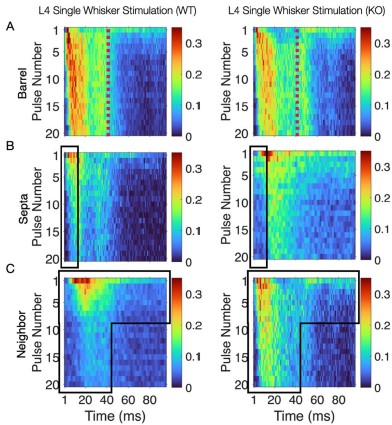
This convergence of response profiles was further clear in stimulus-aligned stacked images, where the emergent differences between barrels and septa under SWS were largely abolished in the KO (Figure 4B). A distinction between directly stimulated barrels and neighboring barrels persisted in the KO. In addition, the initial response continued to differ between barrel and septa and also septa and neighbor (Figure 4B). This initial stimulus selectivity potentially represents distinct feedforward thalamocortical activity, which includes PV+ interneuron recruitment that is not directly impacted by the Elfn1 KO (Sun et al., 2006; Tan et al., 2008). PV+ cells are strongly excited by thalamocortical inputs, but these exhibit short-term depression, as does their output, contrasting with the sustained facilitation observed in SST+ neurons. These findings suggest that in WT animals, activity spillover from principal barrels is normally constrained by the progressive engagement of SST+ interneurons in septal regions, driven by Elfn1-dependent facilitation at their excitatory synapses. In the absence of Elfn1, this local inhibitory mechanism is disrupted, leading to longer responses in barrels, delayed but stronger responses in septa, and persistently stronger responses in unstimulated neighbors, resulting in a loss of distinction between the responses of barrel and septa domains that normally diverge over time (see Author response image 1 below).

Author response image 1.

(A) Barrel responses are longer following whisker stimulation in KO. (B) Septal responses are slightly delayed but stronger in KO. (C) Unstimulated neighbors show longer persistent responses in KO.

(4) Line 585 “the earliest CSD sink was identified as layer 4…” were post-hoc measurements made to determine where the different shank leads were based on the post-hoc histology?

Post hoc histology was performed on plane-aligned brain sections which would allow us to detect barrels and septa, so as to confirm the insertion domains of each recorded shank. Layer specificity of each electrode therefore could therefore not be confirmed by histology as we did not have coronal sections in which to measure electrode depth.

(5) For the retrograde tracing studies, how were the M1 and S2 injections targeted (stereotaxically or physiologically)? How was it determined that the injections were in the whisker region (or not)?

During the retrograde virus injection, the location of M1 and S2 injections was determined by stereotaxic coordinates (Yamashita et al., 2018). After acquiring the light-sheet images, we were able to post hoc examine the injection site in 3D and confirm that the injections were successful in targeting the regions intended. Although it would have been informative to do so, we did not functionally determine the whisker-related M1 and whisker-related S2 region in this experiment.

(6) Were there any baseline differences in spontaneous activity in the septa versus barrel regions, and did this change in the KO animals?

Thank you for this interesting question. Our previous study found that there was a reduction in baseline activity in L4 barrel cortex of KO animals at postnatal day (P)12, but no differences were found at P21 (Stachniak et al., 2023).

Reviewer #3 (Public Reviews):

Summary:

This study investigates the functional differences between barrel and septal columns in the mouse somatosensory cortex, focusing on how local inhibitory dynamics, particularly involving Elfn1-expressing SST⁺ interneurons, may mediate temporal integration of multiwhisker (MW) stimuli in septa. Using a combination of in vivo multi-unit recordings, calcium imaging, and anatomical tracing, the authors propose that septa integrate MW input in an Elfn1-dependent manner, enabling functional segregation from barrel columns.

Strengths:

The core hypothesis is interesting and potentially impactful. While barrels have been extensively characterized, septa remain less understood, especially in mice, and this study's focus on septal integration of MW stimuli offers valuable insights into this underexplored area. If septa indeed act as selective integrators of distributed sensory input, this would add a novel computational role to cortical microcircuits beyond what is currently attributed to barrels alone. The narrative of this paper is intellectually stimulating.

We thank the reviewer for finding the study intellectually stimulating.

Weaknesses:

The methods used in the current study lack the spatial and cellular resolution needed to conclusively support the central claims. The main physiological findings are based on unsorted multi-unit activity (MUA) recorded via low-channel-count silicon probes. MUA inherently pools signals from multiple neurons across different distances and cell types, making it difficult to assign activity to specific columns (barrel vs. septa) or neuron classes (e.g., SST⁺ vs. excitatory).

The recording radius (~50-100 µm or more) and the narrow width of septa (~50-100 µm or less) make it likely that MUA from "septal" electrodes includes spikes from adjacent barrel neurons.

The authors do not provide spike sorting, unit isolation, or anatomical validation that would strengthen spatial attribution. Calcium imaging is restricted to SST⁺ and VIP⁺ interneurons in superficial layers (L2/3), while the main MUA recordings are from layer 4, creating a mismatch in laminar relevance.

We thank the reviewer for pointing out the possibility of contamination in septal electrodes. Importantly, it may not have been highlighted, although reported in the methods, but we used an extremely high threshold (7.5 std, in methods, line 583) for spike detection in order to overcome the issue raised here, which restricts such spatial contaminations. Since the spike amplitude decays rapidly with distance, at high thresholds, only nearby neurons contribute to our analysis, potentially one or two. We believe that this approach provides a very close approximation of single unit activity (SUA) in our reported data. We will include a sentence earlier in the manuscript to make this explicit and prevent further confusion.

Regarding the point on calcium imaging being performed on L2/3 SST and VIP cells instead of L4. Both reviewer 1 and 2 brought up the same issue and we responded as follows. As shown in our supplementary figure, the divergence is also observed in L2/3 where we do not have a differential distribution of SST cells, at least based on a columnar analysis extending from L4. There are multiple scenarios that could explain this “discrepancy” that one would need to examine further in future studies. One straightforward one is that the divergence in spiking in L2/3 domains may be inherited from L4 domains, where L4 SST act on. Another is that even though L2/3 SST neurons are not biased in their distribution their input-output function is, something which one would need to examine by detailed in vitro electrophysiological and perhaps optogenetic approaches in S1. Despite the distinctive differences that have been found between the L4 circuitry in S1 and V1 (Scala F et al., 2019), recent observations indicate that small but regular patches of V1 marked by the absence of muscarinic receptor 2 (M2) have high temporal acuity (Ji et al., 2015), and selectively receive input from SST interneurons (Meier et al., 2025). Regions lacking M2 have distinct input and output connectivity patterns from those that express M2 (Meier et al., 2021; Burkhalter et al., 2023). These findings, together with ours, suggest that SST cells preferentially innervate and regulate specific domains -columns- in sensory cortices.

Furthermore, while the role of Elfn1 in mediating short-term facilitation is supported by prior studies, no new evidence is presented in this paper to confirm that this synaptic mechanism is indeed disrupted in the knockout mice used here.

We thank Reviewer #3 for noting the absence of new evidence confirming Elfn1’s disruption of short-term facilitation in our knockout mice. We acknowledge that our study relies on previously strong published data demonstrating that Elfn1 mediates short-term synaptic facilitation of excitatory inputs onto SST+ interneurons (Sylwestrak and Ghosh, 2012; Tomioka et al., 2014; Stachniak et al., 2019, 2023). These studies consistently show that Elfn1 knockout abolishes facilitation in SST+ synapses, leading to altered temporal dynamics, which we hypothesize underlies the observed loss of barrel-septa response divergence in our Elfn1 KO mice (Figure 4). Nevertheless, to address the point raised, we will clarify in the revised manuscript (around lines 245-247 and 271-272) that our conclusions are based on these established findings, stating: “Building on prior evidence that Elfn1 knockout disrupts short-term facilitation in SST+ interneurons (Sylwestrak and Ghosh, 2012; Tomioka et al., 2014; Stachniak et al., 2019, 2023), we attribute the abolished barrel-septa divergence in Elfn1 KO mice to altered SST+ synaptic dynamics, though direct synaptic measurements were not performed here.”

Additionally, since Elfn1 is constitutively knocked out from development, the possibility of altered circuit formation-including changes in barrel structure and interneuron distribution, cannot be excluded and is not addressed.

We thank Reviewer #3 for raising the valid concern that constitutive Elfn1 knockout could potentially alter circuit formation, including barrel structure and interneuron distribution. To address this, we will clarify in the revised manuscript (around line ~271 and in the Discussion) that in our previous studies that included both whole-cell patch-clamp in acute brain slices ranging from postnatal day 11 to 22 (P11 - P21) and in vivo recordings from barrel cortex at P12 and P21, we saw no gross abnormalities in barrel structure, with Layer 4 barrels maintaining their characteristic size and organization, consistent with wildtype (WT) mice (Stachniak et al., 2019, 2023). While we cannot fully exclude subtle developmental changes, prior studies indicate that Elfn1 primarily modulates synaptic function rather than cortical cytoarchitecture (Tomioka et al., 2014). Elfn1 KO mice show no gross morphological or connectivity differences and the pattern and abundance of Elfn1 expressing cells (assessed by LacZ knock in) appears normal (Dolan and Mitchell, 2013).

We will add the following to the Discussion: “Although Elfn1 is constitutively knocked out, we find here and in previous studies that barrel structure is preserved (Stachniak et al., 2019, 2023). Further, the distribution of Elfn1 expressing interneurons is not different in KO mice, suggesting minimal developmental disruption (Dolan and Mitchell, 2013).

Nonetheless, we acknowledge that subtle circuit changes cannot be ruled out without the usage of time-depended conditional knockout of the gene.”

Recommendations for the authors:

Reviewer #1 (Recommendations for the authors): 

(1) My biggest concern is regarding statistics. Did the authors repeatedly apply independent tests (Mann-Whitney) without any correction for multiple comparisons (Figures 1 and 4)? In that case, the chances of a spurious "significant" result rise dramatically. 

In response to the reviewer’s comment, we now present new statistical results by utilizing ANOVA and blended these results in the manuscript between lines 172 and 192 for WT data and 282 and 298 for Elfn1 KO data. This new statistical approach shows the same differences as we had previously reported, hence consolidating the statements made. 

(2) The findings only hint at a mechanism involving SST+ neurons for how SWS and MWS are processed differently in the barrel vs septal domains. As a direct test of SST+ neuron involvement in the divergence of barrel and septal responses, the authors might consider SST-specific manipulations - for example, inhibitory chemo- or optogenetics during SWS and MWS stimulation.

We thank the reviewer for this comment and agree that a direct manipulation of SST+ neurons via inhibitory chemo- or opto-genetics could provide further supporting evidence for the main claims in our study. We have opted out from performing these experiments for this manuscript as we feel they can be part of a future study.  At the same time, it is conceivable that such manipulations and depending on how they are performed may lead to larger and non-specific effects on cortical activity, since SST neurons will likely be completely shut down. So even though we certainly appreciate and value the strengths of such approaches, our experiments have addressed a more nuanced hypothesis, namely that the synaptic dynamics onto SST+ neurons matter for response divergence of septa versus barrels, which could not have been easily and concretely addressed by manipulating SST+ cell firing activity.  

(3) In general, it is hard to comprehend what microcircuit could lead to the observed divergence in the MWS/SWS ratio in the barrel vs septal domain. There preferential recruitment of SST+ neurons during MWS is not specific to a particular domain, and the higher density of SST+ neurons specifically in L4 septa cannot per se explain the diverging MWS/SWS ratio in L4 septal neurons since similar ratio divergence is observed across domains in L2/3 neurons without increase SST+ neuron density in L2/3. This view would also assume that SST+ inhibition remains contained to its own layer and domain. Is this the case? Is it that different microcircuits between barrels and septa differently shape the response to repeated MWS? This is partially discussed in the paper; can the authors develop on that? What would the proposed mechanism be? Can the short-term plasticity of the thalamic inputs (VPM vs POm) be part of the picture?

We thank the reviewer for raising this important point. We propose that the divergence in MWS/SWS ratios across barrel and septal domains arises from dynamic microcircuit interactions rather than static anatomical features such as SST+ density, which we describe and can provide a hint. In L2/3, where SST+ density is uniform, divergence persists, suggesting that trans-laminar and trans-domain interactions are key. Barrel domains, primarily receiving VPM inputs, exhibit short-term depression onto excitatory cells and engage PV+ and SST+ neurons to stabilize the MWS/SWS ratio, with Elfn1-dependent facilitation of SST+ neurons gradually increasing inhibition during repetitive SWS. Septal domains, in contrast, are targeted by facilitating POm inputs, combined with higher L4 SST+ density and Elfn1-mediated facilitation, producing progressive inhibitory buildup that amplifies the MWS/SWS ratio. SST+ projections in septa may extend trans-laminarly and laterally, influencing L2/3 and neighboring barrels, thereby explaining L2/3 divergence despite uniform SST+ density in L2/3. In this regards, direct laminar-dependent manipulations will be required to confirm whether L2/3 divergence is inherited from L4 dynamics. In Elfn1 KO mice, the loss of facilitation in SST+ neurons likely flattens these dynamics, disrupting functional segregation. Future experiments using VPM/POm-specific optogenetic activation and SST+ silencing will be critical to directly test this model.

We expanded the discussion accordingly.

(4) Can the decoder generalize between SWS and MWS? In this condition, if the decoder accuracy is higher for barrels than septa, it would support the idea that septa are processing the two stimuli differently. 

Our results show that septal decoding accuracy is generally higher than barrel accuracy when generalizing from multi-whisker stimulation (MWS) to single-whisker stimulation (SWS), indicating distinct information processing in septa compared to barrels.

In wild-type (WT) mice, septal accuracy exceeds barrel accuracy across all time windows (150ms, 51-95ms, 1-95ms), with the largest difference in the 51-95ms window (0.9944 vs. 0.9214 at pulse 20, 10Hz stimulation). This septal advantage grows with successive pulses, reflecting robust, separable neural responses, likely driven by the posterior medial nucleus (POm)’s strong MWS integration contrasting with minimal SWS activation. Barrel responses, driven by consistent ventral posteromedial nucleus (VPM) input for both stimuli, are less distinguishable, leading to lower accuracy.

In Elfn1 knockout (KO) mice, which disrupt excitatory drive to somatostatin-positive (SST+) interneurons, barrel accuracy is higher initially in the 1-50ms window (0.8045 vs. 0.7500 at pulse 1), suggesting reduced early septal distinctiveness. However, septal accuracy surpasses barrels in later pulses and time windows (e.g., 0.9714 vs. 0.9227 in 51-95ms at pulse 20), indicating restored septal processing. This supports the role of SST+ interneurons in shaping distinct MWS responses in septa, particularly in late-phase responses (51-95ms), where inhibitory modulation is prominent, as confirmed by calcium imaging showing stronger SST+ activation during MWS.

These findings demonstrate that septa process SWS and MWS differently, with higher decoding accuracy reflecting structured, POm- and SST+-driven response patterns. In Elfn1 KO mice, early deficits in septal processing highlight the importance of SST+ interneurons, with later recovery suggesting compensatory mechanisms. 

We have added Supplementary Figure 4 and included this interpretation between lines 338353. 

We thank the reviewer for suggesting this analysis.

(5) It is not clear to me how the authors achieve SWS. How is it that the pipette tip "placed in contact with the principal whisker" does not detach from the principal whisker or stimulate other whiskers? Please clarify the methods. 

Targeting the specific principal whisker is performed under the stereoscope.  

Specifically, we have added this statement in line 628:

“We trimmed the whiskers where necessary, to avoid them touching each other and to avoid stimulating other whiskers. By putting the pipette tip very close (almost touching) to the principal whisker, the movement of the tip (limited to 1mm) would reliably move the targeted whisker. The specificity of the stimulation of the selected principal whisker was observed under the stereoscope.”

(6) The method for calculating decoder accuracy is not clearly described-how can accuracy exceed 1? The authors should clarify this metric and provide measures of variability (e.g., confidence intervals or standard deviations across runs) to assess the significance of their comparisons. Additionally, using a consistent scale across all plots would improve interoperability. 

We thank the reviewer for raising this point. We have now changed the way accuracies are calculated and adopted a common scale among different plots (see updated Figure 5). We have also changed the methods section accordingly.

(7) Figure 1: The sample size is not specified. It looks like the numbers match the description in the methods, but the sample size should be clearly stated here. 

These are the numbers the reviewer is inquiring about. 

WT: (WT) animals: a 280 × 95 × 20 matrix for the stimulated barrel (14 Barrels, 95ms, 20 pulses), a 180 × 95 × 20 matrix for the septa (9 Septa, 95ms, 20 pulses), and a 360 × 95 × 20 matrix for the neighboring barrel (18 Neighboring barrels, 95ms, 20 pulses). N=4 mice.

KO: 11-barrel columns, 7 septal columns, 11 unstimulated neighbors from N=4 mice.

Panels D-F are missing axes and axis labels (firing rate, p-value). Panel D is mislabeled (left, middle, and right). I can't seem to find the yellow line. 

Thank you for this observation. We made changes in the figures to make them easier to navigate based on the collective feedback from the reviewers.

Why is changing the way to compare the differences in the responses to repeated stimulation between SWS and MWS? 

To assess temporal accumulation of information, we compared responses to repeated single-whisker stimulation (SWS) and multi-whisker stimulation (MWS) using an accumulative decoding approach rather than simple per-pulse firing rates. This method captures domain-specific integration dynamics over successive pulses.

The use of the term "principal whisker" is confusing, as it could refer to the whisker that corresponds to the recorded barrel. 

When we use the term principal whisker, the intention is indeed to refer to the whisker corresponding to the recorded barrel during single whisker stimulation. The term principal whisker is removed from Figure legend 1 and legend S1C where it may have led to  ambiguity.    

Why the statement "after the start of active whisking"? Mice are under anesthesia here; it does not appear to be relevant for the figure. 

“After the start of active whisking” refers to the state of the barrel cortex circuitry at the time of recordings. The particular reference we use comes from the habit of assessing sensory processing also from a developmental point of view. The reviewer is correct that it has nothing to do the with the status of the experiment. Nevertheless, since the reviewer found that it may create confusion, we have now taken it out. 

(8) Figure 3: The y-axis label is missing for panel C. 

This is now fixed. (dF/F).

(9) Figure 4: Axis labels are missing.

Added.

Minor: 

(10) Line 36: "progressive increase in septal spiking activity upon multi-whisker stimulation". There is no increase in septal spiking activity upon MWS; the ratio MWS/SWS increases.

We have changed the sentence as follows: Genetic removal of Elfn1, which regulates the incoming excitatory synaptic dynamics onto SST+ interneurons, leads to the loss of the progressive increase in septal spiking ratio (MWS/SWS) upon stimulation.

(11) Line 105: domain-specific, rather than column-specific, for consistency.

We have changed it.

(12) Lines 173-174: "a divergence between barrel and septa domain activity also occurred in Layer 4 from the 2nd pulse onward (Figure 1E)". The authors only show a restricted number of comparisons. Why not show the p-values as for SWS?

The statistics is now presented in current Figure 1E.

(13) Lines 151-153: "Correspondingly, when a single whisker is stimulated repeatedly, the response to the first pulse is principally bottom-up thalamic-driven responses, while the later pulses in the train are expected to also gradually engage cortico-thalamo-cortical and cortico-cortical loops." Can the authors please provide a reference?

We have now added the following references : (Kyriazi and Simons, 1993; Middleton et al., 2010; Russo et al., 2025).

(14) Lines 184-186: "Our electrophysiological experiments show a significant divergence of responses over time upon both SWS and MWS in L4 between barrels (principal and neighboring) and adjacent septa, with minimal initial difference". The only difference between the neighboring barrel and septa is the responses to the initial pulse. Can the author clarify? 

We have now changed the sentence as follows: Our electrophysiological experiments show a significant divergence of responses between domains upon both SWS and MWS in L4. (Line 198 now)

(15) Line 214: "suggest these interneurons may play a role in diverging responses between barrels and septa upon SWS". Why SWS specifically?

We have changed the sentence as follows: These results confirmed that SST+ and VIP+ interneurons have higher densities in septa compared to barrels in L4 and suggest these interneurons may play a role in diverging responses between barrels and septa. (Line 231 now).

(16) Line 235: "This result suggests that differential activation of SST+ interneurons is more likely to be involved in the domain-specific temporal ratio differences between barrels and septa". Why? The results here are not domain-specific.

We have now revised this statement to: This result suggested that temporal ratio differences specific to barrels and septa might involve differential activation of SST+ interneurons rather than VIP+ interneurons.

(17) Lines 241-243: "SST+ interneurons in the cortex are known to show distinct short-term synaptic plasticity, particularly strong facilitation of excitatory inputs, which enables them to regulate the temporal dynamics of cortical circuits." Please provide a reference.

We have now added the following references: (Grier et al., 2023; Liguz-Lecznar et al., 2016).

(18) Lines 245-247: "A key regulator of this plasticity is the synaptic protein Elfn1, which mediates short-term synaptic facilitation of excitation on SST+ interneurons (Stachniak et al., 2021, 2019; Tomioka et al., 2014)". Is Stachniak et al., 2021 not about the role of Elf1n in excitatory-to-VIP+ neuron synapses?

The reviewer correctly spotted this discrepancy . This reference has now been removed from this statement.

(19) Lines 271-272: "Building on our findings that Elfn1-dependent facilitation in SST+ interneurons is critical for maintaining barrel-septa response divergence". The authors did not show that.

We have now changed the statement to: Building on our findings that Elfn1 is critical for maintaining barrel-septa response divergence  

(20) Line 280: second firing peak, not "peal".

Thank you, it is now fixed.

(21) Lines 304-305: "These results highlight the critical role of Elfn1 in facilitating the temporal integration of 305 sensory inputs through its effects on SST+ interneurons". This claim is also overstated. 

We have now changed the statement to: These results highlight the contribution of Elfn1 to the temporal integration of sensory inputs. (Line 362)

(22) Line 329: Any reason why not cite Chen et al., Nature 2013?

We have now added this reference, as also pointed out by reviewer 1.

(23) Line 341-342: "wS1" and "wS2" instead of S1 and S2 for consistency.

Thanks, we have now updated the terms.

Reviewer #2 (Recommendations for the authors): 

(1) Figure 3D - the SW conditions are labeled but not the MW conditions (two right graphs) - they should be labeled similarly (SSTMW, VIPMW). 

The two right graphs in Figure 3D represent paired SW vs MW comparisons of the evoked responses for SST and VIP populations, respectively.

(2) Figure 6 D and E I think it would be better if the Depth measurements were to be on the yaxis, which is more typical of these types of plots. 

We thank the reviewer for this comment. Although we appreciate this may be the case, we feel that the current presentation may be easier for the reader to navigate, and we have hence kept it. 

(3) Having an operational definition of septa versus barrel would be useful. As the authors point out, this is a tough distinction in a mouse, and often you read papers that use Barrel Wall versus Barrel Hollow/Center - operationally defining how these areas were distinguished would be helpful. 

We thank the reviewer for this comment and understand the point made.

We have now updated the methods section in line 611: 

DiI marks contained within the vGlut2 staining were defined as barrel recordings, while DiI marks outside vGlut2 staining were septal recordings.

Reviewer #3 (Recommendations for the authors): 

To support the manuscript's major claims, the authors should consider the following:

(1) Validate the septal identity of the neurons studied, either anatomically or functionally at the single-cell level (e.g., via Ca²⁺ imaging with confirmed barrel/septa mapping). 

We thank the reviewer for this suggestion, but we feel that these extensive experiments are beyond the scope of this study. 

(2) Provide both anatomical and physiological evidence to assess the possibility of altered cortical development in Elfn1 KO mice, including potential changes in barrel structure or SST⁺ cell distribution. 

To address the reviewer’s point, we have now added the following to the Discussion: “Although Elfn1 is constitutively knocked out, we find here and in previous studies that barrel structure is preserved (Stachniak et al., 2019, 2023). Further, the distribution of Elfn1 expressing interneurons is not different in KO mice, suggesting minimal developmental disruption (Dolan and Mitchell, 2013). Nonetheless, we acknowledge that subtle circuit changes cannot be ruled out without conditional knockouts.”,

(3) Examine the sensory responses of SST⁺ and VIP⁺ interneurons in deeper cortical layers, particularly layer 4, which is central to the study's main conclusions.

We thank the reviewer for this suggestion and appreciate the value it would bring to the study. We nevertheless feel that these extensive experiments are beyond the scope of this study and hence opted out from performing them. 

Minor Comments:

(1)  The authors used a CLARITY-based passive clearing protocol, which is known to sometimes induce tissue swelling or distortion. This may affect anatomical precision, especially when assigning neurons to narrow domains such as septa versus barrels. Please clarify whether tissue expansion was measured, corrected, or otherwise accounted for during analysis.

Yes, the tissue expansion was accounted during analysis for the laminar specification. We excluded the brains with severe distortion. 

(2) While the anatomical data are plotted as a function of "depth from the top of layer 4," the manuscript does not specify the precise depth ranges used to define individual cortical layers in the cleared tissue. Given the importance of laminar specificity in projection and cell type analyses, the criteria and boundaries used to delineate each layer should be explicitly stated.

Thank you for pointing this out. We now include the criteria for delineating each layer in the manuscript. “Given that the depth of Layer 4 (L4) can be reliably measured due to its welldefined barrel boundaries, and that the relative widths of other layers have been previously characterized (El-Boustani et al., 2018), we estimated laminar boundaries proportionally. Specifically, Layer 2/3 was set to approximately 1.3–1.5 times the width of L4, Layer 5a to ~0.5 times, and Layer 5b to a similar width as L4. Assuming uniform tissue expansion across the cortical column, we extrapolated the remaining laminar thicknesses proportionally.”

(3)  In several key comparisons (e.g., SST⁺ vs. VIP⁺ interneurons, or S2-projecting vs. M1projecting neurons), it is unclear whether the same barrel columns were analyzed across conditions. Given the anatomical and functional heterogeneity across wS1 columns, failing to control for this may introduce significant confounds. We recommend analyzing matched columns across groups or, if not feasible, clearly acknowledging this limitation in the manuscript.

We thank the reviewer for raising this important point. For the comparison of SST⁺ versus VIP⁺ interneurons, it would in principle have been possible to analyze the same barrel columns across groups. However, because some of the cleared brains did not reach the optimal level of clarity, our choice of columns was limited, and we were not always able to obtain sufficiently clear data from the same columns in both groups. Similarly, for the analysis of S2- versus M1-projecting neurons, variability in the position and spread of retrograde virus injections made it difficult to ensure measurements from identical barrel columns. We have now added a statement in the Discussion to acknowledge this limitation.

(4) Figure 1C: Clarify what each point in the t-SNE plot represents-e.g., a single trial, a recording channel, or an averaged response. Also, describe the input features used for dimensionality reduction, including time windows and preprocessing steps.

In response to the reviewer’s comment, we have now added the following in the methods: In summary, each point in the t-SNE plots represents an averaged response across 20 trials for a specific domain (barrel, septa, or neighbor) and genotype (WT or KO), with approximately 14 points per domain derived from the 280 trials in each dataset. The input features are preprocessed by averaging blocks of 20 trials into 1900-dimensional vectors (95ms × 20), which are then reduced to 2D using t-SNE with the specified parameters. This approach effectively highlights the segregation and clustering patterns of neural responses across cortical domains in both WT and KO conditions.

(5) Figures 1D, E (left panels): The y-axes lack unit labeling and scale bars. Please indicate whether values are in spikes/sec, spikes/bin, or normalized units.

We have now clarified this. 

(6) Figures 1D, E (right panels): The color bars lack units. Specify whether the values represent raw firing rates, z-scores, or other normalized measures. Replace the vague term "Matrix representation" with a clearer label such as "Pulse-aligned firing heatmap."

Thank you, we have now done it.

(7) Figure 1E (bottom panel): There appears to be no legend referring to these panels. Please define labels such as "B" and "S." 

Thank you, we have now done it.

(8) Figure 1E legend: If it duplicates the legend from Figure 1D, this should be made explicit or integrated accordingly. 

We have changed the structure of this figure.

(9) Figure 1F: Define "AUC" and explain how it was computed (e.g., area under the firing rate curve over 0-50 ms). Indicate whether the plotted values represent percentages and, if so, label the y-axis accordingly. If normalization was applied, describe the procedure. Include sample sizes (n) and specify what each data point represents (e.g., animal, recording site). 

The following paragraph has been added in the methods section:

The Area Under the Curve (AUC) was computed as the integral of the smoothed firing rate (spikes per millisecond) over a 50ms window following each whisker stimulation pulse, using trapezoidal integration. Firing rate data for layer 4 barrel and septal regions in wild-type (WT) and knockout (KO) mice were smoothed with a 3-point moving average and averaged across blocks of 20 trials. Plotted values represent the percentage ratio of multi-whisker (MW) to single whisker (SW) AUC with error bars showing the standard error of the mean. Each data point reflects the mean AUC ratio for a stimulation pulse across approximately 11 blocks (220 trials total). The y-axis indicates percentages.

(10) Figure 3C: Add units to the vertical axis.

We have added them.

(11) Figure 3D: Specify what each line represents (e.g., average of n cells, individual responses?). 

Each line represents an average response of a neuron.  

(12) Figure 4C legend: Same with what?". No legend refers to the bottom panels - please revise to clarify. 

Thank you. We have now changed the figure structure and legends and fixed the missing information issue.

(13) Supplementary Figure 1B: Indicate the physical length of the scale bar in micrometers. 

This has been fixed. The scale bar is 250um.

(14) Indicate the catalog number or product name of the 8×8 silicon probe used for recordings.

We have added this information. It is the A8x8-Edge-5mm-100-200-177-A64

References

(1) Beierlein, M., Gibson, J. R. & Connors, B. W. (2003). Two dynamically distinct inhibitory networks in layer 4 of the neocortex. J. Neurophysiol. 90, 2987–3000.

(2) Burkhalter, A., D’Souza, R. D. & Ji, W. (2023). Integration of feedforward and feedback information streams in the modular architecture of mouse visual cortex. Annu. Rev. Neurosci. 46, 259–280.

(3) Chen, J. L., Margolis, D. J., Stankov, A., Sumanovski, L. T., Schneider, B. L. & Helmchen, F. (2015). Pathway-specific reorganization of projection neurons in somatosensory cortex during learning. Nat. Neurosci. 18, 1101–1108.

(4) Connor, J. R. & Peters, A. (1984). Vasoactive intestinal polypeptide-immunoreactive neurons in rat visual cortex. Neuroscience 12, 1027–1044.

(5) Cruikshank, S. J., Lewis, T. J. & Connors, B. W. (2007). Synaptic basis for intense thalamocortical activation of feedforward inhibitory cells in neocortex. Nat. Neurosci. 10, 462–468.

(6) Dolan, J. & Mitchell, K. J. (2013). Mutation of Elfn1 in mice causes seizures and hyperactivity. PLoS One 8, e80491.

(7) Gibson, J. R., Beierlein, M. & Connors, B. W. (1999). Two networks of electrically coupled inhibitory neurons in neocortex. Nature 402, 75–79.

(8) Ji, W., Gămănuţ, R., Bista, P., D’Souza, R. D., Wang, Q. & Burkhalter, A. (2015). Modularity in the organization of mouse primary visual cortex. Neuron 87, 632–643.

(9) Martin-Cortecero, J. & Nuñez, A. (2014). Tactile response adaptation to whisker stimulation in the lemniscal somatosensory pathway of rats. Brain Res. 1591, 27–37.

(10) Mégevand, P., Troncoso, E., Quairiaux, C., Muller, D., Michel, C. M. & Kiss, J. Z. (2009). Long-term plasticity in mouse sensorimotor circuits after rhythmic whisker stimulation. J. Neurosci. 29, 5326–5335.

(11) Meier, A. M., Wang, Q., Ji, W., Ganachaud, J. & Burkhalter, A. (2021). Modular network between postrhinal visual cortex, amygdala, and entorhinal cortex. J. Neurosci. 41, 4809– 4825.

(12) Meier, A. M., D’Souza, R. D., Ji, W., Han, E. B. & Burkhalter, A. (2025). Interdigitating modules for visual processing during locomotion and rest in mouse V1. bioRxiv 2025.02.21.639505.

(13) Scala, F., Kobak, D., Shan, S., Bernaerts, Y., Laturnus, S., Cadwell, C. R., Hartmanis, L., Froudarakis, E., Castro, J. R., Tan, Z. H., et al. (2019). Layer 4 of mouse neocortex differs in cell types and circuit organization between sensory areas. Nat. Commun. 10, 4174.

(14) Stachniak, T. J., Sylwestrak, E. L., Scheiffele, P., Hall, B. J. & Ghosh, A. (2019). Elfn1induced constitutive activation of mGluR7 determines frequency-dependent recruitment of somatostatin interneurons. J. Neurosci. 39, 4461–4475.

(15) Stachniak, T. J., Kastli, R., Hanley, O., Argunsah, A. Ö., van der Valk, E. G. T., Kanatouris, G. & Karayannis, T. (2021). Postmitotic Prox1 expression controls the final specification of cortical VIP interneuron subtypes. J. Neurosci. 41, 8150–8166.

(16) Stachniak, T. J., Argunsah, A. Ö., Yang, J. W., Cai, L. & Karayannis, T. (2023). Presynaptic kainate receptors onto somatostatin interneurons are recruited by activity throughout development and contribute to cortical sensory adaptation. J. Neurosci. 43, 7101–7118.

(17) Sun, Q.-Q., Huguenard, J. R. & Prince, D. A. (2006). Barrel cortex microcircuits: Thalamocortical feedforward inhibition in spiny stellate cells is mediated by a small number of fast-spiking interneurons. J. Neurosci. 26, 1219–1230.

(18) Sylwestrak, E. L. & Ghosh, A. (2012). Elfn1 regulates target-specific release probability at CA1-interneuron synapses. Science 338, 536–540.

(19) Tan, Z., Hu, H., Huang, Z. J. & Agmon, A. (2008). Robust but delayed thalamocortical activation of dendritic-targeting inhibitory interneurons. Proc. Natl. Acad. Sci. USA 105, 2187–2192.

(20) Tomioka, N. H., Yasuda, H., Miyamoto, H., Hatayama, M., Morimura, N., Matsumoto, Y., Suzuki, T., Odagawa, M., Odaka, Y. S., Iwayama, Y., et al. (2014). Elfn1 recruits presynaptic mGluR7 in trans and its loss results in seizures. Nat. Commun. 5, 4501.

(21) Yamashita, T., Vavladeli, A., Pala, A., Galan, K., Crochet, S., Petersen, S. S. & Petersen, C. C. (2018). Diverse long-range axonal projections of excitatory layer 2/3 neurons in mouse barrel cortex. Front. Neuroanat. 12, 33.

Reviewer #2 (Public review):

Summary:

In this manuscript, Pereira de Castro and coworkers are studying potential competition between a more standard splicing factor SF1 and an alternative splicing factor called QK1. This is interesting because they bind to overlapping sequence motifs and could potentially have opposing effects on promoting the splicing reaction. To test this idea, the authors KD either SF1 or QK1 in mammalian cells and uncover several exons whose splicing regulation follows the predicted pattern of being promoted for splicing by SF1 and repressed by QK1. Importantly, these have introns enriched in SF1 and QK1 motifs. The authors then focus on one exon in particular with two tandem motifs to study the mechanism of this in greater detail and their results confirm the competition model. Mass spec analysis largely agrees with their proposal; however, it is complicated by apparently quick transition of SF1 bound complexes to later splicing intermediates. An inspired experiment in yeast shows how QK1 competition could potentially have a determinental impact on splicing in an orthogonal system. Overall these results show how splicing regulation can be achieved by competition between a "core" and alternative splicing factor and provide additional insight into the complex process of branch site recognition. The manuscript is exceptionally clear and the figures and data very logically presented. The work will be valuable to those in the splicing field who are interested in both mechanism and bioinformatics approaches to deconvolve any apparent "splicing code" being used by cells to regulate gene expression.

Strengths:

(1) The main discovery of the manuscript involving evidence for SF1/QK1 competition is quite interesting and important for this field. This evidence has been missing and may change how people think about branch site recognition.

(2) The experiments and the rationale behind them are clearly and logically presented.

(3) The experiments are carried out to a high standard and well-designed controls are included.

(4) The extrapolation of the result to yeast in order to show the potentially devastating consequences of QK1 competition was creative and informative.

Weaknesses:

Overall the weaknesses are relatively minor and involve cases where conclusions could potentially have been strengthened with additional experimentation. For example, pull-down of the U2 snRNP could be strengthened by detection of the snRNA whereas the proteins may themselves interact with these factors in the absence of the snRNA. In addition the discussion is a bit speculative given the data, but compelling nonetheless.

Author response:

The following is the authors’ response to the original reviews.

eLife Assessment

This important manuscript provides insights into the competition between Splicing Factor 1 (SF1) and Quaking (QKI) for binding at the ACUAA branch point sequence in a model intron, regulating exon inclusion. The study employs rigorous transcriptomic, proteomic, and reporter assays, with both mammalian cell culture and yeast models. Nevertheless, while the data are convincing, broadening the analysis to additional exons and narrowing the manuscript's title to better align with the experimental scope would strengthen the work.

Public Reviews:

Reviewer #1 (Public review):

In this manuscript, the authors aimed to show that SF1 and QKI compete for the intron branch point sequence ACUAA and provide evidence that QKI represses inclusion when bound to it.

Major strengths of this manuscript include:

(1) Identification of the ACUAA-like motif in exons regulated by QKI and SF1.

(2) The use of the splicing reporter and mutant analysis to show that upstream and downstream ACUAAC elements in intron 10 of RAI are required for repressing splicing.

(3) The use of proteomic to identify proteins in C2C12 nuclear extract that binds to the wild type and mutant sequence.

(4) The yeast studies showing that ectopic lethality when Qki5 expression was induced, due to increased mis-splicing of transcripts that contain the ACUAA element.

The authors conclusively show that the ACUAA sequence is bound by QKI and provide strong evidence that this leads to differences in exons inclusion and exclusion. In animal cells, and especially in human, branchpoint sequences are degenerate but seem to be recognized by specific splicing factors. Although a subset of splicing factors shows tissue-specific expression patterns most don't, suggesting that yet-to-be-identified mechanisms regulate splicing. This work suggests that an alternate mechanism could be related to the binding affinity of specific RNA binding factors for branchpoint sequences coupled with the level of these different splicing factors in a given cell.

We thank the reviewer for the positive comments.

Reviewer #2 (Public review):

Summary:

In this manuscript, Pereira de Castro and coworkers are studying potential competition between a more standard splicing factor SF1, and an alternative splicing factor called QK1. This is interesting because they bind to overlapping sequence motifs and could potentially have opposing effects on promoting the splicing reaction. To test this idea, the authors KD either SF1 or QK1 in mammalian cells and uncover several exons whose splicing regulation follows the predicted pattern of being promoted for splicing by SF1 and repressed by QK1. Importantly, these have introns enriched in SF1 and QK1 motifs. The authors then focus on one exon in particular with two tandem motifs to study the mechanism of this in greater detail and their results confirm the competition model. Mass spec analysis largely agrees with their proposal; however, it is complicated by the apparently quick transition of SF1-bound complexes to later splicing intermediates. An inspired experiment in yeast shows how QK1 competition could potentially have a detrimental impact on splicing in an orthogonal system. Overall, these results show how splicing regulation can be achieved by competition between a "core" and alternative splicing factor and provide additional insight into the complex process of branch site recognition. The manuscript is exceptionally clear and the figures and data are very logically presented. The work will be valuable to those in the splicing field who are interested in both mechanism and bioinformatics approaches to deconvolve any apparent "splicing code" being used by cells to regulate gene expression. Criticisms are minor and the most important of them stem from overemphasis on parts of the manuscript on the evolutionary angle when evolution itself wasn't analyzed per se.

We thank the reviewer for the positive comments and very clear and fair critical points.

Strengths:

(1) The main discovery of the manuscript involving evidence for SF1/QK1 competition is quite interesting and important for this field. This evidence has been missing and may change how people think about branch site recognition.

(2) The experiments and the rationale behind them are exceptionally clearly and logically presented. This was wonderful!

Thank you so much. We felt the overall flow of the paper and data make for a nice “story” that conveys a relatively easy-to-understand explanation for a complex subject.

(3) The experiments are carried out to a high standard and well-designed controls are included.

(4) The extrapolation of the result to yeast in order to show the potentially devastating consequences of the QK1 competition was very exciting and creative.

We agree this is a very exciting result and finding! Thanks.

Weaknesses:

Overall the weaknesses are relatively minor and involve cases where clarification is necessary, some additional analysis could bolster the arguments, and suggestions for focusing the manuscript on its strengths.

(1) The title (Ancient...evolutionary outcomes), abstract, and some parts of the discussion focus heavily on the evolutionary implications of this work. However, evolutionary analysis was not performed in these studies (e.g., when did QK1 and SF1 proteins arise and/or diverge? How does this line up with branch site motifs and evolution of U2? Any insight from recent work from Scott Roy et al?). I think this aspect either needs to be bolstered with experimental work/data or this should be tamped down in the manuscript. I suggest highlighting the idea expressed in the sentence "A nuanced implication of this model is that loss-of-function...". To me, this is better supported by the data and potentially by some analysis of mutations associated with human disease.

We have revised the title and dampened the evolutionary aspects of the previous version of the manuscript.

(2) One paper that I didn't see cited was that by Tanackovic and Kramer (Mol Biol Cell 2005). This paper is relevant because they KD SF1 and found it nonessential for splicing in vivo. Do their results have implications for those here? How do the results of the KD compare? Could QK1 competition have influenced their findings (or does their work influence the "nuanced implication" model referenced above?)?

This is an interesting point, and thank you for the suggestion. We have now included a brief description of this study in the Introduction of the revised manuscript and do note that the authors measured intron retention of a beta globin reporter and SF3A1, SF3A2, and SF3A3 during SF1 knockdown, but did not detect elevated unspliced RNA in these targets.

(3) Can the authors please provide a citation for the statement "degeneracy is observed to a higher degree in organisms with more alternative splicing"? Does recent evolutionary analysis support this?

We have removed the statement, as it did not add much to the content and I am not sure I can state the concept I was attempting to convey in a simple manner with few citations.

(4) For the data in Figure 3, I was left wondering if NMD was confounding this analysis. Can the authors respond to this and address this concern directly?

We have not measured if the reporters used in Figure 3 produce protein(s). Presumably, though, all spliced reporter RNA would be degraded equally (the included/skipped isoforms’ “reading frames” are not altered from one another). This would not be case for unspliced nuclear reporter RNA, however. Given this difference, and that our analysis can not resolve the subcellular localization of the different reporter species, we have removed the measurement of and subsequent results describing unspliced reporter RNA from Figure 3.

(5) To me, the idea that an engaged U2 snRNP was pulled down in Figure 4F would be stronger if the snRNA was detected. Was that able to be observed by northern or primer extension? Would SF1 be enriched if the U2 snRNA was degraded by RNaseH in the NE?

We did not measure any co-associating RNAs in this experimental approach, but agree that this approach would strengthen the evidence for it.

(6) I'm wondering how additive the effects of QK1 and SF1 are... In Figure 2, if QK1 and SF1 are both knocked down, is the splicing of exon 11 restored to "wt" levels?

This is an interesting question that we were unfortunately unable to address experimentally here.

(7) The first discussion section has two paragraphs that begin "How does competition between SF1..." and "Relatively little is known about how...". I found the discussion and speculation about localization, paraspekles, and lncRNAs interesting but a bit detracting from the strengths of the manuscript. I would suggest shortening these two paragraphs into a single one.

We have revised the Discussion.

Reviewer #3 (Public review):

Summary:

In this manuscript, the authors were trying to establish whether competition between the RNA-binding proteins SF1 and QKI controlled splicing outcomes. These two proteins have similar binding sites and protein sequences, but SF1 lacks a dimerization motif and seems to bind a single version of the binding sequence. Importantly, these binding sequences correspond to branchpoint consensus sequences, with SF1 binding leading to productive splicing, but QKI binding leading instead to association with paraspeckle proteins. They show that in human cells SF1 generally activates exons and QKI represses, and a large group of the jointly regulated exons (43% of joint targets) are reciprocally controlled by SF1 and QKI. They focus on one of these exons RAI14 that shows this reciprocal pattern of regulation, and has 2 repeats of the binding site that make it a candidate for joint regulation, and confirm regulation within a minigene context. The authors used the assembly of proteins within nuclear extracts to explain the effect of QKI versus SF1 binding. Finally, the authors show that the expression of QKI is lethal in yeast, and causes splicing defects.

How this fits in the field. This study is interesting and provides a conceptual advance by providing a general rule on how SF1 and QKI interact in relation to binding sites, and the relative molecular fates followed, so is very useful. Most of the analysis seems to focus on one example, although the molecular analysis and global work significantly add to the picture from the previously published paper about NUMB joint regulation by QKI and SF (Zong et al, cited in text as reference 50, that looked at SF1 and QKI binding in relation to a duplicated binding site/branchpoint sequence in NUMB).

Thank you for the encouraging remarks.

Strengths:

The data presented are strong and clear. The ideas discussed in this paper are of wide interest, and present a simple model where two binding sites generate a potentially repressive QKI response, whereas exons that have a single upstream sequence are just regulated by SF1. The assembly of splicing complexes on RNAs derived from RAI14 in nuclear extracts, followed by mass spec gave interesting mechanistic insight into what was occurring as a result of QKI versus SF1 binding.

Weaknesses:

I did not think the title best summarises the take-home message and could be perhaps a bit more modest. Although the authors investigated splicing patterns in yeast and human cells, yeast do not have QKI so there is no ancient competition in that case, and the study did not really investigate physiological or evolutionary outcomes in splicing, although it provides interesting speculation on them. Also as I understood it, the important issue was less conserved branchpoints in higher eukaryotes enabling alternative splicing, rather than competition for the conserved branchpoint sequence. So despite the the data being strong and properly analysed and discussed in the paper, could the authors think whether they fit best with the take-home message provided in the title? Just as a suggestion (I am sure the authors can do a better job), maybe "molecular competition between variant branchpoint sequences predict physiological and evolutionary outcomes in splicing"?

Thank you for this point (Reviewer 2 had a similar comment) and the suggestion. We have revised the title.

Although the authors do provide some global data, most of the detailed analysis is of RAI14. It would have been useful to examine members of the other quadrants in Figure 1C as well for potential binding sites to give a reason why these are not co-regulated in the same way as RAI14. How many of the RAI14 quadrants had single/double sites (the motif analysis seemed to pull out just one), and could one of the non-reciprocally regulated exons be moved into a different quadrant by addition or subtraction of a binding site or changing the branchpoint (using a minigene approach for example).

This is an interesting point that we have considered. Our intent with the focus on RAI14 was to use a naturally occurring intron bps with evidence of strong QKI binding that did not require a high degree of sequence manipulation or engineering.

Recommendations for the authors:

Reviewer #1 (Recommendations for the authors):

(1) Most of my recommendations are really centered on the figures. In their current state, they detract from the data shown and could be improved: I recommend the authors use a uniform font. For example, Figure 1E and F have at least three different fonts of varying sizes making it very messy. In Figure 1C, the authors could bold the Ral14 ex11 or simply indicate that the blue is this exon in the legend, thus removing the text from this very busy graph. In Figure 4F, I would recommend, having all the labels the same size and putting those genes of interest like Sf3a1 in bold. This could also be done in Figure 4E.

Thank you for the suggestion and we have edited these (FYI the font in Fig’s 1E and 1F were from the rMAPS default output, but I agree, it gives a sloppy appearance).

(2) In Figures 4D and 4G, is there QKI binding to the downstream deletion mutant after 30 minutes? Also, in Figure 4G, are these all from the same blot? The band sizes seem to be very different between lanes. If these were not on the same blot, the original gels should be submitted.

A small amount of Qki appears to be binding after 30 min. All lanes/blots are from the same gels/membranes; see new Supplemental Figure 4 for the original (uncropped) images of the blots.

(3) The authors should indicate, the source and concentration of the antibodies used for their WB. They should also indicate the primers used for RT-PCRs.

We have revised the methods to include the antibody information and have uploaded a supplemental table 8 with all oligonucleotide sequences used (which I (Sam Fagg) neglected to do initially, so that’s my bad).

Reviewer #2 (Recommendations for the authors):

(1) This may come down to the author's preference but branch point and branch site are frequently two words, not a single compound word (branch point vs. branchpoint). In addition, the authors may want to use branchsite with the abbreviation BS more frequently since they often don't describe the specific point of branching, and bp and bps could be confused for the more frequent abbreviations for base pair(s).

Good suggestion; we have edited the text accordingly.

(2) In general the addition of page numbers and line numbers to the manuscript would greatly aid reviewers!

Point taken…

(3) Introduction; "...under normal growth conditions they are efficiently spliced". I would say MOST introns in yeast are efficiently spliced. This is definitely not universal.

Text edited to indicate that most are efficiently spliced.

(4) Introduction; " recognition of the bps by SF1 (mammals) (20)". The choice of reference 20 is an odd one here. I think the Robin Reed and Michael Rosbash paper was the first to show SF1 was the human homolog of BBP.

Got it, thanks (added #14 here and kept #20 also since it shows the structure of SF1 in complex with a UACUAAC bps.)

(5) Results; "QK1 and SF1 co-regulate.."; it may be useful for the reader if you could explain in more detail why exon inclusion and intron retention are expected outcomes for QK1 knockdown and vice versa for SF1. The exon inclusion here is more obvious than the intron retention phenotype. (In other words, if more exons are included shouldn't it follow that more introns are removed?)

We explain the expected results for exon inclusion in the Introduction and this paragraph of the Results. Although we have observed more intron retention under QKI loss-of-function approaches before, I am uncertain where the reviewer sees that we indicate any expected result for intron retention from either QKI or SF1 knockdown. I believe the statement you refer to might be on line 162 and starts with: “Consistent with potentially opposing functions in splicing…” ?

Also, I agree that if SF1 is a “splicing activator,” one might expect more IR in its absence (but this is not the case; there is, in fact, less), but nonetheless, the opposite outcome is observed with QKI knockdown (more IR). It is unclear why this is the case, and we did not investigate it.

(6) Results; "QK1 and SF1 co-regulate.."; "Thus the most highly represented set.." To me, the most highly represented set is those which are not both QK1-repressed and SF1-activated. Does this indicate that other factors are involved at most sites than simple competition between these two?

We have revised the sentence in question to include the text “by quadrant” in order to convey our meaning more precisely.

(7) Throughout the manuscript, 5 apostrophes and 3 apostrophes are used instead of 5 prime symbols and 3 prime symbols.

Thank you for pointing that out. We have fixed each instance of this.

(8) Sometimes SF1 is written as Sf1. (also Tatsf1)

This was a mouse/human gene/protein nomenclature error that we have fixed; thank you for pointing this out.

(9) You may want to make sure that figures are labeled consistently with the manuscript text. In Figure 1B, it is RI rather than IR. In Figure 4 it is myoblast NE rather than C2C12 nuclear extract.

We have fixed these, checked for other examples, and where relevant, edited those too.

(10) I think Figure 1A could be improved by also including a depiction of the domain arrangements of SF1 and QK1.

Done.

(11) I was a bit confused with all the lines in Figure 1E and 1F. What is the difference between the log (pVal) and upregulated plots? Can these figures be simplified or explained more thoroughly?

Based on this comment and one from Reviewer 1, we have slightly revised the wording (and font) on the output, which hopefully clarifies. These are motif enrichment plots generated by rMAPS (Refs 61 and 62) analysis of rMATS (Ref 60) data for exons more included (depicted by the red lines) or more skipped (depicted by the blue lines) compared to control versus a “background” set of exons that are detectable but unchanged. The -log₁₀ is P-value (dotted line) indicates the significance of exons more included in shRNA treatment vs control shRNA (previously read “upregulated”) compared to background exons that are detectable but unchanged; the solid lines indicate the motif score; these are described in the references indicated.

(12) Figure 1B, it is a bit hard to conclude that there is more AltEx or "RI/IR" in one sample vs. the other from these plots since the points overlay one another. Can you include numbers here?

Added (and deleted Suppl Fig S1, which was simply a chart showing the numbers).

(13) How was PSI calculated in Figure 2A?

VAST-tools (we state this in the legend in the revised version).

You may want to include rel protein (or the lower limit of detection) for Figure 2B to be consistent with 2C. Why is KD of SF1 so poor and variable between 2C and 2D?

We have not investigated this, but these blots show an optimized result that we were able to obtain for the knockdown in each cell type. It may be that HEK293 cells (Fig 2B) have a stronger requirement for SF1 than C2C12 cells…? I would argue that it is not necessarily “poor” in Fig 2C, as we observe ~70% depletion of the protein.

Why are two bands present in the gel?

Two to three isoforms of SF1 are present in most cell types.

A good (or bad, really) example of an SF1 western blot (and knockdown of ~35% in K562 or ~45% in HepG2 can also be seen on the ENCODE project website, for reference:

https://www.encodeproject.org/documents/6001a414-b096-4073-94ff-3af165617eb5/@@download/attachment/SF1_BGKLV28-49.pdf

By comparison, I think ours are much more cosmetically pleasing, and our knockdown (especially in C2C12) is much more efficient.

(14) Figure 3, The asterisk refers to a cryptic product. Can the uaAcuuuCAG be used as a branch point? Presumably the natural 3' SS is now too close so this would result in activation of a downstream 3'SS?

We did not pursue determining the identity of this minor and likely artefactual product, but we (and others) have observed a similar phenomenon when using splicing reporter-based mutational approaches.

(15) For the methods. The "RNA extraction, RT -PCR,..." subheading needs to be on its own line. Please add (w/v) or (v/v) to percentages where appropriate. Please convert ug to the symbol for "micro".

Thank you, we have made these changes.

(16) In Figure 4B, the text here and legend are microscopic. Even with reading glasses, I couldn't make anything out!

We have increased the font sizes for the text and scale bar…when referring to “legend” does the reviewer mean the scale bar?

(17) As a potential discussion item, it is worth noting that SF1 could also repress splicing if it could either not engage with U2AF or be properly displaced by U2 snRNP so the snRNA could pair. I was wondering if QK1 could similarly be activating if it could engage with U2AF. I'm unsure if this could be tested by domain swaps (and is beyond the scope of this paper). It just may be worth speculating about.

Good point and suggestion…we are looking into this.

Reviewer #3 (Recommendations for the authors):

(1) Is the reference in the text to Figure 5F correct for actin splicing (this is just before the discussion)?

I see references several lines up from this, but I do not see a reference just before the discussion…?

(2) I was not sure why the minigene experiments showed such high levels of intron retention that seemed to be impacted also by deletion of the branchpoint sequences, and suggest that the two branchpoints are not equal in strength.

Neither were we, but Reviewer 2 has suggested that degradation of the spliced products could be rapid (NMD substrates) which could complicate the interpretation of what appears to be higher levels of intron retention. Given the possibility that this could be a non-physiological artefact, we have removed the measurement of unspliced reporter and now only show the spliced products (equally subject to degradation) and report their percent inclusion.

Reviewer #1 (Public review):

Summary:

In this manuscript, the authors investigate the nanoscopic distribution of glycine receptor subunits in the hippocampus, dorsal striatum, and ventral striatum of the mouse brain using single-molecule localization microscopy (SMLM). They demonstrate that only a small number of glycine receptors are localized at hippocampal inhibitory synapses. Using dual-color SMLM, they further show that clusters of glycine receptors are predominantly localized within gephyrin-positive synapses. A comparison between the dorsal and ventral striatum reveals that the ventral striatum contains approximately eight times more glycine receptors and this finding is consistent with electrophysiological data on postsynaptic inhibitory currents. Finally, using cultured hippocampal neurons, they examine the differential synaptic localization of glycine receptor subunits (α1, α2, and β). This study is significant as it provides insights into the nanoscopic localization patterns of glycine receptors in brain regions where this protein is expressed at low levels. Additionally, the study demonstrates the different localization patterns of GlyR in distinct striatal regions and its physiological relevance using SMLM and electrophysiological experiments. However, several concerns should be addressed.

Specific comments on the original version:

(1) Colocalization analysis in Figure 1A. The colocalization between Sylite and mEos-GlyRβ appears to be quite low. It is essential to assess whether the observed colocalization is not due to random overlap. The authors should consider quantifying colocalization using statistical methods, such as a pixel shift analysis, to determine whether colocalization frequencies remain similar after artificially displacing one of the channels.

(2) Inconsistency between Figure 3A and 3B. While Figure 3B indicates an ~8-fold difference in the number of mEos4b-GlyRβ detections per synapse between the dorsal and ventral striatum, Figure 3A does not appear to show a pronounced difference in the localization of mEos4b-GlyRβ on Sylite puncta between these two regions. If the images presented in Figure 3A are not representative, the authors should consider replacing them with more representative examples or providing an expanded images with multiple representative examples. Alternatively, if this inconsistency can be explained by differences in spot density within clusters, the authors should explain that.

(3) Quantification in Figure 5. It is recommended that the authors provide quantitative data on cluster formation and colocalization with Sylite puncta in Figure 5 to support their qualitative observations.

(4) Potential for pseudo replication. It's not clear whether they're performing stats tests across biological replica, images, or even synapses. They often quote mean +/- SEM with n = 1000s, and so does that mean they're doing tests on those 1000s? Need to clarify.

(5) Does mEoS effect expression levels or function of the protein? Can't see any experiments done to confirm this. Could suggest WB on homogenate, or mass spec?

(6) Quantification of protein numbers is challenging with SMLM. Issues include i) some of FP not correctly folded/mature, and ii) dependence of localisation rate on instrument, excitation/illumination intensities, and also the thresholds used in analysis. Can the authors compare with another protein that has known expression levels- e.g. PSD95? This is quite an ask, but if they could show copy number of something known to compare with, it would be useful.

(7) Rationale for doing nanobody dSTORM not clear at all. They don't explain the reason for doing the dSTORM experiments. Why not just rely on PALM for coincidence measurements, rather than tagging mEoS with a nanobody, and then doing dSTORM with that? Can they explain? Is it to get extra localisations- i.e. multiple per nanobody? If so, localising same FP multiple times wouldn't improve resolution. Also, no controls for nanobody dSTORM experiments- what about non-spec nb, or use on WT sections?

(8) What resolutions/precisions were obtained in SMLM experiments? Should perform Fourier Ring Correlation (FRC) on SR images to state resolutions obtained (particularly useful for when they're presenting distance histograms, as this will be dependent on resolution). Likewise for precision, what was mean precision? Can they show histograms of localisation precision.

(9) Why were DBSCAN parameters selected? How can they rule out multiple localisations per fluor? If low copy numbers (<10), then why bother with DBSCAN? Could just measure distance to each one.

(10) For microscopy experiment methods, state power densities, not % or "nominal power".

(11) In general, not much data presented. Any SI file with extra images etc.?

(12) Clarification of the discussion on GlyR expression and synaptic localization: The discussion on GlyR expression, complex formation, and synaptic localization is sometimes unclear, and needs terminological distinctions between "expression level", "complex formation" and "synaptic localization". For example, the authors state: "What then is the reason for the low protein expression of GlyRβ? One possibility is that the assembly of mature heteropentameric GlyR complexes depends critically on the expression of endogenous GlyR α subunits." Does this mean that GlyRβ proteins that fail to form complexes with GlyRα subunits are unstable and subject to rapid degradation? If so, the authors should clarify this point. The statement "This raises the interesting possibility that synaptic GlyRs may depend specifically on the concomitant expression of both α1 and β transcripts." suggests a dependency on α1 and β transcripts. However, is the authors' focus on synaptic localization or overall protein expression levels? If this means synaptic localization, it would be beneficial to state this explicitly to avoid confusion. To improve clarity, the authors should carefully distinguish between these different aspects of GlyR biology throughout the discussion. Additionally, a schematic diagram illustrating these processes would be highly beneficial for readers.

(13) Interpretation of GlyR localization in the context of nanodomains. The distribution of GlyR molecules on inhibitory synapses appears to be non-homogeneous, instead forming nanoclusters or nanodomains, similar to many other synaptic proteins. It is important to interpret GlyR localization in the context of nanodomain organization.

Significance:

The paper presents biological and technical advances. The biological insights revolve mostly on the documentation of Glycine receptors in particular synapses in forebrain, where they are typically expressed at very low levels. The authors provide compelling data indicating that the expression is of physiological significance. The authors have done a nice job of combining genetically tagged mice with advanced microscopy methods to tackle the question of distributions of synaptic proteins. Overall, these advances are more incremental than groundbreaking.

Comments on revised version:

The authors have addressed the majority of the significant issues raised in the review and revised the manuscript appropriately. One issue that can be further addressed relates to the issue of pseudo-replication. The authors state in their response that "All experiments were repeated at least twice to ensure reproducibility (N independent experiments). Statistical tests were performed on pooled data across the biological replicates; n denotes the number of data points used for testing (e.g., number of synaptic clusters, detections, cells, as specified in each case).". This suggests that they're not doing their stats on biological replicates, and instead are pseudo replicating. It's not clear how they have ensured reproducibility, when the stats seem to have been done on pooled data across repeats.

Author response:

The following is the authors’ response to the current reviews.

We thank the editors of eLife and the reviewers for their thorough evaluation of our study. As regards the final comments of reviewer 1 please note that all experimental replicates were first analyzed separately, and were then pooled, since the observed changes were comparable between experiments. This mean that statistical analyses were done on pooled biological replicates.

The following is the authors’ response to the original reviews.

General Statements

We thank the reviewers for their thorough and constructive evaluation of our work. We have revised the manuscript carefully and addressed all the criticisms raised, in particular the issues mentioned by several of the reviewers (see point-by-point response below). We have also added a number of explanations in the text for the sake of clarity, while trying to keep the manuscript as concise as possible.

In our view, the novelty of our research is two-fold. From a neurobiological point of view, we provide conclusive evidence for the existence of glycine receptors (GlyRs) at inhibitory synapses in various brain regions including the hippocampus, dentate gyrus and sub-regions of the striatum. This solves several open questions and has fundamental implications for our understanding of the organisation and function of inhibitory synapses in the telencephalon. Secondly, our study makes use of the unique sensitivity of single molecule localisation microscopy (SMLM) to identify low protein copy numbers. This is a new way to think about SMLM as it goes beyond a mere structural characterisation and towards a quantitative assessment of synaptic protein assemblies.

Point-by-point description of the revisions

Reviewer #1 (Evidence, reproducibility and clarity): 

In this manuscript, the authors investigate the nanoscopic distribution of glycine receptor subunits in the hippocampus, dorsal striatum, and ventral striatum of the mouse brain using single-molecule localization microscopy (SMLM). They demonstrate that only a small number of glycine receptors are localized at hippocampal inhibitory synapses. Using dual-color SMLM, they further show that clusters of glycine receptors are predominantly localized within gephyrinpositive synapses. A comparison between the dorsal and ventral striatum reveals that the ventral striatum contains approximately eight times more glycine receptors and this finding is consistent with electrophysiological data on postsynaptic inhibitory currents. Finally, using cultured hippocampal neurons, they examine the differential synaptic localization of glycine receptor subunits (α1, α2, and β). This study is significant as it provides insights into the nanoscopic localization patterns of glycine receptors in brain regions where this protein is expressed at low levels. Additionally, the study demonstrates the different localization patterns of GlyR in distinct striatal regions and its physiological relevance using SMLM and electrophysiological experiments. However, several concerns should be addressed. 

The following are specific comments: 

(1) Colocalization analysis in Figure 1A. The colocalization between Sylite and mEos-GlyRβ appears to be quite low. It is essential to assess whether the observed colocalization is not due to random overlap. The authors should consider quantifying colocalization using statistical methods, such as a pixel shift analysis, to determine whether colocalization frequencies remain similar after artificially displacing one of the channels. 

Following the suggestion of reviewer 1, we re-analysed CA3 images of Glrb^eos/eos hippocampal slices by applying a pixel-shift type of control, in which the Sylite channel (in far red) was horizontally flipped relative to the mEos4b-GlyRβ channel (in green, see Methods). As expected, the number of mEos4b-GlyRβ detections per gephyrin cluster was markedly reduced compared to the original analysis (revised Fig. 1B), confirming that the synaptic mEos4b detections exceed chance levels (see page 5). 

(2) Inconsistency between Figure 3A and 3B. While Figure 3B indicates an ~8-fold difference in the number of mEos4b-GlyRβ detections per synapse between the dorsal and ventral striatum, Figure 3A does not appear to show a pronounced difference in the localization of mEos4bGlyRβ on Sylite puncta between these two regions. If the images presented in Figure 3A are not representative, the authors should consider replacing them with more representative examples or providing an expanded images with multiple representative examples. Alternatively, if this inconsistency can be explained by differences in spot density within clusters, the authors should explain that. 

The pointillist images in Fig. 3A are essentially binary (red-black). Therefore, the density of detections at synapses cannot be easily judged by eye. For clarity, the original images in Fig. 3A have been replaced with two other examples that better reflect the different detection numbers in the dorsal and ventral striatum. 

(3) Quantification in Figure 5. It is recommended that the authors provide quantitative data on cluster formation and colocalization with Sylite puncta in Figure 5 to support their qualitative observations. 

This is an important point that was also raised by the other reviewers. We have performed additional experiments to increase the data volume for analysis. For quantification, we used two approaches. First, we counted the percentage of infected cells in which synaptic localisation of the recombinant receptor subunit was observed (Fig. 5C). We found that mEos4b-GlyRa1 consistently localises at synapses, indicating that all cells express endogenous GlyRb. When neurons were infected with mEos4b-GlyRb, fewer cells had synaptic clusters, meaning that indeed, GlyR alpha subunits are the limiting factor for synaptic targeting. In cultures infected with mEos4b-GlyRa2, only very few neurons displayed synaptic localisation (as judged by epifluorescence imaging). We think this shows that GlyRa2 is less capable of forming heteromeric complexes than GlyRa1, in line with our previous interpretation (see pp. 9-10, 13). 

Secondly, we quantified the total intensity of each subunit at gephyrin-positive domains, both in infected neurons as well as non-infected control cultures (Fig. 5D). We observed that mEos4bGlyRa1 intensity at gephyrin puncta was higher than that of the other subunits, again pointing to efficient synaptic targeting of GlyRa1. Gephyrin cluster intensities (Sylite labelling) were not significantly different in GlyRb and GlyRa2 expressing neurons compared to the uninfected control, indicating that the lentiviral expression of recombinant subunits does not fundamentally alter the size of mixed inhibitory synapses in hippocampal neurons. Interestingly, gephyrin levels were slightly higher in hippocampal neurons expressing mEos4b-GlyRa1. In our view, this comes from an enhanced expression and synaptic targeting of mEos4b-GlyRa1 heteromers with endogenous GlyRb, pointing to a structural role of GlyRa1/b in hippocampal synapses (pp. 10, 13).

The new data and analyses have been described and illustrated in the relevant sections of the manuscript.

(4) Potential for pseudo replication. It's not clear whether they're performing stats tests across biological replica, images, or even synapses. They often quote mean +/- SEM with n = 1000s, and so does that mean they're doing tests on those 1000s? Need to clarify. 

All experiments were repeated at least twice to ensure reproducibility (N independent experiments). Statistical tests were performed on pooled data across the biological replicates; n denotes the number of data points used for testing (e.g., number of synaptic clusters, detections, cells, as specified in each case). We have systematically given these numbers in the revised manuscript (n, N, and other experimental parameters such as the number of animals used, coverslips, images or cells). Data are generally given as mean +/- SEM or as mean +/- SD as indicated.

(5) Does mEoS effect expression levels or function of the protein? Can't see any experiments done to confirm this. Could suggest WB on homogenate, or mass spec? 

The Glrb^eos/eos knock-in mouse line has been characterised previously and does not to display any ultrastructural or functional deficits at inhibitory synapses (Maynard et al. 2021 eLife). GlyRβ expression and glycine-evoked responses were not significantly different to those of the wildtype. The synaptic localisation of mEos4b-GlyRb in KI animals demonstrates correct assembly of heteromeric GlyRs and synaptic targeting. Accordingly, the animals do not display any obvious phenotype. We have clarified this in the manuscript (p. 4). In the case of cultured neurons, long-term expression of fluorescent receptor subunits with lentivirus   has proven ideal to achieve efficient synaptic targeting. The low and continuous supply of recombinant receptors ensures assembly with endogenous subunits to form heteropentameric receptor complexes (e.g. [Patrizio et al. 2017 Sci Rep]). In the present study, lentivirus infection did not induce any obvious differences in the number or size of inhibitory synapses compared to control neurons, as judged by Sylite labelling of synaptic gephyrin puncta (new Fig. 5D).

(6) Quantification of protein numbers is challenging with SMLM. Issues include i) some of FP not correctly folded/mature, and ii) dependence of localisation rate on instrument, excitation/illumination intensities, and also the thresholds used in analysis. Can the authors compare with another protein that has known expression levels- e.g. PSD95? This is quite an ask, but if they could show copy number of something known to compare with, it would be useful. 

We agree that absolute quantification with SMLM is challenging, since the number of detections depends on fluorophore maturation, photophysics, imaging conditions, and analysis thresholds (discussed in Patrizio & Specht 2016, Neurophotonics). For this reason, only very few datasets provide reliable copy numbers, even for well-studied proteins such as PSD-95. One notable exception is the study by Maynard et al. (eLife 2021) that quantified endogenous GlyRβcontaining receptors in spinal cord synapses using SMLM combined with correlative electron microscopy. The strength of this work was the use of a KI mouse strain, which ensures that mEos4b-GlyRβ expression follows intrinsic regional and temporal profiles. The authors reported a stereotypic density of ~2,000 GlyRs/µm² at synapses, corresponding to ~120 receptors per synapse in the dorsal horn and ~240 in the ventral horn, taking into account various parameters including receptor stoichiometry and the functionality of the fluorophore. These values are very close to our own calculations of GlyR numbers at spinal cord synapses that were obtained slightly differently in terms of sample preparation, microscope setup, imaging conditions, and data analysis, lending support to our experimental approach. Nevertheless, the obtained GlyR copy numbers at hippocampal synapses clearly have to be taken as estimates rather than precise figures, because the number of detections from a single mEos4b fluorophore can vary substantially, meaning that the fluorophores are not represented equally in pointillist images. This can affect the copy number calculation for a specific synapse, in particular when the numbers are low (e.g. in hippocampus), however, it should not alter the average number of detections (Fig. 1B) or the (median) molecule numbers of the entire population of synapses (Fig. 1C). We have discussed the limitations of our approach (p. 11).

(7) Rationale for doing nanobody dSTORM not clear at all. They don't explain the reason for doing the dSTORM experiments. Why not just rely on PALM for coincidence measurements, rather than tagging mEoS with a nanobody, and then doing dSTORM with that? Can they explain? Is it to get extra localisations- i.e. multiple per nanobody? If so, localising same FP multiple times wouldn't improve resolution. Also, no controls for nanobody dSTORM experiments- what about non-spec nb, or use on WT sections? 

As discussed above (point 6), the detection of fluorophores with SMLM is influenced by many parameters, not least the noise produced by emitting molecules other than the fluorophore used for labelling. Our study is exceptional in that it attempts to identify extremely low molecule numbers (down to 1). To verify that the detections obtained with PALM correspond to mEos4b, we conducted robust control experiments (including pixel-shift as suggested by the reviewer, see point 1, revised Fig. 1B). The rationale for the nanobody-based dSTORM experiments was twofold: (1) to have an independent readout of the presence of low-copy GlyRs at inhibitory synapses and (2) to analyse the nanoscale organisation of GlyRs relative to the synaptic gephyrin scaffold using dual-colour dSTORM with spectral demixing (see p. 6). The organic fluorophores used in dSTORM (AF647, CF680) ensure high photon counts, essential for reliable co-localisation and distance analysis. PALM and dSTORM cannot be combined in dual-colour mode, as they require different buffers and imaging conditions. 

The specificity of the anti-Eos nanobody was demonstrated by immunohistochemistry in spinal cord cultures expressing mEos4b-GlyRb and wildtype control tissue (Fig. S3). In response to the reviewer's remarks, we also performed a negative control experiment in Glrb^eos/eos slices (dSTORM), in which the nanobody was omitted (new Fig. S4F,G). Under these conditions, spectral demixing produced a single peak corresponding to CF680 (gephyrin) without any AF647 contribution (Fig. S4F). The background detection of "false" AF647 detections at synapses was significantly lower than in the slices labelled with the nanobody. We conclude that the fluorescence signal observed in our dual-colour dSTORM experiments arises from the specific detection of mEos4b-GlyRb by the nanobody, rather than from background, crossreactivity or wrong attribution of colour during spectral demixing. We have added these data and explanations in the results (p. 7) and in the figure legend of Fig. S4F,G.

(8) What resolutions/precisions were obtained in SMLM experiments? Should perform Fourier Ring Correlation (FRC) on SR images to state resolutions obtained (particularly useful for when they're presenting distance histograms, as this will be dependent on resolution). Likewise for precision, what was mean precision? Can they show histograms of localisation precision. 

This is an interesting question in the context of our experiments with low-copy GlyRs, since the spatial resolution of SMLM is limited also by the density of molecules, i.e. the sampling of the structure in question (Nyquist-Shannon criterion). Accordingly, the priority of the PALM experiments was to improve the sensibility of SMLM for the identification of mEos4b-GlyRb subunits, rather than to maximize the spatial resolution. The mean localisation precision in PALM was 33 +/- 12 nm, as calculated from the fitting parameters of each detection (Zeiss, ZEN software), which ultimately result from their signal-to-noise ratio. This is a relatively low precision for SMLM, which can be explained by the low brightness of mEos4b compared to organic fluorophores together with the elevated fluorescence background in tissue slices.

In the case of dSTORM, the aim was to study the relative distribution of GlyRs within the synaptic scaffold, for which a higher localisation precision was required (p. 6). Therefore, detections with a precision ≥ 25 nm were filtered during analysis with NEO software (Abbelight). The retained detections had a mean localisation precision of 12 +/- 5 for CF680 (Sylite) and 11 +/- 4 for AF647 (nanobody). These values are given in the revised manuscript (pp. 18, 22).

(9) Why were DBSCAN parameters selected? How can they rule out multiple localisations per fluor? If low copy numbers (<10), then why bother with DBSCAN? Could just measure distance to each one. 

Multiple detections of the same fluorophore are intrinsic to dSTORM imaging and have not been eliminated from the analysis. Small clusters of detections likely represent individual molecules (e.g. single receptors in the extrasynaptic regions, Fig. 2A). DBSCAN is a robust clustering method that is quite insensitive to minor changes in the choice of parameters. For dSTORM of synaptic gephyrin clusters (CF680), a relatively low length (80 nm radius) together with a high number of detections (≥ 50 neighbours) were chosen to reconstruct the postsynaptic domain with high spatial resolution (see point 8). In the case of the GlyR (nanobody-AF647), the clustering was done mostly for practical reasons, as it provided the coordinates of the centre of mass of the detections. The low stringency of this clustering (200 nm radius, ≥ 5 neighbours) effectively filters single detections that can result from background noise or incorrect demixing. An additional reference explaining the use of DBSCAN including the choice of parameters is given on p. 22 (see also R2 point 4).

(10) For microscopy experiment methods, state power densities, not % or "nominal power". 

Done. We now report the irradiance (laser power density) instead of nominal power (pp. 18, 21). 

(11) In general, not much data presented. Any SI file with extra images etc.? 

The original submission included four supplementary figures with additional data and representative images that should have been available to the reviewer (Figs. S1-S4). The SI file has been updated during revision (new Fig. S4E-G). 

(12) Clarification of the discussion on GlyR expression and synaptic localization: The discussion on GlyR expression, complex formation, and synaptic localization is sometimes unclear, and needs terminological distinctions between "expression level", "complex formation" and "synaptic localization". For example, the authors state:"What then is the reason for the low protein expression of GlyRβ? One possibility is that the assembly of mature heteropentameric GlyR complexes depends critically on the expression of endogenous GlyR α subunits." Does this mean that GlyRβ proteins that fail to form complexes with GlyRα subunits are unstable and subject to rapid degradation? If so, the authors should clarify this point. The statement "This raises the interesting possibility that synaptic GlyRs may depend specifically on the concomitant expression of both α1 and β transcripts." suggests a dependency on α1 and β transcripts. However, is the authors' focus on synaptic localization or overall protein expression levels? If this means synaptic localization, it would be beneficial to state this explicitly to avoid confusion. To improve clarity, the authors should carefully distinguish between these different aspects of GlyR biology throughout the discussion. Additionally, a schematic diagram illustrating these processes would be highly beneficial for readers. 

We thank the reviewer to point this out. We are dealing with several processes; protein expression that determines subunit availability and the assembly of pentameric GlyRs complexes, surface expression, membrane diffusion and accumulation of GlyRb-containing receptor complexes at inhibitory synapses. We have edited the manuscript, particularly the discussion and tried to be as clear as possible in our wording.

We chose not to add a schematic illustration for the time being, because any graphical representation is necessarily a simplification. Instead, we preferred to summarise the main numbers in tabular form (Table 1). We are of course open to any other suggestions.

(13) Interpretation of GlyR localization in the context of nanodomains. The distribution of GlyR molecules on inhibitory synapses appears to be non-homogeneous, instead forming nanoclusters or nanodomains, similar to many other synaptic proteins. It is important to interpret GlyR localization in the context of nanodomain organization. 

The dSTORM images in Fig. 2 are pointillist representations that show individual detections rather than molecules. Small clusters of detections are likely to originate from a single AF647 fluorophore (in the case of nanobody labelling) and therefore represent single GlyRb subunits. Since GlyR copy numbers are so low at hippocampal synapses (≤ 5), the notion of nanodomain is not directly applicable. Our analysis therefore focused on the integration of GlyRs within the postsynaptic scaffold, rather than attempting to define nanodomain structures (see also response to point 8 of R1). A clarification has been added in the revised manuscript (p. 6).

Reviewer #1 (Significance): 

The paper presents biological and technical advances. The biological insights revolve mostly on the documentation of Glycine receptors in particular synapses in forebrain, where they are typically expressed at very low levels. The authors provide compelling data indicating that the expression is of physiological significance. The authors have done a nice job of combining genetically-tagged mice with advanced microscopy methods to tackle the question of distributions of synaptic proteins. Overall these advances are more incremental than groundbreaking. 

We thank the reviewer for acknowledging both the technical and biological advances of our study. While we recognize that our work builds upon established models, we consider that it also addresses important unresolved questions, namely that GlyRs are present and specifically anchored at inhibitory synapses in telencephalic regions, such as the hippocampus and striatum. From a methodological point of view, our study demonstrates that SMLM can be applied not only for structural analysis of highly abundant proteins, but also to reliably detect proteins present at very low copy numbers. This ability to identify and quantify sparse molecule populations adds a new dimension to SMLM applications, which we believe increases the overall impact of our study beyond the field of synaptic neuroscience.

Reviewer #2 (Evidence, reproducibility and clarity): 

In their manuscript "Single molecule counting detects low-copy glycine receptors in hippocampal and striatal synapses" Camuso and colleagues apply single molecule localization microscopy (SMLM) methods to visualize low copy numbers of GlyRs at inhibitory synapses in the hippocampal formation and the striatum. SMLM analysis revealed higher copy numbers in striatum compared to hippocampal inhibitory synapses. They further provide evidence that these low copy numbers are tightly linked to post-synaptic scaffolding protein gephyrin at inhibitory synapses. Their approach profits from the high sensitivity and resolution of SMLM and challenges the controversial view on the presence of GlyRs in these formations although there are reports (electrophysiology) on the presence of GlyRs in these particular brain regions. These new datasets in the current manuscript may certainly assist in understanding the complexity of fundamental building blocks of inhibitory synapses. 

However I have some minor points that the authors may address for clarification: 

(1) In Figure 1 the authors apply PALM imaging of mEos4b-GlyRß (knockin) and here the corresponding Sylite label seems to be recorded in widefield, it is not clearly stated in the figure legend if it is widefield or super-resolved. In Fig 1 A - is the scale bar 5 µm? Some Sylite spots appear to be sized around 1 µm, especially the brighter spots, but maybe this is due to the lower resolution of widefield imaging? Regarding the statistical comparison: what method was chosen to test for normality distribution, I think this point is missing in the methods section. 

This is correct; the apparent size of the Sylite spots does not reflect the real size of the synaptic gephyrin domain due to the limited resolution of widefield imaging including the detection of outof-focus light. We have clarified in the legend of Fig. 1A that Sylite labelling was with classic epifluorescence microscopy. The scale bar in Fig. 1A corresponds to 5 µm. Since the data were not normally distributed, nonparametric tests (Kruskal- Wallis one-way ANOVA with Dunn’s multiple comparison test or Mann-Whitney U-test for pairwise comparisons) were used (p. 23). 

Moreover I would appreciate a clarification and/or citation that the knockin model results in no structural and physiological changes at inhibitory synapses, I believe this model has been applied in previous studies and corresponding clarification can be provided. 

The Glrbeos/eos mouse model has been described previously and does not exhibit any structural or physiological phenotypes (Maynard et al. 2021 eLife). The issue was also raised by reviewer R1 (point 5) and has been clarified in the revised manuscript (p. 4).

(2) In the next set of experiments the authors switch to demixing dSTORM experiments - an explanation why this is performed is missing in the text - I guess better resolution to perform more detailed distance measurements? For these experiments: which region of the hippocampus did the authors select, I cannot find this information in legend or main text. 

Yes, the dSTORM experiments enable dual-colour structural analysis at high spatial resolution (see response to R1 point 7). An explanation has been added (p. 6).

(3) Regarding parameters of demixing experiments: the number of frames (10.000) seems quite low and the exposure time higher than expected for Alexa 647. Can the authors explain the reason for chosing these particular parameters (low expression profile of the target - so better separation?, less fluorophores on label and shorter collection time?) or is there a reference that can be cited? The laser power is given in the methods in percentage of maximal output power, but for better comparison and reproducibility I recommend to provide the values of a power meter (kW/cm2) as lasers may change their maximum output power during their lifetime. 

Acquisition parameters (laser power, exposure time) for dSTORM were chosen to obtain a good localisation precision (~12 nm; see R1 point 8). The number of frames is adequate to obtain well sampled gephyrin scaffolds in the CF680 channel. In the case of the GlyR (nanobody-AF647), the concept of spatial resolution does not really apply due to the low number of targets (see R1, point 13). Power density (irradiance) values have now been given (pp. 18, 21).

(4) For analysis of subsynaptic distribution: how did the authors decide to choose the parameters in the NEO software for DBSCAN clustering - was a series of parameters tested to find optimal conditions and did the analysis start with an initial test if data is indeed clustered (K-ripley) or is there a reference in literature that can be provided? 

DBSCAN parameters were optimised manually, by testing different values. Identification of dense and well-delimited gephyrin clusters (CF680) was achieved with a small radius and a high number of detections (80 nm, ≥ 50 neighbours), whereas filtering of low-density background in the AF647 channel (GlyRs) required less stringent parameters (200 nm, ≥ 5) due to the low number of target molecules. Similar parameters were used in a previous publication (Khayenko et al. 2022, Angewandte Chemie). The reference has been provided on p. 22 (see also R1 point 9).

(5) A conclusion/discussion of the results presented in Figure 5 is missing in the text/discussion. 

This part of the manuscript has been completely overhauled. It includes new experimental data, quantification of the data (new Fig.5), as well as the discussion and interpretation of our findings (see also R1, point 3). In agreement with our earlier interpretation, the data confirm that low availability of GlyRa1 subunits limits the expression and synaptic targeting of GlyRa1/b heteropentamers. The observation that GlyRa1 overexpression with lentivirus increases the size of the postsynaptic gephyrin domain further points to a structural role, whereby GlyRs can enhance the stability (and size) of inhibitory synapses in hippocampal neurons, even at low copy numbers (pp. 13-14). 

(6) In line 552 "suspension" is misleading, better use "solution" 

Done.

Reviewer #2 (Significance): 

Significance: The manuscript provides new insights to presence of low-copy numbers by visualizing them via SMLM. This is the first report that visualizes GlyR optically in the brain applying the knock-in model of mEOS4b tagged GlyRß and quantifies their copy number comparing distribution and amount of GlyRs from hippocampus and striatum. Imaging data correspond well to electrophysiological measurements in the manuscript. 

Field of expertise: Super-Resolution Imaging and corresponding analysis 

Reviewer #4 (Evidence, reproducibility and clarity): 

In this study, Camuso et al., make use of a knock-in mouse model expressing endogenously mEos4b-tagged GlyRβ to detect endogenous glycine receptors using single-molecule localization microscopy. The main conclusion from this study is that in the hippocampus GlyRβ molecules are barely detected, while inhibitory synapses in the ventral striatum seem to express functionally relevant GlyR numbers. 

I have a few points that I hope help to improve the strength of this study. 

- In the hippocampus, this study finds that the numbers of detections are very low. The authors perform adequate controls to indicate that these localizations are above noise level. Nevertheless, it remains questionable that these reflect proper GlyRs. The suggestion that in hippocampal synapses the low numbers of GlyRβ molecules "are important in assembly or maintenance of inhibitory synaptic structures in the brain" is on itself interesting, but is not at all supported. It is also difficult to envision how such low numbers could support the structure of a synapse. A functional experiment showing that knockdown of GlyRs affects inhibitory synapse structure in hippocampal neurons would be a minimal test of this. 

It is not clear what the reviewer means by “it remains questionable that these reflect proper GlyRs”. The PALM experiments include a series of stringent controls (see R1, point 1) demonstrating the existence of low-copy GlyRs at inhibitory synapses in the hippocampus (Fig. 1) and in the striatum (Fig. 3), and are backed up by dSTORM experiments (Fig. 2). We have no reason to doubt that these receptors are fully functional (as demonstrated for the ventral striatum (Fig. 4). However, due to their low number, a role in inhibitory synaptic transmission is clearly limited, at least in the hippocampus and dorsal striatum. 

We therefore propose a structural role, where the GlyRs could be required to stabilise the postsynaptic gephyrin domain in hippocampal neurons. This is based on the idea that the GlyRgephyrin affinity is much higher than that of the GABAAR-gephyrin interaction (reviewed in Kasaragod & Schindelin 2018 Front Mol Neurosci). Accordingly, there is a close relationship between GlyRs and gephyrin numbers, sub-synaptic distribution, and dynamics in spinal cord synapses that are mostly glycinergic (Specht et al. 2013 Neuron; Maynard et al. 2021 eLife; Chapdelaine et al. 2021 Biophys J). It is reasonable to assume that low-copy GlyRs could play a similar structural role at hippocampal synapses. A knockdown experiment targeting these few receptors is technically very challenging and beyond the scope of this study. However, in response to the reviewer's question we have conducted new experiments in cultured hippocampal neurons (new Fig. 5). They demonstrate that overexpression of GlyRa1/b heteropentamers increases the size of the postsynaptic domain in these neurons, supporting our interpretation of a structural role of low-copy GlyRs (p. 14).

- The endogenous tagging strategy is a very strong aspect of this study and provides confidence in the labeling of GlyRβ molecules. One caveat however, is that this labeling strategy does not discriminate whether GlyRβ molecules are on the cell membrane or in internal compartments. Can the authors provide an estimate of the ratio of surface to internal GlyRβ molecules? 

Gephyrin is known to form a two-dimensional scaffold below the synaptic membrane to which inhibitory GlyRs and GABAARs attach (reviewed in Alvarez 2017 Brain Res). The majority of the synaptic receptors are therefore thought to be located in the synaptic membrane, which is supported by the close relationship between the sub-synaptic distribution of GlyRs and gephyrin in spinal cord neurons (e.g. Maynard et al. 2021 eLife). To demonstrate the surface expression of GlyRs at hippocampal synapses we labelled cultured hippocampal neurons expressing mEos4b-GlyRa1 with anti-Eos nanobody in non-permeabilised neurons (see Author response image 1). The close correspondence between the nanobody (AF647) and the mEos4b signal confirms that the majority of the GlyRs are indeed located in the synaptic membrane.

Author response image 1.

Left: Lentivirus expression of mEos4b-GlyRa1 in fixed and non-permeabilised hippocampal neurons (mEos4b signal). Right: Surface labelling of the recombinant subunit with anti-Eos nanoboby (AF647). 

- “We also estimated the absolute number of GlyRs per synapse in the hippocampus. The number of mEos4b detections was converted into copy numbers by dividing the detections at synapses by the average number of detections of individual mEos4b-GlyRβ containing receptor complexes”. In essence this is a correct method to estimate copy numbers, and the authors discuss some of the pitfalls associated with this approach (i.e., maturation of fluorophore and detection limit). Nevertheless, the authors did not subtract the number of background localizations determined in the two negative control groups. This is critical, particularly at these low-number estimations. 

We fully agree that background subtraction can be useful with low detection numbers. In the revised manuscript, copy numbers are now reported as background-corrected values. Specifically, the mean number of detections measured in wildtype slices was used to calculate an equivalent receptor number, which was then subtracted from the copy number estimates across hippocampus, spinal cord and striatum. This procedure is described in the methods (p. 20) and results (p. 5, 8), and mentioned in the figure legends of Fig. 1C, 3C. The background corrected values are given in the text and Table 1.

- Furthermore, the authors state that "The advantage of this estimation is that it is independent of the stoichiometry of heteropentameric GlyRs". However, if the stoichometry is unknown, the number of counted GlyRβ subunits cannot simply be reported as the number of GlyRs. This should be discussed in more detail, and more carefully reported throughout the manuscript. 

The reviewer is right to point this out. There is still some debate about the stoichiometry of heteropentameric GlyRs. Configurations with 2a:3b, 3a:2b and 4a:1b subunits have been advanced (e.g. Grudzinska et al. 2005 Neuron; Durisic et al. 2012 J Neurosci; Patrizio et al. 2017 Sci Rep; Zhu & Gouaux 2021 Nature). We have therefore chosen a quantification that is independent of the underlying stoichiometry. Since our quantification is based on very sparse clusters of mEos4b detections that likely originate from a single receptor complex (irrespective of its stoichiometry), the reported values actually reflect the number of GlyRs (and not GlyRb subunits). We have clarified this in the results (p. 5) and throughout the manuscript (Table 1). 

- The dual-color imaging provides insights in the subsynaptic distribution of GlyRβ molecules in hippocampal synapses. Why are similar studies not performed on synapses in the ventral striatum where functionally relevant numbers of GlyRβ molecules are found? Here insights in the subsynaptic receptor distribution would be of much more interest as it can be tight to the function. 

This is an interesting suggestion. However, the primary aim of our study was to identify the existence of GlyRs in hippocampal regions. At low copy numbers, the concept of sub-synaptic domains (SSDs, e.g. Yang et al. 2021 EMBO Rep) becomes irrelevant (see R1 point 13). It should be pointed out that the dSTORM pointillist images (Fig. 2A) represent individual GlyR detections rather than clusters of molecules. In the striatum, our specific purpose was to solve an open question about the presence of GlyRs in different subregions (putamen, nucleus accumbens).

- It is unclear how the experiments in Figure 5 add to this study. These results are valid, but do not seem to directly test the hypothesis that "the expression of α subunits may be limiting factor controlling the number of synaptic GlyRs". These experiments simply test if overexpressed α subunits can be detected. If the α subunits are limiting, measuring the effect of α subunit overexpression on GlyRβ surface expression would be a more direct test. 

Both R1 and R2 have also commented on the data in Fig. 5 and their interpretation. We have substantially revised this section as described before (see R1 point 3) including additional experiments and quantification of the data (new Fig. 5). The findings lend support to our earlier hypothesis that GlyR alpha subunits (in particular GlyRa1) are the limiting factor for the expression of heteropentameric GlyRa/b in hippocampal neurons (pp. 13-14). Since the GlyRa1 subunit itself does not bind to gephyrin (Patrizio et al. 2017 Sci Rep), the synaptic localisation of the recombinant mEos4b-GlyRa1 subunits is proof that they have formed heteropentamers with endogenous GlyRb subunits and driven their membrane trafficking, which the GlyRb subunits are incapable of doing on their own.

Reviewer #4 (Significance): 

These results are based on carefully performed single-molecule localization experiments, and are well-presented and described. The knockin mouse with endogenously tagged GlyRβ molecules is a very strong aspect of this study and provides confidence in the labeling, the combination with single-molecule localization microscopy is very strong as it provides high sensitivity and spatial resolution. 

The conceptual innovation however seems relatively modest, these results confirm previous studies but do not seem to add novel insights. This study is entirely descriptive and does not bring new mechanistic insights. 

This study could be of interest to a specialized audience interested in glycine receptor biology, inhibitory synapse biology and super-resolution microscopy. 

My expertise is in super-resolution microscopy, synaptic transmission and plasticity 

As we have stated before, the novelty of our study lies in the use of SMLM for the identification of very small numbers of molecules, which requires careful control experiments. This is something that has not been done before and that can be of interest to a wider readership, as it opens up SMLM for ultrasensitive detection of rare molecular events. Using this approach, we solve two open scientific questions: (1) the demonstration that low-copy GlyRs are present at inhibitory synapses in the hippocampus, (2) the sub-region specific expression and functional role of GlyRs in the ventral versus dorsal striatum.

The following review was provided later under the name “Reviewer #4”. To avoid confusion with the last reviewer from above we will refer to this review as R4-2.

Reviewer #4-2 (Evidence, reproducibility and clarity):  

Summary:

Provide a short summary of the findings and key conclusions (including methodology and model system(s) where appropriate).

The authors investigate the presence of synaptic glycine receptors in the telencephalon, whose presence and function is poorly understood. 

Using a transgenically labeled glycine receptor beta subunit (Glrb-mEos4b) mouse model together with super-resolution microscopy (SLMM, dSTORM), they demonstrate the presence of a low but detectable amount of synaptically localized GLRB in the hippocampus. While they do not perform a functional analysis of these receptors, they do demonstrate that these subunits are integrated into the inhibitory postsynaptic density (iPSD) as labeled by the scaffold protein gephyrin. These findings demonstrate that a low level of synaptically localized glycerine receptor subunits exist in the hippocampal formation, although whether or not they have a functional relevance remains unknown.

They then proceed to quantify synaptic glycine receptors in the striatum, demonstrating that the ventral striatum has a significantly higher amount of GLRB co-localized with gephyrin than the dorsal striatum or the hippocampus. They then recorded pharmacologically isolated glycinergic miniature inhibitory postsynaptic currents (mIPSCs) from striatal neurons. In line with their structural observations, these recordings confirmed the presence of synaptic glycinergic signaling in the ventral striatum, and an almost complete absence in the dorsal striatum. Together, these findings demonstrate that synaptic glycine receptors in the ventral striatum are present and functional, while an important contribution to dorsal striatal activity is less likely.

Lastly, the authors use existing mRNA and protein datasets to show that the expression level of GLRA1 across the brain positively correlates with the presence of synaptic GLRB.

The authors use lentiviral expression of mEos4b-tagged glycine receptor alpha1, alpha2, and beta subunits (GLRA1, GLRA1, GLRB) in cultured hippocampal neurons to investigate the ability of these subunits to cause the synaptic localization of glycine receptors. They suggest that the alpha1 subunit has a higher propensity to localize at the inhibitory postsynapse (labeled via gephyrin) than the alpha2 or beta subunits, and may therefore contribute to the distribution of functional synaptic glycine receptors across the brain.

Major comments:

- Are the key conclusions convincing?

The authors are generally precise in the formulation of their conclusions.

(1) They demonstrate a very low, but detectable, amount of a synaptically localized glycine receptor subunit in a transgenic (GlrB-mEos4b) mouse model. They demonstrate that the GLRB-mEos4b fusion protein is integrated into the iPSD as determined by gephyrin labelling. The authors do not perform functional tests of these receptors and do not state any such conclusions.

(2) The authors show that GLRB-mEos4b is clearly detectable in the striatum and integrated into gephyrin clusters at a significantly higher rate in the ventral striatum compared to the dorsal striatum, which is in line with previous studies.

(3) Adding to their quantification of GLRB-mEos4b in the striatum, the authors demonstrate the presence of glycinergic miniature IPSCs in the ventral striatum, and an almost complete absence of mIPSCs in the dorsal striatum. These currents support the observation that GLRB-mEos4b is more synaptically integrated in the ventral striatum compared to the dorsal striatum.

(4) The authors show that lentiviral expression of GLRA1-mEos4b leads to a visually higher number of GLR clusters in cultured hippocampal neurons, and a co-localization of some clusters with gephyrin. The authors claim that this supports the idea that GLRA1 may be an important driver of synaptic glycine receptor localization. However, no quantification or statistical analysis of the number of puncta or their colocalization with gephyrin is provided for any of the expressed subunits. Such a claim should be supported by quantification and statistics 

A thorough analysis and quantification of the data in Fig.5 has been carried out as requested by all the other reviewers (e.g. R1, point 3). The new data and results have been described in the revised manuscript (pp. 9-10, 13-14).

- Should the authors qualify some of their claims as preliminary or speculative, or remove them altogether?

One unaddressed caveat is the fact that a GLRB-mEos4b fusion protein may behave differently in terms of localization and synaptic integration than wild-type GLRB. While unlikely, it is possible that mEos4b interacts either with itself or synaptic proteins in a way that changes the fused GLRB subunit’s localization. Such an effect would be unlikely to affect synaptic function in a measurable way, but might be detected at a structural level by highly sensitive methods such as SMLM and STORM in regions with very low molecule numbers (such as the hippocampus). Since reliable antibodies against GLRB in brain tissue sections are not available, this would be difficult to test. Considering that no functional measures of the hippocampal detections exist, we would suggest that this possible caveat be mentioned for this particular experiment.

This question has also been raised before (R1, point 5). According to an earlier study the mEos4b-GlyRb knock-in does not cause any obvious phenotypes, with the possible exception of minor loss of glycine potency (Maynard et al. 2021 eLife). The fact that the synaptic levels in the spinal cord in heterozygous animals are precisely half of those of homozygous animals argues against differences in receptor expression, heteropentameric assembly, forward trafficking to the plasma membrane and integration into the synaptic membrane as confirmed using quantitative super-resolution CLEM (Maynard et al. 2021 eLife). Accordingly, we did not observe any behavioural deficits in these animals, making it a powerful experimental model. We have added this information in the revised manuscript (p. 4). 

In addition, without any quantification or statistical analysis, the author’s claims regarding the necessity of GLRA1 expression for the synaptic localization of glycine receptors in cultured hippocampal neurons should probably be described as preliminary (Fig. 5).

As mentioned before, we have substantially revised this part (R1, point 3). The quantification and analysis in the new Fig. 5 support our earlier interpretation.

- Would additional experiments be essential to support the claims of the paper? Request additional experiments only where necessary for the paper as it is, and do not ask authors to open new lines of experimentation.

The authors show that there is colocalization of gephyrin with the mEos4b-GlyRβ subunit using the Dual-colour SMLM. This is a powerful approach that allows for a claim to be made on the synaptic location of the glycine receptors. The images presented in Figure 1, together with the distance analysis in Figure 2, display the co-localization of the fluorophores. The co-localization images in all the selected regions, hippocampus and striatum, also show detections outside of the gephyrin clusters, which the authors refer to as extrasynaptic. These punctated small clusters seem to have the same size as the ones detected and assigned as part of the synapse. It would be informative if the authors analysed the distribution, density and size of these nonsynaptic clusters and presented the data in the manuscript and also compared it against the synaptic ones. Validating this extrasynaptic signal by staining for a dendritic marker, such as MAP-2 or maybe a somatic marker and assessing the co-localization with the non-synaptic clusters would also add even more credibility to them being extrasynaptic. 

The existence of extrasynaptic GlyRs is well attested in spinal cord neurons (e.g. Specht et al. 2013 Neuron; this study see Fig. S2). The fact that these appear as small clusters of detections in SMLM recordings results from the fact that a single fluorophore can be detected several times in consecutive image frames and because of blinking. Therefore, small clusters of detections likely represent single GlyRs (that can be counted), and not assemblies of several receptor complexes. Due to their diffusion in the neuronal membrane, they are seen as diffuse signals throughout the somatodendritic compartment in epifluorescence images (e.g. Fig. 5A). SMLM recordings of the same cells resolves this diffuse signal into discrete nanoclusters representing individual receptors (Fig. 5B). It is not clear what information co-localisation experiments with specific markers could provide, especially in hippocampal neurons, in which the copy numbers (and density) of GlyRs is next to zero.

In addition we would encourage the authors to quantify the clustering and co-localization of virally expressed GLRA1, GLRA2, and GLRB with gephyrin in order to support the associated claims (Fig. 5). Preferably, the density of GLR and gephyrin clusters (at least on the somatic surface, the proximal dendrites, or both) as well as their co-localization probability should be quantified if a causal claim about subunit-specific requirements for synaptic localization is to be made.

Quantification of the data have been carried out (new Fig.5C,D). The results have been described before (R1, point 3) and support our earlier interpretation of the data (pp. 13-14).

Lastly, even though it may be outside of the scope of such a study analysing other parts of the hippocampal area could provide additional important information. If one looks at the Allen Institute’s ISH of the beta subunit the strongest signal comes from the stratum oriens in the CA1 for example, suggesting that interneurons residing there would more likely have a higher expression of the glycine receptors. This could also be assessed by looking more carefully at the single cell transcriptomics, to see which cell types in the hippocampus show the highest mRNA levels. If the authors think that this is too much additional work, then perhaps a mention of this in the discussion would be good. 

We have added the requested information from the ISH database of the Allen Institute in the discussion as suggested by the reviewer (p. 12). However, in combination with the transcriptomic data (Fig. S1) our finding strongly suggest that the expression of synaptic GlyRs depends on the availability of alpha subunits rather than on the presence of the GlyRb transcript. This is obvious when one compares the mRNA levels in the hippocampus with those in the basal ganglia (striatum) and medulla. While the transcript concentrations of GlyRb are elevated in all three regions and essentially the same, our data show that the GlyRb copy numbers at synapses differ over more than 2 orders of magnitude (Fig. 1B, Table 1). 

- Are the suggested experiments realistic in terms of time and resources? It would help if you could add an estimated cost and time investment for substantial experiments.

Since the labeling and some imaging has been performed already, the requested experiment would be a matter of deploying a method of quantification. In principle, it should not require any additional wet-lab experiments, although it may require additional imaging of existing samples.

- Are the data and the methods presented in such a way that they can be reproduced?

Yes, for the most part.

- Are the experiments adequately replicated and statistical analysis adequate?

Yes

Minor comments:

- Specific experimental issues that are easily addressable.

N/A

- Are prior studies referenced appropriately?

Yes

- Are the text and figures clear and accurate?

Yes, although quantification in figure 5 is currently not present.

A quantification has been added (see R1, point 3).

- Do you have suggestions that would help the authors improve the presentation of their data and conclusions?

This paper presents a method that could be used to localize receptors and perhaps other proteins that are in low abundance or for which a detailed quantification is necessary. I would therefore suggest that Figure S4 is included into Figure 2 as the first panel, showcasing the demixing, followed by the results. 

We agree in principle with this suggestion. However, the revised Fig. S4 is more complex and we think that it would distract from the data shown in Fig. 2. Given that Fig. S4 is mostly methodological and not essential to understand the text, we have kept it in the supplement for the time being. We leave the final decision on this point to the editor.

Reviewer #4-2 (Significance): 

[This review was supplied later]

- Describe the nature and significance of the advance (e.g. conceptual, technical, clinical) for the field.

Using a novel and high resolution method, the authors have provided strong evidence for the presence of glycine receptors in the murine hippocampus and in the dorsal striatum. The number of receptors calculated is small compared to the numbers found in the ventral striatum. This is the first study to quantify receptor numbers in these region. In addition it also lays a roadmap for future studies addressing similar questions. 

- Place the work in the context of the existing literature (provide references, where appropriate).

This is done well by the authors in the curation of the literature. As stated above, the authors have filled a gap in the presence of glycine receptors in different brain regions, a subject of importance in understanding the role they play in brain activity and function. 

- State what audience might be interested in and influenced by the reported findings.

Neuroscientists working at the synaptic level, on inhibitory neurotransmission and on fundamental mechanisms of expression of genes at low levels and their relationship to the presence of the protein would be interested. Furthermore, researchers in neuroscience and cell biology may benefit from and be inspired by the approach used in this manuscript, to potentially apply it to address their own aims. 

We thank the reviewer for the positive assessment of the technical and biological implications of our work, as well as the interest of our findings to a wide readership of neuroscientists and cell biologists. 

- Define your field of expertise with a few keywords to help the authors contextualize your point of view. Indicate if there are any parts of the paper that you do not have sufficient expertise to evaluate.

Synaptic transmission, inhibitory cells and GABAergic synapses functionally and structurally, cortex and cortical circuits. No strong expertise in super-resolution imaging methods.

Author response:

The following is the authors’ response to the original reviews.

Reviewer #1 (Public review): 

Summary: 

This very thorough anatomical study addresses the innervation of the Drosophila male reproductive tract. Two distinct glutamatergic neuron types were classified: serotonergic (SGNs) and octopaminergic (OGNs). By expansion microscopy, it was established that glutamate and serotonin /octopamine are co-released. The expression of different receptors for 5-HT and OA in muscles and epithelial cells of the innervation target organs was characterized. The pattern of neurotransmitter receptor expression in the target organs suggests that seminal fluid and sperm transport and emission are subjected to complex regulation. While silencing of abdominal SGNs leads to male infertility and prevents sperm from entering the ejaculatory duct, silencing of OGNs does not render males infertile. 

Strengths: 

The studied neurons were analysed with different transgenes and methods, as well as antibodies against neurotransmitter synthesis enzymes, building a consistent picture of their neurotransmitter identity. The careful anatomical description of innervation patterns together with receptor expression patterns of the target organs provides a solid basis for advancing the understanding of how seminal fluid and sperm transport and emission are subjected to complex regulation. The functional data showing that SGNs are required for male fertility and for the release of sperm from the seminal vesicle into the ejaculatory duct is convincing. 

Weaknesses: 

The functional analysis of the characterized neurons is not as comprehensive as the anatomical description, and phenotypic characterization was limited to simple fertility assays. It is understandable that a full functional dissection is beyond the scope of the present work. The paper contains experiments showing neuron-independent peristaltic waves in the reproductive tract muscles, which are thematically not very well integrated into the paper. Although very interesting, one wonders if these experiments would not fit better into a future work that also explores these peristaltic waves and their interrelation with neuromodulation mechanistically. 

Reviewer #2 (Public review): 

Summary: 

Cheverra et al. present a comprehensive anatomical and functional analysis of the motor neurons innervating the male reproductive tract in Drosophila melanogaster, addressing a gap in our understanding of the peripheral circuits underlying ejaculation and male fertility. They identify two classes of multi-transmitter motor neurons-OGNs (octopamine/glutamate) and SGNs (serotonin/glutamate)-with distinct innervation patterns across reproductive organs. The authors further characterize the differential expression of glutamate, octopamine, and serotonin receptors in both epithelial and muscular tissues of these organs. Behavioral assays reveal that SGNs are essential for male fertility, whereas OGNs and glutamatergic transmission are dispensable. This work provides a high-resolution map linking neuromodulatory identity to organ-specific motor control, offering a valuable framework to explore the neural basis of male reproductive function. 

Strengths: 

Through the use of an extensive set of GAL4 drivers and antibodies, this work successfully and precisely defines the neurons that innervate the male reproductive tract, identifying the specific organs they target and the nature of the neurotransmitters they release. It also characterizes the expression patterns and localization of the corresponding neurotransmitter receptors across different tissues. The authors describe two distinct groups of dual-identity neurons innervating the male reproductive tract: OGNs, which co-express octopamine and glutamate, and SGNs, which co-express serotonin and glutamate. They further demonstrate that the various organs within the male reproductive system differentially express receptors for these neurotransmitters. Based on these findings, the authors propose that a single neuron capable of co-releasing a fast-acting neurotransmitter alongside a slower-acting one may more effectively synchronize and stagger events that require precise timing. This, together with the differential expression of ionotropic glutamate receptors and metabotropic aminergic receptors in postsynaptic muscle tissue, adds an additional layer of complexity to the coordinated regulation of fluid secretion, organ contractility, and directional sperm movement-all contributing to the optimization of male fertility. 

Weaknesses: 

The main weakness of the manuscript is the lack of detail in the presentation of the results. Specifically, all microscopy image figures are missing information about the number of samples (N), and in the case of colocalization experiments, quantitative analyses are not provided. Additionally, in the first behavioral section, it would be beneficial to complement the data table with figures similar to those presented later in the manuscript for consistency and clarity. 

Wider context: 

This study delivers the first detailed anatomical map connecting multi-transmitter motor neurons with specific male reproductive structures. It highlights a previously unrecognized functional specialization between serotonergic and octopaminergic pathways and lays the groundwork for exploring fundamental neural mechanisms that regulate ejaculation and fertility in males. The principles uncovered here may help explain how males of Drosophila and other organisms adjust reproductive behaviors in response to environmental changes. Furthermore, by shedding light on how multi-transmitter systems operate in reproductive control, this model could provide insights into therapeutic targets for conditions such as male infertility and prostate cancer, where similar neuronal populations are involved in humans. Ultimately, this genetically accessible system serves as a powerful tool for uncovering how multi-transmitter neurons orchestrate coordinated physiological actions necessary for the functioning of complex organs. 

Reviewer #3 (Public review): 

Summary: 

This work provides an overview of the motor neuron landscape in the male reproductive system. Some work had been done to elucidate the circuits of ejaculation in the spine, as well as the cord, but this work fills a gap in knowledge at the level of the reproductive organs. Using complementary approaches, the authors show that there are two types of motor neurons that are mutually exclusive: neurons that co-express octopamine and glutamate and neurons that co-express serotonin and glutamate. They also show evidence that both types of neurons express large dense core vesicles, indicating that neuropeptides play a role in male fertility. This paper provides a thorough characterization of the expression of the different glutamate, octopamine, and serotonin receptors in the different organs and tissues of the male reproductive system. The differential expression in different tissues and organs allows building initial theories on the control of emission and expulsion. Additionally, the authors characterize the expression of synaptic proteins and the neuromuscular junction sites. On a mechanistic level, the authors show that neither octopamine/glutamate neuron transmission nor glutamate transmission in serotonin/glutamate neurons is required for male fertility. This final result is quite surprising and opens up many questions on how ejaculation is coordinated. 

Strengths: 

This work fills an important gap in the characterization of innervation of the male reproductive system by providing an extensive characterization of the motor neurons and the potential receptors of motor neuron release. The authors show convincing evidence of glutamate/monoamine co-release and of mutual exclusivity of serotonin/glutamate and octopamine/glutamate neurons. 

Weaknesses: 

(1) Often, it is mentioned that the expression is higher or lower or regional without quantification or an indication of the number of samples analysed. 

(2) The experiment aimed at tracking sperm in the male reproductive system is difficult to interpret when it is not assessed whether ejaculation has occurred. 

(3) The experiment looking at peristaltic waves in the male organs is missing labeling of the different regions and quantification of the observed waves. 

Recommendations for the authors:

Reviewer #1 (Recommendations for the authors): 

(1) While the peripheral innervations are very carefully described, it is not clear to which SGNs and OGNs (i.e., cell bodies in the central nervous system) these innervations belong. Are SV, AG, and ED innervated by branches of one neuron or by separate neurons? Multi-color flip-out experiments could provide an answer to this. 

We agree this is important and are planning these experiments for follow-up study.

(2) In contrast, for the analysis of the VT19028 split line (Figure 9), only vnc and cell body images are shown. How do the arborisations of these split combinations look in the periphery? Are the same reproductive organs innervated as shown in Figure 2?

Figure 9S3 was inadvertently omitted from the initial submission.  That figure is now included and shows that the VT019028 split broadly innervates the SV, AG, and ED.

(3) In the discussion, I think it would be helpful to offer some potential explanations for the role of octopaminergic and glutamatergic signaling. If not required for basic fertility, they probably have some other role.

Thank you, we have included speculation in the Discussion section "Potential for adaptation to environment".

(4) Line 543: Figure 8S4 E, (not 8E). 

Correction made.

Reviewer #2 (Recommendations for the authors): 

(1) Line 213-217 

Comment:

The use of "significantly less expression" may be misleading, as no quantification or statistical analysis is provided to support this comparison. 

Suggestion:

Consider using a more neutral term, such as "markedly less" or "noticeably less," unless quantitative data and statistical analysis are included to substantiate the claim.

Good recommendation.This suggestion has been incorporated.

(2) Line 264-267 

Comment:

The observation regarding the distinct morphology of SGNs and OGNs is interesting and could strengthen the argument regarding functional differences. 

Suggestion: 

Consider including a quantification of morphological complexity (e.g., branching) to support the claim. A method such as Sholl analysis (Sholl, 1953), as adapted in Fernández et al., 2008, could be applied. 

This is a good suggestion, and we will consider it as part of a follow-up study.

(3) Line 269-271 

Comment:

The anatomical context of the observation is not explicitly stated. 

Suggestion:

Add "in the ED" for clarity: "With the TRH-GAL4 experiment in the ED, vGlut-40XMYC (Figure 5S1, A and E) and 6XV5-vMAT (Figure 5S1, B and F) were both present with a highly overlapping distribution (Figure 5S1, I)." 

Suggestion has been incorporated.

(4) Line 275-276 

Comment:

The claim about the reduced ability to distinguish SGNs and OGNs in the ED would benefit from quantitative support. 

Suggestion:

Include a morphological comparison or quantification between SGNs and OGNs in the ED and SV to reinforce this point.

Certain information on morphological comparison can be inferred within the images themselves, and we will include quantitation in a follow-up study.

(5) Line 277-279 

Comment:

As with line 269, the anatomical site could be specified more clearly. 

Suggestion: 

Rephrase as: "With the Tdc2-GAL4 experiment in the ED, vGlut-40XMYC (Figure 5S1, M and Q) and 6XV5-vMAT (Figure 5S1, N and R) were both observed in a highly overlapping distribution (Figure 5S1, U)." 

Suggestion has been incorporated.

(6) Line 348-350 

Comment:

The phrase "significantly higher density" implies a statistical comparison that is not shown. 

Suggestion:

If no quantification is provided, replace with a qualitative term such as "visibly higher" or "notably more dense." Alternatively, add a quantitative analysis with statistical testing to justify the use of "significantly." 

Suggestion has been incorporated.

(7) Lines 415-458 (Section comment) 

Comment:

There appears to be differential localization of neurotransmitter receptor expression (glutamate in muscle vs. 5-HT in epithelium or neurons), which could have functional implications. 

Suggestion:

Expand this section to briefly discuss the differential localization patterns of these receptors and potential implications for signal transduction in male reproductive tissues. 

(8) Lines 638-682 (Section comment) 

Comment:

The table summarizing fertility phenotypes would be more informative with additional detail on experimental outcomes. 

Suggestion:

Add a column showing the number of fertile males over the total tested (e.g., "n fertile / n total"). Also, clarify whether the fertility assays are identical to those reported in Figure 10S2, and whether similar analyses were conducted for females. Consider including a figure summarizing fertility results for all genotypes listed in the table, similar to Figure 10S2. 

The fertility tests reported in Table 1 were separate from those reported in Figure 10S2.  For these tests, the results were clear-cut with 100% of males and females reported as infertile exhibiting the infertile phenotype.  For the males and females reported as fertile, it was also clear-cut with nearly 100% showing fertility at a high level.  In subsequent figures we attempted to assess degrees of fertility.

(9) Line 724-727 

Comment:

There seems to be a mistake in the identification of the driver lines used to silence OA neurons. Also, figure references might be incorrect. 

Suggestion:

The OA neuron driver line should be corrected to "Tdc2-GAL4-DBD ∩ AbdB-AD" instead of TRH-GAL4. Additionally, the figure references should be verified; specifically, the letter "B" (in "Figure 10B, D" and "10B, E") appears to be unnecessary or misplaced.

Thanks for catching this, the corrections have been made.

(10) Line 872-877 

Comment:

The discussion on the co-release of fast-acting glutamate and slower aminergic neurotransmitters is interesting and well-articulated. However, it remains somewhat disconnected from the behavioral findings. 

Suggestion:

Consider linking this proposed mechanism to the results observed in the mating duration assays. For instance, the sequential action of neurotransmitters described here could potentially underlie the prolonged mating observed when specific neuromodulators are active, helping to functionally integrate molecular and behavioral data. 

(11) Line 926-928 

Comment:

The interpretation of 5-HT7 receptor expression in the sphincter is compelling, suggesting a role in regulating its function. However, this anatomical observation could be further contextualized with the functional data. 

Suggestion:

It may strengthen the interpretation to explicitly connect this finding with the fertility assays, where SGNs - presumably acting via serotonergic signaling - are shown to be necessary for male fertility. This would support a functional role for 5-HT7 in reproductive success via sphincter regulation.

This has been added. 

(12) Figure 1 

Comment:

The figure legend is generally clear, but could benefit from more consistency and precision in the color-coded labeling. Additionally, the naming of some structures could be more explicit. 

Suggestion: 

Revise the figure and the legend as follows:

Figure 1. The Drosophila male reproductive system. A) Schematic diagram showing paired testes (colour), SVs (green), AGs (purple), Sph (red), ED (gray), and EB (colour). B) Actual male reproductive system. Te - testes, SV - seminal vesicle, AG - accessory gland, Sph - singular sphincter, ED - ejaculatory duct, EB - ejaculatory bulb. Scale bar: 200 µm.

This suggestion has been incorporated.

(13) Figure 3S2 

Comment:

There appears to be a typographical error in the description of the genotypes, which may lead to confusion. 

Suggestion:

Correct the legend to reflect the appropriate genotypes:

Figure 3S2. Expression of vGlut-LexA and Tdc2-GAL4 in the Drosophila male reproductive system. A, D, G, J, M, P) vGlut-LexA, LexAop-6XmCherry; B, E, H, K, N, Q) Tdc2-GAL4, UAS-6XGFP; C, F, I, L, O, R) Overlay. Scale bars: O - 50 µm; R - 10 µm.

The corrections have been made.

(14) Figure 3S3

Comment:

The genotypes for panels D and E appear to be incomplete; the DBD component of the split-GAL4 drivers is missing. 

Suggestion:

Update the figure legend to: 

Figure 3S3. Fruitless and Doublesex expression in the Drosophila male reproductive system. A) fru-GAL4, UAS-6XGFP; B) vGlut-LexA, LexAop-6XmCherry; C) Overlay; D) Tdc2-AD ∩ dsx-GAL4-DBD; E) TRH-AD ∩ dsx-GAL4-DBD. Scale bar: 200 µm.

The corrections have been made.

(15) Figure 4S4 

Comment: 

There is a repeated segment in the figure legend, which makes it unclear and redundant. 

Suggestion:

Edit the legend to remove the duplicated lines: 

Figure 4S4. Expression of vGlut, TβH-GFP, and 5-HT at the junction of the SV and AGs with the ED of the Drosophila male reproductive system. A) vGlut-40XV5; B) TβH-GFP; C) 5-HT; D) vGlut-40XV5, TβH-GFP overlay; E) vGlut-40XV5, 5-HT overlay; F) TβH-GFP, 5-HT overlay. Scale bar: 50 µm.

The correction has been made.

(16) Figure 6S5 

Comment:

Within this figure, the orientation and/or scale of the tissue varies noticeably between individual panels, making it difficult to directly compare the different experimental conditions. 

Suggestion:

For improved clarity and interpretability, consider standardizing the orientation and size of the tissue shown across all panels within the figure. Consistent presentation will facilitate direct comparisons between treatments or genotypes. 

There is often variation in the size of the male reproductive organs. They were all acquired at the same magnification. The only point of this figure is there is no vGAT or vAChT at these NMJs and the result is unambiguously negative. 

(17) Figure 10 

Comment:

Panel A appears redundant, as it shows the same information as the other panels but without indicating statistical significance. 

Suggestion:

Consider removing panel A and keeping only the remaining four graphs, which include relevant statistical comparisons and clearly show significant differences.

We realize there is some redundancy of panel A with the other panels, but we feel there is value in having all the genotypes in a single panel for comparison.

Reviewer #3 (Recommendations for the authors): 

Here are some suggestions to improve the manuscript: 

(1) Prot B GFP experiment: the authors should explain better the time chosen to look at the sperm content of the male reproductive system. At 10 minutes, it is expected that the male has already ejaculated, and therefore, a failure to ejaculate would result in more sperm in the reproductive system, not less. Since we are not certain when the male ejaculates, it would be important to do the analysis at different time points.

In the Prot-GFP experiments, the 10-minute time point was chosen because we nearly always observe sperm in the ejaculatory duct of control males.  In the experimental males, we never observed sperm in the ejaculatory duct at this time point.  Also, no Prot-GFP sperm were observed in the reproductive tract of females mated to experimental males even when mating was allowed to go to completion, while abundant sperm were found in females mated to Prot-GFP controls.  Figure 10S1 has been updated to include Images of these female reproductive systems.  The results showing the absence of Prot-GFP sperm in the female reproductive tract mated to experimental males indicates sperm transfer in these males isn't occurring earlier during the copulation process than in control males and that we didn't miss it by only examining at the ejaculatory duct.

(2) Discuss what may be the role of the octopamine/glutamate neurons and glutamate transmission in serotonin/glutamate neurons in the male reproductive system, given that they are not required for fertility (at least under the context in which it was tested). It is quite a striking result that deserves some attention. 

We agree it is a surprising result and have included speculation on the role of glutamate and octopamine in male reproduction in the Discussion section "Potential for adaptation to environment".

(3) Very important: 

(a) Figure 3 is present in the Word document but not the PDF. 

(b) Figure 9S3 is not present 

(c) In Figure 5 X), the legend does not correspond to the panel.

All of these corrections have been made. 

(4) Other suggestions:

(a) A summary schematic (or several) of the findings would make it an easier read.

(b) Explain why the ejaculatory bulb was left out of the analysis.

(c) Explain in the main text some of the tools, such as, BONT-C and the conditional vGlut mutation.

Reviewer #2 (Public review):

Summary:

In this manuscript, Arnould et. al. develop an unbiased, affinity-guided reagent to label P2X7 receptor and use super-resolution imaging to monitor P2X7 redistribution in response to inflammatory signaling.

Strengths:

I think the X7-uP probe that they developed is very useful for visualizing localization of P2X7 receptor. They convincingly show that under inflammatory conditions, there is a reorganization of P2X7 localization into receptor clusters. Moreover, I think they have shown a very clever way to specifically label any receptor of interest. This has broad appeal.

I think the authors have done a very nice job addressing my original concerns. Here are those original concerns and my new comments related to how the authors address them.

(1) While the authors state that chemical modification of AZ10606120 to produce the X7-UP reagent has "minimal impact" on the inhibition of P2X7, we can see from Figure 2A and 2B that it does not antagonize P2X7 as effectively as the original antagonist. For the sake of completeness and quantitation, I think it would be great if the authors could determine the IC50 for X7-uP and compare it to the IC50 of AZ10606120.

The authors now show the relative inhibition of X7-uP compared to AZ10606120 at different concentrations. This provides a nice comparison to give the reader an idea of how effectively X7-uP inhibits P2X7 receptor. This is great.

(2) Do the authors know whether modification of the lysines with biotin affects the receptor's affinity for ATP (or ability to be activated by ATP)? What about P2X7 that has been modified with biotin and then labeled with Alexa 647? For the sake of completeness and quantitation, I think it would be great if the authors could determine the EC50 of biotinylated P2X7 for ATP as well as biotinylated and then Alexa 647 labeled P2X7 for ATP and compare these values to the affinity of unmodified WT P2X7 for ATP.

I agree with the authors that assessing the functional integrity of P2X7 following biotinylation and fluorophore labeling is outside the scope of this paper but would be important for studies involving dynamic or post-labeling functional analyses such as live trafficking.

(3) It is a little misleading to color the fluorescence signal from mScarlet green (for example, in Figure 3 and Figure 4). The fluorescence is not at the same wavelength as GFP. In fact, the wavelength (570 nm - 610 nm) for emission is closer to orange/red than to green. I think this color should be changed to differentiate the signal of mScarlet from the GFP signal used for each of the other P2X receptor subtypes.

The authors have now changed the mScarlet color to orange, which solves my concern.

(4) It is my understanding that P2X6 does not form homotrimers. Thus, I was a little surprised to see that the density and distribution of P2X6-GFP in Figure 3 looks very similar to the density and distribution of the other P2X subtypes. Do the authors have an explanation for this? Are they looking at P2X6 protomers inserted into the plasma membrane? Does the cell line have endogenous P2X receptor subtypes? Is Figure 3 showing heterotrimers with P2X6 receptor? A little explanation might be helpful.

The authors address this point very well and include nice data to show that P2X6 does not insert into the plasma membrane as a homotrimer.

(5) It is easy to overlook the fact that the antagonist leaves the binding pocket once the biotin has been attached to the lysines. It might be helpful if the authors made this a little more apparent in Figure 1 or in the text describing the NASA chemistry reaction.

The authors have modified Figure 1 to make it easier to understand the NASA chemistry reaction.

I congratulate the authors on an outstanding paper!

Author response:

The following is the authors’ response to the original reviews.

Public Reviews:

Reviewer #1 (Public review): 

Summary: 

In this paper, the authors developed a chemical labeling reagent for P2X7 receptors, called X7-uP. This labeling reagent selectively labels endogenous P2X7 receptors with biotin based on ligand-directed NASA chemistry (Ref. 41). After labeling the endogenous P2X7 receptor with biotin, the receptor can be fluorescently labeled with streptavidin-AlexaFluor647. The authors carefully examined the binding properties and labeling selectivity of X7-uP to P2X7, characterized the labeling site of P2X7 receptors, and demonstrated fluorescence imaging of P2X7 receptors. The data obtained by SDS-PAGE, Western blot, and fluorescence microscopy clearly show that X7-uP labels the P2X7 receptor. Finally, the authors fluorescently labeled the endogenous P2X7 in BV2 cells, which are a murine microglia model, and used dSTORM to reveal a nanoscale P2X7 redistribution mechanism under inflammatory conditions at high resolution. 

Strengths: 

X7-uP selectively labels endogenous P2X7 receptors with biotin. Streptavidin-AlexaFluor647 binds to the biotin labeled to the P2X7 receptor, allowing visualization of endogenous P2X7 receptors. 

We thank the reviewer for their positive comment.

Weaknesses: 

Weaknesses & Comments 

(1) The P2X7 receptor exists in a trimeric form. If it is not a monomer under the conditions of the pull-down assay in Figure 2C, the quantitative values may not be accurate. 

We thank the reviewer for this comment. As shown in Figure 2C, the band observed on the denaturing SDS-PAGE corresponds to the monomeric form of the P2X7 receptor. While we cannot exclude the presence of non-monomeric species under native conditions, no such higher-order forms are visible in the gel. This observation supports the conclusion that the quantitative values presented are based on the monomeric form and are therefore reliable.

(2) In Figure 3, GFP fluorescence was observed in the cell. Are all types of P2X receptors really expressed on the cell surface ? 

We thank the reviewer for this excellent comment, which was also raised by reviewer 2. To address this concern, we performed a commercial cell-surface protein biotinylation assay to assess whether GFP-tagged P2X receptors reach the plasma membrane. As expected, all P2X subtypes except P2X6 were detected at the cell surface in HEK293T cells, thereby validating our confocal fluorescence microscopy assay. These new data are now included in Figure 3 — figure supplement 1.

(3) The reviewer was not convinced of the advantages of the approach taken in this paper, because the endogenous receptor labeling in this study could also be done using conventional antibody-based labeling methods. 

We thank the reviewer for raising this important point and would like to highlight several advantages of our approach compared to conventional antibody-based labeling.

First, commercially available P2X7 antibodies often suffer from poor specificity and are generally not suitable for reliably detecting endogenous P2X7 receptors, as documented in previous studies (e.g., PMID: 16564580 and PMID: 15254086). While recent advances have been made using nanobodies with improved specificity for P2X7 (e.g., PMID: 30074479 and PMID: 38953020), our strategy is distinct and complementary to nanobody-based approaches.

Second, antibodies rely on non-covalent interactions with the receptor, which can result in dissociation over time. In contrast, our X7-uP probe covalently biotinylates lysine residues on the P2X7 receptor through stable amide bond formation. This covalent labeling ensures that the biotin moiety remains permanently attached, an advantage not afforded by reversible binding strategies.

Third, by selectively biotinylating P2X7 receptors, our method provides a versatile platform for the chemical attachment of a wide range of probes or functional moieties. Although we did not demonstrate this application in the current study, we believe this modularity represents an additional advantage of our approach.

We have now revised the discussion to highlight these key advantages, allowing the reader to form their own opinion. We hope this addresses the reviewer’s concerns and clarifies the benefits of our approach.

(4) Although P2X7 was successfully labeled in this paper, it is not new as a chemistry. There is a need for more attractive functional evaluation such as live trafficking analysis of endogenous P2X7. 

We agree with the reviewer that the underlying chemistry is not novel per se. However, to our knowledge, it has not previously been applied to the P2X7 receptor, and thus constitutes a novel application with specific relevance for studying native P2X7 biology.

We also appreciate the reviewer’s suggestion regarding live trafficking analysis of endogenous P2X7. While this is indeed a valuable and interesting direction, we believe it lies beyond the scope of the present study, as it would first require demonstrating that the labeling itself does not affect P2X7 function (see below). This important step would necessitate additional experiments, which we consider more appropriate for a follow-up investigation.

(5) The reviewer has concerns that the use of the large-size streptavidin to label the P2X7 receptor may perturbate the dynamics of the receptor. 

We thank the reviewer for raising this important point. Although we did not directly measure receptor dynamics, it is indeed possible that tetrameric streptavidin (tStrept-A 647) could promote P2X7 clustering by cross-linking nearby receptors due to its tetravalency (see also point 7 raised by the reviewer). To address this concern, we performed additional dSTORM experiments using a monomeric form of streptavidin-Alexa 647 (mSA) (see PMID: 26979420). Owing to its reduced size and lack of tetravalency, mSA has been shown to minimize artificial crosslinking of synaptic receptors (PMID: 26979420). A drawback of using mSA, however, is that the monomeric form carries only two fluorophores (estimated degree of labeling, DOL ≈ 2, PMID: 26979420), whereas the tetrameric form, according to the manufacturer’s certificate of analysis (Invitrogen S21374), has an average DOL of three fluorophores per monomer, resulting in a total of ~12 fluorophores per streptavidin.

We tested three conditions with mSA incubation: (i) control BV2 cells (without X7-uP), (ii) untreated X7-uP-labeled BV2 cells, and (iii) X7-uP-labeled BV2 cells treated with LPS and ATP (using the same concentrations and incubation times described in the manuscript). As shown in Author response image 1, only LPS+ATP treatment induced a clear increase in the mean cluster density compared to quiescent (untreated) BV2 cells. This effect closely matches the results obtained with tStrept-A 647, supporting the conclusion the tetrameric streptavidin does not artificially promote P2X7 clustering. It is also possible that the cellular environment of BV2 microglia differs from the confined architecture of synapses, which may further explain why cross-linking effects are less pronounced in our system.

As expected, the overall fluorescence signal with mSA was about tenfold lower than with tStrept-A 647, consistent with the expected fluorophore stoichiometry. This lower signal may explain why the values for the untreated condition appeared slightly higher than for the control, although the difference was not statistically significant (P = 0.1455).

We hope these additional experiments adequately address the reviewer’s concerns.

Author response image 1.

BV2 labeling with monomeric streptavidin–Alexa 647 (mSA).(A) Bright-field and dSTORM images of BV2 cells labeled with mSA in the presence (untreated and LPS+ATP) or absence (control) of 1 µM X7-uP. Treatment: LPS (1 µg/mL for 24 hours) and ATP (1 mM for 30 minutes). Scale bars, 10 µm. Insets: Magnified dSTORM images. Scale bars, 1 µm.(B) Quantification of the number of localizations (n = 2 independent experiments). Bars represent mean ± s.e.m. One-way ANOVA with Tukey’s multiple comparisons (P values are indicated above the graph).

(6) It is better to directly label Alexa647 to the P2X7 receptor to avoid functional perturbation of P2X7. 

Directly labeling of Alexa647 to the P2X7 receptor would require the design and synthesis of a novel probe, which is currently not available. Implementing such a strategy would involve substantial new experimental work that lies beyond the scope of the present study.

(7) In all imaging experiments, the addition of streptavidin, which acts as a cross-linking agent, may induce P2X7 receptor clustering. This concern would be dispelled if the receptors were labeled with a fluorescent dye instead of biotin and observed. 

We refer the reviewer to our response in point 5, where we addressed this concern by comparing tetrameric and monomeric streptavidin conjugates. As noted above (see also point 6), directly labeling the receptor with a fluorescent dye would require the development of a new probe, which is outside the scope of the present study.

(8) There are several mentions of microglia in this paper, even though they are not used. This can lead to misunderstanding for the reader. The author conducted functional analysis of the P2X7 receptor in BV-2 cells, which are a model cell line but not microglia themselves. The text should be reviewed again and corrected to remove the misleading parts that could lead to misunderstanding. e.g. P8. lines 361-364

First, it combines N-cyanomethyl NASA chemistry with the high-affinity AZ10606120 ligand, enabling rapid labeling in microglia (within 10 min)

P8. lines 372-373 

Our results not only confirm P2X7 expression in microglia, as previously reported (6, 26-33), but also reveal its nanoscale localization at the cell surface using dSTORM. 

We agree with the reviewer’s comment. We have now modified the text, including the title.

Reviewer #2 (Public review): 

Summary: 

In this manuscript, Arnould et. al. develop an unbiased, affinity-guided reagent to label P2X7 receptor and use super-resolution imaging to monitor P2X7 redistribution in response to inflammatory signaling. 

Strengths: 

I think the X7-uP probe that they developed is very useful for visualizing localization of P2X7 receptor. They convincingly show that under inflammatory conditions, there is a reorganization of P2X7 localization into receptor clusters. Moreover, I think they have shown a very clever way to specifically label any receptor of interest. This has broad appeal 

We thank the reviewer for their positive comment.

Weaknesses: 

Overall, the manuscript is novel and interesting. However, I do have some suggestions for improvement. 

(1) While the authors state that chemical modification of AZ10606120 to produce the X7-UP reagent has "minimal impact" on the inhibition of P2X7, we can see from Figure 2A and 2B that it does not antagonize P2X7 as effectively as the original antagonist. For the sake of completeness and quantitation, I think it would be great if the authors could determine the IC50 for X7-uP and compare it to the IC50 of AZ10606120. 

We thank the reviewer for this insightful comment. Unfortunately, due to the limited availability of X7-uP, we were not able to establish a complete concentration–response curve to determine its IC₅₀, which would require testing at concentrations >1 µM. Nevertheless, to estimate the effect of the modification, we assessed current inhibition at 300 µM X7-uP and compared it with the reported IC₅₀ of AZ10606120 (10 nM). Under these conditions, both compounds produced a similar level of inhibition, indicating that while the chemical modification reduces potency relative to AZ10606120, X7-uP still functions as an effective probe for P2X7. We have now included these data in Figure 2 and revised the text accordingly.

(2) Do the authors know whether modification of the lysines with biotin affects the receptor's affinity for ATP (or ability to be activated by ATP)? What about P2X7 that has been modified with biotin and then labeled with Alexa 647? For the sake of completeness and quantitation, I think it would be great if the authors could determine the EC50 of biotinylated P2X7 for ATP as well as biotinylated and then Alexa 647 labeled P2X7 for ATP and compare these values to the affinity of unmodified WT P2X7 for ATP.

We thank the reviewer for raising this important point. At present, we have not determined whether modification of lysine residues with biotin, or subsequent labeling with Alexa647, affects the ATP sensitivity or functional properties of P2X7. However, we believe this does not impact the conclusions of the current study, as all functional assays were conducted prior to X7-uP labeling. The labeling is used here as a terminal "snapshot" to visualize the endogenous receptor without interfering with the functional characterization.

We fully agree that assessing the functional integrity of P2X7 following biotinylation and fluorophore labeling—such as by determining the EC₅₀ for ATP—would be essential for studies involving dynamic or post-labeling functional analyses, such as live trafficking. However, as noted earlier in our response to Reviewer 1 (point 4), these experiments lie beyond the scope of the current study.

(3) It is a little misleading to color the fluorescence signal from mScarlet green (for example, in Figure 3 and Figure 4). The fluorescence is not at the same wavelength as GFP. In fact, the wavelength (570 nm - 610 nm) for emission is closer to orange/red than to green. I think this color should be changed to differentiate the signal of mScarlet from the GFP signal used for each of the other P2X receptor subtypes. 

As suggested, we changed the mScarlet color to orange for all relevant figures.

(4) It is my understanding that P2X6 does not form homotrimers. Thus, I was a little surprised to see that the density and distribution of P2X6-GFP in Figure 3 looks very similar to the density and distribution of the other P2X subtypes. Do the authors have an explanation for this? Are they looking at P2X6 protomers inserted into the plasma membrane? Does the cell line have endogenous P2X receptor subtypes? Is Figure 3 showing heterotrimers with P2X6 receptor? A little explanation might be helpful.

We thank the reviewer for raising this important point. Indeed, it is well established that P2X6 does not form functional channels, which supports the conclusion that it does not form homotrimeric complexes. Although previous studies have shown that P2X6–GFP expression is generally lower, more diffuse, and not efficiently targeted to the cell surface compared with other P2X subtypes (see PMID: 12077178), the similar fluorescence distribution and density observed in our Figure 3 do not imply that P2X6 forms homotrimers.

We did not directly assess the presence of endogenous P2X6 in our HEK293T cells; however, according to the Human Protein Atlas, there is no detectable P2X6 RNA expression in HEK293 cells (nTPM = 0), indicating that endogenous P2X6 is not expressed in this cell line. To further investigate surface expression (see also point 2 of reviewer 1), we performed a commercial cell-surface protein biotinylation assay to assess whether GFP-tagged P2X6 reaches the plasma membrane. As expected, P2X6 was not detected at the cell surface in HEK293T cells, whereas GFP-tagged P2X1 to P2X5 were readily detected. These results further support the conclusion that P2X6 does not insert into the plasma membrane as a homotrimer, thereby validating our confocal fluorescence microscopy assay. These new data are now included in Figure 3 — figure supplement 1.

(5) It is easy to overlook the fact that the antagonist leaves the binding pocket once the biotin has been attached to the lysines. It might be helpful if the authors made this a little more apparent in Figure 1 or in the text describing the NASA chemistry reaction.

We thank the reviewer for this insightful suggestion. To address this, we have modified Figure 1A and updated the legend.

Reviewer #3 (Public review): 

Summary: 

This manuscript describes the development of a covalent labeling probe (X7-uP) that selectively targets and tags native P2X7 receptors at the plasma membrane of BV2 microglial cells. Using super-resolution imaging (dSTORM), the authors demonstrate that P2X7 receptors form nanoscale clusters upon microglial activation by lipopolysaccharide (LPS) and ATP, correlating with synergistic IL-1β release. These findings advance understanding of P2X7 reorganization during inflammation and provide a generalizable labeling strategy for monitoring endogenous P2X7 in immune cells. 

Strengths: 

(1) The authors designed X7-uP by coupling a high-affinity, P2X7-specific antagonist (AZ10606120) with N-cyanomethyl NASA chemistry to achieve site-directed biotinylation. This approach offers high specificity, minimal off-target reactivity, and a straightforward pull-down/imaging readout. 

(2) The results connect P2X7's nanoscale clustering directly with IL-1β secretion in microglia, reinforcing the role of P2X7 in inflammation. By localizing endogenous P2X7 at single-molecule resolution, the authors reveal how LPS priming and ATP stimulation synergistically reorganize the receptor. 

(3) The authors systematically validate their method in recombinant systems (HEK293 cells) and in BV2 cells, showing selective inhibition, mutational confirmation of the binding site, and Western blot pulldown experiments.

We thank the reviewer for their positive comment.

Weaknesses: 

(1) While the data strongly indicate that P2X7 clustering contributes to IL-1β release, the manuscript would benefit from additional experiments (if feasible) or discussion on how receptor clustering interfaces with downstream inflammasome assembly. Clarification of whether the P2X7 clusters physically colocalize with known inflammasome proteins would solidify the mechanism. 

We thank the reviewer for this valuable suggestion. Determining the physical colocalization of P2X7 clusters with known inflammasome components would provide important insight into the molecular partners involved in inflammasome activation. However, we believe that such an investigation would constitute a substantial study on its own and therefore lies beyond the scope of the present work.

Nevertheless, in response to the reviewer’s suggestion, we have added a short paragraph at the end of the Discussion section addressing potential mechanisms by which P2X7 clustering may contribute to downstream inflammasome activation. We also revised the text to tone down the hypothesis of physical colocalization.

(2) The authors might expand on the scope of X7-uP in other native cells that endogenously express P2X7 (e.g., macrophages, dendritic cells). Although they mention the possibility, demonstrating the probe's applicability in at least one other primary immune cell type would strengthen its general utility. 

We thank the reviewer for this valuable suggestion. Again, we believe that such an investigation would constitute a substantial study on its own and therefore lies beyond the scope of the present work.

(3) The authors do include appropriate negative controls, yet providing additional details (e.g., average single-molecule on-time or blinking characteristics) in supplementary materials could help readers assess cluster calculations. 

As suggested, we have included additional data showing single-molecule blinking events in untreated and LPS+ATP-treated BV2 cells, along with the corresponding movies. The data are now presented in Figure 5—supplement figure 3A and B and Figure 5—Videos 1 and 2.

Recommendations for the authors:

Reviewer #2 (Recommendations for the authors): 

(1) On line 96, the authors refer to the "ballast" domain of P2X7 receptor but do not cite the original article from which this nomenclature originated (McCarthy et al., 2019, Cell). This article should be cited to give appropriate credit. 

Done.

(2) On line 602, the authors state that they use models from PDB 1MK5 and 6U9W to generate the cartoons in Figure 6. The manuscripts from which these PDB files were generated need to be appropriately cited. 

Done.

(3) On line 319, the authors say "300 mM BzATP" but I think they mean 300 uM.

Done. Thank you for catching the typo.

Reviewer #3 (Recommendations for the authors): 

Overall, excellent data quality. The paper would benefit from a discussion of the physiological implications of clustering. It would also be helpful to elaborate about the potential mechanisms for clustering: diffusion and/or insertion. Finally, the authors should comment on work by Mackinnon's (PMID: 39739811) and Santana lab (PMID: 31371391) on two distinct models for clustering of proteins. 

As suggested by the reviewer, we have revised the discussion to incorporate their comments. First, we have added the following text:

“Upon BV2 activation, we observed significant nanoscale reorganization of P2X7. Both LPS and ATP (or BzATP) trigger P2X7 upregulation and clustering, increasing the overall number of surface receptors and the number of receptors per cluster, from one to three (Figure 6). By labeling BV2 cells with X7-uP shortly after IL-1b release, we were able to correlate the nanoscale distribution of P2X7 with the functional state of BV2 cells, consistent with the two-signal, synergistic model for IL-1b secretion observed in microglia and other cell types (Ferrari et al, 1996; Perregaux et al, 2000; Ferrari et al, 2006; Di Virgilio et al, 2017; He et al, 2017; Swanson et al, 2019). In this model, LPS priming leads to intracellular accumulation of pro-IL-1b, while ATP stimulation activates P2X7, triggering NLRP3 inflammasome activation and the subsequent release of mature IL-1b.

What is the mechanism underlying P2X7 upregulation that leads to an overall increase in surface receptors—does it result from the lateral diffusion of previously masked receptors already present at the plasma membrane, or from the insertion of newly synthesized receptors from intracellular pools in response to LPS and ATP? Although our current data do not distinguish between these possibilities, a recent study suggests that the a1 subunit of the Na⁺/K</sup>+</sup>-ATPase (NKAa1) forms a complex with P2X7 in microglia, including BV2 cells, and that LPS+ATP induces NKAa1 internalization (Huang et al, 2024). This internalization appears to release P2X7 from NKAa1, allowing P2X7 to exist in its free form. We speculate that the internalization of NKAa1 induced by both LPS and ATP exposes previously masked P2X7 sites, including the allosteric AZ10606120 sites, thus making them accessible for X7-uP labeling.”

Second, we have added a short paragraph at the end of the Discussion section addressing potential mechanisms by which P2X7 clustering may contribute to downstream inflammasome activation:

“What mechanisms underlie P2X7 clustering in response to inflammatory signals? Several models have been proposed to explain membrane protein clustering, including recruitment to structural scaffolds (Feng & Zhang, 2009), partitioning into membrane domains enriched in specific chemical components such as lipid rafts (Simons & Ikonen, 1997), and self-assembly mechanisms (Sieber et al, 2007). These self-assembly mechanisms include an irreversible stochastic model (Sato et al, 2019) and a more recent reversible self-oligomerization model which gives rise to higher-order transient structures (HOTS) (Zhang et al, 2025). Supported by cryogenic optical localization microscopy with very high resolution (~5 nm), the HOTS model has been observed in various membrane proteins, including ion channels and receptors (Zhang et al, 2025). Furthermore, HOTS are suggested to be dynamically modulated and to play a functional role in cell signaling, potentially influencing both physiological and pathological processes (Zhang & MacKinnon, 2025). While this hypothesis is compelling, our current dSTORM data lack sufficient spatial resolution to confirm whether P2X7 trimers form HOTS via self-oligomerization. Further biophysical and ultra-high-resolution imaging studies are required to test this model in the context of P2X7 clustering.”

Author response:

The following is the authors’ response to the previous reviews.

Reviewer #1 (Public review):

Summary:

This manuscript by Pournejati et al investigates how BK (big potassium) channels and CaV1.3 (a subtype of voltage-gated calcium channels) become functionally coupled by exploring whether their ensembles form early-during synthesis and intracellular trafficking-rather than only after insertion into the plasma membrane. To this end, the authors use the PLA technique to assess the formation of ion channel associations in the different compartments (ER, Golgi or PM), single-molecule RNA in situ hybridization (RNAscope), and super-resolution microscopy.

Strengths:

The manuscript is well written and addresses an interesting question, combining a range of imaging techniques. The findings are generally well-presented and offer important insights into the spatial organization of ion channel complexes, both in heterologous and endogenous systems.

Weaknesses:

The authors have improved their manuscript after revisions, and some previous concerns have been addressed.

Still, the main concern about this work is that the current experiments do not quantitatively or mechanistically link the ensembles observed intracellularly (in the endoplasmic reticulum (ER) or Golgi) to those found at the plasma membrane (PM). As a result, it is difficult to fully integrate the findings into a coherent model of trafficking. Specifically, the manuscript does not address what proportion of ensembles detected at the PM originated in the ER. Without data on the turnover or halflife of these ensembles at the PM, it remains unclear how many persist through trafficking versus forming de novo at the membrane. The authors report the percentage of PLApositive ensembles localized to various compartments, but this only reflects the distribution of pre-formed ensembles. What remains unknown is the proportion of total BK and Ca_V1.3 channels (not just those in ensembles) that are engaged in these complexes within each compartment. Without this, it is difficult to determine whether ensembles form in the ER and are then trafficked to the PM, or if independent ensemble formation also occurs at the membrane. To support the model of intracellular assembly followed by coordinated trafficking, it would be important to quantify the fraction of the total channel population that exists as ensembles in each compartment. A comparable ensemble-to-total ratio across ER and PM would strengthen the argument for directed trafficking of pre-assembled channel complexes.

We appreciate the reviewer’s thoughtful comment and agree that quantitatively linking intracellular hetero-clusters to those at the plasma membrane is an important and unresolved question. Our current study does not determine what proportion of ensembles at the plasma membrane originated during trafficking. It also does not quantify the fraction of total BK and Ca_V1.3 channels engaged in these complexes within each compartment. Addressing this requires simultaneous measurement of multiple parameters—total BK channels, total Ca_V1.3 channels, hetero-cluster formation (via PLA), and compartment identity—in the same cell. This is technically challenging. The antibodies used for channel detection are also required for the proximity ligation assay, which makes these measurements incompatible within a single experiment.

To overcome these limitations, we are developing new genetically encoded tools to enable real-time tracking of BK and Ca_V1.3 dynamics in live cells. These approaches will enable us to monitor channel trafficking and the formation of hetero-clusters, as detected by colocalization. This kind of experiments will provide insight into their origin and turnover. While these experiments are beyond the scope of the current study, the findings in our current manuscript provide the first direct evidence that BK and CaV channels can form hetero-clusters intracellularly prior to reaching the plasma membrane. This mechanistic insight reveals a previously unrecognized step in channel organization and lays the foundation for future work aimed at quantifying ensemble-to-total ratios and determining whether coordinated trafficking of pre-assembled complexes occurs.

This limitation is acknowledged in the discussion section, page 23. It reads: “Our findings highlight the intracellular assembly of BK-Ca_V1.3 hetero-clusters, though limitations in resolution and organelle-specific analysis prevent precise quantification of the proportion of intracellular complexes that ultimately persist on the cell surface.”

Reviewer #2 (Public review):

Summary:

The co-localization of large conductance calcium- and voltage activated potassium (BK) channels with voltage-gated calcium channels (CaV) at the plasma membrane is important for the functional role of these channels in controlling cell excitability and physiology in a variety of systems.

An important question in the field is where and how do BK and CaV channels assemble as 'ensembles' to allow this coordinated regulation - is this through preassembly early in the biosynthetic pathway, during trafficking to the cell surface or once channels are integrated into the plasma membrane. These questions also have broader implications for assembly of other ion channel complexes

Using an imaging based approach, this paper addresses the spatial distribution of BKCaV ensembles using both overexpression strategies in tsa201 and INS-1 cells and analysis of endogenous channels in INS-1 cells using proximity ligation and superesolution approaches. In addition, the authors analyse the spatial distribution of mRNAs encoding BK and Cav1.3.

The key conclusion of the paper that BK and Ca_V1.3 are co-localised as ensembles intracellularly in the ER and Golgi is well supported by the evidence.However, whether they are preferentially co-translated at the ER, requires further work. Moreover, whether intracellular pre-assembly of BK-Ca_V1.3 complexes is the major mechanism for functional complexes at the plasma membrane in these models requires more definitive evidence including both refinement of analysis of current data as well as potentially additional experiments.

The reviewer raises the question of whether BK and Ca_V1.3 channels are preferentially co-translated. In fact, I would like to propose that co-translation has not yet been clearly defined for this type of interaction between ion channels. In our current work, we 1) observed the colocalization between BK and Ca_V1.3 mRNAs and 2) determined that 70% of BK mRNA in active translation also colocalizes with Ca_V1.3 mRNA. We think these results favor the idea of translational complexes that can underlie the process of co-translation. However, and in total agreement with the Reviewer, the conclusion that the mRNA for the two ion channels is cotranslated would require further experimentation. For instance, mRNA coregulation is one aspect that could help to define co-translation. 

To avoid overinterpretation, we have revised the manuscript to remove references to “co-translation” in the Results section and included the word “potential” when referring to co-translation in the Discussion section. We also clarified the limitations of our evidence in the Discussion that can be found on page 25: “It is important to note that while our data suggest mRNA coordination, additional experiments are required to directly assess co-translation.”

Strengths & Weaknesses

(1) Using proximity ligation assays of overexpressed BK and CaV1.3 in tsa201 and INS1 cells the authors provide strong evidence that BK and CaV can exist as ensembles (ie channels within 40 nm) at both the plasma membrane and intracellular membranes, including ER and Golgi. They also provide evidence for endogenous ensemble assembly at the Golgi in INS-1 cells and it would have been useful to determine if endogenous complexes are also observe in the ER of INS-1 cells. There are some useful controls but the specificity of ensemble formation would be better determined using other transmembrane proteins rather than peripheral proteins (eg Golgi 58K).

We thank the reviewer for their thoughtful feedback and for recognizing the strength of our proximity ligation assay data supporting BK–Ca_V1.3 hetero-clusters formation at both the plasma membrane and intracellular compartments. As for specificity controls, we appreciate the suggestion to use transmembrane markers. To strengthen our conclusion, we have performed an additional experiment comparing the number of PLA puncta formed by the interaction of Ca_V1.3 and BK channels with the number of PLA puncta formed by the interaction of Ca_V1.3 channels and ryanodine receptors in INS-1 cells. As shown in the figure below, the number of interactions between Ca_V1.3 and BK channels is significantly higher than that between Ca_V1.3 and RyR₂. Of note, RyR₂ is a protein resident of the ER. These results provide additional evidence of the existence of endogenous complex formation in INS-1 cells. We have added this figure as a supplement.

(2) Ensemble assembly was also analysed using super-resolution (dSTORM) imaging in INS-1 cells. In these cells only 7.5% of BK and CaV particles (endogenous?) co-localise that was only marginally above chance based on scrambled images. More detailed quantification and validation of potential 'ensembles' needs to be made for example by exploring nearest neighbour characteristics (but see point 4 below) to define proportion of ensembles versus clusters of BK or Cav1.3 channels alone etc. For example, it is mentioned that a distribution of distances between BK and Cav is seen but data are not shown.

We thank the reviewer for this comment. To address the request for more detailed quantification and validation of ensembles, we performed additional analyses:

Proportion of ensembles vs isolated clusters: We quantified clusters within 200 nm and found that 37 ± 3% of BK clusters are near one or more CaV1.3 clusters, whereas 15 ± 2% of CaV1.3 clusters are near BK clusters. Figure 8– Supplementary 1A

Distance distribution: As shown in Figure 8–Supplementary 1B, the nearestneighbor distance distribution for BK-to-CaV1.3 in INS-1 cells (magenta) is shifted toward shorter distances compared to randomized controls (gray), supporting preferential localization of BK–CaV1.3 hetero-clusters.

Together, these analyses confirm that BK–CaV1.3 ensembles occur more frequently than expected by chance and exhibit an asymmetric organization favoring BK proximity to CaV1.3 in INS-1 cells. We have included these data and figures in the revised manuscript, as well as description in the Results section. 

(3) The evidence that the intracellular ensemble formation is in large part driven by cotranslation, based on co-localisation of mRNAs using RNAscope, requires additional critical controls and analysis. The authors now include data of co-localised BK protein that is suggestive but does not show co-translation. Secondly, while they have improved the description of some controls mRNA co-localisation needs to be measured in both directions (eg BK - SCN9A as well as SCN9A to BK) especially if the mRNAs are expressed at very different levels. The relative expression levels need to be clearly defined in the paper. Authors also use a randomized image of BK mRNA to show specificity of co-localisation with Cav1.3 mRNA, however the mRNA distribution would not be expected to be random across the cell but constrained by ER morphology if cotranslated so using ER labelling as a mask would be useful?

We thank the reviewer for these constructive suggestions. We measured mRNA colocalization in both directions as recommended. As shown in the figure below, colocalization between KCNMA1 and SCN9A transcripts was comparable in both directions, with no statistically significant difference, supporting the specificity of the observed associations. We decided not to add this to the original figure to keep the figure simple. 

We agree that co-localization of BK protein with BK mRNA is not conclusive evidence of co-translation, and we do not intend to mislead readers in our conclusion. Consequently, we were careful in avoiding the use of co-translation in the result section and added the word “potential” when referring to co-translation in the Discussion section. We added a sentence in the discussion to caution our interpretation: “It is important to note that while our data suggest mRNA coordination, additional experiments are required to directly assess cotranslation.”

Author response image 1.

(4) The authors attempt to define if plasma membrane assemblies of BK and CaV occur soon after synthesis. However, because the expression of BK and CaV occur at different times after transient transfection of plasmids more definitive experiments are required. For example, using inducible constructs to allow precise and synchronised timing of transcription. This would also provide critical evidence that co-assembly occurs very early in synthesis pathways - ie detecting complexes at ER before any complexes 

We appreciate the reviewer’s insightful suggestion regarding the use of inducible constructs to synchronize transcription timing. This is an excellent approach and would allow direct testing of whether co-assembly occurs early in the synthesis pathway, including detection of complexes at the ER prior to plasma membrane localization. These experiments are beyond the scope of the present work but represent an important direction for future studies.

We have added the following sentence to the Discussion section (page 24) to highlight this idea. “Future experiments using inducible constructs to precisely control transcription timing will enable more precise quantification of heterocluster formation in the ER compartment prior to plasma membrane insertion and reduce the variability introduced by differences in expression timing after plasmid transfection.” 

(5) While the authors have improved the definition of hetero-clusters etc it is still not clear in superesolution analysis, how they separate a BK tetramer from a cluster of BK tetramers with the monoclonal antibody employed ie each BK channel will have 4 binding sites (4 subunits in tetramer) whereas Cav1.3 has one binding site per channel. Thus, how do authors discriminate between a single BK tetramer (molecular cluster) with potential 4 antibodies bound compared to a cluster of 4 independent BK channels.

We appreciate the reviewer’s thoughtful comment regarding the interpretation of super-resolution data. We agree that distinguishing a single BK tetramer from a cluster of multiple BK channels is challenging when using an antibody that can bind up to four sites per channel. To clarify, our analysis does not attempt to resolve individual subunits within a tetramer; rather, it focuses on the nanoscale spatial proximity of BK and Ca_V1.3 signals.

We want to note that this limitation applies only to the super-resolution maps in Figures 8C and 9D and does not affect Airyscan-based analyses or measurements of BK–Ca_V1.3 proximity.

To address how we might distinguish between a single BK tetramer and a cluster of multiple BK channels, we considered two contrasting scenarios. In the first case, we assume that all four α-subunits within a tetramer are labeled. Based on cryoEM structures, a BK tetramer measures approximately 13 nm × 13 nm (≈169 nm²). Adding two antibody layers (primary and secondary) would increase the footprint by ~14 nm in each direction, resulting in an estimated area of ~41 nm × 41 nm (≈1681 nm²). Under this assumption, particles smaller than ~1681 nm² would likely represent individual tetramers, whereas larger particles would correspond to clusters of multiple tetramers. 

In the second scenario, we propose that steric constraints at the S9–S10 segment, where the antibody binds, limit labeling to a single antibody per tetramer. If true, the localization precision would approximate 14 nm × 14 nm—the combined size of the antibody complex and the channel—close to the resolution limit of the microscope. To test this, we performed a control experiment using two antibodies targeting the BK C-terminal domain, raised in different species and labeled with distinct fluorophores. Super-resolution imaging revealed that only ~12% of particles were colocalized, suggesting that most channels bind a single antibody.

If multiple antibodies could bind each tetramer, we would expect much greater colocalization.

Although these data are not included in the manuscript, we have added the following clarification to the Results section (page 19): “It is important to note that this technique does not allow us to distinguish between labeling of four BK αsubunits within a tetramer and labeling of multiple BK channel clusters. Hence, particles smaller than ~1680 nm² may represent either a single tetramer or a cluster. This limitation applies to Figures 8C and 9D and does not affect measurements of BK–Ca_V1.3 proximity.”

Author response image 2.

(6) The post-hoc tests used for one way ANOVA and ANOVA statistics need to be defined throughout

We thank the reviewer for highlighting the need for clarity regarding our statistical analyses. We have now specified the post-hoc tests used for all one-way ANOVA and ANOVA comparisons throughout the manuscript, and updated figure legends.

Reviewer #3 (Public review):

Summary:

The authors present a clearly written and beautifully presented piece of work demonstrating clear evidence to support the idea that BK channels and Cav1.3 channels can co-assemble prior to their assertion in the plasma membrane.

Strengths:

The experimental records shown back up their hypotheses and the authors are to be congratulated for the large number of control experiments shown in the ms.

Recommendations for the authors:

Reviewer #1 (Recommendations for the authors):

The authors have sufficiently addressed the specific points previously raised and the manuscript has improved clarity in those aspects. My main concern, which still remains, is stated in the public review.

Reviewer #3 (Recommendations for the authors):

I am content that the authors have attempted to fully address my previous criticisms.

I have only three suggestions

(1) I think the word Homo-clusters at the bottom right of Figure 1 is erroneously included.

We thank the reviewer for bringing this to our attention. The figure has been corrected accordingly.

(2) The authors should, for completeness, to refer to the beta, gamma and LINGO subunit families in the Introduction and include appropriate references:

Knaus, H. G., Folander, K., Garcia-Calvo, M., Garcia, M. L., Kaczorowski, G. J., Smith, M., & Swanson, R. (1994). Primary sequence and immunological characterization of betasubunit of high conductance Ca2+-activated K+ channel from smooth muscle. The Journal of Biological Chemistry, 269(25), 17274-17278.

Brenner, R., Jegla, T. J., Wickenden, A., Liu, Y., & Aldrich, R. W. (2000a). Cloning and functional characterization of novel large conductance calcium-activated potassium channel beta subunits, hKCNMB3 and hKCNMB4. The Journal of Biological Chemistry, 275(9), 6453-6461.

Yan, J & R.W. Aldrich. (2010) LRRC26 auxiliary protein allows BK channel activation at resting voltage without calcium. Nature. 466(7305):513-516

Yan, J & R.W. Aldrich. (2012) BK potassium channel modulation by leucine-rich repeatcontaining proteins. Proceedings of the National Academy of Sciences 109(20):7917-22

Dudem, S, Large RJ, Kulkarni S, McClafferty H, Tikhonova IG, Sergeant, GP, Thornbury, KD, Shipston, MJ, Perrino BA & Hollywood MA (2020). LINGO1 is a novel regulatory subunit of large conductance, Ca2+-activated potassium channels. Proceedings of the National Academy of Sciences 117 (4) 2194-2200

Dudem, S., Boon, P. X., Mullins, N., McClafferty, H., Shipston, M. J., Wilkinson, R. D. A., Lobb, I., Sergeant, G. P., Thornbury, K. D., Tikhonova, I. G., & Hollywood, M. A. (2023). Oxidation modulates LINGO2-induced inactivation of large conductance, Ca2+-activated potassium channels. The Journal of Biological Chemistry, 299 (3) 102975.

We agree with the reviewer’s suggestion and have revised the Introduction to include references to the beta, gamma, and LINGO subunit families. Appropriate citations have been added to ensure completeness and contextual relevance.

Additionally, BK channels are modulated by auxiliary subunits, which fine-tune BK channel gating properties to adapt to different physiological conditions. The β, γ, and LINGO1 subunits each contribute distinct structural and regulatory features: β-subunits modulate Ca²⁺ sensitivity and can induce inactivation; γ-subunits shift voltage-dependent activation to more negative potentials; and LINGO1 reduces surface expression and promotes rapid inactivation (18-24). These interactions ensure precise control over channel activity, allowing BK channels to integrate voltage and calcium signals dynamically in various cell types.

(3) I think it may be more appropriate to include the sentence "The probes against the mRNAs of interest and tested in this work were designed by Advanced Cell Diagnostics." (P16, right hand column, L12-14) in the appropriate section of the Methods, rather than in Results.

We thank the reviewer for this helpful suggestion. In response, we have relocated the sentence to the appropriate section of the Methods, where it now appears with relevant context.

estructura sugerida: 1. Welfare states, commodification & policy feedbacks 2. Distributive justice & market justice 3. Key studies on market justice & main findings 4. Pensions 5. Operationalization

Note: This response was posted by the corresponding author to Review Commons. Content has not been altered except for formatting.

Learn more at Review Commons

Reply to the reviewers

Reviewer #1 (Evidence, reproducibility and clarity):

A previous study by Komada et al. demonstrated that MAP7 is expressed in both Sertoli and germ cells, and that Map7 gene-trap mutant mice display disrupted microtubule bundle formation in Sertoli cells, accompanied by defects in spermatid manchettes and germ cell loss. In the current study, Kikuchi et al. investigated the role of MAP7 in the formation of the Sertoli cell apical domain during the first wave of spermatogenesis. They generated a GFP-tagged MAP7 mouse line and demonstrated that the endogenous MAP7 protein localizes to the apical microtubules in Sertoli cells and to the manchette microtubules in step 9-11 spermatids. They also generated a new Map7 knockout (KO) mouse line in a genetic background distinct from the one used in the previous study. Focusing on stages before the emergence of step 9-11 spermatids, the authors aimed to isolate defects caused by the function of MAP7 in Sertoli cells. They report that loss of MAP7 impairs Sertoli cell polarity and apical domain formation, accompanied by the microtubule remodeling defect. Using the GFP-tagged MAP7 line, they performed immunoprecipitation-mass spectrometry and identified several MAP7-interacting proteins in the testis, including MYH9. They further observed that MAP7 deletion alters the distribution of MYH9. Single-cell RNA sequencing revealed that the loss of MAP7 in Sertoli cells resulted in slight transcriptomic shifts but had no significant impact on their functional differentiation. Single-cell RNA sequencing analysis also showed delayed meiotic progression in the MAP7-deficient testis. Overall, while the study provides some interesting discoveries of early Sertoli cell defects in MAP7-deficient testes, some conclusions are premature and not fully supported by the presented data. The mechanistic investigations remain limited in depth.

Response: We thank the reviewer for this insightful summary. We agree that some of our initial interpretations were speculative and have revised the relevant sections to more accurately reflect the limitations of the current data. We also acknowledge that further mechanistic studies will be important to strengthen our conclusions, and we have outlined these plans in the individual responses below.

Major comments:

• Although the infertility phenotype of the Map7 gene-trap mutant mice has been reported previously, it remains essential to assess fertility in this newly generated MAP7 knockout line. While the authors present testis size and histological differences between WT and KO mice (Extended Fig. 2e and 2f), there is no corresponding description or interpretation in the main text regarding fertility outcomes.

Response: We thank the reviewer for raising this point. Although we had presented the differences in testis size and histology between wild-type and Map7-/- mice, we agree that a description of the corresponding fertility outcomes was missing from the main text. We have now revised the relevant part of the Results section as follows: “Consistent with observations in Map7 gene-trap mice, Map7-/- males exhibited reduced testis size and spermatogenic defects (Supplemental Fig. 2E, F). Notably, the cauda epididymis of Map7-/- males contained no mature spermatozoa (Supplemental Fig. 2F), indicating male infertility.” (page 5, line 33–page 6, line 2)

• In Figure 2C, the authors identified Sertoli cells, spermatogonia cells, and spermatocytes using SEM, based on their cell morphology and adhesion to the basement membrane. Given that the loss of MAP7 disrupts the polarity and architecture of Sertoli cells, the position of germ cells will be affected, making this identification criterion less reliable.

Response: We appreciate the reviewer’s comment. While the reviewer notes that cell identification was based on cell morphology and adhesion to the basement membrane, we clarify that nuclear morphology was also considered, as described in the original manuscript. Specifically, germ cells have spherical nuclei, whereas Sertoli cell nuclei are irregularly shaped (representative segmentation results can be provided as an additional Supplemental Figure upon request). Round spermatids at P21 can be distinguished from spermatocytes by their smaller nuclear size. In addition, spermatogonia remain attached to the basement membrane even in Map7-/- testes, as confirmed by GFRα1-positive spermatogonial stem cells (Figure 6A). Together, these features ensure reliable identification of each cell type, independent of the altered polarity observed in Map7-deficient Sertoli cells.

• In Figure 2e, the number of Sox9-positive Sertoli cells in MAP7 knockout mice appears higher than that in the control at P17. Quantification of total Sox9-positive cells should be done to determine whether MAP7 deletion increases Sertoli cell numbers.

Response: As suggested by the reviewer, we will quantify the density of SOX9-positive Sertoli cells per unit area of seminiferous tubule at P10 and P17 in Map7+/- and Map7-/- testes, and include the results in the revised manuscript.

• To determine whether MAP7's role in regulating Sertoli cell polarity relies on germ cells, the authors treated mice with busulfan at P28 to delete germ cells, a stage after Sertoli cell polarity defect has developed in MAP7 knockout mice. This data is insufficient to support the conclusion that MAP7 regulates Sertoli cell polarity independently of the presence of germ cells. Germ cell deletion should be done before the Sertoli cell defect develops to address this question.

Response: We appreciate the reviewer’s thoughtful comment regarding the interpretation of the busulfan experiments. While depletion of germ cells at P28 enabled us to assess Sertoli cell polarity in the absence of postnatal spermatogonia, these experiments do not definitively determine whether MAP7 regulates Sertoli cell polarity independently of germ cells. Neonatal germ-cell depletion would more directly test germ cell–independent effects; however, systemic busulfan administration at early developmental stages is highly toxic, often causing bone marrow failure and multi-organ damage, which precludes survival and confounds analysis of testis-specific effects. Although germ cell ablation could, in principle, be achieved using transgenic approaches that exploit the natural resistance of mice to diphtheria toxin (DTX) (reviewed in Smith et al., Andrology, 2015), these strategies require multiple transgenes and show minor variability in efficiency, making them impractical for our current experiments. Generating the necessary genetic combinations would require considerable time. We therefore plan to pursue alternative genetic approaches in future work.

In the revised manuscript, we have modified the relevant section to more accurately reflect the limitations of the current experiments, as follows: “Busulfan was administered at P28, and testes were analyzed 6 weeks later, after complete elimination of germ cell lineages. Following treatment, Map7+/- mice showed testis-to-body weight ratios comparable to untreated Map7-/- mice (Supplemental Fig. 3D), and hematoxylin-eosin (HE) staining confirmed germ cell depletion (Fig. 2F; Supplemental Fig. 3E). In Map7+/- testes, most Sertoli nuclei remained basally positioned, indicating that once apical–basal polarity is established, it is stably maintained even in the absence of germ cells. In contrast, Map7-/- Sertoli nuclei were frequently misoriented toward the lumen under the same conditions (Fig. 2F; Supplemental Fig. 3E), suggesting that polarity defects in Map7-deficient Sertoli cells occur independently of germ cell presence.” (page 7, lines 20–28)

In addition, we have added the following sentences to the Discussion section to highlight the implication of these findings: “In addition, even after germ cell depletion by busulfan treatment, Map7-deficient Sertoli cells failed to reestablish basal nuclear positioning, indicating that loss of MAP7 causes an intrinsic polarity defect. These findings suggest that MAP7 acts as a cell-autonomous regulator of Sertoli cell polarity, rather than mediating effects indirectly through germ cell–Sertoli cell interactions.” (page 15, lines17–21)

• The resolution of the SEM images in Figure 3c is insufficient to evaluate tight and adherens junctions clearly. As such, these images do not convincingly support the claim that adherens junctions are absent in the KO testes.

Response: We thank the reviewer for this insightful comment. Tight junctions can be reliably identified in SEM images as dense intercellular structures accompanied by endoplasmic reticulum aligned along the cell boundaries. The region immediately apical to the tight junctions likely corresponds to adherens junctions, which are also associated with the endoplasmic reticulum. Unlike tight junctions, these regions exhibit wider intercellular spaces, consistent with the looser membrane apposition characteristic of adherens junctions, although they cannot be unambiguously distinguished from gap junctions or desmosomes based on morphology alone. In the original figure, 2× binning reduced image resolution, which may have contributed to the reviewer’s concern.

In the revised manuscript, we have re-acquired the SEM images in high-resolution mode, focusing on the relevant regions. The new high-resolution images have replaced the original panels in revised Figure 3C, providing clearer visualization of junctional structures at P10 and P21 in Map7+/- and Map7-/- testes. The original Figure 3C images have been moved to Supplemental Figure 4B for reference.

The corresponding section in the Results has been revised as follows in the updated manuscript: “We then performed SEM to examine the effects of Map7 KO. In P21 Map7+/- testes, electron-dense regions along the basal side of Sertoli–Sertoli junctions corresponded to tight junctions closely associated with the endoplasmic reticulum, consistent with previous reports (Luaces et al. 2023) (Fig. 3C; Supplemental Fig. 4B). The region immediately apical to the tight junctions likely represents adherens junctions, which were also associated with the endoplasmic reticulum. Unlike tight junctions, these regions displayed wider intercellular spaces, reflecting the looser membrane apposition typical of adherens junctions, though they could not be definitively distinguished from gap junctions or desmosomes based on morphology alone (Fig. 3C; Supplemental Fig. 4B). At P10, both Map7+/- and Map7-/- testes lacked clearly defined tight junctions and adherens junction–like structures (Fig. 3C; Supplemental Fig. 4B). In P21 Map7-/- mice, Sertoli cells formed expanded basal tight junctions but failed to establish adherens junction–like structures (Fig. 3C; Supplemental Fig. 4B).” (page 8, line 34–page 9, line 12)

• GFP-tagged reporter mice and HeLa cells were used for immunoprecipitation-mass spectrometry to identify proteins that interact with MAP7. Given that the authors aimed to elucidate the mechanism by which MAP7 regulates Sertoli cell cytoskeleton organization, the rationale for including HeLa cells is unclear and should be better justified or reconsidered.

Response: We thank the reviewer for this comment. MAP7-egfpKI HeLa cells were used as a complementary system to identify MAP7-associated proteins, providing sufficient material and a controlled environment for robust detection. By comparing IP-MS results from MAP7-egfpKI HeLa cells and P17–P20 Map7-egfpKI testes, we can distinguish proteins that are specific to polarized Sertoli cells: proteins detected exclusively in P17–P20 testes may be involved in Sertoli cell polarization, whereas proteins detected in both systems likely represent general MAP7-associated factors that are not specific to Sertoli cell polarity.

This rationale has been clarified in the revised manuscript by adding the following sentence to the Results section: “MAP7-egfpKI HeLa cells were used as a complementary system, providing sufficient material and a controlled environment for robust detection of MAP7-associated proteins. Comparison of IP-MS results between MAP7-egfpKI HeLa cells and P17–P20 Map7-egfpKI testes allows identification of MAP7-associated proteins that are specific to polarized Sertoli cells, whereas proteins detected in both systems likely represent general MAP7-associated proteins.” (page 9 lines 27-32)

• The authors observed that MYH9, one of the MAP7-interacting proteins, does not colocalize with ectopic microtubule and F-actin structures in MAP7 KO testes and concluded that MAP7 facilitates the integration of microtubules and F-actin via interaction with NMII heavy chains. This conclusion is speculative and not adequately supported by the presented data.

Response: We thank the reviewer for this insightful comment. We agree that our initial conclusion was speculative and have revised the relevant section to more accurately reflect the limitations of the current data. The revised text now reads as follows: “These findings indicate that MYH9 localization at the luminal interface depends on MAP7, and suggest that MAP7 helps coordinate microtubules and F-actin, potentially via its association with NMII heavy chains.” (page 10, lines 13–15)

To further elucidate this mechanism, we will perform biochemical domain-mapping to define the MAP7 region responsible for MYH9 complex formation. We have already established a series of human MAP7 deletion mutants (as reported previously, EMBO Rep., 2018) and will conduct co-immunoprecipitation assays in HEK293 cells to identify the specific MAP7 domain required for complex formation with MYH9. Based on these results, we plan to use AlphaFold3 to predict the three-dimensional structure of the MAP7–MYH9 complex. These analyses will help clarify how MAP7 associates with the actomyosin network and provide additional mechanistic insights that complement our in vivo observations of MYH9 mislocalization in Map7-/- testes.

• The authors used Spearman correlation coefficients to analyze six Sertoli cell clusters and generated a minimum spanning tree to infer differentiation trajectories. However, details on the method used for constructing the tree are lacking. Moreover, relying solely on Spearman correlation to define differentiation topology is oversimplified.

Response: We appreciate the reviewer’s valuable feedback. We agree that Spearman correlation alone is insufficient to infer differentiation topology. In response, we reanalyzed the data using Monocle3, which implements branch-aware pseudotime inference to capture both cluster continuity and differentiation directionality. This reanalysis provides a more accurate reconstruction of differentiation trajectories among the six Sertoli cell clusters. Although the overall trajectories appeared different and a higher proportion of Map7-/- Sertoli cells exhibited very low pseudotime values, comparison of the control and Map7-/- trajectories revealed that the average node degree was nearly identical, indicating that the local graph structure—reflecting the connectivity among neighboring cells—was largely preserved. The numbers of branch points and the graph diameter differed slightly, likely due to differences in sample size (311 control vs. 434 Map7-/- Sertoli cells) and distribution bias rather than major topological changes. Accordingly, Figures 5C and 5D have been replaced with the updated Monocle3-based trajectory analysis, and the corresponding text in the Results section and figure legend have been revised as follows:

“To reconstruct differentiation trajectories among the six Sertoli cell clusters, we reanalyzed the datasets using Monocle3, which incorporates branch-aware pseudotime inference. Cluster C1 was selected as the root based on shared specificity and entropy scores, consistent with its metabolically active and transcriptionally diverse profile (Fig. 5B, C; Supplemental Fig. 7). While the overall trajectories appeared altered, the proportion of Map7-/- Sertoli cells with very low pseudotime values was only modestly increased (Fig. 5D). Comparison with controls showed that the average node degree was nearly identical (Fig. 5C), indicating that the local graph structure, reflecting connectivity among neighboring cells, remained largely intact. Minor differences in branch points and graph diameter likely reflect inherent variability in the data rather than major topological changes (Supplemental Fig. 6B). Consistent with this, the relative proportions of the six clusters showed only modest shifts, suggesting that the overall architecture of Sertoli cell differentiation is largely preserved in the absence of MAP7.” (page 11, lines 7-18)

“(C) Control and Map7-/- Sertoli cells were visualized separately using UMAPs constructed in Seurat. Using the same datasets, pseudotime trajectories were inferred with Monocle3. For root selection, shared_score (cluster overlap), specificity_score (cluster uniqueness), and entropy_score (transcriptional diversity) were computed, resulting in cluster 1 being selected as the root. The numbers of nodes, edges, branch points, average degree, and diameter of each trajectory are shown below the corresponding UMAPs. (D) Parallel comparison of pseudotime distributions between control and Map7-/- populations.” (page 30, lines 5-12)

Minor comments:

• Several extended data figures are redundant with main figures and do not provide additional value (e.g., Fig. 2d vs. Extended Data Fig. 3a; Fig. 2f vs. Extended Data Fig. 3d; Fig. 2C vs. Extended Data Fig. 4b; Fig. 3d vs. Extended Data Fig. 4c). The authors should consolidate or remove duplicates.

Response: Regarding the concerns about redundancy between main and Supplemental figures, we would like to clarify the rationale for retaining certain Supplemental figures.

Fig. 2D vs. Supplemental Fig. 3A: Due to space limitations in the main figure, only the merged three-color image was shown. We believe that the single-color grayscale images in Supplemental Fig. 3A provide additional clarity, allowing easier visualization of SOX9-positive Sertoli cell distribution and differences in F-actin structure.

Fig. 2F vs. Supplemental Fig. 3E: In the main figure, only the high-magnification image was shown due to space constraints. The lower-magnification image in Supplemental Fig. 3E demonstrates that the selected field was not chosen arbitrarily, providing context for the observed structures. In addition, Supplemental Fig. 3E includes both low- and high-magnification images of age-matched busulfan (-) testes as a control for the busulfan (+) condition, further supporting the validity of the comparison.

For the above-mentioned cases (Fig. 2D vs. Supplemental. 3A; Fig. 2F vs. Supplemental Fig. 3E), as well as other potentially overlapping figures (e.g., Fig. 3D vs. Supplemental Fig. 4C), we believe that the additional single-channel and lower-magnification images provide important context that cannot be fully conveyed in the main figures due to space limitations. Nevertheless, to address the reviewer’s concern, we will (i) clearly state the purpose of each Supplemental figure in the corresponding legends, and (ii) re-evaluate all figures to consolidate or remove any truly redundant panels. Our goal is to ensure that all figures collectively convey the data in the most concise and informative manner.

• Figure citations in the main text do not consistently match figure content. For example, on page 7 (lines 5-6), the text refers to Extended Data Fig. 4a for SOX9 staining. Yet, it is the extended Data Fig. 3a that contains the relevant data. Similarly, the reference to Extended Data Fig. 4b and 4c on page 7 (lines 7-8) for adult defects is inaccurate.

Response: We thank the reviewer for drawing attention to these inconsistencies. We have carefully checked all figure citations throughout the main text and corrected them so that they consistently match the figure content. The revised manuscript reflects these corrections.

• In Figure 2e, percentages of Sertoli cells across three layers are shown. The figure legend should specify which layer(s) show statistically significant differences between WT and KO.

Response: We are grateful to the reviewer for highlighting this point. Statistical comparisons were performed between Map7+/- and Map7-/- mice within each corresponding layer at P17. Statistical significance was assessed using Student’s t-test, and all three layers showed significant differences between Map7+/- and Map7-/- (P < 2.20 × 10⁻⁴). The figure legend has been revised accordingly as follows: “Statistical comparisons between Map7+/- and Map7-/- mice were performed for each corresponding layer at P17 using Student’s t-test. All three layers showed significant differences between Map7+/- and Map7-/- mice (*, P<2.20 × 10⁻⁴).” (page 28, lines 5-8)

• The current color scheme for F-actin and TUBB3 in Figure 3 lacks sufficient contrast. Adjusting to more distinguishable colors would improve readability.

Response: Response: We thank the reviewer for this helpful suggestion. In the original merged images, four channels (DNA, TUBB3, F-actin, and β-catenin) were displayed together, which reduced contrast between cytoskeletal signals. To improve clarity, we generated new merged images showing only TUBB3 and F-actin, allowing better visual distinction between these components. In addition, β-catenin and DNA are now displayed together as a separate merged image (β-catenin in yellow and DNA in blue) in the final column, highlighting the altered localization of β-catenin in Map7-/- testes.

• Since multiple scale bars with different units are present within the same figures, adding units directly above or beside each scale bar would improve readability.

Response: We thank the reviewer for the suggestion. Following this recommendation, we have added units directly above each scale bar in all figures to improve readability.

• It is recommended to directly mark Sertoli cells, spermatogonia, and spermatocytes on the SEM images in Figure 2C for clearer visualization.

Response: We thank the reviewer for the suggestion. We will follow this recommendation by performing segmentation and directly marking Sertoli cells, spermatogonia, and spermatocytes on the SEM images in Figure 2C to improve visualization.

• The quantification of Sertoli cell positioning shown in Fig. 2C is already described in the main text and is unnecessary in the figure.

Response: We appreciate the reviewer’s comment regarding the quantification of Sertoli cell positioning. Although the results are described in the main text, we believe that the visual presentation in Figure 2C is essential for conveying the spatial distribution pattern in an intuitive and comparative manner. To address the concern about redundancy, we have slightly revised the figure legend (page 27, lines 28–29) to clarify that this panel provides a visual summary of the quantitative data described in the text, thereby improving clarity without unnecessary duplication.

_Referee cross-commenting_

I concur with Reviewer 2 that the Map7-eGFP mouse model is a valuable tool for the research community. I also agree that performing MAP7-MYH9 double immunofluorescence staining to demonstrate their colocalization would further strengthen the authors' conclusions regarding their interaction. My overall assessment of the manuscript remains unchanged: the study represents an incremental advance that extends previous findings on MAP7 function but provides limited new mechanistic insight.

Reviewer #1 (Significance):

This study investigates the role of the microtubule-associated protein MAP7 in Sertoli cell polarity and apical domain formation during early stages of spermatogenesis. Using GFP-tagged and MAP7 knockout mouse models, the authors show that MAP7 localizes to apical microtubules and is required for Sertoli cell cytoskeletal organization and germ cell development. While the study identifies early Sertoli cell defects and candidate MAP7-interacting proteins, the mechanistic insights remain limited, and several conclusions require stronger experimental support. Overall, the discovery represents an incremental advance that extends prior findings on MAP7 function, providing additional but modest insights into the role of MAP7 in cytoskeletal regulation in male reproduction.

Response: We thank the reviewer for their constructive comments and thoughtful evaluation of our manuscript. We appreciate the positive feedback regarding the value of the Map7-egfpKI mouse model for the research community. We also thank the reviewer for the suggestion to perform MAP7–MYH9 double immunofluorescence staining to demonstrate colocalization, which we agree will further strengthen the mechanistic support.

We would like to clarify that several aspects of our findings represent novel contributions within a field where the mechanisms of microtubule remodeling during apical domain formation have remained largely unresolved. In particular, our study provides evidence that MAP7 is asymmetrically enriched at the apical microtubule network in Sertoli cells and contributes to the directional organization of these microtubules—an aspect of Sertoli cell polarity that has not been previously characterized. Our results further indicate that dynamic microtubule turnover, rather than stabilization alone, is required for proper apical domain formation, addressing a gap in current understanding of how microtubules are reorganized during early polarity establishment. In addition, the data support a role for MAP7 in coordinating microtubule and actomyosin organization, suggesting a scaffolding function that links these cytoskeletal systems. We also observe that Sertoli cell polarity can be functionally separated from cell identity and that disruptions in apical domain architecture precede delays in germ cell developmental progression. Taken together, these observations provide mechanistic insight that expands upon previous studies of MAP7 function at the cellular level.

The conclusions are supported by multiple, complementary lines of evidence, including knockout and Map7-egfpKI mouse models, high-resolution electron microscopy, immunoprecipitation–mass spectrometry, and single-cell RNA sequencing. While we agree that further experiments, such as MAP7–MYH9 double staining, will strengthen the mechanistic framework, we will also perform complementary biochemical analyses to provide additional insight. Specifically, we plan to conduct domain-mapping experiments to identify the MAP7 region required for MYH9 complex formation, coupled with co-immunoprecipitation assays in cultured cells to validate this association.

Although generating new mutant mouse lines is not feasible within the scope of this revision, and no in vitro system fully recapitulates Sertoli cell polarization, these complementary approaches will provide further mechanistic support. We believe that these planned experiments, together with the current dataset, will clarify the underlying mechanisms and reinforce the significance of our findings, while appropriately acknowledging the current limits of experimental evidence.

Reviewer #2 (Evidence, reproducibility and clarity):

In this manuscript the authors evaluate the role of Microtubule Associated Protein 7 (MAP7) in postnatal Sertoli cell development. The authors build two novel transgenic mouse lines (Map7-eGFP, Map7 knockout) which will be useful tools to the community. The transgenic mouse lines are used in paired advanced sequencing experiments and advanced imaging experiments to determine how Sertoli cell MAP7 is involved in the first wave of spermatogenesis. The authors identify MAP7 as an important regulator of Sertoli cell polarity and junction formation with loss of MAP7 disrupting intracellular microtubule and F-actin arrangement and Sertoli cell morphology. These structural issues impact the first wave of spermatogenesis causing a meiotic delay that limits round spermatid numbers. The authors also identify possible binding partners for MAP7, key among those MYH9.

The authors did a great job building a complex multi-modal project that addressed the question of MAP7 function from many angles. The is an excellent balance of using many advanced methods while still keeping the project narrowed, to use only tools to address the real questions. The lack of quality testing on the germ cells outside of TUNEL is disappointing, but the Conclusion section implies that this sort of work is being done currently so the omission in this manuscript is acceptable. However, there is an issue with the imaging portion of the work on MYH9. The conclusions from the MYH9 data is currently overstated, super-resolution imaging of Map7 knockouts with microtubule and F-actin stains, and imaging that uses MYH9 with either Map7-eGFP or anti-MAP7 are also needed to both support the MAP7-MYH9 interaction normally and lack of interaction with failure of MYH9 to localize to microtubules and F-actin in knockouts. Since a Leica SP8 was used for the imaging, using either Leica LIGHTNING or just higher magnification will likely be the easiest solution.

Response: We sincerely appreciate the reviewer’s thorough and positive evaluation of our study. We are encouraged that the reviewer recognized the overall strength of our multi-modal approach and the scientific value of the Map7-egfp knock-in and Map7 knockout genome-edited mouse models that we generated. We also thank the reviewer for highlighting the balance between methodological breadth and focused, hypothesis-driven investigation in our work.

Regarding the reviewer’s valuable comments on the imaging data, we have addressed them as follows. We improved the cytoskeletal imaging data as described in response to the reviewer’s minor comments. Specifically, in the revised Figure 3B, we replaced the original images with higher-resolution confocal images to provide a clearer view of cytoskeletal organization. In addition, following Reviewer #1’s suggestion, we modified the panel layout to enlarge each field and enhance the contrast between TUBB3 and F-actin channels, allowing better visualization of their altered localization in Map7-/- testes.

We agree that super-resolution imaging comparing control and Map7-/- testes stained for TUBB3 and F-actin would further strengthen the analysis. If the current resolution is still considered insufficient, we plan to perform additional imaging using a Carl Zeiss Airyscan or Leica Stellaris 5 system to further improve spatial resolution and confirm the observed cytoskeletal phenotypes. Finally, we will perform co-imaging of MYH9 with MAP7 to validate their spatial relationship under normal conditions, complementing the existing data obtained from Map7-/- testes.

This manuscript is nicely organized with almost all of the results spelled out very clearly and almost always paired with figures that make compelling and convincing support for the conclusions. There are minor revision suggestions for improving the manuscript listed below. These include synching up Figure and Supplemental Figure reference mismatches. There are also many minor, but important, details that need to be added to the Methods section including many catalog numbers and some references.

- Some of the imaging, especially Fig4F could benefit and be more convincing with super-resolution imaging in the 150nm range (SIM, Airyscan, LIGHTNING, SoRa) possibly even just imaging with a higher magnification objective (60x or 100x)

Response: We appreciate the reviewer’s suggestion to improve the resolution of the imaging data. In addition to revising Figure 3B as described above, we have also replaced the images in Figure 4F with higher-resolution confocal images to provide a clearer view of MYH9 localization relative to microtubules and F-actin. These revised images highlight that MYH9 specifically accumulates at apical regions where microtubules and F-actin intersect, forming the apical ES, but is not localized to the basal ES-associated F-actin structures. To retain spatial context and allow readers to appreciate the overall distribution pattern, the original lower-magnification images from Figure 4F have been moved to Supplemental Figure 5.

- SuppFig1D: Please add context in the legend to the meaning of the Yellow Stars and "O->U" labels. The latter would seem to be to indicate the Ovarian and Uterine sides of the image

Response: In response to this comment, we revised the figure legend to clarify the annotations. The legend now states: “O, ovary side; U, uterus side. Asterisks indicate secretory cells that lack planar cell polarity.”

- Pg6Line7: up to P23 or up to P35?

Response: We appreciate the reviewer’s attention to this detail. The text has been revised for clarity as follows: “To examine the temporal dynamics of Sertoli cell polarity establishment, we analyzed seminiferous tubule morphology across the first wave of spermatogenesis, from postnatal day (P)10 to P35. To specifically assess the role of MAP7 in Sertoli cells while minimizing contributions from germ cells, our analysis focused on stages up to P23, before MAP7 expression becomes detectable in step 9–11 spermatids (Fig. 1), to exclude potential secondary effects resulting from MAP7 loss in germ cells.” (page 6, lines 5-10)

- SuppFig4B: Does SuppFig4B reference back to Fig3B or Fig3C? If the latter please update this in the legend.

- Pg7Line21-23: Is SuppFig3D,E meant to be referenced and not SuppFig5A,B?

- Pg8Line22-25: Is SuppFig4A meant to be reference and not SuppFig5?

- Pg8Line34-Pg9Line: Is SuppFig4B meant to be reference and not SuppFig5B?

Response: We appreciate the reviewer’s careful reading. All mismatches in Supplemental figure references have been corrected, ensuring that each reference in the text now accurately corresponds to the appropriate data.

- Pg9Line28-33: Would the authors be willing to rework this figure to include images that more closely match the reported findings? The current version does not strongly support the idea that MYH9 fails to localize to microtubule and F-actin domains in Map7 knockout P17 seminiferous tubules. This could also just be a matter of acquiring these images at a higher magnification or with a lower-end (150nm range) super-resolution system (SIM, Airyscan, LIGHTNING, SoRa etc)

Response: Following the reviewer’s recommendation, we replaced the images in Figure 4F with higher-resolution confocal images to better visualize MYH9 localization relative to microtubules and F-actin in Map7+/- and Map7-/- testes. These revised images demonstrate that MYH9 specifically accumulates at apical regions where microtubules and F-actin intersect, but not at the basal ES-associated F-actin structures. To preserve spatial context, the original low-magnification images have been moved to Supplemental Figure 5. If additional resolution is required, we are prepared to acquire further images using an Airyscan or Stellaris 5 system.

- SuppFig7A: The legend notes these are P23 samples but the image label says 8W. Please update this to whichever is the correct age.

Response: We thank the reviewer for pointing out this discrepancy. The figure legend for Supplemental Figure 7A (now revised as Supplemental Figure 8A) has been corrected to indicate that the samples are from 8-week-old mice, consistent with the image label.

- Pg16Line4-5: Please include in the text the vendor and catalog number for the C57BL/6 mice

Response: The text now specifies: “C57BL/6NJcl mice were purchased from CLEA Japan (Tokyo, Japan)” (page 17, line 4). CLEA Japan does not assign catalog numbers to mouse strains.

- Pg16Line18-19: Please include in the text the catalog number for the DMEM

- Pg16Line19-20: Please include in the text the vendor and catalog number for the FBS

- Pg16Line20: Please include in the text the vendor and catalog number for the Pen-Strep

Response: We have added vendor and catalog information as follows: “Wild-type and MAP7-EGFPKI HeLa cells were cultured in Dulbecco’s Modified Eagle Medium (DMEM, 043-30085; Fujifilm Wako Pure Chemical, Osaka, Japan) supplemented with 10% fetal bovine serum (FBS, 35-015-CV; Corning, Corning, NY, USA) and penicillin–streptomycin (26253-84; Nacalai, Kyoto, Japan) at 37 °C in a humidified atmosphere containing 5% CO₂ 18.” (page 17, lines 18-22)

- Pg17Line6-12: Thank you for including organized and detailed information about the primers, please also define the PCR protocol used including temperatures, timing, and cycles for Map7 knockout genotyping

- Pg17Line20-27: Thank you for including organized and detailed information about the primers, please also define the PCR protocol used including temperatures, timing, and cycles for Map7-eGFP genotyping

Response: The text has been updated to include the PCR conditions used for genotyping as follows: “Genotyping PCR was routinely performed as follows. Genomic DNA was prepared by incubating a small piece of the cut toe in 180 µL of 50 mM NaOH at 95 °C for 15 min, followed by neutralization with 20 µL of 1 M Tris-HCl (pH 8.0). After centrifugation for 20 min, 1 µL of the resulting DNA solution was used as the PCR template. Each reaction (8 µL total volume) contained 4 µL of Quick Taq HS DyeMix (DTM-101; Toyobo, Osaka, Japan) and a primer mix. PCR cycling conditions were as follows: 94 °C for 2 min; 35 cycles of 94 °C for 30 s, 65 °C for 30 s, and 72 °C for 1 min; followed by a final extension at 72 °C for 2 min and a hold at 4 °C. PCR products were analyzed using agarose gel electrophoresis. This protocol was also applied to other mouse lines and alleles generated in this study.” (page 18, lines 17–25)

- Pg17Line30: Please include in the text the vendor and catalog number for the Laemmli sample buffer

Response: We clarified that the buffer was prepared in-house.

- Pg17Line32&SuppTable1: Thank you for including an organized and detailed table for the primary antibodies used, please also make either a similar table or expand the current table to include secondary antibody information

- Pg17Line32: Please note in the text which primary antibodies and secondary antibodies from Supp Table 1

Response: Supplementary Table 1 has been updated to include both primary and HRP-conjugated secondary antibodies. In the Immunoblotting section of the Materials and Methods, we specified the antibodies used: “The following primary antibodies were used: mouse anti-Actin (C4, 0869100-CF; MP Biomedicals, Irvine, CA, USA), mouse anti-Clathrin heavy chain (610500; BD Biosciences, Franklin Lakes, NJ, USA), rat anti-GFP (GF090R; Nacalai, 04404-84), rabbit anti-MAP7 (SAB1408648; Sigma-Aldrich, St. Louis, MO, USA), rabbit anti-MAP7 (C2C3, GTX120907; GeneTex, Irvine, CA, USA), and mouse anti-α-tubulin (DM1A, T6199; Sigma-Aldrich). Corresponding HRP-conjugated secondary antibodies were used for detection: goat anti-mouse IgG (12-349; Sigma-Aldrich), goat anti-rabbit IgG (12-348; Sigma-Aldrich), and goat anti-rat IgG (AP136P; Sigma-Aldrich). Detailed information for all primary and secondary antibodies is provided in Supplementary Table 1.” (page 19, lines 14-22)

- Pg18Line2: Please include in the text the vendor and catalog number for the Bouin's

Response: The text has been updated to indicate that Bouin’s solution was prepared in-house

- Pg18Line3: Please include in the text the catalog number for the CREST-coated glass slides

- Pg18Line7: Please include in the text the catalog number for the OCT compound

- Pg18Line11: Please include in the text the vendor and catalog number for the Donkey Serum

- Pg18Line11: Please include in the text the vendor and catalog number for the Goat Serum

Response: The text now includes vendor and catalog information for all these reagents, including CREST-coated slides (SCRE-01; Matsunami Glass, Osaka, Japan), OCT compound (4583; Sakura Finetechnical, Tokyo, Japan), donkey serum (017-000-121; Jackson ImmunoResearch Laboratories, PA, USA), and goat serum (005-000-121; Jackson ImmunoResearch Laboratories).

- Pg18Line13: Thank you for including an organized and detailed table for the primary antibodies used, please also make either a similar table or expand the current table to include secondary antibody information

Response: We thank the reviewer for the suggestion. Supplementary Table 1 already includes information for the antibodies used for immunoblotting, and we have now added information for the Alexa Fluor-conjugated secondary antibodies used for immunofluorescence in this study.

- Pg18Line18: Please include in the text the vendor and catalog number for the DAPI

Response: The text has been updated to include the vendor and catalog number for DAPI (D9542; Sigma-Aldrich).

- Pg18Line19: Please also include information about the objectives used including catalog numbers, detectors used (PMT vs HyD)

Response: We thank the reviewer for the suggestion. The following information has been added to the Histological analysis section in Materials and Methods: “Objectives used were HC PL APO 40×/1.30 OIL CS2 (11506428; Leica) and HC PL APO 63×/1.40 OIL CS2 (11506350; Leica), with digital zoom applied as needed for high-magnification imaging. DAPI was detected using PMT detectors, while Alexa Fluor 488, 594, and 647 signals were captured using HyD detectors. Images were acquired in sequential mode with detector settings adjusted to prevent signal bleed-through.” (page 20, lines 13-17)

- Pg18Line23: Please cite in the text the reference paper for Fiji (Schindelin et al. 2012 Nature Methods PMID: 22743772) and note the version of Fiji used

- Pg18Line24: Please note the version of Aivia used

Response: We have revised the text accordingly by citing the reference paper for Fiji (Schindelin et al., 2012, Nature Methods, PMID: 22743772) and noting the version used (v.2.16/1.54p). In addition, we have added the version of Aivia used in this study (version 14.1).

- Pg18Line25: If possible, please use a more robust and reliable system than Microsoft Excel to do statistics (Graphpad Prism, Stata, R, etc), if this is not possible please note the version of Microsoft Excel used

Response: We appreciate the reviewer’s suggestion. For basic statistical analyses such as the Student’s t-test, we used Microsoft Excel (Microsoft Office LTSC Professional Plus 2021), which has been sufficient for these standard calculations. For more advanced analyses, including ANOVA and single-cell RNA-seq analyses, we used R. These details have now been added to the text.

- Pg18Line25: Please cite in the text the reference paper for R (R Core Team 2021 R Foundation for Statistical Computing "R: A Language and Environment for Statistical Computing") and note the version of R used

- Pg18Line25: Please note the specific R package with version used to do ANOVA, and cite in the text the reference for this package

Response: We have cited the reference for R (R Core Team, 2021. R: A Language and Environment for Statistical Computing. R Foundation for Statistical Computing, Vienna, Austria) and noted the version used (version 4.4.0) in the text. In addition, regarding ANOVA, we have added the following description: “For ANOVA analysis, linear models were fitted using the base stats package (lm function), and analysis of variance was conducted with the anova function.” (page 20, lines 23-25)

- Pg18Line25: Please clarify, was a R package called "AVNOVA" used to do ANOVA or is this a typo?

Response: We thank the reviewer for pointing this out. It was a typographical error — the correct term is “ANOVA”. The text has been corrected accordingly.

- Pg18Line32: Please include in the text the catalog number for the EPON 812 Resin

- Pg19Line3: Please include the version number for Stacker Neo

- Pg19Line5: Please include the vendor and version number for Amira 2022

- Pg19Line5: Please include the version number for Microscopy Image Browser

- Pg19Line5: Please include the version number for MATLAB that was used to run Microscopy Image Browser

Response: We added the catalog number for the EPON 812 resin and the vendor and version information for the software used. The following details have been included in the revised text:

EPON 812 resin: TAAB Embedding Resin Kit with DMP-30 (T004; TAAB Laboratory and Microscopy, Berks, UK)

Stacker Neo: version 3.5.3.0; JEOL

Amira 2022: version 2022.1; Thermo Fisher Scientific

Microscopy Image Browser: version 2.91

Note that although Microscopy Image Browser is written in MATLAB, we used the standalone version that does not require a separate MATLAB installation.

- Pg19Line: 9-10: Please include in the text the catalog number for the complete protease inhibitor

- Pg19Line14: Please include in the text the catalog number for the Magnetic Agarose Beads

- Pg19Line16: Please include in the text the catalog number for the GFP-Trap Magnetic Agarose Beads

Response: We have added the catalog numbers for the complete protease inhibitor (4693116001), control magnetic agarose beads (bmab), and GFP-Trap magnetic agarose beads (gtma).

- Pg19Line21: Please note in the text which primary antibodies and secondary antibodies from Supp Table 1

- Pg19Line21-22: Please include in the text the catalog number for the ECL Prime

Response: We thank the reviewer for the helpful suggestions. The description regarding immunoblotting (“Eluted samples were separated by SDS–PAGE, transferred to PVDF membranes…”) was reorganized: overlapping content has been removed, and the necessary information has been integrated into the “Immunoblotting” section, where details of the primary and secondary antibodies (listed in Supplementary Table 1) are already provided. In addition, the information for ECL Prime has been updated to “Amersham ECL Prime (RPN2236; Cytiva, Tokyo, Japan)”.

- Pg20Line2: Please include the version number for Xcalibur

Response: The version of Xcalibur used in this study (version 4.0.27.19) has been added to the text.

- Pg20Line5: Please cite in the text the reference paper for SWISS-PROT (Bairoch and Apweiler 1999 Nucleic Acid Research PMID: 9847139)

Response: The reference paper for SWISS-PROT (Bairoch and Apweiler, 1999, Nucleic Acids Research, PMID: 9847139) has been cited in the text.

- Pg19Line26: Please include in the text the catalog number for the NuPAGE gels

- Pg19Line28: Please include in the text the catalog number for the SimpleBlue SafeStain

Response: Both catalog numbers have been added in the Mass spectrometry section as follows: 4–12% NuPAGE gels (NP0321PK2; Thermo Fisher Scientific) and SimplyBlue SafeStain (LC6060; Thermo Fisher Scientific).

- Pg20Line26: Please include in the text the catalog number for the Chromium Singel Cell 3' Reagent Kits v3

Response: The catalog number for the Chromium Single Cell 3′ Reagent Kits v3 (PN-1000075; 10x Genomics) has been added to the text.

- Pg21Line3: Please cite in the text the reference paper for R (R Core Team 2021 R Foundation for Statistical Computing "R: A Language and Environment for Statistical Computing")

Response: The reference for R (R Core Team, 2021. R: A Language and Environment for Statistical Computing. R Foundation for Statistical Computing, Vienna, Austria) has already been cited in the “Histological analysis” section, where ANOVA analysis is described.

- Pg21Line3 Please cite in the text the reference for RStudio (Posit team (2025). RStudio: Integrated Development Environment for R. Posit Software, PBC, Boston, MA. URL http://www.posit.co/.)

Response: The reference for RStudio (Posit team, 2025. RStudio: Integrated Development Environment for R. Posit Software, PBC, Boston, MA, USA. URL: http://www.posit.co/) has been added to the text.

- Pg21Line23: Please include the version number for Metascape

Response: The version of Metascape used in this study (v3.5.20250701) has been added to the text.

- SuppFig12: please update the legend to include a description after the title and update the figure labeling to correspond to the legend. Also, this figure is currently not referenced anywhere in the text.

Response: We have updated the legend for Supplemental Figure 12 (Supplemental Figure 13) to include a descriptive sentence after the title and have adjusted the figure labeling to match the legend. The revised legend now reads: “Full-scan images of the agarose gels shown in Supplemental Figs. 1B and 2C are displayed in the upper and lower left panels, respectively, while the corresponding full-scan images of the immunoblots shown in Supplemental Figs. 1C and 2D are presented in the upper and lower right panels, respectively.”

As these images serve as source data, they are not referenced directly in the main text.

_Referee cross-commenting_

I generally agree with Reviewer 1 and specifically concur related to adding details about fertility assessment of the Map7 Knockout line, and enhancing the SEM imaging.

Response: As noted in our response to Reviewer #1, we have re-acquired the SEM images in high-resolution mode, focusing on the relevant regions. The new high-resolution images have replaced the original panels in revised Figure 3C, providing clearer visualization of junctional structures at P10 and P21 in Map7+/- and Map7-/- testes. The original Figure 3C images have been moved to Supplemental Figure 4B for reference.

Reviewer #2 (Significance):

There are mouse lines, and datasets that will be useful resources to the field. This work also advances our understanding of a period in Sertoli cell development that is critical to fertility but very understudied.

Response: We thank the reviewer for the positive comments and for recognizing the potential value of our mouse lines and datasets to the field, as well as the significance of our work in advancing the understanding of this critical but understudied period in Sertoli cell development.

Note: This response was posted by the corresponding author to Review Commons. Content has not been altered except for formatting.

Learn more at Review Commons

Reply to the reviewers

Reviewer #1 (Evidence, reproducibility and clarity):

Summary:

The manuscript titled "Unravelling the Progression of the Zebrafish Primary Body Axis with Reconstructed Spatiotemporal Transcriptomics" presents a comprehensive analysis of the development of the primary body axis in zebrafish by integrating bulk RNA-seq, 3D images, and Stereo-Seq. The authors first clearly demonstrate the application of Palette for integrating RNA-seq and Stereo-Seq using published spatial transcriptomics data of Drosophila embryos. Subsequently, they produced serial bulk RNA-seq data for certain developmental stages of Danio rerio embryos and utilized published Stereo-Seq data. Through robust validation, the authors observe the molecular network involved in AP axis formation. While the authors show that integrating bulk RNA-seq data with Stereo-Seq improves spatial resolution, additional proof is required to demonstrate the extent of this improvement.

Response: We thank the reviewer for the positive feedback on our Palette pipeline, zSTEP construction and analysis of primary body axis development. We appreciate the constructive suggestions provided, which we can implement to improve our manuscript. As pointed out by the reviewer, some analysis procedures were not described in sufficient detail. To address this, we have added more explanatory texts and additional schematic diagrams to make the methods clearer and more understandable. We also thank the reviewer for the meticulous reading and for reminding us to include parameters, references and essential texts, which significantly improve the manuscript quality and make the manuscript more rigorous. Furthermore, as suggested by the reviewer, the extent of the improvement on the spatial resolution was not clearly demonstrated in the manuscript. Therefore, we have provided an additional figure to show the original expression on the stacked Stereo-seq slices and 3D live image compared to the expression from zSTEP, and the results indicate that zSTEP provides better, more continuous expression patterns. We still have two remaining tasks that are expected to be completed within the next month. We hope our responses have address the concerns raised by the reviewer, and we are pleased to provide any additional proof as needed.

Major Comments:

1. Lines 66-68: Discuss the limitations of existing tools and explicitly state the advantages of using Palette.

Response: We thank the reviewer for the valuable suggestion. We have added the following new texts after line 68 to emphasize the features and advantages of Palette.

"Newly developed tools are committed to integrating bulk and/or scRNA-seq data with ST data to enhance spatial resolution, focusing on expression at the spot level. However, gene expression patterns are closely correlated to the biological functions and are more critical for understanding biological processes. Therefore, a tool focusing on inferring spatial gene expression patterns would be desirable."

1. Body Pattern Genes Analysis: For both Drosophila and Danio rerio, it would be valuable to examine body pattern genes in Stereo-Seq and apply Palette to determine if the resolution of the segments improves or merges. The resolution of the A-P axis is convincing, but further evidence for other segments would be beneficial.

Response: We thank the reviewer for the suggestions. For the Drosophila data, we only used two adjacent slices for Palette performance assessment, and thus were only able to evaluate the expression patterns within the slice.

For the zebrafish data, although we have construct zSTEP as a 3D transcriptomic atlas, we have to admit that the left-right (LR) and dorsal-ventral (DV) patterning is not satisfactory enough. Here we show a section from the dorsal part of 16 hpf zSTEP that displays a relatively well-defined left-right pattern (Fig. 2). Along the left-right axis, the notochord cells are centrally located, flanked by somite cells on either side, with the outermost cells being pronephros.

One reason for the limited LR and DV patterning is that the original annotation of the ST data does not clearly distinguish all the cell types. Another reason is likely due to the disordered cell positions when stacking ST slices. Thus, our zSTEP is most suitable for investigating the AP patterns, while the performances on LR and DV patterns may not achieve the same level of accuracy.

See response letter for the figure.

1. Figure 2d: Include the A-P line for which the intensity profile was plotted in the main figure, rather than just in the supplementary material. Additionally, consider simplifying the plot by not combining three lines into one, as it complicates the interpretation of observations.

Response: We thank the reviewer for the helpful suggestions. We have updated Figure 2d and Figure S1b by adding a A-P line on each subfigure (Fig. 3). Additionally, as the reviewer suggested, we have separated the intensity plots so that each subfigure now includes a dedicated intensity plot along A-P axis.

See response letter for the figure.

1. Drosophila Data Analysis: While the alignment and validation of Danio rerio sections are clearly explained, the analysis and validation of Drosophila data are insufficiently detailed. Provide a more thorough explanation of how the intensity profiles between BDGP in situ data and Stereo-Seq data are adjusted.

Response: We thank the reviewer for raising this issue. To make the analysis procedure clearer, we have updated Figure 2a (Fig. 4) and added explanatory texts in the figure legends to describe the processing procedure for the Drosophila ST data.

See response letter for the figure.

Additionally, the following sentences have been added into the Methods section to describe the generation of the intensity profiles.

"The intensity plot profiles along AP axis were generated through the following steps: The expression pattern plot images or in situ hybridization images were imported into ImageJ and converted to grayscale. The colour was then inverted, and a line of a certain width (here set as 10) was drawn across from the anterior part to the posterior part (Fig. S1a). The signal intensities along the width of the line were measured and imported into R for generating intensity plots."

1. Figure 3d: Present a plot with the expected expression profiles of the three genes if the embryo is aligned as anticipated.

Response: We thank the reviewer for this helpful suggestion, which improves the clarity of our manuscript. We have added the following subfigure in as Figure 3d (Fig. 5) to show the expected expression profiles of the three midline genes along left-right axis.

See response letter for the figure.

1. Analysis Without Palette: Between lines 277-438, the outcome of using Palette with bulk RNA-seq and Stereo-Seq is convincing. However, consider the following:

o What would be the observations if the analysis were conducted solely with Stereo-Seq data, without incorporating bulk RNA-seq data and employing Palette?

Response: We thank the reviewer for raising this important question. Here we show the comparison of ST expression on stacked Stereo-seq slices, ST expression projected on 3D live images, and the Palette-inferred expression (Fig. 6). The stacked ST slices do not fully reflect the zebrafish morphology, and the gene expression appears sparse, making it look massive (the first row). While after projecting ST expression onto the live image, the expression patterns can be observed on zebrafish morphology, but the expression is still sparsely distributed in spots (the second row). However, the expression patterns captured by Palette in zSTEP show more continuous expression patterns (the third row), which are more similar to the observations in in situ hybridization images (the fourth row). We are considering put these analyses into the supplementary figure.

See response letter for the figure.

o This study uses only Stereo-Seq as the spatial transcriptomics reference. It would strengthen the argument to use at least one other spatial transcriptomics method, such as Visium or MERFISH, in conjunction with bulk RNA-seq and Palette, to demonstrate whether Palette consistently improves gene expression resolution.

Response: We thank the reviewer for raising this professional question. To demonstrate a broad application of Palette, it would be necessary to test Palette performance using different types of ST references. We plan to perform extra analyses to evaluate Palette performance using Visium and MERFISH data as ST references, respectively. Additionally, our Palette pipeline only takes the overlapped genes for inference. As only hundreds of genes can be detected by MERFISH, Palette can only infer the expression patterns of these genes. As mentioned in the work of Liu et al. (2023), MERFISH can independently resolve distinct cell types and spatial structures, and thus we believe Palette will also show great performance when using MERFISH as ST reference. We've already started the analyses and expect to accomplish it within the next month. And we will update the analyses as separated tutorials to the GitHub repository.

Reference:

Liu, J. et al. Concordance of MERFISH spatial transcriptomics with bulk and single-cell RNA sequencing. Life Sci Alliance 6 (2023).

1. PDAC Data Analysis: Provide a more detailed explanation of the PDAC data analysis and use appropriate colors in the tissue images to clearly distinguish cell types.

Response: We thank the reviewer for the suggestions. We have updated the colours used in the tissue images to be consistent to the colours in tissue clustering analysis. Additionally, we have added an additional subfigure in supplementary figure (Fig. 7) with more explanatory texts in the figure legends to provide a more thorough explanation for the analysis.

See response letter for the figure.

1. Comparison with Other Methods: State the limitations of not using STitch3D and Spateo for alignment and explain why these methods were not employed.

Response: We thank the reviewer for raising this constructive comment. We fully agree with you that the introduction of published alignment algorithms would be helpful in our analysis. Currently, the slice alignment is adjusted manually, and thus the main limitation of not using these tools is that manual operation may induce bias compared to the alignment generated by computational algorithm. Unfortunately, STitch3D and Spateo are not included in this study because of two reasons. First, these two newly developed tools have been recently posted, and our analyses were largely completed before that. Therefore, we only mentioned these tools in the Discussion section. Second, we do not want to embed too many external tools into our analysis, which may increase the difficulties for researchers' operation. Specifically, STitch3D and Spateo are configured to run in Python environment, while Palette is based on R packages. Moreover, without these tools, our current manual alignment also achieves desired performance. However, we value this enlightening suggestion by the reviewer and therefore plan to further compare the performance of manual alignment versus the mentioned two alignment tools. At present, we have a preliminary comparison scheme and collected relevant datasets. Hopefully, we will complete this analysis within the next 1 to 2 weeks.

Minor Comments:

1. References: Add references to the statements in lines 51-53.

Response: We thank the reviewer for reminding us of the missing references. We have added the works of Junker et al. (2014), Liu et al. (2022), Chen et al. (2022), Wang et al. (2022), Shi et al. (2023) and Satija et al. (2015) as references in line 53 as follows.

"Thus, great efforts are ongoing to construct gene expression maps of these models with higher resolution, depth, and comprehensiveness1-6."

References:

1. Junker, J.P. et al. Genome-wide RNA Tomography in the zebrafish embryo. Cell 159, 662-675 (2014).
2. Liu, C. et al. Spatiotemporal mapping of gene expression landscapes and developmental trajectories during zebrafish embryogenesis. Dev Cell 57, 1284-1298 e1285 (2022).
3. Chen, A. et al. Spatiotemporal transcriptomic atlas of mouse organogenesis using DNA nanoball-patterned arrays. Cell 185, 1777-1792 e1721 (2022).
4. Wang, M. et al. High-resolution 3D spatiotemporal transcriptomic maps of developing Drosophila embryos and larvae. Dev Cell 57, 1271-1283 e1274 (2022).
5. Shi, H. et al. Spatial atlas of the mouse central nervous system at molecular resolution. Nature 622, 552-561 (2023).
6. Satija, R. et al. Spatial reconstruction of single-cell gene expression data. Nature biotechnology 33, 495-502 (2015)

1. Scientific Name Consistency: Ensure consistency in using either "Danio rerio" or "zebrafish" throughout the manuscript.

Response: We thank the reviewer for this suggestion. We have changed "Danio rerio" to "zebrafish" to make "zebrafish" consistent throughout the manuscript.

1. Related References: Include the following relevant references:

o https://academic.oup.com/bib/article/25/4/bbae316/7705532

o https://www.life-science-alliance.org/content/6/1/e202201701

Response: We thank the reviewer for bringing these two relevant works to us. Baul et al. (2024) presented STGAT leveraging Graph Attention Networks for integrating spatial transcriptomics and bulk RNA-seq, and Liu et al. (2023) demonstrated the concordance of MERFISH ST with bulk and single-cell RNA-seq. Both are excellent works and relevant to our work. We have added these two references in line 61 and line 68, respectively.

References:

Baul, S. et al. Integrating spatial transcriptomics and bulk RNA-seq: predicting gene expression with enhanced resolution through graph attention networks. Brief Bioinform 25 (2024).

Liu, J. et al. Concordance of MERFISH spatial transcriptomics with bulk and single-cell RNA sequencing. Life Sci Alliance 6 (2023).

1. Figure 1a: In the Venn diagram, include the number of genes in the bulk and Stereo-Seq datasets, as well as the number of overlapping genes.

Response: We thank the reviewer reminding us to include these important numbers. And in our current manuscript, we have added the following sentences in the Methods section to provide the gene numbers (Fig. 8). While the Venn diagram in Figure 1a serves as a schematic representation, so we did not include the gene numbers, as these may vary depending on the actual data.

"Palette was performed on the aligned slices using the overlapped genes. For the 10 hpf embryo, there were 24,658 genes in the bulk data, 18,698 genes in the Stereo-seq data, and 16,601 overlapped genes. For the 12 hpf embryo, there were 23,018 genes in the bulk data, 18,948 genes in the Stereo-seq data, and 16,401 overlapped genes. For the 16 hpf embryo, there were 24,357 genes in the bulk data, 23,110 genes in the Stereo-seq data, and 19,539 overlapped genes."

See response letter for the figure.

1. Figure 1 Improvement: Enlarge Figure 1 and reduce repetitive elements, such as parts of the deconvolution and Figure 1b.

Response: We thank the reviewer for the helpful suggestion. We agree with the reviewer that the deconvolution sections appear repetitive. We have updated Figure 1 (Fig. 9) by replacing these repetitive elements with a clearer and simpler diagram.

See response letter for the figure.

1. Figure 3f: Explain the black discontinuous line in the plot.

Response: We thank the reviewer for the reminder. We are sorry about the lack of the explanation. We have added the below explanation for the black discontinuous line in the legend of Figure 3 (Fig. 10) as follows.

See response letter for the figure.

1. Line 610: State the percentage of unpaired imaging spots.

Response: We thank the review for the reminder. We are sorry about not including the paired and unpaired spot number. We have added the number of paired spots with the percentage in the total spots in the Method section as follows.

"The numbers of mapped spots for the 10 hpf, 12 hpf and 16 hpf embryos are 15,379 (69.4% of the total spots), 14,697 (70.5% of the total spots) and 21,605 (77.2% of the total spots), respectively."

1. Lines 616-618: Specify the unit for the spot diameter.

Response: We thank the reviewer for the reminder. Again, we are sorry about not including the spot diameter information in our previous version of manuscript. We have added the spot diameter in Method section as follows.

"In the Stereo-seq data, each spot contained 15 × 15 DNA nanoball (DNB) spots (The diameter of each spot is near 10 μm)."

Reviewer #1 (Significance):

This algorithm will be useful not only for the field of developmental biology but also for wider applications in spatial omics. Although I have expertise in spatial omics technology development, my understanding of computational biology is limited, which restricts my ability to fully evaluate the Palette algorithm presented in this paper.

Response: We thank the reviewer for recognizing our work, and we greatly appreciate the constructive suggestions from the reviewer. Although the reviewer acknowledged limited expertise in computational biology, the comments from the reviewer are highly professional and valuable. Following the suggestions from the reviewer, we have not only included more explanatory texts and figures to make the analysis procedures clearer and more understandable, but also supplemented the important parameters that were missing in our previous manuscript. We also provided extra figure to demonstrate the improvements of zSTEP on gene expression patterns. We believe that our work is now more scientific and more understandable, and we will continue working to solve the remaining issues as planned. We express our thanks for the reviewer again.

Reviewer #2 (Evidence, reproducibility and clarity):

The authors of the study introduce the Palette method, a novel approach designed to infer spatial gene expression patterns from bulk RNA-sequencing (RNA-seq) data. This method is complemented by the development of the DreSTEP 3D spatial gene expression atlas of zebrafish embryos, establishing a comprehensive resource for visualizing gene expression and investigating spatial cell-cell interactions in developmental biology.

Response: We sincerely appreciate the reviewer's positive feedback on our Palette pipeline and the zSTEP 3D spatial expression atlas of zebrafish embryos. We also thank the reviewer for the professional comments and constructive suggestions. The reviewer raised the concerns from the aspect of algorithm design and computational biology, which we did not address well in our previous manuscript. We agree with the reviewer that we did not clarify the selection criteria of the parameters in detail, and we are now working on the additional analyses to address this issue.

We also agree with the reviewer that we did not provide enough discussion of the strategies used in the pipeline, the features of Palette and the application scenarios of Palette and zSTEP. For wide use of our tools, it is significantly important to state these aspects. In this revised version, we have added more paragraphs in the Discussion section to address this issue. Additionally, we acknowledge that we did not adequately demonstrate the computational efficacy and computational requirements, which are important for researchers. We are also working on the additional analyses to address this issue.

Finally, we thank the reviewer again for the professional and constructive suggestions. These suggestions are addressable, and by following them, we believe our manuscript will see a significant improvement, especially in the Palette pipeline part, making the pipeline more rigorous and easier to access. We are confident that we can complete the planned additional tasks within the next 1-2 months.

1. The efficacy of the Palette method may be compromised by its dependency on the quality of the reference spatial transcriptomics data. As highlighted in the study, variations in data quality can lead to significant challenges in reconstructing accurate spatial expression patterns from bulk data. This underscores the necessity of evaluating quality parameters, such as the number of gene detections and spatial resolution, to ensure reliable outcomes. Additional studies should rigorously assess how these quality factors influence the accuracy and efficiency of the algorithm in various data contexts, particularly under diverse conditions of gene detection.

Response: We thank the reviewer for this valuable suggestion. We agree with the reviewer that the quality of the reference ST data may greatly influence the performance and efficacy of the Palette, and we have added paragraphs in the Discussion section to further discuss the impact of ST data quality on Palette performance. As mentioned by the reviewer, gene detections and spatial resolution are two important parameters that can influence the Palette performance. Low gene detection may impact the clustering process, making the cell types of spots not distinguished well. To evaluate the performance of Palette when ST data shows low gene detection, we plan to applied Palette using MERFISH data as the ST reference, which only captures hundreds of genes. Moreover, we will also investigate the impact of spatial resolution on Palette performance by merging ST spots to simulate lower resolution scenarios, as well as the impact of gene detection by randomly reducing detected genes. Through the comparison among the inferred expression patterns with ST data of different spatial resolutions or different numbers of detected genes, we can better access the performance of Palette and provide guidance to researchers on the appropriate ST data requirements for optimal performance. These analyses will take another one month to accomplish after this round of revision due to the limited response time.

1. The methodology raises pertinent questions regarding how the clustering results from different algorithms may affect the reconstructions by the Palette method. The authors would better provide a detailed discussion/comparison of clustering processes that optimize the reconstruction of spatial patterns, ensuring precision in the downstream analyses.

Response: We thank the reviewer for the constructive comments. We agree with the reviewer that the differences in clustering results would impact the inference of the Palette. In our Palette pipeline, rather than develop a new methodology for clustering, we employ the BayesSpace for spot clustering, which considers both spot transcriptional similarity and neighbouring structure for clustering. In this case, researchers may adjust the parameters in the BayesSpace package to achieve optimal clustering results. Actually, in most cases, the spot identities were achieved through UMAP analysis, which only considers the transcriptional differences but does not consider the spatial information. This kind of clustering strategy will potentially lead to an intricate arrangement of spots belonging to different clusters, and may result in sparse gene expression in Palette outcome, which is different from the patterns in bona fide tissues. Therefore, a suitable clustering strategy will definitely help capture the local patterns.

Moreover, our Palette pipeline also can use the clustering results from the tissue histomorphology. Using tissue histomorphology for clustering would be a good choice, as it is closer to the real case. The following Figure (Fig. 11) displays the Palette performance on PDAC datasets using both spatial clustering and histomorphology clustering strategies. The result using histomorphology clustering captures the weak pattern (indicated by the red circle) that were missed when using the spatial clustering (Fig. 11d).

See response letter for the figure.

1. The choice to utilize only highly expressed genes in the initial stages of the Palette algorithm also warrants further exploration. Addressing the criteria for determining which genes qualify as "highly expressed" and outlining robust cutoff will enhance the algorithm's rigor and applicability. Similarly, in the iterative estimation of gene expression across spatial spots, establishing optimal iteration conditions is crucial. Implementing a loss function may offer a systematic method for concluding iterations, thus refining computational efficiency.

Response: We thank the reviewer for the professional suggestions. As pointed out by the reviewer, the selection of highly expressed genes and the iteration times are two important parameters in our pipeline. The definition of highly expressed genes and the number of highly expressed genes are important for achieving a satisfactory clustering performance. We tested the impact of different numbers of highly expressed genes on cluster performance in our preliminary analyses, while we did not summarize these tests and specify the parameters. Therefore, we plan to include a supplementary figure showing the clustering performances under different definitions of highly expressed genes and different numbers of highly expressed genes. Additionally, for the iteration conditions, we have tested different iteration numbers to find out a suitable iteration number to achieve a stable expression in each spot. The following figure (Fig. 1) shows the results after performing Palette with different iteration times. We randomly selected 20 cells and compared their expression across tests with varying iteration times. The results indicate that for a ST dataset with 819 spots, the expression in each spot becomes nearly stable after 5000 iteration times. We previously did not consider the computational efficiency, while here the reviewer raises a valuable and professional suggestion to implement a loss function to determine the optimal number of iterations. We greatly appreciate this suggestion, and plan to apply a loss function to summarize the optimal iteration times for ST datasets of different sizes. This will provide guidance for potential researchers in selecting iteration times and enhance computational efficiency.

See response letter for the figure.

1. Performance metrics relating to processing speed and computational demands remain inadequately addressed in the current framework. Understanding how the Palette method scales across varying gene counts and bulk RNA-seq datasets will be essential for potential applications in larger biological contexts. Notably, the quantitative demands of analyzing 20,000 genes when processing 10, 100, or 1,000 bulk RNA profiles must be articulated to guide researchers in planning accordingly.

Response: We thank the reviewer for this valuable and professional suggestion. In our previous analyses, we did not consider the computation efficiency, processing speed and computational demands, which are important information for potential researchers. To address this issue, we will list our computer configuration first. And under this configuration, we plan to run Palette on datasets with different numbers of overlapped genes or ST references with varying spot numbers, and then summarize the running times into a metrics table. This will help researchers estimate the running time for their datasets and guide them in planning the analyses. We will begin the analyses soon and expect to complete the analysis within the next 1 to 2 months.

Minor opinions:

1. Despite the promising advances offered by the zebrafish 3D reconstruction, there is a lack of details regarding numbers of the spatial transcriptomics (ST) data utilized, and the number of bulk RNA-seq data employed in the analyses. These parameters need to be clarified.

Response: We thank the reviewer for reminding us of these parameters. We are sorry for not including these parameters in our previous manuscript. We have now included the numbers of bulk, ST and overlap genes in the Methods section as follows (Fig. 12).

"Palette was performed on the aligned slices using the overlapped genes. For the 10 hpf embryo, there were 24,658 genes in the bulk data, 18,698 genes in the Stereo-seq data, and 16,601 overlapped genes. For the 12 hpf embryo, there were 23,018 genes in the bulk data, 18,948 genes in the Stereo-seq data, and 16,401 overlapped genes. For the 16 hpf embryo, there were 24,357 genes in the bulk data, 23,110 genes in the Stereo-seq data, and 19,539 overlapped genes."

See response letter for the figure.

1. Issues regarding spatial cell-cell communication, especially concerning interactions over longer distances, necessitate careful consideration. Introducing spatial distance constraints could help formulate more realistic models of cellular interactions, a vital aspect of embryonic development.

Response: We thank the reviewer for this essential comment. We agree with the reviewer that the spatial distance is an essential factor to investigate in vivo cell-cell communication during embryonic development. Therefore, in our analyses, we employed CellChat for spatial cell-cell communication analysis, which can be used to infer and visualize spatial cell-cell communication network for ST datasets, considering the spatial distance as constrains of the computed communication probability. However, during our analyses, we observed that there were interactions between cell types over longer distances, as mentioned by the reviewer. We then investigated how these interactions of longer distances occurred. Here, we show the FGF interaction between tail bud and neural crest cells from our spatial cell-cell analysis as an example, and the distance between these two cell types appears quite significant (Fig. 13). We labelled tail bud cells and neural crest cells on the selected midline section and observed that, although most neural crest cells are distributed anteriorly, a small number of neural crest cells are located at tail, close to the tail bud cells. Therefore, the observed interaction between tail bud and neural crest cells is likely due to their adjacent distribution in the tail region, while the anteriorly distributed of neural crest spot in spatial cell-cell communication analysis reflects the anterior positioning of most neural crest cells. As a result, the distances shown on the spatial cell-cell communication analysis are not the real distance between two cell types.

In most cases in our spatial cell-cell communication analyses, the observed interactions over longer distances are likely influenced by this visualization strategy. Additionally, pre-processing the dataset may enhance the performance of the analyses. Here we performed systematic analyses of the entire embryo, which can make the interactions between cell types appear massive. To investigate specific biological questions, researchers can subset cell types of interest or categorize them into different subtypes based on their positions.

See response letter for the figure.

1. Evaluation metrics such as the Adjusted Rand Index (ARI) and Root Mean Square Error (RMSE) represent critical tools for systematically measuring the similarity of inferred spatial patterns, yet their specific application within this context should be elaborated.

Response: We thank the reviewer for recommending these two tools. We have applied them to evaluate the similarity between the expression patterns (Fig. 14). The inclusion of these statistical values makes our comparisons of expression patterns more scientific and convincing. And we have added the following texts in the Methods section to describe the calculation of these two values.

"The Adjusted Rand Index (ARI) and Root Mean Square Error (RMSE) were used to evaluate the similarity of the expression patterns. The expression patterns of in situ hybridization images were considered as the expected values, and the expression patterns of ST data and inferred expression patterns were compared to the expected values. Common positions along the AP axis within all three expression profiles were used, and the RMSE were calculated based on the scaled intensity of these positions. Values greater than the threshold were set to 1; otherwise, they were set to 0, and the ARI was then calculated based on the intensity category. Higher ARI and lower RMSE indicate greater similarity."

See response letter for the figure.

1. The study's limitations surrounding ST data quality cannot be overstated. Discussing scenarios where only limited or poor-quality ST data are available will be crucial for guiding future studies. Furthermore, a clear explanation of how enhanced specificity and accuracy translate into tangible biological insights is essential for demystifying the underlying mechanisms driving developmental processes.

Response: We thank the reviewer for raising this essential suggestion. We have realized that in our previous manuscript, our discussion on the advantages and limitations of Palette and zSTEP was neither broad nor detailed enough.

Therefore, in our revised manuscript, we have added the following paragraphs to further discuss the advantages and limitations of Palette and zSTEP, as well as the potential application of zSTEP in developmental biology.

In this section, we have emphasized again the impact of ST data quality on the performance of Palette and zSTEP, and then compared Palette with the strategy that uses well-established marker genes to infer spatial information. We demonstrated that although Palette cannot achieve single cell resolution, it captures the major expression patterns, which are closely correlated to biological functions and critical for embryonic development. Furthermore, we further discussed that zSTEP is not only a valuable tool for investigating gene expression patterns, but also has the potential in evaluating the reaction-diffusion model to investigate the complicated and well-choreographed pattern formation during embryonic development.

As here we have provided a more comprehensive discussion about Palette and zSTEP, we think that the potential researchers will better understand the application scenarios of our inference pipeline and our datasets. We hope our study can assist and inspire further research in the field of spatial transcriptomics and developmental biology.

"Thirdly, the performance of Palette and zSTEP heavily relied on the quality of ST data. If the quality of ST data is not of sufficient quality, the low-expression genes may not be detected or only appear in very few scattered spots, and the performance of spot clustering could also be affected. Moreover, in this study, for example, the Stereo-seq data of 12 hpf zebrafish embryo had fewer slices on the right side (Fig. S3b), resulting in more blank spots in the right part of zSTEP for the 12 hpf embryo. However, with the ongoing advancements in spatial resolution and data quality, the performance of Palette is expected to be enhanced and demonstrate even greater potential for analysing spatiotemporal gene expression.

On the other hand, compared to the brilliant strategy that infers spatial information of scRNA-seq data from well-established genes, our Palette pipeline cannot achieve single cell resolution. However, our Palette pipeline is based on the ST reference, and thus preserves the real positional relationships between spots. Furthermore, the focus of our pipeline is to infer the gene expression patterns, which are closely correlated to biological functions and critical for embryonic development, rather than the sparse expression within individual spots. In this regard, our Palette pipeline can be advantageous, as it allows for reconstruction of the major expression profiles, which are often more relevant for understanding developmental processes. Additionally, our Palette can be applied to serial sections, enabling the construction of 3D ST atlas.

Finally, while the current analyses demonstrated that zSTEP can serve as a valuable tool for identifying genes having specific patterns at certain developmental stages, the exploration of zSTEP is still limited. During animal development, pattern formation is always one of the most important developmental issues. As demonstrated by the reaction-diffusion (RD) model, morphogen molecules are produced at specific regions of the embryo, forming morphogen gradients to guide cell specification, while interactions between different morphogens instruct more complicated and well-choreographed pattern formation. Our Palette constructed zSTEP, as a comprehensive transcriptomic expression pattern during development, could be leveraged to evaluate and prove the RD model during development, including AP patterning. Moreover, the investigation of gene expression patterns should not be limited to morphogens and TFs, and further investigation of their roles in AP patterning is desirable. Additionally, here a random forest model may be sufficient for investigating the most essential morphogens and TFs for AP axis refinement, while more sophisticated machine learning models may be required for addressing more specific biological questions."

Reviewer #2 (Significance):

The Palette pipeline demonstrates a marked improvement in specificity and accuracy when predicting spatial gene expression patterns. Evaluative studies on Drosophila and zebrafish datasets affirm its enhanced performance compared to existing methodologies. By effectively reconstructing spatial information from bulk transcriptomic data, the Palette method innovatively merges the philosophy of leveraging single-cell transcriptomic data for deconvolution analyses. This integration is pivotal, advancing traditional bulk RNA-seq approaches while laying the groundwork for future research.

One of the notable achievements in this work is the construction of the DreSTEP atlas, which integrates serial bulk RNA-seq data with advanced 3D imaging techniques. This resource grants researchers unprecedented access to the visualization of gene expression patterns across the zebrafish embryo, facilitating the investigation of spatial relationships and cell-cell interactions critical for developmental processes. Such capabilities are invaluable for understanding the intricate dynamics of embryogenesis and the distinct roles of individual cell types.

Response: We thank the reviewer for the positive evaluation of our work, either the Palette pipeline or zSTEP. The reviewer has strong expertise in algorithm development and computational biology, and the concerns and suggestions from the reviewer are significantly precious and valuable for us. Regarding the bioinformatics tool development, we did not have extensive experiences, and thus we did not thoroughly address the selection criteria or clarify the parameters used in the pipeline, which may influence the application by other researchers. Therefore, we sincerely appreciate the professional suggestions from the reviewer, which we can follow to address these issues, improve our manuscript and make our work more impactful for researchers. Additionally, we did not consider computation efficiency, processing speed and computational demands, which would be important factors for other researchers to use Palette. We would like to add extra analyses to address these aspects.

Currently, based on the suggestions from the reviewer, we have added extra texts discussing the clustering strategy in Palette pipeline, the advantages and limitations of Palette, and the potential application of zSTEP in developmental biology. We believe that readers will now have a clearer understanding of the performance of Palette and the application scenarios of both Palette and zSTEP. We have not fully addressed the comments raised by the reviewer yet, while we are working on the planned additional analyses and expect to complete all these tasks within the next 1-2 months. We sincerely thank the reviewer for the professional and valuable suggestions, which definitely improve our work and will make it accessible for a wide range of researchers.

Finally, through this review process, we have learned a lot about the important considerations and requirements when designing bioinformatics tools, and we benefit a lot from the thoughtful guidance. We express our thanks to the reviewer again for the guidance, and we will try our best to address the remaining issues to further improve our manuscript.

Reviewer #3 (Evidence, reproducibility and clarity):

Evidence, reproducibility and clarity

In this study, Dong and colleagues developed a computational pipeline to use spatial transcriptomics (ST) datasets as a reference to infer the spatial patterns of gene expression from bulk RNA sequencing data. This approach aims to overcome the low read depth and limited gene detection capabilities in current ST datasets, while exploiting its ability to provide highly resolved spatial information. By combining bulk RNA-seq datasets from 3 developmental stages during early zebrafish development with previously available ST and imaging datasets, the authors build DreSTEP (Danio rerio spatiotemporal expression profiles). Using this approach, they go on to identify the morphogens and transcription factors involved in anteroposterior patterning.

The paper is well written, and the pipeline presented in this study is likely to be useful beyond the case studies included in this study. There are a few questions that, in my view, would be important to clarify to increase the impact of this work:

Response: We sincerely appreciate the positive feedback from the reviewer on the Palette pipeline and zebrafish spatiotemporal expression profiles zSTEP. We thank the reviewer for the constructive suggestions, which have inspired us to think deeply about application and advantages of Palette and zSTEP for future studies.

We fully agree with the reviewer that we do not sufficiently clarify the advantages and limitations of our inference pipeline in the original manuscript. The questions raised by the reviewer are very insightful. For example, while the inference expression patterns may closely resemble the in situ hybridization observation, which we consider as good performance, the reviewer pointed out that we should consider whether weak, yet real expression may have been removed. These questions have motivated us to think more deeply about the underlying principles and assumptions of our inference pipeline. Following the reviewer's questions, we have expanded our discussion on the application of zSTEP in developmental biology and the features of Palette compared to the existing strategies.

We believe that after incorporating the revisions, our current manuscript now demonstrates the application scenario of Palette clearer and suggested the application of zSTEP for investigating biological questions in developmental biology. We are grateful for the reviewer's guidance, which helps us increase the impact of our work.

1. The authors mention that they used a variable factor to adjust expression differences between the ST and bulk RNA-seq datasets. It would be important for the authors to comment on how much overlap in gene expression is necessary between the datasets for an accurate calculation of this variable factor? Can this be directly tested, for instance, by testing how their conclusions vary if expression is adjusted by a variable factor calculated from only a smaller set of genes?

Response: We thank the reviewer for the professional questions. We are sorry about not including the gene numbers in our previous manuscript. And now we have provided the numbers of genes in bulk and ST data and the numbers of the overlapped genes (Fig. 15).

"Palette was performed on the aligned slices using the overlapped genes. For the 10 hpf embryo, there were 24,658 genes in the bulk data, 18,698 genes in the Stereo-seq data, and 16,601 overlapped genes. For the 12 hpf embryo, there were 23,018 genes in the bulk data, 18,948 genes in the Stereo-seq data, and 16,401 overlapped genes. For the 16 hpf embryo, there were 24,357 genes in the bulk data, 23,110 genes in the Stereo-seq data, and 19,539 overlapped genes."

See response letter for the figure.

For Palette implementation, we took all the overlapped genes. To calculate the variable factor, we aggregated the expression of each gene in the ST data, and then used the expression of the bulk data to divide the aggregated expression for variable factor calculation. As a result, each overlapped gene was assigned a variable factor to adjust its expression, based on its difference between bulk and ST data. The rationale behind this approach is that by considering the ST data as a whole, we can effectively reduce the variations among individual spots. This allows the variable factors to provide reasonable adjustment to gene expression.

Above all, the variable factors can be directly calculated. Currently Palette only can infer the expression patterns of overlapped genes. It means when the number of overlapped genes is small, such as MERFISH only detecting hundreds of genes, Palette can only infer the expression patterns of these genes. However, if the MERFISH data have good quality, which enable resolving distinct cell types, we believe Palette will also show good performance when using MERFISH as ST reference. Additionally, we plan to perform Palette using MERFISH as ST reference to further demonstrate its broad application when using different ST references.

1. Palette gives rise to highly spatially precise patterns, which closely match those found in ISH. However, the smoothening of the expression can also remove weak, yet real, local expression patterns, as shown for idgf6 in Fig. 2a. Can the authors test this more extensively for other genes?

Response: We thank the reviewer for this essential question. We agree with the reviewer that weak, yet real expression might be removed in our Palette inference pipeline. The weak, sparse expression may be due to the ST technique itself or the variations in samples. However, that sparse gene expression may not have biological meaning, and the focus of our pipeline in to capture the expression patterns, which are closely correlated with functions and crucial for embryonic development. Therefore, our algorithm considers spot characteristics and emphasize cluster-specific expression, resulting in spatial-specific expression patterns. In most cases, the main gene expression patterns can be captured, which can help understand gene functions and roles in embryonic development. We have updated Supplementary Figure S1a (Fig. 16) to include more gene patterns to demonstrate this point.

See response letter for the figure.

1. Using adjacent slices for ST and "bulk RNA-seq" may provide better results than those obtained when comparing two independent datasets. Could the authors also extend the analysis of Palette's functionalities by using separate, previously available but independent datasets, for ST and bulk RNA-seq in Drosophila as well?

Response: We thank the reviewer for the valuable question. We agree with the reviewer that using adjacent slices may provide better results. The idea here is that the inferred spatial expression patterns from pseudo bulk RNA-seq can be used to compare with the real expression of ST to evaluate Palette performance. We have updated our Figure 2a (Fig. 17) to illustrate the analysis clearer.

See response letter for the figure.

To demonstrate the Palette's functionalities, we have used Palette to infer zebrafish bulk RNA-seq slice (Junker et al., 2014) using Stereo-seq slice (Liu et al., 2022) as ST reference, and these two datasets are separate and independent. We agree with the reviewer that it would be good to use separate datasets to test in Drosophila to further demonstrate the Palette's functionalities. However, unfortunately, we did not find the Drosophila serial bulk RNA-seq data along left-right axis of the corresponding stages, and thus we might be unable to perform the extra analyses using independent Drosophila datasets.

References:

Junker, J.P. et al. Genome-wide RNA Tomography in the zebrafish embryo. Cell 159, 662-675 (2014).

Liu, C. et al. Spatiotemporal mapping of gene expression landscapes and developmental trajectories during zebrafish embryogenesis. Dev Cell 57, 1284-1298 e1285 (2022).

1. The DreSTEP analysis in zebrafish embryos is interesting and validates well-established observations in the field. Can the authors also discuss whether and how their dataset allows them to refine our understanding of the spatial or temporal pattern of the morphogens and TFs involved in AP patterning? This would further validate their approach.

Response: We appreciate the reviewer for recognition of our zSTEP and raising this valuable question, which has inspired us to think more deeply about the potential application of zSTEP in developmental biology. As the reviewer noted, our zSTEP analyses have validated well-established observations in the field. Rather than focusing on the sparse expression detected in ST data, zSTEP emphasizes the gene expression patterns that are closely correlated with biological functions and critical for embryonic development. Therefore, zSTEP can serve as a valuable tool for identifying the genes having specific patterns at certain developmental stages.

Pattern formation is one of the most important developmental issues for all animals. The reaction-diffusion (RD) model is a widely recognized theoretical framework used to explain self-regulated pattern formation in developing animal embryos (Kondo & Miura, 2010). Morphogen molecules are produced at specific regions of the embryo, forming morphogen gradients to guide cell specification. Most importantly, interactions between different morphogens instruct more complicated and well-choreographed pattern formation. Our Palette-constructed zSTEP provides a comprehensive transcriptomic expression pattern, including all morphogens and TFs, across the whole embryo during development. These valuable resources, in our opinion, could be leveraged to evaluate and prove the RD model during development, including AP patterning. In our current zSTEP analyses, we have already identified genes that exhibit specific expression patterns along AP axis, some of which have not been fully characterized. These genes could be potential targets for further investigation into their roles in AP patterning, although they are not the primary focus of this study. Additionally, our analyses only focused on morphogens and TFs, but zSTEP can be used to investigate the expression patterns of other genes as well. Moreover, we employed a random forest model to investigate the most essential morphogens and TFs for AP axis refinement, which is one of the basic applications of zSTEP. To investigate specific biological questions of interest, it would be worth exploring the use of more sophisticated machine learning models.

We have added the following paragraph in the Discussion section to discuss the potential application of zSTEP in future studies.

"Finally, while the current analyses demonstrated that zSTEP can serve as a valuable tool for identifying genes having specific patterns at certain developmental stages, the exploration of zSTEP is still limited. During animal development, pattern formation is always one of the most important developmental issues. As demonstrated by the reaction-diffusion (RD) model, morphogen molecules are produced at specific regions of the embryo, forming morphogen gradients to guide cell specification, while interactions between different morphogens instruct more complicated and well-choreographed pattern formation. Our Palette constructed zSTEP, as a comprehensive transcriptomic expression pattern during development, could be leveraged to evaluate and prove the RD model during development, including AP patterning. Moreover, the investigation of gene expression patterns should not be limited to morphogens and TFs, and further investigation of their roles in AP patterning is desirable. Additionally, here a random forest model may be sufficient for investigating the most essential morphogens and TFs for AP axis refinement, while more sophisticated machine learning models may be required for addressing more specific biological questions."

Reference

Kondo, S. & Miura, T. Reaction-Diffusion model as a framework for understanding biological pattern formation. Science 329, 1616-1620 (2010).

1. Can the authors comment on the limits of this inference pipeline? And how it performs as compared to single-cell RNA sequencing datasets where spatial information is inferred from well-established marker genes?

Response: We appreciate the reviewer for this insightful question, which has inspired us to further explore the advantages and limitations of the Palette pipeline in comparison with other inference strategies. As mentioned in the Discussion section, a key limitation of the inference pipeline is its heavy reliance on the quality of ST data. It is obvious that if the quality of ST data is not of sufficient quality, the low-expression genes may not be detected or only appear in very few scattered spots. We think it is a common issue for any inference tools using ST data as the reference. However, with the ongoing advancements in spatial resolution and data quality, the performance of Palette is expected to be improved.

As a comparison, the single-cell RNA sequencing datasets where spatial information is inferred from well-established marker genes do not face this limitation. The ground-breaking work by Satija et al. (2015) used such a strategy that combined scRNA-seq and in situ hybridizations of well-established marker genes to infer spatial location, enabling single cell resolution, as it maintains the high read depth and gene detection. One advantages of this scRNA-seq-based strategy is that it provides the transcriptomics of individual cells, rather than a combination of cell within a ST spot, although the positional relationships between cells are not real.

However, compared to the inference from ST data, the positional relationships between cells are not directly captured. On the other hand, as the embryonic development progresses, more cell types will be specified, and the body patterning becomes more complex. In this scenario, using well-established marker gene to infer spatial information would be much more challenging. Additionally, there are not many scRNA-seq datasets of serial sections, and thus this strategy may not be used to construct 3D ST atlas.

In contrast, our Palette inference pipeline is based on the ST data, which preserves the real positional relationships between spots. Although our inference pipeline cannot achieve single cell resolution, it focuses on the gene expression patterns rather than the sparse expression within individual spots. By applying Palette to paired serial sections, we were able to generated a 3D spatial expression atlas of zebrafish embryos, which has showed promising performance for investigating gene expression patterns and their involvement in AP patterning.

Reference

Satija, R. et al. Spatial reconstruction of single-cell gene expression data. Nature biotechnology 33, 495-502 (2015)

We have updated the following paragraphs to further demonstrating the limitation of the inference pipeline in details in the Discussion section.

"Thirdly, the performance of Palette and zSTEP heavily relied on the quality of ST data. If the quality of ST data is not of sufficient quality, the low-expression genes may not be detected or only appear in very few scattered spots, and the performance of spot clustering could also be affected. Moreover, in this study, for example, the Stereo-seq data of 12 hpf zebrafish embryo had fewer slices on the right side (Fig. S3b), resulting in more blank spots in the right part of zSTEP for the 12 hpf embryo. However, with the ongoing advancements in spatial resolution and data quality, the performance of Palette is expected to be enhanced and demonstrate even greater potential for analysing spatiotemporal gene expression.

On the other hand, compared to the brilliant strategy that infers spatial information of scRNA-seq data from well-established genes, our Palette pipeline cannot achieve single cell resolution. However, our Palette pipeline is based on the ST reference, and thus preserves the real positional relationships between spots. Furthermore, the focus of our pipeline is to infer the gene expression patterns, which are closely correlated to biological functions and critical for embryonic development, rather than the sparse expression within individual spots. In this regard, our Palette pipeline can be advantageous, as it allows for reconstruction of the major expression profiles, which are often more relevant for understanding developmental processes. Additionally, our Palette can be applied to serial sections, enabling the construction of 3D ST atlas."

Reviewer #3 (Significance):

This study tackles an important challenge in biology - the difficult to resolve gene expression patterns with high spatial precision and in a high-throughput manner. By integrating sequencing datasets from previously published studies, as well as newly-generated datasets, the authors provide evidence that their novel inference pipeline enables them to obtain high-quality spatial information simply from bulk RNA-seq datasets, using ST as a reference. The development of this pipeline - Palette - is a major part of this manuscript and its applicability is validated using datasets from Drosophila and zebrafish embryos. This in an important advance for the field, but it would be nice for the authors to further comment on i) the validity of some of their approaches and how they may influence the quality of their inference, as well as, ii) potential pitfalls/limitations of this approach as compared to others available in the field. This would synthetize both previous and current findings into a conceptual and technological framework that would have a strong impact well beyond cell and developmental biology.

Audience: This study would be relevant for a broad audience of biologists, interested in morphogen signaling, gene regulatory networks and cell fate specification.

Expertise in zebrafish development, gastrulation, morphogen signaling and morphogenesis.

Response: We thank the reviewer for providing the positive feedback, arising these valuable questions, which have motivated us to deeply consider the design concept and further application of Palette and zSTEP. Based on the insightful questions from the reviewer, we have added two extra paragraphs in the Discussion section to further discuss the potential application of zSTEP in developmental biology and application scenarios of the Palette pipeline. Specially, we have demonstrated that the performance of the inference pipeline relies on the spatial resolution and data quality of the ST data. We have then compared the advantages and limitations of Palette with the existing brilliant spatial inference strategy, which infers spatial information of scRNA-seq from well-established marker genes. Although our inference pipeline cannot achieve single cell resolution, it can capture the major expression patterns, which are closely correlated to functions and critical for embryonic development. We believe this will help readers gain a clearer understanding of the advantage and limitations of our pipeline compared to other tools, as well as the tasks for which Palette and our constructed zSTEP can be utilized. We express our thanks to the reviewer again for the valuable comments.

Note: This preprint has been reviewed by subject experts for Review Commons. Content has not been altered except for formatting.

Learn more at Review Commons

Referee #3

Evidence, reproducibility and clarity

In this study, Dong and colleagues developed a computational pipeline to use spatial transcriptomics (ST) datasets as a reference to infer the spatial patterns of gene expression from bulk RNA sequencing data. This approach aims to overcome the low read depth and limited gene detection capabilities in current ST datasets, while exploiting its ability to provide highly resolved spatial information. By combining bulk RNAseq datasets from 3 developmental stages during early zebrafish development with previously available ST and imaging datasets, the authors build DreSTEP (Danio rerio spatiotemporal expression profiles). Using this approach, they go on to identify the morphogens and transcription factors involved in anteroposterior patterning.

The paper is well written, and the pipeline presented in this study is likely to be useful beyond the case studies included in this study. There are a few questions that, in my view, would be important to clarify to increase the impact of this work:

1. The authors mention that they used a variable factor to adjust expression differences between the ST and bulk RNAseq datasets. It would be important for the authors to comment on how much overlap in gene expression is necessary between the datasets for an accurate calculation of this variable factor? Can this be directly tested, for instance, by testing how their conclusions vary if expression is adjusted by a variable factor calculated from only a smaller set of genes?
2. Palette gives rise to highly spatially precise patterns, which closely match those found in ISH. However, the smoothening of the expression can also remove weak, yet real, local expression patterns, as shown for idgf6 in Fig. 2a. Can the authors test this more extensively for other genes?
3. Using adjacent slices for ST and "bulk RNAseq" may provide better results than those obtained when comparing two independent datasets. Could the authors also extend the analysis of Palette's functionalities by using separate, previously available but independent datasets, for ST and bulk RNAseq in Drosophila as well?
4. The DreSTEP analysis in zebrafish embryos is interesting and validates well-established observations in the field. Can the authors also discuss whether and how their dataset allows them to refine our understanding of the spatial or temporal pattern of the morphogens and TFs involved in AP patterning? This would further validate their approach.
5. Can the authors comment on the limits of this inference pipeline? And how it performs as compared to single-cell RNA sequencing datasets where spatial information is inferred from well-established marker genes?

Significance

This study tackles an important challenge in biology - the difficult to resolve gene expression patterns with high spatial precision and in a high-throughput manner. By integrating sequencing datasets from previously published studies, as well as newly-generated datasets, the authors provide evidence that their novel inference pipeline enables them to obtain high-quality spatial information simply from bulk RNAseq datasets, using ST as a reference. The development of this pipeline - Palette - is a major part of this manuscript and its applicability is validated using datasets from Drosophila and zebrafish embryos. This in an important advance for the field, but it would be nice for the authors to further comment on i) the validity of some of their approaches and how they may influence the quality of their inference, as well as, ii) potential pitfalls/limitations of this approach as compared to others available in the field. This would synthetize both previous and current findings into a conceptual and technological framework that would have a strong impact well beyond cell and developmental biology.

Audience: This study would be relevant for a broad audience of biologists, interested in morphogen signaling, gene regulatory networks and cell fate specification.

Expertise in zebrafish development, gastrulation, morphogen signaling and morphogenesis.

Note: This preprint has been reviewed by subject experts for Review Commons. Content has not been altered except for formatting.

Learn more at Review Commons

Referee #2

Evidence, reproducibility and clarity

The authors of the study introduce the Palette method, a novel approach designed to infer spatial gene expression patterns from bulk RNA-sequencing (RNA-seq) data. This method is complemented by the development of the DreSTEP 3D spatial gene expression atlas of zebrafish embryos, establishing a comprehensive resource for visualizing gene expression and investigating spatial cell-cell interactions in developmental biology.

Major concerns:

1. The efficacy of the Palette method may be compromised by its dependency on the quality of the reference spatial transcriptomics data. As highlighted in the study, variations in data quality can lead to significant challenges in reconstructing accurate spatial expression patterns from bulk data. This underscores the necessity of evaluating quality parameters, such as the number of gene detections and spatial resolution, to ensure reliable outcomes. Additional studies should rigorously assess how these quality factors influence the accuracy and efficiency of the algorithm in various data contexts, particularly under diverse conditions of gene detection.
2. The methodology raises pertinent questions regarding how the clustering results from different algorithms may affect the reconstructions by the Palette method. The authors would better provide a detailed discussion/comparison of clustering processes that optimize the reconstruction of spatial patterns, ensuring precision in the downstream analyses.
3. The choice to utilize only highly expressed genes in the initial stages of the Palette algorithm also warrants further exploration. Addressing the criteria for determining which genes qualify as "highly expressed" and outlining robust cutoff will enhance the algorithm's rigor and applicability. Similarly, in the iterative estimation of gene expression across spatial spots, establishing optimal iteration conditions is crucial. Implementing a loss function may offer a systematic method for concluding iterations, thus refining computational efficiency.
4. Performance metrics relating to processing speed and computational demands remain inadequately addressed in the current framework. Understanding how the Palette method scales across varying gene counts and bulk RNA-seq datasets will be essential for potential applications in larger biological contexts. Notably, the quantitative demands of analyzing 20,000 genes when processing 10, 100, or 1,000 bulk RNA profiles must be articulated to guide researchers in planning accordingly.

Minor opinions:

1. Despite the promising advances offered by the zebrafish 3D reconstruction, there is a lack of details regarding numbers of the spatial transcriptomics (ST) data utilized, and the number of bulk RNA-seq data employed in the analyses. These parameters need to be clarified.
2. Issues regarding spatial cell-cell communication, especially concerning interactions over longer distances, necessitate careful consideration. Introducing spatial distance constraints could help formulate more realistic models of cellular interactions, a vital aspect of embryonic development.
3. Evaluation metrics such as the Adjusted Rand Index (ARI) and Root Mean Square Error (RMSE) represent critical tools for systematically measuring the similarity of inferred spatial patterns, yet their specific application within this context should be elaborated.
4. The study's limitations surrounding ST data quality cannot be overstated. Discussing scenarios where only limited or poor-quality ST data are available will be crucial for guiding future studies. Furthermore, a clear explanation of how enhanced specificity and accuracy translate into tangible biological insights is essential for demystifying the underlying mechanisms driving developmental processes.

Significance

The Palette pipeline demonstrates a marked improvement in specificity and accuracy when predicting spatial gene expression patterns. Evaluative studies on Drosophila and zebrafish datasets affirm its enhanced performance compared to existing methodologies. By effectively reconstructing spatial information from bulk transcriptomic data, the Palette method innovatively merges the philosophy of leveraging single-cell transcriptomic data for deconvolution analyses. This integration is pivotal, advancing traditional bulk RNA-seq approaches while laying the groundwork for future research.

One of the notable achievements in this work is the construction of the DreSTEP atlas, which integrates serial bulk RNA-seq data with advanced 3D imaging techniques. This resource grants researchers unprecedented access to the visualization of gene expression patterns across the zebrafish embryo, facilitating the investigation of spatial relationships and cell-cell interactions critical for developmental processes. Such capabilities are invaluable for understanding the intricate dynamics of embryogenesis and the distinct roles of individual cell types.

Note: This preprint has been reviewed by subject experts for Review Commons. Content has not been altered except for formatting.

Learn more at Review Commons

Referee #1

Evidence, reproducibility and clarity

Summary:

The manuscript titled "Unravelling the Progression of the Zebrafish Primary Body Axis with Reconstructed Spatiotemporal Transcriptomics" presents a comprehensive analysis of the development of the primary body axis in zebrafish by integrating bulk RNA-seq, 3D images, and Stereo-Seq. The authors first clearly demonstrate the application of Palette for integrating RNA-seq and Stereo-Seq using published spatial transcriptomics data of Drosophila embryos. Subsequently, they produced serial bulk RNA-seq data for certain developmental stages of Danio rerio embryos and utilized published Stereo-Seq data. Through robust validation, the authors observe the molecular network involved in AP axis formation. While the authors show that integrating bulk RNA-seq data with Stereo-Seq improves spatial resolution, additional proof is required to demonstrate the extent of this improvement.

Major Comments:

1. Lines 66-68: Discuss the limitations of existing tools and explicitly state the advantages of using Palette.
2. Body Pattern Genes Analysis: For both Drosophila and Danio rerio, it would be valuable to examine body pattern genes in Stereo-Seq and apply Palette to determine if the resolution of the segments improves or merges. The resolution of the A-P axis is convincing, but further evidence for other segments would be beneficial.
3. Figure 2d: Include the A-P line for which the intensity profile was plotted in the main figure, rather than just in the supplementary material. Additionally, consider simplifying the plot by not combining three lines into one, as it complicates the interpretation of observations.
4. Drosophila Data Analysis: While the alignment and validation of Danio rerio sections are clearly explained, the analysis and validation of Drosophila data are insufficiently detailed. Provide a more thorough explanation of how the intensity profiles between BDGP in situ data and Stereo-Seq data are adjusted.
5. Figure 3d: Present a plot with the expected expression profiles of the three genes if the embryo is aligned as anticipated.
6. Analysis Without Palette: Between lines 277-438, the outcome of using Palette with bulk RNA-seq and Stereo-Seq is convincing. However, consider the following:<br /> o What would be the observations if the analysis were conducted solely with Stereo-Seq data, without incorporating bulk RNA-seq data and employing Palette?<br /> o This study uses only Stereo-Seq as the spatial transcriptomics reference. It would strengthen the argument to use at least one other spatial transcriptomics method, such as Visium or MERFISH, in conjunction with bulk RNA-seq and Palette, to demonstrate whether Palette consistently improves gene expression resolution.
7. PDAC Data Analysis: Provide a more detailed explanation of the PDAC data analysis and use appropriate colors in the tissue images to clearly distinguish cell types.
8. Comparison with Other Methods: State the limitations of not using STitch3D and Spateo for alignment and explain why these methods were not employed.

Minor Comments:

1. References: Add references to the statements in lines 51-53.
2. Scientific Name Consistency: Ensure consistency in using either "Danio rerio" or "zebrafish" throughout the manuscript.
3. Related References: Include the following relevant references:
4. https://academic.oup.com/bib/article/25/4/bbae316/7705532
5. https://www.life-science-alliance.org/content/6/1/e202201701
6. Figure 1a: In the Venn diagram, include the number of genes in the bulk and Stereo-Seq datasets, as well as the number of overlapping genes.
7. Figure 1 Improvement: Enlarge Figure 1 and reduce repetitive elements, such as parts of the deconvolution and Figure 1b.
8. Figure 3f: Explain the black discontinuous line in the plot.
9. Line 610: State the percentage of unpaired imaging spots.
10. Lines 616-618: Specify the unit for the spot diameter.

Significance

This algorithm will be useful not only for the field of developmental biology but also for wider applications in spatial omics. Although I have expertise in spatial omics technology development, my understanding of computational biology is limited, which restricts my ability to fully evaluate the Palette algorithm presented in this paper.

Reviewer #2 (Public review):

Here, Hudait et al. use CG modeling to investigate the mechanism by which lenacapavir (LEN) treats HIV capsids that dock to the nuclear pore complex (NPC). However, the manuscript fails to present meaningful findings that were previously unreported in the literature, and is thus of low impact. Many claims made in the manuscript are not substantiated by the presented data. Key mechanistic details that the work purports to reveal are artifacts of the parameterization choices or simulation/analysis design, with the simulations said to reveal details that they were specifically biased to reproduce. This makes the manuscript highly problematic, as its contributions to the literature would represent misconceptions based on oversights in modeling, and thus mislead future readers.

(1) Considering the literature, it is unclear that the manuscript presents new scientific discoveries. The following are results from this paper that have been previously reported:

(a) LEN-bound capsid can dock to the nuclear pore (Figure 2; see e.g. 10.1016/j.cell.2024.12.008 or 10.1128/mbio.03613-24).

(b) NUP98 interacts with the docked capsid (Figure 2; see e.g. 10.1016/j.virol.2013.02.008 or 10.1038/s41586-023-06969-7 or 10.1016/j.cell.2024.12.008).

(c) LEN and NUP98 compete for a binding interface (Figure 2; see e.g. 10.1126/science.abb4808 or 10.1371/journal.ppat.1004459).

(d) LEN creates capsid defects (Figure 3 and 5, see e.g. 10.1073/pnas.2420497122).

(e) RNP can emerge from a damaged capsid (Figure 3 and 5; see e.g. 10.1073/pnas.2117781119 or 10.7554/eLife.64776).

(f) LEN hyperstabilizes/reduces the elasticity of the capsid lattice (Figure 6; see e.g. 10.1371/journal.ppat.1012537).

(2) The mechanistic findings related to how these processes occur are problematic, either based on circular reasoning or unsubstantiated, based on the presented data. In some cases, features of parameterization and simulation/analysis design are erroneously interpreted as predictions by the CG models.

(a) Claim: LEN-bound capsids remain associated with the NPC after rupture. CG simulations did not reach the timescale needed to demonstrate continued association or failure to translocate, leaving the claim unsubstantiated.

(b) Claim: LEN contributes to loss of capsid elasticity. The authors do not measure elasticity here, only force constants of fluctuations between capsomers in freely diffusing capsids. Elasticity is defined as the ability of a material to undergo reversible deformation when subjected to stress. Other computational works that actually measure elasticity (e.g., 0.1371/journal.ppat.1012537) could represent a point of comparison, but are not cited. The changes in force constants in the presence of LEN are shown in Figure 6C, but the text of the scale bar legend and units of k are not legible, so one cannot discern the magnitude or significance of the change.

(c) Claim: Capsid defects are formed along striated patterns of capsid disorder. Data is not presented that correlates defects/cracks with striations.

(d) Claim: Typically 1-2 LEN, but rarely 3 bind per capsid hexamer. The authors state: "The magnitude of the attractive interactions was adjusted to capture the substoichiometric binding of LEN to CA hexamers (Faysal et al., 2024). ... We simulated LEN binding to the capsid cone (in the absence of NPC), which resulted in a substoichiometric binding (~1.5 LEN per CA hexamer), consistent with experimental data (Singh et al., 2024)." This means LEN was specifically parameterized to reproduce the 1-2 binding ratio per hexamer apparent from experiments, so this was a parameterization choice, not a prediction by CG simulations as the authors erroneously claim: "This indicates that the probability of binding a third LEN molecule to a CA hexamer is impeded, likely due to steric effects that prevent the approach of an incoming molecule to a CA hexamer where 2 LEN molecules are already associated. ... Approximately 20% of CA hexamers remain unoccupied despite the availability of a large excess of unbound LEN molecules. This suggests a heterogeneity in the molecular environment of the capsid lattice for LEN binding." These statements represent gross over-interpretation of a bias deliberately introduced during parameterization, and the "finding" represents circular reasoning. Also, if "steric effects" play any role, the authors could analyze the model to characterize and report them rather than simply speculate.

(e) Claim: Competition between NUP98 and LEN regulates capsid docking. The authors state: "A fraction of LEN molecules bound at the narrow end dissociate to allow NUP98 binding to the capsid ... Therefore, LEN can inhibit the efficient binding of the viral cores to the NPC, resulting in an increased number of cores in the cytoplasm." Capsid docking occurs regardless of the presence of LEN, and appears to occur at the same rate as the LEN-free capsid presented in the authors' previous work (Hudait &Voth, 2024). The presented data simply show that there is a fluctuation of bound LEN, with about 10 fewer (<5%) bound at the end of the simulation than at the beginning, and the curve (Figure 2A) does not clearly correlate with increased NUP98 contact. In that case, no data is shown that connects LEN binding with the regulation of the docking process. Further, the two quoted statements contradict each other. The presented data appear to show that NUP outcompetes LEN binding, rather than LEN inhibiting NUP binding. The "Therefore" statement is an attempt to reconcile with experimental studies, but is not substantiated by the presented data.

(f) Claim: LEN binding leads to spontaneous dissociation of pentamers. The CG simulation trajectories show pentamer dissociation. However, it is quite difficult to believe that a pentamer in the wide end of the capsid would dissociate and diffuse 100 nm away before a hexamer in the narrow end (previously between two pentamers and now only partially coordinated, also in a highly curved environment, and further under the force of the extruding RNA) would dissociate, as in Figure 2B. A more plausible explanation could be force balance between pent-hex versus hex-hex contacts, an aspect of CG parameterization. No further modeling is presented to explain the release of pentamers, and changes in pent-hex stiffness are not apparent in the force constant fluctuation analysis in Figure 6C.

(g) Claim: WTMetaD simulations predict capsid rupture. The authors state: "In WTMetaD simulations, we used the mean coordination number (Figure S6) between CA proteins in pentamers and in hexamers as the reaction coordinate." This means that the coordination number, the number of pent-hex contacts, is the bias used to accelerate simulation sampling. Yet the authors then interpret a change in coordination number leading to capsid rupture as a discovery, representing a fundamental misuse of the WTMetaD method. Changes in coordination number cannot be claimed as an emergent property when they are in fact the applied bias, when the simulation forced them to sample such states. The bias must be orthogonal to the feature of interest for that feature to be discoverable. While the reported free energies are orthogonal to the reaction coordinate, the structural and stepwise-mechanism "findings" here represent circular reasoning.

(3) Another major concern with this work is the excessive self-citation, and the conspicuous lack of engagement with similar computational modeling studies that investigate the HIV capsid and its interactions with LEN, capsid mechanical properties relevant to nuclear entry, and other capsid-NPC simulations (e.g., 10.1016/j.cell.2024.12.008 and 10.1371/journal.ppat.1012537). Other such studies available in the literature include examination of varying aspects of the system at both CG and all-atom levels of resolution, which could be highly complementary to the present work and, in many cases, lend support to the authors' claims rather than detract from them. The choice to omit relevant literature implies either a lack of perspective or a lack of collegiality, which the presentation of the work suffers from. Overall, it is essential to discuss findings in the context of competing studies to give readers an accurate view of the state of the field and how the present work fits into it. It is appropriate in a CG modeling study to discuss the potential weaknesses of the methodology, points of disagreement with alternative modeling studies, and any lack of correlation with a broader range of experimental work. Qualitative agreement with select experiments does not constitute model validation.

(4) Other critiques, questions, concerns:

(a) The first Results sub-heading presents "results", complete with several supplementary figures and a movie that are from a previous publication about the development of the HIV capsid-NPC model in the absence of LEN (Hudait &Voth, 2024). This information should be included as part of the introduction or an abbreviated main-text methods section rather than being included within Results as if it represents a newly reported advancement, as this could be misleading.

(b) The authors say the unbiased simulations of capsid-NPC docking were run as two independent replicates, but results from only one trajectory are ever shown plotted over time. It is not mentioned if the time series data are averaged or smoothed, so what is the shadow in these plots (e.g., Figures 1,2, and Supplementary Figure 5)?

(c) Why do the insets showing LEN binding in Figure 2A look so different from the models they are apparently zoomed in on? Both instances really look like they are taken from different simulation frames, rather than being a zoomed-in view.

(d) What are the sudden jerks apparent in the SI movies? Perhaps this is related to the rate at which trajectory frames are saved, but occasionally, during the relatively smooth motion of the capsid-NPC complex, something dramatic happens all of a sudden in a frame. For example, significant and apparently instantaneous reorientation of the cone far beyond what preceding motions suggest is possible (SI movie 2, at timestamp 0.22), RNP extrusion suddenly in a single frame (SI movie 2, at timestamp 0.27), and simultaneous opening of all pentamers all at once starting in a single frame (SI movie 2, at timestamp 0.33). This almost makes the movie look generated from separate trajectories or discontinuous portions of the same trajectory. If movies have been edited for visual clarity (e.g., to skip over time when "nothing" is happening and focus on the exciting aspects), then the authors should state so in the captions.

(e) Figure 3c presents a time series of the degree of defects at pent-hex and hex-hex interfaces, but I do not understand the normalization. The authors state, "we represented the defects as the number of under-coordinated CA monomers of the hexamers at the pentamer-hexamer-pentamer and hexamer-hexamer interface as N_Pen-Hex and N_Hex-Hex ... Note that in N_Pen-Hex and N_Hex-Hex are calculated by normalizing by the total number of CA pentamer (12) and hexamer rings (209) respectively." Shouldn't the number of uncoordinated monomers be normalized by the number of that type of monomer, rather than the number of capsomers/rings? E.g., 12*5 and 209*6, rather than 12 and 209?

(f) The authors state that "Although high computational cost precluded us from continuing these CG MD simulations, we expect these defects at the hexamer-hexamer interface to propagate towards the high curvature ends of the capsid." The defects being reported are apparently propagating from (not towards) the high curvature ends of the capsid.

(g) The first half of the paper uses the color orange in figures to indicate LEN, but the second half uses orange to indicate defects, and this could be confusing for some readers. Both LEN and "defects" are simply a cluster of spheres, so highlighted defects appear to represent LEN without careful reading of captions.

(h) SI Figure S3 captions says "The CA monomers to which at least one LEN molecule is bound are shown in orange spheres. The CA monomers to which no LEN molecule is bound are shown in white spheres. " While in contradiction, the main-text Fig 2 says "The CA monomers to which at least one LEN molecule is bound are shown in white spheres. The CA monomers to which no LEN molecule is bound are shown in orange spheres. " One of these must be a typo.

(i) The authors state that: "CG MD simulations and live-cell imaging demonstrate that LEN-treated capsids dock at the NPC and rupture at the narrow end when bound to the central channel and then remain associated to the NPC after rupture." However, the live cell imaging data do not show where rupture occurs, such that this statement is at least partially false. It is also unclear that CG simulations show that cores remain bound following rupture, given that simulations were not extended to the timescale needed to observe this, again rendering the statement partially false.

(j) The authors state: "We previously demonstrated that the RNP complex inside the capsid contributes to internal mechanical strain on the lattice driven by CACTD-RNP interactions and condensation state of RNP complex (Hudait &Voth, 2024). " In that case, why do the present CG models detect no difference in results for condensed versus uncondensed RNP?

(k) The authors state: "The distribution demonstrates that the binding of LEN to the distorted lattice sites is energetically favorable. Since LEN localizes at the hydrophobic pocket between two adjoining CA monomers, it is sterically favorable to accommodate the incoming molecule at a distorted lattice site. This can be attributed to the higher available void volume at the distorted lattice relative to an ordered lattice, the latter being tightly packed. This also allows the drug molecule to avoid the multitude of unfavorable CA-LEN interactions and establish the energetically favorable interactions leading to a successful binding event. " What multitude of unfavorable interactions are the authors referring to? Data is not presented to substantiate the claim of increased void volume between hexamers in the distorted lattice. Capsomer distortion is shown as a schematic in Figure 6A rather than in the context of the actual model.

(l) The authors state that "These striated patterns also demonstrate deviations from ideal lattice packing. " What does ideal lattice packing mean in this context, where hexamers are in numerous unique environments in terms of curvature? What is the structural reference point?

(m) If pentamer-hexamer interactions are weakened in the presence of LEN, why are differences at these interfaces not apparent in the Figure 6C data that shows stiffening of the interactions between capsomer subunits?

(n) The authors state: "Lattice defects arising from the loss of pentamers and cracks along the weak points of the hexameric lattice drive the uncoating of the capsid." The word rupture or failure should be used here rather than uncoating; it is unclear that the authors are studying the true process of uncoating and whether the defects induced by LEN binding relate in any way to uncoating.

(o) The authors state: "LEN-treated broken cores are stabilized by the interaction with the disordered FG-NUP98 mesh at the NPC." But no data is presented to demonstrate that capsid stability is increased by NUP98 interaction. In fact, the presented data could suggest the opposite since capsids in contact with NUP98 in the NPC appeared to rupture faster than freely diffusing capsids.

(p) The authors state: "LEN binding stimulates similar changes in free capsids, but they occur with lower frequency on similar time scales, suggesting that the cores docked at the NPC are under increased stress, resulting in more frequent weakening of the hexamer-pentamer and hexamer-hexamer interactions, as well as more nucleation of defects at the hexamer-hexamer<br /> Interface. ... Our results suggest that in the presence of the LEN, capsid docking into the NPC central channel will increase stress, resulting in more frequent breaks in the capsid lattice compared to free capsids." The first is a run-on sentence. The results shown support that LEN stimulates changes in free capsids to happen faster, but not more frequently. The frequency with which an event occurs is separate from the speed with which the event occurs.

(q) The authors state: "A possible mechanistic pathway of capsid disassembly can be that multiple pentamers are dissociated from the capsid sequentially, and the remaining hexameric lattice remains stabilized by bound LEN molecules for a time, before the structural integrity of the remaining lattice is compromised." This statement is inconsistent with experimental studies that say LEN does not lead to capsid disassembly, and may even prevent disassembly as part of its disruption of proper uncoating (e.g., 10.1073/pnas.2420497122 previously published by the authors).

(r) Finally, it remains a concern with the authors' work that the bottom-up solvent-free CG modeling software used in this and supporting works is not open source or even available to other researchers like other commonly used molecular dynamics software packages, raising significant questions about transparency and reproducibility.

Reviewer #1 (Public review):

Summary:

In this manuscript, Green et al. attempt to use large-scale protein structure analysis to find signals of selection and clustering related to antibiotic resistance. This was applied to the whole proteome of Mycobacterium tuberculosis, with a specific focus on the smaller set of known antibiotic-resistance-related proteins.

Strengths:

The use of geospatial analysis to detect signals of selection and clustering on the structural level is really intriguing. This could have a wider use beyond the AMR-focussed work here and could be applied to a more general evolutionary analysis context. Much of the strength of this work lies in breaking ground into this structural evolution space, something rarely seen in such pathogen data. Additional further research can be done to build on this foundation, and the work presented here will be important for the field.

The size of the dataset and use of protein structure prediction via AlphaFold, giving such a consistent signal within the dataset, is also of great interest and shows the power of these approaches to allow us to integrate protein structure more confidently into evolution and selection analyses.

Weaknesses:

There are several issues with the evolutionary analysis and assumptions made in the paper, which perhaps overstate the findings, or require refining to take into account other factors that may be at play.

(1) The focus on antimicrobial resistance (AMR) throughout the paper contains the findings within that lens. This results in a few different weaknesses:

(a) While the large size of the analysis is highlighted in the abstract and elsewhere, in reality, only a few proteins are studied in depth. These are proteins already associated with AMR by many other studies, somewhat retreading old ground and reducing the novelty.

(b) Beyond the AMR-associated proteins, the proteome work is of great interest, but only casually interrogated and only in the context of AMR. There appears to be an assumption that all signals of positive selection detected are related to AMR, whereas something like cas10 is part of the CRISPR machinery, a set of proteins often under positive selection, and thus unlikely to be AMR-related.

(2) The strength of the signal from the structural information and the novelty of the structural incorporation into prediction are perhaps overstated.

(a) A drop of 13% in F1 for a gain of 2% in PPV is quite the trade-off. This is not as indicative of a strong predictor that could be used as the abstract claims. While the approach is novel and this is a good finding for a first attempt at such complex analysis, this is perhaps not as significant as the authors claim

(b) In relation to this, there is a lack of situating these findings within the wider research landscape. For instance, the use of structure for predicting resistance has been done, for example, in PncA (https://academic.oup.com/jacamr/article/6/2/dlae037/7630603, https://www.sciencedirect.com/science/article/pii/S1476927125003664, https://www.nature.com/articles/s41598-020-58635-x) and in RpoB (https://www.nature.com/articles/s41598-020-74648-y). These, and other such works, should be acknowledged as the novelty of this work is perhaps not as stark as the authors present it to be.

(3) The authors postulate that neutral AA substitutions would be randomly distributed in the protein structure and thus use random mutations as a negative control to simulate this neutral evolution. However, I am unsure if this is a true negative control for neutral evolution. The vast majority of residues would be under purifying selection, not neutral selection, especially in core proteins like rpoB and gyrA. Therefore, most of these residues would never be mutated in a real-world dataset. Therefore, you are not testing positive selection against neutral selection; you are testing positive against purifying, which will have a much stronger signal. This is likely to, in turn, overestimate the signal of positive selection. This would be better accounted for using a model of neutral evolution, although this is complex and perhaps outside the scope. Still, it needs to be made clear that these negative controls are not representative of neutral evolution.

(4) In a similar vein, the use of 15 Å as a cut-off for stating co-localisation feels quite arbitrary. The average radius of a globular protein is about 20 Å, so this could be quite a large patch of a protein. I think it may be good to situate the cut-off for a 'single location' within a size estimator of the entire protein, as 15 Å could be a neighbourhood in a large protein, but be the whole protein for smaller ones.

Reviewer #1 (Public review):

Summary:

This manuscript by Xie and colleagues presents an intriguing behavioral finding for the field of perceptual learning (PL): combining the reactivation-based training paradigm with anodal tDCS induces complete generalization of the learning effect. Notably, this generalization is achieved without compromising the magnitude of learning effects and with an 80% reduction in total training time. The experimental design is well-structured, and the observed complete generalization is robustly replicated across two stimulus dimensions (orientation and motion direction).

However, while the empirical results are methodologically valid and scientifically surprising, the theoretical framework proposed to explain them appears underdeveloped and, in some cases, difficult to reconcile with the existing literature. Several arguments are insufficiently justified. In addition, the introduction of a non-standard metric (NGI: normalized learning gain index) raises concerns about the interpretability and comparability with existing PL literature.

Strengths:

(1) Rigorous experimental design

In this study, Xie and colleagues employed a 2×2 factorial design (Training paradigm: Reactivation vs. Full-Practice × tDCS protocols: Anodal vs. Sham), which allowed clear dissociation of the main and interaction effects.

(2) High statistical credibility

Sample sizes were predetermined using G*Power, non-significant effects were evaluated using the Bayes factor, and the core behavioral findings were replicated in a second stimulus dimension. These strengthen the credibility of the findings.

(3) Strong translational potential

The observed complete generalization could have useful implications for sensory rehabilitation. The large reduction (80%) in total training time is particularly compelling.

Weaknesses:

(1) NGI (Normalized learning gain index) is a non-standard behavioral metric and may distort interpretability.

NGI (pre - post / ((pre + post) / 2)) is rarely used in PL studies to measure learning effects. Almost all PL studies rely on raw thresholds and percent improvements (pre - post / pre), making it difficult to contextualize the current NGI-based results within the broader field. The current manuscript provides no justification for adopting NGI.

A more critical issue is the NGI's nonlinearity: by normalizing to the mean of pre- and post-test thresholds, it disproportionately inflates learning effects for participants with lower post-test thresholds. Notably, the "complete generalization" claims are illustrated mainly with NGI plots. Although the authors also analyze thresholds directly and the results also support the core claim, the interpretation in the text relies heavily on NGI.

The authors may consider rerunning key analyses using the standard percent improvement metric. If retaining NGI, the authors should provide explicit justification for why NGI is superior to standard measures.

(2) The proposed theoretical framework is sometimes unclear and insufficiently supported.

The authors propose the following mechanistic chain:

(a) reactivation-based learning depends on offline consolidation mediated by GABA (page 4 line 73);

(b) online a-tDCS reduces GABA (page 4, line 76), thereby disrupting offline consolidation (page 11, line 225);

(c) disrupted offline consolidation reduces perceptual overfitting (page 4, line 77; page 11, line 225), thereby enabling generalization;

(d) under full-practice training, a-tDCS increases specificity via a different mechanism (page 11 line 235).

While this framework is plausible in broad terms, several components are speculative at best in the absence of neurochemical or neural measurements.

(3) Several reasoning steps require further clarification.

(a) Mechanisms of Reactivation-based Learning.

The manuscript focuses on the neurochemical basis of reactivation-based learning. However, reactivation-induced neurochemical changes differ across brain regions. In the motor cortex, Eisenstein et al. (2023) reported that after reactivation, increased GABA and decreased E/I ratio were associated with offline gains. In contrast, Bang et al. (2018) demonstrated that, in the visual cortex, reactivation decreased GABA and increased E/I ratio. While both studies are consistent with GABA involvement, the direction of GABA modulation differs. The authors should clarify this discrepancy.<br /> More importantly, Bang et al. (2018) demonstrated that reactivation-based (3 blocks) and full-practice (16 blocks) training produced similar time courses of E/I ratio changes in V1: an initial increase followed by a decrease. Given this similarity, the manuscript would benefit from a more thorough discussion of how the two paradigms diverge mechanistically. For example, behaviorally, Song et al. (2021) reported greater generalization with reactivation-based training than with full-practice training, aligning with Kondat et al. (2025). Neurally, Kondat et al. (2024) showed that reactivation-based training increased activity in higher-order brain regions (e.g., IPS), whereas full practice training reduced connectivity between temporal and parietal regions.

(b) tDCS Mechanisms and Protocols.

The effect of a-tDCS on GABA is not consistent across brain regions. While a-tDCS reliably reduces GABA in the motor cortex, recently, a more related work (Abuleli et al., 2025) reports no significant modulation of GABA or Glx in V1, challenging the authors' assumption of tDCS-induced GABA reduction in the visual cortex.

The manuscript proposes that online a-tDCS disrupts offline consolidation is somewhat difficult to interpret conceptually. Online tDCS typically modulates processes occurring during stimulation (e.g., encoding process, attentional state), whereas consolidation occurs afterward. Thus, stating that online tDCS protocols only disrupt offline consolidation without considering the possibility that they first modulate the encoding process is difficult to interpret. Even if tDCS has prolonged effects, the link between online stimulation and disruption of offline consolidation remains unelucidated.

(c) Missing links between GABA modulation and perceptual overfitting.

The proposed chain ("tDCS disrupts consolidation → reduced overfitting → improved generalization") skips a critical step: how GABA modulation translates to changes in neural representational properties (e.g., tuning width, representational overlap between trained/untrained stimuli) that define "perceptual overfitting." The PL literature has not established a link between GABA levels and these representational changes, leaving a key component of the mechanistic explanation underspecified.

(d) Insufficient explanation of the opposite effects.

The manuscript does not fully explain why the same a-tDCS promotes generalization in reactivation-based training but increases specificity in full-practice training. Both paradigms engage offline consolidations, and, as mentioned above, the time courses of E/I ratio changes are similar for 3-block reactivation-based or 16-block training. Thus, if offline consolidation mechanisms (and their associated E/I changes) are comparable across paradigms, it is unclear why identical a-tDCS would produce opposite outcomes in the two paradigms.

Reviewer #2 (Public review):

The authors describe the first deep neurological characterization of WAC mutation in two vertebrate species (zebrafish and mouse). They examine these at various levels, guided by the work in humans that has associated a heterozygous WAC mutation with DeSantos Shinawi Syndrome (DESSH). Therefore, they investigate the animals for a variety of phenotypes, following a template for what is seen when characterizing a new mouse/fish model of a developmental disability gene. Investigations include analysis of skull and jaw for abnormalities(both species), MRI of brain structure(in mice), electrophysiology(mice), assessment of signaling pathways (by Western blot, in mice), cell counts (both, more in mice), transcriptomics (mice), and behavior (both).

Generally, this describes an important first characterization of the consequences of the mutation. Most of the studies appear well-conducted and reasonably powered, thus solid or convincing. However, there are a few places where the data presentation could be improved for clarity, and a few concerns about some choices in analytical approach for a couple of the experiments, where improved statistical approaches could improve their sensitivity and/or better rule out false positives, and thus the support of some of these claims is currently incomplete. There is also some lack of clarity about the rationale for some decisions regarding the fish genetics. Nonetheless, this is an important and useful first characterization of many phenotypes of these lines. Such experiments form a baseline for future mechanistic studies in the same lines and a platform to test approaches to reverse phenotypes.

Individual claims and their strength & weaknesses:

(1) The authors developed mouse and zebrafish models of WAC deletion

They used the existing KOMP floxed WAC line to generate a null allele. For the mouse, there is a Western showing that it is indeed null for the protein. The fish data is less robustly validated - they don't confirm the allele in null at the protein or RNA level, and fish have two paralogs (waca and wacb), and this paper only characterizes one of these. So this evidence is less clear. The evaluated mice are heterozygous (Het), similar to patients, while the fish appear to be evaluated as homozygous mutants.

(2) The authors show that both species show altered craniofacial features

These data appear well powered, and the findings are robust.

(3) Each model altered GABAergic neurons

In mice, the authors stained with PV antibodies and saw a decrease in cells positive for this staining. A second marker, Lhx6, does not show a difference, suggesting this might be a change in PV expression rather than cell number. They could maybe look into the literature to see if this loss of just the protein also occurs in other models. Overall, the sample size here is a bit smaller than other parts of the paper (n=3), and the methods on the cell counts were less clear, so it is not as clear that this finding is as robust. The authors counted several other broad classes of cells, and those appear normal. Interestingly, there might also be some TBR1 mislocalization in layer 6 that might be significant with added power.

The fish data is based on an in situ hybridization for GAD. The measure shown is the width of the positive area in the forebrain. This measure is not one I have seen much before, and has potential to be driven by something unrelated to GABA (e.g., if the whole forebrain were simply a bit smaller). So this analysis could use a couple of other approaches (density of signal?) and/or a control probe for some other brain gene showing the measure is normal, and thus it is not just a size issue.

(4) Mice were more susceptible to the seizure-inducing agent PTZ

These data appear well powered, and the findings are robust. The authors also did a fair amount of useful electrophysiology that was all normal, but appeared to be well executed.

(5) Mice had changes in brain volume that interact with sex

The authors conducted an MRI on a good number of mice and reported a slight increase in global volume just in males. Sample size is fair, but the statistical approach here may be better if it puts males and females in the same model (to boost power and explicitly test for sex by genotype interaction that they report), and there is some chance that the brain region level differences that they report could include some false positives. They tested many regions, and it is not clear whether or not they corrected for the number of tests. Often, an FDR correction would be used in such imaging studies. It may be that only the most robust regional findings will survive those corrections. It is interesting data either way, but the analysis could be improved.

(6) Several behaviors are altered in the mice as well

These studies were fairly well-powered (n=15,16), and they found several positive and negative results, including alterations in memory and sociability in both species. There is a minor statistical flaw in the three-chamber analysis (they don't actually compare the Hets directly to the wildtypes in their statistical testing - a common mistake in neuroscience that should be addressed. But the data look like they will probably still be significant when correctly analyzed. In the supplement, the authors could do a bit more with the data they have to look at hyperactivity (i.e., show total motion in open field, not just time in center vs. periphery), and adding sex to their model might improve sensitivity for genotype effects.

(7) Some biochemical signaling pathways are altered in the brain

These are n=4 immunoblots, and show altered phospho ERK, but no changes in other signaling events predicted from prior WAC literature like H2B ubiquitination. They appear well done, and the authors share the full blots in the supplement.

(8) WAC deletion also alters gene expression in the brain

These studies were well-powered for RNAseq, with 10 and 14 samples, using neonates (P2), just the forebrain. The sequencing quality metrics all looked good, and the approach to analysis was okay. It would be stronger to again include sex in the model, rather than separate by sex. There were some typos in this part of the paper that made part of the conclusions unclear, but the RNAseq nicely confirmed the mutation of the mice, and discovered many differentially expressed genes, consistent with the role of this gene as a regulator of transcription. The presentation could be expanded to make more use of the data. Overall, though, this is a useful first characterization of the transcriptome in the line.

Reviewer #2 (Public review):

Summary:

Previous studies by some of the same authors of the actual manuscript showed that healthy human newborns memorize recently learned nonsense words. They exposed neonates to a familiarization period (several minutes) when multiple repetitions of a bisyllabic word were presented, uttered by the same speaker. Then they exposed neonates to an "interference period" when newborns listened to music or the same speaker uttering a different pseudoword. Finally, neonates were exposed to a test period when infants hear the familiarized word again. Interestingly, when the interference was music, the recognition of the word remained. The word recognition of the word was measured by using the NIRS technique, which estimates the regional brain oxygenation at the scalp level. Specifically, the brain response to the word in the test was reduced, unveiling a familiarity effect, while an increase in regional brain oxygenation corresponds to the detection of a "new word" due to a novelty effect. In previous studies, music does not erase the memory traces for a word (familiarity effect), while a different word uttered by the same speaker does.

The current study aims at exploring whether and how word memory is interfered with by other speech properties, specifically the changes in the speaker, while young children can distinguish speakers by processing the speech. The author's main hypothesis anticipates that new speaker recognition would produce less interference in the familiarized word because somehow neonates "separate" the processing of both words (familiarized uttered by one speaker, and interfering word, uttered by a different speaker), memorizing both words as different auditory events.

From my point of view, this hypothesis is interesting, since the results would contribute to estimating the role of the speaker in word learning and speech processing early in life.

Strengths:

(1) New data from neonates. Exploring neonates' cognitive abilities is a big challenge, and we need more data to enrich the knowledge of the early steps of language acquisition.

(2) The study contributes new data showing the role of speaker (recognition) on word learning (word memory), a quite unexplored factor. The idea that neonates include speakers in speech processing is not new, but its role in word memory has not been evaluated before. The possible interpretation is that neonates integrate the process of the linguistic and communicative aspects of speech at this early age.

(3) The study proposes a quite novel analytic approach. The new mixed models allow exploring the brain response considering an unbalanced design. More than the loss of data, which is frequent in infants' studies, the familiarization, interference and learning processes may take place at different moments of the experiment (e.g. related to changes in behavioural states along the experiment) or expressed in different regions (e.g. related to individual variations in optodes' locations and brain anatomy).

Weaknesses:

I did not find major weaknesses. However, I would like to have more discussion or explanation on the following points.

(1) It would be fine to report the contribution of each infant to the analysis, i.e. how many good blocks, 1 to 5 in sequence 1 and 2, were provided by each infant.

(2) Why did the factor "blocknumber" range from 0 to 4? The authors should explain what block zero means and why not 1 to 5.

(3) I may suggest intending to integrate the changes in brain activity across the 3 phases. That is, whether changes in familiarization relate to changes in the test and interference phases. For instance, in Figure 2, the brain response distinguishes between same and novel words that occurred over IFG and STG in both hemispheres. However, in the right STG there was no initial increase in the brain response, and the response for the same was higher than the one for novels in the 5th block.

(4) Similarly, it is quite amazing that the brain did not increase the activity with respect to the familiarization during the interference phase, mainly over the left hemisphere, even if both the word and speaker changed. Although the discussion considers these findings, an integrated discussion of the detection of novel words and the detection of a novel speaker over time may benefit from a greater integration of the results.

Appraisal:

The authors achieved their aims because the design and analytic approaches showed significant differences. The conclusions are based on these results. Specifically, the hypothesis that neonates would memorize words after interference, when interfered speech is pronounced by a different speaker, was supported by the data in blocks 2 and 5, and the potential mechanisms underlying these findings were discussed, such as separate processing for different speakers, likely related to the recognition of speaker identity.

I think the discussion is well-structured, although I may suggest integrating the changes into the three phases of the study. Maybe comparing with other regions, not related to speech processing.

Evaluating neonates is a challenge. Because physiology is constantly changing. For instance, in 9 minutes, newborns may transit from different behavioral states and experience different physiological needs.

This study offers the opportunity to inspire looking for commonalities and individual differences when investigating early memory capacities of newborns.

<< search

Note: This preprint has been reviewed by subject experts for Review Commons. Content has not been altered except for formatting.

Learn more at Review Commons

Referee #3

Evidence, reproducibility and clarity

This is a good manuscript, well performed and well presented. I have several suggestions/questions to enhance the clarity of the concept, as technically the work is rather well performed.

1. I suggest that the authors explain better the mesenchymal-to-epithelial (MET) transition in reprogramming. Perhaps, explaining that epithelial gene acquisition (e.g., CDH1) and epidermal cell fate are not exactly the same. This approach could also be used to divide the genes they study further in their analyses.
2. KLF4 is both a repressor and an activator in different cell contexts including reprogramming. Does HIC2 act only as repressor? Is it possible that HIC2 is repressing KLF4-activated genes bad for reprogramming (including epidermal genes) and activating KLF4-suppressed genes ncessary for reprogramming? This should not be too difficult to explore with their current dataset and they also could look at available datasets for histone modifications in reprogramming.
3. Does HIC2 bind to genes related to somatic cell identify that need to be suppressed in reprogramming before the MET phase takes place?
4. Does HIC2 influence proliferation during reprogramming?

Referee cross-commenting

Comments by the other reviewers are sound and will help improve the manuscript.

Significance

In this manuscript, Kaji and colleagues perform a CRISPR/Cas9 screen to identify genes involved in mouse somatic cell reprogramming, identifying HIC2 as a target that they further validate. They conclude that HIC2 acts by repressing the epidermal/epithelial program induced by KLF4 during reprogramming. Studying the complex role of transcription factor interactions in the context of cell fate conversions (of any kind and not just somatic cell reprogramming) is highly relevant. This work helps clarify such complexity in a specific context but the work has wider conceptual implications.

Reviewer #1 (Public review):

Summary:

In this paper, the authors develop a biologically plausible recurrent neural network model to explain how the hippocampus generates and uses barcode-like activity to support episodic memory. They address key questions raised by recent experimental findings: how barcodes are generated, how they interact with memory content (such as place and seed-related activity), and how the hippocampus balances memory specificity with flexible recall. The authors demonstrate that chaotic dynamics in a recurrent neural network can produce barcodes that reduce memory interference, complement place tuning, and enable context-dependent memory retrieval, while aligning their model with observed hippocampal activity during caching and retrieval in chickadees.

Strengths:

(1) The manuscript is well-written and structured.

(2) The paper provides a detailed and biologically plausible mechanism for generating and utilizing barcode activity through chaotic dynamics in a recurrent neural network. This mechanism effectively explains how barcodes reduce memory interference, complement place tuning, and enable flexible, context-dependent recall.

(3) The authors successfully reproduce key experimental findings on hippocampal barcode activity from chickadee studies, including the distinct correlations observed during caching, retrieval, and visits.

(4) Overall, the study addresses a somewhat puzzling question about how memory indices and content signals coexist and interact in the same hippocampal population. By proposing a unified model, it provides significant conceptual clarity.

Weaknesses:

The recurrent neural network model incorporates assumptions and mechanisms, such as the modulation of recurrent input strength, whose biological underpinnings remain unclear. The authors acknowledge some of these limitations thoughtfully, offering plausible mechanisms and discussing their implications in depth. It may be worth exploring the robustness of the results to certain modeling assumptions. For instance, the choice to run the network for a fixed amount of time and then use the activity at the end for plasticity could be relaxed.

Author response:

The following is the authors’ response to the original reviews.

Reviewer #1 (Public review):

Summary:

In this paper, the authors develop a biologically plausible recurrent neural network model to explain how the hippocampus generates and uses barcode-like activity to support episodic memory. They address key questions raised by recent experimental findings: how barcodes are generated, how they interact with memory content (such as place and seed-related activity), and how the hippocampus balances memory specificity with flexible recall. The authors demonstrate that chaotic dynamics in a recurrent neural network can produce barcodes that reduce memory interference, complement place tuning, and enable context-dependent memory retrieval, while aligning their model with observed hippocampal activity during caching and retrieval in chickadees.

Strengths:

(1) The manuscript is well-written and structured.

(2) The paper provides a detailed and biologically plausible mechanism for generating and utilizing barcode activity through chaotic dynamics in a recurrent neural network. This mechanism effectively explains how barcodes reduce memory interference, complement place tuning, and enable flexible, context-dependent recall.

(3) The authors successfully reproduce key experimental findings on hippocampal barcode activity from chickadee studies, including the distinct correlations observed during caching, retrieval, and visits.

(4) Overall, the study addresses a somewhat puzzling question about how memory indices and content signals coexist and interact in the same hippocampal population. By proposing a unified model, it provides significant conceptual clarity.

Weaknesses:

The recurrent neural network model incorporates assumptions and mechanisms, such as the modulation of recurrent input strength, whose biological underpinnings remain unclear. The authors acknowledge some of these limitations thoughtfully, offering plausible mechanisms and discussing their implications in depth.

One thread of questions that authors may want to further explore is related to the chaotic nature of activity that generates barcodes when recurrence is strong. Chaos inherently implies sensitivity to initial conditions and noise, which raises questions about its reliability as a mechanism for producing robust and repeatable barcode signals. How sensitive are the results to noise in both the dynamics and the input signals? Does this sensitivity affect the stability of the generated barcodes and place fields, potentially disrupting their functional roles? Moreover, does the implemented plasticity mitigate some of this chaos, or might it amplify it under certain conditions? Clarifying these aspects could strengthen the argument for the robustness of the proposed mechanism.

In our model, chaos is used to produce a random barcode when forming memories, but memory retrieval depends on attractor dynamics. Specifically, the plasticity update at the end of the cache creates an attractor state, and then afterwards for successful memory retrieval the network activity must settle into this attractor rather than remaining chaotic. This attractor state is a conjunction of memory content (place and seed activity) and memory index (barcode activity). Thus a barcode is ‘reactivated’ when network dynamics during retrieval settle into this cache attractor, or in other words chaotic dynamics do not need to generate the same barcode twice.

The reviewer raises an important point, which is how sensitivity to initial conditions and noise would affect the reliability of our proposed mechanism. The key question here is how noise will affect the network’s dynamics during retrieval. Would adding noise to the dynamics make memory retrieval more difficult? We thank the reviewer for suggesting we investigate this further, and below describe our experiments and changes to the manuscript to better address this topic.

We first experimented with adding independent gaussian distributed noise into each unit, drawn independently at each timestep. We analyzed recall accuracy using the same task and methods as Fig. 4F while varying the magnitude of noise. Memory recall was quite robust to this form of noise, even as the magnitude of noise approached half of the signal amplitude. This first experiment added noise into the temporal dynamics of the network. We subsequently examined adding static noise into the network inputs, which can also be thought of as introducing noise into initial conditions. Specifically, we added independent gaussian distributed noise into each unit, with the random value held constant for the extent of temporal dynamics. This perturbation decreased the likelihood of memory recall in a graded manner with noise magnitude, without dramatically changing the spatial profile. Examination of dynamics on individual trials revealed that the network failed to converge onto a cache attractor on some random fraction of trials, with other trials appearing nearly identical to noiseless results. We now include these results in the text and as a new supplementary figure, Figure S4AB.

To clarify the network dynamics and the purpose of chaos in our model, we make the following modifications in text:

Section 2.3, paragraph 2 (starting at “To store memories…”):

“…place inputs arrive into the RNN, recurrent dynamics generate an essentially random barcode, seed inputs are activated, and then Hebbian learning binds a particular pattern of barcode activity to place- and seed-related activity.”

Section 2.3, paragraph 3 (starting at “Memory recall in our network…”): As an example, consider a scenario in which an animal has already formed a memory at some location l, resulting in the storage of an attractor \vec{a} into the RNN. The attractor \vec{a} can be thought of as a linear combination of place input-driven activity $p(l)$, seed input-driven activity $s$, and a recurrent-driven barcode component $b$. Later, the animal returns to the same location and attempts recall (i.e. sets r \= 1, Figure 3B). Place inputs for location l drive RNN activity towards $p(l)$, which is partially correlated with attractor \vec{a}, and the recurrent dynamics cause network activity to converge onto attractor \vec{a}. In this way, barcode activity $b$ is reactivated, along with the place and seed components stored in the attractor state, $p(l)$ and $s$. The seed input can also affect recall, as discussed in the following section.

Section 2.4, final paragraph (starting “We further examined how model hyperparameters affected performance on these tasks”), added the following describing new results on adding noise: We found that adding noise to the network's temporal dynamics had little effect on memory recall performance (Figure S4A). However, large static noise vectors added to the network's input and initial state decreased the overall probability of memory recall, but not its spatial profile (Figure S4B).

It may also be worth exploring the robustness of the results to certain modeling assumptions.  For instance, the choice to run the network for a fixed amount of time and then use the activity  at the end for plasticity could be relaxed.

As described above, chaotic dynamics are necessary to generate a barcode during a cache, but not to reactivate that barcode during retrieval. During a successful memory retrieval, network activity settles into an attractor state and thus does not depend on the duration of simulated dynamics. The choice of duration to run dynamics during caching is important, but only insofar as activity significantly decorrelates from the initial state. We show in Figure S1B that decorrelation saturates ~t=25, and thus any random time point t > 25 would be similarly effective. We used a fixed duration runtime for caches only to avoid introducing unnecessary complication into our model.

Reviewer #2 (Public review):

Summary:

Striking experimental results by Chettih et al 2024 have identified high-dimensional, sparse patterns of activity in the chickadee hippocampus when birds store or retrieve food at a given site. These barcode-like patterns were interpreted as "indexes" allowing the birds to retrieve from memory the locations of stored food.

The present manuscript proposes a recurrent network model that generates such barcode activity and uses it to form attractor-like memories that bind information about location and food. The manuscript then examines the computational role of barcode activity in the model by simulating two behavioral tasks, and by comparing the model with an alternate model in which barcode activity is ablated.

Strengths of the study:

Proposes a potential neural implementation for the indexing theory of episodic memory - Provides a mechanistic model of striking experimental findings: barcode-like, sparse patterns of activity when birds store a grain at a specific location

A particularly interesting aspect of the model is that it proposes a mechanism for binding discrete events to a continuous spatial map, and demonstrates the computational advantages of this mechanism.

Weaknesses:

The relation between the model and experimentally recorded activity needs some clarification

The relation with indexing theory could be made more clear

The importance of different modeling ingredients and dynamical mechanisms could be made more clear

The paper would be strengthened by focusing on the most essential aspects

Comments:

The model distinguishes between "barcode activity" and "attractors". Which of the two corresponds to experimentally-recorded barcodes? I would presume the attractors. A potential issue is that the attractors are, as explained in the text (l.137), conjunctions of place activity, barcode activity and "seed" inputs. The fact that the seed activity is shared across attractors seems to imply that they have a non-zero correlation independent of distance. Is that the case in the model? If I understand correctly, Fig 3D shows correlations between an attractor and barcodes at different locations, but correlations between attractors at different locations are not shown. Fig 1 F instead shows that correlations between recorded retrieval activities decay to zero with distance.

More generally, the fact that the expression "barcode" is apparently used with different meanings in the model and in the experiments is potentially confusing (in the model they correspond to activity generating during caching, and this activity is distinct from the memories; my understanding is that in the experiments barcodes correspond to both caching and retrieval, but perhaps I am mistaken?).

Our intent is to use the expression “barcode” as similarly as possible between model and experimental work. The reviewer points out that the connection between barcodes in experimental and modeling work is unclear, as well as the relation of “attractors” in our model to previous experimental results. The meaning of ‘barcode’ is absolutely critical—we clarify below our intended meaning, and then describe changes to the manuscript to highlight this.

In experiments, we observed that activity during caching looked different than ordinary hippocampal activity (i.e. typical “place activity” observed during visits). Empirically there were two major differences. First, there was a pattern of neural activity which was present during every cache . This pattern was also present when birds visually inspected sites containing a cached seed, but not when visually inspecting an empty site. This is what we refer to as “seed activity”. Second, there was a pattern of neural activity which was unique to each cache. This pattern re-occurred during retrieval, and was orthogonal to place activity (see Fig. 1E-F). This is what we refer to as “barcode activity”. In summary, activity during a cache (or retrieval) contains a combination of three components: place activity, seed activity, and barcode activity.

These experimental findings are recapitulated in our model, as activity during a cache contains a combination of three components: place activity driven by place inputs, seed activity driven by seed inputs, and barcode activity generated by recurrent dynamics. Cache activity in the model corresponds to cache activity in experiments, and barcodes in the model correspond to barcodes in experiments. Our model additionally has “attractors”, meaning that network connectivity changes so that the activity generated during a simulated cache becomes an attractor state of network dynamics. “Attractors” refers to a feature of network dynamics, not a distinct activity state, and we do not yet know if these attractors exist in experimental data.

Figure 3D, as described in the figure legend, is a correlation of activity during cache and retrieval (in purple), for cache-retrieval pairs at the same or at different sites. We believe this is what the reviewer asks to see: the correlation between attractor states for different cache locations. The reviewer makes an important point: seed activity is shared across all attractors, so then why are correlations not high for all locations? This is because attractors also have a place component, which is anti-correlated for distant locations. This is evident in Fig. 3D by noticing that visit-visit correlations (black line, corresponding to place activity only) are negative for distant locations, and the correlation between attractors (purple line, cache-retrieval pairs) is subtly shifted up relative to the black line (place code only) for these distant locations. The size of this shift is due to the relative magnitude of place and seed inputs. For example, if we increase the strength of the seed input during caching (blue line), we can further increase the correlation between attractors even for quite distant sites:

Author response image 1.

To clarify the manuscript, we made the following modifications:

Section 2.2, first paragraph: We model the hippocampus as a recurrent neural network (RNN) (Alvarez and Squire, 1994; Tsodyks, 1999; Hopfield, 1982) and propose that recurrent dynamics can generate barcodes from place inputs. As in experiments, the model’s population activity during a cache should exhibit both place and barcode activity components.

Section 2.3, paragraph 3 (starting at “Memory recall in our network…”): As an example, consider a scenario in which an animal has already formed a memory at some location l , resulting in the storage of an attractor \vec{a} into the RNN . The attractor \vec{a} can be thought of as a linear combination of place input-driven activity $p(l)$, seed input-driven activity $s$, and a recurrent-driven barcode component $b$. Later, the animal returns to the same location and attempts recall (i.e. sets r \= 1, Figure 3B). Place inputs for l drive RNN activity towards $p(l)$, which is partially correlated with attractor \vec{a}, and the recurrent dynamics cause network activity to converge onto attractor \vec{a}. In this way, barcode activity $b$ is reactivated as part of attractor \vec{a}, along with the place and seed components stored in the attractor state, $p(l)$ and $s$. The seed input can also affect recall, as discussed in the following section.

The insights obtained from the network model for the computational role of barcode activity could be explained more clearly. The introduction starts by laying out the indexing theory, which proposes that the hippocampus links an index with each memory so that the memory is reactivated when the index is presented. The experimental paper suggests that the barcode activations play the role of indexes. Yet, in the model reactivations of memories are driven not by presenting bar-code activity, but by presenting place activity (Cache Presence task) or seed activity (Cache Location task). So it seems that either place activity and seed activity play the role of indexes. Section 2.5 nicely shows that ultimately the role of barcode activity is to decorrelate attractors, which seems different from playing the role of indexes. I feel it would be useful that the Discussion reassess more critically the relationship between barcodes, indexing theory, and key-value architectures.

The reviewer highlights a failure on our part to clearly identify the connection between our findings on barcodes, indexing theory, and key-value architectures. This is another major component of the paper, and below we propose changes to the manuscript to clarify these concepts and their relationships. First, we will summarize the key points that were unclear in our original manuscript.

The reviewer equates the concept of an ‘index’ with that of a ‘query’: the signal that drives memory reactivation. This may be intuitive, but it is not how a memory index was defined in indexing theory (e.g. Teyler & DiScenna 1986). In indexing theory, the index is a pattern of hippocampal activity that is (a) generated during memory formation, (b) separate from the activity encoding memory content, and (c) linked to memory content via associative plasticity. After memory formation, a memory might be queried by activating a partial set of the memory contents, which would then drive reactivation of the hippocampal index, leading to pattern completion of memory contents. See, for example, figure 1 of Teyler and DiScenna 1986. The ‘index’ is thus not the same as the ‘query’ that drives recall.

We propose in this work that barcode activity is such an index. Indexing theory originally posited that memory content was encoded by neocortex, and memory index was encoded by hippocampus. However the experiments of Chettih et al. 2024 revealed that the hippocampus contained both memory content and memory index signals, and furthermore there was no division of cells into ‘content’ and ‘index’ subtypes. Thus our model drops the assumption of earlier work that index and content signals correspond to different neurons in different brain areas—a significant advance of our work. Otherwise, the experimentally observed barcodes and the barcodes generated by our computational model play the role of indices as originally defined.

Our original manuscript was unclear on the relationship of indexing theory and key-value systems. Our work connects diverse areas of memory models, including attractor dynamics, key-value memory systems, and memory indexing. A full account of these literatures and their relationships may be beyond the scope of this manuscript, and we note that a recent review article (Gershman, Fiete, and Irie, 2025) further clarifies the relationship between key-value memory, indexing theory, and the hippocampus. We will cite this work in our discussion as a source for the interested reader.

Briefly, a key-value memory system distinguishes between the address where a memory is stored, the ‘key’, and the content of that memory, the ‘value’. An advantage of such systems is that keys can be optimized for purposes independent of the value of each memory. The use of barcodes in our model to decorrelate memories is related to this optimization of keys in key-value memory systems. By generating barcodes and adding this to the attractor state corresponding to a cache memory, the ‘address’ of the memory in population activity is differentiated from other memories. Our work is thus consistent with the idea that hippocampus generates keys and implements a key storage system. However it is not so straightforward to equate barcodes with keys, as they are defined in key-value memory. As the reviewer points out, memory recall can be driven by location and seed inputs, i.e. it is content-addressable. We think of the barcode as modifying the memory address to better separate similar memories, without changing memory content, and the resulting memory can be recalled by querying with either content or barcode. Given the complex and speculative nature of these relationships, we prefer to note the salient connection of our work with ongoing efforts applying the key-value framework to biological memory, and leave the precise details of this connection to future work.

We make the following changes in the manuscript to clarify these ideas:

Introduction, first paragraph: In this scheme, during memory formation the hippocampus generates an index of population activity, and the neurons representing this index are linked with the neurons representing memory content by associative plasticity . Later, re-experience of partial memory contents may reactivate the index, and reactivation of the index drives complete recall of the memory contents.

Discussion, 4th paragraph on key-value: Interestingly, prior theoretical work has suggested neural implementations for both key-value memory and attention mechanisms, arguing for their usefulness in neural systems such as long term memory (Kanerva, 1988; Tyulmankov et al., 2021; Bricken and Pehlevan, 2021; Whittington et al., 2021; Kozachkov et al., 2023; Krotov and Hopfield, 2020; Gershman 2025 ). In this framework, the address where a memory is stored (the key) may be optimized independently of the value or content of the memory. In our model, barcodes improve memory performance by providing a content-independent scaffold that binds to memory content, preventing memories with overlapping content from blurring together. Thus barcodes can be considered as a change in memory address, and our model suggests important connections between recurrent neural activity and key generation mechanisms. However we note that barcodes should not be literally equated with keys in key-value systems as our model’s memory is ‘content-addresable’—it can be queried by place and seed inputs.

The model includes a number of non-standard ingredients. It would be useful to explain which of these ingredients and which of the described mechanisms are essential for the studied phenomenon. In particular:

- the dynamics in Eq.2 include a shunting inhibition term. Is it essential and why?

The shunting inhibition is important as it acts to normalize the network activity to prevent runaway excitation. We hope to clarify this further by amending the following sentence in section 2.2: “g (·) is a leak rate that depends on the average activity of the full network, representing a form of global shunting inhibition that normalizes network activity to prevent runaway excitation from recurrent dynamics.”

- same question for the global inhibition included in the random connectivity;

The distribution from which connectivity strengths are drawn has a negative mean (global inhibition). This causes activity during caching (i.e. r = 1) to be sparser than activity during visits (i.e. r = 0), and was chosen to match experimental findings. In figures 2B and S2B we show that our model can transition between a mode with place code only, barcode only, or a mode containing both, by changing the variance of the weight distribution while holding the mean constant. We suggest clarifying this by editing the following in section 2.2, paragraph 2: “We initialize the recurrent weights from a random Gaussian distribution, . where 𝑁_𝑋 is the number of RNN neurons and μ < 0, reflecting global subtractive inhibition that encourages sparse network activity to match experimental findings (Chettih et al. 2024).”

- the model is fully rate-based, but for certain figures, spikes are randomly generated. This seems superfluous.

Spikes are simulated for one analysis and one visualization, where it is important to consider noise or variability in neural responses across trials. First, for Fig. 2H,J, we generated spikes to allow a visual comparison to figures that can be easily generated from experimental data. Second, and more significantly, for the analysis underlying Fig. 3D, it is essential to simulate variability in neural responses. Because our rate-based models are noiseless, the RNN’s rate vector at site distance = 0 will always be the same and result in a correlation of 1 for both visit-visit and cache-retrieval. However, we show that, if one interprets the rate as a noisy Poisson spiking process, the correlation at site distance = 0 between a cache-retrieval pair is higher than that of two visits. This is because under a Poisson spiking model, the signal-to-noise ratio is higher for cache-retrieval activity, where rates are higher in magnitude. The greater correlation for a cache-retrieval pair at the same site, relative to visits at the same site, is an experimental finding that was critical for our model to reproduce. We detail clarifications to the manuscript below in response to the reviewer’s following and related question.

How are the correlations determined in the model (e.g., Fig 2 B)? The methods explain that they are computed from Poisson-generated spikes, but over which time period? Presumably during steady-state responses, but are these responses time-averaged?

The reviewer points out a lack of clarity in our original manuscript. Correlations for events (caches, retrievals and visits) at different sites are calculated in two sections of the paper (2B, 3D), for different purposes and with slight differences in methods:

- For figure 2B, no spikes are simulated. Note that the methods mentioning poisson spike generation specify only Fig. 2H,J and Fig. 3D. We simply take the network’s rate vector at timestep t=100 (when the decorrelating effect of chaotic dynamics has saturated, S1A-B) and correlate this vector when generated at different locations. We now clarify this in the legend for Figure 2B: “We show correlation of place inputs (gray) and correlation of the RNN's rate vector at t = 100 (black).”

- For Figure 3D, we want to compare the model to empirical results from Chettih et al. 2024, and reproduced in this paper in Fig. 1E-F. These empirical results are derived from correlating vectors of spiking activity on pairs of single trials, and are thus affected by noise or variability in neural responses as described in our response to the reviewer’s previous question. We thus took the RNN’s rate vector at t=100 and simulated spiking data by drawing samples from a poisson distribution to get spike counts. Our original manuscript was unclear about this, and we suggest the following changes:

- Legend for Figure 3D: D. Correlation of Poisson-generated spikes simulated from RNN rate vectors at two sites, plotted as a function of the distance between the two sites.

- Section 2.3, last paragraph: Population activity during retrieval closely matches activity during caching, and is substantially decorrelated from activity during visits (Figure 3C). To compare our model with the empirical results reproduced in Figure 1E,F, we ran in silico experiments with caches and retrievals at varying sites in the circular arena. We simulated Poisson-generated spikes drawn from our network's underlying rates to match the intrinsic variability in empirical data (see Methods).

- Methods, subsection Spatial correlation of RNN activity for cache-retrieval pairs at different sites: To calculate correlation values as in Figure \ref{fig3}D, we simulated experiments where 5 sites were randomly chosen for caching and retrieval. To compare model results to the empirical data in Fig. 1E,F, which includes intrinsic neural variability, we sampled Poisson-generated spike counts from the rates output by our model. Specifically, for RNN activity \vec{r_i} at location i, using the rates at t=100 as elsewhere, we first generate a sample vector of spikes…

I was confused by early and late responses in Fig 2 C. The text says that the activity is initialized at zero, so the response at t=0 should be flat (and zero). More generally, I am not sure I understand why the dynamics matter for the phenomenon at all, presumably the decorrelation shown in Fig 2B depends only on steady state activity (cf previous question).

Thanks for catching this mistake. The legend has been updated to indicate that the ‘early’ response is actually at t=1, when network activity reflects place inputs without the effects of dynamics. The reviewer is correct that we are primarily interested in the ‘late’ response of the network. All other results in the paper use this late response at t=100. As shown in Fig. S2A,B, this timepoint is not truly a steady state, as activity in the network continues to change, but the decorrelation of network activity with place-driven activity has saturated.

We include the early response in Fig. 2C for visual comparison of the purely place-driven early activity with the eventual network response. It is also relevant since, as the reviewer points out above, there is a shunting inhibition term in the dynamics that is present during both low and high recurrent strength simulations.

Related to the previous point, the discussion of decorrelation (l.79 - 97) is somewhat confusing. That paragraph focuses on chaotic activity, but chaos decorrelates responses across different time points. Here the main phenomenon is the decorrelation of responses across different spatial inputs (Fig 2B). This decorrelation is presumably due to the fact that different inputs lead to different non-trivial steady-state responses, but this requires some clarification. If that is correct, the temporal chaos adds fluctuations around these non-trivial steady-state responses, but that alone would not lead to the decorrelation shown in Fig 2B.

We agree with the reviewer that chaotic activity produces a decorrelation across time points. Because of chaotic dynamics, network activity does not settle into a trivial steady-state, and instead evolves from the initial state in an unpredictable way. The network does not settle into a steady-state pattern, but both the decorrelation of network state with initial state and the rate of change in the network state saturate after ~t=25 timesteps, as shown in Fig. S2A-B.

The initial activity for nearby states is similar, due to them receiving similar place inputs.

Because network activity is chaotically decorrelated from this initial state by temporal dynamics, ‘late stage’ network activity between nearby spatial states is less correlated than ‘early stage’ activity. Thus the temporal decorrelation produces a spatial decorrelation. We believe that the changes we have introduced to the manuscript in revision will make this point clearer in our resubmission.

A key ingredient of the model is that the recurrent interactions are switched on and off between "caching" and "visits". The discussion argues that a possible mechanism for this is recurrent inhibition (l.320), which would need to be added. However two forms of inhibition are already included in the model. The text also says that it is unclear how units in the model should be mapped onto E and I neurons. However the model makes explicit assumptions about this, in particular by generating spikes from individual neurons. Altogether, I did not find that part of the Discussion convincing.

We agree with the reviewer that this section is a limitation of our current work, and in fact it is an ongoing area of future research. However we think the advances in this current work warrant publication despite this topic requiring further research. We attempted to discuss this limitation explicitly, and note that the other reviewer pointed this section out as particularly helpful. We do not think it is problematic for a realistic model of the brain to ultimately include 3, or even more forms of inhibition. We do not think that poisson-generated spikes commit us to interpreting network units as single neurons. Spikes are not a core part of our model’s mechanism, and were used only as a mechanism of introducing variability on top of deterministic rates for specific analyses. Furthermore one could still view network units as pools of both E and I spiking neurons. We would welcome further recommendations the reviewer believes are important to note in this section on our model’s limitations.

On lines 117-120 the text briefly mentions an alternate feed-forward model and promptly discards it. The discussion instead says that a "separate possibility is that barcodes are generated in a circuit upstream of where memories are stored, and supplied as inputs to the hippocampal population", and that this possibility would lead to identical conclusions. The two statements seem a bit contradictory. It seems that the alternative possibility would replace the need for switching on and off recurrent interactions, with a mechanism where barcode inputs are switched on and off. This alternate scenario is perhaps more plausible, so it would be useful to discuss it more explicitly.

We apologize for the confusion here, which seems to be due to our phrasing in the discussion section. We do reject the idea that a simple feed-forward model could generate the spatial correlation profile observed in data, as mentioned in the text and included as Fig. S2. Our statement in the discussion may have seemed contradictory because here we intended to discuss the possibility that an upstream area generates barcodes, for example by the chaotic recurrent dynamics proposed in our work, while a downstream network receives these barcodes as inputs and undergoes plasticity to store memories as attractors. We did not intend to suggest any connection to the feedforward model of barcode generation, and apologize for the confusion. Our claim that this ‘2 network’ solution would lead to similar conclusions is because the upstream network would need an efficient means of barcode generation, and the downstream network would need an efficient means of storing memory attractors, and separating these functions into different networks is not likely to affect for example the advantage of partially decorrelating memory attractors. Moreover, the downstream network would still require some form of recurrent gating, so that during visits it exhibits place activity without activating stored memory attractors!

We thus chose a 1 network instead of a 2 network solution because it was simpler and, we believe, more interesting. It is challenging in the absence of more data to say which is more plausible, thus we wanted to mention the possibility of a 2 network solution. We suggest the following changes to the manuscript:

- Discussion, 3rd paragraph: “Alternatively, other mechanisms may be involved in generating barcodes. We demonstrated that conventional feed-forward sparsification (Babadi and Sompolinsky, 2014; Xie et al., 2023) was highly inefficient, but more specialized computations may improve this (Földiak, 1990; Olshausen and Field, 1996; Sacouto and Wichert, 2023; Muscinelli et al., 2023). Another possibility is that barcodes are generated in a separate recurrent network upstream of the recurrent network where memories are stored. In this 2-network scenario, the downstream network receives both spatial tuning and barcodes as inputs. This would not obviate the need for modulating recurrent strength in the downstream network to switch between input-driven modes and attractor dynamics. We suspect separating barcode generation and memory storage in separate networks would not fundamentally affect our conclusions.”

As a minor note, the beginning of the discussion states that the presented model is similar to previous recurrent network models of the hippocampus. It would be worth noting that several of the cited works assign a very different role to recurrent interactions: they generate place cell activity, while the present model assumes it is inherited from upstream inputs.

We are not sure how best to modify the paper to address this suggestion. As far as we know, all of the cited models which deal with spatial encoding do assume that the hippocampus receives a spatially-modulated or spatially-tuned input. For example, the Tsodyks 1999 paper cited in this paragraph uses exponentially-decaying place inputs to each neuron highly similar to our model. Furthermore we explore how our model would perform if we change the format of spatial inputs in Fig. S4, and find key results are unchanged. It is unclear how hippocampal place fields could emerge without inputs that differentiate between spatial locations. We think it is appropriate to highlight the similarity of our model to well known hopfield-type recurrent models, where memories are stored as attractor states of the network dynamics.

On the other hand, we agree that a common line of hippocampal modeling proposes that recurrent interactions reshape spatial inputs to produce place fields. This often arises in the context of hippocampus generating a predictive map, where inputs may be one-hot for a single spatial state, in a grid cell-like format, or a random projection of sensory features. We attempted to address this in section 2.6, using a model which superimposes the random connectivity needed for barcode generation with the structured connectivity needed for predictive map formation. We found that such a model was able to perform both predictive and barcode functions, suggesting a path forward to connecting different lines of hippocampal modeling in future work.

Note: This response was posted by the corresponding author to Review Commons. The content has not been altered except for formatting.

Learn more at Review Commons

Reply to the reviewers

Reviewer #1 (Evidence, reproducibility and clarity (Required)):

In this manuscript, Xiong and colleagues investigate the mechanisms operating downstream to TRIM32 and controlling myogenic progression from proliferation to differentiation. Overall, the bulk of the data presented is robust. Although further investigation of specific aspects would make the conclusions more definitive (see below), it is an interesting contribution to the field of scientists studying the molecular basis of muscle diseases.

We thank the Reviewer for appreciating our work and for their valuable suggestions to improve our manuscript. We have carefully addressed some of the concerns raised, as detailed here, while others, which require more experimental efforts, will be addressed as detailed in the Revision Plan.

In my opinion, a few aspects would improve the manuscript. Firstly, the conclusion that Trim32 regulates c-Myc mRNA stability could be expanded and corroborated by further mechanistic studies:

1. Studies investigating whether Tim32 binds directly to c-Myc RNA. Moreover, although possibly beyond the scope of this study, an unbiased screening of RNA species binding to Trim32 would be informative. Authors’ response. This point will be addressed as detailed in the Revision Plan

If possible, studies in which the overexpression of different mutants presenting specific altered functional domains (NHL domain known to bind RNAs and Ring domain reportedly involved in protein ubiquitination) would be used to test if they are capable or incapable of rescuing the reported alteration of Trim32 KO cell lines in c-Myc expression and muscle maturation.

Authors’ response. This point will be addressed as detailed in the Revision Plan

An optional aspect that might be interesting to explore is whether the alterations in c-Myc expression observed in C2C12 might be replicated with primary myoblasts or satellite cells devoid of Trim32.

Authors’ response. This point will be addressed as detailed in the Revision Plan

I also have a few minor points to highlight:

• • It is unclear if the differences highlighted in graphs 5G, EV5D, and EV5E are statistically significant.*

Authors’ response. We thank the Reviewer for raising this point. We now indicated the statistical analyses performed on the data presented in the mentioned figures (according also to a point of Reviewer #3). According to the conclusion that Trim32 is necessary for proper regulation of c-Myc transcript stability, using 2-way-ANOVA, the data now reported as Figure 5G show the statistically significant effect of the genotype at 6h (right-hand graph) but not at D0 (left-hand graph). In the graphs of Fig. EV5 D and E at D0 no significant changes are observed whereas at 6h the data show significant difference at the 40 min time point. We included this info in the graphs and in the corresponding legends.

- On page 10, it is stated that c-Myc down-regulation cannot rescue KO myotube morphology fully nor increase the differentiation index significantly, but the corresponding data is not shown. Could the authors include those quantifications in the manuscript?

Authors’ response. As suggested, we included the graph showing the differentiation index upon c-Myc silencing in the Trim32 KO clones and in the WT clones, as a novel panel in Figure 6 (Fig. 6D). As already reported in the text, a partial recovery of differentiation index is observed but the increase is not statistically significant. In contrast, no changes are observed applying the same silencing in the WT cells. Legend and text were modified accordingly.

Reviewer #1 (Significance (Required)):

The manuscript offers several strengths. It provides novel mechanistic insight by identifying a previously unrecognized role for Trim32 in regulating c-Myc mRNA stability during the onset of myogenic differentiation. The study is supported by a robust methodology that integrates CRISPR/Cas9 gene editing, transcriptomic profiling, flow cytometry, biochemical assays, and rescue experiments using siRNA knockdown. Furthermore, the work has a disease relevance, as it uncovers a mechanistic link between Trim32 deficiency and impaired myogenesis, with implications for the pathogenesis of LGMDR8. * * At the same time, the study has some limitations. The findings rely exclusively on the C2C12 myoblast cell line, which may not fully represent primary satellite cell or in vivo biology. The functional rescue achieved through c-Myc knockdown is only partial, restoring Myogenin expression but not the full differentiation index or morphology, indicating that additional mechanisms are likely involved. Although evidence supports a role for Trim32 in mRNA destabilization, the precise molecular partners-such as RNA-binding activity, microRNA involvement, or ligase function-remain undefined. Some discrepancies with previous studies, including Trim32-mediated protein degradation of c-Myc, are acknowledged but not experimentally resolved. Moreover, functional validation in animal models or patient-derived cells is currently lacking. Despite these limitations, the study represents an advancement for the field. It shifts the conceptual framework from Trim32's canonical role in protein ubiquitination to a novel function in RNA regulation during myogenesis. It also raises potential clinical implications by suggesting that targeting the Trim32-c-Myc axis, or modulating c-Myc stability, may represent a therapeutic strategy for LGMDR8. This work will be of particular interest to muscle biology researchers studying myogenesis and the molecular basis of muscle disease, RNA biology specialists investigating post-transcriptional regulation and mRNA stability, and neuromuscular disease researchers and clinicians seeking to identify new molecular targets for therapeutic intervention in LGMDR8. * * The Reviewer expressing this opinion is an expert in muscle stem cells, muscle regeneration, and muscle development.

Reviewer #2 (Evidence, reproducibility and clarity (Required)):

Summary: * * In this study, the authors sought to investigate the molecular role of Trim32, a tripartite motif-containing E3 ubiquitin ligase often associated with its dysregulation in Limb-Girdle Muscular Dystrophy Recessive 8 (LGMDR8), and its role in the dynamics of skeletal muscle differentiation. Using a CRISPR-Cas9 model of Trim32 knockout in C2C12 murine myoblasts, the authors demonstrate that loss of Trim32 alters the myogenic process, particularly by impairing the transition from proliferation to differentiation. The authors provide evidence in the way of transcriptomic profiling that displays an alteration of myogenic signaling in the Trim32 KO cells, leading to a disruption of myotube formation in-vitro. Interestingly, while previous studies have focused on Trim32's role in protein ubiquitination and degradation of c-Myc, the authors provide evidence that Trim32-regulation of c-Myc occurs at the level of mRNA stability. The authors show that the sustained c-Myc expression in Trim32 knockout cells disrupts the timely expression of key myogenic factors and interferes with critical withdrawal of myoblasts from the cell cycle required for myotube formation. Overall, the study offers a new insight into how Trim32 regulates early myogenic progression and highlights a potential therapeutic target for addressing the defects in muscular regeneration observed in LGMDR8.

We thank the Reviewer for valuing our work and for their appreciated suggestions to improve our manuscript. We have carefully addressed some of the concerns raised as detailed here, while others, which require more laborious experimental efforts, will be addressed as reported in the Revision Plan.

Major Comments:

The work is a bit incremental based on this:

https://journals.plos.org/plosone/article?id=10.1371/journal.pone.0030445 * * And this:

https://www.nature.com/articles/s41418-018-0129-0 * * To their credit, the authors do cite the above papers.

References

Cameron JM et al. (2019) Encephalopathies with KCNC1 variants: genotype-phenotypefunctional correlations. Annals of Clinical and Translational Neurology 6:1263– 1272.
Clatot J, Hoshi M, Wan X, Liu H, Jain A, Shinlapawittayatorn K, Marionneau C, Ficker E, Ha T, Deschênes I (2017) Voltage-gated sodium channels assemble and gate as dimers. Nature Communications 8.
Makinson CD, Tanaka BS, Sorokin JM, Wong JC, Christian CA, Goldin AL, Escayg A, Huguenard JR (2017) Regulation of Thalamic and Cortical Network Synchrony by Scn8a. Neuron 93:1165-1179.e6.
Oliver KL et al. (2017) Myoclonus epilepsy and ataxia due to KCNC1 mutation: Analysis of 20 cases and K+ channel properties. Annals of Neurology 81.
Park J et al. (2019) KCNC1-related disorders: new de novo variants expand the phenotypic spectrum. Annals of Clinical and Translational Neurology 6:1319–1326.
References:

Chang YW, et al. Spatial and temporal dynamics of ATP synthase from mitochondria toward the cell surface. Communications biology. 2023;6(1).
Wu Z, et al. MISTERMINATE Mechanistically Links Mitochondrial Dysfunction With Proteostasis Failure. Molecular cell. 2019;75(4).
(2) In addition to Figure 1B, it would be interesting to explore CAT-tailed mETC proteins in cancer tissue samples.
This is an excellent point, and we appreciate the question. We conducted staining for ATP5⍺ and key RQC proteins in both tumor and normal mouse tissues. Notably, ATP5⍺ in GBM exhibited a greater tendency to form clustered punctate patterns compared to normal brain tissue, and not all of it co-localized with the mitochondrial marker TOM20 (refer to new Fig. S3C-E). Crucially, we observed a significant increase in NEMF expression within mouse xenograft tumor tissues, alongside a decrease in ANKZF1 expression (refer to new Fig. S1A, B). These findings align with our observations in human samples.
(3) Please knock down ATP5 in the patient's cells and check whether both the upper band and lower band of ATP5 have disappeared or not.
This control was essential and has been executed now. To validate the antibody's specificity, siRNA knockdown was performed. The simultaneous elimination of both upper and lower bands upon siRNA treatment (refer to new Fig. S2A) confirms they represent genuine signals recognized by the antibody.
(4) In Figure 1C and ID, add long exposure to spot aggregation and oligomer. Figure 1D, please add the blots where control and ATP5 are also shown in NHA and SF (similar to SVG and GSC827).
New data are included in the revised manuscript to address the queries. Specifically, the new Fig 1D now displays the full queue as requested, featuring blots for Control, ATP5α, AT3, and AT20. Our analysis reveals that AT20 aggregates exhibit higher expression and accumulation rates in GSC and SF cells.
Fig. 1C has been updated to include experimental groups treated with cycloheximide and sgNEMF. Our results show that sgNEMF effectively inhibits CAT-tailing in GBM cell lines, whereas cycloheximide has no impact. After consulting with the Reporter's original creator and optimizing expression conditions, we observed no significant aggregates with β-globin-non-stop protein, potentially due to the length of endogenous CAT-tail formation (as noted by Inada, 2020, in Cell Reports). Our analysis focused on the ratio of CAT-tailed (red box blots) and non-CAT-tailed proteins (green box blots). Comparing these ratios revealed that both anisomycin treatment and sgNEMF effectively hinder the CAT-tailing process, while cycloheximide has no effect.
(5) In Figure 1E, please double-check the results with the figure legend. ATP5A aggregated should be shown endogenously. The number of aggregates shown in the bar graph is not represented in micrographs. Please replace the images. For Figure 1E, to confirm the ATP5-specific aggregates, it would be better if the authors would show endogenous immunostaining of C-130 and Cox-IV.
Labels in Fig. 1E were corrected to reflect that the bar graph in Fig. 1F indicates the number of cells with aggregates, not the quantity of aggregates per cell. The presence
(6) Figure 3A. Please add representative images in the anisomycin sections. It is difficult to address the difference.
We appreciate your feedback. Upon re-examining the Calcein fluorescence intensity data in Fig. 3A, we believe the images accurately represent the statistical variations presented in Fig. 3B. To address your concerns more effectively, please specify which signals in Fig. 3A you find potentially misleading. We are prepared to revise or substitute those images accordingly.
(7) Figure 3D. If NEMF is overexpressed, is the CAT-tailing of ATP 5 reversed?
Thank you. Your prediction aligns with our findings. We've added data to the revised Fig. S6A, B, which demonstrates that both NEMF overexpression and ANKZF1 knockdown lead to elevated levels of CRC. This increase, however, was not statistically significant in GSC cells. A plausible explanation for this discrepancy is that the MPTP of GSC cells is already closed, thus any additional increase in CAT-tailing activity does not result in further amplification.
(8) Figure 3G. Why on the BN page are AT20 aggregates not the same as shown in Figure 2E?
We appreciate your inquiry regarding the ATP5⍺ blots, specifically those in the original Fig. 3G (left) and 2E (right). Careful observation of the ATP5⍺ band placement in these figures reveals a high degree of similarity. Notably, there are aggregates present at the top, and the diffuse signals extend downwards. Given that this is a gradient polyacrylamide native PAGE, the concentration diminishes towards the top. Consequently, the non-rigid nature of the Blue Native PAGE gel may lead to slight variations in the aggregate signals; however, the overall patterns are very much alike. To mitigate potential misinterpretations, we have rearranged the blot order in the new Fig. 3M.
(9) Figure 4D. The amount of aggregation mediated by AT20 is more compared to AT3. Why are there no such drastic effects observed between AT3 and AT20 in the Tunnel assay?
The previous Figure 4D presents the quantification of cell migration from the experiment depicted in Figure 4C. But this is a good point. TUNEL staining results are directly influenced by mitochondrial membrane potential and the state of mitochondrial permeability transition pores
(MPTP), not by the degree of protein aggregation. Our previous experiments showed comparable effects of AT3 and AT20 on mitochondria (Fig. 2E, 3K), which aligns with the expected similar outcomes on TUNEL staining. As for its biological nature, this could be very complicated. We hope to explore it in future studies.
(10) Figure 5C: The role of NEMF and ANKZF1 can be further clarified by conducting Annexin-PI assays using FACS. The inclusion of these additional data points will provide more robust evidence for CAT-tailing's role in cancer cells.
In response to your suggestion, we have incorporated additional data into the revised version.Using the Annexin-PI kit, we labeled apoptotic cells and detected them using flow cytometry (FACS). Our findings indicate that anisomycin pretreatment, NEMF knockdown (sgNEMF), and ANZKF1 upregulation (oeANKZF1) significantly increase the rate of STS-induced apoptosis compared to the control group (refer to new Fig. S9D-G).
(11) Figure 5F: STS is a known apoptosis inhibitor. Why it is not showing PARP cleavage? Also, cell death analysis would be more pronounced, if it could be shown at a later time point. What is the STS and Anisomycin at 24h or 48h time-point? Since PARP is cleaved, it would also be better if the authors could include caspase blots.
I guess what you meant to say here is "Staurosporine is a protein kinase inhibitor that can induce apoptosis in multiple mammalian cell lines." Our study observed PARP cleavage even in GSCs, which are typically more resistant to staurosporine-induced apoptosis (C-PARP in Fig. S9B). The ratio of C-PARP to total PARP increased. We selected a 180-minute treatment duration because longer treatments with STS + anisomycin led to a late stage of apoptosis and non-specific protein degradation (e.g., at 24 or 48 hours), making PARP comparisons less meaningful. Following your suggestion, we also examined caspase 3/7 activity in GSC cells treated with DMSO, CHX, and anisomycin. We found that anisomycin treatment also activated caspases (Fig. S9A).
(12) In Figure 5, the addition of an explanation, how CAT-tailing can induce cell death, would add more information such as BAX-BCL2 ratio, and cytochrome-c release from the mitochondria.
Thank you for your suggestion. In this study, we state that specific CAT-tails inhibit GSC cell death/apoptosis rather than inducing it. Therefore, we do not expect that examining BAX-BCL2 and mitochondrial cytochrome c release would offer additional insights.
(13) To confirm the STS resistance, it would be better if the author could do the experiments in the STS-resistant cell line and then perform the Anisomycin experiments.
Thank you. We should emphasize that our data primarily originates from GSC cells. These cells already exhibit STS-resistance when compared to the control cells (Fig. S8A-C).
(14) It would be more advantageous if the author could show ATP5 CATailed status under standard chemotherapy conditions in either cell lines or in vivo conditions.
This is an interesting question. It's worth exploring this question; however, GSC cells exhibit strong resistance to standard chemotherapy treatments like temozolomide (TMZ).
Additionally, we couldn't detect changes in CAT-tailed ATP5⍺ and thus did not include that data.
(15) In vivo (cancer mouse model or cancer fly model) data will add more weight to the story.
We appreciate your intriguing question. An effective approach would be to test the RQC pathway's function using the Drosophila Notch overexpression-induced brain tumor model. However, Khaket et al. have conducted similar studies, stating, "The RNAi of Clbn, VCP, and Listerin (Ltn), homologs of key components of the yeast RQC machinery, all attenuated NSC over-proliferation induced by Notch OE (Figs. 5A and S5A–D, G)." This data supports our theory, and we have incorporated it into the Discussion. While the mouse model more closely resembles the clinical setting, it is not covered by our current IACUC proposal. We intend to verify this hypothesis in a future study.
Reference:
Khaket TP, Rimal S, Wang X, Bhurtel S, Wu YC, Lu B. Ribosome stalling during c-myc translation presents actionable cancer cell vulnerability. PNAS Nexus. 2024 Aug 13;3(8):pgae321.
Barutcu AR, Maass PG, Lewandowski JP, Weiner CL, Rinn JL. 2018. A TAD boundary is preserved upon deletion of the CTCF-rich Firre locus. Nat Commun 9: 1444.
Bertero A, Fields PA, Ramani V, Bonora G, Yardımcı GG, Reinecke H, Pabon L, Noble WS, Shendure J, Murry CE. 2019a. Dynamics of genome reorganization during human cardiogenesis reveal an RBM20-dependent splicing factory. Nature communications 10: 1538.
Bertero A, Fields PA, Smith AS, Leonard A, Beussman K, Sniadecki NJ, Kim D-H, Tse H-F, Pabon L, Shendure J, et al. 2019b. Chromatin compartment dynamics in a haploinsufficient model of cardiac laminopathy. Journal of Cell Biology 218: 2919–44.
Kang J, Kim YW, Park S, Kang Y, Kim A. 2021. Multiple CTCF sites cooperate with each other to maintain a TAD for enhancer–promoter interaction in the β-globin locus. The FASEB Journal 35: e21768.
Poleshko A, Shah PP, Gupta M, Babu A, Morley MP, Manderfield LJ, Ifkovits JL, Calderon D, Aghajanian H, Sierra-Pagán JE, et al. 2017. Genome-Nuclear Lamina Interactions Regulate Cardiac Stem Cell Lineage Restriction. Cell 171: 573–587.
Rodríguez-Carballo E, Lopez-Delisle L, Zhan Y, Fabre PJ, Beccari L, El-Idrissi I, Huynh THN, Ozadam H, Dekker J, Duboule D. 2017. The HoxD cluster is a dynamic and resilient TAD boundary controlling the segregation of antagonistic regulatory landscapes. Genes Dev 31: 2264–2281.
Baker, D. H., Vilidaite, G., Lygo, F. A., Smith, A. K., Flack, T. R., Gouws, A. D., & Andrews, T. J. (2021). Power contours: Optimising sample size and precision in experimental psychology and human neuroscience. Psychological methods, 26(3), 295–314. https://doi.org/10.1037/met0000337
Xu, T., Zhang, S., Zhou, F., & Feng, T. (2023). Stimulation of left dorsolateral prefrontal cortex enhances willingness for task completion by amplifying task outcome value. Journal of experimental psychology. General, 152(4), 1122-1133. https://doi.org/10.1037/xge0001312
Again, we wholeheartedly appreciate all of those very helpful and insightful comments, with each one to contribute substantially for the quality of this manuscript. Notably, those response we presented above are merely provisional and initial. We shall revise our manuscript following those suggestions, one-by-one, along with a full-length response letter.
(1) E. Sock and M. Wegner, “Using the lineage determinants Olig2 and Sox10 to explore transcriptional regulation of oligodendrocyte development,” Dev Neurobiol, vol. 81, no. 7, pp. 892–901, Oct. 2021, doi: 10.1002/dneu.22849.
(2) B. A. Barres, M. D. Jacobson, R. Schmid, M. Sendtner, and M. C. Raff, “Does oligodendrocyte survival depend on axons?,” Current Biology, vol. 3, no. 8, pp. 489–497, Aug. 1993, doi: 10.1016/0960-9822(93)90039-Q.
(3) A.-N. Cho et al., “Aligned Brain Extracellular Matrix Promotes Differentiation and Myelination of Human-Induced Pluripotent Stem Cell-Derived Oligodendrocytes,” ACS Appl. Mater. Interfaces, vol. 11, no. 17, pp. 15344–15353, May 2019, doi: 10.1021/acsami.9b03242.
(4) E. G. Hughes and M. E. Stockton, “Premyelinating Oligodendrocytes: Mechanisms Underlying Cell Survival and Integration,” Front. Cell Dev. Biol., vol. 9, Jul. 2021, doi: 10.3389/fcell.2021.714169.
(5) M. Ehrlich et al., “Rapid and efficient generation of oligodendrocytes from human induced pluripotent stem cells using transcription factors,” Proc Natl Acad Sci U S A, vol. 114, no. 11, pp. E2243–E2252, Mar. 2017, doi: 10.1073/pnas.1614412114.
(6) Y. Liu, P. Jiang, and W. Deng, “OLIG gene targeting in human pluripotent stem cells for motor neuron and oligodendrocyte differentiation,” Nat Protoc, vol. 6, no. 5, pp. 640–655, May 2011, doi: 10.1038/nprot.2011.310.
(7) S. A. Goldman and N. J. Kuypers, “How to make an oligodendrocyte,” Development, vol. 142, no. 23, pp. 3983–3995, Dec. 2015, doi: 10.1242/dev.126409.
(8) M. Faiz, N. Sachewsky, S. Gascón, K. W. A. Bang, C. M. Morshead, and A. Nagy, “Adult Neural Stem Cells from the Subventricular Zone Give Rise to Reactive Astrocytes in the Cortex after Stroke,” Cell Stem Cell, vol. 17, no. 5, pp. 624–634, Nov. 2015, doi:10.1016/j.stem.2015.08.002.
(9) F. J. Najm et al., “Transcription factor–mediated reprogramming of fibroblasts to expandable, myelinogenic oligodendrocyte progenitor cells,” Nat Biotechnol, vol. 31, no. 5, pp. 426–433, May 2013, doi: 10.1038/nbt.2561.
(10) A. Mokhtarzadeh Khanghahi, L. Satarian, W. Deng, H. Baharvand, and M. Javan, “In vivo conversion of astrocytes into oligodendrocyte lineage cells with transcription factor Sox10; Promise for myelin repair in multiple sclerosis,” PLoS One, vol. 13, no. 9, p. e0203785, Sep. 2018, doi: 10.1371/journal.pone.0203785.
(11) S. Farhangi, S. Dehghan, M. Totonchi, and M. Javan, “In vivo conversion of astrocytes to oligodendrocyte lineage cells in adult mice demyelinated brains by Sox2,” Mult Scler Relat Disord, vol. 28, pp. 263–272, Feb. 2019, doi: 10.1016/j.msard.2018.12.041.
(12) L.-L. Wang, C. Serrano, X. Zhong, S. Ma, Y. Zou, and C.-L. Zhang, “Revisiting astrocyte to neuron conversion with lineage tracing in vivo,” Cell, vol. 184, no. 21, pp. 5465-5481.e16, Oct. 2021, doi: 10.1016/j.cell.2021.09.005.
(13) I  Matias, J. Morgado, and F. C. A. Gomes, “Astrocyte Heterogeneity: Impact to Brain Aging and Disease,” Front. Aging Neurosci., vol. 11, Mar. 2019, doi: 10.3389/fnagi.2019.00059.
(14) N. Habib et al., “Disease-associated astrocytes in Alzheimer’s disease and aging,” Nat Neurosci, vol. 23, no. 6, pp. 701–706, Jun. 2020, doi: 10.1038/s41593-020-0624-8.
(15)  M. A. Wheeler et al., “MAFG-driven astrocytes promote CNS inflammation,” Nature, vol. 578, no. 7796, pp. 593–599, Feb. 2020, doi: 10.1038/s41586-020-1999-0.
(16) K. Kamimoto, B. Stringa, C. M. Hoffmann, K. Jindal, L. Solnica-Krezel, and S. A. Morris, “Dissecting cell identity via network inference and in silico gene perturbation,” Nature, vol. 614, no. 7949, pp. 742–751, Feb. 2023, doi: 10.1038/s41586-022-05688-9.
(17) P. Kang et al., “Sox9 and NFIA coordinate a transcriptional regulatory cascade during the initiation of gliogenesis,” Neuron, vol. 74, no. 1, pp. 79–94, Apr. 2012, doi:10.1016/j.neuron.2012.01.024.
(18) K. Saito et al., “Microglia sense astrocyte dysfunction and prevent disease progression in an Alexander disease model,” Brain, vol. 147, no. 2, pp. 698–716, Nov. 2023, doi:10.1093/brain/awad358.
(19) S. A. Liddelow et al., “Neurotoxic reactive astrocytes are induced by activated microglia,” Nature, vol. 541, no. 7638, pp. 481–487, Jan. 2017, doi: 10.1038/nature21029.
(20) Q. Zhu et al., “Genetic evidence that Nkx2.2 and Pdgfra are major determinants of the timing of oligodendrocyte differentiation in the developing CNS,” Development, vol. 141, no. 3, pp. 548–555, Feb. 2014, doi: 10.1242/dev.095323.
(21) J. A. Nielsen, J. A. Berndt, L. D. Hudson, and R. C. Armstrong, “Myelin transcription factor 1 (Myt1) modulates the proliferation and differentiation of oligodendrocyte lineage cells,” Mol Cell Neurosci, vol. 25, no. 1, pp. 111–123, Jan. 2004, doi:10.1016/j.mcn.2003.10.001.
(22) J. Liu, X. Feng, Y. Wang, X. Xia, and J. C. Zheng, “Astrocytes: GABAceptive and GABAergic Cells in the Brain,” Front. Cell. Neurosci., vol. 16, Jun. 2022, doi:10.3389/fncel.2022.892497.
(23) A. Sharma et al., “Divergent roles of astrocytic versus neuronal EAAT2 deficiency on cognition and overlap with aging and Alzheimer’s molecular signatures,” Proceedings of the National Academy of Sciences, vol. 116, no. 43, pp. 21800–21811, Oct. 2019, doi:10.1073/pnas.1903566116
(1) Moneeza A Agha, Sandeep Kishore, and David L McLean. Cell-type-specific origins of locomotor rhythmicity at different speeds in larval zebrafish. eLife, July 2024
(2) Nikhil Bhattasali, Anthony M Zador, and Tatiana Engel. Neural circuit architectural priors for embodied control. In S. Koyejo, S. Mohamed, A. Agarwal, D. Belgrave, K. Cho, and A. Oh, editors, Advances in Neural Information Processing Systems, volume 35, pages 12744–12759. Curran Associates, Inc., 2022.
(3) Salif Komi, August Winther, Grace A. Houser, Roar Jakob Sørensen, Silas Dalum Larsen, Madelaine C. Adamssom Bonfils, Guanghui Li, and Rune W. Berg. Spatial and network principles behind neural generation of locomotion. bioRxiv, 2024
(4) James M Murray and G Sean Escola. Learning multiple variable-speed sequences in striatum via cortical tutoring. eLife, 6:e26084, May 2017.
(5) Alexei Samsonovich and Bruce L McNaughton. Path integration and cognitive mapping in a continuous attractor neural network model. Journal of Neuroscience, 17(15):5900–5920, 1997.
(6) K Zhang. Representation of spatial orientation by the intrinsic dynamics of the head-direction cell ensemble: a theory. Journal of Neuroscience, 16(6):2112–2126, 1996.
(1) Xu R, et al. The Toll pathway mediates Drosophila resilience to Aspergillus mycotoxins through specific Bomanins. EMBO Rep 24, e56036 (2023).
(2) Huang J, et al. A Toll pathway effector protects Drosophila specifically from distinct toxins secreted by a fungus or a bacterium. Proc Natl Acad Sci U S A 120, e2205140120 (2023).
(3) Gobert V, et al. Dual Activation of the Drosophila Toll Pathway by Two Pattern Recognition Receptors. Science 302, 2126-2130 (2003).
(4) Gottar M, et al. Dual Detection of Fungal Infections in Drosophila via Recognition of Glucans and Sensing of Virulence Factors. Cell 127, 1425-1437 (2006).
(5) Gottar M, et al. The Drosophila immune response against Gram-negative bacteria is mediated by a peptidoglycan recognition protein. Nature 416, 640-644 (2002).
(6) Thibault ST, et al. A complementary transposon tool kit for Drosophila melanogaster using P and piggyBac. Nat Genet 36, 283-287 (2004).
(7) Rutschmann S, Jung AC, Hetru C, Reichhart J-M, Hoffmann  JA, Ferrandon D. The Rel protein DIF mediates the antifungal, but not the antibacterial,  response in Drosophila. Immunity 12, 569-580 (2000).
(8) Rutschmann S, Jung AC, Rui Z, Silverman N, Hoffmann JA, Ferrandon D. Role of Drosophila IKKg in a Toll-independent antibacterial immune response. Nat Immunology 1, 342-347 (2000).
(9) Jung A, Criqui M-C, Rutschmann S, Hoffmann J-A, Ferrandon D. A microfluorometer assay to measure the expression of ß-galactosidase and GFP reporter genes in single Drosophila flies. Biotechniques 30, 594- 601 (2001).
(10) Nam HJ, Jang IH, You H, Lee KA, Lee WJ. Genetic evidence of a redox-dependent systemic wound response via Hayan protease-phenoloxidase system in Drosophila. Embo J 31, 1253-1265 (2012).
(11) Kocks C, et al. Eater, a transmembrane protein mediating phagocytosis of bacterial pathogens in Drosophila. Cell 123, 335-346 (2005).
(12) Bretscher AJ, et al. The Nimrod transmembrane receptor Eater is required for hemocyte attachment to the sessile compartment in Drosophila melanogaster. Biology open 4, 355-363 (2015).
(13) Binggeli O, Neyen C, Poidevin M, Lemaitre B. Prophenoloxidase activation is required for survival to microbial infections in Drosophila. PLoS Pathog 10, e1004067 (2014).
(14) Dudzic JP, Kondo S, Ueda R, Bergman CM, Lemaitre B. Drosophila innate immunity: regional and functional specialization of prophenoloxidases. BMC Biol 13, 81 (2015).
(15) Dudzic JP, Hanson MA, Iatsenko I, Kondo S, Lemaitre B. More Than Black or White: Melanization and Toll Share Regulatory Serine Proteases in Drosophila. Cell reports 27, 1050-1061 e1053 (2019).
(16) Perkins LA, et al. The Transgenic RNAi Project at Harvard Medical School: Resources and Validation. Genetics 201, 843-852 (2015).
(17) Goman A, et al. Uncovering a new family of conserved virulence factors that promote the production of host-damaging outer membrane vesicles in gram-negative bacteria. J Extracell Vesicles 14, e270032 (2025).
1. Osvětlení LED Připevňuje se přímo na konstrukci stanu. Osvětlení je k dispozici v provedeních s 1, 2 a 4 lampami.
use previous correction
2. Osvětlení LED Připevňuje se přímo na konstrukci stanu. Osvětlení je k dispozici v provedeních s 1, 2 a 4 lampami.
LED osvětlení Připevňuje se přímo na konstrukci, dostupné v provedení s 1, 2 a 4 LED zdroji.
1. Osvětlení LED pro Jehlan Připevňuje se přímo na konstrukci. Dostupné v 1-, 2- a 4-halogenové verzi. Bílé světlo. Napájecí kabel o délce 5 m.
2. Hvězdový stan od MITKO, tedy plná bezpečnost   To, co skutečně odlišuje hvězdový stan od MITKO, je bezpečnost konstrukce. Stany Jehlan jsou navrženy pro použití v náročných venkovních podmínkách. Jejich hliníkové stožáry o průměru až 76 mm jsou pevnou oporou, která v kombinaci s velkými ocelovými základy zajišťuje stabilitu celé konstrukce. Při správném ukotvení stan odolává poryvům větru o rychlosti až 100 km/h, což z něj činí nejbezpečnější volbu pro venkovní akce bez ohledu na počasí. Není to jen efektní prvek programu, ale také promyšlená investice do komfortu a klidu organizátorů. Potvrzením kvality je 2letá záruka a 10letý pozáruční servis, díky kterému máte jistotu, že i po letech můžete počítat s technickou podporou a dostupností náhradních dílů. Navíc v MITKO můžete počítat s bezplatným grafickým návrhem a plnou podporou obchodníka v každé fázi procesu, od prvního dotazu po realizaci. To je záruka, že vše proběhne hladce a hotový stan bude přizpůsoben jak vašim potřebám, tak vizuální identitě značky.   Hvězdový stan – efektní prostor, který je vidět zdaleka   Pokud chcete být dobře viditelní a mít solidní pracovní prostor uvnitř, volba je jednoduchá – hvězdový stan od MITKO. Unikátní konstrukce s centrálním stožárem a rozložitými rameny přitahuje pozornost, ale stejně důležité je, že poskytuje až 227 m² zastřešení bez bočních podpěr. V praxi to znamená místo na lehátka, pódium, lavice – a stále spoustu volnosti. Skvěle se hodí na rozsáhlé plochy, náměstí a všude tam, kde záleží na prvním dojmu.   Hvězdový stan, který pracuje pro vaše branding   S hvězdovým stanem od MITKO se snadno odlišíte. Můžete na něj natisknout velké logo nebo grafiku – díky výšce přes 4 metry budou viditelné i z dálky. Umístěte vedle reklamní vlajky, které ještě lépe přitáhnou pozornost a pomohou návštěvníkům najít váš stánek. Chcete, aby se zastavili na déle? Přidejte lehátka s vlastním potiskem a reklamní slunečníky – celé to bude vypadat souvisle a profesionálně, bez nutnosti shánět prvky z různých zdrojů.   Flexibilita konstrukce hvězdového stanu (Jehlan) – vybíráte verzi, která se hodí k události   Nemusíte hádat, zda se hvězdový stan osvědčí na vaší akci. V MITKO nabízíme tři konfigurace Jehlana Base: s 1, 2 nebo 3 stožáry. Díky tomu si vybíráte konstrukci přesně podle potřeb události – od menších realizací po velké venkovní akce. Nejčastěji vybíraná verze s jedním stožárem je kompromisem mezi silným vizuálním efektem a efektivním provozem. Montáž trvá od 30 do 45 minut a vyžaduje pouze 2–3 osoby, v závislosti na velikosti stanu. V případě potřeby můžete konstrukci rozšířit o boční stěny, vstupní předsíňku nebo bezpečnostní sadu (kolíky, šňůry, kladivo) – všechny prvky jsou připraveny k okamžitému použití.   Hvězdový stan bez zprostředkovatelů   Místo řetězce subdodavatelů – jedno místo, plná kontrola. Každý hvězdový stan MITKO vzniká v Polsku. Sami jej šijeme, testujeme a odesíláme přímo k vám. Máte konkrétní termín? Realizujeme ho bez problémů – nic nemusí cestovat přes půl Evropy. Neobvyklé požadavky, např. stěny s oknem? U nás je to standard, nikoli „volitelná verze za 6 týdnů“. Pokud je potřeba úprava – nenarazíte na infolinku, ale mluvíte s lidmi, kteří tento stan skutečně vytvářejí.
it´s already written several times above, is it necessary?
3. Osvětlení LED pro Jehlan Připevňuje se přímo na konstrukci. Dostupné v 1-, 2- a 4-halogenové verzi. Bílé světlo. Napájecí kabel o délce 5 m.
LED osvětlení Připevňuje se přímo na stožár, dostupné v provedení s 1, 2 a 4 LED zdroji. Napájecí kabel 5 m.
1. TABLE 5 PROFICIENCY LEVEL AND TRANSLANGUAGING My high level of English proficiency and competence in English is a result of my instructor's use of Arabic in my English lessons. S/N Option Frequency Percent 1 Strongly Agree 77 48.4 2 Agree 31 19.5 3 Neutral 27 17 4 Disagree 15 9.4 5 Strongly Disagree 9 5.7
This is the proficiency for English with translanguage
1. __________________________________________________________________ /*<![CDATA[*/#mt-toc-container {display: none !important;}/*]]>*//*<![CDATA[*/ $(function() { if(!window['autoDefinitionList']){ window['autoDefinitionList'] = true; $('dl').find('dt').on('click', function() { $(this).next().toggle('350'); }); } });/*]]>*/ /*<![CDATA[*/window.addEventListener('load', function(){$('iframe').iFrameResize({warningTimeout:0, scrolling: 'omit'});})/*]]>*//*<![CDATA[*/ window.PageNum = "auto"; window.InitialOffset = "false"; window.PageName = "10.5: Stress"; /*]]>*/ /*<![CDATA[*/ //<!-- MathJax Config --> var front = window.PageNum.trim(); if(front=="auto"){ front = window.PageName.replace('\"', '\\\"').trim(); //front = "'..string.matchreplace(PageName,'\"','\\\"')..'".trim(); if(front.includes(":")){ front = front.split(":")[0].trim(); if(front.includes(".")){ front = front.split("."); front = front.map((int)=>int.includes("0")?parseInt(int,10):int).join("."); } front+="."; } else { front = ""; } } front = front.trim(); function loadMathJaxScript() { try { const script = document.createElement('script'); script.id = "mathjax-script"; script.src = "https://cdn.jsdelivr.net/npm/mathjax@4/tex-mml-svg.js"; script.type = "text/javascript"; script.defer = true; document.head.appendChild(script); } catch (err) { console.error(err); } } document.addEventListener('DOMContentLoaded', (e) => { loadMathJaxScript(); }); if (window.PageName !== 'Realtime MathJax'){ MathJax = { options: { ignoreHtmlClass: "tex2jax_ignore", processHtmlClass: "tex2jax_process", menuOptions: { settings: { zscale: "150%", zoom: "Double-Click", assistiveMml: true, // true to enable assitive MathML collapsible: false, // true to enable collapsible math }, }, }, output: { scale: 0.85, mtextInheritFont: false, displayOverflow: "linebreak", linebreaks: { width: "100%", }, }, startup: { pageReady: () => { if (window.activateBeeLine) { window.activateBeeLine(); } return MathJax.startup.defaultPageReady(); }, }, chtml: { matchFontHeight: true, }, tex: { tags: "all", tagformat: { number: (n) => { if (window.InitialOffset) { const offset = Number(window.InitialOffset); if(!offset) { return front + n; // If offset is falsy (nan, undefined, etc.) } const added = Number(n) + offset; return front + added; } else { return front + n; } }, }, macros: { eatSpaces: ['#1', 2, ['', ' ', '\\endSpaces']], PageIndex: ['{' + front.replace(/\./g, '{.}') + '\\eatSpaces#1 \\endSpaces}', 1], test: ["{" + front + "#1}", 1], mhchemrightleftharpoons: "{\\unicode{x21CC}\\,}", xrightleftharpoons: ['\\mhchemxrightleftharpoons[#1]{#2}', 2, ''] }, packages: { "[+]": [ "mhchem", "color", "cancel", "ams", "tagformat" ], }, }, loader: { '[tex]/mhchem': { ready() { const {MapHandler} = MathJax._.input.tex.MapHandler; const mhchem = MapHandler.getMap('mhchem-chars'); mhchem.lookup('mhchemrightarrow')._char = '\uE42D'; mhchem.lookup('mhchemleftarrow')._char = '\uE42C'; } }, load: [ "[tex]/mhchem", "[tex]/color", "[tex]/cancel", "[tex]/tagformat", ], }, }; }; //<!-- End MathJax Config -->/*]]>*/
Exercise regularly. practice relaxation techniques, and get enough sleep.
Baum, M. (1968). Reversal learning of an avoidance response and the Kamin effect. Journal of Comparative and Physiological Psychology, 66(2), 495.<br /> Chalkia, A., Schroyens, N., Leng, L., Vanhasbroeck, N., Zenses, A. K., Van Oudenhove, L., & Beckers, T. (2020). No persistent attenuation of fear memories in humans: A registered replication of the reactivation-extinction effect. Cortex, 129, 496-509.<br /> Ryan, T. J., Roy, D. S., Pignatelli, M., Arons, A., & Tonegawa, S. (2015). Engram cells retain memory under retrograde amnesia. Science, 348(6238), 1007-1013.<br /> Storm, B. C., Bjork, E. L., & Bjork, R. A. (2012). On the durability of retrieval-induced forgetting. Journal of Cognitive Psychology, 24(5), 617-629.